dr. ir. R. Rabbinge Hoogleraar in de theoretische produktie ...
264
Promotoren: dr. ir. R. Rabbinge Hoogleraar in de theoretische produktie-ecologie dr. ir. H. van Keulen Hoogleraar in de duurzame dierlijke produktie Co-promotor: dr. G.L Hammer Principal Research Scientist, APSRU, Queensland Dept. of Primary Industries, Toowoomba, Australia
-
Upload
khangminh22 -
Category
Documents
-
view
4 -
download
0
Transcript of dr. ir. R. Rabbinge Hoogleraar in de theoretische produktie ...

Promotoren: dr. ir. R. Rabbinge Hoogleraar in de theoretische produktie-ecologie
dr. ir. H. van Keulen Hoogleraar in de duurzame dierlijke produktie
Co-promotor: dr. G.L Hammer Principal Research Scientist, APSRU, Queensland Dept. of Primary Industries, Toowoomba, Australia

Improving wheat simulation capabilities in Australia
from a cropping systems perspective
Improving wheat simulation capabilities in Australia
from a cropping systems perspective
Holger Meinke
Proefschrift
ter verkrijging van de graad van doctor in de landbouw- en milieuwetenschappen op gezag van de rector magnificus dr. C.M. Karssen, in het openbaar te verdedigen op woensdag 26 juni 1996 des namiddags te vier uur in de Aula van de Landbouwuniversiteit te Wageningen
^JS^jV)^

CIP-DATA KONINKLIJKE BIBLIOTHEEK, DEN HAAG
Meinke, Holger
Improving wheat simulation capabilities in Australia :
from a cropping systems perspective / Holger Meinke. -[S.1.:s.n.] Thesis Landbouwuniversiteit Wageningen. - With réf. - With summary in Dutch. ISBN 90-5485-511-8 Subject headings: wheat cropping; simulation; Australia / cropping systems.
BIBLIOTHEEK lANDBOuwuNivERsrrarr
WAGEMNGEN
Cover design: Julie Meinke Sculpture: "Boxed Wheat from Bencubbin", Andrew MacDonald Photography: Peter Waddington
This research was supported by the Queensland Government through their
'SARAS' scheme which assists staff in undertaking further studies. The Dutch
Government also assisted through a visiting fellowship grant. Some of the
research conducted forms part of a project, financially supported by the Rural
Industry Research and Development Corporation (RIRDC), Australia.

?o> £ /£2_
Propositions
1. To utilize nature's full potential, a better understanding of its rules is needed. Simplicity and elegance should be the main principles of predictive models. This thesis
The organized complexity of biological systems is a consequence of the complexity of interactions of systems components rather than a direct consequence of component properties. This thesis
Models that corroborate the measurements well, without having to rely on latent variables with large values inspire ... more confidence than models that require these latent variables to take on large values. Willems, J.C. 1989. Some thoughts on modelling. In: Newton to Aristotle. Toward a theory of models for living systems (Eds: John Casti and Anders Kariqvist), Birkhauser, Bosten, 1989. pp 91-119.
4. When modifying models to suit new tasks the following guiding principles should be adopted: (i) identify and derive conservative parameters, i.e. parameters that are not highly sensitive to fluctuations in the value of input variables and (ii) minimize the number of uncertain input variables needed to define the starting conditions of the system. This thesis
Six weeks of a Dutch winter are longer than six weeks of a Dutch summer.
Caution is needed so that new, scientific products are not pushed into a market prematurely because this process, dictated by economic rationale, can undermine the open knowledge systems on which scientific activity is largely based. This thesis
7. Nitrogen from deeper soil layers can contribute greatly to higher wheat yields and better grain quality, especially when water is limiting. This thesis

Green leaf area alone does not suffice to estimate light interception when canopy cover is incomplete. This thesis
9. The environmental conditions and interactions affecting kernel number and kernel weight are difficult to quantify and are so sensitive to small variations in environmental conditions that the approach is unsuitable for predictive models. This thesis
10. There is no unique relationship between leaf area and leaf mass - specific leaf area is variable and a consequence of environmental interactions and the stage of crop development. Within physiological limits, growth and area development are independent processes. This thesis
11. Only through change is it possible to perceive - if something is constant, perception ceases.
12. The claim that building biological models is art rather than science is unfounded because all human activity, including science, is always influenced by cultural experience. This thesis
13. Floods are frequent in water-limited environments
14. It is imperative that the primary purpose for model development is clearly stated so that for any task the appropriate model can be chosen. This thesis
Propositions associated with the Ph.D. thesis of Holger Meinke: Improving wheat simulation capabilities in Australia from a cropping systems perspective.
Wageningen, June 26, 1996.

Abstract
A methodology to objectively compare model components within a cropping systems model is introduced. It allows effective and efficient comparisons of modelling approaches with the help of a versatile cropping systems shell. This highly modular simulation environment allows inclusion of desired modules at the click of a button. The methodology is applied to some key wheat models currently in use for systems analysis and decision support in Australia. Thus, comprehensive data sets for model testing were required. One such data set, comprising various levels of applied nitrogen and water, is analysed using a crop physiological framework that provides all necessary parameter values for inclusion into a predictive wheat model of intermediate complexity. Further, detailed measurements of light interception during early growth showed that leaf sheaths and stems intercept a substantial amount of light during this phase. If this effect is not accounted for in a model, it can lead to a significant underestimate of anthesis dry matter when a maximum leaf area index of 2 is not exceeded. Data sets from Northern and Southern Australia, New Zealand and the USA were then used to evaluate performance of four wheat and one barley model currently used in Australia. In particular, resource utilization (water and nitrogen) was tested since the condition of the soil at the end of one cropping cycle determines the starting conditions of the next. Based on the strong and weak points highlighted during testing, the Integrated Wheat Model (l_WHEAT) was developed. Its main objective is to provide better predictive wheat modelling capabilities for inclusion in a cropping systems model. I_WHEAT combines well performing approaches from the tested models with some newly developed components. The number of input parameters needed is kept to a minimum and all coefficients can be easily derived from experimental data. It avoids the necessity of having to simulate green leaf dry matter as a means to predict leaf area. This avoids sensitive feedbacks that can generate significant error. I_WHEAT performed better than any of the tested models for resource utilization, leaf area and grain nitrogen content. Amongst others, it will be applied in Australia to investigate options for manipulating either the crop or the cropping system as an aid to pursuing improved sustainable farming practices.
Key words: wheat, cropping systems, modelling, Australia, systems analysis

Preface
This thesis was a truly international effort. The idea was first formed in discussions with one of my supervisors, Graeme Hammer, on an 18 hour drive from Canberra to Brisbane. At the time it became apparent that a newly focused, improved wheat simulation capability was required for cropping systems analysis in Australia. The question was how to make best use of the existing capabilities. Some time later, I had the good fortune to visit Wageningen where I gave a seminar on the use of models in Australian agriculture. During the subsequent discussions I became acquainted with many of the staff at TPE and AB-DLO (then CABO), who would eventually become my colleagues and friends. Amongst them were Herman van Keulen and Rudy Rabbinge, the two Dutch supervisors of my thesis. Back in Australia, Brian Keating (CSIRO), Graeme and myself developed the PhD program and began experimentation at Gatton (APS 2 and 6, see Chapter 5). A major experiment was designed specifically for model testing (APS 15, Chapters 3 and 4). On his way to CIMMYT, Mexico, Herman was able to visit Toowoomba and significantly contribute to the objective setting and design of the experiment. The successful conclusion of the experimental work would not have been possible without the highly skilled technical support of Shayne Cawthray, Perry Poulton and Les Zeller. Dean Holzworth and John Hargreaves provided the essential programming back-up and were always available when needed, even at short notice. Brian Keating and Merv Probert gave me access to some of their unpublished data (APS 14) which contributed significantly to the test data set. Peter Jamieson, New Zealand, also contributed a very valuable, yet unpublished data set. Many other colleagues also assisted in times of need - thanks. After being successful in obtaining a Visiting Fellowship from the Dutch Government, my employer, the Queensland Department of Primary Industries, granted me 14 months study leave as part of a scheme that assists staff in further studies. On my way to The Netherlands I stopped for a few days at CIMMYT, Mexico, where I had fruitful discussions with Tony Fischer and Prem Bindraban. Thanks for the use of your unpublished data, Tony.
Living in Europe (again) was a wonderful experience for my wife Julie, son Nicolai and myself. It was great to experience the Dutch life-style, meet old friends and visit relatives in Germany. Nicolai managed to speak German and to understand Dutch within months. At work, I was immediately made welcome and enjoyed the lively debates while consuming many birthday cakes - what a wonderful Dutch tradition. I tried to be a worthy ambassador

for my adopted country, Australia and hope I succeeded. The very least, I was a typical representative of the multi-cultural Australian society, speaking the "Aussie lingo" with a German accent. Besides my supervisors, there are a number of people who deserve a special mention: Gon van Laar became a close friend and was always willing to share her knowledge, experience and, most of all, her house while she was on an extended, overseas assignment. We loved your house, Gon, it was one of the few places Nicolai actually called "home". Also, without your editorial skills this thesis would never have been published. Jan Goudriaan also provided valuable scientific and moral support on many occasions, interspersed with the odd bottle of wine. Daniel van Kraalingen was a great help with programming, while the cooking of his wife Kitty surpassed all my culinary expectations - it is worthwhile coming back just for one of her meals! Without Rob Dierkx and his computing skills, neither printing or EMAIL communication with Australia would have been possible; thanks for your patience, Rob. Thanks also to Jacques Withagen for his help with the statistical analysis of the data. Special thanks to my friend and tennis partner, Marcos Bernardes. Our experiences from different continents, yet similar environments will hopefully lead to some exciting, scientific interaction in the future. I also had many fruitful, at times heated debates about modelling approaches and their applications with Bas Bouman, Barbara Habekotté, Martin Kropff, Peter Leffelaar, Klaas Metselaar, Frits Penning de Vries, Marcel van Oijen, Walter Rossing and Willem Stol. Finally, I like to thank my office mate, Joop de Kraker for enduring the last, sometimes stressful stages of this thesis and the sometimes philosophical discussions. I am already looking forward to coming back to Wageningen.
Finally, a special thanks has to go to my family for all the understanding and moral support they provided. Families are the ones who usually suffer most from such endeavours. Their patience with a stressed husband and father, and their acceptance and tolerance of the extended periods of separation significantly contributed to the overall success of this project. Julie, you have done a marvellous job in keeping things organized and on track. Your cover design and professional advice regarding the production of the thesis is more than appreciated. And Nicolai, I apologize if I wasn't quite the Dad I should have been during the last few years -1 hope I will be able to make up for it in time. Last, but not least, I wish to thank my parents who have always supported me in my professional development and who provided so well for Nicolai during the months he stayed with them in Germany - vielen, vielen Dank für Alles!
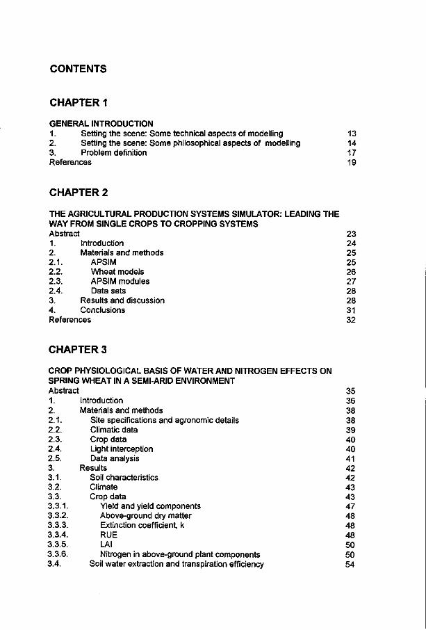
CONTENTS
CHAPTER 1
GENERAL INTRODUCTION 1. Setting the scene: Some technical aspects of modelling 13 2. Setting the scene: Some philosophical aspects of modelling 14 3. Problem definition 17 References 19
CHAPTER 2
THE AGRICULTURAL PRODUCTION SYSTEMS SIMULATOR: LEADING THE WAY FROM SINGLE CROPS TO CROPPING SYSTEMS Abstract 23
24 25 25 26 27 28 28 31 32
CROP PHYSIOLOGICAL BASIS OF WATER AND NITROGEN EFFECTS ON SPRING WHEAT IN A SEMI-ARID ENVIRONMENT Abstract 35 1. Introduction 36 2. Materials and methods 38 2.1. Site specifications and agronomic details 38 2.2. Climatic data 39 2.3. Crop data 40 2.4. Light interception 40 2.5. Data analysis 41 3. Results 42 3.1. Soil characteristics 42 3.2. Climate 43 3.3. Crop data 43 3.3.1. Yield and yield components 47 3.3.2. Above-ground dry matter 48 3.3.3. Extinction coefficient, k 48 3.3.4. RUE 48 3.3.5. LAI 50 3.3.6. Nitrogen in above-ground plant components 50 3.4. Soil water extraction and transpiration efficiency 54
1. 2. 2.1. 2.2. 2.3. 2.4. 3. 4.
Introduction Materials and methods
APSIM Wheat models APSIM modules Data sets
Results and discussion Conclusions
References
CHAPTER 3

4. 4.1. 4.2. 4.3. 4.4. 4.5. 4.6. 5.
Discussion Vapour pressure deficit Yield and yield components Radiation use efficiency Leaf area Water extraction, T and TE in the dry treatment Nitrogen in above-ground dry matter
Conclusions References
CHAPTER 4
57 57 57 60 60 62 64 65 66
LIGHT INTERCEPTION IN SPRING WHEAT: THE EXTINCTION COEFFICIENT DURING EARLY GROWTH Abstract 73 1. Introduction 74 2. Methods 76 2.1. Experimental details 76 2.2. Analytical details 77 3. Results and discussion 79 3.1. Constant k 79 3.2. Variable k 81 3.3. Sensitivity analysis 87 4. Conclusions 91 References 91
CHAPTER 5
TESTING SIMULATION CAPABILITIES OF WHEAT GROWTH AND RESOURCE USE (WATER, NITROGEN AND SOLAR RADIATION) IN AUSTRALIA Abstract 95 1. Introduction 97 2. Materials and methods 98 2.1. The systems model APSIM and its components 99 2.1.1. Water balance 99 2.1.2. Nitrogen balance 99 2.1.3. Wheat models incorporated into APSIM 100 2.2. Environments and data sets used for model testing 108 2.2.1. Environments 108 2.2.2. Datasets 108 2.3. Model testing 111 2.3.1. Test I, model evaluation across environments 111 2.3.2. Test II, model process testing at Toowoomba 112 2.3.3. Test III, model process testing when inputting potential
carbon production 113 3. Results 113 3.1. Test I, model evaluation across environments 113 3.1.1. Test against data with varying water availability 114 3.1.2. Test against data with varying nitrogen availability 120 3.2. Test II, model process testing at Toowoomba 125 3.2.1. Total, above-ground dry matter 125

3.2.2. 3.2.3. 3.2.4. 3.3. 3.3.1. 3.3.2. 4. 4.1. 4.2. 4.3. 4.4. 4.5. 4.6.
Leaf area index and intercepted solar radiation Water use Nitrogen use
Test III, model process testing at Toowoomba Total dry matter Interactions with other variables
Discussion Kernel yield Total dry matter Leaf area Water extraction in the dryland treatment at Toowoomba Nitrogen uptake at Toowoomba Nitrogen distribution in the plant at Toowoomba
References
CHAPTER 6
127 129 131 136 137 138 141 142 144 147 149 151 152 153
ENHANCED WHEAT MODELLING CAPABILITIES FOR CROPPING SYSTEMS SIMULATION IN AUSTRALIA - THE INTEGRATED WHEAT MODEL (l_WHEAT) Abstract 161 1. Introduction 162 2. Model description 165 2.1. Phenology 167 2.2. Kernel yield 167 2.3. Aboveground dry matter accumulation 168 2.4. Leaf area development 170 2.4.1. Potential leaf area production 170 2.4.2. Leaf area senescence 171 2.4.3. Green leaf area 173 2.5. Soil water uptake 173 2.6. Nitrogen supply 173 2.7. Nitrogen demand 174 2.8. Plant nitrogen balance 175 3. Model performance 176 3.1. Methods 176 3.2. Test results 177 3.2.1. Simulation of TDM, KY and HI 177 3.2.2. Final tiller number and grain nitrogen percentage 178 3.2.3. Testing leaf area simulation 178 3.2.4. Water and nitrogen use at Toowoomba 186 3.3. Future improvements 189 4. Conclusions 190 References 191

CHAPTER 7
GENERAL DISCUSSION 1. Outline 197 2. Problems with models 197 2.1. Model development 197 2.2. Model application 199 3. Why yet another wheat model? 201 3.1. Model development 201 3.2. Data sets 202 4. An example of a farm-based application 203 5. Where to from here? 204 References 205
SUMMARY
207
SAMENVATTING 213
OTHER PUBLICATIONS BY THE AUTHOR 221
CURRICULUM VITAE 225
APPENDIX I 227
APPENDIX II 265

General Introduction
Chapter 1
General Introduction
"Perhaps an objective science that takes the world apart only to reassemble it with the aid of ever larger computers does not lead to a rational view of the world after all?" Edelglass et al. (1992)
1. Setting the scene: Some technical aspects of modelling
Use of models in agricultural decision making goes back to the first seeds sown. For this action to occur, a prior knowledge was required that encapsulated some basic, crop physiological understanding. The farmers who had sown these seeds had already developed a mental model telling them that, if planted at a certain time and in a certain way, these seeds would develop into a mature crop. Over time, farmers developed increasingly sophisticated rules of thumb, i.e. they refined their mental model based on experience and observations. A more structured approach to modelling, introducing the concept of systems dynamics, evolved last century with pioneers such as Justus von Liebig, Albrecht Thaer and Carl von Wulffen. Their work led to a realization of the interdependence of variables in agricultural systems and to an understanding of nutrient cycling depending on the three production parameters: quantity, intensity and efficiency (de Wit, 1990).
The advent of crop physiological models, implemented on computers, can be traced back to some ground-breaking work in the 1950s, such as Monsi and Saeki's (1953) paper on light interception and de Wit's (1958) classic 'Transpiration and Crop Yields' that also draws on some of Penman's early work (e.g. Penman, 1948). These and similar publications constructed the framework for the emerging formalism of systems analysis (Zadoks and Rabbinge, 1985). Phrasing physiological processes in mathematical terms led to today's proliferation of computer simulation models developed and used in agriculture.
13

Chapter 1
Understanding and predicting systems behaviour (including crop growth) is the basis for rational decision-making. This is where models can help, because they are a convenient tool to aggregate a multitude of interactions. However, they must not be seen as the panacea for all agricultural problems and, only after it has been established that a modelling approach is desirable, the most appropriate model must be selected (see Chapter 2). For this selection process, it is important to understand the model's purpose, realm of validity and limitation. Some basic model classification can help in this process.
Models can be categorized in many ways based on their structure, design objectives or complexity. Spitters (1990) discussed two useful schemes. First, based on structure, models can be categorized as either regression models, where relationships are described by some empirical functions devoid of biological meaning (e.g. polynomial curves) or as mechanistic models that explain growth from underlying physiological processes. Generally speaking, a useful regression model considers major variables of a dynamic system, and mechanistic models always have some components based on regression. Second, models can be classified, based on their design objectives, as either predictive or explanatory models. This classification is not straightforward and all models considered in this study contain elements from both categories. Generally, predictive models are simpler and contain fewer parameters than explanatory models that combine explanation and integration of underlying principles. Rabbinge and de Wit (1989) further distinguish between conceptual models, comprehensive models and summary models as three steps in model development, based current knowledge and understanding of the system. The latter two of these steps correspond to Spitters' (1990) categories of explanatory and predictive models, respectively. All have their role to play and differences between them are discussed in more detail in the following section and in Chapter 6 of this thesis.
2. Setting the scene: Some philosophical aspects of modelling
Simulation models of agricultural plants, crops and cropping systems are becoming commonplace. Traditionally, they have been used as "knowledge depositories" by scientists in order to describe an area of interest. Once they became available, interest quickly shifted from curiosity about the underlying principles to using models in a predictive capacity (e.g. to develop scenarios
14

General Introduction
or as a decision support tool) or in an explanatory capacity to investigate interactions between processes usually only studied in isolation. This use of models has started a debate about the appropriate way of mathematically describing biological relationships, and the level of detail needed for a "good" model. Defining this "goodness", by clearly stating the objectives of every modelling endeavour could make much of that debate redundant.
All soil/plant/crop/cropping systems simulation models known to me are mechanistic at their core, i.e. they are primarily concerned with describing phases and states of crop and soil components. This is largely the result of a Newtonian view of the world on which science is based, whereby it is assumed that every material system can be explained through its state-transitions sequences. Arguments about the "right" way of modelling have largely concentrated on the level of empiricism acceptable when representing such sequences mathematically. This debate has not been very helpful, since it has been conducted by groups interested in using models for different purposes, namely to either explain how a system operates or to predict the system's behaviour. In other words "the more complex a model is, the more it explains; the less predictive possibilities it has, the less desirable it is" (Willems, 1989). Both purposes are legitimate, but it is doubtful that they can be achieved using identical tools. Passioura (1996) referred to these processes as "science" and "engineering", respectively. He asserted that scientific models aspire to improve our understanding of physiology and environmental interactions, while engineering models take robust, empirical relations to get a job done. In doing so, he takes a rather narrowly focused view of what constitutes scientific activity, a view based on the traditional, reductionist paradigm of Western science. While this differentiation is valid, it also reinforces the disassociation of scientific and engineering modelling rather than leading towards a synthesis of the different approaches that could harness synergies from improved system performance. Rather than setting engineering aside from sciences, and alienating many professionals in the process, it might be more useful to view it as the pragmatic end of a continuous quest for knowledge and solutions to problems. Often agricultural scientists, and particularly modellers, are caught between the two extremes and are criticized for being not scientific and not pragmatic enough at the same time. Used constructively, this polarity should advance future model development.
A shortcoming of most simulation models is that they hardly attempt to simulate holistic features of biological systems. This is a direct consequence
15

Chapter 1
of the tradition of Western science which has been founded on the method of reductionism. Descartes first proposed the "Machine Metaphor", whereby it is postulated that organisms form a proper subclass of the class of machines and the study of biology thus is subsumed under the study of mechanisms and becomes a part of physics. Newton, a physicist, perfected this approach and provided us with the notion of entailment, i.e. the assertion that all behaviours of organisms are entailed by the laws of mechanism (Rosen, 1989). This Newtonian view dictates that any system can be described by phases or states, whereby the environment is the seat of external forces which set initial conditions, configurations and velocities. These are beyond the reach of causality which is restricted to the state-transition sequence within the system. Everything in this system and the system as a whole is simulable, i.e. it can be described as either particles or forces, and can thus be expressed mathematically. This provides a direct measure of the complexity, whereby complexity of a physical system is defined as the length of the minimal algorithm needed to simulate or describe this system (Gell-Mann, 1995). However, Gödel has already proven that even the science of numbers cannot be completely expressed as software (Chaitin, 1995). Rosen (1989) defined complexity as a material system in which causality is no longer imaged as a state-transition sequence. As he put it "...the difficulties encountered in attempting to characterize the living state are not merely technical; they arise precisely because organisms are complex in our sense, and our science is geared only to deal with the simple. In a nutshell, if Descartes had been right, and organisms were automata, we would be able to express them as software; but we cannot, he was not, and organisms are not."
However, even in biological science the Newtonian framework has served us well since most biological processes can be reduced to their basic physics or chemistry. The framework does, however, miss a "vital" ingredient - life. This emergent property of biological systems is not entailed by the state-transition sequence and thus outside the realm of traditional, Newtonian science. Aristotle, a biologist, saw the notion of entailment within the much wider framework of his categories of causation, namely material, efficient, formal and final causes. It is the latter that is not considered by Newton, but which was seen by Aristotle as the most important category. Indeed, the term "teleology", i.e. the study of final causes, was originally invented to set it aside from science and to banish it from polite, scientific debate (cf. Casti, 1989; Davies, 1992). Ironically, modern systems science can be defined as the study of systems properties emphasising formal and final causes (Casti,
16

General Introduction
1989). Davies (1992) stressed the growing appreciation in the scientific community that both approaches, reductionistic and holistic, are needed, for they provide two complementary ways of studying physical phenomena. The dilemma we have to face is that we have a solid tool-kit, based on over 300 years of experience, to peruse the former, but very little experience in following the latter approach. A way forward might be to have the courage to search for more all-encompassing, conservative relations and let them interact freely (i.e. with little or no constraints). While this would reduce complexity on one hand by reducing the number of processes simulated explicitly, it also increases complexity by providing for "richer" interactions among the processes considered. However, care needs to be taken whenever the level of process detail is reduced that we can demonstrate this simplification is based on a sound understanding of the underlying processes. We might be able to "capture" some of the emergent systems properties through such simplification by increasing the complexity of interactions. To reduce number and uncertainty of parameters in simulating biological systems, a process based approach can be replaced by a phenomenological description of that process without sacrificing scientific principles. This requires that (a) the process is already understood at the more basic level and (b) the phenomenological description is general across a wide range of conditions and of low complexity with easily derived parameter values. This will increase predictive ability of the model and may eventually lead to a more advanced, formal framework for dealing with holistic concepts (Gell-Mann, 1995).
Modern problem-solving theory can give us some guidance on how simplification can be achieved without loss of scientific rigour. When a given case or rule is combined with an observation, the logical processes of inductive and abductive inference can be used to hypothesize either a general rule or a specific result, respectively. In situations where multiple hypotheses are possible, one can discriminate amongst them based on their plausibility (Peng and Reggia, 1990). This plausibility is given by the parsimony principle, or Occam's razor, whereby the most plausible explanation is that which contains the simplest ideas and least number of assumptions (Davies, 1990). It is this principle, that has been chosen as a leitmotiv for this thesis.
17

Chapter 1
3. Problem definition
Spring wheat (sown in autumn) is the major dryland winter crop in Australia with an average, yearly production of over 15 million tonnes, varying strongly from season to season (ABARE, 1994). This yield variability is largely caused by a rainfall variability that is amongst the highest in the world and is typical for this region of the Pacific (Nicholls and Wong, 1991). Consequently, farm managers are confronted with uncertainty and a high level of production risk, but also with the opportunity for large profits if the right management decisions are taken at an opportune moment (Hammer et al., 1996). This led to the development of regionally based decision support tools for wheat production. Many of these are based on output from dynamic simulation models. Examples are: (a) WHEATMAN, a decision support package for the Northern Australian wheat belt (Woodruff, 1992) using data from the model by Hammer et al. (1987); (b) O'Leary et al. (1985) developed a model for tactical wheat management in Victoria; (c) SIMTAG (Stapper, 1984), a model widely used in the Southern Australian wheat belt to evaluate planting strategies (Stapper and Fischer, 1990); and (d) TACT, a wheat management support tool for Western Australia (Robinson and Abrecht, 1994). All of these tools are production oriented and concentrated on single season issues such as variety choice, frost avoidance or tactical nitrogen management.
Recent advances in computer technology have made it possible not only to consider single crops and/or single seasons but whole cropping systems. This led to the development of cropping systems simulators such as PERFECT (Littleboy et a l , 1992) or APSIM (McCown et al., 1996) and the possibility of using process simulation models to explore issues related to both, productivity and efficiency (i.e. 'sustainable production'), and resource utilization across crops and seasons.
Chapter 2 outlines a methodology that can be used to simulate cropping systems and that provides the necessary flexibility to configure a systems model according to specific needs. However, to simulate whole cropping systems, crop models must not only give reliable predictions of yield, they must also quantify the water and nutrient use well, so that the status of the soil at maturity is a good representation of the starting conditions for the next cropping sequence. This issue is difficult to address because frequently the necessary data to assess7 such simulation capabilities are lacking. Chapter 3 reports and interprets one such data set and discusses some of the key crop physiological parameters. Chapter 4 provides further detail regarding the
18

General Introduction
Simulation of light interception at the crop level. Testing and developing of simulation approaches requires high quality experimental data, specifically collected for this purpose. Only then can (a) necessary coefficients be derived with the degree of accuracy needed to apply the model confidently, and (b) parameter values be determined that allow a thorough testing of the simulation of individual processes. Such data, together with the necessary, crop physiological framework are presented in Chapters 3 and 4.
Historically, resource utilization has not been a major objective when developing crop simulation models. Thus, the models' suitability for these new tasks needs to be tested and, if necessary, models need to be modified (Chapter 5). Much of the existing simulation capability may be adequate for these new demands, but this needs to be demonstrated. Identifying simulation approaches that perform well will speed up the development process, avoid frustrating duplication of research efforts and save costs. These approaches can then be combined with new model components that have to be developed in cases where none of the existing models perform adequately (Chapter 6). Finally, model testing can also help to elucidate discrepancies in other models and so highlight areas still insufficiently understood (Oreskes et al., 1994).
Based on the wealth of existing models, the purpose of this thesis is to improve, and further develop, a simulation capability for spring wheat that • is suitable for use in cropping systems models, • is robust in its predictive ability across a wide range of environmental
conditions in Australia, • and does not require parameters that are difficult to derive.
References
Australian Bureau of Agricultural and Resource Economics (ABARE), 1994. Crop Report No 82, 18 January 1994, Canberra.
Casti, J.L., 1989. Newton, Aristotle, and the modeling of living systems. In: Newton to Aristotle. Toward a Theory of Models for Living Systems. J. Casti and A. Karlqvist (Editors), Birkhauser, Bosten, pp. 48-89.
Chaitin, G.J., 1995. Randomness in Arithmetic and the Decline and Fall of Reductionism in Pure Mathematics. In: Nature's Imagination. J. Comwell (Editor), Oxford University Press, pp. 314-328.
19

Chapter 1
Davies, P., 1990. God and the New Physics. Penguin Books, London, UK, 255 pp.
Davies, P., 1992. The Mind of God. Science and the Search for Ultimate Meaning. Penguin Books, London, UK, 254 pp.
Edelglass, S., Maier, G., Gebert, H. and Davy, J., 1992. Matter and Mind -Imaginative Participation in Science. Floris Books, Edinburgh, Great Britain, 136 pp.
Gell-Mann, M., 1995. The Quark and the Jaguar - Adventures in the Simple and Complex. Abacus, London, UK, 392 pp.
Hammer, G.L., Woodruff, D.R. and Robinson, J.B., 1987. Effects of climatic variability and possible climatic change on reliability of wheat cropping - A modelling approach. Agric. Forest Metorol., 41: 123-142.
Hammer, G.L, Holzworth, D.P. and Stone, R., 1996. The value of skill in seasonal climate forecasting to wheat crop management in a region with high climatic variability. Aust. J. Agric. Res., in press.
Littleboy, M., Silburn, D.M., Freebairn, D.M., Woodruff, D.R., Hammer, G.L. and Leslie, J.K. 1992. Impact of soil erosion on production in cropping systems. I. Development and validation of a simulation model. Aust. J. Soil Res., 30: 757-74.
McCown, R.L., Hammer, G.L., Hargreaves, J.N.G., Holzworth, D.P. and Freebairn, D.M., 1996. APSIM: A novel software system for model development, model testing, and simulation in agricultural research. Agric. Syst., 50:255-271.
Monsi, M. and Saeki, T., 1953. Über den Lichtfaktor in den Pflanzengesellschaften und seine Bedeutung für die Stoffproduktion. Jap. J. Bot., 14: 22-52.
Nicholls, N. and Wong, K.K., 1991. Dependence of rainfall variability on mean latitude and the Southern Oscillation. J. Climate, 3: 163-170.
O'Leary, G.J., Connor, D.J. and White, D.H., 1985. A simulation model of the development, growth and yield of the wheat crop. Agric. Syst., 17: 1-26.
Oreskes, N., Shrader-Frechette, K. and Belitz, K., 1994. Verification, validation, and confirmation of numerical models in the earth sciences. Science, 263:641-646.
Passioura, J.B., 1996. Simulation models: Science, snake oil, education or engineering? Agron. J., in press.
Peng, Y. and Reggia, J.A., 1990. Abduction Inference Models for Diagnostic Problem-solving. Springer Series: Symbolic Computation - Artificial Intelligence. D.W. Loveland (Editor), Springer-Verlang, New York, 284 pp.
Penman, H.L., 1948. Natural evaporation from open water, bare soil and grass. Proc. Roy. Soc. A, 193: 120-146.
20

General Introduction
Rabbinge, R. and de Wit, CT., 1989. Systems, modeis and simulation. In: Simulation and systems management in crop protection. Rabbinge, R., Ward, S.A. and van Laar, H.H. (Editors), Pudoc, Wageningen, pp. 3-15.
Robinson, S. and Abrecht, D., 1994. TACT - a seasonal wheat sowing decision aid. User Manual. Economic Management and Crop Science Dept. of Agriculture Western Australia, Program version 2.7, February 1994.63 pp.
Rosen, R., 1989. The Roles of Necessity in Biology. In: Newton to Aristotle. Toward a Theory of Models for Living Systems. J. Casti and A. Karlqvist (Editors), Birkhauser, Bosten, pp. 11-37.
Spitters, C.J.T., 1990. Crop growth models: their usefulness and limitations. Acta Horticulturae, 267: 349-368.
Stapper, M., 1984. SIMTAG: A Simulation Model of Wheat Genotypes. Model Documentation. ICARDA, Aleppo, Syria and Univ. of New England, Armidale, NSW, Australia. 108 pp.
Stapper, M. and Fischer, R.A., 1990. Genotype, sowing date and plant spacing influence on high-yielding irrigated wheat in Southern New South Wales. III. Potential yields and optimum flowering dates. Aust. J. Agric. Res., 41: 1043-1056.
Willems, J.C., 1989. Some thoughts on modelling. In: Newton to Aristotle. Toward a Theory of Models for Living Systems. J. Casti and A. Karlqvist (Editors), Birkhauser, Bosten, pp. 91-119.
Wit, CT. de, 1958. Transpiration and crop yields. Versl. Landbouwk. Onderz., 64(6): 1-88.
Wit, CT. de, 1990. Making Predictions About Farming. In: Scientific Europe, Research and Technology in 20 Countries, Foundation Scientific Europe (Editors), Nature & Technology Scientific Publishers Ltd., Maastricht, The Netherlands, pp. 188-191.
Woodruff, D.R., 1992. 'WHEATMAN' a decision support system for wheat management in subtropical Australia. Aust. J. Agric. Res., 43: 1483-1499.
Zadoks, J.C and Rabbinge, R., 1985. Modelling to a purpose. Adv. Plant Pathol., 3:231-244.
21

The Agricultural Production systems SIMulator
Chapter 2
The Agricultural Production systems SIMulator: Leading the way from single crops to cropping
systems
"It is more important to have beauty in one's equations than to have them fit experiments." Paul Dirac
Abstract
Aspects of the functionality of the Agricultural Production Systems SIMulator (APSIM) are demonstrated. APSIM is being developed as part of a systems and operational research approach to problems in production systems of north-eastern Australia. Any reliable systems model requires modules that accurately quantify resource use. However, most of the current, stand-alone crop simulation models have not been developed specifically for use within systems models and require modification and re-evaluation before they can be used in a systems context. In the past this was often more difficult and time consuming (and more difficult to publish!) than developing new models. In some quarters this has brought modelling into disrepute and it is now time to capitalize on already existing models. APSIM provides a very powerful and flexible infrastructure for model development, testing and application. Its modular structure helps to better understand the mathematical representation of physiological processes and their interactions. Communication amongst scientists is also improved by using a common simulation platform. By incorporating two existing wheat models into APSIM we demonstrate how model testing and comparing can lead to a more reliable modelling capability without re-inventing the wheel.
1. Introduction
Production systems modelling can be used to answer questions at various levels of aggregation. Care needs to be taken, however, that the methodology used is appropriate for the task. Modelling should not be seen as the panacea for all agricultural problems but rather as a convenient way of aggregating environmental interactions thus providing higher level data upon
23

Chapter 2
which decisions can be based. It integrates our knowledge of agricultural systems, allows generation of information useful to systems managers (e.g. What if? When? How often?) and highlights gaps in current understanding of the system. It is a means of making agricultural research more relevant to practice and thus adds value to existing knowledge and our research efforts. By simulating the production system, the state of the system at any point in time is known, and alternative management options and their long-term impact on sustainability and productivity can be evaluated. Crop models form the basis of a production systems model, but it has been claimed that even after 25 years of work they have produced few sustained successes (Seligman, 1990). Better predictive performance of crop models is more likely to be achieved by improving existing models than by developing new ones. The Agricultural Production System SIMulator (APS IM) contributes to better predictive modelling. It provides an infrastructure to support convergent effort by teams in testing and improving models, with change taking place simultaneously on many fronts (McCown et al., 1996). Thus APSIM greatly improves communication between modellers without the usual sacrifice of individuality in modelling approaches, and provides direction for systematic model improvements.
Although APSIM is being developed as part of a systems and operational research approach to problems in production systems of north-eastern Australia, it is an ideal tool for similar applications elsewhere. Its main objectives are to combine crop and pasture models to simulate various production systems using soil and crop processes at levels that are balanced and appropriate to proposed applications. The WINDOWS® based platform allows easy integration of existing models or modules. A sophisticated communication protocol and a modular structure assist users to combine desired modules at the click of a button. This configuration of modules can then be used to simulate the impact of land use on resources for a range of management scenarios associated with crop sequence, fertilization, tillage and pest control. The necessary management rules for these scenarios can easily be constructed without re-compiling. Information thus generated enables analysis of economic and resource risks in the variable climatic and marketing environments faced by most agricultural production systems in Australia.
At present, crop modules are operational in APSIM for wheat, barley, sorghum, sunflower, maize, cotton and peanuts. They are all based on existing models with varying degrees of adaptation. Modules for chickpeas, soybean, mungbean, cowpea and pasture are under development.
24
The Agricultural Production systems SIMulator
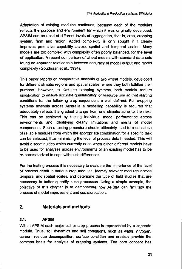
Adaptation of existing modules continues, because each of the modules reflects the purpose and environment for which it was originally developed. APSIM can be used at different levels of aggregation, that is, crop, cropping system, farm and region. Added complexity is only sought if it clearly improves predictive capability across spatial and temporal scales. Many models are too complex, with complexity often poorly balanced, for the level of application. A recent comparison of wheat models with standard data sets found no apparent relationship between accuracy of model output and model complexity (Goudriaan et al., 1994).
This paper reports on comparative analysis of two wheat models, developed for different climatic regions and spatial scales, where they both fulfilled their purpose. However, to simulate cropping systems, both models require modification to ensure accurate quantification of resource use so that starting conditions for the following crop sequence are well defined. For cropping systems analysis across Australia a modelling capability is required that adequately reflects the gradual change from one climatic zone to the next. This can be achieved by testing individual model performance across environments and identifying clearly limitations and merits of model components. Such a testing procedure should ultimately lead to a collection of reliable modules from which the appropriate combination for a specific task can be selected, thus minimizing the level of process detail needed. This will avoid discontinuities which currently arise when either different models have to be used for analyses across environments or an existing model has to be re-parameterized to cope with such differences.
For the testing process it is necessary to evaluate the importance of the level of process detail in various crop modules, identify relevant modules across temporal and spatial scales, and determine the type of field studies that are necessary to better quantify such processes. Using a simple example, the objective of this chapter is to demonstrate how APSIM can facilitate the process of model improvement and communication.
2. Materials and methods
2.1. APSIM
Within APSIM each major soil or crop process is represented by a separate module. Thus, soil dynamics and soil conditions, such as water, nitrogen, carbon, residue decomposition, surface condition and erosion, provide the common basis for analysis of cropping systems. The core concept has
25

Chapter 2
changed from that of a crop responding to resource supplies in existing crop models to that of a soil responding to weather, management and crops. All modules are independent and communication between modules is handled by a central 'engine' which uses a unique message passing system. A standard interface design enables easy removal, replacement or exchange of modules without disrupting operation of the system. The shell allows rapid evaluation and further development of new modules. This structure facilitates the collaborative effort required in the development of a systems simulation model, \lyhere different processes are understood and developed by different people, and where alternative representations of a single process are sometimes needed (McCown et al., 1996).
2.2. Wheat models
In Australia spring wheat is a major component of the dryland farming system (Doyle and Holford, 1993). The wheat models used in this paper are Hammer-Woodruff (HW; Hammer et al., 1987) and SI (SIMTAG; Stapper, 1984), which were developed for a sub-tropical climate with summer rainfall and a mediterranean climate, respectively. They were chosen because both represent examples of successful model applications in two distinctly different climatic regions of Australia. The regional differences are reflected in a key feature of the models, the way dry matter accumulation is calculated. For the predominately water-limited environment of north-eastern Australia, HW uses a transpiration x transpiration efficiency approach. For the mainly temperature/radiation limited environment in the south-east, SI uses intercepted radiation x radiation use efficiency. It has since been suggested that both approaches should be combined to obtain more stable models across a wider range of climatic conditions (Chapman et al., 1993). Both models do not account for crop damage due to pests, diseases, weeds, waterlogging, lodging or frost. For the purpose of this paper both models assume that nutrients are non-limiting, although HW includes a nitrogen balance.
Crop growth in HW is determined from the product of transpiration and transpiration efficiency. Leaf area index (LAI) is calculated from crop growth rate and stage of phenological development and is further modified by a water stress index. LAI is used to determine the actual, daily amount of transpiration. Yield is estimated using equations based on dry matter accumulation up to flowering and crop growth rate around flowering (+ / -10 d). HW accounts for a decrease in yield potential with later sowings as reported for north-eastern Australia (Woodruff and Tonks, 1983). Anthesis
26

The Agricultural Production systems SIMulator
date is based on the average number of days or thermal time from sowing for a cultivar in a particular district. The level of complexity (and hence the number of processes simulated) is kept to the minimum needed for reliable yield prediction in this, mostly water-limited, environment. HW has been used in PERFECT and the WHEATMAN software packages. PERFECT is a model to analyze risks of soil erosion to long-term crop production. It simulates interactions between soil type, climate, fallow management strategy and crop sequence (Littleboy et al., 1992). WHEATMAN is a decision support system developed for farmers to aid variety choice (frost avoidance) and fertilizer management for wheat crops in Queensland (Woodruff, 1992).
SI is also based on physiological, ontogenic, morphological and physical principles but at a more detailed level than HW. Equally important processes are represented at a similar level of detail. All dynamic processes are rationalized to 'simple' relationships between major contributing factors. Phasic development is modelled as a function of temperature and photoperiod. The green area index is simulated from leaf appearance, leaf size, leaf senescence, tillering, tiller senescence and stem/spike area as a function of temperature, stage of development and water availability. Green-area index determines the intercepted photosynthetically active irradiance, which is converted into plant dry weight with a radiation use efficiency factor. Daily growth is reduced for water stress and sub-optimal temperatures and is partitioned to roots, leaves, stems, chaff or kernels, depending on the stage of development. SI has been used for an assessment of maturity type productivity (Stapper and Harris, 1989) and evaluation of fallow management (Fischer et al., 1990).
2.3. APSIM modules
Both wheat models were incorporated in APSIM making use of a crop template which structures models into their main components as modules, thus allowing cross comparisons (McCown et al., 1996). The underlying soil process modules of APSWAT were used in the comparison of both wheat models. APSWAT has been developed as the water balance in APSIM by improving existing water balances of the CERES (Ritchie, 1985) and PERFECT (Littleboy et al., 1992) models. The APSIM versions of HW and SI were compared with their stand-alone models which resulted in only minor differences, mainly caused by differences between the original water balances and APSWAT.
27

Chapter 2
2.4. Data sets
Wheat data sets from Toowoomba, Queensland (lat. 27 °S, cv. 'Hartog') and Wagga Wagga, New South Wales (lat. 35 °S, cv. 'WW33G') were used in this comparison. These data sets are independent from model development. They were randomly selected and were sufficiently detailed to parameterize the models. The first data set is in the area covered by the HW model and the second data set is typical of locations for which SI was developed. For both locations a wet and dry data set was selected, for Toowoomba dry and irrigated treatments in 1993 (APS 15, sown 25 June, Chapter 3) and for Wagga Wagga a dry (1982, sown 2 June) and wet (1983, sown 28 April) season (Fischer, unpubl.). Observed phenology was used as input to eliminate differences in crop growth and yield caused by prediction of crop development.
3. Results and discussion
When we compared actual and predicted yields we were at first surprised about the good results, especially when we account for the deviation in the field measurements (Fig. 2.1). Because the test data sets were sufficiently detailed, we could parameterize the models well which is often a problem when comparing different models with the same data sets (Goudriaan et al., 1994; Porter, pers. comm.). HW overpredicted the dry treatment for Toowoomba and the wet season for Wagga Wagga, whilst SI overpredicted the dry season for Wagga Wagga. All other results were within one standard deviation around the measured means.
For APS15 dry, the water uptake pattern caused the prediction error of HW by varying the timing of water stress. That in turn was related to transpiration driven by leaf area, which increased too slowly at the start of the season and reached a peak only at anthesis. This resulted in lower than measured water extraction and more plant available water around anthesis, the critical period for yield formation in this environment (Woodruff, 1983). The model's sensitivity to conditions around anthesis can be shown by delaying the time to anthesis by five days. By then (i) more soil water has been used and (ii) mean temperatures and evaporative demands are higher, resulting in lower transpiration efficiency and hence reduced growth rate. This simulated delay reduced yield estimates by 27% to 378 g m'2 (Fig. 2.1). The overprediction of HW for Wagga 83 was caused by the inappropriate use of the yield function, as it was developed for a warmer, drier environment (Woodruff and Tonks,
28

The Agricultural Production systems SIMulator
1983). Delaying anthesis by five days under these water non-limiting conditions further increased dry matter production and hence yield.
In SI water stress during early growth did not sufficiently retard leaf area development. This resulted in an overprediction of yield at Wagga Wagga in the extremely dry season of 1982 (available soil moisture at sowing: 77 mm, < 30 mm effective, in-season rain).
i 1 ^
• HW 0 Observed • Simtag
APS 15 irr APS15dry Wagga83 Wagga 82
Figure 2.1: Observed and simulated grain yield. Vertical bars on actual data indicate + / - one standard deviation, vertical bars on simulations indicate change in grain yield when delaying anthesis by five days.
It is instructive to compare water stress indices for the two models, calculated as actual transpiration divided by demand for water (potential transpiration). For APS15 dry it clearly shows the later onset of stress predicted by HW, caused by slow leaf area development and hence lower transpiration (Fig. 2.2a). Anthesis date corresponded with rapid development of water stress, which explains the large effect of delaying anthesis date by five days on grain yield. After day 280 stress levels were similar for both models, although less variable for SI.
At Wagga Wagga HW's slower leaf area development was also apparent (Fig. 2.2b). However, this had no impact on yield predictions, because anthesis occurred at the time of maximum water stress. In SI the predicted water stress between day 240 and 270 failed to reduce leaf area sufficiently to avoid overprediction of light interception and hence dry matter production and yield. After day 265 water stress levels of both models were very similar. This type of comparison is meaningful because the two models use the same water balance (i.e. APSWAT) with identical input parameters. Therefore, any
29

Chapter 2
observed differences in actual : potential transpiration must have been caused by differences between the crop models.
Finally we observed that HW failed to extract all available water by the end of the season because transpiration was severely restricted once fraction of transpirable soil water fell below a certain threshold. Whilst the yield calculation based on soil water availability seems to be remarkably stable, quantification of water use needs to be improved before this model can be used within a farming systems framework.
? 1.0 w
•S 0.8
$ 0.6
>. 0.4 a a 3 °-2
s % o.o
—HW
SIMTAG
APS15,dry
200 220 240 260
Day of the year
280 300 320
(a)
? 1.0-, e •8 0.8
I 0.6 Ï
Î . 0.4 a a 3 0.2 I».
ai 15 0.0
Wagga, 82
210 230 250 270. 290
Day of the year 310 330
(b)
Figure 2.2: Ratio of actual : potential transpiration at (a) Toowoomba (APS15 dry) and (b) Wagga Wagga, 1982. The horizontal line (<—• ) indicates the period of + / -10 d around anthesis.
Stability is important in models at aggregation levels of crop and above. Although there are obvious areas of improvement in both models, they performed well in terms of yield prediction even in an environment other than that they were developed for. This is likely related to the high degree of decoupling of the calculation of state variables such as leaf area, water use
30

The Agricultural Production systems SIMulator
and crop growth. Checks during the verification stage of model building can then evaluate the ranges of important ratios such as transpiration ratio and specific leaf area. Using ratios to link important processes means that an error in one variable is either (i) compounded into others with cumulative effects or (ii) cancelled through compensating errors in another variable. Both problems need to be avoided.
Crop development (i.e. phenology) is another important factor to create stability by having many intermediate developmental stages between emergence and anthesis, and between anthesis and maturity. These stages can be used as checks to delay or quicken the start of change in rates. This requires robust phenology sub-models, able to predict crop development across a wide range of temperatures and photoperiods. For future model improvement we would thus strongly recommend the use of common cultivars in experimentation across such different environments.
In this example, we focused on yield and water use under nitrogen non-limiting conditions only. Obviously, other aspects such as nitrogen uptake and use and their interactions with water availability also need to be considered, particularly in light of their importance for final grain quality (Angus et al., 1993). Total biomass production needs to be tested so that reliable estimates of (i) standing stubble and (ii) organic matter added to the system can be obtained. These are important inputs for the surface management module and the soil-carbon module, respectively. The purpose of this paper is to demonstrate the methodology that can be adopted to improve existing models. For a more thorough analysis more data sets, covering a wider range of environmental conditions need to be used for testing. The testing process of modules in APSIM is on-going. Parallel to improving the crop modules, water and nitrogen modules are also being improved using a similar methodology (McCown et al., 1996).
4. Conclusions
With the help of two wheat models we demonstrated how APSIM can facilitate model improvement and scientific communication. The former was achieved by incorporating the models as modules into APSIM which subsequently allowed the use of a common file structure and a common water balance, thus removing ambiguity when interpreting model output (i.e. all differences found in water use were entirely caused by differences in the crop
31

Chapter 2
models and not in the water balance). Other features, such as graphic routines to analyze output (see McCown et al., 1996) also proved to be convenient and time efficient. The highly modular structure increased transparency of simulated processes. One feature of APSIM allows variable name changes at the press of a button. This greatly enhanced communication at a technical level through the use of common variable names. At a personal level such improved communication is more difficult to demonstrate. However, we found that we identified problems in simulations faster than ever before whilst quickly gaining an appreciation for other modelling approaches.
We found that in order to conduct a meaningful comparison of model components (i) data sets for testing have to be sufficiently detailed to parameterize models well and (ii) main aspects of areas not covered in the comparison need to be identical to avoid ambiguity when interpreting results. Based on such an analysis we identified leaf area development (HW and SI) and water uptake patterns and yield prediction functions (HW) as the main areas of improvement before either model can be used for a broad range of systems analyses under nitrogen non-limiting conditions.
References
Angus, J.F., Bowden, J.W. and Keating, B.A., 1993. Modelling nutrient responses in the field. Plant Soil, 155/156: 57-66.
Chapman, S.C., Hammer, G.L. and Meinke H., 1993. A crop simulation model for sunflower. I. Model development. Agronomy J., 85: 725-735.
Doyle, A.D. and Holford, I.CR., 1993. The uptake of nitrogen by wheat, its agronomic efficiency and their relationship to soil and fertilizer nitrogen. Aust. J. Agric. Res., 44: 1245-1258.
Fischer, R.A., Armstrong, J.S. and Stapper, M., 1990. Simulation of soil water storage and sowing day probabilities with fallow and no-fallow in southern New South Wales. I. Model and long term mean effects. Agric. Syst., 33: 215-240.
Goudriaan, J., Van de Geijn, S.C. and Ingram, J.S.I., 1994. GCTE Focus 3 wheat modelling and experimental data comparison workshop report. Lunteren, Netherlands, Nov. 1993. GCTE Focus 3 Office, Univ. of Oxford, Oxford.
32

The Agricultural Production systems SIMulator
Hammer, G.L., Woodruff, D.R. and Robinson, J.B., 1987. Effects of climatic variability and possible climatic change on reliability of wheat cropping - A modelling approach. Agric For. Meteorol., 41:123-42.
Littleboy, M., Silburn, D.M., Freebairn, D.M., Woodruff, D.R., Hammer, G.L. and Leslie, J.K., 1992. Impact of soil erosion on production in cropping systems. I. Development and validation of a simulation model. Aust. J. Soil Res., 30: 757-74.
McCown, R.L., Hammer, G.L., Hargreaves, J.N.G., Holzworth, D.P. and Freebairn, D.M., 1996. APSIM: A novel software system for model development, model testing, and simulation in agricultural systems research. Agric. Syst., 50: 255-271.
Ritchie, J.T., 1985. User-oriented model of the soil water balance in wheat. In: Wheat Growth and Modelling. E. Fry and T.K. Atkins (Editors). Plenum Publishing Co., NATO-ASI Series, pp. 293-306.
Seligman, N.G., 1990. The crop model record: Promise or poor show? In: Theoretical Production Ecology: Reflections and Prospects. R. Rabbinge, J. Goudriaan, H. van Keulen, F.W.T. Penning de Vries, H.H. van Laar (Editors). PUDOC, Wageningen, pp. 249-258.
Stapper, M., 1984. SIMTAG: A Simulation Model of Wheat Genotypes. Model Documentation. ICARDA, Aleppo, Syria and Univ. of New England, Armidale, NSW, Australia, 108 pp.
Stapper, M. and Harris, H.C., 1989. Assessing the productivity of wheat genotypes in a mediterranean climate, using a crop-simulation model. Field Crops Res., 20: 129-152.
Woodruff, D.R., 1983. The effect of a common date of either anthesis or planting on the rate of development and grain yield of wheat. Aust. J. Agric. Res., 34: 13-22.
Woodruff, D.R., 1992. 'WHEATMAN' a decision support system for wheat management in subtropical Australia. Aust. J. Agric. Res., 43: 1483-1499.
Woodruff, D.R. and Tonks, J., 1983. Relationship between time of anthesis and grain yield of wheat genotypes with differing developmental patterns. Aust. J. Agric. Res., 34: 1-11.
33

Crop Physiological Basis of Water and Nitrogen Effects
Chapter 3
Crop Physiological Basis Of Water And Nitrogen Effects On Spring Wheat In A Semi-Arid Environment
"It is the combination of contingency and intelligibility which prompts us to search for new and unexpected forms of rational order. " Ian Barbour
Abstract
Systems approaches may help to evaluate and improve the agronomic and economic viability of nitrogen application in the frequently water-limited environment of Northern Australia. This requires a sound understanding of crop physiological processes and well tested simulation models. Thus, this experiment on spring wheat aimed to further our understanding of water x nitrogen interaction effects on wheat and generate a data set for detailed testing of simulation routines. Experimental results were analyzed according to a framework defining the key physiological determinants of crop growth and yield.
For spring wheat grown under four levels of nitrogen (0 to 360 kg N) and either entirely on stored soil moisture or under full irrigation, kernel yields ranged from 343 to 719 g m"2. Yield increases were strongly associated with increases in kernel number (9148 - 19950 kernels m"2), indicating the sensitivity of this parameter to water availability and N level around anthesis. Total water extraction in the dry treatment was estimated at 240 mm with a maximum extraction depth of 1.6 m. A substantial amount of mineral nitrogen available deep in the profile (below 90 cm) was also taken up by the crop. This was likely the source of nitrogen uptake observed after anthesis in all treatments. Under dry conditions this late uptake accounted for approximately 50% of total nitrogen uptake and resulted in high (>2%) kernel nitrogen percentages even when no nitrogen was applied. Anthesis LAI values under sub-optimal water supply were reduced by 63% and under sub-optimal nitrogen supply by 50%. Radiation use efficiency (RUE) based on total incident short-wave radiation was 1.34 g MJ"1 and did not differ among treatments. The conservative nature of RUE was the result of the crop
35

Chapter 3
reducing leaf area rather than leaf nitrogen content (which would have affected photosynthetic activity) under these moderate levels of nitrogen stress. The transpiration efficiency coefficient was also conservative and averaged 4.7 g m"2 mm'1 kPa in the dry treatments. During kernel-filling a substantial amount of nitrogen was translocated from leaves and stems, which began with N contents of around 5%. Values at final harvest averaged 0.79% for leaves and 0.25% N for stems, except for the high water and nitrogen treatment where final values averaged 1.27%*N and 0.64% N, respectively. Kernel nitrogen percentage varied from 2.08 to 2.42%. An index of physiological efficiency of absorbed nitrogen that quantifies the amount of kernel produced per unit of total plant nitrogen (PEN, g kernel g"1 plant nitrogen) also proved to be conservative and averaged 38.5, except for the very high nitrogen and water treatment where luxury consumption of N occurred (PEN = 29.4).
This study has improved the understanding and quantification of crop responses to water and N limitations and provided a data set and a basis to consider ways to improve simulation capabilities of water and N effects on growth of spring wheat.
1. Introduction
In north-eastern Australia, spring wheat is a major component of the dryland cropping system. A risky economic environment combined with extreme rainfall variability in this region (Meinke et al., 1993a), often makes doubtful the economic feasibility of nitrogen application (Stone et al., 1993). In low rainfall years, crop yield is usually related directly to the amount of stored soil moisture, while nitrogen requirements are usually met by mineralization. In high rainfall years, nitrogen availability often limits production, unless fertilizer is applied. This is particularly true of soils that have been cropped continuously for many years. Fertility declines seriously because of decreased soil organic matter content and an associated reduction in nitrogen mineralization rates (Dalai and Mayer, 1986, 1990; Doyle and Holford, 1993). In economic analyses, the costs of applied nitrogen are commonly attributed to the crop in that season (Stone et al., 1993). Residual effects of applied nitrogen have been documented (e.g. Doyle and Holford, 1993), but are poorly quantified. Cropping systems analysis, using simulation techniques, can provide such quantification, thus allowing better economic analysis. Additionally, cropping systems simulation can provide base data for
36

Crop Physiological Basis of Water and Nitrogen Effects
environmental impact assessment of nitrogen management strategies, including nitrate leaching (e.g. McCown et al., 1996).
A diversity of efforts has been applied to improve understanding of water and nitrogen effects on wheat (e.g. Cooper, 1980; Green, 1987; Heitholt, 1989; Pheloung and Siddique, 1991; Doyle and Holford, 1993; Ellen, 1993). The crop physiological basis of these effects can be examined using a framework that defines the determinants of crop growth and yield (Charles-Edwards et al., 1986; Monteith, 1988). In such a framework, biomass accumulation is defined by either the product of intercepted radiation and its efficiency of use, or by the product of transpiration rate and transpiration efficiency. Crop duration defines the period over which biomass accumulates. Kernel yield can be defined either as the product of total biomass and harvest index or as the product of kernel number and kernel size. The development of canopy leaf area is a major determinant in this framework as it controls light interception and transpiration. The influence of environmental factors, such as water and nitrogen availability, must be mediated via these key determinants of crop growth and yield. The diversity of efforts applied to understand environmental effects on wheat has facilitated the development of a wide range of simulation models (e.g. Rasmussen and Hanks, 1978; Woodruff and Tonks, 1983; Passioura, 1984; Stapper, 1984; Angus and Moncur, 1985; Ritchie et al., 1985; O'Leary et al., 1985; Hammer et al., 1987; van Keulen and Seligman, 1987; Stöckle and Campbell, 1989; Sinclair and Amir, 1992). Whilst many of these simulation approaches aim to be generic and thus universally applicable, each model has, to the best of our knowledge, been biased towards particular environments. Although bias towards particular environments exists, certain features in each model may still be regarded as universal. To improve our current simulation capability, the challenge is to identifiy and use conservative parameters with coefficients that differ little with varying environmental conditions. This requires data sets containing sufficient detail to initialize, parameterize and test such models, as well as all necessary environmental input data. Such data sets are scarce (cf. Groot and Verberne, 1991).
The objectives for this study were: • to determine and quantify the effect of water and nitrogen limitations on
wheat by using the physiological framework defining determinants of crop growth and yield to identify generic factors and concepts where possible,
37

Chapter 3
• to investigate if all necessary coefficients to simulate the growth of wheat using a dynamic model of low to intermediate complexity can be easily derived from a field experiment,
• to compare the derived coefficients with values reported elsewhere and • to generate a detailed data set suitable for use in comparative evaluation
and improvement of existing wheat simulation models.
In subsequent chapters, this data set is used to evaluate and improve wheat simulation capability.
2. Materials and methods
2.1. Site specifications and agronomic details
Spring wheat (cv. Hartog) was grown either under full irrigation (irr) or entirely on stored soil moisture (dry) during the winter of 1993 on an experimental farm on the Darling Downs, Queensland, Australia (27°34'S, 151°52'E). Four levels of nitrogen, termed here as ON, 40N, 120N and 360N (in kg ha*1), were applied to a wheat crop grown on a uniform, alluvial, heavy cracking clay (Ug 5.24; Northcote, 1979) with high plant available water holding capacity (PAWC). To deplete soil nitrogen reserves and create a nitrogen responsive soil environment, three cover crops were grown on the site in succession prior to the experiment. Rainfall was excluded from the dryland site using an automatic rain shelter (12 x 6 m) covered with clear plastic. Each treatment was replicated twice and plot sizes were 3.75 x 2.25 m in the irrigated and 2.75 x 2.25 m in the dryland area, with a minimum border size of 0.5 m. Rows had a north-south orientation with a row spacing of 0.25 m. Sub-plots for destructive harvests measured two rows by 0.5 m (0.25 m2).
Since little rain fell between removal of the last cover crop and commencement of the experiment, the soil was dry to the maximum depth of observation (1.5 m). Prior to sowing the site was irrigated four times with a total amount of 235 mm. Spring wheat was sown on 24 June (day of the year, DOY 175) at a target population of 100 plants m"2. All plots received a basal fertilizer dressing immediately after sowing, containing the trace elements Mo, Cu and Zn as well as 15 kg ha'1 P. Nitrogen fertilizer was broadcast on 6 July at rates of 5, 40 and 120 kg N ha"1 to the ON, 40N and 120N treatments, respectively. A dose of 5 kg N ha"1 was given to the control treatment (ON) to avoid poor establishment due to very early nitrogen deficiencies. The largest
38

Crop Physiological Basis of Water and Nitrogen Effects
N application (360N) was split into three doses of 120 kg ha"1 each, given on 6 July, 30 July and 9 September (27 days before anthesis). All plots were irrigated (25 mm) after the first nitrogen application. Subsequently, the dryland treatments received no further irrigation. On 30 July, herbicide was applied at recommended rates to control broad-leaved weeds. Soil samples to determine background nitrogen levels and volumetric soil water content were taken four weeks prior to sowing. Additional soil samples were taken at anthesis and immediately after final harvest.
Soil samples were analyzed for N03 and NH4 following procedures outlined by Standley (1993) and described in detail for N03 by Best (1976) and for NH4 by Crooke and Simpson (1971). Organic carbon content of the soil was determined from initial soil samples using Walkley and Black's method (1934).
2.2. Climatic data
Environmental data were recorded electronically at five minute intervals
throughout the experiment and values integrated to daily data.
Daily vapour pressure deficit (VPD, kPa), a measure of atmospheric evaporative demand, is commonly used to calculate crop transpiration efficiency (Sinclair et al., 1983). Tanner and Sinclair (1983) described a method to estimate average daily VPD from daily maximum (Tmax) and minimum temperatures (Tmin). This method assumes that dew point temperature is always reached at Tmin and uses an empirical parameter, a, to calculate a weighted daily average VPD (VPDav) from the difference between saturated vapour pressure (Svp) at Tmin and Tmax, respectively:
VPDar=ax(SvpTaia-SypTmJ (1)
The authors report a value of 0.75 but point out that the coefficient a may vary with season and environment. However, data to derive this coefficient are rarely available and generally the value reported by Tanner and Sinclair (1983) is assumed.
From the temperature and humidity data, hourly values of VPD were calculated and weighted for the day-time period of crop transpiration by using hourly incident solar radiation. These values were then compared to those obtained from equation (1 ).
39

Chapter 3
2.3. Crop data
Neutron access tubes were installed prior to sowing to a maximum depth of 150 cm and measurements were taken at weekly intervals. Within each plot, six (dryland) or seven (irrigated) sub-plots were randomly selected for destructive sampling (harvest = H). Sampling dates are given in Table 3.1. H3 was omitted in the dry treatments due to space limitations. Plants were partitioned into green leaf, stem and eventually dead leaf and spike. Leaf area was determined using an area meter (Delta-T Devices Ltd.). At anthesis, green leaf area was further segregated into flag leaf, and the rest as equal numbers into "middle" leaves and "bottom" leaves. Kernel yield (KY) was determined by threshing spikes taken at final harvest. Kernel number (KN) and kernel weight (KW) were measured by weighing 300 randomly selected seeds from each plot. All plant samples were dried for at least 72h at 105°C before determining dry weight. Nitrogen content was determined for all samples using Kjeldahl digests (Standley, 1993). Phenological development was recorded by monitoring a set number of plants and establishing the dates when 50% of plants had reached a particular stage.
Table 3.1 : Calendar of events indicating harvest number and date.
Event
Sowing First harvest Second harvest Third harvest Fourth harvest Fifth harvest Sixth harvest Seventh harvest Seventh harvest
Seventh harvest
Code
S H1 H2 H3 H4 H5 H6 H7 H7
H7
Date
24/06 19/07 12/08 02/09 06/10 19/10 02/11 12/11 16/11
19/11
DAS
0 25 49 70 104 117 131 141 145
148
Comments
irrigated treatments only "anthesis" harvest
dryland treatments only irrigated ON, 40N and 120N treatments irrigated 360N only
2.4. Light interception
Tube solarimeters (Delta-T Devices Ltd.) that provide a continuous measure of incident total short-wave radiation were installed at 25 days after sowing (DAS) in all sub-plots allocated for final harvest. To account for reduced radiation on days when the shelter was closed, two reference tubes were installed, one above the irrigated and one above the dryland crops. Additional solarimeters were placed on the soil surface perpendicular to the rows in (a)
40

Crop Physiological Basis of Water and Nitrogen Effects
each replicate of the dryland experiment and (b) in replicate 2 of the irrigated treatment. Two of the sensors (120N dry replicate 2 and 120N irr) failed during the experiment and thus no data are available from these plots. Drought conditions prevailed throughout winter/spring of 1993 and the shelter was used only occasionally, mainly when irrigation was applied on the adjacent plots. Cumulative incident solar radiation differed by less than 8% between the two areas. Differences in incident radiation have been taken into account for where appropriate.
2.5. Data analysis
Data and derived variables from the experiment were analyzed as a combined analysis of variance. With respect to soil water characteristics the experimental site was uniform as it varied little in the key parameters of upper and lower soil water content. Thus, the main effects of water could be tested against the residual term of the ANOVA (Payne, 1993). Data from harvest 3, that were only available for the irrigated treatments, were analyzed as a one-factorial design. The probabilities from the F-test for main effects water (Pw), nitrogen (P„), their interactions (Pwn) and the associated standard error of differences for the interactions (SEd) were estimated.
Soil water extraction data were analyzed using a framework developed by Passioura (1983) and Monteith (1986) and described in detail by Meinke et al. (1993b) for sunflower and Robertson et al. (1993) for sorghum. By fitting continuous functions to measurements of soil water contents, cumulative soil water extraction can be calculated for any period. Parameters derived in this way can be used as input into a soil water balance. The framework accounts for maximum plant available water content (MAWC) in each soil layer, the rate at which the soil water extraction front descends through the profile (EFV) and the rate of water extraction in each soil layer (kl). MAWC is defined as the difference in volumetric soil water content between the lower limit (0L, lowest soil water content recorded in each layer of each plot of the dry treatment, usually at final harvest) and the drained upper limit (0u). Thus, PAWC equals MAWC if the profile is fully charged at planting. Values for ©u and wet bulk densities were determined from an unused area ponded for several weeks in the course of the experiment. The time course of soil water extraction for each layer of a fully wet soil profile can then be described by equations (2) to (4):
MAWC = ®u -@L (2)
41

Chapter 3
AWC - { ' MAWC if t<t„
(3) MAWC*fixp(-klx(t-tc)) if f> / c
dAWCIdt = { (-£/) x fTC
if t<tc
if *>*„ (4)
where AWC is the actual available water content in each layer at time (t) in DAS, kl is the rate of soil water extraction (d"1, equation (4)) and tc the time of first water extraction (DAS) in each layer.
Values for U can be derived from equation (5)
EF = EFVx(t-t0) '\U>tn (5)
where EF is the depth of the extraction front (cm) at time t, EFV is the extraction front velocity (cm d"1) and to is the time at which the extraction front commences its descent at rate EFV (DAS). Hence,
t=EFxEFV-x+tn (6)
Based on equations (2) - (5) cumulative soil water extraction at any time equals the sum over all layers of the difference between MAWC and AWC.
Parameter values for 0^ ,@L, kl and EFV were determined by fitting equation (3) to neutron moisture meter data from each depth increment and access tube.
Results
3.1. Soil characteristics
Table 3.2 shows variation in background soil N03 concentrations across the experimental site. Only one treatment area, that eventually became the 40N irr, replicate two, had considerably higher mineral N concentrations at sowing than other plots. Because this difference affected plant growth, results from
42

Crop Physiological Basis of Water and Nitrogen Effects
this replicate are, where necessary, presented and discussed separately. In all cases, nitrogen concentration increased below 90 cm. Soil samples in the ON treatments at anthesis indicated that nitrogen was extracted to a depth of 1.2 - 1.5 m in the dry treatment and either used or flushed below the maximum sampling depth under irrigation (Table 3.2). Soil organic carbon content ranged from 2.24% at the surface to 0.65% at depth; wet bulk densities ranged from values around one in the top 80 cm to 1.35 g cm"3 at depth.
3.2. Climate
Fig. 3.1 a-c provides an overview of the prevailing climatic conditions during the experiment. Average daily solar radiation increased steadily during the experiment from values below 10 to around 25 MJ m"2 d'1, but average daytime temperature remained relatively constant around 12 to 14°C until about DOY 260 (19 days prior to anthesis). Thereafter daily average temperatures increased rapidly to values around 20°C and radiation increased more slowly to peak values around 25 MJ m'2 d"1 (Fig. 3.1 a,b). Relative humidity decreased gradually from above 80% to average values around 60% during kernel-filling (data not presented). This corresponds to increases in VPD from low values around 0.5 to a peak value of 3 kPa (Fig. 3.1c). VPD estimates using Tanner and Sinclair's (1983) method compared well (R2 = 0.84) with those calculated from hourly humidity and temperature data. There was a slight tendency for the Tanner and Sinclair method to overestimate VPD values below one and to underestimate values above two (Fig. 3.2). The environment can thus be described as initially mild and conducive to growth, but gradually becoming harsher with hot, dry conditions prevailing during kernel-filling.
For details on light interception and the determination of the extinction coefficient, k, see Chapter 4.
3.3. Crop data
Under irrigation, 50% anthesis occurred at 104 DAS, except in ON where it occurred at 99 DAS. All dry treatments reached 50% anthesis between 97 and 99 DAS.
43

Chapter 3
E E. c o 'S te O)
«8 c n
120 -,
100
80
60
40
20
0
170
• • R a i n & Irrigation
-e—Rel. Humidity 120
200 230 260 290
Day number of the year(DOY)
320
(c)
Figure 3.1: Climatic conditions throughout the experiment: (a) maximum (closed symbols) and minimum (open symbols) temperature, (b) solar radiation in the irrigated (closed symbols) and dryland (open symbols) treatments and (c) VPD, rainfall and irrigation.
44

Crop Physiological Basis of Water and Nitrogen Effects
• a
c 2 3.0 c 18 J?
acco
rdin
g to
S
incl
air (
k
b
b
O Q. ^ nn - *
0.0
Régression line ,
0 câbl"9® o°
° q a ^ ^ P ^ ^ y = 0.86x + 0.22
. 3 * ^ o R2 = 0.84
0.5 1.0 1.5 2.0 2.5 3.0
Actual weighted daily average VPD (kPa)
1
3.5
Figure 3.2: Comparison between actual, weighted average vapour pressure deficit (VPD) and calculated VPD according to Tanner and Sinclair (1983).
2000 -
1600 Cjl
S 1200
**l 800 S Q
400
0
(
c . ^ - "
°o o J ^ ^ o 0 J ^ ^ 0
o o~^^ o
^<f**
<s^^^
) 200 400 600 800 1000 1200
Cumulative intercepted radiation (MJ m"2)
1400
Figure 3.3: Correlation between cumulative intercepted total shortwave radiation (MJ m"2) and total above-ground biomass (DM_tot, g m"2) across all treatments. The regression line was forced through the origin (y = 1.34 x, R2 = 0.90).
45

Chapter 3
co
I CO
• w .
CO
o
°-( "1.0) £ - £ «0 «0
0)
* • »
• o c CO CO
'11 CO co 1 CO CO s- TJ
e = c o g CO E sz
•c * '
co -«r CO ' (O
ÊI o c C CO c Q-Ç c o > ~ S E
J3 LU CO CO
JZ - - ' Z !2 CO o
"E » •
g "E S . = - f Q. «J <" 0> c ü t co m —
g - ö z O » T T
l'üc 5 * • ® «1 TJ E co E P •X> CD •—
Ç0 tp U)
<N co
ID o Q .
co
o
Q.
10
'm co
E co •ü-
CO £ - I ö .
co •o
i q s . co CM o> s . co r-~ ' f * - o> i o o oS
T— T- ^" T- T- T- CO
o o o' o o o p
(D (O M O (M T- O) o ó o o' o o o
w co T - t - o co CD
ö o o ' o o ' o p
CO • * M" T- O • * r-T-" o o' o ö o *-'
O ^" *~ O) v- T— CO
o o' o ö oi ö ö
q oo o) s N O) N lO r O r ' ih (O s
P o P o t o * fÇ ö ö o' o' o c\i ö
o' ó o' d r ri ui
10 CM T - O CD CN 00 T^ O' O Ó O' • * T^
S CO CO co p> s ^ CN O Ö Ö o ' 1^ T^
O)
% o 10
£« •o
i
z
LO O
"Sf co
• *
o
LO T-
o • " -
CD T-
o> *-
CO lO
0> CN
O CO
CN CN
CO co
•* T-
co ^
lO o o o o o o T - co (O O) CM i n co
• I I I ^ —. «— O 10 O O i i i
i - co co o o o O) CM IO
•o
z1
o co co
o
co T~
o o * » — " co I--co
0> o
o LO
to CN
LO co
v-
o CN
h-O CO
LO O
TJ-
CO
10 T-
O
CO o
o TT
O CN
TT LO v-
• *
O
CO T—
• *
o
r o
co CN
LO T-T"
M-O
LO
"
o co IO
o o
co T~
CD o
CN LO
T -
o
co o
o
LO o
LO T*
^ co
o
co
o co o co
o
CO o
co o
co CN
co o
r v-
o o
"* o
co CN
co •tf
0>
co LO
o co o <o
o
LO o
^ co
co •*
T -
CM
CM LO
CD o
co co
co co
"* co T~
C3) CN
o co
o CN
o 0>
o
co o
o co
LO LO
o
co CO
CD o
•* CO
co o
co o CM
CN CN
0) co
o 10
o CN
0) o
h-«N
co co
o co
co o
N-r-
co o
co CO
• *
T -
r» (N T"
• *
co
-
o co
o IA
46

Crop Physiological Basis of Water and Nitrogen Effects
Table 3.3: Yield and yield components at final harvest. Shown are kernel yield, kernel number, kernel weight, harvest index (HI), fertile tiller number, and kernel nitrogen percentage. Also shown are probabilities based on the F-test for the main effect of water (Pw), nitrogen (P„), interactions (Pw,,) and the standard errors of treatment differences (SEd). Values presented in bold indicate significance at P < 0.05.
DRY NO N40 N120 N360
Kernel yield (g m"2) 436 367 343 387
Kernel number(m2) 10931 9148 9172 9926
Kernel weight (mg K"1) 39.9 40.3 37.3 39.1
Harvest index (g g"1) 0.44 0.41 0.42 0.42
Final tiller number (m'2) 360 318 238 330
Kernel nitrogen percentage 2.08 2.10 2.07 2.16
IRR NO
427
N40
603
N120
542
N360
719
9448 14841 14263 19950
45.2
0.41
492
2.10
40.5
0.39
472
2.27
38.0
0.37
585
2.11
36.0
0.40
678
2.42
Pw
<0.01
<0.01
0.22
0.02
<0.01
0.16
Pn
0.25
0.06
<0.01
0.28
0.46
0.32
'vm
0.10
0.02
<0.01
0.67
0.30
0.68
SE„
86
2014
1.2
0.02
98
0.16
3.3.1. Yield and yield components
Irrigation increased mean kernel yield (KY) by 50% from 383 (dry) to 573 g m"2 (irr). Within the irrigated treatment, nitrogen application also increased GY, but high variability within the 40N treatment (486 vs 721 g m'2) resulted in a Pw, value of 0.1 (Table 3.3). Irrigation reduced final harvest index (HI) from an average of 0.42 to 0.39 (Table 3.3).
Kernel number (KN) increased with irrigation from 9800 to 14650 kernels m"2
(+49%) and with nitrogen application from 10200 to 14950 kernels m"2
(+47%). Significant interactions also occurred in the irrigated treatment where nitrogen application increased KN from 9450 (ON) to 19950 kernels m'2
(360N, Table 3.3). Under irrigation kernel weight (KW) was reduced by nitrogen application (Table 3.3).
Final fertile tiller number (FTN) differed significantly among irrigation treatments, but not among nitrogen levels and ranged from an average of 312
47

Chapter 3
in the dry treatment to 678 in the 360N irr treatment (Table 3.3). Maximum tiller number was reached in the dry treatments at H2 where ON was lower than the other treatments (332 vs average of 530 tillers m"2) and in the irrigated treatments by H3 where increasing N levels had 720, 800, 960 and 1230 tillers m'2, respectively. Competition for light subsequently reduced tiller number under irrigation to near final values around anthesis. Under dry conditions, fertilized treatments had a slight reduction in tiller number with time, but tiller number remained constant in the ON treatment (data not presented).
3.3.2. Above-ground dry matter
Total above-ground dry matter production (DM_tot) differed among water treatments from anthesis to final harvest. Final values also differed for nitrogen levels under irrigation ranging from 1033 to 1807 g m"2 (Table 3.4). The additional residual mineral N available in 40N irr, replicate two, was the main source of the large standard errors. At final harvest, replicate one yielded 1297 and replicate two 1742 g m"2, respectively. Their respective kernel nitrogen concentrations were 1.98 and 2.55%, the latter value being the highest measured in the experiment. Whilst the high variability in this particular treatment resulted in non-significant differences for many measurements, it serves to highlight a possible, often unnoticed, cause for spatial variability on apparently uniform soils.
3.3.3. Extinction coefficient, k
The value for k was high (> 2.0) during early growth but decreasing rapidly to a value of 0.42 when LAI > 1. During stem elongation this value increased again to 0.51 by anthesis as the canopy became more erectophile (see Chapter 4 for detailed discussion on light interception and k).
3.3.4. RUE
Radiation use efficiency (RUE) was calculated for each treatment by fitting regressions of total plot dry matter against cumulative intercepted short wave radiation and forcing the regression through the origin. Only data from H2 to H6 were considered and values from H6 were disregarded if the amount of dry matter at that time was less than at H5. None of the slopes differed significantly and consequently neither nitrogen nor water levels affected RUE, which had a value of 1.34 g MJ"1 for the whole experiment (Fig. 3.3).
48

Crop Physiological Basis of Water and Nitrogen Effects
Table 3.4: Time course of dry matter accumulation for above-ground dry matter components. Also presented are the probabilities based on the F-test for the main effect of water (Pw), nitrogen (Pn), interactions (P,,,,) and the standard errors of treatment differences (SEd). Values presented in bold indicate significance at P < 0.05. 'N' indicates that measurements were not available; dates denoted by * indicate that some treatments were harvested on different dates (see Table 3.1).
DAS DRY
NO N40N120N360 IRR NO N40N120N360 Pw Pn Pw SEd
Total dry matter (g m ) 25 3 4 3 4 49 36 54 50 58 70 N N N N
104 602 785 824 665
3 40
282
2 61
336
3 34
385
6 47
449
0.75 0.53
N
0.17 0.13 0.11
0.25 0.50
N
1 12 30
914 976 1128 1131 <0.01 0.25 0.60 140 117 880 1067 1062 772 1171 1246 1281 1497 <0.01 0.68 0.21 184 131 903 1318 1064 1202 1145 1561 1551 1467 0.02 0.11 0.82 213
145* 995 899 817 918 1033 1519 1457 1807 <0.0f 0.10 0.03 185
Leaf dry 25 49 70
104 117 131
matter (gm' 3 4
25 37 N N
84 120 43 77 N N
2) 3
35 N
127 96 N
3 40 N
106 54 N
Senesced leaf dry matter (g m"2) 70
104 117 131
145*
N N 40 45 63 75
106 164 120 128
Stem dry matter (g m 25 49 70
104 117 131
145*
0 0 10 17 N N
319 399 366 392 266 365 284 284
Spike dry matter (g rr 104 117 131
145*
159 221 408 523 531 790 590 488
N 43 42
150 105
• 2 )
0 15 N
416 442 300 247
>-2) 238 481 614 465
N 42 52
166 124
0 18 N
336 298 296 285
181 368 740 509
3 19
135 169 136 54
20 35 54 88 49
0 21
127 528 587 431 151
183 395 573 832
2 24
171 198 131 101
20 56 71
127 81
0 37
146 533 580 581 197
189 463 752
1242
3 15
210 226 163 80
23 77 85
172 80
0 19
152 616 628 621 174
210 406 679
1204
5 22
249 313 219 109
18 69
132 145 80
1 25
181 556 732 592 203
193 414 621
1524
0.75 <0.01
N <0.01 <0.01
N
N 0.06 0.05 0.30
<0.01
0.78 0.03
N <0.01 <0.01 <0.01 <0.01
0.72 0.54 0.83
<0.01
0.17 0.25 0.02 0.03 0.02 0.09
0.93 0.25 0.27 0.03 0.84
0.26 0.22 0.36 0.40 0.71 0.21 0.36
0.18 0.33 0.12 0.51
0.25 0.55
N 0.06 0.01
N
N 0.34 0.08 0.45 0.33
0.26 0.52
N 0.85 0.15 0.55 0.24
0.54 0.72 0.66 0.09
1 7
14 32 19 10
4 15 23 25 27
0 8
14 75 78 83 40
32 81
111 188
49

Chapter 3
Table 3.5: Time course of leaf area index (LAI). Presented are the probabilities based on the F-test for the main effect of water (Pw), nitrogen (P„), interactions (Pwn) and the standard errors of treatment differences (SEd). Values presented in bold indicate significance at P < 0.05. 'N' indicates that measurements were not available.
DAS
25 49 70
104 117 131
DRY NO
0.06 0.43
N 1.19 0.48
N
N40 N120 N360
0.07 0.71
N 1.94 0.89
N
0.07 0.06 0.67 0.80
N N 1.97 1.58 1.34 0.64
N N
IRR NO
0.05 0.29 3.30 2.93 2.22 0.71
N40 N120 N360
0.04 0.06 0.09 0.39 0.35 0.39 4.49 5.93 7.04 4.11 4.75 6.78 2.21 2.99 4.08 1.79 1.28 1.88
Pw
0.62 >0.01
N >0.01 >0.01
N
Pn
0.33 0.11 0.01 0.05 0.07 0.06
Pwn
0.22 0.49
N 0.08 0.07
N
SEd
0.02 0.12 0.44 0.85 0.52 0.20
3.3.5. LAI
Green leaf area index (LAI) measured at H2 differed significantly across water treatments. Mean LAI in the dry treatments (0.65) was almost double that under irrigation (0.36; Table 3.5). This was caused by higher soil temperatures in the dry treatment accelerating leaf area development (Chapter 4) and anthesis date. At anthesis (H4), LAI trends were reversed with respect to water treatments and LAI in irrigated treatments averaged 4.6 compared to 1.7 in the dry treatments. There was also a significant effect of nitrogen on LAI. Under irrigation, anthesis LAI in 360N was more than double that of the ON treatment. Anthesis LAI in the dry treatment did not differ significantly across N Levels, although it was much lower for the ON treatment. Specific leaf area (SLA, cm2 g"1) in the dry treatment declined linearly from a range of 178 to 250 cm2 g"1 at H1 to 112 to 140 cm2 g"1 at H5 with no effects of N levels. Under irrigation pre-anthesis values at first increased between H1 and H3 to values between 244 and 282 cm2 g'1. Subsequently, values decreased for all nitrogen levels reaching minimum values of 131 in the NO and 163 to 178 cm2 g"1 in all other nitrogen treatments at H6, respectively (data not presented).
3.3.6. Nitrogen uptake and concentrations in above-ground plant components
The amount of total, above-ground plant nitrogen continued to increase after anthesis in all treatments (Fig. 3.4). In fact, in most dry treatments more than 50% of all nitrogen was taken up between 104 and 131 DAS when maximum values were reached. Only under irrigation were N uptake rates reduced after anthesis, but even then the ON irr treatment accumulated 25% of its total N
50

Crop Physiological Basis of Water and Nitrogen Effects
during kernel-filling. Only under well-watered and fertilized conditions (i.e. 360 N irr) were nitrogen amounts in plant tissue at anthesis (H4) similar to maximum values at H6 (22.0 and 24.4 g m"2, respectively).
25
2 20
2
Nitr
ogen
upta
ke
Ol
O
Ol
0 -\
<
(a)
25 -i tN
£ 20
2 0)
* 15
S. 1 10 4) O)
S 5 z 0 -I
c
(b)
Irrigated
- -o- - ON
—B—40N
A- 120N
—^» — OOUiM
) 20 40
Dryland
- -«• - ON
—»— 40N
A 120N
- — ' B — OOU0J
J f 1 1 II ' * "
) 20 40
ST* *
60 80
DAS
- « ^
60 80
DAS
• / . . *
. - " - • " "
100 120 140
/ 7 , i
****0^ T ^ * ^ *
i i i
100 120 140
Figure 3.4: Cumulative nitrogen uptake from H1 to H6 in (a) the irrigated and (b) the dryland treatments. Vertical bars indicate +/- one standard error.
51

Chapter 3
Green leaf nitrogen concentration (Lf_N%, Table 3.6) was around 5% of dry matter for all treatments at H1 and then declined almost linearly to values just above 2% in the dry treatment (H5). Under irrigation, only the 360N treatment had a significantly higher Lf_N% (3.5%) at anthesis. This difference was maintained until H6 when the last green leaf was sampled in the irrigated plots and Lf_N% values ranged from 1.7 (ON) to 2.7% (360N). Leaf nitrogen profiles determined at anthesis revealed that N concentration was greater in the upper part of the canopy than in the lower canopy. However, nitrogen profiles varied little among treatments. When green leaf area was partitioned into flag leaves, middle leaves and bottom leaves no treatment effects were found and values averaged 3.19, 2.86 and 2.2% N, respectively. Specific leaf nitrogen (SLN, g m"2) at H1 ranged between 2.06 and 2.85 in the dry treatment and between 2.46 and 3.04 under irrigation, respectively. By anthesis both treatments had reached their minimum values of 1.8 in the case of the dry treatment, 1.3 for 0 to 120N irr and 1.6 g m'2 for 360N irr treatment (data not presented).
Total plant nitrogen concentration (Tot_N%) did not differ with treatments and declined linearly from a starting value of around 5% to values between 1 and 2% at anthesis with little change during kernel-filling (Table 3.6).
Kernel nitrogen concentration (K_N%) showed no significant difference for the effects of water, nitrogen or their interactions. Within the dryland treatment K_N% varied between 2.08 and 2.16%; under irrigation K_N% varied from 2.10 to 2.42% (Table 3.3). This is equivalent to a kernel protein range of 12.4 to 14.3%. The non-significant result was caused by the high variability within the 40N irr treatment where K_N% varied from 1.98% in replicate one to 2.55% in replicate two. Rather than presenting the time course of nitrogen re-distribution on an organ by organ basis, an index of physiological efficiency of absorbed nitrogen was calculated (PEN, g kernel g"1 plant nitrogen; Novoa and Loomis, 1981; Isfan, 1993). PEN proved to be rather conservative and averaged 38.2 (+/- 1.7) in the dry treatment and 38.7 g g"1 (+/- 4.7) in the ON to 120N irr. Only the 360N irr treatment clearly differed from the rest (29.4 g g"1 +/- 0.3).
52

Crop Physiological Basis of Water and Nitrogen Effects
Table 3.6: Time course of nitrogen percentage of total, above-ground dry matter components. Presented are the probabilities based on the F-test for the main effect of water (Pw), nitrogen (Pn), interactions (P™,) and the standard errors of treatment differences (SEd). Values presented in bold indicate significance at P < 0.05. 'N' indicates that measurements were not available; dates denoted by * indicate that some treatments were harvested on different dates (see Table 3.1).
DAS DRY
NO N40 N120 N360
Total dry matter (N%) 25 49 70
104 117 131
145*
5.06 3.75
N 1.13 1.03 1.42 1.02
Leaf (N%) 25 49 70
104 117 131
5.06 4.00
N 2.44 2.19
N
Senesced leaf 70
104 117 131
145*
N 0.92 0.84 0.77 0.83
Stem (N%) 49 70
104 117 131
145*
3.14 N
0.67 0.49 0.30 0.24
5.12 3.78
N 1.26 1.21 1.46 1.07
5.12 4.06
N 3.02 2.66
N
N%) N
0.81 0.88 0.75 0.74
3.18 N
0.68 0.62 0.32 0.24
5.08 3.87
N 1.22 1.21 1.43 1.21
5.08 4.06
N 2.84 2.59
N
N 0.85 0.92 0.92 0.85
3.42 N
0.67 0.60 0.27 0.24
Spike dry matter (g m"2) 104 117 131
145*
1.35 1.41 2.12 1.43
1.44 1.49 2.14 1.64
1.39 1.52 2.12 1.81
5.02 3.96
N 1.02 1.31 1.64 1.20
5.02 4.22
N 2.20 2.74
N
N 0.90 1.00 1.01 0.93
3.36 N
0.43 0.67 0.43 0.32
1.43 1.67 2.25 1.76
IRR NO
4.92 3.49 2.35 1.17 0.97 1.24 0.95
4.92 3.86 3.35 2.58 2.29 1.72
1.14 0.80 0.64 0.72 0.56
3.14 1.46 0.67 0.41 0.31 0.21
1.36 1.41 1.97 1.11
N40 N120 N360
5.12 4.11 2.67 1.32 1.20 1.41 1.10
5.12 4.48 3.52 2.68 2.45 2.23
1.26 0.87 0.97 1.01 0.82
3.88 1.85 0.80 0.65 0.60 0.26
1.47 1.59 1.98 1.25
4.96 4.00 2.96 1.24 1.10 1.20 0.95
4.96 4.38 3.70 2.73 2.47 2.24
1.35 0.84 0.85 0.86 0.78
3.68 2.17 0.72 0.56 0.51 0.24
1.31 1.45 1.80 1.06
5.16 3.98 3.52 1.95 1.54 1.59 1.41
5.16 4.28 4.18 3.48 3.15 2.71
1.84 1.21 1.27 1.33 1.27
3.68 2.78 1.28 1.07 1.00 0.64
1.65 1.60 2.01 1.53
Pw Pn
0.67 0.54 0.51 0.04
N 0.02 0.05 0.26 0.74 <0.01
<0.01 <0.01 0.70 0.02
0.67 0.54 0.03 0.01
N 0.02 0.49 0.88 0.64 <0.01
N 0.01
N 0.01 0.29 0.06 0.70 0.01 0.07 <0.01 0.71 <0.01
<0.01 0.04 N 0.02
"wn
0.48 0.15
N o.os 0.04 0.21 0.10
0.48 0.04
N 0.40 0.16
N
N 0.11 0.10 0.08 0.03
0.14 N
<0.01 0.30 <0.01 0.02 <0.01 <O.01
<0.01 <0.01 <0.01 0.04 <0.01
0.51 0.23 0.80 0.02
<0.01 <0.01 <0.01 0.02
0.02
0.52 0.45 0.13 0.07
SEd
0.14 0.16 0.14 0.22 0.07 0.07 0.11
0.14 0.12 0.10 0.69 0.18 0.11
0.08 0.11 0.12 0.11 0.11
0.18 0.16 0.13 0.05 0.07 0.06
0.14 0.08 0.05 0.12
53

Chapter 3
For the 360N irr treatment, final nitrogen concentration in the senesced leaf (Dlf_N%) represented 25% ofthat in the green leaves at H1. Across all other treatments it averaged 16%. Similarly, stem nitrogen concentrations (Stem_N%) at final harvest was 17% of the value at H2 (insufficient amount of stem material present at H1) for 360N irr but only 7% for all other treatments (Table 3.6).
3.4. Soil water extraction and transpiration efficiency in the dry treatment
Total water extraction in the dry treatment was not influenced by nitrogen treatments and averaged 240 mm (standard deviation 26 mm). Water extraction was calculated by assuming that (i) soil water in the top 10 cm was entirely lost to evaporation, (ii) the sphere of influence of the neutron source had a radius of 10 cm, and thus (iii) maximum extraction depth was 1.5 m (Fig. 3.5). Parameter values derived for each plpt in the dry treatment were averaged. Values corresponded well with those determined from soil sampling at harvest (0L) and in the ponded area (0u, data not presented). This indicates that (i) the calibration used for the neutron moisture meter was adequate and (ii) the entire soil profile was at 0u shortly after sowing. Values for 0L increased continuously with depth, whereas values for 0u showed no such trend (Fig. 3.5). Average rates of moisture extraction (kl) remained around 0.03 d"1 to a depth of 0.8 m and then started to increase to a maximum value of 0.06 d*1 (Fig. 3.6). EFV values were estimated by regressing te against depth (equation (6)), where the slope of the regression represents EFV (1.96 cm d'1) and the intercept with the x-axis to (21 DAS; Fig. 3.7). This framework was used to calculate average daily rates of water extraction for the dry treatment across all nitrogen levels (Fig. 3.8). It revealed a rapid increase up to about 55 DAS. At this time the crop became water limited and daily extraction rates declined from values > 4 to about 2.5 mm d"1 around anthesis. Shortly after anthesis, water extraction below 1 m commenced (Fig. 3.7) and, coupled with increasing VPD around that time (Fig. 3.1c), led again to an increase in daily extraction rates.
Transpiration efficiencies (TE, g m"2 mm"1) under dry conditions, calculated at H5 (early kernel-filling) and final harvest, were 4.3 and 3.9, respectively. When these values were corrected for average VPD, the transpiration efficiency coefficient for above-ground biomass (TEC, g m"2 mm"1 kPa) was 4.8 and 4.6, respectively, regardless of N treatment.
54

Crop Physiological Basis of Water and Nitrogen Effects
Vol Water Content (%)
20 40 60 80
Figure 3.5: Drained upper (open symbols) and lower limits (closed symbols) of soil water, averaged across the dry treatment. Horizontal bars indicate +/-one standard error.
0.00 0.02 kl(a~1)
0.04 0.06 0.08
0
20
40
Ê" 60 o £ 80
I" 100 120
140
160
i—•—i
i—•—i
i—•—i
i • 1
i • 1
Figure 3.6: Rate of soil water extraction, kl (d~1) versus soil layer. Horizontal bars indicate +/- one standard error.
55

Chapter 3
20
Days After Sowing (DAS)
40 60 80 100
Figure 3.7: Start of soil water extraction in a soil layer (tc) versus depth of the layer. The slope of the regression represents the extraction front velocity, EFV (1.96), whereas the x-axis intercept represents commencement of extraction front descent, to = 21.3 (R2 = 0.91); see equation (5). Horizontal bars indicate +/- one standard error.
30 50 70 90 110
Days after sowing (DAS)
130 150
Figure 3.8: Time course of daily soil water extraction averaged for the dry treatment.
56

Crop Physiological Basis of Water and Nitrogen Effects
Discussion
4.1. Vapour pressure deficit (VPD)
Crop transpiration efficiency (TE, g m"2 mm"1) can be derived by dividing the transpiration use efficiency coefficient (TEC, g m"2 mm'1 kPa), a conservative value for many species, by VPD (Tanner and Sinclair, 1983; Morrison and Gifford, 1984; Monteith, 1988). Carberry and Bristow (1991) have shown the large impacts that errors in estimated VPD can have on crop simulations when using a maize model. Bristow and Carberry (1991) report that the assumption of minimum temperature equalling dew point temperature is not always valid, particularly under higher evaporative demand and in drier environments. Good agreement between actual and estimated VPD using Tanner and Sinclair's (1983) method was obtained in this experiment, but data were collected only during the winter/spring period, a time of generally low VPD (Fig. 3.1c). It is likely, as found by Bristow and Carberry (1991), that the accuracy of VPD estimates would decline on hot, dry summer days. Such a tendency is indicated by a slope < 1 of the regression in Fig. 3.2 corresponding to an under-estimation of high VPD values. This is supported by Abawi (1994) who developed regression equations based on rainfall, location and time of the year to estimate dew point temperatures from minimum temperatures for this region. Although the data were collected from a met station adjacent to the irrigated area, there was no evidence of irrigation affecting micrometerological parameters measured. It appears that at least for the winter/spring period, Tanner and Sinclair's (1983) method can be used to estimate day-time average VPD in this region.
4.2. Yield and yield components
Yield differences were mainly associated with differences in kernel number (KN). Fischer (1985) points out that much of the environmental yield variation occurring in wheat grown under optimal conditions at various locations is due to differences in KN. The variation could be explained by the amount of intercepted radiation in the 30-day period just prior to anthesis. In a later publication, Fischer (1993) reported a similar effect for wheat grown with different rates of applied nitrogen. At unchanged RUE, greater LAI and hence greater radiation interception lead to larger growth rates and consequently increased biomass production. Fig. 3.9 illustrates that intercepted radiation in this pre-anthesis period was linearly related to KN in the irrigated treatments. Under dry conditions there was no relationship. The increase in KN with
57

Chapter 3
increased nitrogen application under irrigation was associated with a slight, but significant linear reduction in kernel weight (KW, Fig. 3.10). Treatments grown under dry conditions did not differ significantly in KN, KW or GY. While these treatments differed in amounts of intercepted radiation around anthesis (Fig. 3.9), this did not relate to KN, probably because growth was constrained by water limitation. Woodruff (1983) and Woodruff and Tonks (1983) reported a strong relationship between transpiration, KN, and GY for wheat grown in water-limited environments. In this experiment, daily transpiration rates around anthesis were 2.5 to 3 mm d"1 for all N levels in the dryland treatment (Fig. 3.8), which probably explains their similar KN.
20000 -, * — > • ,
\ 17000 k .
ia 14000 E 3 c 11000 -o E ® 8000
cnnn OuUU
200
•
2* j T
yT ^ r
O y S • • O 0 ° » aT
° *^ *
I I I I I
250 300 350 400 450
Intercepted radiation (MJ)
i
500
Figure 3.9: Relation between cumulative intercepted short wave radiation for the period 30d prior to anthesis to anthesis and kernel number. Individual plot data for dry (open symbols) and irrigated (closed symbols) plots. The regression is for irrigated plots only (y = 71 x -16541; R2 = 0.71).
The ratio of kernel yield : total above-ground biomass (i.e. the harvest index, HI), has long been of interest to plant breeders and crop physiologists (e.g. Dalling, 1985; Barneix, 1989; Shorter et al., 1991). HI can be increased by either decreasing the proportional vegetative biomass or by increasing sink size relative to vegetative biomass. HI is often a fairly conservative figure for a given cultivar but can vary with severity and timing of water stress, particularly during time of yield formation (Cooper, 1980). In the present case HI varied little, except for a slight reduction under irrigation as water and nitrogen stresses were gradual in onset and not severe. Most of the response by the crop was mediated by effects on biomass accumulation rather than by its partitioning (Table 3.3).
58

Crop Physiological Basis of Water and Nitrogen Effects
^ 50 v o E 46 o .* O) . _ E 42 -.c .2» 38 i 5 _ | 34 » *
30 -1 t ) 5000
•
O o ^ " ^ ^ w •
°° ° * ^ ^ ^ o • •^•^ 0
10000 15000
Kernel number (m"2)
""•v^« •
1
20000 1
25000
Figure 3.10: Relation between kernel number (KN m"2) and kernel weight (KW mg kernel"1). Closed symbols are for the irrigated and open symbols for the dry treatment. The indicated regression is for the irrigated treatment only (y = -0.0007 x + 49.5; R2 = 0.58).
Available water content (%)
0 5 10 15 20 25 0 -
20 -^ 40 1 60 J 80 o 100 ° 120
140 160 -I
l-OH
H-en
v*^^
30 ,
Figure 3.11: Changes in plant available water content (PAWC) with depth. Regression line was fitted to layers below 50 cm (y 0.93). Horizontal bars indicate +/- one standard error.
5 x - 177; R'
59

Chapter 3
4.3. RUE
Although nitrogen and water availability affected growth in many ways, RUE did not vary among treatments. This is in contrast to Green (1987) who reports a quasi linear relation between nitrogen application and RUE for winter and spring wheat grown in the UK. His data for spring wheat were somewhat inconclusive, however, and only the zero nitrogen treatment differs clearly from the rest (1.12 vs average of 1.48 g MJ"1). Green's RUE value of 1.48 g MJ'1 is approximately 10% larger than observed here and is likely a result of the non-linear relation between RUE and radiation flux density as affected by atmospheric transmission. Hammer and Wright (1994), in a theoretical analysis of RUE in peanut, report RUE increases of up to 0.4 g MJ'1 as atmospheric transmission decreased from 0.75 (clear sky) to 0.35 (heavy cloud). This is comparable to the difference in conditions for wheat grown during the dry season in Northern Australia and wheat grown in the UK. Sinclair et al. (1992) report similar effects for soybean and maize. Some of the smaller values (0.94 - 1.34) reported by Siddique et al. (1989) were likely the result of more severe water stress limiting dry matter production in some of their experiments. This is supported by their small anthesis LAI.
RUE is related to specific leaf nitrogen content (SLN). Sinclair and Horie (1989) suggested that rice and wheat have a similar relationship between SLN and RUE, with RUE reaching maximum values of >1.3 g DM MJ"1 at SLN values of >1.6 g N m'2. Data from the ON irr treatment suggests that even values as low as 1.3 g m"2 do not affect RUE in spring wheat. Because SLN remained high throughout the experiment and RUE did not vary with N treatment, the significantly smaller biomass and yield in the low N irrigated treatments must have been caused by a reduction in LAI and hence affected growth by reducing light interception and transpiration.
4.4. Leaf area
There is ample evidence for wheat that nitrogen shortage affects biomass production first via effects on leaf expansion, leaf number and tillering, before net photosynthesis, and hence RUE, are affected (Greenwood, 1966; Gallagher and Biscoe, 1978; Green, 1987). Fischer (1993) also showed strong effects of nitrogen shortage on LAI and found that leaf area was more responsive to nitrogen deficiency than was net photosynthesis. Strong effects of water deficiency on leaf expansion are also well known (e.g. Hsiao, 1973; Turner, 1986; Passioura and Gardner, 1990). Therefore, water and nitrogen
60

Crop Physiological Basis of Water and Nitrogen Effects
deficiencies affect intercepted radiation and transpiration via leaf area development, canopy structure and leaf area duration. These sensitive crop physiological processes are responsible for the frequently reported conservative nature of RUE (cf. Monteith, 1994) and demonstrate the importance of adequate LAI predictions in simulation models.
Although Chapter 4 showns k to vary with LAI during early crop growth, this variation occurred during a time when neither water nor nitrogen limitation affected LAI development and hence it had no influence on the value of k.
Significantly larger LAI at H2 in the dry treatment was the result of higher soil temperatures caused by reduced soil evaporation (Spitters and Kramer, 1986). This promoted growth and development. During early crop growth, when the apex is still close to the surface, soil temperatures exert a more controlling influence than air temperatures (Spitters and Kramer, 1986).
Leaf area duration has been shown to increase with increasing nitrogen supply (Milthorpe and Moorby, 1979; Barneix, 1989). The opposite appears to have happened in treatment ON irr of this study, which had a lower rate of senescence than any of the other treatments (Table 3.5). This was most likely due to nitrogen available deep in the profile that became accessible to the crop just prior to anthesis (Table 3.2). In essence, tillering and leaf expansion were reduced by low nitrogen levels during the early vegetative phase and when more nitrogen became available just prior to anthesis, leaf area could be maintained longer, as nitrogen demand could be met largely by uptake. The same effect was observed in studies using late nitrogen application (Fischer and Kohn, 1965). In the semi-arid subtropics, where large LAI often cannot be sustained due to low sub-soil moisture and insufficient rain, such an effect is desirable, because it increases the amount of photosynthate produced during kernel-filling, and hence, yield. This stresses the value of nitrogen available deep in the soil profile in this environment (Strong and Cooper, 1980). The same process is presumably largely responsible for the high green leaf nitrogen levels across all treatments at anthesis (Table 3.6).
In their spring wheat model, Sinclair and Amir (1992) used a critical value of SLN of 0.8 g N m'2 below which leaf area development was affected. In the present experiment, anthesis LAI at ON irr was only 43% of that for 360N irr, although SLN never fell below 1.3 g N nrf2. Hence, SLN thresholds affecting leaf area dynamics in wheat need to be better quantified for use in simulation models.
61

Chapter 3
4.5. Water extraction, T and TE in the dry treatment
Results of the analysis of water extraction pattern in the dry treatment reveal that concepts that have proven useful for summer crops (e.g. sunflower, Meinke et al., 1993a; sorghum, Robertson et al., 1993) and for barley (Thomas et al., 1995) also apply to wheat. PAWC remained constant to a depth of approximately 0.6 m after which it declined (Fig. 3.11). Such triangular distributions of PAWC have been reported for many soil types and species (McCown et al., 1976; Gardner and Coughlan, 1982; Meinke et al., 1993b, Thomas et al., 1995) and are likely related to root length density. In the present work the extraction front started its descent at 21 DAS (t0, equation (5)) at a rate of 1.96 cm d"1 (EFV, equation (5)). Monteith (1986) also found an EFV of 2 cm d"1 for barley re-calculated from data by Day et al. (1978) and Thomas et al. (1995) reported a value of 2.07 cm d'1 with corresponding to of 19.3 d for barley grown on a soil and under climatic conditions similar to those in our experiment. Meinke et al. (1993b) found t0
values for sunflower ranging from 18 to 26 DAS with corresponding EFVs ranging from 3.5 to 4.9 cm d'1, depending on the available water range in any given soil. Generally, values for EFV are considerably smaller for winter than for summer crops. This is likely related to (i) lower atmospheric demand and hence less water extraction and (ii) lower crop growth rates due to lower temperatures and solar radiation during winter/spring.
Our finding of an increase in the rate of water extraction (kl) below a depth of 0.8 m is in contrast to other work reported (Meinke et al., 1993b; Robertson et al., 1993). This can be explained by examining the time course of daily water extraction (Fig. 3.8): During the first 50 days, plant growth progressed at near potential rates. The steep increase in water extraction rates indicates the onset of the exponential growth phase and hence increasing demand. From Fig. 3.7, the actual root front velocity can be estimated by regressing U values from layers 0.8 to 1.4 m against soil depth and forcing the regression through zero (1.5 cm d'1). These values represent the theoretical lower limits for EFV and to. This indicates that by 51 DAS the root system was well developed and roots were able to supply water from a total depth of 0.8 m which resulted in a maximum extraction rate of 5.2 mm d'1. This marks the time when depth of the extraction front, which initially lagged behind the root front development by 21 days (to), equalled depth of the root front and can be regarded as a switch from a demand to a supply-limited situation. This implies that for the first 50 days water extraction was determined by crop demand and hence proceeded below potential rates as determined by moisture availability and root
62

Crop Physiological Basis of Water and Nitrogen Effects
characteristics, resulting in extraction rates (kl) for layers accessible during that time also below potential. Hence, kl values between 0.05 and 0.06 d"1, as found in the two deepest layers (Fig. 3.6), are more likely to represent potential extraction rates than those from shallower soil layers.
Meinke et al. (1993b) suggested that differences in EFV found for sunflower grown on different soil types, but under similar environmental conditions, were proportional to differences in to (i.e. the lag period before the extraction front starts its descent). They argued that under similar levels of demand for soil water (similar environments), differences in soil water supply (i.e. soil type effects) caused differences in the supply:demand ratio and hence in EFV and to. Thomas et al. (1995), on the other hand, did not find such an association with soil type and attributed the differences they found in the lag phase to differences in air temperature and their effects on root and shoot growth. They investigated differences in crop water demand by varying the planting date for crops grown on the same soil (their experiments 1 and 2). Both cases can be explained by considering the supply:demand ratio. Either decreasing supply or increasing demand reduced the supply:demand ratio and resulted in lower EFV and a shorter lag phase. Further, when Thomas et al. (1995) compared results for barley grown in different environments and on different soils (their experiment 3) they did not find an association between EFV and to as both demand and supply varied.
In annual crops, root extension ceases around anthesis (Robertson et al., 1993). Based on our parameter values for to and EFV, extraction depth at anthesis would have been 1.5 m, a value that corresponds well with results on water extraction (Figs. 3.6 and 3.11).
By anthesis, the crop had extracted 176 mm, or 73% of the total 240 mm extracted by maturity. This is similar to the critical fraction of transpirable soil water (FTSW, defined as: 1 minus water used / total available water in the profile) of 0.3 used by Amir and Sinclair (1991), to predict inhibition of gas exchange in spring wheat due to stomatal closure. Other workers have reported similar values (e.g. Meyer and Green, 1980: wheat 0.25; Robertson et al., 1993: sorghum 0.3; Hammer et al., 1995: peanut 0.35). Due to the availability of subsoil moisture (Fig. 3.11), however, coupled with a high extraction rate (Fig. 3.6), transpiration could be maintained at a rate that exceeded 3 mm d"1 up to 10 d after anthesis. The water extraction pattern (Fig. 3.8) indicates that water supply fell short of demand after 50 DAS. This reduced leaf expansion rates and tiller formation below potential rates as
63

Chapter 3
observed in the 360N irr treatment. During the critical period for yield formation (20 to 30 d prior to anthesis to 10 d after anthesis; Woodruff, 1983; Fischer, 1993), water extraction rates increased again and were maintained above 3 mm d'1. Leaf area was reduced by water deficiency to an extent where it significantly reduced transpiration and intercepted radiation and thus affected biomass production. Although crops were water-limited during the critical time of yield formation, the effect was mainly on total dry matter production. This explains the high HI under dry conditions in this experiment and emphasizes the importance of timing in water stress responses.
The observed average value for TEC of 4.7 compares well with values of 4.5 g m"2 mm"1 kPa reported for other C3 species (Monteith, 1988) in line with the conservative nature of TEC. Thus, providing LAI is estimated correctly, DM_tot can be calculated with identical results using either RUE x intercepted radiation or the T x TEC. However, it still seems appropriate to switch between the two approaches as suggested by Monteith (1986) and Chapman et al. (1993) since under more severe nitrogen limitation than in the present experiment, SLN is likely to fall to levels at which RUE would also be reduced. Building models that "switch" between energy and water-limited situations allows one to fully utilize the convenient and physiologically sound concept of RUE (Monteith, 1994). At the same time it overcomes the concern raised by Demetriades-Shah et al. (1994) that growth calculated as a function of accumulated light interception and RUE can conceal the effect of other environmental factors.
4.6. Nitrogen in above-ground dry matter
Although total nitrogen uptake differed markedly across treatments (Fig. 3.4), this was associated with corresponding changes in biomass. This explains why nitrogen percentages did not differ among treatments, except for 360N irrigated where luxury consumption occurred.
Substantial uptake of N after anthesis as observed here, is in contrast to some work reported elsewhere (e.g. Gregory et al., 1981; Campbell et al., 1983) and to the assumptions on N uptake in Sinclair and Amir's (1992) wheat model. The availability of nitrogen deep in the profile, combined with an active and well established root system was the likely cause of substantial nitrogen uptake after anthesis. Spiertz and Ellen (1978) found similar uptake patterns in their winter wheat experiment. It seems likely, particularly under semi-arid conditions, that potentially available N in the upper layers of the soil profile cannot be taken up by the plants due to soil dryness, whilst at depth
64

Crop Physiological Basis of Water and Nitrogen Effects
there is often little N available. Conversely, in the more humid, European-type climates so much N is available during early crop growth that N requirements are largely satisfied by anthesis (cf. 360N irr). These conditions have probably contributed to the frequently made assumption that N uptake ceases at or shortly after anthesis. This is supported by data from de Ruiter and Brooking (1994) who found a strong, negative, correlation in pre- to post-anthesis nitrogen uptake in barley. Our results demonstrate how valuable N reserves deep in the profile can be during kernel-filling.
The conservative nature of PEN indicates that in all treatments, except 360N irr, N translocation proceeded at similar and, presumably, potential rates. This explains why final Stem_N% and Dlf_N% values varied little, except for 360N irr, in which, presumably, luxury levels of nitrogen occurred (Table 3.6).
The relatively high K_N% in the ON irrigated treatment and the narrow range of K_N% across all treatments also indicates that nitrogen shortage was not severe (Strong, 1986). When nitrogen limitation occurred, growth was moderated via changes in LAI whilst most other physiological processes were kept constant.
5. Conclusions
In this study the crop physiological basis of water and nitrogen effects on spring wheat is examined by deriving many relevant crop physiological parameters from a detailed data set covering a range of water and nitrogen levels. Using a crop physiological framework that considers the determinants of crop growth and yield and relating these findings to those found elsewhere should have improved the understanding and quantification of crop responses to water and nitrogen limitations. This study provides a data set and a basis to consider ways to improve simulation capabilities of water and nitrogen effects on spring wheat.
Further insight could be gained by studying a range of cultivars at various locations and sowing dates in a similar fashion. Interactions between phenological processes and crop growth also deserve further attention.
65

Chapter 3
References
Abawi, G.Y., 1994. An operations research model of wheat harvest management in north-eastern Australia. PhD thesis, University of Queensland, Brisbane, Australia, 300 pp.
Amir, J. and Sinclair, T.R., 1991. A model of water limitation on spring wheat growth and yield. Field Crops Res., 28: 59-69.
Angus, J.F. and Moncur, M.W., 1985. Models of growth and development of wheat in relation to plant nitrogen. Aust. J. Agric. Res., 36: 537-544.
Angus, J.F., Bowden, J.W. and Keating, B.A., 1993. Modelling nutrient responses in the field. Plant Soil, 155/156: 57-66.
Barneix, A.J., 1989. Yield variation in wheat: Nitrogen accumulation, light interception and harvest index. In: H. Lambers (Editor), Causes and Consequences of Variation in Growth Rate and Productivity of Higher Plants. SPB Academic Publishing bv, The Hague, The Netherlands, pp. 87-100.
Best, E.K., 1976. An automated method for determining nitrate nitrogen in soil extracts. Qld. J. Agric. Animal Sei., 33: 161-166.
Bristow, K.L. and Carberry, P.S., 1991. Minimum air temperature as a predictor of daily mean vapor density. Conference on Agricultural Meteorology, Extended Abstracts. 17-19 July 1991, Australian Bureau of Meteorology, Melbourne, Australia, pp. 301-304.
Campbell, CA., Davidson, H.R. and McCaig, T.N., 1983. Disposition of nitrogen and soluble sugars in Manitou spring wheat as influenced by N fertilizer, temperature and duration and stage of moisture stress. Can. J. Plant Sei., 63: 73-90.
Carberry, P.S. and Bristow, K.L., 1991. Sensitivity of crop yield prediction to errors in daily vapor pressure deficit. Conference on Agricultural Meteorology, Extended Abstracts. 17-19 July 1991, Australian Bureau of Meteorology, Melbourne, Australia, pp. 297-300.
Chapman, S.C., Hammer, G.L and Meinke, H., 1993. A sunflower simulation model: I. Model development. Agron. J., 85: 725-735.
Charles-Edwards, D.A., Doley, D. and Rimmington, G.M., 1986. Modelling Plant Growth and Development. Academic Press, Sydney, Australia, 235
PP-Cooper, F.L., 1980. The effect of nitrogen fertilizer and irrigation frequency on
a semi-dwarf wheat in south-east Australia. Aust. J. Exp. Agric. Anim. Husb., 20: 359-364.
66

Crop Physiological Basis of Water and Nitrogen Effects
Crooke, W.M. and Simpson, W.E., 1971. Determination of ammonium in Kjeldahl digests of crops by an automated procedure. J. Sei. Food Agric, 22: 9-10.
Dalai, R.C. and Mayer, R.J., 1986. Long-term trends in fertility of soils under continuous cultivation and cereal cropping in Southern Queensland. V. Rate of loss of total nitrogen from the soil profile and changes in carbon : nitrogen ratios. Aust. J. Soil Res., 24: 497-504.
Dalai, R.C. and Mayer, R.J., 1990. Long-term trends in fertility of soils under continuous cultivation and cereal cropping in Southern Queensland. VII. Available nitrogen indices and their relationships to crop yield and N uptake. Aust. J. Soil Res., 28: 563-75.
Dalling, M.J., 1985. The physiological basis of nitrogen redistribution during grain filling in cereals. In: J.E. Harper, L.E. Schrader and R.W. Howell (Editors). Exploitation of Physiological and Genetic Variability to Enhance Crop Production. Am. Soc. Plant Physiol., Rockville, Maryland, pp. 55-69.
Day, W., Legg, B.J., French, B.K., Johnston, A.E., Lawlor, D.W. and Jeffers, W. de C, 1978. A drought experiment using mobile shelters. J. Agric. Sei., Camb., 91:599-623.
Demetriades-Shah, T.H., Fuchs, M., Kanemasu, E.T. and Flitcroft, I.D., 1994. Further discussions on the relationship between cumulated intercepted solar radiation and crop growth. Agric. Forest Meteorol., 68: 231-242.
de Ruiter, J.M. and Brooking, I.R., 1994. Nitrogen and dry matter partitioning of barley grown in a dryland environment. New Zealand J. Crop Hort. Sei., 22: 45-55.
Doyle, A.D. and Holford, I.CR., 1993. The uptake of nitrogen by wheat, its agronomic efficiency and their relationship to soil and fertilizer nitrogen. Aust. J. Agric. Res., 44: 1245-1258.
Ellen, J., 1993. Growth, yield and composition of four winter cereals. I. Biomass, grain yield and yield formation. Neth. J. Agric. Sei., 41:153-156.
Fischer, R.A., 1985. Number of kernels in wheat crops and the influence of solar radiation and temperature. J. Agric. Sei., Camb., 105: 447-461.
Fischer, R.A., 1993. Irrigated spring wheat and timing and amount of nitrogen fertilizer. II. Physiology of grain yield response. Field Crops Res., 33: 57-80.
Fischer, R.A. and Kohn, G.D., 1965. The relationship of grain yield to vegetative growth and post-flowering leaf area in the wheat crop under limited soil moisture. Aust. J. Agric. Res., 17: 281-295.
Gallagher, J.N. and Biscoe, P.V., 1978. Radiation absorption, growth and yield of cereals. J. Agric. Sei., Camb., 91: 47-60.
67
Chapter 3
Gardner, E.A. and Coughlan, K.J., 1982. Physical factors determining soil suitability for irrigated crop production in the Burdekin-Elliott River area. Tech. Rep. No. 20. Qld. Dept. Primary Ind., Agric. Chem. Branch, Brisbane, 1982,49 pp.
Green, CF., 1987. Nitrogen nutrition and wheat growth in relation to absorbed solar radiation. Agric. Forest Metorol., 41: 207-248.
Greenwood, E.A.N., 1966. Nitrogen stress in wheat - its measurement and relation to leaf nitrogen. Plant Soil, 24: 279-288.
Gregory, P.J., Marshall, B. and Biscoe, P.V., 1981. Nutrient relations of winter wheat. 3. Nitrogen uptake, photosynthesis of flag leaves and translocation of nitrogen to grain. J. Agric. Sei. Camb., 96: 539-547.
Groot, J.J.R. and Verbeme, E.L.J., 1991. Response of wheat to nitrogen fertilization, a data set to validate simulation models for nitrogen dynamics in crop and soil. Fert. Res., 27: 349-383.
Hammer, G.L. and Wright, G.C., 1994. A theoretical analysis of nitrogen and radiation effects on radiation use efficiency in peanuts. Aust. J. Agric. Res., 45: 575-589.
Hammer, G.L., Woodruff, D.R. and Robinson, J.B., 1987. Effects of climatic variability and possible climatic change on reliability of wheat cropping - A modelling approach. Agric. Forest Metorol., 41:123-42.
Hammer, G.L., Sinclair, T.R., Boote, K.J., Wright, G.C., Meinke, H. and Bell, M.J., 1995. A peanut simulation model: I. Model development and testing. Agron. J., 87:1085-1093.
Heitholt, J.J., 1989. Water use efficiency and dry matter distribution in nitrogen- and water-stressed winter wheat. Agron. J., 81: 464-469.
Hsiao, T.C., 1973. Plant responses to water stress. Ann. Rev. Plant Physiol., 24: 529-570.
Isfan, D., 1993. Genotypic variability for physiological efficiency index of nitrogen in oats. Plant Soil, 154: 53-59.
Keulen, H. van and Seligman, N.G., 1987. Simulation of Water Use, Nitrogen Nutrition and Growth of a Spring Wheat Crop. Simulation Monographs. Pudoc, Wageningen, The Netherlands, 309 pp.
McCown, R.L., Murtha, G.G. and Smith, G.D., 1976. Assessment of available water storage capacity of soils with restricted subsoil permeability. Water Res. Res., 12: 1255-1259.
McCown, R.L., Hammer, G.L, Hargreaves, J.N.G., Holzworth, D.P. and Freebairn, D.M., 1996. APSIM: A novel software system for model development, model testing, and simulation in agricultural research. Agric. Syst., 50:255-271.
68

Crop Physiological Basis of Water and Nitrogen Effects
Meinke, H., Hammer, G.L. and Chapman, S.C., 1993a. A crop simulation model for sunflower. II. Simulation analysis of production risk in a variable sub-tropical environment. Agron. J., 85: 735-742.
Meinke, H., Hammer, G.L. and Want, P.J., 1993b. Potential soil water extraction by sunflower on a range of soils. Field Crops Res., 32: 59-81.
Meyer, W.S. and Green, G.C., 1980. Water use by wheat and plant indicators of available soil water. Agron. J., 72: 253-257.
Milthorpe, F.L. and Moorby, J., 1979. An Introduction to Crop Physiology. Cambridge University Press, Cambridge, UK, 244 pp.
Monteith, J.L., 1986. How do crops manipulate supply and demand? Phil. Trans. R. Soc. London A. 316: 245-259.
Monteith, J.L., 1988. Does transpiration limit the growth of vegetation or vice versa? J. Hydrol., 100: 57-68.
Monteith, J.L., 1994. Validity of the correlation between intercepted radiation and biomass. Agric. Forest Metorol., 68: 213-220.
Morrison, J.I.L. and Gifford, R.M., 1984. Plant growth and water use with limited water supply in high C02 concentrations. II. Plant dry weight, partitioning and water use efficiency. Austr. J. Plant Physiol., 11: 375-384.
Northcote, K.H., 1979. A Factual Key for the Recognition of Australian Soils. 4th edn. Rellin Tech. Publications, Adelaide, Australia, 123 pp.
Novoa, R. and Loomis, R.S., 1981. Nitrogen and plant production. Plant Soil, 58: 177-204.
O'Leary, G.J., Connor, D.J. and White, D.H., 1985. A simulation model of the development, growth and yield of the wheat crop. Agric. Syst., 17: 1-26.
Payne, R.W. (Editor), 1993. Genstat™ 5 Release 3 Reference Manual. Clarendon Press, Oxford, UK, 796 pp.
Passioura, J.B., 1983. Roots and drought resistance. Agric. Water Manage., 7: 265-280.
Passioura, J.B., 1984. Roots and water economy of wheat. In: Proceedings of a NATO Advanced Research Workshop on Wheat Growth and Modelling. NATO ASI series. Series A, Life Sciences, V. 86, Bristol, UK, Plenum Press, New York, pp. 185-198.
Passioura, J.B. and Gardner, P.A., 1990. Control of leaf expansion in wheat seedlings growing in drying soil. Aust. J. Plant Physiol., 17: 149-157.
Pheloung, P.C. and Siddique, K.H.M., 1991. Contribution of stem dry matter to grain yield in wheat cultivars. Aust. J. Plant Physiol., 18: 53-64.
Rasmussen, V.P. and Hanks, R.J., 1978. Spring wheat yield model for limited moisture conditions. Agron. J., 70: 940-944.
69

Chapter 3
Ritchie, J.T., Godwin, D.C. and Otter-Nacke, S., 1985. CERES-Wheat. A Simulation Model of Wheat Growth and Development. Texas A&M University Press, College Station.
Robertson, M.J., Fukai, S., Ludlow, M.M and Hammer, G.L., 1993. Water extraction by grain sorghum in a sub-humid environment. I. Analysis of the water extraction pattern. Field Crops Res., 33: 81-97.
Shorter, R., Lawn, R.J. and Hammer, G.L., 1991. Improving genotypic adaptation in crops - a role for breeders, physiologists and modellers. Exp. Agric.,27: 155-175.
Siddique, K.H.M., Beiford, R.K., Perry, M.W. and Tennant, D., 1989. Growth, development and light interception of old and modern wheat cultivars in a mediterranean-type environment. Aust. J. Agric. Res., 40: 473-487.
Sinclair, T.R. and Horie, T., 1989. Leaf nitrogen, photosynthesis and crop radiation use efficiency: A review. Crop Sei., 29: 90-98.
Sinclair, T.R. and Amir, J., 1992. A model to assess nitrogen limitations on the growth and yield of spring wheat. Field Crops Res., 30: 63-78.
Sinclair, T.R., Tanner, C.B. and Bennett, J.M., 1983. Water-use efficiency in crop production. BioScience, 34: 36-40.
Sinclair, T.R., Shiraiwa, T. and Hammer G.L., 1992. Variation in crop radiation-use efficiency with increased diffuse radiation. Crop Sei., 32: 1281-1284.
Spiertz, J.H.J, and Ellen, J., 1978. Effects of nitrogen on crop development and grain growth of winter wheat in relation to assimilation and utilization of assimilates and nutrients. Neth. J. Agric. Sei., 26: 210-231.
Spitters, C.J.T. and Kramer, Th., 1986. Differences between spring wheat cultivars in early growth. Euphytica, 35: 273-299.
Standley, J., 1993. References to soil and plant analysis procedures used by the analytical section at the Queensland Wheat Research Institute. Analytical Note No. 4, Qld Wheat Res. Inst., Toowoomba, Australia. 6 pp.
Stapper, M., 1984. SIMTAG: A simulation model of wheat genotypes. Model documentation. ICARDA, Aleppo, Syria and Univ. of New England, Armidale, NSW, Australia. 108 pp.
Stockle, CO. and Campbell, G.S., 1989. Simulation of crop response to water and nitrogen: An example using spring wheat. Trans, of the ASAE 32: 66-74.
Stone, R.C., Hammer, G.L. and Woodruff, D., 1993. Assessment of risk associated with climate prediction in management of wheat in North-Eastern Australia. Proceedings of the 7th Australian Agronomy Conf., 19-24 September 1993, Adelaide, Australia. The Australian Society of Agronomy, pp 174-177.
70

Crop Physiological Basis of Water and Nitrogen Effects
Strong, W.M., 1986. Effects of nitrogen application before sowing, compared with effects of split applications before and after sowing, for irrigated wheat on the Darling Downs. Aust. J. Exp. Agric, 26: 201-207.
Strong, W.M. and Cooper, J.E., 1980. Recovery of nitrogen by wheat from various depths in cracking clay soil. Aust. J. Exp. Agric. Anim. Husb., 68: 82-87.
Tanner, C.B. and Sinclair, T.R., 1983. Efficient water use in crop production: Research or re-search? In: H.M. Taylor, W.R. Jordan and T.R. Sinclair (Editors). Limitations to Efficient Water Use in Crop Production. ASA, Madison, Wisconsin, pp. 1-27.
Thomas, Fukai, S. and Hammer, G.L., 1995. Growth and yield response of barley and chickpea to water stress under three environments in Southeast Queensland. II. Root growth and soil water extraction pattern. Aust. J. Agric. Res., 46: 35-48.
Turner, N.C., 1986. Crop water deficits: A decade of progress. Adv. Agron. 39: 1-51.
Walkley, A. and Black, I.A., 1934. An examination of the Degtjareff method for determining soil organic matter, and a proposed modification of the chromic acid titration method. Soil Sei., 63: 251-264.
Woodruff, D.R., 1983. The effect of a common date of either anthesis or planting on the rate of development and grain yield of wheat. Aust. J. Agric. Res., 34: 13-22.
Woodruff, D.R. and Tonks, J., 1983. Relationship between time of anthesis and grain yield of wheat genotypes with differing developmental patterns. Aust. J. Agric. Res., 34: 1-11.
71

Chapter 3
Appendix
All abbreviations, their description and units in alphabetical order.
Abbreviation
0u,eL
AWC DAS Dlf N% DM dlf DMJf DM_spike DM stem DM tot DOY EF EFV FTSW FTNo HI k K N% kl KN KW KY LAI Lf N% MAWC NHI
PAR PAWC PEN • w » f"n» " v m
RUE SEd SLA SLN Spike N% Stem_N% Svp t T to
tc TE TEc 'max
1 min
Tot N% VPD
Description
upper and lower water content in each soil layer actual available water content per soil layer days after sowing senesced leaf N concentration senesced leaf dry matter green leaf dry matter spike dry matter stem dry matter total above-ground dry matter day of the year depth of extraction front at time t extraction front velocity fraction of tranpirable soil water final fertile tiller number harvest index light extinction coefficient kernel nitrogen concentration rate of water extraction per soil layer kernel number kernel weight kernel yield leaf area index green leaf nitrogen concentration maximum plant available water content per soil layer nitrogen harvest index
photosynthetically active radiation plant available water holding capacity of soil profile index of physiological efficiency of absorbed nitrogen probabilities for main effects of water, nitrogen and their interactions radiation use efficiency standard error of difference specific leaf area specific green leaf nitrogen spike nitrogen concentration stem nitrogen concentration saturation vapour pressure time crop transpiration time at which extraction front commences its descent at rate EFV time of first water extraction in each soil layer crop transpiration efficiency transpiration use efficiency coefficient maximum temperature minimum temperature total above-ground plant nitrogen concentration vapour pressure deficit
Unit
mm mm"1
mm
% gm"2
gm"2
gm'2
gm'2
gm'2
cm cm d"1
gg"1
% d'1
g kernel"1
gm'2
m2 m'2
% mm g kernel N g'1 plant N MJ mm g kernel g'1 plant N
gMJ'1
TJ g m % % kPa DAS mm DAS
-2 -1
g m mm g m"2 mm"1 kPa °C °C % kPa
72

Light Interception in Spring Wheat
Chapter 4
Light Interception In Spring Wheat: The extinction coefficient during early growth
"There appear to exist general organizing principles that supervise the behavior of complex systems at higher organizational levels, principles that exist alongside the laws of physics (which operate at the bottom level of individual particles). These organizing principles are consistent with, but cannot be reduced to, or derived from, the law of physics. " Davies (1992)
Abstract
The light extinction coefficient, k, is an important parameter in many crop growth studies and as input into simulation models. For spring wheat, reported values range from 0.3 to 0.8 and variations are associated with canopy density and structure, spectral composition of measured light, and measured leaf area. To improve simulation capabilities for spring wheat, fractional light interception (f) and k were compared for both photosynthetically active radiation (PAR) and total short-wave radiation (TS). Causes of variation in k during early crop growth were investigated and the importance of such variations on simulated biomass production was assessed. The data suggested a very high (2.0) kPAR value shortly after emergence, declining rapidly towards a more conventional value of 0.45 when LAI > 1. Correcting leaf area measurements for possible interception by other photosynthetically active plant components (i.e. leaf sheaths and stems) during this early growth stage reduced the starting value for kPAR to just above 1, declining rapidly to a minimum of 0.45 when LAI > 1. Changes in canopy structure, such as stem elongation and ear emergence, could be responsible for a subsequent slow increase in kPAR up to anthesis. Increases after anthesis are likely associated with interception by senesced material not accounted for in the calculation of k. Assessing the importance of early variation in kPAR on simulated biomass production revealed that early dry matter production at 49 DAS was underestimated by a factor 3 to 4 when using a conventional interception model (i.e. a constant k). Assuming high anthesis LAI values (LAImax = 7), the underestimation diminished quickly with
73

Chapter 4
time and simulated anthesis dry matter differed by less than 4%. When, however, LAIma« did not exceed 2, anthesis dry matter was up to 34% lower when the higher efficiency of light interception during early growth was ignored.
1. Introduction •
The capture of light by crop canopies is essential for photosynthesis and biomass production. Hence, it has to be considered by any dynamic crop simulation model. Since Monsi and Saeki (1953) proposed that light flux density in canopies declines exponentially with depth, Lambert's Law for the extinction of light intensity (equation (1)) has frequently been used to estimate light attenuation in crops (e.g. de Wit, 1965; Stapper, 1984; Jones and Kiniry, 1986; Versteeg and van Keulen, 1986):
/ = l-exp-*x" / (1)
where f is the fraction of the incoming radiation intercepted by a crop, k is the extinction coefficient for this canopy and LAI is leaf area index. The slope of the regression - ln(1 - f) versus LAI is often used as an estimate of k (Method 1; e.g. Szeicz, 1974b; Yunusa et al., 1993). This approach assumes that k does not vary over the period of measurement. However, it also biases estimates of k heavily towards values measured at higher LAI by log transforming the interception data and forcing a linear regression through the origin, usually in conjunction with a paucity of data for low LAI values. Thus, estimates of k obtained by this method tend to imply a conservative nature of k for a particular crop over a wide range of canopy densities.
Lambert's Law assumes that leaves act like a homogenous medium for light with leaves being randomly distributed resulting in exponential extinction of light intensity. Under full canopy cover, coefficients describing this exponential light extinction will vary little as crop and canopy development progresses. In sparse canopies, such as broad-acre crops during the early stages of growth, the assumption of random distribution of leaves is not valid (Monsi et al., 1973; Jackson and Palmer, 1979). Thus, temporal changes in these coefficients can be expected, possibly resulting in a variable k value at various stages of crop growth and development. This is equally true for canopies when major structural changes, such as associated with stem elongation, occur (Yunusa et al., 1993).
74
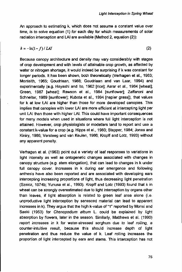
Light Interception in Spring Wheat
An approach to estimating k, which does not assume a constant value over time, is to solve equation (1) for each day for which measurements of solar radiation interception and LAI are available (Method 2, equation (2)):
k = -\n(l-f)/LAI (2)
Because canopy architecture and density may vary considerably with stages of crop development and with levels of attainable crop growth, as affected by water or nitrogen shortage, it would indeed be surprising if k was constant for longer periods. It has been shown, both theoretically (Verhagen et al., 1963; Monteith, 1965; Goudriaan, 1988; Goudriaan and van Laar, 1994) and experimentally (e.g. Hayashi and Ito, 1962 [rice]; Asrar et al., 1984 [wheat]; Green, 1987 [wheat]; Rawson et al., 1984 [sunflower]; Zaffaroni and Schneiter, 1989 [sunflower]; Kubota et al., 1994 [napier grass]), that values for k at low LAI are higher than those for more developed canopies. This implies that canopies with lower LAI are more efficient at intercepting light per unit LAI than those with higher LAI. This could have important consequences for many models when used in situations where full light interception is not attained. However, crop physiologists or modellers tend to report and use a constant k-value for a crop (e.g. Hipps et al., 1983; Stapper, 1984; Jones and Kiniry, 1986; Versteeg and van Keulen, 1986; Kropff and Lotz, 1993) without any apparent penalty.
Verhagen et al. (1963) point out a variety of leaf responses to variations in light intensity as well as ontogenetic changes associated with changes in canopy structure (e.g. stem elongation), that can lead to changes in k under full canopy cover, increases in k during ear emergence and following anthesis have also been reported and are associated with developing ears intercepting increasing proportions of light, thus decreasing light penetration (Szeicz, 1974b; Yunusa et al., 1993). Kropff and Lotz (1993) found that k in wheat can be strongly overestimated due to light interception by organs other than leaves, if light absorption is related to green leaf area alone (i.e. unproductive light interception by senesced material can lead to apparent increases in k). They argue that the high k-value of " 1 " reported by Monsi and Saeki (1953) for Chenopodium album L. could be explained by light absorption by flowers, later in the season. Similarly, Matthews et al. (1990) report increases in k for water-stressed sorghum due to leaf rolling, a counter-intuitive result, because this should increase depth of light penetration and thus reduce the value of k. Leaf rolling increases the proportion of light intercepted by ears and stems. This interception has not
75

Chapter 4
been accounted for by Matthews et al. (1990) when calculating k and may explain their result. Some of the higher k values reported by Yunusa et al. (1993) for dry-land wheat might also be associated with water stress decreasing the ratio of leaf area to stem and ear area and the way k is calculated based on LAI, particularly when considering their low anthesis LAI values.
About 50% of incident TS radiation is photosynthetically active (cf. Szeicz, 1974a). Differences in spectral distribution between TS (0.4 - 2 um) and PAR (0.4 - 0.7 |j.m) radiation, however, result in a non-linear relationship between measured f-values for both radiation components. Yunusa et al. (1993) report values for k based on TS that are approximately 30% smaller than estimates based on PAR. These differences are largely caused by the substantially higher absorption by green tissue of PAR than of the near-infrared fraction (NIR, 0.7 - 2 urn) of TS. Goudriaan and van Laar (1994) point out that k for NIR is about half of kPAR. Such differences need to be considered in simulation analysis when estimating dry matter production based on light interception.
Thus, to improve accuracy in estimates of k and, as a result, also in crop growth simulation, this study aims • to compare estimates of light interception and k based on either PAR or TS
measurements, • to investigate causes of changes in k during early crop growth, and • to assess the impact of such changes on simulated biomass production.
Methods
2.1. Experimental details
An experiment investigating the effects of water and nitrogen on the growth of spring wheat (cv. Hartog) was conducted during winter of 1993 on the Darling Downs, Queensland, Australia (27°34'S, 151°52'E). The crop was grown under either full irrigation (irr) or entirely on stored soil moisture (dry) and under four levels of applied nitrogen (0, 40, 120 and 360 kg N ha'1 ). The soil is an alluvial, heavy cracking clay (Ug 5.24; Northcote, 1979) with a high plant-available water-holding capacity (240 mm). The soil profile was filled to capacity at sowing. Full experimental details and results are presented in Chapter 3.
76

Light Interception in Spring Wheat
Daily fraction of intercepted total short-wave radiation (frs) by the crop canopy was determined using tube solarimeters (Delta-T Devices Ltd., 0.4 - 2 (xm) from July 19 (25 days after sowing, DAS) to final harvest (145 DAS). One tube each was placed above the dryland and the irrigated plots, respectively, to obtain reference readings. All other sensors were placed on the soil surface, at right angles to the rows in (a) each of two replicates of the dryland experiment and (b) replicate 2 of the irrigated treatment. Two of the sensors failed during the experiment (dry, 120N, replicate 2 and irr, 120N).
Fraction of intercepted photosynthetically active radiation (fPAR) was measured at approximately weekly intervals from 36 DAS to 85 DAS using a 1-m quantum sensor (0.4 - 0.7 um, LI-COR, Lincoln, Nebraska). In each plot, the sensor was placed perpendicular to the rows, first above the crop and then under the crop on the soil surface. Each reading was integrated over a 10 s period and an average was obtained by repeating this procedure three times for each plot in rapid succession. Readings were taken between 11 am and 2.15 pm. To calculate cumulative light interception from these measurements, negative exponential curves of the form I = l-axexp("DAS) were fitted to measurements from each plot, where I is the fraction of intercepted PAR, a and b are fitted coefficients. The curves described the data well with R2 varying from 0.84 to 0.98.
Destructive leaf area and dry matter samples were taken prior to anthesis on DAS 49 (dry and irr) and 70 (irr only), and at anthesis on DAS 104. PAR interception was determined just prior to destructively sampling an area of 0.25 m2 in each plot. Plants were separated into leaf and stem, whereby leaf sheaths were classed as stem material. After measuring leaf area using a LI-COR leaf area meter, dry matter of plant fractions was determined.
2.2. Analytical details
From these experimental data, values for kTs and kPAR were determined using the two methods based either on equation (1) or (2). Marshall and Willey (1983) describe the relation between fTs and fPAR as:
ln ( l - / r e ) = (ln(l-/™))/<7 (3)
where q is an empirical factor derived from measurements of light absorption. Marshall and Willey (1983) and Squire (1990) report a value of 1.4 for q for
77

Chapter 4
various species. Based on these measurements q was also calculated for spring wheat.
The impact of using either a constant or a variable k on estimates of above-ground biomass production was investigated for the period up to anthesis for two levels of maximum LAI. For this assessment, leaf area development was described using a logistic function of the form:
LAI = LAIma I (1 + exp(-a(7T - *))) (4)
where LAImax is the maximum LAI, TT is thermal time from sowing (base temperature = 0 °C) and a and b are fitted coefficients (Milroy and Goyne, 1995). Coefficient a characterizes the steepness of the curve and b is the value of TT at which LAI equals half LAImax. Biomass at any time was calculated as cumulative intercepted TS radiation multiplied by RUE of 1.34 g MJ"1 (Chapter 3). Temperature, solar radiation, LAI and TDM data were also those presented in Chapter 3. Leaf area development was described using equation (4) with an LAImax of 2.0 (a typical value under dryland conditions in Australia) and 7.0 (maximum LAI under non-limiting growing conditions), respectively. Coefficients a and b were fitted to average LAI data of the dry treatment and of the irrigated, 360N treatment, respectively (Fig. 4.1). The aim was not to accurately describe time course of leaf area development in these treatments, but rather to show the applicability of such generalized LAI functions to irrigated and dryland situations, respectively.
3
8
6 -
4 -
2
0 0
dry irr
• APS15_irr o APS15_dry
20 40
f~* / J
/
ƒ 60
DAS
1
80
*
£ i
100
Figure 4.1: Schematic representation of leaf area development for the dryland (APS15_dry) and irrigated treatments (APS15_irr, observed data from Chapter 3). Coefficients a and b (Equation 4) were fitted to LAI data on DAS 49 (dry and irr) and DAS 70 (irr only). Vertical bars represent +/-one standard error.
78

Light Interception in Spring Wheat
Results and discussion
3.1. Constant k
Based on equation (1) a value of kPAR = 0.48 was calculated (Fig. 4.2). Yunusa et al. (1993) report a similar value of kPAR = 0.52 for three spring wheat cultivars prior to ear emergence. Under low LAI (i.e. LAI < 1) the regression in Fig. 4.2 under-estimates light interception. This is the result of the strong influence of the high LAI values on the slope of the regression and implies that the slope of the exponential decay function for light interception is not constant.
Figure 4.2: Linear regression of log transformed fPAR on LAI for all available data (dry and irrigated treatments). The regression line was forced through the origin (R = 0.91).
Measurements of fTs were available throughout the experiment, but not for all treatments and/or replicates. Conversely, fpAR data were collected for all treatments and replicates, but only for a limited period of time (DAS 36 to 85). Thus, it needed to be established whether fPAR could be converted to fTs using equation (3) and whether the estimates of k obtained in this way were similar.
Based on equation (3), the logarithmic values of TS and PAR transmission were plotted for all measurements taken on DAS 49. The linear regression was forced through the origin because TS and PAR transmission are identical when no light is intercepted (Fig. 4.3). High LAI values, giving fPAR and fTS
values near unity, were excluded to avoid artifacts associated with log
79

Chapter 4
transformation. Assuming a negative exponential decay for the extinction of both radiation components, it follows that the slope of this regression (q, equation (3)) equals the inverse ratio of the two extinction coefficients. Because fTs integrates two components, fPAR and fNiR (transmission of near-infrared radiation), which have widely different extinction coefficients, it also follows that at high values of LAI nearly all transmitted radiation belongs to the NIR fraction of the spectrum, whereas at low LAI the ratio is close to 0.5. Thus, fTs is not exponential in the true mathematical sense, and the theoretical relation between In (1 - fTs) and In (1 - fPAR) is curvilinear. Even when extreme values for kPAR and kN!R are assumed, however, the theoretical curve only deviates slightly from a straight line and it can be assumed that experimental error outweighs by far such small differences, allowing us to assume a linear relation (Fig. 4.3). However, the value of q = 1.14 (R2 = 0.75) differs from the 1.4 value reported by Marshall and Willey (1983). This is likely related to the fact that fPAR was only measured at solar noon, whereas fTs was based on daily integrals. Since f varies proportionally with solar angle and reaches its minimum at solar noon (Charles-Edwards and Lawn, 1984; Hammer and Vanderlip, 1989) the estimate of q must be smaller than when comparing daily integral measurements of fPAR and fTs- Yunusa et al. (1993) also compared solar noon fPAR measurements with daily integrals of fTs, but their measurements were (i) taken earlier in the season and (ii) at a location 5° further south. Compared with this experiment, both these factors result in a smaller solar angle at noon, which explains their finding of q = 1.3.
-2.0 -1.5
y = 1.14 x
o o
o 0
o
ê O
ln(1-fTs) -1.0 -0.5
o. o , o o oo^^svtr
0 CD
0.0
oö<p
u.u
-0.5
- -1.0
-1.5
-2.0
-2.5
L -3.0
'S <
Figure 4.3: Relation between fraction of intercepted total short-wave and photosynthetically active radiation (fTs and fPAR) for dryland and irrigated spring wheat prior to anthesis. The linear regression was forced through the origin (R2 = 0.84, 5% confidence interval of the regression slope: +/- 0.07).
80
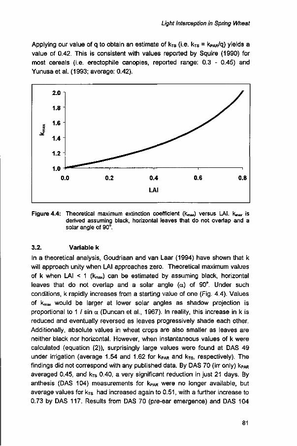
Light Interception in Spring Wheat
Applying our value of q to obtain an estimate of kTs (i.e. kTs = kPAR/q) yields a value of 0.42. This is consistent with values reported by Squire (1990) for most cereals (i.e. erectophile canopies, reported range: 0.3 - 0.45) and Yunusa et al. (1993; average: 0.42).
Figure 4.4: Theoretical maximum extinction coefficient (Km) versus LAI. I w is derived assuming black, horizontal leaves that do not overlap and a solar angle of 90°.
3.2. Variable k
In a theoretical analysis, Goudriaan and van Laar (1994) have shown that k will approach unity when LAI approaches zero. Theoretical maximum values of k when LAI < 1 (kmax) can be estimated by assuming black, horizontal leaves that do not overlap and a solar angle (a) of 90°. Under such conditions, k rapidly increases from a starting value of one (Fig. 4.4). Values of kmax would be larger at lower solar angles as shadow projection is proportional to 1 / sin a (Duncan et al., 1967). In reality, this increase in k is reduced and eventually reversed as leaves progressively shade each other. Additionally, absolute values in wheat crops are also smaller as leaves are neither black nor horizontal. However, when instantaneous values of k were calculated (equation (2)), surprisingly large values were found at DAS 49 under irrigation (average 1.54 and 1.62 for kPAR and kTs, respectively). The findings did not correspond with any published data. By DAS 70 (irr only) kPAR
averaged 0.45, and kTs 0.40, a very significant reduction in just 21 days. By anthesis (DAS 104) measurements for kPAR were no longer available, but average values for kTs had increased again to 0.51, with a further increase to 0.73 by DAS 117. Results from DAS 70 (pre-ear emergence) and DAS 104
81

Chapter 4
(anthesis) are similar to those of Yunusa et al. (1993) who reported average kTs for three spring wheat cultivars grown in Western Australia of 0.42 and 0.50 during the pre-ear emergence and pre-anthesis periods, respectively. This increase in k is the result of light interception by the emerging ears and can differ from cultivar to cultivar and season to season (Yunusa et al., 1993). For this data it was assumed that the increase in k after anthesis was due mainly to the rapid onset of leaf senescence and subsequent interception by senesced material (Chapter 3). Because no further structural canopy changes besides senescence are likely to occur during that period, it appears appropriate to ignore this apparent increase in k after anthesis and thus ignore the unproductive light interception by senesced material.
It is likely that ontogenetically induced changes in k occur in most graminae and some evidence for a similar response in barley was obtained (data not presented). Kubota et al. (1994) argue for napier grass that an early decrease in k is caused by stem elongation, resulting in the canopy of grass species changing from a planophile to an erectophile type. The presented data reveal that minimum values of k in spring wheat are reached prior to stem elongation. Canopy changes associated with stem elongation are thus not likely to be the cause of the observed early variation in k.
3.0
2.5 -
2.0 -1
J- 1.5 -
1.0
0.5
n n -
o
i
\
i
0
>
L
\
k. „°o°o
1
2
•
• •
1
4
LAI
•
— • m
6 i
8
Figure 4.5: Relationship between kPAR and LAI. Closed symbols are from the experiment described in Chapter 3. Open symbols represent spring wheat data for the same cultivar grown at a different location in 1992 (Keating and Meinke, unpublished). The line was fitted to closed symbols only.
82

Light Interception in Spring Wheat
Plotting kpAR from DAS 49 and DAS 70 against LAI (Fig. 4.5) shows a relationship of the form
kPAR =cxexp(-dxLAI) + e (5)
where c = 6.2, d = 5.4 and e = 0.45 (R = 0.74). Unpublished data from Keating and Meinke using the same cultivar in the preceding year at a different location revealed a similar trend (open symbols, Fig. 4.5). Equation (5) indicates that kPAR prior to ear emergence remained constant at a value around 0.45 (coefficient e), once a critical LAI value of about one was exceeded. This is supported by the results presented in Fig. 4.2 and identical to values reported elsewhere for wheat (e.g. Gallagher and Biscoe, 1978). This does not explain the large values when LAI < 1. Because light interception was measured according to common practice and theoretical deliberations (Fig. 4.4) combined with knowledge of canopy structure (i.e. leaf angle, mutual shading; cf. Goudriaan and van Laar, 1994) does not permit such high k-values, the measurements of LAI were investigated as a potential source of error. It is possible that excessively high, but rapidly declining k-values could be related to reduced interception by sheath and stem and reduction in the importance of such interception as development progresses. Such tissue has not been included in the LAI measurements.
1.5 -
1.0
2 0.5
0.0 ~i (
: t s ^
I
) 200 i
400
Stem number m"2
I
600 '
800
Figure 4.6: Relationship between LAI and stem number for LAI < 1 (R = 0.90). The dotted line represents the sowing density of 100 plants m"2.
83

Chapter 4
During early growth of spring wheat, tillering is largely responsible for LAI
increases, as indicated by the linear relation between LAI and stem number
during this phase (Fig. 4.6). Although a data-set with various levels of
nitrogen fertiliser and + / - irrigation was used, early crop growth (DAS < 50)
was not limited by either of these factors. The only observed difference during
this phase was a higher soil temperature in the dry treatment, which
accelerated leaf area development, resulting in a significantly larger LAI at
DAS 49 then under irrigation (Chapter 3). The linearity between stem number
and LAI implies that the higher soil temperature resulted in more tillers and
hence faster leaf area development. This is in agreement with Spitters and
Kramer (1986) who showed that early leaf area development can be fully
described as a function of soil temperature.
Nitrogen effects on LAI were not significant at DAS 49, but were highly
significant at DAS 70 (Chapter 3). Green (1987) found that nitrogen supply
had little effect on the optical properties of foliage and concluded that
variations in k prior to canopy senescence result from differences in canopy
structure. Unpublished data from a fully irrigated spring wheat experiment
near Gatton, Australia, revealed a highly significant nitrogen effect on early
LAI for samples taken at 40 DAS. Nitrogen deficiency early in that experiment
also reduced tiller production, again affecting canopy structure. This resulted
in a similar relationship between LAI and k to that observed in this study (Fig.
4.5; Keating and Meinke, pers. comm.).
3.0
2.5
2.0
1.5
1.0
0.5
0.0
0.0 0.5 1.0
LAIc
1.5 2.0
Figure 4.7: Fitted curves to kpAR data calculated based on LAI adjusted for stem dry matter (LAIC) using a weighting factor (w).
84

Light Interception in Spring Wheat
When LAI is small, it is likely that LAI measurements that exclude the sheath and stem area are a poor approximation for the plant surfaces actually intercepting solar radiation. Sheehy et al. (1980) incorporated this effect in their perennial ryegrass model by adding a constant value of 0.5 to green LAI. In their rice model, Kropff et al. (1994) account for assimilation by stem material by adding 50% of stem area to their green LAI calculations. Dry matter (DM, g m"2) and specific leaf area data (SLA, cm2 g"1) corresponding with these LAI measurements is reported in Chapter 3. Stem DM was converted to a stem area estimate by multiplying with SLA and a weighting factor (w) to account for the lower specific area of stems. These stem area estimates were added to LAI, assuming values of w ranging from zero to one. Equation (5) was then re-fitted to the newly obtained green area estimates ("corrected" LAI, LAIC). Fig. 4.7 shows the fitted curves in increments of 0.2 for w. The curves were curtailed at LAIC of 0.15, which represents the extrapolation of the LAI vs stem number relationship (Fig. 4.6) to the plant density. Although these curves result in vastly different kPAR estimates at low LAU, values at LAI = 1 are near-identical (range: 0.47 to 0.50; Table 4.1). Furthermore, the asymptotic values for estimates of kPAR (coefficient e, equation 5 and Table 4.1) are outside the normal range reported for kpAR when w > 0.2 (Squire, 1990). This could indicate that w declines from a maximum value of one at a theoretical LAI of zero to zero when LAI approaches unity.
1.2 -
1.0 -
0.8 -u. 2 0.6 -
0.4
0.2
\>M
0.0
* *
«# s
' 0.5
> s •
" " k =-0.85* LAI+ 1.3
• w = 1-LAI
^ ~ k = 0.45 s
1.0 1.5
LAI«
I
2.0
Figure 4.8: Relation of kpAR and LAIC derived when applying a linearly scaled weighting factor, w, to adjust green LAI data for light interception by stem material at LAI < 1. See text for details.
85

Chapter 4
A decline in w with development appears logical considering that stem thickness increases rapidly during this time. As new leaves form, their sheaths are rolled around each other and therefore each new sheath contributes less to stem area than the preceding one. Hence, morphogenetic processes are responsible for a disproportionate increase in stem weight : stem surface area. On the basis of data presented in Fig. 4.7 such a linear decline in w (i.e. w = 1 - LAI; LAI < 1) was plotted for kPAR versus LAIC at increments of 0.2 and fitted a linear regression to the data (Fig. 4.8).
Table 4.1: Coefficients fitted to equation (5) for curves presented in Fig. 6 (kpAR versus LAIC). Also shown are kPAR values at LAI = 0.15 (emergence) and LAI = 1 for w ranging from 0 to 1 (see text for detailed explanation).
w
0.0
0.2
0.4
0.6
0.8
1.0
c
6.191
3.657
2.222
1.594
1.199
1.000
d
5.356
3.811
2.732
2.141
1.704
1.458
e
0.454
0.391
0.344
0.310
0.281
0.259
Rs
0.74
0.65
0.61
0.58
0.57
0.56
LAIC = 0.15
kpAR
3.23
2.46
1.82
1.47
1.21
1.06
LAIC = 1
kpAR
0.48
0.47
0.49
0.50
0.50
0.49
Based on data presented in Fig. 4.5, k is kept constant at 0.45 when LAI > 1 during the pre-ear emergence stage. Using w as a linearly scaled weighting factor to correct green LAI for light interception by stems, kPAR can now be expressed as:
kPÀR = -0.85 x LAIC +1.3 for LAIC < 1 kPAR = 0.45 for LAI > 1, LAI = LAIC (6)
The effect on light interception of using LAIC values and equation (6) is near-identical to using measured, green LAI values in equation (5). Some wheat models predict LAI based on green LAI measurement methods as used in this study (e.g. Sinclair and Amir, 1991), others include leaf sheaths, but not stems (Ritchie et al., 1985) whilst some assume green area instead of LAI (Stapper, 1984; van Keulen and Seligman, 1987). It is therefore important to clearly distinguish these different approaches when quantifying parameter
86

Light Interception in Spring Wheat
values for light interception simulation. While it is biologically sensible to use adjusted LAI and equation (6) to estimate k during early growth, not all models simulate stem and sheath dry weight that could be used to obtain LAIC. If the effect of more efficient light interception when LAI < 1 is to be incorporated in such models, equation (5) offers a simple, albeit empirical way of doing so. Although the generality of the coefficients of this equation is uncertain, data from the same cultivar grown in a different temperature environment, and under levels of nitrogen ranging from severe nitrogen shortage to abundant availability, indicate at least some commonality (Keating and Meinke, unpublished data, Fig. 4.5).
3.3. Sensitivity analysis
We assessed the impact of constant versus variable k on simulated dry matter production. For this purpose the various values of kPAR were converted to kTs equivalents (kTs') using equation (3) and the measured value of q = 1.14. Whilst this is appropriate to convert mid-day PAR measurements to daily integrals of TS, the value of q depends on time of the year and latitude. Dry matter production was calculated based on estimated TS interception and a conversion efficiency value (RUETS) of 1.34 (Chapter 3). The use of either (i) a constant kTs> of 0.42 or (ii) a variable k (kTs-_v) based on equation (5) was compared. In accordance with the data, the asymptotic value of kTs*_v was increased by 0.003 d"1 after DAS 70 to reach a maximum value of kTs-_v = 0.48 at anthesis. Simulations with these parameter values are referred to as "reference conditions". Using kTs*_v predicted the time course of TDM production well and within the error of measurement, regardless of water treatment (Fig. 4.9). The constant k method initially underpredicted TDM by about 40 g m"2 and maintained this difference up to anthesis.
As pointed out earlier, including measurements of interception at high LAI values to calculate a constant k can lead to an underestimation of that value. We therefore assessed the sensitivity on TDM production of either over- or underestimating a constant k by 25%. The effect is expressed as TDM difference between TDM estimates based on kTs-_v and a constant k value (Fig. 4.10). Reference conditions show the strong effect on early biomass production with only a small subsequent increase in TDM difference up to anthesis (Fig. 4.10a). The initial, rapid increase in TDM differences ceases at about DAS 50 - 55 when LAI reaches unity, w = 0 and kTS-_v becomes constant. Subsequently, it depends on the intercepted light differential and the conversion efficiency as to whether TDM differences diminish, are maintained or increase with time. When k is overestimated by 25% (i.e. kTS- =
87

Chapter 4
0.52) TDM is still underestimated during early growth but the difference diminished with time (Fig. 4.10b). This resulted in no TDM difference for the irrigated treatment and a 31 g m"2 higher estimate of TDM for the dryland treatment by anthesis when using a constant k (Fig. 4.10b). Conversely, when a constant k is underestimated by 25% (kTs- = 0.32) TDM differences between the methods continue to increase in a quasi linear fashion up to anthesis (Fig. 4.10c) when the observed differences in TDM for the dryland and irrigated simulations were 170 and 128 gm"2, respectively (Fig. 4.10c). While this difference constitutes 34% of TDM produced under dryland conditions we acknowledge that this represents a potential maximum effect since (i) a k value of 0.31 is at the low end of expected values and would rarely be used and (ii) under more severe water limitations than in the present situation, RUE would likely be reduced, thus reducing the effect of light interception on TDM accumulation.
The sensitivity analysis shows that in situations where high leaf area can be achieved, the slight under-estimation of early dry matter production by conventional simulations that use a constant k has no significant consequences for dry matter production at anthesis, unless the constant k is substantially underestimated.
However, in situations where maximum LAI values are low, as is frequently the case in dryland wheat production, anthesis dry matter can be underestimated by up to 34%, if light interception by photosynthetically active material other than leaves during early growth is ignored and k is underestimated.
88
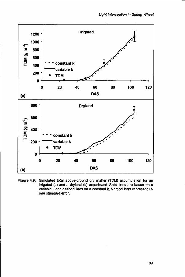
Light Interception in Spring Wheat
1200
_ 1000 est
E 800 O)
g 600 Q
t- 400
200
0
Irrigated
constant k
'variable k
• TDM
20 40
(a)
60
DAS
80 100 120
E 3 o 1-
800
600
400i
200
n
" " " constant k
variable k • TDM
1 • - f
Dryland
20 40
(b)
60
DAS
80 100 120
Figure 4.9: Simulated total above-ground dry matter (TDM) accumulation for an irrigated (a) and a dryland (b) experiment. Solid lines are based on a variable k and dashed lines on a constant k. Vertical bars represent +/-one standard error.
89

Chapter 4
150 -i
CM
E ra 100
TDM
diff
eren
ce
Ul
o
o
-50 J
C
(a)
100
E ra 50
diff
eren
ce
o
S -50 Q 1-
-100
(b)
200 -,
CM
E ra 150 -
TDM
diff
eren
ce
Ol
o
o
o
o
-1
1 1
0
(c)
k = 0.42
Dryland
- - - - Irrigated
20
i k = 0.52
- - - - Irrigated
0 20
k = 0.32
Irrigated
•
20
y»
• i i
40 60
DAS
St ^ ^ ^ f c
St ^ ^
40 60
DAS
Xt f t
/1 ^ £ t
40 60
DAS
80
80
fg{*"~
80
1
100
100
-s ^-*
100
Figure 4.10: Impact on simulated dry matter production (TDM) of using constant k-values versus a variable value for a range of constant k values, (a) Reference conditions, k = 0.42, (b) k = 0.52, (c) k = 0.32. Data are presented as the difference between TDM calculated using a variable k or a constant value for total short-wave interception. Solid lines refer to a simulated dryland situation with a LAImax of 2 and dashed lines to an irrigated situation (LAImax = 7).
90

Light Interception in Spring Wheat
4. Conclusions
We have quantified and attempted to explain possible causes of changes in k during early growth of spring wheat. Our results suggest that while k varies with LAI and structural canopy changes, much of the observed early variation can be attributed to interception by plant material other than leaves. Values of k will decrease as LAI increases to one, followed by an increase during ear emergence and a further increase due to interception by senesced material. The simulation study indicated that high k values during early crop growth are unimportant, if high maximum LAI values are attained. However, if LAImax is low, as is frequently the case in dryland wheat production, the error can be substantial.
References
Asrar, G., Hipps, L.E. and Kanemasu, E.T., 1984. Assessing solar energy and water use efficiency in winter wheat: A case study. Agric. For. Meteorol., 31:47-58.
Charles-Edwards, D.A. and Lawn, R.J., 1984. Light interception by grain legume row crops. Plant, Cell and Env., 7: 247-251.
Davies, P., 1992. The Mind of God. Science and the Search for Ultimate Meaning. Penguin Books, London, UK, 254 pp.
Duncan, W.G., Loomis, R.S., Williams, W.A. and Hanau, R., 1967. A model for simulating photosynthesis in plant communities. Hilgardia, 38:181-205.
Gallagher, J.N and Biscoe, P.V., 1978. Radiation absorption, growth and yield of cereals. J. Agric. Sei., Camb., 91: 47-60.
Goudriaan, J., 1988. The bare bones of leaf-angle distribution in radiation models for canopy photosynthesis and energy exchange. Agric. For. Meteorol., 43: 155-169.
Goudriaan, J. and van Laar, H.H., 1994. Modelling Potential Crop Growth Processes. Kluwer Academic Publishers, Dordrecht, The Netherlands, 238
PP-Green, CF., 1987. Nitrogen nutrition and wheat growth in relation to
absorbed solar radiation. Agric. For. Meteorol., 41: 207-248. Hammer, G.L. and Vanderlip, R.L., 1989. Genotype-by-environment
interactions in grain sorghum I. Effects of temperature and radiation use efficiency. Crop Sei., 29: 370-376.
91

Chapter 4
Hayashi, K. and Ito, I., 1962. Studies on the form of plant in rice varieties: I. Significance of the extinction coefficient. Proc. Crop Sei. Soc. Japan, 30: 329.
Hipps, L.E., Asrar, G. and Kanemasu, E.T., 1983. Assessing the interception of photosynthetically active radiation in winter wheat. Agric. Meteorol., 28: 253-259.
Jackson, J.E. and Palmer, J.W., 1979. A simple model of light transmission and interception by discontinuous canopies. Ann. Bot., 44: 381-383.
Jones, C.A. and Kiniry, J.R., 1986. CERES-Maize. A Simulation Model of Maize Growth and Development. Texas A&M University Press, College Station, 194 pp.
Keulen, H. van and Seligman, N.G., 1987. Simulation of Water Use, Nitrogen Nutrition and Growth of a Spring Wheat Crop. Simulation Monographs, Pudoc, Wageningen, The Netherlands. 309 pp.
Kropff, M.J. and Lotz, L.A.P., 1993. Eco-physiological characterization of the species. In: Modelling crop-weed interactions. M.J. Kropff and H.H. van Laar (Editors), CAB International, Wallingford, Oxon, UK, 83-104 p.
Kropff, M.J., van Laar, H.H. and Matthews, R.B. (Editors), 1994. ORYZA1 An ecophysiological model for irrigated rice production. SARP Research Proceedings - September 1994. DLO-Research Institute for Agrobiology and Soil Fertility, Wageningen, The Netherlands, 110 pp.
Kubota, F., Matsuda, Y., Agata, W. and Nada, K., 1994. The relationship between canopy structure and high productivity in napier grass, Pennisetum purpureum Schumach. Field Crops Res., 38:105-110.
Marshall, B. and Willey, R.W., 1983. Radiation interception and growth in an intercrop of pearl millet/groundnut. Field Crops Res., 7: 141-192.
Matthews, R.B., Azam-Ali, S.N. and Peacock, J.M., 1990. Response of four sorghum lines to mid-season drought. II. Leaf characteristics. Field Crops Res., 25: 297-308.
Milroy, S.P. and Goyne, P.J., 1995. Leaf area development in barley - model construction and response to soil moisture status. Aust. J. Agric. Res., 46: 845-860.
Monsi, M. and Saeki, T., 1953. Über den Lichtfaktor in den Pflanzengesellschaften und seine Bedeutung für die Stoffproduktion. Jap. J. Bot., 14: 22-52.
Monsi, M., Uchijima, Z. and Oikawa, T., 1973. Structure of foliage canopies and photosynthesis. Ann. Rev. Ecol. Syst., 4: 301-327.
Monteith, J.L., 1965. Light distribution and photosynthesis in field crops. Ann. Bot., 29: 17-37.
92

Light Interception in Spring Wheat
Northcote, K.H., 1979. A Factual Key for the Recognition of Australian Soils, 4th edn. Rellin Tech. Publications, Adelaide, Australia, 123 pp.
Rawson, H.M, Dunstone, R.L., Long, M.J. and Begg, J.E., 1984. Canopy development, light interception and seed production in sunflower as influenced by temperature and radiation. Aust. J. Plant Physiol., 11: 255-265.
Ritchie, J.T., Godwin, D.C. and Otter-Nacke, S., 1985. CERES-Wheat. A Simulation Model of Wheat Growth and Development. Texas A&M University Press, College Station.
Sheehy, J.E., Cobby, J.M. and Ryle, G.J.A., 1980. The use of a model to investigate the influence of some environmental factors on the growth of perennial ryegrass. Ann. Bot., 46: 343-365.
Sinclair, T.R. and Amir, J., 1991. A model of the temperature and solar-radiation effects on spring wheat growth and yield. Field Crops Res., 28: 47-58.
Squire, G.R., 1990. Dry Matter Production by Interception and Conversion of Solar Radiation. In: G.R. Squire (Editor). The Physiology of Tropical Crop Production. CAB International, Wallingford, Oxon, UK, pp 71-102.
Spitters, C.J.T. and Kramer, Th., 1986. Differences between spring wheat cultivars in early growth. Euphytica, 35: 273-292.
Stapper, M., 1984. SIMTAG: A Simulation Model of Wheat Genotypes. Model Documentation. ICARDA, Aleppo, Syria and University of New England, Armidale, NSW, Australia, 108 pp.
Szeicz, G., 1974a. Solar radiation for plant growth. J. Appl. Ecol., 11: 617-636.
Szeicz, G., 1974b. Solar radiation in crop canopies. J. Appl. Ecol., 11: 1117-1156.
Verhagen, A.M.W, Wilson, J.H. and Britten, E.J., 1963. Plant production in relation to foliage illumination. Ann. Bot., 27: 627-640.
Versteeg, M.N. and van Keulen, H., 1986. Potential crop production prediction by some simple calculation methods, as compared with computer simulation. Agric. Syst., 19: 249-272.
Wit, CT. de, 1965. Photosynthesis of leaf canopies. Agricultural Research Reports 663, Pudoc, Wageningen, 82 pp.
Yunusa, I.A.M., Siddique, K.H.M., Belford, R.K. and Karimi, M.M., 1993. Effect of canopy structure on efficiency of radiation interception and use in spring wheat cultivars during the pre-anthesis period in a mediterranean-type environment. Field Crops Res., 35: 113-122.
93

Chapter 4
Zaffaroni, E. and Schneiter, A.A., 1989. Water-use efficiency and light interception of semidwarf and standard-height sunflower hybrids grown in different row arrangements. Agron. J., 81: 831-836.
Appendix
All abbreviations, their description and units in alphabetical order.
Abbreviation
DAS DM DOY dry f fNIR
fpAR
fra irr k kpAR
kjs kjs* kjs* v LAI LAIc NIR PAR q RUE RUETS
SLA TDM I max
I min
TS TT w
Description
days after sowing dry matter day of the year treatment where rainfall or irrigation was excluded fractional light interception fraction of NIR interception fraction of PAR interception fraction of TS interception fully irrigated treatment light extinction coefficient light extinction coefficient for PAR light extinction coefficient for TS kpAR converted to kTs using q variable kTs* leaf area index LAI adjusted for interception by other plant material near-infrared fraction of TS photosynthetically active radiation conversion coefficient between frs and fPAR radiation use efficiency RUE based on intercepted TS radiation specific leaf area total, above-ground dry matter maximum temperature minimum temperature total short-wave radiation thermal time weighting factor for stem DM
Unit
gm"2
m2 m"2
m2 m"2
um MJ
gMJ-1
gMJ"1
g m °C °c MJ deg d
94

Testing Simulation Capabilities
Chapter 5
Testing Simulation Capabilities Of Wheat Growth And Resource Use (Water, Nitrogen And Solar Radiation)
In Australia
"Find out the cause of this effect, or rather say, the cause of this defect, for this effect defective comes by cause. " W. Shakespeare
Abstract
To simulate whole cropping systems, crop models must not only give reliable predictions of yield across a wide range of environmental conditions, they must also quantify the water and nutrient use well, so that the status of the soil at maturity is a good representation of the starting conditions for the next cropping sequence. So far this has not been a major objective when developing crop models. To assess the suitability for this task, the following wheat models, currently used in Australia, were tested: a modified, CERES-style model (NW; Probert et al., 1995), Sinclair and Amir's (1992) model (SA), a model by Hammer et al. (1987; HW), SIMTAG (Stapper, 1984; SI) and a barley model (Goyne et al., 1996; BA). The models differed in their design objectives, complexity and structure and two (SI and BA) do not contain a plant nitrogen balance. Models were (i) tested on diverse, independent data sets from a wide range of environments and (ii) model components were further evaluated with one detailed data set from a semi-arid environment. Models were coded into the cropping systems shell APS IM, which provides a common and well tested soil water and nitrogen balance. Furthermore, crop development was used as input, thus any difference between simulations was caused entirely by difference in simulating crop growth. Performance of model components was evaluated by means of root mean square deviation and by regression techniques.
Across five environments and seven experiments with a range of water and nitrogen treatments yield was generally better predicted than dry matter. Under nitrogen non-limiting conditions between 73 and 85% of the observed yield variation was explained by the models. This was in spite of the models
95
Chapter 5
inability to predict yield components well such as either kernel number and kernel weight or harvest index. Reasons for this apparent contradiction are discussed. Under nitrogen non-limiting conditions, a model using transpiration and transpiration efficiency (HW) to predict biomass and yield gave best results. When using data sets with potentially varying nitrogen supply, only one model (NW) predicted dry matter and yield responses well and errors in yield prediction in other models were strongly associated with overestimates of total dry matter under low nitrogen supply or overestimates of nitrogen uptake when water was limiting.
Leaf area was predicted poorly by all models and errors were associated, among others, with timing of leaf area development, effect of water or nitrogen stresses and poor simulation of tiller number. When measured light interception from one experiment containing four nitrogen and two water treatments was used as input, most models improved in their prediction of dry matter and yield, but in some cases water by nitrogen interaction also resulted in the opposite. This test, in particular, highlighted a range of compensating errors in all modelling approaches.
Time course and final amount of water extraction of a rain shelter experiment was simulated well by two models (SA and BA), while the other models left a substantial amount of potentially available soil water in the profile (up to 25%). This was associated with overestimating transpiration efficiency coupled with assumed restrictions of water uptake when fraction of available soil water is low. Applying various stress indices to growth resulted in a good to fair prediction of dry matter and yield in spite of the poor quantification of water use. Causes and consequences of these errors are discussed and improvements suggested.
While kernel nitrogen percentage was predicted poorly by all models due to its sensitivity to small dry matter changes, nitrogen percentages of other plant components were predicted well by NW. Predictions of total amount of plant nitrogen were confounded by errors in dry matter prediction.
This study identified strengths and weaknesses of a number of simulation approaches with particular emphasis on resource utilization. These findings should help to attain more reliable wheat simulation capabilities suitable to be included in a cropping systems framework.
96

Testing Simulation Capabilities
1. Introduction
Spring wheat is a major component of the Australian dryland cropping system with an average annual production of over 15 million tonnes (ABARE, 1994). Due to the extreme rainfall variability (Nicholls and Wong, 1991), annual production varies widely with region and season. Thus, producers are faced with high production risks and income fluctuation. Low, seasonal rainfall often masks effects of low soil fertility, which is only expressed in years when water does not limit production. Similar problems have been identified in other, semi-arid regions (van Keulen and Seligman, 1987). Nevertheless, Hamblin and Kyneur (1993) have shown some positive association with regional wheat yields and regions that use grain legumes, nitrogen fertilizers and legume-pasture in rotations. Simulation analysis provides an ideal tool to better quantify such effects and to devise detailed, regional management strategies that optimize farm incomes within a sustainable production system. Such simulation tools need to accurately quantify kernel yield and quality attributes, such as kernel nitrogen percentage. They also have to be capable of predicting the long-term effect of management strategies on soil resources such as organic matter, soil water and soil nitrogen content. The former requires a plant-oriented simulation approach, the latter is much more soil focused. Such objectives have often been tackled separately by plant and soil scientists, respectively. Hence, when developing simulation models, emphasis has often been either on the simulation of plant processes (Stapper, 1984; Hammer et al., 1987) or on soil processes (Parton and Rasmussen, 1994).
The shift of focus from predicting individual crop responses to analyzing the behaviour of cropping systems poses a particular challenge for crop models (Angus .et al., 1993; Meinke and Stapper, 1995). Through advances in computer technology it has become feasible to evaluate simultaneously crop responses to climate, soil conditions and crop management as well as the long-term impact of management scenarios on the resource base (Littleboy et al., 1992; McCown et al., 1996; Probert et al., 1995). A modular simulation environment allows scientists from many different disciplines to support convergent effort in testing, improving and applying models with change taking place simultaneously on many fronts (McCown et al., 1996; Meinke and Stapper, 1995).
One such systems model, APSIM, allows segregation of crop models into logical units or modules and provides the opportunity to test a range of
97

Chapter 5
modules using a common, state-of-the-art soil water and soil nitrogen balance (McCown et al., 1996). This feature, coupled with a common input file structure, removes ambiguity when interpreting model output, since all simulated differences in crop growth, water and nitrogen can be traced back to differences in the crop models (Meinke and Stapper, 1995).
Several wheat models have been developed and/or used for Australian wheat production, differing in objectives and hence design and level of process detail considered (Stapper, 1984; Hammer et al., 1985; O'Leary et al., 1985; Sinclair and Amir, 1992; Probert et al., 1995). All have proven useful for the purposes for which they were developed, but none have been designed specifically for accurate prediction of resource utilization and therefore for use within a systems model framework. They have been developed with data from a limited range of environments and cannot confidently be applied outside these environments without re-calibration and testing, resulting in modifications to the original model (e.g. Carberry et al., 1989). To arrive at a simulation capability applicable across all wheat producing regions in Australia, these models should be harnessed to stimulate model development, avoid duplication of research and foster collaboration amongst model builders and users. Thus the objectives of this study were:
• to assess and quantify the capabilities of current wheat models in Australia by testing their performance on a wide range of independent data from different environments,
• to test the models' abilities to predict soil water and soil nitrogen utilization as well as crop growth and yield and,
• to identify necessary improvements to simulation routines for crop processes.
2. Materials and methods
Testing of simulation models consists of two main activities: (i) establishing that the source codes representing the models perform as intended, and (ii) confirming that the simulation models accurately reproduce emperical data. Kleijnen (1995) refers to these two activities as model verification and validation (V & V), respectively. Although Oreskes et al. (1994) have shown that V & V, when applied to numerical models, are fallacies in a strict, philosophical sense, they are commonly used when model performance is discussed (e.g. McKinion and Baker, 1982). This study will concentrate on the latter activity, which, rather than validation, might be more appropriately
98

Testing Simulation Capabilities
referred to as model confirmation. To achieve this, data from seven independent and detailed experiments from five environments were used.
Four wheat models and one barley model were installed in the APS IM shell (McCown et al., 1996). Model source code was tested to the best of our ability using the APSIM philosophy of model desegregation and structuring the code into small, self-contained, logical modules (Fig. 5.1). Simulation of above-ground processes may differ among models but soil water and soil nitrogen balances are identical. As part of source code testing, the APSIM version of each model was compared to it's original, stand-alone version. For potential production these comparisons always yielded near-identical results. Minor discrepancies for water- and nitrogen-limited production could be attributed to differences between the original water and nitrogen balances and those used by APSIM.
2.1. The systems model APSIM and its components
The software system APSIM consists of a collection of models of crops, pastures, soil water, nutrients and erosion which can be configured to simulate diverse agricultural production systems (McCown et al., 1996). The following section briefly introduces the key features of APSIM modules used in this study (Fig. 5.1).
2.1.1. Water balance
APSIM_Water is similar to many cascading water balance models. It contains some processes, such as runoff and drainage that are described by Littleboy et al. (1992) and computes the daily change in soil water content by layer, whereby number and thickness of layers are input. It provides daily estimates of actual and potential evaporation (two stage evaporation algorithm; Ritchie, 1972) and potential évapotranspiration, based on leaf area index (LAI) supplied by a crop model. Actual, daily water extraction (i.e. actual transpiration), however, is determined by the crop model. Besides climatic data, essential inputs for the soil water module are drained upper limit, lower limit and wet bulk density for each soil layer.
2.1.2. Nitrogen balance
APSIM_Nitrogen is based on a CERES style nitrogen balance, but with some major modifications, such as the representation of the soil organic matter by two distinct pools differing in their rate of decomposition (Dimes, 1996;
99

Chapter 5
Probert et al., 1996). Processes such as nitrification and denitrification are calculated daily for each layer based on environmental conditions. A carbon and nitrogen balance is maintained. Essential inputs are initial N03 and organic matter content per layer. For model testing, necessary input parameters for APSIM_Water and APSIM_Nitrogen were determined seperately for each data set in consultation with the scientists conducting the experiment and scientists responsible for the further development of these models within APSIM.
2.1.3. Wheat models incorporated into APSIM
APSIM module configuration
APSIM_HW_Wheat
APSIM_SI_Wheat
APSIM_SA_Wheat
APSIM_NW_Wheat
APSIM_BA_Barley
^ Wi
APSIM_Manager
t •
/ E \
I N \^
G |
I I
V N / \ E yw>.
Other Module A
APSIM_Water
APSIM_Nitrogen
/^ Radiation ^ \ ( Temperature j V Rainfall J
Figure 5.1: APSIM module configuration. Communication among modules occurs through the central engine (for details see McCown et al., 1996). Solid arrows indicate the active modules.
100

Testing Simulation Capabilities
Based on the objective to improve systems analysis tools in Australia and faced with the constraints of parameterization, four spring wheat models and one barley model were incorporated into APSIM for detailed testing. For a simulation model to be useful (i) it must be conceptually appropriate for the question to be answered and (ii) its input requirements must be practically met (Carberry et al., 1989). A model also needs to be reliable, i.e. it needs to recurrently agree with observed phenomena, before it can be confidently used as a predictive tool. Denning (1990) argues that a model with many parameters is unlikely to be reliable because it is not feasible to explore the parameter space completely during testing. For this study the main interest is in models to assist decision making at the paddock, farm or policy level. This limited the selection of models to those of low to intermediate complexity where the necessary inputs have either been measured or can be readily derived. A recent report identified 12 wheat models currently in use worldwide without claiming to be a comprehensive review of all available wheat models (GCTE, 1994). Model selection was further restricted to those models that have already been successfully used in Australia. Since many models have common features and the selected models differ widely in their approaches, many features from other models, not explicitly tested, are nevertheless represented (e.g. Weir et al., 1984; O'Leary et al., 1985; van Keulen and Seligman, 1987).
The five models chosen were re-coded in FORTRAN using the standards as applied generally for the development of APSIM modules. This satisfied Kleijnen's (1995) demand for model verification. The origin of these models and the descriptive code assigned, which is used in all future references, are: • NW (NWheat; Probert et al., 1995) • SA (Amir and Sinclair, 1991a; Amir and Sinclair, 1991b; Sinclair and Amir,
1992) • HW (Woodruff and Tonks, 1983; Hammer et al., 1987) • SI (SIMTAG; Stapper, 1984) • BA (a barley model; Milroy and Goyne, 1995; Goyne et al., 1996)
All five models tested have the capability of simulating crop development, but differ strongly in the degree of detail. In some instances only temperature effects are considered (SA, HW), while others account for temperature and photoperiod (BA) or temperature, photoperiod and vernilization (NW, SI). Preliminary tests showed that the development routines of all models were either inadequate or required additional experimentation to derive coefficients to adequately simulate the range of cultivars and experiments in this study.
101

Chapter 5
Porter et al. (1993) reported similar discrepancies for wheat grown in New Zealand. After calibrating CERES-Wheat (on which NW is largely based), they found discrepancies of up to 28 days in prediction of anthesis date. This inability to predict crop development would confound the results of the simulation of crop growth. Thus, the processes of development and growth were de-coupled as much as possible and phenological observations were used as input so that simulations of growth processes could be compared and objectively assessed. While this highlights the need for improvement of phenology predictions, this will not be considered in this study.
All five models simulate crop growth based on input of daily rainfall, solar radiation, maximum and minimum air temperature. In some instances additional measurements such as soil temperature, vapour pressure deficit (VPD) or wind speed might improve simulations. However, such measurements are rarely available in conjunction with experimental data or with long-term, historical meteorological data, which is a necessary requirement for most applications of models (Meinke et al., 1993a, 1995). Hence, such additional environmental data were not used in this study.
The key features of each model and modifications from the published versions that were necessary to run the models within the APSIM framework will now be described:
2.1.3.1. NW This model was briefly described and used by Probert et al. (1995) for an analysis of a long-term fallow management trial in north-eastern Australia. It is largely based on CERES Wheat Version 2 (Ritchie et al., 1985), but contains some modifications. Processes simulated within NW include: • Total, above-ground dry matter (TDM) accumulation is based on total short
wave radiation interception and radiation conversion efficiency (RUE). RUE is derived from a continuous function of daily incident radiation and ranges from values above two when incident radiation is less than four to below 1.1 g MJ"1 when radiation exceeds 30 MJ d'1. This potential RUE is reduced under sub-optimal temperature, water and/or nitrogen conditions.
• RUE is on a net carbon basis, hence respiration is not simulated. Also, it is based on above-ground growth only. Carbon for roots is "generated" using partitioning coefficients.
• Leaf area development is simulated based on biomass partitioned to leaf, leaf number, leaf appearance, tillering, leaf senescence and specific leaf area (SLA). A leaf sheath biomass pool is maintained.
102
Testing Simulation Capabilities
The initial value of SLA is reduced quickly after emergence from 350 to reach a constant value of 250 cm2 g'1. Light interception is based on Lambert's law with an extinction coefficient (k) of 0.6 and 0.7 during the pre- and post-anthesis periods, respectively. A high temperature stress factor accelerates senescence of leaf area when maximum air temperatures exceeds 34 °C. Carbon is partitioned to roots, leaves, leaf sheaths, stem, ear and kernel. All plant components have critical and minimum nitrogen concentrations that depend on stage of development. Kernel number per plant is estimated as the product of stem weight on the first day of kernel growth and a genetic parameter. Potential kernel demand for carbohydrates and hence kernel weight (KW) is a function of a genetic factor (input) and temperature. Final kernel yield (KY) is the product of plant number, kernel number per plant and KW. Crop water demand is linked to biomass production via a transpiration efficiency coefficient (TEC) instead of being a function of potential evaporation and LAI as in the original CERES. Daily transpiration is calculated from a TEe of 6 g m"2 mm"1 kPa, VPD and amount of biomass produced on that day. The root system extends at a rate of 2.2 mm per °C after emergence. This extension rate can be reduced (i) under dry soil conditions or (ii) by insufficient dry matter production. The CERES water uptake and soil water deficit routines were replaced with alternative routines based on a fraction of transpirable soil water (FTSW). TDM production is limited when FTSW < 0.25, expansion growth (e.g. leaf area development) is limited when FTSW < 0.45, and tillering begins to be limited when FTSW < 1.0 and stops when FTSW = 0.5. Nitrogen uptake per layer is calculated as a function of root length density (mm ha"1), a maximum daily uptake rate per mm of roots, amount of nitrogen available based on APSIM_Nitrogen and FTSW in the layer. Maximum C:N ratio in kernels is 10:1. The fraction of biomass partitioned to roots decreases as a continuous function from 30% at emergence to 8% during kernel-filling. Translocation of nitrogen and carbon to kernels occurs during kernel filling. Water and nitrogen deficits and unfavourable temperatures (including frosts) affect key crop growth processes. Minor modifications were made to functions from the original CERES Wheat Version 2 that control frost damage, tillering, SLA, radiation use efficiency, k, and carbon partitioning between leaves, stem and roots.
103

Chapter 5
• Accumulated thermal time (TT, °Cd) from sowing to emergence and from emergence to the end of the juvenile phase can be input to better control phenology.
2.1.3.2. SA This model was used by Meinke et al. (1995) for the evaluation of weather data generators in sub-tropical Australia. It's key features are: • TDM accumulation is calculated from RUE (1.5 g TDM MJ'1) and amount of
intercepted radiation. As for rice (Sinclair and Horie, 1989), RUE is exponentially reduced when specific leaf nitrogen content (SLN) falls below three, and reaches zero when SLN approaches 0.3 g N m'2.
• Seed growth occurs in the period in which harvest index (HI) increases linearly. This period begins 90°Cd TT after anthesis and HI increases at a rate of 0.011 d'1.
• Leaf area is calculated as a function of TT, plant density, leaf appearance rate, leaf number on the mainstem and tillers, tiller number and an exponential regression of main-stem leaf area on number of leaves. LAI is reduced when either water or nitrogen is limiting.
• Leaf area development is retarded when the fraction of transpirable soil water (FTSW) falls below 0.4 and RUE is restricted when FTSW falls below 0.3.
• Light interception is based on total short wave radiation and calculated using Lambert's law with k = 0.5.
• Daily transpiration is calculated from TEC (set to 5.8 g m"2 mm"1 kPa, Tanner and Sinclair, 1983), VPD and amount of biomass produced on that day.
• Maximum daily rate of nitrogen uptake is calculated as a linear function of TT from emergence and reaches a maximum of 0.4 g m"2 when TT = 1200°Cd.
• Nitrogen uptake ceases after anthesis. • Minimum SLN for leaf area development is 0.8 g N m"2. This equals a leaf
N concentration (Leaf_N%) of 2% at a constant SLA of 250 cm2 g'1. Senesced leaves are assumed to retain 1 % nitrogen. Minimum stem N% is set to 1.2% and to 0.3% before and after translocation of nitrogen to seeds, respectively.
• It is assumed that 40% of N translocated from leaves to seeds results in a reduction of leaf area index (LAI) and the remaining 60% in a reduction of SLN.
• Seed nitrogen content cannot fall below 1.5%.
104

Testing Simulation Capabilities
Differences between published model and SA are: • A root front velocity was added (15 mm d"1 starting one day after sowing).
This was necessary in order to maintain a layered water and nitrogen balance. However, FTSW is calculated on a total profile basis as in the original.
• In the original model TT accumulation was accelerated by 6 °C each day FTSW fell below 0.2 in order to enhance phenological development. This feature was removed to match phenology with observed data.
• Provisions were made to specify the TT requirement for stages from (i) sowing to emergence, (ii) emergence to end of leaf growth, (iii) end of leaf growth to anthesis and (iv) anthesis to maturity.
• The TT requirement for the emergence of one leaf (phyllochron index) was defined as an input parameter to match actual phenology and final leaf number.
• Nitrogen can only be taken up by the crop if (i) roots are present in a layer and (ii) available soil water in a particular layer is greater than zero.
2.1.3.3. HW HW has been used in PERFECT and the WHEATMAN software packages. PERFECT is a model to analyze effects of soil erosion to long-term crop production. It simulates interactions between soil type, climate, fallow management strategy and crop sequence (Littleboy et al., 1992). WHEATMAN is a decision support system developed for farmers to aid variety choice (frost avoidance) and fertilizer management for wheat crops in Queensland, Australia (Woodruff, 1992). In this model the level of complexity (and hence the number of processes simulated) was kept to the minimum needed for reliable yield prediction in this, mostly water-limited, environment. The main features are: • Potential crop growth is determined from the product of transpiration and
transpiration efficiency (TE; g TDM mm"1). • TE is a function of potential evapo-transpiration (ET; mm) and decreases
from values of nine when ET < 1 to two when ET > 15 mm (Fischer, 1979). • Potential crop growth is modified by water and nitrogen stress indices to
determine observed dry matter production. • LAI is calculated from crop growth rate and leaf area ratio (LAR; cm2 leaf
g'1 TDM) and is modified by a water and a nitrogen stress index. LAR is related to phenological development.
• LAI is used by the water balance model to partition evaporative demand (i.e. ET) into potential soil evaporation (Ep) and potential transpiration (Tp).
105

Chapter 5
• Actual transpiration (Ta) is determined as the lesser of the potential transpiration and plant uptake capacity, which is based on soil water content and root depth.
• Optimum and minimum nitrogen contents for above-ground plant material declines with phenological development from maximum values of 9.0 and 3.5% at emergence, to minimum values of 1.3% and 0.9% at maturity, respectively.
• Demand for nitrogen is calculated from crop growth and required plant nitrogen concentration. Uptake of nitrogen depends on demand and the amount of nitrogen available and is further restricted when FTSW in a layer is low. A nitrogen stress factor is defined as the ratio of nitrogen uptake and nitrogen demand.
• KY is estimated using equations based on dry matter accumulation up to anthesis and crop growth rate around anthesis. HW accounts for a decrease in yield potential with later sowings as reported for north-eastern Australia (Woodruff and Tonks, 1983).
HW was re-coded from an original, stand-alone FORTRAN version without modifications to its intended logic.
2.1.3.4. SI SI has been used to assess effects of maturity type on productivity (Stapper and Harris, 1989) and to evaluate fallow management options in southeastern Australia (Fischer et al., 1990). It has been developed for winter rainfall, Mediterranean-type climates where spring wheat is sown in winter and matures in early summer. Wheat growth under these conditions is mainly temperature and/or radiation limited, particularly during the early stages of crop growth. SI is responsive to water deficit, but does not contain a nitrogen balance. The following processes are simulated: • Green area index is simulated from leaf appearance, leaf size, leaf
senescence, tillering, tiller senescence and stem/spike area as a function of temperature, stage of development and water availability. Potential leaf size of the first leaf on the main-stem is a cultivar specific input.
• Green area index determines the intercepted photosynthetically active irradiance (PAR).
• TDM accumulation is computed from intercepted radiation and RUE. • RUE is set to 2.9 and 2.3 g MJ"1 d'1 (on a PAR basis) during the pre- and
post anthesis period, respectively.
106

Testing Simulation Capabilities
• Light interception is based on PAR and calculated using Lambert's law with k = 0.45.
• Daily growth is reduced for water stress and sub-optimal temperatures and is partitioned to roots, leaves, stems, chaff or kernels, using factors that depend on the stage of development.
• Kernel number (KN) and hence maximum sink size is determined as a function of anthesis dry weight and a cultivar specific input parameter.
• Potential daily kernel growth depends on KN, TT and a cultivar dependent kernel growth factor that is negatively related to KN.
• A maximum limit of 20,000 kernels m"2 was removed in the APSIM version to allow simulation of environments where higher KN are observed. No further modifications were made to the logic of the model during re-coding.
2.1.3.5. BA This model was developed to assess regional production potential and to conduct risk analysis for barley production in north-eastern Australia (Goyne et al., 1996). Its general structure is based on the sunflower model of Chapman et al. (1993). BA was developed under the APSIM framework and did not require any modification. Although it was developed to simulate barley rather than wheat, many concepts are similar, if not identical, for both crops. Maximum tiller number is a cultivar specific input to the model and is usually between 12 and 18 tillers per plant for barley. The default value for barley of 13.8 tillers per plant was halfed for all wheat simulations to reflect the slower leaf area development of wheat. This was the only change made to the model. Similar to SI, the model is responsive to water limitation but does not contain a nitrogen balance. The main features are:
• TDM production is based either on the amount of intercepted radiation and RUE or on Ta and TE. Switching between the two approaches depends on the daily assessment of the most limiting resource, i.e. either intercepted solar radiation or amount of transpirable soil water, respectively.
• RUE has a value of 1.25 for intercepted, total short-wave radiation. After anthesis this value is decreased daily by 0.02 to account for the lower photosynthetic activity of ageing leaves.
• Light interception is based on total short wave radiation and calculated using Lambert's law with k = 0.4.
• TE is calculated daily as a function of VPD and a constant TEe of 5.5 g m"2
mm"1 kPa. • LAI is calculated on an area basis as a function of TT, development and
available soil water (Milroy and Goyne, 1995).
107

Chapter 5
• Soil water extraction is calculated from the extension of the root system, the amount of water present in each layer and a negative exponential time constant (kl) for water extraction (Meinke et al., 1993b; Thomas et al., 1995).
• KY is estimated from a linear increase of harvest index with TT and ceases when 90% of the TT from anthesis to maturity has been reached.
2.2. Environments and data sets used for model testing
For thorough model testing, detailed data sets from a wide range of environments were collated. All data sets were carefully screened to ensure that they contained sufficient detail for model parameterization. Although the objective was to improve wheat modelling capability in Australia, two data sets from other regions were also included to assess model performance under widely varying climatic conditions.
2.2.1. Environments
Data sets from five environments varying in temperature, solar radiation, rainfall amount and rainfall distribution were selected for testing. Table 5.1 summarises these environments, gives the precise location of the experiment used for model testing and a code that will be used to refer to these environments henceforth.
Some models require genetic input parameters to connect phenological processes with growth processes. For most cultivars the necessary genetic input parameters were available, but for cultivars at environment L input parameters had to be estimated using data from the irrigated and well fertilized treatments. Obviously, such a method is not desirable and highlights the need for models using published and easily accessible input parameters that are updated regularly as new cultivars become available.
2.2.2. Data sets
Seven data sets containing sufficient detail for parameterization of the various modules within APSIM were identified (Table 5.2). Experimental design and conditions will be described briefly for each experiment.
108

Testing Simulation Capabilities
Table 5.1 : Environments for which data sets were available for model testing.
Code Location Latitude Longitude Altitude Climate
G Gatton,
Australia
27°32'S 152°20'E 100 m sub-tropical, mild, dry
winters, summer rain
"T Toowoomba, 27°34'S 15r52'E
Australia
500 m sub-tropical,
cool, dry winters,
summer rain
' "35Ws" W Wagga-
Wagga,
Australia
145 10'E 300 m mediterranean,
cool, wet winters,
summer dry
'WfTN 85S36'W" M Michigan,
USA
300 m temperate, continental,
cold winters, hot and
dry summers
L Lincoln, 43°60'S 172°50'E
New Zealand
10 m temperate, maritime,
cool to mild, rain year
round
2.2.2.1. APS2
Yield potential of spring wheat (cultivar Hartog) was determined in 1991 for
two sowing dates (30.V. and 30.VII.; sowing density 100 plants m'2). The soil
was a deep, alluvial clay with high water holding capacity, but very low in
residual nitrogen. To avoid any possible water limitation, the crop was
planted into a soil profile filled to capacity and irrigated weekly with a
minimum of 30 mm. A total of 360 kg N was applied in three equal splits
starting at sowing and finishing prior to anthesis. Above-ground dry matter
was sampled several times and partitioned in green and dead leaves, stems
and spikes. Green leaf area was determined. Fertile tiller number (FTN),
TDM, KY and yield components (i.e. KN and KS) were measured at final
harvest. All climatic data were automatically recorded on site.
2.2.2.2. APS6
In 1992, a rate of nitrogen experiment was conducted using spring wheat
(cultivar Hartog) on a site adjacent to APS2 (same soil type). The experiment
was sown on 17.VI. at a rate of 120 plants m'2. Adequate weekly irrigation
and a profile filled to capacity at sowing guaranteed absence of water
limitation. Rates of applied fertilizer were 0, 40, 80, 120, 160 and 360 kg N
ha'1, the latter three treatments applied as split applications. All sampling
procedures were identical to APS2.
109

Chapter 5
Table 5.2:
Data set
APS2
APS6
APS14
APS15
MSU
Data-sets used for model testing.
Environment
G
G
G
T
M
Treatments
time of sowing
nitrogen
nitrogen
water x
nitrogen
water
Treatment
levels
2
6
4
8
4
Source
this study
this study
Probert and Keating,
unpublished
Chapter 3
Robertson and Giunta,
1994
NZ time of sowing
x water x
nitrogen
water
16 Jamieson, unpublished
WW W Fischer, unpublished
2.2.2.3. APS14 Spring wheat (cultivar Hartog) was sown at a rate of 100 plants m"2 on 29.VI. 1993 into a full soil water profile (Probert and Keating, unpublished). Four rates of nitrogen (0, 40, 80 and 200 kg N ha"1) were applied to plots located adjacent to APS6. All surface residues from previous crops were removed. Measurement type and frequency were similar to APS2 and APS6.
2.2.2.4. APS15 Spring wheat (cultivar Hartog) was grown either entirely on stored soil moisture (240 mm plant available water) using an automatic rain shelter or under full irrigation. Four levels of nitrogen fertilizer were applied (0, 40, 120 and 360 kg ha'1, the latter in three split applications prior to anthesis). The crop was sown on 24.VI.1993 at a rate of 100 plants m"2. Soil water and soil nitrogen was monitored and nitrogen content of all plant components was determined. Other measurements and their frequency were similar to those in the other APS experiments. For further details see Chapter 3.
2.2.2.5. MSU Spring wheat (cultivar Yecora 70) was sown at a rate of 280 plants m"2 on 4. IV. 1992 on a deep, sandy loam. Nitrogen fertilizer was applied at a rate of
110
Testing Simulation Capabilities
10 g N m'2 and crops were either irrigated based on evapo-transpiration estimates (control) or water was withheld at three different periods prior to kernel-filling, using rain shelters. The effect of early, mid and late water stress prior to the start of kernel-filling on KY and yield components was investigated. Further details are given by Robertson and Giunta (1994).
2.2.2.6. NZ In 1991, three spring wheat cultivars (Kokako, CRSW18 and CRSW50) were sown at three dates (17.VI.; 23.VII.; 28.IIX.), under either 'high' or 'low" management on a silty loam. Data for cultivar Kokako are available only for sowings 2 and 3. High management consisted of regular irrigation to avoid water limitations and application of 140 kg ha"1 of mineral nitrogen at sowing. No water or nitrogen was applied to the low management treatments. However, the soil was relatively high in residual nitrogen (ca. 100 kg ha"1 in the top 30 cm). The data set was specifically collected for model testing and measurements were similar to those in the APS experiments (Jamieson, unpublished data).
2.2.2.7. WW During three seasons, spring wheat (cultivar Egret in 1979 and cultivar WW33G in 1982 and 83) was sown on a red-brown earth at densities of 136, 257 and 176 plant m"2, respectively. Crops were well managed and nitrogen was applied to avoid N deficiencies. Crops were grown on stored soil moisture and rainfall without irrigation. Seasons differed strongly in rainfall amount and distribution (295, 73 and 485 mm in-season rainfall for the three seasons, respectively). Starting plant available soil moisture conditions also varied, ranging from 96 mm in 1979, 77 mm in 1982 to 21 mm in 1983. TDM and LAI were determined at regular intervals and KY and yield components were measured at final harvest (Fischer, unpublished data).
2.3. Model testing
2.3.1. Test I, model evaluation across environments
As part of a 3-tier evaluation process model performance was firstly evaluated for final harvest data across all environments. This test gives an indication of model stability across a wide range of climatic conditions. All five models can simulate growth under sub-optimal water supply, but two of the models (SI and BA) do not consider possible nitrogen limitations. Hence, data sets were grouped in two categories: (i) production under optimum nitrogen supply with varying water supply and (ii) production under potentially varying
111

Chapter 5
water and nitrogen supply. Data from potential yield treatments were used in both categories. For situation (i) the five models were tested with data from the five environments; for situation (ii) the three models containing nitrogen balances were tested using data from the three environments where rate of nitrogen experiments were conducted, namely environments G, L and T (Table 5.2).
The models' predictive performance for KY, final TDM, HI and LAI across all environments and data sets was tested. Final tiller number (FTN) and the yield components KN and KW were also tested where appropriate. Root mean square deviation (RMSD) was used to quantify goodness of fit of model predictions and measurements. RMSD was expressed as a percentage of the observed mean within environments and across environments (Wallach and Goffinet, 1989). Following Jamieson et al. (1991) predictions with RMSD < 20% of mean observed were classified as good, 20% < RMSD < 30% as fair and RMSD > 30% as poor. In addition, linear regressions were fitted to observed versus predicted data for all environments and regression coefficients were tested against the 1:1 line. Finally, the ratio of predicted average and observed average data across environments was calculated. RMSD allows comparative assessment of model performance at particular environments, linear regression expresses model stability across a range of environmental conditions (the closer the regression is to the 1:1 line, the better the model's stability) and the ratio of average predicted to average observed data helps to assess general over- or underprediction.
2.3.2. Test II, model process testing at Toowoomba
Test I provides objective information about the predictive ability of the models in terms of final TDM, KY and yield components, but provides no information to allow an assessment of the time course of dry matter accumulation, resource use (i.e. water, nitrogen and solar radiation) and nitrogen distribution within the plant. It also does not explain why in some instances model performance was adequate for final TDM or KY in spite of a poor prediction of HI, KN or KW and/or LAI. Hence, it is also important to assess the models capacity to simulate the time course of crop growth (Passioura, 1973; Porter et al., 1993). Such evaluation requires more detailed data sets where many more parameters and variables have been determined or measured, respectively. However, even for models of intermediate complexity, as the ones used in this study, such data sets are rare and if experiments have been conducted, the detailed information necessary for model testing is usually not accessible. The more parameter values have to
112

Testing Simulation Capabilities
be assumed the less useful the testing procedure becomes. The appropriate level of testable process detail must therefore be determined by the availability of input data, or else the testing procedure becomes farcical. Therefore, a data set was used that was specifically collected for testing model processes (Chapter 3). Data presented for models SI and BA is always for the high nitrogen treatments because these models do not contain a nitrogen balance.
2.3.3. Test III, model process testing when inputting potential carbon production
Discrepancies between simulated and observed data at any process level can often be attributed to errors in potential carbon (and hence biomass) production. Previously, the impact of such errors was assessed by inputting LAI and hence controlling intercepted radiation (Goudriaan et al., 1994). This, however, interferes with the simulation of processes such as plant nitrogen distribution, when partitioning coefficients are used to allocate biomass, and nitrogen dynamics are simulated on the basis of tissue nitrogen concentrations and SLN (cf. NW and SA). Moreover, in different models, light interception at a given LAI will differ due to the different values for the light extinction coefficient and the different definitions of LAI (i.e. green leaves only, green leaves and leaf sheaths or total green biomass). Therefore, measured, daily intercepted radiation was used as input, regardless of the LAI value predicted by the models. Only HW does not use intercepted radiation to estimate dry matter production. LAI in this model is used to determine potential transpiration by partitioning ET into its components Ep
and Tp. Therefore, LAI was used as input into HW to achieve the comparable result of, essentially, pre-determined carbon production.
Results
3.1. Test I, model evaluation across environments
For this test models were evaluated by comparing final harvest data ith data from five contrasting environments.
113

Chapter 5
3.1.1. Test against data with varying water availability, nitrogen non-limiting
Twenty-one final harvest measurements from seven experiments in five environments were available to assess model performance under nitrogen non-limiting conditions (Fig. 5.2). Fourteen of these data points were from fully irrigated experiments and represent situations, where potential yields should have been achieved. The remaining seven data points represent varying degrees of water limitation. The experiments spanned a wide range of observed final TDM and KY, i.e. from 330 - 2000 and from 100 - 820 g m"2, respectively.
3.1.1.1. Total dry matter, kernel yield and harvest index Results are summarized in Fig. 5.2 and Table 5.3. NW and HW were the only models to predict TDM with slopes close to one (R2 of 0.68 and 0.75, respectively) and intercepts close to zero and can thus be considered stable across the environmental conditions encountered. HW had the lowest average RMSD of 24% and was the only model to predict four of five environments well. SA had a slope of 1.01, but overestimated average TDM by 28%. NW and SA substantially overestimated final TDM at W, SI and BA at L. All models predicted crop growth at M poorly either overestimating water-limited production (SA) or underestimating production in the control and early stress treatments (all other models; Fig. 5.2a; Table 5.3).
Generally, models predicted KY better than final TDM (Fig. 5.2b, Table 5.3). None of the regression coefficients differed significantly from the 1:1 line, although NW and SI had high regression slopes (>1.20) caused by overestimating L and underestimating M, respectively. The other three models did not differ in slope by more than 7% from unity and in intercept by more then 70 g m"2 from zero. HW, SI and BA predicted average KY very well, while NW and SA both overestimated it by 8%. Overall, HW predicted well with low RMSD, least bias in slope and intercept and an average predicted : average observed ratio of near unity. Based on RMSD values across environments, HI was predicted well by BA and fair to well by the other models, except at sites M and W that were predicted poorly by NW and HW, respectively (Table 5.3). The two models that use HI to predict KY, (SA and BA) predicted HI better than the other models. However, regression coefficients show that none of the models can reliably predict HI across environments. Since observed variation in HI is relatively small (range: 0.3 to 0.5) associated values for RMSD are also low. This can lead to the erroneous conclusion that HI is predicted well. Fig. 5.2c shows that this is clearly not the case.
114

Testing Simulation Capabilities
3000
2500
(a)
Total Dry Matter x NW
o SA
A HW
o SI
• BA
— 1 : 1 line
500 1000 1500 2000 Observed (g m"2)
2500 3000
^ "Ji
fc 3 T> « U
•o V 1 -Q.
1000
800
600
400
200
0
Yield
-
o°^ HTi o
Sü
Sô
0
i
O
K o M o
0 a
a n a
I I
200 400 600 800 1000
(b) Observed (g m )
^ 0 . 5
°>0.4 H O)
| 0 . 2 o a 0.1
0.0
Harvest Index
i i
^"""i •
X
M *
£ & ^5-^""
S o
I I
(c)
0.0 0.1 0.2 0.3 0.4
Observed (g g"1)
0.5
Figure 5.2: Observed and predicted (a) total dry matter, (b) kernel yield and (c) harvest index for all models across all environments for experiments without nitrogen limitation (Test I).
115

Chapter 5
Figure 5.3: Observed and predicted (a) kernel number, (b) kernel weight and (c) fertile tiller number for models NW and SI across all environments for experiments without nitrogen limitation (Test I).
116

Testing Simulation Capabilities
• ° <5 o ? * E | o 2
g> £ c
Jff.8 "S "o "E w c 15 2>.2>
o > ÎÇ
si* °- a) <D >* y
£ 3 " ^ c ° « , ID ID ( n o d ) a> o Q. t.-ë-2 c <° «2 u> *— " = Jit = w «2
l l . s C Q . - 0
2 o ç "> te « (D T3 <
_ CO T3 T3
£ a> c/>
si O c CO a> E
"a £
.£ w 5> $ =» £ (D *-
E ni
a> o c CO
% m
T3
a> >.
a> o..*: • o c a) F V) V) CD CO V) <
> n t 1 (0 b
(0 T3 <-;>
S m OT O <" ri 2 v &8> V> Q)
2 Q. a: w
I .Q a) jg N 'S T3 > c CO t a
«0 tri o
.2
CO
CO
CO
• *
en
o CM
r>-
T-CN
CO
CM CM
CO
CM
T-
co
m CM
CO CM
O
05
~
T—
CO
CD CO
V
CO
CO
CM
in
T—
co CN
co
o
to
co CM
CM
CM CM
CO CM
lO
m co
m
o CO
o m
T-
CM
CO
CM
o>
05
co
o
co
CO CN
-
CO
o
05
co T-
o CM
CO 1^
CM
CM
CO CO
00 CM
CM
CO
O CO
(0 O) E 2
CD CO 05 CO CN
(M O) 0 ) * (O m co i - CM
O CO CM CD 05 CO T" t - T - T -
a> co oo co •* CM CM CO CM T -
w co co o> co l O T - CO T -
5 o H
* CM O
CO CO O
lO o 4 CO w o
CM
* CM
o CM CM O
CO CM O
o
co o
o
ö
w o o 00
o'
o> CM o
LO CO
co 00 o
o> o
co T -
co o
co o
s o co °. T ••*•: T - Ö
T - O LO CM CM 00 •^ V o'
(O Ol o O) T- co ö o
in en CM 05 CO 00 o ö
co M - co CM OO 00 ^ ' o
CO CO 05 t O (£)
^ «? d
co CM m Cl ^ N
1^ T- * ' ' Q
m o
00 co o
c o '<n V)
s. a « j u t :
S- £ 'S M^ Ci » .E ü£
a
CO m *••
« -a «
> « gH < ^ S St § S . Q. tt
1 1 7

Chapter 5
12 -|
10 -
•o 8 <D
I B S' °- 4
2
0 i o
12
10
•o 8 0) +* 1 6
°- 4
2
0
LAI-NW 1rl line x G
o M A W o T - L
A A ^ ^ A A Jf X
• >. 5 ^ - •-"k"
^iJ^x' 0go8 <*&»<*> «**> • * X 1 1 1 1
2 4 6 8 ' Observed ° °
LAI-HW
.
X • ^ ^ * A" ' J; " x
- A ^ — x - * AO ^ < X • " X - - -
0 2 4 6 8 Observed
12
10
•o 8 -
1 6 0) c o. 4
2
12 -,
10 -
•o 8 0)
£ 0. 4 _
2 i
n .
LAI - SA
• • ^ > - s . g - -
••» a ^S^m
coo-- " » ^ ^ ^
0 2 4 6 8 Observed
12
10
•o 8 0) ** 1 6
0- 4
2
n
LAI - SI
. - . , - . „ - . . - . .
"" ^ ^ " ~ X a
A. A« <^£* A**
0 2 4 6 8 Observed
LAI-"BA -
• • • _ ^ ^ A
- . ._A _ A- o- S .»-<«co«x. A. ^r
Jt X
o r a g—, , , ,
0 2 4 6 8 Observed
Figure 5.4: Observed and predicted LAI for all five models at all environments with possible water shortage, but without nitrogen limitation (Test I).
3.1.1.2. Kernel number, kernel weight and fertile tiller number KN, KW and FTN are only predicted by SI and NW (Fig. 5.3, Table 5.4). Both models strongly underpredicted KN at M. SI predicted KN well at G and T, but poorly at W, the site for which it was developed. The overprediction at W was caused by the removal of the original 20,000 kernels m"2 limit. NW only
118

Testing Simulation Capabilities
predicted KN well at G and T, the sites for which it was developed (Table 5.4, Fig. 5.3a).
Although RMSDs for KW predictions were low, regression analysis showed little, if any predictive ability by either model (Table 5.4, Fig. 5.3a). Again, this was caused by the narrow range in observed data, as in the case of HI.
Likewise, the prediction of FTN across environments (Fig. 5.3c) was poor. Only the dry treatments at environment T were predicted well, but irrigated treatments were substantially underpredicted by both models. Regression slopes were low and intercepts high, indicating a lack of responsiveness to environmental conditions that cause variation in FTN (Table 5.4).
Table 5.4: Model assessment across all environments (Test I) for the prediction of kernel number (KN), kernel weight (KW) and fertile tiller number (FTN) under optimal nitrogen supply but with varying degree of water availability. RMSD is expressed as % of mean observed data. A * indicates slopes or intercepts that differ significantly from one and zero, respectively (P<0.05). FTN at environment L was not recorded (N/A).
Variable:
Model:
Environment
(i) RMSD Average
M L W G T
(ii) Regression slope intercept R2
(iii) Average predicted / average actual
KN
NW
36
67 30 47 16 22
1.22 -2078
0.64
1.09
SI
30
65 23 34 18 12
1.10 -1678
0.69
1.00
KW
NW
22
39 7
30 11 21
0.39* 21*
0.09
1.01
SI
17
20 5
17 17 24
0.48* 17*
0.20
0.98
FTN
NW
43
35 N/A 54 42 30
0.53 263* 0.09
1.14
SI
37
32 N/A 38 26 54
0.10* 246* 0.40
0.67
119

Chapter 5
3.1.1.3. Leaf area index Models that use LAI to obtain estimates of either intercepted light or amount of water transpired to calculate TDM are sensitive to errors in LAI estimates, especially when LAI is low and full canopy cover is not attained. The following assessment will concentrate on LAI prediction at the two environments where all models performed poorly, namely the cool, maritime environment L and the hot, continental environment M (Fig. 5.4). LAI at L was either underestimated (HW) or overestimated (all other models), especially at LAI < 3, when canopy cover is incomplete. HW predicted onset of LAI development and senescence much later than observed, but it predicted the progression of the LAI development better than any of the other models (time series data not shown). The onset of LAI development for the late sowing at L (sowing 3) was well predicted by all models except HW. Time-course of senescence was predicted well for sowing 1 by SA, for sowing 2 by NW and HW and for sowing 3 by NW, HW and SI. SA and BA always overestimated LAI. At environment M, NW and HW substantially underestimated LAI, with both models not predicting any values above one. The other models either substantially underestimated high LAI values (SI and BA) or severely overestimated low LAI values (SA; Fig. 5.4).
3.1.2. Test against data with varying water and nitrogen availability
Four experiments at three environments had various levels of nitrogen application that made them suitable for assessing nitrogen responsiveness of the models. A total of 30 measurements were available for this assessment, 11 of them fully fertilized control experiments that represent yield potential attainable under those conditions. The lowest TDM and KY data points have all been recorded at environment G under full irrigation and with low N input.
3.1.2.1. Total dry matter and kernel yield NW predicted all three environments well with the lowest RMSD, slope closest to unity, intercept closest to zero and 6% overestimation of average TDM (Table 5.5). As under optimum nitrogen conditions, SA overestimated TDM, on average by 39%. HW predicted the high nitrogen treatments well, but did not reduce TDM production sufficiently when nitrogen was limiting (Fig. 5.5a). Slope and intercept for SA and HW differed significantly from one and zero, respectively (Table 5.5).
NW predicted KY well with neither slope nor intercept significantly different from one and zero, respectively (Table 5.5). SA predicted high KY (> 600
120

Testing Simulation Capabilities
g m'2, mainly from environment L) better than either NW or HW but overestimated, as did HW, the medium to low yield ranges (Fig. 5.5b). HI was predicted poorly by all models, but varied only over a relatively narrow range, hence the low RMSD (Fig. 5.5c, Table 5.5).
Table 5.5: Model assessment across all environments (Test I) for the prediction of total above-ground dry matter (TDM), kernel yield (KY) and harvest index (HI) under varying degree of water and nitrogen availability. RMSD is expressed as % of mean observed data. A * indicates slopes or intercepts that differ significantly from one and zero, respectively (P<0.05).
Environment
(i) RMSD Average
G L T
(ii) Regression slope intercept R2
(iii) Average predicted / average actual
TDM
NW
14
17 14 12
0.90 206 0.85
1.06
SA
41
58 40 24
0.71* 864* 0.74
1.39
HW
31
50 21 21
0.37* 968* 0.40
1.13
KY
NW
20
23 21 15
1.01 39
0.77
1.09
SA
23
40 13 16
0.79* 184* 0.77
1.13
HW
36
62 20 27
0.41* 434* 0.51
1.20
HI
NW
16
15 16 18
-0.11* 0.48* 0.01
1.01
SA
19
18 30 10
-0.18* 0.42* 0.04
0.81
HW
14
21 8
13
0.39* 0.30* 0.20
1.08
121

Chapter 5
Table 5.6: Assessment of the model NW at environments G, L and T (Test I) for the prediction of kernel number (KN), kernel weight (KW) and fertile tiller number (FTN) under varying degree of water and nitrogen availability. RMSD is expressed as % of mean observed data. A * indicates slopes or intercepts that differ significantly from one and zero, respectively (P<0.05). FTN at environment L was not recorded (N/A).
Environment
(i) RMSD Average
G L T W
(ii) Regression slope intercept R2
(iii) Average predicted / average actual
KN
26
21 41 15
N/A
1.04 3389 0.75
1.28
KW
19
9 38
9 N/A
-0.69* 61*
0.11
0.86
FTN
54
67 N/A 31 65
0.49* 324* 0.20
1.37
122

Testing Simulation Capabilities
3000
- 2500
icte
d (g
m'
en
o
o
o
o
o
=5 1000 £ °- 500
0
(a)
1000 -i
« r 800 E
edic
ted
(g
^
<j>
o
o
o
o
£ 200
0
0
(b)
en 0.4 -O)
?0.3
£ 0.2 Q> t 0.1
ft ft U.U
0.0
(c)
Total Dry Matter
q o ° a o o d 3 0 ° ° ° J L ° ^
2 * * ^ " ^ ^ 6
l l l
x NW
* ° SA
* A HW
1:1 line
i I I
D 500 1000 1500 2000 2500 3000
Observed (g m'2)
Yield
AA A • A A . A * Alfe-^
* s ^
I I I
I 200 400 600
Observed (g m"2)
Harvest Index XA
^^*^^ O
I I I
0.1 0.2 0.3
Observed (g g"1)
X
" ^ A
I I
800 1000
tev&i^*^ cP o
1 1
0.4 0.5
Figure 5.5: Observed and predicted total dry matter (a), kernel yield (b) and harvest index (c) across all environments for experiments with possible water and/or nitrogen limitation (Test I).
123

Chapter 5
3.1.2.2. Kernel number, kernel weight and fertile tiller number NW was the only model tested that was able to predict KN, KW and FTN in response to nitrogen. KW was severely underestimated (by the factor 2) for the low management treatments at environment L, hence the high RMSD (Table 5.6). These treatments had higher observed KW values than when well managed, a fact not predicted by the model. Some of that error was compensated by an overestimation in KN resulting in a fair KY prediction. Observed KN was reduced by 37% under low management, but the predicted reduction was only 19%. FTN was again poorly predicted across all environments with an RMSD of 217 tillers m"2.
12 -
10 -
( D O
« 4 -2 0 '
(
LAI-NW 1:1 line o T
- L x G
JCX acx x»»*(r . x . .
) 2 4 6 8 Observed
12
10
o 8 "
2
0 4 <
12 -
10 -1 0 R 0) O +•»
| 6 £ 4
2 i
LAI - SA
u - - 1 1 1 1
0 2 4 6 8 Observed
LAI-HW
m — ICK -Jf. j ^ " ^ Mi
. -JÜ#.*3***' ' - •*•• . - J P ^ ^ J O « o o Cciii ~
) 2 4 6 8 Observed
Figure 5.6: Observed and predicted LAI at all environments with possible nitrogen limitation (Test I).
3.1.2.3. Leaf area index NW predicted LAI well for environment G, for which it was developed, all other predictions were poor (Fig. 5.6). NW and HW predicted the timing of LAI development and senescence incorrectly and SA substantially overestimated peak LAI values (time series data not shown). Although all models predicted the trend to lower LAI for the low management treatments at
124

Testing Simulation Capabilities
L, the measured reduction, when compared with the high management treatments, was much greater.
3.2. Test II, model process testing at Toowoomba
For this test, models were evaluated by comparing simulated time course as well as final harvest data with those from one detailed, water by nitrogen experiment (Chapter 3, Table 3.2). Light interception was simulated by each model in accordance with their respective, simulated LAI values.
E 2000 O)
2 1600
Ë 1200 « 800 -
=5 400 £ 0. 0 H
(
(a)
CM
E 2000 -
g 1600 -
° 1200
« 800 o =5 400 SI o- 0 i
(
(b)
x NW o SA A HW o SI D BA
1:1 line
^^ 3k
p
) 400
x NW
o SA
A HW
1:1 line
oo^er^' __^-$rïî* ^m
) 400
o _,
800 1200 1600
Actual TDM (gm2)
0
A £ A I ^ ° a o° ^--«vTf
*>- - *X x * - * " ^ X
800 1200 1600
Actual TDM (gm2)
o , — "
8 0
1
2000
2000
Figure 5.7: Actual and predicted above-ground dry matter (TDM) at Toowoomba for (a) the two nitrogen unlimited treatments (all models) and (b) all treatments (NW, SA and HW only). In each model light interception was calculated based on predicted leaf area index (Test II).
3.2.1. Total, above-ground dry matter
All models showed a reasonable predictive capability of TDM over time (Fig. 5.7). Under optimum nitrogen conditions NW and BA performed equally well with little bias in slope. NW underestimated average TDM by 6% whilst BA
125

Chapter 5
overestimated by 7% (Table 5.7a). SA predicted the irrigated treatments well,
but overestimated the dry treatment, HW underestimated the irrigated and
overestimated the dry treatment and SI underestimated both (Fig. 5.7a).
When simulating all nitrogen treatments the seemingly good result by HW
was caused by this model's lack of responsiveness to N application whereby
high N treatments were underestimated and low N treatments overestimated.
Coincidentally this resulted in a good estimate of the overall experimental
mean and regression coefficients close to one and zero, respectively (Fig.
5.7b; Table 5.7b). NW underestimated average TDM by 10% while SA
overestimated by 19% (Table 5.7b). The four data points shown on Fig. 5.7b
that have observed values between 300 and 500 g m"2, but differ little in their
simulated values, are the result of the four levels of nitrogen application
under irrigation. The models predicted no nitrogen effect on TDM at that
harvest, although a trend is obvious from the observed data.
Table 5.7: Model assessment of actual and predicted total, above-ground dry matter at Toowoomba (Test II) when LAI was predicted for (a) nitrogen unlimited treatments (all models) and (b) all treatments (NW, SA and HW only). RMSD is expressed as % of mean observed data. A * indicates slopes or intercepts that differ significantly from one and zero, respectively (P<0.05).
NW SA HW SI BA
(a) MJRMSD 19 2 4 2 3 33 18
(ii) Regression slope 0.90 1.02 0.87 0.73 0.91 intercept R2
(iii) average predicted / average actual
(b) (i) RMSD
18 0.95
0.94
22
100 0.95
1.16
27
39 0.93
0.93
22
37 0.95
0.79
118 0.95
1.07
(ii) Regression slope 0.90 1.06 0.96 intercept 3 93 24 R2 0.94 0.95 0.92
(iii) average 0.90 1.19 0.99 predicted / average actual
126

Testing Simulation Capabilities
3.2.2. Leaf area index and intercepted solar radiation
LAI is the main determinant of resource utilization and hence biomass production. In HW, LAI is used to partition ET into Ep and Tp, which determines biomass accumulation. The other models use LAI to estimate light interception with different values for the extinction coefficient. Intercepted radiation is then converted into a daily biomass increment using RUE. Hence, it is important to assess the models' capabilities of simulating the time course of LAI in response to water and nitrogen. Results for all models are summarized in Fig. 5.8 and show the time course of LAI under irrigated or dryland conditions and for both the lowest (ON) or highest (360N) nitrogen treatment.
None of the models performed satisfactorily, but NW and HW predicted at least some of the tendencies of the observed water by nitrogen interactions. SA failed to do so, because SLN is calculated by converting leaf area (which is calculated independently from growth) to leaf mass by assuming a constant SLA of 250 cm"2 g. Most observed values for SLA were substantially lower for most of the time (Chapter 3) and, combined with underestimating LAI for non-limiting conditions (Fig. 5.8), leaf biomass was also underestimated resulting in overestimates of Leaf_N% and SLN (data not shown).
While NW predicted dryland LAI well, it underestimated under irrigation, regardless of nitrogen supply. Nevertheless, observed light interception was overestimated in the 0 to 120N irrigated treatments, indicating that the extinction coefficient, k, was too high (data not shown).
SA only predicted LAI of the ON irrigated treatment well. Predictions differed little between dryland and irrigated treatments, hence values for all dryland treatments were overestimated and those for the high N, irrigated treatments underestimated. Simulated LAI values did not exceed a value of three and, because k was set to 0.5, light interception never exceeded 78% of incident radiation (cf. 88% for NW at LAI = 3 and k = 0.7). This resulted in underestimation of observed light interception in the 40 to 360 N irrigated treatments.
HW predicted the ON treatment under irrigation well, but underestimated pre-anthesis LAI when N was not limiting due to the model's structure of predicting peak LAI values at anthesis. Post-anthesis LAI for the irrigated treatments was predicted well, but overestimated for the dryland treatments.
127

Chapter 5
180 220 260 DOY
300 180 220 260 300 DOY
8
6
2
0
-i SA.360N
-
f^i
I I I
11 •*- B »
180 220 260 DOY
300 180 220 260 DOY
300
180 220 260 DOY
300 180 220 260 DOY
300
180 220 260 DOY
300 180 220 260 DOY
300
Figure 5.8: Time course of observed and predicted LAI for the high (360N) and low (ON) nitrogen treatments, either fully irrigated (I) or dryland (D). Solid lines are model predictions for I, dashed lines predictions for D. Error bars on observed data indicate + / - one standard error. Data for SI and BA are for high nitrogen treatments only (Test II).
128

Testing Simulation Capabilities
SI predicted the time-course of LAI development for both, irrigated and dryland treatments well, but peaked at a value of 4.8 rather than the observed LAI of 7 under irrigation.
BA overestimated initial LAI development, as could be expected from a barley model. Subsequently, it predicted the time-course of LAI in the irrigated treatment well. No values above 5.5 were predicted because of the competition senescence routine that reduces LAI due to light competition to that value (Milroy and Goyne, 1995). Prediction for the dry treatment differed little from those for the irrigated treatment and were overestimated.
3.2.3. Water use
Observed and predicted water use in the dry treatments did not vary among nitrogen levels. Hence we will present and discuss average results across N levels for the dryland treatment.
Prior to anthesis, cumulative water uptake in the dry treatment was similar and close to observed uptake for SA, SI and BA (Fig. 5.9a). NW and HW both substantially underestimated early water use (DOY 179 to 240). After DOY 240, but prior to anthesis, daily water uptake was similar among all models. At anthesis only SA and BA predicted cumulative water use correctly, although both models underestimated water use from the top 0.4 cm and overestimated water use below 1.2 m. NW, HW and SI underestimated water use at that time because LAI, and hence demand for water, was underestimated. NW underestimated water extraction from all layers, HW from the upper 1 m and SI from below 1.2 m (Fig. 5.9b).
Cumulative water extraction at maturity was predicted well by SA, although on a layer by layer basis BA also predicted final water content within one standard error of measurement, except for the surface layer (Fig. 5.9c). APSIM_Water predicted between 52 and 54 mm of cumulative soil evaporation for all models. Only SA extracted all the potentially available water. BA left 5%, NW 13%, SI 18% and HW 25% of the potentially available water in the profile, respectively.
129

Chapters
250 -1 —* E £ 200 c S 150 o 2 S 100 « « 50 (0
g n
180 (a)
0.15 n U
? Ä 40 £ <w Q. a> •o 80 0)
p t 120
(b) 160 J -
0.15 A U
1 40 • * • '
•C +* Q.
« 80 -v V c S 120 -O.
(c) 160 J
• Observed » • NW • / " " " • — — -
Hw y* '*V^-^rrrrrr H" ; |A o£'"'/~-
Jtr V-^'''"
€S sS ^r.^^r^ /v '
*r\^^ t ^^J^L****^*^
200 220 240 260 280 300 320 DOY
Vol water content at anthesis (mm/mm) 0.25 0.35 0.45 0.55 0.65
• i i i i
G>w • O X A •
«hOD X A • %
m x A * » ^^
Observed i^ * * ) . ' ' x NW ia<6 a -' ° SA oT^>M A HW \ O SI DOM*«» ^ , -D BA H V H > X » '
DUL
Vol water content at final harvest (mm/mm) 0.25 0.35 0.45 0.55 0.65
i i i i i
K ^ D O X A i
^ ^ ^ \ A ' *< ~. Wl* A * » Observed \ N
x NW * ? * A
o SA w>x A » ' ' A HW , \ H < K A
D BA i . - ' ' DUL ^ ^
Figure 5.9: Observed and predicted water use in the dry treatment at Toowoomba; (a) cumulative water extraction, arrow indicates anthesis date, (b) volumetric soil water content at anthesis and (c) volumetric soil water content at final harvest. Drained upper limit (DUL) of the profile is also shown (Test II).
130

Testing Simulation Capabilities
3.2.4. Nitrogen use
Nitrogen use was assessed by examining (i) total crop nitrogen uptake and its distribution among organs and (ii) residual nitrogen in the soil profile at harvest. To assess long-term nitrogen management strategies, reliable simulation capabilities are required for both aspects. Although residual N is simulated by APSIM_Nitrogen, rather than by the wheat models, and predictions are influenced by climate and soil type specific parameters, it is largely a consequence of nitrogen use by the crop. Thus, to simplify presentation of results, we will attribute predicted residual nitrogen levels also to the individual crop models.
3.2.4.1. Nitrogen distribution within the plant HW only simulates total nitrogen uptake (and hence total plant nitrogen concentration), but not nitrogen percentages of plant components. NW predicted nitrogen concentration for TDM (TDM_N%), Leaf_N% and stem nitrogen percentage (Stem_N%) better than other models (Table 5.8). Experimental data for Leaf_N% differed little among treatments and declined from values of above 5% three weeks after sowing to about 1% at final harvest (Chapter 3). NW simulated this trend well, but SA considerably overestimated Leaf_N%, often by more than a factor of two (cf. Table 5.8; data not shown). Stem_N% of less than 1% was also predicted well by NW, but observed values above 1 % were overestimated. SA did not predict any of the observed trends in Stem_N% (Table 5.8). For SA and HW much of the error in predicting N% of plant components was associated with the overestimation in the dry treatment (data not shown). This effect carried through to the prediction of final, total nitrogen uptake where SA consistently overestimated nitrogen uptake in the dryland treatment at all nitrogen levels (Fig. 5.10). Although SA also overestimated Leaf_N% and Stem_N% under irrigation, total nitrogen uptake was simulated well, due to compensating errors in particularly leaf dry matter simulation (cf. LAI, Fig. 5.8). Cumulative nitrogen uptake in the low (ON) and high (360N) nitrogen treatments is shown in Fig. 5.11.
131

Chapter 5
Table 5.8: Model assessment for the prediction of nitrogen percentage of the total, above-ground plant material (TDM_N%), and the components leaves (Leaf_N%) and stems (Stem_N%) for all treatments at Toowoomba (Test II). RMSD is expressed as % of mean observed data. A * indicates slopes or intercepts that differ significantly from one and zero, respectively (P<0.05). N.B. HW does not simulate plant component N percentage.
(i) RMSD
(ii) Regression slope intercept R2
(iii) Average predicted / average actual
TDM_N%
NW
18
1.19* -0.35*
0.96
1.00
SA
34
0.56* 0.80 0.68
0.99
HW
55
0.84 0.31 0.44
1.01
Leaf_N%
NW
22
1.24 -0.83 0.96
0.93
SA
108
2.04* -0.16 0.82
1.99
Stem_N%
NW SA
46 158
1.25 -0.06* 0.08 1.62* 0.97 0.01
1.32 2.24
Prediction of kernel nitrogen percentage was unsatisfactory. Only the 120N and 360N irrigated treatments and the 40N dry treatment were predicted within one standard error by SA and NW, respectively (Fig. 5.12). Particularly under dryland conditions SA substantially overestimated K_N% because of the excess N translocated from leaf and stem. NW substantially underestimated K_N% for the low nitrogen treatments under irrigation. Although TDM_N% was predicted well, TDM for these treatments was underestimated by 14%, while KY was overestimated by 6% (data not presented). Hence, in the model insufficient N was available for translocation to kernels, resulting in low K_N%.
132

Testing Simulation Capabilities
Total N uptake
Irrigated
Total N uptake
Dryland o CM CO
40 35 30
r, 25
; » »15
10
5 H 0
Residual Soil N EDHW BNW • SA B Observed
Residual Soil N
-ni.fi Irrigated Dryland
o O (O co
Figure 5.10: Observed and predicted total nitrogen uptake and amount of residual soil nitrogen at final harvest for all treatments at Toowoomba (Test II).
133

Chapter 5
( ppm N03
) 5 10 15 2
' ^ j ^ P Observed
''X/ -*-NW cil -«-SA
(
<
0
L
0
ONJ
ppm N03
0
- 0 -20 ?
40 3.
O O
Pro
file d
epth
160
) 5 10 15 20 i •
'''/f ^
40NJ
ppm N03
5 10 15 2 1 •
ÏÏ "~l IP \ \ I 120NJ
ppm NO3 10 20 30 40 50 (
• 1 • 1
360NJ
- 0 20 ?
40 3. 60 £ 80 « 100 ' 120 f 140 £ 160
0
20 ?
40 0, 60 £ 80 0 100 « 120 '§ 140 £
L 160
>0
-20 ?
40 0. 60 £
- 80 v 100 0 « O Ç
- 140 £ L 160
<
ppm NO3
D 5 10
'ff •
1 ^5?""»^
ppm N03
g 5 10
, 1» ^Ê000*-
? ^ ^ ^ 0
L '
<
(
ppm N03
10 20
,
/tX^^^^
r^ \ ppm NO3
) 50
~^-<—-— 3T^^^
\ "ï\
15 21
0N_D
) 0 20 ?
40 3.
* 1
0 0
0 0
Pro
file
dep
th
160
15 20
,
\ 40N_D
0 20 f 40 3. 60 £ 80 0 100 'S 120 | 140 £ 160
30 40
, A— *
120N_D
20 ?
40 0,
10 0
0
0 0
0 of
ile dep
th
140 £ L 160
100 150
, = = = = A . O
360N_D
-20 ?
40 0,
-1
1 1
r—
10 0
0
0 0
0 of
ile d
epth
140 £ L 160
Figure 5.11: Observed and predicted N03 concentration of the soil by layer at final harvest at Toowoomba. Shown are all nitrogen treatments (0 - 360N) and water treatments (I = irrigated; D = dryland). Note that the scale differs depending on application rate; the 10 cm value for NW (360N_D) is too high to be displayed (283 ppm; Test II).
134

Testing Simulation Capabilities
190 210 230 250 270 290 310
DOY
T 1 1 -
190 210 230 250 270 290 310
DOY
Dryland, ON
190 210 230 250 270 290 310
DOY
Dryland, 360N
—I 1 1 1 1
190 210 230 250 270 290 310
DOY
Figure 5.12: Observed and predicted total plant nitrogen uptake for the highest (360N) and lowest (ON) treatment at Toowoomba. Vertical bars indicate + / - one standard error (Test II).
3.2.4.2. Nitrogen uptake and residual soil nitrogen All three models predicted trends in final plant nitrogen uptake under irrigation reasonably well. Under dryland conditions only NW performed within the error of measurement (Fig. 5.10). SA overestimated N uptake at all levels of nitrogen application and HW underestimated the ON, but substantially overestimated the 360N treatment. Residual soil nitrogen at final harvest was predicted well for all, except the highest N treatments by (i) NW and SA under irrigation and (ii) NW and HW under dry conditions (Fig. 5.10). Under irrigation the 360N treatments were overestimated by all models. On a layer-by-layer basis, it became apparent that overestimation by NW under dryland conditions was caused by a gross (factor 5) overestimation of N03
concentration in the surface layer (Fig. 5.11). SA and HW showed a similar, but less extreme trend. Generally, SA predicted no residual N for the 0 to 120 N treatments, while both NW and HW had at least some capability of
135

Chapter 5
predicting post-harvest N03 concentrations on a soil layer-by-layer basis. Prediction of total plant N uptake varied depending on water and nitrogen treatments. NW was the only model that predicted tendencies in observed interactions across these treatments (Fig. 5.12). Kernel nitrogen concentration was also predicted best by NW, but there was a trend to underpredict low N treatments under irrigation and overpredict high N treatments under dryland conditions (Fig. 5.13).
Irrigated
INW ISA D Actual
(a) ON 40N 120N 360N
Dryland
(b) ON 40N 120N 360N
Figure 5.13: Observed and predicted kernel nitrogen percentage (all treatments) for models NW and SA at Toowoomba. Vertical bars indicate + / - one standard error (Test II).
3.3. Test III, model process testing at Toowoomba using observed light interception
To assess the impact of inaccurate estimates of radiation interception on model processes, measured intercepted radiation was used as an input for all models, except for HW where LAI was input.
136

Testing Simulation Capabilities
°*E 2000 -
5 1600
° 1200 -
«j 800 -o =5 400 -S a O H
(
(a) \ 2000
5 1600
P 1200
| 800 o •5 400 2. Q. 0 HI
(
(b)
x NW o SA A HW o SI • BA
1:1 line
) 400
x NW o SA A HW
1:1 line
0 95^-"
) 400
o CO
0 ^^^Tt
o 2 i^^t*
i i i
800 1200 1600
Observed TDM (gm"2)
°o° A o i v - " ^
°0 \1*^ * X *
i I I
800 1200 1600
Observed TDM (gm'2)
o 3--—""
"Il
1
2000
o
" *
1
2000
Figure 5.14: Observed and predicted total, above-ground dry matter (TDM) at Toowoomba for (a) the two nitrogen unlimited treatments (all models) and (b) all treatments (NW, SA and HW) when light interception was given (Test III).
3.3.1. Total dry matter
Predictions by NW, HW, SI and BA improved under nitrogen non-limiting conditions when light interception or LAI was input (Fig. 5.14 vs Fig. 5.7). RMSD was reduced from 19 to 16, from 23 to 13, from 33 to 18 and from 18 to 15% for the four models, respectively (Table 5.9). Regression slopes and the ratio of average predicted to average observed TDM were also closer to one (cf. Table 5.7). For NW, the previously underestimated irrigated treatment was now predicted well, while predictions for the dry treatment hardly changed. SI, which initially underestimated TDM by 21%, now overestimated by 8%, whereas for BA the initial 7% overestimation was reduced to 3%. HW predicted TDM accurately and better than any other model (Table 5.9). Conversely, predictions from SA were less accurate than before with RMSD increasing from 24 to 34% and the regression slope increasing from 1.02 to 1.18.
137

Chapter 5
Table 5.9: Model assessment of observed and predicted TDM at Toowoomba (Test III) when LAI (HW) or intercepted radiation (all other models) was used as input for (a) nitrogen unlimited treatments (all models) and (b) all treatments (NW, SA and HW). RMSD is expressed as % of mean observed data. A * indicates slopes or intercepts that differ significantly from one and zero, respectively (P<0.05).
(a) (i) RMSD
(ii) Regression slope intercept R2
(iii) average predicted / average actual
(b) (i) RMSD
(ii) Regression slope intercept R2
(iii) average predicted / average actual
NW
16
0.96 27
0.96
1.00
64
0.86* 24
0.88
0.89
SA
34
1.18* 55
0.96
1.25
32
1.17* 43
0.96
1.23
HW
13
0.92 41
0.98
0.97
18
0.97 23
0.95
1.00
SI
18
1.05 23
0.96
1.08
BA
15
0.95 57
0.96
1.03
3.3.2. Interactions with other variables
All models underestimated total intercepted radiation under both water regimes when nitrogen was not limiting. This resulted in underestimation of dry matter, except for SA, which predicted TDM well because of overestimation of RUE. When intercepted light was used as a forcing function, models reacted differently, depending on their structure. Under irrigation, final TDM always increased by between 4% (BA) and 21% (SI) and predictions improved except for SA (Fig. 5.15b). Under dryland conditions, where LAI was generally overestimated (cf. Fig. 5.8), using observed light interception decreased final TDM predictions, except for SA. Generally, TDM was predicted more accurately, regardless of water treatment, except for SA under irrigation. Fig. 5.15 gives an overview of model responses to observed
138

Testing Simulation Capabilities
and predicted light interception on TDM and KY under optimum nitrogen
conditions.
1000
(a) NW SA SI BA HW
2500 IP Irr DO Irr IP_Dry IO_Dry
(b) NW SA SI BA HW
Figure 5.15: Kernel yield and dry matter predictions when (i) light interception was calculated based on predicted leaf areas index (predicted interception, PJrr and P_Dry) or (ii) observed intercepted radiation (NW, SA, SI, BA) or LAI (HW) were used as input (observed interception, OJrr and 0_Dry). Shown are data from the high fertilizer treatment under either irrigation (Irr) or dryland (Dry) conditions. Horizontal lines indicate observed values (solid line = dryland, dashed line = irrigated).
3.3.2.1. NW
Under nitrogen non-limiting conditions and under irrigation NW predicted a
final TDM increase of 5% over the initial simulation to values close to those
observed (Fig. 5.15). KY, which was previously predicted well, decreased by
10% caused by a predicted decrease in KW from 39.9 to 32.4 mg K"1
(observed: 36.0). Predicted KN increased from 17670 to 19960 K m"2
(observed: 19950). Anthesis LAI was increased by 0.8 to just above four, but
139

Chapter 5
was still substantially underestimated. Anthesis TDM, already overestimated by 10%, was now overestimated by 24%.
Under dry conditions and across nitrogen treatments NW predicted 41 mm more water use by anthesis, but final water use remained unchanged. The higher anthesis TDM production led to a further overestimation of KN (13911 to 15173; observed: 9926) and also resulted in more severe water stress during kernel-filling (water stress factor of 0.18 compared to 0.67 in the initial simulation; 1 = no stress). This affected kernel-filling and predicted KW was reduced from 28.8 to 15.1 mg K"1 (observed: 39.1).
These effects were similar across all nitrogen treatments and total nitrogen uptake varied proportionally with changes in TDM. The nitrogen stress factor (NFACT2) differed only marginally between simulations. K_N% was, however, much more affected: under irrigation it initially ranged from 1.22 to 2.15%, but when using intercepted radiation as input the range was 1.01 to 2.68% (observed: 2.10 to 2.42%). Similarly, under dryland conditions the predicted range increased from 1.85 - 2.46% to 2.42 - 3.08% due to lower predicted yields (observed: 2.08 to 2.16%).
3.3.2.2. SA SA predicted very little difference in LAI among water and N treatments (Fig. 5.8). Under irrigation, it underestimated LAI for the fertilized treatments, but overestimated it for the ON treatment. Accordingly, input of observed, intercepted radiation resulted in higher biomass production for the former and lower biomass production for the latter. The changes are also reflected in KY (Fig. 5.15) and water use. Forcing light interception did not affect LAI predictions because of their independence from dry matter production in SA. However, it had large effects for the ON dryland treatment where TDM, KY and water use were reduced by 11 %. Variations in K_N% were similar to NW, i.e. the increased yield predictions under irrigation led to a much wider range in K_N% than observed (model range: 1.44 - 2.08%). Under dry conditions SA predicted unrealistically high nitrogen percentages (model range: 2.65 -3.81%).
3.3.2.3. HW In Test II, anthesis dry weight, a major yield determining factor in HW, was underestimated under irrigation (up to 21%) and overestimated under dryland conditions (up to 16%). Using observed LAI as a forcing function improved anthesis dry matter predictions to within 10% of the observed values.
140

Testing Simulation Capabilities
Cumulative water use under dryland conditions decreased up to 25 mm, depending on nitrogen treatment, and in accordence with differences in TDM predictions. All yield predictions improved, under irrigation by between 1 and 12% and under dryland conditions between 17 and 26%. Nitrogen uptake differed only marginally and in line with changes in dry matter production.
3.3.2.4. SI In Test II, SI underestimated final TDM under irrigation by 25%. This was reduced to 2% in Test III. KY was initially underestimated by 5%, whereby KN was under- and KW overestimated by 14 and 7%, respectively. Use of observed radiation resulted in a 20% overestimation of KN and a slight increase in KW and hence led to a 25% overestimation of KY. Under dry conditions KY, initially underestimated, increased to 325 g m"2 (observed KY: 387 g m'2) as a result of a 26% increase in KN to 11730 K m"2. KW also increased slightly from 26.8 to 27.7 mg K"1. LAI and water use remained unchanged.
3.3.2.5. BA BA, which is structurally similar to SA, underestimated irrigated LAI slightly but overestimated under dry conditions. Thus, using observed light interception as input increased TDM, KY and water use by 4% under irrigation. Under dryland conditions TDM and KY decreased by 10% and water use by 7%.
4. Discussion
Strengths and weaknesses of five models to simulate (i) growth, (ii) yield, (iii) water use and (iv) nitrogen use of spring wheat under a wide range of environmental conditions were identified. Such comparative analyses can provide guidance for the development of cropping systems models, that must be able to reliably simulate crop growth and resource use across environments and over long time periods. None of the models tested was specifically developed for this objective and it is not surprising that no single model was able to accurately simulate all variables for all environmental conditions. This questions the appropriateness of including such models in generic decision support systems that are likely to be used beyond the model's original design objective (e.g. IBSNAT, 1990).
141

Chapter 5
4.1. Kernel yield
KY is either predicted as the product of KN and KW (NW, SI), or as a function of dry matter accumulation and HI (SA, BA). HW uses dry matter at anthesis and accumulated T„ during the period critical for kernel set to predict KY directly rather than from individual yield components, and thus has elements of both approaches (Woodruff and Tonks, 1983; Ortiz-Monasterio et al., 1994). Under optimum nitrogen conditions the HW approach worked best for yield prediction, although it did not perform satisfactorily in two environments, namely M and W (Table 5.3). However, for a wide range of nitrogen applications NW was the only model capable of predicting these responses (Table 5.5). Inaccurate yield predictions by SA and HW were mainly associated with errors in predicting TDM and will be discussed later.
In NW, as in other models (e.g. van Keulen and Seligman, 1987), KN determines the potential sink size, while KW is a function of current assimilate supply and carbon translocated to kernels from other organs. Various indices have been used to describe growth conditions influencing KN. Fischer (1985) reports that much of the yield variation under optimal management at various locations can be explained by differences in KN. Under optimal soil moisture conditions he found good correlations between cumulative light interception in the period four weeks prior to anthesis and KN. For water-limited environments Woodruff (1983) and Woodruff and Tonks (1983) report a strong correlation between Ta around anthesis and KN, which is used as a basis to predict in yield in HW. Relations between dry weight at anthesis (Woodruff and Tonks, 1983; Stapper, 1984) or stem weight at anthesis (Ritchie et al., 1985) can also be used to predict KN. The relationship between KN and KW varies with cultivar, whereby some cultivars have larger but fewer kernels while others have smaller, but more kernels under similar environmental conditions (Spiertz and van de Haar, 1978; Stapper, 1984). A cultivar-specific coefficient can be determined to describe the relation between potential KN and potential KW (Stapper, 1984). This relation can be affected by water or nitrogen limitation. In Chapter 3, for instance, a negative correlation between KN and KW under a range of nitrogen application is shown for one cultivar, demonstrating that a low KN can be compensated to some extent by higher KW and vice versa. NW simulates such trends, although it overestimates the magnitude (cf. Test II and Test III). Under dryland conditions a slight increase in anthesis dry matter increased KN predictions but resulted in more severe water stress, which in turn caused very low KW. Similarly, over- and underestimation of KN by NW and SI at environments L and M, respectively, were a consequence of
142

Testing Simulation Capabilities
corresponding errors in the prediction of TDM at anthesis. The environmental conditions and interactions affecting KN and KW can be understood in principle, but they are difficult to quantify and the strong sensitivity of these parameters to small variations in environmental conditions often result in inadequate simulations of these variables, but can still result in reasonable predictions of KY, due to compensating errors.
Alternatively, HI has been used widely to predict yield for many crops (e.g. soybeans, Sinclair, 1986; sunflower, Chapman et al., 1993; sorghum, Hammer and Muchow, 1994; peanut, Hammer et al., 1995; barley, Goyne et al., 1996). This approach does not simulate kernel set and growth separately and assumes that after anthesis TDM is partitioned to kernels at a constant rate. HI increases with time or TT are reported to be linear and conservative for a wide range of environmental conditions and during most of the kernel-filling period (Sinclair, 1986; Goyne et al., 1996). Although it is difficult to predict the termination of kernel-filling (Sinclair and Amir, 1992; Hammer et al., 1995) and small deviations in timing can result in large errors in HI, final HI varies only over a relatively narrow range (in case of the test data sets between 0.3 and 0.5), thus the impact on yield predictions is relatively small. Other workers have reported a similar range in HI for wheat grown either under varying nitrogen conditions (Barneix, 1989) or for different cultivars grown with irrigation or as dryland crops (Aggarwal et al., 1986). The sensitivity of final HI to small changes in TDM prediction can be illustrated by increasing TDM by 10%. This reduces an initial HI of, for instance, 0.5 to a value of 0.45. This represents a 25% reduction when compared to the range of measured values. SA and BA both underestimate final HI by approximately 15%. This is the reduction in measured TDM often reported during the last one or two weeks of a field experiment (cf. Spiertz and van de Haar, 1978; Campbell et al., 1983; Chapter 3). Such TDM losses may be attributed to a combination of sampling error, loss of decomposing plant material and respiratory losses and are not accounted for by any of the models tested. During model development the emphasis is usually on accurate yield prediction. This explains why (i) final HI, when calculated from predicted TDM, is often under- and final TDM overestimated and (ii) KY is often predicted more accurately than final TDM.
HW, which predicted yield best for potentially water-limited situations, uses a combination of KN, KW and the HI approach. Anthesis dry matter determines maximum, final HI (i.e. sink size). This is analogous to determining KN. Further, anthesis dry matter and Ta around anthesis are used to index growth,
143

Chapter 5
and hence predict dry matter production, which is analogous to either KW or HI increase. This approach circumvents the problem of compensating errors by not simulating the components KN and KW explicitly. Errors in predicting KY under optimum soil moisture conditions when LAI was input and nitrogen supply low, are associated with errors in predicting TDM and are discussed in the following section.
4.2. Total dry matter
The tested models use either intercepted radiation and RUE (NW, SA, SI), or Ta and TE (HW), or both, depending on whether radiation or water is limiting production (BA), to calculate biomass accumulation. Both approaches aim to describe biomass accumulation in accordance with resource utilization and both concepts have been proven useful under a range of environmental conditions. Chapter 3 showed that even under varying water and nitrogen supply conservative values can be derived for the two coefficients RUE and TEe that correspond well with those published elsewhere. This implies that effects of mild water or nitrogen shortage are mediated via leaf area and hence affect total intercepted radiation and Ta, rather than the conversion efficiencies. Conversion efficiencies will only decrease under severe resource limitations. Sinclair and Horie (1989) have shown that RUE decreases once SLN falls below a threshold level. Tanner and Sinclair (1983) have demonstrated a similar effect on TEC, although at much lower SLN levels. Water shortage can also reduce RUE and is often simulated to take effect once more than two-thirds of potentially available soil water reserves are exhausted (Amir and Sinclair, 1991b; Hammer et al., 1995).
When predicting TDM under varying water and nitrogen supply, various potential sources of error need to be considered: (i) over- or underestimates of base values for the coefficients RUE or TEC, (ii) incorrect estimates of intercepted radiation and (iii) incorrect quantification of effects of nitrogen and water shortage on growth processes. While (i) can be overcome simply by measuring RUE and TEC experimentally, (ii) can have a range of causes (e.g. wrong LAI prediction; inadequate value for k) and is more difficult to correct and (iii) can be very difficult to identify and rectify because of multiple interactions among the various processes involved. Some examples using data from the three tests will be discussed.
SA generally overestimated TDM in Test II by 16% (Table 5.7), despite considerable underestimation of LAI, particularly under high nitrogen and irrigation (Fig. 5.8). The slightly higher k value of 0.5, compared to a value of
144

Testing Simulation Capabilities
0.42 reported in Chapter 3, compensated for errors made in estimates of light interception caused by low LAI somewhat, but most of the overestimation in TDM was due to the high base value of 1.5 g MJ'1 for RUE, as assumed in SA. When observed light interception was used as input, the compensating effect of underestimating light interception was removed and predicted TDM was even higher (Fig. 5.15b). While water stress effects on TDM appear adequate, SA overestimates TDM under optimum N supply by 15 to 20% (Table 5.7), in line with it's high base value of RUE.
Under irrigation without nitrogen application, NW underestimated peak LAI values (Fig. 5.8). However, light interception was overestimated in this treatment since dry matter predictions decreased by 15% when observed intercepted radiation was input. Moreover, values for RUE must have been too low, as even with light interception overestimated, TDM was slightly underestimated (data not shown). Average incident daily radiation during the growth cycle of APS15 was 18.2 MJ m2 d"1 which results in an average maximum RUE of approximately 1.3 for NW. The clear improvement in dry matter predictions under optimum nitrogen conditions when radiation was input shows that the base value of RUE was within the correct range (Table 5.9a). Erroneous RUE values under low nitrogen supply must have been the result of overestimating effects of nitrogen limitation on RUE. This also explains the improvement in predicted TDM under optimum nitrogen supply when light interception was input, but predictions were less accurate when all nitrogen treatments were considered (Table 5.9a,b). Another possible source of error in TDM prediction could be that any carbon left after discounting the potential leaf biomass increment for water or nitrogen limitation is respired. This could have contributed to low RUE under nitrogen limitation. NW performs well over a wide range of nitrogen applications at three environments (Table 5.5). However, this is associated with underestimating LAI (see discussion later), overestimating light interception at a given LAI and an effect of nitrogen limitation on RUE that appears too severe.
The approach by HW of estimating Ta to calculate TDM worked well, except for environment M. At this environment, both NW and HW strongly underestimated LAI and hence light interception and Ta, respectively. At environment T (Fig. 5.14b), HW performed well on all three statistical indicators used (Table 5.9b). However, effects of low nitrogen content on plant growth are poorly predicted and need to be improved (Fig. 5.5).
145

Chapter 5
BA predicted environments W and L poorly because of gross overestimation of LAI in these cool environments, but it predicted environments G (no water limitation) and T (including water limitation) well. This indicates that there might be merit in the approach of alternating the calculation of TDM based on the most limiting resource. It combines the physiologically sound concept of using light interception to calculate growth when water is not limiting with a robust method of calculating growth under water limitation (Monteith, 1986, 1994). It also avoids the need to add another stress factor to RUE under water-limited conditions.
SI underestimated environments M and T. For environment M this was in agreement with the other models that all predicted some water limitation for the control treatment, in contrast to the data reported (Robertson and Giunta, 1994). SI also predicts some water stress for the irrigated treatment at environment T, unlike any of the other models and also in contrast to the data reported in Chapter 3. It appears, therefore, that while SI is capable of predicting effects of water limitation on TDM in some environments, improvements are needed for others. As for BA, overestimation at environment L was caused by the gross overestimation of LAI under those conditions (Fig. 5.4).
In SI, Tp is estimated from LAI and ET, similarly to HW. However, Ta is not coupled to growth and equals Tp as long as LAI > 3 and FTSW > 0.5. Once FTSW is less than 0.5, water stress effects will reduce growth. This was the case for the irrigated treatment at environment T, where predicted FTSW by both SI and SA exceeded 0.6 up to anthesis, but reached a minimum value of 0.44 just prior to maturity. While in SA this has no impact on growth (i.e. RUE), the predicted growth reduction in SI was approximately 20% at that level of FTSW. When intercepted radiation was input, TDM increased proportionally to increases in intercepted radiation without influencing water use. The result would have been identical, if observed LAI instead of intercepted radiation had been used, since predicted LAI already exceeded a value of three and Ta thus equaled Tp. Inputting intercepted radiation improved TDM predictions, but led to overestimation of KN and thus to an unrealistically high HI of 0.56. In the original version of SI this would have been prevented by limiting KN to an arbitrary value of 20, 000, a feature that would have made evaluation at environment L impossible.
146

Testing Simulation Capabilities
4.3. Leaf area
LAI is a pivotal variable for biomass accumulation. It determines resource use (i.e. water, radiation and nitrogen), regardless of the approach taken to calculate biomass accumulation. LAI can be simulated in numerous ways and at varying levels of detail (e.g. Carberry et al., 1993; Benbi, 1994). In the models tested, LAI is determined as a function of (i) leaf number, leaf size, tiller number, specific leaf area and dry matter partitioned to leaf (NW), (ii) temperature and leaf number modified by water or nitrogen limitation (SA), (iii) morphological plant characteristics (i.e. leaf area ratio) and growth rate (HW), (iv) leaf appearance rate, leaf size, senescence, tillering, temperature and water availability (SI), or (v) sowing density, temperature and water availability (BA).
As this study showed, none of the approaches is adequate to simulate leaf area development accurately under the range of environmental conditions of the test data sets. While specific approaches can be calibrated to match conditions encountered at one environment, none of the approaches taken are sufficiently general to be applied across all environments.
Both, NW and HW, showed the right tendencies for prediction of water by nitrogen interaction but they did not quantify effects well (Fig. 5.8). In NW, LAI determines growth, while dry matter partitioned to leaves determines LAI increases. The two variables are interdependent and sensitive to changes in their respective values. Thus, errors easily perpetuate and can result in either considerable over- or underestimation, as for environments W and M (cf. Fig. 5.4 and Table 5.3). A further problem is the inability of the models to predict FTN in response to water and nitrogen limitation, a problem shared with SI (Table 5.4).
SA does not quantify effects of water or nitrogen limitation on LAI well. Because leaf number and leaf appearance rate were input, the parameters used in the function to describe leaf area from number of leaves must have been inadequate for environment T. While such a relationship can probably be developed for a specific location, it is doubtful generally applicable relationships can be derived across environments. A further problem is the underestimate of leaf dry matter when leaf area is converted to leaf mass via a constant SLA. Because total plant nitrogen content under irrigation is predicted accurately (Fig. 5.10) and leaf biomass is underestimated caused by a combination of underestimating LAI and overestimating SLA, SLN is overestimated and hence nitrogen does not limit leaf area growth at
147

Chapter 5
environment T, even without nitrogen application. This is the result, as in NW, of the lack of insight in the feed-back mechanisms between leaf area increase and dry matter production and the need in both models to explicitly introduce a unique relation between leaf area and leaf mass. Teittinen et al. (1994) also encountered this problem in their spring wheat model and showed that a 5% change in leaf mass can lead to an 18% change in GY and a 22% change in K_N%, respectively. Stockle and Campbell (1989) encountered similar problems with their spring wheat model when trying to predict low nitrogen treatments. It is well known that growth and area development of leaves are largely independent processes and SLA should consequently be predicted by the models, rather than being a driving variable. So far no reliable methods are available (de Wit, 1990).
Although HW does not accurately predict timing and magnitude of peak LAI values, it captures the relative nitrogen effect on LAI under irrigation at environment T (Fig. 5.8). This indicates that there could be merit in the decoupling of leaf area from growth and estimating nitrogen effects on LAI via total plant nitrogen content rather than via SLA and SLN (van Keulen et al., 1988).
SI underestimated the absolute value of LAI at environment T under irrigation was underestimated. This was probably related to the default value used for the potential size of the first leaf (400 cm2) and again highlights difficulties that arise when parameter values cannot easily be established. Time course and effects of water limitation on LAI were predicted accurately at environment T (Fig. 5.8), and overestimations at the cool environment L were related to high tiller numbers. SI uses an approach similar to the LAR method used by HW.
BA overestimated LAI in the cool environments (Fig. 5.4). This was expected because coefficients for the leaf area model by Milroy and Goyne (1995) refer to barley rather than wheat and were derived from a relatively narrow environmental range. However, BA also failed to reduce LAI sufficiently under water limitation.
Considering the poor predictions of LAI in all models it is surprising how well TDM and GY were predicted (cf. Figs. 5.1 and 5.7). It appears that errors in LAI prediction either have been calibrated into the models by "adjusting" parameter values or are mitigated by compensating errors elsewhere. Thus, if LAI prediction, and hence light interception, are improved in these models,
148

Testing Simulation Capabilities
changes need to be made in the description of biomass accumulation (i.e. RUE and TE) and/or the effects of water stress factors on biomass production and formation of yield components.
4.4. Water extraction in the dryland treatment at Toowoomba
Final water use was predicted satisfactorily by SA and BA but underestimated considerably by the other models (Fig. 5.9a).
In SA water uptake in the root zone is not restricted when either FTSW is reduced (SI, HW) or by a negative exponential function of water content limiting daily uptake (BA). Hence, all accessible water in the root zone may be used to meet the demand associated with TDM production on any particular day. Not constraining maximum daily uptake can result in overestimating supply in some instances. Demand, however, is reduced under water stress by reducing RUE and leaf area, once FTSW falls below threshold levels. While this approach guarantees that all plant available water is used once demand exceeds supply, it can overestimate potential supply when FTSW is low. This means that in this model the supply : demand ratio, as used by BA, is not an appropriate measure for water deficit effects on growth.
The 5% underestimation by BA is a consequence of expressing water uptake as a negative exponential function with time (Meinke et al., 1993b). When the lower limit of water content is defined as the soil water content measured at maturity and the parameter kl is an exponential time constant for water extraction, a fraction of water will remain at maturity. The amount left depends on the value of kl and the time from start of water extraction to maturity. For instance, for BA the kl value was set to 0.06 d"1. After 50 d of water extraction, 95% of the plant available water will have been used and 5% will remain. For a better approximation of observed water use, the percentage left at the end of the simulation needs to be added to the total amount of available water at the onset of the simulation. So far this has been omitted.
SI predicted initial water uptake to DOY 260 well. This day coincides with FTSW falling below the threshold level 0.4 below which water uptake is restricted. Since water uptake is only influenced by Tp, which is a function of LAI, and is not coupled to growth, rate of water uptake declines rapidly as FTSW declines further and LAI falls below 3. This approach is based on the assumption that FTSW is a fair approximation of relative water content throughout the profile. However, as the root front extends downwards through
149

Chapter 5
the profile, water from deeper layers is more easily accessible and readily taken up, which is in contrast to the assumptions made (Fig. 5.9b,c). Thus, the approach is inadequate for simulating cropping systems where crop growth and final water use need to be estimated well.
SI shares this inadequacy with HW, where a stress index is calculated to reduce LAI and growth based on the ratio of Tp to Ta. However, Ta is strongly reduced when FTSW is low (Woodruff and Tonks, 1983), which results in values of less than 1 mm d'1, regardless of demand, at a time when at environment T 50 mm of water were still available for transpiration. This feature, combined with underestimating early LAI, and hence demand, caused some of the underprediction of final water use. Considering that water use was underestimated by 25% it is surprising that TDM and KY were predicted satisfactorily. Re-calculating TE from predictions of final TDM, root dry matter (estimated but not used by HW) and final water use, resulted in a value of 8 g m"2 mm'1. The value of TE in HW is based on work by Fischer (1979) and is consistent with expected TE values at environment W during August where Fischer conducted his work. De Wit (1958) already showed that TE decreases as evaporative demand increases. Fischer (1979) provided quantification of this effect for spring wheat in a winter rainfall environment by developing an empirical relation between TE and ET. Tanner and Sinclair (1983) further demonstrated the robustness of this approach by introducing the transpiration efficiency coefficient, TEe, and showing its conservative nature across environments. This method was applied in Chapter 3 to calculated TE and TEC for APS15 (excluding roots) and yielded values of 4.3 g m'2 mm'1 and 4.8 g m"2 mm"1 kPa, respectively. These values compare well with those reported by Monteith (1988) and indeed with TE values predicted by the other models in our test (SI: 3.8; SA and BA: 4.6; NW: 5.3 g mm"1). The value for TEe in NW is set to 6 g m"2 mm"1 kPa and, although higher than the value reported in Chapter 3, proportional differences between TE and TEe are identical, further supporting the measurements. However, this finding is hard to reconcile with a TE of 8 g m"2 mm"1 as predicted by HW. While the shape of the TE/ET relationship developed by Fischer (1979) is generally applicable, its parameters are likely to be environment-specific. Hence, errors in the estimation of TE at environment T are compensated by restricting water use as FTSW decreases. This results in good predictions of TDM and KY, but poor estimates of seasonal water use.
In NW, as in HW, early LAI values in the dryland treatment were slightly underestimated (Fig. 15.8). This, coupled with overestimates of TE in both
150

Testing Simulation Capabilities
models, particularly during the first eight to ten weeks of crop growth when VPD was often below one (cf. Chapter 3, Fig. 3.1c), resulted in low demand and hence low water extraction. In NW, as FTSW declines, progressively more growth processes are affected by water shortage (i.e. first tillering, then leaf expansion and senescence, and finally dry matter production). Applying these stress factors to a range of processes resulted in a rapidly decreasing demand for water, well before water resources were exhausted. This resulted in residual water at maturity and is in direct contradiction with the definition of the input parameter "plant extractable water". This is in essence the same problem discussed for SI and HW. It is also possible that through accelerated senescence, water stress effects on photosynthesis have already been implicitly accounted for. Although this is difficult to verify, such indirect effects could contribute to the lack of water extraction during kernel-filling, while the high TEC value of 6 g m"2 mm"1 kPa resulted in low water extraction during early crop growth. Again it appears that errors in water extraction have been compensated during calibration of the model via stress factors.
The most robust way of simulating water uptake and effects of water limitation on growth appears to be implemented in BA where daily potential uptake is a function of the distribution of both water and roots in the profile. A stress index is calculated as a ratio of potential uptake integrated over the profile : demand for water on that day, which takes into account soil physical properties, atmospheric demand as well as the current crop status (i.e. LAI).
4.5. Nitrogen uptake at Toowoomba
Total nitrogen uptake under irrigation was reasonably well predicted by all models (Fig. 5.10). Under dryland conditions, SA consistently overestimated nitrogen uptake which was not sufficiently constrained by either physical (e.g. reduced uptake under low water content) or physiological (e.g. upper limits of plant nitrogen concentrations) limits (Seligman et al., 1975). In other words, nitrogen uptake needs to be limited by demand (van Keulen et al., 1988). This also caused the underestimation of residual nitrogen by SA under those conditions.
Assuming that (i) no nitrogen losses due to processes such as denitrification or leaching occurred and (ii) a constant mineralization rate, residual fertilizer in the ON treatment plus the amount of fertilizer applied should equal the amount of residual fertilizer in each plot plus the amount of nitrogen present in TDM from these plots. This is indeed the case for all simulations (afterall N cannot escape from a computer) and for the measured data from all ON and
151

Chapter 5
40N plots. In the 360N treatments, however, only 62 and 49% of this amount is accounted for by measurements in the irrigated and dry treatments, respectively. This raises several possibilities: In the dry treatment neither leaching nor denitrification would have occurred. Hence, the 51% of unaccounted nitrogen was probably lost as gaseous nitrogen products to the atmosphere due to volatilization, a process not accounted for in APSIM_Nitrogen. Such gaseous losses are unlikely when irrigation is applied that leaches the applied fertilizer quickly into the root zone. Large losses due to denitrification are also unlikely since this requires either the soil profile to be supersaturated or the occurrence of large-scale anaerobic conditions; we did not measure such conditions at any time during the experiment. According to Rolston et al. (1984), whose functions have been incorporated into APSIM_Nitrogen (Probert et al., 1996), denitrification ceases completely once soil water content falls below the drained upper limit. Some nitrogen could have been leached below the maximum depth of sampling. This process is incorporated in APSIM_Nitrogen, but even in the model with the lowest water extraction (HW), and hence the largest "water throughput" under irrigation, no leaching was predicted. It is possible that the high supply of mineral N has lead to higher immobilization rates and hence incorporation of N in the soil organic material.
Generally, NW and HW appear to have some capability of predicting nitrogen profiles in the soil, although there is obvious need for improvement (cf. HW irrigated, 120N, Fig. 5.13). It is beyond the scope of this study to discuss such processes in detail.
4.6. Nitrogen distribution in the plant at Toowoomba
The considerable underestimation by NW and SA of kernel nitrogen percentage under irrigation when 0 or 40 kg N were applied (Fig. 5.12) was partly the result of inadequate amount of stem dry matter, and hence nitrogen, being available for translocation to other organs. Since nitrogen percentage in plant components was predicted adequately in NW there might be scope for improving the prediction of kernel nitrogen percentage via a more accurate prediction of other plant dry matter components. Although a better prediction of the decline in stem dry matter would make sufficient nitrogen available for translocation and thus could improve prediction of the low nitrogen, irrigated treatment, it could also exacerbate overestimation of kernel nitrogen percentage under dry conditions and/or high fertilizer input. Of concern is particularly the sensitivity of K_N% to small differences in TDM, as can be seen when comparing results from Test II with Test III. As it
152

Testing Simulation Capabilities
appears unlikely that this can be improved using the tested approaches, alternative approaches could be considered, such as a constant nitrogen harvest index, which might prove more conservative and would hence be more useful for a predictive model (van Keulen et al., 1988).
Since most of the error in nitrogen content, as predicted in NW, is caused by inadequate prediction of dry matter accumulation there should be scope for improving the model descriptions. Particularly for TDM this study has highlighted several areas where improvements could be made to existing models.
References
Aggarwal, P.K., Singh, A.K., Chaturvedi, G.S. and Sinha, S.K., 1986. Performance of wheat and triticale cultivars in a variable soil - water environment. II. Evapotranspiration, water use efficiency, harvest index and grain yield. Field Crops Res., 13: 301-315.
Amir, J. and Sinclair, T.R., 1991a. A model of the temperature and solar-radiation effects on spring wheat growth and yield. Field Crops Res., 28: 47-58.
Amir, J. and Sinclair, T.R., 1991b. A model of water limitation on spring wheat growth and yield. Field Crops Res., 28: 59-69.
Angus, J.F., Bowden, J.W. and Keating, B.A., 1993. Modelling nutrient responses in the field. Plant Soil, 155/156: 57-66.
Australian Bureau of Agricultural and Resource Economics (ABARE), 1994. Crop Report No 82,18 January 1994, Canberra.
Barneix, A.J., 1989. Yield variation in wheat: Nitrogen accumulation, light interception and harvest index. In: H. Lambers (Editor), Causes and Consequences of Variation in Growth Rate and Productivity of Higher Plants. SPB Academic Publishing bv, The Hague, The Netherlands, pp. 87-100.
Benbi, D.K., 1994. Prediction of leaf area indices and yields of wheat. J. Agric. Sei., Camb., 122: 13-20.
Campbell, CA., Davidson, H.R. and McCaig, T.N., 1983. Disposition of nitrogen and soluble sugars in Manitou spring wheat as influenced by N fertilizer, temperature and duration and stage of moisture stress. Can. J. Plant Sei., 63: 73-90.
Carberry, P.S., Muchow, R.C. and McCown, R.L., 1989. Testing the CERES-Maize simulation model in a semi-arid tropical environment. Field Crops Res., 20:297-315.
153

Chapter 5
Carberry, P.S., Hammer, G.L. and Muchow, R.C., 1993. Modelling genotypic and environmental control of leaf area dynamics in grain sorghum. III. Senescensce and prediction of green leaf area. Field Crops Res., 33: 329-351.
Chapman, S.C., Hammer, G.L. and Meinke, H., 1993. A sunflower simulation model: I. Model development. Agron. J., 85: 725-735.
Denning, P.J., 1990. Modeling Reality. American Scientist, 78: 495-498. Dimes, J.P., 1996. Simulation of mineral N supply to no-till crops in the semi-
arid tropics. PhD Thesis, Griffith University, Queensland, Australia, in press.
Fischer, R.A., 1979. Growth and water limitation to dryland wheat in Australia: A physiological framework. J. Aust. Inst. Agric. Sei., 45: 83-94.
Fischer, R.A., 1985. Number of kernels in wheat crops and the influence of solar radiation and temperature. J. Agric. Sei., Camb., 105: 447-461.
Fischer, R.A., Armstrong, J.S. and Stapper, M., 1990. Simulation of soil water storage and sowing day probabilities with fallow and no-fallow in southern New South Wales. I. Model and long term mean effects. Agric. Syst., 33: 215-240.
GCTE, 1994. Global change and terrestrial ecosystems Report No. 2. GCTE Focus 3 Wheat Network: 1993 Model and experimental meta data. GCTE Core Project Office, Canberra, Australia, 1994. 147 pp.
Goudriaan, J., Van de Geijn, S.C. and Ingram, J.S.I., 1994. GCTE Focus 3 wheat modelling and experimental data comparison workshop report. Lunteren, Netherlands, Nov. 1993. GCTE Focus 3 Office, Univ. of Oxford, Oxford.
Goyne, P.J., Meinke, H., Milroy, S.P., Hammer, G.L. and Hare, J.M., 1996. Development and use of a barley crop simulation model to evaluate production management strategies in north east Australia. Aust. J. Agric. Res., in press.
Hamblin, A.P. and Kyneur, G.W., 1993. Is Australia's wheat productivity under threat? Proceedings 7th Australian Agronomy Conference. McDonald, G.K. and Bellotti, W.D. (Editors), Adelaide, September 1993, pp. 272-275.
Hammer, G.L. and Muchow, R.C., 1994. Assessing climatic risk to sorghum production in water-limited subtropical environments. I. Development and testing of a simulation model. Field Crops Res., 36: 221-234.
Hammer, G.L., Woodruff, D.R. and Robinson, J.B., 1987. Effects of climatic variability and possible climatic change on reliability of wheat cropping - A modelling approach. Agric. For. Meteorol., 41:123-142.
154

Testing Simulation Capabilities
Hammer, G.L, Sinclair, T.R., Wright, G.C., Meinke, H. and Bell, J., 1995. A peanut simulation model: I. Model development and testing. Agron. J., 87:1085-1092.
IBSNAT, 1990. Technical Report 5, Documentation for IBSNAT Crop Model Input and Output Files: For the Decision Support System for Agrotechnology Transfer (DSSAT V.2.1). Version 1.1. Department of Agronomy and Soil Science, College of Tropical Agriculture and Human Resources, University of Hawaii, Honolulu, Hawaii, 61 pp.
Jamieson, P.D., Porter, J.R. and Wilson, D.R., 1991. A test of the computer simulation model ARCWHEAT1 on wheat crops grown in New Zealand. Field Crops Res., 27: 337-350.
Kleijnen, P.C., 1995. Verification and validation of simulation models. European J. Operational Res., 82: 145-162.
Keulen, H. van and Seligman, N.G., 1987. Simulation of water use, nitrogen nutrition and growth of a spring wheat crop. Simulation Monographs, Pudoc, Wageningen, The Netherlands, 309 pp.
Keulen, H. van, Goudriaan, J. and Seligman, N.G., 1988. Modelling the effects of nitrogen on canopy development and crop growth. In: Plant canopies: Their growth, form and function. SEB Seminar Series, 31, G. Russell, B. Marshall and P.G. Jarvis (Editors), Cambridge University Press, p. 83-104.
Littleboy, M., Silburn, D.M., Freebairn, D.M., Woodruff, D.R., Hammer, G.L. and Leslie, J.K., 1992. Impact of soil erosion on production in cropping systems. I. Development and validation of a simulation model. Aust. J. Soil Res., 30: 757-74.
McCown, R.L., Hammer, G.L., Hargreaves, J.N.G., Holzworth, D.P. and Freebairn, D.M., 1996. APSIM: A novel software system for model development, model testing, and simulation in agricultural research. Agric. Syst., 50:255-271.
McKinion, J.M. and Baker, D.N., 1982. Modeling, experimentation, verification and validation: Closing the feedback loop. Trans. ASAE 25: 647-653.
Meinke, H. and Stapper, M., 1995. The Agricultural Production system SIMulator: Leading the way from single crops to cropping systems. In: Proceedings of the First International Symposium on Mathematical Modelling and Simulation in Agriculture & Bio-Industries, Vol. IV, May 9-12, 1995, IMACS/IFAC, Brussels, Belgium, VIII.A.3, p. 1-6.
Meinke, H., Hammer, G.L. and Chapman, S.C., 1993a. A crop simulation model for sunflower. II. Simulation analysis of production risk in a variable sub-tropical environment. Agron. J., 85: 735-742.
155

Chapter 5
Meinke, H., Hammer, G.L. and Want, P.J., 1993b. Potential soil water extraction by sunflower on a range of soils. Field Crops Res., 32: 59-81.
Meinke, H., Carberry, P.S., McCaskill, M.R., Hills, M. and McLeod, I., 1995. Evaluation of radiation and temperature data generators in the Australian tropics and sub-tropics using crop simulation models. Agric. For. Meteorol. 72: 295-316.
Milroy, S.P. and Goyne, P.J., 1995. Leaf area development in barley - model construction and response to soil moisture status. Aust. J. Agric. Res., 46: 845-860.
Monteith, J.L., 1986. How do crops manipulate supply and demand? Phil. Trans. R. Soc. London A., 316: 245-259.
Monteith, J.L., 1988. Does transpiration limit the growth of vegetation or vice versa? J. Hydr., 100: 57-68.
Monteith, J.L., 1994. Validity of the correlation between intercepted radiation and biomass. Agric. For. Meteorol., 68: 213-220.
Nicholls, N. and Wong, K.K., 1991. Dependence of rainfall variability on mean latitude and the Southern Oscillation. J. Climate, 3: 163-170.
O'Leary, G.J., Connor, D.J. and White, D.H., 1985. A simulation model of the development, growth and yield of the wheat crop. Agric. Syst., 17: 1-26.
Oreskes, N., Shrader-Frechette, K. and Belitz, K., 1994. Verification, validation, and confirmation of numerical models in the earth sciences. Science, 263:641-646.
Ortiz-Monasterio, J.I., Dhillon, S.S. and Fischer, R.A., 1994. Date of sowing effects in grain yield and yield components of spring wheat cultivars and their relationship with radiation and temperature in Ludhiana, India. Field Crops Res., 37:169-184.
Parton, W.J. and Rasmussen, P.E., 1994. Long-term effects of crop
management in wheat-fallow: II. CENTURY model simulations. Soil Sei. Soc. Am. J., 58: 530-536.
Passioura, J.B., 1973. Sense and nonsense in crop simulation. J. Aust. Inst. Agric. Sei., 39: 181-183.
Porter, J.R., Jamieson, P.D. and Wilson, D.R., 1993. Comparison of the wheat simulation models AFRCWHEAT2, CERES-Wheat and SWHEAT for non-limiting conditions of crop growth. Field Crops Res., 33: 131-157.
Probert, M.E., Dimes, J.P., Dalai, R.C. and Strong, W.M., 1996. APSIM's water and nitrogen modules and simulation of the dynamics of water and nitrogen in fallow systems. Ag. Syst., in press.
Probert, M.E., Keating, B.A., Thompson, J.P. and Parton, W.J., 1995. Modelling water, nitrogen and crop yield for a long-term fallow management experiment. Aust. J. Exp. Agric, 35: 941-950.
156

Testing Simulation Capabilities
Ritchie, J.T., 1972. Model for predicting evaporation from a row crop with incomplete cover. Water Res. Res., 8: 1204-1213.
Ritchie, J.T., Godwin, D.C. and Otter-Nacke, S., 1985. CERES-Wheat. A Simulation Model of Wheat Growth and Development. Texas A&M University Press, College Station.
Robertson, M.J. and Giunta, F., 1994. Responses of spring wheat exposed to pre-anthesis water stress. Aust. J. Agric. Res., 45: 19-35.
Rolston, D.E., Rao, P.S.C., Davidson, J.M. and Jessup, R.E., 1984. Simulation of denitrification losses of nitrate fertilizer applied to uncropped, cropped, and manure-amended field plots. Soil Sei., 137: 270-278.
Seligman, N.G., Keulen, H. van and Goudriaan, J., 1975. An elementary model of nitrogen uptake and redistribution by annual plant species. Oecologia, 21:243-261.
Sinclair, T.R., 1986. Water and nitrogen limitations in soybean grain production. I. Model development. Field Crops Res., 15: 125-141.
Sinclair, T.R. and Horie, T., 1989. Leaf nitrogen, photosynthesis, and crop radiation use efficiency: A review. Crop Sei., 29: 90-98.
Sinclair, T.R. and Amir, J., 1992. A model to assess nitrogen limitations on the growth and yield of spring wheat. Field Crops Res., 30: 63-78.
Spiertz, J.H.J, and van de Haar, H., 1978. Differences in grain growth, crop photosynthesis and distribution of assimilates between a semi-dwarf and a standard cultivar of winter wheat. Neth. J. agric. Sei., 26: 233-249.
Stapper, M., 1984. SIMTAG: A simulation model of wheat genotypes. Model documentation. ICARDA, Aleppo, Syria and Univ. of New England, Armidale, NSW, Australia, 108 pp.
Stapper, M. and Harris, H.C., 1989. Assessing the productivity of wheat genotypes in a mediterranean climate, using a crop-simulation model. Field Crops Res., 20: 129-152.
Stockle, CO. and Campbell, G.S., 1989. Simulation of crop response to water and nitrogen: An example using spring wheat. Trans. ASAE, 32: 66-74.
Tanner, C.B. and Sinclair, T.R., 1983. Efficient water use in crop production: Research or re-search? In: Limitations to efficient water use in crop production. ASA, Madison, Wl, pp. 1-27.
Teittinen, M., Karvonen, T. and Peltonen, J., 1994. A dynamic model for water and nitrogen limited growth in spring wheat to predict yield and quality. J. Agron. Crop Sei., 172: 90-103.
Thomas, Fukai, S. and Hammer, G.L., 1995. Growth and yield response of barley and chickpea to water stress under three environments in Southeast Queensland. II. Root growth and soil water extracton pattern. Aust. J. Agric. Res., 46: 35-48.
157

Chapters
Wallach, D. and Goffinet, B., 1989. Mean squared error of prediction as a criterion for evaluating and comparing system models. Ecol. Modelli., 44: 299-306.
Weir, A.H., Bragg, P.L., Porter, J.R. and Rayner, J.H., 1984. A winter wheat model without water or nutrient limitations. J. Agric. Sei., Camb., 102: 371-382.
Wit, CT. de, 1958. Transpiration and crop yields. Versl. Landbouwk. Onderz., 64(6): 1-88.
Wit, CT. de, 1990. Making predictions about farming. In: Scientific Europe, Research and Technology in 20 Countries, Foundation Scientific Europe (Editors), Nature & Technology Scientific Publishers Ltd., Maastricht, The Netherlands, pp. 188-191.
Woodruff, D.R., 1983. The effect of a common date of either anthesis or planting on the rate of development and grain yield of wheat. Aust. J. Agric. Res., 34: 13-22.
Woodruff, D.R. 1992. 'WHEATMAN' a decision support system for wheat management in subtropical Australia. Aust. J. Agric. Res., 43: 1483-1499.
Woodruff, D.R. and Tonks, J., 1983. Relationship between time of anthesis and grain yield of wheat genotypes with differing developmental patterns. Aust. J. Agric. Res., 34: 1-11.
158

Testing Simulation Capabilities
Appendix
All abbreviations, their description and units in alphabetical order.
Abbreviation Description Unit
APSIM systems model environment (McCown et al., 1996) BA barley model (Goyne et al., 1996) DUL drained upper limit of volumetric soil water content Ep potential soil evaporation ET potential évapotranspiration FTN fertile tiller number FTSW fraction of transpirable soil water G environment code for Gatton, Australia (Table 5.1) HI harvest index HW wheat model (Hammer et al., 1987) k light extinction coefficient K_N% kernel nitrogen concentration KN kernel number KW kernel weight KY kernel yield L environment code for Lincoln, NZ (Table 5.1) LAI leaf area index LAR leaf area ratio (leaf area : TDM) Leaf_N% green leaf nitrogen concentration kl rate of soil water extraction in each layer M environment code for Michigan, USA (Table 5.1) NW wheat model (NWheat, Probert et al., 1995) PAR photosynthetically active radiation RMSD root mean square deviation
RUE radiation use efficiency SA wheat model (Sinclair and Amir, 1992) SI wheat model (SIMTAG, Stapper, 1984) SLA specific leaf area SLN specific leaf nitrogen content Stem_N% stem nitrogen concentration T environment code for Toowoomba, Australia (Table 5.1) Ta actual crop transpiration TDM total, above-ground dry matter TDM_N% nitrogen concentration in above-ground dry matter TE crop transpiration efficiency TE0 transpiration use efficiency coefficient
Tot_N% total above-ground plant nitrogen concentration Tp potential transpiration TT accumulated thermal time VPD vapour pressure deficit W environment code for Wagga-Wagga, Australia (Table 5.1)
mm mm mm mm tillers m"2
mm mm"1
gg-1
% kernel m"2
g kernel'1
g m ' 2
2 -1 c m ' g 1
MJ % of mean observed gMJ ' 1
2 -1
crr rg 1
gNm'2
mm gm'2
% g m"2 mm"1
g m"2 mm"1
kPa % mm °C kPa
159

Enhanced Wheat Modelling Capabilities
Chapter 6
Enhanced Wheat Modelling Capabilities For Cropping Systems Simulation In Australia - The Integrated
Wheat Model (l_WHEAT)
"... there is no one perfect and universal crop model. A promising strategy will be to develop a coherent set of submodels of different degrees of complexity for each of the different processes. " Spitters (1990)
Abstract
Previous work has identified several short-comings of four spring wheat and one barley model in their ability to simulate crop processes and resource utilization (mainly water and nitrogen). This can have important implications when such models are used within systems models where final soil water and nitrogen conditions of one crop define the starting conditions of the following crop. In an attempt to overcome these limitations and to reconcile a range of modelling approaches, already existing components that worked demonstrably well were combined with newly developed components in cases where existing capabilities were inadequate. This resulted in the Integrated Wheat Model (l_WHEAT), which was developed as a module of the cropping systems model APSIM. With the aim of increasing predictive capability of the model, process detail was reduced where possible by replacing groups of processes with conservative, biologically meaningful parameters. I_WHEAT does not contain its own soil water or soil nitrogen balance, these are present as other modules of APSIM.
In l_WHEAT, yield is simulated using a linear increase in harvest index based on progression of accumulated thermal time from anthesis to maturity. Nitrogen or water limitations can lead to early termination of grainfilling and hence, cessation of harvest index increase. Dry matter increase is calculated either from the amount of intercepted radiation and radiation conversion efficiency or from the amount of water transpired and transpiration efficiency, depending on whether radiation or water is the most limiting resource. Leaf area and tiller formation are calculated from thermal time and a cultivar
161

Chapter 6
specific phyllochron interval. Nitrogen limitation first reduces leaf area and then affects radiation conversion efficiency as it becomes more severe. Water or nitrogen limitations result in reduced leaf expansion, accelerated leaf senescence or tiller death. This reduces the radiation load on the crop canopy (and hence demand for water) and can make nitrogen available for translocation to other organs. By having environmental effects acting directly on leaf area development, rather than via biomass production, l_WHEAT avoids the necessity of having to simulate green leaf dry matter as a means to predict leaf area. This avoids sensitive feedbacks that can generate significant error as well as the introduction of a range of biologically meaningless coefficients. This makes the model more stable across environments without losing the interactions between the different external influences.
When tested on independent data from various agro-climatic regions ranging from the semi-arid subtropics to a temperate, maritime location, l_WHEAT simulated yield and dry matter with little bias, although in some instances there was large variability between simulated and observed data. Reasons for that are discussed. When comparing model output with models tested in Chapter 5, yield and biomass predictions were equal to the best of those models, but improvements could be demonstrated for simulating leaf area dynamics in response to water and nitrogen supply, simulating kernel nitrogen content and simulating quantification of total water and nitrogen use. These features make l_WHEAT more suitable for cropping systems simulations than the models tested in the companion study. I_WHEAT does not require calibration for any of the environments tested. Further model improvement should concentrate on (i) improving phenology simulations, (ii) a more thorough derivation of coefficients to describe leaf area development and (iii) a better quantification of some processes related to nitrogen dynamics.
1. Introduction
Simulation models in agricultural science and related disciplines can be categorized as either (i) explanatory models used to further our knowledge and understanding of underlying processes or as (ii) predictive models, used to predict systems behaviour in response to external, environmental influences (Spitters, 1990). Willems (1989) discusses the dichotomy arising from these two different objectives and states that the more complex a model
162

Enhanced Wheat Modelling Capabilities
is, the more it explains but the less predictive possibilities it has. To overcome this impasse it is necessary to clearly state what the primary purpose for model development is, so that for any task the most appropriate model can be chosen.
Today, simulation models of agricultural crops are used for many purposes and in many different ways. Applications range, among many others, from giving guidance to policy makers (Netherlands Scientific Council for Government Policy, 1992), land use evaluation (Meinke and Hammer, 1995a), assisting management decisions at the farm level (Woodruff, 1992), plant breeding and adaptation (Shorter et al., 1991; Loomis, 1993; Hammer et al., 1995a), risk analysis (Meinke and Hammer, 1995b; Meinke et al., 1996) to teaching of crop physiological principles (Lövenstein et al., 1995). In addition to such, often single crop applications, simulation techniques are increasingly used for cropping systems analysis (Littleboy et al., 1992; Fischer, 1995; McCown et al., 1996). This increases demands for the predictive capabilities of models since in addition to predicting crop responses to environmental conditions well, models must now also be able to accurately quantify resource utilization, so that the starting conditions for the next cropping season are well defined. In Chapter 5, this capability was identified as one of the main missing features when five simulation models were tested.
Models contain parameters, i.e. properties that are time-invariant over the period of observation (Kell and Sonnleitner, 1995). Parameter values, or coefficients, are derived under certain environmental conditions (input variables) that vary in space and time. This can influence the derived coefficients, depending on their sensitivity to such variation. Therefore, models require calibration of their coefficients before they can be used in agro-climatic zones outside their realm of development. Generally, the more detailed a model is, the more parameters it contains and the more calibration is required in response to changing environmental conditions (Spitters, 1990).
While detailed, mechanistic models are useful to gain insight into the functioning of physiological processes, they have a low predictive capability due to the impossibility of accurate parameterization and calibration from field data, i.e. estimates are necessarily inaccurate (Spitters, 1990). A more holistic modelling approach aims to find conservative parameters (i.e. parameters with little sensitivity to variation in input variables) that can be derived more easily from field experimentation to summarize groups of processes. These parameters can then be used to describe the behaviour of
163

Chapter 6
the system at a higher organizational level. This, combined with a process description that tries to minimize the uncertainty and number of input variables, might enable us to better capture emergent properties, i.e. aspects of the organized complexity of biological systems (Davies, 1992). These are systems characteristics that are a consequence of the complexity of interactions of systems components rather than a direct consequence of component properties. The "vague" category of genotype-environment interactions (Loomis, 1993) is an example for such characteristics. Such an approach should ideally not require any calibration and have minimal constraints on interactions. While this might increase a models predictive ability, it's value for describing process detail can be reduced.
Increasingly models that were initially developed as descriptive tools are being modified and used for the development of future scenarios that often go beyond the models' original realm of validity. Such modifications need to be scrutinized carefully to ensure that the model is appropriate for the new task. However, there appears to be little guidance on how appropriate model modifications could be achieved. Two principles appear useful in this context: • identify and derive, as far as possible, conservative parameters, i.e.
parameters that are not highly sensitive to fluctuations in the value of input variables and
• minimize the number of uncertain input variables needed to define the starting conditions of the system.
Adopting these principles will lead to models that contain less process detail but have an increased predictive ability. This can only be achieved by clearly demonstrating that there is a sound physiological basis for the derivation of these conservative parameters and this requires a thorough, descriptive modelling tool kit. In other words: Increased predictive ability can be achieved by reducing process detail, however such a reduction requires the understanding of these details in the first instance (Charles-Edwards et al., 1986).
Based on these deliberations and on the model test results presented in Chapter 5, the objectives for the development of l_WHEAT were: Building on existing crop simulation models, develop and improve wheat simulation capabilities for Australia that • are robust and have a high predictive ability across a wide range of
environmental conditions,
164

Enhanced Wheat Modelling Capabilities
are appropriate for use in cropping systems simulation studies with particular emphasis on utilization of available water and nitrogen resources, are suitable to simulate time course of leaf area and dry matter development as well as kernel yield and nitrogen content across a range of environmental conditions and do not require parameter values that are difficult to derive and/or are likely to be sensitive to small variations in environmental conditions.
2. Model description
Chapter 5 presents the results of the performance of five wheat models tested on independent data sets covering a wide range of environmental conditions. Based on these findings the Integrated Wheat Model (l_WHEAT) was developed and will be presented here. To avoid duplication of research efforts and in an attempt to integrate and reconcile a range of different modelling approaches, l_WHEAT uses existing model components where appropriate. However, as the companion study showed, certain crop physiological aspects were not simulated well using existing models and thus required further development. In the presentation and discussion of l_WHEAT we will concentrate on these newly developed aspects.
The approach taken is largely the result of the detailed model testing of existing capabilities described in Chapter 5 and reference to that chapter will be omitted henceforth unless required for clarity. In keeping with the objectives of this study, no parameters are included in l_WHEAT that are either environment specific or difficult to derive. Some of the rules used in l_WHEAT are based on fuzzy reasoning, i.e. a "what i f approach to problem solving. This allows for the inclusion of verbally formulated information that is not crisp in a quantitative sense (Kell and Sonnleitner, 1995).
Throughout the remainder of this chapter, l_WHEAT will be referred to as a module rather than a model because it forms a sub-system of the APSIM simulation environment and as such does not contain either a soil water or a soil nitrogen balance (McCown et al., 1996). These are provided by the modules APSIM_Water and APSIM_Nitrogen, respectively. APSIM's communication protocol maintains the linkages between modules via the central engine (Fig. 6.1).
165

Chapter 6
APSIM module configuration
Other Crop A
APSIM*l5vfieat'\ :«±H- - .
Other Crop B
Other Module C
Figure 6.1: Configuration of the cropping systems simulation model APSIM. Solid lines indicate the active modules.
In the following sections, individual crop processes simulated by l_WHEAT are described. Using long variable names (up to 20 characters) and extensive comments throughout the program makes the role of subroutines and variables intuitively understandable and hence no further reference is made to the various subroutines during the description of the model. Fig. 6.2 gives an overview of all the subroutines comprising the module l_WHEAT. The simulation environment APSIM forms part of a confidentiality agreement between two government organizations. Hence, only subroutines that are not the subject of this agreement are freely available (see Appendix I, p. 227). These are indicated by the use of solid outlines in Fig. 6.2.
166

Enhanced Wheat Modelling Capabilities
In Chapter 3, a range of conservative parameter values for spring wheat were derived. Most of these parameters are used in l_WHEAT. Some parameters included in l_WHEAT are "best estimates" and not derived from experimental data. This is a consequence of inadequacies of current modelling capabilities identified in the companion paper. Because for some of these processes the necessary experimental data are either not yet available or experiments have not yet been conducted, "best estimates" are used where necessary. In light of the overall satisfactory performance of l_WHEAT this seems appropriate and indicates that there could be considerable scope for future improvements.
2.1. Phenology
Chapter 5 identified the need to improve phenology simulations and showed the impact of erroneous phenology prediction on overall model performance. However, the objective was to improve the performance of wheat growth simulation capabilities. This was achieved by carefully parameterizing phenology routines of existing models so that they reflected as closely as possible observed phenological events. Likewise, the development of l_WHEAT was focused on predicting wheat growth and was thus coupled, for the time being, to the existing phenology routines of NW (Probert et al., 1995). This allows the use of the same input parameter files as used for NW in Chapter 5.
2.2. Kernel yield
Similar to the barley model by Goyne et al. (1996), potential kernel yield is simulated using a linear increase in harvest index (HI) with accumulated thermal time from the beginning of grainfilling to maturity. However, instead of using a set rate of HI increase based either on time or thermal time, as is done in many models (e.g. Sinclair and Amir, 1992; Chapman et al., 1993; Hammer et al., 1995b; Goyne et al., 1996), the maximum potential HI (Hlmax) is reached at maturity and the rate of HI increase thus intrinsically depends on maturity type. Changing the value of Hlmax allows simulation of cultivars differing in this parameter, should such be identified. Currently, a value of 0.5 is used for Hlmax based on data by Aggarwal et al. (1986) and Barneix (1989). To account for severe water or nitrogen limitations, HI increase is halted when LAI nears zero (LAI < 0.08). Dry matter allocation (but not nitrogen transfer, see section 2.8.) to grain is further reduced if kernel nitrogen percentage (K_N%) is below 2.3% when more than two-thirds of the thermal time between the beginning of grainfilling and maturity has elapsed. This
167

Chapter 6
linear reduction factor has a maximum of one when K_N% > 2.3 and a minimum of 0.4 when K_N% is at its minimum value of 1.4%. Similar to sunflower (Chapman et al., 1993), a minimum HI of 0.2 is assumed at maturity to account for some translocation of carbon from vegetative biomass to grain even under severely limiting conditions.
2.3. Above-ground dry matter accumulation
Total, above-ground dry matter accumulation is calculated either as the product of intercepted solar radiation and radiation use efficiency (RUE, g m'2
MJ"1) or as the product of the amount of water transpired and transpiration efficiency (TE, g m"2 mm"1), depending on whether radiation or water is the most limiting resource. This approach has shown to be robust and the derived coefficients are conservative and differ little across environments (Fischer, 1979; Sinclair and Horie, 1989; Spitters, 1990; Chapman et al., 1993). Tanner and Sinclair (1983) have shown how TE can be calculated by dividing the conservative transpiration efficiency coefficient (TEC, g m"2 mm'1 kPa) by average daytime vapour pressure deficit (kPa). They estimated TEC for wheat at around 5 g m"2 mm'1 kPa. In l_WHEAT values used for RUE and the TEC
are 1.34 g MJ'1 and 4.8 g m'2 mm"1 kPa, respectively, based on data presented in Chapter 3.
Sinclair and Horie (1989) demonstrated for a range of crops how low specific leaf nitrogen content (SLN, g N m'2 leaf) affects photosynthetic capacity and hence reduces RUE. However, Chapter 3 showed that under moderate nitrogen deficiency SLN in spring wheat did not fall below a value of 1.3 g N m"2 leaf and did not reduce RUE, although leaf area production was considerably lower under low nitrogen conditions. Hence, based on data from Sinclair and Horie (1989) for rice and the data from Chapter 3, l_WHEAT uses a SLN threshold value of 1.1 g N m"2 leaf below which a linear RUE reduction factor is applied (see section 2.4.). This is slightly higher than the 0.8 used by Sinclair and Amir (1992), who derived this value by assuming a fixed specific leaf area (SLA) of 250 cm2 g'1. Canopy light interception is simulated using Lambert's law in conjunction with a variable extinction coefficient prior to anthesis as described in Chapter 4.
168

Enhanced Wheat Modelling Capabilities
[iw J i
ilW
Tiw ::3
[rw~
|_rw
;iw_
>
r. :ero variables •
Subroutine structure of modu
nitialise r^i lW get other variables
r ::::. :„:~::~::::: >repa re h^iiy^?®™1-^3."^!??
[etwother_yariabjes i
,ow crop ]~^{iw readjparameters
f " " " arocess J-WlW_crop_main
i
No
i
Yes »" * » , d • Mat ^ •
'1
ilW management i
:::t::::::::::::; ,IW set other variables (
: : : * : : : : : : : : : : : : : !|W harvest crop !
: : * : : : : : : : : : : : : . 'IW send my variable [
* : : : : : : : . •IW set my variable •
:::t::::::::::::: •IW capture event i
'"f—
urity •
* i'
. rK l w_ysçL°r i
.1
le l_Wheat
T>J|W thermal time '
..y.:::::::::, • IW vernalization i
; : > : : : : : : : : : : ; [W development j
|IW_rad_aecum_10d | . T IW till area_pot t IW sla est
LJÉL |IW_dm_plt_tot_pot
|IW_sw_demand
|IW_ef_depth
|lW_sw_supply
HW set sw deficit
|IW_lf_sen
^ r IIW lai act
L±z |IW_lf_dm
IIW wat up
t IIW dm incr
t |IW set n cone
|IW_n_uptake
1 J
|-WlW_int_rad
1 |
^-•,ÏVv_root_pTOp
| » I W If sen comp
• |IW_lf_sen_phys
r IlW If water stress
v -|IW_n_till_kill
H h»IW_sla_est
H J>|IW_sla_est
|>|IW_sla_est
h«IW_n_supply
|IW_n_demand
i_p1ant_balance|
|»IW_kvalue I
. - J
IXlW.kvalue |
h H I W kvalue I
^-•<JW_root_propJ
"1
Figure 6.2: Subroutine staicture of the APSIM module l_WHEAT. Fortran source code of subroutines presented in solid outlines is presented in Appendix I (p. 227).
169

Chapter 6
2.4. Leaf area development
Potential leaf area development is calculated from thermal time since emergence and is not linked to biomass accumulation. Water and nitrogen limitations affect leaf area development directly rather than via dry matter production. This approach circumvents the mathematical associations between dry matter production and leaf area development that do not reflect plant functions realistically (de Wit, 1990) and thus require constraints reducing model sensitivity to water x nitrogen interactions (Chapter 5). Tillering is simulated using a general approach for the development of both, primary and higher order tillers. Under water and nitrogen non-limiting conditions the time course of leaf area production depends on crop phenology, population density and the light environment within the canopy. Water and nitrogen limitations result in either a reduction of leaf expansion and tiller growth or in an acceleration of leaf senescence and tiller death. Hence, final tiller number, which is determined at anthesis, emerges as a function of relevant crop - environment interactions up to anthesis.
2.4.1. Potential leaf area production Time course of leaf area production of the main stem and on primary tillers is described as a logistic function of thermal time after emergence:
£ .= I . . m / ( l + exp(o(7T-P,)-/0)
where L„ is the leaf area of tiller n (mainstem: n = 1), Ln_max the maximum leaf area (cm2) of tiller n, TT the thermal time since emergence, P„ a cultivar specific phyllochron index multiplied by n and coefficients a and ß determine the steepness and inflection of the logistic curve, respectively. The approach taken is similar to that of Milroy and Goyne (1995) who applied such a function to describe the whole canopy development of barley. In l_WHEAT, Ln_max is inversely related to plant density (Umax = min [20,000 cm2 or 106 cm2
/ plants m"2]). To ensure synchrony among tillers, coefficients a and ß are also inversely related and their product equals 7.2. For the mainstem, coefficient a = 0.018, hence ß = 400. For all primary tillers a = 0.036 and ß = 200. For the main stem, coefficients a and ß are approximately double or half, respectively, the values reported by Milroy and Goyne (1995) for the whole leaf canopy of barley. Some corroborating evidence for the magnitude changes in curvature parameters between main stem and primary tillers is provided by Faivre and Masle (1988). In their exponential model describing dry matter increases of individual tillers of winter wheat (tiller dry matter = e x
170

Enhanced Wheat Modelling Capabilities
exp [y x TT]), they found parameter y to have approximately double the value for first order tillers when compared with the main stem. A more physiologically based approach would simulate tiller number from a reduction in carbon availability caused by competition of tillers for assimilates. This requires a sound simulation of SLA, since it is well known that growth and area of leaves are, within limits, independent processes (de Wit, 1990). This is an area of continuing research.
Tiller development starts when TT = 5 x P whereby the first four tillers start to develop simultaneously. This simplification avoids the explicit simulation of higher order tillers. Thereafter, another tiller starts to develop whenever TT equals P x n (n>5). Maximum potential tiller number per plant is equal to the maximum leaf number (either input or predicted by phenology routines). Leaf area development ceases at anthesis so that potential tiller number is a function of P and thermal time from emergence to anthesis. Potential leaf area production per plant is obtained from the sum of potential production on the main stem and tillers.
Water limitation affects leaf area development in two ways: Firstly, by reducing leaf area (i.e. cell) expansion and secondly, when water limitation becomes more severe, by senescing leaves and tillers (see section 2.4.2.3.). In l_WHEAT leaf area expansion is reduced linearly once the water supply / water demand ratio (S/D) falls below two and leaf area expansion stops when S/D equals unity. This is similar to the approach by Chapman et al. (1993) for sunflower.
2.4.2. Leaf area senescence
Four processes resulting in leaf senescence are considered:
2.4.2.1. Leaf senescence due to ageing This process is identical to that used in CERES wheat (Ritchie et al., 1985) and in the model used by Probert et al. (1995). Physiological senescence starts once the end of the vegetative growth stage is reached. After anthesis the rate of physiological senescence accelerates so that LAI equals zero at the end of grainfilling. However, physiological senescence only occurs if leaf area has not been reduced by a greater amount due to other factors.
2.4.2.2. Leaf senescence due to light limitation As a canopy develops and leaves start to progressively shade each other, light competition increases and can reach levels at which net respiration of
171

Chapter 6
shaded leaves exceeds their photosynthesis. Once this compensation point is reached it is no longer economical for the plant to maintain such leaves and they are senesced. I_WHEAT assumes that this compensation point is reached when radiation levels somewhere in the canopy fall below 1 MJ m'2
d"1. A ten-day running mean of incident solar radiation is used to dampen any short-term, diurnal variations in incident radiation (Loomis, 1993). Radiation is intercepted by tillers in order of their appearance, starting with the mainstem. All tillers receiving less radiation than the compensation point are senesced and their leaf nitrogen is re-distributed (see section 2.8.).
2.4.2.3. Leaf senescence due to water limitation Leaf senescence or tiller death occurs once S/D falls below a value of 0.8, which is a similar value to the relative transpiration deficit used by van Keulen and Seligman (1987) to reduce leaf growth. "Equilibrium" leaf area is defined as the leaf area that would result in a S/D of unity under current radiation and transpiration conditions. When S/D falls below the threshold value of 0.8, one tenth of the difference between actual and sustainable leaf area is senesced. This is an example where concepts used in fuzzy reasoning have proven useful (Kell and Sonnleitner, 1995). A sensitivity analysis showed that either doubling or halving the amount of this daily senescence has next to no consequence on the final simulation result because the system is, to a large extent, self-correcting (data not presented). Overestimating senescence on one day results in a smaller amount of senescence the following day. Hence, a reasonable estimate of the amount of daily senescence suffices. Senescence reduces the radiation load on the canopy (i.e. D) and hence increases S/D. Prior to anthesis this senescence occurs by killing the youngest tillers first and so affects final tiller number. After anthesis no further tiller death occurs and a proportional amount of leaf area is taken from each tiller.
2.4.2.4. Leaf senescence due to nitrogen limitation Large differences for maximum LAI (range: 3.3 to 7.0) and final tiller number (range: 492 to 678 tillers m"2) are reported in Chapter 3 between unfertilized controls and the highest nitrogen treatment. Palta and Fillery (1995a) report that most differences in dry matter between their nitrogen treatments could be explained by differences in tiller number. To simulate such effects, l_WHEAT calculates a linear reduction factor based on SLN. The critical SLN level is set to 1.1 g N m'2 leaf (see section 2.7.). The value of the reduction factor equals unity when actual SLN > critical SLN and 0.25 when (actual SLN -minimum SLN) / (critical SLN - minimum SLN) < 0.25. If this factor is less
172

Enhanced Wheat Modelling Capabilities
than unity prior to anthesis, the youngest, currently developing tiller (minimum leaf area = 0.1 x maximum leaf area) is senesced and it's translocatable leaf nitrogen re-distributed to the remaining leaves. All growing tillers that do not fulfil the minimum leaf area requirement are also senesced and their leaf nitrogen is re-distributed. After senescence, tillers are prohibited from further development. Palta and Fillery (1995b) found this nitrogen re-distribution to be an important source of nitrogen for the main stem and early formed tillers when nitrogen was limiting production. To avoid instability in a daily timestep model, the process of tiller senescence can occur only once every three days. If the reduction factor falls below one after anthesis, the leaf area of all tillers is reduced by 10% and the available leaf nitrogen is re-distributed.
2.4.3. Green leaf area
Daily green leaf area increment is calculated from the increases in total green leaf area and total leaf senescence. Tiller formation can occur up to anthesis, although it is often reported to stop at the onset of stem elongation. It appears that this is the result of a lack of assimilates (van Keulen and Seligman, 1987), a process adequately covered by the senescence routines discussed in the previous sections.
2.5. Soil water uptake
Potential soil water uptake is simulated assuming a linear extension of the root system up to anthesis and a negative exponential exploitation rate of soil water in each soil layer. This framework and its adequacy in modelling water uptake is described in detail by Meinke et al. (1993) for sunflowers and Thomas et al. (1995) for barley. Necessary parameter values for spring wheat grown in a semi-arid environment are reported in Chapter 3. When demand for soil water is less than supply, soil water uptake is calculated by reducing potential uptake proportionally in all soil layers. In contrast to mechanistic approaches to modelling root growth and water uptake, this framework can be parameterized easily and dry matter accumulation has been shown to have low to intermediate sensitivity to variation in parameter estimates (Meinke et al., 1993). This improves model robustness and predictive ability, which is the prime objective of this study.
2.6. Nitrogen supply
The potentially available soil nitrogen is calculated in the APSIM_Nitrogen module (Probert et al., 1996) and made available to the l_WHEAT module
173

Chapter 6
through APSIM's communication protocol (McCown et al., 1996; Fig. 6.1). This nitrogen is assumed to be present in soluble form in the plant available soil water fraction. Hence, nitrogen uptake through transpiration depends on the amount of soil water uptake per layer and its nitrogen concentration (mass flow). This amount of nitrogen is always taken up. However, diffusion can lead to additional nitrogen uptake in situations of high nitrogen demand (van Keulen and Seligman, 1987). Hence, l_WHEAT also calculates "active" daily nitrogen uptake from each layer currently accessible by the root-system. It is assumed that a maximum of 50% of the plant available nitrogen on any day can be taken, providing the plant available soil water content in that layer exceeds 50% of maximum soil water and anthesis has not yet been reached. This is supported by Gregory et al. (1979) who report a cessation of nitrogen uptake after anthesis under water-limited condtions. Active uptake only occurs if a plant demand for N needs to be satisfied.
2.7. Nitrogen demand
Under optimal nitrogen supply, nitrogen concentration of plant components other than kernels decreases with time as a function of crop development (van Keulen and Seligman, 1987). These critical nitrogen concentrations are used in l_WHEAT to determine nitrogen demand and are identical to those reported by Ritchie et al. (1985). Stems of wheat plants often contain considerable amounts of nitrogen that can be translocated to other plant organs (e.g. Palta et al., 1994). Hence, l_WHEAT uses stems as the depository for plant nitrogen from where it is available for translocation to either leaves or kernels. Once stem nitrogen falls below the critical nitrogen concentration, plant nitrogen demand equals the difference between the nitrogen content at the critical nitrogen concentration and actual stem nitrogen content. The demand for nitrogen by green leaf area is also defined as the difference between the critical leaf nitrogen concentration and actual leaf nitrogen concentration, whereby the critical leaf nitrogen concentration equals 1.2 x critical SLN x SLA x 0.00001. Providing there is excess plant nitrogen available for translocation, this leaf demand is taken initially from stems and, if the amount is still insufficient, from senesced leaves. Since leaf area development ceases at anthesis and critical and minimum nitrogen levels of plant organs decrease with development, leaf nitrogen concentration after anthesis only falls below the critical level if kernels require nitrogen to satisfy demand. This occurs if demand cannot be satisfied by uptake and translocating nitrogen from other organs (i.e. stems or senesced leaves) and so photosynthetic capacity is maintained for as long as possible.
174

Enhanced Wheat Modelling Capabilities
Kernel demand for nitrogen is set to zero during the first third of the grainfilling period and kernel nitrogen concentration depends on the amount of nitrogen in the dry matter translocated from stems to kernels during that time. Thereafter, kernel nitrogen demand equals the difference between the maximum kernel nitrogen content and is set to 0.026 x kernel dry matter (Woodruff, 1992) and actual kernel nitrogen content. However, the maximum daily nitrogen translocation to kernels is limited to 0.04 x kernel dry matter increase. A similar type of response can be recalculated from data by Oscarson et al. (1995).
2.8. Plant nitrogen balance
It is a deliberate design feature of l_WHEAT to simulate leaf area and dry matter as independent processes (de Wit, 1990). Thus, partitioning is simulated rather than using predetermined algorithms to allocate carbon resources, which is a weakness of most crop models (Loomis, 1993). However, the plant nitrogen balance requires an estimate of dry matter components in order to calculate nitrogen uptake and nitrogen content of plant components such as leaves (to calculate SLN) and kernels (to calculate protein content). In other models this nitrogen transfer is frequently achieved by either assuming a constant value for SLA (Ritchie et al., 1985; Probert et al., 1995) or by using fixed allometric relationships that define proportional weight of plant components based on stage of development (O'Leary et al., 1985; Hammer et al., 1987). I_WHEAT uses an estimate of SLA to calculate green leaf dry weight from leaf area whereby SLA varies with stage of development (proportion of young leaves to old leaves in the canopy; similar to the function used by Kropff et al., 1994 for rice) and light intensity. This SLA relationship approximates SLA data presented in Chapter 3, however a much better quantification of SLA responses to environmental conditions is needed that should also include temperature effects (Charles-Edwards et al., 1986). This is an area where further research of the morphogenesis of wheat is needed since the growth of weight and area in leaves are, within limits, independent processes. SLA is a consequence and not a cause of the growth process and should therefore not be a driving input into a model (de Wit, 1990). In l_WHEAT, green leaf weight equals green leaf area x the estimated SLA on any day and senesced leaf weight equals the senesced leaf weight accumulated so far plus leaf area senesced today x SLA. These leaf weight estimates are then used to maintain the plant nitrogen balance. This is their sole function.
175

Chapter 6
Once leaf area is senesced, the difference between it's current leaf nitrogen content and a minimum nitrogen concentration is available for translocation to other organs. Stem nitrogen concentration is limited to twice the critical stem nitrogen concentration, while kernel nitrogen content is limited to 75% of total plant nitrogen uptake (Oscarson et al., 1995). This is equivalent to a maximum nitrogen harvest index (NHI) of 0.75. Palta and Fillery (1995b) report actual NHI for spring wheat grown in Western Australia on a duplex soil of 0.68.
The growth of kernels can be influenced by plant nitrogen status. If a minimum kernel nitrogen concentration of 1.4% is not reached once grainfilling is two thirds completed, the further growth of kernel dry matter is reduced until this minimum nitrogen level is reached.
In some instances luxury nitrogen consumption can occur and some nitrogen can be lost from aerial plant parts to the atmosphere (Wetselaar and Farquhar, 1988; Parton et al., 1988). In l_WHEAT daily luxury nitrogen consumption amounts to 5% of the nitrogen taken up in excess of nitrogen demand, similar to the model by Aggarwal et al. (1994).
The plant nitrogen balance is performed at the end of the simulated day and hence any nitrogen deficiencies do not affect plant growth until the next day.
Model performance
3.1. Methods
As in the previous Chapter, model performance was evaluated using the same seven data sets from five environments containing various levels of applied water and nitrogen (cf. Tables 5.1 and 5.2 in Chapter 5 for a detailed description of environments and data sets, respectively). Three methods to quantify goodness of fit of model performance were used. Firstly, the root mean square deviation (RMSD) between simulations and measurements was calculated and expressed as a percentage of the observed mean within environments and across environments. Secondly, linear regressions were fitted to observed versus predicted data for all environments and regression coefficients were tested against the 1:1 line. Thirdly, the ratio of predicted average and observed average data was calculated across environments. The RMSD allows a comparative assessment of how well model components
176
Enhanced Wheat Modelling Capabilities
performed at particular environments, linear regression measures model stability across a range of environmental conditions (the closer the regression is to the 1:1 line, the better the model's stability) and the ratio of average predicted to average observed data helps to assess general over- or underprediction.
3.2. Test results
In Chapter 5, the model NW (Probert et al., 1995) performed best in terms of dry matter (TDM) and kernel yield (KY) prediction across a wide range of water and nitrogen conditions, although other models such as HW (Hammer et al., 1987) and SI (Stapper, 1984) sometimes performed better when only water limitations were considered. Hence, new routines were only developed where needed and the strengths of the other models are integrated into LWHEAT. For the variables KY, TDM and harvest index (HI) l_WHEAT performed either better or as well as the best model tested in Chapter 5. The simulation of other variables, such as LAI, kernel nitrogen percentage (K_N%), water use and nitrogen use were improved when compared to the other models tested, whereby particularly the simulated interactions between water and nitrogen availability and their effect on LAI are encouraging.
3.2.1. Simulation of TDM, KY and HI
For ease of presentation, only comparisons with the three models containing a plant nitrogen balance (i.e. NW, SA and HW) are presented. I_WHEAT predicted the variables KY, TDM or HI as good or better than any of the other models tested in Chapter 5. Regressions did not differ from the 1:1 line, although data for environments M and L showed, based on their RMSD statistic, considerable variability (Table 6.1, Fig. 6.3). At environment M, KY and TDM were generally underpredicted, in line with other models, while some high management treatments at environment L were overpredicted. This is likely a reflection of a lack of information available for parameterization (particularly for soil water at M and phenology at L) than an inherent inability of the models to perform.
I_WHEAT predicted TDM and KY at environments G and T well but showed a tendency to overpredict the lowest N treatments at environment G. This, however, was associated with APSIM_Nitrogen supplying approximately 50% more N than was measured experimentally under those conditions (data not presented).
177

Chapter 6
HI, although still variable, was predicted better than by any of the models (Table 6.1). At environment L, HI was underpredicted because predicted nitrogen limitations during grainfilling in the low management treatment reduced the rate of HI increase. This appears not to have been the case in the experiment and there are some uncertainties about the parameterization of initial conditions in the soil nitrogen balance. The number of measurements from this environment (16 in total) would have dominated any regression analysis and were therefore removed so that performance across environments could still be assessed.
3.2.2. Final tiller number and grain nitrogen percentage
Measurements of final tiller number were available from environments G, T and M, grain N percentages were available from environments G and T (Table 6.2). However, besides l_WHEAT only one other model (NW) predicts tillers and two models predict grain nitrogen (NW and SA). The prediction of tiller number was improved slightly over NW (Fig. 6.4), but was still highly variable. Likewise, the simulation of grain N percentage was improved and did not differ from the 1:1 line, although the variability across environments was still considerable (Fig. 6.5). At environment T, kernel nitrogen percentage was predicted within the error of measurement for all fertilized plots under irrigation, while NW underpredicted all irrigated treatments (Fig. 6.6). Under dry conditions, low nitrogen treatments were predicted well, but both models overpredicted the high nitrogen plots.
3.2.3. Testing leaf area simulation
l_WHEAT predicted effects of water and nitrogen on LAI with higher sensitivity than any of the other models. The following section examines the observed and simulated time course of leaf area development at environment T, L and W.
Environments L and W were chosen because they represent two distinctly different climatic zones and differ profoundly from environment T, where l_WHEAT was developed. However, none of the test data sets were used for the development of leaf area routines. Environment T is classified as subtropical with cool to mild, dry winters, W represents a mediterranean type climate with mainly winter rain and L a temperate, maritime climate with no distinct rainy season (Chapter 3, Table 3.1). Since it cannot be explained beyond doubt why results at environment M could not be reproduced by any of the tested models, it was excluded from further evaluation.
178

Enhanced Wheat Modelling Capabilities
£
S •o S o '•5 S o.
1200
1000
800
600
400
200
0
1 Kernel Yield -
A A
O
l^^fl ^ H " ^ D
° ^ _ A • AA A BA iB^
s0 "°jyr A&j J U B ^ * P
0 o j ,
8
D X
^ S É S ^ ' A
" f i A ° x NW
o SA A HW
G IW
1:1 line
200 400 600 800 Observed (g m'2)
1000 1200
2500 -
•Ç 2000 -
O)
r 1500 -
| 1000 -2 °- 500-
o -
Total Dry Matter
2 0 fPi
A a
o " 3 ^ o^a
^X A
I
G I A Q C A ^
S ^ - 0 H B
G
• 1
G G D
¥ D 0
^ A * AA A
1
a
2!
i i
500 1000 1500 2000 2500 Observed (g m' )
0.5 i
7™ 0-4 -
CT v 0.3 -ai u =5 0.2 -£ a.
0.1
0.0
Harvest Index
i i
^ - ^ o A G
X
X ^ " A A " J» * ^^^
A w A * * " ^ * ^
njfll-Sff *
^cPo * s e « 0
O 0 G of-P O
..,,.. ,
0.0 0.1 0.2 0.3 0.4 Observed (g g"1)
0.5
Figure 6.3: Observed versus predicted kernel yield, total dry matter and harvest index for the three models NW, SA and l_WHEAT across five environments and a diverse range of water and nitrogen treatments.
179

Chapter 6
2 TO 0)
c CD to CD 1—
0.
C TO a> E
« • -o
1 0 W
> > T 3 Q . CL 3 10
c ID
2 c
T3 C CO
a)
*-* i » t —
o tO
CD
> o O ) c
to
> O ) c 'c (0
c o u </) c CD E c o u-'> c Q)
CD
U—
CD CO (O
£ CL X a> (0
O CO S Di ^ X
X CD
• o Ç
(0
(0
T3 C 10
X k: • ^ ^
T3 CD '>.
E
2 O b u. 01 E S
o f £ E 10 a>
</> CO ' t - *
ra T3 O )
c 'tO 3
4 - * C
E tO tO d> 10
(0
"CD T3 O
" 5
£• •o c 3 O
O ) 1
a> > o
TO J=
O
z o o v CL,
CD
É> CD C L to
£ 2 CD N
T3 C
TO (D C O
E 2
c
s 'c O )
'to
CD ! t 'o TO
to
*-» CL
2 0)
o to 0) CL O to
to CD
TO O
X> _c « j a .
03
o "*~^ l _
o
**— to
3 to CD
JS TO T3
T3 CD £ CD to
. Q
«J
CD CD to
to 'to
>. TO c TO C O
'to to
2 O ) CD
CD £
E o
CD T3 3 U
CD
c CD CD _a to TO sz _ l •w c CD E c 2 > c m
- 5 x z
£i
is
r - « U t a « « •«- * - CM CM * -
o • * co i>- o> ro CM t o CM r - * -
m r - t o un CD t o CN t ) r * i - r
r - o oo • * CM i -CM t o CM T - CM <r-
t o T - o CO CM 00 CO "O CM CM U Î CM
CO O ^ Ol O ^ CM l O CM CM T -
l O 0 0 00 l O CM r-CM - » C O CM •«-
CM O r - i n • * CM CO CO CM T - • < * CM
O 0> O CO CM t o M- CM • * m tO CM
00 t o • * t o lO CM CM t o i - • * t - r -
co o en o ö ö
•«- t o lO CM ö o'
I D CM
Ö Ö
• « - CO
Ö Ö
CO CO
Ö
o> o
Ö
o>
Ö
O) o Ö
O) o
t o
«— to 00 Ö
to q T ^
t o t o O O N N ^ ' Ö
Ï , i s "> P S3 "> r"~ t o • 0 - CM O <o< o oo oo CO S «N 5 O T - o
M O O) o *- r>-^ ' ó
r - • * CM
i - C M N
* * t o CM CD î f t o m J ; „ • t o o
<o i , "* 00 ÇO («. d t o o
O) t o o o i i g N ö o'
Q o> § 2
< 5 _i 5 O
cu §
- w .E Ct
•o
1 CU to
^ -s 2 * ? | l l I C Q. CO
cV
(O
J2
180
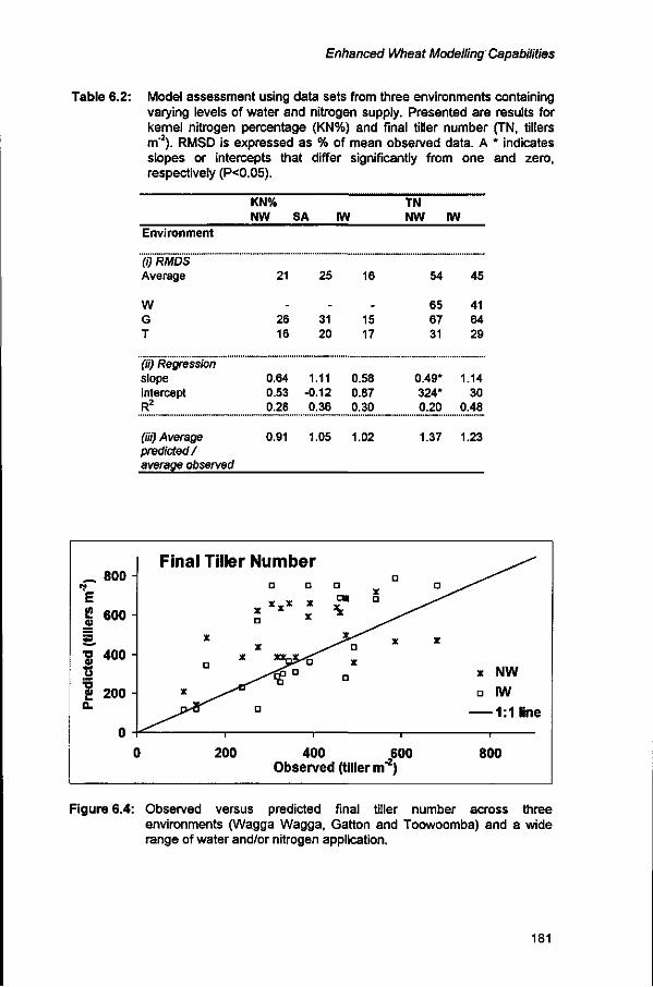
Enhanced Wheat Modelling Capabilities
Table 6.2: Model assessment using data sets from three environments containing varying levels of water and nitrogen supply. Presented are results for kernel nitrogen percentage (KN%) and final tiller number (TIM, tillers m"2). RMSD is expressed as % of mean observed data. A * indicates slopes or intercepts that differ significantly from one and zero, respectively (P<0.05).
KN% NW SA W
TN NW W
Environment
(i) RMDS Average
W G T
(ii) Regression slope intercept R2
(Hi) Average predicted/ average observed
21
26 16
0.64 0.53 0.28
0.91
25
31 20
1.11 -0.12 0.36
1.05
16
15 17
0.58 0.87 0.30
1.02
54
65 67 31
0.49* 324* 0.20
1.37
45
41 64 29
1.14 30
0.48
1.23
_ 800 -c$i
E C 600 -
+3
"g 400 -5 S g 200 -Q.
U 1
(
Final Tiller Number D
D D D D X
x x x x X £ " D ^ ^
^K * x xx-x^r * J " ^ V Q x
^ £ U X ^s^^
jy%L D
i i i
) 200 400 600 Observed (tiller m"2)
x NW D IW
1:1 line
i
800
Figure 6.4: Observed versus predicted final tiller number across three environments (Wagga Wagga, Gatton and Toowoomba) and a wide range of water and/or nitrogen application.
181
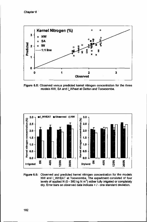
Chapter 6
•o
S2
'•o
£ Q. 1 -
Kernel Nitrogen (%) x NW o SA • IW
— 1 : 1 line
Observed
Figure 6.5: Observed versus predicted kernel nitrogen concentration for the three models NW, SA and l_Wheat at Gatton and Toowoomba.
LWHEAT • Observed Q N W -»3.0
Dryland ° § ° S
Figure 6.6: Observed and predicted kernel nitrogen concentration for the models NW and l_WHEAT at Toowoomba. The experiment consisted of four levels of applied N (0 - 360 kg N m"2) either fully irrigated or completely dry. Error bars on observed data indicate + / - one standard deviation.
182

Enhanced Wheat Modelling Capabilities
180 200 220 240 260 280 300 320 DOY
180 200 220 240 260 280 300 320 DOY
180 200 220 240 260 280 300 320
DOY
180 200 220 240 260 280 300 320
DOY
Figure 6.7: Observed and simulated time course of LAI development at Toowoomba for four levels of nitrogen application (0 to 360 kg ha"1) and either under irrigation or under dry conditions (DOY = day of the year). Error bars on measured data points represent + / - one standard deviation. Solid lines and closed symbols represent irrigated simulations and measurements, dashed lines and open symbols represent dryland simulations and measurements, respectively.
3.2.3.1. Time course of leaf area development at environment T
In the absence of water and nitrogen limitation it is temperature, phenology
and the light conditions within the leaf canopy that determine leaf growth and
senescence. Water and nitrogen limitations result in reduced leaf expansion,
accelerated leaf senescence and even leaf or tiller death. It is the interactions
of all these factors that causes the simulated variability in leaf area shown in
Fig. 6.7. The simulated data fitted the observations well, although at least one
instance could be identified where predicted nitrogen limitations reduced LAI
by a larger amount than observed (Fig. 6.7, ON irrigated, DOY 245). However,
by senescing some leaf area and re-distributing the nitrogen of the senesced
material, simulated leaf area recovered quickly and fitted the remainder of the
183

Chapter 6
observed data well. Overall, the interactions between water, nitrogen and
light limitations appear to have been captured adequately and better than by
any other model tested (cf. Chapter 5, Fig. 5.8).
10 1
8 -
6
4
2 -
0 -
High management, NW
s - D
D | D D
•5 ! ' k.;. a p D D , , ^ ! g
B crPI F • D | a
250 285 320 355 390
DOY
10 n
8 -
6 -
4 -
2 -
0 -
High management, IW
• s | a i i «8 •• . D D ° D * .
g § D Dct&PB *P
1 1 1 H — r -
250 285 320 355 390 DOY
Low management, NW Low management, IW
250 285 320 355 390 DOY
250 285 320 355 390 DOY
Figure 6.8: Observed (open symbols) and predicted (closed symbols) time course of LAI development at Lincoln, New Zealand, for three cultivars, three sowing dates and high and low management strategies. The models NW and l_WHEAT (IW) are compared.
3.2.3.2. Time course of leaf area development at environments L and W
While all the necessary input data to adequately parameterize a simulation
model of similar complexity to l_WHEAT were available at environments T
and G, this was not always the case for the other environments. Phenology
coefficients, for instance, had to be derived from limited, observed data.
Other inputs, such as starting nitrogen content of individual soil layers were
also not available and had to be estimated from other sources. In spite of
these uncertainties, l_WHEAT was able to capture the environmental effects
on LAI better than the leaf area routines in NW, which are not very
responsive.
184

Enhanced Wheat Modelling Capabilities
At environment L and under high management (i.e. added N fertilizer and irrigation) l_WHEAT overpredicted LAI, although the general time course of LAI development was simulated well (Fig. 6.8). It is possible that the introduction of a base temperature could improve particularly the early LAI simulations in this low temperature environment. At least in one instance the observed, experimental data showed that even under high management some limitation reduced leaf area in mid season but with subsequent recovery (Sowing 2, cv. CRAW 50, data not presented). I_WHEAT predicted a similar response under these conditions, although not the recovery. Other measured LAI data could also be interpreted as being the result of sub-optimal conditions in high management treatments (e.g. cv. Kokako, sowing 2 and 3).
Under low management conditions there was closer correspondence of measured and predicted LAI (Fig. 6.8). While there was some considerable variation in observed LAI values, general trends in leaf area development were simulated well.
8 1 1 9 7 9
6
34-2
0 -!
_ /
i
205 230
.x..
'""X
''y/a\^
1 1 1
255 280 305 DOY
8 -i
6
2
U "1
8n 1 9 8 2 —
6
3<" 2 -
. . . B . .
-X-
X
x
U I I
205 230 255 DOY
1983
"X
1 / ^ ^
155 180 205 230 255 280 305 DOY
-Observed - LWHEAT NW
X
i O i
280 305
Figure 6.9: Time course of observed and simulated LAI at Wagga Wagga. Dashed lines and open symbols represent simulations, solid lines and closed symbols are measurements. Shown are data from three seasons (1979, 1982 and 1983) and two cultivars (Egret and WW30G).
185

Chapter 6
Time course of LAI was predicted well for two of three years at environment W, namely 1982 and 1983 (Fig. 6.9). In 1979, early leaf area development was overpredicted, but LAI during grainfilling was predicted well. It is possible that for this old cultivar coefficients used in the leaf area routines are inappropriate.
3.2.4. Water and nitrogen use at environment T
A comparison of observed and simulated water uptake at environment T does not represent a model validation in the strict sense because some model components were developed on this data set. However, no other data sets containing the necessary detail were available and it is important to demonstrate the current capability to simulate water uptake even if the data set is not completely independent. These concerns do not extend to nitrogen uptake and use, or leaf area routines since these algorithms were developed independently.
The simulation of cumulative water extraction was adequate, although there was a slight but consistent tendency to underpredict water use (Fig. 6.10a). Final water use was underpredicted by 8%, mainly caused by underpredicting water use in the lowest layer of the profile (Fig. 6.10b,c). In l_WHEAT the extraction front ceases its extension at anthesis, i.e. at a depth of 1.5 m, although water extraction was observed to a depth of 1.6 m (Chapter 3).
Total plant nitrogen uptake was simulated within one standard error of measurement for all treatments (Fig. 6.11). Under dryland conditions predictions were similar to those by NW, however l_WHEAT performed better under irrigation.
Residual soil nitrogen after final harvest was simulated mostly within the error of measurement for irrigated treatments but tended to be lower than measured for high fertilizer input under dryland conditions. In contrast, NW overpredicted high fertilizer treatments under both water regimes (Fig. 6.11 ).
In most instances, the general shape of nitrogen distribution in the profile was captured by both models (Fig. 6.12). In some cases the amount of nitrogen in the two surface layers was overpredicted with high nitrogen input.
186

Enhanced Wheat Modelling Capabilities
g 250 E •jr 200 o •g 150 2 'S 100 G)
JÜ 5 0 ra
3 „
- -o- - Observed
1 Wheat •o - -o
180 200
(a)
320
0.20
Vol. water content at anthesis (mm/mm)
0.30 0.40 0.50 0.60
E Ä 40
a> | 120 a
(b) 160
•
o Observed DUL 1 Wheat
0.20
Vol. water content at final harvest (mm/mm)
0.30 0.40 0.50 0.60
E ü. 40 S.
8" 80 o; | 120 o.
160 (c)
o Observed DUL 1 Wheat
Figure 6.10: Observed and predicted water use in the dry treatment at Toowoomba; (a) cumulative water extraction, arrow indicates anthesis date, (b) volumetric soil water content at anthesis and (c) volumetric soil water content at final harvest. Drained upper limit (DUL) of the profile is also shown.
187

Chapter 6
Total N uptake
Irrigated o o O
(O co
O)
30
25
20
15
10
Total N uptake
ml Dryland
o CM
O
CO
Residual Soil N Residual Soil N
Irrigated Dryland
Figure 6.11: Observed and simulated total nitrogen uptake and amount of residual soil nitrogen at final harvest for all treatments at Toowoomba.
188

Enhanced Wheat Modelling Capabilities
NO, (mg kg1) 5 10 15 20
-Observed -a—L.WHEAT •X---NW
40 ?
80 6 Q.
• 120 S
0N_l L 160
NO, (mg kg'1) 0 S 10 15 20
ON D
Mo ? Ü
-80 g n. ai
120 O
160
5 N O ' ^ k 9 - , ) 15 20 NO, (mg kg"1)
5 10 15
40N I
40 ?
u 80 g
a ai
-120O 160
NO, (mg kg'1) 10 20 30 40
NO, (mg kg1) 10 20 30 40
4 0 ?
u 80g
a. a>
12(D
120NJ L 1 6 0 120N D
40 ?
u 80 £
o. CI
•120Q
• 160 NO, (mg kg1)
20 40 0
r NO,
100 (mg kg
200 30
360N D
40 ?
O
80 £ a. at
120O 160
Figure 6.12: Observed and simulated NO3 concentration of the soil by layer at final harvest at Toowoomba. Shown are all nitrogen treatments (0 - 360N) and water treatments (Irrigated and Dryland). Note that the scale differs depending on application rate.
3.3. Future improvements
Several aspects of l_WHEAT require further attention.
• Phenology: At this stage phenology routines used by l_WHEAT are
identical to those used in the model by Probert et al. (1995). These
routines could be improved by (i) making the derivation of necessary
parameters more explicit, (ii) the determination of coefficients for a wider
189

Chapter 6
range of cultivars and (iii) the development of facilities that allow easy input of observed phenology. These activities are in progress.
• Coefficients used for leaf area development: Coefficients used to describe leaf area increases in response to temperature are "best estimates" and are not derived from experimental data. Using experiments comprising a wide range of environments and cultivars to derive these coefficients might further improve model performance.
• Effect of plant density on leaf area: Currently, M/VHEAT assumes a direct, inversely proportional effect of changes in plant density on maximum plant leaf area. While this over-simplification of a dynamic, competitive process appears to be adequate for the conventional densities encountered in the test data sets, it is likely to be inappropriate at either substantially higher (more than 250 plants m'2) or lower (less than 50 plants m"2) densities. This should be addressed.
• Plant nitrogen dynamics: Due to a lack of experimental data, several assumptions had to be made in the development of the crop nitrogen dynamics. For instance, the phenomenon of luxury nitrogen consumption, although observed and reported in the literature, could not be satisfactorily quantified and should be addressed. Others, such as the kernel nitrogen dynamics, also contain some assumptions that require either better quantification or modification to the phenomenological process description.
4. Conclusions
Concerns about the suitability of existing wheat models for use within the framework of cropping systems simulation have been raised. In response to such concerns, this study addressed short-comings of existing wheat modelling capabilities in Australia through the incorporation of tested and well performing model components from many sources into a new APSIM module for spring wheat. In cases where none of the previously tested model components performed adequately, new routines were developed. This resulted in improved model performance for the simulation of LAI and grain nitrogen content as well as water and nitrogen utilization. This increased predictive ability of l_WHEAT was achieved by (i) keeping the level of process detail included in the model to the minimum required for the tasks, (ii) using conservative parameters that do not require re-calibration when used in different environments and (iii) not including any parameters that are difficult or impossible to derive from field studies. This approach reduces the unintentional calibration of model parameter values to erroneous estimates of
190

Enhanced Wheat Modelling Capabilities
input variables and makes simulations of l_WHEAT more stable than other models tested, when used over a wide range of environmental conditions. More accurate simulations of soil water and nitrogen utilization were obtained by using l_WHEAT. This allows a better estimates for the starting conditions of the following crop.
References
Aggarwal, P.K., Singh, A.K., Chaturvedi, G.S. and Sinha, S.K., 1986. Performance of wheat and triticale cultivars in a variable soil-water environment. II. Evapotranspiration, water use efficiency, harvest index and grain yield. Field Crops Res., 13: 301-315.
Aggarwal, P.K., Kalra, N., Singh, A.K. and Sinha, S.K., 1994. Analyzing the limitations set by climatic factors, genotype, water and nitrogen availability on productivity of wheat. I. The model description, parameterization and validation. Field Crops Res., 38: 73-91.
Barneix, A.J., 1989. Yield variation in wheat: Nitrogen accumulation, light interception and harvest index. In: H. Lambers (Editor), Causes and Consequences of Variation in Growth Rate and Productivity of Higher Plants. SPB Academic Publishing bv, The Hague, The Netherlands, pp. 87-100.
Chapman, S.C., Hammer, G.L. and Meinke, H., 1993. A sunflower simulation model. I. Model development. Agron. J., 85: 725-735.
Charles-Edwards, D.A., Doley, D. and Rimmington, G.M., 1986. Modelling plant growth and development. Academic Press, Sydney, Australia, 235 pp.
Davies, P., 1992. The mind of God. Science and the search for ultimate meaning. Penguin Books, London, UK, 254 pp.
Faivre, R. and Masle, J., 1988. Modeling potential growth of tillers in winter wheat. Acta Ecologica, 9: 179-196.
Fischer, K.S., 1995. Systems approach to understanding genotype by environment interactions. In: Applications of systems approaches in plant breeding. Aggarwal, P.K., Matthews, R.B., Kropff, M.J. and van Laar, H.H. (Editors). SARP Research Proceedings, AB-DLO, TPE-WAU, Wageningen and IRRI, Los Banos, 1995, pp. 1-4.
Fischer, R.A., 1979. Growth and water limitation to dryland wheat in Australia: A physiological framework. J. Aust. Inst. Agric. Sei., 45: 83-94.
191

Chapter 6
Goyne, P.J., Meinke, H., Milroy, S.P., Hammer, G.L and Hare, J.M., 1996. Development and use of a barley crop simulation model to evaluate production management strategies in North East Australia. Aust. J. Agric. Res., in press.
Gregory, P.J., Crawford, D.V. and McGowan, M., 1979. Nutrient relations of winter wheat. 1. Accumulation and distribution of Na, K, Ca, Mg, P, S and N. J. Agric. Sei., 93: 485-494.
Hammer, G.L., Woodruff, D.R. and Robinson, J.B., 1987. Effects of climatic variability and possible climatic change on reliability of wheat cropping - A modelling approach. Agric. For. Meteorol., 41:123-142.
Hammer, G.L., Butler, D., Muchow, R.C. and Meinke, H. 1996a. Integrating physiological understanding and plant breeding via crop modelling and optimisation. Proceedings Int. Workshop on sorghum breeding. ICRISAT, Hyderabad, India, Dec. 1994, in press.
Hammer, G.L., Sinclair, T.R., Wright, G.C, Meinke, H. and Bell, J., 1995b. A peanut simulation model: I. Model development and testing. Agron. J., 87:1085-1092.
Keil, D.B. and Sonnleitner, B., 1995. GMP - good modelling practice: An essential component of good manufacturing practice. Trends Biotechnol., 13:481-492.
Keulen, H. van and Seligman, N.G., 1987. Simulation of water use, nitrogen nutrition and growth of a spring wheat crop. Simulation Monographs, Pudoc, Wageningen, The Netherlands. 309 pp.
Kropff, M.J., van Laar, H.H. and Matthews, R.B. (Eds), 1994. ORYZA1, an ecophysiological model for irrigated rice production. SARP Research Proceedings, IRRI, Los Banos and AB-DLO, TPE-WAU, Wageningen, 110 pp.
Littleboy, M., Silburn, D.M., Freebairn, D.M., Woodruff, D.R., Hammer, G.L. and Lesley, J.K., 1992. Impact of soil erosion on production in cropping systems. I. Development and validation of a simulation model. Aust. J. Soil Res., 30: 757-774.
Loomis, R.S., 1993. Optimization theory and crop improvement. International Crop Science I. Crop Science Soc. Amer. pp. 583-588.
Lövenstein, H., Lantinga, E.A., Rabbinge, R. and van Keulen, H., 1995. Principles of production ecology. TPE-WAU, Wageningen, 121 pp.
McCown, R.L., Hammer, G.L, Hargreaves, J.N.G., Holzworth, D.P. and Freebairn, D.M., 1996. APSIM: A novel software system for model development, model testing, and simulation in agricultural research. Agric. Syst. 50:255-271.
192

Enhanced Wheat Modelling Capabilities
Meinke, H. and Hammer, G.L., 1995a. A peanut simulation model. II. Assessing regional production potential. Agronomy J., 87:1093-1099.
Meinke, H. and Hammer, G.L., 1995b. Climatic risk to peanut production: A simulation study for northern Australia. Aust. J. Exp. Agric, 35: 777-780.
Meinke, H. and Stapper, M., 1995. The Agricultural Production system SIMulator: Leading the way from single crops to cropping systems. In: Proceedings of the First International Symposium on Mathematical Modelling and Simulation in Agriculture & Bio-Industries, Vol. IV, May 9-12, 1995, IMACS/IFAC, Brussels, Belgium, VIII.A.3, p. 1-6.
Meinke, H., Hammer, G.L. and Want, P.J., 1993. Potential soil water extraction by sunflower on a range of soils. Field Crops Res., 32: 59-81.
Meinke, H., Stone, R.C. and Hammer, G.L, 1996. SOI phases and climatic risk to peanut production: A case study for Northern Australia. Int. J. Climatolo. 16: 1-7.
Milroy, S.P. and Goyne, P.J., 1995. Leaf area development in barley - model construction and response to soil moisture status. Aust. J. Agric. Res., 46: 845-860.
Netherlands Scientific Council for Government Policy, 1992. Ground for choices. Sdu Publishers, The Hague, 144 pp.
O'Leary, G.J., Connor, D.J. and White, D.H., 1985. A simulation model of the development, growth and yield of the wheat crop. Agric. Syst., 17: 1-26.
Oscarson, P., Lundborg, T., Larsson, M. and Larsson, C.-M., 1995. Genotypic differences in nitrate uptake and nitrogen utilization for spring wheat grown hydroponically. Crop Sei., 35: 1056-1062.
Palta, J.A. and Fillery, I.R.P., 1995a. N application increases pre-anthesis contribution of dry matter to grain yield in wheat grown on a duplex soil. Aust. J. Agric. Res., 46: 507-518.
Palta, J.A. and Fillery, I.R.P., 1995b. N application enhances remobilization and reduces losses of pre-anthesis N in wheat grown on a duplex soil. Aust. J. Agric. Res., 46: 519-531.
Palta, J.A., Kobata, T., Turner, N.C. and Fillery, I.R., 1994. Remobilization of carbon and nitrogen in wheat as influenced by postanthesis water deficits. Crop Sc, 34: 118-124.
Parton, W.J., Morgan, J.A., Hofen, J.M.A. and Harper, L.A., 1988. Ammonia volatilization from spring wheat crops. Crop Sei., 80: 419-425.
Probert, M.E., Keating, B.A., Thompson, J.P. and Parton, W.J., 1995. Modelling water, nitrogen and crop yield for a long-term fallow management experiment. Aust. J. Exp. Agric, 35: 941-950.
193

Chapter 6
Probert, M.E., Dimes, J.P., Dalai, R.C. and Strong, W.M., 1996. APSIM's water and nitrogen modules and simulation of the dynamics of water and nitrogen in fallow systems. Ag. Syst., in press.
Ritchie, J.T., Godwin, D.C. and Otter-Nacke, S., 1985. CERES-Wheat. A Simulation Model of Wheat Growth and Development. Texas A&M University Press, College Station.
Shorter, R., Lawn, R.J. and Hammer, G.L., 1991. Improving genotypic adaptation in crops - a role for breeders, physiologists and modellers. Exp. Agric, 27: 155-175.
Sinclair, T.R. and Horie, T., 1989. Leaf nitrogen, photosynthesis and crop radiation use efficiency: A review. Crop Sei., 29: 90-98.
Sinclair, T. R. and Amir, J., 1992. A model to assess nitrogen limitations on the growth and yield of spring wheat. Field Crops Res., 30: 63-78.
Sinclair, T.R., Tanner, C.B. and Bennett, Ü.M., 1983. Water-use efficiency in crop production. BioScience, 34: 36-40.
Spitters, C.J.T., 1990. Crop growth models: Their usefulness and limitations. Acta Horticulturae, 267: 349-368.
Stapper, M., 1984. SIMTAG: A simulation model of wheat genotypes. Model documentation. ICARDA, Aleppo, Syria and Univ. of New England, Armidale, NSW, Australia. 108 pp.
Tanner, C.B. and Sinclair, T.R., 1983. Efficient water use in crop production: research or re-search? In: Limitations to Efficient Water Use in Crop Production. ASA, Madison, Wl, pp. 1-27.
Thomas, Fukai, S. and Hammer, G.L., 1995. Growth and yield response of barley and chickpea to water stress under three environments in Southeast Queensland. II. Root growth and soil water extraction pattern. Aust. J. Agric. Res., 46: 35-48.
Wetselaar, R. and Farquhar, G.D., 1988. Nitrogen losses from the tops of plants. Adv. Agron., 33: 263-302.
Willems, J.C., 1989. Some thoughts on modelling. In: Newton to Aristotle. Toward a theory of models for living systems (John Casti and Anders Karlqvist, Editors), Birkhauser, Bosten, 1989. pp. 91-119.
Wit, CT. de, 1990. Making predictions about farming. In: Scientific Europe, Research and Technology in 20 Countries, Foundation Scientific Europe (Editors), Nature & Technology Scientific Publishers Ltd., Maastricht, The Netherlands, pp. 188-191.
Woodruff, D.R., 1992. 'WHEATMAN' a decision support system for wheat management in subtropical Australia. Aust. J. Agric. Res., 43: 1483-1499.
194

Enhanced Wheat Modelling Capabilities
Appendix
All abbreviations, their description and units in alphabetical order.
Abbreviation Description Unit
APSIM D DOY G HI • " m a x
HW L.WHEAT K_N% KY L LAI U M NHI NW P RMSD
RUE S SA SI SLA SLN T TT TDM TE TEC
VPD W
systems model environment (McCown et al., 1996) water demand mm <f1
day of the year environment code for Gatton, Australia (Table 5.1) harvest index g g"1
maximum potential harvest index g g"1
wheat model (Hammer et al., 1987) the Integrated Wheat Model kernel nitrogen concentration % kernel yield environment code for Lincoln, NZ (Table 5.1) leaf area index leaf area of tiller n environment code for Michigan, USA (Table 5.1) nitrogen harvest index wheat model (NWheat, Probert et al., 1995) phyllochron index, cultivar specific root mean square deviation
radiation use efficiency water supply wheat model (Sinclair and Amir, 1992) wheat model (SIMTAG, Stapper, 1984) specific leaf area specific leaf nitrogen content environment code for Toowoomba, Australia (Table 5.1) thermal time total, above-ground dry matter crop transpiration efficiency transpiration use efficiency coefficient
accumulated thermal time °C vapour pressure deficit kPa environment code for Wagga-Wagga, Australia (Table 5.1)
g m '
rv,2 „,"2 m m cm2 tiller"1
TT leaf1
% of mean observed gMJ-1
mmd"1
cm2 g"1
gNm"2
degd gm"2
g m"2 mm"1
g m"2 mm"1
kPa
195

General Discussion
Chapter 7
General Discussion
"/ suggest modelling is an activity of the right brain side. It can be learnt, unless inhibited by an overriding left side reductionist mind set!"
Hearn (1996)
1. Outline
Simulation models in agriculture are a reality. They have been and will continue to be used for a multitude of issues with varying success. They are a convenient and indispensable tool in systems analysis and are used as knowledge depositories for the wealth of accumulated insight into chemical, physical, biological and physiological processes. They vary in structure, design objectives and quality (see also General Introduction). They also pose uncountable pitfalls for developers and users. Based on the work presented in the previous chapters, some causes and possible solutions of such problems are discussed. Finally, an example is given that outlines how the methodology developed in this thesis will be applied.
2. Problems with models
2.1. Model development
It is essential that models are developed based on a clear formulation of objectives concerning their use. These objectives determine the boundaries of the system under study and the degree of necessary or desirable simplification (Loomis et al., 1979; Zadoks and Rabbinge, 1985). In this context, it is vital to consider issues of scale since larger-scale applications require models of lower complexity and, as a general rule, not more than three aggregation levels can be usefully considered by any one model (Rabbinge and van Ittersum, 1994). This process of coarse graining (Gell-Mann, 1995) is essential, because it clearly defines the level below which finer details are being ignored. However, level confusion is largely at the root of the debate about "mechanistic" versus "empirical" modelling approaches, or, as Passioura (1996) puts it, the "scientific" versus the "engineering"
197
Chapter 7
approach. Traditionally, a description or empirical statement at one level is regarded as the basis for an explanation or mechanism for the level above (Hearn, 1996). This assertion arises from the scientific paradigm that is based on the study of closed, linear systems. Lately, however, scientists have begun to realize that most systems are open and nonlinear and must be understood holistically, whereby local, linear relations are a necessary, but not a sufficient condition to gain insight into the behaviour of systems. In practice that means that constraints, boundary conditions and initial conditions play a much more fundamental role in determining system behaviour (Davies and Gribbin, 1992). Their interactions result in higher levels also acting downward upon lower levels, resulting in often lawlike behaviour in spite of being indeterministic (Davies, 1992). This introduces an element of teleology without which evolution could not occur and papers like "strategies of response to water stress" (Ludlow, 1989) could not be written. It is a feature shared by all complex adaptive systems, whereby complex behaviour emerges from simple rules. "The trick in designing a manageable simulation is to prune the rules so as to make them even simpler, but in such ways that the most interesting kinds of emergent behaviour remain. The designer of a simulation must then know a good deal about the effects of changes in the rules on behaviour in many different scenarios. ...the intuition is based partly on a priori reasoning and partly on experience of fiddling with the rules and then watching what happens under the modified rules in particular computer runs" (Gell-Mann, 1995).
Irrespective of scale, processes of equal importance should be represented at the same level of detail and precision throughout a model. This is often constrained by scientists' narrowly-focused expertise and hence limited knowledge of processes that, although not directly part of their field of interest, need to be included in the model. Particularly when moving from single crops to cropping systems models, this becomes increasingly difficult as more and more disciplines are expected to contribute to the model. Additionally, only few agricultural scientists have had any formal training in software development that enables them to structure and write computer code efficiently and with the necessary precision and flexibility. The same rigour that is applied to vetting the science underlying the model should be applied to its implementation and to its maintenance (McCown et al., 1996).
Chapter 2 addresses these issues and puts forward one approach that can alleviate some of the problems. The Agricultural Production systems SIMulator (APSIM) provides a versatile and flexible infrastructure for model
198

General Discussion
development, testing and application (McCown et al., 1996). Its engine, written by professional software developers, facilitates communication between modules, based on a plug-in, pull-out principle. This allows scientists to concentrate on developing individual modules in their area of expertise without being divorced from development activities in other areas. It also enhances communication among those scientists and supports model development activities through a range of tools such as graphic routines to analyze output or changing variable names throughout the module at the press of a button. It allows a fast and thorough evaluation of alternative modelling approaches.
2.2. Model application
Once a model has been developed, problems with its application can arise for the following reasons:
1. a simulation approach is used where either it is inappropriate or alternative approaches might be more useful,
2. although a modelling approach is appropriate for the task, an inappropriate model is chosen,
3. an appropriate model is used incorrectly, or 4. output from a well-conducted simulation analysis is interpreted wrongly or
presented in a misleading or inappropriate way.
This thesis attempts to give some objective guidance to avoid problems particularly of the categories 2 and 3 (e.g. Chapters 1, 5 and 6), but some further elaboration is warranted. Although important, category 4 problems of model application do not form part of this study.
Causes for category 1 and 2 problems are frequently found outside the realm of scientific objectivity1. Institutions and individual scientists often expend considerable resources on the development of a core simulation methodology. This investment can pay off, if the development is driven by well-defined needs for model application. However, these needs change constantly and these changes must be taken into account when developing the simulation tools. This is a dynamic process and it is a fallacy to assume that once the methodology has been developed, the applications will follow. It is analogous to the statement by Bill Gates, who said: "By the time the
1 The notion of scientific objectivity or at least its implementation through the peer review process can be challenged in its own right (cf. Edelglass et al., 1992). This debate, however, is beyond the scope of this thesis.
199

Chapter 7
layman has read the manual for a piece of software it will be obsolete." Although rarely admitted, most modelling applications are conducted either with prototypes or with a modified version of the original model.
A further danger, that can be intellectually stifling, is the pressure on scientists from science managers and funding agencies for a monetary return on their investment in software development. This product, rather than an outcome-focused view, can lead to bias when selecting the most appropriate model for a new task. It bears the risk of bringing a dynamic process to a halt, thus quickly making a useful tool obsolete. It also puts pressure on finding new applications for this technology to justify its existence and further development and can lead to the exclusion of more appropriate methods. In other words, the politics of science are often responsible when more appropriate approaches are ignored. Caution is needed so that new, scientific products are not pushed into a market prematurely because this process, dictated by economic rational, can seriously undermine the open knowledge systems on which scientific activity is largely based. This pressure for a short-term, monetary return of model development is in itself an example for an erroneous model application: Economic, free market principles are applied to a process that is, by its nature, not part of this market because its benefits cannot easily be measured by the performance indicators ofthat framework.
Problems of the category 3 and 4 types have different causes. Errors made in applying an appropriate model, frequently relate to its parameterization. The more complex a model, the more parameters it requires and the fewer people will be able to apply the model correctly. Chapter 5 demonstrates how difficult it can be to parameterize even models of intermediate complexity on high quality, experimental data sets. Often parameters are inter-related and either difficult or impossible to derive. Frequently, even scientists who have developed a model will have problems with model application, once a certain, albeit not well-defined, threshold of complexity is reached. Such highly detailed, mechanistic simulation models often only serve the purpose of self-education for the developer and their scientific content is no longer transmissible to others (Passioura, 1996). The multitude of processes described can lead to an imbalance between the degree of detail and perceived accuracy of the model on one hand and the crude and often inappropriate assumptions that need to be made to parameterize the model on the other. Once the appropriate type of model for a particular application has been chosen, further model selection should depend on the availability of
200

General Discussion
sound input data rather than on the availability of a particular model or by political pressure.
3. Why yet another wheat model?
3.1. Model development
As part of this thesis a new wheat model was developed, adding to the multitude of existing wheat models. However, the driving force behind this development was not the need for a new wheat model per se. Rather, it was the need to test current wheat modelling capabilities at the cropping systems level since most crop models were originally designed as stand-alone versions. Often, such models assume that starting conditions are re-initialized before the next simulation. Therefore, the suitability of such models to predict resource utilization needs to be scrutinized, since this determines the starting conditions of the next cropping sequence. In this thesis, a process was developed to test this ability and to harness existing modelling capabilities as much as possible, thus minimizing efforts spent on model development. This was achieved by using empirical data, specifically collected for model testing, combined with a versatile simulation environment. Benefits from this activity are threefold: First, the data sets compiled for model testing also further our understanding of crop physiological processes, i.e. they contribute to the further advancement of science. Second, detailed model component testing clearly identifies strengths and weaknesses in current wheat models. Third, a new, composite model, based largely on existing, demonstrably well-performing components, avoids duplication of research efforts and the resulting model is more credible to a broader group of potential users.
A main objective for the development of the Integrated Wheat Model (l_WHEAT) was the need for a robust model with a high predictive ability across the wide range of environmental conditions encountered in Australia (Chapter 6). This required a clear differentiation between predictive and explanatory models (Spitters, 1990), a differentiation that is often blurred because many models started as explanatory models but are increasingly used predictively. For the development of l_WHEAT, a more holistic modelling approach was taken that can be used to describe systems behaviour at a higher organizational level, thus increasing stability of the model by reducing the number of input parameters needed. The approach aims to identify and use conservative parameters wherever possible, i.e.
201

Chapter 7
parameters with little sensitivity to variation in input variables. In some instances, approaches based on fuzzy reasoning, i.e. a "what i f approach to problem solving, were included (Kell and Sonnleitner, 1995). These have proven useful in cases where precise parameter values are unknown, but the relevant process exhibits little sensitivity to the actual parameter value used. The model performed satisfactorily over a wide range of data from various agro-climatic regions. This was achieved without calibration of the model for individual regions and clearly demonstrates the improved predictive capability of the model and its suitability for scenario analysis across the tested environments. Leaf area dynamics and resource utilization in response to water and nitrogen supply were improved. Areas for further improvements, such as phenology and a more thorough derivation of certain parameter values, were identified.
3.2. Data sets
The main data-set used for model testing is described in detail in Chapter 3. The data analysis is presented as a crop physiological framework that provides all necessary parameter values for inclusion into a predictive wheat model of intermediate complexity. This also includes parameter values for the water and nitrogen balance. Although most of the parameters have also been reported elsewhere, they are rarely presented and discussed for the same data-set. The work aimed to identify as far as possible existing, conservative relations that differ little within and across environments. While, for instance, the value of 1.34 g MJ"1 for radiation use efficiency (RUE) was well within expected limits (Green, 1987; Siddique et al., 1989), it was interesting that the transpiration efficiency coefficient (TEC, 4.7 g m"2 mm"1 kPa) also compared well with reported values (Monteith, 1988). Both coefficients varied little with either nitrogen or water application. These findings further support the concept of using either intercepted radiation and radiation use efficiency, or amount of transpired water and transpiration efficiency, (depending on the most limiting resource), when estimating biomass production (Monteith, 1988; Chapman et al., 1993). Although both RUE and TEC were conservative, biomass production differed strongly among treatments. This pointed to the sensitivity of leaf area development to even moderate levels of nitrogen and water deficiency and hence the importance of leaf area predictions in response to resource availability in simulation models. The data also showed that considerable amounts of nitrogen can be taken up after anthesis and demonstrated the value of nitrogen deep in the soil profile under dryland conditions. Such information adds value to the data collected for model
202
General Discussion
testing, since it allows the study and quantification of environmental interactions and so enhances our understanding of crop physiology.
Data on light interception led to an investigation about the validity of using a constant value for the extinction coefficient (k) in simulation models. Chapter 4 discusses the reasons behind the very high values for k (>2) found during early growth. Briefly, the work showed that when interception by plant components other than leaves was accounted for, values for k reduced to conventional values (k<1). However, not all simulation models account for such interception. A sensitivity analysis showed that, if models do not account for this effect, anthesis dry weight could be underestimated by as much as 34% if maximum leaf area index did not exceed a value of two. However, when maximum leaf area index was high, anthesis dry weight differed by less than 4%. This improved understanding of light interception at the crop level led to a simple, empirical method to include this effect into any LAI-based light interception model. It is a typical example of a summary model that is simple but could not have been developed without the knowledge at a finer level of resolution (Rabbinge and de Wit, 1989).
4. An example of a farm-based application
Cropping systems models have many potential applications ranging from environmental issues and policy matters to farm optimization and variety adaptation (e.g. Netherlands Scientific Council for Government Policy, 1992, Penning de Vries et al., 1993; Goldsworthy and Penning de Vries, 1994; Hammer et al., 1996a). Since it is beyond the scope of this thesis to review these applications comprehensively, a current example is presented to demonstrate how the improved simulation capability for wheat will be used in Australia.
Recent advances in long-range rainfall and frost forecasting allow a preseason evaluation of likely growing conditions in Eastern Australia (Stone and Auliciems, 1992; Stone et al., 1996). In this region of high climatic variability (Nicholls and Wong, 1991), a skilful seasonal forecast provides an opportunity for farm managers to better tailor crop management decisions to the season (Hammer et al., 1996b). Meinke et al. (1996) have shown in a case study for peanuts how such a probabilistic climatic forecasting system can be combined with a dynamic simulation model to forward estimate production levels and risk. However, implications of a seasonal forecast
203

Chapter 7
system go beyond single crop issues. Their impact on key cropping systems decisions, such as crop choice and cropping sequence, needs to be assessed. Other issues, such as the residual value of applied nitrogen to the following crop require agronomic and economic quantification. More substantive tactical manipulation of either the cropping system or the whole farm offers potential for substantially improved management of farming risk and greater economic benefit. To confidently address such issues, crop simulation models of similar standards need to be available for the key crops in the cropping system. Recent efforts have concentrated on the further development of APSIM modules for cotton, sorghum, peanuts and sunflower, all of which are now available for this type of analysis. The work from this thesis provides an improved wheat modelling capability. Since wheat is the major winter crop in north-eastern Australia, this will allow evaluation of a tactical approach to farm management through simulation and whole-farm economic analysis. In close collaboration with farmers, the seasonal forecast techniques and modelling capabilities will be used to gain improved insight in the longer-term consequences of possible decision options. This four year project commences in 1996 and is financially supported by the Rural Industry, Research and Development Corporation (RIRDC) in Australia.
5. Where to from here?
Tools and methods discussed in this thesis offer one way forward in systems analysis. The work generally contributes to the further development of sound simulation methodologies but also provides a tool to solve some very specific problems. There are many other, equally valid, approaches. At a technical level, possible improvements have been flagged where appropriate (e.g. phenology predictions need to be improved in l_WHEAT). New, challenging questions will undoubtedly arise, requiring further changes and improvements to the existing methodology. As part of the dynamic process of improving our scientific understanding, some modelling approaches will quickly be superseded, while others will prove more general and robust. As scientists, we should welcome these continuous challenges to the development and use of our tools and their underlying scientific knowledge base. A methodology that is no longer challenged, actively discussed and then modified, has either captured the essence of system responses or has outlived its usefulness.
204

General Discussion
References
Chapman, S.C., Hammer, G.L. and Meinke, H., 1993. A sunflower simulation model: I. Model development. Agron. J., 85: 725-735.
Davies, P., 1992. The mind of God. Science and the search for ultimate meaning. Penguin Books, London, UK, 254 pp.
Davies, P. and Gribbin, J., 1992. The matter myth - beyond chaos and complexity. Penguin Books, London, UK, 314 pp.
Edelglass, S., Maier, G., Gebert, H. and Davy, J., 1992. Matter and mind -imaginative participation in science. Floris Books, Edinburgh, Great Britain. 136 pp.
Gell-Mann, M., 1995. The Quark and the Jaguar - Adventures in the Simple and Complex. Abacus, London, UK, 392 pp.
Goldsworthy, P. and Penning de Vries, F. (Editors), 1994. Opportunities, use, and transfer of systems research methods in agriculture to developing countries. Systems Approaches for Sustainable Agricultural Development, Vol. 3, Kluwer Academic Publishers, Dordrecht, The Netherlands, 367pp.
Green, CF., 1987. Nitrogen nutrition and wheat growth in relation to absorbed solar radiation. Agric. For. Metorol., 41: 207-248.
Hammer, G.L., Butler, D., Muchow, R.C. and Meinke, H. 1996a. Integrating physiological understanding and plant breeding via crop modelling and optimisation. Proceedings Int. Workshop on sorghum breeding. ICRISAT, Hyderabad, India, Dec. 1994, in press.
Hammer, G.L., Holzworth, D.P. and Stone, R., 1996b. The value of skill in seasonal climate forecasting to wheat crop management in a region with high climatic variability. Aust. J. Agric. Res., in press.
Hearn, A.B., 1996. An agronomist's Odyssey. Proceedings Eighth Australian Agronomy Conference. M. Ashgar (Editor), Australian Society of Agronomy, 1996, Toowoomba, Australia, pp. 2-16.
Keil, D.B. and Sonnleitner, B., 1995. GMP - good modelling practice: An essential component of good manufacturing practice. Trends Biotechnol., 13:481-492.
Loomis, R.S., Rabbinge, R. and Ng, E., 1979. Explanatory models in crop physiology. Ann. Rev. Plant Physiol., 30: 339-367.
Ludlow, M.M., 1989. Strategies of response to water stress. In: Structural and functional responses to environmental stresses. Kreep, K.H., Richter, H. and Hinckley, T.M. (Eds.), SPB Academic Publishing, The Hauge, The Netherlands, pp. 269-281.
McCown, R.L., Hammer, G.L., Hargreaves, J.N.G., Holzworth, D.P. and Freebairn, D.M., 1996. APSIM: A novel software system for model
205

Chapter 7
development, model testing, and simulation in agricultural research. Agric. Syst., 50: 255-271.
Meinke, H., Stone, R.C. and Hammer, G.L., 1996. SOI phases and climatic risk to peanut production: A case study for Northern Australia. Int. J. Climatology, 16: 1-7.
Monteith, J.L., 1988. Does transpiration limit the growth of vegetation or vice versa? J. Hydr., 100:57-68.
Netherlands Scientific Council for Government Policy, 1992. Ground for choices. Sdu Publishers, The Hague, 144 pp.
Nicholls, N. and Wong, K.K., 1991. Dependence of rainfall variability on mean latitude and the Southern Oscillation. J. Climate, 3:163-170.
Passioura, J.B., 1996. Simulation models: Science, snake oil, education or engineering? Agron. J., in press.
Penning de Vries, F., Teng, P. and Metselaar, K. (Editors), 1993. Systems approaches for agricultural development. Systems Approaches for Sustainable Agricultural Development, Vol. 2, Kluwer Academic Publishers, Dordrecht, The Netherlands, 543 pp.
Rabbinge, R. and de Wit, CT., 1989. Systems, models and simulation. In: Simulation and systems management in crop protection. Rabbinge, R., Ward, S.A. and van Laar, H.H. (Editors), Pudoc, Wageningen, pp. 3-15.
Rabbinge, R. and van Ittersum, M.K., 1994. Tension between aggregation levels. In: The future of the land - mobilising and integrating knowledge for land use option. Fresco, L.O., Stroosnijder, L, Bouma, J. and van Keulen, H. (Editors), John Wiley & Sons, Chichester, UK, pp. 31-40.
Siddique, K.H.M., Beiford, R.K., Perry, M.W. and Tennant, D., 1989. Growth, development and light interception of old and modern wheat cultivars in a Mediterranean-type environment. Austr. J. Agric. Res., 40: 473-487.
Spitters, C.J.T., 1990. Crop growth models: Their usefulness and limitations. Acta Horticulturae, 267: 349-368.
Stone, R. and Auliciems, A., 1992. SOI phase relationships with rainfall in eastern Australia. Int. J. Climatology, 12: 625-636.
Stone, R., Nicholls, N. and Hammer, G.L., 1996. Frost in NE Australia: Trends and influences of phases of the Southern Oscillation. J. Climate, in press.
Zadoks, J.C. and Rabbinge, R., 1985. Modelling to a purpose. Adv. Plant Pathol., 3: 231-244.
206

Summary
Summary
Simulation models in agriculture originated in the 1950s when the first formalism of systems analysis emerged. The ability to phrase physiological processes in mathematical terms led to today's proliferation of computer simulation models developed and used in agriculture. With these tools, we can gain insight into crop growth and systems behaviour and use it as a basis for decision making. Models are a convenient tool to aggregate the multitude of interactions between crops, management and the environment.
In Australia, spring wheat is the major dryland winter crop with an average, yearly production of over 15 million tonnes, varying strongly from season to season. High rainfall variability results in high production risk, but also in the opportunity for the occasional large profit if the right management decisions are taken at the opportune moment. Tactical and strategic management options can be evaluated with simulation models to aid farm managers in their decision making. Simulating whole cropping systems allows the exploration of issues related to sustainable production, profitability and resource utilization across crops, seasons and environments. However, most existing crop simulation models were never developed specifically for such tasks. Thus, their suitability to perform within systems models needs to be tested and, if necessary, the models need to be modified. Identifying simulation approaches that perform well will speed up the development process, avoid frustrating duplication of research efforts and save costs.
In Chapter 2, aspects of the functionality of the Agricultural Production systems SIMulator (APSIM) are demonstrated. APSIM is being developed as part of a systems and operational research approach to problems in the production systems of North-eastern Australia. In its development it brings together scientists from all agricultural disciplines. APSIM provides a powerful and flexible infrastructure for model development, testing and application. Its modular structure helps to better understand the mathematical representation of physiological processes and their interactions. Communication amongst scientists is facilitated by using a common simulation platform across disciplines. By incorporating two existing wheat models into APSIM a methodology was developed that allows efficient model testing and comparison.
207

Summary
Systems approaches can help to evaluate and improve the agronomic and economic viability of nitrogen application in the frequently water-limited environment of north-eastern Australia. This requires a sound understanding of crop physiological processes and well-tested simulation models. Chapter 3 describes a detailed experiment specifically conducted (i) to determine the most important model parameters from a field study, (ii) to further our understanding of water x nitrogen interaction effects on wheat and (iii) to generate a data set for detailed testing of simulation routines. Experimental results were analyzed according to a framework defining the key physiological determinants of crop growth and yield.
When spring wheat was grown under four levels of nitrogen (0 to 360 kg N) and either entirely on stored soil moisture or under full irrigation, kernel yields ranged from 343 to 719 g m'2. Yield increases were strongly associated with increases in kernel number, indicating the sensitivity of this parameter to water availability and N level around anthesis. A substantial amount of mineral nitrogen available deep in the profile (below 90 cm) was taken up by the crop. This was likely the source of nitrogen uptake observed after anthesis. Under dry conditions this accounted for approximately 50% of total nitrogen uptake and resulted in high (>2%) kernel nitrogen percentages even when no nitrogen was applied. Kernel nitrogen percentage varied from 2.08 to 2.42%. Anthesis LAI values under sub-optimal water supply were reduced by 63% and under sub-optimal nitrogen supply by 50%. Radiation use efficiency (RUE) based on total incident short-wave radiation was 1.34 g MJ'1
and did not differ among treatments. The conservative nature of RUE was the result of the crop reducing leaf area rather than leaf nitrogen content under these moderate levels of nitrogen stress. The transpiration efficiency coefficient was also conservative and averaged 4.7 g m'2 mm'1 kPa.
Chapter 4 investigates light interception in spring wheat during early growth. The value of the light extinction coefficient, k, is an important parameter in many crop growth studies and as input into simulation models. For spring wheat, reported values range from 0.3 to 0.8 and variations are associated with canopy density and structure, spectral composition of light, and leaf area. Fractional light interception and k are compared for both, photosynthetically active radiation (PAR) and total short-wave radiation (TS). Causes of variation in k during early crop growth and the importance of such variations for simulated biomass production are assessed. The data suggested a very high (2.0) kPAR value shortly after emergence, declining rapidly towards a more conventional value of 0.45 when LAI > 1. Adjusting
208

Summary
leaf area for interception by other photosynthetically active plant components (i.e. leaf sheaths and stems) during early growth reduced the starting value for kPAR to just above one, declining rapidly to a minimum of 0.45 when LAI > 1. Changes in canopy structure, such as stem elongation and ear emergence, could be responsible for a subsequent slow increase in kPAR up to anthesis. Increases after anthesis are likely associated with interception by senesced material not accounted for in the calculation of k. Assessing the importance of early variation in kPAR on simulated biomass production showed that early dry matter production at 49 days after sowing was underestimated by a factor 3-4 when using a constant value for k. When assuming high anthesis LAI values (LALax = 7) the underestimation diminished quickly with time and simulated anthesis dry matter differed by less than 4%. When, however, LAI,™ did not exceed two, anthesis dry matter was up to 34% lower when interception by plant material other than leaves was ignored.
To simulate whole cropping systems, crop models must not only give reliable predictions of yield, they must also quantify the water and nutrient use well, so that the status of the soil at maturity is a good representation of the starting conditions for the next cropping sequence. So far, this has not been a major objective when developing crop models. To assess the suitability for this task, the following models and their components, all currently used in Australia, were tested: A modified, CERES-style model (NW), Sinclair and Amir's model (SA), the model by Hammer and colleagues (HW), SIMTAG (SI) and a barley model (BA). The models differed in their design objectives, complexity and structure and two (SI and BA) do not contain a plant nitrogen balance. They were (i) tested on diverse, independent data sets from a wide range of environments and (ii) model components were further evaluated using the data set presented in Chapter 3. Models were coded into the APSIM shell, which provides a common and well tested soil water and nitrogen balance. Crop development was used as input, thus any difference between simulations were caused entirely by differences in simulating growth. Model performance was evaluated using root mean square deviation and regression techniques.
Across five environments and seven experiments with a range of water and nitrogen treatments yield was generally better predicted than dry matter. Under nitrogen non-limiting conditions between 73 and 85% of the observed yield variation was explained by the models. This was in spite of the models' inability to predict yield components well. Reasons for this apparent contradiction are discussed. Under potentially water-limited conditons, a
209

Summary
model using transpiration and transpiration efficieny (HW) to predict biomass and yield gave best results. When using data sets with potentially varying nitrogen supply, only NW predicted dry matter and yield responses well. Errors in yield prediction in other models were strongly associated with overestimating total dry matter under low nitrogen supply or overestimating nitrogen uptake when water was limiting.
Leaf area was predicted poorly by all models and errors were associated with timing of leaf area development, effect of water or nitrogen stresses and poor simulation of tiller number. When measured light interception was used as input, most models predicted dry matter and yield better than before. This test highlighted a range of compensating errors in all modelling approaches.
Time course and final amount of water extraction of a rain shelter experiment was simulated well by two models (SA and BA), while the other models left a substantial amount of potentially available soil water in the profile (up to 25%). This was associated with overestimating transpiration efficiency coupled with assumed restrictions of water uptake when fraction of available soil water was low. Applying various stress indices to growth resulted in a good to fair prediction of dry matter and yield in spite of the poor quantification of water use.
While kernel nitrogen percentage was predicted poorly by all models due to its sensitivity to small dry matter changes, nitrogen percentages of plant components was predicted well by NW. Predictions of total amount of plant nitrogen were confounded by errors in dry matter prediction.
Based on these test results, a composite wheat model (M/VHEAT) was developed and tested in Chapter 6. It uses existing components that worked demonstrably well, combined with newly developed components in cases were existing capabilities were inadequate. With the aim of increasing predictive ability, process detail was reduced where possible by representing groups of processes through conservative, biologically meaningful parameters.
In l_WHEAT, yield is simulated using a linear harvest index based on thermal time from anthesis to maturity. Nitrogen or water limitations can lead to early termination of grain filling. Dry matter increase is calculated either from the amount of intercepted radiation or from the amount of water transpired, depending on the most limiting resource. Leaf area and tiller formation is
210

Summary
calculated from thermal time and a cultivar specific phyllochron interval. Nitrogen limitation reduces first leaf area before affecting radiation conversion efficiency. Water or nitrogen limitations result in reduced leaf expansion, accelerated leaf senescence or tiller death. This reduces the radiation load on the crop canopy (and hence demand for water) and can make nitrogen available for translocation to other organs. By having environmental effect acting directly on leaf area development, rather than via biomass production, l_WHEAT avoids the necessity of having to simulate green leaf dry matter explicitly and thus breaks the frequently observed positive feedback between dry matter accumulation and leaf area production. This makes the model more stable across environments without losing the interactions between the different external influences. I_WHEAT does not require calibration for any of the environments tested.
I_WHEAT simulated with little bias yield and dry matter data from various agro-climatic regions ranging from the semi-arid sub-tropics to a temperate, maritime location. When comparing model output with models tested in Chapter 5, major improvements were the simulation of leaf area dynamics in response to water and nitrogen supply, the simulation of kernel nitrogen content and improved quantification of total water and nitrogen use. These features make l_WHEAT more suitable for cropping systems simulations than other models tested. Further model improvement should concentrate on (i) improving phenology simulations, (ii) a more thorough derivation of coefficients to describe leaf area development and (iii) a better quantification of some processes related to nitrogen dynamics.
Chapter 7 re-emphasizes that the objectives for model development must determine the limits of the system under study and the degree of necessary or desirable model simplification. It also gives an example that shows how the methodology developed in this thesis will be applied in Australia. Specifically, it highlights some of the pitfalls for model developers and users. These can range from not representing equally important processes equally well when developing a model to using a model incorrectly. Causes are discussed and some possible solutions suggested.
The work from this thesis provides an improved wheat modelling capability. Since wheat is the major winter crop in north-eastern Australia, this will allow the evaluation of a tactical approach to farm management through simulation and whole-farm economic analysis. More substantive tactical manipulation of either the cropping system or the whole farm offers potential for substantially
211

Summary
improved management of farming risk and greater economic benefit. Recent advances in long-range rainfall and frost forecasting allow a pre-season evaluation of likely growing conditions in eastern Australia. This probabilistic climatic forecasting system can be combined with dynamic simulation models to forward estimate production levels and risk. At the cropping systems level, the consequences of decisions, such as crop choice, cropping sequence or the residual value of applied nitrogen to the following crop, can so be assessed. In close collaboration with farmers, the seasonal forecast techniques and modelling capabilities will be used to gain improved insight into the longer-term consequences of possible decision options.
212

Summary
Samenvatting
Het gebruik van simulatiemodellen in de landbouwwetenschappen vindt zijn oorsprong in de vijftiger jaren met de eerste formele beschrijvingen van systeemanalyse. De mogelijkheid om fysiologische processen te beschrijven in formele wiskundige termen markeerde het begin van een ontwikkeling die heeft geleid tot de overvloed aan simulatiemodellen die op het ogenblik gebruikt worden in de landbouw. Ze fungeren als hulpmiddelen bij het vergroten van het inzicht in gewasgroei en het gedrag van landbouwkundige systemen, en worden gebruikt als onderdeel van beslissingsondersteunende systemen op verschillende niveau's. Modellen zijn handige instrumenten om de veelheid aan interacties tussen gewas, omgeving en beheer samen te vatten.
In Australië is zomertarwe het belangrijkste regenafhankelijke wintergewas met een gemiddelde jaarlijkse produktie van meer dan 15 miljoen ton, maar met sterke jaar-tot-jaar schommelingen. De grote variabiliteit in regenval leidt tot hoge produktierisico's, maar biedt ook mogelijkheden voor grote winsten wanneer de goede managementbeslissingen op het juiste moment worden genomen. De beschikbare ruimte die wordt geboden door verschillende tactische en strategische beslissingen, kan worden verkend met behulp van simulatiemodellen, als ondersteuning voor de beslissingen van de ondernemer. Simulatie van teeltsystemen biedt de mogelijkheid vergelijkende verkenningen uit te voeren met betrekking tot duurzame produktie, winstmogelijkheden en gebruik van natuurlijke hulpbronnen, voor verschillende gewassen, seizoenen en agro-klimatologische omstandigheden. De meeste bestaande gewasgroeimodellen zijn echter niet specifiek voor dat doel ontworpen. Daarom moet nagegaan worden in hoeverre deze modellen geschikt zijn om binnen teeltsysteemmodellen te functioneren. Zonodig moeten ze worden aangepast. Het vooraf identificeren van geschikte simulatiebenaderingen kan leiden tot versnelde ontwikkeling van modellen, vermijden van frustrerende duplicering van onderzoeks-inspanningen en kostenbesparing.
In Hoofdstuk 2 worden functionele aspecten van de Landbouwkundige Produktiesystemen Simulator (Agricultural Production systems SIMulator, APS IM) behandeld. APS IM is ontwikkeld als onderdeel van een systeemgericht, operationeel onderzoeksprogramma gericht op problemen in de produktiesystemen van Noordoost Australië. Het systeem wordt
213

Summary
ontwikkeld via een gezamenlijke inspanning van onderzoekers uit alle landbouwkundige disciplines. APSIM vormt een krachtige en flexibele infrastructuur voor het ontwikkelen, testen en toepassen van modellen. De modulaire structuur waaruit het is opgebouwd, vergemakkelijkt het verkrijgen van inzicht in de wiskundige beschrijving van fysiologische processen en hun interacties. Communicatie tussen onderzoekers wordt vergemakkelijkt door het gebruik van een gemeenschappelijk simulatieplatform door alle disciplines. Door het opnemen van twee bestaande gewasgroeimodellen voor tarwe in APSIM is een hulpmiddel ontwikkeld dat het mogelijk maakt snel en efficiënt modellen te testen en te vergelijken.
De systeembenadering biedt de mogelijkheid de landbouwkundige en economische haalbaarheid van stikstofbemesting in de vaak waterbeperkte omgeving van Noord Australië te evalueren en zo mogelijk te verhogen. Hiervoor is inzicht nodig in de gewasfysiologische processen, alsmede goed geteste simulatiemodellen. In Hoofdstuk 3 wordt een experiment beschreven speciaal gericht op (i) het bepalen van de meest belangrijke modelparameters in het veld, (ii) het vergroten van het inzicht in de interactieve effecten van water en stikstof op tarwe en (iii) het verzamelen van een gedetailleerde dataset voor het testen van verschillende subroutines uit het model. De proefgegevens zijn geanalyseerd volgens een kader waarin de voornaamste fysiologische factoren van gewasgroei en opbrengst zijn gedefinieerd.
De opbrengsten van zomertarwe verbouwd bij vier stikstofniveau's (0 - 360 kg ha"1) en bij een vochtvoorziening gebaseerd op regenval en bodemvoorraad of op volledige irrigatie, varieerden van 343 tot 719 g m"2. De gemeten opbrengsten waren sterk gecorreleerd met de korreldichtheden, hetgeen de gevoeligheid illustreert van deze opbrengstcomponent voor de water- en stikstofbeschikbaarheid rond de bloei. Aanzienlijke hoeveelheden minerale stikstof werden opgenomen uit de diepere lagen van het profiel (> 90 cm). Het is aannemelijk dat de waargenomen opname na de bloei afkomstig was van deze stikstof. Onder de water-gelimiteerde omstandigheden vertegenwoordigde deze opname ongeveer 50% van de totale stikstofopname van het gewas en resulteerde in hoge (> 2%) stikstofgehalten in de korrel, zelfs zonder stikstofbemesting. Het stikstofgehalte in de korrel varieerde van 2,08 tot 2,42%. De waarden van de bladoppervlakteindex (LAI) bij de bloei in de water-gelimiteerde situatie waren 63%, en in de stikstof-gelimiteerde situatie 50% lager dan onder optimale omstandigheden. De stralingsbenuttingsefficiëntie (RUE), gebaseerd op totale globale straling,
214

Summary
was 1,34 g MJ'1 en was constant bij de verschillende behandelingen. Het conservatieve karakter van RUE was het gevolg van het feit dat het matige stikstofgebrek in deze proef resulteerde in een lager bladoppervlak en niet in verlaging van het stikstofgehalte in het blad. De transpiratie-efficiëntie was eveneens vrijwel constant en bedroeg gemiddeld 4,7 g m'2 mm'1 kPa.
In Hoofdstuk 4 wordt de lichtonderschepping door zomertarwe tijdens de vroege groei behandeld. De lichtuitdovingscoefficiënt, k, is een belangrijke parameter in studies over gewasgroei en in gewasgroeisimulatiemodellen. In de literatuur vermelde waarden voor zomertarwe variëren tussen 0,3 en 0,8, en deze variatie is gecorreleerd met verschillen in gewasdichtheid en -structuur, in spectrale samenstelling van het licht en in bladoppervlak. De fractie onderschept licht en k zijn vergeleken zowel voor fotosynthetisch actief licht (PAR), als voor totale globale straling (TS). De oorzaken van verschillen in k tijdens de jeugdgroei van het gewas zijn vastgesteld, evenals de invloed daarvan op de gesimuleerde biomassaproduktie. De gegevens suggereerden een zeer hoge (2,0) waarde voor kPAR direct na opkomst, met een snelle afname tot een meer gebruikelijke waarde van 0,45 bij een LAI > 1. Aanpassing van de waarde van LAI, om te corrigeren voor andere lichtonderscheppende structuren (bladscheden en stengels) gedurende de jeugdgroei, leidde tot beginwaarden voor kPAR net boven 1, die snel afnamen tot een minimum van 0,45 bij een LAI > 1. Veranderingen in de structuur van het gewas, veroorzaakt door stengelstrekking en verschijning van de aar, zouden de oorzaak kunnen zijn van de waargenomen langzame toename in kpAR tot de bloei. De waargenomen toename na de bloei is waarschijnlijk het gevolg van onderschepping van de straling door verouderende organen, waarmee geen rekening is gehouden bij de berekening van k. Analyse van de invloed van de variatie in kPAR tijdens de jeugdgroei op de gesimuleerde biomassaproduktie, toonde aan dat totale bovengrondse biomassaproduktie 49 dagen na inzaai onderschat werd met een factor 3-4 bij gebruik van een constante waarde voor kPAR. Wanneer een hoge waarde werd aangenomen voor LAI bij de bloei (LAImax = 7), werd de onderschatting in de tijd snel minder en verschilde de gesimuleerde biomassa bij de bloei minder dan 4%. Echter, wanneer LAI,™« geen hogere waarde bereikte dan 2, was de gesimuleerde biomassa bij de bloei nog 34% lager, wanneer geen rekening werd gehouden met de onderschepping door andere organen dan de bladschijven.
Om teeltsystemen goed te kunnen te simuleren, moeten gewasgroeimodellen niet alleen een betrouwbare berekening van de groei en de opbrengst geven,
215

Summary
maar moeten ook de water- en stikstofhuishouding goed worden gesimuleerd, zodat de gesimuleerde bodemtoestand bij afrijpen van het gewas een goed startpunt vormt voor de erop volgende gewassen. Tot dusver is daar weinig of geen rekening mee gehouden bij het ontwikkelen van gewasgroeimodellen. Om hun geschiktheid voor dit doel vast te stellen zijn de volgende modellen, op het ogenblik allemaal in gebruik in Australië, getest: een aangepaste versie van het CERES-model (NW), het model van Sinclair en Amir (SA), het model van Hammer en collega's (HW), SIMTAG (SI) en een gerstmodel (BA). De modellen verschilden in hun doelstelling, complexiteit en structuur, en in twee van de modellen (SI en BA) was de stikstofhuishouding van het gewas niet opgenomen. De modellen zijn (i) getest aan de hand van verschillende onafhankelijke datasets, representatief voor een brede range in omgevingstoestanden, (ii) verschillende componenten van het model zijn verder getest aan de hand van de dataset gepresenteerd in Hoofdstuk 3. De modellen zijn ingevoerd in de 'APSIM-shell', die gemeenschappelijke, goed geteste bodemwater en -stikstofmodules bevat. De fenologische ontwikkeling van het gewas is als 'forcing function' ingevoerd, zodat verschillen in modeluitkomsten alleen het gevolg zijn van verschillen in simulatie van de gewasgroei. De modelresultaten zijn geëvalueerd via gebruik van 'root mean square deviation' en regressietechnieken (Hoofdstuk 5).
Voor de totale set van vijf locaties in verschillende omgevingen en zeven experimenten, over een range van water- en stikstofbehandelingen, was de gesimuleerde korrelopbrengst over het algemeen nauwkeuriger dan de totale drogestofproduktie. Onder optimale stikstofvoorziening werd tussen de 73 en 85% van de waargenomen variatie in korrelopbrengst verklaard door de modellen. Dit ondanks het feit dat de modellen geen goede voorspelling gaven van de opbrengstcomponenten. De redenen voor deze schijnbare tegenstelling worden besproken. Onder omstandigheden waar de watervoorziening eventueel limiterend zou kunnen zijn, gaf een model dat gebruik maakte van transpiratie en transpiratie-efficiëntie (HW) voor het voorspellen van de drogestofproduktie en de korrelopbrengst de beste resultaten. Voor de datasets waarin de stikstofbeschikbaarheden varieerden, gaf alleen NW bevredigende voorspellingen van de respons van totale drogestofproduktie en korrelopbrengsten. Onnauwkeurigheden in de voorspellingen van de andere modellen waren sterk gecorreleerd met overschatting van de totale drogestofproduktie onder lage stikstof-beschikbaarheid en overschatting van de stikstofopname onder water-gelimiteerde omstandigheden.
216

Summary
De ontwikkeling van het bladoppervlak werd slecht voorspeld door alle modellen en onnauwkeurigheden hingen samen met de ontwikkeling in de tijd van het bladoppervlak, de effecten van water- en stikstofgebrek en onnauwkeurige beschrijving van de spruitaantallen. Gebruik van de gemeten lichtonderschepping als input leidde bij alle modellen tot een verbetering van de voorspellingen. Deze test illustreerde dat in alle modellen een aantal elkaar compenserende fouten voorkwamen.
De dynamiek van wateropname en de totaal opgenomen hoeveelheid in een 'regenkap'-experiment werden goed gesimuleerd door twee modellen (SA en BA), terwijl in de andere modellen substantiële hoeveelheden (tot 25%) potentieel beschikbaar water in het profiel achterbleven. Deze fouten hingen samen met overschatting van de transpiratie-efficiëntie en de te sterke vermindering van de wateropname bij lage waterbeschikbaarheden. Gebruik van verschillende stressindices om het effect van watergebrek te kwantificeren resulteerde in goede tot redelijke voorspellingen van totale drogestofproduktie en korrelopbrengsten, ondanks de onnauwkeurigheden in de beschrijving van het watergebruik.
Het stikstofgehalte van de korrels werd slecht voorspeld, als gevolg van de gevoeligheid voor kleine verschillen in drogestofproduktie, maar NW voorspelde de stikstofgehalten van de verschillende gewascomponenten goed. De voorspellingen van de totale stikstofopname waren verstrengeld met de onnauwkeurigheden in voorspelling van de totale drogestofproduktie.
Op basis van de resultaten van deze test is een 'samengesteld' tarwemodel (l_WHEAT) ontwikkeld en getest (Hoofdstuk 6). Het bestaat uit componenten die hadden bewezen goed te werken, gecombineerd met nieuw ontwikkelde componenten voor processen die onvoldoende nauwkeurig waren beschreven in de bestaande modellen. Om de voorspellende waarde van het model te vergroten, is, waar mogelijk, detail in de beschrijving van processen verminderd, en vervangen door conservatieve parameters met een biologische betekenis.
In l_WHEAT wordt de korrelopbrengst gesimuleerd door gebruik te maken van een lineaire toename van de oogstindex met toenemende temperatuursom tussen bloei en afrijpen. Stikstof- en/of waterbeperkingen kunnen leiden tot vroegtijdig afbreken van de korrelvulling. De snelheid van drogestofproduktie wordt berekend als het minimum bepaald door de
217

Summary
onderschepte straling of door de gewastranspiratie. Bladoppervlak- en spruitvorming worden berekend via de temperatuursom en een cultivar-specifiek phyllochron interval. Stikstofgebrek leidt eerst tot een reduktie in bladgroei voordat de lichtbenuttingsefficiëntie wordt beïnvloed. Water- en/of stikstofgebrek leidden tot verminderde bladgroei, versnelde veroudering van het blad en afsterven van spruiten. Dit heeft een lagere stralingsonderschepping tot gevolg (en dus een lagere waterbehoefte) en kan leiden tot herverdeling van stikstof naar andere organen. Door de omgevingsfactoren direct op de bladgroei te laten inwerken, in plaats van via de drogestofproduktie, is het in l_WHEAT niet nodig de groene bladmassa expliciet te simuleren, hetgeen de vaak waargenomen positieve feedback doorbreekt tussen drogestofproduktie en ontwikkeling van bladoppervlak. Het model is daardoor stabieler onder verschillende uitwendige omstandigheden, en houdt toch rekening met de interacties tussen de verschillende omgevingsfactoren. I_WHEAT hoeft niet apart gecalibreerd te worden voor de verschillende omgevingen.
I_WHEAT bleek in staat drogestofproduktie en korrelopbrengst voor verschillende agro-klimatologische streken, variërend van de semi-aride droge tropen tot een gematigd zeeklimaat, goed te voorspellen. Vergelijking van de resultaten van dit model met die van de verschillende modellen uit Hoofdstuk 5, toont verbeteringen met name voor de beschrijving van de invloed van water en stikstof op de dynamiek van het bladoppervlak, die van het stikstofgehalte in de korrel en de kwantificering van het totale water- en stikstofgebruik. Dat maakt dit model beter geschikt voor het simuleren van teeltsystemen. Verdere verbeteringen in het model moeten vooral gericht zijn op: (i) beschrijving van de fenologische ontwikkeling, (ii) een beter gefundeerde afleiding van de coëfficiënten voor beschrijving van de bladontwikkeling en (iii) betere kwantificering van processen rondom de dynamiek van stikstof.
In Hoofdstuk 7 wordt opnieuw benadrukt dat bij modelontwikkeling de doelstellingen van het model bepalend zijn voor vaststelling van de grenzen van het systeem en de noodzakelijke (en gewenste) vereenvoudigingen in de beschrijving van het systeem. Er wordt daarnaast een voorbeeld gegeven van de mogelijke toepassingen van het model in Australië. Meer in het bijzonder wordt er ingegaan op een aantal van de 'pitfalls' voor de ontwikkelaars en gebruikers van modellen. Die kunnen betrekking hebben op onevenwichtigheid in modelontwikkeling, waarbij processen die van gelijk belang zijn, niet op even gedetailleerde manier in het model worden opgenomen, of
218

Summary
op het gebruik van een model voor een doel waarvoor het niet was ontwikkeld. Oorzaken van deze fouten worden besproken en mogelijke oplossingen aangegeven.
De studie beschreven in dit proefschrift heeft geresulteerd in een verbeterd instrument voor de simulatie van de groei van tarwe. Omdat tarwe het voornaamste wintergewas is in Noordoost Australië, biedt dat de mogelijkheid tactische beslissingen te evalueren door een combinatie van modelmatig onderzoek en economische analyse op bedrijfsniveau. Meer ingrijpende tactische maatregelen met betrekking tot teeltsystemen of op bedrijfsniveau bieden mogelijkheden beter inzicht te krijgen in risico's, daar op in te spelen, en zo de economische levensvatbaarheid te vergroten. Recente ontwikkelingen op het gebied van lange-termijn voorspelling van regenval en nachtvorst bieden de mogelijkheid vantevoren een inschatting te maken van te verwachten groeiomstandigheden in Noordoost Australië. Dit op waarschijnlijkheden gebaseerde systeem voor weersvoorspelling kan worden gecombineerd met dynamische simulatiemodellen om voorspellingen te doen over opbrengstniveau's en risico's. Op het niveau van teeltsystemen kunnen zo de consequenties worden vastgesteld van beslissingen met betrekking tot gewaskeuze, rotaties of de residuele waarde van kunstmeststikstof voor het volgende gewas. Deze verbeterde technieken met betrekking tot lange-termijn voorspellingen zullen worden gebruikt om, in nauwe samenwerking met boeren, beter inzicht te krijgen in de lange-termijn consequenties van verschillende beslismogelijkheden.
219

Publications
Other Publications by the Author
Journal Papers
Chapman, S.C., Hammer, G.L. and Meinke H., 1993. A crop simulation model for sunflower. I. Model development. Agron. J., 85: 725-735.
Goyne, P.J., Meinke, H., Milroy, S.P., Hammer, G.L. and Hare, J.M., 1996. Evaluation of planting strategies for barley production in North East Australia using a simulation model. Aust. J. Agric. Res., in press.
Hammer, G.L, Sinclair, T.R., Boote, K.J., Wright, G.C., Meinke, H. and Bell, M.J., 1995. A peanut simulation model: I. Model development and testing. Agron. J., 87:1085-1093.
Meinke, H., 1994. Peanuts - potential to grow? Rural Research 163: 18. Meinke, H. and Karnatz, A., 1990. Influence of air and soil temperature on
grafted and self-rooted Passiflora hybrids. Scientia Hortic, 43: 237-246. Meinke, H. and Hammer, G.L., 1995. A peanut simulation model. II.
Assessing regional production potential. Agron. J., 87:1093-1099. Meinke, H. and Hammer, G.L., 1995. Climatic risk to peanut production: A
simulation study for northern Australia. Aust. J. Exp. Agric, 35: 777-780. Meinke, H., Hammer, G.L. and Chapman, S.C., 1993. A crop simulation
model for sunflower. II. Simulation analysis of production risk in a variable sub-tropical environment. Agron. J., 85: 735-742.
Meinke, H., Hammer, G.L. and Want, P., 1993. Potential soil water extraction by sunflower on a range of soils. Field Crops Res., 32: 59-81.
Meinke, H., Carberry, P.S., McCaskill, M.R., Hills, M. and McLeod, I., 1995. Evaluation of radiation and temperature data generators in the Australian tropics and sub-tropics using crop simulation models. Agric. Forest Meteorol., 72: 295-316.
Meinke, H., Stone, R.C. and Hammer, G.L, 1996. Using SOI phases to forecast climatic risk to peanut production: A case study for northern Australia. Int. J. Climatol., 16: 1-7.
221

Publications
Conference Papers
Chapman, S.C., Meinke, H. and Hammer, G.L., 1990. A crop simulation model for a sunflower management decision package. Proceedings 8th Australian Sunflower Association Workshop, 1990, Kooralbyn, Australia, pp. 94-97.
Chapman, S.C., Meinke, H. and Hammer, G.L., 1991. Analysing the climatic risk to yield of dryland sunflower in Australia. Agronomy Abstracts, Am. Soc. of Agron., Madison, Wl, p. 15.
Chapman, S.C., Meinke H. and Hammer, G.L., 1992. A dynamic simulation model for dryland sunflower. Proceedings: 13th International Sunflower Conference, Vol. 1,1992, Pisa, Italy, pp. 74-79.
Hammer, G.L. and Meinke, H., 1992. Optimising design of crop plants in variable environments. Proceedings: Int. Crop Science Congress, July 1992, Iowa State University, Iowa, USA.
Hammer, G.L, Meinke, H. and Chapman, S.C., 1992. Analysing production risk to dryland sunflower in Australia - a modelling approach. Proceedings 9th Australian Sunflower Association Workshop, Yeppoon, Australia, pp. 163-166.
Hammer, G. L, Meinke, H. and Marcussen, T., 1994. Development and use of historical climate data bases in modelling production systems. Workshop "Research and Modelling Approaches to Examine Sugarcane Production Opportunities and Constraints", 10-11 November 1994, St. Lucia, Australia, pp. 135-140.
Jamieson, A., Hammer, G.L. and Meinke, H., 1992. A computer based decision aid for sunflower, sorghum and wheat. Proceedings: 13th International Sunflower Conference, Vol. 1,1992, Pisa, Italy, pp. 202-207.
Jamieson, A., Hammer, G.L. and Meinke, H., 1992. A field crop planting decision aid. Sixth Australian Agronomy Conference. Australian Society of Agronomy (Editors), 1992, Armidale, Australia, pp. 493.
Meinke, H. and Hammer, G.L., 1994. Peanut yield potential in NE Australia -a simulation study. Proc. 1st Aust. Peanut Conf., Gladstone, pp. 95-97.
Meinke, H. and Stone, R., 1992. Impact of skill in climate forecasting on tactical management of dryland sunflower - a simulation study. Proceedings: 13th International Sunflower Conference, Vol. I, 1992, Pisa, Italy, pp. 253-259.
Meinke, H., Hammer, G.L. and Want, P., 1990. Soil water extraction in sunflower. Proceedings 8th Australian Sunflower Association Workshop, 1990, Kooralbyn, Australia, pp. 90-92.
222

Publications
Meinke, H., Hammer, G.L and Holzworth, D., 1991. Climatic risk to peanut production in northern Australia. Extended Abstracts: Conference on Agricultural Meteorology, National Committee on Agrometeorology (Editors), University of Melbourne, July 1991, Australia, pp. 77-80.
Meinke, H., Hammer, G.L. and Chapman, S.C., 1992. Using a model to quantify climatic risk to dryland sunflower production. Sixth Australian Agronomy Conference. Australian Society of Agronomy (Editors), 1992, Armidale, Australia, pp. 222-225.
Meinke, H., Hammer, G.L., Hills, M.A. and Hatfield, P.M., 1993. Potential yield of peanuts in north-eastern Australia. Seventh Australian Agronomy Conference. Australian Society of Agronomy (Editors), 1993, Adelaide, Australia, pp. 182-185.
Meinke, H., Carberry, P.S., McCaskill, M.R., Hills, M. and McLeod, I., 1994. Performance evaluation of radiation and temperature data generators using dynamic crop simulation models. Proceedings of the 8th Australasian Forum on Climatology. February 1994, Toowoomba, Australia, pp. 35.
Wade, L.J. and Meinke, H., 1992. The contributions of plant number, spatial distribution and individual plant vigour to grain yield in uneven plant stands of sunflower. Proceedings: 13th-International Sunflower Conference, Vol. I, 1992, Pisa, Italy, pp. 465-470.
Book Chapters
Hammer, G.L, Irmansyah, Meinke, H., Wright, G.C. and Bell, M.J., 1992. Development of a peanut growth model to assist in integrating knowledge from management and adaptation studies. In: G.C. Wright, and K.J. Middleton (Editors). Proceedings of an ACIAR/ AARD/QDPI collaborative review meeting, Malang, East Java, 19-23 August 1991. ACIAR Proceedings No. 40, 108 p.
Hammer, G.L., Butler, D., Muchow, R.C. and Meinke, H., 1996. Integrating Physiological Understanding and Plant Breeding via Crop Modelling and Optimisation. In: M. Cooper and G.L. Hammer (Editors). Plant Adaptation and Crop Improvement. CAB International, ICRISAT and IRRI, in press.
223
Curriculum Vitae
Curriculum Vitae
Holger Meinke was born on 12 April 1957 in Heidelberg, Germany. After graduating from High School in 1977, he spent two years in the air force as part of the compulsory military service. In 1980, after finishing a one year practical course on a diverse, broad-acre farm near Stuttgart, he started his under-graduate degree in Agriculture at the University of Hohenheim, Germany. In 1983, he enrolled in the Masters Degree Course at the Technical University of Berlin, Faculty of International Agricultural Development, where he also worked part-time as a research assistant. He graduated from the Technical University in 1986 and migrated to Australia. From 1987 to 1988 he was employed by the University of Melbourne, School of Agriculture and Forestry, as tutor in plant science. In April 1988 he took up a position as an agricultural research scientist with the Queensland Department of Primary Industries (DPI) in Brisbane, Australia. In 1991 the Agricultural Production Systems Research Unit (APSRU) was formed as a joint unit between the federal research organization, CSIRO, and DPI. The unit is based in Toowoomba, in the centre of the major dryland cropping region of north-eastern Australia. He transferred to APSRU in 1991 to develop simulation techniques and apply systems analysis to relevant problems in agriculture. In 1992 he started his PhD programme on spring wheat in Australia. From October 94 to November 95 he was a Visiting Fellow at the Department of Theoretical Production Ecology (TPE) at the University of Wageningen and the Research Institute for Agrobiology and Soil Fertility (AB-DLO) in The Netherlands. Most of this thesis was written during this 14 months of study leave. He is now back at APSRU to continue his duties.
225

Appendix I
FORTRAN source code for some of the key subroutines of the spring wheat model l_WHEAT (see also Fig. 6.2, p. 169)
N.B. Only code that does not from part of the confidentiality agreement between DPI and CSIRO is presented. This not a complete listing of all necessary source code for IWHEAT.
* = = = = = = = = = = = = = = = = = = = = = = = = s = = = = = = = = = = = = = = = = = = = : = = = = = = = = = = = = = = = =
subroutine iw_crop main 0
short description: main calling routine, simulates crop processes, these include biomass production, phenological stages, plant component development, water uptake, nitrogen uptake and leaf senescence.
implicit none
global variables include real integer real real
i wheat.inc' iw_degdy iw level sum real array iw rad accum_10d
internal variables integer logical real
real real real real real real real real real real
nrlayr set n ef_depth_dlt
sw supply lyr(mxlayr) ep la dit sla est sen dit dm If dit dm dlf dit dm stem dit dm grain dit till tot
real n_uptake
common block function function function real function
number of layers with roots flag to initialize n cone, extraction front increment
(mm d-1) water supply per layer (mm) plant transpiration (mm) change in leaf area estimate of sla change in sen. leaf area change in green leaf weight change in sen. leaf weight change in stem weight change in grain weight actual plant leaf area {cm2 plt-1) today's n uptake (gm-2)
executable code section ! set daily thermal time
dtt = iw_degdy ()
need to call this function at least 10 days before it is needed, hence we do it here and read value into a variable, so that we only have to call it once a day.
acc_rad_lOd = iw_rad_accum_lOd()
! this calculates potential increase in tiller leaf area if(istage.It.grnfil.or.istage.gt.fallow) call iw_till_area_pot()
! this returns an estimate of sla based on age of the canopy and ! light intensity
call iw_sla_est(sla__est)
! potential biomass production based on intercepted radiation call iw_dm_plt_tot_pot ()
demand for soil water. subroutine iw_sw_demand uses dm_plt_tot_act_dlt to work out demand for soil water based on a tec of 4.7
call iw sw demand ()
227

! returns increment in extraction front (mm) ef_depth_dlt =0.0 if(istage.It.emerg) ef_depth = 0.0 call iw_ef_depth(ef_depth_dlt) ef_depth = ef_depth + ef_depth_dlt
! calculates potential supply of soil water based on water ! availability kl and depth of extraction front
call iw_sw_supply (sw_supply_lyr)
! uses sw_supply over sw^demand to calculate possible water stress call iw_set_swdef ()
! leaf senescence call iw_lf_sen {)
! calculate lai_act, la_dlt and sen_dlt call iw_lai_act (la_dlt,senjilt,till_tot)
! estimates leaf dry matter based on lai and sla if{lai_act.gt.0.0) then
call iw_lf_dm(dm_lf_dlt,dm_dlf_dlt,la_dlt,sen_dlt) else dm_lf_dlt =0.0 dm_dlf_dlt =0.0 la_dlt =0.0 sen_dlt =0.0
endif
! moved from iw_lai_act lai_act = till_tot * plants !/ sm2smm * 100 lai_act = lai_act / 10000.0
! calculate actual water uptake by layer and supply/demand ratio call iw_wat_up(sw_supply_lyr)
if(sw supply.gt.0.0) call subtract realgarray (rwu, swdep, mxlayr)
! ep should really be called tp - the evaporation is done in ! the water balance,
ep = sum_real_array (rwu, mxlayr) cumep = cumep + ep
! calculate effects of cold weather call iw_vernalization ()
! phenology - growth stage call iw_phase (istage)
! needed for nitrogen uptake rtdep = e f_depth
! set critical and nimimum n concentrations cal1 iw_set_nconc (cnc, mnc)
! report any events and current status call iw_event ()
! initialise plant n if(pl_wt(tot).eq.O.0) set_n = .true. if(set_n) then
n_plt(stem) = .06 * pl_wt(stem) n_plt(leaf) = .06 * pl_wt(leaf) n_plt(dleaf) = .06 * pl_wt(leaf) n_plt(tot) = .06 * pl_wt(tot) n pit(grain) = 0.0 if(n_plt(tot).gt.0.0) set_n = .false,
else endif
228

! Co avoid any further development during and after maturity if (istage.eq.mature .or. istage.eq.fallow) then
goto 900 else
endif
! increase leaf emergence ! get fraction of leaf emerged - needed to update leaf number
call iw 1f_emerg (ti)
! update number of fully expanded leaves,- constrains them to the maximum ! number of leaves.
cumph(istage) = cumph(istage) + ti
! we need to set today's nitrogen stresses here call iw_set_nfact ()
! Swithches dry matter calculation from intercepted radiation to ! soil water supply when water is limiting dry matter production.
if{sw_demand.gt.0.0.and.sw_supply/sw_demand.It.1.0) then dm_plt_tot_act_dlt = dm_plt_tot_act_dlt * sw_supply/sw_demand
endif
! increment dry matter, has to be done before n translocation is ! calculated
call iw_dm_incr (dm_stem_dlt,dm_grain_dlt,dm_dlf_dlt)
! find actual plant n uptake call iw_n_uptake(snup_no3, snup_nh4, n_uptake)
this calls the plant nitrogen balance, if there is insufficient n for plant growth it won't affect today's biomass production, tomorrow's production will however be affected appropriately,
if (lai_act.gt.0.0) call iw_n_plant_balance(n_uptake, dm_dlf_dlt,dm_grain_dlt,sla_est)
! calculates cumulative nitrogen uptake, this can be ! higher than plant n content due to luxury consuption.
nrlayr = iw_level(ef_depth) n_cum_tot_up = n_cum_tot_up + sum_real_array (snup_no3, nrlayr)
: + sum_real_array (snup_nh4, nrlayr)
! removes the amount of n taken up from the soil layers, if(n_cum_tot_up.gt.0.0) then
call subtract_real_array (snup_no3, sno3, nrlayr) call subtract_real_array (snup_nh4, snh4, nrlayr) call add_real_array (pnup, n_plt, mxpart)
endif
! add on today's growth sumcbo(istage) = sumcbo(istage) + dm_plt_tot_act_dlt
! plsc(mxleaf) accumulates leaf area in an array for ! each phylochron interval
plsc(int(cumph(istage))+2) = plsc(int(cumph(istage))+2) : + (dm_lf_dlt * sla_est)
continue
c a l l iw_cr to t ()
r e t u r n end
229

real function iw rad accum lOd ()
short description: accumulates solar radiation over a 10 day period
declaration section implicit none
global variables include 'i_wheat.inc' ! common block
internal variables integer max_day ! number of days over which rad
parameter (max_day = 10) integer n real rad_accum_tot real rad_accum (max_day)
is accumulated
do loop counter total ace. radiation (mj) intercepted rad. on day n
executable code section if (istage.It.emerg) then
call fill_real_array(rad_accum,0.0,max_day) endif
do n = 1, (max_day - 1) rad_accum(n) = rad_accum(n+l)
enddo
rad_accum(max_day) = solrad
do n = 1, max_day rad_accum_tot = rad_accum_tot + rad_accum{n)
enddo
iw_rad_accum_10d = rad_accum_tot
return end
230

subroutine iw_till_area_pot 0
short description : returns increment in total tiller area
declaration section implicit none
global variables include 'convert.inc' include 'i wheat.inc'
sm2 smm common block
internal variables integer n integer today
parameter (today = 1) integer ysday
parameter (ysday = 2) real l_bound
phyl_ind real
real
real
real
real
till_area_tot_dlt
till_curve {1f_no_max)
till_tt_infl (lf_no_max)
tt til
save till_tt_inf1 save till_curve save tt til
do loop counter
array counter
array counter
function
phyllocron index (deg c per leaf) total increase tiller area (m2 m-2) curvature coefficient for tillers inflection point for tiller development temp. variable
phyl_ind = phint
executable code section
! crop hasn't emerged yet if(istage.ge.fallow) then
! till__curve and till_tt_infl are inversely related and ! their product equals 7.2. till_tt_infl for the first ! tiller is half of that for the whole plant, all subsequent ! tillers have half of till tt infl of tiller l. 11 area tot dit 11 area tot{today) 11 area tot(ysday) 11 area(1,today) 11 curved) 11 area max(l) 11 tt infl(l) (istage.eq.sowing) tt
= 0.0 = 0.0 = 0.0 = 0.0 = 0.018 = 1.0 / = 400.0 = 0.0
(plants/sm2smm*100.0)
if (istage .-ge .germ) then tt = tt + dtt
endif
do n = 2, 1f_no_max till_area(n,today) till_curve(n) till_area_max(n) till_tt_infl(n)
end do
= 0.0 = till_curve(l) * 2.0 = 1.0 / (plants/sm2smm*100.0) = till tt infl(1) / 2.0
else ! crop has emerged, calculate leaf area tt = tt + dtt till_area_tot(ysday) = till_area_tot(today) till_area_tot(today) = 0 . 0 till area tot dit = 0 . 0
231

do n = 1, 1f_no_max till__area(n,ysday) = till_area (n, today}
end do
if(anth_date.eq.0) then only grows leaves if anthesis date has not yet been reached, after one phyl_ind the crop starts to develop (main stem only). until then, any growth (i.e. leaf area) is not considered and is assumed to come from seed reserves (not modelled). this avoids the problems of very early growth predictions. the following section is for the mainstem tiller only.
if((tt - phyl_ind) .le. 0.0) then till_area(1,today) = 0.0
else till_area(1,today) = till_area_max(l) /
(1.0 + exp( - till_curve(1) * ( (tt - phyl_ind) - till_tt_inf1(1))))
endif
this section is for all other tillers. tillering starts after 5 phyl_ind at a rate of 1 tiller per phyl_ind (tiller 2 - 5 start to grow simultaneously).
do n = 2, 5 tt_til = tt - 5.0 * phyl_ind if(tt_til.le.0.0) then
till_area(n,today) =0.0 else
tillarea(n,today) = till_area_max(n) / (1.0 + exp( - till_curve(n) * (tt_til - till_tt_inf1(n))))
endif end do
do n = 6, 1f_no_max tt_til = tt - real(n) * phyl_ind if(tt_til.le.0.0) then
till_area(n,today) = 0.0 else
till_area(n,today) = till_area_max(n) / (1.0 + exp( - till_curve(n) * (tt_til - till_tt_inf1(n))))
endif end do
else continue ! don't do anything, leaves have stopped growing
endif endif
do n = 1, lf_no_max till_area_dlt(n) = l_bound(till_area(n,today) -
till area{n,ysday),0.0) till_area_tot(today) = till_area(n,today) +
till_area_tot(today) till_area_tot_dlt = till_area_tot_dlt + till_area_dlt(n)
end do
return end
232

subroutine iw sla est (sla est)
short description: calculates specific leaf area based on age fraction and light intensity, sla is in cm2 leaf area per g leaf dry matter.
declaration section
implicit none subroutine arguments
include 'i wheat.inc'
internal variables real lf_young_fre real sla_young real sla_old real sla_est real age_fre{mxstag,2)
initial data values data age_frc{emerg,1) /1.00/ data age_frc(endjuv,1) /0.75/
data age_fre(endveg,1) /0 . 60/ data age_fre(endear,1) /0.50/ data age_frc(grnfil,1) /0.38/
fraction of young leaves sla of young leaves{cm2 g-1) sla of old leaves {cm2 g-1) est. of sla (cm2 g-1) young leaf fraction as a
function of phenology
age_frc(emerg,2) /0 . 25/ age_frc{endjuv,2) /0.15/ age_frc{endveg,2) /0 .10/ age_frc{endear,2} /0 .14/
age_fre{grnfil,2) /O . 3 8/
executable code section
if (istage.eq.grnfil) then return
endif
calculates proportion of young leaves in the canopy, this equals 1 at emergence, 0.5 at the end of the vegetative phase (just prior to anthesis), and zero at maturity, array (*,l) quantifies the relative age fraction at the beginning of each stage and array (*,2) is the proportion of change in each stage.
if (istage,ge.1. lf_young_fre
else lf_young_fre
endif
and.istage.It.6) then = age_fre(istage,1) - age_fre(istage,2) *
(sumdtt(istage) / pgdd(istage))
) ! it should never have to use this while leaves are ! growing, else there is an error somewhere.
! reduces sla as accumulated radiation over a lOd period increases to a ! maximum value of 100 m j . once maximum is reached, sla is kept constant ! at values of 250 and 150 cm2g-l for young and old leaves, respectively.
if(acc rad lOd.It.100.0) then
sla sla
else sla
sla endif
young old
young
old
sla est = sla
return end
sla
= ace = ace
= 300 = 150
rac
rad
0 0
young * old *
lOd * lOd *
(-(-
1 f young (1.0 - If
1 1
5) + 5) +
Ere + young
400 300
fre)
0 0
233

subroutine iw_dm_plt_tot_pot 0
short description: potential biomass production from intercepted radiation
declaration section implicit none
subroutine arguments
real dm_plt_tot_pot_dlt daily potential dm production per plant {g plt-l d-l)
global variables include 'i_wheat.inc' real divide
common block function
internal variables real rue unlimited temp. variable for
radiation use efficiency under non-limiting conditions (g mj-1)
radiation intercepted by leaves
(mj m-2 d-l)
executable code section
! get intercepted short wave radiation.
call iw int rad (int rad)
! rue has a constant value of 1.34. this is set in *.inc rue_unlimited = rue
! this is potential biomass production based on ! intercepted radiation.
dm_plt_tot_pot_dlt = divide (rue_unlimited * int_rad, plants, 0.0)
! this is the current, actual biomass production dm_plt_tot_act_dlt = dm_plt_tot_pot_dlt * rue_red_fac
r e t u r n end
234

subroutine iwintrad (int rad)
short description: total short wave radiation intercepted by leaves (mj/mA2)
declaration section implicit none
subroutine arguments real int_rad
global variables include 'i_wheat.inc' real iw kvalue
! radiation intercepted ! by leaves (mj/mA2)
! common block. ! function
internal variables real extn coeff extinction coefficient for
light interception fraction of short wave radiation that is intercepted by leaves (0-1)
executable code section extn coeff = iw kvalue ()
radfr = 1.0 - exp (-extn_coeff*lai_act)
int rad = radfr * solrad
return end
235

real function iw_Jcvalue 0
short description: calculates k value
declaration section implicit none
global variables include 'i_wheat.inc' ! common block real bound ! function
internal variables real kvalue extinction coefficient for
light interception leaf area index (m2/m2)
executable code section
lai = lai_act
! values for k are based on meinke, 1996 {thesis} if (lai.It.1.0.and.anth_date.eq.0) then
kvalue = (6.2*exp(-5.4*lai)+0.45) / 1.14 else if {lai.ge.1.0.and.anth_date.eq.0) then kvalue =0.42
else if {lai.ge.4.0.and.anth_date.ne.0} then kvalue = 0.42
else kvalue =0.52
endif
kvalue = bound{kvalue,0.42,2.0) iw_kvalue = kvalue
return end
236

subroutine iw sw demand ()
short description: returns crop water demand by the crop radiation and vpd
based on intercepted
assumptions : the temperatures are > -237.3 oc for the svp function. average saturation vapour pressure for ambient temperature during transpiration is calculated as part-way between that for minimum temperature and that for the maximum temperature, tanner & Sinclair (1983) used .75 and .67 of the distance as representative of the positive net radiation (rn). daily svp should be integrated from about 0900 hours to evening when rn becomes negative.
declaration section implicit none
global variables include 'convert.inc' include 'i_wheat.inc'
real divide
! g2mm, mb2kpa ! common block
! function
internal real
real real
real
variables svp
temp c transp eff
vpd transp
function to get saturation vapour pressure for a given temperature in oc (kpa) dummy temperature for function (oc) transpiration efficiency for converting mm water to g dry matter (g dm/mA2/mm water)
vapour pressure deficit (kpa) during positive net radiation period (tanner & Sinclair, 1983)
constant values real svp_fr parameter (svp_fr
fraction of distance between svp at min temp and svp at max temp (0-1)
real t ransp_e f f_coef f
parameter (transp effcoeff
transpiration efficiency coefficient this value is based on meinke, 1996, thesis 0.0048) to convert vpd to transpiration efficiency (kpa) although this is expressed as a pressure, it is really in the form kpa*g dm per m*2 / g water per mA2 and this can be converted to kpa*g dm per mA2 / mm water because lg water = 1 cmA3 water
initial data values ! set up saturation vapour pressure function
svp(temp_c) = 6.1078 : * exp (17.269*temp_c/ (237.3 + temp_c))
* mb2kpa
executable code section
! get vapour pressure deficit when net radiation is positive.
vpd_transp = svp_fr* (svp (tempmx) - svp (tempmn))
! get potential transpiration from potential ! dry matter production and transpiration efficiency
transp_eff = divide {transp_eff_coeff, vpd^transp, 0.0) /g2mm
! water demand based on potential production {int. rad and rue) ! and transpiration efficiency coef.
sw__demand = divide (dm_plt_tot_act_dlt*plants, transp_eff, 0.0) return
end
237

subroutine iwef depth (ef_depth_dlt)
short description: returns the potential in extraction front {ef) depth (mm)
assumptions : that extraction front stops 5 days after anthesis
declaration section
implicit none
subroutine arguments
real ef_depth_dlt ! change in extraction front (mm)
global variables include 'i_wheat.inc'
internal variables logical efv_extension ! check if efv is
! still extending
initial data values save efv_extension
executable code section ! the following code stops efv extension 5 days after anthesis
if(istage.le.endveg) then efv_extension=.true.
else if ((anth_date+5).eq.day_of_year) then !stops 5d after anth efv_extension = .false,
endif
if <efv_extension) then ef_depth_dlt = ef_rate
else ef_depth_dlt =0.0
endif
return end
238

subroutine iwswsupply (swsupplylyr)
short description: returns potential water uptake (i.e. supply) as determined by (i) depth of extraction front (ii) kl and (iii) act. water content.
declaration section implicit none
global variables include 'i_wheat.inc' integer iw_level real 1 bound
common block function function
subroutine arguments real sw_supply_lyr(mxlayr) ! sw supply by layer (mm)
internal variables
real water_av integer layer integer ef_layr
real root_prop (mxlayr)
available soil water (mm) soil profile layer number layer containing current extraction front proportion of each layer explored by roots (0 - 1)
executable code section ! get potential uptake call fill_real_array (sw_supply_lyr, 0.0, mxlayr) call fill_real_array (root_prop, 0.0, mxlayr) sw_supply = 0.0
cal1 iw_root_prop (root_prop)
ef_layr = iw_level(ef_depth)
root_prop(layer) do layer = l,ef_layr
water_av = (swdep(layer) - lldep(layer) water_av = max{0.0,water_av) sw_supply_lyr(layer) = water_av * kl(layer) sw_supply_lyr(layer) = l_bound {sw_supply_lyr(layer), 0.0) sw_supply = sw^supply + sw_supply_lyr(layer)
end do
return end
239

subroutine i w I f sen ()
short description : this subroutine returns senesced plant and tiller leaf area {cmA2) on any given day, based on either physiological sen., water stress or light competition.
implicit none declaration section
global variables include 'i_wheat.inc' real bound function
internal variables
integer n ! do loop counter integer p ! day counter real divide ! function real till_sen_area_phys (lf_no_max) ! senesced tiller area due to physi-
! ological (ageing) processes (cmA2/plant) real till_water_stress(lf_no_max) ! senesced tiller area due to
! water stress real till_sen_comp_dlt(lf_no_max) ! senesced tiller area increment
! due to light competitions (cmA2) real till_sen_area_today (lf_no_max) ! today's senesced total
! tiller area (cmA2) real till_sen_area_ysday (lf_no_max) ! yesterdays senesced total
! tiller area (cmA2) real lf_sen_water_dlt ! actual daily tiller senescence (cmA2)
executable code section if (istage.le.emerg) then
do n = 1, lf_no_max till_sen_comp_dlt(n) = 0.0 till_sen_area_phys(n) = 0.0 till_sen_area_today(n) = 0.0 till_sen_area_ysday(n) = 0.0
end do
else if{istage.le.mature)then
if {istage.It.endjuv) then do n = 1, 1f_no_max
till_sen_comp_dlt(n) till_sen_area_today(n) till_sen_area_ysday(n) till_sen_area_dlt(n)
end do else do n = 1, 1f_no_max
t i l I s en_are a_ys day{n) till_sen_area_today(n) till_sen_area_dlt{n) till_sen_comp_dlt(n)
end do
till_sen_area_today(n) 0.0 0.0 0.0
competition sen. occurs when a minimum compensation point of 1 mj d-1 is reached somewhere in the canopy. these tillers are then killed
call iw_lf_sen_comp (till_sen_comp_dlt)
! physiological sen. is calculated every day ! when stage = > endjuv
call iw_lf__sen_phys(till_sen_area_phys)
240

! first check if today's physiological senescence is larger ! than yesterday's cumulative senescence - only then does ! ageing occur, then check for the largest value in either
! physiological or competition senescence. do n = 1, lf_no_max
till_sen_area_today(n) = max(0.0, till_sen_area_phys(n) -till_sen_area_ysday(n))
till__sen_area_today(n) = max(till_sen_area_today(n), till_sen_comp_dlt(n))
end do endif
endif endif
the following section checks for water stress and reduces leaf area by 1/10 of the difference between actual and sustainable leaf area for present conditions (see subroutine iw_leaf_water_stress)
i f ( sw_demand.gt.0.0) then if{sw_supply/sw_demand.It.0.8) then
call iw_lf_water_stress(lf_sen_water_dlt) else lf_sen_water_dlt = 0.0
endif endif
! this reduces leaf area of all tillers proportionally, but only after ! anthesis. prior to anthesis, youngest tillers are killed first and ! hence final tiller number is determined at anthesis. till_area_tot(1) ! is today's total tiller area, (2) is yesterdays.
if{anth_date.ne.0) then do n = 1, 1f_no_max
if(till_area_act(n).gt.0.0.and. lf_sen_water_dlt.gt.0.0) then till_water_stress(n) = lf_sen_water_dlt * divide(till_area_act(n),till_area_tot(1),0.0)
else till_water_stress(n) = 0.0
endif end do
else ! we have not yet reached anthesis => kill young tillers
do n = 1f_no max, 1, - 1 if(till_area_act(n).gt.0.0.and.lf_sen_water_dlt
.gt.0.0)then if(till_area_act(n).ge.lf_sen_water_dlt) then
till_water_stress(n) = lf_sen_water_dlt lf_sen_water_dlt = 0.0
else till_water_stress(n) = till_area_act(n) till_area_max(n) = 0.0 lf_sen_water_dlt = lf_sen_water_dlt -
till_water_stress(n) endif
else till_water_stress(n) = 0.0.
endif end do
endif
call fill_real_array {till_n_stress, 0.0, lf_no_max)
! this sets the flag for the day counter of the tiller death ! routine to "one" at the beginning of the program,
if (lai_act.lt.0.05) p = 1
241

if sin falls below a threshold level, rue_red_fac will be less than one and the tiller killing routine is invoked, this can only happen if lai is greater than 0.05.
if {rue_red_fac.It.1.0.and.lai_act.gt.0.05) then call iw_n_till_kill(p)
endif
checks for the largest value in senescence. dlt_leaf_water_stress has to be added to yesterday's spla in order to obtain a total estimate of senescence, since all other calculations are accumulated totals and only dlt_leaf_water_stress is a daily amount,
do n = l, lf_no_max till_sen_area_today(n) = max{till_sen_area_today(n),
till_water_stress(n)) till_sen_area_today{n) = max{till_sen_area today(n),
till_n_stress(n)) end do
do n = l, 1f_no_max till_sen_area_dlt(n) till_sen_area_dlt(n)
till_sen area_today(n)
end do
= till_sen_area_today(n) = bound(till_sen_area_dlt(n),0.0,
till_area_act(n)) = till_sen_area_dlt(n) +
till_sen_area_ysday(n)
! at anthesis work out the live number of tillers that ! have a minimum of 1 cm2 green leaf.
if(anth_date.ge.day_of_year.or.anth_date.eq.0) then till_count = 0 do n = 1, 1f_no_max
if(till_area_act(n).It.1.0) then ! don't do anything
else till_count = till_count + 1
endif end do
endif
return end
242

subroutine iw lf_sen_comp (till_sen compdlt)
short description: calculates leaf senescence due to light competition
assumptions : tillers are killed if they receive less than 1 mj d-1 of incident short wave radiation (10 d moving average of total incident rad.)
declaration section implicit none
subroutine arguments include 'i_wheat.inc' real till_sen_comp_dlt(lf_no_max) ! senesced tiller area due to
! physio, senescence {cm*2/tiller)
global variables include 'convert.inc' ! sm2smm real iw kvalue ! function
internal variables integer n real lai_till(lf_no_max) real rad_trans
constant values
do loop counter lai of tiller n incident radiation for tiller n
character*(*) myname ! name of this procedure parameter (myname = 'iw_lf_sen_comp')
initial data values save lai_till save rad trans
executable code section rad_trans = acc_rad_10d / 10.0
do n = 1, (1f_no_max - 1) lai_till(n) = till_area_act(n) * plants / sm2smm * 100 rad_trans = exp(-iw_kvalue() * lai_till(n)) * rad_trans
if(rad_trans.It.1.0) then till_sen_comp_dlt(n+1) = till__area_act(n+1) till_area_max(n+l) = 0.0
endif
return end
243

subroutine iw_lf_sen_phys (tillsenareaphys)
short description: this subroutine calculates physiological senescence due to ageing
declaration section implicit none
subroutine arguments include 'i_wheat.inc' real till_sen_area_phys(lf_no_max) senesced tiller area due to
physio, sen. {cm2/tiller) internal variables
integer n real till_area_phys(lf_no_max)
do loop counter temp, variable, should be
replaced with till_area_max executable code section
! the following section calculates physiological senescence in the same way as nw does it, except that calculations are based on cumulative amounts rather than deltas, this was necessary, so that physiological senescence can only take place if other stresses have not reduced leaf area by a greater amount already, till area_phys could be replaced with till_area_max for simplification.
do n = 1, lf_no_max if(istage.It.endveg) then
till_area_phys(n) endif till_area_phys(n)
till_area_phys(n) =
if(istage,eq.endveg) then till_sen_area_phys(n) =
elseif{istage.eq.endear) till_sen_area_phys(n) =
= till_area_max(n)
= max(till_area_phys(n), till_area__act (n) )
= min(till_area_phys(n), till_area_max(n))
till area_phys(n) * 0.00037 * sumdtt(istage) then till_area_phys(n) * 0.00075 * sumdtt(istage) then elseif(istage.eq.grnfil
till_sen_area_phys(n) = till_area_phys(n) * {sumdtt(istage) ** 2) / (pgdd(grnfil)
endif enddo
2) else till_sen_area_phys(n) =
return end
244

subroutine iw If water stress{If sen water dit)
short description: if sw_supply/sw_demand is less than 1.0, leaf area is reduced by-one tenth of the difference between actual lai and lai at which sw_supply/sw_demand would be "1".
declaration section implicit none
subroutine arguments real If sen_water_dlt
global variables include 'i_wheat.inc* ! iw common block real iwkvalue ! k value for light interception
internal variables real rint act
real lai sustainable
actual intercepted rad (mj m-2 d-1)
effective lai under stress
constant values character*(*) myname ! name of this procedure parameter (myname = 'iw_lf_water_stress')
initial data values
executable code section If sen_water_dlt = 0.0
! calculates intercepted radiation needed to produce new biomass rint_act = dm_plt_tot_act_dlt / (rue * rue__red_fac * solrad) if(rint_act.ge.0.95) rint_act = 0.95
! calculates the effective lai to produce this amount of biomass lai_sustainable = (alog(l.0-rint_act)) / (-iw_kvalue())
! calculates 1/10 of the difference between actual and ! effective lai
lf__sen_water_dlt = (lai_act - lai_sustainable) / 10.0
! converts reduction in lai to cmA2 per plant lf_sen_water_dlt = lf_sen_water_dlt * (10000.0 / plants)
return end
245

subroutine iw_n_till kill (p)
short description : kills tillers when n is scares.
for translocation recovers n from killed tillers
declaration section implicit none
global variables include 'i wheat.inc'
internal variables integer n integer p real till max check
do loop counter day counter temporary variable
executable code section ! this works by reducing leaf area of all tillers by 10%, but only after anthesis. prior to anthesis, youngest tillers are killed first (one at a time if area is at least 5% of max) and hence final tiller number is determined at anthesis.
if(anth_date.ne.0.or.till_count.eq.1) then do n = 1, 1f_no_max
if(till_area_act(n).gt.0.0) then till_n_stress(n) = till_area_act(n) * 0.1
else till_j\_stress (n) = 0.0
endif end do
note: now all tillers, except for main stem can be killed, we have not yet reached anthesis => kill young tillers, but only every third day. p check when the last tiller was attempted to be killed, it is set to "one" in the calling routine.
else if(p.It.(day_of_year - 2)) then p = day_of_year do n = If no_max, 2, -l
if(till_area_act(n).gt.0.0) then till_n_stress(n) = till_area_act(n)
if(till_n_stress(n),ge.till_area_max(n) * 0.10) then 0.0 till_area_max(n)
goto 19 else till_area max(n) max{0.0, till_area_max(n)
till n stress(n))
endif enddo continue
else continue
endif
if the first six tillers have already been killed, don't allow further tillering, this does not include main stem and tillers which are already growing,
i f(anth_date.eq.0) then do n = 2, 7
till_max_check = till_area_max(n) enddo if(till_max_check.eq.0.0) then
do n = 2, 1f_no_max if(till_area_act(n).eq.0.0) till_area_max(n) = 0.0
enddo endif
endif
return end
246

subroutine iw_lai_act (la_dlt,sen_dlt,till_tot)
short description : calculates actual lai
declaration section
implicit none
global variables include 'i wheat.inc' ! common block
internal integer real
real
real
variables n till_tot
la_dlt
sen dit
do loop counter actual plant leaf area (cm2 plt-l)
change in green leaf area per plant {cm2 plt-l) note: can be negative increment in sen. leaf area per plant (cm2 plt-l)
executable code section
! zero plant variables till_tot = 0 . 0 la_dlt = 0 . 0 sen dit = 0.0
! this do loop calculates leaf area, increase in leaf area and ! senescence on a per plant basis, i.e. individual tillers need ! to be added up.
do n = 1 , 1 f _ n o _ m a x if(till_area_max(n).eq.0.0) till_area_act(n) = 0.0 la_dlt = la_dlt + till_area_dlt(n) * swdef(cellxp) sen_dlt = sen_dlt + till_sen_area_dlt(n) till_area_act(n) = till_area_act(n) + till_area_dlt(n) *
swdef(cellxp) - till_sen_area_dlt(n)
till_area_act(n) = max{0.0,till_area_act(n)) till_tot = till_tot + till_area_act(n)
end do
return end
247

subroutine iwlfdm <dm_lf_dlt,dmdlfdlt,ladlt,sendlt)
short description: calculates leaf dry matter based on estimated specific leaf area.
declaration section implicit none
subroutine arguments include 'i_wheat.inc' real dm_lf_dlt
real dm_dlf_dlt
real la_dlt
real senjdlt
internal variables real sla_est
real sla_est_ysday
real dm_lai_today
real dm_lai_ysday
real dm lai diff
increment in leaf dm (g plt-1)
increment in dead leaf dm (g plt-i)
change in green leaf area per plant (cm2 plt-l) (note: value can be negative) increment in sen. leaf area per plant (cm2 plt-l)
today's est. of sla {cm2 g-1)
yesterday's est. of sla (cm2 g-1)
today's green leaf dm (gm-2)
yesterday's green leaf dm (gm-2)
daily change in green leaf dm (gm-2)
executable code section call iw sla est(sla est)
if(istage.It.emerg) then dm_lai_ysday = 0.0
endif
! complicated conversion: lai is in m2 m-2, dm_tot is in g m-2 ! and sla is in cm2 g-1. thus * 10000 to get from m2 to cm2.
dm_lai_today = divide (lai_act * 10000.0 : , sla_est*plants : , 0.0)
if(sla_est_ysday.gt.0.0) then dm_lai_ysday = divide (lai_act * 10000.0
: , sla_est_ysday*plants , 0.0)
endif
dm_lai_diff = dm_lai_today - dm_lai_ysday dm_lf_dlt = divide (la_dlt, sla_est, 0.0) dm_dlf_dlt = divide (sen_dlt, sla_est, 0.0)
dm lai diff
! this avoids problems with negative dm that could occur ! shortly after emergence due to changes in sla_est.
if(dm__lf_dlt.lt.0.0.and.sumdtt(emerg).gt.75.0) then dm_dlf_dlt = dm_dlf_dlt - dm_lf_dlt
else if{dm_lf_dlt.lt.0.0) then dm_dlf_dlt =0.0 dm_lf_dlt =0.0
endif
s1a_e s t_ys day = sia_e s t dm_lai_diff = 0.0
return end
248

subroutine iw_wat_up (sw_supply_lyr)
short description: water uptake routine, based on kl approach
declaration section implicit none
subroutine arguments include *i_wheat.inc' ! common block real sw_supply_lyr(mxlayr)
internal variables integer n ! do loop counter
initial data values
executable code section -! the following implies that water is taken proportionally from ! all layers and not from the top.
i f(sw_demand.ne.0.0)then if(sw_supply.It.sw_demand) then
do n = 1,mxlayr rwu(n) = sw_supply_lyr(n)
end do else do n = 1,mxlayr
rwu(n) = sw_supply_lyr(n) / (sw_supply / sw_demand) end do
endif else do n = 1,mxlayr
rwu(n) =0.0 end do
endif
return end
249

subroutine iwdmincr(dm_stem_dlt,dia_grain_dlt,din_dlf_dlt)
short description: calculates daily increments in plant component dry matter
implicit none
subroutine arguments real dm_stem_dlt real dm_grain_dlt real dm dlf dit
increment in stem dm (gm-2) increment in grain dm (gm-2) increment in dead leaf dm (gm-2)
global variables include 'i_wheat.inc' real divide
! common block ! function
internal integer real real real real real real real paramet real
variables n dummy sla est dm trns nit trns hi tt hi incr hi max
er (hi max = 0 hi red fac
do loop counter dummmy variable for n balance today's estimate of sla (cm2 g-1) dm translocated to stem (g plt-1) n translocatable (g plt-1) hi increase per deg c (deg c-l) today's hi increment maximum hi
hi reduction factor when grain n% falls below 2.3% (index, range 0.4 to 1.0)
executable code section the next section increments plant component dry matter, "reserve" is the amount of biomass produced on the first days of leaf emergence in excess of biomass production by light interception.
if(istage.le.emerg.and.lai_act.eq reserve = 0.0 dm_dlf_dlt =0.0 dm_stem__dlt= 0.0 do n = 1, mxpart
pl_wt(n) = 0.0 n_plt(n) =0.0
enddo endif
0.0) then ! zero variables
if(lai_act.eq.O.0) then dm_dlf_dlt =0.0 dm_stem_dlt =0.0
endif
zero variables
! here used as a surrogate for dm_stem_yesterday, saves variables dm_stem_dlt = pl_wt(stem)
calculates today's plant component dry matters based on today's lai and sla. assumes that lai has already been incremented
call iw_sla_est(sla_est) pl_wt(leaf) = divide(lai_act*10000.0, sla_est*plants, 0.0) pl_wt(dleaf) = max(pl_wt(dleaf), pl_wt(dleaf) + dm_dlf_dlt) pl__wt(tleaf) = max(pl_wt(tleaf), pl_wt(leaf) + pl_wt(dleaf)) pl_wt(tot) = pl_wt(tot) + dm_plt_tot_act_dlt
! on the first day of leaf growth the increase in dm comes from ! seed reserves,
if(pl_wt(tot) .It. pl_wt(tleaf)) then reserve = reserve + (pl_wt(tleaf) - pl_wt(tot)) pl_wt(tot) = pl_wt(tleaf)
endif
250

if (istage.ne.gmfil) pl_wt (grain) = 0.0 ! just to make sure
this reduces hi during the last third of grain filling by up to 6 0% (hi_red_fac = 0.4) if n concentration falls below 2.3% (max: 2.6%). uses a linea reduction factor that reaches it's maximum value of 0.4 when grain n% reaches it's mimimum value of 1.4%.
if(istage.eq.grnfil.and.sumdtt(grnfil)/pgdd(grnfil).gt.0.66) then
hi_red_fac = 1.2 -((n_plt_frc_cr(grain) - n pit fre(grain)) * 100)/l.5
hi_red_fac = min(1.0, hi_red_fac = max(0.4,
else hi_red_fac = 1.0
endif
- n_plt_fre(grain)) hi_red_fac) hi red fac)
this is the linear harvest index increase. hi_max is 0.5 and reached at the end of grainfilling. hi increase stops when lai falls below 0.08.
if(istage.eq.grnfil.and.lai_act.gt.0.08) then hi_tt = hi_max / pgdd(grnfil) hi_incr = hi_tt * dtt dm_grain_dlt = pl_wt(tot) * hi_incr * hi_red_fac
else dm_grain_dlt = 0.0 pl_wt(grain) = pl_wt(grain)
endif
! severe resource limitation can lead to a very low lai and hence ! terminate grainfilling before it even starts, thus, the ! following section allocates 20% of total dry matter to grain. ! this is equivalent to a minimum hi of 0.2. ! this only happens when 90% of the grain filling ! period has elapsed, in that case, a maximum of 40% of above ! ground n is allocated to grain,
dummy = 0.0 if(istage.eq.grnfil.and.sumdtt(grnfil)/pgdd(grnfil).ge.0.9)
then if(pl_wt(grain).eq.0.0) then
dm_grain_dlt = pl_wt(tot) * 0.2 n_plt(grain) = (n_plt(stem)+n_plt(dleaf)+n_plt(leaf))*0.4 if(n_plt(stem).gt.n_plt(grain)) then
n_plt(stem) = n_plt(stem) - n_plt(grain) else dummy = n_plt(grain) - n_plt(stem) n_plt(stem) = 0.0
endif if(n_plt(dleaf).gt.dummy) then
n_plt(dleaf) = n_j?lt(dleaf) - dummy else
dummy = dummy - n_plt(dleaf) n_plt(dleaf) =0.0 n_plt(grain) = n_plt(grain) - dummy
endif else
continue endif
endif
pl_wt(grain) pl_wt(stem)
dm stem dit
= pl_wt(grain) + dm_grain_dlt = max(0.0, pl_wt(tot)
(pl_wt(tleaf) + pl_wt(grain))) = pl_wt(stem) - dm stem_dlt
shovels a bit of carbon around from dead leaves to stem if stem dry matter drops below 20% of total leaf dry matter, this also needs to adjust n pools,
if (lai_act.eq.0.0) then dm_trns = 0.0 nit_trns =0.0
endif
251

if(pl_wt(stem).It.pl_wt(tleaf)*0.2 if(pl_wt(dleaf) .gt.pl_wt(stem))
dm_trns = (pl_wt(dleaf) pl_wt(dleaf) = pl_wt(dleaf) pl_wt(tleaf) = pl_wt(tleaf) pl_wt(stem) = pl_wt(stem) nit_trns = dm trns n_plt(dleaf) = n_plt(dleaf) n_plt(stem) = n_plt(stem)
endif endif
endif
return end
then then
- pl_wt(stem)) / - dm trns - dm trns + dm trns * n_plt_fre(dleaf - nit_trns + nit_trns
252

subroutine iw setnconc (pcnc, pmnc)
short description: calculates the critical n concentration below which plant growth is affected and minimum n concentration below which it is not allowed to fall, these are analogous to the water concentrations of dul and 11.
implicit none declaration section
subroutine arguments real pcnc (*)
real pmnc (*)
real 1 bound
critical n concentration {g n/g part)
minimum n concentration (g n/g part)
function
global variables include 'i wheat.inc' common block
internal variables real sla est estimate of sla (cm2 g-1)
initial data values none
executable code section call fill_real_array (pcnc, 0.0, mxpart)
call fill_real array {pmnc, 0.0, mxpart)
if {xstage.gt.0.0) then
the critical n percentage concentration is the non-grain shoot concentration below which n concentration begins to affect plant growth,
if (plv .ge. 0.03)then pcnc(stem) = - 5.01124 - 6.35067 * zstage
+ 14.9578 * sqrt(zstage) + 0.223819*zstage**2 else
pcnc(stem) = 7.45318 - 1.79078 * zstage + 0.60928 * sqrt(zstage) + 0.0933967*zstage**2
endif
if (zstage .gt. 6.0) then pcnc(stem) = pcnc(stem)
else endif
(zstage - 6.0)
call iw_sla__est (sla_est)
! enh note that enc's can be negetive if istage > mature pcnc(stem) = pcnc(stem) / 100. pcnc(leaf) = pcnc(stem)
! calculates leaf n% at which rue is reduced based on an ! estimate of sin.
pcnc(leaf) = max(pcnc(leaf), (sln_cr * sla_est + sln_cr * sla_est * 0.2))
pcnc(dleaf) = pcnc(stem) pcnc(tot) = pcnc(stem) pcnc(grain) = 0.026
! the minimum n concentration is the n concentration ! below which n does not fall.
pmnc(stem) = (2.97 - 0.455 * xstage) / 100.
253

lower boundary for stover n % = 0.25% pmnc(stem) pmnc(leaf) pmnc(dleaf ) pmnc(tot) pmnc(grain)
else endif
return
= l_bound (pmnc(stem), = pmnc(stem) = 0.002 Ipmnc(stem) = pmnc(stem) = 0.015
0.0025)
254

subroutine iwnuptake (snuptk_no3, snuptk_nh4, n_uptake)
short description: returns actual plant nitrogen uptake to each plant part from each soil layer and for each nitrogen type.
declaration section implicit none
global variables include 'i_wheat.inc' real sum_real_array
common block function
subroutine arguments
real snuptk_no3 (mxlayr)
real snuptk_nh4 (mxlayr)
real njaptake
actual plant n uptake from no3 in each layer (kg/ha) actual plant n uptake from nh4 in each layer (kg/ha) today's n uptake (gm-2)
internal variables integer 1 integer layer real n_demand (mxpart) real n_demand_today real n_supply_pas real n_supply_act real no3_potup_pas (mxlayr) real nh4_potup_pas (mxlayr) real no3_potup_act (mxlayr)
do loop counter soil layer number of profile total nitrogen demand (g/plant) n demand today total, pas. n supply (g/plant) total, act. n supply (g/plant) pot. no3 supply by pas. uptake pot. nh4 supply by pas. uptake pot. no3 supply by act. uptake
executable code section ! initialise variables
if(lai_act.eq.0.0) then cal1 fill_real_array (no3_potup_pas, cal1 fill_real_array (nh4_potup_pas, call fill_real_array (no3_potup_act, call fill_real_array (snuptk_no3, call fill_real_array (snuptk_nh4, call fill_real_array (n_demand, n_demand_today = 0.0 n_supply_pas = 0.0 n_supply_act = 0.0 n_uptake =0.0
endif
mxlayr) mxlayr) mxlayr) mxlayr) mxlayr) mxpart)
! find n supply call iw_n_supply (no3_potup_pas,nh4_potup_pas,no3_potup_act)
! iw_n_supply and iw_n_demand return values in g m-2 ! determine n demand
call iw_n_demand(n_demand,n_demand_today)
! add up n supply from all layers n_supply_pas = sum_real_array(no3_potup_pas, mxlayr) +
sum_real_array(nh4_potup_pas, mxlayr) n_supply_act = sum_real_array{no3_potup_act, mxlayr)
! limits max active uptake to 10% of current biomass n_supply_act = min{n_supply_act, pl_wt(tot) * 10.0)
passive uptake needs to be taken even if demand is lower. active uptake is taken from the top down. note that n_demand_today is demand for n by the daily increment of dry matter, regardless if there is n available for translocation or not. if there is sufficient n available through translocation, the following cede works as if there is active uptake, but in fact active uptake is set to zero in n_supply_act. likewise active uptake does not occur after the beginning of grain filling,
uptake = n_supply_pas
255

if(n_supply_act.eq.0.0.or.n_demand_today.eq.0.0) then do layer = 1, mxlayr
snuptk_no3(layer) = no3_potup_pas(layer) snuptk_nh4(layer) = nh4_potup_pas(layer)
end do n_demand_today = max{0.0, n_demand_today - n_supply_pas) n_uptake = n_supply_pas
else do layer = l, mxlayr
snuptk_no3(layer) = no3_potup_pas(layer) snuptk_nh4(layer) = nh4_potup_pas(layer)
end do n_demand_today = max(0.0, n_demand_today - n_supply_pas) n_uptake = n_supply_pas if(n_demand_today.gt.0.0.and.n_demand_today.le.n_supply_act) then
do 1 = 1, mxlayr if{n_demand_today.gt,no3_potup_act(1)) then
snuptk_no3(1) = snuptk_no3(1) + no3__potup_act(1) n_demand_today = n_demand_today - no3_potup_act(1) n_uptake = n_uptake + no3_potup_act(1)
else snuptk_no3(1) = snuptk_no3(1) + n_demand_today n_uptake = n_uptake + n_demand_today n_demand_today = 0.0
endif enddo
else if(n_demand_today.gt.0.0) then do 1 = X, mxlayr
snuptk_no3(1) = no3_potup_act(1) n_uptake = n_uptake + no3_potup_act(1)
end do n_demand_today = max(0.0, n_demand_today - n_supply_act)
else continue
endif endif
! convert from g m-2 to kg ha-l do layer = 1, mxlayr
snuptk_no3(layer) = snuptk_no3(layer) * 10 snuptk_nh4(layer) = snuptk_nh4(layer) * 10
end do
return end
256

subroutine iw_n_eupply(no3_potup_pas, nh4_potup_pas, no3_potup_act)
short description: calculates potential active and passive n uptake from each
soil layer
declaration section
implicit none
global variables include 'i_wheat.inc'
subroutine arguments real no3_potup_pas (mxlayr) real nh4_potup_pas (mxlayr) real no3_potup_act (mxlayr)
internal variables logical did_it_once integer 1 integer nrlayr integer iw_level real n_cum_plt real n_return2sys
real root_prop (mxlayr)
real no3_av (mxlayr)
real nh4_av (mxlayr)
logical flag do loop counter do loop counter function
accumulated n in a plant excess n returned to soil, (kg n ha-1)
proportion of roots in a layer available no3 in a layer (g n m-2) available nh4 in a layer (g n m-2)
initial data values call fill_real_array(no3_potup_pas, 0.0, mxlayr)
call fill_real_array(nh4_potup_pas, 0.0, mxlayr) call fill_real_array(no3_potup_act, 0.0, mxlayr) call fill_real_array(root_prop, 0.0, mxlayr)
executable code section
call iw_root_prop(root_prop)
nrlayr = iw_level(ef_depth)
! takes unavailable fraction off available n. ! converts from kg n ha-1 to g n m-2 (factor 10)
do 1 = 1, nrlayr no3_av(l) = (sno3(l) - sno3mn(D) / 10.0 nh4_av(l) = (snh4(l) - snh4mn(l)) / 10.0
end do
converts kg ha-l to g m-2 and calculates amount of n per mm of plant available water, this is then multiplied by the amount of water taken and constitutes the passive uptake, this always
has to be taken. 1 = 1 , nrlayr if(swdepd) - lldep(l) .le.0.0) then
end
no3_potup_pas(1)
nh4_potup_pas(1) else
no3_potup_pas(1) no3_potup_pas(1)
nh4_potup_pas(1) nh4_potup_pas(1)
endif do
= =
-= = =
0.0 0.0
no 3 av(l) / (swdep{1)
no3_potup_pas(1) * rwu
nh4 nh4
av(l) / _potup_pa
{swdep(1) s ( 1 ) * rwu
- lldep(D) (1) - lldep(D) (1)
257

calculates active uptake by assuming that half of the available n can be taken on any day. it takes account of partially exploited layers (root_prop). however, active uptake can only occur prior to the start of grain filling.
if(istage.It.grnfil.and.(n_lf_dmd.gt.0.0.or.n_stem_dmd.gt.0.0)) then
do 1 = 1, nrlayr no3_potup_act(1) = 0.5 * (no3_av(1) - no3_potup_pas(1)) *
root_prop(1) if((swdep(l)-lldep(l))/(duldep(l)-lldep(l)).It.0.5) then
no3_potup_act(1) =0.0 endif
end do else no3_potup_act(1) = 0.0
endif
! returns the excess n taken by the plant but not incorporated in ! any plant parts {luxury consumption) to the soil, this should ! really be a continuous process rather than a single event and ! requires more research, half of the amount is assumed lost to ! the atmosphere; the rest is returned as equal portions to ! layers l and 2.
if(istage.eq.grnfil.and.sumdtt(grnfil)/pgdd(grnfil).gt.0.9)then if(did_it_once) then
continue else n_cum_j?lt = (n_plt(leaf) + n_plt(dleaf) + n_plt(stem) +
n_plt(grain)) * plants n_return2sys = n_cum_tot_up - n_cum_plt * 10.0 n_return2 sys = max(0.0, n_return2 sys) sno3(1) = n_return2sys / 4.0 sno3(2) = n_return2sys / 4.0 n_cum_tot_up = n_cum_tot_up - n_return2sys / 2.0 did_it_once = .true.
endif call fill_real_array(no3_potup_pas, 0.0, mxlayr) call fill_real_array(nh4_potup_pas, 0.0, mxlayr)
else did_it_once = .false. n_cum_plt = 0.0
endif
return end
258

subroutine iwndemand (n_demand,n_demand_today)
short description: return plant nitrogen demand for each plant component
declaration section implicit none
subroutine arguments include 'i_wheat.inc' real n_demand (mxpart)
real n_demand_today
global variables real l_bound
internal variables real n_cont_crit
integer part
common block plant nitrogen
demand (g/plant part) g n plt-1
critical n amount (g/plant part) plant part
executable code section get n demand of new growth from dry weight increase of the above ground biomass and their critical n concentration, get n demand from difference between actual n concentrations and critical n concentrations of stem, optimum level is defined as critical level + 30%.
n_demand_today = 0.0
if(istage.ge.mature.or.istage.It.emerg) then do part = 1, mxpart
n_demand(part) = 0.0 end do
else if {pl_wt(tot).gt.0.0) then
n_cont_crit = pl_wt(stem) * (cnc(stem) + cnc(stem) * 0.3)
n_demand{stem) = max(0.0, n_cont_crit - n_plt(stem)) n_demand(stem) = l_bound (n_demand(stem), 0.0) n_demand_today = n_demand(stem)
else n_demand(stem) = 0.0
endif endif
! convert from g per plant to g m-2 n_demand_today = n_demand_today * plants
return end
259

subroutine iw_n_plant_balance(nuptake, dm_dlf_dlt,dmgraindlt,slaest)
short description: performs the plant nitrogen balance (distribution) implicit none
global variables include 'i wheat.inc' common block
internal intege real real real real real real real
real real
variables r n sla est divide dm dlf dit dm grain dit n If temp store n_uptake n lux
n lux cum pi wt grain
do loop counter estimate of sla (cm2 g-1) function increment in dead leaf dm (gm-2) increment in grain dm (gm-2) temp, variable to store value today's n uptake (gm-2) today's amount of luxury n consuption (g plant-1) cum. luxury n consuption (g plant-1) temp, variable to store value
executable code section if(istage.lt.grnfil) then n_plt_frc_cr(stem) n_plt_frc_cr(dleaf) n_plt_frc_cr(leaf)
else n_plt_frc_cr(stem) n_j?lt_frc_cr (dleaf ) n_plt_frc_cr(leaf) n_plt_frc_cr(grain)
endif
cnc(stem) cnc(dleaf) cnc(leaf)
cnc(stem) cnc(dleaf) cnc(leaf) cnc(grain)
! set up minimum n fractions if(istage.lt.grnfil) then
n_j?lt_frc_mn (stem) n_plt_frc_mn(dleaf) n_plt_frc_mn(leaf)
else n_plt_frc_mn(stem) n_plt_frc_mn(dleaf) n_plt_frc_mn(leaf) n_plt_frc_mn(grain)
endif
mnc(stem) mnc(dleaf) mnc(leaf)
mnc(stem) mnc(dleaf) mnc(leaf) mnc(grain)
update n fractions based on increase in dry matter without considering translocation, max stem n concentration is limited to 100% above critical level, grain n cone, is limited to critical n concentration or to 75% of total n uptake. n_plt(stem) can reach a maximum of 2 * n_plt_frc_cr(stem).
if{pl_wt(tot).gt.0.0) then n_plt(stem) = n_plt(stem) - dm_grain_dlt *
n_plt_frc(stem) n_plt(stem) = n_plt(stem) + (n_uptake / plants) njplt(stem) = min(n_plt(stem),pl_wt(stem) *
(n_plt_frc_cr(stem) + n_jplt_frc_cr(stem) * 1.0))
n_plt(grain) = n_plt(grain) + dm_grain_dlt * n_plt_fre(stem)
n_plt(grain) = min(n_plt(grain),(n_cum_tot_up/plants) * 0.075)
n_plt(grain) = min(njplt(grain),(pl_wt(grain) * n_plt_frc_cr(grain)))
n_plt(dleaf) = n_plt(dleaf) + dm_dlf_dlt * n_plt_frc(leaf)
n_plt(leaf) = n_plt(leaf) - dm_dlf_dlt * n_plt_frc(leaf)
260

update all n fractions based on weight and n content do n = 1, mxpart
n_plt_frc(n) n_plt_fre(n) n_plt_frc(n)
enddo endif
divide (njplt(n), pl_wt (n) ,0.0) min (n_plt_frc(n), 0.1) max (n_plt_frc(n), 0.0)
luxury consumption occurs when n_plt_fre(stem) > n_plt_frc_cr(stem). 5% of n_plt(stem) is assumed to be lost if n__plt_f re (stem) > n_plt_frc_cr(stem). this only occurs prior to grain filling.
if(lai_act.eq.0.0) then n_lux_cum = 0.0 n_lux =0.0
endif
if(anth_date.eq.0.or.anth_date.gt.day_of_year) then if(n_plt_frc(stem).gt.n_plt_frc_cr(stem).and.lai_act.gt.0.05)
then n_lux n_plt(stem) n_plt_fre(stem) n_lux_cum
endif endif
n_plt(stem) * 0.05 n_plt(stem) - n_lux divide (n_plt(stem), pl_wt(stem), 0. n lux cum + n lux
this limits green leaf n content to a max of p_nit_fre(leaf) + 50% if during grainfilling the potentially available, translocatable n is not used,
if(istage.eq.grnfil) then n_plt_frc(leaf) = min (n_plt_frc(leaf), n_plt_frc_cr(leaf) +•
n_plt_frc_cr(leaf) * 0.5) endif
! checks if stem n content is below min and if so, attempts to take ! missing amount from leaves, this is only possible if leaf n content ! is higher than p_nit_frc_cr(leaf).
n_stem_dmd = 0.0 if(n_plt_frc(stem).It.n_plt_frc_cr(stem).and.istage.It.grnfil)
then n_stem_dmd = (n_plt_frc_cr(stem) - n_plt_frc(stem)) *
pl_wt(stem) if(n_plt_frc(leaf).ge.n_plt_frc_cr(leaf)) then
njplt(leaf) = n_plt(leaf) - n_stem_dmd n_plt(stem) = n_plt(stem) + n_stem_dmd n_plt_fre(stem) = divide(n_plt(stem),pl_wt(stem),0.0) n_plt_frc(leaf) = divide(n_plt(leaf),pl_wt(leaf),0.0)
endif endif
! determine if (istage.It
n_tr_stem n_tr_stem n_tr_dleaf n_tr_dleaf n_tr_leaf
else n_tr_stem n_tr_stem n_tr_dleaf n_tr_dleaf n_tr_leaf n_tr_leaf
endif
amount of n that can be translocated .grnfil) then = max(0.0, n_j?lt_f re (stem) = n_tr_stem * pl_wt(stem) = max(0.0, n_plt_frc(dleaf) = n_tr_dleaf * pl_wt(dleaf) = 0.0
n_plt_frc_mn(stem))
n_plt_frc_mn(dleaf))
max(0.0, n_plt_fre(stem) - n_plt_frc_mn(stem)) n_tr_stem * pl_wt(stem) max(0.0, n_plt_fre(dleaf)- n_plt_frc_mn(dleaf)) n_tr_dleaf * pl_wt(dleaf) max(0.0, n_plt_fre(leaf) - n_plt_frc_mn(leaf)) n_tr_leaf * pl_wt(leaf)
261

! stem demand for n is satisfied first if there is excess n from ! dead leaves.
n_stem_dmd =0.0 if(n_plt__frc(stem).It.n_plt_frc_cr(stem).and.istage.It.grnfil)
then n_stem_dmd = {n_plt_frc_cr(stem) - n_plt_f re (stem) ) *
pl_wt(stem) if{n_stem_dmd.gt.0.0.and.n_tr_dleaf.gt.0.0) then
if(n_stem_dmd.gt.n_tr_dleaf) then n_stem_dmd = n_stem_dmd - n_ t r_d lea f n_pl t (s tem) = n_pl t ( s tem) + n_ t r_d lea f n _p l t ( d l e a f ) = n _p l t ( d l e a f ) - n_ t r_d lea f n_ t r_d lea f = 0.0
e l s e n_ t r_d lea f = n_ t r_d lea f - n_stem_dmd n jp l t ( s t em) = n_p l t (stem) + n_stem_dmd n j p l t (dleaf) = n _p l t ( d l e a f ) - n_sterr_dmd n_stem_dmd = 0.0
endif endif
endif
if(pl_wt(stem) .le.0.0) n_tr_stem = 0.0 if(pl_wt(leaf ) .le.0.0) n_tr_leaf =0.0 if(pl_wt{dleaf).le.0.0) n_tr_dleaf =0.0
! translocate n to leaves if needed. ! checks leaf n content and uses n from dleaf and stem if insufficient
n_lf_dmd =0.0 if (istage.lt.grnfil
.and.n_plt_frc{leaf).It.n_plt_frc_cr(leaf)) then n_lf_dmd = {n_plt_frc_cr(leaf) - n_plt_frc(leaf)) * pl_wt(leaf)
if{n_lf_dmd.gt.(n_tr_stem + n_tr_dleaf)) then n_plt(stem) = n_plt(stem) - n_tr_stem n_plt(dleaf)= n_j>lt(dleaf)- n_tr_dleaf n_plt(leaf) = n_plt{leaf) + n_tr_stem + n_tr_dleaf n_lf_dmd = n_lf_dmd - (n_tr_stem + n_tr_dleaf) n_tr_stem = 0.0 n__tr_dleaf =0.0
else if(n_lf_dmd.gt.0.0.and.n_lf_dmd.lt. (n_tr_stem + n_tr_dleaf)) then
n_plt(leaf) = n_plt(leaf) + n_lf_dmd
if (n_lf_dmd. le . n_tr__dleaf ) then n_plt(dleaf) = n_plt(dleaf) - n_lf_dmd n_tr_dleaf = n_tr_dleaf - n_lf_dmd n_lf_dmd = 0.0
else n_p l t ( d l e a f ) = n _p l t ( d l e a f ) - n_ t r_d lea f n_lf__dmd = n_lf_dmd - n_ t r_d lea f n_tr_dleaf =0.0
endif
if(n_lf_dmd.gt.0.0) then n_plt(stem) = n_plt(stem) - n_lf_dmd n_tr_stem = n_tr_stem - n_lf_dmd n_lf_dmd =0.0
endif endif
endif
! translocates n to grain n_grain_dmd = 0.0 if(istage.eq.grnfil.and.n_plt_fre(grain)
.It.n_plt_frc_cr(grain)) then
262

set to zero until one third through grainfilling, then limited to "plumbing", i.e. max of 4% n in dry matter can be translocated per day.
n_grain_dmd = {n_plt_frc_cr{grain) - n_plt_fre(grain)) *
pl_wt(grain) if((sumdtt(grnfil)/pgdd(grnfil)).It.0.33) then
n_grain_dmd = 0.0 else
n_grain_dmd = min(n_grain_dmd, dm_grain__dlt * (0.04 - n_plt_frc(stem)))
endif
! this limits grain n content to a maximum of 75% of total plant ! n uptake.
if(n_plt(grain).ge.(n_cum_tot_up/plants)*0.075) n_grain_dmd = 0.0
! the efficiency of translocation of n to grain is 70%, the rest is ! presumed "lost".
n_tr_dleaf = n_tr_dleaf * 0.7 n_tr_stem = n_tr_stem * 0.7 n_tr_leaf = n_tr_leaf * 0.7
! if grain n cone, is high, no n transfer from green leaves occurs, if(n_plt_fre(grain).ge.n_plt_frc_cr(grain)*0.8) then
n_lf_temp_store = n_tr_leaf n_tr_leaf = 0 . 0
else n_lf_temp_store = 0.0
endif
if(n_grain_dmd.gt n_plt(stem) = n_plt(dleaf) = n_plt(leaf) n_plt(grain) =
n_grain_dmd =
tr dleaf
(n tr stem
(n_tr_stem + n_tr_dleaf + n_tr_leaf)) then n_plt(stem) - n_tr_stem n_plt(dleaf) - n_tr_dleaf n_plt(leaf) - n_tr_leaf n_plt(grain) + n_tr_stem n_tr_leaf max(0.0, n_grain_dmd n_tr_dleaf + n_tr_leaf))
n_tr_stem = 0.0 n_tr_dleaf = 0 . 0 n_tr__leaf = 0 . 0
else if(n_grain_dmd.gt.0.0.and.n_grain_dmd.It. (n_tr_stem + n_tr_dleaf + n_tr_leaf)) then
n_plt(grain) = n_plt(grain) + n_grain_dmd
if(n_grain_dmd.le.n_tr_dleaf) then n_plt(dleaf) = n_plt(dleaf) n_tr_dleaf n_grain_dmd
else n_plt(dleaf) n_grain_dmd n_tr_dleaf
endif
= n tr_dleaf = 0.0
= n_plt(dleaf ) = n_grain_dmd = 0.0
n_grain_dmd n_grain_dmd
n_tr_dleaf n tr dleaf
if(n_grain_dmd.le.n_tr_leaf) then
n_plt(leaf) n_tr_leaf n_grain_dmd
else n_plt(leaf) n_grain_dmd n_tr_leaf
endif
= n_plt(leaf) = n_tr_leaf = 0.0
= n_plt(leaf) = n_grain_dmd = 0.0
n_grain_dmd n_grain_dmd
n_tr_leaf
n tr leaf
if(n_grain_dmd.gt.0.0) then n_plt(stem) n_tr_stem n_grain_dmd
endif endif
n_plt(stem) n tr stem
n_grain_dmd n_grain_dmd
263

! any left over, translocatable n is converted back to its original ! amount.
if(n_lf_temp_store.gt.0.0) n_tr_leaf = n_lf_temp_store n tr dleaf = n tr dleaf n tr stem = n tr stem n tr leaf = n tr leaf
endif
/ / /
0 0 0
7 7 7
if (istage.eq.grnfil) then
! this limits grain n% to a minimum value of 1.4% if{n_plt_fre(grain).It.0.014.and.sumdtt(grnfil)/
pgdd(grnfil).gt.0.66) then pl_wt_grain = n_plt(grain)/0.014 pl_wt(stem) = pl_wt(stem) + pl_wt(grain) n_plt(stem) = n_plt(stem) + pl_wt(grain)
pl_wt_grain * 0.014 n_plt(grain)= pl_wt_grain * 0.014 pl_wt (grain) = pl__wt_grain
endif endif
pl_wt_grain n_plt_fre(grain) -
after translocation update all n fractions based on weight and n content.
do n = l, mxpart n_plt_fre(n) n_plt_fre(n) n_plt_fre(n) n_plt(n)
enddo
divide (n_plt(n), min (n_plt_frc(n), max (n_plt_fre(n),
pl_wt(n) 0.1) 0.0)
pl_wt(n) * n_plt_frc(n)
do n = 2, mxpart if(pl_wt(n).gt.0.0) then
n_plt_frc(n) = n_plt(n) / pl_wt(n) endif
enddo
calculates a factor to either kill tillers, reduce leaf expansion or reduce rue once n content falls below a threshold sin level, this cannot happen during the very first days of crop growth (emergence + 75 deg c ) .
if(pl_wt(tot).gt.0.0) then
if(n_plt_frc(leaf) .It. (sln_cr * sla_est)) then rue_red_fac = (n_plt_fre(leaf) - n_plt_frc_mn(leaf)) /
(sln_cr * sla_est - n_plt_frc_mn(leaf)) rue_red_fac = max(rue_red_fac, 0.25) if(sumdtt(emerg) .It .75 .0) rue_red_fac = 1.0
else rue_red_fac = 1.0
endif else
rue_red_fac = 1.0 endif
return end
264

Appendix II
Selected FORTRAN source code for the include file of the spring wheat model l_WHEAT (l_wheat.inc)
symbolic constant values
integer mxlayr parameter (mxlayr = 11)
integer lf_no_max parameter (lf_no_max = 12)
integer tot parameter (tot = 1)
maximum number of layers
maximum number of leaves plt-1
total
integer stem parameter (stem = 2)
integer leaf parameter (leaf = 3)
integer dleaf parameter (dleaf = 4)
integer tleaf parameter (tleaf = 5)
green leaf
dead leaf
total leaf
integer grain parameter (grain = 6)
integer mxpart parameter (mxpart = 6)
number of plant parts
common /iw_weather/
real
real real real real real
lat ,solrad ,rad int ,tempmn ,tempmx ,acc_rad lOd
lat
solrad rad int tempmn tempmx ace rad lOd
latitude (degrees, negative for southern hemisphere)
solar radiation (mj m-2 d-1) intercepted radiation (mj m-2 d-1) minimum air temperature (oc) maximum air temperature (oc) stores accum. rad. over a lOd period
common /iw_manage/
plants ,sdepth ,iw_status , isow
real real
plants sdepth
declaration section ! plant density (pits m-2) ! sowing depth (mm)
265

integer integer
iw_status isow
status flag for management sowing day (day of year)
common /iw__output/
real
real
real real integer real
real
real
real real real
atanc ,atcnc , cep ,ctnup ,sndem
,stanc ,stcnc ,snupt ,sno3mn ,snh4mn ,ioutcm
atanc
atcnc
cep ctnup ioutcm
sndem
stanc
stcnc
snupt sno3mn(mxlayr) snh4mn(mxlayr)
average n cone. (g n/g part)
average critical n cone. (9 n/g part)
cumulative transpiration (mm) cumulative total n uptake (g/plant) duration since last output sum of n demand since last output
(g/plant) sum of actual n cone.
(g n/g part) sum of critical n cone.
(g n/g part) sum of n uptake (g n/plant) unavailable part of available n unavailable part of available n
common /iw date/
year ,day_of_year , das
integer integer integer
year day_of_year das
declaration section year day of year days after sowing
common /iw_npool/
nh4tnn ,no3mn , snh4 , sno3
declaration section
real nh4mn ! minimum allowable nh4 in soil (ppm)
real no3mn ! minimum allowable no3 in soil (ppm) real snh4 (mxlayr) ! ammonium nitrogen in layer 1 (kg n/ha) real sno3 (mxlayr) ! nitrate nitrogen in layer 1 (kg n/ha)
common /iw_plantl/
enc , cumph , mnc , dm_plt_tot_act_dlt
266

, p_la , phint , pldmd , plsc > pi.wt , n_plt , rtdep , sen_la , sumcbo , ti , tiln
common /iw_plant2/
tilsw sentil cumep stage_gpla till_gpla emer_date mat_date lai^act sw_demand sw_supply till_area till_area_tot till_area_max till__area_dlt anth date
common /iw__plant3/
till_area_act till_sen_area_dlt till_n_stress tt ef_depth n_plt_fre n_plt_frc_cr n_plt_frc_mn n_lf_dmd n_stem_dmd n_grain_dmd
common /iw_plant4/
n_tr_dleaf , n_tr_stem , n_tr_leaf , rue_red_fac , reserve , kl , ef_rate , till_count
declaration section integer mxleaf parameter (mxleaf = 30)
real rue ! radiation use efficiency ! coefficient (g mj-1)
parameter (rue = 1.34) real sln_cr ! critical specific leaf n content
! (g n cm-2 leaf) parameter (sln_cr = 0.00011)
267

real kl(mxlayr)
real ef_rate real cnc(mxpart) real cumph(mxstag)
real mnc(mxpart) real dm_plt_tot_act_dlt
real p_la real phint real pldmd(mxpart)
real plsc (mxleaf)
real pl_wt(mxpart) real n_plt(mxpart) real rtdep
kl water extr. value for each layer (d-1)
rate of extraction front extention {mm critical n concentration (g n/g part) cumulative phyllochron intervals or
fully expanded leaves minimum n concentration (g n/g part) potential dry matter production with
optimum water, nitrogen and temp. conditions (g/plant)
plant leaf area (mmA2) phylochron interval (deg day) biomass demand of the plant parts
(g/plant) cum. leaf area at the time mainstem
leaf reaches full size plant dry weight (biomass) (g plt-l) plant nitrogen content (g n plt-l) depth of roots (mm)
d-1)
real
real
sen la
sumcbo(mxstag)
real real real
real real real
ti tiln tilsw
sentil cumep stage gpla
till_gp1a{1f_no_max)
real emer_date integer anth_date real mat_date real lai_act real sw_demand real sw_supply real till_area (1f_no_max,2) real till_area_tot(2) real till_area_max (lf_no_max) real till_area_dlt (lf_no_max) real till_area_act (lf_no_max) real till sen area dit (If no max)
real till n stress (If no max)
real tt integer till_count
real real real real real real real real
real
ef depth n_plt fre(mxpart) n pit fre cr(mxpart n_plt_frc_mn(mxpart n If dmd n stem dmd n_grain_dmd n_tr_dleaf
n tr stem
real n_tr_leaf
real rue_red_fac
real reserve
area of leaf that senesces from plant (tnmA2 /plant)
total dry matter production per stage (g/plant)
fraction of oldest leaf expanded tiller number (mA-2) potential tiller stem wt
(g/tiller) senesced tiller no. (/plant) cumulative ep (mm) green plant leaf area at start of
growth stage (mm2/plant) tiller area at start of a
growth stage emergence date estimated date of anthesis maturity date actual lai after water limitation total crop demand for water (mm) total crop supply of water (mm) individual tiller area (cm2) total tiller area {cm2 plt-l) max. area per tiller (cm2) change in tiller area (cm2) actual area per tiller (cm2) todays sen. tiller area
(cm2) todays sen. tiller area due
to n limitation (cm2) thermal time (deg c d-1) number of live tillers at
anthesis(plant-1) depth of extraction front (mm) actual n fraction (g dm / g n) critical n fraction (g dm / g n) minimum n fraction (g dm / g n) leaf demand for n (g n plt-l) stem demand for n (g n plt-l) grain demand for n (g n plt-l) potentially translocatable n from
senesced leaves (g n plt-l) potentially translocatable n from
stem (g n plt-l) potentially translocatable n from
green leaves (g n plt-l) rue reduction factor caused by low
n content of leaves amount of biomass produced from stem reserves on first day of
growth{g plt-l)
268

common /iw_n_plant/
pndem ,pntrans ,pnup ,snup_no3 ,snup_nh4 ,n_cum_tot_up
declaration
real pndem {mxpart) real pntrans (mxpart)
real pnup (mxpart)
real real real
snup_no3 (mxlayr) snup_nh4 (mxlayr) n_cum_tot_up
section plant nitrogen demand (g/part) nitrogen translocated from parts
to grain (g/part) actual n uptake into plant
(g/plant part) actual no3 uptake from soil (kg/ha) actual nh4 uptake from soil (kg/ha) cumulative plant n uptake (kg/ha)
common /iw_para_in/
real
real
real real real
real
real
real
real
grnmx ,grnrat ,plv
,pld
.P5 ,stmmx
,pgdd ,plwtmn , sla
grnmx
grnrat
plv pld P5
pgdd (mxstag)
plwtmn (mxpart)
stmmx
sla
section variable not used - left to run
model with old param, files variable not used - left to run
model with old param, files phenology coefficient phenology coefficient growing degree days to complete
grainfill (deg c) cumulative growing degree days
required for each stage (deg c) minimum weight of each plant part
(g/plant) variable not used - left to run
model with old param, files specific leaf area (cm2 g-l)
common /iw_wat_uptake/
11 dep , rwu
real
real
declaration section
lldep (mxlayr)
rwu (mxlayr)
lower limit of plant-extractable soil water for soil layer 1 (mm)
water uptake in each layer (mm water)
common /iw_soil_profile/
bd ,dlayr ,du1dep ,satdep ,swdep
269
real
real
real
real
real
bd (mxlayr)
dlayr (mxlayr)
duldep (mxlayr)
satdep(mxlayr)
swdep (mxlayr)
declaration section -! moist bulk density of soil ! (g cm-3) ! thickness of soil layer 1 (mm)
drained upper limit soil water content for layer 1 (mm layer-l)
soil water content at saturation (mm layer-l)
soil water content of layer 1 (mm layer-l)
270