Course Code:

HYDROLOGY & WATER

RESOURCES ENGINEERING

L T P Credit CIA Marks 40

Course Category:

PCC 2 0 2 3 SEE Marks 60

COURSE OBJECTIVES:

• To study occurrence movement and distribution of water that is a prime resource for development of a civilization..

• To know diverse methods of collecting the hydrological information, which is essential, to understand surface and ground water hydrology.

• To know the basic principles and movement of ground water and properties of groundwater flow.

COURSE OUTCOMES:

• Provide a background in the theory of hydrological processes and their measurement • Apply science and engineering fundamentals to solve current problems and to anticipate,

mitigate and prevent future problems in the area of water resources management • An ability to manipulate hydrological data and undertake widely-used data analysis. • Can define the key components of a functioning groundwater, can determine the main aquifer

properties – permeability, transmissivity and storage Identify geological formations capable of storing and transporting groundwater.

• Different methods and importance of rain water harvesting.

After learning the course the students should be able to:

COS NO. Course Outcomes Bloom’s level

CO1 Provide a background in the theory of hydrological processes and their measurement

Understand

CO2 Apply science and engineering fundamentals to solve current problems and to anticipate, mitigate and prevent future problems in the area of water resources management

Apply

CO3 An ability to manipulate hydrological data and undertake widely-used data analysis.

Analysis

CO4

Can define the key components of a functioning groundwater, can determine the main aquifer properties – permeability, transmissivity and storage Identify geological formations capable of storing and transporting groundwater.

Understand, Analysis

CO5 Different methods and importance of rain water harvesting Apply

Mapping of Course Outcome to Program Outcomes:

Mapping of COs with POs

COs/POs PO1 PO2 PO3 PO4 PO5 PO6 PO7 PO8 PO9 PO10 PO11 PO12

CO1 L L L L L S M L L M S S

CO2 M M M L L M M M L M S M

CO3 L L L M S L L L M M S S

CO4 L S --- L --- S S M L M S M

CO5 L M L L M M M L L L M M

SYLLABUS:

MODULE I

INTRODUCTION

Hydrologic cycle, Climate and water availability, Water balances, Precipitation: Forms, Classification, Variability, Measurement, Data analysis, Evaporation and its measurement, Evapo-transpiration and its measurement, Penman Monteith method. Infiltration: Factors affecting infiltration, Horton’s equation and Green Ampt method.

MODULE II

HYETOGRAPH AND HYDROGRAPH ANALYSIS

Hyetograph, Runoff: drainage basin characteristics, Hydrograph concepts, assumptions and limitations of unit hydrograph, Derivation of unit hydrograph, S- hydrograph, Flow duration curve

Groundwater: Occurrence, Darcy’s law, Well hydraulics, Well losses, Yield, Pumping and recuperation test

MODULE III

RESERVOIR AND HYDROELECTRIC POWER

Reservoir: Types, Investigations, Site selection, Zones of storage, Safe yield, Reservoir capacity, Reservoir sedimentation and control. Introduction to Dams Introduction and types of dams, spillways and ancillary works, Site assessment and selection of type of dam, Information about major dams and reservoirs of India

Hydroelectric Power: Low, Medium and High head plants, Power house components, Hydel schemes

MODULE IV

FLOOD MANAGEMENT and HYDROLOGIC ANALYSIS

Flood Management: Indian rivers and floods, Causes of floods, Alleviation, Leeves and floodwalls, Floodways, Channel improvement, Flood damage analysis.

Hydrologic Analysis : Design flood, Flood estimation, Frequency analysis, Flood routing through reservoirs and open channels.

MODULE V

DROUGHT MANAGEMENT AND WATER HARVESTING

Definition of drought, Causes of drought, measures for water conservation and augmentation, drought contingency planning. Water harvesting: rainwater collection, small dams, runoff enhancement, runoff collection, ponds, tanks.

LEARNING RESOURCES:

Text Books

1. K Subramanya, Engineering Hydrology, Mc-Graw Hill. New Delhi.

2. K N Muthreja, Applied Hydrology, Tata Mc-Graw Hill.

3. K Subramanya, Water Resources Engineering through Objective Questions, Tata Mc-

Graw Hill.

4. G L Asawa, Irrigation Engineering, Wiley Eastern

References:

1. L W Mays, Water Resources Engineering, Wiley.

2. J D Zimmerman, Irrigation, John Wiley & Sons

3. C S P Ojha, R Berndtsson and P Bhunya, Engineering Hydrology, Oxford.

4. R.K. Sharma and T.K. Sharma, Hydrology and Water Resources Engineering, Prentice Hall of

India, New Delhi.

1

Introduction of HydrologyHYDROLOGY:-

Hydrology is the science, which deals with the occurrence, distribution and disposal of wateron the planet earth.

Hydro=Water Logy=Science

HYDROLOGIC CYCLE

Hydrologic cycle is the water transfer cycle, which occurs continuously in nature; thethree important phases of the hydrologic cycle are: (a) Evaporation and evapotranspiration

(b)precipitationand (c) runoff

Evaporation from the surfaces of ponds, lakes, reservoirs. ocean surfaces, etc. and transpiration from surfacevegetation i.e., from plant leaves of cropped land and forests, etc. take place. These vapours rise to the sky and arecondensed at higher altitudes by condensation nuclei and form clouds, resulting in droplet growth. The clouds meltand sometimes burst resulting in precipitation of different forms like rain, snow, hail, sleet, mist, dew and frost. Apart of this precipitation flows over the land called runoff and part infilters into the soil which builds up the groundwater table. The surface runoff joins the streams and the water is stored in reservoirs. A portion of surface runoffand ground water flows back to ocean. Again evaporation starts from the surfaces of lakes, reservoirs and ocean,and the cycle repeats. Of these three phases of the hydrologic cycle, namely, evaporation, precipitation and runoff,it is the ‘runoff phase’, which is important to a civil engineer since he is concerned with the storage of surface runoffin tanks and reservoirs for the purposes of irrigation, municipal water supply hydroelectric power etc.

2

FORMS OF PRECIPITATION

Drizzle — a light steady rain in fine drops (0.5 mm) and intensity <1 mm/hr

Rain — the condensed water vapour of the atmosphere falling in drops (>0.5 mm, maximum size—6 mm) from theclouds.

Glaze — freezing of drizzle or rain when they come in contact with cold objects.

Sleet — frozen rain drops while falling through air at subfreezing temperature.

Snow — ice crystals resulting from sublimation (i.e., water vapour condenses to ice)

Snow flakes — ice crystals fused together.

Hail — small lumps of ice (>5 mm in diameter) formed by alternate freezing and melting, when they are carried upand down in highly turbulent air currents.

Dew — moisture condensed from the atmosphere in small drops upon cool surfaces.

Frost — a feathery deposit of ice formed on the ground or on the surface of exposed objects by dew or watervapour that has frozen

Fog — a thin cloud of varying size formed at the surface of the earth by condensation of atmospheric vapour(interfering with visibility)

Mist — a very thin fog

SCOPE OF HYDROLOGYThe study of hydrology helps us to know

(i)the maximum probable flood that may occur at a given site and its frequency; this is required for the safe designof drains and culverts, dams and reservoirs, channels and other flood control structures.

(ii) the water yield from a basin—its occurrence, quantity and frequency, etc; this is necessary for the design ofdams, municipal water supply, water power, river navigation, etc.

(iii) the ground water development for which a knowledge of the hydrogeology of the area, i.e., of theformation soil, recharge facilities like streams and reservoirs, rainfall pattern, climate, cropping pattern, etc. arerequired.

(iv) the maximum intensity of storm and its frequency for the design of a drainage project in the area.

3

TYPES OF PRECIPITATION

The precipitation may be due to

(i) Thermal convection (convectional precipitation)This type of precipiation is in the form of local whirling thunder storms and is typical of the tropics.The air close to the warm earth gets heated and rises due to its low density, cools adiabatically toform a cauliflower shaped cloud, which finally bursts into a thunder storm. When accompanied bydestructive winds, they are called ‘tornados’.

(ii) Conflict between two air masses (frontal precipitation)When two air masses due to contrasting temperatures and densities clash with each other,condensation and precipitation occur at the surface of contact, Fig. 2.1. This surface of contact iscalled a ‘front’ or ‘frontal surface’. If a cold air mass drives out a warm air mass’ it is called a ‘coldfront’ and if a warm air mass replaces the retreating cold air mass, it is called a ‘warm front’. On theother hand, if the two air masses are drawn simultaneously towards a low pressure area, the frontdeveloped is stationary and is called a ‘stationary front’. Cold front causes intense precipitation oncomparatively small areas, while the precipitation due to warm front is less intense but is spread overa comparatively larger area. Cold fronts move faster than warm fronts and usually overtake them, thefrontal surfaces of cold and warm air sliding against each other. This phenomenon is called ‘occlusion’and the resulting frontal surface is called an ‘occluded front’.

(iii) Orographic lifting (orographic precipitation)The mechanical lifting of moist air over mountain barriers, causes heavy precipitation on thewindward side (Fig. 2.2). For example Cherrapunji in the Himalayan range and Agumbe in the westernGhats of south India get very heavy orographic precipitation of 1250 cm and 900 cm (average annualrainfall), respectively.

(iv) Cyclonic (cyclonic precipitation)This type of precipitation is due to lifting of moist air converging into a low pressure belt, i.e., due topressure differences created by the unequal heating of the earth’s surface. Here the winds blowspirally inward counterclockwise in the northern hemisphere and clockwise in the southernhemisphere. There are two main types of cyclones—tropical cyclone (also called hurricane or typhoon)of comparatively small diameter of 300-1500 km causing high wind velocity and heavy precipitation,and the extra-tropical cyclone of large diameter up to 3000 km causing wide spread frontal typeprecipitation.

4

MEASUREMENT OF PRECIPITATION

Rainfall may be measured by a network of rain gauges which may either be of non-recording orrecording type.

5

The non-recording rain gauge used in India is the Symon’s rain gauge (Fig. 2.3). It consists of a funnel with a circularrim of 12.7 cm diameter and a glass bottle as a receiver. The cylindrical metal casing is fixed vertically to themasonry foundation with the level rim 30.5 cm above the ground surface. The rain falling into the funnel iscollected in the receiver and is measured in a special measuring glass graduated in mm of rainfall; when full it canmeasure 1.25 cm of rain. The rainfall is measured every day at 08.30 hours IST. During heavy rains, it must bemeasured three or four times in the day, lest the receiver fill and overflow, but the last measurement should be at08.30 hours IST and the sum total of all the measurements during the previous 24 hours entered as the rainfall ofthe day in the register. Usually, rainfall measurements are made at 08.30 hr IST and sometimes at 17.30 hr IST also.Thus the non-recording or the Symon’s rain gauge gives only the total depth of rainfall for the previous 24 hours(i.e., daily rainfall) and does not give the intensity and duration of rainfall during different time intervals of the day.It is often desirable to protect the gauge from being damaged by cattle and for this purpose a barbed wire fencemay be erected around it.

Recording Rain Gauge

This is also called self-recording, automatic or integrating rain gauge. This type of rain gauge Figs. 2.4, 2.5 and 2.6,has an automatic mechanical arrangement consisting of a clockwork, a drum with a graph paper fixed around itand a pencil point, which draws the mass curve of rainfall Fig. 2.7. From this mass curve, the depth of rainfall in agiven time, the rate or intensity of rainfall at any instant during a storm, time of onset and cessation of rainfall, canbe determined. The gauge is installed on a concrete or masonry platform 45 cm square in the observatory enclosureby the side of the ordinary rain gauge at a distance of 2-3 m from it. The gauge is so installed that the rim of thefunnel is horizontal and at a height of exactly 75 cm above ground surface. The self-recording rain gauge isgenerally used in conjunction with an ordinary rain gauge exposed close by, for use as standard, by means of whichthe readings of the recording rain gauge can be checked and if necessary adjusted.

There are three types of recording rain gauges—tipping bucket gauge, weighing gauge and float gauge.

6

Tipping bucket rain gauge.

This consists of a cylindrical receiver 30 cm diameterwith a funnel inside (Fig. 2.4). Just below the funnel a pair oftipping buckets is pivoted such that when one of the bucket receives a rainfall of 0.25 mm it tips and empties into atankbelow, while the other bucket takes its position and the process is repeated. The tipping of the bucket actuateson electric circuit which causes a pen to move on a chart wrapped round a drum which revolves by a clockmechanism. This type cannot record snow.

Weighing type rain gauge. In this type of rain-gauge, when a certain weight of rainfall is collected in a tank, whichrests on a spring-lever balance, it makes a pen to move on a chart wrapped round a clockdriven drum (Fig. 2.5). Therotation of the drum sets the time scale while the vertical motion of the pen records the cumulative precipitation.

Float type rain gauge. In this type, as the rain is collected in a float chamber, the float moves up which makes apen to move on a chart wrapped round a clock driven drum (Fig. 2.6). When the float chamber fills up, the watersiphons out automatically through a siphon tube kept in an interconnected siphon chamber. The clockwork revolvesthe drum once in 24 hours. The clock mechanism needs rewinding once in a week when the chart wrapped roundthe drum is also replaced. This type of gauge is used by IMD.

The weighing and float type rain gauges can store a moderate snow fall which the operator can weigh or melt andrecord the equivalent depth of rain.

7

ESTIMATE OF MISSING RAINFALL DATA

(i) Station-year methodIn this method, the records of two or more stations are combined into one long record providedstation records are independent and the areas in which the stations are located are climatologicallythe same. The missing record at a station in a particular year may be found by the ratio of averages orby graphical comparison. For example, in a certain year the total rainfall of station A is 75 cm and forthe neighbouring station B, there is no record. But if the a.a.r. at A and B are 70 cm and 80 cm,respectively, the missing year’s rainfall at B (say, PB) can be found by simple proportion as:

PB = 85.7 cmThis result may again be checked with reference to another neighbouring station C.

(ii) By simple proportion (normal ratio method).

(iii) Double-mass analysisThe trend of the rainfall records at a station may slightly change after some years due to a change inthe environment (or exposure) of a station either due to coming of a new building, fence, planting oftrees or cutting of forest nearby, which affect the catch of the gauge due to change in the windpattern or exposure. The consistency of records at the station in question (say, X) is tested by a doublemass curve by plottting the cumulative annual (or seasonal) rainfall at station X against theconcurrent cumulative values of mean annual (or seasonal) rainfall for a group of surroundingstations, for the number of years of record (Fig. 2.9). From the plot, the year in which a change inregime (or environment) has occurred is indicated by the change in slope of the straight line plot. Therainfall records of the station x are adjusted by multiplying the recorded values of rainfall by the ratioof slopes of the straight lines before and after change in environment.

WATER LOSSES:

The hydrologic equation states thatRainfall–Losses = Runoff

(i) Interception loss-due to surface vegetation, i.e., held by plant leaves.(ii) Evaporation:

(a) from water surface, i.e., reservoirs, lakes, ponds, river channels, etc.(b) from soil surface, appreciably when the ground water table is very near the soil surface.

(iii) Transpiration—from plant leaves.(iv) Evapotranspiration for consumptive use—from irrigated or cropped land.(v) Infiltration—into the soil at the ground surface.(vi) Watershed leakage—ground water movement from one basin to another or into thesea.The various water losses are discussed below:

Interception loss—The precipitation intercepted by foliage (plant leaves, forests) andbuildings and returned to atmosphere (by evaporation from plant leaves) without reaching theground surface is called interception loss. Interception loss is high in the beginning of stormsand gradually decreases; the loss is of the order of 0.5 to 2 mm per shower and it is greater inthe case of light showers than when rain is continuous. Fig. 3.1 shows the Horton’s mean curveof interception loss for different showers.

Effective rain = Rainfall – Interception loss

8

EVAPORATION:

Evaporation from free water surfaces and soil are of great importance in hydro-meterological studies.

Evaporation from water surfaces (Lake evaporation):

The factors affecting evaporation are air and water temperature, relative humidity, wind velocity, surface area(exposed), barometric pressure and salinity of the water, the last two having a minor effect. The rate ofevaporation is a function of the differences in vapour pressure at the water surface and in the atmosphere, and theDalton’s law of evaporation is given by

E = K (ew – ea)

where E = daily evaporationew = saturated vapour pressure at the temperature of waterea = vapour pressure of the air (about 2 m above)K = a constant.The Dalton’s law states that the evaporation is proportional to the difference in vapourpressures ew and ea. A more general form of the Eq. (3.2) is given by

E = K′ (ew – ea) (a + bV)

where K′, a, b = constantsand V = wind velocity.

EVAPORATION PANS:

(i) Floating pans (made of GI) of 90 cm square and 45 cm deep are mounted on a raft floatingin water. The volume of water lost due to evaporation in the pan is determined by knowing thevolume of water required to bring the level of water up to the original mark daily and aftermaking allowance for rainfall, if there has been any.

(ii) Land pan. Evaporation pans are installed in the vicinity of the reservoir or lake to determinethe lake evaporation. The IMD Land pan shown in Fig. 3.2 is 122 cm diameter and 25.5 cm deep,made of unpainted GI; and set on wood grillage 10 cm above ground to permit circulation of airunder the pan. The pan has a stilling well, vernier point gauge, a thermometer with clip and may becovered with a wire screen. The amount of water lost by evaporation from the pan can be directlymeasured by the point gauge. Readings are taken twice daily at 08.30 and 17.30 hours I.S.T. Theair temperature is determined by reading a dry bulb thermometer kept in the Stevenson’s screenerected in the same enclosure of the pan. A totalising anemometer is normally mounted at thelevel of the instrument to provide the wind speed information

9

required. Allowance has to be made for rainfall, if there has been any. Water is added to the panfrom a graduated cylinder to bring the water level to the original mark, i.e., 5 cm below the top ofthe pan. Experiments have shown that the unscreened pan evaporation is 1.144 times that ofthe screened one.

(iii) Colarado sunken pan. This is 92 cm square and 42-92 cm deep and is sunk in the ground suchthat only 5-15 cm depth projects above the ground surface and thus the water level is maintainedalmost at the ground level. The evaporation is measured by a point gauge

Pan coefficient—Evaporation pan data cannot be applied to free water surfaces di- rectly but must be

adjusted for the differences in physical and climatological factors. For ex- ample, a lake is larger anddeeper and may be exposed to different wind speed, as compared to a pan. The small volume ofwater in the metallic pan is greatly affected by temperature fluc- tuations in the air or by solarraditions in contrast with large bodies of water (in the reservoir) with little temperaturefluctuations. Thus the pan evaporation data have to be corrected to obtain the actualevaporation from water surfaces of lakes and reservoirs, i.e., by multiplying by a coefficient calledpan coefficient

TRANSPIRATION:

Tanspiration is the process by which the water vapour escapes from the living plant leaves andenters the atmosphere. Various methods are devised by botanists for the measurement oftranspiration and one of the widely used methods is by phytometer. It consists of a closedwater tight tank with sufficient soil for plant growth with only the plant exposed; water isapplied artificially till the plant growth is complete. The equipment is weighed in the begin- ning(W1) and at the end of the experiment (W2). Water applied during the growth (w) is meas-ured and the water consumed by transpiration (Wt) is obtained as

Wt = (W1 + w) – W2The experimental values (from the protected growth of the plant in the laboratory) have

to be multiplied by a coefficient to obtain the possible field results.Transpiration ratio is the ratio of the weight of water absorbed (through the root sys-

tem), conveyed through and transpired from a plant during the growing season to the weight ofthe dry matter produced exclusive of roots.

For the weight of dry matter produced, sometimes, the useful crop such as grains ofwheat, gram, etc. are weighed. The values of transpiration ratio for different crops vary from300 to 800 and for rice it varies from 600 to 800 the average being 700.

Evaporation losses are high in arid regions where water is impounded while transpira- tionis the major water loss in humid regions.

EVAPOTRANSPIRATION

Evapotranspiration (Et) or consumptive use (U) is the total water lost from a cropped (or irri-gated) land due to evaporation from the soil and transpiration by the plants or used by theplants in building up of plant tissue. Potential evapotranspiration (Ept) is the evapotranspirationfrom the short green vegetation when the roots are supplied with unlimited water covering thesoil. It is usually expressed as a depth (cm, mm) over the area.

10

Estimation of EvapotranspirationThe following are some of the methods of estimating evapotranspiration:

(i) Tanks and lysimeter experiments

(ii) Field experimental plots(iii) Installation of sunken (colarado) tanks(iv) Evapotranspiration equations as developed by Lowry-Johnson, Penman,

Thornthwaite, Blaney-Criddle, etc.(v) Evaporation index method, i.e., from pan evaporation data as developed by

Hargreaves and Christiansen.

Factors Affecting Evapotranspiration

From the above equations it can be seen that the following factors affect the evapotranspiration:

(i) Climatological factors like percentage sunshine hours, wind speed, mean monthlytemperature and humidity.

(ii) Crop factors like the type of crop and the percentage growing season.

(iii) The moisture level in the soil.

INFILTRATION:

Water entering the soil at the ground surface is called infiltration. It replenishes the soil mois- turedeficiency and the excess moves downward by the force of gravity called deep seepage orpercolation and builds up the ground water table. The maximum rate at which the soil in anygiven condition is capable of absorbing water is called its infiltration capacity (fp). Infiltration(f) often begins at a high rate (20 to 25 cm/hr) and decreases to a fairly steady state rate (fc) asthe rain continues, called the ultimate fp (= 1.25 to 2.0 cm/hr) (Fig. 3.6). The infiltrationrate (f)at any time t is given by Horton’s equation.

f = fc + (fo – fc) e– kt

f0 − fck =

Fc

where f0 = initial rate of infiltration capacity

fc = final constant rate of infiltration at saturation

k = a constant depending primarily upon soil and vegetation

e = base of the Napierian logarithm

Fc = shaded area in Fig. 3.6

t = time from beginning of the storm

11

The infiltration takes place at capacity rates only when the intensity of rainfall equals orexceeds fp; i.e., f = fp when i ≥ fp; but when i < fp, f < fp and the actual infiltration rates areapproximately equal to the rainfall rates.

The infiltration depends upon the intensity and duration of rainfall, weather (tempera-ture), soil characteristics, vegetal cover, land use, initial soil moisture content (initial wet- ness),entrapped air and depth of the ground water table. The vegetal cover provides protec- tionagainst rain drop impact and helps to increase infiltration.

Methods of Determining InfiltrationThe methods of determining infiltration are:

(i) Infiltrometers(ii) Observation in pits and ponds

(iii) Placing a catch basin below a laboratory sample(iv) Artificial rain simulators(v) Hydrograph analysis

( i ) Double-ring infiltrometer.A double ring infiltrometer is shown in Fig. 3.7. The two rings (22.5 to 90 cm diameter) are driveninto the ground by a driving plate and hammer, to penetrate into the soil uniformly without tiltor undue disturbance of the soil surface to a depth of 15 cm. After driving is over, any disturbedsoil adjacent to the sides tamped with a metal tamper. Point gauges are fixed in the centre ofthe rings and in the annular space be- tween the two rings. Water is poured into the rings tomaintain the desired depth (2.5 to 15 cm with a minimum of 5 mm) and the water added tomaintain the original constant depth at regular time intervals (after the commencement of theexperiment) of 5, 10, 15, 20, 30, 40, 60 min, etc. up to a period of atleast 6 hours is noted and theresults are plotted as infiltration rate in cm/hr versus time in minutes as shown in Fig. 3.8. Thepurpose of the outer tube is to eliminate to some extent the edge effect of the surrounding driersoil and to prevent the water within the inner space from spreading over a larger area after

12

penetrating below the bottom of the ring.

13

Tube infiltrometer.This consists of a single tube about 22.5 cm diameter and 45 to 60 cm long which is driven into

the ground atleast to a depth up to which the water percolates during the experiment and thusno lateral spreading of water can occur (Fig. 3.9). The water added into the tube at regular timeintervals to maintain a constant depth is noted from which theinfiltration curve can be drawn.

INFILTRATION INDICES

The infiltration curve expresses the rate of infiltration (cm/hr) as a function of time. The areabetween the rainfall graph and the infiltration curve represents the rainfall excess, while thearea under the infiltration curve gives the loss of rainfall due to infiltration. The rate of loss isgreatest in the early part of the storm, but it may be rather uniform particularly with wet soilconditions from antecedent rainfall.

Estimates of runoff volume from large areas are sometimes made by the use of infiltra- tionindices, which assume a constant average infiltration rate during a storm, although in actualpractice the infiltration will be varying with time. This is also due to different states of wetness ofthe soil after the commencement of the rainfall. There are three types of infiltration indices:

( I ) φ-index(ii) W-index(iii) fave-index

(i) φ-index—The φ-index is defined as that rate of rainfall above which the rainfallvolume equals the runoff volume. The φ-index is relatively simple and all losses due to infiltra-tion, interception and depression storage (i.e., storage in pits and ponds) are accountedfor; hence,

14

basin rechargeφ-index = duration of rainfall

provided i > φ throughout the storm. The bar graph showing the time distribution of rainfall,storm loss and rainfall excess (net rain or storm runoff) is called a hyetograph, Fig. 3.12. Thus, the φ-index divides the rainfall into net rain and storm loss.

(ii) W-index—The W-index is the average infiltration rate during the time rainfall in-tensity exceeds the infiltration capacity rate, i.e.,

where P = total rainfallQ = surface runoffS = effective surface retentiontR = duration of storm during which i > fp

Fp = total infiltration

The W-index attempts to allow for depression storage, short rainless periods during astorm and eliminates all rain periods during which i < fp. Thus, the W-index is essentiallyequal to the φ-index minus the average rate of retention by interception and depression storage,i.e., W < φ.

15

Information on infiltration can be used to estimate the runoff coefficient C in computing thesurface runoff as a percentage of rainfall i.e.,

Q = CP

(iii) fave-index—In this method, an average infiltration loss is assumed throughout thestorm, for the period i > f.

WATER RESOURCES ENGINEERING

LECTURE NOTES

Module – II

Run off: Computation, factors affecting runoff, Design flood: Rational

formula, Empirical formulae, Stream -flow: Discharge measuring

structures, approximate average slope method, area-velocity method, stage-discharge relationship.

Hydrograph; Concept, its components, Unit hydrograph: use and its

limitations, derivation of UH from simple and complex storms, S-

hydrograph, derivation of UH from S-hydrograph. Synthetic unit hydrograph: Snyder’s approach, introduction to instantaneous unit

hydrograph (IUH).

Lecture Note 1

Runoff

Introduction Runoff can be defined as the portion of the precipitation that makes it’s way towards rivers or

oceans etc, as surface or subsurface flow. Portion which is not absorbed by the deep strata. Runoff

occurs only when the rate of precipitation exceeds the rate at which water may infiltrate into the

soil.

Types of Runoff

• Surface runoff – Portion of rainfall (after all losses such as interception, infiltration, depression

storage etc. are met) that enters streams immediately after occurring rainfall – After laps of few

time, overland flow joins streams – Sometime termed prompt runoff (as very quickly enters

streams)

• Subsurface runoff – Amount of rainfall first enter into soil and then flows laterally towards

stream without joining water table – Also take little time to reach stream

• Base flow

– Delayed flow

– Water that meets the groundwater table and join the stream or ocean

– Very slow movement and take months or years to reach streams

Factors affecting runoff

• Climatic factors

– Type of precipitation

• Rain and snow fall

– Rainfall intensity

• High intensity rainfall causes more rainfall

– Duration of rainfall

• When duration increases, infiltration capacity decreases resulting more runoff

– Rainfall distribution

• Distribution of rainfall in a catchment may vary and runoff also vary

• More rainfalls closer to the outlet, peak flow occurs quickly

• Direction of prevailing wind

– If the wind direction is towards the flow direction, peak flow will occur quickly

• Other climatic factors

– Temperature, wind velocity, relative humidity, annual rainfall etc. affect initial loss of

precipitation and thereby affecting runoff

• Physiographic factors

– Physiographic characteristics of watershed and channel both

– Size of watershed

• Larger the watershed, longer time needed to deliver runoff to the outlet

• Small watersheds dominated by overland flow and larger watersheds by runoff

– Shape of watershed

• Fan shaped, fan shaped (elongated) and broad shaped

• Fan shaped – runoff from the nearest tributaries drained out before the floods of farthest

tributaries. Peak runoff is less

• Broad shaped – all tributaries contribute runoff almost at the same time so that peak flow is more

– Orientation of watershed

• Windward side of mountains get more rainfall than leeward side

– Landuse

• Forest – thick layer of organic matter and undercover

– huge amounts absorbed to soil

– less runoff and high resistance to flow

• barren lands

– high runoff

– Soil moisture

• Runoff generated depend on soil moisture

– more moisture means less infiltration and more runoff

• Dry soil

– more water absorbed to soil and less runoff

– Soil type

• Light soil (sandy)

– large pores and more infiltration

• Heavy textured soils

– less infiltration and more runoff

– Topographic characteristics

• Higher the slope, faster the runoff

• Channel characters such as length, shape, slope, roughness, storage, density of channel

influence runoff

- Drainage density

More the drainage density, runoff yield is more

Runoff Computation

• Computation of runoff depend on several factors

• Several methods available

– Rational method

– Cook’s method

– Curve number method

– Hydrograph method

– Many more

Rational Method

• Computes peak rate of runoff

• Peak runoff should be known to design hydraulic structures that must carry it.

= Peak runoff rate (m3

/s) C = runoff coefficient

I = rainfall intensity (mm/h) for the duration equal to the time of

concentration A = Area of watershed (ha)

1.1.1 .1 Runoff coefficient

– Ratio of peak runoff rate to the rainfall intensity

– No units, 0 to 1

– Depend on landuse and soil type

– When watershed has many land uses and soil types, weighted average runoff coefficient is calculated

3.1.1 .2 Time of concentration (Tc )

– Time required to reach the surface runoff from remotest point of watershed to its outlet

– At Tc all the parts of watershed contribute to the runoff at outlet

– Have to compute the rainfall intensity for the duration equal to time of concentration

– Several methods to calculate Tc

– Kirpich equation

L = Length of channel reach (m)

S = Average channel slope (m/m)

Computation of rainfall intensity for the duration of Tc

Assumptions of Rational Method -Rainfall occur with uniform intensity at least to the Tc

–Rainfall intensity is uniform throughout catchment

Limitations of Rational Method

–Uniform rainfall throughout the watershed never satisfied

–Initial losses (interception, depression storage, etc). are not considered

1.1.2 Cook’s Method

Computes runoff based on 4 characteristics (relief, infiltration rate, vegetal cover and surface

depression)

•Numerical values are assigned to each

Steps in calculation

•Step 1

–Evaluate degree of watershed characteristics by comparing with similar conditions

Step 2

Fig. (2) Numerical values for Cook’s Method

–Assign numerical value (W) to each of the characteristics

•Step 3

–Find sum of numerical values assigned

ΣW = total numerical value

R, I, V, and D are marks given to relief character, initial infiltration, vegetal cover and surface

depression respectively

Step 4

–Determine runoff rate against ΣW using runoff curve (valid for specified geographical region

and 10 year recurrence interval)

•Step 5

–Compute adjusted runoff rate for desired recurrence interval and watershed location =P.R.F.S

= Peak runoff for specified geographical location and recurrence interval (m3/s)

P = Uncorrected runoff obtained from step 4

R = Geographic rainfall factor

F = Recurrence interval factor

S = Shape factor

1.1.1 Curve Number Method

• Calculates runoff on the retention capacity of soil, which is predicted by wetness status

(Antecedent Moisture Conditions [AMC]) and physical features of watershed

• AMC - relative wetness or dryness of a watershed, preceding wetness conditions

• This method assumes that initial losses are satisfied before runoff is generated

Q = Direct runoff

P = Rainfall depth

S = Retention capacity of soil

CN = Curve Number

•CN depends on land use pattern, soil conservation type, hydrologic condition, hydrologic soil

group

Fig (2) Curve Numbers

Procedure

•Step 1

–Find value of CN using table

–Calculate S using equation

–Use equation and calculate Q (AMC II)

–Use correction factor if necessary to convert to other AMCs)

•Three AMC conditions

Fig (3) Conversion Factor

AMC I –Lowest runoff generating potential –dry soil

•AMC II –Average moisture status

•AMC III –Highest runoff generating potential –saturated soil

•Soil A –low runoff generating potential, sand or gravel soils with high infiltration rates

•Soil B –Moderate infiltration rate, moderately fine to moderately coarse particles

•Soil C –Low infiltration rate, thin hard layer prevents downward water movement, moderately

fine to fine particles

•Soil D –High runoff potential due to very low infiltration rate, clay soils

Classification of Streams

•Based on flow duration, streams are classified into

–Perennial

•Streams carry flow throughout the year

•Appreciable groundwater contribution throughout the year

–Intermittent

• Limited groundwater contribution

• In rainy season, groundwater table rises above stream bed

•Dry season stream get dried

–Ephemeral

• In arid areas

•Flow due to rainwater only

•No base flow contribution

Fig (4) Classification of Stream

Flow Duration Curve

•Gives the variability of stream flow in a year

–Arrange stream flow data in descending order

–Assign rank number

–Calculate plotting position (Probability)

–Plot plotting position and discharge

Water Resources Engineering 2016

Fig (4) Flow Duration Curve

Characteristics of flow duration curve

–Steep slope –highly variable flow

–Flat slope –little variation in the flow

–Flat portion at top of curve –stream has large flood plain

–Flat portion at lower end –considerable baseflow

Uses of flow duration curve

–Discharge for any probability can be known

–Variation of flow within a year can be known

–Plan water resources projects

–Design of drainage structures

–Decide on flood control structures to be used

–Evaluate hydropower potential

–Determine sediment load carried by stream

Introduction

Lecture Note 2

Streamflow Measurement

Streamflow, or channel runoff, is the flow of water in streams, rivers, and other channels, and is

a major element of the water cycle. It is one component of the runoff of water from the land

to water bodies, the other component being surface runoff. Water flowing in channels comes from

surface runoff from adjacent hill slopes, from groundwater flow out of the ground, and from water

discharged from pipes. The discharge of water flowing in a channel is measured using stream

gauges or can be estimated by the Manning equation. The record of flow over time is called a

hydrograph. Flooding occurs when the volume of water exceeds the capacity of the channel.

Sources of Streamflow

Surface and subsurface sources: Stream discharge is derived from four sources: channel

precipitation, overland flow, interflow, and groundwater.

Channel precipitation is the moisture falling directly on the water surface, and in most

streams, it adds very little to discharge. Groundwater, on the other hand, is a major source of

discharge, and in large streams, it accounts for the bulk of the average daily flow.

Groundwater enters the streambed where the channel intersects the water table, providing a

steady supply of water, termed baseflow, during both dry and rainy periods. Because of the

large supply of groundwater available to the streams and the slowness of the response of

groundwater to precipitation events, baseflow changes only gradually over time, and it is

rarely the main cause of flooding. However, it does contribute to flooding by providing a

stage onto which runoff from other sources is superimposed.

Interflow is water that infiltrates the soil and then moves laterally to the stream channel in

the zone above the water table. Much of this water is transmitted within the soil itself, some

of it moving within the horizons. Next to baseflow, it is the most important source of

discharge for streams in forested lands. Overland flow in heavily forested areas makes

negligible contributions to streamflow.

In dry regions, cultivated, and urbanized areas, overland flow or surface runoff is usually a

major source of streamflow. Overland flow is a stormwater runoff that begins as thin layer of

water that moves very slowly (typically less than 0.25 feet per second) over the ground.

Under intensive rainfall and in the absence of barriers such as rough ground, vegetation, and

absorbing soil, it can mount up, rapidly reaching stream channels in minutes and causing

sudden rises in discharge. The quickest response times between rainfall and streamflow

occur in urbanized areas where yard drains, street gutters, and storm sewers collect overland

flow and route it to streams straightaway. Runoff velocities in storm sewer piper can reach

10 to 15 feet per second.

Measurement

Streamflow is measured as an amount of water passing through a specific point over time. The

units used in the United States are cubic feet per second, while in majority of other

countries cubic meters per second are utilized. One cubic foot is equal to 0.028 cubic meters.

There are a variety of ways to measure the discharge of a stream or canal. A stream gauge

provides continuous flow over time at one location for water resource and environmental

management or other purposes. Streamflow values are better indicators than gage height of

conditions along the whole river. Measurements of streamflow are made about every six weeks

by United States Geological Survey (USGS) personnel. They wade into the stream to make the

measurement or do so from a boat, bridge, or cableway over the stream. For each streamgaging

station, a relation between gage height and streamflow is determined by simultaneous

measurements of gage height and streamflow over the natural range of flows (from very low

flows to floods). This relation provides the current condition streamflow data from that

station.[2] For purposes that do not require a continuous measurement of stream flow over time,

current meters or acoustic Doppler velocity profilers can be used. For small streams — a few

meters wide or smaller — weirs may be installed.

2.2 Methods of forecasting streamflow

For most streams especially those with small watershed, no record of discharge is available. In

that case, it is possible to make discharge estimates using the rational method or some modified

version of it. However, if chronological records of discharge are available for a stream, a short

term forecast of discharge can be made for a given rainstorm using a hydrograph.

Unit Hydrograph Method. This method involves building a graph in which the discharge

generated by a rainstorm of a given size is plotted over time, usually hours or days. It is called

the unit hydrograph method because it addresses only the runoff produced by a particular

rainstorm in a specified period of time- the time taken for a river to rise, peak, and fall in

response to a storm. Once rainfall-runoff relationship is established, then subsequent rainfall data

can be used to forecast streamflow for selected storms, called standard storms. A standard

rainstorm is a high intensity storm of some known magnitude and frequency. One method of unit

hydrograph analysis involves expressing the hour by hour or day by day increase in streamflow

as a percentage of total runoff. Plotted on a graph, these data from the unit hydrograph for that

storm, which represents the runoff added to the prestorm baseflow. To forecast the flows in a

large drainage basin using the unit hydrograph method would be difficult because in a large

basin geographic conditions may vary significantly from one part of the basin to another. This is

especially so with the distribution of rainfall because an individual rainstorm rarely covers the

basin evenly. As a result, the basin does not respond as a unit to a given storm, making it difficult

to construct a reliable hydrograph.

Magnitude and frequency method. For large basins, where unit hydrograph might not be

useful and reliable, the magnitude and frequency method is used to calculate the probability of

recurrence of large flows based on records of past years’ flows. In United States, these records

are maintained by the Hydrological Division of the U.S. Geological Survey for most rivers and

large streams. For a basin with an area of 5000 square miles or more, the river system is typically

gauged at five to ten places. The data from each gauging station apply to the part of the basin

upstream that location. Given several decades of peak annual discharges for a river, limited

projections can be made to estimate the size of some large flow that has not been experienced

during the period of record. The technique involves projecting the curve (graph line) formed

when peak annual discharges are plotted against their respective recurrence intervals. However,

in most cases the curve bends strongly, making it difficult to plot a projection accurately. This

problem can be overcome by plotting the discharge and/or recurrence interval data on

logarithmic graph paper. Once the plot is straightened, a line can be ruled drawn through the

points. A projection can then be made by extending the line beyond the points and then reading

the appropriate discharge for the recurrence interval in question.

Categorisation Of Streamflow Measurement

Stream flow techniques are broadly classified into two categories:-

(1) Direct determination of discharge

(2) Indirect determination of discharge

Direct Method

• Direct determination of stream discharge measurement includes :- (a) Area velocity method

(b) Dilution techniques

(c) Electromagnetic method

(d) Ultrasonic method

Indirect Method

• Indirect method of stream discharge measurement includes :-

(a) Slope area method

(b) Hydraulic structures

Continuous measurement of stream discharge is very difficult. As a rule direct measurement of discharge is a very time consuming and costly procedure.

Hence a two step procedure is followed.

At first the discharge in a given stream is related to the elevation of the water

surface(stage) through avseries of careful measurement.

In the next step, the stage of the stream is observedvroutinely in a relatively inexpensive manner and thevdischarge is estimated by using the previouslyvdetermined stage-

discharge relationship.

This method of discharge determination of streams is adopted universally.

Measurement Of Stage • The stage of a river is defined as its water surface elevation measured above a datum(Mean Sea

Level or any datum connected independently to MSL)

• For the measurement of stage we have:-

(1). Manual gauges

(2). Automatic stage recorder

• Under Manual gauges we have

(a). Staff gauge

(b). Wire gauge

Water Resources Engineering 2016

Stage Data • The stage data is often represented in the form of a plot of stage against chronological time.

• This is popularly known as stage hydrograph

• Stage data is of utmost importance in design of hydraulic structures, flood warning and flood

protection work.

Abscissa- Time

Ordinate- Stage

Measurement Of Velocity • For the accurate determination of velocity in a stream we have a mechanical device known as

CURRENT METER.

• It is the most commonly used instrument in Hydrometry to measure the velocity at a point in

the flow cross-section.

• It essentially consists of a rotating element which rotates due to the reaction of the

stream current with an angular velocity proportional to the stream velocity.

• Robert Hooke(1663) invented a propeller type current meter for traversing the distance

covered by ship.

• Later on it was Henry(1868) who invented present day cup- type instrument and the

electrical make-and-break mechanism.

Types Of Current Meter

• VERTICAL AXIS METERS

• HORIZONTAL AXIS METERS

A current meter is so designed that its rotation speed varies linearly with the stream velocity v .

• A typical relationship is:-

v = a Ns+ b

Where v= stream velocity at the instrument location.

Ns= no of revolutions per second of the meter

a, b= constants of the meter.

Calibration Equation • Now we need to find out the relation between the stream velocity and revolutions per

second of the meters which is nothing but the calibration equation.

• The calibration equation is unique to each instrument .

• It is determined by towing the instrument in a special tank

• A towing tank is a long channel containing still water with arrangements for moving a

carriage longitudinally over its surface at constant speed.

The instrument to be calibrated is mounted on the carriage with the rotating element immersed

to a specified depth in the water body in the tank.

• The carriage is then towed at a predetermined constant speed(v) and the corresponding avg

value of revolutions per second is determined.

• In India we have an excellent towing tank facilities for calibration of current meters at

CWPRS(Central Water And Power Research Station) and IIT MADRAS.

Water Resources Engineering 2016

Value Of Velocity For Field Use • The velocity distribution in a stream across a vertical section is logarithmic in nature.

• The velocity distribution is given by

v =5.75v* log10 (30y/ks )

• V= velocity at a point y above the bed • V* = shear velocity

• Ks = equivalent sand grain roughness

• In order to determine the accurate avg velocity in a vertical section one has to measure the

velocity at large no of points which is quite time consuming. So certain specified procedure have

been evolved.

• For the streams of depth 3.0 m the velocity measured at 0.6 times the depth of flow below the

water surface is taken as the average velocity.(single point observation model)

V(avg)= v0.6

• For the depth between 3.0m to 6.0 m we have

V(avg)= (v0.2 +v0.8 )/2

•For the river having flood flow we have

v(avg)= k*vs where vs( surface velocity) and k( reduction coefficient)

Value of k lies between 0.85 to 0.95

Sounding Weight • Current meter is weighted down by lead weight called sounding weight.

• It is connected to the current meter with a hangar bar and pin assembly.

• These weights are of steramlined shapes with a fin in the rear

• The minimum weight of sounding weight is estimated as

w=50*vavg*d

Where d= depth of flow at vertical

vavg = avg velocity

Vertical Axis Meters

• This instrument consist of a series of conical cups mounted around a vertical axis.

• The cups rotate in a horizontal plane .

• The cam attached to the vertical axial spindle records generated signals proportional to the

revolutions of the cup assembly.

• Range of velocity is 0.155m/s to 2.0m/s.

• It can not be used in situations where there are appreciable vertical components of

velocities.

• Price current meter and Gurley current meter are some of its type.

Fig (1) Vertical Axis Current Meter

Horizontal Axis Meters • This instrument consist of a propeller mounted at the end of horizontal shaft .

• The propeller diameter is in the range of 6 to 12cm

• It can register velocities from 0.155m/s to 4.0m/s.

• This meter is not affected by oblique flows of as much as 150 .

• Ott, Neyrtec, Watt type meters are typical instruments under this kind.

Fig (2) Propeller type Current Meter

Area Velocity Method • This method of discharge measurement consists essentially of the area of cross section of the

river at a selected section called the gauging site and measuring the velocity of flow through the

cross sectional area.

• The gauging site must be selected with care to ensure that the stage discharge curve is

reasonably constant over a long period over a few years. Toward the statement given in the

previous slide the following criteria are adopted

• (a) The stream should have a well defined cross section which does not change in various

seasons.

• (b) It should be easily accessible all through the year.

• (c) The site should be in straight, stable reach.

• (d) The gauging site should be free from backwater effects in the channel

Fig (3) Stream section for area velocity method

How basically the depth of a river is determined?• . At the selected site, the section line is marked off by permanent survey markings and the cross

section is determined.

Case 1 – when the stream depth is small.

• (The depth at various locations are measured by sounding rods or sounding weights.)

Case 2 – when the stream depth is large or when result is needed with higher accuracy.

• (An instrument named echo-depth recorder is used. In this, a high frequency sound wave is sent

down by a transducer kept immersed in water surface and the echo reflected by the bed is

recorded by the same transducer. By comparing the time interval between the transmission of the

signal and the receipt of the echo the distance is measured and is shown . It is particularly

advantageous in high velocity streams.)

How cross section of a river is determined?• The cross section is considered to be divided into large number of subsections by verticals. The

average velocity in these subsections are measured by current meters or by floats. • It is quite obvious that the accuracy of discharge estimation increases with the increase in

number of subsections.

• The following are some of the guidelines to select the number of segments

• (a) the segment width should not be greater than 1/15 or 1/20 of the width of the river.

• (b) the discharge in each segment should be smaller than the 10% of the total discharge.

• (c) the difference of velocities in adjacent segments should not be more than 20%

• This is also called Standard Current Meter Method.

Moving Boat Method

• Discharge measurement of large alluvial rivers, such as the ganga by the standard current

meter method is very time consuming even the flow is low or moderate.

• When the river is spate, it is impossible to use the standard current meter technique due to the

difficulty in keeping the boat stationary on the fast moving surface of the stream .

• It is such circumstances that the moving boat techniques prove very helpful

• In this method, a special propeller- type current meter which is free to move about a vertical

axis is towed in a boat at a velocity vb at right angle to the stream flow . If the flow velocity is vf,

the meter will align itself in the direction of the resultant velocity vg making an angle θ with the

direction of the boat . The meter will register the velocity vr . If vb normal to vf then:-

vb= vr cosθ and vf = vr sinθ

• If the time of transit between two verticals is Δt then the width between the two verticals is

w = vb Δt

• The flow in the sub-area between two verticals i and i+1 where the depths are yi and yi+1

respectively by assuming the current meter to measure the average velocity in the vertical is :-

ΔQi =[{yi + yi+1 }/2]wi+1 vf

ΔQi = [{yi +yi+1 }/2]v2 r sinθ cosθ Δt

• Summation of the partial discharges ΔQi over the whole width of the stream gives the stream

discharge.

Dilution Technique • Also known as chemical method.

• Depends on the continuity principle. This principle is applied to a tracer which is allowed to

mix completely with the flow.

• Two methods of dilution technique:-

(a) sudden injection method/ gulp / integration method.

(b) constant rate injection method/plateau gauging

NOTE

• Dilution method of gauging is based on the assumption of steady flow. If the flow is unsteady

and the flow changes appreciably during gauging. There will be a change in the storage volume

in the reach and the steady state continuity equation is not valid.

Constant Rate Injection Method • It is one particular way of using the dilution principle by injecting the tracer of a concentration

c1 at constant rate Q1 at section1. At section 2 the concentration gradually rises from the

background value of c0 at time t1 to a constant value c2 .so at the steady state, the continuity

equation for the tracer is :-

QtC1 + QC0 = (Q+Qt)C2

Q = Qt(C1- C2)/(C2-C0)

IMPORTANT POINTS REGARDING TRACERS

• Tracers are of three main types:- (a) chemicals (sodium chloride, sodium dichromate)

(b) fluorescent dyes (rhodamine- WT, sulpho-rhodamine)

(c) radioactive materials(bromine-82, sodium-22,iodine-132)

Tracers should ideally follow the following property:-

• 1 non-toxic

• 2 not be very expensive

• 3 should be capable of being detected even at a very small concentrations

• 4 should not get absorbed by the sediments or vegetation.

• 5 it should be lost by evaporation.

• 6 should not chemically react with any of the surfaces like channel boundary or channel beds

Length Of Reach • It is the distance between the dosing section and sampling section which should be large

enough to have the proper mixing of the tracer with the flow.

• The length depends on the geometric dimensions of the channel cross section , discharge and

turbulence levels.

• Empirical formula suggested by RIMMAR (1960) for the estimation of the mixing length

.

L = 0.13B2C{0.7C+2(g1/2)}/gd

• L= MIXING LENGTH, B= AVG WIDTH, d= AVG DEPTH, C= CHEZY’S CONSTANT g =

ACCLN DUE TO GRAVITY

The dilution method has the major advantage that the discharge is estimated directly in an

absolute way. It is particularly attractive for small streams such as mountainous rivers

• It can be used occasionally for checking the calibration , stage discharge ,curves etc obtained

by other methods.

Ultrasonic Methods • It is essentially an area velocity method. • The average velocity is only measured using ultrasonic signals.

• Reported by SWENGEL(1955)

Indirect Methods

• These category include those methods which make use of the relationship between the flow

discharge and the depths at specified locations.

• Two broad categories under this method is:-

(a) flow measuring structures

(b) slope area method

Flow Measuring Structures • Structures like notches, weir, flumes and sluice gates for flow measurements in hydraulic

laboratories are well known.

• These conventional structures are used in the field conditions but their use is limited by the

ranges of head, debris or sediment load of the stream and the backwater effects produced by the

streams.

The basic principle governing the use of these structure is that these structure produce a unique

control section in the flow. At these structure the discharge Q is the function of the water surface

elevation measured from the specified datum.

Q = f(H)

H= water surface elevation measured from the specified datum

e.g. Q = KHn where[ K =2/3 cd b(2g)1/2 ] used basically for weirs. K and n are system constants.

•The above red marked equation is valid as long the downstream water level is below a

certain limiting water level known as modular limit.

•The flows which are independent of downstream water level are known as free flows.

• If the tail water conditions do affect the flow then the flow is called drowned flow /submerged

flow.

• Discharges under drowned conditions are estimated by VILLEMONTE FORMULA.

Qs =Q1 [1-(H2 /H1 )n ]0.85

Qs = submerged discharge Q1 = free flow discharge under H1

H1 = Upstream water surface elevation measured above weir crest

H2 = downstream water surface elevation measured above weir crest

n = for rectangular weir n = 1.5

CATEGORIZATION OF HYDRAULIC STRUCTURE

(a) thin plate structures

(b) long base weirs[ broad crested structures] (c) flumes[ made of concrete, masonry, metal sheets etc]

SLOPE AREA METHOD

• Manning’s formula is used to relate depth at either section with the discharge.

• Knowing the water surface elevation at the two section, it is required to estimate the discharge.

Applying the energy equation to sections 1 and 2,

• Z1 +Y1 + {V1 2 / 2g} = Z2 +Y2 + {V2

2 /2g} +hL

• hL= he + hf where he = eddy loss and hf = frictional loss.

• hf = (h1 – h2 ) +{(v1 2 /2g) –(v2

2 /2g)} – he

• If L = Length of the reach then hf/ /L = Sf = Q2 /K2 = Energy slope

• K= conveyance of the channel =(1/n)A(R2/3)

• n= manning’s roughness coefficients

• In non uniform flow k={k1 k2 }1/2

• He = Ke [( v1 2/2g) – (v2

2 /2g)] where Ke = eddy loss coefficient .

Stage Discharge Relationship • The stage discharge relationship is also known as rating curve. • The measured value of discharges when plotted against the corresponding stages gives

relationship that represents the integrated effects of a wide range of channel and flow parameters.

• The combined effects of these parameters is known as control.

• If the (G-Q) relationship for a gauging section is constant and does not change with time, the

control is called permanent.

• If it changes with time , it is called shifting control

Fig (5) Rating Curve

Permanent Control • Non alluvial rivers basically exhibit permanent control.

• Q= Cr (G-a) β

• Q= stream flow discharge

• Cr and β are rating curve constant

• a = constant representing the gauge reading corresponding to zero discharge.

NOTE

• Cr and β need not be the same for the full range of stages, Best possible way to find the value

of cr and β(Rating curve constant)

• It is best obtained by the least square errorvmethod.

• Mathematically one can represent it in :-

• logQ = βlog(G-a) +logcr

• Y = βX+ b

β = {N(ΣXY)-(ΣX)(ΣY)}/{N(ΣX2)- (ΣX)2}

b= {ΣY – β(ΣX)}/N

•Pearson product moment correlation coefficient

. r = N(ΣXY)- (ΣX)(ΣY)/[{N(ΣX2)-(ΣX)2}{N(ΣY)2-(ΣY)2]1/2

If r = 0.6 to 1.0 , it is generally taken as a good Correlation

Shifting Control • The control that exists in between stage discharge relationship changes due to:-

• (1). Changing characteristics caused by the weed growth, dredging or channel encroachment

• (2).aggradation or degradation phenomenon in an alluvial channel.

• (3). Variable backwater effects affecting the gauging station.

• (4). Unsteady flow effects of a rapidly changing stage.

Introduction

Lecture Note 3

Hydrograph

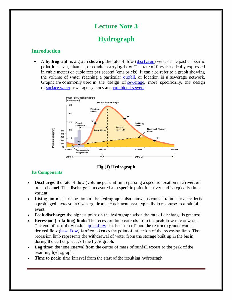
A hydrograph is a graph showing the rate of flow (discharge) versus time past a specific

point in a river, channel, or conduit carrying flow. The rate of flow is typically expressed

in cubic meters or cubic feet per second (cms or cfs). It can also refer to a graph showing

the volume of water reaching a particular outfall, or location in a sewerage network.

Graphs are commonly used in the design of sewerage, more specifically, the design

of surface water sewerage systems and combined sewers.

Fig (1) Hydrograph

Its Components

Discharge: the rate of flow (volume per unit time) passing a specific location in a river, or

other channel. The discharge is measured at a specific point in a river and is typically time

variant.

Rising limb: The rising limb of the hydrograph, also known as concentration curve, reflects

a prolonged increase in discharge from a catchment area, typically in response to a rainfall

event.

Peak discharge: the highest point on the hydrograph when the rate of discharge is greatest.

Recession (or falling) limb: The recession limb extends from the peak flow rate onward.

The end of stormflow (a.k.a. quickflow or direct runoff) and the return to groundwater-

derived flow (base flow) is often taken as the point of inflection of the recession limb. The

recession limb represents the withdrawal of water from the storage built up in the basin

during the earlier phases of the hydrograph.

Lag time: the time interval from the center of mass of rainfall excess to the peak of the

resulting hydrograph.

Time to peak: time interval from the start of the resulting hydrograph.

Unit Hydrograph

A unit hydrograph (UH) is the hypothetical unit response of a watershed (in terms of

runoff volume and timing) to a unit input of rainfall. It can be defined as the direct runoff

hydrograph (DRH) resulting from one unit (e.g., one cm or one inch) of effective rainfall

occurring uniformly over that watershed at a uniform rate over a unit period of time. As a

UH is applicable only to the direct runoff component of a hydrograph (i.e., surface

runoff), a separate determination of the baseflow component is required.

A UH is specific to a particular watershed, and specific to a particular length of time

corresponding to the duration of the effective rainfall. That is, the UH is specified as

being the 1-hour, 6-hour, or 24-hour UH, or any other length of time up to the time of

concentration of direct runoff at the watershed outlet. Thus, for a given watershed, there

can be many unit hydrographs, each one corresponding to a different duration of effective

rainfall.

The UH technique provides a practical and relatively easy-to-apply tool for quantifying

the effect of a unit of rainfall on the corresponding runoff from a particular drainage

basin. UH theory assumes that a watershed's runoff response is linear and time-invariant,

and that the effective rainfall occurs uniformly over the watershed. In the real world,

none of these assumptions are strictly true. Nevertheless, application of UH methods

typically yields a reasonable approximation of the flood response of natural watersheds.

The linear assumptions underlying UH theory allows for the variation in storm intensity

over time (i.e., the storm hyetograph) to be simulated by applying the principles of

superposition and proportionality to separate storm components to determine the resulting

cumulative hydrograph. This allows for a relatively straightforward calculation of the

hydrograph response to any arbitrary rain event.

An instantaneous unit hydrograph is a further refinement of the concept; for an IUH, the

input rainfall is assumed to all take place at a discrete point in time (obviously, this isn't

the case for actual rainstorms). Making this assumption can greatly simplify the analysis

involved in constructing a unit hydrograph, and it is necessary for the creation of a

geomorphologic instantaneous unit hydrograph.

Fig (2) Unit Hydrograph

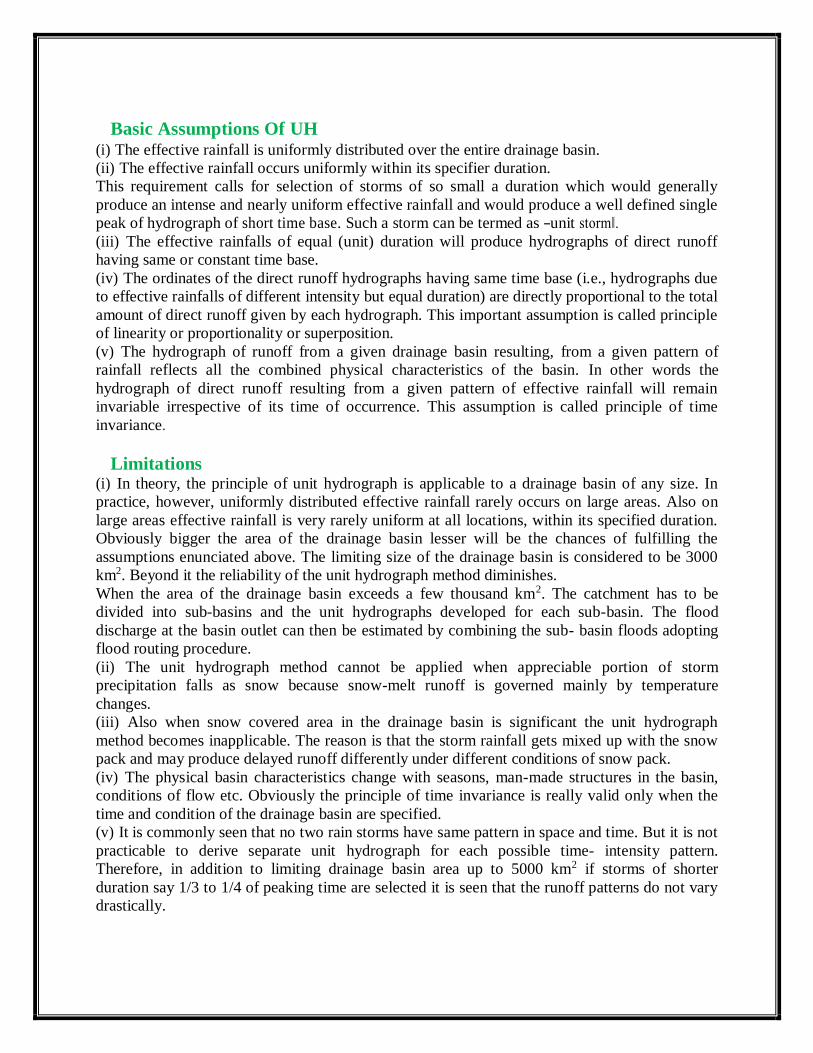
Basic Assumptions Of UH (i) The effective rainfall is uniformly distributed over the entire drainage basin.

(ii) The effective rainfall occurs uniformly within its specifier duration.

This requirement calls for selection of storms of so small a duration which would generally

produce an intense and nearly uniform effective rainfall and would produce a well defined single

peak of hydrograph of short time base. Such a storm can be termed as ―unit storm‖.

(iii) The effective rainfalls of equal (unit) duration will produce hydrographs of direct runoff

having same or constant time base.

(iv) The ordinates of the direct runoff hydrographs having same time base (i.e., hydrographs due

to effective rainfalls of different intensity but equal duration) are directly proportional to the total

amount of direct runoff given by each hydrograph. This important assumption is called principle

of linearity or proportionality or superposition.

(v) The hydrograph of runoff from a given drainage basin resulting, from a given pattern of

rainfall reflects all the combined physical characteristics of the basin. In other words the

hydrograph of direct runoff resulting from a given pattern of effective rainfall will remain

invariable irrespective of its time of occurrence. This assumption is called principle of time

invariance.

Limitations (i) In theory, the principle of unit hydrograph is applicable to a drainage basin of any size. In

practice, however, uniformly distributed effective rainfall rarely occurs on large areas. Also on

large areas effective rainfall is very rarely uniform at all locations, within its specified duration.

Obviously bigger the area of the drainage basin lesser will be the chances of fulfilling the

assumptions enunciated above. The limiting size of the drainage basin is considered to be 3000

km2. Beyond it the reliability of the unit hydrograph method diminishes.

When the area of the drainage basin exceeds a few thousand km2. The catchment has to be

divided into sub-basins and the unit hydrographs developed for each sub-basin. The flood

discharge at the basin outlet can then be estimated by combining the sub- basin floods adopting

flood routing procedure.

(ii) The unit hydrograph method cannot be applied when appreciable portion of storm

precipitation falls as snow because snow-melt runoff is governed mainly by temperature

changes.

(iii) Also when snow covered area in the drainage basin is significant the unit hydrograph

method becomes inapplicable. The reason is that the storm rainfall gets mixed up with the snow

pack and may produce delayed runoff differently under different conditions of snow pack.

(iv) The physical basin characteristics change with seasons, man-made structures in the basin,

conditions of flow etc. Obviously the principle of time invariance is really valid only when the

time and condition of the drainage basin are specified.

(v) It is commonly seen that no two rain storms have same pattern in space and time. But it is not

practicable to derive separate unit hydrograph for each possible time- intensity pattern.

Therefore, in addition to limiting drainage basin area up to 5000 km2 if storms of shorter

duration say 1/3 to 1/4 of peaking time are selected it is seen that the runoff patterns do not vary

drastically.

(vi) The principle of linearity is also not completely valid. This is so because due to variability in

proportion of surface, subsurface and groundwater runoff components during smaller and larger

storms of same duration, the maximum ordinate (peak) of the unit hydrograph derived from

smaller storm is smaller than the one derived from larger storm. Obviously the character and

duration of recession limb which is a function of the peak flow will also be different. When

appreciable non-linearity is seen to exist it is necessary to use derived unit hydrographs only for

reconstructing events of similar magnitude.

(vii) The unit hydrograph can be used theoretically to construct a flood hydrograph resulting

from a storm having same unit duration. Obviously it necessitates construction of several unit

hydrographs to cover different durations of storms. In practice however it is seen that a tolerance

of ± 25% in unit hydrograph duration is acceptable. Thus a 2 hour unit hydrograph can be

applied to storms of 1.5 to 2.5 hours duration.

Advantages of Unit Hydrograph Theory:

The limitation to the theory of unit hydrograph can be overcome to a large extent by remaining

within the various ranges and restrictions indicated above.

The unit hydrograph theory has several advantages to its credit which can be summarised

as below:

(i) Flood hydrograph can be calculated with the help of very short record of data.

(ii) In addition to peak flow unit hydrograph also gives total volume of runoff and its time

distribution.

(iii) The unit hydrograph procedure can be computerised easily to facilitate calculations.

(iv) It is very useful in checking the reliability of flows obtained by using statistical methods.

Derivation Of Unit Hydrographs 1. A number of isolated storm hydrographs caused by short spells of rainfall excess, each of

approximately the same duration (0.9 to 1.1D h) are selected from a study of continuously

gauged runoff of the stream

2. For each of these surface runoff hydrographs, the base flow is separated

3. The area under DRH is evaluated and the volume of direct runoff obtained is divided by the

catchment area to obtain the depth of ER

4. The ordinates of the various DRHs are divided by the respective ER values to obtain the

ordinates of the unit hydrograph

Flood hydrographs used in the analysis should be selected so as to meet the following

desirable features with respect to the storms responsible for them:

1. The storms should be isolated storms occurring individually

2. The rainfall should be fairly uniform during the duration and should cover the entire

catchment area

3. The duration of rainfall should be 1/5 to 1/3 of the basin lag

4. The rainfall excess of the selected storm should be high (A range of ER values of 1.0 to 4.0

cm is preferred)

• A number of unit hydrographs of a given duration are derived as mentioned above and then

plotted

• Because of spatial and temporal variations in rainfall and due to deviations of the storms from

the assumptions in the unit hydrograph theory, the various unit hydrographs developed will not

be exactly identical

and the ordinates of the composite DRH be

• In general, the mean of these curves is adopted as the unit hydrograph of the given duration for

the catchment

• The average of the peak flows and the time to peaks are computed first

• Then a mean curve of best fit (by eye judgment) is drawn through the averaged peak to close on

an averaged base length

• The volume of the DRH is determined and any departure from unity is corrected by adjusting

the peak value

• Note – It is customary to draw the averaged ERH of unit depth in the plot of the unit

hydrograph to indicate the type and duration of rainfall creating the unit hydrograph.

• It is assumed that the rainfall excess occurs uniformly over the catchment during the duration D

hours of a unit hydrograph

• An ideal duration for a unit hydrograph is one in which small fluctuations in rainfall intensity

does not have any significant effect on the runoff

• The duration of the unit hydrograph should not exceed 1/5 to 1/3 of the basin lag

• In general, for catchments larger than 250 sq.km., 6 hour duration is satisfactory.

5.3.4 Unit Hydrograph from a Complex Storm • When suitable simple isolated storms are not available, data from complex storms of long

duration will have to be used to derive the unit hydrograph

• The problem is to decompose a measured composite flood hydrograph into its component

DRHs and base flow

• A common unit hydrograph of appropriate duration is assumed to exist

• This is the inverse problem of derivation of the flood hydrograph

• Consider a rainfall excess made up of three consecutive durations of D hours and ER values

of .

• After base flow separation of the resulting composite flood hydrograph, a composite DRH is

obtained. Let the ordinates of the composite DRH be drawn at a time interval of D hours.

• At various time intervals 1D, 2D, 3D, ……. from the start of the ERH let the ordinates of unit

hydrograph be

Fig(3)

• The values of can be determined from the above

• Disadvantage of this method – Errors propagate and increase as computation proceeds

S-Hydrograph

• It is the hydrograph of direct surface discharge that would result from a continuous succession

of unit storms producing 1cm(in.)in tr –hr

• If the time base of the unit hydrograph is Tb hr, it reaches constant outflow (Qe) at T hr, since 1

cm of net rain on the catchment is being supplied and removed every tr hour and only T/tr unit

graphs are necessary to produce an S-curve and develop constant outflow given by,

Qe = (2.78·A) / tr

where Qe = constant outflow (cumec)

tr = duration of the unit graph (hr)

A = area of the basin (km2 or acres)

• In India, only a small number of streams are gauged (i.e., stream flows due to single and

multiple storms, are measured)

• There are many drainage basins (catchments) for which no stream flow records are available

and unit hydrographs may be required for such basins

• In such cases, hydrographs may be synthesized directly from other catchments, which are

hydrological and meteorologically homogeneous, or indirectly from other catchments through

the application of empirical relationship

• Methods for synthesizing hydrographs for ungauged areas have been developed from time to

time by Bernard, Clark, McCarthy and Snyder. The best known approach is due to Snyder

(1938).

Fig (4) S-Hydrograph

Snyder’s method

Snyder (1938) was the to develop a synthetic UH based on a study of watersheds in the

Appalachian Highlands. In basins ranging from 10 – 10,000 mi.2

Snyder relations are

tp = Ct (LLC)0.3

where tp= basin lag (hr)

L= length of the main stream from the outlet to the divide (mi)

Lc = length along the main stream to a point nearest the watershed centroid (mi)

Ct = Coefficient usually ranging from 1.8 to 2.2

Qp = 640 CpA/tp

where Qp = peak discharge of the UH (cfs)

A = Drainage area (mi2)

Cp = storage coefficient ranging from 0.4 to 0.8, where larger values of cp are associated with

smaller values of Ct

Tb = 3+tp/8

where Tb is the time base of hydrograph Note: For small watershed the above eq. should be replaced by multiplying tp by the value varies

from 3-5

• The above 3 equations define points for a UH produced by an excess rainfall of duration

D= tp/5.5

Fig (5) Snyder’s hydrograph parameter

Instantaneous Unit Hydrograph (IUH).

• The instantaneous unit hydrograph is defined as a unit hydrograph produced by an effective

rainfall of 1 mm and having an infinitesimal reference duration (in other words the duration

tends towards zero).

• IUH is the direct runoff hydrograph resulted from an impulse function rainfall i.e., one unit of

effective rainfall at a time instance.

Fig (6) IUH

REFERENCES

1. Engineering Hydrology by K. Subramanya. Tata Mc Graw Hill Publication

2. Elementary Hydrology by V.P. Singh, Prentice Hall Publication

3. Hydrology by P. Jayarami Reddy

4. Handbook of applied hydrology, V.T. Chow, Mc Graw Hill.

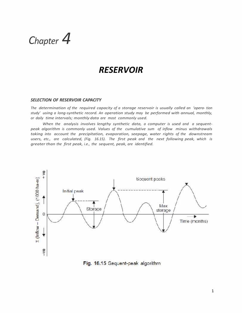
1

Chapter 4

RESERVOIR

SELECTION OF RESERVOIR CAPACITY

The determination of the required capacity of a storage reservoir is usually called an ‘opera- tionstudy’ using a long-synthetic record. An operation study may be performed with annual, monthly,or daily time intervals; monthly data are most commonly used.

When the analysis involves lengthy synthetic data, a computer is used and a sequent-peak algorithm is commonly used. Values of the cumulative sum of inflow minus withdrawalstaking into account the precipitation, evaporation, seepage, water rights of the downstreamusers, etc., are calculated, (Fig. 16.15). The first peak and the next following peak, which isgreater than the first peak, i.e., the sequent, peak, are identified.

2

The maximum difference between this sequent peak and the lowest trough during theperiod under study is taken as the required storage capacity of the reservoir.

RESERVOIR MASS CURVE

A mass curve (or Rippl diagram, 1882) is a cumulative plotting of net reservoir inflow (Fig. 16.14),and is expressed as

where V(t) = volume of runoffQ(t) = reservoir inflow

both as functions of time

3

The instantaneous rate of flow at any point on the mass curve is given by the slope of the tangent at the point, i.e.

As already discussed, the mass curve has many useful applications in the design of a storage reservoir, such asdetermination of reservoir capacity, operations procedure and flood routing.

RESERVOIR MASS CURVE AND STORAGE

During high flows, water flowing in a river has to be stored so that a uniform supply of water canbe assured, for water resources utilisation like irrigation, water supply, power generation, etc.during periods of low flows of the river.

A mass diagram is a graphical representation of cumulative inflow into the reservoirversus time which may be monthly or yearly. A mass curve is shown in Fig. 10.1 for a 2-yearperiod. The slope of the mass curve at any point is a measure of the inflow rate at that time.Required rates of draw off from the reservoir are marked by drawing tangents, having slopesequal to the demand rates, at the highest points of the mass curve. The maximum departurebetween the demand line and the mass curve represents the storage capacity of the reservoirrequired to meet the demand. A demand line must intersect the mass curve when extendedforward, otherwise the reservoir is not going to refill. The vertical distance between the suc-cessive tangents represent the water wasted over the spillway. The salient features in themass curve of flow in Fig. 10.1 are:

a-b: inflow rate exceeds the demand rate of x cumec and reservoir is overflowingb: inflow rate equals demand rate and the reservoir is just full

b-c: inflow rate is less than the demand rate and the water is drawn from storagec: inflow rate equals demand rate and S1 is the draw off from the reservoir (Mm3)

c-d: inflow rate exceeds demand rate and the reservoir is filling

4

d: reservoir is full againd-e: same as a-b e:

similar to b

e-f: similar to b-cf: inflow rate equals demand rate and S2 is the draw off from the reservoir

f-g: similar to c-dTo meet the demand rate of x cumec the departure S2 > S1; hence, the storage capacity of

the reservoir is S2 Mm3. If the storage capacity of the reservoir, from economic considera- tions, iskept as S1 Mm3, the demand rate of x cumec can not be maintained during the time e-f and it canbe at a lesser rate of y cumec (y < x).

5

The use of mass curve is to determine:(i) the storage capacity of the reservoir required to meet a particular withdrawal rate. (ii)

the possible rate of withdrawal from a reservoir of specified storage capacity.The observed inflow rates have to be adjusted for the monthly evaporation from the

reservoir surface, precipitation, seepage through the dam, inflow from adjacent basins, re-quired releases for downstream users, sediment inflow, etc. while calculating the storage ca-pacity of the reservoir.

The average flow figures for the site of a proposed dam are collected for about 10 years.From this record the flow figures for the driest year are used for drawing the mass flow curve.Graphical analysis is enough for preliminary studies. Final studies are made by tabular com-putation. If tangents are drawn to the crest and trough of the mass curve such that the depar-ture of the lines represents the specified reservoir capacity, the slope of the tangent at thecrest gives the continuous flow that can be maintained with the available storage capacity.From this the greatest continuous power output for the available fall at the site for a givenplant efficiency and load factor can be determined.

From the daily flow data a hydrograph or a bar graph is drawn for the maximum flood during theperiod of 10 years and the spillway capacity to pass this flood with the available storage capacity isdetermined. Thus, the power and the flood control potentialities of the site are investigated.

The mass curve of water utilisation need not be a straight line. The dashed curve in Fig.10.2 shows the cumulative requirements of water use in different months as compared withmonthly cumulatively inflow. The maximum draft in the reservoir (i.e., maximum depar- ture of thewater use and inflow curves) occurs by the end of April. The reservoir again be-comes full by the end of September when the two curves intersect.

6

FLOW DURATION CURVES

Flow duration curves show the percentage of time that certain values of discharge weekly,monthly or yearly were equalled or exceeded in the available number of years of record. Theselection of the time interval depends on the purpose of the study. As the time interval in- creasesthe range of the curve decreases, Fig. 10.4. While daily flow rates of small storms are useful for thepondage studies in a runoff river power development plant, monthly flow rates for a number ofyears are useful in power development plants from a large storage reservoir. The flow durationcurve is actually a river discharge frequency curve and longer the period of record, more accurate isthe indication of the long term yield of a stream. A flat curve indicates a river with a few floods withlarge ground water contribution, while a steep curve indicates frequent floods and dry periods withlittle ground water contribution.

7

SEDIMENT MOVEMENT AND DEPOSITION

As the silt originates from the water shed, the characteristics of the catchment such itsareal extent, soil types, land slopes, vegetal cover and climatic conditions like temperature,nature and intensity of rainfall, have a great significance in the sediment production in theform of sheet erosion, gully erosion and stream, channel erosion. In regions of moderate rain- fall,sheet erosion is the dominant source of total sediment load while in arid and semi-arid regions,gullying and stream-channel erosion furnish the greater part of the load.

Experiments have shown that the erosive power of water, flowing with a velocity V, variesas V 2 while the transporting ability of water varies as V 6. Sediment moves in the stream assuspended load (fine particles) in the flowing water, and as bed load (large parti- cles), whichslides or rolls along the channel bottom. Sometimes, the particles (small particles of sand andgravel) move by bouncing along the bed, which is termed as ‘saltation’, which is a transitionalstage between bed and suspended load. The material, which moves as bed load at one section maybe in suspension at another section.

The suspended sediment load of streams is measured by sampling the water, filtering toremove the sediment, drying and weighing the filtered material.

The samplers may be of ‘depth-integrating type’ or ‘point samplers’. Point samplers are usedonly where it is not possible to use the depth integrating type because of great depth of highvelocity, or for studies of sediment distribution in streams. The sample is usually col- lected in‘pint bottle’ held in a sample of stream-lined body so as not to disturb the flow while collecting arepresentative sample.

The relation between the suspended-sedimenttransport Qs and stream flow Q is given

and is often represented by a logarithmic plot of Qs vs. Q (Fig. 11.1); Qs = K when Q = 1, and nis the slope of the straight line plot and 2 to 3.

The sediment rating curve from a continuous record of stream flow provides a roughestimate of sediment inflow to reservoirs and the total sediment transport may be estimated byadding 10-20% to the suspended sediment transport to allow for the bed load contribution.

When the sediment-laden water reaches a reservoir, the velocity and turbulence aregreatly reduced. The dense fluid-solid mixture along the bottom of the reservoir moves slowly inthe form of a density current or stratified flows, i.e., a diffused colloidal suspension having adensity slightly different from that of the main body of reservoir water, due to dissolvedminerals and temperature, and hence does not mix readily with the reservoir water (Fig. 11.2).Smaller particles may be deposited near the base of the dam. Some of the density currents andsettled sediments near the base of the dam can possibly be flushed out by operating the sluicegates. The modern multipurpose reservoirs are operated at various water levels, which are

8

significant in the deposition and movement of silt in the reservoir.

9

The total amount of sediment that passes any section of a stream is referred to as thesediment yield or sediment production. The mean annual sediment production rates generallyrange from 250-2000 tons/km2 or 2.5-18 ha-m/100 km2 and the Indian reservoirs are losing astorage capacity of 0.5-1% annually.

REDUCTION IN RESERVOIR CAPACITY

The useful life of a reservoir gets reduced due to sediment deposition causing a decrease in itsstorage capacity.The factors affecting the pattern of sediment deposition in reservoirs are:

(i) sediment load (i.e., sediment inflow rate) (ii)sediment size (i.e., gradation of silt)

(iii) compaction of sediment (iv) river inflow pattern(v) river valley slope (vi) shape of reservoir

(vii) capacity of reservoir (its size and storage period)(viii) vegetal growth at the head

(ix) outlets in the dam (their types, location and size) (x)reservoir operation

(xi) upstream reservoirs, if any.It has been found by experience that a low sediment inflow rate, large fraction of fine

particles, steep slope, no vegetation at head of reservoir, low flow detention time in the reservoir (byoperation of outlets of suitable size at different levels), possibly series of upper tanks or reservoirupstream (where deposition occurs) do not favour sediment deposition and compaction. The siltcarried in the rainy season may be excluded from the reservoir by means of scouring sluicesslightly above the deep river-bed, which discharge the heavily silt-laden water at high velocity. Thepercent of the inflowing sediment, which is retained in a reservoir is called the trap efficiency andit is a function of the ratio of reservoir capacity to total annual sediment inflow, since a smallreservoir on a large stream passes most of its inflow quickly (giving no time for the silt to settle)while a large reservoir allows more detention time for the suspended silt to settle. The relationbetween trap efficiency of reservoir vs. capacity-inflow ratio is shown in Fig. 11.3 (Brune, 1953), onthe basis of data from surveys of existing reservoirs. The rate at which the capacity of a reservoiris reduced by sediment deposition depends on

(i) the rate of sediment inflow, i.e., sediment load.(ii) the percentage of the sediment inflow trapped in the reservoir, i.e., trap efficiency. (iii)

the density of the deposited sediment.

RESERVOIR SEDIMENTATION CONTROL

Sediment deposition in reservoirs can not be actually prevented but it can be retarded byadopting some of the following measures:

(i) Reservoir sites, which are prolific sources of sediment should be avoided.(ii) By adopting soil-conservation measures in the catchment area, as the silt originates in

the watershed. See art 8.7 in Chapter 8.

10

(iii) Agronomic soil conservation practices like cover cropping, strip cropping, contourfarming, suitable crop rotations, application of green manure (mulching), proper control overgraze lands, terracing and benching on steep hill slopes, etc. retard overland flow, increaseinfiltration and reduce erosion.

(iv) Contour trenching and afforestation on hill slopes, contour bunding gully plugging bycheck dams, and stream bank stabilisation by the use of spurs, rivetments, vegetation, etc. aresome of the engineering measures of soil conservation.

(v) Vegetal cover on the land reduces the impact force of rain drops and minimiseserosion.

(vi) Sluice gates provided in the dam at various levels and reservoir operation, permit thedischarge of fine sediments without giving them time to settle to the bottom.

(vii) Sediment deposits in tanks and small reservoirs may be removed by excavation,dredging, draining and flushing either by mechanical or hydraulic methods and sometimesmay have some sales value.

Floods Management & Hydrologic Analysis

SIZE OF FLOODSA flood is an unusual high stage of a river due to runoff from rainfall and/or melting of snow inquantities too great to be confined in the normal water surface elevations of the river orstream, as the result of unusual meteorological combination.

The maximum flood that any structure can safely pass is called the ‘design flood’ and isselected after consideration of economic and hydrologic factors. The design flood is related tothe project feature; for example, the spillway design flood may be much higher than theflood control reservoir design flood or the design flood adopted for the temporary cofferdams. A design flood may be arrived by considering the cost of constructing the structureto provide flood control and the flood control benefits arising directly by prevention of damage tostructures downstream, disruption communication, loss of life and property, damage to cropsand under- utilisation of land and indirectly, the money saved under insurance andworkmen’s compensation laws, higher yields from intensive cultivation of protected lands andelimination of losses arising from interruption of business, reduction in diseases resulting frominundation of flood waters. The direct benefits are called tangible benefits and the indirectbenefits are called intangible benefits. The design flood is usually selected after making a cost-benefit analysis and exercising engineering judgement.

When the structure is designed for a flood less than the maximum probable, thereexists a certain amount of flood risk to the structure, nor is it economical to design for100% flood protection. Protection against the highest rare floods is uneconomical becauseof the large investment and infrequent flood occurrence.

In the design flood estimates, reference is usually made to three classes:(a) Standard Project Flood (SPF). This is the estimate of the flood likely to occur from

the most severe combination of the meteorological and hydrological conditions, which arerea- sonably characteristic of the drainage basin being considered, but excluding extremelyrare combination.

(b) Maximum Probable Flood (MPF). This differs from the SPF in that it includes theextremely rare and catastrophic floods and is usually confined to spillway design of very highdams. The SPF is usually around 80% of the MPF for the basin.

(c) Probable Maximum Precipitation (PMP). From the observations of air moisture fromthe maximum due-point and temperature recorded and air-inflow (from the wind speedand barometric pressure recorded), the moisture inflow index in the storm is determined. Thebest known upward adjustment to be applied to the historical and hypothetical major stormsis the

maximisation with respect to moisture charge. The adjusted storm rainfall is assumed tobear the same ratio to the observed storm rainfall, as the maximum moisture charge overthe basin to the moisture charge of the observed storm. From the critical combinations ofstorms, and moisture adjustment the PMP is derived which, after minimising losses, whenapplied on the design unit hydrograph for the basin, will produce the MPF. Occasionallywhen enough storm data for the given basin is not available, PMP can be estimated byadopting a severe storm over neighbouring catchment (which is meteorologicallyhomogeneous) and transposing it to the catchment under consideration.

(d) Design Flood—It is the flood adopted for the design of hydraulic structures likespillways, bridge openings, flood banks, etc. It may be the MPF or SPF or a flood of any desiredrecurrence interval depending upon the degree of flood protection to be offered and costeco- nomics of construction of structures to the desired flood stage; the design flood is usuallyse- lected after making a cost-benefit analysis, i.e., the ratio of benefit to cost may be desiredto be the maximum.

ESTIMATION OF PEAK FLOOD

The maximum flood discharge (peak flood) in a river may be determined by the followingmethods:

(i) Physical indications of past floods—flood marks and localenquiry

(ii) Empirical formulae and curves(iii) Concentration time method(iv) Overland flow hydrograph(v) Rational method(vi) Unit hydrograph(vii) Flood frequency studies

The above methods are discussed below:

(i) Observations at nearby structure. By noting the flood marks (and by local enquiry), depths,affluxes (heading up of water near bridge openings, or similar obstructions to flow) andother items actually at an existing bridge, on anecut (weir) in the vicinity, the maximum flooddischarge may be estimated. The flood marks are connected by levelling, the profile is plottedand HFL marked on it, and the cross sectional area is determined. The surface fall at HFL iscalculated from the difference in HFL at known distance apart. It may be checked with the bedslope; Q = CA3/4

the coefficient C = 11–14, where the aar is 60–120 cm= 14–19 in Madhya Pradesh= 32 in western Ghats

up to 35, maximum value2. Ryves formula derived from a study of rivers in south India

A = CA2/3

Coefficient C = 6.8 within 80 km of coast= 8.3 for areas between 80 and 2400 km from the coast= 10.0 for limited area near the hills up to 40,

actual observed values3. Inglis formula for fan-shaped catchments of Bombay state (Maharashtra)

124 AQ =

A 10.4

4. Myers formula Q = 175 A0.5

5. Ali Nawab Jang Bahadur formula for the old Hyderabad state

Q = CA(0.993 – 1/14 log A) .the coefficient C varies from 48 to 60

Maximum value of C = 85

6. Fuller’s formula (1914)

Q = CA0.8 (1 + 0.8 log TT)(1 + 2.67 A–0.3) . constants

derived from the basins in USA 10 years data is required for sufficient reliability.The coefficient C varies from 0.026 to 2.77; T = recurrence interval in years. Fullerwas the first to suggest that frequency should be considered as a factor inestimating floods.

7. Greager’s formula for USA

Q = C(0.386 A)0.894(0.386 A)0.048

8. Burkli Ziegler formula for USA

Q = 412 A3/4

In all the above formula, Q is the peak flood in cumec and A is the area of the drainagebasin in km2.

(iii) Envelope Curves. Areas having similar topographical features and climatic condi-tions are grouped together. All available data regarding discharges and flood formulaeare compiled along with their respective catchment areas. Peak flood discharges are thenplotted against the drainage areas and a curve is drawn to cover or envelope the highestplotted points. Envelope curves are generally used for comparison only and the designfloods got by other methods, should be higher than those obtained from envelope curves. ForIndian rivers, envel- oping curves from observed floods have been developed by Kanwar Sain andKarpov, Fig. 8.1 (a).

(iv) Concentration Time Method. The concentration time method of estimating thepeak discharge consists of two steps:

(i) Determination of the concentration time, etc.(ii) Selection of the period of maximum net rainfall for the concentration time duration.

This method can be used for design storms or in conjunction with intensity-duration- frequency curves.

(v) Rational Method. The rational method is based on the application of the formulaQ = CiA ...(8.9)

where C is a coefficient depending on the runoff qualities of the catchment called therunoff coefficient (0.2 to 0.8). The intensity of rainfall i is equal to the design intensity orcriticalintensity of rainfall ic corresponding to the time of concentration tc for the catchment fora given recurrence interval T; the design intensity of rainfall i (= ic) can be found from theintensity-duration-frequency curves, for the catchment corresponding to tc and T. If theintensity-duration-frequency curves, are not available for the catchment and amaximumprecipitation of P cm occurs during a storm period of tR hours, then the design intensity i (= ic)can be obtained from theequation

(vi) The Unit Hydrograph Method. For small and medium size basins (A < 5000 km2,i.e., when a single unit hydrograph could be applied to the entire basin) in developing designflood hydrographs by applying the unit hydrograph for the basin, the design stormestimates are made by the following methods.

(i) Selection of major storms(ii) Maximization of selected storms

(iii) Plotting the depth-area-duration curves and their analysis(iv) Moisture adjustment(v) Storm transposition to a critical position

(vi) Envelopment of the transposed adjusted storms(vii) Use of minimum infiltration indicesIn the depth-area-duration analysis of a particular storm, the maximum average

depths of rainfall over various sizes of area during certain periods of storm (hr or days), saycm over1000 km2 in 1 day, 2 days or 3 days from the isohyetal maps contructed (see Fig. 2.15). Suchvalues determined for all the transposable storms provide the basic data to estimate thePMPover the basin.

FLOOD FREQUENCY STUDIES

When stream flow peaks are arranged in the descending order of magnitude they constitutea statistical array whose distribution can be expressed in terms of frequency of occurrence.There are two methods of compiling flood peak data—the annual floods and the partialduration series. In the annual floods, only the highest flood in each year is used thus ignoringthe next highest in any year, which sometimes may exceed many of the annual maximum. Inthe par- tial duration series, all floods above a selected minimum are taken for analysis,regardless of the time-interval, so that in some years there may be a number of floods abovethe basic stage, while in some other years there may not any such flood at all. Thedisadvantage of the partial duration series is that the data do not furnish a proper frequency(true distribution) series and so a reasonable statistical analysis cannot be made. But all thelarger floods are used in this analysis, which is an advantage while in annual flood seriessome big floods are omitted because they were not the highest floods in any year considered.Usually the basic stage is as- sumed sufficiently low so that as many peaks (4 or 5) as

possible each year are above this stage. The two series give very nearly the same recurrenceinterval for the larger floods, but the partial series indicates higher floods for shorterrecurrence intervals. For information about floods of fairly frequent occurrence, as isrequired during the construction period of a large dam (say, 4-5 years), the partial seriesare the best, while for the spillway design flood the annual series are preferable, since theflood should not be exceeded in the dam’s life time, say 100 years.

Annual Flood Series The return period or recurrence interval (T) is the average numberof years during which a flood of given magnitude will be equalled or exceeded once and iscomputed by one of the following methods.

California method (1923):

nT =

m

Weilbul method (1939):

T =n 1

...(8.11 b)m

where n = number of events, i.e., years of recordm = order or rank of the event (flood item) when the flood magnitudes (items) are

ar- ranged in the descending order (m = 1 for the highest flood, m = n for thelowest flood)

T = recurrence interval (T = n-yr for the highest flood, T = 1 yr for the lowest flood, byCalifornia method)

The probability of occurrence of a flood (having a recurrence interval T-yr) in any year,i.e., the probability of exceedance, is

1P = ...(8.12)

Tand the probability that it will not occur in a given year, i.e., the probability of non-exceedance(P), is

P= 1 – P ...(8.12 b) Oneinteresting example of the application of statistics to a hydrologic problem (i.e., stochastic

hydrology), is Gumbel’s theory of extreme values. The probability of an event ofmagnitude x not being equalled or exceeded (the probability of non-occurrence, P), based

onthe argument that the distribution of floods is unlimited (i.e., for large values of n, say n > 50),

METHODS OF FLOOD CONTROL

A flood is an unusual high stage of a river overflowing its banks and inundating the marginallands. This is due to severe storm of unusual meteorological combination, sometimes com-bined with melting of accumulated snow on the catchment. This may also be due to shifting ofthe course of the river, earthquake causing bank erosion, or blocking of river, or breaching ofthe river flood banks. Floods have swept vast regions in India, particularly in the basins ofrivers Kosi, Brahmaputra, Godavari, Narmada and Tapti. Floods cause much loss of life andproperty, disruption of communication, damage to crops, famine, epidemic diseases andother indirect losses.

Design magnitudes of floods are needed for the design of spillways, reservoirs, bridgeopenings, drainage of cities and air ports, and construction of flood walls and levees (floodbanks). The maximum flood that any structure can safely pass is called the ‘design flood’.

The damages due to the devastating floods can be minimised by the following floodcontrol measures, singly or in combination.

(i) by confining the flow between high banks by constructing levees (flood banks) ,dykes, or flood walls.

(ii) by channel improvement by cutting, straightening or deepening and following rivertraining works.

(iii) by diversion of a portion of the flood through bypasses or flood ways. In some casesa fuse plug levee is provided. It is a low section of levee, which when once over topped, willwash out rapidly and develop full discharge capacity into the flood-way. In other locations, aconcrete sill, weir or spillway controlled by stop logs or needles may be provided so that theoverflow occurs at a definite river stage. Sometimes dynamiting a section of levee is resortedto bypass the flood.

(iv) by providing a temporary storage of the peak floods by constructing upstreamreser- voirs and retarding basins (detention basins).

(v) by adopting soil conservation measures (land management) in the catchmentarea. (vi) by temporary and permanent evacuation of the flood plain, and flood plain

zoningby enacting legislation.

(vii) by flood proofing of specific properties by constructing a ring levee or flood wallaround the property.

(viii) by setting up flood forecasting—short term, long term, rhythm signals andradar, and warning centres at vulnerable areas.Flood Control by Reservoirs

The purpose of a flood control reservoir is to temporarily store a portion of the flood so thatthe flood peaks are flattened out. The reservoir may be ideally situated immediatelyupstream of the area to be potected and the water discharged in the channel downstreamat its safe capac- ity (known from its stage-discharge curve), i.e., the peak has been reducedby AB, Fig. 8.6. All the inflow into the reservoir in excess of the safe channel capacity isstored until the inflow drops below the channel capacity and the stored water is released torecover the storage capac-ity for the next flood.

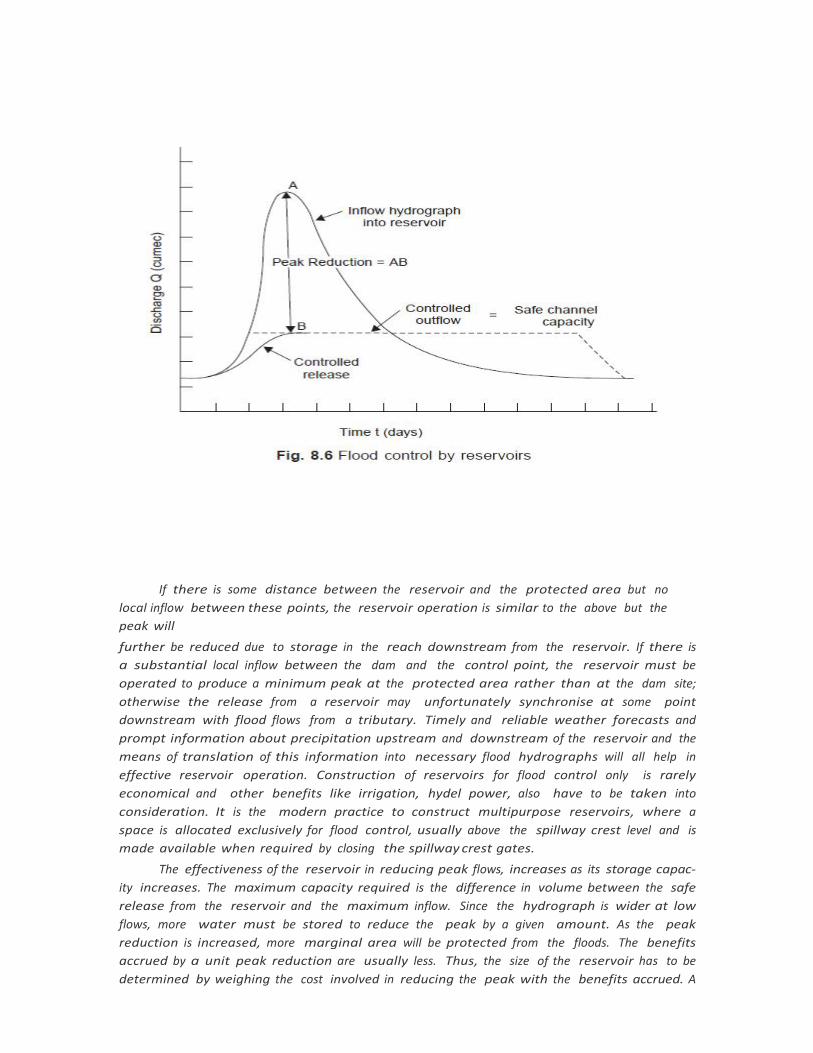
If there is some distance between the reservoir and the protected area but nolocal inflow between these points, the reservoir operation is similar to the above but thepeak willfurther be reduced due to storage in the reach downstream from the reservoir. If there isa substantial local inflow between the dam and the control point, the reservoir must beoperated to produce a minimum peak at the protected area rather than at the dam site;otherwise the release from a reservoir may unfortunately synchronise at some pointdownstream with flood flows from a tributary. Timely and reliable weather forecasts andprompt information about precipitation upstream and downstream of the reservoir and themeans of translation of this information into necessary flood hydrographs will all help ineffective reservoir operation. Construction of reservoirs for flood control only is rarelyeconomical and other benefits like irrigation, hydel power, also have to be taken intoconsideration. It is the modern practice to construct multipurpose reservoirs, where aspace is allocated exclusively for flood control, usually above the spillway crest level and ismade available when required by closing the spillway crest gates.

The effectiveness of the reservoir in reducing peak flows, increases as its storage capac-ity increases. The maximum capacity required is the difference in volume between the saferelease from the reservoir and the maximum inflow. Since the hydrograph is wider at lowflows, more water must be stored to reduce the peak by a given amount. As the peakreduction is increased, more marginal area will be protected from the floods. The benefitsaccrued by a unit peak reduction are usually less. Thus, the size of the reservoir has to bedetermined by weighing the cost involved in reducing the peak with the benefits accrued. A

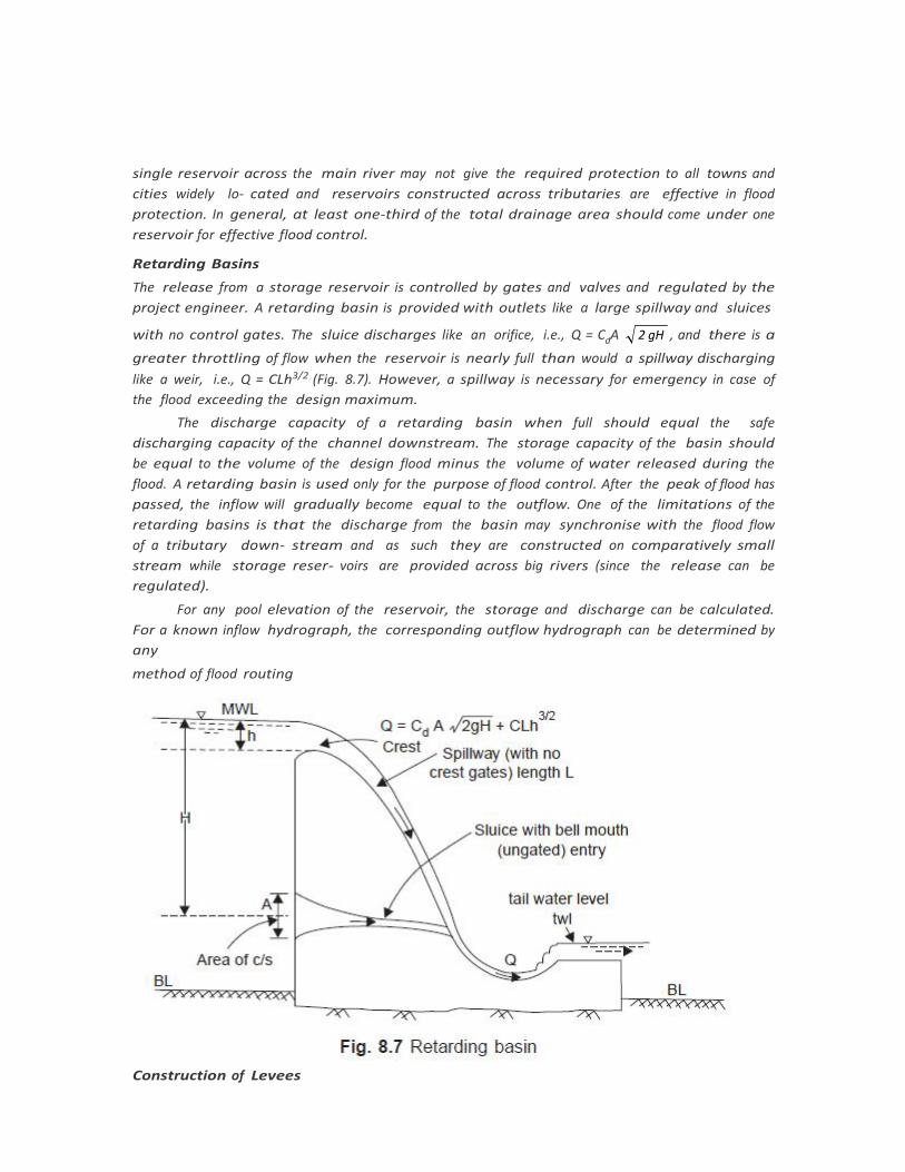
single reservoir across the main river may not give the required protection to all towns andcities widely lo- cated and reservoirs constructed across tributaries are effective in floodprotection. In general, at least one-third of the total drainage area should come under onereservoir for effective flood control.

Retarding Basins

The release from a storage reservoir is controlled by gates and valves and regulated by theproject engineer. A retarding basin is provided with outlets like a large spillway and sluices

with no control gates. The sluice discharges like an orifice, i.e., Q = CdA 2 gH , and there is agreater throttling of flow when the reservoir is nearly full than would a spillway discharginglike a weir, i.e., Q = CLh3/2 (Fig. 8.7). However, a spillway is necessary for emergency in case ofthe flood exceeding the design maximum.

The discharge capacity of a retarding basin when full should equal the safedischarging capacity of the channel downstream. The storage capacity of the basin shouldbe equal to the volume of the design flood minus the volume of water released during theflood. A retarding basin is used only for the purpose of flood control. After the peak of flood haspassed, the inflow will gradually become equal to the outflow. One of the limitations of theretarding basins is that the discharge from the basin may synchronise with the flood flowof a tributary down- stream and as such they are constructed on comparatively smallstream while storage reser- voirs are provided across big rivers (since the release can beregulated).

For any pool elevation of the reservoir, the storage and discharge can be calculated.For a known inflow hydrograph, the corresponding outflow hydrograph can be determined byanymethod of flood routing

Construction of Levees

The construction of levees (flood banks or dykes) is extensively followed in India, since it is aneconomical, direct and immediate method. The design and construction of levees are similarto those of an earth dam. The levees are constructed beyond the meander belt of a river, Fig. 8.8(a) and they tame a river not to change its course. As far as possible, there should be veryfew curves in their alignment. They require constant watch and after the floods recede,repairs and restoration of levees should be resorted to.

The spacing and height of levees are determined by a series of trials. A height is as-sumed and the discharge through the proper channel is computed for the assumed highwater flow, which is the level of the top of bank less the free board. This flow subtractedfrom the estimated probable maximum flood discharge gives the discharge to be passedover the flood ways between the proper channel and the levees (Figs. 8.8 (a) and (b), 8.9 and8.10). Area of the flood ways is then obtained by dividing it by the velocity of flow. The spacingof levees thus obtained, should give a minimum value for the cost of levees and the value ofthe submerged land in the flood way. The effects of levees on flood flow are:

(i) increase in the rate of flood flow(ii) increase in the flood water elevation

(iii) increase in the carrying capacity of the channel(iv) increase in the scouring action(v) decrease of surface slope of stream above the leveed section

Channel Improvement

Channel improvement increases the discharging capacity of the stream therebydecreasing the height and duration of the flood. Flood carrying capacity can be increasedeither by in- creasing the cross-sectional area or by increasing the velocity along the river.Enlarging the section is attempted only for narrow and shallow channels with smallwatersheds, the limit of such enlargement in width being 30-40 m. Deepening is preferredto widening since the hy- draulic mean radius increases more with depth (for the sameincrease in the sectional area) thus increasing the velocity.

The channel velocity (given by Manning’s or Chezy’s formulae) is affected by hydraulicmean radius, slope of river bed and roughness of the bed and sides. Roughness can bereduced by

(i) removing sand bars.(ii) prevention of cropping on river beds near banks.

(iii) removal of fallen trees and other snags.(iv) elimination of sharp bends of meandars by providing cutoffs (Fig. 8.11).In a stream, deepening results in the loss of slope as its outlet can not usually be low-

ered. Deepening can be resorted to only when cutoffs are provided, when the slope of thechannel is increased due to the reduction in the length of flow. Thus, a cutoff helps

(i) in increase the velocity by increasing the slope,(ii) to shorten the path of flow by elimination of meandars, and consequently

(iii) to shorten the levees necessary to confine flood waters.Elimination of meanders by providing straight cutoffs has been done on the river Mis-

sissippi in USA.

RESERVOIR ROUTING

Flood routing is the process of determining the reservoir stage, storage volume of theoutflow hydrograph corresponding to a known hydrograph of inflow into the reservoir; thisis called reservoir routing. For this, the capacity curve of the reservoir, i.e., ‘storage vs poolelevation’, and ‘outflow rate vs. pool elevation’, curves are required. Storage volumes fordifferent pool elevations are determined by planimetering the contour map of the reservoirsite. For exam- ple, the volume of water stored (V) between two successive contours havingareas A1 and A2 (planimetered) and the contour interval d, is given by

dCone formula, V =

Prismoidal formula, V =

3(A1 + A2 + A1 A2 ) ...(9.1)

d6

(A1 + A2 + 4Am) ...(9.2)

STREAM FLOW ROUTING

In a stream channel (river) a flood wave may be reduced in magnitude and lengthened intravel time i.e., attenuated, by storage in the reach between two sections. The storage inthe reach may be divided into two parts-prism storage and wedge storage, Fig. 9.5, since thewater surface is not uniform during the floods. The volume that would be stored in thereach if the flow were uniform throughout, i.e., below a line parallel to the stream bed, iscalled ‘prism storage’ and the volume stored between this line and the actual watersurface profile due to outflow being different from inflow into the reach is called ‘wedgestorage’. During rising stages the wedge storage volume is considerable before the outflowactually increases, while during falling stages inflow drops more rapidly than outflow, thewedge storage becoming negative.

In the case of stream-flow routing, the solution of the storage equation is morecompli- cated, than in the case of reservoir routing, since the wedge storage is involved.While the storage in a reach depends on both the inflow and outflow, prism storagedepends on the outflow alone and the wedge storage depends on the difference (I – O). Acommon method of stream flow routing is the Muskingum method (McCarthy, 1938)where the storage is ex- pressed as a function of both inflow and outflow in the reach as

S = K [xI + (1 – x) O] ...(9.9)where K and x are called the Muskingum coefficients (since the Eq. (9.9) was first developed bythe U.S. Army Corps of Engineers in connection with the flood control schemes in theMuskingum River Basin, Ohio), K is a storage constant having the dimension of time and x is

a dimensionless constant for the reach of the river. In natural riverchannels x ranges from0.1 to 0.3. The Eq. (9.9) in most flood flows approaches a straight line. Trial values of x areas- sumed and plots of ‘S vs. [xI + (1 – x) O]’ are in the form of storage loops; for a particularvalue of x, the plot is a straight line and the slope of the line gives K. If S is in cumec-day and I,O are in cumec, K is in day.

y

FLOOD FREQUENCY METHODS

For the annual flood data of Lower Tapti River at Ukai (30 years: 1939–1968) in Example 8.5the flood frequencies of 2–, 10–, 50–, 100–, 200–, and 1000-year floods have been worked outbelow by the probability methods developed by Fuller, Gumbel, Powell, Ven Te Chow, andstochastic methods, and the flood frequency curves are drawn on a semi-log paper as shownin Fig. 15.1. It can be seen that the Gumbel’s method gives the prediction of floods of aparticular frequency exceeding the observed floods by a safe margin and can be adopted inthe design of the structure.

1. Fuller’s formula. QT = Q (1 + 0.8 log T) ...(15.1) From

Table 8.5, Q = 14.21 thousand cumec (tcm)

T log T 0.8 log T QT = Q (1 + 0.8 log T)

(tcm)

1000 3.0 2.4 48.3200 2.3010 1.8408 40.4100 2.0 1.6 37.0

50 1.6990 1.3592 33.510 1.0 0.8 25.6

2 0.3010 0.2408 17.35

2. Gumbel’s method. According to the extreme value distribution, the probability of occur-rence of a flood peak Q, is given by

P = 1 – ee

the reduced variate y is given by

3. Ven Te Chow method. Another modification of the Gumbel’s method was made by V.T.Chow by using the frequency factor. The equation is

QT = a + bXT ...(15.12)

F TIwhere XT = logHG log

T 1KJ ...(15.12 a)

a, b = parameters estimated by the method of moments from the observed data. Thefollowing equations are derived from the method of least squares.

Q = an + b XT

(QXT) = a XT + b(XT2) ...(15.13)

from which a and b can be solved.In this method, a plotting position has been assigned for each value of Q when

arranged in the descending order or magnitude of flood peaks. For example, if an annualflood peak QThas a rank m, its plotting position

15FLOOD FREQUENCY—PROBABILITY AND STOCHASTIC METHODS

G I

HG

STOCHASTIC METHOD

Anual Floods: The methods described earlier were either probabilistic or deterministic, anddid not consider the element of time which is possible only by the stochastic approach. Work inthe field of stochastic hydrology has been introduced in USA by Yevdjevich, Ven Te Chow andothers. One of the well known equations based on annual flood data using Poissonprobability law and theory of sums of random number of random variables is

QT = Qmin + 2.3 (Q – Qmin) log

n

F nf

H n. TKJ ...(15.17)

where T =m

nf = number of recorded floods, counting only one for the same flood peak occuring indifferent years.

Computations are made by using Eq. (15.17) for the lower Tapti river at Ukai, below.Here nf = n = 30, Q = 14.21 tcm, Qmin = 3.68 tcm

QT = 3.68 + 2.3 (14.21 – 3.68) log F 30. T

30 KIJ

16FLOOD FREQUENCY—PROBABILITY AND STOCHASTIC METHODS

Drought management & water harvesting

Introduction

Drought is a deficiency in precipitation over an extended period, usually a season or more, resulting in a water shortagecausing adverse impacts on vegetation, animals, and/or people. It is a normal, recurrent feature of climate that occurs invirtually all climate zones, from very wet to very dry. Drought is a temporary aberration from normal climatic conditions,thus it can vary significantly from one region to another. Drought is different than aridity, which is a permanent feature ofclimate in regions where low precipitation is the norm, as in a desert.

Human factors, such as water demand and water management, can exacerbate the impact that drought has on a region.Because of the interplay between a natural drought event and various human factors, drought means different things todifferent people. In practice, drought is defined in a number of ways that reflect various perspectives and interests. Beloware three commonly used definitions:

Defining a drought is difficult because of the word normal. In many areas, normal conditions generally mean conditions thatdo not deviate from long-term averages. However, these averages themselves can change over time.

Types of Drought

Meteorological Drought

Meteorological drought is usually defined based on the degree of dryness (in comparison to some “normal” or average) andthe duration of the dry period. Drought onset generally occurs with a meteorological drought. A lack of precipitation is themost common definition of drought and is usually the type of drought referred to in news reports and the media. Mostlocations around the world have their own meteorological definition of drought based on the climate normals in the area. Anormally rainy area that gets less rain than usual can be considered in a drought.

Agricultural Drought

Agricultural drought links various characteris- tics of meteorological (or hydrological) drought to agricultural impacts,focusing on precipita- tion shortages, soil water deficits, reduced ground water or reservoir levels needed for irrigation, and soforth. When soil moisture becomes a problem, the agricultural industry is in trouble with drought. Shortages inprecipitation, changes in evapo-transpiration, and reduced ground water levels can create stress and problems for crops.

Hydrological Drought

Hydrological drought usually occurs following periods of extended precipitation shortfalls that impact water supply (i.e.,streamflow, reservoir and lake levels, ground water), potentially re- sulting in significant societal impacts. Becauseregions are interconnected by hydrologic systems, the impact of meteorological drought may extend well beyond theborders of the precipitation-deficient area. Many watersheds experience depleted amounts of available water. Lack ofwater in river systems and reservoirs can impact hydroelectric power companies, farmers, wildlife, and communities.Hydrological drought usually occurs following periods of extended precipitation shortfalls that impact water supply (i.e.,streamflow, reservoir and lake levels, ground water), potentially re- sulting in significant societal impacts. Becauseregions are interconnected by hydrologic systems, the impact of meteorological drought may extend well beyond theborders of the precipitation-deficient area.

Causes Droughts

The cause of droughts is easily understood, but hard to prevent. Depending on the location, crop failures,famine, high food prices, and deaths can occur. One of the scariest parts of a drought is the onset time.Unlike other forms of severe weather or natural disasters, droughts often develop slowly

Droughts are caused by a depletion of precipitation over time. Unlike a dry spell, prolonged lack of rainwill cause regions around the world to slowly dry out. Because of the slow onset of droughts, their cost isoften only estimated. Frequently, droughts are billion dollar weather events and are one of the top threethreats to population in the world (along with famine and flooding).

Sometimes a drought takes decades to develop fully and predicting droughts is difficult. The frequency ofdroughts in the United States is literally every year. In other words, somewhere in the US in any givenyear, a drought is occurring. Droughts are completely natural, but their devastation can be far-reachingand severe. Atmospheric conditions such as climate change, ocean temperatures, changes in the jetstream, and changes in the local landscape are all culprits in the long story of the causes of droughts.

We already know that a drought occurs when not enough rain falls to the ground. However, water vaporcondenses only if air rises into the colder regions of the atmosphere. If the air doesn’t rise, then no rainwill form. When there is high air pressure, air falls instead of rising. With the air pressing down in a highpressure zone, no currents of water vapor are carried upward. As a result, no condensation occurs, andlittle rain falls to earth. In addition, high-pressure areas push clouds and air currents downward andaway, resulting in sunny, cloudless weather. Low-pressure systems see more cloudy, stormy weather.

Usually, however, we experience both high- and low-pressure systems. It is normal for a high-pressuresystem to pass over an area and move on, being replaced by a low-pressure system. However, when ahigh-pressure system is stalled, the sunny weather can drag on for days. If it keeps on going, the result isa drought.

High-pressure systems can be stalled by jet streams, wide bands of fast-moving air (up to 335 miles perhour) in the upper atmosphere. Masses of air that usually move from place to place can be locked in onearea by jet streams.

Unusual currents of cold and warm water in the ocean can also stall a high-pressure system. In thePacific, a warm water current known as El Nino brings low-pressure systems that cause hurricanes andother violent storms to North America, while a cold water current known as La Nina brings drought. InAsia, the opposite occurs, with El Nino bringing drought and La Nina stormy weather.

Or droughts occur because water vapor is not brought by air currents to the right areas at the righttimes. Water that evaporates from the oceans is brought inland by wind to regions where it is needed.However, sometimes those winds are not strong enough. In the eastern United States, moisture is carriedup from the Gulf of Mexico by northward blowing winds. This moisture is then pushed by other windsuntil it reaches the Midwest. This water then falls to the ground, supporting the farms in that region.However, if the winds don’t blow at the right time, in the right direction, or with enough force, themoisture falls in other areas and that Midwest region suffers from drought. A similar phenomenonoccurs in southeast Asia. Usually, summer winds known as monsoons carry water vapor north from the

Indian Ocean inland, providing desperately needed rain. Sometimes, however, instead of blowing fromnorth to south, they blow east to west. When that happens, the vapor doesn’t leave the Indian Oceanand many people suffer from the resulting droughts.

Mountains can prevent wind from blowing moisture to needed regions. As air is moving past a mountainrange, it is forced to rise in order to pass over the peaks. However, as the air rises, it becomes colder andthe vapor condenses into rain or snow. The rain then falls on that side of the mountain, known as thewindward side (the side that is turned toward the wind). When the air mass finally makes it over themountain, it has lost much of its vapor. This is another reason why many deserts are found on the side ofa mountain facing away from the ocean. This phenomenon is known as the rain shadow effect.

Impacts of Drought

While droughts do not often cause deaths in the United States, the Dust Bowl in the US Midwest is oneexample of the devastation that can occur. This site has a great list of otherfamous droughts.

1. There are three main ways droughts impact lives and communities. First, the economic impacts ofdrought include losses in the timber, agricultural, and fisheries communities. Many of these lossesare then passed on to consumers in the form of higher commodity pricing.

2. Next social impacts include increased chance of conflict over commodities, fertile land, and waterresources. Other social impacts include abandonment of cultural traditions, loss of homelands,changes in lifestyle, and increased chance of health risks due to poverty and hygiene issues.

3. Finally, the environmental impacts of drought include loss in species biodiversity, migrationchanges, reduced air quality, and increased soil erosion.

Other parts of the world experience long periods without rains as well. Even during monsoon season,areas that depend on the seasonal rains will often experience drought if the monsoon rains fail. Oncecrops fail, famine can become a major problem. In some African countries, rain rituals are often usedto try and thwart the dry seasons and bring on the rain. While it is no cure, modern technology hasdeveloped ways to help see potential famine situations as satellites see famine conditions from space.

Why Conserve Water?

Water conservation is an ongoing component of water resource management.

The Washington State Department of Health's Municipal Water Conservation Analysis andRecommendations states:

Ensuring the efficient use of our limited water resources is a key component to the overall managementof the state water resources and to salmon recovery efforts. Efficient water use benefits state naturalresources by keeping as much water as possible in the natural environment. It also benefits waterutilities and local governments by lowering water demands that may require costly new sourcedevelopment projects and by helping to ensure that water is available to meet economic and populationgrowth consistent with local Growth Management Act planning efforts.

What is rainwater harvesting?Rainwater harvesting is a technology used to collect, convey and store rain for later use from relativelyclean surfaces such as a roof, land surface or rock catchment. The water is generally stored in arainwater tank or directed to recharge groundwater. Rainwater infiltration is another aspect ofrainwater harvesting playing an important role in stormwater management and in the replenishment ofthe groundwater levels. Rainwater harvesting has been practiced for over 4,000 years throughout the world, acticed for over 4,000 years throughout the world,traditionally in arid and semi-arid areas, and has provided drinking water, domestic water and water forlivestock and small irrigation. Today, rainwater harvesting has gained much on significance as a modern,water-saving and simple technology.The practice of collecting rainwater from rainfall events can be classified into two broad categories: land-based and roof-based. Land-based rainwater harvesting occurs when runoff from land surfaces iscollected in furrow dikes, ponds, tanks and reservoirs. Roof-based rainwater harvesting refers tocollecting rainwater runoff from roof surfaces which usually provides a much cleaner source of waterthat can be also used for drinking.Gould and Nissen-Petersen (1999) categorised rainwater harvesting according to the type of catchmentsurface used and the scale of activity (Figure 1).

Why rainwater harvesting?

In many regions of the world, clean drinking water is not always available and this is only possible withtremendous investment costs and expenditure. Rainwater is a free source and relatively clean and withproper treatment it can be even used as a potable water source. Rainwater harvesting saves high-qualitydrinking water sources and relieves the pressure on sewers and the environment by mitigating floods,soil erosions and replenishing groundwater levels. In addition, rainwater harvesting reduces the potablewater consumption and consequently, the volume of generated wastewater.

Application areas

Rainwater harvesting systems can be installed in both new and existing buildings and harvestedrainwater used for different applications that do not require drinking water quality such as toiletflushing, garden watering, irrigation, cleaning and laundry washing. Harvested rainwater is also used inmany parts of the world as a drinking water source. As rainwater is very soft there is also less

consumption of washing and cleaning powder. With rainwater harvesting, the savings in potable watercould amount up to 50% of the total household consumption.

Components of a rooftop rainwater harvesting systemAlthough rainwater can be harvested from many surfaces, rooftop harvesting systems are mostcommonly used as the quality of harvested rainwater is usually clean following proper installation andmaintenance. The effective roof area and the material used in constructing the roof largely influence theefficiency of collection and the water quality.Rainwater harvesting systems generally consist of four basic elements:(1) a collection (catchment) area(2) a conveyance system consisting of pipes and gutters(3) a storage facility, and(4) a delivery system consisting of a tap or pump.Figure 2 shows a simple schematic diagram of a rooftop rainwater harvesting system includingconveyance and storage facilities.

1) A collection or catchment system is generally a simple structure such as roofs and/or gutters thatdirect rainwater into the storage facility. Roofs are ideal as catchment areas as they easily collect largevolumes of rainwater.

The amount and quality of rainwater collected from a catchment area depends upon the rain intensity,roof surface area, type of roofing material and the surrounding environment. Roofs should be

constructed of chemically inert materials such as wood, plastic, aluminium, or fibreglass. Roofingmaterials that are well suited include slates, clay tiles and concrete tiles. Galvanised corrugated iron andthatched roofs made from palm leaves are also suitable. Generally, unpainted and uncoated surfaceareas are most suitable. If paint is used, it should be non-toxic (no lead-based paints).(2) A conveyance system is required to transfer the rainwater from the roof catchment area to thestorage system by connecting roof drains (drain pipes) and piping from the roof top to one or moredownspouts that transport the rainwater through a filter system to the storage tanks. Materials suitablefor the pipework include polyethylene (PE), polypropylene (PP) or stainless steel.Before water is stored in a storage tank or cistern, and prior to use, it should be filtered to removeparticles and debris. The choice of the filtering system depends on the construction conditions. Low-maintenance filters with a good filter output and high water flow should be preferred. “First flush”systems which filter out the first rain and diverts it away from the storage tank should be also installed.This will remove the contaminants in rainwater which are highest in the first rain shower.

(3) Storage tank or cistern to store harvested rainwater for use when needed. Depending on the spaceavailable these tanks can be constructed above grade, partly underground, or below grade. They may beconstructed as part of the building, or may be built as a separate unit located some distance away fromthe building.

The storage tank should be also constructed of an inert material such as reinforced concrete,ferrocement (reinforced steel and concrete), fibreglass, polyethylene, or stainless steel, or they could bemade of wood, metal, or earth. The choice of material depends on local availability and affordability.Various types can be used including cylindrical ferrocement tanks, mortar jars (large jar shaped vesselsconstructed from wire reinforced mortar) and single and battery (interconnected) tanks. Polyethylenetanks are the most common and easiest to clean and connect to the piping system. Storage tanks mustbe opaque to inhibit algal growth and should be located near to the supply and demand points to reducethe distance water is conveyed.

Water flow into the storage tank or cistern is also decisive for the quality of the cistern water. Calmrainwater inlet will prevent the stirring up of the sediment. Upon leaving the cistern, the stored water isextracted from the cleanest part of the tank, just below the surface of the water, using a floatingextraction filter. A sloping overflow trap is necessary to drain away any floating matter and to protectfrom sewer gases. Storage tanks should be also kept closed to prevent the entry of insects and otheranimals.(4) Delivery system which delivers rainwater and it usually includes a small pump, a pressure tank and atap, if delivery by means of simple gravity on site is not feasible.Disinfection of the harvested rainwater, which includes filtration and/or ozone or UV disinfection, isnecessary if rainwater is to be used as a potable water source.