Multiobjective particle swarm optimization for parameter

estimation in hydrology

M. Kashif Gill,1 Yasir H. Kaheil,1 Abedalrazq Khalil,1,2 Mac McKee,1 and Luis Bastidas1

Received 22 August 2005; revised 3 March 2006; accepted 31 March 2006; published 22 July 2006.

[1] Modeling of complex hydrologic processes has resulted in models that themselvesexhibit a high degree of complexity and that require the determination of variousparameters through calibration. In the current application we introduce a relatively newglobal optimization tool, called particle swarm optimization (PSO), that has already beenapplied in various other fields and has been reported to show effective and efficientperformance. The PSO approach initially dealt with a single-objective function but hasbeen extended to deal with multiobjectives in a form called multiobjective particle swarmoptimization (MOPSO). The algorithm is modified to account for multiobjective problemsby introducing the Pareto rank concept. The new MOPSO algorithm is tested on three casestudies. Two test functions are used as the first case study to generate the true Paretofronts. The approach is further tested for parameter estimation of a well-known conceptualrainfall-runoff model, the Sacramento soil moisture accounting model having 13parameters, for which the results are very encouraging. We also tested the MOPSOalgorithm to calibrate a three-parameter support vector machine model for soil moistureprediction.

Citation: Gill, M. K., Y. H. Kaheil, A. Khalil, M. McKee, and L. Bastidas (2006), Multiobjective particle swarm optimization for

parameter estimation in hydrology, Water Resour. Res., 42, W07417, doi:10.1029/2005WR004528.

1. Introduction and Background

[2] A mathematical model, no matter how sophisticated itis, will require some calibration procedure to fit its outputsto particular conditions. This calibration process can be-come difficult when the data are scarce, which is often thecase in hydrology. We also agree with Gupta et al. [1998,p. 751], ‘‘. . .With the growing popularity of sophisticated‘physically-based’ watershed models the complexity of thecalibration problem has been multiplied many folds.’’There are also further difficulties associated with themultiplicity of the local solutions, which increases theprobability of the calibration process getting trapped at alocal optimum. The solution of this complex problem maybe found in two ways. The first approach deals with theapplication of artificial intelligence (AI) tools in hydrologythat may reduce the dimensionality of the parameter spaceand hence the complexity of the problem. The secondapproach focuses on the development and use of moreeffective optimization algorithms. In this paper we empha-size new, effective optimization techniques and illustratethem with applications to the calibration of analytic testfunctions with known solutions, a conceptual rainfall-runoff (CRR) model, and a support vector machine(SVM) model for soil moisture prediction.

[3] There have been various advancements in modelcalibration procedures in the past decades and many manualand automatic optimization procedures have been devised toaddress model calibration problems. Manual calibrationprocedures mainly revolve around trial-and-error methodsor exhaustive visual search of response surfaces, and arelaborious and time consuming [Hogue et al., 2000]. Manualcalibration can also be done in an interactive multistagefashion as devised by Brazil [1988]. With the advent ofdigital computers, emphasis has been placed on the devel-opment of automatic calibration procedures. One suchdevelopment is the shuffled complex evolution (SCE-UA)algorithm by Duan et al. [1992], which combines a down-hill simplex algorithm with a complex shuffling strategy.The SCE-UA is an efficient algorithm, but it is based on asingle objective function, which limits its capabilities incapturing conflicting yet important characteristics of hydro-logic model responses. Yapo et al. [1998] and Gupta et al.[1998] later extended this algorithm to address multiobjec-tive functions in the multiobjective complex evolution(MOCOM-UA) algorithm. It has already been shown byVrugt et al. [2003] that MOCOM-UA algorithm has variousdrawbacks such as nonconvergence and clustering of Paretosolutions. Vrugt et al. [2003] proposed a new algorithm,called the multiobjective shuffled complex evolution Me-tropolis (MOSCEM-UA) that combines the strength ofSCE-UAwith Markov chain Metropolis, using a new fitnessassignment method by Zitzler and Thiele [1999].MOSCEM-UA can be considered as a recently establishedbenchmark for the calibration of hydrologic models.Thiemann et al. [2001] proposed a Bayesian approachfor calibration in an online fashion known as Bayesianrecursive estimation (BARE.)

1Utah Water Research Laboratory and Department of Civil andEnvironmental Engineering, Utah State University, Logan, Utah, USA.

2Now at Department of Earth and Environmental Engineering, ColumbiaUniversity, New York, New York, USA.

Copyright 2006 by the American Geophysical Union.0043-1397/06/2005WR004528$09.00

W07417

WATER RESOURCES RESEARCH, VOL. 42, W07417, doi:10.1029/2005WR004528, 2006ClickHere

for

FullArticle

1 of 14

[4] The goal of an optimization method is to efficientlyconverge to a global optimum, in the case of a singleobjective function, and to describe a trade-off surface inthe case of multiobjective functions. Overall, global opti-mization (GO) methods have two main categories:deterministic and probabilistic. Deterministic methods usewell-defined mathematical search algorithms (e.g., linearprogramming, gradient search techniques) to reach theglobal optimum, and sometimes use penalties to escapefrom a local optimum. Probabilistic methods employprobabilistic inference to reach the global optimum. (SeeParsopoulos and Vrahatis [2002] for comment on deter-ministic versus probabilistic search methods.)[5] In the present study, a relatively new optimization

algorithm known as the particle swarm optimization (PSO)method by R. C. Eberhart and J. Kennedy is presented[Eberhart and Kennedy, 1995]. This method was inspiredfrom the behavior of schools of fish or flocks of birds[Eberhart and Kennedy, 1995; Kennedy and Eberhart,1995; Eberhart et al., 1996] as they seek food or otherresources. In the PSO, collections of ‘‘particles’’ ‘‘fly’’through the search space as they look for a global optimum.The method originates from the swarm paradigm, calledparticle swarm, and is expected to provide the so-calledglobal or near-global optimum. PSO is often considered tobe an evolutionary computation (EC) method that, incontrast to various adaptive stochastic search algorithms,reaches the so-called global or near-global optimum byexploiting a set of potential solutions, called populations,through their cooperation and competition [Back et al.,1997]. The PSO is a relatively new addition to the evolu-tionary computation methodology, but its performance isreported to be comparable to various other methodologies[Kennedy and Spears, 1998; Eberhart and Shi, 1998; Shiand Eberhart, 1999].[6] In an optimization algorithm, we are seeking the

minimum (or maximum) of a real valued function f:S ! < i.e., finding optimum parameter set x* 2 S such that

f x*ð Þ � f xð Þ; 8 x 2 S ð1Þ

where S � <D is the feasible range for x (the parameter set,having D dimensions) and <D represents the D-dimensionalspace of real number.[7] A single objective, no matter how carefully it is

chosen, cannot properly capture all the characteristics ofthe observed data due to the structural inadequacies of thehydrologic model [Vrugt et al., 2003]. That forces us tocalibrate the model using more than one function, therebymaking the calibration process a multiobjective optimiza-tion problem. There have been a few efforts to extend thePSO strategy to deal with multiobjective problems [e.g.,Coello and Lechuga, 2003; Hui et al., 2003; Mostaghimand Teich, 2003a, 2003b, 2004; Coello et al., 2004].Coello et al. [2004] also discussed various other evolu-tionary computation methods and their drawbacks, such asthe failure to generate the ‘‘true fronts’’ and the problemwith ‘‘premature convergence.’’ Another drawback inprevious MOPSO approaches, as recognized by Coelloet al. [2004], is the ‘‘lack of diversity’’ found in the Paretofronts. We believe that our solutions address all of thesedrawbacks. The results presented here are based on three

case studies including test functions and two real prob-lems. The inclusion of real cases represents a departurefrom previous applications of MOPSO where only testfunctions are examined.

2. Material and Methods

[8] In this section, we will introduce the PSO algorithm,the modifications for the multiobjective framework, anddescribe the algorithmic steps.

2.1. Particle Swarm Optimization

[9] PSO is characterized by an adaptive algorithm basedon a social-psychological metaphor [Eberhart and Kennedy,1995; Kennedy and Eberhart, 1995; Eberhart et al., 1996]involving individuals who are interacting with one anotherin a social world. This sociocognitive view can beeffectively applied to computationally intelligent systems[Kennedy et al., 2001]. The governing factor in PSO isthat the individuals, or ‘‘particles,’’ keep track of theirbest positions in the search space thus far obtained, andalso the best positions obtained by their neighboringparticles. The best position of an individual particle iscalled ‘‘local best,’’ and the best of the positions obtainedby all the particles is called the ‘‘global best.’’ Hence theglobal best is what all the particles tend to follow.[10] If we assume that the problem to be optimized has

‘‘D’’ dimensions, then the position of the ith swarm particleis represented as a D-dimensional vector

Xi ¼ xi1; xi2; . . . ::; xiDð ÞT ð2Þ

where (.)T denotes vector transpose. Similarly, the positionchange (termed as ‘‘velocity’’) is given as

Vi ¼ vi1; vi2; . . . ::; viDð ÞT ð3Þ

The previously attained best position of the ith swarmparticle is given as

Pi ¼ pi1; pi2; . . . ::; piDð ÞT ð4Þ

Also, the best position achieved so far by any of theparticles in the swarm is given as

Pg ¼ pg1; pg2; . . . ::; pgD� �T ð5Þ

where g is the index of the best particle in the swarm. In thesubsequent iteration, the updated equations are given asfollows:

vtþ1id ¼ wvtid þ c1r

t1 ptid � xtid� �

þ c2rt2 ptgd � xtid

� �ð6Þ

xtþ1id ¼ xtid þ vtþ1

id ð7Þ

where d = 1, . . ..., D is the dimension of the problem(parameter space), i = 1, 2, . . ..., N, and N is the populationsize of the swarm, and t denotes the iteration number. r1 andr2 are uniformly distributed random numbers in the interval[0,1]. c1 and c2 are the constants known as the cognitive and

2 of 14

W07417 GILL ET AL.: MULTIOBJECTIVE CALIBRATION OF HYDROLOGIC MODELS W07417

social parameters, respectively. Kennedy [1998] andCarlisle and Dozier [2001] conducted tests on thesensitivity of the PSO algorithm and its ability to solvevarious test functions by varying the values of both thecognitive and social parameters. They proposed that c1 + c2� 4 in order to have a reasonable compromise between localand global search regions. w is the ‘‘inertia weight’’ and isset to decrease with the number of iterations. The concept ofinertial weight was introduced by Shi and Eberhart [1998a,1998b] to enhance the performance of PSO.[11] The value given to the inertia weight controls the

search abilities between the global and local search, as it isset to decrease with the number of iterations. Hence thehigher values of the inertia weight at the beginning help toexplore the search space globally. As the number ofiterations increase the values for w are set to decrease.This helps facilitate the local exploration. The suggestedvalues for w are in the range of [0.9, 1.2] as shown by thework of Shi and Eberhart [1998b]. One can run PSO afew times and determine a rate of decrease suited to aparticular problem. The w parameter is very similar to the‘‘temperature’’ parameter in the simulated annealing algo-rithm. In simulated annealing, a ‘‘quenching factor’’ isused to control the rate of decrease of temperature,whereas in PSO no unique approach is used to controlthe decrease in the inertial weight, w. The process wefollowed for determining the inertia weight consists of twosteps: (1) setting an initial weight that is held constant fora prespecified number of iterations, and (2) thereafter,decreasing the weight by a constant amount in eachsubsequent iteration such that the inertia weight reachesa desired target minimum value when the maximumnumber of iterations is reached. Note in equation (6),(pid

t � xidt ) tells how far a particle is from its best

position and, similarly, (pgdt � xid

t ) is the measure of itsdistance from the best particle in the swarm.[12] Following the social-psychological analogue of PSO,

the movement of a particle is based on its current directiondetermined by v, its memory of where it found its personalbest, pid, and a desire to be the best particle in thepopulation, pgd [Voss, 2003; Voss and Howland, 2003].Unlike genetic algorithms (GA), PSO does not employcrossover though there is still an ongoing debate over thisin EC community. The particle’s movement in PSO is basedon the velocity weighted by a random number, which can beanalogous to the concept of ‘‘mutation’’ in genetic algo-rithms, although the concept of velocity is foreign to GAs.In genetic algorithms, chromosomes share information anda mutation operator is used to alter genes within thechromosomes. The difference is that the mutation in PSOis based on the particle’s own experience and also on theswarm’s experience. Hence the mutation in PSO is gov-erned by ‘‘conscience’’ [Shi and Eberhart, 1998a].

2.2. Multiobjective Particle Swarm Optimization(MOPSO)

[13] PSO, like other evolutionary algorithms (EAs), hasgained popularity for solving multiobjective problems. It isalso reported that multiobjective optimization is an areawhere EAs perform better than the other blind searchstrategies [Fonseca and Fleming, 1995; Valenzuela-Rend’onand Uresti-Charre, 1997]. In the work presented here, thetraditional PSO algorithm is modified to be used in a

multiobjective manner. A multiobjective approach differsfrom a single objective method in that the objective functionto be minimized (or maximized) is now a vector containingmore than one objective function. The task therefore of theoptimization method is to map out a trade-off surface(otherwise known as Pareto front), unlike finding a singlescalar-valued optimum in case of single objective problems.The multiobjective approach to the PSO algorithm isimplemented by using the concept of Pareto ranks anddefining the Pareto front in the objective function space.[14] Mathematically, a Pareto optimal front is defined as

follows: A decision vector ~x1 2 S is called Pareto optimalif there does not exist another ~x2 2 S that dominates it[Mostaghim and Teich, 2003a, 2003b]. Let P � <m be aset of vectors. The Pareto optimal front P* � P containsall vectors ~x1 2 P, which are not dominated by any vector~x2 2 P:

P* ¼ ~x1 2 Pj 6 9~x2 2 P :~x2 �~x1f g ð8Þ

The idea of Pareto ranking is to rank the population in theobjective space and separate the points with rank 1 in a setP* from the remaining points. This establishes a Paretofront defined by a set P*. All the points in the set P* are the‘‘behavioral’’ points (or nondominated solutions), and theremaining points in set P become the ‘‘nonbehavioral’’points (or inferior solution or dominated solutions).[15] The reason behind using the Pareto optimality con-

cept is that there are solutions for which the performance ofone objective function cannot be improved without sacri-ficing the performance of at least one other. The curve orsurface joining such solutions is called the nondominatedfront or Pareto front [Fieldsend and Singh, 2002]. In theMOPSO algorithm, as devised here, the particles will followthe nearest neighboring member of the Pareto front based ontheir proximity in the objective function (solution) space. Atthe same time, the particles in the front will follow the bestindividual in the front, which in our formulation is selectedas the median of the Pareto front. The term follow meansthat for a given particle in the population, an assignment ofa direction and offset (known as ‘‘velocity’’) will be madefor the subsequent iteration. These assignments are donebased on the proximity of the particle to the particle closestto it on the nondominated surface in the objective functionspace. This competitiveness leads to an efficient method forthe solution of the multiobjective problems. Furthermore, italso helps to maintain the diversity of the front; gaps thatexist within the front at the beginning of the search processare filled by more particles as the number of iterationsincreases. This phenomenon is called ‘‘covering’’ of thefront and ensures the diversity in the front. Covering hasbeen well studied in the field of swarm intelligence (SI)algorithms and further is given by Mostaghim and Teich[2004]. We argue that choosing median as the best solutioncan work as long as the diversity of the front is preserved,which is ensured by using the covering phenomenon. The‘‘best’’ individual in the population is defined in a relativesense and may change from iteration to iteration dependingupon the value of objective function.[16] Assume that for the kth individual on the nondomi-

nated front, where k = 1, 2, . . ., n and n is the total numberof individuals on the front, there is a vector of objective

W07417 GILL ET AL.: MULTIOBJECTIVE CALIBRATION OF HYDROLOGIC MODELS

3 of 14

W07417

functions, OFk = {OFki}, i = 1, . . ., m, where m is thenumber of objective functions. We seek a minimum (ormaximum) value w.r.t. x (the parameter set) for this set ofobjective functions in our calibration model. In the presentpaper, we use a weighting mechanism that helps project thePareto front in high dimensional space (two or more) to asingle dimension (row). For the kth individual on the non-dominated front, the weighted objective function is termedas WOFk.[17] The first step in calculating the WOFs is to find the

normalized values (weights) of the OFs for each member ofthe population in the nondominated set. The nonnormalizedweights are determined for the objective function valuesfrom

Zki ¼Xnj¼1

OFkj; j 6¼ i ð9Þ

where Zki is the nonnormalized weight for the ith objectivefunction of the kth individual on the nondominated front.[18] Next, these nonnormalized weights are normalized to

produce a unit-weighting vector, Bk = {bki}, for the kthindividual:

bki ¼Zki

Zk k where Z ¼ Zkif g; i ¼ 1; . . . ;m ð10Þ

In order to calculate theWOF value for the kth individual onthe nondominated front, we multiply each normalizedweight by the corresponding OF value for that individual:

WOFk ¼Xni¼1

bki:OFki ð11Þ

The last step is to find the median of the nondominated frontfrom the elements of the WOF vector.

2.3. Algorithmic Steps

[19] The steps involved in the algorithm are (also seeFigure 1) as follows.[20] 1. Define the population size, model parameter

ranges, and PSO parameters (inertia weight, cognitive andsocial parameters).[21] 2. Assign the solution criteria and sample the param-

eters using the Latin hypercube.[22] 3. Initialize the population by assigning random

initial positions and velocities to the particles.[23] 4. Find the Pareto front (as defined by the non-

dominated solutions obtained so far) and assign eachparticle in the dominated population to the nearest memberof the nondominated front based on their proximity inobjective function space.[24] 5. Determine the WOF values corresponding to

the Pareto front particles. Assign each member of thenondominated front to that particle on the front with themedian WOF value. (This ‘‘assignment’’ of nondominatedparticles to follow the median particle in the next iteration isanalogous to the assignment of dominated particles tofollow the nearest nondominated particle, as described inthe previous step.)

[25] 6. Move to the next iteration and update the positionbased on the velocity.[26] 7. Keep iterating until the maximum number of

iterations is reached or the solution criteria are otherwisemet. Also keep reducing the inertia weight in a decrementalway to reduce the influence of past velocity and to explorethe region more locally. The flowchart for MOPSO isshown in Figure 1.

3. Results and Discussion

[27] The above methodology is tested on three casestudies. As a first case, we tested the MOPSO algorithmon two test functions in order to generate the true Paretofront. The applicability of the MOPSO algorithm isfurther tested on two very different hydrologic models.In the first case study, a conceptual rainfall-runoff (CRR)model is calibrated using MOPSO to estimate streamflow.The second case study involves calibration of a relativelynew statistical learning model used for forecasting of soilmoisture.[28] In all the case studies, we used same set of PSO

parameters (inertia weight, cognitive and social parameters)each time, as found in literature. The cognitive and socialparameters, c1 and c2, were both chosen to be 0.5 assuggested by Parsopoulos and Vrahatis [2002]. The inertiaweight parameter w was determined from experimentationand set to decrease in a manner with the number ofiterations from 0.9 to 0.01. The selection of appropriatepopulation size is also very important for efficiency andeffectiveness of any evolutionary algorithm. Carlisle andDozier [2001] conducted a study comparing different

Figure 1. Flowchart of MOPSO.

4 of 14

W07417 GILL ET AL.: MULTIOBJECTIVE CALIBRATION OF HYDROLOGIC MODELS W07417

population sizes for various test functions and concludedthat a population size of 30 is small enough to be efficientyet large enough to be reliable. The population size for casestudy I is fixed, based on previous applications. Weexperimented with the population sizes for case studies IIand III and finally chose it to be 100 and 50, respectively.

3.1. Case Study I

[29] The first case study was chosen to test our algorithmagainst theoretical functions with analytical solutions.3.1.1. Test Function 1[30] The first test function was chosen to compare our

algorithm against the MOPSO and other evolutionaryalgorithms provided by Coello et al. [2004]. Theproblem is to maximize the following function [Kita etal., 1996]:

Maximize F ¼ f1 x; yð Þ; f2 x; yð Þð Þ ð12Þ

where

f1 x; yð Þ ¼ �x2 þ y; f2 x; yð Þ ¼ x

2þ yþ 1

subject to

0 � x

6þ y� 6:5; 0 � x

2þ y� 7:5; 0 � 5xþ y� 30; x; y � 0

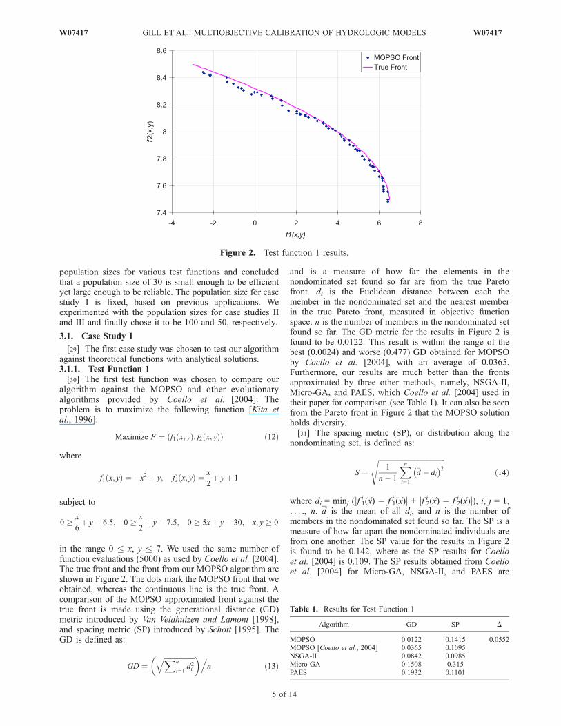
in the range 0 � x, y � 7. We used the same number offunction evaluations (5000) as used by Coello et al. [2004].The true front and the front from our MOPSO algorithm areshown in Figure 2. The dots mark the MOPSO front that weobtained, whereas the continuous line is the true front. Acomparison of the MOPSO approximated front against thetrue front is made using the generational distance (GD)metric introduced by Van Veldhuizen and Lamont [1998],and spacing metric (SP) introduced by Schott [1995]. TheGD is defined as:

GD ¼ffiffiffiffiffiffiffiffiffiffiffiffiffiffiffiffiffiffiXn

i¼1d2i

q� .n ð13Þ

and is a measure of how far the elements in thenondominated set found so far are from the true Paretofront. di is the Euclidean distance between each themember in the nondominated set and the nearest memberin the true Pareto front, measured in objective functionspace. n is the number of members in the nondominated setfound so far. The GD metric for the results in Figure 2 isfound to be 0.0122. This result is within the range of thebest (0.0024) and worse (0.477) GD obtained for MOPSOby Coello et al. [2004], with an average of 0.0365.Furthermore, our results are much better than the frontsapproximated by three other methods, namely, NSGA-II,Micro-GA, and PAES, which Coello et al. [2004] used intheir paper for comparison (see Table 1). It can also be seenfrom the Pareto front in Figure 2 that the MOPSO solutionholds diversity.[31] The spacing metric (SP), or distribution along the

nondominating set, is defined as:

S ¼ffiffiffiffiffiffiffiffiffiffiffiffiffiffiffiffiffiffiffiffiffiffiffiffiffiffiffiffiffiffiffiffiffiffiffiffiffiffiffi1

n� 1

Xni¼1

�d � di� �2s

ð14Þ

where di = minj (jf 1i (~x) � f 1j (~x)j + jf 2i (~x) � f 2

j (~x)j), i, j = 1,. . . ., n. d is the mean of all di, and n is the number ofmembers in the nondominated set found so far. The SP is ameasure of how far apart the nondominated individuals arefrom one another. The SP value for the results in Figure 2is found to be 0.142, where as the SP results for Coelloet al. [2004] is 0.109. The SP results obtained from Coelloet al. [2004] for Micro-GA, NSGA-II, and PAES are

Figure 2. Test function 1 results.

Table 1. Results for Test Function 1

Algorithm GD SP D

MOPSO 0.0122 0.1415 0.0552MOPSO [Coello et al., 2004] 0.0365 0.1095NSGA-II 0.0842 0.0985Micro-GA 0.1508 0.315PAES 0.1932 0.1101

W07417 GILL ET AL.: MULTIOBJECTIVE CALIBRATION OF HYDROLOGIC MODELS

5 of 14

W07417

provided in Table 1. We are also reporting the diversitymetric (D) value (0.0553) for MOPSO in Table 1. Thedefinition of the diversity metric is given by Robic andFilipic [2005].3.1.2. Test Function 2[32] The second test function is to show the MOPSO

performance in comparison with the MOSCEM algorithmdescribed by Vrugt et al. [2003]. The questions here are thefollowing: (1) Does MOPSO provide a good spread ofPareto rank 1 particles over the parameter space, or are theparticles clustered in one region? (2) Is this affected bypopulation size?[33] The problem is to minimize the following function

[Vrugt et al., 2003]:

Minimize F x1; x2ð Þ ¼ F1;F2;F3f g ð15Þ

where

F1 ¼ x21 þ x22

F2 ¼ x1 � 1ð Þ2þx22

F3 ¼ x21 þ x2 � 1ð Þ2

The true Pareto front for equation (15) in the parameterspace is a triangular region with corner points (0,0), (0,1),and (1,0) for x1 and x2. We used 5000 functionevaluations using MOPSO to generate Pareto fronts forthe population sizes of 50, 100, and 500. The Pareto rank1 points are shown in Figure 3 for each population sizein the parameter space for all 5000 function evaluations.The triangle is the true parameter space region, whereasthe dots represent the points with Pareto rank 1. Thenumber of rank 1 points for population sizes of 50, 100,and 500, respectively, are 3544, 3259, and 2566.Moreover, the rank 1 points generated by MOPSO coverthe parameter space without any clustering for thepopulation sizes of 100 and 500, as can be seen inFigures 3b and 3c. There is a slight a clustering for thepopulation size of 50 (Figure 3a). The population size of100 produces the best coverage of the front in theparameter space with a good number of rank 1 points(3259), whereas the number of rank 1 points decreases(2566) when the population size is increased to 500. Theresults in this case are very comparable to those provided

by Vrugt et al. [2003] for the MOSCEM-UA algorithmfor 5000 function evaluations.

3.2. Case Study II: SACSMA Model

[34] As the second application, the MOPSO algorithm istested on the Sacramento soil moisture accounting(SACSMA) model (Figure 4), a very well known concep-tual rainfall-runoff (CRR) model introduced first byBurnash et al. [1973]. It is a component of the NationalWeather Service River Forecast system. The SACSMAmodel was selected purposely to compare the MOPSOperformance from the previously used optimization schemesapplied on the same model for streamflow estimations in theLeaf River. Various authors have documented the results ofefforts to calibrate the SACSMA model for this watershed[Sorooshian and Gupta, 1983; Brazil, 1988; Duan et al.,1994; Gupta et al., 1998; Thiemann et al., 2001; Vrugt etal., 2003]. The SACSMA is a 16-parameter model and isconsidered to present a very difficult optimization task incalibration due to the problems associated with parameterinteraction and the high dimensionality of the parameterspace. Furthermore, the interaction between varioussystem components within the model also gives rise tothe notion of ‘‘equifinality’’ addressed by Beven [1993]and Beven and Freer [2001]. According to Peck [1976],three of the 16 parameters are fixed and do not requirecalibration. The names and ranges for the 13 parametersare given in Table 2.[35] The model is tested for the data obtained from

National Weather Service Hydrology Laboratory (HL) forthe Leaf River watershed (1950 km2) near Collins, Mis-sissippi. The data consist of mean aerial precipitation(mm/day), potential evapotranspiration (mm/day), andstreamflow (m3/s). More details on the Leaf River andthe SACSMA model are given by Sorooshian et al.[1993], Duan et al. [1994], and Yapo et al. [1998]. TheSACSMA model was calibrated with daily time resolu-tion to estimate streamflow on a 10-year period (WY1948–1958). The results that follow in this section arebased on an 11-year validation period (WY 1952–1963)in order to compare the predictions with the previousstudies [Brazil, 1988; Thiemann et al., 2001]; hence thereare six years of overlap between the training and thevalidating set. We used the MOPSO algorithm for 5000function evaluations to optimize in terms of two objectivefunctions: root-mean-square error (RMSE) and bias. Thisnumber of function evaluations was considerably smaller

Figure 3. Test function 2: Scatterplots for the rank 1 points for 5000 function evaluations with apopulation size of (a) 50, (b) 100, and (c) 500.

6 of 14

W07417 GILL ET AL.: MULTIOBJECTIVE CALIBRATION OF HYDROLOGIC MODELS W07417

than that reported for MOSCEM-UA [Vrugt et al., 2003],i.e., 10000 and 30000 evaluations, respectively, for caseswith and without prior information. The RMSE and biasobjective functions are calculated as:

RMSE ¼

ffiffiffiffiffiffiffiffiffiffiffiffiffiffiffiffiffiffiffiffiffiffiffiffiffiffiffiPni¼1

Oi � Pið Þ2

l

vuuut

Bias ¼

Pni¼1

Oi � Pið Þ

l

where O denotes the observations, P represents thepredictions, l is the total number of samples, and i is thesample counter.

[36] The SACSMA model prediction results are shown inFigures 5–8. The parameter spread for the Pareto set isshown in Figure 5. Note that all 13 parameter values arenormalized between �1 and 1 based on the upper and lowerbounds that have been set for each. Each line connectingthe parameters represents a parameter set. The dark line isthe parameter set that gives the best RMSE value on thevalidation set. Furthermore, it can be seen that the param-eters with a thin spread are very well determined, and theones with a wider spread are not particularly well deter-mined. Hence it can be said that MOPSO was able tocapture information about the uncertainty in most of theparameters. The Pareto rank projection is shown in Figure 6.The darker dots on the left represent the Pareto front on theobjective function space OF1 (RMSE) and OF2 (Bias),whereas the small light gray dots represent all the otherranks. The points on the extreme ends of the Pareto frontsare the best single criterion solutions.

Table 2. SAC-SMA Model Results

Parameters Range MOPSO Range MOSCEM Range Brazil [1988] Thiemann et al. [2001]

uztwm 1–150 26.33–43.45 3.52–9.74 9 33.61uzfwm 1–150 37.64–48.20 4.37–34.02 39.8 76.12uzk 0.1–0.5 0.28–0.35 0.10–0.45 0.2 0.332pctim 0–0.1 0.0052–0.0082 0.0–0.01 0.003 0.016adimp 0–0.4 0.29–0.3317 0.31–0.40 0.25 0.266zperc 1–250 160.47–183.80 58.46–242.59 250 117.3rexp 0–5 1.31–1.42 0.07–1.62 4.27 4.948lztwm 1–500 319.09–331.25 241.90–302.48 240 235.6lzfsm 1–1000 20.36–25.93 12.68–27.44 40 131.9lzfpm 1–1000 80.34–90.44 59.26–115.15 120 123.5lzsk 0.01–0.25 0.137–0.143 0.22–0.25 0.2 0.089lzpk 0.0001–0.025 0.0066–0.0138 0.01–0.02 0.006 0.015pfree 0–0.1 0.0335–0.0471 0.0–0.02 0.024 0.146RMSE 19.76 20.3 24.059CoE 0.996MAE 8.59

Figure 4. Conceptual flow diagram of the SAC-SMA model (redrawn from Thiemann et al. [2001]).

W07417 GILL ET AL.: MULTIOBJECTIVE CALIBRATION OF HYDROLOGIC MODELS

7 of 14

W07417

[37] The particle trajectories are plotted in Figure 7, whichalso shows the evolution of the MOPSO in the parameterspace projected over the first two parameters of the SACSMAmodel (uztwm and uzfwm). Note that the open circles are theprevious positions of the particles, whereas the dots are thecurrent particle positions. Moreover, the triangles representthe previous positions of the Pareto set, and stars show thecurrent positions for the Pareto set; the best particle accordingto the median concept is shown by the asterisk. The swarmevolution is shown for the first four iterations and for iteration

numbers 10 and 20. By following the particle positions fromiterations 1 to 4, one can visualize and understand theMOPSO evolution. The particles follow the closest particlein the Pareto set, whereas the Pareto set particles tend tofollow the best amongst them (again, defined here as theparticle with the median value of the WOFs). One can alsonotice the switch in the best particle between the iteration 2and iteration 3. In iteration 20, it is obvious that almost allthe particles are clustered around the Pareto set with theexception of a few that are trapped at local minima.

Figure 5. Parameter spread for SAC-SMA.

Figure 6. Pareto rank projection. The darker dots represent the rank 1 points, whereas the lighter smalldots represent other ranks. The best single-criteria solution for each objective functions is shown with acircle on each side of the Pareto front.

8 of 14

W07417 GILL ET AL.: MULTIOBJECTIVE CALIBRATION OF HYDROLOGIC MODELS W07417

[38] The results for the 1953 water year are shown inFigure 8. The plot shows the observed and model outputstreamflow in transformed space obtained using a Box-Coxtransformation (z = (yl � 1)/l) with l = 0.5. The observed

streamflow is represented using dots, the gray lines on theplot represent the Pareto set predictions, and the dark linerepresents the fit with the best RMSE. The predictionscapture the trend very well but still underpredict at certain

Figure 7. Particle trajectories in parameter space projected on the two parameters uzfwm and uztwm.Open circles are the positions in last iteration, dots represent the current positions, triangles and stars arethe previous and current positions for rank 1 points, respectively, and the asterisk represents the medianbest of the front.

W07417 GILL ET AL.: MULTIOBJECTIVE CALIBRATION OF HYDROLOGIC MODELS

9 of 14

W07417

areas of the hydrograph. We also show the 11-year (WY1953–1963) time series in Figure 9 in order to compare theresults against those of previous studies. The results forthe 11-year period are reported in Table 2 along with the‘‘goodness of fit’’ measures. The parameter ranges and thegoodness of fit values are also compared with those reportedin previous studies, e.g., by Brazil [1988], Vrugt et al.[2003] (MOSCEM-UA), and Thiemann et al. [2001]

(BARE). Note from Table 2 that there is reasonableagreement on most parameter values obtained by theMOPSO algorithm and those provided from other studies,most of the parameter ranges calculated by MOPSO arenarrower than those given for MOSCEM (i.e., 11 out of 13parameter ranges are narrower for MOPSO than MOS-CEM), and the MOPSO RMSE is less than those reportedby Brazil [1988] and Thiemann et al. [2001].

Figure 8. Daily streamflow predictions for WY 1953 in the transformed space. The dots represent theobserved streamflow, the thick line is the one that gives best RMSE, and the gray shaded area representsthe Pareto rank 1 output.

Figure 9. Daily streamflow predictions for 11 years (WY 1953–1963). The dots represent the observedstreamflow, the thick line is the one that gives best RMSE, and the gray shaded area represents the Paretorank 1 output.

10 of 14

W07417 GILL ET AL.: MULTIOBJECTIVE CALIBRATION OF HYDROLOGIC MODELS W07417

3.3. Case Study III: SVM Soil Moisture Model

[39] Support vector machines are used in the third casestudy. The SVM is a learning strategy developed by Vapnik[1995, 1998]. In the few years since its introduction, it hasbeen shown to perform better than most other systems in awide variety of applications [Cristianini and Shaw-Taylor,2000]. Over the past few years there have been variousapplications of SVM in hydrologic science [Dibike et al.,2001; See and Abrahart, 2001; Liong and Sivapragasam,2002; Asefa and Kemblowski, 2002; Gill et al., 2003, 2006;Asefa et al., 2004; Khalil, 2005; Khalil et al., 2005a, 2005b,2005c, 2006; Asefa et al., 2005]. It is a far more robustmachine than ANNs [Khalil, 2005; Khalil et al., 2005a],and it has been seen to reduce the dimensionality of thecalibration procedure considerably as compared to aphysical/conceptual model, e.g., Sacramento soil moistureaccounting (SACSMA) model. There are three SVMparameters that must be determined through calibration:trade-off C, tolerance e, and kernel parameter g. The modeltested here is the same as the one already used in a previousstudy for soil moisture prediction [Khalil et al., 2005b]. Theinputs to the SVM model are meteorological data (relativehumidity, average solar radiation, soil temperature at 5 cmand 10 cm, air temperature, and wind speed) and soilmoisture values at t � 1 and t. The output is the soilmoisture prediction at t + 5, where t is in days. The data forthis case study are taken from the Soil Climate AnalysisNetwork (SCAN) site at the Little Washita River Experi-mental Watershed (LWREW) in Southwestern Oklahoma inthe Southern Great Plains region of the United States. TheSoil Climate Analysis Network (SCAN) was created by theU.S. Department of Agriculture for the purpose of providinga soil and climate data bank. There are more than 90 SCANstations all over the United States at which daily and hourlymeasurements for meteorological and soil moisture data areobtained using various sensors and instruments. The LittleWashita watershed has an area of 611 km2, and has been a

center of soil-water related research activities for manydecades, including the 1936 soil erosion control project, theUSDA Agricultural Research Service (ARS) data collectioneffort in 1961, and the remote sensing experiments ofNASA-USDA (T. J. Jackson, Southern Great Plains 1997(SGP97) Hydrology Experiment plan, report, available athttp://hydrolab.arsusda.gov/sgp97/explan/). The land use inLWREW is about 60% rangeland, 20% cropland, and 20%miscellaneous (riparian, forest, urban, etc.). LWREW has awide range of soil types with fine sand, loamy fine sand,fine sandy loam, loam, and silty loams being thepredominant soil surface textures [Allen and Naney,1991]. The training set consists of 800 samples forthe above mentioned inputs at daily time resolution. TheMOPSO calibrated SVM performance is shown for thetesting set for 352 days starting 14 May 2001 (test samplesize).[40] The SVM model parameters were determined

through the MOPSO algorithm for the two objective func-tions, i.e., root-mean-square error and bias. The soil mois-ture predictions are shown along with the observed soilmoisture in Figure 10. The predictions are represented bythe thick line whereas the thin line is the observations.Figure 10 also contains the SVM prediction results withmanual calibration (dashed line). Figure 10 clearly showsthe difference in performance of the MOPSO, which cap-tures the observation pattern very well despite the lagproblem that is found in most of the series predictionmodels. Notice that the results shown here are the normal-ized soil moisture values. The performance is also shown bythe goodness of fit measures in Table 3. The RMSE, MAE,and bias values are reported for both manual and MOPSOcalibration and are compared with a previously conductedstudy by Khalil et al. [2005b] on SVMs for the sameproblem. Another important criterion in judging theperformance of a learning algorithm such as SVMs isthe ‘‘number of support vectors’’. The ‘‘support vectors’’ are

Figure 10. Soil moisture predictions at ‘‘t + 5.’’ Thin line is the observed time series, thick linerepresents the MOPSO calibrated SVM predictions, and the dotted line represents the output withoutMOPSO calibration.

W07417 GILL ET AL.: MULTIOBJECTIVE CALIBRATION OF HYDROLOGIC MODELS

11 of 14

W07417

the points in the full training sample that are used to definethe input-output relationship for a particular problem [Gill etal., 2006]. This leads to the conclusion that the smaller thenumber of support vectors, the more sparse and efficientwill be the learning machine, and vice versa. The number ofsupport vectors for the MOPSO calibrated soil moistureSVM model is shown in Table 3. The support vectorsobtained from a previous study on the same data by Khalilet al. [2005b] are also reported. These data show that theMOPSO calibrated model has fewer support vectors thanthe model reported by Khalil et al. [2005b], i.e., 130 versus286, respectively. Hence, using the MOPSO calibrationprocedure, the soil moisture prediction results improveconsiderably not only in terms of goodness of fit measuresbut also in terms of model complexity.[41] The evolution of MOPSO for 30 iterations is shown

in Figure 11 as it converges to the best fit. The dotted linesare the predictions for the 29 iterations, whereas the thickline is the prediction obtained after the last iteration. Thethin continuous line shows the observations. These can alsobe seen in Figure 12 where the function values are reportedfor three different runs with different initial conditions

(sampling of parameter sets). The function value on the yaxis is obtained using the weighting methodology explainedearlier for the two objective functions (RMSE and bias).The MOPSO algorithm took 10 iterations, at most, toconverge.

4. Conclusions

[42] In the present study, a new and efficient techniquecalled particle swarm optimization (PSO) is introduced thatprovides a global or near-global optimum. The Paretoconcept is introduced to address the multiobjective natureof the parameter optimization problem. Two test functionswere used to compare the performance of the MOPSOalgorithm presented here against the performance reportedfor previous efforts. The MOPSO algorithm was able tospan its search in parameter space without significantclustering, and it was able to provide a good approximationof the true nondominated front. Further, for the test func-tions examined, it captured the diversity of the front betterthan previous approaches.[43] The formulation was further tested on two very

different models, namely, a statistical learning approachand a conceptual rainfall-runoff (CRR) model. The 13-parameter Sacramento soil moisture accounting (SACSMA)CRR model was calibrated using MOPSO for runoff esti-mation. The results for this calibration show that theMOPSO algorithm performed efficiently to identify theoptimal parameter set. The parameter spread results depictnarrowed ranges for the MOPSO-calibrated SACSMAmodel parameters in comparison to calibration resultsrepresented in previous studies.[44] Statistical learning machines are gaining popularity

in many applications where the traditional physical andconceptual models are cumbersome. One of the mainreasons for this popularity is that statistical learningmachines in general require very few parameters and arerelatively easier to calibrate. In the present paper, we used

Table 3. SVM Model Results

SVM Parameters MOPSOManual

CalibrationKhalil et al.[2005b]

Cost C 40.25–43.10Gamma g 0.001–0.009Tolerance e 0.12–0.14RMSE 3.463 4.4 4.08Normalized RMSE 0.302 0.38Number of SV 130 286MAE 2.23 3.16 2.9Normalized MAE 0.19 0.27Bias 1.23 2.47Normalized bias 0.1 0.22

Figure 11. Soil moisture predictions showing the evolution of MOPSO.

12 of 14

W07417 GILL ET AL.: MULTIOBJECTIVE CALIBRATION OF HYDROLOGIC MODELS W07417

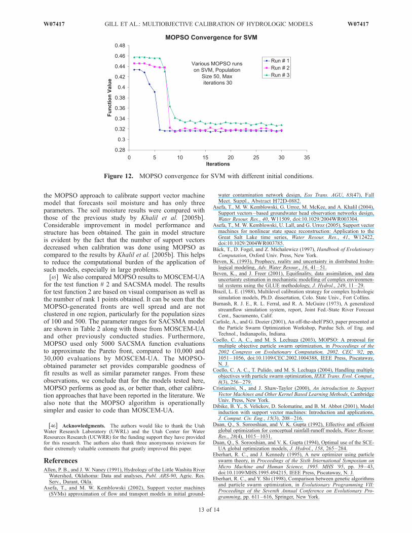
the MOPSO approach to calibrate support vector machinemodel that forecasts soil moisture and has only threeparameters. The soil moisture results were compared withthose of the previous study by Khalil et al. [2005b].Considerable improvement in model performance andstructure has been obtained. The gain in model structureis evident by the fact that the number of support vectorsdecreased when calibration was done using MOPSO ascompared to the results by Khalil et al. [2005b]. This helpsto reduce the computational burden of the application ofsuch models, especially in large problems.[45] We also compared MOPSO results to MOSCEM-UA

for the test function # 2 and SACSMA model. The resultsfor test function 2 are based on visual comparison as well asthe number of rank 1 points obtained. It can be seen that theMOPSO-generated fronts are well spread and are notclustered in one region, particularly for the population sizesof 100 and 500. The parameter ranges for SACSMA modelare shown in Table 2 along with those from MOSCEM-UAand other previously conducted studies. Furthermore,MOPSO used only 5000 SACSMA function evaluationsto approximate the Pareto front, compared to 10,000 and30,000 evaluations by MOSCEM-UA. The MOPSO-obtained parameter set provides comparable goodness offit results as well as similar parameter ranges. From theseobservations, we conclude that for the models tested here,MOPSO performs as good as, or better than, other calibra-tion approaches that have been reported in the literature. Wealso note that the MOPSO algorithm is operationallysimpler and easier to code than MOSCEM-UA.

[46] Acknowledgments. The authors would like to thank the UtahWater Research Laboratory (UWRL) and the Utah Center for WaterResources Research (UCWRR) for the funding support they have providedfor this research. The authors also thank three anonymous reviewers fortheir extremely valuable comments that greatly improved this paper.

ReferencesAllen, P. B., and J. W. Naney (1991), Hydrology of the Little Washita RiverWatershed, Oklahoma: Data and analyses, Publ. ARS-90, Agric. Res.Serv., Durant, Okla.

Asefa, T., and M. W. Kemblowski (2002), Support vector machines(SVMs) approximation of flow and transport models in initial ground-

water contamination network design, Eos Trans. AGU, 83(47), FallMeet. Suppl., Abstract H72D-0882.

Asefa, T., M. W. Kemblowski, G. Urroz, M. McKee, and A. Khalil (2004),Support vectors–based groundwater head observation networks design,Water Resour. Res., 40, W11509, doi:10.1029/2004WR003304.

Asefa, T., M. W. Kemblowski, U. Lall, and G. Urroz (2005), Support vectormachines for nonlinear state space reconstruction: Application to theGreat Salt Lake time series, Water Resour. Res., 41, W12422,doi:10.1029/2004WR003785.

Back, T., D. Fogel, and Z. Michalewicz (1997), Handbook of EvolutionaryComputation, Oxford Univ. Press, New York.

Beven, K. (1993), Prophecy, reality and uncertainty in distributed hydro-logical modeling, Adv. Water Resour., 16, 41–51.

Beven, K., and J. Freer (2001), Equifinality, data assimilation, and datauncertainty estimation in mechanistic modelling of complex environmen-tal systems using the GLUE methodology, J. Hydrol., 249, 11–29.

Brazil, L. E. (1988), Multilevel calibration strategy for complex hydrologicsimulation models, Ph.D. dissertation, Colo. State Univ., Fort Collins.

Burnash, R. J. E., R. L. Ferral, and R. A. McGuire (1973), A generalizedstreamflow simulation system, report, Joint Fed.-State River ForecastCent., Sacramento, Calif.

Carlisle, A., and G. Dozier (2001), An off-the-shelf PSO, paper presented atthe Particle Swarm Optimization Workshop, Purdue Sch. of Eng. andTechnol., Indianapolis, Indiana.

Coello, C. A. C., and M. S. Lechuga (2003), MOPSO: A proposal formultiple objective particle swarm optimization, in Proceedings of the2002 Congress on Evolutionary Computation, 2002. CEC ’02, pp.1051–1056, doi:10.1109/CEC.2002.1004388, IEEE Press, Piscataway,N. J.

Coello, C. A. C., T. Pulido, and M. S. Lechuga (2004), Handling multipleobjectives with particle swarm optimization, IEEE Trans. Evol. Comput.,8(3), 256–279.

Cristianini, N., and J. Shaw-Taylor (2000), An introduction to SupportVector Machines and Other Kernel Based Learning Methods, CambridgeUniv. Press, New York.

Dibike, B. Y., S. Velickov, D. Solomatine, and B. M. Abbot (2001), Modelinduction with support vector machines: Introduction and applications,J. Comput. Civ. Eng., 15(3), 208–216.

Duan, Q., S. Sorooshian, and V. K. Gupta (1992), Effective and efficientglobal optimization for conceptual rainfall-runoff models, Water Resour.Res., 28(4), 1015–1031.

Duan, Q., S. Sorooshian, and V. K. Gupta (1994), Optimal use of the SCE-UA global optimization models, J. Hydrol., 158, 265–284.

Eberhart, R. C., and J. Kennedy (1995), A new optimizer using particleswarm theory, in Proceedings of the Sixth International Symposium onMicro Machine and Human Science, 1995. MHS ’95, pp. 39–43,doi:10.1109/MHS.1995.494215, IEEE Press, Piscataway, N. J.

Eberhart, R. C., and Y. Shi (1998), Comparison between genetic algorithmsand particle swarm optimization, in Evolutionary Programming VII:Proceedings of the Seventh Annual Conference on Evolutionary Pro-gramming, pp. 611–616, Springer, New York.

Figure 12. MOPSO convergence for SVM with different initial conditions.

W07417 GILL ET AL.: MULTIOBJECTIVE CALIBRATION OF HYDROLOGIC MODELS

13 of 14

W07417

Eberhart, R. C., R. W. Dobbins, and P. Simpson (1996), ComputationalIntelligence PC Tools, Elsevier, New York.

Fieldsend, J. E., and S. Singh (2002), A multi-objective algorithm basedupon particle swarm optimization, an efficient data structure and turbu-lence, paper presented at 2002 U.K. Workshop on Computational Intelli-gence, Sch. of Comput. Sci., Univ. of Birmingham, Birmingham, U. K.

Fonseca, C. M., and P. J. Fleming (1995), An overview of evolutionaryalgorithms in multiobjective optimization, Evol. Comput., 3(1), 1–16.

Gill, M. K., T. Asefa, Q. Shu, and M. W. Kemblowski (2003), Soil moistureprediction using support vector machines, paper presented at INRA 2003Subsurface Science Symposium, Inland Northwest Res. Alliance, SaltLake City, Utah, 6 –8 Oct.

Gill, M. K., T. Asefa, M. McKee, and M. W. Kemblowski (2006), Soilmoisture prediction using support vector machines, J. Am. Water Resour.Assoc., in press.

Gupta, H. V., S. Sorooshian, and P. O. Yapo (1998), Toward improvedcalibration of hydrologic models: Multiple and noncommensurate mea-sures of information, Water Resour. Res., 34(4), 751–763.

Hogue, T. S., S. Sorooshian, H. Gupta, A. Holz, and D. Braatz (2000), Amulti-step automatic calibration scheme for river forecasting models,J. Hydrometeorol., 1, 524–542.

Hui, X., R. C. Eberhart, and Y. Shi (2003), Particle swarm with extendedmemory for multiobjective optimization, in Proceedings of the 2003IEEE Swarm Intelligence Symposium, 2003. SIS ’03, pp. 193–197,doi:10.1109/SIS.2003.1202267, IEEE Press, Piscataway, N. J.

Kennedy, J. (1998), The behavior of particles, in Evolutionary Program-ming VII: Proceedings of the Seventh Annual Conference on Evolution-ary Programming, pp. 581–589, Springer, New York.

Kennedy, J., and R. C. Eberhart (1995), Particle swarm optimization, inProceedings of IEEE International Conference on Neural Networks, IV,vol. 4, pp. 1942–1948, doi:10.1109/ICNN.1995.488968, IEEE Press,Piscataway, N. J.

Kennedy, J., and W. M. Spears (1998), Matching algorithms to problems:An experimental test of the particle swarm and some genetic algorithmson the multimodal problem generator, in The 1998 IEEE InternationalConference on Evolutionary Computation, Proceedings, pp. 78–83,doi:10.1109/ICEC.1998.699326, IEEE Press, Piscataway, N. J.

Kennedy, J., R. C. Eberhart, and Y. Shi (2001), Swarm Intelligence,Elsevier, New York.

Khalil, A. (2005), Computational learning theory in water resources man-agement and hydrology, Ph.D. dissertation, 159 pp., Dep. of Civ. andEnviron. Eng., Utah State Univ., Logan.

Khalil, A., M. N. Almasri, M. McKee, and J. J. Kaluarachchi (2005a),Applicability of statistical learning algorithms in ground water qualitymodeling, Water Resour. Res., 41, W05010, doi:10.1029/2004WR003608.

Khalil, A., M. K. Gill, and M. McKee (2005b), New applications for in-formation fusion and soil moisture forecasting, in Proceedings of 8thInternational Conference on Information Fusion, pp. 1–7, IEEE Press,Piscataway, N. J.

Khalil, A., M. McKee, M. W. Kemblowski, and T. Asefa (2005c), Basin-scale water management and forecasting using multisensor data andneural networks, J. Am. Water Resour. Assoc., 41(1), 195–208.

Khalil, A., M. McKee, M. W. Kemblowski, T. Asefa, and L. Bastidas(2006), Multiobjective analysis of chaotic systems using sparse learningmachines, Adv. Water Resour., 29(1), 72–88.

Kita, H., Y. Yabumoto, N. Mori, and Y. Nishikawa (1996), Multi-objectiveoptimization by means of the thermodynamical genetic algorithm, inParallel Problem Solving From Nature: PPSN IV, edited by H.-M. Voigtet al., pp. 504–512, Springer, New York.

Liong, S., and C. Sivapragasam (2002), Flood stage forecasting with sup-port vector machines, J. Am. Water Resour. Assoc., 38(1), 173–186.

Mostaghim, S., and J. Teich (2003a), Strategies for finding good local guidesin multi-objective particle swarm optimization (MOPSO), in Proceedingsof the 2003 IEEE Swarm Intelligence Symposium, 2003. SIS ’03, pp. 26–33, doi:10.1109/SIS.2003.1202243, IEEE Press, Piscataway, N. J.

Mostaghim, S., and J. Teich (2003b), The role of e-dominance in multi-objective particle swarm optimization methods, in Proceedings of theCongress on Evolutionary Computation (CEC’03), pp. 1764–1771,IEEE Press, Piscataway, N. J.

Mostaghim, S., and J. Teich (2004), Covering Pareto-optimal fronts bysubswarms in multi-objective particle swarm optimization, in 2004 Con-

gress on Evolutionary Computation (CEC’04), vol. 2, pp. 1404–1411,doi:10.1109/CEC.2004.1331061, IEEE Press, Piscataway, N. J.

Parsopoulos, K. E., and M. N. Vrahatis (2002), Recent approaches to globaloptimization problems through particle swarm optimization, Nat. Com-put., 1(2–3), 235–306.

Peck, E. L. (1976), Catchment modeling and initial parameter estimationfor National Weather Service River forecast system, Tech. Memo. NWSHydro-31, NOAA, Silver Spring, Md.

Robic, T., and B. Filipic (2005), DEMO: Differential evolution for multi-objective optimization, in Evolutionary Multi-criterion Optimization:Third International Conference, EMO 2005, Lect. Notes Comput. Sci.,vol. 3410, pp. 520–533, Springer, New York.

Schott, J. R. (1995), Fault tolerant design using single and multicriteriagenetic algorithm optimization, M.S. thesis, Dep. of Aeronaut. and As-tronaut., Mass. Inst. of Technol., Cambridge, Mass.

See, L., and R. J. Abrahart (2001), Multi-model data fusion for hydrologicalforecasting, Comput. Geosci., 27, 987–994.

Shi, Y., and R. C. Eberhart (1998a), Parameter selection in particle swarmoptimization, in Evolutionary Programming VII: Proceedings of the Se-venth Annual Conference on Evolutionary Programming, pp. 591–600,Springer, New York.

Shi, Y. H., and R. C. Eberhart (1998b), A modified particle swarm optimi-zer, in The 1998 IEEE International Conference on Evolutionary Com-putation Proceedings, pp. 69–73, doi:10.1109/ICEC.1998.699146, IEEEPress, Piscataway, N. J.

Shi, Y., and R. C. Eberhart (1999), Empirical study of particle swarmoptimization, in Proceedings of the Congress of Evolutionary Computa-tion, vol. 3, edited by P. J. Angeline et al., pp. 1945–1950, IEEE Press,Piscataway, N. J.

Sorooshian, S., and V. K. Gupta (1983), Automatic calibration of concep-tual rainfall-runoff models: The question of parameter observability anduniqueness, Water Resour. Res., 19(1), 260–268.

Sorooshian, S., Q. Duan, and V. K. Gupta (1993), Calibration of rainfall-runoff models: Application of global optimization to the Sacramentosoil moisture accounting model, Water Resour. Res., 29(4), 1185–1194.

Thiemann, M., M. Trosset, H. Gupta, and S. Sorooshian (2001), Bayesianrecursive parameter estimation for hydrologic models, Water Resour.Res., 37(10), 2521–2535.

Valenzuela-Rend’on, M., and E. Uresti-Charre (1997), A nongenerationalgenetic algorithm for multiobjective optimization, in Proceedings 7thInternational Conference on Genetic Algorithms, edited by T. Back,pp. 658–665, Elsevier, New York.

Van Veldhuizen, D. A., and G. B. Lamont (1998), Multiobjective evolu-tionary algorithm research: A history and analysis, Tech. Rep. TR-98-03,Dep. of Electr. Comput. Eng., Grad. Sch. of Eng., Air Force Inst. ofTechnol., Wright-Patterson Air Force Base, Ohio.

Vapnik, V. (1995), The Nature of Statistical Learning Theory, Springer,New York.

Vapnik, V. (1998), Statistical Learning Theory, John Wiley, Hoboken, N. J.Voss, M. S. (2003), Social programming using functional swarm optimiza-tion, in Proceedings of the IEEE Swarm Intelligence Symposium 2003.SIS 2003, pp. 103–109, IEEE Press, Piscataway, N. J.

Voss, M. S., and J. C. Howland (2003), Financial modelling using socialprogramming, in FEA 2003: Financial Engineering and Applications,Paper 401–028, ACTA Press, Calgary, Alberta, Canada.

Vrugt, J. A., H. V. Gupta, L. A. Bastidas, W. Bouten, and S. Sorooshian(2003), Effective and efficient algorithm for multiobjective optimizationof hydrologic models, Water Resour. Res., 39(8), 1214, doi:10.1029/2002WR001746.

Yapo, P. O., H. V. Gupta, and S. Sorooshian (1998), Multi-objective globaloptimization for hydrologic models, J. Hydrol., 204, 83–97.

Zitzler, E., and L. Thiele (1999), Multi-objective evolutionary algorithms:A comparative case study and the strength Pareto approach, IEEE Trans.Evol. Comput., 3(4), 257–271.

����������������������������L. Bastidas, M. K. Gill, Y. H. Kaheil, and M. McKee, Utah Water

Research Laboratory, Utah State University, Logan, UT 84322-8200, USA.(kashif@cc.usu.edu)

A. Khalil, Department of Earth and Environmental Engineering,Columbia University, New York, NY 10027, USA.

14 of 14

W07417 GILL ET AL.: MULTIOBJECTIVE CALIBRATION OF HYDROLOGIC MODELS W07417