Computational Modelling in the Management of Patients with ...

1

Computational Modelling in the

Management of Patients with Aortic Valve

Stenosis

University of Sheffield

Department of Infection, Immunity and Cardiovascular

Disease

Dr Gareth Archer MBChB (Hons) MRCP (Lond) PgCert

Submitted for the degree of Doctor of Philosophy

May 2020

2

Abstract

Background

Stenosis of the aortic valve causes increased left ventricular pressure leading to adverse clinical

outcomes. The selection and timing of intervention (surgical replacement or transcatheter

implantation) is often unclear and is based upon limited data.

Hypothesis

A comprehensive and integrated personalised approach, including recognition of cardiac energetics

parameters extracted from a personalised mathematical model, mapped to patient activity, has the

potential to improve diagnosis and the planning and timing of interventions.

Aims

This project seeks to implement a simple, personalised, mathematical model of patients with aortic

stenosis (AS), which can ‘measure’ cardiac work and power parameters that provide an effective

characterisation of the demand on the heart in both rest and exercise conditions and can predict the

changes of these parameters following an intervention. The specific aims of this project are:

• to critically review current diagnostic methods

• to evaluate the potential role of pre- and post-procedural measured patient activity

• to implement a simple, personalised, mathematical model of patients with AS

• to evaluate the potential role of a clinical decision support system

Methods

Twenty-two patients with severe AS according to ESC criteria were recruited. Relevant clinical,

imaging, activity monitoring, six-minute walk test, and patient reported data were collected, before

and early and after treatment. Novel imaging techniques were developed to help in the diagnosis of

3

AS. A computational model was developed and executed using the data collected to create non-

invasive pressure volume loops and study the global haemodynamic burden on the left ventricle.

Simulations were run to predict the haemodynamic parameters both during exercise and following

intervention. Modelled parameters were validated against clinically measured values. This

information was then correlated with symptoms and activity data. A clinical decision support tool

was created and populated with data obtained and its clinical utility evaluated.

Outcomes

The results of this project suggest that the combination of imaging and activity data with

computational modelling provides a novel, patient-specific insight into patients’ haemodynamics and

may help guide clinical decision making in patients with AS.

4

Acknowledgements

The work in this thesis was carried out under the auspices of the EurValve project. The recruitment,

clinical data collection, image acquisition, image analysis, activity monitoring, execution of the

MATLAB script for case processing and data analysis were performed by the author. 4D flow CMR

analysis of the LV blood pool kinetic energy was undertaken in part by Alaa Elhawaz under the

supervision of the author as part of an MRes degree. Resultant data are presented in section 3.6.

The concept of a purely mathematically derived model was that of the author’s, the derivation of the

mathematical formulae was the work of Professor Hose. The computing infrastructure,

segmentation of the images, processing of the CFD and 0D models and of the raw activity data were

carried out by members of the EurValve consortium. The MATLAB script was written by Professor

Hose. The clinical decision support system was developed in conjunction with Therenva using data

and methodology described in this thesis.

I would like to express my gratitude to Professor Rod Hose, Professor Julian Gunn, Mr Norman Briffa

and Professor Pat Lawford for all their help, support and supervision throughout this work and giving

me the opportunity to undertake this project. I would also like to thank the wider EurValve project

team for their help and input, particularly Herman ter Horst for the processing of the raw data from

the Philips Health Watch and James Pope and Ryan McConville for technical support and the

processing of the raw data from the Sphere kit. I would like to thank Dr Ever Grech for his support

enabling me to complete the third year of this project and Dr Pankaj Garg for his enthusiasm and

sharing his extensive knowledge of emerging CMR imaging techniques.

Finally, and most importantly, I would like to thank my wonderful family. First, my wife, Sarah who

has put up with the long hours of work whilst looking after our two beautiful boys, William and

Theo. This has been a stressful time and a family effort; you make it all worthwhile. Second, I would

like to thank my parents Jennifer and Graham who have, as ever, offered support and wise words of

advice throughout. I love you all.

5

Publications

G. Archer, A. Elhawaz, N. Barker, B. Fidock, A. Rothman, and P. Garg, Validation of four-dimensional

flow cardiovascular magnetic resonance for aortic stenosis assessment. Sci. Reports, Nature. Jun

2020. https://doi.org/10.1038/s41598-020-66659-62020.

G Archer, N Briffa, I Hall, J Wild, P Garg, E Grech. Novel Methods in the Assessment of Aortic

Stenosis. J Am Coll Cardiol. Volume 75, Issue 11 Supplement 1, Mar 2020.

DOI: 10.1016/S0735-1097(20)32311-1

A. Elhawaz, G. Archer, P. Garg, J. Wild, I. Hall, and E. Grech, “Altered left ventricular blood flow

pattern and kinetic energy in patients undergoing aortic valve intervention,” J. Am. Coll. Cardiol., vol.

75, no. 11, p. 1763, Mar. 2020.

R McConville, G Archer, I Craddock, H ter Horst, R Piechocki, J Pope, R Santos-Rodriguez. Online

heart rate prediction using acceleration from a wrist worn wearable. KDD Workshop on Machine

Learning for Medicine and Healthcare. London, UK. 2018.

https://arxiv.org/search/stat?searchtype=author&query=McConville%2C+R

https://arxiv.org/search/stat?searchtype=author&query=Archer%2C+G

https://arxiv.org/search/stat?searchtype=author&query=Craddock%2C+I

https://arxiv.org/search/stat?searchtype=author&query=ter+Horst%2C+H

https://arxiv.org/search/stat?searchtype=author&query=Piechocki%2C+R

https://arxiv.org/search/stat?searchtype=author&query=Pope%2C+J

https://arxiv.org/search/stat?searchtype=author&query=Santos-Rodriguez%2C+R

6

Conference Papers

D R Hose, K Czechowicz, G Archer, P Lawford. Model-based personalised decision support for heart

valve interventions. World Congress of Biomechanics in Dublin, Ireland. 2018.

K Czechowicz, G Archer, P Lawford, D R Hose. Patient specific 0D model of the systemic circulation to

simulate the effects of valve stenosis and regurgitation. VPH. Zaragoza, Spain. 2018

Presentations

Invited speaker BCS conference. Computational modelling in the management of aortic stenosis.

Manchester, UK. 2019.

BHVS Young Investigators Award 2019 (Finalist). Computational modelling in the management of

aortic stenosis. London, UK. 2019.

Activity monitoring in patients with valvular heart disease. Computational models for the clinic:

Cardiac/cardiovascular application, Workshop Krakow, Poland. 2019

7

Table of Contents

Abstract ……………………………………………………………………………………………………………………………2

Acknowledgements ..................................................................................................................................................... 4

Publications .................................................................................................................................................................... 5

Conference Papers....................................................................................................................................................... 6

Presentations ................................................................................................................................................................. 6

Acronyms ..................................................................................................................................................................... 13

List of figures .............................................................................................................................................................. 14

List of tables ................................................................................................................................................................ 16

CHAPTER 1 .................................................................................................................................................................. 17

1. Introduction ............................................................................................................................................. 17

1.1. Anatomy .................................................................................................................................................... 17

1.2. Epidemiology .......................................................................................................................................... 19

1.3. Pathophysiology .................................................................................................................................... 20

1.3.1. Disease progression and prognosis ............................................................................................... 23

1.3.2. Haemodynamics in AS ......................................................................................................................... 23

1.4. Diagnosis ................................................................................................................................................... 26

1.4.1. Symptoms ................................................................................................................................................. 27

1.4.2. Imaging in AS........................................................................................................................................... 27

1.4.2.1. Echocardiography ................................................................................................................................. 27

1.4.2.2. Other imaging techniques .................................................................................................................. 32

1.4.3. Cardiac catheterisation ....................................................................................................................... 34

1.4.4. Other Biomarkers .................................................................................................................................. 36

1.5. Quantification of AS .............................................................................................................................. 37

1.6. Clinical management and interventions ...................................................................................... 39

1.6.1. Medical therapy ...................................................................................................................................... 39

1.6.2. Evolution of treatment in AS ............................................................................................................ 39

1.6.3. Surgical AVR ............................................................................................................................................ 40

1.6.4. TAVI ............................................................................................................................................................ 44

1.7. Prognosis after treatment .................................................................................................................. 47

1.8. Guidelines ................................................................................................................................................. 48

1.8.1. Timing of intervention ........................................................................................................................ 50

1.9. Assessing symptoms and Outcomes .............................................................................................. 53

1.9.1. Assessment of function ....................................................................................................................... 54

1.9.2. Exercise testing in clinical practice ................................................................................................ 54

1.9.3. Six-minute walk test ............................................................................................................................. 56

1.10. Wearable or pervasive activity monitoring ................................................................................ 57

1.10.1. Clinical research using activity monitoring ................................................................................ 57

1.10.2. Monitoring outcome ............................................................................................................................. 58

8

1.10.3. Patient reported outcome measures ............................................................................................. 59

1.11. Computational modelling ................................................................................................................... 61

1.11.1. What model and why? ......................................................................................................................... 62

1.11.2. Current use of modelling in clinical practice ............................................................................. 62

1.11.3. Model Choices ......................................................................................................................................... 63

1.11.4. Systems model (Zero-dimensional, ‘lumped’ parameter) .................................................... 65

1.11.5. 3D valve model ....................................................................................................................................... 66

1.11.6. Model Personalisation ......................................................................................................................... 67

1.11.7. Model validation .................................................................................................................................... 68

1.11.8. Pressure-volume Loops ...................................................................................................................... 70

1.12. Summary ................................................................................................................................................... 72

1.13. Hypothesis ................................................................................................................................................ 74

1.14. Aims ............................................................................................................................................................ 74

CHAPTER 2 .................................................................................................................................................................. 75

2. Methods ..................................................................................................................................................... 75

2.1. Clinical Study Design and Management ....................................................................................... 75

2.1.1. Overview ................................................................................................................................................... 75

2.1.2. Ethics .......................................................................................................................................................... 76

2.1.3. Inclusion and Exclusion Criteria ..................................................................................................... 76

2.1.4. Clinical Study Protocol ........................................................................................................................ 77

2.1.5. Data management ................................................................................................................................. 78

2.1.6. Patient recruitment .............................................................................................................................. 79

2.1.7. Clinical data .............................................................................................................................................. 80

2.1.7.1. Basic demographics .............................................................................................................................. 82

2.1.7.2. Symptoms ................................................................................................................................................. 82

2.1.8. Physical examination and blood pressure assessment ......................................................... 82

2.1.9. ECG .............................................................................................................................................................. 82

2.2. Imaging ...................................................................................................................................................... 83

2.2.1. Cardiac ultrasound ................................................................................................................................ 83

2.2.1.1. Transthoracic echocardiogram........................................................................................................ 83

2.2.1.2. Transoesophageal ................................................................................................................................. 85

2.2.1.3. Ultrasound data collection ................................................................................................................. 86

2.2.2. Cardiac magnetic resonance imaging (CMR) ............................................................................. 86

2.2.3. MRI 4D flow assessment of AS ......................................................................................................... 87

2.2.3.1. 4D Flow Acquisition ............................................................................................................................. 87

2.2.3.2. 4D flow pressure gradient assessment ........................................................................................ 88

2.2.3.3. 4D flow effective orifice area assessment ................................................................................... 88

2.2.3.4. Left ventricular blood flow kinetic energy assessment ......................................................... 89

2.2.3.5. LV blood Flow Component Analysis .............................................................................................. 90

9

2.2.3.6. Cardiac computed tomography ....................................................................................................... 91

2.3. Intervention Data .................................................................................................................................. 92

2.4. Computational Modelling methods ................................................................................................ 92

2.4.1. Lumped parameter model of left side of heart and systemic circulation ...................... 92

2.4.1.1. Inputs.......................................................................................................................................................... 94

2.4.1.1.1. Valves ......................................................................................................................................................... 94

2.4.1.1.2. Systemic circulation ............................................................................................................................. 95

2.4.1.1.3. Heart chambers ...................................................................................................................................... 96

2.4.1.2. Model Outputs ........................................................................................................................................ 98

2.4.1.2.4 Modelling in the exercise state ....................................................................................................... 105

2.4.1.2.5. Combining activity data .................................................................................................................... 105

2.4.1.2.6. Modelling after intervention........................................................................................................... 106

2.4.2. Three-dimensional model ................................................................................................................ 107

2.4.2.1. Segmentation and mesh formation .............................................................................................. 107

2.4.2.2. Computational fluid dynamics ....................................................................................................... 108

2.4.2.3. Boundary conditions .......................................................................................................................... 110

2.4.2.4. Reduced order models derived from 3D models ................................................................... 110

2.4.3. Analysis protocols ............................................................................................................................... 110

2.4.3.1. Protocol 1 ................................................................................................................................................ 111

2.4.3.2. Protocol 2 ................................................................................................................................................ 113

2.4.3.3. Protocol 3 ................................................................................................................................................ 114

2.4.3.4. Protocol 4 ................................................................................................................................................ 115

2.4.4. Summary of processing steps for modelling protocols 2-4. .............................................. 116

2.4.5. Validation ................................................................................................................................................ 117

2.5. Activity Data .......................................................................................................................................... 119

2.5.1. Wearable pervasive monitoring .................................................................................................... 119

2.5.2. Sphere activity monitoring system .............................................................................................. 119

2.5.3. Philips Health Watch .......................................................................................................................... 120

2.5.4. Six-minute walk test ........................................................................................................................... 121

2.6. Patient reported measures .............................................................................................................. 123

2.6.1. Minnesota ‘living with heart failure’ questionnaire .............................................................. 123

2.6.2. World Health Organization Quality of Life questionnaire .................................................. 123

2.7. Development of a clinical decision support system .............................................................. 124

2.8. Evaluation of the clinical decision support system ............................................................... 127

2.9. Statistical analyses .............................................................................................................................. 130

2.9.1. Protocol comparisons and validation ........................................................................................ 130

2.9.2. Correlations between modelled and measured ...................................................................... 130

2.9.3. 4D flow data ........................................................................................................................................... 131

2.9.4. Evaluation of clinical decision support system. ...................................................................... 131

10

CHAPTER THREE .................................................................................................................................................... 133

3. Results ...................................................................................................................................................... 133

3.1. Baseline Patient Characteristics .................................................................................................... 133

3.2. Imaging .................................................................................................................................................... 135

3.2.1. Transthoracic echocardiography .................................................................................................. 135

3.2.2. Transoesophageal echocardiography ......................................................................................... 138

3.2.3. Computed tomography ..................................................................................................................... 140

3.2.4. Magnetic Resonance Imaging ......................................................................................................... 141

3.3. Measured pressure-volume loop .................................................................................................. 143

3.4. Outcome measures ............................................................................................................................. 144

3.4.1. Activity Data .......................................................................................................................................... 144

3.4.1.1. Six-minute walk Test ......................................................................................................................... 144

3.4.1.2. Sphere data ............................................................................................................................................ 145

3.4.1.2.1. Case study illustrating the Sphere results ................................................................................. 147

3.4.1.3. Philips Health watch data ................................................................................................................ 150

3.4.1.3.1. Case study illustrating the Philips Health watch results ..................................................... 153

3.4.1.4. Combining activity data information .......................................................................................... 156

3.4.2. Quality of life data ............................................................................................................................... 157

3.4.2.1. Minnesota ‘Living with Heart Failure’ Questionnaire .......................................................... 157

3.4.2.2. WHOQOL ................................................................................................................................................. 158

3.5. Diagnostic capability of 4D flow MRI .......................................................................................... 160

3.5.1. 4D flow pressure gradient and effective orifice area assessment ................................... 161

3.5.1.1. Invasive pressure gradient validation ........................................................................................ 161

3.5.1.2. EOA validation ...................................................................................................................................... 162

3.5.2. Left ventricular blood flow kinetic energy assessment ....................................................... 165

3.6. Computational modelling ................................................................................................................. 170

3.6.1. Elastance model comparison .......................................................................................................... 171

3.7. Comparison of model protocols .................................................................................................... 172

3.8. Protocol 4 ................................................................................................................................................ 175

3.8.1. Segmentation process........................................................................................................................ 176

3.8.2. CFD simulation results ...................................................................................................................... 177

3.9. Diagnostic utility .................................................................................................................................. 184

3.9.1. Association of standard clinical parameters with activity measures ............................ 184

3.9.2. Modelling as a diagnostic tool ........................................................................................................ 185

3.9.3. Assessment of left ventricular failure ......................................................................................... 186

3.9.4. Modelling as a predictive tool ........................................................................................................ 187

3.9.4.1. Illustrative results for one case ..................................................................................................... 188

3.9.4.2. Prediction of post intervention gradient and activity for the cohort ............................ 190

3.10. Evaluation of clinical support system ......................................................................................... 193

11

3.10.1. Demographics of participants ........................................................................................................ 193

3.10.2. Utility of the clinical decision support tool components .................................................... 194

3.10.3. Influence on the decision-making process................................................................................ 194

3.10.4. Clinical need and feedback .............................................................................................................. 196

CHAPTER 4 ................................................................................................................................................................ 198

4. Discussion ………… ..................................................................................................................... 198

4.1. Study design and patient cohort ................................................................................................... 198

4.2. Imaging .................................................................................................................................................... 200

4.2.1. Transthoracic echocardiography .................................................................................................. 200

4.2.2. Transoesophageal echocardiography ......................................................................................... 202

4.2.3. Computed tomography ..................................................................................................................... 203

4.2.4. Magnetic Resonance Imaging ......................................................................................................... 204

4.3. Measured pressure volume loop ................................................................................................... 205

4.4. Outcome measures ............................................................................................................................. 207

4.5. 4D flow CMR .......................................................................................................................................... 210

4.5.1. Peak gradient and effective orifice area assessment ............................................................ 210

4.5.2. Left ventricular intra-cavity blood flow kinetic energy assessment .............................. 212

4.6. Computational modelling ................................................................................................................. 214

4.6.1. Elastance model ................................................................................................................................... 215

4.6.2. Model protocols ................................................................................................................................... 217

4.6.3. Diagnostic utility .................................................................................................................................. 222

4.6.4. Predictive utility .................................................................................................................................. 225

4.7. Clinical decision support system .................................................................................................. 227

4.8. Key limitations ...................................................................................................................................... 229

CHAPTER 5 ................................................................................................................................................................ 231

5. Conclusion and further work.................................................................................................... 231

5.1. Conclusion .............................................................................................................................................. 231

5.2. Further work ......................................................................................................................................... 235

5.2.1. Model personalisation ....................................................................................................................... 235

5.2.2. Improved estimation of input parameters ............................................................................... 237

5.2.3. Normalisation of modelled parameters ..................................................................................... 237

5.2.4. Wearable devices for activity assessment ................................................................................ 238

5.3. Clinical decision support system .................................................................................................. 239

5.4. Other clinically important applications ..................................................................................... 240

5.4.1. Low flow low gradient AS ................................................................................................................ 240

5.4.2. Asymptomatic severe AS .................................................................................................................. 241

5.4.3. Other valvular pathologies .............................................................................................................. 241

5.5. Educational tool ................................................................................................................................... 242

5.6. Final conclusion ................................................................................................................................... 242

12

6. References………………………………………………………………………..…………………………………………………..243

7. Appendices……………………………………………………………………………………………………………………………259

i. cMR protocol ......................................................................................................................................... 259

ii. Sphere kit instructions developed for participants .............................................................. 262

iii. Derivation of equations used in protocol 1. ............................................................................. 265

iv. Modelling the exercise state ........................................................................................................... 268

iii. Clinical details of cases included in the CDSS .......................................................................... 272

iv. Interventional data and details of valves implanted …………..……………………………... 271

13

Acronyms

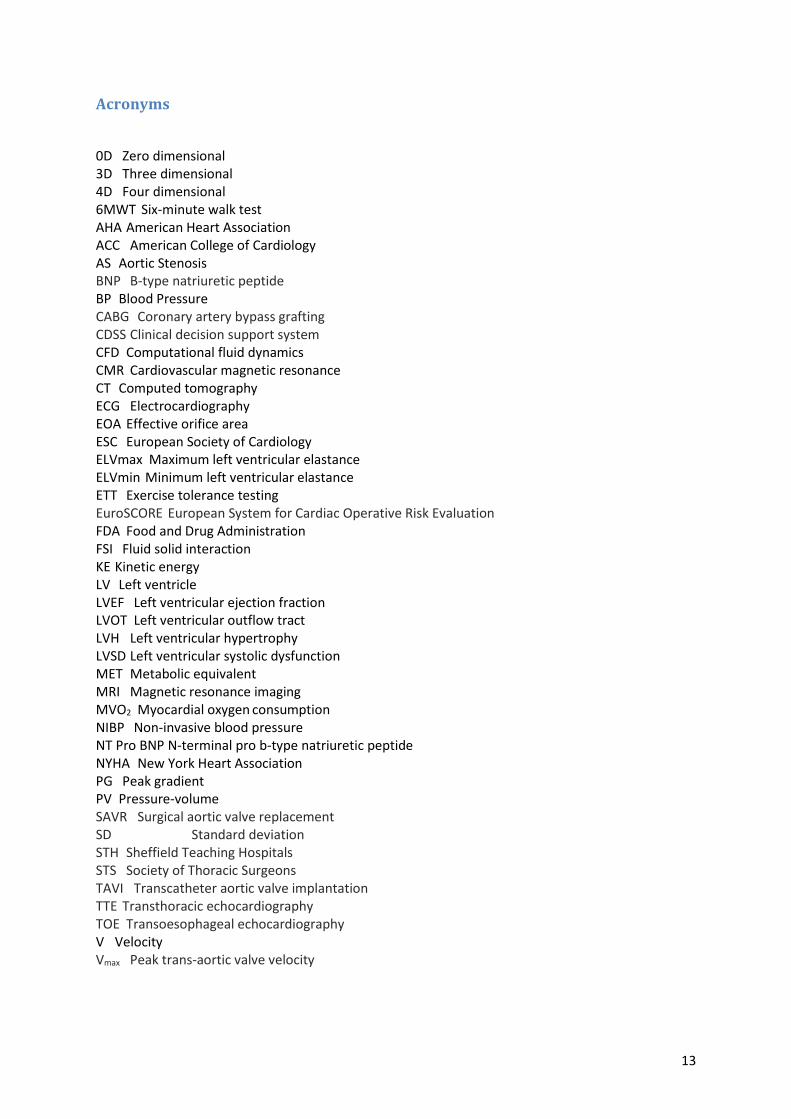
0D Zero dimensional 3D Three dimensional 4D Four dimensional 6MWT Six-minute walk test AHA American Heart Association ACC American College of Cardiology AS Aortic Stenosis BNP B-type natriuretic peptide BP Blood Pressure CABG Coronary artery bypass grafting CDSS Clinical decision support system CFD Computational fluid dynamics CMR Cardiovascular magnetic resonance CT Computed tomography ECG Electrocardiography EOA Effective orifice area ESC European Society of Cardiology ELVmax Maximum left ventricular elastance ELVmin Minimum left ventricular elastance ETT Exercise tolerance testing EuroSCORE European System for Cardiac Operative Risk Evaluation FDA Food and Drug Administration FSI Fluid solid interaction KE Kinetic energy LV Left ventricle LVEF Left ventricular ejection fraction LVOT Left ventricular outflow tract LVH Left ventricular hypertrophy LVSD Left ventricular systolic dysfunction MET Metabolic equivalent MRI Magnetic resonance imaging MVO2 Myocardial oxygen consumption NIBP Non-invasive blood pressure NT Pro BNP N-terminal pro b-type natriuretic peptide NYHA New York Heart Association PG Peak gradient PV Pressure-volume SAVR Surgical aortic valve replacement SD Standard deviation STH Sheffield Teaching Hospitals STS Society of Thoracic Surgeons TAVI Transcatheter aortic valve implantation TTE Transthoracic echocardiography TOE Transoesophageal echocardiography V Velocity Vmax Peak trans-aortic valve velocity

14

List of figures

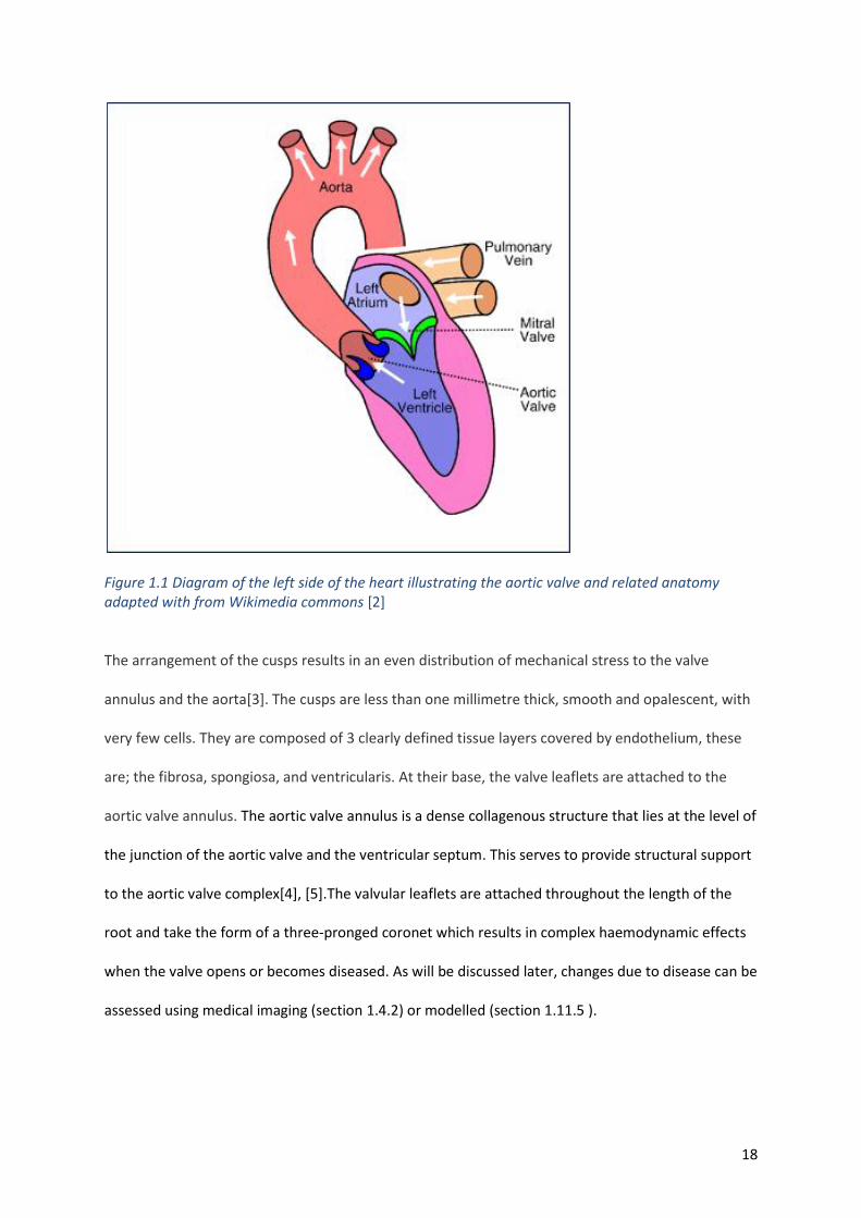
Figure 1.1 Diagram of the left side of the heart ................................................................................................... 18

Figure 1.2 Illustrating the pathological process in AS ........................................................................................... 21

Figure 1.3 Schematic demonstrating a constriction that may represent a stenotic valve ................................... 25

Figure 1.4 Illustrating the concepts and components of the continuity equation. .............................................. 29

Figure 1.5 Images of the aortic valve of a patient in the study ............................................................................ 31

Figure 1.6 Images of a stenotic valve of a patient in the study taken with CT and MRI ....................................... 34

Figure 1.7 Simultaneous aortic and LV pressures obtained during cardiac catheterisation ................................ 35

Figure 1.8 Diagnostic algorithm to assess the severity of aortic stenosis. ........................................................... 38

Figure 1.9 Timeline showing the important steps in AV intervention since 1953 ................................................ 40

Figure 1.10 Image showing open heart surgery in a patient in the study. ........................................................... 41

Figure 1.11 Illustrating the survival of patients with AS with and without surgical intervention ........................ 41

Figure 1.12 Graph showing a downward trend in surgical mortality ................................................................... 42

Figure 1.13 Graph showing the predicted mortality of patients undergoing AVR. .............................................. 43

Figure 1.14 Fluoroscopic image of a TAVI procedure in this study. ...................................................................... 45

Figure 1. 15 Schematic illustrating the optimal time of intervention ................................................................... 52

Figure 1.16 Effect of aortic stenosis on quality of life in patients over the age of 70 years. ................................ 60

Figure 1.17 Graph showing change in quality of life parameters following aortic valve replacement. ............... 61

Figure 1.18 A schematic diagram of an idealised pressure volume loop. ............................................................ 72

Figure 2.1 Flow of patients through the study ..................................................................................................... 78

Figure 2.2 Illustration of data stored in ArQ the EurValve database .................................................................... 79

Figure 2.3 Timings of cardiac cycle method of acquisition used and how calculated………………………………………..84

Figure 2.4 Images from a 3D full volume TTE study performed………………………………………………………………………..85

Figure 2.5 Maximum velocity and the EOA calculated from 4D flow CMR acquisition. ....................................... 89

Figure 2.6 Case example of LV blood flow kinetic energy assessment ................................................................. 90

Figure 2.7 Lumped parameter model of the left side of the heart and systemic circulation ............................... 93

Figure 2.8 double-Hill elastance models ............................................................................................................... 97

Figure 2.9 Ideal PV loop ........................................................................................................................................ 99

Figure 2.10 An example of the sensitivity matrix used ....................................................................................... 104

Figure 2.11 Schematic of the process undertaken to produce the PV loop in protocol 1 .................................. 111

Figure 2.12 Typical time-series pressure curves and piecewise quadratic representation in AS ....................... 112

Figure 2.13 Example of measured and personalised elastance using a double-Hill model ................................ 114

Figure 2. 14 Tuned model outputs ..................................................................................................................... 115

Figure 2.15 Sphere equipment used to monitor patients around their homes ................................................. 119 Figure 2.16 Illustrating CDSS flow chart to guide clinicians through the ESC guidelines………………………….……..123 Figure 2.17 Risk sores within the CDSS .............................................................................................................. 125 Figure 2.18 Demonstrating the results of a using CBR ....................................................................................... 126 Figure 2.19 A summary of activity data captured by the Philips Health Watch and the Sphere device ............ 126

Figure 2.20 Modelled PV loops using protocol 4 and the resulting parameters. ............................................... 127

Figure 2.21 Excerpt from the JotForm questionnaire platform .......................................................................... 129

Figure 3.1 Box plots showing the trend of the transthoracic echocardiogram parameters............................... 136

Figure 3.2 Example of standard TTE measurements in one patienst ................................................................. 137

Figure 3.3 Illustrating the assessment of diastolic function ............................................................................... 137

Figure 3 Appropriate and inappropriated segmented meshes from 3D TOE images ......................................... 139

Figure 3.5 Appropriate and inappropriated segmented meshes from CT images ............................................. 141

Figure 3. 6 Box plots of how the standard CMR parameters measured change following intervention. .......... 142

Figure 3.7 Measured PV loop for one patient in the study ................................................................................ 143

15

Figure 3.8 Box plots showing the trend in activity metrics from the Sphere kit ................................................ 147

Figure 3.9 Raw data from the Sphere kit ............................................................................................................ 148

Figure 3.10 Inferred time spent lying, sitting, walking and time spent outside the home during monitoring... 148

Figure 3.11 Bar chart showing how a patient’s walking activity varied throughout the week .......................... 149

Figure 3.12 Shows a heatmap of the location of the patient in three monitoring periods ................................ 150

Figure 3.13 Graph of the step count of patients over the periods of observation ............................................. 151

Figure 3.14 Graph of the total energy expenditure and active energy expenditure .......................................... 152

Figure 3.15 Graph of minutes performing moderate activity light activitynover the periods of observation. .. 153

Figure 3.16 Raw data from the Philips Health Watch ......................................................................................... 154

Figure 3.17 Graphs indicating range and frequency of observations from the Philips Health Watch ............... 155

Figure 3.18 Shows heart rate and total energy expenditure for one patient over a monitoring period………….156

Figure 3.19 Illustrating how the Philips Health Watch data and Sphere data can be combined ....................... 157

Figure 3.20 Mean percentage scores from the Minnesota living with heart failure questionnaire. .................. 158

Figure 3.21 Bar chart illustrating the change of quality of life scores following intervention............................ 159

Figure 3.22 Peak pressure gradients measured by catheterisation, Doppler TTE and 4D flow CMR ................. 162

Figure 3.23 Bland-Altman plots for pressure gradients by 4D flow CMR and TTE against invasive study. ........ 162

Figure 3.24 Histogram and Bland-Altman plots for EOA between TTE and 4Dflow methods. ........................... 163

Figure 3.25 Aassociations between the 6MWT distance with the severity of stenosis assessed by TTE and 4D

flow CMR derived PG and EOA. ................................................................................................................. 164

Figure 3.26 Associations of LV blood flow KE properties with the 6MWT distance achieved. ........................... 167

Figure 3.27 Association of LV remodelling post SAVR/TAVI with pre-intervention LV blood flow KE ................ 170

Figure 3.28 Comparison of elastance models to the measured elastance in one patient. ................................ 171

Figure 3.29 Left: PV loops produced in one patient using different protocols and measured data................... 174 Figure 3.30 Results of the automated segmentation process in one patient in the study................................. 176

Figure 3.31 CFD analysis of aortic valve flow in an example case. ..................................................................... 177

Figure 3.32 Pressure flow relationship with a quadratic curve fitted to the results. ......................................... 178

Figure 3.33 Screenshot of the execution of the 0D model in MATLAB .............................................................. 179

Figure 3.34 Modelled data tuned to measured data for pressures and volumes .............................................. 180

Figure 3.35 A measured PV loop and modelled PV loop produced by protocol 4.............................................. 181

Figure 3.36 Graph showing the model derived aortic valve gradients using protocol 4 and the measured

gradient ...................................................................................................................................................... 183

Figure 3.37 Bland-Altman plot of measured gradients by TTE and the computed gradients. ........................... 183

Figure 3.38. Graph illustrating the relationship between ejection fraction and ELVmax. .................................. 187

Figure 3.39 PV loops in the rest, exercise pre and post intervention in a patient in this study ......................... 189

Figure 3.40 Graph showing the correlation between the measured and predicted peak gradients following

valve replacement...................................................................................................................................... 191

Figure 3.41 Bland-Altman plot s measured and modelled residual peak gradient following intervention.. ...... 192

Figure 3.42 Correlation between the exercise capacity measured post valve replacement with the exercise

capacity predicted by the model ............................................................................................................... 192

Figure 3.43 Bland-Altman plot of measured and model predicted exercise capacity following intervention ... 193

Figure 3.44 How useful clinicians found the activity data, modelling and simulation data and interaction with

the simulation tool. .................................................................................................................................... 194

Figure 3.45 How a CDSS using data from the sudy may influence decision making .......................................... 195

Figure 3.46 How certainty in decision mages may improved when presented by additional information in the

clinical decision support software. ............................................................................................................ 196

Figure 4.1 Mathematically derived pressure curves during ejection ................................................................. 219

Figure 5.1. Illustrating the modelled flow through the aortic valve and measured flow in the aorta .............. 236

Figure 5.2 Modelled flow through the mitral valve and the velocity profile through the mitral valve .............. 236

16

Figure 5.3 Risk and benefit scores are summarised in a mock up presented in the CDSS. ................................ 240

List of tables

Table 1. 1. Trend of the number of aortic valves being replaced in the UK. ........................................................ 42 Table 1.2 Management of severe aortic stenosis ................................................................................................. 49 Table 2.1 Table of concepts .................................................................................................................................. 81 Table 2.3 Analogous electrical and fluid dynamic metrics ................................................................................... 94 Table 2.4 Illustrating model outputs .................................................................................................................... 98 Table 3.1 Baseline patient characteristics pre and post intervention. ............................................................... 134

Table 3.2 Indicates the number of major adverse events that occurred in the cohort separated into treatment

type. ........................................................................................................................................................... 134

Table 3.3 TTE derived data showing the severity of the aortic stenosis, indicators of diastolic dysfunction and

intraventricular pressure pre and post intervention ................................................................................. 135

Table 3.4 Findings when the segmented geometries from TOE were compared with the clinical images. ....... 139

Table 3.5 Findings when the segmented geometries from CT were compared with the clinical images.. ........ 140

Table 3.6.Standard CMR parameters measured ................................................................................................ 141

Table 3.7 Invasive LV pressure measurements from cardiac catheterisation during the TAVI procedure. ....... 143

Table 3.8 6MWT results ...................................................................................................................................... 144

Table 3.9 Activity parameters measured by the Sphere kit................................................................................ 146

Table 3.10 Metrics derived from the Philips health watch ................................................................................. 150

Table 3.11 Percentage scores of the MLHFQ pre and post intervention ........................................................... 158

Table 3.12 Percentage scores of the WHOQOL-BREF questionnaire pre and post intervention ....................... 159

Table 3.13 Patient demographics ....................................................................................................................... 160

Table 3.14 Correlations between standard CMR and TTE parameters and 4D flow derived peak gradient and

EOA with 6MWT and NYHA class. .............................................................................................................. 164

Table 3.15 Association of relative LV mass change to relative change in other imaging markers pre-/post aortic

valve intervention. ..................................................................................................................................... 165

Table 3.16 Pre and post-operative changes in cardiac haemodynamics, imaging parameters and functional

parameters at 3-months. ........................................................................................................................... 166

Table 3. 17 Correlation of NYHA class and 6MWT distance to all haemodynamic and CMR parameters. ........ 168

Table 3.18 Correlation of LV mass change pre-/post aortic valve replacement to imaging parameters. .......... 169

Table 3.19 Haemodynamic parameters produced from protocols 1-3 .............................................................. 172

Table 3.20 Personalised parameters from CFD simulations and optimisation in one patirent. ......................... 179

Table 3.21 The haemodynamic parameters produced by protocol 4 ................................................................ 181

Table 3.22 Haemodynamic parameters produced by protocol 4 compared with the measured data…………….182

Table 3.23 Guideline indication according 2017 ESC/ EACTS guidelines for each case in the CDSS................... 195

Table 4.1 Key limitations of the study ................................................................................................................ 230

Table 5.2 identifies what this study achieved against originally stated hypothesis and aims ............................ 234

17

CHAPTER 1

1. Introduction

Aortic stenosis (AS) is a narrowing of the orifice of the aortic valve that causes an increased

resistance to blood flow from the ventricle into the systemic circulation. The heart maintains flow, at

the cost of increased pressure, triggering a series of pathophysiological processes leading to adverse

clinical outcomes. In this introduction the current knowledge of AS, its importance, and how and

why it is currently treated, will be reviewed, highlighting areas where computational modelling may

provide additional information in the decision-making process. This will be followed by an overview

of what computational modelling is, how it is already employed in healthcare and, in particular, how

it may be useful in the management of patients with aortic stenosis.

1.1. Anatomy

The aortic valve is sited between the left ventricle and the aorta. It usually has three leaflets and its

size varies significantly from person to person [1]. Its function is to maintain the flow of blood in a

single direction. When the ventricle contracts and the pressure in the left ventricle exceeds that in

the aorta, the valve opens, and oxygenated blood is pumped to the systemic circulation.

18

Figure 1.1 Diagram of the left side of the heart illustrating the aortic valve and related anatomy adapted with from Wikimedia commons [2]

The arrangement of the cusps results in an even distribution of mechanical stress to the valve

annulus and the aorta[3]. The cusps are less than one millimetre thick, smooth and opalescent, with

very few cells. They are composed of 3 clearly defined tissue layers covered by endothelium, these

are; the fibrosa, spongiosa, and ventricularis. At their base, the valve leaflets are attached to the

aortic valve annulus. The aortic valve annulus is a dense collagenous structure that lies at the level of

the junction of the aortic valve and the ventricular septum. This serves to provide structural support

to the aortic valve complex[4], [5].The valvular leaflets are attached throughout the length of the

root and take the form of a three-pronged coronet which results in complex haemodynamic effects

when the valve opens or becomes diseased. As will be discussed later, changes due to disease can be

assessed using medical imaging (section 1.4.2) or modelled (section 1.11.5 ).

19

The aortic root is a continuation of the left ventricular outflow tract. Its components include the

sinuses of Valsalva, the fibrous inter-leaflet triangles, and the valvar leaflets themselves. Problems

resulting in thickening and calcification of these structures leads to AS. AS describes the condition

where the valve orifice is narrowed. This increases the resistance and thus a greater force of

contraction is required to eject the same volume of blood. Since the blood is ejected through a

smaller orifice, the velocity of the blood leaving the heart increases, and this is often measured

clinically to assess the severity of the stenosis (section 1.4.2.1).

1.2. Epidemiology

Although rheumatic heart disease is uncommon in developed countries such as the UK, it remains an

important cause of AS worldwide. In 2015, 33.4 million people were estimated to be living with

rheumatic heart disease around the world, with sub-Saharan Africa, South Asia, and Oceania having

the highest prevalence[6].

Calcific-degenerative AS (see section 1.3) is the most common valvular disease in the developed

world and associated with significant morbidity and mortality; this is the focus of this thesis. Two

percent of adults over 65 years old and four percent over 85 have clinically significant disease [7].

With the ageing population, this already important pathology will become increasingly prevalent and

its diagnosis and management will have an even greater impact upon healthcare.

The UK Hospital Episode Statistics (HES) database suggests that at least 200,000 people were

admitted to hospital in England between 2002 and 2012 due to AS[8]. Considering that 0.87% of all

heart failure admissions are due to AS[9], the cost of managing these patients in terms of financial

cost, hospital bed capacity and clinicians time is huge. Even without specific treatment, the average

cost of a patient with severe AS is estimated at £31,096 per year[12]. The problem may be greater

20

than appreciated; many patients with clinically significant (moderate or severe) valve disease being

undiagnosed (6.4% in the Ox-valve study)[10]. Patients were twice as likely to have significant

undiagnosed disease if they were of low socioeconomic status and three times as likely if they had

atrial fibrillation[10]. These groups may present with complications of the disease or late in the

disease process so may potentially be of higher risk. In 2017 there were approximately 103,000

deaths worldwide attributed to non-rheumatic aortic valve disease, which is approximately 1% of

global cardiovascular deaths - an increase of 40% over the previous 10 years[11].

1.3. Pathophysiology

Aortic valve stenosis was described first by Lazare Riviere in 1663[12]. Mönckeberg in 1904 went on

to describe AS as a passive degenerative process associated with rheumatic fever or ageing, where

serum calcium attaches to the valve surface and forms nodules[13]. The decline in rheumatic fever

and ageing of the population have led to a demographic transition towards fibrocalcific disease. In

contrast to the cusp fusion seen with rheumatic heart disease, this process results in increased valve

stiffness, reduced cusp excursion, and progressive orifice narrowing. Although calcification is still

viewed by some as a passive process and termed ‘age related’ or ‘degenerative’, it has now been

shown to be caused by an inflammatory process similar to that of atherosclerosis, with similar risk

factors [14] (see figure 1.2).

The process starts with endothelial injury, infiltration of lipids, lipid oxidation and a proinflammatory

response. Following this, osteoblast-like cells promote progressive valvular calcium and bone matrix

deposition. The osteogenic phenotype involves many molecules involved in bone formation and is

both self-perpetuating and highly regulated[15]. Advances in imaging now allow for non-invasive

assessment of both the burden and activity of calcification to be measured (see section 1.4.2.2).

Endothelial damage is thought to be caused by increased mechanical stress and reduced shear

21

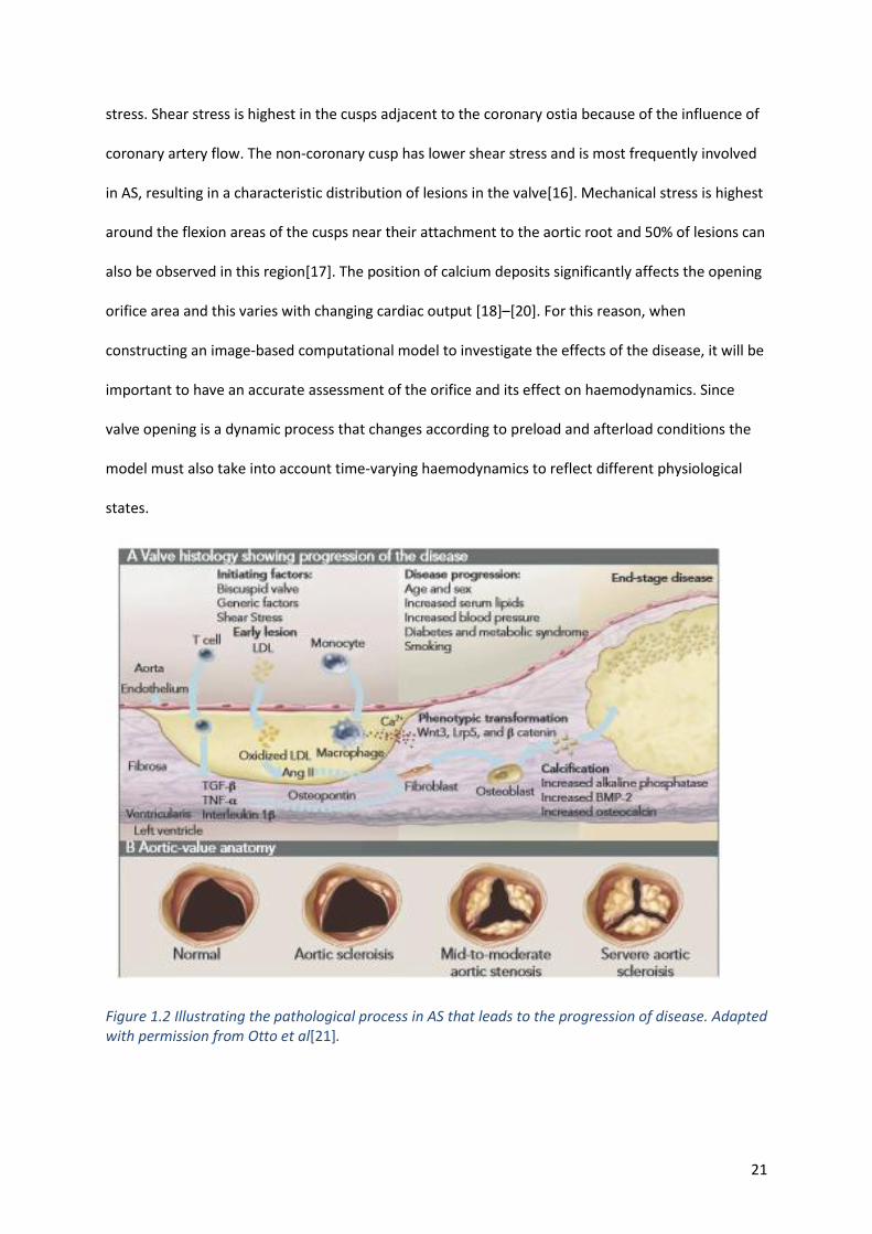
stress. Shear stress is highest in the cusps adjacent to the coronary ostia because of the influence of

coronary artery flow. The non-coronary cusp has lower shear stress and is most frequently involved

in AS, resulting in a characteristic distribution of lesions in the valve[16]. Mechanical stress is highest

around the flexion areas of the cusps near their attachment to the aortic root and 50% of lesions can

also be observed in this region[17]. The position of calcium deposits significantly affects the opening

orifice area and this varies with changing cardiac output [18]–[20]. For this reason, when

constructing an image-based computational model to investigate the effects of the disease, it will be

important to have an accurate assessment of the orifice and its effect on haemodynamics. Since

valve opening is a dynamic process that changes according to preload and afterload conditions the

model must also take into account time-varying haemodynamics to reflect different physiological

states.

Figure 1.2 Illustrating the pathological process in AS that leads to the progression of disease. Adapted with permission from Otto et al[21].

22

The usual focus of AS assessments has been on the valve. However, the disease process not only

affects the valve but also reduces arterial compliance and alters the geometry of the left ventricle;

for this reason it is viewed as a systemic disease [22]. The left ventricular myocardial response to

pressure overload is important[16]. The response of the left ventricle (LV) to an increased afterload

is quite complex. It often consists of a combination of wall thickening and a change in cavity size,

affecting systolic and diastolic function, although remodelling and LV dilatation can occur [23]. There

are many theories around how pressure overload and the resultant LV hypertrophy (LVH) may

impair LV systolic function. These include intermittent ischaemia, apoptosis, neurohumoral

activation and changes to the myocardial cytoskeleton [24]. Interestingly, the correlation between

echocardiographic measures of AS severity and the degree of LVH is moderate at best[25],

suggesting that there are other factors which, in combination, increase the load on the ventricle.

LVH maintains wall stress and cardiac output but pressure-induced LVH also initiates a series of

events at the molecular level that may eventually lead to cell death and myocardial fibrosis, resulting

in LV dilatation and decompensation[26].

Congenital bicuspid aortic valve anatomy is found in 0.5–2.0% of the population although it is

relatively uncommon compared to calcific AS. However, AS affecting a bicuspid valve is the most

common indication for surgical aortic valve re placement (SAVR) in patients <70 years of age.

Bicuspid AS is associated with specific anatomic challenges which impact on treatment choices (see

section 1.6.3); these include heavy valve calcification, an eccentrically shaped annulus, and a

horizontal, dilated aorta. The complex haemodynamics of a bicuspid valve may be better understood

using 4D flow MRI and or computational modelling.

23

1.3.1. Disease progression and prognosis

The clinical course of AS is usually characterised by a long asymptomatic period that is followed by a

shorter symptomatic period when patients may physically decline quite rapidly. However, the rate of

progression of AS is quite variable, which highlights differences in the disease process in individual

valves and patients [21]. Peak AV velocity can change by 0.24±0.30 m/s/year[28]), but this is subject

to scan–rescan variation. This presents a challenge to clinicians in terms of when to follow patients

up and when to intervene by replacing the valve. Currently patients are followed up at varying

intervals based on clinical opinion using 2D ultrasound. Once symptoms develop, the mortality rate

is 50% at two years without intervention [27] but when LV dysfunction is primarily caused by the

increase in afterload as a result of the stenosis, the prognosis after aortic valve replacement appears

to be good, with improved cardiac function [28].

Currently there is no easy and accepted method to predict which patients may deteriorate rapidly

and, apart from a few exceptions (see section 1.8), the general recommendation is not to intervene

if asymptomatic and LV function is preserved [29]–[31]. In recent years there has been a move to

operate on asymptomatic patients with very severe AS (see section 1.8). The valve area at which

patients become symptomatic is variable [32] suggesting, that, the haemodynamics may be complex,

some hearts are able to cope with a greater degree of obstruction than others, and other factors

that load the ventricle such as hypertension need to be considered. The whole physiological system

needs to be considered - not just the valve in isolation; a model representing the patient’s valve and

systemic circulation could do this.

1.3.2. Haemodynamics in AS

The pressure gradient across the aortic valve results from both increased resistance due to the

reduced orifice area and the disturbed nature (including turbulence) of the flow distal to the valve.

24

The magnitude of the pressure drop is mainly determined by the degree of stenosis and the flow

across the valve. However, the aortic valve is coupled to the systemic arterial vasculature and the

variability in derived stenosis severity is dependent on events occurring downstream i.e. the

pressure-flow relation in the systemic arterial circulation. Therefore, analysis of stenosis severity

under various physiological conditions must take into account the dependence of aortic valve

pressure gradient on systemic arterial haemodynamics. The resistance in the circulation, however, is

complex to model as a number of factors affect vascular tone and there are many controlling

mechanisms including those which are local, chemical-mediated and neurohumoral. The aim of

these mechanisms is to achieve homeostasis, maintaining a constant flow when the metabolic

demand is stable.

Flow through a linear resistor, representative of elements of the systemic circulation can be

considered in the following equation, analogous to Ohm’s Law (see section 1.11.4 for further detail):

Flow(Q)= Pressure(P)/Resistance (R)

When blood flows through a stenotic aortic valve, the effective resistance is a nonlinear function of

the flow. Irrespective of the vessel cross-sectional area the volume of flow passing through must be

the same, and so the velocity must increase as the blood accelerates into the throat of the stenosis.

This causes an increase in kinetic energy and a concomitant decrease in potential energy, which is

proportional to pressure. Thus, the pressure immediately after the stenosis is lower than the

proximal pressure and the pressure drop can be computed from Bernoulli’s equation (see below).

When the flow decelerates after the orifice the pressure does not fully recover, due to energy lost

through flow disturbances and viscous resistances.

25

Figure 1.3 Schematic demonstrating a constriction that may represent a stenotic valve. The flow in the LVOT (point 1) should equal the flow in the proximal aorta (point 3). At the vena contracta (point 2) the flow converges into a narrow high velocity jet.

Bernoulli's principle is derived from the principle of conservation of energy. In a steady flow, along a

streamline, the total kinetic and potential energies proximal to the stenosed valve must equal the

total of the kinetic and potential energies distal to the stenosed valve. There is transition from

potential to kinetic energy as the flow accelerates into the stenosis, and the reverse as the jet

expands again after the stenosis, as described above; but, as previously stated, there is some loss of

energy and therefore the potential energy (pressure per unit volume) does not fully recover in the

distal vessel.

Bernoulli’s equation states that:

𝑃1 +1

2𝑣1

2 + 𝑔ℎ1 = 𝑃2 +1

2𝑣2

2 + 𝑔ℎ2 Eq. 1.1

Where P= hydrostatic pressure in pascals (pressure in a fluid is a measure of energy per unit volume)

= fluid density replacing mass in the energy equations, g = acceleration due to gravity, v=velocity

and h=height of the fluid.

As there is there is a negligible change in height of the blood and the potential energy is the same

the gravitational potential energy can be ignored, and the equation can be simplified to:

𝑃1 +1

2𝑣1

2 = 𝑃2 +1

2𝑣2

2 Eq. 1.2

This can be rearranged to:

26

𝑃1 − 𝑃2 =1

2𝑣2

2 −1

2𝑣1

2

𝑃 =1

2(𝑣2

2 − 𝑣1 2 ) Eq. 1.3

This equation can be further simplified by substituting the density of blood, neglecting the proximal

velocity (which is much lower than the velocity in the orifice) and converting from SI units to clinical

units of pressure and velocity.

Then

𝑃 = 4𝑣2 2 Eq. 1.4

The inputs to this equation are usually measured clinically using ultrasound imaging. The accuracy of

the Bernoulli equation and of this simplified formula (Eq. 1.4) in the context of aortic valve disease is

discussed in section 1.4.2.1. Computational fluid dynamics can be used to solve the Navier-Stokes

equations which mathematically describe the flow of incompressible fluids. This can improve the

estimated pressure drop across the valve (see section 1.11.5), but solving the Navier-Stokes

equations with flexible vessel walls and a flexible aortic valve is complex[33]. There is of course

energy loss as blood flows through any vessel, as described by Poiseuille’s law but, since this is much

less significant than the loss across a stenosis, it is not usually calculated in the routine assessment of

AS.

1.4. Diagnosis

Currently the diagnosis of AS is based upon clinical history, examination and investigations, including

limited objective measurements from clinical imaging.

27

1.4.1. Symptoms

The classical triad of symptoms of AS, which typically occur upon exertion, are angina, shortness of

breath and syncope, all of which are thought to be a consequence of pressure overload and the

resulting response of the myocardium. Although the exact mechanism of syncope is uncertain, the

vasodilatory effect of exercise with a relatively fixed cardiac output is thought to be a contributing

factor [24]. There is a link between these symptoms and prognosis [27], [34]. Dyspnoea is the most

common symptom and, as patients progress into heart failure, leg swelling or fatigue may occur [35].

Assessment of symptoms can be challenging in elderly patients due to multiple co-morbidities,

which may have similar symptoms to AS, and inactivity which can conceal exertional symptoms.

AS can be suspected from the patient history and examination; the classic ejection systolic murmur

radiating to the neck may be heard. With increasing severity, other signs may be present such as a

diminishing S2 heart sound and a slow rising pulse. When suspicion is raised, the clinician can order a

number of investigations. An ECG may show evidence of LVH, delayed AV conduction and T wave

abnormalities. Occasionally calcification is seen on the chest x-ray. Blood tests may reveal a raised

BNP or troponin. Whilst tests such as these may confirm probable AS, more informative diagnostic

tests are required.

1.4.2. Imaging in AS

1.4.2.1. Echocardiography

The diagnostic test most commonly used to view and confirm AS is transthoracic echocardiography

using Doppler ultrasound [29], [31]. Continuous Doppler through the aortic valve gives the velocity

of blood through the narrowed aortic orifice and the pressure gradient across the valve can then be

calculated. In the simplest form, it is assumed that the velocity is uniform across the area of the

28

valve orifice and that the probe can be orientated and positioned to capture this velocity. The

pressure gradient can then be estimated by the simplified Bernoulli equation. There are two

important limitations; Doppler measurements are operator-dependent and the Bernoulli equation is

a gross simplification of valve haemodynamics [36], [37]. It is an idealised formula that holds true for

cases of steady laminar flow with an assumption that there is only forward flow of blood as the

result of the kinetic energy. This is obviously not the case in AS where there is turbulence, friction

and vortex formation. Based on conservation of energy, the Bernoulli equation predicts a recovery in

hydrostatic pressure (energy) but because of the energy loss there is non-recovery in the distal

vasculature which is not considered. On average, the Bernoulli formulation overestimates the

pressure drop across the valve by 54%. This is primarily due to the use of a single peak value of

velocity, neglecting the variation in velocity across the valve plane. Accuracy could be improved with

analysis of other components of the pressure drop [38]. However, the author concedes that the

pressure drop is mainly driven by the spatial (convective) acceleration of blood, which is taken into

account in the Bernoulli formula.

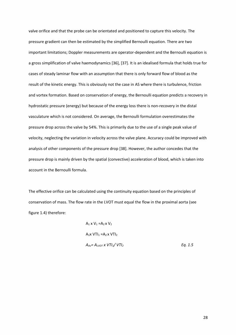
The effective orifice can be calculated using the continuity equation based on the principles of

conservation of mass. The flow rate in the LVOT must equal the flow in the proximal aorta (see

figure 1.4) therefore:

A1 x V1 =A2 x V2

A1x VTI1 =A2 x VTI2

AAv= ALVOT x VTI1/ VTI2 Eq. 1.5

29

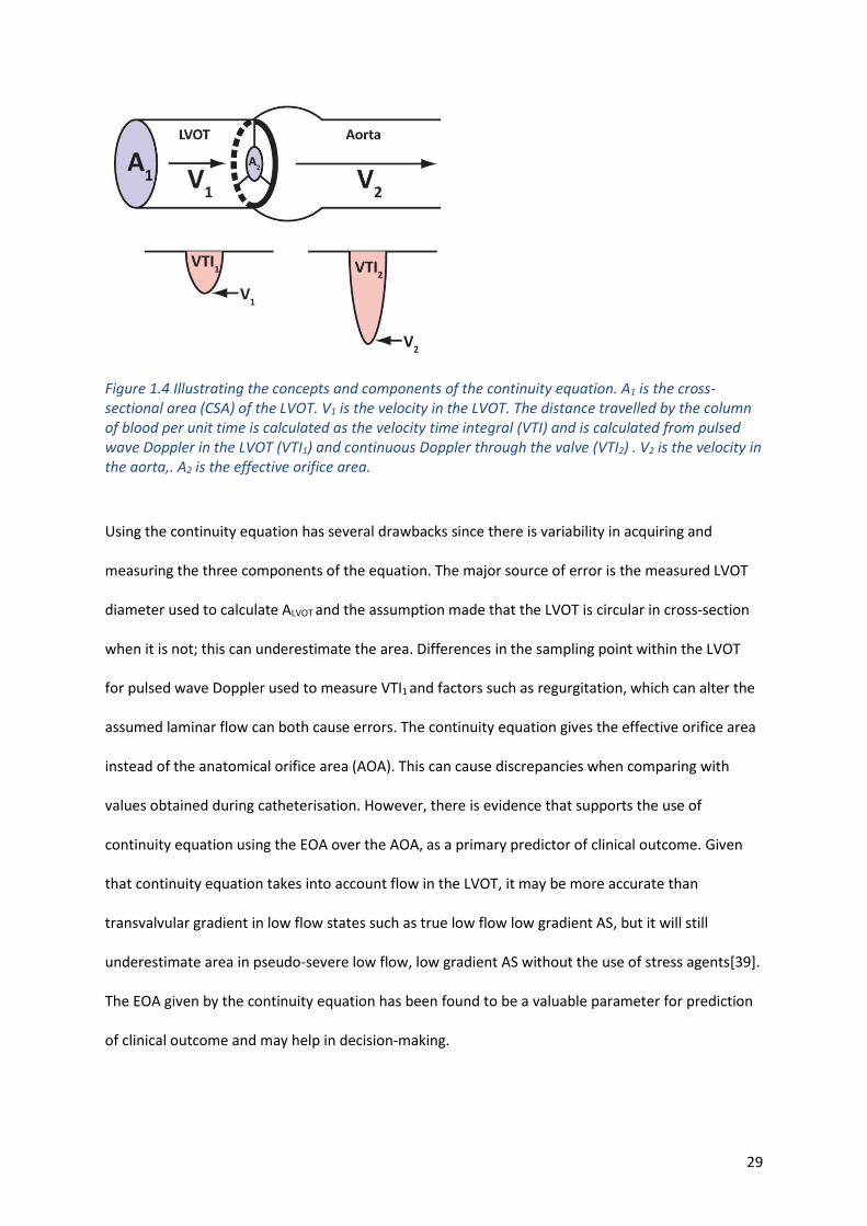
Figure 1.4 Illustrating the concepts and components of the continuity equation. A1 is the cross-sectional area (CSA) of the LVOT. V1 is the velocity in the LVOT. The distance travelled by the column of blood per unit time is calculated as the velocity time integral (VTI) and is calculated from pulsed wave Doppler in the LVOT (VTI1) and continuous Doppler through the valve (VTI2) . V2 is the velocity in the aorta,. A2 is the effective orifice area.

Using the continuity equation has several drawbacks since there is variability in acquiring and

measuring the three components of the equation. The major source of error is the measured LVOT

diameter used to calculate ALVOT and the assumption made that the LVOT is circular in cross-section

when it is not; this can underestimate the area. Differences in the sampling point within the LVOT

for pulsed wave Doppler used to measure VTI1 and factors such as regurgitation, which can alter the

assumed laminar flow can both cause errors. The continuity equation gives the effective orifice area

instead of the anatomical orifice area (AOA). This can cause discrepancies when comparing with

values obtained during catheterisation. However, there is evidence that supports the use of

continuity equation using the EOA over the AOA, as a primary predictor of clinical outcome. Given

that continuity equation takes into account flow in the LVOT, it may be more accurate than

transvalvular gradient in low flow states such as true low flow low gradient AS, but it will still

underestimate area in pseudo-severe low flow, low gradient AS without the use of stress agents[39].

The EOA given by the continuity equation has been found to be a valuable parameter for prediction

of clinical outcome and may help in decision-making.

30

Planimetry of the aortic valve area is sometimes performed but, in heavily calcified valves for which

the image quality is poor, this is often difficult. If transthoracic imaging windows are poor and the

Doppler signal is suboptimal, transoesophageal echocardiography (TOE) could be performed. Data

suggest that computed tomography (CT) and cardiovascular magnetic resonance (CMR) imaging

measurements of the aortic valve orifice area correlate well with planimetric measurements

obtained at transoesophageal echocardiography. A good correlation also exists between CMR

estimates and the area obtained with the continuity equation at TTE[40] or the Gorlin equation at

cardiac catheterisation[41]. However, planimetric measurements, irrespective of the radiologic

imaging technique used, tend to be larger than measurements derived from velocity and pressure

relationships. This is probably explained by the complex 3D structure of the aortic valve, with the

valve area formed by the free edges of the AV leaflets [42].

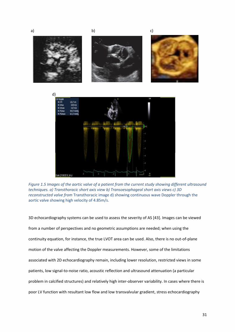
31

a) b) c)

d)

Figure 1.5 Images of the aortic valve of a patient from the current study showing different ultrasound techniques. a) Transthoracic short axis view b) Transoesophageal short axis views c) 3D reconstructed valve from Transthoracic image d) showing continuous wave Doppler through the aortic valve showing high velocity of 4.85m/s.

3D echocardiography systems can be used to assess the severity of AS [43]. Images can be viewed

from a number of perspectives and no geometric assumptions are needed; when using the

continuity equation, for instance, the true LVOT area can be used. Also, there is no out-of-plane

motion of the valve affecting the Doppler measurements. However, some of the limitations

associated with 2D echocardiography remain, including lower resolution, restricted views in some

patients, low signal-to-noise ratio, acoustic reflection and ultrasound attenuation (a particular

problem in calcified structures) and relatively high inter-observer variability. In cases where there is

poor LV function with resultant low flow and low transvalvular gradient, stress echocardiography

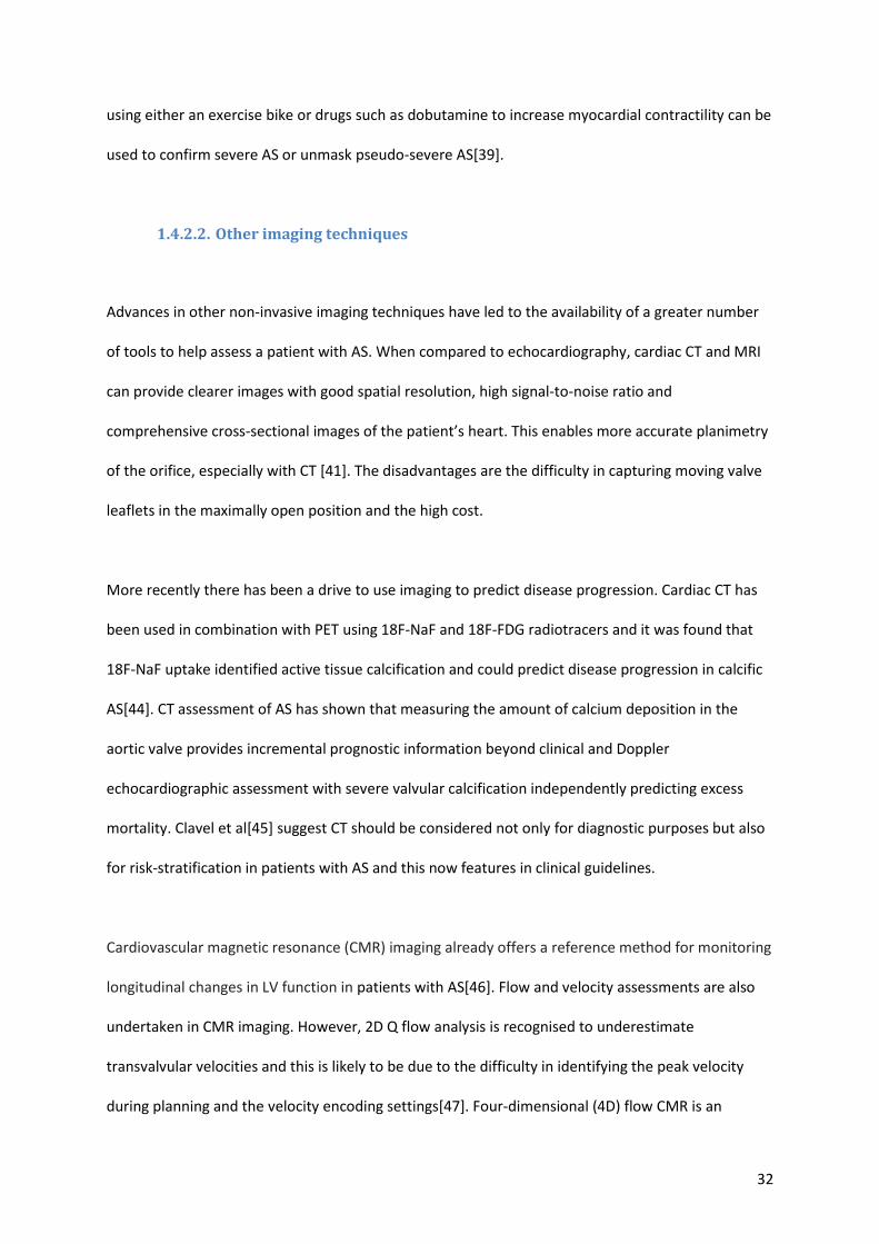
32

using either an exercise bike or drugs such as dobutamine to increase myocardial contractility can be

used to confirm severe AS or unmask pseudo-severe AS[39].

1.4.2.2. Other imaging techniques

Advances in other non-invasive imaging techniques have led to the availability of a greater number

of tools to help assess a patient with AS. When compared to echocardiography, cardiac CT and MRI

can provide clearer images with good spatial resolution, high signal-to-noise ratio and

comprehensive cross-sectional images of the patient’s heart. This enables more accurate planimetry

of the orifice, especially with CT [41]. The disadvantages are the difficulty in capturing moving valve

leaflets in the maximally open position and the high cost.

More recently there has been a drive to use imaging to predict disease progression. Cardiac CT has

been used in combination with PET using 18F-NaF and 18F-FDG radiotracers and it was found that

18F-NaF uptake identified active tissue calcification and could predict disease progression in calcific

AS[44]. CT assessment of AS has shown that measuring the amount of calcium deposition in the

aortic valve provides incremental prognostic information beyond clinical and Doppler

echocardiographic assessment with severe valvular calcification independently predicting excess

mortality. Clavel et al[45] suggest CT should be considered not only for diagnostic purposes but also

for risk-stratification in patients with AS and this now features in clinical guidelines.

Cardiovascular magnetic resonance (CMR) imaging already offers a reference method for monitoring

longitudinal changes in LV function in patients with AS[46]. Flow and velocity assessments are also

undertaken in CMR imaging. However, 2D Q flow analysis is recognised to underestimate

transvalvular velocities and this is likely to be due to the difficulty in identifying the peak velocity

during planning and the velocity encoding settings[47]. Four-dimensional (4D) flow CMR is an

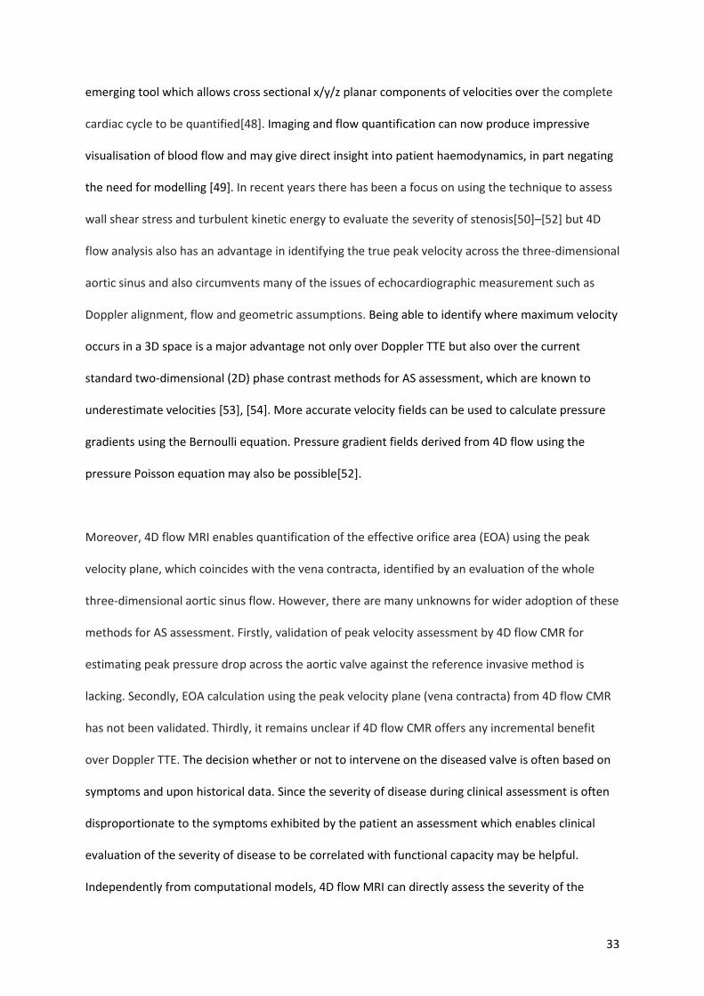
33

emerging tool which allows cross sectional x/y/z planar components of velocities over the complete

cardiac cycle to be quantified[48]. Imaging and flow quantification can now produce impressive

visualisation of blood flow and may give direct insight into patient haemodynamics, in part negating

the need for modelling [49]. In recent years there has been a focus on using the technique to assess

wall shear stress and turbulent kinetic energy to evaluate the severity of stenosis[50]–[52] but 4D

flow analysis also has an advantage in identifying the true peak velocity across the three-dimensional

aortic sinus and also circumvents many of the issues of echocardiographic measurement such as

Doppler alignment, flow and geometric assumptions. Being able to identify where maximum velocity

occurs in a 3D space is a major advantage not only over Doppler TTE but also over the current

standard two-dimensional (2D) phase contrast methods for AS assessment, which are known to

underestimate velocities [53], [54]. More accurate velocity fields can be used to calculate pressure

gradients using the Bernoulli equation. Pressure gradient fields derived from 4D flow using the

pressure Poisson equation may also be possible[52].

Moreover, 4D flow MRI enables quantification of the effective orifice area (EOA) using the peak

velocity plane, which coincides with the vena contracta, identified by an evaluation of the whole

three-dimensional aortic sinus flow. However, there are many unknowns for wider adoption of these

methods for AS assessment. Firstly, validation of peak velocity assessment by 4D flow CMR for

estimating peak pressure drop across the aortic valve against the reference invasive method is

lacking. Secondly, EOA calculation using the peak velocity plane (vena contracta) from 4D flow CMR

has not been validated. Thirdly, it remains unclear if 4D flow CMR offers any incremental benefit

over Doppler TTE. The decision whether or not to intervene on the diseased valve is often based on

symptoms and upon historical data. Since the severity of disease during clinical assessment is often

disproportionate to the symptoms exhibited by the patient an assessment which enables clinical

evaluation of the severity of disease to be correlated with functional capacity may be helpful.

Independently from computational models, 4D flow MRI can directly assess the severity of the

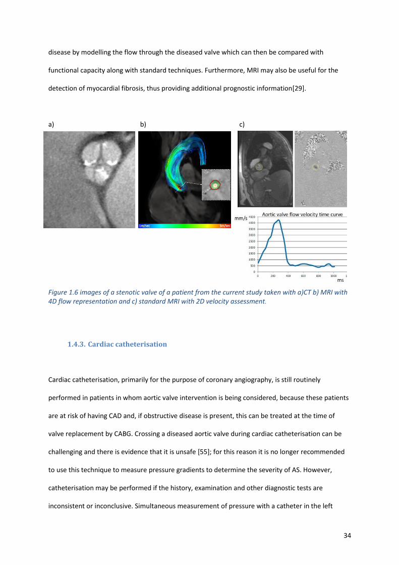
34

disease by modelling the flow through the diseased valve which can then be compared with

functional capacity along with standard techniques. Furthermore, MRI may also be useful for the

detection of myocardial fibrosis, thus providing additional prognostic information[29].

a) b) c)

Figure 1.6 images of a stenotic valve of a patient from the current study taken with a)CT b) MRI with 4D flow representation and c) standard MRI with 2D velocity assessment.

1.4.3. Cardiac catheterisation

Cardiac catheterisation, primarily for the purpose of coronary angiography, is still routinely

performed in patients in whom aortic valve intervention is being considered, because these patients

are at risk of having CAD and, if obstructive disease is present, this can be treated at the time of

valve replacement by CABG. Crossing a diseased aortic valve during cardiac catheterisation can be

challenging and there is evidence that it is unsafe [55]; for this reason it is no longer recommended

to use this technique to measure pressure gradients to determine the severity of AS. However,

catheterisation may be performed if the history, examination and other diagnostic tests are

inconsistent or inconclusive. Simultaneous measurement of pressure with a catheter in the left

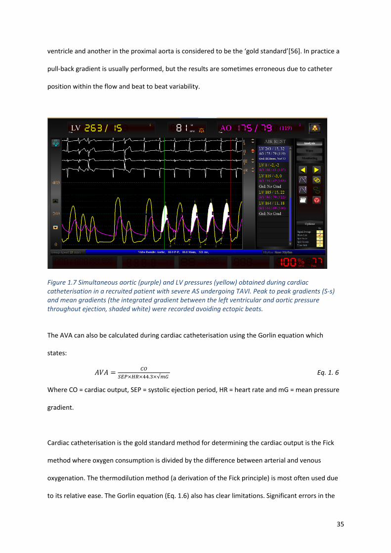
35

ventricle and another in the proximal aorta is considered to be the ‘gold standard’[56]. In practice a

pull-back gradient is usually performed, but the results are sometimes erroneous due to catheter

position within the flow and beat to beat variability.

Figure 1.7 Simultaneous aortic (purple) and LV pressures (yellow) obtained during cardiac catheterisation in a recruited patient with severe AS undergoing TAVI. Peak to peak gradients (S-s) and mean gradients (the integrated gradient between the left ventricular and aortic pressure throughout ejection, shaded white) were recorded avoiding ectopic beats.

The AVA can also be calculated during cardiac catheterisation using the Gorlin equation which

states:

𝐴𝑉𝐴 =𝐶𝑂

𝑆𝐸𝑃×𝐻𝑅×44.3×√𝑚𝐺 Eq. 1. 6

Where CO = cardiac output, SEP = systolic ejection period, HR = heart rate and mG = mean pressure

gradient.

Cardiac catheterisation is the gold standard method for determining the cardiac output is the Fick

method where oxygen consumption is divided by the difference between arterial and venous

oxygenation. The thermodilution method (a derivation of the Fick principle) is most often used due

to its relative ease. The Gorlin equation (Eq. 1.6) also has clear limitations. Significant errors in the

36

calculation of cardiac output are common and in deriving their equation , the Gorlins assumed that

for the aortic valve, the coefficients of orifice contraction and velocity loss were 1, which is not

possible.

1.4.4. Other Biomarkers

Because of reliance upon patient-reported symptoms and imprecise imaging techniques, other

objective prognostic biomarkers have been pursued, the main ones being BNP and NT-pro BNP. A

correlation has been shown between the level of serum BNP and NT-Pro BNP and symptoms and it

has been suggested that these biomarkers could be used to predict the onset of symptoms and

guide prognosis [24]. However, Ben-Dor et al [57] failed to show a correlation between BNP, severity

of AS or mortality. Problems may arise because of the wide range of levels of these markers with

differing significance in terms of symptom onset and prognosis. In addition, the test itself may be

affected by other disease states such as renal disease and pulmonary hypertension. More recently

natriuretic peptides have been shown to predict symptom-free survival and outcome in studies of

normal and low-flow severe AS [58], [59] and therefore BNP is the first cardiac biomarker to be

included in guidelines[29].

Cardiac troponin is released during myocardial injury and can be detected in the blood steam at very

low levels. In AS, raised troponins are associated with an increased LV wall thickness, myocardial

fibrosis and outcomes[60]. However, elevation in cardiac troponin is not specific and is not routinely

used in clinical practice. In the EVoLVeD study (Early Valve Replacement guided by Biomarkers of

Left Ventricular Decompensation in Asymptomatic Patients with Severe Aortic Stenosis) that is

currently underway, investigators are studying patients at risk of LV dysfunction as determined by

raised troponin, or a strain pattern on ECG, to see if early myocardial fibrosis is present on CMR and

whether or not early intervention is beneficial to these patients. Novel calculated biomarkers such as

valvulo-impedance which assesses the load on the left ventricle and has been linked to mortality

37

have also been suggested [61]. This has a similar rationale of assessing the system physiology to the

computational modelling process presented in this thesis.

1.5. Quantification of AS

As discussed above, there is debate about the best method of quantifying the severity of AS and to

risk-stratify the patient. The major studies linking symptoms and severity of AS to mortality have

been catheter-based studies [34], but we now use cardiac ultrasound to help make the same

judgments with less evidence [62]. However, this difference in approach is unlikely to matter so long

as whichever method is used is reproducible and correlates with outcome. Cardiac ultrasound and

Doppler measurements will continue to be used [29] at least until other methods can be shown to

predict morbidity and mortality more accurately. ESC guidelines recommend the use of ultrasound

as the main diagnostic tool and for assessing severity of the stenosis using mean and maximum

transvalvular velocities and a possible diagnostic workflow is shown in figure 1.8.

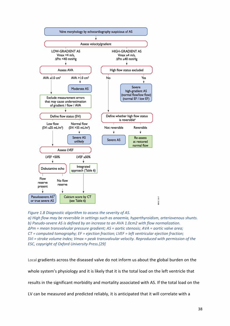
38

Figure 1.8 Diagnostic algorithm to assess the severity of AS. a) High flow may be reversible in settings such as anaemia, hyperthyroidism, arteriovenous shunts. b) Pseudo-severe AS is defined by an increase to an AVA 1.0cm2 with flow normalization. ΔPm = mean transvalvular pressure gradient; AS = aortic stenosis; AVA = aortic valve area; CT = computed tomography; EF = ejection fraction; LVEF = left ventricular ejection fraction; SVi = stroke volume index; Vmax = peak transvalvular velocity. Reproduced with permission of the ESC, copyright of Oxford University Press.[29]

Local gradients across the diseased valve do not inform us about the global burden on the

whole system’s physiology and it is likely that it is the total load on the left ventricle that

results in the significant morbidity and mortality associated with AS. If the total load on the

LV can be measured and predicted reliably, it is anticipated that it will correlate with a

39

patient’s symptoms and activity more directly than other measures such as the severity of

the stenosis.

1.6. Clinical management and interventions

1.6.1. Medical therapy

Medical therapy such as statins [63] have been suggested early in the disease to slow progression.

Other medications to treat any resulting heart failure or to treat hypertension and hence reduce the

load on the left ventricle are often required. However, despite the clear similarities with

atherosclerosis, large randomised trials have failed to show significant effect on disease progression

or clinical outcome[64]. Therefore, currently, there is no medical treatment apart from that used to

treat the heart failure that may ensue from AS. This has no place in modifying the valve disease

process or treating the underlying cause.

1.6.2. Evolution of treatment in AS

Advances in surgical techniques and technology over the last 40 years means that conventional

surgical aortic valve replacement is safer than it used to be[65]. In addition, there are new, less

invasive techniques, such as minimally invasive SAVR and TAVI. Advances in cardiopulmonary bypass

have seen the addition of novel defoaming agents, heparin coated circuitry, ultrafiltration,

miniaturised circuit design and integrated arterial filters with an oxygenator[66].

Figure 1.9 shows the important steps made in the history of aortic valve surgery after the initial

catastrophic valvotomies undertaken in the 1940s. The invention of the cardiopulmonary bypass

machine in 1953 dramatically changed the outcome of aortic valve surgery.

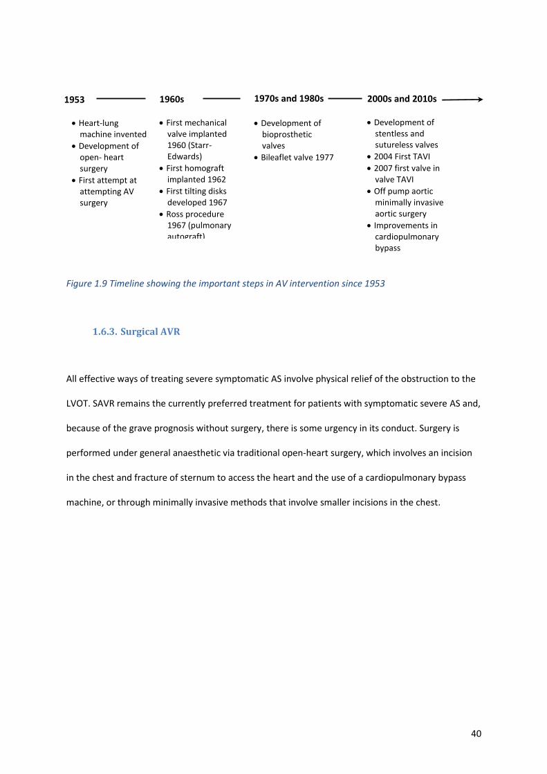
40

Figure 1.9 Timeline showing the important steps in AV intervention since 1953

1.6.3. Surgical AVR

All effective ways of treating severe symptomatic AS involve physical relief of the obstruction to the

LVOT. SAVR remains the currently preferred treatment for patients with symptomatic severe AS and,

because of the grave prognosis without surgery, there is some urgency in its conduct. Surgery is

performed under general anaesthetic via traditional open-heart surgery, which involves an incision

in the chest and fracture of sternum to access the heart and the use of a cardiopulmonary bypass

machine, or through minimally invasive methods that involve smaller incisions in the chest.

2000s and 2010s

• Development of stentless and sutureless valves

• 2004 First TAVI

• 2007 first valve in valve TAVI

• Off pump aortic minimally invasive aortic surgery

• Improvements in cardiopulmonary bypass

1.1. M

i

n

i

m

a

l

e

x

t

r

a

c

o

r

p

o

r

e

a

l

c

i

r

c

u

l

a

1970s and 1980s • Development of

bioprosthetic valves

• Bileaflet valve 1977

1960s

• First mechanical valve implanted 1960 (Starr-Edwards)

• First homograft implanted 1962

• First tilting disks developed 1967

• Ross procedure 1967 (pulmonary autograft)

1953

• Heart-lung machine invented

• Development of open- heart surgery

• First attempt at attempting AV surgery

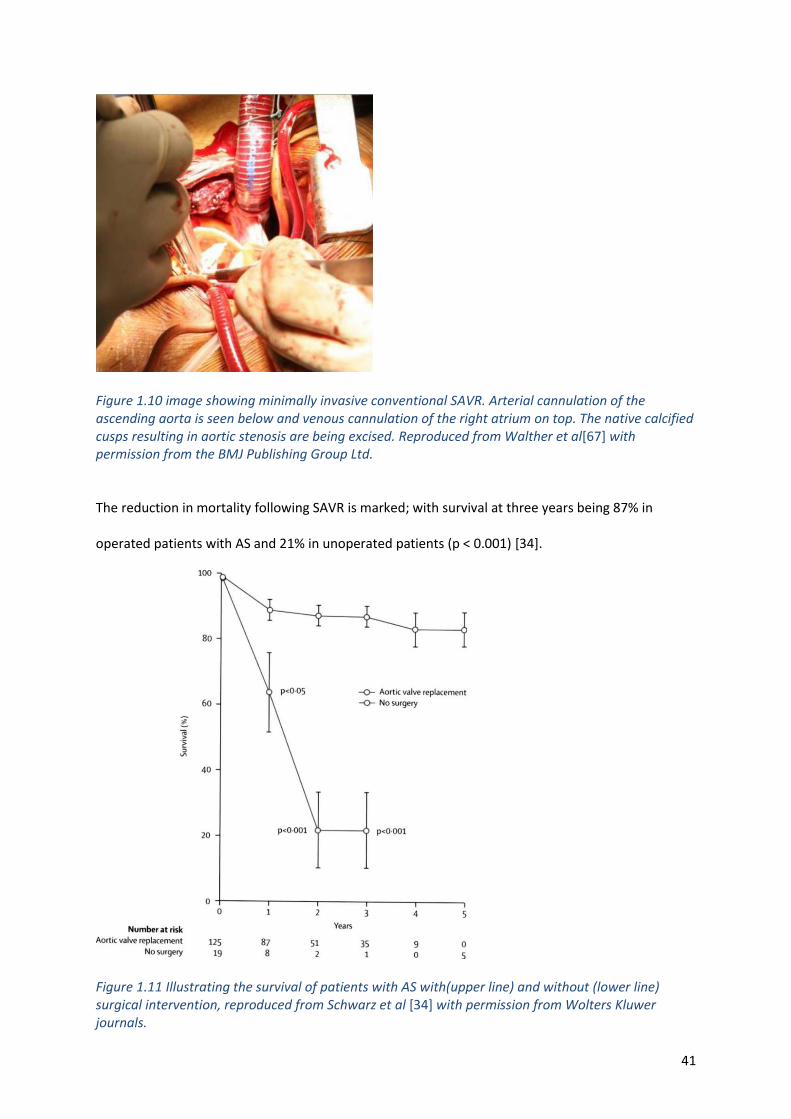
41

Figure 1.10 image showing minimally invasive conventional SAVR. Arterial cannulation of the ascending aorta is seen below and venous cannulation of the right atrium on top. The native calcified cusps resulting in aortic stenosis are being excised. Reproduced from Walther et al[67] with permission from the BMJ Publishing Group Ltd.

The reduction in mortality following SAVR is marked; with survival at three years being 87% in

operated patients with AS and 21% in unoperated patients (p < 0.001) [34].

Figure 1.11 Illustrating the survival of patients with AS with(upper line) and without (lower line) surgical intervention, reproduced from Schwarz et al [34] with permission from Wolters Kluwer journals.

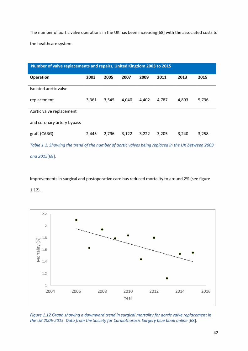
42

The number of aortic valve operations in the UK has been increasing[68] with the associated costs to

the healthcare system.

Number of valve replacements and repairs, United Kingdom 2003 to 2015

Operation 2003 2005 2007 2009 2011 2013 2015

Isolated aortic valve

replacement 3,361 3,545 4,040 4,402 4,787 4,893 5,796

Aortic valve replacement

and coronary artery bypass

graft (CABG) 2,445 2,796 3,122 3,222 3,205 3,240 3,258

Table 1.1. Showing the trend of the number of aortic valves being replaced in the UK between 2003

and 2015[68].

Improvements in surgical and postoperative care has reduced mortality to around 2% (see figure

1.12).

Figure 1.12 Graph showing a downward trend in surgical mortality for aortic valve replacement in the UK 2006-2015. Data from the Society for Cardiothoracic Surgery blue book online [68].

1

1.2

1.4

1.6

1.8

2

2.2

2004 2006 2008 2010 2012 2014 2016

Mo

rtal

ity

(%)

Year

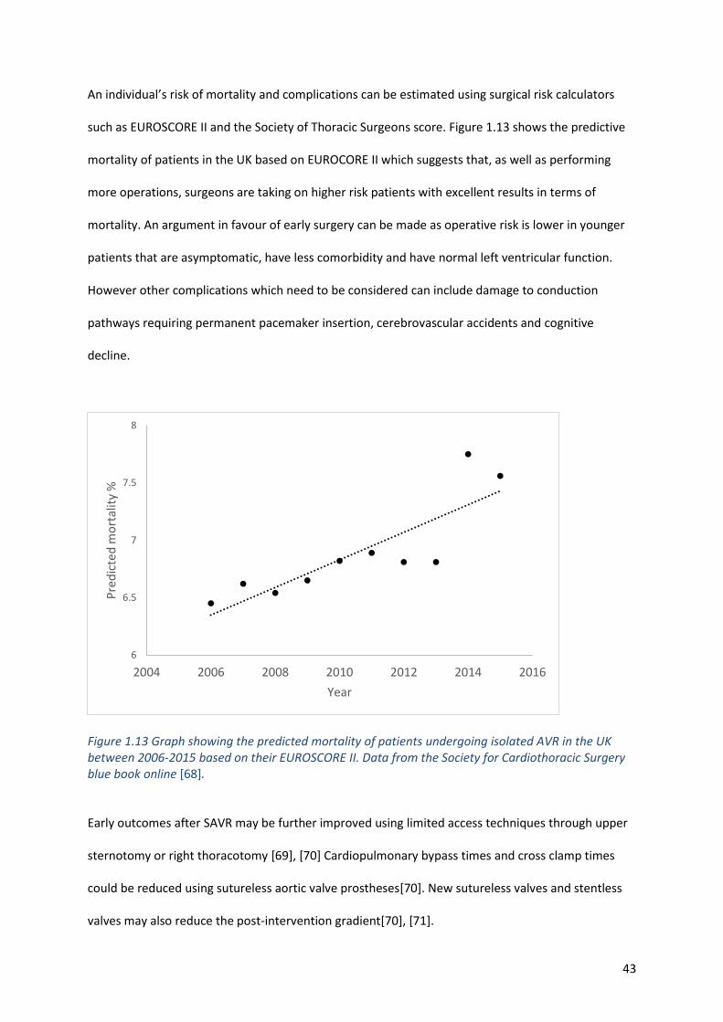
43

An individual’s risk of mortality and complications can be estimated using surgical risk calculators

such as EUROSCORE II and the Society of Thoracic Surgeons score. Figure 1.13 shows the predictive

mortality of patients in the UK based on EUROCORE II which suggests that, as well as performing

more operations, surgeons are taking on higher risk patients with excellent results in terms of

mortality. An argument in favour of early surgery can be made as operative risk is lower in younger

patients that are asymptomatic, have less comorbidity and have normal left ventricular function.

However other complications which need to be considered can include damage to conduction

pathways requiring permanent pacemaker insertion, cerebrovascular accidents and cognitive

decline.

Figure 1.13 Graph showing the predicted mortality of patients undergoing isolated AVR in the UK between 2006-2015 based on their EUROSCORE II. Data from the Society for Cardiothoracic Surgery blue book online [68].

Early outcomes after SAVR may be further improved using limited access techniques through upper

sternotomy or right thoracotomy [69], [70] Cardiopulmonary bypass times and cross clamp times

could be reduced using sutureless aortic valve prostheses[70]. New sutureless valves and stentless

valves may also reduce the post-intervention gradient[70], [71].

6

6.5

7

7.5

8

2004 2006 2008 2010 2012 2014 2016

Pre

dic

ted

mo

rtal

ity

%

Year

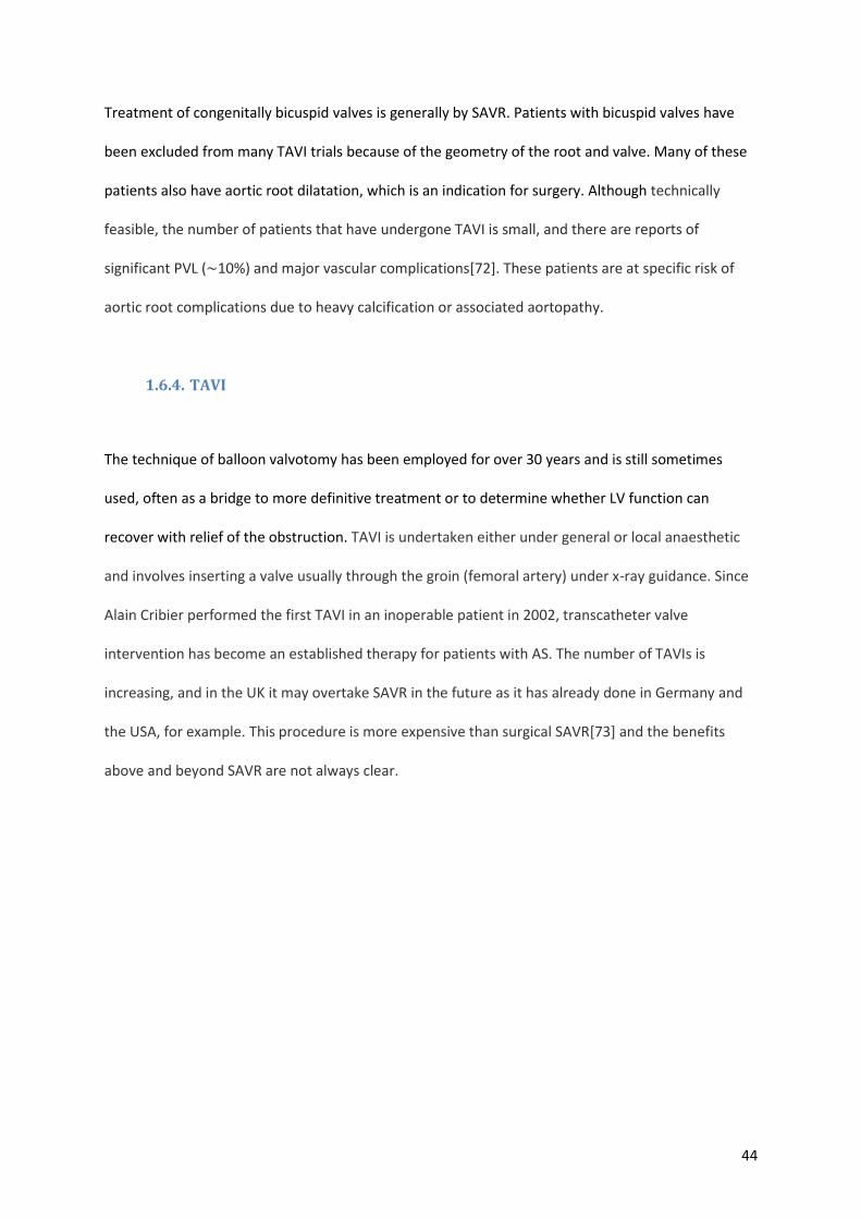
44

Treatment of congenitally bicuspid valves is generally by SAVR. Patients with bicuspid valves have

been excluded from many TAVI trials because of the geometry of the root and valve. Many of these

patients also have aortic root dilatation, which is an indication for surgery. Although technically

feasible, the number of patients that have undergone TAVI is small, and there are reports of

significant PVL (∼10%) and major vascular complications[72]. These patients are at specific risk of

aortic root complications due to heavy calcification or associated aortopathy.

1.6.4. TAVI

The technique of balloon valvotomy has been employed for over 30 years and is still sometimes

used, often as a bridge to more definitive treatment or to determine whether LV function can

recover with relief of the obstruction. TAVI is undertaken either under general or local anaesthetic

and involves inserting a valve usually through the groin (femoral artery) under x-ray guidance. Since

Alain Cribier performed the first TAVI in an inoperable patient in 2002, transcatheter valve

intervention has become an established therapy for patients with AS. The number of TAVIs is

increasing, and in the UK it may overtake SAVR in the future as it has already done in Germany and

the USA, for example. This procedure is more expensive than surgical SAVR[73] and the benefits

above and beyond SAVR are not always clear.

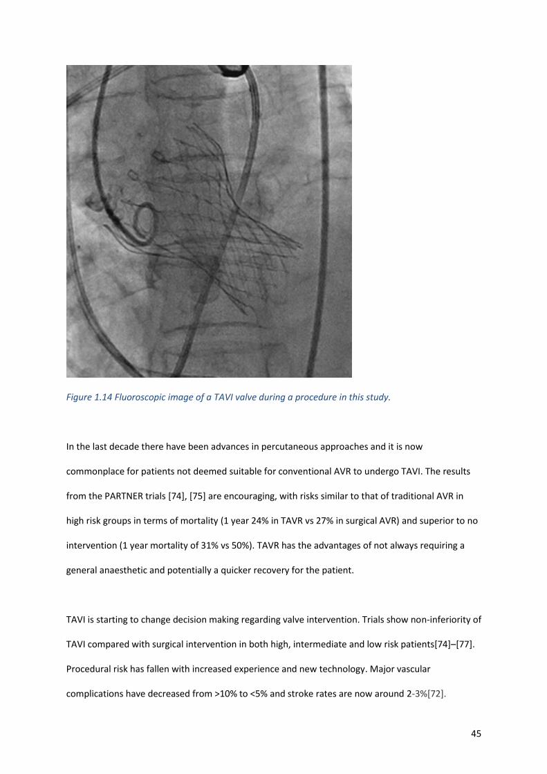
45

Figure 1.14 Fluoroscopic image of a TAVI valve during a procedure in this study.

In the last decade there have been advances in percutaneous approaches and it is now

commonplace for patients not deemed suitable for conventional AVR to undergo TAVI. The results

from the PARTNER trials [74], [75] are encouraging, with risks similar to that of traditional AVR in

high risk groups in terms of mortality (1 year 24% in TAVR vs 27% in surgical AVR) and superior to no

intervention (1 year mortality of 31% vs 50%). TAVR has the advantages of not always requiring a

general anaesthetic and potentially a quicker recovery for the patient.

TAVI is starting to change decision making regarding valve intervention. Trials show non-inferiority of

TAVI compared with surgical intervention in both high, intermediate and low risk patients[74]–[77].

Procedural risk has fallen with increased experience and new technology. Major vascular

complications have decreased from >10% to <5% and stroke rates are now around 2-3%[72].

46

However, the requirement for permanent cardiac pacing post procedure remains consistently higher

than surgical intervention at >10%[72] and while TAVI allows for rapid patient recovery and

mobilisation, the long-term durability of these bioprostheses has not been demonstrated[78]. This

will be key before their widespread use in younger or asymptomatic patient groups can be

recommended. The TAVR UNLOAD trial[79] will determine whether the increase in afterload caused

by moderate stenosis has an adverse outcome in patients with impaired LVSF. Looking at the total

load on the ventricle rather than individual components which can be achieved using computational

modelling may add insight to questions such as this.

A meta-analysis examined trial results and compared the outcomes of patients with symptomatic AS

randomised to TAVI or SAVR. This suggested that all-cause mortality was lower after TAVI with a 17%

relative risk reduction up to two years in patients undergoing a transfemoral procedure, although

absolute risk reductions were not reported. The risk of stroke was lower after TAVI up to two years,

and the relative risk reduction was 19%. Although there was lower overall risk of major bleeding,

new onset atrial fibrillation and AKI, there was an increased risk of permanent pacemaker

implantation and major vascular complications in patients treated with TAVI.[80] In a study by

Barbanti et al, at five years post-intervention, the opposite was suggested. At 5 years, the rate of

death from any cause was 35.8% in the surgical group and 48.3% in the TAVI group (hazard ratio,

1.38; 95% CI, 1.12–1.69; P=0.002). This is relatively high in both groups and may be due to the fact

that the patients are elderly and approaching their life average expectancy, when they present with

symptoms and have an intervention. Similarly, TAVR was associated with an increased risk of major

adverse cardiac and cerebrovascular events as compared with SAVR (42.5% versus 54.0%; hazard

ratio, 1.35; 95% CI, 1.11–1.63; P=0.003) [81].

As discussed above, treatment of bicuspid aortic valve stenosis is primarily with SAVR. However,

TAVI outcomes may improve with advances in technology and new devices. In a bicuspid TAVR

47

registry of 301 patients, moderate or severe PVL was less frequent with newer devices ( (0.0% vs.

8.5%, P = 0.002)[82].

1.7. Prognosis after treatment

It is accepted that valve replacement should only be considered in patients without comorbidities

which would render the procedure futile due to competing causes of death. Life expectancy

following AVR should be expected to be at least one year following intervention[29]. As described in

sections 1.6.3 and 1.6.4, if current guidelines are adhered to, the prognosis following valve

replacement is better than a conservative approach in the majority of patients, irrespective of which

technique is used. However, survival after AVR depends on a number of clinical variables, including

pattern of pre-operative LVH, severity of myocardial dysfunction, and cardiac fibrosis[83] and

therefore it is difficult to predict which patients will do really well with increased activity levels,

improved quality of life and longevity. Early LVH regression after AVR seems to be related to gender,

with more pronounced regression in women than in men[84]. If there is a lack of LV regression, this

indicates a worse prognosis[85]. Again, this may be due to other factors that load the ventricle which

were not studied.

Strong correlations have been found between AVR-induced increase in myocardial efficiency and

changes in exercise work [86], parameters that a computational model can also measure. The effects

of AS upon myocardial efficiency have been debated [87], [88]. However, work and power may be

predictors for disease progression and prognosis and therefore it would be useful if this can be

modelled accurately. In patients with LV dysfunction, the ejection fraction (a measure of cardiac

function) does not improve in approximately 25% of patients[89]–[91] who are more likely to remain

symptomatic and have adverse long-term outcomes, they are twice as likely to die over 5 years

follow-up[92].

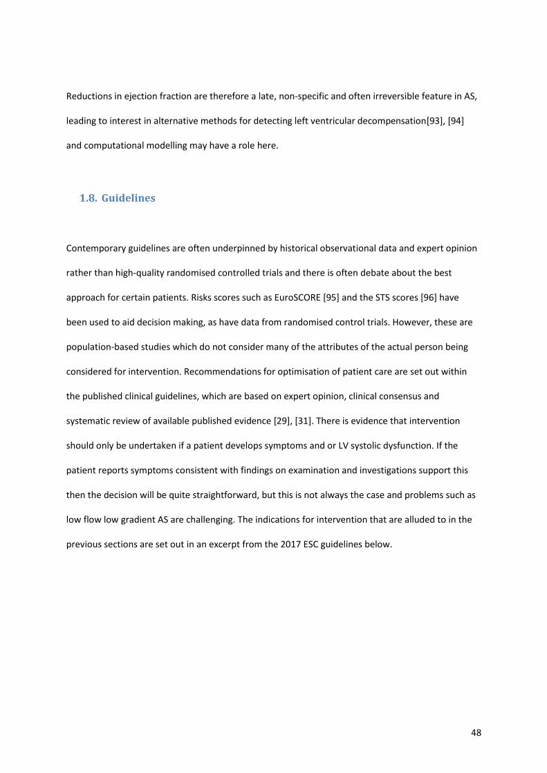
48

Reductions in ejection fraction are therefore a late, non-specific and often irreversible feature in AS,

leading to interest in alternative methods for detecting left ventricular decompensation[93], [94]

and computational modelling may have a role here.

1.8. Guidelines

Contemporary guidelines are often underpinned by historical observational data and expert opinion

rather than high-quality randomised controlled trials and there is often debate about the best

approach for certain patients. Risks scores such as EuroSCORE [95] and the STS scores [96] have

been used to aid decision making, as have data from randomised control trials. However, these are

population-based studies which do not consider many of the attributes of the actual person being

considered for intervention. Recommendations for optimisation of patient care are set out within

the published clinical guidelines, which are based on expert opinion, clinical consensus and

systematic review of available published evidence [29], [31]. There is evidence that intervention

should only be undertaken if a patient develops symptoms and or LV systolic dysfunction. If the

patient reports symptoms consistent with findings on examination and investigations support this

then the decision will be quite straightforward, but this is not always the case and problems such as

low flow low gradient AS are challenging. The indications for intervention that are alluded to in the

previous sections are set out in an excerpt from the 2017 ESC guidelines below.

49

Table 1.2 Management of severe AS with class of recommendation (a) and level of evidence (b). Reproduced with permission of the ESC, copyright of Oxford University Press [29].

50

1.8.1. Timing of intervention

The onset of symptoms is an indication to intervene and replace the aortic valve, because the

prognosis is poor if the condition is managed conservatively[35]. The evidence that forms the basis

for management today is over 50 years old and is based upon retrospective data from 12 patients

with bicuspid and rheumatic aortic valve disease. The mean age of death in the study was 63 years

and, not truly representative of the demographic we see today. The changing characteristics of our

much older population who have a different aetiology makes the relevance and interpretation of this

historical data difficult.

Sometimes patients are operated on before it is necessary, exposing them to surgical risk

prematurely, including the risk of valve thrombus and it is conceivable that repeat surgery may be

necessary due to valve degeneration. Occasionally, intervention is too late, and the left ventricle is

irreparably damaged. If the onset of symptoms occurs late in the disease process, it is associated

with an ominous prognosis, with increased frequency of sudden death[29].

These risks are also heavily influenced by replacement valve type, with both major bleeding

associated with anticoagulant use (1.8%–2.6% per year) and thromboembolism (0.7%–1.0% per

year) more frequent if a mechanical valve is implanted[97]. However structural degeneration is

exceedingly rare in mechanical valves. Bioprosthetic valves have a limited lifespan with valve

degeneration usually starting at 10 years following implantation and earlier in younger patients[98].

This is an extremely important issue if bioprosthetic valves are to be used in younger asymptomatic

patients as suggested in some of the recent TAVI trials of patients at low operative risk. The use of a

transcatheter valve inside a surgical bioprosthetic valve (valve-in-valve TAVI) may reduce the risk of

future procedures should valve degeneration occur; however, this would again adversely impact

fluid dynamics with reduced EOA, and long-term outcomes are needed in this patient cohort. There

51

is also an increased risk of endocarditis (1%–3% during year one then <0.5% per year[99]), which is

associated with high morbidity and mortality.

Even when the decision is made to replace the aortic valve, the urgency of such replacement needs

to be assessed. The risk of death from AS is approximately 1% per year without symptoms but when

diagnosed and intervention planned 4% would die within the first three months from diagnosis[100].

Up to 14% of patients would die on a six month surgical waiting list[101]. There is therefore some

urgency even when a decision has been made to intervene. However, it is often difficult to decide

who requires immediate surgery and who is safe to wait on the list. Given that delays from referral

are common in most healthcare systems, this should also inform decisions.

Rapid progression (>0.3 m/s/year) and significant valve calcification have a rate of symptom

development or mortality of 79% at 2 years[102]. However, as discussed, due to imaging limitations

and logistical issues identifying these patients in clinical practice is difficult. The referral for surgical

intervention in these patients is recommended in the guidelines[29]. This is based on limited

observational data. Delaying intervention until there is evidence of advanced left ventricular

dysfunction results in greater perioperative risks. Observational studies have quoted increased

perioperative mortality (9%–19%)[89], [92], [103] . Risk stratification can be performed by looking

for contractile reserve using stress echocardiography. If present, there is lower perioperative

mortality (5% vs 22%–32%)[91], [104] but longer outcome data are needed. The mortality and

morbidity burden related to delaying valve intervention appears to occur in the months and years

following AVR. As discussed, patients with an impaired ejection fraction prior to AVR have a poor

long-term prognosis. However, given the dismal prognosis of untreated AS, improved long-term

survival can be achieved in patients with poor LV systolic function even without contractile reserve.

Using fibrosis to predict the probability of LV decompensation, a study found that more than half

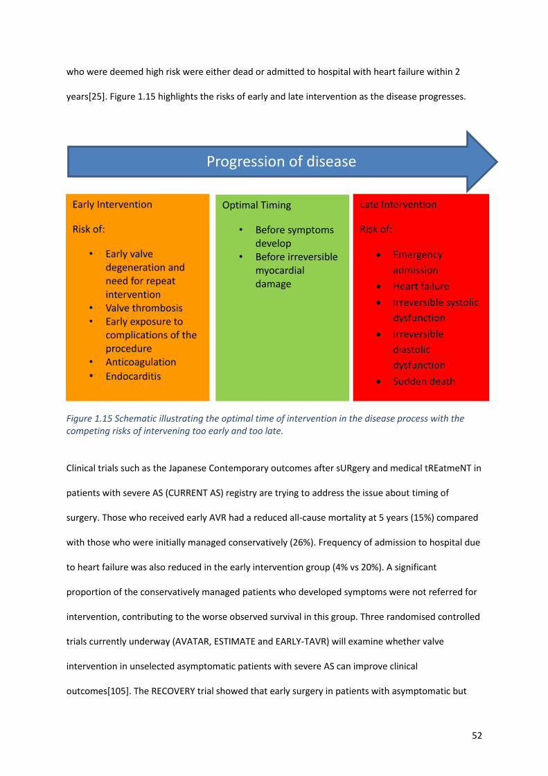
52

who were deemed high risk were either dead or admitted to hospital with heart failure within 2

years[25]. Figure 1.15 highlights the risks of early and late intervention as the disease progresses.

Figure 1.15 Schematic illustrating the optimal time of intervention in the disease process with the competing risks of intervening too early and too late.

Clinical trials such as the Japanese Contemporary outcomes after sURgery and medical tREatmeNT in

patients with severe AS (CURRENT AS) registry are trying to address the issue about timing of

surgery. Those who received early AVR had a reduced all-cause mortality at 5 years (15%) compared

with those who were initially managed conservatively (26%). Frequency of admission to hospital due

to heart failure was also reduced in the early intervention group (4% vs 20%). A significant

proportion of the conservatively managed patients who developed symptoms were not referred for

intervention, contributing to the worse observed survival in this group. Three randomised controlled

trials currently underway (AVATAR, ESTIMATE and EARLY-TAVR) will examine whether valve

intervention in unselected asymptomatic patients with severe AS can improve clinical

outcomes[105]. The RECOVERY trial showed that early surgery in patients with asymptomatic but

Early Intervention

Risk of:

• Early valve degeneration and need for repeat intervention

• Valve thrombosis • Early exposure to

complications of the procedure

• Anticoagulation

• Endocarditis

Progression of disease

Optimal Timing

• Before symptoms develop

• Before irreversible myocardial damage

Late Intervention

Risk of:

• Emergency

admission

• Heart failure

• Irreversible systolic

dysfunction

• Irreversible

diastolic

dysfunction

• Sudden death

53

very severe AS (transvalvular velocity >4.5m/s) results in improved survival out to 8 years compared

with watchful waiting, suggesting that we should perhaps intervene on patients earlier than the

current guideline recommendation of 5.5m/s[106].

A study examined the total haemodynamic load, quantified by calculating the valvulo-arterial

impedance (ZVa = (systolic blood pressure + mean AV gradient)/indexed LV stroke volume), seen by

the left ventricle and its ability to predict outcome[107]. This measure has consistently been shown

to be an independent marker of adverse outcome in asymptomatic patients[107] and load on the

ventricle warrants further study for its use in determining the timing of intervention, this can be

achieved with computational modelling. Another approach is to quantify valvular calcium burden

using CT calcium scoring. Validated, gender-specific thresholds for severe AS have been proposed

which provide powerful prediction of clinical events of incremental value to echocardiographic

assessments[29], [45] .

Most of the guidelines are based on limited observational data and supported by expert consensus

opinion. There is therefore a need for randomised controlled trials assessing the optimal timing of

surgery and novel objective methods to guide this major clinical decision that could be produced by

computational modelling are needed.

1.9. Assessing symptoms and Outcomes

Over the past decade we have seen a rise in the involvement of patients in decisions about their

health and care. Measuring ‘what matters to patients’ is crucial in improving patient care. Data can

also be used to assess health technology, assist in drug development, determine health service

commission and improve communication between patients and healthcare professionals. Due to the

variations in presentation and reporting of symptoms as discussed above, exercise testing is already

54

performed in certain situations to help guide management decisions [30], [105]. The clinical utility of

activity monitoring as part of the process of interventional planning and outcome assessment will be

investigated in this research study. This section reviews potential measures of functional status and

the technology required.

1.9.1. Assessment of function

Characterisation of functional status in older adults with AS is essential to help guide management

decisions. Frailty is linked with an increase in morbidity and mortality after cardiac surgery [108],

[109]. Now, with the advent of TAVI, frailer patients, that would not have previously been offered an

operation can still be treated effectively [74], [75], so it is becoming more important. Frailty

measures now feature in the logistic EuroSCORE [95] used to assess the risk of an individual

undergoing intervention and many clinicians use such scores to inform decisions. The use of gait

speed is recognised as a marker of frailty and predictor of outcomes in adults undergoing

cardiovascular intervention.

1.9.2. Exercise testing in clinical practice

Management of asymptomatic patients with severe AS is controversial [30]. Exercise testing using

the Bruce protocol is the best-studied risk stratification tool to identify those in whom an

intervention can be offered before the risk of sudden death and operative morbidity increase, but

positive predictive value is poor [110]. Negative predictive value for predicting subsequent cardiac

events is reasonable at 79% [111]. However, data are limited to small observational studies with risk

of bias and different perceptions of what constitutes an abnormal test. Guidelines state that when

exercise testing provokes symptoms, patients should be considered symptomatic and there is a

55

recommendation for valve replacement [112], but symptoms should be clearly shown to be related

to AS. This may be difficult, particularly in the elderly and in patients with low physical activity levels.

There are arguments against stress testing in the clinical environment. Stress testing is

contraindicated or unreliable in some patient groups and, indeed, patients with AS are often elderly;

and up to 20%[113] will not be able to perform an exercise test at all due to poor mobility. Also pre-

existing ECG abnormalities are present in up to 50% of patients, confounding test

interpretation[113]. Exercise testing may also detect abnormalities caused by coexistent coronary

disease, which is an important determinant of both management and prognosis[114].

Brala et al have shown that exercise capacity determined by cardio pulmonary exercise testing can

identify high risk patients with AS who may benefit from valve replacement, independently of echo

parameters, reported symptoms, age, and sex[115]. Due to the resources required, cardiopulmonary

exercise testing is rarely used in the day to day assessment of AS.

Measurements made outside the clinical environment might be more representative of the patient’s

capacity and function. Pervasive or wearable monitors, used in the home environment, may provide

information that could help guide decision making and prognosis. Following open heart surgery, the

recovery time can vary from weeks to months [86], but clinical investigation of exercise capacity is

usually conducted at a single point in time which is inequitable. The assessment of recovery of

patients from SAVR made at four weekly intervals, over six months, revealed marked improvement

of most patients within the first six weeks; some patients continued improvement to six months,

although ADLs were not assessed. Since it is impractical to perform tests at multiple time points

routinely, wearable monitors might have a role in this situation.

56

1.9.3. Six-minute walk test

The six-minute walk test (6MWT) can reflect overall hemodynamic function if the patient’s effort is

good and there is no limitation imposed by mobility issues or other conditions such as respiratory

disease. Hence the 6MWT could contribute to risk assessment in patients. A study showed, in

asymptomatic patients with aortic valve stenosis, that the 6MWT is an independent predictor of all-

cause and cardiovascular mortality. It was also shown to be of incremental value to

echocardiographic evaluation, suggesting it might be useful to guide clinical follow-up intervals and

treatment strategy[116].

De Arenaza et al investigated the added prognostic value of the six-minute walk test to the

Euroscore in a study comparing stented and stentless aortic valves[117]. In a Cox regression analysis,

6MWT distance was the only variable retained as an independent predictor of the composite

outcome of death, MI or stroke at 12 months, providing potentially important functional and

prognostic information to clinical and risk assessment.

A study by Altisent et al [118] showed that just less than a quarter of patients undergoing TAVI had

no improvement of their exercise capacity at six months, as measured by a 6MWT. Poor functional

recovery was linked to increasing age, female sex, presence of COPD, periprocedural bleeding and

new onset anaemia at 6 months. The study also found that failure to increase a 6MWT distance by

20% was independently associated with all-cause mortality, CV death or re-hospitalisation for

cardiovascular causes. This suggests that exercise capacity assessment pre- and post-TAVR may help

to improve patient risk stratification.

6MWTs have been used to monitor outcome and assess time to recovery following surgical valve

replacement. One week post operatively there was a significant decline in function; this was back to

57

baseline at four to six weeks with significantly improved walk test distances achieved at three

months post operatively. Significant improvements were seen in six-minute walk test distances and

physical quality of life measures[119]. One systematic review showed considerable variation in the

clinical characteristics of patients undergoing TAVI and in the amount of improvement in functional

outcomes and quality of life after TAVI across 62 studies with many studies using a 6MWT to assess

this [118].

1.10. Wearable or pervasive activity monitoring

1.10.1. Clinical research using activity monitoring

Several studies have addressed the potential utility of activity monitoring in diagnosis, interventional

planning and outcome assessment. Mukhopadhyay postulated that emerging technologies could be

used to predict the future health condition of individuals, affecting both the health decisions and the

doctor patient relationship [120]. Wearable sensors have supported home care for patient groups

who would usually spend longer in hospital, but how best to monitor human activity is unclear [120].

Activity data could be used as early predictors of disease severity and progression, in disease

understanding, in care delivery or in monitoring post-surgery recovery in cardiac patients,

pulmonary rehabilitation and others [121], [122]. Integration with other data to inform management

is seldom done, often because the focus is on establishing the feasibility of monitoring activity and

establishing an association between measured activity with short-term benefits. There is a need for

validation and reliability assessment against existing clinical standards [121]. Accelerometers are

often used for monitoring in outpatient settings but there is no consistency in devices used or in

reported outcome measures[123]. Knowing what happens between clinic visits means interventions

can be tuned to the needs of individuals, systems can be tailored to individual patients and

monitored remotely [124]. Pervasive activity monitoring can be used in randomised control trials.

58

Accurate and objective measures of outcome from wearable devices could reduce the number of

subjects and the duration of treatment needed to observe an effect in a trial of a new therapy,

although there is no experimental evidence to support this at present. It is functional status and

quality of life that are important to the patient as well as life expectancy. Wearable devices may give

more insight to a patient’s quality of life than current clinical methods to assess activity.

1.10.2. Monitoring outcome

Activity measures have been used in patients with AS. Green et al [125] examined the relationship

between gait speed and activity of daily living. They showed that gait speed was independently

associated with dependency for activities of daily living and this was thought to be a good objective

measure for risk stratification. However, the patients were not studied after the intervention to see

whether gait speed improved and if there were any relationship to outcome measures. Gait speed

was assessed in a clinical environment under test conditions and it is likely that gait speed will be

better in the patient’s own environment where they are more confident. It is already known that

frailty is linked with an increase in morbidity and mortality after cardiac surgery [108], [109]. Studies

have reported the use of activity sensors at home to monitor outcomes in specific applications.

Toogood [126] studied 33 patients following hip arthroplasty using a Fitbit™ ankle accelerometer.

There was good compliance with the device and increases in step counts were recorded up to 30

days post operatively. Manson [127] used accelerometers to assess 12 patients with Parkinson’s

disease, correlating results with the severity of dyskinesia. Uswatte[128] tracked changes in motor

function in 20 patients after stroke and found that this can be used as a feedback tool for guiding the

rehabilitation process. No published studies have used wearable technology to assess the functional

state of the patient before and after aortic valve intervention; this application would be novel. There

are disadvantages and challenges of implementing patient activity monitoring. There are hardware

and software constraints, monitors need to be light-weight and low energy consumers, and there

59

are safety requirements, patient burden, privacy issues and cost. However, activity monitoring and

personal data collection offers the potential for patient engagement, personalising health care and

offering clinicians real world assessments of their patients’ daily activity patterns. Monitoring the

patient’s activity would give an objective measurement before and after intervention. More

continuous monitoring, allowing identification of trends of activity, may be able to help detect

deterioration or improvement in the patient’s condition. In the context of AS, monitoring the heart

rate may also give an insight into the reduction of cardiac work, because a lower heart rate may be

needed to produce the same cardiac output when performing activity. In this project a correlation

between the severity of the stenosis, assessed by different techniques and the activity of patients

will be sought.

A model can be used to predict measurements in an exercise state, so tuning the model with patient

activity data may help predict their expected capacity for work following intervention. However,

since even elite athletes spend most of their time in a resting state, it is likely that assessing the rest

state accurately is equally, if not more, important.

1.10.3. Patient reported outcome measures

Clinicians’ understanding of the effect of disease and treatment on patients’ daily lives is recognised

to be poor. Standardised measures have been developed to assess symptom status, social function

and mental health but the use of patient-reported outcome measures (PROMS) routinely in clinical

practice is hindered, mainly by social, cultural, legal, and logistic barriers[111]. Therefore, such tools

have often failed to improve care from the patient’s perspective. However, the use of PROMs in

research and clinical trials is well established and can provide evidence on the burden of disease and

the efficacy and cost effectiveness of treatments [112], [113]. It is likely that integrated approaches

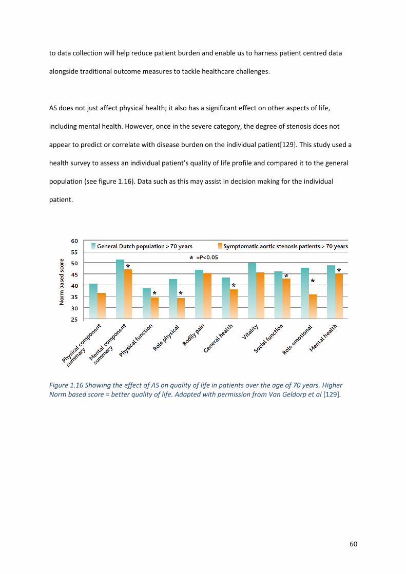
60

to data collection will help reduce patient burden and enable us to harness patient centred data

alongside traditional outcome measures to tackle healthcare challenges.

AS does not just affect physical health; it also has a significant effect on other aspects of life,

including mental health. However, once in the severe category, the degree of stenosis does not

appear to predict or correlate with disease burden on the individual patient[129]. This study used a

health survey to assess an individual patient’s quality of life profile and compared it to the general

population (see figure 1.16). Data such as this may assist in decision making for the individual

patient.

Figure 1.16 Showing the effect of AS on quality of life in patients over the age of 70 years. Higher Norm based score = better quality of life. Adapted with permission from Van Geldorp et al [129].

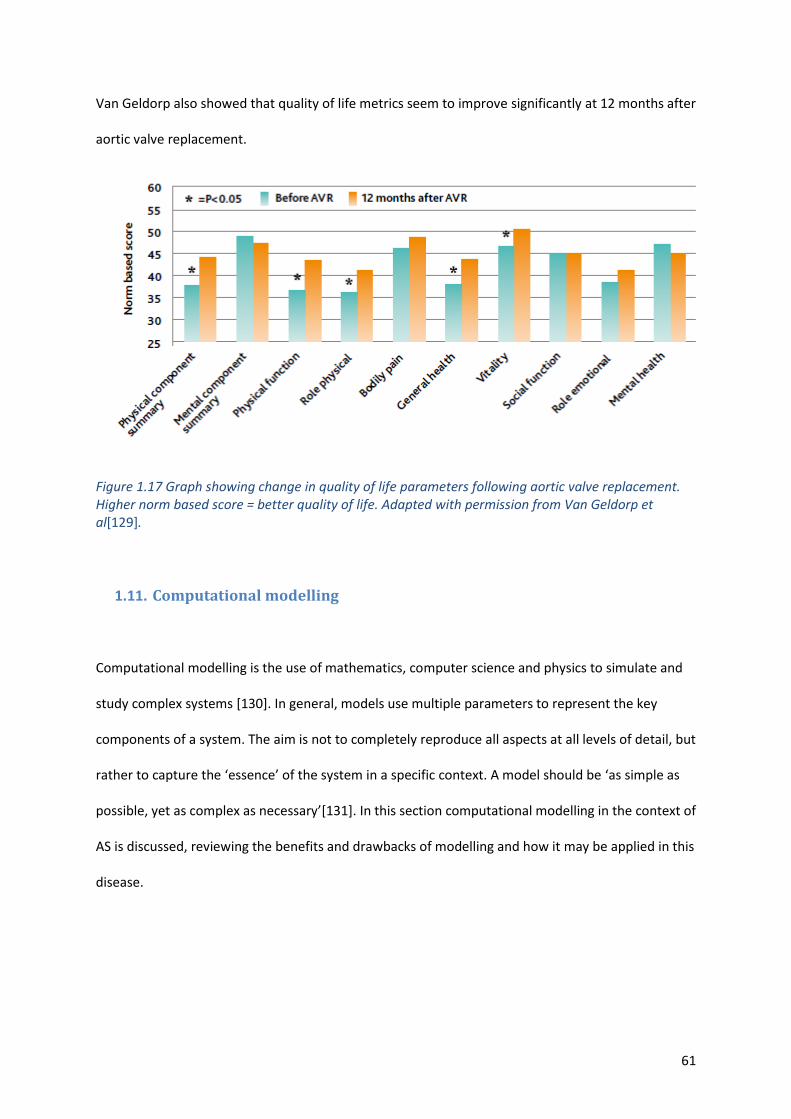
61

Van Geldorp also showed that quality of life metrics seem to improve significantly at 12 months after

aortic valve replacement.

Figure 1.17 Graph showing change in quality of life parameters following aortic valve replacement. Higher norm based score = better quality of life. Adapted with permission from Van Geldorp et al[129].

1.11. Computational modelling

Computational modelling is the use of mathematics, computer science and physics to simulate and

study complex systems [130]. In general, models use multiple parameters to represent the key

components of a system. The aim is not to completely reproduce all aspects at all levels of detail, but

rather to capture the ‘essence’ of the system in a specific context. A model should be ‘as simple as

possible, yet as complex as necessary’[131]. In this section computational modelling in the context of

AS is discussed, reviewing the benefits and drawbacks of modelling and how it may be applied in this

disease.

62

1.11.1. What model and why?

The haemodynamics of the circulation are complex, being controlled by a range of factors affected

by mechanics, hormones and the neurological system. Creating in vivo experiments to display the

complex interactions would be difficult, whereas computational modelling can account for these

complex interactions and their effect [126]. By using an appropriate model, researchers can carry

out thousands of simulated experiments in a safe (virtual) environment.

If the model adequately represents the system being studied then it can be used to comprehensively

explore the effects of changing any combination of the input variables in a way that is impossible in

any clinical study for many practical reasons, including the numbers needed, time and cost. All

interactions between elements that are represented in the model can be captured and analysed in

detail [132]. A general model, representing an average individual, can be used to gain insight into the

basic physiological processes. A personalised model, in which some of the parameters are tuned to

reproduce measurements made in the individual, might be both diagnostic (the personalised

parameters might themselves have diagnostic utility) and prognostic (the parameters can be

extrapolated to describe other physiological states and/or to describe prospective interventions).

1.11.2. Current use of modelling in clinical practice

The use of computational modelling to support engineering design is well established in almost

every industrial sector, including biomedical applications such as in designing heart valve prostheses

[133]. However, although there are hundreds of research studies that have contributed to our

understanding of haemodynamics and of disease processes [132], [134]–[136], computational

modelling generally has yet to make a major impact upon clinical practice. One of the reasons is that

it is difficult to personalise the model to represent an individual patient. Anatomical personalisation,

63

based upon exquisite medical imaging, is increasingly available, but the challenge is the

personalisation of patient physiology. Perhaps the most advanced of clinical applications is the CT-

FFR computation for coronary artery disease, developed and marketed by HeartFlow™, and recently

recommended for clinical use by NICE in the UK [137], which allies an anatomical model and CFD to

compute coronary blood flow. The recognition that it is the interplay between the local stenosis and

the system characteristics that determines the contribution to the overall physiological burden of

the disease is the fundamental factor underpinning the success of fractional flow reserve (FFR), in

assessment of coronary disease[138]. In the context of coronary artery disease, the question is: by

how much the flow to the myocardium is compromised by the disease. In the context of AS, the

question might be the degree to which the heart must work harder to achieve the flows demanded

by the system.

1.11.3. Model Choices

In developing a model strategy, the sophistication of the model with practical availability of clinical

physiological data need to be balanced. Cardiac models have advanced significantly [139] and they

are now among the best-developed theoretical representations of any organ [140]. However, to

achieve its aims, the model must represent not just the anatomy of the heart and the diseased valve

but also the systems physiology and the model has to be tuned to the individual, using the limited

clinical data available. Anatomical description of the aortic valve can be available from medical

imaging and obviously the valve characteristics will have the main effect on local haemodynamics.

Three-dimensional information would be needed to build a truly patient specific model with the

effects of valve disease on flow characterised. However, a local valve model needs ‘boundary

conditions’ to describe the interaction with the rest of the system. The geometry of the aortic valve

is important, but not in isolation from the proximal and distal haemodynamics of the circulation.

Numerous vascular conditions, including coarctation of the aorta[141], [142], have been modelled in

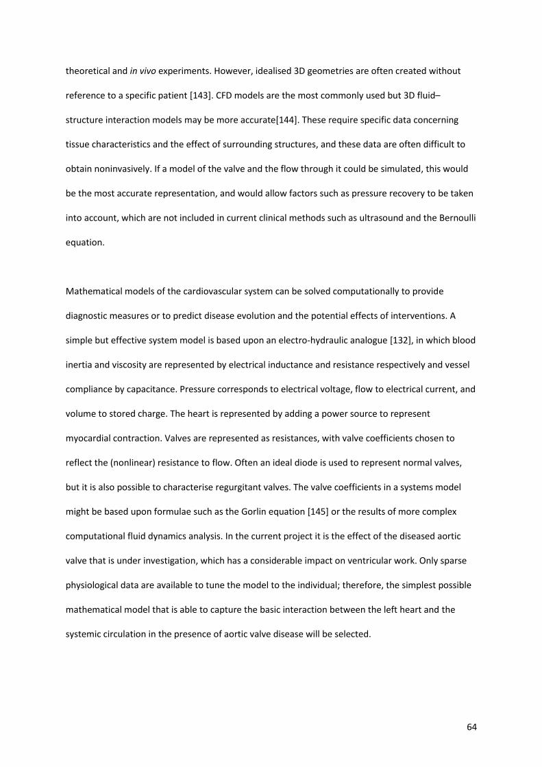
64

theoretical and in vivo experiments. However, idealised 3D geometries are often created without

reference to a specific patient [143]. CFD models are the most commonly used but 3D fluid–

structure interaction models may be more accurate[144]. These require specific data concerning

tissue characteristics and the effect of surrounding structures, and these data are often difficult to

obtain noninvasively. If a model of the valve and the flow through it could be simulated, this would

be the most accurate representation, and would allow factors such as pressure recovery to be taken

into account, which are not included in current clinical methods such as ultrasound and the Bernoulli

equation.

Mathematical models of the cardiovascular system can be solved computationally to provide

diagnostic measures or to predict disease evolution and the potential effects of interventions. A

simple but effective system model is based upon an electro-hydraulic analogue [132], in which blood

inertia and viscosity are represented by electrical inductance and resistance respectively and vessel

compliance by capacitance. Pressure corresponds to electrical voltage, flow to electrical current, and

volume to stored charge. The heart is represented by adding a power source to represent

myocardial contraction. Valves are represented as resistances, with valve coefficients chosen to

reflect the (nonlinear) resistance to flow. Often an ideal diode is used to represent normal valves,

but it is also possible to characterise regurgitant valves. The valve coefficients in a systems model

might be based upon formulae such as the Gorlin equation [145] or the results of more complex

computational fluid dynamics analysis. In the current project it is the effect of the diseased aortic

valve that is under investigation, which has a considerable impact on ventricular work. Only sparse

physiological data are available to tune the model to the individual; therefore, the simplest possible

mathematical model that is able to capture the basic interaction between the left heart and the

systemic circulation in the presence of aortic valve disease will be selected.

65

1.11.4. Systems model (Zero-dimensional, ‘lumped’ parameter)

In a zero-dimensional (0D) model the elements of the system are described by simple electrical

analogue models. They describe the global behaviour of the modelled system. The fundamental

outputs of the model are pressure, flow and volume at discrete locations within the cardiovascular

system, and each of these outputs varies over the cardiac cycle. As the name suggests, there is no

representation of a spatial distribution of these quantities within any specific component; so, for

example, the pressure throughout the left ventricle is represented as uniform at any instant in time.

The equations describing the electrical analogue systems are a series of ordinary differential

equations that represent the fundamental outputs and their temporal gradients. The first such

model developed for cardiovascular application was the Windkessel model described in 1899 [146].

There are a number of validated models available [147], and it is important to select the right model

for the question being addressed. If models have too many parameters, it is not possible to find a

unique fit to the available clinical data.

Extra resistance elements can be connected in series with the Windkessel model, which is often

referred to as the Westkessel model [148]. This improves the performance of the model

representing the systemic circulation. The overall resistance equals the total systemic vascular

resistance. The capacitance represents elasticity and the storage properties of large arteries. Studies

show this model provides a good representation of after-load but it can overestimate and

underestimate some parameters[132]. Another drawback with this model is that the venous

pressure is assumed to be zero. This will often be incorrect in patients with AS, as many will have

LVH, diastolic dysfunction and pulmonary hypertension. Also, it cannot show pressure and flow

changes in specific sections of the circulation as results are ‘lumped’ together. However, for the

purposes of the current study, this type of model would provide reasonable accuracy and is simple

66

enough to populate with clinical data that is obtained in routine practice. It has been widely used in

cardiovascular simulations as the after-load to evaluate cardiac function under various pathological

and physiological conditions [132]. The left ventricle and left atrium are often described by variable

elastance models, which represent the relationship between chamber pressure and volume as a

function of time and thus provide a simple description of the active contraction of the heart. There

are alternatives, for example the single fibre model [149]. 0D models are frequently used to improve

boundary conditions for 3-D models of pathology[136], [137] this could be achieved in this study.

One of the first steps following model selection should be to perform a sensitivity analysis[150], to

separate those parameters in the candidate model that have a significant impact upon model

outcomes from those that have a minimal effect. The parameters that have a significant impact

should be accurately represented and personalised. Conversely, parameters that do not have a great

effect could be estimated using population based data. This is important, as to obtain certain data

may subject patients to risk, as discussed in the case of exercise testing and invasive catheter

pressure measurements, so knowing how important that data is allows a risk benefit analysis to take

place.

1.11.5. 3D valve model

A local 3D model of the valve can be derived from the segmented medical image (see section 2.4.2),

a process that is compatible with clinical routine [144]. If this is possible in our cohort, a non-invasive

estimation of the pressure gradient using only the geometry of the valve, LVOT and proximal aorta

may be obtained through computational fluid dynamics (CFD) calculations. CFD is a branch of fluid

mechanics that involves solving mathematical equations that describe fluid motions in three

dimensions [151]. Most analyses are based upon the governing equations of fluid motion; the

Navier-Stokes and continuity equations. These should produce more physiological and accurate

67

information about the haemodynamics through the stenosis than echocardiography because there is

no operator-dependency upon Doppler alignment, avoiding the need for the many assumptions

made during echocardiographic assessment, and pressure recovery could be taken into account. The

relationship between flow and pressure can then be derived. CFD ‘solvers’, are used to solve the

Navier-Stokes and continuity equations. For complex geometries analytical solutions often do not

exist and an ‘approximate’ numerical solution is found by the solver. Because of their non-linearity

(due to convective fluid acceleration), solutions often require the use of high performance

computers and can take considerable time to run [136], [152]. However, CFD is not perfect. In

response to an FDA initiative, 28 groups from the international CFD community performed

independent simulations of a simple benchmark problem. This highlighted a significant amount of

measurement error and variability in flow measurements to standardised methods [153]. Despite

this, many believe that these equations and methods that are used in chemical, aerospace and

aeronautic engineering and the automotive industry have emerged as valuable tools in biomedical

engineering [136], [154]. Modelling blood flow in deforming vascular structures represents one of

the major challenges in this field [155]. It can take days, even with major computational resource, to

run complex 3D models [156]. For clinical utility, simplifications will be required and the application

of an advanced form of reduced order modelling (ROM) to reduce the computational time to enable

results to be produced in real time [157]. An alternative method of assessing the haemodynamics in

more detail than echocardiography may be CMR 4D flow assessment (see section 1.4.2.2).

1.11.6. Model Personalisation

Several experiments have been carried out using simulated data or population average data and

these have shown that models of the cardiovascular system, including when the system is diseased,

such as with AS, are valid and can be effective tools in the assessment of patients. Few studies using

animal data [158], and even fewer using human data, have been conducted. The process of

68

personalisation of the parameters for these models, to make them clinically useful, is new and

challenging [159]. Even lumped-parameter models often require many inputs and detail that are not

available from sparse clinical data sets [156]. Hann described a process in which parameters are

adjusted and their effect on the output measured. A focus can then be on collecting data that is

important and readily available. Reducing the number of datasets required to run a model and

focusing on data that are available in routine clinical practice means that less data needs to be

simulated or obtained from population values. Sophisticated optimisation methods, similar to those

described, and beyond the scope of this thesis, are used to tune the parameter values of the models

to match measured flow distribution, pressures and measures of cardiac function. These inputs may

derive from patient-specific data, population data, data from other models or assumptions [160] and

provide information for quantities such as cardiac output and microcirculatory resistance [151].

As an example of successful personalisation of a simple systems model, quantified personalised

assessment of cardiovascular function has been made from the combination of limited clinical data

with a cardiovascular model [161]. This small experiment, using only data that can be routinely

acquired in clinical care, successfully identified patients with left ventricular systolic dysfunction in a

group of seven patients undergoing coronary artery bypass grafting. The model limitations included

the availability of clinical data, different pre- and post-operative sampling times and natural variation

in the patient’s physiological state. More in-depth knowledge of a patient’s haemodynamic state

given by the combination of clinical and modelling data may add value.

1.11.7. Model validation

Most studies utilising models combining clinical data have been validated in porcine experiments

and clinical applications are limited without patient data based validation[161]. Validating

computational models in clinical practice is challenging but is vital to clinical acceptance [141], [143],

69

[162], [163]. A logical approach might be to replicate directly measured data, then to develop

representative model parameters by training on a subset of data. This could then be used to

accurately predict measurements from data not included in the fitting process [163]. A number of

theoretical experiments, particularly in AS, address only the first step [61]. Some experiments claim

that a model has been validated by clinical data, but models compared against limited data provide a

plausible representation of the system under study only. Most models ignore age as a predictor of

disease and therefore cannot be valid in all cases [164]. Models will eventually need to account for

biological variations associated with inter-subject differences in experimental data.

A model based upon the combination of the time-varying elastance representation of the left

ventricle with a four-element Windkessel model has been used and validated in human and animal

studies [165]. However, this model assumes that the aortic valve is normal, and is not applied in

patients with AS. Some models include the effect of AS [166], [167], in which AS was represented by

the increase in valve resistance (as the ratio of the instantaneous pressure to the trans-valvular flow

rate).

There has been an attempt at validating a coupled lumped-parameter model in the presence of AS

using clinical data[168]. This was a small cohort study of only six patients. The ventricular-valvular-

vascular (V3) model consists of the time-varying elastance model of the LV combined with the

instantaneous trans-valvular pressure-flow relationship for the aortic valve and a Windkessel

representation of the vascular system. In this study the mathematical description of AS was

incorporated into the V3 model without patient specific imaging data. Despite this, there was very

good agreement between the estimated and the measured left ventricular and aortic pressure

waveforms. The total relative error reported between estimated and measured pressures was 7.5%

(SD 2.3). The authors claim that their model explicitly and accurately describes the behaviour of LV if

nine cardiovascular parameters are known. There are several limitations of this study, not least the

70

sample size. The aortic valve area was calculated and therefore not as accurate as measuring this

directly from the patients. Also, data were obtained invasively at the time of intervention. If

modelling is to be used to help guide decision making processes, then modelling needs to take place

early in the patient journey and the invasive measurements described are not practicable.

1.11.8. Pressure-volume Loops

The outputs of computational models can be used to produce pressure-volume (PV) loops, from

which a number of diagnostic parameters can be derived. An important challenge though, as

described above, is how to personalise the model to represent an individual using the available

clinical data.

The use of pressure volume (PV) loops to assess cardiac haemodynamics was first described in 1895

by Otto Frank [146], in which relationships between pressure and volumes were used to assess

cardiac function. Ejection fraction is often used to classify ventricular function, but this single

measure is a summary of many complex interactions including individual components such as LV

volume, contractility and VA coupling. Parameters such as ejection fraction can be extracted from

the PV loop, but other clinically important information including quantification of ventricular

contractility, compliance and work can be assessed[169]–[173]. These parameters are inaccessible

by other methods. The relative importance of each of these parameters in determining prognosis is

currently unknown in the aortic stenotic population. Although considered to be the gold standard by

many [171], the use of PV loops is not standard in clinical practice, for a number of reasons.

Obtaining simultaneous recordings of pressure and volumes typically involves invasive techniques

using conductance catheters [174]–[176]. This requires significant resources, exposes patients to

potential risk and clinicians may not be familiar with the resultant parameters, which makes

interpretation difficult. The use of invasive PV loops in AS poses an additional problem in that there

71

are increased risks of crossing the diseased valve with a catheter [55]. However, there is growing

interest in producing PV loops using non-invasive clinical data and physiological modelling concepts

to create reliable and safe diagnostic tools which would overcome some of these issues.

PV loops are produced by plotting the left ventricular pressure (Y axis) against left ventricular volume

(X axis) over a cardiac cycle. As well as the standard measures such as stroke volume and ejection

fraction, many other haemodynamic parameters may be derived that inform us about patients’

haemodynamics and are not routinely available in clinical practice; these are illustrated in Figure

1.18.

Measures such as ELVmax which represents contractility, and ELVmin which represents the

compliance of the myocardial tissue, are derived from the gradients of the ESPVR and EDPVR

respectively; stroke work and arterial elastance have all been shown to be useful diagnostic and

prognostic markers in a number of studies[1], [7]–[12]. Therefore, a reliable and safe method of

producing pressure volume loops would be desirable for the evaluation of the haemodynamics of

these patients and could have diagnostic and prognostic implications.

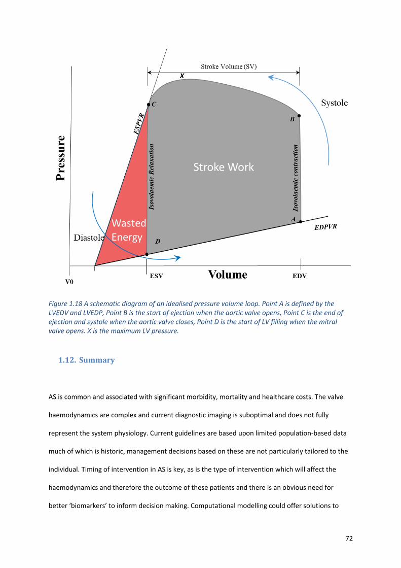
72

Figure 1.18 A schematic diagram of an idealised pressure volume loop. Point A is defined by the LVEDV and LVEDP, Point B is the start of ejection when the aortic valve opens, Point C is the end of ejection and systole when the aortic valve closes, Point D is the start of LV filling when the mitral valve opens. X is the maximum LV pressure.

1.12. Summary

AS is common and associated with significant morbidity, mortality and healthcare costs. The valve

haemodynamics are complex and current diagnostic imaging is suboptimal and does not fully

represent the system physiology. Current guidelines are based upon limited population-based data

much of which is historic, management decisions based on these are not particularly tailored to the

individual. Timing of intervention in AS is key, as is the type of intervention which will affect the

haemodynamics and therefore the outcome of these patients and there is an obvious need for

better ‘biomarkers’ to inform decision making. Computational modelling could offer solutions to

X

73

some of the problems in current practice but its use in AS, thus far, has been limited, primarily due

to the data available and the difficulty in personalising the physiology in these models. Pressure-

volume loops are the gold standard in assessing cardiac haemodynamics; if computational modelling

could be used to produce non-invasive pressure-volume loops this could be a useful clinical tool for

decision making. Studies have shown that modelling has promise in the healthcare setting and its

ability to run simulations and be predictive could help identify the likely outcomes for patients. Use

of other techniques that can model flow through the diseased aortic valve, such as 4D flow MRI

assessment, have not been fully explored and there may be a possibility of exploiting this alone or in

combination with a modelling process.

Objectively measuring the effect of the disease and outcome of intervention is rarely done routinely

in clinical practice. Most research to date has used tests such as the exercise tolerance test or six-

minute walk test to assess this. Pervasive wearable monitors may provide more information about

the patient’s functional status and how the disease is impacting on a patient’s life. There is an

obvious need to identify new markers of disease severity that may help guide clinicians in the

decision-making process.

Risk scores such as STS and EuroScore are frequently calculated when considering an intervention

but it is the role of the clinician to weigh up both risks and benefits for that individual. It is

sometimes unclear what the benefit to a specific patient may be. Questions frequently asked by the

patient include the following. Will I be able to do more after the operation? Will my symptoms get

better? Will my heart recover? What operation should I have? When should I have the operation?

And will I live longer? In the future computational modelling may be able to help to answer at least

some of these questions.

74

1.13. Hypothesis

Computational modelling can aid in the diagnosis and management of AS by producing non-invasive

pressure volume loops to study LV haemodynamics. Resultant parameters will be better associated

with the patient’s symptoms and outcome following intervention.

1.14. Aims

The aims of the current thesis are to answer the following questions:

1. Can a simple, personalised, mathematical model of a patient with AS ‘measure’ cardiac work

and power parameters that provide an effective characterisation of the demand on the

heart in both rest and exercise conditions and predict the changes of these parameters

following a prospective intervention?

2. Can 4D flow MRI data provide novel diagnostic methods of AS and add to the

haemodynamic assessment, negating the need for computational modelling?

3. Does computational modelling have an advantage over and above current clinical

assessment of AS?

4. Do pervasive wearable monitors give a better insight into how AS affects a patient’s activity

and how this changes following intervention?

5. Can a decision support tool be created, using data generated in this study, that can be

utilised in clinical practice?

75

CHAPTER 2

2. Methods

The study reported in this thesis was part of the larger multicentre EurValve project for which data

was also collected from the German Heart Centre, Berlin and Catharina Hospital. The primary focus

of this thesis, and of this chapter, is on the analysis of the Sheffield cohort of 22 aortic cases but,

where relevant, reference is made to the wider study.

2.1. Clinical Study Design and Management

2.1.1. Overview

This section describes a prospective cohort study carried out at Sheffield Teaching Hospitals NHS

Foundation Trust. This is a proof-of-concept study, with the resultant pilot data used to address the

aims stated above. Although there is overlap with the multi-centre EurValve study, a number of

extensions in terms of both data collection and in methods of analysis were specific to this work.

Patients were recruited who had standard indications for aortic valve replacement according to

ESC/EACTS guidelines[29], [31]. Relevant clinical, imaging, activity monitoring, six-minute walk test,

and patient reported outcome measures were recorded. These data were collected prior to

intervention, at discharge, and 3-4 months after intervention (early follow-up). After the initial

follow-up phase, the results and patient feedback suggested that 3-4 months was not adequate to

allow patients to recover fully, particularly after SAVR. Therefore, patients were invited to undergo

activity monitoring for a further period at 12-18 months (extended follow-up) and report their

longer-term outcome.

76

2.1.2. Ethics

The study received a favourable opinion from the Health Research Authority and the Research Ethics

Committee (17/LO/0283) and was permitted by Sheffield Teaching Hospitals NHS FT research and

development board.

2.1.3. Inclusion and Exclusion Criteria

Inclusion Criteria:

• Informed consent obtained

• Elective cases

• Severe aortic valve disease

• Patients may have concurrent coronary artery bypass grafting or other interventions such as

surgery of the aorta and tricuspid valves.

Exclusion Criteria

• Age < 18 years

• Inability or unwillingness to give formal consent

• Emergency interventions

• Active infective valvular disease or evidence of valvular damage by recent endocarditis

• Valvular malfunction directly associated with aortic root disease

• Moderate or severe mitral valve disease

• Aortic regurgitation as the leading aortic valve pathology

• Inability or unwillingness to complete follow up

• MRI contraindications such as implanted pacemaker, metallic foreign bodies or implants or

severe claustrophobia

• CT contraindications such as iodine or contrast agent allergy, hyperhidrosis or pregnancy

77

2.1.4. Clinical Study Protocol

The clinical study protocol included the recording of a comprehensive range of clinical parameters.

Since the emphasis of the study was on physiological characterisation of the patient, special

attention was paid to directly relevant data including pressures, flows and volumes, and measures of

physical activity. Although not standard practice, most patients in the current cohort (20 out of 22)

underwent cMR imaging because this is particularly valuable for physiological assessment, and one

of the aims of the study was to evaluate whether cMR can offer any additional benefit in assessment

of these patients compared with more standard techniques. A fundamental tenet of this study was

that, in order to minimise obstacles to clinical uptake, it should exploit maximally the data that is

captured in the routine clinical pathways, and this is reflected in the modelling protocols described

in section 2.4.3. Due to variations in clinical practice it was expected that not all data will be

available for all patients; this reflects reality.

Patients underwent three initial phases of assessment: pre-intervention, discharge and post-

intervention. The pre-intervention assessment, which could occur at any point from the time the

patient was accepted for intervention to their procedure, typically occurred within 18 weeks. This

consisted of 3D cardiac imaging. Resting blood pressure and heart rate were recorded at the time of

imaging. Patients’ activity levels were recorded using wearable devices (see section 2.5) for at least

14 consecutive days and as a secondary measure, the clinically validated six-minute walk test was

performed. Quality of life was also measured using questionnaires.

Following intervention, the same data were recorded 12-16 weeks after the intervention, when it is

expected that most people would have recovered following their procedure. Although AHA

guidelines suggest a recovery period of 4-8 weeks[177], local experience was that the recovery

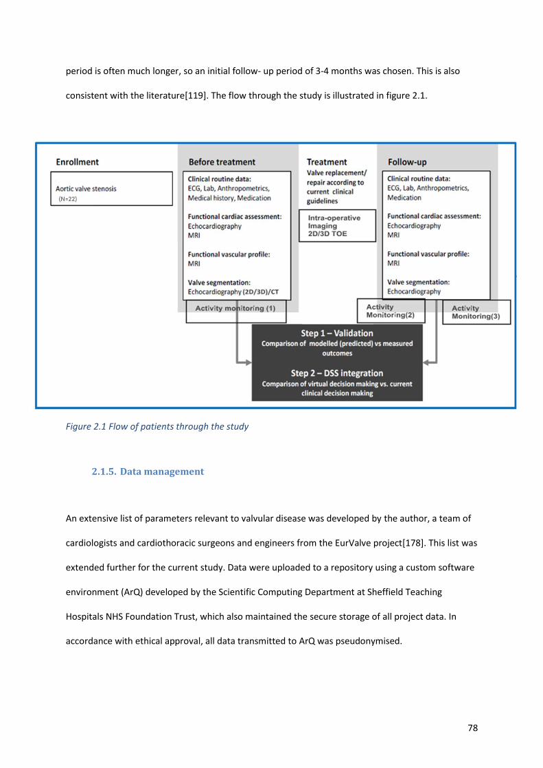
78

period is often much longer, so an initial follow- up period of 3-4 months was chosen. This is also

consistent with the literature[119]. The flow through the study is illustrated in figure 2.1.

Figure 2.1 Flow of patients through the study

2.1.5. Data management

An extensive list of parameters relevant to valvular disease was developed by the author, a team of

cardiologists and cardiothoracic surgeons and engineers from the EurValve project[178]. This list was

extended further for the current study. Data were uploaded to a repository using a custom software

environment (ArQ) developed by the Scientific Computing Department at Sheffield Teaching

Hospitals NHS Foundation Trust, which also maintained the secure storage of all project data. In

accordance with ethical approval, all data transmitted to ArQ was pseudonymised.

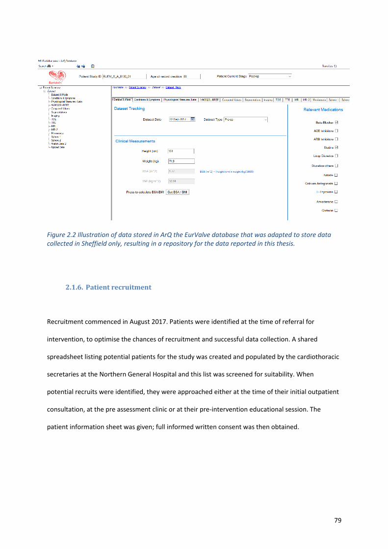
79

Figure 2.2 Illustration of data stored in ArQ the EurValve database that was adapted to store data collected in Sheffield only, resulting in a repository for the data reported in this thesis.

2.1.6. Patient recruitment

Recruitment commenced in August 2017. Patients were identified at the time of referral for

intervention, to optimise the chances of recruitment and successful data collection. A shared

spreadsheet listing potential patients for the study was created and populated by the cardiothoracic

secretaries at the Northern General Hospital and this list was screened for suitability. When

potential recruits were identified, they were approached either at the time of their initial outpatient

consultation, at the pre assessment clinic or at their pre-intervention educational session. The

patient information sheet was given; full informed written consent was then obtained.

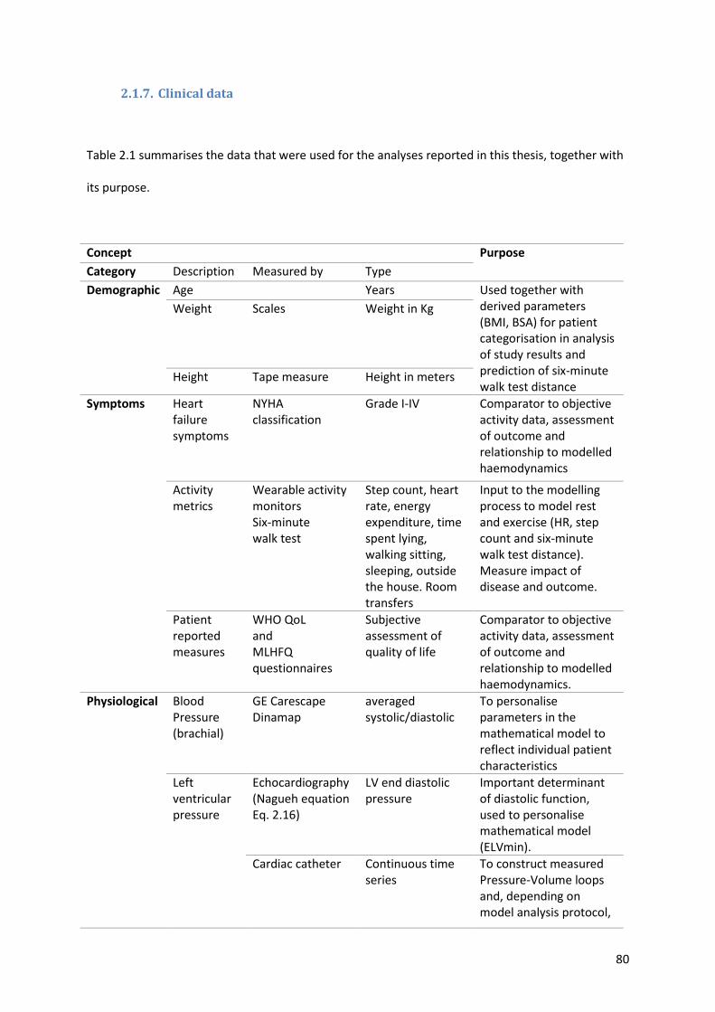
80

2.1.7. Clinical data

Table 2.1 summarises the data that were used for the analyses reported in this thesis, together with

its purpose.

Concept

Purpose

Category Description Measured by Type

Demographic Age

Years Used together with derived parameters (BMI, BSA) for patient categorisation in analysis of study results and prediction of six-minute walk test distance

Weight Scales Weight in Kg

Height Tape measure Height in meters

Symptoms Heart failure symptoms

NYHA classification

Grade I-IV Comparator to objective activity data, assessment of outcome and relationship to modelled haemodynamics

Activity metrics

Wearable activity monitors Six-minute walk test

Step count, heart rate, energy expenditure, time spent lying, walking sitting, sleeping, outside the house. Room transfers

Input to the modelling process to model rest and exercise (HR, step count and six-minute walk test distance). Measure impact of disease and outcome.

Patient reported measures

WHO QoL and MLHFQ questionnaires

Subjective assessment of quality of life

Comparator to objective activity data, assessment of outcome and relationship to modelled haemodynamics.

Physiological Blood Pressure (brachial)

GE Carescape Dinamap

averaged systolic/diastolic

To personalise parameters in the mathematical model to reflect individual patient characteristics

Left ventricular pressure

Echocardiography (Nagueh equation Eq. 2.16)

LV end diastolic pressure

Important determinant of diastolic function, used to personalise mathematical model (ELVmin).

Cardiac catheter Continuous time series

To construct measured Pressure-Volume loops and, depending on model analysis protocol,

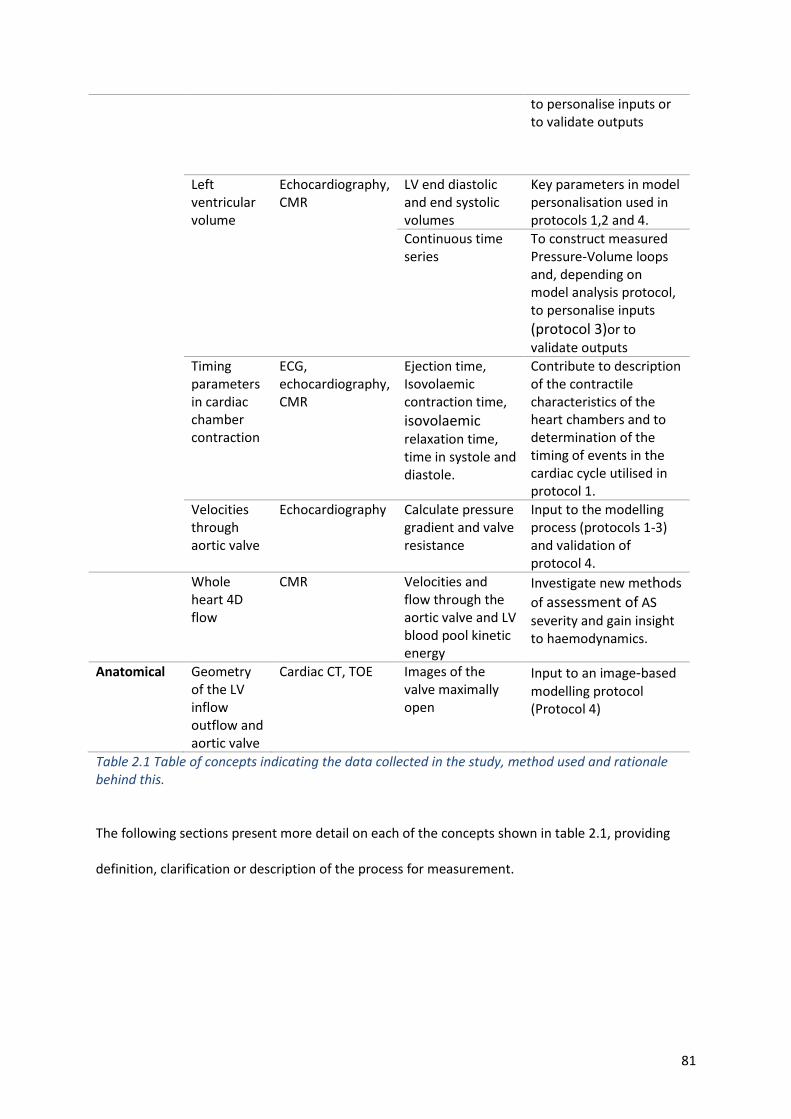
81

to personalise inputs or to validate outputs

Left ventricular volume

Echocardiography, CMR

LV end diastolic and end systolic volumes

Key parameters in model personalisation used in protocols 1,2 and 4.

Continuous time series

To construct measured Pressure-Volume loops and, depending on model analysis protocol, to personalise inputs

(protocol 3)or to validate outputs

Timing parameters in cardiac chamber contraction

ECG, echocardiography, CMR

Ejection time, Isovolaemic contraction time,

isovolaemic relaxation time, time in systole and diastole.

Contribute to description of the contractile characteristics of the heart chambers and to determination of the timing of events in the cardiac cycle utilised in protocol 1.

Velocities through aortic valve

Echocardiography Calculate pressure gradient and valve resistance

Input to the modelling process (protocols 1-3) and validation of protocol 4.

Whole heart 4D flow

CMR Velocities and flow through the aortic valve and LV blood pool kinetic energy

Investigate new methods

of assessment of AS severity and gain insight to haemodynamics.

Anatomical Geometry of the LV inflow outflow and aortic valve

Cardiac CT, TOE Images of the valve maximally open

Input to an image-based modelling protocol (Protocol 4)

Table 2.1 Table of concepts indicating the data collected in the study, method used and rationale behind this.

The following sections present more detail on each of the concepts shown in table 2.1, providing

definition, clarification or description of the process for measurement.

82

2.1.7.1. Basic demographics

Factors that may influence the outcome of the patient and computational modelling process such as

age, height and weight were recorded at the pre-assessment clinic prior to intervention. BMI and

BSA were computed using standard calculations.

2.1.7.2. Symptoms

Patient symptoms were determined either through direct consultation with the patient or from

clinical records and were recorded using the standard New York Heart Association

classification[179]; specific symptoms (syncope and angina) related to AS were also recorded. GP

records, hospital records and direct patient consultation were used as sources for past medical

history and a list of current medications were recorded.

2.1.8. Physical examination and blood pressure assessment

A physical examination was carried out as part of routine care. The findings were available through

the clinical record but were not specifically used in the study. Blood pressure assessment at the time

of imaging was needed for the modelling process. Immediately prior to LV volumetric assessment,

an average of three brachial artery pressures was taken using a GE Carescape V100 dinamap (GE

Healthcare, Boston, USA).

2.1.9. ECG

Standard 12 lead ECGs[180] were recorded prior to intervention during the patient’s clinical

consultation and following intervention prior to discharge. Heart rate, rhythm and QRS duration

were recorded.

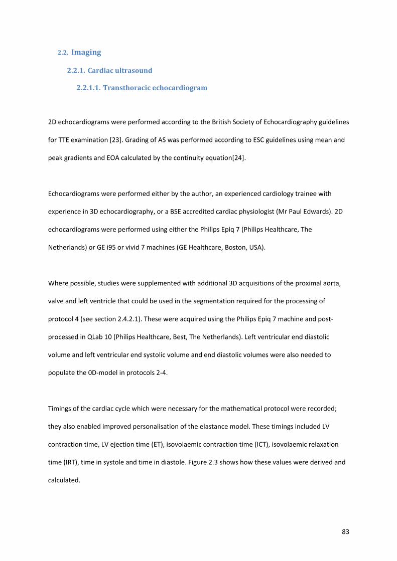
83

2.2. Imaging

2.2.1. Cardiac ultrasound

2.2.1.1. Transthoracic echocardiogram

2D echocardiograms were performed according to the British Society of Echocardiography guidelines

for TTE examination [23]. Grading of AS was performed according to ESC guidelines using mean and

peak gradients and EOA calculated by the continuity equation[24].

Echocardiograms were performed either by the author, an experienced cardiology trainee with

experience in 3D echocardiography, or a BSE accredited cardiac physiologist (Mr Paul Edwards). 2D

echocardiograms were performed using either the Philips Epiq 7 (Philips Healthcare, The

Netherlands) or GE i95 or vivid 7 machines (GE Healthcare, Boston, USA).

Where possible, studies were supplemented with additional 3D acquisitions of the proximal aorta,

valve and left ventricle that could be used in the segmentation required for the processing of

protocol 4 (see section 2.4.2.1). These were acquired using the Philips Epiq 7 machine and post-

processed in QLab 10 (Philips Healthcare, Best, The Netherlands). Left ventricular end diastolic

volume and left ventricular end systolic volume and end diastolic volumes were also needed to

populate the 0D-model in protocols 2-4.

Timings of the cardiac cycle which were necessary for the mathematical protocol were recorded;

they also enabled improved personalisation of the elastance model. These timings included LV

contraction time, LV ejection time (ET), isovolaemic contraction time (ICT), isovolaemic relaxation

time (IRT), time in systole and time in diastole. Figure 2.3 shows how these values were derived and

calculated.

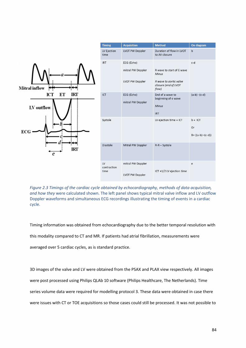
84

Figure 2.3 Timings of the cardiac cycle obtained by echocardiography, methods of data acquisition, and how they were calculated shown. The left panel shows typical mitral valve inflow and LV outflow Doppler waveforms and simultaneous ECG recordings illustrating the timing of events in a cardiac cycle.

Timing information was obtained from echocardiography due to the better temporal resolution with

this modality compared to CT and MR. If patients had atrial fibrillation, measurements were

averaged over 5 cardiac cycles, as is standard practice.

3D images of the valve and LV were obtained from the PSAX and PLAX view respectively. All images

were post processed using Philips QLAb 10 software (Philips Healthcare, The Netherlands). Time

series volume data were required for modelling protocol 3. These data were obtained in case there

were issues with CT or TOE acquisitions so those cases could still be processed. It was not possible to

85

acquire adequate images of the valve for segmentation using MRI due to flow artefacts from the

high velocity jets caused by the stenosis.

Figure 2.4 Images from a 3D full volume TTE study performed on a subject unable to undergo cardiac MRI for LV volume analysis and time series data.

2.2.1.2. Transoesophageal

These scans were performed using Philips IE33 machines in all patients that underwent SAVR in

cardiac theatres when the patient was anaesthetised for surgery. 2D echocardiograms were

performed to the standards specified by the British society of echocardiography[181]. Due to the

improved spatial resolution 3D images of the valve and proximal aorta were acquired and used in

preference to the TTE images for the model protocols in which 3D images were required and CT data

were not available. Where image quality was good, this was used instead of CT and MRI imaging as

there is better temporal resolution[167]. Some studies have shown them to be equivalent for

86

volumetric assessment[168]. However, the use of TOE derived volumetric data was avoided due to

the different (non-physiological) loading conditions under general anaesthetic.

2.2.1.3. Ultrasound data collection

Data were extracted in raw DICOM format, at the highest resolution (uncompressed) to ensure

compatibility with the segmentation process (see section 2.4.2.1). All DICOM data were uploaded to

the trial connect platform (Telekom Healthcare Solutions, Bonn, Germany)[182].This is a

telemedicine certified repository, which ensures de-identification of the data and made data

available for the automatic segmentation process.

2.2.2. Cardiac magnetic resonance imaging (CMR)

An MRI protocol was developed (see appendix i). CMR was performed prior to the intervention

(within 16 weeks of the procedure) and repeated during the 3-4 month follow up period. A standard

MRI safety questionnaire was administered before each MRI study. For the follow-up scan, the

surgical material and prostheses used were recorded and these were checked for MRI compatibility.

The total SAR and spatial gradient in the protocol was calculated to ensure patient safety. Scans

were performed on a 3 Tesla Philips Healthcare Ingenia system equipped with a 28-channel coil and

Philips dStream digital broadband MR architecture technology. The CMR protocol included baseline

survey, cine images (vertical long axis, horizontal long axis, short‐axis contiguous left‐ventricle

volume stack 3-chamber (left ventricular outflow tract (LVOT) views) and aortic valve views). Cine

images were acquired during end-expiratory breath-hold with a balanced steady-state free

precession (bSSFP), single-slice breath-hold sequence. The number of LV short-axis slices varied

according to the size of each patient’s heart.

87

Cine images had a spatial resolution of 2.5 × 2.5 mm2, a pixel size of 1.56× 1.56 mm2, and a slice

thickness of 10 mm with contiguous slices for the short axis stack. Other imaging parameters were

30 phases, echo time (TE) = 1.5 ms, repetition time (TR) = 3.05 ms, flip angle= 45°, the field of view

(FOV) was 400 mm, and SENSE factor 2–3. All images were post-processed and analysed using offline

research software called MASS (Version 2019 EXP, Leiden University Medical Centre, Leiden, The

Netherlands). LV volumes and mass were measured from the short axis stack of bSSFP cine images in

the standard way [183]. Time series volume data were generated by repeating the volumetric

analysis in all 20 phases across the cardiac cycle.

2.2.3. MRI 4D flow assessment of AS

To address the aims of the study the current diagnostic methods that are available in clinical practice

were initially examined. 4D flow MRI may give insights into the valve haemodynamics and the effect

on the ventricle. An exploration of what additional information could be gleaned from MRI with 4D

flow analysis was undertaken before employing computational modelling. The following three

sections describe the methods relating to 4D flow studies and analysis.

2.2.3.1. 4D Flow Acquisition

Initial VENC (velocity encoding) setting was estimated from TTE peak velocity and tested using a

through-plane two-dimensional phase contrast acquisition. Further increments were added until

aliasing disappeared across the aortic valve. Field-of-view was planned to cover the whole heart,

aortic valve and ascending aorta. The 4D flow sequence used echo-planar imaging acceleration

factor of 5 with no respiratory gating. This sequence has been validated by previous studies for

valvular flow quantification in humans [170]. Other standard scan parameters were acquired voxel

size = 3x3x3mm, reconstructed voxel size = 1.5x1.5x1.5mm, echo time (TE) = 3.5 ms, repetition time

88

(TR) = 10 ms, flip angle 10°, the FOV 340x340 and 30 cardiac phases. Data pre-processing was done

on the scanner for correcting phase offset errors such as eddy currents, Maxwell effects, and

encoding errors related to gradient field distortions to avoid impairment of the measurements and

inaccuracies in flow quantification [184], [185].

2.2.3.2. 4D flow pressure gradient assessment

All three phase directions were screened for aliasing artefact, and if present this was manually

corrected using established phase unwrapping methods [186], [187]. Any spatial misalignment with

cine superimposition was manually corrected throughout the cardiac cycle prior to any

quantification. The precise location of the maximum velocity (Vmax) in the aorta during systole was

identified in the 4D flow data set and the velocity recorded in a similar method to Donati et al [38].

The maximum velocity determined in the 3D velocity data was used to determine the peak pressure

drop by the simplified Bernoulli equation = 4(Vmax)2.

2.2.3.3. 4D flow effective orifice area assessment

For EOA estimation, Bernoulli principles and the law of conservation of flow at the level of vena

contracta across all systolic phases where the valve is maximally open, were applied. Time resolved

flow and velocity data were recorded and as flow = area * velocity, EOA was estimated using the

following equation:

EOA = Flowt / Vmaxt

where Flowt and Vmaxt are the flows and peak velocity measurements through the aortic valve at

each of the recorded systolic phases (see figure 2.5).

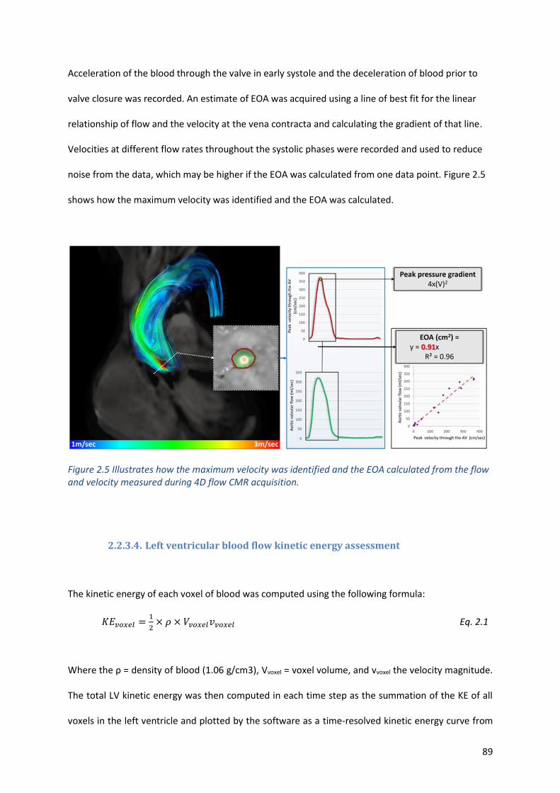
89

Acceleration of the blood through the valve in early systole and the deceleration of blood prior to

valve closure was recorded. An estimate of EOA was acquired using a line of best fit for the linear

relationship of flow and the velocity at the vena contracta and calculating the gradient of that line.

Velocities at different flow rates throughout the systolic phases were recorded and used to reduce

noise from the data, which may be higher if the EOA was calculated from one data point. Figure 2.5

shows how the maximum velocity was identified and the EOA was calculated.

Figure 2.5 Illustrates how the maximum velocity was identified and the EOA calculated from the flow and velocity measured during 4D flow CMR acquisition.

2.2.3.4. Left ventricular blood flow kinetic energy assessment

The kinetic energy of each voxel of blood was computed using the following formula:

𝐾𝐸𝑣𝑜𝑥𝑒𝑙 =1

2× 𝜌 × 𝑉𝑣𝑜𝑥𝑒𝑙𝑣𝑣𝑜𝑥𝑒𝑙 Eq. 2.1

Where the ρ = density of blood (1.06 g/cm3), Vvoxel = voxel volume, and vvoxel the velocity magnitude.

The total LV kinetic energy was then computed in each time step as the summation of the KE of all

voxels in the left ventricle and plotted by the software as a time-resolved kinetic energy curve from

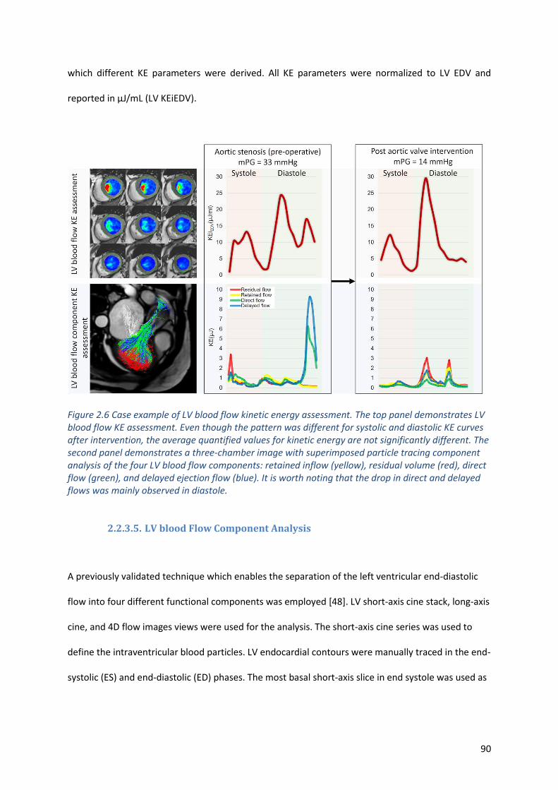
90

which different KE parameters were derived. All KE parameters were normalized to LV EDV and

reported in μJ/mL (LV KEiEDV).

Figure 2.6 Case example of LV blood flow kinetic energy assessment. The top panel demonstrates LV blood flow KE assessment. Even though the pattern was different for systolic and diastolic KE curves after intervention, the average quantified values for kinetic energy are not significantly different. The second panel demonstrates a three-chamber image with superimposed particle tracing component analysis of the four LV blood flow components: retained inflow (yellow), residual volume (red), direct flow (green), and delayed ejection flow (blue). It is worth noting that the drop in direct and delayed flows was mainly observed in diastole.

2.2.3.5. LV blood Flow Component Analysis

A previously validated technique which enables the separation of the left ventricular end-diastolic

flow into four different functional components was employed [48]. LV short-axis cine stack, long-axis

cine, and 4D flow images views were used for the analysis. The short-axis cine series was used to

define the intraventricular blood particles. LV endocardial contours were manually traced in the end-

systolic (ES) and end-diastolic (ED) phases. The most basal short-axis slice in end systole was used as

91

the inflow/outflow plane and particles were considered as invalid when they were below the

inflow/outflow plane and outside the LV epicardial contours in ES phase.

The end-diastolic blood flow was separated into four functional flow components, according to the

transit of blood flow through the left ventricular chamber for the complete cardiac cycle: (1) direct

flow is the volume of blood that enters the LV and is ejected during the same cardiac cycle, (2)

delayed ejection flow is the volume of the ejected blood that enters the left ventricle from a

previous cardiac cycle, (3) retained inflow is the volume of blood that enters the left ventricle but

does not eject in the same cardiac cycle, and (4) the residual volume is the blood that resides in the

LV over the entire cardiac cycle for at least 2 cardiac cycles. The results of particle tracing were

reviewed visually, and data quality was checked as previously described[48]. After the quality was

assessed, the KE of the volume of each flow component was calculated over a complete cardiac

cycle.

2.2.3.6. Cardiac computed tomography

Patients for whom the heart team considered TAVI underwent cardiac CT. This provided yet another

method to obtain LV volume data across the cardiac cycle and for a 3D valve geometry. The superior

spatial resolution compared with ultrasound and MRI may result in a greater accuracy in defining the

anatomical shape of the valve, improving the precision of the 3D modelling. Images were acquired

on an Aquilion ONE™, GENESIS Edition CT scanner (Canon medical systems Ltd, Crawley, UK)

according to the local TAVI protocol developed by STH. For study patients, this protocol was adapted

to ensure the mid systolic phase, where the valve is maximally open, was included enabling

segmentation for the 3D model. Whenever possible, a prospectively gated scan was performed to

minimise radiation exposure to the patient, scanning for 20-80% of the cardiac cycle. Data were

saved to the hospital server in 10% intervals of the cardiac cycle. Scans were reported as part of

92

routine clinical care; raw DICOM data were extracted and uploaded to the trial connect platform to

enable the segmentation process.

2.3. Intervention Data

The type of intervention (TAVI or SAVR) and the technique used in each procedure were recorded.

The make, and size, of the prosthesis implanted were also recorded. For the modelling process the

effective orifice of the replaced valve was also required. Since this varies depending upon the size of

the patient and the aorta, the manufacturer’s stated EOA was indexed for the individual’s body

surface area (see appendix iv).

2.4. Computational Modelling methods

This section describes a series of four protocols for the computation of pressure, volume and flow in

the compartments of the left heart and systemic circulation from which LV pressure-volume loops

and other measures were derived. The purpose of the multiple protocols is to support analysis for

multiple levels of available clinical data and computational resource. The results for each protocol

are discussed and compared in section 3.7.

2.4.1. Lumped parameter model of left side of heart and systemic circulation

The lumped parameter 0D model (see section 1.11.4) illustrated in figure 2.7 was used to represent

the circulation. This was based upon the validated lumped-parameter cardiovascular model with

Westkessel after-load [147] and is similar to the model used by Garcia et al[168] where AS was

modelled as an increase in AV resistance. This model was used as the basis for protocols 2, 3 and 4,

the differences being in which data were used to personalise the model (see section 2.4.1) and how

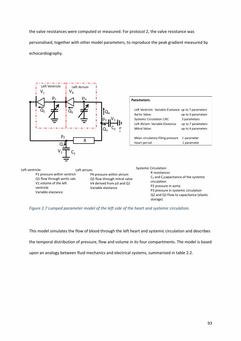
93

the valve resistances were computed or measured. For protocol 2, the valve resistance was

personalised, together with other model parameters, to reproduce the peak gradient measured by

echocardiography.

Figure 2.7 Lumped parameter model of the left side of the heart and systemic circulation.

This model simulates the flow of blood through the left heart and systemic circulation and describes

the temporal distribution of pressure, flow and volume in its four compartments. The model is based

upon an analogy between fluid mechanics and electrical systems, summarised in table 2.2.

Left ventricle:

P1 pressure within ventricle Q1 flow through aortic valve V1 volume of the left ventricle Variable elastance

Left atrium:

P4 pressure within atrium Q5 flow through mitral valve V4 derived from p3 and Q1 Variable elastance

Systemic Circulation:

R resistances C3 and C2capacitance of the systemic circulation P2 pressure in aorta P3 pressure in systemic circulation Q2 and Q3 Flow to capacitance (elastic storage)

P4

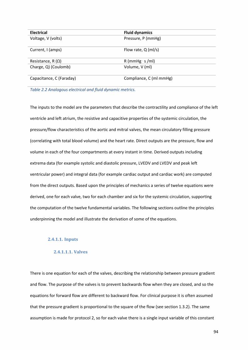
94

Electrical Fluid dynamics

Voltage, V (volts)

Pressure, P (mmHg)

Current, I (amps) Flow rate, Q (ml/s)

Resistance, R (Ω) R (mmHg . s /ml)

Charge, Q) (Coulomb)

Volume, V (ml)

Capacitance, C (Faraday) Compliance, C (ml mmHg)

Table 2.2 Analogous electrical and fluid dynamic metrics.

The inputs to the model are the parameters that describe the contractility and compliance of the left

ventricle and left atrium, the resistive and capacitive properties of the systemic circulation, the

pressure/flow characteristics of the aortic and mitral valves, the mean circulatory filling pressure

(correlating with total blood volume) and the heart rate. Direct outputs are the pressure, flow and

volume in each of the four compartments at every instant in time. Derived outputs including

extrema data (for example systolic and diastolic pressure, LVEDV and LVEDV and peak left

ventricular power) and integral data (for example cardiac output and cardiac work) are computed

from the direct outputs. Based upon the principles of mechanics a series of twelve equations were

derived, one for each valve, two for each chamber and six for the systemic circulation, supporting

the computation of the twelve fundamental variables. The following sections outline the principles

underpinning the model and illustrate the derivation of some of the equations.

2.4.1.1. Inputs

2.4.1.1.1. Valves

There is one equation for each of the valves, describing the relationship between pressure gradient

and flow. The purpose of the valves is to prevent backwards flow when they are closed, and so the

equations for forward flow are different to backward flow. For clinical purpose it is often assumed

that the pressure gradient is proportional to the square of the flow (see section 1.3.2). The same

assumption is made for protocol 2, so for each valve there is a single input variable of this constant

95

of proportionality. For this study it is assumed that there is no regurgitation, and so the flow is, in

principle, set to zero when the flow reverses (in fact for numerical reasons associated with the

stability of the solver the gradient/flow curve is smoothed close to the point of zero pressure

gradient but this has no significant effect on results).

2.4.1.1.2. Systemic circulation

As illustrated in figure 2.7, the systemic circulation is composed of two capacitors and a resistor.

Based on the principles of Ohm’s law as discussed in section 1.11.4, for a resistor, Pressure(P)=

Flow (Q) x Resistance (R). Continuity dictates that the flow in the systemic resistor is Q1 − Q2 and so:

p2 − p3 = R(Q1 − Q2) Eq. 2.2

The rate of change of charge on a capacitor is the flow of charge onto it and so, for the proximal and

distal systemic capacitors in the current model:

𝑑𝑉2

𝑑𝑡= Q2 Eq. 2.3

𝑑𝑉3

𝑑𝑡= Q3 Eq. 2.4

The equation for a capacitor dictates that charge is proportional to voltage (Capacitance= Charge

/Voltage); therefore, flow is proportional to rate of change of pressure.

Q2 = C2 𝑑p2

𝑑𝑡 Eq. 2.5

Q3 = C3 𝑑p3

𝑑𝑡 Eq. 2.6

Finally, for continuity:

Q1 − Q2 − Q3 = Q4 Eq. 2.7

In total, therefore, there are six equations for the systemic circulation.

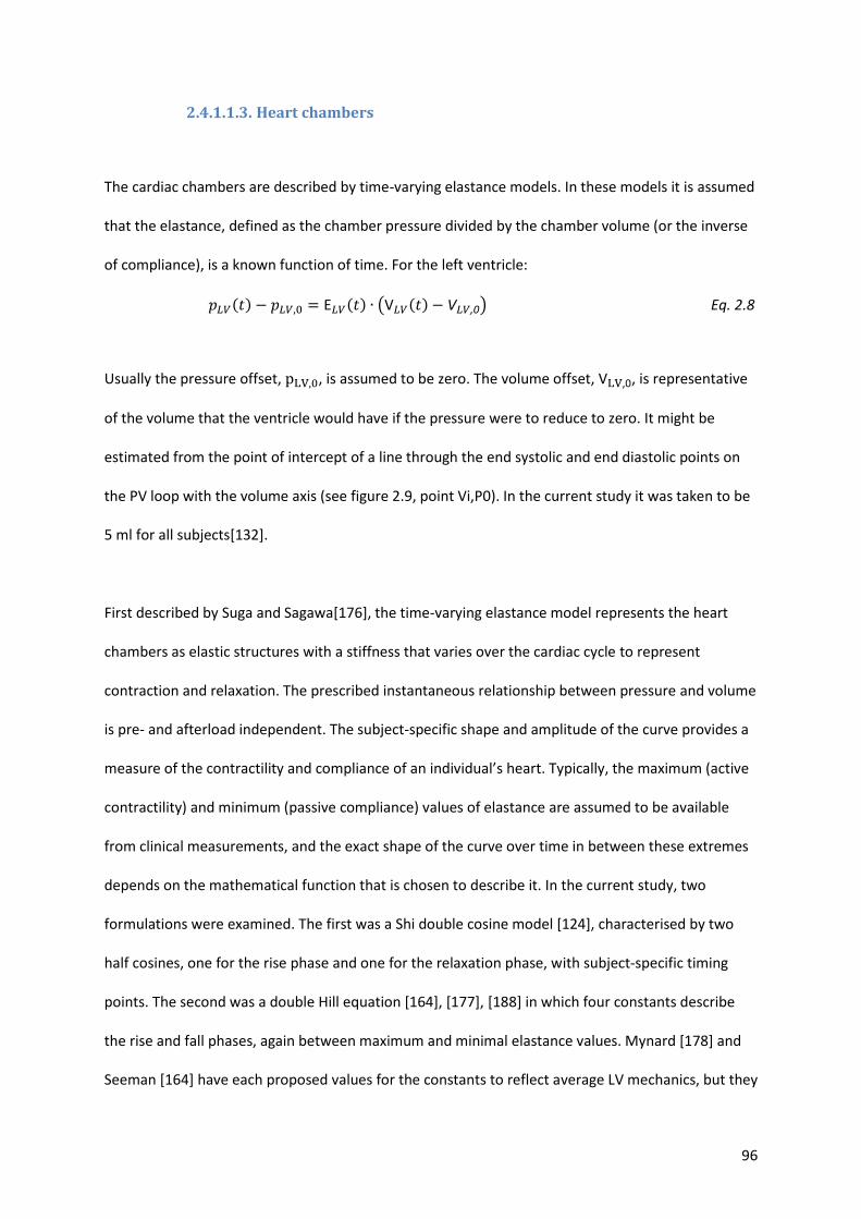
96

2.4.1.1.3. Heart chambers

The cardiac chambers are described by time-varying elastance models. In these models it is assumed

that the elastance, defined as the chamber pressure divided by the chamber volume (or the inverse

of compliance), is a known function of time. For the left ventricle:

𝑝𝐿𝑉(𝑡) − 𝑝𝐿𝑉,0 = E𝐿𝑉(𝑡) ∙ (V𝐿𝑉(𝑡) − V𝐿𝑉,0) Eq. 2.8

Usually the pressure offset, pLV,0, is assumed to be zero. The volume offset, VLV,0, is representative

of the volume that the ventricle would have if the pressure were to reduce to zero. It might be

estimated from the point of intercept of a line through the end systolic and end diastolic points on

the PV loop with the volume axis (see figure 2.9, point Vi,P0). In the current study it was taken to be

5 ml for all subjects[132].

First described by Suga and Sagawa[176], the time-varying elastance model represents the heart

chambers as elastic structures with a stiffness that varies over the cardiac cycle to represent

contraction and relaxation. The prescribed instantaneous relationship between pressure and volume

is pre- and afterload independent. The subject-specific shape and amplitude of the curve provides a

measure of the contractility and compliance of an individual’s heart. Typically, the maximum (active

contractility) and minimum (passive compliance) values of elastance are assumed to be available

from clinical measurements, and the exact shape of the curve over time in between these extremes

depends on the mathematical function that is chosen to describe it. In the current study, two

formulations were examined. The first was a Shi double cosine model [124], characterised by two

half cosines, one for the rise phase and one for the relaxation phase, with subject-specific timing

points. The second was a double Hill equation [164], [177], [188] in which four constants describe

the rise and fall phases, again between maximum and minimal elastance values. Mynard [178] and

Seeman [164] have each proposed values for the constants to reflect average LV mechanics, but they

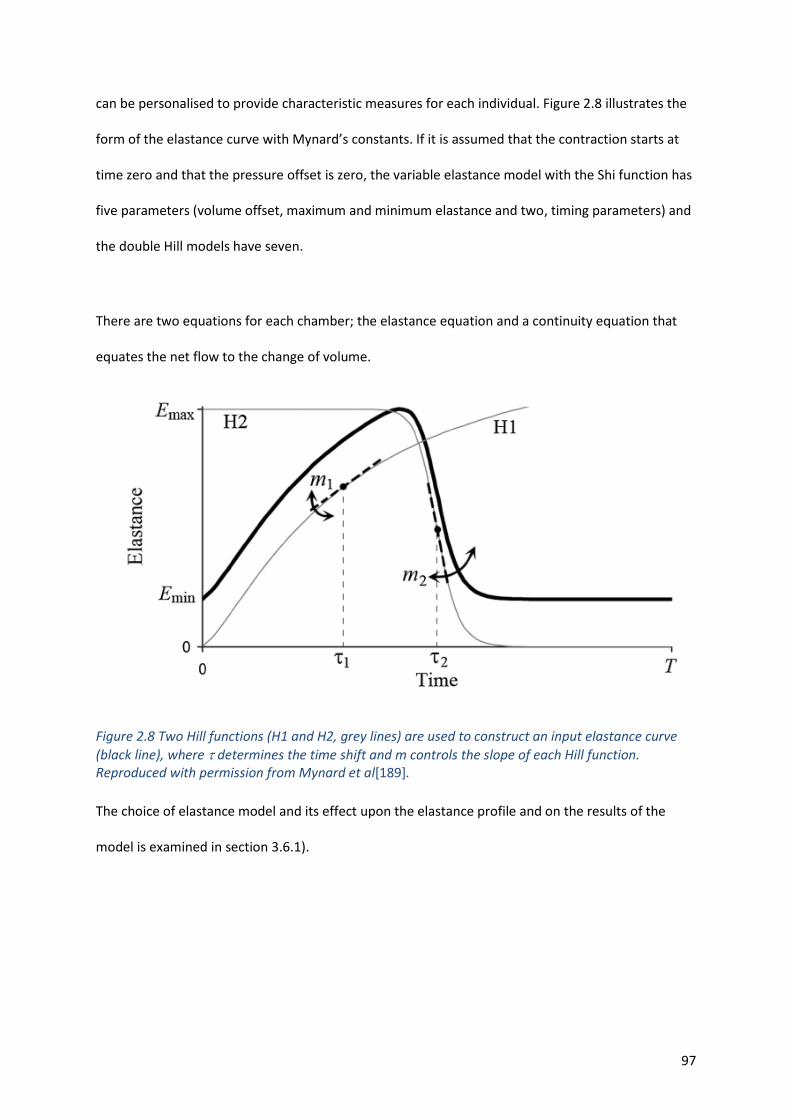
97

can be personalised to provide characteristic measures for each individual. Figure 2.8 illustrates the

form of the elastance curve with Mynard’s constants. If it is assumed that the contraction starts at

time zero and that the pressure offset is zero, the variable elastance model with the Shi function has

five parameters (volume offset, maximum and minimum elastance and two, timing parameters) and

the double Hill models have seven.

There are two equations for each chamber; the elastance equation and a continuity equation that

equates the net flow to the change of volume.

Figure 2.8 Two Hill functions (H1 and H2, grey lines) are used to construct an input elastance curve

(black line), where determines the time shift and m controls the slope of each Hill function. Reproduced with permission from Mynard et al[189].

The choice of elastance model and its effect upon the elastance profile and on the results of the

model is examined in section 3.6.1).

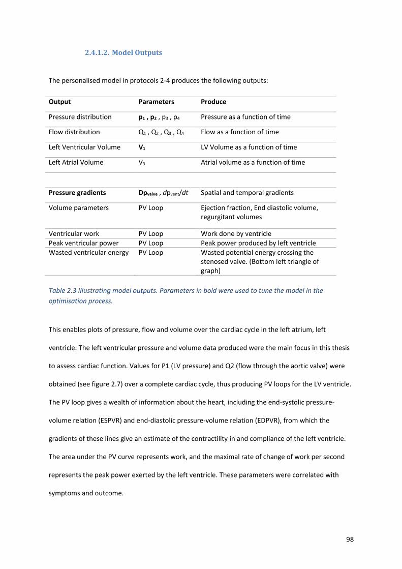
98

2.4.1.2. Model Outputs

The personalised model in protocols 2-4 produces the following outputs:

Output Parameters Produce

Pressure distribution p1 , p2 , p3 , p4 Pressure as a function of time

Flow distribution Q1 , Q2 , Q3 , Q4 Flow as a function of time

Left Ventricular Volume V1 LV Volume as a function of time

Left Atrial Volume V3 Atrial volume as a function of time

Pressure gradients Dpvalve , dpvent/dt Spatial and temporal gradients

Volume parameters PV Loop Ejection fraction, End diastolic volume, regurgitant volumes

Ventricular work PV Loop Work done by ventricle

Peak ventricular power PV Loop Peak power produced by left ventricle

Wasted ventricular energy PV Loop Wasted potential energy crossing the stenosed valve. (Bottom left triangle of graph)

Table 2.3 Illustrating model outputs. Parameters in bold were used to tune the model in the

optimisation process.

This enables plots of pressure, flow and volume over the cardiac cycle in the left atrium, left

ventricle. The left ventricular pressure and volume data produced were the main focus in this thesis

to assess cardiac function. Values for P1 (LV pressure) and Q2 (flow through the aortic valve) were

obtained (see figure 2.7) over a complete cardiac cycle, thus producing PV loops for the LV ventricle.

The PV loop gives a wealth of information about the heart, including the end-systolic pressure-

volume relation (ESPVR) and end-diastolic pressure-volume relation (EDPVR), from which the

gradients of these lines give an estimate of the contractility in and compliance of the left ventricle.

The area under the PV curve represents work, and the maximal rate of change of work per second

represents the peak power exerted by the left ventricle. These parameters were correlated with

symptoms and outcome.

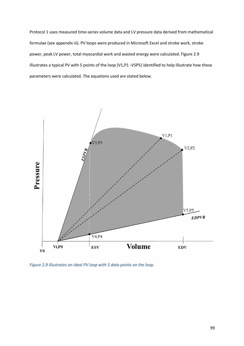
99

Protocol 1 uses measured time-series volume data and LV pressure data derived from mathematical

formulae (see appendix iii). PV loops were produced in Microsoft Excel and stroke work, stroke

power, peak LV power, total myocardial work and wasted energy were calculated. Figure 2.9

illustrates a typical PV with 5 points of the loop (V1,P1 -V5P5) identified to help illustrate how these

parameters were calculated. The equations used are stated below.

Figure 2.9 Illustrates an ideal PV loop with 5 data points on the loop.

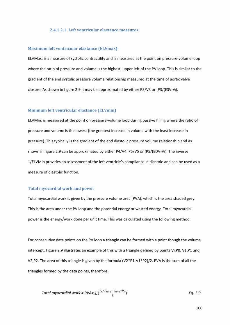
100

2.4.1.2.1. Left ventricular elastance measures

Maximum left ventricular elastance (ELVmax)

ELVMax: is a measure of systolic contractility and is measured at the point on pressure-volume loop

where the ratio of pressure and volume is the highest, upper left of the PV loop. This is similar to the

gradient of the end systolic pressure volume relationship measured at the time of aortic valve

closure. As shown in figure 2.9 it may be approximated by either P3/V3 or (P3/(ESV-Vi).

Minimum left ventricular elastance (ELVmin)

ELVMin: is measured at the point on pressure-volume loop during passive filling where the ratio of

pressure and volume is the lowest (the greatest increase in volume with the least increase in

pressure). This typically is the gradient of the end diastolic pressure volume relationship and as

shown in figure 2.9 can be approximated by either P4/V4, P5/V5 or (P5/(EDV-Vi). The inverse

1/ELVMin provides an assessment of the left ventricle’s compliance in diastole and can be used as a

measure of diastolic function.

Total myocardial work and power

Total myocardial work is given by the pressure volume area (PVA), which is the area shaded grey.

This is the area under the PV loop and the potential energy or wasted energy. Total myocardial

power is the energy/work done per unit time. This was calculated using the following method:

For consecutive data points on the PV loop a triangle can be formed with a point though the volume

intercept. Figure 2.9 illustrates an example of this with a triangle defined by points Vi,P0, V1,P1 and

V2,P2. The area of this triangle is given by the formula (V2*P1-V1*P2)/2. PVA is the sum of all the

triangles formed by the data points, therefore:

Total myocardial work = PVA= (𝑉𝑛∗𝑃𝑛−1−𝑉𝑛−1∗𝑃𝑛

2) Eq. 2.9

101

Total myocardial power = (𝑉𝑛∗𝑃𝑛−1−𝑉𝑛−1∗𝑃𝑛

2) 𝑑𝑡⁄ Eq. 2.10

dt is given by the interval time at which the data points were acquired over the cardiac cycle. In this

study LV volumes were measured across 20 phases. To ensure the data wraps around, 21 data points

were plotted with the first point the same as the last giving 20 time intervals. The length of these

intervals is determined by the heart rate. Therefore, dt= (60/heart rate(bpm))/20.

Stroke work and wasted energy

Stroke work is the useful energy that contributes to cardiac output. This is the area under the PV

loop which is given by the PVA minus the wasted energy defined by the triangle formed by ViP0,

V3,P3 and V4P4 and indicated by the white dashed line in figure 2.9.

Wasted energy can be calculated using the following formula:

𝑊𝑎𝑠𝑡𝑒𝑑 𝑒𝑛𝑒𝑟𝑔𝑦 = ((𝐸𝑆𝑉 − 𝑉𝑖 ∗ 𝑃3)/2 – (𝐸𝑆𝑉 − 𝑉𝑖 ∗ 𝑃4)/2) Eq. 2.11

𝑊𝑎𝑠𝑡𝑒𝑑 𝑝𝑜𝑤𝑒𝑟 = ((𝐸𝑆𝑉 − 𝑉𝑖 ∗ 𝑃3)/2 – (𝐸𝑆𝑉 − 𝑉𝑖 ∗ 𝑃4)/2)/𝑑𝑡 Eq. 2.12

Stroke work can be calculated using the following formula:

𝑆𝑡𝑟𝑜𝑘𝑒 𝑤𝑜𝑟𝑘 = 𝑇𝑜𝑡𝑎𝑙 𝑚𝑦𝑜𝑐𝑎𝑟𝑑𝑖𝑎𝑙 𝑤𝑜𝑟𝑘 – 𝑊𝑎𝑠𝑡𝑒𝑑 𝑒𝑛𝑒𝑟𝑔𝑦

𝑆𝑡𝑟𝑜𝑘𝑒 𝑤𝑜𝑟𝑘 = (𝑉𝑛∗𝑃𝑛−1−𝑉𝑛−1∗𝑃𝑛

2) − ((𝐸𝑆𝑉 − 𝑉𝑖 ∗ 𝑃3)/2 – (𝐸𝑆𝑉 − 𝑉𝑖 ∗ 𝑃4)/2)) Eq. 2.13

Peak left Ventricular power

Is the maximum work done by the LV per unit time and given by the maximum result from:

𝐿𝑉 𝑃𝑒𝑎𝑘 𝑝𝑜𝑤𝑒𝑟 = ½(𝑉𝑛 ∗ 𝑃𝑛−1 − 𝑉𝑛−1 ∗ 𝑃𝑛)/2))/𝑑𝑡 Eq. 2. 14

102

2.4.1.2.2. Parameter personalisation (model optimisation)

Most analyses reported in this thesis were performed using the double Hill model for ventricular

elastance (7 parameters) and the Shi double cosine model for atrial elastance (5 parameters).

Together with the three systemic circulation parameters, one parameter for each valve, the mean

circulatory pressure and the heart rate, there were 19 input parameters. The purpose of the model

is to compute the outputs, including the LV PV loop and the cardiac energetics parameters, for each

individual. Some of the outputs, including for example the LVEDV and LVESV, were measured in the

clinical workflow. This offers the opportunity to tune, or personalise, some of the model inputs so

that the outputs are matched. The selection of which parameters to tune is made based on an

analysis of the sensitivity of the target outputs to each of the inputs (section 2.4.1.2.3). For protocol

2 the heart rate was set based on measured values and target (measured) outputs were: left

ventricular end systolic and end diastolic volumes, mean arterial blood pressure, diastolic blood

pressure, estimated LVEDP (using the same method as protocol 1) and peak transvalvular gradient.

The input parameters that were personalised were maximum and minimum LV elastance, systemic

resistance and proximal compliance, aortic valve quadratic coefficient and mean circulatory filling

pressure.

There are many methods by which estimates of the input parameters that most closely reproduce

observed outputs can be made. The implementation of the model for this study was performed in

MATLAB Version R2018b, MathWorks Inc, USA, which supports several alternatives. For the work

reported in this thesis the number of inputs that were personalised was exactly equal to the number

of clinically observed outputs that were used for this tuning, utilising a multi-dimensional Newton

method, with relaxation to improve stability and with analytical function derivatives. This method

starts from an initial estimate of the parameters, for which generic values for a normal healthy

103

individual were chosen and updates the estimates iteratively until the error in the solution of the

equations is less than a threshold value. This was chosen to be much less than the error margins on

the clinical measurements. The coding was carried out by members of the EurValve consortium, and

its execution and analysis for the study cohort was performed by the author.

2.4.1.2.3. Sensitivity analysis

There were not enough data to personalise all parameters in the model, and furthermore the

personalisation process is more robust when focused on only the most important parameters whilst

setting the remaining ones to mean or population levels. Sensitivity analysis ranks the input

parameters with respect to their effect on selected output parameters. The simplest way to perform

a sensitivity analysis is to change each input parameter, one at a time, and record the effect on each

output. Figure 2.10 below illustrates the sensitivity of the basic model, varying around a population

mean. The number in the matrix is the proportional change of output per change in input. It is

computed by increasing the input by 1% and recording the change in output. An output increase of

1% would produce a matrix value of 1, and an output decrease of 0.5% would produce a matrix value

of -0.5. The columns associated with the target outputs are highlighted green and the matrix values

indicating an absolute value of sensitivity of greater than 0.5 are highlighted gold.

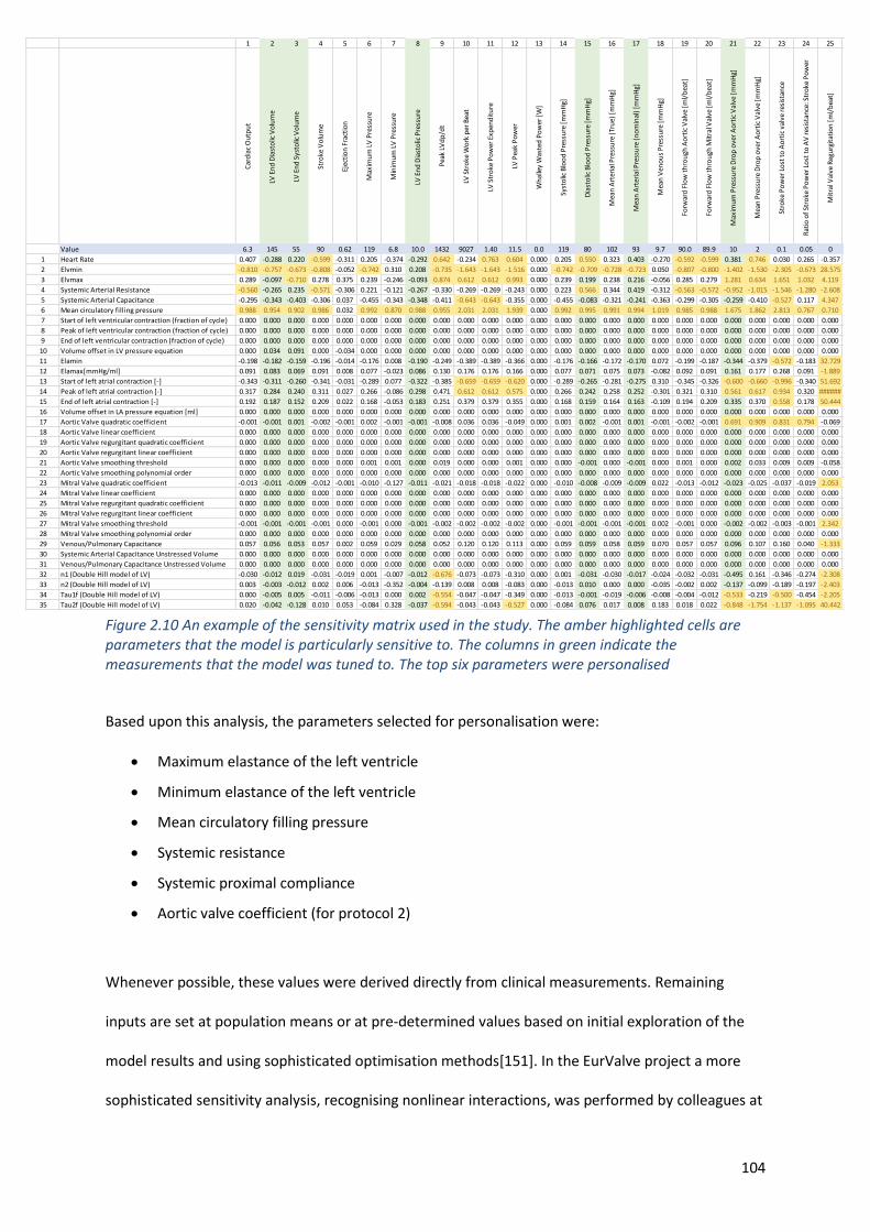
104

1 2 3 4 5 6 7 8 9 10 11 12 13 14 15 16 17 18 19 20 21 22 23 24 25 26 27 28 29 30 31 32 33 34 35 36

Car

dia

c O

utp

ut

LV E

nd

Dia

sto

lic V

olu

me

LV E

nd

Sys

tolic

Vo

lum

e

Stro

ke V

olu

me

Ejec

tio

n F

ract

ion

Max

imu

m L

V P

ress

ure

Min

imu

m L

V P

ress

ure

LV E

nd

Dia

sto

lic P

ress

ure

Pea

k LV

dp

/dt

LV S

tro

ke W

ork

per

Bea

t

LV S

tro

ke P

ow

er E

xpen

dit

ure

LV P

eak

Po

wer

Wh

alle

y W

aste

d P

ow

er [

W]

Syst

olic

Blo

od

Pre

ssu

re [

mm

Hg]

Dia

sto

lic B

loo

d P

ress

ure

[m

mH

g]

Mea

n A

rter

ial P

ress

ure

(Tr

ue)

[m

mH

g]

Mea

n A

rter

ial P

ress

ure

(n

om

inal

) [m

mH

g]

Mea

n V

eno

us

Pre

ssu

re [

mm

Hg]

Forw

ard

Flo

w t

hro

ugh

Ao

rtic

Val

ve [

ml/

bea

t]

Forw

ard

Flo

w t

hro

ugh

Mit

ral V

alve

[m

l/b

eat]

Max

imu

m P

ress

ure

Dro

p o

ver

Ao

rtic

Val

ve [

mm

Hg]

Mea

n P

ress

ure

Dro

p o

ver

Ao

rtic

Val

ve [

mm

Hg]

Stro

ke P

ow

er L

ost

to

Ao

rtic

val

ve r

esis

tan

ce

Rat

io o

f St

roke

Po

wer

Lo

st t

o A

V r

esis

tan

ce: S

tro

ke P

ow

er

Mit

ral V

alve

Reg

urg

itat

ion

[m

l/b

eat]

Mit

ral V

alve

Reg

urg

itan

t Fr

acti

on

[-]

Stro

ke P

ow

er L

ost

to

Reg

urg

itan

t M

V

Rat

io o

f St

roke

Po

wer

Lo

st t

o R

egu

rgit

ant

MV

: Str

oke

Po

wer

Ao

rtic

Val

ve R

egu

rgit

atio

n [

ml/

bea

t]

Ao

rtic

Val

ve R

egu

rgit

ant

Frac

tio

n [

-]

Stro

ke P

ow

er L

ost

to

Reg

urg

itan

t A

V

Rat

io o

f St

roke

Po

wer

Lo

st t

o R

egu

rgit

antA

V: S

tro

ke P

ow

er

Ao

rtic

Val

ve O

pen

s (t

ime

frac

tio

n)

Ao

rtic

Val

ve C

lose

s (t

ime

frac

tio

n)

Mit

ral V

alve

Op

ens

(tim

e fr

acti

on

)

Mit

ral V

alve

Clo

ses

(tim

e fr

acti

on

)

Value 6.3 145 55 90 0.62 119 6.8 10.0 1432 9027 1.40 11.5 0.0 119 80 102 93 9.7 90.0 89.9 10 2 0.1 0.05 0 0.00 0.00 0.00 0 0.00 0.00 0.00 0.065 0.398 0.498 0.977

1 Heart Rate 0.407 -0.288 0.220 -0.599 -0.311 0.205 -0.374 -0.292 0.642 -0.234 0.763 0.604 0.000 0.205 0.550 0.323 0.403 -0.270 -0.592 -0.599 0.381 0.746 0.030 0.265 -0.357 0.000 0.000 0.000 -5.248 0.000 0.000 0.000 -0.029 -0.009 -0.001 0.017

2 Elvmin -0.810 -0.757 -0.673 -0.808 -0.052 -0.742 0.310 0.208 -0.735 -1.643 -1.643 -1.516 0.000 -0.742 -0.709 -0.728 -0.723 0.050 -0.807 -0.800 -1.402 -1.530 -2.305 -0.673 28.575 0.000 0.000 0.000 2.339 0.000 0.000 0.000 0.013 0.000 0.009 -0.005

3 Elvmax 0.289 -0.097 -0.710 0.278 0.375 0.239 -0.246 -0.093 0.874 0.612 0.612 0.993 0.000 0.239 0.199 0.238 0.216 -0.056 0.285 0.279 1.281 0.634 1.651 1.032 4.119 0.000 0.000 0.000 -3.956 0.000 0.000 0.000 -1.567 -0.002 0.001 0.000

4 Systemic Arterial Resistance -0.560 -0.265 0.235 -0.571 -0.306 0.221 -0.121 -0.267 -0.330 -0.269 -0.269 -0.243 0.000 0.223 0.566 0.344 0.419 -0.312 -0.563 -0.572 -0.952 -1.015 -1.546 -1.280 -2.608 0.000 0.000 0.000 -4.053 0.000 0.000 0.000 -0.029 -0.011 -0.001 -0.001

5 Systemic Arterial Capacitance -0.295 -0.343 -0.403 -0.306 0.037 -0.455 -0.343 -0.348 -0.411 -0.643 -0.643 -0.355 0.000 -0.455 -0.083 -0.321 -0.241 -0.363 -0.299 -0.305 -0.259 -0.410 -0.527 0.117 4.347 0.000 0.000 0.000 -3.723 0.000 0.000 0.000 -0.029 -0.011 0.002 -0.001

6 Mean circulatory filling pressure 0.988 0.954 0.902 0.986 0.032 0.992 0.870 0.988 0.955 2.031 2.031 1.939 0.000 0.992 0.995 0.991 0.994 1.019 0.985 0.988 1.675 1.862 2.813 0.767 0.710 0.000 0.000 0.000 -1.312 0.000 0.000 0.000 -0.006 0.000 0.000 0.010

7 Start of left ventricular contraction (fraction of cycle) 0.000 0.000 0.000 0.000 0.000 0.000 0.000 0.000 0.000 0.000 0.000 0.000 0.000 0.000 0.000 0.000 0.000 0.000 0.000 0.000 0.000 0.000 0.000 0.000 0.000 0.000 0.000 0.000 0.000 0.000 0.000 0.000 0.000 0.000 0.000 0.000

8 Peak of left ventricular contraction (fraction of cycle) 0.000 0.000 0.000 0.000 0.000 0.000 0.000 0.000 0.000 0.000 0.000 0.000 0.000 0.000 0.000 0.000 0.000 0.000 0.000 0.000 0.000 0.000 0.000 0.000 0.000 0.000 0.000 0.000 0.000 0.000 0.000 0.000 0.000 0.000 0.000 0.000

9 End of left ventricular contraction (fraction of cycle) 0.000 0.000 0.000 0.000 0.000 0.000 0.000 0.000 0.000 0.000 0.000 0.000 0.000 0.000 0.000 0.000 0.000 0.000 0.000 0.000 0.000 0.000 0.000 0.000 0.000 0.000 0.000 0.000 0.000 0.000 0.000 0.000 0.000 0.000 0.000 0.000

10 Volume offset in LV pressure equation 0.000 0.034 0.091 0.000 -0.034 0.000 0.000 0.000 0.000 0.000 0.000 0.000 0.000 0.000 0.000 0.000 0.000 0.000 0.000 0.000 0.000 0.000 0.000 0.000 0.000 0.000 0.000 0.000 0.000 0.000 0.000 0.000 0.000 0.000 0.000 0.000

11 Elamin -0.198 -0.182 -0.159 -0.196 -0.014 -0.176 0.008 -0.190 -0.249 -0.389 -0.389 -0.366 0.000 -0.176 -0.166 -0.172 -0.170 0.072 -0.199 -0.187 -0.344 -0.379 -0.572 -0.183 32.729 0.000 0.000 0.000 -1.377 0.000 0.000 0.000 -0.010 0.000 0.009 -0.008

12 Elamax[mmHg/ml] 0.091 0.083 0.069 0.091 0.008 0.077 -0.023 0.086 0.130 0.176 0.176 0.166 0.000 0.077 0.071 0.075 0.073 -0.082 0.092 0.091 0.161 0.177 0.268 0.091 -1.889 0.000 0.000 0.000 1.057 0.000 0.000 0.000 0.007 0.000 -0.001 0.012

13 Start of left atrial contraction [-] -0.343 -0.311 -0.260 -0.341 -0.031 -0.289 0.077 -0.322 -0.385 -0.659 -0.659 -0.620 0.000 -0.289 -0.265 -0.281 -0.275 0.310 -0.345 -0.326 -0.600 -0.660 -0.996 -0.340 51.692 0.000 0.000 0.000 -2.972 0.000 0.000 0.000 -0.022 -0.001 0.015 0.170

14 Peak of left atrial contraction [-] 0.317 0.284 0.240 0.311 0.027 0.266 -0.086 0.298 0.471 0.612 0.612 0.575 0.000 0.266 0.242 0.258 0.252 -0.301 0.321 0.310 0.561 0.617 0.934 0.320 ###### 0.000 0.000 0.000 4.161 0.000 0.000 0.000 0.028 0.001 -0.001 0.592

15 End of left atrial contraction [-] 0.192 0.187 0.152 0.209 0.022 0.168 -0.053 0.183 0.251 0.379 0.379 0.355 0.000 0.168 0.159 0.164 0.163 -0.109 0.194 0.209 0.335 0.370 0.558 0.178 50.444 0.000 0.000 0.000 1.610 0.000 0.000 0.000 0.011 0.000 -0.001 0.270

16 Volume offset in LA pressure equation [ml] 0.000 0.000 0.000 0.000 0.000 0.000 0.000 0.000 0.000 0.000 0.000 0.000 0.000 0.000 0.000 0.000 0.000 0.000 0.000 0.000 0.000 0.000 0.000 0.000 0.000 0.000 0.000 0.000 0.000 0.000 0.000 0.000 0.000 0.000 0.000 0.000

17 Aortic Valve quadratic coefficient -0.001 -0.001 0.001 -0.002 -0.001 0.002 -0.001 -0.001 -0.008 0.036 0.036 -0.049 0.000 0.001 0.002 -0.001 0.001 -0.001 -0.002 -0.001 0.691 0.909 0.831 0.794 -0.069 0.000 0.000 0.000 -0.775 0.000 0.000 0.000 -0.001 0.001 0.000 0.000

18 Aortic Valve linear coefficient 0.000 0.000 0.000 0.000 0.000 0.000 0.000 0.000 0.000 0.000 0.000 0.000 0.000 0.000 0.000 0.000 0.000 0.000 0.000 0.000 0.000 0.000 0.000 0.000 0.000 0.000 0.000 0.000 0.000 0.000 0.000 0.000 0.000 0.000 0.000 0.000

19 Aortic Valve regurgitant quadratic coefficient 0.000 0.000 0.000 0.000 0.000 0.000 0.000 0.000 0.000 0.000 0.000 0.000 0.000 0.000 0.000 0.000 0.000 0.000 0.000 0.000 0.000 0.000 0.000 0.000 0.000 0.000 0.000 0.000 0.000 0.000 0.000 0.000 0.000 0.000 0.000 0.000

20 Aortic Valve regurgitant linear coefficient 0.000 0.000 0.000 0.000 0.000 0.000 0.000 0.000 0.000 0.000 0.000 0.000 0.000 0.000 0.000 0.000 0.000 0.000 0.000 0.000 0.000 0.000 0.000 0.000 0.000 0.000 0.000 0.000 0.000 0.000 0.000 0.000 0.000 0.000 0.000 0.000

21 Aortic Valve smoothing threshold 0.000 0.000 0.000 0.000 0.000 0.001 0.001 0.000 0.019 0.000 0.000 0.001 0.000 0.000 -0.001 0.000 -0.001 0.000 0.001 0.000 0.002 0.033 0.009 0.009 -0.058 0.000 0.000 0.000 1.321 0.000 0.000 0.000 0.003 0.002 0.000 0.000

22 Aortic Valve smoothing polynomial order 0.000 0.000 0.000 0.000 0.000 0.000 0.000 0.000 0.000 0.000 0.000 0.000 0.000 0.000 0.000 0.000 0.000 0.000 0.000 0.000 0.000 0.000 0.000 0.000 0.000 0.000 0.000 0.000 0.000 0.000 0.000 0.000 0.000 0.000 0.000 0.000

23 Mitral Valve quadratic coefficient -0.013 -0.011 -0.009 -0.012 -0.001 -0.010 -0.127 -0.011 -0.021 -0.018 -0.018 -0.022 0.000 -0.010 -0.008 -0.009 -0.009 0.022 -0.013 -0.012 -0.023 -0.025 -0.037 -0.019 2.053 0.000 0.000 0.000 -0.226 0.000 0.000 0.000 -0.002 0.000 0.000 0.011

24 Mitral Valve linear coefficient 0.000 0.000 0.000 0.000 0.000 0.000 0.000 0.000 0.000 0.000 0.000 0.000 0.000 0.000 0.000 0.000 0.000 0.000 0.000 0.000 0.000 0.000 0.000 0.000 0.000 0.000 0.000 0.000 0.000 0.000 0.000 0.000 0.000 0.000 0.000 0.000

25 Mitral Valve regurgitant quadratic coefficient 0.000 0.000 0.000 0.000 0.000 0.000 0.000 0.000 0.000 0.000 0.000 0.000 0.000 0.000 0.000 0.000 0.000 0.000 0.000 0.000 0.000 0.000 0.000 0.000 0.000 0.000 0.000 0.000 0.000 0.000 0.000 0.000 0.000 0.000 0.000 0.000

26 Mitral Valve regurgitant linear coefficient 0.000 0.000 0.000 0.000 0.000 0.000 0.000 0.000 0.000 0.000 0.000 0.000 0.000 0.000 0.000 0.000 0.000 0.000 0.000 0.000 0.000 0.000 0.000 0.000 0.000 0.000 0.000 0.000 0.000 0.000 0.000 0.000 0.000 0.000 0.000 0.000

27 Mitral Valve smoothing threshold -0.001 -0.001 -0.001 -0.001 0.000 -0.001 0.000 -0.001 -0.002 -0.002 -0.002 -0.002 0.000 -0.001 -0.001 -0.001 -0.001 0.002 -0.001 0.000 -0.002 -0.002 -0.003 -0.001 2.342 0.000 0.000 0.000 -0.019 0.000 0.000 0.000 0.000 0.000 0.000 0.000

28 Mitral Valve smoothing polynomial order 0.000 0.000 0.000 0.000 0.000 0.000 0.000 0.000 0.000 0.000 0.000 0.000 0.000 0.000 0.000 0.000 0.000 0.000 0.000 0.000 0.000 0.000 0.000 0.000 0.000 0.000 0.000 0.000 0.000 0.000 0.000 0.000 0.000 0.000 0.000 0.000

29 Venous/Pulmonary Capacitance 0.057 0.056 0.053 0.057 0.002 0.059 0.029 0.058 0.052 0.120 0.120 0.113 0.000 0.059 0.059 0.058 0.059 0.070 0.057 0.057 0.096 0.107 0.160 0.040 -1.333 0.000 0.000 0.000 -0.172 0.000 0.000 0.000 -0.001 0.000 -0.001 0.001

30 Systemic Arterial Capacitance Unstressed Volume 0.000 0.000 0.000 0.000 0.000 0.000 0.000 0.000 0.000 0.000 0.000 0.000 0.000 0.000 0.000 0.000 0.000 0.000 0.000 0.000 0.000 0.000 0.000 0.000 0.000 0.000 0.000 0.000 0.000 0.000 0.000 0.000 0.000 0.000 0.000 0.000

31 Venous/Pulmonary Capacitance Unstressed Volume 0.000 0.000 0.000 0.000 0.000 0.000 0.000 0.000 0.000 0.000 0.000 0.000 0.000 0.000 0.000 0.000 0.000 0.000 0.000 0.000 0.000 0.000 0.000 0.000 0.000 0.000 0.000 0.000 0.000 0.000 0.000 0.000 0.000 0.000 0.000 0.000

32 n1 (Double Hill model of LV) -0.030 -0.012 0.019 -0.031 -0.019 0.001 -0.007 -0.012 -0.676 -0.073 -0.073 -0.310 0.000 0.001 -0.031 -0.030 -0.017 -0.024 -0.032 -0.031 -0.495 0.161 -0.346 -0.274 -2.308 0.000 0.000 0.000 -1.720 0.000 0.000 0.000 1.528 0.017 -0.001 0.000

33 n2 (Double Hill model of LV) 0.003 -0.003 -0.012 0.002 0.006 -0.013 -0.352 -0.004 -0.139 0.008 0.008 -0.083 0.000 -0.013 0.010 0.000 0.000 -0.035 -0.002 0.002 -0.137 -0.099 -0.189 -0.197 -2.403 0.000 0.000 0.000 -4.819 0.000 0.000 0.000 -0.027 0.090 -0.202 0.000

34 Tau1f (Double Hill model of LV) 0.000 -0.005 0.005 -0.011 -0.006 -0.013 0.000 0.002 -0.554 -0.047 -0.047 -0.349 0.000 -0.013 -0.001 -0.019 -0.006 -0.008 -0.004 -0.012 -0.533 -0.219 -0.500 -0.454 -2.205 0.000 0.000 0.000 -4.321 0.000 0.000 0.000 -0.029 0.021 -0.001 0.000

35 Tau2f (Double Hill model of LV) 0.020 -0.042 -0.128 0.010 0.053 -0.084 0.328 -0.037 -0.594 -0.043 -0.043 -0.527 0.000 -0.084 0.076 0.017 0.008 0.183 0.018 0.022 -0.848 -1.754 -1.137 -1.095 40.442 0.000 0.000 0.000 -2.721 0.000 0.000 0.000 -0.029 0.987 1.017 0.000

Figure 2.10 An example of the sensitivity matrix used in the study. The amber highlighted cells are parameters that the model is particularly sensitive to. The columns in green indicate the measurements that the model was tuned to. The top six parameters were personalised

Based upon this analysis, the parameters selected for personalisation were:

• Maximum elastance of the left ventricle

• Minimum elastance of the left ventricle

• Mean circulatory filling pressure

• Systemic resistance

• Systemic proximal compliance

• Aortic valve coefficient (for protocol 2)

Whenever possible, these values were derived directly from clinical measurements. Remaining

inputs are set at population means or at pre-determined values based on initial exploration of the

model results and using sophisticated optimisation methods[151]. In the EurValve project a more

sophisticated sensitivity analysis, recognising nonlinear interactions, was performed by colleagues at

105

the Technical University of Eindhoven, but in this case it confirmed the selection indicated by this

simpler process.

2.4.1.2.4. Modelling in the exercise state

As discussed previously, modelling has the advantage of being predictive and simulations can be run

to predict the effect of exercise on the patient’s physiology. By extending the model to consider

exercise, predictions can then be made about the patient’s expected exercise capacity post

intervention which could be used to help counsel the patient. This was achieved using data from the

six-minute walk test and Philips Health Watch (see sections 2.4.1.2.5 and 2.4.1.2.6). A number of the

parameters in the model change under exercise conditions. Work by Professor Hose (see appendix

iv) allowed application of 0D models to study exercise physiology and enable extrapolation from a

model tuned in the rest state to the exercise state This work was based on studies by Chantler[190]

and Bombardini[191] who studied the effects of exercise on several parameters relevant to the

model, including heart rate, left ventricular end systolic elastance, arterial elastance and systemic

resistance. The exercise state could be modelled in protocols 2-4.

2.4.1.2.5. Combining activity data

Equations were derived for the parameters in the model under exercise conditions (see appendix iv).

Using these patient specific exercise states could be modelled. This was performed using activity

data obtained during the study. The true rest state of the patient (Metabolic equivalent (MET)=1)

could be extrapolated backwards from the examination state using the resting heart rate from the

Philips Health Watch (see section 2.5.3).

(Heart Rate_exercise) = (0.7464∙(PWR)_exercise+1)∙(Heart Rate_rest) Eq. 2.15

106

Power-to-weight ratio (PWR) was calculated from the level of activity achieved by the patient. The

maximum elastance, arterial elastance and capacitance was then personalised. The exercise capacity

of the patient in terms of METS was calculated from the six-minute walk test and the true rest state

of the patient from the Philips Health Watch. This activity data was used to personalise the rest

exercise state pre-intervention. Rest states (MET=1) were used to compare pre and post

intervention.

The predictive post-intervention exercise capacitance in terms of METs can be compared with the

measured activity levels for the patients in the study (see section 3.9.4).

2.4.1.2.6. Modelling after intervention

In the predicted post-intervention data several assumptions were made. It was assumed that, when

symptoms develop in severe AS, the heart is working at (or close to) its maximum capacity. It was

also assumed that, following an intervention, if required, the heart could work as hard as it did

before the intervention. The energy initially wasted in overcoming the resistance of the stenotic

valve could then be converted to useful energy and the increase in exercise capacity could then be

calculated. In the model, the cardiac work was therefore fixed following intervention and

extrapolated backwards using the exercise formula (section 2.4.1.2.4 and appendix iv). Maximum

activity levels after intervention could then be predicted. Following intervention, either through

homeostatic mechanisms or medical therapy, there would be an effort to maintain mean arterial

pressure and therefore organ perfusion. The coefficients of the implanted aortic valve were used;

these were derived from the stated indexed EOA of each valve implanted (see appendix iv) and the

valve coefficient personalised for each patient to model the post intervention state.

107

2.4.2. Three-dimensional valve model

The model is highly sensitive to the input of peak pressure gradient across the valve (see section

2.4.1.2.3.). Therefore, an accurate assessment of this parameter is critical. As discussed there are

number of limitations in using echocardiography to assess peak pressure gradient (see sections

1.4.2.1 and 1.11.5). A local 3D valve model using segmented medical images and CFD can accurately

define the pressure flow relationship through the valve overcoming many of these limitations. A 3D

valve model was therefore developed using the steps described below.

2.4.2.1. Segmentation and mesh formation

Segmentation is the process of identifying and separating areas of interest from clinical images.

Geometric representations of structures from which data can be extracted can then be

reconstructed. These define the physical bounds of the region of interest in the model. If images are

acquired over a cardiac cycle the process needs to be dynamic and track anatomical motion or, as in

the case of this project, be captured during a specific cardiac phase. This required ECG gating and the

images used were those where the aortic valve was maximally open. This process results in a

parameterised model of the aortic valve with few values that describe the aortic valve. Trained

software identifies the edges of structures and a generic mesh is adapted; this is a method of

‘simulated search’ [182]. A shape-constrained deformable model which relies upon a pre-defined

shape space, with deviations allowed to give flexibility, is used to segment the areas of interest. This

works with the different imaging modalities (CT and echocardiography) that are used in this project.

The rest of the heart and other valve anatomy may be captured by additional post-processing steps

that extract information from the segmentation results - such as chamber volumes, annulus

dimensions and aortic valve area.

108

A mesh was formed by dividing the geometry into a number of discrete volumetric elements or cells.

With flow problems which are unsteady, solutions are required where the position is a function of

time. Temporal discretisation involves the integration of terms in different equations over a time

step. This is required as the numerical stability and accuracy of the analysis are influenced by both

temporal- and spatial-refinement[183]. The mesh and time-step captured the important

haemodynamic behaviour of the valve with the final solution independent of the mesh parameters.

Highly refined meshes were needed to produce more accurate results, especially in regions with high

pressure and flow gradients such as in AS but this was at the expense of increased simulation times.

2.4.2.2. Computational fluid dynamics

The segmented valve and geometries of the inflow and outflow tracts from either 3D TOE or CT

image acquisitions were used to run CFD simulations using ANSYS Fluent software (ANSYS Inc.

Pennsylvania, United States). The CFD software solves the steady state equations of fluid flow

(Navier-Stokes and continuity) in three dimensions using the conservation form of the finite volume

method. Inputs to the CFD simulation are the pressure volume relationship described by the time

varying elastance model, the radius of the valve and the valve stenosis severity described by the 11

parameters given by the segmentation process, the outputs being the pressure flow relationship in

the aorta.

A steady-flow protocol was used to achieve an adequate representation of valve characteristics.

Gorlin and Gorlin have shown that the pulsatility of flow can be ignored and that equations that are

derived from steady flow through fixed orifices are adequate to predict effective orifice area[145].

The analysis enabled the computation of the pressure gradient across the aortic valve as a function

of the flow, allowing implementation in a clinically oriented workflow. An outlet section was created

by the extrusion of a distal plane of the segmented ascending aorta, by a distance of six equivalent

diameters along the local tangent to the centre line. The inlet boundary condition was the flow, or

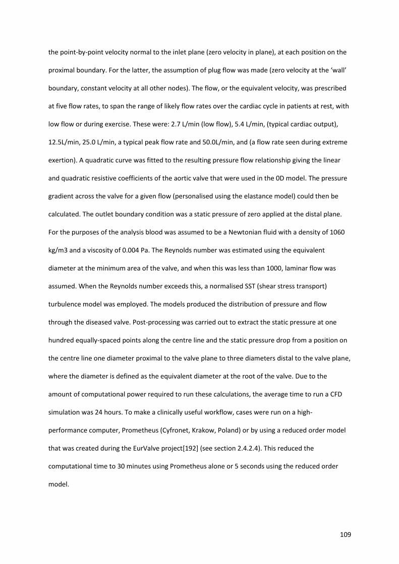
109

the point-by-point velocity normal to the inlet plane (zero velocity in plane), at each position on the

proximal boundary. For the latter, the assumption of plug flow was made (zero velocity at the ‘wall’

boundary, constant velocity at all other nodes). The flow, or the equivalent velocity, was prescribed

at five flow rates, to span the range of likely flow rates over the cardiac cycle in patients at rest, with

low flow or during exercise. These were: 2.7 L/min (low flow), 5.4 L/min, (typical cardiac output),

12.5L/min, 25.0 L/min, a typical peak flow rate and 50.0L/min, and (a flow rate seen during extreme

exertion). A quadratic curve was fitted to the resulting pressure flow relationship giving the linear

and quadratic resistive coefficients of the aortic valve that were used in the 0D model. The pressure

gradient across the valve for a given flow (personalised using the elastance model) could then be

calculated. The outlet boundary condition was a static pressure of zero applied at the distal plane.

For the purposes of the analysis blood was assumed to be a Newtonian fluid with a density of 1060

kg/m3 and a viscosity of 0.004 Pa. The Reynolds number was estimated using the equivalent

diameter at the minimum area of the valve, and when this was less than 1000, laminar flow was

assumed. When the Reynolds number exceeds this, a normalised SST (shear stress transport)

turbulence model was employed. The models produced the distribution of pressure and flow

through the diseased valve. Post-processing was carried out to extract the static pressure at one

hundred equally-spaced points along the centre line and the static pressure drop from a position on

the centre line one diameter proximal to the valve plane to three diameters distal to the valve plane,

where the diameter is defined as the equivalent diameter at the root of the valve. Due to the

amount of computational power required to run these calculations, the average time to run a CFD

simulation was 24 hours. To make a clinically useful workflow, cases were run on a high-

performance computer, Prometheus (Cyfronet, Krakow, Poland) or by using a reduced order model

that was created during the EurValve project[192] (see section 2.4.2.4). This reduced the

computational time to 30 minutes using Prometheus alone or 5 seconds using the reduced order

model.

110

2.4.2.3. Boundary conditions

Boundary conditions are applied physiological parameters (which may vary over time) that define

the physical conditions at the inlets and outlets within the model. Inlet and outlet boundaries

conditions must be specified and precisely representing the physiological behaviour at the

boundaries of a model is critical to its accuracy. In this study they were based on patient specific

data, population data, lower order physical models such as the elastance model and OD models

described above. Where possible individual patient data will be used in preference to ensure the

modelling process is as personalised as possible.

.

2.4.2.4. Reduced order models derived from 3D models

A reduced order model (ROM) was used in the clinical decision support tool to enable near real-time

processing. This was made available by ANSYS (ANSYS Inc., Canonsburg, PA, United States) and

provides approximate values for CFD simulations for an individual patient using pre-computed CFD

results in what can be described as a giant look-up table. As mentioned previously, the aortic valve

can be described by just a few parameters, for example; annulus diameter, aortic valve area, valve

aortic angle. All permutations can be created in advance to run CFD simulations. When a valve is

segmented, the precomputed results from the CFD simulations can be found instantaneously for a

valve the same as, or extremely similar to, those of that patient. This serves to substitute the lengthy

CFD calculations that would be impractical in a clinical setting.

2.4.3. Analysis protocols

Four protocols were developed of varying complexity. This was to enable all cases to be processed

even if there were missing data and medical images could not be segmented accurately. It also

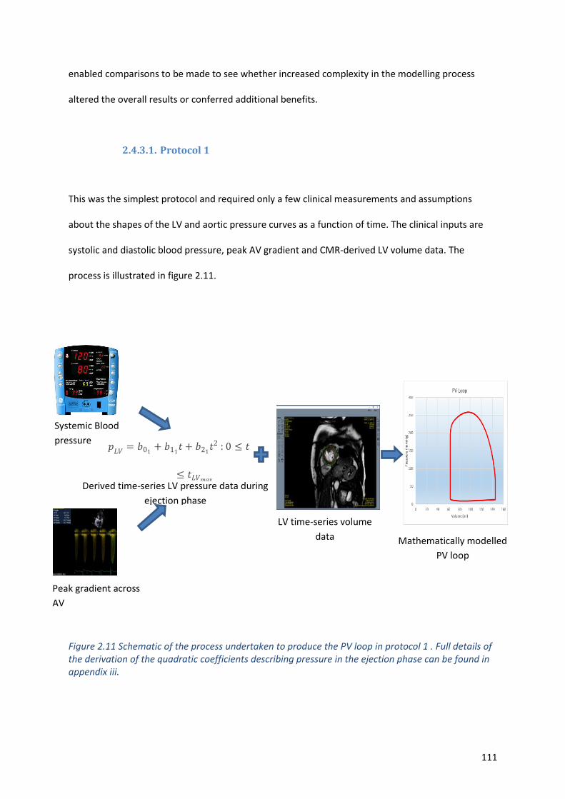
111

enabled comparisons to be made to see whether increased complexity in the modelling process

altered the overall results or conferred additional benefits.

2.4.3.1. Protocol 1

This was the simplest protocol and required only a few clinical measurements and assumptions

about the shapes of the LV and aortic pressure curves as a function of time. The clinical inputs are

systolic and diastolic blood pressure, peak AV gradient and CMR-derived LV volume data. The

process is illustrated in figure 2.11.

Figure 2.11 Schematic of the process undertaken to produce the PV loop in protocol 1 . Full details of the derivation of the quadratic coefficients describing pressure in the ejection phase can be found in appendix iii.

Systemic Blood

pressure

𝑝𝐿𝑉

= 𝑏01+ 𝑏11

𝑡 + 𝑏21𝑡2 : 0 ≤ 𝑡

≤ 𝑡𝐿𝑉𝑚𝑎𝑥

Peak gradient across

AV

Derived time-series LV pressure data during

ejection phase

LV time-series volume

data Mathematically modelled

PV loop

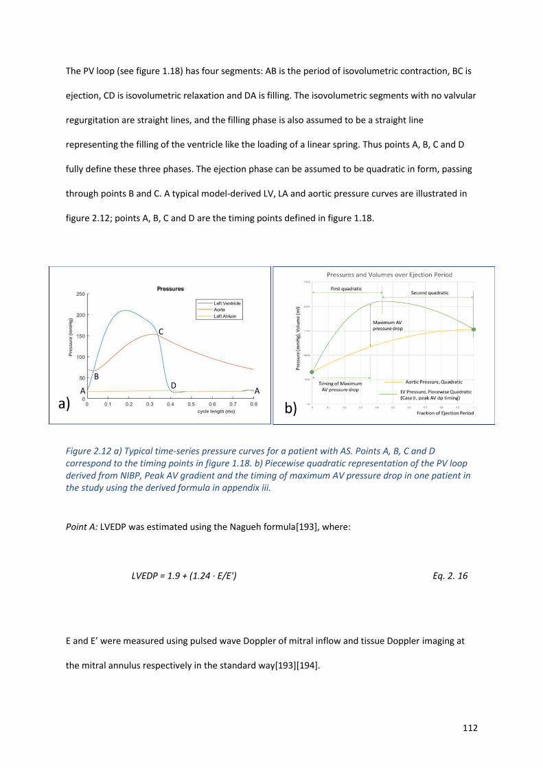
112

The PV loop (see figure 1.18) has four segments: AB is the period of isovolumetric contraction, BC is

ejection, CD is isovolumetric relaxation and DA is filling. The isovolumetric segments with no valvular

regurgitation are straight lines, and the filling phase is also assumed to be a straight line

representing the filling of the ventricle like the loading of a linear spring. Thus points A, B, C and D

fully define these three phases. The ejection phase can be assumed to be quadratic in form, passing

through points B and C. A typical model-derived LV, LA and aortic pressure curves are illustrated in

figure 2.12; points A, B, C and D are the timing points defined in figure 1.18.

Figure 2.12 a) Typical time-series pressure curves for a patient with AS. Points A, B, C and D correspond to the timing points in figure 1.18. b) Piecewise quadratic representation of the PV loop derived from NIBP, Peak AV gradient and the timing of maximum AV pressure drop in one patient in the study using the derived formula in appendix iii.

Point A: LVEDP was estimated using the Nagueh formula[193], where:

LVEDP = 1.9 + (1.24 · E/E') Eq. 2. 16

E and E’ were measured using pulsed wave Doppler of mitral inflow and tissue Doppler imaging at

the mitral annulus respectively in the standard way[193][194].

cycle length (ms)

Pre

ssu

re (

mm

Hg

)

113

Points B and C: Points B (aortic valve opening) and C (aortic valve closing) occur when the aortic and

ventricular pressures cross over. The pressure at point B is the minimum pressure in the aorta. The

maximum pressure in the aorta might exceed that at point C but the curve illustrated is typical and

the maximum aortic pressure and is a reasonable estimate of that. Minimum and maximum aortic

pressures were taken to be diastolic and systolic cuff pressures measured at the time of imaging. An

average of three brachial artery pressures was taken using a GE Carescape V100 dinamap (GE

Healthcare, Boston, USA).

Point D: The mitral valve opens, and the LV starts to fill. This can be extrapolated from the LVEDP ,

knowing the volume intercept at a pressure of 0mmHg, from the literature [195], [196].

Segment BC: The shape of the aortic pressure curve during the ejection phase is reasonably

represented by a quadratic equation passing through the points of crossover with the ventricular

pressure curve and with the maximum at the end of the ejection phase. The LV pressure in the

ejection phase, illustrated in figure 2.12b, is assumed to be piecewise quadratic in form, passing

through points B and C and with a specified (measured, echocardiography) peak AV gradient.

Detailed derivation of the quadratic coefficients defining the ejection phase is presented in appendix

iii.

2.4.3.2. Protocol 2

Protocol 2 utilised the methods described in section 2.4.1 to describe the aortic valve and

circulation. Contraction of the heart chambers was represented by the elastance model with Mynard

constants[189]. The aortic valve quadratic coefficient in this protocol is added to the parameters to

be personalised based upon a measurement of the gradient through the aortic valve using the 2D

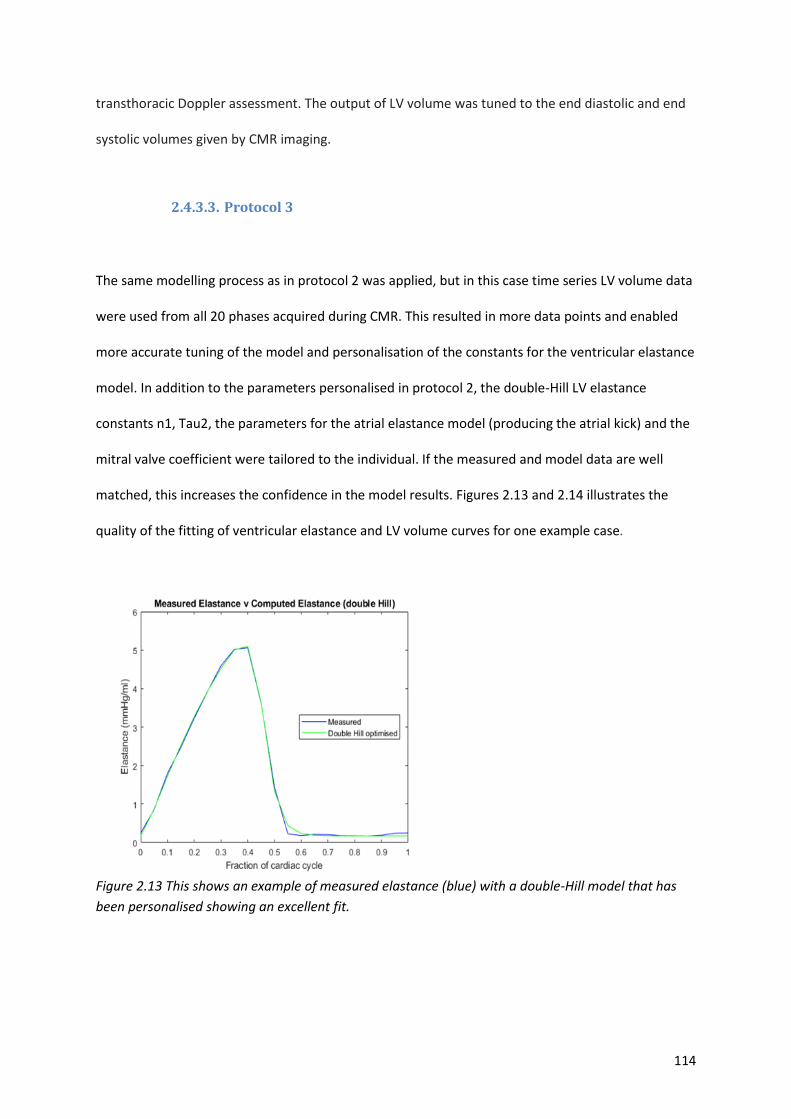
114

transthoracic Doppler assessment. The output of LV volume was tuned to the end diastolic and end

systolic volumes given by CMR imaging.

2.4.3.3. Protocol 3

The same modelling process as in protocol 2 was applied, but in this case time series LV volume data

were used from all 20 phases acquired during CMR. This resulted in more data points and enabled

more accurate tuning of the model and personalisation of the constants for the ventricular elastance

model. In addition to the parameters personalised in protocol 2, the double-Hill LV elastance

constants n1, Tau2, the parameters for the atrial elastance model (producing the atrial kick) and the

mitral valve coefficient were tailored to the individual. If the measured and model data are well

matched, this increases the confidence in the model results. Figures 2.13 and 2.14 illustrates the

quality of the fitting of ventricular elastance and LV volume curves for one example case.

Figure 2.13 This shows an example of measured elastance (blue) with a double-Hill model that has

been personalised showing an excellent fit.

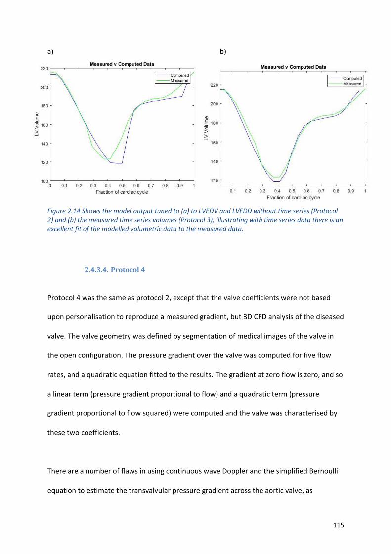
115

a) b)

Figure 2.14 Shows the model output tuned to (a) to LVEDV and LVEDD without time series (Protocol 2) and (b) the measured time series volumes (Protocol 3), illustrating with time series data there is an excellent fit of the modelled volumetric data to the measured data.

2.4.3.4. Protocol 4

Protocol 4 was the same as protocol 2, except that the valve coefficients were not based

upon personalisation to reproduce a measured gradient, but 3D CFD analysis of the diseased

valve. The valve geometry was defined by segmentation of medical images of the valve in

the open configuration. The pressure gradient over the valve was computed for five flow

rates, and a quadratic equation fitted to the results. The gradient at zero flow is zero, and so

a linear term (pressure gradient proportional to flow) and a quadratic term (pressure

gradient proportional to flow squared) were computed and the valve was characterised by

these two coefficients.

There are a number of flaws in using continuous wave Doppler and the simplified Bernoulli

equation to estimate the transvalvular pressure gradient across the aortic valve, as

116

discussed previously. Imaged-based segmentation and CFD assessment could overcome

some of them[42]. Using images of the aortic valve acquired from either CT or TOE, the

aortic valve was segmented along with the LVOT and the proximal aorta, when the valve

was maximally open. Using CFD modelling with Ansys Fluent™ software, and the boundary

conditions described by the 0D model ( personalised elastance model and the systemic

vascular resistance), an image-based gradient across the diseased valve for the individual

patient was produced.

2.4.4. Summary of processing steps for modelling protocols 2-4.

The primary modelling protocol, followed for each individual recruited to the study, was as follows:

1) Seven key clinical observations, including heart rate, were recorded for the individual at the

time of image acquisition for LV volumes and 6MWT assessment (the examination state).

2) Personalisation of the parameters in the mathematical model to represent the individual in

the examination state was performed.

3) Derived parameters including left ventricular stroke work and power, wasted energy and

minimum and maximum LV elastance from the pressure-volume loop were computed in the

examination state.

4) Based upon published associations in the literature and measurements of the patient heart

rate during the observation period prior to intervention, extrapolation to represent the true

rest state and an activity state reflecting what the patient actually achieved was undertaken.

5) Derived model parameters in rest and active states were computed.

6) Virtual intervention was performed, replacing the valve coefficient for the diseased valve

with a coefficient representative of a candidate valve for a prospective intervention. It was

not expected that there would be a significant change in mean arterial pressure (MAP) post-

117

intervention, either because of autoregulation or medical therapy, the MAP for the post-

intervention rest state was fixed to the pre-intervention level.

7) Predicted parameters in the post-intervention rest state were computed.

8) These parameters were extrapolated to predict the activity state for the post-intervention

condition assuming that heart rate is the same as the pre-intervention level.

9) Derived parameters in the active state post-intervention.

10) As a further extension, derived parameters were computed in the active state under an

alternative hypothesis that left ventricular work rather than heart rate is maintained post

intervention (to address the question of how much more flow might be generated by the

heart for the same work expenditure).

2.4.5. Validation

In our cohort, ten patients underwent TAVI implantation. It is routine practice to cross the valve and

obtain LV pressures prior to valve deployment, so PV loops with invasive pressure data and volume

data obtained from CMR were produced to validate the protocols. Cardiac catheterisation was

performed using standard techniques via the femoral artery (14). 7-french pigtail catheters were

placed in the aortic root and the left ventricular (LV) cavity and simultaneous pressures were

recorded[179]. Analysis was performed by the Xper CardioFlex system (Philips Healthcare, The

Netherlands). Although MRI measured LV volumes are more accurate than assessment by

conductance catheter[180], [181] they were not performed simultaneously. Therefore, they were

normalised for cardiac cycle length and pressure data synchronised with the LV volume data. The PV

loops were produced in Microsoft Excel™ with the following parameters calculated:

- Stroke work

- Stroke power

- Peak power

118

- Wasted energy

- Maximum LV elastance

- Minimum LV elastance

The accuracy of personalisation of the model was assessed by calculating the standard error of the

modelled parameters that were tuned from measured data (peak pressure gradient across the valve,

EDV, ESV, diastolic blood pressure and mean arterial pressure).

Protocol 4 (the coupled 0D-3D model) was used in cases in which there was a high level of

confidence in the clinical data and when an accurate segmentation of the valve was possible. This

was a clinical judgement made by the author after assessing the data, the quality of the imaging and

comparing the segmented valve geometries to the appearance of the valve in the raw image data

(see sections 3.2.2 and 3.2.3). This quality control check was introduced as the segmentation process

is crucial to obtaining accurate results in this model and had the greatest potential for the

introduction of error. The multiscale model results included the peak gradient of the aortic valve,

which is completely image and model dependent, not measured using ultrasound. Comparing the

results of the model in terms of pressure gradient with the pressure gradient obtained by ultrasound

formed the basis of validation in this protocol. When the model results predicted post-intervention

gradients and activity levels these were correlated with measured data to assess the predictive

capabilities of the model.

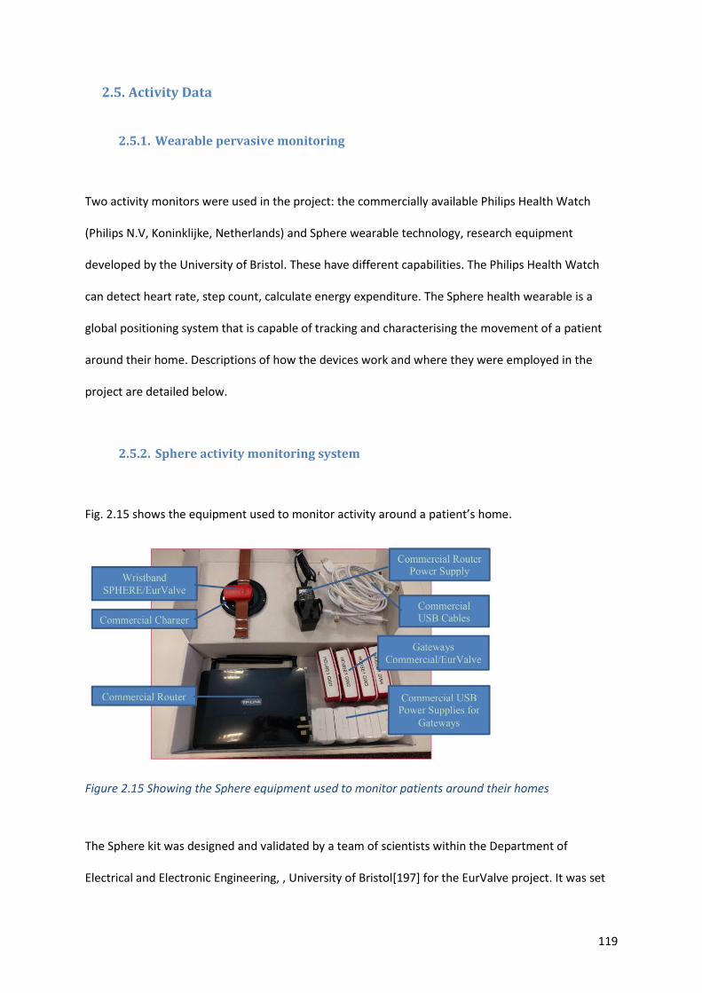
119

2.5. Activity Data

2.5.1. Wearable pervasive monitoring

Two activity monitors were used in the project: the commercially available Philips Health Watch

(Philips N.V, Koninklijke, Netherlands) and Sphere wearable technology, research equipment

developed by the University of Bristol. These have different capabilities. The Philips Health Watch

can detect heart rate, step count, calculate energy expenditure. The Sphere health wearable is a

global positioning system that is capable of tracking and characterising the movement of a patient

around their home. Descriptions of how the devices work and where they were employed in the

project are detailed below.

2.5.2. Sphere activity monitoring system

Fig. 2.15 shows the equipment used to monitor activity around a patient’s home.

Figure 2.15 Showing the Sphere equipment used to monitor patients around their homes

The Sphere kit was designed and validated by a team of scientists within the Department of

Electrical and Electronic Engineering, , University of Bristol[197] for the EurValve project. It was set

120

up, calibrated and data collected by the author in the homes of the 22 patients with AS. The

wristband uses a piezo-electric tri-axial accelerometer and communicates with ‘Gateways’ using

Bluetooth low energy giving a received signal strength indicator (RSSI). Each Gateway has a different

RSSI that is roughly correlated with distance. ‘Gateways’ communicated with the router using a Wi-Fi

connection, transmitting hourly, which allowed near real time monitoring to ensure that, they were

functioning, and that data were being collected. It also gave information regarding the battery status

of the wristbands so patients could be advised regarding charging. Data were copied from the SD

card, within each ‘Gateway,’ and transmitted securely every night to servers at the University of

Bristol providing a safety-net to prevent data loss. The data from the SD card were manually

downloaded and then uploaded to a secure cloud space. The raw data were downloaded and

processed by Ryan McConville (Computer Scientist, University of Bristol) using training data and

algorithms that had been specifically developed and data on step count, room transfers within the

house, time outside the house and number of times the patient exited the house were recorded and

transferred back to the author in a CSV file for analysis. Verbal and written instructions were given to

the patients to help them use the equipment (see appendix v). Since many of the patients were

unwell and elderly, they required help setting the equipment up, which entailed multiple patient

visits. Due to the limited number of equipment kits (10) and the 66 periods of monitoring required,

the kits were retrieved, and data downloaded after each two-week period. Patients were advised to

wear the wristband 24 hours a day for a minimum of 14 days during each of the three phases of the

study, taking it off when bathing or showering and charging it at that time. This duration was

considered to be adequate in order to gain insight into a patient’s daily routine.

2.5.3. Philips Health Watch

The Philips health watch is a commercially available product that can continuously track activity. It

has FDA approval for medical use after being tested against a number of reference standards [198].

121

The device uses a piezo-electric tri-axial accelerometer to measure motion, similar to the Sphere

wristband, and green light-emitting diodes and a photodiode to create a photoplethysmogram. The

accelerometer output and the photoplethysmogram signal are analysed to determine heartbeat,

activity type, steps taken, and are used as input for estimation of energy expenditure when the

patient’s weight and height are programmed into the watch. Patients were asked to wear the watch

for 24 hours a day for 14 days, coinciding with the Sphere wristband. The watch was pre-programed

for each patient and therefore required no set up by them. Other than wearing the watch with good

skin contact only charging the watch via the USB charger was required.

Using an iPod™ with a software application supplied and installed by Philips Research Centre,

Eindhoven, it was possible to communicate with the watch, uploading patient characteristics such as

age, height, weight and resting heart rate for the estimations of energy expenditure and it was also

possible to use this application to download the data from the watch. Raw data were processed by

HH (Philips Research, Eindhoven) and graphs and CSV files were produced from which the analysis

was performed. After experimenting with the devices, it was found that the watch could hold

approximately 14 days of data on its internal memory, after which the previously stored data was

overwritten; for this reason, the watch was retrieved at the same time as the Sphere equipment and

data downloaded at that point.

2.5.4. Six-minute walk test

The 6MWT is a validated clinical tool. Based on our population demographic, it was selected to

measure activity as opposed to the exercise tolerance test. This has previously been used to assess

severity of AS and the response to treatment in a number of studies[117], [199], [200]. The tests

were carried out according to the guidelines outlined by the American Thoracic Society[201]. All

122

tests were performed by the author at the same location to avoid bias. Patients who had poor

mobility either prior to intervention or after intervention did not undergo the 6MWT at that stage.

The 6MWT was performed at baseline and used as an input to the model to simulate exercise

conditions and then repeated four months following intervention. The post-intervention result was

then compared with the predicted exercise capacity from the model. Distance recorded during a

standard 6MWT [202]was converted into METs using the formula METs = [0.1 x speed (m∙min-1) +

3.5mLO2∙kg∙min-1] ÷ 3.5mLO2∙kg∙min-1 [203]. These data were used as an input to model the

exercise state; the extrapolation was based on previous published data (see appendix iv). Predicted

6MWT performance was calculated for each patient and used to compare their activity with an

average age, gender, height and weight matched population prior to intervention and following

valve replacement. To calculate the predicted 6MWT distance the following validated formulae were

used[204]–[206].

For male participants:

6MWT distance (m) = (7.57 × height(cm) – (5.02 × age) – (1.76 × weight(kg)) – 309 Eq.2. 17

Lower limit of normal = Distance walked – 153

For female participants:

6MWT distance(m) = (2.11 × height(cm) – (2.29 × weight(kg)) – (5.78 × age) + 66 Eq. 2. 18

Lower limit of normal = Distance walked – 139

The results were recorded on a data sheet and entered onto the ArQ database. Metrics recorded

included: The predicted distance, the achieved distance, the converted metabolic equivalent, a Borg

scale assessment of effort reported by the patient, the pre- and post-test heart rate, blood pressure

and O2 saturations.

123

2.6. Patient reported measures

2.6.1. Minnesota ‘living with heart failure’ questionnaire

This questionnaire has been validated for use with patients with valvular heart disease undergoing

treatment[207] [208]; therefore it was used in this cohort. Physical, emotional, and social items were

totalled separately using a previously validated method[209]. Scores were calculated pre- and post -

intervention. Patients were asked to complete the questionnaire at the pre-intervention visit and

again at 3-4 months following intervention. A comparison was made between the patient reported

physical activity and the objective active measurements made from the 6MWT and with the

pervasive activity monitoring.

2.6.2. World Health Organization Quality of Life—abbreviated version of the

WHOQOL 100 (WHOQOL_BREF)

Symptoms are key to determining treatment strategy and since the patient’s view of the disease,

and the impact of the disease is now thought to be of the utmost importance, a second quality of life

questionnaire (WHOQOL- BREF) was administered in conjunction with the Minnesota ‘living with

heart failure’ questionnaire. This questionnaire was developed to reflect cultural differences of the

patient cohort with quality of life defined as the “individuals' perceptions of their position in life in

the context of the culture and value systems in which they live and in relation to their goals,

expectations, standards and concerns”[210]. The WHOQOL- BREF questionnaire was selected as it

assesses other aspects of life such as financial status, the home environment and access to

healthcare, which is not covered in the Minnesota ‘living with heart failure’ questionnaire. Again, the

results are given as a total quality of life score which is broken down into four domains: physical

health, psychological, social relationships and environment. As before, this was compared with other

metrics that measured the physical activity of the patient.

124

2.7. Development of a clinical decision support system

The content of the clinical decision support system was decided upon by a clinical panel, including

the author, that was part of the EurValve Consortium. The design and creation of the CDSS was

developed in conjunction with Therenva (Rennes, France) as an extension of their already existing

product, Endosize™ [211]. It incorporates clinical and imaging data with data from wearable activity

monitoring devices, parameters from the modelling process as a result of the work in this thesis. It

also includes clinical guidelines from the European Society of Cardiology, commonly used risk scores

and a case-based reasoning tool. Case-based reasoning uses complex statistical analysis (beyond the

scope of this thesis) to search a database of cases of AS that have previously undergone surgery with

the outcome of that intervention recorded to find a case that is similar to the details that were

entered. It returns ‘cases like yours’ with a similarity index and details what happened to the patient

in that scenario. The tool was developed and validated by a team at the University of Rennes, France

[212]as a wider part of the EurValve project. The platform allows clinicians to run different

simulations at the bedside or clinic, such as assessment of patient haemodynamics during exercise

or assessing treatment effects such as the reducing blood pressure or replacing the valve.

The content and presentation of the decision support tool is illustrated below.

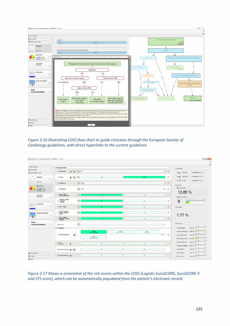
125

Figure 2.16 Illustrating CDSS flow chart to guide clinicians through the European Society of Cardiology guidelines, with direct hyperlinks to the current guidelines.

Figure 2.17 Shows a screenshot of the risk scores within the CDSS (Logistic EuroSCORE, EuroSCORE II and STS score), which can be automatically populated from the patient’s electronic record.

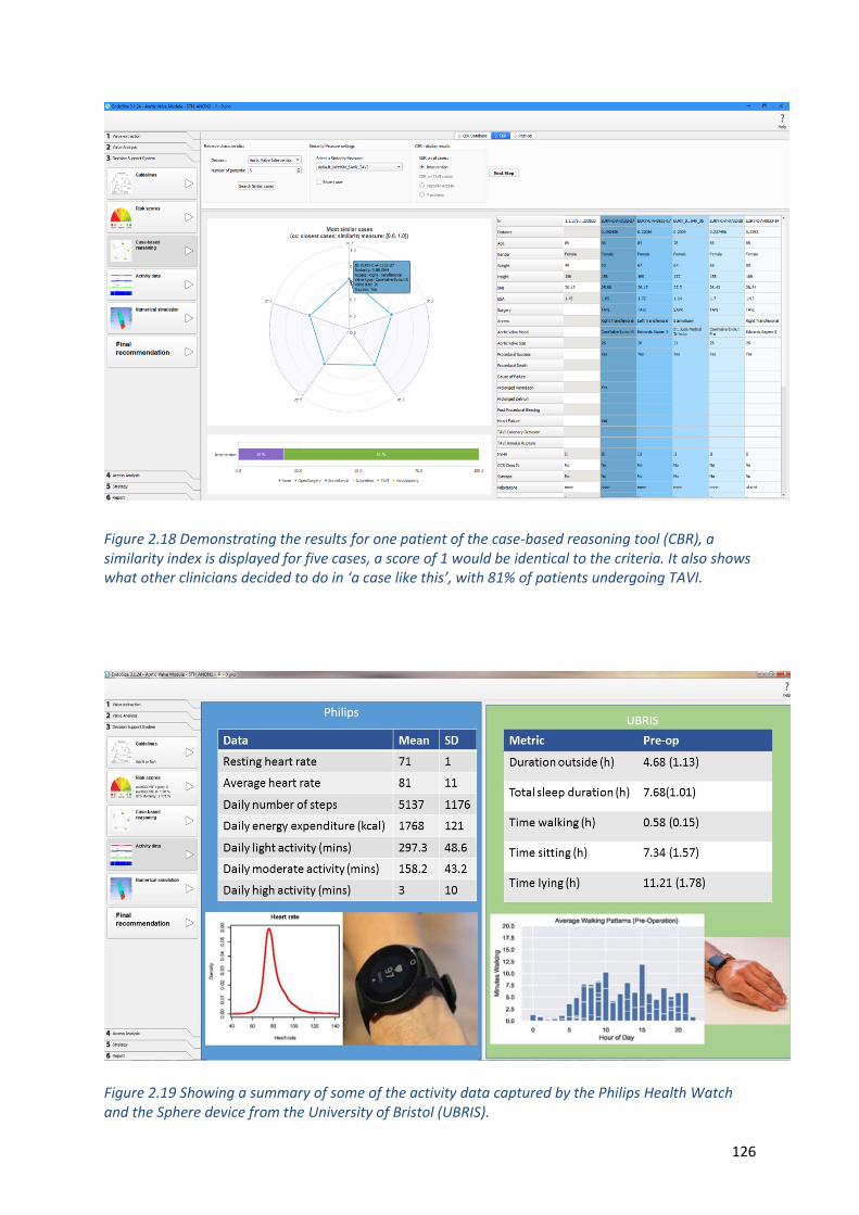
126

Figure 2.18 Demonstrating the results for one patient of the case-based reasoning tool (CBR), a similarity index is displayed for five cases, a score of 1 would be identical to the criteria. It also shows what other clinicians decided to do in ‘a case like this’, with 81% of patients undergoing TAVI.

Figure 2.19 Showing a summary of some of the activity data captured by the Philips Health Watch and the Sphere device from the University of Bristol (UBRIS).

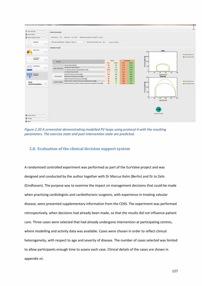
127

Figure 2.20 A screenshot demonstrating modelled PV loops using protocol 4 with the resulting parameters. The exercise state and post-intervention state are predicted.

2.8. Evaluation of the clinical decision support system

A randomised controlled experiment was performed as part of the EurValve project and was

designed and conducted by the author together with Dr Marcus Kelm (Berlin) and Dr Jo Zelis

(Eindhoven). The purpose was to examine the impact on management decisions that could be made

when practising cardiologists and cardiothoracic surgeons, with experience in treating valvular

disease, were presented supplementary information from the CDSS. The experiment was performed

retrospectively, when decisions had already been made, so that the results did not influence patient

care. Three cases were selected that had already undergone intervention at participating centres,

where modelling and activity data was available. Cases were chosen in order to reflect clinical

heterogeneity, with respect to age and severity of disease. The number of cases selected was limited

to allow participants enough time to assess each case. Clinical details of the cases are shown in

appendix vii.

128

For each case, two datasets were produced. The first dataset (control) included conventional clinical

information and imaging data currently recommended as standard diagnostic work-up in clinical

practice guidelines. The second dataset (experimental) included information from the decision

support system.

The study was powered to identify the difference in decisions made between the experimental and

control group and required at least 36 participants. This was based on a predicted effect of 10%

difference between the two groups in terms of the primary endpoint. Given the lack of similar

evaluations in the literature, this could not be based on previous empirical studies. Cardiologists and

cardiothoracic surgeons were eligible for inclusion in the study if they had frequent exposure to

patients with valvular heart disease. Pilot testing was conducted by cardiologists who were members

of the EurValve project, to ensure readability and interpretability of the case summaries and

accompanying questions. Each centre sought a minimum of 12 participants. Each participant

reviewed cases selected at random. Whether study participants received the first or second dataset

was dependent on their group allocation, as described below. The randomised controlled trial design

was used to improve the internal validity of the study. We used a web-based survey platform

(JotForm, JotForm Inc. San Francisco, CA, USA) for participants to record their decisions and views of

the CDSS. This was selected based on reliability, ease of creation, and ease of use and collection of

responses.

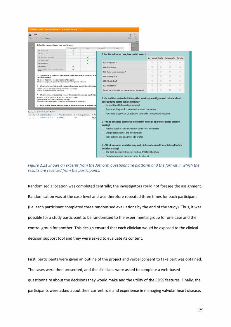
129

Figure 2.21 Shows an excerpt from the JotForm questionnaire platform and the format in which the results are received from the participants.

Randomised allocation was completed centrally; the investigators could not foresee the assignment.

Randomisation was at the case-level and was therefore repeated three times for each participant

(i.e. each participant completed three randomised evaluations by the end of the study). Thus, it was

possible for a study participant to be randomized to the experimental group for one case and the

control group for another. This design ensured that each clinician would be exposed to the clinical

decision support tool and they were asked to evaluate its content.

First, participants were given an outline of the project and verbal consent to take part was obtained.

The cases were then presented, and the clinicians were asked to complete a web-based

questionnaire about the decisions they would make and the utility of the CDSS features. Finally, the

participants were asked about their current role and experience in managing valvular heart disease.

130

Questions were devised to explore participants’ willingness to recommend intervention in the

presented cases depending upon the type of information presented to them (experimental vs.

control). Participants were first asked whether they felt there was a guideline for intervention for

each case and then whether they would intervene or not based on the information presented. The

primary endpoint was “decision to intervene”, referring to a clinician decision to recommend either

surgery or catheter lab (collectively, “intervention”) as opposed to follow-up with or without

medication (“no intervention”). Each of the participants were then asked to rank the utility of each

component of the CDSS.

2.9. Statistical analyses

2.9.1. Protocol comparisons and validation

Statistical analysis was carried out using IBM SPSS® Statistics version 25 software. Results of the

three protocols are presented in tables with means and standard deviations. Due the limited data

for comparison protocol 4 was analysed separately and differences between this and measured data

were explored. Differences between the protocols were analysed using Friedman’s statistical test in

non-parametric data and one-way ANOVA for parametric testing. Where there were missing data, a

mixed-effects analysis was performed. A value of P<0.05 was used to define a significant difference.

Any significant differences between the protocols were investigated with either Dunn’s or Holm-

Sidak’s tests for pairwise comparisons, to identify which protocol differed. Residual (standard errors)

from the model optimisation process were calculated using MATLAB version R2018B.

2.9.2. Correlations between modelled and measured

Pearson or Spearman correlations were reported depending upon the normality of the data. Level of

agreement was deemed poor for intra-class correlation coefficient in the range of 0.00 to 0.30, weak

131

between 0.31 and 0.50, moderate between 0.51 and 0.70, strong between 0.71 and 0.90, and

excellent between 0.91 and 1.0 [213].

2.9.3. 4D flow data

Statistical analysis was carried out with IBM SPSS® Statistics version 25 software. Continuous

measurements are presented as median with interquartile ranges (IQR). Normality of data was

assessed by the Shapiro–Wilk test. Given the non-normal distribution of the data, a paired

nonparametric two-tailed test (Wilcoxon signed-rank test) was used for paired analysis. The Mann-

Whitney test was used for all continuous variables to compare differences between two different

procedure options of the aortic valve replacement (TAVI and SAVR), for categorical variables, P-value

was calculated using Chi-squared T-Test. Correlation between variables was assessed using the

Spearman correlation coefficient (rho), a value of P < 0.05 was considered significant.

Comparison of variables amongst different NYHA classes was performed using Kruskal-Wallis H test.

A Jonckheere-Terpstra test was carried out to find which specific groups of these independent

variables were significantly different from each other. Results with a P values of < 0.05 were

considered statistically significant.

2.9.4. Evaluation of clinical decision support system.

Descriptive statistics were used to compare the experimental and control groups at baseline.

Differences between study groups in terms of outcomes were then evaluated using Fisher’s exact

test for proportions, and chi square analysis with categories adjusted to avoid cells with <5 expected

values. Statistical significance was defined as a P value of <0.05 assuming a 2-tailed hypothesis. All

132

analyses were repeated for sub-groups according to the experience level of participants. Statistical

analyses were performed in STATA (version 14; STATA Corp LLC, College Station, TX, USA).

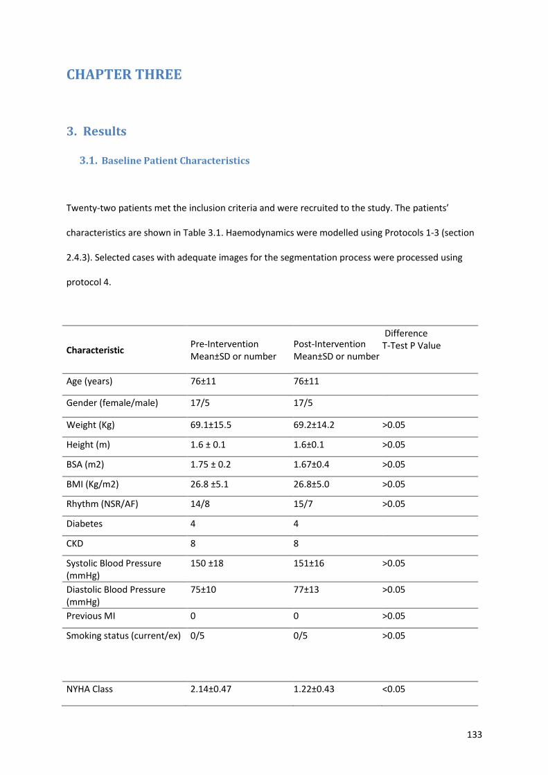
133

CHAPTER THREE

3. Results

3.1. Baseline Patient Characteristics

Twenty-two patients met the inclusion criteria and were recruited to the study. The patients’

characteristics are shown in Table 3.1. Haemodynamics were modelled using Protocols 1-3 (section

2.4.3). Selected cases with adequate images for the segmentation process were processed using

protocol 4.

Characteristic Pre-Intervention Mean±SD or number

Post-Intervention Mean±SD or number

Difference T-Test P Value

Age (years) 76±11 76±11

Gender (female/male) 17/5 17/5

Weight (Kg) 69.1±15.5 69.2±14.2 >0.05

Height (m) 1.6 ± 0.1 1.6±0.1 >0.05

BSA (m2) 1.75 ± 0.2 1.67±0.4 >0.05

BMI (Kg/m2) 26.8 ±5.1 26.8±5.0 >0.05

Rhythm (NSR/AF) 14/8 15/7 >0.05

Diabetes 4 4

CKD 8 8

Systolic Blood Pressure (mmHg)

150 ±18 151±16 >0.05

Diastolic Blood Pressure (mmHg)

75±10 77±13 >0.05

Previous MI 0 0 >0.05

Smoking status (current/ex) 0/5 0/5 >0.05

NYHA Class 2.14±0.47 1.22±0.43 <0.05

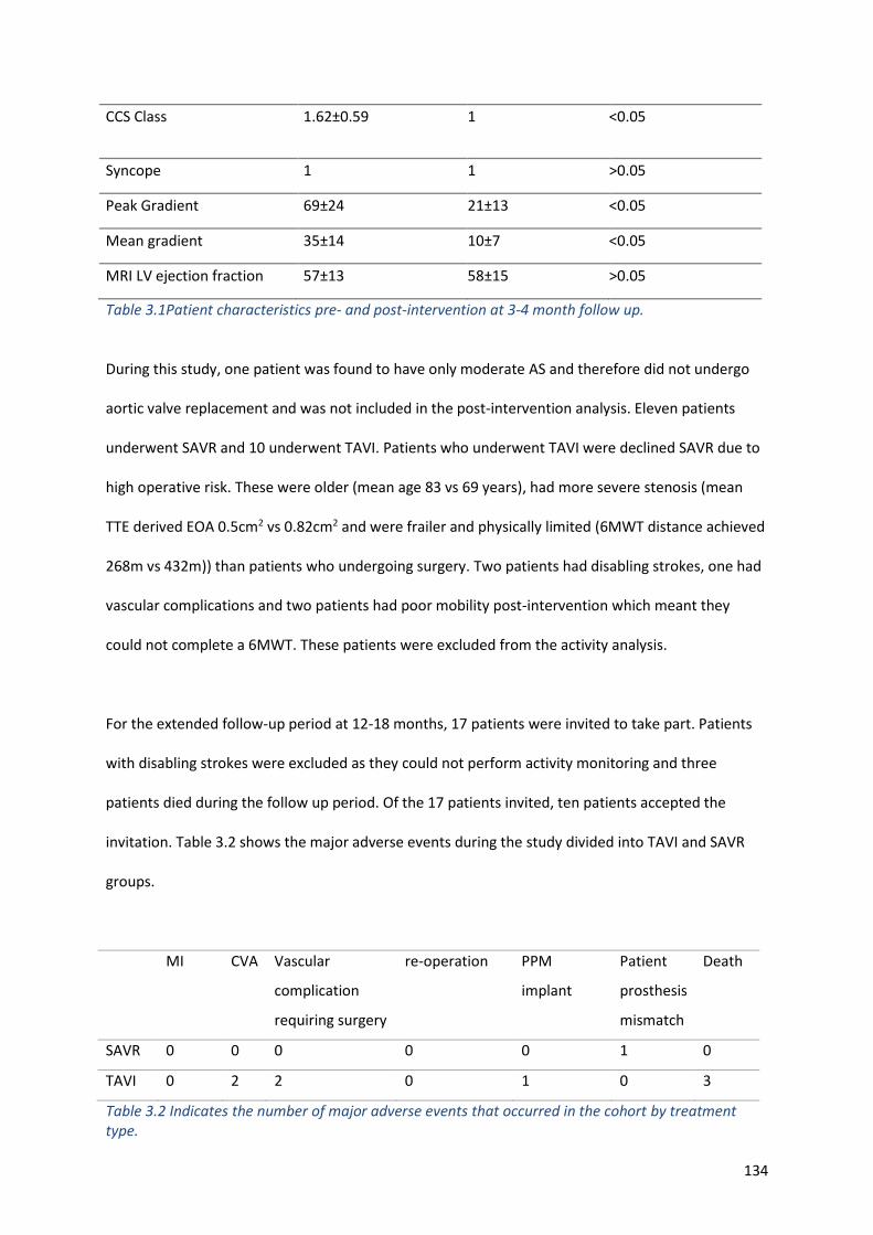
134

CCS Class 1.62±0.59 1 <0.05

Syncope 1 1 >0.05

Peak Gradient 69±24 21±13 <0.05

Mean gradient 35±14 10±7 <0.05

MRI LV ejection fraction 57±13 58±15 >0.05

Table 3.1Patient characteristics pre- and post-intervention at 3-4 month follow up.

During this study, one patient was found to have only moderate AS and therefore did not undergo

aortic valve replacement and was not included in the post-intervention analysis. Eleven patients

underwent SAVR and 10 underwent TAVI. Patients who underwent TAVI were declined SAVR due to

high operative risk. These were older (mean age 83 vs 69 years), had more severe stenosis (mean

TTE derived EOA 0.5cm2 vs 0.82cm2 and were frailer and physically limited (6MWT distance achieved

268m vs 432m)) than patients who undergoing surgery. Two patients had disabling strokes, one had

vascular complications and two patients had poor mobility post-intervention which meant they

could not complete a 6MWT. These patients were excluded from the activity analysis.

For the extended follow-up period at 12-18 months, 17 patients were invited to take part. Patients

with disabling strokes were excluded as they could not perform activity monitoring and three

patients died during the follow up period. Of the 17 patients invited, ten patients accepted the

invitation. Table 3.2 shows the major adverse events during the study divided into TAVI and SAVR

groups.

MI CVA Vascular

complication

requiring surgery

re-operation PPM

implant

Patient

prosthesis

mismatch

Death

SAVR 0 0 0 0 0 1 0

TAVI 0 2 2 0 1 0 3

Table 3.2 Indicates the number of major adverse events that occurred in the cohort by treatment type.

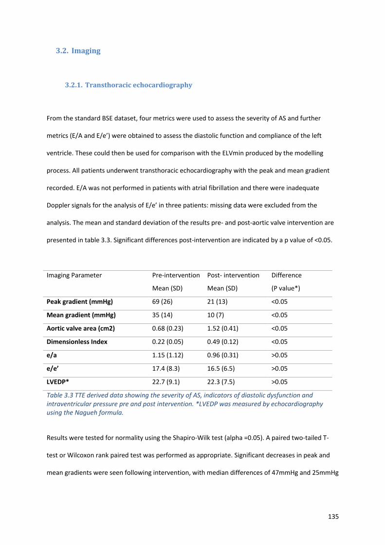
135

3.2. Imaging

3.2.1. Transthoracic echocardiography

From the standard BSE dataset, four metrics were used to assess the severity of AS and further

metrics (E/A and E/e’) were obtained to assess the diastolic function and compliance of the left

ventricle. These could then be used for comparison with the ELVmin produced by the modelling

process. All patients underwent transthoracic echocardiography with the peak and mean gradient

recorded. E/A was not performed in patients with atrial fibrillation and there were inadequate

Doppler signals for the analysis of E/e’ in three patients: missing data were excluded from the

analysis. The mean and standard deviation of the results pre- and post-aortic valve intervention are

presented in table 3.3. Significant differences post-intervention are indicated by a p value of <0.05.

Imaging Parameter Pre-intervention

Mean (SD)

Post- intervention

Mean (SD)

Difference

(P value*)

Peak gradient (mmHg) 69 (26) 21 (13) <0.05

Mean gradient (mmHg) 35 (14) 10 (7) <0.05

Aortic valve area (cm2) 0.68 (0.23) 1.52 (0.41) <0.05

Dimensionless Index 0.22 (0.05) 0.49 (0.12) <0.05

e/a 1.15 (1.12) 0.96 (0.31) >0.05

e/e’ 17.4 (8.3) 16.5 (6.5) >0.05

LVEDP* 22.7 (9.1) 22.3 (7.5) >0.05

Table 3.3 TTE derived data showing the severity of AS, indicators of diastolic dysfunction and intraventricular pressure pre and post intervention. *LVEDP was measured by echocardiography using the Nagueh formula.

Results were tested for normality using the Shapiro-Wilk test (alpha =0.05). A paired two-tailed T-

test or Wilcoxon rank paired test was performed as appropriate. Significant decreases in peak and

mean gradients were seen following intervention, with median differences of 47mmHg and 25mmHg

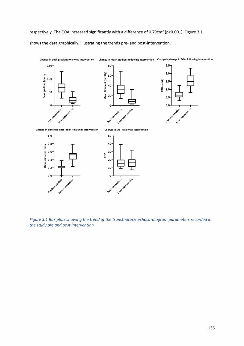
136

respectively. The EOA increased significantly with a difference of 0.79cm2 (p<0.001). Figure 3.1

shows the data graphically, illustrating the trends pre- and post-intervention.

Pre-In

terv

entio

n

Post in

terv

entio

n

0

50

100

150

Change in peak gradient following intervention

Pe

ak

grad

ien

t (m

mH

g)

Pre-In

terv

entio

n

Post in

terv

entio

n

0

20

40

60

80

Change in mean gradient following intervention

Me

an

Gra

die

nt

(mm

Hg)

Pre-In

terv

entio

n

Post i

nterv

entio

n

0.0

0.5

1.0

1.5

2.0

2.5

Change in change in EOA following intervention

EO

A (

cm

2)

Pre-In

terv

entio

n

Post in

terv

entio

n

0.0

0.2

0.4

0.6

0.8

1.0

Change in dimensionless index following intervention

Dim

en

sio

nle

ss in

de

x

Pre-In

terv

entio

n

Post in

terv

entio

n

0

10

20

30

40

50

Change in E/e' following intervention

E/e

'

Figure 3.1 Box plots showing the trend of the transthoracic echocardiogram parameters recorded in the study pre and post intervention.

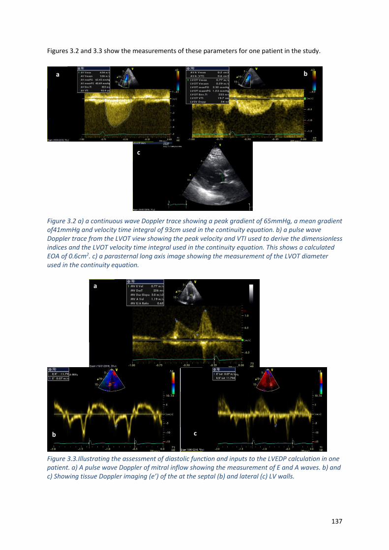
137

Figures 3.2 and 3.3 show the measurements of these parameters for one patient in the study.

Figure 3.2 a) a continuous wave Doppler trace showing a peak gradient of 65mmHg, a mean gradient of41mmHg and velocity time integral of 93cm used in the continuity equation. b) a pulse wave Doppler trace from the LVOT view showing the peak velocity and VTI used to derive the dimensionless indices and the LVOT velocity time integral used in the continuity equation. This shows a calculated EOA of 0.6cm2. c) a parasternal long axis image showing the measurement of the LVOT diameter used in the continuity equation.

.

Figure 3.3.Illustrating the assessment of diastolic function and inputs to the LVEDP calculation in one patient. a) A pulse wave Doppler of mitral inflow showing the measurement of E and A waves. b) and c) Showing tissue Doppler imaging (e’) of the at the septal (b) and lateral (c) LV walls.

a

b c

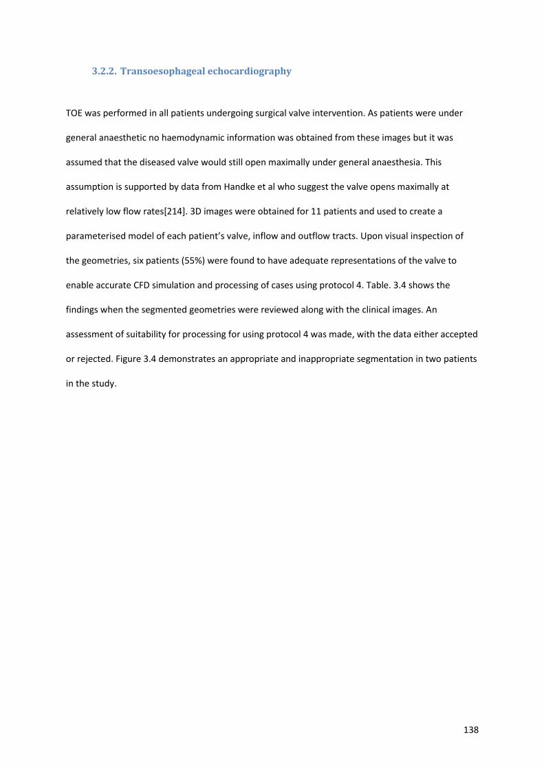
138

3.2.2. Transoesophageal echocardiography

TOE was performed in all patients undergoing surgical valve intervention. As patients were under

general anaesthetic no haemodynamic information was obtained from these images but it was

assumed that the diseased valve would still open maximally under general anaesthesia. This

assumption is supported by data from Handke et al who suggest the valve opens maximally at

relatively low flow rates[214]. 3D images were obtained for 11 patients and used to create a

parameterised model of each patient’s valve, inflow and outflow tracts. Upon visual inspection of

the geometries, six patients (55%) were found to have adequate representations of the valve to

enable accurate CFD simulation and processing of cases using protocol 4. Table. 3.4 shows the

findings when the segmented geometries were reviewed along with the clinical images. An

assessment of suitability for processing for using protocol 4 was made, with the data either accepted

or rejected. Figure 3.4 demonstrates an appropriate and inappropriate segmentation in two patients

in the study.

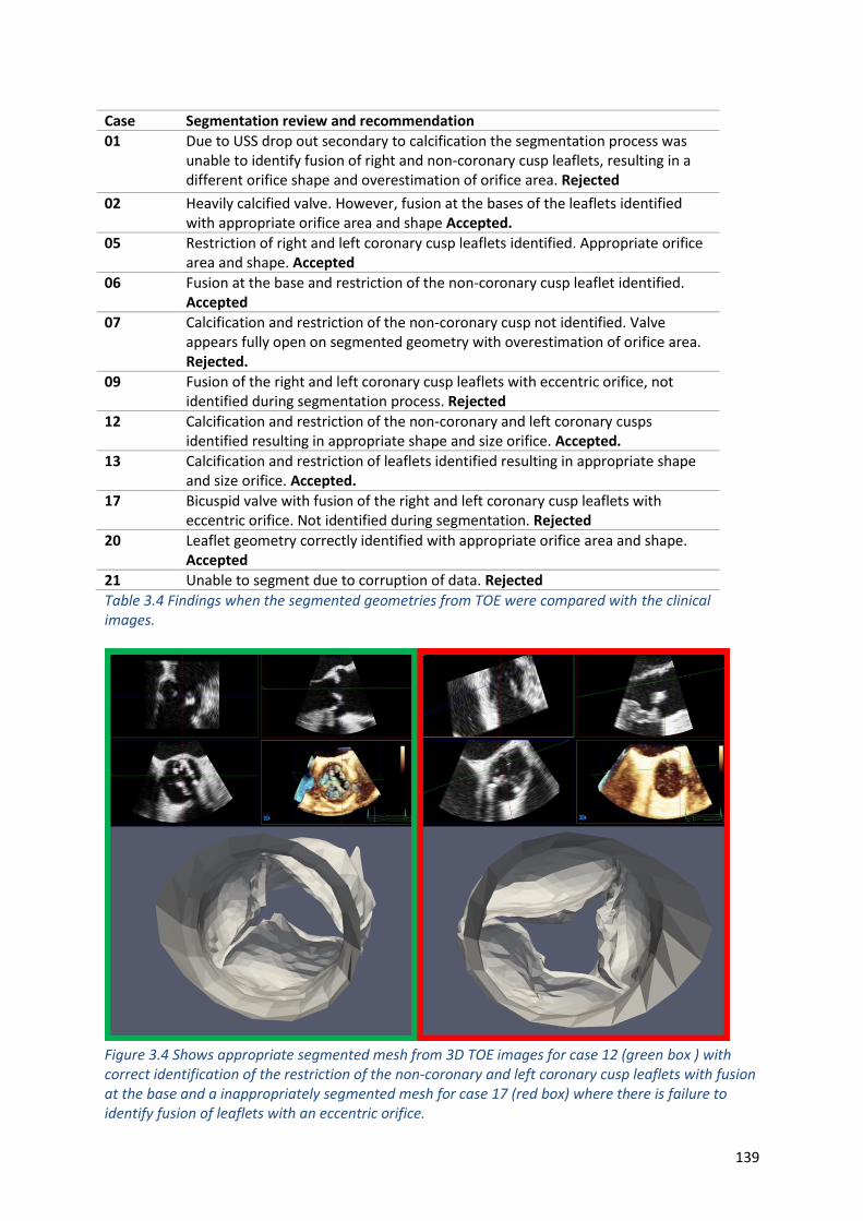
139

Table 3.4 Findings when the segmented geometries from TOE were compared with the clinical images.

Figure 3.4 Shows appropriate segmented mesh from 3D TOE images for case 12 (green box ) with correct identification of the restriction of the non-coronary and left coronary cusp leaflets with fusion at the base and a inappropriately segmented mesh for case 17 (red box) where there is failure to identify fusion of leaflets with an eccentric orifice.

Case Segmentation review and recommendation

01 Due to USS drop out secondary to calcification the segmentation process was unable to identify fusion of right and non-coronary cusp leaflets, resulting in a different orifice shape and overestimation of orifice area. Rejected

02 Heavily calcified valve. However, fusion at the bases of the leaflets identified with appropriate orifice area and shape Accepted.

05 Restriction of right and left coronary cusp leaflets identified. Appropriate orifice area and shape. Accepted

06 Fusion at the base and restriction of the non-coronary cusp leaflet identified. Accepted

07 Calcification and restriction of the non-coronary cusp not identified. Valve appears fully open on segmented geometry with overestimation of orifice area. Rejected.

09 Fusion of the right and left coronary cusp leaflets with eccentric orifice, not identified during segmentation process. Rejected

12 Calcification and restriction of the non-coronary and left coronary cusps identified resulting in appropriate shape and size orifice. Accepted.

13 Calcification and restriction of leaflets identified resulting in appropriate shape and size orifice. Accepted.

17 Bicuspid valve with fusion of the right and left coronary cusp leaflets with eccentric orifice. Not identified during segmentation. Rejected

20 Leaflet geometry correctly identified with appropriate orifice area and shape. Accepted

21 Unable to segment due to corruption of data. Rejected

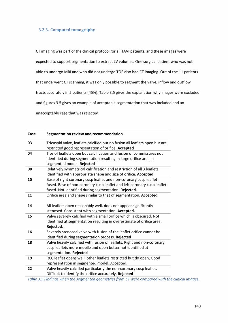
140

3.2.3. Computed tomography

CT imaging was part of the clinical protocol for all TAVI patients, and these images were

expected to support segmentation to extract LV volumes. One surgical patient who was not

able to undergo MRI and who did not undergo TOE also had CT imaging. Out of the 11 patients

that underwent CT scanning, it was only possible to segment the valve, inflow and outflow

tracts accurately in 5 patients (45%). Table 3.5 gives the explanation why images were excluded

and figures 3.5 gives an example of acceptable segmentation that was included and an

unacceptable case that was rejected.

Case Segmentation review and recommendation

03 Tricuspid valve, leaflets calcified but no fusion all leaflets open but are restricted good representation of orifice. Accepted

04 Tips of leaflets open but calcification and fusion of commissures not identified during segmentation resulting in large orifice area in segmented model. Rejected

08 Relatively symmetrical calcification and restriction of all 3 leaflets identified with appropriate shape and size of orifice. Accepted

10 Base of right coronary cusp leaflet and non-coronary cusp leaflet fused. Base of non-coronary cusp leaflet and left coronary cusp leaflet fused. Not identified during segmentation. Rejected.

11 Orifice area and shape similar to that of segmentation. Accepted

14 All leaflets open reasonably well, does not appear significantly stenosed. Consistent with segmentation. Accepted.

15 Valve severely calcified with a small orifice which is obscured. Not identified at segmentation resulting in overestimate of orifice area. Rejected.

16 Severely stenosed valve with fusion of the leaflet orifice cannot be identified during segmentation process. Rejected

18 Valve heavily calcified with fusion of leaflets. Right and non-coronary cusp leaflets more mobile and open better not identified at segmentation. Rejected

19 RCC leaflet opens well, other leaflets restricted but do open, Good representation in segmented model. Accepted.

22 Valve heavily calcified particularly the non-coronary cusp leaflet. Difficult to identify the orifice accurately. Rejected

Table 3.5 Findings when the segmented geometries from CT were compared with the clinical images.

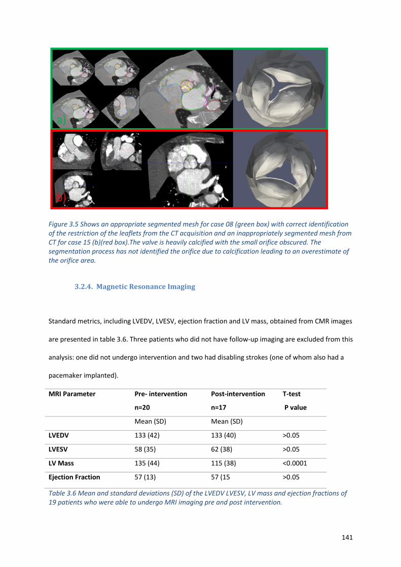
141

Figure 3.5 Shows an appropriate segmented mesh for case 08 (green box) with correct identification of the restriction of the leaflets from the CT acquisition and an inappropriately segmented mesh from CT for case 15 (b)(red box).The valve is heavily calcified with the small orifice obscured. The segmentation process has not identified the orifice due to calcification leading to an overestimate of the orifice area.

3.2.4. Magnetic Resonance Imaging

Standard metrics, including LVEDV, LVESV, ejection fraction and LV mass, obtained from CMR images

are presented in table 3.6. Three patients who did not have follow-up imaging are excluded from this

analysis: one did not undergo intervention and two had disabling strokes (one of whom also had a

pacemaker implanted).

MRI Parameter Pre- intervention

n=20

Post-intervention

n=17

T-test

P value

Mean (SD) Mean (SD)

LVEDV 133 (42) 133 (40) >0.05

LVESV 58 (35) 62 (38) >0.05

LV Mass 135 (44) 115 (38) <0.0001

Ejection Fraction 57 (13) 57 (15 >0.05

Table 3.6 Mean and standard deviations (SD) of the LVEDV LVESV, LV mass and ejection fractions of 19 patients who were able to undergo MRI imaging pre and post intervention.

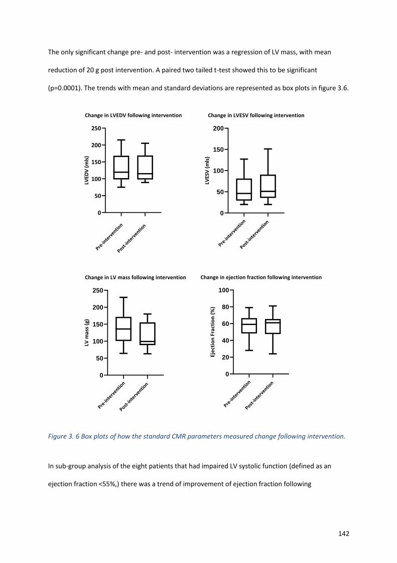
142

The only significant change pre- and post- intervention was a regression of LV mass, with mean

reduction of 20 g post intervention. A paired two tailed t-test showed this to be significant

(p=0.0001). The trends with mean and standard deviations are represented as box plots in figure 3.6.

Pre-in

terv

ention

Post-in

terv

ention

0

50

100

150

200

250

Change in LVEDV following intervention

LVED

V (

mls

)

Pre-in

terv

ention

Post-in

terv

ention

0

50

100

150

200

Change in LVESV following intervention

LVES

V (

mls

)

Pre-in

terv

ention

Post-in

terv

ention

0

50

100

150

200

250

Change in LV mass following intervention

LV m

ass

(g)

Pre-in

terv

ention

Post-in

terv

ention

0

20

40

60

80

100

Change in ejection fraction following intervention

Eje

ctio

n F

ract

ion

(%

)

Figure 3. 6 Box plots of how the standard CMR parameters measured change following intervention.

In sub-group analysis of the eight patients that had impaired LV systolic function (defined as an

ejection fraction <55%,) there was a trend of improvement of ejection fraction following

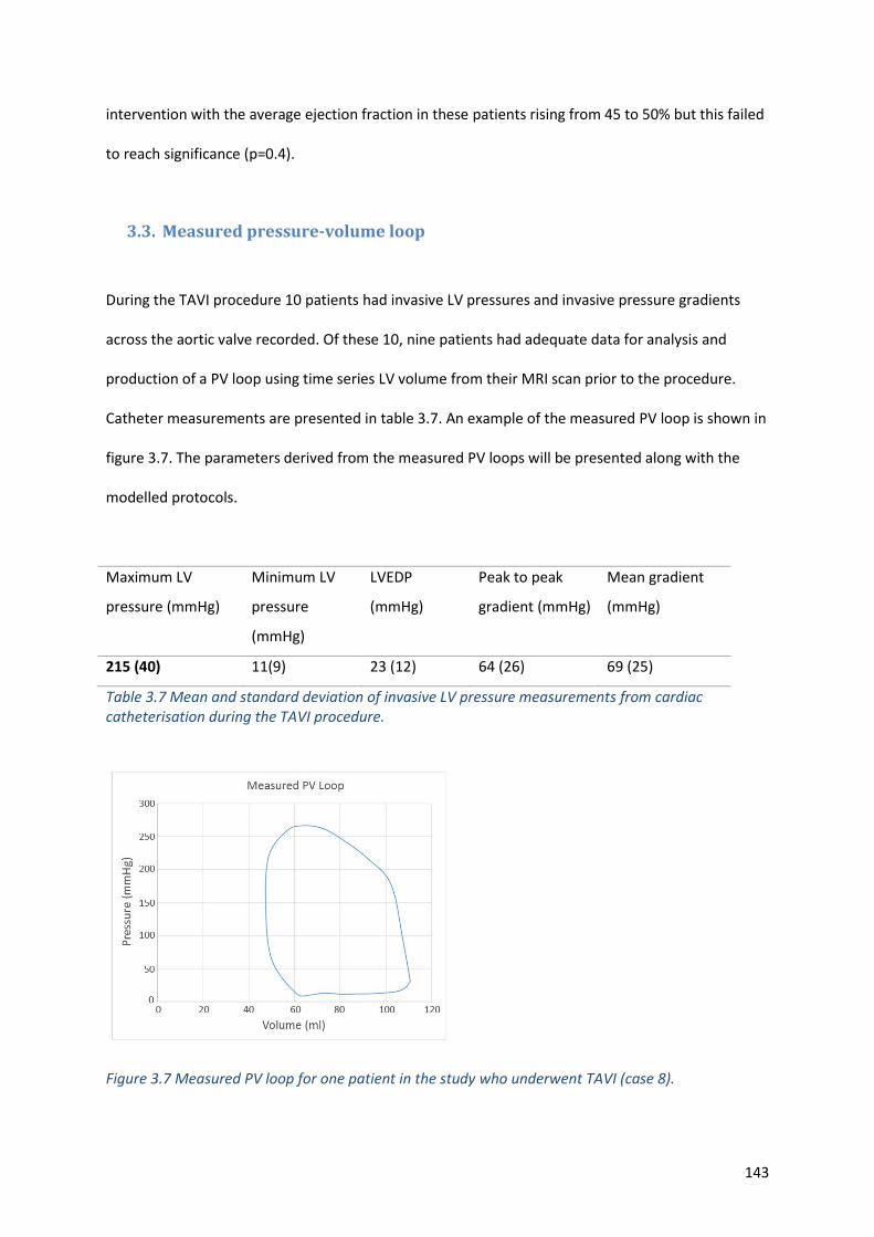
143

intervention with the average ejection fraction in these patients rising from 45 to 50% but this failed

to reach significance (p=0.4).

3.3. Measured pressure-volume loop

During the TAVI procedure 10 patients had invasive LV pressures and invasive pressure gradients

across the aortic valve recorded. Of these 10, nine patients had adequate data for analysis and

production of a PV loop using time series LV volume from their MRI scan prior to the procedure.

Catheter measurements are presented in table 3.7. An example of the measured PV loop is shown in

figure 3.7. The parameters derived from the measured PV loops will be presented along with the

modelled protocols.

Maximum LV

pressure (mmHg)

Minimum LV

pressure

(mmHg)

LVEDP

(mmHg)

Peak to peak

gradient (mmHg)

Mean gradient

(mmHg)

215 (40) 11(9) 23 (12) 64 (26) 69 (25)

Table 3.7 Mean and standard deviation of invasive LV pressure measurements from cardiac catheterisation during the TAVI procedure.

Figure 3.7 Measured PV loop for one patient in the study who underwent TAVI (case 8).

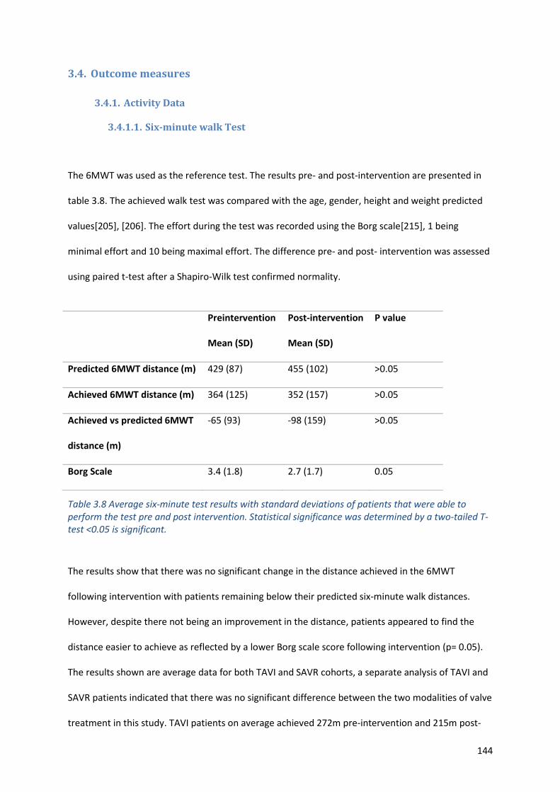
144

3.4. Outcome measures

3.4.1. Activity Data

3.4.1.1. Six-minute walk Test

The 6MWT was used as the reference test. The results pre- and post-intervention are presented in

table 3.8. The achieved walk test was compared with the age, gender, height and weight predicted

values[205], [206]. The effort during the test was recorded using the Borg scale[215], 1 being

minimal effort and 10 being maximal effort. The difference pre- and post- intervention was assessed

using paired t-test after a Shapiro-Wilk test confirmed normality.

Table 3.8 Average six-minute test results with standard deviations of patients that were able to perform the test pre and post intervention. Statistical significance was determined by a two-tailed T-test <0.05 is significant.

The results show that there was no significant change in the distance achieved in the 6MWT

following intervention with patients remaining below their predicted six-minute walk distances.

However, despite there not being an improvement in the distance, patients appeared to find the

distance easier to achieve as reflected by a lower Borg scale score following intervention (p= 0.05).

The results shown are average data for both TAVI and SAVR cohorts, a separate analysis of TAVI and

SAVR patients indicated that there was no significant difference between the two modalities of valve

treatment in this study. TAVI patients on average achieved 272m pre-intervention and 215m post-

Preintervention

Mean (SD)

Post-intervention

Mean (SD)

P value

Predicted 6MWT distance (m) 429 (87) 455 (102) >0.05

Achieved 6MWT distance (m) 364 (125) 352 (157) >0.05

Achieved vs predicted 6MWT

distance (m)

-65 (93) -98 (159) >0.05

Borg Scale 3.4 (1.8) 2.7 (1.7) 0.05

145

intervention (p=0.29), and SAVR patients 434m pre- and 451m post-operatively (P=0.23). Although

not significantly different, there was a trend for improvement following SAVR and a trend for decline

at 3-4 months following TAVI.

3.4.1.2. Sphere data

Using the activity monitoring kit described in section 2.5.2 the raw accelerometer and received

signal strength indicator data was processed by the team at University of Bristol. This enabled the

time spent walking, sitting and lying to be determined. In patients for whom successful calibration of

the device was achieved (65%), we were able to localise the patient within the home and enable

calculation of number of room transfers, how many times the patient exited the house and the

duration of time spent out the house. These data could be used as a marker of function. Data were

collected pre-intervention, at discharge, at 3-4 months following surgery (early follow-up) and at 12-

18 months (extended follow-up.)

On average, the patients wore the sphere watch with valid data for 16.5 days in the pre-intervention

period, 14.7 days at discharge, 14.6 days at early follow-up and 15.5 days at extended follow-up,

showing good compliance with the device. The mean and standard deviations of the parameters

measured by the Sphere kit are presented in table 3.9.

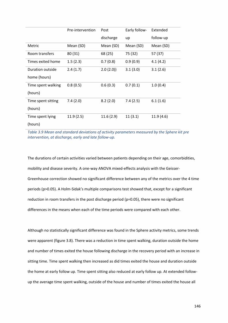
146

Pre-intervention Post

discharge

Early follow-

up

Extended

follow-up

Metric Mean (SD) Mean (SD) Mean (SD) Mean (SD)

Room transfers 80 (31) 68 (25) 75 (32) 57 (37)

Times exited home 1.5 (2.3) 0.7 (0.8) 0.9 (0.9) 4.1 (4.2)

Duration outside

home (hours)

2.4 (1.7) 2.0 (2.0)) 3.1 (3.0) 3.1 (2.6)

Time spent walking

(hours)

0.8 (0.5) 0.6 (0.3) 0.7 (0.1) 1.0 (0.4)

Time spent sitting

(hours)

7.4 (2.0) 8.2 (2.0) 7.4 (2.5) 6.1 (1.6)

Time spent lying

(hours)

11.9 (2.5) 11.6 (2.9) 11 (3.1) 11.9 (4.6)

Table 3.9 Mean and standard deviations of activity parameters measured by the Sphere kit pre intervention, at discharge, early and late follow-up.

The durations of certain activities varied between patients depending on their age, comorbidities,

mobility and disease severity. A one-way ANOVA mixed-effects analysis with the Geisser-

Greenhouse correction showed no significant difference between any of the metrics over the 4 time

periods (p>0.05). A Holm-Sidak’s multiple comparisons test showed that, except for a significant

reduction in room transfers in the post discharge period (p=0.05), there were no significant

differences in the means when each of the time periods were compared with each other.

Although no statistically significant difference was found in the Sphere activity metrics, some trends

were apparent (figure 3.8). There was a reduction in time spent walking, duration outside the home

and number of times exited the house following discharge in the recovery period with an increase in

sitting time. Time spent walking then increased as did times exited the house and duration outside

the home at early follow up. Time spent sitting also reduced at early follow up. At extended follow-

up the average time spent walking, outside of the house and number of times exited the house all

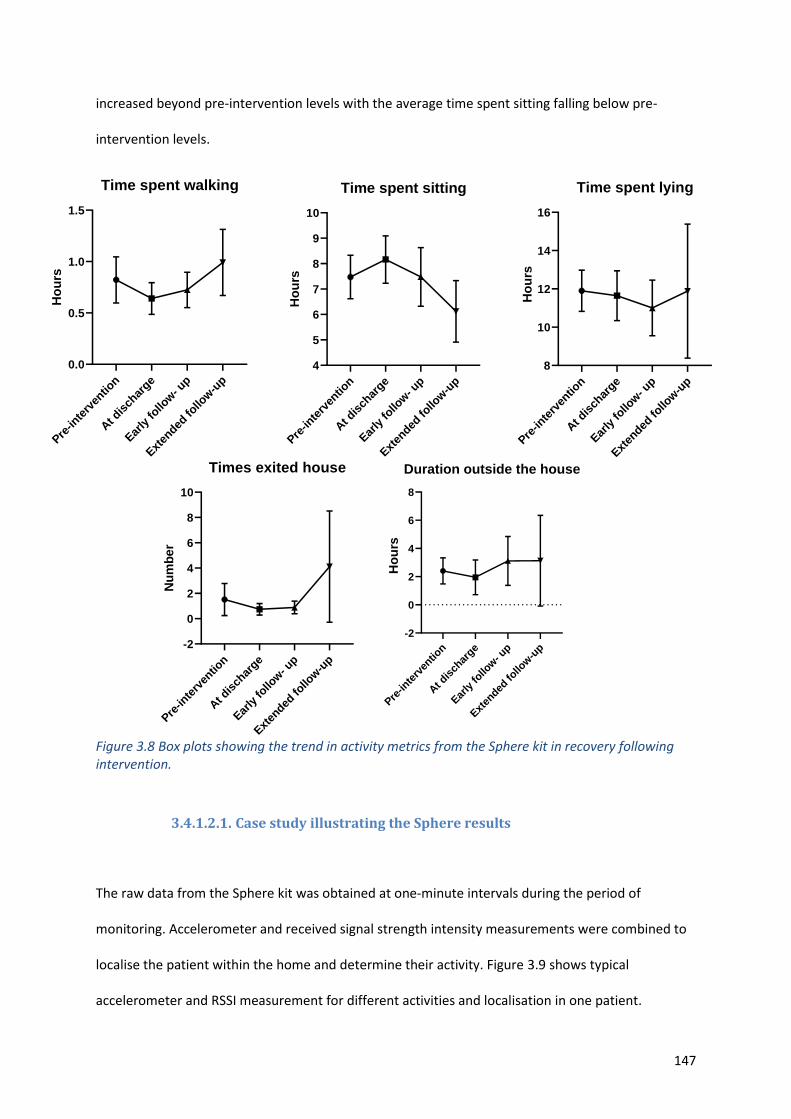
147

increased beyond pre-intervention levels with the average time spent sitting falling below pre-

intervention levels.

Figure 3.8 Box plots showing the trend in activity metrics from the Sphere kit in recovery following intervention.

3.4.1.2.1. Case study illustrating the Sphere results

The raw data from the Sphere kit was obtained at one-minute intervals during the period of

monitoring. Accelerometer and received signal strength intensity measurements were combined to

localise the patient within the home and determine their activity. Figure 3.9 shows typical

accelerometer and RSSI measurement for different activities and localisation in one patient.

Pre-in

terv

entio

n

At d

isch

arge

Early

follo

w- u

p

Exten

ded fo

llow

-up

4

5

6

7

8

9

10

Time spent sitting

Ho

urs

Pre-in

terv

entio

n

At d

isch

arge

Early

follo

w- u

p

Exten

ded fo

llow

-up

-2

0

2

4

6

8

10

Times exited house

Nu

mb

er

Pre-in

terv

entio

n

At d

isch

arge

Early

follo

w- u

p

Exten

ded fo

llow

-up

0.0

0.5

1.0

1.5

Time spent walking

Ho

urs

Pre-in

terv

entio

n

At d

isch

arge

Early

follo

w- u

p

Exten

ded fo

llow

-up

-2

0

2

4

6

8

Duration outside the house

Pre-in

terv

entio

n

At d

isch

arge

Early

follo

w- u

p

Exten

ded fo

llow

-up

4

5

6

7

8

9

10

Time spent sitting

Ho

urs

Pre-in

terv

entio

n

At d

isch

arge

Early

follo

w- u

p

Exten

ded fo

llow

-up

8

10

12

14

16

Time spent lying

Pre-in

terv

entio

n

At d

isch

arge

Early

follo

w- u

p

Exten

ded fo

llow

-up

4

5

6

7

8

9

10

Time spent sitting

Ho

urs

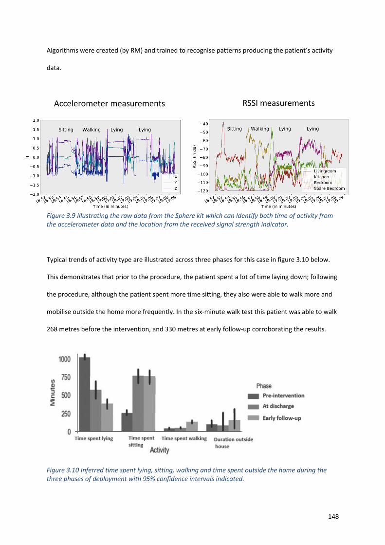
148

Algorithms were created (by RM) and trained to recognise patterns producing the patient’s activity

data.

Figure 3.9 Illustrating the raw data from the Sphere kit which can Identify both time of activity from the accelerometer data and the location from the received signal strength indicator.

Typical trends of activity type are illustrated across three phases for this case in figure 3.10 below.

This demonstrates that prior to the procedure, the patient spent a lot of time laying down; following

the procedure, although the patient spent more time sitting, they also were able to walk more and

mobilise outside the home more frequently. In the six-minute walk test this patient was able to walk

268 metres before the intervention, and 330 metres at early follow-up corroborating the results.

Figure 3.10 Inferred time spent lying, sitting, walking and time spent outside the home during the three phases of deployment with 95% confidence intervals indicated.

Accelerometer measurements RSSI measurements

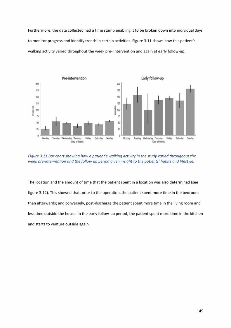
149

Furthermore, the data collected had a time stamp enabling it to be broken down into individual days

to monitor progress and identify trends in certain activities. Figure 3.11 shows how this patient’s

walking activity varied throughout the week pre- intervention and again at early follow-up.

Figure 3.11 Bar chart showing how a patient’s walking activity in the study varied throughout the week pre-intervention and the follow up period given insight to the patients’ habits and lifestyle.

The location and the amount of time that the patient spent in a location was also determined (see

figure 3.12). This showed that, prior to the operation, the patient spent more time in the bedroom

than afterwards; and conversely, post-discharge the patient spent more time in the living room and

less time outside the house. In the early follow-up period, the patient spent more time in the kitchen

and starts to venture outside again.

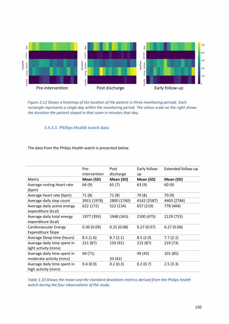
150

Figure 3.12 Shows a heatmap of the location of the patient in three monitoring periods. Each rectangle represents a single day within the monitoring period. The colour scale on the right shows the duration the patient stayed in that room in minutes that day.

3.4.1.3. Philips Health watch data

The data from the Philips Health watch is presented below.

Pre-intervention

Post discharge

Early follow-up

Extended follow-up

Metric Mean (SD) Mean (SD) Mean (SD) Mean (SD)

Average resting Heart rate (bpm)

64 (9) 65 (7) 63 (9) 60 (9)

Average heart rate (bpm) 71 (8) 71 (8) 70 (8) 70 (9)

Average daily step count 3915 (1978) 2800 (1760) 4142 (2587) 4403 (2784)

Average daily active energy expenditure (kcal)

622 (172) 522 (134) 657 (219) 778 (404)

Average daily total energy expenditure (kcal)

1977 (393) 1948 (343) 2100 (475) 2129 (715)

Cardiovascular Energy Expenditure Slope

0.30 (0.09) 0.25 (0.08) 0.27 (0.07) 0.27 (0.06)

Average Sleep time (hours) 8.5 (1.6) 8.7 (2.1) 8.5 (2.0) 7.7 (2.1)

Average daily time spent in light activity (mins)

221 (87) 159 (91) 215 (87) 219 (73)

Average daily time spent in moderate activity (mins)

69 (71) 33 (42)

49 (43) 101 (85)

Average daily time spent in high activity (mins)

0.4 (0.9) 0.2 (0.3) 0.2 (0.7) 2.5 (3.3)

Table 3.10 Shows the mean and the standard deviations metrics derived from the Philips health watch during the four observations of the study.

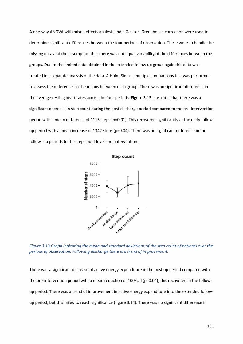
151

A one-way ANOVA with mixed effects analysis and a Geisser- Greenhouse correction were used to

determine significant differences between the four periods of observation. These were to handle the

missing data and the assumption that there was not equal variability of the differences between the

groups. Due to the limited data obtained in the extended follow up group again this data was

treated in a separate analysis of the data. A Holm-Sidak’s multiple comparisons test was performed

to assess the differences in the means between each group. There was no significant difference in

the average resting heart rates across the four periods. Figure 3.13 illustrates that there was a

significant decrease in step count during the post discharge period compared to the pre-intervention

period with a mean difference of 1115 steps (p=0.01). This recovered significantly at the early follow

up period with a mean increase of 1342 steps (p=0.04). There was no significant difference in the

follow -up periods to the step count levels pre intervention.

Figure 3.13 Graph indicating the mean and standard deviations of the step count of patients over the periods of observation. Following discharge there is a trend of improvement.

There was a significant decrease of active energy expenditure in the post op period compared with

the pre-intervention period with a mean reduction of 100kcal (p=0.04); this recovered in the follow-

up period. There was a trend of improvement in active energy expenditure into the extended follow-

up period, but this failed to reach significance (figure 3.14). There was no significant difference in

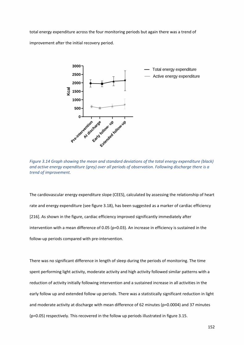
152

total energy expenditure across the four monitoring periods but again there was a trend of

improvement after the initial recovery period.

Pre-in

terv

entio

n

At d

isch

arge

Early

follo

w- u

p

Exten

ded fo

llow-u

p

0

500

1000

1500

2000

2500

3000K

cal

Active energy expenditure

Total energy expenditure

Figure 3.14 Graph showing the mean and standard deviations of the total energy expenditure (black) and active energy expenditure (grey) over all periods of observation. Following discharge there is a trend of improvement.

The cardiovascular energy expenditure slope (CEES), calculated by assessing the relationship of heart

rate and energy expenditure (see figure 3.18), has been suggested as a marker of cardiac efficiency

[216]. As shown in the figure, cardiac efficiency improved significantly immediately after

intervention with a mean difference of 0.05 (p=0.03). An increase in efficiency is sustained in the

follow-up periods compared with pre-intervention.

There was no significant difference in length of sleep during the periods of monitoring. The time

spent performing light activity, moderate activity and high activity followed similar patterns with a

reduction of activity initially following intervention and a sustained increase in all activities in the

early follow up and extended follow up periods. There was a statistically significant reduction in light

and moderate activity at discharge with mean difference of 62 minutes (p=0.0004) and 37 minutes

(p=0.05) respectively. This recovered in the follow up periods illustrated in figure 3.15.

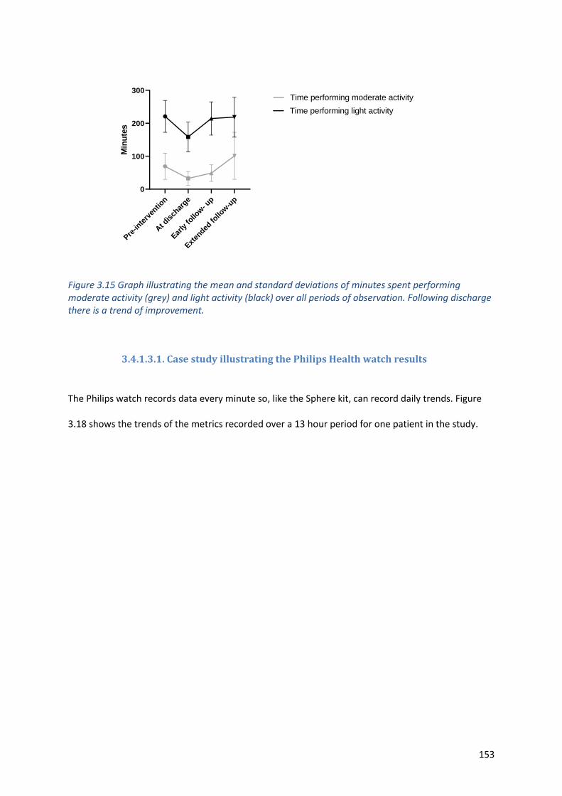
153

Pre-in

terv

entio

n

At d

isch

arge

Early

follo

w- u

p

Exten

ded fo

llow

-up

0

100

200

300

Min

ute

s

Time performing moderate activity

Time performing light activity

Figure 3.15 Graph illustrating the mean and standard deviations of minutes spent performing moderate activity (grey) and light activity (black) over all periods of observation. Following discharge there is a trend of improvement.

3.4.1.3.1. Case study illustrating the Philips Health watch results

The Philips watch records data every minute so, like the Sphere kit, can record daily trends. Figure

3.18 shows the trends of the metrics recorded over a 13 hour period for one patient in the study.

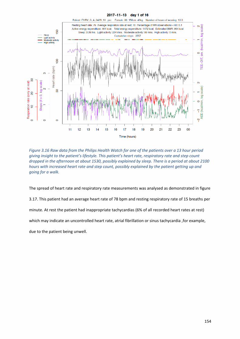
154

Figure 3.16 Raw data from the Philips Health Watch for one of the patients over a 13 hour period giving insight to the patient’s lifestyle. This patient’s heart rate, respiratory rate and step count dropped in the afternoon at about 1530, possibly explained by sleep. There is a period at about 2100 hours with increased heart rate and step count, possibly explained by the patient getting up and going for a walk.

The spread of heart rate and respiratory rate measurements was analysed as demonstrated in figure

3.17. This patient had an average heart rate of 78 bpm and resting respiratory rate of 15 breaths per

minute. At rest the patient had inappropriate tachycardias (6% of all recorded heart rates at rest)

which may indicate an uncontrolled heart rate, atrial fibrillation or sinus tachycardia ,for example,

due to the patient being unwell.

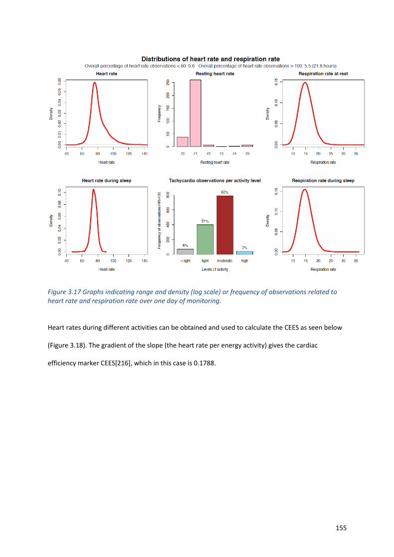
155

Figure 3.17 Graphs indicating range and density (log scale) or frequency of observations related to heart rate and respiration rate over one day of monitoring.

Heart rates during different activities can be obtained and used to calculate the CEES as seen below

(Figure 3.18). The gradient of the slope (the heart rate per energy activity) gives the cardiac

efficiency marker CEES[216], which in this case is 0.1788.

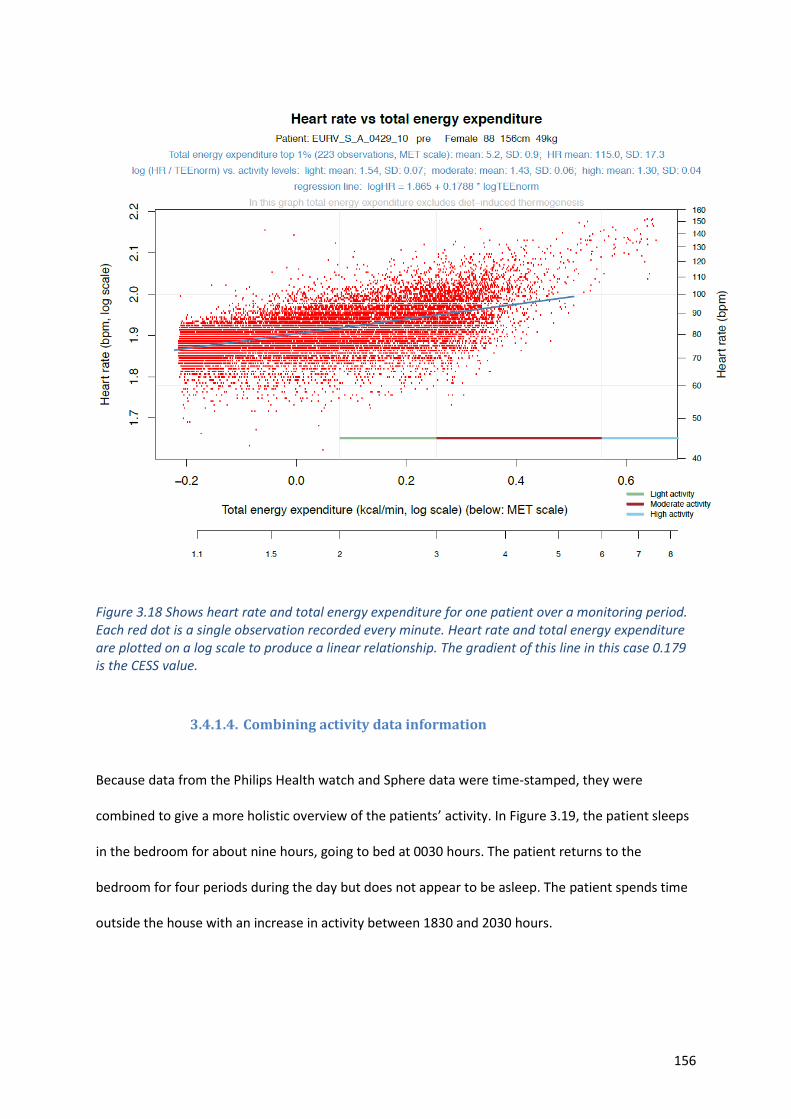
156

Figure 3.18 Shows heart rate and total energy expenditure for one patient over a monitoring period. Each red dot is a single observation recorded every minute. Heart rate and total energy expenditure are plotted on a log scale to produce a linear relationship. The gradient of this line in this case 0.179 is the CESS value.

3.4.1.4. Combining activity data information

Because data from the Philips Health watch and Sphere data were time-stamped, they were

combined to give a more holistic overview of the patients’ activity. In Figure 3.19, the patient sleeps

in the bedroom for about nine hours, going to bed at 0030 hours. The patient returns to the

bedroom for four periods during the day but does not appear to be asleep. The patient spends time

outside the house with an increase in activity between 1830 and 2030 hours.

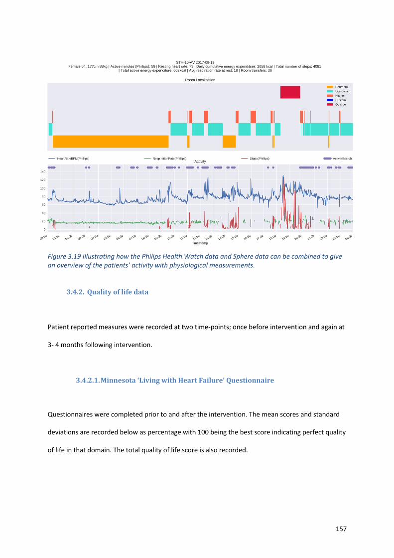
157

Figure 3.19 Illustrating how the Philips Health Watch data and Sphere data can be combined to give an overview of the patients’ activity with physiological measurements.

3.4.2. Quality of life data

Patient reported measures were recorded at two time-points; once before intervention and again at

3- 4 months following intervention.

3.4.2.1. Minnesota ‘Living with Heart Failure’ Questionnaire

Questionnaires were completed prior to and after the intervention. The mean scores and standard

deviations are recorded below as percentage with 100 being the best score indicating perfect quality

of life in that domain. The total quality of life score is also recorded.

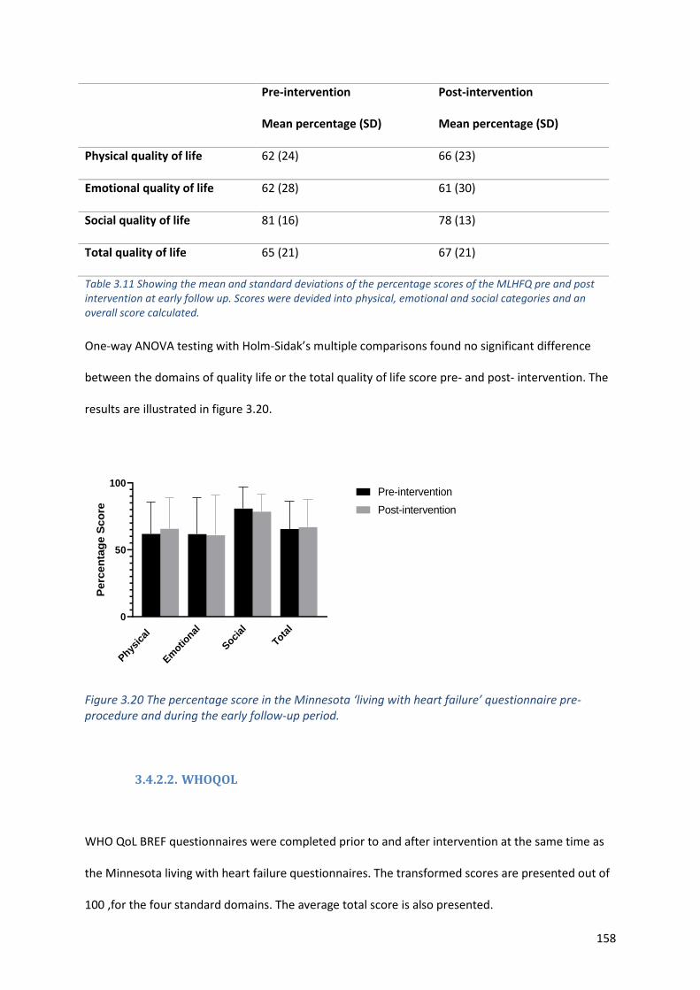
158

Pre-intervention

Mean percentage (SD)

Post-intervention

Mean percentage (SD)

Physical quality of life 62 (24) 66 (23)

Emotional quality of life 62 (28) 61 (30)

Social quality of life 81 (16) 78 (13)

Total quality of life 65 (21) 67 (21)

Table 3.11 Showing the mean and standard deviations of the percentage scores of the MLHFQ pre and post intervention at early follow up. Scores were devided into physical, emotional and social categories and an overall score calculated.

One-way ANOVA testing with Holm-Sidak’s multiple comparisons found no significant difference

between the domains of quality life or the total quality of life score pre- and post- intervention. The

results are illustrated in figure 3.20.

Phys

ical

Em

otional

Soci

al

Tota

l0

50

100

Perc

en

tag

e S

co

re

Pre-intervention

Post-intervention

Figure 3.20 The percentage score in the Minnesota ‘living with heart failure’ questionnaire pre-procedure and during the early follow-up period.

3.4.2.2. WHOQOL

WHO QoL BREF questionnaires were completed prior to and after intervention at the same time as

the Minnesota living with heart failure questionnaires. The transformed scores are presented out of

100 ,for the four standard domains. The average total score is also presented.

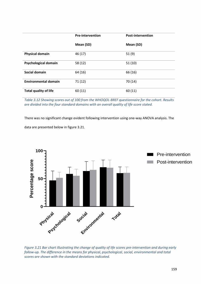
159

Pre-intervention

Mean (SD)

Post-intervention

Mean (SD)

Physical domain 46 (17) 51 (9)

Psychological domain 58 (12) 51 (10)

Social domain 64 (16) 66 (16)

Environmental domain 71 (12) 70 (14)

Total quality of life 60 (11) 60 (11)

Table 3.12 Showing scores out of 100 from the WHOQOL-BREF questionnaire for the cohort. Results are divided into the four standard domains with an overall quality of life score stated.

There was no significant change evident following intervention using one-way ANOVA analysis. The

data are presented below in figure 3.21.

Physic

al

Psych

ologic

al

Social

Enviro

nmen

tal

Total

0

50

100

Perc

en

tag

e s

co

re

Pre-intervention

Post-intervention

Figure 3.21 Bar chart illustrating the change of quality of life scores pre-intervention and during early follow-up. The difference in the means for physical, psychological, social, environmental and total scores are shown with the standard deviations indicated.

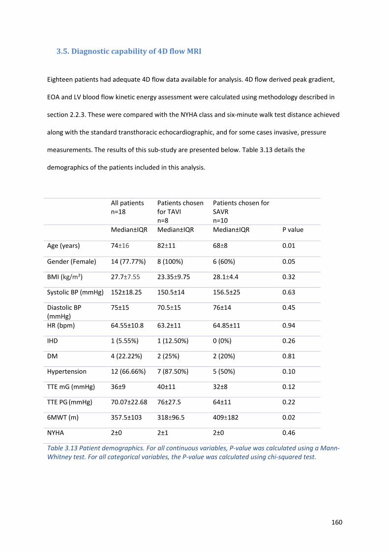
160

3.5. Diagnostic capability of 4D flow MRI

Eighteen patients had adequate 4D flow data available for analysis. 4D flow derived peak gradient,

EOA and LV blood flow kinetic energy assessment were calculated using methodology described in

section 2.2.3. These were compared with the NYHA class and six-minute walk test distance achieved

along with the standard transthoracic echocardiographic, and for some cases invasive, pressure

measurements. The results of this sub-study are presented below. Table 3.13 details the

demographics of the patients included in this analysis.

All patients n=18

Patients chosen for TAVI n=8

Patients chosen for SAVR n=10

Median±IQR Median±IQR Median±IQR P value

Age (years) 74±16 82±11 68±8 0.01

Gender (Female) 14 (77.77%) 8 (100%) 6 (60%) 0.05

BMI (kg/m²) 27.7±7.55 23.35±9.75 28.1±4.4 0.32

Systolic BP (mmHg) 152±18.25 150.5±14 156.5±25 0.63

Diastolic BP (mmHg)

75±15 70.5±15 76±14 0.45

HR (bpm) 64.55±10.8 63.2±11 64.85±11 0.94

IHD 1 (5.55%) 1 (12.50%) 0 (0%) 0.26

DM 4 (22.22%) 2 (25%) 2 (20%) 0.81

Hypertension 12 (66.66%) 7 (87.50%) 5 (50%) 0.10

TTE mG (mmHg) 36±9 40±11 32±8 0.12

TTE PG (mmHg) 70.07±22.68 76±27.5 64±11 0.22

6MWT (m) 357.5±103 318±96.5 409±182 0.02

NYHA 2±0 2±1 2±0 0.46

Table 3.13 Patient demographics. For all continuous variables, P-value was calculated using a Mann-Whitney test. For all categorical variables, the P-value was calculated using chi-squared test.

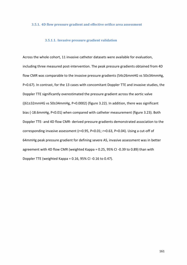
161

3.5.1. 4D flow pressure gradient and effective orifice area assessment

3.5.1.1. Invasive pressure gradient validation

Across the whole cohort, 11 invasive catheter datasets were available for evaluation,

including three measured post-intervention. The peak pressure gradients obtained from 4D

flow CMR was comparable to the invasive pressure gradients (54±26mmHG vs 50±34mmHg,

P=0.67). In contrast, for the 13 cases with concomitant Doppler TTE and invasive studies, the

Doppler TTE significantly overestimated the pressure gradient across the aortic valve

((61±32mmHG vs 50±34mmHg, P=0.0002) (figure 3.22). In addition, there was significant

bias (-18.6mmHg, P<0.01) when compared with catheter measurement (figure 3.23). Both

Doppler TTE- and 4D flow CMR- derived pressure gradients demonstrated association to the

corresponding invasive assessment (r=0.95, P<0.01; r=0.63, P=0.04). Using a cut-off of

64mmHg peak pressure gradient for defining severe AS, invasive assessment was in better

agreement with 4D flow CMR (weighted Kappa = 0.25, 95% CI -0.39 to 0.89) than with

Doppler TTE (weighted Kappa = 0.16, 95% CI -0.16 to 0.47).

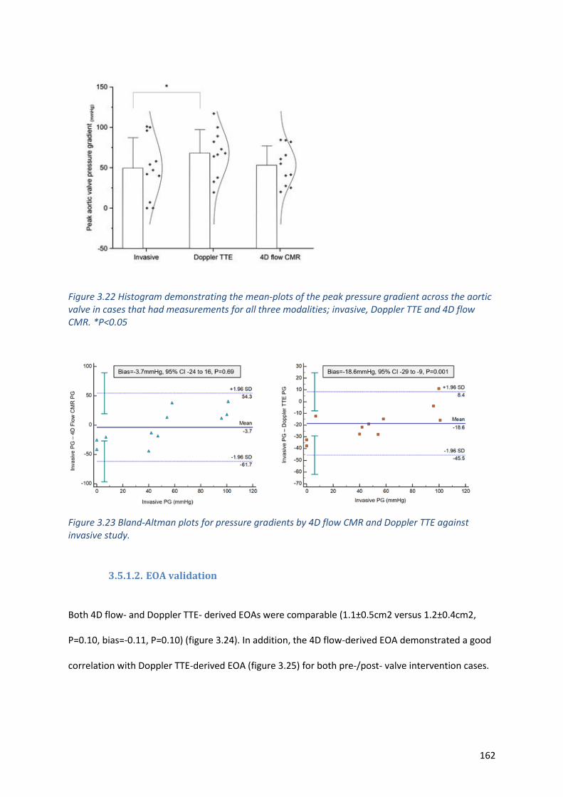
162

Figure 3.22 Histogram demonstrating the mean-plots of the peak pressure gradient across the aortic valve in cases that had measurements for all three modalities; invasive, Doppler TTE and 4D flow CMR. *P<0.05

Figure 3.23 Bland-Altman plots for pressure gradients by 4D flow CMR and Doppler TTE against invasive study.

3.5.1.2. EOA validation

Both 4D flow- and Doppler TTE- derived EOAs were comparable (1.1±0.5cm2 versus 1.2±0.4cm2,

P=0.10, bias=-0.11, P=0.10) (figure 3.24). In addition, the 4D flow-derived EOA demonstrated a good

correlation with Doppler TTE-derived EOA (figure 3.25) for both pre-/post- valve intervention cases.

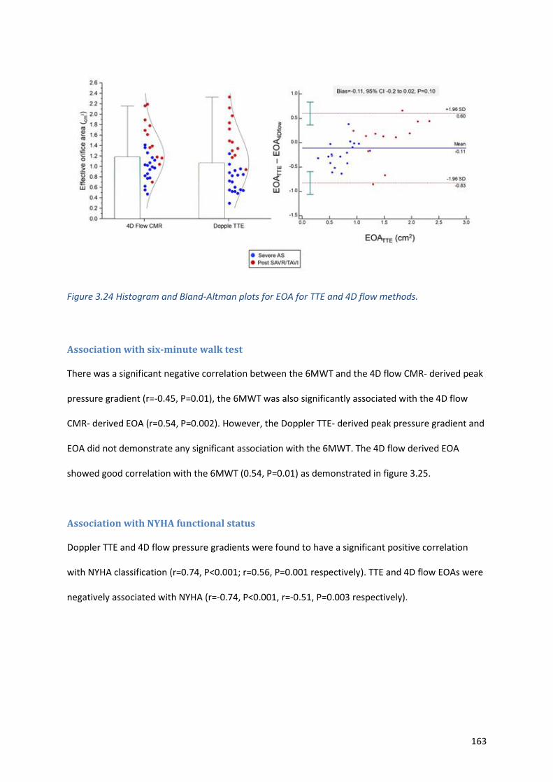
163

Figure 3.24 Histogram and Bland-Altman plots for EOA for TTE and 4D flow methods.

Association with six-minute walk test

There was a significant negative correlation between the 6MWT and the 4D flow CMR- derived peak

pressure gradient (r=-0.45, P=0.01), the 6MWT was also significantly associated with the 4D flow

CMR- derived EOA (r=0.54, P=0.002). However, the Doppler TTE- derived peak pressure gradient and

EOA did not demonstrate any significant association with the 6MWT. The 4D flow derived EOA

showed good correlation with the 6MWT (0.54, P=0.01) as demonstrated in figure 3.25.

Association with NYHA functional status

Doppler TTE and 4D flow pressure gradients were found to have a significant positive correlation

with NYHA classification (r=0.74, P<0.001; r=0.56, P=0.001 respectively). TTE and 4D flow EOAs were

negatively associated with NYHA (r=-0.74, P<0.001, r=-0.51, P=0.003 respectively).

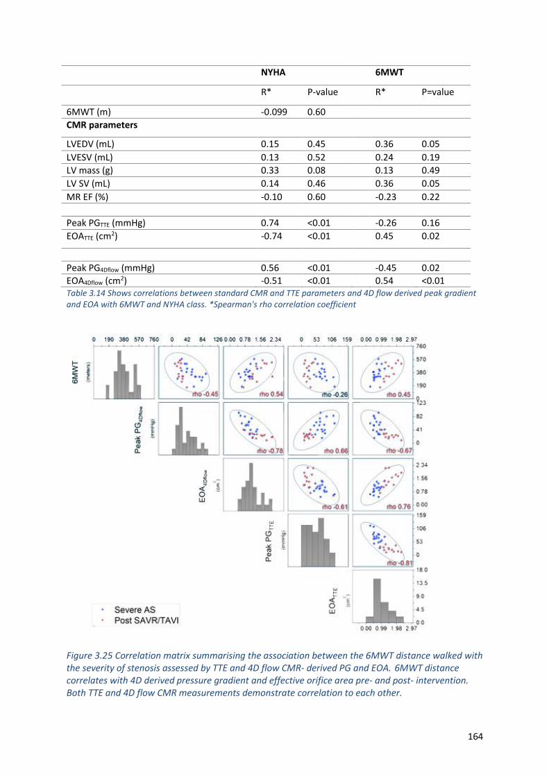
164

NYHA 6MWT

R* P-value R* P=value

6MWT (m) -0.099 0.60

CMR parameters

LVEDV (mL) 0.15 0.45 0.36 0.05

LVESV (mL) 0.13 0.52 0.24 0.19

LV mass (g) 0.33 0.08 0.13 0.49

LV SV (mL) 0.14 0.46 0.36 0.05

MR EF (%) -0.10 0.60 -0.23 0.22

Peak PGTTE (mmHg) 0.74 <0.01 -0.26 0.16

EOATTE (cm2) -0.74 <0.01 0.45 0.02

Peak PG4Dflow (mmHg) 0.56 <0.01 -0.45 0.02

EOA4Dflow (cm2) -0.51 <0.01 0.54 <0.01 Table 3.14 Shows correlations between standard CMR and TTE parameters and 4D flow derived peak gradient and EOA with 6MWT and NYHA class. *Spearman's rho correlation coefficient

Figure 3.25 Correlation matrix summarising the association between the 6MWT distance walked with the severity of stenosis assessed by TTE and 4D flow CMR- derived PG and EOA. 6MWT distance correlates with 4D derived pressure gradient and effective orifice area pre- and post- intervention. Both TTE and 4D flow CMR measurements demonstrate correlation to each other.

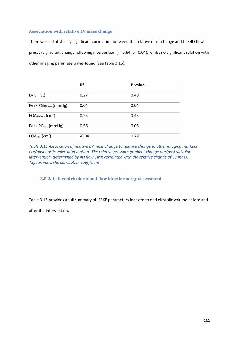
165

Association with relative LV mass change

There was a statistically significant correlation between the relative mass change and the 4D flow

pressure gradient change following intervention (r= 0.64, p= 0.04), whilst no significant relation with

other imaging parameters was found (see table 3.15).

R* P-value

LV EF (%) 0.27 0.40

Peak PG4Dflow (mmHg) 0.64 0.04

EOA4Dflow (cm2) 0.25 0.45

Peak PGTTE (mmHg) 0.56 0.06

EOATTE (cm2) -0.08 0.79

Table 3.15 Association of relative LV mass change to relative change in other imaging markers pre/post aortic valve intervention. The relative pressure gradient change pre/post valvular intervention, determined by 4D flow CMR correlated with the relative change of LV mass. *Spearman's rho correlation coefficient

3.5.2. Left ventricular blood flow kinetic energy assessment

Table 3.16 provides a full summary of LV KE parameters indexed to end diastolic volume before and

after the intervention.

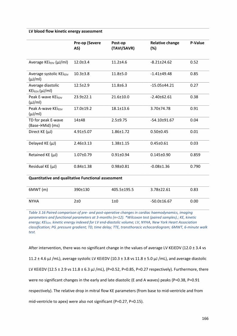
166

LV blood flow kinetic energy assessment

Pre-op (Severe AS)

Post-op (TAVI/SAVR)

Relative change (%)

P-Value

Average KEiEDV (μJ/ml) 12.0±3.4 11.2±4.6 -8.21±24.62 0.52

Average systolic KEiEDV

(μJ/ml) 10.3±3.8 11.8±5.0 -1.41±49.48 0.85

Average diastolic KEiEDV (μJ/ml)

12.5±2.9 11.8±6.3 -15.05±44.21 0.27

Peak E-wave KEiEDV (μJ/ml)

23.9±22.1 21.6±10.0 -2.40±62.61 0.38

Peak A-wave KEiEDV (μJ/ml)

17.0±19.2 18.1±13.6 3.70±74.78 0.91

TD for peak E-wave (Base→Mid) (ms)

14±48 2.5±9.75 -54.10±91.67 0.04

Direct KE (μJ) 4.91±5.07 1.86±1.72 0.50±0.45 0.01

Delayed KE (μJ) 2.46±3.13 1.38±1.15 0.45±0.61 0.03

Retained KE (μJ) 1.07±0.79 0.91±0.94 0.145±0.90 0.859

Residual KE (μJ) 0.84±1.38 0.98±0.81 -0.08±1.36 0.790

Quantitative and qualitative Functional assessment

6MWT (m) 390±130 405.5±195.5 3.78±22.61 0.83

NYHA 2±0 1±0 -50.0±16.67 0.00

Table 3.16 Paired comparison of pre- and post-operative changes in cardiac haemodynamics, imaging parameters and functional parameters at 3-months (n=12). *Wilcoxon test (paired samples).; KE, kinetic energy; KEiEDV, kinetic energy indexed for LV end-diastolic volume; LV, NYHA, New York Heart Association classification; PG, pressure gradient; TD, time delay; TTE, transthoracic echocardiogram; 6MWT, 6-minute walk test.

After intervention, there was no significant change in the values of average LV KEiEDV (12.0 ± 3.4 vs

11.2 ± 4.6 μJ /mL), average systolic LV KEiEDV (10.3 ± 3.8 vs 11.8 ± 5.0 μJ /mL), and average diastolic

LV KEiEDV (12.5 ± 2.9 vs 11.8 ± 6.3 μJ /mL), (P=0.52, P=0.85, P=0.27 respectively). Furthermore, there

were no significant changes in the early and late diastolic (E and A waves) peaks (P=0.38, P=0.91

respectively). The relative drop in mitral flow KE parameters (from base to mid-ventricle and from

mid-ventricle to apex) were also not significant (P=0.27, P=0.15).

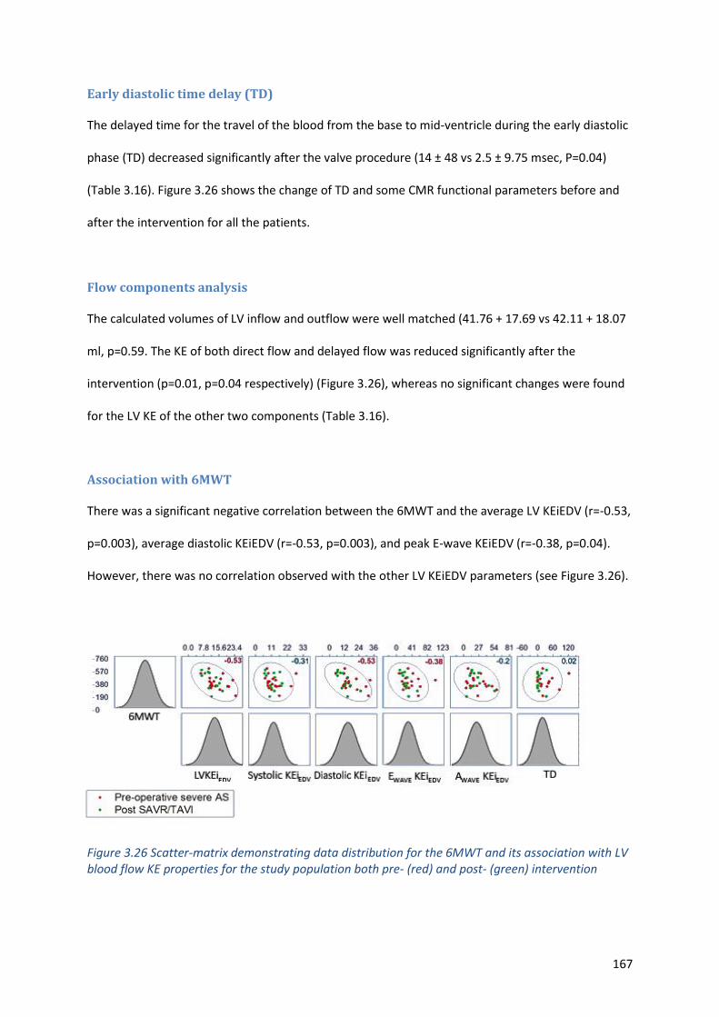
167

Early diastolic time delay (TD)

The delayed time for the travel of the blood from the base to mid-ventricle during the early diastolic

phase (TD) decreased significantly after the valve procedure (14 ± 48 vs 2.5 ± 9.75 msec, P=0.04)

(Table 3.16). Figure 3.26 shows the change of TD and some CMR functional parameters before and

after the intervention for all the patients.

Flow components analysis

The calculated volumes of LV inflow and outflow were well matched (41.76 + 17.69 vs 42.11 + 18.07

ml, p=0.59. The KE of both direct flow and delayed flow was reduced significantly after the

intervention (p=0.01, p=0.04 respectively) (Figure 3.26), whereas no significant changes were found

for the LV KE of the other two components (Table 3.16).

Association with 6MWT

There was a significant negative correlation between the 6MWT and the average LV KEiEDV (r=-0.53,

p=0.003), average diastolic KEiEDV (r=-0.53, p=0.003), and peak E-wave KEiEDV (r=-0.38, p=0.04).

However, there was no correlation observed with the other LV KEiEDV parameters (see Figure 3.26).

Figure 3.26 Scatter-matrix demonstrating data distribution for the 6MWT and its association with LV blood flow KE properties for the study population both pre- (red) and post- (green) intervention

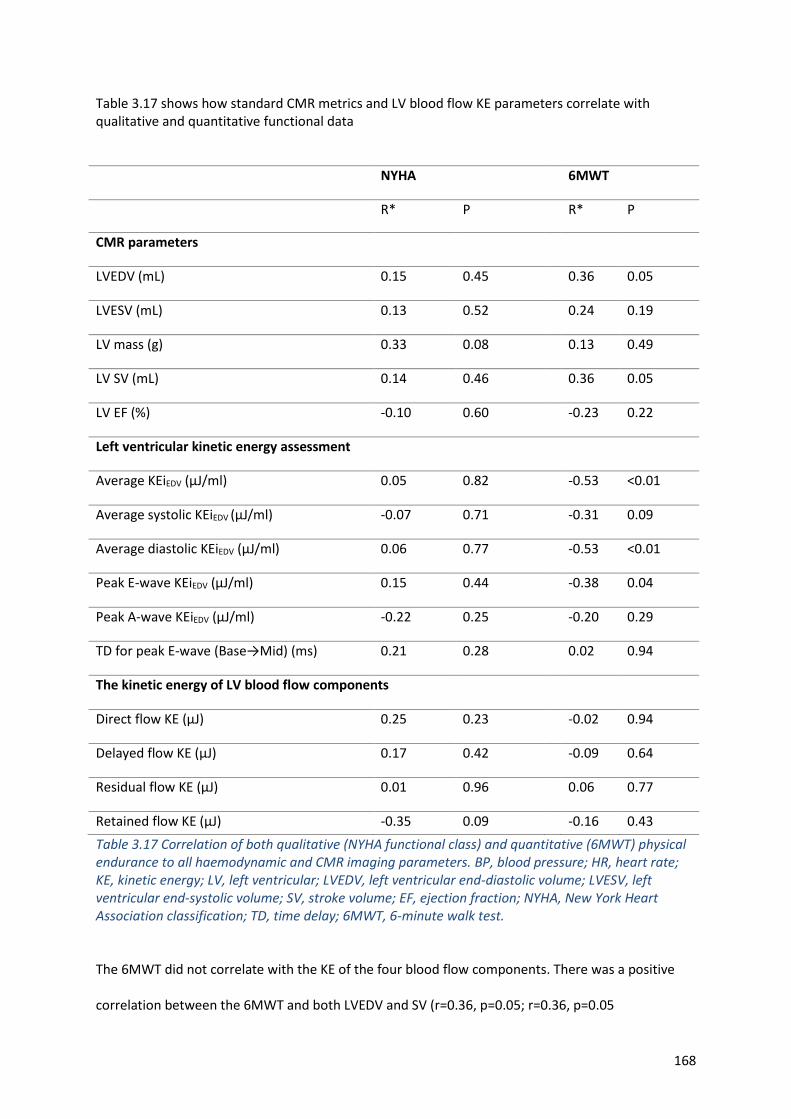
168

Table 3.17 shows how standard CMR metrics and LV blood flow KE parameters correlate with qualitative and quantitative functional data

NYHA 6MWT

R* P R* P

CMR parameters

LVEDV (mL) 0.15 0.45 0.36 0.05

LVESV (mL) 0.13 0.52 0.24 0.19

LV mass (g) 0.33 0.08 0.13 0.49

LV SV (mL) 0.14 0.46 0.36 0.05

LV EF (%) -0.10 0.60 -0.23 0.22

Left ventricular kinetic energy assessment

Average KEiEDV (μJ/ml) 0.05 0.82 -0.53 <0.01

Average systolic KEiEDV (μJ/ml) -0.07 0.71 -0.31 0.09

Average diastolic KEiEDV (μJ/ml) 0.06 0.77 -0.53 <0.01

Peak E-wave KEiEDV (μJ/ml) 0.15 0.44 -0.38 0.04

Peak A-wave KEiEDV (μJ/ml) -0.22 0.25 -0.20 0.29

TD for peak E-wave (Base→Mid) (ms) 0.21 0.28 0.02 0.94

The kinetic energy of LV blood flow components

Direct flow KE (μJ) 0.25 0.23 -0.02 0.94

Delayed flow KE (μJ) 0.17 0.42 -0.09 0.64

Residual flow KE (μJ) 0.01 0.96 0.06 0.77

Retained flow KE (μJ) -0.35 0.09 -0.16 0.43

Table 3.17 Correlation of both qualitative (NYHA functional class) and quantitative (6MWT) physical endurance to all haemodynamic and CMR imaging parameters. BP, blood pressure; HR, heart rate; KE, kinetic energy; LV, left ventricular; LVEDV, left ventricular end-diastolic volume; LVESV, left ventricular end-systolic volume; SV, stroke volume; EF, ejection fraction; NYHA, New York Heart Association classification; TD, time delay; 6MWT, 6-minute walk test.

The 6MWT did not correlate with the KE of the four blood flow components. There was a positive

correlation between the 6MWT and both LVEDV and SV (r=0.36, p=0.05; r=0.36, p=0.05

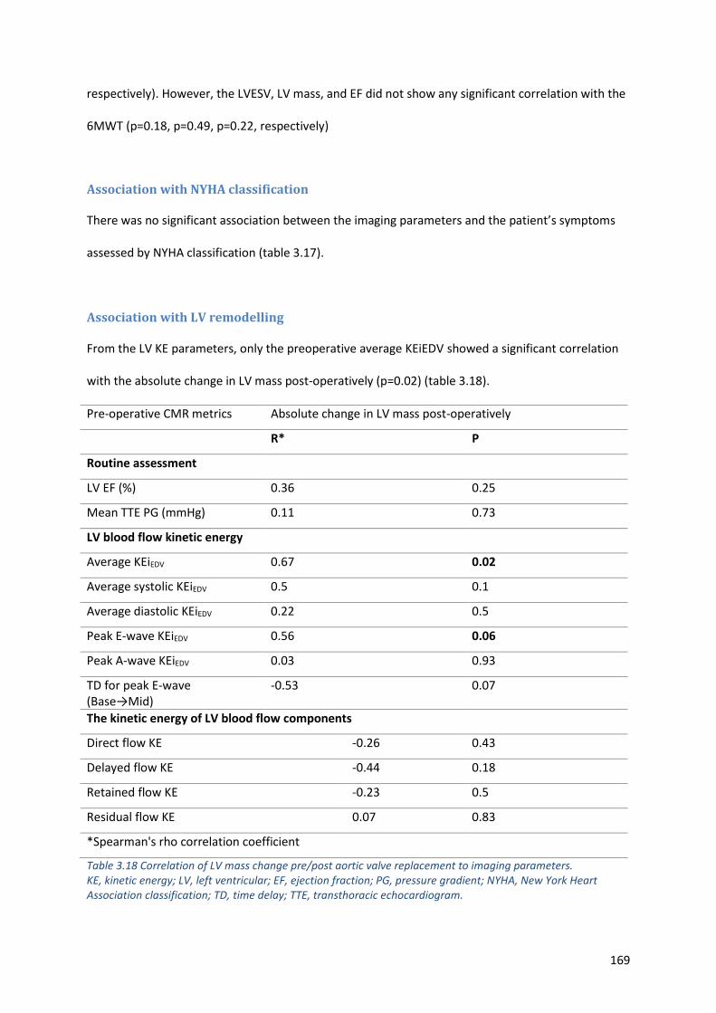
169

respectively). However, the LVESV, LV mass, and EF did not show any significant correlation with the

6MWT (p=0.18, p=0.49, p=0.22, respectively)

Association with NYHA classification

There was no significant association between the imaging parameters and the patient’s symptoms

assessed by NYHA classification (table 3.17).

Association with LV remodelling

From the LV KE parameters, only the preoperative average KEiEDV showed a significant correlation

with the absolute change in LV mass post-operatively (p=0.02) (table 3.18).

Pre-operative CMR metrics Absolute change in LV mass post-operatively

R* P

Routine assessment

LV EF (%) 0.36 0.25

Mean TTE PG (mmHg) 0.11 0.73

LV blood flow kinetic energy

Average KEiEDV 0.67 0.02

Average systolic KEiEDV 0.5 0.1

Average diastolic KEiEDV 0.22 0.5

Peak E-wave KEiEDV 0.56 0.06

Peak A-wave KEiEDV 0.03 0.93

TD for peak E-wave (Base→Mid)

-0.53 0.07

The kinetic energy of LV blood flow components

Direct flow KE -0.26 0.43

Delayed flow KE -0.44 0.18

Retained flow KE -0.23 0.5

Residual flow KE 0.07 0.83

*Spearman's rho correlation coefficient

Table 3.18 Correlation of LV mass change pre/post aortic valve replacement to imaging parameters. KE, kinetic energy; LV, left ventricular; EF, ejection fraction; PG, pressure gradient; NYHA, New York Heart Association classification; TD, time delay; TTE, transthoracic echocardiogram.

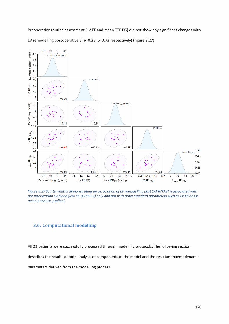
170

Preoperative routine assessment (LV EF and mean TTE PG) did not show any significant changes with

LV remodelling postoperatively (p=0.25, p=0.73 respectively) (figure 3.27).

Figure 3.27 Scatter matrix demonstrating an association of LV remodelling post SAVR/TAVI is associated with pre-intervention LV blood flow KE (LVKEiEDV) only and not with other standard parameters such as LV EF or AV mean pressure gradient.


All 22 patients were successfully processed through modelling protocols. The following section

describes the results of both analysis of components of the model and the resultant haemodynamic

parameters derived from the modelling process.

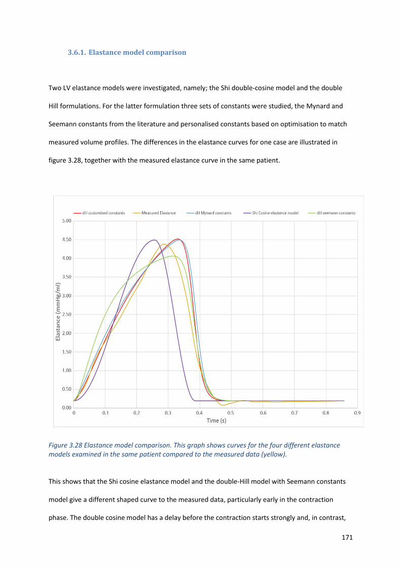
171

3.6.1. Elastance model comparison

Two LV elastance models were investigated, namely; the Shi double-cosine model and the double

Hill formulations. For the latter formulation three sets of constants were studied, the Mynard and

Seemann constants from the literature and personalised constants based on optimisation to match

measured volume profiles. The differences in the elastance curves for one case are illustrated in

figure 3.28, together with the measured elastance curve in the same patient.

Figure 3.28 Elastance model comparison. This graph shows curves for the four different elastance models examined in the same patient compared to the measured data (yellow).

This shows that the Shi cosine elastance model and the double-Hill model with Seemann constants

model give a different shaped curve to the measured data, particularly early in the contraction

phase. The double cosine model has a delay before the contraction starts strongly and, in contrast,

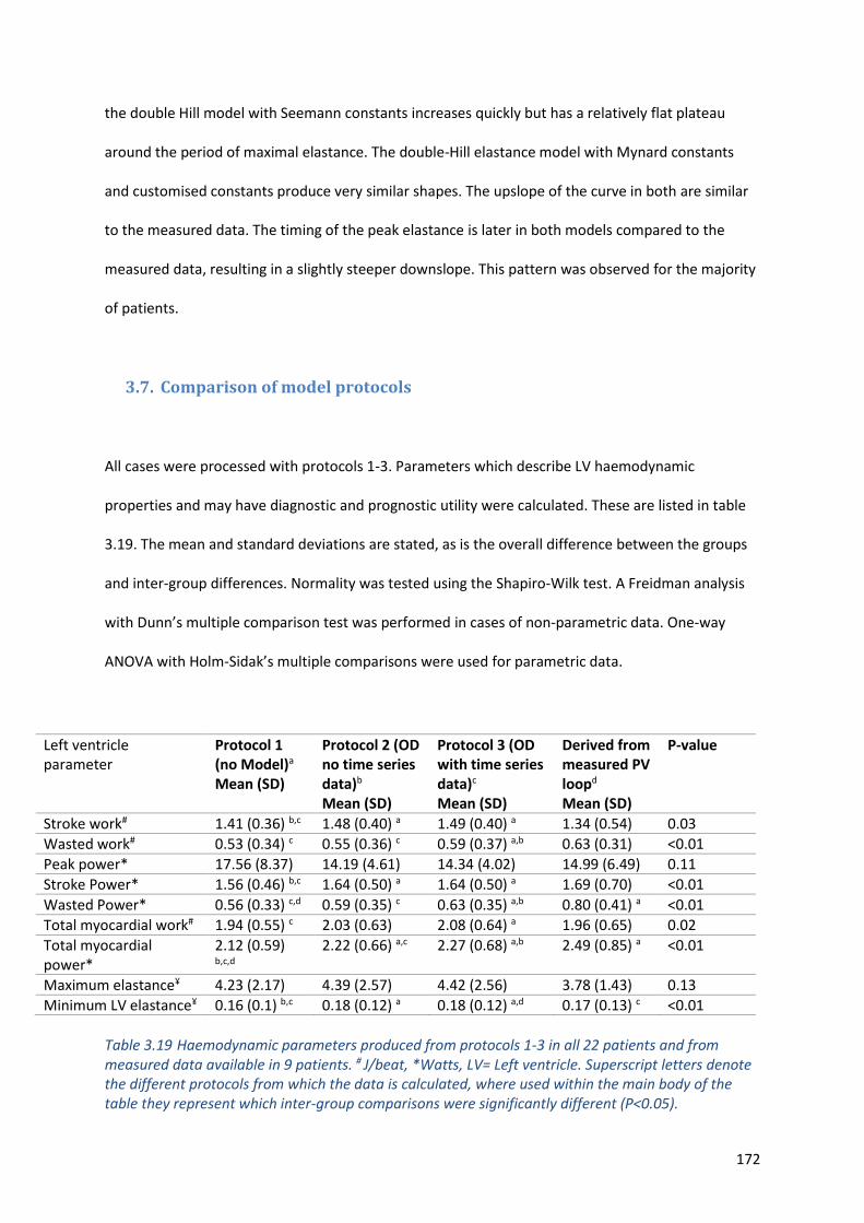
172

the double Hill model with Seemann constants increases quickly but has a relatively flat plateau

around the period of maximal elastance. The double-Hill elastance model with Mynard constants

and customised constants produce very similar shapes. The upslope of the curve in both are similar

to the measured data. The timing of the peak elastance is later in both models compared to the

measured data, resulting in a slightly steeper downslope. This pattern was observed for the majority

of patients.

3.7. Comparison of model protocols

All cases were processed with protocols 1-3. Parameters which describe LV haemodynamic

properties and may have diagnostic and prognostic utility were calculated. These are listed in table

3.19. The mean and standard deviations are stated, as is the overall difference between the groups

and inter-group differences. Normality was tested using the Shapiro-Wilk test. A Freidman analysis

with Dunn’s multiple comparison test was performed in cases of non-parametric data. One-way

ANOVA with Holm-Sidak’s multiple comparisons were used for parametric data.

Table 3.19 Haemodynamic parameters produced from protocols 1-3 in all 22 patients and from measured data available in 9 patients. # J/beat, *Watts, LV= Left ventricle. Superscript letters denote the different protocols from which the data is calculated, where used within the main body of the table they represent which inter-group comparisons were significantly different (P<0.05).

Left ventricle parameter

Protocol 1 (no Model)a

Mean (SD)

Protocol 2 (OD no time series data)b Mean (SD)

Protocol 3 (OD with time series data)c Mean (SD)

Derived from measured PV loopd Mean (SD)

P-value

Stroke work# 1.41 (0.36) b,c 1.48 (0.40) a 1.49 (0.40) a 1.34 (0.54) 0.03

Wasted work# 0.53 (0.34) c 0.55 (0.36) c 0.59 (0.37) a,b 0.63 (0.31) <0.01

Peak power* 17.56 (8.37) 14.19 (4.61) 14.34 (4.02) 14.99 (6.49) 0.11

Stroke Power* 1.56 (0.46) b,c 1.64 (0.50) a 1.64 (0.50) a 1.69 (0.70) <0.01

Wasted Power* 0.56 (0.33) c,d 0.59 (0.35) c 0.63 (0.35) a,b 0.80 (0.41) a <0.01

Total myocardial work# 1.94 (0.55) c 2.03 (0.63) 2.08 (0.64) a 1.96 (0.65) 0.02

Total myocardial power*

2.12 (0.59) b,c,d

2.22 (0.66) a,c 2.27 (0.68) a,b 2.49 (0.85) a <0.01

Maximum elastance¥ 4.23 (2.17) 4.39 (2.57) 4.42 (2.56) 3.78 (1.43) 0.13

Minimum LV elastance¥ 0.16 (0.1) b,c 0.18 (0.12) a 0.18 (0.12) a,d 0.17 (0.13) c <0.01

173

There was no significant difference between the results obtained using the four different methods

used to derive maximum LV elastance (ELVmax). For the key parameter of stroke work there was no

significant difference between any of the protocols and the value derived from the measured data.

Wasted work (the area of the triangular segment between the isovolumetric relaxation portion of

the PV loop and the point indicating the LV volume under zero pressure) was significantly less when

assessed using protocol 1 compared to using protocols 2 and 3, but the absolute percentage

difference in the means is less than 10% and, since wasted work is typically of the order of one third

of total ventricular work, these differences are unlikely to be significant in terms of diagnostic utility.

Stroke power and wasted power are calculated by dividing stroke work and wasted work, by the

length of the of the cardiac cycle. Power and work parameters will show the same relation unless

the heart rate used for the computations is different. For the modelled protocols the rest state was

extrapolated from the heart rate obtained by the Philips Health watch. Stroke power was similar

when calculated using the 0D model and the measured data but there was a tendency of protocol 1

to underestimate this parameter. Although there was a difference in the value produced for wasted

power from protocols 2 and 3, both were broadly comparable to the values from the measured data.

The results obtained for peak LV power were similar using all four protocols and also similar to the

measured data. LV power can also be assessed over the cardiac cycle using the measured data (see

figure 3.29, for an illustrative case). The PV loops in figure 3.29 indicate, for all the protocols

assessed, that peak LV power occurs in the early ejection phase just after the valve opens (red,

yellow and green data points), this is consistent with the measured data.

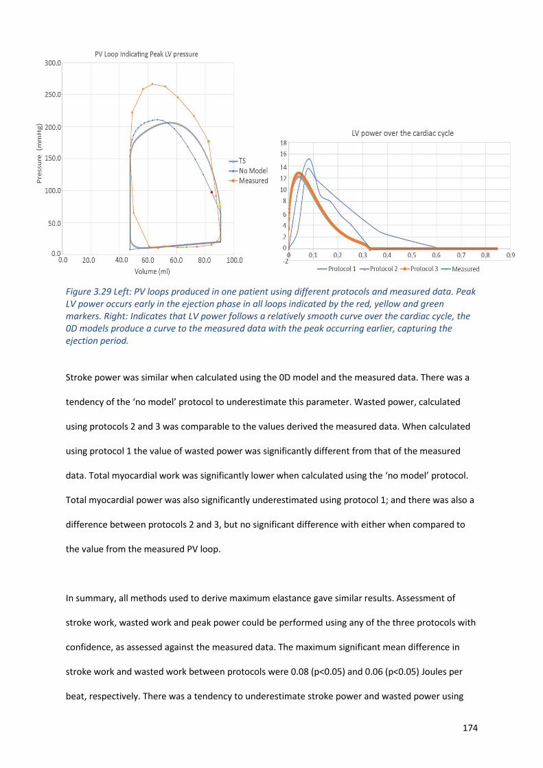
174

Figure 3.29 Left: PV loops produced in one patient using different protocols and measured data. Peak LV power occurs early in the ejection phase in all loops indicated by the red, yellow and green markers. Right: Indicates that LV power follows a relatively smooth curve over the cardiac cycle, the 0D models produce a curve to the measured data with the peak occurring earlier, capturing the ejection period.

Stroke power was similar when calculated using the 0D model and the measured data. There was a

tendency of the ‘no model’ protocol to underestimate this parameter. Wasted power, calculated

using protocols 2 and 3 was comparable to the values derived the measured data. When calculated

using protocol 1 the value of wasted power was significantly different from that of the measured

data. Total myocardial work was significantly lower when calculated using the ‘no model’ protocol.

Total myocardial power was also significantly underestimated using protocol 1; and there was also a

difference between protocols 2 and 3, but no significant difference with either when compared to

the value from the measured PV loop.

In summary, all methods used to derive maximum elastance gave similar results. Assessment of

stroke work, wasted work and peak power could be performed using any of the three protocols with

confidence, as assessed against the measured data. The maximum significant mean difference in

stroke work and wasted work between protocols were 0.08 (p<0.05) and 0.06 (p<0.05) Joules per

beat, respectively. There was a tendency to underestimate stroke power and wasted power using

175

protocols 1-3, and protocols 2 or 3 were preferable, because there was no significant difference

between the values produced by these and the measured data. All of the protocols successfully

calculated total myocardial work, but protocol 1 was inaccurate in calculating total myocardial

power.

Upon review of the model results presented here, protocol 2 produced the most similar results to

the measured data for all parameters. The accuracy of protocol 2 was assessed further by calculating

the residual errors in achieving the target clinically measured parameters, following an optimisation

process. The residual errors were very small, increasing the confidence in the model. The average

residual errors when converging on the target values were as follows: LVEDV (0.5%), LVESV (0.3%),

LVEDP (0.03%), diastolic BP (0.1%) MAP (0.02%) PG (0.02%). For these reasons, and with reference

to the computing power and time needed to tune the model to the time-series volume in protocol 3,

protocol 2 was selected as the standard protocol for predictive simulation. Protocol 1 could not be

used for this purpose. For consistency, protocol 2 was also used for comparison with activity data to

investigate modelling for diagnostic purposes and correlation with activity metrics.

3.8. Protocol 4

Protocol 4 was not performed in all cases used due to problems with image acquisition and

inaccurate segmentation. The processes of this protocol are illustrated in this section in a case where

segmentation was successful. The results of the 11 cases with adequate images for processing are

then presented.

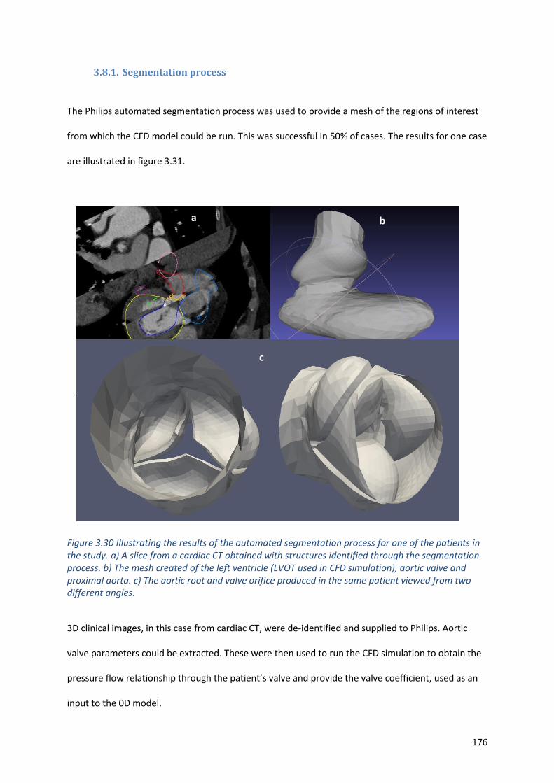
176

3.8.1. Segmentation process

The Philips automated segmentation process was used to provide a mesh of the regions of interest

from which the CFD model could be run. This was successful in 50% of cases. The results for one case

are illustrated in figure 3.31.

b)

Figure 3.30 Illustrating the results of the automated segmentation process for one of the patients in the study. a) A slice from a cardiac CT obtained with structures identified through the segmentation process. b) The mesh created of the left ventricle (LVOT used in CFD simulation), aortic valve and proximal aorta. c) The aortic root and valve orifice produced in the same patient viewed from two different angles.

3D clinical images, in this case from cardiac CT, were de-identified and supplied to Philips. Aortic

valve parameters could be extracted. These were then used to run the CFD simulation to obtain the

pressure flow relationship through the patient’s valve and provide the valve coefficient, used as an

input to the 0D model.

b

a

c

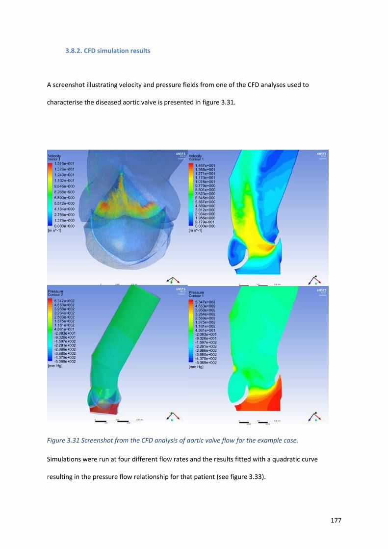
177

3.8.2. CFD simulation results

A screenshot illustrating velocity and pressure fields from one of the CFD analyses used to

characterise the diseased aortic valve is presented in figure 3.31.

Figure 3.31 Screenshot from the CFD analysis of aortic valve flow for the example case.

Simulations were run at four different flow rates and the results fitted with a quadratic curve

resulting in the pressure flow relationship for that patient (see figure 3.33).

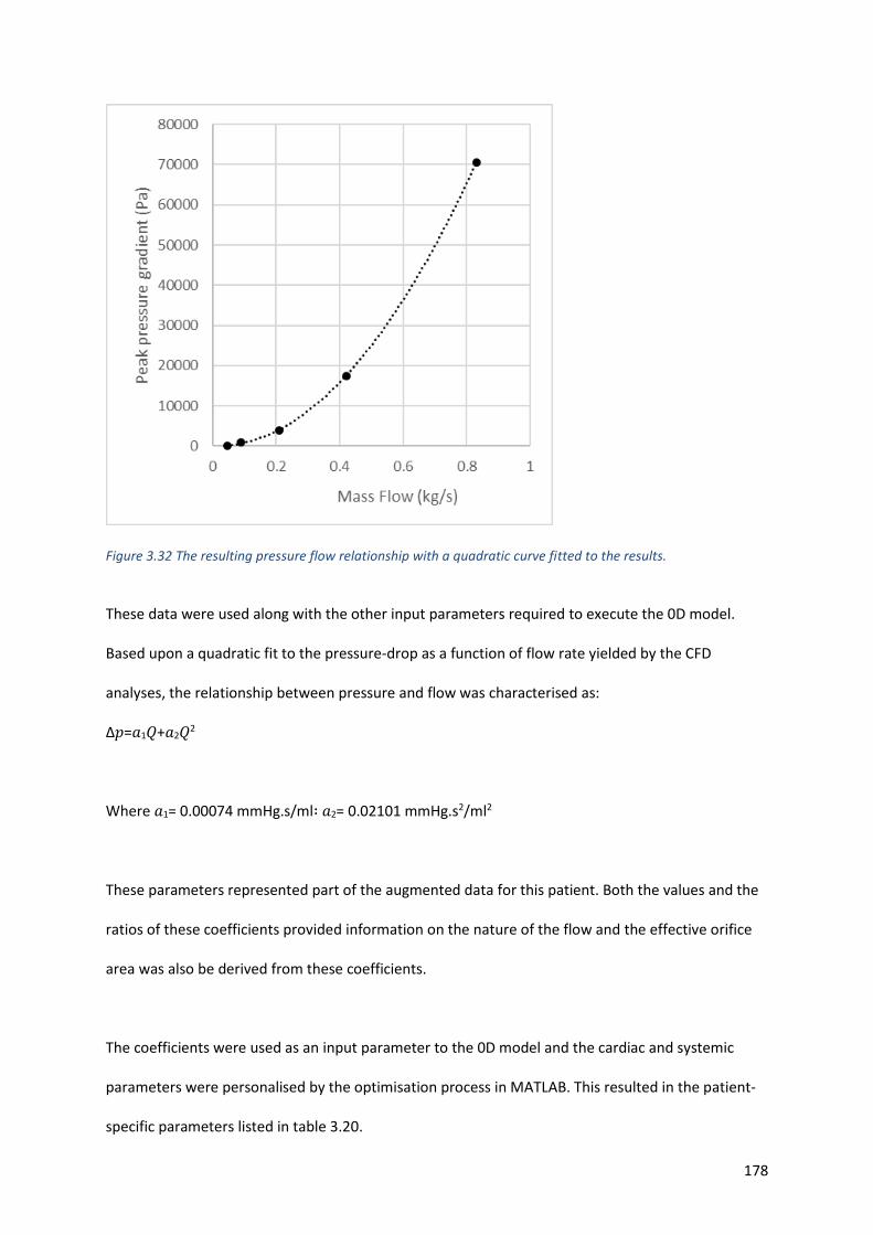
178

Figure 3.32 The resulting pressure flow relationship with a quadratic curve fitted to the results.

These data were used along with the other input parameters required to execute the 0D model.

Based upon a quadratic fit to the pressure-drop as a function of flow rate yielded by the CFD

analyses, the relationship between pressure and flow was characterised as:

Δ𝑝=𝑎1𝑄+𝑎2𝑄2

Where 𝑎1= 0.00074 mmHg.s/ml∶ 𝑎2= 0.02101 mmHg.s2/ml2

These parameters represented part of the augmented data for this patient. Both the values and the

ratios of these coefficients provided information on the nature of the flow and the effective orifice

area was also be derived from these coefficients.

The coefficients were used as an input parameter to the 0D model and the cardiac and systemic

parameters were personalised by the optimisation process in MATLAB. This resulted in the patient-

specific parameters listed in table 3.20.

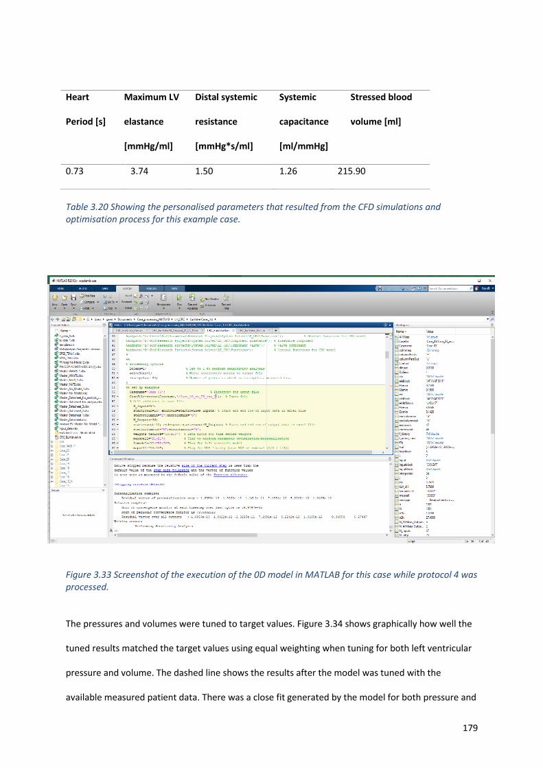
179

Table 3.20 Showing the personalised parameters that resulted from the CFD simulations and optimisation process for this example case.

Figure 3.33 Screenshot of the execution of the 0D model in MATLAB for this case while protocol 4 was processed.

The pressures and volumes were tuned to target values. Figure 3.34 shows graphically how well the

tuned results matched the target values using equal weighting when tuning for both left ventricular

pressure and volume. The dashed line shows the results after the model was tuned with the

available measured patient data. There was a close fit generated by the model for both pressure and

Heart

Period [s]

Maximum LV

elastance

[mmHg/ml]

Distal systemic

resistance

[mmHg*s/ml]

Systemic

capacitance

[ml/mmHg]

Stressed blood

volume [ml]

0.73 3.74 1.50 1.26 215.90

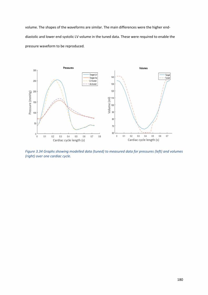
180

volume. The shapes of the waveforms are similar. The main differences were the higher end-

diastolic and lower end systolic LV volume in the tuned data. These were required to enable the

pressure waveform to be reproduced.

Figure 3.34 Graphs showing modelled data (tuned) to measured data for pressures (left) and volumes (right) over one cardiac cycle.

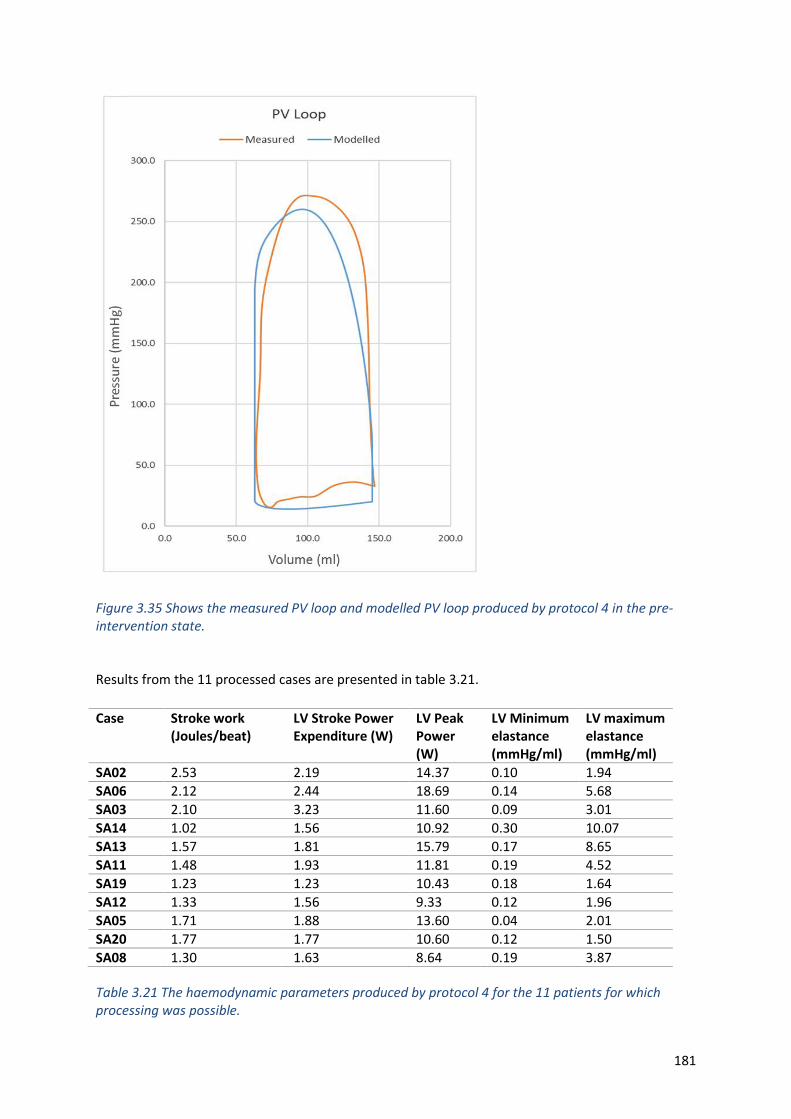
181

Figure 3.35 Shows the measured PV loop and modelled PV loop produced by protocol 4 in the pre-intervention state.

Results from the 11 processed cases are presented in table 3.21.

Table 3.21 The haemodynamic parameters produced by protocol 4 for the 11 patients for which processing was possible.

Case Stroke work (Joules/beat)

LV Stroke Power Expenditure (W)

LV Peak Power (W)

LV Minimum elastance (mmHg/ml)

LV maximum elastance (mmHg/ml)

SA02 2.53 2.19 14.37 0.10 1.94

SA06 2.12 2.44 18.69 0.14 5.68

SA03 2.10 3.23 11.60 0.09 3.01

SA14 1.02 1.56 10.92 0.30 10.07

SA13 1.57 1.81 15.79 0.17 8.65

SA11 1.48 1.93 11.81 0.19 4.52

SA19 1.23 1.23 10.43 0.18 1.64

SA12 1.33 1.56 9.33 0.12 1.96

SA05 1.71 1.88 13.60 0.04 2.01

SA20 1.77 1.77 10.60 0.12 1.50

SA08 1.30 1.63 8.64 0.19 3.87

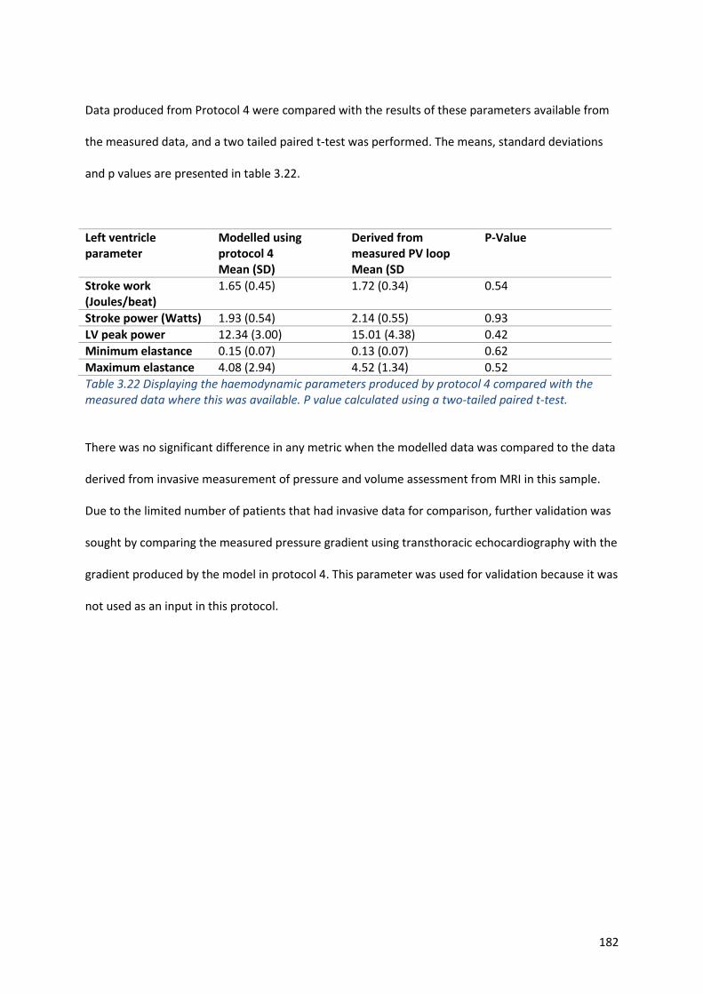
182

Data produced from Protocol 4 were compared with the results of these parameters available from

the measured data, and a two tailed paired t-test was performed. The means, standard deviations

and p values are presented in table 3.22.

Left ventricle parameter

Modelled using protocol 4 Mean (SD)

Derived from measured PV loop Mean (SD

P-Value

Stroke work (Joules/beat)

1.65 (0.45) 1.72 (0.34) 0.54

Stroke power (Watts) 1.93 (0.54) 2.14 (0.55) 0.93

LV peak power 12.34 (3.00) 15.01 (4.38) 0.42

Minimum elastance 0.15 (0.07) 0.13 (0.07) 0.62

Maximum elastance 4.08 (2.94) 4.52 (1.34) 0.52

Table 3.22 Displaying the haemodynamic parameters produced by protocol 4 compared with the measured data where this was available. P value calculated using a two-tailed paired t-test.

There was no significant difference in any metric when the modelled data was compared to the data

derived from invasive measurement of pressure and volume assessment from MRI in this sample.

Due to the limited number of patients that had invasive data for comparison, further validation was

sought by comparing the measured pressure gradient using transthoracic echocardiography with the

gradient produced by the model in protocol 4. This parameter was used for validation because it was

not used as an input in this protocol.

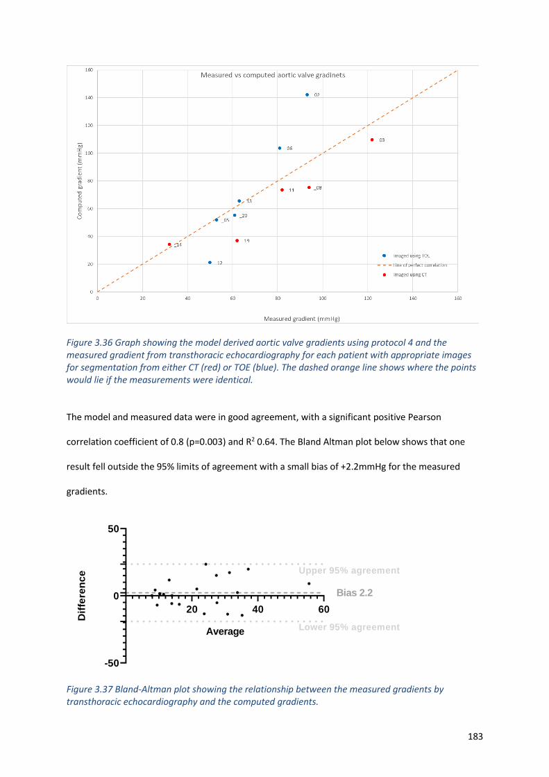
183

Figure 3.36 Graph showing the model derived aortic valve gradients using protocol 4 and the measured gradient from transthoracic echocardiography for each patient with appropriate images for segmentation from either CT (red) or TOE (blue). The dashed orange line shows where the points would lie if the measurements were identical.

The model and measured data were in good agreement, with a significant positive Pearson

correlation coefficient of 0.8 (p=0.003) and R2 0.64. The Bland Altman plot below shows that one

result fell outside the 95% limits of agreement with a small bias of +2.2mmHg for the measured

gradients.

20 40 60

-50

0

50

Average

Dif

fere

nc

e Upper 95% agreement

Lower 95% agreement

Bias 2.2

Figure 3.37 Bland-Altman plot showing the relationship between the measured gradients by transthoracic echocardiography and the computed gradients.

184

3.9. Diagnostic utility

Image-based modelling (protocol 4) may be used to assess the gradient across the valve as shown

above. As discussed in section 1.3, AS is a systemic disease and plays only one part in the loading of

the left ventricle that results in a patient’s symptoms. The parameters produced by the model may

correlate better with patient symptoms. This hypothesis was tested by first comparing the disease

severity in terms of aortic stenotic gradients with activity metrics, and then by comparing the model

parameters with these same activity metrics.

3.9.1. Association of standard clinical parameters with activity measures

Peak pressure gradient

Peak gradient was negatively correlated with 6MWT distance achieved (r= -0.61, p= 0.004) but not

with any other activity metric, degree of symptoms, LV ejection fraction or LV mass.

Mean pressure gradient

Mean gradient was negatively correlated with the 6MWT distance achieved (r=-0.52, p=0.02) but not

with any other activity metric, degree of symptoms, LV ejection fraction or LV mass.

Effective orifice area

EOA showed a weak, but significant, correlation with 6MWT distance (r=0.57, p=0.01). It was also

weakly correlated with total energy expenditure (r=0.61, p=0.02). It did not correlate with any other

activity metric, LV ejection fraction or LV mass.

185

Ejection fraction

Ejection fraction was negatively correlated with the amount of time spent sleeping and the cardiac

efficiency slope (r=-0.65, p=0.01 and r=-0.56, p= 0.04 respectively). There was no correlation with

any other activity metrics, or the patient reported symptoms.

LV mass

There was no association with any activity metrics or LV ejection fraction.

3.9.2. Modelling as a diagnostic tool

Because AS is a systemic disease, it is difficult to assess severity purely by examining the anatomy

and using standard imaging methods. However, one can expect that the more severe the disease

and the effects on the patient’s physiology, the more limiting it is in terms of functional capacity.

This is akin to the argument of anatomical vs functional severity of coronary artery disease. The

following model-derived parameters take into account the total physiological burden of AS.

ELVmin

A significant and strong negative correlation was identified between ELVmin and the total energy

expenditure of the patients measured by the Philips health watch (r=-0.73, p=0.002). This also

correlated with LV mass (r=0.74, p=0.001) and step count (r=-0.62, p=0.003). A negative correlation

with the six-minute walk distance achieved was seen (r=-0.62, p=0.002).

ELVmax

There was a strong negative correlation with LV mass (r=-0.84, p=0.0002) and step count (r=0.58

p=0.03). Although there was correlation with ejection fraction (r=0.77, p=0.0001), there was no

correlation with between measured EF and any activity metric.

186

LV work

LV work was significantly associated with LV mass (r=0.59, p=0.006), the total energy expenditure of

the patient (r=0.76, p=0.001) and the six-minute walk test distance achieved (r=0.58, p=0.006).

LV peak power

A significant positive correlation was found with both step count (r=0.66, p=0.007) and total energy

expenditure (r=0.61, p=0.002). There was no correlation with LV mass.

Wasted energy

A strong correlation with LV mass was found (r=0.79, p=0.0002). There was no association with any

activity metrics.

3.9.3. Assessment of left ventricular failure

ELVmax, which may be a better assessment of the global contractile function of the LV than ejection

fraction (see section 1.11.8), exhibited a correlation with ejection fraction in this cohort (r=0.77

p=0.05). In healthy men and women, in the resting state, reported values of ELVmax are 2.3 ± 1.0

mmHg/ml [194], [215]. Within this range, only 33% had a normal ejection fraction. In adapting to AS,

the normal response is for the contractility (ELVmax) to increase in patients with preserved ejection

fraction, which was found in 75% of the cohort. Four patients had modelled elastance greater than

twice the upper limit of normal, indicating that these ventricles were well adapted, continuing to

function effectively in the presence of increased load. These data are illustrated in figure 3.39.

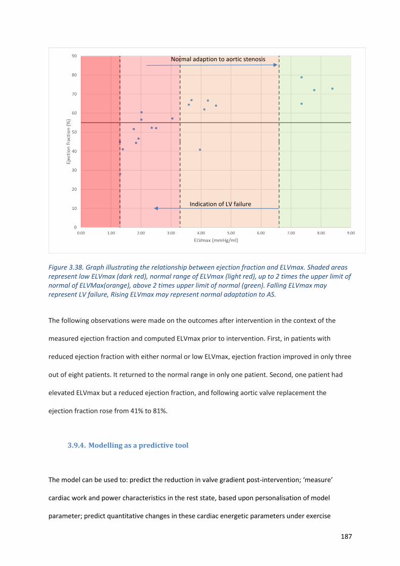
187

Figure 3.38. Graph illustrating the relationship between ejection fraction and ELVmax. Shaded areas represent low ELVmax (dark red), normal range of ELVmax (light red), up to 2 times the upper limit of normal of ELVMax(orange), above 2 times upper limit of normal (green). Falling ELVmax may represent LV failure, Rising ELVmax may represent normal adaptation to AS.

The following observations were made on the outcomes after intervention in the context of the

measured ejection fraction and computed ELVmax prior to intervention. First, in patients with

reduced ejection fraction with either normal or low ELVmax, ejection fraction improved in only three

out of eight patients. It returned to the normal range in only one patient. Second, one patient had

elevated ELVmax but a reduced ejection fraction, and following aortic valve replacement the

ejection fraction rose from 41% to 81%.

3.9.4. Modelling as a predictive tool

The model can be used to: predict the reduction in valve gradient post-intervention; ‘measure’

cardiac work and power characteristics in the rest state, based upon personalisation of model

parameter; predict quantitative changes in these cardiac energetic parameters under exercise

Normal adaption to aortic stenosis

Indication of LV failure

188

conditions pre-intervention and under both rest and exercise conditions post-intervention; and infer,

from the changes in cardiac energetics’ the degree to which activity might be increased if left

ventricular work were to be maintained.

3.9.4.1. Illustrative results for one case

For this individual, the measured peak and mean AV pressure gradients at rest pre-intervention were

89mmHg and 62 mmHg, and post-intervention they were reduced to 10 mmHg and 5 mmHg,

respectively. The model predictions for this case, post-intervention, were 11 mmHg and 4 mmHg.

Figure 3.40 shows modelled PV loops for this patient, at rest and in an exercise state, both pre- and

post-intervention.

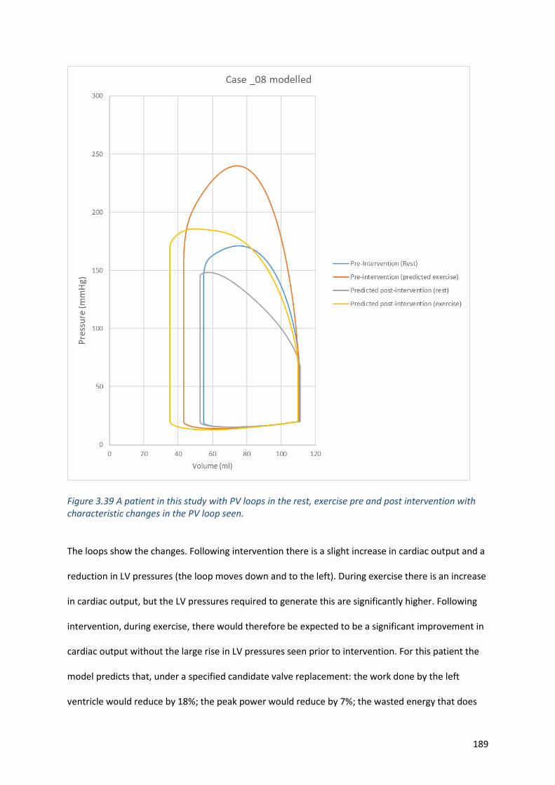
189

Figure 3.39 A patient in this study with PV loops in the rest, exercise pre and post intervention with characteristic changes in the PV loop seen.

The loops show the changes. Following intervention there is a slight increase in cardiac output and a

reduction in LV pressures (the loop moves down and to the left). During exercise there is an increase

in cardiac output, but the LV pressures required to generate this are significantly higher. Following

intervention, during exercise, there would therefore be expected to be a significant improvement in

cardiac output without the large rise in LV pressures seen prior to intervention. For this patient the

model predicts that, under a specified candidate valve replacement: the work done by the left

ventricle would reduce by 18%; the peak power would reduce by 7%; the wasted energy that does

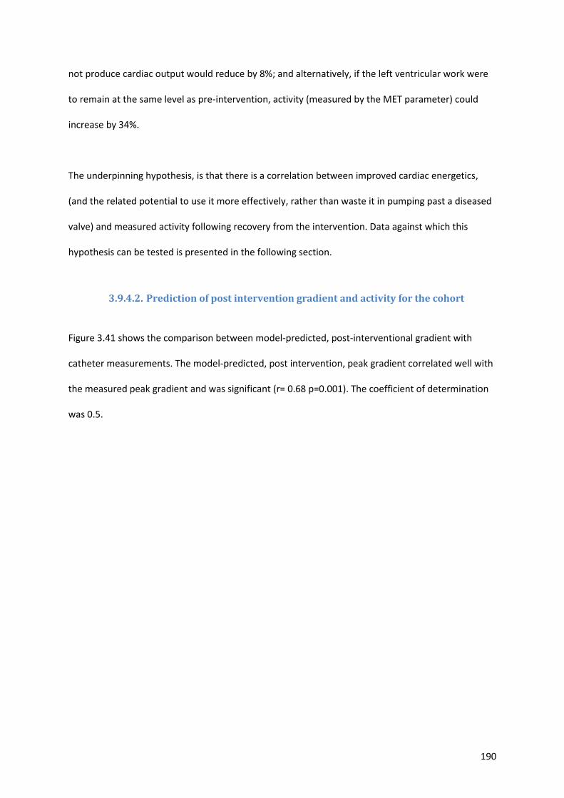
190

not produce cardiac output would reduce by 8%; and alternatively, if the left ventricular work were

to remain at the same level as pre-intervention, activity (measured by the MET parameter) could

increase by 34%.

The underpinning hypothesis, is that there is a correlation between improved cardiac energetics,

(and the related potential to use it more effectively, rather than waste it in pumping past a diseased

valve) and measured activity following recovery from the intervention. Data against which this

hypothesis can be tested is presented in the following section.

3.9.4.2. Prediction of post intervention gradient and activity for the cohort

Figure 3.41 shows the comparison between model-predicted, post-interventional gradient with

catheter measurements. The model-predicted, post intervention, peak gradient correlated well with

the measured peak gradient and was significant (r= 0.68 p=0.001). The coefficient of determination

was 0.5.

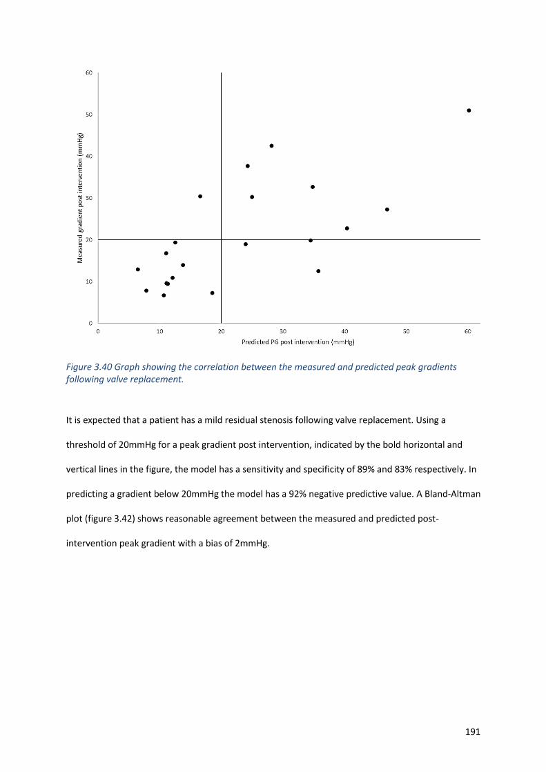
191

Figure 3.40 Graph showing the correlation between the measured and predicted peak gradients following valve replacement.

It is expected that a patient has a mild residual stenosis following valve replacement. Using a

threshold of 20mmHg for a peak gradient post intervention, indicated by the bold horizontal and

vertical lines in the figure, the model has a sensitivity and specificity of 89% and 83% respectively. In

predicting a gradient below 20mmHg the model has a 92% negative predictive value. A Bland-Altman

plot (figure 3.42) shows reasonable agreement between the measured and predicted post-

intervention peak gradient with a bias of 2mmHg.

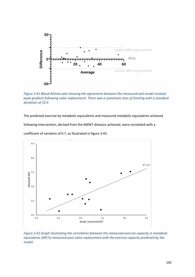
192

20 40 60

-50

0

50

Average

Dif

fere

nc

e Upper 95% agreement

Lower 95% agreement

Bias

Figure 3.41 Bland-Altman plot showing the agreement between the measured and model residual peak gradient following valve replacement. There was a systematic bias of 2mmHg with a standard deviation of 10.9.

The predicted exercise by metabolic equivalents and measured metabolic equivalents achieved

following intervention, derived from the 6MWT distance achieved, were correlated with a

coefficient of variation of 0.7, as illustrated in figure 3.43.

Figure 3.42 Graph illustrating the correlation between the measured exercise capacity in metabolic equivalents (METs) measured post valve replacement with the exercise capacity predicted by the model.

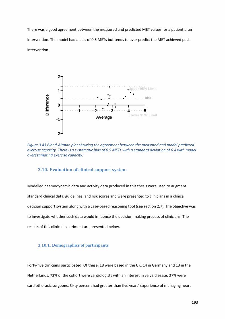
193

There was a good agreement between the measured and predicted MET values for a patient after

intervention. The model had a bias of 0.5 METs but tends to over predict the MET achieved post

intervention.

1 2 3 4 5

-2

-1

0

1

2

Average

Dif

fere

nc

e

Lower 95% Limit

Upper 95% Limit

Bias

Figure 3.43 Bland-Altman plot showing the agreement between the measured and model predicted exercise capacity. There is a systematic bias of 0.5 METs with a standard deviation of 0.4 with model overestimating exercise capacity.

3.10. Evaluation of clinical support system

Modelled haemodynamic data and activity data produced in this thesis were used to augment

standard clinical data, guidelines, and risk scores and were presented to clinicians in a clinical

decision support system along with a case-based reasoning tool (see section 2.7). The objective was

to investigate whether such data would influence the decision-making process of clinicians. The

results of this clinical experiment are presented below.

3.10.1. Demographics of participants

Forty-five clinicians participated. Of these, 18 were based in the UK, 14 in Germany and 13 in the

Netherlands. 73% of the cohort were cardiologists with an interest in valve disease, 27% were

cardiothoracic surgeons. Sixty percent had greater than five years’ experience of managing heart

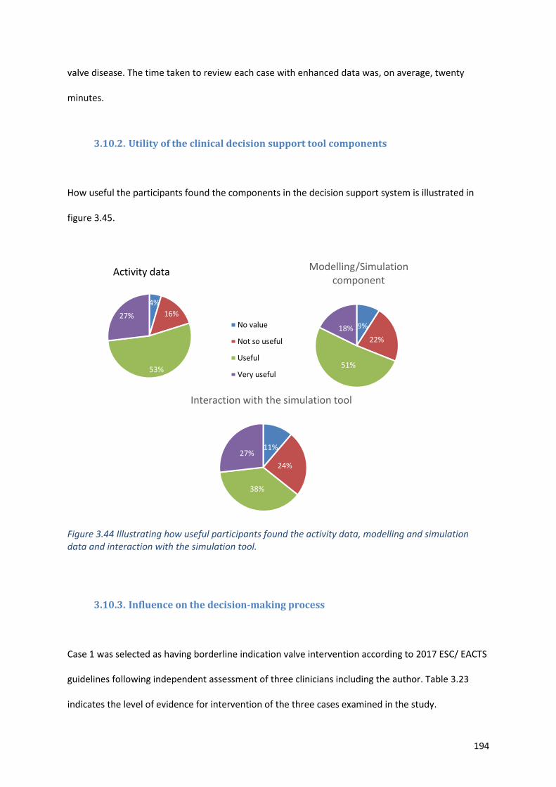
194

valve disease. The time taken to review each case with enhanced data was, on average, twenty

minutes.

3.10.2. Utility of the clinical decision support tool components

How useful the participants found the components in the decision support system is illustrated in

figure 3.45.

Figure 3.44 Illustrating how useful participants found the activity data, modelling and simulation data and interaction with the simulation tool.

3.10.3. Influence on the decision-making process

Case 1 was selected as having borderline indication valve intervention according to 2017 ESC/ EACTS

guidelines following independent assessment of three clinicians including the author. Table 3.23

indicates the level of evidence for intervention of the three cases examined in the study.

4%

16%

53%

27%

Activity data

No value

Not so useful

Useful

Very useful

9%

22%

51%

18%

Modelling/Simulation component

11%

24%

38%

27%

Interaction with the simulation tool

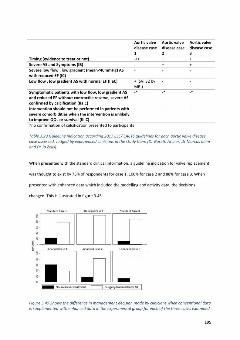
195

Aortic valve disease case 1



Timing (evidence to treat or not) -/+ + +

Severe AS and Symptoms (IB) - + +

Severe low flow , low gradient (mean<40mmHg) AS with reduced EF (IC)

- - -

Low flow , low gradient AS with normal EF (IIaC) + (SVi 32 by MRI)

- -

Symptomatic patients with low flow, low gradient AS and reduced EF without contractile reserve, severe AS confirmed by calcification (IIa C)

-* -* -*

Intervention should not be performed in patients with severe comorbidities when the intervention is unlikely to improve QOL or survival (III C)

- - -

*no confirmation of calcification presented to participants

Table 3.23 Guideline indication according 2017 ESC/ EACTS guidelines for each aortic valve disease case assessed. Judged by experienced clinicians in the study team (Dr Gareth Archer, Dr Marcus Kelm and Dr Jo Zelis).

When presented with the standard clinical information, a guideline indication for valve replacement

was thought to exist by 75% of respondents for case 1, 100% for case 2 and 88% for case 3. When

presented with enhanced data which included the modelling and activity data, the decisions

changed. This is illustrated in figure 3.45.

Figure 3.45 Shows the difference in management decision made by clinicians when conventional data is supplemented with enhanced data in the experimental group for each of the three cases examined.

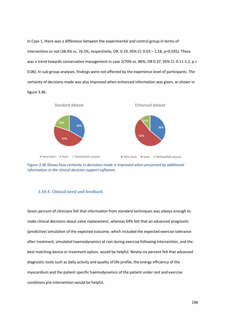
196

In Case 1, there was a difference between the experimental and control group in terms of

intervention or not (38.4% vs. 76.5%, respectively; OR: 0.19, 95% CI: 0.03 – 1.18, p=0.035). There

was a trend towards conservative management in case 2(70% vs. 86%; OR 0.37, 95% CI: 0.11-1.2, p =

0.06). In sub-group analyses, findings were not affected by the experience level of participants. The

certainty of decisions made was also improved when enhanced information was given, as shown in

figure 3.46.

Figure 3.46 Shows how certainty in decisions made is improved when presented by additional information in the clinical decision support software.

3.10.4. Clinical need and feedback

Seven percent of clinicians felt that information from standard techniques was always enough to

make clinical decisions about valve replacement, whereas 69% felt that an advanced prognostic

(predictive) simulation of the expected outcome, which included the expected exercise tolerance

after treatment, simulated haemodynamics at rest during exercise following intervention, and the

best matching device or treatment option, would be helpful. Ninety-six percent felt that advanced

diagnostic tools such as daily activity and quality of life profile, the energy efficiency of the

myocardium and the patient specific haemodynamics of the patient under rest and exercise

conditions pre-intervention would be helpful.

33%

47%

20%

Standard dataset

Very Sure Sure Somewhat unsure

36%

53%

11%

Enhanced dataset

Very Sure Sure Somewhat unsure

197

Participants were invited to leave free text comments about the clinical decision support system.

Overall, it was felt that the clinical decision support system would be a useful addition to the heart

team, with one participant predicting that it may replace some of the work of the heart team.

Clinicians indicated that it may increase in certainty in decision making especially in borderline cases

and asymptomatic cases. Providing an overview of the whole patient by combining anatomical and

physiological information appears very useful to the majority. Participants liked the concept of

utilising activity data and modelling data to predict outcome but there was the overwhelming

opinion that this data need validating in a much bigger cohort before the tool entered clinical

practice.

198

CHAPTER 4

4. Discussion

This work was designed as a pilot study to investigate whether non-invasive pressure volume loops

could be created using mathematical and computational models in cases of AS and whether they

had advantages over standard diagnostic techniques and novel imaging techniques such as 4D flow

MRI. There was also an exploration of how the functional assessment of these patients, to which

these techniques were compared, may be undertaken using both standard techniques and novel

wearable devices. In summary, it was found that mathematical and computational models could be

produced and may be helpful in the diagnosis of and management of AS, particularly in the timing

and type of intervention, and the likely impact on the patients haemodynamics. These techniques

have several advantages over standard clinical measures that do not take into account the global

haemodynamic burden of this systemic disease and are not predictive. 4D flow MRI examination

may give more insight to the haemodynamic effects of AS and provide different ways to assess the

severity of AS. Wearable devices giving insight into a patient’s lifestyle and the effect of the disease

on the individual monitoring trends in patients may help in identifying when medical intervention is

needed and help determine the frequency of clinical review. Clinical decisions support systems that

help present patient-specific data may be helpful to clinicians in the management of AS and can

influence the decisions made.

4.1. Study design and patient cohort

The number of patients recruited to the study was small; however, this is comparable to similar

studies[168] and large amounts of clinical, simulated and functional capacity data were obtained for

each patient. An important tenet of this study was that the model could add value within a routine

199

clinical care pathway, in which incomplete data is common. Even within this well-controlled study

there were a number of patient, procedural, technical and logistical issues which resulted in missing

data. These are discussed in the relevant sections below, as are the attempts made to mitigate the

effects. Consequently, although some of the associations investigated reached statistical

significance, several other trends require larger and appropriately powered clinical studies for

confirmation or otherwise.

The average age of the cohort, 76, was typical and representative of the demographic present with

calcific AS. There was a greater proportion of female patients in the study than male (77 vs 23%).

Thirty-two percent had atrial fibrillation, which is not unexpected in a population that have

increased pressures in the left side of the heart [217]. The beat to beat variability was not

represented in the model, but clinical data for model personalisation or validation were averaged

over five cardiac cycles and an arrhythmia rejection protocol was applied to MRI data to mitigate for

this problem. Blood pressure in this patient cohort was not well controlled, and this tended to

further amplify the load on the ventricle beyond that directly attributable to the AS. This may

account for some of the differences in the associations with activity and positive remodelling and

underpins the hypothesis that it is the total load on the ventricle that is important.

The TAVI cohort were older, frailer and had more severe disease that the patients undergoing SAVR.

There were peri-procedural complications in several patients that underwent TAVI. Two patients

were unable to complete the study due to disabling strokes. Two further patients had femoral access

complications that required further surgical intervention and affected mobility. One patient had

osteoarthritis and was unable to attempt the 6MWT. These patients were excluded from the activity

analysis, which could also have influenced and biased the results. Due to deaths during the study,

complications and a poor response to the invitation to participate, there was a limited number in the

200

extended follow-up group. Although trends could be identified, the small numbers and resultant

large standard deviations meant that significant differences were difficult to identify.

Despite no known prior contraindications, two patients were not able to undergo MRI pre-

intervention. One was claustrophobic and was unable to complete the scan. One had previous facial

reconstruction with metal plates and the scan was abandoned. Alternative imaging protocols were

used so that their other data could be included in the study. LV volumes that were essential for the

processing of the modelling protocols were obtained by gated cardiac CT in one case, and 3D

transthoracic echocardiography in the other. This introduced some variability of the assessment of

LV volumes, which could have affected the results, but the alternative techniques have been

reported to produce comparable results [218].

4.2. Imaging

4.2.1. Transthoracic echocardiography

As expected, transthoracic echocardiography showed a significant reduction in peak and mean

gradients following intervention. The magnitude of the reduction differed depending upon the type

and size of the valve implanted, the surgical technique and patient size. The gradient also depends

upon other haemodynamic factors such as heart rate and systemic vascular resistance. These are not

usually taken into account in routine clinical practice but could be in the modelling process. This

study highlights that this measure is dependent upon such factors and, ideally, when gradients are

reported this should take into account both heart rate and loading conditions.

Doppler derived measures are well recognised to overestimate the gradient across the aortic

valve[38] and this may explain some differences in the measured and the modelled gradients seen.

None of the transthoracic 3D acquisitions yielded images that could support accurate segmentation

201

of the valve anatomy. This was mainly due to poor image resolution and artefacts from calcification

and arrhythmias. This is important because, ideally, the modelling process should operate with

routine non-invasive clinical data. This can be the case for protocols 1-3 but, to run an image-based

protocol such as protocol 4, either more invasive tests such as transoesophageal echocardiography,

or tests that require ionising radiation such as CT, would be needed.

It is recognised that, as the left ventricle adapts to the increase in afterload due to AS, it

hypertrophies, and this is associated with reduced myocardial compliance and diastolic dysfunction.

This was evidenced in this cohort by the pseudo-normalised E/A ratios in the majority of patients

indicating grade 2 diastolic dysfunction, with significantly elevated E/e’ ratios with an average of

17.4 (normal range 6.5±3.7)[219] and elevated LVEDP when calculated using the Nagueh formula.

Following valve replacement, although there is a trend in reduction of E/e’ in the early follow up

period, this was not significant and still remained abnormal. This differs from a study which found

that diastolic function was significantly affected in patients with severe AS before surgery but

returned toward normal early and late after AVR.[220]. My findings are consistent with the study by

Gjertsson et al which showed that diastolic function was unchanged following intervention despite a

reduction in LV mass [221]. In that and the present study no attempt was made to control for

hypertension following surgery which may contribute to persistent diastolic dysfunction. In the

current study there was no significant difference between the systolic and diastolic blood pressures

before and after intervention; so it could be the effect of valve replacement that is being observed,

or perhaps hypertension has a greater influence on diastolic dysfunction than AS. Early follow-up in

both these studies was two years and the method of assessing diastolic function was different which

makes it difficult to make comparisons. There is no specific guidance as to how optimally to assess

diastolic dysfunction following aortic valve replacement. When using tissue Doppler imaging,

perhaps rather than averaging the septal and lateral velocities as is the norm and has previously

been suggested following AVR[222], only the velocities at the lateral valve annulus should be used. It

202

is likely that the sewing in of the replacement valve would affect the motion of the tissue at the

septum and therefore the inaccuracies of these measurements could be why there was no

correlation of diastolic parameters with modelled parameters or exercise capacity.

The Nagueh formula used to calculate LVEDP and used as an input to the modelling process has a

number of flaws, including the fact that it has not been validated in atrial fibrillation (32% of our

cohort) or in patients with AS[193]. However, the relationship between E/e’ and LVEDP has been

extensively studied in the AS population by Dalsgaard et al[223]. There is a clear relationship and

therefore the method used to estimate LVEDP seems reasonable. The measured and derived LVEDP

were also consistent (see section 3.3) which again gives confidence in the results.

4.2.2. Transoesophageal echocardiography

This technique can produce accurate data for segmentation (six out of eleven examinations in this

cohort). It is probably superior to CT, which is limited by calcification in identifying the valve orifice.

With development in the imaging and post-processing software, it is likely that the images will

improve, making this technique even more suitable for use in the segmentation process. It also

provides accurate data for LV volumetric assessment but was not used in this cohort because the

patients underwent TOE under anaesthesia immediately prior to valve replacement and were under

the influence of various medications that would affect the preload and afterload and hence the LV

volumes. All protocols, including protocol 4, could be run entirely with data derived from a standard

TOE not under anaesthetic conditions. A small number of patients undergo TOE as a work-up to

aortic surgery, so it would not be part of routine practice as was intended when this project was

conceived. It is also rather invasive, so the benefit of the examination would need to be apparent,

with validation in larger cohorts and eventually studies looking at the outcome of patients. A benefit

of using this modality of imaging is that there is no ionising radiation, in contrast to cardiac CT.

203

4.2.3. Computed tomography

It was anticipated at the start of the project that CT may yield the highest resolution images that

were the most suitable for segmentation and use in protocol 4. Unfortunately, due to heavy

calcification in some valves, suitable images were only obtained for five out of eleven patients that

underwent CT. CT was used in one patient that had inadequate 3D transthoracic imaging and was

unable to complete the MRI scan due to claustrophobia. These LV volumes were used as inputs to

the model for protocols 1-3; this patient was excluded from protocol 4 due to poor imaging of the

valve. This could have introduced some variability in the results, but LV volumetric data from CT is

comparable to that obtained by both 3D echocardiography and CMR imaging[218], [224]. Another

issue is that most cardiac CTs are prospectively gated to reduce the amount of radiation to which the

patient is exposed. In some protocols for aortic assessment for TAVI only 40-80% of the R-R interval

is obtained; this would often exclude images at mid-systole when the valve was fully open, and these

are the exact images required for the segmentation and modelling process in protocol 4. In routine

clinical scans the valve and aorta are often assessed during diastole, when there is less motion of the

heart, but as the heart contracts the size of the aortic root changes. Therefore, measurement of the

size in mid- systole when the valve is fully open is helpful. In this cohort, 20-40% of the cardiac cycle

was also imaged. Due the balance of data collection, storage and analysis time, it was decided that

data would be stored only at 10% intervals. It is likely that mid-systole did not occur at exactly 30%

of the R-R interval; it could have occurred at 25%, 28%, 32% etc, potentially missing the valve at its

maximally open point and affecting the results. It was judged that this is unlikely to have affected

the results as the valve opens quickly even in AS to its maximum (within approximately 130ms[214])

and stays relatively open until the end of systole, so examining at 20% and 30% of the cardiac cycle

should be representative. In low flow, low gradient AS, when the stroke volume is less than 35ml,

this is more likely to be a problem (only one case in this study). Missing the point of the valve

maximally open is less likely to happen if retrospective gating is used, when data is acquired across

the entire cardiac cycle. Although this technique requires more radiation, it is useful in patients with

204

arrhythmias; and a high proportion of patients with AS have atrial fibrillation. If the use of the tools

and concepts developed in this thesis could be further validated and a clear benefit to patients

shown, then the benefit may outweigh the small risk of increased radiation dose.

Use of a static image and not capturing the dynamic motion of the aortic valve is also a limitation.

The mean aortic gradient is best to determine the severity of the stenosis, and this is calculated

across the systolic period. However, due to the complexity of modelling flows through the moving

structure, it was not performed in this project. Assessing the flow through the outflow tract and

valve could be performed using 4D flow CMR imaging and used as boundary conditions to the

model, obviating the need for a valve image and segmentation (this is discussed in sections 4.5 and

5.2.2).

4.2.4. Magnetic Resonance Imaging

Volumes for the model processing were acquired using this method for the majority of patients (20

out of 22) as, whilst comparable to 3D echocardiography and CT, it is thought by many to be the

‘gold standard’ test due to its accuracy and reproducibility[218]. The results showed that there was

no real change in volumes or significant change in ejection fraction following intervention, but this

may be because only eight patients had evidence of LV systolic dysfunction prior to intervention. The

majority had mild impairment, so in this cohort it may be difficult to appreciate a significant

difference overall. However, even in a sub-group analysis of the patients with LV systolic

impairment, although there was a trend of increasing ejection fraction, this was not significant, and

the majority of these patients still had systolic impairment following intervention. As mentioned in

section 1.11.8, there is an issue with the use of ejection fraction as a measure of cardiac function.

Ejection fraction should be seen really as a measure of performance rather than function, as the

function depends upon the loading conditions of the ventricle. For instance, a normal ejection

fraction in severe mitral regurgitation suggests that the left ventricle is failing, because a higher than

205

normal ejection fraction should be expected. Similarly, in AS, although the ejection fraction is

normal, the heart may be failing. This is illustrated in section 3.9.3, where elastance may be a better

assessment of the true function of the left ventricle.

Following intervention, and reduction of the load on the ventricle, as evidenced by the reduction in

pressure gradient, there was a significant reduction of LV mass. There is evidence that hypertrophy

is associated with excess cardiac mortality and morbidity in those undergoing aortic valve

replacement[225] [226]. It is therefore important to know the likelihood of positive

remodelling[227] which was associated with a number results from the modelling process.

Favourable or adverse left ventricular remodelling is affected by several factors including age,

gender, haemodynamics, patient prosthesis mismatch, type of valve replacement, blood pressure

control and ethnicity. Myocardial metabolism and coronary artery circulation are also involved in the

changes occurring after aortic valve replacement[228]. In a further study older age, advanced NYHA

class, reduced left ventricle ejection fraction, hypertension, and high pre-operative left ventricular

mass index were associated with reduced survival. Early myocardial regression as seen in this study

was weakly associated with mid-term outcome[229].

4.3. Measured pressure volume loop

From the measured loops it was possible to calculate stroke work, wasted work and total myocardial

work and to estimate peak power, stroke power and wasted power; the mathematical formulae are

described in section 2.4.1.2. These were used as one of the comparators for data obtained in the

modelling process. Data were obtained in patients undergoing TAVI only to help validate the results

of the modelling; but there were a number of issues that could affect accuracy of these results.

However, the LV pressure data obtained were consistent with data obtained by other imaging

modalities and generated by the modelling process. The mean measured LVEDP of 23 ± 12mmHg

206

was consistent with the LVEDP calculated by the Nagueh formula and TTE Doppler data 23mmHg ±

9mmHg.

This work is the first attempt at creating a PV loop using invasive pressure data coupled with MRI

derived LV volumes. The advantage of this technique is that the MRI derived LV volumes are more

accurate than volumes usually derived from conductance catheters[230]. However, the pressures

and flows were not measured simultaneously; some MRIs were performed up to 3 weeks prior to

the procedure where the invasive pressure measurements were obtained. However, during this

period there were no changes in medications and the degree of stenosis will not have changed

significantly, but the loading conditions due to fluid intake and the timing of the procedures, e.g.

occurring first thing in the morning after medications, may have affected the data. Also, as the data

were not acquired simultaneously, there were differences in cardiac cycle length that had to be

taken into account. To minimise this issue, care was taken to select the pressure traces that were a

similar cycle length, and the pressure data was re-scaled temporally to the same cardiac period as

that for MRI volume data. A further disadvantage was that the pressure was obtained using a 7

French catheter which crossed the aortic valve. This will have introduced some aortic regurgitation

and although this was not evident on a number of tracings, it could be seen in some of the PV loops,

suggesting significant aortic regurgitation which may also have affected the results. A similar if not

larger size catheter is used in the conductance catheter method.

Data suggest the average stroke work is approximately 1.21 joules/beat [231]. The average age of

this literature cohort was younger at 60, and 50% were hypertensive although the systolic and

diastolic blood pressures were not stated. As expected, the patients in the current study had higher

stroke work, averaging 1.34 Joules/beat.

207

As seen in section 3.8 the modelled and measured data produce a similar smooth curve of LV power

over the cardiac cycle suggesting that that the measured data produces a reasonable estimate of

cardiac power. This is the first study that illustrates that the peak LV power occurs in early systole

just after the valve opens giving insight into cardiac haemodynamics.

4.4. Outcome measures

NYHA class assessed by the clinician and the Borg scale of effort during the 6MWT were the only

markers to suggest there was an improvement in functional capacity following intervention in this

study. The NYHA class assessment has a number of deficiencies, including the fact that it is

subjective, is made by the clinician who would like the patient to improve following a treatment

(which may introduce some bias) and that it is an assessment made at a single point of time from

the patient’s description of their symptoms. Again, the Borg scale is the patient’s subjective

assessment at the time of the activity, so perhaps may be more accurate; but again, this may be

subject to bias and the placebo effect.

The use of wearable technology to examine the patient’s activity prior to intervention, during the

recovery period and subsequently is feasible and initial results seem to correlate with both patients

reported outcomes and the results of the 6MWT. This is the first research using wearable devices in

the context of aortic valve disease that gives us an insight not just into patients’ overall exercise

capacity but their daily lives. Using both wearable technologies the trend of decline at discharge and

significant recovery at 3-4 months was clearly seen. The trend of improvement and increased activity

continued into the extended follow up periods when a number of parameters from the Sphere kit

and Philips health watch were examined (see sections 3.4.1.2 and 3.4.1.3). There are large standard

deviations in this data suggesting some patients did very well and some very poorly. Due to the

limited numbers in this group it would be difficult to identify reasons for this. In a larger cohort a

208

multivariate analysis may identify patient or procedural factors that contribute to the difference in

recovery.

The objective measures from the wearable devices (Sphere kit and Philips watch) were consistent

with each other and with the six-minute walk test results at early follow-up, and the patient

reported measures of physical activity from the MLHFQ and the WHO BREF questionnaire. These

indicate that overall, there was no significant improvement in physical activity pre and post

intervention at 3-4 months. This mutual correlation of data from alternative modalities might give

some confidence in this novel approach using wearable devices to assess quantitatively the changes

in patient’s activity following aortic valve intervention. From a clinical perspective, it is disappointing

to see such minimal change following the intervention in this cohort.

The time of day when patients undertake certain activities, and where they perform these activities,

could be identified. This could be helpful clinically, for instance identifying when patients are

sleeping in a chair in the living room because of heart failure which may prompt medical contact. It

could also be used to counsel patients about how much exercise to take and inform a structured

rehabilitation programme which is known to be beneficial to patients following valve

replacement[232]. Identifying patients who are performing well post intervention can help plan

follow-up and reduce the need for clinic visits. Conversely, if a patient’s activity levels are declining

following intervention then close follow up or further treatments could be instigated.

There is a lack of consistency in reports of change of activity following TAVI. Some suggest

improvement, whilst others reflect the results of the current study. A meta-analysis[233] suggests

there is an overall improvement in the activity in patients who underwent TAVI but the majority of

patients included in the analysis were followed up at 12 months, with the minimum follow-up period

of 6 months. This makes , it difficult to make comparisons with the data presented in this thesis and

may explain the differences. Hiltrop et al also showed a significant increase in walk test difference at

209

one, six and twelve months of 8.2, 8.1 and 8.8 meters respectively when 147 patients were followed

up over a four-year period. However, it could be argued that an improvement of up to 9m during a

six-minute walk test is unlikely to translate to a functional benefit in day-to-day living. Other studies

that have looked at change in physical activity following TAVI showed similar results[200]. Green et

al[234], in patients undergoing TAVI, showed that post intervention 6MWT distance was dependent

upon distance walked pre-intervention. Generally, for people who could walk reasonably well prior

to TAVI, their walk distance reduced up to 12 months after the procedure; however, the people who

were slow walkers or unable to walk pre-intervention significantly improved following intervention.

Again, there were wide standard deviations, with some people doing considerably better and some

considerably worse than others. A further more recent study shows that a third of patients that

undergo TAVI do not improve their exercise capacity following intervention[235]. There is a paucity

of literature describing the change in functional capacity following aortic valve surgery, particularly

with objective measures. In a study by Kim et al, patients undergoing SAVR, who were relatively

healthier and had higher baseline function compared with TAVI patients, experienced a subjective

NYHA class functional status improvement in three quarters of cases, remained stable in

approximately one fifth, and declined in very few[236].

In this study, it was envisaged that patients would be able to set up equipment and calibrate the

equipment for activity monitoring themselves. It was designed to be as simple as possible with

detailed written instructions and demonstrations given by the author. However, with the older

demographic that presents with AS, this proved difficult. The author had to make numerous home

visits to set up and retrieve the equipment. This would have to be taken into account in future

studies or if such technologies were to be used in clinical practice. Rather than dichotomising end

points of function or disease specific decline in patients undergoing treatment with SAVR or TAVI,

preoperative assessment of their functional status using wearable devices may offer clinicians and

patients important information beyond the risk score about their expected trajectory following

210

intervention. This has already been shown using the six-minute walk test. Further research is needed

to see if these data could be used to guide patient selection.

It could be argued that most people would want to have increased physical capacity following their

procedure or find the activities that they could do before the intervention easier. The data suggests

that although trends were seen there was no significant increase in the amount of activity the

patient performed following intervention in this cohort which suggest they were not limited by the

disease prior to intervention, they had not fully recovered, or that the intervention had no benefit.

The improvement in the reported Borg score at the 6MWT and the reduction in NYHA class suggests

that the first is more likely; and that, although patients could still perform tasks, they found them

easier following intervention.

4.5. 4D flow CMR

4.5.1. Peak gradient and effective orifice area assessment

This is the first research to validate peak pressure gradient across the aortic valve by 4D flow CMR

against a reference invasive method. In addition, a novel 4D flow derived method for EOA in pre-

post-aortic valve intervention is described and validated against Doppler TTE. Importantly, 4D flow

derived pressure gradient and EOA demonstrated an association with the 6MWT. The 4D flow-

derived peak pressure gradient also demonstrated association to LV mass regression at three-

months.

Previous studies have demonstrated that there is discordance between the invasive and Doppler TTE

peak pressure gradient assessment. It is established that Doppler methods overestimate the peak

pressure drop[237], [238]. Many reasons for this over-estimation have been proposed. First, due to

211

the inherent differences between Doppler pressure gradient method, which provides a maximum

instantaneous pressure gradient at one time point versus the invasive method that provides the

peak-to-peak gradient which occurs at two different time points can lead to this over-

estimation[239]. Second, if the gain setting on the Doppler scale is set high, it can lead to over-

estimation of peak velocity. Other reasons include human errors associated with the Doppler

methods[240] and pressure recovery in the distal vessel[38]. Although the 4D flow methods

described in this thesis share some of these flaws, there was no overestimation as a result. In fact,

for defining severe AS, 4D flow derived pressure gradient was more consistent with invasive method.

Reduction in over-estimation could be because the peak velocity plane was spatially identified by

velocity vector visualization. This technique is not routinely applied in Doppler TTE, as peak velocity

assessment is made by continuous wave Doppler which sums all velocities in one direction.

EOA assessment can offer complementary information when making comprehensive assessment of

AS. EOA is relatively pre-load independent when compared to peak velocity assessment. In addition,

the novel EOA derived by 4D flow described in this thesis is not subject to the geometric

assumptions made using transthoracic echocardiography. As this method is the gradient of the linear

regression line between flow and velocity through the aortic valve, it may remain relevant in slow

flow, low gradient AS but larger studies are needed to evaluate our proposed methods in these

challenging cases of AS.

One of the most important clinical criteria to determine the timing of aortic valve intervention is

symptoms onset. Studies have demonstrated that the 6MWT predicts clinical outcomes and, in some

centres, a 6MWT is part of the routine assessment for patients referred for TAVI[118]. It was

noteworthy that, compared with measures from transthoracic echocardiography, it was only 4D flow

derived pressure gradient and EOA which were associated with both NYHA functional class and,

more importantly, with the 6MWT distance; this may help with prognostication.

212

As discussed above, LV mass regresses with decrease in afterload. LV mass regression is

independently associated with improved long-term survival[226] . It is plausible to expect a

proportional decrease in afterload, or the pressure gradient across the aortic valve and LV mass post

aortic valve replacement. In this study, LV mass regression demonstrated correlation to only 4D

flow-derived pressure gradient change; once again suggesting its superiority over the standard

methods of assessment.

Limited as it is by the small number of patients studied, this study offers hypothesis-generating data

for future larger studies. However, it is still plausible to suggest that 4D flow CMR offers an

alternative non-invasive method to quantify AS and its severity. Another limitation in the CMR

methodology included omission of respiratory navigation, which may have had an impact on the

accuracy of derived velocity parameters. However, studies that carried out a head-to-head

comparison of whole-heart 4D flow have demonstrated that for quantification of intra-cardiac KE,

both respiratory , and non-respiratory navigated, 4D flow acquisitions are comparable[241]. Other

limitations were a low temporal resolution (40ms), and variation in the heart rate and physiological

condition between the two acquisitions.

4.5.2. Left ventricular intra-cavity blood flow kinetic energy assessment

This is the first research into the LV blood flow KE in patients with AS, both pre- and post- valvular

intervention. It gives mechanistic insight into changes associated with AS by the assessment of KE of

the blood flow component. The main findings were that the average KE of the blood flow through

the left ventricle does not change significantly after valve intervention. However, the time delay,

direct flow and delayed flow were significantly modified after intervention indicating valve

replacement alters how blood is ejected from the heart, making the process more energy efficient

and suggesting an improvement in diastolic function. LV blood flow KE metrics demonstrated an

association with the 6MWT and LV remodelling at three-months was associated with the delayed

213

flow component of left ventricular flow. Different components of blood flow KE demonstrated

changes pre vs post valve intervention. Both direct and delayed flow components KE were

significantly reduced post valvular intervention. The rise in direct and delayed flow components in

severe AS patients was mainly observed in the late diastolic filling phase but further research is

warranted to explain this phenomenon.

LV blood flow KE demonstrated an inverse correlation to the 6MWT distance achieved. This was not

seen for standard CMR derived functional and volumetric assessment. An increase in the LV blood

flow KE may provide a novel haemodynamic biomarker of physical endurance that could be a useful

early parameter in the assessment of function, morbidity and perhaps prognosis in patients with AS.

Future studies should evaluate clinical cut-offs which predict outcomes in AS.

Normally, blood flows rapidly into the LV cavity from the base to the apex of the heart. The time

delay of this has been described previously as a marker of LV compliance and diastolic function

[242], [243]. In this cohort there was a significant reduction in time delay, reflecting an improvement

in restrictive LV filling after the valve intervention. This was not seen with diastolic assessment using

echocardiography so perhaps this is a more sensitive marker. In this, the time delay is derived

automatically using 3D flow quantified data versus echocardiographic methods which very

susceptible to operator and variability. Averaged LV blood flow KEiEDV for the complete cardiac

cycle demonstrated an association with LV remodelling post intervention. Peak E wave KEiEDV

showed a trend towards association with LV remodelling.

Although healthy controls were not recruited in this research, patients with AS appear to have

higher LV KE when compared to similar age group patients in previous studies (12.0±3.4μJ/ml versus

8±1.3μJ/ml) [244]. This is plausibly explained by the increased outflow tract velocity in this cohort.

Also, the diastolic and peak E-wave KE were higher in this study when compared to Crandon et al’s

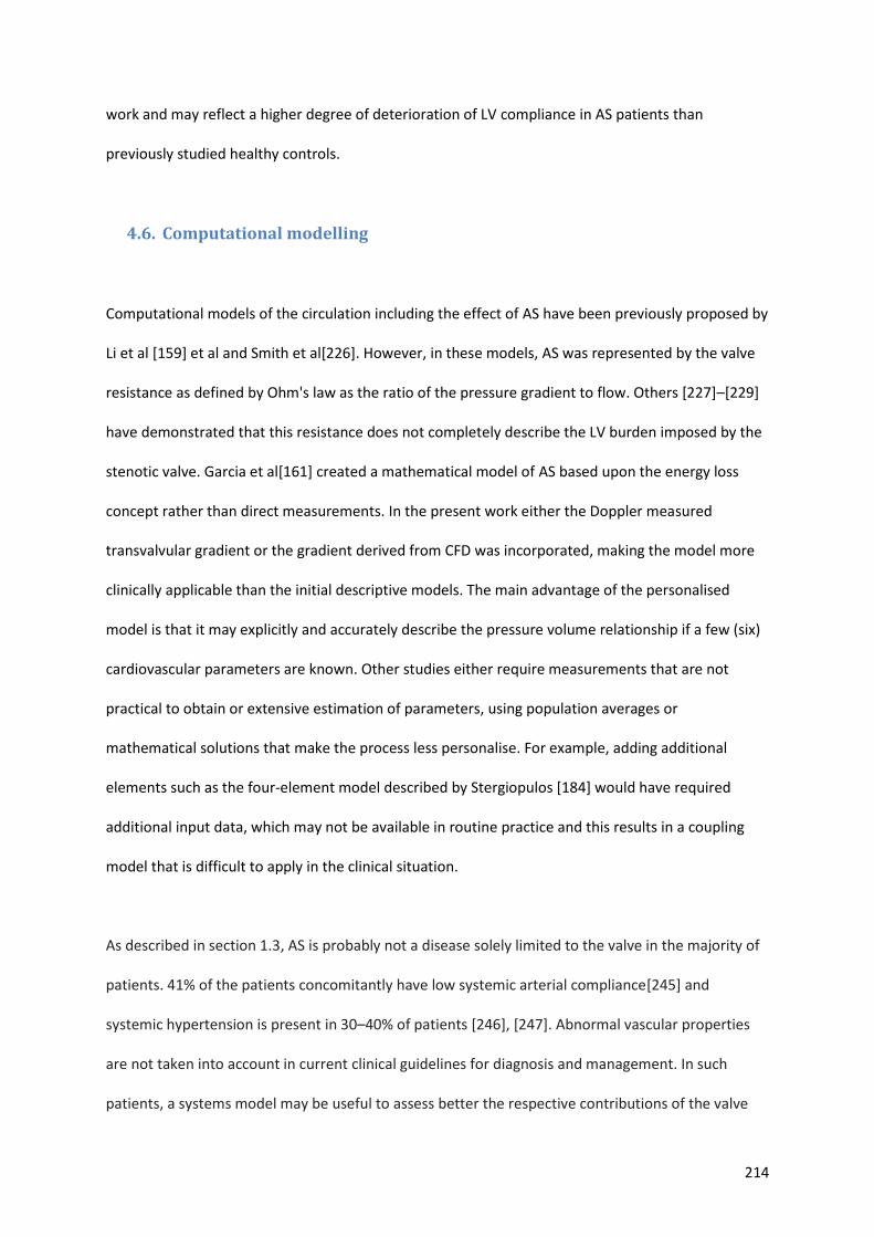
214

work and may reflect a higher degree of deterioration of LV compliance in AS patients than

previously studied healthy controls.


Computational models of the circulation including the effect of AS have been previously proposed by

Li et al [159] et al and Smith et al[226]. However, in these models, AS was represented by the valve

resistance as defined by Ohm's law as the ratio of the pressure gradient to flow. Others [227]–[229]

have demonstrated that this resistance does not completely describe the LV burden imposed by the

stenotic valve. Garcia et al[161] created a mathematical model of AS based upon the energy loss

concept rather than direct measurements. In the present work either the Doppler measured

transvalvular gradient or the gradient derived from CFD was incorporated, making the model more

clinically applicable than the initial descriptive models. The main advantage of the personalised

model is that it may explicitly and accurately describe the pressure volume relationship if a few (six)

cardiovascular parameters are known. Other studies either require measurements that are not

practical to obtain or extensive estimation of parameters, using population averages or

mathematical solutions that make the process less personalise. For example, adding additional

elements such as the four-element model described by Stergiopulos [184] would have required

additional input data, which may not be available in routine practice and this results in a coupling

model that is difficult to apply in the clinical situation.

As described in section 1.3, AS is probably not a disease solely limited to the valve in the majority of

patients. 41% of the patients concomitantly have low systemic arterial compliance[245] and

systemic hypertension is present in 30–40% of patients [246], [247]. Abnormal vascular properties

are not taken into account in current clinical guidelines for diagnosis and management. In such

patients, a systems model may be useful to assess better the respective contributions of the valve

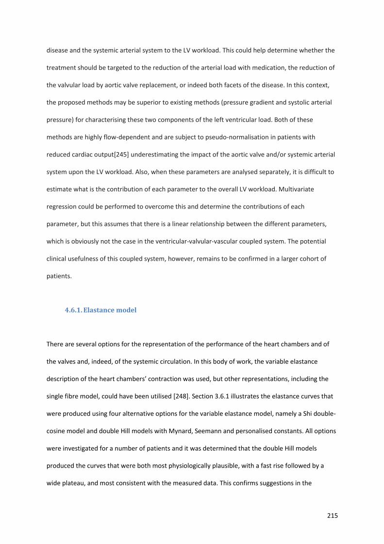
215

disease and the systemic arterial system to the LV workload. This could help determine whether the

treatment should be targeted to the reduction of the arterial load with medication, the reduction of

the valvular load by aortic valve replacement, or indeed both facets of the disease. In this context,

the proposed methods may be superior to existing methods (pressure gradient and systolic arterial

pressure) for characterising these two components of the left ventricular load. Both of these

methods are highly flow-dependent and are subject to pseudo-normalisation in patients with

reduced cardiac output[245] underestimating the impact of the aortic valve and/or systemic arterial

system upon the LV workload. Also, when these parameters are analysed separately, it is difficult to

estimate what is the contribution of each parameter to the overall LV workload. Multivariate

regression could be performed to overcome this and determine the contributions of each

parameter, but this assumes that there is a linear relationship between the different parameters,

which is obviously not the case in the ventricular-valvular-vascular coupled system. The potential

clinical usefulness of this coupled system, however, remains to be confirmed in a larger cohort of

patients.

4.6.1. Elastance model

There are several options for the representation of the performance of the heart chambers and of

the valves and, indeed, of the systemic circulation. In this body of work, the variable elastance

description of the heart chambers’ contraction was used, but other representations, including the

single fibre model, could have been utilised [248]. Section 3.6.1 illustrates the elastance curves that

were produced using four alternative options for the variable elastance model, namely a Shi double-

cosine model and double Hill models with Mynard, Seemann and personalised constants. All options

were investigated for a number of patients and it was determined that the double Hill models

produced the curves that were both most physiologically plausible, with a fast rise followed by a

wide plateau, and most consistent with the measured data. This confirms suggestions in the

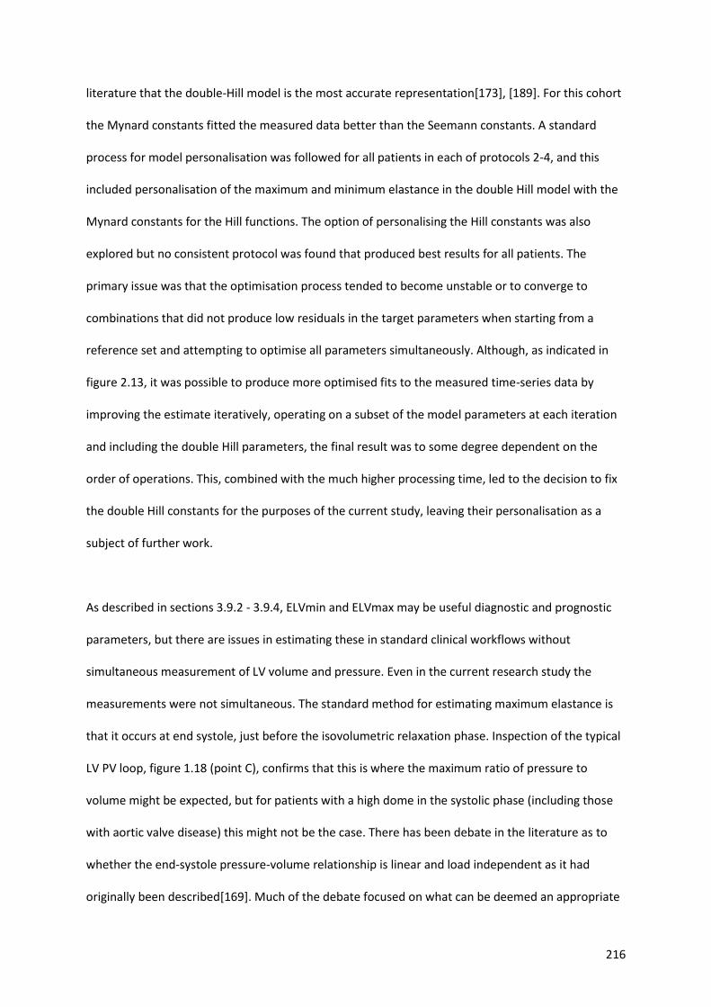
216

literature that the double-Hill model is the most accurate representation[173], [189]. For this cohort

the Mynard constants fitted the measured data better than the Seemann constants. A standard

process for model personalisation was followed for all patients in each of protocols 2-4, and this

included personalisation of the maximum and minimum elastance in the double Hill model with the

Mynard constants for the Hill functions. The option of personalising the Hill constants was also

explored but no consistent protocol was found that produced best results for all patients. The

primary issue was that the optimisation process tended to become unstable or to converge to

combinations that did not produce low residuals in the target parameters when starting from a

reference set and attempting to optimise all parameters simultaneously. Although, as indicated in

figure 2.13, it was possible to produce more optimised fits to the measured time-series data by

improving the estimate iteratively, operating on a subset of the model parameters at each iteration

and including the double Hill parameters, the final result was to some degree dependent on the

order of operations. This, combined with the much higher processing time, led to the decision to fix

the double Hill constants for the purposes of the current study, leaving their personalisation as a

subject of further work.

As described in sections 3.9.2 - 3.9.4, ELVmin and ELVmax may be useful diagnostic and prognostic

parameters, but there are issues in estimating these in standard clinical workflows without

simultaneous measurement of LV volume and pressure. Even in the current research study the

measurements were not simultaneous. The standard method for estimating maximum elastance is

that it occurs at end systole, just before the isovolumetric relaxation phase. Inspection of the typical

LV PV loop, figure 1.18 (point C), confirms that this is where the maximum ratio of pressure to

volume might be expected, but for patients with a high dome in the systolic phase (including those

with aortic valve disease) this might not be the case. There has been debate in the literature as to

whether the end-systole pressure-volume relationship is linear and load independent as it had

originally been described[169]. Much of the debate focused on what can be deemed an appropriate

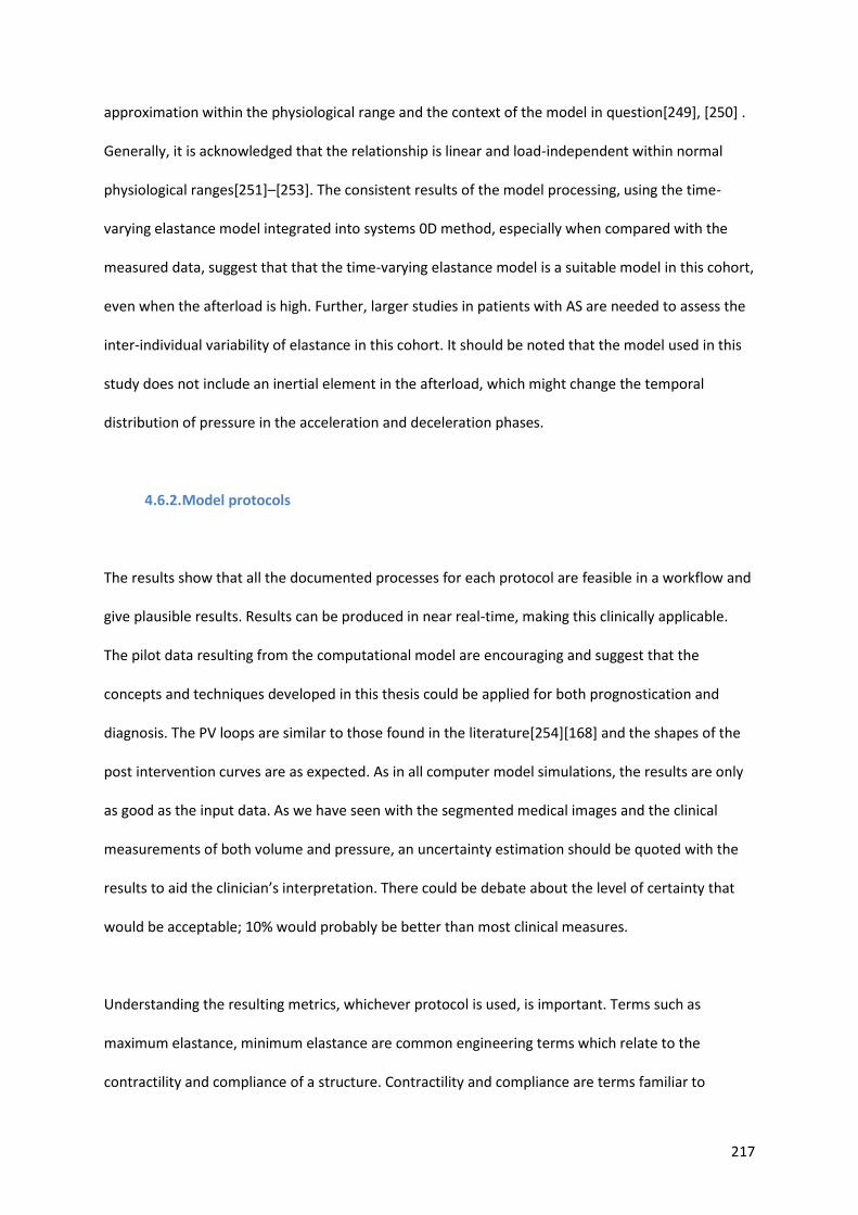
217

approximation within the physiological range and the context of the model in question[249], [250] .

Generally, it is acknowledged that the relationship is linear and load-independent within normal

physiological ranges[251]–[253]. The consistent results of the model processing, using the time-

varying elastance model integrated into systems 0D method, especially when compared with the

measured data, suggest that that the time-varying elastance model is a suitable model in this cohort,

even when the afterload is high. Further, larger studies in patients with AS are needed to assess the

inter-individual variability of elastance in this cohort. It should be noted that the model used in this

study does not include an inertial element in the afterload, which might change the temporal

distribution of pressure in the acceleration and deceleration phases.

4.6.2. Model protocols

The results show that all the documented processes for each protocol are feasible in a workflow and

give plausible results. Results can be produced in near real-time, making this clinically applicable.

The pilot data resulting from the computational model are encouraging and suggest that the

concepts and techniques developed in this thesis could be applied for both prognostication and

diagnosis. The PV loops are similar to those found in the literature[254][168] and the shapes of the

post intervention curves are as expected. As in all computer model simulations, the results are only

as good as the input data. As we have seen with the segmented medical images and the clinical

measurements of both volume and pressure, an uncertainty estimation should be quoted with the

results to aid the clinician’s interpretation. There could be debate about the level of certainty that

would be acceptable; 10% would probably be better than most clinical measures.

Understanding the resulting metrics, whichever protocol is used, is important. Terms such as

maximum elastance, minimum elastance are common engineering terms which relate to the

contractility and compliance of a structure. Contractility and compliance are terms familiar to

218

clinicians and therefore should be used in the reporting of the modelling parameters, if such

techniques are to be successfully translated into clinical practice. The compliance and resistance

reported in such computer models are very consistent with the ones directly obtained from

experimental data[168]. Further research is needed to understand what ranges of results are

clinically relevant. For example, is there a load that a ventricle may struggle to cope with and would

cause it to fail within a certain time period? These techniques would need to be applied to a much

larger cohort and patients studied longitudinally to help answer this question. Also, is there either an

absolute reduction of work or a percentage of work reduction that is needed to lead to positive

remodelling and improved outcomes? The author was unable to demonstrate this in this cohort but,

this may be due to the short follow up with lack of hard end points.

Stroke work refers to the work done by the ventricle to eject the stroke volume. The force applied to

the blood is the intraventricular pressure. Stroke work could be estimated as the product of mean

systolic pressure during the ejection period and the stroke volume. In a normal heart, the LV

pressure can be approximated by the mean aortic systolic pressure or the mean arterial pressure,

although using the MAP will underestimate the stroke work. When aortic pressure or MAP are used

instead of intraventricular pressure, it is assumed that kinetic energy is negligible, which although

generally true at rest, is not always the case. In AS this is complicated further, and the pressure drop

across the valve must be taken into account.

This is the first piece of work to describe a purely mathematical model that can produce a PV loop

from non-invasive blood pressure measurements and imaging data in AS. The difficulty of this

method was in describing the PV curve during ejection. Four mathematical models were trialled (see

figure4.1).

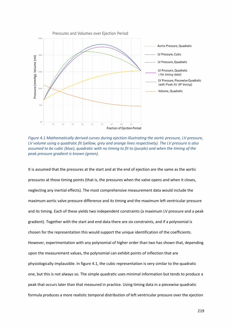
219

Figure 4.1 Mathematically derived curves during ejection illustrating the aortic pressure, LV pressure, LV volume using a quadratic fit (yellow, grey and orange lines respectively). The LV pressure is also assumed to be cubic (blue), quadratic with no timing to fit to (purple) and when the timing of the peak pressure gradient is known (green). It is assumed that the pressures at the start and at the end of ejection are the same as the aortic

pressures at those timing points (that is, the pressures when the valve opens and when it closes,

neglecting any inertial effects). The most comprehensive measurement data would include the

maximum aortic valve pressure difference and its timing and the maximum left ventricular pressure

and its timing. Each of these yields two independent constraints (a maximum LV pressure and a peak

gradient). Together with the start and end data there are six constraints, and if a polynomial is

chosen for the representation this would support the unique identification of the coefficients.

However, experimentation with any polynomial of higher order than two has shown that, depending

upon the measurement values, the polynomial can exhibit points of inflection that are

physiologically implausible. In figure 4.1, the cubic representation is very similar to the quadratic

one, but this is not always so. The simple quadratic uses minimal information but tends to produce a

peak that occurs later than that measured in practice. Using timing data in a piecewise quadratic

formula produces a more realistic temporal distribution of left ventricular pressure over the ejection

220

period, and therefore more plausible LV PV loops. This is why this method was selected for

processing cases through protocol one.

The results from protocol 1 are encouraging. There were no significant differences in the key

parameters of stroke work, wasted work, peak LV power and maximum elastance and minimum

elastance compared with the measured data. Due to the low numbers of patients and the wide

standard deviations, the study may have been underpowered to detect a statistical significance but,

as pilot data, this is interesting and warrants further study.

This protocol runs without modelling or simulations and therefore may not be able to predict the

haemodynamic changes following an intervention accurately and cannot be used to model a patient

in the exercise state. Therefore, this was not performed in the current study. However, changing the

peak gradient to 10-20mmg, a plausible post intervention gradient and keeping the other variables

the same, could give an initial first estimate. The calculated parameters in protocol 1 require very

little computing power and can be performed in an Excel® (Microsoft, CA, USA) spreadsheet

almost instantaneously and with very little cost. This would be an advantage as the clinician would

be able to assess the data with the patient in front of them during a clinical consultation. This would

give the clinician an idea of the global burden on the LV.

Protocols 2 and 3 yielded very similar results for many of the calculated parameters; this was

unexpected. The author believed that incorporating LV time series data to enable personalisation of

the double-Hill model would lead to improved accuracy. Although this may be the case, it did not

result in significant difference when assessing stroke work, stroke power, maximum and minimum

elastance. It is assumed that, where there was a difference in results, protocol 3 was more accurate

due to the increased information provided to the model. For assessing wasted work, wasted power

and total myocardial power, protocol 3 should ideally be used.

221

Protocol 4 was the most sophisticated, incorporating medical imaging data in a 3D model coupled to

the OD model and using information from wearable devices to run predictive simulations. The step

that is prone to the most error was segmentation. It is difficult to quantify the accuracy of

segmentation, especially as there is no gold standard against which to compare. Inaccurate

segmentation would lead to incorrect haemodynamic parameters, because the model was sensitive

to this input parameter. This was why, after careful analysis of the medical images and segmented

models, only 11 cases were fully analysed. Analysis of these cases showed a good correlation with

the measured peak gradient, with an overestimation of the peak gradient by echocardiography as

expected, in part validating this technique. In hindsight the difficulty in imaging a calcified diseased

valve should have been foreseen and limits its utility in clinical practice. However, as technology

improves, it may be possible to image these valves better with ultrasound and CT in the future,

improving the accuracy. Although there were limited measured data for comparison, there was no

difference in the calculated stroke work, stroke power, LV peak power and maximum and minimum

elastance. This protocol seems superior to the other two modelling protocols when assessing LV

peak power.

The point in the cardiac cycle that peak LV power occurs in AS can be assessed using computer

modelling, this occurs in the early ejection phase after the valve has started to open. Although

perhaps expected, this has not previously been described. These data suggest that the sampling rate

of the measured data was high enough to capture the gradients in the curve which may explain why

the modelled data did not produce a higher peak power. The model does give confidence that the

measured data may give reasonable estimates of LV power outputs and vice versa. One might have

expected the modelled data to be more accurate than data derived from the measured data using a

purely mathematical formula and result in higher values, as the computer model is based more on

physiology rather than being a simple numerical equation.

222

4.6.3. Diagnostic utility

One hypothesis of this study, quite independent of any mathematical modelling, was that the degree

of activity (whether intensity or duration) that a patient undertakes in the pre-intervention state

might be a diagnostic marker of disease severity, but this was not proven in this small cohort. There

was a significant negative correlation between both peak and mean gradients assessed by standard

Doppler echocardiography with the distance achieved during the 6MWT, but no association with LV

function. As there was no association with any other activity metric or symptoms reported by the

patient, which suggests that, although limited when asked to exercise to their maximum capacity,

even with severely stenotic valves, their day-to-day activities were not limited by the disease. There

was also no correlation with mass or ejection fraction, which suggests that other factors that load

the ventricle and cause it to fail such as hypertension are important, consistent with the above

hypothesis.

Interestingly, there was no correlation between ejection fraction with either the 6MWT or step

count. Ejection fraction, although often stated as measure of function, is more a measure of

performance and the function depends on the loading of the ventricle. Patients often have a normal

ejection fraction, yet the ventricle may have already started to fail. These data may provide some

evidence for this. There was a suggestion that the higher the ejection fraction, the more energy the

patient could expend and that, if the ejection fraction were lower, the patient may spend longer

asleep. If there is reduction of ejection fraction, this is a relatively late stage in the disease process,

so it is perhaps not surprising that these patients do not expend as much energy and spend more

time asleep.

Compared with the standard clinical techniques to assess the severity of the disease, the calculated

parameters from the computer model seem to perform better with stronger and more frequent

223

correlation with the activity data. ELVmin or left ventricular compliance seems to be the most

consistent parameter in determining the effect on patient function and negative myocardial

remodelling. It exhibited relatively strong correlations with objective measures of activity, including

the 6MWT, as well as a number of parameters from the wearable devices. It also correlated with LV

mass. It is likely that it is the rise in myocardial mass that results in the elevated ELVmin. This is

consistent with what is already known. ELVmin can be considered analogous to LV strain

assessment[255], [256] and it is likely to change prior to any changes in LV systolic function. This

could be the consequence of fibrosis, as seen on CMR[25]. Assessing early diastolic dysfunction using

calculated ELVMin may be more reliable and reproducible than strain and fibrosis assessment, but

more research is needed.

ELVmax had a strong correlation with ejection fraction or LV systolic performance. It reflects the

systolic contractility of the heart but also takes into account the loading conditions, which could

provide a reason for why this is better associated with adverse myocardial modelling and average

daily step count than ejection fraction. The negative correlation with LV mass is interesting. It

suggests that the LV hypertrophy that develops in an attempt to cope with the increased afterload is

actually maladaptive, and although ejection fraction is maintained or increased, contractility is

reduced. This can be seen in other conditions such as hypertrophic cardiomyopathy and is likely

caused by fibrosis and infiltration that has been seen during MRI in severe AS[25]. This pathological

process reduces the compliance of the ventricle. There was no correlation with the 6MWT, which

was unexpected, but could be explained by the patient being in the adaptive phase with preserved

ventricular function or in decline, with the heart starting to fail (see section 3.9.3), yet still having a

normal ejection fraction.

ELVmax has promise when a patient is followed longitudinally to detect early signs of LV failure. In

terms of identifying patients for intervention, ELVmax may help in selecting patients before a

224

reduction in ejection fraction is seen. Serial monitoring of modelled ELV max could be used (see

figure 3.39). An increase in ELVmax , from normal (red) to supra-normal (green) shows that the LV is

adapting to the increase in load. When the ELVmax moves from supra-normal towards the normal

range this is likely to be a sign that the LV is starting to fail. Assessment of ELVmax might identify

changes in cardiac function before there are apparent changes in the ejection fraction. If ELVmax

were to be serially measured in an individual, this may help in the timing of intervention. In patients

with reduced ejection fraction prior to intervention ELVmax may help identify the likelihood of

recovery in ejection fraction following intervention. Further research into this notion is required in a

larger cohort.

LV work, not LV peak power, was significantly correlated with LV mass. This suggests that it is the

work over the cardiac cycle rather than instantaneous peak power that results in LV hypertrophy.

Whether average work over the cardiac cycle or peak LV power leads to hypertrophy has not

previously been investigated. However, these findings make sense as the amount of time the heart is

exposed to peak LV pressure is very short. There was a better association between peak LV power

and activity, suggesting that it is the heart’s ability to generate a high-pressure during exercise which

is important.

It is not known whether values of peak or mean power might be the most relevant in the context of

progression of cardiac remodelling, towards heart failure. In normal engineering materials, peak

stresses are often critical in failure modes. Because peak power is a temporal gradient of work, it is

particularly sensitive to inaccuracies in the measurement process, and to assumptions made in the

interpolation process. For this reason, if the underpinning computational models of elastance are

capturing the proper form of the contraction curve, it is likely that the 0D models more accurately

estimate this parameter. It will be interesting to see if, in extended clinical trials, this parameter

proves to be associated with disease progression and outcome of interventions. If it does then it

225

would both increase our understanding of the underlying factors in these events and demonstrate

the utility of a physiology-based computational model in assisting clinical decision support. Wasted

energy correlated well with myocardial mass, which may be expected. There was no correlation with

the patient’s symptoms or activity.

It is possible that using a multi-biomarker strategy to identify LV decompensation may prove

superior to any single biomarker. In the EVoLVeD trial[257], patients are initially screened with an

ECG and a high sensitivity troponin I blood test. Patients in whom these tests are normal are deemed

to have a normal heart with no further imaging required. Patients with LVH and abnormal strain

pattern, or an elevated level of troponin, proceed to cardiac magnetic resonance imaging. Those

found to have mid-wall fibrosis are then randomised to either early valve intervention or routine

clinical care. It is hoped that this strategy will target valve intervention to those patients who will

derive greatest benefit. The same could be achieved with ‘bio-markers’ resulting from the modelling

process such as maximum elastance as illustrated in section 3.9.

4.6.4. Predictive utility

PV loops were produced for each patient in the rest and exercise state pre- and post- intervention.

The loops produced were consistent with the known physiological changes and the expected

changes previously published[191], [258], [259]. The results are physiologically plausible, suggesting

that the model can be predictive. Further validation of the exercise PV loops is needed but this is

difficult to do practically and, as the level of activity the patient performed was used as an input to

the model, activity levels cannot be used as a surrogate marker for validation. The model predicts

and quantifies the expected reductions in cardiac work and wasted energy following intervention

(section 3.9.2) but, as discussed previously, it is as yet unclear what reduction in work or wasted

energy is clinically significant and result in positive remodelling and a reduction of symptoms. The

226

author was unable to show a relationship between either the relative or the absolute reduction in

modelled parameters and the degree of clinical improvement or LV mass regression. If there is a

relationship, a much larger cohort would be needed to demonstrate this.

The post-intervention gradient could be predicted and measured. The determinants of the pressure

gradient following intervention are the size of the valve implanted and the size of the patient.

However, the model-predicted peak gradient following intervention had a better correlation with

the measured peak than the BSA indexed EOA of the valve implanted (r2 = 0.47 and r2 =0.38,

respectively). This suggests that simulating the patients’ haemodynamics following intervention

improves predictive capability. For one patient, the model predicted a post-operative gradient of

60mmHg, and the measured post-operative gradient in this patient was 51mmHg. This patient

remained symptomatic following intervention, suggesting a patient-prosthesis mismatch. This was

confirmed, with the estimated iEOA was calculated to be 0.6cm2[260]. Had the model been run prior

to the planned intervention, this could have been avoided. A sutureless valve or a TAVI may have

been the preferred option for this patient. The model’s sensitivity and sensitivity of predicting a

successful reduction in pressure gradient (to <20mmHg) suggests that this may be a good tool to

help clinicians with valve selection in their patients. This could be as an adjunct to BSA, which was

not used as an input to the model.

There are two main reasons to replace the diseased valve; one is to improve prognosis and the other

is to relieve symptoms. The modelled pre-operative ELVmax may help predict a recovery in ejection

fraction following intervention, which is known to determine outcome [261], [262]. In patients in this

study with low ELVmax and low ejection fraction, the ejection fraction did not return to normal

following intervention. Ejection fraction returned to normal in only one out of six patients with an

ELVmax in the normal range prior to intervention.

227

Symptoms are subjective and there are well-documented problems with self-reported symptoms

and the NYHA assessment [263], [264]. It would be beneficial if improvement in physical capacity

following intervention could be predicted for an individual ; this would help manage patients’

expectations and be helpful to clinicians when counselling a patient about a procedure. There are a

number of patients that undergo aortic valve replacements in the late stage of the disease, when the

heart has remodelled and become stiff, who do not get an improvement in their symptoms or

exercise capacity following intervention.

The model-predicted post-operative activity levels correlated well with measured activity post-

intervention in terms of METs calculated from the 6MWT distance. There was a systematic bias of

the model, over-predicting activity by 0.5 METS. Thus, expected capacity following intervention

could be predicted as the modelled exercise capacity – 0.5METS. However, post-intervention

exercise capacity is likely to be determined, primarily, by pre-intervention capacity as shown in

previous studies[234], [236].

4.7. Clinical decision support system

Clinical decision support systems (CDSS) are tools that incorporate clinical knowledge and patient

information to enhance patient care. In this case it also incorporates patient-specific modelled

information. CDSS can encompass an array of strategies supporting a variety of topics and are

designed to assist the physician-patient encounter at multiple points from initial consultation to

diagnosis to follow up. The expectation is that a properly equipped clinical decision support system

will significantly benefit patient care at all levels[265]. Despite promising initial data from systems

based around medication management[266], [267] and pathology systems[268], [269], the majority

of CDSS’s have not provided features beyond reminders, general alerts , automated information

retrieval and summary dashboards[270], [271].

228

The modelling and activity components of this specific clinical decision support system were well-

received by the clinicians involved, with about 80% of participants finding the information useful or

very useful. It is interesting that, in some cases, this data has the ability to influence decisions and

improve confidence in decisions, irrespective of the accuracy. This suggests that, once fully

validated, these tools and techniques could impact on patient care. Larger studies are needed

(including a randomised control trial) to investigate whether such a tool could have a positive effect

upon outcome. What this experiment did not do was assess whether the management of the patient

would change in terms of the method of intervention. In the cases where there was a clear and

confident decision to intervene, would the patient have been offered a different treatment such as

TAVI instead of SAVR or a different approach to the surgery or a different type of valve as a result of

the information presented?

The job of the clinician is to weigh up benefit and risk, to the individual patient in front of them, of

intervening and replacing the valve or not. In the guidelines, there is a focus on risk scores such as

the EuroScore and the STS score; indeed 89% of our participants found such scores helpful.

Quantifying benefit for an individual appears to be much more difficult. Which of these patients will

live a lot longer and by how much? Which will see an improvement of ventricular function and by

how much? Which of these patients will see a reduction of symptoms and how much more will they

be able to do? This pilot study suggests that computational modelling may go some way to

addressing some of these questions. In our cohort, 96% of clinicians certainly suggested that a

summary of potential risks and potential benefits would be useful.

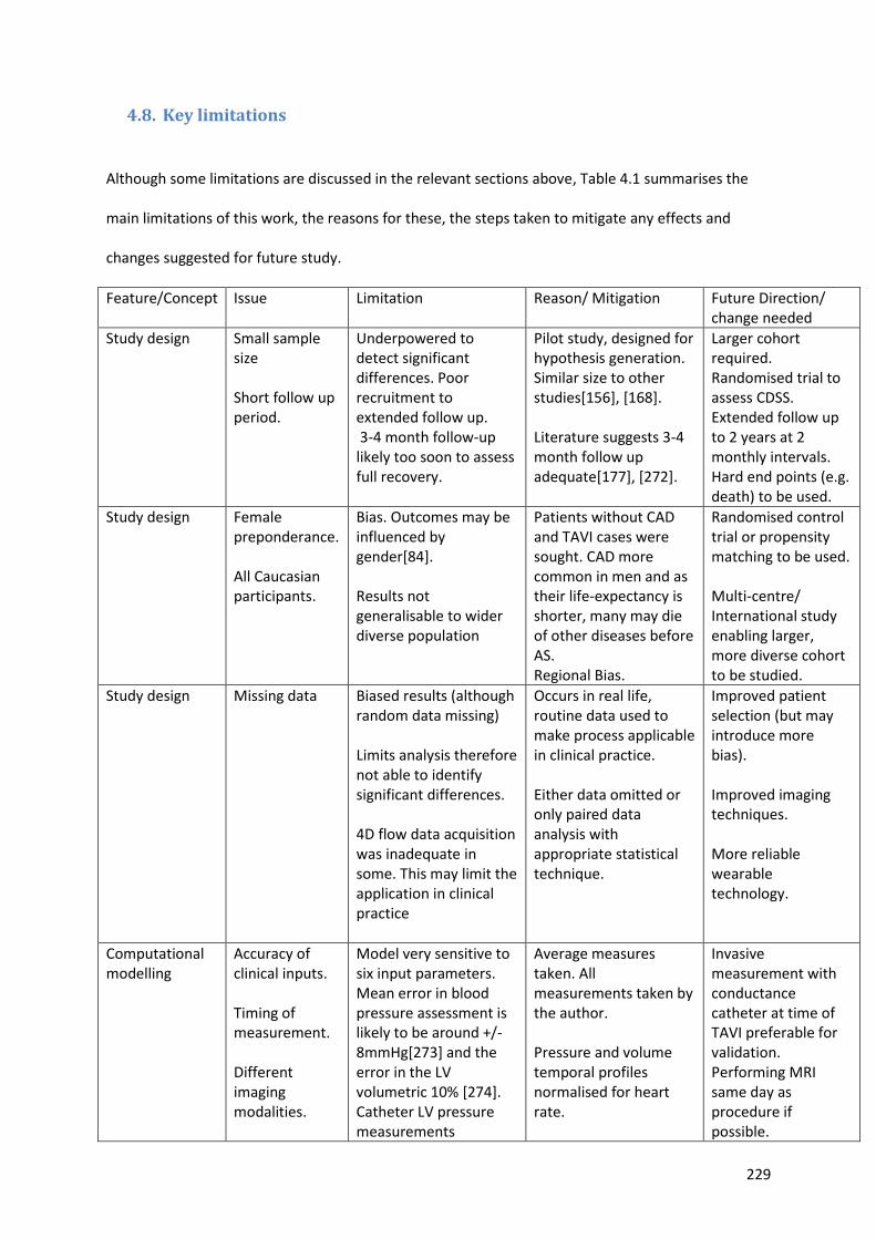
229

4.8. Key limitations

Although some limitations are discussed in the relevant sections above, Table 4.1 summarises the

main limitations of this work, the reasons for these, the steps taken to mitigate any effects and

changes suggested for future study.

Feature/Concept Issue Limitation Reason/ Mitigation Future Direction/ change needed

Study design Small sample size Short follow up period.

Underpowered to detect significant differences. Poor recruitment to extended follow up. 3-4 month follow-up likely too soon to assess full recovery.

Pilot study, designed for hypothesis generation. Similar size to other studies[156], [168]. Literature suggests 3-4 month follow up adequate[177], [272].

Larger cohort required. Randomised trial to assess CDSS. Extended follow up to 2 years at 2 monthly intervals. Hard end points (e.g. death) to be used.

Study design Female preponderance. All Caucasian participants.

Bias. Outcomes may be influenced by gender[84]. Results not generalisable to wider diverse population

Patients without CAD and TAVI cases were sought. CAD more common in men and as their life-expectancy is shorter, many may die of other diseases before AS. Regional Bias.

Randomised control trial or propensity matching to be used. Multi-centre/ International study enabling larger, more diverse cohort to be studied.

Study design Missing data Biased results (although random data missing) Limits analysis therefore not able to identify significant differences. 4D flow data acquisition was inadequate in some. This may limit the application in clinical practice

Occurs in real life, routine data used to make process applicable in clinical practice. Either data omitted or only paired data analysis with appropriate statistical technique.

Improved patient selection (but may introduce more bias). Improved imaging techniques. More reliable wearable technology.

Computational modelling

Accuracy of clinical inputs. Timing of measurement. Different imaging modalities.

Model very sensitive to six input parameters. Mean error in blood pressure assessment is likely to be around +/- 8mmHg[273] and the error in the LV volumetric 10% [274]. Catheter LV pressure measurements

Average measures taken. All measurements taken by the author. Pressure and volume temporal profiles normalised for heart rate.

Invasive measurement with conductance catheter at time of TAVI preferable for validation. Performing MRI same day as procedure if possible.

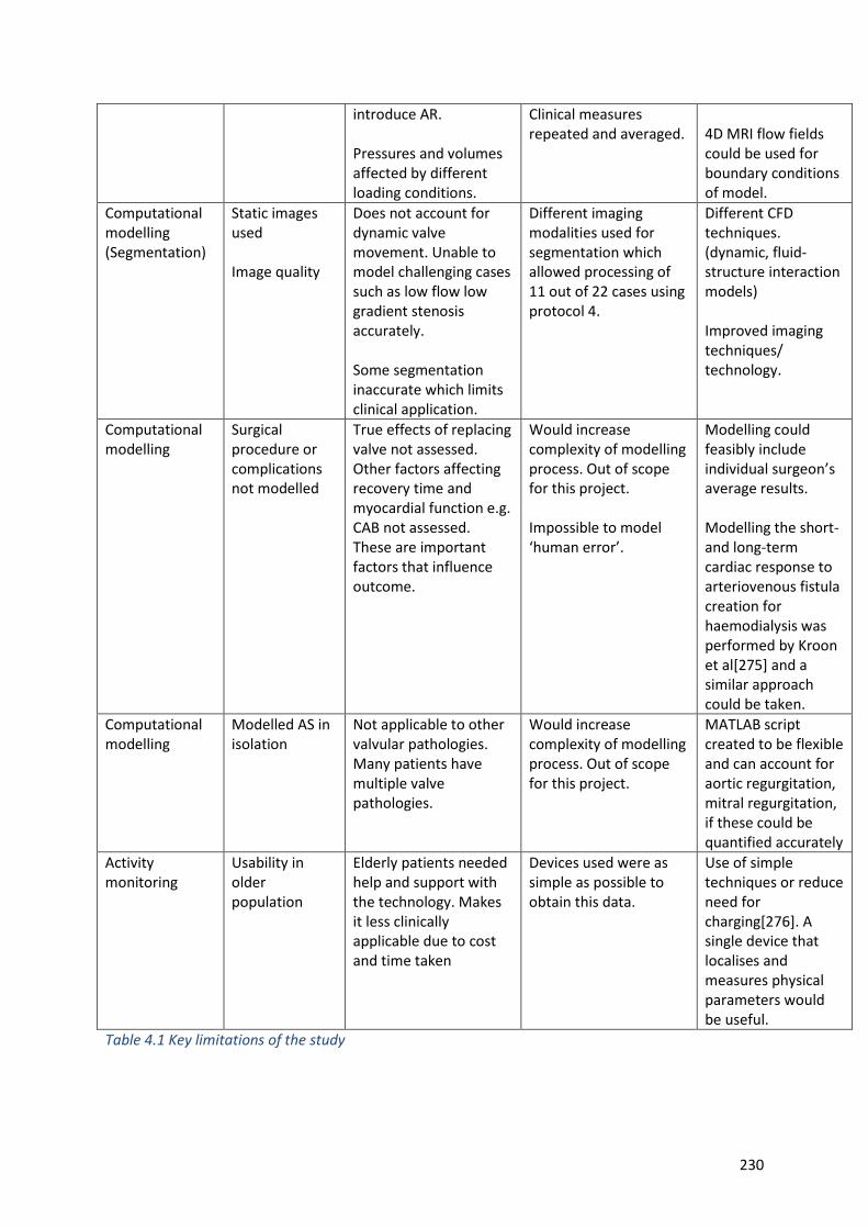
230

introduce AR. Pressures and volumes affected by different loading conditions.

Clinical measures repeated and averaged.

4D MRI flow fields could be used for boundary conditions of model.

Computational modelling (Segmentation)

Static images used Image quality

Does not account for dynamic valve movement. Unable to model challenging cases such as low flow low gradient stenosis accurately. Some segmentation inaccurate which limits clinical application.

Different imaging modalities used for segmentation which allowed processing of 11 out of 22 cases using protocol 4.

Different CFD techniques. (dynamic, fluid-structure interaction models) Improved imaging techniques/ technology.


Surgical procedure or complications not modelled

True effects of replacing valve not assessed. Other factors affecting recovery time and myocardial function e.g. CAB not assessed. These are important factors that influence outcome.

Would increase complexity of modelling process. Out of scope for this project. Impossible to model ‘human error’.

Modelling could feasibly include individual surgeon’s average results. Modelling the short- and long-term cardiac response to arteriovenous fistula creation for haemodialysis was performed by Kroon et al[275] and a similar approach could be taken.


Modelled AS in isolation

Not applicable to other valvular pathologies. Many patients have multiple valve pathologies.

Would increase complexity of modelling process. Out of scope for this project.

MATLAB script created to be flexible and can account for aortic regurgitation, mitral regurgitation, if these could be quantified accurately

Activity monitoring

Usability in older population

Elderly patients needed help and support with the technology. Makes it less clinically applicable due to cost and time taken

Devices used were as simple as possible to obtain this data.

Use of simple techniques or reduce need for charging[276]. A single device that localises and measures physical parameters would be useful.

Table 4.1 Key limitations of the study

231

CHAPTER 5

5. Conclusion and further work

5.1. Conclusion

AS is an important entity that is associated with significant morbidity and mortality. There are

several limitations with the current diagnostic approach. This work demonstrates that the physiology

of patients with AS can be characterised using computational models. A number of processing

protocols have been developed that show it is possible to ‘measure’ cardiac work and run

simulations that predict haemodynamic changes under exercise and following valve replacement,

achieving the first aim of this project; however, further validation is necessary in a larger cohort. The

accuracy of the model will be affected by the clinical data available and it is a case of balancing this

with practical and patient constraints. Linking the reduction of cardiac work or indeed the prediction

of reduced work with activity and outcome will be the next goal. This work takes the first steps

towards this, showing how this may be done in this patient cohort and that wearable devices can be

used to measure outcome. However, although trends were seen, this study failed to show a

significant, measurable, improvement in functional capacity following intervention.

MRI 4D flow for the assessment and grading of AS appears promising. The assessment of aortic valve

gradient and effective orifice area using these techniques are comparable to invasive and

transthoracic echocardiographic assessment and provide a viable alternative. In addition, 4D flow-

derived valve metrics have minimal bias and superior association to prognostically relevant 6MWT

and LV mass regression. Discordance between EOA and the pressure gradient to grade the severity

of AS frequently occurs and can lead to confusion. It is clinically desirable to have more non-invasive

tools to reduce the clinical dilemma and make an affirmative diagnosis and grading of AS. The

accuracy of 4D flow pressure gradient assessment was slightly inferior to Doppler TTE when

compared against the reference invasive methods. However, the precision was much better with 4D

232

flow pressure gradient. Hence, in patients where Doppler TTE is inconsistent with symptoms and has

discordant results, 4D flow CMR could help in clinical decision making for deciding on aortic valve

intervention.

Assessment of the kinetic energy of the blood pool of the left ventricle gives an insight to the

haemodynamics and may provide a further diagnostic tool. The results of these techniques

correlated better with the symptoms, functional capacity and LV remodelling than routine

echocardiographic assessment. Although 4D flow assessment may add incremental value to the

assessment and prognostication of patients with severe AS, it does not provide the same

haemodynamic information as the modelling process and different scenarios cannot be simulated

with this method. Therefore, 4D flow assessment, although adding to our understanding, does not

negate the need for modelling. In fact, the two techniques could work synergistically with MRI,

producing flow fields that could be used as boundary conditions for the model.

Wearable devices are well-tolerated by patients and provide insight to both their recovery and daily

life patterns, which could in turn provide valuable information for clinicians and help determine

timing of intervention, treatment type and follow up required. This small study failed to show a

significant increase in exercise capacity, but it does perhaps suggest that patients found it easier to

do the same level of activity following intervention. It suggests that patients in this cohort may have

not been limited by the disease with other factors contributing to the poor exercise capacity or that

the valve intervention offered no significant benefit in terms of activity for the majority of people.

The other possibility is that the study was not powered to detect the difference. The objective

measures may be better than standard NYHA assessment. The NYHA assessment suggested

significant improvement in symptoms following intervention but this was not borne out in the any of

the objective measures or the patient reported outcomes in the questionnaires completed and

suggests its subjective assessment is not accurate.

233

The clinical decision support system which was able to provide an overview of the whole patient and

summarise both risks and potential benefit for a patient was well-received by the clinicians that

trialled the platform. It would appear that once validated, the modelling and activity data could

influence the care of patients particularly in borderline cases. Being able to simulate different

scenarios in a ‘virtual’ safe environment was a feature incorporated into the clinical decision support

system and may help predict outcome. With more understanding of the information, this may be a

useful tool in clinical practice and/or as an educational tool. For patients with hypertension and AS,

treating the hypertension first to see if there is an improvement in symptoms, may delay the need

for an operation. This may not be a revelation, but this model can potentially assess individual

factors affecting the load on the left ventricle and suggest whether a reduction in BP or intervention

or both is necessary in such a patient. This pilot study has identified several areas that need further

research and validation in a large cohort. The processes and techniques developed, once validated,

need assessment in a randomised control trial to see if they can have a positive impact on the

outcomes of patients with severe AS.

Table 5.1 identifies what this study achieved against originally stated hypothesis and aims of the

thesis.

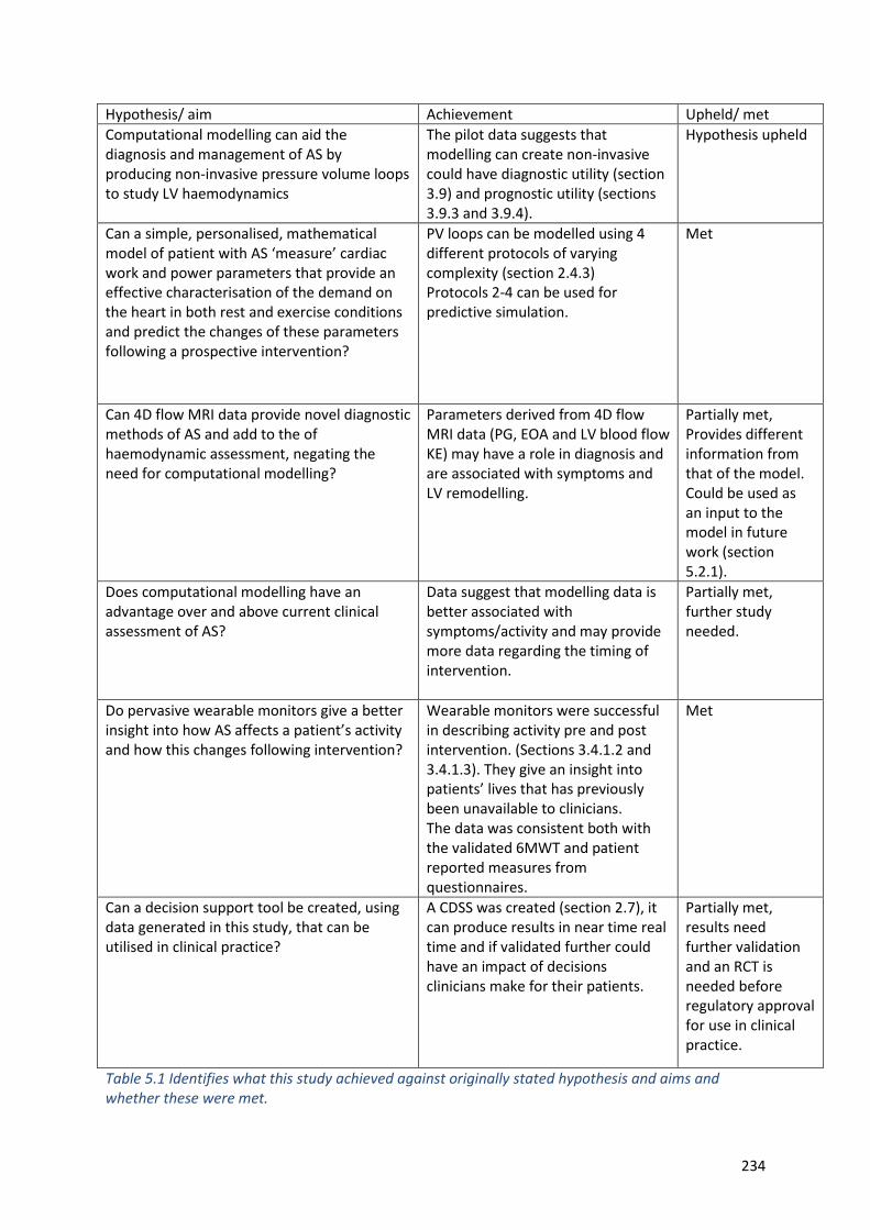
234

Hypothesis/ aim Achievement Upheld/ met

Computational modelling can aid the diagnosis and management of AS by producing non-invasive pressure volume loops to study LV haemodynamics

The pilot data suggests that modelling can create non-invasive could have diagnostic utility (section 3.9) and prognostic utility (sections 3.9.3 and 3.9.4).

Hypothesis upheld

Can a simple, personalised, mathematical model of patient with AS ‘measure’ cardiac work and power parameters that provide an effective characterisation of the demand on the heart in both rest and exercise conditions and predict the changes of these parameters following a prospective intervention?

PV loops can be modelled using 4 different protocols of varying complexity (section 2.4.3) Protocols 2-4 can be used for predictive simulation.

Met

Can 4D flow MRI data provide novel diagnostic methods of AS and add to the of haemodynamic assessment, negating the need for computational modelling?

Parameters derived from 4D flow MRI data (PG, EOA and LV blood flow KE) may have a role in diagnosis and are associated with symptoms and LV remodelling.

Partially met, Provides different information from that of the model. Could be used as an input to the model in future work (section 5.2.1).

Does computational modelling have an advantage over and above current clinical assessment of AS?

Data suggest that modelling data is better associated with symptoms/activity and may provide more data regarding the timing of intervention.

Partially met, further study needed.

Do pervasive wearable monitors give a better insight into how AS affects a patient’s activity and how this changes following intervention?

Wearable monitors were successful in describing activity pre and post intervention. (Sections 3.4.1.2 and 3.4.1.3). They give an insight into patients’ lives that has previously been unavailable to clinicians. The data was consistent both with the validated 6MWT and patient reported measures from questionnaires.

Met

Can a decision support tool be created, using data generated in this study, that can be utilised in clinical practice?

A CDSS was created (section 2.7), it can produce results in near time real time and if validated further could have an impact of decisions clinicians make for their patients.

Partially met, results need further validation and an RCT is needed before regulatory approval for use in clinical practice.

Table 5.1 Identifies what this study achieved against originally stated hypothesis and aims and whether these were met.

235

5.2. Further work

A larger cohort study with a longer follow-up to further validate and extend the work in this thesis is

required. If successful, the techniques developed should be trialled in clinical practice to see if the

outcomes of patients with AS can be improved using the data that the techniques in this thesis

provide. A number of questions and further research opportunities have arisen from the work

carried out.

5.2.1. Model personalisation

Further model personalisation could be achieved utilising more data from medical images. The

model could be tuned to both aortic and mitral flows, which could be obtained from cardiac MRI

imaging, either using 2D phase contrast or 4D flow studies. Echocardiography can measure the

velocity profile through the valves, and this could also be used to help tune the shape of the flow

profiles in the model. Figure 5.1 shows the modelled aortic flow and measured aortic flow for one

patient in the study. Figure 5.2 shows the modelled flow through the mitral valve and the velocity

profile through the mitral valve obtained from echocardiography.

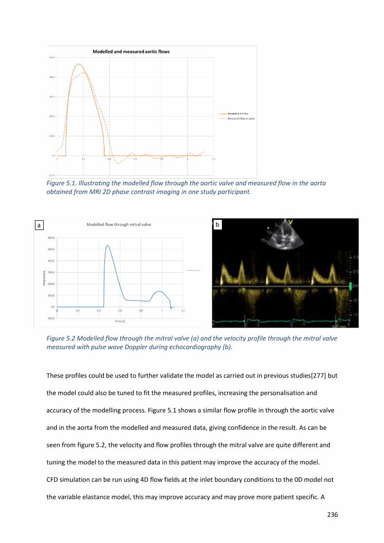
236

Figure 5.1. Illustrating the modelled flow through the aortic valve and measured flow in the aorta obtained from MRI 2D phase contrast imaging in one study participant.

Figure 5.2 Modelled flow through the mitral valve (a) and the velocity profile through the mitral valve measured with pulse wave Doppler during echocardiography (b).

These profiles could be used to further validate the model as carried out in previous studies[277] but

the model could also be tuned to fit the measured profiles, increasing the personalisation and

accuracy of the modelling process. Figure 5.1 shows a similar flow profile in through the aortic valve

and in the aorta from the modelled and measured data, giving confidence in the result. As can be

seen from figure 5.2, the velocity and flow profiles through the mitral valve are quite different and

tuning the model to the measured data in this patient may improve the accuracy of the model.

CFD simulation can be run using 4D flow fields at the inlet boundary conditions to the 0D model not

the variable elastance model, this may improve accuracy and may prove more patient specific. A

b a

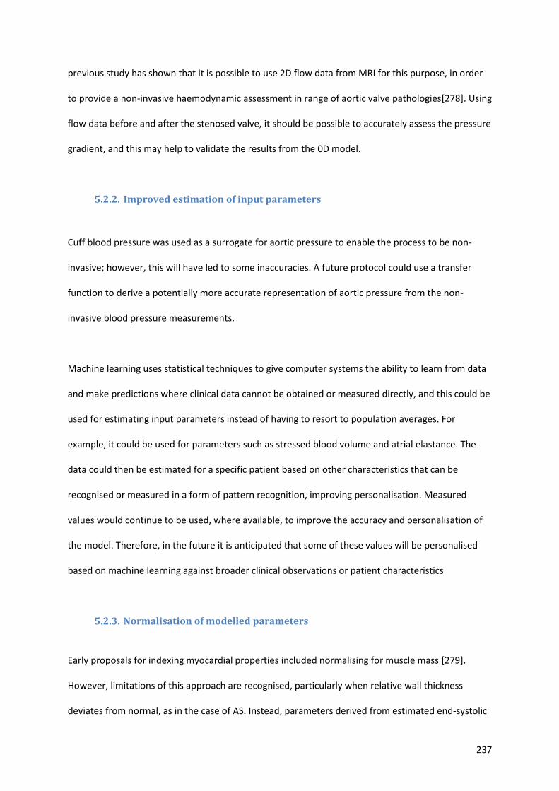
237

previous study has shown that it is possible to use 2D flow data from MRI for this purpose, in order

to provide a non-invasive haemodynamic assessment in range of aortic valve pathologies[278]. Using

flow data before and after the stenosed valve, it should be possible to accurately assess the pressure

gradient, and this may help to validate the results from the 0D model.

5.2.2. Improved estimation of input parameters

Cuff blood pressure was used as a surrogate for aortic pressure to enable the process to be non-

invasive; however, this will have led to some inaccuracies. A future protocol could use a transfer

function to derive a potentially more accurate representation of aortic pressure from the non-

invasive blood pressure measurements.

Machine learning uses statistical techniques to give computer systems the ability to learn from data

and make predictions where clinical data cannot be obtained or measured directly, and this could be

used for estimating input parameters instead of having to resort to population averages. For

example, it could be used for parameters such as stressed blood volume and atrial elastance. The

data could then be estimated for a specific patient based on other characteristics that can be

recognised or measured in a form of pattern recognition, improving personalisation. Measured

values would continue to be used, where available, to improve the accuracy and personalisation of

the model. Therefore, in the future it is anticipated that some of these values will be personalised

based on machine learning against broader clinical observations or patient characteristics

5.2.3. Normalisation of modelled parameters

Early proposals for indexing myocardial properties included normalising for muscle mass [279].

However, limitations of this approach are recognised, particularly when relative wall thickness

deviates from normal, as in the case of AS. Instead, parameters derived from estimated end-systolic

238

myocardial stress-strain relations are suggested[280]. The slope of the end-systolic myocardial

stress-strain relationship has been shown to be load independent [281] and sensitive to changes in

myocardial contractility when geometry is also changing[282]. Other authors have normalised stroke

work to stroke volume[283]; the rationale for this is unclear but it is suggested this may have a role

in low flow low gradient AS. In this study, when following these patients longitudinally and trying to

associate outcome with predicted changes of work, no normalisation was required. However, when

using parameters such as stroke work and maximum elastance as diagnostic measures linked to

functional capacity, normalising these values to the size of the heart seems logical.

The best approach for normalising myocardial mechanical properties for chamber size and geometry

is uncertain. It is likely that myocardial contractility is assessed most appropriately using the

myocardial stress-strain relationship. In the next phase of investigation it is therefore suggested that

this method is adopted, following concepts proposed by Burkhoff et al[280].

5.2.4. Wearable devices for activity assessment

Data for both the Philips Health Watch and the Bristol device are encoded with time stamps;

although the time reference points are different, this enables the data to be combined within an

accuracy of a few seconds. The feasibility of combining activity data was demonstrated in one case

within the study (see figure 3.19). The data could be used to measure HR accurately for a given

activity such as climbing a flight of stairs. This, then, could be compared pre- and post-intervention.

This may give an indication of myocardial efficiency but could be significantly affected by changes in

medication such as beta blockers following intervention. There has been research into the effect of

resting heart rate on outcome and mortality [284], [285]. The effect could be studied accurately in

this patient cohort using the Philips Healthwatch. The follow-up was too short to assess this in this

study. There was an indication that resting heart rate may be important as it was found to correlate

239

to LV mass (r=-0.684P=0.007) and total energy expenditure of the patient r=-0.525 p=0.04, but more

research is needed. O’sullivan et al attempted to show a correlation with resting heart rate and

outcome; the study concluded that the baseline and discharge resting heart rates were not

associated with adverse outcomes after TAVI[284].However, this study had a number of limitations

including that the resting heart rate was measured using 12 lead ECG which may not represent the

true resting heart rate and that the heart rates of patients were dichotomised to low (<77bpm) and

high (≥77bpm). There may be a link between the resting heart rate before and after aortic valve

intervention in terms of physical activity and patient reported outcomes. It is also thought that heart

rate variability may also play a role [286] in outcome and this also could be studied. Using wearable

activity monitors to assess outcomes, in future larger cardiovascular trials to assess outcomes seems

a feasible next step.

5.3. Clinical decision support system

Further validation is needed and a randomised control trial to see if such a platform could influence

clinical care as mentioned above. Future work that may make the system more useful for clinicians is

the development of a benefit score and summary of the benefits and risk, indicating what course of

action may be of benefit to the patient. This would require a large database and a retrospective

analysis of outcome.

Once the database is populated with cases, a multi-regression analysis could be performed to create

the weightings for the benefit score, much in the way that risk scores are developed. An example of

how this data could be presented is given in figure 5.3.

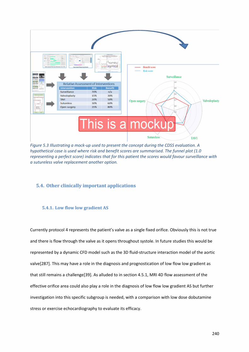
240

Figure 5.3 Illustrating a mock-up used to present the concept during the CDSS evaluation. A hypothetical case is used where risk and benefit scores are summarised. The funnel plot (1.0 representing a perfect score) indicates that for this patient the scores would favour surveillance with a sutureless valve replacement another option.

5.4. Other clinically important applications

5.4.1. Low flow low gradient AS

Currently protocol 4 represents the patient’s valve as a single fixed orifice. Obviously this is not true

and there is flow through the valve as it opens throughout systole. In future studies this would be

represented by a dynamic CFD model such as the 3D fluid-structure interaction model of the aortic

valve[287]. This may have a role in the diagnosis and prognostication of low flow low gradient as

that still remains a challenge[39]. As alluded to in section 4.5.1, MRI 4D flow assessment of the

effective orifice area could also play a role in the diagnosis of low flow low gradient AS but further

investigation into this specific subgroup is needed, with a comparison with low dose dobutamine

stress or exercise echocardiography to evaluate its efficacy.

241

5.4.2. Asymptomatic severe AS

Modelling in this cohort may help with the timing of intervention. This study suggests that markers

such as ELVmax may be used to monitor a patient so that intervention can be performed before the

left ventricle is irreparably damaged. Longitudinal studies of patients who are deemed to have

asymptomatic AS are needed to test this hypothesis. A retrospective study could also be performed

looking at the outcome of patients who were previously observed could also be performed.

5.4.3. Other valvular pathologies

The 0D model utilised in this work describes the left heart which includes the aortic and the mitral

valves. Pathologies affecting both these valves could potentially be modelled. The MATLAB script

was written to be flexible; if the gradient through or orifice of the mitral valve in mid-diastole can be

a measured, the model could be used to assess mitral stenosis this could be inputted into the model

and mitral stenosis assessed. Similarly, if the regurgitant orifice in mid-systole can be measured, the

effect of mitral regurgitation could be assessed. Image-based geometries would potentially be more

accurate as it is difficult to quantify the degree if mitral regurgitation or stenosis using current

diagnostic techniques[288]–[290]. However, this would involve imaging small orifice areas which,

again, may be difficult in a diseased valve, especially with a complex structure like the mitral valve.

The effect of aortic regurgitation could also be assessed using the same rationale and technique if

the regurgitant volume could be accurately measured or the valve orifice imaged precisely during

diastole.

242

5.5. Educational tool

Finally, one of the great advantages of using computational modelling is to be able to run

simulations in a safe environment. This can help us understand the impact of changing certain

conditions on the global haemodynamics of the patient. For example, the effects of given

medications such as vasodilators, beta blockers diuretics and inotropes can be studied by altering

the systemic vascular resistance, heart rate, stressed blood volume and ELVMax respectively in the

model. This could be exploited as an educational tool in the undergraduate or clinical setting.

Computational models have already been used in e-learning platforms for conditions affecting the

cardiovascular system[291]. The effect of using this model for educational purposes could be studied

in a similar way. For instance, in AS assessment with echocardiography we do not normalise the

gradient for heart rate, perhaps we should do as it is likely to have a significant effect on the

gradient. Understanding the effect of heart rate on gradient may influence how scans are reported.

5.6. Final conclusion

Understanding the global haemodynamic burden of AS and how this affects an individual patient has

clear benefits. This body of work begins to explore how computational modelling can provide new

insights, making use of routine, non-invasive, measurements. Data obtained can be used in

conjunction with other information from complementary techniques such as pervasive monitoring

from wearable devices and 4D flow MRI, allowing an assessment of functional status and other

haemodynamic parameters. This can help describe the likely physiological envelope for an

individual. These preliminary findings show that the concepts and processes are feasible and could

realistically be translated into a clinical workflow once the essential validation step has been

successfully completed. Further research is needed to examine if these data can help in improve

patient experience and outcome.

243

6. References

[1] S. J. Choo, G. McRae, J.Olomon et al. “Aortic root geometry: pattern of differences between leaflets and sinuses of Valsalva.,” J. Heart Valve Dis., vol. 8, no. 4, pp. 407–15, 1999.

[2] Wikimedia Commons. "Diagram of the human heart" (Online). Available: https://commons.wikimedia.org/wiki/File:Diagram_of_the_human_heart.svg (Accessed: 10-Feb-2018).

[3] M. J. Thubrikar, S. P. Nolan, J. Aouad, and J. D. Deck. “Stress sharing between the sinus and leaflets of canine aortic valve.,” Ann. Thorac. Surg., vol. 42, no. 4, pp. 434–40, 1986.

[4] A. Hamdan, V. Guetta, Konen, Eli et al. “Deformation dynamics and mechanical properties of the aortic annulus by 4-dimensional computed tomography: Insights into the functional anatomy of the aortic valve complex and implications for transcatheter aortic valve therapy,” J. Am. Coll. Cardiol., vol. 59, no. 2, pp. 119–127, 2012.

[5] M. Misfeld and H. H. Sievers. “Heart valve macro- and microstructure,” Philosophical Transactions of the Royal Society B: Biological Sciences, vol. 362, no. 1484. Royal Society, pp. 1421–1436, 2007.

[6] D. A. Watkins, C. Johnson, S. Colquhoun et al. “Global, Regional, and National Burden of Rheumatic Heart Disease, 1990–2015,” N. Engl. J. Med., vol. 377, no. 8, pp. 713–722, 2017.

[7] P. G. Supino, J. S. Borer, J. Preibisz, and A. Bornstein, “The Epidemiology of Valvular Heart Disease: a Growing Public Health Problem,” Heart Fail. Clin., vol. 2, no. 4, pp. 379–393, 2006.

[8] Heart Valve Voice . “Giving a voice to those with heart valve disease.,” A Heart Valve Voice White Paper. 2014.

[9] P. Faggiano, F. Antonini-Canterin, F. Baldessin et al. “Epidemiology and cardiovascular risk factors of aortic stenosis,” Cardiovasc. Ultrasound, vol. 4, 2006.

[10] J. L. D’Arcy, S. Coffey, M. A. Loudon et al. “Large-scale community echocardiographic screening reveals a major burden of undiagnosed valvular heart disease in older people: The OxVALVE Population Cohort Study,” Eur. Heart J., vol. 37, no. 47, pp. 3515-3522a, 2016.

[11] G. A. Roth, D. Abate, H. Abate et al. “Global, regional, and national age-sex-specific mortality for 282 causes of death in 195 countries and territories, 1980-2017: a systematic analysis for the Global Burden of Disease Study 2017". Lancet, vol 392, pp.1736–88, 2018.

[12] S. N. Vaslef and W. C. Roberts. “Early descriptions of aortic stenosis,” Am. Heart J., vol. 125, pp. 1475–1483, 1993.

[13] J. G. Mönckeberg. “Der normale histologische Bau und die Sklerose der Aortenklappen,” Virchows Arch. Pathol. Anat. Physiol. Klin. Med., vol. 176, no. 3, pp. 472–514, 1904.

[14] N. M. Rajamannan. “Update on the pathophysiology of aortic stenosis,” Eur. Hear. J. Suppl., vol. 10, no. suppl_E, pp. E4–E10, 2008.

[15] T. A. Pawade, D. E. Newby, and M. R. Dweck. “Calcification in aortic stenosis: The skeleton key,” J. Am. Coll. Cardiol., vol. 66, no. 5, pp. 561–577, 2015.

[16] M. R. Dweck, N. A. Boon, and D. E. Newby. “Calcific aortic stenosis: A disease of the valve and the myocardium,” J. Am. Coll. Cardiol., vol. 60, no. 19. pp. 1854–1863, 2012.

[17] C. M. Otto, J. Kuusisto, D. D. Reichenbach et al. “Characterization of the early lesion of ‘degenerative’ valvular aortic stenosis: Histological and immunohistochemical studies,” Circulation, vol. 90, no. 2, pp. 844–853, 1994.

[18] R. A. Nishimura, J. A. Grantham, H. M. Connolly et al. “Low-output, low-gradient aortic stenosis in patients with depressed left ventricular systolic function: the clinical utility of the dobutamine challenge in the catheterization laboratory.,” Circulation, vol. 106, no. 7, pp. 809–13, 2002.

[19] I. G. Burwash. “Low-flow, low-gradient aortic stenosis: from evaluation to treatment,” Curr. Opin. Cardiol., vol. 22, no. 2, pp. 84–91, 2007.

[20] W. J. Paulus, S. U. Sys, G. R. Heyndrickx, and E. Andries. “Orifice variability of the stenotic aortic valve: Evaluation before and after balloon aortic valvuloplasty,” J. Am. Coll. Cardiol.,

244

vol. 17, no. 6, pp. 1263–1269, 1991. [21] C. M. Otto. “Calcific Aortic Stenosis — Time to Look More Closely at the Valve,” N. Engl. J.

Med., vol. 359, no. 13, pp. 1395–1398, Sep. 2008. [22] P. Pibarot and J. G. Dumesnil, “Improving assessment of aortic stenosis,” J. Am. Coll. Cardiol.,

vol 60, no. 3, pp. 169-180, 2012. [23] J. Chambers. “The left ventricle in aortic stenosis: evidence for the use of ACE inhibitors.,”

Heart, vol. 92, no. 3, pp. 420–3, Mar. 2006. [24] B. A. Carabello, W. J. Paulus, W. J. Paulus, P. Blase, and A. Carabello, “Aortic stenosis,” Lancet,

vol. 373, pp. 956–966, 2009. [25] C. W. L. Chin et al. “Myocardial Fibrosis and Cardiac Decompensation in Aortic Stenosis,” JACC

Cardiovasc. Imaging, vol. 10, no. 11, pp. 1320–1333, 2017. [26] J. A. Hill and E. N. Olson. “Cardiac plasticity,” New England Journal of Medicine, vol. 358, no.

13. Massachussetts Medical Society, p. 1370, 2008. [27] R. Ramaraj and V. L. Sorrell. “Degenerative aortic stenosis.,” BMJ, vol. 336, no. 7643, pp. 550–

5, 2008. [28] B. A. Carabello, L. H. Green, W. Grossman et al. “Hemodynamic determinants of prognosis of

aortic valve replacement in critical aortic stenosis and advanced congestive heart failure.,” Circulation, vol. 62, no. 1, pp. 42–8, 1980.

[29] H. Baumgartner et al. “2017 ESC/EACTS Guidelines for the management of valvular heart disease,” Eur. Heart J., vol. 38, no. 36, pp. 2739–2791, 2017.

[30] G. P. McCann, C. D. Steadman, S. G. Ray, et al. “Managing the asymptomatic patient with severe aortic stenosis: randomised controlled trials of early surgery are overdue,” Heart, vol. 97, no. 14, pp. 1119–21, 2011.

[31] R. A. Nishimura et al. “2017 AHA/ACC Focused Update of the 2014 AHA/ACC Guideline for the Management of Patients With Valvular Heart Disease: A Report of the American College of Cardiology/American Heart Association Task Force on Clinical Practice Guidelines,” Circulation, vol. 135, no. 25, pp. 1159–1195, 2017.

[32] C. M. Otto et al. “Prospective study of asymptomatic valvular aortic stenosis. Clinical, echocardiographic, and exercise predictors of outcome.,” Circulation, vol. 95, no. 9, pp. 2262–70, May 1997.

[33] F. Sotiropoulos and I. Borazjani. “A review of state-of-the-art numerical methods for simulating flow through mechanical heart valves,” Med. Biol. Eng. Comput., vol. 47, no. 3, pp. 245–256, 2009.

[34] F. Schwarz, P. Baumann, J. Manthey et al. “The effect of aortic valve replacement on survival.,” Circulation, vol. 66, no. 5, pp. 1105–10, Nov. 1982.

[35] J. Ross and E. Braunwald, “Aortic stenosis.,” Circulation, vol. 38, no. 1 Suppl, pp. 61–7. 1968. [36] L. Hatle, A. Brubakk, A. Tromsdal, and B. Angelsen. “Noninvasive assessment of pressure drop

in mitral stenosis by Doppler ultrasound,” Br. Heart J., vol. 40, pp. 131–140, 1978. [37] A. P. Yoganathan, E. G. Cape, H. W. Sung et al. “Review of hydrodynamic principles for the

cardiologist: applications to the study of blood flow and jets by imaging techniques.,” J. Am. Coll. Cardiol., vol. 12, no. 5, pp. 1344–53, 1988.

[38] F. Donati, S. Myerson, M. M. Bissell et al. “Beyond Bernoulli: Improving the Accuracy and Precision of Noninvasive Estimation of Peak Pressure Drops.,” Circ. Cardiovasc. Imaging, vol. 10, no. 1, p. e005207, 2017.

[39] M. A. Clavel, J. Magne, and P. Pibarot. “Low-gradient aortic stenosis,” European Heart Journal, vol. 37, no. 34, pp. 2645–2657, 2016.

[40] A.-C. Pouleur, J.-B. le Polain de Waroux, A. Pasquetet al. “Planimetric and continuity equation assessment of aortic valve area: Head to head comparison between cardiac magnetic resonance and echocardiography,” J. Magn. Reson. Imaging, vol. 26, no. 6, pp. 1436–1443, 2007.

[41] A. C. Pouleur, J.B. le Polain de Waroux, A. Pasquet et al. “Aortic Valve Area Assessment: Multidetector CT Compared with Cine MR Imaging and Transthoracic and Transesophageal

245

Echocardiography,” Radiology, vol. 244, no. 3, pp. 745–754, 2007. [42] J. Weese, A. Lungu, J. Peters et al. “CFD- and Bernoulli-based pressure drop estimates: A

comparison using patient anatomies from heart and aortic valve segmentation of CT images,” Med. Phys., vol. 44, no. 6, pp. 2281–2292, 2017.

[43] D. Muraru. “Impact :of 3D Echo on the Assessment of Aortic Stenosis Severity.” (online). Available https://www.escardio.org/static_file/Escardio/education/live-events/courses/imaging/3D-AS-severity-Muraru.pdf (Accessed: 18-Dec-2017).

[44] M. R. Dweck, W.Jenkins, A. Vesey et al. “18F-Sodium Fluoride Uptake Is a Marker of Active Calcification and Disease Progression in Patients With Aortic Stenosis,” Circ. Cardiovasc. Imaging, vol. 7, no. 2, pp. 371–378, 2014.

[45] M. A. Clavel, P. Pibarot, D. Messika-Zeitoun et al. “Impact of aortic valve calcification, as measured by MDCT, on survival in patients with aortic stenosis: Results of an international registry study,” J. Am. Coll. Cardiol., vol. 64, no. 12, pp. 1202–1213, 2014.

[46] S. Plein, J. P. Greenwood, and J. P. Ridgway, Cardiovascular MR manual. Springer, 2011. [47] P. J. Cawley, J. H. Maki, and C. M. Otto, “Cardiovascular magnetic resonance imaging for

valvular heart disease. Technique and validation,” Circulation, vol. 119, no. 3, pp. 468–478, 2009.

[48] R. J. van der Geest and P. Garg, “Advanced Analysis Techniques for Intra-cardiac Flow Evaluation from 4D Flow MRI,” Current Radiology Reports, vol. 4, no. 7, 2016.

[49] I. Valverde, S. Nordmeyer, S. Uribe et al. “Systemic-to-pulmonary collateral flow in patients with palliated univentricular heart physiology: measurement using cardiovascular magnetic resonance 4D velocity acquisition,” J. Cardiovasc. Magn. Reson., vol. 14, no. 1, p. 25, 2012.

[50] C. Binter, A. Gotschy, S. Sündermann et al. “Turbulent Kinetic Energy Assessed by Multipoint 4-Dimensional Flow Magnetic Resonance Imaging Provides Additional Information Relative to Echocardiography for the Determination of Aortic Stenosis Severity.,” Circ. Cardiovasc. Imaging, vol. 10, no. 6, p. e005486, 2017.

[51] J. Garcia, A. J. Barker, and M. Markl, “The Role of Imaging of Flow Patterns by 4D Flow MRI in Aortic Stenosis,” JACC: Cardiovascular Imaging, vol. 12, no. 2., pp. 252–266, 01-Feb-2019.

[52] B. Casas, J. Lantz, P. Dyverfeldt, and T. Ebbers, “4D Flow MRI-Based Pressure Loss Estimation in Stenotic Flows: Evaluation Using Numerical Simulations.” Magnetic Resonance in Medicine, vol. 75: pp. 1808–1821. 2016.

[53] B. P. Adriaans, J. Westenberg, Y. Cauteren et al. “Clinical assessment of aortic valve stenosis: Comparison between 4D flow MRI and transthoracic echocardiography,” J. Magn. Reson. Imaging, vol. 51, no. 2, pp. 472–480, 2020.

[54] M. Markl, S. Schnell, C. Wu et al. “Advanced flow MRI: emerging techniques and applications,” Clinical Radiology, vol. 71, no. 8., pp. 779–795, 2016.

[55] J. Chambers, D. Bach, J. Dumesnil et al. “Crossing the aortic valve in severe aortic stenosis: no longer acceptable?,” J. Heart Valve Dis., vol. 13, no. 3, pp. 344–6, 2004.

[56] M. E. Assey, M. R. Zile, B. W. Usher et al. “Effect of catheter positioning on the variability of measured gradient in aortic stenosis,” Cathet. Cardiovasc. Diagn., vol. 30, no. 4, pp. 287–92, 1993.

[57] I. Ben-Dor, S. Minha, I. Barbash et al., “Correlation of Brain Natriuretic Peptide Levels in Patients With Severe Aortic Stenosis Undergoing Operative Valve Replacement or Percutaneous Transcatheter Intervention With Clinical, Echocardiographic, and Hemodynamic Factors and Prognosis,” Am. J. Cardiol., vol. 112, no. 4, pp. 574–579, 2013.

[58] J. Bergler-Klein, U. Klaar, M. Heger et al. “Natriuretic peptides predict symptom-free survival and postoperative outcome in severe aortic stenosis,” Circulation, vol. 109, no. 19, pp. 2302–2308, 2004.

[59] M. A. Clavel, J. Malouf, H. Michelena et al., “B-type natriuretic peptide clinical activation in aortic stenosis: Impact on long-term survival,” J. Am. Coll. Cardiol., vol. 63, no. 19, pp. 2016–2025, 2014.

[60] C. W. L. Chin, A. Shah, D. McAllister, et al. “High-sensitivity troponin i concentrations are a

246

marker of an advanced hypertrophic response and adverse outcomes in patients with aortic stenosis,” Eur. Heart J., vol. 35, no. 34, pp. 2312–2321, 2014.

[61] G. Soulat, N. Kachenoura,E. Bollache et al., “New estimate of valvuloarterial impedance in aortic valve stenosis: A cardiac magnetic resonance study,” J. Magn. Reson. Imaging, vol. 45, no. 3, pp. 795–803, 2017.

[62] S. Maréchaux, A. Ringle, D. Rusinaru et al. “Prognostic Value of Aortic Valve Area by Doppler Echocardiography in Patients With Severe Asymptomatic Aortic Stenosis.,” J. Am. Heart Assoc., vol. 5, no. 5, p. e003146, 2016.

[63] L. M. Moura, S. F. Ramos, J Zamorano et al. “Rosuvastatin Affecting Aortic Valve Endothelium to Slow the Progression of Aortic Stenosis,” J. Am. Coll. Cardiol., vol. 49, no. 5, pp. 554–561, 2007.

[64] A. B. Rossebo, T. R. Pedersen, K. Boman et al., “Intensive Lipid Lowering with Simvastatin and Ezetimibe in Aortic Stenosis,” N. Engl. J. Med., vol. 359, no. 13, pp. 1343–1356, 2008.

[65] A. Hussain, A. Auensen, C. Brunborg et al. “Age-dependent morbidity and mortality outcomes after surgical aortic valve replacement'” Interactive CardioVascular and Thoracic Surgery, vol 27, no. 5, pp. 650–656, 2018.

[66] M. Sarkar and V. Prabhu, “Basics of cardiopulmonary bypass,” Indian Journal of Anaesthesia, vol. 61, no. 9. pp. 760–767, 2017.

[67] T. Walther, J. Blumenstein, A. Van Linden, and J. Kempfert, “Contemporary management of aortic stenosis: Surgical aortic valve replacement remains the gold standard,” Heart, vol. 98, no. Suppl. 4, pp. iv23–iv29, 01-2012.

[68] Cardiac Surgery Audit Data. “SCTS Blue Book Online ” (Online). Available: http://bluebook.scts.org/. (Accessed: 28-Nov-2019).

[69] M. A. Borger, V. Moustafine, L. Conradi et al. “A randomized multicenter trial of minimally invasive rapid deployment versus conventional full sternotomy aortic valve replacement,” in Annals of Thoracic Surgery, 2015, vol. 99, no. 1, pp. 17–25.

[70] D. Gilmanov, A. Miceli, M. Ferrarini et al. “Aortic valve replacement through right anterior minithoracotomy: can sutureless technology improve clinical outcomes?,” Ann. Thorac. Surg., vol. 98, no. 5, pp. 1585–1592, 2014.

[71] R. Chandola, K. Teoh, A. Elhenawy, and G. Christakis, “Perceval Sutureless Valve – are Sutureless Valves Here?,” Curr. Cardiol. Rev., vol. 11, no. 3, pp. 220–228, 2014.

[72] T. J. Cahill, M. Chen, K. Hayashida et al. “Transcatheter aortic valve implantation: current status and future perspectives,” Eur. Heart J., vol. 39, no. 28, pp. 2625–2634, Jul. 2018.

[73] R. Orlando, M. Pennant, S. Rooney et al. “Cost-effectiveness of transcatheter aortic valve implantation (TAVI) for aortic stenosis in patients who are high risk or contraindicated for surgery: A model-based economic evaluation,” Health Technology Assessment, vol. 17, no. 33. pp. 1–86, 2013.

[74] M. B. Leon, C. R. Smith, M. Mack et al. “Transcatheter Aortic-Valve Implantation for Aortic Stenosis in Patients Who Cannot Undergo Surgery,” N. Engl. J. Med., vol. 363, no. 17, pp. 1597–1607, 2010.

[75] C. R. Smith, M. B. Leon, M. J. Mack et al. “Transcatheter versus Surgical Aortic-Valve Replacement in High-Risk Patients,” N. Engl. J. Med., vol. 364, no. 23, pp. 2187–2198, Jun. 2011.

[76] M. J. Reardon et al., “Surgical or transcatheter aortic-valve replacement in intermediate-risk patients,” N. Engl. J. Med., vol. 376, no. 14, pp. 1321–1331, 2017.

[77] M. J. Mack, M. B. Leon, V. H. Thourani et al. “Transcatheter Aortic-Valve Replacement with a Balloon-Expandable Valve in Low-Risk Patients,” N. Engl. J. Med., vol. 380, no. 18, pp. 1695–1705, 2019.

[78] M. J. Mack, M. B. Leon, C. R. Smith et al., “5-year outcomes of transcatheter aortic valve replacement or surgical aortic valve replacement for high surgical risk patients with aortic stenosis (PARTNER 1): A randomised controlled trial,” Lancet, vol. 385, no. 9986, pp. 2477–2484, 2015.

247

[79] E. Spitzer, N. M. Van Mieghem, P. Pibarot et al., “Rationale and design of the Transcatheter Aortic Valve Replacement to UNload the Left ventricle in patients with ADvanced heart failure (TAVR UNLOAD) trial,” Am. Heart J., vol. 182, pp. 80–88, 2016.

[80] G. C. M. Siontis, P. Overtchouk, T. Cahill, et al., “Transcatheter aortic valve implantation vs. surgical aortic valve replacement for treatment of symptomatic severe aortic stenosis: an updated meta-analysis,” Eur. Heart J., vol. 40, no. 38, pp. 3143–3153, 2019.

[81] M. Barbanti, C. Tamburino, P. D'Errigo, et al. “Five-Year Outcomes of Transfemoral Transcatheter Aortic Valve Replacement or Surgical Aortic Valve Replacement in a Real World Population.,” Circ. Cardiovasc. Interv., vol. 12, no. 7, p. e007825, 2019.

[82] S. H. Yoon, T. Lefèvre, J. M. Ahn et al., “Transcatheter Aortic Valve Replacement With Early- and New-Generation Devices in Bicuspid Aortic Valve Stenosis,” J. Am. Coll. Cardiol., vol. 68, no. 11, pp. 1195–1205, 2016.

[83] A. D. Milano, G. Faggian, M. Dodonov et al. “Prognostic value of myocardial fibrosis in patients with severe aortic valve stenosis,” J. Thorac. Cardiovasc. Surg., vol. 144, no. 4, pp. 830–837, 2012.

[84] G. Petrov, V. Regitz-Zagrosek, E. Lehmkuhl et al., “Regression of myocardial hypertrophy after aortic valve replacement: faster in women?,” Circulation, vol. 122, no. 11 Suppl, pp. S23-8, 2010.

[85] G. Petrov et al., “Maladaptive remodeling is associated with impaired survival in women but not in men after aortic valve replacement,” JACC Cardiovasc. Imaging, vol. 7, no. 11, pp. 1073–1080, 2014.

[86] A. Gü Çlü, P. Knaapen, H. J. Harms et al. “Myocardial efficiency is an important determinant of functional improvement after aortic valve replacement in aortic valve stenosis patients: a combined PET and CMR study.” Eur. Heart J. – Cardiovascular Imaging, vol16, pp. 882–889, 2015.

[87] R. J. Hicks et al. “Assessment of myocardial oxidative metabolism in aortic valve disease using positron emission tomography with C-11 acetate.,” Am. Heart J., vol. 123, no. 3, pp. 653–64, 1992.

[88] J. Schwitter et al. “Myocardial oxygen consumption in aortic valve disease with and without left ventricular dysfunction,” Br Hear. J, vol. 67, pp. 161–9, 1992.

[89] H. M. Connolly et al. “Aortic valve replacement for aortic stenosis with severe left ventricular dysfunction. Prognostic indicators.,” Circulation, vol. 95, no. 10, pp. 2395–400, 1997.

[90] H. L. Dauerman et al. “Early Recovery of Left Ventricular Systolic Function After CoreValve Transcatheter Aortic Valve Replacement.,” Circ. Cardiovasc. Interv., vol. 9, no. 6, 2016.

[91] C. Tribouilloy et al., “Outcome After Aortic Valve Replacement for Low-Flow/Low-Gradient Aortic Stenosis Without Contractile Reserve on Dobutamine Stress Echocardiography,” J. Am. Coll. Cardiol., vol. 53, no. 20, pp. 1865–1873, 2009.

[92] B. Vaquette et al., “Valve replacement in patients with critical aortic stenosis and depressed left ventricular function: Predictors of operative risk, left ventricular function recovery, and long term outcome,” Heart, vol. 91, no. 10, pp. 1324–1329, 2005.

[93] D. Cramariuc et al. “Low-Flow Aortic Stenosis in Asymptomatic Patients. Valvular-Arterial Impedance and Systolic Function From the SEAS Substudy,” JACC Cardiovasc. Imaging, vol. 2, no. 4, pp. 390-399, 2009.

[94] K. Kusunose et al. “Incremental prognostic value of left ventricular global longitudinal strain in patients with aortic stenosis and preserved ejection fraction,” Circ. Cardiovasc. Imaging, vol. 7, no. 6, pp. 938–945, 2014.

[95] S. A. M. Nashef et al. “EuroSCORE II,” Eur. J. Cardio-Thoracic Surg., vol. 41, no. 4, pp. 734–745, 2012.

[96] The Society of Thoracic Surgeons. “Risk Calculators | STS.” (Online). Available: https://www.sts.org/resources/risk-calculators. (Accessed: 21-Dec-2017).

[97] S. C. Cannegieter, F. R. Rosendaal, and E. Briët. “Thromboembolic and bleeding complications in patients with mechanical heart valve prostheses,” Circulation, vol. 89, no. 2, pp. 635–641,

248

1994. [98] D. R. Johnston et al. “Long-term durability of bioprosthetic aortic valves: Implications from

12,569 implants,” Ann. Thorac. Surg., vol. 99, no. 4, pp. 1239–1247, 2015. [99] N. Glaser, V. Jackson, M. J. Holzmann, A. Franco-Cereceda, and U. Sartipy, “Prosthetic Valve

Endocarditis After Surgical Aortic Valve Replacement.,” Circulation, vol. 136, no. 3, pp. 329–331, 2017.

[100] P. A. Pellikka, R. A. Nishimura, K. R. Bailey, and A. J. Tajik. “The natural history of adults with asymptomatic, hemodynamically significant aortic stenosis,” J. Am. Coll. Cardiol., vol. 15, no. 5, pp. 1012–1017, 1990.

[101] S. C. Malaisrie et al. “Mortality while waiting for aortic valve replacement,” Ann. Thorac. Surg., vol. 98, no. 5, pp. 1564–1571, 2014.

[102] R. Rosenhek, T. Binder, G. Porenta et al.“Predictors of outcome in severe, asymptomatic aortic stenosis,” N. Engl. J. Med., vol. 343, no. 9, pp. 611–617, 2000.

[103] A. Flores-Marín et al. “Long-Term Predictors of Mortality and Functional Recovery After Aortic Valve Replacement for Severe Aortic Stenosis With Left Ventricular Dysfunction,” Rev. Española Cardiol. (English Ed.) vol. 63, no. 1, pp. 36–45, 2010.

[104] J.-L. Monin, J. Quéré, M. Monchi et al. “Low-gradient aortic stenosis: operative risk stratification and predictors for long-term outcome: a multicenter study using dobutamine stress hemodynamics.,” Circulation, vol. 108, no. 3, pp. 319–24, 2003.

[105] R. J. Everett, M. A. Clavel, P. Pibarot, and M. R. Dweck, “Timing of intervention in aortic stenosis: A review of current and future strategies,” Heart, vol. 104, no. 24, pp. 2067–2076, Dec. 2018.

[106] D. J. Kumbhani. “Randomized Comparison of Early Surgery Versus Conventional Treatment in Very Severe Aortic Stenosis - American College of Cardiology.” (Online). Available: https://www.acc.org/latest-in-cardiology/clinical-trials/2019/11/15/17/34/recovery. (Accessed: 19-Feb-2020).

[107] Z. Hachicha, J. G. Dumesnil and P. Pibarot, “Usefulness of the Valvuloarterial Impedance to Predict Adverse Outcome in Asymptomatic Aortic Stenosis,” J. Am. Coll. Cardiol., vol. 54, no. 11, pp. 1003–1011, 2009.

[108] S. Sündermann, A. Dademasch, J. Praetorius et al. “Comprehensive assessment of frailty for elderly high-risk patients undergoing cardiac surgery,” Eur. J. Cardio-Thoracic Surg., vol. 39, no. 1, pp. 33–37, 2011.

[109] J. Afilalo, M. J. Eisenberg, J. Morin et al. “Gait Speed as an Incremental Predictor of Mortality and Major Morbidity in Elderly Patients Undergoing Cardiac Surgery,” J. Am. Coll. Cardiol., vol. 56, No. 20. pp. 1668–1676, 2010.

[110] A. Singh, J. P. Greenwood, C. Berry et al. “Comparison of exercise testing and CMR measured myocardial perfusion reserve for predicting outcome in asymptomatic aortic stenosis: the PRognostic Importance of MIcrovascular Dysfunction in Aortic Stenosis (PRIMID AS) Study,” Eur. Heart J., vol. 38, no. 16, pp. 1222–1229, 2017.

[111] A. M. Rafique, S. Biner, I. Ray et al. “Meta-Analysis of Prognostic Value of Stress Testing in Patients With Asymptomatic Severe Aortic Stenosis,” Am. J. Cardiol., vol. 104, no. 7, pp. 972–977, 2009.

[112] A. Vahanian, O. Alfieri, F. Andreotti et al. “Guidelines on the management of valvular heart disease (version 2012): The Joint Task Force on the Management of Valvular Heart Disease of the European Society of Cardiology (ESC) and the European Association for Cardio-Thoracic Surgery (EACTS),” Eur. Heart J., vol. 33, no. 19, pp. 2451–2496, 2012.

[113] C. M. Otto, I. G. Burwash, M. E. Legget et al. “Prospective study of asymptomatic valvular aortic stenosis. Clinical, echocardiographic, and exercise predictors of outcome.,” Circulation, vol. 95, no. 9, pp. 2262–70, 1997.

[114] J. M. Paradis et al. “Aortic stenosis and coronary artery disease: What do we know? A comprehensive review of the literature with proposed treatment algorithms,” European Heart Journal, vol. 35, no. 31, 2014.

249

[115] D. Brala, H. I. Michelena, M. E. Sarano et al. “Abstract 16957: Predictive Value of Cardiopulmonary Exercise Testing in Patients With Aortic Stenosis: Comparison With Traditional Echocardiographic Parameters,” Circulation, vol. 128, no. Suppl 22, 2013.

[116] P. E. Sigvardsen, L. H. Larsen, H. G. Carstensen et al. “Six-minute walking test and long term prognosis in patients with asymptomatic aortic valve stenosis,” Int. J. Cardiol, vol. 249, pp. 334–339, 2017.

[117] D. P. De Arenaza et al. “Preoperative 6-minute walk test adds prognostic information to Euroscore in patients undergoing aortic valve replacement,” Heart, vol. 96, no. 2, pp. 113–117, Jan. 2010.

[118] O. Abdul-Jawad Altisent et al. “Predictors and Association With Clinical Outcomes of the Changes in Exercise Capacity After Transcatheter Aortic Valve Replacement,” Circulation, vol. 136, no. 7, pp. 632–643, 2017.

[119] J. Petersen, E. Vettorazzi, L. Winter, et al. “Physical and mental recovery after conventional aortic valve surgery,” The Journal of Thoracic and Cardiovascular Surgery, Vol 152, No. 6 pp. 1549 1556.e2, 2016.

[120] S. C. Mukhopadhyay, “Wearable Sensors for Human Activity Monitoring: A Review,” IEEE Sens. J., vol. 15, no. 3, pp. 1321–1330, 2015.

[121] E. Chiauzzi, C. Rodarte, and P. DasMahapatra. “Patient-centered activity monitoring in the self-management of chronic health conditions.,” BMC Med., vol. 13, p. 77, 2015.

[122] D. M. Sherrill, M. L. Moy, J. J. Reilly, and P. Bonato, “Using hierarchical clustering methods to classify motor activities of COPD patients from wearable sensor data.,” J. Neuroeng. Rehabil., vol. 2, no. 1, p. 16, 2005.

[123] N. A. Fini, A. E. Holland, J. Keating et al. “How is physical activity monitored in people following stroke?,” Disabil. Rehabil., vol. 37, no. 19, pp. 1717–1731, 2015.

[124] P. Castillejo, J.-F. Martinez, J. Rodriguez-Molina, and A. Cuerva, “Integration of wearable devices in a wireless sensor network for an E-health application,” IEEE Wirel. Commun., vol. 20, no. 4, pp. 38–49, 2013.

[125] P. Green, A. E. Woglom, P. Genereux et al. “Gait Speed and Dependence in Activities of Daily Living in Older Adults With Severe Aortic Stenosis,” Clin. Cardiol., vol. 35, no. 5, pp. 307–314, 2012.

[126] P. A. Toogood, M. P. Abdel, J. A. Spear et al. “The monitoring of activity at home after total hip arthroplasty,” Bone Joint J., vol. 98-B, no. 11, pp. 1450–1454, 2016.

[127] A. J. Manson, P. Brown, J. D. O’Sullivan et al. “An ambulatory dyskinesia monitor.,” J. Neurol. Neurosurg. Psychiatry, vol. 68, no. 2, pp. 196–201, 2000.

[128] G. Uswatte, W. L. Foo, H. Olmstead et al. “Ambulatory monitoring of arm movement using accelerometry: an objective measure of upper-extremity rehabilitation in persons with chronic stroke.,” Arch. Phys. Med. Rehabil., vol. 86, no. 7, pp. 1498–501, 2005.

[129] M. W. A. van Geldorp, H. J. Heuvelman, A. P. Kappetein et al., “Quality of life among patients with severe aortic stenosis,” Netherlands Hear. J., vol. 21, no. 1, pp. 21–27, 2013.

[130] National Institute of Biomedical Imaging and Bioengineering. "Basics of modelling what it is -Computational Modeling” (Online). Available: https://www.nibib.nih.gov/science-education/science-topics/computational-modeling. (Accessed: 23-Nov-2017).

[131] A. Garny, D. Noble, and P. Kohl, “Dimensionality in cardiac modelling,” Prog. Biophys. Mol. Biol. vol. 87, no. 1, pp. 47–66, 2005.

[132] Y. Shi, P. Lawford, and R. Hose, “Review of Zero-D and 1-D Models of Blood Flow in the Cardiovascular System,” Biomed. Eng. Online, vol. 10, no. 1, p. 33, 2011.

[133] H. Mohammadi and K. Mequanint, “Prosthetic aortic heart valves: Modeling and design,” Med. Eng. Phys., vol. 33, no. 2, pp. 131–147, 2011.

[134] S. Tu, E. Barbato, Z. Köszegi et al. “Fractional Flow Reserve Calculation From 3-Dimensional Quantitative Coronary Angiography and TIMI Frame Count,” JACC Cardiovasc. Interv., vol. 7, no. 7, pp. 768–777, 2014.

[135] B. T. Tang, S. S. Pickard, F. P. Chan, et al. “Wall Shear Stress is Decreased in the Pulmonary

250

Arteries of Patients with Pulmonary Arterial Hypertension: An Image-Based, Computational Fluid Dynamics Study,” Pulm. Circ., vol. 2, no. 4, pp. 470–476, 2012.

[136] P. D. Morris, A. Narracott, H. von Tengg-Kobligk et al. “Computational fluid dynamics modelling in cardiovascular medicine,” Heart, vol. 102, no. 1, pp. 18–28, 2016.

[137] NICE. “HeartFlow FFRCT for estimating fractional flow reserve from coronary CT angiography" (Online) Medical technologies guidance [MTG32]. 2017. Available: https://www.nice.org.uk/guidance/mtg32 (Accessed: 04-06-2019).

[138] P. A. L. Tonino, B. De Bruyne, N. H. J. Pijls et al. “Fractional Flow Reserve versus Angiography for Guiding Percutaneous Coronary Intervention,” N. Engl. J. Med., vol. 360, no. 3, pp. 213–224, 2009.

[139] D. Noble, A. Garny, and P. J. Noble. “How the Hodgkin-Huxley equations inspired the Cardiac Physiome Project,” J. Physiol., vol. 590, no. 11, pp. 2613–2628, 2012.

[140] N. A. Trayanova. “Whole-Heart Modeling Applications to Cardiac Electrophysiology and Electromechanics,” Circ Res.Circ Res.Circ Res, vol. 108, pp. 70–8485, 2011.

[141] G. Biglino, C. Capelli, J. Bruse et al. “Computational modelling for congenital heart disease: how far are we from clinical translation?” Heart, vol. 103, pp. 98-103, 2017.

[142] L. Itu, P. Sharma, K. F. Ralovich et al. “Non-Invasive Hemodynamic Assessment of Aortic Coarctation: Validation with In Vivo Measurements,” Annals of Biomedical Engineering, vol. 41, no. 4, April pp. 669–681, 2013.

[143] M. A. Quail and A. M. Taylor. “Computer Modeling to Tailor Therapy for Congenital Heart Disease.” Curr Cardiol Rep, 15, pp. 395, 2013.

[144] B. Su, L. Zhong, X. Wang et al. “Numerical simulation of patient-specific left ventricular model with both mitral and aortic valves by FSI approach,” Comput. Methods Programs Biomed., vol. 113, no. 2, pp. 474–482, 2014.

[145] R. Gorlin and S. G. Gorlin. “Hydraulic formula for calculation of the area of the stenotic mitral valve, other cardiac valves, and central circulatory shunts. I,” Am. Heart J., vol. 41, no. 1, pp. 1–29, 1951.

[146] K. Sagawa, R. K. Lie, and J. Schaefer. “Translation of Otto Frank’s paper, Zeitschrift für Biologie" 37: 483-526 (1899),” J. Mol. Cell. Cardiol., vol. 22, no. 3, pp. 253–4, 1990.

[147] C. M. Lloyd, J. R. Lawson, P. J. Hunter, and P. F. Nielsen. “The CellML Model Repository,” Bioinformatics, vol. 24, no. 18, pp. 2122–2123, 2008.

[148] N. Westerhof, G. Elzinga, and P. Sipkema. “An artificial arterial system for pumping hearts,” J. Appl. Physiol., vol. 31, no. 5, pp. 776–81, 1971.

[149] H. M. Spotnitz. “Macro design, structure, and mechanics of the left ventricle,” J. Thorac. Cardiovasc. Surg., vol. 119, no. 5, pp. 1053–1077, 2000.

[150] T. O’Hara, L. Virág, A. Varró, and Y. Rudy. “Simulation of the Undiseased Human Cardiac Ventricular Action Potential: Model Formulation and Experimental Validation,” PLoS Comput. Biol., vol. 7, no. 5, p. e1002061, 2011.

[151] C. A. Taylor and C. A. Figueroa. “Patient-Specific Modeling of Cardiovascular Mechanics,” Annu. Rev. Biomed. Eng. 11, pp. 109–34. 2009.

[152] M. S. Vieira, T. Hussain, and C. A. Figueroa. “Patient-Specific Image-Based Computational Modeling in Congenital Heart Disease: A Clinician Perspective,” J. Cardiol. Ther., vol. 2, no. 6, pp. 436–448, 2015.

[153] S. F. C. Stewart, P. Hariharan, E. G. Paterson et al. “Results of FDA’s First Interlaboratory Computational Study of a Nozzle with a Sudden Contraction and Conical Diffuser,” Cardiovasc. Eng. Technol., vol. 4, no. 4, pp. 374–391, 2013.

[154] J. R. Cebral, M. A. Castro, S. Appanaboyina et al. “Efficient pipeline for image-based patient-specific analysis of cerebral aneurysm hemodynamics: technique and sensitivity.,” IEEE Trans. Med. Imaging, vol. 24, no. 4, pp. 457–67, 2005.

[155] C.A. Taylor. “Method and system for image processing to determine patient-specific blood flow characteristics,” HeartFlow Inc. US Patent US20160113528A1. 2015.

[156] C. E. Hann, J. G. Chase, T. Desaive et al. “Unique parameter identification for cardiac diagnosis

251

in critical care using minimal data sets,” Comput. Methods Programs Biomed., vol. 99, pp. 75–87. 2010.

[157] S. Walton, O. Hassan, and K. Morgan. “Reduced order modelling for unsteady fluid flow using proper orthogonal decomposition and radial basis functions,” Appl. Math. Model., vol. 37, no. 20–21, pp. 8930–8945, 2013.

[158] C. E. Hann, J. Revie, D. Stevenson et al. “Patient Specific Identification of the Cardiac Driver Function in a Cardiovascular System Model.” Computer Methods and Programs in Biomedicine, Vol. 101. No. 2. pp. 201-207, 2011.

[159] K. B. Chandran and H. Kim. “Computational Mitral Valve Evaluation and Potential Clinical Applications,” Ann. Biomed. Eng., vol. 43, no. 6, pp. 1348–1362, 2015.

[160] A. G. Brown, Y. Shi, A. Arndt, et al. “Importance of realistic LVAD profiles for assisted aortic simulations: evaluation of optimal outflow anastomosis locations,” Comput. Methods Biomech. Biomed. Engin., vol. 15, no. 6, pp. 669–680, 2012.

[161] K. Sughimoto, F. Liang, Y. Takahara et al. “Assessment of cardiovascular function by combining clinical data with a computational model of the cardiovascular system,” J. Thorac. Cardiovasc. Surg., vol. 145, pp. 1367–1372, 2013.

[162] T. A. Quinn and P. Kohl. “Combining wet and dry research: experience with model development for cardiac mechano-electric structure-function studies,” Cardiovasc. Res., vol. 97, no. 4, pp. 601–611, 2013.

[163] S. A. Niederer and N. P. Smith, “At the heart of computational modelling.,” J. Physiol., vol. 590, no. 6, pp. 1331–8, 2012.

[164] D. Houle, D. R. Govindaraju, and S. Omholt. “Phenomics: the next challenge,” Nat. Rev. Genet., vol. 11, no. 12, pp. 855–866, 2010.

[165] P. Segers, E. R. Rietzschel, M. L. De Buyzere et al., “Three- and four-element Windkessel models: Assessment of their fitting performance in a large cohort of healthy middle-aged individuals,” Proc. Inst. Mech. Eng. Part H J. Eng. Med., vol. 222, no. 4, pp. 417–428, 2008.

[166] J. K. Li, J. Y. Zhu, and M. Nanna. “Computer modeling of the effects of aortic valve stenosis and arterial system afterload on left ventricular hypertrophy.,” Comput. Biol. Med., vol. 27, no. 6, pp. 477–85, 1997.

[167] B. W. Smith, J. G. Chase, R. I. Nokes, et al. “Minimal haemodynamic system model including ventricular interaction and valve dynamics,” Med. Eng. Phys., vol. 26, no. 2, pp. 131–139, 2004.

[168] D. Garcia, P. J. C. Barenbrug, P. Pibarot et al. “A ventricular-vascular coupling model in presence of aortic stenosis,” Am. J. Physiol. Heart Circ. Physiol., vol. 288, no. 4, pp. H1874-84, 2005.

[169] K. Sagawa, H. Suga, A. A. Shoukas, and K. M. Bakalar. “End-systolic pressure/volume ratio: A new index of ventricular contractility,” Am. J. Cardiol., vol. 40, no. 5, pp. 748–753, 1977.

[170] K. Sagawa. “The end-systolic pressure-volume relation of the ventricle: Definition, modifications and clinical use,” Circulation, vol. 63, no. 6 I. pp. 1223–1227, 1981.

[171] D. Burkhoff. “Pressure-volume loops in clinical research,” Journal of the American College of Cardiology, vol. 62, no. 13. Elsevier USA, pp. 1173–1176, 2013.

[172] B. Ky, B. French, A. May Khan et al. “Ventricular-arterial coupling, remodeling, and prognosis in chronic heart failure,” J. Am. Coll. Cardiol., vol. 62, no. 13, pp. 1165–1172, 2013.

[173] F. Seemann, P. Arvidsson, D. Nordlund, et al. “Noninvasive Quantification of Pressure-Volume Loops From Brachial Pressure and Cardiovascular Magnetic Resonance,” Circ. Cardiovasc. Imaging, vol. 12, no. 1, p. e008493, 2019.

[174] P. Steendijk. “Pressure-volume measurements by conductance catheter during cardiac resynchronization therapy,” Eur. Hear. J. Suppl., vol. 6, pp. D35–D42, 2004.

[175] J. Baan, T. Van Der Velde, H. G. De Bruin et al. “Continuous measurement of left ventricular volume in animals and humans by conductance catheter.” Circulation vol. 70, no. 5, pp. 812-823, 1984.

[176] D. Georgakopoulos, W. A. Mitzner, C. Chen-Huan et al., “In vivo murine left ventricular

252

pressure-volume relations by miniaturized conductance micromanometry,” Am. J. Physiol., vol. 274, no. 4 PART2, 1998.

[177] American Heart Association. “Heart Valve Surgery Recovery and Follow Up,” 2016. (Online). Available: http://www.heart.org/HEARTORG/Conditions/More/HeartValveProblemsandDisease/Heart-Valve-Surgery-Recovery-and-Follow-Up_UCM_450700_Article.jsp#.Wvg2tmgvyUk. (Accessed: 13-May-2018).

[178] European Commission Directorate General for Communications Networks, "EurValve Deliverable 4.1: Digital Patient Definition.” Horizon 2020, PHC-30-2015, 689617,Research and Innovation Action, 2016. (Online). Available: https://cordis.europa.eu/project/id/689617/results. (Accessed: 04-06-2019).

[179] New York Heart Association. “The Criteria Committee for the New York Heart Association. Nomenclature and Criteria for Diagnosis of Diseases of the Heart and Great Vessels.,” Little, Brown Co., Boston, MA, USA, no. 9th ed., pp. 253–255, 1994.

[180] J. Eldridge and D. Richley. “Clinical Guidelines by Consensus Recording a standard 12-lead electrocardiogram,” Society for Cardiological Science & Technology (SCST). v2, pp1-26, 2014.

[181] R. Wheeler, R. Steeds, B. Rana et al. “A minimum dataset for a standard transoesophageal echocardiogram: A guideline protocol from the British Society of Echocardiography,” Echo Research and Practice, vol. 2, no. 4, pp. G29–G45, 015.

[182] T. H. Solutions, “TrialConnect.” [Online]. 2019. Available: https://dhzb.trialconnect.de/home. [Accessed: 19-Dec-2019].

[183] D. Pennell, U. P. Sechtem, C. B. Higgins et al. “Clinical indications for cardiovascular magnetic resonance (CMR): Consensus Panel report?,” Eur. Heart J., vol. 25, no. 21, pp. 1940–1965, 2004.

[184] R. Lorenz, J. Bock, J. Snyder et al. “Influence of eddy current, Maxwell and gradient field corrections on 3D flow visualization of 3D CINE PC-MRI data,” Magnetic Resonance in Medicine, vol. 72, no. 1., pp. 33–40, 2014.

[185] M. E. MacDonald, N. D. Forkert, G. B. Pike, and R. Frayne. “Phase error correction in time-averaged 3D phase contrast magnetic resonance imaging of the cerebral vasculature,” PLoS One, vol. 11, no. 2, 2016.

[186] D. C. Ghiglia and M. D. Pritt, Two-dimensional phase unwrapping : theory, algorithms, and software. Wiley, New Jersey, USA. 1998.

[187] K. S. Nayak, J. F. Nielsen, M. A. Bernstein et al. “Cardiovascular magnetic resonance phase contrast imaging,” Journal of Cardiovascular Magnetic Resonance, vol. 17, no. 1, 2015.

[188] N. Stergiopulos, J.-J. Meister, and N. Westerhof. “Determinants of stroke volume and systolic and diastolic aortic pressure,” Am. J. Physio, vol 270, no. 39, pp. H2050-H2059, 1996.

[189] J. P. Mynard, M. R. Davidson, D. J. Penny, and J. J. Smolich, “A simple, versatile valve model for use in lumped parameter and one-dimensional cardiovascular models,” Int. j. numer. method. biomed. eng., vol. 28, no. 6–7, pp. 626–641, 2012.

[190] P. D. Chantler, E. G. Lakatta, and S. S. Najjar, “Arterial-ventricular coupling: Mechanistic insights into cardiovascular performance at rest and during exercise,” Journal of Applied Physiology, vol. 105, no. 4. American Physiological Society, pp. 1342–1351, 2008.

[191] T. Bombardini, L. A. Mulieri, S. Salvadori et al., “Pressure-volume Relationship in the Stress-echocardiography Laboratory: Does (Left Ventricular End-diastolic) Size Matter?,” Rev Esp Cardiol, vol. 70, no. 2, pp. 96–104, 2017.

[192] M. Hoeijmakers, M. Rochette, M. Kasztelnik. et al “Real-Time Patient-Specific Transaortic Pressure Gradient Computation from Parameterized Aortic Valve Geometries .” 8th World Congress of Biomechanics, Dublin, 2018.

[193] S. F. Nagueh, K. J. Middleton, H. A. Kopelen, et al. “Doppler tissue imaging: a noninvasive technique for evaluation of left ventricular relaxation and estimation of filling pressures,” J. Am. Coll. Cardiol., vol. 30, no. 6, pp. 1527–33, 1997.

[194] G. Wharton, R. Steeds, J. Allen et al. “A minimum dataset for a standard adult transthoracic

253

echocardiogram: A guideline protocol from the British Society of echocardiography,” Echo Research and Practice, vol. 2, no. 1. BioScientifica Ltd., pp. G9–G24, 2015.

[195] P. M. Heerdt, S. Korfhagen, H. Ezz, and C. Oromendia. “Accuracy of a Simulation Algorithm for Modelling LV Contractility, Diastolic Capacitance, and Energetics Using Data Available From Common Hemodynamic Monitors and Echocardiography,” J. Cardiothorac. Vasc. Anesth., vol. 32, no. 1, pp. 381–388, 2018.

[196] H. Asanoi, S. Sasayama, and T. Kameyama, “Ventriculoarterial coupling in normal and failing heart in humans,” Circ. Res., vol. 65, no. 2, pp. 483–493, 1989.

[197] J. Pope, R. McConville, M. Kozlowski et al., “SPHERE in a Box: Practical and Scalable EurValve Activity Monitoring Smart Home Kit,” 2017 IEEE 42nd Conference on Local Computer Networks Workshops, LCN Workshops, pp. 128–135, 2017.

[198] J. Hendrikx, L. S. Ruijs, L. G. Cox, P. M. Lemmens et al. “Clinical Evaluation of the Measurement Performance of the Philips Health Watch: A Within-Person Comparative Study.,” JMIR mHealth uHealth, vol. 5, no. 2, p. e10, 2017.

[199] P. Chodór, K. Wilczek, T. Zielińska et al., “Assessment of cardiovascular function following transcatheter aortic valve implantation based on six-minute walk test,” Cardiol. J., vol. 24, no. 2, pp. 167–175, 2017.

[200] B. Iung. “Quality of life after transcatheter aortic valve implantation: the need for more a complete appraisal,” Eur. Hear. J. - Qual. Care Clin. Outcomes, vol. 2, no. 3, pp. 147–148, 2016.

[201] R. O. Crapo, R. Casaburi, A. L. Coates et al. “ATS statement: Guidelines for the six-minute walk test,” American Journal of Respiratory and Critical Care Medicine, vol. 166, no. 1. American Lung Association, pp. 111–117, 2002.

[202] Thamhain Hans. “Accelerating product developments via phase-gate processes,”, Project Management Institute Annual Seminars & Symposium, Houston, Texas 2000.

[203] D. Riebe, J. K. Ehrman, G. Liguori, and M. Magal , ACSM’s guidelines for exercise testing and prescription, Tenth Edition. American College of Sports Medicine. Wolters Kluwer, Baltimore, Maryland, 2017.

[204] P. L. Enright and D. L. Sherrill. “Reference equations for the six-minute walk in healthy adults,” Am. J. Respir. Crit. Care Med., vol. 158, no. 5 PART I, pp. 1384–1387, 1998.

[205] P. L. Enright, M. A. McBurnie, V. Bittner et al. “The 6-min walk test: A quick measure of functional status in elderly adults,” Chest, vol. 123, no. 2, pp. 387–3982003.

[206] P. L. Enright. “The six-minute walk test,” Respiratory Care, vol. 48, no. 8, pp. 783–785, 2003. [207] C. Holmes and N. Briffa. “Patient-Reported Outcome Measures (PROMS) in patients

undergoing heart valve surgery: why should we measure them and which instruments should we use?,” Open Hear., vol. 3, no. 1, p. e000315, 2016.

[208] L. Shan, A. Saxena, R. Mcmahon, el al. “A systematic review on the quality of life benefits after aortic valve replacement in the elderly,” J. Thorac. Cardiovasc. Surg., vol. 145, pp. 1173–1189, 2013.

[209] A. Bilbao, A. Escobar, L. García-Perez et al. “The Minnesota living with heart failure questionnaire: comparison of different factor structures.,” Health Qual. Life Outcomes, vol. 14, p. 23, 2016.

[210] World Health Organization. "WHOQOL-BREF, Field Trial Version", WHO Programme On Mental Health, Geneva, pp 17-18 1996.

[211] A. Kaladji, A. Lucas, G. Kervio, et al. “Sizing for Endovascular Aneurysm Repair: Clinical Evaluation of a New Automated Three-Dimensional Software,” Ann. Vasc. Surg., vol. 24, no. 7, pp. 912–920, 2010.

[212] H. Feuillâtre, V. Auffret, M. Castro, et al. “Study of similarity measures for case-based reasoning in transcatheter aortic valve implantation,” Computing in Cardiology, vol. 44, pp. 1–4, 2017.

[213] J. M. LeBreton and J. L. Senter. “Answers to 20 Questions About Interrater Reliability and Interrater Agreement,” Organ. Res. Methods, vol. 11, no. 4, pp. 815–852, 2008.

254

[214] M. Handke, G. Heinrichs, F. Beyersdorf, et al.“In vivo analysis of aortic valve dynamics by transesophageal 3-dimensional echocardiography with high temporal resolution,” J. Thorac. Cardiovasc. Surg., vol. 125, no. 6, pp. 1412–1419, 2003.

[215] G. Borg. Physical performance and perceived exertion. Lund, Copenhagen: Berlingska boktryckeriet, C. W. K. Gleerup. 1962.

[216] European Commission Directorate General for Communications Networks, " EurValve Deliverable 4.6: Activity Monitoring.” Horizon 2020, PHC-30-2015, 689617,Research and Innovation Action, 2018. (Online). Available: https://cordis.europa.eu/project/id/689617/results. (Accessed: 04-06-2019).

[217] J. S. Dahl, A. Brandes, M. K. Poulsen, et al. “Atrial fibrillation in severe aortic valve stenosis - Association with left ventricular left atrial remodeling,” IJC Hear. Vessel., vol. 4, no. 1, pp. 102–107, 2014.

[218] M. Rigolli, S. Anandabaskaran, J. P. Christiansen, and G. A. Whalley. “Bias associated with left ventricular quantification by multimodality imaging: a systematic review and meta-analysis,” Open Hear., vol. 3, no. 1, p. e000388, 2016.

[219] A. D’Andrea, F. Ferrara, R. Cocchia et al. “Reference ranges and physiologic variations of left E/e’ ratio in healthy adults: Clinical and echocardiographic correlates,” J. Cardiovasc. Echogr., vol. 28, no. 2, pp. 101–108, 2018.

[220] B. Villari, G. Vassaili, E. S. Monrad et al. “Normalization of diastolic dysfunction in aortic stenosis late after valve replacement,” Circulation, vol. 91, no. 9, pp. 2353–2358, 1995.

[221] P. Gjertsson, K. Caidahl, and O. Bech-Hanssen. “Left ventricular diastolic dysfunction late after aortic valve replacement in patients with aortic stenosis,” Am. J. Cardiol., vol. 96, no. 5, pp. 722–727, 2005.

[222] W. Ma, W. Zhang, W. Shi, Y. Kong, and X. Ma. “Left Ventricular Diastolic Function After Aortic Valve Replacement for Chronic Aortic Regurgitation,” Ann. Thorac. Surg., vol. 106, pp24–9, 2018.

[223] M. Dalsgaard, J. Kjaergaard, R. Pecini et al. “Left Ventricular Filling Pressure Estimation at Rest and During Exercise in Patients With Severe Aortic Valve Stenosis: Comparison of Echocardiographic and Invasive Measurements,” J. Am. Soc. Echocardiogr., vol. 22, no. 4, pp. 343–349, 2009.

[224] J. Greupner, E. Zimmermann, A. Grohmann et al., “Head-to-Head Comparison of Left Ventricular Function Assessment with 64-Row Computed Tomography, Biplane Left Cineventriculography, and Both 2- and 3-Dimensional Transthoracic Echocardiography: Comparison With Magnetic Resonance Imaging as the Reference Standard,” J. Am. Coll. Cardiol., vol. 59, no. 21, pp. 1897–1907, 2012.

[225] E. Villa et al. “Factors affecting left ventricular remodeling after valve replacement for aortic stenosis. An overview,” Cardiovascular Ultrasound, vol. 4. BioMed Central, p. 25, 2006.

[226] A. Ali, A. Patel, Z. Ali, et al. “Enhanced left ventricular mass regression after aortic valve replacement in patients with aortic stenosis is associated with improved long-term survival,” J. Thorac. Cardiovasc. Surg., vol. 142, no. 2, pp. 285–291, 2011.

[227] M. Natsuaki, T. Itoh, S. Tomita, and K. Naito, “Reversibility of cardiac dysfunction after valve replacement in elderly patients with severe aortic stenosis.,” Ann. Thorac. Surg., vol. 65, no. 6, pp. 1634–8, 1998.

[228] H. P. Beyerbacht, H.J Lamb, A. Van Der Laarse, et al. “Aortic valve replacement in patients with aortic valve stenosis improves myocardial metabolism and diastolic function,” Radiology, vol. 219, no. 3, pp. 637–643, 2001.

[229] M. Gaudino, F. Alessandrini, F. Glieca, et al, “Survival after aortic valve replacement for aortic stenosis: does left ventricular mass regression have a clinical correlate?,” Eur. Heart J., vol. 26, no. 1, pp. 51–7, 2005.

[230] R. S. Szwarc, D. Laurent, P. R. Allegrini, and H. A. Ball. “Conductance catheter measurement of left ventricular volume: Evidence for nonlinearity within cardiac cycle,” Am. J. Physiol. - Hear. Circ. Physiol., vol. 268, no. 4 37-4, 1995.

255

[231] C. S. Hayward, W. V. Kalnins, and R. P. Kelly. “Gender-related differences in left ventricular chamber function,” Cardiovasc. Res., vol. 49, no. 2, pp. 340–350, 2001.

[232] G. S. Ribeiro, R. D. Melo, L. F. Deresz, et al. “European Society of Cardiology: Cardiac rehabilitation programme after transcatheter aortic valve implantation versus surgical aortic valve replacement: Systematic review and meta-analysis.” European Journal of Preventive Cardiology, vol. 24, no. 7, pp. 688–697, 2017.

[233] N. Straiton, K. Jin, R. Bhindi, and R. Gallagher, “Functional capacity and health-related quality of life outcomes post transcatheter aortic valve replacement: a systematic review and meta-analysis.,” Age Ageing, vol. 47, no. 3, pp. 478–482, 2018.

[234] P. Green, A. Kirtane, P. Genereux et al., “The Impact Of Six–Minute Walk Test Performance On Outcomes After Transcatheter Aortic Valve Replacement: Insights From The Partner Trial,” J. Am. Coll. Cardiol., vol. 61, no. 10, pp. E1971, 2013.

[235] O. Abdul-Jawad Altisent et al. “Predictors and Association With Clinical Outcomes of the Changes in Exercise Capacity After Transcatheter Aortic Valve Replacement.,” Circulation, vol. 136, no. 7, pp. 632–643, 2017.

[236] C. A. Kim, S. P. Rasania, J. Afilalo, et al. “Functional Status and Quality of Life After Transcatheter Aortic Valve Replacement,” Ann. Intern. Med., vol. 160, no. 4, p. 243, 2014.

[237] H. Baumgartner, J. Hung, J. Bermejo et al. “Recommendations on the echocardiographic assessment of aortic valve stenosis: a focused update from the European Association of Cardiovascular Imaging and the American Society of Echocardiography,” Eur. Hear. J. - Cardiovasc. Imaging, vol. 18, no. 3, pp. 254–275, 2017.

[238] H. Baumgartner, T. Stefenelli, J. Niederberger, et al. “‘Overestimation’ of catheter gradients by Doppler ultrasound in patients with aortic stenosis: a predictable manifestation of pressure recovery.,” J. Am. Coll. Cardiol., vol. 33, no. 6, pp. 1655–61, 1999.

[239] A. E. Abbas and P. Pibarot. “Hemodynamic characterization of aortic stenosis states,” Catheter. Cardiovasc. Interv., vol. 93, no. 5, pp. 1002–1023, 2019.

[240] E. Y. L. Lui, A. H. Steinman, R. S. C. Cobbold, and K. W. Johnston. “Human factors as a source of error in peak Doppler velocity measurement,” J. Vasc. Surg., vol. 42, no. 5, pp. 972.e1-972.e10, 2005.

[241] M. Kanski et al. “Whole-heart four-dimensional flow can be acquired with preserved quality without respiratory gating, facilitating clinical use: a head-to-head comparison,” BMC Med. Imaging, vol. 15, no. 1, p. 20, 2015.

[242] P. Garg, S. Crandon, P. P. Swoboda et al. “Left ventricular blood flow kinetic energy after myocardial infarction - Insights from 4D flow cardiovascular magnetic resonance,” J. Cardiovasc. Magn. Reson., vol. 20, no. 1, p. 61, Aug. 2018.

[243] P. Garg, R. J. van der Geest, P. P. Swoboda et al., “Left ventricular thrombus formation in myocardial infarction is associated with altered left ventricular blood flow energetics.,” Eur. Heart J. Cardiovasc. Imaging, vol. 20, no. 1, pp. 108–117, 2019.

[244] S. Crandon, J. J. M. Westenberg, P. P. Swoboda et al. “Impact of Age and Diastolic Function on Novel, 4D flow CMR Biomarkers of Left Ventricular Blood Flow Kinetic Energy,” Sci. Rep., vol. 8, no. 1, p. 14436, 2018.

[245] M. Briand et al. “Reduced systemic arterial compliance impacts significantly on left ventricular afterload and function in aortic stenosis: Implications for diagnosis and treatment,” J. Am. Coll. Cardiol., vol. 46, no. 2, pp. 291–298, 2005.

[246] F. Antonini-Canterin, G. Huang, E. Cervesato et al. “Symptomatic aortic stenosis: Does systemic hypertension play an additional role?,” Hypertension, vol. 41, no. 6, pp. 1268–1272, 2003.

[247] G. E. Pate, “Association between aortic stenosis and hypertension.” J. Heart Valve Dis., vol. 11, no. 5, pp. 612–4, 2002.

[248] S. Bozkurtid. “Mathematical modeling of cardiac function to evaluate clinical cases in adults and children,” 2019.

[249] D. A. Kass, R. Beyar, E. Lankford, et al. “Influence of contractile state on curvilinearity of in

256

situ end-systolic pressure-volume relations.,” Circulation, vol. 79, no. 1, pp. 167–78, 1989. [250] D. Burkhoff, S. Sugiura, D. T. Yue, and K. Sagawa, “Contractility-dependent curvilinearity of

end-systolic pressure-volume relations.,” Am. J. Physiol., vol. 252, no. 6 Pt 2, pp. H1218-27, 1987.

[251] T. Noda, C. P. Cheng, P. P. De Tombe, and W. C. Little, “Curvilinearity of LV end-systolic pressure-volume and dP/dtmax-end-diastolic volume relations.,” Am. J. Physiol., vol. 265, no. 3 Pt 2, pp. H910-7, 1993.

[252] E. A. Ten Brinke, R. J. Klautz, H. F. Verwey, et al. “Single-beat estimation of the left ventricular end-systolic pressure-volume relationship in patients with heart failure,” Acta Physiol., vol. 198, no. 1, pp. 37–46, 2010.

[253] T. Kind, N. Westerhof, T. J. C. Faes, et al.“Cardiac phase-dependent time normalization reduces load dependence of time-varying elastance,” Am. J. Physiol. - Hear. Circ. Physiol., vol. 296, no. 2, pp. H342-9, 2009.

[254] Z. M. Malik and M. Zammert. “Anesthetic goals in patients with valvular heart disease,” in Essential Clinical Anesthesia Review, L. S. Aglio, R. W. Lekowski, and R. D. Urman, Eds. Cambridge: Cambridge University Press, pp. 18–21, 2015

[255] J. S. Dahl, S. Barros-Gomes, L. Videbaek et al. “Early Diastolic Strain Rate in Relation to Systolic and Diastolic Function and Prognosis in Aortic Stenosis,” JACC Cardiovasc. Imaging, vol. 9, pp. 519–528, 2016.

[256] E. M. Vollema, T. Sugimoto, M. Shen et al. “Association of left ventricular global longitudinal strain with asymptomatic severe aortic stenosis natural course and prognostic value,” JAMA Cardiol., vol. 3, no. 9, pp. 839–847, 2018.

[257] R. Bing, R. J. C. Everett, C. Tuck, et al. “Rationale and design of the randomized, controlled Early Valve Replacement Guided by Biomarkers of Left Ventricular Decompensation in Asymptomatic Patients with Severe Aortic Stenosis (EVOLVED) trial,” Am. Heart J., vol. 212, pp. 91–100, 2019.

[258] P. Green, S. Kodali, M. B. Leon, and M. S. Maure. “Echocardiographic assessment of pressure volume relations in heart failure and valvular heart disease: Using imaging to understand physiology,” Minerva Cardioangiologica, vol. 59, no. 4. pp. 375–389, 2011.

[259] R. J. Baciie, Y. Wang, and C. R. Jorgensen, “Hemodynamic Effects of Exercise in Isolated Valvular Aortic Stenosis.” Circulation; Volume XLIV, pp. 1003-1013, 1971.

[260] R. Bilkhu, M. Jahangiri, and C. M. Otto, “Patient-prosthesis mismatch following aortic valve replacement,” Heart, vol. 105, no. Suppl 2, pp. S28–S33, 2019.

[261] S. Ito, W. Miranda, J. Thaden et al. “Impact of Left Ventricular Ejection Fraction Between 50 And 60% Versus ≥60% on Mortality After Aortic Valve Replacement for Severe Aortic Stenosis,” J. Am. Coll. Cardiol., vol. 71, no. 11, p. A1968, 2018.

[262] A. Furer, S.Chen, B.Redfors et al. “Effect of Baseline Left Ventricular Ejection Fraction on 2-Year Outcomes After Transcatheter Aortic Valve Replacement: Analysis of the PARTNER 2 Trials.,” Circ. Heart Fail., vol. 12, no. 8, p. e005809, 2019.

[263] C. Raphael, C. Briscoe, J. Davies et al. “Limitations of the New York Heart Association functional classification system and self-reported walking distances in chronic heart failure,” Heart, vol. 93, no. 4, pp. 476–482, 2007.

[264] E. Spitzer, R. T. Hahn, P. Pibarot et al. “Aortic Stenosis and Heart Failure: Disease Ascertainment and Statistical Considerations for Clinical Trials,” Card. Fail. Rev., vol. 5, no. 2, pp. 99–105, 2019.

[265] C. Castaneda, K. Nalley, C. Mannion et al. “Clinical decision support systems for improving diagnostic accuracy and achieving precision medicine,” J. Clin. Bioinforma., vol. 5, no. 1, 2015.

[266] R. Kaushal, K. G. Shojania, and D. W. Bates, “Effects of computerized physician order entry and clinical decision support systems on medication safety: A systematic review,” Archives of Internal Medicine, vol. 163, no. 12. pp. 1409–1416, 2003.

[267] D. W. Bates, J. M. Teich, J. Lee et al. “The impact of computerized physician order entry on medication error prevention,” J. Am. Med. Informatics Assoc., vol. 6, no. 4, pp. 313–321,

257

1999. [268] O. Eminaga, M. Abbas, R. Hinkelammert et al. “CMDX©-based single source information

system for simplified quality management and clinical research in prostate cancer,” BMC Med. Inform. Decis. Mak., vol. 12, no. 1, p. 141, 2012.

[269] D. A. Berry, E. S. Iversen, D. F. Gudbjartsson et al., “BRCAPRO validation, sensitivity of genetic testing of BRCA1/BRCA2, and prevalence of other breast cancer susceptibility genes,” J. Clin. Oncol., vol. 20, no. 11, pp. 2701–2712, 2002.

[270] M. W. M. Jaspers, M. Smeulers, H. Vermeulen, and L. W. Peute, “Effects of clinical decision-support systems on practitioner performance and patient outcomes: A synthesis of high-quality systematic review findings,” J. Am. Med. Informatics Assoc., vol. 18, no. 3, pp. 327–334, 2011.

[271] T. J. Bright, A. Wong, R. Dhurjati et al., “Effect of clinical decision-support systems: A systematic review,” Annals of Internal Medicine, vol. 157, no. 1. American College of Physicians, pp. 29–43, 2012.

[272] J. Petersen, E. Vettorazzi, L. Winter et al. “Physical and mental recovery after conventional aortic valve surgery,” J. Thorac. Cardiovasc. Surg., vol. 152, no. 6, pp. 1549-1556.e2, 2016.

[273] GE Healthcare “CARESCAPE V100 Vital Signs Monitor .” (Online) CARESCAPE V100 SpecificationDOC0385787 rev7 4/2020. Available: https://www.vingmed.dk/wp-content/uploads/sites/3/2020/06/CARESCAPE-V100-Spec-Sheet_DOC0385787-rev7.pdf (Accessed: 05-05-20).

[274] W. G. O’Dell. “Accuracy of Left Ventricular Cavity Volume and Ejection Fraction for Conventional Estimation Methods and 3D Surface Fitting.,” J. Am. Heart Assoc., vol. 8, no. 6, p. e009124, 2019.

[275] W. Kroon, M. Bosboom, W. Huberts et al. “Computational model for estimating the short- and long-term cardiac response to arteriovenous fistula creation for hemodialysis,” Med. Biol. Eng. Comput., vol. 50, no. 12, pp. 1289–1298, 2012.

[276] R. McConville, G. Archer, I. Craddock et al., “Online Heart Rate Prediction using Acceleration from a Wrist Worn Wearable.” KDD Workshop on Machine Learning for Medicine and Healthcare. London, UK. 2018.

[277] Z. Keshavarz-Motamed, J. Garcia, E. Gaillard et al. “Non-Invasive Determination of Left Ventricular Workload in Patients with Aortic Stenosis Using Magnetic Resonance Imaging and Doppler Echocardiography,” PLoS One, vol. 9, no. 1, p. e86793, 2014.

[278] P. Youssefi, A. Gomez, T. He et al., “Patient-specific computational fluid dynamics—assessment of aortic hemodynamics in a spectrum of aortic valve pathologies,” J. Thorac. Cardiovasc. Surg., vol. 153, no. 1, pp. 8-20.e3, 2017.

[279] H. Suga, R. Hisano, Y. Goto, and O. Yamada, “Normalization of end systolic pressure volume relation and emax of different sized hearts,” Jpn. Circ. J., vol. 48, no. 2, pp. 136–143, 1984.

[280] D. Burkhoff, I. Mirsky, H. Suga, and D. Burkhoff, “Assessment of systolic and diastolic ventricular properties via pressure-volume analysis: a guide for clinical, translational, and basic researchers,” Am J Physiol Hear. Circ Physiol, vol. 289, pp. 501–512, 2005.

[281] H. Takaoka, G. Esposito, L. Mao, et al. “Heart size-independent analysis of myocardial function in murine pressure overload hypertrophy,” Am. J. Physiol. - Hear. Circ. Physiol., vol. 282, no. 6 51-6, pp. 2190-7, 2002.

[282] K. Tobita and B. B. Keller, “End-systolic myocardial stiffness is a load-independent index of contractility in stage 24 chick embryonic heart.,” Am. J. Physiol., vol. 276, no. 6, pp. 2102-8, 1999.

[283] Z. Keshavarz-Motamed, J. Garcia, E. Gaillard et al. “Non-Invasive Determination of Left Ventricular Workload in Patients with Aortic Stenosis Using Magnetic Resonance Imaging and Doppler Echocardiography,” PLoS One, vol. 9, no. 1, p. e86793, 2014.

[284] C. J. O’Sullivan, E. Spitzer, D. Heg et al. “Effect of resting heart rate on two-year clinical outcomes of high-risk patients with severe symptomatic aortic stenosis undergoing transcatheter aortic valve implantation,” EuroIntervention, vol. 12, no. 4, pp. 490–498, 2016.

258

[285] D. Zhang, X. Shen, and X. Qi, “Resting heart rate and all-cause and cardiovascular mortality in the general population: a meta-analysis,” Can. Med. Assoc. J., vol. 188, no. 3, pp. E53–E63, 2016.

[286] J. L. Vukasovic, F. Florenzano, P. Adriazola, and E. Escobar. “Heart rate variability in severe aortic stenosis.,” J. Heart Valve Dis., vol. 8, no. 2, pp. 143–8, 1999.

[287] J. H. Spühler, J. Jansson, N. Jansson, and J. Hoffman, “3D fluid-structure interaction simulation of aortic valves using a unified continuum ALE FEM model,” Front. Physiol., vol. 9, 2018.

[288] M. Enriquez-Sarano and C. Tribouilloy, “Quantitation of mitral regurgitation: Rationale, approach, and interpretation in clinical practice,” Heart, vol. 88, no. suppl. 4., pp. iv1–iv3, 2002.

[289] P. A. Grayburn, N. J. Weissman, and J. L. Zamorano. “Quantitation of mitral regurgitation,” Circulation, vol. 126, no. 16. pp. 2005–2017, 2012.

[290] F. Helvacioglu, O. Yildirimturk, C. Duran et al. “The evaluation of mitral valve stenosis: comparison of transthoracic echocardiography and cardiac magnetic resonance.,” Eur. Heart J. Cardiovasc. Imaging, vol. 15, no. 2, pp. 164–9, Feb. 2014.

[291] D. R. Warriner, M. Bayley, Y. Shi, et al. “Computer model for the cardiovascular system: Development of an e-learning tool for teaching of medical students,” BMC Med. Educ., vol. 17, no. 1, 2017.

259

7. Appendices

i. cMR protocol

3T EurValve STUDY

Cardiac

Investigator: Dr Gareth Archer Protocol: EurValve

Research Flag: 3T EurValve

Study Information

• Recruited patients will be scanned twice - Pre and Post Aortic Valve Replacement

SAFETY

The patients recruited for this study will have all had heart valves inserted prior to their 2nd scan. The

investigator will provide the make and model for safety to be clarified and appropriate steps taken to ensure

compliance.

Registering Patient on Scanner

Name & Register: Subject id number

Date of Birth = 01 + Patient’s month & year

Exam Name: EurValve Visit no

Accession Number: MRI no

Referring Physician: NPB

Study Comments: EurValve Visit no

Patient Positioning

• Use body phased array coil

260

COMMENTS

1) Survey NON BREATH-HOLD

2) B1_CALIBRATION

3) SSH_BTFE_M2D AXIAL TROUGH HEART AND CHEST FOR PLANNING 2 X BREATH HOLD

4) Cine LVLA LVLA CINE SINGLE BREATH-HOLD

5) Cine pSA SA CINE SINGLE BREATH-HOLD

6) Cine 4CH 4CH CINE SINGLE BREATH-HOLD

7) SA STACK SA STACK TO COVER WHOLE OF VENTRICLES – MULTIPLE BREATH-HOLDS

8) 4CH STACK 4CH STACK TO COVER WHOLE HEART – MULTIPLE BREATH-HOLDS

9) GRID_SA_MID TAGGING SEQ IN SHORT AXIS PLANE. 1 SL MID LT VENTRICLE SINGLE BREATH-HOLD

10) GRID_SA_BASAL AS ABOVE BUT POSITION AT SLICE AT LT VENTRICULAR BASE

11) GRID_SA_APICAL AS ABOVE BUT POSITION AT SLICE AT LT VENTRICULAR APEX

12) GRID_LVLA TAGGING SEQ IN LVLA PLANE

13) GRID_4CH TAGGING SEQ IN 4CH PLANE

GIVE GADOLINIUM

14) CINE AORTIC ARCH PLAN ON AXIAL, SAG OBLIQUE THROUGH ARCH- SINGLE BREATH-HOLD

15) CINE AXIAL AORTA AXIAL CINE AT LEVEL OF PULMONARY ARTERY BIFURCATION, PERPENDICULAR TO ASCENDING AORTA, SINGLE BREATH-

HOLD

16) CINE LIFOF LIFOF FOR PLANNING, PLAN ON APICAL SLICE OF SA STACK, SINGLE BREATH-HOLD

17) AA QFLOW PLAN PERPENDICULAR TO LIFOF, FOR PLANNING, SINGLE BREATH-HOLD

18) AA QFLOW THROUGH AND PERPENDICULAR TO ASCENDING AORTA AT LEVEL OF PULMONARY ARTERY, SINGLE BREATH-HOLD

19) LOOK LOCKER MORE THAN 8 MINS POST GAD - SA SINGLE SLICE WITH MULTIPLE TI. PLAN ON LVLA AND 4CH. LOAD RESULTANT IMAGES

INTO VIEWER AND SELECT THE IMAGE WITH THE BEST SUPPRESSION OF VIABLE MYOCARDIUM. NOTE THE TD OF THIS

IMAGE.

20) IR_TFE_BH_2BEATS SA STACK, COVERAGE FROM BASE TO APEX. MULTIPLE BREATH HOLDS. SELECT CONTRAST TAB, SCROLL DOWN TO TFE

DELAY TIME AND TYPE IN THE NUMBER YOU NOTED FROM THE LOOK LOCKER + 20MS. NB SPEED IS NOW OF THE

ESSENCE BEFORE THE TI DRIFTS OFF!

21) IR_TFE_BH_2BEATS LVLA SINGLE SLICE BREATH-HOLD. POSITION COPIES FROM LVLA GRID. ALTER THE TFE DELAY TIME AS ABOVE +

ANOTHER 20MS TO TAKE ACCOUNT OF THE FURTHER TIME DELAY. SINGLE BREATH HOLD (PLUS SENSE REF BREATH-

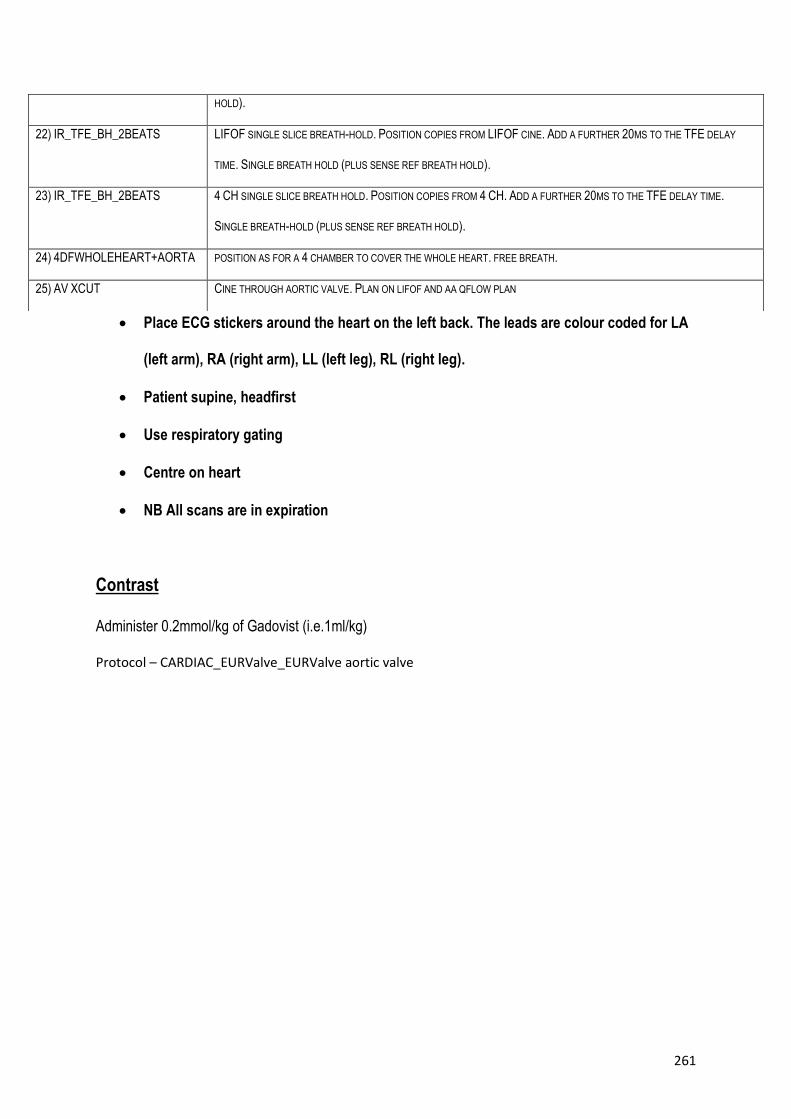
261

• Place ECG stickers around the heart on the left back. The leads are colour coded for LA

(left arm), RA (right arm), LL (left leg), RL (right leg).

• Patient supine, headfirst

• Use respiratory gating

• Centre on heart

• NB All scans are in expiration

Contrast

Administer 0.2mmol/kg of Gadovist (i.e.1ml/kg)

Protocol – CARDIAC_EURValve_EURValve aortic valve

HOLD).

22) IR_TFE_BH_2BEATS LIFOF SINGLE SLICE BREATH-HOLD. POSITION COPIES FROM LIFOF CINE. ADD A FURTHER 20MS TO THE TFE DELAY

TIME. SINGLE BREATH HOLD (PLUS SENSE REF BREATH HOLD).

23) IR_TFE_BH_2BEATS 4 CH SINGLE SLICE BREATH HOLD. POSITION COPIES FROM 4 CH. ADD A FURTHER 20MS TO THE TFE DELAY TIME.

SINGLE BREATH-HOLD (PLUS SENSE REF BREATH HOLD).

24) 4DFWHOLEHEART+AORTA POSITION AS FOR A 4 CHAMBER TO COVER THE WHOLE HEART. FREE BREATH.

25) AV XCUT CINE THROUGH AORTIC VALVE. PLAN ON LIFOF AND AA QFLOW PLAN

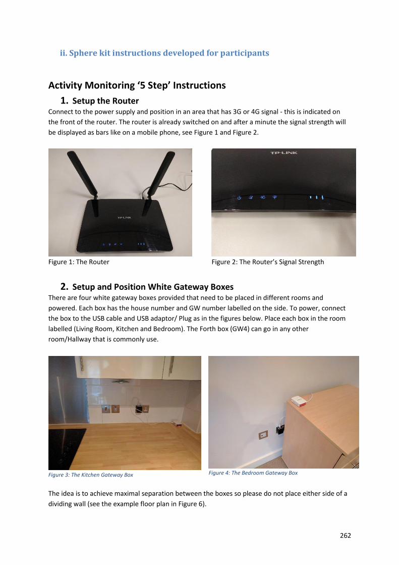
262

ii. Sphere kit instructions developed for participants

Activity Monitoring ‘5 Step’ Instructions

1. Setup the Router Connect to the power supply and position in an area that has 3G or 4G signal - this is indicated on

the front of the router. The router is already switched on and after a minute the signal strength will

be displayed as bars like on a mobile phone, see Figure 1 and Figure 2.

Figure 1: The Router

Figure 2: The Router’s Signal Strength

2. Setup and Position White Gateway Boxes There are four white gateway boxes provided that need to be placed in different rooms and

powered. Each box has the house number and GW number labelled on the side. To power, connect

the box to the USB cable and USB adaptor/ Plug as in the figures below. Place each box in the room

labelled (Living Room, Kitchen and Bedroom). The Forth box (GW4) can go in any other

room/Hallway that is commonly use.

Figure 3: The Kitchen Gateway Box

Figure 4: The Bedroom Gateway Box

The idea is to achieve maximal separation between the boxes so please do not place either side of a

dividing wall (see the example floor plan in Figure 6).

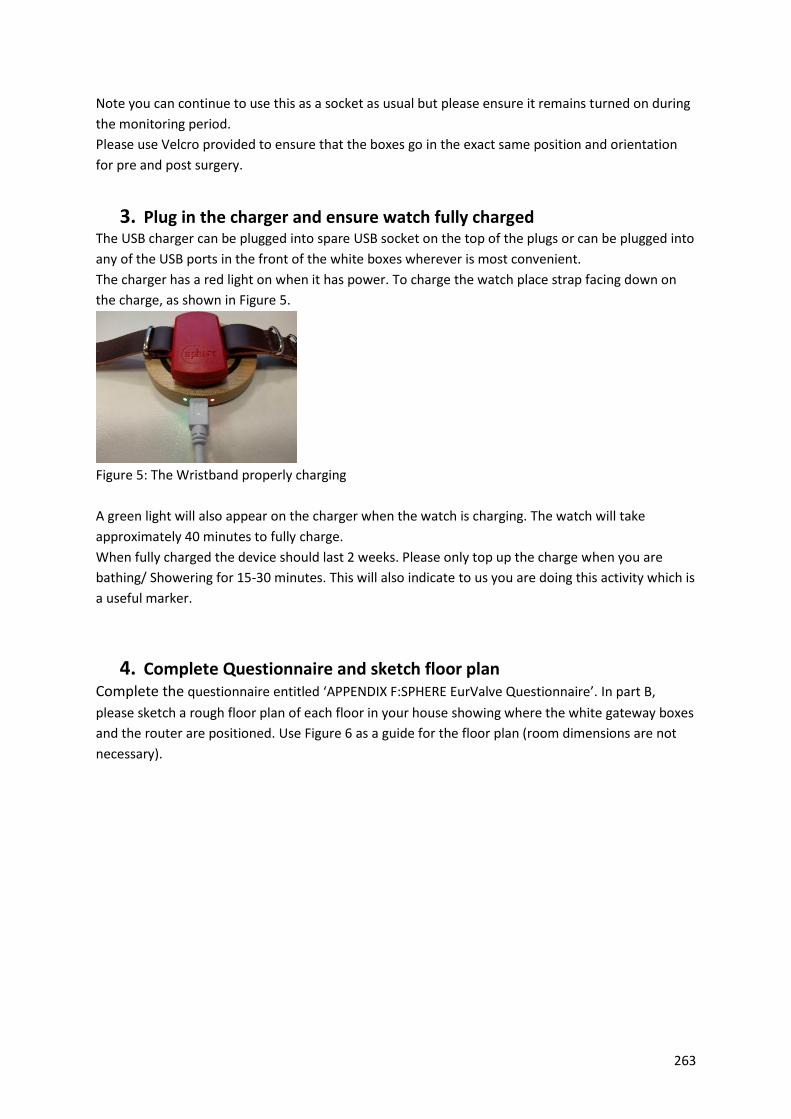
263

Note you can continue to use this as a socket as usual but please ensure it remains turned on during

the monitoring period.

Please use Velcro provided to ensure that the boxes go in the exact same position and orientation

for pre and post surgery.

3. Plug in the charger and ensure watch fully charged The USB charger can be plugged into spare USB socket on the top of the plugs or can be plugged into

any of the USB ports in the front of the white boxes wherever is most convenient.

The charger has a red light on when it has power. To charge the watch place strap facing down on

the charge, as shown in Figure 5.

Figure 5: The Wristband properly charging

A green light will also appear on the charger when the watch is charging. The watch will take

approximately 40 minutes to fully charge.

When fully charged the device should last 2 weeks. Please only top up the charge when you are

bathing/ Showering for 15-30 minutes. This will also indicate to us you are doing this activity which is

a useful marker.

4. Complete Questionnaire and sketch floor plan Complete the questionnaire entitled ‘APPENDIX F:SPHERE EurValve Questionnaire’. In part B,

please sketch a rough floor plan of each floor in your house showing where the white gateway boxes

and the router are positioned. Use Figure 6 as a guide for the floor plan (room dimensions are not

necessary).

264

Figure 6 Example Floor plan

5. Calibrate the system

Please complete steps 1-4 (the router and gateways should be on) before

performing this important step.

1. Place your wrist with the wristband as close to the white ‘gateway’

in your living room as possible for around ten seconds.

2. Next, in the living room, please sit on your sofa / chair as naturally

as possible (i.e. like you normally do) for around two minutes. Then

go to the kitchen.


in your kitchen as possible for around ten seconds.

4. Next, in the kitchen, please walk around as naturally as possible for

around two minutes. Then go to the bedroom.


in your bedroom as possible for around ten seconds.

6. Next, in the bedroom, please lie on your bed as you normally do

(for e.g. when sleeping) for around two minutes. Now go to the

fourth white ‘gateway’ in the other room.


in your fourth location as possible for around ten seconds

265

8. In the fourth location, please do whatever activity you normally

do in this room for around two minutes.

Date and Time of Calibration

____________________________________________________________

_

Person who performed the Calibration

____________________________________________________________

_

What activity did you do in the fourth room?

____________________________________________________________

_

Please wear the Wristband as much as you can. You should wear the Wristband on the hand

you use most (i.e. your dominant hand). If possible wear it at night too, since sleep is an

important part of health. The Wristband battery will last for a couple of weeks so you will

not need to recharge it during the trial. Do not forget to take the Wristband off during

showers/bathing.

iii. Derivation of equations used in protocol 1.

Aortic Pressure

Assume that during the period of forward flow the aortic pressure has a parabolic distribution

with its peak at the end, when the aortic valve closes:

𝑝𝑎𝑜𝑟𝑡𝑎 = 𝑎0 + 𝑎1𝑡 + 𝑎2𝑡2

where t is normalised to the period of forward flow, 0 at start and 1 at end.

𝑑𝑝𝑎𝑜𝑟𝑡𝑎

𝑑𝑡= 𝑎1 + 2𝑎2𝑡

Then:

𝑎0 = 𝑝𝑠𝑡𝑎𝑟𝑡 ; 𝑎1 = 2(𝑝𝑒𝑛𝑑 − 𝑝𝑠𝑡𝑎𝑟𝑡) ; 𝑎2 = −(𝑝𝑒𝑛𝑑 − 𝑝𝑠𝑡𝑎𝑟𝑡)

Left Ventricular Volume

Assume that during systole the left ventricular volume has a parabolic distribution with its minimum

at end systole:

𝑉𝐿𝑉 = 𝑐0 + 𝑐1𝑡 + 𝑐2𝑡2

where t is normalised to the period of systole, 0 at start and 1 at end.

𝑑𝑉𝐿𝑉

𝑑𝑡= 𝑐1 + 2𝑐2𝑡

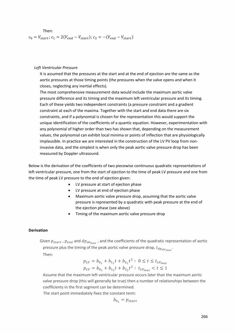
266

Then:

𝑐0 = 𝑉𝑠𝑡𝑎𝑟𝑡 ; 𝑐1 = 2(𝑉𝑒𝑛𝑑 − 𝑉𝑠𝑡𝑎𝑟𝑡) ; 𝑐2 = −(𝑉𝑒𝑛𝑑 − 𝑉𝑠𝑡𝑎𝑟𝑡)

Left Ventricular Pressure

It is assumed that the pressures at the start and at the end of ejection are the same as the

aortic pressures at those timing points (the pressures when the valve opens and when it

closes, neglecting any inertial effects).

The most comprehensive measurement data would include the maximum aortic valve

pressure difference and its timing and the maximum left ventricular pressure and its timing.

Each of these yields two independent constraints (a pressure constraint and a gradient

constraint at each of the maxima. Together with the start and end data there are six

constraints, and if a polynomial is chosen for the representation this would support the

unique identification of the coefficients of a quantic equation. However, experimentation with

any polynomial of higher order than two has shown that, depending on the measurement

values, the polynomial can exhibit local minima or points of inflection that are physiologically

implausible. In practice we are interested in the construction of the LV PV loop from non-

invasive data, and the simplest is when only the peak aortic valve pressure drop has been

measured by Doppler ultrasound.

Below is the derivation of the coefficients of two piecewise continuous quadratic representations of

left ventricular pressure, one from the start of ejection to the time of peak LV pressure and one from

the time of peak LV pressure to the end of ejection given:

• LV pressure at start of ejection phase

• LV pressure at end of ejection phase

• Maximum aortic valve pressure drop, assuming that the aortic valve

pressure is represented by a quadratic with peak pressure at the end of

the ejection phase (see above)

• Timing of the maximum aortic valve pressure drop

Derivation

Given 𝑝𝑠𝑡𝑎𝑟𝑡 , 𝑝𝑒𝑛𝑑 and 𝑑𝑝𝐴𝑉𝑚𝑎𝑥 , and the coefficients of the quadratic representation of aortic

pressure plus the timing of the peak aortic valve pressure drop, 𝑡𝑑𝑝𝐴𝑉𝑚𝑎𝑥.

Then:

𝑝𝐿𝑉 = 𝑏01+ 𝑏11

𝑡 + 𝑏21𝑡2 ∶ 0 ≤ 𝑡 ≤ 𝑡𝐿𝑉𝑚𝑎𝑥

𝑝𝐿𝑉 = 𝑏02+ 𝑏12

𝑡 + 𝑏22𝑡2 ∶ 𝑡𝐿𝑉𝑚𝑎𝑥

< 𝑡 ≤ 1

Assume that the maximum left ventricular pressure occurs later than the maximum aortic

valve pressure drop (this will generally be true) then a number of relationships between the

coefficients in the first segment can be determined.

The start point immediately fixes the constant term:

𝑏01= 𝑝𝑠𝑡𝑎𝑟𝑡

267

The pressure drop across the aortic valve is:

𝑑𝑝𝐴𝑉 = (𝑏01− 𝑎0) + (𝑏11

− 𝑎1)𝑡 + (𝑏01− 𝑎0)𝑡2

and, since the constant coefficients are the same:

𝑑𝑝𝐴𝑉 = (𝑏11− 𝑎1)𝑡 + (𝑏21

− 𝑎2)𝑡2

The peak pressure drop and its timing are known:

𝑑𝑝𝐴𝑉𝑚𝑎𝑥= (𝑏11

− 𝑎1)𝑡𝑑𝑝𝐴𝑉𝑚𝑎𝑥+ (𝑏21

− 𝑎2)𝑡𝑑𝑝𝐴𝑉𝑚𝑎𝑥

2

The temporal gradient of the AV pressure drop is:

𝑑(𝑑𝑝𝐴𝑉)

𝑑𝑡= (𝑏11

− 𝑎1) + 2(𝑏21− 𝑎2)𝑡

and since this is zero when the gradient is a peak:

0 = (𝑏11− 𝑎1) + 2(𝑏21


From these two equations:

𝑑𝑝𝐴𝑉𝑚𝑎𝑥= −(𝑏21


2

𝑏21= 𝑎2 −

𝑑𝑝𝐴𝑉𝑚𝑎𝑥

𝑡𝑑𝑝𝐴𝑉𝑚𝑎𝑥

2

𝑑𝑝𝐴𝑉𝑚𝑎𝑥=

(𝑏11− 𝑎1)

2𝑡𝑑𝑝𝐴𝑉𝑚𝑎𝑥

𝑏11= 𝑎1 + 2

𝑑𝑝𝐴𝑉𝑚𝑎𝑥


Hence the coefficients of the first quadratic segment are fully defined from the two

points and the known temporal gradient.

The temporal gradient of the LV pressure is:

𝑑𝑝𝐿𝑉

𝑑𝑡= 𝑏11

+ 2𝑏21𝑡

and this is a maximum when:

𝑡𝐿𝑉𝑚𝑎𝑥= −

𝑏11

2𝑏21

= −1

2

𝑎1 + 2𝑑𝑝

𝐴𝑉𝑚𝑎𝑥


𝑎2 −𝑑𝑝



2

= −𝑡𝑑𝑝𝐴𝑉𝑚𝑎𝑥

2∙

𝑎1𝑡𝑑𝑝𝐴𝑉𝑚𝑎𝑥+ 2𝑑𝑝


𝑎2𝑡𝑑𝑝𝐴𝑉𝑚𝑎𝑥

2 − 𝑑𝑝𝐴𝑉𝑚𝑎𝑥

The maximum LV pressure, 𝑝𝐿𝑉𝑚𝑎𝑥 , can be derived by substituting this value of time

into the quadratic equation for the first segment.

Now consider the second quadratic segment:

𝑝𝐿𝑉 = 𝑏02+ 𝑏12

𝑡 + 𝑏22𝑡2 ∶ 𝑡𝐿𝑉𝑚𝑎𝑥

< 𝑡 ≤ 1

At the end of the ejection period:

𝑝𝑒𝑛𝑑 = 𝑏02+ 𝑏12

+ 𝑏22

At 𝑡𝐿𝑉𝑚𝑎𝑥 the pressure is:

𝑝𝐿𝑉𝑚𝑎𝑥= 𝑏02

+ 𝑏12𝑡𝐿𝑉𝑚𝑎𝑥

+ 𝑏22𝑡𝐿𝑉𝑚𝑎𝑥

2

and the temporal gradient is:

0 = 𝑏12+ 2𝑏22

𝑡𝐿𝑉𝑚𝑎𝑥

Eliminating 𝑏02 from the first two equations:

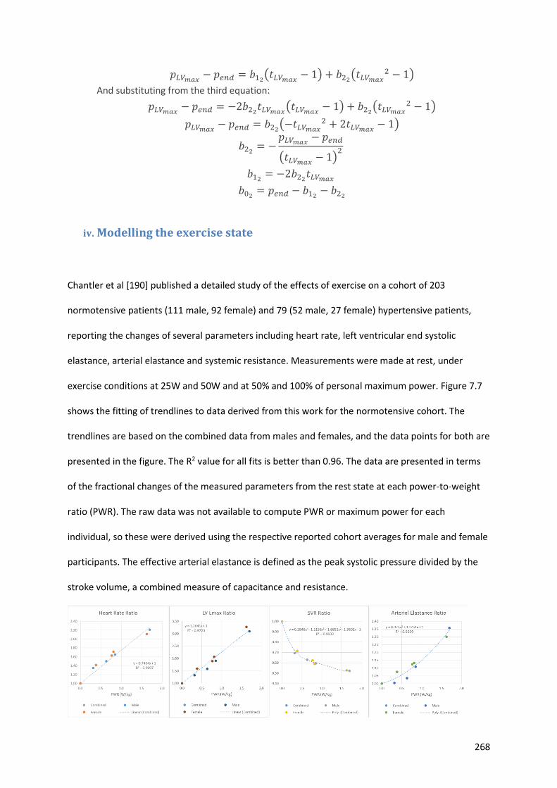
268

𝑝𝐿𝑉𝑚𝑎𝑥− 𝑝𝑒𝑛𝑑 = 𝑏12

(𝑡𝐿𝑉𝑚𝑎𝑥− 1) + 𝑏22

(𝑡𝐿𝑉𝑚𝑎𝑥2 − 1)

And substituting from the third equation:

𝑝𝐿𝑉𝑚𝑎𝑥− 𝑝𝑒𝑛𝑑 = −2𝑏22

𝑡𝐿𝑉𝑚𝑎𝑥(𝑡𝐿𝑉𝑚𝑎𝑥

− 1) + 𝑏22(𝑡𝐿𝑉𝑚𝑎𝑥

2 − 1)

𝑝𝐿𝑉𝑚𝑎𝑥− 𝑝𝑒𝑛𝑑 = 𝑏22

(−𝑡𝐿𝑉𝑚𝑎𝑥2 + 2𝑡𝐿𝑉𝑚𝑎𝑥

− 1)

𝑏22= −

𝑝𝐿𝑉𝑚𝑎𝑥− 𝑝𝑒𝑛𝑑

(𝑡𝐿𝑉𝑚𝑎𝑥− 1)

2

𝑏12= −2𝑏22

𝑡𝐿𝑉𝑚𝑎𝑥

𝑏02= 𝑝𝑒𝑛𝑑 − 𝑏12

− 𝑏22

iv. Modelling the exercise state

Chantler et al [190] published a detailed study of the effects of exercise on a cohort of 203

normotensive patients (111 male, 92 female) and 79 (52 male, 27 female) hypertensive patients,

reporting the changes of several parameters including heart rate, left ventricular end systolic

elastance, arterial elastance and systemic resistance. Measurements were made at rest, under

exercise conditions at 25W and 50W and at 50% and 100% of personal maximum power. Figure 7.7

shows the fitting of trendlines to data derived from this work for the normotensive cohort. The

trendlines are based on the combined data from males and females, and the data points for both are

presented in the figure. The R2 value for all fits is better than 0.96. The data are presented in terms

of the fractional changes of the measured parameters from the rest state at each power-to-weight

ratio (PWR). The raw data was not available to compute PWR or maximum power for each

individual, so these were derived using the respective reported cohort averages for male and female

participants. The effective arterial elastance is defined as the peak systolic pressure divided by the

stroke volume, a combined measure of capacitance and resistance.

269

Figure 7.7: Fractional changes of cardiac and arterial parameters under exercise conditions for normotensive cohort. Data

processed from the information presented in Chantler, Melenovsky et al (2008)

Thus, the equations for the parameters under exercise conditions, derived from these data, are:

𝐻𝑒𝑎𝑟𝑡 𝑅𝑎𝑡𝑒𝑒𝑥𝑒𝑟𝑐𝑖𝑠𝑒 = (0.7464 ∙ 𝑃𝑊𝑅𝑒𝑥𝑒𝑟𝑐𝑖𝑠𝑒 + 1) ∙ 𝐻𝑒𝑎𝑟𝑡 𝑅𝑎𝑡𝑒𝑟𝑒𝑠𝑡

ELVmax 𝑒𝑥𝑒𝑟𝑐𝑖𝑠𝑒 = (1.2641 ∙ 𝑃𝑊𝑅𝑒𝑥𝑒𝑟𝑐𝑖𝑠𝑒 + 1) ∙ ELVmax 𝑟𝑒𝑠𝑡

𝑆𝑉𝑅𝑒𝑥𝑒𝑟𝑐𝑖𝑠𝑒 = (0.2848 ∙ 𝑃𝑊𝑅𝑒𝑥𝑒𝑟𝑐𝑖𝑠𝑒4 − 1.2158 ∙ 𝑃𝑊𝑅𝑒𝑥𝑒𝑟𝑐𝑖𝑠𝑒

3 + 1.8852 ∙ 𝑃𝑊𝑅𝑒𝑥𝑒𝑟𝑐𝑖𝑠𝑒2

− 1.3692 ∙ 𝑃𝑊𝑅𝑒𝑥𝑒𝑟𝑐𝑖𝑠𝑒 + 1) ∙ 𝑆𝑉𝑅𝑟𝑒𝑠𝑡

𝐴𝑟𝑡. 𝐸𝑙𝑎𝑠𝑡𝑎𝑛𝑐𝑒𝑒𝑥𝑒𝑟𝑐𝑖𝑠𝑒 = (0.075 ∙ 𝑃𝑊𝑅𝑒𝑥𝑒𝑟𝑐𝑖𝑠𝑒2 + 0.0751 ∙ 𝑃𝑊𝑅𝑒𝑥𝑒𝑟𝑐𝑖𝑠𝑒 + 1) ∙ 𝐴𝑟𝑡. 𝐸𝑙𝑎𝑠𝑡𝑎𝑛𝑐𝑒𝑟𝑒𝑠𝑡

The effective arterial elastance is defined as the peak systolic pressure divided by the stroke volume.

An estimate of the arterial capacitance in the zero-dimensional model can be made by consideration

of the change in systemic pressure over the period of diastole. The resulting formula is:

C =t_dias

R𝑙𝑛 ((psys − pvenous)

(pdias − pvenous))

Data includes information on the systolic pressure, the heart period and the systemic vascular

resistance index. There is no information on venous pressure, and for the purposes of this

calculation it is assumed to be zero. In the absence of other information, it is further assumed that

the period of diastole scales with the heart period and that the diastolic pressure in normotensives

does not change under exercise conditions. Under these assumptions, and using the index data

provided by Chantler:

C =60 ∙ t_diasfraction

HR ∙ SVR Index

BSA ∙ 𝑙𝑛 (End Systolic PressureEnd Diastolic Pressure

)

To be consistent with the index definitions, a capacitance index would be defined by dividing the

capacitance by the body surface area (since the volume term is on the top line).

C Index =60 ∙ t_diasfraction

HR ∙ SVR Index∙ 𝑙𝑛 (End Systolic PressureEnd Diastolic Pressure

)

Figure 7.8 illustrates the fractional change of the capacitance, or capacitance index, derived from the

Chantler data using this calculation.

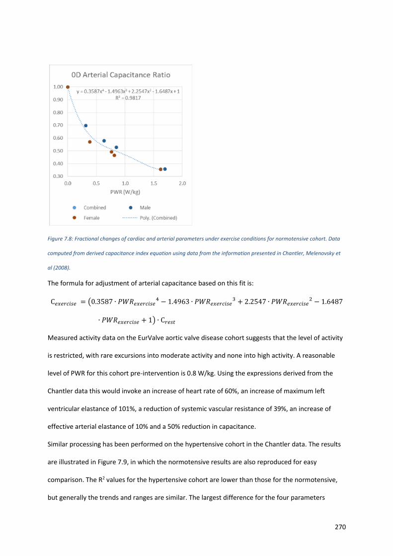
270

Figure 7.8: Fractional changes of cardiac and arterial parameters under exercise conditions for normotensive cohort. Data

computed from derived capacitance index equation using data from the information presented in Chantler, Melenovsky et

al (2008).

The formula for adjustment of arterial capacitance based on this fit is:

C𝑒𝑥𝑒𝑟𝑐𝑖𝑠𝑒 = (0.3587 ∙ 𝑃𝑊𝑅𝑒𝑥𝑒𝑟𝑐𝑖𝑠𝑒4 − 1.4963 ∙ 𝑃𝑊𝑅𝑒𝑥𝑒𝑟𝑐𝑖𝑠𝑒

3 + 2.2547 ∙ 𝑃𝑊𝑅𝑒𝑥𝑒𝑟𝑐𝑖𝑠𝑒2 − 1.6487

∙ 𝑃𝑊𝑅𝑒𝑥𝑒𝑟𝑐𝑖𝑠𝑒 + 1) ∙ C𝑟𝑒𝑠𝑡

Measured activity data on the EurValve aortic valve disease cohort suggests that the level of activity

is restricted, with rare excursions into moderate activity and none into high activity. A reasonable

level of PWR for this cohort pre-intervention is 0.8 W/kg. Using the expressions derived from the

Chantler data this would invoke an increase of heart rate of 60%, an increase of maximum left

ventricular elastance of 101%, a reduction of systemic vascular resistance of 39%, an increase of

effective arterial elastance of 10% and a 50% reduction in capacitance.

Similar processing has been performed on the hypertensive cohort in the Chantler data. The results

are illustrated in Figure 7.9, in which the normotensive results are also reproduced for easy

comparison. The R2 values for the hypertensive cohort are lower than those for the normotensive,

but generally the trends and ranges are similar. The largest difference for the four parameters

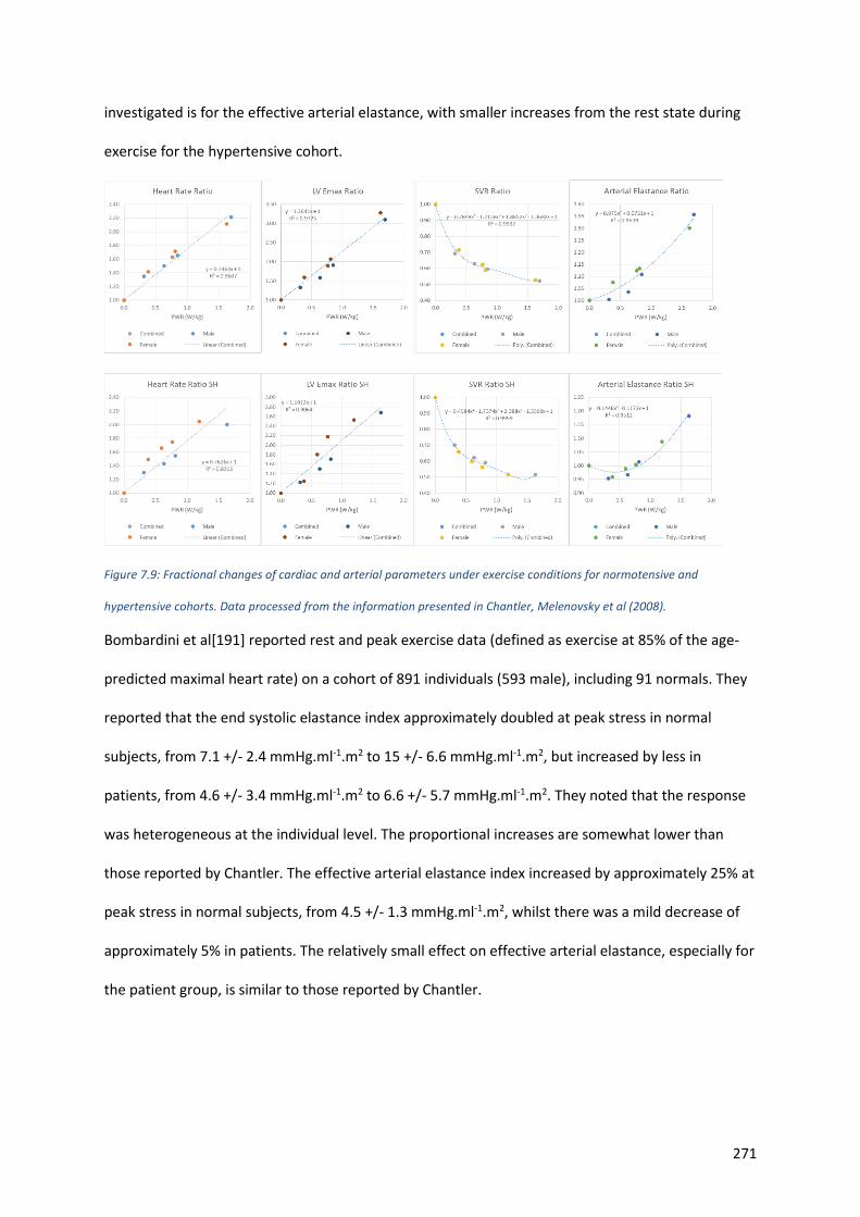
271

investigated is for the effective arterial elastance, with smaller increases from the rest state during

exercise for the hypertensive cohort.

Figure 7.9: Fractional changes of cardiac and arterial parameters under exercise conditions for normotensive and

hypertensive cohorts. Data processed from the information presented in Chantler, Melenovsky et al (2008).

Bombardini et al[191] reported rest and peak exercise data (defined as exercise at 85% of the age-

predicted maximal heart rate) on a cohort of 891 individuals (593 male), including 91 normals. They

reported that the end systolic elastance index approximately doubled at peak stress in normal

subjects, from 7.1 +/- 2.4 mmHg.ml-1.m2 to 15 +/- 6.6 mmHg.ml-1.m2, but increased by less in

patients, from 4.6 +/- 3.4 mmHg.ml-1.m2 to 6.6 +/- 5.7 mmHg.ml-1.m2. They noted that the response

was heterogeneous at the individual level. The proportional increases are somewhat lower than

those reported by Chantler. The effective arterial elastance index increased by approximately 25% at

peak stress in normal subjects, from 4.5 +/- 1.3 mmHg.ml-1.m2, whilst there was a mild decrease of

approximately 5% in patients. The relatively small effect on effective arterial elastance, especially for

the patient group, is similar to those reported by Chantler.

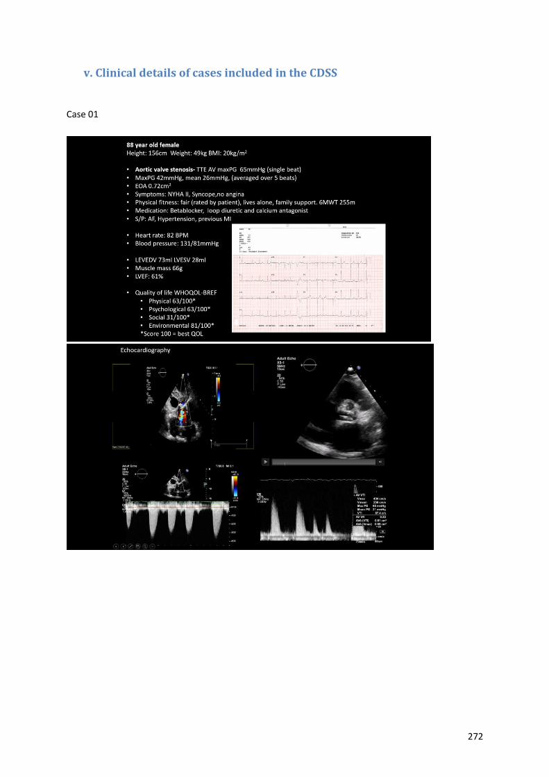
272

v. Clinical details of cases included in the CDSS

Case 01

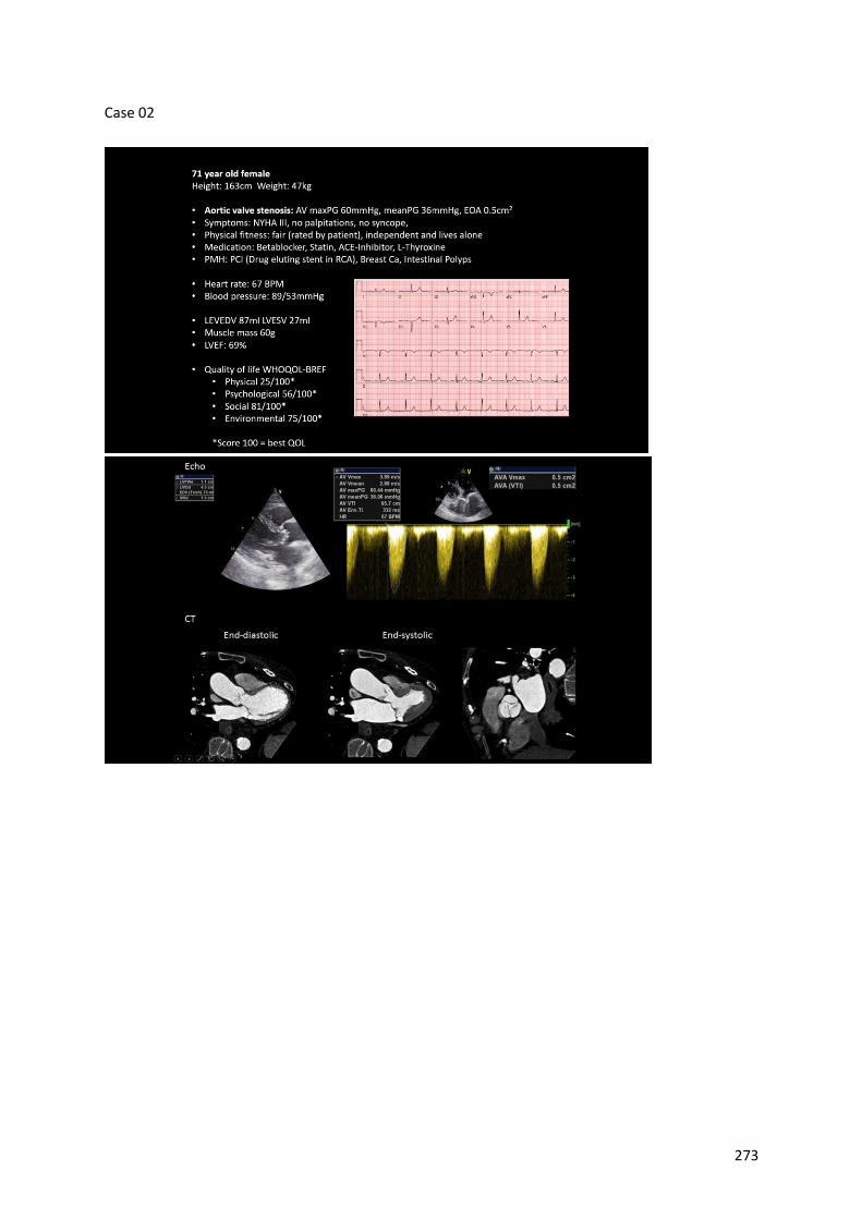
273

Case 02

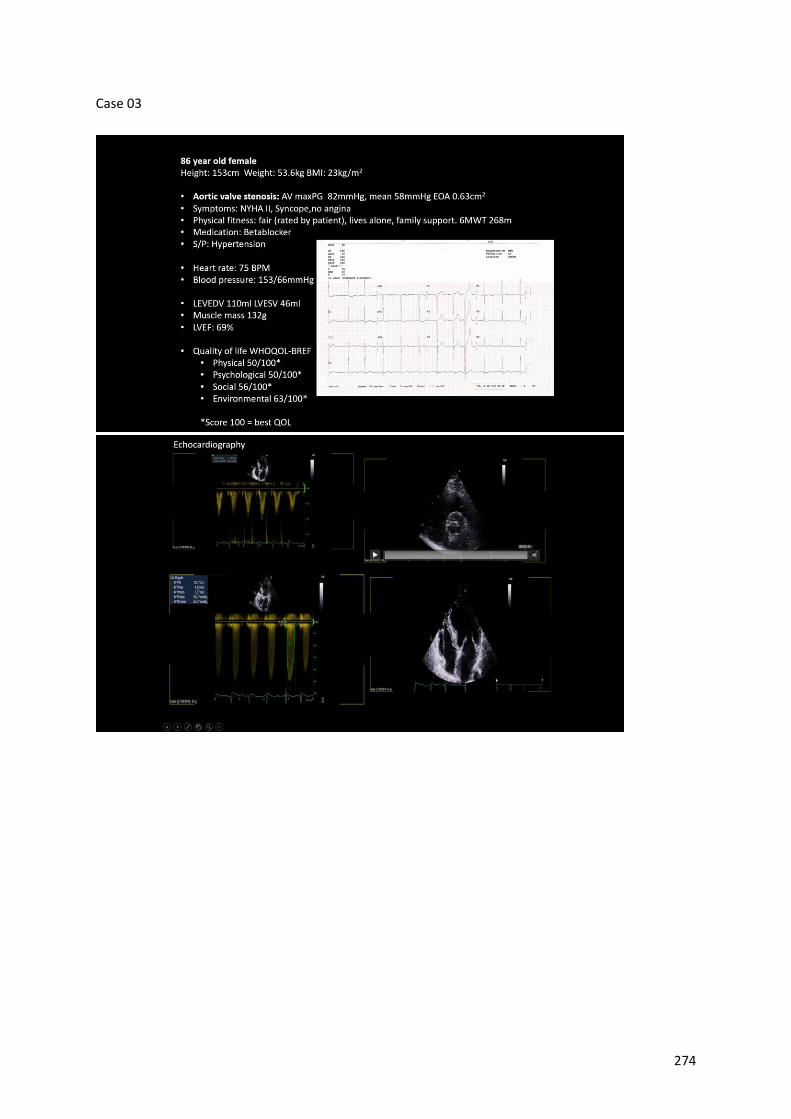
274

Case 03

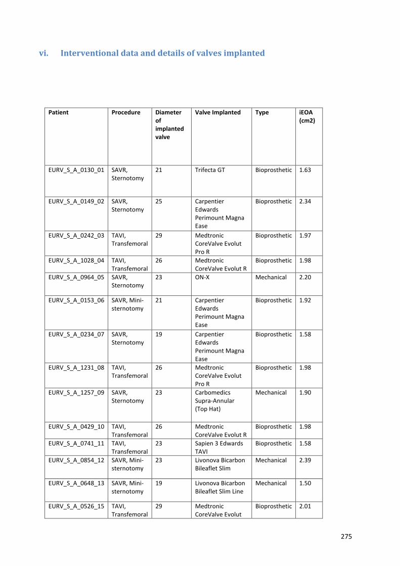
275

vi. Interventional data and details of valves implanted

Patient Procedure Diameter of implanted valve

Valve Implanted Type iEOA (cm2)

EURV_S_A_0130_01 SAVR, Sternotomy

21 Trifecta GT Bioprosthetic 1.63


25 Carpentier Edwards Perimount Magna Ease

Bioprosthetic 2.34

EURV_S_A_0242_03 TAVI, Transfemoral

29 Medtronic CoreValve Evolut Pro R

Bioprosthetic 1.97


26 Medtronic CoreValve Evolut R

Bioprosthetic 1.98


23 ON-X Mechanical 2.20

EURV_S_A_0153_06 SAVR, Mini-sternotomy


Bioprosthetic 1.92



Bioprosthetic 1.58



Bioprosthetic 1.98


23 Carbomedics Supra-Annular (Top Hat)

Mechanical 1.90



Bioprosthetic 1.98


23 Sapien 3 Edwards TAVI

Bioprosthetic 1.58


23 Livonova Bicarbon Bileaflet Slim

Mechanical 2.39


19 Livonova Bicarbon Bileaflet Slim Line

Mechanical 1.50


29 Medtronic CoreValve Evolut

Bioprosthetic 2.01

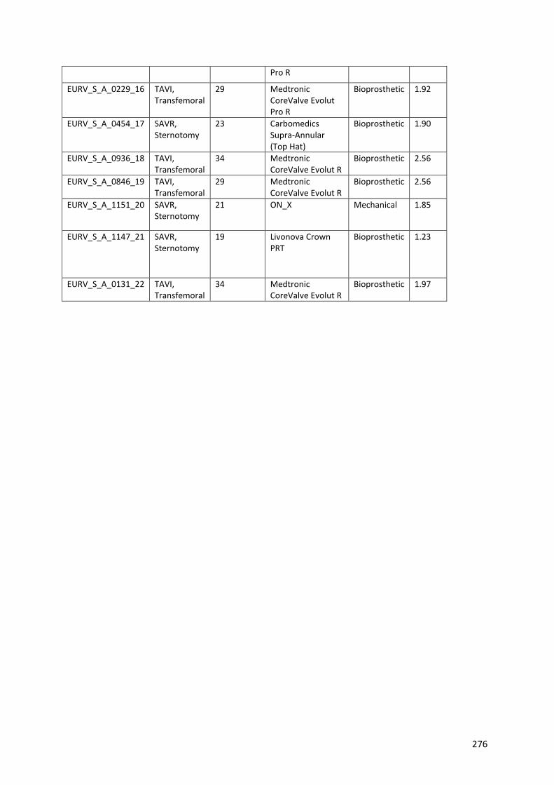
276

Pro R



Bioprosthetic 1.92


23 Carbomedics Supra-Annular (Top Hat)

Bioprosthetic 1.90



Bioprosthetic 2.56



Bioprosthetic 2.56


21 ON_X Mechanical 1.85


19 Livonova Crown PRT

Bioprosthetic 1.23



Bioprosthetic 1.97

Computational Modelling in the Management of Patients with ...

Documents

Transcript of Computational Modelling in the Management of Patients with ...