Quality Control Manual for Computational Estuarine Modelling

Quality Control Manual for Computational Estuarine Modelling

Research and Development

Technical Report W168

fB A ENVIRONMENT AGENCY

All pulps used in production of this paper is sourced from sustainable managed forests and are elemental chlorine free and wood free

Qualitjc Control Manual for Computational. EStuarine Modelling .’

Technical Report-W1 68

J M Bartlett

Research Contractor: Binnie Black’ &--Veatch.

Further copies of this report are available from: Environment Agency R&D Dissemination Centre, c/o WRc, Frankland Road, Swindon, Wilts SN5 SYF WC tel: 01793-865000 fax: 01793-514562 e-mail: [email protected]

Publishing Organisation: Environment Agency Rivers House Waterside Drive Almonsbury Aztec West Bristol BS32 4UD Tel: 01454 624400 Fax: 01454 624409

SO-6/98-B-BCXH

0 Environment Agency 1998

All rights reserved. No part of this document may be produced, stored in a retrieval system or transmitted, in any form or by any means, electronic, mechanical, photocopying, recording or otherwise without the prior permission of the Environment Agency.

The views expressed in this document are not necessarily those of the Environment Agency. Its officers, servants or agents accept no liability whatsoever for any loss or damage arising from the interpretation or use of the information, or reliance upon views contained herein. Worked and funded as part of the Agency’s national R&D programme.

Dissemination status Internal: Released to Regions External: Public Domain

Statement of use This report presents a methodology for the determination of the freshwater flow needs of estuaries. The information within this document is for use by Agency staff involved in the licensing of freshwater abstractions from rivers and in the computational modelling of estuaries.

Research Contractor This document was produced under R&D Project Project W6-010 by:

Binnie Black & Veatch Grosvenor House 69 London Road Redhill Surrey RI31 1LQ Tel: 01737 774155 Fax: 01737 772767

Environment Agency’s Project Manager The Environment Agency’s Project Manager for R&D Project Project W6-010 was: Oliver Pollard - Environment Agency, Southern Region

R&D Technical Report WI 68

CONTENTS Page

Executive summary

1 INTRODUCTION 1.1. Scope of manual 1.2 Background 1.3 Need for computaticnal modelling

2. PROJECT DEFINITION 2.1 Scope of work 2.2 Preliminary .assessment 2.3 Type of model 2.4 Technical specification 2.5 Data collection needs 2.6 Cost and programme allowances 2.7 Project plan -.

3 TENDER PROCEDURES/PROCUREMENT GUIDE ‘1 3.1 Introduction 3.2. Specification 3.3 Supplier selection and appraisal I’ : 3.4 . Tendering 3.5. Tender opening 3.6 Tender evaluation ‘. 3.7 Post, tender negotiation 3.8 Contract award. 3.9 Contract management

4 FIELD WORK 14

4.1 :. Project plan 14

4.2 Preliminary assessment 14, :

4.3 Data collection techniques 14 ‘!

4.4 Data storage and transfer 22

4.5 Checking and validation I 22

5 COMPUTATIONAL MODELLING 25.

5.1 Project plan .’ 25

5.2 Model capabilities and limitations 25

5.3 Selection of software 30

5.4 Change control ’ 35

5.5 Building, calibration and validation 36

5.6 Run referencing and archiving 37

5.7 Reporting- 40 ‘>

5.8 Transfer arrangements 41

5 5 5 6 7 8 8 g .”

11 .. 11. ’ 11 ::.

11 12 12 12 13. 13 13

R&D Technical Report WI68 i

STATISTICAL APPROACHES 42 6.1 Environmetrics 42 6.2 Stochastic techniques 42 6.3 Intervention models 43 6.4 Data requirements 43 6.5 Data quality 44 6.6 Quality control 44 6.7 Conclusions 45

7 CONTINUED USE OF MODEL 46 7.1 General 46 7.2 Run referencing and archiving 46 7.3 Change control 47 7.4 Re-validation using additional data sets 47 7.5 Risks of inappropriate application of model 47

8 ESTUARINE MODELLING AND DATA COLLECTION STRATEGY 48 8.1 Modelling strategy 48 8.2 Data collection strategy 48 8.3 Sets of models and supporting data 49 8.4 Detailed budget guidelines 55

9 LIST OF CONSULTEES 67 9.1 Environment Agency 67 9.2 Other UK organisations 68 9.3 Overseas consultees 68

10 BIBLIOGRAPHY 69 10.1 Residual ff ows 69 10.2 Estuary characteristics 69 10.3 Estuary management 70 10.4 Computational modelling 71 10.5 Risk; impact and sensitivity analysis 72 10.6 Water quality and salinity 72 10.7 Sediment and morphology 73 10.8 Ecology and fish 73 10.9 Other 74

11 GLOSSARY OF TERMS

APPENDIX A - TYPICAL MODEL SPECIFICATION

75

R&D Techical Report WI 68 ii

EXECUTIVE SUMMARY

Scope of study

The overall aim of this study is to establish.best practice, shortcomings and future research needs in determining freshwater-flow.needs of estuaries. In particular, the study has examined the use of computational, including statistical, modelling in determining. these needs. It is hoped that. the resultingSdocuments will be of practical use across all disciplines working within estuaries.

The outputs .fi-om-the study are:

. an R&D Technical Report-that identifies shortcomings, best practice, implementation benefits and-future R&D of freshwater flow needs to.estuaries.

. this quality control-manual to be used when undertaking a computational estuary model study..

This manual contains guidance on:--

. how-to define modelling~projects;

. how.to tender a modelling study;

. field data collection techniques;

. model types and quality control;

. modelling and data.collection strategy.

The layout of the manual is shown below. It is hoped that this manual will pr0vide.a framework : for modelling.for the beginner, but will also provide information useful .for the experienced practitioner.

Computational modelling

The use of computational.models is one of the most powerful tools available to,quantify the. effect of variations of freshwater. .residual flows when- applied -to estuarine water .. quality/morphology-processes. The prolonged and detailed public enquiries that are likely to accompany. future applications to increase abstraction and reduce MRF in estuaries will require supportable evidence of the impact of increased abstraction. Any new national methodology must provide such quantified evidence.

R&D -T&chnical Report WI 68 . . . 111

LAYOUT OF QUALITY CONTROL MANUAL

There are two main types of modelling techniques available to test the effect of residual flows on the estuarine transport/residence processes:

. Statistical models are a relatively quick approach which are useful in initial studies to qualitatively assess the effects of different MRFs on the estuary.

. Deterministic/hydrodynamic models use mathematical descriptions of physical laws and processes, and require detailed research and carefully designed field data.

There is also a need for guidance on how reliable the model results should be, and what the most appropriate models are to answer specific queries or requirements for data. A system is needed to ensure that procedures are correctly followed and to check that the software is being correctly applied. This manual provides appropriate guidance in these areas.

R&D Technical Report WI68 iV

1’ INTRODUCTION

1.1 Scope of manual

The overall aim of this study is to establish best practice, shortcomings and future research needs in determining freshwater flow needs of estuaries. In particular, the study. has examined the use of computational,.including statistical, modelling in determining these needs. Although written from a water. resources perspective, it is recognised that this aim also impacts a number. of other disciplines, such as water quality,-flood defence and fisheries.

It is hoped that the resulting documents will be of practical use across all disciplines working within estuaries.

The outputs from-the study are:

. an R&D : Technical :Report (W-l 13) that identifies shortcomings, best practice, implementation benefits and-future R&D of freshwater flow needs to estuaries.

. this quality control manual to be used when undertaking a computational estuary model study.

This manual contains guidance on:

. how to define modelling.projects;

. how to tender a modelling.study;

. field data colledtion techniques;

. model types and quality control;

. modelling and data collection strategy.

The layout of the manualis shown on Figure 1.1. It is difficult ,to write guidance that is relevant for all levels of modelliig experience. It is also recognised that parts of the Agency already have their own quality control:procedures. However, it is hoped that this manual will .@rovide a framework, for modelling for the beginner,. but..will also provide information useful for the experienced practitioner.

L2 Background

The Environment Agency has a statutory duty under the Water Resources Act 199 1 to conserve, redistribute or otherwise augment water resources and secure ::their proper use. The determination. of minimum residual. flows (MRF) to estuaries -is one .of the -key steps in evaluating the water resource potential .of a river; and in the .effective management of the. estuarine environment. The MRF is defined as the river flow at which a licenced abstraction ceases, ie river flows can naturally fall below.the MRF value.

R&D. Technical Report WI68 1

accompany future applications to increase abstraction and reduce MRF in estuarieswill require supportable’:evidence of the impact of increased abstraction. -Any new national.methodology must provide..such quantified evidence;

1.3 Need.for computational modelling

There are two main types of modelling techniques available to test the effect of residual flows on the estuarine transport/residence processes:

. Statistical models are.a relatively quick approach which uses linear regression analysis to relate empirically the observed values of variables.- Statistical models are useful in initial studies to ,qualitatively assess the .effects of different MRFs on the:.estuary. Statistical models are limited in their ability to,account,for the-scatter. in field data; and. need a large amount of field data.

Deterministic/hydrodynamic models use mathematical descriptions of physical laws and processes, and require detailed research and carefully designed field data. Deterministic models can -considerably improve on the prediction accuracy and reliability of the statistical regression models; -and can establish the quantitative effect of residual flows on. the estuary. The degree of reliability required of model -predictions determines how much is spent on the data needed by the model- and the type of model used. Sensitivity . analysis using deterministic models can establish the key areas of uncertainty and help focus: where and -what field data is needed. There are several deterministic models-, available and not all are equally appropriate or easy to use..

Within the industry, some are still. resistant to the use of computer modelling to help determine. residual flow needs. Others strongly support modelling, perhaps without proper consideration of the limitations or appropriate:use of the model;. There is.a need for a methodology ‘that sets out a considered and-balanced use of models

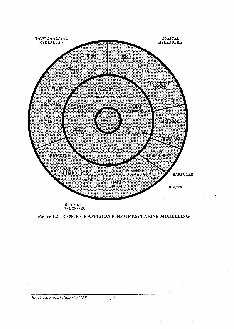
There is also a need for guidance on how reliable the model results should be, and ,what the most appropriate modelsare to answer specific queries or requirements for data. A system is needed to ensure that procedures are correctly followed and to check that the software-is being correctly applied. It is hoped.that this manual provides appropriate guidance in these areas. Figure 1.2 shows the wide range of applications-that can be analysed, using the types of computational models available.

R&D Technical Report WI 68 3

RS

SEDIMENT PROCESSES

Figure 1.2 - RANGE OF APPLICATIONS OF ESTUAFUNE MODELLING

R&D Technical Report WI 68 .4.

2. PROJECT DEFINITION

2.1 Scope of work

As with any project, successful execution of a modelling. study requires a focussed and detailed. scope of work.. This scope should be the first stage of any modelling project definition The scope should definer:

. the reason for and aims of the project;

. the background. to,the project;

. the expected interaction between this study and other. disciplines within a project; and

. the expected deliverables from the project;

2.2 Preliminary assessment

Having defined the scope of work, for a large project, a preliminary assessment of the problem should be considered.. This may consist of:

. a matrix risk assessment to determine critical estuary uses and processes; and

. a simple model to aid Ml model design and .data collection.

The: methods of matrix risk assessment are presented in the main (W113) report of this R&D project. The term “computational model” has been taken-in the Technical Report and this volume to include:

. Statistical and. empirical models; as well as

. Full hydrodynamic models.

A simple model can be used.to determine:

. the likely magnitude of problems, :and whether detailed study is required; . the likely areas of particular interest, for. example the main areas of sedimentation or thei

limits of significant salinity;

The results from the modelcan then be used to guide the design.of the detailed model. It may aid definition of the model limits and the grid size or section spacing in particular areas or interest.. It’may also guide the extent of data-collection,.additional data.being taken from theareas of particular interest.

It is also possible that the simple model may.show that there is no problem with a particular use or process, and no further modelling will be necessary.

R&D Technical Report.- WI68 5

A simple, preliminary model may be:

. an existing model, perhaps built for another discipline;

. built from coarse data, such as Admiralty charts and existing surveys;

. a coarse model using a 1-D rather than 2-D or a non-stratified rather than stratified model; or

. an uncalibrated and unverified model.

In all cases it should be remembered that the accuracy of the preliminary model may be low. Interpretation of results must take this into account. In addition, the preliminary model must not become too complex; in that case one might as well go straight to a full study.

2.3 Type of model

The range of computational models available for analysis of estuaries, and the choice of an appropriate model are described in Section 5.2. The choice of model is an important one in any project. Models by definition are only a representation of reality. The limitations on the current models are computing power and an understanding of the physical processes. In the first instance, the choice of model will depend on:

. the form of the estuary to be modelled; and

. the application to be modelled.

However, as indicated in Section 5.2, the choice of model is in some ways pragmatic, based on availability, budget and experience of use. The choice of model type will therefore also be determined on:

. the accuracy required for each general use category;

. the ability of models to give that level of accuracy;

. the sensitivity of various types of model; and

. the-minimum level of modelling that is required.

The choice of model according to use category will be dependant on the potential damage if the set limit of water quality, salinity or sediment deposition is exceeded. If the hazard is low and the risk is low, then the confidence needed in the result is also low and it is not necessary to carry out a large program of field work and modelling at great expense. Conversely if the hazard is high and the risk is significant, then such expenditure may well be necessary and this will influence the selection of the model and fieldwork program.

Choice of model should further take account of:

. the reliability of information available and any additional field work required;

. the capability of the model and the likely modeller;

. the cost of modelling / field work exercise;


. the need to continue and update -the process with time including monitoring costs;

. economic benefits of environmental and water quality improvement.

In some cases, a model may already exist, perhaps from another discipline.. The matrix allows some assessment as to the suitability of the existing model for a new project. Shortcomings in the existing model for its new purpose may not be critical- since a high degree of accuracy is not required.

At all times, it is important toask whether a complex modelling exercise is-at all necessary. It has become fashionable to build complex models. However, in many cases, adequate solutions may be developed-by a simple model;

2.4 Technical specification

A detailed technical specification for the modelling,and data collection phases of a project should be drawn.up. This specification will be used: :

. to coni%m the scope of work. A detailed modelling specification will:help assess whether the proposed modelling approach is technically.appropriate,-and pitched at-the correct level of complexity;

. to set costs and programme. The specification will allow initial cost estimates to be made and ,revision of the scope of work if they exceed available’budgets; -and

. as part of the tender document.. A clear and detailed technical specification. greatly simplifies the tendering process.

The specification should.include the following:.

.

.

.

The purpose of the model; The relationship of the model with other disciplines and.parts of the project; The type,of model to be used and, if appropriate, the software and hardware to be used. The aim of convergence of software and hardware platforms withinsthe Agency should be considered; The; geographical limits of the model, thus defining its size;. Zones of particular interest in the model that may.require detailed.survey and simulation; The scale. and detail of the model Typical grid sizes or cross-section spacing will aid costing and programming;. The extent of available data. .This could include information on existing models as well as topographicj.flow, tide, quality or sediment data; ,. The extent ofthe required data collection programme. Although this may be interpreted from the above two items; some statement of the data requirements should be’made; Calibration and validation. This section should include the calibration parameters, the. number of calibration locations and events and the accuracy of calibration expected;.. An indication of the scope of model.production runs to be carried out; ‘. Reporting requirements and deliverables; and Model transfer.requirements. If the software is specified, this may include the computer files required.

R&D Technical Report WI68 7

2.5 Data collection needs

Following definition of the model type and the technical specification, the nature and extent of data that needs to be collected should be drawn up. Although a detailed collection programme may be the responsibility of the modelling consultant, an initial programme should be drawn up to assess the feasibility of the programme and its cost.

The following should be considered:

. the suitability and extent of any existing data;

. the physical parameters to be collected; . the extent, frequency and duration of any data collection programme; 0 the likely methods of data collection; . downloading and data transfer; . quality assurance of data and calibration of recording instruments; and

l the cost of the programme.

Completing this task may result in revisions to the modelling specification. Data collection can be extremely expensive. In some cases, the cost of collecting data may outweigh the benefits fi-om itscollection. Field work is considered in more detail in Chapter 4.

2.6 Cost and programme allotiances

2.6.1 Costs, inputs and programme

This section gives an overview of the implications to costs, input and programme from using computational models. Detailed costs, inputs and programmes are presented in Chapter 7 of this report.

In any study there are two parts to the cost of a modelling project:

. Survey and data collection costs; and

. Model building and running costs.

Modelling studies have. significant cost. This cost may be small when included within, say, design of flood defences, but as a stand-alone study to check a licence application, may be an unacceptably high proportion of the auditing Agency area’s budget. However, it must also be stressed that modelling studies will almost invariably provide an improved quality of result over manual methods of analysis.

It is interesting to note that although computing power and model complexity have increased together, the costs of modelling projects have not risen in step with these factors.

Survey costs are dependent on the level of spatial and calibration detail required in the model.


As such-they are relatively fixed, for a typical model to be run over a series of spring, neap and average tides. A more complex, model may need little ‘more.topographical survey detail,. but . . additional level and quality. survey points for calibration. Costs rise steeply for-long.term data collection,, where instruments are left in place for months rather. than days..

Modelling.costs are linked closely. to time input by the modellers. These inputs do not -increase linearly with model complexity since:,

. most if not all computing can be carried out on standard EC based machines with a acceptably short run times, resulting in fixed computing.overheads; and

. use of data processing.tools such as GIS allows quick processing of complex data sets.,

Use of computational modelling does impose programme implications onto any study. ‘. Of the data collection and modelling-components to the work, it is the data collection that may provide the greatest constraint.- Survey contracts may need to be tendered, and .appropriate periods in the :. year chosen to collect data for calibration.-

2.6.2 Bala’ncing- modelling costs,with accuracy benefits

The-most practical time-to consider. the balance between modelling costs and the-reliability..or accuracy. of the.final model is. at an early stage while there is still time to influence the data collection programme-and the model assumptions. Time may be usefully’spent reviewing the issues. of importance for an estuary study, and if appropriate developing a simple preliminary model to gain a better feel for the key features of the estuary.

If problems,with the assumptions of the model;or the-extent of data,collection are not thought 1. through at an early stage, they may not become evident until model .development is well.advanced and the costs of the required changes are large. In such circumstances the costs and benefits of: additional modelling ,need to be carefiJly.considered, especially as additional funding will often need to- be obtained and justified.

Where the expense of the required modelling approach is not justified by the scale of the.proposed development, two approaches may be considered.. The scope of the modelling may be reduced to what is affordable with experienced engineering judgement applied to cover issues which,. cannot becovered adequately by the model.. Alternatively, if modelling at the required detail is I’ essential, additional funding can be sought for the modelling. This is-only likely to b&forthcoming where the scope of the model can be extended to allow its use on a widerrange, of proposals in the estuary.

2.7 Project plan

A project plan should be drawn up to direct the overall quality-control of the project. Such a plan is a requirement of most certified QA schemes; However, even if a certified scheme, perhaps to BS5750, is not-in use, the project plan is a useful documentthat.can be issued to all staff working on a project. It may include the following, the exact contents depending on whether a project is


to be carried out in-house or tendered. It should be noted that these contents overlap with those of the technical specification; the specification will form part of the plan:

. “Client’s” requirements - the scope of the project and what the project’s proponent requires to be done.

l Project organisation - how the project is to be organised and divided into components and activities; who is to undertake each activity and how it is to be checked and reviewed; .any internal procedures that are to be followed; how calculations and other records are to be kept.

. Design policy - summarising the technical constraints under which the work is to be done and any relevant design philosophies, criteria and parameters.

. Project management - defining how the project will be managed to achieve its objectives within time and budget.

It should be stated that there is no “right” way of producing such a plan; all Agency regions and discipline have different procedures. However, close quality control of the project requires the above elements to be correctly documented. The project plan will also contains “good housekeeping” procedures for archiving and the like. These are described in Chapters 4 & 5.

R&D Technical Report iTI68 10

3- TENDER PROCEDURES/PROCUREMENT GUIDE

3.1 Introduction

Agency staff are referred, particularly to the Agency’s. Procurement Manual,- from- .which information in this chapter is based.

In general, the procurement .process can be broken down into the following ‘seven stages, including tendering:

0 Specification ‘I, 0 Supplier selection & appraisal 0 Quotations/Tendering :. 0 Tender Evaluation. 0 Post Tender Negotiation 0 Contract Award I, 0 Contract-Management

Agency Regional-Procurement teams must be involved in all contracts in excess of &lO,OOO.

3.2 Specification

The specification is;the description of the service required. An effective specification should not be biased towards any one company and should enable the supplier to tender/quote on azommon basis The specification will form part of thezontract.with the selected supplier, it is therefore very important,to include all the key deliverables. Regional Procurement teams, can provide Agency staff with examples of relevant-specifications, and. help .with any new requirements.,

3.3 Supplier-Selection & Appraisal

This process falls into two stages;

0 identification of potentially capable suppliers 0 assessment.of capabilities.

Identification of Suppliers:

In many cases, a list of potential suppliers can be produced through the previous experience and market knowledge of the contract manager. When EC Procurement Directives apply, contracts must be advertised-in the:Offrcial Journal of the European Community (OJEC). Other sources available are as follows:

0 reference to trade directories such as Kelly’.s and Kompass 0 trade journals a regional Procurement teams

R&II Technical Report-WI68 . 11

Supplier Appraisal:

Once potential suppliers have been identified, they should be assessed to ensure that they are capable of meeting requirements. This assessment should be on technical, commercial and financial grounds and may take the form of a pre-qualification document.

In all cases suppliers should be contacted prior to the issue of invitation to tender in order to establish:

0 that they are willing to tender for the work 0 timescales for return of tenders 0 a contact name

3.4 Tendering

An invitation to tender comprises the following documentation:

0 Covering letter 0 Conditions of tender 0 Conditions of contract 0 Financial Cost Statement l Specification 0 Form of Offer

Procurement can provide advice on format and content if required, although they must be involved in contracts in excess of &lO,OOO.

The time allowed for return of tenders depends on the complexity of the contract and the amount of information being requested as part of the tender submission. This period should be agreed with all companies being invited to tender at this stage.

3.5 Tender Opening

When tenders are received they should be opened simultaneously. Tenders opening should be administered by Procurement staff who wili record prices and sign tender documents accordingly to ensure propriety and regularity.

3.6 Tender Evaluation

Tenders must be evaluated to ensure that the best value for money tender is accepted. Consultancy tenders must be evaluated on both cost and pre-defined quality criteria, and a judgement must be made, if the lowest cost tender is not preferred, as to whether the increase in cost involved is compensated by a suitable and relevant increase in quality. This, in essence, is the assessment of value for money. The regional Procurement team will have a standard tender


evaluation model to quantify thisassessment, and can assist with developing this model to suit particular requirements..

3.7 Post Tender Negotiation

Once bids have been evaluated, it may be possible to improve the overall value for money of the bid through the use of,post tender negotiation (PTN). This process must always involve Procurement.

PTN will normally be entered into .with. the two or three tenderers who offer best overall value for money. In deciding. to negotiate, it is important to remember that potential areas of improvement may involve areas other than cost which Procurement can provide Iadvice and. ‘r assistance. on.

3.8 Cdntract Award

It is necessary to complete an.Award of Contract - Tender Evaluation form, which:is submitted + to the Regional Procurement Manager for approval..

Once authorisation-has been obtained; a contract award letter will be sent by Procurement to the successful tenderer, for contractsin excess of &lO,OOO.- For contracts below thisthreshold, the supplier will officially be notified via the Purchase Order, which will .be raised by the relevant. buyer.or Procurement team,.,-

3.9. Contract Management

Once a contract has been let; it is the responsibility of the Agency’s contract manager to ensure. that the. service is delivered to time, cost. and quality. Procurement assistance is available if required. Procurement should always be advised in cases of unsatisfactory performance, in order that;

0 such measures can be taken under the contract, such.as compensation,’ and as a last resort termination and

0 such. incidents can be considered before inviting .the contractor to tender for other contracts,

R&D -Techical Report WI68 13

4 FIELD WORK

4.1”: Project plan,- --

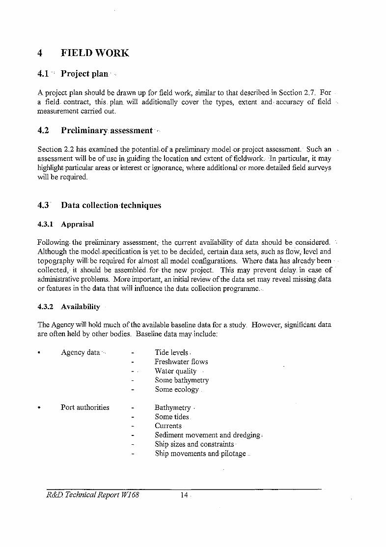
A project plan should be drawn up for field work, similar-to that described,in Section 2.7: For. a field. contract, this.. plan will additionally cover the. types, extent and<-accuracy of field measurement carried out.

4.2 Preliminary: assessment. s~

Section 2.2 has examined the potential.of a preliminary model-or. project assessment.. Such an assessment will- be of use in guiding the location and extent of fieldwork., In particular, it ,may highlight~~particular areas or interest or ignorance, where additional-or. more detailed field surveys will be required.

4.3.’ Data collection%echniques

4.3.1 Appraisal

Following. the preliminary assessment; the current -availability of data should be considered. ‘, Although the.model,specification is yet. to be decided, certain data sets, such as flow,- level and topography will.be required.for almost all model configurations. Where data-has already been collected,. it should be assembled for the new project. This may prevent delay in case of administrative problems. More important, an initial review of the data set may reveal missing data or features in the data that will influence the data collection programme. .

4.3.2 Availability

The Agency will hold much of the’available baseline data for a study. However, signifidant data are often held by other bodies. Baseline data may include:

. Agency data ... - Tide levels. Freshwater flows Water quality Some bathymetry Some ecology

Port authorities - Bathymetry I Some tides Currents Sediment movement and dredging-; Ship sizes and constraints Ship movements and, pilotage


. Fisheries data - From MAFF, sea fisheries consultative committees (SFCC) and fishermen Fish species and stocks Shellfish

. Local authorities - Particularly for uses

. Nature interests - From English Nature, RSPB, wildlife trusts Other ecology

. Industry Abstractions and returns.

. Research Universities. Research programmes such as LOIS (Land Ocean Interaction Study) and SABRJNA.

It is important to collect information about proposed developments and uses as well as the existing and historic conditions. Liaison will be needed with the planning authorities.

4.3.3 Collection - general

The accuracy of an estuarine model will depend largely on the quality of the data set used to build and calibrate the model It may have a greater effect on the model results than the software used or the design of the model itself The design of surveys is therefore a critical aspect of the modelling process.

The data collection techniques used by the industry are of known accuracy often greater than that needed for a model. Perhaps a more important aspect is the coverage of data. Data must .be collected in sufficient detail in critical areas such as:

. Model boundaries;

. Areas at the focus of a project, such as outfalls and navigation channels; and

. Areas that control the behaviour of the estuary, such as ebb and flood channels, sandbars and mudflats.

This section discusses the collection of data required for modelling studies.

4.3.4 Topographic data

The most basic items of data for an estuarine model are the basic topography (bathymetry) of the study area and the shape of the estuary’s coastline.


level.

Thus it must be possible to represent:

. the diurnal and weekly fluctuation of loads from a sewage treatment works;

. a synthesised sequence of river flows and concentrations;

. the sudden loading produced over a short period of.time corn a CSO; and

. the loading produced by a discharge controlled by tide-locked gates or tidal tanks.

These representations must be achieved in the context of the continual operation of the tidal forcing function at the seaward boundaries of the modelling-system and a wind forcing function over the water surface.

The contractor is also invited to offer a representation of the effects of waves of representative period, e.g. swells:

. as derived from the wind field stresses; and/or

. as propagated through the modelled area from prescribed boundary conditions, on mixing in the water column and re-suspension of sediments from the bed.

Such modelling could be carried out in a separate module and its output, in-terms of enhanced dispersion or raised :‘ bottom shear stresses, added to a given scenario to represent the effects of a storm.

[Warning: Creating this number of suitable input data files will be a substantial task for the user and Will result in a huge number of combinations which will require careful documentation.]

A.211 Output to be Generated

The modelling system must be capable of producing suitable@ots of the output from the hydrodynamic modelling.. These will include line plots of water surface height as function of time at a given point, line plots of water surface height as a function of position at a given time, colourxoded contour plots of water surface height Viewed in plan at given times, vector plots of water veldcity at given times, streak plots of the -movement of simulated floats or drogues. and- extended track plots showing the.long term movement of simulated floats or drognes. Where appropriate these plots should be reproducible in a time sequence.

The modelling.system must be capable of producing colour-coded contour plots of the concentration of water. quality parameters, viewed in plan. These should-be reproducible in a time sequence. The modelling system ‘. should be capable of producing line plots of concentration at a point as a function of time or at a time as a function of position along a chosen transect.

The modelling system should.be capable of producing ASCII files holding model output, for’further analysis by other programs. The modelling system should be capable’of producing summary statistics (such as mean, standard deviation; percentiles) concerning the concentrations of a particular parameter at a particular point. One important additional statistic-will be .the percentile measure of the number of, occasions when a particular parameter, such as faecal coliform concentration, exceeds a given level, such as the guideline value for bathing beaches. A similarly vital statistic would be a percentile measure. of the number .of occasions that DO concentration is less than some given value; thiswould be appropriate for assessing estuarine water quality with regard to migratory fish.

For those regions of water where there are significant variations of water quality with depth, the modelling system should be capable’of producing.colour-coded contour plots of the concentration of water quality parameters, viewed in elevation (on a cross-section).

The modelling system should be capable of producing plots of statistical .fimctions of concentrations, such as maximum, minimum, mean; standard deviation, percentiles either as contour plots or as line plots, in plan or in

R&D Technical Report- WI68 A9

Coverage

Due to the difiiculty in measuring tidal flows, rivers are measured upstream of the hydraulic tidal limit although with ultrasonic gauges it is technically possible to measure tidal flows. Estuaries like the Thames, Severn and Trent extend for many kilometres upstream from their mouths. Even if there is a gauging station near the tidal limit on the main river, there could be many side tributaries or areas of direct runoff that drain to the estuary downstream of the tidal limit on the main river. These tributaries may or may not be gauged. The term “coverage” refers to the extent to which freshwater inflows to an estuary are actually measured. Estimates of freshwater flows from ungauged areas will almost certainly be less accurate than measured runoff. There is no way of assessing the magnitude of the errors introduced into the estuary water balance. If there is a large ungauged area., coverage might be said to be “poor” and there will inevitably be more uncertainty attached to the reliability of results from any model of the estuary.

“Coverage” might also be used to refer to the completeness of a flow record. If the total volume of runoff over a year or season is the critical parameter, numerous or lengthy gaps in the flow might be said to reduce the data coverage and reliability.

Accuracy

There is a degree of uncertainty associated with even “measured” flows although this uncertainty is far less than that due to poor “coverage”. At a well-constructed and suitably-sited gauging station, flow might be expected to be measured to an accuracy, on average, of within 5%. However, this accuracy may well vary with different levels of flow. Where discharges are computed from a rating curve, flows will be less accurate or even ill-defined where the observed stage lies outside the range of the defined stage/discharge relationship (eg. at unusually low or high stages). In most cases, the accuracy of a flow record depends on:

. the accuracy and reliability of the source water level data; and

. how well the stage/discharge relationship has been derived from observed current meter measurements of discharge.

Nowadays, flow velocities can be measured directly (eg. by ultrasonic or electromagnetic gauges). In these cases the accuracy of a flow record will depend on the accuracy of the measured cross- section and the instrument calibration rather than on the stage/discharge relationship.

4.3.6 The measurement of tidal flows and levels

Tidal flow and level data will be required for:

l Boundary conditions for both calibration and simulation; and . Internal model measurements for calibration.


Seaward boundary conditions.may often be derived from existingtidal records and.known tidal- harmonics.: Calibration data will usually require the collection of a special set of data-for the study area, including:

. current meter. data;

. current direction data; and

. water level data.

The following approaches may be considered to collect portions of this data:

. Drogue tracking; l Ocean Surface Current-Radar (OSCR) .data, although care may be needed: with shallow

waters; and . Acoustic Doppler Current Profiler (ADCP) data.

Decisions to be made include:

. Duration of measurements - does the project need a series of snapshots, a tidal cycle, spring,and neap tides, or a prolonged collection period of weeks or months;

. Frequency of measurement - this could be as low as 15 minutes;

. Type of measurement-: can results be depth or width averaged,. or are profiles or traverses needed; and i

. Type of meters - for example propeller/ultrasonic current. meters. Appropriate instruments should- be chosen for- the expected range of result.

For all these measurements,*a Geographical Positioning, System (GPS) should be considered to locate the site. Although the positional accuracy should be related to the-needs of the study, a GPS may be the most efficient and economical approach.

4.3.7 The’measurement- of-water quality

The issues concerning-measurement ofwater quality are similar to those to be made for tidal flow and level. In addition:

. data may need to be collected to define.water. quality boundary,conditions in the model;:.

. calibration measurements may take the form of dye dispersion studies; bacterial spore dispersion studies; or load studies at outfalls and overflows.

collection techniques may include: bottle/sample’collectors; depth integrators; and probes.

R&D Technical Report WI 68 ,’ 18

Standard water quality parameters for measurement are:

Temperature; Salinity ; Total and faecal coliforms; Dissolved oxygen, biochemical and sediment oxygen demand; Ammoniacal and oxides of nitrogen; Turbidity (suspended solids); Phosphates; and Chlorophyll.

Salinity should always be measured as a conservative solute which can be cheaply and accurately measured in-situ. Additional parameters may need to be considered to meet the needs of a particular study. It should, however, be recognised that non-standard parameters may either be expensive to collect or require expensive non-standard laboratory procedures.

4.3.8 Morphological field work

The collection of sediment data to assess short term changes is a routine process, although a large scale data collection exercise will be an expensive exercise. It must also be remembered that the measurements of sediment flux collected may be of low accuracy and the actual flux may vary considerably between sites and depths. All data collected must be thoroughly checked and validated.

Long term morphological changes are less easy to quantify. Possible sources of data are:

. Historical data sets covering a period of morphological change, such as construction of a barrage;

. Routine data collection, such as for Shoreline Management Systems, ports and occasionally for major construction projects; and

. Research projects, such as LOIS, JoNuS and the like.

If no data is available in the estuary of interest, a programme may need to be designed. Such a programme should consider new data collection techniques such as:

. Remote sensing by satellite;

. Acoustic Doppler Current Profilers;

. Bed frames; and

. Remote bathymetric surveying,

Morphological field work is discussed in more detail in HR Wallingford’s recent report on Estuary Morphology and Processes (1996).


4.3.9 EcologiCal assessments

The main purpose(s) or objectives of the estuary model being undertaken will determine to a very. great degree-the inputs that are needed to make the results of the project meaningful ecologically. There has. b&en a wide range of estuary. models. Historically many estuarine models were developed for navigational (much work by ABP; Associated British Ports) or pollution control purposes such. as the -Thames Estuary model developed by. the Water- Pollution Research Laboratory (WPRL; now closed) tid.had little or no ecological input or output. In the last thirty years- a number of specialist studies of specific estuaries have been undertaken by ,research establishments that have attempted to model the whole estuary ecosystem;such as work on the Dutch polders by-DelR Laboratory, or by IMER (now. PML, Plymouth Marine Laboratories) on I theSevern estuary (Uncles, 1980):

There is therefore no generally applicable list as to what elements. of estuarine ecosystems should. be includedin a model study. IHowever as a guide a small number of the types of study are liSted in Table 4.1; below with a comment on the environmental. data that should be-considered.

Table-4.1 - ENVIRONMENTAL‘DATA NEEDED

Ref Reason for model. Environmental data need4 ; ,:

1 .,.;’ Flood defence Tidal, wind and morphological data

I I 2 Sediment movement/geomo@hology I As (1) plus sediment analysis data I

3 Navigation/water movement Wind, tidal and fluvial flows

4 Water quality/pollution control Tidal and fluvial flows, water quality and pollutant loads.

5 Primary production :,.- As (4) plus nutrient data, plant biomass, plant vital data &cluding grazing losses-

6 Secondary production As (5) plus animal.biomass, and appropriate zoological vital data

7 I I Fisheries As (5) ifecosystem approach is taken, or fishery statistics if. fishery analysis required

Omitholom I As (6) or (7), plus bird count records and flight path data I

Methods of collecting most of the ecological data sets are similar to standard methods that have been devised over the last century for simple routine enumeration or biomass evaluation of these components. These methods have been compiled in a number of convenient handbooks of the Estuarine and Coastal Sciences Association (ECSA), in documents prepared for the Joint Etiropean Estuaries Project (JEEP);! and innumerous.specialist works such as manuals by WPRL :’ and IMER including some recent NRA compilations.. The methods are not fixther described in . . this manual. 1

R&D ~Technical Report WI 68 20 ..

Such routine sampling methods may not be wholly adequate in all cases of ecoIogica1 modelling so that an ecologist should be available to advise upon the need to adopt special sampling measures. For example, in models of dockland areas of estuaries, the effects of filter feeding molluscs growing on vertical walls on phytoplankton mortality could require special sampling techniques. However, the most important requirement that ecological modelling introduces is the need for vital or life cycle data which is used by the model to simulate the effects of the components of the ecosystem on other parts of the ecosystem. Table 4.2, below, shows typical arrays of these vital data, many of which are rate dependant, are shown for selected ecosystem components.

Table 4.2 - VITAL ENVIRONMENTAL DATA

Organism or trophic level

Bacteria

Vital environmental data needed

Energy requirement: - heterotrophic = carbon - autotrophic = sulphate, ammonia

Specific need for nutrients per g biomass Respiratory demand for oxygen per g biomass Growth rate and temperature coefficient Settlement rate for loss to bed Natural mortality rate Rate of return of nutrients from decaying biomass

Phytoplankton Similar to those needed for bacteria, plus Specific growth rate for photosynthesis Specific light occlusion caused by cells Grazing losses Possible rate of release of soluble metabolites

Zooplankton Similar to those needed for phytoplankton, plus Ingestion rate for selected organisms _ Coefficient of conversion to biomass of ingestate Rate of reproduction

Other animals All similar to zooplankton, but: often with specific prey organisms mobile animals need to have a migration term between model segments and perhaps out of and into, the model boundaries on a seasonal basis


4.4 ‘. .. Data storage and transfer

Data storage and- transfer arrangements should:be designed to:

. Minimise therisk of data loss; and

. Store the data-in a form that is readily accessible to the subsequent users.

To ensure these aims:

. Survey contractors should be expected, wherever possible,.to use computer loggers and direct down loading of data;

. Survey specifications should-include agreed formats and transfer procedures to the project. office;-

. Backup and data security should follow similar procedures as defined for the modelling. itself;. and :

. Use of a Geographical Information System (GIS) should be considered for the .longer term storage-and presentation of data. Such a system may require and initial investment of time and money, but often has considerable mid- and long-term benefits.

4.5 Che‘ckixig and validation

4.5.1 Data set assessment

All data collected in the field should be checked and validated, as far as ispossible.::. All data are subject to error. This error will include:

. gross errors;

. minor errors; and

. natural .variability.

4.5.2 Data errors

Occasional inaccurate measurements or errors in the processing of raw data are present in many data sets. Gross errors can often be detected by screening and the suspect point may then be treated with caution. It is bad practice to completely ignore a suspect point as it is rarely possible I to prove that an unusual value is the result of an error and not a correct measurement of a rarely occurring event. These points should be retained in the data set, but treated as outliers; so that the effects of either including or excluding them can be considered. In addition to gross errors many data sets will Contain smaller data errors that cannot be detected by. screening, but may be subject to significant error. These errors.will show themselves as occasional scatter in model calibration and verification.

R&D Technical Report. WI 68 22

4.5.3 Natural variability

Another source of scatter in model calibration or verification is ‘natural variability’, when apparently similar conditions lead to different values that have been correctly measured. Natural variability is an intrinsic feature of natural systems that are only partially monitored, For example, in river flow measurements, similar water flows may be associated with different water levels because of unmeasured changes in river cross-section. As another example, water quality may vary in an apparently random manner because of unmeasured changes in run off or effluent flow and quality.

Natural variability causes data scatter whose range can only be defined by repeated measurement, or reduced by more extensive and intensive surveys. The amount of natural variability needs to be carefully considered in the design of data collection for model calibration and verification as all too easily a single data set can be used for model calibration with no knowledge of how the measured value relates to its natural variability.

4.5.4 Checking of data

Following collection, data checks carried out may include:

. screening for outliers;

. correlation with existing periods of record; and

. statistical analysis.

Statistical analysis will generally involve the plotting of a time series, or series of annual maxima or minima, using a selected statistical distribution. Visual inspection or further analysis of the plotted time series may reveal:

. autocorrelation and persistence - linear dependence amongst the data may cause certain types of loose patterns in the data. For example, there may be a series of wet or dry years in a flow record;

. seasonality - data may show seasonal trends, and need to be split into these seasons for analysis. Examples of this are fish migration and monthly water demands of a major city;

. nonstationarity or trend - data may show long term drift of the sample mean, due either to gradual change in the physical environment or measurement error. Topical examples of environmental changes are global warming and sea-level rise, but one is more likely to encounter changes due to creeping urbanisation;

. periodic&y and cycles - periodic&y is typified by water temperature, which fluctuates from day to night and from season to season on a regular daily or annual basis. Cycles are of long period, and often the period of record of data is too short for them to be detected. One of the best examples, albeit far from the UK estuarine situation, is the 30 year rain- drought cycle in sub-Saharan Africa. Water and irrigation schemes were designed when only wet cycle records were available. These schemes have proved unreliable as Africa has moved into the dry part of the cycle.

. extreme values - outliers are easily detected, but care must be taken whether to accept the value as part of the record, or omit it as an error or outside intervention. Correlation with


similar records from geographically adjacent areas may help analyse such outliers; and known or unknown. interventions - for example, construction of a dam, increased. abstraction or construction of a sewage treatment works will.cause a “step” in the time series data of flow and quality. .Only. part of the record may be useable for statistical analysis, or the whole record may need to be.“naturalised” into its pre-construction state..

Some errors will, however, only be revealed during model calibration. One simple.data error that is often missed is a datum shift or error. Consistent calibration errors in a model.maybe due to trends such as settlement of a gauge, or zero error on an instrument. Such an error is often hard to verify, but may otherwise inexplicable model problems.

4.5.5 Infilling of data

Most data records have some missing.data values. These may need to be infilled to obtain a. continuous record for the purpose of computational modelling.-. Methods that may be used for infilhng~ are:

. for single values - inspection.or averaged adjacent records; . for short sequences - correlation with other nearby records; and : .I . for long sequences - creation of artificial records by statistical generation.

If significant lengths of record need to be infilled, statistical checks of the resulting record should be carried out to ensure that the record is homogeneous.

R&D Technical R&port Wl68 24

5 COMPUTATIONAL MODELLING

5.1 Project plan -.

Chapter 2 discusses the possible use of a project plan under an organisation- wide quality assurance system such as BS.5750. Such a plan will direct the overall organisation. and technical execution of a project. However, .computational .modelling:projects will, in general, require a number of additional quality.procedures for the modelling aspects.

These procedures will usually include:

. guidance on selection of a! suitable model; . guidance on model .building, calibration and validation; and ; . good housekeeping techniques; such as reporting, backup and archiving.

Even for :organisations without .a full quality .assurance system,. there #are clear benefits from properly regulated modelling procedures. A number of systems have been set out, internally and; outside the Agency. The following sections draw on these references.

5.2 :. Model capabilities and limitations

5.2.1 Model types.

The term “computational model” has been taken in this report and to include:

. Statistical and empirical models; as well as

. Full hydrodynamic models.

5.2.2 Modelling physical .processes

At the present time, :it is computing power that restricts our ability to simulate time scale and ,. length scales that nature uses. For example, sediment entrainment is governed by small scale turbulence of the order of millimetres acting in an unsteady fashion over a period of seconds. To represent anything other than the entrainment of a single sediment particle requires computing... power beyond that of the most advanced mainframe. The same is true of boundary friction,. diffusion and dispersion of pollutants and freshwater mixing.

The pragmatic way around this problem at present is to integrate processes over much greater time and distance scales. Small scale turbulence will be averaged over a model element of 1OOm ” or more in space and over minutes, hours, tidal cycles or even 1onger:in time. The way in which such integration or averaging is carried out determines the type of model.developed. For example : a steady state model of an estuary may .well produce very acceptable results in terms of the seasonal variation of water quality or salinity, but it would not be very-good for determining the magnitude of processes within the tidal cycle. Similarly a one dimensional model integrates the processes over an entire cross-section of an estuary, whilst a two dimensional model integrates.

R&Ll Technical Report WI 68 25.

processes over.the vertical and over a set width of the estuary. Three dimensional models integrate processes over smaller parcels of water within the flow. With increasing complexity, the computing power required increases dramatically, and also the time required for a simulation. Many two dimensional models still only run at the same speed as the prototype. Three dimensional models can be significantly slower.

Hence there are still real practical problems with using a computational model, particularly if it is required to simulate a long period of time, such as a year or more to investigate seasonal trends. Model choice is therefore paramount in determining the success of a project.

Coupled with ihe choice of the type of model is the degree of accuracy required. This is dependent upon the final use and is determined not only by the scale of the model but also by the accuracy with which those processes are represented in the model. The physical laws built into the models are not precise. As discussed above the laws are derived to represent the integration of process occurring at much smaller scales. Furthermore some of those smaller scale processes, such as the adsbrption of metals on particles, or the resistance of moveable bed forms in a tidal flow are not tilly understood at present. Hence there are a wide range of approximations that have to be taken into account and tolerances applied to the model results.

5.2.3 lModelling low flows in UK estuaries

Saline balance

The pattern and limit of saline intrusion in tidal deltaic channels is determined by the balance between the rate of longitudinal mixing causing the landward movement of dissolved salt and the net seaward movement induced by a fresh water discharge. The rate of longitudinal mixing is governed by the strength of the tidal velocities, shape of the channel cross-section and by gravitational circulations induced by longitudinal density (salinity) gradients. The 1D cross- sectionally averaged rate of longitudinal mixing may be quantified in terms of an effective coefficient of longitudinal dispersions, D, (m2/s). As yet, this coefficient can only be quantified using relatively crude empirical relationships which have to be calibrated for each estuary. This means that for a 1D model to be accurate at low flows they must be included in the calibration tests.

Gravitational circulation

One of the most important aspects of the hydraulics of the deeper seaward reaches of many UK estuaries is-the longitudinal gravitational circulation that is driven by the longitudinal density gradients within the estuary. The magnitude of the net longitudinal pressure gradient, dp/dx, at a depth, z, which causes the gravitational circulation is a function of the slope of the mean tide level, dq,,/dx, and the vertical variation in the tide-averaged longitudinal density gradient, dp/dx, as follows:


Where pS is the density of surface water (kg/me)- g is the acceleration of gravity (9.8 1 m/s2)

The strength of the gravitational circulation varies directly with the magnitude of the product of. the depth and the longitudinal density gradient. .It is reduced by vertical mixing, whichis usually heavily damped in stratified flows; and by energy dissipation at the bed, which is increased bythe occurrence-of high tidal velocities in the:lower layers. The presence of a longitudinal. density gradient within. arrestuary causes the mean-tide levels to rise in a landward direction. The net landtiard pressure gradient and the net.landward residual flow disappear at a ‘null point? in the estuary where the two terms on the right hand side of the above equation cancel each other out.

Stratification and 2-DV models

The pattern ofthe gravitational circulation will vary according to the degree of stratification, but.. it is not dependent on the existence of vertical density stratification. Many relative deep.,estuaries with weak or negligible’.‘vertical, stratification have strong. gravitational circulations. The longitudinal density gradients-tend,to distort the shape of the velocity profile on the flood and ebb i’. phases of the tide and thereby induce a net landward longitudinal movement of water in the bed I layers seaward of the .‘null point’. where ,a turbidity, maximum usually occurs. There is .a corresponding net seawa.rd.flow of water in the surface layers of the estuary giving-rise to a two-. layer circulation,- which controls the water,quality in ,many.UK estuaries. The effect is strongest in deep sluggish estuaries and weakest in shallow estuaries with. strong tidal currents. It can only be modelled by using a layered 2D in-the-vertical model.

The predictive capability of layered width-averaged models of deeper estuaries (ie the Tyne or : Itchen) depends largely on the- method..of simulating the effect of stratification on vertical .: turbulent exchange. This should be a well formulated. universal function with well defined ‘. coefficients that do not have-to be adjusted for each estuary. A less important longitudinal dispersion coefficient incorporates the effects of lateral variations in identity and flow velocity.

3-D models

Full three dimensional models have so far, only been used usually to simulate the seaward reaches of the larger UK-estuaries. To date, it has not, been economic to use 3D.models to-simulate the fine details of all the bends etc in a small estuary. The fine grid,required to do this gives rise to impartially long run times. There-is usually-little benefit in using 3;5 relatively coarse cells to . simulate variations across an estuary, because they would not be able to resolve the detail the secondary flows in the cross-section. However, .,3D models do not necessarily need more calibration data-than simpler .models.

R&D Technical Report WI 68 . . 27

5.2.4 Model types and their limitations

Numerical models of hydrodynamics, water quality and the like for estuaries are now so widely used that a diverse range of models types and applications have come into being. These may be divided into three main groups of models:

. Statistical models;

. Empirical or ‘black box’ models;

. Simplified hydrodynamic models, such as water quality ‘box’ and plume models;

. Full hydrodynamic models, with an accurate representation of the hydrodynamic equations, often with additional modules to simulate water quality and the like.

Figure 1.2 has shown the wide range of model types available and the applications to which they are typically applied. Hydrodynamic models may further be defined as listed below (based on Cooper and Dearnaley, 1996). Flow, quality, sediment and ecological modelling may require:

. fully 3D flow models;

. hydrostatic pressure 3D flow models (3DH);

. Boussinesq 2DH models;

. hydrostatic pressure 2DH models;

. 2D 2 layer models (2D2L);

. hydrostatic 2DV models (horizontal 1D models with vertical variation modelled); and

. 1D models.

Quality and sediment modelling may also use plume models.

Sediment modelling may further require point models and particle (Lagrangain) models.

Despite the trend towards single program suites with a wide range of modules, it remains’ difficult to build a model that can be used for a wide range of purposes, such as ‘flood defence, water quality, morphology and wave modelling. There are significant differences in:

. Scale and detail of the models; and

. Time steps and scales of the processes modelled.

However, it may be possible to use base topographical data, flow and level data, and. other general models between applications.

All model types have inherent limitations, and should not be applied outside the applications for which they were designed. The strengths and limitations of the model types available are set out in Figure 5.1.


Figure 5.-l - COMPUTATIONAL MODELS - STRENGTHS AND LIMITATIONS

Model type. ;,., Strengths

Full 3D !’ i) Full and accurate modelling of transverse and vertical variations of parameters in estuary..,

Limitations .

1) Limited application to date to estuary and coastal applications. 2) Free surface treatment complex. 3) Extensive data collection required for calibration. 4) Expensive to run.

Hydrostatic 3D 1) Good modelling of transverse and vertical variations of parameters in estuary. 2) Wider use to date than full 3D approach,.

1) With some grid layouts, less accurate in modelling of density effects than full 3D models. 2j Extensive data collection required for calibration. 3) Expensive to run.

Hydrostatic 2D . . 1) Established modelling approach. :l) Vertical profiles due to stratification 2) Model can be built from similar data &t represented. set to 1D model. 2) Care needed at model limits to 3) Calibration data requirements not e&ablish realistic boundary conditions. excessive. 4) Will give reasonable representation i of most modelled uses and processes. .’

2D 2 layer

Hydrostatic 2DW

1) Allows simulation of stratified flow without using full 3D model.

1) Allows simulation of stratified estuary without complexity of full 3D model. 2) Uses similar data set to 1D model.

1 j Care needed to establish realistic layers and flows between layers.

1) Transverse variations across estuary not represented.

I 1D 1) Simple and cheap to set up. 1) Transverse variations across estuary

2) Robust in operation not represented. 3) Existing model may exist. 2) Vertical profiles due to stratification

not represented:

Phmej point &- particle

1) Gives accurate representation of surface and 3D plumes not truly represented by 2D models. 2). Simple to use.

1) May require float tracking or 2D modelling to establish flow paths.

Statistical 1) Often quick and inexpensive to carry out analysis. 2) Analysis closely reflects recorded data.

1) May not be easy to simulate changes in the system. 2) Not suited to detailed or localised modelling studies. :

For examples of model.types, see Figure.5.5.

R&D Technical Report..W’l&J 29

5.3 Selection of software

5.3.1 Model types for estuary uses

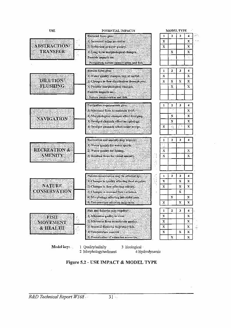
As indicated in Section 2.3, the choice of model is in some ways pragmatic, based on availability, budget and experience of use. However, at the start of a project a the best model type for that application should be selected. Figures 5.2 to 5.5 present a series of tables that can be used to assist in the model selection for a range of. particular uses. These figures indicate what type of model ideally to use for different types of estuaries and different estuary uses:

. Figure 5.2 shows the model types that may be needed to study a particular estuarine use;

. Figure 5.3 and 5.4 show the range of applications that may be available for any model type; and

. Figure 5.5 gives a decision matrix leading from estuary classification to model type.

5.3.2 Other factors

However, the choice of a software package also should be based on a range of technical and practical factors, such as:

. technical suitability of software for project;

. organisation policy on standardised software;

. availability of software in-house;

. cost and project budget;

. staff experience and/or training.

In many cases, a degree of compromise may be needed in selecting software for a project. A small project may not justify purchase of a complex modelling system; less but sufficiently accurate results may be obtained from a simpler package already existing in-house. Conversely, it may be efficient to use a complex package on a simple task if it is already available and there is an experienced user base.

If a new software package is to be purchased two groups of features need to be assessed:

. technical capabilities, or the algorithms within the software; and

. user features, such as menus and presentation graphics.

Fortunately, most new commercial sofiware contains both established and reliable solution techniques and a high degree of user-friendliness and quality of output. However, the visual benefits of the software should not be put before its technical suitability for a project.

MODEL.TYPE

X- X l!!Bzl x X

X X

Model key:. 1 Quality/salinity 3 Ecological 2 Morphology/sediment 4 Hydrodynamic

Figure 5.2‘- USE IMPACT & MODEL TYPE

I Ix 1 X

R&D Technical R&port. WI 68 .- 31 :.

....... .:.:. ........ .:. ';- ... .:.: ... .y.> ............. . .. ............. . .:.:. ..................................... ...................................................... . .. :.;:. ...............................

..... ..::::.:.:.:::.:::.:::::.:::.‘::::I:: .: i~~~~~~~~~~~~~~~~~~.~~~~~ %jii ~~~;.c;; i $i?ii?;;j~ %;;gg;?i.j; i; ;i;;%z.;i ;:;; ii iilz.i :irc .. .. ........ ...... ;.ii~,liiiii-ii::-i~.l~i;;;;iii--::.::.i~ %~~.&Z&j~~~~~,;jj iii~~~~.-;li.~~~~~~~~~~~~~ :~::.-::.:.:‘:.::::‘:.:::::.:j::.:...:::.:.:.:.::: eco .............. g! .., .............................. ._ ................. ..................................... .,.,_. .. . . ..... _:_. ..... “““-.,.-“““‘“-.“.‘:‘::)‘: . .... . . ............. . ................... ............ . ..... .:. -.-.‘.\‘.l\::~::.:~:.: ..~..................~.........~~~.~~...~ ......... ........ . ... ::.:::.:.:::..:.: .: .... >_ .t::.:.:::.:.:. ..... . ... :..i .:.: ........... . . :i ... .:. .. . ....... :‘; .:.: ....... .: ... 1-z. ........ ~-.:.~.~.:.~.:......-...~ ....... :..:::::.:::::.::.:;::::.:::.:::::.::.::..:::.:::::::::.::::::.:::::.:.::::.:.:::.:.:::::.~.::.:.:::::.::.:.~~~~:~: ~ :::.:: .:. I::.:j);jl:.:.wj:.:;: .:;::::.:.:,

. . _. .‘.“.....> ,___ . . _.:._: . ...::> ,::.:: ::.: :.:::

-j::::::::i:.:::.ij,::.:.~..~.~.~.~.~.~.~.~.~~.~:::.:.:.:.~.~:.~.::::.::~: ‘;‘~ii~i~~DRO~,~~~uc~~ ;;.;:(:f;: :.-i:,i)3’i::::i3i:.i~~~~~~iiii.iiii’ii-iii’iiiii

i. i. :. i . . .._ :. ” . . . . . : ../.,. ..:_ . . . .._ _ . . . _. .:._ .: _.._ ii... i.. . . . .._ . . . . . . . . . . . . . . . . . . . -- . . . . . . . . . . . . . . . . . . .../.. :........ . . . . . . . . . . .

.:.::.:::.y.:-::::.: .:::::. j::::::::::,;:.::.:,:: ::.:: ::::.::.\::::::,-:.:::.:‘:::: z:::.:.:: .:.:::.:::::::.:. :::.:.::::::j:.:.:,::.::;:,:,:.:.:::::::.::~:,::.:::.:::::.:.:::.:.::.:::.~:::.::::::.~:.:.:.::::~::::.:.::::.:~:.::.:::::.:.:::::::::::::.:.

Figure 5.3 - COMPUTATIONAL MODEL APPLICATIONS


Model, Application Appropriate type-.

Flow 1) 1 or 2D models usually .adequate 2) Floods 3) Storm surge 4) Sea level rise 5) Deltas 6) Large area.model & density-variations 7) Flow in bends and tidal eddies 8). Intakes (detailed model) 9) Flow over trench or channel

lD/2DH 2DH .::,’ 2DH.

Looped ,lD 3DH. 3D’.,. 3D- .I 3D ,.

1) :,-Travel distance into estuary. 1D 2) Travel distance into estuary, stratified. 2DV ,. 3) Distribution,across estuary. I 2D

“” 4) Distribution across estuary, stratified.. :.3D or 2D2L 5) Long-term quality models. ::. 2DH or.

coarse 3D 6) Plumes. 2DH.plus

plume or 3D 7) Cooling water. 3D

Sediment 1) lD,models rarely appropriate. 2) Sediment movement due to engineering works. 3) Siltation/flushing of harbour basin. 4) .Dredging and resuspension of ‘. sediment.-- 5) ‘. Long term morphology.

2DH or 2D2L

3D ;:. Plume ...

2jJJ-J :I.

Adapted-from Cooper and Dearnaley (1996)

Figure 5.4 - MODEL APPLICATIONS AND APPROPRIATE TYPES

R&D Technical R&port WI68 33

4 No I

Ye6

(Available programs

Hydrostatic 3-D TELEMACBD TltW;3D

Tl%!ET ADCIRC

Wailable programs

TELEMACPD TlDfR:sL;2D

MIKE 21 DIVAST

In-house programs

Available programs

TIDk;ky’DV

Figure 5.5 - MODEL TYPE SELECTION

lvailable programs

ISIS MIKE 11

Other in-house progrmams


5.3.3 Validation of software .

IS0 -49003 defines validation as the evaluation of software for compliance with specified requirements. It is rarely possible to carry out validation of a computational modelling program. due to the complexity of the software. For some programs, a “validation document” may be available. Otherwise, independent bench marking reviews, such as those recently carried out for I the Agency may be preferred (Cooper, 1996). If no other.information is available, reliance may have to -be put on the software’s reputation within the water industry, !or the reputation of the software company.

5.4 Cliange control

5.4.1 --Definition- .

Change control is an important-feature of all quality:assurance systems. For modelling projects, change control implies the recording of all changes to the input conditions to any phase of work or activity. -These records should,be part of a procedure that creates an audit-trail; in addition, all staff ,who are affected by the changes should be informed of them.

5.4.2 Change control of modellin’g work

Typical change within a modelling project could be:

. revised, or more often more detailed survey data;

. correction to errors of recorded flow or level data;

. modifications to the configuration of a model due to increased understanding of the processes involved.

For many modelliig projects,, only a small number of people are involved in the actual. modelling work. In:.this case, change control may-be exercised using.the project-run- log, described in Section 5.6.1, below. Any significant. change should .be clearly marked in the log.,,

For larger projects, the modelling director may issue a memo or change note detailing the changes and requiring, staff to sign ofI the memo when they -have taken action to. assess the impact of the change on their work.

5.4.3 .. Change control of software

The majority of modelling projects at this.time use commercially developed software. Change control of software is therefore-not.often an issue. If, however, commercial software is upgraded or a new release installed, during ,a projectj the new software should,be validated against the previously used version. Experience has shown that small numerical differences do on occasion occur .with such upgrades. The new software should be tested on typical sets of data from-the project, to check consistency.

R&D ,Technical Report -WI68 35

If the project does require the writing or modification of software, such writing should ideally follow one of the industry standard specifications. If one of these specifications is not used, a detailed specification of the programming work should still be followed. If software changes are made during the course of a project, such changes should be tested and validated both on project data and data independent of the project.

5.5 Building, calibration and validation

5.5.1 Building

Following project definition and data collection, building the model should be a straightforward process. It is, however, important that:

. construction is carried out in a logical and well recorded manner. Records. should be kept of all data used, and modifications made to the data in the course of building. This will allow future review of the model during the project; and

l the model discretisation is reviewed during construction. Modifications to the original model design may be necessary in the light of data collection.

5.5.2 Calibration

Calibration points will have been defined before the data collection exercise. These points and the data to be collected will be dependent on:

. the accuracy required of the model and the important model areas where the highest accuracy is needed;

. the range of calibration conditions, such as seasonal data, spring and neap tides.

Model parameters should be chosen with care. In particular:

. parameters should lie within published ranges. Data collected showing parameters outside these ranges should be carefully reviewed, since errors in data collection are probable rather than the usual physical limits of a parameter been extended.

. automatic calibration of models by the software should be viewed with caution. Again, physically realistic parameters must be chosen.

Procedures should be selected to assess the goodness of fit of the calibrated points. These will include assessments of maximum, minimum and average values, and perhaps root mean squared errors between recorded and modelled values.


It should be accepted that there will always be differences between the calibrated model and the recorded values. Models become increasingly difficult to calibrate with.increasing dimensionality. It. is important. that model calibration reports draw attention to both areas of good and poor calibration,. and explain the areas of poor fit. It is particularly important that poor- fits are. explained;:rather than the model “forced” to a fit, since:

.

.

5.5.3

Although such forcing may: be .corrected during validation, it is .also -possible that calibration and validation by similar recorded conditions may give acceptable results.. However, the model may not-be fit for purpose for simulation of a more extreme event;. and Hiding a poor fit may be misleading for future users of the model, especiallywhere the fit is later found to be due to data errors - perhaps an inaccurate flow or level gauge - rather than.a fault with the model..

Validation

The expressions “verification” and -“validation” have both been used for the proving. of .a computational model.. Verification implies that the model is shown to be.true to life. Although ” this is necessary, it is also essential that the model is validated - that is fit for purpose and-meeting its performance objectives.

Validation should be carried out usingTan independent data set. -It may also be possible to use different types of data measurement from those used in .calibration - for example float tracks rather than current meters. No model parameters should bechanged between the calibration and validation tests.

5.6 Run referencing and archiving ...

5.6.1. Runsreferencing ..

The user should allocate a serial number.to each ‘production’ run that is undertaken.. Production runs are those that form part of the calibration, validation, scenario testing and design process. No record need be kept of test runs, say, whilst. constructing a model and obtaining an error free run, although this may be useful. ‘.

The runs shall be recorded on a log sheet. Use of a standard log sheet. is to be preferred; an example is included as Figure 5.6. These records should be sufficient to allow another person to repeat the runs .without reference to the original user. The run number should be used-for cross- referencing between input/output listings and other.related calculations or documentation. :

R&D TechnicalReport WI68 37

Figure 5.6 - TYPICAL RUN LOG SHEET


5.6.2 Run-archiving

Regular.backup of project-files should be an established discipline for all computer users; it is surprising, though, how often this essential.action.is omitted by.the user and work is lost. It is : therefore worthwhile defining a backup-policy for all modelling projects. This will usually follow one of the following forms:

. For organisations with-networked computers and .a regular central backup facility, all project files should be.held on media-that is regularly backed up;- This may be-a central server, or a specified area of the user’s own PC.

. Some backup-systems require data to be copied from a local PC to an area on-the server.. A procedure-should be set up for project files to be regularly copied to this area.

. For a stand-alone computer system, a project specific backup ,procedure should -be developed. The frequency of backup should, reflect the magnitude ,and intensity; of working on a project. For some projects, weekly backup could be acceptable; for others . . a daily, save will be essential.. In all cases, a full backup should be retained at monthly intervals. This both allows the recovery of historic project data during the course of the project, and introduces new recording media into,the save-cycle.

Project backups,do-not require .the level-of documentation required for archiving. ‘It may be assumed:that the backup is only used to recover lost or corrupted files, and that the user will be . . able to identify the required files from his run log and: other working notes.

Full archiving will generally occur at the end of a project, or a major stage of the-project. The user should ensure that sufficient records are kept of any computer generated calculations so that : the method and, sequence of the modelling study or- design.can be clearly seen by others without . neediig.to refer to the originaluser. .All paper and digital media records should be clearly ,labelled and indexed.,

In general, a mixture of paper copy and digital media should be archived. The balance between these mediawill depend on the nature of the model software,, and the extent to which it can output its own maps; diagrams and the like. However, sufficient paper records should be kept to enable a fi.tture user to gain a reasonable understanding of the model from-these records before accessing the ,digital data. The paper archive, should- hold: ‘:

a copy of the modelling report; I details of the.model schematisation; i details of survey, flow and other data used for-model construction; details of model parameters; details of the calibration and validation; a copy of the run log sheets; typical input and,. whereypossible, output files; and ; a complete index of computer files for the model.


Ideally, much of the above information can be included in the modelling report.

In many complex modelling programs, particularly the 2-D models used in estuarine modelling, it is impracticable to retain hard copies of model input and output, either due to the output not being held in an ASCII file, or due to its size. In this case, all data should be archived on digital media, but should be cross-referenced to the paper records.

A degree of judgement should be exercised as to the extent of model data to be retained. Experience has shown that it is often more difficult to restart a project aRer a long interval from extensive archived model input files, than from a few strategically selected files. The aim should be to archive sufficient files to allow the new user to reproduce the progression of production runs recorded on the run log sheet.

Duplicate copies of archived digital media should be retained at separate locations, preferably in separate buildings to guard against:

. deterioration of the digital media; and

. disaster such as fire.

On completion of a modelling project, and when all paper and digital records are archived, any copies of the project digital data stored on ‘active’ computer systems should be deleted.

5.7 Reporting

5.7.1 Approach to reporting

The object of reporting is to provide a permanent record of the modelling work. It should include:

. the reasons why a modelling study has been carried out;

. a detailed description of the work;

. the results;

. the Way the model results relate to the overall study objectives; and

. the conclusions.

The computational modelling report of a project forms the primary record of the work carried out. A comprehensive modelling report is essential for the smooth handover or transfer of a completed model. It also forms a starting place for any additional work carried out in the future. It, is important that the report contains:

R&D Tekhtiical Report WI 68 40

. a detailed description of the modelling process and assumptions;

. a discussion on the uncertainty of the model predictions due to uncertainty. of model parameters, input data and inherent limitations of the model; and

. a balanced view of the modelling,. including discussion of problems encountered in the modelling process, shortcomings, in calibration and data, and the likely accuracy of.the results.

57.2 Contents

It is preferable‘to establish a report structure at.an early stage of a project. Elements of the report ,I can then be completed as the.work is carried out.. This is particularly helpful in areas such as calibration of the model and also scenarioitesting, where despite the run logs and other records kept, it is easy to forget details of the work. The report should include the following:

.

Summary Background; including description of the problem and the study area Methodolo,T, including choice and limitations of modelling technique Modelling:

Data collection Model design Model building;.including model.parameters Model calibration and validation Scenario testing/design

Discussion of results Applied to project objectives Applied to,other related studies (eg.environmental)

Conclusions and recommendations References Appendices

Detailed- calibration report (if.too long for main text) Index of model files

The text should be supported by suitable tables :and figures as appropriate.

5.8. Transfer arrangements

As discussed above, the transfer of a model to another user, either internally or from consultant to client, is greatly simplified by a comprehensive modelling report and careful archiving of the model- data. : It is recommended that when a modelling contract. is let, these reporting and archiving requirements are specified in the modelling terms of reference. Such an arrangement. benefits both client and consultant, since the former .gets what they want .and the latter knows. what is expected..

R&D Technical Report. WI 68 41

6- STATISTICAL.APPROACHES .’

6.1 Environmetrks

The--discipline of environmetrics is defined as the development and application, of statistical methodologies and techniques in environmental sciences. It has grown largely from the traditional application of statistics to hydrological and~water quality data. These methods are familiar to most practising engineers-and estuary managers, and include:

. statistical distributions;

. informative graphical techniques;

. regression analysis; and

. nonparametric tests.

However,- a range of new techniques have been developed for the analysis oftime series data. These can only be dealt with briefly in this manual,: but the reader is referred to references such as Hipel(1994) for a full treatment of the subject.

6.2 Stochastic techniques

The two overall categories into:which mathematical models can be placed are:

. deterministic - where a model can be employed for determining exactly all the states of a system. Most computer modelling systems are deterministic; and

. stochastic - where -the state of a system .can only be described using.:probabilistic statements and hence its precise value cannot be known.

Most natural phenomena occurring in environmental systems behave in random or,probabilistic- ways. Hence, stochastic techniques will always have a significant part to play in estuarine or other water related studies, even if only providing- boundary. conditions to a computer. model.

Figure 6.1 shows a further classification of stochastic models; according to. their time- and space state.- Most stochastic approaches suitable for environmental engineering .fall into the time series model group: ,The reason for this is-that in order to record, the behaviour, of, or to understand a natural system, scientists or. engineers,take measurements at discrete intervals over time;

Time series models are available for data analysis, forecasting, simulating systems and decision making. Of these models, perhaps the.most relevant to the kind of impact analyses carried out during estuarine studies is the intewention.model,


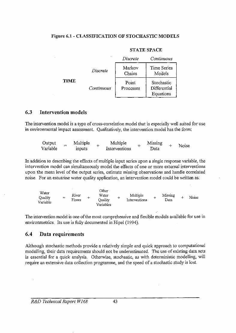
Figure 6.1- CLASSIFICATION OF STOCHASTIC MODELS

TIME

STATE SPACE

Discrete Continuom

Discrete Markov Chains

Time Series Models

6.3 Intervention models

The intervention model is a type of cross-correlation model that is especially well suited for use in environmental impact assessment. Qualitatively, the intervention model has the form:

output Variable =

Multiple + Multiple + Missing inputs Interventions Data + Noise

In addition to describing the effects of multiple input series upon a single response variable, the intervention model can simultaneously model the effects of one or more external interventions upon the mean level of the output series, estimate missing observations and handle correlated noise. For an estuarine water quality application, an intervention model could be written as:

Water Water Quality = g:‘s + Quality = g:‘s + Variable Variable

Other Other Water Water Multiple Multiple Missing Missing + Noise + Noise Quality + Interventions + Quality + Interventions + Data Data

Variables Variables

The intervention model is one of the most comprehensive and flexible models available for use in environmetrics. Its use is fully documented in Hipel(l994).

6.4 Data requirements

Although stochastic methods provide a relatively simple and quick approach to computational modelling, their data requirements should not be underestimated. The use of existing data sets is essential for a quick analysis. Otherwise, stochastic, as with deterministic modelling, will require an extensive data collection programme, and the speed of a stochastic study is lost.


6.5 Data quality

Aside from-statistical modelling of estuaries in its own right, statistical approaches will probably be used to derive inflow sequences to a hydrodynamic model. Further, statistical approaches can be used to assess the quality of data. Any assessment of the quality of-data used-in a mathematical model of an estuary depends-on answers to the-following questions:

1. 2. 3. 4.

How complete is the coverage of data on. freshwater flows into the estuary? How accurately are gauged flows measured? How accurately, can the ungauged portion of inflows be estimated? How sensitive is the process being ,modeIled (eg. sedimentation, waterquality/salinity, biological response) to the level of freshwater inflows and the fresh/salt water balance?

The answer to these questions should guide the investigator as to whether computational modelling. is a viable option to provide -the required answers and if so, as .to the degree of confidence that should ,be placed on the answers;

6.6 Quality control

The. following procedure is a list of checks that the modeller/analyst should .go through to assess/verify the quality of data being used. to represent freshwater-flows to an estuary.

Coverage

1. Estimate the proportion of the-land area contributing freshwater flows to the estuary that- is gauged by. flow -monitoring stations.

2. Assess how accurately flows from ungauged areas can be estimated.

3. Consider whether there might:be any significant groundwater flows to the estuary via:.. springs in its bed and/or banks in addition to surface water flows.. (Look at the.: hydraulic gradient indicated by groundwater contours).

Accuracy. _- rapid/gross checks

4. Consider the gross annual water balance of the gauged catchment(s) in terms of depth in millimetres:

precipitation - runoff = catchment losses

Long:term mean annual precipitation can be read from, an isohyetal map such as that produced by the Meteorological Office forthe 1941-70 standard period.-

In the UK, catchment losses generally fall. in the range 300 mm to 600 mm withthe. majority of values lying between 350 and 500. Losses can lie outside this range but .’

R&D Technical Report WI 68 44 ..

are less likely to be genuine values. Such values indicate a possible problem either with the estimate of catchment precipitation or with the flows themselves and should be checked in detail.

5. Where flow data are stored in computer files, rapid checks can be carried out by plotting daily or monthly flow hydrographs for the available period of record. Daily flow hydrographs in particular can often allow suspect periods of record to be quickly identified from the range of flows and from the pattern of floods and recession curves.

6. Where data are available for more than one location on the same or adjacent rivers, comparison of flow hydrographs should reveal similar patterns of flow (eg. approximate coincidence of peaks and troughs) if the data are consistent and reliable.

7. If spot measurements of discharge are available, plotting these in superimposition on the daily flow hydrograph can indicate if there is a systemmatic bias in the computation of a flow record (eg. a rating curve that consistently under- or over-estimates discharge for a given water level).

Accuracy - detailed checks

8. If both water level and discharge data are stored on computer file, a plot of one against the other will show:

a) the accuracy and consistency of the flow computation b) the stage/discharge relationships that have been used to compute flow

9. If a stage/discharge relationship has been used to compute the flow record, discharge computed from current meter measurements can be plotted against contemporaneous readings of gauge-height to check the validity of the relationship.

6.7 Conclusions

In recent years, the deterministic computer model has become the focus of modelling studies. However, advances is statistical approaches have also been made. The statistical model remains a powerful, and often simple, tool to facilitate data analysis and decision making.. However, the extent of data collection required for a stochastic approach may be little different than that for a deterministic model.

The most effective modelling approach is perhaps one where stochastic and deterministic methods are used side by side. The stochastic model is used to prepare and check time series data sets as input to the deterministic model. The deterministic model is used for local and detailed examination of a problem. Its results are then analysed stochastically for reliability and significance. Such as approach is used today in most modelling studies. However, a fuller use of stochastic models could be used for data preparation and analysis.

RcW Technical Report WI68 45

7 CONTINUED USE OF MODEL

7.1 General

It is oRen necessary for a computation model to be used on occasion after a project, or a stage of a project, is completed. The model may be.used:

. to produce additional runs with-minor data variations; . to progress a design, say,.from feasibility to detailed design; or . to aid a new study in the same estuary.

In addition, the model may be transferred from client to consultant,. or vice versa, or between staff. in either organisation.

In all cases, particular. care must be taken to-ensure that the new users understand the model; its purpose and its,limitations. If the mode1.ha.s been documented and archived correctly, this process will be simplified. However, the project manager should allow adequate time for the new user to:

. read. documentation and, if available, calculations and working files for the model;

. carry out a series of test runs to establish for themselves the stability and performance of the model;

. contact, if possible,- the last user to discuss the construction and running.of the model. There .are often undocumented details in the.model construction, that may not. appear significant to the original constructor, that later users find difficult to understand.

The procedures followed in running and-reporting on the:model.should:be-as described in the. preceding sections. The following sections-highlight..particular points in the continuing use of a model

7.2 Run refekencitig, and archiving :

Run -referencing may follow the same procedures as for the original.use of the.model;, or those generally adopted by the new users. It is, however, prudent.to:.

. maintain,a consistent set of file names between users;. and

. never to re-use file names.

R&D Technical Report WI68 46.

7.3 Change control

Similarly, all changes to the model should be documented. However, particular care should be taken by the new user to ensure that they understand the overall impact of the change on the

.model, and that the validity of the model is not diminished by these changes.

7.4 Re-validation using additional data sets

If a model is being re-used after some time, it is likely that additional data are available for additional calibration and re-validation of the model. Wherever possible, such re-validation should be carried out.

7.5 Risks of inappropriate application of model

When a model is re-used, there is always a finite risk that it is used inappropriately. This may be ’ due to:

. Lack of understanding of the model by the new user;

. Use of the model for parameter ranges for which it was not designed; or

. Use.of the model for purposes for which it was not designed.

As noted above, lack of understanding of the new user can best be overcome by good documentation and allowing time for the user to familiarise themselves with the model.

Change of parameters could, for example, be use of a flood flow model for simulating low flows in a water resources study. A well calibrated model for flood flow could be 100% out in predicting recession and low flows.

Change of purpose could, for example, be the use of a flood model for water quality or morphological studies. The survey requirements for these studies may vary. Flood models will require more detailed knowledge of out of bank areas, whilst morphological models may require more detailed survey of the main channels and areas of known sediment movement. Time scales of the model run may change, too, from hours to days to years.

Despite the above risks, much base topographical, flow and level data in a model will be use&l for all uses. The risk of inappropriate use of the model can be minimised by:

. re-validation of the model for its new parameters or purpose;

. additional survey in critical portions of the model; and

. use of sensitivity analyses to assess potential errors.

R&D Technic& Report WI 68 47

8’ ESTUARINE MODELLING AND DATA COLLECTION STRATEGY

8.1.,‘.-i Modelling strategy

The R&D.Teclmical-Report (W113) accompanying&is manual sets out a management and technical approach to freshwater flow need studies. The approach is designed to make best use of existing and emergipg technology, .using concepts-from risk assessment. This approach is~summarised below:

Review existing reports and check data availability.

1 @‘AGE 13 1

-1

Classify estuary type and select estuary reaches.

Classify estuary type and select estuary reaches.

For low impact uses and processes, use simple analysis methods.

jjfappropriate, carry out preliminary analysis.

Review design standards and set out study standards.

Complete risk matrix, seasonal variations and risk assessment.

For each use and reach, select appropriate analysis method.

Rationalise and optimise model design.

Cost modelling studies:

Consider joint funding of modelling, or simpler models.

Set up modelling contracts.

Carry out or manage modelling studies. .‘.

Analyse model results and set MRF: ..

1 Post-project appraisal.

8.2 Data collection strategy

The management approach stresses the need for a coherent data management policy. At present data collected by the Agency may not always be easily .retrievable forfuture studies. A poljcy is needed that:

R# ‘Technical Report., WI68

. Encourages project teams to archive data; and

. Creates a simple, yet comprehensive, database to allow retrieval of this data.

The range of data requirements for modelling projects is defined in the tables in this Chapter. Existing data will normally be available from a range of sources, and will include:

. baseline data, such as topographic survey and mapping;

. routine data collection and sampling; and

. project specific data.

Although some Agency regions aim to collect data by routine sampling that will be adequate for future modelling needs, most studies will need to apply data in the following way:

.

.

.

baseline data can be used for basic model construction; additional survey will be needed for localised topographic detail and calibration for the area of interest; and sampling data and earlier studies can be used for secondary calibration and validation.

8.3 Sets of models and supporting data

8.3.1 Hydrodynamics

The hydrodynamic model itself may be of marginal use for water resources studies, except perhaps in navigation studies.

However, a hydrodynamic base model often forms the basis of other, for example quality, studies, the results from one forming an input to the second model.

Features of estuarine hydrodynamic models are shown in Table 8.1.

8.3.2 Quality/salinity

The simulation of water quality by computational models, is an established analysis technique. Simulation may be of conservative parameters, such as salinity, or may include algorithms for the decay or reaction of parameters, such as biological oxygen demand (E3OD).

Features of estuarine quality models are shown in Table 8.2.

R&D Technical Repor? WI 68 49

8.3.3 Morphology/sediment

Short term modelling.of sediment movement is well established.

The choice of sediment transport equation used in an analysis often has a significanteffect on the volume of material transported. Calibration of the model is often difficult, as care must be taken. to obtain representative field measurements..

Long term morphological modelling is a growing.science. The extrapolation of short term models can only give indicative results.: Long term, moving bed, models that can, say, simulate the effect of a dredged channel must.be ‘considered approximate in nature at present. Any such model may at present include-a degree of research.

Features of estuarine-morphological models are shown in Table 8.3.

8.3.4. .,Ecology/Fish

Ecological modelling ,is still-in its infancy: Although models that simulate biological processes have been written, their use should, at present; be considered complicated, .possibly: with a degree of research included in the project..- ’

However, simpler methods will give an insight into the ecological impact on an estuary.

Quality-models maybe used- where a quality parameter is directly.:associated with ecological: factors, for example temperature and the migratory fish.

Features of estuarine morphological models are shown in Table 8.4.

R&D Technical Report- WI68 50

Table 8.1 - MODEL APPLICATIONS - HYDRODYNAMIC

MODEL TYPE

SIMPLE INTERMEDIATE COMPLICATED MODEL MODEL MODEL

ShPlZ ‘hyddrodynamic” models Traditional I-D, depth and width Detailed 2-D hydrodynamic model. general consist of statistical analysis averages dynamic hydrodynamic Small grid size. of flow or level records. model.

Correlation ofthis record with other Simple 2-D model, built from All 3-D models. records, such as fish counts or existing data or Admiilty charts. dredging quantities, can provide a Large grid size. reliable basis for decision making

DATA NEEDS

Basic data needs are flow or Ievel Topographic data Topographic data records.

Flow and level data for boundary Flow and level data for boundary If statistical analysis is to be carried conditions and calibration. conditions and calibration. out, as long a record as possible should be used.

ASSUMPTIONS The hydrological or tidal data used For I-D model, depth and width For 2-D model, grid assumed to follows a known statistical avemgedflows assumed to be a good capture character of tidal currents to distribution approximation. a good approximation.

If this data is correlated with other For 2-D model, coarse grid assumed For 3-D model, assumptions may parameters, it is assumed that there is to capture character of tidal currents need to be made for horizontal slices a real correlation between these to a good approximation. between the saline and fresh water parameters, and that the system is layers of the model, or the independent of other data mechanisms for vertical interchange

of water between the layers.

UNCERTAINTY Results will only be as accurate as Results will be accurate as input data Results will be accurate as input data IN RESULTS/ the confidence limits of the statistical to model. to model.

DATA analysis. Results will only be as accurate as the data sets; care should For I-D, and to a lesser extent 2-D For 2-D, and to a lesser extent 3-D be taken in checking the quality of models, local variations in flow and models, local variations in flow and gauged records. level may not be correctly modelled level may not be correctly modelled.

EXAMPLE Statistical correlation has been 1-D flow models have been used 2-D models, for example the series of carried out between flow and fish successfblly on the Norfolk models used in Poole Harbour, numbers in the River Severn. Broadland, where extensive flood Dotset have been used to capture the

banks and urbanisation at Great complex two dimensional layout of Yarmouth have limited the width of the estuary and the differing ebb and the estuary. flood tidal channels.

3-D models should be considered for stratified estuaries.

TIMESCALE AND COST

Timescale will be low - analysis will Typical analysis time will be 2 Typical analysis time will be 4 take less than a month. months for the modelling, months for the modelling.

Cost in the range LZ,OOO to 65,000. Modelling costs in the range LlO,OOO Modelliig costs iu the range MO,000 to L20,000. to L80,OOO.

Survey costs in the range L20,OOO to Survey costs in the range L30,OOO to L30,ooo. f60,OOO.


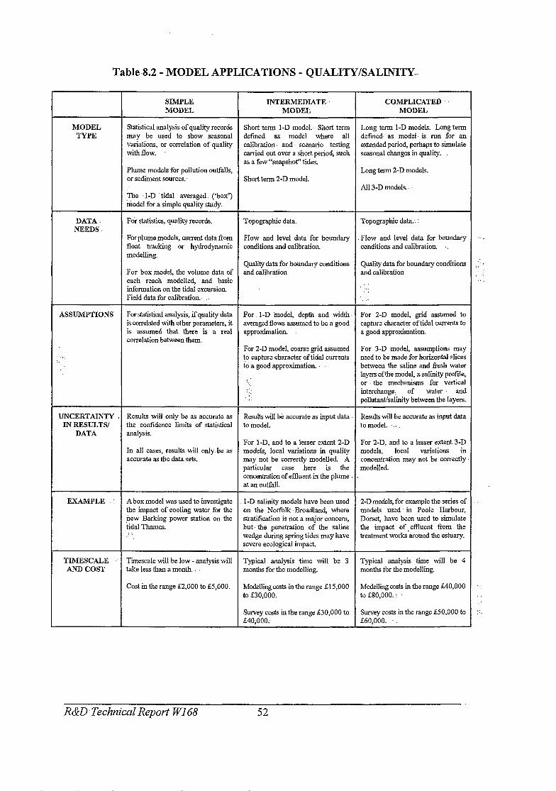
Table%2 - MODEL APPLICATIONS - QUALITY/SALINITY.,

SIMPLE INTERMEDIATE MODEL MODEL

COMPLICATED MODEL

MODEL TYPE

Statistical analysis of quality records Short term I-D model. Short term Long term I-D models. Long term may be used to show seasonal defmed as model where all defmed as model is run for an variations, or correlation of quality calibration. and scenario testing extended period, perhaps to simulate with flow. carried out over a short period, such seasonal changes in quality.

as a few “snapshot” tides. Plume models for pollution outfalls, Long term 2-D models. or sediment sources. Short term 2-D model.

AU 3-D models. .The ‘1-D tidal averaged (‘box’) model for a simple quality study.

DATA. NEEDS.

For statistics, quality records. Topographic data. Topographic data:

For plume models, current data from Flow and level data for boundary Flow and level data for boundary float tracking or hydrodynamic conditions and calibration. conditions and calibration. modelling.

Quality data for boundary conditions Quality data for boundary conditions For box model, the volume data of and calibration and calibration each reach modelled, and basic information on the tidal excursion. ._

Field data for calibration.. .-

ASSUMPTIONS For statistical analysis, if quality data For 1-D inodel, depth and width. For 2-D model, grid assumed to is correlated with other parameters, it averagedflows assumed to be a good capture character oftidal currents to is assumed that there is a real approximation. a good approximation. correlation between them.

For 2-D model, coarse grid assumed For 3-D model, assumptions may ‘F. to capture character of tidal currents need to be made for horizontal slices

to a good approximation. between the saline and fresh water Iayes ofthe model, a salinity profile,

‘:: or the mechanisms for vertical .:, interchange. of water and

pollutantkahnity between the layers.

UNCERTAINTY Results will only be as accurate as Results will be accurate as input data Results will be accurate as input data IN RESULTS/ the confidence limits of statistical to model. to model. . . .

DATA analysis. For l-D, and to a lesser extent 2-D For 2-D, and to a lesser extent 3-D

In all cases, results-will only be as models, local variations in quality models, local variations in accurate as the data sets. may not be correctly modelled. A concentration may not be correctly

particular case here is the modelled. concentration of effluent in the plume I . at an outfall.

EXAiiPLE A box model was used to investigate I-D salinity models have been used 2-D models, for example the series of the impact of cooling water for the on the Norfolk -Broadland, where models used in Poole Harbour, new Barking power station on the tidal Thames.

stratification is not a major concern, Dorsef have been used to simulate but’ the penetration of the saline the impact of .effluent from. the

: wedge during spring tides may have treatment works around the estuary.

severe ecological impact

TIMESCALE AND COST

Tiescale will be low - analysis will Typical analysis time will be 3 Typical analysis time will be 4 take less than a month. months for the modelling. months for the modelling.

Cost in the range E2,OOO to &5,000. Modelliig costs in the range E15,OOO Modelling costs in the range f40,OOO to E30,OOO. to E80,OOO.

Survey costs in the range E30,OOO to Survey costs in the range 00,000 to 640,000. f60,OOO.


Table 8.3 - MODEL APPLICATIONS - MORPHOLOGY/SEDIMENT

SIMPLE LWERMEDIATE MODEL MODEL

COMPLICATED MODEL

MODEL TYPE

Statktical analysis of records such as Short term fixed bed 1-D model. Long term 1-D and 2-D models. dredged volume may show Short term defined as model where Long term defmed as model run for correlation of deposition with flow. all calibration and scenario testing an extended period, perhaps to

carried out over a short period, such simulate seasonal@ in quality. Plume models conform a simple as a few “‘snapshot” tides. approach for sediment modelling All 3-D models. close to sediment sources. Short term fixed bed 2-D model.

Al1 moveable bed models.

DATA NEEDS

For statistics, sedimentation data and Topographic data, Topographic data. flow.

Flow and level data for boundary Flow and level data for boundary For plume models, current data conditions and calibration. conditions and calibration.

Ifpossible, tield data for calibration Sediment data for boundary Sediment data for boundary conditions and calibration conditions and calibration

ASSUMPTIONS For statistical analysis, if sediment For 1-D model, depth and width For 2-D model, grid assumed to data is correlated with other averaged flows assumed to be a good capture character oftidal currents to parameters, it is assumed that there is approximation. a good approximation. a real correlation between them Analysis may, however, show that For 2-D model, coarse grid assumed For 3-D model, assumptions may there is no correlation. to capture character of tidal currents need to be made for horizontal slices

to a good approximation between the saline and tiesh water layers ofthe model, a salinity profile,

For all models, sediment transport or the mechanisms for vertical formulae. interchange of water and sediment

between the layers.

UNCERTAINTY IN RESULTS/

DATA

Results will only be as accurate as Results will be accurate as input data Results will be accurate as input data the confidence limits of statistical to model. to model. analysis.

For l-D, and to a lesser extent 2-D For 2-D, and to a lesser extent 3-D In all cases, results will only be as models, local variations in sediment models, local variations in sediment accurate as the data sets. flux may not be correctly modelled flux may not be correctly modelled

Seaward boundary sediment flux may be diicult to detine.

EXAMPLE Estimates for the tidal reaches of the A 1-D hydrodynamic and sediment In Kelantan, Malaysia, a moveable river Trent suggest that reducing the model was used to estimate the bed 1-D model was used to simulate freshwater flow by Im’/s may impact ofatidal power barrage in the the change in river and estuarine bed increase dredged volumes by River Duddon. profdes for the next 100 years, using 15,OOOm’ per year (Binnie & a 1-D moveable bed sediment model. Partners 1993).

TIMESCALE AND COST

T&scale will be low - analysis will Typical analysis time will be 3 Typical analysis time will be 5 take less than a month. months for the modelling. months for the modelling.

Cost in the range &2,000 to f5,OOO. Modelliigcosts in the range f15,OOO Modelling costs in the range GO,000 to L30,OOO. to f80,OOO.

Survey costs in the range L30,OOO to Survey costs in the range L50,OOO to

f40,OOO. f60,OOO.


Table 8.4 -.MODEL APPLICATIONS - ECOLOGY/FISH

SIMPLE INTERMEDIATE MODEL MODEL.

. COMPLICATED

MODEL :i

MODEL .- Statistical analysis of flow/quality Use of 1-D and 2-D water quality Any full ecological model. TYPE against ecological parameters. models. .: Ecological impacts are

:. assumedto be accurately assessed by Extension of models such as Historic and data analysis of changes in quality parameters. PHABSIM into estuaries. flow/quality against ecological parameters such as population. Simple ecological models, such as

BENOSS. These are one step- Correlation with flow, quality and * beyond a quality based study, but other parameters. only model certain, simple, aspects of

the ecology ofthe estuary.

DATA. NEEDS ;

Ecological data, such as fish counts*: Topographic data. Topographic data. or bird counts..

Flow and level data for boundary Flow and level data for boundary For statistical analysis, if ecological conditions and calibration. conditions and calibration. data : is correlated with other . . parameters, it is assumed that there is Quality and/or. ecological data for Ecological data for boundary a real correlation between them. boundary conditions and calibration. conditions and calibration

-‘k%U~MPTIONS Results will only be as accurate as &logical impact can be adequately Ecological impact can be adequately * the confidence limits of statistical assessed by quality impacts. expressed by model algorithms. analysis.

UNCERTAINTY’ In all cases, results will only be as Many ecologkal processes are poorly Many ecological processes are poorly IN RESULTS/ accurate as the data sets. understood, in terms of cause and understood, in terms of cause and

DATA effect from flow and water quality. effect from flow and water quality. Interpretation of results must reflect Interpretation of results must reflect these unknowns. these unknowns.

EXAMPLE Inthe river Severn, Agency research has shown good correlation between salmon movement and salinity. In the Wash however, it has proved difficult to correlate bird and invertebrate numbers with freshwater flow from the Ouse. !

TIMESCALE AND COST-

Tiiescale will be low - analysis will Similar to an equivalent quality rModelling. costs high as R&D take less than a month. model. element likely to be included.

Cost in the range ~52,000 to 0,000.


8.4 Detailed budget guidelines

8.4.1 Basis of tables

Tables 8.1 to 8.4 provides approximate modelling costs for a range of model complexity, given at 1997 prices; these are summarised in Table 8.5. However, the cost of modelling work varies with supply and demand. A more constant measure is the estimated man-day input by staff with the appropriate experience. The tables in this chapter are therefore presented in man-day format.

Even so, in the case of modelling, the amount of staff time to complete a given task varies depending mainly on the quality of the data and whether it is provided in digital form. The staff input is therefore based on the assumption that the model is iXly packaged and user friendly. No allowance is made for the cost of purchasing the model.

8.4.2 Project costs

Table 8.5 provides approximate modelling and survey costs for a range of model complexity, given at 1997 prices. It should be noted that these costs are an estimate, and real tender costs will depend on market conditions.

8.4.3 Staff costs

The following tables of staff input are given in the following pages:

. Staff time to complete a 1-D intertidal modelling study.

. Staff time to complete a 2 or 3-D intertidal modelling study.

. Stafftime to establish a functional relationship between a estuarine phenomena and river flow predictive and other variables.

. Staff time to execute low flow surveys.

The tables should be used with the following guidelines:

. The experience required for staff of a given grade for a given task relates to experience applying mostly that type of model to mostly the same type of problem and not general experience. However, staff with longer but more general experience may be substituted.

. The experience should relate mostly to UK estuaries and not general experience. Staff with longer but more general overseas experience may be substituted.

. It should be recognised that there is a balance of experience here. Detailed experience of a type of model on a type of problem will usually provide an efficient approach to a project. However, when wider experience is applied to a task, it often provides external insights that improve the results from the task:

. In general, Graduate staff may be substituted by MSc staff with slightly less or more general experience. Technician staff may be substituted by junior Graduate staff with appropriate experience, depending on the task to be completed.

A table of typical staff rates are also included, at 1997 prices. These rates are indicative only.

R&l Technical Report WI 68 55

8.44 ~Survey costs

The same principles apply to the method of estimating staff time required to execute surveys in UK estuaries.

In the case of field surveys there are many other significant.costs besides staff time.. Downtime is usually not-a problem in the sheltered waters of the upstream.part of most -UK estuaries.

Boat hire costs andsample’transport and analysis costs vary from regionto regionand often on availability. ;

Equipment hire costs are often expressed-as a fraction of their capital costs.

To emphasis the variation in survey costs, Table 8.14 gives budget costs quoted by West (1995) :. for modelling studies into the flow requirements in the tidal Trent.

All figures quoted, except where stated, refer to short term, snapshot, data collection. Long term . . data collection costs will depend largely on the extent and methods of collection. However, typical costs will be typically-50%‘of snapshot costs per.annum.


Table 8.5 -APPROXIMATE PROJECT COSTS

Model type

Hydrodynamic Simple Intermediate Complicated

Timescale Modelling cost (months) (%I

1 2 - 5,000 2 10 - 20,000 4 40 - 80,000

Quality/Salinity Simple Intermediate Complicated

Morphology/Sediment Simple Intermediate Complicated

1 2 - 5,000 3 15 - 30,000 4 40 - 80,000

1 2 - 5,000 3 15 - 30,000 5 60 - 80,000

Ecology/Fish Simple Intermediate Complicated

Survey cost @)

20 - 30,000 30 - 60,000

30 - 40,000 50 - 60,000

30 - 40,000 50 - 60,000

30 - 40,000 High

Notes: All costs from late 1997. Long term survey costs are typically 50% of snapshot costs per annum.


Table 8.6 - ESTlMATES OF STAFF TIME REQUIRED TO APPLY l-DaINTER-TIDAL MODELLING FOR SHALLOW TURBULENT NARROW.

CROSS-SECTIONALLY WELL MIXED ESTUARIES

TIDAL FL0 WAND SALZNE INTRUSION (FS)

No. Task :.

FSl FS2 FS3 FS4

Collate and check cross-sectional data* Schematise.UK estuary h-rout cross-sectional data to model Input sea boundary harmonic tidal level constants. Check-predictions* Collate, check and input daily fluvial inflows”

FS5

FS6

FS7

FS8

FS9

FSlO

FSll FS12

FS13 FS14

FS15

Collate, check and input tidal level, velocity and salinity calibration data* Estimate bed roughness type specify calibration accuracy targets. Simulate period of intensive inter-tidal’. survey compare with tidal level and tidal : velocity data and optimise bed rou ghness.. Use salinity data under steady flows to estimate coefficient of longitudinai dispersal Set empirical constants in equation defining coefficient of longitudinal dispersion Simulate annual cycle and compare with long term salinity observations: Optimise longitudinal mixing Validate model on indenendent set of data Carry out sensitivity tests on calibration constants for low flows. Estimate error bar on position of 0.5ppt and 5ppt salinity fronts Prepare calibration report Predict design low flow year and analyse results . Technical Management

Estimate of Man-day Gradelexperience

using model-

Tech/l 0 years or Grad/2 years

2-4 per 1 year hydrograph Tech00 year’. I Grad/2 vears

2-4 per record 1 Tech/l 0 years

3 5

Specialist/l 0 years Tech/l 0 years

3-6 per test. (Total 1 O-30)

Tech/l 0 years ‘.

3-6 ner test I

1 Tech/l 0 vears

* excludes measurement or purchase of data ... ** most time needed if bed seditient.fine sand (<0.25mm)

. . . .

R&D Technical Report WI68 :’ 58

Table 8.7 - ESTIMATES OF STAFF TIME REQUIRED TO APPLY 1-D INTER-TIDAL MODELLING FOR SHALLOW TURBULENT NARROW

CROSS-SECTIONALIiY WELL MIXED ESTUARlES

Sand transport, siltation and erosion (8) (refinedflow mode9

No. Task I I Grade/experience Estimate of Man-day using model

Sl s2 s3 s4

input (min years) Collate long term bed level data IO-30 Tech/l0 years Collate sediment size fraction data 5-10 Tech/:! years Select appropriate sand transport function 5 Specialist.00 years Test model 5 Grad/5 years

s5

S6

Simulate observed drought and compare with bed level changes. Adjust coefficients to obtain best tit Validate modelagainst independent data

5 S/test (Total 20-30)

S/test (Total 10-l 5) 3Itest (Total 1 O-1 5) l-3 I-4 3Itest year 2ltest year 10-15

Tech/2 years Grad/5 years

Grad/s years

s7

S8

s9

SIO

Carry out sensitivity tests and evaluate error bar (ie f 0.5m) Prepare calibration report

Predict design low flow year and analyse results Technical management

Grad/5 years

Tech/2 years Grad/5 years Tech/5 years Specialist00 years Specialist/IO vears

Note: 1D model will not simulate trapping of sand in lower estuary by saline wedge at high flows

R&B Technical Report WI 68 59

Table 8.8 ; ESTIMATESOF STAFF TIME -REQUIRED TO APPLY 1-D’INTER-TlDALzMODELLING FOR SHALLOW TURBULENT NARROW

CROSS-SECTIONALLY WELL,MlXED ESTUARIES

WATER QUALITY INCLUDING SUSPENDED SOLIDS.(e) (requiiesflow model)

No.

Ql

Task .:I’. Eitimate of Man-day input

Collate daily fluvial pollution loading data 3-6

Q2

43.

44

Q5

46

Determine diurnal, weekly and seasons variations in effluent flows and pollution loads Collate sea boundary data

Collate calibration data

Input loading, sea boundary and calibration data Review bio-chemical processes and set

2-10 l-2

1-3 0.5. 5-10 2-3. 5-10 1-2 2-4

rate constants and specify calibration targets Simulate period of intensive survey and 5-15 compare with observations and optimise 2-6 rate constants to obtain best fit Simulate whole annual cycle and compare 5- 10 with sparse data and make further l-2. adjustment ifnecessary Carry out sensitivity tests on critical 5-10 constants 1-2 Prepare calibration report 5

5 Predict design low flow year and analyse 4ltest year results 2/test vear

1 412 ( Technical Management r’

1 IO-15

Grade/experience using model I (min years)

Tech/S years Grad/5 years Tech/S years- Grad/S years

Tech/S years Grad/5 years Tech/5 years Grad/5 years Tech/2 years Grad/5 years Specialist.0 0 years

Tech/S years Grad/S years

Tech/S years ~ Grad/S years

Tech/S years Grad/S years Tech/2 years Grad/5 years Tech/2 years Grad/S vears Specialist/IO years

Note:. 1D models will not siiulate turbidity maximum caused by gravitational circulation in the deeper parts of many estuaries.


Table 8.9 - ESTIMATES OF STAFF TIME REQUIRED TO APPLY MULTI-LAYERED INTER-TIDAL MODELLING

FOR DEEP NARROW PARTIALLY MIXED ESTUARIES

TIDAL FL0 WAND SALmTE INTRUSION (FS)

calibration accurac

FS9

defining longitudinal dispersion within layers Simulate period of intensive inter-tidal survey and compare with tidal level and tidal velocity and salinity profile data and optimise bed roughness. Check

3-5 per test Grad/5 years or (Total 15-40)*** Tech/l 5 years

stratification and gravitational circulation is correctly reproduced. Make fine adjustments to coefficients

FSlO Simulate annual cycle and compare with 3 -6 per test. Tech/l 5 years long term salinity observations. Fine tune longitudinal mixing and turbulence

(Total lo-30)*** Grad/5 years

closure model FSll Validate model on independent set of data 3-6 per test Tech/l 0 years FS12 Carry out sensitivity tests on calibration 5-10 Grad/5 years

constants for low flows. Estimate error bar on position of 0.5ppt and Sppt salinity fronts

FS13 Prepare calibration report 4-8 Grad/5 years FS 14 Predict design low flow year and analyse 2/test year Tech 2 years

results 1 /test year Grad 5 years FS-I 5 Technical Management 5-10 Specialist 15 years

* excludes measurement or purchase of data ** most time needed if data not recent *** most time needed if degree of saline stratification varies widely with tidal range and river flow or field data is

not simultaneous


Table 8.10 ; ESTIMATESOF~STAFF TIME REQUIRED .TO APPLY MULTI-LAYER INTER-TIDAL MODELLING

FOR DEEP.NARROW PARTIALLY MIXED ESTUARIES

WATER.QUALITYlNCLUDING SUSPENDED SOLIDS (QJ (requires flow model) -:

42

43

44

Qj

46

Q7

Q8

;9

QlO

Qll

Q12

Task.

Collate daily fluvial pollution loading data.

Determine diurnal, weekly and-seasons variations in effluent flows and pollution loads Collate sea boundary data

Collate calibration data

Input loading; sea boundary and calibration data Review bio-chemical processes and set rate constants and specifycalibration tar-nets Simulate period of intensive survey and compare with observations and optimise rate constants to obtain best fit Simulate summer season and compare with sparse data and make further adjustment ifnecessary Carry out sensitivity tests on critical constants Prepare calibration report

Predict design low flow year and analyse results Technical Management

Grade/experience. Estimate of Mawday using model

input: (min years) 3-6 Tech/S years 1 Grad/5 years 2-10 TeW5 years 1-2 Grad/5 years

l-3 0.5. 7-15* 2-3 s-10* l-2 2-4.

lo-25* 4-12

Tech/5 years Grad/S years Tech/S years Grad/5 years Tech/2 years Grad/S years Specialist.00 years

Tech/S years Grad/5 years

,’

,. :.

:

,j:’ :.

.:

.:

7-15* Ted5 years 2-3 Grad/5 years

7-15 2-3 4-8 4-8 41test year 2ltest year 10-20”

Ted5 y+rs Grad/5 years Ted2 years Grad/5 years Ted2 years Grad/5 years Specialist/l 0 years

Note: Most time needed if pollution loads or boundary conditions are-poorljr defined or results are sensitive to algal kinetics.

R&D Technical Report WI 68,. 62

Table 8.11 - ESTIMATES OF ADDITIONAL STAFF TIME REQUIRED TO APPLY MULTI-LAYER INTER-TIDAL MODELLING

TO DEEP NARROW PARTIALLY MIXEri ESTUARIES

TIDAL FLOWAND SALINE INTRUSION WlTHA TIDAL BARRAGE (refined model)

No.

Bl

Grade/experience Task Estimate of Man-day using model

input (min years) Analyse discharge characteristics and 2-4* Specialist/l5 years operating procedure of barrage, including 6-10 Grad/5 years

B2

B3

B4

automatic control 6-10 Write bespoke barrage operating sub- l-3 routine 5-10 Modify multi layer model to accomodate l-3 exchange flows and pollution fluxes 5-10 Test model over full range of barrage 1 per test

B5

operations as regards flows, saline stratification and pollution transport Technical management

2 per test . (Total 10-20) 5-10

Tech/l 0 years Specialist/l 5 years Grad/5 years Specialist/l 5 years Grad/S years Grad/5 years Tech/l 0 years

Specialist/l 5 vears

\Jote: Most time needed with compound moving structures.

R&D Technical Report WI68

Table-8.12.- ESTIMATES-OF STAFF TIME REQUIRED TO ESTABLISH A FUNCTIONAL RELATIONSHIP BETWEEN AN ESTUARINE PHENOMENA.AND RIVER FLOW

PREDICTIVE AND OTHER VARIABLES

, Estimate of Man-day. input

3-6*”

Grade/experience usin& model ‘. (min.years)

Specialist/l5 years

lo-20* .’ Tech/2 years 2 Grad/5 years 5-10 Grad/S years 2 Specialist/l 5 years 5-10** Grad/5 years 3-6” Specialist/l 5 years

2-4 Tech/2 years

2 Specialist/l5 years

0.5-l per test series 3-6”*

1 Tech/2 years. I SDecialist/l5 vears

* Most time needed to analyse bathmetric charts. ** Most time needed in case of complex correlations.

R&D. Technical Report WI 68 : 64

Survey

tY P

Methodology Equipment Tasks Estimated man- day input

Staff grade and

experience

Long term Deployment of salinity recording Battery powered multi-point 4-10 Teclr specialist monitoring and logging instrumentation at a monitoring syslem with integral data installation 5 years of salinity fixed position over an extended logging and at least six separate l/ 2 (m011t111y) variations in period. To measure temporal measurement channels. 0.5-I (monthly) an estuary variations in salinity at a given site. presentation (continuous Savings could by or during expected with multiple droug!lts) sites

Rapid NW Rapid drop profiles through water Fast survey vessel. Multi-parameter 3 Hydrographic slack surveys column for insitu measurement of sonde or sensor wit!1 integral data lisation [Savings surveyor 10 yrs (regu!ar or ad salinity, temperature, dissolved logging. expected by using 5 Tec!mician 5 yrs hoc during oxygen and turbidity to measure the local craf!] droughts) maximum landward movement of

salt at HW slack spring tides 1 Hydrographic surveyor 10 yrs

1 Technician 5 yrs 1 Hydrograpllic

presentation per surveyor 10 yrs survey I Technician 5 yrs

Detailed In site measurement of current year Suitable survey vessel. Multi- 3/station Hydrographic surveys of and direction, salinity, temperature, parameter sonde or sensor array and lisation surveyor 10 yrs water quality dissolved oxygen and turbidity at 30 current meter or ADCP, both with 3/station Skipper 5 yrs in an estuary minute intervals tlrough tide cycle. integral data logging. S/station Technician 5 y’s at 5-10 fixed Collection of 1.5 water samples for l/station Hydrographic stations laboratory determination of Water samplers, water sample surveyor 10 yrs (For suspended solids, BOD content at containers, suitable sample handling l/station Skipper 5 yrs calibration HW, LW and mid tide times. To facilities and rapid transport to l/station Teclmician 5 yrs purposes) measure inter-tidal variations at a accredited laboratory. I /station Hydrographic

single vertical. presentation surveyor 10 yrs (1 station day) G-lO/station Teclmician 5 yrs

Z/station Specialist 10 yrs

Notes: Position fixing assumed to be based on landmarks rather than differential GPS. Boat and equipment hire costs not estimated as they vary. Sample transport aud Canalysis costs not estimated. Survey of effluent inflows and loads not included.

Table 8.14 ;:EXAMPLE OF RANGE OF MODELLING AND SURVEY COSTS

COMPONENT-, Timescale. Modelling .’ Survey (months) cost (5) cost (Q

Desk study for first estimate conclusions

1-D sediment transport model

Use above model as basis of. :. morphological model

I Fieldwork for all above modelling work I 1. 2 1 10 -75,000 1

Notes: From West (1995) -for tidal Trent All costs from late 1995.

Table 8.15 - APPROXlMATESTAFF:RATES

Staff member cost (&/day).

Specialist 15 years experience 10 years experience

Graduate/MSc 5 years experience 2 years experience .

Technician- 10 years experience: 5 years experience 2 years experience

450 400

275, 225

225 175 125

Note: All rates from late 1997.

R&D Technical-Report. WI 68. 66

9 LIST- OF CONSULTEES-

9.1 Environment Agency

Name Title Type of consultation

Ken Allison Flood Defence Manager, Southern Region Ian Barker Regional Water Resources Manager, Welsh Region Gary Beamish Flood Defense, Southern Region’ Geoff Bell Abstraction Control Manager, Thames Region Simon Bingham . . Thames Region Dr Paul Crocket Senior Resources Engineer/Modeller, Midland Region Keith Davies Welsh Region John Ellis . . . Regional Resources Management Officer, Southern Region Adrian Fewings Fisheries Scientist, Southern Region Richard Freestone Environmental Modelling Principal Officer, North East Region Rob Grew Senior Planner, South Western Region Trevor Hardy North East Region Gordon Hargreaves Regional Licencing Officer, Anglian Region Catherine .Hohnan Southern Region Carolyn Hopper Anghan Region Pete Jonas Senior Scientist (WQ Modelling) South Western Region Aileen Kirmond Headquarters Dave Lowthion Southern Region Nigel Milner Area Environmental Appraisal Manager, Welsh Region John Morgan Area FRCN Manager, Southern Region Neil Murdoch South West Region-’ Dr. Betty Ng Environmental Modeller, Welsh Region Oliver Pollard Hydrologist, Southern Region Alaistair Pratt Water quality modeller, Southern Region Brian Repton Licencing .and Monitoring Manager, North West Region Sheila Sowerby North West Region Cameron Thomas Licensing and Transfers Manager, Anglian Region Dr Roger Wade Area Water Resources & Planning Manager, Midlands Region Dave Willis Thames Region Tony Warn Anglian Region Ann Watts Midlands Region Stephen Worral Coastal Processes Manager, Anglian Region

P P,W

P P N

P,W N P

p,w p,w p,w

N P N N P P N P W

P,N P&W PJLW

P P N P P P N N M

Key to consultation types: P Telephone conversation M -: Meeting W Written submission : N Consultation at NAMOG seminar: :

R&D Technical Report WI 68. 67

9.2 Other UK Organisations

Name

Roger Falconer Kathy Kennedy Frank Law Nicholas Odd Tony Polson Paul Samuels Peter Whitehead Richard Whitehouse

Title

Department of Civil Engineering, University of Cardiff Project Manager, Thames Estuary Project, English Nature Institute of Hydrology Hydraulics Research Wallingford

Hydraulics Research Wallingford ABP Research & Consultancy Ltd Hydraulics Research Wallingford

Key to consultation types: P Telephone conversation M Meeting W Written submission

9.3 Overseas Consultees

Type of consultation

P M

P.M PA&W

P,M P

p,w W

Name

Neal Armstrong Professor, University of Texas Ted Burgess Director, Binnie Black & Veatch, Indonesia Gerald M Hansler Executive Director, Delaware River Basin Commission Vic Hobcroft Project Director, Binnie BIack & Veatch, Thailand Karsten Havno Danish Hydraulic Institute Gerald R Miller Black & Veatch (Kansas City) Geoff Piggott Country Director, Binnie Black & Veatch, Singapore Beth Quinlan Black & Veatch (Kansas City) Andries Roelfzema Manager Marine Environment Group, Delft HydrauIics Nick Townsend Director, Binnie Consultants Ltd (Hong Kong)

Title Type of consultation

P W 1.4 _

MW P W W w W

M,W

Key to consultation types: P Telephone conversation M Meeting W Written submission

The help of the above persons, and of Oliver Pollard in collating some Agency responses, is acknowledged as essential in the completion of this report.

R&D Technical Report WI68 68 ‘1

IO BIBLIOGRAPHY

10.1. Residual flows

Central Water Planning.Unit (1979) Residual Flows to Estuaries.

Evans, D. (1997) Assessing the Flow Nee& of Rivers. Journal CIWEM, .1997-l 1, October.:

Fraser, J.C. (1975) Determining dischargesforf resources. FA0 Fisheries Technical Paper, No‘.143, Food and A gricultural Organisation of the United Nations.

Jensen, R (1994). A@esh look atj?eshwater inflows. New TWDTPWD s&&provides better method- to assess estuary nee&. Texas Water Resources Newsletter, -volume 20, no.3, 5pp; Texas Water Resources Institute..

Law, F. (1972) Determination of residual riverflows. Paper to theInstitution of Civil Engineers.

National Rivers Authority, .Anglian Region (1995) Defining River and Estuary Flow Needs. Notes from Wadenhoe Seminar.

Petts, G., Crawford, C. and Clarke, R. (1996) .De termination of Minimum Flows. National Rivers Authority R&D Note 449.

Wade, R.J., Hutchers0nN.T.S. and Goodhew, R.C (1992) Residual Flows to Estuaries:A review of the current situation andguidance on determination. National Rivers Authority, ,Severn-Trent Region.-

Wade, R.J. (1996) Flow Requirements to Estuaries. In Water Environment 1996:

West, J.R. and Webster, P. (1995) Flow Requirements-in the Tidal Trent to Maintain Navigation - Scoping Study. University .o f Birmingham. .I

10;2.-.-- Estuary characteristics

Dyer, K.R. (1977) Estuaries: A Physical Introduction. Wiley.

Kennedy, V.S. (Ed) (1984) The Estuary as a Filter. Academic Press.

Kestner, F.J.T. (1966) Z&e Effects.of-Engineering Works on.Tidal Estuaries. In: Thom,R.B., (Ed).. River Engineering and Water Conservation Works, Chapter 17. Butter-worth.

McDowell, D:M. & O’Connor; B:-A. (1977).Hydraulic Behaviour of E&caries. MacMillan..

R&D Technical Report. WI68 69.

Pritchard, D.W. (1955) Estuarine Circulation Patterns. Proc. ASCE. Separate 717, Vol. 81, pp 717/l-717/11.

Silvester, R. (1974) Coastal Engineering, Volume 2.

Simmons H.B. (1955). Some Efects of UplandDischarge on Estuarine Hydraulics. Proc. ASCE Hyd. Div., Vol., 81, Paper 792.

10.3 Estuary management

Binnie Black & Veatch (1993) River Trent Control Rules - Final Report.

Binnie Black & Veatch (1997) Internal note on Humber Estuary Management Strategy

Constanza, R. (1994). Ecological economics and the management of coastal and estuarine systems. In Changes in Fluxes in Estuaries: Implications from Science to Management. Olsen & Olsen, Fredensborg, Denmark.

Environment Agency (1997) Surface Water Abstraction Licensing Procedure (SWAMP) - Guidance for the Application of the ProposedMethodology. Working Draft Version 1 .l, EA Internal Document.

HR Wallingford (1993) Structure and Operational Framework for a Coastal Management System: A Scoping Report. Report EX 273 6

Mlay, M. (1994). Applying the watershed protection approach to estuaties and wetlands. In Changes in Fluxes in Estuaries: Implications from Science to Management. Olsen & Olsen, Fredensborg, Denmark.

National Rivers Authority (1995). Surjace Water Abstraction Licensing Policy Development - Core Report. Foundation for Water Research R&D Note 438.

Smit, H. (1997). Strategies to combine the functions of Ecology andNnvigation in the Scheldt Estuary. J.CIWEM, 1997, 11, August.

.Streeter, R. (1997). Tradeable rights for water abstract&n. J.CIWEM 1997, 11, August.

Suszkowski J. & Schubel J.R. (1994). Hope for the Hu&on: new opportunities for managing an estuav. In Changes in Fluxes in Estuaries: Implications from Science to Management. Olsen & Olsen, Fredensborg, Denmark.

Thames Estuary Project (1996) Thames Estuary Management Plan - Draft for Consultation. English Nature.

Thames Estuary Project (1996) Thames Estuary Management Plan - Strategy for


Implementation., English Nature.

Townend,.I:H. ,and Leggett, -D. (1992) GISfor Shoreline Management.. . InlCC 92.

10.4 Computational modelling

Abbott, MB. (1997) Range. of TiaW Floiv-Modelling; One-Dimensional and. Two-Dimensional ModeZx. Journal of Hydraulic Engineering, Vol: 123 No. 4, April 1997.

Cooper, A.J. and Dearnaley, M.P. (1996).Guidelines for the use of computational models in coastal and estauinestudies. Report SR.446. HR:Wallingford.

Environment Agency (1997) Portable Estuary Models: ..R&D..Technical Report 23. Evans; .G.P: (1993) A FranZework for Marine and Estuarine Model,Specification in the UK. Report No. FR. 0374, Foundation for. Water Research.

Evans, G.P. (1993) Marine-andEstuarine Modelling: Current Practice in the UK. Report No. FR.0356, Foundation for Water.Research.

Festa, J.F. & Hansen, D:V. (1976). A Two Dimensional Numerical-Model. of Estuarine Circulation: The Effects of Altering Depths and River Discharge. Est. & Coastal Marine Science,:4, pp:309-323.

Lavedrine, .I. A. and Anastasiadou-Partheniou, L; ‘( 1995). Calibration criteriafor ID river models - Assessment of objective functions and automatic calibration. Report SR442; HR Wallingford;

Mar, B .W: (1974) Problems encountered in .multidisciplinary resources and simulation models. In Journal. OfEnvironmental Management, Vol2, 83-100:

Matsumoto, J., Powell,, G. and Brock, D; (1994) Frtishwater-inflow need of estuary computed by Texas.Estuarine MP model. Journal of Water Resoures Planning & Management, Volume 120, no.5, pp. ..693-714.

Powell, G.‘, Matsumoto, J., Dyer, K.R., Orth, R.J. (1994): Texas Estuarine-Mathematical- Programming model: A toolfok@eshwaterJlow management. In Changes in Fluxes in Estuaries: Implications from Science to Management. Olsen & Olsen, Fredensborg, Denmark.

Seed,bD.J., ‘Samuels, P.G. and Ramsbottom, D.M. (1978) Quality Assurance in Computational River Modelling. Report SR374. HR Wallingford.

R&D Technical Report W.68 71

10.5 Risk, impact and sensitivity analysis

WS Atkins (199 1) Broad Oak Reservoir - Hydrology.

Hipel, K.W. and McLeod, A.I. (1994) Time series modelling of water resources and environmental systems. Developments in water science 45, Elsevier.

Pollard, 0. G. (199 1) Review of Uncertainty Analysis Techniques applied to DissoZved Oxygen in Rivers. Partial submission for Msc in Engineering Hydrology, University of Newcastle upon Tyne.

10.6 Water quality and salinity

Ayers, R. S. and Westcot, D. W. (1974) Water quality for agriculture. FA0 Irrigation and Drainage Paper, No 29.

Environment Agency (1997) B?e Water Quality of the River Thames. London: The Stationary Office.

Gameson, A.L.H.(Ed) (1982) The Quality of the Humber Estuary -A Review of the Results of Monitoring, 1961-1981. Yorkshire Water Authority.

Humber Estuary Research Committee (1971) Salinity Effects in the Humber Estuary. HERC Research Note No. 2.

Kimmerer, W.J. and Schubel, J.R. (1994). Managing freshwaterflows into San Francisco Bay using a salinity stan&rd: results of a workshop. In Changes in Fluxes in Estuaries: Implications from Science to Management. Olsen & Olsen, Fredensborg, Denmark.

National Rivers Authority (1991) Qua& of Rivers Canals & Estuaries in England & Wales - 1990 Survey. NRA Water Quality Series No. 4.

Rintema, P E. (198 1) Quality Standards for irrigation water. Acta Horticulture 119.

WRc (1992) E nvironmental Quality Standards to Protect Identtjied Uses of Controlled Waters. NRA R&D Project 0 10/9/N.

Wade, R. J. (1983) Saline Intrusion in the Severn Estuary: lmphcations for Abstractions and Residual River Flows. Internal note for Severn Trent Water Authority.

R&D Technical Report W168 72

10.7 Sediment and morphology

ABP Research (199 1) ABP Grimsby h Immingham - Sunk Dredged Channel Deepening. Research Report No:R.406.

ABP. Research (1993) ABP Humber - Sunk.Dredged Channel, Relationship Between Estuary Freshwater Flows and-Siltation. Research.Rep0r-t No. R:447,

BTDB (1970) SiltMovement in the Humber Estuary. British Transport Docks Board,-Research Report No R.22 1. .:.

HR Wallingford (1997.) Estuary Morphology and Processes - A review of recent research and user needs. Report SR 446:

HR Wallingford (1978) River Stour, Kent - Sediment Flux Observations .in Lower Estuary October-November 1978. ReportEX 858.

HR Wallingford (1992) Environmental Assessment of Proposals to Reduce Minimum Residual Flows at Denver - An Analysis of the Effect of Fluvial Flows on Siltation in the Great Ouse Estuary Based on Data 1960-1991. HR Report EX 2585.

HR Walling ford (1993) Environmental Assessment of Proposals to Reduce Minimum Residual Flows at Denver - An Analysis of the Influence.of FIuvial Flows on Shoals in the Navigation Channel to the Port of ,King ‘s Lynn. HR Report EX 2712.

Ippen, A.T. (1966)Estuary and Coastline Hydrodynamics. Chapter 15: Sedimentation in Estuaries. McGraw-Hill:

Noel, J.M:; Chamberlain, R.H. and Steinman; A.D. (1995). Environmentalfactors influencing suspended solid5 in the Loxahatchee-Estuary, Floria%x Water Resources Bulliten, volume 3 1, no,l, pp.21-32:

10.8 Ecology-and-fish:: :

Alabaster, .J. S;. and Gough, P. J. (1986) The dissolved oxygen and-temperature requirements of AtIantic~Salmon, Sa2mo saIar~L., in the Thames Estuary. Journal of Fish Biology 29; 613-621.

Alabaster, J.S. and Lloyd, R. (1980) Water Quah@Criteriafor@eshwaterJish. Butterworths.

Berman, C.H. and,Quinn, L.P.: (1991).Behavioural thermoregulation and homing. by spring chinook salmon, Oncorhynchus tsawytscha (Walbaumj, .in the YTakima River. Journal of Fish Biology 39, 301-3 12.

Buller and Falkus (1994) Freshwater Fishing, .Grange Books.


Duel, H., Specken, B.P.M., Denneman, W.D. and Kwakernaak, C. (1995) Water Science and Technology 31 (8) 387-391.

Ibbitson, A and Ladel, M. (1997) Review ofpow needs forfish and$sheries - a progress report. IFE Report T11068E7ll.

Mills, D.H. (1989) The Atlantic salmon, Chapman & Hall.

NERC (1984). Predicted effects of proposed changes in patterns of water abstraction on the ecosystems of the Lower River Thames and its tidal Estuary. Final Report for Thames Water Authority (Commercial in confidence).

Potter, E.C.E. (1988) Journal Fish Biology (1988) 33 (Supplement A), 153-159.

Priede, LG., De LG Solbe, J.F., Notte, J.E. 0’ Grady, K.T. and Cragg-Hine, D. (1988) Behaviour of adult Atlantic almon, Salmo salar L., in theestuary of the River Ribble in relation to variations in dissolved oxygen and tidal~ow. Journal of Fish Biology (1988) 33 (Supplement A) 133-139.

Radford, P.J. (1979) Role of GEMBASE in tia!id power and estuary management. Edited by Severn RT., Dinnerleyand, D. and Hawke, L.E. in 30th Symposium Colston Research Society, Scientecnnica pp 40-46.

Radford, P.J., Burkhill, P.H., Collins, N.R. and Williams, R. (1987) Validation of scientific associations of ecosystem nzodel of the Bristol Channel in Advances in EcologicaiiModelling, AE Marani Proc ISEM conference Italy..

Radford, P.J. (1994) Pre- andpost- barrage scenario’s of the relative production ofbenthic andpelagic sub-systems in Evaluation and changes of the Bristol Channel and Severn Estuary. Editor Mettam, C. Proceedings of Linnean Society Biological Journ Linnean Society 51, 5-16.

Uncles, R. J. and ‘Radford, P.J. (1980) Seasonal and spring-neap tidal dependence of axial dispersion coefficients in the Severn - a wide, vertically mixed estuary. Journal of Fluid Mechanics 98,4, 703-726.

10.9 Other

Fewings, A (1997) Internal EA communication.

United Kingdom ‘Climate Change Impacts Review Group (1996) Review of the PotentiaZ Effects of Climate Change in the United Kingdom. Second Report. DOE, HMSO.


11 GLOSSARY OF TERMS

1-D hydrodynamic model Computational model, usually used for rivers and narrow estuaries where all flow is assumed to be depth and width averaged

2-D hydrodynamic model Computational model, usually used for open sea and wide estuaries where flow is assumed to be depth averaged only

3-D hydrodynamic model Computational model, usually used for stratified estuaries where all flow is simulated in three dimensions

-Automatic calibration Calibration of a computational model by algorithms within the computer software to select optimum model parameters

Barrage Structure built across a river or estuary, comprising a series of gates designed to regulate the upstream water level and pass flood water without an appreciable rise in the upstream water level

Baseline

Bathymetry

Beach

Benthic.

Biochemical Oxygen Demand (BOW

The present condition of the river or estuary

Topography of the bed of the sea, estuary or other water body

Shore of sand or shingle

Referring to life in or on the sea bed

Is the amount of dissolved oxygen consumed by chemical and microbiological action when a sample effluent is incubated for 5 days at 20°C

Calibration The adjustment of parameters in a computational model to achieve agreement between the model and observed results

Catchment . The land which drains (normally naturally) to a given point on a river or drainage system.

Catchment area

Channel ‘.

The area of a catchment

(1). Natural or man-made open passage designed to contain and convey water

(2) The part of a body of water deep enough to be used for navigation through an area otherwise too shallow for navigation

(3). The deepest part of a body of water through which the main volume of current passes

Coastal defence works::, Flood defence worlds in a coastal area, designed to protect the land against erosion, encroachment orflooding by the sea (includes coastprotection works and sea defence works)

Cdastal lagoon Shallow body of water close to the sea, usually with a shallow restricted con- nection to the sea

Coastal zone management The process of ensuring that all the problems within a coastal zone relating to the environment are presented within a management tmrnework which aims to promote the well-being of the coastal zone

Coast protection works Works to protect land against erosion or encroachment by the sea ”

R&D Technical. Report WI 68 75

Combined sewerage overflow WSO)

Compensation water

Overflow from municipal sewerage network that carries both foul sewage and stormwater runoff

Water released by law or custom from a reservoir or diversion structure to the downstream watercourse to meet the needs of downstream water users and satisfy environmental requirements

Computational model Statistical or deterministic numerical simulation of reality, often in the form of computer software

Control structure Device constructed across a channel or between water bodies or water passages, used to control the discharge passing the device and/or the water level on either side of the device

Deterministic model A computational model that uses mathematical descriptions of physical laws and provesses

Ebb tide

Empirical model

Environmental Quality Objectives (EQOs)

Environmental Quality Standards (EQSs)

That part of the tide in which the water level is falling; also the outflow of water from coastal bays and estuaries during the falling tide

Mathematical expression that is fitted to observed conditions without consideration of physical laws

Are categories relating to the use of particular stretches of water. For each use an associated series of quantitative standards applies

Are concentrations of substances in the receiving water which must not be exceeded if the water is to be suitable for a particular purpose or use, or to achieve a certain level of protection for aquatic life

Estuary The mouth of a river connected to the sea, where bothji’uvial and tidal effects occur and interact

Estuarine

Fish kill

Relating to an estztaly

Localised high mortality of fish population caused by lack of oxygen or other pollution

Flood tide That part of the tide in which the water level is rising; also the flow of water into coastal bays and estuaries during the rising tide

Freshwater flow need The residualflow required in the estuary to maintain required uses and habitats

Flushing time Is the time taken for the freshwater and associated contaminants to pass out to sea. It depends to a large extent on the size of estuary and the relative volume of freshwater discharging into it

Fluvial

Geographical Information System (GIS)

Heavy metals

Relating to a river

Computerised database that can visualise and analyse data in a spatial or geographical form.

A general term for those metals which are toxic when present in elevated concentrations. These include elements such as zinc, copper.. lead, nickel and mercury, all of which are commonly used by industry

High water Highest water level reached by eachflood tide (see also tides)


Holistic catchment management

Hydrodynamic model :

Hydrograph

Hydrography.

Intertidal

Intake

Invertebrate.

Low water-

Minimum residual flow

Morphology

Neap tides

Outfall

Reach

Residual flow

Risk assessment ‘.

River . .

Salinity. -,,

Sahnonid (:

Saltation

Salting (or salt marsh)‘,

Sand dune. .

Sea defence works

Sea level rise

Seawall

Sediment

Recognition that many parameters within a catchnzent interact, and a management approach that takes an overview of these parameters

Mathematical model of water movement using the laws of motion

Graph that shows the variation with time of level or discharge of water in a river, channel or other water body

The study of water bodies and their movements

Between the levels or lines of low tide and high tide

Structure through which water is drawn out of a river or other body of water

Animals without a backbone.

Lowest water level reached by each ebb tide (see also tides)

The lowest residzlalflow allowed in a river or estuary to satisfy downstream users

The study of change of form of a river or estuary

Tides on the two occasions per lunar month when the predicted range between successive high water and low water is least

Structure through which water is discharged into a channel or other body of water

A length of channel between defined boundaries

Flow remaining in a river or estuary after all users have taken water.

Decision making methodology that considers the likelihood of an event and the potential impact resulting from the event

Any natural watercourse (including modified watercourses) carrying perennial flow

The extent to which salts are dissolved in water.

The family of migratory fish that include salmon and trout

Sedinzent transport in which the particles remain close to the bed and are bounced along

Area of land adjacent to the sea or estztaiy which is periodically covered by saline water and usually supports vegetation

Hillock of wind-blown sand

Works to prevent or alleviateflooding by the sea ..

Increase in mean sea level due to global warming

A shoreline structure, usually parallel to the coast, designed to prevent Jlooding, erosion and other damage caused by high sea levels or waves

Fine material transported in a liquid that settles or tends to settle

R&D Technical Report.Wl68

Sediment transport

Semi-diurnal tides

Sensitivity analysis

Shoal

Shore

Siltation

Spring tides

Statistical model

Stratification

Tidal

Tidal barrier

Tidal excursion

Tidal limit

Tidal prism

Tidal range

Tidal sluice

Tides

Mighest astronomical tide (HAT) and lowest astronomical tide (TAT)

Mean high water springs (MHWS) and mean low water springs (MLWS)

Tide-locked

Verification

Waterway

Movement of sediment under the action of lvaves and currents

Tides with a period of about 12% hours between tcvo successive high or low waters

Variation of computational model parameters to assess impact of each parameter on model results

Localised area of siltation or sediment deposition

Strip of land at the edge of the sea, lake or coastal lagoon

Deposition of sediment onto the river or estuary bed

Tides on the two occasions per lunar month when the predicted range between successive high water and low water is greatest (see also tides)

A computational model that uses linear regression analysis to relate empirically the observed values of variables

The separation of fresh and salt water into separate layers in an estuary

Relating to the tides

Gated structure located in an estuary or coastal area that can be closed to prevent high tides and/or surges reaching inland areas vulnerable toflooding.

The distance travelled by a body of water between low and high tides

Furthest upstream point on an estuary or river where there is a tangible tidal. influence

Volume of water contained in estuary or other tidal body of water between the levels of the high and low tides

Is the difference in height between high and low tide

Structure designed to prevent or control the ingress of seawater into a coastal watercourse, whilst allowing seawards flow to occur at times of low water

Periodic rising and falling of water resulting from the gravitational attraction of the moon, sun and other astronomical bodies, together with the effects of coastal aspect and bathymetry

Highest and lowest levels respectively which are predicted to occur under average meteorological conditions and any combination of astronomical conditions, excluding any surges

Annual average, during year when average maximum declination of the moon is 23 %“, of the elevations of two successive high waters and low waters respectively, at the times (approximately once per fortnight) when the tidal range is greatest

Situation where flow into the sea is prevented by the level of the tide

Testing of a calibrated computational model with alternative data sets to confirm that the model is fit for purpose

Channel used, previously used, or intended for the passage of vessels


Wave

Wave amplitude Half the wuve height

Wave energy spectrum Graph showing the distribution of the kinetic energy content of waves in relation to wave period

Wave forecasting

Wave height .Y.

Wave hindcasting

Wavelength

Wave period: ..

Wave protection

Waverider buoy

Wave setup,

Wave steepness

Wave train’ :

Wave velocity

(1) Short period oscillation of a water surface caused by the action of wind or by the passage of vessels (see wake)

(2) Long period movement of water surface due to tide, surge or the passage of a flood hydrograph

Estimation of future wave characteristics likely to be associated with particular meteorological conditions

Vertical distance between the crest and trough of a wave

Use of historical weather data to estimate the characteristics of waves which have already occurred

Distance between two successive wave crests

Time for two successive wave crests to pass a fixed point

Material applied toflood defence works to provide protection against wave attack

Floating device used to measure water level fluctuations due to waves

Tilting of mean water level profile near a sloping shore associated with the conversion of wave energy to potential energy

Ratio of wave height to wavelength

Group of waves originating from the same fetch (see group velocity)

Speed of advance of an individual wave (see group velociq)

R&D. Technical Report WI68 79

APPENDIX A - TYPICAL MODEL SPECIFICATION

R&D, Technical Report FYI 68

CONTENTS Page

FOREWORD A3 .

A. 1 SUMMARY OF THE SAMPLE SPECIFICATION

A.2 : OBJECTIVES A.2.1 The Customers A.2.2 The Mathematicai Modelling System .’ A.2.3 Use of the Results A.2.4 Outline of Study Area A.25 Water. Quality Parameters to be Modelled A.2.6 .’ Spatial and Temporal Resolutions of the Models A.2.7. Gridding and Meshing (Internal) A.2.8 Geographical Referencing Systems .. A.2.9 Numerical Schemes and Mathematical Reference.Systems A.2.10 Inputs to be Handled A.2.11 Output to be Generated

A.3 BUILDING THE MODELLING SYSTEM A.3.1 Data Flow Diagrams A.3.2 Bathymetry A.3.3 Boundary Conditions A.3.4 Pilot Modelling

A.4 PROVING THE MODELS A.4.1 Calibration A.4.2 Validation

A.5 USING THE MODELS : A: 5.1 User Guide A.5.2 User Interface A.5.3 Model Run Times A.5.4 Scenarios A.5.5 Graphics A.5.6 Statistical Summaries A.5.7 Tabular Output ‘: A. 5.8 Data Management

cont..:.

A4

A4 A5 A5 A5 A6 A6 A7 A7 A8 A8 A8 A9

A10:~ A10 All :I Al 1. .. Al2

Al2 Al2 Al3

Al5. Al5 Al6 Al7 Al7 A19 A20 A20- A20

R&D Technical Report WI 68 Al t

CONTENTS Page

A.6 SUPPORTING MATERIAL. A.6.1 Theory A.6.2 Previous Experience A.6.3 Quality Assurance A.6.4 Acceptance Testing A.6.5 Training A.6.6 Maintenance A.6.7 Support A.6.8 Updating and New Versions A.6.9 Manuals A. 6.10 User Group A.6.11 Consultancy

A21 A21 A22 A22 A23 A23 A23 A23 A.24 A.24 A24 A24

R&G Technical Report WI 68 A2

APPENDIX A - SAMPLE SPECIFICATION FOR COASTAL AND ESTUARINE.-MODELLING

FOREWORD

This Appendix is taken from Evans, G.P. (1993) A Framework for Marine and Esiuarine Model SpeciJcation in the UK. Report No. FR 0374, Foundation for.Water Research.

It is provided as a model or template only. It should be adapted to suit particular studies and applications. Alternative model documents are available from some Agency Regions, in particular NAMOG in the water quality function.

This Appendix is not intended to be used as a blueprint for the specification of any particular modelling system.. Instead it should be used as a ‘checklist’ for aspects of the specification which should be considered. ‘.,

The sample specification is very ambitious and would probably result in an expensive system which in many simpler,cases would be’unjustified for the task in hand. The document refers to a requirement for a range of different types of models: one-dimensional estuary models, two-dimensional coastalmodels, three-dimensional plume models, which are. supposed to communicate with each other,. produce standard types of output, receive standard types .of input etc. It is very possible that no one manufacturer-would have suitable .versions of all of these model types, ready to run as an integrated system without further development.

Where possible, the purpose of the document as a checklist has been made more explicit by the use of ‘bulleted lists; these should act as a warning to the ,reader that not all features need be selected. Warning notes have sometimes-been included for the reader as [Warning: ;.. 1.

The specification is written as if the client were a water company, but it is hoped that it could be found useful by other industries, the regulator, or a supervising consultant working for the client to specify and manage a modelling’ study.

One of the most difficult aspects of writing the specification has been the treatment of model accuracy in calibration and :validation. The specification requires the contractor to state in a proposal what the performance of the models will be in,this respect, but then goes on to suggest some typical accuracies for various parameters. Whether this latter step should or should not have been taken was the subject of some debate inthe Steering Group, but it was eventually agreed that the reader would need to be given some’idea of what would be a reasonable attainment.

The document was shown in an earlier dratl to a number of existing customers and model users, and several model manufacturers and contractors As might be expected, the emphasis of comment differed between the two ‘sides’. Some model suppliers expressed concern about even the suggestion of guideline performance in calibration and validation, others pointed out the investment required to secure all of the aspects of required model output, compatibility and security. Some of the users as well were concerned about the cost irnplications.of such a-? specification and, for opposite reasons, about the use of guideline figures, for model performance. There was agreement about the value of a rigorous system for logoing and labelling model runs and about a number of other features of the proposed system.

Taking these views into account but bearing in mind that this document is only an Appendix to the second of two reports, both of which discuss the broader aspects of marine and estuarine,.water quality modelling in the UK including general performance objectives, the Steering Group decided to publish the sample specification with these appropriate qualifications: . this is not a blueprint but a checklist for what might be found useful; . appropriate model types and accuracies depend on the complexity of the problems to be solved and the:.

type and accuracy of the answers required by the client;

R&D Technical Report WI 68 I. A3

. too detailed a specification may reduce the scope for manufacturers to provide their own innovations; and the more demanding the specification the higher will be the price.

A. 1 SUMMARY OF THE SAMPLE SPECIFICATION

This document specifies the requirements for a mathematical modelling system which is simulate water quality in the coastal and estuarine waters to which the client discharges effluent. The client requires the modelling system both as a design tool and also to form the basis of discussions with the then National Rivers Authority (NRA)(now Environment Agency) as part of the process of obtaining consents to discharge.

A.2 OBJECTIVES

The client has the task of treating sewage Ii-om several large conurbations on the coast. At present sewage from these townships is discharged into the sea, after screening but without any other form of treatment, through short outfalls which terminate just below the level of Lowest Astronomical Tide (LAT). There are two important bathing beaches in the area which presently fail the standards required by the European Commission Bathing Waters Directive; there are also two estuaries whose water quality must be safeguarded.

The client is considering a number of options for altering collection and treatment order to bring the beaches up to standard:

. the collection systems may be joined together so that they drain (or are pumped) to a single treatment plant; or

. several treatment plants may be built;

. treatment may be primary or secondary with or without disinfection;

. outfalls to sea of various lengths may be constructed; . treatment plants may be sited inland so as to discharge, through relatively short . outfalls, to one or two of the estuaries which open into the sea along this stretch of coast.

The client wishes to purchase and operate a mathematical modelling system, incorporating both hardware and software, to evaluate the consequences, on the local coastal and estuarine waters, of adopting one or more of these options.

It must also be borne in mind that the existing sewerage systems are principally combined networks, so that the flows are heavily dependent on rainfall. It is thus inevitable, for a11 but the most expensive design options, that combined sewer overflows (CSOs) will continue to be necessary in any new schemes. Therefore the client also requires that:

. The modelling system be capable of simulating the effects of intermittent discharges from CSOs, in conjunction with discharge of treated effluent from the regular outfalls.

. While bacterial quality is an important consideration, affecting the suitability of water for bathing and shell fish farming, it is also vital that any scheme which incorporates substantial discharges to the estuarine waters does not result in eutrophication and increased potential for algal blooms. In addition, itwill be necessary to examine the fate of conservative substances, such as heavy metals and persistent organ&, as they disperse in the water cohmm and interact with cohesive sediments, either on the bed or in the water coiumn.

A.2.1 The Customers

The contractual customer for the modelling system will be the client; but the ultimate customers for the results ofthe modelling work include the client, the NRA, the Offke of Water Services (OFWAT) and the general public.

R&D Technical Report WI 68 A4

The client requires the modelling system for strategic design purposes, as outlined above,-the NRA requires the results of the modelling in order to satisfy itself that the design proposals of the client will result in satisfactory water quality, whether. that be assessed with respect. to Environmental Quality Objectives (EQOs) or Environmental Quality Standards (EQSs). In effect, the client. will test various practicable treatment options coupled with various scenarios (tides, winds, etc.), in order to see whether the options are likely to satisfy the NRA, either in a consent application, or in response to an NRA request for treatment improvements.

OFWAT will require to be assured by the results of the-modelling work that the proposed treatment options are not excessively expensive for the environmental benefits which they bring. The output of the modelling must also be sufficiently convincing and compelling to persuade the general public itself - not forgetting that the general public includes pressure groups and local government - that correct decisions are being made inits name.. For; : by way of water and sewerage charges and taxation; members of the general public will be the ultimate funders of the ameliorative works as well as being the beneficiaries.

A.2.2 The Mathematical Modelling,System

The client requires the contractor to supply software to fulfil the needs for mathematical modelling described in this document. Thecontractor is also required to discuss the.type.of computing system which the client wilb need in order to run the sotlware supplied by the contractor; at the offices of the client. The contractor should bear in mind the target run times for the various models, and the types of output, in deciding the type of hardware that. should be employed. It will be advantageous if the contractor’s software can be run satisfactorily on machines which theclient already possesses.

A.2.3 Use of the Results:..:

The results from the modelling work may be used in discussions with the NRA in support of applications for consent to discharge. In order to be sure that an application is likely to succeed, the client wishes to test worst-case- scenarios; the NRA on the other hand, may also be interested .in the statistics of likely water quality in certain key areas. This means that the modelling system must be capable of operating either. in ‘worst-case mode’ or in ! simulation of relatively lengthy periods of time, in which v&-ious- combinations of loads and natural : : environmental conditions are brought together ina realistic sequence. The length of time for which extended simulations will -be required depends on the circumstances, but is unlikely .to exceed 28 days (a . . Spring-Neap-Spring-Neap cycle). Combinations of extended simulations (for example,.with different seasonal. characteristics) will be used to represent longer periods of time. The client will also need to use results from the modelling for public relations (RR) purposes: to persuade local government, pressure groups and the media&at the design proposals will result in no detriment to the environment -, and indeed, preferably, an improvement.

R&D Technical Report WI68- A5

A.2.4 Outline of Study Area

The study area covers approximately 200 km of coastline and two major estuaries (here there could be a map and description of the off-shore sea, tidal ranges, estuaries and river flows). The study area is to be envisaged as being split into a number of ‘fields’:

. the near-fields, which will be the regions in the immediate vicinity of outfalls, where jet mixing and initial dilution must be simulated;

. the mid-fields where the dispersion of extended plumes is to be simulated; and

. the far-fields where resultant quasi-steady-state or slowly varying (at tidal frequency) concentrations are to be modelled.

The software must be able to simulate the interaction of these various fields in a unified modelled system.

A.23 Water Quality Parameters to be Modelled

In this section the client outlines the minimum set of water quality parameters to be modelled. This is not intended to place on the contractor a restriction of the nmnber of parameters which may need to be modelled to provide an authentic description of the processes affecting the minimum set. For example, salinity and temperature will affect the buoyancy and difksion of an outfall plmne, while for consenting purposes only concentrations of coliforms may be relevant.

In the coastal waters, which are usually well flushed and where dilution volumes are adequate, the principal parameters to be modelled are the concentrations in the sea of viable Total and Faecal Coliforms. It is expected that these will only be of sign&ant magnitude in the near- and mid-fields (with respect to the originating outfall). Where the mid-field encompasses bathing beaches, coliform concentrations at the water’s edge are to be modelled.

[Warning: this laststipulation might be very diffkult and expensive.]

In the estuarine waters, which may be less well flushed, the modelling system must be able to simulate the evolution of concentrations of the following water quality parameters:

.

.

.

.

.

.

.

.

.

.

.

Temperature; Salinity; Total Coliforms; Faecal Coliforms; Dissolved Oxygen; Ammoniacal Nitrogen; Biochemical Oxygen Demand; Oxides of Nitrogen; Orthophosphate; Chlorophyll; and 6 user defined (first order) pollutants.

[Warning: the number of modelled pollutants will affect the size and run-time of the model.]

In the estuaries, the modelling system must be capable of simulating the near-field, the mid-field and the far-field.

The contractor should also provide an option for modelling the erosion, deposition and re-suspension of muddy (cohesive) sediments so as to simulate the effect of concentrations of those solids on:

. Turbidity (and thus T90 values for bacteria); and


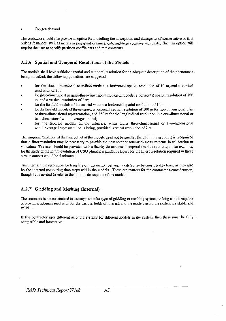
. Oxygen demand.

The contractor should also provide an option for modelling the adsorption, and desorption of conservative or first order substances, such as metals or persistent organ&, onto andfrom cohesive sediments. Such an option will require the user to specify partition coefficients and rate constants.

A.2.6 Spatial and Temporal Resolutions,of the Models

The models shall have sufficient spatial and temporal resolution for an adequate description of the phenomena. being modelled; the following,guidelines are suggested:

. for the- three-dimensional near-field models: a horizontal spatial resolution of 10 m,. and a vertical resolution of 2 m;

. for tbreedimensional or quasi-tbreedimensional mid-field models:% horizontal spatial resolution of 100 m; and a vertical resolution of 2 m;

. for-the far-field models of the coastal waters: a horizontal spatial resolution of 1 km; . for the far-field models of the estuaries: a horizontal spatial resolution of 100 m for two-dimensional plan.

or three-dimensional representation; and 230 m for the longitudinal resolution in a one-dimensional or two-dimensional width-averaged model;

. for the far-field models of. the estuaries, when either three-dimensional or two-dimensional width-averaged representation is being, provided: vertical resolution of 2 rn;

The temporal resolution of the fmal output of the models need not be smaller than 30 minutes, but it is recognised that a finer resolution may be necessary to provide the best comparisons with measurements in calibration or validation. The user should be provided with a facility for enhanced temporal resolution of output, for example, for the study of the initial evolution of CSO plumes; a guideline figure for the finest resolution required in those circumstances would be 5 minutes;

The internal time resolution for transfers of information between models may be considerably finer, as may also be the internal computing timesteps .within the models. These are matters for the contractorkconsideration, though he is invited to refer to them in his description of the models.

A.2.7‘ Gridding and.Meshing (Internal)

The contractor is not constrained to use any particular type of gridding or meshing system, so long as it is capable of providing adequate resolution for.the various fields of interest, and the models using the system are stable and valid.

If the. contractor uses different gridding.systems for different models in the system, then these must -be fully compatible and interactive.


A.2.8 Geographical Referencing Systems

A.2.8.1 Horizontal position

It must always be possible to describe the horizontal position of an output from the model, in terms of Ordnance Survey (OS) co-ordinates, and in terms of Latitude and Longitude. It must be possible to specify positions of load sites in similar terms reference in final output to position in the model gridding system alone is not sufllcient.

A.2.8.2 Vertical position

In addition, it must be possible to describe the vertical position of a model output (where vertical dimensionality is provided) with respect either to Ordnance Datum or to local chart datum. Obviously similar considerations apply to model predictions of water surface level, and representations of sea bed depths.

A.2.8.3 Geographical Information Systems (GIS)

A facility to exchange data, input or output, in an industry-standard format with a Geographical Information System (GIS) is essential. In this way both the client and the NRA will be able to present results of the modelling operations in the context of maps of their own making, such as:

. maps of sewerage systems and treatment facilities;

. maps of catchment water quality; and

. maps of air quality relating to the location of incineration facilities.

[Warning: this would require special investment by the model manufacturer.]

A.2.9 Numerical Schemes and Mathematical Reference Systems

The contractor is not obliged to use any particular type of numerical scheme nor reference system. For example, he may use finite difference or finite element schemes, explicit or implicit methods, and Eulerian or Lagrangian reference systems. He must, however, provide justification for the efficacy of the schemes or systems in his description of the models.

A.2.10 Inputs to be Handled

The modelling system must be capable of handling the following input variables:

. time-varying tidally generated water levels and fluxes at the boundaries;

. time-varying wind fields over the water surface;

. time-varying solar radiation; . time-varying air temperature; . time-varying river flows; . time varying effluent flows; and . time-varying effluent concentrations.

The modelling system must be capable of accepting the last three items, which cover the principal inputs of loads to the modelled areas, as either:

. constant values;

. values varying diurnally and/or weekly according to a prescribed cycle; l values received from a file created by another program or by the user; or . values calculated Corn a user-supplied algorithm which relates flows and concentrations to the local water

R&D Technical Report WI68 A8

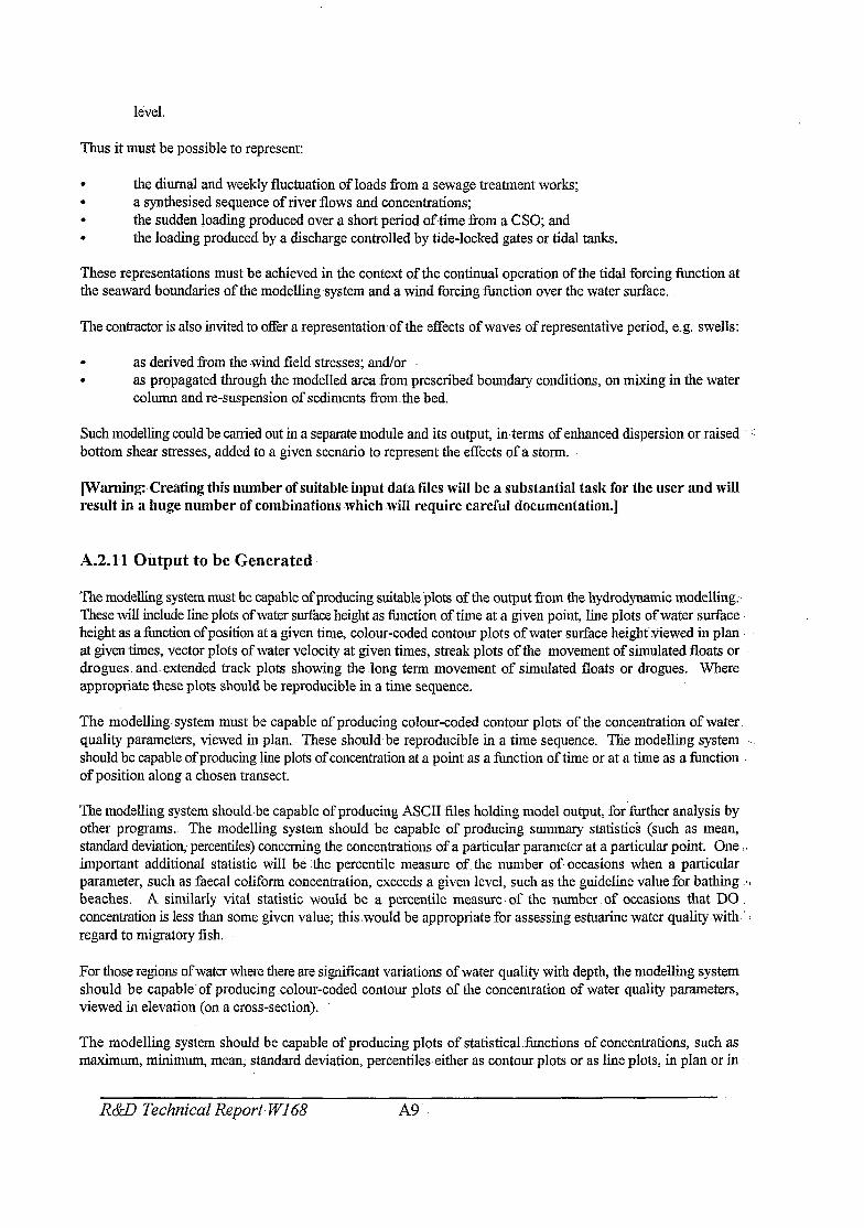
level.

Thus it must be possible to represent:

. the diurnal and weekly fluctuation of loads from a sewage treatment works;

. a synthesised sequence of river flows and concentrations;

. the sudden loading produced over a short period of.time corn a CSO; and

. the loading produced by a discharge controlled by tide-locked gates or tidal tanks.

These representations must be achieved in the context of the continual operation of the tidal forcing function at the seaward boundaries of the modelling-system and a wind forcing function over the water surface.

The contractor is also invited to offer a representation of the effects of waves of representative period, e.g. swells:

. as derived from the wind field stresses; and/or

. as propagated through the modelled area from prescribed boundary conditions, on mixing in the water column and re-suspension of sediments from the bed.

Such modelling could be carried out in a separate module and its output, in-terms of enhanced dispersion or raised :‘ bottom shear stresses, added to a given scenario to represent the effects of a storm.

[Warning: Creating this number of suitable input data files will be a substantial task for the user and Will result in a huge number of combinations which will require careful documentation.]

A.211 Output to be Generated

The modelling system must be capable of producing suitable@ots of the output from the hydrodynamic modelling.. These will include line plots of water surface height as function of time at a given point, line plots of water surface height as a function of position at a given time, colourxoded contour plots of water surface height Viewed in plan at given times, vector plots of water veldcity at given times, streak plots of the -movement of simulated floats or drogues. and- extended track plots showing the.long term movement of simulated floats or drognes. Where appropriate these plots should be reproducible in a time sequence.

The modelling.system must be capable of producing colour-coded contour plots of the concentration of water. quality parameters, viewed in plan. These should-be reproducible in a time sequence. The modelling system ‘. should be capable of producing line plots of concentration at a point as a function of time or at a time as a function of position along a chosen transect.

The modelling system should.be capable of producing ASCII files holding model output, for’further analysis by other programs. The modelling system should be capable’of producing summary statistics (such as mean, standard deviation; percentiles) concerning the concentrations of a particular parameter at a particular point. One important additional statistic-will be .the percentile measure of the number of, occasions when a particular parameter, such as faecal coliform concentration, exceeds a given level, such as the guideline value for bathing beaches. A similarly vital statistic would be a percentile measure. of the number .of occasions that DO concentration is less than some given value; thiswould be appropriate for assessing estuarine water quality with regard to migratory fish.

For those regions of water where there are significant variations of water quality with depth, the modelling system should be capable’of producing.colour-coded contour plots of the concentration of water quality parameters, viewed in elevation (on a cross-section).

The modelling system should be capable of producing plots of statistical .fimctions of concentrations, such as maximum, minimum, mean; standard deviation, percentiles either as contour plots or as line plots, in plan or in

R&D Technical Report- WI68 A9

elevation as appropriate.

The contractor may wish to quote for the supply of a three-dimensional colour-coded contour plotting package which would permit the viewing of the initial evolution and dilution of plumes. Such a package would allow the plume to be seen in isometric or perspective projection, rotated or sliced according to the wishes of the user; it would thus enable the fulfilment of all of the requirements for two-dimensional viewing outlined above.

Wherever appropriate, it should be possible to display the results of modelling in conjunction with the results of calibration and validation exercises, preferably with the simultaneous display of various statistical measures of the goodness of fit between modelled output and measurements.

Contractor should arrange that the decision, as to which output is to be used to demonstrate the effects of any given treatment option and scenario, can be delayed as long as possible - preferably until after all modelling for that scenario has been completed. It is accepted by the client that this will require the storage of large files of output data. The contractor should bear this in mind when discussing hardware requirements.

The contractor should endeavour to provide the utmost degree of modularity in the output tools. Thus output tools should, whenever possible, not be seen as specific to a given model. It will be highly desirable to be able to present two-dimensional tiormation, such as contour plots of concentration, in the context of maps produced from other sources with a GIS.

A.3 BUILDING THE MODELLING SYSTEM

The contractor is to build the modelling system, choosing model components appropriate to the regions to be studied. He must indicate the regions where special sub-models will be required in order to resolve detail. The client has shown in Figure A the regions of especial interest to it and to the NRA. The contractor should describe the types of models which will be applied in each area. By way of guidance, the client has been told by the NRA that two-dimensional depth-averaged models will s&ice for the mid- and far-fields in the open sea area, while a three-dimensional representation of initial dilution is required in the near-fields adjacent to proposed outfalls. In addition, while estuary P is well-mixed over depth, estuary Q is deep and subject to considerable variation with depth of salinity and quality during neap tides and during high flows. For this reason, the client is of the opinion that a special three-dimensional model will be required for estuary Q.

A.3.1 Data Flow Diagrams

The client understands that it may well be possible to separate the modelling process into two key stages:

. hydrodynamic modelling; and

. water quality modelling,

which may be carried out in sequence for any given modelled region. This is because, in general the results of water quality modelling do not impinge on the results of hydrodynamic modelling. Exceptions may occur when salinity (and thus density) gradients are large or when pollutant loads added in a water quality are of necessity accompanied by large flows of water.

. The contractor must clearly indicate and justify the type of models or sub-models which he intends to provide in order to construct the modelling system.

l He must also clearly state whether the models are to be fully interactive, or whether sub-models are to be run with boundary conditions supplied from the output of previous and separately conducted model IWIS.

. In the proposal the contractor should provide data flow diagrams in order to show the sequences in which

R&D Technical Report W168 A10

the’various modelling processes are runand the exchange of information between them and the user.. The data flow diagrams should also place the modelling components in the context of the modelling system as a whole, showing, the links between the pre-processing or input stages, the models, and the post-processing or output stages, and the degree to which they are, or are not, independent of each other.

A.3.2 Bathymetry _

It is the contractor’s responsibility to ensure that the description used within the models of the bed-depths of the sea and estuaries (the bathymetry)-is fit,for purpose. The,contractor must indicate whether be intends to use Admiralty chart data, Admiralty fair sheets, local port authority data, special survey data or a combination of one or more of all of these. It should be borne in mind that-Admiralty and port authority charts are primarily intended for navigation and thus tend to be biased towards an underestimation of depths.

A.3.3 Boundary Conditidns,

A.3.3.1 Spatial boundaries: quantity.

The contractor is responsible for obtaining information about the appropriate tidal.conditions at the spatial boundaries of the modelling system. He may wish to extend the modelled area beyond the region of prime interest to the client in order to acquire better-documented and more tractable boundary conditions.-

A.3.3.2 Temporal.boundaries: quzgtity and quality

Boundary conditions in the temporal sense are also important. .The contractor is responsible for ensuring that appropriate initial. or start-up conditions can be provided to-the modelling system, and for indicating how soon after start-up the output of the model will be realistic and unaffected by transients. Thus, for reasons of economy, the user may wish- to study a repeating tide of given amplitude at M2 frequency; here one must ascertain the number of tidal cycles which must be simulated with the hydrodynamic model(s) before the water,movements themselves repeat themselves sufliciently closely. Alternatively,:the user may Fish to commence simulationwithin a Spring-Neap cycle; one must then ascertain how long it is before,the hydrodynamic modelling system accurately tracks that longer term evolution of water movement. -It is to be expected that start-up will be most rapid if the : initial conditions of the hydrodynamic~model are derived from a ‘warm-start’ file saved on a previous occasion at the relevant point in time from an extended simulation. Therefore; the contractor should provide a facility for warm-starting the models from a suite of.warm-start files, created and logged on previous occasions.

A.3.3.3 Spatial boundary conditions:. quality .

Boundary concentrations of the water quality parameters of interest will be of great importance, especially for the long-term fa-field modelling. The client has obtained agreement Tom the NRA that an appropriate source of such information for.the concentrations on the seaward boundaries and the freshwater (river) boundaries will be the NRA itself. The contractor must indicate how the modellingsystem will deal with the export and subsequent re-import of mass of a given water quality parameter.

A.3.3.4 Free.surface boundary conditions

It should not.be forgotten that a further boundary condition has to be supplied to the hydrodynamic model(s) at the free surface of the water .body, in the form of a wind shear stress field. .~Similarly air temperature may be an important boundary condition for the water quality. model(s).

R&D Technical Report WI 68: All

A.3.4 Pilot Modelling

The contractor is to build a pilot modelling system, to help the design of the calibration and validation experiments. The client has an extensive set of previously acquired survey data encompassing:

. water levels;

. velocities;

. float (drogue) tracking;

. tracer data;

. bacterial concentrations; and

. other water quality data.

It is not intended that the models should necessarily be calibrated or validated against this set of data but the contractor will have access to it in order to make initial design decisions about the sub-models. (A description of the survey data would be given in an Appendix to the specification.) The contractor may employ the historic data set in order to modify key internal model parameters corn the values quoted in the literature or previously used by the contractor himself. The contractor may choose a coarser grid for the pilot modelling than the grid which he intends to use for the final product.

[Note: The staging of a modelling exercise to include a pilot model may actually save more elapsed time than proceeding directly to a full model with insufticient preliminary information.]

A.4 PROVING THE MODELS

The client and the NRA will require to be assured that the final modelling system is simulating reality with reasonable accuracy. For this reason the modelling system and its components must be calibrated and validated. Calibration is to be taken as meaning the adjustment of certain internal model parameters so as to optimise the simulation of reality in comparison with a set of measurements. Validation is to be taken as meaning the testing of the calibrated models in comparison with new sets of measurements. The calibration and validation exercises will require an extensive programme of field measurements which is to be designed by the contractor, subject to acceptance by the client. The client will provide the funds agreed to be necessary to carry out the work but the surveys are to be performed under the personal supervision of at least one member of the contractor’s staff. Additional supervision will be provided by a third party, such as the NRA The contractor is to indicate in the proposal the likely scope and duration of the calibration and validation exercises; guidelines are given below.

A.4.1 CaIibration

The contractor is to calibrate the hydrodynamic aspects of the models in terms of water levels and velocities as functions of time. On the assumption that a two-dimensional depth-averaged model will suBice for the far-field coastal model, the client envisages a calibration of the hydrodynamics of that model using measured levels and estimates of depth-averaged velocities horn two representative tides: mean spring and mean neap. A similar study will also suffice for estuary P; estuary Q, however, is likely to require measurements of velocity, salinity and temperature at various depths. The contractor may wish to calibrate the model over a longer period and adjust its performance with reference to the goodness of fit of harmonic constituents. warning: this may increase the cost of the surveys.]

The contractor is to calibrate the proposed water quality models: near-field, mid-field and far-field. It is presumed that calibration of the near-field models will have to be restricted to the measurement of tracer concentrations - for no buoyant jet of representative size will yet be available in a representative environment. Calibration of the mid-field models will likewise consist of the measurement of the evolution and dispersion of a tracer plume, which may have depth-varying properties in estuary Q. The client invites the contractor to suggest an appropriate tracer, the frequency and the spatial spread of the sampling or measurements. Bacillus globigii spores could be used, supplemented with dye in order to allow the plume to be tracked in real-time and thus increasing the chance of

R&D Technical Report WI68 Al2

sampling spores from the water. The client envisages that the tracer experiments will be carried out for-two representative tides: mean spring and mean neap; and over several tidal cycles and under certain specified wind conditions in the case of B. globigii tracing.

Far-field calibration .will be of most relevance for the estuary models, in which the previously enumerated dissolved water quality parameters are to be measured over two representative tidal cycles: mean spring and mean neap. In general, measurements along the estuary will suffice-(boat runs at various stages of the tide);but these should be supplemented by measurements across the estuary in the wide mouth of estuary P and measurements through depth in estuary Q.

Far-field calibration will require the simulation of inlluent loads over some period time priorto the intensive surveys. The client will indicate to the contractor the principal pollutant loading sites on the estuaries;.and the contractor must state the duration and frequency of load sampling which must take place at these sites in the run-up to the intensive survey.

For both hydrodynamic and water quality calibration experiments, the contractor is to specify the meteorological measurements which are to be made.

The results of the calibration exercises are-to be made available.to the client in the of hard-copy graphics and tabular material, as well as inthe form of screen-based material, such as movin- graphic displays. Examples of output will be:

arrow vector plots for hydrodynamic modelling;-. float (drogue) tracks for hydrodynamic modelling; level v. time plots at fixed positions; level v. position,plots at fixed times (e.g. for an estuary); colour-coded contour plots for tracer experiments; concentration v. time plots for various modelled water quality parameters; concentration v. position plots for various modelled water quality parameters; statistical measures of the degree of agreement between model and measurements, e.g. root mean square (rms) error.

The contractor is to stipulate in the proposal the manner in which these results are to be presented. He-is also to define measures of the performance of the model at the calibration stage and.values of those measures which he expects to achieve. In doing this-he should make reference to the expected errorsin the measurements.

[Warning: the contractor will he justified in referring to the variability of the real world as well as to measurement error.]

A.4.2 Validation

The purpose of validation is to determine whether the models are ‘Fit for purpose’. This exercise is not to be thought of as ‘verification’ - for that implies asserting that a model is true to reality -which will never be entirely the case. The validation experiments will be substantially similar to the calibration experiments, subject to the inevitable variability of the real world. The models should be applied, with no alteration or further calibration, so as to simulate conditions during the validation experiments. It may be that the contractor has found different values of internal parameters appropriate to the separate cases of-say, mean spring and mean neap tides in the calibration experiments. For example,.the best-fitting bed-diction coefficient or Manning’s n for a mean spring tide may differ from the best-fitting value for a mean neaptide. However, the contractor must not explicitly’reset these values in order to produce best-fit with the validation measurements; instead, he must provide some sort of automatic functiorrwhich will provide a value appropriate to the amplitude of the tide being simulated in the : validation tests.. In other words, he must incorporate the variation of that parameter as part of the internal design of a unified model. Similar considerations apply to the effects of other forcing functions such as river flow.

R&D Technical Report. WI68

In the proposal the contractor must define measures of performance of the models in validation and values of those measures which he undertakes to obtain in validation. In doing this he should make reference to the expected errors in the measurements.

Performance of the models in validation is not expected to be as good as that in calibration.

[Warning: the contractor will be justified in referring to the variability of the real world as well as to measurement error.]

A.4.2.1 Coastal areas

Guidelines for required performance at the validation stage are, for hydrodynamics:

. levels to within *O.lm;

. speeds to within ~0.1 m/s;

. directions to within &lo degrees;

. timing of high water to within *15 minutes.

Alternatively some of these could be expressed in percentage terms:

. speeds to within AlO-20% of observed speed;

. levels to within 10% of Spring tidal ranges or 15% of Neap tidal ranges.

It is accepted that these criteria might be too testing for all regions of the modelled area; a less stringent expectation might thus be that these conditions should be satisfied for 90% of position/time combinations evaluated. As another alternative the contractor may choose to express the agreement behveen modelled results and measurements by reference to harmonic’constituents.

Guidelines for required performance at the validation stage are, for water quality:

. tracer concentration at a point in a mid-field model to within a factor of 5; . temperature to within 0.5 deg. C; . salinity to within 1 practical salinity unit (psu) (approx.=ppt); . area1 extent of a concentration contour of a tracer plume in a mid-field model to within a factor of 2.

Other measures of model accuracy for hydrodynamics and quality include:

. description of track accuracy (e.g. mean distance of modelled floats or drogues frommeasured floats or drogues after given times);

. description of position of the centre of mass of a modelled plume with respect to thecentre of mass of a measured plume (with due regard to the uncertainty of estimate of the latter from measurements).

A.4.2.2 Estuaries

Guidelines for required performance at the validation stage are, for hydrodynamics:

. levels to within 30. lm at the mouth, *0.3m at the head;

. speeds to within *0.2 m/s;

. directions to within ~20 degrees (does not apply to one-dimensional models);

. timing of high water at the mouth to within 4~15 minutes; &25 minutes at the head;

. salinity &l psu at the mouth and head, *5 psu or more in the region of most rapid change.

Alternatively some of these could be expressed in percentage terms:

R&B Technical Report Wl68 Al4

. speeds to within &lo-20% of observed speed;

. levels to within 15% of Spring tidal ranges or 20% of Neap tidal ranges.

It is accepted that these criteria might be too testing for all regions of the modelled area; a less stringent expectation might thus be that these conditions should be satisfied 90% of position/time combinations evaluated. As another alternative the -contractor. may choose to .express the .agreement between modelled ,results and measurements by reference to harmonic constituents;

Guidelines for required performance for the validation stage of an estuary waterquality model will not be indicated . . here.

[Warning: estuarine water.qualityis inherently much more variable in space,and time than marine.water quality especially:.

. in the mid-reaches where salinity changes rapidly;

. where anoxic.bottom sediments are prone to re-suspensiotrby extreme flow or wave events;

. and in any eutrophic.regions where a combination of variable freshwater flows, intermittent., .. discharges and weather conditions can cause extreme eventssuch as the growth,and collapse of algal blooms..

. Therefore the contractor may,require to see extensive measured results before committing himself. to any expectations of model.performance.1

A.5 USING THE MODELS

The contractor is to provide a modelling system which incorporates all of the models which he has seen fit to provide to cover the various regions lying within the study area. The system of programs is to be,loaded onto the agreed hardware platform at the client’s offices.

warning: the client’s insistence on using his’own hardware and system.may result in longer delivery time and the possibility of more teething troubles, if.the contractor’s preferred system is greatly different.]

A.5.1 User Guide..

The contractor must provide a printed user-guide,. which is to -be regarded as part of a ‘user interface’. The contractor may arrange for this user-guide to be machine-readable and mounted on the machine so as to be accessible Corn an on-line,help system.

The user guide should contain a clear description of the modelling system, with data flow diagrams, showing the pre-processing components (data input and control), the models and the post-processing components (dam output).

The guide must catalogue the scope of the models, describing their dimensionality and the parameters which can be modelled, as well as the permissible duration of the runs and the resolution in space and time with which results are presented.

Worked examples of model runs should be provided, including a step-by-step guide to data entry and run control as well as a guide to the choice of appropriate model output.

The guide must have an Appendix detailing the theoretical basis of the models aspects of their implementation specific to the areas to be modelled.

R&D-Tichnical Report WI68 A15

A.5.2 User Interface

The modelling system must be provided with a user interface which can provide three different levels of interaction between the user and the system. The levels will reflect:

. the expertise of the user in water quality modelling; . the familiarity of the user with computing in general and with the contractor’s modelling system in

particular; . the authority of the user within the framework of the client’s modelling programme.

The operation of the models is seen as being split into three key stages:

. preparing the data files and control files for the models; . running the models; . viewing the output from the models.

These three stages may be referred to as: pre-processing, processing and post-processing. It has been mentioned earlier that it should not be necessary to specify the type of output Corn the models before they are run. Instead all of the output from model should be kept until after the viewing stage - when it may then be deleted archived off the system. Access to the system is to be password protected with various entry levels depending on the authority of the user. The levels are indicated below, with the most senior level at the start of the list:

. Level 1 - this will be available only to the contractor, for the purpose of modifying, key model parameters held within a special contractor’s parameter file or files, and to the client’s System Manager;

. Level 2 - the user will be permitted to control the spatial extent of the models; and to construct edited copies of the contractor’s bathymetry files, and maps of eddy diffnsivity and dispersion coefficients; chemical rate constants, T90s and the like;

. Level 3 - the user will be pernutted to choose the duration of the run, the tidal forcing function, river flows, loading sites, outfall diffuser lengths, loading rates, wind speed fields.

The contractor may wish to provide a mouse-driven windows environment as an alternative to a basic menu system A menu or windows data-entry environment will be a convenient method of introducing a new user to the system. The menu or windows environment option should provide on-line help, with paragraphs appropriate to the stage in the data-entry process. At any one of the levels the user must be able to make (those permitted) changes to the model input and control files by menu or with the mouse system. Direct editing of the files using the computer system editor is onIy to be permitted at Level 1.

A mouse-driven, windows environment may be particularly usem for trying new experimental combinations of outfall positions. However, it is important that any such experimental use is well documented automatically. If a mouse is used to locate an object such as the end of an outfall, the co-ordinates of that point should be echoed in OS co-ordinates and/or Latitude and Longitude, and, of course, described automatically in the input data file.

The client understands that editing the data-files directly using the computer system editor could result in the mis-identification of model output. For this reason this facility is to be restricted to the contractor and the client’s Systems Manager.

It will be the responsibility of the client or the contractor to generate new file names for directly modiied files, not reusing the old names, so that the ‘pedigree’ of model is always clear. However, in the case of menu or windows environment entry of data, the contractor must take responsibility for ensuring either that the user supplies a new name for the new file or that a new and appropriate file name is generated automatically.

R&D Technical Report WI68 Al6

AS.3 Model Run Times

The run times ofthe models must not be excessive. In considering the necessary hardware, note will-be taken of run times estimated by the contractor for various modelled scenarios. The contractor should provide an estimate of the- time taken to run the entire-modelling- suite, with full. interaction between component models, for a spring-neap-spring-neap cycle - that is to say, simulating 28 days.

At the implementation stage, expected run times should be indicated to the user model control tiles have been set up but before runs are started. This will permit better organisation of the modelling work.

A.5.4 Scenarios

A scenario will be defined as the circumstances surrounding a run of the model or models, consisting,of

. the starting conditions of the nm;

. the duration of the run;-

. the tidal forcing-function; . the freshwater river flows;

l the season; . the wind fields; and . the loads.

The latter five conditions may be time-varying for any given run.

Not all combinations of these input conditions need be studied; instead the investigationprocess may follow a tree-like structure in which a set of hydrodynamic conditions is first established, e.g. a repeating mean neap tide : with a ur&ormWesterly Force 8 wind and 95%ile (high) river flow, to be followed by a series of runs of a water quality model with various different loads.

It is essential that the scenario underlying a particular piece of output is clearly documented on the output itself, by means of a unique run number.

AS.41 Tides

The user must be able to choose either the amplitude of a repeating tide to be applied at &seaward boundaries of the modelling system or the duration of a sequence of tides to be applied, in which the amplitude of the tides is derived Corn the combination of known tidalharmonic constants.

A repeating tide will be applied as a boundary condition for a number of tidal cycles to be specified by the user. A sufEcient number of cycles should be-chosen so as to ensure that the hydrodynamic flow field repeats itself . cyclically by the end of the modelled period. The contractor should indicate the number of cycles which will be necessary for this and also provide, in the hydrodynamic models, a measure of the degree to which the hydrodynamic flow fields are repeating themselves from tidal cycle to tidal cycle:

In the case of a sequence of tides, it will not be necessary to model more than a single spring-neap-spring neap tidal cycle, that is to say, twenty eight days.

The process of setting the boundary conditions must be made as simple as possible for the user. In the case of a repeating tide it should not be necessary for the user to specify the phase and amplitude of the tidal wave all along the boundaries, Instead the contractor should provide functions for this;so that the user is merely required to specify the tidal amplitude as a ratio to the M2 amplitude or to the spring amplitude.’

R&D Technical. Report WI 68 Al7

Similar considerations apply to the spring-neap-spring-neap cycle. The user should only be required to supply the day in the cycle at which modelling is to commence.

The output from the tidal hydrodynamic modelling is to be stored in files which may be used for warm-starting the hydrodynamic modelling in future and also for driving the water quality models.

A.5.4.2 Freshwater flows

In parts of the modelling system these may be expected to have an effect on the hydrodynamic flow fields; this will be particularly true of the estuary models, salinity changes may also be important.

The user must be able to define points of entry of freshwater flows on the landward boundaries of the models, and especially at the tidal limits of the estuary models.

The user must be able to define the magnitude of each flow either as constant, or as read from specified input files or as synthesised from statistical descriptions (functions of season, random noise, auto-correlation and cross-correlation with other fresh water flows).

The contractor must provide the facility for restarting hydrodynamic modelling with altered freshwater flow conditions, so as to provide new hydrodynamic flow fields after a suEcient period of hydrodynamic modelling (see previous section).

Freshwater flows may also be used a method for introducing pollutants or water quality properties in general; this will be the most appropriate way of introducing high volumes of polluted water in estuary models (see the section on Loads).

A.5.4.3 Winds

The user must be able to specify wind fields to be applied as appropriate at the hydrodynamic modelling stage. It will be sufficient to describe these as uniform in speed and direction, but modified ifrequired with an editing facility so as to permit the ‘shading’ of certain areas by high terrain. The user must also be able to stipulate a sequence of wind fields to be applied during an extended period of hydrodynamic modelling.

The contractor must provide the facility for restarting hydrodynamic modelling with altered wind field conditions, so as to provide new hydrodynamic flow fields after a suflicient period of hydrodynamic modelling.

A.5.4.4 Loads

The user must be able to defme up to 100 points of entry of pollutant loads to the water quality models. Loads must be specifiable in a number of ways, not all of which need to be the same in any one water quality model run. The user must be able to specify loads either as loading rates or as combinations of flow and concentration (after which the system should calculate the mass loading rates) so as to simulate:

. constant mass loading rate for any of the prescribed pollutants;

. time-varying loads (diurnally and weekly);

. CSO loads (by user-specified time profile, or synthesised according to user-specified statistics);

. time-varying loads controlled by a user-supplied algorithm which relates-flows and concentrations to a local water level or time after high water.

The user must also,be able to speci@ diffuse pollution loading rates (e.g. agricultural pollution) over stretches of coastline or estuary bank.

warning: estimates of these are difficult to make.]

R&D Technical Report WI68 A18

In addition the user must be able to specify the concentrations of pollutants (or properties) in the Water entering the water quality models in the freshwater flows. Concentrations m-these inputs should be specifiable in the same ways as those outlined for mass loading above.

A.5.5 Graphics

It is appreciated that the modelling systems-will produce large quantities.of information which will require graphical presentation, in orderthat they may understood by the user and the eventual customers;

According to the types of models supplied by the contractor the following types of display graphics should be produced:

.

.

line plots of time-varying boundary conditions; colour-coded contour plots of bathymetry (both after digitising stage and &er.model gridding); colour-coded contour plots of wind-field shear stress; time-sequences of vector plots showing instantaneous velocities in the hydrodynamic flow fields; time-sequences of streak plots shonving the tracks of simulated floats (drogues) in plan as they would ‘I be driven by the hydrodynamic flow. fields;. contour plots of tidal phase (level) for a given tidal cycle; contour plots of tidal phase (speed) for a given tidal cycle; tidal ellipses for.various tidal constituents;. line plots of water level as function of time at a fixed position; line plots of water level as a function of position at a fixed time; time-sequences of colour-coded contour plots of pollutant (or water quality parameter) concentration, in plan-or in elevation as appropriate; line plots of pollutant (or water-qualityparameter) concentration as function of time at a fixed position; line plots of pollutant (or water quality parameter) concentration as function of position at a fixed time.

[Warningi the client should consider carefully whether-all of these are needed.]

The displays are to be designed to incorporate measurements from calibration or.validationXhese should x be plotted to the same scale in the case of line plots or with appropriate colours in the case of contour plots of concentration. Measured float (drogue) tracks should be shown in a distinctive colour, as should tidal ellipses derived, say, from OSCR measurements. Appropriate statistics.describing goodness of fit should be quoted on the plots.

The contractor should not-apply a contour smoothing package to the colour-coded contour plots. Instead, the:- resolutionof the output should reflect the resolution of the model which produced the results.

Those outputs designated as ‘time sequences’ are to be designed especially for rapid sequential display, so as to convey the movement of bodies of water and plumes of pollutant irrthe most compelling manner. Itshould be remembered however tbat interpolation between ‘frames’ of model output is an artefact of display. Controls must be provided so that the user may halt the display at any time in order to focus attention on a particular &me.

The colour-coded graphical output should of course, contain a key box to identify the concentration ranges implied by any particular colour. Also, distinctive coloursshould be chosen to indicate areas of land and areas of sea or estuary bed which have dried at any given state of the tide.. Similarly,.line plots should have clearlymarked and labelled axes. Each display should also showthe time and state of the tide where appropriate, or, in the case of line plots at fixed positions should clearly indicate the position described.

Time may be quoted with respect to high water.at a designated position or:absolutely by reference to date and time. of day. in hours and minutes.

R&D Technical Report WI@ A19

In addition, each piece of output must contain a unique run number for the model which generated it. This run number, coupled with a system log which will be described under data management below, will uniquely iden@ the modelling process which generated it and all assumptions and input data used. This run number must appear on any hard copy (see later) made of the screen contents.

In considering the design of the output graphics, the contractor should bear in mind a prime requirement of the client:

l that a representative version of the output should be portable and displayable on commonly available computers.

ASS.1 Hard copy

The contractor must ensure that hard copies can be made of any of the screen displays, so that, for instance, the copies may be included in submissions to the NRA. The contractor should specify what additional computer hardware (if any) is necessary to achieve this requirement.

A.5.6 Statistical Summaries

Either as part of the graphical displays or separately, statistical summaries of the modelled quantities should be provided as appropriate. Essential are the following estimates:

. rms deviation between measured and modelled speeds over a tidal cycle or cycles at a point;

. rms deviation behveen measured and modelled levels over a tidal cycle or cycles at a point;

. percentile values of concentration of a water quality parameter at a point, e.g. 5%ile, median, 95%ile;

. mean value of a water quality parameter at a point.

Over a time period, the variance should be given as well as the (arithmetic) mean, both for modelled and measured quantities (where appropriate).

Another useful statistic, which should be displayable on request, is the duration for which a parameter either exceeds or is less than a given value.

A.5.7 Tabular Output

The modelling system must be able to produce (on request) ASCII (character files) which can be used subsequently by user-supplied programs for further analysis and interpretation of the modelled results. The user must be able to specify the variables), positions), and time resolution of the data, as well as the format of the file. Clearly there will be practical limits on combinations of these quantities and the contractor must give exampies of what could be achieved.

A.5.8 Data Management

It is essential that the modelling s_y_stem contains a data management system which logs the progress of the modelling process and labels each data file used for input or produced as output by any of the models in the system.

A.5.8.1 Modelling log

An automatic log shall be kept which shall record each model run, giving the user identity, model name and version number. Each model run shall be automatically allocated a run number unique to that particular model,


unless the user chooses to supply a number. ln the latter case;the system shall check to ensure that the supplied number is unique and shall suggest alternatives ifnot so.

The details of each run shall be stored in a file, in run number order, which shall give for each nm:

. the user identity;

. the model name;

. the version number;

. the names of the input files;

. the names of the output tiles..

A.582 Pedigree

In addition each input file prepared by the user with the contractor’s menu system shall be automatically given header records which shall indicate the user identity and date of preparation. *Where files are prepared using the computer system editor, the user.shall be responsible for supplying these records.

Each intermediate or output file produced by a model shall be given a header record which shall indicate the user identity, model name, version and nm number responsible for creating the file;-iHeader records from-input,files shall be copied onto the front of output files: before the header record which refers to the current run. In this way. a final output file will contain a series of records which together may be used as a record of the processes which gave rise to that particular output or result.

The con&actor shall arrange for this sequence’of records to-be displayable on all output material: plots, graphics and tabular material, at the user’s request. The record which refers to the last modelling process shall always be reproduced. The contractor shall provide a utility which shall be capable of re-tracing the process or processes which produced an eventual result by recourse to the model log files.: The full documentation of the series of processes and their inputs and outputs which gave rise to the output in question (whether final or intermediate), which we shall term the ‘pedigree’, shall be displayable at the user’s request on the screen or on hard copy. It must also be possible to make a file copy of the .pedigree for. future reference.

A.6 --. SUPPORTING MATERIAL

The contractor must provide supporting material, describing,the theory behind the models and previous modelling~. experience. He should describe the authenticity of the models (in terms of physics and chemistry), the numerical schemes employed and their stability (time steps, run times, over- and under-damping). He must also.outline the, quality .assurance methods employed. The contractor must describe how he-proposes to train the client’s staff, maintain the code, and provide updating of the modelling system.

A.6.1 Theory

The contractor must set out the theoretical basis of each modelling procedure he proposes to employ. He must explain the key variables which are to be simulated and give an analytical description of the processes which relate. them: He must then explain and justify the approximations made m-the numerical simulation as well as the numerical scheme(s) which he uses. It will probably be useful to split-the descriptions into.several portions, describing, e.g.:

. hydrodynamics (mid- and far-fields);

. hydrodynamics (near-fields);

. water quality (far-fields);

. water quality (mid-fields).

R&D .Technical Report Kl68 A21

He should explain and justify the methods for assigning:

. bed-shear stress;

. wind-shear stress;

. wave-generated shear stress (if modelled);

. momentum diffusion coefficient (eddy viscosity);

. water quality dispersion/di&sion coefficient;

. boundary conditions, open, land and surface.

He should explain and justify the dimensionality of the models, for example, justifying a two-dimensional depth-averaged model of coastal waters, or the number of layers required to discriminate the’stratitication’ of estuary Q.

He must explain the gridding system he proposes to use, and, when models pass information between each other, whether that transfer is one-way or fully interactive.

He should explain and justify the spatial and temporal resolution of the models, bearing in mind the physical size of the areas being modelled and the duration of the time-periods to be simulated.

In the case of a tiniteditference scheme, he should explain the scheme - whether it is explicit, staggered, alternate direction implicit, etc. - and whether it is diffusive or conditionally or unconditionally stable.

He should explain whether Eulerian methods or Lagrangian particle-tracking methods are being used, and, in the case of a near-field plume model, any analytical expressions being used to deliver concentrations or particles to cells within the mid-field models.

He should describe the methods he uses for dealing with floodinc, and drying areas.

In the case of Eulerian advection-diffusion modelling, he should give estimates of the amount of numerical (artificial) dispersion and compare that with the magnitude of genuine dispersion to be expected.

He should explain the constraints on the magnitudes of time or distance steps.

In the case of Lagrangian particle-tracking modelling, he should explain the random-walk technique, indicating the way in which dispersive random steps are allocated in depth-averaged modelling for two orthogonal directions or, for quasi-three-dimensional modelling, three orthogonal directions. He should indicate whether the directions in the horizontal plane are to be thought as of as in the streamnvise direction and in the direction at right angles to the stream, or whether they are to be thought of as in the (x,y) directions. He should also explain the relationship between the dispersion coefficients assigned and the proportion of the expected turbulence spectrum which is being represented by those dispersion coefficients. He should explain what cross-correlation, if any, is applied to random walks of particles which are near each other, and what auto-correlation, if any, is applied to the consecutive random walks of individual particles - i.e. to what extent the coherent structure of the real turbulent field is being represented.

A.62 Previous Experience

The contractor is invited to describe previous experience and projects ,vith the proposed modelling system or Nvith a system at an earlier stage of development. The contractor is invited to give a demonstration of an existing modelling system, on hardware of his choice and/or to provide testimonials from previous customers.

A.6.3 Quality Assurance

The contractor shall describe his quality assurance methods, covering: project management, software production and maintenance, training, and post-delivery support.


A.6.4 Acceptance Testing-:

It is seen as advantageous to split the acceptance testing into two stages: one at the contractor’s premises and the other at the client’s. In this way the testing of the performance of the contractor’s programs can be separated from ..: the testing of their performance on the client’s system, which may be different from the contractor’s system.

A.6.4.1 Preliminary acceptance trial

The contractor must describe a procedure, to be carried out at the contractor’s offices, which will serve as a test that the modelling system is fit for purpose. The procedure must include a method for recording faults which need to be corrected.

A.6;4;2 Commissioning trial on the client’s system.

The contractor must describe a procedure, to be carried out atthe client’s offices, which will~serve as a test that the installed modelling system provided is fit for.purpose. The procedure must include a method for recording< faults which need to be corrected. The contractor may propose that the acceptance test take place either before or . . after training (see below).

A.6.5 Training

The contractor must provide a training programme for the client’s staff who are to use the models. Some users~will :. require training in computer methods generally, others in the principles of water quality-modelling; all will require training in the operation of the contractor’s modelling system in particular.:

The contractor must provide a training programme matched to the various levels of user expertise,, in order to produce users fit to operate the system at either Level 2 or Level 3. It is recognised that training is not something which can ever be regarded as complete and, further, that there may well be staE changes during the progress of the modelling work at the client’s offices. Therefore the contractor must be ready to re-train users and to train new users as the need arises.

A.6.6 Maintenance

The contractor should 0ffer.a maintenance and guarantee service, with a quoted price for the first three years. Thereafter prices will be negotiable. The maintenance service should’cover-the free correction of malfunctions in the software, but not enhancements of the system as accepted. The-users’ log.will facilitate arbitration in any dispute and will also provide vital clues to the contractor to help him solve the problems.

A.6.7 Suppqrt

The contractor must offer a support service at various levels:

. telephone support (with various response times);

. fax support (with various response times);

. sample data-file-support, e.g. by diskette (with various response times);

. call-out support (with various response times); .’

. re-training.or continued training at-the client’s premises or at the contractor’s premises (see training above).

Support contracts should be charged by time and rate with estimates of typical effort required. Alternatively, the contractor may offer certain amounts of support of particular kinds, e.g. up to 3 man days of telephone support at a fured price, with hourly rates thereafter.

R&D -Technical Report WI68 A23

A.63 Updating and New Versions

The contractor should consider updating the models and the modelling system from time to time in order to meet new user requirements. A method should be developed for bundling together user requests for improvements into ‘wish lists’, which the contractor should review now and again. Naturally, the contractor may wish to introduce changes on his own initiative. When a suitable combination of changes has been identified the contractor should quote for new versions of the models or modelling system, it is natural that he may also wish gradually to withdraw support for older versions of the models or modelling system; but he should give good notice of his intentions.

A.6.9 Manuals

At appropriate times during the project, the contractor must provide the following items of a set of manuals or reports consisting of

. a theoretical manual (related to the study area); . a report on model proving (calibration/validation); . a training manual; and . a user-guide.

A.6.10 User Group

The contractor should consider setting up a user group for the models or modelling system. This could include users from the client as well as other customers for the modelling system. It should include a representative of the contractor’s stafF. Such a group could discuss ways in which the system might be improved and could put forward ideas for improvement for use in the wish lists mentioned earlier. Such a group might also consider methods for the flexible interchange of data with programs outside the contractor’s modelling system.

A.6.11 Consultancy

It may be that, because of staff shortage or time-pressure, the client will require assistance in carrying out its evaluation of sewage treatment options or in presenting a case for a particular option to the NRA. The contractor is invited to quote day rates for consultancy. At a later date the contractor may be invited to quote fixed prices for complete studies yet to be defined.


Quality Control Manual for Computational Estuarine Modelling

Documents

Transcript of Quality Control Manual for Computational Estuarine Modelling