Engineering Applications of Computational Fluid Mechanics Vol COUPLED ATOMIZATION AND SPRAY...

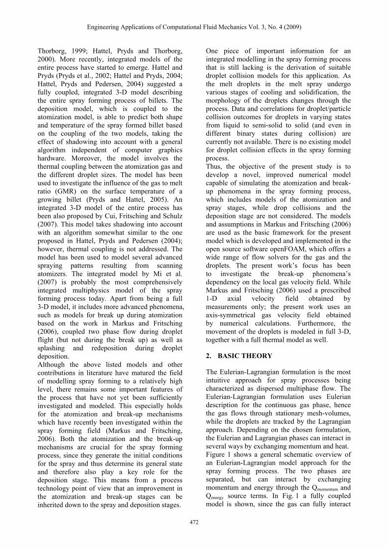
Engineering Applications of Computational Fluid Mechanics Vol. 3, No. 4, pp. 471–486 (2009)

COUPLED ATOMIZATION AND SPRAY MODELLING IN THE SPRAY FORMING PROCESS USING OPENFOAM

Rasmus Gjesing*, Jesper Hattel* and Udo Fritsching**

* Department of Mechanical Engineering, Technical University of Denmark, Building 425, DK-2820 Kgs. Lyngby, Denmark

** Institute for Materials Science, Bremen University, Badgasteiner Str. 3, D-28359 Bremen, Germany E-Mail: [email protected] (Corresponding Author)

ABSTRACT: The paper presents a numerical model capable of simulating the atomization, break-up and in-flight spray phenomena in the spray forming process. The model is developed and implemented in the freeware code openFOAM. The focus is on studying the coupling effect of the melt break-up phenomena with the local gas and droplets flow fields. The work is based on an Eulerian-Lagrangian description, which is implemented in a full 3D representation. The gas is described by the incompressible RANS equations, whereas the movement of the droplets is modeled by a tracking approach, together with a full thermal model for droplet cooling and solidification. The model is tested and validated against results from literature and experiments. Subsequently, the model is used to simulate the complex flow fields in the spray forming process and the results are discussed. The presented model of the spray forming process is able to predict the droplet size distribution of the spray from the process conditions, by introducing submodels for the melt fragmentation and successive secondary break-up processes as part of the spray model. Furthermore, the competition of drop break-up and solidification is derived by describing the thermal state of the particles in the spray. Therefore, the model includes a full thermal solver for the droplets, which also takes the rapid solidification of different drop sizes into account.

Keywords: spray simulation, atomization model, spray forming process, drop break-up and solidification, openFoam

1. INTRODUCTION

Spray forming is an advanced and complex material process providing the possiblity to produce preforms with enhanced mechanical properties. Spray forming can be used for producing preforms in near net shape. The spray forming process is most commonly used with stainless steels, super alloys, cast irons, tool steels, aluminum alloys and copper alloys. However, the spray forming process provides the possibility of handling new alloys, which can lead to even better mechanical properties compared to ingot metallurgy (Fritsching, 2004). Also MMCs (Metal Matrix Composites) are produced by co-injecting particles into the spray (Zhou, Wu and Lavernia, 1997). A more thorough description of the process and its advantages and limitations can be found in literature, see for example Fritsching (2004). The spray forming process is complex, since it involves highly transient and coupled phenomena. The increased understanding of the process based on numerical modeling and simulation makes it possible to consider how the process can be controlled and optimized. For the spray forming process a minimization of the gas

consumption (through a minimal gas to melt ratio (GMR)), higher yield of the process (thus avoiding overspraying and reducing the production time) and minimizing the porosity of the spray deposited product are aims for process optimization. The three general steps in the spray forming process, i.e. atomization, droplet flight and deposition have been modeled and reported extensively in the literature (reviewed in Fritsching (2004)). These models include numerical simulation of the dynamic and the thermal behaviour of individual droplets during flight stage (Mathur, Apelian and Lawley, 1989; Grant, Cantor and Katgerman, 1993; Bergmann, Fritsching and Bauckhage, 2000; Xu and Lavernia, 2001), models which describe the shape and the thermal state of the deposited material on the basis of thermal considerations (Mathur et al., 1991; Gutierrez-Miravete et al., 1989; Fritsching, Zhang and Bauckhage, 1994) and models that describe the billets shape based on geometrical considerations (Frigaard, 1995; Seok et al., 1998). Models taking the thermal coupling between gas and droplets into account have also been presented (Hattel et al., 1999; Pryds, Hattel and

Received: 4 Dec. 2008; Revised: 20 Mar. 2009; Accepted: 9 Apr. 2009

471

Engineering Applications of Computational Fluid Mechanics Vol. 3, No. 4 (2009)

Thorborg, 1999; Hattel, Pryds and Thorborg, 2000). More recently, integrated models of the entire process have started to emerge. Hattel and Pryds (Pryds et al., 2002; Hattel and Pryds, 2004; Hattel, Pryds and Pedersen, 2004) suggested a fully coupled, integrated 3-D model describing the entire spray forming process of billets. The deposition model, which is coupled to the atomization model, is able to predict both shape and temperature of the spray formed billet based on the coupling of the two models, taking the effect of shadowing into account with a general algorithm independent of computer graphics hardware. Moreover, the model involves the thermal coupling between the atomization gas and the different droplet sizes. The model has been used to investigate the influence of the gas to melt ratio (GMR) on the surface temperature of a growing billet (Pryds and Hattel, 2005). An integrated 3-D model of the entire process has been also proposed by Cui, Fritsching and Schulz (2007). This model takes shadowing into account with an algorithm somewhat similar to the one proposed in Hattel, Pryds and Pedersen (2004); however, thermal coupling is not addressed. The model has been used to model several advanced spraying patterns resulting from scanning atomizers. The integrated model by Mi et al. (2007) is probably the most comprehensively integrated multiphysics model of the spray forming process today. Apart from being a full 3-D model, it includes more advanced phenomena, such as models for break up during atomization based on the work in Markus and Fritsching (2006), coupled two phase flow during droplet flight (but not during the break up) as well as splashing and redeposition during droplet deposition. Although the above listed models and other contributions in literature have matured the field of modelling spray forming to a relatively high level, there remains some important features of the process that have not yet been sufficiently investigated and modeled. This especially holds for the atomization and break-up mechanisms which have recently been investigated within the spray forming field (Markus and Fritsching, 2006). Both the atomization and the break-up mechanisms are crucial for the spray forming process, since they generate the initial conditions for the spray and thus determine its general state and therefore also play a key role for the deposition stage. This means from a process technology point of view that an improvement in the atomization and break-up stages can be inherited down to the spray and deposition stages.

One piece of important information for an integrated modelling in the spray forming process that is still lacking is the derivation of suitable droplet collision models for this application. As the melt droplets in the melt spray undergo various stages of cooling and solidification, the morphology of the droplets changes through the process. Data and correlations for droplet/particle collision outcomes for droplets in varying states from liquid to semi-solid to solid (and even in different binary states during collision) are currently not available. There is no existing model for droplet collision effects in the spray forming process. Thus, the objective of the present study is to develop a novel, improved numerical model capable of simulating the atomization and break-up phenomena in the spray forming process, which includes models of the atomization and spray stages, while drop collisions and the deposition stage are not considered. The models and assumptions in Markus and Fritsching (2006) are used as the basic framework for the present model which is developed and implemented in the open source software openFOAM, which offers a wide range of flow solvers for the gas and the droplets. The present work’s focus has been to investigate the break-up phenomena’s dependency on the local gas velocity field. While Markus and Fritsching (2006) used a prescribed 1-D axial velocity field obtained by measurements only; the present work uses an axis-symmetrical gas velocity field obtained by numerical calculations. Furthermore, the movement of the droplets is modeled in full 3-D, together with a full thermal model as well.

2. BASIC THEORY

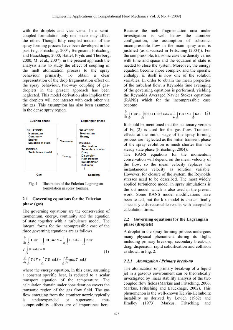
The Eulerian-Lagrangian formulation is the most intuitive approach for spray processes being characterized as dispersed multiphase flow. The Eulerian-Lagrangian formulation uses Eulerian description for the continuous gas phase, hence the gas flows through stationary mesh-volumes, while the droplets are tracked by the Lagrangian approach. Depending on the chosen formulation, the Eulerian and Lagrangian phases can interact in several ways by exchanging momentum and heat. Figure 1 shows a general schematic overview of an Eulerian-Lagrangian model approach for the spray forming process. The two phases are separated, but can interact by exchanging momentum and energy through the Qmomentum and Qenergy source terms. In Fig. 1 a fully coupled model is shown, since the gas can fully interact

472


473

with the droplets and vice versa. In a semi-coupled formulation only one phase may affect the other. Though fully coupled models of the spray forming process have been developed in the past (e.g. Fritsching, 2004; Bergmann, Fritsching and Bauckhage, 2000; Hattel, Pryds and Thorborg, 2000; Mi et al., 2007), in the present approach the analysis aims to study the effect of coupling of the melt atomization process to the spray behaviour primarily. To obtain a clear representation of the drop fragmentation effect on the spray behaviour, two-way coupling of gas-droplets in the present approach has been neglected. This model derivation also implies that the droplets will not interact with each other via the gas. This assumption has also been assumed in the dense spray region.

Fig. 1 Illustration of the Eulerian-Lagrangian formulation in spray forming.

2.1 Governing equations for the Eulerian phase (gas)

The governing equations are the conservation of momentum, energy, continuity and the equation of state together with a turbulence model. The integral forms for the incompressible case of the three governing equations are as follows

1d d d

d 0

d d grad dPr

CV CS CS CV

CS

CV CS CS

V S St

S

T V T S T St

ρ

ρ

υ

∂ + ⋅ = ⋅ +∂

⋅ =

∂ + ⋅ = ⋅∂

∫ ∫ ∫ ∫

∫

∫ ∫ ∫

U UU n T n b

U n

U n n

dV

(1)

where the energy equation, in this case, assuming a constant specific heat, is reduced to a scalar transport equation of the temperature. The calculation domain under consideration covers the transonic region of the gas flow field. The gas flow emerging from the atomizer nozzle typically is underexpanded or supersonic, thus compressibility effects are of importance here.

Because the melt fragmentation area under investigation is well below the atomizer configuration, the assumption of subsonic, incompressible flow in the main spray area is justified (as discussed in Fritsching (2004)). For the compressible, transonic case the density varies with time and space and the equation of state is needed to close the system. Moreover, the energy equation become more complex and the specific enthalpy, h, itself is now one of the solution variables. In order to obtain the mean properties of the turbulent flow, a Reynolds time averaging of the governing equations is performed, yielding the Reynolds Averaged Navier Stokes equations (RANS) which for the incompressible case become

( ) VSSVt CVCSCSCV

dd1d''d ∫∫∫∫ +⋅=⋅++∂∂ bnTnUUUUU

ρ (2)

It should be mentioned that the stationary version of Eq. (2) is used for the gas flow. Transient effects at the initial stage of the spray forming process are neglected as the initial transient phase of the spray evolution is much shorter than the steady state phase (Fritsching, 2004). The RANS equations for the momentum conservation will depend on the mean velocity of the flow, so the mean velocity replaces the instantaneous velocity as solution variable. However, for closure of the system, the Reynolds stresses need to be described. The most widely applied turbulence model in spray simulations is the k-ε model, which is also used in the present work. Some RANS model modifications have been tested, but the k-ε model is chosen finally since it yields reasonable results with acceptable calculation times.

2.2 Governing equations for the Lagrangian phase (droplets)

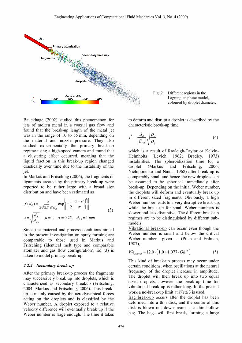
A droplet in the spray forming process undergoes many physical phenomena during its flight, including primary break-up, secondary break-up, drag, dispersion, rapid solidification and collision as shown in Fig. 2.

2.2.1 Atomization / Primary break-up

The atomization or primary break-up of a liquid jet in a gaseous environment can be theoretically investigated by linear stability analysis of the two coupled flow fields (Markus and Fritsching, 2006; Markus, Fritsching and Bauckhage, 2002). This phenomenon is the well-known Kelvin-Helmholtz instability as derived by Levich (1962) and Bradley (1973). Markus, Fritsching and


Fig. 2 Different regions in the Lagrangian phase model, coloured by droplet diameter.

Bauckhage (2002) studied this phenomenon for jets of molten metal in a coaxial gas flow and found that the break-up length of the metal jet was in the range of 10 to 55 mm, depending on the material and nozzle pressure. They also studied experimentally the primary break-up regime using a high-speed camera and found that a clustering effect occurred, meaning that the liquid fraction in this break-up region changed drastically over time due to the instability of the jet. In Markus and Fritsching (2006), the fragments or ligaments created by the primary break-up were reported to be rather large with a broad size distribution and have been estimated as

( )2

0.50.5

1exp22 2

, 1, 0.25, 1

dd

d

x xf dd

dx d md

μσπ σ

μ σ

⎧ ⎫−⎪ ⎪⎡ ⎤= −⎨ ⎬⎢ ⎥⎣ ⎦⎪⎩

= = = = m

⎪⎭ (3)

Since the material and process conditions aimed in the present investigation on spray forming are comparable to those used in Markus and Fritsching (identical melt type and comparable atomizer and gas flow configuration), Eq. (3) is taken to model primary break-up.

2.2.2 Secondary break-up

After the primary break-up process the fragments may successively break up into droplets, which is characterized as secondary breakup (Fritsching, 2004; Markus and Fritsching, 2006). This break-up is mainly caused by the aerodynamical forces acting on the droplets and is classified by the Weber number. A droplet exposed to a relative velocity difference will eventually break up if the Weber number is large enough. The time it takes

to deform and disrupt a droplet is described by the characteristic break-up time

g

d

rel

d

udt

ρρ

v=* (4)

which is a result of Rayleigh-Taylor or Kelvin-Helmholtz (Levich, 1962; Bradley, 1973) instabilities. The spheroidization time for a droplet (Markus and Fritsching, 2006; Nichiporenko and Naida, 1968) after break-up is comparably small and hence the new droplets can be assumed to be spherical immediately after break-up. Depending on the initial Weber number, the droplets will deform and eventually break up in different sized fragments. Obviously, a high Weber number leads to a very disruptive break-up, while the break-up for small Weber numbers is slower and less disruptive. The different break-up regimes are to be distinguished by different sub-models. Vibrational break-up can occur even though the Weber number is small and below the critical Weber number given as (Pilch and Erdman, 1987),

( )61077.10.10.12 .critical OhWe ⋅+⋅= (5)

This kind of break-up process may occur under certain conditions, when oscillations at the natural frequency of the droplet increase in amplitude. The droplet will then break up into two equal sized droplets, however the break-up time for vibrational break-up is rather long. In the present work a no-break-up limit at We ≤ 3 is used. Bag break-up occurs after the droplet has been deformed into a thin disk, and the centre of this disk is blown out downstream as a thin hollow bag. The bags will first break, forming a large

474


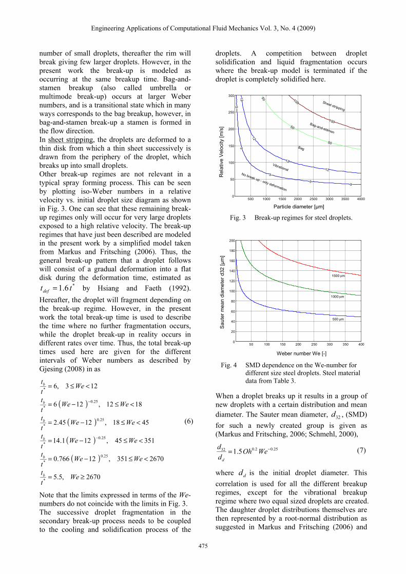
number of small droplets, thereafter the rim will break giving few larger droplets. However, in the present work the break-up is modeled as occurring at the same breakup time. Bag-and-stamen breakup (also called umbrella or multimode break-up) occurs at larger Weber numbers, and is a transitional state which in many ways corresponds to the bag breakup, however, in bag-and-stamen break-up a stamen is formed in the flow direction. In sheet stripping, the droplets are deformed to a thin disk from which a thin sheet successively is drawn from the periphery of the droplet, which breaks up into small droplets. Other break-up regimes are not relevant in a typical spray forming process. This can be seen by plotting iso-Weber numbers in a relative velocity vs. initial droplet size diagram as shown in Fig. 3. One can see that these remaining break-up regimes only will occur for very large droplets exposed to a high relative velocity. The break-up regimes that have just been described are modeled in the present work by a simplified model taken from Markus and Fritsching (2006). Thus, the general break-up pattern that a droplet follows will consist of a gradual deformation into a flat disk during the deformation time, estimated as

by Hsiang and Faeth (1992). Hereafter, the droplet will fragment depending on the break-up regime. However, in the present work the total break-up time is used to describe the time where no further fragmentation occurs, while the droplet break-up in reality occurs in different rates over time. Thus, the total break-up times used here are given for the different intervals of Weber numbers as described by Gjesing (2008) in as

*6.1 ttdef =

123,6* <≤= Wettb

( ) 1812,126 25.0* <≤−= − WeWe

ttb

( ) 4518,1245.2 25.0* <≤−= WeWe

ttb (6)

( ) 35145,121.14 25.0* <≤−= − WeWe

ttb

( ) 2670351,12766.0 25.0* <≤−= WeWe

ttb

2670,5.5* ≥= Wettb

Note that the limits expressed in terms of the We-numbers do not coincide with the limits in Fig. 3. The successive droplet fragmentation in the secondary break-up process needs to be coupled to the cooling and solidification process of the

droplets. A competition between droplet solidification and liquid fragmentation occurs where the break-up model is terminated if the droplet is completely solidified here.

500 1000 1500 2000 2500 3000 3500 40000

50

100

150

200

250

300

Particle diameter [μm]

Rel

ativ

e V

eloc

ity [m

/s]

33

3

33

12

12

12

12

50

50

50

100

100 Sheet stripping

Bag-and-stamen

Bag

VibrationalNo break up - only deformation

Particle diameter [µm]

Rel

ativ

e Ve

loci

ty [m

/s]

Fig. 3 Break-up regimes for steel droplets.

50 100 150 200 250 300 350 4000

20

40

60

80

100

120

140

160

180

200

Weber Number, We

Saut

er M

ean

Dia

met

er, d

32

500 μm

1000 μm

1500 μm

Sau

ter m

ean

diam

eter

d32

[µm

]

Weber number We [-] Fig. 4 SMD dependence on the We-number for

different size steel droplets. Steel material data from Table 3.

When a droplet breaks up it results in a group of new droplets with a certain distribution and mean diameter. The Sauter mean diameter, , (SMD) for such a newly created group is given as (Markus and Fritsching, 2006; Schmehl, 2000),

32d

25.02.032 5.1 −= WeOhdd

d

(7)

where is the initial droplet diameter. This correlation is used for all the different breakup regimes, except for the vibrational breakup regime where two equal sized droplets are created. The daughter droplet distributions themselves are then represented by a root-normal distribution as suggested in Markus and Fritsching (2006) and

dd

475


476

Schmehl (2000) with a mean diameter given by Eq. (7). Figure 4 shows the resulting SMD diameter for breakup of respectively a 500, 1000 and 1500 μm droplet exposed to different Weber numbers. A smaller droplet will yield a lower SMD than that of a larger droplet, and the SMD will decrease with increasing Weber numbers. The mass median diameter, , is related to the SMD by

5.0d

2.132

5.0 =dd (8)

and Schmehl (2000) found that for the bag and multimode regimes, the resulting droplet clusters could be described by the distribution given in Eq. (3) with σ = 0.238, which is also assumed in the present investigation.

Ti

Tem

pera

tur

me

e

1

2

3

4

5

TM

TL

TN

TS

Time

Tem

pera

ture

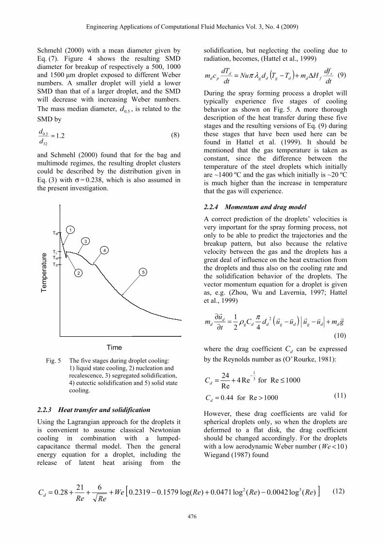
Fig. 5 The five stages during droplet cooling:

1) liquid state cooling, 2) nucleation and recalescence, 3) segregated solidification, 4) eutectic solidification and 5) solid state cooling.

2.2.3 Heat transfer and solidification

Using the Lagrangian approach for the droplets it is convenient to assume classical Newtonian cooling in combination with a lumped-capacitance thermal model. Then the general energy equation for a droplet, including the release of latent heat arising from the

solidification, but neglecting the cooling due to radiation, becomes, (Hattel et al., 1999)

( )dtdfHmTTdNu

dtdTcm s

fddgdgd

pd Δ+−= λπ (9)

During the spray forming process a droplet will typically experience five stages of cooling behavior as shown on Fig. 5. A more thorough description of the heat transfer during these five stages and the resulting versions of Eq. (9) during these stages that have been used here can be found in Hattel et al. (1999). It should be mentioned that the gas temperature is taken as constant, since the difference between the temperature of the steel droplets which initially are ~1400 ºC and the gas which initially is ~20 ºC is much higher than the increase in temperature that the gas will experience.

2.2.4 Momentum and drag model

A correct prediction of the droplets’ velocities is very important for the spray forming process, not only to be able to predict the trajectories and the breakup pattern, but also because the relative velocity between the gas and the droplets has a great deal of influence on the heat extraction from the droplets and thus also on the cooling rate and the solidification behavior of the droplets. The vector momentum equation for a droplet is given as, e.g. (Zhou, Wu and Lavernia, 1997; Hattel et al., 1999)

( ) gmuuuudCt

um ddgdgddgd

drvrvr

r

+−−=∂∂ 2

421 πρ

(10)

where the drag coefficient can be expressed by the Reynolds number as (O’Rourke, 1981):

dC

1324 4Re for Re 1000

RedC−

= + ≤

0.44 for Re 1000dC = > (11)

However, these drag coefficients are valid for spherical droplets only, so when the droplets are deformed to a flat disk, the drag coefficient should be changed accordingly. For the droplets with a low aerodynamic Weber number ( ) Wiegand (1987) found

10<We

62128.0ReRe

Cd ++= [ ])(log0042.0)(log0471.0)log(1579.02319.0 32 ReReReWe −+−+ (12)


For droplets that are exposed to a high Reynolds number, the drag coefficient will eventually equal the drag coefficient for a flat disk, i.e. Cd = 1.11. Thus, the drag coefficient over the deformation time is linearly increasing from 0.44 up to 1.11, expressed as (Markus and Fritsching, 2006):

⎭⎬⎫

⎩⎨⎧

><≤+

=1/11.1

1/044.0/65.0

def

defdefd ttfor

ttforttC (13)

2.2.5 Dispersion model

The mean gas velocity fields will be used, either obtained from an empirical formula or a simulated velocity field, and thus a dispersion model is needed to model the fluctuating velocity effect on the droplet behaviour and thus the transient motion caused by the turbulence. The dispersion model by Gosman and Ioannides is applied (Fritsching, 2004) with the eddy life time given as

ετ kcEE = (14)

where ε is the dissipation rate, k is the turbulent kinetic energy and cE = (0.3) is a constant. The residence time of a droplet in an eddy is given as

23R

g d

ku u

τ = =−l

lr v Eτ

)

(15)

where l is the length scale of the turbulent eddy. Thus, the interaction time between the droplet and the eddy can be defined as the minimum of the eddy life time and the residence time

( REI τττ ,min= (16)

The fluctuating velocity component is randomly selected from a Gaussian distribution with a standard deviation of 3/2k , which characterizes an isotropic turbulence field. The randomly selected fluctuating velocity component is then added to the mean component and a new fluctuating velocity component is first selected when the interaction time has passed, and thus either the eddy has dissipated or the droplet has left the eddy, and entered a new eddy with a new interaction time.

3. NUMERICAL SOLUTION IN OpenFOAM

The name openFOAM is compounded by the word “open” and the abbreviation “FOAM”. The word “open” implies that the computer program is

freely distributed as an open source code under the conditions and terms given by the GNU license, while “FOAM” is an abbreviation for Field Operation And Manipulation. OpenFOAM is a large open source C++ library which contains all kinds of tools for performing field operation and manipulation within the continuum mechanics; however openFOAM is especially strong on fluid dynamics. All the source code in openFOAM is freely available at www.opencfd.co.uk/openfoam/. The physical sub-models describing the gas and droplet behaviour in the spray forming process are implemented in open FOAM. The grid configuration used is adapted to the flow field under investigation, with small control volume size in the initial spray and atomization region and a coarser grid in the developed region of the spray. The total number of CV’s is ~52.000, obtaining a good compromise between accuracy and computaional effort, as has been proven by grid sensitivity testing versus the benchmark data (see below). Pressure boundaries are assumed at the circumference and the outlet areas of the computational domain.

4. VALIDATION AND RESULTS

The implemented model is benchmarked against the fundamental work by Grant, Cantor and Katgerman (1993) that is used as a reference. Droplets of melt (Al-4 wt% Cu) of different sizes (10 μm, 20 μm, 30 μm, 50 μm, 80 μm, 120 μm and 200 μm) are inserted into a prescribed axial atomization gas (N2) velocity field (material properties shown in Tables 1 & 2). Hence the case

Table 1 Material properties for the Al-4 wt% Cu melt, from Grant, Cantor and Katgerman (1993).

Melt properties Unit Al-4 wt% Cu

Density, ρ [kg/m3] 2950.4 Specific heat capacity, c p [J/kg K] 883.2 Heat of fusion, ∆H f [J/kg] 3,92*105 Melting temperature, T f [K] 933,05 Liquidus temperature, T liq [K] 919.4 Solidus temperature, T sol [K] 821,15 Partition coefficient, k e [-] 0,1667 Superheat, ∆T [°C] 150

477


478

Table 2 Material properties for the N2 atomization gas, from Grant, Cantor and Katgerman (1993).

Table 3 Material properties for steel, from Markus and Fritsching (2006).

Gas properties Unit N2

Density, ρ [kg/m3] 1,1346 Specific heat capacity, c p [J/kg K] 1042,11 Viscosity, μ [Pa s] 2,3*10-5 Heat conductivity, λ [W/m2 K] 0,026

Property Symbol Unit Steel

Melt flow-rate m [kg/s] 0.19Melt temperature, initial Tmelt [K] 1661.7Liquidus temperature Tliquidus [K] 1511.7Solidus temperature Tsolidus [K] 1467.4Density ρ [kg/m3] 6995Viscosity, dynamic μ [kg/m s] 0.0052Surface tension σ [N/m] 1.825Specific heat at liquidus cp, liquidus [J/kg K] 840Specific heat at solidus cp, solidus [J/kg K] 720Heat of fusion ΔHf [J/kg] 276 500

Axial distance [m] Axial distance [m]

Solid

frac

tion

[-]

Solid

frac

tion

[-]

Fig. 6 Comparison of results for A1-4 wt% Cu droplet axial solid fraction. Left: From Grant, Cantor and Katgerman

(1993). Right: Present work.

is a 1D calculation since only axial movement is considered; however since openFOAM always operates in 3D, the calculations are performed in 3D. The droplets are inserted at z = 0 mm and are then tracked until they leave the domain at z = 400 mm. The calculation is semi-coupled, hence only the gas influences the droplets and not vice versa. Moreover, even though the present model calculates the nucleation temperature based on Hattel et al. (1999), it was fixed in the benchmark case because this was the assumption in the original work by Grant, Cantor and Katgerman (1993). Figure 6 shows that only the 10 to 50 μm droplets are fully solidified for distances lower than 0.4 m. As in Hattel et al. (1999) the agreement with the results of Grant Cantor and Katgerman (1993) is excellent. A much more thorough description of this first validation case with all its assumptions and specific details including material properties

can be found in Hattel et al. (1999) and Gjesing (2008). Another case study is taken from Markus and Fritsching (2006), however there are some differences from the models applied in Markus and Fritsching (2006) and the models used in this work. Here, the calculations are done in full 3D and using a more advanced solidification model. However, as in Markus and Fritsching, the calculations are semi-coupled, neglecting droplet collision effects and tracking all droplets (no parcels) throughout the calculation domain. The gas velocity field is given by empirically found expressions from Markus and Fritsching (2006) while the gas temperature is held constant at 25 °C. Steel (material data in Table 3) is used for the melt material since Markus and Fritsching show most results for this material making the results applicable for direct comparison. Moreover, Markus and Fritsching operate with


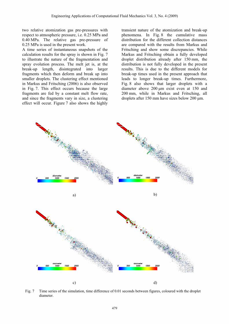
two relative atomization gas pre-pressures with respect to atmospheric pressure, i.e. 0.25 MPa and 0.40 MPa. The relative gas pre-pressure of 0.25 MPa is used in the present work. A time series of instantaneous snapshots of the calculation results for the spray is shown in Fig. 7 to illustrate the nature of the fragmentation and spray evolution process. The melt jet is, at the break-up length, disintegrated into larger fragments which then deform and break up into smaller droplets. The clustering effect mentioned in Markus and Fritsching (2006) is also observed in Fig. 7. This effect occurs because the large fragments are fed by a constant melt flow rate, and since the fragments vary in size, a clustering effect will occur. Figure 7 also shows the highly

transient nature of the atomization and break-up phenomena. In Fig. 8 the cumulative mass distribution for the different collection distances are compared with the results from Markus and Fritsching and show some discrepancies. While Markus and Fritsching obtain a fully developed droplet distribution already after 150 mm, the distribution is not fully developed in the present results. This is due to the different models for break-up times used in the present approach that leads to longer break-up times. Furthermore, Fig. 8 also shows that larger droplets with a diameter above 200 μm exist even at 150 and 200 mm, while in Markus and Fritsching, all droplets after 150 mm have sizes below 200 μm.

a)

b)

c)

d) Fig. 7 Time series of the simulation, time difference of 0.01 seconds between figures, coloured with the droplet

diameter.

479


0%

50%

100%

0 100 200 300 400particle size d [µm]

cum

ulat

ive

mas

s

100 mm150 mm200 mm

Particle size [µm]Particle size [µm]

Cum

ulat

ive

mas

s

Cum

ulat

ive

mas

s

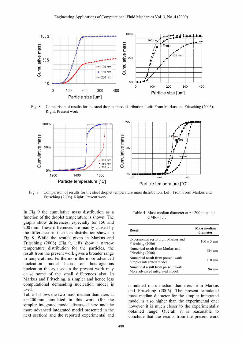
Fig. 8 Comparison of results for the steel droplet mass distribution. Left: From Markus and Fritsching (2006).

Right: Present work.

0%

50%

100%

1200 1400 1600particle temperature T [°C]

cum

ulat

ive

mas

s

100 mm150 mm200 mmC

umul

ativ

em

ass

Cum

ulat

ive

mas

s

Particle temperature [°C] Particle temperature [°C]

Fig. 9 Comparison of results for the steel droplet temperature mass distribution. Left: From From Markus and Fritsching (2006). Right: Present work.

In Fig. 9 the cumulative mass distribution as a function of the droplet temperature is shown. The graphs show differences, especially for 150 and 200 mm. These differences are mainly caused by the differences in the mass distribution shown in Fig. 8. While the results given in Markus and Fritsching (2006) (Fig. 9, left) show a narrow temperature distribution for the particles, the result from the present work gives a broader range in temperatures. Furthermore the more advanced nucleation model based on heterogenous nucleation theory used in the present work may cause some of the small differences also. In Markus and Fritsching, a simpler and hence less computational demanding nucleation model is used. Table 4 shows the two mass median diameters at z = 200 mm simulated in this work (for the simpler integrated model discussed here and the more advanced integrated model presented in the next section) and the reported experimental and

Table 4 Mass median diameter at z=200 mm and GMR=1.1.

Result Mass median diameter

Experimental result from Markus and Fritsching (2006) 100 ± 5 µm

Numerical result from Markus and Fritsching (2006) 134 µm

Numerical result from present work Simpler integrated model 110 µm

Numerical result from present work More advanced integrated model 94 µm

simulated mass median diameters from Markus and Fritsching (2006). The present simulated mass median diameter for the simpler integrated model is also higher than the experimental one; however it is much closer to the experimentally obtained range. Overall, it is reasonable to conclude that the results from the present work

480


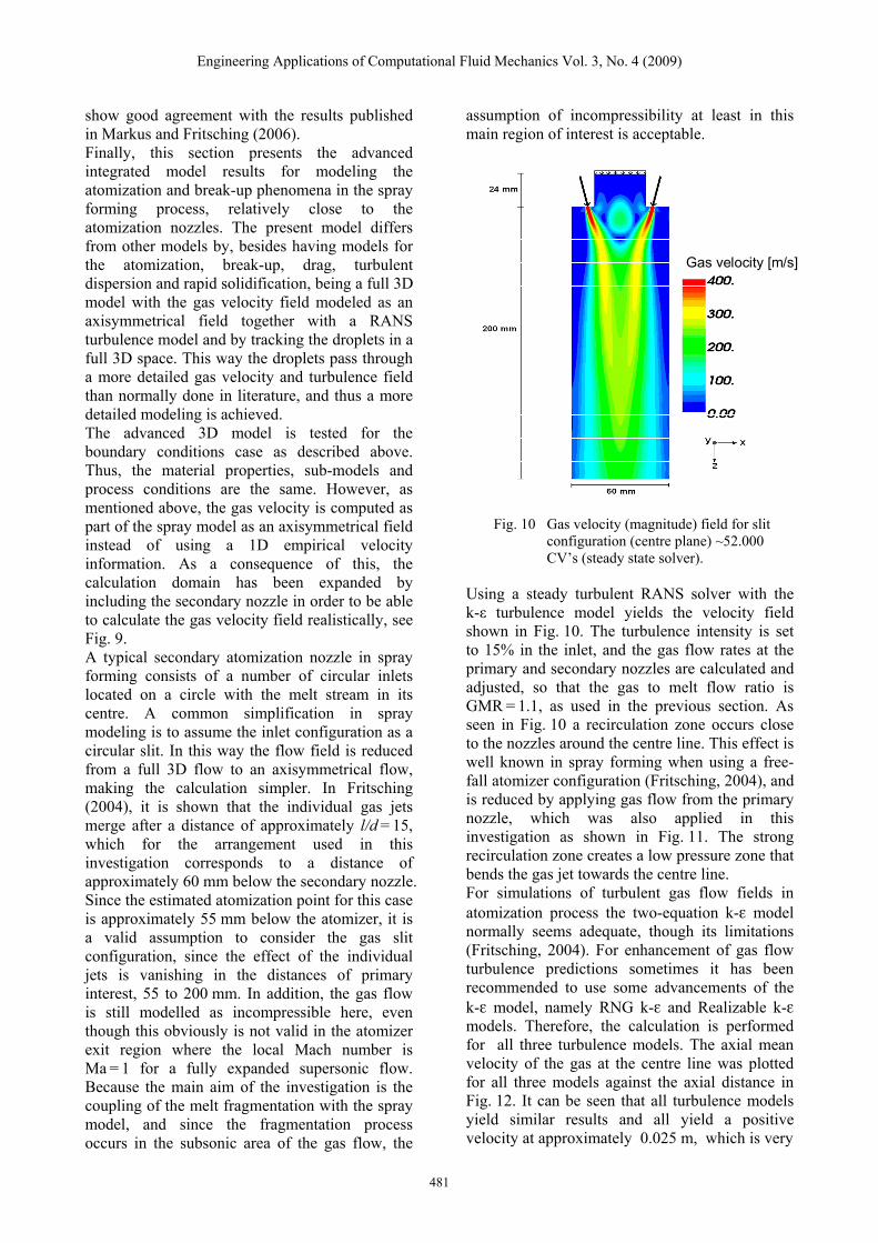
show good agreement with the results published in Markus and Fritsching (2006). Finally, this section presents the advanced integrated model results for modeling the atomization and break-up phenomena in the spray forming process, relatively close to the atomization nozzles. The present model differs from other models by, besides having models for the atomization, break-up, drag, turbulent dispersion and rapid solidification, being a full 3D model with the gas velocity field modeled as an axisymmetrical field together with a RANS turbulence model and by tracking the droplets in a full 3D space. This way the droplets pass through a more detailed gas velocity and turbulence field than normally done in literature, and thus a more detailed modeling is achieved. The advanced 3D model is tested for the boundary conditions case as described above. Thus, the material properties, sub-models and process conditions are the same. However, as mentioned above, the gas velocity is computed as part of the spray model as an axisymmetrical field instead of using a 1D empirical velocity information. As a consequence of this, the calculation domain has been expanded by including the secondary nozzle in order to be able to calculate the gas velocity field realistically, see Fig. 9. A typical secondary atomization nozzle in spray forming consists of a number of circular inlets located on a circle with the melt stream in its centre. A common simplification in spray modeling is to assume the inlet configuration as a circular slit. In this way the flow field is reduced from a full 3D flow to an axisymmetrical flow, making the calculation simpler. In Fritsching (2004), it is shown that the individual gas jets merge after a distance of approximately l/d = 15, which for the arrangement used in this investigation corresponds to a distance of approximately 60 mm below the secondary nozzle. Since the estimated atomization point for this case is approximately 55 mm below the atomizer, it is a valid assumption to consider the gas slit configuration, since the effect of the individual jets is vanishing in the distances of primary interest, 55 to 200 mm. In addition, the gas flow is still modelled as incompressible here, even though this obviously is not valid in the atomizer exit region where the local Mach number is Ma = 1 for a fully expanded supersonic flow. Because the main aim of the investigation is the coupling of the melt fragmentation with the spray model, and since the fragmentation process occurs in the subsonic area of the gas flow, the

assumption of incompressibility at least in this main region of interest is acceptable.

Gas velocity [m/s]

Fig. 10 Gas velocity (magnitude) field for slit configuration (centre plane) ~52.000 CV’s (steady state solver).

Using a steady turbulent RANS solver with the k-ε turbulence model yields the velocity field shown in Fig. 10. The turbulence intensity is set to 15% in the inlet, and the gas flow rates at the primary and secondary nozzles are calculated and adjusted, so that the gas to melt flow ratio is GMR = 1.1, as used in the previous section. As seen in Fig. 10 a recirculation zone occurs close to the nozzles around the centre line. This effect is well known in spray forming when using a free-fall atomizer configuration (Fritsching, 2004), and is reduced by applying gas flow from the primary nozzle, which was also applied in this investigation as shown in Fig. 11. The strong recirculation zone creates a low pressure zone that bends the gas jet towards the centre line. For simulations of turbulent gas flow fields in atomization process the two-equation k-ε model normally seems adequate, though its limitations (Fritsching, 2004). For enhancement of gas flow turbulence predictions sometimes it has been recommended to use some advancements of the k-ε model, namely RNG k-ε and Realizable k-ε models. Therefore, the calculation is performed for all three turbulence models. The axial mean velocity of the gas at the centre line was plotted for all three models against the axial distance in Fig. 12. It can be seen that all turbulence models yield similar results and all yield a positive velocity at approximately 0.025 m, which is very

481


482

similar to what is found from the empirical results. It should be noted that the maximal value of ~275 m/s for the axial gas velocity is predicted well by all turbulence models. Therefore, the standard k-ε model formulation is used in the present computation.

0 500 1000 1500 2000 2500 3000 3500 40000

0.002

0.004

0.006

0.008

0.01

0.012

Partic le Diameter [μm]

Num

ber f

requ

ency

0 500 1000 1500 2000 2500 3000 3500 40000

0.002

0.004

0.006

0.008

0.01

0.012

Partic le Diameter [μm]

Num

ber f

requ

ency

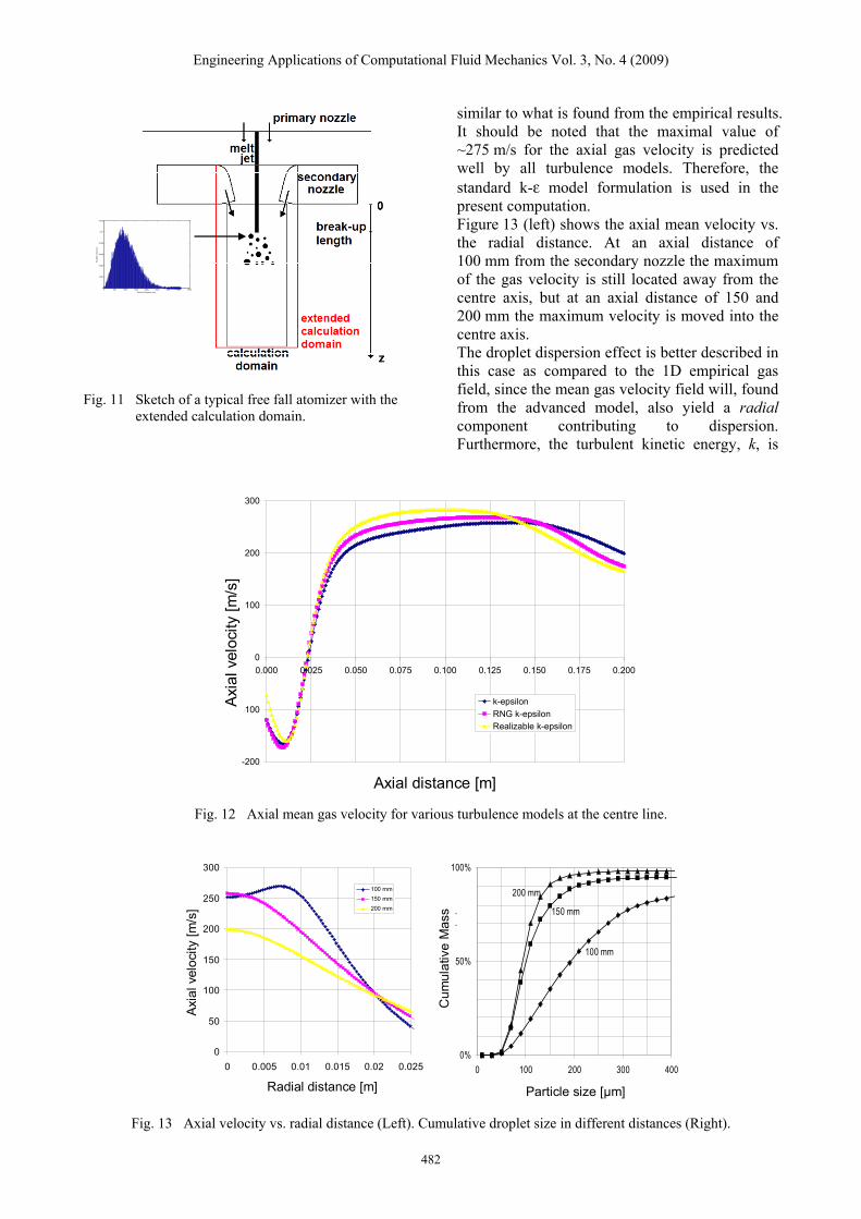
Figure 13 (left) shows the axial mean velocity vs. the radial distance. At an axial distance of 100 mm from the secondary nozzle the maximum of the gas velocity is still located away from the centre axis, but at an axial distance of 150 and 200 mm the maximum velocity is moved into the centre axis. The droplet dispersion effect is better described in this case as compared to the 1D empirical gas field, since the mean gas velocity field will, found from the advanced model, also yield a radial component contributing to dispersion. Furthermore, the turbulent kinetic energy, k, is

Fig. 11 Sketch of a typical free fall atomizer with the extended calculation domain.

-200

-100

0

100

200

300

0.000 0.025 0.050 0.075 0.100 0.125 0.150 0.175 0.200

Axial distance [m]

Axi

al v

eloc

ity [m

/s]

k-epsilonRNG k-epsilonRealizable k-epsilon

Axial distance [m]

Axia

l vel

ocity

[m/s

]

Fig. 12 Axial mean gas velocity for various turbulence models at the centre line.

0

50

100

150

200

250

300

0 0.005 0.01 0.015 0.02 0.025Radial distance [m]

Axi

al v

eloc

ity [m

/s]

100 mm150 mm200 mm

0%

50%

100%

0 100 200 300 400

Particle Size [µm]

Cum

ulat

ive

Mas

s (%

)

100 mm

150 mm

200 mm

Radial distance [m]

Axia

l vel

ocity

[m/s

]

Cum

ulat

ive

Mas

s

Particle size [µm] Fig. 13 Axial velocity vs. radial distance (Left). Cumulative droplet size in different distances (Right).


modeled as a distributed field, whereas in the previous section and in Markus and Fritsching (2006) it was assumed as constant for the entire calculation domain. This means that the turbulent intensity is dynamically calculated dependent on the position of the droplet, and this affects both the turbulent droplet dispersion and also the heat transfer from the droplet. The resulting cumulative mass droplet distributions are shown in Fig. 13 (right). This result, when compared to the case in Fig. 8 (right), shows that smaller droplets are more rapidly formed in the advanced model. This is primarily caused by the higher Weber numbers that are caused by the higher relative velocity resulting from the advanced model. Since the jet is fully modelled here, higher gas velocities will occur for the advanced model having their maximum value

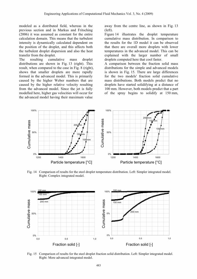
away from the centre line, as shown in Fig. 13 (left). Figure 14 illustrates the droplet temperature cumulative mass distribution. In comparison to the results for the 1D model it can be observed that there are overall more droplets with lower temperatures in the advanced model. This can be explained with the larger number of small droplets computed here that cool faster. A comparison between the fraction solid mass distributions for the simple and advanced models is shown in Fig. 15. There are large differences for the two models' fraction solid cumulative mass distributions. Both models predict that no droplets have started solidifying at a distance of 100 mm. However, both models predict that a part of the spray begins to solidify at 150 mm,

0%

50%

100%

1200 1400 1600Particle Temperature [°C]

Cum

ulat

ive

Mas

s (%

)

100 mm

150 mm

200 mm

0%

50%

100%

1200 1400 1600Particle Temperature [°C]

Cum

ulat

ive

Mas

s (%

)

100 mm

150 mm200 mm

Particle temperature [°C]Particle temperature [°C]

Cum

ulat

ive

mas

s

Cum

ulat

ive

mas

s

Fig. 14 Comparison of results for the steel droplet temperature distribution. Left: Simpler integrated model.

Right: Complex integrated model.

0%

50%

100%

0,0 0,5 1,0Fraction Solid [-]

Cum

ulat

ive

Mas

s (%

100 mm

200 mm

150 mm

Fig. 15 Comparison of results for the steel droplet fraction solid distribution. Left: Simpler integrated model.

Right: More advanced integrated model.

)

0%

50%

100%

0,0 0,5 1,0Fraction Solid [-]

Cum

ulat

ive

Mas

s (%

)

200 mm

150 mm

100 mm

Cum

ulat

ive

mas

s

Cum

ulat

ive

mas

s

Fraction solid [-] Fraction solid [-]Fraction Solid [-] Fraction Solid [-]Fraction solid [-] Fraction solid [-]

483


although with some difference, since the simpler model predicts that only 3 mass percent of the spray started solidifying here, while the advanced model predicts that 20 mass percent of the spray has already started solidifying. This difference increases at 200 mm, where the simple model predicts that 17 mass percent of the spray has started solidifying and 0 mass percent has finished solidifying. As opposed to this, the advanced model predicts that 67 mass percent of the spray has started solidifying, while 3 percent has finished solidifying, leaving 64 mass percent within the solidification interval at 200 mm. Thus only a small fraction of the spray begins to solidify using the 1D model, while the advanced model predicts that a much larger fraction of the spray begins solidifying. The difference can be explained by the overall smaller droplet diameter obtained by the advanced model, and because turbulence effects have been modeled in more detail, thus affecting the Nusselt number obtained from the modified Ranz-Marshall equation. The fraction solid is an important process parameter in soray forming, since the mass fraction solid is aimed at about 50% at the deposition point. For this case, using the advanced model, the mass median fraction solid is around 0.25 at an axial distance of 200 mm from the secondary nozzle, and thus the spray should solidify further before a successful deposition may take place. The mass median doplet diameter in the final spray for the advanced model is computed as 94 µm. In Table 4 all the obtained mass median droplet diameters are listed. The overall performance of the advanced integrated model can be evaluated by comparing the mass median diameter with experimental and modeling results reported in Markus and Fritsching (2006) in Table 4. The advanced model obtains a better estimate of the spray mass median diameter than any other models, followed by that of the 1D simple model which is also fairly close to the measurements. However, the simple model may be preferred over the advanced model, since it obtains reasonable results within a computation time significantly lower than that of the advanced model. Therefore, it is possible to perform more parameter variations and thus increase the understanding of the break-up phenomena and mechanisms in the spray forming process. However, the simple model needs the gas velocity distribution a priori, thus making the model dependent on empirical data, whereas the advanced model predict the gas velocity field as part of the simulation, thus making this model more general. Even though both models obtain

droplet sizes close to the experimental data, the results for the solid fraction differ quite substantially. This underlines the importance of an advanced description of the gas velocity field to the modeling results.

5. SUMMARY AND CONCLUSIONS

In the present work an integrated 3D model for simulating the coupled melt atomization and spray behavior within the spray forming process has been developed. The model is able to predict the final droplet size distribution of the spray, resulting from atomization and successive secondary droplet break-up. Furthermore, the thermal state of the spray is modelled, and the model also includes a full thermal solver for the droplets that takes rapid solidification into account. The nucleation temperature is dynamically calculated for every single droplet along its flight. Furthermore, the drag phenomena for the deformed droplets are modeled. The integrated 3D model includes several sub-models each accounting respectively for atomization, secondary breakup, drag, rapid solidification and turbulent dispersion. The integrated model formulation is implemented in openFOAM, thus making it accessible to everyone. Therefore, it is easy to investigate and replace the different sub-models, e.g. to couple the droplet to a simulated gas flow field. The advanced model shows a good ability to predict the resulting mass median diameter in the spray. The simulation results show that the incorporation of turbulence effects is important, however, the choice of the actual isotropic turbulence model seems to have a limited effect only. The open implemenation in openFOAM makes future incorporation of other sub-models, e.g. for droplet collisions, possible.

NOMENCLATURE

Small Latin letters

b Body force per unit mass (N kg-1) cp Specific heat capacity (J kg-1K-1) d Diameter (m, mm or μm)

d 0.5 Mass median diameter (m, mm or μm)

d 32 Sauter mean diameter (m, mm or μm)f ( ) Propability f s Fraction solid (mass based) g Acceleration due to gravity (ms-2) k Turbulent kinetic energy (m2 s-2) k Equilibrium partition coefficient

484


m Mass (kg) m& Mass flow rate (kg s-1) n Outward pointing normal p Pressure (Pa) t Time (s) u , , v w Velocity (m s-1) x , y , z Distance (m) Capital Latin letters A Area (m2) Cd Drag coefficient ∆H f Latent heat (J kg-1) S Surface area (m2) T Stress tensor (Pa) T Temperature (K) U Velocity (m s-1) U Velocity vector (m s-1) V Volume (m3) Greek letters ε Dissipation of turbulent kinetic

energy (m2 s-3) λ Thermal conductivity (Wm-1K-1) μ Viscosity (kg m-1s-1) ρ Density (kg m-3) σ Standard deviation

Cτ Collision response time (s)

Eτ Eddy life time (s)

Iτ Interaction time (s)

Rτ Residence time (s) Dimensionless numbers Ma Mach number Nu Nusselt number Oh Ohnesorge number Pr Prandtl number Re Reynolds number We Weber number Subscripts and superscripts b break up d droplet def deformation g gas

REFERENCES

1. Bergmann D, Fritsching U, Bauckhage K (2000). A mathematical model for cooling and rapid solidification of molten metal droplets. Int. J. Therm. Sci. 39:53–62.

2. Bradley D (1973). On the atomization of liquids by high-velocity gases, Part 1. J. Phys. D: Appl. Phys. 6:1724–1736, and Part 2., J. Phys. D: Appl. Phys. 6:2267–2272.

3. Crowe CT, Sommerfeld M, Tsuji Y (1998). Multiphase Flows with Droplets and Particles. CRC Press, Boca Raton, USA.

4. Cui C, Fritsching U, Schulz A (2007). Three-dimensional mathematical modeling and numerical simulation of billet shape in spray forming using a scanning gas atomizer. Metallurgical and Materials Transactions B 38B, 333–346.

5. Frigaard IA (1995). Growth dynamics of spray formed aluminium billets. SIAM J. Appl. Math. 55(5):1161–1203.

6. Fritsching U (2004). Spray Simulation: Modelling and Numerical Simulation of Sprayforming Metals. Cambridge University Press, Cambridge, UK.

7. Fritsching U, Zhang H, Bauckhage K (1994). Numerical simulation of temperature distribution and solidification behaviour during spray forming. Steel Res. 65:273–278.

8. Gjesing R (2008). A New Integrated Numerical Model of the Atomization and In Flight Phenomena in the Spray Forming Process. Ph.D. thesis, Department of Mechanical Engineering, Technical University of Denmark, DTU.

9. Grant PS, Cantor B, Katgerman L (1993). Modelling of droplet dynamic and thermal histories during spray forming. Acta Metall. Mater. 41(11):3097–3108.

10. Gutierrez-Miravete E, Lavernia EJ, Trapaga GM, Szekely J, Grant NJ (1989). A mathematical model of the liquid dynamic compaction process. Metall. Trans. A 20, 71.

11. Hattel JH, Pryds NH (2004). A unified spray forming model for the prediction of billet shape geometry. Acta Mater. 52(18):5275–5288.

12. Hattel JH, Pryds NH, Pedersen TB (2004). An integrated numerical model for the prediction of Gaussian and billet shapes. Materials Science and Engineering A 383(1):184–189.

13. Hattel JH, Pryds NH, Thorborg J (2000). A numerical investigation of the effect of droplet size distribution on gas temperature

485


486

during spray forming. Scripta Materialia 42:145–150.

14. Hattel JH, Pryds NH, Thorborg J, Ottosen P (1999). A quasi-stationary numerical model of atomized metal droplets I. Modelling and Simulation in Materials Science and Engineering 7(3):413–430.

15. Hsiang LP, Faeth GM (1992). Near limit drop deformation and secondary breakup. Int. J. Multiphase Flow 18(5):635–652.

16. Levich VG (1962). Physicochemical Hydrodynamics. Prentice Hall, Upper Saddle River, NJ, pp. 501–667.

17. Markus S, Fritsching U (2006). Discrete break-up modeling for melt sprays. International Journal of Powder Metallurgy 42(4):23–32.

18. Markus S, Fritsching U, Bauckhage K (2002). Jet break up of liquid metals in twin fluid atomization. Materials Science and Eng. A 326:122–133.

19. Mathur P, Annavarapu S, Apelian D, Lawley A (1991). Spray casting: an integrated model for process understanding and control. Mater. Sci. Eng. A 142:261–276.

20. Mathur P, Apelian D, Lawley A (1989). Analysis of the spray deposition process. Acta Metall. 37:429–443.

21. Mi J, Grant PS, Fritsching U, Belkessam O, Garmendia I, Landabarea A (2008). Multiphysics modelling of the spray forming process. Mat. Sci. Engng. A 477:2–8.

22. Nichiporenko S, Naida YI (1968). Heat exchange between metal particles and gas in the atomization process. Soviet Powder Metall. Metal Ceramics 7(7):509–512.

23. OpenCFD Limited. http://www.opencfd.co.uk/openfoam/

24. O’Rourke PJ (1981). Collective Drop Effects on Vaporizing Liquid Sprays. Technical Report LA-9069-T, Los Alamos National Laboratory.

25. Pilch M, Erdman CA (1987). Use of breakup time data and velocity history data to predict the maximum size of stable fragments for acceleration-induced breakup of a liquid drop. Int. J. Multiphase Flow 13(6):741–757.

26. Pryds NH, Hattel JH (2005). A numerical investigation of the influence of the gas to melt ratio on the billet surface temperature. International Journal of Thermal Sciences 44(6):587–597.

27. Pryds NH, Hattel JH, Pedersen TB, Thorborg J (2002). An integrated numerical model of the spray forming process. Acta Mater. 50(16):4075–4091.

28. Pryds NH, Hattel JH, Thorborg J (1999). A quasi-stationary numerical model of atomized metal droplets 2. Modelling and Simulation in Materials Science and Engineering 7(3):431–446.

29. Schmehl R (2000). CFD Analysis of fuel atomization, secondary droplet breakup and spray dispersion in the premix duct of a LPP combustor. 8th International Conference on Liquid Atomization and Spray Systems, Pasadena, CA, USA.

30. Seok HK, Yeo DH, Oh KH, Lee HI, Ra HY (1998). A three-dimensional model of the spray forming process. Metallurgical and Materials Transactions B 29B, 699–708.

31. Wiegand H (1987). Die Einwirkung eines ebenem Strömungsfeldes auf frei bewegliche Tropfen und ihren Widerstandsbeiwert im Reynoldszahlbereich von 50 bis 2000. Fortschr.-Ber. VDI Reihe 7, Nr. 120, VDI-Verlag, Düsseldorf, Germany.

32. Xu Q, Lavernia EJ (2001). Influence of nucleation and growth phenomena on microstructural evolution during droplet-based deposition. Acta Mater. 49:3849–3861.

33. Zhou Y, Wu Y, Lavernia EJ (1997). Process modeling in spray deposition: A review. Int. J. Non-equilibrium Processing 10:95–186.

Engineering Applications of Computational Fluid Mechanics Vol COUPLED ATOMIZATION AND SPRAY...

Documents

Transcript of Engineering Applications of Computational Fluid Mechanics Vol COUPLED ATOMIZATION AND SPRAY...