A computational framework for fluid-solid-growth modeling in cardiovascular simulations
Upload
khangminh22Category
view
1download
0

Lecture Notesin Computational Scienceand Engineering
Timothy J. BarthMichael GriebelDavid E. Keyes
Dirk RooseTamar Schlick
Risto M. Nieminen
Editors
For further volumes:http://www.springer.com/series/3527
74

•

Editors
123
●Damien Tromeur-Dervout●
Parallel Computational FluidDynamics 2008
Parallel Numerical Methods, Software
Development and Applications
Gunther Brenner David R. Emerson Jocelyne Erhel

Printed on acid-free paper
ISSN 1439-7358
Springer is part of Springer Science + Business Media (www.springer.com)
Springer Heidelberg Dordrecht London New York
Cover design: deblik, Berlin
This work is subject to copyright. All rights are reserved, whether the whole or part of the material is
or parts thereof is permitted only under the provisions of the German Copyright Law of September 9,
liable to prosecution under the German Copyright Law.The use of general descriptive names, registered names, trademarks, etc. in this publication does not imply,
and regulations and therefore free for general use.
concerned, specifically the rights of translation, reprinting, reuse of illustrations, recitation, broadcasting,reproduction on microfilm or in any other way, and storage in data banks. Duplication of this publication
even in the absence of a specific statement, that such names are exempt from the relevant protective laws
1965, in its current version, and permission for use must always be obtained from Springer. Violations are
EditorsDamien Tromeur-DervoutUniversité Lyon 1 - CNRSInstitut Camille JordanBd du 11 Novembre 1918 4369622 [email protected]
Gunther BrennerTU ClausthalInstitut für Technische MechanikAdolph-Roemer-Str. 2A38678 [email protected]
David R. Emerson
Daresbury LaboratoryScience and Technology Facilities Council
Daresbury Science and Innovation CampusWA4 4AD Warrington CheshireUnited Kingdom
Jocelyne ErhelINRIA - SAGECampus de Beaulieu35042 [email protected]
ISBN 978-3-642-14437-0 e-ISBN 978-3-642-14438-7DOI: 10.1007/978-3-642-14438-7
Mathematics Subject Classification Numbers (2010): 65F10, 65N06, 65N08, 65N22, 65N30, 65N55, 65Y05, 65Y10, 65Y20, 15-06, 35-06, 76-XX 76-06
© Springer-Verlag Berlin Heidelberg 2010
Library of Congress Control Number: 2010935447

Preface
Parallel CFD 2008, the twentieth in the high-level international series of meetingsfeaturing different aspect of parallel computing in computational fluid dynamics andother modern scientific domains was held May 19−22, 2008 in Lyon, France.
The themes of the 2008 meeting included the traditional emphases of this con-ference, and experiences with contemporary architectures. Around 70 presentationswere included into the conference program in the following sessions:Parallel Algorithms and solversParallel performances with contemporary architecturesStructured and unstructured grid methods, boundary methodssoftware framework and components architectureCFD applications (Bio fluid, environmental problem) Lattice Boltzmann method andSPHOptimisation in Aerodynamics
This book presents an up-to-date overview of the state of the art in Parallel Com-putational Fluid Dynamics from Asia, Europe, and North America. This reviewedproceedings included about sixty percent of the oral lectures presented at the confer-ence.
The editors.

VI Preface
Parallel CFD 2008 was organized by the Institut Camille Jordan of the Univer-sity of Lyon 1 in collaboration with the Center for the Development of the ParallelScientific Computing.
The Scientific Committee and Local Organizers of Parallel CFD 2008 are de-lighted to acknowledge the generous sponsorship of the following organizations,through financial or in-kind assistance. Assistance of our sponsors allowed to or-ganize scientific as well as social program of the conference.
Scientific Comittee Intel, Germany SGI, FranceUniversity Lyon 1
Institut Camille Jordan Region Rhone-AlpesUniversity Lyon 1
Center for Development of Fluorem ModelysUniversity Lyon 1
Many people worked to organize and execute the conference. We are especiallygrateful to all members of the international scientific committee. We also want tothank the key members of the local organizing committee David Guibert, Toan PhamDuc, Patrice linel, Simon Pomarede, Thomas Dufaud, Nicolas Kielbasievich, DanielFogliani, Fabienne Oudin, Brigitte Hautier, Sandrine Montingy.
We also thank our colleagues Frederic Desprez from the Laboratoired’Informatique du Parallelisme (LIP) Ecole Normale Superieure de Lyon, MichelLance from the Laboratoire de Mecanique des Fluides et d’Accoustique (LMFA)Ecole Centrale de Lyon, and Patrick Quere from the Computer Science Laboratoryfor mechanics and Engineering Sciences (LIMSI) for their help to promote this event.
Damien Tromeur-DervoutChairman, Parallel CFD 2008.

Contents
Part I Invited speakers
Large Scale Computations in Nuclear Engineering: CFD for MultiphaseFlows and DNS for Turbulent Flows with/without Magnetic FieldTomoaki Kunugi, Shin-ichi Satake, Yasuo Ose, Hiroyuki Yoshida, KazuyukiTakase . . . . . . . . . . . . . . . . . . . . . . . . . . . . . . . . . . . . . . . . . . . . . . . . . . . . . . . . . . 3
Scalable algebraic multilevel preconditioners with application to CFDAndrea Aprovitola, Pasqua D’Ambra, Filippo Denaro, Daniela di Serafino,Salvatore Filippone . . . . . . . . . . . . . . . . . . . . . . . . . . . . . . . . . . . . . . . . . . . . . . . . 15
Acceleration of iterative solution of series of systems due to better initialguessDamien Tromeur-Dervout, Yuri Vassilevski . . . . . . . . . . . . . . . . . . . . . . . . . . . . . 29
Part II Optimisation in Aerodynamics Design
Aerodynamic Study of Vertical Axis Wind TurbinesMerim Mukinovic, Gunther Brenner, Ardavan Rahimi . . . . . . . . . . . . . . . . . . . . 43
Parallel Shape Optimization of a Missile on a Grid InfrastructureErdal Oktay, Osman Merttopcuoglu, Cevat Sener, Ahmet Ketenci, Hasan U.Akay . . . . . . . . . . . . . . . . . . . . . . . . . . . . . . . . . . . . . . . . . . . . . . . . . . . . . . . . . . . 51
Analysis of Aerodynamic Indices for Racing Sailing Yachts: aComputational Study and Benchmark on up to 128 CPUs.Ignazio Maria Viola, Raffaele Ponzini, Daniele Rocchi, Fabio Fossati . . . . . . . . 61
Parallel implementation of fictitious surfaces method for aerodynamicshape optimizationS. Peigin, B. Epstein, S. Gali . . . . . . . . . . . . . . . . . . . . . . . . . . . . . . . . . . . . . . . . . 71

VIII Contents
Path Optimization of Dual Airfoils Flapping in a Biplane Configurationwith RSM in a Parallel Computing EnvironmentMustafa Kaya, Ismail H. Tuncer . . . . . . . . . . . . . . . . . . . . . . . . . . . . . . . . . . . . . . 83
Part III Grid methods
Convergence Improvement Method for Computational Fluid DynamicsUsing Building-Cube MethodTakahiro Fukushige Toshihiro Kamatsuchi Toshiyuki Arima and Seiji Fujino . . . 93
Aerodynamic Analysis of Rotor Blades using Overset Grid with ParallelComputationDong-Kyun Im, Seong-Yong Wie, Eugene Kim, Jang-Hyuk Kwon, Duck-JooLee, and Ki-Hoon Chung, and Seung-Bum Kim . . . . . . . . . . . . . . . . . . . . . . . . . . 101
Large scale massively parallel computations with the block-structuredelsA CFD softwareM. Gazaix, S. Mazet, M. Montagnac . . . . . . . . . . . . . . . . . . . . . . . . . . . . . . . . . . 111
Applications on Hybrid Unstructured Moving Grid Method forThree-Dimensional Compressible FlowsHiroya Asakawa Masashi Yamakawa and Kenichi Matsuno . . . . . . . . . . . . . . . . 119
Progressive Development of Moving-Grid Finite-Volume Method forThree-Dimensional Incompressible FlowsShinichi ASAO, Sadanori ISHIHARA, Kenichi MATSUNO, Masashi
YAMAKAWA . . . . . . . . . . . . . . . . . . . . . . . . . . . . . . . . . . . . . . . . . . . . . . . . . . . . . 127
Part IV Boundary methods
Flow Computations Using Embedded Boundary Conditions on BlockStructured Cartesian GridT. Kamatsuch, T. Fukushige, K. Nakahashi . . . . . . . . . . . . . . . . . . . . . . . . . . . . . 137
Computation of Two-phase Flow in Flip-chip Packaging Using Level SetMethodTomohisa Hashimoto, Keiichi Saito, Koji Morinishi,, Nobuyuki Satofuka . . . . . . 145
A Parallel Immersed Boundary Method for Blood-like Suspension FlowSimulationsF. Pacull, M. Garbey . . . . . . . . . . . . . . . . . . . . . . . . . . . . . . . . . . . . . . . . . . . . . . . 153

Contents IX
Part V High Order methods
3D Spectral Parallel Multi-Domain computing for natural convectionflowsS. Xin, J. Chergui, P. Le Quere . . . . . . . . . . . . . . . . . . . . . . . . . . . . . . . . . . . . . . 163
3D time accurate CFD simulations of a centrifugal compressorAndreas Lucius, Gunther Brenner . . . . . . . . . . . . . . . . . . . . . . . . . . . . . . . . . . . . 173
Part VI Parallel Algorithms and Solvers
Multicolor SOR Method with Consecutive Memory AccessImplementation in a Shared and Distributed Memory ParallelEnvironmentKenji Ono, Yasuhiro Kawashima . . . . . . . . . . . . . . . . . . . . . . . . . . . . . . . . . . . . . 183
Proper Orthogonal Decomposition In Decoupling Large DynamicalSystemsToan Pham, Damien Tromeur-Dervout . . . . . . . . . . . . . . . . . . . . . . . . . . . . . . . . . 193
Performance Analysis of the Parallel Aitken-Additive Schwarz WaveformRelaxation Method on Distributed EnvironmentHatem Ltaief, Marc Garbey . . . . . . . . . . . . . . . . . . . . . . . . . . . . . . . . . . . . . . . . . 203
Aitken-Schwarz Acceleration not based on the mesh for CFDD. Tromeur-Dervout . . . . . . . . . . . . . . . . . . . . . . . . . . . . . . . . . . . . . . . . . . . . . . . 211
From extruded-2D to fully-3D geometries for DNS: a Multigrid-basedextension of the Poisson solverA. Gorobets, F. X. Trias, M. Soria, C. D. Perez-Segarra, A. Oliva . . . . . . . . . . . 219
Parallel direct Poisson solver for DNS of complex turbulent flows usingUnstructured MeshesR.Borrell, O.Lehmkuhl, F.X.Trias, M.Soria, A.Oliva . . . . . . . . . . . . . . . . . . . . . . 227
A numerical scheme for the computation of phase transition incompressible multiphase flowsVincent Perrier . . . . . . . . . . . . . . . . . . . . . . . . . . . . . . . . . . . . . . . . . . . . . . . . . . . 235
Part VII Lattice Boltzman and SPH Methods
Lattice Boltzmann Simulations of Slip Flow of Non-Newtonian Fluids inMicrochannelsRamesh K. Agarwal and Lee Chusak . . . . . . . . . . . . . . . . . . . . . . . . . . . . . . . . . . 247
Multiple Relaxation Time Lattice Boltzmann simulation of binarydroplet collisionsErnesto Monaco, Kai H. Luo, Gunther Brenner . . . . . . . . . . . . . . . . . . . . . . . . . . 257

X Contents
High-Performance Computing and Smoothed Particle HydrodynamicsC. Moulinec, R. Issa, D. Latino, P. Vezolle, D.R. Emerson and X.J. Gu . . . . . . . . 265
Part VIII software Framework and Component Architecture
An integrated object-oriented approach for parallel CFDDominique Eyheramendy,David Loureiro, Fabienne Oudin-Dardun . . . . . . . . . . 275
Fast Multipole Method for particle interactions: an open source parallellibrary componentF. A. Cruz, M. G. Knepley, L. A. Barba . . . . . . . . . . . . . . . . . . . . . . . . . . . . . . . . 285
Hybrid MPI-OpenMP performance in massively parallel computationalfluid dynamicsG. Houzeaux, M. Vazquez, X. Saez and J.M. Cela . . . . . . . . . . . . . . . . . . . . . . . . 293
Hierarchical adaptive multi-mesh partitioning algorithm onheterogeneous systemsY. Mesri, H. Digonnet, T. Coupez . . . . . . . . . . . . . . . . . . . . . . . . . . . . . . . . . . . . . 299
Part IX Parallel Performance
Towards Petascale Computing with Parallel CFD codesA.G. Sunderland, M. Ashworth, C. Moulinec, N. Li, J. Uribe, Y. Fournier . . . . . 309
Scalability Considerations of a Parallel Flow Solver on Large ComputingSystemsErdal Yilmaz, Resat U. Payli, Hassan U. Akay, Akin Ecer, and Jingxin Liu . . . . . 321
Large Scaled Computation of Incompressible Flows on Cartesian MeshUsing a Vector-Parallel SupercomputerShun Takahashi, Takashi Ishida, Kazuhiro Nakahashi, Hiroaki Kobayashi,Koki Okabe, Youichi Shimomura, Takashi Soga, Akihiko Musa . . . . . . . . . . . . . 331
Dynamic Load Balancing on Networked Multi-core ComputersStanley Chien, Gun Makinabakan, Akin Ecer, and Hasan Akay . . . . . . . . . . . . . 339
On efficiency of supercomputers in CFD simulationsAndrey V. Gorobets, Tatiana K. Kozubskaya, Sergey A. Soukov . . . . . . . . . . . . . . 347
Part X Environment and biofluids applications
Numerical Study of Pulsatile Flow Through Models of Vascular Stenoseswith Physiological Waveform of the HeartJason D. Thompson, Christian F. Pinzn and Ramesh K. Agarwal . . . . . . . . . . . . 357

Contents XI
Fluid Flow - Agent Based Hybrid Model for the Simulation of VirtualPrairiesMarc Garbey, Cendrine Mony, Malek Smaoui . . . . . . . . . . . . . . . . . . . . . . . . . . . 369
HPC for hydraulics and industrial environmental flow simulationsReza Issa, Fabien Decung, Emile Razafindrakoto, Eun-Sug Lee, Charles
Moulinec, David Latino, Damien Violeau, Olivier Boiteau . . . . . . . . . . . . . . . . . 377
Multi-parametric intensive stochastic simulations for hydrogeology on acomputational gridJ. Erhel, J.-R. de Dreuzy, E. Bresciani . . . . . . . . . . . . . . . . . . . . . . . . . . . . . . . . . 389
Parallel computation of pollutant dispersion in industrial sitesJ. Montagnier, M. Buffat, D. Guibert . . . . . . . . . . . . . . . . . . . . . . . . . . . . . . . . . . 399
Part XI General fluid
3D Numerical Simulation Of Gas Flow Around Reentry VehiclesS.V. Polyakov, T.A. Kudryashova, E.M. Kononov, A.A. Sverdlin . . . . . . . . . . . . 409
Effective Parallel Computation of Incompressible Turbulent Flows onNon-uniform GridHidetoshi Nishida, Nobuyuki Ichikawa . . . . . . . . . . . . . . . . . . . . . . . . . . . . . . . . . 417
Secondary flow structure of turbulent Couette-Poiseuille and Couetteflows inside a square ductHsin-Wei Hsu, Jian-Bin Hsu, Wei Lo, Chao-An Lin . . . . . . . . . . . . . . . . . . . . . . . 425

•

Part I
Invited speakers

Large Scale Computations in Nuclear Engineering:CFD for Multiphase Flows and DNS for TurbulentFlows with/without Magnetic Field
Tomoaki Kunugi1, Shin-ichi Satake2, Yasuo Ose1, Hiroyuki Yoshida3, andKazuyuki Takase3
1 Kyoto University, Yoshida, Sakyo, Kyoto 6060-8501, Japan2 Tokyo University of Science, 2641 Yamazaki, Noda 278-8510, Japan3 Japan Atomic Energy Agency, 2-4, Shirakata, Tokai-mura 319-1195, [email protected]
Abstract. Large scale computations are being carried out in nuclear engineering fields suchas light water reactors, fast breeder reactors, high temperature gas-cooled reactors and nuclearfusion reactors. The computational fluid dynamics (CFD) regarding not only the single-phaseflows but also the two-phase flow plays an important role for the developments of advancednuclear reactor systems. In this review paper, some examples of large scale computations innuclear engineering fields are illustrated by using a parallel visualization.
Key words: Direct numerical simulation; Multiphase flows; Turbulent flows; Paral-lel visualization; Magnetohydrodynamics; Nuclear reactors; Fusion reactors.
1 Numerical Simulation of Boiling Phenomena
It is important to remove the heat from industrial devices and nuclear reactors witha high heat flux to insure their safety. In order to enhance the heat transfer, phasechange phenomena such as evaporation and condensation have to be utilized, so thatit is important to understand the mechanism of boiling to design industrial devices.Although many researchers have experimentally studied the boiling phenomena, ithas not been clarified yet because it consists of a lot of complicated phenomena. Asfor pool boiling experiments, Kenning & Yan measured the spatial and temporal vari-ations of wall temperature in nucleate boiling by using a liquid crystal thermometry.They pointed out the importance of non-uniform wall temperature distribution andsuggested that the transient heat conduction model proposed by Mikic & Rohsenow[2] was unrealistic because of the assumption of uniform transient heat conduction.It is relatively difficult to perform numerical analysis of boiling phenomenon be-cause it includes the phase change. On the other hands, a critical heat flux (CHF)is also very important for high heat flux removal. However, the empirical correla-tion of the CHF is used in most designs. In general, the prediction of CHF is very
D. Tromeur-Dervout (eds.), Parallel Computational Fluid Dynamics 2008,Lecture Notes in Computational Science and Engineering 74,DOI: 10.1007/978-3-642-14438-7 1, c© Springer-Verlag Berlin Heidelberg 2010

4 T.Kunugi, S.Satake, Y.Ose, H.Yoshida and K.Takase
difficult because of the complexity of relation between the nucleation boiling andthe bubble departure due to flow convection. Welch [3] carried out the numericalstudy on two-dimensional two-phase flow with a phase change model using a finitevolume method combined with a moving grid, however it can be applied only to alittle deformation of gas-liquid interface. Son & Dhir [4] also carried out the two-dimensional pool boiling simulation using a finite difference method with a movinggrid. Recently, Juric & Tryggvason [5] conducted a film boiling with a front track-ing method by Unverdi & Tryggvason [6]. They pointed out the importance of thetemporal and spatial temperature distribution of the heating plate: heat conduction inthe slab. The author developed a new volume tracking method, so-called gMARS:Multi-interface Advection and Reconstruction Solver[7].
This section describes that the MARS is applied to the force convective flowboiling in the channel with an appropriate phase change model: a model for boilingand condensation phenomena based on a homogeneous nucleation and a well-knownenthalpy method. This model is good for metal casting problems because of no su-perheating of liquid. As for the water, it has to be considered the liquid superheatfor nucleate boiling phenomena. The direct numerical simulations with this phasechange model for pool nucleate boiling and forced convective flow boiling have beenperformed. The aims of this study are to develop a direct numerical method to simu-late boiling phenomena and to simulate the three-dimensional pool nucleate boilingand forced convective flow boiling by the direct numerical simulation (DNS) basedon the MARS combined the enthalpy method considered the liquid superheat as thephase change model.
1.1 Numerical Simulation based on MARS
Governing equations.
In this section, the direct numerical multiphase flow solver (MARS) is briefly ex-plained. As for m fluids including the gas and liquid, the spatial distribution of fluidscan be defined as
〈F〉 =∑Fm = 1.0 (1)
The continuity equation of the multiphase flows for m fluids:
∂Fm
∂ t+∇ · (FmU)−Fm∇U = 0 (2)
The momentum equation with the following CSF (Continuum Surface Force)model proposed by Brackbill [9] is expressed as:
∂U∂ t
+∇(UU) = G− 1〈ρ〉∇P−∇ · τ+
1〈ρ〉FV (3)
CSF model :FV = σκn〈ρ〉/ρ (4)

Large Scale Computations in Nuclear Engineering 5
here, the mean density at interface, ρ = (ρg +ρl)/2, the suffix g denotes vapor and lfor water. κ is curvature of the surface, σ the surface tension coefficient and n is thenormal vector to the surface.
The momentum equation (3) can be solved by means of the well-known projec-tion method. The Poisson equation for the pressure can be solved by the ILUBCGmethod. Finally, the new velocity field can be obtained. Once the velocity field canbe obtained, it can be transported the volume of fluid by the MARS, i.e., a kind ofPLIC (Piecewise Linear Calculation) volume tracking procedure [24] for Eq. (2).The detail description of the solution procedure is described in the reference [7].
The energy equation is expressed as:
∂∂ t
〈ρCv〉T +∇ · (〈ρCv〉UT ) = ∇ · (〈λ 〉∇T )−P(∇ ·U)+ Q, (5)
where Cv, T , λ , Q is specific heat, temperature, heat conductivity, heat generationterm, respectively. The second term of the right hand side of the equation (5), theClausius-Clapeyron relation is considered as the work done by the phase change.
Phase Change Model.
As mention in the introduction section, nucleate boiling phenomena need to be mod-eled. One of ideas for this modeling can be considered:
Nucleate boiling model = Nucleation model + Bubble growth model
Nucleation model: This model gives the homogeneous superheat limit of liquid andthe size of nucleus of bubble. A superheat limit Ts is got from the kinetic theory[8] or the usual cavity model. Typically Ts is around 110◦C in water pool boiling atan atmospheric pressure. The equilibrium radius re of nucleus corresponding to Ts
can be calculated by Eq. (6) based on the thermodynamics. The F-value of nucleuscorresponding to the ratio of a cell size to a size of nucleus where the shape ofnucleus is assumed to be a sphere is given to a computational cell with greater thanTs. In this study, Ts is a parameter. Although Ts varies in spatial on the heated surfacefrom the experiment [1], Ts is assumed to be uniform on the heated surface in thepresent study. Therefore, particular nucleation sites are not specified.
re =2σ
Psat (Tl)exp{vl [Pl −Psat (Tl)]/RTl}−Pl,(Tl ≥ Ts) (6)
where re is a radius of bubble embryo, σ is an interfacial tension, Tl is a temperatureof liquid, Psat is a pressure corresponding saturation conditions, Pl is a pressure ofliquid, vl is a volume of liquid per unit mass, and R is the ideal gas constant on a perunit mass basis.
Bubble growth model: Increasing the temperature, liquid water becomes vapor par-tially if the temperature of liquid is greater than the liquid saturation line (Tl), i.e.,liquid-gas mixture (two-phase region) and then eventually becomes the superheatedgas phase if the temperature is greater than the gas saturation lime (Tg). This processcan be treated by the enthalpy method.

6 T.Kunugi, S.Satake, Y.Ose, H.Yoshida and K.Takase
Fig. 1. Computational domain for forced convective flow boiling
1.2 Results and Discussions on Forced Convective Flow Boiling
In order to get some insights into the mechanism of three-dimensional forced con-vective subcooled flow boiling. Figure 1 shows the computational domain that isa three-dimensional vertical channel and the sidewall is heated with constant heatflux because of considering the spatial and temporal variations of temperature in thesolid sidewall. The length of flow channel is 60 mm, 6 mm in height and 5 mm inwidth. The computational domain is a half channel because of the symmetry. Theheating conditions are as follows: 0.3 mm in length from inlet is adiabatic and fol-lowing 50 mm by heating of a constant heat flux, 2.4 MW/m2 from the outside ofsolid sidewall of 0.6 mm in thickness and the remaining 9.7 mm is also adiabatic.The inlet mean velocity is 0.5 m/s with a parabolic profile. The no-slip condition atthe sidewall, the slip velocity at the symmetric boundary and constant pressure atthe outlet are imposed as the boundary conditions. The periodic velocity and tem-perature conditions are applied to the spanwise boundaries. The water pressure isatmospheric and the degree of water subcooling is 20 K. The solid wall is assumedto be a stainless steel. The degree of superheat is set to be 50 K. The computationalcell is uniform cubic shape and the size of cell is 100 μm and the number of cells is36(x) 600(y) 50(z)=1,080,000. Time increment is 5 μsec. The fictitious temperaturedifference used in the enthalpy method is ΔT=0.1 K.
Resulting from the forced convective flow boiling computation as shown in Fig.2, the series of bubble growth are depicted as black spots, and the gray contours showthe temperature distribution at x=0.25 mm every 52.5 msec. From the temperature

Large Scale Computations in Nuclear Engineering 7
evolution, the thermal boundary layer has been developing during computation anddoes not reach to the equilibrium state at the downstream in this computation, so thatit is necessary to carry out much longer computation. The maximum size of bub-ble is around 1 mm at the present stage. It is interesting that the higher temperaturestagnation region is formed in the middle of the channel and three higher tempera-ture streaks are observed in the thermal boundary layer. The bubble generated in theupstream region becomes just like an obstacle and makes a high temperature stagna-tion or recirculation region behind the nucleated bubbles. Eventually, another bubblewill generate in that stagnation or recirculation region because the degree of liquidsubcooling could be decreased, i.e., it can be saying a “chain generation of boilingbubbles.”
[°C]101.0
95.8
90.5
85.3
80.0
Fig. 2. Bubble growth and temperature distribution every 52.5 msec
2 CFD for Two-Phase Flow Behaviors in Nuclear Reactor
Subchannel analysis codes [11]-[13] and system analysis codes [14, 15] are usuallyused for the thermal-hydraulic analysis of fuel bundles in nuclear reactors. As for theformer, however, many constitutive equations and empirical correlations based onexperimental results are needed to predict the water-vapor two-phase flow behavior.If there are no experimental data such as an advanced light-water reactor which hasbeen studied at the Japan Atomic Energy Agency (JAEA) in Japan and named as

8 T.Kunugi, S.Satake, Y.Ose, H.Yoshida and K.Takase
a reduced moderation water reactor (RMWR), it is very difficult to obtain the pre-cise predictions [16, 17, 18]. The RMWR core has a remarkably narrow gap spacingbetween fuel rods (i.e., around 1 mm) and a triangular tight lattice fuel rod configu-ration in order to reduce the moderation of the neutron. In such a tight-lattice core,there is no sufficient information about the effects of the gap spacing and the effectof the spacer configuration on the two-phase flow characteristics. Therefore, in orderto analyze the water vapor two-phase flow dynamics in the tight-lattice fuel bundle,a large-scale simulation under the full bundle size condition is necessary. The EarthSimulator [19] enables that lots of computational memories are required to attain thetwo-phase flow simulation for the RMWR core.
In JAEA, numerical investigation on the physical mechanisms of complicatedthermal-hydraulic characteristics and the multiphase flow behavior with phase changein nuclear reactors has been carried out In this numerical research, some of the au-thors in JAEA pointed out the improvements of the conventional reactor core ther-mal design procedures and then proposed a predicting procedure for two-phase flowcharacteristics inside the reactor core more directly than the conventional proceduresfor the first time in the world by reducing the usage of constitutive and empiricalequations as much as possible [20]. Based on this idea, a new thermal design pro-cedure for advanced nuclear reactors with the large-scale direct simulation method(TPFIT: Two-Phase flow simulation code using advanced Interface Tracking) [21]has been developed at JAEA. Especially, thermal hydraulic analyses of two-phaseflow positively for a fuel bundle simulated by the full size using the Earth Simulatorare performed [22]. This section describes the preliminary results of the large-scalewater-vapor two-phase flow simulation in the tight-lattice fuel bundle of the RMWRcore by the TPFIT code.
2.1 Numerical Simulation of Two-Phase Flow Behavior in 37 RMWR FuelRods
The TPFIT code is based on the CIP method [23] using the modified interface-tracking method [24]. The surface tension of bubble is calculated using the CSF[9]. Figure 3 shows the computational geometry consisting of 37 RMWR fuel rods.The geometry and dimensions simulate the experimental conditions done by JAEA[25]. Here, the fuel rod outer diameter is 13 mm and the gap spacing between eachrod is 1.3 mm. The casing has a hexagonal cross section and a length of one hexag-onal side is 51.6 mm. An axial length of the fuel bundle is 1260 mm. The waterflows upward from the bottom of the fuel bundle. A flow area is a region in whichdeducted the cross-sectional area of all fuel rods from the hexagonal flow passage.The spacers are installed into the fuel bundle at the axial positions of 220, 540, 750and 1030 mm from the bottom. The axial length of each spacer is 20 mm. Inlet con-ditions of water are as follows: temperature 283◦C, pressure 7.2 MPa, and flow rate400 kg/m2s. Moreover, boundary conditions are as follows: fluid velocities for x-, y-and z-directions are zero on every wall (i.e., an inner surface of the hexagonal flowpassage, outer surface of each fuel rod and surface of each spacer); velocity profile atthe inlet of the fuel bundle is set to be uniform. The present simulations were carried

Large Scale Computations in Nuclear Engineering 9
out under the non-heated isothermal flow condition in order to remove the effect ofheat transfer due to the fuel rods to the fluid. A setup of a mixture condition of waterand vapor at the heating was performed by changing the initial void fraction of waterat the inlet of the analytical domain.
Fuel Rod diameter
51.6 mm
Outlet
Spacer
Spacer
Spacer
Spacer
Flo
w d
irect
ion
20 m
m
220
mm 54
0 m
m 750
mm 10
30 m
m
1260
mm
Inlet
1.3 mmGap spacing
f = 13 mm
Fig. 3. Outline of three-dimensional analytical geometry of a tight-lattice fuel bundle
2.2 Results and Discussions
Figure 4 shows an example of the predicted vapor structure around the fuel rods.Here, the distribution of void fraction within the region from 0.5 to 1 is shown: 0.5indicates just an interface between the water and vapor and is shown by green; and 1indicates the non-liquid vapor and is shown by red. Vapor flows from the upstreamto downstream like a streak through the triangular region, and the interaction of thevapor stream to the circumferential direction is not seen. On the other hand, sincethe vapor is disturbed behind a spacer, the influence of turbulence by existence of thespacer can be predicted.
In order to predict the water-vapor two-phase flow dynamics in the RMWR fuelbundle and to reflect them to the thermal design of the RMWR core, a large-scalesimulation was performed under a full bundle size condition using the Earth Sim-ulator. Details of water and vapor distributions around fuel rods and a spacer were

10 T.Kunugi, S.Satake, Y.Ose, H.Yoshida and K.Takase
Water Film Flow Vapor
Vertical
Cross-sectionalView
Horizontal
Cross-sectional
View
High speed region
Vapor
bubble
Spacer
Region
Flow
Fig. 4. Predicted vapor structure around fuel rods; black region indicates the water (void frac-tion is 0), and light grey region indicates an interface between water and vapor which meansthe void fraction is in between 0 and 1.
clarified numerically. A series of the present preliminary results were summarized asfollows: 1) The fuel rod surface is encircled with thin water film; 2) The bridge for-mation by water film appears in the region where the gap spacing between adjacentfuel rods is narrow; 3) Vapor flows into the triangular region where the gap spacingbetween fuel rods is large; 4) A flow configuration of vapor shows a streak structurealong the triangular region.
3 DNS for Turbulent Flows with/without Magnetic Field
On the other hand, in the gas-cooled reactor and the fast breeder reactors the coolantis a single-phase flow at mostly turbulent situation. Direct numerical simulations(DNSs) for turbulent flows have been carried out to investigate the turbulent structurein the flow passage and around each fuel rod surface at Reynolds number of 78,000as shown in Fig. 5. A second order finite difference method is applied to the spatialdiscretization, the 3rd order Runge-Kutta method and the Crank-Nicolson methodare applied to the time discretization, and the time advancing scheme is the fractionaltime step is used for the coupling scheme, so called, Dukowcz-Dvinsky scheme. Thenumber of used central processing unit is 1,152 and it corresponds to 144 nodes.The total memory is 2 terabytes and the total number of computational grid is 7,200

Large Scale Computations in Nuclear Engineering 11
million points [26, 27]. The flow visualization is very important to grasp the entirepicture of the flow behavior, so that a parallel visualization technique is applied in thiscase. As for the thermofluid behavior in fusion reactors, the magnetohydrodynamic(MHD) effect is very important. DNS for turbulent flow in a parallel channel has beenperformed as shown in Fig. 7 [28] drawn by the parallel visualization. The turbulentstructure is suppressed by the magnetic field, i.e., Lorentz force: Hartmann numbersare 0 (non-MHD) and 65 (MHD).
Fig. 5. Second invariant contour surface of velocity tensor of single-phase turbulent flow in apipe Re=78,000, 7,200 Mega grids, 2 Tera Bytes
4 Conclusion
The computational fluid dynamics (CFD) regarding not only the single-phase flowsbut also the two-phase flow plays an important role for the developments of advancednuclear reactor systems. To establish the large-scale simulation procedure withhigher prediction accuracy is very important for the detailed reactor-core thermal-design in the nuclear engineering. Moreover, the parallel visualization technique isvery useful to understand the detailed flow and heat transfer phenomena.

12 T.Kunugi, S.Satake, Y.Ose, H.Yoshida and K.Takase
Flo
w
Flo
w
Magnetic Field
Ha=65Ha=0
Magnetic Field Magnetic Field
Fig. 6. Magnetic field effect on turbulent flow in a parallel channel: Second invariant contourof velocity tensor
[1] Kenning, D. B. R., Youyou, Y Pool boiling heat transfer on a thin plate: featuresrevealed by liquid crystal thermography International Journal of Heat andMass Transfer, Vol. 39, No. 15, 3117-3137, 1996.
[2] Mikic, B. B., Rohsenow, W. M Bubble growth rates in non-uniform temperaturefield ASME J. Heat Transfer 91, 245-250, 1969.
[3] Welch, S. W. J Local Simulation of Two-Phase Flows Including InterfaceTracking with Mass Transfer J. Comput. Phys., vol. 121, 142-154, 1995.
[4] Son, G., Dhir, V. K Numerical Simulation of Saturated Film Boiling on aHorizontal Surface J. Heat Transfer, Vol. 119, 525-533, 1997.
[5] Juric, D., Tryggvason, G Computations of boiling flows Int. J. MultiphaseFlow, vol. 24, 387-410, 1998.
[6] Unverdi, S., Tryggvason, G A front-tracking method for viscous, incompress-ible, multifluid flows J. Comput. Phys., vol. 100, 25-37, 1992.

Large Scale Computations in Nuclear Engineering 13
[7] Kunugi, T MARS for Multiphase Calculation Computational Fluid DynamicsJournal, Vol.9, No. 1, 563-571, 2001
[8] Carey, V. P Liquid-vapor Phase-change Phenomena - An introduction to theThermophysics of Vaporization and Condensation Processes in Heat TransferEquipment, Chapters 5 and 6, Taylor & Francis, 1992.
[9] Brackbill, J. U., Kothe, D. B., Zemach, C A continuum method for modelingsurface tension J. Comput. Phys., Vol. 100, 335-354, 1992.
[10] Kunugi, T., Saito, N., Fujita, Y., Serizawa, A Direct Numerical Simulation ofPool and Forced Convective Flow Boiling Phenomena Heat Transfer 2002,Vol. 3, 497-502, 2002.
[11] Kelly, J. E., Kao, S. P., Kazimi, M. S THERMIT-2: A two-fluid model for lightwater reactor subchannel transient analysis MIT-EL-81-014, 1981.
[12] Thurgood, M. J COBRA/TRAC - A thermal-hydraulic code for transient anal-ysis of nuclear reactor vessels and primary coolant systems, equation and con-stitutive models NURREG/CR-3046, PNL-4385, Vol. 1, R4, 1983.
[13] Sugawara, S., Miyamoto, Y FIDAS: Detailed subchannel analysis code basedon the three-fluid and threefield model Nuclear Engineering and Design,vol.129, 146-161, 1990.
[14] Taylor, D TRAC-BD1/MOD1: An advanced best estimated computer pro-gram for boiling water reactor transient analysis, volume 1 - model descriptionNUREG/CR-3633, 1984.
[15] Liles, D TRAC-PF1/MOD1: An advanced best-estimate computer program forpressurized water reactor analysis NUREG/CR-3858, LA-10157-MS, 1986.
[16] Iwamura, T., Okubo, T Development of reduced-moderation water reactor(RMWR) for sustainable energy supply Proc. 13th Pacific Basin Nuclear Con-ference (PBNC 2002), Shenzhen, China, 1631-1637, 2002.
[17] Iwamura, T Core and system design of reduced-moderation water reactor withpassive safety features Proc. 2002 International Congress on Advanced in Nu-clear Power Plants (ICAPP 2002), No.1030, Hollywood, Florida, USA, 2002.
[18] Okubo, T., Iwamura, T Design of small reduced-moderation water reactor(RMWR) with natural circulation cooling Proc. International Conference onthe New Frontiers of Nuclear Technology; Reactor Physics, Safety and High-Performance Computing (PHYSOR2002), Seoul, Korea, 2002.
[19] Earth Simulator Center, Annual report of the earth simulator center (April2002- March 2003) Japan Marine Science and Technology Center, 2003.
[20] Takase, K., Tamai, H., Yoshida, H., Akimoto, H Development of a Best Esti-mate Analysis Method on Two-Phase Flow Thermal-Hydraulics for Reduced-Moderation Water Reactors Proc. Best Estimate Twenty-O-Four (BE2004), Ar-lington, Washington D.C., USA, November, 2004.
[21] Yoshida, H., Takase, K., Ose, Y., Tamai, H., Akimoto, H Numerical simulationof liquid film around grid spacer with interface tracking method Proc. Interna-tional Conference on Global Environment and Advanced Nuclear Power Plants(GENES4/ANP2003), No.1111, Kyoto, Japan, 2003.
[22] Takase, K., Yoshida, H., Ose, Y., Kureta, M., Tamai, H., Akimoto, H Numeri-cal investigation of two-phase flow structure around fuel rods with spacers by

14 T.Kunugi, S.Satake, Y.Ose, H.Yoshida and K.Takase
large-scale simulations Proc. 5th International Conference on Multiphase Flow(ICMF04), No.373, Yokohama, Japan, June, 2004.
[23] T. Yabe, T The constrained interpolation profile method for multiphase analysisJ. computational Physics, vol.169, No.2, 556-593, 2001.
[24] Youngs, D.L Numerical methods for fluid dynamics, Edited by Morton K.W.& Baine, M.J. Academic Press, 273-285, 1982.
[25] Kureta, M., Liu, W., Tamai, H., Ohnuki, A., Mitsutake, T., Akimoto, H De-velopment of Predictable Technology for Thermal/Hydraulic Performance ofReduced-Moderation Water Reactors (2) - Large-scale Thermal/Hydraulic Testand Model Experiments - Proc. 2004 International Congress on Advanced inNuclear Power Plants (ICAPP 2002), No.4056, Pittsburg, Pennsylvania, USA,June, 2004.
[26] Satake, S., Kunugi, T. Himeno, R High Reynolds Number Computation forTurbulent Heat Transfer in a Pipe Flow, M. Valero et al. (Eds.), Lecture Notesin Computer Science 1940 High Performance Computing, 514-523, 2000.
[27] Satake, S., Kunugi, T., Takase, K., Ose, Y., Naito, N Large Scale Structures ofTurbulent Shear Flow via DNS, A. Veidenbaum et al. (Eds.), Lecture Notes inComputer Science 2858 High Performance Computing, 468-475, 2003.
[28] Satake, S., Kunugi, T., Takase, K., Ose, Y Direct numerical simulation of tur-bulent channel flow under a uniform magnetic field for large-scale structures athigh Reynolds number Physics of Fluid, 18, 125106, 2006.

Scalable algebraic multilevel preconditioners withapplication to CFD
Andrea Aprovitola1, Pasqua D’Ambra2, Filippo Denaro1,Daniela di Serafino3, and Salvatore Filippone4
1 Department of Aerospace and Mechanical Engineering, Second University of Naples, viaRoma 29, I-81031 Aversa, Italy,[email protected]& [email protected]
2 Institute for High-Performance Computing and Networking (ICAR), CNR, via PietroCastellino 111, I-80131 Naples, Italy,[email protected]
3 Department of Mathematics, Second University of Naples, via Vivaldi 43, I-81100 Caserta,Italy,[email protected]
4 Department of Mechanical Engineering, University of Rome “Tor Vergata”, viale delPolitecnico 1, I-00133, Rome, Italy,[email protected]
Abstract. The solution of large and sparse linear systems is one of the main computationalkernels in CFD applications and is often a very time-consuming task, thus requiring the use ofeffective algorithms on high-performance computers. Preconditioned Krylov solvers are themethods of choice for these systems, but the availability of “good” preconditioners is crucialto achieve efficiency and robustness. In this paper we discuss some issues concerning the de-sign and the implementation of scalable algebraic multilevel preconditioners, that have shownto be able to enhance the performance of Krylov solvers in parallel settings. In this context,we outline the main objectives and the related design choices of MLD2P4, a package of multi-level preconditioners based on Schwarz methods and on the smoothed aggregation technique,that has been developed to provide scalable and easy-to-use preconditioners in the ParallelSparse BLAS computing framework. Results concerning the application of various MLD2P4preconditioners within a large eddy simulation of a turbulent channel flow are discussed.
Key words: Preconditioning technique, Schwarz domain decomposition, Krylovmethods.
1 Introduction
The solution of linear systems is ubiquitous in CFD simulations. For example, theintegration of time-dependent PDEs modelling CFD problems, by using implicit orsemi-implicit methods, leads to linear systems
D. Tromeur-Dervout (eds.), Parallel Computational Fluid Dynamics 2008,Lecture Notes in Computational Science and Engineering 74,DOI: 10.1007/978-3-642-14438-7 2, c© Springer-Verlag Berlin Heidelberg 2010

16 A. Aprovitola, P. D’Ambra, F. Denaro. D. di Serafino, S. Filippone
Ax = b, (1)
where A is a real n× n matrix, usually large and sparse, whose dimension and en-tries, conditioning, sparsity pattern and coupling among the variables may changeduring the simulation. Furthermore, because of the high computational requirementsof large-scale CFD applications, parallel computers are often used and hence thematrix A is distributed among multiple processors.
Krylov solvers are the methods of choice for such linear systems, but their effi-ciency and robustness is strongly dependent on the coupling with suitable precondi-tioners that are able to provide a good approximation of the matrix A at a reasonablecomputational cost. Unfortunately, among the various available preconditioners, noone can be considered the “absolute winner” and experimentation is generally neededto select the best one for the problem under investigation. Furthermore, developingparallel implementations of preconditioners is not trivial, since the effectiveness andthe parallel performance of a preconditioner often do not agree.
Algebraic multilevel preconditioners have received an increasing attention in thelast fifteen years, as testified also by the development of software packages basedon them [13, 21, 22, 27]. These preconditioners, which approximate the matrix Athrough a hierarchy of coarse matrices built by using information on A, but not onthe geometry of the problem originating A (e.g. on the discretization grid of a PDE),are potentially able to automatically adapt to specific requirements of the problem tobe solved [31]. Furthermore, they have shown effectiveness in enhancing the conver-gence and robustness of Krylov solvers in a variety of applications [25, 24].
In this paper we discuss some issues in the design and develoment of softwareimplementing parallel algebraic multilevel domain decomposition preconditionersbased on Schwarz methods. We start from a description of such preconditioners, toidentify algorithmic features that are relevant to the development of parallel soft-ware (Section 2). Then we present MLD2P4, a package providing parallel alge-braic multilevel preconditioners based on Schwarz domain decomposition methods,in the context of the Parallel Sparse BLAS (PSBLAS) computing framework fordistributed-memory machines (Section 3). Specifically, we outline the main objec-tives and the related design choices in the development of this package. Furthermore,we report on the application of different MLD2P4 multilevel preconditioners, cou-pled with GMRES, to linear systems arising within a Large Eddy Simulation (LES)of incompressible turbulent channel flows, and discuss the results obtained in termsof numerical effectiveness and parallel performance (Sections 4 and 5). We give afew concluding remarks at the end of the paper (Section 6).
2 Algebraic Multilevel Schwarz Preconditioners
Domain decomposition preconditioners are based on the divide and conquer tech-nique; from an algebraic point of view, the matrix to be preconditioned is dividedinto submatrices, a “local” linear system involving each submatrix is (approximately)solved, and the local solutions are used to build a preconditioner for the whole origi-nal matrix. This process often corresponds to dividing a physical domain associated

Scalable algebraic multilevel preconditioners with application to CFD 17
to the original matrix into subdomains (e.g. in a PDE discretization), to (approxi-mately) solving the subproblems corresponding to the subdomains and to buildingan approximate solution of the original problem from the local solutions. On paral-lel computers the number of submatrices usually matches the number of availableprocessors.
Additive Schwarz (AS) preconditioners are domain decomposition precondition-ers using overlapping submatrices, i.e. with some common rows, to couple the localinformation related to the submatrices (see, e.g., [29]). We assume that the matrixA in (1) has a symmetric nonzero pattern, which is not too restrictive if the ma-trix arises from some PDE discretization. By using the adjacency graph of A, wecan define the so-called δ -overlap partitions of the set of vertices (i.e. row indices)W = {1,2, . . . ,n} [8]. Each set W δ
i of a δ -overlap partition of W identifies a subma-trix Aδi , corresponding to the rows and columns of A with indices in W δ
i . Let Rδi bethe (restriction) matrix which maps a vector v of length n onto the vector vδi contain-ing the components of v corresponding to the indices in W δ
i . The matrix Aδi can beexpressed as Aδi = Rδi A(Rδi )T and the classical AS preconditioner is defined by
M−1AS =
m
∑i=1
(Rδi )T (Aδi )−1Rδi ,
where m is the number of sets of the δ -overlap partition and Aδi is assumed to benonsingular. Its application to a vector v within a Krylov solver requires the follow-ing basic operations: restriction of v to the subspaces identified by the W δ
i ’s, i.e.vi = Rδi v; solution of the linear systems Aδi wi = vi; prolongation and sum of the wi’s,i.e. w = ∑m
i=1(Rδi )T wi. The linear systems at the second step are usually solved ap-
proximately, e.g. using incomplete LU (ILU) factorizations. Variants of the classicalAS preconditioners exists; the most commonly used one is the Restricted AS (RAS)preconditioner, since it is generally more effective in terms of convergence rate andof parallel performance [9].
From the previous description we see that the AS preconditioners exhibit an in-trinsic parallelism, which makes them suitable for a scalable implementation, i.e.such that the time per iteration of the preconditioned solver is kept constant as theproblem size and the number of processors are proportionally scaled. On the otherhand, the convergence rate of iterative solvers coupled with AS preconditioners dete-riorates as the number of sets W δ
i , and hence of processors, increases [29]. Thereforesuch preconditioners do not show algorithmic scalability, i.e. the capability of keep-ing constant the number of iterations to get a specified accuracy, as the number ofprocessors grows.
Optimal Schwarz preconditioners, i.e. such that the number of iterations isbounded independently of the number of the submatrices (and of the size of the grid,when the matrix comes from a PDE discretization) can be obtained by introducinga global coupling among the overlapping partitions, through a coarse-space approx-imation AC of the matrix A. The two-level Schwarz preconditioners are obtained bycombining a basic Schwarz preconditioner with a coarse-level correction based onAC. In this context, the basic preconditioner is called smoother.

18 A. Aprovitola, P. D’Ambra, F. Denaro. D. di Serafino, S. Filippone
In a pure algebraic setting, AC is usually built with a Galerkin approach. Given aset WC of coarse vertices, with size nC, and a suitable nC ×n restriction matrix RC, AC
is defined as AC = RCARTC and the coarse-level correction operator to be combined
with a generic AS preconditioner M1L is obtained as
M−1C = RT
CA−1C RC,
where AC is assumed to be nonsingular. The application of M−1C to a vector v corre-
sponds to the restriction w = RCv, to the solution of the linear system ACy = w andto the prolongation z = RT
Cy.The operators MC and M1L may be combined in either an additive or a multi-
plicative framework. In the former case, at each iteration of a Krylov solver, M−1C
and M−11L are independently applied to the relevant vector v and the results are added.
This corresponds to the two-level additive Schwarz preconditioner
M−12LA = M−1
C + M−11L .
In the multiplicative case, a possible combination consists in applying first M−1C and
then M−11L , as follows: coarse-level correction of v, i.e. w = M−1
C v; computation of theresidual y = v−Aw; smoothing of y and update of w, i.e. z = w+M−1
1L y. These stepscorrespond to the following Schwarz preconditioner, that we refer to as two-levelhybrid post-smoothed preconditioner:
M−12LH−POST = M−1
1L +(I−M−1
1L A)
M−1C .
Similarly, the smoother may be applied before the coarse-level correction operator(two-level hybrid pre-smoothed preconditioner), or both before and after the correc-tion (two-level hybrid symmetrized preconditioner).
An algebraic approach to the construction of the set of coarse vertices is providedby the smoothed aggregation [4]. The basic idea is to build WC by suitably groupingthe vertices of W into disjoint subsets (aggregates), and to define the coarse-to-finespace transfer operator RT
C by applying a suitable smoother to a simple piecewiseconstant prolongation operator. The aggregation algorithms are typically sequen-tial and different parallel versions of them have been developed with the goal ofachieving a tradeoff between scalability and effectiveness [32]. The simplest parallelaggregation strategy is the decoupled one, in which every processor independentlyapplies the sequential algorithm to the subset of W assigned to it in the initial datadistribution. This version is embarrassingly parallel, but may produce non-uniformaggregates near boundary vertices, i.e. near vertices adjacent to vertices in other pro-cessors, and is strongly dependent on the number of processors and on the initial par-titioning of the matrix A. Nevertheless, the decoupled aggregation has been shown toproduce good results in practice [32].
Preconditioners that are optimal in the sense defined above do not necessarilycorrespond to minimum execution times. For example, when the size of the systemto be preconditioned is very large, the use of many processors, i.e. of many small

Scalable algebraic multilevel preconditioners with application to CFD 19
submatrices, may lead to large coarse-level systems, whose exact solution is gen-erally computationally expensive and deteriorates the implementation scalability ofthe basic Schwarz preconditioner. A possible remedy is to solve the coarse level-system approximately; this is generally less time expensive, but the correction, andhence the preconditioner, may lose effectiveness. Therefore, it seems natural to usea recursive approach, in which the coarse-level correction is re-applied starting fromthe current coarse-level system. The corresponding preconditioners, called multilevelpreconditioners, can significantly reduce the computational cost of preconditioningwith respect to the two-level case. Additive and hybrid multilevel preconditioners areobtained as direct extensions of the two-level counterparts; a detailed descrition maybe found in [29, Chapter 3]. In practice, finding a good combination of the numberof levels and of the coarse-level solver is a key point in achieving the effectivenessof a multilevel preconditioner in a parallel computing setting; the choice of thesetwo features is generally dependent on the characteristics of the linear system to besolved and on the characteristics of the parallel computer.
3 The MLD2P4 software package
The MultiLevel Domain Decomposition Parallel Preconditioners Package based onPSBLAS (MLD2P4) [13] implements multilevel Schwarz preconditioners, that canbe used with Krylov solvers available in the PSBLAS framework [20] for the so-lution of system (1). Both additive and hybrid multilevel variants are available; thebasic AS preconditioners are obtained by considering just one level. An algebraic ap-proach, based on the decoupled smoothed aggregation technique, is used to generatea sequence of coarse-level corrections to any basic AS preconditioner, as explained inSection 2. Since the choice of the coarse-level solver is important to achieve a trade-off between optimality and efficiency, different coarse-level solvers are provided,i.e. sparse distributed and sequential LU solvers, as well as distributed block-Jacobiones, with ILU or LU factorizations of the blocks. More details on the various pre-conditioners implemented in the package can be found in [13].
The package has been written in Fortran 95, to enable immediate interfacing withFortran application codes, while following a modern object-based approach throughthe exploitation of features such as abstract data type creation, functional overloadingand dynamic memory management. Single and double precision implementations ofMLD2P4 have been developed for both real and complex matrices, all usable througha single generic interface.
The main “object” in MLD2P4 is the preconditioner data structure, containingthe matrix operators and the parameters defining a multilevel Schwarz precondi-tioner. According to the object-oriented paradigm, the user does not access this struc-ture directly, but builds, modifies, applies and destroys it through a set of MLD2P4routines. The preconditioner data structure has been implemented as a Fortran 95derived data type; it basically consists of an array of base preconditioners, where abase preconditioner is again a derived data type, storing the part of the preconditionerassociated to a certain level and the mapping from it to the next coarser level. This

20 A. Aprovitola, P. D’Ambra, F. Denaro. D. di Serafino, S. Filippone
choice enables to reuse, at each level, the same routines for building and applyingthe preconditioner, and to combine them in various ways, to obtain different precon-ditioners. Furthermore, starting from a description of the preconditioners in terms ofbasic sparse linear algebra operators, as outlined in Section 2, the previous routineshave been implemented as combinations of building blocks performing basic sparsematrix computations (for more details see [6, 12]). The PSBLAS library, which in-cludes parallel versions of most of the Sparse BLAS computational kernels proposedin [17] and sparse matrix management functionalities, has been used as softwarelayer providing the building blocks. The vast majority of data communication op-erations required by MLD2P4 have been encapsulated into PSBLAS routines; onlyvery few direct MPI calls occur in the package. The choice of a modular approach,based on the PSBLAS library, has been driven by objectives such as extensibility,portability, sequential and parallel performance.
The modular design has naturally led to a layered software architecture, wherethree main layers can be identifed. The lower layer consists of the PSBLAS kernels.The middle one implements the construction of the preconditioners and their applica-tion within a Krylov solver. It includes the functionalities for building and applyingvarious types of basic Schwarz preconditioners, for generating coarse matrices fromfine ones and for solving coarse-level linear systems; furthermore, it provides theroutines combining these functionalities into multilevel preconditioners. The middlelayer includes also interfaces to the third-party software packages UMFPACK [14],SuperLU [15] and SuperLU DIST [16], performing sequential or distributed sparseLU factorizations and related triangular system solutions, that can be exploited atdifferent levels of the multilevel preconditioners. The upper layer provides a uniformand easy-to-use interface to all the preconditioners implemented in MLD2P4. It con-sists of few black-box routines suitable for users with different levels of expertise;non-expert users can easily select the default basic and multilevel preconditioners,while expert ones can choose among various preconditioners, by a proper setting ofdifferent parameters.
A more detailed description of MLD2P4 can be found in [7, 13]; a deep analysisof the effectiveness and parallel performance of MLD2P4 preconditioners, as well asa comparison with state-of-the-art multilevel preconditioning software, can be foundin [7, 12].
4 Using MLD2P4 in the LES of turbulent channel flows
MLD2P4 has been used within a Fortran 90 code performing a LES of turbulentincompressible channel flows, in order to precondition linear systems which are amain computational kernel in an Approximate Projection Method (APM). We brieflydescribe the numerical procedure implemented in the code, to show how MLD2P4has been exploited; for more details the user is referred to [1].
Incompressible and homothermal turbulent flows can be modelled as initialboundary-value problems for the Navier-Stokes (N-S) equations. We consider anon-dimensional weak conservation form of these equations, involving the volume

Scalable algebraic multilevel preconditioners with application to CFD 21
average of the velocity field v(x,t) [23]. In the LES approach v(x,t) is decomposedinto two contributions, i.e. v(x,t)= v(x,t)+v′(x,t), where v is the resolved (or large-scale) filtered field and v′ is the non-resolved (or small-scale) field. In particular, theso-called top-hat filter (with uniform filter width) is equivalent to the volume-averageoperator, hence the N-S equations in weak conservation form can be considered asfiltered governing equations [28].
In our application, an approximate differential deconvolution operator, Ax, is ap-plied to v, to recover the frequency content of the velocity field near the grid cutoffwavenumber, which has been smoothed by the application of the volume-averageoperator [2]. The resulting deconvolution-based N-S equations have the followingform:
∫
∂Ω(x)
v ·n dS = s, A−1x
(∂ v∂ t
)= fconv + fdi f f + fpress + fsgs, (2)
where Ω(x) is a finite volume contained into the region of the flow, v = Ax (v),fconv, fdi f f and fpres are the convective, diffusive and pressure fluxes of the filteredequations, and fsgs contains the unresolved subgrid-scale terms, that can be modeledeither explicitly or implicitly. We disregard the source term s and adopt an implicitsubgrid-scale modelling, hence fsgs = 0 (see [2] for more details).
The computational domain is discretized by using a structured Cartesian grid.Uniform grid spacings are used in the stream-wise (x) and span-wise (z) directions,where the flow is assumed to be homogenous (periodic conditions are imposed onthe related boundaries). A non-uniform grid spacing, refined near the walls, is con-sidered in the wall-normal direction (y), where no-slip boundary conditions are pre-scribed. The equations (2) are discretized in space by using a finite volume method,with flow variables co-located at the centers of the control volumes; a third-ordermultidimensional upwind scheme is applied to the fluxes.
A time-splitting technique based on an APM is used to decouple the velocityfrom the pressure in the deconvolved momentum equation (see [3] for the details).According to the Helmholtz-Hodge decomposition theorem, the unknown velocityfield v is evaluated at each time step through a predictor-corrector approach based onthe following formula:
vn+1 = v∗ −Δt∇φn+1,
where v∗ is an intermediate velocity field, Δ t is the time step, and φ is a scalar fieldsuch that ∇φ is an O(Δt) approximation of the pressure gradient. In the predictorstage, v∗ is computed using a second-order Adams-Bashforth/Crank-Nicolson semi-implicit scheme to the deconvolved momentum equation, where the pressure termis neglected. The correction stage requires the computation of ∇φ n+1 to obtain avelocity field v which is divergence-free in a discrete sense. To this aim, φn+1 isobtained by solving a Poisson equation with non-homogeneous Neumann boundaryconditions, which has a solution, unique up to an additive constant, provided thata suitable compatibility condition is satisfied. By discretizing this equation (usuallycalled pressure equation) with a second-order central finite volume scheme, we have

22 A. Aprovitola, P. D’Ambra, F. Denaro. D. di Serafino, S. Filippone
−φn+1i, j,k
[2Δx2 +
2Δz2 +
1hy
(1
Δy j+1+
1Δy j
)]+φn+1
i+1, j,k +φ n+1i−1, j,k
Δx2 +
+φn+1
i, j,k+1 +φn+1i, j,k−1
Δz2 +φ n+1
i, j+1,k
hyΔy j+1+φ n+1
i, j−1,k
hyΔy j= b,
(3)
where φn+1i, j,k is the (approximated) value of φ n+1 in the center of the (i, j,k)-th control
volume and the right-hand side b depends on the intermediate velocity field, on thegrid spacings and on the time step. The equations (3) are suitably modified near theboundaries to accomplish the divergence-free velocity constraint.
The pressure equations form a sparse linear system, whose size is the number ofcells of the discretization grid and hence, owing to resolution needs, increases as theReynolds number grows. Usual orderings of the grid cells lead to a system matrix, A,which has a symmetric sparsity pattern, but is unsymmetric in value, because of thenon-uniform grid spacing in the y direction. The linear system is singular but resultsto be compatible, since a discrete compatibility condition is ensured according to theprescribed boundary conditions.
The solution of the pressure system at each time step of the APM-based proce-dure usually accounts for a large part of the whole simulation time, hence it requiresvery efficient solvers. It is easy to verify that R(A)∩N (A) = {0}, where R(A)and N (A) are the range space and the null space of A; this property, coupled withthe compatibility of the linear system, ensures that in exact arithmetic the GMRESmethod computes a solution before a breakdown occurs [5]. In practice, the RestartedGMRES (RGMRES) method is used, because of the high memory requirements ofGMRES, and the application of an effective preconditioner that reduces the conditionnumber of the restriction of A to R(A) is crucial to decrease the number of iterationsto achieve a required accuracy in the solution.5
Different MLD2P4 preconditioners, coupled with the RGMRES solver imple-mented in PSBLAS, have been applied to the discrete pressure equation. Since theoriginal LES code is sequential and matrix free, this has required the matrix A to beassembled and distributed among multiple processors. The sparse matrix manage-ment facilities provided by PSBLAS have been used to perform these operations.Note that the cost of this pre-processing step is not significant, since A does notchange throughout the simulation and a very large number of time steps is requiredto obtain a fully developed flow. Similarly, the time for the construction of any pre-conditioner can be neglected, since this task must be performed only once, at thebeginning of the simulation.
5 Numerical experiments
The LES code exploiting the MLD2P4 preconditioners has been run to simulate bi-periodical channel flows with different Reynolds numbers. For the sake of space, we
5 The computed solution has the form x0 + z, where z ∈ K (A,r0) ⊆ R(A) and K (A,r0) isa Krylov space of suitable dimension associated to A and r0 = b−Ax0.

Scalable algebraic multilevel preconditioners with application to CFD 23
report only the results concerning a single test case, focusing on the effectiveness andthe performance of various MLD2P4 proconditioners in the solution of the discretepressure system.
For the selected test problem, the domain size is 2πl × 2l × πl, where l is thechannel half-width, and the Reynolds number referred to the shear velocity is Reτ =1050; a Poiseuille flow, with a random Gaussian perturbation, is assumed as initialcondition. The computational grid has 64 × 96× 128 cells, leading to a pressuresystem matrix with dimension 786432 and 5480702 nonzero entries. The time stepΔ t is 10−4, to meet stability requirements.
The experiments have been carried out on a HP XC 6000 Linux cluster with64 bi-processor nodes, operated by the Naples branch of ICAR-CNR. Each nodecomprises an Intel Itanium 2 Madison processor with clock frequency of 1.4 Ghz andis equipped with 4 GB of RAM; it runs HP Linux for High Performance Computing 3(kernel 2.4.21). The main interconnection network is Quadrics QsNetII Elan 4, whichhas a sustained bandwidth of 900 MB/sec. and a latency of about 5 μsec. for largemessages. The GNU Compiler Collection, v. 4.3, and the HP MPI implementation,v. 2.01, have been used. MLD2P4 1.0 and PSBLAS 2.3 have been installed on top ofATLAS 3.6.0 and BLACS 1.1.
The pressure matrix has been distributed among the processors according to a 3Dblock decomposition of the computational grid. The restarting parameter of RGM-RES has been set to 30; to stop the iterations it has been required that the ratiobetween the 2-norm of the current and the initial residual is less than 10−7. At eachtime step, the solution of the pressure equation computed at the previous time stephas been choosen as starting guess, except at the first time step, where the null vec-tor has been considered. Multilevel hybrid post-smoothed preconditioners have beenapplied, as right preconditioners, using 2, 3 and 4 levels. Different solvers have beenconsidered at the coarsest level: 4 parallel block-Jacobi sweeps, with ILU(0) or LUon the blocks, have been applied to the coarsest system, distributed among the pro-cessors (the corresponding preconditioners are denoted by xLDI and xLDU, respec-tively, where x is the number of levels); alternatively, the coarsest matrix has beenreplicated on all the processors and a sequential LU factorization has been used (thecorresponding preconditioners are denoted by xLRU). All the LU factorizations havebeen computed by UMFPACK. RAS has been used as smoother, with overlap 0 and1 and ILU(0) on each submatrix; RAS has been also applied as preconditioner, forcomparison purposes. Similar results have been obtained for each preconditionerwith both the overlap values; for the sake of space, we show here only the resultsconcerning the overlap 0.
In Table 1 we report the mean number of RGMRES iterations over the first 10time steps, on 1, 2, 4, 8, 16, 32 and 64 processors. Although this number of timesteps is very small compared with the the total number of steps to have a fully devel-oped flow (about 105), it is large enough to investigate the behaviour of RGMRESwith the various preconditioners. No test data are available for 2LRU because thecoarse matrix at level 2 is singular, and therefore the UMFPACK factorization fails;moreover, on one processor 2LDU is the same as 2LRU, thus it is missing too. Thesmallest iteration count is obtained by 3LRU, followed by 4LRU; in both cases, the

24 A. Aprovitola, P. D’Ambra, F. Denaro. D. di Serafino, S. Filippone
Table 1. Mean number of iterations of preconditioned RGMRES on the pressure equation
Procs 2LDI 2LDU 3LDI 3LDU 3LRU 4LDI 4LDU 4LRU RAS
1 42 — 22 18 18 18 18 18 1322 44 17 21 18 17 18 18 17 1424 44 21 22 20 18 21 21 20 1518 46 24 24 23 18 23 23 21 160
16 45 25 25 23 18 22 22 20 15932 50 33 26 26 19 26 26 22 17764 49 34 26 26 19 25 25 20 175
12 4 8 16 32 64
100
101
102
103
procs
mea
n ex
ecut
ion
time
(sec
.)
2LDI2LDU3LDI3LDU3LRU4LDI4LDU4LRURAS
12 4 8 16 32 64124
8
16
32
64
procs
spee
dup
2LDI
3LDI
3LDU
3LRU
4LDI
4LDU
4LRU
RAS
Fig. 1. Mean execution times (left) and speedup (right) of preconditioned RGMRES on thepressure equation.
number of iterations is bounded independently of the number of processors. 3LDI,3LDU, 4LDI and 4LDU are less effective in reducing the iterations; the main reasonis the approximate solution of the corresponding coarsest-level systems through theblock-Jacobi method. The number of iterations is about the same with 3LDU, 4LDIand 4LDU, while it is slightly larger with 3LDI, according to the lower accuracyachieved by 3LDI in the solution of its coarsest-level systems (with 4 levels, the lo-cal submatrices at the coarsest level are very small and almost dense, and the ILU(0)factorization is practically equivalent to the LU one). For the same accuracy rea-sons, the two-level preconditioners are the least effective among the multilevel ones.The data concerning RAS confirm the effectiveness of the coarse-level corrections inreducing the iterations almost independently of the number of processors.
In Figure 1 we show the mean execution time, in seconds, of RGMRES withthe various preconditioners and the related speedup. The speedup for 2LDU is miss-ing, because 2LDU does not work on 1 processor (using as reference 2LDU on 2processors gives a misrepresentation of the performance of 2LDU). We see that thesmallest execution times are obtained with 4LRU, although 3LRU performs betterin terms of iteration count; this is because the small size of the coarsest matrix in4LRU yields a significant time saving in the solution of the coarsest-level system.Conversely, the execution times concerning 3LRU are greater than the times of the

Scalable algebraic multilevel preconditioners with application to CFD 25
remaining three- and four-level preconditioners, just because of the cost of dealingwith the coarsest matrix. The speedup achieved by 4LRU is satisfactory (in particu-lar, it is 14.4 on 32 processors and 24.6 on 64), while the speedup of 3LRU confirmsthat, for the problem at hand, this preconditioner lacks parallel performance. Using3LDI, 3LDU, 4LDI and 4LDU leads to close execution times, except on 64 proces-sors, on which the three-level preconditioners are slightly faster. Accordingly, on 64processors, 3LDI and 3LDU show a better speedup than their four-level counterparts.2LDI and 2LDU generally require a larger time than the other multilevel precondi-tioners; this is in agreement with the larger size of the coarsest matrix and with theiteration count of these preconditioners. Furthermore, 2LDU is also more costly thanRAS. Finally, RAS achieves the highest speedup values (e.g., 32.0 on 64 processors),despite an increase in the number of iterations of more than 30% when going from1 to 64 processors; this confirms that a tradeoff between optimality and parallelismmust be sought after when using Schwarz preconditioners.
6 Conclusions
In this paper we focused on the design and implementation of scalable algebraicmultilevel Schwarz preconditioners, which are recognized as effective tools for ob-taining efficiency and robustness of Krylov methods in the solution of linear systemsarising in CFD (and other) applications. We described a Fortran 95 package, namedMLD2P4, which provides various versions of the above preconditioners through auniform and simple interface, thus giving the user the possibility of making the mosteffective choice for his specific problem. Finally, we discussed the application ofdifferent MLD2P4 preconditioners in the solution of linear systems arising in thenumerical simulation of an incompressible turbulent channel flow. The results ob-tained demonstrate that this application may benefit from the use of MLD2P4 andshow the potential of the package in the development of scalable codes for CFDsimulations.
[1] Andrea Aprovitola, Pasqua D’Ambra, Filippo Denaro, Daniela di Serafino,and Salvatore Filippone. Application of parallel algebraic multilevel domaindecomposition preconditioners in large eddy simulations of wall-bounded tur-bulent flows: first experiments. Technical Report RT-ICAR-NA-07-02, ICAR-CNR, Naples, Italy, 2007.
[2] Andrea Aprovitola and Filippo M. Denaro. On the application of congruent up-wind discretizations for large eddy simulations. J. Comput. Phys., 194(1):329–343, 2004.
[3] Andrea Aprovitola and Filippo M. Denaro. A non-diffusive, divergence-free,finite volume-based double projection method on non-staggered grids. Internat.J. Numer. Methods Fluids, 53(7):1127–1172, 2007.
[4] Marian Brezina and Petr Vanek. A black-box iterative solver based on a two-level Schwarz method. Computing, 63(3):233–263, 1999.
[5] Peter N. Brown and Homer F. Walker. GMRES on (nearly) singular systems.SIAM J. Matrix Anal. Appl., 18(1):37–51, 1997.

26 A. Aprovitola, P. D’Ambra, F. Denaro. D. di Serafino, S. Filippone
[6] Alfredo Buttari, Pasqua D’Ambra, Daniela di Serafino, and Salvatore Filip-pone. Extending PSBLAS to build parallel schwarz preconditioners. InK. Madsen J. Dongarra and J. Wasniewski, editors, Applied Parallel Com-puting, volume 3732 of Lecture Notes in Computer Science, pages 593–602,Berlin/Heidelberg, 2006. Springer.
[7] Alfredo Buttari, Pasqua D’Ambra, Daniela di Serafino, and Salvatore Filip-pone. 2LEV-D2P4: a package of high-performance preconditioners for sci-entific and engineering applications. Appl. Algebra Engrg. Comm. Comput.,18(3):223–239, 2007.
[8] Xiao-Chuan Cai and Yousef Saad. Overlapping domain decomposition algo-rithms for general sparse matrices. Numer. Linear Algebra Appl., 3(3):221–237,1996.
[9] Xiao-Chuan Cai and Marcus Sarkis. A restricted additive Schwarz precondi-tioner for general sparse linear systems. SIAM J. Sci. Comput., 21(2):792–797,1999.
[10] Xiao-Chuan Cai and Olof B. Widlund. Domain decomposition algorithmsfor indefinite elliptic problems. SIAM J. Sci. Statist. Comput., 13(1):243–258,1992.
[11] Tony F. Chan and Tarek P. Mathew. Domain decomposition algorithms. In Actanumerica, 1994, Acta Numer., pages 61–143. Cambridge Univ. Press, Cam-bridge, 1994.
[12] Pasqua D’Ambra, Daniela di Serafino, and Salvatore Filippone. On the devel-opment of PSBLAS-based parallel two-level Schwarz preconditioners. Appl.Numer. Math., 57(11-12):1181–1196, 2007.
[13] Pasqua D’Ambra, Daniela di Serafino, and Salvatore Filippone.MLD2P4 User’s and Reference Guide, September 2008. Available fromhttp://www.mld2p4.it.
[14] Timothy A. Davis. Algorithm 832: UMFPACK V4.3—an unsymmetric-patternmultifrontal method. ACM Trans. Math. Software, 30(2):196–199, 2004.
[15] James W. Demmel, Stanley C. Eisenstat, John R. Gilbert, Xiaoye S. Li, andJoseph W. H. Liu. A supernodal approach to sparse partial pivoting. SIAM J.Matrix Anal. Appl., 20(3):720–755, 1999.
[16] James W. Demmel, John R. Gilbert, and Xiaoye S. Li. An asynchronous paral-lel supernodal algorithm for sparse Gaussian elimination. SIAM J. Matrix Anal.Appl., 20(4):915–952, 1999.
[17] Iain S. Duff, Michele Marrone, Giuseppe Radicati, and Carlo Vittoli. Level3 basic linear algebra subprograms for sparse matrices: a user-level interface.ACM Trans. Math. Software, 23(3):379–401, 1997.
[18] Evridiki Efstathiou and Martin J. Gander. Why restricted additive Schwarzconverges faster than additive Schwarz. BIT, 43(suppl.):945–959, 2003.
[19] Salvatore Filippone and Alfredo Buttari. PSBLAS: User’s and Reference Guide,2008. Available from http://www.ce.uniroma2.it/psblas/.
[20] Salvatore Filippone and Michele Colajanni. PSBLAS: A library for parallellinear algebra computation on sparse matrices. ACM Trans. Math. Software,26(4):527–550, 2000. See also http://www.ce.uniroma2.it/psblas/.

Scalable algebraic multilevel preconditioners with application to CFD 27
[21] Michael W. Gee, Christofer M. Siefert, Jonathan J. Hu, Ray S. Tuminaro, andMarzio G. Sala. ML 5.0 smoothed aggregation user’s guide. Technical Re-port SAND2006-2649, Sandia National Laboratories, Albuquerque, NM, andLivermore, CA, 2006.
[22] Van Emden Henson and Ulrike Meier Yang. BoomerAMG: A parallel algebraicmultigrid solver and preconditioner. Appl. Numer. Math., 41:155–177, 2000.
[23] Randall J. LeVeque. Finite volume methods for hyperbolic problems. Cam-bridge Texts in Applied Mathematics. Cambridge University Press, Cambridge,2002.
[24] Paul T. Lin, Marzio G. Sala, John N. Shadid, and Ray S. Tuminaro. Perfor-mance of fully-coupled algebraic multilevel domain decomposition precon-ditioners for incompressible flow and transport. Int. J. Numer. Meth. Eng.,67:208–225, 2006.
[25] Gerard Meurant. Numerical experiments with algebraic multilevel precondi-tioners. Electron. Trans. Numer. Anal., 12:1–65 (electronic), 2001.
[26] Yousef Saad. Iterative methods for sparse linear systems. Society for Industrialand Applied Mathematics, Philadelphia, PA, second edition, 2003.
[27] Yousef Saad and Masha Sosonkina. pARMS: A package for the parallel iter-ative solution of general large sparse linear systems user’s guide. TechnicalReport UMSI2004-8, Minnesota Supercomputing Institute, Minneapolis, MN,2004.
[28] Pierre Sagaut. Large eddy simulation for incompressible flows. An introduction.Scientific Computation. Springer-Verlag, Berlin, third edition, 2005.
[29] Barry F. Smith, Petter E. Bjørstad, and William D. Gropp. Domain decom-position. Parallel multilevel methods for elliptic partial differential equations.Cambridge University Press, Cambridge, 1996.
[30] Marc Snir, Steve Otto, Steven Huss-Lederman, David W. Walker, and Jack J.Dongarra. MPI: The Complete Reference. Vol. 1 – The MPI Core. Scientific andEngineering Computation. The MIT Press, Cambridge, MA, second edition,1998.
[31] Klaus Stuben. A review of algebraic multigrid. J. Comput. Appl. Math., 128(1-2):281–309, 2001.
[32] Ray S. Tuminaro and Charles Tong. Parallel smoothed aggregation multigrid:Aggregation strategies on massively parallel machines. In Proceedings of the2000 ACM/IEEE conference on Supercomputing, Dallas, TX, 2000. CDROM.


Acceleration of iterative solution of series of systemsdue to better initial guess
Damien Tromeur-Dervout1 and Yuri Vassilevski2
1 University of Lyon, University Lyon 1, CNRS, Institut Camille Jordan F-69622Villeurbanne Cedex, France [email protected]
2 Institute of Numerical Mathematics, Gubkina str. 8, 119333 Moscow, [email protected]
Abstract. Efficient choice of the initial guess for the iterative solution of series of systemsis considered. The series of systems are typical for unsteady nonlinear fluid flow problems.The history of iterative solution at previous time steps is used for computing a better initialguess. This strategy is applied for two iterative linear system solvers (GCR and GMRES). Areduced model technique is developed for implicitly discretized nonlinear evolution problems.The technique computes a better initial guess for the inexact Newton method. The methodsare successfully tested in parallel CFD simulations. The latter approach is suitable for GRIDcomputing as well.
Key words: Krylov method, Newton method, Proper Orthogonal Decomposition,client-server architecture, grid computing
1 Introduction
Large systems of equations are solved iteratively. Any iterative technique consists ofthree basic procedures: the choice of the initial guess, the computation of the nextiterate, and the stopping criterion. Each procedure influences the efficiency of theiterative solution in its own way: smart start, fast convergence, and prevention ofoversolving. The fast convergence is conventionally achieved by a combination ofan appropriate Krylov type method and a preconditioning technique. The stoppingcriteria have been considered both for nonlinear (sufficient reduction of residual forinner solves) [5] and linear solves (reliable estimate of true errors) [7, 8, 3].
In this paper we address the choice of the initial guess when a series of systemsproduced by time stepping schemes has to be solved [15]. In particular, we con-sider series of linear systems with the same nonsymmetric matrix and with differentnonsymmetric matrices. For Newton type solvers of nonlinear systems generated byfully implicit discretizations, we present a new method of the choice of an initialguess based on the model reduction [14, 15, 16]. The solution of the reduced modelprovides more efficient initial guess than the solution from the previous time step. In
D. Tromeur-Dervout (eds.), Parallel Computational Fluid Dynamics 2008,Lecture Notes in Computational Science and Engineering 74,DOI: 10.1007/978-3-642-14438-7 3, c© Springer-Verlag Berlin Heidelberg 2010

30 D.Tromeur-Dervout and Yu.Vassilevski
spite of an extra work spent on the solution of the reduced model, the total complex-ity of each time step decreases considerably, due to the super-linear convergence ofthe inexact Newton solver.
The considered methods are parallel since they use basic linear algebra opera-tions only. Numerical results presented below show actual acceleration in parallelCFD simulations and demonstrate the applicability of the reduced model method inGRID computing [16]. The series of systems are generated by time stepping methodsfor different formulations of unsteady Navier-Stokes equations.
The paper outline is as follows. In section 2 we consider series of linear sys-tems with the same matrix generated by the projection method for the unsteady 3DNavier-Stokes equations. In section 3 we consider series of linear systems with differ-ent matrices produced by the projection method for the unsteady Low Mach numberequations. In section 4 we present a new algorithm INB-POD for series of nonlin-ear systems which appear in a fully implicit scheme for the unsteady Navier-Stokesequations in the streamfunction-vorticity formulation.
2 Linear systems with the same matrix
We consider a series of linear systems appearing in the numerical simulation of un-steady incompressible fluid flow. The projection scheme for the unsteady Navier-Stokes equations with Dirichlet boundary condition is based on the pressurecorrection. Its idea is to project a predicted velocity field onto the divergence-freespace by solving an elliptic equation for the pressure correction. In discrete form, theprojection reduces to a series of linear systems
Ax = bk (1)
with different right hand sides bk. The standard choice of the initial guess is the zerovector since the unknown solution x represents a pressure increment.
The matrix A is the product of finite difference discretizations of the divergenceand gradient operators, and is singular and stiff. Symmetry of the matrix dependson whether the divergence and gradient mesh operators are conjugate with respect toEuclidian scalar product; in our discretization they are not conjugate due to particularfinite difference stencils and the matrix A is nonsymmetric.
For the iterative scheme we use the Generalized Conjugate Residual (GCR)method
1. Compute r0 = b−Ax0. Set p0 = r0.2. For j = 0,1,2, . . . , until convergence Do:
3. αi =(r j,Ap j)
(Ap j,Ap j)4. x j+1 = x j +α j p j5. r j+1 = r j −α jAp j
6. Compute βi j = − (Ar j+1,Api)(Api,Api)
, for i = 0,1, . . . , j
7. p j+1 = r j+1 +j∑
j=0βi j pi

Acceleration of iterative solution 31
8. EndDo
Although GMRES method requires less vectors to be accumulated, in compari-son to the GCR method, and provides similar convergence rate, the additional dataavailable in GCR allow us to construct a very good initial guess. Indeed, besides theKrylov subspace vectors K = {p j}k
j=1 which are AT A-orthogonal, we possess ex-
tra data, vectors {Ap j}kj=1. Since the projection of b onto the space AK is equal to
k∑j=1
(b,Ap j)(Ap j,Ap j)−1Ap j, the projection of the solution x = A−1b onto K is [17]
x =k
∑j=1
(b,Ap j)(Ap j,Ap j)
p j. (2)
This observation implies that the projection of an unknown solution onto the accu-mulated Krylov subspace may be easily computed (k scalar products). The accumu-lation of the subspaces K and AK may be continued for several right hand sides,if the initial guess for each subsequent solve is computed by (2), and x0 is set to x.It is evident that the larger is the subspace K , the better is the approximation x tox. The accumulation of vectors p j and Ap j is limited by a practical capacity of thecomputer memory: as soon as it is exhausted, the data p j and Apj are erased and thenew accumulation process begins. Another restriction for the number of accumulatedvectors is imposed by the expense of computation of k scalar products. It should besmaller than the cost of the iteration stage.
0.16m1.95m
2.5m
0.1m
0.15m0.45m0.41m
0.41m
(0,0,H)(0,0,0)
(0,H,0)
Inflow plane
Outflow plane
z
U=V=W=0
U=V=W=0
U=V=W=0
0.1m y
x
Fig. 1. Computational domain in the case of quasi-periodic flow
We illustrate the method on the test case 3D-2Z of quasi-periodic flow describedin details in [13]. The obstacle (thin cylinder) is lifted 1 mm above the plane of sym-metry of the rectangular channel (Fig.1). The unsymmetry produces quasi-periodic

32 D.Tromeur-Dervout and Yu.Vassilevski
flows with vortex separations for Re = 100. The inflow and outflow Dirichlet bound-ary conditions simulate the Poiseuille flow, the other part of the boundary representsthe no-slip condition. We consider the mesh 80× 72× 72 and 800 time steps withΔ t = 0.01. The size of system (1) is 3.5 · 105, the stopping criterion is ‖r j‖ < 10−5
which implies 1011-fold reduction of the initial residual for x0 = 0. The system (1) issolved by the preconditioned GCR method on 16 processors of a COMPAQ clusterof alpha ev6 processors (667MHz). In Table 1 we show the total number of GCRiterations, ntot , and the total GCR time t, for different maximal dimensions of the ac-cumulated Krylov subspace max#K . We observe that the minimal computation timeis achieved for moderate (50-80) dimensions of Krylov subspaces. The reduction ofthe total number of iterations for higher values of max#K does not compensate theincrease of the projection (2) expense. We remark that for the fully developed flowthe projection with even max#K = 50 provides 105 −106-fold reduction of the ini-tial residual due to the trivial initial guess. This results in 4-5 GCR iterations per timestep, in contrast to 11-12 iterations for x0 = 0. However, the actual speed-up is 1.5due to the overhead of the projection computation.
Table 1. Total number of GCR iterations, the iterative solution time and maximal dimensionof the accumulated Krylov subspace
max#K 0 50 80 125
ntot 10385 5272 4525 4187t (s) 1668 1108 1107 1217
3 Linear systems with different matrices
In this section we consider a series of linear systems appearing in the numerical sim-ulation of unsteady compressible fluid flow. The non reactive flow of compressiblefluid with prescribed values of the velocity on the boundary obeys the full systemof Navier-Stokes equations. The low-Mach number approximation [6] reduces it toa system of two momentum-type equations for velocity and temperature fields and aconstrained divergence equation. The projection scheme generates a series of linearsystems
Akx = bk (3)
with different matrices Ak and different right hand sides bk. The matrix Ak is the prod-uct of a diagonal matrix with temperature entries and finite difference discretizationsof the divergence and gradient operators, and is singular and stiff. Symmetry of thematrix depends on whether the divergence and gradient mesh operators are conju-gate; in our discretization they are not conjugate and, therefore, Ak is nonsymmetric.The principal feature of the series {Ak} is that the matrices (and their eigenvectorsand eigenvalues) vary slowly with the growth of k since the temperature changes

Acceleration of iterative solution 33
slowly at each time step. The standard choice of the initial guess for (3) is the zerovector since the unknown solution x represents a pressure increment.
Since the matrices Ak are different, their common Krylov subspace cannot begenerated and the advantages of the GCR method may not be used. The proposedapproach is to accumulate the sequence of independent Krylov subspaces and asso-ciated images of matrices Ak produced by the GMRES method. The Krylov subspaceK consists of mutually orthonormal vectors {v j}m
j=1 such that
AVm = Vm+1Hm+1,m,
where matrix Vm is composed of the vectors v j and Hm+1,m is an upper Hessenbergmatrix containing the projection of Ak onto Vm. The error ek
0 = x0 − x satisfies thesystem Akek
0 = Akx0 − bk which may be projected onto K . This projection is usedfor the correction of the initial guess x0:
x = x0 −VmH−1m,mGmV T
m (Akx0 −bk) (4)
where Gm is a sequence of Givens rotations such that G−1m reduces Hm+1,m to an upper
triangular matrix Hm,m. All the operations of the projection (4) are implemented inthe standard realization of the GMRES method.
In the framework of a series (3), the choice of a better initial guess may be statedas follows. Assume that k − 1 systems have been solved and for the i-th system,i = k− l, ...,k−1, the following data are accumulated: mi, Vmi , Gmi , Hmi,mi . Then theinitial guess xk
0 for the k-th system is computed by the sequence of projections (4)
xi+10 = xi
0 −VmiH−1mi,mi
GmiVTmi
(Aixi0 −bi), i = k− l, ...,k−1 (5)
with xk−l0 = 0. In contrast to the projection (2), the number of accumulated data
l is restricted not only by the practical capacity of the computer memory, but thediscrepancy between the eigenvectors and eigenvalues of Ak−l and Ak−1.
The method was tested for a model chemical reactor [15]. The projection (4)with l = 3 reduces the norm of the initial residual (due to the trivial initial guess) byfour orders of magnitude. However, the computed initial guess causes slow down ofthe convergence rate. As a result, the computational gain is as much as 15% of thesolution time.
If the matrices in the series (3) are not “close” to each other, the projection (4)may even increase the initial residual, in comparison with the trivial initial guess.For example, our numerical evidence shows that the projection (4) is useless for theseries of systems produced by the Newton method (rf. Table 2).
We conclude this section with the remark that the projection (4) may save certainamount of computations, if the eigendata of matrices of systems (3) are relativelyclose to each other, and the number of GMRES iterations and the computer memoryallow to accumulate the projection data. In this respect, we mention a Ritz’s valuebased strategy [4, 12] for the choice of appropriate vectors from a series of Krylovsubspaces.

34 D.Tromeur-Dervout and Yu.Vassilevski
4 Series of nonlinear systems
Implicit discretizations of unsteady nonlinear problems generate series of nonlinearsystems
Fi(ui) = 0. (6)
The nonlinear system may be solved by the Inexact Newton Backtracking (INB)method [1, 2, 9] with the finite difference approximation of the Jacobian-vector mul-tiplication. The INB method offers global convergence properties combined withpotentially fast local convergence. The method has outer (nonlinear) and inner (lin-ear) iterations. The inner linear solve uses a preconditioner. The effective choice ofthe initial guess reduces the number of outer iterations due to the super-linear con-vergence of the outer iterations.
The basic step of the INM method is the approximate solution of linear system
(Fi)′(uk)sk = −Fi(uk) (7)
with relative reduction of the residual (for trivial initial guess) ηk. The forcing termηk is chosen dynamically so that to avoid oversolving the systems (7). Backtrackingis used to update sk in order to globalize the convergence. The iterative solution of (7)requires only evaluation of (Fi)′(uk) on a vector. This allows to replace (Fi)′(uk)vby its finite difference approximation, e.g.,
(Fi)′(uk)v =1δ
[Fi(uk + δv)−Fi(uk)]. (8)
Hereinafter, the GMRES method restarted after each 30 iterates (GMRES(30))method is used for the iterative solution of (7). The arithmetical complexity of theINB method is expressed as the total number of function evaluations nevF and thetotal number of preconditioner evaluations nevP (if any); the remaining overheads arenegligible.
We remark that the method (4) of computation of the initial guess for the se-quence of linear systems (7) is ineffective: the values nevF , nevP do not decrease incomparison with the trivial initial guess. To illustrate the assertion, we consider thesteady counterpart of the unsteady nonlinear problem discussed in the next section.The problem is discretized on a square mesh with h = 2−6 and the parameter v is setto 1. The nonlinear system with 3969 unknowns is solved by the algorithm INB (forother details we refer to the end of the section). The stopping criterion for the INBalgorithm is ‖F(uk)‖ < 10−7‖F(0)‖. In Table 2 we show the total number of lineariterations nlit , nevF and nevP for different strategies of choosing the initial guess forGMRES iterations: the trivial vector corresponding to l = 0 in (5), or l �= 0 in (5)corresponding to l consequent projections on the l newest Krylov subspaces.
The data of Table 2 indicate that the complexity of the INB algorithm increaseswith l growing. The inefficiency of the strategy (5) may be explained by essentialdifferences in spectral properties of subsequent Jacobian matrices. In contrast, anappropriate choice of the initial guess for nonlinear iterations reduces considerablythe arithmetical complexity of the method. To this end, we introduce two notions.

Acceleration of iterative solution 35
Table 2. Complexity of the algorithm INB for different numbers of Krylov subspaces used inthe projection.
l in (5) 0 1 2
nlit 306 290 363nevF 344 350 442nevP 325 329 420
Proper orthogonal decomposition (POD) provides a way to find optimal lowerdimensional approximations of the given series of data. It produces an orthonormalbasis for representing the data series in a certain least squares optimal sense [10, 11].Combined with the Galerkin projection, the POD is a tool for generation of reducedmodels of lower dimension. The reduced models may give a better initial guess forthe Newton solution at the next time step.
The POD gives the solution to the problem: find m-dimensional subspace S ⊂ RN
most close to the given set of n RN-vectors {ui}ni=1:
S = arg minS∈RN×m
n
∑i=1
‖ui −PSui‖2.
Here PS is the orthogonal projection onto S. In order to solve this problem, we definethe correlation matrix R = XXT , X = {u1 . . .un}, and find m eigenvectors of theproblem
Rwj = λ jwj , λ1 ≥ ·· · ≥ λN ≥ 0 (9)
corresponding to m largest eigenvalues λ1 ≥ ·· · ≥ λm. Then
S = span{wj}mj=1,
n
∑i=1
‖ui−PSui‖2 =N
∑j=m+1
λ j. (10)
The computational cost of finding m largest eigenvalues of symmetric matrix Ris modest. For m ∼ 10, the application of the Arnoldi process requires a few tens ofR-matrix-vector multiplications in order to retrieve the desirable vectors with a goodaccuracy. The matrix-vector multiplication is cheap and parallel due to the factoredrepresentation R = XXT . Alternatively, the solution of (9) may be reduced to thesolution of n-dimensional eigenvalue problem
Rw j = λ jw j, λ1 ≥ ·· · ≥ λn ≥ 0
with explicitly calculated matrix R = XT X .A reduced model is generated on the basis of POD for a sequence of n solutions
of (6) {ui}ib+n−1i=ib
. The eigenvectors {wj}mj=1 form the basis of the m-dimensional
subspace and matrix Vm = {w1 . . .wm} ∈ RN×m is the projector onto this subspace.The reduced model is the Galerkin projection of (6) onto this subspace:
V Tm Fi(Vmui) = 0, or F i(ui) = 0, (11)

36 D.Tromeur-Dervout and Yu.Vassilevski
where the unknown vector ui ∈ Rm and F i : Rm → Rm.The reduced model is the nonlinear equation of very low dimension m. For its
solution, we adopt the same INB algorithm with the finite difference approximationof the Jacobian-vector multiplication. Being the formal Galerkin projection, eachevaluation of function Fi(ui
k) in the kth INB iterate is the sequence of the follow-ing operations: ui
k = Vmuik, f i
k = Fi(uik), and f i
k = V Tm f i
k. Therefore, the overheadis matrix-vector multiplications for Vm and V T
m , i.e., 4Nm flops which is negligiblecompared to the evaluation of function F(u). Another important consequence of lowdimensionality of (11) is that the INB algorithm may be applied without any precon-ditioner.
Coupling POD and reduced model gives a powerful tool for acceleration of thefully implicit schemes [14, 15]. Let n, the length of data series, be defined, as well asthe desirable accuracy ε for Fi: ‖Fi(ui)‖ ≤ ε . For any time step i = 1, . . . , perform:
ALGORITHM INB-PODIF i ≤ n, SOLVE Fi(ui) = 0 BY PRECONDITIONED INB
WITH THE INITIAL GUESS ui0 = ui−1 AND ACCURACY ε
ELSE
1. IF(mod(i,n) = 1):A) FORM X = {ui−n . . .ui−1};
B) FIND SO MANY LARGEST EIGENVECTORS w j OF R = XXT THATN∑
j=m+1λ j ≤ ε ;
C) FORM Vm = {w1 . . .wm}2. SET ui
0 = V Tm ui−1
3. SOLVE F i(ui) = 0 BY NON-PRECONDITIONED INBWITH THE INITIAL GUESS ui
0 AND ACCURACY ε/104. SET ui
0 = Vmui
5. SOLVE Fi(ui) = 0 BY PRECONDITIONED INBWITH THE INITIAL GUESS ui
0 AND ACCURACY ε
The reduced model is slightly oversolved, this provides better initial guess ui0.
The number of eigenvectors is chosen adaptively in the above algorithm: it allowsto form a reduced model that approximates the original model with the desirableaccuracy ε .
The appealing feature of the method is its modularity: computation of the re-duced model solution is separated from the original solver and is based on its simplealgebraic modification. It makes the INB-POD algorithm easy to implement in codeswith a complex architecture.
We tested the method for the backward Euler approximation of the unsteady2D Navier-Stokes equations [15]. The classical lid driven cavity problem in thestreamfunction-vorticity formulation was considered. The computational domainwas the unit square, and the Reynolds number was 1000. The velocity of the lidwas periodic, v(t) = 1 + 0.2sin(t/10), and the flow demonstrated the quasiperiodicbehavior. Indeed, in the case of v(t) = 1, the unsteady solution is stabilized withints ∼ 150. Therefore, to get a quasi-periodic solution, we need the periodic forcingterm with the period T < ts but comparable with ts, T ∼ ts. If T � ts, the inertia of

Acceleration of iterative solution 37
the dynamic system will smear out the amplitude of the oscillations; if T > ts, thedynamic system will have enough time to adapt to the periodic forcing term and todemonstrate periodic behavior. The function sin(t/10) has the period T = 20π whichfits perfectly the above restrictions for the quasi-periodicity. It is well known that thefeasible time step Δt for approximation of periodic solutions satisfies 12Δt = T , andwe set Δ t ∼ 5.
In Table 3 we compare the performance of the standard INB implicit solver withthe initial guess equal to the solution at the previous time step ui
0 = ui−1 and theproposed INP-POD solver on the square mesh with mesh size 2−8.
Table 3. Performance of the algorithms INB and INB-POD for the lid driven cavity problem.
INB INB-PODtime step, i 10 20 30 32 42 52
‖Fi(ui0)‖ 0.36 0.79 0.09 22e-6 1e-6 2.6e-6
nevF 166 186 189 44+55 45+11 44+19nevP 160 180 183 0+51 0+ 9 0+16CPU time 13.4 15.3 16.1 1.2+4.2 1.1+1.1 1.1+1.2
The parameters of the algorithm INB-POD were as follows. The data (solutions)series are {u20k−10 . . .u20k+9}, k = 1,2, . . . , i.e., n = 20, and the dimension of the re-duced model is fixed to m = 10. In Table 3 we present the arithmetical complexity ofcertain time steps, in terms of nevF , nevP and the CPU time, as well as the quality ofthe initial guess ‖Fi(ui
0)‖ due to ui0 = ui−1 or due to the reduced model, ui
0 = Vmui.The first entry of each sum in the Table corresponds to the contribution of the re-duced model, the second one is due to the original model. The first observation isthat the acceleration is significant, ∼2-6-fold in comparison with the standard algo-rithm INB. The reason is in much better initial guess for the original model solver(cf.‖Fi(ui
0)‖). Due to the super-linear convergence of the INB algorithm, this resultsin smaller values of nevF , nevP. The price to be paid for this reduction is the cost of thereduced problem solution. As it was mentioned before, the complexity of functionF evaluation only slightly exceeds that for F , whereas the number of preconditionerevaluations is zero for the reduced model. Since in the considered application (aswell as in the absolute majority of applications), the complexity of the preconditionerevaluation dominates over the complexity of the function evaluation, the speed-up isattributable to the ratio of nevP for the standard algorithm and the accelerated one.As it is seen from the Table, this ratio depends on the time moment. At the time step32, the quasi-periodic flow is not yet very well stabilized, and the prediction of thereduced model is not as good (‖Fi(ui
0)‖ ∼ 10−5) yielding only 2-fold acceleration.At the time steps 42 and 52, the initial guess due to the reduced model is very good,(‖Fi(ui
0)‖ ∼ 10−6) and the acceleration is 6-fold.We note that the solution of the eigenvalue problem may be performed asyn-
chronously with the implicit solution: as soon as Vm is formed, the reduced modelbecomes the active substep. Moreover, the POD and the implicit INB solution may

38 D.Tromeur-Dervout and Yu.Vassilevski
be performed on different computers: the data to be exchanged are X and V only, andthe communication delay does not block the simulation. The underlying client-serverarchitecture of the method makes it very appealing in GRID computing applications[16]. The target architecture is represented by a set of low cost computational re-sources (clusters) connected via a standard slow Ethernet communication networkwith high latency time.
The POD acceleration can be used wherever POD data are available. The asyn-chronous non-blocking communications between the POD generator and the solverresource provide computation of the time step without idling. Therefore, a slow net-work with high latency time is affordable for the proposed technology. Also, thePOD generator task is waiting for data from the solver resource and computing thePOD basis when sufficient data are gathered. For the sake of more efficient use ofthe POD generation resource, it may work with other tasks as well. For instance, thePOD generator can be used by several solvers and perform the POD on different setsof solutions tagged by the generating solver. In addition, the reduced basis may beused for other postprocessing tasks such as data visualisation or a posteriori errorestimation.
Our GRID experiments involve a computer A (SGI Altix350 with Ithanium 2processors, 1.3Gb/s network bandwidth) and a computer B (6 nodes Linux clusterwith AMD BiAthlon 1600+ MP processors, 100Mb/s Ethernet internal network).A latency of 140 μs and a maximum bandwidth of 71Mb/s have been measuredfor the communication network between the computers A and B. Figure 2 presentsthe elapsed time of the INB solver for the quasi-periodic flow with and without PODacceleration, on a homogeneous parallel computer and in the GRID architecture con-text. The Figure shows that the INB-POD algorithm gives quite similar results whenit performs on the GRID context A-B or on the homogeneous computer A. Conse-quently, the computer B can be used with no penalty on the performance.
Acknowledgement
This work has been supported by the Region Rhone-Alpes in the framework ofthe project: ”Developpement de methodologies mathematiques pour le calcul sci-entifique sur grille”.
[1] S. Eisenstat and H. Walker, Globally convergent inexact Newton methods.SIAM J. Optim. 4, 1994, 393-422.
[2] S. Eisenstat and H. Walker, Choosing the forcing terms in an inexact Newtonmethod. SIAM J. Sci. Comput., 17, 1996, 16-32.
[3] G. Golub and G. Meurant, Matrices, moments and quadrature II: how to com-pute the norm of the error in iterative methods. BIT, 37-3, 1997, 687-705.
[4] P. Gosselet and Ch. Rey, On a selective reuse of Krylov subspaces in Newton-Krylov approaches for nonlinear elasticity. Domain decomposition methods inscience and engineering, Natl. Auton. Univ. Mex., Mexico, 2003, 419-426.
[5] C. T. Kelley, Iterative Methods for Optimization. Frontiers in Applied Mathe-matics 18. SIAM, Philadelphia, 1999

Acceleration of iterative solution 39
20 30 40 50 60 70 80 900
10
20
30
40
50
60
Periodic case 256 × 256
timestep
time
(s)
INB without POD comput. AINB with POD comput.AINB with POD GRID (A−B)
Fig. 2. Elapsed time of GRID computation A-B and computation on homogeneous parallelcomputer A.
[6] I. Keshtiban, F. Belblidia and M. Webster Compressible flow solvers for LowMach number flows – a review. Technical report CSR2, Institute of Non-Newtonian Fluid Mechanics, University of Wales, Swansea, UK, 2004.
[7] G. Meurant, Computer solution of large linear systems. Amsterdam, North-Holland, 1999.
[8] G. Meurant, The computation of bounds for the norm of the error in the conju-gate gradient algorithm.Numerical Algorithms, 16, 1998, 77-87.
[9] M. Pernice and H. Walker, NITSOL: a Newton iterative solver for nonlinearsystems. SIAM J. Sci. Comput., 19, 1998, 302-318.
[10] M.Rathinam and L.Petzold, Dynamic iteration using reduced order models: amethod for simulation of large scale modular systems. SIAM J. Numer.Anal.,40, 2002, 1446-1474.
[11] M. Rathinam and L. Petzold, A new look at proper orthogonal decomposition.SIAM J. Numer.Anal., 41, 2003, 1893-1925.
[12] F. Risler and Ch. Rey, Iterative accelerating algorithms with Krylov subspacesfor the solution to large-scale nonlinear problems. Numer. Algorithms 23, 2000,1-30.
[13] M. Schefer and S. Turek, Benchmark Computations of Laminar Flowaround a Cylinder. In: Flow Simulation with High-Performance Computers II(E.H.Hirschel ed.), Notes on Numerical Fluid Mechanics,52, Vieweg, 1996,547-566.
[14] D. Tromeur-Dervout and Y. Vassilevski, POD acceleration of fully implicitsolver for unsteady nonlinear flows and its application on GRID architecture.

40 D.Tromeur-Dervout and Yu.Vassilevski
Proc. Int. Conf. PCFD05, 2006, 157-160.[15] D. Tromeur-Dervout and Y. Vassilevski, Choice of initial guess in iterative so-
lution of series of systems arising in fluid flow simulations. J.Comput.Phys.219, 2006, 210-227.
[16] D. Tromeur-Dervout and Y. Vassilevski, POD acceleration of fully implicitsolver for unsteady nonlinear flows and its application on grid architecture.Adv.Eng. Softw. 38, 2007, 301-311.
[17] D. Tromeur-Dervout, Resolution des Equations de Navier-Stokes en Formula-tion Vitesse Tourbillon sur Systemes multiprocesseurs a Memoire Distribuee.Thesis, Univ. Paris VI, 1993.


Part II
Optimisation in Aerodynamics Design

Aerodynamic Study of Vertical Axis Wind Turbines
Merim Mukinovic1, Gunther Brenner1, and Ardavan Rahimi1
Institute of Applied Mechanics, Clausthal University of Technology, [email protected],[email protected],[email protected]
1 Introduction
With respect to wind energy, there is an increasing interest in decentralized, smallsystems with a nominal power output of 5-25 kW. This has motivated the resurgenceof interest in Vertical-Axis Wind Turbines (VAWT), that offer several advantagesto the more conventional Horizontal-Axis (HAWT) machines. The VAWT is inher-ently omnidirectional, and hence obviates the need to provide a yawing mechanism.Due to their simpler configuration the productions costs and service effort is poten-tially lower than for HAWT. In one sense, the price paid for structural simplicity isaerodynamic complexity: VAWT aerodynamics is inherently unsteady, and highlynonlinear. However, recent development in CFD methods capable of prediction indetail the unsteady aerodynamics has greatly increased the understanding of VAWTaerodynamics.
The present paper is organized as follows: In the section a short overview of thecomputational model is presented. Subsequently, parameter models used to optimizeVAWT and the CFD model is presented. In order to present most important aero-dynamic effects, some of the current two dimensional and three dimensional CFDsimulation results are presented together with VAWT parameter model.
2 Computational models
Figure 1 presents a simplified cross-section of the rotor. The rotor consists of twostraight NACA-4418 airfoils which are at both ends connected with the shaft. Duringone revolution of the rotor the relative velocity Urel at the airfoil is changing due tolarge variations of the angle of attack α , often as much as ±20◦ − 30◦. The bladesare then operated in a stalled condition most of the time. If the rate of variationof the angle of attack is large enough, a hysteresis effect known as dynamic stallmay occur. Such nonlinear phenomena require that the simulations be carried outin the time domain.The respective parameters as well as free-stream conditions arepresented in the Table 1.
D. Tromeur-Dervout (eds.), Parallel Computational Fluid Dynamics 2008,Lecture Notes in Computational Science and Engineering 74,DOI: 10.1007/978-3-642-14438-7 4, c© Springer-Verlag Berlin Heidelberg 2010

44 Merim Mukinovic, Gunther Brenner, and Ardavan Rahimi
Uw
Urel
U
Uw
U
Urel
Fig. 1. Definition of Coordinate Systems and velocities.
airfoil cord span rotor radius wind velocityc [m] H [m] R [m] Uw
[ms
]
NACA 4418 0.5 2 1.73 10 m/s
Table 1. Parameters of the rotor and free stream conditions.
2.1 Aerodynamic parameter model
One of the most successful approaches for predicting VAWT is the Double MultipleStreamtube (DMST) model [1]. This approach is capable to predict the periodic loadsand average output power of the rotor. The loading in a blade element depends on thelocal relative velocity, which is the result of the local wind speed and the rotationalmotion. The local wind speed depends on the retardation of the wind speed past theupwind blade element, which depends in turn on the loading of the downwind bladeelement. This interaction is modeled using the DMST approach. Since the focusof the present paper is on the CFD simulations, details regarding this approach areomitted here. Crucial input parameters of the model are the aerodynamic coefficientsof the profile which are typically available for static variations of angle of attackup to about ±20◦ [2]. In present investigation aerodynamic coefficients for Re =850000 and α =±90◦ are used [3]. Larger variations of angle of attack as well as thedynamic effects have to be modeled based on empirical ideas, such as the Gormontmodel for the hysteresis effect [4]. This parameter model, once validated, allows afast analysis of the flow, forces and loads acting on the blades and is therefore thebase for further optimization of the rotor. However, in order to qualify this approach,a more details analysis of the 2D and 3D flow around the rotor is requires. This maybe obtained using CFD calculations.

Aerodynamic Study of Vertical Axis Wind Turbines 45
2.2 CFD Analysis
For the two-dimensional CFD analysis, representing the flow in one plane thoughthe rotor, the commercial package ANSYS CFX is used. The flow is assumed to beincompressible and fully turbulent. The shear stress transport model is used togetherwith scalable wall functions. A single processor is sufficient to run these cases withthe overall grid size of about 200 000 cells. In the rectangular stationary domain, arotational domain is embedded using the sliding mesh interface. Critical issues withrespect to the setup of the problem are the size of the domain which has to be largeenough in order to avoid interference in particular with the outflow boundaries (seeFigure 2). The spatial resolution along the airfoils has to be reasonably fine. For the
RR1
ω B
L1 L2
Fig. 2. Domain geometry. L1 = 2B = 30R, R1 = 2R, L2 = 50R.
three dimensional, transient analysis, the DLR TAU code [5] is used. In that code,a Chimera overlapping grid technique is used for the variable interpolation betweenthe rotating and the stationary domain. This code solves the compressible RANSequations with preconditioning to improve the convergence for the present low Machnumber flows. The 3D results presented in the following section are obtained on amassive parallel system installed at the German Aerospace Center.
3 Results
One of the most important parameters of the VAWT is the solidity σ = Nc/R whereN is number of airfoils. Beside a strong influence on the power coefficient of theVAWT [6], for σ < 0.5 the DMST model have a poor agreement with experiment.For the current setup σ = 0.578. One of the measure for efficiency of VAWT is thepower coefficient CP which is usually plotted versus tip speed ratio λ = Uϕ/Uw.Figure 3 shows quite good agreement of of DMST and CFD results for λ up to the1.5. However, for large λ , larger deviations are observed. This may be explained with

46 Merim Mukinovic, Gunther Brenner, and Ardavan Rahimi
the dynamic stall effects [4] which are not included in the current implementation ofthe DMST model.
0 1 2 3 4λ
0
0.1
0.2
0.3
0.4
0.5C
P
DMST ModelCFD Simulation
Fig. 3. Power coefficient of the VAWT CP = P/(ρU3wHR). 2D-CFD simulations versus DMST
model. For the parameters see table 1.
The dynamic stall effects become obvious in Figure 4 where the moment ofthe single airfoil is compared. Underestimated static aerodynamic coefficients in theDMST model leads to significantly smaller peak moment (maximal angle of attack)as compared with the CFD simulation. Both results predict significantly smaller mo-ment in the downstream positions of the rotor because a large part of the wind energyis exerted in the upstream area.
0 45 90 135 180 225 270 315 360Rotor position [deg]
-0.2
0
0.2
0.4
0.6
0.8
1
MZ/M
Z m
ax
CFD SimulationDMST Model
Fig. 4. Normalized moment of the single airfoil with respect to the rotor position. λ = 2.5

Aerodynamic Study of Vertical Axis Wind Turbines 47
One of the aerodynamic effects which is not included in the present DMST modelis the moment of the aerodynamic forces around the aerodynamic center of the air-foil (pitching moment). Figure 5 shows the overall moment of aerodynamic forcesMz and the moment of the resulting aerodynamic forces acting on the single airfoilMzFxy. The pitching moment (Mz−MzFxy) obviously gives negative contribution tothe resulting rotor moment.
0 45 90 135 180 225 270 315 360Rotor position [deg]
-0.2
0
0.2
0.4
0.6
0.8
1
1.2
M /
MZ
max
MzMzFxy
Fig. 5. The effect of the pitching moment,λ = 2.5.
The above presented CFD results are obtained for a simplified 2D configurationwhich does not include the rotor shaft. The real configuration contains also and theparts which connects the airfoils and the shaft what requires full 3D simulation. Inthis case, 3D simulations are only possible using parallel computers. For λ = 2.5 thefull 3D model is simulated on the above mentioned cluster using 96 processors. Themodel consists of 14.5 million cells and a computational time of about 40 hours isspent per single rotor revolution.
Figure 6 shows the comparison of 2D and 3D model results where the differ-ence in the peak moment is remarkable. This is mainly due to the influence of thefinite span and the drag of the rotor connecting parts. Pressure difference contourspresented in Figure 7 illustrate the influence of the finite span. Non-continuous dis-tribution in spanwise direction results in decreased moment as compared to the 2Dsimulation. 3D simulation results shows also that the drag moment of the rotor con-necting parts is about 15% of the maximal moment.
4 Conclusion
In the present paper the incompressible, time dependant and turbulent flow past avertical axis wind turbine (VAWT) was simulated in two and three dimensions. The

48 Merim Mukinovic, Gunther Brenner, and Ardavan Rahimi
0 45 90 135 180 225 270 315 360Rotor position [deg]
-0.4
-0.2
0
0.2
0.4
0.6
0.8
1
MZ/M
Z m
ax
3D TAU2D TAU
Fig. 6. Normalized resulting moment of the rotor during the second rotor revolution.
dp220200180100
-100-180-200-220
Fig. 7. Pressure difference distribution.λ = 2.5
results serve to validate parameter models (such as DMST) which are used to op-timize such wind turbines. A quite large disagreement between the DMST modeland the two dimensional CFD results is observed. This discrepancy motivates theimprovement to the parameter models in order to take into account e.g. for dy-namic stall effects, which is suspected to be the predominant cause for uncertainties.

Aerodynamic Study of Vertical Axis Wind Turbines 49
Additionally, large differences between the two- and three-dimensional CFD simu-lations are observed. This leads to the conclusion that 2D CFD simulation may notbe sufficient for the aerodynamic analysis of VAWTs due to a large variation of liftalong the airfoil span. Thus, 2D approaches may be very useful in order to demon-strate the effect of constructional changes of the rotor in a more qualitative way. Fora quantitative analysis of the aerodynamic loads as well as to provide reliable datafor parameter models three dimensional simulations of the time dependant flow fieldpast the VAWT are indispensable.
Acknowledgement. The authors would like to thank Arbeitsgemeinschaft industriellerForschungsvereinigungen “AIF” for the financial support and German Aerospace Center forthe code and computational resources.
[1] I. Paraschivoiu. Aerodynamic Loads and Performance of the Darrieus Rotor.Journal of Energy, 6(6):406–412, 1981.
[2] I.H. Abbott and Albert E. von Doenhoff. Theory of Wing Sections. Dover Pub-lications, Inc., New York, 1959.
[3] U.S. Paulsen. Aerodynamics of a full-scale, non rotating wind turbine bladeunder natural wind conditions. Technical Report Risø-M-2768, Risø NationalLaboratory, Denmark, 1989.
[4] R.E. Gormont. An analytical model of unsteady aerodynamics and radial flowfor application to helicopter rotors. Technical Report 72-67, U.S. Army AirMobility Research and Development Laboratory, 1973.
[5] D. Schwamborn, T. Gerhold, and R. Heinrich. The DLR TAU-CODE: Re-cent Applications in Research and Industry. In P. Wesseling, E. Onate, andJ. Periaaux, editors, European Conference on Computational Fluid Dynamics,ECCOMAS CFD 2006. TU Delft, The Netherlands, 2006.
[6] M. Fallen and J. Ziegler. Leistungsberechnung fur einen Windenergiekonvertermit vertikaler Achse. Brennsoff-Warme-Kraft, 33(2):54–59, 1981.


Parallel Shape Optimization of a Missile on a GridInfrastructure
Erdal Oktay1, Osman Merttopcuoglu2, Cevat Sener3, Ahmet Ketenci3, Hasan U.Akay4
1 EDA – Engineering Design & Analysis Ltd. Co., Ankara, [email protected]
2 ROKETSAN – Missile Industries, Inc., Ankara, [email protected]
3 Dept. of Computer Engineering, Middle East Technical University, Ankara, Turkey{sener, ketenci}@ceng.metu.edu.tr
4 Dept. of Mechanical Engineering, Indiana University-Purdue University Indianapolis,Indiana, USA [email protected]
Abstract. A computational tool is developed to be used in the preliminary designof an air vehicle. This tool parametrically optimizes the airframe shape. In orderto search the entire solution space thoroughly, a genetic algorithm is used. Codeparallelization is utilized to decrease the convergence time of the airframe shapedesign of a realistic missile geometry on a Grid infrastructure to further improve thesearch quality. In this work, a generic missile geometry is taken as a test case for adesign application. The problem is to maximize the weighted average of lift-to-dragratio for given mass and propulsion unit.Keywords: Design Optimization, Shape Optimization, Genetic Algorithms, ParallelComputing, Grid Computing.
1 Introduction
Conventional methods that use gradient information have been used many times forengineering design problems in the past [1, 11, 3]. But, they often fall into difficultyof handling the high dimensional problems. It is hard to search the entire design spaceby these methods, especially if the problem includes disjoint solution sets. Besides,they require gradient information which is hard to obtain, or nonexistent.
Heuristic methods have become widespread [4, 5, 6, 7]. They can deal with suchstiff problems with high dimensionality and with large number of local solutions,and are able to avoid unfeasible regions and handle inequality constraints.
In this paper, genetic algorithms are used, because they are well suited for parallelcomputing, which is an important property for engineering design problems withlarge number of parameters. There has been an increasing tendency in the use of
D. Tromeur-Dervout (eds.), Parallel Computational Fluid Dynamics 2008,Lecture Notes in Computational Science and Engineering 74,DOI: 10.1007/978-3-642-14438-7 5, c© Springer-Verlag Berlin Heidelberg 2010

52 E. Oktay, O. Merttopcuoglu, C. Sener, A. Ketenci, H.U. Akay
parallel genetic algorithms during the last decade [8, 9]. In this study, such a parallelimplementation is realized on a Grid infrastructure.
2 Problem Definition
2.1 The Cruise Flight
The aim is to obtain an airframe geometry that provides the longest flight possible.Consider the following cruise equations, for γ = 0:
x = V , (1)
z = 0 , (2)
V = (FD + FT )/m , (3)
V.γ = FL/m−g . (4)
where V and γ are speed and flight path angles, respectively. FT is thrust force, m ismass, and they are functions of time. FD and FL are the drag and lift forces, respec-tively, and are calculated as follows:
FD =12.ρ .V 2.Sre f .CD , (5)
FL =12.ρ .V 2.Sre f .CL . (6)
Here the drag and lift coefficients CD and CL are functions of Mach number M andangle of attack α . These coefficients correspond to the trim values; therefore, it isnot necessary to deal with the short term variations. Since angle of attack is arbitrary,it is chosen so as to satisfy the condition γ = 0. The atmospheric variables density ρ ,and speed of sound c are found from the standard atmosphere model. The problemdemands that, for a given set of initial and terminal values of V , the final value ofrange x f be maximum. Additionally, different configurations are checked for a staticstability requirement that the minimum value of the stability margin should be greaterthan a reference value.
2.2 Shape Optimization
In this work, it is assumed that propulsion, warhead and instruments sections arepreviously defined. This way, the length and diameter of the body, and the noseshape are already determined. Thus, the properties related to the body are taken asconstants, and are not considered into optimization process. The configuration isbuilt with a body with circular cross section and two sets of fins. The first fin set(wing section), consists of two panels whereas the second set (tail section) consistsof cross-oriented four fins. The following parameters are selected as design variableson cross-sectional plane of each fin set:

Parallel Shape Optimization of a Missile on a Grid Infrastructure 53
1. Position of leading edge on the body ll2. Leading edge sweep angle Λl
3. Root chord length cr
4. Aspect ratio A = b2/2S, S: plan-form area5. Taper ratio λ = ct/cr
Each plane is of double wedged cross section. It is assumed that thickness-to-chordratios are fixed along the half span. The following parameters are selected as designvariables for airfoil geometries, for each set:
1. Thickness-to-chord ratios of upper and lower wedges t/c2. Cone angles for leading edges of upper and lower wedges γl3. Cone angles for trailing edges of upper and lower wedges γt
A typical airframe geometry, as well as the design parameters are illustrated inFigure 1.
lw
ct
cr
cr
tuul
tl
ut
ltll
Fin cross sectionFin planform
b/2
Fig. 1. Airframe geometry.
3 Method
3.1 Genetic Algorithms
The genetic algorithms technique is used frequently in non-linear optimization andconstraint satisfaction problems. For a given problem, it maintains a population ofcandidate solutions; then it evaluates these solutions and assign objective values asthe fitness values (in maximization). Based on the fitness values of the candidates,a new generation of candidate solutions is reproduced by means of operators in-spired from evolutionary biology, such as mutation, selection, and crossover. Thisreproduction process favors for the better candidates (principle of the survival of the

54 E. Oktay, O. Merttopcuoglu, C. Sener, A. Ketenci, H.U. Akay
fittest), thus it reduces the probability of appearance of non-fitted solutions in thenew generation.
The process is iterated until solutions converge to an optimum fitness value;hence it is a simulated evolution process which typically requires a large numberof fitness evaluations.
3.2 Shape Optimization of a Missile
At each step of iteration, the master (i.e., the genetic algorithm’s engine) generatesconfiguration parameters as the solution set, which are combined to form the individ-ual. All these values are bounded with both upper and lower limits, which are phys-ical or geometrical constraints. These design variables are represented by integerscalled genes, thus the desired resolution of each parameter must also be specified.
The total set of solution proposals (individuals) is called population, which isdivided into sub-populations. Each sub-population, in the form of a set of configura-tion parameters, is sent by the master to a separate worker. The sub-population sizeis set to the population size divided by the number of workers configured.
Each worker calculates a series of fitness values belonging to a group of indi-viduals. The fitness value of an individual is the objective value being equal to thefinal range covered at the end of the cruise flight Moreover, the violations of staticstability requirement are punished by means of inhibition of breeding, which reducesuseless search space.
In the evaluation, an aerodynamic preliminary-design tool is required. This refersto the family of industry-standard codes, which combine the linear aerodynamic the-ory with experimental data, and use component build-up methods to handle wholeconfiguration through its parts. The simulation needs drag and lift values. The semi-empirical aerodynamic analysis tool MISSILE DATCOM calculates these coeffi-cients; and they are supplied in tabular form with respect to several Mach numbersand angle of attack α values [10].
All the fitness values calculated by workers are transferred back to the masterwhere the population is updated as the best performances are rewarded with higherreproductive rates. That is, the master finds the fittest (best) solutions, out of theones provided by workers, using the user supplied parameters for mutation, selection,and crossover genetic operators. The flow of this mentioned process is illustrated inFigure 2.
3.3 Implementation of Problem on GridAE
In this study, the genetic algorithms technique is implemented on the Grid environ-ment since the search space is extremely large. This enables to obtain a higher levelof diversification, and it becomes possible to find better solutions within this large so-lution space by the use of a Grid infrastructure. The method is experienced using theGrid-based Artificial Evolution framework (GridAE)5 deployed on the South Eastern
5 The development of GridAE is supported by the SEE-GRID project, funded by the Euro-pean Commission under the contract FP6 RI-002356.

Parallel Shape Optimization of a Missile on a Grid Infrastructure 55
Simulations[AerodynamicsDATCOM – CD, CL]
WorkerMaster
Fitness[xf, Vf]
ConfigurationParameters
Crossover
Selection
Mutation
Result of Objective &Penalty Evaluation
Fig. 2. Illustration of an overall solution flow where the master acts as the genetic engine andeach worker calculates the fitness values.
European Grid (SEE-GRID) infrastructure [11, 12], which, like the other EGEE-likeGrids, consists of a set of middleware services deployed on a broad collection ofcomputational and storage resources, plus the services and support structures put inplace to operate them [13]. It is a stable infrastructure, running the gLite Grid mid-dleware on Scientific Linux Operating System instances [14, 15], for any scientificresearch, especially for projects where the time and resources needed for runningthe applications are considered impractical when using traditional IT infrastructures.Currently, it has about 40 sites (clusters) over 13 countries in the region with around2000 various types of CPUs.
The GridAE framework aims to create a transparent interface for the user whichwould distribute the execution of artificial evolution applications (through the geneticalgorithms technique) onto the Grid. Other than using its built-in genetic library, auser may develop and use his/her own genetic operators. This framework is designedto fit to EGEE-like Grid infrastructures, currently supporting the gLite middleware.
GridAE employs the master-worker paradigm, where it is theoretically possibleto submit thousands of workers. As messaging is not supported among the sites bythe infrastructure, it reserves and uses some temporary area on the Grid storage el-ements to simulate a shared memory region for the GridAE tasks to communicatewith each other. Hence, submitting all the tasks to a single site and using a storageelement located nearby obviously increase the evolution performance; however, onemay need to wait for a very long time before that many processors in one site be-come available. Thus, GridAE makes use of the resource brokers for multi-site Gridexecution of its tasks, where load-balancing is provided implicitly.

56 E. Oktay, O. Merttopcuoglu, C. Sener, A. Ketenci, H.U. Akay
4 Test Case
A shape optimization test case is carried out as an application. Constants of the prob-lem are specified in Table 1. These constants include, ballistic and inertial parametersof the generic missile which is handled in this work, body geometry shape parame-ters, and initial and terminal flight conditions.
The shape optimization process takes the following set of design parameters intoconsideration:
1. Design parameters for the wing section – 11 values2. Design parameters for the tail section – 11 values
Resultant geometry parameters for each planform section are given in Table 2.In order to give an insight into how the genetic algorithms work, some steps
from the convergence history of a design parameter are given in Figure 3, as anexample. The figures illustrate how the diversity in the population reduces and finallyconverges to an optimum value. Each dot in the figures represents an individual forcorresponding AR (aspect ratio of the tail) value. The figure shows four ensemblesbelonging to different stages of the iteration. This c uses a 125-member population,and the final values of the design parameters are presented in Table 2.
In addition, the effects of number of generations and population size on the max-imum fitness achieved are illustrated in Figure 4. It can be observed that the popu-lation size is directly proportional to maximum fitness values when the number ofgenerations is fixed. Thus, it can be claimed that increasing the population size willresult in less number of generations for the parameters to converge their optimum.Also, the maximum fitness values tend to increase as population evolves as one mayexpect. The drops on the graph can be avoided by using improved parameters for thegenetic algorithm or introducing elitism.
Full Mass 2100 kg Body Length 5.0 m Z0 2000 mEmpty Mass 1010 kg Diameter 0.6 m V0 240 m/sFull Com 3.0 m Exit Diameter 0.4 m zr 2000 mEmpty Com 2.3 m Nose Length 0.8 m Vr 280 m/sThrust 40 kN Nose Shape Ogive γr 30 degBurnout Time 70 sec αlim 8 deg
Table 1. Constant parameters used in the test case
5 Conclusions
Genetic algorithms prove to be reliable engineering design tools, especially in prob-lems with a high degree of parameters space. It can safely be used in aeronauticaldesign applications, in which the number of design variables are high, the sensitivity

Parallel Shape Optimization of a Missile on a Grid Infrastructure 57
1.05a b
1.000.95
0.900.85
0.80AR
0.750.700.650.600.55
1.05
1.000.950.900.850.80A
R
0.750.700.650.600.55
25 50 75 100Population
250 50 75 100 125Population
1.05c
1.000.950.900.850.80A
R
0.750.700.650.600.55
1.05d
1.000.950.900.850.80A
R
0.750.700.650.600.55
25 50 75 100Population
250 50 75 100 125Population
Fig. 3. Selected steps in the convergence history of aspect ratio of the tail (a) Initial, (b) After30 generations, (c) After 50 generations, (d) After 80 generations
functions are inaccurate or unavailable, and the design space includes discontinuesparts.
More importantly, the genetic algorithm technique is very suitable for paralleliza-tion. In current technology, this aspect is invaluable and even crucial. Parallel geneticalgorithm applications fit very well to the loosely-coupled nature of the Grid infras-tructures. This makes it possible to submit genetic algorithm applications onto Gridenvironments with many ten thousands of processors. These advantages encouragethe inclusion of the more advanced methods or handling of the more stiff problemsin design.
[1] O. Baysal,M.E. Eleshaky, Aerodynamic Design Optimization Using SensitivityAnalysis and Computational Fluid Dynamics. AIAA 91-0471 (1991)
[2] Ide, H., Abdi, F., Shankar, V.J.: CFD Sensitivity Study for Aerodynamic/ControlOptimization Problems. AIAA 88-2336 (1988)

58 E. Oktay, O. Merttopcuoglu, C. Sener, A. Ketenci, H.U. Akay
48000
47500
47000
46500
46000Fitn
ess
45500
45000
44500
Generation
10 30 50 70 90 110
130
150
170
190
210
230
250
270
290
47700
47400
a b
47500
47600
47300
47200
47100
Fitn
ess
47000
46900
4680040 80 160
Population Size
320 640
Fig. 4. (a) Maximum fitness values achieved at each 10th generation where population sizeis fixed at 40. (b) Maximum fitness values achieved for different population sizes after 100generations.
(a) wing case (b) tail caselw 2.3 m tu 0.037 lw 4.48 m tu 0.041cr 1.74 m tl 0.077 cr 0.75 m tl 0.071ct/cr 0.42 γul 15.5 deg ct/cr 0.67 γul 24.8 degb2/2S 0.46 γut 11.0 deg b2/2S 0.74 γut 25.5 degΛl 10.9
degγll 7.8 deg Λl 26.6
degγll 23.8 deg
γlt 7.9 deg γlt 24.4 deg
Table 2. Shape optimisation (a) for wing , (b) for tail
[3] Reuther, J., Jameson, A., Farmer, J., Martinelli, L., Suanders, D.: AerodynamicShape Optimization of Complex Aircraft Configurations via an Adjoint Formula-tion. AIAA 96-0094 (1996)
[4] Anderson, M.B., Burkhalter, J.E., Jenkins, R.M.: Missile Aerodynamic ShapeOptimization Using Genetic Algorithms. AIAA 99-0261 (1999)
[5] Foster, N.F., Dulikravich, G.S.: Three-Dimensional Aerodynamic Shape Opti-mization Using Genetic and Gradient Search Algorithms. J. Spacecraft and Rock-ets 34, 36–41 (1997)
[6] Blaize, M., Knight, D., Rasheed, K.: Automated Optimal Design of Two Dimen-sional High Speed Missile Inlets. AIAA 98-0950 (1998)
[7] Tekinalp, O., Bingl, M.: Simulated Annealing for Missile Optimization: Devel-oping Method and Formulation Techniques. J. Guidance, Control, and Dynamics27, 616–626 (2004)
[8] Lee, J., Hajela, P.: Parallel Genetic Algorithm Implementation in Multidisci-plinary Rotor Blade Design. J Aircraft 33 (1996)

Parallel Shape Optimization of a Missile on a Grid Infrastructure 59
[9] Jones, B.R., Crossley, W.A., Lyrintzis, A.S.: Aerodynamic and Aeroacoustic Op-timization of Rotorcraft Airfoils via a Parallel Genetic Algorithm. J Aircraft 37(2000)
[10] Buns, K.A., Stoy, S.L., Vukelich, S. R.: Missile DATCOM: User Manual – 1997Fortran 90 Revision (1998)
[11] GridAE: Grid-based Artificial Evolution Framework,http://GridAE.ceng.metu.edu.tr
[12] South Eastern European Grid-enabled Infrastructure Development GridProject, http://www.see-grid.eu
[13] Enabling Grids for E-sciencE, http://www.eu-egee.org[14] Lightweight Middleware for Grid Computing, http://glite.web.cern.ch/glite[15] Scientific Linux, https://www.scientificlinux.org


Analysis of Aerodynamic Indices for Racing SailingYachts: a Computational Study and Benchmark on upto 128 CPUs.
Ignazio Maria Viola1, Raffaele Ponzini2, Daniele Rocchi3, Fabio Fossati3
1 Research Unit, the University of Auckland, New [email protected]
2 High-Performance Computing Group, CILEA Consortium, Milan, Italy3 Mechanical Department, Politecnico di Milano, Milan, Italy
Abstract. This work presents a feasibility study for trustable and affordable CFD analysisof aerodynamic indices of racing sailing yachts. A detailed reconstructed model of a recentAmerica’s Cup class mainsail and asymmetrical spinnaker under light wind conditions hasbeen studied using massive parallel RANS modeling on 128 CPUs. A detailed comparisonbetween computational and experimental data has been performed and discussed, thanks towind tunnel tests performed with the same geometry under the same wind conditions. Thecomputational grid used was of about 37 millions of tetrahedra and the parallel job has beenperformed on up to 128 CPUs of a distributed memory Linux cluster using a commercial CFDcode. An in deep analysis of the CPU usage has been performed during the computation bymeans of Ganglia and a complete benchmark of the studied case has been done for 64, 48, 32,16, 8 and 4 CPUs analyzing the advantages offered by two kind of available interconnectiontechnologies: Ethernet and Infiniband. Besides to this computational benchmark, a sensitivityanalysis of the global aerodynamic force components, the lift and the drag, to different gridresolution size has been performed. In particular, mesh size across three orders of magnitudehave been investigated: from 0.06 million up to 37 million cells. The computational resultsobtained here are in great agreement with the experimental data. In particular, the fully tetra-hedral meshes allow appreciating the beneficial effect of the increasing of the grid resolutionwithout changing grid topology: a converging trend to the experimental value is observed. Inconclusion, the present results confirm the validity of RANS modeling as a design tool andshow the advantages and costs of a large tetrahedral mesh for downwind sail design purposes.Keywords: CFD, Parallel Computing, Benchmarks, Yacht Sail Plans, Downwind Sails, WindTunnel Tests.
1 Introduction
RANS analysis is playing a central role in the recent America’s Cup (AC) races forboth hydrodynamic and aerodynamic design aspects. In the last 30 years computa-tional analysis capabilities and affordability have grown so much that in the last AC(2007, Valencia, Spain) all the twelve syndicates had invested a comparable amount
D. Tromeur-Dervout (eds.), Parallel Computational Fluid Dynamics 2008,Lecture Notes in Computational Science and Engineering 74,DOI: 10.1007/978-3-642-14438-7 6, c© Springer-Verlag Berlin Heidelberg 2010

62 I.M. Viola , R. Ponzini , D. Rocchi , F. Fossati
of money in experimental tests and in computational resources. It is only in last fewyears that RANS has become a trustable design tools, in particular in the sail designfield. In fact, in some sailing condition the flow around the sails are largely sepa-rated and a large computational effort is required to accurately compute the resultantaerodynamic forces. The aerodynamics of sails can be divided in three branches:the aerodynamic of upwind sails, reaching sails and running sails. Upwind sails areadopted when sailing at small apparent wind angle (AWA), typically smaller than35, where AWA is generally defined as the angle between the yacht course and theundisturbed wind direction at the 10m reference height above the sea surface. Singlemast yachts, namely sloop, adopt a mainsail and a jib or a genoa, which are lightcambered airfoils designed to work close to the optimum efficiency, i.e. to maximizethe lift/drag ratio. The flow is mainly attached and consequently un-viscous codehas been adopted with success since sixties to predict aerodynamic global coeffi-cients [1], [2], and in the last decades several RANS applications have shown a goodagreement with wind tunnel tests [3], [4]. Reaching sails are adopted when sailingat larger AWA, typically from 45 to 160. Sloop modern racing yachts often adoptthe mainsail and the asymmetrical spinnaker, which are more cambered airfoils de-signed to produce the maximum lift [5], [6]; in fact sailing at 90 AWA the lift forcecomponent is aligned with the course direction. The flow is attached for more of thehalf chord of the sail and separation occurs on the trailing edge of the asymmetricalspinnaker. In particular, the flow field is strongly three dimensional because of theincreasing of the vertical velocity component, the tip and root vortexes are stronglyconnected to the trailing edge vortex. Reaching sail aerodynamics requires the ca-pability to correctly compute the separation edge on the leeward spinnaker surface,hence un-viscous code are not applicable and Navier-Stokes code might be adopted.The first RANS analysis has been performed by Hedges in 1993 [7], [8] with lim-ited computational resources. More recently, in 2007 [9] and 2008 [10] two worksperformed with less than 1 million of tetrahedral cells show good agreement withwind tunnel data: differences between computed and measured force componentsare between 11Running sails are adopted at larger AWA and sloop yachts generallyadopt a mainsail and a symmetrical spinnaker. The flow is mostly separated and sailswork as bluff bodies. Separation occurs on the sail perimeters and the drag has to bemaximized [5], [6]. In the AC races, the racing curse is around two marks positionedalong the wind direction, in such a way that half of the race has to be sailed upwindand half downwind. In the leeward leg, yacht sails at closer AWA to increase the ap-parent wind component (due to their own speed) in light air, and sails al larger AWAto reduce the sailed course in stronger breeze. In the recent AC races a wind speedlimitation lead to sail mainly reaching than running and for this reason particularfocus has been placed on asymmetrical spinnakers.
In the present work, an America’s Cup Class, version 5 [11], are studied in adownwind reaching configuration sailing at 45 AWA with mainsail and asymmetri-cal spinnaker and a RANS analysis has been performed to investigate the benefitsin the global force computation accuracy with a very large mesh. A 37 millions ofcells mesh has been performed with the commercial codes Gambit and Tgrid by An-sys Inc., which adopt a bottom-down approach: meshes are generated from lower to

Analysis of Aerodynamic Indices for Racing Sailing Yachts 63
higher topology, hence from edges to surfaces and than to volumes. Only tetrahedralcells have been adopted. The computation has been performed with Fluent 6.3.26(Ansys Inc.) solving the uncompressible Navier-Stokes-equations. In Figure 1 a vi-sualization of the mathematical model is showed. The herein obtained computationalresults on the 37 million-cell mesh have been compared with both computational(previously obtained on smaller meshes and under the same fluid dynamics con-ditions) and experimental data acquired in the Politecnico di Milano Twisted FlowWind Tunnel. In the following of the paper the experimental set-up is described, thenthe computational aspects are highlighted together with the hardware and the inter-connection technologies used in the parallel run of the numerical simulations, finallynumerical results are discussed and compared with experimental measurements interms of aerodynamics indices such as lift and drag global coefficients.
Fig. 1. static pressure coefficient distribution on sails and hull (Cp=(p-p0)/q, where p0 is theoutflow undisturbed reference pressure and q is the inflow undisturbed reference dynamicpressure). Path lines colored by time show the boom and the mainsail tip vortexes. The yachtis sailing at 45 of apparent wind angle (i.e. the angle between the hull longitudinal axes and theincident wind at the reference height of 10m full scale) and is 5 leeward heeled. The America’sCup Class (version 5) mainsail and asymmetrical spinnaker for light wind are trimmed toproduce the maximum driving force in the boat direction.
2 Experimental measurements
Experimental test has been performed in the Politecnico di Milano Twisted FlowWind Tunnel. It is a closed circuit wind tunnel with two test sections respectively

64 I.M. Viola , R. Ponzini , D. Rocchi , F. Fossati
designed for civil and aerospace applications. On the left of Figure 1 the wind tun-nel rendering is presented, airflow is running anti clockwise. On the lower side,aerospace low turbolence test section is showed. On the upper side, the long civilboundary layer test section, 36m length, 14m wide and 4m high, where sail plantests are performed, which is showed on the right of Figure 2. The 1:12,5 scaled
Fig. 2. left: Politecnico di Milano Twisted Flow Wind Tunnel closed circuit; right: sail plantest in the boundary layer test section.
model is fitted on a 6-component dynamometer and it is supplied of 7 drums to trimsails as in real life, operated through a proportional radio control system. Sails aretrimmed to produce the maximum aerodynamic force component in boat direction,i.e. driving force. Then actual measurements are obtained by sampling the data over30 seconds at 100Hz. Coefficients are obtained dividing forces with a reference dy-namic pressure and sail area. Reference wind speed is measured 5m windward atthe reference height corresponding to 10m in full scale. Wind tunnel tests have beenperformed with target velocity and twisted profiles according specific situation of anACC yacht sailing in Valencia atmospheric boundary layer. More details about windtunnel tests can be found in [12].
3 Numerical analysis
The commercial code Fluent (Ansys Inc.) with a segregated solver strategy has beenused to solve the equations of the flow around the sailing boat without consideringtime dependence (i.e. steady state), volume forces (i.e. gravity) and density varia-tions and therefore energy equation hasnt been solved. SIMPLE scheme has beensolved and first discretization order has been adopted. None turbulence model hasbeen adopted. All the computations were performed on a Linux Cluster equippedwith 74 CPUs AMD Opteron 275 dual-core (2.2 GHz, 2 GB/core) interconnectedwith Infiniband 4x (10GB/s) and Gigabit Ethernet. Due to the lack of information forsuch kind of models we launched the execution of the computation on 128 CPUs ac-cording to the maximum degree of parallel processing permitted by the license. The

Analysis of Aerodynamic Indices for Racing Sailing Yachts 65
overall computation together with all the input and output operations and file writingtook about one week. During the computation we monitored and analyzed the usageof the CPU using Ganglia (a system able to monitoring and store data concerning theusage of network and CPU in clusters computers); observing that the usage of theCPU was sub-optimal, we decide to perform an accurate benchmark in order to findout the optimal CPU usage. In particular we perform a descending benchmark on 64,48, 32, 16, 8 and 4 CPUs testing two type of interconnection network, Infiniband andEthernet Gigabit, and performing 100 iterations starting from the archived data. Thebenchmarking could not be performed on less then 4 CPUs since it was not possibleto allocate in memory the 37 million elements mesh on less then 32GB of memoryand wondering to take advantage of the multi-core architecture. For this reason allthe results concerning the speed-up evaluation and the efficiency are referred to the 4CPUs test case. In Figure 3 (left) the total wall time is plotted against the number ofthe used CPU for the two interconnections considered. In Figure 3 (rigth) the speed-
14.000total wall time [s]
infiniband
infiniband
ethernet
number of CPUnumber of CPU
ideal
ethernet
speed up*‘ref: 4CPU
4.0
3.5
3.0
2.5
2.0
1.5
1.0
0.5
0.0
12.000
10.000
8.000
6.000
4.000
2.000
00 16 32 48 64 80 96 112 128 0 16 32 48 64 80 96 112 128
Fig. 3. Results on 100 iterations, left: Total wall time; right: speed-up.
up with respect to the 4 CPUs test is plotted against the number of the used CPU forthe two interconnections considered, in Figure 4 the efficiency, again with respectto the 4 CPUs test case, is plotted against the number of the used CPU for the twointerconnections considered. In order to better appreciate the gain on using a moreperforming interconnection and due to the fact that we did not had the possibility tocompute the bench on less then 4 CPUs, in Figure 4 we plot the relative speed-upcomputed at a fixed value of used CPU according to:
Relative speed-up = (Infiniband speed-up)/(Ethernet speed-up) (1)
The relative speed-up shows that Infiniband speed-up rise up to about double theEthernet speed-up in the case of 128 CPUs. All the benchmark results are consistent

66 I.M. Viola , R. Ponzini , D. Rocchi , F. Fossati
1.2efficiency*
‘ref: 4CPUethernet relative speed up
infinibandinfiniband/Ethernet
with 4CPU reference
number of CPU number of CPU
1.5
1.02.0
2.5
1.0
0.8
0.6
0.4
0.2
0.00 16 32 48 64 80 96 112 128 0 16 32 48 64 80 96 112 128
0.0
0.5
Fig. 4. Results on 100 iterations, left: efficiency; right: gain on speed-up computed as in equa-tion (1).
to the fact that for this case the optimal usage of the CPU is obtained with a degreeof parallelism equal to 32, moreover significant advantages are obtainable by meansof a high performing interconnection (Infiniband) using higher number of CPU asshown in Figure 4 right.
4 Results
The numerical simulations showed a good agreement with the experimental data, the37M cells mesh shows differences smaller than 3% in both the global aerodynamicforce coefficients lift and drag, defined as following:
CD =drag
12ρV 2S
, CL =li f t
12ρV 2S
(2)
Where drag and li f t are forces along the wind and perpendicular to the wind,respectively, in the horizontal plane acting on the yacht model above the water-plane(included hull rigging and sails), ρ air density, V undisturbed incoming referencewind speed measured at 10m height full-scale, S sail area (sum of the two sail sur-faces).
The converging criteria is based on the drag and lift coefficients, which are mon-itored every iteration until the average values become stable. Figure 5 shows thesensitivity analysis to the mesh dimension: the drag (left) and lift (right) coefficientsdivided by the experimental values are plotted for the 37M cells mesh together withthree other meshes of 0.06M, 1M, 6.5M respectively, obtained in previously vali-dated studies and under the same fluid dynamics conditions. Circle and square marks

Analysis of Aerodynamic Indices for Racing Sailing Yachts 67
show the average value and the error bars show the standard deviation of the coef-ficient oscillations. Increasing the mesh size of about three order of magnitude anincreasing accuracy is obtained: the maximum differences between computed liftand drag with respect to the experimental values is smaller than 8% for the coarsermesh and becomes smaller than 3% for the finer mesh. By the way, the lift coeffi-cients trend comes across the experimental values: lift is overestimated with coarsermesh and underestimated with finer mesh. Increasing mesh size both drag and liftcurve are decreasing monotone. Further researches will be aimed to explore meshlarger than 100 million-cells, which has not been performed up to now because ofthe computational requirements that would be larger than 100GB of memory usage.Nevertheless the herein discussed work shows that some kind of large scale parallelapproaches to RANS code applications in this filed can be a valid candidate to over-come these technical limits. The four meshes are fully tetrahedral and with similar
1.10
1.05
1.00
num
eric
al/e
xper
imen
tal c
oeffi
cien
t rat
ios
num
eric
al/e
xper
imen
tal c
oeffi
cien
t rat
ios
0.95
0.901,E+04 1,E+05 1,E+06
number of cells1,E+07 1,E+08 1,E+04
CLratioexp
CLratioexp
1,E+05 1,E+06number of cells
1,E+07 1,E+08
1.10
1.05
1.00
0.95
0.90
Fig. 5. numerical/experimental coefficient ratios are plotted versus the overall number of cells.Circle and squared marks show drag CD (left) and lift CL (right) average values, respectively,and error bars show the standard deviation of the coefficient signals.
grow rate (the linear dimension ratio between two adjacent cells in the wall-normaldirection), hence they are all topologically similar. The wall adjacent tetrahedron di-mension, and hence the distance between the tetrahedron centre and the wall (namelythe first cell-centre-height y1) have a dramatic impact onto the resultant overall cellsnumber. In Figure 6 on the left, the ratio between the first cell-centre-height of eachmesh and the cell-centre-height of the coarser mesh are plotted versus the resultantoverall number of cells. In Figure 6 on the right, the y+ values are plotted versus theoverall number of cells. An horizontal section at 1/3 height of the yacht model fromthe water-plane has been considered and the y+ values are referred to the asymmetricspinnaker leeward edge intersecting the plane.

68 I.M. Viola , R. Ponzini , D. Rocchi , F. Fossati
Values are collected from the cells placed on the asymmetrical spinnaker at 1/3height of the yacht model from the water-plane at the last iteration stage. In figurethe maximum, minimum and average y+ values are plotted for each mesh.
1,E+041,E–02
1,E–01
y 1/y
1_m
ax
y+
y+ meany+ miny+ max
1,E+00
1,E+05 1,E+06
number of cells
1,E+07 1,E+08
90
80
70
60
50
40
30
20
10
01,E+04 1,E+05 1,E+06
number of cells
1,E+07 1,E+08
Fig. 6. left: first cell-centre-height of each mesh divided by the first cell-centre-height of thecoarser mesh of 0.06 million cells are plotted versus the overall mesh size; right: maximum,minimum and average y+ values computed at the last iteration stage and collected from thecells of the asymmetrical spinnaker at 1/3 height of the yacht model from the water-plane areplotted versus the overall mesh size.
5 Conclusion
In the present work a detailed study of feasibility of CFD approaches on the studyof aerodynamics indices in racing sailing yachts is discussed. The main purpose ofthe study was to understand the usefulness of parallel computational approaches onthe evaluation of several typical aerodynamic indices used to design and test in asynthetic manner the performance of a racing sailing yacht. In order to reach thisscope a 37 million cells computational model of a ACC-V5 yacht model have beenstudied on 128 CPUs at the CILEA computer centre, using the parallel version ofthe commercial code Fluent (Ansys, Inc.) and all the typical aerodynamic factors,such as lift and drag coefficients, as been computed under steady state condition.Computed coefficients have been compared with experimental measurements per-formed at the Politecnico di Milano Twisted Flow Wind Tunnel, showing very goodagreement: differences in both lift and drag smaller than 3%. In order to evaluate theusefulness of such approach (i.e. using a 37 million mesh) with respect to smaller dis-cretization, we compared the herein obtained results with other pre-computed onesobtained respectively with a 0.06M, 1M, and 6.5M elements and under the same

Analysis of Aerodynamic Indices for Racing Sailing Yachts 69
fluid dynamics conditions. An increase in force coefficient computed accuracy hasbeen observed increasing the mesh size. Finally wondering to understand the betterbalancing between number of processors, mesh dimension and CPU usage, we per-formed a benchmark of 100 iteration of the same computational model using 64, 48,32, 16, 8 and 4 CPUs and with two king of interconnection technologies. In this sensethe best configuration is obtained using Infiniband interconnection and 32 CPUs. Inconclusion this work show the feasibility of very large parallel CFD processing witha concrete gain in accuracy that confirm the usefulness of computational approachesas trustable and affordable tools for design and hypothesis testing today more andmore complementary to the necessary experimental analysis.
Acknowledgement
The Authors are grateful to the Fluent Italia (Ansys) personnel and in particular inthe person of Marco Rossi for their support and the confidence accorded during thisexperimentation.
[1] J.H. Milgram: The Aeodynamic of Sails; proceedings of 7th Symposium ofNaval Hydrodynamic, pp. 1397-1434, 1968.
[2] Arvel Gentry: The Application of Computational Fluid Dynamics to Sails; Pro-ceedings of the Symposium on Hydrodynamic Peformance Enhancement for Ma-rine Applications, Newport, Rhode Island, US, 1988.
[3] H. Miyata, Y.W. Lee. Application of CFD Simulation to the Design of Sails.Journal of Marine Science and Technology, 4:163-172, 1999.
[4] A.B.G. Querard and P.A. Wilson. Aerodynamic of Modern Square HeadSails: a Comparative Study Between Wind-Tunnel Experiments and RANSSimulations. In the Modern Yacht, Southampton, UK, 11-12 Oct 2007. Lon-don, UK, The Royal Institution of Naval Architects, 8 pp. 107-114, 2007.http://eprints.soton.ac.uk/49314/.
[5] P.J. Richards, A. Johnson, A. Stanton: America’s Cup downwind sails - verti-cal wings or horizontal parachutes?; Journal of Wind Engineering and IndustrialAerodynamics, 89:1565–1577, 2001.
[6] William C. Lasher, James R. Sonnenmeier, David R. Forsman, Jason Tomcho:The aerodynamics of symmetric spinnakers; Journal of Wind Engineering andIndustrial Aerodynamics, 93:311-337, 2005.
[7] K.L. Hedges: Computer Modelling of Downwind Sails; MF Thesis, Universityof Auckland, New Zealand, 1993.
[8] K.L. Hedges, P.J. Richards, G.D. Mallison: Computer Modelling of DownwindSails; Journal of Wind Engineering and Industrial Aerodynamics 63 95-110, 1996.
[9] William C. Lasher and Peter J. Richards: Validation of Reynolds-AveragedNavier-Stokes Simulations for International America’s Cup Class SpinnakerForce Coefficients in an Atmospheric Boundary Layer; Journal of Ship Research,Vol. 51, No. 1, pp. 22–38, March 2007.

70 I.M. Viola , R. Ponzini , D. Rocchi , F. Fossati
[10] William Lascher & James R. Sonnenmeier: An Analysis of Practical RANSSimulations for Spinnaker Aerodynamics; Journal of Wind Engineering and In-dustrial Aerodynamics, 96 143–165, 2008.
[11] Challenger of Record and Defender for America’s Cup XXXII: America’s CupClass Rule, Version 5.0; 15th December 2003;
[12] F. Fossati, S. Muggiasca, I.M. Viola, A. Zasso: Wind Tunnel Techniques forInvestigation and Optimization of Sailing Yachts Aerodynamics; proceedings of2nd High Performance Yacht Design Conference; Auckland, NZ, 2006.

Parallel implementation of fictitious surfaces methodfor aerodynamic shape optimization
S. Peigin1, B. Epstein2, and S. Gali3
1 Israel Aerospace Industries, Israel2 The Academic College of Tel-Aviv Yaffo, Israel3 R&D IMoD, Israel
Abstract. An efficient approach to optimization of real-life 3D aerodynamic shapes for mini-mum drag is presented. The method allows for substitution of fictitious surfaces for those partsof aircraft which are not subject to modification in the process of design. The approach essen-tially reduces the geometrical complexity of computational models thus making the optimiza-tion of complete aerodynamic configurations practically feasible and, eventually, increasingthe accuracy and reliability of optimization. The optimization framework is that of OPTIMAS,the in-house IAI optimization tool based on Genetic Algorithms and full Navier-Stokes com-putations. The method is illustrated by example of wing shape optimization for the full config-uration of generic business jet with close coupled wing-body-nacelle, and vertical/horisontaltails. The results indicate the applicability of the method to practical aerodynamic design.
1 INTRODUCTION
The objective of reducing the design cycle of an aircraft prompted a major researchand industrial effort into CFD driven optimization methods. Based on this effort,a certain progress has been achieved in the incorporation of automatic CFD-basedtools into the overall technology of aerodynamic design [1]- [2].
As the technology for high-speed flight had matured, the development of com-petitive business jets requires the application of advanced design methods able tosubstantially reduce the design cycle and to improve the aerodynamic performance[3]. This leads to the necessity of a greater exploitation of automatic CFD drivenoptimization tools in the process of aerodynamic design of business jets.
In particular, a new technology of aerodynamic design, based on CFD driven con-strained optimization for minimum drag, has been recently developed by the authorsin Israel Aerospace Industries (IAI). This technology makes use of the in-house opti-mization tool OPTIMAS driven by Genetic Algorithms and accurate drag prediction(see Ref. [4]-[6]). With this technology, wing shape was optimized separately andthen incorporated into the whole aircraft ([5]) or optimized as an integral part ofwing-body configuration as in Ref. [6].
The applicability of automatic optimizers to more complex aerodynamic con-figurations such as wing-body-nacelle-pylon combination is generally plagued by
D. Tromeur-Dervout (eds.), Parallel Computational Fluid Dynamics 2008,Lecture Notes in Computational Science and Engineering 74,DOI: 10.1007/978-3-642-14438-7 7, c© Springer-Verlag Berlin Heidelberg 2010

72 S. Peigin, B. Epstein, and S. Gali
several reasons. Even if the design is restricted to only lifting surface(s), aerody-namic accuracy considerations demand to sufficiently resolve at least those parts ofthe configuration which directly influence the optimized parts of the aircraft or/andmay change the design conditions such as the total lift.
This poses the following problems. Firstly, sufficiently resolved complex aerody-namic shapes require the huge computational volume for their optimization makingthe full-scale optimization impractical. This problem is not likely to be fully solved inthe near future even with the advent of more powerful computer resources. Secondly,the optimization of complex shapes requires the use of fine computational grids notonly for the initial configuration but for the whole family of tested geometries. Thesegrids must be consistent in the following sense. The computational error promptedby the change in a numerical grid (which is due to the change in a tested shape)must be negligible compared to the accuracy of CFD computations. The latter repre-sents a small value of about 0.0001-0.0004 in terms of drag coefficient. The problemlooks intractable where unstructured grids are employed since in this case a changein shape results in grid restructuring, which frequently leads to significant changesin the value of drag coefficient. Even with structured grids (used in OPTIMAS), thisstill may present a problem especially where important parts of the designed aircraftare closely coupled and/or include ”dire straits” between them. In this case, a meshmovement is performed in a very bounded space region which increases the meshgenerated computational error. Body installed nacelle-pylon closely coupled with awing gives a realistic example of the above problem.
The existing practice is to reduce the design geometry to a simpler configuration(e.g. by omitting nacelle) or, alternatively, to drastically reduce the search space.
In this work we show that a simple ”naive” reduction of geometrical complexitymay yield low optimization accuracy (that is, to significantly reduce the potentialgain in aerodynamic performance). It is proposed to overcome the above describedobstacles by replacing a part of optimized aircraft (which by itself is not subject tomodification) by an infinitely thin surface in the way which allows to reproduce theneeded aerodynamic effect.
The method is exemplified by optimizing the wing of a generic business jet withbody installed nacelle, which greatly influences the flow around the wing. In this ex-ample, the nacelle is replaced by an infinitely thin surface which simulates the neededblockage effect. The geometrical reduction of this kind allowed for sufficiently rep-resentative search spaces keeping the overall accuracy to a good level.
The results indicate the applicability of the method to practical aerodynamic de-sign in engineering environment.
2 OPTIMIZATION METHOD
In this section, we briefly describe the optimization method recently developed bythe authors. Two-dimensional applications of the method may be found in [4], theoptimization of isolated 3D wings was considered in [5], while the optimization ofwing-body configuration was reported in [6].

Fictitious surfaces method of aerodynamic shape optimization 73
The driver of the optimization search is a variant of Genetic Algorithms (GAs).The main features of the method include a new strategy for efficient handling ofnonlinear constraints in the framework of GAs, scanning of the optimization searchspace by a combination of full Navier-Stokes computations with the Reduced OrderModels (ROM) method and multilevel parallelization of the whole computationalframework which efficiently makes use of computational power supplied by mas-sively parallel processors (MPP).
2.1 Design Space and Search Algorithm
In this work it is assumed that:1) The geometry is described by the absolute Cartesian coordinate system (x,y,z),
where the axes x, y and z are directed along the streamwise, normal to wing surfaceand span directions, respectively;
2) Wing planform is fixed;3) Wing surface is generated by a linear interpolation (in the span direction)
between sectional 2D airfoils;4) The number of sectional airfoils Nws is fixed;5) The wing-body boundary (the wing root airfoil) is not subject to change in the
optimization process;6) Shape of sectional airfoils is determined by Bezier curves of order N.In the absolute coordinate system, the location of the above profiles is defined
by the corresponding span positions of the trailing edge on the wing planform, twistangles {αtw
i } and dihedral values {γdhi } (relatively to the root section).
Thus the design space includes the coordinates of the Bezier control points andtwist and dihedral values. The dimension ND of the search space is equal to:
ND = (Nws −1) · (2N−3)
and a search string S contains ND floating point variables a j ( j = 1, ...,ND). The stringcomponents are varied within the search domain D. The domain D is determined byvalues Min j and Max j , which are the lower and upper bounds of the variable aj.
The optimization tool OPTIMAS uses Genetic Algorithm as its search engine.Genetic Algorithms became highly popular as optimization methods in the last twodecades. The basic idea behind Genetic Algorithms is to mathematically imitate theevolution process of nature. They are semi-stochastic optimization methods that areconveniently presented using the metaphor of natural evolution: a randomly initial-ized population of individuals (set of points of the search space at hand) evolvesfollowing a crude parody of the Darwinian principle of the survival of the fittest.The main point is that the probability of survival of new individuals depends on theirfitness: the best are kept with a high probability, the worst are rapidly discarded.
As a basic algorithm, a variant of the floating-point GA is employed [7]. We usedthe tournament selection, which enables us to increase the diversity of the parents,single point crossover operator, the non-uniform mutation and elitism principle.
The constraints handling can be basically outlined as follows (for more detail see[8]):

74 S. Peigin, B. Epstein, and S. Gali
• Instead of the traditional approach where only feasible points may be included ina path, it is proposed to employ search paths through both feasible and infeasiblepoints
• With this end in view, the search space is extended by evaluating (in terms offitness) the points, which do not satisfy the constraints imposed by the optimiza-tion problem. A needed extension of an objective function may be implementedby means of GAs due to their basic property: contrary to classical optimizationmethods, GAs are not confined to only smooth extensions.
2.2 Computational Efficiency
Low computational efficiency of GAs is the main obstacle to their practical use wherethe evaluation of the cost function is computationally expensive as it happens in theframework of the full Navier-Stokes model.
To resolve this problem, we use Reduced-Order Models approach, where the so-lution functionals are approximated by a local data base. The data base is obtained bysolving the full Navier-Stokes equations in a discrete neighbourhood of a basic point(basic geometry) positioned in the search space. Specifically a mixed linear-quadraticapproximation is employed. One-dimensionally, the one-sided linear approximationis used in the case of monotonic behaviour of the approximated function, and thequadratic approximation is used otherwise.
In order to ensure the accuracy and robustness of the method a multidomainprediction-verification principle is employed. That is, on the prediction stage thegenetic optimum search is concurrently performed on a number of search domains.As the result each domain produces an optimal point, and the whole set of thesepoints is verified (through full Navier-Stokes computations) on the verification stageof the method, and thus the final optimal point is determined.
In order to additionally improve the computational efficiency of the tool, we em-ploy an embedded multilevel parallelization strategy [9] which includes: Level 1 -Parallelization of full Navier-Stokes solver; Level 2 - Parallel CFD scanning of thesearch space; Level 3 - Parallelization of the GAs optimization process; Level 4 -Parallel optimal search on multiple search domains and Level 5 - Parallel grid gen-eration.
2.3 Incorporation of fictitious surfaces
The proposed method of fictitious surfaces consists in replacing certain parts in thegeometrical model of an aircraft by infinitely thin surfaces. It is assumed that thereplaced part of the configuration is not subject to shape modification.
In the present framework, the technical implementation is especially simple.First, the initial geometry is reduced by excluding the part which is to be simulatedby an infinitely thin surface, and a multi-block structured computational grid for thereduced configuration is constructed. In the next stage, an appropriate face of an ”air-block” is chosen and declared to be a fictitious surface. The major requirement to thechoice of the fictitious surface is, in terms of location and size, to simulate (in a very
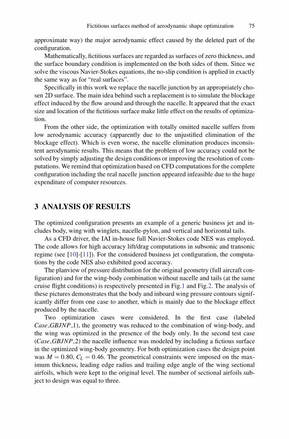
Fictitious surfaces method of aerodynamic shape optimization 75
approximate way) the major aerodynamic effect caused by the deleted part of theconfiguration.
Mathematically, fictitious surfaces are regarded as surfaces of zero thickness, andthe surface boundary condition is implemented on the both sides of them. Since wesolve the viscous Navier-Stokes equations, the no-slip condition is applied in exactlythe same way as for “real surfaces”.
Specifically in this work we replace the nacelle junction by an appropriately cho-sen 2D surface. The main idea behind such a replacement is to simulate the blockageeffect induced by the flow around and through the nacelle. It appeared that the exactsize and location of the fictitious surface make little effect on the results of optimiza-tion.
From the other side, the optimization with totally omitted nacelle suffers fromlow aerodynamic accuracy (apparently due to the unjustified elimination of theblockage effect). Which is even worse, the nacelle elimination produces inconsis-tent aerodynamic results. This means that the problem of low accuracy could not besolved by simply adjusting the design conditions or improving the resolution of com-putations. We remind that optimization based on CFD computations for the completeconfiguration including the real nacelle junction appeared infeasible due to the hugeexpenditure of computer resources.
3 ANALYSIS OF RESULTS
The optimized configuration presents an example of a generic business jet and in-cludes body, wing with winglets, nacelle-pylon, and vertical and horizontal tails.
As a CFD driver, the IAI in-house full Navier-Stokes code NES was employed.The code allows for high accuracy lift/drag computations in subsonic and transonicregime (see [10]-[11]). For the considered business jet configuration, the computa-tions by the code NES also exhibited good accuracy.
The planview of pressure distribution for the original geometry (full aircraft con-figuration) and for the wing-body combination without nacelle and tails (at the samecruise flight conditions) is respectively presented in Fig.1 and Fig.2. The analysis ofthese pictures demonstrates that the body and inboard wing pressure contours signif-icantly differ from one case to another, which is mainly due to the blockage effectproduced by the nacelle.
Two optimization cases were considered. In the first case (labeledCase GBJNP 1), the geometry was reduced to the combination of wing-body, andthe wing was optimized in the presence of the body only. In the second test case(Case GBJNP 2) the nacelle influence was modeled by including a fictious surfacein the optimized wing-body geometry. For both optimization cases the design pointwas M = 0.80, CL = 0.46. The geometrical constraints were imposed on the max-imum thickness, leading edge radius and trailing edge angle of the wing sectionalairfoils, which were kept to the original level. The number of sectional airfoils sub-ject to design was equal to three.

76 S. Peigin, B. Epstein, and S. Gali
The first “no-nacelle” optimization Case GBJNP 1 showed a significant gain indrag (about 9 aerodynamic counts at the design point) in comparison with the originalwing-body configuration. This is illustrated by Fig.3, where lift/drag was computedfor the stand alone wing-body combination without nacelle.
However, for practical design, the success of optimization should be estimatedin terms of drag reduction for the complete business jet configuration (includingnacelle-pylon). Unfortunately the analysis of the complete aircraft, in the presence ofthe nacelle (Fig.4), showed that the real gain at the design point falls to nearly zero.Note that this “naive” optimization nevertheless yields a better off-design lift/dragbehaviour at higher than the design lift and Mach values (see Fig.4 and Fig.5).
We must emphasize that attempts were made to improve the above optimizationby a better adjustment of design conditions (which may be regarded as a ”cheap”simulation of the nacelle influence) but they did not yield consistent results.
Thus it became clear that the nacelle influence must be simulated in the opti-mization process in order to increase the gain in the aerodynamic performance. Inprincipal, the ultimate way to do it is to use as an objective function the total dragof the complete aircraft geometry. However, a simple estimation shows, that this re-quires the huge computational resources which makes the optimization infeasiblefrom practical viewpoint.
In order to overcome this we propose to simulate the blockage effect caused bynacelle through the incorporation of a fictitious surface into the computational model.With this end in view, in the second test case Case GBJNP 2, the computationalgrid previously used for the wing-body combination, was modified by choosing ajoint face of two computational ”air-blocks” as the fictitious surface. Technicallythis means that the transparent block boundary condition (which previously mergedthe neighboring blocks, see Ref. [10]) was replaced by the Navier-Stokes no slipcondition. Note that this boundary condition was applied on the both sides of the face(which belongs to two original computational blocks). Aerodynamically this meansthat the face was treated as a fictitious infinitely thin surface. Thus, in the processof optimization, the actual complete geometry was replaced by the above describedcomputational model ( Fig.6), and the wing was optimized as an integral part ofthis composite computational model. Finally, the optimal shape was analyzed in theframework of the complete configuration which included the real nacelle junctionand the vertical/horizontal tails.
The optimization yielded a significant gain in drag in terms of the actually op-timized geometry (wing-body-fictitious-surface). An important point is that, con-trary to the first (no-nacelle) optimization, the most of gain was retained in terms ofthe full aircraft configuration analyzed a posteriori. The total drag of the completeconfiguration was reduced by 10 aerodynamic counts at the design conditions. Thecorresponding pressure distrubution for the optimized configuration at the designconditions is given in Fig.7 while for the original shape it was presented in Fig.1.A more detailed analysis demonstrates that the optimization resulted in a smootherpressure distribution on the wing upper surface.
The off-design behaviour of the optimized business jet may be assessed fromFig.8-9, where lift/drag polars at M = 0.80, M = 0.82, and Mach drag rise at

Fictitious surfaces method of aerodynamic shape optimization 77
CL = 0.46 are respectively compared with the original curves. It is clearly seen thatthe gain due to optimization increases at higher free-stream lift and Mach values.
It is interesting to compare the difference between the considered optimizationcases in terms of the resulting wing shapes. The corresponding airfoil shapes at2y/b = 0.10, 2y/b = 0.26 and 2y/b = 1.0 are respectively depicted in Fig.10-12.As aerodynamically expected, the “nacelle influence” is more significant in the in-board part of the wing gradually diminishing towards the tip region. At the tip, theboth optimized wing sections are practically identical.
Finally, it appeared that the exact size and location of the fictitious surface makelittle effect on the results of optimization. It is important from the practical viewpointthat, as the analysis showed, the fictitious surface may be determined approximatelywith the only requirement to roughly simulate the blockage effect caused by thenacelle.
4 CONCLUSIONS
Fictitious surface method for reducing the geometrical complexity of full aircraftconfigurations has been developed. The method was successfully applied to designof a complete transonic business jet with close coupled wing-body-nacelle-pylon,and vertical/horisontal tails. The results indicate good accuracy and robustness ofthe method which make it suitable for practical engineering design.
[1] Kroo, I., and Manning, V., “Collaborative Optimization: Status and Directions”Optimization in Aerodynamics”, AIAA paper, AIAA-2000-4721, 2000.
[2] Piperni, P., Abdo, M., and Kafyeke, F., “The Application of Multi-DisciplinaryOptimization Technologies to the Design of a Business Jet”, AIAA paper, AIAA-2004-4370, 2004.
[3] Jameson, A., Martinelli, L., and Vassberg, J., “Using Computational Fluid Dy-namics for Aerodynamics - a Critical Assessment”, Proceedings of ICAS 2002,Paper ICAS 2002-1.10.1, Optimage Ltd., Edinburgh, Scotland, U.K., 2002.
[4] Epstein, B., and Peigin, S., “Robust Hybrid Approach to Multiobjective Con-starined Optimization in Aerodynamics”, AIAA Journal, Vol. 42, No.8, 2004, pp.1572–1581.
[5] Epstein, B., and Peigin, S., “Constrained Aerodynamic Optimization of 3DWings Driven by Navier-Stokes Computations” AIAA Journal, Vol. 43, No. 9,2005, pp.1946-1957.
[6] Peigin, S., and Epstein, B., ”Multipoint Aerodynamic Design of Wing-BodyConfigurations for Minimum Drag”, Journal of Aircraft, Vol. 44, No. 3, 2007,pp.971-980.
[7] Michalewicz, Z., Genetic Algorithms + Data Structures = Evolution Programs(New-York: Springer Verlag), 1996
[8] Peigin, S. and Epstein, B., “Robust handling of non-linear constraints for GAoptimization of aerodynamic shapes”, Int. J. Numer. Meth. Fluids, Vol. 45, No.8,2004, p.1339–1362.

78 S. Peigin, B. Epstein, and S. Gali
[9] Peigin, S., and Epstein, B., “Embedded parallelization approach for optimizationin aerodynamic design”, The Journal of Supercomputing, Vol.29, No. 3, 2004,p.243–263.
[10] Epstein, B., Rubin, T., and Seror, S., “Accurate Multiblock Navier-StokesSolver for Complex Aerodynamic Configurations. AIAA Journal, Vol. 41, No.4, 2003, pp.582–594.
[11] Seror, S., Rubin, T., Peigin, S. and Epstein, B., “Implementation and Validationof the Spalart-Allmaras Turbulence Model for a Parallel CFD Code”, Journal ofAircraft, Vol. 42, No.1, 2005, pp.179–188.

Fictitious surfaces method of aerodynamic shape optimization 79
Cp
1.03
–1.05
Fig. 1. Generic business jet. Pressure distri-bution for full aircraft configuration: originalgeometry.
Cp
1.03
–1.05
Fig. 2. Generic business jet. Pressure distri-bution for wing-body configuration: originalgeometry.
0.44
0.46
0.48
0.5
0.52
0.54
230 240 250 260 270 280 290 300 310 320
CL
CD
Generic Business Jet. Drag polar at M=0.80
Original WBWCase_GBJNP_1
Fig. 3. Generic business jet. Drag polar atM = 0.80 for wing-body configuration. Orig-inal wing vs. optimal one (Case GBJNP 1).
0.42
0.44
0.46
0.48
0.5
0.52
290 300 310 320 330 340 350
CL
CD
Generic Business Jet. Drag polar at M=0.80
Original
Case_GBJNP_1
Fig. 4. Generic business jet. Drag polar atM = 0.80 for full aircraft configuration. Orig-inal wing vs. optimal one (Case GBJNP 1).
310
320
330
340
350
360
370
0.8 0.805 0.81 0.815 0.82 0.825 0.83
CD
Mach
Generic Business Jet. Mach drag rise at CL=0.46
Original
Case_GBJNP_1
Fig. 5. Generic business jet. Mach dragdivergence curve for full aircraft config-uration. Original wing vs. optimal one(Case GBJNP 1).

80 S. Peigin, B. Epstein, and S. Gali
Fig. 6. General view of a generic business jet:computational model.
1.03
–1.05
Cp
Fig. 7. Generic business jet. Pressure dis-tribution for full aircraft configuration:Case GBJNP 2.
0.41
0.42
0.43
0.44
0.45
0.46
0.47
0.48
0.49
0.5
280 290 300 310 320 330 340
CL
CD
Generic Business Jet. Drag Polars at M=0.80
OriginalCase_GBJNP_2
Fig. 8. Generic business jet. Drag polar atM = 0.80 for full aircraft configuration. Orig-inal wing vs. optimal one (Case GBJNP 2).
300
310
320
330
340
350
360
370
0.8 0.805 0.81 0.815 0.82 0.825 0.83
CD
Mach
Generic Business Jet. Mach drag rise at CL=0.46.
OriginalCase_GBJNP_2
Fig. 9. Generic business jet. Mach dragdivergence curve for full aircraft config-uration. Original wing vs. optimal one(Case GBJNP 2).
-0.06
-0.04
-0.02
0
0.02
0.04
0.06
0 0.2 0.4 0.6 0.8 1
y
x
Section shape at 2y/b = 0.10
Case_GBJNP_1Case_GBJNP_2
Fig. 10. Generic business jet. Wing sectionalshape at 2y/b = 0.10. Case GBJNP 1 vs.Case GBJNP 2.
-0.06
-0.04
-0.02
0
0.02
0.04
0.06
0 0.2 0.4 0.6 0.8 1
y
x
Section shape at 2y/b = 0.26
Case_GBJNP_1Case_GBJNP_2
Fig. 11. Generic business jet. Wing sectionalshape at 2y/b = 0.26. Case GBJNP 1 vs.Case GBJNP 2.

Fictitious surfaces method of aerodynamic shape optimization 81
-0.06
-0.04
-0.02
0
0.02
0.04
0.06
0 0.2 0.4 0.6 0.8 1
y
x
Section shape at 2y/b = 1.0
Case_GBJNP_1Case_GBJNP_2
Fig. 12. Generic business jet. Wing sec-tional shape at 2y/b = 1.0. Case GBJNP 1vs. Case GBJNP 2.


Path Optimization of Dual Airfoils Flapping in aBiplane Configuration with RSM in a ParallelComputing Environment
Mustafa Kaya1 and Ismail H. Tuncer2
1 Middle East Technical University, Ankara, Turkey [email protected] Middle East Technical University, Ankara, Turkey [email protected]
Abstract. The path of dual airfoils in a biplane configuration undergoing a combined, non–sinusoidal pitching and plunging motion is optimized for maximum thrust and/or propulsiveefficiency. The non–sinusoidal, periodic flapping motion is described using Non-Uniform Ra-tional B-Splines (NURBS). The Response Surface Methodology (RSM) is employed for theoptimization of NURBS parameters in a parallel computing environment. A gradient basedoptimization algorithm, steepest ascent method is started from the optimum point of responsesurfaces. Unsteady, low speed laminar flows are also computed in parallel using a Navier-Stokes solver based on domain decomposition. It is shown that the parallel optimization pro-cess with RSM suggests a quick and accurate initial guess for a gradient based optimizationalgorithm.
1 INTRODUCTION
Flow characteristics of flapping wings are currently investigated experimentally andnumerically to shed some light on the lift, drag and propulsive power considerationsfor a MAV flight[1, 2]. It should be noted that in order to maximize the thrust and/orthe propulsive efficiency of a flapping airfoil, its kinematic parameters, such as theflapping path, the frequency and the amplitude of the flapping motion, need to beoptimized.
In earlier studies, the present authors employed a gradient based optimizationof sinusoidal and non–sinusoidal flapping motion parameters of flapping airfoils[3,4]. These optimization studies with a limited number of optimization variablesshow that the thrust generation and efficiency of flapping airfoils may be increasedsignificantly. However, the gradient based global optimization process becomes com-putationally expensive as the number of optimization variables increases in the non–sinusoidal flapping motion definition with NURBS.
Response surface methodology (RSM) is mainly employed for the constructionof global approximations to a function based on its values computed at variouspoints[5]. The method may also be employed for the optimization of a function whenthe objective function is expensive in terms of computational resources[5, 6].
D. Tromeur-Dervout (eds.), Parallel Computational Fluid Dynamics 2008,Lecture Notes in Computational Science and Engineering 74,DOI: 10.1007/978-3-642-14438-7 8, c© Springer-Verlag Berlin Heidelberg 2010

84 Kaya & Tuncer
Fig. 1. Flapping-wing MAV model (Jones and Platzer)
In the present study, the thrust generation of dual airfoils flapping in a biplaneconfiguration undergoing a combined non–sinusoidal pitching and plunging motionis optimized using RSM. First, a single airfoil undergoing a non-sinusoidally flappingmotion is considered. RSM for 3 optimization variables is assessed and optimizationdata are compared to the gradient based optimization method in terms of the perfor-mance and the accuracy. Next, the non–sinusoidal flapping motion of dual airfoilswith seven optimizationvariables is considered.
2 Response Surface Methodology, RSM
RSM is based on building approximate models for unknown functional relationshipsbetween input and output data. In this study, the function is the average thrust coef-ficient, Ct , which is based on the integration of the drag coefficient over a flappingperiod. It is a function of flapping parameters, Vi, in a given flight condition and canbe written as
Ct = η(V1,V2,V3, . . .) (1)
The function η(V) is in fact the solution of the Navier-Stokes equations. An approx-imate response surface, g(V) ∼= η(V) may then be constructed over some V region[5]. In this study, g(V), is chosen to be a quadratic function of Vi’s:
g(Vi) = a11V 21 + 2a12V1V2 + 2a13V1V3 + · · ·+ a22V
22 + . . . (2)
The constants, ai j, are evaluated throught a least-square minimization of the error be-tween the response surface and a certain number of the Navier-Stokes solutions basedon a design of experiment (DoE). In this study, the Box-Behnken[7] DoE method isemployed.
3 Periodic Path defined by NURBS
A smooth curve S based on a general nth degree rational Bezier segment is definedas follows[9]:

Path Optimization of Dual Flapping Airfoils 85
fh( t)ωh ofα(ωt+φ)αo
fα(ω t + φ)αo ho fh( t)ωh = -
Free stream
h = α =
α = −
yo
Fig. 2. Out-of-phase flapping motion of twoairfoils in a biplane configuration
ωt
(0,-1)
(0,P)
(0,1)
f(ωt)
(2P,-1 ). .
. (2P,1)
.
2.
C
C C
C0 1
23
1
0
Fig. 3. Flapping path defined by a 3rd de-gree NURBS
S(u) = (x(u),y(u)) =∑n
i=0 WiBi,n(u)Ci
∑ni=0 WiBi,n(u)
0 ≤ u ≤ 1 (3)
where Bi,n(u) ≡ n!i!(n−i)! u
i(1− u)n−i are the classical nth degree Bernstein polyno-
mials, and Ci = (xpi,ypi), are called control points with weights, Wi. Note thatS(u = 0) = C0 and S(u = 1) = Cn. A closed curve which describes the upstrokeand the downstroke of a flapping path is then defined by employing a NURBS com-posed of two 3rd degree rational Bezier segments. The periodic flapping motion isfinally defined by 3 parameters. The first parameter P0 defines the center of the rota-tion vector on a closed curve. The remaining two points, P1 and P2 are used to definethe x coordinates of the control points, which are C1 = (2P1,−1) and C2 = (2P2,1)(Figure 3).
The x and y coordinates on the periodic NURBS curve may be obtained as afunction of the parameter u:
x(u) =2P1u(1−u)2 + 2P2u2(1−u)
2u2−2u + 1y(u) =
2u−12u2 −2u + 1
(4)
A non-sinusoidal periodic function, f , is then defined by y(u). For a given ωt posi-tion, the Equation 5 is solved for u. Once u is determined, y(u) ≡ f (ωt) is evaluatedusing Equation 4.
tan(ωt) = − x(u)y(u)−P0
(5)
4 Numerical Method
Unsteady, viscous flowfields around flapping airfoils in a biplane configuration arecomputed by solving the Navier-Stokes equations on moving and deforming oversetgrids. A domain decomposition based parallel computing algorithm is employed.PVMmessage passing library routines are used in the parallel solution algorithm. Thecomputed unsteady flowfields are analyzed in terms of time histories of aerodynamicloads, and unsteady particle traces.

86 Kaya & Tuncer
Fig. 4. Moving and deforming overset grid system
4.1 Flow Solver
The strong conservation-law form of the 2-D, thin-layer, Reynolds averaged Navier-Stokes equations is solved on each subgrid. The convective fluxes are evaluated usingOsher’s third–order accurate upwind–biased flux difference splitting scheme. Thediscretized equations are solved in parallel by an approximately factored, implicit al-gorithm. The overset grid system (Figure 4) is partitioned into subgrids. The holes inthe background grid are excluded from the computations by an i-blanking algorithm.The conservative flow variables are interpolated at the intergrid boundaries formedby the overset grids[10].
4.2 Flapping Motion
The flapping motion of the upper airfoil in plunge, h, and in pitch, α , is defined by:
h(t) = h0 fh(ωt)α(t) = α0 fα (ωt +φ) (6)
where ho and αo are the plunge and pitch amplitudes, f is a periodic function basedon NURBS, ω is the angular frequency which is given in terms of the reduced fre-quency, k = ωc
U∞. φ is the phase shift between plunge and pitching motions. The pitch
axis is located at the mid-chord. The flapping motion of the lower airfoil is in counter-phase. The average distance between the dual airfoils is set to y0 = 1.4.
The flapping motion of the airfoils are imposed by moving the airfoil grids overthe background grid (Figure 4). The airfoil grids are deformed as they come close tothe symmetry line between the airfoils.
4.3 Optimization based on the Steepest Ascent Method
Optimization based on the Steepest Ascent is also performed for validation. Thegradient vector of the objective function is given by

Path Optimization of Dual Flapping Airfoils 87
∇O(V) =∂O∂V1
v1 +∂O∂V2
v2 + · · ·
where Vi’s are the optimization variables. The components of the gradient vector areevaluated numerically by computing an unsteady flow solution for a perturbation ofthe optimization variables one at a time.
4.4 Parallel Processing
The parallel solution algorithm is based on the domain decomposition. The movingand deforming overset grid system is decomposed into its subgrids first, and thesolution on each subgrid is computed in parallel. Intergrid and overlapping boundaryconditions are exchanged among subgrid solutions at each time step of the unsteadysolution. The unsteady flow solutions needed for the RSM and the gradient vectorcomponents, are also carried out in parallel. PVM (version 3.4.5) library routines areused for inter–process communication. Computations are performed in a cluster ofLinux based computers with dual Xeon and Pentium-D processors.
5 Results and Discussion
A validation study is first performed. The optimization result with RSM is comparedagainst the gradient based optimization. The path optimization of the flapping airfoilsin a biplane configuration with 8 optimization variables is performed next.
5.1 Validation Study
The optimization of a single airfoil flapping on a non-sinusoidal path is studiedfirst. The flapping motion is a combination of non-sinusoidal pitching and sinusoidalplunging. The values for the reduced flapping frequency, k ≡ ωc
U∞, and the plunge am-
plitude, h0, are fixed at k = 1.0 and h0 = 0.5. The optimization variables are the pitchamplitude, α0, the phase shift between plunging and pitching, φ , and the NURBSparameter, P0α (Table 1). The flowfields are computed at Mach number of 0.1 and aReynolds number of 104.
Table 4 gives the design points used for constructing the response surface. Designpoints are chosen based on Box-Behnken matrix of runs[7]. The P1 and P2 values areconstrained within the range 0.2 to 5.0, and P0 in the range −0.9 to 0.9, in order todefine a proper flapping motion which does not impose excessively large accelera-tions.
The parallel computations for 13 unsteady flow solutions take about 2 hours ofwall clock time using 40 processors. The cross sections of the constructed responsesurface are shown in Figure 5. The same optimization case is also studied using thesteepest ascent method. The initial conditions required for this method are given inTable 2. The parallel computations, which required 58 unsteady flwo solutions, takeabout 20 hours of wall clock time using 15 processors.

88 Kaya & Tuncer
Table 1. Fixed parameters and optimization variables invalidation study
Case k h0 P1α P2α P0h P1h P2h P0α α0 φ1.0 0.5 1.0 1.0 0.0 1.0 1.0 V V V
Table 2. Initial conditions for steepest ascent method
Case k h0 P1α P2α P0h P1h P2h P0α α0 φ Ct
1.0 0.5 1.0 1.0 0.0 1.0 1.0 0.0 20o 90o 0.09
Table 3. Optimization results for the validation study
Case αo(o) φ(o) P0α Ct
RSM 9.3 90.6 0.03 0.17Steepest Ascent 9.2 90.7 −0.01 0.15
Table 4. RSM design points forthe validation study
DoE αo(o) φ(o) P0α1 5.0 30.0 0.02 5.0 150.0 0.03 35.0 30.0 0.04 35.0 150.0 0.05 5.0 90.0 −0.96 5.0 90.0 0.97 35.0 90.0 −0.98 35.0 90.0 0.99 20.0 30.0 −0.9
10 20.0 30.0 0.911 20.0 150.0 −0.912 20.0 150.0 0.913 20.0 90.0 0.0
-0.6
-0.3
0
0.3
Ct
010
2030
40
α0
-1
-0.5
0
0.5
1
P0α
Cross Section at φ = 90.6o
Maximum
(deg)
-0.6
-0.3
0
0.3
Ct
010
2030
40
α0
030
6090
120150
180
φ
Cross Section at P0α = 0.03
Maximum
(deg)(deg)
-0.6
-0.3
0
0.3
Ct
-1
-0.5
0
0.5
1P
0α
030
6090
120150
180
φ
Cross Section at α0 = 9.3o
Maximum
(deg)
Fig. 5. Response surfaces for the validation case
Table 3 gives the optimization results based on the RSM and the steepest ascentmethod. It is observed that while the optimum solution is about the same in bothcases, the number of unsteady flow solutions is significantly smaller in the RSMthan in the steepest ascend method.
5.2 Optimization for Dual Airfoils
Dual airfoils flapping in a biplane configuration is studied next with 8 optimizationvariables, namely, the NURBS parameters defining the plunging path, P0h, P1h, P2h,the NURBS parameters defining the pitching path, P0α , P1α , P2α , the pitching am-plitude, α0 and the phase shift between plunging and pitching, φ . The values forthe reduced flapping frequency, k ≡ ωc
U∞, and the plunge amplitude, h0, are fixed at
k = 1.5 and h0 = 0.53.These values are from an earlier study which optimized the sinusoidal flapping
motion of dual airfoils in biplane[8]. At this study, the maximum thrust is computedto be Ct = 0.45.
Design of experiment due to Box-Behnken is summarized in Table 5. A total of113 unsteady flow solutions are computed in about 10 hours of wall clock time using

Path Optimization of Dual Flapping Airfoils 89
Table 5. RSM design points and the computed thrust values
Desing No. P0h P1h P2h P0α P1α P2α α0(o) φ(o) Ct
1 0.0 0.5 0.5 0.0 1.0 1.0 9.0 90.0 0.422 0.0 0.5 2.0 0.0 1.0 1.0 9.0 90.0 0.49... ... ... ... ... ... ... ... ... ...
112 0.0 1.0 1.0 0.0 1.0 1.0 12.0 105.0 0.46113 0.0 1.0 1.0 0.0 1.0 1.0 9.0 90.0 0.42
Table 6. Optimization results
P0h P1h P2h P0α P1α P2α α(o) φ(o) Ct
RSM −0.30 2.00 2.00 −0.30 1.13 2.00 10.1 90.1 0.89Navier-Stokes −0.30 2.00 2.00 −0.30 1.13 2.00 10.1 90.1 0.85
Flapping Period (deg)
Plu
nge
Pos
ition
0 60 120 180 240 300 360-0.6
-0.3
0
0.3
0.6
0.9
Optimum Non-Sinusoidal MotionOptimum Sinusoidal Motion
M=0.1 Re=10000 k=1.5 y0=1.4
Fig. 6. Variation of optimum plunge position
Flapping Period (deg)
Pitc
hP
ositi
on(d
eg)
0 60 120 180 240 300 360
-10
-5
0
5
10
15
20
Optimum Non-Sinusoidal MotionOptimum Sinusoidal Motion
M=0.1 Re=10000 k=1.5 y0=1.4
Fig. 7. Variation of optimum pitch position
h = 0
Symmetry Line
h = 0
Fig. 8. Optimum non-sinusoidal flapping mo-tion
h = 0
Symmetry Line
h = 0
Fig. 9. Optimum sinusoidal flapping motion
64 processors. The response surface has 45 parameters (Eqn. 2). The optimizationresults are given in Table 6. The flow solution performed at the optimum conditionsproduces a thrust value of Ct = 0.85, which is about 4% off from the RSM prediction.The optimum sinusoidal and non-sinusoidal flapping motions are given in Figures 6,8 and 9.

90 Kaya & Tuncer
6 Conclusion
The path optimization of flapping airfoils with 8 optimziation variables is success-fully performed using RSM in a parallel computing environment. In a validationstufy it is shown that RSM is highly efficient in comparison to a gradient basedmethod.
[1] T.J. Mueller (editor), Fixed and Flapping Wing Aerodynamics for Micro Air Ve-hicles, AIAA Progress in Aeronautics and Astronautics, Vol 195, Reston, VA,2001.
[2] W. Shyy, M. Berg and D. Lyungvist, ”Flapping and Flexible Wings for Biologi-cal and Micro Air Vehicles”, Pergamon Progress in Aerospace Sciences, Vol 35,p: 455-505, 1999.
[3] I.H. Tuncer and M. Kaya, ”Optimization of Flapping Airfoils For MaximumThrust and Propulsive Efficiency”, AIAA Journal, Vol 43, p: 2329-2341, Nov2005.
[4] M. Kaya and I.H. Tuncer, ”Path Optimization of Flapping Airfoils Based onNURBS”, Proceedings of Parallel CFD 2006 Conference, Busan, Korea, May15-18, 2006.
[5] Roux, W.J., Stander, N. and Haftka, R.T., Response Surface Approximations forStructural Optimization, International Journal for Numerical Methods in Engi-neering, Vol. 42, 1998, pp. 517-534.
[6] D. H. Van Campen, R. Nagtegaal and A. J. G. Schoofs, Approximation methodsin structural optimization using experimental designs for for multiple responses,in H. Eschenauer, J. Koski and A. Osyczka (eds.), Multicriteria Design Opti-mization, Springer, Berlin, 1990, pp. 205-228.
[7] Box, G. E. P. and Behnken, D. W., Some new three level designs for the study ofquantitative variables, Technometrics, Vol. 2, pp. 455475.
[8] M. Kaya, I.H. Tuncer, K.D. Jones and M.F. Platzer, ”Optimization of FlappingMotion of Airfoils in Biplane Configuration for Maximum Thrust and/or Effi-ciency”, AIAA Paper, No 2007-0484, Jan 2007.
[9] L. Piegl and W. Tiller, The NURBS Book, 2nd ed., Springer-Verlag, Berlin, 1997.[10] I.H. Tuncer, ”A 2-D Unsteady Navier-Stokes Solution Method with Moving
Overset Grids”, AIAA Journal, Vol. 35, No. 3, March 1997, pp. 471-476.


Part III
Grid methods

Convergence Improvement Method for ComputationalFluid Dynamics Using Building-Cube Method
Takahiro Fukushige1 Toshihiro Kamatsuchi1 Toshiyuki Arima1 andSeiji Fujino2
1 Fundamental Technology Research Center, Honda R&D Co., Ltd.1-4-1 Chuo, Wako-shi, Saitama, 351-0193, Japantakahiro [email protected]
2 Kyushu University6-10-1, Hakozaki, Higashi-ku, Fukuoka-shi, 812-858, Japan
1 Introduction
Computational Fluid Dynamics (CFD) has become an important tool for aerody-namics by the improvements of computer performance and CFD algorithm itself.However, the computational time of CFD continues to increase, while progress ofcomputer has been made. One of the reasons is considered that application of CFDhas become more complex. For example, CFD is employed to estimate aerodynamicsperformance for a complex shaped object such as formula one car (Fig. 1) Concern-ing complex shape, however, the problem of grid generation still remains. It requiresso much time and labor. To overcome the problem in meshing for complex-shapedobject, we have already proposed an algorithm [3]. The algorithm consists of twoapproaches. One is Immersed Boundary method [6], and the other is Building-CubeMethod (BCM) [4]. The basic idea of Immersed Boundary method is applied to cellsin the vicinity of solid boundary, and Cartesian grid method is performed for othercells. These approaches have several advantages except for solution convergence. Inthis paper, Implicit Residual Smoothing (IRS) [2] is proposed for improvements ofsolution convergence.
Fig. 1. Formula 1 race car (Honda Racing F1 Team RA106).
D. Tromeur-Dervout (eds.), Parallel Computational Fluid Dynamics 2008,Lecture Notes in Computational Science and Engineering 74,DOI: 10.1007/978-3-642-14438-7 9, c© Springer-Verlag Berlin Heidelberg 2010

94 T. Fukushige., T. Kamatsuchi., T. Arima and S. Fujino.
2 Numerical Methods
2.1 Computational Gird of BCM
The computational grid used in this study is based on the Building-Cube Method.BCM grid generation consists of two steps: the first is to generate ’cube’ of varioussizes to fill the flow field as shown in Fig. 2. The second step is to generate Cartesiangrid in each cube (Fig. 3). Three cells overlap between adjacent cubes to exchangethe flow information at the boundaries.
Fig. 2. Cube boundary around airfoil. Fig. 3. Cartesian mesh around airfoil.
2.2 Flow Simulation
In this study, the non-dimensionalized Navier-Stokes equations governing compress-ible viscous flow are used for solving flow field. It can be written in the conservativeform as,
∂Qj
∂ t+∂Fj
∂x j− 1
Re∂Gj
∂x j= 0 ( j = 1,2,3), (1)
where t, x, and Re are time, the coordinate, and the Reynolds number, respec-tively. The conservation variables vector Q, the inviscid flux vector F, and viscousflux vector G are defined by
Qj =
⎡
⎣ρρui
ρe
⎤
⎦ ,Fj =
⎡
⎣ρu j
ρuiu j + pδi j
u j(ρe + p)
⎤
⎦ ,Gj =
⎡
⎣0τi j
ukτk j +λ (∂T/∂x j)
⎤
⎦ . (2)
Here, ρ , p,e,t, and λ are density, pressure, specific total energy, temperature, andthermal conductivity of fluid, respectively. ui represents the velocity component ofthe flow in the coordinate direction xi . It is noted that subscripts i, j, and k representcoordinate indices, and Einstein’s summation rule is applied. This set of equations isclosed by the equation of state for perfect gas.

Convergence Improvement Method for CFD Using BCM 95
p = (γ−1)ρ(
e− 12
ujuj
). (3)
where γ is the ratio of the specific heats. The components of viscous stress tensorτi jare given by
τi j = μ(∂ui
∂x j+∂u j
∂xi
)− 2
3μ∂uk
∂xkδi j. (4)
whrere δi j is Kronecker’s delta symbol and μ is viscosity coefficient, calcu-late by Surthrerland’s relationship. For turbulent flow simulation, the viscosity μis replaced by eddy viscosity which is evaluated by the Spalart and Allmaras one-equation model.
Specifications of the flow solver in this study are as follows.
• Discretization : FVM• Convection term : HLLEW (Riemann’s solver) [5]• High-resolution scheme : 4th order compact MUSCL TVD [9]• Time marching scheme : LU-SGS [10]• Turbulence model (RANS) : Spalart-Allmaras 1eq. model [7]• Other numerical technique : Preconditioning method for Mach-uniform formulae
[8]
2.3 Parallelization
The flow solver described above is parallelized with Message Passing Interface(MPI) library. In order to achieve optimal parallel performance, an identical num-ber of cubes is assigned to each CPU and only information of boundary cells areexchanged. Figure. 4 shows a overall flow-solution procedure of this flow solver.According to this figure, only once communication is occurred in each iteration. Italso contributes to obtain good parallel performance.
Fig. 4. Overall flow-solution procedure.
2.4 Validation
To validate of this flow solver, flow simulation around a 2D-airfoil (RAE2822) wascarried out. The computational grid is shown in Fig. 5. The total number of cubes

96 T. Fukushige., T. Kamatsuchi., T. Arima and S. Fujino.
is 618 with 16x16 cells in each cube. Therefore total number of computational cellsare about 150,000. The inflow Mach number, Reynolds number and angle of attackare 0.73, 6.56 million and 2.70 degrees. Detailed flow conditions can be found in theexperiment report by Cook et al. [1]Figure 6 shows Mach number contour in the flow field. A shockwave is observed atabout 55% chord length from the leading edge on the upper surface of the airfoil.The computed surface-pressure and skin-friction distributions are compared with ex-perimental data (Figures 7 and 8). The result of computation shows overall goodagreement with the experiment.
Fig. 5. Computational grid.
1.21.060.9
0.6
0.3
00.15
0.75
0.45
MAOH
Fig. 6. Mach number contours.
1.5
1
0.5
0
–0.5
–CP
–1
–1.50 10.2 0.4 0.6
X0.8
Fig. 7. Comparison of computed surface pres-sure coefficient with experimental data.
0.012
0.008
–0.008
0.004
–0.004
0
0.2 0.4 0.6X
0.8 1
Cf
Fig. 8. Comparison of computed skin frictioncoefficient with experimental data.
2.5 Implicit Residual Smoothing (IRS)
The governing equations discretized by FVM are solved by LU-SGS scheme. Toimprove solution convergence, the IRS is adopted. Ri is defined as,
Ri = Γ−1[∂F(Qi)∂x
− 1Re∂G(Qi)∂x
]. (5)
where, Γ−1 is preconditioning matrix [8]. In this study the explicit residual Riismodified as,

Convergence Improvement Method for CFD Using BCM 97
Ri = Ri + εΣ(R j − Ri). (6)
where Riis the smoothed residual, R jis residual of cell j adjoining cells i and εis a positive parameter used to control the smoothing. Equation (6) can be solved byJacobi iteration described as follows,
Rmi =
Ri + εΣ ¯Rm−1j
1 + εΣ1. (7)
3 Results and Discussion
To investigate the effect of the IRS on solution convergence, flow simulation arounda 3D airfoil was carried out. Computational conditions are shown in Table 1. Thecomputational grids used in the investigation are shown in Table 2. The total numberof grids and computational region for all cases is same so that the grid density isuniform. Figure 9 shows these computational grids.
Table 1. Computational conditions.
Condition Value
Reynolds Number 1.5x10⁶
Mach Number 0.19Number of Surface Element 4.0x10⁶
Turbulence Model On
Table 2. Specification of computational grid arrangements.
Type Number of cubes Number of cell per cube Total number of cells
A 1 2,097,152(=1283) 2,097,152B 8(=23) 262,144(=643) 2,097,152C 64(=43) 32,768(=323) 2,097,152D 512(=83) 4,096(=163) 2,097,152

98 T. Fukushige., T. Kamatsuchi., T. Arima and S. Fujino.
Fig. 9. Computational grids.
• Convergence History of ’single-cube’ and ’multi-cube’ without IRS
Convergence history is shown in Fig. 10. As the number of cubes increases, theconvergence history gets worse with oscillation. One of the reasons is poor infor-mation transfer at cube interfaces which might have caused duller solution near theinterface. To overcome this problem, the IRS was applied.
• Convergence History of ’single-cube’ with IRS
Convergence history is shown in Fig. 11. The convergence history depends onthe value of ε . The following ’multi-cube’ computations were performed using ε=1.2 determined by a series of numerical tests.
• Convergence History of ’multi-cube’ with IRS
Convergence history is shown in Fig. 12. The IRS is used on each cube. Regard-less of the number of cubes, significant improvement for convergence is obtainedby the IRS. Possible reason is that the IRS promotes propagation and attenuation ofresidual error across cube interface.
Finally, the IRS is applied to a practical computational grid in which cubes ofheterogeneous size were used to represent complex geometries. In this case cell sizeat interface is different which, in general, makes convergence worse. Figure 13 showsa computational grid. Good solution convergence was obtained as shown in Fig. 14.
• Parallel Efficiency
The computations were performed using NEC SX-8 which is vector parallel com-puter with 64 GB main memory and 8 processors in each node. The communicationdevice between nodes is Crossbar. To evaluate parallel efficiency, grid D in Table. 2was used. Good parallel efficiency was obtained as shown in Fig. 15. Moreover, it isunaffected even with the IRS.

Convergence Improvement Method for CFD Using BCM 99
STEP
Re
lative
Err
or
0 5000 10000 15000 20000 2500010-20
10-18
10-16
10-14
10-12
10-10
10-8
(A) ’s-cube’
(B) ’8-cube’
(C) ’64-cube’
(D) ’512-cube’
Fig. 10. Convergence history for several cubearrangements w/o IRS.
STEP
Re
lative
err
or
0 5000 10000 15000 20010-20
10-18
10-16
10-14
10-12
10-10
10-8
w/o IRS
IRS (e=1.2)
IRS(e=0.5)
Fig. 11. Convergence history for ’s-cube’ withand w/o IRS.
STEP
Re
lative
Err
or
0 5000 10000 15000 2000010-20
10-18
10-16
10-14
10-12
10-10
10-8
(A) ’s-cube’ w/o IRS
(B) ’8-cube’ w/ IRS
(C) ’64-cube’ w/ IRS
(D) ’512-cube’ w/ IRS
Fig. 12. Convergence history for several cubearrangements w/ IRS.
Fig. 13. Computational grid for actual prob-lem.
4 Conclusion
A method was proposed to improve convergence for ’multi-cube’ CFD. The basicidea behind the present method was to apply the IRS to ’multi-cube’ CFD. Regard-less of the number of cubes and their sizes, significant improvement for convergencewas obtained without deteriorating parallel efficiency. In the case of heterogeneouscube arrangement good solution convergence was also confirmed.
[1] P. H. Cook, M. A. McDonald, and M. C. P. Firmin. Airfoil rae2822-pressuredistributions, and boundary layer and wake measurements. Experimental DataBase for Computer Program Assessment, AGARD-AR-138, 1979.
[2] A. Jameson. The evolution of computational methods in aerodynamics. Journalof Applied Mechanics Review, 50(2):1052–1070, 1983.

100 T. Fukushige., T. Kamatsuchi., T. Arima and S. Fujino.
STEP
Re
lative
err
or
0 5000 10000 15000 20010-20
10-18
10-16
10-14
10-12
10-10
10-8
w/o IRS
w/ IRS
Fig. 14. Convergence history for actual prob-lem w/ and w/o IRS.
STEP
Re
lative
err
or
0 5000 10000 15000 20010-20
10-18
10-16
10-14
10-12
10-10
10-8
w/o IRS
IRS (e=1.2)
IRS(e=0.5)
Fig. 15. Speed-up ratio on SX-8.
[3] T. Kamatsuchi. Turbulent flow simulation around complex geometries withcartesian grid method. SIAM J. Sci. Stat. Comput, 13(2):631–644, 2007.
[4] K. Nakahashi and L. S. Kim. Building-cube method for large-scale, high reso-lution flow computations. AIAA Paper, 2004-0423, 2004.
[5] S. Obayashi and G. P. Guruswamy. Convergence acceleration of a navier-stokessolver for efficient static aeroelastic computations. AIAA Journal, 33(6):1134–1141, 1995.
[6] C. S. Peskin. Flow patterns around heart valves: A numerical method. Journalof Computational Physics, 10(2):252–271, 1972.
[7] P. R. Spalart and S. R. Allmaras. A one-equation turbulence model for aerody-namic flows. AIAA Paper, 92-0439, 1992.
[8] J. M. Weiss and W. A.Smith. Preconditioning applied to variable and con-stant density time-accurate flows on unstructured meshes. AIAA Journal,33(11):2050–2057, 1995.
[9] S. Yamamoto and H. Daiguji. Higher-order-accurate upwind schemes for solv-ing the compressible euler and navier-stokes equations. Computer and Fluids,22(2/3):259–270, 1993.
[10] S. Yoon and A. Jameson. Lower-upper symmetric-gauss-seidel method foreuler and navier-stokes equations. AIAA Journal, 26(9):1025–1026, 1998.

Aerodynamic Analysis of Rotor Blades using OversetGrid with Parallel Computation
Dong-Kyun Im1, Seong-Yong Wie1, Eugene Kim1, Jang-Hyuk Kwon1, Duck-JooLee1, and Ki-Hoon Chung2, and Seung-Bum Kim2
1 Dep. of Aerospace Engineering, Korea Advanced Institute of Science and Technology,373-1 Guseong-dong, Yuseong-gu, Daejeon, 305-701, Republic of Korea
2 Korea Aerospace Research Institute , 115 Gwahangro, Yuseong, Daejeon, 305-333,Republic of Korea
Abstract. The helicopter aerodynamics is simulated in hovering and forwarding flight usingthe unsteady Euler equations. As the steady condition, flight test of DLR-F6 and hoveringflight test data of Caradonna & Tung’s rotor blades were used, and as the unsteady condition,non-lift forwarding flight test data of the rotor blades were used. The parallelized numericalsolver was validated with the two of data above. By using this solver, AH-1G rotor blades toforwarding flight numerical test were conducted. In the test of forwarding flight, the numericaltrim was applied to decide cyclic pitching angles using the Newton-Raphson method, and theresults were good well match to the experimental data, Especially, the BVI effects were wellsimulated in advancing side in comparison with other numerical results. To consider the blademotion and moving effects, an overset grid technique is applied and for the boundary, Riemanninvariants condition is used for inflow and outflow.Keywords: Overset Grid, Helicopter Rotor, Hovering Flight, Forward Flight
1 Introduction
A helicopter has unique flying characteristics, that are complex aerodynamic phe-nomena. Continuous changes of aerodynamic environment and loads give rise tothe significant difficulty of rotorcraft aerodynamics. Strong tip vortices in the rotorwakes cause the flow-field to became highly unsteady and non-uniform at the rotordisk. These characteristics increase the calculation time and memory size in numer-ical analysis. Moreover, in forwarding flight, the periodic motions - pitching andflapping - of the rotor blades should be considered with aerodynamic stability. Thisstudy is covering the numerical analysis of the rotor blades in hovering and forward-ing flight using parallelized overset grid with rotor trim. The parallelized oversetgrids system uses a static load balancing tied to the flow solver based on the grid sizeof a decomposed domain [1]. The solver is based on a cell-centered finite volumemethod [2]. The parallelization is based on a domain decomposition; communica-tion is realized using MPI. The numerical fluxes at cell interface are computed usingthe Roe’s flux difference splitting method and the third order MUSCL (Monotone
D. Tromeur-Dervout (eds.), Parallel Computational Fluid Dynamics 2008,Lecture Notes in Computational Science and Engineering 74,DOI: 10.1007/978-3-642-14438-7 10, c© Springer-Verlag Berlin Heidelberg 2010

102 Dong-Kyun Im & al
Upwind Scheme for Conservation Law) scheme. The diagonalized ADI method isused with second order dual time stepping algorithm for the time integration. First,the steady condition was tested for verification of the parallelized solver. The DLR-F6 aircraft configuration was selected for the steady condition. The configurationwas provided in the DPW II and III (Drag Prediction Workshop which has been or-ganized by AIAA Applied Aerodynamics Technical Committee) and is a twin enginewide body aircraft which has a wing-body-nacelle-pylon and wing-body-fairing air-craft. The numerical hovering flight test was conducted using Caradonna & Tung’srotor blades that consist of NACA0012 airfoil section and AH-1G rotor blades wereused for the forwarding flight with rotor trim. The rotor trim of cyclic pitch anglewas made to be zero value of the periodic moments of rotor disk direction in reason-able averaged thrust. And for the iteration method of rotor trim, the Newton-Raphsonmethod was used [7].
2 Validation of Parallelized Solver
First, for the validation of numerical solver of helicopter aerodynamics, the DLR-F6aircraft configuration was analyzed in steady condition. The structured grid basedsolver KFLOW3D which has been developed at KAIST ASDI Lab is a parallelizedsolver. For the high performance parallel computing, 28 Pentium 4 2.13GHz proces-sors are used [3].
2.1 DLR-F6
Computations are implemented on DLR F6 wing-body configuration in Figure 1. TheDLR F6 wing body configuration model represents a transonic wing-body transportconfiguration. The structured grids are provided by the website of Boeing Com-mercial Airplanes group. In computations, three difference density grids (coarse,medium, medium fine) are used as shown Table 1. The computational conditionsare M∞ = 0.75, Re∞ = 3× 10⁶ at α = −3.0◦,−2.0◦,−1.5◦,0.0◦,1.0◦,1.5◦. Fullyturbulent boundary layer is assumed in the computations.
Grid points Y+ No. of BL cell Avg. Time (hours)Coarse 2.1M 1.25 18 6.5Medium 3.7M 1.0 36 15fine 13.0M 0.8 36 32
Table 1. Summary of the Grid System
Figure 2 (left) shows the drag polar results using the three grid sets in Table1. These results are in good agreement with the experimental data, and exhibit theconvergence, with respect to the grid density, of numerical results toward the exper-imental data.. The lift coefficients with the angle of attack are shown in Figure 2(right), and the results also show good agreement with experimental data.

Aerodynamic Analysis of Rotor Blades using Overset Grid 103
Fig. 1. DLR-F6 configuration and pressure distribution [3]
Fig. 2. (left) Drag Polar [3] and (right) CL vs. AOA curves [3]
3 Rotor Blades
The helicopter rotor blades were simulated in hovering flight and forwarding flightusing the parallelized solver. To consider motions of rotor blades such as pitchingand flapping, the overset grid technique wasapplied, and due to large grid size and

104 Dong-Kyun Im & al
computing time, the simulation was parallelized by Intel Core 2 CPU 2.13GHz 20nodes. The governing equation is 3-D unsteady Euler equations.
3.1 Overset Grids
Caradonna & Tung’s rotor blades were used for the hover flight test [4]. The airfoilof rotor blades is NACA0012 and the blades have no twist, no taper and 1.143m oflength, and an aspect ratio of 6. The computational grids consist of 5 shown in Figure2. The H-type grid was generated over rotor blades (41×67×105) and backgroundgrid (89×97×97). For the forward flight tests, two kinds of blades were considered.In the non-lift forward fight test, the Caradonna & Tung’s rotor blades with an aspectratio of 7 was used [5]. AH-1G rotor blades with a linear twist angle of −10◦ wereused in the forward flight with pitching and flapping motion [6]. The computationalgrids of AH-1G rotor blades also consist of 5 blocks that are the structured oversetgrid as Figure 3. The H-type grid also was generated over rotor blades (65×67×133)and background grid (89×97×97). The AH-1G rotor blades have an aspect ratio of9.8. A Linux PC cluster with 20 nodes Intel Core 2 CPU 2.13GHz processors and a100Mbps Ethernet network were used.
a. 3 bodies with 5 blocs
c. blades tip grid
b. blade grids with 2 bodies
Fig. 3. Overset grid

Aerodynamic Analysis of Rotor Blades using Overset Grid 105
Fig. 4. AH-1G Rotor Blades
3.2 Numerical Analysis Method
The solver, KFLOW3D, has been developed for the solution of RANS (ReynoldsAveraged Navier-Stokes Equations). In this study, the governing equations were un-steady Euler equations for the compressible inviscid flow discretized by a cell cen-tered finite-volume scheme using a structured grid. The discretization of the inviscidfluxes has been realized with upwind scheme, 3rd -order MUSCL (Monotone Up-stream Scheme for Conservation Laws) with minmod limiter using Roe-FDS (FluxDifference Splitting) with the Harten’s entropy fix function [8][9][10]. The steadystate is reached using the unsteady equations with the diagonalized ADI time integra-tion scheme. A dual time stepping method is also used to increase the time accuracyof the scheme [11][12]. Riemann Invariant was applied to the boundary condition forconvergence and stability.
3.3 Overset Grid Technique and Parallel Implementation
The overset grid method can be applied to any complex geometry which can be di-vided into some sub-grids having their own meshing. The independent grid systemtransfers information to each sub-grid using interpolation point by domain connec-tivity method. In this study, the domain connectivity method was used for modifiedoverset grid technique for the sake of the robustness and accuracy of flow analy-sis by arranging interpolation points of overlapped grids away from the boundaryof multi-sub-grid. A structured grid assembly is parallelized by using a static loadbalancing tied to the flow solver based on the grid size of a decomposed domain.The parallel algorithm is modified for a distributed memory system. To parallelizethe grid assembly, message passing programming model based on the MPI library isimplemented using the SPMD (Single Program Multiple Data) paradigm. The paral-lelized flow solver can be executed in each processor with the static load balancingby pre-processor.

106 Dong-Kyun Im & al
4 Rotor Flight Test and Results
4.1 Hovering Flight Test
The collective pitch angle is 8◦ and tip Mach number is 0.439. In this test, the rotorblades were rotated in 6 revolutions and it takes about 6 hours of wall clock time.The thrust coefficient is shown in Table 2 and Fig 6 displays the sectional pressuredistribution in hovering flight test case. The results were compared with experimentaldata at 0.5, 0.68, 0.8, and 0.96 of span location(r/R). The results of the numericalcomputation and experiments are almost same.
Thrust Coefficient (CT)Experiment 0.00459Numerical result 0.00473
Table 2. Thrust coefficient in hovering flight
Fig. 5. Pressure coefficient of rotor blades in hover flight
4.2 Non-lift Forwarding Flight Test
The collective pitch angle is 0◦, tip Mach number is 0.8 and advancing ratio is0.2. These test data were usually used for validation of forward flight by severalresearchers. In this test, the rotor blades were fixed at 0◦ collective pitch angle. Thatmeans the pitching and flapping motion were not considered. Also, the rotor bladeswere rotated with 6 revolutions and it takes about 6 hours of wall clock time. Figure5 shows the pressure distribution of upper surface rotor blades in non-lift forward-ing flight test case. The strong shock was occurred at 90 azimuth angle because tipMach number is 0.8 and advancing ratio is 0.2. Figure 6 displays the results that werecompared with experimental data on 30◦,60◦,90◦,120◦,150◦,180◦ azimuth angle at0.8925 of span location(r/R). The reason why the pressure difference of upper andlower surface is zero is that the collective pitch angle is zero and there is no pitch and

Aerodynamic Analysis of Rotor Blades using Overset Grid 107
flapping motion and the strong shock also is shown at advancing side in Figure 6.The results of the numerical computation and experiments are almost same as seenin Figure 6.
Fig. 6. Pressure coefficient of rotor blades in non-lift forward flight
Fig. 7. Pressure coefficient at 0.8925 of span location (r/R)

108 Dong-Kyun Im & al
4.3 Forwarding Flight Test
The forwarding flight test with pitching and flapping motion was conducted usingAH-1G rotor blades. The rotor trim for pitching angle also was considered in for-warding test [6]. In this test, the blades have cyclic motions with the pitching andflapping. The flapping motion is caused by structural deformation such as the aeroe-lasiticity, and the trim of cyclic pitch angle only was considered. The rotor trim wasconducted to meet zero periodic moments of rotor disk direction in reasonable aver-aged thrust. For the iteration method of rotor trim, the Newton-Raphson method wasused [7]. The 5 revolutions need to get the proper averaged thrust and 3 revolutionsalso need to get the result of trim pitch angle. However, for the convergence of rotortrim, 3 iterations also need. Therefore, the numerical forward flight test can carry outafter 30 revolutions. It takes about 32 hours of wall clock time.
Table 3 shows the pitching angles after rotor trim and table 4 displays the thrustcoefficients with trim and without trim. Equation of motions of the pitching andflapping are represented at (1) and (2).
θ (ψ) = θ0 +θ1c cos(ψ)+ θ1s sin(ψ) (1)
β (ψ) = β0 +β1c cos(ψ)+β1s sin(ψ) (2)
Degree θ0 θ1c θ1s β1c β1s
Experiment[5] 6 1.7 -5.5 2.13 -0.15Numerical result 6.11 1.32 -5.07 2.13 -0.15
Table 3. Pitching and Flapping angle after rotor trim
Thrust Coefficient (CT)Experiment 0.00464Numerical result (Trim) 0.00464Numerical result (No Trim) 0.00448
Table 4. Averaged Thrust Coefficients in forwarding flight
The results were compared with experimental data at 0.6, 0.75, 0.86, and 0.91of span location(r/R) pictured in Figure 7, and the numerical results with rotor trimare almost same with experimental computation in Figure 7 and show the weak BVIeffect at 90◦ azimuth angle that is on advancing side.
5 Conclusion
The hover and forward flight aerodynamic analyses were conducted using paral-lelized overset grid. For the high performance computation, 20 nodes of Intel Core 2

Aerodynamic Analysis of Rotor Blades using Overset Grid 109
Fig. 8. Sectional Thrust coefficient as Azimuth angle
2.13GHz processors were used by applying the parallelized overset grid technique.The rotor trim of cyclic pitch angle also was considered in forward flight. The nu-merical results with rotor trim are much more similar to experimental data than theresults without rotor trim.
Acknowledgement
This study has been supported by the KARI under KHP Dual-Use Component De-velopment Program funded by the MKE
[1] Eugene Kim, J. H. Kwon and S. H. Park, ” Parallel Performance Assessment ofMoving Body Overset Grid Application on PC Cluster”, pp59-66, Parallel Com-putational Fluid Dynamics-Parallel Computing and Its Applications 2007.

110 Dong-Kyun Im & al
[2] S. H. Park, Y. S. Kim and J. H. Kwon, ”Prediction of Damping Coeffi-cients Using the Unsteady Euler Equations”, Journal of Spacecraft and Rockets,Vol.40,No.3,2003,pp.356-362
[3] Y. Kim, S. H. Park and J. H. Kwon, ”Drag Prediction of DLR-F6 Using theTurbulent Navier-Stokes Calculations with Multigrid,” AIAA Paper 2004-0397,42nd Aerospace Science Meeting and Exhibit, Reno, NV, Jan. 2004.
[4] F. X. Caradonna and C. Tung, ”Experimental and Analytical Studies of a ModelHelicopter Rotor in Hover,” NASA TM-81232, Sep. 1981.
[5] F. X. Caradonna, F. X., G. H. Laub and C. Tung, ”An Experimental Investigationof the Parallel Blade-Vortex Interaction,” NASA TM-86005, 1984.
[6] J. L. Cross and M. E. Watts, ”Tip Aerodynamics and Acoustics Test: A Reportand Data Survey,” NASA-RP-1179, NASA Ames Research Center, Dec. 1988.
[7] K. H. Chung, C. J. Hwang, Y. M. Park, W. J. Jeon and D. J. Lee, ” Numer-ical Predictions of Rotorcraft Unsteady air-loadings and BVI noise by using atime-marching free-wake and acoustic analogy”, 31th European Rotorcraft Fo-rum, 2005.
[8] P. L. Roe, ”Approximate Riemann Solver, Parameter Vectors and DiffernceSchemes”, Journal of Computational Physics, Vol 43, pp. 357-372, 1981.
[9] A. Harten, ”High Resolution Schemes for Hyperbolic Conservation Laws,” Jour-nal of Computational Physics, Vol. 49, pp.357-393, 1983.
[10] W. K. Anderson, J. L. Tomas, and B. Van Leer, ”Comparison of Finite VolumeFlux Vector Splittings for the Euler Equations,” AIAA Journal, Vol. 24, No. 9, pp.1453-1460. 1986.
[11] T. Pulliam and D. chaussee, ” A diagonal form of an implicit approximate-factorization algorithm”, Journal of Computational Physics, Vol. 39, pp. 347-363,1981.
[12] K. W. Cho, J. H. Kwon, and S. Lee., ”Development of a Fully SystemizedChimera Methodology for Steady/Unsteady Problems”, Journal of Aircraft, Vol.36, No. 6, pp. 973-980, Nov. Dec. 1999

Large scale massively parallel computations with theblock-structured elsA CFD software
M. Gazaix1 ∗, S. Mazet2, and M. Montagnac3
1 Computational Fluid Dynamics and Aeroacoustics Department, ONERA,92322 Chatillon Cedex, France
2 Communication & Systemes,Le Plessis Robinson, France
3 Advanced Aerodynamics and Multiphysics, CERFACS,42, Avenue Gaspard Coriolis. 31057 Toulouse Cedex 01, France
Abstract. We describe work performed inside the elsA (http://elsa.onera.fr) block-structuredCFD software to analyse and improve parallel computation efficiency. Details of MPI imple-mentation are discussed. Computational results are given for realistic industrial configurations(28 106 mesh points) on several massively parallel platforms up to 1024 processors.
1 Introduction
The elsA software is a widely used CFD code developed by Onera, Cerfacs andother research centers [1]. This software elsA is able to simulate a wide range ofaerodynamic flows occuring in aircraft, turbomachinery or helicopter configurations.elsA is now an essential component of the design process of major industrial partners(Airbus, Safran, Eurocopter, MBDA, CEA).
elsA solves the compressible Navier-Stokes equations using a cell-centered, fi-nite volume, block-structured formulation. Spatial discretization schemes includesecond order upwind or centred schemes; the semi-discrete equations are integratedin time, either by multistage Runge-Kutta schemes with implicit residual smooth-ing, or by backward Euler integration with implicit operator solved with robust LUrelaxation methods. A very efficient multigrid technique can be selected to furtheraccelerate convergence.
In order to cope with more and more geometrically complex configurations,in addition to matching block connectivity, highly flexible advanced techniques ofmultiblock structured meshes are available including non conforming block connec-tivity, hierarchical mesh refinement, and Chimera technique for overlapping meshes.
elsA is mostly written in C++, with intensive numerical computations delegatedto Fortran subroutines. Users interact with the elsA kernel with a Python scriptinginterface.∗ This work is partially funded within the framework of the Airbus FUSIM project.
D. Tromeur-Dervout (eds.), Parallel Computational Fluid Dynamics 2008,Lecture Notes in Computational Science and Engineering 74,DOI: 10.1007/978-3-642-14438-7 11, c© Springer-Verlag Berlin Heidelberg 2010

112 M. Gazaix, S. Mazet, and M. Montagnac
elsA has been ported to most high-performance computing platforms, achievinggood CPU efficiency on both scalar multi-processor computers and vector comput-ers. To run in parallel, elsA uses a standard coarse-grained SPMD approach whereeach block is allocated to a processor, and communications between blocks are im-plemented with the MPI standard library. Several blocks can be allocated to the sameprocessor. An internal load balancing tool with block splitting capability is availableto allocate automatically blocks to processors.
As any other parallel scientific software, the benefits of parallelism are twofold:
• increase the amount of computer memory available, thus allowing to increase thenumber of mesh points;
• reduce the (wall clock) return time between user request and full job output.
Indeed, if there is no strong time constraint to get a job output, the best practice tooptimise the computing platform throughput is to choose the minimum number ofcomputing nodes providing the required memory. Conversely, if a time constraintis encountered such as a deadline in the design process, the number of processorsis computed taking into account the estimated single processor cost and the parallelefficiency.
2 Detailed analysis of elsA parallel performance
Earlier versions of elsA exhibit a marked decrease of parallel efficiency when thenumber of processors increases. In the following subsections, the probable causes ofthis degradation are identified and corrections are described.
2.1 Load balancing
As the number of processors increases, it is well known that load balancing is harderto maintain (Amdahl’s law). This is specially difficult to achieve with structuredmultiblock code, where the problem of finding the best ”block splitting” can be chal-lenging, particularly if the number of coarse grid levels has to be maintained. It mustbe acknowledged that partitioning an unstructured mesh is inherently simpler, whereseveral public domain tools are available (Metis, Scotch, Chaco...). We have observedthat many claims of poor parallel scaling are ill-founded and often vanish if care isexercised to obtain good enough load balancing. Note however that contrary to theunstructured case, memory constraints are much lower for block-structured splitting,so there is no need to parallelize the splitting algorithm itself to avoid memory bot-tlenecks.
A load balancing algorithm is available in elsA, closely following the strategy de-scribed by A. Ytterstrom [2] (”greedy” algorithm). Note that block splitting respectsthe multigrid constraint.
When block splitting does not occur, the load balancing algorithm is very simple.Blocks are first ordered by size (number of cells), and dispatched in a “zig-zag” way

Large scale massively parallel computations with elsA 113
on the NP processors: each of the NP biggest blocks are assigned to a separate pro-cessor, the NP next blocks are each assigned to a separate processor, in reverse orderof sizes, and so on until no blocks are left. In the test case studied, the following ruleof thumb applies: load balancing degradates rapidly when the number of processorsreaches one tenth of the number of blocks. For a test case of circa 350 blocks, theload balancing thus achieved degradates rapidly above 32 processors, and for a testcase of circa 1000 blocks, the load balancing thus achieved degradates rapidly abovecirca 100 processors. To overcome this degradation, it is necessary to split the largestblocks, using the automatic splitting capability of elsA internal load balancing tool.
In addition, we have also tested the Metis tool to load balance a limited numberof configurations 4. We have observed that on a large configuration (1037 blocks,128 processors) only pmetis gives a result; kmetis fails to give a distribution.
2.2 MPI message scheduling
Once the blocks are assigned to processors in a balanced way, one can classicallysetup a communication graph. Vertices in this graph are processors. An edge is addedbetween two vertices for each boundary condition that links two structured blocks,resulting in a multi-graph.
During each communication phase, every edge of the communication graph givesrise to one message being passed between the two underlying processors.
One singularity of the elsA software is the use of send/receive/replace strat-egy for message passing. Specifically, this strategy is used between blocks thatare connected with “coincident” meshes on either side of the interface. An impor-tant consequence of this is that the global ordering of communications is crucialto parallel scalability. The send/receive/replace strategy, while saving memory andbuffer management, allows for little hardware data buffering since each MPI call(MPI_Sendrecv_replace())must wait for all the requested data to be arrivedin order to return.
The first implementation of MPI message exchanges between blocks did not payattention to message ordering. Basically, the MPI messages ordering was determinedby the ordering of the topology description in the Python input script.
This bottleneck can be illustrated on a simple four vertices graph as in figure 1.For the ordering on the left of the figure, communications take place in the followingorder:
1. First wave: edge 1, processor P1 and P2,2. Second wave: edge 2, processor P2 and P3,3. Third wave: edge 3, processor P3 and P4,4. Fourth wave: edge 4, processor P4 and P1.
Thus processor P4 must wait for all communications between processors P1 andP2 and then between processors P2 and P3 to be over before it can start communi-cating with processor P3.
In the ordering on the right of the figure, communications take place as follows:
4 Metis can not split structured blocks.

114 M. Gazaix, S. Mazet, and M. Montagnac
1. First Wave: edge 1 and 2, processor P1 and P2, processors P3 and P4,2. Second Wave: edge 3 and 4, processor P2 and P3, processors P4 and P1.
Fig. 1. Different global communication orderings for a simple graph
Each “communication wave” (edges 1 and 2, and edges 3 and 4 in figure 1(b)),is a set of independent edges of the graph (so-called “matching” in graph theory).
The generalization to bigger graphs is straightforward. Note G0 the whole graphand put N0 = 0. At step i >= 1, do the following:
• determine a set of Ni independent edges on the communication graph,• number the edges (communications) in this set from Ni−1 + 1 to Ni−1 + Ni,• remove processed edges from graph Gi to obtain graph Gi+1
• continue until no edges are left.
As an example of efficiency improvement, the return time for a 128 processorcomputation was reduced by a factor of 2 when using the re-scheduling algorithm.
Remarks
Three remarks are in order.It is known that the problem of finding the optimal set of independent edges is
NP-complete. In the cases presented here, the greedy heuristic gives good resultsbecause of the sizes of the graphs involved (no more than a few hundred processorsat the moment). It is our opinion that sophisticated heuristics would not significantlyimprove the graph coverage (number of connected nodes) for graphs of these sizes.
A basic improvement to the greedy heuristic is to order edges according to theirweight. In this case, the weights of edges in one set are close, and every message inone communication “wave” should take approximately the same amount of time totravel. The weight of an edge is linked to the amount of communication incurred, i.e.the size of the interface meshes involved.

Large scale massively parallel computations with elsA 115
2.3 Test of different implementations of MPI messages
Use of MPI Sendrecv replace()
The original MPI parallel implementation uses point-to-point MPI communicationroutine (MPI Sendrecv replace()). As shown in section 2.2, it was necessaryto develop a scheduler to reach high performances.
Concatenation of messages to reduce latency
In the current elsA version, each matching block connectivity is implemented with acall to MPI Sendrecv replace(). However, since several matching boundariesmay induce communications with the same couple of processors, another implemen-tation has been tested, using a single buffer for each couple of processors; during thesend stage, the buffer concatenates (gather) all the messages to be exchanged; afterthe receive step, the buffer data are scattered to all the individual matching block con-nectivities. The reduction in the number of exchanged messages may lead to betterefficiency, specially if the communication network used by MPI has a high latency.Up to now, we have not observed any improvement using message concatenation;however, the current implementation use unnecessary buffer copy to fill the concate-nated exchanged buffers, and so is far from optimak; work is in progress to removesuch unnecessary data copy.
Use of MPI Bsend()
In all cases, use of MPI Bsend() lead to strong decrease in parallel efficiency.
Replacing blocking with non-blocking MPI routines
Another idea was to develop a non-blocking communication scheme to get rid of thescheduler. The other major interest of this approach is to enable the overlapping ofcommunication and computation. Nevertheless, the latter has not been achieved upto now.
In the first stage, all processors are told to get ready to receive MPI messages witha non-blocking receive instruction. The second stage consists in sending messages.As shown in table 1, no scheduler is needed anymore.
2.4 Influence of block splitting on numerical convergence
Since the implicit stage is done on a block basis, block splitting performed to achievea good load balancing may reduce the numerical efficiency of the implicit algorithm.In practice, we have never observed any significant convergence degradation.

116 M. Gazaix, S. Mazet, and M. Montagnac
comm. scheme greedy/sched. greedy/no sched. Metis/sched. Metis/no sched0 108.47 471.47 85.88 252.501 21.62 35.51 29.90 34.372 22.06 34.27 30.24 33.023 21.67 21.54 29.98 29.91
Table 1. 128 processors, CPU time spent to run one solver iteration on IBM BlueGene/L,0 : MPI BSend(), 1 : MPI Sendrecv replace(), 2 : MPI Sendrecv replace()with message concatenation, 3 : MPI ISend() (asynchronous)
3 elsA parallel efficiency
In this section, we present the parallel speedup measured on several parallel plat-forms, using the same test case.
3.1 Test case description
We have chosen a realistic industrial configuration, typical of civil aircraft config-urations computed with elsA. It is a 27.8 106 mesh points, with 1037 blocks. Thenumerical settings include a multigrid algorithm (3 levels), and Spalart (one equa-tion) turbulence model. The following plots give the computed parallel speedup, withthe following assumptions:
• Since the total CPU time is dominated by CPU time spent in the time loop, theinitialization phase (Python script interpretation, mesh file reading,...) is not takeninto account.
• Post-processing has been switched off, both during time loop and after loop ter-mination.
• For large number of processors, the configuration has to be splitted; for examplefor 1024 processors, we end up with 1774 blocks. This splitting leads to a smallmemory and CPU increase.
3.2 IBM BlueGene/L
The minimum number of processors which allows to run the test case is 64. SeeFigure 2.(a).
3.3 BULL Novascale (Itanium Montecito 1.6GHz)
This platform is equipped with an Infiniband network. See Figure 2.(b).
3.4 SGI Altix XE (Xeon Woodcrest 3GHz dual core)
See Figure 2.(c).

Large scale massively parallel computations with elsA 117
X
X
X
X
X
Number of Processors
Sp
ee
du
p
0 128 256 384 512 640 768 896 10240
4
8
12
16
Ideal Speedup
Measured SpeedupX
BlueGene/L (Cerfacs)(normalized with Nproc=64)
(a) IBM BlueGene/L. (b) BULL Novascale (Itanium Montecito1.6GHz).
(c) SGI Altix XE (Xeon Woodcrest 3GHz dualcore).
(d) (HP Cluster Opteron AMD 2.4 GHz).
Fig. 2. Parallel Speed-up of the Elsa code on different computing architectures
3.5 HP Cluster (Opteron AMD 2.4 GHz)
See Figure 2.(d).
[1] L. Cambier, J.P. Veuillot, Status of the elsA CFD software for Flow Simulationand Multidisciplinary Application, AIAA Paper 2008-664, Reno (January 2008).
[2] Anders Ytterstrom, A Tool for Partitioning Structured Multiblock Meshes forParallel Computational Mechanics, International Journal of High PerformanceComputing Applications, Vol. 11, No. 4, 336-343 (1997)


Applications on Hybrid Unstructured Moving GridMethod for Three-Dimensional Compressible Flows
Hiroya Asakawa1 Masashi Yamakawa1 and Kenichi Matsuno2
1 Division of Mechanical and System Engineering, Kyoto Institute of Technology,Matsugasaki, Sakyo-ku, Kyoto 606-8585, Japan [email protected]
2 Division of Mechanical and System Engineering, Kyoto Institute of Technology,Matsugasaki, Sakyo-ku, Kyoto 606-8585, Japan [email protected]
Abstract. For CFD problem with a complicated moving boundary, the unstructured moving-grid finite-volume method has been proposed and its ability recognized. However, the methodwas limited for applications using inviscid compressible flows. In this paper, the method isdeveloped to apply to three-dimensional Navier-Stokes equations for viscous compressibleflows. We formulate a control volume for prismatic element well adapted to unstructuredmesh. Then, the method is applied to a flow around oscillating ONERA M6 airfoil at highReynolds nmber. And the computation is executed in OpenMP parallel environment.
Key Words: Unstructured Grid, Compressible Flow, OpenMP Parallelization
1 Introduction
A numerical simulation of flows around moving complicated bodies is very inter-esting. To simulate such a flow field in the body-fitted coordinated system, greatskewness of gridline may occur according to the motion of the body. In this case, itis necessary to consider a geometric conservation law[1] for moving grid. So, if thegeometric conservation law is not satisfied, a numerical result will have error affect-ing movement of grid. For the issue, we have proposed the unstructured moving-gridfinite-volume method[2]. A characteristic of the method is that it satisfies a conser-vation of flow parameter on moving grid, so it satisfies a geometric conservationlaw on such a moving grid in addition to satisfy a physical conservation law. Themethod adopts a control volume in a space-time unified domain on the unstructuredgrid system, then it is implicit and is solved iteratively at every time-step. How-ever, the method was limited for applications using inviscid compressible flows onunstructured grid system which consist of tetrahedral meshes in three-dimensionalgrid system. However, generation of tetrahedral mesh for boundary layer is quitedifficult. In those regions the large gradients occur in the direction normal to thesurface, which requires mesh of very large aspect ratio. Thus, the prismatic meshis superior in capturing the directionality of the flowfield over viscous regions. So,we adapt a hybrid grid system of a prismatic mesh for boundary layer regions and
D. Tromeur-Dervout (eds.), Parallel Computational Fluid Dynamics 2008,Lecture Notes in Computational Science and Engineering 74,DOI: 10.1007/978-3-642-14438-7 12, c© Springer-Verlag Berlin Heidelberg 2010

120 Hiroya Asakawa Masashi Yamakawa and Kenichi Matsuno
tetrahedral mesh for other region. In this paper, there are two objectives. First, in athree-dimensional viscous flow, we propose the method that physical and geometricconservation laws are satisfied in moving grid system. Second, A numerical simu-lation of flow around a body is computed using moving grid method in OpenMPparallel environment. Then, it is applied to three-dimensional compressible flow inhybrid unstructured grid system.
2 Hybrid Unstructured Moving-Grid Finite Volume Method
2.1 Governing Equation
The Navier-Stokes equation in three-dimensional coordinate system is written in theconservation law form as follow:
∂q∂ t
+∂E∂x
+∂F∂y
+∂G∂ z
=1
Re∞
(∂EV
∂x+∂FV
∂y+∂GV
∂ z
)(1)
where, q is a vector of conservative variables,E, F and G are inviscid fluxes, EV ,FV and GV are viscous fluxes.
2.2 Numerical Algorithm
Then, the equation(1) is integrated for control volume of hybrid mesh as shown inFig.1. In the case of three-dimensional system, the method is featured treatmentof a control volume on the space-time unified domain (x, y, z, t), which is four-dimensional system in order that the method satisfies the geometric conservationlaws. The present method is based on a cell-centered finite-volume method, thus wedefine flow variables at the center of a cell in unstructured mesh. So the cells areprism and tetrahedron in three-dimensional (x, y, z, t)-domain. When grid moves, thecontrol volume becomes a complicated polyhedron in the (x, y, z, t)-domain.

Hybrid Unstructured Moving Grid Method for 3D Compressible Flows 121
(a) Tetrahedral element. (b) Prismatic element.
Fig. 1. Control volume
For these control volume, the governing equation is integrated as follow:
∫
Ω
[∂q∂ t
+∂E∂x
+∂F∂y
+∂G∂ z
− 1Re∞
(∂EV
∂x+∂FV
∂y+∂GV
∂ z
)]dΩ = 0. (2)
The equation can be written as the equation
∫
Ω
[(∂∂x
,∂∂y
,∂∂ z
,∂∂ t
)·(
E− 1Re∞
EV ,F− 1Re∞
FV ,G− 1Re∞
GV ,q)]
dΩ = 0. (3)
The equation can be represented using Gauss’s Theorem:
Ns+2
∑l=1
(qnt +Φ)ldSl = 0 (4)
where
Φ = H−HV , (5)
H = Enx + Fny + Gnz, (6)
HV =1
Re∞(EV nx + FV ny + GV nz). (7)
Here S is boundary of control volume surface. nl = (nx,ny,nz,nt)l (l = 1,2, · ··,Ns +2 ) is the normal vector of control volume surface, and the length of the vectorequals to the area of the surface. Then Ns is number of boundary, so in the case ofprism Ns = 5. l = 1,2, · · ·,Ns is presented as volume which is generated according tomovement from n to n + 1 time-step. l = Ns + 1,Ns + 2 is presented as cell itself atn time-step and n + 1 time-step. The volume at n and n + 1 time-step of the controlvolume are perpendicular to t-axis, and therefore they have only nt component andcorrespond to the areas in the ( x, y, z )-space at time tn+1 and tn, respectively. Thus,Eq.(4) can be expressed as,

122 Hiroya Asakawa Masashi Yamakawa and Kenichi Matsuno
qn+1(nt)Ns+2 + qn(nt)Ns+1 +Ns
∑l=1
[qn+1/2nt +Φn+1/2
]
ldSl = 0 (8)
Here, the conservative variable vector and flux vector at n + 1/2-time step are
estimated by the average between n-time and (n+1)-time steps. Thus, qn+ 12 andΦn+ 1
2
can be expressed as,
qn+ 12 =
12(qn+1 + qn), (9)
Φn+ 12 =
12(Φn+1 +Φn). (10)
It is Crank-Nicolson type. However, Calculating flowfield at high Reynolds num-ber, we use backward Euler type to get stability follow as:
qn+ 12 = qn+1, (11)
Φn+ 12 = Φn+1. (12)
The flux vectors are evaluated using the Roe flux difference splitting scheme[3] with MUSCL approach, as well as the Venkatakrishnan limiter [4]. The methoduses the variable at n + 1-time step, and thus the method is completely implicit.We introduce sub-iteration strategy with a pseudo-time approach [5] to solve theimplicit algorithm. Now by defining that the operating function L(qn+1) as Eq.(13),the pseudo-time sub-iteration is represented as Eq.(14).
L(qn+1,<m+1>
)=
1�t(nt)Ns+2
[
qn+1,<m+1>(nt)Ns+2 + qn(nt)Ns+1
+Ns
∑l=1
[(1−θ )
(qn+1,<m+1>nt +Φn+1,<m+1>
)+θ (qnnt +Φn)
]l dSl
]
(13)
∂q∂τ
= −L(qn+1,<m+1>
)(14)
Here, the equation is Crank-Nicolson type at θ = 1/2, and it is backward Eulertype at θ = 0 Where m is index for iteration, and τ is pseudo-time step. To solveEq.(14), we adopted the LU-SGS implicit scheme [6] to advance δτ pseudo-timestep. When m inner iteration is converged, we can get n + 1-time step solution qn+1.
3 Application
3.1 Calculating condition
The hybrid unstructured moving-grid finite-volume method is applied to a flowaround oscillating ONERA M6. The number of prism elements is 865,836 and the

Hybrid Unstructured Moving Grid Method for 3D Compressible Flows 123
number of tetrahedron is 935,566, total is 1,801,402. An initial grid ( whole appear-ance, cut view, around the wing ) are shown as Fig2. The hybrid grid is generated byMarching step method [7]. Then the grid is moved according to a motion of the wingby Spling method [8].
X
-10
-5
0
5
10
Y
-10
-5
0
5
10Z
0
5
10
(a)
X
-10
-5
0
5
10
Y
-10
-5
0
5
10
Z
0
5
10
(b)
(c)
Fig. 2. Computational grid.
The flowfield is computed at Re = 11.7x10⁶, M∞ = 0.84, α = 3.06. Initial con-dition is steady solution of this case. A computational region is shown as Fig.3. AOscillation is defined as an amplitude at a wingtip by Eq.(15). Here, β = 1.875/L.Then, a maxium amplitude at a wingtip is 0.1L and A Frequency is 60Hz. In thiscase, we introduce Spalart-Allmaras one equation model [9] as turbulence model.
y(z,t) = A ·Hsin(ω · t) (15)

124 Hiroya Asakawa Masashi Yamakawa and Kenichi Matsuno
11L
AHsin(wt)11L
11L
11L
Fig. 3. Computational region.
H = {(sin(βL)− sinh(βL)) · (sin(β z)− sinh(β z))+ (cos(βL)+ cosh(βL)) · (cos(β z)− cosh(β z))} (16)
3.2 Result
Fig.4 shows the results of the flow field (pressure contours) at t = 0.000, 1.125, 2.375,3.625, 4.625 and 5.875 respectively. We can see moving shocks on the wing surface.When the wing travels to upward, the shock generated on center of the wing surfacemoves to in front of wing. On the other hand, when the wing travels to downward,interaction between the shock generated in front of wing surface and generated incenter of the wing generates clearly Lambda shock. This result confirmed that themethod can calculate flow field and is promising to develop a three-dimensionalviscous flow around moving body.
The parallel computation of the hybrid unstructured moving-grid finite-volumemethod is carried on for the flow field using OpenMP library on PC. The computerhas two Intel processors ( E6850: Core2 3.0GHz ) and 8GB shared memory. The op-erating system is Windows Vista 64bit, fortran compiler is Intel Fortran 10.1. Then,a results of the estimating is shown in Table 1.
There was little number of the samples, however, we cannot get enough speedup in these environment. It is thought that we should examine a method to adopttechnique such as division of the domain or MPI parallel environment.
Number of elements 1,300,000 1,800,000
Speed up 0.950 0.980
Table 1. Parallel computing performance

Hybrid Unstructured Moving Grid Method for 3D Compressible Flows 125
0.26 0.34 0.42 0.5 0.58 0.66 0.74 0.82 0.9 0.98 1.06
Non dimensional time = 0.000000
t = 0.0000.26 0.34 0.42 0.5 0.58 0.66 0.74 0.82 0.9 0.98 1.06
Non dimensional time = 1.125000
t = 1.125
0.26 0.34 0.42 0.5 0.58 0.66 0.74 0.82 0.9 0.98 1.06
Non dimensional time = 2.375000
t = 2.3750.26 0.34 0.42 0.5 0.58 0.66 0.74 0.82 0.9 0.98 1.06
Non dimensional time = 3.625000
t = 3.625
0.26 0.34 0.42 0.5 0.58 0.66 0.74 0.82 0.9 0.98 1.06
Non dimensional time = 4.625000
t = 4.6250.26 0.34 0.42 0.5 0.58 0.66 0.74 0.82 0.9 0.98 1.06
Non dimensional time = 5.875000
t = 5.875
Fig. 4. Pressure contours
4 Conclusions
The unstructured moving-grid finite-volume method was formulated for three-dimensional viscous flows and developed in tetrahedral-prismatic hybrid grid sys-tem. Then, the result of a flow around oscillating wing showed applicable to

126 Hiroya Asakawa Masashi Yamakawa and Kenichi Matsuno
three-dimensional moving boundary problem for viscous compressible flows. Forthis problem, however, parallel efficiency was not obtained in OpenMP parallel en-vironment. In future work, the efficiency will be estimated in dividing a domain, withintroduction of MPI.
[1] K. Matsuno, K. Mihara. and N. Satofuka, ”A Moving-Mesh Finite-Volume Scheme for Compressible Flows with Traveling Wall Boundaries”,ComputationalFluidDynamics2000, Springer July, (2001) pp705-710.
[2] M. Yamakawa and K. Matsuno, ”Unstructured Moving-Grid Finite-Volume Method for Unsteady Shocked Flows”,Journalo fComputationalFluidsEngineering, Vol. 10, No.1, (2005), pp24-30.
[3] P. L. Roe, ”Approximate Riemann Solvers Parameter Vectors and DifferenceSchemes”, Journalo fComputationalPhysics., Vol. 43, (1981), pp 357-372.
[4] V. Venkatakrishnan, ”On the Accuracy of Limiters and Convergence to SteadyState Solutions”, AIAAPaper, 93-0880, (1993)
[5] C. L. Rumsey, M. D. Sanetrik, R. T. Biedron, N. D. Melson, and E. B. Parlette,”Efficiency and Accuracy of Time-Accurate Turbulent Navier-Stokes Compu-tations”, ComputersandFluids, Vol. 25, (1996), pp 217-236.
[6] A. Jameson, and S. Yoon, ”Lower-Upper Implicit Scheme with Multiple Gridsfor the Euler Equations”, AIAAJornal, Vol.25, (1987), pp 929-935
[7] S. Pirzadeh, ”Three-Dimensional Unstructured Viscous Grid by the Advancing-Layer Method”, AIAAJornal, Vol.34, (1996), pp 43-49
[8] J. T. Batine, ”Unsteady Euler Algorithm with Unstructured Dynamic Mesh forComplex-Aircraft Aerodynamics Analysis”, AIAAJornal, Vol.29, (1991), pp327-333
[9] P. R. Spalart and S. R. Allmaras, ”One-Equation Turbulence Model for Aero-dynamics Flows”, AIAAPaper, 92-0349, (1992)

Progressive Development of Moving-GridFinite-Volume Method for Three-DimensionalIncompressible Flows
Shinichi ASAO1, Sadanori ISHIHARA1, Kenichi MATSUNO2 and MasashiYAMAKAWA2
1 Kyoto Institute of Technology, Matsugasaki, Sakyo-ku, Kyoto 606-8585, [email protected]
2 Kyoto Institute of Technology, Matsugasaki, Sakyo-ku, Kyoto 606-8585, [email protected]
Abstract. In this paper, parallel computation of three-dimensional incompressible flowsdriven by moving multiple bodies is presented using a new moving embedded zonal gridmethod. Moving embedded zonal grid method is the method such that the embedded zonalgrid can move freely in one direction in a main grid which covers the whole of the flowfield. The feature of the method is to satisfy both geometric and physical conservation lawssimultaneously. The method is applied to a flow driven by two cubes moving in the origi-nally stationary fluid. The computation was performed using multi-core CPUs and the parallelalgorithm has been implemented in the Poisson solver and the performance has been tested.
keyword: Incompressible flow, Moving-Grid Finite-Volume method, OpenMP
1 Introduction
Today, one of the interesting problems in Computational Fluid Dynamics is an un-steady flow and it is very important to calculate a moving boundary problem. Es-pecially, in the case that body moves in the fluid is interesting on engineering. Forexample, these are a flow by stir, a flow around the turbine, and so on.
When we simulate such flow field, we encounter some problems to be overcome.One of the problems is on grid system. When the body moves in the flow field, aconventional single body-fitted grid system is hard to adjust the motion of body. Oneof the most popular methods for such a moving boundary problem is an overset gridmethod [1] where sub-grid placed around a moving body moves in main-grid. How-ever the overset grid method does not satisfy conservation law rigorously in generaldue to unavoidable interpolation error. From the view point of accurate computation,the body-fitted single grid system is desirable, but is not difficult for the case that thebody travels long distance in the flow field because of resultant highly skewed grid.
D. Tromeur-Dervout (eds.), Parallel Computational Fluid Dynamics 2008,Lecture Notes in Computational Science and Engineering 74,DOI: 10.1007/978-3-642-14438-7 13, c© Springer-Verlag Berlin Heidelberg 2010

128 S. ASAO, S. ISHIHARA, K. MATSUNO and M. YAMAKAWA
To overcome this problem, we have proposed a moving embedded-grid method[2] for two-dimensional space. The method patches a local grid generated around abody in a stationary ”main grid” and shifts the embedded local grid in any directionthrough the main grid with eliminating front-side grids and adding back-side gridwith satisfying both physical and geometric conservation laws. As a flow solver, themoving-grid finite-volume method [3] is modified and used in the moving embedded-grid method.
The purpose of this paper is two fold. One is to introduce the moving embed-ded zonal grid method as the first step in building up the three-dimensional movingembedded-grid method. In this method, the movement of embedded zonal grid islimited to one direction. The interactive flow field driven by the movement of themultiple cubes is demonstrated. The other is to implement a parallel procedure intopresent method and to investigate the parallel performance of the present method onthe multi-core and/or parallel environment of the small laboratory.
2 Moving Embedded zonal grid method
2.1 Governing Equations
Governing equations are the continuity equation and the incompressible Navier-Stokes equations and are written in divergent form as,
∇ ·q = 0 (1)
∂q∂ t
+∂E∂x
+∂F∂y
+∂G∂ z
= 0 (2)
where, q is velocity vector, E , F and G are flux vectors of x, y and z direction respec-tively. These flux vectors are composed of advection, pressure and viscous term.
2.2 Moving Grid Finite Volume Method
To assure the geometric conservation laws, we adopt a control volume in the space-time unified domain (x,y,z,t), which is four-dimensional in the case of three-dimensional flows. Now, Eq.(2) can be written in divergence form as,
∇ · F = 0 (3)
where,
∇=[∂∂x
∂∂y
∂∂z
∂∂ t
]T, F =
[E F G q
]T(4)
The present method is based on a cell-centered finite-volume method and, thus, theflow variables are defined at the center of the cell in the (x,y,z) space. The control

Progressive Development of Moving-Grid Finite-Volume Method 129
n+1
n
1
53
2
4
6
Fig. 1. Schematic view of control volume in (x,y,z,t) space-time unified domain.
volume becomes a four-dimensional polyhedron in the (x,y,z,t)-domain, as schemat-ically illustrated in Figure 1.
We apply volume integration to Eq.(2) with respect to the control volume illus-trated in Figure 1. With use of the Gauss theorem, Eq.(3) can be written in surfaceintegral form as,
∫
Ω∇ · FdΩ =
∮
SF · ˜ndS =
8
∑l=1
(F · n)l = 0 (5)
Here, ˜n is a outward unit vector normal to the surface, S, of the polyhedron con-trol volume Ω , and, nl = (nx,ny,nz,nt)l , (l = 1,2,. . . 8) denotes the surface normalvector of control volume and its length equals to the boundary surface area in four-dimensional (x,y,z,t) space. The upper and bottom boundary of the control volume(l = 7 and 8) are perpendicular to t-axis, and, therefore they have only nt componentand its length is corresponding to the volume of the cell in the (x,y,z)-space at timetn and tn+1 respectively. Thus, Eq.(5) can be expressed as,
qn+1(nt)8 + qn(nt)7 +6
∑l=1
(F n+1/2 · n
)
l= 0 (6)
To solve Eq.(6), we apply the SMAC method[4]. Thus, Eq.(6) can be solvedat three following stages. The equation to be solved at the first stage contains theunknown variables at n+1-time step in the flux terms. Thus the equation is iterativelysolved using the LU-SGS method[5]. The equation to be solved at the second stage isthe Poisson equation about the pressure correction. This equation is iteratively solvedusing the Bi-CGSTAB method[6]. The flux vectors are evaluated using the QUICKmethod. While the flux vectors of the pressure and viscous terms are evaluated in thecentral-difference-like manner.
2.3 Moving Embedded Zonal Grid Method
The present moving embedded zonal grid method is the method such that the zonegrid in which bodies are included is embedded in the main grid and the embeddedzonal grid moves in one direction freely with adding and/or removing gird plane inthe main grid as illustrated in Figure 2. The front grid plane of the embedded zonalgird is eliminated from the main grid to avoid grid folding according to decrease of

130 S. ASAO, S. ISHIHARA, K. MATSUNO and M. YAMAKAWA
the grid spacing due to the movement of the embedded zonal grid, while a grid planeis added newly between the rear plane of the embedded zonal grid and the main gridin order to keep the allowable maximum grid spacing. Hence the present methodincludes essentially the two inevitable procedures: addition and elimination of gridplane.
Step 1 Step 2 Step 3
Grid PlaneEliminatingAdding
Grid PlaneZonal GridEmbedded
Fig. 2. Moving embedded zonal grid method.
The addition of the grid plane is performed as follows. Suppose that the gridcell I at time step n deforms as well as moves to new position, and separates intotwo grid cells I and I′ at time step n + 1, as illustrated in Figure 3(a). This meansthat the new grid plane i′ is inserted or added between the grid plane i− 1 and i.Under this situation, we have to treat two control volume, I and I′, to get solutionsat time step n + 1. For control volume I, the Eq.(6) is applied and no any otherextra procedure is necessary. For newly appearing control volume I ′, we need tomodify Eq.(6) considering that the volume of cell I′ at time n is zero. This meansthat (nt)7 = 0 for control volume I′. Thus the finite volume equation for I′ becomes:
qn+1(nt)8I′ +6
∑l=1
(F n+1/2 · n
)
l= 0 (7)
The elimination of the grid plane is accomplished through merging the two re-lated control volumes. Suppose that the i′-th grid plane is eliminated at (n + 1)-timestep. Then we consider that the i′-th and i-th planes of cells at n-time step are mergedat (n + 1)-time step and only i-th plane of cells remains. In this situation, the con-trol volume in space-time unified domain, (x,y,z,t), can be illustrated in Figure 3(b).Thus Eq.(8) replaces Eq.(6).
qn+1(nt)8I + qn(nt)7I + qn(nt)7I′ +6
∑l=1
(F n+1/2 · n
)
l= 0 (8)
In the present method, the addition and elimination of grid plane are performedsimultaneously when the grid spacing at the boundary between the main and embed-ded grids exceeds a user-specified tolerance.

Progressive Development of Moving-Grid Finite-Volume Method 131
yz
x
n+1n
I II’
A B
C
GH
J K L
MP
E
D
Addition ofGrid Plane
N
Q R
V U T
SF
(a)
yz
x
A CB
FE D
G
M
H
I’
L K
J
N
Q
P
n +1n
S T
V U
RII
Elimination ofGrid Plane
(b)
Fig. 3. Control volumes for (a) adding grid plane and (b) eliminating grid plane.
3 Numerical results
3.1 Validation 1: Geometric Conservation Laws
At first it is necessary to confirm that the method satisfies the ”Geometric Conser-vation Law” (GCL condition)[7], which means the method can calculate an uniformflow on the moving mesh system without any error, when the embedded grid is mov-ing in main grid with adding and eliminating grid planes. To verify that the methodsatisfies the GCL condition, we apply the present method to the uniform flow. After100,000 time step, the error keeps the order of 10−17, in a word, machine zero, whichmeans the method satisfies GCL perfectly.
3.2 Validation 2: Computation of Incompressible Flow-Field Driven byMoving Cube in the Stationary Fluid
In order to check the present method, we have compared two physically equivalentflow fields. The one is the semi-steady flows driven by the cube with a constantspeed in a stationary flow field, the other is the steady flows around the cube in anuniform flow. As the calculation condition, the Reynolds number is 40 in the both
(a) (b)
Fig. 4. (a) Moving cube with a constant speed in a stationary flow field. (b) The flows aroundthe cube in a uniform flow.
cases. Figure 5 shows the vorticity contours. Since two physically equivalent flowfields are obtained, the reliability of code is confirmed.

132 S. ASAO, S. ISHIHARA, K. MATSUNO and M. YAMAKAWA
(a) (b)
Fig. 5. Vorticity contours ((a) Using moving embedded zonal grid method, (b) Referencesolution).
3.3 Computation of Incompressible Flow-Field Driven by Moving Twin Cubesin the Stationary Fluid
As an application of the present method, we simulate a flow-field driven by twincubes moving a stationary fluid, as illustrated in Figure 6.
Fig. 6. The flows driven by multiple cubes.
The size of the whole computational domain is Lx = 15.0L, Ly = 10.0L, Lz =10.0L, where L is the side length of the cube. The initial position of the cubes arex = 12.5L, y = 4L,6L, and z = 5L. The twin cubes move at constant speed of Ub = 1.0after the constant acceleration of 0.1 from the stationary condition. The initial sta-tionary condition of pressure, velocity components in the x,y,z directions are givenby p = 1.0, u = v = w = 0.0. As the calculation condition, the Reynolds number is 40and time step size is Δt = 0.01. The number of the main grid is 151×101×101 andthe embedded zonal grid is 14×101×101. Figure 7 shows the pressure distributionon the cubes as well as the vorticity contours at t = 5.0, 10.0 and 15.0.
The pressure in front of the cubes becomes higher as the speed of cube increases.We can capture the twin vortex which corresponds to Re = 40. The vortex made bythe left body joins the vortex made by the right body at time t = 15. Therefore theseare physically-meaningful flows, and it is confirmed that the moving embedded zonalgrid method is useful for this application.

Progressive Development of Moving-Grid Finite-Volume Method 133
(a) t = 5 (b) t = 10 (c) t = 15
Fig. 7. Surface pressure distribution and vorticity contour.
4 Parallel implementation
The second stage of the SMAC method is the Poisson solver for the pressure correc-tion, where the Bi-CGSTAB method is used in the present method. In spite of theefficiency of the Bi-CGSTAB method, this Poisson solver still consumers 90 % ofwhole of computer time. Thus we have implemented parallelization on this stage.The Bi-CGSTAB method includes the ILU decomposition. When we parallelize theILU decomposition, we have to consider the data dependencies. We have applied the”Domino method” to the present method. The detail of the present ”Domino method”is described as fallows.
(i) The calculation region is divided as illustrated in Figure 8(a).(ii) The calculation region 1 of Figure 8(b) is calculated sequentially.
(iii) The calculation region 2,3 and 4 of Figure 8(c) is calculated in parallel aftercalculation of (ii) has finished.
(iv) The calculation region 5,6,7,8,9 and 10 of Figure 8(d) is calculated in parallelafter calculation of (iii).
(v) The calculation region of Figure 8(e)∼(h) are calculated in a similar way.
Thus, the method can avoid the data dependences.
(a) (b) (c) (d)
(e) (f) (g) (h)
Fig. 8. Schematic diagrams of Domino method (3×3×3).
The parallel computation is carried out using OpenMP library on PC for a flowwhere two cubes move in the stationary fluid. As the operating system, we adopt

134 S. ASAO, S. ISHIHARA, K. MATSUNO and M. YAMAKAWA
Fedora core 6, which is a 64bit Linux operating system. The computer has one IntelCore-two-duo 2.66GHz processors and 4GB shared memory. The Fortran compileris Intel Fortran 10.0. The whole of the domain is divided into 64(= 4× 4× 4) sub-domains.
As a result, the ”Speed up” is 1.19 for the two CPU-core processors. For this case,the result is miserable and the expected efficiency was not obtained in the presentnumerical experiment. One of the reasons might be that the number of processors isdifferent from the division number in some calculation regions, and the paralleliza-tion efficiency has been down. With this result, we need further efforts to improveefficiency.
5 Concluding remarks
In this paper, the moving embedded zonal grid method has been introduced andapplied to the flows driven by moving multiple bodies. As a result, physically-meaningful flows are obtained, and it is confirmed that the moving embedded zonalgrid method is useful for the simulation of a flow-field driven by multiple bodiesmoving a stationary fluid. The second stage of the flow solver, the part of the Pois-son solver, is parallelized using ”Domino” method, and the expected speed up is notobtained. Further attempts have been continued for further parallel efficiency in thelaboratory computer environment.
Acknowledgement. This work was supported by KAKENHI(18560169).
[1] Steger, J. L., Dougherty, F. C. and Benek, J. A., A Chimera Grid Scheme; Ad-vances in Grid Generation, ASME, 5, (1983), 55-70.
[2] Asao, S. and Matsuno, K., A Moving Embedded-Grid Method for Simulationof Unsteady Incompressible Flows with Boundaries Traveling Long Distances,JSME, 74-737 B, (2008), 25-33.
[3] Matsuno, K., Mihara, K., and Satofuka, N., A Moving-Mesh Finite-VolumeScheme for Compressible Flows, Comp. F. Dyna. 2000, Springer, (2001), 705-710.
[4] Amsden, A.A. and Harlow, F.H., A Simplified MAC Technique for Incompress-ible Fluid Flow Calculations, J. Comp. Phys, 6, (1970b), 322-325.
[5] Yoon, S. and Jameson, A., Lower-Upper Symmetric-Gauss-Seidel Method forthe Euler and Navier-Stokes Equations, AIAA J., 26, (1988), 1025-1026.
[6] H. A. van der Vorst, Bi-CGSTAB, SIAM, 13-2, (1992), 631-644[7] Zhang, H., Reggio, M., Trepanier, J.Y. and Camarero, R., Discrete Form of the
GCL for Moving Meshes and Its Implimentation in CFD Schemes, Computersand Fluids, 22, (1993), 9-23.


Part IV
Boundary methods

Flow Computations Using Embedded BoundaryConditions on Block Structured Cartesian Grid
T. Kamatsuch1, T. Fukushige2 and K. Nakahashi3
1 Fundamental Technology Research Center, Honda R&D Co. Ltd., Chuo 1-4-1,Wako351-0193, Japan. toshihiro [email protected]
2 Fundamental Technology Research Center, Honda R&D Co. Ltd., Chuo 1-4-1,Wako351-0193, Japan. takahiro [email protected]
3 Department of Aerospace Engineering, Tohoku University, Aoba 6-6-01, Sendai 980-8579,Japan. [email protected]
1 Introduction
Computational Fluid Dynamics (CFD) has been increasingly relied on as an impor-tant tool for the aerodynamic design. However, mesh generation for 3D complexgeometries is still the most time-consuming task in CFD. Recently, Cartesian gridmethods have become popular because of their advantages of fast, robust, and auto-matic grid generation. Authors proposed a new approach based on a block-structuredCartesian grid approach, named Building-Cube Method (BCM, [5]). This method isaimed for large-scale, high-resolution computations of flows. In the original BCM,however, the wall boundary is defined by a staircase representation to keep the sim-plicity of the algorithm. Therefore, to resolve boundary layers, vast amounts of gridpoints are required especially for high-Reynolds number flows of practial applica-tions. In this paper, a new embedded boundary treatment suitable for high-Reynoldsviscous flows on BCM is proposed. The scalability performance on cluster comput-ers is also investigated with this method.
2 Building-Cube Method
The BCM basically employs a uniformly-spaced Cartesian mesh because of the sim-plicity in the mesh generation, the numerical algorithm, and the post processing.A flow field is described as an assemblage of building blocks of cuboids, named“Cube”, as shown in Fig. 1. The geometrical size of each cube is determined byadapting to the geometry and the local flow length by the omnitree refinementmethod. In each cube, a uniformly-spaced Cartesian mesh is generated as shownin Fig. 2. All cubes have the same mesh density so that the local computational res-olution is determined by the cube size. The same mesh density within all cubes alsokeeps simple algorithm in the parallel computations.
D. Tromeur-Dervout (eds.), Parallel Computational Fluid Dynamics 2008,Lecture Notes in Computational Science and Engineering 74,DOI: 10.1007/978-3-642-14438-7 14, c© Springer-Verlag Berlin Heidelberg 2010

138 T. Kamatsuch, T. Fukushige and K. Nakahashi
Fig. 1. Cube boundaries around RAE2822 air-foil
Fig. 2. Cartesian mesh inside the cube(256x256 cells)
3 Governing Equations
Non-dimensionalized Navier-Stokes equations governing compressible viscous flowscan be written in the Cartesian coordinates x j( j = 1,2,3) as
∂U∂ t
+∂F j
∂x j− 1
Re
∂G j
∂x j= 0, (1)
where U = (ρ ,ρu,ρv,ρw,ρe) is the vector of conservative variables, ρ is the density,u, v, w, are the velocity components in the x1, x2, x3 directions and e the specific totalenergy. The vector F(U) and G(U) represent the inviscid and viscous flux vectorsrespectively, and Re is the Reynolds number. Spalart and Allmaras’ one equationmodel ( [9]) for turbulent flow is used to evaluate eddy viscosity.
Fig. 3. Nodal assignment for boundary conditions

Embedded Boundary Conditions on Block Structured Cartesian Grid 139
4 Numerical Method
4.1 Boundary Conditions
The boundary conditions are treated by the embedded boundary approach. This con-cept was first introduced for performing simulation of flow in a heart as the immersedboundary method ( [7]). In this approach a body force is introduced at interface celli to impose boundary conditions as shown in Fig. 3.The original Navier-Stokes equations of Eq. (1) can then be written as follows:
∂U∂ t
= RHSi + Si. (2)
RHSi contains inviscid and viscous fluxes, and is given by
RHSi = −(∂F j
∂x j− 1
Re
∂G j
∂x j
). (3)
Body force Si is defined by
Si = −RHSi + RHSIB. (4)
RHSIB is the components of the body force term applying boundary condition, andis given by
RHSi = −(∂F j
∂x j
)
IB
+1
Re
(∂G j
∂x j
)
IB
, (5)
where, (∂F j/∂x j)IB and (∂G j/∂x j)IB are the inviscid and viscous fluxes respec-tively, imposed by the immersed approach. For all interface cells, inviscid and vis-cous flux term of Eq. (5) is discretized with a gridless method ( [3]). In this approach,however, gridless method was used as the boundary conditions of Euler computationson the Cartesian cells. In this work, these gridless approaches are extended to high-Reynolds number flow simulations with compressible Navier-Stokes equations.The gridless method requires the notion of a “cloud” and its nodal shape functions.The spatial derivative of any particular variable f in the jth coordinate direction isfinally written in terms of a derivative shape function as
∂ f∂x j
= ∑k∈C(i)
∂φik
∂x jfik. (6)
Here, C(i) is the set of cloud points for a given point i. Let fik denote the value offunctions f at the midpoint of the edge ik , where k ∈ C(i). The inviscid flux ofRHSIB can then be estimated with the formula of Eq. (6) as
(∂F j
∂x j
)
IB
= ∑k∈C(i)
∂φik
∂x j(F j)ik = ∑
k∈C(i)Eik. (7)
The flux term E at the midpoint is expressed as

140 T. Kamatsuch, T. Fukushige and K. Nakahashi
E =
⎡
⎣ρU
ρuiU + ∂φ∂xi
pU(ρe + p)
⎤
⎦ , (8)
where U is so-called contravariant velocity defined as
U =∂φ∂x j
u j. (9)
In the evaluation of the numerical fluxes at the midpoints, the approximate Riemannsolver ( [6]) is used, instead of directly introducing artificial damping terms. Withthis approach, no intrinsic measure of length is required and upwinding can be natu-rally introduced into the body force term for the embedded boundary approach. Theviscous terms of the RHSIB contain the following derivative
∂∂x
(μ∂u∂x
). (10)
The second derivative is estimated using Eq. (6) as
∂∂x
(μ∂u
∂x
)∣∣∣∣i= ∑
k∈C(i)
∂φik
∂x
(μ∂u
∂x
). (11)
For practical applications, the Reynolds number may become very large (∼ 107).In such high-Reynolds number flow, computation only with Cartesian mesh is stilldifficult by current computer capacity, since a very fine mesh is required to resolveviscous sublayers in the boundary regions. In the present work, the embedded methodis extended for using a “Subgrid” to retain near-wall accuracy while reducing thenumber of overall Cartesian mesh points. A subgrid consists of new computationalnodes, which is added independently to the Cartesian mesh as shown in Fig. 4. Theinviscid and viscous fluxes of the subgrid are also discretized by using the gridlessapproach described above.
4.2 Solution Algorithm
The governing equations are solved based on a cell-centered, finite-volume schemeon Cartesian mesh. In this discretization, preconditioning system ( [10]) is used inorder to improve the efficiency for solving low Mach number flow problem withvariable or constant density. The numerical flux is computed using an approximateRieman solver of Harten-Lax-van Leer-Einfeldt-Wada (HLLEW, [6]). The primitivevariables at the dual cell interfaces are evaluated by MUSCL approach ( [11]) inorder to achieve more than third-order accuracy. The lower/upper symmetric Gauss-Seidel (LU-SGS, [12]) implicit method is used for the time integration. In order tokeep the second-order accuracy in time, a sub-iteration scheme ( [4]) is employed.

Embedded Boundary Conditions on Block Structured Cartesian Grid 141
Fig. 4. Nodal assignment for boundary conditions with Subgrid
4.3 Parallelization
Because of the same mesh density of all cubes, the parallel computation of thepresent method is straightforward. It is easily implemented by distributing the cubesto the CPUs in a sequential manner as shown in Fig. 5. For the parallelization, theflow solver was modified using the MPI library for parallel computers. The domaindecomposition technique is used for the parallelizing strategy. All cubes should bepartitioned so that the leaf cubes are equally distributed to each processor, since onlythe leaf cubes are used for flow computation. In this work, Morton ordering ( [8]),which is one of the Space-filling curves, was employed for domain decompositionbecause of a simple recursive algorithm. It was tested on the Opteron cluster with 64CPUs. The scalability result of Fig. 6 is for flow computation using about 4 millionCartesian cells. With 64 CPUs, the speedup was about 54 times of the single CPUcomputation.
5 Numerical Results
Flow simulations around the Ahmed body ( [1]) with the 35◦ slant-back configura-tions were performed. Computational mesh used here is shown in Figs. 7 and 8. Theconfigurations for the computations have been specifically chosen to match Lien-hart’s experiment ( [2]). The inflow velocity was 40 [m/s]. This results in a Reynoldsnumber Re = 2.8 million (based on the body length of 1044 [mm]). For the front part,the profiles of the mean streamwise velocity on the symmetry plane are comparedwith the experimental data in Fig. 9. The flow upstream of the body is properly pro-duced in the simulation. In Fig. 10 the profiles of the mean streamwise velocity atthe rear body part on the symmetry plane are shown with the experimental results.The simulation results are in good agreement with experimental data.

142 T. Kamatsuch, T. Fukushige and K. Nakahashi
Fig. 5. Overall flow-solution procedure
Fig. 6. Scalability test on the Opteron com-puter
Fig. 7. Cube frames in the computational do-main
Fig. 8. Mesh cells around the body
6 Conclusion
A new embedded boundary treatment suitable for the Buildin-cube method was dis-cussed for high-Reynolds number flow computations using parallel computers. Inthis approach, a body force terms were introduced only at boundary cells to imposewall boundary conditions. This method was extended for using a subgrid to retainnear-wall accuracy while reducing the number of overall Cartesian cells. Because ofthe same mesh density of all cubes, the parallel computation of the present methodwas straightforward. All cubes were partitioned so that the leaf cubes were equallydistributed to each processor. It was tested on the Opteron cluster and the scalabilityresult showed good performance with present approach. The developed method was

Embedded Boundary Conditions on Block Structured Cartesian Grid 143
Fig. 9. Mean streamwise velocity profiles at the front body on the symmetry plane
Fig. 10. Mean streamwise velocity profiles at the rear body and near wake on the symmetryplane
used to compute viscous flow past Ahmed body, and the simulation results were ingood agreement with experimental data.
[1] S. R. Ahmed, G. Ramm, and G. Faltin. Some salient features of the time aver-aged ground vehicle wake. SAE Paper, 840300, 1984.
[2] H. Lienhart, C. Stoots, and S. Becker. Flow and turbulence structures in thewake of a simplified car model (ahmed model). DGLR Fach Sym. der AGSTAB, 2000.
[3] H. Luo, J. D. Baum, and R. Lohner. A hybrid cartesian grid and gridless methodfor compressible flows. Journal of Computational Physics, 214(2):618–632,

144 T. Kamatsuch, T. Fukushige and K. Nakahashi
2006.[4] K. Matsuno. Improvement and assessment of an arbitrary-higher-order time-
accurate algorithm. Computer and Fluids, 22(2/3):311–322, 1993.[5] K. Nakahashi and L. S. Kim. Building-cube method for large-scale, high reso-
lution flow computations. AIAA Paper, 2004-0423, 2004.[6] S. Obayashi and G. P. Guruswamy. Convergence acceleration of a navier-stokes
solver for efficient static aeroelastic computations. AIAA Journal, 33(6):1134–1141, 1995.
[7] C. S. Peskin. Flow patterns around heart valves: A numerical method. Journalof Computational Physics, 10(2):252–271, 1972.
[8] H. Samet. The Design and Analysis of Spatial Data Structures. Addison-Wesley, 1990.
[9] P. R. Spalart and S. R. Allmaras. A one-equation turbulence model for aerody-namic flows. AIAA Paper, 92-0439, 1992.
[10] J. M. Weiss and W. A. Smith. Preconditioning applied to variable and con-stant density time-accurate flows on unstructured meshes. AIAA Journal,33(11):2050–2057, 1995.
[11] S. Yamamoto and H. Daiguji. Higher-order-accurate upwind schemes for solv-ing the compressible euler and navier-stokes equations. Computer and Fluids,22(2/3):259–270, 1993.
[12] S. Yoon and A. Jameson. Lower-upper symmetric-gauss-seidel method foreuler and navier-stokes equations. AIAA Journal, 26(9):1025–1026, 1988.

Computation of Two-phase Flow in Flip-chipPackaging Using Level Set Method
Tomohisa Hashimoto1, Keiichi Saito2, Koji Morinishi3, and Nobuyuki Satofuka4
1 Department of Mechanical Engineering, Kinki University, 3-4-1 Kowakae, Higashi-Osaka,Osaka, 577-8502, Japan, [email protected]
2 Plamedia Corporation, Honcho, Nakano-ku, Tokyo, 164-0012, Japan,[email protected]
3 Department of Mechanical and System Engineering, Kyoto Institute of Technology,Matsugasaki, Sakyo-ku, Kyoto, 606-8585, Japan, [email protected]
4 The University of Shiga Prefecture, 2500 Hassaka-cho, Hikone-shi, Shiga, 522-8533,Japan, [email protected]
In flip-chip packaging technology, the underfill encapsulation is one of the importantprocesses to obtain a significant improvement in fatigue lifetime for the solder jointsbetween IC chip and substrate. The advanced design of electronic devices aiming atthe enhancement of the performance involves the increase of the number of solderbumps, smaller size of the IC chip and smaller gap height between IC chip and sub-strate. That leads to various problems caused by the flow behavior, such as voids inunderfill and mis-placed IC chip. The numerical analysis is more and more stronglyrequired for simulating the underfill flow behavior, including the condition of dis-pensing the underfill material on the substrate. In fact, it is desirable to predict thefilling time, the final fillet shape formed around IC chip and the occurrence of air trapespecially around the solder bump in the underfill process, considering the effect ofcontact angle, viscosity and surface tension of the underfill material for increasingthe reliability of flip-chip packaging.
We developed a numerical method for simulating the underfill flow in flip-chippackaging, especially for designing the optimum condition of solder joint perfor-mance [6]. The two types of processes are presented for applying the underfill en-capsulant to the gap between IC chip and substrate. One is conventional capillaryflow type and the other is no-flow type. Both underfilling processes are illustrated inFig. 1. In the capillary flow type, multiple processing steps are involved. The solderjoints between IC chip and substrate are formed, which is called solder bump reflow,and then thermosetting epoxy resin is driven into the cavity by capillary action. Af-ter the resin is completely filled, the assembly is taken to an oven where the resinis cured. On the other hand, the no-flow type was invented to reduce the process-ing steps in the capillary flow type, which provides cost savings. The epoxy resin isdirectly dispensed on the substrate and is compressed by pre-heated IC chip. Whilethe IC chip is mounted on the substrate, the solder joints are formed with curing of
D. Tromeur-Dervout (eds.), Parallel Computational Fluid Dynamics 2008,Lecture Notes in Computational Science and Engineering 74,DOI: 10.1007/978-3-642-14438-7 15, c© Springer-Verlag Berlin Heidelberg 2010

146 T. Hashimoto, K. Saito, K. Morinishi and N. Satofuka
Fig. 1. The underfilling processes of conventional capillary flow type (left) and no-flow type(right)
the resin. We need to understand the flow behavior and filling time of underfill ma-terial for various solder bump patterns; solder bump diameter, bump pitch and gapheight, taking into account the drag force acting on the solder bump. In the under-fill flow analysis, the governing equations for three-dimensional incompressible floware solved by using the finite difference method (FDM) incorporating the pseudocompressibility approach [7] on a non-uniform Cartesian grid. In the numericalmethod, a central difference scheme with artificial dissipation is used for the spa-tial discretization. The forward Euler explicit method is used as an iterative schemein the pseudo time integration method. Our basic concept of numerical approach tothe underfill encapsulation process can be found in [5, 4]. The level set method [8]is used as an interface capturing algorithm to represent the gas-liquid interface. Thecontinuum surface force (CSF) model [1] is used for treating the surface tension.It is assumed that temperature distribution in the underfill material is uniform. Thepower-law model is adopted as a constitutive equation for treating the mould flowbehavior of non-Newtonian fluid. The simulations especially in the no-flow type arecarried out by coupling the Navier-Stokes equations and the equations of motion ofIC chip.
For solving such a large scale problem, parallel computation is needed. In [2,3], an efficient parallel computational algorithm has been studied for analyzing thecompressible flow around a multi-element airfoil and incompressible flow around amoving circular cylinder using an overset grid method. In the implementation on aparallel computer, the domain decomposition method is used. The parallel code isapplied to the underfill flow simulation.
In this paper, the model is presented for providing the underfill material, movingin a dispenser along the circumference of the IC chip.

Two-phase Flow in Flip-chip Packaging Using Level Set Method 147
Fig. 2. The analytical model for the conventional capillary flow type
Table 1. Density, viscosity and surface tension
density [kg/m3] viscosity [Pa · s] surface tension [N/m]
gas 1.0 1.0×10⁻⁵ −liquid 1.0×10² 1.5×10⁻² 1.0×10⁻²
1 Numerical Simulation of Capillary Flow Undefill
As one of the analytical models for the conventional capillary flow type, a semi-spherical liquid as shown in Fig. 2, or a sequence of spherical liquids dispensed onthe substrate near the IC chip is driven by capillary action into the cavity with a gapheight between IC chip and substrate. The solder bump in the gap is modeled as therectangular cylinder. In this model, the surface tension is caused by prescribing thecontact angle on the surface of IC chip and substrate. The effect of gravity forceis included. The dimension of die is about 1.0mm × 1.0mm, and the gap heightbetween IC chip and substrate is about 0.1mm. The array pattern of solder bump is5× 5. The bump diameter is 0.1mm and the bump pitch is 0.2mm. The number ofgrid points is about 37000. In the properties of gas and liquid, the density, viscosityand surface tension are shown in Table 1.
2 Numerical Results
In the case1, the solder bump between IC chip and substrate is neglected and theflow front profile and filling time are evaluated by changing the contact angle. The

148 T. Hashimoto, K. Saito, K. Morinishi and N. Satofuka
(a) (b)
(c) (d)
(e) (f)
(g) (h)
Fig. 3. The initial state of dispensing a semi-spherical liquid (a), the histories of propagatinginterface with increasing the time (b)-(g) and the final fillet shape (h) in the existence of nosolder bumps (case1)

Two-phase Flow in Flip-chip Packaging Using Level Set Method 149
(a) (b)
(c) (d)
(e) (f)
(g) (h)
Fig. 4. The initial state of dispensing a semi-spherical liquid (a), the histories of propagatinginterface with increasing the time (b)-(g) and the final fillet shape (h) in the existence of solderbumps (case2)

150 T. Hashimoto, K. Saito, K. Morinishi and N. Satofuka
(a)
(b) (c)
(d) (e)
(f) (g)
Fig. 5. The initial state of dispensing a sequence of spherical liquids (a), the histories of prop-agating interface with increasing the time (b)-(f) and the final fillet shape (g) in the existenceof solder bumps (case3)

Two-phase Flow in Flip-chip Packaging Using Level Set Method 151
filling times of the contact angles of 30◦, 45◦ and 60◦ are about 1.0s, 1.2s and 1.4s,respectively. The initial state, the histories of the propagating gas-liquid interfacewith increasing the time and the final fillet shape obtained for the contact angle 30◦are shown in Fig. 3. It is observed that as the contact angle becomes larger, thefilling time is longer due to decrease of the flow velocity, and that the final filletshapes for the three contact angles are different, depending on the collapse of semi-spherical liquid and the spread especially in the plus direction of x-axis. It is foundthat the effect of capillary action on the flow behavior is one of the most importantfactors in predicting the filling time and the final fillet shape. It is also confirmedthat the curve of flow front is a meniscus. For the next cases, the solder bump ofrectangular cylinder between IC chip and substrate is considered, fixing the contactangle 30◦. In the case2, the histories of the propagating gas-liquid interface withincreasing the time and the final fillet are shown in Fig. 4. The filling time is about3.5s. The spread of liquid in the plus direction of x-axis is larger than that of case1due to the increase of flow resistance to the solder bumps. In the case3, the providingthe underfill material, moving a dispenser along the circumference of the IC chip ismodeled using a sequence of spherical liquids at the initial state as shown in Fig.5(a). The center position and radius of the spherical liquids is determined by theflow rate of the underfill material at the gate of the dispenser moving at a speed. Theheight between center position of the spherical liquids and substrate increases for thetime delay. The histories of the propagating interface with increasing the time andthe final fillet shape are shown in Fig. 5(b)-(f) and (g), respectively. The filling isabout 3.0s and the good final fillet shape is obtained.
3 Conclusions
In the model of providing the underfill material, moving in a dispenser along thecircumference of the IC chip, it is considered that the use of a sequence of sphericalliquids is very effective. In the future work, the numerical results should be confirmedby comparing with the available experimental data. The parallelization is essentialfor treating a large scale problem and reducing the computational time.
[1] J. U. Brackbill, D. B. Kothe, and C. Zemach. A continuum method for modelingsurface tension. J. Comput. Phys., 100:335–354, 1992.
[2] T. Hashimoto, K. Morinishi, and N. Satofuka. Parallel computation of multigridmethod for overset grid. In ICCFD3, pages 167–174, 2002.
[3] T. Hashimoto, K. Morinishi, and N. Satofuka. Parallel computation of vortex-induced vibration of a circular cylinder using overset grid. In Parallel Computa-tional Fluid Dynamics, pages 403–410, 2003.
[4] T. Hashimoto, K. Morinishi, and N. Satofuka. Numerical simulation for im-pact of elastic deformable body against rigid wall under fluid dynamic force. InICCFD3, pages 375–380, 2004.
[5] T. Hashimoto, K. Morinishi, and N. Satofuka. Numerical simulation of unsteadyflow around deformable elastic body under fluid dynamic force. In ECCOMAS2004, number 364, pages 1–19, 2004.

152 T. Hashimoto, K. Saito, K. Morinishi and N. Satofuka
[6] T. Hashimoto, S. Tanifuji, K. Morinishi, and N. Satofuka. Computers & fluids.Numerical simulation of conventional capillary flow and no-flow underfill in flip-chip packaging, 37(5):520–523, 2008.
[7] S. E. Rogers and D. Kwak. Upwind differencing scheme for the time-accurateincompressible navier-stokes equations. AIAA Journal, 28:253–262, 1990.
[8] M. Sussman, P. Smeraka, and S. Osher. A level set approach for computingsolutions to incompressible two-phase flow. J. Comput. Phys., 114:146–159,1994.

A Parallel Immersed Boundary Method for Blood-likeSuspension Flow Simulations
F. Pacull1 and M. Garbey2
1 Fluorem - Ecully, France - [email protected] Department of Computer Science - University of Houston - Houston, USA [email protected]
This paper presents a numerically efficient implementation of the Immersed Bound-ary Method (IBM), originally developed by [7] to simulate fluid/elastic-structureinteractions. The fluid is assumed to be incompressible with uniform density, viscos-ity, while the immersed boundaries have fixed topologies with a linear elastic behav-ior. Based on the finite-difference method, a major numerical advantage of the IBMis the high level of uniformity of mesh and stencil, avoiding the critical interpola-tion processes of the cut-cell/direct methods. The difficulty of accurately simulatinginteraction phenomena involving moving complex geometries can be overcome byimplementing large and parallel IBM computations on fine grids, as described in [1].While this paper is restricted to a two-dimensional low-Reynolds-number flow, mostof the concepts introduced here should apply to three-dimensional bio-flows. We de-scribe here the decomposition techniques applied to the IBM, in order to decreasethe computational time, in the context of the parallel Matlab toolbox of [3]. Finally,we apply the method to a blood-like suspension flow test-case.
1 The Fluid/elastic-structure interaction equations
1.1 The Context
Blood is a suspension flow: its primary purpose is transporting cells. The proportionof blood volume occupied by red blood cells is normally between forty and fiftypercent. This implies the implementation of multi-scale models, taking into accountthese numerous small immersed bodies. However, we restrict ourselves only to asmall-scale domain and present here a parallel simulation of a cavity flow with a sig-nificant volume of immersed elastic bodies. For simplicity reasons, further necessaryreductions are also made on the fluid, assumed to be Newtonian, incompressible andinert, while blood is non-Newtonian, slightly compressible and with highly complexchemical properties.
As discussed by [8], various techniques have been proposed in the literature totreat moving boundary problems. The IBM, originally developed by C.S. Peskin,
D. Tromeur-Dervout (eds.), Parallel Computational Fluid Dynamics 2008,Lecture Notes in Computational Science and Engineering 74,DOI: 10.1007/978-3-642-14438-7 16, c© Springer-Verlag Berlin Heidelberg 2010

154 F. Pacull and M. Garbey
combines respectively Eulerian and Lagrangian descriptions of flow and movingelastic boundaries, using discrete Dirac delta functions as integration kernels toswitch from one description to the other. The incompressible Navier-Stokes and elas-ticity theories can be unified by the same set of equations to get a combined model ofthe interaction. There are numerous applications of the IBM in Bio-Engineering or inmore general Computational Fluid Dynamics applications. We give, in the followingsubsection, a brief description of the method.
1.2 The Temporal discretization of the IBM
A complete and accurate introduction to the IBM can be found in [7]. We start withthe incompressible Navier-Stokes equations of momentum and mass conservation:
ρ[∂V∂ t
+(V.∇)V]
= −∇P+μΔV + F (1)
∇.V = 0 (2)
The primitive variables are V and P, respectively the velocity and pressure of thefluid, which physical parameters are the uniform viscosity μ and the uniform densityρ . The fluid domain Ω ∈ R
d (d = 2,3) is described by the Cartesian coordinatevector x. Γ ⊂Ω is the immersed elastic boundary, which curvilinear dimension is m(m < d). X is the Lagrangian position vector of Γ , expressed in the d-dimensionalCartesian referential. The Lagrangian vector f is the local elastic force density alongΓ , also expressed in the Cartesian referential. The IBM requires the extrapolation ofthe Lagrangian vector f into the Eulerian vector field F , which is then plugged intoEq. (1). A distribution of Dirac delta functions δ is used for that purpose:
F(x,t) =∫
Γf (s,t)δ (x−X(s,t))ds =
{f (s,t) if x = X(s,t)0 otherwise
(3)
The motion of the immersed boundary should match the motion of the neighboringfluid particles thanks to a no-slip boundary condition. Eq. (4) approximates this lattercondition using the Dirac delta function as an interpolating tool for V , from Ω to Γ :
∂X(s,t)∂ t
=∫
ΩV (x,t)δ (x−X(s,t))dx =
{V (X(s,t),t) if x = X(s,t)0 otherwise
(4)
The immersed boundary obeys Hooke’s law of elasticity, i.e., the tension T of theimmersed boundary is a linear function of the strain. For a one-dimensional bound-ary, we have:
T (s,t) = σ∣∣∣∣∂X(s,t)∂ s
∣∣∣∣ (5)

A Parallel Immersed Boundary Method 155
where σ is the boundary elasticity coefficient. The local elastic force density f isdefined as:
f (s,t) =∂ (T (s,t)τ(s,t))
∂ s, τ(s,t) =
∂X(s,t)/∂ s|∂X(s,t)/∂ s| (6)
τ is the unit tangent vector to Γ . Finally, by plugging Eq. (5) into the set of Eqs.(6),we get:
f (s,t) = σ∂ 2X(s,t)∂ s2 (7)
The practical implementation of the IBM of Peskin offers dozens of different possi-bilities regarding the choice of the temporal scheme, the space discretization, thediscrete approximation of the Dirac function and so on. Overall, there is clearlya compromise between the stability of the scheme that suffers from sharp sourcesterms in the equations, for the pressure to be discontinuous, and accuracy that needsthis numerical feature. We refer to the thesis of the first author [5] and its bibli-ography for an extensive comparison of possible implementations against standardbenchmark problems.
For the temporal discretization of the fluid equations, we use the following fractional-step method (H is the convective term):
ρ[
V ∗ −Vn
Δ t
]= −∇Pn− 1
2 +μ2Δ(3V n −Vn−1)
− ρ2
[3H(Vn)−H(V n−1)
]+
32
Fn − 12
Fn−1 (8)
ΔΠ =ρΔ t∇.V ∗ (9)
ρ[
V n+1 −V∗
Δ t
]= −∇Π (10)
Pn+ 12 = Pn− 1
2 +Π (11)
This is a second-order scheme, with only one system to solve per time step, Eq. (9).Similarly, the elastic body motion is discretized using the midpoint rule for the timederivative, the trapezoidal rule and an Adams-Bashforth scheme respectively for thefluid velocity and the boundary position extrapolated at time step tn+ 1
2 :
Xn+1 −Xn
Δ t=∫
Ω
(V n+1 +V n
2
)δ(
x− 32
Xn +12
Xn−1)
dx (12)
Finally, the local elastic force density f n+1 is computed as a function of Xn+1 andextrapolated onto Ω :
Fn+1 =∫
Γf n+1δ
(x−Xn+1)ds (13)

156 F. Pacull and M. Garbey
Spatially, we use a staggered grid with second-order discretization. The widths of thedivergence operator and Laplace operator stencils are equal respectively to one spacestep and two space steps, leading to less smear out for the numerical approximationof the pressure front at the immersed boundary location. The discrete Dirac deltafunction used in this study is the traditional 2D function δh that has a 4h support (hbeing the uniform space step):
δh(x1,x2) =1hφ(x1
h
) 1hφ(x2
h
)(14)
with:
φ(r) =
⎧⎪⎪⎨
⎪⎪⎩
18
(3−2|r|+√1 + 4|r|−4r2
)if |r| ≤ 1
18
(5−2|r|−√−7 + 12|r|−4r2
)if 1 < |r| ≤ 2
0 if |r| > 2
(15)
2 The Parallel flow solver
Most of the computational cost of the IBM at each time-step corresponds to thepressure equation of the projection scheme Eq. (9). In the case of a closed drivencavity, this is a Poisson equation with homogeneous Neumann boundary conditions.Consequently, we used the analytic additive Aitken-Schwarz algorithm of [2], whichis an excellent candidate to allow efficient distributed computing with high latencynetworks. We also refer to [1] for more details on the method. The Matlab paralleltoolbox used to implement the solver is MatlabMPI, a set of Matlab scripts thatimplements a subset of MPI and allow any Matlab program to be run on a parallelcomputer. We now describe successively the pressure and IBM solvers.
2.1 The Pressure solver
The rectangular uniform mesh is decomposed into an unidirectional partition of over-lapping strip domains. The method is a post-process of the standard Schwarz methodwith an Aitken-like acceleration of the sequences of interfaces produced with theblock-wise Schwarz relaxation. We use a Fourier expansion to describe the solu-tion on the interface and initially compute analytically each damping factor for eachwave number. Thus, the Aitken acceleration for each wave number can be performedindependently. The algorithm of this exact solver is summarized as follows:
• step 0: compute analytically each damping factor for each wave number• step 1: solve the one-dimensional system corresponding to the zeroth Fourier
mode and subtract this mode from the right-hand side (because of the homoge-neous Neumann boundary conditions)
• step 2: perform one additive Schwarz iterate• step 3: apply the generalized Aitken acceleration on the interfaces

A Parallel Immersed Boundary Method 157
– 3.1: compute the expansion of the traces on the artificial interfaces from theSchwarz iterate
– 3.2: apply the generalized Aitken acceleration separately to each wave coef-ficient, in order to get the exact solution on the artificial interfaces, expressedin the Fourier basis
– 3.3: transfer back the interface values into the physical space• step 4: compute the solution for each subdomain in parallel• step 5: add the field corresponding to the zeroth Fourier mode
2.2 The IBM solver
The main steps of the parallel flow solver are:
• step 1: exchange interface data (from V n and Pn− 12 ) in order to compute locally
V ∗• step 2: exchange interface data (from V ∗) in order to compute locally the right-
hand side of the pressure equation• step 3: solve the pressure equation with the Aitken-Schwarz pressure solver de-
scribed above• step 4: compute V n+1 and Pn+ 1
2
Fig. 1 shows the speedup of the flow solver with respect to the number of processorsand for three different domain sizes with our parallel implementation of the completeNavier-Stokes code. Performance speedup is based on the reference time providedby the code running with two subdomains on two processors. This speedup is there-fore significantly better than what one obtains by comparing our parallel code withits sequential version. The speedup of the parallel code with two processors com-pared to the sequential code running on one processor is only 1.56. The overhead inthe sequential code comes partially from the nature of the algorithm itself, which re-quires two subdomain solves, and partly from the fact that the parallel code has manymore lines of code to be interpreted by Matlab. Another aspect of the parallelizationis that we gain computational time in the decomposition of the operator process: thistime is divided by the square of the number of subdomains since the complexity ofthe decomposition is proportional to the bandwidth of the subdomains. While thespeedup obtained in Fig. 1 is not optimal, the MatlabMPI implementation still seemsvery attractive and fitted for solving relatively large size problems.
For the boundary treatment, the difficulty is that the discrete Dirac delta functionhas a support larger than the overlap. Each moving boundary point has a zone ofinfluence corresponding to its support, which can be spread across two contiguoussub-domains, but which should only be taken into account once in the fluid/structureinteraction. For example, in the no-slip boundary condition Eq. (4), we split the sum-mation operator between the nsub non-overlapping sub-domains {Ωi}1≤i≤nsub :

158 F. Pacull and M. Garbey
Fig. 1. Speedup of the flow solver with respect to the number of processors and for threedifferent domain sizes
∂X(s,t)∂ t
=∫
ΩV (x,t)δ (x−X(s,t))dx
=nsub
∑i=1
∫
Ωi
V (x,t)δ (x−X(s,t))dx (16)
This means that one process needs to know the position the boundary points locatedinside but also in the neighborhood of its subdomains Ωi. The width of this neigh-borhood is depending on the width of the δ support. This is also true for the localforce density extrapolation Eq. (3).
3 The Test-case
The geometry is a square cavity Ω = [0,1]2 in which the upper wall is sliding andwith a fixed cylinder of radius 0.1 and center (0.5,0.75) implemented using the directforcing method of [4]. The physical parameters are μ = ρ = 1, σ = 100. The upperwall velocity is u(x,1) = 40x(1− x). We have included 35 bubbles of radius 0.05,which represent around 31% of the fluid domain. Initially, the fluid is at rest, thenthe moving bodies are pushed between the cylinder and the sliding wall, as shownon Fig. 2. To prevent the moving bubbles from sticking to the cylinder, which mayhappen when the immersed boundary force terms of both kinds overlap, we foundthat the fixed boundary force term in the momentum equation should be slightlyspread on, in our case on the nodes neighboring the cylindric obstacle. Contactsgenerate numerical perturbations and thus require a minimum level of discratizationaccuracy. In order to better visualize the dynamic of the simulation in Fig. 2, weadded a cross inside each bubble, these crosses are not actual elastic boundaries butvisual markers.

A Parallel Immersed Boundary Method 159
t = 0.025 t = 0.050
t = 0.075 t = 0.100
Fig. 2. Immersed boundaries and contour of the verctical velocity component at different times
4 Conclusion
We presented an efficient implementation of the IBM, based on the Aitken-Schwarzalgorithm. Although strong model reductions have to be made toward blood flowsimulations, it is of particular interest that these techniques, which are relativelysimple to implement, give access to such complex fluid flow problems, taking fulladvantage of parallel computers. Regarding our particular test-case, we noted thatthe domain partition needs to be strictly non-overlapping for the boundary treatment.The total number of immersed boundaries being reasonable in the present case, eachprocess could manage to gather all the Lagrangian boundary data at each time step,which are the curvilinear position and force density vectors X and s. However, the

160 F. Pacull and M. Garbey
corresponding computational cost would increase significantly with more immersedboundaries, and would finally strongly penalize the scalability of the solver. In thefuture, a simple algorithm will be implemented, in order to minimize the boundarydata required by each processor in the boundary treatment process. We also refer to[6] for a Fourier representation of the discretized immersed boundary coordinatesvectors, allowing us to use less boundary points, thus gaining efficiency, and to filterthe possible non-physical high-frequency oscillations along the moving boundaries.
[1] M. Garbey and F. Pacull. A Versatile incompressible Navier-Stokes solver forblood flow application. International Journal for Numerical Methods in Fluids,54(5):473–496, 2007.
[2] M. Garbey and D. Tromeur-Dervout. Aitken-Schwarz method on Cartesiangrids. In N. Debit, M. Garbey, R. Hoppe, J. Periaux, and D. Keyes, editors, Proc.Int. Conf. on Domain Decomposition Methods DD13, pages 53–65. CIMNE,2002.
[3] J. Kepner and S. Ahalt. MatlabMPI. Journal of parallel and distributed comput-ing, 64(8):997–1005, 2004.
[4] J. Mohd-Yusof. Combined immersed boundaries/b-splines methods for simu-lations of flows in complex geometries. Ctr annual research briefs, StanfordUniversity, NASA Ames, 1997.
[5] F. Pacull. A Numerical Study of the Immersed Boundary Method. Ph.D. Disser-tation, University of Houston, 2006.
[6] F. Pacull and M. Garbey. A numerically efficient scheme for elastic immersedboundaries. In (to appear) Proc. Int. Conf. on Domain Decomposition MethodsDD18, 2008.
[7] C. S. Peskin. The Immersed boundary method. Acta Numerica, 11:479–517,2002.
[8] W. Shyy, M. Francois, H.-S. Udaykumar, N. N’dri, and R. Tran-Son-Tay. Mov-ing boundaries in micro-scale biofluid dynamics. Applied Mechanics Reviews,54(5):405–454, September 2001.


Part V
High Order methods

3D Spectral Parallel Multi-Domain computing fornatural convection flows
S. Xin1, J. Chergui2, and P. Le Quere2
1 Cethil, UMR 5008, INSA-Lyon, UCBL, 9, Rue de la Physique, 69621 Villeurbanne,France
2 L.I.M.S.I.-C.N.R.S., BP 133, 91403 Orsay Cedex, France
1 Introduction
Natural convection in cavities is a well-known configuration of CFD community. Re-cently there is increasing interest in numerical study of 3D natural convection at highRayleigh number [3, 5, 7, 8] and the corresponding direct numerical simulations oftransitional flow regime are approaching the limiting case of single-processor com-puting even on a computer of NEC-SX8. Parallel computing is therefore needed forstudying higher Rayleigh number and turbulent flow regime.
Spectral Chebyshev collocation method [1, 2] has been widely used for investi-gating natural convection in cavities and suits especially the flow regime of separatedboundary layers because of the special distribution of the collocation points (Gausspoints). But it suits less the stretched geometries and the corresponding multi-cellularflow structures [10]. Even in a square cavity when the instabilities of the verticalboundary layer move more and more upstream with increasing Rayleigh number,the distribution of Gauss points is less suitable: for example, a grid transformationtechnique has been used for a 2D square cavity at a Rayleigh number of 1010 [6, 9].In these cases, multi-domain or domain decomposition can be applied in order toovercome the drawbacks of Gauss points. In the sense of parallel computing, parallelmulti-domain is needed to overcome the drawbacks related to the collocation points.
The present work is thus realized under the two-fold motivations. Natural con-vection in a cubic differentially heated air-filled cavity is chosen as an example toillustrate the motivations and numerical results of parallel computing are presented.
2 Basic ideas
Multi-domain is first associated with Schur complement or influence matrix tech-nique in order to handle the problem on the interfaces between the subdomains. Take
a 1D Helmholtz equation
(d2
dx2 −λ)
f = s for example, the initial domain is divided
D. Tromeur-Dervout (eds.), Parallel Computational Fluid Dynamics 2008,Lecture Notes in Computational Science and Engineering 74,DOI: 10.1007/978-3-642-14438-7 17, c© Springer-Verlag Berlin Heidelberg 2010

164 S. Xin, J. Chergui, and P. Le Quere
into subdomains and both f and its first derivative should be continuous on the inter-faces. Spectral collocation method leads to a block-structured global matrix whichare coupled through the interface conditions. To take advantage of the block struc-ture, it is usual to impose Dirichlet conditions (continuous f ) on the interfaces andforget the condition of continuous d f/dx: different blocks can be solved indepen-dently on different processors. The condition of continuous d f/dx can be recoveredby using the Schur complement which is constructed and inverted in a preliminarystage as there exists a linear relationship between the function and its first deriva-tive on the interfaces. The well-known two iteration procedure is the following: inthe first iteration the independent blocks are solved with guessed interface values toobtain the guessed subdomain solutions, one calculates on the interfaces the d f/dxdifferences of the guessed subdomain solutions and the corrections to the guessedinterface values by using the inverse of Schur complement; in the second iterationthe independent blocks are solved with the corrected interface values and the finalsubdomain solutions satisfy the conditions of continuous f and d f/dx on the inter-faces.
For parallel computing, one independent block is given to one processor and oneprocessor has either a guessed or a final solution of one subdomain. Communica-tions between processors are needed to construct Schur complement and calculatethe d f/dx differences on the interfaces: for example, one processor gives the d f/dxvalue of the guessed solution on the left interface to its left neighboring processor andthis is a MPI Sendrecv communication. In this way, one processor has either onlyone column of the Schur complement or only one value of d f/dx difference (exceptfor the last one which may have nothing if the model problem is not periodic). Al-though this is not an interesting case for one 1D problem, it becomes interesting fora set of 1D problems: the first processor has the first column of all the Schur com-plements (or all the d f/dx differences on the first interface), the second processorhas the second column of all the Schur complements (or all the d f/dx differenceson the second interface), etc. In this particular situation, an MPI Alltoall communi-cation will allow each processor to possess a certain number of Schur complementsor the d f/dx differences on all the interfaces for a certain number of 1D problems.Concerning the interface problems, one processor will invert a certain number ofSchur complements in order to obtain the corrections to the guessed interface values.Another MPI Alltoall communication will allow each processor to possess the cor-rections to the guessed values on the right interface. Each processor should give thenthe corrections to its right neighboring processor so that the final subdomain solutioncan be obtained using the corrected interface values.
It is important to note that for the 1D problems the corresponding Schur comple-ments are tridiagonal. Therefore in practice the Schur complements are not inverteddirectly because the TDMA (Tri-Diagonal Matrix Algorithm) is more suitable andcost effective.
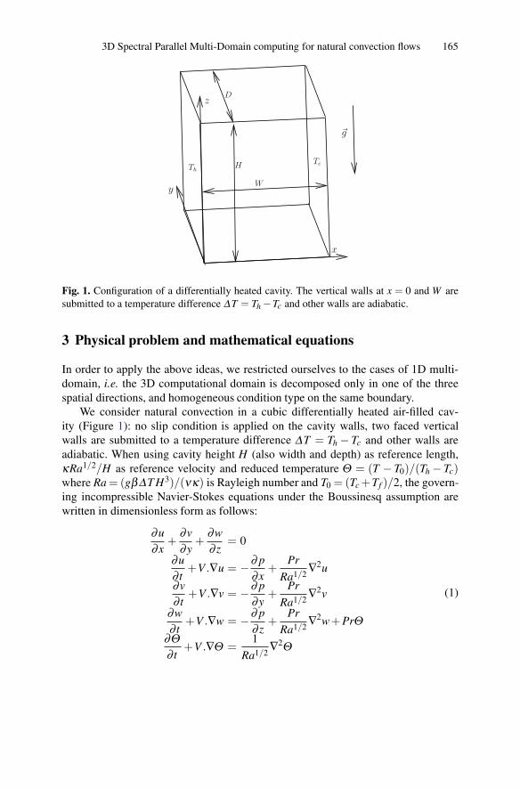
3D Spectral Parallel Multi-Domain computing for natural convection flows 165
D
H
z
Th
Tc
y
x
�g
W
Fig. 1. Configuration of a differentially heated cavity. The vertical walls at x = 0 and W aresubmitted to a temperature difference ΔT = Th −Tc and other walls are adiabatic.
3 Physical problem and mathematical equations
In order to apply the above ideas, we restricted ourselves to the cases of 1D multi-domain, i.e. the 3D computational domain is decomposed only in one of the threespatial directions, and homogeneous condition type on the same boundary.
We consider natural convection in a cubic differentially heated air-filled cav-ity (Figure 1): no slip condition is applied on the cavity walls, two faced verticalwalls are submitted to a temperature difference ΔT = Th − Tc and other walls areadiabatic. When using cavity height H (also width and depth) as reference length,κRa1/2/H as reference velocity and reduced temperature Θ = (T − T0)/(Th − Tc)where Ra = (gβΔT H3)/(νκ) is Rayleigh number and T0 = (Tc +Tf )/2, the govern-ing incompressible Navier-Stokes equations under the Boussinesq assumption arewritten in dimensionless form as follows:
∂u∂x
+∂v∂y
+∂w∂ z
= 0
∂u∂ t
+V .∇u = −∂ p∂x
+Pr
Ra1/2∇2u
∂v∂ t
+V .∇v = −∂ p∂y
+Pr
Ra1/2∇2v
∂w∂ t
+V .∇w = −∂ p∂ z
+Pr
Ra1/2∇2w+ PrΘ
∂Θ∂ t
+V .∇Θ =1
Ra1/2∇2Θ
(1)

166 S. Xin, J. Chergui, and P. Le Quere
where (x,y,z) ∈ [0,1]× [0,1]× [0,1], V = (u,v,w), V .∇= u∂∂x
+ v∂∂y
+w∂∂ z
, ∇2 =
∂ 2
∂x2 +∂ 2
∂y2 +∂ 2
∂ z2 and Pr = ν/κ is Prandtl number.
4 Numerical schemes and parallel algorithm
Equations (1) are discretized in time by the well-known second-order Euler-backwardAdams-Bashforth scheme. This leads essentially to Helmholtz equations apart fromthe velocity-pressure coupling. When using any variant of projection method [4], oneobtains a pseudo-Laplacian operator for pressure and has to solve a pseudo-Poissonequation (a special Helmholtz equation). In this way, Equations (1) are reduced toHelmholtz equations after the time discretization. The parallel algorithm is thus il-lustrated through a model Helmholtz equation.
Given f , one of u, v, w, p and Θ , and (∇2 −λ ) f = s. The domain in one of x,y and z directions can be divided into subdomains and for convenience x directionis chosen for illustration. Each subdomain is discretized by spectral methods andthe continuity of f and its first derivative in x is required on the interfaces. Due tothe assumption of homogeneous condition type on the same boundary, all the sub-doamins have the same continuous and discret operators in both y and z directions.For the model equation, it is the operators of the second-derivatives modified by thecorresponding boundary conditions. In practice, these discret operators are full ma-trices and they are diagonalizable and diagonalized when using spectral collocationmethods to solve the model equation. In the eigen-spaces of the discret operators, the
model equation is written as follows:
(∂ 2
∂x2 −λ +λ j +λk
)f jk = s jk where λ j and
λk are respectively the eigen-values of the discret operators in y and z direction. Onethus has a set of 1D problems and the basic ideas described above can be appliedto the model equation and to the equations (1). For each variable, instead of a Schurcomplement in the physical space, one has a set of small-block Schur complements inthe eigen-spaces: the Schur complement in the physical space is diagonalized in theeigen-spaces into tridiagonal blocks. The tridiagonal blocks are divided into groups,distributed each group to one processor through MPI Alltoall communications andsolved by the well-known TDMA.
It is important to note that when spectral collocation methods are used to solvea 3D Helmholtz equation the resolution method is usually the total diagonalisation.Diagonalising the Schur complement into blocks in the eigen-spaces is the naturaland convenient way to do it. Although the MPI Alltoall and MPI Sendrecv commu-nications used to construct and distribute the small-block Schur complements maybe expensive, in the context of time-stepping or time-marching, the construction andinversion of small-block Schur complements are done only once and they repre-sent only a preprocessing step before the time loop. In fact, for each variable, one
time-step needs one neighbor-to-neighbor (MPI Sendrecv) communication of∂ f∂x

3D Spectral Parallel Multi-Domain computing for natural convection flows 167
on the interfaces (in order to obtain the∂ f∂x
differences), one MPI Alltoall commu-
nication of∂ f∂x
differences on the interfaces, one MPI Alltoall communication of
the corrections of f on the interfaces (after each processor solves the correspond-ing small-block Schur complement problems) and one final neighbor-to-neighbor(MPI Sendrecv) communication of the f corrections. As can be seen later, thepresent parallel algorithm is very efficient and cost effective.
5 Code behavior and numerical results
A numerical code in F90 has been developed under MPI (Message Passing Inter-face). In order to understand the parallel performance of the new code, parallel com-putation with increasing subdomains (or processors) for different spatial resolutionshas been performed on a small cluster of Opteron 250 with Gigabit switch network.The tests concern natural convection in differentially heated cavities: the domain inz direction has been decomposed into subdomains, the spatial resolution in x and ydirections is kept the same, i.e. 50× 50 and three spatial resolutions in z direction,20, 30 and 50, have been tested. The Walltime per processor (subdomain) shown inFigure 2 remains approximately constant. This behavior is confirmed by computa-tions performed with more processors on the IBM Power4 and Power4+ of IDRIS:unfortunately it was not possible to choose the type of nodes and the two types ofnodes used prevented us from providing similar curves as in Figure 2. Nevertheless,it is to note that different tests performed with 30 and 60 processors showed that thecommunication time is less than 15 percent of the total Walltime.
400
600
800
1000
1200
1400
1600
2 3 4 5 6 7 8
Wal
ltim
e/P
roce
ssor
(s)
Number of processors/subdomains
50x50x2050x50x3050x50x50
Fig. 2. Walltime per subdomain (or processor) for different spatial resolution. The domain inz direction is divided into subdomains.

168 S. Xin, J. Chergui, and P. Le Quere
The parallel code has also been used for benchmarking: numerical simulationshave been done for a cubic differentially heated cavity at Ra = 106 [5]. The numberof subdomains ranges from 2 to 6 and the spatial direction in which the domain isdecomposed into subdomains is either x or y direction. The benchmark solutions ob-tained with 3 subdomains (or processors) are listed in Table 1: reasonable agreementis observed. Figure 3 displays the corresponding isotherms obtained at Ra = 106 with4 subdomains (or processors).
NP=3 DD=2 DD=1 Reference [5]Nu0 8.6401 8.6399 8.6407umax .12634 .12695 .12697vmax .02544 .02550 .02556wmax .23412 .23032 .23672
Table 1. Benchmark solutions at Ra = 106 obtained by parallel computations with 3subdomains (or processors) (NP=3). DD=2 means that the y direction is decomposed andthe corresponding subdomain resolution is 50×20×50. DD=1 means that the x direction isdecomposed and the corresponding subdomain resolution is 20× 50× 50. Nu0 is averagedNusselt number on the hot wall (x = 0), umax, vmax and wmax are respectively the maxima ofvelocity components.
Fig. 3. Isotherms at Ra = 106. The domain in y direction is divided into 4 subdomains.

3D Spectral Parallel Multi-Domain computing for natural convection flows 169
Previous studies [5, 3] showed that the onset of time-dependent flows occurs atapproximately Ra = 3.2× 10⁷ in a cubic differentially heated air-filled cavity. Theinstable modes break the reflection symmetry in y direction, their spatial distributionis mainly located about y = 0.5. Parallel computations have been realized for Ra =3.5×10⁷ using 4 subdomains (or processors), the decomposed direction is y directionand a subdomain resolution of 80× 20× 80. As the first two instable modes havealmost the same critical Rayleigh number, symmetry constraining has been applied:either the 2D centro-symmetry in (x,z) or the full 3D centro-symmetry has beenimposed. Figure 4 depicts the numerical results of x component of vorticity field:instable structures about y = 0.5 are clearly shown and the results are similar tothose presented in [3]
Fig. 4. Instantaneous x component of vorticity obtained at Ra = 3.5× 10⁶. The front is thecold wall at x = 1. On the left, the 2D centro-symmetry in (x,z) is imposed while on the rightthe full 3D centro-symmetry has been forced.

170 S. Xin, J. Chergui, and P. Le Quere
6 Summary
A 3D spectral parallel multi-domain code has been developed using Schur comple-ment for interface problems and validated with known results of natural convectionin a differentially heated cavity in the literature.
It solves the unsteady incompressible Navier-Stokes equations and is based onparallel algorithm for solving Helmholtz equations. In fact, any time scheme reducesthe N-S equations to Helmholtz equations and any variant of projection method leadsto a pseudo-Poisson equation for pressure (a particular Helmholtz equation).
In order to have efficient parallel algorithm, Schur complement of the interfaceproblems is not treated in physical space but in the eigen-spaces: it is diagonalizedinto small diagonal blocks and this reduces efficiently Walltime related to the inter-face problems. Tests performed on IBM Power4 and Power4+ show that the com-munication time remains less than 15 percent of the total Walltime even when 60processors are used. The developed parallel code has good scalability and will beused for doing DNS of 3D turbulent natural convection flows in cavities.
Acknowledgement: The present work has been conducted under LIMSI researchproject ASP. Computations have been performed at IDRIS under research project70326.
[1] C. Bernardi and Y. Maday. Approximations spectrales de problemes aux limiteselliptiques. In Collection Mathematiques & Applications. Springer Verlag, Berlin,1992.
[2] C. Canuto, M.Y. Hussaini, A. Quarteroni, and T.A. Zang. Spectral methods influid dynamics. Springer Verlag, New York, 1988.
[3] G. de Gassowski, S. Xin, and O. Daube. Bifurcations et solutions multiples encavite 3D differentiellement chauffee. C. R. Acad. Sci., Ser. II b, 331:705–711,2003.
[4] J.-L. Guermond and L. Quartapelle. On the approximation of the unsteadyNavier-Stokes equations by finite element projection methods. Numer. Math.,80(5):207–238, 1998.
[5] G. Labrosse, E. Tric, H. Khallouf, and M. Betrouni. A direct (peudo-spectral)solver of the 2D/3D Stokes problem : Transition to unsteadiness of natural-convection flow in a differentially heated cubical cavity. Num. Heat Trans. B,31:261–276, 1997.
[6] P. Le Quere. A modified Chebyshev collocation algorithm for directsimulationof 2D turbulent convection in differentially heated cavities. Finite Element in Ana.& Design, 16:271–283, 1994.
[7] S.H. Peng and L. Davidson. Large eddy simulation for turbulent buoyant flow ina confined cavity. Int. J. Heat & Fluid Flow, 22:323–331, 2001.
[8] J. Salat, S. Xin, P. Joubert, A. Sergent, F. Penot, and P. Le Quere. Experimentaland numerical investigation of turbulent natural convection in a large air-filledcavity. Int. J. Heat & Fluid Flow, 25(5):824–932, 2004.

3D Spectral Parallel Multi-Domain computing for natural convection flows 171
[9] S. Xin and P. Le Quere. Numerical simulations of two-dimensional turbulentnatural convection in differentially heated cavities of aspect ratios 1 and 4. InEurotherm ERCOFTAC Workshop on Direct and Large Eddy Simulation, pages423–434, Univ. of Surrey, UK, 1994.
[10] S. Xin, X. Nicolas, and P. Le Quere. Stability analyses of longitudinal rolls ofPoiseuille Rayleigh-Benard flows in air-filled channels of finite transversal exten-sion. Num. Heat Trans. A, 50(5):467–490, 2006.


3D time accurate CFD simulations of a centrifugalcompressor
Andreas Lucius1 and Gunther Brenner1
Institute of Applied Mechanics, Department of Fluid Mechanics,Clausthal University of Technology, Adolph-Roemer Str. 2a,38678 Clausthal Zellerfeld, Germany
[email protected]@tu-clausthal.de
In this paper results of unsteady CFD computations of a centrifugal compressor arepresented and compared to steady state solutions. Two cases are examinated, the firstcase is a rotor with spiral casing close to the design point. This simulations showsthe unsteady rotor stator interaction. In the second case the same rotor followed by avaneless diffuser without spiral casing is simulated at part load. The aim is to showthe unsteady rotating stall effect without disturbance coming from the geometry. Afrequency analysis for both cases is conducted. As expected the blade passing fre-quency and its multiples are dominating in the calculation with casing. For the rotat-ing stall typical unsteady vortices are observed. The unsteady pressure fluctuationsare a magnitude higher in comparison to the calculation at design point.
1 Introduction
CFD simulations are today state of the art in the design and optimization process forturbomachinery applications. Progress in development of numerical techniques andthe increasing computational power make it possible to run 3D Navier Stokes codeson small workstations. For standard problems in the turbomachinery design process- like optimization in terms of effciency for the design point - this is sufficient. For atypical calculation only a part of the impeller e.g. the flow around one or two bladesis modelled, with periodic boundary conditions applied in the circumferential direc-tion. This approach is valid only for axially symmetric geometries. For this reason itis not applicable, if a volute is used as a collector for the fluid. A complete analysisof machine performance is only possible, if the full 360 Rotor coupled with the sta-tor geometry is considered. In addition to the need of including the whole machinewith rotor and stator domains, transient effects appear in the flow. This is especiallythe case for operation in off-design conditions. In such an operational point the flow
D. Tromeur-Dervout (eds.), Parallel Computational Fluid Dynamics 2008,Lecture Notes in Computational Science and Engineering 74,DOI: 10.1007/978-3-642-14438-7 18, c© Springer-Verlag Berlin Heidelberg 2010

174 Andreas Lucius and Gunther Brenner
conditions do not match the volute design resulting in an asymmetric pressure dis-tribution. For this reason the rotating blades are loaded with differing back pressureduring one rotation, resulting in a strongly unsteady flow in the impeller itself. Thusa more detailed transient analysis for off-design operation is needed, which requiressubstantially more computational ressources.In the past several simplified approaches have been attempted to account for this ef-fect. Hillewaert has simulated the transient rotor stator interaction with an inviscidunsteady flow solver [5]. Hagelstein et al. [2] used an unsteady Euler code usinga correction term accounting for viscous effects. Their simulation showed in gen-eral a good agreement with measurements, but at low mass flow seperation was notpredicted. In the work of Treutz [7] a transient Navier Stokes solver was appliedto simulate the unsteady effects in a water pump. He pointed out the differencesbetween steady state solutions and time accurate results. In his work the whole char-acteristic curve was calculated in one simulation via reduction of massflow in time.Allthough grid dependence was pointed out to be small, the number of grid points isvery low. (160,000 CVs for the whole pump including volute were used). Turunen-Saaresti [6] also used an unsteady Navier Stokes solver for the calculations. He useda quite coarse grid neglecting the tip clearance.For the present paper different approaches for coupling the rotating impeller and thestationary volute are tested and compared against transient calculations. Computa-tional time and effort were evaluated, in order to reach accurate solutions econom-ically. All calculations were performed on the HLRN High performance computerin Hannover, using the general purpose CFD code ANSYS CFX 10.0 with up to16 processors in parallel. In the end results are compared with performance mea-surements obtained for an industrial compressor. Furthermore a transient simulationof the rotating stall phenomenon was conducted. For this simulation the impellerwithout volute was calculated, since stall is a part load problem induced by leadingedge separation. The results show the typical travelling vortices and strong pressurefluctuations, which may lead to resonance problems.
2 Transient effects in turbomachinery
There are several sources of unsteadiness in turbomachines ranging from turbulentfluctuations at very small time and length scales up to rotating stall and surge wherethe length scales are of the dimension of the machine [3]. The turbulent fluctuationsare usually modelled, since the direct simulation of turbulence is not possible forhigh Re number flows. In addition a resolution of turbulence is often not of interest,but its influence on the mean flow.For this investigation the unsteady effects resulting from rotor stator interactions areof main interest. One source of instability is due to the interaction of the rotor wakewith the volute tongue appearing at timescales depending on the number of bladesand the rotational speed. On the other hand a perfect axially symmetric pressurefield cannot be expected. In the volute tongue region a distortion of the pressurefield is usually observed. In addition to that, a volute can only be designed for one

3D time accurate CFD simulations of a centrifugal compressor 175
operational point. If the machine operates in off-design conditions, the pressure dis-tortion will increase, resulting in a highly unsteady back pressure for the blading.In part load an additional unsteady phenomenon appears, which is referred to as ro-tating stall [1]. With decreasing flow rate the inlet velocity triangle changes, result-ing in separation on the suction side of the blades. This separation leads to a reducedflow through the stalled channel, influencing the adjacent flow channels. The stallcells travel through the blading at a fraction of machine rotational speed, introducinganother source of instability. The simulation of this effect is another scope of thiswork.As was shown before, unsteady effects appear at many time and length scales. Nearthe design point steady state calculations may be sufficient, but in off-design condi-tions transient effects cannot be neglected. Apart from accurately predicting the flowthrough the compressor, transient results are interesting with respect to Fluid Struc-ture Interaction [4] or noise prediction. With further development in these fieldsunsteady CFD calculations in turbomachines will become more common.
3 Numerical Procedure
For all CFD calculations the finite volume code ANSYS CFX 10.0 was used. Thecode solves the Reynolds Averaged Navier Stokes equations, turbulence was mod-elled using the SST k-ω model. In all simulations transition was neglected. The wallboundary layers were calculated using scalable wall functions. As the grid resolu-tion plays an important role, a study of grid convergence was first conducted. For theblading a block structured grid was generated, using a J-grid topology. This topologyavoids highly skewed elements at the leading edge of the impeller. The smallest an-gles were of 34 degrees, on blade surfaces a high orthogonality with near 90 angleswas achieved. The blade tip clearance was gridded with an own O-grid topology withminimum 8 nodes in the gap. The grid contains a stationary inlet domain, one bladepassage of the rotor and a vaneless diffuser (Fig. 1a). The inlet boundary is placed3 tube diameters upstream from the leading edge, the outlet is placed at 1.6 timesthe rotor outlet diameter. Table 1 shows the results obtained for single passage cal-culations with periodic boundary conditions. These calculations took up to 5 hourson a standard PC in serial mode.In terms of pressure rise convergence was reachedalready for the coarse grid. The isentropic pressure coefficient is defined as
Ψs =2Δhs
u22
(1)
where Δhs is the isentropic change in static enthalpy and u2 is the rotational velocityat the trailing edge. The maximum y+ is found at a very small amount of cells at thetrailing edge of the rotor blade. As you can see from the computed tip clearance massflow, the resolution in the tip gap influences the results. The coarse grid had 8 nodesin the tip gap whereas 10 respectively 14 nodes were used in the two other cases.Thus at least 10 nodes are needed to obtain accurate tip clearance flow. Due to thesmall differences in pressure rise and the high number of nodes for the full machine,

176 Andreas Lucius and Gunther Brenner
the coarse grid was chosen or further calculations.The full machine model contains 3 domains (Fig. 1b): the inlet domain, the rotorcontaining 13 flow channels, and the volute. Due to the complexity of the geome-try a single structured grid could not be applied at the volute tongue region. Hereseparate structured meshes were generated and merged in the flow solver. The restof the volute and the cone diffuser were meshed with an own block structured grid.The total number of nodes was 2.7 million for this case. The computations weredone on the HLRN 1 system in Hannover (Norddeutscher Verbund fur Hoch undHochstleistungsrechnen). The complex consists of 16 p690 compute servers with 32processors each. Until now up to 16 processors were used in parallel. MPICH wasapplied as parallelization algorithm. The time step was chosen in order to resolve onerevolution with 64 respectively 128 time steps, which corresponds to approximately5 (10) timesteps per blade passage.
Table 1. Grid convergence
Nr. of nodes max y+ mean y+ Ψs relative tip clearance mass flow [%]143,000 358 31 1.06 15.9251,000 115 18.9 1.05 16.9405,000 45.2 9.1 1.05 16.8
a) b)
Fig. 1. Problem setup a) single passage b) full machine with volute

3D time accurate CFD simulations of a centrifugal compressor 177
4 Results
4.1 Compressor with volute
For coupling stationary and rotating domains 3 methods exist. For steady state sim-ulations the interface can be modelled either as a mixing plane or as a frozen rotor.A mixing plane averages the circumferential profiles of all variables and transfersonly the mean values to the stator domain. The frozen rotor interface directly trans-fers the circumferential profiles. A steady state solution with frozen rotor interfacesdepends on the actual position of the rotor. For this reason several calculations areusefull in order to obtain mean values. The most accurate approach is to couple therotor and the stator in a transient simulation. First of all steady state simulations wereconducted. The operational point was chosen near the design point at measured rota-tional speed which was about 60 % of the design speed. First a mixing plane interfacewas applied. The rotor wakes disappear in the vaneless diffuser due to averaging atthe interface. The pressure coefficient was calculated to 0.99, the measured valuewas 1.11. For the frozen rotor interface, only a small change in the pressure rise wasobserved. In order to see an influence of the actual rotational position, the bladeswere rotated in several steps 25 % of one pitch (27.3 ◦), but the influence is less than1 % between the different cases (Table 2).The transient calculation was done using 128 time steps per revolution. The time av-
Table 2. Comparison of simulated results
stage 0◦ 6.9◦ 13.9◦ 20.8◦ transient measurementΨs 0.994 1.002 0.999 0.997 1.003 1.05 1.11
eraged pressure coefficient was calculated to 1.05, but no real periodic state could befound within 5 rotations of the impeller. This may be a result of a separation appear-ing in the cone diffuser. The deviation of about 10 % for the steady state calculationsis quite high. For a steady state calculation the computational time was about 17 h,the transient simulation took about 70h for one revolution. Both were done with 8CPUs in parallel. An analysis of the pressure signal shows a change of the transientbehaviour after 3 revolutions, where a superposition of low frequency fluctuationsis observed. A FFT analysis of the time dependent pressure signal shows, that theblade passing frequency is dominating, especially near the rotor. Similar low fre-quency fluctuations can be found at both locations (Fig. 2).
4.2 Compressor without volute
The rotating stall phenomenon was simulated at part load at 65% of mass flow com-pared to the point with maximum efficiency. In contrast to the results shown before,the compressor volute was not included in these calculations to avoid disturbancecoming from the asymetric geometry. The fluid domain is a full circle setup of

178 Andreas Lucius and Gunther Brenner
0 1 2 3 4 5simulation time [revolutions]
1.2
1.25
1.3
1.35
1.4
1.45p /
po
pressure diffuser inletpressure diffuser middle
0 1 2 3 4 5f / f
blade
0
0.5
1
1.5
2
2.5
3
p /
p0
diffuser inletdiffuser middle
a) b)
Fig. 2. Simulated pressure at two locations, a) variation in time b) FFT transformed signal
the single passage calculation conducted for the convergence study. The operationalpoint was chosen according to the low limit of the performance curve determinedfrom steady state single passage calculations. In Fig. 3 one can see the stall cellsdisplayed as areas with negative streamwise velocity. The stalled regions travel witha negative rotational velocity through the machine seen from the rotating frame ofreference.The pressure history shows a noticeable difference when changing from 64 to 128
a) b)
Fig. 3. Travelling rotating stall cells displayed as negative streamwise velocity, a) and b) twodifferent time steps
time steps per revolution (Fig. 4a). For this reason only the last revolutions with thesmaller time step were analyzed in more detail. We observed strong fluctuations inpressure, but the signal seems random with no visible periodic behaviour. For thiscase the FFT analysis shows, that high amplitude fluctuations at low frequencies are

3D time accurate CFD simulations of a centrifugal compressor 179
0 5 10simulation time [rev]
1
1.5
2
2.5
3p /
p0
p diff middle dt = rev/64p diff middle dt = rev/128
0 1 2 3 4 5f / f
blade
0
10
20
30
40
50
p /
p0
p diffuser middle
a) b)
Fig. 4. a) Pressure history during rotating stall b) FFT transformed signal
dominating, while the blade frequency is of minor importance (Fig. 4b). This is ex-pected since rotating stall usually appears at frequencies lower than rotational speed.In order to obtain an accurate value of the stall frequency, a simulation time of atleast 8 or more revolutions is needed.
5 Summary
As expected, a transient simulation for the rotor with volute gives a better resultscompared to steady state simulations in terms of pressure rise. The relatively highdifference in comparison to the measurements may be explained with the apperanceof a large separated area in the outlet diffuser following the volute. This separationmay not be captured correctly with the used turbulence model. The difference be-tween the 4 frozen rotor positions is neglegible, a stage interface showed nearly thesame result. The computation time for the transient calculation was about 20 timescompared to a single steady state solution, but gives superior results. Such an increasein effort is usually not nessecary to obtain accurate results near the design point, butit is important if the transient behaviour is of interest. In case of the rotating stall ef-fect we were able to simulate the typical behaviour of stalled cells travelling throughthe rotor and to determine low frequency high amplitude pressure fluctuations. Thesimulation time was too short to determine an accurate value for the stall frequency.The calculation of transient phenomena like rotating stall requires transient CFD.Since pressure fluctuates in time, blade vibrations may appear leading to damage ofthe blading. CFD is able to calculate the frequencies of pressure fluctuations and theiramplitudes, which enables to identify possible resonance. This is especially true foroff - design conditions were other than the blade passing frequency are dominatingexcitation mechanisms.

180 Andreas Lucius and Gunther Brenner
6 Acknowledgements
The research project was funded through the EFRE (European Regional Develop-ment Fund). The authors also thank Mr. H.J. Ring and Mr. J. Adomako (PillerIndustrieventilatoren GmbH, Mohringen) for their contributions and providing themeasurement data.
[1] Lakshminarayana B. Fluid Dynamics and Heat Transfer of Turbomachinery.John Wiley and Sons Inc, 1996.
[2] Hagelstein D., Hillewaert K., Van den Braembussche R.A., Engada A., KeiperR., and Rautenberg M. Experimental and numerical investigatation of the flow ina centrifugal compressor volute. ASME Journal of Turbomachinery, 122:22–31,2000.
[3] Greitzer E.M. An introduction to unsteady flow in turbomachines. In Thermo-dynamics and fluid mechanics of turbomachinery, volume 2. Martinus NijhoffPublishers, 1985.
[4] Dickmann H.P., Secall Wimmel T., Szwedopwicz J., Filsinger D., and RodunerC.H. Unsteady flow in a turbocharger centrifugal compressor 3d-cfd-simulationand numerical and experimental analysis of impeller blade vibration. ASMEPaper, (GT2005-68235).
[5] Hillewaert K. and Van den Braembussche R.A. Numerical simulation ofimpeller-volute interaction in centrifugal compressors. ASME Journal of Tur-bomachinery, 121:603–608, 1999.
[6] Turunen-Saaresti T. Computational and Experimental Analysis of Flow Field inthe Diffusers of Centrifugal Compressors. PhD thesis, Lappeeranta Universityof Technology, 2004.
[7] G. Treutz. Numerische Simulation der instationaren Stromung in einerKreiselpumpe. PhD thesis, Darmstadt University of Technology, 2002.


Part VI
Parallel Algorithms and Solvers

Multicolor SOR Method with Consecutive MemoryAccess Implementation in a Shared and DistributedMemory Parallel Environment
Kenji Ono1,2 and Yasuhiro Kawashima3
1 RIKEN, 2-1 Hirosawa, Wako, 351-0198, Japan [email protected] Division of Human Mechanical Systems and Design, Faculty and Graduate School of
Engineering, Hokkaido University, N13, W8, Kita-ku, Sapporo, 060-8628, Japan3 Fujitsu Nagano Systems Engineering, 1415 Midori-cho, Tsuruga, Nagano, 380-0813,
Japan [email protected]
1 Introduction
Elliptic partial difference equations like Poisson’s equation are used in many fields ofapplication. However, the coefficient matrix of the derived algebraic equation is largeand sparse, and so its inversion is expensive. Various iterative methods are used tosolve such a sparse matrix system. Although there have been many studies on solv-ing the large sparse matrix system [1, 2, 3, 4, 5, 6, 7], there have been few reports onthe implementation and performance of the iterative method with multicolor order-ing. In this paper, a novel implementation technique to enhance the performance ofthe 2-colored SOR method is proposed, which eliminates the recursion for the stan-dard 7-point stencil on the Cartesian grid in three dimensions. The performance ofthe multicolor SOR method is investigated on both a shared memory vector/parallelcomputer and a symmetric multiprocessor machine in a distributed memory environ-ment.
2 Multicolor Ordering with Sorting of Memory Layout
2.1 Issues and Concept of Improvement
A linear system can be solved by various iterative methods such as the Jacobi, SOR,and conjugate gradient methods. The Jacobi method offers high execution speed andsimple implementation in terms of vectorization and parallelization, but is slow toconverge. Meanwhile, although the SOR method converges faster than the Jacobimethod, its performance is low due to the forward recursion of the iterative pro-cedure, which disturbs full vectorization of a loop. A hyper-plane or a multicolorordering is often introduced to eliminate the recursion of the SOR iteration.
D. Tromeur-Dervout (eds.), Parallel Computational Fluid Dynamics 2008,Lecture Notes in Computational Science and Engineering 74,DOI: 10.1007/978-3-642-14438-7 19, c© Springer-Verlag Berlin Heidelberg 2010

184 Kenji Ono and Yasuhiro Kawashima
Two colors are sufficient to eliminate the dependency of the recursion for the7-point stencil, which is generated from the Laplace operator. To take account of thevectorization and/or the parallelization, the minimum number of colors is preferable,because both the vector length and granularity of the parallelization increase as thenumber of colors decreases. Furthermore, fewer color minimizes the number of timesof synchronization, thus boosting parallel performance.
There is an important performance issue in code implementation. Here, letus consider the discretized Laplace equation (1) of 7-point stencil on a three-dimensional Cartesian mesh.
pi, j,k = pi−1, j,k + pi+1, j,k + pi, j−1,k + pi, j+1,k + pi, j,k−1 + pi, j,k+1 (1)
It is common to describe a multicolor SOR code by a stride in a do-loop in List 1,which yields stride memory access (SMA). However, SMA prevents efficient usageof cache and vector pipelines. On the other hand, the natural ordering realizes con-secutive memory access (CMA), and so CMA is expected to offer better performancethan SMA. Therefore, a novel technique that combines the SOR method and CMAimplementation is proposed.
List 1 Pseudo code for 2-colored ordering SOR with stride memory access.
do c=0,1do k=2,nx-1do j=2,nx-1do i=2+mod(k+j+c,2), nx-1, 2
s0= p(i+1,j ,k ) + p(i-1,j ,k ) &+ p(i ,j+1,k ) + p(i ,j-1,k ) &+ p(i ,j ,k+1) + p(i ,j ,k-1)
ss=(s0-p(i,j,k))p(i,j,k)=p(i,j,k)+omg*sser = er + ss*ss
end doend doend do
end do
Note: Variables nx, c and er represent a dimension size, color and error, respectively. Array pindicates some potential.
2.2 Implementation of 2-Colored Ordering SOR with Consecutive MemoryAccess
The 2-colored ordering as shown in Fig. 1 is well known. First, a computational do-main of size imax× jmax× kmax is divided by a 2× 2× 2 sub-domain that formsa unit block in three dimensions. Then, the computational domain is consists ofNI×NJ×NK blocks, where NI = imax/2+1 for index i. Therefore, the dimensionsize is limited to an even number in each direction. The shape of the dimension canbe described by P(NI*NJ*NK, 4, 2). The first element in the dimension represents

Multicolor SOR Method with CMA implementation 185
the serialized one-dimensional address of the block. The second and third elementsrepresent the position index inside a block and color, which are indicated in Fig. 1.
Next, the relationship between variables is described for each position in the unitblock. For example, the code of equation (1) can be written by List 2 for variable P(i,1, 1) in Fig. 1.
OR (1, 2)GR (1, 1)
GR (3, 1)
GR (4, 1)
GR (2, 1)OR (2, 2)
OR (3, 2)
OR (4, 2)
RORG
1 n Nmax
Pos 1 Pos 2 Pos 3 Pos 4 Pos 1 Pos 2 Pos 3 Pos 4
(n, 4, 1)
Array P(NI*NJ*NK, 4, 2)
Fig. 1. 2-colored ordering with consecutive memory access. Indexes in parenthesis in the leftfigure are position (Pos = 1, 2, 3, 4) and color (OR = 1, GR = 2), respectively. Index N in theright figure has four continuous variables corresponding to inside a unit cube in the left figure.
List 2 Pseudo code of CMA for P(i, 1, 1).
do i=ist,ieds0= p(i , 1, 2) + p(i-1 , 1, 2)*f2 &
+ p(i , 2, 2) + p(i-ni , 2, 2)*f4 &+ p(i , 3, 2) + p(i-nij, 3, 2)*f6
ss= (s0-p(i,1,1))p(i,1,1)=p(i,1,1)+omg*sser = er + ss*ss
end do
Note: Variables ist and ied represent the start and end address of a block. A neighbor indexbeyond the own block is taken from a neighbor block in consideration of periodicity. The loadbalance becomes optimal because loop i is parallelized and vectorized simultaneously.
2.3 Performance Evaluation
We consider the Laplace equation ∇2ϕ = 0 on the Cartesian grid system to inves-tigate the convergence rate and the performance for iterative methods. Details ofproblem setting are given in [7]. A norm to determine the convergence is defined by:
√∑i, j,k
(∣∣ϕm+1 −ϕm∣∣)
i, j,k, (2)

186 Kenji Ono and Yasuhiro Kawashima
where m indicates the number of iterations. The computational space is defined by aunit cube Ω = [0,1]3, which is divided by NX ×NX ×NX , where NX is dimensionsize.
3 Results and Discussion
3.1 Performance on a Shared Memory Vector Computer
Table 1 shows measured performance obtained by a hardware performance moni-tor on one CPU of a Cray Y-MP8/664. The Jacobi method shows high performancebecause the consecutive data access can utilize the high bandwidth of a vector com-puter. Although the natural ordering SOR method is inherently consecutive mem-ory access, the performance is not high because the recursion interference preventsthe code from vectorizing. When a programmer implements the multicolor SOR bystride memory access, the memory-bound occurs at runtime even in a vectorizedcode.
Therefore, it is important to employ a strategy for the division and sorting ofthe variable array such that the processor can access the memory consecutively. Themeasured MFLOPS score of multicolor CMA code indicates that it is as fast as theJacobi code which can utilize the full bandwidth of the vector computer as shown inTable 1. It was confirmed that the expected performance was obtained on the vectorcomputer.
Fig. 2 shows the measured convergence history on the vector machine. In thistest case, the size of dimension NX is 33. It is observed that the convergence rate ofthe Jacobi method is the worst among them, and one of the 2-colored SOR-SMA andthe 2-colored SOR-CMA are identical. Therefore, the multicolor SOR method by theCMA implementation is the best candidate from the aspect of the both performanceand convergence rate.
Table 1. Performance (MFLOPS) on a shared memory vector machine.
Jacobi SOR Multicolor SMA Multicolor CMA
236 60 150 232
Next, the parallel efficiency on a Cray C90, which is a similar vector/parallel ma-chine, is shown in Fig. 3. The Jacobi method is written by the triple loop of indicesk, j, i. The outer loop k is parallelized and the inner loop i is vectorized. In this case,according to the number of CPUs, an imbalance of the load may reduce the perfor-mance. This phenomenon is of particular note when the residue number of outer loopis small compared to the number of CPUs. For the same reason, the efficiency of theSMA multicolor SOR method becomes the worst among the methods because of theinefficient stride memory access. On the other hand, since both the Jacobi and CMA

Multicolor SOR Method with CMA implementation 187
0 20 40 60 80 100 120
Iteration
1x10⁻⁵
1x10⁻⁴
1x10⁻³
1x10⁻²
1x10⁻¹
1
1x101
Nor
m
JacobiSORSOR2-SMASOR2-CMA
Fig. 2. Convergence history for several iterative methods against norm defined by Euation (2).
Fig. 3. Efficiency of thread parallelization on a Cray C90.
code are consecutive memory access, the performance is better than the SMA code.Especially, the CMA code shows excellent parallel efficiency because the inner loopof the array for each color is serialized and hence the load balance becomes optimal.It was found that the CMA multicolor SOR code is as fast as the Jacobi code andshows excellent parallel efficiency on a shared memory vector computer.
3.2 Performance on a Symmetric Multiprocessor Computer
The proposed CMA implementation of the SOR method on a SMP machine is ex-amined. The code was parallelized by OpenMP directives. The test environment wasa Xeon 5360 (4 cores x dual CPUs, 3GHz) with Intel compiler 10.1 on a Mac OSX

188 Kenji Ono and Yasuhiro Kawashima
10.5.4. The evaluated iterative methods were the Jacobi, the 2-colored SOR-SMA,and SOR-CMA.
Fig. 4 shows the measured timing for in-cache and out-of-cache sizes and num-ber of threads for one iteration. It is found that the 2-colored CMA code shows thebest performance among the methods. In terms of parallel efficiency, the CMA codedoes not show good parallel performance because the CMA code is already saturatedbeyond two threads. However, the execution time of the CMA code is the shortest.
The CMA code have the reason for high performance on the scalar machine. Thatis the relationship between the bandwidth and the amount of load/store. In termsof bandwidth, the number of arrays to be loaded and stored is important for theperformance. The number of loads/stores of the SOR group is two. Meanwhile, theJacobi need an additional work array. The CMA also needs an small additional workarray for sorting, but this is trivial. In fact, the feature of fewer amount of load/storeand fast memory access allows high performance. This aspect has a larger influencefor the SMP machine than the shared memory vector machine because of the limitedbandwidth.
Fig. 4. Timing for in-cache size (NX = 33, left) and out-of-cache size (NX = 513) against num-ber of threads. Vertical and horizontal axes indicate time and number of threads, respectively.In all cases, the CMA code shows the best performance.
3.3 Performance in a Distributed Memory Parallel Environment
The performance was investigated in a distributed environment. The OpenMPI li-brary was used for the parallel computation with the domain decomposition method.The computer resource used was the Quest system in RIKEN, which consists of 1024nodes (2048 cores) of a Core2Duo cluster (L7400, 1.5GHz, L2 4GB). The intercon-nect is GbE and 2Gbps for each node. Fig. 5 shows the measured performance for

Multicolor SOR Method with CMA implementation 189
Fig. 5. Comparison of performance on Core2Duo cluster. Intel Compiler 10.1, option O3 wasused. The left figure shows the scalability based on elapsed time. The right figure shows thescalability based on only calculation time. CMA indicates super-linear behavior and the othermethods show good scalability.
the fixed size of 416×416×416. This is a strong scaling test, which is obtained forthe case of one core per node.
Scalability based on measured elapsed time indicates that all methods show goodscalability up to 256 nodes and saturated behavior above 256 nodes. However, re-garding scalability based on the timing for only the calculation part as shown in theright panel of Fig. 5, all methods show very good scalability, and CMA in particularis super-linear. The is because beyond 512 nodes, the computation size for each colorarray becomes less than 26×26×26, which fits into cache.
One issue is the communication part. Table 2 shows the communication cost periteration. It is found that almost all of the time cost is occupied by communicationover 256 nodes and that the CMA code is faster below 256 nodes. As mentionedabove, beyond 512 nodes, all data are in-cache in CMA code, so the communica-tion cost becomes relatively large. At present, since the communication part wasimplemented by a brute-force method, there is still room for improvement. In thisenvironment, the measured results reveal that the stencil-based calculation is almostsaturated for this size of problem.
In the CMA implementation, we need to sort the array once depending on theordering before and after the iteration. Table 3 indicates the cost of sorting. Threearrays and one array need to be sorted before and after iteration, respectively. Thetiming data showed a relative cost ratio for pre-sorting to post-sorting of almost 3:1.This sorting cost is equivalent to the cost for one or two iterations.
Table 2. Cost of communication part for one iteration (percent).
Node 2 4 8 16 32 64 128 256 512 1024
Jacobi 1.5 2.7 6.3 8.8 13.3 21.0 29.9 46.1 52.8 72.52-colored SMA 1.2 2.5 4.4 7.9 9.0 14.9 24.8 34.7 57.3 68.42-colored CMA 2.1 3.4 6.4 9.4 14.0 21.3 40.7 58.2 75.0 84.7

190 Kenji Ono and Yasuhiro Kawashima
Table 3. Timing of sorting part in CMA code (sec). The ratio is the sum of pre-sorting andpost-sort time divided by the time for one iteration.
Node 2 4 8 16 32 64 128 256 512
pre-sort 6.96e-1 3.65e-1 1.79e-1 9.08e-2 4.69e-2 2.38e-2 1.78e-2 6.07e-3 3.06e-3post-sort 2.21e-1 1.13e-1 5.71e-2 2.89e-2 1.47e-2 7.77e-3 9.47e-3 2.04e-3 1.05e-3Ratio 1.4 1.2 1.2 1.3 1.2 1.3 2.3 1.1 0.7
4 Conclusions
A new implementation of the multicolor SOR was proposed including the variablesorting to achieve consecutive memory access. Its effect was confirmed on a sharedmemory vector/parallel and SMP machines, and it was found that the multicolorSOR method with consecutive memory access demonstrates excellent performanceon both types of machine. The CMA multicolor SOR method retains almost thesame convergence rate of the original SOR method and its execution speed is muchfaster than the original SOR on a vector computer. On the other hand, the parallelperformance on a vector/parallel machine was greatly improved by one-dimensionalserialization of the array, which leads to excellent load balance between cores. On anSMP machine, the CMA code showed the best performance among the test codes.In addition, good scalability was confirmed up to 256 nodes using a medium size of416×416×416 for all tested methods in a distributed memory parallel environment.Especially, for the strong scaling test case, the CMA code showed super-linear be-havior for a small number of CPUs compared with the other methods. Thus, if thesize of the problem becomes bigger as the number of CPUs increases, i.e., the weakscaling case, then scalability seems to be promising.
Acknowledgement
This research was supported by the Research and Development on Next-GenerationIntegrated Simulation of Living Matter, which is part of the Development and Use ofthe Next-Generation Supercomputer Project of the Ministry of Education, Culture,Sports, Science and Technology (MEXT).
[1] L.M. Adams and H.F. Jordan. Is sor color-blind? SIAM J. Sci. Stat. Comput.,7(2):1507–1520, apr 1986.
[2] S. Doi and A. Lichnewsky. Some parallel and vector implementations of pre-conditioned iterative methods on cary-2. International Journal of high SpeedComputing, 2(2):143–179, 1990.
[3] S. Fujino, M. Mori, and T. Takeuchi. Performance of hyperplane ordering onvector computers. J. Comp. and Appl. Math., 38:125–136, 1991.
[4] R.J. Leveque and L.N. Trefethen. Fourier analysis of the sor iteration. ICASEReport 86-63, NASA, 1986.

Multicolor SOR Method with CMA implementation 191
[5] E.L. Poole and J.M. Ortega. Multicolor iccg methods for vector computers.SIAM J. Numer. Anal., 24(6), 1987.
[6] R.S. Varga. Matrix Iterative Analysis. Springer, second edition, 2000.[7] M. Yokokawa. Vector-parallel processing of the successive overrelaxation
method. JAERI-M 88-017, Japan Atomic Energy Research Institute, 1988.


Proper Orthogonal Decomposition In DecouplingLarge Dynamical Systems
Toan Pham1, Damien Tromeur-Dervout1
Universite de Lyon, Universite Lyon 1, CDCSP/Institute Camille JordanUMR5208-U.Lyon1-ECL-INSA-CNRS, F-69622 Villeurbanne Cedex, [email protected],[email protected]
Abstract. We investigate the proper orthogonal decomposition (POD) as a powerfull tool indecoupling dynamical systems suitable for parallel computing. POD method is well known tobe useful method for model reduction applied to dynamical system having slow and fast dy-namics. It is based on snapshot of previous time iterate solutions that allows to generate a lowdimension space for the approximation of the solution.Here we focus on the parallelism po-tential with decoupling the dynamical system into subsystems spread between processors. Thenon local to the processor sub-systems are approximated by POD leading to have a numberof unknowns smaller than the original system on each processor. We provide a mathematicalanalysis to obtain a criterion on the error behavior in using POD for decoupling dynamicalsystems. Therefore, we use this result to verify when the reduced model is still appropriatedfor the system in order to update the basis. Several examples show the efficient gain in term ofcomputational effort of the present method.Keywords: POD, reduced-order modelling, dynamical systems, parallel computing.
1 Introduction
Proper orthogonal decomposition (POD) is known as an application of the singu-lar value decomposition (SVD) to the approximation of general dynamical systems.Usually, it is used to separate the low and fast dynamics of a dynamical system. Inthis paper, we focus on it use to solve large dynamical systems on a parallel systemleading to a robust approach based on a priori criterion to communicate updated databetween processors.
Related works on decoupling large dynamical systems on parallel architecture arebased on extrapolation techniques. In [4], the decoupling is done by extrapolatingcomponents involved on the sub-system but not managed by the current processor.This technique has been extended to asynchronous adaptative time steps [11]. In[13] or in [12], some multirate integration formulae are applied for solving largedynamical systems in parallel. Nevertheless, the major drawbacks of using thesemethods based on extrapolation technique are first the only feedback comes from an
D. Tromeur-Dervout (eds.), Parallel Computational Fluid Dynamics 2008,Lecture Notes in Computational Science and Engineering 74,DOI: 10.1007/978-3-642-14438-7 20, c© Springer-Verlag Berlin Heidelberg 2010

194 Toan Pham, Damien Tromeur-Dervout
a posteriori error estimate between the extrapolated in time data and the received cor-responding data from other systems. If the error is to high, the integration must restartfrom a previous checking point with changing the extrapolation formulae reducingthe order approximation of the extrapolation or the delay in the data to compute theextrapolation. Second, for stiff non linear dynamical system that must be solved byimplicit time integration method, only the components managed by the processor areinvolved in the Jacobian matrix leading to less influence of the other components ofthe system in the computing.Our approach consists in the decoupling of the system through the model reductionmethod that provides an answer to the two drawbacks mentioned above. First, wecan derive an a priori error estimate, to know when the data from other sub systemsmust be updated. Second, we still incorporate the influence of the other sub-systems(extra-systems) in the non linear solve of the current sub-systems (intra-system). In-deed, extra-systems solved in reduced form are very computational attractive. Whenapplying model reduction to dynamical systems, the snapshots of previous time stepsare used to compute the POD basis vectors to yield an optimal representation of thedata in sense of optimal least squares approximation. Combined with Galerkin pro-jection method, we can generate a lower dimensional model of the systems. We ex-tend this notion of model reduction to decouple the system into smaller subsystems.Each subsystem is solved separately on parallel computer and a model reduction ofthe other subsystem is performed.Basic error estimation for reduced order models has been proposed in [14] - theoriginal problem is linearized in the neighborhood of the initial time. Other resultcan be found in [9], where bounds for errors resulting from reduced models hasbeen computed. In [7], we found some results on the influence of perturbations inthe original system on the quality of the approximation given by the reduced model.Here our goal is to find a criterion to know when we need to update the POD basisto compute the extra-subsystems with no introducing error in the intra-subsystem.
The plan of this paper is as follows. In section 2 we recall some properties ofthe POD, while in section 3.2 we give an analysis of the error on the global systemwhen subsytems are approximated by POD. Then we derive an a priori estimated toupdate the POD basis that appoximated the subsytems. Section 4 gives the decou-pling algorithm and its parallel implementation. Numerical tests and performancesare summarized in section 5 before the conclusion in section 6.
2 Proper Orthogonal Decomposition and Model reduction
2.1 Singular Value Decomposition
Property 0.1. For any matrix A ∈ Cm×n, there exist two unitary matrices U ∈ C
m×m
and V ∈ Cn×n such as:
UT AV = Σ = diag(σ1, . . . ,σm) (1)
σ1 ≥ ·· · ≥ σm ≥ 0. This decomposition is called the SVD of the matrix A, σi =√λi(A∗A) are called singular values of A where λi is the ith eigenvalue.

POD in Decoupling Large Dynamical Systems 195
A can be written as : A = ∑mi=1σiuiv∗i
Remark 0.1. Given a matrix A ∈ Cn×m, the solution X of
minX∈Cn×m,rank(X)≤k<rank(A)
‖A−X‖2 = σk+1(A) (2)
is obtained by truncating the SVD to the k first singular modes: X = σ1u1v∗1 +σ2u2v∗2 + . . .σkukv∗k (c.f [1] or [8]).
2.2 POD in model reduction
POD method is widely used in generating a lower dimensional model for dynamicalsystems. We present here a procedure called Garlerkin projection. Once found theapproximating subspace to the data set of the system, we are seeking for the corre-sponding vector field on the subspace that represents the reduced order model.Given a system of dimension n:
x(t)′ = f(t,x(t)) (3)
x(t0) = x0 (4)
for t ∈ [t0,t f ], x,x0 ∈ Rn and f : R
n ×R → Rn. Collect the solutions of (3)-(4) at
m time points and form the matrix X = [x(t1), . . . ,x(tm)]. POD consists of findingthe matrix P ∈R
n×n defining the projection onto a subspace S ∈Rn minimizing the
total square distances ‖X−PX‖2. Using eq. (2), the singular decomposition of thematrix of snapshots X = UΣV T gives a such minimizer as P = UkUT
k ∈ Rn×n where
Uk correspond to the k columns of U associated to singular values σ1 ≥ . . . ≥ σk. Uk
spanes as a natural orthogonal basis the space S . The reduced model to the system(3) is constructed by projecting onto S the vector field f (s,t) at each point s ∈ S .If ξ are the subspace coordinates of s, then the reduced model is:
ξ ′(t) = UTk f(Ukξ (t),t) (5)
where x(t) ≈Ukξ (t), ξ (t) ∈ Rk.
2.3 POD for decoupling systems
In this part we present how POD can be useful in decoupling system for parallelpurpose. Given an ODE system of state variable x(t) = (x1(t),x2(t)):
x(t)′ = f(t,x(t)) =(
f (t,x1,x2)g(t,x1,x2)
), x(0) = x0 (6)
We take some snapshots of the whole system by solving globally the system. Let sayq steps are taken for initialization:
X = (x1,x2, . . . ,xq) (7)
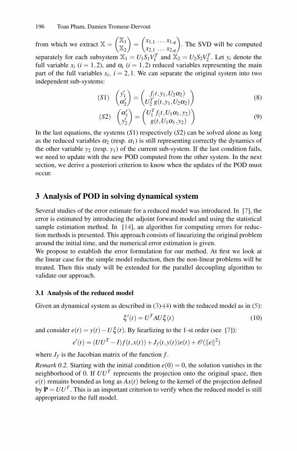
196 Toan Pham, Damien Tromeur-Dervout
from which we extract X =(
X1
X2
)=(
x1,1 . . . x1,q
x2,1 . . . x2,q
). The SVD will be computed
separately for each subsystem X1 = U1S1V T1 and X2 = U2S2V T
2 . Let yi denote thefull variable xi (i = 1,2), and αi (i = 1,2) reduced variables representing the mainpart of the full variables xi, i = 2,1. We can separate the original system into twoindependent sub-systems:
(S1)(
y′1α ′
2
)=(
f(t,y1,U2α2)UT
2 g(t,y1,U2α2)
)(8)
(S2)(α ′
1y′2
)=(
UT1 f(t,U1α1,y2)g(t,U1α1,y2)
)(9)
In the last equations, the systems (S1) respectively (S2) can be solved alone as longas the reduced variables α2 (resp. α1) is still representing correctly the dynamics ofthe other variable y2 (resp. y1) of the current sub-system. If the last condition fails,we need to update with the new POD computed from the other system. In the nextsection, we derive a posteriori criterion to know when the updates of the POD mustoccur.
3 Analysis of POD in solving dynamical system
Several studies of the error estimate for a reduced model was introduced. In [7], theerror is estimated by introducing the adjoint forward model and using the statisticalsample estimation method. In [14], an algorithm for computing errors for reduc-tion methods is presented. This approach consists of linearizing the original problemaround the initial time, and the numerical error estimation is given.We propose to establish the error formulation for our method. At first we look atthe linear case for the simple model reduction, then the non-linear problems will betreated. Then this study will be extended for the parallel decoupling algorithm tovalidate our approach.
3.1 Analysis of the reduced model
Given an dynamical system as described in (3)-(4) with the reduced model as in (5):
ξ ′(t) = UT AUξ (t) (10)
and consider e(t) = y(t)−Uξ (t). By liearlizing to the 1-st order (see [7]):
e′(t) = (UUT − I) f (t,x(t))+ Jf (t,y(t))e(t)+O(‖e‖2)
where Jf is the Jacobian matrix of the function f .
Remark 0.2. Starting with the initial condition e(0) = 0, the solution vanishes in theneighborhood of 0. If UUT represents the projection onto the original space, thene(t) remains bounded as long as Ax(t) belong to the kernel of the projection definedby P = UUT . This is an important criterion to verify when the reduced model is stillappropriated to the full model.

POD in Decoupling Large Dynamical Systems 197
3.2 Analysis of POD in decoupling systems
Consider at the system (6). We apply POD method to have two separated systems(8) and (9) and we are looking for the error estimates of the decoupled solution.Consider at first the system (8), denote its solution by (y1, y2)T = (y1,U2α2)T . Thenwe introduce the error as e1 = y1 − x1 and e2 = y2 − x2 = U2α2 − y2. Linearizing theright hand side to the first order gives up to:
e′1 = Jf (y1)e1 + Jf (y2)e2 +O(‖x−y‖2)
e′2 = (U2UT2 − I)g(x1,x2,t)+U2U
T2 [Jg(y1)e1 + Jg(y2)e2]+O(‖x−y‖2)
where J is the jacobian matrix. We drop remaining terms in last equation to obtain:
e′(t) =Φe(t)+Θ(t) (11)
where e(t) = (e1(t),e2(t))T , Φ =(
Jf (y1) Jf (y2)U2UT
2 Jg(y1) U2UT2 Jg(y2),
)and Θ (t) =
(0n1
(U2UT2 − I)g
)where 0n1 is a zero vector of length n1.
Remark 0.3. From (11), assumed no error in building the SVD, i.e. e(t0) = 0, and theerror is bounded whenΘ (t) “small enough”. This can be viewed as:
y′2 = g ∈ Ker(U2UT2 − I) (12)
Indeed, the right hand side of the equation results in an error estimation for thereduced system and then the decoupled solution (e1 is function of e2). If (U2 −I )y′2(t) = ε (a “small” vector), then e(t) = εt and if T is finite, the error term re-mains bounded.
In a technical point of view, as long as we compute the decoupled numericalsolution, one needs to verify that x′2 = g belongs to the kernel of the projection.Otherwise, if the last condition fails, we need to update the basis.
4 Parallel implementation and algorithm
We decouple the system (6) into two separated sets of states. We propose the algo-rithm that follows:
Algorithm 1 Parallel algorithm with PODInitialization of the POD basis from time iterate snapshotsSend the first components of the POD to construct the reduced systemif RECEIVE the new basis then
Update to the reduced sub-systemend ifRun the two modelsif Check the orthogonality of yi’s to the projection as in (12) succeed then
Go to the next stepelse
Reconstruction of the new basis and go to the next stepend if

198 Toan Pham, Damien Tromeur-Dervout
This algorithm is suitable for parallel computer. The point is, once the orthogonalbasis is no longer representative to the system, we can either restart a whole newbasis or incrementally shifting POD basis. The restarting technique just drop the oldPOD and recompute the POD from newer data set. In further implementation, weare considering to explore the technique that allows to reuse the main part of thePOD and shifting only for some newer values c.f. [6] and [10]. Let consider a ndimensional system. The complexity of an implicit numerical method is mainly dueto function and jacobian evaluations and the complexity of inverting the mass matrixwithin Newton (or Newton-liked) iterations.
The main advantage of decoupled POD technique is in the fact that the decoupledsystem lies on a reduced dimensional space. Even if the gain in function evaluationsare the same in both cases ( f (x) and U ′ f (Uξ ) have the same complexity), but thereduced order equation takes advantage in jacobian evaluation: since the reduced sys-tem is n1,n2 dimensional(n1+n2 < n), thus all numerical Jacobian evaluations of the
required for Newton iteration is greatly reduced (by 0(
n21+n2
2n2
)factor). Beside, one
of the most advantage of decoupled method results from solving the linear system.The method requires also the evaluation of the POD basis. As in [5], let say
our data required for constructing the POD lie in Rn×m(n � m- by construction we
chose only a “small” step number compared to the dimension of the system), thenwe can obtain the POD with the cost of 6mn2 + 20n3-which is relatively small sincewe choose m in general much smaller than n. Therefore, on parallel computers, com-puting the POD can be done by separated processor.
5 Numerical tests
All the SVD are applied for q steps, the SVD is truncated to the first k singularvalues. In general, the n−k last singular values are dropped since they represent noisemodes. k is taken such that:σl < 1 ·e−6∑m
i=1σi, ∀l > k. Once subsystem received theorthonormal basis, its goes for the next r steps, and send those q for the other toreevaluate the SVD. Then we define a cycle i as q SVD steps, r steps for independentsolvers. And we loop for p cycles to the end of the simulation.
We apply our decoupled POD method for splitting the ODE system into sub-systems. Via MPI interface, the new basis is communicated for each subsystems bysending messages. We measure the the performance of our new method by compar-ing it with a single solver execution. The quality of the decoupled solution is alsoconsidered.
Diurnal Kinetic Advection-Diffusion problem
The problem consists of a pair of kinetics-advection-diffusion partial differentialequations. The PDE can be written as:
∂ci
∂ t= Kh
∂ 2ci
∂x2 +V∂ci
∂x+∂∂y
Kv(y)∂ci
∂y+ Ri(c1,c2,t) (i = 1,2) (13)

POD in Decoupling Large Dynamical Systems 199
0 1 2 3 4 5 6 7 8
x 104
0
5
10x 10
7 C1
0 1 2 3 4 5 6 7 8
x 104
0
5
10x 10
11 C2
at BL
at MD
at BL
Fig. 1. Reference solution in time at some sample points: BL bottom left, MD: middle, TR:top right on the space grid
Table 1. Compare a multi-subsystems version vs single solver version: e(tend) =‖u−y‖2/‖y‖2
N procs Single 2 3system S S1 S2 S1 S2 S3
Size 800 420 420 307 307 306Fevals 2651 3957 5455 4102 6175 6281LUs 771 1152 1336 1053 1627 1614
Elapsed Times (s) 667.51 200.5 200.5 31.41 31.46 31.45e(tend) 0.0 1.05 ·10−2 1.81 ·10−2
where t ∈ [0,7.26 ·104] and
R1(c1,c2,t) = −q1c1c3 −q2c1c2 + 2q3(t)c3 + q4(t)c2, (14)
R2(c1,c2,t) = q1c1c3 −q2c1c2 −q4(t)c2 (15)
0 ≤ x ≤ 20, 30 ≤ y ≤ 50 (in km).The various constants and parameters are: Kh =4.0 ·10−6,V = 10−3, Kv = 10−8exp(y/5), q1 = 1.63 ·10−16, q2 = 4.66 ·10−16, c3 =3.7 ·1016 and
qi(t) ={
exp(−ai/sinωt), for sinωt > 00, for sinωt ≤ 0
}(i = 3,4)

200 Toan Pham, Damien Tromeur-Dervout
0 2 4 6 8
x 104
0
0.01
0.02C1 BL
t
2 solvers
3 solvers
0 2 4 6 8
x 104
0
0.01
0.02C1 MD
t
0 2 4 6 8
x 104
0
0.01
0.02C1 TR
t
0 2 4 6 8
x 104
0
0.01
0.02C2 BL
t
0 2 4 6 8
x 104
0
0.02
0.04C2 MD
t
0 2 4 6 8
x 104
0
0.02
0.04C2 TR
t
Fig. 2. Relative error in time compared to the reference solution at individual sample points:2-solver and 3-solver solution compared to the reference solution
where ω = π/43200, a3 = 22.62, a4 = 7.601. Homogeneous Neumann boundaryconditions are imposed on each boundary. We discretize spatially with standard finitedifference on a 20×20 mesh, giving and ODE system of size 800.
For a constant step size version, we use q = 30 time steps for constructing thePOD. We exchange the basis every r = 90 time steps. The time step is constant at10 (s). The solver used is based on GEARs method, c.f. [2] for more detail on theCVODE solver.
The solution at some sample points are ploted in the figure 1 and the relativeerror can be showed in the figure 2. The individual relative error compared to thereference solution is not larger than 2%.
The numerical properties of our solver are reported in the table 1. Some statisticsas Size of the systems, number of function evaluations (Fevals), number of LU de-composition (LUs) done for solving linear system, elapsed time and the norm of theerror at the end of the simulation.
Our method results in high performance code (great speed up according to thehigher number of proccessors).
Beside, we do not ommit here that since we use the DENSE linear solver, the LUdecomposition is therefore applied for dense full matrix. And the reduced modelshave drastic advantage to make it reduced LU decomposition compared to the fullmodel. That explain the high speed up obtained in this case. In general, we expect tohave a little lower performance when using sparse (or band) solver.

POD in Decoupling Large Dynamical Systems 201
6 Conclusions and future work
Our first implementation of the method show a promising method for decouplingdynamical systems. The method works well with stiff problem and has significantperformance. Especially for large dynamical systems provided from CFD and otherfield of applications (c.f. [3]), reduced order method can drastically have reasonableapproximated solutions with lower cost.
We analysed the method and established its error formulation, that allows to havean a priori estimate on the validity of the POD basis to represent for a sub-system theinfluence of the other sub-systems.
We are currently considering the new approach of shifting the POD for betterperformance, as well as optimizing function and jacobian evaluation for the reducedsystem.
[1] Moody T. Chu, Robert E. Funderlic, and Gene H. Golub. A rank-one reductionformula and its applications to matrix factorizations. SIAM Rev., 37(4):512–530, 1995.
[2] S.D. Cohen and A.C. Hindmarsh. CVODE, a stiff/nonstiff ODE solver in C.Computers in Physics, 10(2):138–143, 1996.
[3] F. Fang, CC Pain, IM Navon, MD Piggott, GJ Gorman, P. Allison, and AJHGoddard. Reduced order modelling of an adaptive mesh ocean model. Inter-national Journal for Numerical Methods in Fluids, sub-judice, 2007.
[4] M. Garbey and D. Tromeur-Dervout. A parallel adaptive coupling algorithmfor systems of differential equations. J. Comput. Phys., 161(2):401–427, 2000.
[5] Gene H. Golub and Charles F. Van Loan. Matrix computations, volume 3 ofJohns Hopkins Series in the Mathematical Sciences. Johns Hopkins UniversityPress, Baltimore, MD, second edition, 1989.
[6] Ming Gu and Stanley C. Eisenstat. Downdating the singular value decomposi-tion. SIAM J. Matrix Anal. Appl., 16(3):793–810, 1995.
[7] Chris Homescu, Linda R. Petzold, and Radu Serban. Error estimation forreduced-order models of dynamical systems. SIAM Rev., 49(2):277–299, 2007.
[8] Lawrence Hubert, Jacqueline Meulman, and Willem Heiser. Two purposesfor matrix factorization: a historical appraisal. SIAM Rev., 42(1):68–82 (elec-tronic), 2000.
[9] K. Kunisch and S. Volkwein. Galerkin proper orthogonal decomposition meth-ods for a general equation in fluid dynamics. SIAM J. Numer. Anal., 40(2):492–515 (electronic), 2002.
[10] Marc Moonen, Paul Van Dooren, and Filiep Vanpoucke. On the QR algorithmand updating the SVD and the URV decomposition in parallel. Linear AlgebraAppl., 188/189:549–568, 1993.
[11] T. Pham and F. Oudin-Dardun. c(p,q, j) scheme with adaptive time step andasynchronous communications. volume to appear of Lecture Note in Compu-tational Science and Engineering, Parallel CFD 2007. Lecture OPTNote inComputational Science and Engineering, 2009.

202 Toan Pham, Damien Tromeur-Dervout
[12] Stig Skelboe. Accuracy of decoupled implicit integration formulas. SIAM J.Sci. Comput., 21(6):2206–2224 (electronic), 2000.
[13] Stig Skelboe. Adaptive partitioning techniques for ordinary differential equa-tions. BIT, 46(3):617–629, 2006.
[14] Senol Utku, Jose L. M. Clemente, and Moktar Salama. Errors in reductionmethods. Comput. & Structures, 21(6):1153–1157, 1985.

Performance Analysis of the Parallel Aitken-AdditiveSchwarz Waveform Relaxation Method on DistributedEnvironment
Hatem Ltaief1 and Marc Garbey2 ∗
1 University of Tennessee, Department of Electrical Engineering and Computer Science,1508 Middle Drive, Knoxville TN 37996, USA [email protected]
2 University of Houston, Department of Computer Science, 501 PGH Hall, Houston TX77204, USA [email protected]
1 Introduction
Grids provide an incredible amount of resources spread geographically to scientistsand researchers, but the poor performance of the interconnection network is often alimiting factor for most parallel applications based on partial differential equationswhere intensive communications are required. Furthermore, the evolution towardsmulticore architecture has further exacerbated the problem and a strong endeavor isemerging from the scientific community to effectively exploit parallelism at an un-precedented scale. Indeed, standard softwares and algorithms need to be rethoughtand redesigned to be able to benefit from the power that new generations of multicoreprocessors offer (hundreds of thousands of nodes). The Aitken-Additive SchwarzWaveform Relaxation (AASWR) for parabolic problems [9] is the analogue of theAitken-like acceleration method of the Additive Schwarz algorithm (AS) for ellipticproblems [1]. We have generalized the original algorithm of [9] to a grid-efficientParallel AASWR version (PAASWR). The first results were successfully presentedat PARCFD’07 [7] on a single cluster computing. The Parallel Non Blocking Win-dowed approach was selected to be the most efficient in solving a million of un-knowns. The main contribution of the paper is to present the performance analysis ofthe method in grid computing environment. The fundamental concept of the AASWRmethod is to postprocess the sequence of interfaces generated by the domain decom-position solver. Many researchers have studied the optimization of the transmissionconditions for domain decomposition techniques using other approaches - see for ex-ample [6, 2, 4, 10, 3] and their references. Ideally a numerical solver should satisfyload balancing, scalability, robustness and fault tolerance to face the grid challenge.We will show how the PAASWR method for parabolic problems is able to achievethose features. The paper is organized as follows. Section 2 recalls the fundamental
∗ Research reported here was partially supported by Award 0305405 from the National Sci-ence Foundation.
D. Tromeur-Dervout (eds.), Parallel Computational Fluid Dynamics 2008,Lecture Notes in Computational Science and Engineering 74,DOI: 10.1007/978-3-642-14438-7 21, c© Springer-Verlag Berlin Heidelberg 2010

204 Hatem Ltaief and Marc Garbey
steps of the three dimensional space and time PAASWR algorithm. Section 3 de-scribes the parallel implementation on the grid. Section 4 presents a comparison ofthe experimental results performed on a single parallel machine and on distributedgrid computing. Finally, section 5 summarizes the study and defines the future workplan.
2 The PAASWR Algorithm
2.1 Definition of the Problem and its Discretization
The problem definition is the following Initial Boundary Value Problem (IBVP):
∂u∂ t
= L[u] + f (x,y,z,t),(x,y,z,t) ∈Ω = (0,1)3 × (0,T ) (1)
u(x,y,z,0) = uo(x,y,z), (2)
completed by Dirichlet boundary conditions. L is a separable second order linearelliptic operator. We assume that the problem is well posed and has a unique solution.The domain Ω = (0,1)3 is decomposed into q overlapping strips Ωi = (Xi
l ,Xir)×
(0,1)2, i = 1..q with X2l < X1
r < X3l < X2
r , ...,Xql < Xr
q−1. We write the discretizedproblem as follows
Un+1 −Un
dt= Dxx[Un+1] + Dyy[Un+1]+ Dzz[Un+1] (3)
+ f (X ,Y,Z,tn+1), n = 0, . . . ,M−1,
with appropriate boundary conditions corresponding. To simplify the presentation,let us deal with homogeneous Dirichlet boundary conditions. We introduce the fol-lowing expansion for the discrete solution using the sine base functions:
Un(X ,Y,Z,t) = ∑Myj=1∑
Mzk=1Λ
nj,k(X ,t) sin( jy) sin(kz) , (4)
uo(X ,Y,Z) = ∑Myj=1∑
Mzk=1λ j,k(X)sin( jy) sin(kz) (5)
and f (X ,Y,Z,tn) =∑Myj=1∑
Mzk=1 f n
j,k(X ,tn). (6)
My and Mz are the number of modes in the y and z direction. Then, by plugging intothe discrete solution from (4-6) to (3), we end up with the following independent onedimensional My ×Mz problems based on the Helmotz operator:
Λn+1j,k −Λn
j,k
dt= Dxx[Λn+1
j,k ] − (μ j + μk)Λn+1j,k + f j,k(X ,tn+1), (7)
n = 0, . . . ,M−1,
Λ0j,k = λ j,k(X). (8)

Perf. Analysis of the PAASWR Method on Distributed Environment 205
μ j and μk are respectively the eigenvalues of Dyy and Dzz. This algorithm gener-ates a sequence of vectors W n = (Λn
2,l ,Λn1,r,Λ
n3,l,Λ
n2,r, . . . ,Λ
nq,l) corresponding to the
boundary values on the set
S = (X2l ,X1
r ,X3l ,X2
r , . . . ,Xql ,Xq−1
r )× (t1, ...,tM)
of the Λ j,k for each iterate n. The trace transfer operator is decomposed into My×Mz
independent trace transfer operators as well and is defined as follows:
W nj,k −W∞
j,k → W n+1j,k −W∞
j,k.
Let Pj,k be the matrix of this linear operator. Pj,k has a bloc diagonal structure and canbe computed prior to the PAASWR and once for all. In the next section, we describethe general algorithm.
2.2 General Algorithm
The general PAASWR algorithm can then be summarized in three steps:
1. Compute the 1st iterate of ASWR for the 3D parabolic problem (1).2. Expand the trace of the solution in the eigenvectors basis and solve the linear
problem component wise (Aitken-like acceleration)
(Id −Pj,k)W∞j,k = W 1
j,k −Pj,k W 0j,k, (9)
∀ j ∈ {1, . . . ,My}, ∀k ∈ {1, . . . ,Mz}.
Assemble the boundary conditions W∞ = ∑Myj=1∑
Mzk=1 W∞
j,k sin( jy) sin(kz).3. Compute the 2nd iterate using the exact boundary value W∞.
The computation of each subdomain in the first and third steps can be processed byany linear solvers of choice (Multigrid, Krylov, etc.). In the application, we use acombination of Fourier transform and LU decomposition. More details on the abovesteps and their proof can be found in [9]. In the following section, we will discussthe parallel implementation for the grid.
3 Parallel Implementation extended to the Grid
3.1 The Concept of Subdomain Solver and Interface Solver
From the different steps explained in section 2.2, we determine two process groups:the Subdomain Solver (SS) processes and the Interface Solver (IS) processes. TheSS processes work on the parallel computation of the solution of the IBVP in eachsubdomain Ωi × (0,T), i = 1 . . .q with q the number of subdomains (Step 1 and 3in 2.2) The IS processes execute the Aitken-like acceleration and solve the inter-face problem (Step 2 in 2.2). Not only are they part of the main computation, theyalso checkpoint indirectly the application. Compared to [5] with the spare process

206 Hatem Ltaief and Marc Garbey
concept, we do not add any overheads since it is part of the PAASWR algorithm tosave in main memory the interface subdomain solutions. This algorithm is, therefore,called naturally fault tolerant. Figure 1 draws this framework. We have one dimen-sional processor topology implemented in each process group. There are no localneighborhood communications within the groups. The communications are only es-tablished between the SS and the IS groups. We do not need as many IS processesas SS processes since the main time-consuming task (the subdomain computation) isperformed by the SS processes. In the next section, we describe a new Parallel Non
Fig. 1. SS / IS Group Configuration.
Fig. 2. The Parallel Non Blocking Win-dowed Approach.
Blocking Windowed Version revisited for the grid which are built upon this structureof groups.
3.2 The Parallel Non Blocking Windowed Version revisited
The Parallel Non Blocking Windowed approach was introduced in [7]. Its goal wasto allocate more IS processes to handle first the simultaneous communications andsecond, to parallelize the interface problem resolution. Besides the parallelization inspace coming from the domain decomposition in the SS group, this version appendsa second level of parallelization in the IS group for the interface problem resolution.That was possible thanks to the nature of the interface problem. Indeed, all eigen-vector components are given by the solution of a set of My ×Mz parabolic problemscompletely decoupled. One can then distribute straightaway these problems on aset of IS processes, for example, by allocating to each one My/nsp×Mz problems,nsp being the number of IS processes. Figure 2 presents the new framework. Thismethod is very efficient and benefits the best from the SS / IS concept. It is alsovery challenging to set it up, since many ongoing communications have to be cau-tiously managed. Figure 3 highlights the critical sections where communications areinvolved. For simplicity’s sake, we did not represent all the communication chan-nels between the two process groups. For instance, in Figure 3(a), the SS process 0

Perf. Analysis of the PAASWR Method on Distributed Environment 207
distributes equally its subdomain interface to all IS processes. This operation cor-responds actually to the collective communication MPI SCATTER function wherethe current SS process and all the processes from the IS group are involved. Thesame communication scheme is repeated for each SS process. Collective operationsare blocking and may dramatically slow down overall performance on a parallelmachine, let alone on a grid. Therefore, we have instead developed our own nonblocking communication schemes which offer more opportunities to overlap com-munication by computation. Conversely, in Figure 3(b), the IS process 0 sends backthe new computed interface solutions to all SS processes. This operation correspondsin fact to the collective communication MPI GATHER function. The same commu-nication scheme is repeated for each IS process. Again, for performance purposeswe did not take this direction and preferred instead to implement it in a non blockingmanner. Further, the TW size (Mopt) must be estimated empirically to get optimal
(a) Stage 2: the pseudo MPI SCATT ER. (b) Stage 4: the pseudo MPI GAT HER.
Fig. 3. Communication Patterns.
performance. Indeed, we need to find a balance between the space data size and thenumber of time steps per TW to better minimize the idle process time between theSS and IS groups. Another methodology would be to build a statistical model withsome parameters (number of mesh points in each direction and number of time stepsper TW) to theoretically determine the Mopt. A similar approach for load balancinghas been implemented in [8]. In the next section, we present a comparison of theexperimental results performed on a single parallel machine and on distributed gridcomputing.
4 Performance Results on Distributed Environment
The first tests have been performed on a single parallel system to select the best ap-proach to be used later for the grid. At the same time, we determined empirically theideal Mopt to reduce the waiting time. Each SS process is in charge of solving onesubdomain and the ratio of SS / IS processes is 2 : 1. On a single parallel machine, theParallel Non Blocking Windowed approach appeared to be the most efficient methodand was capable of solving 1003 unknown problems with 25 time steps in 4.56 sec-onds with a window size of 3. The network performance may not be affected by

208 Hatem Ltaief and Marc Garbey
dealing with sendings and receivings of small messages so often (each 3 time steps).The network of the parallel system seems to handle frequent and small messages(TW=3) better than occasional and large messages (TW=6). Then, we experimentwith the selected Parallel Non Blocking Windowed algorithm on the grid and seewhether a TW size of three time steps is also applicable for distributed comput-ing environments. We are distributing the whole domain among three heterogeneoussites: the Itanium 2 cluster (1.3GHz) Atlantis in Houston (U.S.A.), the Xeon EM64Tcluster (3.2GHz) Cacau in Stuttgart (Germany) and the Itanium 2 cluster (1.6GHz)Cluster150 in Moscow (Russia). The application runs for 25 or 26 time steps de-pending on the TW size. Table 1 presents the data repartition on each host per sub-domain that satisfies load balancing. Three different global sizes are presented: small(90× 72× 72), medium (120× 72× 72), and large (170× 72× 72). Cacau obtainsthe largest data allocation and seems to be the fastest machine. To lower the commu-
Mopt 3 4 5 6 N y N z
Cacau small 32 33 32 33 72 72Cluster150 small 30 28 29 27 72 72
Atlantis small 28 29 29 30 72 72
Cacau medium 46 47 47 49 72 72Cluster150 medium 44 41 42 38 72 72
Atlantis medium 40 42 41 43 72 72
Cacau large 60 62 62 65 72 72Cluster150 large 59 54 55 50 72 72
Atlantis large 51 54 53 55 72 72
Table 1. Local Subdomain Grid Sizes in X space direction.
nication overhead between remote sites due to the slow network interconnect, a filterhas been implemented to only send half of the modes in each direction (Y and Z) ofthe interface solutions, sufficient to still keep the spectral approximation better thanthe finite difference approximation. Therefore, from table 1, the actual total numberof modes in the two directions sent is 36×36. We could actually even decrease theratio of SS / IS processes since the interface problems solved by the IS processes arenow smaller. Figures 4(a), 4(b) and 4(c) represent the execution time in seconds withthe different data grid sizes depending on the TW size. We show the overall perfor-mance when dis/enabling communications between the SS and IS groups. One cannotice that the higher the TW size, the lower the communication time and thus, thebetter the execution time. It takes 16.3 seconds to solve 24 subdomains on the gridwith a total number of 7 million unknowns and 25 time steps. Figure 4(d) presentsthe scalability with the optimal TW size of 6 time steps. The elapsed time staysroughly identical when doubling the number of SS processes and keeping the samelocal subdomain size.

Perf. Analysis of the PAASWR Method on Distributed Environment 209
3 4 5 60
5
10
15
20
25
30
35
Time Window Size
Exe
cutio
n T
ime
in S
econ
ds
W/O Comm SmallW Comm SmallW/O Comm MediumW Comm MediumW/O Comm LargeW Comm Large
(a) Performance with 6 subdomains.
3 4 5 60
5
10
15
20
25
30
35
Time Window Size
Exe
cutio
n T
ime
in S
econ
ds
W/O Comm SmallW Comm SmallW/O Comm MediumW Comm MediumW/O Comm LargeW Comm Large
(b) Performance with 12 subdomains.
3 4 5 60
5
10
15
20
25
30
35
Time Window Size
Exe
cutio
n T
ime
in S
econ
ds
W/O Comm SmallW Comm SmallW/O Comm MediumW Comm MediumW/O Comm LargeW Comm Large
(c) Performance with 24 subdomains.
SMALL MEDIUM LARGE0
2
4
6
8
10
12
14
16
18
DATA SIZE
Exe
cutio
n T
ime
in S
econ
ds
6 subdomains12 subdomains24 subdomains
(d) Scalability.
Fig. 4. PAASWR Execution Time in Seconds.
5 Conclusion
In this paper, we have described how PAASWR can achieve load balancing, scal-ability, robustness and fault tolerance under grid environments. The Parallel NonBlocking Windowed methodology is the most efficient compared to the other ap-proaches. Indeed, the identification of five successive stages in the general algorithmpermits applying a pipelining strategy and therefore, takes advantage of the SS / ISprocess concept. Also, the parallelization of the interface problem resolution makesPAASWR scalable as the number of subdomains increases. Furthermore, PAASWRis naturally fault tolerant, and in case of failures can restart the computation from theinterface solutions located in the IS process main memory. The application will thenterminate as if no failures occurred.
[1] Nicolas Barberou, Marc Garbey, Matthias Hess, Michael M. Resch, TuomoRossi, Jari Toivanen, and Damien Tromeur-Dervout. Efficient metacomput-ing of elliptic linear and non-linear problems. J. Parallel Distrib. Comput.,63(5):564–577, 2003.
[2] Bruno Despres. Decomposition de domaine et probleme de Helmholtz. C.R.Acad. Sci. Paris, 1(6):313–316, 1990.

210 Hatem Ltaief and Marc Garbey
[3] M. Gander, F. Magoules, and F. Nataf. Optimized schwarz methods withoutoverlap for the helmholtz equation. SIAM Journal on Scientific Computing,24(1):38–60, 2002.
[4] Martin J. Gander, Laurence Halpern, and Frederic Nataf. Optimized Schwarzmethods. In Tony Chan, Takashi Kako, Hideo Kawarada, and Olivier Piron-neau, editors, Twelfth International Conference on Domain DecompositionMethods, Chiba, Japan, pages 15–28, Bergen, 2001. Domain DecompositionPress.
[5] Marc Garbey and Hatem Ltaief. On a fault tolerant algorithm for a parallel cfdapplication. Parallel Computational Fluid Dynamics, Theory and Applications,pages 133–140, 2006.
[6] Pierre Louis Lions. On the Schwarz alternating method. II. In Tony Chan,Roland Glowinski, Jacques Periaux, and Olof Widlund, editors, Domain De-composition Methods, pages 47–70, Philadelphia, PA, USA, 1989. SIAM.
[7] Hatem Ltaief and Marc Garbey. A parallel aitken-additive schwarz waveformrelaxation method for parabolic problems. Parallel Computational Fluid Dy-namics, 2007.
[8] Hatem Ltaief, Rainer Keller, Marc Garbey, and Michael Resch. A grid solverfor reaction-convection-diffusion operators. Submitted to the Journal of HighPerformance Computing Applications (University of Houston Pre-Print UH-CS-07-08).
[9] M. Garbey. A direct solver for the heat equation with domain decompositionin space and time. Domain Decomposition in Science and Engineering XVII,Editor Ulrich Langer et Al, Lecture Notes in Computational Science and Engi-neering No 60, Springer, pages 501–508, 2007.
[10] V. Martin. An optimized schwarz waveform relaxation method for unsteadyconvection-diffusion equation. Applied Num. Math., 52(4):401–428, 2005.

Aitken-Schwarz Acceleration not based on the meshfor CFD
D. Tromeur-Dervout1
Universite de Lyon, Universite Lyon 1, CNRS, Institut Camille Jordan, 43 blvd du 11novembre 1918, F-69622 Villeurbanne-Cedex, [email protected]
1 Introduction
The generalized Schwarz alternating method (GSAM) was introduced by [4]. Itspurely linear convergence in the case of linear operators suggests that the conver-gent sequence of trace solutions at the artificial interfaces can be accelerated bythe well known process of Aitken convergence acceleration. This is the basis of theAitken-Schwarz method proposed by [1]. In [3] authors extend the Aitken accelera-tion method to nonuniform meshes, by developing a new original method to computethe Non Uniform Discrete Fourier Transform (NUDFT) based on the function valuesat the nonuniform points. Nevertheless, the acceleration used was based on the mesh,as it requires an orthogonal basis related to this mesh to decompose the iterated so-lution at the artificial interfaces. In this paper, we develop a technique that have thesame benefits as the Fourier transform: an orthogonal basis to represent the iteratedsolution and a decrease of the coefficient of the solution related to this basis. Thistechnique creates a robust framework for the adaptive acceleration of the Schwarzmethod, by using an approximation of the error operator at artificial interfaces basedon a posteriori estimate of the modes behavior.
The structure of this paper is as follows. Section 2 introduces the pure linearconvergence of the GSAM. Then section 3 extends the Aitken acceleration of theconvergence technique to the vectorial case with the help of Singular Value Decom-position (SVD). Then the robustness of the method has been validated on Darcy flowproblem containing permeability coefficients with considerable contrast in 4.
2 Aitken-Schwarz Method for Linear Operators
Consider Ω = Ω1 ∪Ω2 where Ωi, i = {1,2} are two overlapping subdomains. LetΓi = (∂Ωi\∂Ω)∩Ωmod(i+1,2), i = {1,2} the artificial interfaces of the DDM. TheGeneralized Schwarz Additive Method algorithm [4] to solve the linear problemL(x)u(x) = f (x),∀x ∈ Ω , u(x) = g(x),∀x∂Ω writes:
D. Tromeur-Dervout (eds.), Parallel Computational Fluid Dynamics 2008,Lecture Notes in Computational Science and Engineering 74,DOI: 10.1007/978-3-642-14438-7 22, c© Springer-Verlag Berlin Heidelberg 2010

212 D. Tromeur-Dervout
Algorithm 2 General Schwarz Alternating methodRequire: Λi’s some operators, λi’s constants1: Starting n = 0 and arbitrary conditions u0
2 compatible with boundary conditions on Γ2
2: while (||u2n+11|Γ1
−u2n−11|Γ1
|Γ1||∞ > ε) do3: Solve
L(x)u2n+11 (x) = f (x), ∀x ∈Ω1, (1)
u2n+11 (x) = g(x), ∀x ∈ ∂Ω1\Γ1, (2)
Λ1u2n+11 + λ1
∂u2n+11 (x)∂n1
=Λ1u2n2 +λ1
∂u2n2 (x)∂n1
, ∀x ∈ Γ1. (3)
4: Solve
L(x)u2n+22 (x) = f (x), ∀x ∈Ω2, (4)
u2n+22 (x) = g(x), ∀x ∈ ∂Ω2\Γ2, (5)
Λ2u2n+22 + λ2
∂u2n+22 (x)∂n2
=Λ2u2n+11 +λ2
∂u2n+11 (x)∂n2
, ∀x ∈ Γ2. (6)
5: end while
For example (Λ1 = I,λ1 = 0,Λ2 = 0,λ2 = 1) gives the Schwarz Neumann-Dirichlet Algorithm. In [4] it is shown that if λ1 = 1 and Λ1 is the Dirichlet to Neu-mann mapping operator (DtN) at Γ1 associated to the homogeneous PDE in Ω2 withhomogeneous boundary condition on ∂Ω2∩∂Ω then GSAM converges in two steps.Let beΩ =Ω1∪Ω2, Ω12 =Ω1∩Ω2, Ωii =Ωi\Ω12. Then en
i = u−uni inΩi satisfies
:
(Λ1 +λ1S1)R1e2n+11 = (Λ1 −λ1S11)R22P2R∗
2R2e2n2 (7)
(Λ2 +λ2S2)R2e2n+22 = (Λ2 −λ2S22)R11P1R∗
1R1e2n+11 (8)
with the projection Pi : H1(Ωi) → H1(Ωii), Si (respectively Sii) the DtN mappingoperator in Γi associated to the problem in Ωi (respectively Γmod(i,2)+1 associated to
the problem in Ωii), the trace operators Ri : H1(Ωi) → H1/2(Γi), and Rii : H1(Ωii) →H1/2(Γmod(i,2)+1) R∗
i to be the left inverse operator of Ri, i.e.,such that R∗i : R∗
i Ri = I,
∀g ∈ H1/2(Γi), L(x)R∗i g = 0,R∗
i g = g onΓi,R∗i g = 0 on ∂Ωi\Γi. Equations (7) and (8)
can be written as:(
R1e2n+11
R2e2n+22
)=(
P1P2 00 P2P1
)(R1e2n−1
1R2e2n
2
)de f= P
(R1e2n−1
1R2e2n
2
)(9)
withPi = (Λi +λiSi)−1(Λi −λiSii)Rj jPjR∗j (10)
Intensive works in the domain decomposition community try to approximate theSteklov-Poincare operators λiSii by the operator Λi see for example [4]. The ideaof the Aitken-Schwarz methodology is to try to build exactly or approximately theoperator P (or P2P1) instead of λiSii. We have then more flexibility to approximate

Aitken-Schwarz Acceleration not based on the mesh for CFD 213
the operator P and we can derive it explicitly for some separable problem on simplegeometries for which the matrix P is diagonal and the acceleration can be appliedon each component [2]. Then the solution at artificial interface is obtained by theAitken formula: R1u∞ = (I−P)−1(R1u3 −PR1u1). The discretizing of the operatorsdoes not change the nature of the pure linear convergence of the GSAM.
3 The Aitken acceleration for a sequence of vectors
This section focus on the Aitken acceleration to a sequence of vectors that extendsquite naturally the scalar case with the help of the SVD. Let us define first the exten-sion of the pure linear convergence for the vectorial case:
Definition 0.1. A sequence of vectors (ui)i∈N defined on Rn converges purely linearly
towards a limit u∞ if: ui+1−ui = P(ui−ui−1), ∀i > 1, where P is a Rn×n non singular
matrix independent of i.
Let the relaxed Jacobi G be the iterative method to solve a linear system Au = b whithu,b ∈ R
n and A ∈ Rn×n is decomposed in A = D−E −F where D is the main diag-
onal , −E (resp. −F) the strict lower (resp. upper) triangular part of A. ui+1 = G (ui)writes ui+1 = ωD−1(b + (E + F)ui)) + (1−ω)ui for ω ∈]0,2[. Consequently theerror satisfies ui+1 − u∞ = (I −ωD−1A)(ui − u∞) and thus P = (I −ωD−1A) in-dependently of i. Then Aitken acceleration gives: u∞ = (I − P)−1(u1 −Pu0) with(I − P)−1 = 1
ω A−1D, and (u1 − Pu0) = (u1 − (I −ωD−1A)u0) = ωD−1b. Conse-quently the Aitken acceleration technique consists to solve the problem directly. Theinterest to apply this acceleration will not be obvious if we cannot save some com-puting in the building of P and (I −P)−1. The following algorithm of the vectorialAitken acceleration based on the sequence of vectors written in their original canon-ical basis of R
n named physical space writes:
Algorithm 3 Vectorial Aitken acceleration in the physical spaceRequire: G : R
n → Rn an iterative method having a pure linear convergence
Require: (ui)1≤i≤n+1, n+1 successive iterates of G starting from an arbitrary initial guessu0
1: Form Ei = ui+1 −ui, 0 ≤ i ≤ n2: if
[En−1, . . . ,E0
]is invertible then
3: P =[En, . . . ,E1
][En−1, . . . ,E0
]−1
4: u∞ = (In −P)−1(un+1 −Pun)5: end if
This algorithm is limited to a sequence of small size vectors because it needsn+1 of iterates related to the vector size n. The main difficulty is to invert the matrix[En−1, . . . ,E0
]which can be closed to singular. The objective is then to save as mush
computing as possible with the SVD.

214 D. Tromeur-Dervout
3.1 The Singular Value Decomposition
A SVD of a real n×m (n > m) matrix A is the factorization A = UΣV∗, where U =
[U1, . . . ,Um] is an n×m matrix with orthonormal columns, Σ is an m×m nonnegativediagonal matrix with Σii = σi, 1 ≤ i ≤ m and the m ×m matrix V = [V1, . . . ,Vm]is orthogonal. The left U and right V singular vectors are the eigenvectors of AA∗and A∗A respectively. It readily follows that Avi = σiui, 1 ≤ i ≤ m. Assume that theσi,1 ≤ i ≤ m are ordered in decreasing order and there exits r such that σr > 0 whileσr + 1 = 0. Then A can be decomposed in a dyadic decomposition:
A = σ1U1V ∗1 +σ2U2V ∗
2 + . . .+σrUrV∗r . (11)
This means that SVD produces an orthonormal basis for representing the data seriesin a certain least squares optimal sense as follows:
Theorem 0.1. X∗ = σ1U1V ∗1 +σ2U2V ∗
2 + . . .+σkUkV ∗k is a non unique minimizer of
the problem minX ,rankX=k ||A−X ||2 reaching the value σk+1(A).
Consider the matrix A,B∈Rn, the Fan inequalities write σr+s+1(A+B)≤ σr+1(A)+
σs+1(B) with r,s ≥ 0, r + s+1 ≤ n. Considering the perturbation matrix E such that||E|| = O(ε), then |σi(A + E)−σi(A)| ≤ σ1(E) = ||E||2, ∀i. This good propertiesallow us to search the acceleration of the convergence of the sequence of vectors inthe basis linked to its SVD.
Proposition 0.1. Let (ui)1≤i≤m m successive iterates satisfying the pure linear con-vergence property: ui − u∞ = P(ui−1 − u∞) . Then there exists an orthogonal basisU =
[U1,U2, . . . ,Um
]of a subset of R
n such that ui = ∑mk=1α i
kUk,∀i ∈ {1, ...,m}
with a decrease of α ik with respect to k. Moreover, (α∞1 , . . . ,α∞m )t de f
= U∗u∞, the limit
of the sequence of vectors in the space generated by U satistfies:
(α j+11 −α∞1 , . . . ,α j+1
m −α∞m)t = P(α j1 −α∞1 , . . . ,α j
m −α∞m)t , j = 1, . . . ,m. (12)
where Pde f= U
∗PU.
proof: by the theorem 0.1 there exist a SVD decomposition of[u1, . . . ,um
]= UΣV
and we can identify α ik as σkV ∗
ik. The orthonormal property of V associated to thedecrease of σk with increasing k lead to a decrease of α i
k with respect to k. Takingthe pure linear convergence of ui in the matrix form, and applying U
∗ leads to:
U∗(ui −u∞) = U
∗PUU∗(ui−1 −u∞) (13)
(α i1 −α∞1 , . . . ,α i
m −α∞m)t = P(α i−11 −α∞1 , . . . ,α j
m −α∞m)t (14)
We can then derive the following algorithm:
Proposition 0.2. Algorithm 4 converges to the limit u∞.

Aitken-Schwarz Acceleration not based on the mesh for CFD 215
Algorithm 4 Vectorial Aitken acceleration in the SVD space with invertingRequire: G : R
n → Rn an iterative method having a pure linear convergence
Require: (ui)1≤i≤m+2, m+2 successive iterates of G starting from an arbitrary initial guessu0
1: Form the SVD decomposition of Y =[um+2, . . . ,u1
]= USV′
2: set l the index such that l = max1≤i≤m+1 {S(i, i) > tol}, {ex.:tol = 10−12.}3: set Y1:l,1:l+2 = S1:l,1:lVt
1:l,m−l:m+2
4: set E1:l,1:l+1 = Y1:l,2:l+2 − Y1:l,1:l+1
5: if E1:l,1:l is invertible then6: P = E1:l,2:l+1 E−1
1:l,1:l
7: y∞1:l,1 = (Il − P)−1 (Y1:l,l+1 − P Y1:l,l) {Aitken Formula}8: u∞ = U:,1:l y∞1:l,19: end if
Proof: as the sequence of vector ui converges to a limit u∞ then we can write Ξ =[u1, . . . ,um
]= [u∞, . . . ,u∞]+E where E is a n×m matrix with decreasing coefficients
with respect to the columns. The SVD of Ξ∞ = [u∞, . . . ,u∞] leads to have U1 = u∞
and σi(Ξ∞) = 0, i ≥ 2. The fan inequalities lead to have σi(Ξ)≤ σ1(E) = ||E||2, i ≥2. Consequently, the algorithm 4 decreases the number of non zero singular valuesat each loop iterate.
In Algorithm 4 the building of P needs the inversion of the matrix E−11:l,1:l which
can contain very small singular values even if we selected those greater than a toler-ance. A more robust algorithm can be obtained without inverting E−1
1:l,1:l . It consistson building P with applying the iterative method G to the selected columns of U thatappears in Algorithm 4. Then P = U
∗1:n,1:lG (U1:n,1:l).
Two main parallel techniques to compute the SVD have been proposed [5] [6].One consists in two phases: the first phase transforms the matrix in a bidiagonal ma-trix and then the second phase computes the singular values of this bidiagonal matrixbased on a rank one modification.A quasi optimal implementation of a parallel di-vide and conquer algorithm using cyclic reduction was performed in [5]. The secondapproach consists in using the Jacobi method which is based on transformation withGiven’s rotations to compute the eigenvalues of a symmetric matrix. In [6] authorsobtained comparable computational efficiency to the bidiagonalisation approach withmore accuracy. Bidiagonal Divide and Conquer (BDC) algorithm computes all thesingular values of a N ×N matrix in O(N2) time and all the singular values and sin-gular vectors in O(N3) time. By using the fast multipole method in [7], BDC can beaccelerated to compute all the singular values in O(Nlog2N) time and all the singularvalues and singular vectors in O(N2).
4 Numerical results on Darcy equation
The 2D Darcy equation writes: ∇.(K(x,y)∇u) = f , onΩ , u = 0, on ∂Ω

216 D. Tromeur-Dervout
0.4 0.45 0.5 0.55 0.60
0.1
0.2
0.3
0.4
0.5
0.6
0.7
0.8
0.9
1
−6
−4
−2
0
2
4
Ω1 Ω220 40 60 80 100
−12
−10
−8
−6
−4
−2
0
ith Schwarz iterate
log1
0(||u
i Γ1−
u∞ Γ1|| ∞
Convergence of Aitken−Schwarz−SVD
Aitken−Scwharz−SVDSchwarz Classical
Fig. 1. Schwarz DDM accelerated by the Aitken SVD procedure: (left) random distribution ofK along the interfaces , (right) the convergence of the Aitken-Schwarz
In the case of 2D medium, the computational domain is a regular grid on whicha random hydraulic conductivity field K is generated. K follows a stationary log-normal probability distribution Y = ln(K), which is defined by a mean mY and a
covariance function CY (x,y) = σY exp(−[( xλx
)2 +( yλy
)2]12 ) where σY is the variance
of the log hydraulic conductivity and λx and λy) are the directional correlation lengthscales in each direction. The porous medium is assumed to be isotropic. To generatethe random hydraulic field, a spectral simulation based on the FFT method is used .For sake of simplicity, we take the same value λ for λx and λy.
The σ and λ parameters have an impact on the stiffness of the linear system to besolved. The range of σ2 is usually from 2 to 6 and the λ goes from 2 to 10. σ playson the amplitude of the permeability K, for σ2 = 4 the K varies in mean from 10−7.28
to 107.68. λ represents the length scale for the change of K, smaller is λ greater isthe probability that the K vary strongly from cell to cell.
The domain is discretized by a regular grid of stepsizes (hx,hy) and the operatoris discretized by second order finite differences leading to a five points stencil wherecorresponding coefficients in the matrix are taken as the harmonic mean of perme-ability in the neighboring cells. The diagonal term is thus the negative sum of thefour other terms.
We apply the Aitken-Schwarz method with overlapping GSAM algorithm withλ1 = λ2 = 0 and Λ1 = Λ2 = I on the domain Ω = [0,1]2 split in Ω1 and Ω2. Theoverlap is chosen to as 5hx in order to have a small convergence. The solution is setto be 16∗ y∗ (y−1)∗x∗ (x−1)∗exp(−40∗ ((x−1/2)2+(y−1/2)2)). The numberof points in each direction is nx = 200 and ny = 100 Figure 1 left part gives therandom distribution of the permeability K on the domain with λ = 5 and σ2 = 4.As it can be seen, the permeability fluctuates strongly along the two interfaces. Thepermeability varies from 10−7.28to107.68. Figure 1 right shows the convergence of theAitken-Schwarz with the acceleration based on the SVD. We computed 30 Schwarziterations to generate the SVD of the iterated solution trace on Γ1. Then only 16modes of this SVD are used in the acceleration process for the first acceleration.Based on this information we perform only 16 iterations for the second acceleration.

Aitken-Schwarz Acceleration not based on the mesh for CFD 217
0 50 100 150
10−10
10−5
100
Schwarz iterates
||uk −
u∞|| ∞
Aitken−Schwarz acceleration based on SVD (nx=50 , n
y=1000)
SchwarzSVD=10SVD=20SVD=30SVD=40
Fig. 2. Convergence of Aitken-Schwarz with respect to the number of iterates in the SVD
For the second acceleration, only four modes are needed and then the solution enterin the numerical noise area. The size of the vectors in the sequence is reduced due tothe Schwarz domain decomposition, compared to the entire domain. Figure 2 givesthe convergence of the Aitken Schwarz with the SVD applied recursively on thesequence of 10, 20, 30, and 40 iterates of Schwarz. The λ = 5 and σ2 = 5, the numberof discretizing points on the interface is set to ny = 1000, the number of points nx
in each subdomain is set to 50. The overlap is again 5hx cells. Consequently theSchwarz overlap is greater leading to a better convergence rate of the algorithm. TheAitken Schwarz exhibits quite good convergence even with a limit set of singularvectors; The convergence is reached in nearly the same amount of global Schwarziterates for the 4 cases. The Algorithm 4 was used.
5 Conclusions
We present the Aitken-Schwarz methodology which is linked to the pure linear con-vergence of the Schwarz method when applied to linear operators. In case of a prob-lem with separable operators, we can find some basis linked to the operator or to themesh in order to expand the solution in this basis. Then the scalar Aitken accelera-tion can be applied to each mode. Morerover, when the operator is no more separableand/or the mesh is no more regular, the decoupling of modes of the solution is nomore available. We then propose to accelerate the sequence of vectors generated bySchwarz with the Aitken acceleration in a matrix form. For this we proceed to theSVD decomposition of the sequence of vectors which has the property to generatean orthogonal set of vectors and a dyadic decomposition of the sequence of vectorsin this basis. We obtain then a method for the acceleration that is mesh independent

218 D. Tromeur-Dervout
and for which we have an a posteriori estimate based on the singular values. We pro-pose two algorithms to compute the acceleration, and show their efficiency on Jacobimethod and also on Darcy problem with high contrasts in permeability. Large scalecomputations on Darcy equation with this technique are under development. We arealso looking to develop parallel SVD decomposition to only compute the basis asso-ciated to the largest singular values.Acknowledgement:this work has been supported by the french National Agency ofResearch through the projects ANR-07-CIS7-004 MICAS and ANR-07-TLOG-06LIBRAERO, the Region Rhone-Alpes in the framework of the project CHP of clus-ter ISLES
[1] M. Garbey and D. Tromeur-Dervout, Two level domain decomposition for Mul-ticlusters, 12th Int. Conf. on Domain Decomposition Methods DD12, T. Chan& Al editors, ddm.org, pp. 325–339, 2001.
[2] M. Garbey and D. Tromeur-Dervout, On some Aitken like acceleration of theSchwarz method., Internat. J. Numer. Methods Fluids 40(12), 1493–1513, 2002.
[3] A. Frullone, D. Tromeur-Dervout, A new formulation of NUDFT applied toAitken-Schwarz DDM on nonuniform meshes, Parallel Computational FluidDynamics 2005, 493–500, 2006.
[4] B. Engquist, H. K. Zhao, Absorbing boundary conditions for domain decom-position, Appl. Numer. Math. 27 (4), 341–365, 1998.
[5] I. Bar-On, M. Leoncini, Reliable parallel solution of bidiagonal systems Nu-mer. Math., 90, 415–440, 2002.
[6] Z. Drmac, K. Veselic, New fast and accurate Jacobi SVD algorithm. I. SIAMJ. Matrix Anal. Appl. 29(4), 1322–1342, 2008.
[7] J. Carrier, L. Greengard, V. Rokhlin, A fast adaptive multipole algorithm forparticle simulations. SIAM J. Sci. Statist. Comput., 9(4),669–686, 1988.

From extruded-2D to fully-3D geometries for DNS: aMultigrid-based extension of the Poisson solver
A. Gorobets, F. X. Trias, M. Soria, C. D. Perez-Segarra, and A. Oliva
Centre Tecnologic de Transferencia de Calor (CTTC)ETSEIAT, c/ Colom 11, 08222 Terrassa, SpainE-mail: [email protected], web page: http://www.cttc.upc.edu
Abstract. Direct numerical simulation (DNS) of incompressible flows is an essential tool forimproving the understanding of the physics of turbulence and for the development of betterturbulence models. The Poisson equation, the main bottleneck from a parallel point of view,usually also limits its applicability for complex geometries. In this context, efficient and scal-able Poisson solvers on fully-3D geometries are of high interest.
In our previous work, a scalable algorithm for Poisson equation was proposed. It per-formed well on both small clusters with poor network performance and supercomputers usingefficiently up to a thousand of CPUs. This algorithm named Krylov-Schur-Fourier Decom-position (KSFD) can be used for problems in parallelepipedic 3D domains with structuredmeshes and obstacles can be placed inside the flow. However, since a FFT decompositionis applied in one direction, mesh is restricted to be uniform and obstacles to be 2D shapesextruded along this direction.
The present work is devoted to extend the previous KSFD algorithm to eliminate theselimitations. The extension is based on a two-level Multigrid (MG) method that uses KSFD asa solver for second level. The algorithm is applied for a DNS of a turbulent flow in a channelwith wall-mounted cube. Illustrative results at Reτ = 590 (based on the cube height and thebulk velocity Reh = 7235) are shown.
Keywords: parallel 3D Poisson solver; Schur complement method; FFT; Multigrid;Preconditioned Conjugate Gradient; Wall-mounted cube; DNS;
1 Introduction
Direct numerical simulation (DNS) has become an important area of contemporaryfluid dynamics, because its interest for improving the understanding of the physicsof turbulence and because it is an essential tool for the development of better turbu-lence models. In this context, high resolution DNS results at of relatively complexgeometries and configurations are of extreme importance for further progress. Themain idea behind this is to assess the validity of turbulence models in more realis-tic configurations, understand their limitations and finally improve them. Therefore,
D. Tromeur-Dervout (eds.), Parallel Computational Fluid Dynamics 2008,Lecture Notes in Computational Science and Engineering 74,DOI: 10.1007/978-3-642-14438-7 23, c© Springer-Verlag Berlin Heidelberg 2010

220 A. Gorobets et al.
this is really a crucial issue since turbulence modelling ultimately becomes an essen-tial tool for engineering applications. In this context, the availability of efficient andscalable Poisson solvers for fully-3D geometries is of extreme importance.
For simplicity, we restrict ourselves to parallelepipedic geometries. In such con-figurations, the complexity of DNS increases dramatically with the number of arbi-trarily meshed directions. This is mainly due to the fact that the discrete Laplacianoperator cannot be analytically diagonalized in such directions. Consequently, mostof the DNS simulations have been restricted to flows with at least one homogeneousdirection. In this context, efficient and scalable Poisson solvers applicable to solvefully-3D flows are of high interest. Immersed boundary (IB) methods has become analternative to circumvent the Poisson solver problem. However, IB methods sufferstrong grid limitations and can introduce significant non-physical effects.
In the previous version of our DNS code (see [4] and [1]) the Poisson solverwas based on combination of FFT and Conjugate Gradient (CG) method (see [2], forinstance) preconditioned with a direct Schur Decomposition (DSD) method (see [3],for example). The Fourier decomposition is used to uncouple the original 3D Pois-son equation into a set of independent 2D planes. Then, each 2D problem in solvedusing a CG method preconditioned by a DSD algorithm. To do that, each plane isdecomposed into blocks and each of them in solved with the DSD solver. However,the use of the FFT has the following restrictions:
• Mesh must be uniform in the direction where FFT is applied.• Obstacles geometry is restricted to be extruded-2D through such direction.
In what follows such geometry will be denoted as limited-3D geometry as it isan extrusion of a 2D geometry with a constant mesh step. Therefore, the number ofarbitrarily meshed directions can not be more than two.
The main goal of the present work has been to extend the KSFD solver to beable to solve fully-3D cases with non-uniform mesh in all three spatial directions(that allows to resolve all boundary layers) and arbitrary obstacles. The fairly goodscalability of the original method should be preserved with a reasonable efficiency.Finally most promising results were obtained when combining a two-level Multigrid(MG) with the KSFD method.
2 Governing equations and numerical method for DNS
The non-dimensional incompressible Navier-Stokes equations in a parallelepipedicdomain Ω = (0,Lx)× (0,Ly)× (0,Lz) ⊂ R
3 in primitive variables are considered
∂u∂ t
+(u ·∇)u =1
ReΔu−∇p ; ∇ ·u = 0 (1)
where Re is the non-dimensional Reynolds number.Equations (1) are discretized on a staggered grid in space by symmetry-preserving
schemes by [7]. For the temporal discretization, a fully explicit dynamic second-order one-leg scheme is used for both convective and diffusive terms. Finally, to

Poisson solver for DNS of complex turbulent flows 221
solve the pressure-velocity coupling a classical fractional step projection method isused. Further details about the time-integration method can be found in [6, 5].
3 On the extension of the KSFD algorithm for fully-3D problems
In this work, we investigate the feasibility of using the limited-3D solver, i.e KSFDsolver, as an approximation of the fully-3D case. Initially, two different strategieshave been explored:
• CG-KSFD: to use KSFD solver as preconditioner for a Krylov CG method.• MG-KSFD: a two-level Multigrid (MG) approach using KSFD as a second-level
solver. Then, a CG with a local band-LU preconditioner is used as smoother.
Original fully-3D system to be solved and limited-3D system are respectively de-noted
A3Dx3D = b3D (2a)
Ax = b (2b)
where A3D and A are both symmetric positive definite matrices. Both algorithms arebriefly outlined in the next subsections. CG-KSFD approach is not considered furthersince it was substantially outperformed by MG-KSFD.
3.1 CG-KSFD approach:
Algorithm on i-th iteration:
1. Call to preconditioner: M(A,z3Di ,r3D
i )2. Using z3D
i obtain new x3Di+1 by means of CG algorithm inner operations.
where r3Di is the residual of (2a) on i-th iteration and A is matrix of the limited-
3D system (2b).
Algorithm of preconditioner M(A,z3Di ,r3D
i ):
1. Transfer r3Di by means of operator Q to limited-3D mesh: ri = Qr3D
i .2. Solve Azi = ri using KSFD algorithm.3. Transfer zi by means of operator P back to fully-3D case: z3D
i = Pzi
The choice of operators P and Q will be further considered.

222 A. Gorobets et al.
3.2 MG-KSFD approach:
A two-level MG method is proposed. Second-level of MG becomes a limited-3D case that is then solved using the KSFD algorithm.
Algorithm on i-th iteration:
1. Smoother: Obtain approximate solution x3Di of (2a) using CG with local precon-
ditioner. It does not demand any data exchange.2. Calculate residual r3D
i of system (2a).3. Transform residual to second MG level ri = Qr3D
i4. Solve error equation Azi = ri on second level using KSFD algorithm.5. Transform error from the limited-3D second level to fully-3D: z3D
i = Pzi
6. Correct x3Di+1 = x3D
i + z3Di
Here matrices Q and P represent restriction and prolongation operators.The idea behind of the MG-KSFD method is the following: KSFD algorithm solvinglimited-3D case efficiently eliminates low-frequencies of error and smoother pro-vides fast convergence on higher frequencies.
4 Solution of the second MG level
Solution of the second MG level is provided by KSFD solver (see [4] and [1]). Forthe sake of simplicity, we have kept the number of nodes on the second MG levelequal to the first level. In this way, no additional data numeration and allocation isrequired. Two different remapping approaches have been tested:
• A first-order conservative interpolation. Conservative interpolation preserves theintegral of the quantity:
N
∑i=1Ωixi =
N
∑i=1Ωixi (3)
whereΩi and Ωi are control volumes of first and second level respectively, xi andxi are values from the first and second level. This conservative inter-level transferprovides stability of the iterative process.
• No remapping. As the numbers of nodes are equal, vectors are taken withouttransformations (Q and P are identity matrixes)
Preliminary tests performed using first-order conservative interpolation (3)showed stable convergence but no substantial gain compared with second (no remap-ping) approach was observed. Higher-order accurate interpolation remappingschemes may improve the convergence. However, the main goal of the current workhas been to demonstrate the robustness of the MG-KSFG algorithm without pretend-ing to achieve the optimal performance yet. Hence, further research on more accuraterestriction/prolongator operators remain as an interesting area for future research.

Poisson solver for DNS of complex turbulent flows 223
5 Motivation: DNS of a wall-mounted cube
Flow around a wall-mounted cube in a channel flow has been chosen as a first demon-strative DNS application for the MG-KSFD solver. Despite the simple geometry ofthe flow around parallelepipedic 3D bluff obstacles several aspects strongly limittheir DNS simulations:
• Region around obstacle demands higher resolution. Thus, arbitrary meshing isdesirable in order to achieve the resolution requirements without wasting a hugeamount of computational resources in order regions.
• Additionally, the presence of a 3D bluff obstacle itself does not allow to applydirectly an FFT-based method (unless some IB approach is used).
In the last two decades this configuration has been experimental and numericallystudied. Results showed that this flow is mainly characterized by the appearance ofa horseshoe-type vortex at the upstream face, an arc-shaped vortex in the wake ofthe cube, flow separation at the top and side faces of the cube and vortex shedding.However, most of the numerical studies have been performed using RANS and LESmodelling techniques while accurate DNS simulations are quite scarce and limitedto very low Reynolds number (the reader is referred to the review by [8] and thereferences therein). Moreover, since this flow configuration is used for benchmarkingpurposes to validate turbulence models and numerical methods the availability ofDNS results at relatively high Reynolds numbers is of extreme importance.
h
17h
3h
6h
7h
X
Y
Z
u
Y X
Z
X
Fig. 1. Geometry of the wall-mounted cube in a channel.
The geometry of the wall-mounted cube in a channel is displayed in figure 1. Thecomputational domain is 17h× 6h× 3h in the streamwise, spanwise and normal tothe channel wall directions where h is the cube height. The upstream face of the cubeis located at 7h from the inlet. For the sake of clarity1 the following analytical profilehas been prescribed at the inlet
1 Influence of inflow boundary conditions have been studied. Transient fully-developed chan-nel flow, channel flow averaged profile and analytic profile (4) have been considered. It was
found that for cube locations far enough from the inlet (>∼ 5h, for the range of Reτ -number

224 A. Gorobets et al.
U+ = U/uτ = min(y+,k lny+ + B
)(4a)
V+ = W+ = 0 (4b)
where y+ = (y/H)Reτ , uτ = Reτν/H, k = 0.25 and B = 5.0. H is the channel half-height (in our case H = 1.5h). Convective boundary conditions are in imposed atthe outflow. Global mass conservation is forced through a minor2 correction of theoutflow conditions. Non-slip boundary conditions are imposed at the channel and atthe obstacle surfaces. Periodic boundary conditions are imposed at the y-direction.
0
5
10
15
20
25
30
0 2e+06 4e+06 6e+06 8e+06 1e+07 1.2e+07
Num
ber
of
MG
ite
rati
ons
Total number of nodes
Fig. 2. Scalability test: number of MG iterations with mesh growth
6 Convergence and parallel performance tests
Several scalability tests up to 200 CPUs have been performed to estimate perfor-mance of the MG-KSFD algorithm for the DNS described in the previous section3.Averaged number of iterations for meshes varying from 2×10⁵ to 1.2×10⁷ nodes isdisplayed in figure 2. Reτ -number was initially set to 425 for these tests. The solverhas following configuration is the following:
• Residual tolerance for MG solver is set to 10−5.
studied) no significant differents are observed. Therefore, since the analytical profile is thesimplest and easiest-to-reproduce we adopted this inlet boundary conditions.
2 In practice, several orders of magnitude lower than velocity values.3 Total number of nodes has been distributed according to spatial resolution requirements for
the selected DNS problem. The criteria used here is the same used by [5]. Further detailsabout the mesh spacing functions and geometry are beyond the scope of the present work.

Poisson solver for DNS of complex turbulent flows 225
Fig. 3. Surface mounted cube in a channel flow at Reτ = 590 (based on the cube height andthe bulk velocity Reh = 7235). Pressure iso-surfaces with streamlines.
• Smoother consists on 15 preconditioned CG iterations. Jacobi (diagonal scaling)is used as preconditioner.
• Restriction/prolongation operators are identity matrix (no remapping).• Residual tolerance for second MG level is set to 10−2.
We observe that the number of MG iterations is increased about 4.5 times whilethe number of nodes is increased by a factor of 60. However, it must be noted thatthere are several parameters that can be tuned, in particular the number of smootheriterations, in order to improve the overall performance. For instance, preliminaryDNS series for Reτ = 590 (based on the cube height and the bulk velocity Reh =7235) the number of MG iterations for a mesh of 24×106 nodes was around 6 ∼ 7after further solver tuning (number of smoother iterations equal to 25). A illustrativesnapshot of this DNS simulation in displayed in figure 3.
7 Conclusions and future research
A scalable algorithm for solving the Poisson equation arising from fully-3D prob-lems has been proposed and tested. It is based on a two-level MG using KSFD as asecond-level solver. Preliminary scalability tests show that the MG-KSFD algorithmperforms good enough to carry out DNS simulations on meshes up to about 30 ∼ 40millions of nodes using second-order discretization. The algorithm have been suc-cessfully applied for a DNS of a turbulent flow in a channel with a wall-mountedcube at Reτ = 590. Further research on more accurate restriction/prolongator oper-ators and the influence of solver parameters remain as interesting areas for futureresearch.

226 A. Gorobets et al.
Acknowledgement. This work has been financially supported by the Ministerio de Educaciony Ciencia, Spain, (Project: “Development of high performance parallel codes for the optimaldesign of thermal equipments”. Contract/grant number ENE2007-67185) and a postdoctoralfellowship Beatriu de Pinos (2006 BP-A 10075) by the Generalitat de Catalunya.
Calculations have been performed on the IBM MareNostrum supercomputer at theBarcelona Supercomputing Center and on the MVS 100000 supercomputer at the Joint Su-percomputer Center of RAS. The authors thankfully acknowledge these institutions.
[1] A. Gorobets, F. X. Trias, M. Soria, and A. Oliva. A scalable Krylov-Schur-Fourier Decomposition for the efficient solution of high-order Poisson equationon parallel systems from small clusters to supercomputers. Computers and Flu-ids, under revision, 2008.
[2] Yousef Saad. Iterative Methods for Sparse Linear Systems. PWS, 1996.[3] M. Soria, C. D. Perez-Segarra, and A. Oliva. A Direct Parallel Algorithm for the
Efficient Solution of the Pressure-Correction Equation of Incompressible FlowProblems Using Loosely Coupled Computers. Numerical Heat Transfer, Part B,41:117–138, 2002.
[4] F. X. Trias, A. Gorobets, M. Soria, and A. Oliva. DNS of Turbulent Natural Con-vection Flows on the MareNostrum Supercomputer. In Parallel ComputationalFluid Dynamics, Antalya, Turkey, May 2007. Elsevier.
[5] F. X. Trias, M. Soria, A. Oliva, and C. D. Perez-Segarra. Direct numerical simu-lations of two- and three-dimensional turbulent natural convection flows in a dif-ferentially heated cavity of aspect ratio 4. Journal of Fluid Mechanics, 586:259–293, 2007.
[6] F. X. Trias, M. Soria, C. D. Perez-Segarra, and A. Oliva. A Direct Schur-FourierDecomposition for the Efficient Solution of High-Order Poisson Equations onLoosely Coupled Parallel Computers. Numerical Linear Algebra with Applica-tions, 13:303–326, 2006.
[7] R. W. C. P. Verstappen and A. E. P. Veldman. Symmetry-Preserving Discretiza-tion of Turbulent Flow. Journal of Computational Physics, 187:343–368, May2003.
[8] A. Yakhot, T. Anor, H. Liu, and N. Nikitin. Direct numerical simulation ofturbulent flow around a wall-mounted cube: spatio-temporal evolution of large-scale vortices. Journal of Fluid Mechanics, 566:1–9, 2006.

Parallel direct Poisson solver for DNS of complexturbulent flows using Unstructured Meshes
R.Borrell12, O.Lehmkuhl12, F.X.Trias1, M.Soria1, and A.Oliva1
1 Centre Tecnologic de Transferencia de Calor, Technical University of Catalonia, ETSEIAT,C/Colom 11, 08222 Terrassa, Spain [email protected]
2 Termo Fluids, S.L., Mag Colet, 8, 08204 Sabadell (Barcelona), Spain
Abstract. In this paper a parallel direct Poisson solver for DNS simulation of turbulent flowsstatistically homogeneous in one spatial direction is presented. It is based on a Fourier diago-nalization and a Schur decomposition on the spanwise and streamwise directions respectively.Numerical experiments carried out in order to test the robustness and efficiency of the algo-rithm are presented. This solver is being used for a DNS of a turbulent flow around a circularcylinder at Re = 1×10⁴, the size of the required mesh is about 104 M elements and the dis-crete Poisson equation derived is solved in less than one second of CPU time using 720 CPUsof Marenostrum supercomputer.
Keywords: parallel Poisson solver, Schur decomposition, FFT, DNS, unstructuredmeshes.
1 Introduction
Direct Numerical Simulation (DNS) of turbulent flows are rarely used for ’real ap-plications’. This is because the size of the required mesh and the time step are pro-portional to Re9/4 and Re1/2 respectively. However, DNS are of high interest for thestudy of the physics of turbulent flows because the numerical results are obtainedwithout modelling any term of the Navier-Stokes equations. Besides, DNS has be-come very important for the improvement and validation of new turbulence models.
In the numerical algorithm used for DNS, the resolution of a Poisson equation,which arises from the incompressibility constraint and has to be solved at least onceat each time step, is usually the main bottleneck in terms of RAM memory and CPUtime requirements. In this context, efficient and scalable algorithms for the solutionof the Poisson equation are of high interest.
A parallel Schur-Fourier Decomposition algorithm for the solution of discretePoisson equation on extruded unstructured meshes is proposed in the present work.This method has been used before to carry out DNS for a differentially heated cavityat high Rayleigh numbers using Cartesian grids [5]. The goal of the present work isto extend it to unstructured meshes.
D. Tromeur-Dervout (eds.), Parallel Computational Fluid Dynamics 2008,Lecture Notes in Computational Science and Engineering 74,DOI: 10.1007/978-3-642-14438-7 24, c© Springer-Verlag Berlin Heidelberg 2010

228 R. Borrell et al.
2 Numerical method for DNS
2.1 Spatial discretization of Navier-Stokes equations
In this paper, turbulent flows that are statistically homogeneous in one spatial direc-tion are considered. These flows can be handled very well using periodic boundaryconditions in that direction. The absence of boundary layers, together with the ho-mogeneity of the flow, yields to use extruded unstructured meshes with uniform stepon the spanwise direction. The advantage of unstructured type, compared with body-fitted structured or Cartesian grids with cut cells, is that any computational domaincan be easily dealt with. On the other hand, the refinement around internal bodies islocal and does not generate unnecessary cells in other parts of the domain. However,from a computational point of view, the lack of structure yields to a more complexdata management.
The finite volume discretization of the Navier-Stokes and continuity equations inan arbitrary mesh can be written as
ρΩduc
dt+C(uc)uc +Duc +ΩGpc = 0c (1)
Muc = 0c (2)
where uc ∈ R3n and pc ∈ R
n are the velocity vectors and pressure, respectively. Thematrix Ω∈R
3n×3n is a diagonal matrix of velocity cell control volumes. The matricesC(uc), D ∈ R
3n×3n are the convective and diffusive operators, respectively. And fi-nally, G∈ R
3n×n represents the discrete gradient operator, and the matrix M∈ Rn×3n
is the divergence operator.The conservative nature of the Navier-Stokes equations is intimately tied with
the symmetries of their differential operators. In this paper a symmetry-preservingdiscretization of the differential operators is used. This means that the discrete op-erators conserve the symmetry properties of its continuous counterparts. For furtherdetails about the symmetry-preserving discretization, the reader is referred to [6].
2.2 Time integration
The temporal discretization is carried out using a central difference scheme for thetime derivative term, a fully explicit second-order one-leg scheme for R(uc) :=−C(uc)uc −Duc ( [6]), and a first-order backward Euler scheme for the pressure-gradient term. Incompressibility constraint is treated implicitly. Thus, the fully-discretized Navier-Stokes equations are obtained:
Mun+1c = 0 (3)
(β + 1/2)un+1c −2βun
c +(β −1/2)un−1c
Δt= R
((1 +β )un
c −βun−1c
)−Gc pn+1c (4)

Parallel direct non-structured Poisson solver for DNS 229
where the parameter β is computed each time-step to adapt the linear stability do-main of the time-integration scheme to the instantaneous flow conditions in order touse the maximum Δt possible. For further details about the time-integration method,the reader is referred to [5].
To solve the velocity-pressure coupling, a classical fractional step projection isused. In this method, a discrete Poisson equation has to be solved at each time step.The matrix of this system L := MΩ−1
c M∗ remains constant if the mesh does notchange.
3 Poisson solver
As a result of the discretization, the Poisson equation obtained is:
Lx = b (5)
where L ∈ Rn×n is a Laplacian operator, symmetric and positive definite. The pe-
riodicity and uniformity of the mesh on the spanwise direction allow to solve thePoisson equation by means of a Fourier diagonalization method. As a result of this,the problem is decoupled into a set of 2D systems reducing dramatically the RAMmemory requirements and the arithmetical complexity of the algorithm.
The 2D systems are solved by means of a Schur Complement based decomposi-tion method. In general, this method can be very fast compared with an iterativesolver but some disadvantages are the RAM memory requirements and the pre-processing time. However, on this particular case the systems considered are 2D, andthe memory resources are still reasonable with very large problems (see section 4).On the other hand, the pre-process is carried out only once (L is constant). Typically,for DNS applications the number of time steps is 105 ∼ 106, thus the computationalcost (per time-step) of the pre-processing stage can be neglected.
The parallelization is done in two directions, on the spanwise direction divid-ing the set of frequencies, and on the streamwise direction by means of the SchurComplement based decomposition method.
3.1 Fourier diagonalization
When the mesh is uniform and periodic in one direction, the 1D restrictions of thePoisson equation in that direction are circulant matrices. On the other hand, the 2Drestrictions of the Poisson equation are the same for all the planes. With this con-ditions, a Fourier diagonalization method can be used and the initial system is de-composed into a set of 2D mutually independent systems. The idea is that the systemhas a diagonal block structure in a spectral space. Thus the block associated to eachfrequency can be solved independently from the others. An important point of thesemethods is that the change of basis from the physical space to the spectral space andvice versa, can be accomplished with an FFT algorithm that has O(nlogn).
The linear system associated to each frequency is of the form

230 R. Borrell et al.
(L2D + Di)xi = bi i ∈ {1, ...,nper} (6)
where L2D ∈ Rn2D×n2D is the 2D restriction of the Poisson equation replacing the
diagonal elements by zeros. Di ∈ Rn2D×n2D are the diagonal matrices given by the
spanwise eigenvalues. And xi, bi ∈ Cn2D are the components of the i’th frequency,
in the spectral space, of the vectors x and b. As the matrix of system 6 is real, theimaginary and real parts of xi are solved simultaneously by means of a matricialsystem.
Regarding the parallelization, the set of 2D systems is partitioned and each sub-set solved by a group of processors. The parallel solver used for the 2D systemsis described in the next section. To apply the FFT to the spanwise sub-vectors it isnecessary to have the values of all of their components. As a consequence, if theset of frequencies is partitioned, before applying FFT it is necessary to perform anall to all communication between processors in the same spanwise line. This is themain limitation for the parallelization in this direction.
3.2 Schur Complement Decomposition
After Fourier diagonalization is carried out, a set of independent 2D systems of equa-tions is obtained. These systems are of the form
Ax = b (7)
where A ∈ Rn2D×n2D is symmetric and positive definite.
The main idea of Schur complement methods is to decompose the initial systemof equations into a number of internal systems and one interface system. This de-composition verifies that the unknowns of different internal systems are not directlycoupled but indirectly by the interface. As a consequence, the internal equations areseparated from the distributed system and solved by each processor independently.
As a first step of the Schur Complement algorithm, a set of independent subsets ofunknowns is evaluated D := {U1, ...,Up}, this means that two unknowns of differentsubsets are not directly coupled by the system (7). The elements of these subsetsare here named internal unknowns. If D was a partition of the total unknowns setY , the system would be diagonalisable by blocks. However, in general, this is notpossible and it is necessary a subset of unknowns, named interface unknowns S ,that decouples the different inner subsets.
There are different options to select the internal and interface subsets. One optionis to determine the interface as the local unknowns that are coupled with unknownsof other processors. This option is convenient because S can be determined locallyby each processor, but its size (|S |) is not minimal.
In this paper, in order to reduce the complexity of the interface system, its sizeis minimised. To determine S , firstly a partition {Y1,...,Yp} of Y is accomplishedusing METIS software, [3]. Then, if two unknowns of different processors are cou-pled, only the unknown of the processor with higher rang is fixed as interface, theother is maintained as internal. After this process, each processor has a subset of

Parallel direct non-structured Poisson solver for DNS 231
interface and internal unknowns (Yi = Si �Ui), and the internal sets are mutuallyuncoupled. However, the sizes of S1,...,Sp can be very different. Thus, it has beendeveloped an algorithm to balance their load. In the main step of this algorithm, anunknown k ∈ Si is moved to the internal set Ui and, at the same time, the unknownsof other processors coupled with k are moved to the interface. For further details thereader is referred to [1].
Therefore, if the unknowns are labelled with the order U1,...,Up,S1,...,Sp thesystem matrix has the following block structure:
⎡
⎢⎢⎢⎢⎢⎣
AU1 0 · · · 0 FU1
0 AU2 · · · 0 FU2...
...0 0 · · · AUp FUp
EU1 EU2 · · · EUp AS
⎤
⎥⎥⎥⎥⎥⎦
⎡
⎢⎢⎢⎢⎢⎣
xU1
xU2...
xUp
xS
⎤
⎥⎥⎥⎥⎥⎦
=
⎡
⎢⎢⎢⎢⎢⎣
bU1
bU2...
bUp
bS
⎤
⎥⎥⎥⎥⎥⎦
(8)
where AUi are the linear dependences between unknowns in Ui. AS the linear de-pendences in S . Fi ∈ Ui ×S the linear dependences between internal and interfaceunknowns and EUi = FT
Ui. Gaussian elimination is applied to (8) and the Schur Com-
plement matrix is derived:
C = AS −p
∑i=1
EUiA−1Ui
FUi (9)
In the solution stage the internal systems are solved twice: firstly to obtain thenew r.h.s. for the interface system b
′S = bS −∑p
i=1 EUi A−1Ui
bUi , and secondly, after
the Schur complement system CxS = b′S is solved, to obtain the internal unknowns
AUi xUi = bUi −FUixS .The different algorithms based on a Schur decomposition depend on the solvers
used for the interface and internal systems. In this paper a sparse LU factorization,[2], is used for the internal systems. On the other hand, a complete explicit evaluationof the inverse of the Schur Complement matrix is performed. The two methods aredirect solvers, thus the solver derived from its composition is also direct. In general,for a system of dimension m, the explicit evaluation of the inverse is cumbersome interms of RAM memory requirements O(m2). In addition, in terms of CPU time, isvery costly as the system has to be solved m times to get the inverse matrix. However,when the systems decomposed are two-dimensional, the size of S is much smallerthan m, consequently these inconvenients are not important. Once the inverse of AS
is evaluated the parallelization is straightforward.After Fourier diagonalization, the matrices of all the independent 2D systems
have the same sparcity pattern (see section 3.1), this implies that the communicationtopologies are the same. This situation is taken into account and the communicationsepisodes of all the 2D solvers are done together. This procedure is specially beneficialin networks that have a high latency.

232 R. Borrell et al.
4 Numerical Experiments and DNS applications
The discretization method and the Poisson solver described were used to carry out aDNS of a flow past a circular cylinder at a Reynolds number of 3900. The domainconsidered was a rectangular box of dimensions [−4D,20D], [−4D,4D], [0,πD] witha circular cylinder of diameter D centered in (0,0,0). At the inflow (u,v,w) = (1,0,0)was prescribed. Periodic boundary conditions in the spanwise direction were fixedand, for the rest of the boundaries, pressure based conditions were used (outflowboundaries). The validation was carried out comparing with experimental data from[4]. The mesh used for the discretization was a 6M element mesh partitioned into 46CPU. After this validation a DNS of this flow at Re = 1×10⁴ is being studied. Themesh used for the discretization has 104 M elements, and it is composed by 96 planesof 1.08M nodes each one. In the figure (1) a snapshot of the vorticity isosurfaces ofperiodic component is shown.
Fig. 1. Snapshot of the vorticity isosurfaces of periodic component for flow past circular cylin-der at Re = 1×10⁴.
The figure 2 shows the results of the parallel performance tests for the Poissonsolver. All these tests have been carried out in Marenostrum supercomputer. At themoment when the results were obtained, it was basicly composed of 10240 IBMPower PC 970MP processors at 2.3GHz interconnected with a Myrinet network.
In the left part of figure 2, a strong scalability test for the Direct Schur comple-ment method is shown. The mesh considered is the 2D mesh used for the cylinder atRe = 1× 10⁴. The results show that the speed up is ideal until 40 CPU. The degra-dation of the speedup is caused by the growth of the interface with the number ofCPU.
In the right part of figure 2, the weak scalability of the parallelization in the span-wise direction is considered. The first point in the graphic is the CPU time requiredfor the solution of the Poisson equation discretized in a mesh of 16 planes with 1.08Mnodes each one (17.3M elements). The number of CPUs used is 120, and the timespend is 0.36 seconds. To solve this system no parallelization in the spanwise direc-tion is carried out. The second point in the figure corresponds to a mesh of 32 planes

Parallel direct non-structured Poisson solver for DNS 233
numb er of processors
spee
du
p
0 4 8 12 16 20 24 28 32 36 40 44 48
1
2
3
4
5
6
7
8
9
10
11
12
13
ideal
direct Schur
numb er of processors
CPU
tim
ein
sec
on
ds
200 400 600 800 10000
0.25
0.5
0.75
1
1.25
1.5
1.75
2
Fig. 2. Left: Strong speedup for direct Schur solver on a 1.08M mesh. Right: Scalability inspanwise direction, constant load per CPU is 1.4×10⁵ unknowns.
(two blocks of 16 planes) parallelized with 240 CPUs. The successive points in thefigure were obtained adding two blocks of 16 planes and 240 CPUs, to the meshand the set of processors respectively. For example, the 4th point corresponds to asystem of 104M unknowns, 720 CPUs, and the CPU time required to solve it was0.95 seconds.The main reason of the speedup degradation is the all to all commu-nication necessary to transport data from physical to spectral space and vice versa.It can be observed that up to 720 processors the scalability is good, the CPU timegrows approximately 50% slower than the problem size. Nevertheless for more than6 blocks the degradation grows faster.
5 Concluding remarks
A Poisson solver together with the basic ideas of the non-structured discretization ofNavier-Stokes equations, for DNS simulation of flows statistically homogeneous inone spatial direction, are presented in this paper. This solver is based on a Fourierdiagonalization and a Schur decomposition on the spanwise and streamwise direc-tions respectively. It is being used for the simulation of flow past circular cylinder atRe = 1× 10⁴. The numerical experiments, carried out with the discretization mesh,show an ideal strong scalability up to 40 CPUs of the streamwise parallelization. Agood performance of the weak scalability on the spanwise direction up to 720 CPUis observed. However, the main benefit of this solver is that it can be very fast. Forexample, the resolution of the Poisson equation discretized in a 104M element meshused for DNS of cylinder at Re = 1×10⁴, takes 0.95 seconds of CPU time with 720CPUs of Marenostrum supercomputer.
Acknowledgement. This work has been financially supported by Termofluids S.L and by theMinisterio de Educacin y Ciencia, Spain, (Project: ’Development of high performance paral-lel codes for the optimal design of thermal equipments’. Contract grant number ENE2007-67185). Calculations have been performed on the JFF cluster at the CTTC, and on the IBM

234 R. Borrell et al.
MareNostrum supercomputer at the Barcelona Supercomputing Center. The authors thank-fully acknowledge these institutions.
[1] R. Borrell, O. Lehmkuhl, M. Soria, and A. Oliva. Schur Complement Meth-ods for the solution of Poisson equation with unstructured meshes. In ParallelComputational Fluid Dynamics, Antayla, Turkey, May 2007. Elsevier.
[2] T. A. Davis. A column pre-ordering strategy for the unsymmetric-pattern mul-tifrontal method. ACM Transactions on Mathematical Software, 30, no. 2:165–195, 2004.
[3] G.Karypis and V.Kumar. MeTIS: A software package for partitioning unstruc-tured graphs, partitioning meshes and computing fill-reducing ordering of sparsematrixes. Technical report, 1998.
[4] A. G. Kravchenko and P. Moin. Numerical studies of flow over a circular cylin-der at ReD = 3900. Physic of Fluids, 12:403–417, 2000.
[5] F. X. Trias, M. Soria, A. Oliva, and C. D. Perez-Segarra. Direct numerical simu-lations of two- and three-dimensional turbulent natural convection flows in a dif-ferentially heated cavity of aspect ratio 4. Journal of Fluid Mechanics, 586:259–293, 2007.
[6] R. W. C. P. Verstappen and A.E.P. Veldman. Symmetry-Preserving Discretisationfor Direct Numerical Simulation of Turbulence. Lecture Notes in Physics, 529,2003.

A numerical scheme for the computation of phasetransition in compressible multiphase flows
Vincent Perrier1,2
Universite de Lyon 1Institut Camille Jordan and CDCSP43 Boulevard du 11 Novembre 191869622 Villeurbanne [email protected]
Abstract. This paper is devoted to the computation of compressible multiphase flows involv-ing phase transition. The compressible model is the system of Euler, without viscosity. Ouraim is to simulate such a system, and for that, it is mandatory to understand well the Riemannproblem with such an equation of state. We then propose a 2nd order numerical scheme, whichis validated and proved to be accurate on one dimensional cases. Last, a 2D version of the codeis proposed.
Introduction
In this paper, we are interested in the simulation of phase transition in compressibleflows. The model is the inviscid compressible Euler system
⎧⎨
⎩
∂tρ + div(ρu)=0∂t(ρu)+ div(ρu⊗u+ PI)=0∂t(ρE)+ div((ρE + P)u)=0
where ρ is the density, u the velocity, P the pressure. E is the total energy
E =|u|2
2+ ε
where ε is the specific internal energy. To close the system, an equation of stateis necessary, that links the different thermodynamic parameters, for example ε =ε(P,ρ).
The simulation of phase transition is difficult for (at least) two reasons
1. We hope that the system is hyperbolic (this is true provided
(∂P∂ρ
)
sis positive).
Numerical approximation of hyperbolic systems is difficult, because of the nonuniqueness of the weak solution.
D. Tromeur-Dervout (eds.), Parallel Computational Fluid Dynamics 2008,Lecture Notes in Computational Science and Engineering 74,DOI: 10.1007/978-3-642-14438-7 25, c© Springer-Verlag Berlin Heidelberg 2010

236 Vincent Perrier
2. The very model of equation of state for modelling phase transition is still an openquestion. The most widely spread model is the van-der-Waals model of [7]. Inthis case, system is not hyperbolic in the whole phase space, so that higher orderterms are required for recovering the well-posedness of the Cauchy problem. Inthis paper, we are interested in a different model for which no regularization isneeded.
This paper is organized as follows: in Section 1, we briefly record the model weuse. In Section 2, we explain how to solve the Riemann problem with such a modelof equation of state. Then in Section 3, we give a second order numerical schemefor simulating phase transition. In Section 4, we validate the scheme and give a twodimensions test.
1 Thermodynamic model
We denote by a subscript l all that refers to the liquid, and by a subscript g all that islinked to the gas. A subscript i will be used when the equation holds for both of thephases. We suppose that each of the phase has its own equation of state. The totalspecific energy ε , specific entropy s, and specific volume τ (τ = 1/ρ) are equal to
ε=ylεl +(1− yl)εg
s=ylsl +(1− yl)sg
τ=ylτl +(1− yl)τg
(1)
where yl is the mass fraction of the liquid. In order to reduce the number of un-knowns, we choose the most stable mixture state, which is the one that optimizes thetotal entropy with fixed total specific volume and energy. As proved in [6], the moststable state is
• either a pure liquid or a pure gas,• or a mixture of both of the phases, with equality of pressure, temperature and
energy.
To simplify, we suppose from now on that both of the phases are described by aperfect gas equation of state:
εi(Pi,τi) =Piτi
Γi
where Γi is the Gruneisen constant. As explained in [6], this model is not able toaccount well for physics, but it nevertheless has the same mathematical characteris-tics as the realistic one. Moreover, all the computations can be led explicitly. All thedetails can be found in [6]. If we denote by
α = exp(1)
(ΓΓ2
2
ΓΓ11
) 1Γ1 −Γ2
,
by τi = Γi/α , and if we suppose that Γl < Γg then the situation is as follows.

A numerical scheme for phase transition 237
• for τ < τl , the most stable state is the liquid,• for τ > τg, the most stable state is the gas,• for τl < τ < τg, the most stable state is a mixture at thermodynamic equilibrium;
it follows the equation of state ε = P/α .
We note that the equation of state is continuous on τ = τi, but it has two differentsderivative on the left and on the right. This means that the sound velocity is discon-tinuous. This will induce problems in solving the Riemann problem, and this is theissue of the next section.
2 Solution of the Riemann problem
Solving the Riemann problem is mandatory for building a numerical scheme basedon a Godunov’ method. The solution is well known when the equation of state hasa continuous derivative, and when the isentropes are convex, see [2]. Solving theRiemann problem for the Euler equations relies on computing the simple waves (see[2]) for the waves u± c, and then intersecting them in the (P,u) plane. Note that thecomputation of the velocity never deals with any problem, it is computed with theRiemann invariants or the Rankine-Hugoniot relations depending on the regularityof the wave. That is why we concentrate on the computation of the thermodynamicparameters along the wave curves.
As we said in the previous section, the derivatives of the equation of state are notcontinuous along τ = τi. Problems might occur when the wave curves cross τ = τi,which will be called in the following “phase transition”. We then have to use theLiu criterion (see [4]) and other references ( [8]) to build the wave curves. In thefollowing, we detail how to compute them, depending on the thermodynamic stateof the initial point.
2.1 The initial point is a gas
If a gaseous state undergoes an undercompressive wave, it begins by an isentrope,which means that τ increases. Therefore, it never meets any curve τ = τi, so that nophase transition occurs.
If a gaseous state undergoes a compressive wave, it begins by a shock, so thatthe line τ = τg might be crossed. This is typically the situation described in [4]: theshock may be split into two shocks: a first one that leads to a saturated liquid (i.e.with τ = τl), followed by another shock.
2.2 The initial point is a mixture
If a mixture point undergoes a rarefaction wave, it may cross the line τ = τg. Onthis point, the characteristics of the left and right states are crossing, so that the wavecurve cannot be composed only of an isentrope. Following [8], the rarefaction waveis a composite wave, which can be composed of

238 Vincent Perrier
P
τ
τl
mixture gasliquid
τg
P
τ
Initial state
Shock
Isentrope
(a) (b)
Fig. 1. (a): The thermodynamic plane is divided into three zones in which either a pure phase(liquid or gas) is stable, or a mixture is stable. On the lines τ = τi, the equation of state iscontinuous, but cannot be differentiated. (b): A wave curve in the thermodynamic plane (τ ,P)is a decreasing curve. Under the initial state, the wave curve is an isentrope, whereas above,the wave curve is a shock.
• a mixture isentrope,• or a mixture isentrope, followed by an undercompressive discontinuity• or a mixture isentrope, followed by an undercompressive discontinuity, followed
by a gaseous isentrope,• or an undercompressive discontinuity• or an undercompressive discontinuity, followed by a gaseous isentrope.
If a mixture point undergoes a shock, the wave curve may cross the line τ = τl .Nevertheless, as the Hugoniot curve remains convex, the shock cannot be split (see[4]).
2.3 The initial point is a liquid
If a liquid point undergoes a shock, τ decreases, so that it does not cross any curveτ = τi. Therefore, no phase transition occurs.
If a liquid point undergoes a rarefaction wave, it may cross the line τ = τl . Onthis point, characteristics do not cross, so that the wave curve can be continued by amixture rarefaction wave, which may be a composite wave, as seen in the previoussubsection.

A numerical scheme for phase transition 239
3 Numerical scheme
3.1 Numerical scheme
Simulation of multiphase flows is a difficult task; the most advanced algorithms relyon the level set method, see [5]. Nevertheless, this algorithm is not conservative, andtherefore is not accurate for capturing shocks.
Another way to simulate multiphase flows if the Volume Of Fluid (VOF) method.It nevertheless deals with many geometrical problems, and is also not very developedin the compressible framework.
Moreover, these two algorithms are well suited for the simulation of materialinterfaces, in which the interface moves at the velocity u, whereas in the phase tran-sition context, they move at a sonic or subsonic velocity.
The numerical scheme we use is based on [3]. Nevertheless, in this last reference,the way to deal with mixture was left unclear. One of the problems in simulation ofmultiphase flows is that the strong disparities in the nonlinearity of the equationof state induces pressure oscillations, see [1]. In the phase transition context, thenonlinearity of the equation of state strongly changes from one to the other phase,but also from one phase to the mixture zone. That is why we use a three phasealgorithm, for which the mixture at thermodynamic equilibrium is considered as athird phase.
3.2 Second order extension
The second order accuracy is achieved by a MUSCL-Hancock strategy: first, thevariables are interpolated and then limited in each cell. This limitation is done witha Van Albada limiter, and also takes into account the thermodynamic stability of thestates. More precisely,
• either the color function α is such that 0 < α < 1, and then the color function isinterpolated, the phase thermodynamic parameters and velocity are not interpo-lated.
• or the color function α is equal to 0 or 1, and the phase thermodynamic parame-ters and velocity are interpolated.
Then a time predictor-corrector scheme is used, with a special integration formulafor dealing with nonconservative terms.
4 Numerical results
All the computations are made with Γl = 0.9 and Γg = 0.2. With this choice ofGruneisen coefficients, the limit of saturation of the phases are equal to ρl = 0.566and ρg = 2.544. We first validate the code with Riemann problems in dimension 1.We then give a 2 dimensional test.

240 Vincent Perrier
4.1 Validation test 1: split rarefaction wave
In the first test, the left state is composed of a mixture at thermodynamic equilibrium.Its density is equal to 1, and its pressure is equal to 5× 10⁵ Pa. The right state iscomposed of a gas, with density 0.1 and pressure 105 Pa. In the two sides, the velocityis equal to 0. Results obtained are shown on Figure 2, and perfectly match with theanalytical solution. The pressure ratio is such that it will induce a rarefaction wavein the mixture zone, which will be split because of the phase transition.
0 0.2 0.4 0.6 0.8 1
x (m)
1e+05
2e+05
3e+05
4e+05
5e+05
Pre
ssure
(P
a)
computed
analytical
0 0.2 0.4 0.6 0.8 1
x (m)
0
100
200
300
400
500
600
700
Vel
oci
ty (
m.s
-1)
computed
analytical
0 0.2 0.4 0.6 0.8 1
x (m)
0
0.2
0.4
0.6
0.8
1
Den
sity
(kg.m
-3)
computed
analytical
x (m)0
0.2
0.4
0.6
0.8
1
Den
sity
(kg.m
-3) computed
analytical
Fig. 2. Comparison of the numerical solution obtained and the analytical one for a split rar-efaction wave for density, pressure and velocity. The last figure is a zoom on the split rarefac-tion wave.
4.2 Validation test 2: Liu solution of a split shock
In this test, the left state is a liquid, with velocity 100m.s−1, and the right state isa gas, with velocity −100m.s−1. This induces a liquefaction shock, that is split, see[4]. Results and comment are on Figure 3.

A numerical scheme for phase transition 241
0 0.2 0.4 0.6 0.8 1
x (m)
1e+05
1.2e+05
1.4e+05
1.6e+05
1.8e+05
2e+05
Pre
ssure
(P
a) computed
analytical
0 0.2 0.4 0.6 0.8 1
x (m)
-100
-50
0
50
100
Vel
oci
ty (
m.s
-1)
computed
analytical
0 0.2 0.4 0.6 0.8 1
x (m)
0
1
2
3
4
5
Den
sity
(kg.m
-3)
computed
analytical
0.6 0.8
x (m)
0.5
0.6
0.7
Den
sity
(kg.m
-3)
computed
analytical
computed 2nd order
Fig. 3. Comparison of the numerical solution obtained and the analytical one for a shocksplitting, for density, pressure and velocity. The last figure is a zoom on the split shock, inwhich we compare the first and second order computed solutions.
4.3 2 dimensional test
In this test, we consider a metastable phase transition. For details on the modellingand the way to solve the Riemann problem, see [6]. Results and comments are shownon Figure 4.
5 Conclusion
In this article, a numerical scheme for simulating phase transition was developedand validated. Originality of this method relies on that it is fully variational; its finitevolume formulation gives a good potentiality for being extended to higher order withthe Discontinuous Galerkin method, which is a compact method; the time integrationis led explicitly. Therefore it has a strong potentiality for being easily used on parallelenvironment.
[1] Remi Abgrall. How to prevent pressure oscillations in multicomponent flowcalculations: a quasi-conservative approach. J. Comput. Phys., 125(1):150–160,1996.

242 Vincent Perrier
(a) (b)
(c) (d)
Fig. 4. On this four figures, the density is in grey-scale: the higher is the darker; the velocityis shown with arrows, and the bubble is represented with an iso of the volume fraction. At thebeginning, a bubble of liquid is inside a gas (a). The liquid is metastable, which induces aphase transition front, and sonic waves: a shock is emitted inside (b), then focus in the centerof the bubble (c). Last, the bubble disappears (d), and behaves as a single phase problemwhich goes at rest.
[2] Edwige Godlewski and Pierre-Arnaud Raviart. Numerical approximation of hy-perbolic systems of conservation laws, volume 118 of Applied MathematicalSciences. Springer-Verlag, New York, 1996.
[3] Olivier Le Metayer, Jacques Massoni, and Richard Saurel. Modelling evapora-tion fronts with reactive Riemann solvers. J. Comput. Phys., 205(2):567–610,2005.
[4] Tai Ping Liu. The Riemann problem for general systems of conservation laws.J. Differential Equations, 18:218–234, 1975.
[5] Stanley Osher and Ronald Fedkiw. Level set methods and dynamic implicit sur-faces, volume 153 of Applied Mathematical Sciences. Springer-Verlag, NewYork, 2003.
[6] Vincent Perrier. The Chapman-Jouguet closure for the Riemann problem withvaporization. SIAM J. Appl. Math., 68(5):1333–1359, 2008.

A numerical scheme for phase transition 243
[7] Marshall Slemrod. Dynamic phase transitions in a van der Waals fluid. J. Dif-ferential Equations, 52(1):1–23, 1984.
[8] Burton Wendroff. The Riemann problem for materials with nonconvex equationsof state. II. General flow. J. Math. Anal. Appl., 38:640–658, 1972.


Part VII
Lattice Boltzman and SPH Methods


Lattice Boltzmann Simulations of Slip Flow ofNon-Newtonian Fluids in Microchannels
Ramesh K. Agarwal1 and Lee Chusak1
Mechanical, Aerospace and Structural Engineering Department, Washington University inSt. Louis, MO 63130 email: [email protected]
Abstract. This paper considers the application of Lattice Boltzmann Method (LBM)to non-Newtonian flow in micro-fluidic devices. To set ideas, we first considerthe pressure driven gaseous slip flow with small rarefaction through a long micro-channel and formulate the problem in LB framework. The non-Newtonian fluids arecharacterized by the non-linear stress-strain constitutive models formulated by Cas-son, Carreau & Yasuda, Herschel, and Cross, and the well known power law model.The formulation of the LBM for slip flow of non-Newtonian flow is presented. Forplanar constant area micro-channel for power law fluid, it is possible to obtain an ana-lytical solution for both no-slip and slip flow. For other non-Newtonian fluid models,LBM results are compared with the numerical solutions obtained by using the com-mercial software FLUENT. The LBM results agree well with the analytical solutionsand the numerical solutions. Small differences in the results are noticed using thedifferent models characterizing the non-Newtonian flow.Keywords: Lattice Boltzmann Method, Non-Newtonian Fluid Flows
1 Introduction
Historically originating from the seminal work of Frisch, Hasslacher, and Pomeau[1] in 1986 on lattice gas automata (LGA), the lattice Boltzmann method (LBM)has recently developed into an alternative and very promising numerical scheme forsimulating fluid flows [2]. The lattice Boltzmann algorithms are simple, fast and verysuitable for parallel computing. It is also easy to incorporate complicated boundaryconditions for computing flows on complex geometries. The algorithms have beensuccessfully applied to compute flows modeled by the incompressible Navier-Stokesequations including reactive and multiphase flows. Attempts have also been made toinclude the turbulence models in LBM.
Unlike the conventional numerical methods which directly discretize the con-tinuum equations of fluid dynamics on a finite-difference, finite-volume or finite-element mesh, the LBM derives its basis from the kinetic theory which models themicroscopic behavior of gases. The fundamental idea behind LBM is to construct the
D. Tromeur-Dervout (eds.), Parallel Computational Fluid Dynamics 2008,Lecture Notes in Computational Science and Engineering 74,DOI: 10.1007/978-3-642-14438-7 26, c© Springer-Verlag Berlin Heidelberg 2010

248 R. K. Agarwal and L. Chusak
simplified kinetic models that capture the essential physics of microscopic behaviorso that the macroscopic flow properties (calculated from the microscopic quantities)obey the desired continuum equations of fluid dynamics. Thus LBM is based on theparticle dynamics governed by a simplified model of the Boltzmann equation, thesimplification is usually to the nonlinear collision integral. In 1992, a major sim-plification to the original LBM was achieved by Chen et al. [3] and Qian et al. [4]by employing a single relaxation time approximation due to Bhatnagar, Gross andKrook (BGK) to the collision operator in the lattice Boltzmann equation. In this lat-tice BGK (LBGK) model, one solves the evolution equations of the distribution func-tions of fictitious fluid particles colliding and moving synchronously on a symmetriclattice. The symmetric lattice space is a result of the discretization of the particle ve-locity space and the condition for synchronous motions. That is, the discretizationsof time and particle phase space are coherently coupled together. This makes theevolution of lattice Boltzmann equation very simple; it consists of only two steps:collision and advection. Furthermore, the advection operator in phase space (veloc-ity space) is linear in contrast to the nonlinear convection terms in the macroscopiccontinuum equations of fluid dynamics. Thus, this simple linear advection operatorin LBM combined with the simplified BGK collision operator results in the recoveryof nonlinear macroscopic convection. It has been shown by Qian et al. [4] amongothers, using multiple scale expansion that the local equilibrium particle distributionfunction obtained from the BGK-Boltzmann equation can recover the Navier-Stokesequations and the incompressible Navier-Stokes equations can be obtained in thenearly incompressible limit of LBGK method.
Thus, there are three essential ingredients in the development of a lattice Boltz-mann method for a single physics or multi-physics fluid flow problem which areneeded to be completely specified: (1) a discrete lattice on which the fluid particlesreside, (2) a set of discrete velocities ei to represent particle advection from one nodeof the lattice to its nearest neighbor, and (3) a set of rules for the redistribution ofparticles on a node to mimic collision processes in the fluid, which are provided bythe distribution functions fi of these particles; the evolution of distribution functionsin time (for a discrete time step Δ t ) is obtained by solving the LBGK equation.The LBGK equation for fi requires the knowledge of the equilibrium distribution
function f (0)i . The discrete velocities ei are determined so that the macroscopic den-
sity and momentum satisfy the constraints ρ = ∑i fi and ρu = ∑i fiei respectively,where u is the macroscopic-averaged fluid velocity. Therefore, the determination ofappropriate equilibrium particle distribution function for a given fluid flow problemis essential for solving the problem by LBM.
Accurate treatment of boundary conditions (B.C.) is very important in any nu-merical scheme. In LBM, the standard treatment of no-slip boundary condition at asolid wall is bounce back boundary condition which is second-order accurate on aflat wall. On a curved wall, the bounce back B.C. becomes first-order accurate andmost treatments proposed in the literature for increasing the accuracy to secondorderrequire that the particle distribution function be handled with given macroscopicquantities. For slip flow on the wall, the specular B.C. is normally employed. For

LB Simulations of Slip Flow of Non-Newtonian Fluids in Microchannels 249
slip flow in microgeometries, the correct formulation of slip boundary conditionsis very important for obtaining accurate results with both the conventional finite-volume continuum solvers and the LBGK solvers. For flows in continuum-transitionregime at moderate Knudsen numbers, the correct treatment of temperature-jump andslip-velocity boundary conditions becomes even more important for accurate calcu-lation of the flow field. The correct formulation of slip boundary conditions remainsa major research issue in all flow solvers. Beginning with the formulation of Maxwelland Smoulchowski [5], significant advances have been made in recent years to im-prove on their seminal work. For isothermal LBGK solvers, the earliest paper of Niu,Doolan and Chen [6] employed the modified bounce-back type boundary conditionby assuming slip velocity known from the data. Lim et al. [7] successfully employedthe specular B.C. at low Knudsen numbers. Tang, Tao and He [8] have recommendedthe combined bounce-back and specular B.C. Several researchers have proposed ki-netic B.C. to account for the particles and solid surface interactions in a more realisticmanner to include the diffuse-scattering [9]. In this paper, we consider the applica-tion of LBM to flow in micro-fluidic devices, which requires special considerationbecause of the variation in Knudsen number as the fluid moves along these devicesdriven by pressure or acceleration. We first consider the pressure driven gaseous slipflow with small rarefaction through a long micro-channel and formulate the problemin LB framework. We follow the approach by Lim et al. [7]. The accuracy of theLB solution is checked by comparing it with analytical solution with slip boundarycondition and the numerical solutions of Navier-Stokes and augmented Burnett equa-tions without and with slip boundary condition. For planar microchannel flow, thiswork has been reported earlier by Agarwal [10]. Here we report the results for slipflow in a lid-driven microcavity. Next, we consider the flow of non-Newtonian fluidscharacterized by the non-linear stress-strain constitutive models formulated by Cas-son, Carreau & Yasuda, Herschel, and Cross, and the well known power law model.All these models are described in the various books [11, 12]. The LB formulation fornon- Newtonian flow is described. It is similar to the approach described in papers byGabbanelli et al. [13] and Ashrafizaadeh and Bakhshaei [14] for no-slip flow. For slipflow calculations described in this paper, the approach of Lim et al. [7] is includedin the formulation. For planar constant area micro-channel for power law fluid, it ispossible to obtain an analytical solution for both no-slip and slip-flow. For other non-Newtonian fluid models, LBM results are compared with the numerical solutions ob-tained by using the commercial software FLUENT. The LBM results agree well withthe analytical solutions and the numerical solutions. Small differences in the resultsare noticed using different models characterizing the non- Newtonian flow.
2 Brief review of basic theory of laticce Boltzmann method
We briefly describe here the basic equations for the simplest and most widely usedform of LBM, known as the Lattice-BGK (LBGK) method. For simplicity, we con-sider a square lattice in 2D, as shown in Figure 1, with unit spacing on which eachnode has eight nearest neighbors connected by eight links. Particles can only reside

250 R. K. Agarwal and L. Chusak
on the nodes and move to their nearest neighbors along the links in unit time. Thereare two types of moving particles: the particles that move along the axis with speed|ei| = 1, i = 1,2,3,4 and the particles that move along the diagonals with speed|ei| =
√2, i = 5,6,7,8. Also, there are rest particles with speed zero at each node.
The occupation of these three types of particles is described by the single particledistribution function fi where the subscript i indicates the velocity direction. Thedistribution function fi is the probability of finding a particle i at node x at time twith velocity ei. We assume that the particle distribution function fi evolves in timeaccording to the LBGK equation:
fi(x + eiΔ t,t +Δ t) = fi(x,t)+ΩiΔt, whereΩi = −1τ[ fi(x,t)− f − i(0)(x,t)], (1)
which is a discretized form of the discrete BGK equation
∂ fi
∂ t+ ei.∇ fi = −1
τ[ fi − f − i(0)]. (2)
In equations (1) and (2), f 0i is the equilibrium particle distribution function and τ is
the single relaxation time which controls the rate of approach to equilibrium. The hy-drodynamic equilibrium particle distribution function (derived from the Maxwellian)is given by:
f (0)i = ρwi[1 +
u.ei
c2S
+uu.(ei.ei − c2
SI)2c4
S
] (3)
where ρ is the fluid density, u is the flow speed, I is the identity tensor, and cS is thelattice sound speed defined by the condition:
c2SI =∑
i
wieiei. (4)
In equation (4), wi are a set of directional weights normalized to unity. These weightsare given as w0 = 4/9,w1 = w2 = w3 = w4 = 1/9,andw5 = w6 = w7 = w8 = 1/36.The local equilibria obey the following conservation relations:
ρ =∑i
fi,ρu =∑i
fiei, and∑i
fieiei = ρ [uu + c2SI] (5)
In the limit of long wavelengths, where a particles mean free-path sets the scale; thefluid density and velocity satisfy the Navier-Stokes equations for a quasi-incompressible fluid. The macroscopic fluids equations can be derived using theChapman-Enskog expansion as:
∂ρ∂ t
+∇.(ρu) = 0, (6)
∂ρu∂ t
+∇.(ρuu) = −∇P+∇.[μ(∇u)S +λ (∇.u)I]. (7)

LB Simulations of Slip Flow of Non-Newtonian Fluids in Microchannels 251
2
0
6 5
13
48
j-1, k+1
j-1, k
j-1, k-1j+1, k-1
j+1, k
j+1, k+1
j, k+1
j, k
j, k-1
Fig. 1. Nine-Speed Square Lattice.
where P is the fluid pressure, (∇u)S is the symmeterized strain tensor, μ is the dy-namic viscosity, and λ is the bulk viscosity. According to the definition of the pres-sure P, the LBGK fluid obeys an ideal equation of state. Using the standard lineartransport theory, with careful handling of the artifacts the lattice introduces, the dy-namic and bulk viscosity coefficients become :
μ = c2S(τ−
Δt2
)ρ , andλ = (1−2c2S)ρ[1− Δt
2] (8)
In equation (7), P = ρ .c2S . The derivation of LBGK equation (1) assumes that the
particles velocities are much smaller than the sound speed and the flow is isothermal,thus the flow field is quasi- incompressible. For computing the LBGK solution, a uni-form lattice with equally spaced points is created with square cells. The relaxationtime t is calculated from equation (8). The flow field is initialized by assuming a dis-tribution of density and velocity field. The initial values of the distribution function
(as equilibrium distribution function f (0)i at t = 0) are then determined on the lattice
from equations (5). The updating of the particle distribution functions fi at subse-quent time steps is done as described in equation (1). The procedure is repeated untilthe convergence of the distribution function is obtained. The macroscopic variablesare then calculated from equations (5). In equations (1) (5), i represents summationover all lattice points.
3 Non-newtonian fluid models
In literature [11, 12], a number of constitutive models have been proposed to describethe behavior of shear-thinning and shear-thickening non-Newtonian fluids. Thesemodels are briefly described below. Let T = ρ[uu + c2
S] = ∑i fieiei,Tν = μ(S)S,S =
( ∂ui∂x j
+ ∂u j∂xi
), and γ =√
12 S : S then in LB method for non-Newtonian fluid, we employ
the following relations:
S =1
2τc2S
Tν , orS =1
2τc2S∑
i( fi − f (0)
i )eiei (9)

252 R. K. Agarwal and L. Chusak
The relaxation time is given by:
τ− τ∞τ0 − τ∞ =
μ− μ∞μ0 − μ∞ = F(γ(τ)) (10)
The various non-Newtonian models employed in the study are Power law model,Casson model, Carreau- Yasuda model, Cross model and Hershel-Bulkley model[11, 12]. The details of these models are not described here but are given in [11, 12].
4 Results
4.1 Newtonian and Non-Newtonian Flow in a Microcavity
These computations were performed to validate the LB method for non-Newtonianfluids. Numerical solutions in a lid-driven square cavity were computed for New-tonian (n =1.0) and shear thinning Power law fluid (n = 0.5) using both the LBGKmethod and FLUENT. Identical solutions were obtained on the same uniform grid.Figures 2 and 3 show the solutions for normalized u- velocity along the y-axis at thecenter of the cavity and normalized v-velocity along the x-axis at the center of thecavity. These graphs show the difference between the Newtonian and non-Newtoniansolutions as the Reynolds number increases.
4.2 No-Slip and Slip Flow of Non-Newtonian Fluids in a Microchannel
Figure 4 shows the LB solutions for various non-Newtonian fluid models. LB solu-tions compare well with the analytical solutions for power law fluid and with FLU-ENT solutions for other non-Newtonian models. Figure 5 shows the LB solutions fora power law fluid which are in excellent agreement with the analytical solutions. Inthese calculations, Pin/Pout = 2.28; Umax is the maximum velocity at the centerlineof the channel at the exit.
Figures 6, 7 and 8 show the LB solutions for slip flow of a non-Newtonian fluidin a microchannel using the power law shear-thickening model, power law shearthinning model and Carreau-Yasuda shear-thinning model respectively. It should benoted that these solutions are in excellent agreement with the FLUENT solutions.The flow conditions are Pin/Pout = 2.28, Knin = 0.088, Knout = 0.2; Ubar is theaverage velocity.
5 Parallelization
The parallelization of the LB code is straightforward. Computations were performedon a 126processor SGI Origin 2000 parallel supercomputer. In the calculations, only16 processors were used. SGI Origin 2000 is a cache-coherent non-uniform accessmultiprocessor architecture. The memory is physically distributed among the nodes

LB Simulations of Slip Flow of Non-Newtonian Fluids in Microchannels 253
10.90.8
0.81
0.70.6
0.6
0.50.4
0.4
0.30.2
0.2
–0.2–0.4–0.6
–0.5 0.5u/U
y/U
X Axis
Y A
xis
0.5
–0.8
–1–1 1 1
0.10
0 0
0
Fig. 2. Identical LB and Fluent solutions for flow in a lid-driven square cavity; Re = 1000,128x128 uniform grid, solid line: Newtonian fluid (n = 1), dashed line: Power law fluid (n =0.5) .
10.90.8
0.81
0.70.6
0.6
0.50.4
0.4
0.30.2
0.2
–0.2–0.4–0.6
y/U
Y A
xis
–0.8–1
0.10
0
–0.5 0.5u/U X Axis
0.5–1 1 10 0
Fig. 3. Identical LB and Fluent solutions for flow in a lid-driven square cavity; Re = 10000,512x512 uniform grids, Newtonian fluid (n = 1).
1.2 Newtonion(n =1)
Powerlaw Thinning (n=0.5)
Powerlaw Thickening (n=2)
Carreau-Yasuda Thinning
Cross Thinning (n=0.5)
Cross Thickening (n=2)
Casson(n=.5)
Herschel-Bulkey Thinning
Herschel-Bulkey Thickening
1
0.8
0.6
u/U
ma
0.4
0.2
00 0.2 0.4 0.6
y/H
0.8 1
(n=0.5)
(n=0.5)
(n=0.5)
Fig. 4. Velocity profiles at the exit of the microchannel with no slip boundary condition.
but is globally accessible to all processors through interconnection network. The dis-tribution of memory among processors ensures that memory latency is achieved. Par-allelization was achieved by MPI. For the 512x512 grid calculation, 95.2% speedup

254 R. K. Agarwal and L. Chusak
1.2
0.8
0.6
0.4
0.2
00 0.2 0.4 0.6
y/H0.8
Newtonian (n=1)
Powerlaw Thinning
Powerlaw Thickening
1
1
u/U
na
(n=0.5)
(n=2)
Fig. 5. Velocity profiles at the exit of the microchannel with no slip boundary condition.
1.006
1.004
1.002
0.998u/ub
a
0.996
0.994
0.992
y/H
1
Powerlaw Thickening n=2(x/L=0.8)
Powerlaw Thickening n=2(x/L=0.5)
Powerlaw Thickening n=2(x/L=0.2)
0 0.2 0.4 0.6 0.8 1
Fig. 6. LB Velocity profiles at the exit of the microchannel for power law shear-thickeningfluid .
efficiency was achieved on 16 processors. On coarser girds, the speedup efficiencyranged between 91 to 93%.
6 Conclusions
A Lattice-Boltzmann method has been developed for computing Non-Newtonian slipflow of shearthinning and shear-thickening fluids in microgeometries. The methodhas been validated by comparing the LB solutions with analytical solutions (whereavailable) and the numerical solutions of the Navier-Stokes equations using FLU-ENT.
[1] U. Frisch, B. Hasslacher, and Y. Pomeau, Lattice-Gas Automata for the Navier-Stokes Equations, Phys. Rev. Lett., Vol. 56, p. 1505 (1986).
[2] S. Chen and G.D. Doolen, Lattice Boltzmann Method for Fluid Flows, Annu.Rev. Fluid Mech., Vol. 30, pp. 329-364 (1998).

LB Simulations of Slip Flow of Non-Newtonian Fluids in Microchannels 255
0 0.2 0.4 0.6y/H
0.8
Powerlaw Thinning n=0.5(x/L =0.8)Powerlaw Thinning n=0.5(x/L = 0.5)Powerlaw Thinning n=0.5(x/L =0.2)
1
U/u
ba
1.2
1.4
0.8
0.6
0.4
0.2
0
1
Fig. 7. LB Velocity profiles at the exit of the microchannel for power law shear-thinning fluid.
0 0.2 0.4 0.6y/H
0.8
Carreaun=0.5(x/L=0.8)
Carreaun=0.5(x/L=0.5)
Carreaun=0.5(x/L=0.2)
1
U/u
ba
1.2
1.4
0.8
0.6
0.4
0.2
0
1
Fig. 8. LB Velocity profiles at the exit of the microchannel for Carreau-Yasuda shear-thinningfluid.
[3] H. Chen, S. Chen, and W.H. Matthaeus, Recovery of the Navier-Stokes Equa-tions Using a Lattice- Gas Boltzmann Method, Phys. Rev. A, Vol. 45, pp. R 5339-5342 (1992).
[4] Y.H. Qian, D. DHumieres, and P. Lallemand, Lattice BGK models for Navier-Stokes Equations, Europhys. Lett., Vol. 17, pp. 479-484 (1992).
[5] J.C. Maxwell, On Stresses in Rarefied Gases Arising from Inequalities of Tem-perature, Phil. Trans. Royal Soc., London, Vol. 170, pp. 231-256 (1878).
[6] X. Niu, G. Doolen, S. Chen, Lattice Boltzmann Simulations of Fluid Flows inMEMS, J. Stat. Phys., Vol. 107, pp. 279-289 (2002).
[7] C.Y. Lim, C. Shu, X.D. Niu, Y.T. Chew, Application of Lattice BoltzmannMethod to Simulate Microflows, Phys. Fluids., Vol. 107, pp. 2299-2308 (2002).
[8] G.H. Tang, W.Q. Tao, Y.L. He, Lattice Boltzmann Method for Gaseous Mi-croflows Using Kinetic Theory Boundary Conditions, Phys. Fluids., Vol. 17, pp.05101-1 to 058101-4 (2005).
[9] F. Toschi and S. Succi, Lattice Boltzmann Method at Finite Knudsen Numbers,Europhys. Lett., Vol. 69, pp.549-555 (2005).

256 R. K. Agarwal and L. Chusak
[10] R.K. Agarwal, Lattice-Boltzmann Simulation of Slip Flow in Micro-devices,MEMS Engineering Handbook, M. Gad-El-Hak, Editor, CRC Press, pp. 8-1 to8-15 (2005).
[11] H-C Huang, Z-H Li, A.S. Usmani and K. Ozbay, Finite Element Analysis ofNon-Newtonian flow: Theory and Software, Springer-Verlag (2004).
[12] R. P. Chhabra and J. F. Richardson, Non-Newtonian Flow in the Process Indus-tries, Elsevier, 1999.
[13] S. Gabbanelli, G. Drazer and J. Koplik, Lattice Boltzmann Method for Non-Newtonian (Power Law) Fluids, Phys. Rev. E, Vol.72, 046312-1 to 046312-7(2005)
[14] M. Ashrafizaadeh and H. Bakhshaei, A Comparison of Non-Newtonian Modelsfor Lattice- Boltzmann Blood Flow Simulations, Elsevier Science (2007).

Multiple Relaxation Time Lattice Boltzmannsimulation of binary droplet collisions
Ernesto Monaco1, Kai H. Luo2 and Gunther Brenner1
1 Institute of Applied Mechanics, Clausthal University,Germany [ernesto.monaco,gunther.brenner]@tu-clausthal.de
2 Energy Technology Group, School of Engineering Sciences, Southampton University,United Kingdom [email protected]
The Lattice Boltzmann method is employed to simulate binary droplet collisions.The Shan-Chen multiphase model, improved in the equation of state and in the incor-poration of the body force, is integrated into the Multiple Relaxation Time scheme.Qualitative comparisons with the experiments show very good agreement.
1 Introduction
Droplet collisions are encountered in natural phenomena and in many industrial pro-cesses like spray applications. The parameters characterizing this phenomenon arethe densities and viscosities of liquid and gaseous phases, respectively ρl , ρg, μl
and μg, the surface tension σ , the droplets radii R1 and R2, their relative speed Uand finally their displacement in the direction normal to U . These quantities arereported in Fig. 1. The whole process is therefore described by five nondimen-sional quantities, namely the Weber and Reynolds numbers, respectively given byWe = ρLU2(R1 + R2)/σ and Re = ρLU(R1 + R2)/μL, the size and viscosity ratios,and finally the impact factor B = χ/(R1 +R2). Experimental studies like [10, 1, 12]
Fig. 1. Physical and geometrical parameters characterizing binary droplet collision.
D. Tromeur-Dervout (eds.), Parallel Computational Fluid Dynamics 2008,Lecture Notes in Computational Science and Engineering 74,DOI: 10.1007/978-3-642-14438-7 27, c© Springer-Verlag Berlin Heidelberg 2010

258 Ernesto Monaco, Kai H. Luo and Gunther Brenner
allowed the identification of five possible collisional regimes: adopting the notationof [12], it is possible to observe “coalescence” (Regime I), “bouncing” (II), “coa-lescence with major deformation” (III), “head-on separation” (IV) and “off-centreseparation” (V). These regimes can be identified by transition curves on B −Weplane. Coalescence occurs when, at very small We, the gas is pushed out of the gapbetween the approaching droplets till the thickness of this gap is reduced to the or-der of molecular interactions. If the minimum thickness is higher than this value, thedroplets will bounce. Regime III occurs at intermediate We, when the initial kineticenergy is sufficient only to cause extensive deformation to the coalesced droplet . Athigh We number it is possible to observe Regimes IV or V,depending on B. The co-alesced droplet can experience either disruption, that produces again two droplets,orfragmentation, producing catastrophic break-up into many small droplets.Droplet collisions represent a challenging case for numerical simulations, because ofthe necessity of following the evolution of variable interfaces. As pointed out in [12],the amount of gas absorbed in the liquid surface layer during the collision is negli-gible, so mass conservation represents another issue for a numerical scheme. Two-and three-dimensional simulations were presented for instance in [7, 8], employingrespectively the volume of fluid (VOF) and the front-tracking schemes ; in [9], re-markable agreement with the experiments of [12] by using the level-set method isobserved. All these methods require some artificial technique for interface trackingdiscretizing the Navier-Stokes equation.The Lattice Boltzmann method (LB) [3] is attracting more and more attention inmultiphase flow simulations. Its kinetic nature allows the incorporation of interfacemodels without suffering from the limitations in terms of length and time scales typ-ical of Molecular Dynamics simulations. Besides, the method is simple to code andhighly parallelizable, and does not present nonlinear convective terms like in classi-cal CFD schemes.In this study, the LB method is adopted to simulate binary droplet collisions at dif-ferent We and B values. The goal is to reproduce the five possible collision regimes.To do that, the Shan-Chen (SC) [15] multiphase model improved by the inclusion ofmore effective equations of state (EOS) [18] and by the “Exact Difference Method”(EDM) [6] is used. To deal with low-viscosity flows, this model is integrated in theframework of a Multiple-Relaxation-Time scheme [4].
2 The Lattice Boltzmann Method for single and multiphase flows
The Boltzmann equation is the fundamental equation of kinetic theory. It expressesthe rate of change of the “single particle probability distribution function” (PDF),which represents the probability of finding, at time t, a particle in position x withspeed ξ , because of particle streaming and collisions. The LB equation can be ob-tained by discretizing the phase space of the Boltzmann equation over a lattice de-fined by a set of b finite speeds ei [5]:

Multiple Relaxation Time Lattice Boltzmann simulation of binary droplet collisions 259
fi (x+ eiΔ t,t +Δ t)− fi (x,t) = −Λi j
(f j (x,t)− f eq
j (x,t))
, i, j = 0, ..,b−1 (1)
The left hand side of (1) represents the streaming operator, while the right handside represents the collision operator, which preserves mass and momentum and iscompletely local, making LB particularly suited for massively parallel computations.The collision matrix Λ is diagonal, with all its elements equal to the collision fre-quency 1/τ: (1) is thus called single-relaxation-time LB (SRT-LB). The collisionrelaxes the fi to its equilibrium value f eq
i , which depends on local macroscopic den-sity and speed [17]. By means of a Chapman-Enskog expansion, the incompressibleNS equation is recovered, in the limit of low Mach number. To achieve that, thelattice and the f eq
i must be carefully chosen [3]. Density, momentum and energyare obtained as discrete momenta of the feq, while pressure and kinematic viscosityare respectively given by p = ρc2
sδi j and ν = 2τ−16 cΔx . The constant cs = Δx
Δt
√3 is
termed “lattice speed of sound”. Pressure is therefore obtained by an ideal gas equa-tion of state (EOS).To model non-ideal gas effects, the SC model introduces a forcing term derived asdiscrete gradient of an interparticle potential, ψ(ρ), termed “effective mass”:
F(x,t) = −c2sψ
k−1
∑j=0
Gbwkψ (x+ eiΔt)ei. (2)
The discrete gradient can be computed employing different numbers k of nodesand corresponding weights wk [14]. In the original SC formulation, ψ = ρ0(1−ρ/ρ0). The general form of the EOS associated with the SC model is p = ρc2
s +12 Gbc2
sψ2.The role of temperature is played by the “coupling constant” Gb. It is possible to
show that this EOS exhibits a region of the P− ρ curve at temperatures below thecritical value (represented by a critical value of Gb) in which each pressure corre-sponds to three different densities, one for the liquid phase, one for the gas phase andthe last in the region in which ∂ p/∂ρ < 0 : the existence of this unphysical regionallows to maintain self-generated sharp interfaces.The force modelled by (2) modifies the local equilibrium velocity in f eq
i depend-ing on τ according to Ueq = U + Fτ/ρ . This method is first order accurate in ΔU.A more effective way of including body forces in LB is the “Effective DifferenceMethod” (EDM) presented in [6]: it consists in adding at right hand side of (1), theterm Δ f eq
i =(
f eqi (U+ΔU,t)− f eq
i (U,t)), where ΔU = FΔ t/ρ .
The SC model as described so far cannot handle density ratios over O(10). Toaddress this limitation, the form of ψ proposed in [18] is adopted: this form can beused to incorporate any EOS (van der Waals, Peng-Robinson or others) into the LBscheme.
The SRT-LBM is very simple, but is known to fail when dealing with low viscos-ity flows. The Multiple-Relaxation-Times LB (MRT-LB) [4] overcomes this limita-tion by performing the collision not in fi space as done so far, but in a moment spacemi determined by a linear transformation driven by the matrix T. See [4] for moredetails. The MRT-LB equation integrated by the EDM scheme reads as:

260 Ernesto Monaco, Kai H. Luo and Gunther Brenner
fi (x+ eiΔ t,t +Δ t)− fi (x,t) = −T−1i j S jkΔmk +Δ f eq
i , (3)
In (3) the matrix S = T−1ΛT is diagonal and its elements are the relaxation fre-quencies of the different hydrodynamic moments, while Δmk = mk −meq
k . Streamingand boundary conditions are performed in fi space as before. The strategy proposedin [4] is adopted to code (3) with limited increase of computational cost.
3 Results
In the rest of the paper the D3Q19 model is used; the relaxation times are equal to 1except s9 = s11 = s13− s16 = 1/τ [4]. The EOS used to computeψ is the Carnahan-Starling [2]:
p∗ = ρRT1−bρ/4 +(bρ/4)2 − (bρ/4)3
(1−bρ/4)3 −aρ2, (4)
with a = 1,b = 4 and R = 1.Finally, in (2), the discrete gradient operator has 6thorder isotropy [14]To illustrate the capabilities of the scheme described above, two preliminary testshave been conducted. The first test consists in comparing the coexistence curveobtained by numerical simulations the theoretical curve predicted by the Maxwellequal-area construction. The result is shown in Fig. 2, from which it is possible tosee an excellent agreement. The maximum density ratio achieved was about 1340,as [18]. The second test consists in taking one spherical droplet in a fully periodi-cal domain and in evaluating the minimum viscosity and the maximum density ratioachievable. The grid is 100× 100× 100 and the initial radius is 30Δx. At densityratio of 100 the minimum viscosity achieved was 1/500.
In the following, LB simulations of binary droplet collisions are presented andqualitatively compared with corresponding cases of [12]. In all cases the densityratio is 100 and the droplets radii are 40Δx. Fig. 3 corresponds to case a in [12],(Re = 14.8,We = 0.2 and B = 0.2, Regime I). The grid is 141× 121× 121. Thecoalesced drop takes a cylindrical shape, then tends to reach a spherical configurationto minimize surface energy.
Regime III is illustrated in Fig. 4 (a-b), corresponding respectively to cases f(Re = 210.8,We = 32.8 and B = 0.08) and k (Re = 327.7,We = 70.8 and B = 0.25).The expected different behavior under different B is clearly reproduced. In the firstcase, the tangential component of the impact inertia is almost zero, and a thin diskis initially formed, that later contracts and forms a cylinder and then a dumbell,without any rupture of the film. In the second case, the higher tangential componentof the impact inertia is expected to cause an extensive rotational motion, and that isprecisely what the simulation shows. In both cases the grid is 251× 141× 141 andthe simulation took about 4 hours on 16 processors.

Multiple Relaxation Time Lattice Boltzmann simulation of binary droplet collisions 261
Fig. 2. Comparison between coexistence curve obtained from simulation and theoretical onerelative to the CS-EOS.
Fig. 3. Simulation of case a from [12]. The nondimensional time is computed as t∗ = tU/2R
Fig. 5 is concerned with case g (Regime IV) (Re = 228,We = 37.2 and B = 0.01):the evolution is similar to case f previosly seen, but this time initial kinetic energy isenough to overtcome the surface tension force and split the coalesced drop. Again,good agreement is found with the experiments.

262 Ernesto Monaco, Kai H. Luo and Gunther Brenner
(a) Case f
(b) Case k
Fig. 4. Simulations of cases relative to Regime III from [12]. The nondimensional time ist∗ = tU/2R
A further increase of B causes a reduction of the contact region: if We is highenough, like in case m (Re = 302.8,We = 60.1 and B = 0.55), Regime V is ob-served: the LB simulation in Fig. 6 clearly reproduces the formation of a thin necklinking two main globes and its subsequent rupture by means of the “end-pinching”mechanism, producing three droplets.

Multiple Relaxation Time Lattice Boltzmann simulation of binary droplet collisions 263
Fig. 5. Simulation of case g from [12]. The nondimensional time is t∗ = tU/2R
Fig. 6. Simulation of case m from [12]. The nondimensional time is t∗ = tU/2R
4 Discussion and Conclusions
The LB formulation described in this study allows stable simulations of all the col-lision regimes except bouncing (not observed) at an higher density ratio than whatreported in other similar works [16, 13, 11]. Besides, the SC model does not requiretwo different sets of PDFs like the models employed in the aforementioned works.Density ratios similar to the experiments have been reached for static droplet tests,but collisions at high We are often unstable, due to the high spurious currents at in-terfaces. Their reduction, together with comparisons with analytical models, will bethe subject of future study.

264 Ernesto Monaco, Kai H. Luo and Gunther Brenner
[1] N. Ashgriz and Y. Poo. Coalescence and separation in binary collisions ofliquid drops. J. Fluid. Mech., 221:183–204, 1990.
[2] N. Carnahan and K. Starling. Equation of state for non attracting rigid spheres.J. Chem. Phys., 51:635, 1969.
[3] S. Chen and G. Doolen. Lattice boltzmann model for fluid dynamics. Annu.Rev. Fluid Mech., 30:329–364, 1998.
[4] D. D’Humieres, I. Guinzburg, M. Krafczyk, P. Lallemand, and L.S. Luo. Multi-ple relaxation time lattice boltzmann method in 3d. ICASE, 20:329–364, 2002.
[5] X. He and L.S. Luo. Theory of lattice boltzmann method: From the boltzmannequation to the lattice boltzmann equation. Annu. Rev. Fluid Mech., 30:329–364, 1997.
[6] A. Kupershtokh and D. Medvedev. Lattice boltzmann equation method in elec-trodynamic problems. J. Electrostatics, 2006.
[7] B. Lafaurie, C. Nardone, R. Scardovelli, S. Zaleski, and G. Zanetti. Modelingmerging and fragmentation in multiphase flows with surfer. J. Comput. Phys.,113:134, 1994.
[8] Y.J. Jan M. Nobari and G. Tryggvason. Head-on collision of drops-a numericalinvestigation. Phys. Fluids, 29, 1996.
[9] Y. Pan and K. Suga. Numerical simulations of binary liquid droplet collision.Phys. Fluids, 17, 082105, 2005.
[10] S.G. Jennings P.R. Brazier-Smith and J. Latham. The interaction of fallingwater drops: coalescence. Proc. R. Soc. Lond. A, 326:393–408, 1972.
[11] K.N. Premnath and J. Abraham. Simulations of binary drop collisions with amultiple-relaxation-time lattice-boltzmann model. Phys. Fluids, 17, 122105,2005.
[12] J. Qian and C.K. Law. Regimes of coalescence and phase separation in dropletcollision. J. Fluid. Mech., 331:59–80, 1997.
[13] B. Sakakibara and T. Inamuro. Lattice boltzmann simulation of collision dy-namics of unequal-size droplets. Int. J. Heat Mass Transfer, 51:3207–3216,2008.
[14] M. Sbaraglia, R. Benzi, L. Biferale, S. Succi, K. Sugiyama, and F. Toschi. Gen-eralized lattice boltzmann method with multirange pseudopotential. Phys. Rev.E, 2007.
[15] X.W. Shan and H.D. Chen. Lattice boltzmann model for simulating flows withmultiple phases and components. Phys. Rev. E, 47:1815, 1993.
[16] F. Ogino T. Inamuro, S. Tajima. Lattice boltzmann simulation of droplet colli-sion dynamics. Int. J. Heat Mass Transfer, 47, 2004.
[17] D. d’Humieres Y.H. Quian and P. Lallemand. Lattice bgk models for the navier-stokes equation. Europhys. Lett., 17:479, 1992.
[18] P. Yuan and L. Schaefer. Equations of state in a lattice boltzmann model. Phys.Fluids, 18, 042101, 2006.

High-Performance Computing andSmoothed Particle Hydrodynamics
C. Moulinec1, R. Issa2, D. Latino3, P. Vezolle4, D.R. Emerson1 and X.J. Gu1
1 STFC Daresbury Laboratory, WA4 4AD, UK [email protected] EDF R&D, National Hydraulics and Environment Laboratory, and Saint-Venant
Laboratory for Hydraulics, 6, quai Watier, 78400 Chatou, F [email protected] IBM Middle East, Dubai Internet City, P.O. Box 27242, Dubai, [email protected]
4 IBM France, Rue de la Vieille Poste, BP 1021, F-34006, Montpellier, [email protected]
Abstract
Smoothed Particle Hydrodynamics is a gridless numerical method that can be usedto simulate highly complex flows with one or more free surfaces. In the contextof engineering applications, very few 3-D simulations have been carried out dueto prohibitive computational cost since the number of particles required in 3-D isusually too large to be handled by a single processor. In this work, an improvedversion of a parallel 3-D SPH code, Spartacus-3D, is presented. Modifications to thecode, which include a localisation of all the previously global arrays combined witha switch from global communications to local ones where possible, lead to a moreefficient parallel code and allow for a substantial increase in the number of particlesin a simulation.
1 Introduction
The Smoothed Particle Hydrodynamics (SPH) method has been successfully appliedin fluid mechanics to simulate strongly distorted free surface flows in situationswhere classical Eulerian Computational Fluid Dynamics (CFD) approaches wouldfail because of grid steepness [2] [3] [4]. However, 3-D SPH simulations remaincostly as a large number of particles are necessary in order to accurately simulatesuch flows and because of the nature of classical SPH, which requires a homoge-neous initial particle distribution for incompressible flows. A parallel 3-D SPH code,namely Spartacus-3D, was developed in 2006 based on the MPI library [5], but mostof the arrays were global. This approach limited the total number of particles thatcould be handled and the memory required by processors was largely over-estimated.Moreover, global communications were compulsary.
D. Tromeur-Dervout (eds.), Parallel Computational Fluid Dynamics 2008,Lecture Notes in Computational Science and Engineering 74,DOI: 10.1007/978-3-642-14438-7 28, c© Springer-Verlag Berlin Heidelberg 2010

266 C. Moulinec, R. Issa, D. Latino, P. Vezolle, D.R. Emerson and X.J. Gu
The Spartacus-2D code was developed in 1999 at EDF R&D, mainly for modellingcoastal and environmental applications, such as spillways, dam breaking, and break-ing waves. Based on this 2-D version, a 3-D version was first developed [1] in 2004and initially parallelised in 2006 [5]. In this paper, details concerning the latest ver-sion of the code, where the focus has been on array localisation, will be presented.In Section 2, the methodology is explained and Section 3 introduces the equations inSPH framework. Section 4 discusses parallelisation and Section 5 highlights the newresults and we conclude with some final remarks Section 6.
2 Methodology
The pseudo-compressible Navier-Stokes equations written in Lagrangian form forNewtonian fluids and incompressible, laminar flows augmented by the position equa-tion read:
DuDt
= − 1ρ∇p +∇ · (ν∇u)+ Fe,
DρDt
= ρ∇ ·u,DrDt
= u. (1)
where D·/Dt is a Lagrangian derivative, u the velocity vector, t the time, ρ the den-sity, p the pressure, ν the kinematic viscosity, and Fe an external force. In addition,’∇’ and ’∇·’ are the gradient and divergence operators, respectively. This system isclosed by the following equation of state:
p =ρ0c2
0
γ
[(ρρ0
)γ−1
](2)
where ρ0 is the reference density, c0 a numerical speed of sound, and γ a constantcoefficient. Equations 1 are discretised explicitly in time (first order) and the SPHapproach is used to perform the spatial discretisation.
3 Equations in SPH framework
The SPH continuity equation and momentum equation are given by:
Dρa
Dt= ρa∑
b
mb
ρbuab ·∇awab, (3)
Dua
Dt= −∑
b
mbpa + pb
ρaρb∇awab + 16∑
b
νρa +ρb
uab · rab
r2ab
∇awab + Fea, (4)
where the subscripts a and b, respectively, represent the particle which the operatorsare calculated for, and its neighbours contained in the kernel compact support, uab =ua −ub, wab = wh(rab), rab = |rab| = |ra − rb|. wh is the kernel as a function of thesmoothing length, ∇awab is the gradient of the kernel with respect to a, m is the

High-Performance Computing and Smoothed Particle Hydrodynamics 267
particle mass, and Fea is an external force applied to particle a. Note that the pressure
gradient expression selected here is anti-symmetric with respect to the subscripts aand b and the viscous term is symmetric. This allows a reduction in computationalcost because, when calculating the SPH operators, b’s contribution can always bededuced from a’s.
4 Parallelisation
Equations 3 and 4 show that SPH operators are expressed as differences or sums ofcontribution from particles a and b, with a sum on b. Due to the particle motion andthe fact that neighbouring particles (neighbouring particles of particle a are particleswhich belong to the compact support, whose centre is the position of a) at a giventime step might not be neighbouring particles at the next time step, the search forparticles b has to be performed at each temporal iteration. The CPU time would nor-mally scale as N3 (in 3-D) where N denotes the total number of particles, if the searchfor neighbours would be carried out over the whole set of particles. Since spline ker-nels have a compact support, each particle a is only linked to its closest neighboursb for which rab < ht , where ht is the kernel compact support size. A coarse Cartesiangrid made of homogeneous cubic cells embeds the physical domain to speed-up thesearch for the links.
Profiling the serial version of Spartacus-3D shows that the search for particle a’slinks is the most expensive part of a temporal iteration, consuming up to 60% ofthe CPU time. When running in parallel, another section that takes a lot of time isthe rebuilding of the list of particles by re-indexing them at each temporal iteration,which is done in order to minimise the communications between processors in theequation resolution stage. Some problems identified in the previous parallel versionof the code came from the declaration of gobal arrays for the main variables (veloc-ity, density, pressure, viscosity,...) and from the global communications required tobuild SPH operators. The way to circumvent most of these problems is described inthe following, with a special focus on the attempt to use arrays whose size varies perprocessor, depending on the number of particles of a given processor augmented bythe number of particles located on other processsors, which play a role in buildingthe SPH operators.
In the new parallel version of Spartacus-3D, four main steps are carried out per tem-poral iteration. At the (n + 1)th iteration, for instance it yields:
• Step 1: Generation of the new particle list,
• Step 2: Search for particle links,
• Step 3: Link particle re-indexing,
• Step 4: Resolution of the equations.
Steps 1 to 4 are detailed in the following sections.

268 C. Moulinec, R. Issa, D. Latino, P. Vezolle, D.R. Emerson and X.J. Gu
4.1 Step 1. Generation of the new particle list
If the total number of processors is NP the general idea is to approximately assignN/NP particles a per processor to ensure load-balancing, while reducing the numberof processors containing the neighbours b of the N/NP particles a. In the presentversion of the code, there is no weight depending on the computing effort requiredper particle, even though different operations are carried out for wall (respectivelydummy) particles and fluid ones.
• The Cartesian grid is generated and the cubes denoted by Ci (i = 1,NC) arelinerarly ordered, where NC is the whole number of cubes. The loop is carriedout over NC. This is parallelised.
• Denoting the number of particles per cube Ci as NPCi, a temporary arrayDISPTBi is built from the NPCis as the accumulated number of particles con-tained in the cubes already listed until cube of index ’i’, i.e. DISPTBi =∑i
j=1 NPCj . The loop is carried out over NC.• NP blocks BLOl are built from DISPTBi, with approximately N/NP particles
per block. The loop is over NC.• The next step consists of detecting which particles (whose index is defined in the
list corresponding to iteration n) located on a given processor PROCk belong toa given block BLOl as defined in the previous item. At the end of this operation,each processor has access to the number of its particles located on block BLOl ,and to the local list of its own particles per block. Both arrays are not completeas the loop is performed over the particles present on each processor PROCk atiteration n, and not over the total number of particles N.
• The full local list assembled on the master node is then broadcast to the otherprocessors. Note that this array is still global in this version of the code.
• The global list is built up from the local list.
4.2 Step 2. Search for particle links
Links between particles a and their neighbouring particles b used in the calculation ofthe operators are locally constructed by processors, with the help of the cube struc-ture. The next step differs from the previous version of the code, in the sense thatarrays containing the main variables are now locally defined rather than globally. Foreach particle located on a given processor, the neighbouring particles (which maynot be on the same processor) are gathered in extra arrays, and the rank of thoseprocessors stored. If the first loop of Step 2 goes over particle a located on proces-sor PROCk as before, the second one goes on the neighbouring cubes of the cubecontaining particles a, taking into account the particles not located on the processorwhere particle a is.
4.3 Step 3. Link particle re-indexing
After the search for the links, the particle links are re-indexed in order to limit thecommunications between processors in the calculation phase. This means that thearray containing the list of neighbouring particles has to be updated.

High-Performance Computing and Smoothed Particle Hydrodynamics 269
4.4 Step 4. Resolution of the equations
The equations are solved explicitly. The operators are built per processor, with loopsgoing over the list of particles on PROCk at iteration n + 1. The neighbouring par-ticles, which may not be located on the processor of concern, are collected in anexternal array and used to calculate the various operators. As a result, only localcommunication is necessary to build these operators.
5 Results
5.1 Description of the Machines
Simulations have been performed on Blue Gene/L, BlueGene/P and IBM AIX sys-tems. Both single rack Blue Gene systems contain 1,024 chips, with 2 processorcores per chip in the L system and 4 processor cores per chip in the P system, giv-ing a total of 2,048 cores and 4,096 cores, respectively. Memory is provided at 512Mbytes per core in both systems. The basic processor in the L system is the Power440 running at 700 MHz, whilst the P system uses a processor from Power 450family running at 850 MHz. The HPCx system uses an IBM eServer 575 nodes forthe compute and IBM eServer 575 nodes for login and disk I/O. Each eServer nodecontains 16 1.5 GHz 2Gb memory POWER5 processors. The main HPCx serviceprovides 160 nodes for compute jobs for users, giving a total of 2,560 processors [6].
5.2 Accuracy
The first test is carried out to validate this laminar parallel version against the analyt-ical Poiseuille solution. The Reynolds number based on the bulk velocity is equalto 100. The run is performed on 128 cores of BG/P. Figure 1 (Left) shows thatSpartacus-3D’s output compares well to the analytical solution.
5.3 Performance of the Code
Due to the update of the particle positions at each time step, each iteration consistsof both a new partitioning to ensure load-balancing and the fluid dynamics calcu-lation itself. For this approach, two types of performance are analyzed showing thetotal CPU time per iteration per processor, and the CPU time for the dynamics periteration per processor, to be able to compare with any other CFD Eulerian softwaredealing with non-moving grids.The results of the previous parallel version of the code are shown in Fig. 1 (Right)for 355,000 particles. This was carried out on a cluster of thin nodes, each of themhaving 4Gb memory per processor. The code scales well up to 8 processors, but from16 processors it can be seen that the generalized use of global communications hasan important impact on the performance.

270 C. Moulinec, R. Issa, D. Latino, P. Vezolle, D.R. Emerson and X.J. Gu
Fig. 1. Left: Poiseuille flow at Re = 100. Comparison between SPH and the analytical solution.Right: Speed-up of the previous parallel version of the code.
Fig. 2. Speed-up of the code on BGL without optimisation in the sorting of the links (Left)and with optimisation there (Right).
Another important factor of the previous test case of 335,000 particles is that it can-not be run with the former version of the code on the Blue Gene’s (BG’s) because ofinsufficient memory per processor. However, the new version, based on using localcommunications and a smaller amount of memory per processor, can be ran on theBG’s and even more particles can be considered. In this work, the case of a 2M par-ticle channel is simulated.
Table 1 shows the CPU time per iteration in 4 cases.Two versions of the codes are considered, the former without optimisation of the linkre-indexing (denoted as P for portable) and the latter with this optimisation (denotedas NPO for non-portable, as the IBM ESSL library is used for that purpose). Figures3 and 4 show the speed-up of the code from 64 to 1,024 processors (CO mode for

High-Performance Computing and Smoothed Particle Hydrodynamics 271
Number of cores
Sp
ee
d-U
p
0 256 512 768 10240
1
2
3
4
5
6
7
8
Full Iteration
Equations Part
Ideal
Performance on BG/P
Number of cores
Sp
ee
d-U
p
0 256 512 768 10240
1
2
3
4
5
6
7
8
Full Iteration
Equations Part
Ideal
Performance on HPCx
Fig. 3. Speed-up of the code on BGP without optimisation in the sorting of the links (Left)and on HPCx with optimisation there (Right).
BGP (P) BGL (P) BGL (NPO) HPCx (NPO)CPU Time/Iteration 1.2894s 1.6919s 0.9689s 0.5732s
Table 1. CPU Time/Iteration on 1,024 processors on various machine, with a portable (P)version and a non-portable (NPO) one.
BG/L and SMP mode for BG/P). The scaling is generally good on both BG’s, withor without optimisation of the link sorting. On the other hand, if the calculation partscales well on HPCx, almost no gain is observed from 512 to 1,204 processors. Itmight be necessary to increase the number of particles, and also to localise the lastglobal array to increase performance.
Note that the code reaches 6.3% of peak of HPCx system (IBM AIX), which isin the range for CFD codes (the peak computational speed of the HPCx system is15.3 Tflops and the test has been carried out on 96 processors).
6 Concluding remarks
This paper showed that the new version of Spartacus-3D for HPC can efficientlyhandle very large simulations. This is due to the localisation of most of the arrays,and the use of local communications instead of global ones, wherever possible. Theperformance for such an amount of particles is good in terms of calculation time periteration, but relatively poor for the total calculation time per iteration. The reasonis that the particle search is managed through the construction of a global array forthe particle list. As a result, some global communications are still required, whichimpacts on the performance. This is an area we aim to look at in the future.

272 C. Moulinec, R. Issa, D. Latino, P. Vezolle, D.R. Emerson and X.J. Gu
[1] R. Issa, Numerical assessment of the Smoothed Particle Hydrodynamics gridlessmethod for incompressible flows and its extension to turbulent flows, PhD thesis,UMIST, (2004).
[2] J. J. Monaghan, Particle Methods for Hydrodynamics. Comput. Phys. Rep., 3(1985) 71.
[3] J.J. Monaghan, Smoothed Particle Hydrodynamics, Ann. Rev. of Astronomy andAstrophysics. 30 (1992) 543.
[4] J. P. Morris and P. J. Fox and Y. Zhu, Modelling low Reynolds Number Incom-pressible Flows Using SPH, J. of Comp. Phys., 136 (1997) 214.
[5] C. Moulinec, R. Issa, J.C. Marongiu and D. Violeau, Parallel 3-D SPH Simula-tions. Comp. Mod. in Engineering and Science 25 (2008), 133.
[6] http://www.hpcx.ac.uk.


Part VIII
software Framework and Component Architecture

An integrated object-oriented approach for parallelCFD
Dominique Eyheramendy1,David Loureiro2, Fabienne Oudin-Dardun3
1 Ecole Centrale Marseille LMA-CNRS, Technopole de Chateau-Gombert 38 rue FredericJoliot Curie, 13451 Marseille, [email protected]
2 LIP/ENS-LYON/INRIA/CNRS/UCBL, 46 Allee d’Italie, 69364 Lyon, [email protected]
3 Universite de Lyon, Universite Lyon 1, CNRS UMR5208, Institut Camille Jordan,CDCSP-ISTIL, 15 Blvd Latarget, 69622 Villeurbanne, [email protected]
Abstract. In this paper, we present a global computer science approach to deal withparallel computations. The proposed approach consists in managing at the same leveleither multithreading or distributed strategies, whatever the computation may be. Theintegration of the concept is held in a Java framework which proposes both, a pureobject-oriented paradigm and, convenient libraries to deal with threads managementand communications schemes. The approach is illustrated on a domain decomposi-tion method for a Navier-Stokes flow.Keywords: Finite elements, object-oriented programming, domain decomposition,multi-threaded computing, distributed computing.
1 Introduction
In this paper, we present the key ideas of a Java application to a finite element code.This approach is based on the reusability of code and the portability of applicationin the case of parallel application. The key idea of the developments is that the par-allel algorithms are programmed within the application using a single programmingconcept and a single language. In classical approaches, the programming language(C, C++, Fortran) is associated to additional libraries such as PVM or MPI. Exist-ing libraries in the Java environment are used here. Thus, the maintenance of theapplication is made easier, which is important from an industrial point of view. Theproposed approach offers the advantage of a high level of reusability of the differentparts of the code whatever the computational strategy is. The consequence of it is ahigh reliability of the software for domain decomposition methods. This reliability isobtained through a classical object-oriented paradigm which allows the programmer
D. Tromeur-Dervout (eds.), Parallel Computational Fluid Dynamics 2008,Lecture Notes in Computational Science and Engineering 74,DOI: 10.1007/978-3-642-14438-7 29, c© Springer-Verlag Berlin Heidelberg 2010

276 D. Eyheramendy, D. Loureiro, F. Oudin-Dardun
to separate the management of finite elements data, the solution algorithms, the man-agement of different processes and the communication schemes.
In section 2, we give a state of the art for Java applications in Computational Me-chanics that most often includes parallel computations. In section 3, we describedtwo different implementations of an overlapping Schwarz domain decompositionmethod within the same finite element code. In section 4, we give a numerical appli-cation that has been run using the same code on different systems.
2 Java in Computational Mechanics
Until now, most of the developments in Java computational mechanics have beenconsidered by the computational science community, in general concerned by par-allel computations. In the domain of numerical computations, Java retained someattention for its networking capabilities and its Internet easy portability. E.g. in [1], atrivial application based on a boundary element method has been developed. Similardevelopments may be found directly on the Internet, including basic finite elementapplications, such as in [2] for an application of fracture mechanics. In the compu-tational mechanics community, Java is often considered as a simple tool to produceapplications on the Internet and/or to effectuate computation on the network. For ex-ample, Java kind technologies are often used to couple and manage traditional codeswritten in C/C++/Fortran. This permits the developers to use ancient codes or partof code in coupled applications. A consequence of it is to keep a real computationalefficiency. E.g. in [3], an interactive finite element application based on a coupledC++/Java is described. Comparative tests with FORTRAN and C are conducted onsmall problems using direct solvers based on tensor computations; this aims at illus-trating the high efficiency computational potential of Java. In [4], the developmentof GUIs is put in prominent position on an unstructured mesh generator. In [5], theJava code CartaBlanca is presented. It is an environment for distributed computa-tions of complex multiphase flows. Based on a finite volume approach, a solutionscheme based on a Newton-Krylov algorithm is described. The code exhibits goodperformances. A similar environment has been developed to simulate electromag-netisms problems in [6]. Both applications show the high potential of the approachto design more complex and general computational tools in mechanics for example.These developments exhibit the networking facilities provided in Java. A large num-ber of publications shows the interest of Java and its efficiency: direct solution oflinear systems [7], FFT and iterative and direct linear systems solvers on Euler typeflows [8], solution of Navier-Stokes flows [9] and [10]. Again, in all these papers,multiprocesses’ management and networking capabilities of Java are put forward. In[8], [9] and [11], performances of Java are tested on simple matrix/vector products.Compared to C/C++ code, only 20 to 30% of efficiency is lost. More recently, the de-scription of a finite element code in Java was proposed in [12]. The proposed designremains rather similar to the existing ones based on classical object-oriented ap-proaches. Nevertheless, this paper shows that it is possible to develop a global codebased on a pure Java approach. The latter can be applied to design large complex

An integrated object-oriented approach for parallel CFD 277
applications in computational mechanics taking into account complexity in moderncomputational mechanics: multiscale, multiphysics and multiprocesses applications.Firstly, enhanced and homogeneous data organization schemes to deal with com-plexity are proposed in Java. Secondly, developing a global application in a uniformenvironment including all the libraries needed is somehow an attractive idea for sci-entists and industrials. It is worth noting that similar approaches exist in C# (e.g. see[15], [16]). This brief analysis shows that even if performances do not achieve theone of C/C++/Fortran but get close to a certain extent, Java or similar approaches canbe used in computational mechanics including CFD. These strategies offer the mainadvantage to design the simulation tools such a way that the technical strategies andthe numerical algorithms are integrated in a seamless way.
3 Schwarz multiplicative multithreaded and distributedapplications
The Schwarz multiplicative algorithm is described in [11]. In Fig. 1, the same de-composed domain is shown to be solved in a multi-threaded application or in a dis-tributed application. Solving both problems is made through the same basic codefor the physics and numerical algorithm. A description of the code goes beyond thescope of this paper and can be found in [13], [17] and [18]. The description of themultithreaded application is given in [17]. As shown in Fig. 1, the general structureof the code organization is the same. In the distributed version, the global Schwarz al-gorithm is managed through a thread located on the computer 1. The algorithm lies intwo points: the management of the domains located on alternative computers and thecommunication schemes between these domains located on various computers. Theglobal management is held by the way of distributed objects. The Java RMI packageis used for that purpose. It permits the programmer to keep a natural and homoge-neous organization of classes to deal with the domain decomposition algorithm. Theconsequence of it is to keep exactly the same structure as in both algorithms, man-aging real objects in the one case, and distributed objects in the other case. The laterremains seamless for the programmer. The Schwarz algorithm is given in both casesas follows (programming details are omitted in the following code):public void solve( ){
// . . . INITIALIZING OF THE SOLVERfor(int it = 0; (it < maxIteration) && (! iteration.converged() ); it++){
for( int color = 0 ; color < 2 ; color++ ){
int anteColor = ( color + 1 ) % 2 ;//**************** solution *****************// SOLUTION BLOCK OMMITED//*************** exchanges ****************// EXCHANGES BLOCK OMMITED

278 D. Eyheramendy, D. Loureiro, F. Oudin-Dardun
//*****************************************}// FINALIZING THE ITERATIONS// . . .
}}
SchwarzMultiplicative
Algorithm
SchwarzMultiplicative
Algorithm
Thread 0
Thread
2T
hreadT
hreadT
hread
Computer 1
Multi-threaded application
Computer 1
Domain 1
Com
pt.2
34
53
45
Com
pt.C
ompt.
Com
pt.
Domain 2
Domain 2
Domain 4
Domain 1
Domain 2
Domain 2
Domain 4
Distributed application
Globalsynchronization
of thecomputations:distant objectmanagement byindependentprocesses
Globalsynchronization
of thecompinations:distant objectmanagement byindependentprocesses
Fig. 1. Multi-threaded application versus distributed application.
The major differences between both approaches remain the initialization phases inthe different threads (solution, exchanges,. . . ). We give here the example of thethread creation to solve the physical problem for a given domain:Thread threadii = new Thread ( new Runnable ()
{

An integrated object-oriented approach for parallel CFD 279
int number = Ni ;public void run(){
domains[number].solveSchwarz () ;}
} ) ;The variable called domains[number] represents the domain (numbered number) tobe solved at a given time. In the distributed version, the same piece of code becomes:Thread threadii = new Thread( new Runnable()
{public void run() {
try {((ServerDomain) listOfServerDomain.get(indice0a)).solveSchwarz();
} catch (RemoteException e) { }}
});In this piece of code, the equivalent domain is called using the code: listOfServer-Domain.get(indice0a) but the global scheme remains the same. In the first approach,the domain is located in the same memory space, as in the second approach, it islocated on a separate computer. The lack of efficiency in communication schemes isthe main drawback of the use of RMI distributed objects. The latter is not a problemfor the management of the global Schwarz algorithm but produces a bottleneck whenexchanging data. This is the reason why communications are programmed using theSocket Java class which a point to point communication scheme. This scheme is im-plemented at the level of boundary conditions object where the information providedby the neighbor domain id needed. Once again, only a local modification is neededwithin the global framework. For illustration purposes, both schemes are applied toa Navier-Stokes flow. For programming details in Java, the reader may refer to [19].
4 Numerical application
To illustrate both approaches, we study a Galerkin Navier-Stokes formulation sta-bilized by adding least-squares type terms. The equations of the problem and theformulation are presented in Fig. 2. Linearization of the problem is introduced in aNewton like scheme in the Schwarz multiplicative scheme. A direct linear systemsolver based on a Crout decomposition is used to solve the linear system at eachiteration. Note, the same code is compiled once and run on all systems. The multi-threaded version of code is run on a SGI Altix 16-processors Itanium2 1.3Ghz, 32Go of RAM. The distributed version is run on a set of simple cluster of PC linkedby a classical network. The code used for both applications is exactly the same. Theglobal solution algorithm and the boundary conditions in charge of the communica-tion scheme are of course not the same. The formulation is applied to the computationof a flow through a set of cylinders shown in Fig. 3. The domain is a periodic layerof cylinders. Numerical results are given in Fig. 3. First, the pressure contour on a

280 D. Eyheramendy, D. Loureiro, F. Oudin-Dardun
typical cell is plotted. Secondly, the mean velocity computed overall the domain isgiven with respect to the gradient of pressure over the cell in the direction of themain flow. The latter represent the homogenized flow through the cylinders. For lowvelocities, the relation between the mean velocity and the gradient of pressure is lin-ear. From a global point of view this can be assimilated to a Darcy’s flow. But asfar as the mean velocity is increasing the linearity disappears. The advection termis no more negligible and the global flow cannot be assimilated to Darcy’s flow. Itshows the influence of the advection term on the homogenized flow, that cannot anymore considered as a linear Darcy’s flow. Filtration laws could be established such away. The same computation has been held using both approaches. From a practicalpoint of view, we show that the same code can be run on heterogeneous systems.As both systems are different, we cannot compare the efficiency of both algorithms.This goes beyond the scope of our qualitative test. We show here that we can easilyswitch from a computer to another one without any problem using exactly the samecode and without compiling it. This feature can be very interesting from an industrialpoint of view.
Fig. 2. Navier-Stokes model. Initial-boundary value problem and stabilized finite elementsformulation.
5 Conclusion
In this paper, we have presented two computational approaches based on the samenumerical algorithm, a Schwarz overlapping domain decomposition method. The

An integrated object-oriented approach for parallel CFD 281
first approach is a multithreaded approach of the algorithm; the second one is a dis-tributed version of it. In the first one, which is to be run on a share memory system, nocommunication between the domains is needed. The second one is based on two dif-ferent communication schemes. The first one permits a master to manage the globalSchwarz algorithm based on a classical object-oriented approach for distributed ob-jects. Communications for data exchanges are implemented using classical sockets.This point to point communication scheme allows us to achieve efficiency. The im-plementation is held in Java which ensures the code to be run directly on all thesystems. The same code is run for both applications. The advantages of such an ap-proach are:
1. from a programmer point of view: a single language and a single approach forall the algorithms which means simplicity and reliability due to the fact that thefinite element core remains identical.
2. From a user point of view: the same code can be used on heterogeneous systemsdepending on the availability of different systems.
We advocate that such an approach may simplify a lot the use of complex systemsfor single applications. This opens new tracks in the design of code that can be usedin the context of either a shared memory system or a distributed memory system. Inthis context, mixing both approaches within a single application, taking advantage ofthe heterogeneous computers systems available at a given time is made possible in asimple way.
[1] M. Nuggehally, Y.J. Lui, S.B. Chaudhari and P. Thampi, An internet-basedcomputing plateform for the boundary element method, Adv. In Engrg. Software,34 (2003) 261-269.
[2] G.P. Nikishkov and H. Kanda, The development of a Java engineering applica-tion for higher-order asymptotic analysis of crack-tip fields, Advances in Engi-neering Software 30 (1999) 469-477.
[3] G.R. Miller, P. Arduino, J. Jang and C. Choi, Localized tensor-based solvers forinteractive finite element applications using C++ and Java, Comp. & Struct. 81(2003) 423-437.
[4] R. Marchand, M. Charbonneau-Lefort and M. Dumberry, ARANEA, A programfor generating unstructured triangular meshes with a Java Graphics User interface,Comp. Phys. Communications, 139 (2001) 172-185.
[5] N.T. Padial-Collins, W.B. VanderHeyden, D.Z. Zhang, E.D. Dendy and D.Livescu, Parallel operation of CartaBlanca on shared and distributed memorycomputers, Concurrency and Computation: Practice and Experience 16 (2004)61-77.
[6] L. Baduel, F. Baude, D. Caromel, C. Delb, N. Gama, S. El Kasmi and S.Lanteri, A parallel object-oriented application for 3-D electromagnetism, ECCO-MAS 2004, Jyvskyl, Finland (2004).
[7] G.P. Nikishkov, Y.G Nikishkov and V.V Savchenko, Comparison of C and Javaperformance in finite element computations, Computer & Structures, 81 (2003)2401-2408.

282 D. Eyheramendy, D. Loureiro, F. Oudin-Dardun
Fig. 3. Flow through cylinders. Computational domain, decomposed domain, numerical re-sults: detail of iso-pressures, curve velocity/gradient of pressure (Experiment and simulation).
[8] J.M. Bull, L. A. Schmith, L. Pottage and R. Freeman, Benchmarking Java againstC and Fortran for Scientific Applications, Joint ACM JavaGrande - ISCOPE 2001Conference, Stanford Universtity, June 2-4, 2001.
[9] J. Huser, T. Ludewig, R.D. Williams, R. Winkelmann, T. Gollnick, S. Brunettand J. Muylaert, A test suite for high-performance parallel Java, Advances in En-gineering Software, 31 (2000) 687-696.
[10] C.J. Riley, S. Chatterjee and R. Biswas, High-performance Java codes for com-putational fluid dynamics, Concurrency and Computation: Practice and Experi-ence 15 (2003) 395-415.
[11] D. Eyheramendy, Object-oriented parallel CFD with JAVA, 15th InternationalConference on Parallel Computational Fluid Dynamics, Eds. Chetverushkin, Ecer,Satofuka, Priaux, Fox, Ed. Elsevier, (2003) pp. 409-416.
[12] D. Eyheramendy, Advanced object models for mathematical consistency en-forcement in scientific computing, WSEAS Transactions on Mathematics, vol. 4,N◦ 4, (2005), pp. 457-463.
[13] D. Eyheramendy, High abstraction level frameworks for the next decade incomputational mechanics, Innovation in Engineering Computational Technology,Eds. B.H.V. Topping, G. Montero and R. Montenegro, c©Saxe-Cobourg Publica-tions, Chap. 3, (2006) pp. 41-61.

An integrated object-oriented approach for parallel CFD 283
[14] G.P.Nikishkov, Object oriented design of a finite element code in Java. Com-puter Modeling in Engineering and Sciences 11 (2006) pp. 81-90.
[15] R.I. Mackie, Object-oriented design of pre-conditionned iterative equationsolvers using .NET, Proceedings of 5th Int. Conf. on Engineering ComputationalTechnology, Las Palmas de Gran Canaria, Spain, 12-15 Sept. 2007.
[16] R.I. Mackie, Lessons learnt from using .NET for distributed finite element anal-ysis, Proceedings of 11th Int. Conf. on Civil, Structural and Environmental Engi-neering Computing, St. Julians, Malta, 18-21 Sept. 2007.
[17] D. Eyheramendy and F. Oudin, Advanced object-oriented techniques for cou-pled multiphysics, In Civil Engineering Computation: Tools and Techniques, Ed.B.H.V. Topping, c©Saxe-Cobourg Publications, ISBN 978-1-874672-32-6 Chap.3, (2007) pp. 37-60.
[18] D. Eyheramendy, Advanced object models for mathematical consistency en-forcement in scientific computing, WSEAS Transactions on Mathematics, vol. 4,N◦ 4, (2005), pp. 457-463.
[19] D. Flanagan, Java in a Nutshell, Fourth edition, Ed. O’reilly (2002).

Fast Multipole Method for particle interactions: anopen source parallel library component
F. A. Cruz1, M. G. Knepley2, and L. A. Barba1
1 Department of Mathematics, University of Bristol,University Walk, Bristol BS8 1TW, United Kingdom
2 Mathematics and Computer Science Division, Argonne National Laboratory,9700 S. Cass Avenue, Argonne, IL 60439 U.S.A.
Abstract. The fast multipole method is used in many scientific computing applications suchas astrophysics, fluid dynamics, electrostatics and others. It is capable of greatly acceleratingcalculations involving pair-wise interactions, but one impediment to a more widespread useis the algorithmic complexity and programming effort required to implement this method. Weare developing an open source, parallel implementation of the fast multipole method, to bemade available as a component of the PETSc library. In this process, we also contribute tothe understanding of how the accuracy of the multipole approximation depends on the pa-rameter choices available to the user. Moreover, the proposed parallelization strategy providesoptimizations for automatic data decomposition and load balancing.
1 INTRODUCTION
The advantages of the fast multipole method (FMM) for accelerating pair-wise in-teractions or N-body problems are well-known. In theory, one can reduce an O(N2)calculation to O(N), which has a huge impact in simulations using particle methods.Considering this impact, it is perhaps surprising that the adoption of the FMM algo-rithm has not been more widespread. There are two main reasons for its seeminglyslow adoption; first, the scaling of the FMM can really only be achieved for simula-tions involving very large numbers of particles, say, larger than 103 −−104. So onlythose researchers interested in solving large problems will see an advantage with themethod. More importantly, perhaps, is the fact that the FMM requires considerableextra programming effort, when compared with other algorithms like particle-meshmethods, or treecodes providing O(N logN) complexity.
One could argue that a similar concern has been experienced in relation to mostadvanced algorithms. For example, when faced with a problem resulting in a largesystem of algebraic equations to be solved, most scientists would be hard pressed tohave to program a modern iterative solution method, such as a generalized minimumresidual (GMRES) method. Their choice, in the face of programming from scratch,will most likely be direct Gaussian elimination, or if attempting an iterative method,
D. Tromeur-Dervout (eds.), Parallel Computational Fluid Dynamics 2008,Lecture Notes in Computational Science and Engineering 74,DOI: 10.1007/978-3-642-14438-7 30, c© Springer-Verlag Berlin Heidelberg 2010

286 F. A. Cruz, M. G. Knepley, and L. A. Barba
the simplest to implement but slow to converge Jacobi method. Fortunately, there isno need to make this choice, as we nowadays have available a wealth of librariesfor solving linear systems with a variety of advanced methods. What’s more, thereare available parallel implementations of many librarires, for solving large problemsin a distributed computational resource. One of these tools is the PETSc library forlarge-scale scientific computing [1]. This library has been under development formore than 15 years and offers distributed arrays, and parallel vector and matrix op-erations, as well as a complete suite of solvers, and much more. We propose that aparallel implementation of the FMM, provided as a library component in PETSc, is awelcome contribution to the diverse scientific applications that will benefit from theacceleration of this algorithm.
In this paper, we present an ongoing project which is developing such a librarycomponent, offering an open source, parallel FMM implementation, which further-more will be supported and maintained via the PETSc project. In the developmentof this software component, we have also investigated the features of the FMM ap-proximation, to offer a deeper understanding of how the accuracy depends on theparameters. Moreover, the parallelization strategy involves an optimization approachfor data decomposition among processors and load balancing, that should make thisa very useful library for computational scientists.
This paper is presented as follows, in section §2 we present an overview of theoriginal FMM [2], in section §3 we present our proposed parallelization strategy,and in §4 scaling results of the parallel implementation are presented.
2 CHARACTERIZATION OF THE MULTIPOLEAPPROXIMATION
2.1 Overview of the algorithm
The FMM is a fast summation method that accelerates the multiple evaluation offunctions of the form:
f (y j) =N
∑i=1
ciK(y j,xi) (1)
where the function f (·) is evaluated at a set of {y j} locations. In a single evaluationof (1) the sum over a set of sources {(ci,xi)} is carried out, where each source ischaracterized by its weight ci and position xi. The relation between the evaluationand source points is given by the the kernel K, in general, the kernel function isrequired to decay monotonically.
In order to accelerate the computations, the FMM uses the idea that the influenceof a cluster of sources can be approximated by an agglomerated quantity, when suchinfluence is evaluated far enough away from the cluster itself. The method works bydividing the computational domain into a near-domain and a far-domain:
Near domain: contains all the particles that are near the evaluation point, and is usu-ally a minor fraction of all the N particles. The influence of the near-domain is

Fast Multipole Method for particle interactions 287
computed by directly evaluating the pair-wise particle interactions with (1). Thecomputational cost of directly evaluating the near domain is not dominant as thenear-domain remains small.
Far domain: contains all the particles that are far away from the evaluation point, andideally contains most of the N particles of the domain. The evaluation of the fardomain will be sped-up by evaluating the approximated influence of clusters ofparticles rather than computing the interaction with every particle of the system.
The approximation of the influence of a cluster is represented as Multipole Ex-pansions (MEs) and as Local Expansions (LEs); these two different representationsof the cluster are the key ideas behind the FMM. The MEs and LEs are Taylor series(or other) that converge in different subdomains of space. The center of the series foran ME is the center of the cluster of source particles, and it only converges outsidethe cluster of particles. In the case of an LE, the series is centered near an evaluationpoint and converges locally.
The first step of the FMM is to hierarchically subdivide space in order to formthe clusters of particles; this is accomplished by using a tree structure, illustrated inFigure 1, to represent each subdivision. In a one-dimensional example: level 0 is thewhole domain, which is split in two halves at level 1, and so on up to level l. Thespatial decomposition for higher dimensions follows the same idea but changing thenumber of subdivisions. In two dimensions, each domain is divided in four, to obtaina quadtree, while in three dimensions, domains are split in 8 to obtain an oct-tree.Independently of the dimension of the problem, we can always make a flat drawing ofthe tree as in Fig. 1, with the only difference between dimensions being the numberof branches coming out of each node of the flat tree.
Level 0
Level 1
Level 2
Level 1
Level 2
Level 3
Level 4
Fig. 1. Sketch of a one-dimensional domain (right), divided hierarchically using a binary tree(left), to illustrate the meaning of levels in a tree and the idea of a final leaf holding a set ofparticles at the deepest level.

288 F. A. Cruz, M. G. Knepley, and L. A. Barba
Level 2
Local Expansion, LE
To child:
LE to LE
To sibling: ME to LE
Downward Sweep
Create
Multipole Expansion, ME
Translate ME
to parent
Translate ME
to grand-parent
Upward Sweep
Fig. 2. Illustration of the upward sweep and the downward sweep of the tree. The multipoleexpansions (ME) are created at the deepest level, then translated upwards to the center ofthe parent cells. The MEs are then translated to a local expansion (LE) for the siblings at alllevels deeper than level 2, and then translated downward to children cells. Finally, the LEs arecreated at the deepest levels.
After the space decomposition, the FMM builds the MEs for each node of the treein a recursive manner. The MEs are built first at the deepest level, level l, and thentranslated to the center of the parent cell, recursively creating the ME of the wholetree. This is referred to as the upward sweep of the tree. Then, in the downwardsweep the MEs are first translated into LEs for all the boxes in the interaction list.At each level, the interaction list corresponds to the cells of the same level that arein the far field for a given cell, this is defined by simple relations between nodesof the tree structure. Finally, the LEs of upper levels are added up to obtain thecomplete far domain influence for each box at the leaf level of the tree. The resultis added to the local influence, calculated directly with Equation (1).These ideas arebetter visualized with an illustration, as provided in Figure 2. For more details of thealgorithm, we cite the original reference [2].
3 PARALLELIZATION STRATEGY
In the implementation of the FMM for parallel systems, the contribution of this worklies on automatically performing load balance, while minimizing the communica-tions between processes. To automatically perform this task, first the FMM is de-composed into more basic algorithmic elements, and then we automatically optimizethe distribution of these elements across the available processes, using as criteria theload balance and minimizing communications.
In our parallel strategy, we use sub-trees of the FMM as the basic algorithmicelement to distribute across processes. In order to partition work among processes,we cut the tree at a certain level k, dividing it into a root tree and 2dk local trees,

Fast Multipole Method for particle interactions 289
Level k
Sub-tree
Data decomposition
Sub-tree
Fig. 3. Sketch to illustrate the parallelization strategy. The image depicts the FMM algorithmas a tree, this tree is then “cut” at a chosen level k, and all the resulting sub-trees are distributedamong the available processes.
as seen in Figure 3. By assigning multiple sub-trees to any given process, we canachieve both load balance and minimimal communication. A basic requirement ofour approach is that when decomposing the FMM, we produce more sub-trees thanavailable processes.
To optimally distribute the sub-trees among the processes, we change the prob-lem of distributing the sub-trees into a graph partitioning problem, that we later par-tition in as many parts as processes available. First, we assemble a graph whosevertices are the sub-trees, with edges (i, j) indicating that a cell c in sub-tree j isin the interaction list of cell c′ in sub-tree i, as seen in Figure 4. Then weights areassigned to each vertex i, indicating the amount of computational work performedby the sub-tree i, and to each edge (i, j) indicating the communication cost betweensub-trees i and j.
One of the advantages of using the sub-trees as a basic algorithmic elements, isthat due to its well defined structure, we can rapidly estimate the amount of work andcommunication performed by the sub-tree. In order to produce these estimates, theonly information that we require is the depth of the sub-trees and neighbor sub-treeinformation.
By using the work and communication estimates, we have a weighted graphrepresentation of the FMM. The graph is now partitioned, for instance usingParMetis [3], and the tree information can be distributed to the relevant processes.
Advantages of this approach, over a space-filling curve partitioning for example,include its simplicity, the reuse of the serial tree data structure, and reuse of existingpartitioning tools. Moreover, purely local data and data communicated from otherprocesses are handled using the same parallel structure, known as Sieve [4]. TheSieve framework provides support for parallel, scalable, unstructures data structures,and the operations defined over them. In our parallel implementation, the use of
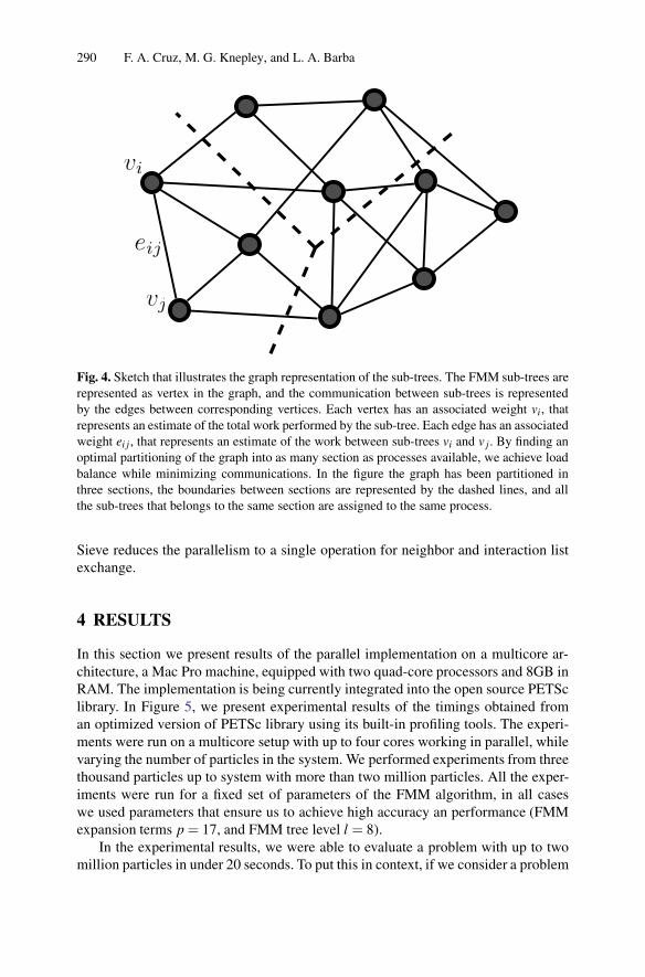
290 F. A. Cruz, M. G. Knepley, and L. A. Barba
vj
vi
eij
Fig. 4. Sketch that illustrates the graph representation of the sub-trees. The FMM sub-trees arerepresented as vertex in the graph, and the communication between sub-trees is representedby the edges between corresponding vertices. Each vertex has an associated weight vi, thatrepresents an estimate of the total work performed by the sub-tree. Each edge has an associatedweight ei j , that represents an estimate of the work between sub-trees vi and v j. By finding anoptimal partitioning of the graph into as many section as processes available, we achieve loadbalance while minimizing communications. In the figure the graph has been partitioned inthree sections, the boundaries between sections are represented by the dashed lines, and allthe sub-trees that belongs to the same section are assigned to the same process.
Sieve reduces the parallelism to a single operation for neighbor and interaction listexchange.
4 RESULTS
In this section we present results of the parallel implementation on a multicore ar-chitecture, a Mac Pro machine, equipped with two quad-core processors and 8GB inRAM. The implementation is being currently integrated into the open source PETSclibrary. In Figure 5, we present experimental results of the timings obtained froman optimized version of PETSc library using its built-in profiling tools. The experi-ments were run on a multicore setup with up to four cores working in parallel, whilevarying the number of particles in the system. We performed experiments from threethousand particles up to system with more than two million particles. All the exper-iments were run for a fixed set of parameters of the FMM algorithm, in all caseswe used parameters that ensure us to achieve high accuracy an performance (FMMexpansion terms p = 17, and FMM tree level l = 8).
In the experimental results, we were able to evaluate a problem with up to twomillion particles in under 20 seconds. To put this in context, if we consider a problem

Fast Multipole Method for particle interactions 291
1
10
100
1000
10000
103
104
105
106
107
Tim
e [s
ec]
Number of particles
1 cpu2 cpu3 cpu4 cpu
Fig. 5. Log-log plot of the total execution time of the FMM parallel algorithm for fixed pa-rameters (expansion terms p = 17, and FMM tree level l = 8) vs. problem size (number ofparticles in the system). In the figure, each line represents the total amount of time used by theparallel FMM to compute the interaction in the system when using 1, 2, 3, and 4 processors.
with one million particles (N = 106), the direct computation of the N2 operationswould be proportional to 1 Tera floating point operations (1012 operations), in orderto compute all the particles interactions of the system. Instead, the FMM algorithmaccelerates the computations and achieve an approximate result with high accuracyin only 10 Giga floating point operations, meaning 100 times less floating point op-erations.
5 CONCLUSIONS AND FUTURE WORK
In this paper we have presented the first open source project of a parallel Fast Multi-pole Method library. As second contribution in this work, we also introduced a newparallelization strategy for the Fast Multipole Method algorithm that automaticallyachieves load balance and minimization of the communication between processes.The current implementation is capable of solving N-body problems for millions ofunknowns in a multicore machine with good results. We are currently tuning thelibrary and running experiments on a cluster setup.
With this paper we expect to contribute to widespread the use of fast algorithmsby the scientific community, and the open source characteristic of the FMM library

292 F. A. Cruz, M. G. Knepley, and L. A. Barba
is the first step towards this goal. The open source project is currently being incor-porated into the PETSc library [1] and a first version of the software is going to bereleased by October 2008.
[1] S. Balay, K. Buschelman, W. D. Gropp, D. Kaushik, M. Knepley, L. Curfman-McInnes, B. F. Smith, and H. Zhang. PETSc User’s Manual. Technical ReportANL-95/11 - Revision 2.1.5, Argonne National Laboratory, 2002.
[2] L. Greengard and V. Rokhlin. A fast algorithm for particle simulations. J. Com-put. Phys., 73(2):325–348, 1987.
[3] George Karypis and Vipin Kumar. A parallel algorithm for multilevel graphpartitioning and sparse matrix ordering. Journal of Parallel and DistributedComputing, 48:71–85, 1998.
[4] Matthew G. Knepley and Dmitry A. Karpeev. Mesh algorithms for pde withsieve i: Mesh distribution. Scientific Programming, 2008. to appear.


Hybrid MPI-OpenMP performance in massivelyparallel computational fluid dynamics
G. Houzeaux1 ∗, M. Vazquez1, X. Saez1 and J.M. Cela1
Computer Applications in Science and Egineering DepartmentBarcelona Supercomputing Center Edificio C6-E201, Campus Nord UPC, Jordi Girona 1-3,Spain
Abstract. We analyze in this paper the parallel performance of a computational mechanicscode, based on a hybrid MPI-OpenMP parallelization. The specific problems considered arean explicit compressible flow solver and an implicit incompressible flow solver. Their perfor-mance using a fully MPI approach and a Hybrid approach are compared. The performanceobtained on different architextures are also compared.
1 Introduction
In a previous paper [4],the authors presented the parallel performance of a computa-tional mechanics code, which parallelization was based on a mesh partitioning tech-nique using MPI as a communication library. The physical problems treated werethe following: the incompressible Navier-Stokes(NS) equations; the compressibleNS equations; the wave equation. The latter was solved using an implicit monolithicapproach where as the last two problems were solved using an explicit time integra-tion scheme. This paper presents the developments carried out on the incompressibleand compressible NS equations. In the first set of equations, a projection methodwas developed and parallelized. In the second set of equations, OpenMP was im-plemented in the code. The objective of this work consists in assessing the parallelperformance obtained on these sets of equations, on different architectures.
2 Incompressible flow equations
Given ρ the density of the fluid, μ its viscosity, u and p its velocity and pressure, theincompressible flow equations are:
ρ ∂u∂ t +ρ(u ·∇)u−∇ · [2με(u)]+∇p = ρ f inΩ ,
∇ ·u = 0 inΩ .(1)
∗ This work has been carried out in the framework of the Spanish Project OPTIDIS(ENE2005-05274). The research of Dr. Houzeaux has been partly done under a Ramony Cajal contract with the Spanish Ministerio de Educacion y Ciencia.
D. Tromeur-Dervout (eds.), Parallel Computational Fluid Dynamics 2008,Lecture Notes in Computational Science and Engineering 74,DOI: 10.1007/978-3-642-14438-7 31, c© Springer-Verlag Berlin Heidelberg 2010

294 G. Houzeaux , M. Vazquez , X. Saez and J.M. Cela
where f is a force term. This system must be provided with appropriate initial andboundary conditions. Time discretization is achieved with the trapezoidal rule withconstant θ and a time step δ t. Space discretization is carried out in the finite elementcontext together with a variational multiscale approach [2]. Let superindex i denotethe linearization loop counter and n the time loop counter. When unknowns are con-sidered at current linearization step i+ 1 or time step n + 1, superscript are omitted.We end up solving the following algebraic system:
[Auu Aup
Apu App
][up
]=[
bu
bp
](2)
Matrix App comes from the stabilization of the pressure term (GLS like term), en-abling the use of equal order interpolation. In a variational multiscale context, thisterm comes from the algebraic approximation of the subgrid scale equation [2]. Pi-cards method is used to linearize the convection term. The direct solution of (2) isreferred to as the monolithic solution of the equations. It is well known that the con-vergence properties of classical iterative solvers like GMRES is very poor, due tothe coupling of the velocity and pressure. Therefore, another approach is envisaged,similar to projection methods [5] [3] and extensively described in [1]. It consistsin solving a preconditioned Richardson iteration for the Schur complement of thepressure. In addition, this iteration is coupled to the linearization loop. The precon-ditionner is a slightly modified Laplacian matrix, δ tL. The modification is necessaryto take into account the Neumann part of the boundaries. In algebraic words, at eachtime step n + 1, given an initial u0 and p0, solve for i = 0,1,2... until convergence
Auuui+1 = bu −Auppi, (3)
(App +δ tL)pi+1 = bp −Apuui+1 + δ tLpi. (4)
This predictor-corrector scheme is similar to classical incremental projection meth-ods. The differenceis thatweiterate within each time step to obtain the solution ofthemonolithic scheme. In fact, note that when pi+1 = pi, we recover the monolithic so-lution. A not strict continuous representation of this scheme is the following system:
ρui+1,n+1−un
θδ t+ρ(ui,n+1 ·∇)ui+1,n+1 −∇ · [2με(ui+1,n+1)] = ρ f −∇pi,n+1, (5)
δ tΔ pi+1,n+1 = −∇ ·ui+1,n+1 + δ tΔ pi,n+1. (6)
3 Compressible flow equations
Let U be the linear momentum, T the temperature, E the total energy and k thethermal conductivity. The compressible flow equations in its conservative form are[7]:
∂tU +∇ · (U ⊗u)∇ · [2με(u)]+∇p = ρg,∂ρ∂ t +∇ ·U = 0,∂E∂ t +∇ · (uE− k∇T −u ·σ) = ρu ·g.
(7)

Hybrid MPI-OpenMP performance in massively parallel CFD 295
This system is closed with a state equation, typically the ideal gas’one. Additionally,laws for the viscosity and the thermal conductivity can be used for some particu-lar regimes or materials. Boundary and initial conditions must be provided. Acrossthe literature, different sets of unknowns have been proposed to properly solve thecompressible flow equations. The conservative set Φ = (U,ρ ,E) is one of the mostfavored due to its properties face to the discretization process. This is the unknowns’set chosen to run the compressible flow benchmarks below.
After space and time discretization and linearization, we obtain the followingsystem ⎡
⎣AUU AUρ AUE
AρU Aρρ AρE
AEU AEρ AEE
⎤
⎦
⎡
⎣Φ
⎤
⎦=
⎡
⎣bU
bρbE
⎤
⎦ (8)
that can be compactly written as:AΦ = b (9)
where A is the system matrix that can be decomposed in blocks according to thecoupling among the different unknowns. Matrix A structure is heavily dependenton the unknowns set, the linearization, the stabilization procedure, the shock cap-turing technique or the time and space discretizations. In this paper, when dealingwith compressible flow we follow an explicit formulation, meaning tha the system issolved using a preconditioned Richardson equation at each time step as follows:
Un+1 = un + P−1[bU −AUρρn −AUEEn)−AUUUn],ρn+1 = ρn + P−1[bρ −AρUUn −AρEEn)−Aρρρn],En+1 = En + P−1[bE −AEUUn −AEρρn)−AEEEn],
(10)
and in compact form,Φn+1 =Φn + P−1
c Rn (11)
The preconditionner P is taken as
P =1δ t
M, (12)
where M is the diagonal mass matrix, computed using a closed integration rule forwhich the integration points are located on the nodes. Pc is its extension in compactnotation, considering that each equation can have its own time step.
Additionally, in order to deal with low-Mach regions in an accurate and stableway, fractional step techniques are used. They are so-called fractional because theNavier-Stokes equations are solved by seggregating the operators, leading to a solu-tion scheme of succesive stages. In this paper,we follow the strategy proposed by theCBS algorithm [6], where the fractional step is taken on the pressure gradient termin the momentum equation. In compact form, the fractional explicit algorithm hereused is: at each time step solve
U = Un + P−1RnU
Φn+1 = Φn + P−1c Rn (13)

296 G. Houzeaux , M. Vazquez , X. Saez and J.M. Cela
where U is the fractional momentum, RnU is the space residual of the linear momen-
tum equation with the pressure gradient term seggregated2 and Φn = (U ,ρ ,E).
4 Parallelization strategy
Concerning the MPI communication, the parallelization strategy was already pre-sented in [4]. As long as the explicit compressible flow solver is concerned, OpenMPdirectives were implemented to the loop elements. Criticial sections are only locatedat the scatter of the local residual to the global residual.
5 Performance
The speedup for the incompressible flow solver is shownin Figure 1(Left). The datawere obtained on a BlueGene/L and aBlueGene/P.The number of elements is 5Mhexahedra, which is relatively low with respect to the number of CPUs used. On 4000CPUs the average number of elements per CPU is a bit higher that 1000. However,the speedup is around 85%.
Fig. 1. Speedup, incompressible flow solver. Comparison BlueGene/L and/P.
Figure 1(Right) shows the speedup obtained with a full MPI approach and an hy-brid MPI-OpenMP approach. The mesh is composed of 2.6M hexahedra elements.Both give similar speedup results, with a slightly lower speedup for the hybrid ap-proach. Note that not all the loops were parallelized in this case.
[1] G. Houzeaux and M. Vazquez, Parallel implementation of an incompressibleNavier-Stokes solver, in preparation.
[2] G. Houzeaux and J. Principe, A variational subgrid scale model for transientincompressible flows, Int. J. CFD, (2008), In press.
2 Seggregated means that the pressure term is partially considered, multiplied by a incremen-tal factor ranging from 0 to 1.

Hybrid MPI-OpenMP performance in massively parallel CFD 297
[3] S. Badia and R. Codina, Algebraic pressure segregation methods for the incom-pressible Navier-Stokes equations, Arch. Comp. Meth. Eng., (2008), Inpress.
[4] G. Houzeaux, M. Vazquez, R. Grima, H. Calmet and J.M. Cela, Experiencein Parallel Computational Mechanics on MareNostrum, PARCFD2007, (2007),Antalya(Turkey), May 21-24.
[5] A. Quarteroni, F. Saleri and A. Veneziani, Factorization methods for the nu-merical approximation of Navier-Stokes equations, Comp. Meth. Appl. Mech.Eng.,(2000), 188, 505-526.
[6] O.C. Zienkiewicz, P. Nithiarasu, R. Codina, M. Vazquez and P. Ortiz. The char-acteristic based- split procedure: an efficient and accurate algorithm for fluid prob-lems. Int. J. Numer. Meth. Fluids, (1999), 31, 359-392.
[7] L.D. Landau and E.M. Lifshitz.Fluid Mechanics. Butterworth -Heinemann(1987).


Hierarchical adaptive multi-mesh partitioningalgorithm on heterogeneous systems
Y. Mesri1, H. Digonnet1, T. Coupez1
CIM group, Centre For Material Forming, ENSMP,Rue Claude Daunesse BP 207 06904 Sophia Antipolis cedex, France
Abstract. Heterogeneous systems are increasingly being used as platforms forresource-intensive distributed parallel mesh applications. A critical contributors tothe performance of such applications is i) the scheduling of constituent applicationtasks ont he system and ii) the mesh partitioning. Since often application submis-sions from users cannot improve the total turnaround time, the application mustbe scheduled automatically by the scheduler using information about its scalabil-ity characteristics. To obtain the best performance, it is imperative to take into ac-count both application-specific and dynamic system information in developing i) aschedule which meets his performance criteria and ii) a mesh partitioning schemethat takes into account this system heterogeneity. In [1], we have presented a meshpartitioning scheme, that takes into account the heterogeneity of CPU and networks.Load balancing mesh partition strategy improves the performance of parallel appli-cations running in a heterogeneous environment. In this work, we present a newhierarchical adaptive scheme that allows to optimize the scheduling of N parallelmesh applications simultaneously on a heterogeneous system. The new scheme con-sists in selecting the partition size of each application and then partitioning eachapplication on the allocated heterogeneous ressources. We illustrate our schedulingapproach with a detailed description and results for a distributed 3D CFD applicationon a heterogeneous platform.
1 Introduction
Computational fluid dynamics(CFD) applications usually operate on a huge set ofapplication data associated to unstructured meshes. For this reason CFD problemsrepresent a significant part of high performance supercomputing applications. Finiteelement and finite volume methods use unstructured meshes. We represent the appli-cation as a weighted undirected graph W = (V (W ),E(W )), which we will call theworkload graph . Each vertex v has a computational weight ω(v), which reflects theamount of the computation to be done atv. An edge between vertices u and v, denoted
D. Tromeur-Dervout (eds.), Parallel Computational Fluid Dynamics 2008,Lecture Notes in Computational Science and Engineering 74,DOI: 10.1007/978-3-642-14438-7 32, c© Springer-Verlag Berlin Heidelberg 2010

300 Y. Mesri, H. Digonnet, T. Coupez
{u,v}, has a computational weight ω({u,v}), which reflects the data dependency be-tween them. Partitioning applications onto heterogeneous architecture such as a Gridenvironment requires a special model architecture that reflects both heterogeneousresource characteristics and also non homogeneous communication network betweenthese different resources. The machine architecture can be represented as a weightedundirected graph A = (V (A),E(A)), which we will call the architecture graph. Itconsists in a set of vertices V (A) = {p1, p2, ..., pn}, denoting processors, and a set ofedges E(A) = {{pi,}|pi, p j ∈ P}, representing communication links between pro-cessors. Each processor p has a processing weight sp, modeling its processing powerper unit of computation. Each link has a link weight vpq, that denotes the communi-cation bandwidth per unit of communication between processors p and q. In [1] wehave proposed a heterogeneous re-partitioning algorithm, called MeshMigration thattakes into account the architecture characteristics. MeshMigration generates a highquality partition and provides a load balance on each processor of the heterogeneousarchitecture. In this paper, we develop an iterative scheme that performs automati-cally a heuristic based search for a schedule that minimizes average turnaround timecoupled with the mesh partitioning scheme described in [1]. Figure 1 represents a di-agram of the coupled multi-mesh partitioning algorithm. This paper is organized asfollows: In section 2, we define formally an iterative scheduling algorithm, followedby a description of the partitioning problem in section 3. Section 5 discusses thehierarchical mesh partitioner MeshMigration. Finally in section 6, we will describepreliminary experimental results for a finite element code executed on the Grid.
Fig. 1. A diagram of the global multi-mesh partitioning approach

Hierarchical adaptive multi-mesh partitioning algorithm 301
2 The iterative scheduling algorithm
An optimal moldable scheduling strategy would inherently take into account the effi-ciency, job size and system load without the need to tune parameters. In this section,we describe an iterative scheme that does so. Our iterative algorithm begins by giv-ing each job an initial minimal partition of one processor. A conservative scheduleis generated; this schedule is iteratively modified by giving a processor to the mostworthy job, the job that,if given an additional processor,has the greatest decrease inruntime. If the addition of a processor to the most worthy job decreased the averageresponse time of the schedule, the addition is accepted, otherwise not.
1. Input List of reserved jobs2. unmark all jobs and set partition sizes to one3. While unmarked jobs exist
a) find unmarked candidate job j(see Algorithm 2)b) add one to partition size of job jc) create a conservative schedule for all jobsd) If average turnaround time did not improve
i. mark job jii. decrement partition size of candidate job j
iii. create a conservative schedule for all jobse) end if
4. end while
Algorithm 1: The iterative scheduling algorithm
Algorithm 1 shows the algorithm for the iterative algorithm. Initially each job isassigned one node. This allocation results in optimal per job efficiency, but may resultin poor average turn around and system utilization. The next step(lines3to4) searchesfor a schedule with an improved average turn around time. Step3-(a) chooses thejob which will benefit the most of receiving an extra processor. This job is a goodcandidate to try to increasing its processor allocation. Step 3-(b) to 3-(e) determine ifthe increased allocation results in a better schedule. If the increase produces a worseschedule,the job is marked as a bad choice and the remaining jobs are considered.
1. Input List of reserved jobs2. set bestImprovement to zero3. for each unmarked job j in the reserved job list
a) let n be the current node assignment if job jb) let i be the expected runtime on n processorsc) i be the expected runtime on n+1 processorsd) if (i− i′ > bestImprovement)
i. set best Improvement to i− i′ii. set best Job to j
e) end if4. end for

302 Y. Mesri, H. Digonnet, T. Coupez
5. return best Job
Algorithm 2: The unmarked candidate search algorithm
This approach takes all the aspects discussed previously into account: load, scal-ability, job size, and utilization. If a job is small,the improvement from adding aprocessor will be minimal, and thus it will be less likely to receive an increasedallocation. Likewise, if a job scales poorly,it will benefit less from receiving moreprocessors, and will be less likely to be chosen as the candidate. If the load is low,wider jobs will result in a better average turnaround time, and wider allocations willbe given. If the load is high, increasing the allocation of poorly scalable jobs willincrease average turnaround time. Finally, the system achieves a good utilization,as processors will not be wasted unless there is no work to be done or using theprocessor reduces the average turnaround time.
We evaluate our iterative algorithm via simulation. The simulation is basedon the workload logs archive of the machine SP2 of th eCornell Theory Cen-ter(CTC).The CTC workloads are available on the web at http://www.cs.huji.ac.il/labs/parallel/workload/. We use Downeys model [4] ofthe speedup (S(n) = t1/tn) of parallel jobs to derive execution time for a partitionsize n. Downeys speedup model uses two parameters: A (the average parallelism)and σ (an approximation of the coefficient of variance in parallelism). The speedupof a job j is then given by:
S(n) =
⎧⎪⎪⎪⎪⎪⎨
⎪⎪⎪⎪⎪⎩
AnA+σ(n−1)/2 σ ≤ 1, 1 ≤ n ≤ A
Anσ(A−1/2)+n(1−σ/2) σ ≤ 1, A ≤ n ≤ 2A−1A σ ≤ 1, n ≥ 2A−1
nA(σ+1)σ(n+A−1)+A σ ≥ 1, 1 ≤ n ≤ A + Aσ−σA σ ≥ 1, n ≥ A + Aσ−σ
(1)
Figure 2 shows the results comparison between the rigid workload extracted fromthe log files of the CTC machine and our moldable scheduling algorithm. In theseexperiments, we supposethatjobsscaletothe size of the system(A = system size). Re-sults show that our algorithm is able to reduce the turn-around time to about half ofthat obtained by the user request.
3 Partitioning Problem
We consider a workload graph W (V (W ),E(W ))which represents the application, anda architecture graph A(V (A),E(A)) which represents the Grid. On a computationalgrid, the machine architecture is heterogeneous both for network and processors.So we consider the characteristics of architecture graph to define the partitions. Amapping of a workload graph onto a architecture graph can be formally describedby:
m : V (W ) →V (A) (2)

Hierarchical adaptive multi-mesh partitioning algorithm 303
Ave
rage
TA
T
0.65 0.75 0.85 0.95
Iterative
User’s choice
80000
70000
60000
50000
40000
30000
20000
10000
0
Fig. 2. Effective load (EL= (Number of jobs)/Number of processors)
where m(v) = p, if the vertex v of W is assigned to a processor p of A. In orderto evaluate the quality of a mapping,we define two cost models: one for estimatingthe computational cost and the other one for the communication cost evaluation. Foreach mapping of the workload graph onto the architecture graph we can estimatethe computational cost as follows: If a vertex v is assigned to a processor p, thecomputational cost is given by tv
p = ω(v)/sp, that is the ratio of the computationalweight of v per the processing weight of p. Computational cost estimates the timeunits required by p to process v. The communication cost is introduced when wehave a data communication transfer between two different nodes in the target graph.Suppose {u,v} ∈ E(W ) and u ∈ V (W ) is assigned to processor p and v ∈ V (W ) isassigned to processor q. The data is transferred from the local memory of p to thelocal memory of q via message passing. In this case, the communication cost is givenby cu,v
pq = ω({u,v})/vpq, that is the ratio of the communication weight of edge {u,v}per the link weight between p and q. The communication cost represents the timeunits required for data transfer between the vertices u and v. As in [1], we define acost function as follows: Φ(W,A,m) := T +C where
• T = (1, ...,tcard(V (A)))t , tp = C(p,m)sp
the computational time of p, and C(p,m) isthe weight of subgraph assigned to p.
• C = (C(1,m), ...,C(card(V (A)),m)t and C(p,m) = ∑q∈V(A) �=pC({p,q} ,m) thecommunication time associated to a processor p with his neighbors.
The definition of the graph partitioning problem is to find a partition (mappingm) which minimizes the cost functionΦ(W,A,m). Clearly, the problem is extensibleto the classical graph partitioning and task assignment problem, and it is well knownthat this problem is NP-complete. In the next section, we describe the iterative algo-rithm chosen to minimize this cost function and find the efficient partitioning.

304 Y. Mesri, H. Digonnet, T. Coupez
4 Hierarchical partitioning strategy
In order to provide an efficient partitioning in a heterogeneous system as the Gridenvironment, we introduce a hierarchical approach. We define two architecture levelsin the target graph: level one is the set of processors, and the second level is the setof clusters. Then, the partitioning is carried out in two stages:
1. We consider a grid composed by several clusters. We decompose the mesh inorder to assign one partition to each cluster taking into account the bandwidth ofcommunications layers between these various clusters. The decomposition takesplace via the relationship defined in [1]. We denote N numbers of clusters andG = {C0, ...,CN−1} the set of clusters. Formally:Let p and q two processors in the architecture graph, p ∈Ci and q ∈Cj :
⎧⎨
⎩
ifCi �= Cj
Friendship(p,q) = max(F0|pq −F pmin,F0|pq −Fq
min)elseFriendship(p,q) = 0.
(3)
2. We denoteΠ = {π0, ...,πN−1}, the set of the sub-domains mapped on G. For ev-ery partitionπi assigned to the cluster Ci = {p0, ..., pI−1}, where I is the numberof processors of Ci, we re-partitioned πi on the set of processors of Ci: For everyp and q two processors on the architecture graph, p ∈Ci and q ∈Cj:
⎧⎨
⎩
ifCi = Cj
Friendship(p,q) = max(F0|pq −F pmin,F0|pq −Fq
min)elseFriendship(p,q) = 0.
(4)
5 Experimentation of a finite element code on the grid
5.1 Pour of a jerrican
This application depicts the flow of a fluid by the neck of a jerrican (see [2] for moredetails). At the beginning of the simulation, the fluid is completely in the jerricanwhich is reversed; its open neck is directed downwards. The fluid then starts to flowby the opening neck, while the air is engulfed in the jerrican in the form of bub-bles. Thus, the cavity empties little by little its initial contents and filled with air,until the fluid is completely poured. The flow isgoverned by Navier-Stokes equa-tions and the evolution of the two involved phases (liquid and air) is ensured by thetransport of a Level Set function which enables the capture of theinterface [2]. Themesh discretizing the domain contains 500,000 nodes and 2,750,000 elements. Theparameters used are as follows: the fluid has a viscosity of 10 Pa.s and a densityof 1000kg/m3, air has a viscosity of 1 Pa.s and a density of 1kg/m3. The boundaryconditions are of sticking type, i.e. a null speed is imposed on all surfaces of the ge-ometry. Figure 3 represents the interface between the fluid and the air at times t = 0sand t = 18s. Whereas air bubbles go up in the jerrican (the top cavity), the fluid flows

Hierarchical adaptive multi-mesh partitioning algorithm 305
in the bottom cavity through the neck of the jerrican. A total of 15 processors, and 3clusters (NINA,PF and IUSTI) of MecaGrid1 are used to carry out this application.It chosen to allocate 4 NINA and 5 PF and 6 IUSTI. This choice is justified by thecalculated power of the processors: for both NINA and IUSTI clusters,the power isapproximately 125M f lops/s, and for the PF, it is 44M f lops/s, that is to say 2.5times lower. On the INRIA site, 2 NINA are replaced by 5 PF. Thus, with 4 NINA,5 PF and 6 IUSTI, the computing power distributed on the two sites is almost thesame ones. Measurements of following times are raised after 100 time increments,with homogeneous partitions, than optimized partitions. In Table 1, we use a ILU(1)preconditioning and a MinRes solver to solve the linearized flow system. The firstobservation is that the gain of timeprovided by the optimized partitioning is very im-portant; the execution time passed from 2 days and 19 hours to one day and 8 hours,which makes a gain of 53%. Furthermore distributing the workload equitably, the hi-erarchical partitioning algorithm allows to decrease considerably the very penalizinginter sites communication while cutting the mesh in a place where there is few nodes.Finally, the hierarchical partitioning approach saved almost 53% of the computingtime of MecaGrid.
4 PF-5 NINA-6 IUSTI Homogeneous partition optimized partitionNb procs 15 15NSAssembling(s) 3680 1904NSResolution(s) 235504 107899Alphaassembling(s) 2357 2896Alpha resolution(s) 258 113Total(s) 241799 113364
Table 1. run time on Grid with ILU(1) preconditionner
Fig. 3. simulation of jerrican poor: sequences at t=0s (left) and t=18s (right)
1 www-sop.inria.fr/smash/mecagrid

306 Y. Mesri, H. Digonnet, T. Coupez
6 Conclusion
In this paper, we have presented a new adaptive multi-mesh partitioning approach, forpartitioning workloads graph onto heterogeneous architecture graph. This algorithmruns in parallel and have shown that optimized load balancing strategies improvethe performance of the applications executed on a heterogeneous environment. Onenote that the results presented here are associated to just a single mesh application, awork-in progress consists in applied this approach to multi-mesh applications.
[1] Y. Mesri, H. Digonnet and H. Guillard, Mesh partitioning for parallel computa-tional fluid dynamics applications on a grid, in Finite volumes for complex appli-cations IV, Hermes Science Publisher, 2005, p. 631-642
[2] O. Basset, H. Digonnet, T. Coupez and H. Guillard Multi-phase flow calculationswith interface tracking coupled solution, in Coupled Problems 2005, barcelona,Spain, CIMNE, 2005
[3] A. Basermann and al., (2000), Dynamic load balancing of finite element appli-cations with the DRAMA library Appl. Math. Modelling, 25(2).83-98
[4] A. Downey. A model for speedup of parallel programs. U.C.Berkely Technicalreport CSD-97-933, January 1997.


Part IX
Parallel Performance

Towards Petascale Computing with Parallel CFDcodes
A.G. Sunderland1, M. Ashworth1, C. Moulinec1, N. Li2, J. Uribe3, Y. Fournier4
1 STFC Daresbury Laboratory, Warrington, UK2 NAG Ltd, Wilkinson House, Jordan Hill Road, Oxford, UK3 University of Manchester, UK4 EDF R&D, Chatou, France
Keywords: Petascale, High-End Computing, Parallel Performance, Direct Numeri-cal Simulations, Large Eddy Simulations
1 Introduction
Many world leading high-end computing (HEC) facilities are now offering over 100Teraflops/s of performance and several initiatives have begun to look forward toPetascale computing5 (1015 flop/s). Los Alamos National Laboratory and Oak RidgeNational Laboratory (ORNL) already have Petascale systems, which are leading thecurrent (Nov 2008) TOP500 list [1]. Computing at the Petascale raises a numberof significant challenges for parallel computational fluid dynamics codes. Most sig-nificantly, further improvements to the performance of individual processors willbe limited and therefore Petascale systems are likely to contain 100,000+ proces-sors. Thus a critical aspect for utilising high Terascale and Petascale resources is thescalability of the underlying numerical methods, both with execution time with thenumber of processors and scaling of time with problem size. In this paper we analysethe performance of several CFD codes for a range of datasets on some of the latesthigh performance computing architectures. This includes Direct Numerical Simula-tions (DNS) via the SBLI [2] and SENGA2 [3] codes, and Large Eddy Simulations(LES) using both STREAMS LES [4] and the general purpose open source CFDcode Code Saturne [5].
2 Parallel CFD codes
We analyse the parallel performance of several parallel CFD codes on the targethigh-end computing systems. The codes have been chosen to reflect a range of appli-
5 Petascale assumes 10s of Petaflop/s Peak Performance and 1 Petaflop/s Sustained Perfor-mance on HEC applications
D. Tromeur-Dervout (eds.), Parallel Computational Fluid Dynamics 2008,Lecture Notes in Computational Science and Engineering 74,DOI: 10.1007/978-3-642-14438-7 33, c© Springer-Verlag Berlin Heidelberg 2010

310 A.G. Sunderland & al
cations (e.g. turbulence at the shock/boundary layer interaction, combustion) usingboth DNS-based and LES-based computational methods. All codes are written inFortran with MPI [6] for data transfer between processors. The Code Saturne pack-age also has modules written in the C programming language and the Python script-ing language.
2.1 SBLI
Fluid flows encountered in real applications are invariably turbulent. There is, there-fore, an ever-increasing need to understand turbulence and, more importantly, to beable to model turbulent flows with improved predictive capabilities. As computingtechnology continues to improve, it is becoming more feasible to solve the gov-erning equations of motion, the Navier-Stokes equations, from first principles. Thedirect solution of the equations of motion for a fluid, however, remains a formidabletask and simulations are only possible for flows with small to modest Reynolds num-bers. Within the UK, the Turbulence Consortium (UKTC) has been at the forefrontof simulating turbulent flows by direct numerical simulation (DNS). UKTC has de-veloped the parallel code SBLI to solve problems associated with shock/boundary-layer interaction. SBLI [2] is a compressible DNS code based on finite differencemethod using high-order central differencing in space and explicit Runge-Kutta fortime marching. A grid transformation routine enables this code to simulate relativelycomplex-geometry flows. The parallel version is under active development and itsparallel performance has been fine-tuned. A set of test cases, some with complexgeometry involving multiple Cartesian-topology blocks, have been specified for itstesting and benchmarking on a range of HPC platforms.
2.2 SENGA2
The SENGA2 [3] code has been developed at The University of Cambridge andhas been designed to facilitate combustion DNS with any desired level of chem-istry, from single-step Arrhenius mechanisms through all classes of reduced reactionmechanisms up to fully detailed reaction mechanisms. The Navier-Stokes momen-tum equations are solved in fully compressible form together with the continuityequation and a conservation equation for the stagnation internal energy, as well asany required number of balance equations for species mass fraction. Each componentof the reacting mixture is assumed to obey the equations of state for a semi-perfectgas. Boundary conditions are specified using an extended form of the Navier-StokesCharacteristic Boundary Condition formulation, and available boundary conditionsinclude periodic as well as several types of walls, inflows and outflows. The numer-ical framework is based on a finite-difference approach for spatial discretisation to-gether with a Runge-Kutta algorithm for time-stepping. High-order explicit schemesare preferred due to their speed of execution and ease of parallel implementation,and a 10th order explicit scheme is standard for interior points. The code is fully par-allel using domain decomposition over a cubic topology. Current HEC architecturespermit 3D DNS of the turbulent flow fields but with only limited representation of

Towards Petascale Computing with Parallel CFD codes 311
the combustion chemistry and a highly simplified representation of the geometry. Atthe Petascale it will be possible to move towards more complex configurations thatare much closer to industrial requirements.
2.3 STREAMS-LES
STREAM-LES [4] is a CFD package developed at Imperial College, London, forLarge Eddy Simulations (LES) of incompressible flow. Its numerical framework restson a general structured, multi-block, collocated-storage finite volume method withnon-orthogonal mesh capability. The spatial scheme is second-order central and thetime-matching is based on a fractional-step method in which a provisional velocityfield is made divergence-free through the solution of the pressure-Poisson equation.The code is fully parallelized using MPI through standard domain decompositionand runs on several high-end computing platforms.
2.4 CODE SATURNE
Code Saturne [5] is an open source general purpose computational fluid dynamicssoftware package developed by EDF [7]. It is based on a co-located Finite Volumeapproach that accepts meshes with any type of cell, including tetrahedral, hexahedral,prismatic, pyramidal, polyhedral and any type of grid structure, including unstruc-tured, block structured, hybrid, conforming or with hanging nodes. Its basic capabili-ties enable the handling of either incompressible or expandable flows with or withoutheat transfer and turbulence (mixing length, 2-equation models, v2f, Reynolds stressmodels, Large Eddy Simulations etc.). Dedicated modules are available for specificphysics such as radiative heat transfer, combustion (e.g. gas, coal), magneto-hydrodynamics, compressible flows, two-phase flows (Euler-Lagrange approach with two-way coupling) with extensions to specific applications (e.g. for atmospheric environ-ment: code Mercure Saturne).
3 High-End Computing Platforms
3.1 HPCx
HPCx [8] is the UK’s National Capability Computing service, located at the Compu-tational Science and Engineering Department at STFC Daresbury Laboratory [9] andcomprising of 160 IBM eServer 575 nodes. Each eServer node contains 16 1.5 GHzPOWER5 processors, giving a total of 2560 processors for the system. The total mainmemory of 32 GBytes per node is shared between the 16 processors of the node. Thenodes in the HPCx system are connected via IBM’s High Performance Switch. Thecurrent configuration has a sustained Linpack performance of 12.9 Tflop/s.

312 A.G. Sunderland & al
3.2 HECToR
HECToR [10] is the UKs latest high-end computing resource, located at the Uni-versity of Edinburgh and run by the HPCx consortium. It is a Cray XT4 systemcomprising 1416 compute blades, each of which has 4 dual-core processor sockets.This amounts to a total of 11,328 cores, each of which acts as a single CPU. Theprocessor is an AMD 2.8 GHz Opteron. Each dual-core socket shares 6 GB of mem-ory, giving a total of 33.2 TB in all. The Linpack performance of the system is 54.6Tflops/s, positioning the system at number 46 in the current (Nov 2008) TOP500 list.We have extended the available range of processor counts with runs on the Jaguar6
Cray XT4 at ORNL [11]. Jaguar has quad-core nodes running at 2.1 GHz but isotherwise similar to the HECToR system.
3.3 BlueGene
STFC Daresbury Laboratory operates single rack Blue Gene/L and Blue Gene/Psystems. Both systems contain 1024 chips, with 2 processor cores per chip in theL system and 4 processor cores per chip in the P system, giving a total of 2048cores and 4096 cores respectively. Memory is provided at 512 Mbytes per core inboth systems. The basic processor in the L system is the Power440 running at 700MHz, whilst the P system uses a processor from the Power450 family running at 850MHz. Inter-processor communications take place via two different networks: a 3-Dtorus for general communications and a tree network for collective communicationoperations. The philosophy behind the Blue Gene design is that the speed of the pro-cessor is traded in favour of very dense packaging and low power consumption. As aconsequence of these features, Blue Gene systems have featured prominently in theGreen500 supercomputer list [12].
4 Performance Results
Performance results are presented in this section for the codes and platforms underinvestigation.
4.1 SBLI
The benchmark case for the SBLI code is a simple turbulent channel flow benchmarkrun for 100 timesteps using grid sizes of 3603 (360× 360× 360), 4803, 6003 and10243. The most important communications structure is a halo-exchange betweenadjacent computational sub-domains. Providing the problem size is large enough togive a small surface area to volume ratio for each sub-domain, the communicationscosts are small relative to computation and do not constitute a bottleneck and we see
6 This Jaguar system was the older system available to general users in late 2008, not thePetascale system of the same name from the Nov 2008 TOP500 list.

Towards Petascale Computing with Parallel CFD codes 313
almost linear scaling from all systems out to 1024 processors. Performance for thethree smaller grid sizes is shown in Figure 1. In order to be able to compare differentproblem sizes the performance is defined as the number of grid points times thenumber of timesteps divided by the execution time. Some cache effects are seen upto around 1000 processors where the smaller grid sizes perform better as the sub-domains on each processor fit into cache at lower processor counts. However, above1000 processors we see that, as expected, the scalability is better for larger problemsizes due to the better compute/communication ratio. This is confirmed by profilingmeasurements which show that the time spent in MPI routines reaches 42% for thesmallest grid size on 6144 processors.
Fig. 1. Performance of SBLI on up to 8192 processors of the HECToR Cray XT4 for threegrid sizes.
Parallel performance on jaguar up to 24576 processors, on HECToR up to 8192and on HPCx on up to 1536 is shown in Figure 2 for the largest problem size of10243 grid points. Scalability is good right out to 24576 processors with parallelefficiency of 61% at this point relative to 1024 processors, the smallest practicalconfiguration for this data size due to memory constraints. HPCx has very similarper-processor performance to jaguar. HECToR is faster per processor than jaguar byabout 16%, rather less than is expected from the 33% faster clock speed (2.8 GHz vs.2.1 GHz). There are many factors e.g. dual-core vs. quad-core, memory architectureand OS, compiler and library version differences which could be responsible for this.Hardware profiling studies of this code have shown that its performance is highlydependent on the cache utilization and bandwidth to main memory [13]. This isconfirmed by under-populating the nodes (using only one core per node on HECToRand only one or two cores per node on jaguar), which shows a speed-up of 33%

314 A.G. Sunderland & al
Fig. 2. Performance of SBLI on the HECToR, jaguar and HPCx systems for the 10243 gridsize.
using only half the available cores and 50% when using only one core of the quad-core nodes.
4.2 STREAMS-LES
The test case is a turbulent channel flow using 2,097,152 grid points calculated for75000 time steps. The arbitrary performance shown is relative to the time taken tocomplete the simulation on 128 processors of BlueGene/P. Parallel efficiency is be-tween around 76% to around 96% for the three platforms up to 256 processors. How-ever from 256 to 512 processors the parallel efficiency falls to approximately 45%(BG/P), 53% (Cray XT4) and 64% (IBM Power5). Currently, further investigationof the parallel performance of STREAMS-LES is being undertaken, including theanalysis of larger datasets where possible.
4.3 Code Saturne
The parallel performance of Code Saturne on the IBM PWR5, BG/P and BG/L sys-tems is shown in Figure 4. This test case consists of a LES at Reynolds number basedof the friction velocity of 395 in a channel. The dimension of the box is 6.4×2×3.2and a 256×256×256 (16M cells) mesh is considered. Periodic boundary conditionsapply in stream-wise and span-wise directions and no-slip conditions in the wall nor-mal ones. Van Driest damping is used at walls and the flow is driven by a constantpressure gradient. The parallel scaling properties up to 1024 processors is very goodfor all the IBM platforms considered here, with the PWR5-based architecture per-forming around twice as fast as the BG/P, which in turn is around 40% faster thanthe BG/L. Figure 5 shows the parallel performance of Code Saturne on the Hector

Towards Petascale Computing with Parallel CFD codes 315
Fig. 3. Performance of STREAMS-LES on high-end systems.
Fig. 4. Performance of Code Saturne for a 16M cell open channel dataset on IBM platforms.
Cray XT4 platform. Here a larger problem involving an unstructured grid and 100million cells is chosen as the dataset for the parallel performance appraisal. The sim-ulation represents the flow of around a bundle of tubes in a nuclear reactor, wherethe geometry is too complex to be represented by structured gridding. The problem

316 A.G. Sunderland & al
Fig. 5. Performance of Code Saturne for a 100M cell ”Mixing Grid” dataset on Hector (CrayXT4).
represents a very large-scale computational challenge (requiring high-end systems)as the flow is strongly three dimensional, with secondary vortices existing betweenpipes. Two sets of parallel performance results from the Hector machine are shownin Figure 5: one data series shows how the performance for an individual iterationscales with processor count, the other data series shows the total time based on acalculations involving 1000 iterations. It can be seen that the time taken per itera-tion in the solver stage scales near-linearly up to the maximum processor count of8192. However the total time is scaling less perfectly as overheads in the partitioningstage and the I/O stages increase relative to solver time on larger processor counts.Evidently large-scale simulations that involve many thousands of time-steps and/oriterations will suffer less from these overheads than simulations involving relativelyfew steps in the solver.
4.4 SENGA2
The two datasets, whose performance is examined here, are outlined below.
1. A 4-step calculation, which is an early example of a reduced methane-air mecha-nism due to Peters and Williams. It uses 4 forward steps (two of them reversible)and 7 species, and is notoriously stiff. It is there to test the ability of the codeto cope with stiff chemistry. The benchmark calculation is undertaken with eachprocessor holding 323 grid points. Therefore the global grid size is expanded lin-early with the number of processors used and is used to assess the weak scalingproperties of the code.

Towards Petascale Computing with Parallel CFD codes 317
2. A 1-step calculation is a simple global 1-step generic non-reversible Arrhenius-type mechanism. It is representative of the previous generation of combustionDNS, and is inexpensive to run. A volume of 1cm3 of air with periodic boundarycondition is simulated over 10 time steps of 1 ps. Initial conditions are 300K andatmospheric pressure with an initial turbulent filed. Snapshot data is dumpedevery 5 steps (twice over the simulation length).
In common with other Direct Numerical Simulation codes, memory band-width is expected to be the dominant constraint on performance. Communicationswithin Senga2 are dominated by halo-exchange between adjacent computational sub-domains. Providing the problem size is large enough to give a small surface area tovolume ratio for each sub-domain, the communications costs are small relative tocomputation and do not constitute a bottleneck. This is exemplified in Figures 6, 7,and 8, below where both weak scaling and strong scaling properties are very goodon the target platforms. Scaling on the Blue Gene /P is generally good, but overallspeed is around 2.5 times slower than the Cray XT4. However it should be notedthat this performance ratio betters the relative clock speeds (2800/800 MHz) of themachines’ underlying processors.
Fig. 6. Weak scaling performance of Senga2-4 Step reduced-air methane mechanism 323 gridpoints per processor.

318 A.G. Sunderland & al
Fig. 7. Strong scaling performance of Senga2-1 Step Arrhenenius-type Mechanism with 5003
global grid points.
Fig. 8. Strong scaling performance of Senga2-1 Step Arrhenius-type Mechanism with 10003
global grid points.
5 Summary
The parallel performance of all four CFD codes analyzed here is encouraging as wehead towards future Petascale computing environments. It is demonstrated that threeof the codes - SBLI, Code Saturne and Senga2 - perform well up to many thousandsof processing cores, with the performance of SBLI improving right out to 12288

Towards Petascale Computing with Parallel CFD codes 319
cores on the Jaguar Cray XT4 at Oakridge National Laboratory. All but one of thetests measured the generally more challenging strong scaling properties of the codewhere global problem size is constant for all runs, rather than weak scaling propertieswhere problem size is scaled up as processor count increases. In practice it is likelythat CFD researchers will be interested in both properties when running leading-edgecalculations. It is becoming clear that new challenges will arise when computingat the Petascale. In the past much attention has been paid to applying state-of-the-art parallel algorithms to the solving of the mathematical equations at the heart ofthe simulation. For effective use of available computing power when utilizing manyhundreds of thousands of cores code optimizers may now have to attention to newareas, such as the application of highly effective, load-balanced algorithms for mesh-partitioning and efficient parallel I/O methods.
Acknowledgements
This research used resources of the National Center for Computational Sciences atOak Ridge National Laboratory, which is supported by the Office of Science of theDepartment of Energy under Contract DE-ASC05-00OR22725. The authors wouldalso like to express their gratitude to Dr Stewart Cant at the University of Cambridgefor his input.
[1] Top 500 Supercomputer sites, http://www.top500.org/[2] N.D. Sandham, M. Ashworth and D.R. Emerson, Direct Numerical Simulation
of Shock/Boundary Layer Interaction, , http://www.cse.clrc.ac.uk/ceg/sbli.shtml[3] http://www.escience.cam.ac.uk/projects/cfd/senga.xsd[4] L. Temmerman, M.A. Leschziner, C.P. Mellen, and J. Frohlich, Investigation of
wall-function approximations and subgrid-scale models in large eddy simulationof separated flow in a channel with streamwise periodic constrictions, Interna-tional Journal of Heat and Fluid Flow, 24(2): 157–180, 2003.
[5] F. Archambeau, N. Mechitoua, and M. Sakiz, Code Saturne: a finite volumecode for the computation of turbulent incompressible flows industrial applica-tions, Int. J. Finite Volumes, February 2004.
[6] MPI: A Message Passing Interface Standard, Message Passing Interface Forum1995, http://www.netlib.org/mpi/index.html
[7] EDF Research and Development, http://rd.edf.com/107008i/EDF.fr/Research-and-Development/softwares/Code-Saturne.html
[8] HPCx -The UK’s World-Class Service for World-Class Research,www.hpcx.ac.uk
[9] STFC’s Computational Science and Engineering Department, http://www.cse.scitech.ac.uk/
[10] HECToR UK National Supercomputing Service, http://www.hector.ac.uk[11] Supercomputing at Oak Ridge National Laboratory, http://computing.ornl.
gov/supercomputing.shtml.[12] The Green Top 500 List, http://www.green500.org/lists/2007/11/green500.php.

320 A.G. Sunderland & al
[13] Single Node Performance Analysis of Applications on HPCx, M. Bull,HPCx Technical Report HPCxTR0703 2007, http://www.hpcx.ac.uk/ research/hpc/technical reports/HPCxTR0703.pdf.
[14] J. Bonelle, Y. Fournier, F. Jusserand, S.Ploix, L. Maas, B. Quach, Numericalmethodology for the study of a fluid flow through a mixing grid, Presentation toClub Utilisateurs Code Saturne, 2007, http://research.edf.com/fichiers/fckeditor/File/EDFRD/Code Saturne/ClubU/ 2007/07-mixing grid HPC.pdf.

Scalability Considerations of a Parallel Flow Solver onLarge Computing Systems
Erdal Yilmaz, Resat U. Payli, Hassan U. Akay, Akin Ecer, and Jingxin Liu1
Computational Fluid Dynamics Laboratory, Dept. of Mechanical Engineering, IndianaUniversity-Purdue University Indianapolis, Indianapolis, Indiana, 46202 USAhttp://www.engr.iupui.edu/cfdlab
Abstract. In this paper, we present scalability characteristics of a parallel flow solver on twolarge computing systems. The flow solver is based cell-centered finite volume discretizationsalong with explicit and implicit time integration methodologies. It has capability to solvemoving body problems using Overset grid approach. Overset option is yet in sequential form.This solver is compared with another in-house flow solver for the parallel performance on twolarge-scale parallel computing platforms up to 2048 number of processors. Parallel timingperformance of the solver was analyzed using the Vampir timing tool for DLR-F6 wing bodyconfiguration with 18 million elements. Timing of the Overset component was tested for abutterfly valve flow problem in a channel.
Key words: Parallel CFD, Overset Grid, unstructured grid, parallel performance.
1 Introduction
In today’s code development environment with several software and hardware re-sources at the disposal of the researchers in academic and research institutions, de-veloping a new Computational Fluid Dynamics (CFD) code may not seem to be aschallenging as in the past couple of decades. However, making it well-performingon scattered and constantly upgraded computing platforms for variety of problemswould be an art form researchers sometimes feel challenged. It could be an elaborateprocess beyond dealing with the nuts and bolts CFD codes and parallel computers.Ultimate goal would be making the code as scalable as possible for changing sizesof the computing resources as well as the problem itself.
If not designed at the developing phase, adjustments would be needed to theparallel codes for better run-time performance. The reason for poor parallel perfor-mance can be very complex and developers need to understand correct performanceproblems. Performance tools can help by monitoring a program’s execution and pro-ducing data that can be analyzed to locate and understand areas of poor performance.Several commercial and research tools are available to conduct performance analysissuch as Vampir [1, 2], Pablo[3], Tau[4], and Paradyn [5]. These performance tools
D. Tromeur-Dervout (eds.), Parallel Computational Fluid Dynamics 2008,Lecture Notes in Computational Science and Engineering 74,DOI: 10.1007/978-3-642-14438-7 34, c© Springer-Verlag Berlin Heidelberg 2010

322 E. Yilmaz, R.U. Payli, H.U. Akay, A. Ecer, and J. Liu
include libraries to time stamp and record the solver sequential and parallel events.Most of these tools do not require any changes in sources codes but links with thesolvers at the building phase along with Message Passing Interface libraries. Out-come can be visualized for CPU time, communication time, message sizes, relativecomparisons, etc. In this paper, we used Vampir tool to extract timing information.
Performance of flow solvers can also vary with the algorithms and mesh datastructures used. For unstructured mesh based finite volume flow solvers, usually twotypes of mesh data structure are most popular: cell-center based and cell-vertex (ornode ) based. While cell-center based solvers integrate fluxes on the faces of indi-vidual cells, node-based solvers integrates the fluxes over the cells connected to in-dividual nodes. Though numbers of faces are the same in both approaches, the actualfinite volume used in the cell-vertex approach is smaller than the node-based one,hence better actual spatial resolution. On the other hand, the node-based approachworks with less memory, as it does not need values at cell centers. Usually numberof cells for tetrahedral meshes are five-six times higher than nodes. Besides, face val-ues calculated from nodes will be more accurate than from cell values. We comparedtiming of two different solvers, one with cell-vertex based one with cell-centered, forthis purpose.
Besides the algorithms and physics, mesh capabilities to handle complex prob-lems such as overset mesh method for moving components makes performance man-agements even difficult. As the number of moving blocks increases, complexity ofthe problem makes parallel computing a challenge. Different than a few solver-embedded overset capabilities for unstructured grids [6, 7], Dirtlib/Suggar [8, 9]overset grid package can be considered as a stand alone pluggable package for un-structured grid solver. However, its parallel performance yet to be evaluated. In thispaper, we will give flavor of our overset capability implemented in our cell-centerbased flow solver, however full parallelization using MPI was not demonstrated yet.In the following two sections, we will present algorithmic details of our parallelsolvers, called PACER3D and SunFlo3D, overset grid methodology employed inSunFlo3D, parallel performance and timing studies of both solvers, and performancewith the overset version. Finally we will draw our conclusions.
2 Flow Solver
2.1 Features of the Flow Solver
Our flow solver is based on earlier versions of an existing code, USM3D, devel-oped at NASA [10], an Euler version of which was parallelized and extended todynamically deforming meshes at IUPUI [11]. The fluid motion is governed by thetime-dependent Navier-Stokes equations for an ideal gas, which express the conser-vation of mass, momentum, and energy for a compressible Newtonian fluid in the ab-sence of external forces. The equations are non-dimensionalized with the freestreamreference values for density and speed of sound. Three-dimensional turbulent flowequations are solved on unstructured grids. Spatial discretization is accomplished

Scalability of Parallel Flow Solver on Large Computing Systems 323
by a cell-centered finite-volume formulation using an accurate linear reconstructionscheme and upwind flux differencing. Inviscid flux quantities are computed acrosseach cell face using the Roe flux-difference splitting approach, [12] or the Van Leerflux-vector splitting technique [13]. Spatial discretization is accomplished by a novelcell reconstruction process, which is based on an analytical formulation for comput-ing solution gradients within tetrahedral cells. The viscous fluxes are approximatedat centroids of cell faces by linear reconstruction, which provides a continuous repre-sentation of the solution variables across the cell faces. The viscous computations areadvanced to steady state by the implicit time integration algorithm of reference [14].The scheme uses the linearized, backward Euler time differencing approach to up-date the solution at each time step for the set of equations. Convergence to the steadystate solution is accelerated by sacrificing the time accuracy of the scheme, and ad-vancing the equations at each mesh point in time by the maximum permissible timestep in that region. Closure of the Reynolds stress is provided by the one-equationSpalart-Allmaras (S-A) turbulence model [15]. The S-A model requires that the dis-tance of each cell to the nearest wall be provided for the near-wall damping terms forcells, which are in proximity to ‘viscous’ surfaces. These distances are determinedprior to the code execution for cells in the “viscous” layers and contribute to only asmall portion of the overall overhead.
At IUPUI, we have rewritten the original solver code in Fortran 90 language totake advantage of dynamic allocations feature for vectors and arrays and convenienceof the efficient structure and syntax of Fortran 90. The flow solver is parallelized us-ing MPI. Single program multiple data parallelization procedure is employed fordistributed memory architectures. Solution domain is partition into blocks with one-element overlap interfaces via in-house General Divider program [16]. General Di-vider program prepares the sending and receiving cells and nodes at the interfacewhich requires exchanging the flow variables between blocks. At each iteration, cellflow values at the block interfaces exchange between neighbor blocks before invis-cid and viscous fluxes are calculated. L2 norm of the residuals are calculated foreach block and using the reduction function of the MPI maximum value of the cal-culated norm values distributed to all blocks for both implicit and explicit solvers.For the implicit solver, Gauss Seidel iterative procedure is used to solve a sparse setof equations. 20 sub-iterations are carried out to complete for one iteration. At theend of each sub-iteration flow values of the interfaces are exchanged between neigh-bor blocks. Also, calculated nodal values at the interfaces are exchanges betweenneighbor blocks both for implicit and explicit solvers.
2.2 Overset Grid Method
The overset or Chimera grid methodology has been in use as a technique in CFD tosimplify grid generation of complex geometries or to enable relative motion betweengeometry components. An overset grid system utilizes a set of grids to discretize thedomain with each component grid generated locally around a portion of the geom-etry. The grids are allowed to overlap without needing to match point-to-point withother grids like in a traditional multi-block structured grids system. This ability to

324 E. Yilmaz, R.U. Payli, H.U. Akay, A. Ecer, and J. Liu
grid locally greatly simplifies the grid generation process for complex geometries.In addition, the flexibility of overlapping grids allows the grids to move relative toeach other to accommodate relative motion. The flow solution uses interpolation atappropriate points to couple the solutions on the different grids. The result is a flex-ible gridding strategy that allows components of the geometry to be easily added ormoved without global re-gridding. There are two major steps to establish communi-cations in this overset method: 1) automatic hole cutting, which essentially involvesblanking cells of a grid in regions that overlap with non-flow-domain in the othergrids of an overset grid system and identifying the Chimera boundary cells that liealong the hole or fringe boundary surfaces as well as interpolation boundary surfacesand 2) identification of interpolation stencils, which involves searching donor cellsand getting interpolation coefficients for all intergrid boundaries cells.
2.3 Comparison of Two Flow Solvers
The SunFlo3D flow solver is compared against another in-house CFD code, Pacer3D[17, 18]. Pacer3D is an explicit cell vertex based flow solver based on Euler flowequations. Therefore, we compared explicit version of the SunFlo3D flow solver withthe Pacer3D flow solver. Table 1 summarizes features of both codes for comparison.
PACER3D SUNFLO3D(explicit time stepping version)
Finite volume spatial discretization for compressible Euler flow equationsusing unstructured tetrahedral mesh
Vertex based Cell-center based(better spatial resolution than vertex-based
Central differencing with artificial dissipationof Jameson
Roe’s flux difference splitting
Implicit residual smoothingLocal Time stepping for steady flows
Explicit 3-stage Runge-Kutta time steppingEnthalpy damping N/A
Table 1. Scheme details of the two flow solvers
3 Numerical Simulations
3.1 Parallel CFD Application
For the parallel performance evaluations we used an external transonic flow overDLR F6 airplane geometry, which is composed of only wing and body. This testcase has 18 millions of tetrahedral cell elements. Grid is divided into 256, 512, 1024,and 2048 numbers of partitions using Metis [19].

Scalability of Parallel Flow Solver on Large Computing Systems 325
Parallel computations have been performed on parallel clusters in Indiana Uni-versity (BigRed) and San Diego Supercomputing Center (SDSC) for the cases. Thosetwo platforms have different architectures for internal communications. Clock speedof BigRed is three times faster than that of SDSC. More details of the parallel clustersare given in Table 2.
Parallel performances studies on BigRed and BlueGene are summarized in Fig-ures 1 and 2, for speedups and elapsed times, respectively. Both codes were run at thesame flow conditions as inviscid for fair comparison. SunFlo3D shows linear scal-ability on both platforms while Pacer3D tips off after 1024 processors in BigRed.This could be associated with the higher CPU speed of BigRed as it would resultin lower computation/communication ratio as we increase number of processors. OnBlueGene. Pacer3D shows super linear speedup as CPU clock time on this machineis slower compared to BigRed. In addition to CPU speed, architectures and commu-nications patters are much different for these two platforms.
BigRed (IBM e1350)Indiana University
IBM BlueGene/LSan Diego Supercomputing Center
768 JS21 Bladeserver nodes It has 3072 compute an 384 I/O nodesPowerPC 970MP processors, PowerPC processors2 x 2.5GHz dual-core 2 x 700MHz8GB 533MHz DDR2 SDRAM 32KB, 32-byte line, 64 way L1 cache; 16
128-byte lines L2 cache act as prefetch buffer4MB 35 cycles shared L3 cache
1 x Myricom M3S-PCIXD-2-I (Lanai XP) 3D torus for point-to point message passing;Global tree for collective message passing
Table 2. Features of the computing platforms
Fig. 1. Speedup of the solvers on two computing platforms

326 E. Yilmaz, R.U. Payli, H.U. Akay, A. Ecer, and J. Liu
Fig. 2. Timing comparison of the solvers on two parallel computing platforms
3.2 Timing Analysis by Vampir Tool
We used Vampir tool to analyze timing of different functions in both solvers. Vampirprovides detailed execution times breakdown of individual routines and functions ofthe applications. It also provides timing information regarding MPI related activi-ties in the solvers. Figure 3 shows timing of Pacer3D and SunFlo3D obtained by theVampir tool. Pacer3D takes 49 seconds and SunFlo3D takes 113 seconds to complete100 explicit time steps. MPI related time includes initialization of the parallel envi-ronment, message send and receive between the processors, reduction and gatheringof the shared parameters, and finalization of the parallel environment. Pacer3D uses29 seconds for the parallelization related activities while SunFlo3D uses 67 seconds.Application time includes all the computations including I/O processes. Pacer3Duses 19 seconds for the application part while SunFlo3D uses 44 seconds. Therefore,the SunFlo3D solver performs 2.3 times slower than Pacer3D for both computationand communication.
Table 3 lists breakdown of the timing for both solvers. The SunFlo3D solverneeds to update residuals for all blocks. This puts additional burden in the commu-nication of the blocks. The update of the residuals takes significant amount of time –almost 60 percent of total communication time. However, SunFlo3D performs betterfor exchange of the flow parameters between the neighbors since it uses cell cen-ter values while Pacer3D uses nodal values. This is due to the fact that the numberof cells at the overlapping interface would be less than the number of nodes. Fluxcalculations for both codes take almost the same time, though each uses differentmethodology. However, residual smoothing takes significantly more time in Sun-Flo3D.

Scalability of Parallel Flow Solver on Large Computing Systems 327
Fig. 3. Timing for Pacer3D and SunFlo3D flow solvers for 100 time steps obtained by Vampirtool, respectively
Components Pacer3D SunFlo3DCommunication-1: send andreceive at the interfaces
14 seconds 8 seconds
Communication-2: shareresiduals and other commonparameters
N/A 44 seconds
Parallel initialize/finalize Same (14.8 seconds) Same (14.6 seconds)Flux calculation Central differencing and arti-
ficial dissipation of Jameson(11 seconds)
Roe’s Flux difference split-ting(11 seconds)
Residual smoothing Operates on edge of the celland nodes (3.4 seconds)
Operates over cells and facesof the cell. Usually # of cellsis 5-6 folds of # of nodes (19seconds)
Local time stepping 1. 7 seconds 2.3 secondsI/O 1.0 seconds 2.2 secondsOthers (main, Runge-Kutta,pre-proc, etc)
3 seconds 20 seconds
Table 3. Breakdown of timing for Pacer3D and SunFlo3D by Vampir tool
3.3 Performance of the Overset Version
Overset component of our flow solver have been tested for various flow problemsincluding internal and external flows. Details of our overset research will be givenin a separate study. However, here only a flavor of it will be presented. Test casewe present here is a valve problem based on the geometry and the flow boundaryconditions from experiments of Morrison and Dutton [20]. Steady-state simulationsat various angles of the attack of the valve relative to the flow channel are considered.Numerical simulations are made for cases including fully opened status (0 degreevalve-position angle), 5-degree position angle, 10-degree valve-position angle andeven near-closed sate of 60-degree position. The valve disk angle of 30-degree isapproximately a mid-way between the wide open and closed valve conditions. Whencompared with available experimental data, pressure distributions of the numericalresults on the valve disk surfaces are close to that of the experiment. Valve gridpositions and static pressure comparison for 30 degrees of the valve position are

328 E. Yilmaz, R.U. Payli, H.U. Akay, A. Ecer, and J. Liu
given in Figure 4 and 5, respectively. Timing of the developed overset method is alsotested against an available literature. The solver code was vectorized using compileroptions so that all available processor cores of our computing platform, which isBigRed cluster of IU, are used. At this time, MPI parallelization is not ready yet.Therefore, only timing of the serial and vectorized code is compared in Table 4. Thetiming cost of the overset component compared to the flow solver part per time stepis found to be 2.7 times, which much better than reported in reference [7], which is23.2.
Overset grid only Flow Solver Total Time Overset/SolverSequential 165.41 19.03 184.44 8.7Vectorized 41.53 15.30 56.83 2.71Speedup 3.98 1.24 3.25
Table 4. Timing (in seconds) of the overset and flow solver (one node with 4 cores)
Fig. 4. Valve viscous mesh at 30 degrees and overset mesh at 30 and 60 degrees
x
P1.2
1
0.8
0.6
Sta
tic p
ress
ure
retio
P/P
0
0.4
0.2
–0.6 –0.4 –0.2 0Valve surface coordinate (X/D)
0.2 0.4
inviscid simulation
viscous simulation
experimental data
0.60
0.80410.77840.75280.72710.70150.67580.65020.62450.59890.57320.54760.52190.49520.47060.4449
z
x
z
Fig. 5. Pressure contours and comparison with the experiment at 30 degrees of valve position

Scalability of Parallel Flow Solver on Large Computing Systems 329
4 Conclusions
Detailed parallel performance of two finite volume codes are evaluated using a com-mercially available parallel performance tool. Both codes were found scalable on twoparallel systems. While the node-based finite volume code has better computationtiming and memory usage and super linear speedup in one of the parallel clusters,cell-vertex based code demonstrated linear speedup up to 2048 processors. Vampirperformance tool was found very effective to get detailed timing of the events andcomponents of the code for parallel runs. Overset component of the solver performsvery well on multi cores of a compute node. Parallel MPI implementation of theoverset component is yet to be done.
Acknowledgments
This research was supported in part by the National Science Foundation under GrantsNo. ACI-0338618l, OCI-0451237, OCI-0535258, and OCI-0504075 and was sup-ported in part by the Indiana METACyt Initiative. The Indiana METACyt Initiativeof Indiana University is supported in part by Lilly Endowment, Inc. and by the SharedUniversity Research grants from IBM, Inc. to Indiana University.
[1] Vampire performance tool: http://www.vampir.eu.[2] Brunst, H. Winkler, M., Nagel, W.E., and Hoppe, H. C.: Performance Optimiza-
tion for Large Scale Computing: The Scalable VAMPIR Approach. InternationalConference on Computational Science (ICCS2001) Workshop on Tools and En-vironments for Parallel and Distributed Programming, San Francisco, CA (2001).
[3] Reed, D.A. Roth, P.C. Aydt, R.A. Shields, K.A. Tavera, L.F. Noe, R.J. Schwartz,B.W.: Scalable Performance Analysis: the Pablo Performance Analysis Environ-ment. Proceedings of Scalable Parallel Libraries Conference (1993).
[4] Shende, S., and Malony, A.D.: TAU: The TAU Parallel Performance System.International Journal of High Performance Computing Applications, Volume 20,Number 2, Pages 287-331 (2006).
[5] Miller, B. P., Callaghan, M.D., Cargille, J. M., Hollingsworth, J. K., Irvin, R. B.,Karavanic, K. L., Kunchithapadam, K., and Newhall, T.: The Paradyn ParallelPerformance Measurement Tool. IEEE Computer 28, 11: 37-46. Special issueon performance evaluation tools for parallel and distributed computer systems(1995).
[6] Meakin, R.L. and Suhs, N.E.: Unsteady Aerodynamic Simulation of MultipleBodies in Relative Motion. AIAA-89-1996-CP (1989).
[7] Togashi, F., Ito, Y., and Nakahashi, K.: Extension of Overset Unstructured Gridto Multiple Bodies in Contact. AIAA 2002-2809 (2002).
[8] Noack, R.W.: DiRTLiB: A Library to Add an Overset Capability to Your FlowSolver. AIAA Paper 2005-5116, 17th AIAA Computational Fluid Dynamics Con-ference, Toronto, Ontario, Canada (2005).

330 E. Yilmaz, R.U. Payli, H.U. Akay, A. Ecer, and J. Liu
[9] Noack, R.W.: SUGGAR: A General Capability for Moving Body Overset GridAssembly. AIAA Paper 2005-5117, 17th AIAA Computational Fluid DynamicsConference, Toronto, Ontario, Canada (2005).
[10] Frink, N.T.: Assessment of an Unstructured-Grid Method for Predicting 3-DTurbulent Viscous Flows. AIAA Paper 96-0292 (1996).
[11] Uzun, A., Akay, H.U., and Bronnenberg, C.: Parallel Computations of Un-steady Euler Equations on Dynamically Deforming Unstructured Grids. ParallelCFD ’99 Proceedings, Edited by D. Keyes, et al., Elsevier Science, pp. 415-422(2000).
[12] Roe, P.L.: Characteristic Based Schemes for the Euler Equations. Annual Re-view of Fluid Mechanics, Vol. 18, pp. 337-365 (1986).
[13] Van Leer, B.: Flux-Vector Splitting for the Euler Equations. Eighth Interna-tional Conference on Numerical Methods in Fluid Dynamics, E. Krause, ed., Vol-ume 170 of Lecture Notes in Physics, Springer-Verlag, pp. 507-512 (1982).
[14] Anderson, W.K.: Grid Generation and Flow Solution Method for Euler Equa-tions on Unstructured Grids. NASA TM- 4295 (1992)
[15] Spalart, P.R. and Allmaras, S.R.: A One-Equation Turbulence Model for Aero-dynamic Flows. AIAA Paper 92-0439 (1992).
[16] Bronnenberg, C.E.: GD: A General Divider User’s Manual - An UnstructuredGrid Partitioning Program. CFD Laboratory, IUPUI (1999).
[17] Yilmaz, E., Kavsaoglu, M.S., Akay, H.U., and Akmandor, I.S.: Cell-vertexBased Parallel and Adaptive Explicit 3D Flow Solution on Unstructured Grids.International Journal of Computational Fluid Dynamics, Vol. 14, pp. 271-286(2001).
[18] Payli, R.U., Yilmaz, E., Akay, H.U., and Ecer, A.: Impact of the TeraGrid onLarge-Scale Simulations and Visualizations. Parallel CFD 2007, Antalya, Turkey,May 21-24 (2007).
[19] Karypis, G. and Kumar, V.: Multilevel k-way Partitioning Scheme for IrregularGraphs. J. Parallel Distrib. Comput. 48: 96–129 (1998).
[20] Morrris, M., Dutton, J., and Addy A.L.: Peak Torque Characteristics of Butter-fly Valves. Proceedings of the Forum on Industrial Applications of Fluid Mechan-ics, ASME FED-Vol. 54, pp. 63–66 (1987).

Large Scaled Computation of Incompressible Flows onCartesian Mesh Using a Vector-ParallelSupercomputer
Shun Takahashi1, Takashi Ishida1, Kazuhiro Nakahashi2, Hiroaki Kobayashi3, KokiOkabe4, Youichi Shimomura5, Takashi Soga6, and Akihiko Musa7
1 Ph.D. candidate, Dept. of Aerospace Engineering, Tohoku University, Japan2 Professor, Dept. of Aerospace Engineering, Tohoku University, Japan3 Professor, Cyberscience center, Tohoku University, Japan4 Researcher, Cyberscience center, Tohoku University, Japan5 Engineer, NEC Software Tohoku, Japan6 Engineer, NEC, Japan7 Engineer, NEC Corporation, Japan
Abstract. Present incompressible Navier-Stokes flow solver is developed in the framework ofBuilding-Cube Method (BCM) which is based on a block-structured, high-density Cartesianmesh method. In this study, flow simulation around a formula-1 car which consists of 200million cells was conducted by vector-parallel supercomputer NEC SX-9. For exploiting theperformance of SX-9, the present flow solver was highly optimized for vector and parallelcomputation. In this paper, the computational result from the large scale simulation and theparallel efficiency in using flat-MPI or hybrid-MPI are discussed.
1 Introduction
Today’s supercomputers have a large number of processors in the system. In orderto utilize the large scale parallel computers, one of the authors proposed a block-structured Cartesian mesh method named Building-Cube Method (BCM). [2] It ba-sically employs an equally-spaced Cartesian mesh bacause of the simplicities in themesh generation, in introducing a spatially higher-order solution algorithm, and inthe post processing. These simplicities of Cartesian mesh for all stages of a flow com-putation as well as the less memory requirement per cell will become more importantfor large scale computations.
One of the issues of the Cartesian mesh, however, is how to fit the mesh spacingto the local flow scale without introducing algorithm complexities. In the presentmethod, a flow field is described as an assemblage of building blocks of cuboids,named ’cube’. Each cube is a sub-domain which has the same number of cells init. It is useful for local refinement strategy which is difficult to perform in uniformCartesian mesh system.
D. Tromeur-Dervout (eds.), Parallel Computational Fluid Dynamics 2008,Lecture Notes in Computational Science and Engineering 74,DOI: 10.1007/978-3-642-14438-7 35, c© Springer-Verlag Berlin Heidelberg 2010

332 S.Takahashi et al.
In this study, large scale simulations on BCM are demonstrated by using thelatest NEC vector-parallel supercomputer, SX-9, which was installed at the end ofMarch 2008 at Cyberscience center of Tohoku University. This system consists of 16nodes of SX-9 and each node includes 16 vector processors. In this paper, the parallelefficiency of the present BCM solver was investigated from large scale simulation byusing the multi-node system of SX-9.
2 Computational methods
2.1 Building-Cube Method
The BCM is aimed for high-resolution flow computations around real geometries us-ing high-density mesh. In this method, entire flow field is described as an assemblageof cuboids as shown in Fig. 1. Each cube is a sub-domain which includes the samenumber of equally-spaced Cartesian cells, by which an object is represented withstaircase pattern. In BCM, local flow characteristic can be captured easily by sim-ple refinement of cubes with keeping practical computational resource. Moreover, ithas advantages about fast and robust mesh generation [6] around complicated ge-ometries and easy introducing spatially higher-order scheme from the character ofCartesian mesh method.
Fig. 1. Example of computational mesh around formula-1 car
In the present flow solver, 3D incompressible Navier-Stokes equations (Eq.(1))are solved by fractional-step method with staggered arrangement. [7, 8, 5]
{∂u∂ t +
(u ·∇)u = −∇p+ 1
Re∇2u
∇ ·u = 0(1)
In the fractional-step method, three processes are implemented sequentially ateach time step. In this paper, second order accurate Adams-Bashforth explicit timeintegration is implemented in solving the temporal velocity field u∗ in Eq. (2).

Large Scaled Computation on Cartesian Mesh... 333
u∗ −un
Δt= −
(32
An − 12
An−1)
+(
32
Bn − 12
Bn−1)
(2)
Here the convection term A and diffusion term B are discretized by third or-der upwind finite difference scheme [1] and second order central finite differencescheme respectively. When larger CFL number is needed like a moving boundaryproblem, second order accurate Crank-Nicolson implicit time integration with dualtime stepping method [4] in Eq. (3) is available. In this process, the inner iterationabout fictitious time τ is implemented to keep the second order time accuracy. Whenthe Eq. (3) was converged by m →∞ ideally, the first term of Eq. (3) is vanished withΔum → 0. Finally, the original equation is satisfied.
Δum
Δτ+
un,m −un
Δ t= −
(12
An,m +12
An)
+(
12
Bn,m +12
Bn)
(3)
The pressure filed pn+1 is solved by Poisson equation of Eq. (4). In solving in-compressible Navier-Stokes equations, most of computational cost is paid for theprocedure. Therefore hyper-plane method is used with SOR method to exploit vec-tor processing of SX-9 by eliminating data dependency. Detail of the technique isdescribed below.
Moreover pressure perturbation in incompressible flow field should be propa-gated to far field at once ideally. Then flow information of each cube is exchangedbetween adjacent cubes because of the multi-block structure of the BCM compu-tational mesh. This process is also highly optimized for vector processing by MPIPUT/GET function of MPI-2.
∇2pn+1 =1Δt∇ ·u∗ (4)
Finally the real velocity field un+1 is solved by the temporal velocity field andthe pressure as shown in Eq. (5).
un+1 −u∗
Δt= ∇pn+1 (5)
In the present computations, a wall object is expressed by simple staircase pat-tern. Hence nonslip velocity boundary condition and non pressure gradient boundarycondition along with normal direction are applied to staircase cells directly.
2.2 Vectorization and parallelization
The present code is optimized to exploit the vector-parallel supercomputer NEC SX-9 shown in Fig. 2.

334 S.Takahashi et al.
Fig. 2. Single node and 16 multi-node system of NEC SX-9
One of techniques for the vectorization is loop fusion. It is used to extend thelength of the vector processing by fusing multiple loops into single loop. In BCM, itis easy to implement because most of loops of the equally-spaced Cartesian cells ineach cube consist of simple IJK indices.
As mentioned above, the hyper-plane method as shown in Fig. 3 is applied toSOR method in solving the Poisson equation. Though vector processing is not beable to be utilized in usual SOR method because of the data dependency, it is elim-inated by using the hyper-plane method and elements on the same hyper-plane arecalculated at once by the vector processing. As a result, about 99.6 percent vectorratio is successfully achieved.
Fig. 3. Schematics of hyper-plane and traveling direction in 2D and 3D
The parallelization is implemented by MPI and OpenMP. In this paper, flat-MPIwhich consists of only MPI parallelization and hybrid-MPI which consists of MPIand OpenMP parallelization are investigated. For efficient and fast communication,MPI PUT/GET functions of MPI-2 are implemented in this study.
In BCM, the load balance can be kept easily if only dividing whole computationaldomain into several sub-domains of the same number of cubes. Figure 4 shows anexample of the decomposition into 4 domains. The load balance is kept almost same

Large Scaled Computation on Cartesian Mesh... 335
even though the geometrical size of each domain is different and some islands arecreated as Fig. 4.
Fig. 4. Example of 4 decomposed domains
3 Results and discussion
3.1 Computational mesh and result
In this chapter, the parallel efficiency of the present flow solver is investigated fromlarge scale incompressible flow simulation around formula-1 car model [3] by usingSX-9. The computational mesh around the model consists of 5,930 cubes, in which323 cells are included. The total number of cells is 194,314,240. Minimum meshspacing is 7.3× 10⁻⁴ based on the overall length of the model which correspondsto 3.5× 10⁻³ meter in the real scale. Reynolds number is 2.6 million based on theoverall length.
The computational mesh and results are visualized in Figs. 5 and 6 that are coars-ened eighth part of the original data to compress the data size. The robustness of thepresent flow solver could be confirmed from the stable computation around the com-plicated geometry.
Fig. 5. Computational domain and surface representation

336 S.Takahashi et al.
Fig. 6. Instantaneous pressure and velocity field
3.2 Parallel efficiency
The speed-up ratio in using 1, 2 and 4 nodes of SX-9 is discussed here. As men-tioned above, 16 CPU are included in 1 node of SX-9. In this study, flat-MPI andhybrid-MPI computations were conducted. In the case of flat-MPI, whole computa-tional domain is decomposed to the same number of domains with the number of PE(CPU). In the case of hybrid-MPI, on the other hand, whole computational domain isdecomposed to the same number of domains with the number of nodes, and OpenMPparallel computation is implemented in each node at the same time.
Figure 7 and 8 show the speed-up ratio and communication time in each case of1, 2 and 4 nodes, respectively. In using single node, hybrid-MPI shows better per-formance than flat-MPI because the hybrid-MPI computation in single node is justOpenMP parallel computation without any data exchange. In using several nodes, onthe other hand, flat-MPI shows better performance than hybrid-MPI with the reduc-tion of communication time as shown in Fig. 8. The flat-MPI parallel computationis conducted with more sub-domains than hybrid-MPI one. For example, in the caseof 32 parallel computation by 2 nodes, the numbers of sub-domains are 32 and 2 inflat-MPI and hybrid-MPI respectively. Therefore, the amount of data which is ex-changed with adjacent cubes in flat-MPI becomes smaller than one in hybrid-MPI.Now, 130 times speed-up ratio and 99.6 percent parallel ratio are accomplished asshown in Fig. 9 by using flat-MPI on 16 multi-node system (including 256 CPU) ofSX-9 at Cyberscience center of Tohoku University.
Fig. 7. Speed-up ratio

Large Scaled Computation on Cartesian Mesh... 337
Fig. 8. Communication time
Fig. 9. Parallel perfornamce in 16 multi-node system of SX-9
Parallel overhead commonly disturbs the speedup in the highly vectorized com-putation because the vector processing is implemented so rapidly. However thepresent flow solver is achieved good parallel performance with highly vectorizedcomputation. For more efficient parallel computation, appropriate MPI function andparallel algorithm that are suitable for MPP should be considered.
4 Conclusions
The parallel performance of the present flow solver was investigated from large scaleincompressible flow simulation on the latest vector-parallel supercomputer NEC SX-9. The robustness of the present solver was confirmed by the simulation around aformula-1 car of 200 million cells. By the comparison between flat-MPI and hybrid-MPI parallel computation, it was confirmed that the speed-up ratio of hybrid-MPIwas greater than one of flat-MPI in the single node computation. On the other hand,the speed-up ratio of flat-MPI was greater than one of hybrid-MPI in the severalnodes computation. Moreover, the maximum parallel performance was 130 timesspeed-up in using 16 multi-node system including 256 CPU with flat-MPI paral-lel computation. From now, more appropriate MPI function and parallel algorithmsshould be considered to handle MPP in near future.
[1] Computation of high Reynolds number flow around circular cylinder with sur-face roughness, number 84-0340, 1984. AIAA Paper.

338 S.Takahashi et al.
[2] High-Density Mesh Flow Computations with Pre-/Post-Data Compressions,number 2005-4876, 2005. AIAA Paper.
[3] Turbulent Flow Simulation around Complex Geometries with Cartesian GridMethod, number 2007-1459, 2007. AIAA Paper.
[4] Dynamic Load Balancing for Flow Simulation Using Adaptive Refinement, num-ber 2008-920, 2008. AIAA Paper.
[5] J. K. Dukowicz and A. Dvinsky. Approximate factorization as a high order split-ting for the implicit incompressible flow equations. Journal of ComputationalPhysics, 102:336–347, 1992.
[6] T. Ishida, S. Takahashi, and K. Nakahashi. Efficient and robust cartesian meshgeneration for building-cube method. Journal of Computational Science andTechnology, 2, 2008.
[7] J. Kim and P Moin. Application of a fractional-step method to incompressiblenavier-stokes equations. Journal of Computational Physics, 59:308–323, 1985.
[8] J. B. Perot. An analysis of the fractional step method. Journal of ComputationalPhysics, 108:51–58, 1993.

Dynamic Load Balancing on Networked Multi-coreComputers
Stanley Chien1, Gun Makinabakan1, Akin Ecer1, and Hasan Akay1
Purdue School of Engineering and Technology Indiana University-Purdue UniversityIndianapolis 723 W. Michigan Street, Indianapolis, IN 46202, USAMechanical, Aerospace and Structural Engineering Department, Washington University inSt. Louis, MO 63130 [email protected]
Abstract. As multi-core computers becoming the main computation force of thecomputer network, dynamic load balancing for parallel applications on multi-corecomputers needs to be studied. The paper describes a method for extending the dy-namic load balancing tool to support multi-core computers. The method scales allcost function information into per CPU core unit and performs dynamic load balanc-ing in terms of CPU cores. The parallel processes are assigned to each computer (noteach CPU core) assuming that the operating system assigns the parallel processesequally among all CPU cores. The proposed tool has been successfully tested forsupporting parallel CFD applications.
Keywords: parallel computing, multi-core computer, dynamic load balancing.
1 Introduction
The fast improvement of the computer speed has been partially achieved by increas-ing CPU clock speed. However, as the computer clock speed reaches Giga Hertzrange, the CPU clock speed is approaching its physical limitation under the currentfabrication technology [1]. The high CPU clock frequency creates a lot of heat dur-ing operation that results low energy efficiency and causes CPU package and systemdesign problems. Therefore, the new trend in CPU designs have been emphasized onthe multi-core CPUs each of which is a single integrated circuit that consists severalCPU cores. Multi-core CPUs enable increased productivity, computation power andpowerful energy efficient performance. There are two different types of multi-coreCPUs. The first type has homogeneous CPU cores. Most new PCs with Intel pro-cessors use two or more CPU cores which are identical and share the same memory.The second type has heterogeneous CPU cores. An example is IBM cell processordesign which has a master processor core and a set of slave processor cores [2]. Theslave processor cores are different from the master processor core and each slaveprocessor core has its own local memory space. The computer architecture experts
D. Tromeur-Dervout (eds.), Parallel Computational Fluid Dynamics 2008,Lecture Notes in Computational Science and Engineering 74,DOI: 10.1007/978-3-642-14438-7 36, c© Springer-Verlag Berlin Heidelberg 2010

340 S. Chien, G. Makinabakan, A. Ecer, and H. Akay
envision that computers with multi-core CPU will be the main computation force inthe near future.
How to take the advantage of the multi-core CPUs is an interesting subject. Sev-eral directions are currently being explored. One direction is to write parallel codeexplicitly to assign the process to multi-cores. This approach is required for usingIBM Cell multi-core processors. The second direction is to rely on operating sys-tems to assign multiple tasks to different CPU cores. The advantage of the seconddirection is that the existing software can be easily running on the multi CPU corecomputers.
Most existing parallel CFD applications have been developed based on domaindecomposition approach in which the data are segmented into many blocks and theapplication code for processing all blocks are the same. These type applications canbe naturally adapted to multi-core computers based on the second direction. Al-though the operating system can assign parallel processes to multiple CPU coresof a computer, a load-balancing tool is still needed for assigning parallel processesto each multi-core computer.
In this paper, we will discuss the expansion of our dynamic load-balancing tool,DLB [3], to automatically assign parallel CFD processes to networked heterogeneouscomputers with multi homogeneous CPU cores. We will start with the informationgathering needed for load balancing, and then describing the algorithm used for thedynamic load balancing. An experimental example will demonstrate the effective-ness of the method.
2 Dynamic Load Balancing
The goal of load balancing of a parallel application on networked computers is tomake all parallel processes finish at the shortest time. In most cases (when com-munication time between parallel processes is low), this goal can be translated asmaking all computers busy all the time before the parallel application finishes. Inorder to make all computers busy, the speed of the computer, the workload on eachcomputer, and the amount of new work to be assigned onto each computer need tobe known qualitatively so that the execution time (or cost) of each parallel processon each computer can be calculated. Then an optimization method can be adoptedto minimize the cost and hence generate the optimal load balancing. This approachhas been successfully used in for load balancing on networked computers with sin-gle CPU core [4]. Here we extend the same idea for dynamic load balancing ofnetworked multi-core computers.
The steps for achieving dynamic load balancing include: (1) Find the relativecomputation speed of each multi-core computer. (2) Find the extraneous workloadon each computer. (3) Find the workload of every process of a parallel job. (4) Use acost function to predict the effective computation time of each parallel process undera given process distribution. (5) Find a load distribution that minimizes the elapsedprogram execution time.

Dynamic Load Balancing on Networked Multi-core Computers 341
To find the relative computation speed of each multi-core computer, we run asmall single thread benchmark program at the system start up time on each computerand measure the
execution CPU time on each computer. Since the benchmark program can beexecuted on only one CPU core, the measured time provides the speed informationof only one CPU core. The ratios of the measured CPU times of the benchmarkprogram on different computers essentially provide the information of the relativespeed of the CPU cores on different computers. This method for obtaining the CPUcore computation speed frees the user from guessing the computer speed for parallelprocess distribution.
The computation speed of a multi-tasking computer to a particular user is notonly the CPU speed, but also the number of extraneous processes running on thecomputer. Therefore, it is essential to know the extraneous load on the computer be-fore performing load balancing. To find the extraneous workload on each computer,operating system tools can be used. For example, ps command in UNIX or PsToolsfrom Microsoft, can be used to measure the percentage of CPU time used by eachprocess. However, the number of running process measured by these tools is not us-able for load balancing. The reason is that the measured load on a computer alsoincludes the processes of the parallel applications to be dynamically balanced, pro-cesses of other parallel jobs, and demon processes that do not use much computerpower. We solve this problem by letting each computer remember the parallel pro-cess running on it. Therefore, by running ps command on UNIX or PsTools programon Windows, we can find how many single load and how many parallel load arerunning on the computer. During load counting, only the jobs that run over 5% ofone CPU core time are counted as the extraneous load. The processes run under 5%of one CPU core time are usually system demons and other small processes that arenegligible.
Finding the computation required for each process of a parallel job is essentialfor the proper load balancing. To release the burden of the user for providing thisinformation, we developed a profiling library to obtain this information during theexecution of the application code [5]. The library supports MPICH2 [6] and needs tobe linked with the application program.
The profiling library routines are executed during each MPICH2 library access ineach parallel application process and provide the elapsed execution time, the elapsedcommunication time, the execution CPU time, and communication topology infor-mation of all application process. Since all information is measured, it already takesinto account of the effect of the compiler efficiency, the memory sizes on each com-puter, the cache size, and computer configuration differences.
Once the information of the computer speed, the extraneous computation load,the workload of user’s parallel processes, and the communication cost between com-puters are obtained, all these information are scaled to per CPU core basis, such asCPU execution time per CPU core and extraneous load per CPU core. This approachessentially treats a multi-core computer as multiple computers for load balancing,e.g., treat a dual-core computer as two computers. All information are used to con-struct a cost (time) function for parallel process distribution on networked computers.

342 S. Chien, G. Makinabakan, A. Ecer, and H. Akay
Then the greedy algorithm is used to move the parallel processed among the com-puters in the network for minimizing the cost (time) of parallel job execution [4].
In order to take the advantage of dynamic load balancing, the parallel applica-tion must be able to utilize the new load redistribution dynamically suggested byDLB. In order to let the parallel application know that there is a newly suggestedload distribution, two simple DLB interfacing library functions check balance() andapplication stopped() are inserted into the parallel application program (see Figure1). Before each check pointing (to be done at the end of every N time steps), thelibrary function check balance() is called to find if load balancer suggested a bet-ter load distribution. If there is a better load distribution, the parallel program storesthe intermediate information, stops the program and calls the library function appli-cation stopped(). Once DLB detects that the parallel application program stoppedexecution, DLB restarts the parallel application program according to the proposednew load distribution. If it is not possible to include the DLB interfacing library tothe application program, the application program needs to be stopped and restartedperiodically.
Start
End
load balancing
No load balancing
Call application_stopped()
Call int check_balance()
Check pointing
Computation and
communication
Fig. 1. Inserting profiling library function into application code.
To describe how much computation power is used by the processes on a multi-core computer, we define CPU usage percentages as follows:
CPU usage percentage =∑# of processes
i=1 CPUelapsedtimeo f ith bloc
(# of CPU)×Wall clock time100 (1)
In Equation (1), it was assumed that all the CPUs installed in the computer areidentical, which is the case with the currently developed popular multi-core proces-sors. Therefore, if only one process utilizes a CPU, the actual CPU usage percentageof the process is calculated by dividing the processor usage percentage of the process

Dynamic Load Balancing on Networked Multi-core Computers 343
by the number of total CPU cores on the CPU. For example, if a process uses fortyseconds of CPU time in an elapsed one hundred second period in a dual core PC,this process is treated as only uses twenty percent of the total computational powerof this PC.
To evaluate the system utilization of all hardware used for a parallel job, SystemEfficiency (SE) is defined as follows
SE = ∑ni=1 CPi ×CSi
∑ni=1CSi (2)
where CPi is the CPU utilization percentage of the ith computer and CSi is therelative CPU speed of ith PC. SE indicates the percentage of the maximum computa-tional power used by all processes running on the networked multi-core computers.Notes that SE calculation also gives higher weight for high speed computer in effi-ciency calculation since faster computer has high CS. CP for each computer can bedynamically measured during program execution.
3 DLB Implementation
The proposed load balancing method for multi CPU core computers are incorporatedto DLB tool [4]. DLB is a middleware that has three major components, the DynamicLoad Balancing Agent (DLBA) Job Agent, and System Agent (SA). DLBA is auser/system program that supports users to optimally distribute the parallel processesto available computers. Job Agent is responsible to start one parallel job, monitor theexecution health of the job and, providing fault tolerance. SA is a program installedon every computer that provides the computer load information and communicationspeed information. During parallel process dispatching, DLBA requests the com-puter load and speed information and communication speed information from SAof each PC and then determines an optimal load distribution based on greedy algo-rithm. To support multi-core computers, SA is also responsible to communicate withthe operating systems to get the number of CPU core information. This informationis passed to DLBA and be used in the cost function for load distribution optimiza-tion. Although DLBA does load balancing based on each CPU core, the operatingsystem does not allow DLBA to submit the job to each CPU core. Therefore, theDLBA submit the load of all CPU core of a computer to the computer and expect theoperating systems to distribute the job evenly.
4 Experiments
The following experiment demonstrates the effectiveness of the proposed approach.The application code is a parallel CFD test solver which implements a 3D tran-sient heat equation on structured grids with forward time central space differentiationmethod. The code can be downloaded from http://www.engr.iupui.edu/

344 S. Chien, G. Makinabakan, A. Ecer, and H. Akay
Application with the Profiling
Library
&
MPICH2
System Agent
Information Flow
Control Flow
DLB
AGENT
Job
Agent
Fig. 2. The components of DLB.
me/newmerl/cfdl_software.htm. The data grid was divided into twelveequal sized blocks with 2 blocks in X direction, 2 blocks in Y direction, and 3 blocksin Z direction. The block size is approximately 8MB (15,625 nodes/block).
The test code was run on four Windows based computers. Two of these com-puters had two CPU cores, while the other two PCs had only one CPU core. Theexecution CPU time of a small benchmark program on each computer during systemstart up is listed in Table 1. Even though the benchmark code execution CPU timefor the dual CPU core PC is about the same as the single CPU core PC, only oneCPU core of the dual CPU core computer was used to run the benchmark program.Therefore, the dual core PCs were approximately two times faster than the singleCPU core PCs.
PC NameBenchmark ExecutionCPU Time (sec)
Numberof CPUs
in-engr-sl11133 8.234375 1in-engr-sl11132 7.984375 1In-engr-sl11134 8.465625 2In-engr-sl11135 8.578125 2
Table 2. PCs used in the experiment
Twelve data blocks were initially distributed evenly on all PCs (3 on each PC).The execution time for each process is measured by the profiling library. The CPUusage percentages calculated based on the execution time of all processes are shownin Table 2. The system efficiency for the initial load distribution is 68.64%. Since thespeeds of the PCs were not identical, this result was expected, which demonstratesthat the PCs with two CPU cores were underutilized.

Dynamic Load Balancing on Networked Multi-core Computers 345
PC Name TotalLoad BlocksMeasured CPU Usage Per-centage
in-engr-sl11133 3 1 2 3 98.024in-engr-sl11132 3 4 5 6 98.265in-engr-sl11134 3 7 8 9 52.127in-engr-sl11135 3 10 11 12 54.168
Table 4. Experimental results for the initial distribution.
PC Name Total Load BlocksMeasured CPUUsage percentage
in-engr-sl11133 2 1 2 87.014in-engr-sl11132 2 3 4 87.352in-engr-sl11134 4 5 6 7 8 94.914in-engr-sl11135 4 9 10 11 12 97.299
Table 6. Experimental results of the final distribution
Based on the measured timing data, the DLB tool suggested to move blocks fromthe two single CPU core PCs to the dual CPU core PCs in order to balance the load.In the new block distribution, the computers with two CPU cores had twice the loadof the computers with one CPU core. After the parallel application restarted withthe new process distribution, the experimental results (Table 3) showed that the DLBtool responded properly for the dual CPU core PCs. The CPU usage percentage ofthe PC’s with dual CPU core went up from the 50% range to the middle 90% rangeand the efficiency percentage increased by twenty five percent to 93.03%. Figure 3shows the side by side comparison of CPU usage percentage between initial loaddistribution and DLB suggested balanced load distribution. This result demonstratesthat new approach is capable of working in environments which contain multi corePCs and single processor PCs.
Fig. 3. Comparison of CPU usage percentage between initial load distribution and DLB sug-gested balanced load distribution.

346 S. Chien, G. Makinabakan, A. Ecer, and H. Akay
5 Conclusion
Multi-CPU core computers will be widely used in the heterogeneous computer net-work for parallel applications. The proposed method shows that the load balancingmethod can use CPU core as a basic unit for parallel process load balancing if themulti cores are homogeneous on the PC. The CPU usage percentage and system ef-ficiency definitions described in this paper can be used as a measure of the systemperformance. The dynamic load balancing tool was augmented to support multi-coreUNIX based and Microsoft Windows (XP and Vista) based computers. The tool issuccessfully tested for supporting a parallel CFD code on multi core computers.
[1] L. Chai, Q. Gao, Panda, K. Dhabaleswar , Understanding the Impact of Multi-Core Architecture in Cluster Computing: A Case Study with Intel Dual-Core Sys-tem, Seventh IEEE International Symposium on Cluster Computing and the Grid,pp. 471-478 Electronic Edition.
[2] The cell project at IBM research, http://www.research.ibm.com/cell
[3] Y.P. Chien, J.D. Chen, A. Ecer, H.U. Akay, and J. Zhou, DLB 2.0 – A DistributedEnvironment Tool for Supporting Balanced Execution of Multiple Parallel Jobs onNetworked Computers, Proceedings of Parallel Computational Fluid Dynamics2001, May 2001, Amsterdam, Holland.
[4] S. Secer, Genetic Algorithms and Communication Cost Function for ParallelCFD Problems, M.S.E.E. Thesis, Purdue University, May 1997.
[5] CFD test solver, http://www.engr.iupui.edu/me/newmerl/cfdl_software.htm
[6] MPICH 2, http://www-unix.mcs.anl.gov/mpi/mpich2/[7] S. Chien, G. Makinabakan, A. Ecer, and H.U. Akay, Non-Intrusive Data Collec-
tion for Load Balancing of Parallel Applications, Proceedings of Parallel Compu-tational Fluid Dynamics 2006, Busan, Korea, May 13-15, 2006.
On efficiency of supercomputers in CFD simulations
Andrey V. Gorobets1, Tatiana K. Kozubskaya1, Sergey A. Soukov1
Institute for Mathematical Modelling of Rus. Ac. Sci.4A, Miusskaya Sq., Moscow, 125047, Russiae-mail: [email protected], web page: http://www.imamod.ru
Abstract. The present work is reporting the experience on different aspects of using super-computers for CFD applications. Several problems that appear with new supercomputers builtof multi-core nodes are considered. In particular, it is a problem of increased influence of ir-regular memory access, problems with efficient use of such a big numbers of processors thatare available in present time. A hybrid parallelization using MPI and OpenMP technologiesis also considered to improve efficiency of computations. Results of performance tests wherethe hybrid approach outperformed the MPI-only parallelization are shown. Finally, a perfor-mance comparison of Marenostrum and MVS-50000 supercomputers is presented, illustrativenumerical results on the DNS of turbulent flows are also included.
Keywords: supercomputers; parallel algorithms; multi-core architecture; hybrid par-allelization
1 Introduction
A further progress in the CFD applications is directly connected with a possibility ofperforming giant-size DNS computations in order to show the advantages of compu-tational experiments together with (and sometimes instead of) physical ones. Anotherimportant goal of such DNS computations is a calibration of semi-empirical turbu-lence models (RANS, LES and the hybrid RANS/LES models). The only way tocompute such problems is to use high-performance supercomputers which are beingrapidly developed nowadays. Many new machines with Rmax above 100TFlops canbe found in the TOP500 list. Several Petaflop computer systems are being built. Butthose new machines bring new problems. Of course, a primary problem is how to usesupercomputers efficiently. An efficient use of even one CPU is not a trivial task withall this memory cache hierarchy, multithreading, vector operations etc. Each node ofsupercomputer may have several multi-core CPUs and this set of cores shares RAMmemory, network channel etc. So an efficient use even of one node which is itselfa shared memory parallel system is not straightforward, especially considering that
D. Tromeur-Dervout (eds.), Parallel Computational Fluid Dynamics 2008,Lecture Notes in Computational Science and Engineering 74,DOI: 10.1007/978-3-642-14438-7 37, c© Springer-Verlag Berlin Heidelberg 2010

348 A. Gorobets, T. Kozubskaya, S. Soukov
cores can easily be too many for the hardware they installed in (limited RAM mem-ory bandwidth, etc.). And, finally, there are hundreds and thousands of nodes thatmust work together efficiently within a huge DNS or LES computations. Is soundslike a challenging problem.
The most common CFD approach of parallelization is MPI with geometric par-allelism for MMP machines with distributed memory. It also works well on SMPmachines with shared memory and can even outperform its inherent OpenMP paral-lelization. Supercomputer is in fact a hybrid - it is an MMP machine built of SMPnodes. It used to be no problem when single-processor nodes were replaced with twinCPU nodes. Then multi-core CPUs came and now the number of cores is becomingtoo much for RAM memory bandwidth and size, network channels etc. A generaltendency is that a number of cores per node grows much faster than the memory sizeand bandwidth (Imagine a 16-core node with the memory that can work at full speedonly with say 4 cores. If all the 16 processors use the memory intensively the perfor-mance may go down 4 times). This brings new problems that should be considered.OpenMP parallelization in addition to MPI should be also taken into account whendeveloping parallel algorithms. And the requirement of scalability to such a big num-ber of CPUs is also not easy to be satisfied. This leads to the situation which can beoften seen on supercomputers - mostly they are loaded with plenty of small 10-100CPU tasks. They are dragged apart into small pieces instead of running full power tosolve really big cases they are designed for.
This work is devoted to investigation of ways to use efficiently the huge power ofsupercomputers for CFD applications. It is based on particular examples of severalresearch codes and DNS for compressible and incompressible flows performed ondifferent supercomputers.
2 Supercomputers and codes under consideration
Following supercomputers were used for the DNS simulations and efficiency testswithin this work:
1. MVS-50000 (Hewlett-Packard) in Joint SuperComputer Center of RussianAcademy of Science. It has about 450 nodes interconnected with Infiniband net-work. Each node has 2 quad-core CPUs Intel Xeon 3.0 GHz, 8 cores in total,that share 4 Gb of RAM memory.
2. MareNostrum (IBM) in Barcelona Supercomputing Center. It has about 2500nodes interconnected with Myrinet network. Each node has 2 double-core CPUsIBM Power PC 970MP 2.3 GHz , 4 cores in total, that share 8 Gb of RAMmemory.
The following in-house CFD codes are involved:
1. In-house code NOISEtte [2]. It is designed for solving 2D and 3D CFD andaeroacoustics problems on compressible flows using unstructured triangular andtetrahedral meshes and higher-order explicit algorithms [1]. The parallel algo-rithm is well-scalable due to the explicit time integration.

On efficiency of supercomputers in CFD simulations 349
2. In-house code WOMBAT [3]. It is designed for 3D CFD problems, in particularDNS of compressible flows using unstructured meshes. Parallelization is similarin general to the first code.
3. In-house code KSFD from CTTC lab of Technical University of Catalonia [5].It is designed for large DNS of incompressible flows. It uses structured meshes,high-order numerical scheme and is well scalable on parallel systems. It can useefficiently up to at least a thousand of CPU of supercomputer.
The first code is used in efficiency tests and as a playground for hybrid parallelizationMPI with OpenMP. The second code also implements both the MPI and OpenMPtechnologies and is used to evaluate the performance with data reordering for ef-ficient memory access. The third code is used to compare the performance of twosupercomputers Marenostrum vs. MVS-50000.
3 Efficiency of multi-core nodes
The first test shows the problem of performance loss due to multi-core configurationof nodes on MVS-50000. It has 8 CPU cores per node and it is not straightforward touse them all efficiently. The DNS test case was performed with the NOISEtte codeusing unstructured tetrahedral mesh of 106 nodes decomposed into 40 subdomains.This 40-cpu case can run on 5 nodes using all 8 cores of each node. It can also runon 10 nodes using only 4 cores, on 20 nodes using 2 cores and on 40 nodes usingonly 1 core as well.
A wall clock time spent on computation of 100 time steps is measured. Theefficiency shown in figure 1 is simply given by
E = T1/Tp ×100% (1)
where Tp - time for 40 CPU case using P cores per node.The execution on 40, 20, 10, 5 nodes corresponds respectively to P=1, 2, 4, 8.
T1 - the time for execution on 40 nodes having only one process per node. It is clearthat there is a significant decrease of efficiency when all 8 cores are in use. Thecomparison of 4 and 8 processes per node shows 55% performance loss (which is(T8 −T4)/T4 ×100%).
The same behavior was observed with In-house code KSFD [5], when the200CPU case with mesh of 27 millions of nodes was executed first having 4 pro-cesses per node, then 8. A performance loss on 8 cores was 60% comparing with 4cores per node used. A similar test was executed for WOMBAT code and showed thesame problem but in less scale. The results for all three codes are represented in thefigure 1.
The test with NOISEtte code was repeated with all communications switchedoff to ensure that it was not a problem of network operations. The results remainedthe same. This leads to the conclusion that 8 cores are too much for RAM memorybandwidth. When all 8 cores use the memory intensively a significant slowdownhappens. This motivates the use of approaches considered further which allow toimprove efficiency and performance.

350 A. Gorobets, T. Kozubskaya, S. Soukov
Number of cores used per node
Efficiency
1 2 3 4 5 6 7 850
60
70
80
90
100
Noisette, 40 proc., 1M meshWombat, 32 proc., 1.7M meshKSFD, 200 proc., 14M mesh
Fig. 1. Efficiency of using cores in 40 CPU case running on 8-core nodes
4 The two-level preprocessing model
Due to computer memory hierarchy an efficiency of parallel implementation of finite-volume and finite-element methods on unstructured meshes strongly depends on anumeration of the mesh nodes. An order of numbering of the mesh elements deter-mines the arrangement of data needed for the calculation of fluxes on the cell faces,variables gradients, etc. in RAM. The calculations per mesh elements are usually notof high computational costs, so the efficiency is mainly dependent on the memoryaccess. A non-optimal data disposition in RAM memory leads to frequent losses incache. This results in a significant performance decrease, especially for multi-corenodes.
To optimize the memory access, a special algorithm of two level mesh prepro-cessing is implemented in the in-house code WOMBAT. At the first level the mesh isdecomposed into a large number of small micro-subdomains and a coarse graph ofmesh is built. At the second level the coarse graph is decomposed into the requirednumber of subdomains. This approach has the several advantages:
• Decomposition of mesh at the second level can be done sequentially. The coarsegraph is small enough to be decomposed by single CPU, then each CPU cancombine its fragments

On efficiency of supercomputers in CFD simulations 351
• Better load balance. The comparison with ParMetis for the decomposition of2.1 ∗ 108 nodes mesh into 1280 subdomains shows that ParMetis results in loadimbalance 52%, while with 2-level model (1st level decomposition into 20000fragments) it is only 6%.
• Reordering of the mesh elements by micro-subdomains improves memory ac-cess. The size of micro-subdomains is chosen small enough to fit its data in cacheminimizing the cache losses and stabilizing the computation time for differentvariants of original mesh numeration.
5 Hybrid parallelization based on MPI and OpenMP
The hybrid MPI + OpenMP parallelization becomes more popular due to a fastgrowth of the number of cores per node. OpenMP is used for the parallelizationwithin multi-core nodes. A number of cores grows faster than RAM memory andnetwork performance hence the use of OpenMP gives several advantages reducing anumber of MPI processes:
• More RAM memory per MPI process. RAM per core becomes too small whenonly MPI is used. In case of MVS-50000 it is less than 0.5Gb per each of 8 MPIprocesses running on a node.
• Reduction of communications. Without OpenMP multiple MPI processes sharelimited network resources of the node which results in a slowdown.
• Load on file system is reduced since less processes use it simultaneously.
One of the problems with OpenMP parallelization is an intersection of the datathe threads work with. Presence of the critical sections and atomic operations leadto a substantial slowdown. In some cases it can be avoided by a straightforwardreplication of output arrays when the threads write to their own arrays and the resultsare joined afterwards.
A more universal approach is the further decomposition of subdomain belongingto the MPI process into smaller blocks. Elements of the mesh are reordered in a waythat all inner elements of the blocks are grouped in memory and a set of interface el-ements (belonging to more than one block) is separated and also grouped compactly.OpenMP threads process inner elements of the blocks without intersections and thenone thread processes the interface elements.
6 Performance and illustrative results
Speedup results for the code NOISEtte with the hybrid MPI+OpenMP parallelizationare represented in figure 2. The test is done on MVS-50000 using a small mesh ofonly 106 nodes and the higher-order numerical scheme based on the extended spacestencil which requires large data exchange. Apart from the speedup the test showsthe comparison of MPI only (8 MPI processes per node) and MPI+OpenMP (4 MPIprocesses with 2 OpenMP threads each). MPI+OpenMP goes as fast as MPI until 640

352 A. Gorobets, T. Kozubskaya, S. Soukov
CPU but providing twice more memory and at 1280CPU MPI+OpenMP outperformsMPI on about 20%. Further they both decay.
CPU
Sp
ee
du
p
100
101
102 Linear
1 thread 8 proc.
2 thread 4 proc.
1 thread 4 proc. (half load)
200050010016
32
40
80
160
320
640
256
1280
1000
Fig. 2. Comparison of MPI and MPI+OpenMP parallelization in a speedup test using a smallmesh
0
0,5
1
1,5
2
Performance comparison
Marenostrum4x1
MVS50K8x1
MVS50K4x1
+10%
+73%
Fig. 3. Performance comparison of MareNostrum and MVS-50000 on a relatively small par-allel task

On efficiency of supercomputers in CFD simulations 353
Fig. 4. Illustrative DNS snapshots. Turbulence in a resonator chamber, mesh 106 nodes (top);flow around a car body, mesh 2∗108 (bottom)
Another test was carried out to compare performance of the two supercomput-ers MVS-50000 and MareNostrum on a relatively small parallel task of 200 MPIprocesses (overall performance of supercomputers is available in Top500 list).
In the test the KSFD code [5] was used to perform DNS of incompressiblenatural convection turbulent flow in an open cavity. The mesh size is 14∗106 nodes,the scheme is of the 4-th order of accuracy. The results are represented in figure3. On MareNostrum the test was performed with 4 parallel processes per node, onMVS-50000 - with 4 and 8 processes. At the same load with 4 processes per node,MVS-50000 is found substantially faster, but at its full load with 8 processes per nodeMVS-50000 appears only 10% faster than MareNostrum. It also should be noted thatdespite MareNostrum is slower, it offers 4 times more memory per core.
Finally, examples of DNS performed with NOISEtte and WOMBAT codes areshown in figure 4.
Fig. 4 top shows a vortex structure in a resonator mouth. It is a snapshot from theDNS of acoustic wave absorption in the resonator chamber installed in the impedancetube. The simulation was performed using the code NOISEtte within a series of nu-merical experiments with acoustic liners [4].

354 A. Gorobets, T. Kozubskaya, S. Soukov
The code WOMBAT is now used for the DNS of external subsonic flow aroundbodies of complex shapes. Fig. 4 bottom shows streamlines of the flow around a carbody from the illustrative DNS carried out using tetrahedral mesh of 2 ∗ 108 nodesand up to 3000 CPU.
[1] I. Abalakin, A. Dervieux, and T. Kozubskaya. High Accuracy Finite VolumeMethod for Solving Nonlinear Aeroacoustics Problems on Unstructured Meshes.Chinese Journal of Aeroanautics, pages 97–104, 2006.
[2] A. Gorobets and T. Kozubskaya. Technology of parallelization of explicit high-accuracy algorithms on unstructured meshes in computational fluid dynamicsand aeroacoustics. Matematicheskoe modelirovanie, 19 (2):68–86, 2007.
[3] M.V. Iakobovski, S.N. Boldyrev, and S.A. Sukov. Big Unstructured Mesh Pro-cessing on Multiprocessor Computer Systems. Parallel Computational FluidDynamics: Advanced numerical methods software and applications. Proc. of theParallel CFD 2003 Conference Moscow, Russia (May 13-15, 2003), Elsevier,Amsterdam, pages 73–79, 2004.
[4] T. Kozubskaya, I. Abalakin, A. Gorobets, and Alexey Mironov. Simulation ofAcoustic Fields in Resonator-Type Problems Using Unstructured Meshes. AIAAPaper 2519-2006, 2006.
[5] F. X. Trias, A. Gorobets, M. Soria, and A. Oliva. DNS of Turbulent Natural Con-vection Flows on the MareNostrum Supercomputer. In Parallel ComputationalFluid Dynamics, Antalya, Turkey, May 2007. Elsevier.


Part X
Environment and biofluids applications

Numerical Study of Pulsatile Flow Through Models ofVascular Stenoses with Physiological Waveform of theHeart
Jason D. Thompson1, Christian F. Pinzn1 and Ramesh K. Agarwal1
Mechanical, Aerospace and Structural Engineering Department, Washington University inSt. Louis, MO 63130 [email protected]
Abstract. Recently an in-vitro experimental investigation on axisymmetric modelsof stenotic arteries was conducted by Peterson and Plesniak to determine the influ-ence of three fundamental disturbances on stenotic flows: a geometric perturbationresulting in asymmetry of stenosis; a skewed mean inlet velocity profile; and flowdownstream of a bend (skewed mean inlet velocity profile plus secondary flow dueto bend). The goal of this paper is to numerically simulate the flow fields in theexperiments of Peterson and Plesniak and compare the computed results with the ex-perimental data. A commercially available CFD flow solver FLUENT is employedin the numerical simulations. The stenosis is modeled as an axisymmetric 75% areareduction occlusion. The actual physiological waveform of the heart is employedat the inlet in both the simulations and the experiments. Computations are in goodagreement with the experimental data for flow in an axisymmetric stenosis with 75%area reduction occlusion. Computations for flow in an asymmetric stenosis (due tosmall geometric perturbation to axisymmetric configuration) are also in reasonableagreement with the experimental data.Keywords: Vascular Stenosis, Pulsatile Blood Flow in Arteries
1 Introduction
Heart and other circulatory system diseases are among the leading causes of deathin the adult population worldwide. Vascular and aortic valve stenoses are diseasesthat occur when there is narrowing of a blood vessel or valve due to formation ofplaque. Vascular stenosis is caused by the accumulation of intravascular artheroscle-rotic plaques that build up along the vessel wall and extend into the vessel interior;also the impingement of extravascular masses sometimes causes stenosis. Since vas-cular stenosis occurs inside the vessel, it is not easy to diagnose it clinically sinceit cannot be inspected visually. Using invasive pressure drop measurements fromcatheters inserted upstream and downstream of the blockage, an estimate of the throatarea of the stenosis can be obtained by performing a simple fluid dynamics analysis.
D. Tromeur-Dervout (eds.), Parallel Computational Fluid Dynamics 2008,Lecture Notes in Computational Science and Engineering 74,DOI: 10.1007/978-3-642-14438-7 38, c© Springer-Verlag Berlin Heidelberg 2010

358 J.D. Thompson, Ch. F. Pinzn and R.K. Agarwal
Using X-ray contrast angiography, images of severe stenosis can be obtained, butthese images provide little or no information about flow properties such as pressure,velocity and wall shear stress. Doppler ultrasound techniques can also be used tomeasure velocities and waveforms in stenotic vessels and to determine the estimatesof the throat area, however this method also has limitations in providing accuratepredictions of the valve area because of several simplifying assumption involved. Inrecent years, the application of Phase Contrast Magnetic Resonance Imaging (PC-MRI) has become popular in the measurement of velocity field in vascular flows, andhas shown some promise as a tool for diagnosing the vascular disease [1].
It is now well established that several flow related phenomenon play a criticalrole in the progression of the vascular disease. These are oscillating and low wallshear stress, high blood pressure, and flow phenomenon such as recirculating flowregions and turbulence that may occur after the onset of stenosis. In the 1997 reviewpaper, Ku [2] has described in detail the fluid dynamics issues related to the flow ofblood in healthy and diseased arteries, including some of the analytical models andmeasurement techniques used to diagnose the vascular disease. Berger and Jou [3]have reviewed the state of the art in analytical and computational techniques in ana-lyzing the blood flow in stenotic vessels, with emphasis on flow through bifurcationsand junctions including studies of steady and pulsatile flows in two and three dimen-sions. They also discuss the fluid dynamics related factors that may be responsiblefor triggering the buildup of plaque and subsequent formation of stenoses. Young[4] has also provided a very detailed study of the fluid mechanics of flow throughvascular stenoses for both steady and pulsatile flow. Kim et al. [5] have performednumerical studies to simulate the local hemodynamics in the human circulatory sys-tem. In their CFD simulation, they employed non- Newtonian flow models for bloodflow, an analytical model to describe the arterial wall motion due to fluid-wall in-teractions, a vascular bed model based on lump parameters for outflow boundaryconditions, and a model for auto-regulation to account for systemic circulation in theentire cardiovascular system.
In a recent paper, Okpara and Agarwal [6] presented the results of simulationsof steady and sinusoidal pulsatile flow in axisymmetric and 3D concentric phantomsand their comparison with experimental data. The goal of this paper is to extend thework reported in [6] to compute the pulsatile flows with actual physiological wave-form of the heart in models of vessels with varying degrees of stenoses (mild tosevere) for different flow rates to analyze and understand the details of the flow fieldsuch as pressure and velocity distributions, wall shear stress etc. The key objectiveof the study is to validate the experimental data recently obtained by Peterson andPlesniak [7] for actual physiological heart waveform for a 75% area reduction occlu-sion. Peterson and Plesniak recently conducted an experimental study to determinethe influence of three fundamental disturbances on stenotic flows: a geometric pertur-bation resulting in asymmetry of stenosis; a skewed mean inlet velocity profile; andflow downstream of a bend (skewed mean inlet velocity profile plus secondary flowdue to bend). The goal of this paper is to numerically simulate the flow fields in theexperiments of Peterson and Plesniak and compare the computed results with the ex-perimental data. Unsteady Reynolds-Averaged Navier-Stokes (URANS) equations

Numerical Study of Pulsatile Flow Through Models of Vascular Stenoses 359
in conjunction with several turbulence models are solved using the commerciallyavailable CFD flow solver FLUENT. The stenosis is modeled as an axisymmetric75% area reduction occlusion. The actual physiological waveform of the heart isemployed at the inlet in both the simulations and the experiments.
2 CFD Fluent solver
FLUENT is a commercially available numerical flow solver package, which is em-ployed in this paper to compute the flow fields through vascular stenoses. ThisCFD software package solves the governing equations of incompressible, Newto-nian or Non-Newtonian fluid using a finite-volume method. It has several numeri-cal algorithms for both steady and unsteady flow calculations on structured as wellas unstructured grids. The software also has several zero-, one-, and two-equationturbulence models. GAMBIT is the pre-processing grid generation software that isprovided with the FLUENT package; it is used to create the geometry as well as togenerate the appropriate structured or unstructured meshes.
To mimic the blood flow, we use a density of 1030 kg/m3 and viscosity of0.00255 kg/ ms in the calculations assuming the blood to be a Newtonian fluid. In-let velocity profiles are specified with appropriate User Defined Functions (UDFs)to mimic the actual physiological waveform of the heart. The flow is assumed tobe laminar and fully developed upstream of the stenosis. An extrapolation bound-ary condition is applied at the outlet, which assumes zero normal gradients for allflow variables except pressure. In our calculations we have employed a second-orderupwind solver in FLUENT 6.2.16 for solution of the momentum equations. Pressure-velocity coupling in incompressible flow is solved using the Pressure-Implicit withSplitting of Operators (PISO) scheme, and the pressure is computed using the stan-dard Poisson solver. The reduction in area at the throat of the axisymmetric stenosisresults in Reynolds numbers in the transitional/turbulent flow regimes. Therefore aturbulence model was employed; the turbulence model was modified to computeboth the
transitional and fully developed turbulent flow. Three different turbulence mod-els: k− ε , k−ω , and full Reynolds Stress model were tested. The computed resultsusing the Reynolds stress model compared best with the experimental data. Compu-tations were performed on a coarse grid and a fine grid to ensure that the solutionswere grid independent.
3 Results
3.1 Pulsatile Flow in Axisymmetric Stenosed Phantoms
In Reference [6], we computed the pulsatile flow in axisymmetric stenosed phantomsassuming the inlet flow to be sinusoidal. Here we consider the inlet flow to be thephysiological waveform of the heart. The physiologically forcing waveform at the

360 J.D. Thompson, Ch. F. Pinzn and R.K. Agarwal
inlet of the stenosis was obtained by digitizing the data from a graph from SeanPetersons thesis [7]. This data was then fit to a curve using a third-order polynomialspline as shown in Figure 1. The spline was used to acquire a constant time interval.From the spline, an 8th order Fourier series was fit to the blood flow data to removehigh frequencies. The average radius of an aortic stenosis was assumed to be 0.0064meters. The density and viscosity of blood were assumed to be 1060 kg/m3 and0.0035 kg/ms respectively. To match the experimental data (the experiments wereperformed in water), the blood flow and period were scaled to water. From this, theReynolds number over the waveform was determined to be in the range 28.7 - 1402.7and the Womersley number was calculated to be 4.64. The density and viscosity ofwater were assumed to be 1000 kg/m3 and 0.0001 kg/ms respectively. The periodwas scaled to 11.5972 seconds.
+++++ ++++++++++++++++
++
+++
++
++
+
++
+++++++
+
++
+
+
+
++
+
+
++
+
+++
+++++ ++
+ ++++++++++
++++
+++++++++++
+ + +++
++
++
++ + + + + + + +
+
+ + + + + ++
+
+
+
+
+
25
20
15
0 (m
L/se
c)
10
5
00 0.1 0.2 0.3 0.4 0.5
Digitized DataSpline Fit
t (sec)0.6 0.7 0.8 0.9
Fig. 1. Spline fit of the digitized data for the physiological waveform of the heart.
A bench mark computational experiment was first performed. A tube of diameter0.0126 meters and 1.15 meters long was constructed within GAMBIT. The inletboundary condition was set to be the scaled flow rate by using a user defined functionwithin FLUENT. A laminar flow solver in FLUENT was employed and the velocityprofile one meter downstream was recorded. The theoretical solution is well knownWomersley solution which is given as:
uuc
= (1− (rR
)2)+ REAL
{12
∑n=1
12(
Qn
QF0,neiωnt)
}
,where (1)
F0,n =1− J0(i3/2αn
rR )
J0(i3/2αn)
1− 2J1(i3/2αn)i3/2αnJ0(i3/2αn)

Numerical Study of Pulsatile Flow Through Models of Vascular Stenoses 361
In equation (1), Qn are the Fourier coefficients determined before. The computedvelocity (using FLUENT) and the theoretical velocity (given by equation (1)) at var-ious radial locations z (z = 0 being the centerline) of the tube at different time arecompared in Figure 2; excellent agreement between the two is obtained. It shouldbe noted that the graphs in Figure 2 also match perfectly with the experimental dataobtained by Sean Peterson [7]. The Womersley solution was used to develop an inletboundary condition. A transformation was needed due to a limit of 16 digits doubleprecision within FLUENT. This Womersley inlet profile was used as a user definedfunction at the inlet of a tube with a symmetric stenosis. The uniform inlet region was5D long, where D is the diameter of the tube. The stenosis was 2D long and the outlettube was of uniform diameter 23D long. The equation for the stenosis geometry inboth the experiment and computation is as follows:
S(x) =D2
(1− s0(1 + cos( f rac2∗π(x− x0)L))) (2)
The computations inside the 75% area reduction stenotic occlusion were per-formed using the FLUENT with inlet profile given in Figure 2. The centerline ve-locities were computed at various points downstream of the stenosis and are shownbelow in Figure 3. It should be noted that the computed values in Figure 3 are inexcellent agreement with the experimental data. The three-dimensional plots of ve-locity profiles at select postions downstream of the stenosis specifically at a distance2D and 4D from the beginning of the stenosis region are shown in Figure 4. Figure 4shows the corresponding experimental velocity plots at a distance 2D and 4D down-stream from the beginning of the stenosis [7]. Figures 4 and 5 are in reasonably goodagreement; there are some small discrepancies in the reattachment region of the flow.These calculations were performed using the full Reynolds stress model (RSM) ofturbulence.
For this axisymmetric case (Figure 6), pressure plots upstream and downstreamof the stenosis are shown in Figures 6 and 7. Figures show the expected pressuredrop downstream of the stenoses. The peak value of the pressure drop is an impor-tant measure of the area reduction of the occlusion and is used by the physician inassessing the severity of the stenosis.
3.2 Pulsatile Flow in Asymmetric Stenosed Phantoms
As mentioned before, Peterson and Plesniak [7] introduce a small geometric pertur-bation in the stenosed region of axisymmetric stenoses given by equation (2) andFigure 6. They study the effect of this geometric perturbation on the flow field. Inthis section, we simulate this effect. Figure 9 shows the geometry of the asymmetricstenosed phantom. It can be seen in from this figure that there is asymmetry in thethroat region. It should be noted that the cross-section of the phantom in Figure 9 issymmetric about the z-axis and is asymmetric about the y-axis. 3D grid employed inFigure 9 has 76,572 cells and 236,257 faces. Computations are performed with thesecond-order accurate URANS solver with RSM in FLUENT. Three-dimensionalsimulations are compared at various stream-wise stations downstream of the stenosis

362 J.D. Thompson, Ch. F. Pinzn and R.K. Agarwal
3Thertical z/D = 0Thertical z/D = 0.29Thertical z/D = 0.45
Computational z/D = 0Computational z/D = 0.29Computational z/D = 0.45
2.5
1.5
u / u
c
1
0.5
0
–0.50 2 4 6
t (sec)8 10 12
2
Fig. 2. Comparison of computed and theoretical Womersley solution for velocity at variousradial locations.
along the symmetric zaxis and asymmetric y- axis of this eccentric stenosis againstthe experimental results of Peterson and Plesniak. Figures 10-13 compare the resultsof computations with experiments at stream-wise locations 2D and 4D downstreamof the stenosis along both the symmetric z-axis and the asymmetric y-axis. CFDsimulations shown in Figures 10-13 compare reasonably well with the experimentaldata although some disagreement exists for the results along the symmetric z-axis.The simulations overestimate the magnitude of the non-dimensional velocity u/uc;however, this discrepancy could be attributed to the R.M.S. or variance in the veloc-ity measurements represented by the yellow and red colors in the experimental data.However, the three dominant peaks labeled as primary, secondary and tertiary areclearly present in both the computations and the experiments, and their correspond-ing locations (at t/T) are in good agreement.
Figures 14 and 15 present a direct comparison between the experimental andnumerical jet centerline velocity in the eccentric stenosis at different locationsdownstream. A reasonably good agreement between the experimental and numer-ical jet centerline velocities can be observed for most locations downstream, es-pecially the velocities at the primary, secondary and tertiary peaks occurring att/T ≈ 0.2,0.35and0.6. Numerical simulations of the jet centerline velocity appear tohave the same overall shape at each location downstream just like in the experimentalresults.

Numerical Study of Pulsatile Flow Through Models of Vascular Stenoses 363
8
7
–4D2D3D4D6D8D
6
5
4
UC
L/U
C
3
2
1
00 0.1 0.2 0.3 0.4 0.5
t /T0.6 0.7 0.8 0.9 1
Fig. 3. Computed values of the centerline velocity at various distances downstream of thebeginning of the stenosis given by equation (2).
Fig. 4. 3D plots of computed velocity profiles at (a) 2D and (b) 4D distance downstream fromthe beginning of the stenosis given by equation (2).
Overall the computations and the experiments are in acceptable agreement giventhe uncertainty in the computations due to turbulence modeling as well as the uncer-tainty in the measurements.
4 Parallelisation
Computations were performed on a 126-processor SGI Origin 2000 parallel super-computer. Only 16 processors were used in the calculations because the number of

364 J.D. Thompson, Ch. F. Pinzn and R.K. Agarwal
Fig. 5. 3D plots of experimental velocity profiles at (a) 2D and (b) 4D distance downstreamfrom the beginning of the stenosis given by equation (2).
L1 L2
L3
Fig. 6. Axisymmetric stenosis (Equation 2) with specific locations at which pressure was com-puted.
Fig. 7. Average pressure at location L1 upstream of the stenosis.
grid points (76,572) employed were relatively small. SGI Origin 2000 is a cache-coherent non-uniform access multiprocessor architecture. The memory is physicallydistributed among the nodes but is globally accessible to all processors through in-terconnection network. The distribution of memory among processors ensures thatmemory latency is achieved. Parallelization was achieved by MPI. For 3D calcula-tions, parallel speedup efficiency of 94.6% was obtained.

Numerical Study of Pulsatile Flow Through Models of Vascular Stenoses 365
Fig. 8. Average pressure at location L2 downstream of the stenosis.
Fig. 9. Geometry of the stenosed asymmetric phantom [7].
Fig. 10. Experimental (left) and numerical (right) velocity profiles at distance 2D downstreamfrom the beginning of the stenosis along the symmetric z-axis.
5 Conclusions
Computations were performed for pulsatile flow in an axisymmmetric 75% area re-duction occlusion with the actual physiological waveform of the heart at the inlet.Good agreement was obtained with the experimental data of Peterson and Plesniak[7] for all the details of the flow field. Computations were also performed for an

366 J.D. Thompson, Ch. F. Pinzn and R.K. Agarwal
Fig. 11. Experimental (left) and numerical (right) velocity profiles at distance 2D downstreamfrom the beginning of the stenosis along the asymmetric y- axis.
Fig. 12. Experimental (left) and numerical (right) velocity profiles at distance 4D downstreamfrom the beginning of the stenosis along the symmetric z-axis .
asymmetric stenosis by introducing a small perturbation in the throat region of theaxisymmetric stenosis; again reasonable agreement was obtained with the experi-ments of Peterson and Plesniak [7]. It is concluded that the small perturbation in thestenosed geometry does not cause significant change in the velocity downstream andtherefore the pressure drop. The small geometric perturbation is likely to have largereffect for severely stenosed vessel (e.g. with 90% area reduction) or the geometricperturbation has to be large enough which will then reduce the area of the throatsignificantly.
[1] Moghaddam, A.N., Behrens, G., Fatouraee, N., Agarwal, R.K., Choi, E.T., andAmini, A.A., Factors Affecting the Accuracy of Pressure Measurements in Vascu-lar Stenoses from Phase-Contrast MRI, MRM journal, Vol. 52, No. 2, pp. 300-309,2004.

Numerical Study of Pulsatile Flow Through Models of Vascular Stenoses 367
Fig. 13. Experimental (left) and numerical (right) velocity profiles at distance 4D downstreamfrom the beginning of the stenosis along the asymmetric y-axis.
8
6
u CL
/ uC
4
2
0
0 0.2 0.4 0.6t / T
0.8 1
EccentricBaseline
2D8
7
6
5
4UC
L/U
C
3
2
1
00.50 0.1 0.2 0.3 0.4t /T
0.6 0.7 0.8 0.9 1
ECC.StenosisBaseline
Fig. 14. Experimental (left) and numerical simulation (right) comparison of the jet centerlinevelocity in the eccentric stenosis at 2D downstream; the baseline case is for the axisymmetricstenosis.
[2] Ku, D.N., Blood Flow in Arteries, Annu. Rev. Fluid Mech., Vol. 29, pp. 399-434,1997.
[3] Berger, S.A. and Jou, L-D., Flows in Stenotic Vessels, Annu. Rev. Fluid. Mech.,Vol. 32, pp.347-382, 2000.
[4] Young, D.F., Fluid Mechanics of Arterial Stenoses, J. of Biomed. Eng., Vol. 101,pp. 157-175, 1979.
[5] Kim, C.S., Kiris, C., Kwak, D., and David, T., Numerical Models of HumanCirculatory System under Altered Gravity: Brain Circulation, AIAA Paper 2004-1092, 42nd AIAA Aerospace Science Meeting, Reno, NV, 5-8 January 2004.
[6] Okpara, E. and Agarwal, R. K., Numerical Simulation of Steady and PulsatileFlow Through Models of Vascular and Aortic Valve Stenoses, AIAA Paper 2007-4342, AIAA Fluid Dynamics Conference, Miami, FL, 25-28 June 2007.
[7] Peterson, S., On the Effect of Perturbations on Idealized Flow in Model StenoticArteries, Ph.D. Thesis (supervisor: M. Plesniak), Purdue University, December2006.

368 J.D. Thompson, Ch. F. Pinzn and R.K. Agarwal
0.5
8
6
u CL
/ uC
4
2
0
0 0.2 0.4 0.6t / T
0.8 1
84DECC.StenosisBaseline
EccentricBaseline
76
5
4
UC
L/U
C
32
10
0 0.1 0.2 0.3 0.4t /T
0.6 0.7 0.8 0.9 1
Fig. 15. Experimental (left) and numerical simulation (right) comparison of the jet centerlinevelocity in the eccentric stenosis at 4D downstream; the baseline case is for the axisymmetricstenosis.

Fluid Flow - Agent Based Hybrid Model for theSimulation of Virtual Prairies
Marc Garbey1, Cendrine Mony2, and Malek Smaoui1
1 Department of Computer Science, University of Houston, Houston, [email protected], [email protected]
2 UMR CNRS 6553 ECOBIO, University of Rennes 1, Rennes, [email protected]
1 Problem Background
For a long time, natural prairial ecosystems have been considered to be supports forprimary production of agricultural needs. Therefore, research focused on the eval-uation of prairies’ productivity and the effect of management on their agronomicalvalues.
Starting from the 50’s, other roles of prairies in ecosystems functioning havebeen detected, while prairies were degraded to be converted into croplands (througherosion, eutrophication, and biodiversity loss) [8]. International policies defined newgoals for prairial ecosystems to serve new ecological functions. They can be used toface the two major environmental challenges for the following decades which are(1) the availability of fresh, unpolluted irrigation water, (2) the regulation of carbonemission.Consequently, we tend now to create new natural systems, as surrogates of the de-graded ones, to provide these ecological services. Recent works have demonstrated,for example, the capacity/capability of natural prairies to provide alternative biofuels(carbon negative biofuels) [7], or their role in carbon storage [6].
These new systems are elaborated by sowing mixed-species seeds. Then, ques-tions are raised on the temporal evolution of these plants with different lifestrategiesand constantly interacting with one another. Proposing precise design of these sys-tems need to take into account all these complex interactions. The urgent need forshort term responses makes it impossible to respond to this sociological demandthrough the only classical experimental approach which may necessitate long-termsurveys.
Consequently, our goal is to use computational modelling to achieve realisticvirtual experimentations at a broader scale, a cheapest cost and within a shortesttime. Parallel computing is a key tool because these simulation are still compute-intensive. Indeed, such a model usually has a very large parameter space and it isalmost impossible to know apriori which properties will emerge from such complexsystem.
D. Tromeur-Dervout (eds.), Parallel Computational Fluid Dynamics 2008,Lecture Notes in Computational Science and Engineering 74,DOI: 10.1007/978-3-642-14438-7 39, c© Springer-Verlag Berlin Heidelberg 2010

370 M. Garbey, C.Mony and M.Smaoui
We introduce in this paper an hybrid model of a prairial system (modelledthrough multi-agent IBM), coupled with the environment (modelled through PDEs),taking into account biological complexity of ecological ecosystems. Such model mayprovide an original and efficient tool for testing ecological hypotheses on realisticcomplex systems. In the next section we are going to detail our hybrid model.
2 Hybrid Model
Our hybrid model schematic is given in Fig. 1.
Fig. 1. Hybrid model schematic
First, we need to describe the representation and processing of individual clonalplants. So, we use an individual based model (IBM) [4, 3] which is a set of param-eterized rules representing the metabolism process (carbohydrate production, rametand connection costs of production), the plant architecture (ramification, elongationprocesses) and its resource strategy (resource sharing and storage).The plant is represented by a set of cells or modules. Each module is either a rametmodule or a connection module (c.f. Fig. 2).
At t0, the plant has only one initial ramet module (considered also as a rametmodule). Plant spatial colonization is directly linked with branching and elongatingpatterns. We have chosen to work with an hexagonal grid to facilitate the control onthe plant growth. There are only six equivalent directions of potential growth on anhexagonal grid. The creation of a new cell is made either by elongating an existing

Parallel Multiscale Software for Fluid Flow - Agent Based Hybrid Models 371
Fig. 2. Clonal plant model
connection or by branching at an existing ramet node in order to initiate anotherconnection. Thus, at each time step, the IBM decides either to add a connectionmodule (elongation), a ramet module (ramification or branching) or no module atall, according to several factors:
• The order of the branch (primary, secondary, tertiary).• The length of the branch.• The available resources.
The placement of the new module is chosen according to whether it is an elonga-tion process or a branching process. For elongation process, the location of the newmodule follows the direction of the branch. For the ramification process, the locationis a random choice between the different possible directions. The simulation is doneon hundred time steps which corresponds roughly to one season. At a given time t1and before adding a new module, all the ramet modules found on the grid accumulatebiomass by photosynthesis.All the rules of the model obey parameterized probability distributions. This set ofrules is based on the literature [3, 4], but also on a set of controlled experiments thatwe have done. Fig. 3 shows the experimental set up.
Fig. 3. Experiment companion by the image segmentation of the clone
Experiments with various species and environment were run and the structureof the clone was extracted assisted by image analysis. This type of experiments is

372 M. Garbey, C.Mony and M.Smaoui
however very tedious and time consuming. Therefore, we cannot afford to have asmany individual plants as we would prefer. However, our modeling, guided by thisset of experiments, can be used to test scientific hypothesis qualitatively and/or doreverse engineering to match the observations.
Prairies are made of multiple individual that may belong to different species. Ina second step, we supplement the previous IBM with rules representing the interac-tion between plants and the competition between species. In fact, we consider thistime a significantly larger surface where we distribute randomly a given number ofinitial modules (hundreds to thousands). At each prairie-scale time step, we grow theplants one by one using the plant-scale time steps. The order followed for growingthe plants is determined randomly at every prairie-scale time step. Additional IBMrules exclude for example the superposition of ramets of different plants, though con-nexions can overlap. Fig. 4 is an example of the graphic output of the application fora prairie with one hundred individuals.
Additionally, the clonal plants feed on soil resources. Then, our hybrid modeldescribes the coupling between the individual plants growth and ground flow of plantnutrient. We are interested in analyzing the effect of spatio-temporal variations inresource distribution on plant growth and space colonization. The modifications ofnitrate concentration in the soil will be taken as an example. Nitrate is a key elementdetermining plant production. Simulating the complex feedbacks between the soil(nitrate concentration) and the prairie may play a key role in the understanding of theimpact of a prairie on water purification. The nitrate transport in the soil is simulatedby flow models in porous media in the form of PDEs.
We start with a Darcy Law: u = η∇p, which drives the transport of a chemicalsolute:
∂S
∂ t= εΔS−u.∇S−σδi(C)S, (1)
The last term of the rhs is for the consumption of the solute at each ramet loca-tion. Inversely, the energy intake per ramet is a function of the local value of thesolute concentration. We have therefore a non linear feedback mechanism betweenthe prairie dynamic and the transport of solute. The IBM is stochastic and there is nosimple prediction on the outcome of this hybrid model.
Our ongoing research is then to (i) find realistic interactive rules, (ii) analysethe possibility for constructing approximate models in the limit of large population,(iii) test the effect of the initial conditions (density of plants, profiles of individuals,number of different profiles sown) on the nitrate dynamic.
Fig. 4 and 5 show the effect of the non linear coupling between the transport ofSolute in the ground and the virtual prairie after one hundred time steps starting att = 0 from a slick of solute. A small fraction of pollutant leaves the field through theupper half of the right boundary and most of it is absorbed by the plants (red: initialconcentration, dark blue: no nitrates).
More details on this application will be published in a companion paper [5](inpreparation). Now, let’s us discuss the implications in term of computation cost ofthe deployment of our numerical experiments.

Parallel Multiscale Software for Fluid Flow - Agent Based Hybrid Models 373
Fig. 4. Darcy Flow Fig. 5. Concentration of the Solute
3 Computation Needs for Virtual Prairie
As previously mentioned , the IBM obeys a set of parameterized rules. The dimen-sion of the parameter space for one individual plant can reach 16 and even more.This dimension depends on the focus of the ecological study. We need to performtwo tasks:
• Task 1 Get a parameter space response i.e. browse the parameter space withselected values for each parameter and get the simulation results for these parametercombinations.
• Task 2 Perform an optimization process using for example a genetic algorithmor a particle swarm algorithm.
Both steps are necessary and in that order, since the ecologist (end user) does notknow necessarily in advance what emergent properties he is looking for.
Added to that, the IBM is by nature a stochastic algorithm. It relies on randomnumber generation/selection, thus, one simulation of the plant growth is far from be-ing significant. We need to repeat this simulation many times and calculate the meanand the standard deviation of the desired outputs (total biomass accumulated, numberof ramet modules, number of connection modules, length of branch ...) obtained ateach simulation. Actually, part of testing the application was verifying that the meanand standard deviation on the output values tend to a fixed value as the number ofstochastic simulations increases.The convergence of this Monte Carlo method is very slow. We decided to simulatethe growth of a plant with 1000 runs for each parameter setting. Nevertheless, a100x100 grid simulation with enough time steps to represent a little bit less than aseason is still very fast. It takes on an average 45 seconds on an Intel Pentium 1.7GHzwith 1GB of RAM and a Windows XP platform . Although this metric depends enor-mously on the combination of parameter values input of the model, it proved to be agood estimation when we run the computations on the volunteered computers usingBOINC [1]. Browsing a parameter space of dimension 16 with only 3 values perparameter takes about 14 million simulations. These simulations will take around 20years on a single PC. With a 72-nodes dedicated cluster, it may take more than 3months.

374 M. Garbey, C.Mony and M.Smaoui
A simulation of the growth of a mono-species prairie of 100 plants with 1000(stochastic) running in a 600x700 grid and during 100 prairie-scale time steps takessignificantly more time. In fact, the application induces significantly more memoryaccesses to manage the competition for resources between individual plants. Besides,since the size of the problem has also increased, it does not fit anymore in a mediumsize cache. So, this induces much more swapping between the cache and the mainmemory.Overall, we have a huge number of embarrassingly parallel computation jobs. So,volunteer computing fits perfectly this situation and with the computing and storagepotential of this resource, we can expect to achieve the computations in a reasonabletime. We are going now to describe this technique.
4 Virtual Prairie with BOINC
Volunteer computing is an arrangement in which people (volunteers) provide com-puting resources to projects, which use the resources to do distributed computingand/or storage.
• Volunteers are typically members of the general public who own Internet-connected PCs. Organizations such as schools and businesses may also volunteerthe use of their computers.
• Projects are typically academic (university-based) and do scientific research.Several aspects of the project-volunteer relationship are worth noting.
• Volunteers are effectively anonymous; although they may be required to reg-ister and supply email address or other information, there is no way for a project tolink them to a real-world identity.
• Because of their anonymity, volunteers are not accountable to projects.BOINC [1] is a middleware for volunteer computing developed by the team of
Dr. David Anderson at the Berkeley Space Science Lab. Nowadays, there are at least50 volunteer computing projects in different research fields. All the projects are in-dependently operated, see http://boinc.berkeley.edu/.BOINC has a server/client architecture. The volunteers install the client on theircomputers and decide to volunteer their resources to the projects of their choice. Theclient will then download jobs from the different projects, compute them and reportthe results back.The server side hosts a web interface, a data base and a set of functionalities for thedistribution of jobs and aggregation of results. The web interface allows the users toget information about the science involved in the project, consult the work status ofthe project, communicate with each other and with the project administrators via amessage board, consult and edit their accounts and profiles, etc.To handle the work distribution and aggregation, BOINC uses abstractions which aremainly “workunits” and “results”. A workunit is a reference to an application and aninput file. A result is a reference to a workunit and an output file. Since the resources(volunteered computers) are not necessarily reliable, BOINC uses redundant calcula-tion to ensure the correctness of the results obtained for each workunit. So, for each

Parallel Multiscale Software for Fluid Flow - Agent Based Hybrid Models 375
workunit, a predefined number of results are sent to different users and then theiroutput files are compared and validated if they agree.A set of daemons running on the server interacting with a data base work together toensure all these mechanisms. A feeder is responsible for creating the needed resultsfor each workunit according to its status. A scheduler is responsible for dispatchingthese jobs (results) to the clients [2]. A “validator” is responsible for comparing theresults for every workunit and validating or invalidating them. An “assimilator” isresponsible for the post-processing of the validated results on the fly. These demons“communicate” with each other by updating the status of the workunits and the re-sults in the database.
We have used BOINC first to browse the parameter space of the IBM of one in-dividual plant. We ran 22 106 parameter combinations in a fairly systematic way totest our model. At this point we have no apriori knowledge on what is the best fitnessfunction, and we are interested in optimum solution as well as failures of our model.This campaign of experiments did growth 22 109 individual clonal plants and took 3weeks with the equivalent of 800 full time individual PCs of our volunteer commu-nity. The lessons we learned from data mining this large scale numerical experiment,using clustering technic among other things, are the following. First it seems thatthere is no trade-offs between plant traits but there can be some positive correlations.Second the properties involved in clonal plant fitness depend on the output param-eter considered, such as biomass, number of ramet modules, total length of stolonetc... Third, there are several combinations of traits that promote plant performance.In other words, there is no single strategy but a few different ”optimum” strategies.Based on these preliminary results, we are now studying the optimum solutions thatemerge from our hybrid complex model of virtual prairies.
5 Conclusion
We have presented here the first green project of BOINC, and shown the potentialof this approach to analyze a multi-scale complex adaptive ecosystem. The socialaspect of volunteer computing certainly contributes to the awareness of the public onthe cyber-world. We have paid particular attention to the design of a web site for thisBOINC project - see http://vcsc.cs.uh.edu/virtual-prairie/- to recruit our volunteers.The key challenging problem remains however the careful validation of the model.This is a process that traditionally takes time and manpower indeed, since we dependon seasons. We are looking therefore at new innovative ways of accumulating moreexperimental data.
Thanks: We would like to thank Dr. David Anderson for his advice and supportfor the project and Marie Lise Benot for providing data on experimentations describ-ing spacial plant growth. We would like also to acknowledge CNRS & Cemagref forpartly financing the project.

376 M. Garbey, C.Mony and M.Smaoui
[1] David P Anderson. Boinc: A system for public-resource computing and storage.In Proceedings of the 5th IEEE/ACM International Workshop on Grid Comput-ing, pages 1–7, Pittsburgh, PA, 2004.
[2] David P Anderson and Eric Korpela. High-performance task distribution forvolunteer computing. In Proceedings of 1st IEEE International Conference one-Science and Grid Computing, pages 196–203, Melbourne, Australia, 2005.
[3] Uta Bergera, Cyril Pioua, Katja Schiffersb, and Volker Grimm. Competitionamong plants: Concepts, individual-based modellingling approaches, and a pro-posal for a future research strategy. to appear in International Journal on Per-spectives in Plant Ecology, Evolution and Systematics.
[4] Volker Grimm and Steven F Railback. Individual-based Modelling and Ecology.Princeton University Press, Princeton, NJ, 2005.
[5] Cendrine Mony, Marc Garbey, Malek Smaoui, and Marie Lise Benot. Clonalgrowth in optimal conditions: an IBM approach. in preparation, companionpaper.
[6] T. J. Purakayastha, D. R. Hugginsb, and J. L. Smithb. Carbon sequestrationin native prairie, perennial grass, no-till and cultivated palouse silt loam. SoilScience Society of America Journal, 72(2):534–540, February 2008.
[7] David Tilman, Jason Hill, and Clarence Lehman. Carbon-negative biofuels fromlow-input high-diversity grassland biomass. Science, 314(5805):1598–1600,De-cember 2006.
[8] Peter M. Vitousek, John Aber, Robert W. Howarth, Gene E. Likens, Pamela A.Matson, David W. Schindler, William H. Schlesinger, and David G. Tilman. Hu-man alteration of the global nitrogen cycle: sources and consequences. Ecologi-cal Applications, 7(3):737–750, August 1997.

HPC for hydraulics and industrial environmental flowsimulations
Reza Issa12, Fabien Decung1, Emile Razafindrakoto1, Eun-Sug Lee2, CharlesMoulinec3, David Latino4, Damien Violeau12, Olivier Boiteau5
1 EDF R&D, National Hydraulics and Environment Laboratory, 6, quai Watier, 78400,Chatou, France
2 Saint-Venant Laboratory for Hydraulics (Paris-Est University, Joint research unit EDFR&D CETMEF ENPC), 6, quai Watier, 78400, Chatou, France
3 Daresbury Laboratory, Computational Engineering Group, Daresbury, Warrington, WA44AD, United Kingdom
4 IBM Systems and Technology Group, IBM Global Engineering Solutions, IBM MiddleEast, Dubai, P.O. Box 27242, Dubai, United Arab Emirates
5 EDF R&D, SINETICS, 1, avenue du Gnral de Gaulle,92141, Clamart, France
This paper describes the parallelization needs required by the TELEMAC system,a complete hydroinformatics tool developed by EDF R&D. A focus on three codespart of the TELEMAC system, namely Estel-3D, Telemac-3D and Spartacus-3D, isachieved. For each code, performance in terms of speed up is presented, as well asan industrial application.
Keywords: Groundwater flows Free surface flows Finite elements SPH HPCSpillway
1 HPC through the TELEMAC system
The TELEMAC hydroinformatics system has been developed since 1987 at EDFR&D [1]. It addresses free surface and groundwater flows and is composed of sev-eral numerical codes based on the finite element technique except Spartacus-3D codewhich relies on the SPH formalism. Each code aims at modelling a specific physicalphenomenon. Wave effect as well as sediment transport or water quality can be mod-elled in the context of hydraulics or environmental flows. In this framework, threecodes of the Telemac system, namely Estel-3D, Telemac-3D and Spartacus-3D havebeen selected for HPC due to their respective computational time requirements.
1.1 Historic of HPC in the TELEMAC system
HPC in the TELEMAC system began with the emergence of vector computers, henceinducing many changes in algorithms. Because of possible backward dependence, an
D. Tromeur-Dervout (eds.), Parallel Computational Fluid Dynamics 2008,Lecture Notes in Computational Science and Engineering 74,DOI: 10.1007/978-3-642-14438-7 40, c© Springer-Verlag Berlin Heidelberg 2010

378 R. Issa et al.
elementary vector assembling was not automatically vectorized. Renumbering oper-ation allowed us to force vectorization by a compiler instruction. This first perfor-mance development was successfully tested on several vector architectures such asa Cray YMP and Fujitsu computers with respectively 64 and 1024 vector registerlengths [1]. However, even with improved algorithms, this kind of parallelizationtechnique suffers from intrinsic limitations. The idea of extracting most parallelismfrom the codes has been followed in the development by a first implementation ofalgebraic partitioning based on PVM. This release was tested with success on anORIGIN 2400 with distributed memory [1]. As MPI became an international stan-dard, PVM was rapidly replaced by a collection of basic MPI routines.
1.2 TELEMAC, a SPMD hydroinformatics system
According to the Flynn classification, the parallelization technique used for theTELEMAC system corresponds to the SPMD (Single Program Multiple Data) tech-nique. For the sake of simplicity and adaptability to the different physics solved inthe system, algebraic parallelization has been preferred to the parallelization basedon domain decomposition methods. In the case of our implicit algorithms, which ledto solve a linear system, specifications for the parallel structures were:
1. Partitioning of the domain and definition of the parallelism structure;2. Development of a parallel wrapper able to process communications between pro-
cessors and updating values;3. Transformation of scalar to scalable algorithms such as vector assembling, dot
product
Obviously, the way of partitioning the mesh strongly influences the above mentionedpoints. According to our finite element method, partitioning is done without overlap-ping, edge to edge, meaning that elements belong to a unique sub-domain. Then,nodes are shared at the interface between sub-domains. 2D (triangles) and 3D (tetra-hedrons) mesh decomposers are both using METIS decomposer [7] for achievingload balancing. Partition of prisms is easily performed by extracting from a 2D trian-gle partition. As this is done as a - scalar - pre-processing, level of parallelism is veryhigh in the TELEMAC system since MPI runs at the beginning of the simulation.
1.3 Structure of parallelism in the TELEMAC system
A parallel structure is necessary for mapping the message-passing scheme, wheremost difficulties lie. As dot product is easily computed by a sequence of a globalsum reduction and division of the interfacial node value by its multiplicity (meaningthe number of sub-domains it belongs to), the number of nodal values has to beexchanged by point-to-point communication in the case of matrix-vector product.Point to point communication needs special mapping of interface nodes provided bya specific parallel mesh structure. So, extra-arrays, storing initial global number ofnodes and mapping of nodes belonging to different sub-domains, are provided whenpartitioning.

HPC for hydraulics and industrial environmental flow simulations 379
1.4 Point to point communication and data exchange
At first, blocking point-to-point communications have been implemented for valueupdating. This operation is quite complex to achieve but the algorithm, though com-plex, does not occur any deadlock. The transmission is decomposed into a sequenceof 4 tasks, depending on the rank of the processors, as described in figure 1:
Fig. 1. Point to point communication and data exchange
So, the communication scheme can be summarize as follows:
• Transmission of the data to the higher rank processor;• Reception by the higher rank processor;• Transmission of the data to the lower rank processor;• Reception by the lower rank processor.
Each processor separately performs the operation after its own reception. Since as-sociative addition is not valid in parallel computing, the summing task may computevalue with a slight difference on digits on nodes belonging to neighbor processors.This algorithm is being optimized and simplified by using non-blocking communi-cations.
2 HPC through soil pollution with Estel-3D
2.1 Estel-3D code
Estel-3D is developed within the TELEMAC system and is applied to the safety ofwaste nuclear repository projects in France. It solves the following Richards equationwith finite element method:
∂θ∂ t
= ∇ · krKS·∇(h + z)+ S (1)

380 R. Issa et al.
where h is the pressure head and θ is the saturated moisture content. z denotes thevertical distance from the soil surface downward and K
Sthe saturated hydraulic con-
ductivity. kr is the relative permeability of water to air in the unsaturated regime andS a volumetric source/sink term. Flow velocities are determined by differentiationusing the hydraulic head, implying that the spatial accuracy is reduced by one or-der of magnitude. Obviously, accuracy of velocities is crucial for solving advection-dispersion equation within a safety study. The discretization of the flow domain isobtained by using tetrahedral finite elements and linear and piecewise shape func-tions, respectively for pressure head and soil variables such as moisture content orhydraulic conductivity. Integration in time is performed by a forward Picard finite-difference scheme. The current parallel implementation based on domain partitionhas been developed for distributed-memory parallel computer [4]. It is based on thetechnique described in part 1.
2.2 Application of Estel-3D in the vadose zone
The vadose zone is the superficial soil layer with variably moisture located betweenland surface and the phreatic zone content. The vadose zone plays an important rolein refilling aquifers. However, safety studies and risk assessment are generally per-formed only with inclusion of the aquifers although contaminant migration goes fromthe top soil through the vadose zone. The relationships kr = kr(h) and θ = θ (h)strongly depend on the type of porous medium and some experiments are necessaryfor calibration. The following test case is taken from [2] and is used to validate theparallel non-linear scheme. A soil column is composed of homogeneous sand andparameterized by the following constitutive relationships, where the parameters aredefined in table 1: Although this case is a one-dimensional infiltration, the column
kr(h) = AA+|h|λ θ (h) = θr + α(θs−θr)
α+|h|β
Soil parameter A α β y θs θr KS
value 1.17510−6 1.61110−6 3.96 4.74 0.287 0.075 9.4410−3cm/s
Table 1. Constitutive relationships and soil parameters.
size is about 10× 10× 40 cm. The column infiltration problem is chosen such thatpressure at the bottom is −61.5 cm and −20.7 cm at the top. The initial pressureprofile is specified as constant and equal to −61.5 cm. The mesh size is about 11149nodes and 60245 tetrahedrons, meaning that there is less than 200 nodes along thedepth. This test case ran on a IBM BlueGene/L with 500 Mb memory per cores.The continuous line of figure 2 (left) represents the solution calculated by a mass-conservative scheme [3] and Δt = 0.5s while circles represent analytical values takenfrom [2]. The speed-up performance, represented on figure 2 (right), is satisfactoryfor this number of nodes.

HPC for hydraulics and industrial environmental flow simulations 381
05
10152025303540
–65 –55–60 –50 –45PRESSURE HEAD (CM)
–40 –35 –30 –25 –20
DE
PT
H (
CM
)Analytical SolutionESTEL - DT = 120sESTEL - DT = 0.5s
60
50
40
Spp
ed U
p
30
20
10
01 2 16
Theoretical SpUpESTEL-3D SpUp
Number of processors32 64
Fig. 2. Comparisons of analytical and numerical profiles at time T = 360s for the infiltrationcolumn problem: vertical profile of pressure head h in function of depth with different timestep (Left). Estel-3D speed-up.
3 HPC for real environmental applications with Telemac-3D
3.1 Telemac-3D code
Telemac-3D is developed for the modeling of complex 3D free surface flows.Many physical phenomena can be taken into account such as turbulence, effectof vertical density resulting from temperature and/or salinity fluctuations, effect ofwind surface, Applications involving transport of chemical and radiological species,as well as evolution of thermal plumes and/or salinity stratification are achievedwith Telemac-3D. Considering a 3D domain Ω , the following system for a non-hydrostatic free surface model are solved:
dρudt
− ∇ · (μh∇u)− ∂∂ z
(μz∂u∂ z
)+∇(ρgh)+∇π = ρ fu −∇(ρgZF)−∇patm, (2)
dρwdt
− ∇ · (μh∇w)− ∂∂ z
(μz∂w∂ z
)+∂π∂ z
= ρ fw, (3)
∇ · (ρu)− ∂ρw∂ z
) = 0, (4)
dρSi
dt− ∇ · (kh∇Si)− ∂
∂ z(kz∂Si
∂ z) = ρ fSi , (5)
ρ = ρ(S1, . . . ,Si, . . .). (6)
On 2D horizontal projected domain ω :
∂ρh
∂ t+ ∇ · [
∫ ZS
ZF
ρudz] = 0 (7)
where u, w(respectively μhz,μz,kh,kz) are the horizontal and vertical fluid velocity(resp. total dynamic velocity and scalar viscosities, included eddy turbulent viscosi-ties), Si scalar variables (as salinity or temperature, ), fu, fw, fSi source terms, g thegravity, Zs,Zf the z levels of free surface and the bottom, h = Zf −Zs the water col-umn height, π the dynamic pressure and Patm the atmospheric pressure. The systemis completed with appropriate boundaries and initial conditions.

382 R. Issa et al.
3.2 Application to Berre lagoon
Telemac-3D has recently been used to study the impact of fresh water release com-ing from the Saint-Chamas hydraulic power plant in Berre lake. Since this lake isconnected to the Mediterranean sea through Caronte channel, salinity of the lake ishence modified due to Saint-Chamas exploitation, inducing ecosystem perturbation.A measurement campaign, including salinity and temperature, and a programme ofCFD modelling were performed. Velocities and fluxes through the Caronte Channelhave been carefully measured at measurement stations SA1, SA2 and SA3 (see fig-ure 3) to assess the salt and water exchanges with the Mediterranean Sea. Wind, airtemperature and atmospheric pressure are recorded by a meteorological station. ATelemac-3D numerical model has been constructed: 12 000 000 prisms are used forspatial dicretization of the entire 3D domain. For temporal discretization, θ -semi-implicit scheme is used. Thanks to the large datasets of measurements, the resultscould be duly validated and show a very complex hydrodynamics, depending ontide, density gradients due to salinity and mistral, the dominant local wind (see fig-ure 4). The speed up performance relative to IBM BlueGene/P when considering 12million nodes is satisfactory, as displayed on figure 5. 1 hour computing was neededon 8000 processors IBM BlueGene/P in order to simulate 16 hours of physical time.
Fig. 3. Berre lake (right) and its Telemac-3D modeling (left).
4 HPC for complex environmental flows with Spartacus-3D
4.1 The SPH method
Smoothed Particle Hydrodynamics (SPH) is a meshfree particle method initially de-veloped for astrophysical applications. Recently adapted to fluid mechanics [5], it

HPC for hydraulics and industrial environmental flow simulations 383
Fig. 4. Salinity comparisons at measurement stations SA1, SA2 and SA3 (bottom) at 3 watercolumn locations. Measurements (respectively simulation) correspond to thick lines (resp.light lines)
has shown its capability to succesfully handle complex flow modeling with free sur-face, e.g. breaking wave, wave flumes. In the SPH formalism, the fluid is discretizedwith a finite number of macroscopic particles which are characterized by a constantmass ma, a velocity vector ua, a pressure pa, a density ρa and a position vector ra,which are computed at each time step. The momentum equation relative to particle ais usually discretized by:
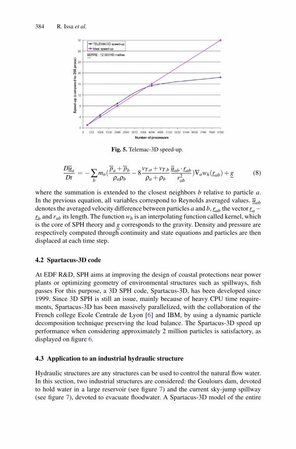
384 R. Issa et al.
Fig. 5. Telemac-3D speed-up.
Dua
Dt= −∑
b
mn(pa + pb
ρaρb−8
vT,a + vT,b
ρa +ρb
uab · rab
r2ab
)∇awh(rab)+ g (8)
where the summation is extended to the closest neighbors b relative to particle a.In the previous equation, all variables correspond to Reynolds averaged values. uabdenotes the averaged velocity difference between particles a and b, rab the vector ra−rb and rab its length. The function wh is an interpolating function called kernel, whichis the core of SPH theory and g corresponds to the gravity. Density and pressure arerespectively computed through continuity and state equations and particles are thendisplaced at each time step.
4.2 Spartacus-3D code
At EDF R&D, SPH aims at improving the design of coastal protections near powerplants or optimizing geometry of environmental structures such as spillways, fishpasses For this purpose, a 3D SPH code, Spartacus-3D, has been developed since1999. Since 3D SPH is still an issue, mainly because of heavy CPU time require-ments, Spartacus-3D has been massively parallelized, with the collaboration of theFrench college Ecole Centrale de Lyon [6] and IBM, by using a dynamic particledecomposition technique preserving the load balance. The Spartacus-3D speed upperformance when considering approximately 2 million particles is satisfactory, asdisplayed on figure 6.
4.3 Application to an industrial hydraulic structure
Hydraulic structures are any structures can be used to control the natural flow water.In this section, two industrial structures are considered: the Goulours dam, devotedto hold water in a large reservoir (see figure 7) and the current sky-jump spillway(see figure 7), devoted to evacuate floodwater. A Spartacus-3D model of the entire

HPC for hydraulics and industrial environmental flow simulations 385
Fig. 6. Spartacus-3D speed-up.
system (involving the real Goulours valley, as well as the dam and the spillway)has been built at EDF R&D. For this purpose, approximately 1 000 000 particleswere considered. In order to simulate 16 s of physical time, 5 days of computingwere needed by using 1024 IBM BlueGene/L processors. As reveal by figure 8, thesimulated flow is realistic and, from a qualitative point of view, match quite wellobservations achieved on an EDF physical model. More quantitative comparisonswill be carried out in 2009.
Fig. 7. Left: picture of an EDF physical model of the Goulours structure; right: real Gouloursdam and spillway.
5 Conclusion
This paper presented the parallelization needs required by the TELEMAC system,a complete hydroinformatics tool developed by EDF R&D. A focus on three codespart of the TELEMAC system, namely Estel-3D, Telemac-3D and Spartacus-3D, has

386 R. Issa et al.
At the physical time of 0 s At the physical time of 0.8 s
At the physical time of 4 sAt the physical time of 2.4 s
At the physical time of 16 sAt the physical time of 8 s
a
c
e
b
d
f
Fig. 8. Snapshots of the simulated flow at different physical time.
been achieved. For each code, performance in terms of speed up is satisfactory andsuitable with industrial needs. However, when refining domain discretization, largeamount of data has to be handled and a suitable post-processor is required for dataanalysis.
[1] J.M Hervouet, Hydrodynamics of Free Surface Flows: Modelling with the Fi-nite Element Method Wiley & Sons, 2007.

HPC for hydraulics and industrial environmental flow simulations 387
[2] Haverkamp R., Vauclin M., Tourna J., Wierenga P., Vachaud G: A comparisonof numerical solution models for one-dimensional infiltration. Soil ScientificSociety America, 41(2), 285-294 (1977)
[3] Celia, M.A., Boutoulas, E.T., Zarba, R.L.: A General Mass-Conservative Nu-merical Solution for the Unsaturated Flow Equation. Water Resources Research26(7),1483-1496 (1990)
[4] Hinkelmann, R., Zielke, W.: Parallelization of a Lagrange-Euler model forthree- dimensional free surface flow and transport processes. Computers & flu-ids, Vol. 29, pp. 301-325 (2000)
[5] Monaghan, J. J.: Simulating free surface flows with SPH, J. Comp Phys., Vol110, pp. 339-406 (1994)
[6] Moulinec, C., Issa,, R., Marongiu, J.-C., Violeau, D.: Parallel 3-D SPH Simu-lations, CMES, Vol. 25, pp. 133 (2008)
[7] Karypis, G., Kumar, V.: Metis mesh partitioner. Unstructured Graph Partition-ing and Sparse Matrix Ordering System, University of Minnesota TechnicalReport (1995)


Multi-parametric intensive stochastic simulations forhydrogeology on a computational grid
J. Erhel1 ∗, J.-R. de Dreuzy2, E. Bresciani1
1 INRIA,35042 Rennes Cedex, France2 Geosciences Rennes, UMR CNRS 6118, France
Abstract. Numerical modelling is an important key for the management and remediation ofgroundwater resources. Numerical simulations must be performed on domains of a large size,at a fine resolution to take into account the scale of geological heterogeneities. Numericalmodels are based on probabilistic data and rely on Uncertainty Quantification methods (UQ).In this stochastic framework, non intrusive methods require to run multiple simulations. Also,each simulation is governed by multiple parameters and a complete study requires to carryout analysis for more than 50 sets of parameters. We have identified three levels of distributedand parallel computing: subdomain decomposition in one simulation, multiple simulationsfor UQ methods, multiparametric studies. Our objective is to use the computing and memoryresources of computational grids to deploy these multiple large-scale simulations. We discussour implementation of these three levels, using an object-oriented approach. We present somepreliminary results, with a strategy to choose between the first and second level.
1 Introduction
Numerical modelling is an important key for the management and remediation ofgroundwater resources. Natural geological formations are highly heterogeneous,leading to preferential flow paths and stagnant regions. The contaminant migrationis strongly affected by these irregular water velocity distributions. In order to ac-count for the limited knowledge of the geological characteristics and for the naturalheterogeneity, numerical models are based on probabilistic data and rely on Uncer-tainty Quantification methods. In this stochastic framework, non intrusive methodsrequire to run multiple simulations. Also, numerical modelling aims at studying theimpact of various physical parameters, such as the Peclet number. Therefore, eachsimulation is governed by multiple parameters and a complete study requires to carryout analysis for more than 50 sets of parameters. The hydraulic simulations must beperformed on domains of a large size, at the scale of management of the groundwa-ter resource or at the scale of the homogeneous medium type in terms of geology.This domain must be discretized at a fine resolution to take into account the scale
∗ this work was partly funded by the Grid’5000 grant from the French government
D. Tromeur-Dervout (eds.), Parallel Computational Fluid Dynamics 2008,Lecture Notes in Computational Science and Engineering 74,DOI: 10.1007/978-3-642-14438-7 41, c© Springer-Verlag Berlin Heidelberg 2010

390 Erhel et al.
of geological heterogeneities. Characterization of transport laws requires simulatingadvection and dispersion on very long times and in turn in very large domains. Ourobjective is to use the computing and memory resources of computational grids todeploy these multiple simulations.
A first level of parallelism is used in each simulation. Indeed, in order to reachthe target of large scale domains, it is necessary to run each simulation on a parallelcomputer with enough memory and with enough computing power. A second level ofparallelism comes from Uncertainty Quantification. A third level of parallelism is thestudy of different sets of parameters. These multiparametric simulations are clearlyindependent and are thus very well-suited to techniques inspired from peer-to-peer.However, it should be kept in mind that each study is in itself a heavy computationinvolving a large number of random simulations, requiring high performance com-puting for each simulation. Our objective is to use current middleware developedfor grid architectures, in order to make the most of the three levels of parallelism.Several difficulties arise, ranging from basic software engineering (compatibility ofsystems, libraries, compilers) to scheduling issues.
2 Existing work
2.1 Parallel Monte-Carlo
The Monte-Carlo method is heavily used in physical simulations, either to evaluateintegrals or in the framework of stochastic models. In general, a run is composed ofmore or less independent simulations, so that a run is embarassingly parallel. Themain difficulty is to generate random numbers correctly. Also, since the flowchart ofa Monte-Carlo run is identical for many applications, it is natural to design a genericsoftware. For example, the ALPS project (Algorithms and Libraries for Physics Sim-ulations) is an open source effort aiming at providing high-end simulation codes forstrongly correlated quantum mechanical systems as well as C++ libraries for sim-plifying the development of such code (http://alps.comp-phys.org/). The ALPS soft-ware contains a module for parallel Monte-Carlo runs and parallel multiparametricsimulations [14]. It is based on a distributed memory paradigm and uses MPI, withclusters as target computers. Currently, each simulation is sequential.
2.2 Distributed multiple simulations and grid applications
Multiparametric experiments arise in many application domains, for example in bi-ology, chemistry and earth science. Computational grids provide interesting powerand memory resources. Many initiatives of grids are built around the world. Forexample, DEISA is a grid gathering several supercomputing centers in Europe(http://www.deisa.org/). Other grids build an infrastructure with several partners tocreate an integrated, persistent computational resource. Some examples are Teragridin USA (http://www.teragrid.org/about/),EGEE in Europe (http://www.eu-egee.org/)

Hydrogeology and HPC 391
and Grid’5000 in France (http://www.grid5000.fr). These infrastructures aim at de-veloping e-science applications using global resources provided by the grid. For ex-ample, the GEON web portal (http://www.geongrid.org) provides tools to a networkof partners in earth science, like SINSEIS, a synthetic seismogram computationtoolkit, built as a grid application. Some applications are multiparametric scien-tific simulations; for example, in earth science, the footprint project (http://www.eu-footprint.org/) develops tools for pesticide risk assessment and management, basedon Monte-Carlo and multiparametric simulations for dealing with uncertainty [10].Whereas most grid initiatives use computing resources of research laboratories orcomputing centers, another approach rely on Internet to run scientific software ondesktop computers. The platform BOINC [2] is a distributed computing tool whichallows to run computationally expensive projects by using the aggregate power ofdesktop computers. The project climateprediction.net [13] uses BOINC to run mil-lions of simulations of a climate model coupling atmosphere and ocean.
2.3 Middleware on grids
Computational grids are often built as a network of several clusters located in differ-ent geographical places. Multiple simulations can in principle run on these clustersby using the grid infrastructure. However, scheduling tools are required to distributethe simulations and to communicate data between the clusters. Some projects en-able scientists and engineers to seamlessly run MPI-conforming parallel applicationon a Computational Grid, such as a cluster of computers connected through high-speed networks or even the Internet. For example, MPICH-Madeleine [6] is a freeMPICH-based implementation of the MPI standard, which is a high-level commu-nication interface designed to provide high performance communications on variousnetwork architectures including clusters of clusters. Another solution is to providea tool specifically devoted to distributed computing. Nimrod/G is an example ofsuch software and has been successfully used with different grids [1]. The Grid’5000project provides the software Oaregrid [7] and Taktuk [12], which can also help todeploy parametric simulations. Other approaches are based on a software componentparadigm [8].
3 Our work
We are developing a scientific platform H2OLab for hydrogeology. Our platform isdesigned in order to ensure integration of new modules and to facilitate coupling ofexisting modules. We use C++ development environments and software engineer-ing tools. We pay a lot of attention to test generation, non regression issues andnumerical validation. Modularity and genericity are essential for a scientific plat-form of this size. These requirements are satisfied by a rigorous design inspired fromUML techniques and by an object-oriented approach. We have identified three levelsof distributed and parallel computing. At the simulation level, we choose to definedistributed memory algorithms and to rely on the MPI library for communications

392 Erhel et al.
between processors. These parallel deterministic simulations are operational in thesoftware H2OLab and we are investigating scalability issues [9]. The intermediatelevel is the Uncertainty Quantification non intrusive method, currently Monte-Carlo.We apply a paragim similar to the software ALPS and have developed a genericMonte-Carlo module. It differs from ALPS in a number of ways including the useof Monte-Carlo, random number generation, the physical application, the memoryand CPU intensive simulations and the development tools used. Our objective is todesign a facility for running this run of Monte-Carlo by choosing either a parallelapproach with MPI or a distributed approach with a grid middleware. We use a spe-cific random number generator in order to guarantee independent simulations. At themultiparametric level, we choose only the distributed approach as is done in mostprojects on computational grids.
3.1 Generic tools in H2OLab
For i = 1..N
Generate new random numbers
Perform simulation
Save simulation results
Save statisticsSatistics (files )
Simulation results (files)
Update statistics with current results
Fig. 1. Monte-Carlo simulations, saving results and collecting statistics.
We have implemented a generic Monte Carlo method where a loop performs Nsimulations and computes first and second statistical moments of the results. Thisloop contains a checkpoint at every iteration with a restore point. This recovery fa-cility allows to resume simulations in case of failure or to complete already existingstatistics with new results. The generic loop is depicted in Figure 1. Some opera-tions are always done by any executable program : reading inputs, creating resultsdirectories, initializing random number generators, launching the simulation, writ-ing the results, initializing visualization tools, etc. All those operations are factorizedand performed by a Launcher class. This is lot-of-time saving for the user. In orderto be generic to any application, the Launcher and the Monte Carlo modules need acommon interface. We thus developed a Simulation virtual class, which owns all nec-essary objects to perform a simulation: parameters, results, random number streams.

Hydrogeology and HPC 393
Monte_Carlo
Simulation
Porous_Simulation Frac_2D_Simulatioin
-params_mca : ParametersGroup-rng_vector : RNG_vector-resuts_stat : Results_Statistics-nb_simul : int
+prepare_rngs()+execute()
#params : ParametersGroup#results : Results#rng_simul : RNG_simul#parallel : parallel_tools
+define()
+perform() : virtual int
+perform() : int +perform() : int
+assign_RNG( master_stream : RngStream_a )
+random_properties_index() : virtual
+random_properties_index() +random_properties_index()
1
Fig. 2. The virtual class simulation, and its use for Monte-Carlo with various applications.
Practically, the user only has to override two functions to define the specific randomproperties associated to the simulation and to write the very job of the simulation.The virtual class is depicted in Figure 2.
We have opted for the XML standard language to define a generic structure forinput parameters. The use of this standard has allowed us to easily define an associ-ated user interface and develop C++ read/write methods thanks to already existingtools. In our scheme, the parameters are defined by four fields: name, value, defaultvalue and description, and can be organized in groups in a recursive manner. Thisstructure facilitates the development of non-conflicting C++ packages.
The simulation results are stored in a generic structure (C++ class) which cancontain scalars, vectors and matrices, organized in categories. This class also pro-vides a method to write the results in files in an appropriate format. Application-specific results and categories are defined in XML files.
Regarding random number generation, we have to deal with several difficulties:a simulation has several random properties, a random property can require severalrandom numbers and this quantity is not fixed in advance, depending on the studiedmedium or phenomenon. Moreover, the run must be reproducible for validation andcomposed of independent simulations for distributed computing. We have designeda set of classes, based on the RngStream package [11], to generate random numbersstreams that solve these difficulties. These classes are generic to any application.

394 Erhel et al.
3.2 Deployment on grid architectures
Multiparametric simulations require more than 50 sets of data and generate as manyresults. We have developed a tool to automatically generate a multiparametric study:from a given range of parameter values, the tool generates all corresponding inputdata files and an associated batch file to run the complete study. This tool is nowready to be deployed on a computational grid using an adapted middlware.
Thanks to our generic module and our random number generation, a run of MonteCarlo contains an embarassingly parallel loop of simulations, which can be readilydistributed on a computational grid. We have currently implemented a parallel ver-sion using the MPI standard. It can be generalized to a version with an extended MPIlibrary or to a distributed version with a grid service. Also, the Monte Carlo modulecan be extended to any non intrusive UQ method.
Finally, each simulation is memory and CPU intensive. The platform relies onfree software libraries such as parallel sparse solvers which use MPI. Thus we chooseto develop parallel software also with MPI. Each simulation is fully parallel with datadistributed from the beginning to the end.
3.3 Experiments on clusters and conclusion
speed-up
7
6
24 sim
50 sim
100 sim
200 sim
400 sim
5
5 6
4
4
3
3
2
2
1
01
Fig. 3. Speed-up versus the number of nodes (2 subdomains per node).
We use the different clusters available thanks to the french grid project Grid’5000.We have made a thorough performance analysis of our parallel simulations appliedto flow and solute transport in heterogeneous porous media [3, 5]. We have alsodone some experiments with parallel simulations applied to flow in Discrete Frac-ture of Networks [4]. This analysis allows us to find out in advance the number ofprocessors necessary for a given set of data. Thus we can rely on a static scheduling

Hydrogeology and HPC 395
Fig. 4. CPU time versus the number of simulations, with 6 nodes.
of resources for each simulation. For a run of Monte Carlo, we can also define thenumber of simulations and use a static scheduling.
Here, we give the results for several experiments combining parallel Monte Carloruns of parallel simulations. In a first step, we run parallel Monte-Carlo simulationsof moderate size so that each simulation can run on one node. We use a cluster ofnodes with a Myrinet network where each node is one-core bi-processor, with 2GBmemory. We apply our method to flow and solute transport in heterogeneous porousmedia, with a mesh of 1024 times 1024 cells. We have done several measures withvarying parameters of the model with similar results, so we plot here the results withone set of parameters. In Figure 3, we plot the speed-up in function of the numberof processors. For a small number of nodes, the speed-up is almost linear, as couldbe expected since parallel Monte-Carlo does not induce communication. In Figure4, we plot the CPU time in function of the number of simulations, using 6 nodesof the same cluster. As could also be expected, we get a stairwise function, due tothe distribution of simulations which is obtained simply by dividing the number ofsimulations by the number of processors.
In a second experiment, we use a two-level parallelism. We run the same appli-cation on a cluster of four nodes and try three configurations, distributing both thesubdomains of one simulation and the Monte-Carlo simulations. Results are givenin Table 3.3. Clearly, Monte-Carlo parallelism is more efficient since subdomain de-composition involves communications. Therefore, the limiting resource is here thememory available and the best strategy is to choose the smallest number of subdo-mains so that each subdomain fits in the memory of one core, defining chunks of pro-cessors. Then Monte-Carlo simulations are distributed among the different chunks.
These results are preliminary but show clearly that what we get is what we expect.So we can now adopt the same strategy for larger computational domains with alarger number of nodes. Also, in a next future, we plan to use middleware availableon grid’5000, in order to run the three levels of distributed computing.
[1] D. Abramson. Applications development for the computational grid. In Ap-plications Development for the Computational Grid, volume 3841 / 2006 ofLecture Notes in Computer Science, pages 1–12, 2006.

396 Erhel et al.
Number of subdomains CPU time2 1294 1998 299
Table 1. Two-level parallelism with 4 nodes (bi-processors): CPU time according to the num-ber of subdomains.
[2] David P. Anderson. Boinc: A system for public-resource computing and stor-age. In 5th IEEE/ACM International Workshop on Grid Computing, Pittsburgh,USA, November 2004.
[3] A. Beaudoin, J-R. de Dreuzy, and J. Erhel. An efficient parallel particle trackerfor advection-diffusion simulations in heterogeneous porous media. In A.-M.Kermarrec, L. Boug, and T. Priol, editors, Euro-Par 2007, LNCS 4641, pages717–726. Springer-Verlag, Berlin, Heidelberg, 2007.
[4] A. Beaudoin, J-R. de Dreuzy, J. Erhel, and H. Mustapha. Parallel simulations ofunderground flow in porous and fractured media. In G.R. Joubert, W.E. Nagel,F.J. Peters, O. Plata, P. Tirado, and E. Zapata, editors, Parallel Computing:Current and Future Issues of High-End Computing, volume 33 of NIC Series,pages 391–398, Jlich, Germany, 2006. NIC.
[5] A. Beaudoin, J. Erhel, and J.-R. de Dreuzy. A comparison between a direct anda multigrid sparse linear solvers for highly heterogeneous flux computations.In Eccomas CFD 2006, volume CD, 2006.
[6] Darius Buntinas, Guillaume Mercier, and William Gropp. Data Transfer in aSMP System: Study and Application to MPI. In Proc. 34th International Con-ference on Parallel Processing(ICPP 2006), Colombus, Ohio, August 2006.
[7] Nicolas Capit, Georges Da Costa, Yiannis Georgiou, Guillaume Huard,Cyrille Marti n, Grgory Mouni, Pierre Neyron, and Olivier Richard. A batchscheduler with high level components. In Cluster computing and Grid 2005(CCGrid05), 2005.
[8] A. Denis, C. Prez, and T. Priol. Achieving portable and efficient parallel corbaobjects. Concurrency and Computation: Practice and Experience, 15(10):891–909, August 2003.
[9] Jocelyne Erhel, Jean-Raynald de Dreuzy, Anthony Beaudoin, Etienne Bres-ciani, and Damien Tromeur-Dervout. A parallel scientific software for hetero-geneous hydrogeology. In Parallel CFD, Antalya (Turkey), May 2007. Invitedplenary talk.
[10] Stenemo F. and Jarvis N.J. Accounting for uncertainty in pedotransfer func-tions in vulnerability assessments of pesticide leaching to groundwater. PestManagement Science, 63(9):867–875, 2007.
[11] Pierre L’ecuyer, Richard Simard, E. Jack Chen, and W. David Kelton. Anobject-oriented random-number package with many long streams and sub-streams. Operations Research, 50(6):1073 – 1075, 2002.

Hydrogeology and HPC 397
[12] Vincent Martin, Jrme Jaffr, and Jean E. Roberts. Modeling fractures and barri-ers as interfaces for flow in porous media. SIAM Journal on Scientific Comput-ing, 26:1667–1691, 2005.
[13] N. Massey, T. Aina, M. Allen, C. Christensen, D. Frame, D. Goodman, J. Ket-tleborough, A. Martin, S. Pascoe, and D. Stainforth. Data access and analysiswith distributed federated data servers in climateprediction.net. Advances inGeosciences, 8:49–56, 2006.
[14] Matthias Troyer, Beat Ammon, and Elmar Heeb. Parallel object oriented montecarlo simulations. In ISCOPE ’98: Proceedings of the Second InternationalSymposium on Computing in Object-Oriented Parallel Environments, pages191–198, London, UK, 1998. Springer-Verlag.


Parallel computation of pollutant dispersion inindustrial sites
J. Montagnier1,2, M. Buffat2, and D. Guibert1,3
1 Modelys, 66, Boulevard Niels Bohr, BP 2132, 69603 Villeurbanne Cedex [email protected]
2 Universite de Lyon, CNRS, Ecole Centrale de Lyon, Universite de Lyon 1, Laboratoire deMecanique des fluides et d’Acoustique, bat Omega 721, 43 bvd du 11 nov. 1918, 69622Villeurbanne Cedex France [email protected]
3 ICJ CNRS UMR 5208, Center for the Developement of Scientific Parallel Computing,University Claude Bernard Lyon 1, ISTIL 15, Boulevard Latarjet, 69622 VilleurbanneCedex France [email protected]
Understanding the pathway of toxic air pollutants from their source is essential togovernment agencies that are responsible for the public health. CFD remains an ex-pansive tool to evaluate the flow of toxic air contaminants and requires to deal withcomplex geometry, high Reynolds numbers and large temperature gradients. To per-form such simulations, the compressible Naviers Stokes equations are solved with acollocated finite volume method on unstructured grid and the computation speed isimproved as a result of parallelism.
The developed computer code is written in an object oriented language (C++)using a 3D finite element library libMesh ( [5]) associated with PETSc ( [1]) a generalpurpose scientific computing library. Parallelization is performed using the domaindecomposition and the parallel linear solvers of PETSc.
In this paper, we propose to evaluate Algebraic Multigrid preconditioning meth-ods used in the Navier Stokes solver.
1 Description of the numerical method
1.1 Implicit Navier Stokes Solver
A classical implicit finite volume discretization of the compressible Reynolds aver-aged Navier-Stokes (RANS) equations may be written as :
ρn+1i −ρn
i + τ ∑j∈V (i)
ρn+1i φn+1
i j = 0 (1)
D. Tromeur-Dervout (eds.), Parallel Computational Fluid Dynamics 2008,Lecture Notes in Computational Science and Engineering 74,DOI: 10.1007/978-3-642-14438-7 42, c© Springer-Verlag Berlin Heidelberg 2010

400 J. Montagnier, M. Buffat, and D. Guibert
(ρu)n+1i − (ρu)n
i + τ ∑j∈V (i)
φn+1i j (ρu)n+1
i
= τ ∑j∈V (i)
Si j pn+1i j
ni j + τ ∑j∈V (i)
Si j∇(νi j(ρu)n+1i j ) (2)
(ρE)n+1i − (ρE)n
i + τ ∑j∈V (i)
(ρH)n+1i φn+1
i j = 0 (3)
with τ = �t/Vi and V (i) is the set of neighboring cells of the cell i.The superscripts n and n+1 indicate the old and the new time step, respectively,
�t is the time step, Vi the volume of cell i. ρ , P, u, H and E denote respectively thedensity, pressure, velocity, total enthalpy and total energy. ∂Ci ∩∂Cj is the interfacelocated between the two cells i and j. Si j and ni j are respectively the surface andnormal vector of the face ∂Ci ∩∂Cj .
For the convective fluxes, the cell face velocity φi j =∫∂Ci∩∂Cj
ui j.ni jds is classi-cally calculated using a specific interpolation ( [10]). On the interface, the transportedquantities are interpolated using a first or second order upwind scheme.
Momentum, energy and mass conservation equations are solved implicitly usinga projection method ( [8]). At each non linear iteration (k), a predictor step (*) fordensity and momentum is calculated from the density and momentum equations :
ρ∗i −ρni + τ ∑
j∈V (i)ρ∗i φ k
i j = 0 (4)
(ρu)∗i − (ρu)ni + τ ∑
j∈V (i)φ k
i j(ρu)∗i = τ ∑j∈V (i)
Si j pki j
ni j + τ ∑j∈V (i)
Si j∇(νi j(ρu)∗i j) (5)
After this prediction step, the pressure correction p′i (and eventually the temper-
ature correction T′
i ) is computed from a Laplace equation based on the energy (andeventually the density equation). Correction equation (8) is obtained by replacing inequation (3) the total energy and the total enthalpy by expression (6) and (7).
(ρE)n+1 = (ρE)∗ +(ρe)∗pp′
(6)
(ρH)n+1i φ n+1
i j = (ρH)∗i φ∗i j + h∗i (ρφ)
′i j (7)
(ρφ)′i j is related to the pressure correction p
′i through the momentum equation
using a SIMPLE algorithm ( [9]).
(ρe)∗p p′i + τ ∑
j∈V (i)h∗i (ρφ)
′i j = −
(
(ρE)∗i − (ρE)ni + τ ∑
j∈V (i)(ρH)∗i φ
∗i j
)
(8)
At each step of this algorithm, we have to solve several large sparse linear sys-tems. The key point of the efficiency of this implicit algorithm is to use an efficientlinear solver.

Parallel computation of pollutant dispersion in industrial sites 401
1.2 Iterative methods for sparse linear systems
Krylov subspace methods are widely used to solve for large and sparse linearsystems. In the present work, the incomplete LU factorisation algorithm and theAlgebraic MultiGrid method (AMG) are used as preconditioners for the GMRESalgorithm. The next section brievly describes the multigrid preconditioner used inthis paper. The reader is refered to the literature for more information (see [11], [2],[12]).
The central idea of AMG is to remove smooth error not eliminated by relaxationon coarser grids. This is done by solving the residual equation on coarse a grid,then interpolating the error back to the finest grid. Significant and important parts ofthe AMG algorithm rely on the coarse-grid selection process and the interpolationoperation.
Coarsening schemes
Various coarsening schemes exist and most are based on the coarsening heuristicsproposed by [11]. However when these traditional algorithms are applied to three-dimensional problems, stencil may grow significantly, leading to computational com-plexity growth and a loss of scalability. For this reason, the Falgout algorithm ( [4])is the only tested classical method.
Recently, [12] developed new methods to obtain sparser coarser grids (see fig-ure 1) that diminish algorithm complexity : The Parallel Modified Independent Set(PMIS) algorithm and the Hybrid Modified Independant Set (HMIS) algorithm arecompared to the more classical Falgout method.
Interpolation
Interpolation is an important operation affecting the convergence factor of the AMGalgorithm. The Falgout coarsening scheme is used with a classical interpolation( [11]) : the error of a refine point (F-point) i is done with a subset of the nearestneighbors of grid point i.
Because of the coarser grids, PMIS and HMIS approach require more accurateinterpolation : we investigate longer range interpolations F-F and F-F1 (see [2]).
2 Description of the tests
2.1 Laplace equation
To select the best precondioning method for our application, scale-up and speed uptests are performed on a Laplace equation Δφ = 1 with a null Dirichlet boundarycondition φΓ = 0. The computational domain is a unit cubic box with tetrahedra cells.Speed up tests used 106 cells mesh, scale-up tests investigated different numbers ofdegree of freedom per processor (dofs) from 12 500 to 400 000 dofs. AMG methodsdescribed in 1.2 are compared with ILU preconditioning.

402 J. Montagnier, M. Buffat, and D. Guibert
Fig. 1. Coarsening schemes and interpolation
2.2 Flow around a complex industrial site
We are interested in an incompressible isothermal flow around a french factory. Thestandard k-epsilon model ( [6]) with wall function ( [7]) was used for assessing tur-bulent flow. The closure coefficients are obtained from [3] to take into account theatmospheric boundary layer.
The three dimensional unstructured mesh used in the simulations is displayed infigure 2 (b) . It contains approximately 5×10⁶ tetrahedra.
(a) Unstructured Cubic Box (b) Details of the industrial site (1.5 × 10⁹
cells)
Fig. 2. Meshes

Parallel computation of pollutant dispersion in industrial sites 403
3 Results
The results were obtained at the High Performance Computing Center P2CHPD,Lyon 1 University. The cluster is a mid-range HPC platform. Each node is composedof 2 inter quad-core processor with a CPU speed of 2.9 GHz and are connected withan infiniband network.
3.1 Laplace equation
In figure 3 (a) we show the results of parallel scaling tests. These results immediatelyhighlight the superiority of AMG preconditioning on parallel ILU. Scalability of ILUis poor due to the increase of the number of iterations with the problem size (tab 1).
It is interesting to observe in Tables 2 that low complexity coarsening schemePMIS with F-F1 interpolation is more efficient than the Falgout coarsening schemeand classical interpolation : complexity is lower and computing time is reduced.HMIS with F-F or F-F1 interpolation show very similar results and are not shownhere. AMG with PMIS coarsening schemes and F-F1 interpolation give the best re-sults. Solving time is five hundred times faster than ILU preconditioning on 64 pro-cessors. The use of classical interpolation with low complexity scheme leads to anincrease of the number of iterations because of sparser grid. Figure 3 (b) displaysthe influence of the problem size on scalability : Communication times are importantand cause a loss in scability.
Table 1. Number of iteration with 200 000 dofs / processor
Method / processor 1 2 4 8 16 32ILU 226 346 368 500 774 955PMIS - F-F1 13 14 14 14 16 16Falgout classical 11 11 11 12 13 13
Table 2. Details of AMG Preconditioning methods with 32 procs, 200 000 dofs
Method Grid Complexity Interpolation Complexity nb itFalgout classical 2.6 18.5 13
PMIS - F-F1 1.42 3.80 16PMIS - classical 1.42 2.28 37
3.2 Flow around a complex industrial site
As seen in 3.1, coarsening scheme PMIS with interpolation F-F1 give the best re-sults in term of speed up and computation time for a Laplace equation. This precon-ditioning method is then evaluated for parallel computation of atmospheric transport

404 J. Montagnier, M. Buffat, and D. Guibert
1
10
100
1000
0 10 20 30 40 50 60 70
Sol
ve T
ime
(s)
Number of processors
Scale Up 400000 dofs / proc
ILUFalgout-classical
PMIS-FF1
(a) Comparison of different preconditioningmethods
0
5
10
15
20
25
0 10 20 30 40 50 60 70
Sol
ve T
ime
(s)
Number of processors
Scale Up of PMIS-FF1
12500 dofs / proc50000 dofs / proc
400000 dofs / proc
(b) Influence of the problem size
Fig. 3. Scale up Results on a Laplace equation
pollutant. Pollutant plume is displayed in figure 5. Figure 4 shows that speed up is ex-cellent with the 5×10⁶ cells but is not good with 1×10⁶ cells due to communicationtimes.
0
10
20
30
40
50
60
70
80
90
100
0 10 20 30 40 50 60 70
Spe
ed-u
p
Number of processors
TotalAssemblage Momentum
Solve MomentumIDEAL SPEED UP
(a) Mesh 1,5×10⁶
15
20
25
30
35
40
45
50
55
60
65
70
15 20 25 30 35 40 45 50 55 60 65
Spe
ed-u
p
Number of processors
TotalAssemblage Momentum
Solve MomentumIDEAL SPEED UP
(b) Mesh 5×10⁶
Fig. 4. Speed up performance of Navier Stokes solver

Parallel computation of pollutant dispersion in industrial sites 405
Fig. 5. Pollutant plume around buildings (1.5×10⁵ cells)
4 Conclusion
The most challenging aspect of parallelizing a Navier Stokes finite volume solver isthe selection of efficient parallel linear solver. We have presented a comparison ofdifferent preconditioning methods for Krylov subspace iterative methods.
The preconditioning methods are first tested on a Laplace equation. The testsindicate that AMG preconditioning exhibit better results than ILU preconditioning.The poor scalability of the ILU preconditioning is due to an increase of iterationnumbers with the problem size. The Falgout coarsening scheme and classical inter-polation have for 3D problems too high complexity algorithm. 3D problems requirea low complexity coarsening scheme associated with a long range interpolation.Among the methods tested, PMIS with interpolation F-F1 gives the best results interm of speed up, scale-up and computing time.
Numerical experiments demonstrated good scalability of PMIS coarseningscheme and F-F1 interpolation applied to the Navier Stokes solution of flow aroundan industrial site. Hence, use of parallel and efficient multigrid preconditioner allowsa fast simulation of pollutant dispersion in industrial sites.
Future research will focus on parallelization of high order schemes for Detachedand Large Eddy Simulations.
[1] Satish Balay, Kris Buschelman, Victor Eijkhout, William D. Gropp, DineshKaushik, Matthew G. Knepley, Lois Curfman McInnes, Barry F. Smith, andHong Zhang. Petsc users manual. ANL-95/11, Argonne National Laboratory,2004.
[2] Butler and Jeffrey. Improving Coarsening and Interpolation for AlgebraicMultigrid. PhD thesis, Department of Applied Mathematics, University of Wa-terloo, 2006.
[3] P.G. Dyunkerke. Application of the E-epsilon turbulence closure model to theneutral and stable atmosphere boundary layer. Journal of the Atmospheric Sci-ences, 45:5, 865–880, 1988.

406 J. Montagnier, M. Buffat, and D. Guibert
[4] Van Emden Henson and Ulrike Meier Yang. Boomeramg: A parallel algebraicmultigrid solver and preconditioner. Applied Numerical Mathematics, 41:155–177, 2000.
[5] B. Kirk, J.W. Peterson, R.H. Stogner, and G.F. Carey. libmesh: A c++ libraryfor parallel adaptive mesh refinement/coarsening simulations. Engineering withComputers, 22:3–4, 237–254, 2006.
[6] B.E. Launder and D.B. Spalding. Lectures in Mathematical Models of Turbu-lence. Academic Press, London, England,, 1972.
[7] B.E. Launder and D.B. Spalding. The numerical computation of turbulentflows. Computer Methods in Applied Mechanics and Engineering, 3:2, 269–289, 1974.
[8] K. Nerinckx, J. Vierendeels, and E. Dick. Mach-uniformity through the cou-pled pressure and temperature correction algorithm. Journal of ComputationalPhysics., 206:597–623, 2005.
[9] S.V. Patankar and D.B. Spalding. A calculation procedure for heat, mass andmomentum transfer in three-dimensional parabolic flows. International Jour-nal of Heat and Mass Transfer, 15:1787, 1972.
[10] C.M. Rhie and W.L. Chow. A numerical study of the turbulent flow past anisolated airfoil with trailing edge separation. AIAA J, 21:1525–1532, 1983.
[11] J. W. Ruge, K. Stuben, and S. F. McCormick. Algebraic multigrid (AMG),volume 3 of Frontiers in Applied Mathematics. SIAM, Philadelphia, 1987.
[12] De Sterck, Hans, Yang, Ulrike M., Heys, and Jeffrey J. Reducing complexityin parallel algebraic multigrid preconditioners. SIAM J. Matrix Anal. Appl.,27(4):1019–1039, 2006.


Part XI
General fluid

3D Numerical Simulation Of Gas Flow AroundReentry Vehicles
S.V. Polyakov1, T.A. Kudryashova1, E.M. Kononov1, and A.A. Sverdlin1,2
1 Institute for Mathematical Modeling, Russian Academy of Sciences,125047, Miusskaya Sq. 4a, Moscow, Russia
2 E-mail: [email protected]
Abstract. Mathematical model of 3D gas flow around reentry vehicle is considered. Thismodel is based on QGD (Quasy-GasDynamics) equations. Numerical methods for solving ofthese equations on tetrahedral meshes are presented. Parallel realization of these methods isbased on MPI and OpenMP technologies. Parallelization is performed using domain decom-position principle.
1 Introduction
Modeling of the gas flow is very important for construction of any spacecraft and inparticular reentry vehicle. Latest experiments show that protection of space vehiclesdesigned decades ago is superfluous, and the destructive factors such as temperaturedo not reach such high values the protection designed against.
Computer modelling allows to save a lot of money and predict parameters ofgas-dynamic processes which cannot be obtained by ground test facilities. Compu-tational Fluid Dynamics (CFD) is the best approach for calculation of aerodynamicheating. The main factors typical for CFD algorithms are: computational complexity,high amounts of memory required, necessity for carrying out all the calculations incase of alteration in one of the flow parameters (such as Mach number, altitude, angleof attack). Therefore using this technique for calculation of the heat flow throughoutspace vehicle trajectory becomes difficult and time consuming task. All the men-tioned factors force the use of high performace parallel systems for modelling hyper-sonic flows.
In the branch where one kilogram means tens and hundreds thousands dollarsit is very important to calculate all the values precisely. The introduced approachallows to make more accurate calculations in comparison to well known and widelyused Navier-Stokes equations system. Also improved stability of numerical methodsallows to take into account additional factors such as radiative energy withdrawalthat has not been considered before.
This work presents 3D flow calculation approach around reentry vehicle in Earthatmosphere using multiprocessor computational clusters. The mathematical model is
D. Tromeur-Dervout (eds.), Parallel Computational Fluid Dynamics 2008,Lecture Notes in Computational Science and Engineering 74,DOI: 10.1007/978-3-642-14438-7 43, c© Springer-Verlag Berlin Heidelberg 2010

410 S.V. Polyakov, T.A. Kudryashova, E.M. Kononov, and A.A. Sverdlin
introduced and completed with numerical implementation. Parallel algorithm imple-menting this numerical method is designed.
2 Mathematical Model
QGD (Quasy-GasDynamic) equations ( [4, 7, 5]) and a set of boundary conditionsare used for description of the gas flow. QGD equations are generalize well knownNavier-Stokes system and differ from it in additional dissipative terms with a smallparameter.
This system binds together gasdynamic variables density, velocity, energy. Addi-tional variables pressure and temperature are calculated according with correspond-ing gas state equations. QGD system has a form of conservation laws (of mass,impulse and energy) and in general terms is written as:
∂ρ∂ t
+ divjm = 0, (1)
∂ (ρu)∂ t
+ div(jm ⊗u)+∇p = divΠ , (2)
∂∂ t
[ρ(
u2
2+ ε)]
+ div
[jm
(u2
2+ ε)]
= divA−divq. (3)
In present work the computation domain is an area inwards closed piecewiselinear triangulable boundary. There are no other limitations on the form of computa-tion domain. The geometry of space object is specified as combination of piecewiselinear elements and spline surfaces. Example of computation domain is presentedon Fig. 1(a). Arrows show the direction of gas flow. X ,Y,Z are the axes of carte-sian space. Boundary conditions representing oncoming flow are held on one side ofcomputational domain (marked as ABCD on Fig. 1(a)). All other bounds allow thegas to run freely out of the computational area. Wall boundary condition specifiedfor the object surface, with no mass flux through the object under consideration. Fig-ure 1(b) shows the example of real computation domain truncated in according tothe symmetry of problem with boundary conditions marked on the faces (1 - inletboundary, 2 - outlet boundary, 3 - planes of symmetry, 4 - surface of the object).
The flow is considered to be quasy-stationary and calculated until establishing.Parameters of the model problem are shown in Table 1.
3 Numerical Implementation
For numerical solution of QGD equations system (1)–(3) we use tetrahedral mesh( [2, 1]). Specially designed mesh generator allows to create locally condensingadaptive meshes in 3D space. This local condensing allows to balance optimal thecalculations precision and computational complexity. The number of nodes in the

3D Numerical Simulation Of Gas Flow Around Reentry Vehicles 411
z
xXY
Z
AB
CD
1234
(a) (b)
Fig. 1. Computation domain examples
Table 1. Model problem parameters
Background gas temperature T0 (K) 266Temperature of head shield T1 (K) 2000−3300Peak shock wave front temperature T2 (K) 12000Pressure P0 (Pa) 4.3 ·10Density ρ0 ( kg
m3 ) 5.63 ·10−4
Characteristic size of problem L0 (m) 3.9Mach number M∞ 12Reynolds number Re 1000
used meshes is vary from 105 to 2 ·106. Example of tetrahedral mesh is presented onFig. 1(b).
Adaptive mesh generator was developed using TetGen ( [8]) library that allows totetrahedralize piecewise linear complexes and a set of vertices in 3D space. In accor-dance with predefined distribution function additional vertices are added to computa-tion domain for local mesh condesing. This approach allows to generate calculationmeshes satisfying the following parameters:
• minimal number of mesh vertices;• predefined maximal volume of calculation cell in areas of solution peculiarity
(for example areas of high density);• necessary mesh condensing for boundary layer modelling;• maximal volume of mesh tetrahedra;• maximal relation of circumsphere radius to minimal cell edge length;• in addition, the maximal volume of adjacent tetrahedral cells can be limited for
each geometry face.

412 S.V. Polyakov, T.A. Kudryashova, E.M. Kononov, and A.A. Sverdlin
Applying Control Volume Method explicit numerical scheme was designedbased on the QGD equations. Control volumes are built around each node of meshand the union of all such control volumes is equal to the whole computational do-main (without holes and overlaps). In present work we use barycentric control vol-umes. Each control volume is an area bounded by faces build on tetrahedra centers(arithmetic mean of its nodes coordinates), centers of tetrahedra faces and centers oftetrahedra edges in all tetrahedra adjacent to referred node. Example of tetrahedralcell is shown on Fig. 2(a) with control volume elements (faces) built around verticesof this tetrahedra. One complete control volume around a calculation node insidemesh region is shown on Fig. 2(b).
(a) (b)
Fig. 2. Tetrahedral cell with control volume elements (a) and tetrahedral mesh region withcontrol volume (b)
The solution of initial boundary problem is calculated by time-explicit finite-difference scheme. Spatial derivatives are approximated with second order of accu-racy while time derivatives are approximated with first order.
Stability of numerical method is provided by QGD-additives with a small multi-plier as parameter. This parameter has the dimension of time and its order is aboutfree path of the molecule. Thus it can be treated as artificial (or numerical) viscosity.
4 Parallelization
Parallelization of QGD calculations code is done using domain decomposition tech-nique. The computational domain is divided into subdomains with near to equalnumbers of nodes. The number of subdomains is equal to number of processors.Number of connections between subdomains (number of shared calculation nodes)is minimized to achieve low communications overhead. The code uses MPI (Mes-sage Passing Interface) library and is highly portable being written in C++. Also forhybrid systems (where one node of distributed memory system actually is a sharedmemory parallel system) the OpenMP technology is applied.

3D Numerical Simulation Of Gas Flow Around Reentry Vehicles 413
Used parallel systems:
• Smaller cases were run on the cluster in IMAMOD (Institute for MathematicalModeling). This consists of 48 CPU cores (Intel Xeon 3.06GHz microproces-sors). Peak performance is 300 GFlops and peak transfer rate is 1GBit/sec (Eth-ernet).
• Larger cases were run on the “MVS-100k” cluster in Joint SuperComputer Cen-ter (JSCC). This consists of 6144 CPU cores (Intel Xeon 5160 3.0Ghz micropro-cessors). Peak performance is 45 TFlops and peak transfer rate is 1400 Mbyte/sec(Infiniband DDR).
• The second high performance cluster used for calculations was “SKIF MSU”(Moscow State University - Research Computing Center). This consists of 5000CPU cores (Intel Xeon E5472 3.0Ghz microprocessors). Peak performance is 60TFlop/s and peak transfer rate is 1540 Mbyte/sec (Infiniband DDR).
Efficiency graphs for parallel algorithm for shared memory architecture are pre-sented on Fig. 3. This code produces one MPI process per each CPU core. For 1Million grid nodes the effectiveness is 75% at 128 processors and goes below 40%at 512 processors. For 2 Millions nodes grid configuration the effectiveness is about76% at 100 processors and falls to 50% at 600 processors.
30
40
50
60
70
80
90
100
128 256 384 512Number of CPU Cores
Eff
icie
ncy,
%
)a(
30
40
50
60
70
80
90
100
0 100 200 300 400 500 600Number of CPU Cores
Eff
icie
ncy,
%
)b(
Fig. 3. Parallelization efficiency for 106 nodes task, 1 MPI process per core on “SKIF MSU”(a) and efficiency for 2 ·106 nodes, 1 MPI process per core on “MVS-100k” (b)
Systems like “MVS-100k” and “SKIF MSU” that have several CPU cores onone computation node allow to realize hybrid parallelization approach and achieveperformance several times higher. In this case we use MPI to distribute tasks amongnodes in cluster while applying OpenMP to distribute computational load amongcores on one node. Thus we eliminate the communications overhead inside this smallgroup (8 for mentioned systems) of computation cores.
Practically we can use 3-5 times more CPU maintaining the same efficiency andobtain the final result about 3 times faster. This comparison is illustrated on Fig. 4.

414 S.V. Polyakov, T.A. Kudryashova, E.M. Kononov, and A.A. Sverdlin
Fig. 4. Comparison of pure MPI parallelization efficiency with hybrid MPI+OpenMP ap-proach (“MVS-100k”)
5 Test case
One of the test cases is Apollo project capsule model. The diameter of the capsule isabout 4 meters. Note that total mass of the capsule is 5800kg and the thermal protec-tion mass is about 850kg. Considering the model is axisymmetric we can truncate itand calculate only one fourth of the original domain. Another parameters of modelproblem are shown in Table 1.
The result of simulation is shown on Fig. 5.
6 Conclusions
This paper is intended to show the evolution of previous work ( [6, 3]).Calculated gasdynamic variables can be refined on each time step using, for ex-
ample, radiative heat transfer model. In this approach QGD calculations modulepasses energy, pressure and temperature fields to RGD (Radiative GasDynamics)module and receives adjusted energy field back.

3D Numerical Simulation Of Gas Flow Around Reentry Vehicles 415
X
02
46
810
Y
0
2
4
Z
0
2
4
T(K)
120001100010000900080007000600050004000300020001000
Fig. 5. Temperature distribution (K) around Apollo capsule model at speed 12Ma
Introduced model can be applied to objects with very complicated shape includ-ing real space vehicles. Improved stability of numerical method allows to take intoaccount additional factors such as radiation and chemical processes.
Grid generator developed allows to construct adaptive locally condensing tetra-hedral grids with high number of nodes (up to 109) suitable for parallel computations.The parallel realization of numerical algorithm allows to take advantage of high per-fomance computer clusters and obtain results in a reasonable time using very precisegrids. The algorithm is designed for distributed and hybrid memory systems andbased on geometrical parallelism principle. Parallel algorithm shows good efficiencyon different type of parallel systems from low-cost clusters (50-100 CPU cores, withEthernet transport) to high perfomance parallel systems (2000-6000 CPU cores con-nected via Myrinet or Infiniband networks).
7 Acknowledgments
The work was performed under research grants: RFBR N06-01-00233, N08-07-00458.

416 S.V. Polyakov, T.A. Kudryashova, E.M. Kononov, and A.A. Sverdlin
[1] I.V. Abalakin, A. Dervieux, and T.K. Kozubskaya. High accuracy finite volumemethod for solving nonlinear aeroacoustics problems on unstructured meshes.Chinese Journal of Aeroanautics, 19(2), 2006.
[2] I.V. Abalakin and S.A. Sukov. Modeling of external flow around bodies onmultiprocessor systems using thetraedral meshes. In Fundamental physico-mathematical problems and modeling of technico-technological systems, vol-ume 7, pages 52–57. Janus-K, 2004. In Russian.
[3] B.N. Chetverushkin, S.V. Polyakov, T.A. Kudryashova, E. Kononov, andA. Sverdlin. Numerical simulation of 2d radiative heat transfer for reentry vehi-cles. In Elsevier, editor, Proc. Parallel CFD 2005 Conference, pages 293–299,2006.
[4] T.G. Elizarova. Quasi-gasdynamic equations and numerical methods for viscousflow simulation. Scientific world, Moscow, 2007. In Russian.
[5] T.G. Elizarova and M. Sokolova. Numerical algorithm for computing of super-sonic flows is based on quasi-hydrodynamics equations. Vestnik of Moscow StateUniversity, Physics and Astronomy, (1):10–15, 2004. In Russian.
[6] I.A. Graur, T.A. Kudryashova, and S.V. Polyakov. Modeling of flow for radiativetransport problems. In Elsevier, editor, Proc. Parallel CFD 2004 Conference,pages 239–245, 2005.
[7] Y.V. Sheretov. Analysis of modified kinetically-consistent scheme stability inacoustic approach. In Application of functional analisis in approach theory,pages 147–160. Tver State University, Tver, 2004. In Russian.
[8] Hang Si. Tetgen: A quality tetrahedral mesh generator. http://tetgen.berlios.de/.

Effective Parallel Computation of IncompressibleTurbulent Flows on Non-uniform Grid
Hidetoshi Nishida1 and Nobuyuki Ichikawa2
1 Department of Mechanical and System Engineering, Kyoto Institute of Technology,Matsugasaki, Sakyo-ku, Kyoto 606-8585, Japan [email protected]
2 Department of Mechanical and System Engineering, Kyoto Institute of Technology,Matsugasaki, Sakyo-ku, Kyoto 606-8585, Japan
In order to improve the parallel efficiency of incompressible turbulent flow solveron non-uniform grid, the multigrid technique with the checkerboard SOR methodor the rational Runge-Kutta (RRK) scheme for the elliptic partial differential equa-tion solver is presented. The 3D test problem and the DNS of 3D turbulent channelflow with the Reynolds number Reτ = 180 are considered. The results show that thechackerboard SOR relaxation has the property that the computational time is shorterbut parallel efficiency is lower than the RRK relaxation. Then, it is necessary to im-prove the parallel performance, but the present approach has the possibility of shortcomputational time with high parallel efficiency.
1 Introduction
The incompressible flow simulations are usually based on the incompressible Navier-Stokes equations. In the incompressible Navier-Stokes equations, we have to solvenot only the momentum equations but also the elliptic partial differential equation(PDE) for the pressure, stream function and so on. The elliptic PDE solvers consumethe large part of total computational time, because we have to obtain the convergedsolution of this elliptic PDE at every time step. In order to analyze the turbulent flows,the large-scale simulations have to be carried out. In these large-scale incompressibleflow simulations, the acceleration of convergence for the elliptic PDE solver is neces-sary. On the other hand, the wall turbulence is usually simulated on non-uniform gridin the wall direction in order to ensure the resolution. In this case, the convergenceof elliptic PDE on non-uniform grid becomes slower than the convergence on uni-form grid. Then, for the incompressible flow simulations, especially the large-scalesimulations, the efficient elliptic PDE solver on non-uniform grid is very importantkey technique.
In the parallel computations, the incompressible Navier-Stokes equations, thatis, the momentum equations, can be solved with almost theoretical speedup on theparallel platform ( [6, 4]). However, the parallel performance of the elliptic PDE
D. Tromeur-Dervout (eds.), Parallel Computational Fluid Dynamics 2008,Lecture Notes in Computational Science and Engineering 74,DOI: 10.1007/978-3-642-14438-7 44, c© Springer-Verlag Berlin Heidelberg 2010

418 Hidetoshi Nishida and Nobuyuki Ichikawa
solver becomes lower than the momentum equations solver. Then, for the practicallarge-scale simulations, the elliptic PDE solver of the multigrid method with highparallel efficiency on the non-uniform grid has high possibility.
In this paper, the multigrid technique with the checkerboard SOR method or therational Runge-Kutta (RRK) scheme ( [8]) on non-uniform grid is presented. For thesimple interpolations between grid levels, that is, restriction and prolongation, the el-liptic PDE is transformed to the computational plane. The present elliptic PDE solveris applied to the direct numerical simulation (DNS) of 3D turbulent channel flows.The message passing interface (MPI) library is applied to make the computationalcodes. These MPI codes are implemented on personal cluster system with PentiumD(3.2GHz) processors. The cluster network is constructed by the gigabit ethernet.The computational MPI codes are compiled by Intel fortran 9.1.
2 Computational Technique
The incompressible Navier-Stokes equations in the Cartesian coordinates can bewritten by
∂ui
∂xi= 0, (1)
∂ui
∂ t+ u j
∂ui
∂x j= − ∂ p
∂xi+ν
∂ 2ui
∂xi∂xi, (2)
where ui (i = 1,2,3) denotes the velocity, p the pressure and ν the kinematic viscos-ity.
2.1 Variable Order Method of Lines
The solution procedure of the incompressible Navier-Stokes equations (1) and (2) isbased on the fractional step approach on the collocated grid system. In the fractionalstep approach, first, the fractional step velocity u∗i is estimated by
u∗i = uni +αΔ t
(−u j
∂ui
∂x j+ν
∂ 2ui
∂xi∂xi
)n
. (3)
Next, the fractional step velocity at the staggered locations is computed by the inter-polation. Then, the velocity at next time step un+1
i can be obtained by
un+1i = u∗i −αΔt
∂ pn+1
∂xi. (4)
Substituting the velocity at next time step into the discrete continuity equation, thepressure equation
∂ 2 pn+1
∂xi∂xi=
1αΔ t
∂u∗ixi
∂xi, (5)

Effective Parallel Computation on Non-uniform Grid 419
is obtained. In these relations, α is the parameter determined by the time integrationscheme. The overbar denotes the interpolated value from the collocated location tothe staggered location.
In the method of lines approach, the spatial derivatives are discretized by theappropriate scheme, so that the partial differential equations (PDEs) in space andtime are reduced to the system of ordinary differential equations (ODEs) in time.The resulting ODEs are integrated by the Runge-Kutta type time integration scheme.
In the spatial discretization, the convective terms are approximated by the vari-able order proper convective scheme ( [4]), because of the consistency of the discretecontinuity equation, the conservation property, and the variable order of spatial ac-curacy. This scheme is the extension of the proper convective scheme ( [2]) to thevariable order. The variable order proper convective scheme can be described by
u j∂ui
∂x j|x =
M/2
∑�=1
c�′u jx jδ�′ui
δ�′x j
�′x j
|x, (�′ = 2�−1), (6)
where M denotes the order of spatial accuracy, and the operators in eq.(6) are definedby
f�′x j |x =
12( fx j+�′/2 + fx j−�′/2), (7)
u jx j |x j±�′/2 =
M/2
∑m=1
cm′
2[u j|x j±{�′+m′}/2 + u j|x j±{�′−m′}/2], (8)
δ�′ui
δ�′x j|x j±�′/2 =
±1�′Δx j
(ui|x j±�′ −ui|x j), (9)
where m′ = 2m−1. In this technique, the arbitrary order of spatial accuracy can beobtained automatically by changing only one parameter M. The coefficients c�′ andcm′ are the weighting coefficients andΔx j denotes the grid spacing in the x j direction.
On the other hand, the diffusion terms are discretized by the modified differentialquadrature (MDQ) method ( [7]) as
∂ 2ui
∂xi∂xi|x =
M/2
∑m=−M/2
Φm′′(x)ui|xi+m, (10)
where Φm′′(x) is the second derivative of the function Φm(x) defined by
Φm(x) =Π(x)
(x−xi+m)Π ′(xi+m), (11)
Π(x) = (x−xi−M/2) · · · (x−xi) · · · (x−xi+M/2). (12)
The coefficients of the variable order proper convective scheme, c�′ , can be computedautomatically by using the MDQ coefficients. Then, the incompressible Navier-Stokes equations are reduced to the system of ODEs in time. This system of ODEsis integrated by the Runge-Kutta type scheme.

420 Hidetoshi Nishida and Nobuyuki Ichikawa
2.2 Pressure Equation Solver
The pressure equation, eq.(5), is solved by the checkerboard SOR method and thevariable order multigrid method ( [5]).
In the variable order multigrid method, the unsteady term is added to the pres-sure equation. Then, the pressure (elliptic) equation is transformed to the parabolicequation in space and pseudo-time, τ .
∂ pn+1
∂τ=∂ 2 pn+1
∂xi∂xi− 1αΔ t
∂u∗ixi
∂xi. (13)
Equation (13) can be solved by the variable order method of lines. The spatial deriva-tives are discretized by the aforementioned MDQ method, so that eq.(13) is reducedto the system of ODEs in pseudo-time,
d−−→pn+1
dτ=−→L (
−−→pn+1). (14)
This system of ODEs in pseudo-time is integrated by the rational Runge-Kutta(RRK) scheme, because of its wider stability region. Then, the same order of spatialaccuracy as the momentum equations can be specified.
In addition, the multigrid technique, i.e., correction storage algorithm ( [1]), isincorporated into the method in order to accelerate the convergence. In the multi-grid method, the checkerboard SOR method and RRK scheme are interpreted as therelaxation method.
In this paper, the multigrid method on non-uniform grid is considered. We pre-pare two approaches. One is that the values on coarse and fine grids are interpo-lated on the corresponding non-uniform grid. Another is that the pressure equationis transformed to the computational plane, so that the values are interpolated on thecomputational plane with uniform grid.
3 Numerical Results
3.1 3D Test Problem
We consider the following 3D test problem.
∂ 2 p∂xi∂xi
= −3sin(x1)cos(x2)sin(x3). (15)
The periodic boundary condition is imposed in x1(= x) and x3(= z) directions. Inx2(= y) direction, the Neumann boundary condition, ∂ p
∂y = 0, is imposed. The com-putational domain is set (0,0,0) < (x,y,z) ≤ (2π,π,2π). The convergence criteronis L2 < 1.0× 10⁻⁶, where L2 denotes the L2-residual of eq.(15). The non-uniformgrid defined by

Effective Parallel Computation on Non-uniform Grid 421
50
100
150
200
250w
ork
Number of grid points
(a) Usual non-uniform grid.
50
100
150
200
wo
rk
Number of grid points
(b) Computational plane.
Figure 1. Multigrid property on non-uniform grid.
y j =tanh[γ(2 j/N−1)]
tanh(γ), (16)
is used in y direction only. The stretching parameter γ is 1.80.Figure 1 shows the comparison of work unit until convergence. Figure 1(a) is the
result on usual non-uniform grid and (b) denotes the result on computational plane.The square and circular symbols are the work unit obtained by the checkerboard SORand RRK relaxation, respectively. In the checkerboard SOR relaxation, the multigridconvergence is confirmed in both cases. On the other hand, the RRK relaxation showsthe dependency on number of grid points. Also, the work unit until convergenceobtained by the checkerboard SOR relaxation is less than that obtained by the RRKrelaxation in all cases.
Next, in order to investigate the parallel efficiency, Fig.2 shows the parallel effi-ciency in this test problem. The parallel efficiency is defined by
E f f iciency =Tsingle
N ·Tparallel×100 (%) , (17)
where Tsingle and Tparallel denote the computational time on single processor element(PE) and on N parallel PEs, respectively. In Fig.2 the present parallel efficiency iscompared with the usual parallel efficiency on non-uniform grid. On 2PEs the highparallel efficiency in which is larger than 80% can be obtained in the large-scalecomputations, that is, 1283 and 2563 grid points. However, the parallel efficiencybecomes lower on 4PEs. In this case, the performance of the RRK relaxation oncomputational plane presents the highest efficiency.
3.2 DNS of 3D Turbulent Channel Flow
In order to simulate the 3D turbulent channel flow, the incompressible Navier-Stokesequations, eq.(1) and eq.(2), are nondimensionalized by the friction velocity uτ(=√τwall/ρ) and half length of channel h. Table 1 shows the computational conditions.
In the table, the conditions of reference simulation ( [3]) are shown, too. The periodicboundary conditions in x and z directions and the Neumann boundary condition in ydirection are imposed. In y direction, the non-uniform grid with γ = 1.80 in eq.(16) isadopted. The DNS of 3D turbulent channel flow with Reτ = 180 is computed on 323,643, and 1283 grid points. The present results are compared with reference solutionobtained by Moser et al.. Figure 3 shows the comparison of the mean streamwise

422 Hidetoshi Nishida and Nobuyuki Ichikawa
Number of grid points
40
50
60
70
80
90
100
Eff
icie
ncy(%
)
(a) 2PEs
(a) 2PEs
Number of grid points
20
25
30
35
40
45
50
55
60
65
70
75
Eff
icie
ncy(%
)
(b) 4PEs
(b) 4PEs
Figure 2. Parallel efficiency of test problem.
Table 1. Compuational conditions for 3D turbulent channel flow.
Present Moser et al.
Grid points 323 643 1283 128×129×128Region 2πh×2h×πh → 4πh×2h×πh 4πh×2h×1.3πhΔx+ 35.3 17.7 17.7 17.7Δy+ 2.47∼21.3 1.17∼10.7 0.57∼5.4 0.16∼4.4Δ z+ 17.7 8.8 4.4 5.9Scheme 2nd order FDM spectral method
velocity, turbulent intensity, and iso-surface of high and low speed regions of u′ andsecond invariant of velocity gradient tensor. The present DNS results, especially highresolution results, are in very good agreement with the reference solution. It is clearthat the present instantaneous flow field, Fig.3(c), shows the characteristic featuresof turbulent channel flow.
On the parallel efficiency, Table 2 shows the present parallel efficiency withcheckerboard SOR and RRK relaxations on 643 and 1283 grid points. The chacker-board SOR relaxation has the property that the computational time is shorter butparallel efficiency is lower than the RRK relaxation. On the contrary, the RRK relax-ation gives the higher performance. The RRK relaxation, however, consumes largecomputational time.
4 Concluding Remarks
In this work, the multigrid technique with the checkerboard SOR method or the RRKscheme for solving the elliptic PDE, i.e., the pressure equation, is presented, in orderto improve the parallel efficiency of incompressible turbulent flow solver on non-uniform grid. The 3D test problem with the periodic and the Neumann boundaryconditions and the DNS of 3D turbulent channel flow with the Reynolds number

Effective Parallel Computation on Non-uniform Grid 423
100 101 102
y+
0
2
4
6
8
10
12
14
16
18
20
u-m
ea
n
+
u =2.5 ln y + 5.5+ +
u = y + +
(a) Mean streamwise velocity.
0 50 100 150y+
0
1
2
3
u’+
rms
,v’+
rms
,w’+
rms u’+rms
w’+rms
’+rmsv
(b) Turbulence intensity.
(c) Iso-surface of high and low speed regions of u′ and second invariant of velocity gradienttensor (643 grid).
Figure 3. Statistical quantities and instantaneous flow field.
Table 2. Parallel efficiency for 3D turbulent channel flow.
Checkerboard SOR RRK
64×64×64 time (sec/step) efficiency (%) time (sec/step) efficiency (%)
single 0.870 - 6.573 -parallel(2PEs) 0.708 61.47 4.937 66.58parallel(4PEs) 0.727 29.93 4.482 36.67
128×128×128 time (sec/step) efficiency (%) time (sec/step) efficiency (%)
single 12.678 - 133.594 -parallel(2PEs) 8.136 77.91 76.205 87.65parallel(4PEs) 6.794 46.65 59.644 56.00

424 Hidetoshi Nishida and Nobuyuki Ichikawa
Reτ = 180 are considered. The results show that the chackerboard SOR relaxationhas the property that the computational time is shorter but parallel efficiency is lowerthan the RRK relaxation. On the contrary, the RRK relaxation gives the higher per-formance. The RRK relaxation, however, consumes large computational time. Then,it is necessary to improve the parallel performance, but the present approach has thepossibility of short computational time with high parallel efficiency.
[1] A. Brandt. Multi-level adaptive solutions to boundary-value problems. Math.Comput., 31:333–390, 1977.
[2] Y. Morinishi, T.S. Lund, O.V. Vasilyev, and P. Moin. Fully conservative higherorder finite difference schemes for incompressible flow. J. Comput. Phys.,143:90–124, 1998.
[3] R. Moser, J. Kim, and N. Mansour. Direct numerical simulation of turbulentchannel flow up to Re = 590. Physics of Fluids, 11:943–945, 1999.
[4] H. Nishida, S. Nakai, and N. Satofuka. Parallel efficiency of a variable ordermethod of lines. In Parallel Computational Fluid Dynamics, pages 321–328.Elsevier, 2003.
[5] H. Nishida and N. Satofuka. Automatic higher-order multi grid method and itsapplication. Memoirs of the Faculty of Engineering and Design, Kyoto Instituteof Technology, 36:24–35, 1987.
[6] H. Nishida, H. Yoshioka, and M. Hatta. Higher order parallel DNS of incom-pressible turbulence using compressible Navier-Stokes equations. In ParallelComputational Fluid Dynamics, pages 121–128. Elsevier, 2005.
[7] N. Satofuka and K. Morinishi. A numerical method for solving vlasov equation.NASA TM, 81339, 1982.
[8] A. Wambecq. Rarional Runge-Kutta method for solving system of ordinarydifferential equations. Computing, 20:333–342, 1978.

Secondary flow structure of turbulentCouette-Poiseuille and Couette flows inside a squareduct
Hsin-Wei Hsu1, Jian-Bin Hsu1, Wei Lo1 and Chao-An Lin1,2
1 Department of Power Mechanical Engineering, National Tsing Hua University, Hsinchu30013, Taiwan
2 [email protected], corresponding author
Turbulent Couette-Poiseuille and Couette flows inside a square duct at bulk Reynoldsnumber 10,000 are investigated using the Large Eddy Simulations. The mean sec-ondary flow is observed to be modified by the presence of moving wall where thesymmetric vortex pattern vanishes. Secondary flow near the top corner shows a grad-ual change of vortex size and position as the moving wall velocity increased. It isinteresting to note that a linear relation exits between the angle and the parameterr = Ww
WBulk, and a change in slope occurs at r ∼1.5. Near the moving wall due to the
reduction of the streamwise velocity fluctuation at the moving wall, turbulence struc-ture gradually moves towards a rod-like axi-symmetric turbulence as r increases. Asthe wall velocity increases further for r > 1.5, the rod like structure disappears, andturbulence reverts to a disk like structure.
1 Introduction
Turbulent Poiseuille, Couette-Poiseuille or Couette flows inside a square or rect-angular cross-sectional duct are of considerable engineering interest because theirrelevance to compact heat exchangers and gas turbine cooling systems. The moststudied problem is the turbulent Poiseuille type flow inside a square duct and is char-acterized by the existence of secondary flow of Prandtl’s second kind ( [16]) which isnot observed in circular ducts nor in laminar rectangular ducts. The secondary flowis a mean circulatory motion perpendicular to the streamwise direction driven bythe turbulence. Although weak in magnitude (only a few percent of the streamwisebulk velocity), secondary flow is very significant with respect to momentum and heattransfer.
There are investigations directed to explore the influences of the bounding wallgeometry, non-isothermal effect, free surface and system rotation on the secondaryflow pattern within turbulent Poiseuille duct flows ( [20], [15], [2]). The above in-vestigations have implied that with careful manipulation, the secondary flow is very
D. Tromeur-Dervout (eds.), Parallel Computational Fluid Dynamics 2008,Lecture Notes in Computational Science and Engineering 74,DOI: 10.1007/978-3-642-14438-7 45, c© Springer-Verlag Berlin Heidelberg 2010

426 Hsu et al.
much promising on enhancement of particle transport or heat transfer in differentindustrial devices. Also, the turbulence anisotropy in non-circular ducts could bemodified by bounding wall geometry, heating, free surface and system rotation. Pre-vious studies on turbulent Couette-Poiseuille flows have been conducted on simpleplane channels. [19] found negative production of streamwise turbulence near theforward moving wall. [8, 4, 5] identified different turbulence statistics and structuresbetween the stationary and moving wall.
However, little is known about the effect of the moving wall on the secondaryflow structure. [11, 12] found that the secondary flow structure correlates with theratio of the speed of the moving wall and duct bulk flow, albeit the ratio was less than1.17. In the present study, focus is also directed to the influences of the moving wallon the secondary flow pattern and hence turbulence structure, but at elevated ratio ofmoving wall velocity and duct bulk velocity.
2 Governing Equations and Modeling
The governing equations are grid-filtered, incompressible continuity and Navier-Stokes equations. In the present study, the Smagorinsky model ( [17]) has been usedfor the sub-grid stress(SGS).
τsi j = −(CsΔ)2 1√
2
√(SklSkl)Si j +
23ρksgsδi j (1)
where Cs = 0.1,Si j = ∂ui∂x j
+ ∂u j∂xi
, and Δ = (ΔxΔyΔz)1/3 is the length scale. It can
be seen that in the present study the mesh size is used as the filtering operator. AVan Driest damping function accounts for the effect of the wall on sub-grid scales is
adopted here and takes the form as, lm = κy[1− exp(− y+
25 )], where y is the distanceto the wall and the length scale is redefined as, Δ = Min[lm,(ΔxΔyΔz)1/3]. Althoughother models which employed dynamic procedures on determining the Smagorinskyconstant (Cs) might be more general and rigorous, the Smagorinsky model is com-putationally cheaper among other eddy viscosity type LES models. Investigationscarried out by [1] on the turbulent Poiseuille flow through a straight and bent squareduct have indicated that, the difference between the predicted turbulence statisticsusing dynamic models and Smagorinsky model is negligible.
3 Numerical and parallel Algorithms
A semi-implicit, fractional step method proposed by [7] and the finite volumemethod are employed to solve the filtered incompressible Navier-Stokes equations.Spatial derivatives are approximated using second-order central difference schemes.The non-linear terms are advanced with the Adams-Bashfoth scheme in time,whereas the Crank-Nicholson scheme is adopted for the diffusion terms. The dis-cretized algebraic equations from momentum equations are solved by the precon-ditioned Conjugate Gradient solver. In each time step a Poisson equation is solved
Secondary flow in square duct flows 427
to obtain a divergence free velocity field. Because the grid spacing is uniform in thestreamwise direction, together with the adoption of the periodic boundary conditions,fast Fourier transform (FFT) can be used to reduce the 3-D Poisson equation to un-coupled 2-D algebraic equations. Here, the fast Fourier transform is performed usingFFTPACK ( [18]). The algebraic equations are solved by the direct solver using LUdecomposition.
As indicated earlier, periodic boundary condition is employed in the streamwisedirection, thus the flow field is driven by the combined effects of the moving wall(Couette type) and the prescribed pressure gradient (Poiseuille type) in this direction.It is noted that a constant force is adopted in the momentum equation to representthe driving pressure gradient. In all the cases considered here the grid size employedis (128x96x96) in the spanwise, normal, and streamwise direction, respectively.
In the present parallel implementation, the single program multiple data (SPMD)environment on a distributed memory system using MPI is adopted. The domaindecomposition is done on the last dimension of the three dimensional computationdomain due to the explicit numerical treatment on that direction. The simulation isconducted on the HP Integrity rx2600 server (192 Nodes) with about 80 percentefficiency when 48 CPUs are employed. Linear speed-up is not reached in presentparallel implementation mainly due to the global data movement required by the FastFourier Transform in the homogenous direction.
A schematic picture of the flows simulated is shown in Figure 1, where D isthe duct width. We consider fully developed, incompressible turbulent Couette-Poiseuille flows inside a square duct where the basic flow parameters are summa-rized in Table 1. Reynolds number based on the bulk velocity (Rebulk) is kept around10,000 for all cases simulated and the importance of Couette effect in this combinedflow field can be indicated by the ratio r = (Ww/WBulk) and − D
ρW 2w
∂P∂ z . Due to the
lack of benchmark data of the flow filed calculated here, the simulation procedureswere first validated by simulating a turbulent Poiseuille flow at a comparable bulkReynolds number (case P). The obtained results (see [10]) exhibit reasonable agree-ment with DNS data from [3]).
4 Results
4.1 Mean secondary flow structure
Mean streamwise velocity distributions from the top wall along the wall bisector, i.e.x/D=0.5, at different mean Couette strain rates are shown in Figure 1. For cases Pand CP1, the velocity distributions follow closely the 2D channel flow DNS data of[14] (Reτ : 395) and [6](Reτ : 300). However, at higher Couette velocity due to thereduction of shear rate, departures from the logarithmic distributions are observedfor cases CP2 - C, which are consistent with the findings of plane Couette-Poiseuilleflow of [8]. It should be noted that for all cases considered logarithmic distributionsprevail at the bottom wall, except in the vicinity of the side wall.

428 Hsu et al.
(D-y)+
(W-W
w)+
100 101 102 103-30
-25
-20
-15
-10
-5
0
5
10
15
20
25
Poiseuille
CP1
CP2
CP3
CP4
CP5
CP6
CP7
CP8
CP9
Couette
LAMINAR
TURB
Moser
Iwamoto
Fig. 1. Geometry and mean streamwise velocity along the wall-bisector.
X
Y
00 .1 0.20 .3 0.40 .50
0.2
0.4
0.6
0.8
1
Poiseuille
X
Y
00 .2 0.40
0.2
0.4
0.6
0.8
1CP6
X
Y
00 .2 0.40
0.2
0.4
0.6
0.8
1CP7
X
Y
00 .2 0.40
0.2
0.4
0.6
0.8
1CP8
X
Y
00 .2 0.40
0.2
0.4
0.6
0.8
1
CP9
X
Y
00 .2 0.40
0.2
0.4
0.6
0.8
1
Couette
X
Y
00 .1 0.20 .3 0.40 .50
0.2
0.4
0.6
0.8
1
CP1
X
Y
00 .2 0.40
0.2
0.4
0.6
0.8
1
CP5
X
Y
00 .1 0.20 .3 0.40 .50
0.2
0.4
0.6
0.8
1
CP2
X
Y
00 .1 0.20 .3 0.40 .50
0.2
0.4
0.6
0.8
1
CP3
X
Y
00 .1 0.20 .3 0.40
0.2
0.4
0.6
0.8
1CP4
θ
Fig. 2. Streamlines of mean secondary flow; solid lines for counter-clockwise rotation, dashedlines for clockwise rotation.
Streamlines of mean secondary flow for cases CP1 to C are shown in Fig-ure 2. The vortex structure is clearly visible, where solid and dashed lines repre-sent counter-clockwise and clockwise rotation, respectively. The angle formed bythe horizonal x axis and the line joining the two vortex cores might become a goodrepresentation of the relative vortex positions. This angle is calculated and plottedagainst the parameter r defined by Ww/Wbulk which can be interpreted as the non-dimensional moving wall velocity. It is interesting to note that a linear relation exitsbetween the angle and the parameter r, as shown in Figure 3 and a change in slopeoccurs at r ∼1.5.
4.2 Anisotropy invariant map
The anisotropy invariant map (AIM) is introduced here in order to provide more spe-cific description of the turbulence structures. The invariants of the Reynolds stress

Secondary flow in square duct flows 429
r
θ
-1 0 1 2 3 4
-40
-20
0
20
40
Fine Grid
Coarse Grid
Poiseuille
cp5
Couette
cp7
cp6
cp4
cp3
cp2
cp1cp9
cp8
Fig. 3. Angles between vortex cores near the top corners
tensors are defined as II = −(1/2)bi jb ji , III = (1/3)bi jb jkbki and bi j =< u′iu′j >/ < u′ku′k > −1/3δi j. A cross-plot of −II versus III forms the anisotropy invari-ant map. All realizable Reynolds stress invariants must lie within the Lumley tri-angle ( [13]). This region is bounded by three lines, namely two component state,−II = 3(III +1/27), and two axi-symmetric states, III = ±(−II/3)3/2. For the axi-symmetric states, [9] described the positive and negative III as disk-like and rod-like turbulence, respectively. The intersections of the bounding lines represent theisotropic, one-component and two-component axi-symmetric states of turbulence.
The AIM along the horizontal wall bisector for cases CP1 to CP4 is presentedin Figure 4. Near the stationary wall (y/D ≤ 0.5), turbulence behaviors of differentCouette-Poiseuille flows resemble those of the Poiseuille flow. In particular, the tur-bulence structure is similar to the plane channel flow, where turbulence approachestwo-component state near the stationary wall due to the highly suppressed wall-normal velocity fluctuation. It moves toward the one-component state till y+ ∼ 8( [20]) and then follows the positive III axi-symmetric branch (disk-like turbulence,[9]) to the isotropic state at the duct center. However, near the moving wall due tothe reduction of the streamwise velocity fluctuation at the moving wall, turbulencestructure gradually moves towards a rod-like axi-symmetric turbulence (negative III)as r increases. As the wall velocity increases further for r > 1.5, the rod like structuredisappears, and turbulence reverts to the disk like structure, as is shown in Fig. 5.
5 Conclusion
The turbulent Couette-Poiseuille and Couette flows inside a square duct are inves-tigated by present simulation procedures. Mean secondary flow is observed to bemodified by the presence of moving wall where the symmetric vortex pattern van-ishes. Secondary flow near the top corner shows a gradual change of vortex sizeand position as the moving wall velocity increased. The vortex pair consists of a

430 Hsu et al.
III
-II
-0.05 0 0.05
0.05
0.1
0.15
0.2
0.25
0.3
0.35CP1
CP2
CP3
CP4
Lumely triangle
Kuroda et al.[ 1993]
Mosere ta l. [1999]
isotropic
2 component
1 component
axi-symmetricIII>0 (disk like)III<0 (rod like)
y
x
Fig. 4. Anisotropy invariant map - cases CP1-CP4
III
-II
-0.05 0 0.050
0.05
0.1
0.15
0.2
0.25
0.3
0.35
CP5
CP6
CP7
CP8
CP9
Couette
Lumley triangle
axi-symmetric
III<0 rodlike)III>0 (disk like)
2 component
y
x
1 component
isotropic
Fig. 5. Anisotropy invariant map - cases CP5-C
dominate (clock-wise) and relatively smaller (counter-clockwise) vortex. It is inter-esting to note that a linear relation exits between the angle and the parameter r, anda change in slope occurs at r ∼1.5. Near the moving wall due to the reduction of thestreamwise velocity fluctuation at the moving wall, turbulence structure graduallymoves towards a rod-like axi-symmetric turbulence (negative III) as r increases. Asthe wall velocity increases further for r > 1.5, the rod like structure disappears, andturbulence reverts to the disk like structure.
6 Acknowledgments
This research work is supported by the National Science Council of Taiwan undergrant 95-2221-E-007 -227 and the computational facilities are provided by the Na-tional Center for High-Performance Computing of Taiwan which the authors grate-fully acknowledge.
[1] M. Breuer and W. Rodi. Large eddy simulation of turbulent flow through astraight square duct and a 180 degree bend. In P. R. Voke et al., editor, Directand Large-Eddy Simulation I, pages 273–285. Kluwer Academic Publishers,1994.
[2] R. Brogolia, A. Pascarelli, and U. Piomelli. Large eddy simulations of ductswith a free surface. J. Fluid Mech., 484:223–253, 2003.
[3] A. Huser and S. Biringen. Direct numerical simulation of turbulent flow in asquare duct. J. Fluid Mech., 257:65–95, 1993.
[4] C. B. Hwang and C. A. Lin. Improved low-reynolds-number k-e model basedon direct numerical simulation data. AIAA J., 36:38–43, 1998.
[5] C. B. Hwang and C. A. Lin. Low-reynolds-number k-e modeling of nonsta-tionary solid boundary flows. AIAA J., 41:168–175, 2003.
[6] K. Iwamoto, Y. Suzuki, and N. Kasagi. Reynolds number effect on wall tur-bulence: toward effective feedback control. International J. of Heat and FluidFlow, 23:678–689, 2002.

Secondary flow in square duct flows 431
Table 1. The flow conditions for simulated cases; Reτ is defined by mean friction velocityaveraged over four solid walls (t=top,b=bottom wall); Ww denotes the velocity of the movingwall and WBulk is the bulk velocity; Rec = WwD
ν ; r = WwWBulk
.
Reτt Reτb ReBulk Rec r − DρW 2
w
∂P∂ z
Case P 600 600 9708 0 0 ∞Case CP1 441 605 9716 4568 0.47 0.0621Case CP2 305 591 9760 9136 0.94 0.0138Case CP3 284 587 9770 11420 1.17 0.0083Case CP4 363 581 10012 13704 1.37 0.0054Case CP5 452 576 10034 15998 1.59 0.0037Case CP6 627 569 10266 20556 2.00 0.0019Case CP7 712 570 10400 22840 2.20 0.0014Case CP8 875 574 10812 27408 2.53 0.00077Case CP9 998 580 11158 30834 2.77 0.00049
Case C 1167 512 10247 34260 3.34 0Kuroda et al. (1993) 35 308 5178 6000 1.16 0.0026
[7] J. Kim and P. Moin. Application of a fractional-step method to incompressiblenaviervstokes equations. J. Comput. Phys., 177:133–166, 1987.
[8] A. Kuroda, N. Kasagi, and M. Hirata. Direct numerical simulation of turbulentplane couettevpoiseuille flows: Effect of mean shear rate on the near wall tur-bulence structures. In Proc. Turbulent Shear Flows, page 241. Springer-Verlag,Berlin, 1993.
[9] M. J. Lee and W. C. Reynolds. Numerical experiments on the structure ofhomogeneous turbulence. Technical Report Report TF-24, Stanford University,Thermoscience Division, 1985.
[10] W. Lo. Large eddy simulations of Couette-Poiseuille flows within square. PhDthesis, National Tsing Hua University, Hsinchu, Taiwan, 2006.
[11] W. Lo and C. A. Lin. Mean and turbulence structures of couette-poiseuilleflows at different mean shear rates in a square duct. Phys. Fluids, 18:068103,2006.
[12] W. Lo and C. A. Lin. Prediction of secondary flow structure in turbulentcouette-poiseuille flows inside a square duct. In Proc. 2006 Parallel Com-putational Fluid Dynamics, pages 173–180. Elsevier S.V., 2007.
[13] J. L. Lumley. Computational modeling of turbulent flows. Adv. Appl. Mech.,18:123–176, 1978.
[14] R. Moser, J. Kim, and N. Mansour. Direct numerical simulation of turbulentchannel flow up to retau=590. Phys. Fluids, 11:943–945, 1999.
[15] J. Pallares and L. Davidson. Large eddy simulations of turbulent heat transferin stationary and rotating square ducts. Phys. Fluids, 14:2804–2816, 2002.
[16] L. Prandtl. Uber die ausgebildete turbulenz. In Fur Tech. Mech.,Zurich,[English translation NACA Tech. Memo. 435, 62], 1926.

432 Hsu et al.
[17] J. Smagorinsky. General circulation experiments with the primitive equations.I. The basic experiment. In Mon. Weather Rev., volume 91 of 3, pages 99–164.1963.
[18] P. N. Swarztrauber. Fast fourier transforms algorithms for vector computers.Parallel Computing, pages 45–63, 1984.
[19] E. M. Thurlow and J. C. Klewicki. Experimental study of turbulent poiseuille-couette flow. Phys. Fluids, 4:865–875, 2000.
[20] M. Salinas Vazquez and O. Metais. Large eddy simulation of the turbulent flowthrough a heated square duct. J. Fluid Mech., 453:201–238, 2002.

Editorial Policy
1. Volumes in the following three categories will be published in LNCSE:
i) Research monographsii) Tutorialsiii) Conference proceedings
Those considering a book which might be suitable for the series are strongly advised to contactthe publisher or the series editors at an early stage.
2. Categories i) and ii). Tutorials are lecture notes typically arising via summer schools orsimilar events, which are used to teach graduate students. These categories will be emphasizedby Lecture Notes in Computational Science and Engineering. Submissions by interdisci-plinary teams of authors are encouraged. The goal is to report new developments – quickly,informally, and in a way that will make them accessible to non-specialists. In the evaluation ofsubmissions timeliness of the work is an important criterion. Texts should be well-rounded,well-written and reasonably self-contained. In most cases the work will contain results of oth-ers as well as those of the author(s). In each case the author(s) should provide sufficient moti-vation, examples, and applications. In this respect, Ph.D. theses will usually be deemed unsuit-able for the Lecture Notes series. Proposals for volumes in these categories should be submittedeither to one of the series editors or to Springer-Verlag, Heidelberg, and will be refereed. A pro-visional judgement on the acceptability of a project can be based on partial information aboutthe work: a detailed outline describing the contents of each chapter, the estimated length, abibliography, and one or two sample chapters – or a first draft. A final decision whether toaccept will rest on an evaluation of the completed work which should include
– at least 100 pages of text;– a table of contents;– an informative introduction perhaps with some historical remarks which should be acces-
sible to readers unfamiliar with the topic treated;– a subject index.
3. Category iii). Conference proceedings will be considered for publication provided that theyare both of exceptional interest and devoted to a single topic. One (or more) expert partici-pants will act as the scientific editor(s) of the volume. They select the papers which are suitablefor inclusion and have them individually refereed as for a journal. Papers not closely related tothe central topic are to be excluded. Organizers should contact the Editor for CSE at Springerat the planning stage, see Addresses below.
In exceptional cases some other multi-author-volumes may be considered in this category.
4. Only works in English will be considered. For evaluation purposes, manuscripts maybe submitted in print or electronic form, in the latter case, preferably as pdf- or zippedps-files. Authors are requested to use the LaTeX style files available from Springer at http://www. springer.com/authors/book+authors?SGWID=0-154102-12-417900-0.
For categories ii) and iii) we strongly recommend that all contributions in a volume be writtenin the same LaTeX version, preferably LaTeX2e. Electronic material can be included if appro-priate. Please contact the publisher.
Careful preparation of the manuscripts will help keep production time short besides ensuringsatisfactory appearance of the finished book in print and online.

5. The following terms and conditions hold. Categories i), ii) and iii):
Authors receive 50 free copies of their book. No royalty is paid.Volume editors receive a total of 50 free copies of their volume to be shared with authors, butno royalties.
Authors and volume editors are entitled to a discount of 33.3 % on the price of Springer bookspurchased for their personal use, if ordering directly from Springer.
6. Commitment to publish is made by letter of intent rather than by signing a formal contract.Springer-Verlag secures the copyright for each volume.
Addresses:
Timothy J. BarthNASA Ames Research CenterNAS DivisionMoffett Field, CA 94035, [email protected]
Michael GriebelInstitut fur Numerische Simulationder Universitat BonnWegelerstr. 653115 Bonn, [email protected]
David E. KeyesMathematical and Computer Sciencesand EngineeringKing Abdullah University of Scienceand TechnologyP.O. Box 55455Jeddah 21534, Saudi [email protected]
and
Department of Applied Physicsand Applied MathematicsColumbia University500 W. 120 th StreetNew York, NY 10027, [email protected]
Risto M. NieminenDepartment of Applied PhysicsAalto University School of Scienceand Technology00076 Aalto, [email protected]
Dirk RooseDepartment of Computer ScienceKatholieke Universiteit LeuvenCelestijnenlaan 200A3001 Leuven-Heverlee, [email protected]
Tamar SchlickDepartment of Chemistryand Courant Instituteof Mathematical SciencesNew York University251 Mercer StreetNew York, NY 10012, [email protected]
Editor for Computational Scienceand Engineering at Springer:Martin PetersSpringer-VerlagMathematics Editorial IVTiergartenstrasse 1769121 Heidelberg, [email protected]

Lecture Notesin Computational Scienceand Engineering
1. D. Funaro, Spectral Elements for Transport-Dominated Equations.
2. H.P. Langtangen, Computational Partial Differential Equations. Numerical Methods and DiffpackProgramming.
3. W. Hackbusch, G. Wittum (eds.), Multigrid Methods V.
4. P. Deuflhard, J. Hermans, B. Leimkuhler, A.E. Mark, S. Reich, R.D. Skeel (eds.), ComputationalMolecular Dynamics: Challenges, Methods, Ideas.
5. D. Kroner, M. Ohlberger, C. Rohde (eds.), An Introduction to Recent Developments in Theory andNumerics for Conservation Laws.
6. S. Turek, Efficient Solvers for Incompressible Flow Problems. An Algorithmic and ComputationalApproach.
7. R. von Schwerin, Multi Body System SIMulation. Numerical Methods, Algorithms, and Software.
8. H.-J. Bungartz, F. Durst, C. Zenger (eds.), High Performance Scientific and Engineering Computing.
9. T.J. Barth, H. Deconinck (eds.), High-Order Methods for Computational Physics.
10. H.P. Langtangen, A.M. Bruaset, E. Quak (eds.), Advances in Software Tools for Scientific Computing.
11. B. Cockburn, G.E. Karniadakis, C.-W. Shu (eds.), Discontinuous Galerkin Methods. Theory, Compu-tation and Applications.
12. U. van Rienen, Numerical Methods in Computational Electrodynamics. Linear Systems in PracticalApplications.
13. B. Engquist, L. Johnsson, M. Hammill, F. Short (eds.), Simulation and Visualization on the Grid.
14. E. Dick, K. Riemslagh, J. Vierendeels (eds.), Multigrid Methods VI.
15. A. Frommer, T. Lippert, B. Medeke, K. Schilling (eds.), Numerical Challenges in Lattice QuantumChromodynamics.
16. J. Lang, Adaptive Multilevel Solution of Nonlinear Parabolic PDE Systems. Theory, Algorithm, andApplications.
17. B.I. Wohlmuth, Discretization Methods and Iterative Solvers Based on Domain Decomposition.
18. U. van Rienen, M. Gunther, D. Hecht (eds.), Scientific Computing in Electrical Engineering.
19. I. Babuska, P.G. Ciarlet, T. Miyoshi (eds.), Mathematical Modeling and Numerical Simulation inContinuum Mechanics.
20. T.J. Barth, T. Chan, R. Haimes (eds.), Multiscale and Multiresolution Methods. Theory and Applica-tions.
21. M. Breuer, F. Durst, C. Zenger (eds.), High Performance Scientific and Engineering Computing.
22. K. Urban, Wavelets in Numerical Simulation. Problem Adapted Construction and Applications.

23. L.F. Pavarino, A. Toselli (eds.), Recent Developments in Domain Decomposition Methods.
24. T. Schlick, H.H. Gan (eds.), Computational Methods for Macromolecules: Challenges andApplications.
25. T.J. Barth, H. Deconinck (eds.), Error Estimation and Adaptive Discretization Methods inComputational Fluid Dynamics.
26. M. Griebel, M.A. Schweitzer (eds.), Meshfree Methods for Partial Differential Equations.
27. S. Muller, Adaptive Multiscale Schemes for Conservation Laws.
28. C. Carstensen, S. Funken, W. Hackbusch, R.H.W. Hoppe, P. Monk (eds.), ComputationalElectromagnetics.
29. M.A. Schweitzer, A Parallel Multilevel Partition of Unity Method for Elliptic Partial DifferentialEquations.
30. T. Biegler, O. Ghattas, M. Heinkenschloss, B. van Bloemen Waanders (eds.), Large-Scale PDE-Constrained Optimization.
31. M. Ainsworth, P. Davies, D. Duncan, P. Martin, B. Rynne (eds.), Topics in Computational WavePropagation. Direct and Inverse Problems.
32. H. Emmerich, B. Nestler, M. Schreckenberg (eds.), Interface and Transport Dynamics. Computa-tional Modelling.
33. H.P. Langtangen, A. Tveito (eds.), Advanced Topics in Computational Partial DifferentialEquations. Numerical Methods and Diffpack Programming.
34. V. John, Large Eddy Simulation of Turbulent Incompressible Flows. Analytical and Numerical Resultsfor a Class of LES Models.
35. E. Bansch (ed.), Challenges in Scientific Computing - CISC 2002.
36. B.N. Khoromskij, G. Wittum, Numerical Solution of Elliptic Differential Equations by Reduction tothe Interface.
37. A. Iske, Multiresolution Methods in Scattered Data Modelling.
38. S.-I. Niculescu, K. Gu (eds.), Advances in Time-Delay Systems.
39. S. Attinger, P. Koumoutsakos (eds.), Multiscale Modelling and Simulation.
40. R. Kornhuber, R. Hoppe, J. Periaux, O. Pironneau, O. Wildlund, J. Xu (eds.), Domain DecompositionMethods in Science and Engineering.
41. T. Plewa, T. Linde, V.G. Weirs (eds.), Adaptive Mesh Refinement – Theory and Applications.
42. A. Schmidt, K.G. Siebert, Design of Adaptive Finite Element Software. The Finite Element ToolboxALBERTA.
43. M. Griebel, M.A. Schweitzer (eds.), Meshfree Methods for Partial Differential Equations II.
44. B. Engquist, P. Lotstedt, O. Runborg (eds.), Multiscale Methods in Science and Engineering.
45. P. Benner, V. Mehrmann, D.C. Sorensen (eds.), Dimension Reduction of Large-Scale Systems.
46. D. Kressner, Numerical Methods for General and Structured Eigenvalue Problems.
47. A. Borici, A. Frommer, B. Joo, A. Kennedy, B. Pendleton (eds.), QCD and Numerical Analysis III.

48. F. Graziani (ed.), Computational Methods in Transport.
49. B. Leimkuhler, C. Chipot, R. Elber, A. Laaksonen, A. Mark, T. Schlick, C. Schutte, R. Skeel (eds.),New Algorithms for Macromolecular Simulation.
50. M. Bucker, G. Corliss, P. Hovland, U. Naumann, B. Norris (eds.), Automatic Differentiation: Appli-cations, Theory, and Implementations.
51. A.M. Bruaset, A. Tveito (eds.), Numerical Solution of Partial Differential Equations on Parallel Com-puters.
52. K.H. Hoffmann, A. Meyer (eds.), Parallel Algorithms and Cluster Computing.
53. H.-J. Bungartz, M. Schafer (eds.), Fluid-Structure Interaction.
54. J. Behrens, Adaptive Atmospheric Modeling.
55. O. Widlund, D. Keyes (eds.), Domain Decomposition Methods in Science and Engineering XVI.
56. S. Kassinos, C. Langer, G. Iaccarino, P. Moin (eds.), Complex Effects in Large Eddy Simulations.
57. M. Griebel, M.A Schweitzer (eds.), Meshfree Methods for Partial Differential Equations III.
58. A.N. Gorban, B. Kegl, D.C. Wunsch, A. Zinovyev (eds.), Principal Manifolds for Data Visualizationand Dimension Reduction.
59. H. Ammari (ed.), Modeling and Computations in Electromagnetics: A Volume Dedicated to Jean-Claude Nedelec.
60. U. Langer, M. Discacciati, D. Keyes, O. Widlund, W. Zulehner (eds.), Domain Decomposition Meth-ods in Science and Engineering XVII.
61. T. Mathew, Domain Decomposition Methods for the Numerical Solution of Partial Differential Equa-tions.
62. F. Graziani (ed.), Computational Methods in Transport: Verification and Validation.
63. M. Bebendorf, Hierarchical Matrices. A Means to Efficiently Solve Elliptic Boundary ValueProblems.
64. C.H. Bischof, H.M. Bucker, P. Hovland, U. Naumann, J. Utke (eds.), Advances in AutomaticDifferentiation.
65. M. Griebel, M.A. Schweitzer (eds.), Meshfree Methods for Partial Differential Equations IV.
66. B. Engquist, P. Lotstedt, O. Runborg (eds.), Multiscale Modeling and Simulation in Science.
67. I.H. Tuncer, U. Gulcat, D.R. Emerson, K. Matsuno (eds.), Parallel Computational Fluid Dynamics2007.
68. S. Yip, T. Diaz de la Rubia (eds.), Scientific Modeling and Simulations.
69. A. Hegarty, N. Kopteva, E. O’Riordan, M. Stynes (eds.), BAIL 2008 – Boundary and Interior Layers.
70. M. Bercovier, M.J. Gander, R. Kornhuber, O. Widlund (eds.), Domain Decomposition Methods inScience and Engineering XVIII.
71. B. Koren, C. Vuik (eds.), Advanced Computational Methods in Science and Engineering.
72. M. Peters (ed.), Computational Fluid Dynamics for Sport Simulation.

73. H.-J. Bungartz, M. Mehl, M. Schafer (eds.), Fluid Structure Interaction II - Modelling, Simulation,Optimization.
74. D. Tromeur-Dervout, G. Brenner, D.R. Emerson, J. Erhel (eds.), Parallel Computational FluidDynamics 2008.
For further information on these books please have a look at our mathematics catalogue at the following
URL: www.springer.com/series/3527

Monographs in Computational Scienceand Engineering
1. J. Sundnes, G.T. Lines, X. Cai, B.F. Nielsen, K.-A. Mardal, A. Tveito, Computing the ElectricalActivity in the Heart.
For further information on this book, please have a look at our mathematics catalogue at the following
URL: www.springer.com/series/7417
Texts in Computational Scienceand Engineering
1. H. P. Langtangen, Computational Partial Differential Equations. Numerical Methods and DiffpackProgramming. 2nd Edition
2. A. Quarteroni, F. Saleri, P. Gervasio, Scientific Computing with MATLAB and Octave. 3rd Edition
3. H. P. Langtangen, Python Scripting for Computational Science. 3rd Edition
4. H. Gardner, G. Manduchi, Design Patterns for e-Science.
5. M. Griebel, S. Knapek, G. Zumbusch, Numerical Simulation in Molecular Dynamics.
6. H. P. Langtangen, A Primer on Scientific Programming with Python.
7. A. Tveito, H. P. Langtangen, B. F. Nielsen, X. Cai, Elements of Scientific Computing.
For further information on these books please have a look at our mathematics catalogue at the following
URL: www.springer.com/series/5151
Copyright © 2022 FDOKUMEN