6

A Magneto-Fluid-Dynamic Model and Computational Solving Methodologies

for Aerospace Applications

Francesco Battista1, Tommaso Misuri2 and Mariano Andrenucci2 1CIRA SCpA Italian Aerospace Research Centre

2ALTA SpA Italy

1. Introduction

Computational plasma physics is concerned primarily with the study of the evolution of plasma by means of computer simulation. The main task of this computational branch is to develop methods able to obtain a better understanding of plasma physics. Therefore a close contact to theoretical plasma physics and numerical methods is necessary. Ideally computational plasma physics acts as a pathfinder to guide scientific and technical development and to connect experiment and theory. To build a valid computer simulation program means to devise a model which is sufficiently detailed to reproduce faithfully the most important physical effects, with a computational effort sustainable by modern computers in reasonable time (Dandy, 1993). Computational models have played an important role in the development of plasma physics since the beginning of the computer age. Advances in our understanding of many plasma phenomena like magnetohydrodynamic instabilities, micro-instabilities, transport, wave propagation, etc. have gone hand-in-hand with the increased computational power available to researchers. Several trends are evident in how computer modelling is carried out: the models are becoming increasingly complex, for example, by coupling separate computer codes together. This allows for more realistic modelling of the plasma. Presently several efforts are carried out in different countries to develop plasma numerical tools for several applications such as fusion, electric propulsion, active control over hypersonic vehicles: these efforts lead to a growing experience in CMFD field (see Park et al. 1999, Kenneth et al 1998, Taku and Atsushi 2004, Cristofolini et al 2007, Miura and Groth 2007, MacCormack 2007, Yalim 2001, Giordano and D’Ambrosio 2004, Battista 2009). The chapter presented was carried out in the context of a research activity motivated by renewed interest in investigating the influence that electromagnetic fields can exert on the thermal and pressure loads imposed on a body invested by a high energetic flow. In this regard, spacecraft thermal protection and the opportunity to use active control surfaces during planetary (re)entry represent the driving engineering applications. The contents of the study should be considered, to a certain extent, a systematic re-examination of past work complemented with somewhat innovative ideas. So, in this chapter, methodologies for plasma modelling have been developed and then implemented and tested into a numerical code EMC3NS, developed in the frame of this

Fluid Dynamics, Computational Modeling and Applications

122

work. This one has been used and tested primarily to support the design of experiments in problems of active flow control over bodies in an electromagnetic field in order to modify shock waves position, and consequently the aerothermal environment. These kind of experiments are not so common in the scientific community especially using air as working gas, thus the lack of experimental data and lesson learned in this field make numerical computation play an important role. So the use of valid computer simulation is crucial for a correct design of a flow control experiment set up diagnostics and to understand main physical phenomena related to this kind of problems. The use of magnetic fields to control external flows is not new (for instance see Bush (1958), Resler & Sears (1958)); recent computational and experimental technologies have moved this approach from mere possibility to real application, highlighting the considerable advantage that may be gained in re-entry operation. The physical ideas are incorporated into the so-called magneto-fluid-dynamic interaction concept: global body forces can be applied to a weakly ionized plasma using electro-magnetic devices embedded in the vehicle. Therefore, there is a growing interest in using weakly ionized gases (plasmas) and electric and magnetic fields in high-speed aerodynamics. Wave and viscous drag reduction, thrust vectoring, reduction of heat fluxes, sonic boom mitigation, boundary-layer and turbulent transition control, flow turning and compression, on-board power generation, and scramjet inlet control are among plasma and MHD technologies that can potentially enhance performance and significantly change the design of supersonic and hypersonic vehicles and thrusters. Meanwhile, despite many studies devoted to these new technologies, a number of fundamental issues have not been adequately addressed. Any plasma created in gas flow and interacting with electric and magnetic fields would result in gas heating. This heating can certainly have an effect on the flow and, in some cases, can be used advantageously. However, a more challenging issue is whether significant non-thermal effects of plasma interaction with electric and magnetic fields can be used for high-speed flow control. In conventional MHD of highly conducting fluid, electric and magnetic effects give rise to ponderomotive force terms, which can be interpreted as gradients of electric and magnetic field pressures. These ponderomotive forces are successfully used for plasma containment in fusion devices and also play an important role in astrophysics. One might hope that these forces can also be used for control of high-speed flow of ionized air. However, the great importance of ponderomotive forces in fusion and astrophysical plasmas is due to the fact that those plasmas are fully, or almost fully, ionized and, therefore, are highly conductive. In contrast, high speed air encountered in aerodynamics is not naturally ionized, even in boundary layers and behind shocks if the flight Mach number is below about 8, due to the low static temperature. So in this case studies are necessary to set up technologies and methodologies to control the flow in such weak ionized regime.

2. Governing equations

In the present section the set of equations to be solved is exposed; as previously described, the choice of a model, and thus the acceptance of all the underlying hypotheses, determines the nature of the results that numerical computations provide. The analysis has been carried out in order to provide a set of equations suitable for the problematic exposed in the introduction, with a limited computational cost and that have a structure easily adaptable

A Magneto-Fluid-Dynamic Model and Computational Solving Methodologies for Aerospace Applications

123

with classical aero-thermo-dynamic codes (e.g. H3NS developed by CIRA) that are nearly in the same field of application. For these scopes three set of equations have been analyzed: multi-fluid equations (Wagner 1998), MHD equations (Helander 2006), and MFD equations for a single fluid composed by more than one species (Giordano 2002). The first set of equations (three fluid equations), where each species (charged and not) is considered as a single fluid interacting with the other through collisions, is one of the more appropriate way to describe plasma flows. However, even if the collision process is well described, it requires a large computational cost because of the large number of equations to be solved (especially in presence of more chemical species (Giordano 2002)). The MHD set of equations describes the motion and the electrodynamics of an electrically neutral but electrically conducting fluid. These assumptions do not permit to have any information about the species present in the flowfield; moreover diffusive transport and charge separation are excluded by this model. These drawbacks are critical in the exclusion of this approach for our purposes. The MFD equations for a single multispecies fluid is the set of equations that more than the others is suitable for our scope since it does not loose information about species (charged and not), and furthermore the collisions process can be modelled by transport coefficients. Besides this model is not computationally heavy and the equation structure is easily adaptable to the one used in typical finite volume codes for aerothermodynamics application. The model that will be used and described further is able to consider a multi-temperature gas with vibrational temperature and electronic temperature in non equilibrium with the translational temperature. The assumptions used to write down the system of equations are the following: 1. the velocity is not relativistic u c ;

2. the phenomena under consideration are slow enough that 2

0/ ce

e

nev Lt m

;

3. the plasma is sufficiently collisional iii

e

mtm

,

4. the Debye length and the ion gyro radius are small D L , i L .

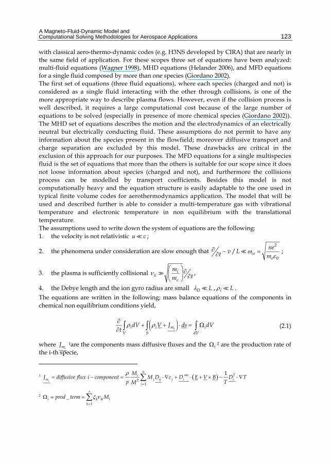
The equations are written in the following; mass balance equations of the components in chemical non equilibrium conditions yield,

ii i m iV S dV

dV V J ds dVt

(2.1)

where imJ 1are the components mass diffusive fluxes and the i 2 are the production rate of

the i-th specie,

1

21

1

i

nme Ti

m j ij j i ij

MJ diffusive flux i component M D c D E V B D T

p TM

2 1

_r

i k ik ik

prod term M

Fluid Dynamics, Computational Modeling and Applications

124

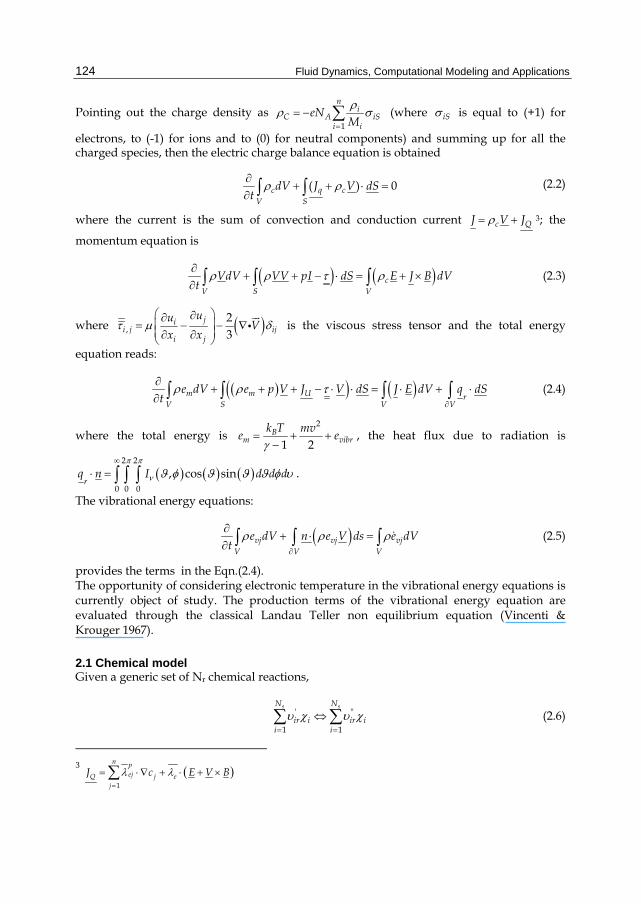
Pointing out the charge density as 1

ni

C A iSii

eNM

(where iS is equal to (+1) for

electrons, to (-1) for ions and to (0) for neutral components) and summing up for all the charged species, then the electric charge balance equation is obtained

( ) 0c q cV S

dV J V dSt

(2.2)

where the current is the sum of convection and conduction current c QJ V J 3; the

momentum equation is

cV S V

VdV VV pI dS E J B dVt

(2.3)

where ,23

jii j ij

i j

uuV

x x

is the viscous stress tensor and the total energy

equation reads:

m m U rV S V V

e dV e p V J V dS J E dV q dSt

(2.4)

where the total energy is 2

1 2B

m vibrk T mv

e e

, the heat flux due to radiation is

2 2

0 0 0

, cos sinr

q n I d d d

.

The vibrational energy equations:

vj vj vjV V V

e dV n e V ds e dVt

(2.5)

provides the terms in the Eqn.(2.4). The opportunity of considering electronic temperature in the vibrational energy equations is currently object of study. The production terms of the vibrational energy equation are evaluated through the classical Landau Teller non equilibrium equation (Vincenti & Krouger 1967).

2.1 Chemical model Given a generic set of Nr chemical reactions,

' ''

1 1

s sN N

ir i ir ii i

(2.6)

3

1

n pejQ j e

j

J c E V B

A Magneto-Fluid-Dynamic Model and Computational Solving Methodologies for Aerospace Applications

125

where ’ir and ’’ir are the stoichiometric coefficients for the r-th reaction and i are the chemical species involved in the reactions, the production rate Ωi of species i can be written as

' '''' '

1 1 1

( )s sr

ir ir

N NN

i i ir ir fr brr i i

M k q k q

1,..., 1si N (2.7)

where kfr and kbr are the forward and backward rate constants of the reaction r, which are assumed to follow the Arrhenius temperature law:

fr

fr

E

RTfr frk A T e

(2.8)

br

br

ERT

br brk A T e

(2.9)

where the pre-exponential factors Ai, the temperature exponents r , and the activation energies Ei depend upon the adopted kinetic scheme. The backward rate constants are related to the forward rate constants through the equilibrium constants Keq,r, i.e.:

r

freq

br

kK

k (2.10)

In some cases the equilibrium coefficients can be given as a function of the temperature, and the backward reaction rate can be calculated directly from the Eqn. (2.9). For argon the reaction coefficients that have been considered in order to account for ionization are:

n. Reaction A [mol-cm-s-K] β Ea [J/mol] 1 AR AR+ + e- 1.52e18 0.50 1520000 2 AR + e AR+ + 2e- 2.50e34 -3.8 1510793

where the reaction rate coefficients of the first reaction have been derived from:

2 212

12

8a aE EBT T

Ak T

k A T e Pd N em

this formula is consequent from the expression of binary collision rate where m12 is the reduced mass, d12 is the mean diameter, kB is the Boltzmann constant and P is the steric factor. The second reaction rate coefficient has been taken from (Gokcet 2004). For air ionization one of the most important reactions governing the distribution of free electrons present in high temperature air plasmas is (Dunn & Lordi 1969):

N O NO e

In this work, in order to model air ionization several 7-species models and 11 species models have been used (Gupta et al. 1989, Park 1993, Kang et al.1973) and compared also with a

Fluid Dynamics, Computational Modeling and Applications

126

model generated using (Park 1993) and (Kang et al.1973) derived in order to better fit experimental data w.r.t. the original 11 species models. The scheme adopted is reported hereinafter specifying for each reaction the respective source.

n. Reaction A [mol-cm-s-K] Β Ea [J/mol] Ref

1 O2 2 O 1.0e22 -1.5 494706.8 P

2 N2 2 N 3.0e22 -1.6 941190.08 P

3 NO N + O 1.1e17 0.0 627737.2 P

4 NO + O N + O2 8.4e12 0.0 161715.08 P

5 N2 + O N + NO 6.4e17 1.0 319257.96 P

6 N + O NO+ + e- 1.6e06 1.5 265892.8 K

7 N + O NO+ + e- 6.7e21 -1.5 0 K

8 O + O O2+ + e- 1.6e17 -0.98 671803.52 K

9 O2+ + e- O + O 8.0e21 -1.5 0 K

10 N + N N2+ + e- 1.4e13 0 671803.52 K

11 N2+ + e- N + N 8.0e21 -1.5 0 K

10 O2 + N2 NO + NO+ + e- 1.38e20 -1.84 1172330.4 K

12 NO + NO+ + e- O2 + N2 8.0e21 -2.5 0 K

13 NO + N2 NO+ + N2 + e- 2.2e15 -0.35 897955.2 K

14 NO+ + N2 + e- NO + N2 2.2e26 -2.5 0.0 K

15 NO + O2 NO+ + O2 + e- 8.8e15 -0.35 897955.2 K

16 NO+ + O2 + e- NO + O2 8.8e26 -2.5 0 K

17 O + e- O+ + e-+ e- 3.9e33 -3.78 1317832.4 P

18 N + e- N+ + e-+ e- 8.8e26 -3.82 1401807.84 P

19 O + O2+ O+ + O2 2.92e18 -1.11 232803.2 P

20 O+ + O2 O + O2+ 7.80e11 0.5 0.0 P

21 N2 + N+ N + N2+ 2.02e18 0.81 108087.2 P

22 N + N2+ N2 + N+ 7.80e11 0.5 0.0 P

23 O + NO+ NO + O+ 3.63e15 -0.6 422371.52 P

24 NO + O+ O + NO+ 1.50e13 0.0 0.0 P

25 N + NO+ NO + N+ 1.00e19 -0.93 507178.4 P

26 NO + N+ N + NO+ 7.80e11 0.0 0.0 P

27 O2 + NO+ NO + O2+ 1.80e15 -0.6 274375.2 P

28 NO + O2+ O2 + NO+ 1.50e13 0.0 0.0 P

29 O + NO+ N++ O2 1.34e13 0.31 642453.69 P

30 N++ O2 O + NO+ 1.00e14 0.0 0.0 P

Table 1. Kinetic scheme obtained using (Park 1993) and (Kang et al.1973)

A Magneto-Fluid-Dynamic Model and Computational Solving Methodologies for Aerospace Applications

127

2.2 Thermodynamic model By definition a thermally perfect gas is characterized by specific heats that depend only on temperature. Hence, for a mixture of thermally perfect gases:

pdh c T dT (2.11)

p RT (2.12)

where R and cp are, respectively, the gas constant and the specific heat at constant pressure of the mixture. They are obtained as weighted average of the gas constants and specific heats of the single species i-th:

i ii

R Y R p i pii

c T Y c T (2.13)

The single species specific heats and enthalpies are computed by using the (Gordon and McBride 1971) polynomial fits:

2 3 41 2 3 4 5

pca a T a T a T a T

R (2.14)

2 3 43 5 62 41 2 3 4 5

a a ah a aa T T T T

RT T (2.15)

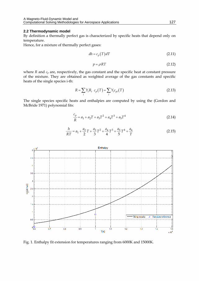
Fig. 1. Enthalpy fit extension for temperatures ranging from 6000K and 15000K.

Fluid Dynamics, Computational Modeling and Applications

128

These fits are written for gases with the maximum temperature of 6000K, so it has been necessary to extend the enthalpy fits to values of temperature typical of ionization problem (up to 15000K). Here is briefly reported the fitting procedure for argon: from literature (Drellishak et al. 1963) thermodynamic properties are derived for high temperatures then the coefficients are found using a least squares fitting procedure. The results for Argon enthalpy are shown in Fig. 1. Thermodynamic properties for high temperature air, used to find fit coefficients, have been found in (Hans & Heims 1968).

2.3 Transport model Another critical point in the simulation of high enthalpy flows is the determination of the transport coefficients. In fact, the widely used Sutherland law is suitable only at low temperatures, while more complex models must be used when temperature exceeds 1000 K. An interesting way to compute transport coefficients is based on the calculation of the collision integral starting from intermolecular potentials knowledge (Hirshfield et al. 1954) and it leads to the following expressions for the diffusivities between the i-th and the j-th species and also for conductivity and viscosity with different sets of constants given in Gupta et al. 1958, Hans & Heims 1968. In this way computational efficiency is maximized since transport coefficients are computed only once at the start of each calculation.

1

1, lnln

nN

nijnij TdD

1

1, lnln

n

N

nini Tb

1

1, lnln

n

N

nini Ta

.

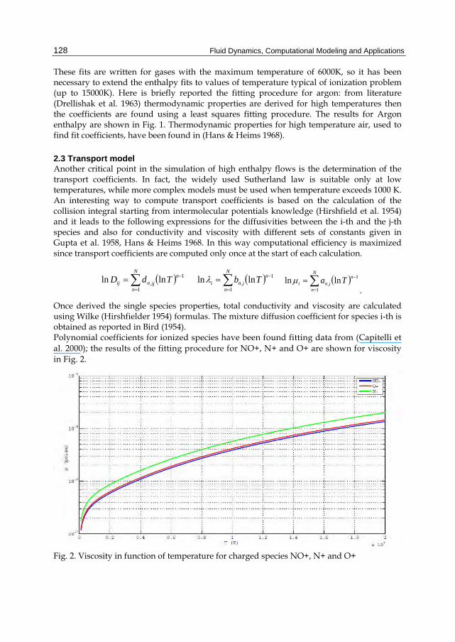
Once derived the single species properties, total conductivity and viscosity are calculated using Wilke (Hirshfielder 1954) formulas. The mixture diffusion coefficient for species i-th is obtained as reported in Bird (1954). Polynomial coefficients for ionized species have been found fitting data from (Capitelli et al. 2000); the results of the fitting procedure for NO+, N+ and O+ are shown for viscosity in Fig. 2.

Fig. 2. Viscosity in function of temperature for charged species NO+, N+ and O+

A Magneto-Fluid-Dynamic Model and Computational Solving Methodologies for Aerospace Applications

129

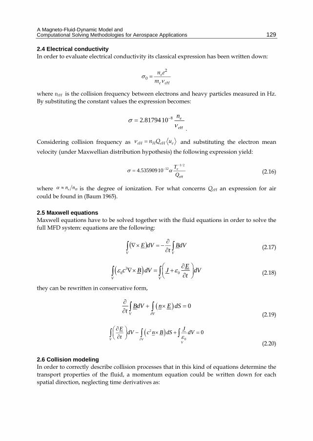
2.4 Electrical conductivity In order to evaluate electrical conductivity its classical expression has been written down:

2

0e

e eH

n em

where υeH is the collision frequency between electrons and heavy particles measured in Hz. By substituting the constant values the expression becomes:

eH

en

81081794.2

.

Considering collision frequency as eH H eH en Q u and substituting the electron mean

velocity (under Maxwellian distribution hypothesis) the following expression yield:

eH

e

Q

T 2/112104.535909

(2.16)

where He nn is the degree of ionization. For what concerns QeH an expression for air could be found in (Baum 1965).

2.5 Maxwell equations Maxwell equations have to be solved together with the fluid equations in order to solve the full MFD system: equations are the following:

VV

dVBt

dVE

(2.17)

2

0 0V V

Ec B dV J dV

t

(2.18)

they can be rewritten in conservative form,

0

V V

BdV n E dSt

(2.19)

2

0

0V V

V

E JdV c n B dS dV

t

(2.20)

2.6 Collision modeling In order to correctly describe collision processes that in this kind of equations determine the transport properties of the fluid, a momentum equation could be written down for each spatial direction, neglecting time derivatives as:

Fluid Dynamics, Computational Modeling and Applications

130

( )

( )

( )

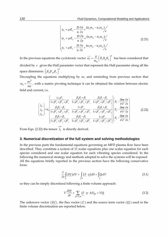
y cz z cyx x

z cx x czy y

x cy y cxz z

u uD nu E

n xD n u uu En y

u uD nu E

n z

(2.21)

In the previous equations the cyclotronic vector T

c x y zie

qB B B

m

has been considered that

divided by gives the Hall parameter vector that represent the Hall parameter along all the

space dimension: T

x y z .

Decoupling the equations multiplying by ne, and reminding from previous section that 2

0nem

, with a matrix pivoting technique it can be obtained the relation between electric

field and current, i.e.

2

2 2 2 2 2 2 2 2 2

2

0 2 2 2 2 2 2 2 2 2

2

2 2 2 2 2 2 2 2 2

11 1 1

11 1 1

11 1 1

y x z x z yx

z y x z y x z y x

qxy x z y y z x

qyz y x z y x z y x

qz

z x y z y x z

z y x z y x z y x

j

j

j

2 2

2 2

2 2

x

y

z

Dm nE

n e xDm n

En e y

Dm nE

n e z

(2.22)

From Eqn. (2.22) the tensor e is directly derived.

3. Numerical discretization of the full system and solving methodologies

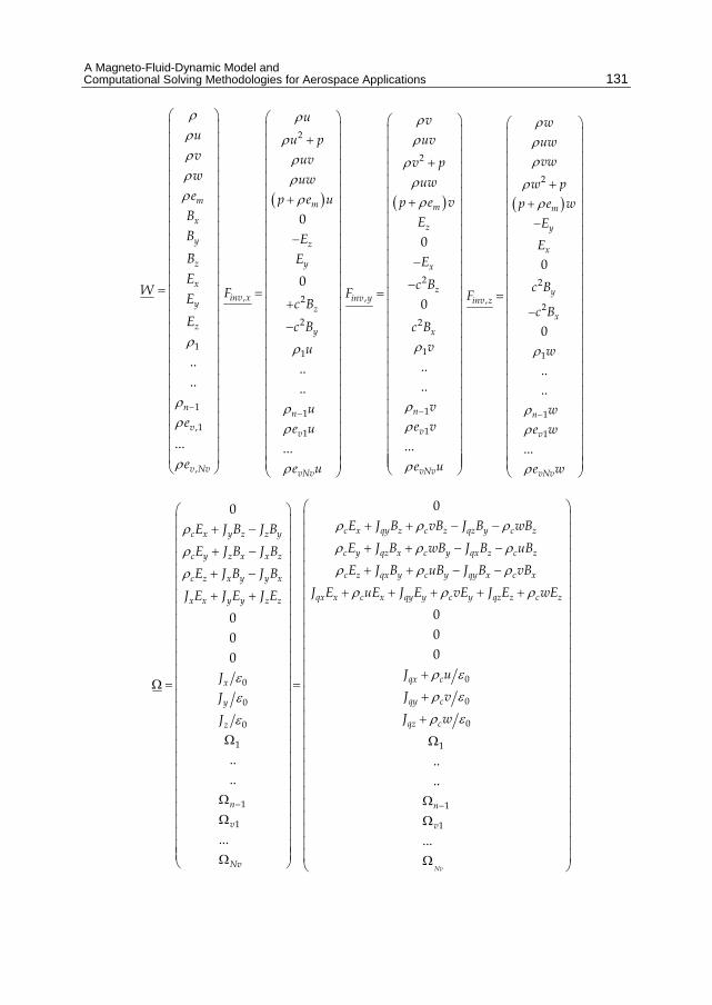
In the previous parts the fundamental equations governing an MFD plasma flow have been described. They constitute a system of 11 scalar equations plus one scalar equation for each species considered and one scalar equation for each vibrating species considered. In the following the numerical strategy and methods adopted to solve the systems will be exposed All the equations briefly reported in the previous section have the following conservative form:

V V V

W dV F n dS dVt

(3.1)

so they can be simply discretized following a finite volume approach:

1,6

( )dW

V F n S Vdt

(3.2)

The unknown vector W , the flux vector ( F ) and the source term vector ( ) used in the finite volume discretization are reported below.

A Magneto-Fluid-Dynamic Model and Computational Solving Methodologies for Aerospace Applications

131

1

1

,1

,

..

..

...

m

x

y

z

x

y

z

n

v

v Nv

uvwe

BB

BE

WE

E

e

e

2

, 2

2

1

1

1

0

0

..

..

...

m

z

y

inv xz

y

n

v

vNv

u

u puvuw

p e u

EE

Fc B

c B

u

ue u

e u

2

2

,

2

1

1

1

0

0

..

..

...

m

z

x

zinv y

x

n

v

vNv

vuv

v puw

p e vE

E

c BF

c Bv

ve v

e u

2

2

,2

1

1

1

0

0

..

..

...

m

y

x

yinv z

x

n

v

vNv

wuwvw

w pp e w

E

E

c BF

c B

w

we w

e w

0

0

0

1

1

1

00

000

..

..

...

c x qy z c z qz y c zc x y z z y

c y qz x c yc y z x x z

c z x y y x

x x y y z z

x

y

z

n

v

Nv

E J B vB J B wBE J B J BE J B wBE J B J B

E J B J B

J E J E J E

JJ

J

0

0

0

1

1

1

000

..

..

...

Nv

qx z c z

c z qx y c y qy x c x

qx x c x qy y c y qz z c z

qx c

qy c

qz c

n

v

J B uB

E J B uB J B vB

J E uE J E vE J E wE

J u

J v

J w

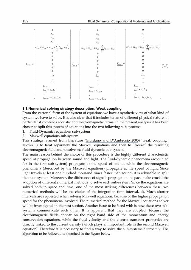
Fluid Dynamics, Computational Modeling and Applications

132

, ,1

,

,1

, 1

,1 1 ,1

, , ,

0

000000

..

..

...

v v v

xx

xy

xzn

xx xy xz Ux i r xi

visc x

x

x n

vx v x

vx N v N x N

u v w J q

F

J

J

q e J

q e J

, ,1

,

,1

, 1

,1 1 ,1

, , ,

0

000000

..

..

...

v v v

xy

yy

yz

n

xy yy yz U y i r yi

visc y

y

y n

vy v y

vy N v N y N

u v w J q

F

J

J

q e J

q e J

, ,1

,

,1

, 1

,1 1 ,1

, , ,

0

000000

..

..

...

v v v

xz

yz

zzn

zx zy zz U z i r zi

visc z

z

z n

vz v z

vz N v N z N

u v w J q

F

J

J

q e J

q e J

(3.3)

3.1 Numerical solving strategy description: Weak coupling From the vectorial form of the system of equations we have a synthetic view of what kind of system we have to solve. It is also clear that it includes terms of different physical nature, in particular it combines acoustic and electromagnetic terms. In the present analysis it has been chosen to split this system of equations into the two following sub-systems: 1. Fluid-Dynamics equations sub-system 2. Maxwell equations sub-system This strategy, named from literature (Giordano and D’Ambrosio 2005) ‘weak coupling’, allows us to treat separately the Maxwell equations and then to ”freeze” the resulting electromagnetic field and to solve the fluid-dynamic sub-system. The main reason behind the choice of this procedure is the highly different characteristic speed of propagation between sound and light. The fluid-dynamic phenomena (accounted for in the first sub-system) propagate at the speed of sound, while the electromagnetic phenomena (described by the Maxwell equations) propagate at the speed of light. Since light travels at least one hundred thousand times faster than sound, it is advisable to split the main system. Moreover, the differences of signals propagation in space make crucial the adoption of different numerical methods to solve each sub-system. Since the equations are solved both in space and time, one of the most striking differences between these two numerical methods will be the choice of the integration time interval, dt. Much shorter intervals are requested when solving Maxwell equations, because of the higher propagation speed for the phenomena involved. The numerical method for the Maxwell equations solver will be investigated in the next section. Another issue to be faced with is how these two sub-systems communicate each other. It is apparent that they are coupled, because the electromagnetic fields appear on the right hand side of the momentum and energy conservation equations, while the fluid velocity and the electric transport properties are directly linked to the current density (which plays an important role in the second Maxwell equation). Therefore it is necessary to find a way to solve the sub-systems alternately. The algorithm to be followed is sketched in the figure below:

A Magneto-Fluid-Dynamic Model and Computational Solving Methodologies for Aerospace Applications

133

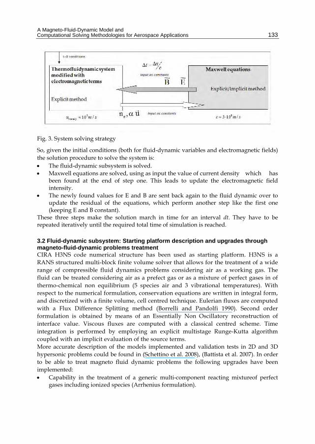
Fig. 3. System solving strategy

So, given the initial conditions (both for fluid-dynamic variables and electromagnetic fields) the solution procedure to solve the system is: The fluid-dynamic subsystem is solved. Maxwell equations are solved, using as input the value of current density which has

been found at the end of step one. This leads to update the electromagnetic field intensity.

The newly found values for E and B are sent back again to the fluid dynamic over to update the residual of the equations, which perform another step like the first one (keeping E and B constant).

These three steps make the solution march in time for an interval dt. They have to be repeated iteratively until the required total time of simulation is reached.

3.2 Fluid-dynamic subsystem: Starting platform description and upgrades through magneto-fluid-dynamic problems treatment CIRA H3NS code numerical structure has been used as starting platform. H3NS is a RANS structured multi-block finite volume solver that allows for the treatment of a wide range of compressible fluid dynamics problems considering air as a working gas. The fluid can be treated considering air as a prefect gas or as a mixture of perfect gases in of thermo-chemical non equilibrium (5 species air and 3 vibrational temperatures). With respect to the numerical formulation, conservation equations are written in integral form, and discretized with a finite volume, cell centred technique. Eulerian fluxes are computed with a Flux Difference Splitting method (Borrelli and Pandolfi 1990). Second order formulation is obtained by means of an Essentially Non Oscillatory reconstruction of interface value. Viscous fluxes are computed with a classical centred scheme. Time integration is performed by employing an explicit multistage Runge-Kutta algorithm coupled with an implicit evaluation of the source terms. More accurate description of the models implemented and validation tests in 2D and 3D hypersonic problems could be found in (Schettino et al. 2008), (Battista et al. 2007). In order to be able to treat magneto fluid dynamic problems the following upgrades have been implemented: Capability in the treatment of a generic multi-component reacting mixtureof perfect

gases including ionized species (Arrhenius formulation).

Fluid Dynamics, Computational Modeling and Applications

134

Electromagnetic terms added at the equations implemented Thermodynamic properties formulation in terms of Gordon-Mc Bride Polynomial fits.

(Gordon and McBride 1971) Extension of thermodynamic properties (specific heat, enthalpy and entropy) to higher

temperatures. Included ionized species transport properties. Effects of electromagnetic field on transport accounted. Models considered for these upgrades have been widely discussed in previous Sections.

3.3 Numerical methodologies for Maxwell equations : Implicit and explicit Maxwell equation solver design In this section the numerical methods used to solve Maxwell equations are discussed. So far, two methods have been employed, one of them is implicit, the other one explicit. Each method has its own strengths and its drawbacks. In the two paragraphs below, they are explained and compared. The equations to be discretized are the Maxwell equations in conservative form ((2.19), (2.20)), i.e.:

M M M

V V V

W dV F dS dVt

(3.4)

With:

x

y

zM

x

y

z

BB

BW

EE

E

2

2

0

0

z

yMx

z

y

EE

F

c B

c B

2

2

0

0

z

xMy

z

x

E

EF

c B

c B

2

2

0

0

y

x

Mz

y

x

E

E

Fc B

c B

0

0

0

000

M

qx c

qy c

qz c

J u

J v

J w

(3.5)

The superscript “M” reminds that this method is being applied to the Maxwell equations.

3.3.1 Implicit methodology The great strength of all implicit numerical schemes is their great stability. Using an implicit method it is possible to choose a larger integration time interval without compromising the stability of the method itself. This is most relevant when dealing with signals which travel so fast as the electromagnetic waves. Explicit schemes make time advancement very simple, but often suffer severe restrictions on time step due to the loss of stability. On the other side, implicit schemes generally have much better numerical properties in term of stability and so allow a larger time step, but require the solution of a system of equations to perform time integration. When analyzing a 3D problem as in the present case, the matrix associated to the system is too large to be inverted in a reasonable computational time. This means that an iterative method has to be applied to solve the system. So, the time saved using a larger time step is actually lost in solving a large linear system of equations at each iteration. To introduce the implicit method, a 1D simple case is described. Then, the result obtained will be extended to the 3D

A Magneto-Fluid-Dynamic Model and Computational Solving Methodologies for Aerospace Applications

135

case. Discretizing equation (3.1), and looking to it is possible to write in a finite volume fashion:

11 1 2( ) ( )

M K K KM M MNIN OUT NN N

WA x F F A A x

t

(3.6)

Here the subscript “N” addresses the cell we are referring to, while the superscript “K” indicates the time interval considered.

MINF and M

OUTF can be written as:

112

M M MIN N NF F F 1

12

M M MOUT N NF F F

Considering again equation (3.6), expanding to the first order all the terms with superscript different than “K” (i.e. the terms that are not evaluated at the instant “k”) and dividing both sides by the surface area A, yields:

1 11 1 1 1

1 1

1 1 12 2 2

12

N N NN N N N

N N

NN N

N

W F Fx F F W W

t W W

x W xW

(3.7)

Here the superscript “k” has been dropped, since it is clear that each term in the above equation (3.7) is evaluated at the time “k”. For a 3D analysis this procedure leads to the following equation (assuming to work on a “x,y,z” Cartesian grid, with cubic cells):

1 11 1

1 1

1 1

[C] [R] [L]

1 11

2 2 2

[R] [LLL] [RRR]

1 1 12 2 2

x yx x

x x

x xN N N

N N NN N N

zy yN n nN n N n

N NN n N n

F Ft t tW W W

W W x W x

FF Ft tW W

W y W y

1

1 1 1

[LLL]

1 12 2

1 12 2

x y

x y

x y

x x x y x y

NN n n

zN n n x x

N N NN n n

y y z zN n N n N n n N n n N

tW

W z

F t tW F F

W z x

t tF F F F t

y z

(3.8)

: is used to indicate a spatial interval : is used to indicate a time interval

, x yn n : are the numbers of cells along x and y apxis respectively

Fluid Dynamics, Computational Modeling and Applications

136

[C], [L], [R], etc… are 6x6 square matrixes (remind that F and W are six-elements vectors). This equation is just a system of totn scalar equations, where totn ( x y zn n n ) is the total number of grid cells. It can be written in the following more compact form:

1 1 1[ ]

2 2 2yx zt t t

D W F F F tx y z

(3.9)

Where:

This system has to be solved at each time step. The unknowns are the temporal increments W , whose knowledge is necessary to update the vector W (containing the intensities of

the electromagnetic fields) all through the spatial domain of integration. [D] is a seven diagonal block matrix. Given the considerable dimensions of the matrix [D] its inversion is very expensive in terms of computational time. Therefore, an iterative method is required to solve the system, i.e. it is strongly necessary to use a proper pre-conditioner to achieve a faster convergence to the solution.

3.3.2 Explicit methodology An explicit method allows to directly find the unknown values for electromagnetic field at each time step, with no need of solving a large system of equations. The explicit method employed is “centred in space” and “forward in time”. As a consequence, the equation (3.1) can be discretized as follows:

M K K KM M MN

IN OUT NN N

WV F F A V

t

(3.10)

Each term is evaluated at instant “k”. Rearranging the previous equation for the simple case of cubic cells:

1 1

1

2 x z x zx x

y yx x z zN N N x y N n n N n n zN n N n

N

tW F F A F F A F F A

V

t

(3.11)

[ ] [ ] 0 0 ... [ ] 0 0 0 ... [ ] 0[ ] [ ] [ ] 0 ... 0 [ ] 0 0 ... 0 [ ]0 0 [ ] 0 ... 0 0 [ ] 0 ... 0 00 0 0 [ ] ... 0 0 0 [ ] ... 0 0... 0 0 ... ... ... ... ... ... ... ... 0

[ ] 0 0 0 0 [ ] 0 0 0 ... [ ] 0[ ]

0 [ ] 0 0 0 0 [ ] 0 0 ... 0 [ ]0 0 [ ] 0 0 0 0 [ ] 0 ... 0 0... ..

C R RR RRR

L C R RR RRR

C RR

C RR

LL C RRD

LL C RR

LL C

00

[ ]0000

[ ]. ... ... ... ... ... ... ... ... ... ... ...

[ ] 0 0 0 [ ] 0 0 0 0 0 [ ] 0 00 [ ] 0 0 0 [ ] 0 0 0 0 0 [ ] [ ]0 0 [ ] 0 0 0 [ ] 0 0 0 0 [ ] [ ]

RRR

RR

LLL LL C

LLL LL C R

LLL LL L C

(nxny)

(nxnynz)

(nxnynz)

(nxny)

A Magneto-Fluid-Dynamic Model and Computational Solving Methodologies for Aerospace Applications

137

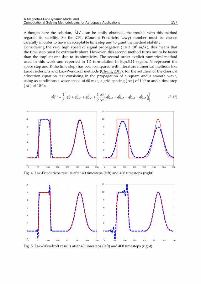
Although here the solution, W , can be easily obtained, the trouble with this method regards its stability. So the CFL (Courant–Friedrichs–Lewy) number must be chosen carefully in order to have an acceptable time step and to grant the method stability. Considering the very high speed of signal propagation ( 83 10 m/sc ), this means that the time step must be extremely short. However, this second method turns out to be faster than the implicit one due to its simplicity. The second order explicit numerical method used in this work and reported in 1D formulation in Eqn.3.11 (again, N represent the space step and K the time step) has been compared with literature numerical methods like Lax-Friederichs and Lax-Wendroff methods (Chung 2010), for the solution of the classical advection equation test consisting in the propagation of a square and a smooth wave, using as conditions a wave speed of 60 m/s, a grid spacing ( x ) of 10-3 m and a time step ( t ) of 10-5 s.

11 1 1 2 1 2

1 13 2

K K K K K K K KN N N N N N N N

tq q q q q q q q

x

(3.12)

0 50 100 150 200 250 300 350-2

0

2

4

6

8

10

12

0 50 100 150 200 250 300 350-2

0

2

4

6

8

10

12

Fig. 4. Lax-Friederichs results after 40 timesteps (left) and 400 timesteps (right)

0 50 100 150 200 250 300 350-2

0

2

4

6

8

10

12

0 50 100 150 200 250 300 350-2

0

2

4

6

8

10

12

Fig. 5. Lax--Wendroff results after 40 timesteps (left) and 400 timesteps (right)

Fluid Dynamics, Computational Modeling and Applications

138

0 50 100 150 200 250 300 350-2

0

2

4

6

8

10

12

0 50 100 150 200 250 300 350-2

0

2

4

6

8

10

12

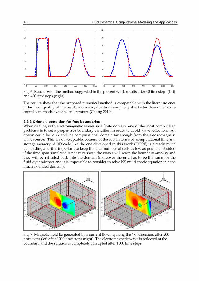
Fig. 6. Results with the method suggested in the present work results after 40 timesteps (left) and 400 timesteps (right)

The results show that the proposed numerical method is comparable with the literature ones in terms of quality of the result; moreover, due to its simplicity it is faster than other more complex methods available in literature (Chung 2010).

3.3.3 Orlanski condition for free boundaries When dealing with electromagnetic waves in a finite domain, one of the most complicated problems is to set a proper free boundary condition in order to avoid wave reflections. An option could be to extend the computational domain far enough from the electromagnetic wave sources. This is not acceptable, because of the cost in terms of computational time and storage memory. A 3D code like the one developed in this work (HOPE) is already much demanding and it is important to keep the total number of cells as low as possible. Besides, if the time span simulated is not very short, the waves will reach the boundary anyway and they will be reflected back into the domain (moreover the grid has to be the same for the fluid dynamic part and it is impossible to consider to solve NS multi specie equation in a too much extended domain).

Fig. 7. Magnetic field Bz generated by a current flowing along the “x” direction, after 200 time steps (left after 1000 time steps (right). The electromagnetic wave is reflected at the boundary and the solution is completely corrupted after 1000 time steps.

A Magneto-Fluid-Dynamic Model and Computational Solving Methodologies for Aerospace Applications

139

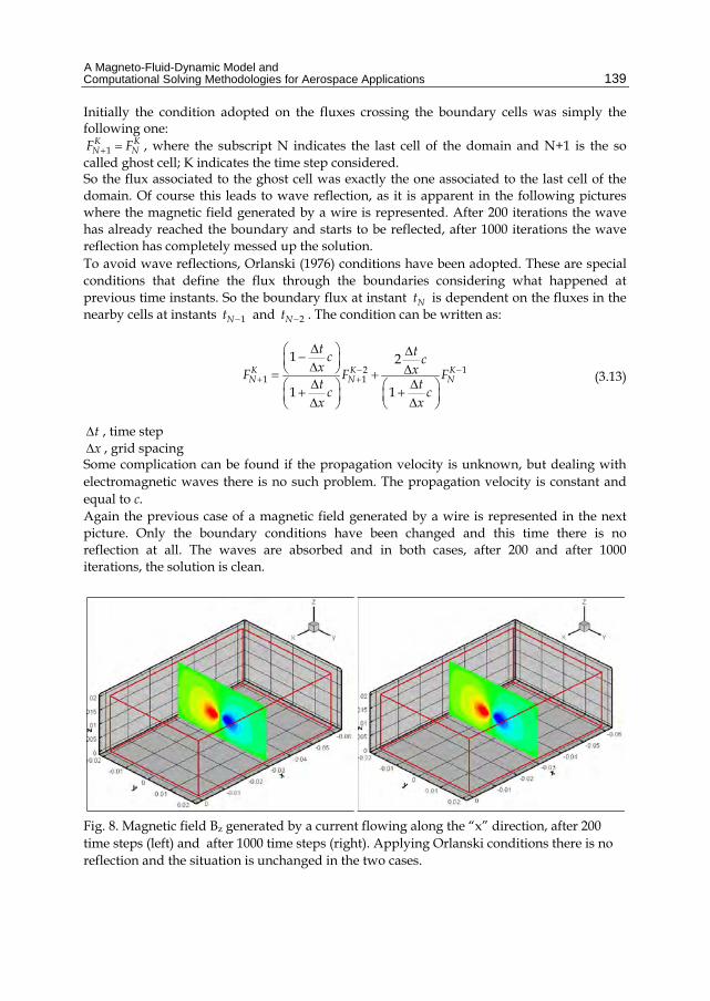
Initially the condition adopted on the fluxes crossing the boundary cells was simply the following one:

1K KN NF F , where the subscript N indicates the last cell of the domain and N+1 is the so

called ghost cell; K indicates the time step considered. So the flux associated to the ghost cell was exactly the one associated to the last cell of the domain. Of course this leads to wave reflection, as it is apparent in the following pictures where the magnetic field generated by a wire is represented. After 200 iterations the wave has already reached the boundary and starts to be reflected, after 1000 iterations the wave reflection has completely messed up the solution. To avoid wave reflections, Orlanski (1976) conditions have been adopted. These are special conditions that define the flux through the boundaries considering what happened at previous time instants. So the boundary flux at instant Nt is dependent on the fluxes in the nearby cells at instants 1Nt and 2Nt . The condition can be written as:

2 11 1

1 2

1 1

K K KN N N

t tc cx xF F Ft t

c cx x

(3.13)

t , time step x , grid spacing

Some complication can be found if the propagation velocity is unknown, but dealing with electromagnetic waves there is no such problem. The propagation velocity is constant and equal to c. Again the previous case of a magnetic field generated by a wire is represented in the next picture. Only the boundary conditions have been changed and this time there is no reflection at all. The waves are absorbed and in both cases, after 200 and after 1000 iterations, the solution is clean.

Fig. 8. Magnetic field Bz generated by a current flowing along the “x” direction, after 200 time steps (left) and after 1000 time steps (right). Applying Orlanski conditions there is no reflection and the situation is unchanged in the two cases.

Fluid Dynamics, Computational Modeling and Applications

140

4. Models validation numerical tests

A simple validation test for different models was presented in Battista et al. (2008, 2009). Hereinafter three main validation tests will be presented.

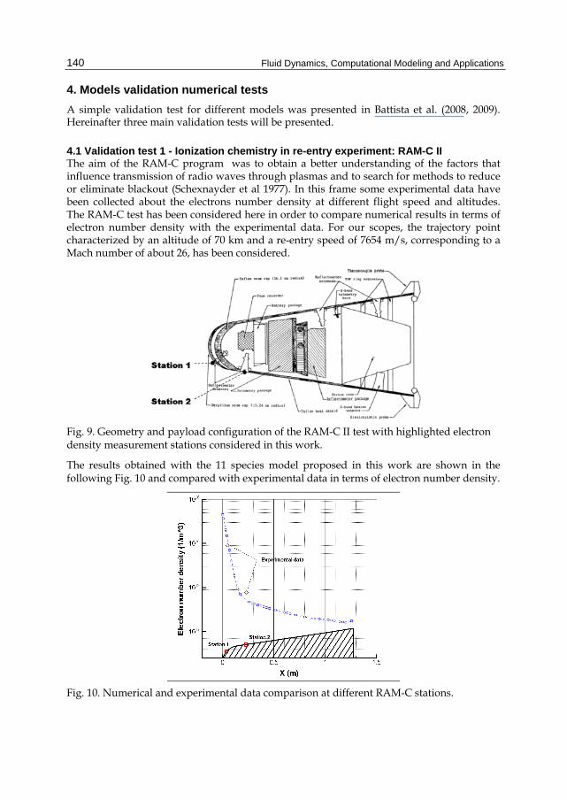
4.1 Validation test 1 - Ionization chemistry in re-entry experiment: RAM-C II The aim of the RAM-C program was to obtain a better understanding of the factors that influence transmission of radio waves through plasmas and to search for methods to reduce or eliminate blackout (Schexnayder et al 1977). In this frame some experimental data have been collected about the electrons number density at different flight speed and altitudes. The RAM-C test has been considered here in order to compare numerical results in terms of electron number density with the experimental data. For our scopes, the trajectory point characterized by an altitude of 70 km and a re-entry speed of 7654 m/s, corresponding to a Mach number of about 26, has been considered.

Fig. 9. Geometry and payload configuration of the RAM-C II test with highlighted electron density measurement stations considered in this work.

The results obtained with the 11 species model proposed in this work are shown in the following Fig. 10 and compared with experimental data in terms of electron number density.

Fig. 10. Numerical and experimental data comparison at different RAM-C stations.

A Magneto-Fluid-Dynamic Model and Computational Solving Methodologies for Aerospace Applications

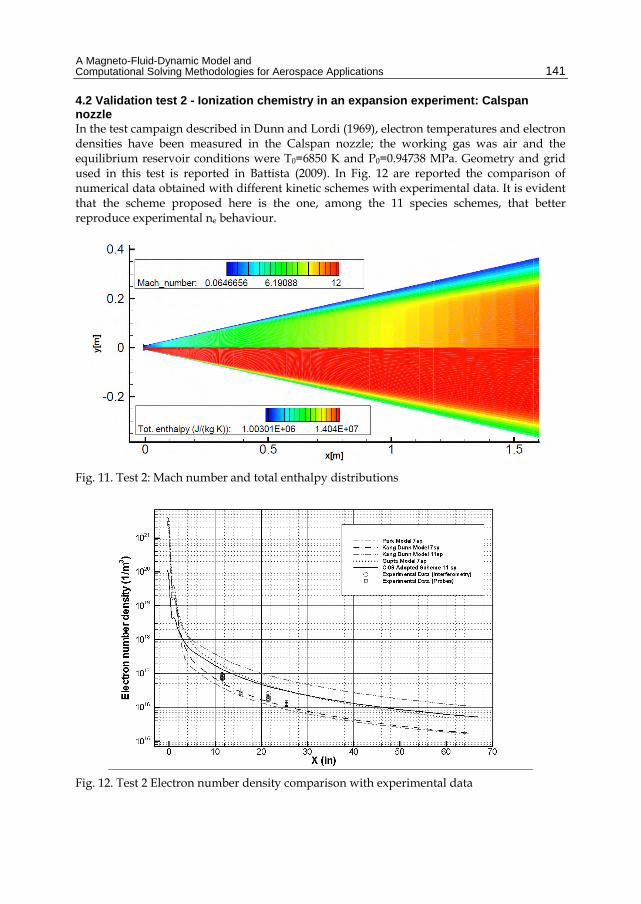
141

4.2 Validation test 2 - Ionization chemistry in an expansion experiment: Calspan nozzle In the test campaign described in Dunn and Lordi (1969), electron temperatures and electron densities have been measured in the Calspan nozzle; the working gas was air and the equilibrium reservoir conditions were T0=6850 K and P0=0.94738 MPa. Geometry and grid used in this test is reported in Battista (2009). In Fig. 12 are reported the comparison of numerical data obtained with different kinetic schemes with experimental data. It is evident that the scheme proposed here is the one, among the 11 species schemes, that better reproduce experimental ne behaviour.

Fig. 11. Test 2: Mach number and total enthalpy distributions

Fig. 12. Test 2 Electron number density comparison with experimental data

Fluid Dynamics, Computational Modeling and Applications

142

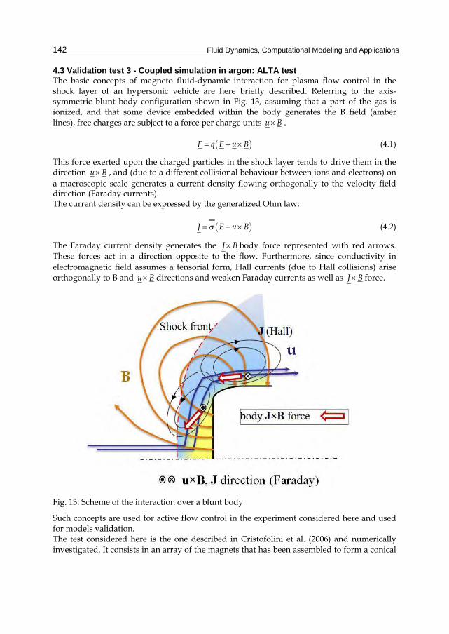
4.3 Validation test 3 - Coupled simulation in argon: ALTA test The basic concepts of magneto fluid-dynamic interaction for plasma flow control in the shock layer of an hypersonic vehicle are here briefly described. Referring to the axis-symmetric blunt body configuration shown in Fig. 13, assuming that a part of the gas is ionized, and that some device embedded within the body generates the B field (amber lines), free charges are subject to a force per charge units u B .

F q E u B (4.1)

This force exerted upon the charged particles in the shock layer tends to drive them in the direction u B , and (due to a different collisional behaviour between ions and electrons) on a macroscopic scale generates a current density flowing orthogonally to the velocity field direction (Faraday currents). The current density can be expressed by the generalized Ohm law:

J E u B (4.2)

The Faraday current density generates the J B body force represented with red arrows. These forces act in a direction opposite to the flow. Furthermore, since conductivity in electromagnetic field assumes a tensorial form, Hall currents (due to Hall collisions) arise orthogonally to B and u B directions and weaken Faraday currents as well as J B force.

Fig. 13. Scheme of the interaction over a blunt body

Such concepts are used for active flow control in the experiment considered here and used for models validation. The test considered here is the one described in Cristofolini et al. (2006) and numerically investigated. It consists in an array of the magnets that has been assembled to form a conical

A Magneto-Fluid-Dynamic Model and Computational Solving Methodologies for Aerospace Applications

143

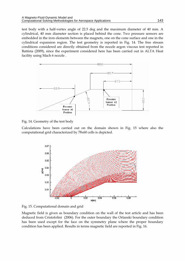
test body with a half-vertex angle of 22.5 deg and the maximum diameter of 40 mm. A cylindrical, 40 mm diameter section is placed behind the cone. Two pressure sensors are embedded in the iron elements between the magnets, one on the cone surface and one in the cylindrical expansion region. The test geometry is reported in Fig. 14. The free stream conditions considered are directly obtained from the nozzle argon viscous test reported in Battista (2009), since the experiment considered here has been carried out in ALTA Heat facility using Mach 6 nozzle .

Fig. 14. Geometry of the test body

Calculations have been carried out on the domain shown in Fig. 15 where also the computational grid characterized by 78x60 cells is depicted.

Fig. 15. Computational domain and grid

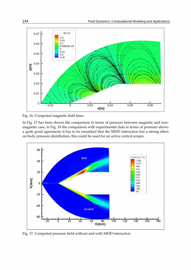
Magnetic field is given as boundary condition on the wall of the test article and has been deduced from Cristofolini (2006). For the outer boundary the Orlanski boundary condition has been used except for the face on the symmetry plane where the proper boundary condition has been applied. Results in terms magnetic field are reported in Fig. 16.

Fluid Dynamics, Computational Modeling and Applications

144

x(m)

y(m

)

-0.02 0 0.02 0.04 0.06 0.080

0.01

0.02

0.03

0.04

0.05

0.06

0.07 BX (T)

0.40.250.16.08653E-080

-0.15-0.3-0.45

Fig. 16. Computed magnetic field lines.

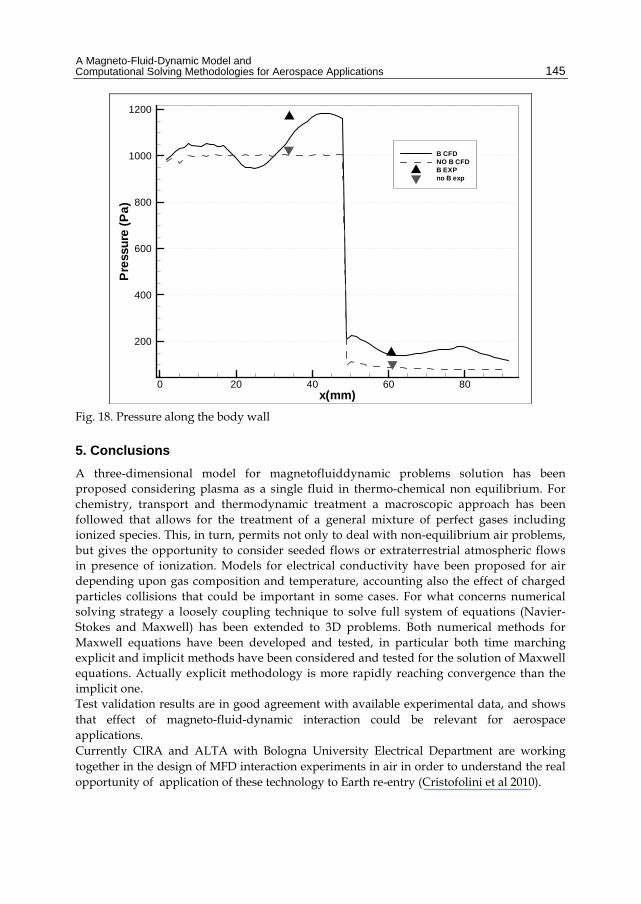
In Fig. 17 has been shown the comparison in terms of pressure between magnetic and non-magnetic case, in Fig. 18 the comparison with experimental data in terms of pressure shows a quite good agreement; it has to be remarked that the MHD interaction has a strong effect on body pressure distribution, this could be used for an active control scopes.

Fig. 17. Computed pressure field without and with MHD interaction

A Magneto-Fluid-Dynamic Model and Computational Solving Methodologies for Aerospace Applications

145

x(mm)

Pre

ssu

re(P

a)

0 20 40 60 80

200

400

600

800

1000

1200

B CFDNO B CFDB EXPno B exp

Fig. 18. Pressure along the body wall

5. Conclusions

A three-dimensional model for magnetofluiddynamic problems solution has been proposed considering plasma as a single fluid in thermo-chemical non equilibrium. For chemistry, transport and thermodynamic treatment a macroscopic approach has been followed that allows for the treatment of a general mixture of perfect gases including ionized species. This, in turn, permits not only to deal with non-equilibrium air problems, but gives the opportunity to consider seeded flows or extraterrestrial atmospheric flows in presence of ionization. Models for electrical conductivity have been proposed for air depending upon gas composition and temperature, accounting also the effect of charged particles collisions that could be important in some cases. For what concerns numerical solving strategy a loosely coupling technique to solve full system of equations (Navier-Stokes and Maxwell) has been extended to 3D problems. Both numerical methods for Maxwell equations have been developed and tested, in particular both time marching explicit and implicit methods have been considered and tested for the solution of Maxwell equations. Actually explicit methodology is more rapidly reaching convergence than the implicit one. Test validation results are in good agreement with available experimental data, and shows that effect of magneto-fluid-dynamic interaction could be relevant for aerospace applications. Currently CIRA and ALTA with Bologna University Electrical Department are working together in the design of MFD interaction experiments in air in order to understand the real opportunity of application of these technology to Earth re-entry (Cristofolini et al 2010).

Fluid Dynamics, Computational Modeling and Applications

146

6. Nomenclature

Latins B Magnetic field D Diffusion coefficients e energy, electron charge e- electron E energy E Electric field h Enthalpy per unit mass k Rate constant J Flux, Currents m mass M Mach number, Molecular Weight n Number density NA Avogadro Number P Pressure q Heat flux q generic system variable R Radius T Temperature t Time S Surface ui velocity components V Velocity V Volume x x-coordinate y y-coordinate z z-coordinate

Greeks

0 Dielectric Vacuum constant

D Debye Length

e Dielectric tensor μ Mobility Production terms ρ Density σ Conductivity Stress tensor

Collision Frequency Frequency

Subscripts a activation freestream conditions ad adiabatic wall

A Magneto-Fluid-Dynamic Model and Computational Solving Methodologies for Aerospace Applications

147

ce electron oscillation e electronic i ionic r radiative v vibrational stag stagnation point tot total w wall

7. Acronyms

BC Boundary Condition

CFD Computational Fluid Dynamics

CFL Courant - Freidricks -Lewy Number

CMFD Computational Magneto Fluid Dynamics

EMC3NS Electro Magnetic Generalized Chemistry High Enthalpy 3D Navier-Stokes solver

ENO Essentially Not Oscillatory

EU Inviscid computation

FDM Finite Difference Method

FVM Finite Volume Method

FDS Flux Difference Splitting

H3NS Hypersonic high enthalpy 3D Navier-Stokes solver.

MFD Magneto Fluid Dynamics

MHD Magneto Hydro Dynamics

NE Non equilibrium computation

NS Navier Stokes computation

PG Perfect Gas approximation computation

PIC Particle In Cell

8. References

Battista F. (2009). Magneto-Fluid-Dynamics Methods for Hypersonic Aerothermodynamics and Space Propulsion Applications, Ph.D. thesis, Pisa University, etd-11302009-122005.

Battista, F., Clemente, M. D., and Rufolo, G. C. (2007). Aerothermal Environment Definition for a Reusable Experimental Re-entry Vehicle Wing Leading edge, 46th AIAA Thermophysics Conference Miami AIAA 2007-4048.

Baum, C. E. (1965). The calculation of Conduction Electron Parameters, Tech. rep., AFWL.

Fluid Dynamics, Computational Modeling and Applications

148

Bird R.B., Stewart W.E., and Lightfoot E.N. (1954). Transport Phenomena, John Wiley and Sons, New York.

Borghi C.A., Cristofolini A., Carraro M.R., Gorse C., Colonna G., Passaro A., Paganucci F. (2006). Non intrusive Characterization of the Ionized Flow Produced by Nozzle of an Hypersonic Wind Tunnel, 14th AIAA/AHI Space Planes and Hypersonic Systems and Technologies Conference, AIAA 2006-8050.

Borrelli, S. and Pandolfi, M. (1990). An Upwind Formulation for the Numerical Prediction of Non Equilibrium Hypersonic Flows, 12th International Conference on Numerical Methods in Fluid Dynamics, Oxford, UK.

Bush, W. (1958). Magnetohydrodynamic-hypersonic flow past a blunt body, Journal of the AeroSpace Sciences, Vol. 25, pp. 685–690.

Capitelli, M., Gorse, C., Longo, S., and Giordano., D. (2000). Collision integrals of high-temperature air species, Journal of Thermophysics and Heat Transfer , Vol. 14, pp. 259–268.

Chung, T.J. (2010). Computational Fluid Dynamics , Cambridge University Press, Second edition.

Cristofolini A. et al. (2006), Experimental Investigation on the MHD Interaction around a Sharp Cone in an Ionized Argon Flow, AIAA-2006-3075, 37th AIAA Plasmadynamics and Lasers Conference, San Francisco, California.

Cristofolini A., Borghi C.A., Neretti G., Passaro A., Baccarella D., Schettino A., Battista F., (2010). Experimental Activities on the MHD Interaction in a Hypersonic Air Flow around a Blunt Body, 41st Plasmadynamics and Lasers Conference, AIAA 2010-4490.

Cristofolini, A., Borghi, C. A., and Colonna, G. (2007). Numerical Analysis of the Experimental Results of the MHD Interaction around a Sharp Cone,” 38th AIAA Plasmadynamics and Lasers Conference.

D’Ambrosio, D. and Giordano, D. (2005). A Numerical Method for Two-Dimensional Hypersonic Fully Coupled Electromagnetic Fluid Dynamics, 36th AIAA Plasmadynamics and Lasers Conference AIAA 2005- 5374.

Dandy, R. (1993). Plasma Physic, Springer-Praxis Series in Space Science and Technology, Cambridge Press, Cambridge.

Drellishak K. S., Knopp C.F., Bulent Cambel A. (1963), Partition Function and Thermodynamic properties of Argon Plasma, The Physics of fluids Volume 6, N.9.

Dunn, M.G., Lordi, J.A. (1969). Measurement of Electron Temperature and Number Density in Shock Tunnel Flows. Part II: Dissociative Recombination rate in air, AIAA Journal Vol.7, N.11,2099-2104.

Giordano D. (2002). Hypersonic Flow Governing Equation with electromagnetic field, AIAA 2002-2165.

Giordano, D. and D’Ambrosio, D.(2004). Electromagnetic Fluid Dynamics for Aerospace applications. Part I, 35rd AIAA Plasmadynamics and Lasers Conference, AIAA Paper 2004-2165.

Gokcet T.(2004), N2-CH4-Ar chemical kinetic model for simulation of Atmospheric Entry to Titan AIAA 2004-2469.

A Magneto-Fluid-Dynamic Model and Computational Solving Methodologies for Aerospace Applications

149

Gordon, S., McBride, P. (1971). Computer Program for Calculation of Complex Chemical Equilibrium Compositions, Rocket performance, Incident and Reflected Shocks and Chapman-Jouguet Detonations, NASA Report SP-273, 1971.

Gupta, R., Yos, J., and Thompson, R. A. (1989). A Review of Reaction Rates and Thermodynamic and Transport Properties for an 11-Species Air Model for Chemical and Thermal Nonequilibrium Calculations to 30000 K, Tech. rep., NASA Technical Memorandum 101528.

Hansen F., Heims P.S.(1968). A review of the thermodynamic, transport and chemical reaction rate properties of high temperature air, NACA Technical note 4359.

Helander P. (2006). Magnetohydrodynamics , 43° Culham Plasma Physic Summer School, Lectures notes.

Hirshfielder, J. O., Curtiss, C. F., and Bird, R. B. (1954). Molecular Theory of Gases and Liquids, John Wiley and Sons.

Kang, S.-W., Jones, W. L., and Dunn, M. G. (1973) Theoretical and MeasuredElectron-Density Distributions at High Altitudes, AIAA Journal, Vol. 11, pp. N.2.

Kenneth, G. P.and Philip, L. R., Timur, J. L., Tamas, I. G., and Darren,L. D. Z. (1998). A Solution-Adaptive Upwind Scheme for Ideal Magnetohydrodynamics, Physics of Plasma, Vol. 154, pp. 204–309.

MacCormack, R. W. (2007). Numerical Simulation of Aerodynamic Flow within a Strong Magnetic Field with Hall Current and Ion Slip, 38th AIAA Plasmadynamics and Lasers Conference, 2007.

Mitchner, M. and Kruger, C. H. (1973), Partially Ionized Gases, chap. IV, John Wiley & Sons, New York.

Miura, K. and Groth, C. (2007). Development of Two-Fluid Magnetohydrodynamics Model for Non-Equilibrium Anisotropic Plasma Flows, 38th AIAA Plasmadynamics and Lasers Conference.

Orlanski, I. (1976). A Simple Boundary Condition for Unbounded Hyperbolic Flows, Journal of Computational Physic, Vol. 21, 1976, pp. 251–269.

Park, W., Belova, E., Fu, G., and Tang, X. (1999). Plasma simulation studies using multilevel physics models, Physics of Plasma, Vol. 6, pp.1796–1803.

Park,C. (1993). Review of Chemical-Kinetic Problems of future NASA Missions, I: Earth Entries, Journal of Thermophysics and Heat Transfer, Vol.7,No.3.

Resler, E. and Sears, W. (1958). The prospects for magneto-aerodynamics, Journal of the Aeronautical Sciences, Vol. 25, pp. 235–245.

Schettino, A., Battista, F., Ranuzzi, G., and D’Ambrosio, D. (2008). Rebuilding of new experimental tests on a double cone at Mach 9, The 6th European Symposium on Aerothermodynamics for Space Vehicles.

Schexnayder C.J., Evans J.S. and Huber Paul W. (1977), Comparison of theoretical and experimental electron density for RAM C flights from The Entry Plasma Sheath and its Effect on Space Vehicle Electromagnetic Systems. NASA SP-252, 622 pages, published by NASA, Washington, D.C., p.277.

Taku, A. and Atsushi, F. (2004). Full Wave Analysis of MHD Modes Using Multi-Fluid Dielectric Tensor in an Inhomogeneous Plasma, J. Plasma Fusion Res., Vol. 6, pp. 164–168.

Fluid Dynamics, Computational Modeling and Applications

150

Vincenti W., and Krouger C., Jr. (1967). Introduction to physical Gas Dynamics, Wiley, New York, pp 21, 197-244.

Wagner H.P., Kaeppeler H.J. and Auweter-Kurts M. (1998). Instabilities in MPD thruster flows: Investigation of drift and gradient driven instabilities using multi-fluid plasma models, Journal of Physics 31 559-541.

Yalim, J., (2001). Implementation of An Upwind FVM Solver for Ideal MHD for Space Weather Applications, Ph.D. thesis, University of Washington.