UWB and mmWave Communication Techniques and Systems for Healthcare
Upload
khangminh22Category
view
1download
0
Clock Synchronisation for UWB
and DECT Communication
Networks
by
Margaret Uzunma Anyaegbu
A thesis submitted in partial fulfilment for the degree of
Engineering Doctorate
atHeriot-Watt University
School of Engineering and Physical Sciences
July 2013
The copyright in this thesis is owned by the author. Any quotation from the thesis
or use of any of the information contained in it must acknowledge this thesis as the
source of the quotation or information.

Abstract
Synchronisation deals with the distribution of time and/or frequency across a network
of nodes dispersed in an area, in order to align their clocks with respect to time and/or
frequency. It remains an important requirement in telecommunication networks, es-
pecially in Time Division Duplexing (TDD) systems such as Ultra Wideband (UWB)
and Digital Enhanced Cordless Telecommunications (DECT) systems. This thesis
explores three different research areas related to clock synchronisation in communica-
tion networks; namely algorithm development and implementation, managing Packet
Delay Variation (PDV), and coping with the failure of a master node.
The first area proposes a higher-layer synchronisation algorithm in order to meet the
specific requirements of a UWB network that is based on the European Computer
Manufacturers Association (ECMA) standard. At up to 480 Mbps data rate, UWB
is an attractive technology for multimedia streaming. Higher-layer synchronisation
is needed in order to facilitate synchronised playback at the receivers and prevent
distortion, but no algorithm is defined in the ECMA-368 standard. In this research
area, a higher-layer synchronisation algorithm is developed for an ECMA-368 UWB
network. Network simulations and FPGA implementation are used to show that the
new algorithm satisfies the requirements of the network.
The next research area looks at how PDV can be managed when Precision Time
Protocol (PTP) is implemented in an existing Ethernet network. Existing literature
indicates that the performance of a PDV filtering algorithm usually depends on the
delay profile of the network in which it is applied. In this research area, a new sample-
mode PDV filter is proposed which is independent of the shape of the delay profile.
Numerical simulations show that the sample-mode filtering algorithm is able to match
or out-perform the existing sample minimum, mean, and maximum filters, at different
levels of network load.
Finally, the thesis considers the problem of dealing with master failures in a PTP
network for a DECT audio application. It describes the existing master redundancy
techniques and shows why they are unsuitable for the specific application. Then a
new alternate master cluster technique is proposed along with an alternative BMCA
to suit the application under consideration. Network simulations are used to show
how this technique leads to a reduction in the total time to recover from a master
failure.

To my parents
Acknowledgments
This goes out to the poeple who got me started on this never-ending (it seemed) EngD
journey; those who supported me along the way; and those who helped me finish.
First of all, a huge thanks to all those who supervised me at one time or the other.
Sandy and Dr Wang, thank you for giving me this opportunity. Your encouragement
and guidance helped a lot, especially in the early years. Stephen, thank you for
mentoring and supporting me when I worked on the FPGA platform. I learnt a lot
from you. Special thanks to William for always giving feedback and keeping me on
my toes. I didn’t utilise you nearly enough, but thank you for being the one who
stayed.
In the past four years, I’ve also had the pleasure of working with many great people.
My friends and colleagues in the AWiTec Research Group at Heriot Watt University,
both past and present: Xuemin Hong, Xiang Cheng, Omar Saeed Salih, Zengmao
Chen, Raul Jose Hernandez Fernandez, Chui Choon Ivan Ku, Fu Yu, Ammar Ghazal,
Yi Yuan, and Fourat Haider - you made research seeem like fun!
For all the folks at TES Electronic Solutions Ltd, I really enjoy working with you.
Thank you for the encouragement, support, feedback, and pastries. I’m sorry for
making you sit through so many lunchtime seminars.
The financial support from the Engineering and Physical Sciences Research Council,
TES Electronic Solutions Ltd, EUWB Research project, and EngD centre for Optics
and Photonics is gratefully acknowledged.
To all the friends who stood by me and encouraged me when I felt like giving up
- Truth, Cheta, Nneoma, Tokoni, Brookey, Hannah, Richard, David, Chioma and
Janine. Good friends are like gold.
Lastly, thanks to my very wonderful family for always believing in me, praying for me,
supporting me unreservedly, and consistently reminding me that I “can do all things
through Christ who strengthens me”. You guys rock! I really couldn’t have done it
without you.
iii
Contents
Abstract i
Acknowledgments iii
List of Figures viii
List of Tables x
Abbreviations xi
Symbols xv
1 Introduction 1
1.1 Problem Statement . . . . . . . . . . . . . . . . . . . . . . . . . . . . . 1
1.2 Motivation . . . . . . . . . . . . . . . . . . . . . . . . . . . . . . . . . . 3
1.3 Contributions . . . . . . . . . . . . . . . . . . . . . . . . . . . . . . . . 4
1.4 Thesis Organisation . . . . . . . . . . . . . . . . . . . . . . . . . . . . . 6
2 Background 7
2.1 Overview of clocks and synchronisation . . . . . . . . . . . . . . . . . . 7
2.1.1 Clock Definitions . . . . . . . . . . . . . . . . . . . . . . . . . . 8
2.1.2 Overview of synchronisation algorithms . . . . . . . . . . . . . . 9
2.2 Higher Layer Synchronisation in ECMA-368 Ultra Wideband . . . . . . 12
2.2.1 Overview of ECMA-368 UWB . . . . . . . . . . . . . . . . . . . 12
2.2.2 Synchronisation in an ECMA-368 UWB Network . . . . . . . . 16
2.2.2.1 MAC-Layer Synchronisation . . . . . . . . . . . . . . . 16
2.2.2.2 Higher-Layer Synchronisation . . . . . . . . . . . . . . 18
2.3 Packet Delay Variation Filtering for IEEE 1588 Synchronisation . . . . 20
2.3.1 The concept of PDV . . . . . . . . . . . . . . . . . . . . . . . . 21
2.3.2 Overview of PTP Synchronisation . . . . . . . . . . . . . . . . . 21
2.3.3 Effect of PDV on the synchronisation performance of PTP . . . 24
iv

Contents
2.3.4 Techniques for dealing with PDV . . . . . . . . . . . . . . . . . 24
2.4 Dealing with Master Failures in IEEE 1588 Synchronisation . . . . . . 30
2.4.1 Description of State-of-the-art . . . . . . . . . . . . . . . . . . . 30
2.4.1.1 PTP Node States . . . . . . . . . . . . . . . . . . . . . 30
2.4.1.2 PTP Clock Categories . . . . . . . . . . . . . . . . . . 31
2.4.1.3 PTP Clock Attributes . . . . . . . . . . . . . . . . . . 32
2.4.1.4 The Default BMCA . . . . . . . . . . . . . . . . . . . 32
2.4.1.5 Master Failure and Recovery . . . . . . . . . . . . . . 34
2.4.2 Survey of Existing Techniques for dealing with PTP MasterFailure . . . . . . . . . . . . . . . . . . . . . . . . . . . . . . . . 36
2.4.2.1 Master-based Approaches . . . . . . . . . . . . . . . . 36
2.4.2.2 Slave-based Approaches . . . . . . . . . . . . . . . . . 37
2.4.2.3 Hybrid Approaches . . . . . . . . . . . . . . . . . . . . 39
2.4.3 Drawbacks of Existing PTP Master Redundancy Techniques . . 39
2.5 Summary . . . . . . . . . . . . . . . . . . . . . . . . . . . . . . . . . . 40
3 Higher Layer Synchronisation in Ultra Wideband Networks 42
3.1 Introduction . . . . . . . . . . . . . . . . . . . . . . . . . . . . . . . . . 42
3.2 Application Requirements . . . . . . . . . . . . . . . . . . . . . . . . . 43
3.3 Selection of Algorithms . . . . . . . . . . . . . . . . . . . . . . . . . . . 45
3.3.1 Delay Measurement Time Synchronisation algorithm . . . . . . 45
3.3.2 Continuous Clock Synchronisation algorithm . . . . . . . . . . . 46
3.3.3 Linear Rate Synchronisation algorithm . . . . . . . . . . . . . . 47
3.4 Design of the Higher Layer Synchronisation Mechanism . . . . . . . . . 47
3.4.1 Case 1: MAC Layer and Higher Layer Application on separateentities . . . . . . . . . . . . . . . . . . . . . . . . . . . . . . . . 48
3.4.2 Case 2: MAC Layer and Higher Layer Application on the sameentity . . . . . . . . . . . . . . . . . . . . . . . . . . . . . . . . 49
3.5 Network Modelling and Simulation . . . . . . . . . . . . . . . . . . . . 49
3.5.1 Network Modelling . . . . . . . . . . . . . . . . . . . . . . . . . 50
3.5.1.1 OPNET Model for a UWB Beacon Group . . . . . . . 50
3.5.1.2 OPNET Model for a Larger Scale Network . . . . . . . 53
3.5.2 Results and Analysis . . . . . . . . . . . . . . . . . . . . . . . . 55
3.5.2.1 Simulations within a UWB Beacon Group . . . . . . . 56
3.5.2.2 Simulations within a Larger Scale Network . . . . . . . 57
3.5.2.3 Analysis of Results . . . . . . . . . . . . . . . . . . . . 58
3.6 Implementation on an FPGA Platform . . . . . . . . . . . . . . . . . . 59
3.6.1 Overview of the TES UWB Demonstration Platform . . . . . . 59
3.6.2 Modifications to the TES UWB Demonstration Platform . . . . 62
3.6.2.1 Updating the Host Demonstration Application . . . . 62
3.6.2.2 Extending the PAL . . . . . . . . . . . . . . . . . . . . 63
3.6.2.3 Modifications in the MAC layer . . . . . . . . . . . . . 64
3.6.3 Description of Synchronisation Mechanism on the platform . . . 68
3.6.3.1 Synchronisation Mechanism at the sync master . . . . 68
v

Contents
3.6.3.2 Synchronisation Mechanism at the sync slave . . . . . 70
3.6.4 Implementation Results . . . . . . . . . . . . . . . . . . . . . . 70
3.7 Summary . . . . . . . . . . . . . . . . . . . . . . . . . . . . . . . . . . 71
4 A Sample-Mode PDV Filter for PTP Synchronisation 73
4.1 Introduction . . . . . . . . . . . . . . . . . . . . . . . . . . . . . . . . . 73
4.2 System Models . . . . . . . . . . . . . . . . . . . . . . . . . . . . . . . 74
4.3 Characterisation of Delay Distributions . . . . . . . . . . . . . . . . . . 75
4.3.1 Frequency of Occurence of Unqueued Packets . . . . . . . . . . 76
4.3.2 Packet Delay Profiles . . . . . . . . . . . . . . . . . . . . . . . . 78
4.3.3 Variance and Average Delays . . . . . . . . . . . . . . . . . . . 80
4.4 Proposed Sample-Mode Algorithm . . . . . . . . . . . . . . . . . . . . 80
4.4.1 Rationale . . . . . . . . . . . . . . . . . . . . . . . . . . . . . . 82
4.4.2 Determining the Mode . . . . . . . . . . . . . . . . . . . . . . . 83
4.4.3 RCF Estimator . . . . . . . . . . . . . . . . . . . . . . . . . . . 84
4.4.3.1 Paxson’s Algorithm . . . . . . . . . . . . . . . . . . . . 85
4.4.3.2 Linear Programming . . . . . . . . . . . . . . . . . . . 85
4.4.3.3 Linear Regression . . . . . . . . . . . . . . . . . . . . . 86
4.4.3.4 “De-noised” Linear Programming . . . . . . . . . . . . 87
4.4.4 Offset Corrector . . . . . . . . . . . . . . . . . . . . . . . . . . . 87
4.5 Simulations and Results . . . . . . . . . . . . . . . . . . . . . . . . . . 88
4.6 Summary . . . . . . . . . . . . . . . . . . . . . . . . . . . . . . . . . . 91
5 An Alternate Master Technique for Dealing with PTP Master Fail-ures 92
5.1 Introduction . . . . . . . . . . . . . . . . . . . . . . . . . . . . . . . . . 92
5.2 Problem Statement . . . . . . . . . . . . . . . . . . . . . . . . . . . . . 93
5.3 Motivation . . . . . . . . . . . . . . . . . . . . . . . . . . . . . . . . . . 94
5.4 The Alternative Best Master Clock Algorithm . . . . . . . . . . . . . . 95
5.5 The Alternate Master Cluster Technique . . . . . . . . . . . . . . . . . 95
5.5.1 Operation of the Alternate Master Cluster . . . . . . . . . . . . 97
5.5.1.1 Attributes of Cluster Members . . . . . . . . . . . . . 98
5.5.1.2 Initialisation of Alternate Master Cluster . . . . . . . . 98
5.5.1.3 Message Transmission within the Alternate Master Clus-ter . . . . . . . . . . . . . . . . . . . . . . . . . . . . . 100
5.5.1.4 Message Reception within the Alternate Master Cluster100
5.5.1.5 Ranking within the Alternate Master Cluster . . . . . 102
5.5.1.6 Master Failure Behaviour within the Cluster . . . . . . 103
5.5.2 Operation of the Non-Cluster Members . . . . . . . . . . . . . . 105
5.5.2.1 Message Transmission outside the Alternate MasterCluster . . . . . . . . . . . . . . . . . . . . . . . . . . 105
5.5.2.2 Message Reception outside the Alternate Master Cluster105
5.5.2.3 Master Failure Behaviour outside the Cluster . . . . . 106
5.6 Simulations and Results . . . . . . . . . . . . . . . . . . . . . . . . . . 107
vi

Contents
5.6.1 Comparing the Default BMCA with the Alternative BMCA . . 108
5.6.1.1 The Default BMCA Scenario . . . . . . . . . . . . . . 108
5.6.1.2 The Alternative BMCA Scenario . . . . . . . . . . . . 109
5.6.2 Verifying the Resilience of the Alternate Master Cluster Technique110
5.6.2.1 Introduction of a cluster node . . . . . . . . . . . . . . 110
5.6.2.2 Introduction of a non-cluster node . . . . . . . . . . . 112
5.7 Implementation Considerations . . . . . . . . . . . . . . . . . . . . . . 113
5.8 Summary . . . . . . . . . . . . . . . . . . . . . . . . . . . . . . . . . . 114
6 Conclusions and Future Work 116
6.1 Conclusions . . . . . . . . . . . . . . . . . . . . . . . . . . . . . . . . . 116
6.2 Future Work . . . . . . . . . . . . . . . . . . . . . . . . . . . . . . . . . 118
A Proof that packets with different delays can end up in the same bin.120
B Proof that packets with the same delay can end up in different bins.121
References 122
vii
List of Figures
2.1 ECMA-368 PHY and MAC platform [1]. . . . . . . . . . . . . . . . . . 13
2.2 ECMA-368 UWB superframe structure. . . . . . . . . . . . . . . . . . . 15
2.3 ECMA-368 UWB superframe MAS map. . . . . . . . . . . . . . . . . . 16
2.4 Generic network topology for PTP. . . . . . . . . . . . . . . . . . . . . 22
2.5 Message sequence for PTP synchronisation. . . . . . . . . . . . . . . . 22
2.6 Illustration of PDV in packet delay measurements. . . . . . . . . . . . . 25
2.7 Illustration of PTP synchronisation with PDV. . . . . . . . . . . . . . . 25
2.8 Internal architecture of a generic Ethernet switch. . . . . . . . . . . . . 28
2.9 Clock comparison algorithm for the default BMCA. . . . . . . . . . . . 33
2.10 State decision algorithm for the default BMCA. . . . . . . . . . . . . . 34
3.1 Generic network topology. . . . . . . . . . . . . . . . . . . . . . . . . . 43
3.2 OPNET network model for UWB beacon group. . . . . . . . . . . . . . 50
3.3 OPNET UWB node model. . . . . . . . . . . . . . . . . . . . . . . . . 51
3.4 OPNET process model for UWB MAC. . . . . . . . . . . . . . . . . . . 52
3.5 OPNET network model for larger scale network. . . . . . . . . . . . . . 54
3.6 OPNET node model for RTP server. . . . . . . . . . . . . . . . . . . . 54
3.7 OPNET node model for AP bridge. . . . . . . . . . . . . . . . . . . . . 55
3.8 OPNET simulation results for a UWB beacon group. . . . . . . . . . . 56
3.9 OPNET simulation results for larger scale network. . . . . . . . . . . . 57
3.10 3rd Party PHY daughtercard on TES Virtex-5 FPGA MAC. . . . . . . 60
3.11 Sub-system architecture of TES demonstration platform. . . . . . . . . 60
3.12 IPoUWB MAS reservation map at initiator for streaming mode. . . . . 61
3.13 IPoUWB MAS reservation map at initiator for non-streaming mode. . . 62
3.14 Extended functionality of host demonstration application. . . . . . . . 63
3.15 Modified IPoUWB MAS reservation map at initiator for streamingmode with higher layer synchronisation. . . . . . . . . . . . . . . . . . 65
3.16 Modified IPoUWB MAS reservation map at initiator for non-streamingmode with higher layer synchronisation. . . . . . . . . . . . . . . . . . 66
3.17 Sync frame transmission latency measured at Sync Master. . . . . . . . 67
3.18 Sequence diagram for synchronisation mechanism at the Sync Master. . 69
3.19 Sequence diagram for synchronisation mechanism at the Sync Slave. . . 71
viii

List of Figures
3.20 Comparison of results from OPNET simulation and (V)HDR FPGAPlatform. . . . . . . . . . . . . . . . . . . . . . . . . . . . . . . . . . . 72
4.1 5-hop Network Topology for cross-traffic. . . . . . . . . . . . . . . . . . 75
4.2 16-hop Network Topology for in-line traffic. . . . . . . . . . . . . . . . . 75
4.3 Average interval between minimum-delayed packets for a 5-hop crosstraffic network. . . . . . . . . . . . . . . . . . . . . . . . . . . . . . . . 77
4.4 Packet Delay Distribution for a 5-hop cross traffic network. . . . . . . . 78
4.5 Packet Delay Distribution for a 16-hop inline traffic network. . . . . . . 79
4.6 Mean of packet delays for different network load levels. . . . . . . . . . 81
4.7 Variance of packet delays for different network load levels. . . . . . . . 81
4.8 RCF Estimation Error for 5-hop cross traffic network. . . . . . . . . . . 89
4.9 Relative clock offset for 5-hop cross traffic network at 40% load. . . . . 90
4.10 Relative clock offset for 16-hop inline traffic network at 80% load. . . . 91
5.1 DECT base station application scenario for PTP master failure. . . . . 93
5.2 System model for PTP master redundancy. . . . . . . . . . . . . . . . . 94
5.3 Alternative BMCA for alternate master cluster. . . . . . . . . . . . . . 96
5.4 Flowchart for handling received SYNC messages in the alternate mastercluster. . . . . . . . . . . . . . . . . . . . . . . . . . . . . . . . . . . . . 101
5.5 Flowchart for handling received ANNOUNCE messages in the alternatemaster cluster. . . . . . . . . . . . . . . . . . . . . . . . . . . . . . . . 101
5.6 Message header field for transmitting IRankYou. . . . . . . . . . . . . . 104
5.7 Message body field for transmitting myRank. . . . . . . . . . . . . . . 104
5.8 Flowchart for handling received ANNOUNCE messages outside thealternate master cluster. . . . . . . . . . . . . . . . . . . . . . . . . . . 106
5.9 Flowchart for handling received SYNC messages outside the alternatemaster cluster. . . . . . . . . . . . . . . . . . . . . . . . . . . . . . . . 106
5.10 Evaluation of downtime caused by master failure for the default BMCAscenario. . . . . . . . . . . . . . . . . . . . . . . . . . . . . . . . . . . . 108
5.11 Evaluation of downtime caused by master failure for the alternativeBMCA scenario. . . . . . . . . . . . . . . . . . . . . . . . . . . . . . . . 110
5.12 Clock offset of slave nodes with respect to current master AM 2 beforethe addition of a cluster node. . . . . . . . . . . . . . . . . . . . . . . . 111
5.13 Clock offset of slave nodes with respect to true time after the additionof a cluster node. . . . . . . . . . . . . . . . . . . . . . . . . . . . . . . 112
5.14 Clock offset of slave nodes with respect to true time after the additionof a non-cluster node. . . . . . . . . . . . . . . . . . . . . . . . . . . . . 113
ix

List of Tables
2.1 Clock stratum levels. . . . . . . . . . . . . . . . . . . . . . . . . . . . . 10
2.2 PTP node states. . . . . . . . . . . . . . . . . . . . . . . . . . . . . . . 31
2.3 PTP clock attributes. . . . . . . . . . . . . . . . . . . . . . . . . . . . . 32
3.1 Message parameters for APP-DeviceHigherLevelSync.request. . . . . . . 64
3.2 Message parameters for MLME-HL-SYNC.request. . . . . . . . . . . . . 67
3.3 Message parameters for MLME-HL-SYNC.confirm. . . . . . . . . . . . 68
3.4 Message parameters for MLME-HL-SYNC.indication. . . . . . . . . . . 68
3.5 Message parameters for MLME-HL-CLOCK-UPDATE.indication. . . . 68
4.1 Simulation parameters for packet delay profiling. . . . . . . . . . . . . . 76
4.2 Simulation parameters for RCF estimation. . . . . . . . . . . . . . . . . 88
4.3 Simulation parameters for filter comparison. . . . . . . . . . . . . . . . 90
5.1 Existing alternate master attributes. . . . . . . . . . . . . . . . . . . . 98
5.2 Proposed alternate master cluster attributes. . . . . . . . . . . . . . . . 98
5.3 Definition of struct alternateMasterDS. . . . . . . . . . . . . . . . . . . 99
5.4 Simulation parameters for master failure analysis. . . . . . . . . . . . . 107
x

Abbreviations
(V)HDR (Very) High Data Rate
ANSI American National Standards Institute
AP Access Point
BMCA Best Master Clock Algorithm
BP Beacon Period
BPST Beacon Period Start Time
CoS Class of Service
CSMA/CA Carrier Sense Multiple Access with Collision Avoid-
ance
DECT Digital Enhanced Cordless Telecommunications
DME Device Management Entity
DRP Distributed Reservation Protocol
DTP Data Transfer Period
ECMA European Computer Manufacturers Association
EUWB European Ultra Wideband
FIFO First In First Out
xi

Abbreviations
FSM Finite State Machine
GPS Global Positioning System
GSM Global System for Mobile Communications
HDR High Data Rate
HMAC Hardware MAC
IE Information Element
IP Internet Protocol
IPoUWB IP over UWB
ITU-T International Telecommunication Union standardiza-
tion sector
LMAC Lower MAC
LTE Long Term Evolution
lwIP light-weight IP
MAC Medium Access Control
MAS Medium Access Slot
MIFS Minimum Inter-Frame Spacing
MLME MAC Layer Management Entity
NTP Network Time Protocol
OCXO Oven Controlled Crystal Oscillator
OFDM Orthogonal Frequency Division Multiplexing
OSI Open Systems Interconnection
OTT one-way transit time
PAL Protocol Abstraction Layer
xii

Abbreviations
PCA Prioritized Contention Access
PDF Probability Distribution Function
PDH Plesiochronous Digital Hierarchy
PDV Packet Delay Variation
PHY Physical Layer
PLCP Physical Layer Convergence Protocol
PLME Physical Layer Management Entity
PMD Physical Medium Dependent
ppb parts per billion
ppm parts per million
PRC Primary Reference Clock
PSU Passenger Service Unit
PTP Precision Time Protocol
PTSF Packet Timing Signal Fail
QoE Quality of Experience
QoS Quality of Service
RCF Rate Compensation Factor
RF Radio Frequency
RTP Real Time Protocol
SAP Service Access Point
SDH Synchronous Digital Hierarchy
SIFS Short Inter-frame Spacing
SONET Synchronous Optical Networking
SOOC slave-only-ordinary-clock
TAI International Atomic Time
TCP Transmission Control Protocol
TDD Time Division Duplexing
xiii

Abbreviations
TDMA Time Division Multiple Access
UDP User Datagram Protocol
UMAC Upper MAC
UMTS Universal Mobile Telecommunications System
UTC Coordinated Universal Time
UWB Ultra Wideband
VLAN Virtual Local Area Network
W-USB Wireless Universal Serial Bus
WLAN Wireless Local Area Network
xiv

Symbols
θ clock offset
µ clock frequency
σ clock skew
ρ clock drift rate
f synchronisation interval
RTE timing difference between expected and actual beacon reception time
RTEppm relative timing error in ppm
RTEsf relative timing over a superframe
BTact actual beacon reception time
BTexp expected beacon reception time
di one-way transit time of the ith packet
dtrans transmission delay of packet
dprop propagation delay of packet
dqueuei queuing delay of the ith packet
dms one-way transit time from master to slave
dsm one-way transit time from slave to master
Mi master origin timestamp of the ith SYNC packet
Li slave timestamp corresponding to the master’s origin timestamp for the ith SYNC packet
Si slave reception timestamp of the ith SYNC packet
Ebest set of clock attributes for the best clock in a PTP domain
D0 set of clock attributes for a PTP node
xv
Symbols
δi packet delay delta value for the ith SYNC packet
W window size for PDV filtering
α threshold value for PDV filtering
d · e ceiling operator
b · c floor operator
Nbins total number of bins
η synchronisation accuracy
RCF rate compensation factor
Ri rank value of the ith node
Rij iRankYou value of j as computed by i or YouRankMe value of j received from i
SLRi scaled log rank value corresponding to Ri
SLRij scaled log rank value corresponding to Rij
xvi

Chapter 1Introduction
1.1 Problem Statement
Clock synchronisation is one of the most fundamental problems in distributed sys-
tems. Broadly speaking, the goal of clock synchronisation is to ensure that physically
distributed processors have a common notion of time and/or frequency. In telecom-
munications, network-wide synchronisation in both time and frequency is a crucial re-
quirement. Frequency synchronisation is necessary for facilitating seamless handover
and preserving connection integrity in cellular wireless systems, while time synchro-
nisation is required for reducing interference or improving capacity in systems that
employ Time Division Duplexing (TDD) or Time Division Multiple Access (TDMA)
techniques.
Traditionally, network-wide synchronisation has been provided via physical layer tim-
ing references in circuit-switched links such as Plesiochronous Digital Hierarchy (PDH),
Synchronous Optical Networking (SONET) and Synchronous Digital Hierarchy (SDH).
However with the recent migration of network operators towards packet-switched
Ethernet-based Next-Generation Networks, there are new requirements to provide
accurate and reliable Primary Reference Clocks (PRCs) at the network nodes [2]–[4].
This is typically achieved in either of two ways. A PRC such as Global Positioning
1

Chapter 1: Introduction
System (GPS) can be deployed at each individual node that requires a timing refer-
ence. This is recommended for base stations in large cellular networks such as Global
System for Mobile Communications (GSM) where the base stations have a view of
the sky and any additional cost of GPS deployment can be borne by many users. For
smaller networks such as Digital Enhanced Cordless Telecommunications (DECT), a
more appropriate solution uses a single PRC at a central master node. The master
node derives its time from the PRC and distributes this time to other slave nodes via
the traffic network or a dedicated network. Such a solution could use a master-slave
packet synchronisation protocol such as Precision Time Protocol (PTP) [5] or Net-
work Time Protocol (NTP) [6] to distribute timing and frequency to other nodes on
the network. However, unlike the physical layer timing references or GPS receivers,
packet synchronisation protocols are susceptible to Packet Delay Variation (PDV).
Additionally, the performance of such protocols depends on the availability of the
master, which represents a single point of failure in the system.
Aside from network-wide synchronisation which occurs at the lower layers of the Open
Systems Interconnection (OSI) model, higher-layer synchronisation can be performed
above the Medium Access Control (MAC) layer for the purpose of synchronising real-
time applications such as multimedia streaming that are transported over the com-
munication network. In general, a multimedia stream contains multiple audio and/or
video streams, that could be transported to different locations such as multiple audio
tracks from a single source transported to different loudspeakers. For such applica-
tions, the presentation times must be synchronised within acceptable thresholds in
order to deliver satisfactory levels of Quality of Service (QoS) [7].
This thesis explores three different areas in synchronisation, namely: how to achieve
higher-layer synchronisation in an Ultra Wideband (UWB) network, how to deal with
the effects of PDV when PTP is used to synchronise base stations in an Ethernet
network, and how to reduce the downtime caused by failure in the master node when
PTP is used to synchronise DECT base stations.
2

Chapter 1: Introduction
1.2 Motivation
When multimedia streaming applications are run on wireless networks such as UWB,
the presentation or play-back times must be synchronised in order to deliver an ac-
ceptable level of QoS from the perspective of the application provider, as well as a
satisfactory Quality of Experience (QoE) for the end user. In the ECMA-368 UWB
standard [8], an optional higher-layer synchronisation feature is highlighted in the
standard, however no algorithm has been defined. The standard also includes a MAC
layer synchronisation algorithm; however it cannot be adapted for higher-layer syn-
chronisation since the algorithm does not actually provide clock correction. Hence
in the first research area, we propose a higher-layer synchronisation algorithm for an
ECMA-368 UWB network.
In the second research area, we consider how a desired level of synchronisation ac-
curacy can be maintained when PTP is deployed in an Ethernet network that also
carries non-synchronisation or background traffic. A typical scenario for this is a
DECT audio network comprising of multiple base stations connected over Ethernet
and in which PTP is deployed for network-wide synchronisation of the base stations.
Contention of the PTP synchronisation traffic with the background audio traffic gives
rise to PDV and filtering is one of the techniques for dealing with PDV. The existing
literature on PDV filtering algorithms indicates that the suitability of any algorithm
depends on the delay distribution of the underlying network, which in turn depends
on the network topology and background network utilisation [9]–[12]. For instance,
the authors of [10] showed that a sample-minimum PDV filtering algorithm was suit-
able for a given network at a background network utilisation of less than 40% because
most of the packets experienced the minimum delay. However at higher levels of
background utilisation levels, they observed that sample-mean or sample-maximum
algorithms performed better. Hence, they proposed an adaptive filtering algorithm
that switches between sample-minimum, sample-maximum, and sample-mean filters,
depending on the delay distribution. However, this approach fails to cater for the
case in which the amount of delay experienced by most packets is not the minimum,
mean, or maximum delay. Therefore, we theorised that a better approach might be
3

Chapter 1: Introduction
obtained if the mode delay was used as the criteria for selecting “good” packets for
synchronisation.
Lastly, we look at how to maintain a desired level of synchronisation accuracy in the
event of a master node failure when using PTP. The application scenario is also the
DECT audio network in which base stations are synchronised using PTP. Addition-
ally, the network is deployed in an indoor environment where the base stations do not
have access to a PRC. Existing master redundancy techniques in the literature gen-
erally fall into two categories. One category assumes that more than one node with
PRC capability exists, such that if one fails, the remaining slave nodes can quickly
switch over to another PRC-capable node, without loss of synchronisation. The other
category involves a group of master nodes that use a democratic algorithm to obtain a
group time which is then broadcast to the remaining nodes via a fault-tolerant group
speaker. This essentially transfers the single point of failure from the master node to
the group speaker. As neither of these approaches fit well with the application scenario
under consideration, a new technique was necessary.
1.3 Contributions
The key contributions of the thesis are summarised as follows:
• A higher-layer synchronisation algorithm for UWB Networks: We
develop a new higher-layer drift-correcting synchronisation algorithm for an
ECMA-368 UWB network and propose new primitives for implementing the
algorithm.
• A sample-mode PDV filtering algorithm for PTP synchronisation: We
propose a new sample-mode PDV filter for PTP synchronisation. The algorithm
incorporates a new skew-estimating algorithm based on linear programming and
“de-noised” samples, and selects synchronisation packets from within a mode
bin for estimating the offset.
4

Chapter 1: Introduction
• An alternate master cluster with alternative Best Master Clock Algo-
rithm (BMCA) for PTP synchronisation: We design an alternate master
cluster technique with alternative BMCA, as a means of dealing with master
failures in PTP synchronisation networks. The technique enhances the optional
grandmaster cluster and alternate master features described in the standard and
uses a new ranking algorithm to reduce the downtime and accumulated offset
caused by a master failure.
The work presented in this thesis has led to the following publications:
Journals
1. M. Anyaegbu, C. -X. Wang, and W. Berrie, “Dealing with Packet Delay Vari-
ation in IEEE 1588 Synchronization Using a Sample-Mode Filter,” IEEE Intel-
ligent Transportation Systems Magazine, accepted for publication, 2013.
Conferences
1. M. Anyaegbu, C. -X. Wang, and W. Berrie, “A Sample-Mode Packet De-
lay Variation Filter for IEEE 1588 Synchronization,” in Proc. IEEE ITST’12,
Taipei, Taiwan, Nov. 2012, pp. 1–6.
2. M. Anyaegbu, A. Weir, and C. -X. Wang, “Higher layer synchronization in
an ECMA-368 Ultra Wideband network,” in Proc. IEEE ICUWB’10, Nanjing,
China, Sep. 2010, vol. 2, pp. 1–4.
Patents
1. M. Anyaegbu, C. -X. Wang, and W. Berrie, “An Alternate Master Cluster
with an Alternate Best Master Clock Algorithm for PTP Synchronisation,” in
draft form, 2013.
5

Chapter 1: Introduction
Technical Reports
1. M. Anyaegbu, “High precision synchronisation for large mesh networks,” EUWB
Deliverable D8a.3.6, Jun. 2011.
2. M. Anyaegbu and A. Weir, “High precision synchronization for large mesh net-
works : Application Requirements for Clock Synchronisation Accuracy,” EUWB
Deliverable D8a.3.6.1, Aug. 2009.
1.4 Thesis Organisation
The remainder of this thesis is organised as follows:
Chapter 2 begins by providing some background for the three research areas that
comprise this thesis. Some important terms related to clocks and synchronisation
that will be used throughout the thesis are then defined. Finally, an overview of each
research area is provided, together with a review of existing work in the areas.
Chapter 3 provides an in-depth description of the work done in proposing the new
higher layer synchronisation algorithm for UWB Networks, evaluating it via simula-
tions, and validating it on an existing UWB FPGA development platform.
Chapter 4 proposes a new sample-mode filtering algorithm for combatting the effects
of PDV. A small cross-traffic network and a larger inline traffic network are used as
case studies. The delay distributions of the networks are characterised and the per-
formance of the sample-mode algorithm is evaluated on the networks, using network
simulation. The sample-mode filter is shown to match or outperform popular filters
in the literature.
Chapter 5 provides an in-depth description of a new alternate master cluster with
alternative BMCA for PTP synchronisation that can reduce the downtime and accu-
mulated offset caused by a master failure, with minimal implementation effort.
Finally, Chapter 6 concludes the thesis and gives some suggestions for future research
topics.
6

Chapter 2Background
This chapter provides some background for the three research areas that comprise this
thesis. In Section 2.1, some important terms related to clocks and synchronisation
that will be used throughout the thesis are defined. Section 2.2 gives a brief overview
of ECMA-368 UWB, before describing the two forms of synchronisation in the UWB
network. In Section 2.3, an overview of the IEEE 1588 synchronisation protocol
is given and the origin of PDV is explored. Some existing PDV algorithms in the
literature are also described in this section. Section 2.4 delves deeper into the master
selection algorithm, the default BMCA, in the IEEE 1588 standard. Other techniques
for coping with master failures in the literature are also explored in this section.
Finally, a summary of the chapter is provided in Section 2.5.
2.1 Overview of clocks and synchronisation
This section provides formal definitions for some clock terminologies, as well as a
classification of synchronisation algorithms.
7

Chapter 2: Background
2.1.1 Clock Definitions
A physical or hardware clock is a device that periodically counts the oscillations of
a crystal or quartz, in order to measure time [13]. At each oscillation, the internal
counter is decremented. When the counter value gets to 0, a “tick” is generated and
the counter is reset from a holding register. For each “tick” of the physical clock, the
corresponding software clock, is incremented by 1.
Mathematically, a clock C(t) is modelled as a piecewise continuous function of t that
is twice differentiable except on a finite set of isolated jump points where the clock is
reset [14], [15]. A perfect clock or “true” clock runs at a constant rate of unity and
reports the “true” time at any time. The closest examples of this are Coordinated
Universal Time (UTC), which is based on the earth’s rotation, and International
Atomic Time (TAI), which is a weighted average of the time kept by over 200 atomic
clocks operating in various national establishments [16]. For a “true” clock Ct,
Ct(t) = t.
Real clocks do not report “true” time. Given two real clocks Ca and Cb, the following
terms can be defined [17]:
1) Offset: The instantaneous difference between the clock’s reading and “true”
time. The offset of Ca is (Ca(t) − t), while the relative offset of clock Cb with
respect to Ca at time t ≥ 0 is Cb(t) − Ca(t). In this thesis, θ is used to denote
a clock’s offset.
2) Frequency: The rate at which the clock progresses. The frequency of Ca at time
t is C ′a(t). If C ′a(t) > 1, then Ca runs faster than the “true” clock Ct; else if
C ′a(t) < 1, then Ca runs slower than Ct. A “true” clock has a frequency of unity.
In this thesis, µ is used to denote a clock’s frequency.
3) Skew: Also known as frequency offset, clock skew is the difference between the
frequency of a real clock and the frequency of the “true” clock. The skew of
Ca is (C ′a(t) − 1), while the relative skew of clock Cb with respect to Ca is
8

Chapter 2: Background
(C ′b(t) − C ′a(t)). A fast clock has a positive skew, a slow clock has a negative
skew, while a “true” clock has zero skew. In this thesis, σ is used to denote a
clock’s skew.
4) Drift: The rate at which the frequency of a clock changes, often due to temper-
ature variation or oscillator aging. The drift of Ca is C ′′a (t), while the relative
drift of clock Cb with respect to Ca at time t ≥ 0 is (C ′′b (t) − C ′′a (t)). The per-
formance of a hardware clock is usually specified in terms of its maximum drift
rate in units of parts per million (ppm) or parts per billion (ppb). In this thesis,
ρ is used to denote a clock’s drift rate.
2.1.2 Overview of synchronisation algorithms
Broadly speaking, synchronisation is the process of instituting a common notion of
time and/or frequency among two or more clocks [18]. Syntonisation refers to the
notion that two clocks share the same rate or frequency; hence syntonisation is syn-
onymous with frequency synchronisation [19]. Clocks are said to be synchronised
in time when their relative offset is zero and synchronised in frequency when their
relative skew is zero. Due to the drift that is inherent in practical clocks, it is nec-
essary to periodically re-synchronise clocks even though they may have been initially
synchronised. The period between two consecutive synchronisation rounds is the syn-
chronisation interval f. Given a maximum specified drift rate ρmax of a clock, the
maximum allowed synchronisation interval that can guarantee a maximum allowed
clock offset θmax in between synchronisation rounds can be computed using
f =θmax
2ρmax
. (2.1)
The American National Standards Institute (ANSI) standard [20] classifies clocks into
different stratum levels, depending on their drift rates. The lowest strata corresponds
to the highest accuracy, as shown in Table 2.1. Additionally, a clock at a given stratum
level should not synchronise to any clock at a higher stratum level.
9

Chapter 2: Background
Table 2.1: Clock stratum levels.
Stratum Accuracy (ppm)1 1 x 10⁻¹¹
2 1.6 x 10⁻⁸
3 4.6 x 10⁻⁶
4 32 x 10−6
A stratum 1 clock refers to a completely autonomous source of timing which is either
derived from an atomic standard such as Cesium Beam, or directly controlled by a
perfect clock such as UTC. Stratum 2 clocks can track input signals from stratum
1 clocks, and maintain an estimate of the reference frequency even when operating
conditions are impaired. Typical examples are Rubidium standards and Double Oven
Controlled Crystal Oscillators (OCXOs). In the same vein, stratum 3 clocks track
stratum 2 clocks and are tracked by stratum 4 clocks. Simple OCXOs exist in stratum
3 while generic quartz clocks can be found at the highest strata. Perfect or true clocks
are assumed to be at stratum 0.
Some key parameters that describe the performance of a synchronisation algorithm
are accuracy, precision, and convergence. Accuracy describes the ability of a clock
to remain synchronised with respect to a global time source while precision refers to
the ability of the a clock to remain synchronised to other clocks on the system while
the system runs, i.e. between two consecutive synchronisation rounds [6], [21]. Thus,
while accuracy is a measure of the maximum clock offset in the network, precision
measures the maximum relative clock offset in the network. Convergence describes the
ability of the algorithm to synchronise the clocks by measuring how close the clocks
are after synchronisation and how many rounds are needed to achieve synchronisation.
Clock synchronisation algorithms can be classified in various ways, including master-
slave versus peer-to-peer; clock correction versus untethered clocks; sender-to-receiver
versus receiver-to-receiver; internal versus external synchronisation; and probabilistic
versus deterministic algorithms [13].
1) Master-Slave versus Peer-to-Peer: In master-slave algorithms, one node (usually
the one with the most accurate clock, the most powerful processor, or the lowest
10

Chapter 2: Background
load) is designated as master while the others are slaves; the slaves consider the
master’s local time as the reference time and attempt to synchronise with the
master. By contrast, each node in a peer-to-peer algorithm can synchronise to
any other node in the network.
2) Clock Correction versus Untethered Clocks: Clock correction algorithms achieve
synchronisation by adjusting the local clock in each network node to run at
par with a global time source or reference clock, and maintain synchronisation
by continually reducing the offset between the clocks. For untethered clock
algorithms, however, each clock maintains its own version of time together with
a table that relates its local clock to every other clock on the network. Local
timestamps are compared and translated appropriately by means of this table,
while the different clocks remain uncorrected.
3) Sender-to-receiver versus Receiver-to-receiver: Sender-to-receiver synchronisa-
tion is the conventional method in which a receiver achieves synchronisation
with a sender based on the timing information it receives from it, while receiver-
to-receiver algorithms perform synchronisation between receivers by comparing
the time at which they receive the same message from the same sender.
4) Internal versus External: External synchronisation algorithms synchronise the
local clocks to a standard reference time source such as UTC or TAI, while inter-
nal algorithms do not have access to a standard source and so aim to minimise
the maximum clock offset in the network. It is important to note that while in-
ternal synchronisation can be achieved in a master-slave or peer-to-peer fashion,
external synchronisation can only be achieved in a master-slave manner because
it requires a master node that can synchronise itself first, and then other nodes,
to an external time source.
5) Probabilistic versus Deterministic: Probabilistic algorithms provide a probabilis-
tic guarantee on the maximum clock offset permitted in the network, together
with a failure probability while deterministic techniques guarantee an upper
bound on the clock offset with certainty.
11

Chapter 2: Background
2.2 Higher Layer Synchronisation in ECMA-368
Ultra Wideband
In recent years, commercial sectors such as personal computing, consumer electronics
and mobile communications have turned their attention towards short-range, high-
speed wireless connectivity for the delivery of real-time multimedia applications such
as video streaming. With its high data rates, advanced QoS, low complexity and
low system costs [22], UWB technology has the potential for delivering such applica-
tions [23]. As a result, various collaborative research projects such as [24] and [25]
were commissioned to explore the economic and commercial opportunities for UWB
technology. The higher layer synchronisation project described in this chapter was de-
rived from one of such collaborative projects, European Ultra Wideband (EUWB) [24],
[26], which was commissioned by the European Commission under the 7th Framework
Programme.
2.2.1 Overview of ECMA-368 UWB
The High Data Rate (HDR) UWB standard [1], [8], developed by the now-defunct
WiMedia industrial consortium and standardised by European Computer Manufac-
turers Association (ECMA), is based on a Multi-Band Orthogonal Frequency Division
Multiplexing (OFDM) Physical Layer (PHY) and is capable of supporting data rates
up to 480 Mbps for expected distances of up to 3 m. The maximum transmission range
is 10 m, but this is only typically achievable at the lowest data rate of 53.3 Mbps and
usually in an ideal operating environment. The 7.5 GHz UWB frequency spectrum
is split into 14 separate bands and the 528 MHz band spacing guarantees that each
OFDM symbol fits perfectly within a band. There are three mandatory data rates
(53.3, 106.7, and 200 Mbps) and five optional data rates between 80 and 480 Mbps
specified in the standard. Spreading techniques together with convolutional coding
are used to vary the data rates and provide a robust signal at the low transmitter
power levels specified by the regulators.
12

Chapter 2: Background
ECMA-368 UWB was designed as a platform for the convergence of multiple tech-
nologies such as Wireless Universal Serial Bus (W-USB), Bluetooth alternative MAC,
and Internet Protocol (IP). All the technologies converge at the MAC sublayer and
this provides a guaranteed QoS across the common wireless channel. The convergence
is accomplished by means of Protocol Abstraction Layers (PALs); such that from the
perspective of the MAC sublayer, each technology and its PAL form a MAC client.
Thus, in a sense, the MAC acts as a server for the different technologies, coordinating
the activities of the different MAC clients so that they can coexist peacefully and
access the shared channel efficiently, but without direct communication between the
clients [1]. Fig. 2.1 provides a detailed view of the ECMA-368 UWB platform, showing
the different layers and the data exchanged between the layers.
PSDUMSDUFigure 2.1: ECMA-368 PHY and MAC platform [1].
The PHY is split into an upper Physical Layer Convergence Protocol (PLCP) sublayer
and a lower Physical Medium Dependent (PMD) sublayer. The PLCP sublayer is re-
sponsible for defining the interface between the MAC and the PHY while the PMD
sublayer is responsible for the physical transmission and reception of data over the
wireless channel. The Physical Layer Management Entity (PLME) and MAC Layer
Management Entity (MLME) provide the management service interfaces for the PHY
and MAC layer management functions respectively, through the Device Management
Entity (DME). The DME is responsible for controlling the whole device, by gathering
status of the layers for the layer management entities and also setting the value of
13

Chapter 2: Background
certain layer-specific parameters. The Service Access Points (SAPs) are logical inter-
faces used for data transfer and management of the PHY and MAC, e.g. the PHY
SAP and MAC SAP are points of data communications while the PLME SAP and
MLME SAP are points of management or control communications.
All the information in the PHY is transmitted in the form of packets, using standard
mode or burst mode. In standard mode, consecutive packets are separated by means
of a Short Inter-frame Spacing (SIFS) of duration 10µs, which allows a device to switch
from transmit state to receive state or vice versa between packets. Burst mode, on
the other hand, allows a sequence of packets to be sent from a single transmitter, such
that consecutive packets are separated by the shorter Minimum Inter-Frame Spacing
(MIFS) of duration 1.875µs.
The fully distributed architecture of the ECMA-368 MAC facilitates peer-to-peer, ad-
hoc networking. The channel time is divided into Medium Access Slots (MASs), each
of 256 µs duration. Each block of 256 consecutive MASs forms a superframe. Each
superframe begins with a Beacon Period (BP) in which beacon frames are transmitted
for the purpose of establishing and maintaining the network, followed by a Data
Transfer Period (DTP) as illustrated in Fig. 2.2. The DTP provides the opportunity
for devices to transmit their data, using either the Distributed Reservation Protocol
(DRP) or the Prioritized Contention Access (PCA) mechanism. The Beacon Period
Start Time (BPST) indicates the start of a superframe and any group of devices that
have the same BPST and exchange beacon frames during the BP form a beacon group.
Beacons frames carry most of the control information required for the existence and
stability of the distributed UWB network, often in the form of Information Elements
(IEs).
PCA is a contention-based Carrier Sense Multiple Access with Collision Avoidance
(CSMA/CA) protocol which allows devices to contend for access to the medium based
on the priority of their traffic, and is suitable for asynchronous traffic (with voice hav-
ing the highest priority and acknowledgement packets having the lowest priority).
As the name implies, DRP allows devices to reserve MASs for the transmission of
isochronous real-time traffic. A DRP reservation can either be specified implicitly
14

Chapter 2: Background
Figure 2.2: ECMA-368 UWB superframe structure.
using a DRP IE within a beacon frame, or explicitly by means of DRP reservation
request/ response command frames. A reservation includes information about the
number of MASs to be reserved and can be hard, soft or private. A hard reservation
gives exclusive transmission rights to the owner of the reservation, while private reser-
vations are used for high-layer MAC clients. A soft reservation, on the other hand,
gives highest-priority transmission rights to the owner so that unused MASs can be
used by other devices. Reservations can also be classed as either safe or unsafe. Unlike
unsafe reservations, safe reservations are not preemptible, i.e. they cannot be taken
over by other devices. A device can have a maximum of 112 safe MAS reservations.
In order to prevent collisions, all devices within a beacon group must respect the
reservations made by their neighbours.
The superframe is often viewed in the form of a two-dimensional matrix of MASs
known as a MAS map. The MAS map view, illustrated in Fig. 2.3, is useful because
it minimises the number of bits required to identify the reserved MASs in a DRP
IE. A 2-byte field known as the Zone Bitmap identifies the zone(s) in the superframe
while another 2-byte field known as the MAS Bitmap specifies the reserved MAS(s)
within the identified zone(s).
15

Chapter 2: Background
OffsetFigure 2.3: ECMA-368 UWB superframe MAS map.
2.2.2 Synchronisation in an ECMA-368 UWB Network
Two types of synchronisation are mentioned in the ECMA-368 standard; namely
synchronisation in the MAC layer, and higher layer synchronisation. MAC layer syn-
chronisation ensures that each device has a common notion of the superframe so that
beacons can be transmitted at the correct time in the BP and data transmission or
reception can be coordinated during the DTP. The idea behind higher layer syn-
chronisation is that applications residing in layers above the MAC layer can transmit
timestamps and achieve synchronisation by using some of the services provided by the
MAC layer. This section provides an overview of these two types of synchronisation.
2.2.2.1 MAC-Layer Synchronisation
As ECMA-368 compliant UWB devices are designed for distributed ad-hoc network-
ing, each device has its own internal PHY clock with a maximum allowed clock drift of
±20 ppm specified in the standard. From this specification, the worst case clock drift
between two devices would be 40 ppm (i.e. when one device’s clock is slower by 20
16

Chapter 2: Background
ppm and the other is faster by the same amount). Thus for every 1 s of elapsed time,
a maximum of 40 µs clock drift is permitted. Hence for the 65.536 ms superframe,
the maximum allowed drift is calculated as
40 ∗ 10−6 ∗ 65.536 ∗ 10−3 = 2.62µs.
Without synchronisation, the clock drift will accumulate indefinitely, leading to signif-
icant errors over time and making the superframe and MAS timing structure useless.
In addition to clock drift, the internal clock resolution and propagation delay are
additional sources of timing error. Since the clock accuracy resolution at the MAC
layer is 1 µs, any timing information in the MAC can have up to ±1 µs of error. The
propagation delay is in the nanoseconds range, due to the short duration of UWB
signals [1].
The goal of synchronisation in the MAC layer is to preserve the timing and structure
of the superframe. This is achieved by means of BPST alignment, i.e. each device
aligns its BPST with that of its slowest neighbour [27]. The slowest member of a
beacon group is the last device to finish its superframe so other devices delay the
start of the next superframe in order to align with the slowest device. To enable the
alignment each device maintains a table of relative time errors RTE. Each entry in
the table represents the timing difference between the actual arrival time BTact and
the expected arrival time BTexp of a unique neighbour’s beacon, i.e.
RTE = BTact −BTexp (2.2)
The table of timing differences may contain positive or negative values for each neigh-
bour. A positive value indicates that the neighbour’s clock is slower while a negative
value indicates a faster clock [28]. Thus the highest positive value corresponds to
the slowest member of a devices beacon group and using this value, the device can
compute the relative time error in ppm as
RTEppm =RTE
BTexp −BPST. (2.3)
17

Chapter 2: Background
This ppm error is mapped to the error over a superframe interval using (2.4).
RTEsf = RTEppm ∗ 65536µs. (2.4)
RTEsf is the actual clock offset, in unit of seconds, within a superframe between a
device and its slowest neighbour. A device achieves synchronisation by delaying the
start of its next superframe by the value of this clock offset. The synchronisation is
done every superframe in order to prevent the accumulation of clock drift.
The MAC protocol allows missing beacons in a BP for up to three consecutive su-
perframes. So if a device’s beacon is missing from the BP, its neighbours may not
assume that it has left the beacon group until at least four consecutive superframes
have passed. Hence it is possible for clock drift to accumulate for up to four super-
frames, resulting in a possible maximum clock drift of 10.49 µs. For this reason, a 12
µs guard time mGuardTime is included after the SIFS at the end of every reservation
block as protection against the maximum clock drift and to compensate for the 2 µs
maximum resolution error inherent in the MAC.
To be considered as synchronised at the MAC layer, a device must receive a beacon
within 2 * mGuardTime of its own beacon transmission, but the maximum synchro-
nisation adjustment that a device can make is 4 µs. Theoretically, this implies that
beacons would eventually converge and maintain synchronisation to within 4 µs, but
practical experience shows that the synchronisation is not maintained for more than
a few superframes due to the amount of clock drift between devices. As a result, it is
very difficult to maintain an ECMA-368 UWB system with beacon reception within
2.62 µs of transmission of the slowest device in the beacon group.
2.2.2.2 Higher-Layer Synchronisation
From the description in Section 2.2.2.1, it is clear that the MAC sublayer synchroni-
sation algorithm uses a peer-to-peer, deterministic, receiver-to-receiver, internal syn-
chronisation approach with untethered clocks. Since the local clocks in each device
18

Chapter 2: Background
are not corrected during synchronisation, reliable timestamps (required for real-time
applications such as multimedia streaming and online transactions) cannot be gen-
erated by the network. For instance when a single source of multimedia content is
streamed to multiple end devices, the audio and video contents require synchronous
play in order to meet QoS targets and achieve a satisfactory QoE for the end user.
Synchronisation is also required in collaborative video conferencing applications such
as [29], where each participant is required to view the same content at exactly the
same time. Hence, a more precise timing and synchronisation mechanism is needed
for generating accurate timestamps and coordinating media playback in ECMA-368
networks.
The ECMA-368 standard [8] defines an optional mechanism that enables higher lay-
ers to accurately synchronise timers located in different devices, using the MLME.
This facility can be used concurrently by different applications. The MLME alerts
the MAC whenever a transmitted or received data frame contains a specific multi-
cast address in its DestAddr field. The synchronisation process is described as fol-
lows. When a higher layer protocol initiates the synchronisation process, an MLME-
HL-SYNC.request primitive is generated. This contains the multicast address of all
the devices in a group that are to receive synchronisation frames. On receipt, the
MLME issues an MLME-HL-SYNC.confirm primitive that indicates the result of
the request: SUCCESS (if the synchronisation mechanism has been activated) or
NOT SUPPORTED (if the device does not support the higher layer synchronisa-
tion mechanism or if the address provided by the MLME-HL-SYNC.request is not
a multicast address). Subsequently, whenever a higher layer synchronisation frame
is successfully transmitted or received by the MAC, an MLME-HL-SYNC.indication
primitive is generated and the DME is notified. Although the synchronisation pro-
cess is described, the actual mechanism for achieving higher layer synchronisation is
beyond the scope of the standard.
Higher-layer synchronisation is especially important for UWB because the MAC layer
synchronisation algorithm does not correct the clocks. This is in contrast to the MAC
layer synchronisation mechanism in Wireless Local Area Networks (WLANs) which
19
Chapter 2: Background
corrects the cloks based on timestamps transmitted in beacon frames. As a result, a
higher-layer application in WLAN can use the existing MAC-layer algorithm but this is
not possible with UWB. To the best of our knowledge, no higher layer synchronisation
algorithm has been proposed for an ECMA-368 UWB network. Hence in Chapter 3,
we propose a higher layer synchronisation algorithm for an ECMA-368 network. Three
candidate algorithms were evaluated using network simulation and the best algorithm
was implemented on an FPGA demonstration platform, as part of the EUWB project.
2.3 Packet Delay Variation Filtering for IEEE 1588
Synchronisation
IEEE 1588 [5], also known as PTP, is a standard for clock synchronisation in packet-
based networks. It is a master-slave, deterministic, sender-to-receiver, clock-correction
synchronisation algorithm. The protocol was originally designed for achieving sub-
microsecond synchronisation accuracy in testing and automation industries, but has
now gained popularity in the telecommunications industry. For instance, the In-
ternational Telecommunication Union standardization sector (ITU-T) has released a
Telecom Profile describing how PTP can be deployed for the syntonisation of base sta-
tions in cellular networks such as GSM, Universal Mobile Telecommunications System
(UMTS), and Long Term Evolution (LTE) [30], [31]. Some DECT system providers
have also started using PTP for synchronising base stations connected over an Eth-
ernet backbone [32], [33]. According to [34] and [35], PDV is the main issue that
affects the accuracy of slave clocks when using packet synchronisation protocols such
as PTP. This is typically because the synchronisation traffic has to compete with
the non-synchronisation traffic for network resources. Hence, the existing PTP-based
DECT Ethernet systems in the market tend to be deployed on separate Ethernet
segments and without layer-3 switches in order to prevent PDV.
In this section, we formally explain the concept of PDV in Section 2.3.1 and give an
overview of PTP in Section 2.3.2. The effect of PDV on PTP synchronisation is shown
20

Chapter 2: Background
in Section 2.3.3, while Section 2.3.4 surveys the existing techniques for dealing with
PDV.
2.3.1 The concept of PDV
PDV refers to the variation in one-way transit times (OTTs) between consecutive
packets from a source node to a particular destination node. This end-to-end OTT
di of a packet typically comprises of the propagation delay dprop, transmission delay
dtrans, and the queuing delay dqueuei , i.e.
di = dtrans + dprop + dqueuei (2.5)
Since the packet size is usually fixed for all synchronisation packets, dtrans is constant;
and if the packets follow the same route from the source to the destination, dprop will
also be constant. It is thus the variable queuing delay dqueuei that is the main cause
of PDV.
2.3.2 Overview of PTP Synchronisation
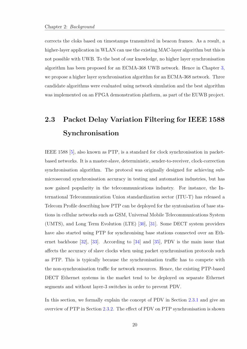
The basic principle of PTP is that the most precise clock on the network (termed the
grandmaster) is used to synchronise all other clocks on the network. The grandmaster
clock is selected from all the clocks in the network based on the source of time it is
connected to, using a BMCA. Apart from the grandmaster, a PTP network also
includes several masters serving groups of local clocks as shown in Fig. 2.4. A logical
grouping of clocks that communicate with each other using the IEEE 1588 protocol
in known as a PTP domain and each domain is served by a single master.
In PTP, synchronisation is carried out in two phases using four types of messages.
During the Offset Measurement phase the master sends multicast SYNC messages to
its slaves in a periodic manner. Each SYNC message contains a time estimate of when
21
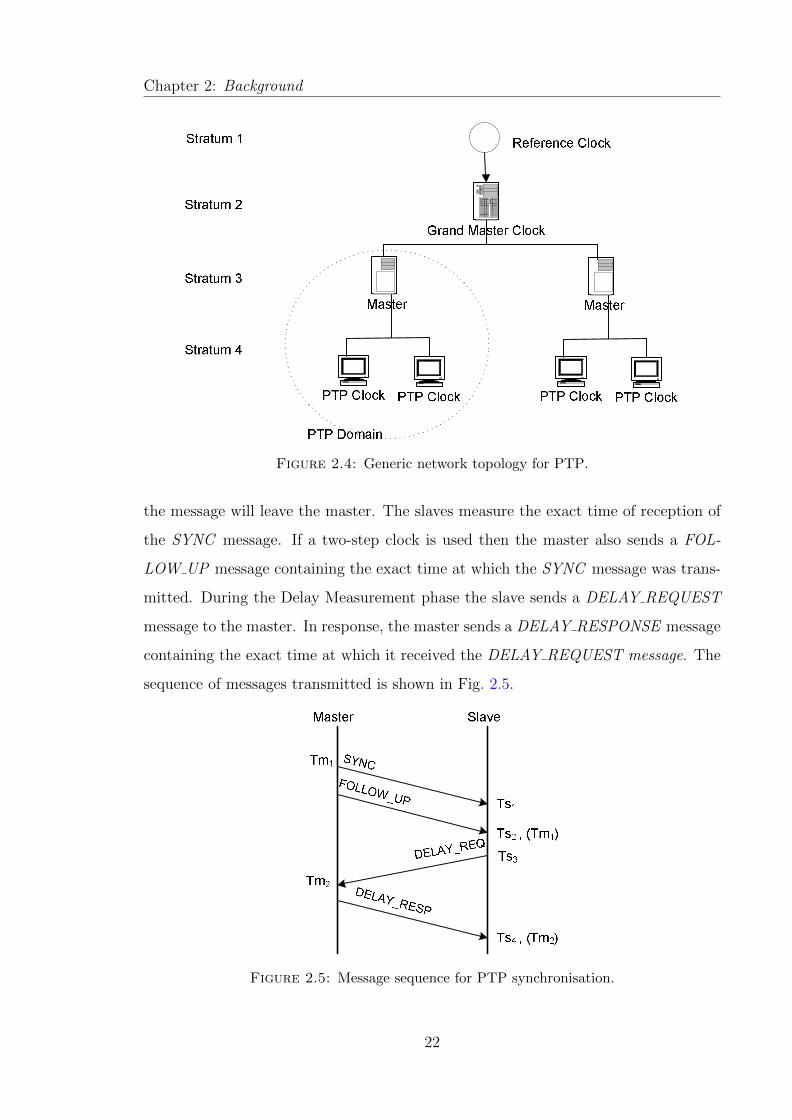
Chapter 2: Background
Figure 2.4: Generic network topology for PTP.
the message will leave the master. The slaves measure the exact time of reception of
the SYNC message. If a two-step clock is used then the master also sends a FOL-
LOW UP message containing the exact time at which the SYNC message was trans-
mitted. During the Delay Measurement phase the slave sends a DELAY REQUEST
message to the master. In response, the master sends a DELAY RESPONSE message
containing the exact time at which it received the DELAY REQUEST message. The
sequence of messages transmitted is shown in Fig. 2.5.
Figure 2.5: Message sequence for PTP synchronisation.
22

Chapter 2: Background
From Fig. 2.5, the following relations hold:
Ts1 = Tm1 + dms −Osm (2.6)
Tm2 = Ts2 + dsm −Osm, (2.7)
where dms and dsm are the OTTs from master to slave and from slave to master,
respectively, and Osm is the clock offset of the slave with respect to the master.
If the delay is symmetric, dms = dsm = d. Hence, Osm and d can be calculated from
(2.6) and (2.7) as:
Osm = 0.5 ∗ ((Ts1 − Tm1)− (Tm2 − Ts2)) (2.8)
d = 0.5 ∗ ((Ts1 − Tm1) + (Tm2 − Ts2)). (2.9)
PTP can also correct for the clock rate mismatch or relative clock skew between the
master and slaves, using a series of SYNC messages. If the master origin timestamps
for the ith and j th SYNC messages are denoted by Mi and Mj, the corresponding
reception timestamps at a slave are Si and Sj, and j > i, then the Rate Compensation
Factor (RCF) is computed as:
RCF =Sj − Si
Mj −Mi
. (2.10)
This RCF is an estimate of the relative clock skew of the slave with respect to the
master. As long as the OTTs di and dj are equal, the estimation will be accurate.
23
Chapter 2: Background
2.3.3 Effect of PDV on the synchronisation performance of
PTP
When PTP is deployed in an existing network, the synchronisation traffic must con-
tend for the network path and share existing network elements with background traffic
in the network. This contention causes variable packet queuing delays at the output
queue buffers of network switches, thus giving rise to PDV. If left unchecked, this
PDV will adversely affect the synchronisation accuracy of the protocol. The specific
effect of PDV on synchronisation accuracy is twofold.
Firstly, the variable queuing delay masks the one-way delays such that it becomes
impossible to distinguish between the one-way transit delay, clock offset and queuing
delay within a timestamp delta value δi = Si −Mi. Secondly, variable queuing delay
means that di 6= dj, and results in an inaccurate computation of RCF. Thus, the
variation in queuing delay from packet to packet in the network essentially introduces
noise in the slave’s estimation of the master’s clock. If the delay was constant, it
would produce a fixed offset that could be easily removed; however the variable delay
produces a varying estimate of the offset that degrades the performance of the slave
clock.
To illustrate this, we consider a simple PTP network comprising of a master and node
connected via intermediate switches. In one scenario there is no background traffic,
while the other scenario considers the case where the network is statically loaded with
the ITU-T data-centric background traffic [36] at 30% utilisation. Fig. 2.6 shows the
variable delay caused by the background traffic and queuing elements, while Fig. 2.7
shows the effect on the synchronisation performance.
2.3.4 Techniques for dealing with PDV
The PTP standard recognizes the problem caused by PDV and offers some techniques
for dealing with it, such as deploying specialised PTP switches at intermediate nodes
in the network, traffic design, priority tagging of synchronisation traffic, and PDV
24

Chapter 2: Background
5 10 15 20 25 30 35 40 45 500
50
100
150
200
250
300
350
400
Simulation Time in seconds
Pac
ket D
elay
in m
icro
seco
nds
No background traffic30% background traffic
Figure 2.6: Illustration of PDV in packet delay measurements.
0 10 20 30 40 50−300
−200
−100
0
100
200
300
400
500
Simulation Time in seconds
Rel
ativ
e C
lock
Offs
et a
t Sla
ve in
mic
rose
cond
s No background traffic30% background traffic
Figure 2.7: Illustration of PTP synchronisation with PDV.
25

Chapter 2: Background
filtering. Other techniques in the literature deal with PDV by coordinating the back-
ground traffic packet departures with the synchronisation packet generation so as to
completely eliminate PDV [37], or by applying Kalman filtering to the received syn-
chronisation packets in order to estimate the master time [38], [39]. In most cases,
more than one technique may be required.
Use of Specialised Switches
PTP transparent clocks or boundary clocks can be deployed in place of standard
switches at intermediate nodes in the network, in order to prevent PDV. A boundary
clock is a multiple-port PTP device, with each port providing access to a separate
PTP communication path. It acts as an interface between separate PTP domains,
intercepting and processing all PTP messages while passing all other network traffic.
One port is the slave port while all other ports are master ports, as determined by the
BMCA. The slave port synchronises to the master port of the domain it is connected
to, and then provides this synchronised time to all other master ports on the device.
Each master port then provides this synchronised time to the domain connected to
it. In this way, cascades of queuing elements are avoided during synchronisation and
PDV is prevented. A transparent clock, on the other hand, is a single-port PTP device
which measures the amount of time a packet spends in the queue buffers of output
ports and stores this residence time in the correction field of the PTP packet [40]. This
residence time is subtracted from the timestamp delta value δi in order to accurately
determine dms and dsm, and then added on to the computed offset, for accurate
synchronisation.
Specialised switches are likely to be the preferred solution for new network instal-
lations, as the switches can be factored into the design and costing of the network.
For existing installations however, it is often cumbersome and costly to replace the
existing network devices.
26

Chapter 2: Background
Traffic Design
Where possible, the traffic patterns in a network can be designed in such a way as
to minimise the amount of background traffic as well as the variation in the traffic
load, so as to reduce PDV. Assuming that each intermediate network switch is an
M/M/1 queue, the entire network will behave like a system of cascaded queues and in
steady state, each queue will have a backlog of packets that are yet to be processed.
The mean backlog B of unprocessed packets can be expressed in terms of the network
utilisation as [41]
B =ρ
1− ρ. (2.11)
For a network utilisation level of 80%, the mean backlog is 4 packets. A synchronisa-
tion packet arriving at the queue will have to wait until the backlog is cleared, thus
incurring additional latency. If the amount of background traffic is reduced, the util-
isation decreases, with a corresponding decrease in latency and PDV. Traffic design
can also be implemented by coordinating the background traffic packet departures
with the synchronisation packet generation so as to completely eliminate PDV [37].
However, this can only be utilised in a network that strictly carries non-real time
traffic such as data.
Priority Tagging of Synchronisation Traffic
The PTP standard also recommends that PTP event messages are sent with a higher
priority, compared with other traffic on the network. In contrast to general messages,
PTP event messages are timed messages that require the generation of accurate times-
tamps when transmitted and received. Such messages include SYNC messages and
DELAY REQ messages.
Prioritisation of synchronisation traffic is useful for managing delay fluctuations at
the ingress ports of switches, but it cannot completely eliminate PDV at the egress
ports. This is because of the way modern switches are designed. In general, a mod-
ern Ethernet switch has the basic internal architecture illustrated in Fig. 2.8. If QoS
is implemented, the traffic manager classifies the incoming traffic based on a traffic
27

Chapter 2: Background
policy such as Class of Service (CoS) while the buffer manager places the traffic in
queues according to the classification. At egress, the buffer manager schedules the
packets for transmission while the traffic manager implements any egress traffic poli-
cies. Regardless of whatever traffic policies or prioritisations are applied, the MAC
unit represents a common First In First Out (FIFO) queue into which all packets
eventually enter [42], [43]. Thus even if PTP event packets are prioritised over back-
ground traffic, the PTP packets would still experience queuing as long as there is a
backlog of packets in the MAC unit. Hence prioritisation of synchronisation traffic
cannot completely eliminate PDV.
Queue 1
Queue 2
Buffer Manager
Traffic Manager
Switch Fabric
MAC
Queue 1
Queue 2 Buffer
Manager Traffic
Manager MAC
Ingress Path
Egress Path
Figure 2.8: Internal architecture of a generic Ethernet switch.
PDV Filtering
Two categories of PDV filtering can be observed in the literature. One category takes
a set of noisy or PDV-impacted synchronisation packets and tries to generate an es-
timate of the master’s time by filtering off the PDV. This is the approach adopted
by [38], [39], [44] in which Kalman filtering is applied to the received synchronisation
packets in order to estimate the master time. However, it has been observed that
Kalman filtering as a means of combatting PDV in synchronisation networks is only
optimal when the network delays follow a Gaussian distribution [44], and this is not
28

Chapter 2: Background
usually the case in real Ethenet networks [45]. The other category of PDV filtering
tries to filter off those packets that were heavily impacted by PDV so that the re-
maining “good” packets can be used to estimate the master time. It is this second
category that is the focus of our second research area.
In general, the goal is to select at least one “good” packet out of several packets
within the received synchronisation traffic and then use the good packet or packets to
achieve synchronisation. However, the definition of “good” can be very subjective. For
most of the PDV filtering algorithms in the literature [11], [12], [46], a “good” packet
is defined as one with the shortest transit time through the network. Hence these
algorithms tend to group the received synchronisation packets into non-overlapping
windows, select the ones that were least impacted by queuing delay, and discard the
remaining packets. The PDV filters which employ such algorithms are referred to as
sample-minimum or earliest arrival packet filters.
Sample-minimum filters can work effectively, as long as packets with minimal queuing
delay are delivered at appropriate intervals. In [9], [10], the authors showed that
this depends on the packet delay distribution of the network, which in turn depends
on the network topology as well as on the network utilisation. The authors also
observed that in some scenarios such as heavily-loaded cross-traffic networks and
moderately-loaded high-hop in-line traffic networks where the probability of finding a
minimum-delay packet was significantly reduced, a sample-mean or sample-maximum
filter could outperform the popular sample-minimum filter.
Since the performance of a PDV filter depends on the probability of finding “good”
packets to use for synchronisation and “good” packets are packets that experienced
the same amount of delay, it seems intuitive that the best place to find such packets is
around the mode packet delay value. Hence in Chapter 4, we propose a new sample-
mode PDV filtering algorithm for a PTP network and use numerical simulations
to compare the performance of the sample-mode filter with the performance of the
existing sample-minimum, sample-maximum, and sample-mean filters.
29
Chapter 2: Background
2.4 Dealing with Master Failures in IEEE 1588
Synchronisation
As mentioned in Section 2.3.2, PTP is a type of master-slave synchronisation algorithm
in which slave clocks synchronise to a single master clock in a domain. Thus, the
master node represents a single point of failure in the system. However, the master
node is not usually hard-wired into the system; rather each node can be in any one
of 9 different states at any time, including MASTER and SLAVE states. The master
node is the node in the PTP domain that is currently operating in the MASTER state
and at any given time, only one node can be in this state. A node transitions to the
MASTER state if it is elected as the best clock based on a standard BMCA which
compares the attributes of the different clocks. A failure of the master clock results in
the election of a new master using the same BMCA, but the downtime caused by the
failure can lead to an accumulation of offset and loss of synchronisation which may
be unacceptable for certain applications.
In this section, we summarise the state of the art, as described in [5]. Then we
highlight the different existing approaches to dealing with master failures, comment
on the advantages and drawbacks of the existing methods and consider the suitability
of the existing methods for our target application.
2.4.1 Description of State-of-the-art
2.4.1.1 PTP Node States
9 possible PTP states exist as shown in Table 2.2 and a node can be in either one of
the states at any particular time.
30

Chapter 2: Background
Table 2.2: PTP node states.
State DescriptionINITIALIZING Used for initialising data sets, hardware, and communication
facilities.
LISTENING In order to ensure the orderly addition of new PTPnodes, an initialised node waits in this state for the AN-NOUNCE RECEIPT TIMEOUT to expire or to receive anANNOUNCE message from a master.
MASTER The node behaves like a master clock.
SLAVE The node synchronises to the selected master clock.
UNCALIBRATED A transient state to update data sets when a new master isdetected and a node is preparing to synchronise with it.
PREMASTER A transient state to allow a new master to take over from anexisting master.
PASSIVE Used for grandmaster clocks that derive their time from an ex-ternal reference time, but which are not elected as the masterof the domain.
FAULTY The faulty state of the protocol.
DISABLED The disabled state of the protocol.
2.4.1.2 PTP Clock Categories
Based on the number of PTP ports, clocks can be categorised as either boundary
clocks or ordinary clocks. An ordinary clock has a single PTP port in a domain, while
a boundary clock has more than one PTP ports in the domain. The BMCA is run on
each port in a PTP domain, so all the ports on a boundary clock do not necessarily
operate in the same state. This allows a boundary clock to receive synchronisation
in one domain using a port in the SLAVE and then transfer the synchronisation to
another domain using a port in the MASTER state.
In addition, clocks are classified as either one-step or two-step clocks. In a one-step
clock, each SYNC message prepared by the master contains an estimate of when the
message would be sent. Two-step clocks, on the other hand, also transmit a FOL-
LOW UP message containing the exact time at which the previous SYNC message
was sent. All the models and simulations in this thesis are based on one-step ordinary
clocks.
31
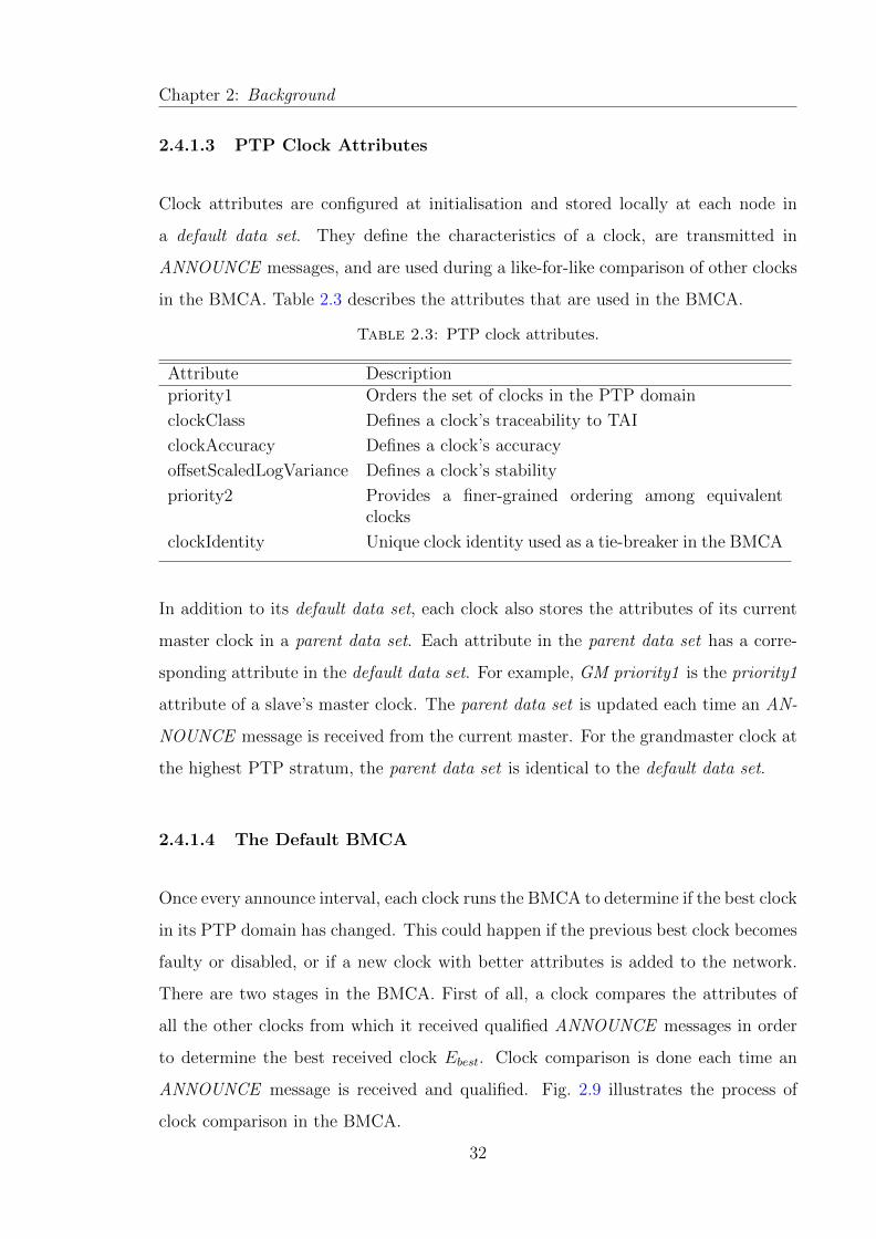
Chapter 2: Background
2.4.1.3 PTP Clock Attributes
Clock attributes are configured at initialisation and stored locally at each node in
a default data set. They define the characteristics of a clock, are transmitted in
ANNOUNCE messages, and are used during a like-for-like comparison of other clocks
in the BMCA. Table 2.3 describes the attributes that are used in the BMCA.
Table 2.3: PTP clock attributes.
Attribute Descriptionpriority1 Orders the set of clocks in the PTP domain
clockClass Defines a clock’s traceability to TAI
clockAccuracy Defines a clock’s accuracy
offsetScaledLogVariance Defines a clock’s stability
priority2 Provides a finer-grained ordering among equivalentclocks
clockIdentity Unique clock identity used as a tie-breaker in the BMCA
In addition to its default data set, each clock also stores the attributes of its current
master clock in a parent data set. Each attribute in the parent data set has a corre-
sponding attribute in the default data set. For example, GM priority1 is the priority1
attribute of a slave’s master clock. The parent data set is updated each time an AN-
NOUNCE message is received from the current master. For the grandmaster clock at
the highest PTP stratum, the parent data set is identical to the default data set.
2.4.1.4 The Default BMCA
Once every announce interval, each clock runs the BMCA to determine if the best clock
in its PTP domain has changed. This could happen if the previous best clock becomes
faulty or disabled, or if a new clock with better attributes is added to the network.
There are two stages in the BMCA. First of all, a clock compares the attributes of
all the other clocks from which it received qualified ANNOUNCE messages in order
to determine the best received clock Ebest. Clock comparison is done each time an
ANNOUNCE message is received and qualified. Fig. 2.9 illustrates the process of
clock comparison in the BMCA.
32

Chapter 2: Background Compare dataset A to BGM Identity of A = GM Identity of BCompare GM priority1 values of A and BCompare GM class values of A and BCompare GM accuracy values of A and BCompare GM offsetScaledLogVariancevalues of A and BCompare GM priority2 values of A and BCompare GM identity values of A and BReturnB better than A ReturnA better than B
Go to algorithm forcomparison of data setsfrom the same GMA > BA > BA > BA > BA > BA > B
A < BA < BA < BA < BA < BA < B
A = BA = BA = BA = BA = B
YESNO
Figure 2.9: Clock comparison algorithm for the default BMCA.
The second stage is the state decision algorithm which recommends a state for the
clock, by comparing its own attributes from the default data set D0 with the attributes
of Ebest. The state decision algorithm is run once every announce interval. The state
decision algoithm is described in Fig. 2.10.
33
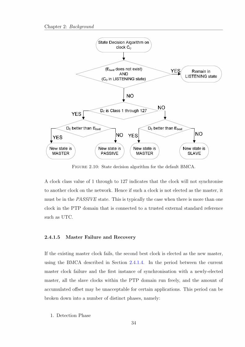
Chapter 2: Background
Figure 2.10: State decision algorithm for the default BMCA.
A clock class value of 1 through to 127 indicates that the clock will not synchronise
to another clock on the network. Hence if such a clock is not elected as the master, it
must be in the PASSIVE state. This is typically the case when there is more than one
clock in the PTP domain that is connected to a trusted external standard reference
such as UTC.
2.4.1.5 Master Failure and Recovery
If the existing master clock fails, the second best clock is elected as the new master,
using the BMCA described in Section 2.4.1.4. In the period between the current
master clock failure and the first instance of synchronisation with a newly-elected
master, all the slave clocks within the PTP domain run freely, and the amount of
accumulated offset may be unacceptable for certain applications. This period can be
broken down into a number of distinct phases, namely:
1. Detection Phase
34

Chapter 2: Background
2. Election Phase
3. Re-synchronisation Phase
A master node sends ANNOUNCE messages to all slaves once every announce inter-
val. At each slave, an ANNOUNCE RECEIPT TIMEOUT timer is used to track the
amount of time elapsed since the receipt of the most recent ANNOUNCE message
from the master. Thus, the timer is restarted every time an ANNOUNCE message
is received from the current master. The timer expires when it reaches the AN-
NOUNCE RECEIPT TIMEOUT value. If this happens, the slaves conclude that the
master has failed and proceed to elect a new master. Hence, the duration of the
detection phase is equivalent to the ANNOUNCE RECEIPT TIMEOUT value. Ac-
cording to [5], the ANNOUNCE RECEIPT TIMEOUT value should be x times the
announce interval, where x = {3, 4, 5, ..., 10} and the announce interval = {1, 2,
4, 8, 16} seconds. Typical values of x and announce interval are 10 and 2 seconds,
respectively.
At the expiry of its ANNOUNCE RECEIPT TIMEOUT timer, a slave transitions to
the MASTER state and starts transmitting ANNOUNCE messages. In the election
phase, each slave (now operating in a MASTER state) implements the BMCA using
all the received ANNOUNCE messages. If its own clock is better than all the other
clocks as specified in the received messages, it becomes the new master and remains
in the MASTER state; otherwise it transitions to the SLAVE state and prepares
to synchronise to the best master. This election phase can take up to 2 times the
announce interval.
After the election phase, the slaves re-synchronize to the new master. At least 2
times the synchronisation interval is required to correct for the clock offset and skew,
assuming that a DELAY REQ message can be sent immediately. The default value
of the synchronisation interval is 1 second.
From the above descriptions, the total period between a master failure and resyn-
chronisation to a newly-elected master can be reduced by decreasing the values of
the announce interval and synchronisation interval. However, these measures result
35

Chapter 2: Background
in an increase in the amount of multicast traffic on the network when there are no
failures in the system. Therefore the anticipated benefit of such measures must be
weighed against the cost of increased traffic, with consideration for the probability of
node failure. This is especially true in the case of the announce interval because the
clock attributes contained in ANNOUNCE messages do not change frequently and
the BMCA must be run each announce interval. Thus in a fully functional non-faulty
system, decreasing the announce interval results in the same clock attributes trans-
mitted more frequently with more iterations of the BMCA which all yield the same
outcome. Furthermore, reducing the announce interval, synchronisation interval, or
both will not completely remove the accumulated offset because the nodes still run
freely until a new master is elected.
2.4.2 Survey of Existing Techniques for dealing with PTP
Master Failure
A number of techniques have been considered for dealing with the effects of a master
failure. As mentioned in Section 1.2, the existing techniques tend to be based on
either one of two approaches: deploying multiple nodes with PRC capability or util-
ising a democratic master group. From an implementation perspective, we can also
categorise them into pure master-based approaches, pure slave-based approaches, or
hybrid approaches; depending on the how they differ from the state of the art.
2.4.2.1 Master-based Approaches
We define master-based approaches as those techniques in which additional function-
ality is only required at the master nodes. For example, the PTP standard [5] defines
an optional grandmaster cluster feature, in which two to five ordinary or boundary
clocks are designated as members of a grandmaster cluster. Each cluster member
maintains a table with the addresses of other cluster members so that it can pe-
riodically exchange unicast query ANNOUNCE messages with all the other cluster
members in the domain. The received ANNOUNCE messages are then used as inputs
36
Chapter 2: Background
to the BMCA, in order to determine the state of each node. All the cluster members
are potential master clocks, with higher priorities than all the other clocks in the
domain. Failure of the current master is detected in the cluster within 1 announce
interval and a new master is elected within another announce interval. Hence, both
the failed master detection time and new master election time are reduced. The draw-
back of this technique is that, like the name implies, the feature is only described for
grandmasters. This means that within the grandmaster cluster, the other nodes that
are not operating in the MASTER state must be in PASSIVE mode, and therefore
do not synchronize to each other. In practice, this would necessitate the provision of
independent synchronisation to a trusted external timing source such as GPS at each
grandmaster clock within the cluster.
Another master-based approach is the democratic master group proposed by the au-
thors of [47]–[50] as a means of providing fault-tolerance in IEEE 1588 synchronisation.
The IEEE 1588 master is replaced with a group of masters that synchronise to each
other using a fault-tolerant peer-to-peer algorithm. In this way, a faulty or malfunc-
tioning master clock can be sorted out, without affecting the accuracy of the slaves.
The speaker for the master group is a specially-designed fault-tolerant switch which
is responsible for keeping track of the democratically agreed time and transmitting
it to the slaves via SYNC packets. In order to maintain some compatibility with
the PTP standard, the democratic stack is derived from the IEEE 1588 protocol and
the messages exchanged between master group members are similar to PTP SYNC
packets. This is useful because the slaves do not require any special functionality;
however the master group speaker is a new device with special functionality. Also,
some modification is required at the master nodes, in order to support the democratic
algorithm.
2.4.2.2 Slave-based Approaches
We define slave-based approaches as those techniques that only require changes to the
slave nodes. For example, the ITU-T has defined a new telecoms profile for applica-
tions that require only frequency synchronisation [30]. It uses unicast transmissions
37

Chapter 2: Background
to separate PTP domains. Unicast messaging ensures that master clocks are isolated
from each other. Moreover, masters do not communicate with each other. Each slave
device consists of multiple instances of independent PTP slave-only-ordinary-clocks
(SOOCs); each SOOC participates in a single PTP domain and is associated with
a single master. Each slave also maintains a list of all the masters it is allowed to
communicate with, together with their priorities. This list is used to instantiate the
SOOC instances. Since the profile is geared towards frequency synchronisation, it is
not mandatory for a slave to support the delay request-response mechanism; however
the master clock must support it. An alternate BMCA is used that produces a value
of M1 (grandmaster clock) for all the master clocks and S1 (slave clock) for all the
SOOC instances. The slave device uses three attributes in order to select a specific
master: the Packet Timing Signal Fail (PTSF) which specifies the failure condition of
a master, the clock class attribute, and the master priority. It selects the master with
the lowest clock class attribute that is not in a failure condition. If the clock class
values are identical, then the master with the highest priority value is selected [51].
The timestamps corresponding to the selected master are used for achieving frequency
synchronisation.
Another slave-based approach is the architecture proposed by [52] in which grand-
master clocks are isolated from each other using separate IEEE802.1Q VLANs. The
grandmaster clocks use the same free-running oscillator so there is no time error be-
tween them at any point and the slave is a VLAN-aware device, so it is able to receive
messages from all the grandmaster clocks. The slave maintains a separate feedback
loop for each grandmaster and synchronises to the grandmaster that announces the
lowest priority1 value. Thus if the current grandmaster clock fails, the failure does
not propagate to the other grandmaster clocks. The slave detects the failure when it
does not receive an ANNOUNCE message, and can immediately switch to the next
functioning grandmaster with the lowest priority1 value. This method requires that
the same oscillator is used for all grandmaster clocks so that the slave can quickly
switch over to a new grandmaster without any transient error at the time of switching.
38

Chapter 2: Background
2.4.2.3 Hybrid Approaches
We define hybrid approaches as those techniques that require changes to both master
and slave nodes. An example of this is the optional alternate master feature defined
in the PTP standard [5]. This feature allows nodes that are not currently operating in
the MASTER state to send SYNC, ANNOUNCE and DELAY RESPONSE messages
to slave nodes. It also allows slave nodes to send DELAY REQUEST messages to
nodes that are not currently operating in the MASTER state. In this way, if the
slaves have to switch over to an alternate master when the current master fails, the
amount of offset during the re-synchronisation phase would be reduced. However, the
lengths of the detection and election phases remain unchanged.
2.4.3 Drawbacks of Existing PTP Master Redundancy Tech-
niques
In the period between a master clock failure and the first instance of synchronisa-
tion with a newly-elected master, all the slave clocks in the PTP domain run freely,
and the amount of accumulated offset during the period may be unacceptable for
certain applications. The existing techniques described in Section 2.4.2 have some
disadvantages. The grandmaster cluster technique [5] reduces both the failed master
detection time and the new master election time; however all the nodes within the
cluster must be synchronised to an external reference time source, such as GPS. The
democratic master group technique [47], [48] uses an averaging algorithm to obtain a
common time for the master group, which is then communicated to the slaves via a
fault-tolerant master group speaker. This master group speaker is a new expensive
device that must be factored into the cost of the system, and essentially represents a
single point of failure in the system. The multi-SOOC slave nodes proposed by [30]
do not offer time synchronisation, and the isolated grandmaster clock architecture
described in [52] requires co-located grandmaster nodes. Lastly, the alternate master
technique [5] has limited effect as it only shortens the re-synchronisation phase.
39

Chapter 2: Background
Our target application is a network of DECT base stations at separate physical lo-
cations that are connected over an Ethernet backbone. The base stations, which do
not have access to an external reference time source, require time synchronisation and
reduced downtime in the event of a master failure. The drawbacks of the technique
make them unsuitable for the target application. In Chapter 5, we describe the target
application in more detail and propose a new alternate master cluster technique for
meeting the requirements of the application.
2.5 Summary
This chapter has provided an overview of the three different research areas that com-
prise this thesis. Section 2.1 has defined some of the important terms related to clocks
and synchronisation and described the existing classes of synchronisation algorithms.
An overview of ECMA-368 UWB has been presented and the two forms of synchro-
nisation have been described in Section 2.2. We have shown that the existing MAC
layer synchronisation is unsuitable for providing synchronisation to higher-layer MAC
clients because the clocks are not corrected and hence the accumulation of clock drift
leads to frequent loss of synchronisation. We have explained the usage of the higher
layer synchronisation MLME primitives, but noted that no algorithms exist for im-
plementing higher layer synchronisation. Therefore, in Chapter 3, we propose a new
higher layer synchronisation algorithm for an ECMA-368 network.
Section 2.3 has provided an overview of the IEEE 1588 synchronisation protocol,
explored the origin of PDV, and demonstrated the effect of PDV on PTP synchroni-
sation. Some existing PDV algorithms in the literature have also been described. We
have considered the category of PDV algorithms that filter off those packets that are
heavily impacted by PDV and noted that the performance of the algorithms depends
on the probability of finding “good” packets from among the received synchronisation
traffic. Based on this observation, we have postulated that the probability of finding
“good” packets can be maximised by selecting packets from around the mode delay
40

Chapter 2: Background
value. Hence, Chapter 4 proposes a new sample-mode PDV filtering algorithm for a
PTP network.
Finally, Section 2.4 has described the default BMCA used for electing masters in the
IEEE 1588 standard and explored some existing techniques for coping with master
failures. We have noted that the drawbacks of the different techniques make them
unsuitable for the target DECT Ethernet base station network. In Chapter 5, we will
describe the target application in more detail and propose a new alternate master
cluster technique for meeting the requirements of the application.
41
Chapter 3Higher Layer Synchronisation in Ultra
Wideband Networks
3.1 Introduction
In this chapter a synchronisation algorithm is developed for an ECMA-368 UWB
network, in order to provide synchronisation for the higher layer applications or MAC
clients that use the UWB network.
Section 3.2 describes the application requirements for the synchronisation algorithm,
as detailed in the EUWB project documents [53]–[55]. Section 3.3 describes the pro-
cess of selecting candidate algorithms for the higher layer synchronisation mechanism,
before describing each algorithm in detail. Since the higher layer synchronisation al-
gorithm is actually implemented in the MAC layer, Section 3.4 describes the design
process in terms of how timestamps are transferred from the higher layer to the MAC
layer before synchronisation, as well as how the computed offset and skew are trans-
ferred back to the higher layer after synchronisation. The UWB OPNET models we
developed are presented in Section 3.5. Simulation results obtained from implement-
ing the three candidate algorithms are also presented and analysed. Based on the
analysis, one candidate algorithm is selected and implemented on an FPGA UWB
platform developed at TES Electronic Solutions Ltd. Section 3.6 gives an overview
42

Chapter 3: Higher Layer Synchronisation in Ultra Wideband Networks
of the FPGA platform, describes the modifications that were made in order to imple-
ment the algorithm, and presents some results obtained from implementation on the
platform. A summary of the chapter is provided in Section 3.7.
3.2 Application Requirements
Real-time video streaming is an important application for the EUWB research project,
in which two scenarios were considered: wireless aircraft cabin management systems
[53], [54] and wireless home entertainment systems [55]. A typical use case for the
former scenario involves the transmission of video, such as in-flight entertainment,
from a cabin server to wireless passenger display units; while the latter might involve
the transfer of video from portable media players to a central hub for subsequent
streaming to television sets. A generic network topology suitable for either scenario
consists of a video server streaming packets to multiple end devices over Ethernet and
UWB links and via switches and access points, as illustrated in Fig. 3.1.
Figure 3.1: Generic network topology.
The generic network consists of a central server system from which data can be trans-
ferred to various wired and wireless end devices via switching units and wireless Access
Points (APs). Multi-hops from a wireless AP to a device are not required. Two main
types of traffic are transmitted over the network: multimedia and control traffic. Mul-
timedia includes pure audio signals from loudspeakers, pure video signals from CCTV
images, and a combination of audio and video signals (AV streaming) from in-flight
43

Chapter 3: Higher Layer Synchronisation in Ultra Wideband Networks
entertainment. Here, control traffic, refers to all other forms of data transmitted over
the network, including data from sensors such as smoke detectors, lighting control
data and data from cabin control terminals such as Passenger Service Units (PSUs)
and exit signs. Traffic is transmitted from the server to the APs via switches. The
AP forwards the traffic to the devices within its beacon group and apart from the
mandatory exchange of beacons, there is no other communication between the end
devices in the network.
There are two key QoS requirements for the network, namely: minimising packet
jitter and minimising the timing difference between co-located devices. Packet jit-
ter, also known as inter-packet delay variation, is the variation in end-to-end delays
experienced by consecutive packets from the same stream. Factors such as lack of
transmission opportunity, prioritisation of different streams, packet retransmission or
the lack of guaranteed bandwidth in wireless networks generally give rise to packet
jitter and a jitter buffer is commonly used to minimise the effects of jitter. Large delay
variations, however, require a larger, more expensive buffer and ultimately results in
the introduction of a larger amount of constant latency at the start of the application
that is unsuitable for real-time streaming. Timing difference refers to the difference
in the event start times of multiple end devices, e.g. audio playback in loudspeak-
ers. When such end devices are in close proximity, minimising the timing difference
becomes an important requirement in order to prevent distortion and achieve a sat-
isfactory QoE for the end user. As well as minimising the timing difference between
devices, synchronisation can reduce the size (and ultimately, cost) of the jitter buffer.
The requirements document for the EUWB project [53] specifies that the higher layer
synchronisation mechanism must deliver a precision of 100µs or better across the
entire network and must be scalable such that it can be extended from a simple beacon
group of UWB devices to the larger scale hybrid wired/wireless network illustrated in
Fig. 3.1.
44

Chapter 3: Higher Layer Synchronisation in Ultra Wideband Networks
3.3 Selection of Algorithms
Due to the sheer number of synchronisation algorithms available in the literature, it
would have been onerous and impractical to sift through all of them to determine
the most suitable one for the generic network. Hence a more realistic approach was
adopted to first determine the most suitable class of algorithm for the network, and
then analyse the algorithms within that class to see which one(s) could satisfy the
application requirements. The specific class of algorithms was determined based on
the classification described in Section 2.1.2.
Due to the hierarchical nature of the generic network and the fact that direct com-
munication between devices is not required, a master-slave synchronization approach
with clock correction is necessary in order to ensure that all devices on the network
are synchronised. For the same reasons a sender-to-receiver algorithm is implied, al-
though a receiver-to-receiver algorithm can be implemented provided that the time
comparison occurs between the sender and receiver, as is the case of the Continuous
Clock Synchronization algorithm described in [56]. Furthermore, the algorithm will
support internal synchronisation since the nodes may not have access to a trusted ex-
ternal time source. Finally, a deterministic approach is necessary in order to guarantee
the accuracy of the system.
Based on this classification, two candidate algorithms were selected, namely: Delay
Measurement Time Synchronisation algorithm [57] and Continuous Clock Synchroni-
sation algorithm [56], [58]. We also proposed a Linear Rate Synchronisation algorithm
that fits with the desired class of algorithms. The following sub-sections describe these
three algorithms.
3.3.1 Delay Measurement Time Synchronisation algorithm
The Delay Measurement Time Synchronisation algorithm combines a master’s times-
tamp with delay measurements, in order to achieve synchronisation of the slaves. Each
slave takes two timestamps: one when it receives the preamble of the synchronisation
45

Chapter 3: Higher Layer Synchronisation in Ultra Wideband Networks
message, and the other after the message has been processed. The difference between
these timestamps is a measure of the data transfer time plus the processing delay.
Each slave also estimates the time taken to transmit the message preamble. Finally,
each slave sets its clock to the sum of the master’s timestamp, the data transfer time
plus processing delay, and the preamble transmission time.
3.3.2 Continuous Clock Synchronisation algorithm
The Continuous Clock Synchronisation algorithm uses an advanced rate-adjustment
algorithm to spread clock correction over a finite interval in order to prevent the time
discontinuity caused by instantaneous clock correction. In this way, the local clock
time is corrected by gradually increasing or decreasing the clock rate. Each node in
the network has both a physical and virtual clock. In this sense, a virtual clock is
simply a transformation function that corrects the skew rate of a physical clock. For
the sake of simplicity, a linear function is used and clock correction is achieved by
changing the parameters of this function after every synchronisation round so that
the slave’s virtual clock matches the master’s physical clock as closely as possible. The
algorithm assumes that message reception is tight, such that a master node receives
its own broadcast message at approximately the same time as the slave nodes [58].
Each synchronisation frame contains the time at which the master node received the
last synchronisation message sent and by comparing this value with its own reception
time for the same message, a slave is able to achieve synchronisation with the master.
The ECMA-368 PCA and DRP data transmission mechanisms do not permit any node
to receive its own broadcast frame, hence adapting the Continuous Clock algorithm
to a UWB network requires a calculation of the expected reception time at the master
node. The processing delay between the synchronisation frame being scheduled by the
MAC and the first symbol being received on-air by the remote device can be added
to the master’s transmission timestamp in order to obtain this value [59].
46

Chapter 3: Higher Layer Synchronisation in Ultra Wideband Networks
3.3.3 Linear Rate Synchronisation algorithm
Another possible implementation of synchronisation is based on a linear-rate function
which relates a slave’s clock to the master’s clock. The master sends its timestamp to
the slaves in the form of a command frame every synchronisation round and each slave
records its local clock time when it receives the synchronisation frame, thus building
a table of pair values in the form [MnSn], where Mn is the local clock time at which
the master sent the nth synchronisation frame and Sn is the local time at which the
slave received the same frame. After two rounds the slave can calculate the relative
skew σ and relative offset θ as follows:
σ =Mn −Mn−1
Sn − Sn−1. (3.1)
θ = Mn − σSn. (3.2)
These values are then used to update the parameters of its virtual clock V which
transforms the hardware clock H to mimic the behaviour of the master’s clock as
shown in (3.3).
V = σH + θ (3.3)
3.4 Design of the Higher Layer Synchronisation
Mechanism
As stated in Section 2.2.2.2, the ECMA-368 standard includes three MLME primitives
to support the higher layer synchronisation function. The MLME-HL-SYNC.request
primitive is sent from the higher layer to the MAC to initiate the synchronisation
mechanism, the MLME-HL-SYNC.confirm returns the result of the request, while
the MLME-HL-SYNC.indication primitive indicates the transmission or reception of
a synchronisation frame.
47

Chapter 3: Higher Layer Synchronisation in Ultra Wideband Networks
Since the goal is to synchronise the clocks of higher layer protocols which may reside
separately from the MAC, it makes sense for the MAC to be responsible for imple-
menting the synchronisation algorithm. Before synchronisation, the higher layer clock
value or timestamp on both master and slave devices must be transferred to the MAC
layer. Furthermore, after synchronisation is complete, there is an additional require-
ment for transferring the calculated clock adjustment back to the higher layer on the
slave device. The manner of fulfilling the first requirement depends on whether the
MAC and higher layer protocol reside on the same entity or on separate entities, i.e.
whether or not the MAC layer can directly access the higher layer clock. Both cases
are considered in the following sub-sections. For the second requirement, a new service
primitive has been defined: the MLME-HL-CLOCK-UPDATE.indication will transfer
the calculated clock offset and skew back to the higher layer so that the parameters
of the higher layer virtual clock can be updated.
3.4.1 Case 1: MAC Layer and Higher Layer Application on
separate entities
In this case, the MAC layer has access to the PHY clock but not to the higher layer
clock. Thus, there is a need for mapping higher layer clock values to PHY layer clock
values, since it is the higher layer clock timestamps that are required as parameters
of the synchronisation algorithm. This is the case in the OPNET UWB simulation
model.
The higher layer clock values are transferred to the MAC layer using the timestamp
field of an empty Real Time Protocol (RTP) packet. The generation of the RTP
packet is triggered by the receipt of the MLME-HL-SYNC.confirm primitive at the
higher layer. The MAC layer reads the PHY clock value immediately it obtains the
higher layer clock and then calculates the relative offset between the higher layer and
PHY layer clocks. The MAC subsequently uses this offset to transform a PHY layer
clock reading to the corresponding higher layer value, as needed.
48

Chapter 3: Higher Layer Synchronisation in Ultra Wideband Networks
Furthermore, the receipt of an MLME-HL-SYNC.indication primitive also triggers the
transfer of the higher layer clock to the MAC via an RTP packet. On receipt of this,
the MAC again reads the PHY clock and subsequently updates the relative offset.
This is particularly important when a synchronisation frame is received so that the
slave device can transform its PHY reception timestamp value into the corresponding
higher layer clock equivalent, before clock adjustment computations are done.
3.4.2 Case 2: MAC Layer and Higher Layer Application on
the same entity
In this case, the MAC layer has direct access to both the PHY clock and the higher
layer clock. Thus, the MAC can directly access the higher layer clock value, as needed,
by simply reading the corresponding register. This is the case that exists on the (Very)
High Data Rate ((V)HDR) FPGA UWB platform. For optimum performance of the
synchronisation mechanism, the MAC layer updates the higher layer clock timestamp
within the synchronisation frame just before transmission over the air.
3.5 Network Modelling and Simulation
Network modelling and simulation is a useful technique for designing and analysing
protocols and applications for communication networks. OPNET Modeler [60] was
selected because it is a powerful modelling tool for network design and analysis with
in-built support for wireless network simulation. The huge library of ready-to-use
network models includes an optional Wireless Suite with models for networks such as
WLAN, UMTS, and Zigbee. Although there was no existing model for UWB, the huge
amount of documentation provided as part of the built-in model libraries, together
with the user-friendly nature of the software allowed us to develop a suitable UWB
model for this project. The software was obtained free of charge under the University
Program licence agreement.
49

Chapter 3: Higher Layer Synchronisation in Ultra Wideband Networks
3.5.1 Network Modelling
Each simulation project in OPNET has a hierarchical structure that is functionally
split into three levels. The highest level is the network level which describes the phys-
ical layout of the network; individual devices like switches and servers are modelled
at the node level, while the lowest process level is used for modelling individual pro-
tocols such as MAC and RTP. Editors are defined for specifying or modifying the
features of each hierarchical level. The Network Editor is used to define the topology
and characteristics of the network, the Node Editor describes the internal architec-
ture of the nodes by illustrating the flow of data between the constituent modules
in a node, while the Process Editor describes the behaviour and functionality of the
programmable modules, using a Finite State Machine (FSM). Every state in the pro-
cess editor includes C/C++ code with a functions library, which can be used for
programming communication protocols.
3.5.1.1 OPNET Model for a UWB Beacon Group
Network Model
Our network model for a beacon group consists of at least two UWB nodes, one of
which has AP functionality, as shown in Fig. 3.2. In this implementation, the AP is
the initiator of all transmissions and serves as the master to which the other device(s)
synchronise. Furthermore, the AP’s DRP reservation MAS map is used for the entire
beacon group such that a DRP Tx slot for the AP represents a DRP Rx slot for
devices in its beacon group and vice versa.
Figure 3.2: OPNET network model for UWB beacon group.
50

Chapter 3: Higher Layer Synchronisation in Ultra Wideband Networks
Node Model
At the node level, each device consists of a source module, sink module, MAC inter-
face module, MAC module and transceiver units, as illustrated in Fig. 3.3. The source
is responsible for generating packets, the sink consumes packets, the MAC interface
performs address resolution, while the MAC implements those functionalities of the
ECMA-368 MAC layer described in Section 2.2.1, but using only the DRP data trans-
fer mechanism. The source module is based on the standard OPNET bursty source
model with three states: an INIT state in which parameters are initialised, an ON
state in which RTP packets are generated, and an OFF state in which no packets are
generated.
Figure 3.3: OPNET UWB node model.
The MAC interface module ensures that packets generated by a node are sent to valid
MAC addresses. If the higher layer synchronisation mechanism is supported, then
this module is also responsible for sending the MLME-HL-SYNC.request primitive at
the start of the synchronisation process and for transferring the higher layer clock
information to the MAC module using the header field of empty RTP packets. Each
node also contains a higher layer clock and a PHY clock, both based on the drifting
clock model presented in [61].
51

Chapter 3: Higher Layer Synchronisation in Ultra Wideband Networks
Process Model
The FSM for the UWB MAC module is illustrated in Fig. 3.4.
Figure 3.4: OPNET process model for UWB MAC.
Initialisation of variables and module registration take place during the UWB INIT
state. The BG INIT state registers the node within a beacon group and gets infor-
mation about other nodes within its beacon group. In the WAIT state, the MAS
allocation map within a superframe is defined based on the DRP reservations for the
node. The beacon period is not explicitly modelled so no beacon frames are actu-
ally transmitted; however the BP state observes the corresponding time interval to
52

Chapter 3: Higher Layer Synchronisation in Ultra Wideband Networks
ensure that no data frames are transmitted while in this state. At the end of the
beacon period a node transitions to either the DRP Tx or DRP Rx state to begin
transmitting or receiving data, respectively. The DRP Tx state represents the hard
DRP MAS reservation slots in which the reservation owner can transmit data or syn-
chronisation frames while the DRP Rx state represents the same hard DRP slots at
the receiving device. The purpose of the FRM END state is to determine the next
state to transition to after the successful transmission of a frame. If the transmitted
frame requires an acknowledgement, the node transitions to the WAIT FOR state to
wait for either the acknowledgement to be received or the timeout period to elapse,
else it returns to the DRP Tx state to resume frame transmission. A node transitions
from the DRP Rx state to the SYNC state when it has received the required number
of synchronisation frames for the particular synchronisation algorithm and when the
higher layer clock information has been received from the MAC Interface module.
3.5.1.2 OPNET Model for a Larger Scale Network
Network Model
Our network model for the larger scale network is similar to the generic network of
Fig. 3.1 with at least one AP and at least two end devices, as shown in Fig. 3.5.
The key issue in extending the synchronisation protocol to a larger network is the task
of transferring the server clock information to the AP. Once this is accomplished, the
AP can use the same synchronisation approach proposed for the beacon group to
synchronise the end devices. As previously mentioned, an empty RTP packet can be
used to transfer the server clock information to the AP; however in order for this value
to be accurate, the processing delay or latency on the path between the server and
the AP must be estimated and added to the original clock information. The Sync and
Sense method proposed by the authors of [62] is useful for estimating this delay as it
uses regular RTP packets to sense the network and determine the delay.
53

Chapter 3: Higher Layer Synchronisation in Ultra Wideband Networks
Figure 3.5: OPNET network model for larger scale network.
Node Models
The RTP server node model consists of source, sink, Ethernet MAC Interface and
Ethernet MAC modules, together with transceiver units, as illustrated in Fig. 3.6.
Figure 3.6: OPNET node model for RTP server.
The source module is responsible for generating RTP packets according to the user-
specified traffic characteristics. It also periodically sends its clock information in the
form of empty RTP packets every synchronisation interval. The sink, Ethernet MAC
54

Chapter 3: Higher Layer Synchronisation in Ultra Wideband Networks
Interface and Ethernet MAC modules are standard OPNET library models and hence
they do not warrant further explanation. The multi-port Ethernet switch is also a
standard OPNET library model that performs layer 2 switching functions.
The AP Bridge is responsible for connecting the wired Ethernet network to the wireless
UWB network. Consequently, the implementation of this node in OPNET consists of
both wired and wireless segments with two MAC modules, as illustrated in Fig. 3.7.
The Ethernet MAC and Standard Bridge Functions modules are standard OPNET
library process models while the UWB PAL serves as the interface between the UWB
MAC and the higher layer MAC clients.
Figure 3.7: OPNET node model for AP bridge.
3.5.2 Results and Analysis
At the start of each simulation, the system is assumed to be operating in an active
quiescent state, i.e. operating channels have been selected, the nodes are initially syn-
chronized, and a beacon group has been formed. Furthermore, hard DRP reservations
have already been negotiated and the nodes are ready to send and receive data over
these reservations.
55

Chapter 3: Higher Layer Synchronisation in Ultra Wideband Networks
3.5.2.1 Simulations within a UWB Beacon Group
We simulated the simple two node beacon group illustrated in Fig. 3.2. The AP acted
as the master while the device was the slave, with clock drift rates of 0ppm and -
20ppm respectively. The synchronisation interval was 2.5 s and the target accuracy
was 100 µs. The three candidate synchronisation algorithms were simulated in turn
and each simulation was run for a period of 20 s. We also considered the scenario in
which no synchronisation algorithm was applied. The results are presented in Fig. 3.8.
0 5 10 15 20−100
−50
0
50
100
150
200
250
300
350
400
Simulation Time in seconds
Rel
ativ
e C
lock
Offs
et a
t Sla
ve in
mic
rose
cond
s
No SynchronisationContinuous Clock Algorithm[56]Delay Measurement Time Algorithm[57]Linear Rate Algorithm
Figure 3.8: OPNET simulation results for a UWB beacon group.
As expected, without synchronisation the relative clock offset of the slave with re-
spect to the master accumulates linearly, at a rate equal to the difference in their
clock drifts. After each synchronisation round, the Delay Measurement Time algo-
rithm reduces the clock offset to zero but between rounds the offset accumulation
resumes. Since the Continuous Clock and Linear Rate algorithms correct for clock
drift, they perform better than the Delay Measurement Time algorithm and are able
to maintain synchronisation within the target accuracy of 100 µs for longer periods
56

Chapter 3: Higher Layer Synchronisation in Ultra Wideband Networks
between synchronisation rounds. Hence, we only consider the Continuous Clock and
Linear Rate algorithms when simulating the larger hybrid network.
3.5.2.2 Simulations within a Larger Scale Network
We also simulated the larger scale UWB network illustrated in Fig. 3.5 in order to
demonstrate the scalability of the higher layer synchronisation protocol. The clock
drift rates were 0ppm for the RTP server, 20ppm for Device 0, and -10ppm for De-
vice 1. The synchronisation interval was kept at 2.5 s and the simulation was also run
for 20 seconds for the Continuous Clock and Linear Rate synchronisation algorithms.
The results are provided in Fig. 3.8.
0 10 20 30 40 50 60 70−150
−100
−50
0
50
100
150
Simulation Time in seconds
Rel
ativ
e C
lock
Offs
et a
t Sla
ve in
mic
rose
cond
s Continuous Clock Algorithm[56] Dev 1Continuous Clock Algorithm[56] Dev 0Linear Rate Algorithm Dev 1Linear Rate Algorithm Dev 0
Figure 3.9: OPNET simulation results for larger scale network.
Again, the results show that the two drift-correcting algorithms are able to bring the
end devices back to synchronisation with the server, within the target accuracy of 100
µs.
57

Chapter 3: Higher Layer Synchronisation in Ultra Wideband Networks
3.5.2.3 Analysis of Results
The simulation results shown in Fig. 3.8 and Fig. 3.9 indicate that the Continuous
Clock and Linear Rate algorithms which correct for clock drift perform better than
the Delay Measurement Time algorithm as they are able to maintain synchronisa-
tion within the target accuracy of 100 µs for longer periods between synchronisation
rounds.
To identify the best algorithm for implementation, we consider the effects of packet
loss and temperature variation. Packet loss results in missed synchronisation rounds
while the latter may change the rate of clock drift. In algorithms, such as the Delay
Measurement Time algorithm, that do not correct for clock drift, the effect of packet
loss is similar to the case of no synchronisation as the clock offset will accumulate
linearly beyond the target accuracy level. Such algorithms would also be least resistant
to large changes in clock drift because they would no longer be able to achieve the
target accuracy using the same synchronization interval.
Finally, although the Continuous Clock synchronisation algorithm yielded a better
clock offset after convergence than the Linear Rate algorithm, the Linear Rate algo-
rithm is more suitable for implementation on the UWB platform. This is because
the Continuous Clock algorithm relies on the ability of the master node to receive its
own broadcast frame, but the DRP and PCA mechanisms do not permit this. In the
OPNET model, the processing delay between the synchronisation frame being sched-
uled by the MAC and the first symbol being received on-air by the remote device
was added to the master’s transmission timestamp in order to obtain an estimated
reception time at the master node but this will not be possible on the platform. There-
fore, from an implementation perspective, the Linear Rate algorithm is more suitable
than the Continuous Clock algorithm. However, in order to improve its performance,
the higher layer clock timestamp in each synchronisation should be updated prior
to transmission. This will further reduce the residual clock offset in the linear rate
algorithm.
58
Chapter 3: Higher Layer Synchronisation in Ultra Wideband Networks
3.6 Implementation on an FPGA Platform
Comparing the performance of the three potential synchronisation algorithms in Sec-
tion 3.5.2 revealed that the linear rate algorithm was the most suitable for implemen-
tation. This section details the process and results of implementing this linear rate
algorithm on the UWB Demonstration platform developed in-house at TES Electronic
Solutions Ltd. Section 3.6.1 describes the TES UWB Demonstration Platform, Sec-
tion 3.6.2 describes the modifications that were made in order to support the higher
layer synchronisation mechanism, while Section 3.6.4 provides the results obtained
from the platform.
3.6.1 Overview of the TES UWB Demonstration Platform
The TES UWB Demonstration platform consists of ECMA-368 MAC and PHY lay-
ers on which applications (e.g. video streaming or file transfer) are run. The MAC is
implemented as a combination of digital hardware and software on an FPGA devel-
opment platform while the PHY, which includes both the Radio Frequency (RF) and
Baseband functionality, is provided on a daughter card. The platform also includes a
MAC/ PHY interface that complies with the ECMA-369 specification [63]. The MAC
module is implemented on a Virtex-5 FXT FPGA ML507 Evaluation board [64] while
the PHY module is supplied by a third party as shown in Fig. 3.10. A Gigabit Eth-
ernet host interface and thin client layer are provided on the firmware released with
the development platform in order to facilitate direct implementation of IP-based
application scenarios such as video streaming.
Fig. 3.11 illustrates the sub-system architecture of the platform. The functionality
of the ECMA-368 MAC layer has been split into 3 sub-layers on the demonstration
platform: the Upper MAC (UMAC), Lower MAC (LMAC), and Hardware MAC
(HMAC). The UMAC is responsible for managing the exchange of protocols between
peer MAC entities. It provides support for the MLME primitives via the MLME SAP
and is responsible for managing the data flows on the medium. The data flows are
managed in the form of links on the medium; each link identified by the pair of (Device
59

Chapter 3: Higher Layer Synchronisation in Ultra Wideband Networks
Figure 3.10: 3rd Party PHY daughtercard on TES Virtex-5 FPGA MAC.
Address, Stream Index) for the DRP channel access mechanism. The LMAC manages
the transmission and reception of multiple streams of frames over the medium; each
stream possessing a set of allocated MAS within a superframe. It is also responsible
for the immediate control of the HMAC.
Figure 3.11: Sub-system architecture of TES demonstration platform.
The MAC client for the UWB platform is light-weight IP (lwIP). lwIP [65] is a low-
resource open source TCP/IP stack developed for embedded systems. This makes it
possible to run IP-based applications such as multimedia streaming and file sharing
60

Chapter 3: Higher Layer Synchronisation in Ultra Wideband Networks
over the UWB PHY. A host demonstration application provides an interface for ini-
tialising the platforms and making the hard DRP reservations required by the MAC
client.
The host demonstration application supports two application types: MAC Perfor-
mance Evaluation in which test frames are transmitted for the purpose of testing and
evaluating the performance of the MAC sublayer, and IP over UWB (IPoUWB) for
transmitting real IP packets over the UWB link. For each application type, a UWB
node can either be the initiator (i.e. a local “server” device), or the target (i.e. a local
“client” device) of the application. Furthermore, the IPoUWB application type sup-
ports both streaming and non-streaming modes for User Datagram Protocol (UDP)
and Transmission Control Protocol (TCP) applications, respectively.
The type of reservation required depends on the type of application. Streaming ap-
plications, such as video transfer, use most of the MASs in the superframe for trans-
mission of data, as illustrated in Fig. 3.12.
Figure 3.12: IPoUWB MAS reservation map at initiator for streaming mode.
For the TCP-based non-streaming mode, the split between Tx and Rx slots is approx-
imately 50/50 as shown in Fig. 3.13, since TCP requires acknowledgments from the
receiver. Fig. 3.12 and Fig. 3.13 show the MAS reservation map for each superframe,
61

Chapter 3: Higher Layer Synchronisation in Ultra Wideband Networks
from the perspective of the application initiator or server. At the target device, the
Tx slots are Rx slots, and vice versa, but the beacon period is identical.
Figure 3.13: IPoUWB MAS reservation map at initiator for non-streaming mode.
3.6.2 Modifications to the TES UWB Demonstration Plat-
form
In this section, we detail the modifications and extensions that were done on the
platform in order to support the higher layer synchronisation mechanism.
3.6.2.1 Updating the Host Demonstration Application
Since the MAC Performance Evaluation application is purely for test purposes, it
does not support the higher layer synchronisation mechanism. However, the syn-
chronisation mechanism is supported for both streaming and non-streaming modes of
the IPoUWB application. The IPoUWB application initiator also serves as the Sync
Master, while the IPoUWB target serves as the Sync Slave. Thus, the target device
synchronises to the initiator using the timestamps it provides.
62

Chapter 3: Higher Layer Synchronisation in Ultra Wideband Networks
Additional features have been added to the C# host demonstrator application, in
order to facilitate the higher layer synchronisation mechanism. These features allow a
user to select a particular synchronisation interval between 2.5 and 30 seconds, select a
multicast EUI address for transmitting the synchronisation frames, and click a button
for enabling the higher layer synchronisation mechanism, as illustrated in Fig. 3.14.
Figure 3.14: Extended functionality of host demonstration application.
3.6.2.2 Extending the PAL
In extending the PAL, a new primitive was created and a higher layer clock was
configured.
1) New Primitive: A new primitive APP-DeviceHigherLevelSync.request is gener-
ated and passed to the PAL when the higher layer synchronisation mechanism
is enabled on the host demonstrator application. This starts the process of
higher layer synchronisation and ensures that the multicast EUI address and
user-defined synchronisation interval are passed to the MAC layer. The mes-
sage parameters for this primitive are shown in Table 3.1.
63

Chapter 3: Higher Layer Synchronisation in Ultra Wideband Networks
Table 3.1: Message parameters for APP-DeviceHigherLevelSync.request.
Name Type DescriptiontMcstEUI tEUI48 Multicast destination address for
synchronisation frames
u16HLSyncInterval u16 User-defined synchronisation in-terval in milliseconds
2) Higher Layer Clock: A higher layer clock was configured at each UWB node,
based on the 125 MHz 32-bit XPS Timer/ Counter module which is attached
to the processor bus. A full specification of the clock is provided in [66]. The
higher layer clock is implemented in two forms: the hardware/ physical clock
and the virtual clock. As described in Section 3.3.3 , the virtual clock is simply a
linear function comprising of offset and skew parameters which can be changed
to transform the value of the physical clock in order to achieve synchronisation
with another clock.
3.6.2.3 Modifications in the MAC layer
As described in Section 3.4, it makes sense for the synchronisation algorithm to be
implemented in the MAC, so that it can be accessed by any MAC client. On the TES
demonstration platform, the implementation is done in the UMAC. Thus the modified
UMAC also provides a service to send synchronisation frames to peer MAC entities.
The modifications done in the MAC layer include the creation of a new synchronisation
stream, low-layer timestamping, and the creation of MLME primitives.
1) Synchronisation Stream: In the OPNET network simulation, the timestamps
were transmitted in the form of command frames; however for the (V)HDR
platform demonstration, data frames were used instead. This was due to the
fact that the transmission and reception of command frames, which was outwith
the scope of this thesis, was not yet fully implemented on the platform. Since
transmission of data frames is achieved by creating links in the UMAC and
streams in the LMAC, the transmission and reception of sync data frames re-
quired a separate link and stream, with a corresponding set of allocated MASs.
64

Chapter 3: Higher Layer Synchronisation in Ultra Wideband Networks
For both streaming and non-streaming modes of the IPoUWB, two MASs in
each superframe were used for the transmission of synchronisation data frames,
as depicted in Fig. 3.15 and Fig. 3.16.
Figure 3.15: Modified IPoUWB MAS reservation map at initiator for streamingmode with higher layer synchronisation.
2) Low-layer Timestamping: Since synchronisation frames can only be sent on a
synchronisation stream which occurs at a specific point in the superframe, the
synchronisation interval in terms of superframes is computed using (3.4), where
f represents the synchronisation interval in seconds and 0.065536 is the length
of a superframe in seconds.
SyncIntSF =f
0.065536. (3.4)
If a synchronisation frame is sent during superframe i, then the next synchro-
nisation frame will be sent in superframe (i + SyncIntSF ). The PAL prepares
the synchronisation frame containing the current higher layer clock value of the
sync master at the start of the superframe. The synchronisation frame is then
65

Chapter 3: Higher Layer Synchronisation in Ultra Wideband Networks
Figure 3.16: Modified IPoUWB MAS reservation map at initiator for non-streaming mode with higher layer synchronisation.
transferred to the UMAC and subsequently queued in the LMAC until the syn-
chronisation MASs are reached. This queuing in the LMAC introduces some
latency, measured in Fig. 3.17, that can seriously degrade the performance of
the synchronisation algorithm. To determine the latency for each synchroni-
sation packet, we obtained the timestamp when the packet was created in the
application layer and obtained another timestamp when the LMAC forwarded
the packet to the HMAC for transmission. The latency was calculated as the
difference between the two timestamps.
From Fig. 3.17, it is clear that the latency consists of two components: a fixed
component measured at about 3320µs, and random component that varies be-
tween 0 and about 180µs. The fixed component represents the delay that is
inherent in the platform, between the UMAC layer and the PHY. The random
component is due to the way the scheduler handles the transmission of synchro-
nisation frames. Even though two MASs are reserved for the synchronisation
frames, the scheduler does not always begin transmission at the start of the
slot. Since the magnitude of the latency is very much larger than the desired
66
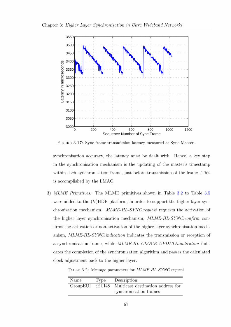
Chapter 3: Higher Layer Synchronisation in Ultra Wideband Networks
0 200 400 600 800 1000 12003000
3050
3100
3150
3200
3250
3300
3350
3400
3450
3500
3550
Sequence Number of Sync Frame
Late
ncy
in m
icro
seco
nds
Figure 3.17: Sync frame transmission latency measured at Sync Master.
synchronisation accuracy, the latency must be dealt with. Hence, a key step
in the synchronisation mechanism is the updating of the master’s timestamp
within each synchronisation frame, just before transmission of the frame. This
is accomplished by the LMAC.
3) MLME Primitives: The MLME primitives shown in Table 3.2 to Table 3.5
were added to the (V)HDR platform, in order to support the higher layer syn-
chronisation mechanism. MLME-HL-SYNC.request requests the activation of
the higher layer synchronisation mechanism, MLME-HL-SYNC.confirm con-
firms the activation or non-activation of the higher layer synchronisation mech-
anism, MLME-HL-SYNC.indication indicates the transmission or reception of
a synchronisation frame, while MLME-HL-CLOCK-UPDATE.indication indi-
cates the completion of the synchronisation algorithm and passes the calculated
clock adjustment back to the higher layer.
Table 3.2: Message parameters for MLME-HL-SYNC.request.
Name Type DescriptionGroupEUI tEUI48 Multicast destination address for
synchronisation frames
67

Chapter 3: Higher Layer Synchronisation in Ultra Wideband Networks
Table 3.3: Message parameters for MLME-HL-SYNC.confirm.
Name Type DescriptioneResultCode MlmeResultCode e Result of the service request
Table 3.4: Message parameters for MLME-HL-SYNC.indication.
Name Type DescriptionGroupEUI tEUI48 Multicast address that was the
destination address for the syn-chronisation frame
SrcEUI tEUI48 Address of the device that sentthe synchronisation frame
SequenceNumber u32 Sequence number of the synchro-nisation frame that was transmit-ted or received
Table 3.5: Message parameters for MLME-HL-CLOCK-UPDATE.indication.
Name Type DescriptionOffset secs u32 Computed clock offset seconds
Offset nsecs u32 Computed clock offsetnanoseconds
OffsetPositive bool Sign of the computed offset
Skew u32 Computed clock skew
3.6.3 Description of Synchronisation Mechanism on the plat-
form
This section uses sequence diagrams to illustrate the higher layer synchronisation
mechanism on the platform for both the sync master or initiator, and the sync slave
or target.
3.6.3.1 Synchronisation Mechanism at the sync master
Fig. 3.18 illustrates the higher layer synchronisation mechanism at the sync master.
The mechanism can be summarised as follows. The user-defined synchronisation inter-
val in milliseconds that is passed as a parameter of the APP-DeviceHigherLevelSync.request
service primitive is converted into units of superframe, SyncInt SF, at the PAL. This
68

Chapter 3: Higher Layer Synchronisation in Ultra Wideband Networks
allows the PAL to determine the transmission time for the next synchronisation frame,
SyncTxTime, by adding this value to the current superframe count, SFn. Thus at the
start of each new superframe, the PAL checks to see if the current superframe count
tallies with the transmission time for the next synchronisation frame. If it tallies, then
a new synchronisation frame is prepared and sent to the MAC layer.Application Layer PAL MAC LayerAPP_DeviceHigherLevelSync_reqCompute SyncInt_SFSet Sync Role as MASTERMLME_MulticastRegister_reqMLME_MulticastRegister_cfmMLME_DRP_reqMLME_HLsync_reqMLME_HLsync_cfmCompute SyncTxTime = SFn + SyncInt_SFMLME_DRP_cfmSFn++If (SFn == SyncTxTime)Read Higher Layer ClockPlace timestamp in new sync frameSyncTxTime = SFn + SyncInt_SFUMAC_Data_req Update timestamp Transmit sync frame REPEATED EVERY SUPERFRAME
MLME_HLsync_indFigure 3.18: Sequence diagram for synchronisation mechanism at the Sync Mas-
ter.
The other primitives in Fig. 3.18 are used as follows. The MLME-MulticastRegister.request
and MLME-MulticastRegister.confirm primitives are for setting up and confirming
69

Chapter 3: Higher Layer Synchronisation in Ultra Wideband Networks
the multicast destination address for the synchronisation frames, while the MLME-
DRP.request and MLME-DRP.confirm primitives are for reserving the MASs for the
synchronisation frames.
3.6.3.2 Synchronisation Mechanism at the sync slave
Fig. 3.19 illustrates the higher layer synchronisation mechanism at the sync slave.
Each time a synchronisation frame is received and the MLME-HL-SYNC.indication
is sent to the PAL, the higher layer clock value corresponding to the reception time is
obtained and paired with the hgiher layer clock value of the master which is contained
in the synchronisation frame. After two pairs are obtained, the linear rate algorithm
computes the offset and skew and passes these back to the higher layer using an
MLME-HL-CLOCK-UPDATE.indication primitive. The offset and skew are used to
update the parameters of the slave’s virtual clock which transforms the hardware clock
to mimic the behaviour of the master’s clock.
The other primitives in Fig. 3.18 are used as follows. The MLME-MABIE.indication
primitive notifies the MAC that a multicast address has been set up, while the MLME-
MulticastActivate.request and MLME-MulticastActivate.confirm primitives are used
for activating the multicast address at the sync slave.
3.6.4 Implementation Results
The implementation of the linear rate algorithm on the platform was validated by
synchronising a target device to the AP initiator. In order to compare the results
from the platform with the OPNET simulation results, the same clock parameters
detailed in Section 3.5.2.1 were used. The results are shown in Fig. 3.20.
The result obtained from the platform is better than the corresponding simulation
result, since the residual clock offset from the platform is about 15 µs less than the
simulation result. This can be directly attributed to the fact that the MAC layer and
the higher layer reside on the same entity. As a result, the MAC is able to obtain
70

Chapter 3: Higher Layer Synchronisation in Ultra Wideband NetworksApplication Layer PAL MAC LayerAPP_DeviceHigherLevelSync_reqCompute SyncInt_SFSet Sync Role as SLAVEMLME_MulticastActivate_reqMLME_MulticastActivate_cfmRxSyncSeqNo++Extract master timestampIf (RxSyncSeqNo > 1)Use algorithm to compute offset and skewREPEATED EVERY TIME SYNC FRAME IS RECEIVEDMLME_MABIE_indMLME_HLsync_indMLME_HLclockupdate_indFigure 3.19: Sequence diagram for synchronisation mechanism at the Sync Slave.
higher layer timestamps directly and update the timestamps in the LMAC just before
the synchronisation frame is transmitted.
3.7 Summary
In this chapter, the application requirements for the synchronisation algorithm have
been extracted from the EUWB project documents [53]–[55]. Based on these require-
ments, we have determined the generic class of algorithms that would be most suitable
for the network. We have selected two existing algorithms from this class and also
proposed a new algorithm for the class. We have determined that the best place for
implementing the algorithm is the MAC layer; hence we have also proposed a method
of transferring the higher layer clock to the MAC layer using empty RTP packets when
the MAC layer does not have direct access to the higher layer clock. We have further
71

Chapter 3: Higher Layer Synchronisation in Ultra Wideband Networks
0 5 10 15 20−20
0
20
40
60
80
100
Time in seconds
Rel
ativ
e C
lock
Offs
et in
mic
rose
cond
s
FPGA PlatformOPNET Simulation
Figure 3.20: Comparison of results from OPNET simulation and (V)HDR FPGAPlatform.
proposed a new MLME primitive for transferring the computed clock parameters back
to the higher layer after synchronisation is complete.
The UWB OPNET models we developed have been described in Section 3.5. The
three candidate algorithms have been implemented in the OPNET simulator, and
we observed that the Continuous Clock and Linear Rate algorithms perform better
than the Delay Time Measurement algorithm since they correct for clock drift and are
therefore able to maintain tighter synchronisation in between synchronisation rounds.
The Linear Rate algorithm is deemed to be the most suitable for the network, therefore
it has been implemented on an FPGA UWB platform developed at TES Electronic
Solutions Ltd. The result obtained from the platform has been compared with the
corresponding OPNET simulations result and the platform result is markedly better.
We attribute this to the fact that the MAC layer is able to obtain the timestamps
directly from the higher layer and also update them as close as possible to the PHY,
just before the synchronisation frames are transmitted.
72

Chapter 4A Sample-Mode PDV Filter for PTP
Synchronisation
4.1 Introduction
In Section 2.3.4, we explored the existing techniques for dealing with PDV, noting
that a combination of techniques may be required in order to achieve a satisfactory
performance. This chapter proposes a new sample-mode PDV filter that combines
PDV filtering with priority tagging of synchronisation traffic.
Research has shown that the success of a particular PDV filtering algorithm depends
on the packet delay distribution of the network being considered. For instance, in [44],
the author showed that the Kalman filtering technique is most useful when the packet
delay distribution is Gaussian. Also, the authors of [9] and [10] demonstrated that the
best PDV filtering algorithm for a lightly-loaded small cross traffic network was the
popular sample-minimum algorithm, since the underlying delay distribution for the
network showed that most of the packets experienced the minimum delay. By similarly
studying the delay distributions of a heavily-loaded cross traffic network and a heavily-
loaded inline traffic network, they showed that the sample-mean and sample-maximum
algorithms, respectively, yielded the best synchronisation performance. Hence, we
theorise that an algorithm based on the mode delay value should at least match the
73

Chapter 4: A Sample-Mode PDV Filter for PTP Synchronisation
performance of the existing algorithms. Furthermore, if the mode delay value does
not coincide with the minimum, mean, or maximum delay in the network, then an
algorithm based on the mode delay value should outperform the other filters.
Therefore in this chapter, we begin by describing two different network topologies in
Section 4.2, before characterising the delay profiles of the networks in Section 4.3.
From the observed delay distributions, we suggest the most likely type of existing
filter that would perform best. In Section 4.4, we describe the proposed iterative
sample-mode PDV filtering technique that selects “good” packets from a mode bin to
achieve synchronisation. The sample-mode PDV filter along with the existing sample-
minimum, sample-maximum, and sample-mean filters are applied to the two networks
using the OPNET network simulator. Simulation results are presented and analysed
in Section 4.5, and a chapter summary is provided in Section 4.6.
4.2 System Models
The first system we consider is a 5-hop network with data-centric background traffic
based on the ITU-T G.8261 Network Traffic Model 2 [36], as illustrated in Fig. 4.1.
Each node generates background traffic that follows the same path as the SYNC
packets. The next node extracts the background traffic and injects new (independent)
traffic along the synchronisation path. In the literature, this type of traffic pattern is
referred to as cross-traffic [10]. QoS was implemented in the model so that the SYNC
packets were transmitted with strict priority queuing at the switch output ports.
We also consider the network scenario depicted by Fig. 4.2, where the background
traffic follows the same path as the synchronisation traffic. This type of traffic, termed
in-line traffic, has practical significance in access aggregation networks such as in
mobile backhaul systems where a network controller provides both timing traffic and
background traffic (such as voice and data) to base stations. We modelled a 16-hop
network in which the size of the packets was uniformly distributed between 64 bytes
and 1500 bytes, which are the minimum and maximum packet sizes for Ethernet,
respectively.
74

Chapter 4: A Sample-Mode PDV Filter for PTP Synchronisation
timing master timing slaveswitch_1 switch_2 switch_5station_1 station_2 station_5
switch_3station_3
switch_4station_4Synchronization trafficBackground traffic
Figure 4.1: 5-hop Network Topology for cross-traffic.timing master timing slaveswitch_1 switch_2 switch_16station_1 station_2Synchronization trafficBackground traffic
Figure 4.2: 16-hop Network Topology for in-line traffic.
Simulation parameters for both networks are shown in Table 4.1.
4.3 Characterisation of Delay Distributions
In order to characterise the delay profile and appreciate the effects of PDV on the
synchronisation performance of the network, the 5-hop cross-traffic and 16-hop inline-
traffic networks described in Section 4.2 were simulated in OPNET for different levels
of background traffic utilisation. For each network, the master node generates a SYNC
packet containing the current master time every synchronisation interval and the slave
75

Chapter 4: A Sample-Mode PDV Filter for PTP Synchronisation
Table 4.1: Simulation parameters for packet delay profiling.
Parameter 5-hop Network 16-hop NetworkDistance between nodes 50 metres 50 metres
Line Rate 100 Mbps 100 Mbps
Number of switches 5 16
Type of traffic Cross Inline
Background traffic model ITU-T G.8261 II 64 - 1500 bytes, uniform
Synchronisation Interval 3.90625 ms 3.90625 ms
Slave skew 2 ppm 2 ppm
node takes a timestamp when it receives the packet. Each SYNC packet is priority-
tagged such that it is transmitted with strict priority queuing at the switch output
ports. For the ith SYNC packet the origin timestamp generated by the master is Mi,
the reception timestamp generated by the slave clock is Si, and the one-way transit
delay d is computed as d = Si−Li, where Li is the slave timestamp corresponding to
the master’s origin timestamp. It is important to note that while Li is easily obtained
via network simulation, it cannot be exactly determined in real-life systems unless the
slave clock is perfectly synchronised with the master’s clock. Thus network simulation
allows an in-depth study of the packet delays, as well as providing the opportunity to
replicate scenarios accurately.
In this section we explore the frequency of occurence of unqueued packets, the packet
delay profiles, and the mean and variance of packet delays, in an attempt to charac-
terise and compare the packet delays in both networks.
4.3.1 Frequency of Occurence of Unqueued Packets
Sample-minimum PDV filtering algorithms make use of the fact that the fastest pack-
ets traverse the network without queuing and do so at an approximately constant
rate. This observation was made during the initial development of the NTP specifica-
tion [67]. The frequency of occurence of such packets give an indication of the amount
of queuing, and hence the amount of PDV, in the network.
76

Chapter 4: A Sample-Mode PDV Filter for PTP Synchronisation
We simulated the 5-hop cross-traffic network using the simulation parameters in Ta-
ble 4.1 and for different levels of background load. For each load level, we measured
the delay of each SYNC packet and calculated the time intervals between the occur-
rences of fastest packets. Then we obtained the average of all the time intervals. In
Fig. 4.3, the average interval between packets that experienced no queuing is shown
for different levels of utilisation in the 5-hop cross traffic network.
0 10 20 30 40 50 60 700
0.5
1
1.5
2
2.5
3
3.5
Network Load (%)
Ave
rage
inte
rval
bet
wee
n fa
stes
t pac
kets
(se
cond
s)
Figure 4.3: Average interval between minimum-delayed packets for a 5-hop crosstraffic network.
From (2.11), 50% is the utilisation level at which there is an average backlog of 1
packet at each intermediate node so this is the point on the graph where there is
a marked increase in the average interval between unqueued packets. At the 70%
utilisation level, the mean backlog is 2.33 so all the packets experience some level of
queuing; thus the average time interval between unqueued packets approaches infinity.
For the 16-hop inline traffic all the packets experience some form of queuing due to the
long cascade of queuing elements, even at low utilisation levels. Hence, the average
time interval between unqueued packets approaches infinity for all utilisation levels.
77

Chapter 4: A Sample-Mode PDV Filter for PTP Synchronisation
4.3.2 Packet Delay Profiles
For both networks simulated, the measured one-way transit delays were used to gener-
ate experimental Probability Distribution Functions (PDFs). Fig. 4.4 shows the delay
distribution for the 5-hop cross traffic network at different levels of background traffic
utilisation. At low loads (typically less than 45%), most of the packets experienced
no queuing in the network, as evidenced by the very strong modes at the minimum
delay value. As the load increased, the minimum packet delay through the network
remained constant but the probability of finding a packet with this minimum delay
decreased due to the increased probability of queuing at one or more switches. In
fact, the PDFs at higher loads have well-defined shapes and can be fitted to Erlang
density distributions.
0 100 200 300 400 500 600 7000
0.002
0.004
0.006
0.008
0.01
0.012
0.014
0.016
0.018
0.02
Sync Packet Delay in microseconds
PD
F
80% Load − Experimental80% Load − Theoretical, Erlang (0.0309, 9)60% Load − Experimental60% Load − Theoretical, Erlang (0.0214, 5)40% Load − Experimental20% Load − Experimental
Figure 4.4: Packet Delay Distribution for a 5-hop cross traffic network.
For the inline traffic network at 20% load level, the delay PDF in this network can
again be fitted to a theoretical Erlang PDF, as depicted in Fig. 4.5; however, none
of the packets experience the minimum delay due to the long chain of queuing ele-
ments in the network. As the load increases, most of the packets tend to experience
78
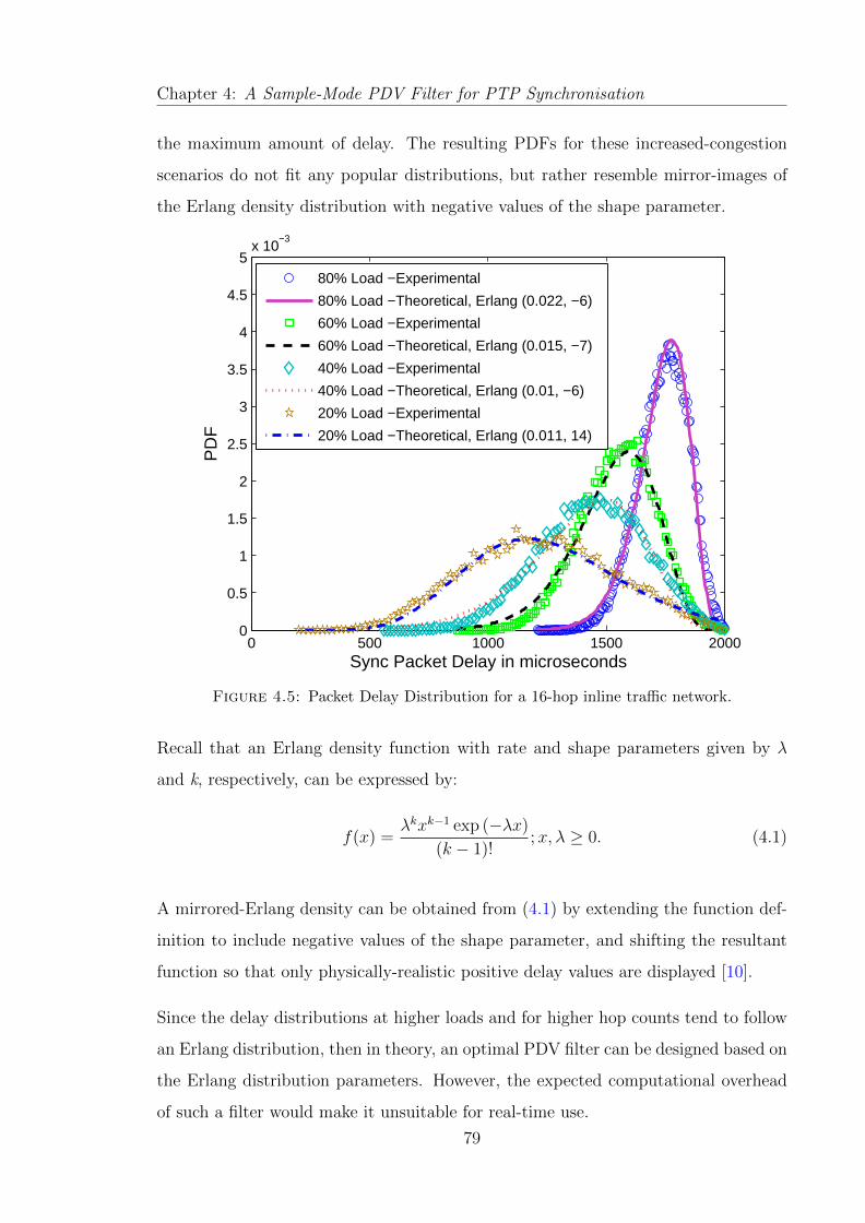
Chapter 4: A Sample-Mode PDV Filter for PTP Synchronisation
the maximum amount of delay. The resulting PDFs for these increased-congestion
scenarios do not fit any popular distributions, but rather resemble mirror-images of
the Erlang density distribution with negative values of the shape parameter.
0 500 1000 1500 20000
0.5
1
1.5
2
2.5
3
3.5
4
4.5
5x 10
−3
Sync Packet Delay in microseconds
PD
F
80% Load −Experimental
80% Load −Theoretical, Erlang (0.022, −6)
60% Load −Experimental
60% Load −Theoretical, Erlang (0.015, −7)
40% Load −Experimental
40% Load −Theoretical, Erlang (0.01, −6)
20% Load −Experimental
20% Load −Theoretical, Erlang (0.011, 14)
Figure 4.5: Packet Delay Distribution for a 16-hop inline traffic network.
Recall that an Erlang density function with rate and shape parameters given by λ
and k, respectively, can be expressed by:
f(x) =λkxk−1 exp (−λx)
(k − 1)!;x, λ ≥ 0. (4.1)
A mirrored-Erlang density can be obtained from (4.1) by extending the function def-
inition to include negative values of the shape parameter, and shifting the resultant
function so that only physically-realistic positive delay values are displayed [10].
Since the delay distributions at higher loads and for higher hop counts tend to follow
an Erlang distribution, then in theory, an optimal PDV filter can be designed based on
the Erlang distribution parameters. However, the expected computational overhead
of such a filter would make it unsuitable for real-time use.
79

Chapter 4: A Sample-Mode PDV Filter for PTP Synchronisation
Inspection of the delay profiles in Fig. 4.4 suggests that the low load scenarios are
amenable to sample-minimum filtering, while the higher load scenarios might benefit
from sample-mean filtering. Inspection of the shapes of the delay profiles in Fig. 4.5
suggests that none of the scenarios would also be amenable to sample-minimum filter-
ing. Sample-maximum filtering might benefit the 80% load scenario, while the other
load scenarios might benefit from sample-mean filtering.
4.3.3 Variance and Average Delays
As a further analysis of the impact of the network load on the packet delay, we
present the mean and variance of the delays in Fig. 4.6 and Fig. 4.7, respectively. We
simulated the 5-hop cross-traffic and 16-hop inline traffic networks using the simulation
parameters in Table 4.1 and for different levels of background load. For each load level,
we measured the delay of each SYNC packet and calculated the mean and variance
of the delays. As expected, the mean packet delay increases with the level of traffic
utilisation for both networks; however the cross-traffic network exhibits a more obvious
linear relationship.
A more interesting result is observed for the variance. For smaller (low hop count)
networks at low loads, the variance is low because most of the packets experience
little or no queuing. As the load increases, the variance increases slightly to reflect
the increased amount of queuing. The converse is true for larger networks. In these
networks the probability of finding a packet that experiences no queuing is statistically
small, even at low load levels; hence the variance is high. However, as the load
increases most packets tend to experience the maximum delay. Hence, the variance
has an inverse relationship with the network load level.
4.4 Proposed Sample-Mode Algorithm
In this section, we describe the rationale behind the idea of the proposed sample-
mode filter and postulate as to why it might yield a better performance than existing
80
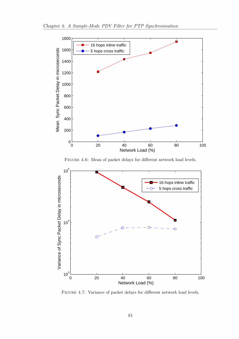
Chapter 4: A Sample-Mode PDV Filter for PTP Synchronisation
0 20 40 60 80 1000
200
400
600
800
1000
1200
1400
1600
1800
Network Load (%)
Mea
n S
ync
Pac
ket D
elay
in m
icro
seco
nds
16 hops inline traffic
5 hops cross traffic
Figure 4.6: Mean of packet delays for different network load levels.
0 20 40 60 80 10010
3
104
105
Network Load (%)
Var
ianc
e of
Syn
c P
acke
t Del
ay in
mic
rose
cond
s
16 hops inline traffic
5 hops cross traffic
Figure 4.7: Variance of packet delays for different network load levels.
81

Chapter 4: A Sample-Mode PDV Filter for PTP Synchronisation
algorithms in the packet-filtering category of PDV filters. We then describe the two
components of the algorithm; namely, the RCF Estimator and the Offset Corrector.
4.4.1 Rationale
As described in Section 2.3.4, the packet-filtering category of PDV algorithms tend to
group the arriving synchronisation traffic into several non-overlapping windows and
then select “good” packet(s) from each window. Three main algorithms have been
considered in the category, namely sample minimum, sample maximum and sample
mean algorithms.
Given a window with W SYNC packets, master origin timestamp Mi, slave reception
timestamp Si, and packet delay delta value δi = Si−Mi for the ith packet (0 < i ≤ W ),
a sample-minimum filter defines a good packet as one which satisfies the following:
δi ≤ δmin + α. (4.2)
Similarly, a good packet for a sample-maximum filter is one with:
δi ≥ δmax − α. (4.3)
For a sample-mean filter, a good packet would satisfy:
(δmean − α/2) ≤ δi ≤ (δmean + α/2) (4.4)
where δmin, δmax, and δmean are the minimum, maximum, and mean, respectively, of
all W δi samples in the window, and the threshold value α depends on the desired
accuracy.
For this category of algorithms, the success of the PDV filtering depends on the proba-
bility of finding “good” packets among a sequence of arriving packets within a window.
Regardless of the actual magnitude of the delay, all packets selected as “good” pack-
ets must have experienced a similar amount of delay. Thus if the distribution of the
82

Chapter 4: A Sample-Mode PDV Filter for PTP Synchronisation
delay is known a-priori, then the best filter to use is the one which matches the delay
distribution, thus maximising the chances of finding good packets. However, if the
delay distribution does not quite match up with any of the filters, then the residual
clock offset after synchronisation might be greater than desired.
Since all “good” packets must have experienced a similar amount of delay, it goes
without saying that the chances of finding “good” packets can be maximised by se-
lecting packets from around the mode. The rationale behind this approach is that
when the delay distribution does not quite match up with any of the existing filters,
the sample mode will yield the largest number of good packets. Thus the sample mode
filter should give a good fit for all traffic distributions, with a relatively low computa-
tional overhead. Therefore, we define a sample-mode filter as one which selects good
packets based on
(δmode − α/2) ≤ δi ≤ (δmode + α/2) (4.5)
where δmode is the centre δi value at the mode bin and the threshold value α represents
the bin width.
4.4.2 Determining the Mode
Consider the ith SYNC packet received by the slave. If the slave clock is perfectly
synchronised to the master, the difference between the reception and origin times-
tamps for each SYNC packet δi = Si −Mi will be equal to the end-to-end delay di
experienced by each packet. However, if the clocks have a non-zero skew σ, then δi
will also include an accumulated offset, as shown in (4.6).
δi = di + (Mi + di)σ. (4.6)
This accumulated offset (Mi + di)σ causes δi to gradually increase or decrease over
time, depending on whether the slave clock runs faster or slower than the master
clock.
83

Chapter 4: A Sample-Mode PDV Filter for PTP Synchronisation
Before determining the mode bin, the total number of bins Nbins is determined using
Nbins =δmax − δmin
α; (4.7)
where α is the width of each bin.
Then for each ith sample, the bin number bi : (0 ≤ bi < Nbins) is computed as
bi = b(δi − δmin
α)c. (4.8)
Finally, the mode bin is selected as the one with the largest number of samples.
4.4.3 RCF Estimator
The first step in our sample mode PDV filter algorithm is the computation of the
RCF. This RCF is used to correct for the relative clock skew at the slave with respect
to the master clock. After the first computation of the RCF, subsequent computations
are done for every frequency synchronisation interval, rather than for every iteration.
This is due to the well-known fact that changes in clock rates are usually caused
by aging of the oscillators or temperature changes, and as such they tend to occur
extremely slowly. In fact, if the maximum clock drift rate ρmax is known, then the
frequency synchronisation interval f can be estimated from the target synchronisation
accuracy η as follows:
f =η
2ρmax
. (4.9)
In our previous work [68], we showed that the RCF could be calculated using the
largest origin timestamp Mmax, least origin timestamp Mmin, largest reception times-
tamp Smax, and least reception timestamp Smin within the mode bin as follows:
RCF =Smax − Smin
Mmax −Mmin
. (4.10)
84
Chapter 4: A Sample-Mode PDV Filter for PTP Synchronisation
For an accurate computation of RCF using (4.10), the packets received by the slave at
timestamps Smax and Smin must have experienced the same delay in the network. In
Appendix A, we prove that it is possible for packets that experienced different delays
to end up in the same bin. If this happens within the mode bin, the RCF computed
using (4.10) will not accurately reflect the actual amount of skew between the master
and slave. Conversely, it is also possible for packets that experienced the same delay
to end up in different bins, as shown in Appendix B. If similarly-delayed packets are
in separate bins, then it might be better to utilise all the samples within a window
when computing the RCF, rather than selected samples from the mode bin. Thus, we
have explored other algorithms for correcting the skew.
4.4.3.1 Paxson’s Algorithm
Paxson’s algorithm [69], [70] was designed to remove clock skew from a set of path
delay measurements. The W δi are partitioned into√W segments, and the minimum
delay measurement from each segment is selected. The selected measurements are
referred to as the “de-noised” OTTs. The slopes of all possible pairs of the “de-
noised” OTTs are computed, and the median slope is selected. If the median slope
is negative, the algorithm assumes that the skew is negative. On the other hand, if
the median slope is positive, a positive skew is assumed. A cumulative minima test is
then performed to see if the number of cumulative minima is large enough to indicate
that the sign of the skew is probabilistically likely. If the test is successful, the median
slope is output as the skew estimate; otherwise the algorithm outputs a skew of zero.
4.4.3.2 Linear Programming
The method of [15] can be used to formulate a linear programming problem from
(4.6). Assuming that δi = δi − δ1 and Mi = Mi −M1, then from (4.6):
δi = (di − d1)(1 + σ) + Miσ. (4.11)
85

Chapter 4: A Sample-Mode PDV Filter for PTP Synchronisation
Using the relation µ = 1 + σ, (4.11) can be re-written as (4.12), where dri = µdi
represents the end-to-end delay of the ith packet measured at the slave.
δi = (dri − dr1) + Mi(µ− 1). (4.12)
From (4.12), δi differs from dri by Mi(µ−1) minus a constant dr1 . If µ > 1, Mi(µ−1)
grows linearly with Mi and δi gets larger. If µ is the estimate of µ or RCF and dri
and dr1 are the estimates of dri and dr1 , respectively, then (4.13) can be obtained from
(4.12).
dri = δi − Mi(µ− 1) + dr1 . (4.13)
The goal is to estimate µ, given δi and Mi. Since the delay dri must always be positive,
the linear programming problem can be formulated as:
δi − Mi(µ− 1) + dr1 ≥ 0, 1 ≤ i ≤ W. (4.14)
The corresponding objective function is stated as:
min {W∑i=1
(δi − Mi(µ− 1) + dr1)}. (4.15)
It is important to note that once µ and dr1 are obtained, the resulting estimated end-
to-end delay of dri calculated as (δi−Mi(µ−1)+ dr1 will be greater than zero, instead
of being greater than mini dri . Thus, dr1 is actually an estimate of (dr1 + mini dri)
and (δi − Mi(µ− 1) + dr1) is actually the variable portion of the end-to-end delay or
the PDV. Hence, the linear programming algorithm tries to minimise the sum of the
PDV.
4.4.3.3 Linear Regression
The standard linear regression technique can also be used for fitting a line to the set
of δi and Mi values. For skew estimation, the linear regression algorithm computes
86

Chapter 4: A Sample-Mode PDV Filter for PTP Synchronisation
estimates of µ and dr1 that minimise the mean square error e in:
W∑i=1
{δi − Mi(µ− 1) + dr1}2. (4.16)
4.4.3.4 “De-noised” Linear Programming
We propose a new algorithm that combines the methods of [69] and [15]. We partition
the W δi samples into Z segments, where Z =√W , and the minimum delay mea-
surement from each segment is selected in order to obtain the “de-noised” values δdeni
and Mdeni. Following through the steps in Section 4.4.3.2, we formulate the linear
programming problem as:
δdeni− Mdeni
(µ− 1) + dr1 ≥ 0, 1 ≤ i ≤ Z. (4.17)
The corresponding objective function is stated as:
min {Z∑i=1
(δdeni− Mdeni
(µ− 1) + dr1)}. (4.18)
4.4.4 Offset Corrector
Once the RCF has been computed, subsequent iterations attempt to reduce the clock
offset between the master and the slave by selecting packets from within the mode bin.
The offset corrector also incorporates an optional feedback mechanism for ensuring
that an optimum number of packets are available within the mode bin.
A packet selection rate is computed as the quotient of the number of packets in
the mode bin and the window size W, and then compared with a packet selection
threshold. If the selection rate exceeds the threshold level, the window size can be
reduced. If no packet is found within the mode bin after increasing the window size
to the maximum, the slave sends a management message to halve the synchronisation
interval at the master.
87

Chapter 4: A Sample-Mode PDV Filter for PTP Synchronisation
4.5 Simulations and Results
To determine the best skew-estimation algorithm, we used OPNET to simulate the
5-hop cross traffic network depicted in Fig. 4.1, using the simulation parameters in
Table 4.2. The three existing skew-estimation algorithms previously described were
implemented, as well as our new “de-noised” linear programming algorithm.
Table 4.2: Simulation parameters for RCF estimation.
Parameter ValueDistance between nodes 50 metres
Line Rate 100 Mbps
Number of switches 5
Type of traffic Cross
Background traffic model ITU-T G.8261 II
Synchronisation Interval 976.5625 µs
Slave skew 2 ppm
Window Size 10000 samples
Fig. 4.8 shows the residual error after RCF estimation, using the different algorithms.
The linear regression algorithm gives unpredictable results because it is not robust in
the presence of outliers. Furthermore, it is only optimal if the network delays have
a normal distribution. Paxson’s algorithm is accurate at low levels of load, where it
is possible to find minimum-delayed packets. Since the linear programming objective
function aims to minimise the sum of the varible delays, the algorithm works well for
low levels of PDV. Combining linear programming with “de-noising” yields the best
performance, since “de-noising” gets rid of excess PDV.
The typical network load in real network is 40 - 50%. Both Paxson’s algorithm and
linear programming yield a low estimation error up to this point. By combining
Paxson’s de-noising technique with linear programming, we are able to obtain a good
skew estimation at 60
We also compared the performance of the proposed sample-mode with those of the
existing filters, by simulating the networks depicted in Fig. 4.1 and Fig. 4.2, using the
simulation parameters in Table 4.3. In Fig. 4.9, we compare the results obtained from
88
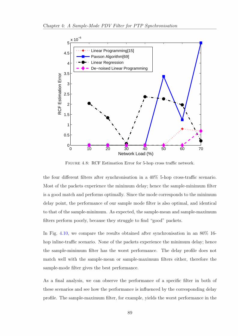
Chapter 4: A Sample-Mode PDV Filter for PTP Synchronisation
0 10 20 30 40 50 60 700
0.5
1
1.5
2
2.5
3
3.5
4
4.5
5x 10
−6
Network Load (%)
RC
F E
stim
atio
n E
rror
Linear Programming[15]
Paxson Algorithm[69]
Linear Regression
De−noised Linear Programming
Figure 4.8: RCF Estimation Error for 5-hop cross traffic network.
the four different filters after synchronisation in a 40% 5-hop cross-traffic scenario.
Most of the packets experience the minimum delay; hence the sample-minimum filter
is a good match and performs optimally. Since the mode corresponds to the minimum
delay point, the performance of our sample mode filter is also optimal, and identical
to that of the sample-minimum. As expected, the sample-mean and sample-maximum
filters perform poorly, because they struggle to find “good” packets.
In Fig. 4.10, we compare the results obtained after synchronisation in an 80% 16-
hop inline-traffic scenario. None of the packets experience the minimum delay; hence
the sample-minimum filter has the worst performance. The delay profile does not
match well with the sample-mean or sample-maximum filters either, therefore the
sample-mode filter gives the best performance.
As a final analysis, we can observe the performance of a specific filter in both of
these scenarios and see how the performance is influenced by the corresponding delay
profile. The sample-maximum filter, for example, yields the worst performance in the
89

Chapter 4: A Sample-Mode PDV Filter for PTP Synchronisation
Table 4.3: Simulation parameters for filter comparison.
Parameter 5-hop Network 16-hop NetworkDistance between nodes 50 metres 50 metres
Line Rate 100 Mbps 100 Mbps
Number of switches 5 16
Type of traffic Cross Inline
Background traffic model ITU-T G.8261 II 64 - 1500 bytes, uniform
Synchronisation Interval 976.5625 µs 976.5625 µs
Window Size 500 samples 500 samples
Threshold α 0.2 µs 0.2µs
Residual Offset at the slave afterfirst RCF estimation
0.03 ppm 0.03 ppm
6 8 10 12 14 16 18 20−5
0
5
10
15
20
25
30
35
40
45
50
Sample Maximum[10]Sample Mean[10]Sample Minimum[9]Sample Mode
Figure 4.9: Relative clock offset for 5-hop cross traffic network at 40% load.
first scenario, as most packets experience the minimum delay. On the other hand, it
performs better than both the sample-minimum and sample-mean filters in the larger
heavier-loaded network scenario which has higher levels of queuing. The converse is
true for the sample-minimum filter.
90

Chapter 4: A Sample-Mode PDV Filter for PTP Synchronisation
16 18 20 22 24 26 28
0
10
20
30
40
50
60
70
80
Sample Maximum[10]Sample Mean[10]Sample Minimum[9]Sample Mode
Figure 4.10: Relative clock offset for 16-hop inline traffic network at 80% load.
4.6 Summary
In this chapter, we have characterised the IEEE 1588 PTP SYNC packet delay pro-
files for a small cross-traffic network and a large in-line traffic network with different
levels of background traffic and observed from the shape of the distributions that
the existing sample-minimum, sample-maximum, and sample-mean filters perform
sub-optimally for some of the load levels in these scenarios. A new skew-estimation
algorithm has been proposed, by utilising some features of two existing algorithms.
This skew-estimation algorithm forms the basis of a low-computation sample-mode
filtering algorithm which selects packets from the mode bin and uses these “good”
packets to achieve synchronisation. Numerical simulations have shown that when the
delay profile is a good match for an existing filter, the sample-mode filter performs as
well as the existing filter. When the delay profile is not a good match for an existing
filter, the sample-mode filter outperforms the existing filters.
91

Chapter 5An Alternate Master Technique for Dealing
with PTP Master Failures
5.1 Introduction
In Section 2.4.2, we explored the existing techniques for dealing with master failures
in PTP, describing the drawback(s) of each technique and noting that the suitability
of a particular technique depends on the specific application or scenario. This chapter
proposes a new alternate master cluster inspired by the optional alternate master and
grandmaster cluster features of the PTP standard, as well as a new alternative BMCA
that reduces both the downtime caused by a master failure and the amount of offset
in the re-synchronisation phase.
In this chapter, we first of all describe the system model for our application scenario
and show why the existing techniques are unsuitable. The alternate master cluster is
described in detail, along with the necessary modifications to the basic PTP algorithm.
The new alternative BMCA is also described. Results from simulating the alternate
master cluster in OPNET are presented and analysed, and conclusions are drawn.
92
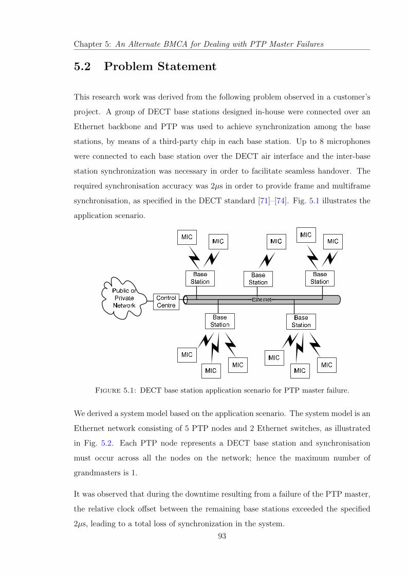
Chapter 5: An Alternate BMCA for Dealing with PTP Master Failures
5.2 Problem Statement
This research work was derived from the following problem observed in a customer’s
project. A group of DECT base stations designed in-house were connected over an
Ethernet backbone and PTP was used to achieve synchronization among the base
stations, by means of a third-party chip in each base station. Up to 8 microphones
were connected to each base station over the DECT air interface and the inter-base
station synchronization was necessary in order to facilitate seamless handover. The
required synchronisation accuracy was 2µs in order to provide frame and multiframe
synchronisation, as specified in the DECT standard [71]–[74]. Fig. 5.1 illustrates the
application scenario.
EthernetBase Station Base Station Base StationBase Station Base StationPublic or Private Network Control Centre MIC MIC MIC MIC MIC MICMIC MIC MIC MIC MIC
Figure 5.1: DECT base station application scenario for PTP master failure.
We derived a system model based on the application scenario. The system model is an
Ethernet network consisting of 5 PTP nodes and 2 Ethernet switches, as illustrated
in Fig. 5.2. Each PTP node represents a DECT base station and synchronisation
must occur across all the nodes on the network; hence the maximum number of
grandmasters is 1.
It was observed that during the downtime resulting from a failure of the PTP master,
the relative clock offset between the remaining base stations exceeded the specified
2µs, leading to a total loss of synchronization in the system.
93

Chapter 5: An Alternate BMCA for Dealing with PTP Master Failures
AM_2 AM_3switch_1 switch_2SO_1 SO_2AM_1
Figure 5.2: System model for PTP master redundancy.
5.3 Motivation
The motivation for the proposed alternate master cluster and alternate BMCA is
that none of the existing techniques described in Section 2.4.2 are suitable for the
application scenario under consideration. In the grandmaster cluster technique, the
other grandmaster nodes that are not currently in the MASTER state must be in
the PASSIVE state; hence the nodes in the cluster do not synchronise to each other.
The drawback of the democratic master group technique is that it requires an entirely
new type of device, the master group speaker, which must also support the demo-
cratic algorithm in addition to PTP. Furthermore, the master group speaker becomes
a single point of failure in the system. The ITU-T telecoms profile is complex and
therefore costly as it utilises multiple clocks at each slave node, and it only provides
frequency synchronisation. The technique proposed by [52] is targeted at a system
architecture in which it is possible for the grandmaster clocks to use the same oscil-
lator, whilst remaining isolated via separate Virtual Local Area Networks (VLANs).
This is markedly different from the system model in Fig. 5.2 where each base station
has its own clock and oscillator. Finally, the alternate master technique is promising
since it is a good fit for the system model and offers a reduction in the length of the
re-synchronisation phase. However, it has no effect on the master failure detection
94

Chapter 5: An Alternate BMCA for Dealing with PTP Master Failures
time and the new master election time. Hence, our proposed alternate master cluster
technique borrows the cluster feature from the grandmaster cluster technique which
is capable of decreasing the lengths of the detection and election phases and combines
it with the alternate master feature, in order to reduce the lengths of the detection,
election, and re-synchronisation phases after a master failure. In addition, we also
devise an alternative BMCA based on a unique ranking algorithm.
5.4 The Alternative Best Master Clock Algorithm
Fig. 5.3 shows the alternative BMCA developed for the alternate master cluster tech-
nique. Just like the default BMCA, the alternative BMCA is run once every announ-
ceInterval and uses the same state decision algorithm.
The difference between the new BMCA and the default BMCA is that a new attribute,
scaledLogRank, has been added to the top of the flowchart for the clock comparison
algorithm . We define the scaledLogRank attribute of a node as an unsigned integer
between 1 and 254 that gives an indication of the availability of the node. The lowest
value of scaledLogRank represents the node with the highest availability, while the
highest value represents the node with the lowest availability. If the two nodes under
comparison have the same scaledLogRank value, then the alternative BMCA reverts
to the default BMCA.
5.5 The Alternate Master Cluster Technique
The proposed alternate master cluster consists of 2 to 5 alternate masters that are
capable of exchanging unicast queryAnnounce messages with each other. Each cluster
member is configured with a lower priority1 value than the non-cluster members so
that as long as there is a functional node in the cluster, the best master clock will
always be selected from within the cluster. A node that is not operating in the
DISABLED, FAULTY or INITIALIZING states is deemed to be functional. Unlike
95

Chapter 5: An Alternate BMCA for Dealing with PTP Master FailuresCompare dataset A to BGM Identity of A = GM Identity of BCompare scaledLogRank values of A and BCompare GM priority1 values of A and BCompare GM class values of A and BCompare GM accuracy values of A and BCompare GM offsetScaledLogVariancevalues of A and BCompare GM priority2 values of A and BCompare GM identity values of A and BReturnB better than A ReturnA better than B
Go to algorithm forcomparison of data setsfrom the same GMA = BA > BA > BA > BA > BA > BA > BA > B
A < BA < BA < BA < BA < BA < BA < B
A = BA = BA = BA = BA = B
YESNO
Figure 5.3: Alternative BMCA for alternate master cluster.
the grandmaster cluster technique described in the PTP standard, functional alternate
masters that are not currently in the MASTER state operate in the SLAVE state
96

Chapter 5: An Alternate BMCA for Dealing with PTP Master Failures
rather than the PASSIVE state, so that synchronisation can also occur within the
cluster. For the sake of simplicity, the following types of nodes are defined in this
work:
• Master Node: A member of the alternate master cluster that is currently
operating in the MASTER state. This is the best clock in the domain.
• Alternate Master Node: A member of the alternate master cluster that is
currently operating in the SLAVE state.
• Slave Node: Any other node in the network that is not part of the alternate
master cluster. Slave nodes cannot operate in the MASTER state unless all the
clocks in the cluster are non-functional.
This section describes the operation of the alternate master cluster as well as the
operation of the rest of the domain outside the cluster.
5.5.1 Operation of the Alternate Master Cluster
The master node and alternate master node(s) make up the alternate master cluster.
Within the alternate master cluster, nodes exchange unicast queryAnnounce mes-
sages and transmit alternateMulticastSync messages. The queryAnnounce messages
are used to compute a scaledRank for each cluster member, while the alternateMul-
ticastSync messages are used to provide origin and reception timestamps so that
re-synchronisation to a new master will be quicker if the current master fails.
In this section, we describe the attributes necessary for the functionality of the alter-
nate master cluster, the behaviour of the cluster members at initialisation, as well as
the messages transmitted by the cluster members. We also highlight the response of
the cluster members to different types of received messages, and show how the cluster
members are ranked.
97
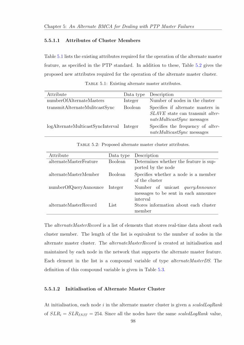
Chapter 5: An Alternate BMCA for Dealing with PTP Master Failures
5.5.1.1 Attributes of Cluster Members
Table 5.1 lists the existing attributes required for the operation of the alternate master
feature, as specified in the PTP standard. In addition to these, Table 5.2 gives the
proposed new attributes required for the operation of the alternate master cluster.
Table 5.1: Existing alternate master attributes.
Attribute Data type DescriptionnumberOfAlternateMasters Integer Number of nodes in the cluster
transmitAlternateMulitcastSync Boolean Specifies if alternate masters inSLAVE state can transmit alter-nateMulticastSync messages
logAlternateMulticastSyncInterval Integer Specifies the frequency of alter-nateMulticastSync messages
Table 5.2: Proposed alternate master cluster attributes.
Attribute Data type DescriptionalternateMasterFeature Boolean Determines whether the feature is sup-
ported by the node
alternateMasterMember Boolean Specifies whether a node is a memberof the cluster
numberOfQueryAnnounce Integer Number of unicast queryAnnouncemessages to be sent in each announceinterval
alternateMasterRecord List Stores information about each clustermember
The alternateMasterRecord is a list of elements that stores real-time data about each
cluster member. The length of the list is equivalent to the number of nodes in the
alternate master cluster. The alternateMasterRecord is created at initialisation and
maintained by each node in the network that supports the alternate master feature.
Each element in the list is a compound variable of type alternateMasterDS. The
definition of this compound variable is given in Table 5.3.
5.5.1.2 Initialisation of Alternate Master Cluster
At initialisation, each node i in the alternate master cluster is given a scaledLogRank
of SLRi = SLRINIT = 254. Since all the nodes have the same scaledLogRank value,
98

Chapter 5: An Alternate BMCA for Dealing with PTP Master Failures
Table 5.3: Definition of struct alternateMasterDS.
Member Data type DescriptionalternateMasterPortIdentity PortIdentity Identity of alternate master
cluster member
alternateMasterMacAddress EUI48 MAC address of alternate mas-ter cluster member
u16AnnounceSequenceId Integer Sequence ID of most recent an-nounce message
u16NoQueryAnnounceReceived Integer Number of unicast queryAn-nounce messages received incurrent announce interval
sSyncOriginTimestamp Timestamp Origin timestamp of most re-cently received alternateMulti-castSync message
sSyncReceptionTimestamp Timestamp Reception timestamp of mostrecently received alternate-MulticastSync message
dfIRankYou Double Rank of this cluster member ascomputed by node
dfYouRankMe Double Rank of node as computed bythis cluster member
boIsMaster Boolean Specifies if this cluster memberis the current master node
the alternative BMCA described in Section 5.4 reverts to the default BMCA described
in Section 2.4.1.4 and the node with the lowest priority1 value is elected as the best
master.
Once the best master has been elected, all the alternate master nodes achieve syn-
chronisation with it. Subsequently, each alternate master node transmits multicast
ANNOUNCE messages with the alternateMasterFlag set to TRUE. Whenever an
alternate master node receives a multicast ANNOUNCE message with the alter-
nateMasterFlag set to TRUE, it creates a new alternateMasterDS data set for the
source node (if one does not already exist) and adds this to its alternateMasterRecord.
Each alternate master node also creates a data set for the master node and adds it to
its alternateMasterRecord. This is how the entries in the alternateMasterRecord list
are built.
99

Chapter 5: An Alternate BMCA for Dealing with PTP Master Failures
5.5.1.3 Message Transmission within the Alternate Master Cluster
The master node multicasts ANNOUNCE messages and SYNC messages as usual,
based on the specified announceInterval and syncInterval in the domain. It also sends
DELAY RESP messages, as usual, in response to DELAY REQ messages sent by non-
master nodes. The only additional transmissions by the master node are the unicast
queryAnnounce messages it sends to the alternate master nodes. The frequency of the
unicast messages is always greater than that of the regular multicast ANNOUNCE
messages, but they have the same packet structure. All transmissions from the master
node have the alternateMasterFlag set to FALSE in the flagField of the message
header, thus indicating that it is in the MASTER state.
Alternate master nodes multicast ANNOUNCE messages to the entire network and
if transmitAlternateMulitcastSync is enabled, then they also multicast SYNC mes-
sages, but with reduced frequency. Additionally, alternate master nodes send unicast
queryAnnounce messages to the other cluster members including the master node.
All transmissions from an alternate master node have the alternateMasterFlag set to
TRUE, thus indicating that it is not in the MASTER state.
5.5.1.4 Message Reception within the Alternate Master Cluster
Within the alternate master cluster, DELAY REQ and DELAY RESP are handled
exactly as described in the PTP standard; however the procedures for SYNC, AN-
NOUNCE, and queryAnnounce messages are handled slightly differently.
• SYNC Messages: The procedure is described in Fig. 5.4. The message is
discarded if the recipient is the master node or if the sender is not a member of
the cluster. Otherwise, the recipient uses the message for synchronisation if the
sender is the master node or updates the alternateMasterRecord if the sender is
an alternate master node.
100

Chapter 5: An Alternate BMCA for Dealing with PTP Master Failures
Figure 5.4: Flowchart for handling received SYNC messages in the alternatemaster cluster.
• ANNOUNCE Messages: If the recipient has already received a queryAn-
nounce from the same sender, the ANNOUNCE message is discarded. Other-
wise if the message is from an alternate master cluster member, a new entry is
created in the alternateMasterRecord. The procedure is shown in Fig. 5.5.
Figure 5.5: Flowchart for handling received ANNOUNCE messages in the alter-nate master cluster.
• queryAnnounce Messages: Upon receipt of a queryAnnounce message, an al-
ternate master cluster member computes a rank iRankYou for the sender. It also
101

Chapter 5: An Alternate BMCA for Dealing with PTP Master Failures
extracts its own rank, youRankMe, as computed by the sender. The iRankYou
and youRankMe values are stored in the alternateMasterDS data set for the
entry corresponding to the sender in the alternateMasterRecord. It transmits
the calculated iRankYou as part of the next queryAnnounce message it sends to
the sender. At the end of its announceInterval, it uses all the youRankMe values
it received from the cluster members, to compute its own rank. The ranking
procedure is described in Section 5.5.1.5.
5.5.1.5 Ranking within the Alternate Master Cluster
The aim of transmitting unicast queryAnnounce messages within the cluster is to
allow the cluster members to be ranked, based on their availability or reliability.
numberOfQueryAnnounce defines the number of queryAnnounce messages within an
announceInterval. Hence, the interval between consecutive unicast messages can be
computed as
queryAnnounceInterval =announceInterval
numberOfQueryAnnounce. (5.1)
Each cluster member maintains a running total of the number of queryAnnounce
messages it receives within an announceInterval from the other nodes within the
cluster. Each time a cluster member receives a queryAnnounce message, it computes
a rank iRankYou for the node who sent the message. This rank essentially compares
the actual number of received queryAnnounce messages at a specific time with the
number of messages that should have been received at that time. Assuming that the
current announceInterval expires at time tex and node i has received nj queryAnnounce
messages from node j at the current time tcur, the number of messages that should
have been received at tcur is given by
Nexp =
⌈numberOfQueryAnnounce− (
(tex − tcur)queryAnnounceInterval
)
⌉. (5.2)
102

Chapter 5: An Alternate BMCA for Dealing with PTP Master Failures
The iRankYou value for j as computed by i is
Rij =nj
Nexp
. (5.3)
Once every announceInterval, node j uses the most recent youRankMe values it has
received from the other cluster members to calculate a rank myRank for itself. It is
important to note that the iRankYou value for j as computed by i is identical to the
youRankMe value received by j from i.
If there are Nc nodes in the cluster, myRank for node j is given by
Rj =
Nc−1∑i=0i 6=j
Rij
Nc
. (5.4)
The computed ranks Rij and Rj are floating point values. We use a scaled log function
to transform these floating point values into 8-bit integers. Given any rank value R,
the corresponding scaledLogRank value SLR is given by
SLR = 1− (⌈24 ∗ log2R
⌉). (5.5)
SLRij is transmitted as part of the next unicast queryAnnounce message sent to node
j from i. The shaded reserved field of the message header is used for this purpose, as
shown in Fig. 5.6. The computed myRank value SLRj is transmitted in subsequent
queryAnnounce and ANNOUNCE messages transmitted by node j using the reserved
field of the message body, as shown in Fig. 5.7.
5.5.1.6 Master Failure Behaviour within the Cluster
When the master node fails, it stops transmitting messages. Instead of using the
ANNOUNCE RECEIPT TIMEOUT timer, our master cluster technique shortens the
detection phase to a maximum of 1.5 times the announceInterval. An alternate master
node concludes that the master node has failed if 50% or more of its queryAnnounce
103

Chapter 5: An Alternate BMCA for Dealing with PTP Master Failures
Figure 5.6: Message header field for transmitting IRankYou.
Figure 5.7: Message body field for transmitting myRank.
messages and its ANNOUNCE message were not received or if 75% or more of its
queryAnnounce message were not received in an announceInterval.
A new master is elected from the cluster within another announceInterval, and re-
synchronisation occurs within a further syncInterval since the origin and reception
timestamps for a SYNC message from the new master are already available.
104

Chapter 5: An Alternate BMCA for Dealing with PTP Master Failures
5.5.2 Operation of the Non-Cluster Members
For the best performance of the alternate master cluster technique, the slave nodes
outside the cluster must be configured with higher priority1 values than the cluster
members. In addition, the scaledLogRank value of each slave node must be set to
the maximum value of 254, since these nodes do not take part in the ranking process.
The same alternate master attributes specified in Table 5.2 apply, although attributes
such as alternateMasterMember and numberOfQueryAnnounce are unused.
5.5.2.1 Message Transmission outside the Alternate Master Cluster
The slave nodes do not necessarily need to transmit any additional messages. How-
ever if faster re-synchronisation is required, the slave nodes may also transmit DE-
LAY REQ messages to alternate master nodes.
5.5.2.2 Message Reception outside the Alternate Master Cluster
The sequences for handling received ANNOUNCE messages and SYNC messages at
slave nodes are illustrated in Fig. 5.8 and Fig. 5.9, respectively.
As usual, SYNC messages from the master node are used to synchronise the slave
nodes. SYNC messages from alternate master nodes are used to update the corre-
sponding alternate master entry in the alternateMasterRecord ; all other SYNC mes-
sages are discarded.
ANNOUNCE messages from alternate master cluster members are used to update the
corresponding alternate master entries in the alternateMasterRecord ; all other AN-
NOUNCE messages are treated as messages from foreign masters. As usual, whenever
an ANNOUNCE is received from the master node, the ANNOUNCE RECEIPT TIMEOUT
timer is reset.
105

Chapter 5: An Alternate BMCA for Dealing with PTP Master Failures
Figure 5.8: Flowchart for handling received ANNOUNCE messages outside thealternate master cluster.
Figure 5.9: Flowchart for handling received SYNC messages outside the alternatemaster cluster.
5.5.2.3 Master Failure Behaviour outside the Cluster
In the default PTP implementation when the master node fails, the slave nodes con-
tinue including the last received ANNOUNCE message from the failed master in the
BMCA until the ANNOUNCE RECEIPT TIMEOUT timer expires. Hence, a new
master cannot be elected until this timer expires.
Since our alternate master cluster technique has essentially delegated the role of mas-
ter selection to the alternate master cluster, some modifications are necessary. The
necessary modification is that the slave node shall not include the last received AN-
NOUNCE message from the master node in the BMCA if:
106
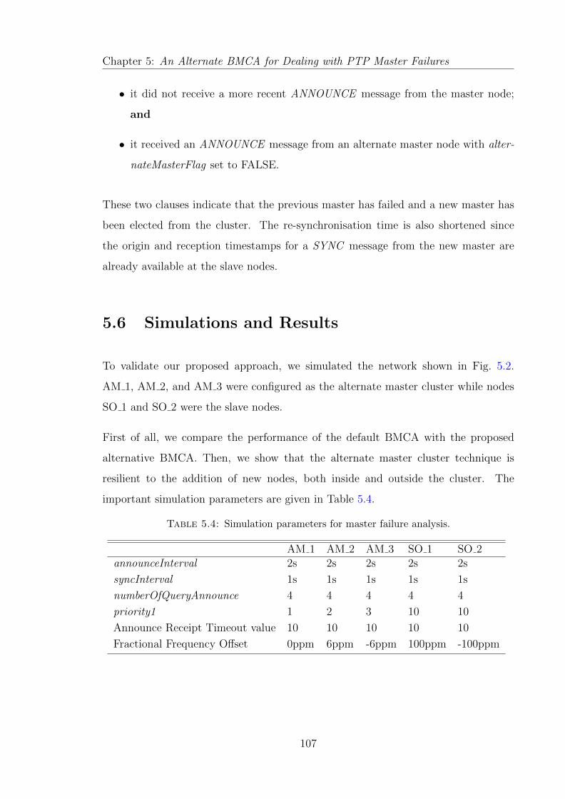
Chapter 5: An Alternate BMCA for Dealing with PTP Master Failures
• it did not receive a more recent ANNOUNCE message from the master node;
and
• it received an ANNOUNCE message from an alternate master node with alter-
nateMasterFlag set to FALSE.
These two clauses indicate that the previous master has failed and a new master has
been elected from the cluster. The re-synchronisation time is also shortened since
the origin and reception timestamps for a SYNC message from the new master are
already available at the slave nodes.
5.6 Simulations and Results
To validate our proposed approach, we simulated the network shown in Fig. 5.2.
AM 1, AM 2, and AM 3 were configured as the alternate master cluster while nodes
SO 1 and SO 2 were the slave nodes.
First of all, we compare the performance of the default BMCA with the proposed
alternative BMCA. Then, we show that the alternate master cluster technique is
resilient to the addition of new nodes, both inside and outside the cluster. The
important simulation parameters are given in Table 5.4.
Table 5.4: Simulation parameters for master failure analysis.
AM 1 AM 2 AM 3 SO 1 SO 2announceInterval 2s 2s 2s 2s 2s
syncInterval 1s 1s 1s 1s 1s
numberOfQueryAnnounce 4 4 4 4 4
priority1 1 2 3 10 10
Announce Receipt Timeout value 10 10 10 10 10
Fractional Frequency Offset 0ppm 6ppm -6ppm 100ppm -100ppm
107

Chapter 5: An Alternate BMCA for Dealing with PTP Master Failures
5.6.1 Comparing the Default BMCA with the Alternative
BMCA
5.6.1.1 The Default BMCA Scenario
In this scenario, the alternate master feature is disabled and the default BMCA is
used for master election. After the nodes are initialised, node AM 1 is elected as the
master since it has the lowest priority1 value. A fault was injected into this node at
time t = 5400s which caused a failure of the master node. After the failure, the clocks
of the other nodes run freely until node AM 2 is elected as the master.
Fig. 5.10 shows the clock offset of nodes SO 1, SO 2, AM 2 and AM 3 with respect
to the previous master AM 1.
5390 5400 5410 5420 5430 5440−1
0
1
2
3
4
5
6
7
Simulation Time in seconds
Clo
ck O
ffset
with
res
pect
to O
ld M
aste
r (m
icro
seco
nds)
New master, AM_2AM_3SO_1SO_2
Figure 5.10: Evaluation of downtime caused by master failure for the defaultBMCA scenario.
Before the master failure, the nodes achieve synchronisation and maintain this syn-
chronisation within approximately 0.1µs. After the master failure at t = 5400s, the
remaining nodes drift apart from the master’s clock, and hence each other during the
108

Chapter 5: An Alternate BMCA for Dealing with PTP Master Failures
detection and election phases, until the new master AM 2 transitions to the MASTER
state.
In the default BMCA scenario, the end of the detection phase coincides with the
expiry of the ANNOUNCE RECEIPT TIMEOUT timer at time t = 5420 s. In the
election phase which occurs within the next announce interval, slave node SO 1 first
tries to synchronise to node SO 2, before finally synchronising to AM 2. The total
downtime as a result of master failure is approximately 28s, and the accumulated
offset within this period is about 4.5µs across all the nodes.
5.6.1.2 The Alternative BMCA Scenario
In this scenario, the alternate master feature is enabled and the alternative BMCA is
used for master election. At power up, all the nodes within the cluster are initialised
to the same rank value. Hence, node AM 1 is elected as the master since it has the
lowest priority1 value. A fault was injected into this node at time t = 5400s which
caused a failure of the master node. After the failure, the clocks of the other nodes
run freely until node AM 2 is elected as the master.
Fig. 5.11 shows the clock offset of nodes SO 1, SO 2, AM 2 and AM 3 with respect to
the previous master AM 1. Just like the default BMCA scenario, the nodes maintain
synchronisation within approximately 0.1µs before the master fails. After the master
failure at t = 5400s, the remaining nodes drift apart from the master’s clock, and
hence each other during the detection and election phases, until the new master AM 2
transitions to the MASTER state.
Our proposed alternative BMCA uses unicast queryAnnounce messages and alter-
nateMasterSync to produce shorter detection, election and re-synchronisation phases.
The master failure is detected within only 4s, the new master AM 2 is elected within
2s, and the re-synchronisation occurs within a further 2s. In total, the downtime is
only 8s, and the accumulated offset within this period is about 2µs.
109

Chapter 5: An Alternate BMCA for Dealing with PTP Master Failures
5390 5395 5400 5405 5410 5415 5420−1
0
1
2
3
4
5
6
7
Simulation Time in seconds
Clo
ck O
ffset
with
res
pect
to O
ld M
aste
r (m
icro
seco
nds)
New master, AM_2AM_3SO_1SO_2
Figure 5.11: Evaluation of downtime caused by master failure for the alternativeBMCA scenario.
5.6.2 Verifying the Resilience of the Alternate Master Clus-
ter Technique
The alternative BMCA simulation scenario in Section 5.6.1.2 demonstrated the re-
silience of the alternate master cluster technique to the failure of the master node.
In this section, we use simulations to demonstrate that the alternate master cluster
technique is also resilient to the addition of both cluster and non-cluster nodes.
5.6.2.1 Introduction of a cluster node
In this scenario we enable the alternate master feature and use the same simulation
parameters listed in Table 5.4. However node AM 1 is not powered up until time
t = 5400s. Hence shortly after initialisation, AM 2 is elected as master and all the
nodes achieve synchronisation with it.
110

Chapter 5: An Alternate BMCA for Dealing with PTP Master Failures
Just before AM 1 is powered up, the slave nodes are still synchronised to AM 2 and
the relative offset is in the sub-microsecond range as shown in Fig. 5.12. However in
terms of the “true” time, there is a significant offset in the order of 104 microseconds
due to the 6ppm clock drift associated with AM 2.
5360 5365 5370 5375 5380 5385 5390 5395 5400−0.1
−0.08
−0.06
−0.04
−0.02
0
0.02
0.04
0.06
0.08
0.1
Simulation Time in seconds
Clo
ck O
ffset
with
res
pect
to m
aste
r A
M_2
(m
icro
seco
nds)
AM_3SO_1SO_2
Figure 5.12: Clock offset of slave nodes with respect to current master AM 2before the addition of a cluster node.
When AM 1 is powered up, it discovers the other members of the cluster and exchanges
queryAnnounce messages with them. It is subsequently elected as master since it
has the lowest priority1 value. When the alternate master nodes and slave nodes
synchronise to it, a step change in clock offset occurs. This is illustrated in Fig. 5.13.
Fig. 5.13 verifies the correct operation of the proposed alternate cluster technique, as
it proves that the system adapts correctly to the introduction of a master node to the
cluster. From an implementation point of view, if the system cannot tolerate the step
change in clock offset (e.g. due to the presence of real-time traffic on the network),
then the new cluster node should be configured with a higher priority1 value than
111
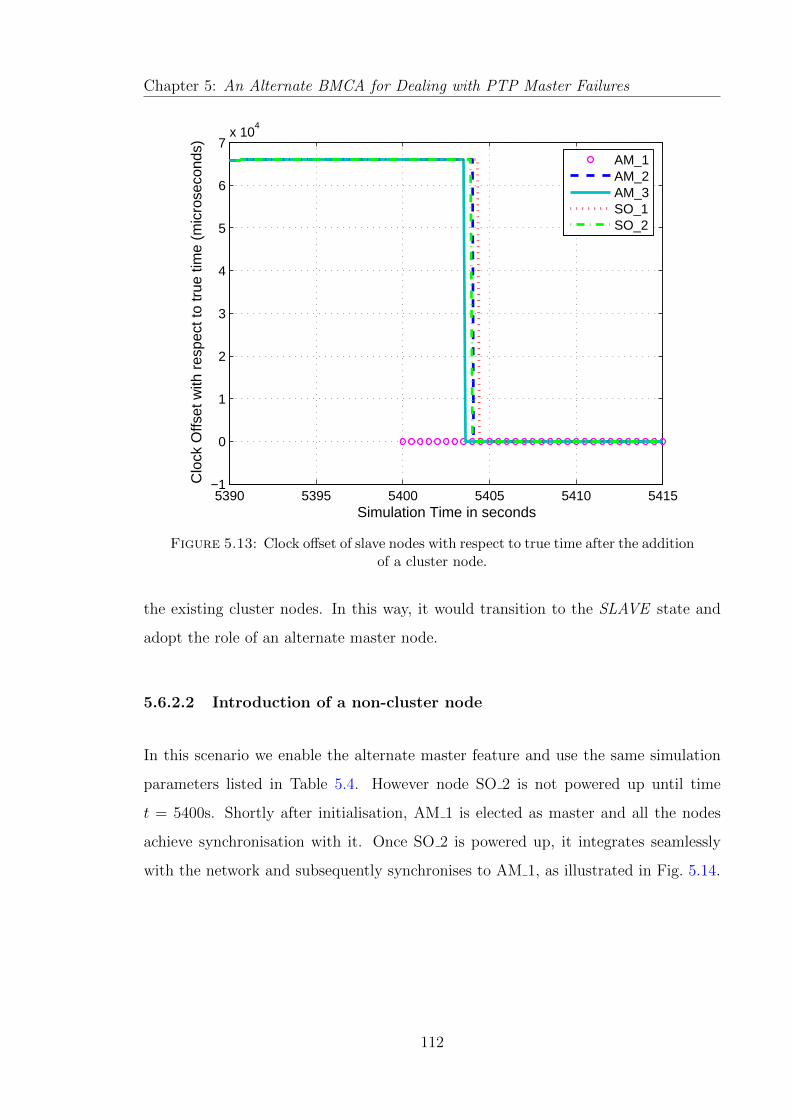
Chapter 5: An Alternate BMCA for Dealing with PTP Master Failures
5390 5395 5400 5405 5410 5415−1
0
1
2
3
4
5
6
7x 10
4
Simulation Time in seconds
Clo
ck O
ffset
with
res
pect
to tr
ue ti
me
(mic
rose
cond
s)
AM_1AM_2AM_3SO_1SO_2
Figure 5.13: Clock offset of slave nodes with respect to true time after the additionof a cluster node.
the existing cluster nodes. In this way, it would transition to the SLAVE state and
adopt the role of an alternate master node.
5.6.2.2 Introduction of a non-cluster node
In this scenario we enable the alternate master feature and use the same simulation
parameters listed in Table 5.4. However node SO 2 is not powered up until time
t = 5400s. Shortly after initialisation, AM 1 is elected as master and all the nodes
achieve synchronisation with it. Once SO 2 is powered up, it integrates seamlessly
with the network and subsequently synchronises to AM 1, as illustrated in Fig. 5.14.
112

Chapter 5: An Alternate BMCA for Dealing with PTP Master Failures
5390 5395 5400 5405 5410 5415−9
−8
−7
−6
−5
−4
−3
−2
−1
0
1x 10
5
Simulation Time in seconds
Clo
ck O
ffset
with
res
pect
to tr
ue ti
me
(mic
rose
cond
s)
AM_1AM_2AM_3SO_1SO_2
Figure 5.14: Clock offset of slave nodes with respect to true time after the additionof a non-cluster node.
5.7 Implementation Considerations
The key implementation requirements for the alternate master cluster members are
as follows:
• Support for unicast messaging, so that queryAnnounce messages can be trans-
mitted within the cluster.
• Additional memory for storing the details of cluster members in alternateMas-
terRecord.
• Implementation of the ranking algorithm.
• Minor modification to the clock comparison algorithm within the BMCA.
• Utilisation of some reserved fields in the ANNOUNCE message for the trans-
mission of scaledLogrank values.
113

Chapter 5: An Alternate BMCA for Dealing with PTP Master Failures
All these requirements can be handled in software, with very low effort.
A key advantage of our proposed approach is that the changes in the non-cluster
members are trivial. Slave nodes can still utilise the default BMCA, with a reduction
in the detection and election phases provided that these two requirements are met:
• Slave nodes have knowledge of the identities of the cluster members, in the
form of port identites and/or MAC addresses. This can be configured once at
initialisation.
• During an announce interval, if the slave did not receive a more recent AN-
NOUNCE message from the master node but instead received an ANNOUNCE
message from an alternate master node with alternateMasterFlag set to FALSE,
this indicates that a master change has occured in the cluster. As such, the pre-
vious ANNOUNCE message from the master node should be excluded from the
BMCA clock comparison algorithm.
5.8 Summary
This chapter has proposed a new alternate master cluster technique for dealing with
master failures in PTP. We have described the application scenario which inspired
this research work, and then developed a corresponding system model. Careful con-
sideration of the merits and demerits of the existing techniques, revealed that a new
technique was required for our application scenario. We have described the alternate
master cluster technique in detail; specifying the behaviour of the different types of
nodes, describing the alternate BMCA, the ranking algorithms, as well as the at-
tributes required. Network simulations in OPNET have been used to illustrate that
our proposed technique can reduce both the downtime resulting from master failure
and the accumulated offset. We have also verified the resilience of the alternate mas-
ter technique to the addition of both cluster and non-cluster nodes. Finally, we have
114

Chapter 5: An Alternate BMCA for Dealing with PTP Master Failures
considered the key requirements for implementing the system and showed that the ef-
fort required would be low and most of the changes will be done within the alternate
master cluster.
115

Chapter 6Conclusions and Future Work
In this thesis, we have explored three different areas in synchronisation, namely: how
to achieve higher-layer synchronisation in an UWB network, how to deal with the
effects of PDV when PTP is used to synchronise base stations in an Ethernet network,
and how to reduce the downtime caused by failure in the master node when PTP is
used to synchronise DECT base stations. This chapter concludes the thesis and offers
suggestions for future work.
6.1 Conclusions
In Chapter 3, we have developed a higher-layer synchronisation algorithm for an
ECMA-368 UWB network. The application requirements for the synchronisation
algorithm have been analysed the generic class of algorithms that required for the
network has been determined. We have selected two existing algorithms from this class
and also proposed a new Linear Rate algorithm for the class. We have determined
that the best place for implementing the algorithm is the MAC layer; hence we have
also proposed a method for transferring the higher layer clock to the MAC layer using
empty RTP packets, when the MAC layer does not have direct access to the higher
layer clock. A new MLME primitive has been specified for transferring the computed
clock parameters back to the higher layer after synchronisation is complete. The
116

Chapter 6: Conclusion
three candidate algorithms have been implemented in the OPNET simulator and we
have observed that the two drift-correcting algorithms perform better. The Linear
Rate algorithm has been judged as the most suitable for the network, therefore it has
been implemented on an FPGA UWB platform. We have also demonstrated that
the performance of the Linear Rate algorithm can be improved if the MAC layer and
higher layer applications reside on the same entity; such that the MAC layer is able
to obtain the timestamps directly from the higher layer and also update them as close
as possible to the PHY, just before the synchronisation frames are transmitted.
Although the higher-layer synchronisation algorithm was designed for a hierarchical
UWB network, in theory it can be applied to any other short-range device-device
communications network that requires master-slave synchronisation. Whilst it has
focused on a multimedia streaming application, it can be used for any other appli-
cation that requires a similar level of synchronisation accuracy. However if tighter
synchronisation is required, then it might be worthwhile to modify the algorithm to
use a quadratic or higher-order equation, rather than the linear approach proposed.
Chapter 4 has described a novel sample-mode PDV filtering algorithm. We have
characterised the IEEE 1588 PTP SYNC packet delay profiles for two types of net-
works with different levels of background traffic and observed from the shape of the
distributions that the existing sample-minimum, sample-maximum, and sample-mean
filters perform sub-optimally for some of the load levels in these scenarios. A new
skew-estimation algorithm has been proposed, by combining some features of Paxson’s
“de-noising” algorithm [69], [70] with a linear programming algorithm [15]. This skew-
estimation algorithm is used as the RCF estimator in our low-computation sample-
mode filtering algorithm. The sample-mode filtering algorithm also incorporates an
offset corrector which selects packets from the mode bin and uses these “good” packets
to achieve synchronisation. Numerical simulations have shown that when the underly-
ing delay profile of the network is a good match for an existing filter, the sample-mode
filter performs as well as the existing filter. However when the mode delay value does
not coincide with the minimum, mean, or maximum delay values, the sample-mode
filter outperforms the existing sample-minimum, sample-mean, and sample-maximum
117

Chapter 6: Conclusion
filters. Although this research area focussed on the PTP synchronisation protocol, the
proposed sample-mode filtering technique can be applied in any other master-slave
synchronisation protocol.
Chapter 5 has proposed a new alternate master cluster technique for dealing with
master failures in PTP. We have described the application scenario which inspired this
research work and by careful consideration of the merits and demerits of the existing
techniques, shown that a new technique is required for our application scenario. The
alternate master cluster technique has been thoroughly specified. The specification
includes the types of nodes, the behaviour of nodes inside and outside the cluster, the
alternate BMCA, the ranking algorithm, as well as the required attributes. Network
simulations in OPNET have been used to illustrate that our proposed technique can
reduce both the downtime resulting from master failure and the accumulated offset.
Finally, we have considered the key requirements for implementing the system and
shown that the effort required would be low and most of the changes will be done in
the alternate master cluster.
6.2 Future Work
Chapter 3 has proposed a novel higher layer synchronisation algorithm for ECMA-368
UWB networks, suitable for multimedia streaming applications. However, the under-
lying UWB network will be unsuitable for streaming, or indeed any other application,
if the MAC layer synchronisation remains unreliable. As mentioned in Section 2.2.2.1,
the synchronisation algorithm in the MAC does not actually correct the cloccks. As a
result, the accumulation of clock drift can lead to frequent loss of synchronisation and
hence temporary loss of connection, if the clock drift remains uncorrected. Future re-
search can consider how to measure the relative clock drift between devices, perhaps
by using the transmission time and/or reception time of multiple beacons, so that
corrective action can be taken. A possible corrective approach can then incorporate
the measured or estimated relative clock drift in the table of relative timing errors.
118

Chapter 6: Conclusion
In Chapter 4, a new sample-mode PDV filtering algorithm was proposed. The offset
corrector aspect of the algorithm which uses packets from the mode bin to achieve
synchronisation, includes an optional feedback mechanism to manipulate the synchro-
nisation interval and/or window size in order to influence the number of samples in
the mode bin. Further work in this area could study the interactions between the syn-
chronisation interval, window size, bin width, and perhaps packer delay variance in
order to determine the optimum values for these parameters for any type of network.
The de-noising linear programming technique proposed used a segmentation size that
was equivalent to the square root of the window size. Future work in the area could
explore different values of the segmentation size to see if any benefit can be obtained.
The alternate master cluster technique developed in Chapter 5 uses a ranking attribute
to provide quicker detection of a master failure. The ranking attribute is based on how
many queryAnnounce messages are received within an announce interval by members
of the alternate master. Future work in this area could consider how the ranking
attribute could be used for detecting congested links within the alternate master
cluster so a less-congested link can be selected with corresponding reduction in the
probability of packet delays and packet loss in the network. For instance, rather than
simply tracking the number of received queryAnnounce messages, the time interval
between each received message could be monitored in order to detect congestion.
119

Appendix AProof that packets with different delays can
end up in the same bin.
Consider the ith and jth SYNC packets received within the same window, where
j − i = n and n > 0. From (4.6), the corresponding timestamp differences are given
by δi = di + (Mi + di)σ and δj = dj + (Mj + dj)σ, respectively. Assuming no packet
loss and equal synchronisation interval f, then Mi+n = Mi + nf holds. Subtracting δi
from δj with substitution and simplification yields
δi+n − δi = (di+n − di)(1 + σ) + nfσ. (A.1)
For the two packets to end up in the same bin, the difference in their δ values must
be within the bin width α. Hence,
α ≥ (di+n − di)(1 + σ) + nfσ. (A.2)
120

Appendix BProof that packets with the same delay can
end up in different bins.
Again, consider the ith and jth SYNC packets received within the same window,
where j − i = n and n > 0. In this case, the end-to-end delay is di = dj = d. From
(4.6), the corresponding timestamp differences are given by δi = d + (Mi + d)σ and
δj = d+ (Mj + d)σ, respectively. Assuming no packet loss and equal synchronisation
interval f, then Mi+n = Mi + nf holds. Subtracting δi from δj with substitution and
simplification yields
δi+n − δi = nfσ. (B.1)
For the two packets to end up in different bins, the difference in their δ values must
be greater than the bin width α. Hence,
α < nfσ. (B.2)
121

References
[1] G. Heidari, WiMedia UWB Technology of Choice for Wireless USB and Blue-
tooth. West Sussex, UK: John Wiley and Sons, 2008.
[2] A. Sutton, “Building better backhaul,” Engineering and Technology Magazine,
vol. 6, no. 5, pp. 72–75, Jun. 2011.
[3] M. Howard, “Using Carrier Ethernet to Backhaul LTE,” White Paper, Infonetics
Research, Feb. 2011.
[4] P. Briggs, R. Chundury, and J. Olsson, “Carrier Ethernet for Mobile Backhaul,”
IEEE Communications Magazine, vol. 48, no. 10, pp. 94–100, Oct. 2010.
[5] IEEE Standard for a Precision Clock Synchronization Protocol for Networked
Measurement and Control Systems, 2nd Edition, IEEE Std. 1588, 2008.
[6] D. Mills, “Network Time Protocol (Version 3) Specification, Implementation and
Analysis,” RFC 1305, Mar. 1992.
[7] R. Steinmetz, “Human perception of jitter and media synchronization,” IEEE
Journal on Selected Areas in Communications, vol. 14, no. 1, pp. 61–72, Jan
1996.
[8] High Rate Ultra Wideband PHY and MAC Standard, 3rd Edition, ECMA Std.
368, 2008.
122

References
[9] I. Hadzic and D. R. Morgan, “On Packet Selection Criteria for Clock Recovery,”
in Proc. IEEE International Symposium on Precision Clock Synchronization for
Measurement, Control and Communication (ISPCS’09), Brescia, Italy, Oct. 2009,
pp. 35–40.
[10] ——, “Adaptive Packet Selection for Clock Recovery,” in Proc. IEEE Interna-
tional Symposium on Precision Clock Synchronization for Measurement, Control
and Communication (ISPCS’10), Portsmouth, USA, Sep. 2010, pp. 42–47.
[11] D. T. Bui, A. Dupas, and M. L. Pallec, “Packet Delay Variation Management for
a better IEEE 1588v2 Performance,” in Proc. IEEE International Symposium on
Precision Clock Synchronization for Measurement, Control and Communication
(ISPCS’09), Brescia, Italy, Oct. 2009, pp. 75–80.
[12] T. Murakami and Y. Horiuchi, “Improvement of Synchronization Accuracy in
IEEE 1588 Using a Queuing Estimation Method,” in Proc. IEEE International
Symposium on Precision Clock Synchronization for Measurement, Control and
Communication (ISPCS’09), Brescia, Italy, Oct. 2009, pp. 12–16.
[13] B. Sundararaman, U. Buy, and A. D. Kshemkalyani, “Clock synchronization for
wireless sensor networks: a survey,” Ad Hoc Networks, vol. 3, no. 3, pp. 281–323,
May 2005.
[14] L. Lamport, “Time, clocks and the ordering of events in a distributed system,”
Communications of the ACM, vol. 21, no. 7, pp. 558–565, Jul. 1978.
[15] S. B. Moon, P. Skelly, and D. Towsley, “Estimation and Removal of Clock
Skew from Network Delay Measurements,” in Proc. IEEE Eighteenth Annual
Joint Conference of the IEEE Computer and Communications Societies (INFO-
COM’99), vol. 1, New York, USA, Mar. 1999, pp. 227–234.
[16] “BIPM Com. Cons. Df. Seconde, 1980, 9, S15 and Metrologia, 1981, 17, 70,”
CCDS Recommendation S 2, Bureau International des Poids et Mesures, 1970.
[17] V. Paxson, G. Almes, J. Mahdavi, and M. Mathis, “Framework for IP Perfor-
mance Metrics,” RFC 2330, May 1998.
123

References
[18] S. Bregni, Synchronization of Digital Telecommunications Networks. West Sus-
sex, England: John Wiley and Sons, 2002.
[19] P. Marsch and G. P. Fettweis, Coordinated Multi-Point in Mobile Communica-
tions: From Theory to Practice. New York, USA: Cambridge University Press,
2011.
[20] “Synchronization Interface Standards for Digital Networks,” ANSI/T1.101-1987,
ANSI, Mar. 1987.
[21] H. Kopetz, Real-Time Systems Design Principles for Distributed Embedded Ap-
plications, 2nd ed., J. A. Stankovic, Ed. New York, USA: Springer, 2011.
[22] M. Ghavami, L. B. Michael, and R. Kohno, Ultra Wideband Signals and Systems
in Communication Engineering (Second Edition). West Sussex, UK: John Wiley
and Sons, 2007.
[23] C. Wei, P. Ranta, T. A. Brown, and C. Reed, “Wireless Video Streaming over
UWB,” in IEEE International Conf. on Ultra-Wideband, ICUWB’07, Singapore,
Sep. 2007, pp. 933–936.
[24] S. Zeisberg and V. Schreiber, “EUWB - Coexisting Short Range Radio by Ad-
vanced Ultra-Wideband Radio Technology,” in ICT-Mobile Summit 2008 Confer-
ence Proceedings, P. Cunningham and M. Cunningham, Eds. IIMC International
Information Management Corporation, 2008.
[25] E. Dimitrov, T. Kaiser, A. Anttonen, A. Krause, and A. Weir, “The PULSER II
view towards very high data rate OFDM based UWB systems,” in Proc. 16th IST
Mobile and Wireless Communications Summit, Budapest, Hungary, Jul. 2007, pp.
1–5.
[26] (2007) EUWB Website. [Online]. Available: http://www.euwb.eu/
[27] M. Balakrishnan and L. Taylor, “Time Synchronization of New Devices in Ad-hoc
Multimedia Networks,” in 4th IEEE Consumer Communications and Networking
Conf., CCNC’07, Las Vegas, USA, Jan. 2007, pp. 336–341.
124

References
[28] R. Aiello and A. Batra, Ultra Wideband Systems Technologies and Applications.
Oxford, UK: Elsevier Inc., 2006.
[29] S.-P. Liou, C. Toklu, and K. Heckrodt, “VideoTalk: a collaborative environment
for video content discussion,” in Proc. IEEE International Conference on Multi-
media Computing and Systems, vol. 2, Florence, Italy, Jun. 1999, pp. 454–459.
[30] “Precision Time Protocol Telecom Profile for Frequency Synchronization,” Rec-
ommendation G.8265.1/Y.1365.1, ITU-T, Oct. 2010.
[31] “Synchronization for Next Generation Networks - The PTP Telecom Profile,”
White Paper, Symmetricom, 2011.
[32] “IP-DECT System data sheet,” ikon GmbH, Ulm, Germany.
[33] “HiPath Cordless IP data sheet,” Siemens Enterprise Communications GmbH,
Munich, Germany.
[34] “Deployment of Precision Time Protocol for Synchronization of GSM and UMTS
Basestations,” Application Brief, Symmetricom, may 2008.
[35] R. Zarick, M. Hagen, and R. Bartos, “The Impact of Network Latency on the
Synchronization of Real-World IEEE 1588-2008 Devices,” in Proc. IEEE Interna-
tional Symposium on Precision Clock Synchronization for Measurement, Control
and Communication (ISPCS’10), Portsmouth, USA, Sep. 2010, pp. 135–140.
[36] “Timing and Synchronization Aspects in Packet Networks,” Recommendation
G.8261, ITU-T, Apr. 2008.
[37] B. Mochizuki and I. Hadzic, “Improving ieee 1588v2 clock performance through
controlled packet departures,” IEEE Communications Letters, vol. 14, no. 5, pp.
459–461, May 2010.
[38] C. Na, R. Scheiterer, D.Obradovic, and J. Nossek, “A Kalman Filter Approach
To Clock Synchronization Of Cascaded Network Elements,” in Proc. First IFAC
Workshop on Estimation and Control of Networked Systems, Venice, Italy, Sep.
2009, pp. 54–59.
125

References
[39] H. Abubakari and S. Sastry, “IEEE 1588 style synchronization over wireless link,”
in Proc. IEEE International Symposium on Precision Clock Synchronization for
Measurement, Control and Communication (ISPCS’08), Ann Arbor, USA, Sep.
2008, pp. 127–130.
[40] “Improving Real World Synchronization Accuracy with IEEE-1588 Transparent
Clocks,” White Paper, Symmetricom, 2009.
[41] W. Stallings, “A practical guide to queuing analysis,” BYTE, vol. 16, no. 2, pp.
309–316, Feb 1991.
[42] “Cisco Nexus 5548P Switch Architecture,” White Paper, Cisco, 2010.
[43] “IXF1110 MAC data sheet,” Cortina Systems, California, USA.
[44] A. Bletsas, “Evaluation of kalman filtering for network time keeping,” IEEE
Transactions on Ultrasonics, Ferroelectrics, and Frequency Control, vol. 52, no. 9,
pp. 1452–1460, Sep. 2005.
[45] W. E. Leland, M. S. Taqqu, W. Willinger, and D. V. Wilson, “On the self-similar
nature of ethernet traffic,” IEEE/ACM Transactions on Networking, vol. 2, no. 1,
pp. 1–15, Feb. 1994.
[46] S. Johannessen, “Time synchronization in a local area network,” IEEE Control
Systems Magazine, vol. 24, no. 2, pp. 61–69, Apr. 2004.
[47] G. Gaderer, R. Holler, T. Sauter, and H. Muhr, “Extending IEEE 1588 to Fault
Tolerant Clock Synchronization,” in Proc. IEEEIEEE International Workshop
on Factory Communication Systems (WFCS’04), Vienna, Austria, Sep. 2004,
pp. 353–357.
[48] G. Gaderer, S. Rinaldi, and N. Kero, “Master Failures in the Precision Time
Protocol,” in Proc. IEEE International Symposium on Precision Clock Synchro-
nization for Measurement, Control and Communication (ISPCS’08), Ann Arbor,
USA, Sep. 2008, pp. 59–64.
126

References
[49] G. Gaderer, P. Loschmidt, and T. Sauter, “Improving fault tolerance in high-
precision in clock synchronization,” IEEE Transactions on Industrial Informatics,
vol. 6, no. 2, pp. 206–215, May 2010.
[50] F. Praus, W. Granzer, G. Gaderer, and T. Sauter, “A Simulation Frame-
work for Fault-Tolerant Clock Synchronization in Industrial Automation Net-
works,” in Proc. IEEE Conference on Emerging Technologies and Factory Au-
tomation(ETFA’07), Patras, Greece, Sep. 2007, pp. 1465–1472.
[51] J.-L. Ferrant, M. Gilson, S. Jobert, M. Mayer, L. Montini, M. Ouellette, S. Ro-
drigues, and S. Ruffini, “Development of the first ieee 1588 telecom profile to ad-
dress mobile backhaul needs,” IEEE Communications Magazine, vol. 48, no. 10,
pp. 118–126, Oct. 2010.
[52] Y. Kozakai and M. Kanda, “Keeping Clock Accuracy on a Master Clock Fail-
ure in Substation Network,” in Proc. IEEE International Symposium on Preci-
sion Clock Synchronization for Measurement, Control and Communication (IS-
PCS’10), Portsmouth, USA, Sep. 2010, pp. 25–29.
[53] S. Bovelli and F. Leipold, “Requirements for public transport applications,”
EUWB Deliverable D8a.2, Dec. 2008.
[54] ——, “Scenario description for public transport applications,” EUWB Deliver-
able D8a.1, Jul. 2008.
[55] P. Hafezi and M. del Rey, “System Parameters and Technical Requirements for
Multiband/Multimode UWB Home Environment Applications,” EUWB Deliv-
erable D8c.2, Dec. 2008.
[56] M. Mock, R. Frings, E. Nett, and S. Trikaliotis, “Continuous Clock Synchro-
nization in Wireless Real-Time Applications,” in 19th IEEE Symp. on Reliable
Distributed Systems, SRDS’00, Nurnberg, Germany, Oct. 2000.
[57] S. Ping, “Delay Measurement Time Synchronization for Wireless Sensor Net-
works,” Intel Research, IRB-TR-03-013, Jun. 2003.
127

References
[58] M. Mock, R. Frings, E. Nett, and S. Trikaliotis, “Clock Synchronization for Wire-
less Local Area Networks,” in Proc. Euromicro-RTS 2000, Stockholm, Sweden,
Jun. 2000.
[59] M. Anyaegbu, A. Weir, and C.-X. Wang, “Higher Layer Synchronization in an
ECMA-368 Ultra Wideband Network,” in IEEE International Conf. on Ultra-
Wideband, ICUWB’10, vol. 2, Nanjing, China, Sep. 2010, pp. 1–4.
[60] OPNET Modeler Documentation Set, OPNET Technologies, Inc., Bethesda, MD,
2011, release 16.0.
[61] Y. Quan and G. Liu, “Drifting Clock Model for Network Simulation in Time Syn-
chronization,” in Proc. 3rd International Conference on Innovative Computing
Information and Control (ICICIC’08), Dalian, China, Jun. 2008, pp. 385–388.
[62] B. Ngamwongwattana and R. Thompson, “Measuring One-Way Delay of VoIP
Packets Without Clock Synchronization,” in Proc. IEEE International Instru-
mentation and Measurement Technology Conference (I2MTC’09), Singapore,
May 2009, pp. 532–535.
[63] MAC-PHY Interface for ECMA-368, 3rd Edition, ECMA Std. 369, 2008.
[64] ML505/ML506/ML507 Evaluation Platform User Guide, UG347, Xilinx, 2011.
[65] lwIP Documentation (lwIP 1.3.0). [Online]. Available: http://http://www.
nongnu.org/lwip/
[66] Xilinx LogiCORE IP XPS Timer/ Counter (v1.02a), DS573, Xilinx, 2010.
[67] D. Mills, “Internet Time Synchronization: The Network Time Protocol,” RFC
1129, Oct. 1989.
[68] M. Anyaegbu, C.-X. Wang, and W. Berrie, “A Sample-Mode Packet Delay Vari-
ation Filter for IEEE 1588 Synchronization,” in Proc. IEEE International Con-
ference on ITS Telecommunications (ITST’12), Taipei, Taiwan, Nov. 2012.
128

References
[69] V. Paxson, “Measurements and analysis of end-to-end internet dynamics,”
Ph.D. dissertation, Univ. of California, Berkeley, Apr. 1997. [Online]. Available:
ftp://ftp.ee.lbl.gov/papers/vp-thesis
[70] ——, “On calibrating measurements of packet transit times,” in Proceedings of
SIGMETRICS’98), Madison, Wisconsin, Jun. 1998.
[71] Digital Enhanced Cordless Telecommunications (DECT); Common Interface
(CI); Part 1: Overview, version 2.4.1, ETSI Std. ETSI EN 300 175-1, 2012.
[72] Digital Enhanced Cordless Telecommunications (DECT); Common Interface
(CI); Part 2: Physical Layer (PHL), version 2.1.1, ETSI Std. ETSI EN 300
175-2, 2007.
[73] Digital Enhanced Cordless Telecommunications (DECT); Common Interface
(CI); Part 3: Medium Access Control (MAC) layer, version 2.2.0, ETSI Std.
ETSI EN 300 175-3, 2008.
[74] J. A. Phillips and G. MacNamee, Personal Wireless Communications with DECT
and PWT. Norwood, USA: Artech House Inc., 1998.
129
Copyright © 2022 FDOKUMEN