Synchronization of Scarce Resources for a Parallel Machine

Lotsizing Problem

Christian Almederab∗, Bernardo Almada-Lobob

May 25, 2010

aUniversity of Vienna, Faculty of Economics, Business and Statistics, Brünnerstr. 72, A-1210

Vienna, Austria, christian.almeder@univie.ac.atbFaculdade de Engenharia da Universidade do Porto, Rua Dr. Roberto Frias s/n, Porto

4200-465, Portugal, almada.lobo@fe.up.pt

Abstract

In this paper we present a novel approach to tackle the synchronization of a secondary

resource in lotsizing and scheduling problems. This kind of problem occurs in different

manufacturing processes (e.g. wafer testing in the semiconductor industry, production and

bottling of soft drinks). We consider a scenario of parallel unrelated machines which have

to be equipped with a tool or need a special kind of resource for processing. Our approach

allows tracing the assignment of these secondary resources across different machines and

synchronizing their usage independently of time periods. We present extensions of the general

lotsizing and scheduling problem and of the capacitated lotsizing problem. We prove that

the latter model is a special case of the first one, but it performs computationally much

better.

Keywords: Lotsizing and Scheduling, Scarce resources, Synchronization, Mixed-integer

programming

∗corresponding author

1

Introduction

Today production processes and systems are getting more complex, increasing the challenges of

managing large shop floors. Lotsizing and scheduling models are tailored for short-term planning

considering the trade-off between time-consuming and costly setup and configuration processes

and high inventory costs. Many formulations (in particular big-bucket models) do not give very

detailed information on how the production lots should be scheduled. Realistic settings are

often neglected and in complex environments it might be sometimes impossible to implement

the results of such models, simply because there is no feasible schedule possible.

In this paper we consider a lotsizing and scheduling problem in a parallel machine environment

with another resource necessary for the production process. The usage of these secondary resource

must be synchronized across the parallel production process on the shop floor. We develop a

general modeling concept for such a situation. In particular, we will use the wafer test process,

a part of the production process of semiconductors, as a template to illustrate how such a

synchronization problem can be tackled. In that case the parallel machines are automatic test

stations and the secondary resource is a test head that is used to perform the according test

operations on the wafers in the test stations (cf. Ellis et al., 2004). Other examples of similar

situations are the front-end wafer production process (cf. Mönch, 2004) or the example of an

automobile supplier as reported in Tempelmeier and Buschkühl (2008). The latter one is a

lotsizing problem enhanced by considering a setup operator who has to perform the setup tasks

on different parallel machines. The setup operator can be modeled as such a secondary resource

necessary to start production. In order to generate a feasible schedule, the timing of the setup

operations have to be modeled explicitly. Another example for necessary synchronization is the

multi-stage production process of small-scale soft drink plants (cf. Ferreira et al., 2009). The

two production stages of preparing the syrup in tanks and bottling it on multiple lines have

to be synchronized. The syrup in the tanks can be seen as a common resource, which is only

temporarily available, but can be used on several bottling machines in parallel.

The main contribution to the research on lotsizing and scheduling in this paper is twofold:

• We analyze the synchronization problem of a secondary scarce resource occurring in lotsiz-

ing and scheduling considering a parallel unrelated machine environment..

• We develop two different model formulations, a model based on the capacitated lotsizing

problem (CLSP) and another one based on the general lotsizing and scheduling model

(GLSP). We show that the GLSP-type approach allows a very accurate modeling of the

situation but is computationally very hard to solve, whereas the CLSP-type model has

some drawbacks for special cases but is much easier to solve. We compare the strength of

both formulations and improve them by adding valid inequalities.

The reminder of the paper is organized as follows: we start with a review of the relevant literature,

followed by a detailed problem description. Furthermore, we develop GLSP- and CLSP-related

models for the lotsizing and scheduling with synchronization problem. A comparison between

models is carried out on a small example as well as the proof that shows that the CLSP-related

model is a special case of the GLSP-related model. Valid inequalities are developed for both

2

models. We report some computational experiments and conclude with final remarks and com-

ments.

Literature review

Motivated by industrial practice, the research community has been trying to solve more re-

alistic and comprehensive production planning problems (e.g. Almada-Lobo et al., 2008b). In

fact, the need to be able to respond quickly to market changes requires refined production plan-

ning models better able to represent and exploit the flexibility of the production process (cf.

Pochet and Wolsey, 2006). Naturally, the strong interrelation between lotsizing and scheduling

decisions emphasize the importance of an integrated decision making.

The capacitated lotsizing problem (CLSP) is considered to be a big-bucket modelas the

planning horizon is partioned into a small number of long time periods allowing for several

products/setups to be produced/performed per bucket (cf. Billington et al., 1983). Standard

CLSP does not sequence or schedule products within a period. Nevertheless, when setup times

are considerable with respect to the length of a period and capacity is tight, it is necessary

to consider which product a machine is ready to process in the beginning of each period, i.e.,

setups need to be carried over to the following periods. Here, lotsizing is linked to partial

sequencing, as the products produced last and first in two consecutive periods are determined

(e.g. Suerie and Stadtler, 2003). In the presence of significant sequence-dependent setup costs

and/or times, it is necessary to schedule production in each time period. Haase (1996) introduces

the capacitated lotsizing problem with sequence-dependent setup costs (CLSD) for a single-

machine and Kang et al. (1999) extend this approach to parallel machines. For the case of

positive sequence-dependent setup times and costs Almada-Lobo et al., 2008a develop an exact

formulation. Quadt and Kuhn (2005) present a framework for applying a CLSP-like model to a

flexible flow line problem. The reader is referred to Karimi et al., 2003 and ? for a recent review

on CLSP formulations and state-of-the-art solution methods and to Quadt and Kuhn (2008) for

a review on the extensions of CLSP.

In contrast to the big-bucket approach, researchers developed also small-bucket models where

at most one setup might be performed in each period. Here, the planning horizon is divided into

many short periods (such as days, shifts, or hours). Naturally, that kind of models delivers a

more detailed production plan than the standard CLSP, because by default a complete production

sequence is generated. Jans and Degraeve (2004) present an application of a small-bucket model

to the production of tires where multiple resources have to be considered. But those approaches

have significant drawbacks, as the period length is determined by the minimal lot size which might

lead to a huge number of periods. Drexl and Kimms (1997) give a detailed overview on small-

bucket and big-bucket models. One mixed approach, which tries to overcome the drawbacks of

small- and big-bucket models is the general lotsizing and scheduling problem (GLSP) developed

by Fleischmann and Meyr (1997) and extended later to parallel machines by Meyr (2002). Here,

the consideration of sequence-dependent setups and multiple machines is straightforward.

Jans and Degraeve (2008) give an overview of recent developments in the field of modeling

deterministic single-level dynamic lotsizing problems to cope with various industrial extensions.

The authors point out interesting areas for future research, such as lotsizing and scheduling

3

on parallel machines and an increasing attention to model specific characteristics of the pro-

duction process, which is valuable in solving real-life planning problems. In many real-world

cases the different production lots cannot be scheduled independently from each other. Either

there might be precedence rules present, such as for the multi-level lotsizing problem or multiple

resources or tools have to be shared among different production processes. When considering

parallel machine environment, i.e. simultaneous production is possible, such interdependencies

have to be respected, otherwise the computed production plan might be impossible to imple-

ment. Dastidar and Nagi (2005) develop a model for scheduling injection molding operations,

where several different resources are necessary for the production. Using a small-bucket approach

the authors are able to block the resources necessary at workcenters for production during the

whole period, even if there is some idle time. Akturk and Onen (2002) describe a lotsizing prob-

lem for a single CNC-machine considering tooling decisions. The lotsizing decisions depend on

the setups of the tooling process, but since it is a single-machine problem they do not consider

sharing the tools with other parallel production processes.

Actually, our work is in line with these research directions. We intend to give new insights

by addressing the synchronization problem and possible ways on how to deal with it.

Problem description

Let us consider a manufacturing environment with N products to be scheduled on M parallel

machines with K secondary resources. External period (usually days or weeks) demand for

products is known in advance. Both product switchover and production on a machine require

an additional resource (hereafter referred as tool) that is continuously attached to the machine

throughout those processes. The following requirements/assumptions are made for the considered

lotsizing and scheduling problem:

• the shop floor is operated 24 hours a day;

• backlogging is allowed to overcome capacity-tight periods;

• two types of scarce resources: non-identical parallel machines and tools (only a few are

available as they are usually very expensive);

• significant tool sequence-dependent setup times and costs are incurred for switchovers from

one tool to another;

• setup times and costs for product switchovers on the same machine with the same tool

are negligible, thus the sequence of batches produced with the same tool is not determined

(this assumption might be dropped, if necessary, by the cost of an increased number of

binary variables);

• the tool remains attached to the machine during the production process;

• both machine and tools are blocked during a tool changeover, and cannot be used at that

time in any other production or setup process.

• triangular inequality holds for tool setup costs and times.

4

For a better understanding Figure 1 illustrates the usage of tools on three parallel machines. In

order to produce products 3, 1 and 7, tool k is attached to machine 1. This tool is blocked on

machine 1 during the switching from l1 to k, the production of those three batches, some idle

time in between and the switching from k to l2. The order of the three production batches is

irrelevant and is not determined.

time

machine 1

machine 2

machine 3

tool k

tool k

tool k

switc

h

prod

uct3

prod

uct

1

prod

uct

7

switc

h

tool l2tool l1

l 1→

k

k→

l 2

Figure 1: Synchronization of the usage of tools across different machines

The above assumptions are in line with the wafer test process. To consider the example of

the automobile supplier, there would be only a single tool in the system representing the setup

operator. That tool would be detached from the machine if the setup operation is finished. In

the case of the soft drink production the tools would represent syrups prepared and stored in the

tanks. Those tools would be available only for a certain time, but might be used simultaneously

on different machines. The total production possible with a tool would be limited by the capacity

of the according tanks.

Model formulation

GLSP-based model formulation

We start by developing a mixed-integer program (MIP) using the concept of the combined small-

bucket–big-bucket approach on which the GLSP is based. (cf. Fleischmann and Meyr, 1997;

Meyr, 2002). The main idea is to use a big-bucket model, where each of the “big” macro-periods

is subdivided into “small” micro-periods. In order to gain more flexibility, the length of the

micro-periods are variable and determined by the production quantities.

In our case a macro-period might be the usual day or week and inventory and backlog levels

are determined based on these longer time periods. Each macro-period consists of several micro-

periods which start with the beginning of a tool switch and end at the beginning of the next

tool switch, except the first (last) micro-period which starts (finishes) at the beginning (end) of

the macro-period. It is necessary to determine in advance the number of micro-periods in each

macro-period. That automatically limits the number of tool switches during a macro-period.

5

In order to formulate the MIP, we first introduce the necessary notation (for simplicity we

assume that the length of a macro period is normalized to one):

Dimension and indices:

N number of products (index: i)

M number of machines (index: m)

K number of tools (index: k)

R number of micro-periods in a macro-period (index: r)

T number of macro-periods considered for production (index: t)

Parameters:

Bi0 initial backlog level of product i

bit penalty cost for the backlog of product i at the end of macro-period t

dit demand of product i in macro-period t

Ii0 initial inventory level of product i

hit holding cost for product i at the end of macro-period t

pimk time for producing one unit of product i on machine m using tool k

Sim set of possible tools that can be used for product i on machine m

smkl setup time for changeover from tool k to tool l on machine m

σmkl setup cost for changeover from tool k to tool l on machine m

ymk0 initial setup state (equals 1 if machine m is set up with tool k)

Decision variables:

Bit backlog of product i at the end of macro-period t

Iit inventory level of product i at the end of macro-period t

ustrm start time of micro-period r in macro-period t on machine m

uftrm release time of the tool used in micro-period r in macro-period t on machine m

Utrmr′m′

1 if micro-period r on machine m starts after micro-period r′ of machine m′

0 otherwise

xitrmk production quantity of product i on machine m in micro-period r using tool k

ytrmk

1 if the tool k is attached to machine m in micro-period r

0 otherwise

ztrmkl

1 if there is a switch from tool k to tool l on machine m in micro-period r

0 otherwise

There are three cost factors occurring in the above problem description, namely inventory

cost, backorder cost and setup cost for changing the tools. Hence, the objective is to minimize

the sum of these costs

minFG = min

T∑

t=1

(

N∑

i=1

(hit · Iit + bit · Bit) +

R∑

r=1

M∑

m=1

K∑

k=1

K∑

l=1

σmkl · ztrmkl

)

, (1)

Since it might happen that we do not switch the tool at the beginning of a certain micro-period

(i.e. ztrmkk = 1) the according cost factor σmkk must be 0. The backorder costs of the last

period biT should be significantly higher than the costs for the other periods in order to penalize

6

unsatisfied demand at the end of the planning horizon.

Demands are given for each macro-period, therefore inventory and backlog levels have to be

computed on that level. Since the production is split up into production on different machines,

micro-periods, and tools, it is necessary to sum up all these production quantities

Iit −Bit − Ii(t−1) +Bi(t−1) −

M∑

m=1

R∑

r=1

K∑

k=1

xitrmk + dit = 0 ∀i, t (2)

In order to avoid the simultaneous usage of the same tool on different machines, we have to

determine the exact times of using a tool. A micro-period is defined to be the time from the

start of the tool exchange until the start of the next tool exchange. Hence, we have to capture

the time point when a micro-period starts. A tool is only available to other machines after the

complete tool exchange has been performed. Therefore, the release time of a tool on a machine

is determined by the start of the next micro-period plus the time for the tool switch. As shown

in Figure 2, a micro-period consists of the tool switch, the total production using that tool and

possible some idle time, which might be necessary for the synchronization of the tools across

different machines.

tool

switc

hpr

oduc

t3

prod

uct

7

tool

switc

h

prod

uct2

tool

switc

hpr

oduc

t4

prod

uct

9

time

start of macro-period end of macro-period

ust1m ust2m ust3muft3muft2muft1m

Figure 2: Values of variables ustrm and uftrm within a macro-period

The following set of constraints is necessary to calculate the correct starting of the micro-

periods and the release times of the tools:

ust1m = 0 ∀t,m (3)

ustrm ≥ ust(r−1)m +

K∑

k=1

K∑

l=1

smkl · zt(r−1)mkl +

N∑

i=1

K∑

k=1

pimk · xit(r−1)mk ∀t,m, r > 1 (4)

uftrm ≥ ust(r+1)m +

K∑

k=1

K∑

l=1

smkl · zt(r+1)mkl ∀t,m, r < R (5)

uftRm ≥ ustRm +K∑

k=1

K∑

l=1

smkl · ztRmkl +N∑

i=1

K∑

k=1

pimk · xiRmk ∀t,m (6)

uftrm ≥ uft(r−1)m ∀t,m, r > 1 (7)

uftRm = 1 ∀t,m (8)

Constraints (3) force the first micro-period to start at the beginning of the macro-period. If

there is no switch of tools at the beginning of the period, a virtual switch from tool k to tool

7

k is performed (zt1mkk = 1). The following constraints (4) relate the start times of subsequent

micro-periods. The coefficients pimk and smkl measure the times necessary to produce one unit

and to perform the tool exchange, respectively. In order to allow idle time for gaining flexibility

for the synchronization inequalities are used. The release times uftrm of a tool that is attached

to the machine m during micro-period r must be set after the tool has been removed. Hence,

we have to consider the start time of the next micro-period and the tool switch occurring at the

beginning of that micro-period. This relation is represented by constraints (5). Because after the

last micro-period there is no start time in the current macro-period, the last micro-period ends

after the start of the last micro-period plus the tool switch and the production, as denoted by

constraints (6). As constraints (5) provide only a lower bound for the release times, constraints

(7) are necessary to ensure the right ordering. Constraints (8) force the last micro-periods to

finish at the end of the macro-periods. Due to this calculation of start and release times, it is

not necessary to include the common capacity constraints. The total production and the tool

exchanges in all micro-periods cannot consume more time than available in the macro-period.

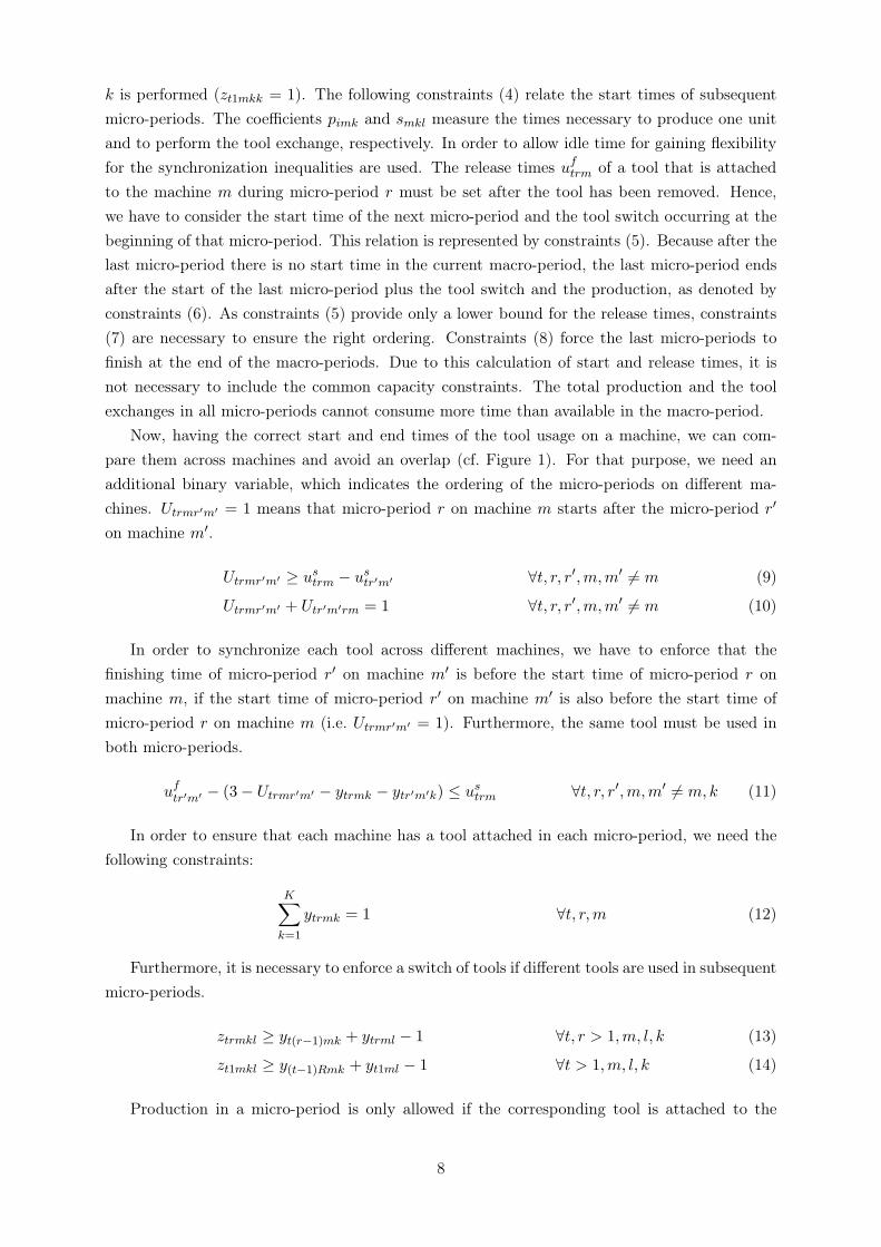
Now, having the correct start and end times of the tool usage on a machine, we can com-

pare them across machines and avoid an overlap (cf. Figure 1). For that purpose, we need an

additional binary variable, which indicates the ordering of the micro-periods on different ma-

chines. Utrmr′m′ = 1 means that micro-period r on machine m starts after the micro-period r′

on machine m′.

Utrmr′m′ ≥ ustrm − ustr′m′ ∀t, r, r′,m,m′ 6= m (9)

Utrmr′m′ + Utr′m′rm = 1 ∀t, r, r′,m,m′ 6= m (10)

In order to synchronize each tool across different machines, we have to enforce that the

finishing time of micro-period r′ on machine m′ is before the start time of micro-period r on

machine m, if the start time of micro-period r′ on machine m′ is also before the start time of

micro-period r on machine m (i.e. Utrmr′m′ = 1). Furthermore, the same tool must be used in

both micro-periods.

uftr′m′ − (3− Utrmr′m′ − ytrmk − ytr′m′k) ≤ ustrm ∀t, r, r′,m,m′ 6= m,k (11)

In order to ensure that each machine has a tool attached in each micro-period, we need the

following constraints:

K∑

k=1

ytrmk = 1 ∀t, r,m (12)

Furthermore, it is necessary to enforce a switch of tools if different tools are used in subsequent

micro-periods.

ztrmkl ≥ yt(r−1)mk + ytrml − 1 ∀t, r > 1,m, l, k (13)

zt1mkl ≥ y(t−1)Rmk + yt1ml − 1 ∀t > 1,m, l, k (14)

Production in a micro-period is only allowed if the corresponding tool is attached to the

8

machine and if no other technical restrictions prohibit it.

pimk · xitrmk ≤ ytrmk ∀i, t, r,m, k (15)

xitrmk = 0 ∀i, t, r,m, k /∈ Sim (16)

Finally we end up with the usual non-negativity and binary constraints. Meyr (2002) has

already shown that it is not necessary to force the integrality of the ztrmkl variables, because due

to constraints (13) and (14) they can take only the values 0 or 1.

Iit, Bit, ustrm, uftrm, xitrmk, ztrmkl ≥ 0, Utrmr′m′ , ytrmk ∈ {0, 1} (17)

Remark. So far in the model description we have assumed that each machine is always equipped

with a tool, which might not be necessary and might make it more difficult to compute feasible

solutions. In order to capture also the situation of empty machines (without any tool attached

during idle times), we might introduce a virtual tool k = 1 which represents the “no-tool” case.

Obviously we have to remove the synchronization restriction for that tool, that means that

constraints (11) must not hold for k = 1.

We refer to this model as general lotsizing and scheduling problem on parallel machines with

tool synchronization (GLSPPMToolSync).

CLSP-based model formulation

As referred beforehand, the CLSP is considered to be a big-bucket problem, because several

setups may be performed per period. In the presence of significant sequence-dependent setup

times and costs, it is necessary to determine the sizes and the sequence of the lots simultaneously.

In this section, we develop an extension of the single-level formulation with sequence-dependent

setups (e.g. Almada-Lobo et al., 2007) considering additional constraints related to the tools

(synchronization, switching, capacity, among others) and multiple machines.

In order to define the model, we use the following additional decision variables:

µstmk start time of the attachment of tool k to machine m in period t

µftmk end time of the tool exchange where tool k is removed from machine m in period t

µmaxtm end time of the last tool exchange performed on machine m in period t

Xitmk production of product i produced in period t on machine m with tool k

αtmk

1 if tool k is attached to machine m at the beginning of period t

0 otherwise

Ttmkl

1 if there is a switch from tool k to l on machine m in period t

0 otherwise

Wtmm′k

1 if tool k is used on machine m after being used on machine m′ in period t

0 otherwise

Note, that α(T+1)mk denotes the final tool attached to each machine at the end of the planning

horizon.

The according lotsizing and scheduling problem reads:

9

minFC = minN∑

i=1

T∑

t=1

(hit · Iit + bit ·Bit) +T∑

t=1

M∑

m=1

K∑

k=1

K∑

l=1

σmkl · Ttmkl (18)

Iit −Bit − Ii(t−1) +Bi(t−1) −M∑

m=1

K∑

k=1

Xitmk + dit = 0 ∀i, t (19)

pimk ·Xitmk ≤

K∑

l=1

Ttmlk + αtmk ∀i, t,m, k (20)

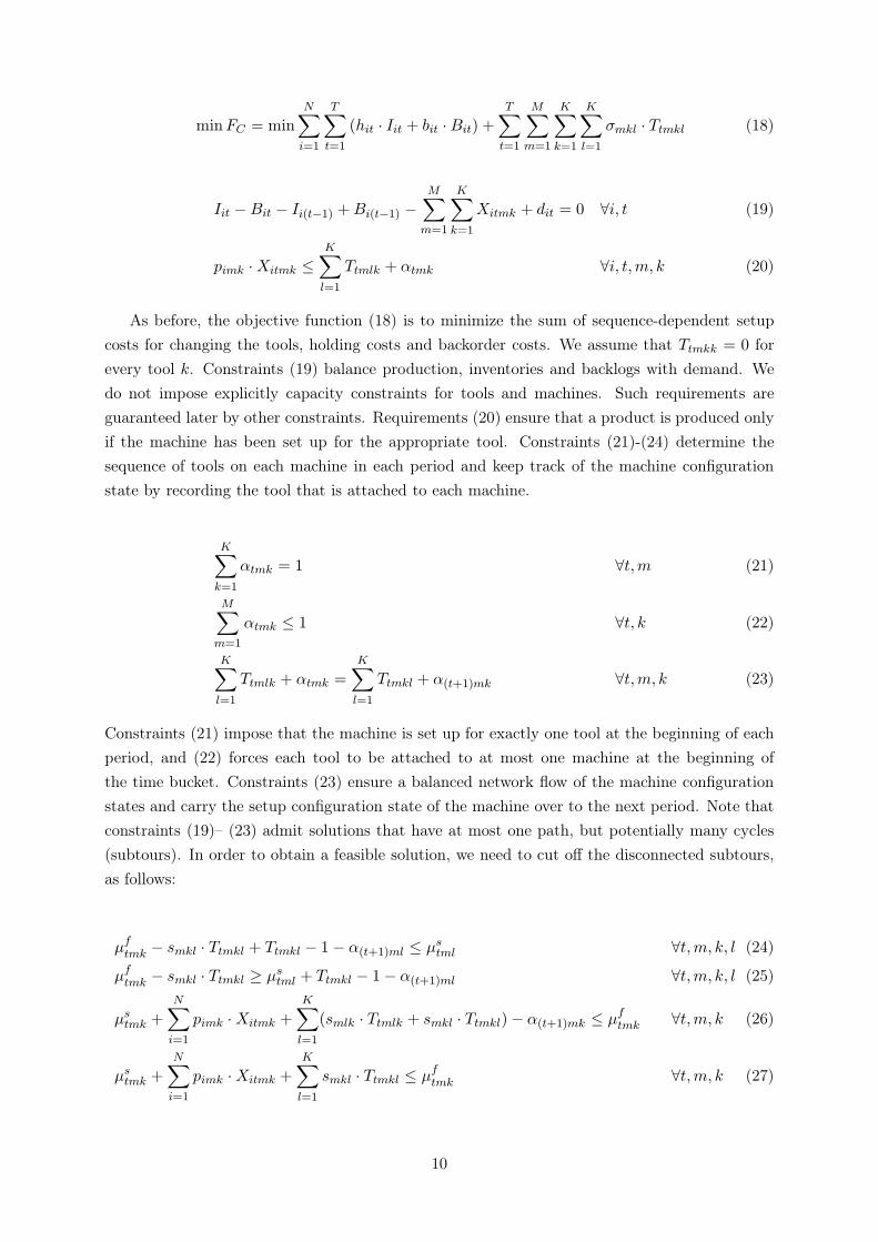
As before, the objective function (18) is to minimize the sum of sequence-dependent setup

costs for changing the tools, holding costs and backorder costs. We assume that Ttmkk = 0 for

every tool k. Constraints (19) balance production, inventories and backlogs with demand. We

do not impose explicitly capacity constraints for tools and machines. Such requirements are

guaranteed later by other constraints. Requirements (20) ensure that a product is produced only

if the machine has been set up for the appropriate tool. Constraints (21)-(24) determine the

sequence of tools on each machine in each period and keep track of the machine configuration

state by recording the tool that is attached to each machine.

K∑

k=1

αtmk = 1 ∀t,m (21)

M∑

m=1

αtmk ≤ 1 ∀t, k (22)

K∑

l=1

Ttmlk + αtmk =K∑

l=1

Ttmkl + α(t+1)mk ∀t,m, k (23)

Constraints (21) impose that the machine is set up for exactly one tool at the beginning of each

period, and (22) forces each tool to be attached to at most one machine at the beginning of

the time bucket. Constraints (23) ensure a balanced network flow of the machine configuration

states and carry the setup configuration state of the machine over to the next period. Note that

constraints (19)– (23) admit solutions that have at most one path, but potentially many cycles

(subtours). In order to obtain a feasible solution, we need to cut off the disconnected subtours,

as follows:

µftmk − smkl · Ttmkl + Ttmkl − 1− α(t+1)ml ≤ µs

tml ∀t,m, k, l (24)

µftmk − smkl · Ttmkl ≥ µs

tml + Ttmkl − 1− α(t+1)ml ∀t,m, k, l (25)

µstmk +

N∑

i=1

pimk ·Xitmk +

K∑

l=1

(smlk · Ttmlk + smkl · Ttmkl)− α(t+1)mk ≤ µftmk ∀t,m, k (26)

µstmk +

N∑

i=1

pimk ·Xitmk +K∑

l=1

smkl · Ttmkl ≤ µftmk ∀t,m, k (27)

10

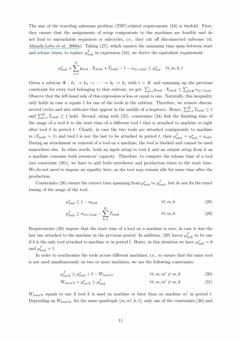
The aim of the traveling salesman problem (TSP)-related requirements (24) is twofold. First,

they ensure that the assignments of setup components to the machines are feasible and do

not lead to unreachable sequences or subcycles, i.e., they cut off disconnected subtours (cf.

Almada-Lobo et al., 2008a). Taking (27), which ensures the minimum time span between start

and release times, to replace µftmk in expression (24), we derive the equivalent requirement:

µstmk +

N∑

i=1

pimk ·Xitmk + Ttmkl − 1− α(t+1)ml ≤ µstml ∀t,m, k, l

Given a subtour Φ : k1 → k2 → · · · → kl → k1 with l < K and summing up the previous

constraint for every tool belonging to that subtour, we get:∑

k,i pimk ·Xitmk ≤∑

k∈Φ α(t+1)mk .

Observe that the left-hand side of this expression is less or equal to one. Naturally, this inequality

only holds in case α equals 1 for one of the tools in the subtour. Therefore, we remove discon-

nected cycles and also subtours that appear in the middle of a sequence. Hence,∑K

l=1 Ttmlk ≤ 1

and∑K

l=1 Ttmkl ≤ 1 hold. Second, along with (25), constraints (24) link the finishing time of

the usage of a tool k to the start time of a different tool l that is attached to machine m right

after tool k in period t. Clearly, in case the two tools are attached contiguously to machine

m (Ttmkl = 1) and tool l is not the last to be attached in period t, then µftmk = µs

tml + smkl.

During an attachment or removal of a tool on a machine, the tool is blocked and cannot be used

somewhere else. In other words, both an input setup to tool k and an output setup from k on

a machine consume both resources’ capacity. Therefore, to compute the release time of a tool

(see constraint (26)), we have to add both switchover and production times to the start time.

We do not need to impose an equality here, as the tool may remain idle for some time after the

production.

Constraints (26) ensure the correct time spanning from µstmk to µf

tmk, but do not fix the exact

timing of the usage of the tool.

µstmk ≤ 1− αtmk ∀t,m, k (28)

µftmk ≥ α(t+1)mk −

K∑

l=1

Ttmlk ∀t,m, k (29)

Requirements (28) impose that the start time of a tool on a machine is zero, in case it was the

last one attached to the machine in the previous period. In addition, (29) forces µftmk to be one

if k is the only tool attached to machine m in period t. Hence, in this situation we have µstmk = 0

and µftmk = 1.

In order to synchronize the tools across different machines, i.e., to ensure that the same tool

is not used simultaneously on two or more machines, we use the following constraints:

µftm′k ≤ µs

tmk + 1−Wtmm′k ∀t,m,m′ 6= m,k (30)

Wtmm′k + µstm′k ≥ µf

tmk ∀t,m,m′ 6= m,k (31)

Wtmm′k equals to one if tool k is used on machine m later than on machine m′ in period t.

Depending on Wtmm′k, for the same quadruple (m,m′, k, t), only one of the constraints (30) and

11

(31) is active. Remark that constraints (24)–(26) are non-active when tool l is the last tool to be

attached to a machine in a period (i.e., α(t+1)ml = 1), therefore µstml and µf

tml are not defined.

However, the minimum time span from µstml to µf

tml is determined by (27) – these constraints

are redundant in any other case. In order to overcome this issue, we use variables µmaxtm , that

denote the release time of the last but one tool on machine m in period t. µmaxtm are computed

as follows:

µmaxtm ≥ µf

tmk + Ttmkl + α(t+1)ml − 2 ∀t,m, k, l (32)

µftmk ≥ µmax

tm + Ttmkl + α(t+1)ml − 2 ∀t,m, k, l (33)

µmaxtm ≤ 1−

N∑

i=1

pimk ·Xitmk + (1 + αtmk − α(t+1)mk) ∀t,m, k (34)

µmaxtm ≤ 1 ∀t,m (35)

Both (32) and (33) only apply when tool l is the last in period t. In such a case, it is easy to

see that µmaxtm = µf

tmk, where k is the tool that precedes l on machine m. Constraints (34) and

(35) bound µmaxtm from above considering the amount produced with the last tool. We assume

that in case of a cycle of size greater than one on tool k (i.e, αtmk = α(t+1)mk = 1), there is only

one batch of production with tool k, which takes place the first time this tool is attached to the

machine (observe that (34) are loose for such cases). Now we just need to synchronize the last

tool across the machines, as follows:

µmaxtm′ −

K∑

l=1

sm′lk · Ttm′lk + (2− 2 · α(t+1)m′k) ≥

µftmk +

(

K∑

l=1

Ttmlk + αtmk − 1

)

∀t,m,m′ 6= m,k (36)

If machine m is set up for tool k at the end of period t, then (36) imposes that the start time

(given by the term µmaxtm′ −

∑

l sm′lk · Ttm′lk) occurs after the release time of the same tool on

other machines in the same time period. The term(

∑Kl=1 Ttmlk + αtmk − 1

)

ensures that the

inequality is inactive if tool k is not used on machine m in the period t.

Finally, we impose technological constraints (37), preventing the assignment of products with

some tools to machines, and the variables domain.

Xitmk = 0 ∀i, t,m, k /∈ Sim (37)

Iit, Bit,Xitmk, µstmk, µ

ftmk, µ

maxtm ≥ 0;αtmk, Ttmkl,Wtmm′k ∈ {0, 1} ∀i, t,m,m′, k, l (38)

Remark. Both machine and component capacity constraints do not need to be explicitly defined

in the model. On one hand, constraints (34) and (35) force the total production and setup

time in each period not to exceed the available machine capacity. On the other hand, the correct

12

synchronization of the tools across the machine (guaranteed by (30), (31) and (36)) clearly avoids

that a tool is used longer than its capacity.

Wolsey (2002) introduced a classification scheme for lotsizing problems. According to these

scheme the present problem may be classified as NK > 1, BB, SQT, SQC/LS − C − B, i.e.

a big-bucket capacitated lotsizing problem with backlogging, multiple machines, and sequence-

dependent setup costs and times. But the consideration of setup components instead of the

individual products as well as their limited availability are new features, not covered by this

classification scheme.

We refer to this model as a capacitated lotsizing and scheduling problem on parallel machines

with tool synchronization (CLSPPMToolSync).

Comparison of the formulations

Illustrative example

We will start with a small example to figure out the main differences of both formulations. The

example consists of two machines, three tools (but only two of them are used for production),

five products, and a planning horizon of two macro-periods. The restrictions of the production

as well as demand, holding and backorder costs, and resource requirements are shown in Table 1.

Setup times and costs are depicted in Table 2. Machine 1 is initially equipped with tool A and

machine 2 is equipped with tool B.

Table 1: Demand and technical restrictions of products for the illustrative example

product restrictions di1 di2 hi1 = hi2 bi1 bi2 pimk

1 machine 1 / tool B 0.1 0 5 50 5000 12 machine 2 / tool B 0.3 0 5 50 5000 13 machine 2 / tool C 0.2 0 5 50 5000 14 machine 1 / tool C 0.15 0.7 5 50 5000 15 machine 2/ tool B 0 1.25 5 50 5000 1

Table 2: Setup times / setup costs for the illustrative example

tool A B C

A 0/0 0.07/1.6 0.07/1.6B 0.07/1.6 0/0 1/3C 0.07/1.6 1/3 0/0

Considering the GLSPPMToolSync, we have at first to decide about the number of micro-periods.

If the synchronization of the tools is not considered, three micro-periods are enough. Since there

are only three tools available, without synchronization the exact timing of the production within

the macro-period does not matter. But in the case of synchronization, it might be optimal to

attach the same tool several times to the same machine. For this small example it is necessary to

consider at least four micro-periods. Figure 3 shows the optimal tooling and production schedule

for both machines. We see, that for machine 1 in period 1 the tool sequenceis A→B→A→C

13

and for machine 2 is B→C→B. The attachment of tool A (which is not used for production)

is mandatory, because tool B is blocked on machine 2 to produce product 2 that cannot be

assigned to machine 1. Due to the tight capacity in the second period it is necessary to go into

the second period again with tool B attached to machine 2. The total cost of this schedule is

12.05 consisting of 1.25 inventory costs and 10.8 due to tool switches.

period 1 period 2

machine 1products

tools A

A→

B B

1 B→

A A

A→

C C

4

machine 2products

tools B

2 5 B→

C C

3 C→

B B

5

Figure 3: Solution of the GLSPPMToolSync

The CLSPPMToolSync has no parameter to be determined in advance, but due to the concept of

subtour elimination, a tool can only be attached twice to the same machine, in case it is the first

and the last in a period. Hence, the optimal solution of the CLSPPMToolSync shown in Figure 4 is

different, as the sequence A→B→A→C is not allowed here. Instead, we have the cycle A→B→A

on machine 1 in the first period and the necessary switch to tool C is only performed in the

second period. The tool sequence on machine 2 is the same as that of the GLSPPMToolSync. The

resulting total costs are 19.55 due to backorder costs of 7.5.

period 1 period 2

machine 1products

tools A

A→

B

1

B

B→

A A

A→

C

4

C

machine 2products

tools

2 5

B

B→

C

3

C

C→

B

5

B

Figure 4: Solution of the CLSPPMToolSync

To illustrate the fact that without synchronization one might get solutions which are not im-

plementable in practice, we solved the above example using CLSPPMToolSync without constraints

(30), (31) and (36) which take care of the synchronization, and adding instead capacity con-

straints for the machines and tools:

14

N∑

i=1

K∑

k=1

pimkxitmk +

K∑

k=1

K∑

l=1

smklTtmkl ≤ 1 ∀t,m

N∑

i=1

M∑

m=1

pimkxitmk +

M∑

m=1

K∑

l=1

(smklTtmkl + smlkTtmlk) ≤ 1 ∀t, k

As we have two machines and two tools and setups for product switches using the same tool

are negligible, one may think that a feasible solution to that problem would be to dedicate each

tool to a machine. However, from the three products to be produced with tool B (see Table 1)

contrarily to products 2 and 5, product 1 has to be manufactured on machine 1. Therefore the

construction of an initial feasible solution is not straight forward. Such situations of non-transitive

production requirements for tools and machines are typical for the semiconductor industry.

The optimal solution for that model without synchronization leads to a tool sequence of

A→B→C for machine 1 and B→C→B for machine 2. Since either tool B or tool C is always

attached to machine 2, it is not possible to make a changeover from tool B to tool C on machine

1, because for a changeover both tools must be available at the same time.

CLSPPMToolSync is a special case of GLSP

PMToolSync

The above example indicates that the two formulations might lead to different solutions. The

CLSPPMToolSync seems more restrictive raising the question if it is a special case of the GLSPPM

ToolSync

or if the two models are structurally different from each other. Beforehand we have to analyse

the structure of the solutions. For a given set of parameters there might be decision variables

which only appear in inactive constraints, i.e. their values are not well defined by the model.

For example in the CLSPPMToolSync, the start and end times µs

tmk and µftmk of a tool k which is

not attached to machine m in period t are not determined. Their values have no impact on the

solution itself. So we define a feasible solution of the CLSPPMToolSync as follows:

Definition 1. A feasible equivalence solution set ξC of the CLSPPMToolSync is a set of equivalent

feasible solutions(

I,B,X,T, α, µs, µf , µmax)

which fulfill all constraints, have the same objective

value and differ in variables only appearing in inactive constraints. XC is the set of all feasible

equivalence solution sets ξC .

Analogously we define for the GLSPPMToolSync:

Definition 2. A feasible equivalence solution set ξG of the GLSPPMToolSync is a set of equivalent

feasible solutions(

I,B,x,y, z,us ,uf)

which fulfill all constraints, have the same objective value

and differ in variables only appearing in inactive constraints, respectively in zero-length micro-

periods. XG is the set of all feasible equivalence solution sets ξG.

Further on we consider any feasible realisation of the decision variables as a representative of

the feasible equivalence solution set it is element of. Now, we postulate the following theorem:

Theorem 3. CLSPPMToolSyncis a special case of the GLSPPM

ToolSync with R ≥ K+1 and there exists

an injective mapping from the set of feasible equivalence solution sets XC of the CLSPPMToolSync

15

into the set of feasible equivalence solution sets XG of the GLSPPMToolSync f : XC → XG; ξC 7→ ξG

such that the values of the objective functions are the same FC (ξC) = FG (f (ξC)).

Remark. The binary variables Wtmm′k and Utrmr′m′ are not considered in the mapping, because

those are only auxiliary variables and their values are determined by the start and end times.

Furthermore, we use the same notation for inventory and backorder levels in the CLSPPMToolSync

and GLSPPMToolSync because they have the same meaning and are identical in both models.

The outline of the proof is that we define the mapping that translates a feasible solution of

the CLSPPMToolSync into a representation of GLSPPM

ToolSync. Based on this mapping it is possible

to prove that all the constraints of the GLSPPMToolSync are fulfilled, and that the values of the

objective functions are identical. A detailed proof can be found in the appendix available at

http://prolog.univie.ac.at/research/publications/downloads/Alm_2010_397.pdf.

Remark. Since CLSPPMToolSync is a special case of GLSPPM

ToolSync, we might introduce additional

constraints for the GLSPPMToolSync to force both approaches to deliver identical solutions. For

that purpose, it is necessary to avoid tooling sequences with subcycles in each macro-period or

in other words, for each tool at most one switch from another tool is allowed.

K∑

l=1l 6=k

ztrmlk ≤ 1 ∀t, r,m, k

In the case of a cycle the CLSPPMToolSync allows only production at the beginning of the period.

So we have to add

pimk · xitrmk ≤ 1− yt1mk ∀i, t,m, k, r > 1.

Valid inequalities

In this section we present classes of valid inequalities to tighten the CLSPPMToolSync and GLSPPM

ToolSync

formulations.

Lemma 4. The inequalities

ztrmkk ≤ ustrm ∀t, r > 1,m, k (39)

are valid for GLSPPMToolSync.

Proof. To show that they hold, we use the equivalence sets of Definition 2. Recall that the

lengths of micro-periods are variable and are determined by production and switchover times.

Requirements (39) force empty (zero-length) micro-periods to be placed at the end of macro-

periods. Start times for these last micro-periods equal one and, as there are neither production

nor tool switches, finishing times are also one. In case of a sequence of micro-periods within

a macro-period with the same tool attached to the machine, (39) reduce the solution space by

forcing the whole batch to be produced in one micro-period or tool k to remain attached until

16

the end of the macro-period. In other words, these inequalities avoid a start-up to be preceded

by a phantom setup (excepting the first micro-period), as follows:

K∑

k=1

K∑

l=1(l 6=k)

zt(r−1)mkl ≥

K∑

k=1

K∑

l=1(l 6=k)

ztrmkl ∀t, r > 2,m

Lemma 5. The following sets of inequalities

Wtmm′k ≤

K∑

l=1

Ttmlk + αtmk ∀t,m,m′ 6= m,k (40)

Wtmm′k ≤ 2− αtmk −

K∑

l=1

Ttm′lk ∀t,m,m′ 6= m,k (41)

are valid for CLSPPMToolSync.

Proof. Note that from (30) and (31) follows that Wtmm′k +Wtm′mk ≤ 1 (this result is somehow

different from the requirement (10) of GLSPPMToolSync). In fact, if tool k is not attached to

machines m and m′ in period t, then Wtmm′k = Wtm′mk = 0, and in case it is not attached just

to m′ then Wtm′mk = 0 and Wtmm′k = 1. Furthermore, relying on (22) and on the fact that

subtours do not appear in the middle of any sequence (such cycles are cut off by (24)), it is

easy to see that the right-hand side of (41) is always nonnegative. Now, to prove that (40) and

(41) are valid, it suffices to consider the case Wtmm′k = 1. If Wtmm′k = 1 then tool k has to be

attached in period t to machine m, i.e.,∑K

l=1 Ttmlk + αtmk ≥ 1, therefore the inequalities (40)

are satisfied.

Requirements (30) and (31) define Wtmm′k to be one if tool k is used on machine m after

it is used on machine m′ in period t or in case m′ is not set up to k. Consider the case both

machines are set up to tool k in period t. If αtmk = 1, then tool k is the first to be attached to

machine m in t, so clearly tool k is scheduled on machine m′ afterwards (i.e. Wtmm′k = 0 and

Wtm′mk = 1), which validates (41). In case tool k is not attached to one of machines m and m′,

constraints (41) are non-active.

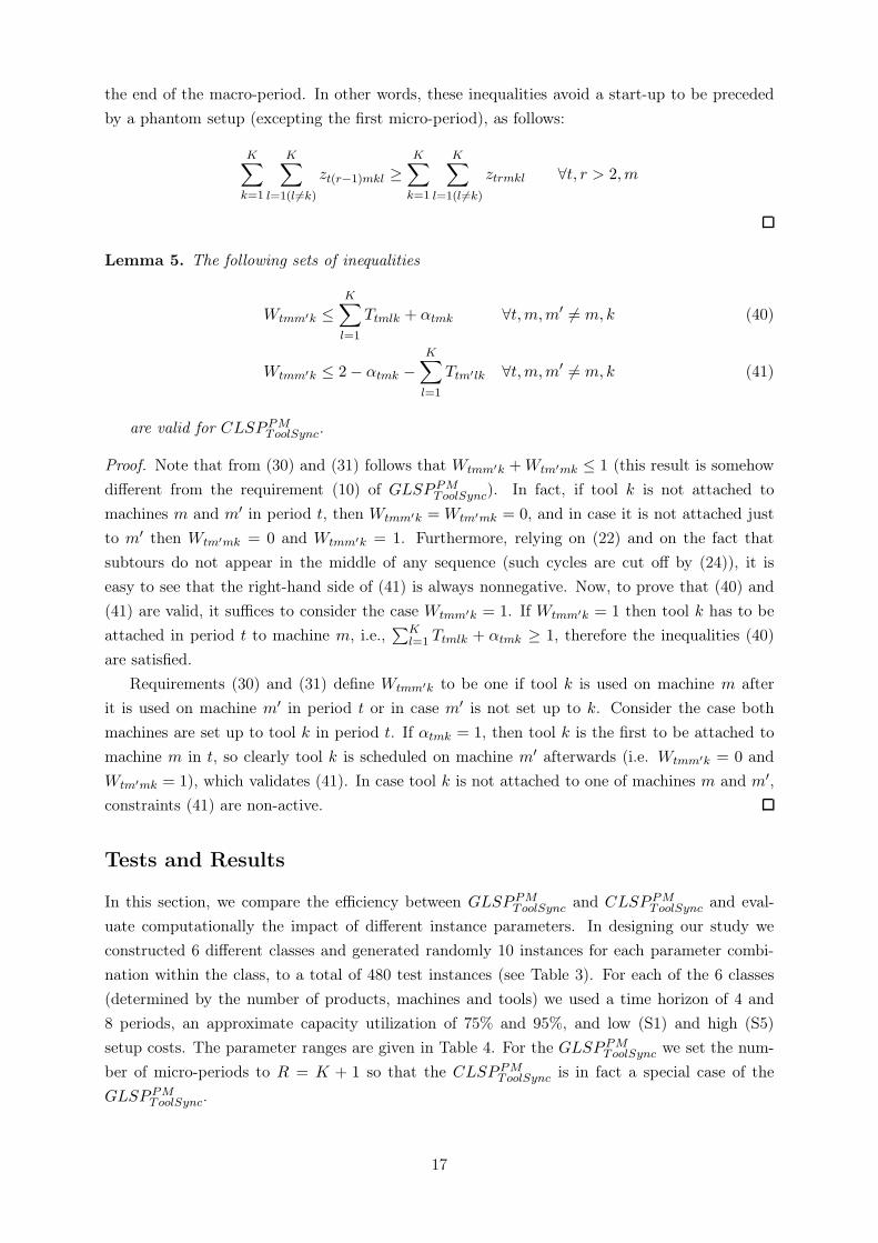
Tests and Results

In this section, we compare the efficiency between GLSPPMToolSync and CLSPPM

ToolSync and eval-

uate computationally the impact of different instance parameters. In designing our study we

constructed 6 different classes and generated randomly 10 instances for each parameter combi-

nation within the class, to a total of 480 test instances (see Table 3). For each of the 6 classes

(determined by the number of products, machines and tools) we used a time horizon of 4 and

8 periods, an approximate capacity utilization of 75% and 95%, and low (S1) and high (S5)

setup costs. The parameter ranges are given in Table 4. For the GLSPPMToolSync we set the num-

ber of micro-periods to R = K + 1 so that the CLSPPMToolSync is in fact a special case of the

GLSPPMToolSync.

17

Table 3: Classes of test instances

class N M K Tcapacity

utilizationsetup cost

N10-M2-K4-Tx-Cx-Sx 10 2 4

4, 8 75%, 95% 1, 5

N10-M2-K8-Tx-Cx-Sx 10 2 8N25-M2-K8-Tx-Cx-Sx 25 2 8N25-M4-K8-Tx-Cx-Sx 25 4 8N25-M4-K12-Tx-Cx-Sx 25 4 12N25-M8-K12-Tx-Cx-Sx 25 8 12

Table 4: Parameter ranges used for the test instances

Parameter Ranges and values used for the test instances

Bi0, Ii0 = 0bit = 3hit for t < T and the last period: biT = 300 ∗ hiT

ditd̄i2 + U [0; d̄i], where d̄i is the average demand computed based onthe given capacity utilization

hit = hi chosen randomly from the set {1, 2, 3}pimk U [0.008; 0.012]

Sim

randomly generated, such that on average 20% of themachine-tool combinations can be used for product i. The sameSim is used for each of the 10 instances of each parametervariation.

smkl U [0.005; 0.01], i.e. a setup takes 0.5-1% of the periods lengthσmkl = 10000smkl (S1) or = 50000smkl (S5)

ymk0 =

{

1 m = k

0 otherwise

Computational experiments were executed on an Intel Pentium D with 3.2 GHz CPU and

4 GB of random access memory. CPLEX 11.1 from ILOG was used as the MIP solver and the

models were coded in OPL version 6.0.1. Tables 5-7 display the percentage of instances that

CPLEX found a feasible solution (%feas), a capacity feasible solution (%capfeas), i.e. solutions

without backlog at the end of the planning horizon, and the optimal solution (%opt), as well as

the average gap (avg. gap) between the upper and lower bounds (in the case of capacity feasible

solutions) and the average CPU times (avg. time) in seconds. For each instance we allow a

maximum CPU time of 1 hour. Furthermore, the last column of Table 5 presents the difference

(%) between the best solution obtained with CLSPPMToolSync to that with GLSPPM

ToolSync.

It is clear that CLSPPMToolSync is always more efficient than GLSPPM

ToolSync. In fact, CPLEX

finds feasible solution to CLSPPMToolSync on every instance type and capacity feasible solutions for

almost all instances with K < 12 and K = 12, M = 4, and K = 12, M = 8, T = 4. Observe

that GLSPPMToolSync is not able to solve within one hour instances with K > 8 and K = 8, M = 4

for T = 8, and to find any feasible solution for instances with M > 2 (that account for 50% of

the total number of instances). Clustering only the instances that both models are able to find

capacity feasible solutions, the overall average gap between upper and lower bounds is 23% for

CLSPPMToolSync and 79% for GLSPPM

ToolSync, and the gap between the two models is -81%. When

both models were solved to optimality, CLSPPMToolSync had also significantly lower solution times

18

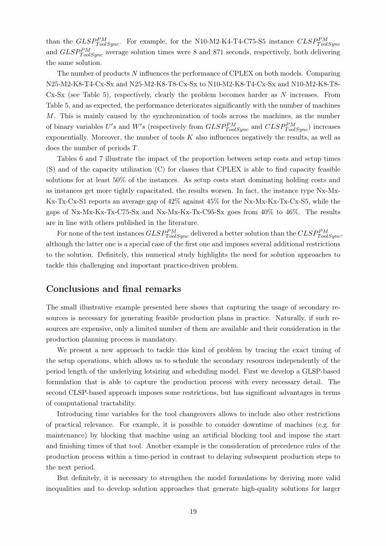
than the GLSPPMToolSync. For example, for the N10-M2-K4-T4-C75-S5 instance CLSPPM

ToolSync

and GLSPPMToolSync average solution times were 8 and 871 seconds, respectively, both delivering

the same solution.

The number of products N influences the performance of CPLEX on both models. Comparing

N25-M2-K8-T4-Cx-Sx and N25-M2-K8-T8-Cx-Sx to N10-M2-K8-T4-Cx-Sx and N10-M2-K8-T8-

Cx-Sx (see Table 5), respectively, clearly the problem becomes harder as N increases. From

Table 5, and as expected, the performance deteriorates significantly with the number of machines

M . This is mainly caused by the synchronization of tools across the machines, as the number

of binary variables U ′s and W ′s (respectively from GLSPPMToolSync and CLSPPM

ToolSync) increases

exponentially. Moreover, the number of tools K also influences negatively the results, as well as

does the number of periods T .

Tables 6 and 7 illustrate the impact of the proportion between setup costs and setup times

(S) and of the capacity utilization (C) for classes that CPLEX is able to find capacity feasible

solutions for at least 50% of the instances. As setup costs start dominating holding costs and

as instances get more tightly capacitated, the results worsen. In fact, the instance type Nx-Mx-

Kx-Tx-Cx-S1 reports an average gap of 42% against 45% for the Nx-Mx-Kx-Tx-Cx-S5, while the

gaps of Nx-Mx-Kx-Tx-C75-Sx and Nx-Mx-Kx-Tx-C95-Sx goes from 40% to 46%. The results

are in line with others published in the literature.

For none of the test instances GLSPPMToolSync delivered a better solution than the CLSPPM

ToolSync,

although the latter one is a special case of the first one and imposes several additional restrictions

to the solution. Definitely, this numerical study highlights the need for solution approaches to

tackle this challenging and important practice-driven problem.

Conclusions and final remarks

The small illustrative example presented here shows that capturing the usage of secondary re-

sources is necessary for generating feasible production plans in practice. Naturally, if such re-

sources are expensive, only a limited number of them are available and their consideration in the

production planning process is mandatory.

We present a new approach to tackle this kind of problem by tracing the exact timing of

the setup operations, which allows us to schedule the secondary resources independently of the

period length of the underlying lotsizing and scheduling model. First we develop a GLSP-based

formulation that is able to capture the production process with every necessary detail. The

second CLSP-based approach imposes some restrictions, but has significant advantages in terms

of computational tractability.

Introducing time variables for the tool changeovers allows to include also other restrictions

of practical relevance. For example, it is possible to consider downtime of machines (e.g. for

maintenance) by blocking that machine using an artificial blocking tool and impose the start

and finishing times of that tool. Another example is the consideration of precedence rules of the

production process within a time-period in contrast to delaying subsequent production steps to

the next period.

But definitely, it is necessary to strengthen the model formulations by deriving more valid

inequalities and to develop solution approaches that generate high-quality solutions for larger

19

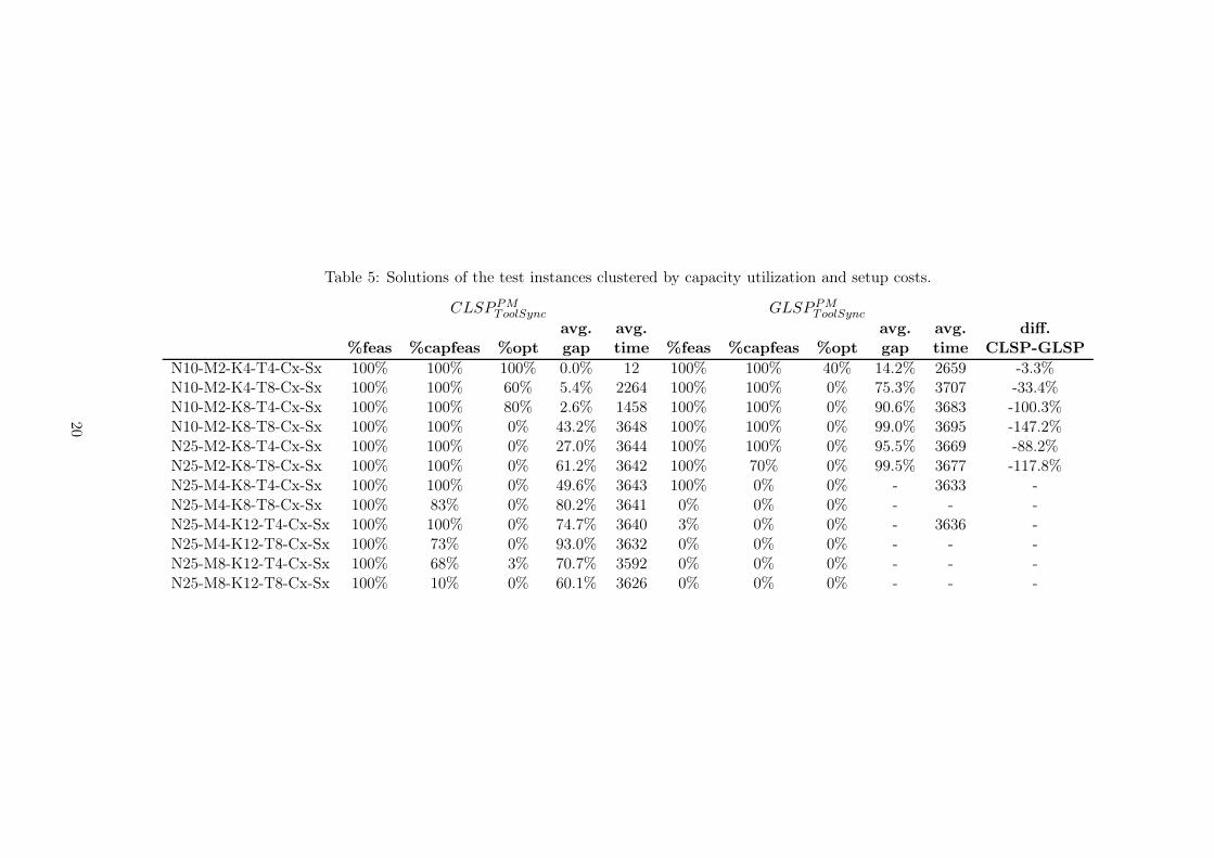
Table 5: Solutions of the test instances clustered by capacity utilization and setup costs.

CLSPPMToolSync GLSPPM

ToolSync

avg. avg. avg. avg. diff.

%feas %capfeas %opt gap time %feas %capfeas %opt gap time CLSP-GLSP

N10-M2-K4-T4-Cx-Sx 100% 100% 100% 0.0% 12 100% 100% 40% 14.2% 2659 -3.3%N10-M2-K4-T8-Cx-Sx 100% 100% 60% 5.4% 2264 100% 100% 0% 75.3% 3707 -33.4%N10-M2-K8-T4-Cx-Sx 100% 100% 80% 2.6% 1458 100% 100% 0% 90.6% 3683 -100.3%N10-M2-K8-T8-Cx-Sx 100% 100% 0% 43.2% 3648 100% 100% 0% 99.0% 3695 -147.2%N25-M2-K8-T4-Cx-Sx 100% 100% 0% 27.0% 3644 100% 100% 0% 95.5% 3669 -88.2%N25-M2-K8-T8-Cx-Sx 100% 100% 0% 61.2% 3642 100% 70% 0% 99.5% 3677 -117.8%N25-M4-K8-T4-Cx-Sx 100% 100% 0% 49.6% 3643 100% 0% 0% - 3633 -N25-M4-K8-T8-Cx-Sx 100% 83% 0% 80.2% 3641 0% 0% 0% - - -N25-M4-K12-T4-Cx-Sx 100% 100% 0% 74.7% 3640 3% 0% 0% - 3636 -N25-M4-K12-T8-Cx-Sx 100% 73% 0% 93.0% 3632 0% 0% 0% - - -N25-M8-K12-T4-Cx-Sx 100% 68% 3% 70.7% 3592 0% 0% 0% - - -N25-M8-K12-T8-Cx-Sx 100% 10% 0% 60.1% 3626 0% 0% 0% - - -

20

Table 6: Solutions of CLSPPMToolSync of the test instances clustered by time periods and capacity

utilization.

%feas %capfeas %opt avg. gap avg. time

N10-M2-K4-Tx-Cx-S1 100% 100% 75% 3.0% 1355N10-M2-K4-Tx-Cx-S5 100% 100% 85% 2.4% 921N10-M2-K8-Tx-Cx-S1 100% 100% 35% 22.5% 2701N10-M2-K8-Tx-Cx-S5 100% 100% 45% 23.3% 2404N25-M2-K8-Tx-Cx-S1 100% 100% 0% 36.7% 3644N25-M2-K8-Tx-Cx-S5 100% 100% 0% 51.6% 3642N25-M4-K8-Tx-Cx-S1 100% 93% 0% 62.0% 3643N25-M4-K8-Tx-Cx-S5 100% 90% 0% 64.9% 3640

N25-M4-K12-Tx-Cx-S1 100% 90% 0% 84.0% 3635N25-M4-K12-Tx-Cx-S5 100% 83% 0% 80.7% 3636

Table 7: Solutions of CLSPPMToolSync of the test instances clustered by time periods and setup

costs.

%feas %capfeas %opt avg. gap avg. time

N10-M2-K4-Tx-C75-Sx 100% 100% 95% 0.3% 602N10-M2-K4-Tx-C95-Sx 100% 100% 65% 5.1% 1674N10-M2-K8-Tx-C75-Sx 100% 100% 50% 17.1% 1957N10-M2-K8-Tx-C95-Sx 100% 100% 30% 28.8% 3149N25-M2-K8-Tx-C75-Sx 100% 100% 0% 38.3% 3641N25-M2-K8-Tx-C95-Sx 100% 100% 0% 49.9% 3645N25-M4-K8-Tx-C75-Sx 100% 90% 0% 62.1% 3642N25-M4-K8-Tx-C95-Sx 100% 93% 0% 64.7% 3642

N25-M4-K12-Tx-C75-Sx 100% 88% 0% 81.9% 3635N25-M4-K12-Tx-C95-Sx 100% 85% 0% 83.0% 3637

instances.

Acknowledgments

This work was partly financed by the Austrian Science Foundation under the contract number

J2815-N13. The authors want to thank Maria Antónia Carravilla and José Fernando Oliveira

for many helpful discussions and comments on this work.

References

Akturk, M., Onen, S., 2002. Dynamic lot sizing and tool management in automated manufac-

turing systems. Computers & Operations Research 29, 1059–1079.

Almada-Lobo, B., Carravilla, M., Oliveira, J., 2008a. A note on "the capacitated lot-sizing

and scheduling problem with sequence-dependent setup costs and setup times. Computers &

Operations Research 35 (1374–1376).

Almada-Lobo, B., Klabjan, D., Carravilla, M., Oliveira, J., 2007. Single machine multi-product

21

capacitated lot sizing with sequence-dependent setups. International Journal of Production

Research 45 (4873–4894).

Almada-Lobo, B., Oliveira, J., Carravilla, M., 2008b. Production planning and scheduling in the

glass container industry: A VNS approach. International Journal of Production Economics

114 (1), 363–375.

Billington, P., McClain, J., Thomas, L., 1983. Mathematical programming approach to capacity-

constrained MRP systems: Review, formulation and problem reduction. Management Science

29 (10), 1126–1141.

Dastidar, S., Nagi, R., 2005. Scheduling injection molding operations with multiple resource

constraints and sequence dependent setup times and costs. Computers & Operations Research

32, 2987–3005.

Drexl, A., Kimms, A., 1997. Lot sizing and scheduling - survey and extensions. European Journal

of Operational Research 99 (2), 221–235.

Ellis, K. P., Lu, Y., Bish, E. K., 2004. Scheduling of wafer test processes in semiconductor

manufacturing. International Journal of Production Research 42 (2), 215–242.

Ferreira, D., Morabito, R., Rangel, S., 2009. Solution approaches for the soft drink integrated

production lot sizing and scheduling problem. European Journal of Operational Research 196,

697–706.

Fleischmann, B., Meyr, H., 1997. The general lotsizing and scheduling problem. OR Spektrum

19, 11–21.

Haase, K., 1996. Capacitated lot-sizing with sequence dependent setup costs. Operations Re-

search Spektrum 18, 51–59.

Jans, R., Degraeve, Z., 2004. An industrial extension of the discrete lot-iszing and scheduling

problem. IIE Transactions 36 (1), 47–58.

Jans, R., Degraeve, Z., 2008. Modeling industrial lot sizing problems: a review. International

Journal of Production Research 46 (6), 1619–1643.

Kang, S., Malik, K., Thomas, L., 1999. Lotsizing and scheduling on parallel machines with

sequence-dependent setup cost. Management Science 45 (2), 273–289.

Karimi, B., Fatemi Ghomi, S., Wilson, J., 2003. The capacitated lot sizing problem: review of

models and algorithms. OMEGA 31, 365–378.

Meyr, H., 2002. Simultaneous lotsizing and scheduling on parallel machines. European Journal

of Operational Research 139, 277 – 292.

Mönch, L., 2004. Scheduling-Framework für Jobs auf parallelen Maschinen in komplexen Pro-

duktionssystemen. Wirtschaftsinformatik 46 (6), 470–480.

22

Pochet, Y., Wolsey, L. A., 2006. Production Planning by Mixed Integer Programming. Springer

Series in Operations Research and Financial Engineering. Springer, New York.

Quadt, D., Kuhn, H., 2005. Conceptual framework for lot-sizing and scheduling of flexible flow

lines. International Journal of Production Research 43 (11), 2291–2308.

Quadt, D., Kuhn, H., 2008. Capacitated lot-sizing with extensions: a review. 4OR 6, 61–83.

Suerie, C., Stadtler, H., 2003. The capacitated lot-sizing problems with linked lot sizes. Manage-

ment Science 49 (8), 1039–1054.

Tempelmeier, H., Buschkühl, L., 2008. Dynamic multi-machine lotsizing and sequencing with

simultaneous scheduling of a common setup resource. International Journal of Production

Economics 113, 401–412.

Wolsey, L., 2002. Solving multi-item lot-sizing problems with an mip solver using classification

and reformulation. Management Science 48 (12), 1587–1602.

23

Synchronization of Scarce Resources for a Parallel Machine Lotsizing

Problem

Appendix

by Christian Almeder and Bernardo Almada-Lobo

Proof for Theorem 3

Proof. Let us consider a feasible solution of the CLSPPMToolSync. Due to the subtour elimination

guaby Christian Almeder and Bernardo Almada-Loboranteed by constraints (23), (24), and (27)

there exists for each period t a well defined sequence of tools Φtm : ktm1 → ktm2 · · · → ktmλtm

of length λtm that are attached to machine m. Such a sequence contains each tool at most

once, except the last tool which might be identical with the first tool (ktm1 = ktmλtm). These

sequences are determined by the values of αtmk and Ttmkl, i.e. if one of the variables are changed,

the corresponding sequence changes and vice versa. From now on, we omit the indices t and m

of ktmν and λtm for an easier representation.

We have to set the number of micro-periods in the GLSPPMToolSync to R ≥ K + 1 (note that

λ ≤ K + 1) and define now a mapping f as follows (for an easy representation all variables of

the GLSPPMToolSync not appearing in that mapping are set to 0):

f

Iit

Bit

Xitmk

αtmk

Ttmkl

µstmk

µftmk

µmaxtm

Φtm

7→

Iit

Bit

xit1mk1 = Xitmk1 , xit2mk2 = Xitmk2 , . . . , xit(λ−1)mkλ−1= Xitmkλ−1

,

xitλmkλ =

Xitmkλ kλ 6= k1

0 kλ = k1

yt1mk1 = yt2mk2 = · · · = ytλmkλ = yt(λ+1)mkλ = . . . ytRmkλ = 1

zt1mk1k1 = zt2mk1k2 = zt3mk2k3 = · · · = ztλmkλkλ = 1,

zt(λ+1)mkλkλ = · · · = ztRmkλkλ = 1

ust1m = µstmk1

, . . . , ust(λ−1)m = µs

tmkλ−1, ustλm = µmax

tm − smkλ−1kλ,

ust(λ+1)m = · · · = ustRm = 1

uft1m = µftmk1

, . . . , uft(λ−1)m

= µftmkλ−1

, uftλm = · · · = uftRm = 1

According to the sequence of tools Φtm of the CLSPPMToolSync solution, the first λ micro-periods

of the GLSPPMToolSync are used each for the production with the corresponding tool. During the

remaining micro-periods no tool exchange is performed and the length of those micro-periods is

set to zero (ustrm = uftrm = 1, r > λ). All decision variables of the CLSPPMToolSync appearing in

active constraints are used in the mapping, i.e. if any of those variables changes in a feasible way,

also the mapped solution of the GLSPPMToolSyncchanges. Hence, the mapping is injective.

Now we show that all constraints of the GLSPPMToolSync are fulfilled. The inventory balance

constraints (2) hold, because the Iit and Bit are not changed, and the total production during a

A-1

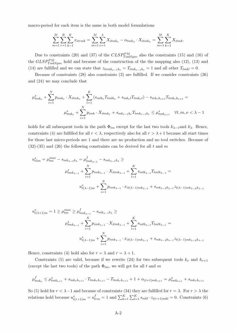
macro-period for each item is the same in both model formulations

M∑

m=1

R∑

r=1

K∑

k=1

xitrmk =M∑

m=1

λ∑

ν=1

Xitmkν − αtmkλ ·Xitmkλ =M∑

m=1

K∑

k=1

Xitmk.

Due to constraints (20) and (37) of the CLSPPMToolSync also the constraints (15) and (16) of

the GLSPPMToolSync hold and because of the construction of the the mapping also (12), (13) and

(14) are fulfilled and we can state that ztνmkν−1kν = Ttmkν−1kν = 1 and all other Ttmkl = 0.

Because of constraints (28) also constraints (3) are fulfilled. If we consider constraints (26)

and (24) we may conclude that

µstmkν

+

N∑

i=1

pimkν ·Xitmkν +

K∑

l=1

(smlkνTtmlkν + smkν lTtmkν l)− smkνkν+1Ttmkνkν+1

=

µstmkν

+

N∑

i=1

pimk ·Xitmkν + smkν−1kνTtmkν−1kν ≤ µstmkν+1

∀t,m, ν < λ− 1

holds for all subsequent tools in the path Φtm except for the last two tools kλ−1and kλ. Hence,

constraints (4) are fulfilled for all r < λ, respectively also for all r > λ+1 because all start times

for those last micro-periods are 1 and there are no production and no tool switches. Because of

(32)-(35) and (26) the following constraints can be derived for all t and m

ustλm = µmaxtm − smkλ−1kλ = µf

tmkλ−1− smkλ−1kλ ≥

µstmkλ−1

+

N∑

i=1

pimkλ−1·Xitmkλ−1

+

K∑

l=1

smlkλ−1Ttmlkλ−1

=

ust(λ−1)m +N∑

i=1

pimkλ−1· xit(λ−1)mkλ−1

+ smkλ−2kλ−1zt(λ−1)mkλ−2kλ−1

ust(λ+1)m = 1 ≥ µmaxtm ≥ µf

tmkλ−1− smkλ−1kλ ≥

µstmkλ−1

+

N∑

i=1

pimkλ−1·Xitmkλ−1

+

K∑

l=1

smlkλ−1Ttmlkλ−1

=

ust(λ−1)m +

N∑

i=1

pimkλ−1· xit(λ−1)mkλ−1

+ smkλ−2kλ−1zt(λ−1)mkλ−2kλ−1

Hence, constraints (4) hold also for r = λ and r = λ+ 1.

Constraints (5) are valid, because if we rewrite (24) for two subsequent tools kν and kν+1

(except the last two tools) of the path Φtm, we will get for all t and m

µftmkν

≤ µstmkν+1

+ smkνkν+1· Ttmkνkν+1

− Ttmkνkν+1+ 1 + α(t+1)mkν+1

= µstmkν+1

+ smkνkν+1

So (5) hold for r < λ−1 and because of constraints (34) they are fulfilled for r = λ. For r > λ the

relations hold because ust(r+1)m = uftrm = 1 and

∑Kk=1

∑Kl=1 smkl · zt(r+1)mkl = 0. Constraints (6)

A-2

are valid, because either λ < R and ustRm = uftRm = 1 and xitRmk = 0 or λ = R and constraints

(32)–(34) and (27) ensure the necessary relations between ustRm and uftRm. Constraints (7) and

(8) follow directly from (24)–(27), (32)–(35) and the definition of the mapping f .

In the remaining part of the proof we will show that the synchronization constraints are

valid. Constraints (11) together with (9) and (10) enforce, that either the start time of micro-

period r on machine m has to be greater or equal than the finishing time of micro-period r′ on a

different machine m′ if the same tool is used in that period or the other way around, depending

which micro-period starts first. Since we only compare micro-periods where the same tools k

are used, the mapping f identifies corresponding start and finishing times µstmk and µf

tm′k of

the CLSPPMToolSync. If tool k is the last tool on machine m and the considered micro-period is

r = λ, we have to take µmaxtm −

∑

l sm′lk · Ttm′lk as start time and 1 as finishing time. Because

of constraints (30), (31), and (36) it is guaranteed, that the start time on one machine is always

after the finishing time on another machine, or the other way around.

Finally, we show that the values of the objective functions are identical. Inventory and

backorder levels are the same and as previously noticed ztrmkl = 1 only if a corresponding

Ttmkl = 1 (for k 6= l). Since the ztrmkl values are determined by the path Φtm and because of the

subtour elimination no tool exchange can occur more than once, we can state that∑R

r=1 ztrmkl =

Ttmkl (for k 6= l). So together with the fact that stmkk = σtmkk = 0 it follows directly that also

the setup cost parts of the objective functions are identical.

A-3