1

Seismic Processing Workshop

SPW™

V 3.4

October 2016

Parallel Geoscience Corporation

2

About This Manual

This manual is organized into two sections. The first section is a user’s manual for the SPW

Flowchart application. The second section is a reference manual that describes each of the

processing steps and associated parameters in the SPW Processing library.

Parallel Geoscience Corporation

PO Box 5989

Incline Village, NV 89450

Tel: +1.541.421.3127

E-mail: support@parallelgeo.com

Web: http://www.parallelgeo.com

SPW, Seismic Processing Workshop, SPW Flowchart, SPW Executor, are trademarks of Parallel

Geoscience Corporation. All other products are trademarks of their respective companies.

This manual is proprietary information of Parallel Geoscience Corporation and is for the internal

use only by licensed purchasers of SPW products.

© 2016 Parallel Geoscience Corporation

3

Contents

Seismic Processing Workshop ............................................................................................ 1 About This Manual ..................................................................................................................... 2 Introduction to SPW ................................................................................................................. 11 Product Support ........................................................................................................................ 12

SPW Flowchart ................................................................................................................. 13 SPW Installer Available Online ................................................................................................ 13 Installing SPW on Windows ..................................................................................................... 15 Creating or Selecting a Project ................................................................................................. 21 SEG Y Processing Format ........................................................................................................ 25

Main Flowchart Window .......................................................................................................... 29

Tool Bar ................................................................................................................................ 29 Processing Categories ........................................................................................................... 32

Processing Steps Lists ........................................................................................................... 33

Building Processing Flows ................................................................................................... 33 Setting Processing Step and Data Step Parameters............................................................... 34 Running a Flow ..................................................................................................................... 35

Console Display .................................................................................................................... 35 Menu Items ............................................................................................................................... 36

FlowChart Menu ....................................................................................................................... 36 Edit Current Project .............................................................................................................. 37 SEG Y Analyzer ................................................................................................................... 38

SEG D Analysis .................................................................................................................... 41 SPS Analysis ......................................................................................................................... 43

The Display Menu..................................................................................................................... 48 Displaying Seismic Data ....................................................................................................... 48

The Display Configuration Wizard ....................................................................................... 50 The Seismic Display ............................................................................................................. 51

Seismic Display Control Panel ............................................................................................. 53 Left Side of the Seismic Display Control Panel ................................................................... 54 Center of the Seismic Display Control Panel – Sort Keys ................................................... 55

Select Sort Key Number ....................................................................................................... 56 Sorting Keys.......................................................................................................................... 57 Data and Display Tools ......................................................................................................... 58

Quick Sort Options ............................................................................................................... 60 Capture an Image Tool.......................................................................................................... 62

Select Color Scale Tool ........................................................................................................ 63 Create Color Scale Tool ........................................................................................................ 64 Opening and Saving the Seismic Display ............................................................................. 65 Attribute Maps ...................................................................................................................... 67 Velocity Analysis Builder ..................................................................................................... 68

Constant Velocity Stacks flow .............................................................................................. 69 Velocity Semblance flow ...................................................................................................... 71 CMP Gathers flow ................................................................................................................ 72

4

Execution .............................................................................................................................. 72

The Survey Menu ...................................................................................................................... 74

The SPS Database ..................................................................................................................... 75 The Image Database .............................................................................................................. 76 Map Displays ........................................................................................................................ 78 The Basemap ......................................................................................................................... 78

Base Map Display Control Panel .............................................................................................. 81

Fold Maps ............................................................................................................................. 83 Compute Fold Difference ..................................................................................................... 85

The Picking Menu ..................................................................................................................... 85 The Wells Menu ........................................................................................................................ 89

VSP Geometry Definition ..................................................................................................... 92

The Help Menu ......................................................................................................................... 93

Displaying Spreadsheets of Auxiliary Data .............................................................................. 94 Early Mute Functions ............................................................................................................ 95

Receiver Statics ..................................................................................................................... 96

Source Statics ........................................................................................................................ 97 Velocity Functions ................................................................................................................ 98 SPS Observers Notes ............................................................................................................ 99

SPS Receiver Locations ...................................................................................................... 100 SPS Source Locations ......................................................................................................... 102

Running the Flowchart ............................................................................................................ 104 Naming and Saving a Flow ................................................................................................. 104

Executing a Flow inside the Flowchart ................................................................................... 106

Executing a Flow on a Cluster ............................................................................................ 107 Example 3D Processing Flows ............................................................................................... 108

Flow 1 - Vertical Geometry ................................................................................................ 110 Flow 2 – Bandpass Filtering and Spherical Divergence Correction ................................... 119

Flow 3 – Normal Moveout Correction and Vertical Stacking ............................................ 123 Flow 4 – Create Time Slice ................................................................................................ 127

Instantaneous Field QC Capabilities and Procedures ............................................................. 131 Real Time Processing ......................................................................................................... 131 Real Time Seismic Displays ............................................................................................... 133

Real Time Map Displays .................................................................................................... 134 FTP Connection ...................................................................................................................... 135

Sending Reports via FTP in Real Time .............................................................................. 136

Sending Image Files via FTP in Real Time ........................................................................ 138 Troubleshooting ...................................................................................................................... 139

No License Key Available .................................................................................................. 139 Killing the Flowchart Process ............................................................................................. 139

The Processing Library: .................................................................................................. 141 Amplitude Adjustment Steps .......................................................................................... 142

AVA Calculator ...................................................................................................................... 143

Amplitude Equalization .......................................................................................................... 145 Amplitude Versus Angle......................................................................................................... 147 Angle Gather ........................................................................................................................... 150

5

Apply Gain .............................................................................................................................. 152

Automatic Gain Control .......................................................................................................... 154

Clipping................................................................................................................................... 156 Offset Amplitude Corrections ................................................................................................. 157 Random Noise ......................................................................................................................... 160 Spherical Divergence .............................................................................................................. 162 Surface Consistent Gain Corrections ...................................................................................... 164

Trace Header Amplitude Math ............................................................................................... 167 Windowed AGC...................................................................................................................... 168 Windowed Trace Balance ....................................................................................................... 170

Creating and Editing Auxiliary Data File ....................................................................... 173 Creating and Editing Auxiliary Data Files .............................................................................. 173

SPS Point Record .................................................................................................................... 190

Creating Card Data Using Excel ............................................................................................. 192 Auxiliary Data A-P ......................................................................................................... 199

CMP Flex Locations ............................................................................................................... 199

CMP Statics ............................................................................................................................ 201 Early Mutes ............................................................................................................................. 203 Exclusion Zones ...................................................................................................................... 205

FK Mutes ................................................................................................................................ 207 Field File Statistics .................................................................................................................. 208

First Break Times .................................................................................................................... 211 Gain Curves ............................................................................................................................ 213 Horizon File ............................................................................................................................ 215

Line Definition File................................................................................................................. 216 Offset Gain Corrections .......................................................................................................... 218

PP NHMO Eta Function ......................................................................................................... 220 PP NHMO Gamma Function .................................................................................................. 222

Polygon Definition .................................................................................................................. 223 Auxiliary Data R-Z ......................................................................................................... 225

Receiver Gain Corrections ...................................................................................................... 226 Receiver Statics ....................................................................................................................... 229 SPS Observer Notes ................................................................................................................ 231

SPS Receiver Locations .......................................................................................................... 233 SPS Source Locations ............................................................................................................. 236 Source Gain Corrections ......................................................................................................... 238

Source Statics .......................................................................................................................... 241 Surgical Mutes ........................................................................................................................ 243

Tail Mutes ............................................................................................................................... 245 UKOOA P1 90 ........................................................................................................................ 247 Velocity Function.................................................................................................................... 247 Window Definition ................................................................................................................. 250

Display Steps .................................................................................................................. 251

Frequency Slices to Time Traces ............................................................................................ 251 Real Time Amplitude Spectrum Plot ...................................................................................... 253 Real Time Data Quality Analysis ........................................................................................... 254

6

Real Time Near Trace Display ............................................................................................... 258

Real Time Quality Analysis Statistics Map ............................................................................ 262

Real Time Quality Analysis Statistics Plot ............................................................................. 266 Real Time Receiver Attribute Map ......................................................................................... 270 Real Time Receiver Spread .................................................................................................... 275 Real Time Seismic Display ..................................................................................................... 280 Real Time Source Attribute Map ............................................................................................ 284

Real Time Stack Display ........................................................................................................ 289 Real Time Trace Header Map ................................................................................................. 293 Time Slices.............................................................................................................................. 298 Time Slices to Traces .............................................................................................................. 300

Editing Steps ................................................................................................................... 302

3D Missing Data Interpolation................................................................................................ 302

Automatic Amplitude Edit ...................................................................................................... 304 Automatic Trace Edit .............................................................................................................. 306

Coherent Noise Attenuation .................................................................................................... 309

Dataset Math ........................................................................................................................... 311 Despike ................................................................................................................................... 312 Dominant Frequency Edits ..................................................................................................... 314

F-X Trace Interpolation .......................................................................................................... 318 Frequency Trace Edits ............................................................................................................ 320

Interpolate Dead Traces .......................................................................................................... 324 Kill Traces ............................................................................................................................... 325 Phase Rotation ........................................................................................................................ 326

Remove DC Bias..................................................................................................................... 328 Remove Reverberation............................................................................................................ 331

Resample Seismic ................................................................................................................... 333 Reverse Traces ........................................................................................................................ 335

Revive Dead Traces ................................................................................................................ 336 S/N Based Record Edits .......................................................................................................... 338

Trace Header Calculation ....................................................................................................... 342 Trace Header Logic................................................................................................................. 344 Trace Header Math ................................................................................................................. 347

Trace Header Resequencing ................................................................................................... 349 Trace Sample Math ................................................................................................................. 351 Vibroseis Correlation .............................................................................................................. 352

Filtering Steps ................................................................................................................. 356 2D Damped Least Squares Filter ............................................................................................ 356

2D Median Filter ..................................................................................................................... 358 3D Diffusion Filter .................................................................................................................. 360 3D Median Filter ..................................................................................................................... 362 Adaptive Radon Demultiple ................................................................................................... 364 Apply F-K Filter ..................................................................................................................... 370

Apply F-K Velocity Filter ....................................................................................................... 373 Butterworth Dip Filtering ....................................................................................................... 377 Butterworth Filtering .............................................................................................................. 379

7

Coherence Enhancement Filter ............................................................................................... 382

Convolution............................................................................................................................. 383

Cross Correlation .................................................................................................................... 384 Derivative ................................................................................................................................ 387 Diffusion Filter........................................................................................................................ 388 F-K Spectrum ..................................................................................................................... 390 F-X Deconvolution ................................................................................................................. 392

F-X Median Filter ................................................................................................................... 395 F-X Noise Attenuation ............................................................................................................ 397 F-X-Y Median Filter ............................................................................................................... 399 Footprint Filter ........................................................................................................................ 401 Horizontal Median Filter......................................................................................................... 404

Integration ............................................................................................................................... 406

Notch Filter ............................................................................................................................. 406 Quadrature Filter ..................................................................................................................... 409

Radial Transform Filter........................................................................................................... 410

Radon Demultiple ................................................................................................................... 414 Ricker Filter ............................................................................................................................ 419 Swell Statics Correction .......................................................................................................... 421

Tau-p Inverse Transform ........................................................................................................ 422 Tau-p Transform ..................................................................................................................... 424

Time Variant Bandpass ........................................................................................................... 428 Time Variant Butterworth ....................................................................................................... 430 Velocity-Guided Butterworth Filter ........................................................................................ 431

Velocity-Guided Noise Rejection Filter ................................................................................. 434 Geometry Steps ............................................................................................................... 437

Bin Fold Limit......................................................................................................................... 440 CMP Binning .......................................................................................................................... 443

CMP Fold - Data ..................................................................................................................... 450 Coordinate Conversion ........................................................................................................... 452

Crooked Line Binning............................................................................................................. 457 Extract Geometry .................................................................................................................... 459 Geometry Definition ............................................................................................................... 461

OBS Positioning...................................................................................................................... 468 Offset Binning ......................................................................................................................... 470 Simple Marine Geometry ........................................................................................................ 472

UKOOA P1/90 Geometry ....................................................................................................... 474 Update Marine Streamer ......................................................................................................... 476

Update Receiver Positions ...................................................................................................... 477 Update Source Positions ......................................................................................................... 480

Migration Steps ............................................................................................................... 482 2D Paraxial Ray Tracing ......................................................................................................... 482 2D Pre-Stack PSPI Migration ................................................................................................. 485

3D Finite Differences Ray Tracing ......................................................................................... 489 Constant Velocity PSKTM ..................................................................................................... 491 Convert Time to Depth ........................................................................................................... 493

8

FK Dip Moveout ..................................................................................................................... 496

PSPI Migration........................................................................................................................ 496

Phase Shift Migration ............................................................................................................. 500 Post-Stack Kirchhoff Time Migration .................................................................................... 503 Pre-Stack Kirchhoff Depth Migration .................................................................................... 506 Pre-Stack Kirchhoff Time Migration ...................................................................................... 508 Stolt Migration ........................................................................................................................ 511

Multi-component Steps ................................................................................................... 514 Apply PS Non-hyperbolic Moveout ....................................................................................... 515 CCP Binning - Asymptotic ..................................................................................................... 519 CCP Binning - Dynamic ......................................................................................................... 522 Constant Gamma Stacks ......................................................................................................... 525

Converted Wave Receiver Statics ........................................................................................... 528

Crooked Line Asymptotic CCP Binning ................................................................................ 530 Crooked Line Dynamic CCP Binning .................................................................................... 532

Horizontal Component Rotations ........................................................................................... 535

Mutes Steps ..................................................................................................................... 539 Apply Early Mute ................................................................................................................... 539 Apply Surgical Mute ............................................................................................................... 543

Apply Tail Mute ...................................................................................................................... 545 Build Mask Model .................................................................................................................. 547

Quality Analysis Steps .................................................................................................... 550 Amplitude Analysis ................................................................................................................ 551 Amplitude Spectrum ............................................................................................................... 553

Autocorrelation ....................................................................................................................... 556 Dead Trace Analysis ............................................................................................................... 558

Frequency Analysis ................................................................................................................. 560 Signal to Noise ........................................................................................................................ 563

Signal to Noise Attribute ........................................................................................................ 565 Source Energy Estimation....................................................................................................... 571

Spectral Comparison ............................................................................................................... 573 Trace Analysis Report............................................................................................................. 578

Seismic Data Steps .......................................................................................................... 581

AutoSeis Real Time Seismic Input ......................................................................................... 582 AutoSeis Seismic Input ........................................................................................................... 584 AutoSeis Seismic Ouput ......................................................................................................... 585

Create Model Data .................................................................................................................. 585 Frequency Cubes ..................................................................................................................... 587

Frequency Gathers .................................................................................................................. 592 Frequency Maps ...................................................................................................................... 596 Real Time Seismic Input ......................................................................................................... 600 SEG 2 Import .......................................................................................................................... 602 SEG D Import ......................................................................................................................... 604

SEG Y Export ......................................................................................................................... 607 SEG Y Field Export ................................................................................................................ 610 SEG Y Field Import ................................................................................................................ 612

9

SEG Y Import ......................................................................................................................... 614

Seismic File ............................................................................................................................. 618

Select Traces ........................................................................................................................... 624 TCPIP Data Input .................................................................................................................... 626 Update SEGY Textheader ....................................................................................................... 630 Virtual Tape Input ................................................................................................................... 631

Spectral Attributes Steps ................................................................................................. 634

Bandwidth ............................................................................................................................... 634 Center Frequency .................................................................................................................... 636 Kurtosis ................................................................................................................................... 637 Mean Amplitude ..................................................................................................................... 639 Minimum Amplitude .............................................................................................................. 640

Peak Amplitude ....................................................................................................................... 641

Peak Amplitude Above Mean ................................................................................................. 643 Peak Frequency ....................................................................................................................... 644

Phase at Peak Frequency ......................................................................................................... 646

RMS Frequency ...................................................................................................................... 647 Skewness ................................................................................................................................. 649 Spectral Variance .................................................................................................................... 650

Spectral Decomposition Steps ........................................................................................ 653 Band Aid ................................................................................................................................. 654

Bandwidth Enhancement ........................................................................................................ 655 Cohen’s Class.......................................................................................................................... 655 Short-Time Fourier Transform ............................................................................................... 655

Stockwell Transform ............................................................................................................... 656 Wavelet Recomposition .......................................................................................................... 656

Wavelet Transform ................................................................................................................. 656 Wigner-Ville Decomposition .................................................................................................. 656

Windowed Wigner-Ville Decomposition ............................................................................... 657 Stacking Summing Steps ................................................................................................ 658

CMP Stack .............................................................................................................................. 658 Horizontal Trace Sum ............................................................................................................. 661 Median Stack .......................................................................................................................... 664

Real Time CMP Stack ............................................................................................................ 667 Receiver Order Stack .............................................................................................................. 669 Source Order Stack ................................................................................................................. 671

Trace Mixing ........................................................................................................................... 674 Statics Steps .................................................................................................................... 676

Apply Statics Shift .................................................................................................................. 677 Datum Statics .......................................................................................................................... 679 First Arrival Picking ............................................................................................................... 682 First Break Auto-Picking ........................................................................................................ 683 Flat Datum Statics ................................................................................................................... 683

Stack-Power Optimization Statics .......................................................................................... 684 Surface Consistent Residual Statics ........................................................................................ 689 Trim Statics ............................................................................................................................. 692

10

Trace Attributes Steps ..................................................................................................... 695

Instantaneous Amplitude ........................................................................................................ 696

Instantaneous Frequency ......................................................................................................... 697 Instantaneous Phase ................................................................................................................ 698

VSP Steps........................................................................................................................ 701 Apply VSP Traveltimes .......................................................................................................... 701 Calculate VSP Traveltimes ..................................................................................................... 704

VSP CMP Transform .............................................................................................................. 707 VSP Corridor Stack................................................................................................................. 709 VSP Deconvolution ................................................................................................................ 711 VSP Downhole Locations ....................................................................................................... 713 VSP Extract Corridor .............................................................................................................. 715

VSP First Arrival Time Picks ................................................................................................. 716

VSP Geometry Definition ....................................................................................................... 716 VSP SPS Relation Records ..................................................................................................... 719

VSP Surface Locations ........................................................................................................... 721

VSP Wavefield Separation ..................................................................................................... 723 Velocity Steps ................................................................................................................. 727

Apply Linear Moveout ............................................................................................................ 728

Apply Normal Moveout .......................................................................................................... 729 Apply PP Non-hyperbolic Moveout ....................................................................................... 732

Constant Velocity Stacks ........................................................................................................ 736 Create Velocity Field .............................................................................................................. 739 Extract Functions .................................................................................................................... 741

Interpolate Field ...................................................................................................................... 745 MASW Calculation ................................................................................................................. 748

Offset Dependent Linear Moveout ......................................................................................... 749 Residual Moveout Analysis .................................................................................................... 751

Residual Moveout Applications .............................................................................................. 755 Velocity Semblance ................................................................................................................ 757

Wavelet Shaping Steps ................................................................................................... 760 Deghosting .............................................................................................................................. 760 FKK Domain Spectral Shaping .............................................................................................. 763

Predictive Deconvolution........................................................................................................ 766 Predicitve Multichannel Deconvolution ................................................................................. 768 Q Filter .................................................................................................................................... 770

Signature Deconvolution ........................................................................................................ 772 Spectral Whitening.................................................................................................................. 774

Spiking Deconvolution ........................................................................................................... 776 Spiking Multichannel Deconvolution ..................................................................................... 778 Surface Consistent Decomposition ......................................................................................... 780 Surface Consistent Deconvolution .......................................................................................... 783

11

Introduction to SPW

Welcome to Seismic Processing Workshop (SPW). SPW is a seismic processing solution written

by Parallel Geoscience Corporation. SPW was originally written for the Macintosh computer

platform and has been redesigned and rewritten for the third time (version 3) using the Qt by Nokia

cross platform framework. SPW is currently available and has been tested on the Windows 10,

Windows 7, Windows Vista, Windows XP, Windows 2003 Server, and Windows 2008 HPC

Server operating systems. Linux, and Macintosh OSX versions will be available sometime in 2014.

The SPW version 3 Flowchart has adopted a project model for data management. Flowchart allows

you to create or select a project, build processing flows, set the parameters for the processing steps

and display seismic data and maps. Another significant change in SPW is the use of SEG Y format

as the default native format for processing data. A simple graphical user interface reduces the

learning curve and accelerates your analysis and processing time

The SPW system is designed to be user expandable. Parallel Geoscience Corporation will release

the programming API interfaces for the SPW Flowchart version 3 to all SPW users in 2014. Since

Qt is available with an open source license, this will allow for easily adding customized processing

algorithms and data formats to the SPW system.

This document is split into two main parts; the first gives an overview of the main features of the

SPW Flowchart – that is the main dialog in which processing flows are built, seismic and other

data are displayed and analyzed, picks are made and where “wizards” are accessed for velocity

analysis. The second part of the document contains the help information for the processing steps

that are built up to make flows.

12

Product Support

For solutions to questions about SPW, first look in this manual or consult the release notes file

accompanying every software release. If you cannot find answers in the documentation, contact

Parallel Geoscience Corporation via E-mail (support@parallelgeo.com), or for time critical issues

by phone (+1.541.421.3127). The support email account is monitored daily by several people. It

is the best way to get a response, since it is checked even when no one is in the office. Please be

ready to provide the following information:

• Your name.

• Your company name.

• The SPW version you are using.

• The operating system you are using.

• The type of hardware you are using.

• What you were doing when the problem occurred.

• The exact wording of any error messages appearing on your screen.

• Any other pertinent data set information.

13

SPW Flowchart

SPW Installer Available Online

The SPW installer package (.msi) is available on the Parallel Geoscience web site. To access the

web site, point your browser at:

www.parallelgeo.com

Select the Downloads tab and navigate to the SPW3 installer package either inside the

currentrelease or betarelease directory.

14

You will see a directory listing as shown below.

SPW 3 Current Release Directory

Finally, download and save the SPW3 msi file to your computer.

15

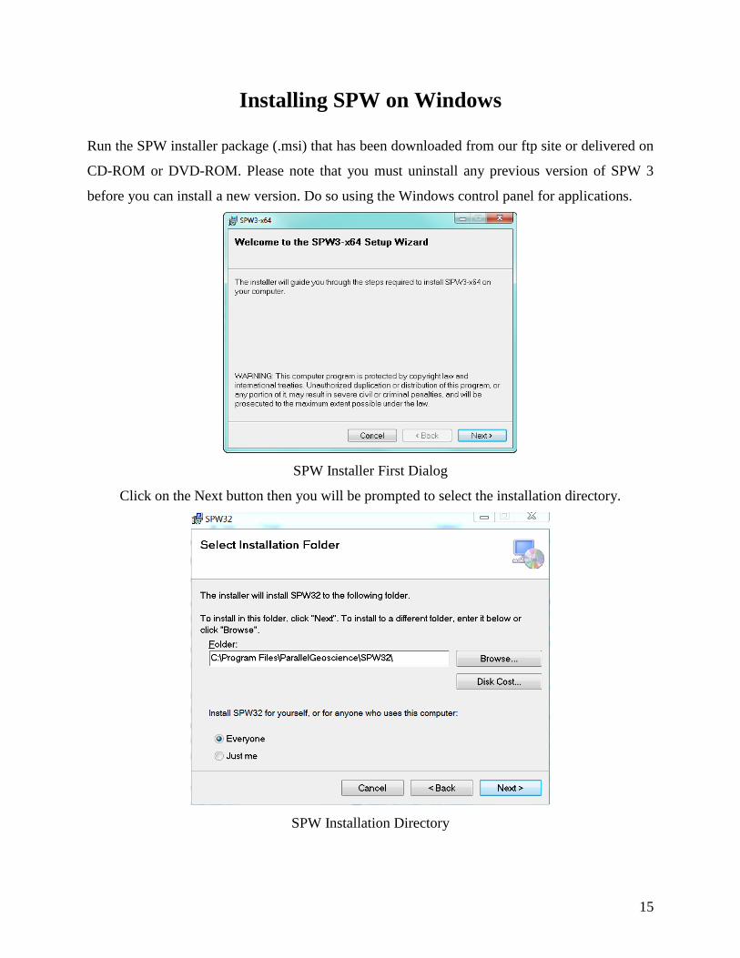
Installing SPW on Windows

Run the SPW installer package (.msi) that has been downloaded from our ftp site or delivered on

CD-ROM or DVD-ROM. Please note that you must uninstall any previous version of SPW 3

before you can install a new version. Do so using the Windows control panel for applications.

SPW Installer First Dialog

Click on the Next button then you will be prompted to select the installation directory.

SPW Installation Directory

16

Click on the Next button then you will be prompted to confirm the installation.

SPW Installation Confirmation

Click on the Next button then the installation will be performed and you will show the status of

the installation.

SPW Installation Status

Finally, the Installation Complete message will be shown. Now SPW is ready for use.

17

SPW Installation Complete

When the installation has finished, your SPW directory will be populated with the files and dll

libraries required for running SPW.

SPW 3 Install Directory

If you do not have the Sentinel software driver installed on your system, please install it by running

the Sentinel Protection Installer executable (.exe) in the SPW3 directory. This driver is required to

recognize and access the Sentinel USB security key used for licensing of SPW.

18

The SPW installation automatically creates a menu item to run Flowchart.exe.

Flowchart Menu Item

19

SPW User Directory

The first time the Flowchart application is executed after the installation, a number of directories

and files are copied to the documents home directory on Windows. This location is different for

each version of Windows and also is different depending on the operating system language. The

images shown here are all for Windows 7 UK English version.

Files Installed into SPW Documents Home Directory

The files written into the …/SPW3/Documents/SPW3InstallBackupFiles are original backup

copies of all the color scales, the online documentation, a SPW3 Project directory (more about

projects later), a default SEGY format definition file and a mp3 file that is played as a warning in

several processing steps inside SPW3. When Flowchart.exe is executed, any of these files and

directories that do not already exist in the user’s home documents directory will be automatically

copied to the users home documents directory.

20

Files in the Users Home Directory (MyDocuments/spw)

If you have previously modified or edited any of the files or projects in a prior SPW 3 installation,

these modified files in the home directory are retained and will not be overwritten during

subsequent installations.

21

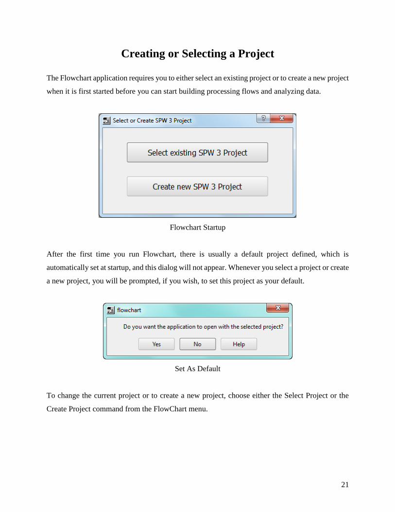
Creating or Selecting a Project

The Flowchart application requires you to either select an existing project or to create a new project

when it is first started before you can start building processing flows and analyzing data.

Flowchart Startup

After the first time you run Flowchart, there is usually a default project defined, which is

automatically set at startup, and this dialog will not appear. Whenever you select a project or create

a new project, you will be prompted, if you wish, to set this project as your default.

Set As Default

To change the current project or to create a new project, choose either the Select Project or the

Create Project command from the FlowChart menu.

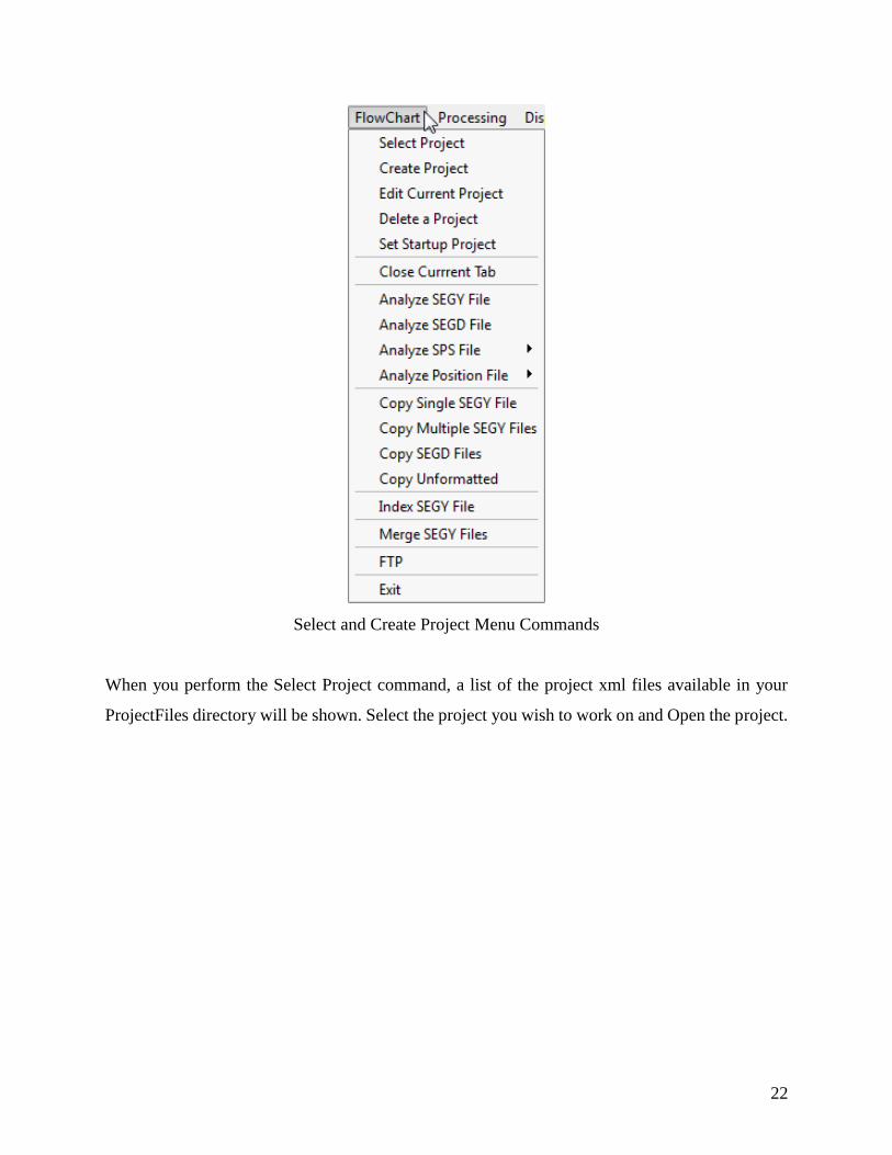
22

Select and Create Project Menu Commands

When you perform the Select Project command, a list of the project xml files available in your

ProjectFiles directory will be shown. Select the project you wish to work on and Open the project.

23

Select Project XML File

If you are starting in a new area or starting FlowChart for the first time, you will need to choose

the Create Project command from the FlowChart menu. When you issue this command, the

following dialog will appear. The main project directory (in this case New3DProject), will be

created inside the selected project root directory. The project root directory can be any mounted

disk on your system including networked disk drives.

24

Create Project Dialog

It is important the Data dimensions, Units and Survey type are entered correctly since these affect

how further options are presented and how the some of the data functions operate. Data units must

be specified as either feet or meters; there is no mixing of these units in SPW. These project

settings can be updated later using the Edit Project option.

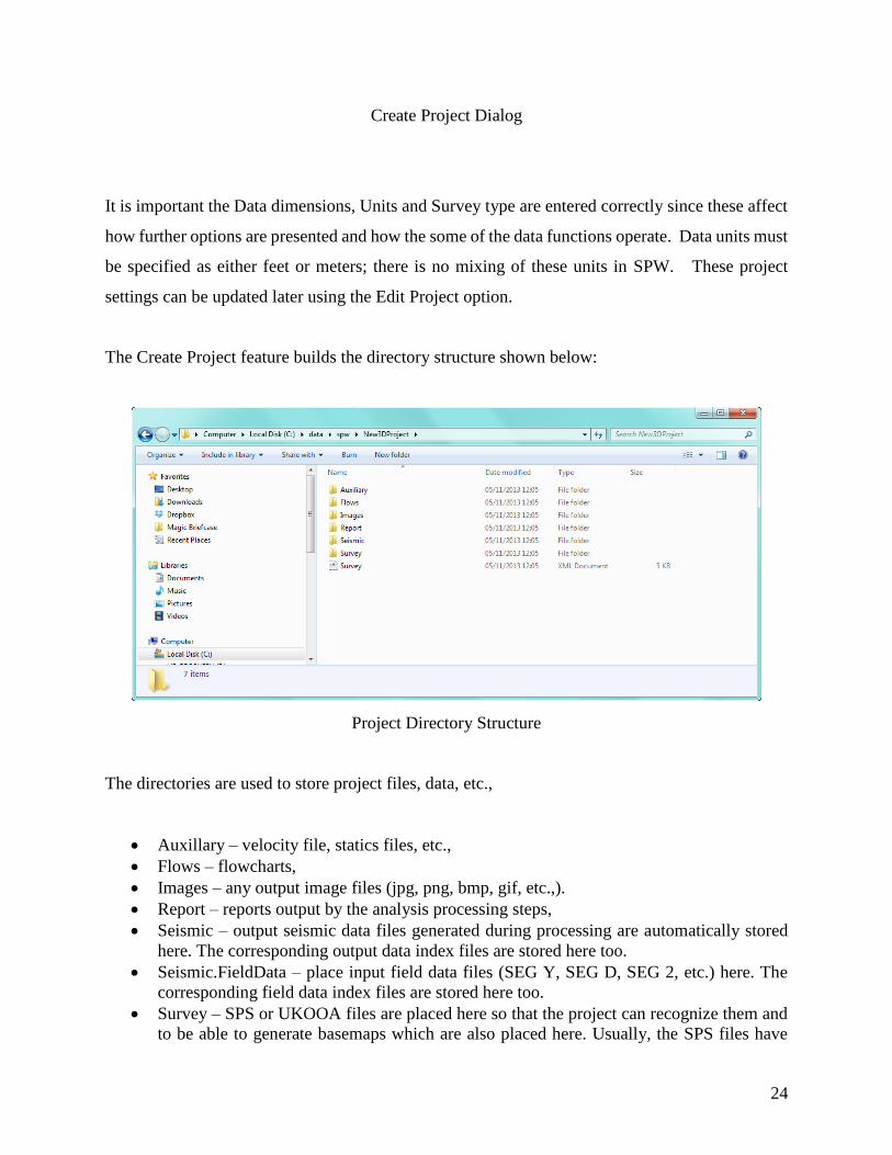
The Create Project feature builds the directory structure shown below:

Project Directory Structure

The directories are used to store project files, data, etc.,

• Auxillary – velocity file, statics files, etc.,

• Flows – flowcharts,

• Images – any output image files (jpg, png, bmp, gif, etc.,).

• Report – reports output by the analysis processing steps,

• Seismic – output seismic data files generated during processing are automatically stored

here. The corresponding output data index files are stored here too.

• Seismic.FieldData – place input field data files (SEG Y, SEG D, SEG 2, etc.) here. The

corresponding field data index files are stored here too.

• Survey – SPS or UKOOA files are placed here so that the project can recognize them and

to be able to generate basemaps which are also placed here. Usually, the SPS files have

25

extensions of .sps for Source Survey files, an extension of .rps for Receiver Survey files

and an extension of .xps for the Cross-reference (observers’ notes) files. Corresponding

survey data index files are stored here too.

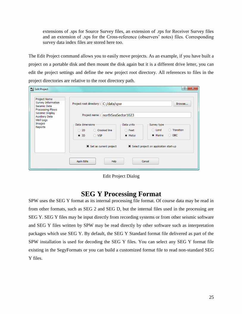
The Edit Project command allows you to easily move projects. As an example, if you have built a

project on a portable disk and then mount the disk again but it is a different drive letter, you can

edit the project settings and define the new project root directory. All references to files in the

project directories are relative to the root directory path.

Edit Project Dialog

SEG Y Processing Format SPW uses the SEG Y format as its internal processing file format. Of course data may be read in

from other formats, such as SEG 2 and SEG D, but the internal files used in the processing are

SEG Y. SEG Y files may be input directly from recording systems or from other seismic software

and SEG Y files written by SPW may be read directly by other software such as interpretation

packages which use SEG Y. By default, the SEG Y Standard format file delivered as part of the

SPW installation is used for decoding the SEG Y files. You can select any SEG Y format file

existing in the SegyFormats or you can build a customized format file to read non-standard SEG

Y files.

26

SEG Y Import Dialog – available from the SEGY Import processing step.

An index file is created for each SEG Y file used in SPW. These files contain important

information used in the processing and are required to be present for processing and displays. If

they are not present, they will be created by the processing or you may create them by using the

Build Index command in the SEG Y Import parameter dialog. Note that the Sorting keys must be

set to valid header fields before you press the Build SEG Y Index button and build the index file.

The SEG Y file format is defined by mappings of the SEG Y binary and trace header positions and

these are saved in XML file format. A default prebuilt SEG Y format definition files is delivered

with SPW (others are available via the Parallel Geoscience web site (www.parallelgeo.com)).

27

SegyFormats Directory

You can create new format definitions by modifying existing file using the Create format file

command in the SEG Y Analyzer or using the Create New SEG Y Format command in the SEG

Y Import dialog:

28

Create SEG Y Format Dialog

29

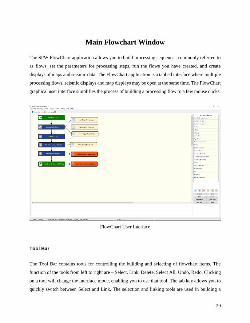
Main Flowchart Window

The SPW FlowChart application allows you to build processing sequences commonly referred to

as flows, set the parameters for processing steps, run the flows you have created, and create

displays of maps and seismic data. The FlowChart application is a tabbed interface where multiple

processing flows, seismic displays and map displays may be open at the same time. The FlowChart

graphical user interface simplifies the process of building a processing flow to a few mouse clicks.

FlowChart User Interface

Tool Bar

The Tool Bar contains tools for controlling the building and selecting of flowchart items. The

function of the tools from left to right are – Select, Link, Delete, Select All, Undo, Redo. Clicking

on a tool will change the interface mode, enabling you to use that tool. The tab key allows you to

quickly switch between Select and Link. The selection and linking tools are used in building a

30

processing flow and Delete allows for deleting either flow items or flow links from a processing

flow.

Tool Bar

Selection Tool – can select either a processing step or the link between the

processing steps. When selected, the Selection Tool button will appear depressed

and the step or link can be selected by clicking the left mouse button with the

pointer over the item to be selected. Selected items then appear highlighted.

Multiple items can be selected by clicking with the left mouse button and then

dragging the pointer – this is illustrated in the flow shown below where the Apply

Normal Moveout, Automatic Gain Control and the Apply Early Mute items have

been selected along with two pick files that apply to selected processing steps.

Linking Tool – allows you to define the data flow between items on the flowchart.

When selected, the Linking Tool button will appear depressed. To link between

two steps, click in the first step and then click in the second step. You may switch

between the Selection and Linking tools by either clicking on the icons on the Tool

Bar or by pressing the Tab key on the keyboard.

Delete Tool –removes selected items or links from the flowchart. Once selected,

you can remove an item or a link by either clicking on the Delete Tool on the tool

bar or by pressing the delete key on the keyboard. On many Windows keyboards

the backspace key is defined as the delete key. If your delete key does not work

then try the backspace key instead. Note: all selected items will be deleted.

Select All – selects all items on the flowchart; all items will be selected and

highlighted; the links will become bright green, and the flow items will be enclosed

by a dark black box and shown in light blue, the auxiliary data items will also be

enclosed by dark black box.

31

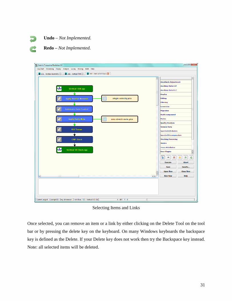
Undo – Not Implemented.

Redo – Not Implemented.

Selecting Items and Links

Once selected, you can remove an item or a link by either clicking on the Delete Tool on the tool

bar or by pressing the delete key on the keyboard. On many Windows keyboards the backspace

key is defined as the Delete. If your Delete key does not work then try the Backspace key instead.

Note: all selected items will be deleted.

32

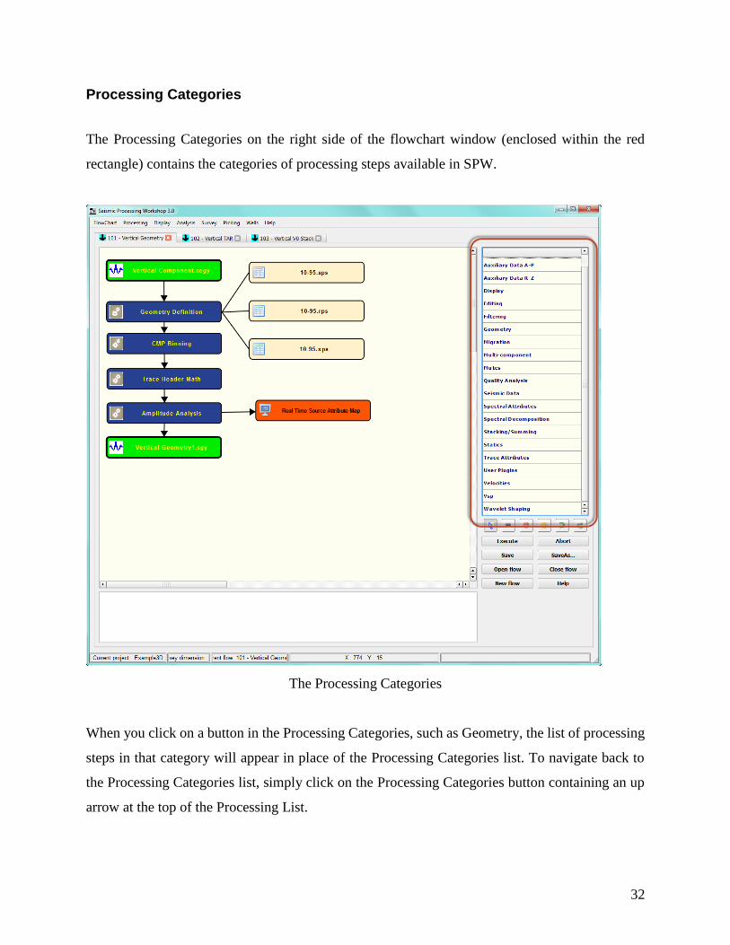
Processing Categories

The Processing Categories on the right side of the flowchart window (enclosed within the red

rectangle) contains the categories of processing steps available in SPW.

The Processing Categories

When you click on a button in the Processing Categories, such as Geometry, the list of processing

steps in that category will appear in place of the Processing Categories list. To navigate back to

the Processing Categories list, simply click on the Processing Categories button containing an up

arrow at the top of the Processing List.

33

Processing Steps Lists

When you click on the desired processing step button, it will appear highlighted in light blue as

shown below. To place the item on the flowchart, select it with a single mouse click, and then click

on the flowchart where you wish to place the item. You may also double mouse click on the item

in the processing step list and it will be placed below the last item you selected on the flowchart.

The item may then be dragged on the flowchart to correctly position it into your processing

sequence.

Processing Step List

Building Processing Flows

To build a flow, start by selecting the steps you wish to use in the processing step lists and placing

them on your flowchart. Next, using the Link Tool, connect each item in the flow as you wish for

the data to move through the processing sequence. The process for using the Link Tool involves

34

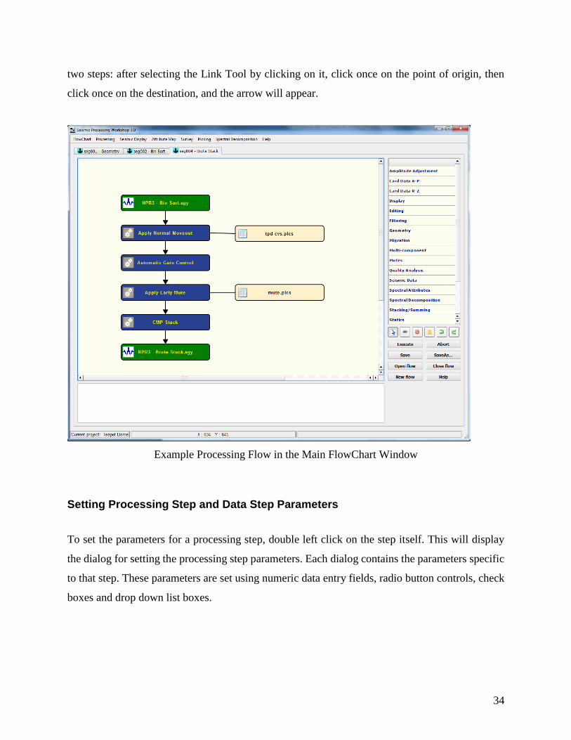
two steps: after selecting the Link Tool by clicking on it, click once on the point of origin, then

click once on the destination, and the arrow will appear.

Example Processing Flow in the Main FlowChart Window

Setting Processing Step and Data Step Parameters

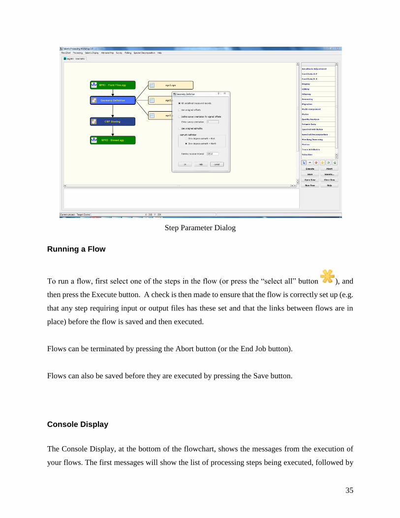
To set the parameters for a processing step, double left click on the step itself. This will display

the dialog for setting the processing step parameters. Each dialog contains the parameters specific

to that step. These parameters are set using numeric data entry fields, radio button controls, check

boxes and drop down list boxes.

35

Step Parameter Dialog

Running a Flow

To run a flow, first select one of the steps in the flow (or press the “select all” button ), and

then press the Execute button. A check is then made to ensure that the flow is correctly set up (e.g.

that any step requiring input or output files has these set and that the links between flows are in

place) before the flow is saved and then executed.

Flows can be terminated by pressing the Abort button (or the End Job button).

Flows can also be saved before they are executed by pressing the Save button.

Console Display

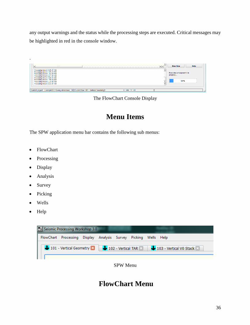
The Console Display, at the bottom of the flowchart, shows the messages from the execution of

your flows. The first messages will show the list of processing steps being executed, followed by

36

any output warnings and the status while the processing steps are executed. Critical messages may

be highlighted in red in the console window.

.

The FlowChart Console Display

Menu Items

The SPW application menu bar contains the following sub menus:

• FlowChart

• Processing

• Display

• Analysis

• Survey

• Picking

• Wells

• Help

SPW Menu

FlowChart Menu

37

The FlowChart menu shown below has a number of tools available for project management.

FlowChart Menu

The Select Project and Create Project commands let you select an existing project or create a new

project. The Edit Current Project command allows you to edit the currently selected project,

whereas Delete a Project will open a file selector from where a selected project can be deleted.

The Set startup project defines the default project to be used when the application launches. Close

Current Tab will close the active tab in the interface.

The remaining Flow Chart menu items are discussed below.

Edit Current Project

38

The Edit Current Project option is available which can be selected and which will open the “Edit

Project” dialog. Usually, the project will have been configured and this option shouldn’t be needed,

but it can be used to set up items such as the directory of the FieldQCLite project and the project’s

depth and distance units.

The Edit Project Dialog

On the left of the Edit Project dialog are several different options – click on these (e.g. Survey

Information) to change the parameters that can be configured.

SEG Y Analyzer

The SEG Y Analyzer allows you to quickly and efficiently open and investigate a SEG Y format

file.

39

SEG Y Analyzer

After you use the File Browse to select a file, then the Analyzer entries are populated with the

information retrieved from the dataset.

SEGY Analyzer – Trace Headers tab

Using the tabs in the dialog, you can display the SEG Y text header (also referred to as the EBCDIC

header), the binary header, multiple selected trace headers or a display of the seismic traces.

40

SEG Y Analyzer – Seismic View tab

The display of the Binary Header allows you to look at the values as either 2 byte or 4 byte words.

Binary Header Values Display

You also can also create a spectrum of a selected range of traces in the Sample format analysis tab

of the Binary header display

41

Spectra Display

The Histogram analysis tab allows you to see the amplitude distribution of the selected data traces

and verify the data has correct and valid amplitudes.

Histogram Analysis Display

SEG D Analysis

The SEG D Analyzer has a similar to the SEG Y Analyzer and allows you to analyze the various

parts of a SEG D file structure.

42

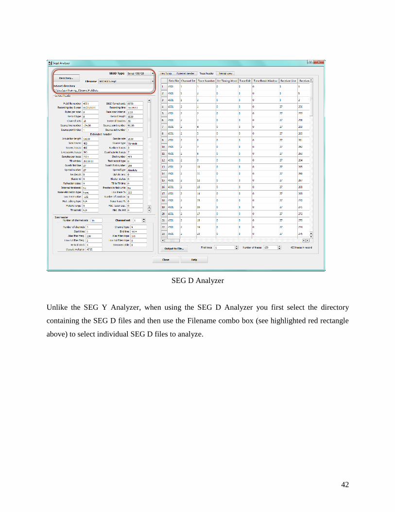
SEG D Analyzer

Unlike the SEG Y Analyzer, when using the SEG D Analyzer you first select the directory

containing the SEG D files and then use the Filename combo box (see highlighted red rectangle

above) to select individual SEG D files to analyze.

43

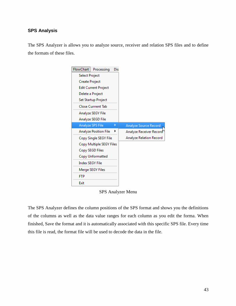
SPS Analysis

The SPS Analyzer is allows you to analyze source, receiver and relation SPS files and to define

the formats of these files.

SPS Analyzer Menu

The SPS Analyzer defines the column positions of the SPS format and shows you the definitions

of the columns as well as the data value ranges for each column as you edit the forma. When

finished, Save the format and it is automatically associated with this specific SPS file. Every time

this file is read, the format file will be used to decode the data in the file.

44

SPS Analyzer

Additional SPS analysis is available as Flowchart steps within the Auxiliary Data (R-Z) section of

the processing steps. These are described in the “Displaying Spreadsheets of Auxiliary Data”

section further down this first part of the manual.

Further SPS tools such as the database and producing maps are available in the “Survey Menu”

section, described further below. Tools for formatting the SPS files are described in the

“Displaying Spreadsheets of Auxiliary Data” section of this manual.

45

Processing Menu

The Processing menu contains the commands for working with the flowcharts.

Processing Menu

The New processing tab command creates tabbed windows for opening or building flowcharts.

The Open flow command will open an existing flow in the current flowchart tab (flows are read

from the project’s Flows directory). The Close flow command closes the current flowchart but

leaves the tab open. The Save command saves the current flow (a check is made before saving to

ensure that the flow is valid, e.g. that the required input and output links are made and that input

and output files have been specified). If it is an existing file, then it is overwritten. If it has not

been named then it issues the Save As command and you are then prompted for a file name.

The View trace headers command opens a spreadsheet view of the trace headers of a selected SEG

Y file (you select a SEG Y file by selecting the Seismic File in the flowchart). If you do not have

a SEG Y file currently selected it does nothing

46

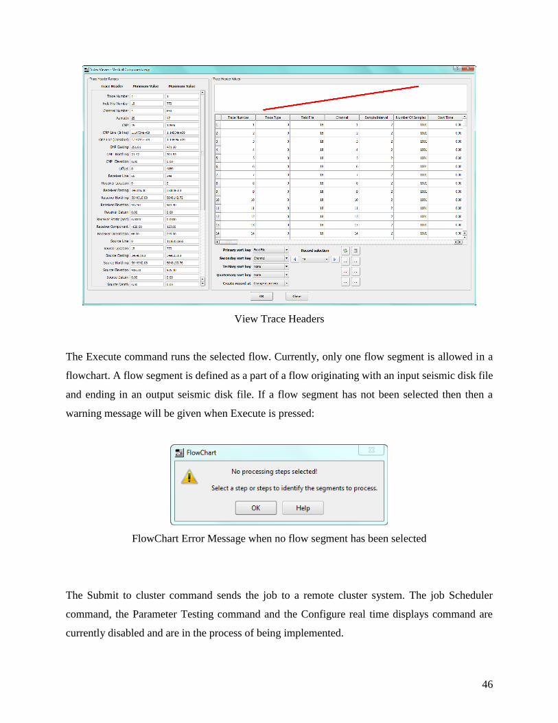
View Trace Headers

The Execute command runs the selected flow. Currently, only one flow segment is allowed in a

flowchart. A flow segment is defined as a part of a flow originating with an input seismic disk file

and ending in an output seismic disk file. If a flow segment has not been selected then then a

warning message will be given when Execute is pressed:

FlowChart Error Message when no flow segment has been selected

The Submit to cluster command sends the job to a remote cluster system. The job Scheduler

command, the Parameter Testing command and the Configure real time displays command are

currently disabled and are in the process of being implemented.

47

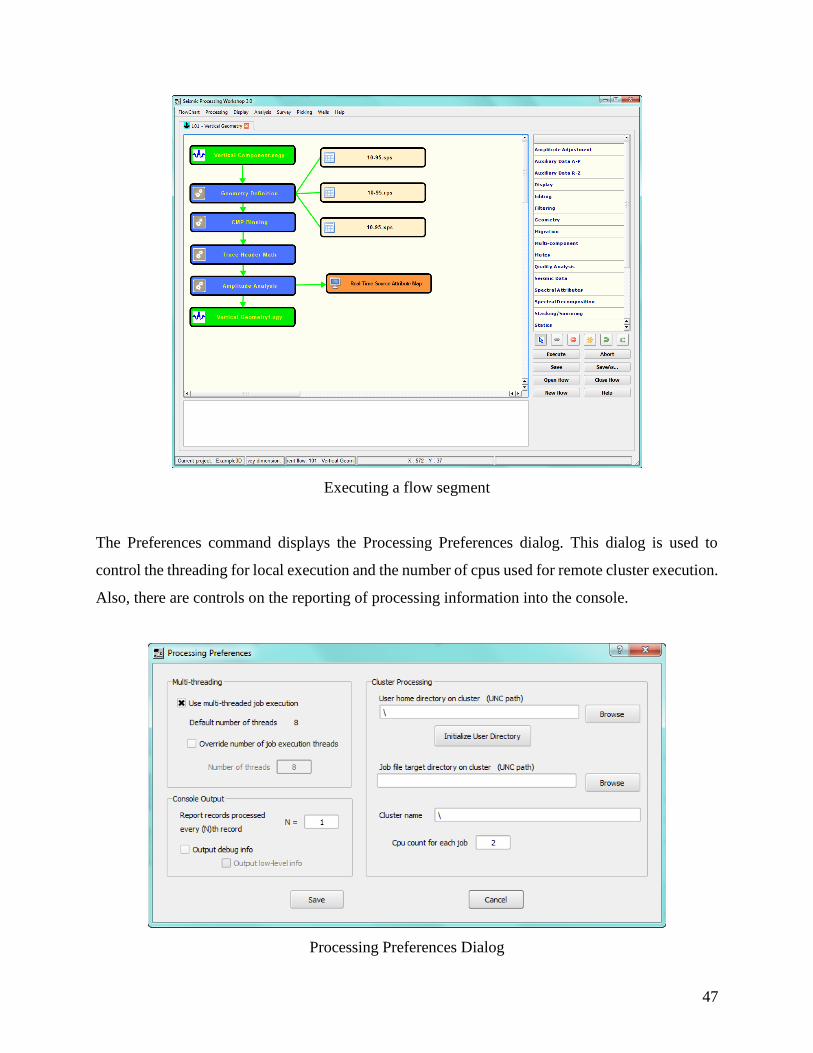
Executing a flow segment

The Preferences command displays the Processing Preferences dialog. This dialog is used to

control the threading for local execution and the number of cpus used for remote cluster execution.

Also, there are controls on the reporting of processing information into the console.

Processing Preferences Dialog

48

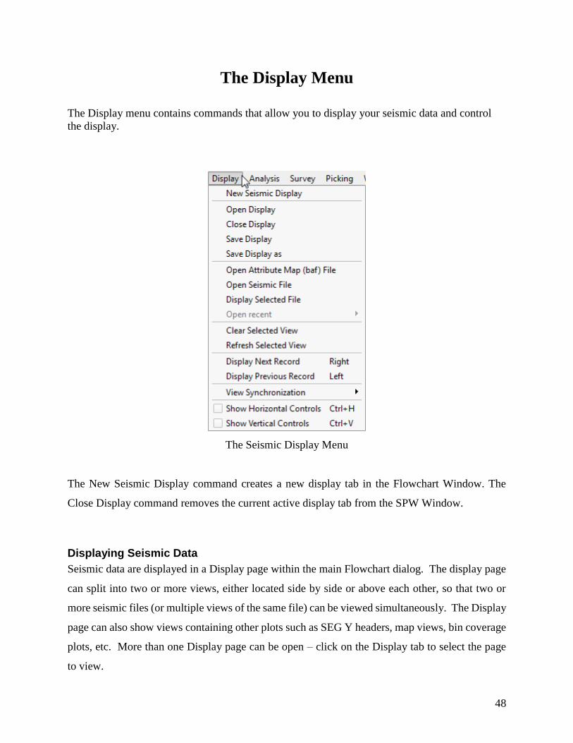
The Display Menu

The Display menu contains commands that allow you to display your seismic data and control

the display.

The Seismic Display Menu

The New Seismic Display command creates a new display tab in the Flowchart Window. The

Close Display command removes the current active display tab from the SPW Window.

Displaying Seismic Data

Seismic data are displayed in a Display page within the main Flowchart dialog. The display page

can split into two or more views, either located side by side or above each other, so that two or

more seismic files (or multiple views of the same file) can be viewed simultaneously. The Display

page can also show views containing other plots such as SEG Y headers, map views, bin coverage

plots, etc. More than one Display page can be open – click on the Display tab to select the page

to view.

49

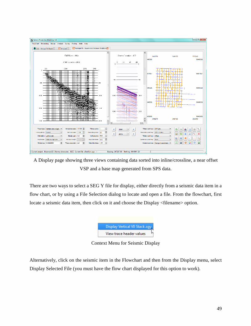
A Display page showing three views containing data sorted into inline/crossline, a near offset

VSP and a base map generated from SPS data.

There are two ways to select a SEG Y file for display, either directly from a seismic data item in a

flow chart, or by using a File Selection dialog to locate and open a file. From the flowchart, first

locate a seismic data item, then click on it and choose the Display <filename> option.

Context Menu for Seismic Display

Alternatively, click on the seismic item in the Flowchart and then from the Display menu, select

Display Selected File (you must have the flow chart displayed for this option to work).

50

Display Selected File Command

To locate and open a SEG Y file directly without using a Flowchart item, select Open Seismic File

from the above Display menu. This brings up a file selector dialog that you can use to locate and

open the SEG Y file directly.

The Display Configuration Wizard

When you open a seismic file for display, whether via the Flowchart or from the Display menu

and no Display page is currently open in the Flowchart dialog, a new Display Page is automatically

opened and the display view added. If one or more Display pages exist then the Display

Configuration Wizard is opened which enables you to select where the new display view will be

placed. The view can be added to a new display page (select “Add Display Page” from the viewer,

or the view can be added within an existing page. Use the “Add New View” button to place the

page to the right of the existing pages, or the arrow buttons to select where to locate the view.

51

The Display Configuration Wizard

The Seismic Display

The SPW Seismic Display is a very simple but powerful display tool allowing you to freely adjust

the display parameters and step through, or scroll through, your data set.

Variable Area Wiggle Seismic Display

52

Variable Density Seismic Display

When traces are displayed, move the pointer over a trace and right click to show a popup menu

that allows you to view the samples or header values of the selected trace:

53

Trace Header Values Popup Dialog

Seismic Display Control Panel

The SPW 3 Seismic Display Control Panel gives you options to select, set, or adjust parameters to

best view your data.

54

Seismic Display Control Panel

Left Side of the Seismic Display Control Panel

Left Side of the Seismic Display Control Panel

Trace type – interactively adjusts the seismic display by type using a drop down menu.

Variable area is a “standard” black and white wiggle display with area fill.

Variable density is a color display, usually shown with a red-white-blue color scale,

although you can change and setup new color scales with the color scale editor and

selectors described below.

Trace polarity – interactively adjusts the seismic display by polarity using a drop down menu.

Normal trace polarity interactively retains the polarity of seismic data on a trace-to-trace

basis.

Reverse trace polarity interactively reverses the polarity of seismic data on a trace-to-trace

basis.

Orientation – interactively adjusts the seismic display by orientation using a drop down menu.

Left-to-right displays the traces in ascending order starting from the left.

Right-to-left displays the traces in ascending order starting from the right.

Amplitudes – interactively adjusts the seismic display by amplitude using a drop down menu.

True amplitude displays the data at absolute input amplitude – usually millivolts.

Relative amplitude scales each trace to the same maximum amplitude.

Trace scaling applies an AGC to the trace using the Window length parameter.

Reference – interactively adjusts the seismic display by reference using up and down arrows, or

numerical data entry.

55

Horizontal scale – interactively scales seismic data horizontally on a trace-to-trace basis using up

and down arrows, or numerical data entry.

Vertical scale – interactively scales seismic data vertically on a trace-to-trace basis using up and

down arrows, or numerical data entry.

Display gain – interactively gains seismic data on a trace-to-trace basis using up and down arrows,

or numerical data entry.

Window length – interactively adjusts the length of the seismic display window using up and down

arrows, or numerical data entry.

Trace excursion – interactively adjusts how far the seismic data extends on a trace-to-trace basis

using up and down arrows, or numerical data entry.

Primary Anno – interactively changes the horizontal annotation of the seismic data according to

the primary sort key display using up and down arrows, or numerical data entry.

Secondary Anno – interactively changes the horizontal annotation of the seismic data according to

the secondary sort key display using up and down arrows, or numerical data entry.

Vertical Anno – interactively changes the vertical annotation of the seismic data display using up

and down arrows, or numerical data entry.

Major Time Lines – interactively adjusts how frequently the major (bold) timing lines annotate the

seismic data display using up and down arrows, or numerical data entry.

Minor Time Lines – interactively adjusts how frequently the minor (fine) timing lines annotate the

seismic data display using up and down arrows, or numerical data entry.

Center of the Seismic Display Control Panel – Sort Keys

Primary Sort Key Selected.

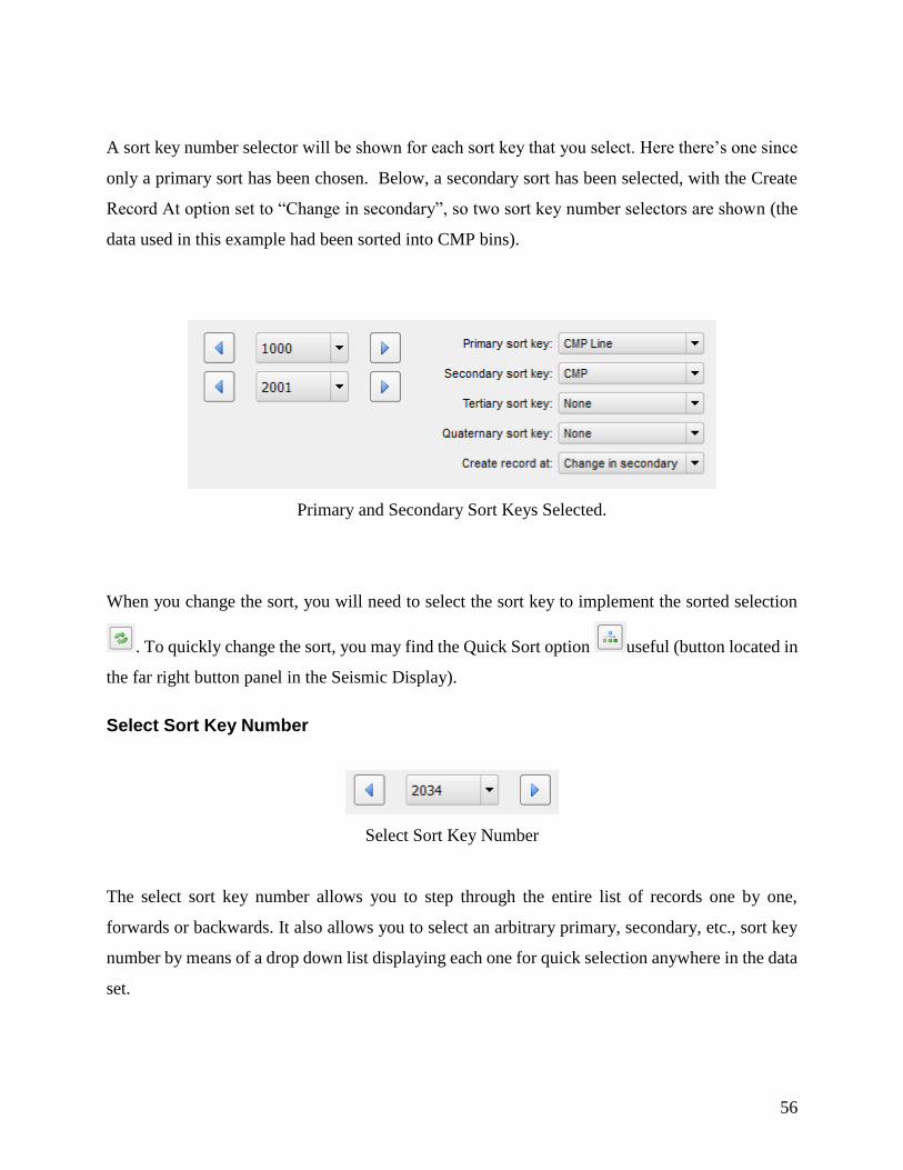
56

A sort key number selector will be shown for each sort key that you select. Here there’s one since

only a primary sort has been chosen. Below, a secondary sort has been selected, with the Create

Record At option set to “Change in secondary”, so two sort key number selectors are shown (the

data used in this example had been sorted into CMP bins).

Primary and Secondary Sort Keys Selected.

When you change the sort, you will need to select the sort key to implement the sorted selection

. To quickly change the sort, you may find the Quick Sort option useful (button located in

the far right button panel in the Seismic Display).

Select Sort Key Number

Select Sort Key Number

The select sort key number allows you to step through the entire list of records one by one,

forwards or backwards. It also allows you to select an arbitrary primary, secondary, etc., sort key

number by means of a drop down list displaying each one for quick selection anywhere in the data

set.

57

Arbitrary Primary Number Drop-down List

Sorting Keys

To the right of the display control panel are drop down menus for selecting primary, secondary,

etc., sort keys.

Display Sort Keys

Primary sort key – interactively adjusts the seismic display by using a drop down menu to select

the first order in sequence by which the data will be sorted.

Secondary sort key – interactively adjusts the seismic display by using a drop down menu to select

the second order in sequence by which the data will be sorted.

Tertiary sort key – interactively adjusts the seismic display by using a drop down menu to select

the third order in sequence by which the data will be sorted.

Quaternary sort key – interactively adjusts the seismic display by using a drop down menu to select

the fourth order in sequence by which the data will be sorted.

58

Create record at – interactively creates a record by change in primary, secondary, tertiary,

quaternary, each trace, or last trace.

Data and Display Tools

There are 24 tools on the right side of the Seismic Display Control Panel which facilitate the

manipulation of your data display. These are described below:

Data and Display Tools

Sort Data Using Current Sort Key – Clicking on this button changes the sort

order of your data using current sort keys. When new sort keys are selected from

the right side of the seismic display control panel, clicking on this button

implements the selection.

Quick Sort Options – Use to quickly sort the data based on popular sorts. This

will update the Primary and Secondary sort keys as necessary to yield the selected

quick sort (see discussion below).

Add Trace Header Plot – Use as a toggle button to place a header display above

the currently selected view. Reveals a panel at the top right of the display panel

where you can select the header to plot and options to configure the header plot.

View Trace Headers – Use the right click option Trace Header Values Popup

Dialog, described above.

Display Processing – Opens the Display Processing Tool which allows you to add

processing steps between reading the seismic file and displaying it. Toggle the

button off to remove the processing step.

59

Seismic Picker – Opens the picking menu panel to the right of the display panel.

Show Location Map – opens a popup Locator Map dialog.

Geometry Quality Control – Shows a calculated first arrival based on the offset

and a velocity. Aim is to QC offsets to ensure that the near trace aligns with the

data first breaks.

View LMO Guided Windows – To use, enter a velocity, start time and end time

and the window will be shown in color on the data. This option is particularly useful

for designing deconvolution operators that move out with offset.

Edit Seismic Traces – when toggled on use the pointer and MB1 to select trace

groups to mute out. This is a temporary mute, to reverse the mute move the display

record forward and back.

Reverse Trace Polarity – toggle on and off to reverse the trace polarity.

Show Dead Traces In Red – toggle on and off.

Calculate Individual Trace Spectra – when toggled on, use the pointer and MB1

to select trace groups. A popup display of the spectra of the selected traces is then

shown. Toggle off to remove the selection facility.

Calculate Spectra in a Rectangular Window – when toggled on, use the pointer

and MB1 to select a trace/time window. A popup display of the spectra of the

selected and gated traces is then shown. Toggle off to remove the selection facility.

Calculate Spectra in a Polygonal Window – when toggled on, use the pointer

and MB1 to select a polygon. A popup display of the spectra of the trace samples

within the window is then shown. Toggle off to remove the selection facility.

Estimate Linear Velocity – when toggled on, use the pointer to select two points

on the display. The linear velocity is then shown as an overlay on the display.

Toggle off to remove the linear velocity selection and clear the velocity text.

Requires an offset sort.

Estimate Hyperbolic Velocity – when toggled on, use the pointer to select two

points on the display. The hyperbolic velocity is then shown as an overlay on the

60

display. Toggle off to remove the hyperbolic velocity selection and clear the

velocity text. Requires and offset sort.

Zoom – when toggled on, use the central mouse button or mouse tracker ball to

zoom the currently selected view in or out.

Range Limit Data In the Display – when toggled on this will a panel at the top

right of the display panel will be shown giving options for selecting sort keys and

setting the display ranges of the keys. Multiple sort ranges can be set. Toggle off

to remove the range limit and to reset the ranges applied to each key.

Capture an Image – Opens the Setup Image Dialog box (described below).

Select or View a Current Color Scale – Opens the Select Color Tool dialog from

which you can view currently available color scales and select a different scale to

view (described below).

Create a New Color Scale or Edit an Existing One – Opens the Color Scale

Editor dialog (described below).

Propagate Display Settings – click to propagate the display settings of the

currently selected view to other views in the same display panel.

Synchronize Scrolling – click to synchronize the horizontal and vertical scrolling.

You can use this in collaboration with the Display menu’s Synchronize options.

The sorts need to match for the synchronizing to operate.

Quick Sort Options

When the Quick Sort button is pressed, there are a number of sort options to choose from. The

sorts available depend on whether the project is set for surface seismic data (the default) or VSP

data.

61

Surface Seismic Quick Sort Options

The quick sorts are set using the following keys:

Quick Sort Primary Key Secondary Key Tertiary Key

Shot Source Line Source Location

Receiver Receiver Line Receiver Location

CMP CMP Line CMP Location Offset

Offset Offset CMP Line CMP Location

Field File Channel Field File

Channel Field File Channel

Inline CMP Line CMP Location

Crossline CMP Location CMP Line

VSP data can be sorted into Source and Downhole gathers.

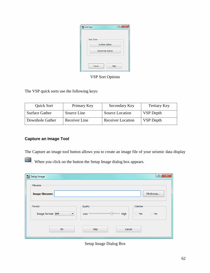
62

VSP Sort Options

The VSP quick sorts use the following keys:

Quick Sort Primary Key Secondary Key Tertiary Key

Surface Gather Source Line Source Location VSP Depth

Downhole Gather Receiver Line Receiver Location VSP Depth

Capture an Image Tool

The Capture an image tool button allows you to create an image file of your seismic data display

. When you click on the button the Setup Image dialog box appears.

Setup Image Dialog Box

63

Specify a name for the image file and browse for the destination. Then specify the format (BMP,

JPEG, TIFF, PNG) from the Image format drop-down list. Set the image quality on the Low-High

sliding continuum, and determine whether or not to use the Colorbar. Clicking OK captures the

image and stores it in the project image folder.

Select Color Scale Tool

The Select color scale tool button allows you to select from a variety of color scales to apply to

your data . When you click on this button the Color Scale Viewer dialog box opens from

which you can select your preferred color scale.

Color Scale Viewer Dialog Box

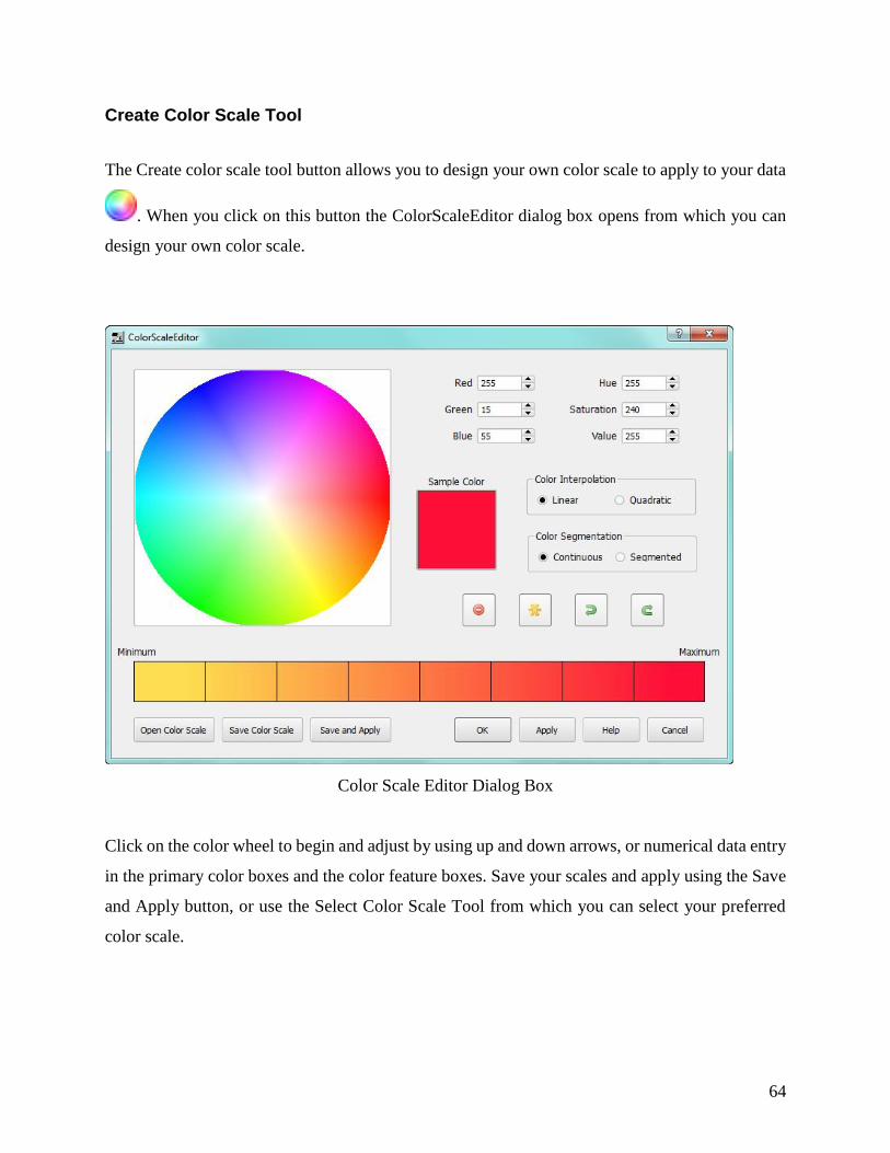
64

Create Color Scale Tool

The Create color scale tool button allows you to design your own color scale to apply to your data

. When you click on this button the ColorScaleEditor dialog box opens from which you can

design your own color scale.

Color Scale Editor Dialog Box

Click on the color wheel to begin and adjust by using up and down arrows, or numerical data entry

in the primary color boxes and the color feature boxes. Save your scales and apply using the Save

and Apply button, or use the Select Color Scale Tool from which you can select your preferred

color scale.

65

Opening and Saving the Seismic Display

When you have created a Seismic Display containing one or more display views, you can save the

view into an Xml file stored within your project for future use. For example, you may have

configured your display with different sorts, data ranges, display options, etc. From the Display

menu, select Save Display as to save the current configuration with the project files.

The Save and Open Display Options

To open a previously saved display configuration, select Open Display; this gives you access to a

file selector pointing to the Displays directory of your current project. Once a display is open,

you can continue to make changes to the display configuration; if you select Save Display these

changes will be updated in the display file for future use.

The command “Close Display” will close the currently selected Seismic Display tab.

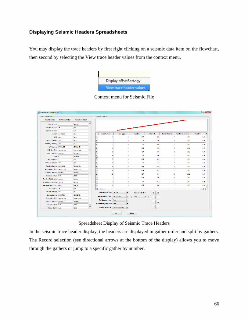
66

Displaying Seismic Headers Spreadsheets

You may display the trace headers by first right clicking on a seismic data item on the flowchart,

then second by selecting the View trace header values from the context menu.

Context menu for Seismic File

Spreadsheet Display of Seismic Trace Headers

In the seismic trace header display, the headers are displayed in gather order and split by gathers.

The Record selection (see directional arrows at the bottom of the display) allows you to move

through the gathers or jump to a specific gather by number.

67

Attribute Maps

Attribute maps map be generated from seismic files to show the variation of certain properties of

the data in a map view. Amplitude and frequency attributes are commonly used to quality control

data. The Amplitude Analysis and Frequency Analysis processing steps are commonly used to

generate these attribute and save them in the seismic trace headers. Attributes can be displayed in

a Seismic Display by selecting “Open Attribute Map File” from the Display menu:

The Display Menu

68

Velocity Analysis Menu

The Analysis menu contains for the seismic analysis tools in SPW. The Velocity Analysis tool and

the Multi-Channel Surface Wave (MASW) utility are available in the current version.

Analysis Menu

Velocity Analysis Builder

The velocity analysis wizard will build the flows and display panel necessary for creating the RMS

velocity fields used to perform normal moveout (NMO) correction. The input is a file of CMP

gathered seismic data and the output, after the velocity analysis has been completed, is a file of the

NMO corrected data, together with the RMS velocities. The wizard builds and initiates three

flows: a constant velocity stack flow, a velocity semblance flow and a flow to compute the CMP

gathers.

The wizard opens with the following multi-tab dialog:

69

Velocity Analysis Builder (Wizard)

Select an input CMP sorted SEG Y file, which is used as the input to all three analysis flows. Also

select the flows you want to run, which would usually be “Constant Velocity Stacks”, “Velocity

Semblance” and “CMP gathers”. The “Velocity picks” can also be saved to enable the NMO flow

to be run separately at a later time, perhaps after some editing of the picks has been made.

Constant Velocity Stacks flow

Select the Constant velocity stacks checkbox in the dialog and set the following parameters:

70

Constant Velocity Stacks flow parameters

Velocity range: select a range of velocities and an increment large enough to encompass expected

range in the survey area.

Processing and Mute Control: prior to displaying the data, you can add a filter and AGC options

along with mutes to help in identifying events for picking.

Line and Location Range: select the inline and crossline ranges and the increments of the data set

that you wish to analyze. Each stack displayed will require picking so you may want to choose a

coarse data selection to begin with.

Trace Amplitude Definition: select from relative, true or RMS amplitude scaling.

Stack normalization: enter the scaling exponent. Traces will be scaled by the fold^Exp.

Interpolation Type Selection: select the interpolation type (linear or quadratic). The moveout

operator will cause trace data samples to be moved in time to new locations, which will not usually

be exactly at the sample interval of the data. Here the data is interpolated to be evenly sampled at

the correct interval. See, for example, the description of the Apply Normal Moveout step in the

Processing Steps of this manual for further details.

Constant velocity stack file: enter the name for SEG Y in which the constant velocity stacks will

be saved.

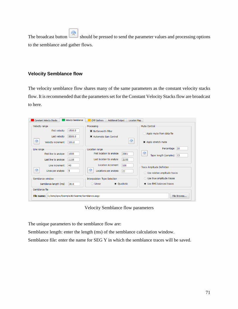
71

The broadcast button should be pressed to send the parameter values and processing options

to the semblance and gather flows.

Velocity Semblance flow

The velocity semblance flow shares many of the same parameters as the constant velocity stacks

flow. It is recommended that the parameters set for the Constant Velocity Stacks flow are broadcast

to here.

Velocity Semblance flow parameters

The unique parameters to the semblance flow are:

Semblance length: enter the length (ms) of the semblance calculation window.

Semblance file: enter the name for SEG Y in which the semblance traces will be saved.

72

CMP Gathers flow

The CMP gathers flow applies to the velocity picks to the input CMP stacked data to create stacks

of NMO corrected data.

CMP Gathers flow parameters

Set the following parameters:

Normal Moveout: use the parameters here for how to apply the NMO and whether mutes should

be applied to the data – see the description of the Apply Normal Moveout step in the Processing

Steps of this manual for further details of the mutes and the percentage and taper length parameters

used by the stretch mute.

Processing: processing steps for filtering, AGC and the creation of supergathers can be added to

the traces when creating stacks of NMO corrected data.

Line and location range – generally these will have been broadcast from the Constant Velocity

Stacks and Velocity Semblance flows.

Execution

73

Once the selected analysis output flows (velocity stacks, semblance, CMP gathers) have been

parameterized, you can now execute these flows and interactively make velocity picks. Press

Execute to build the flows and start them. Once the flows are executed, the FlowChart window

will be refreshed with tabs containing the selected flows and a display tab showing the CMP gather,

semblance display and constant velocity stacks.

74

The Survey Menu

The Survey menu contains commands for displaying maps of the data locations, defining the 3D

coordinate binning information and quality checking of the geometry information.

The Survey Menu

To use the map options in this menu, the survey files (SPS files) should be stored in the current

project’s Survey directory.

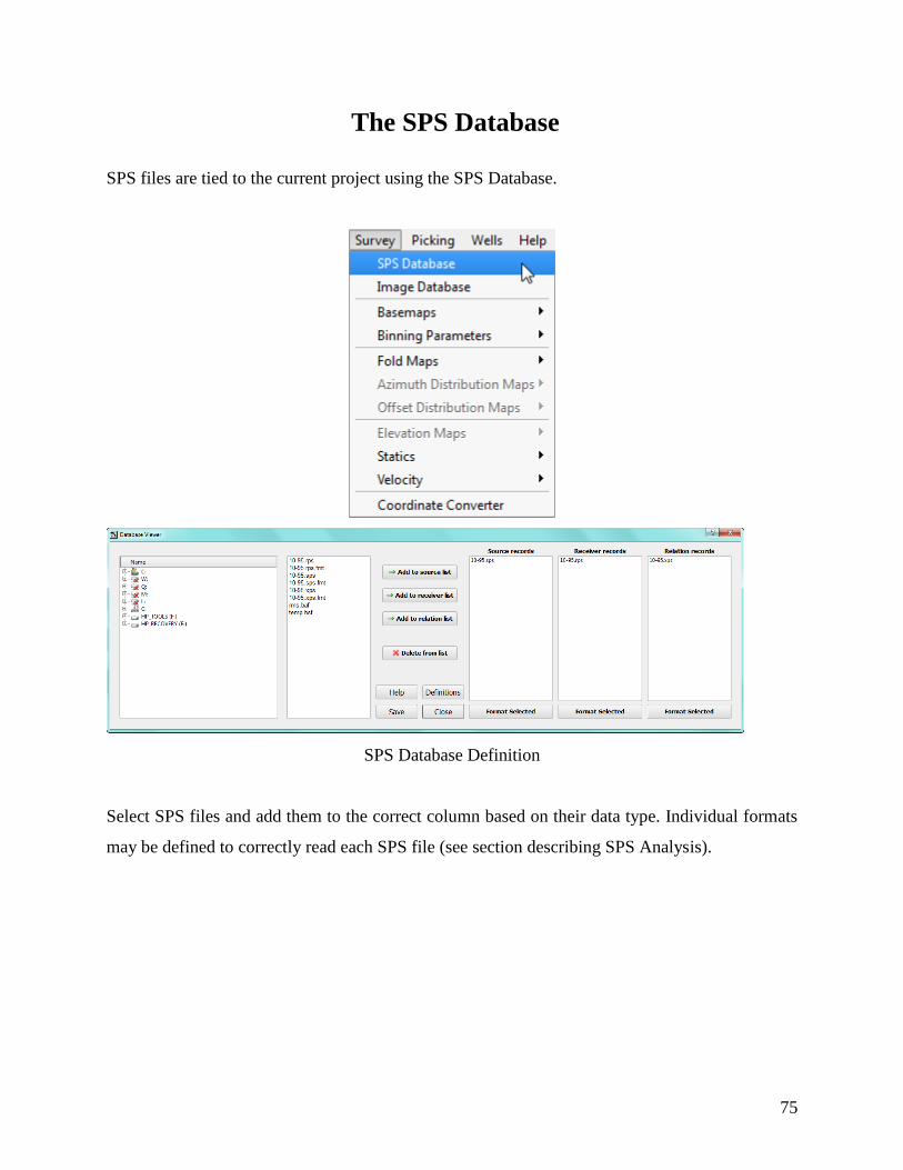
75

The SPS Database

SPS files are tied to the current project using the SPS Database.

SPS Database Definition

Select SPS files and add them to the correct column based on their data type. Individual formats

may be defined to correctly read each SPS file (see section describing SPS Analysis).

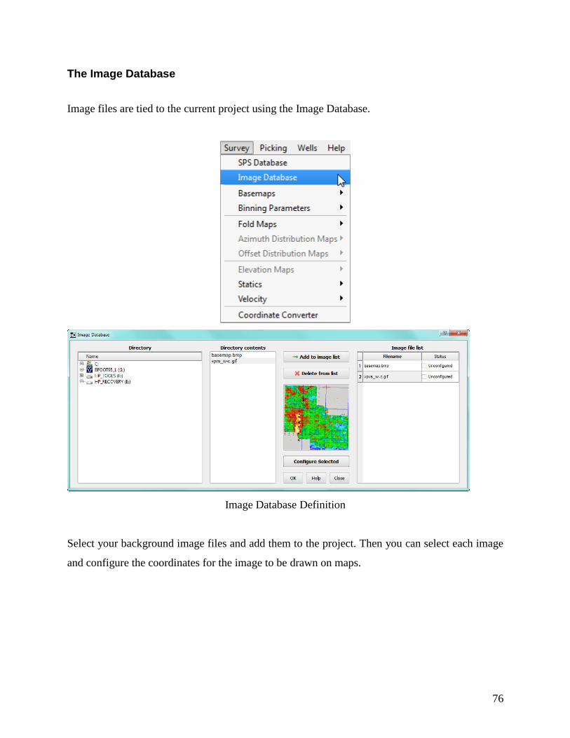
76

The Image Database

Image files are tied to the current project using the Image Database.

Image Database Definition

Select your background image files and add them to the project. Then you can select each image

and configure the coordinates for the image to be drawn on maps.

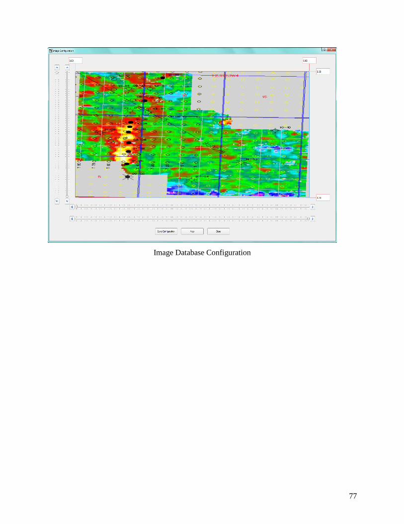
77

Image Database Configuration

78

Map Displays

Map displays are new in SPW 3. There are a number of different types including base maps, fold

maps and attribute maps.

The Basemap

Previously computed basemaps can be selected and new ones generated from SPS geometry files.

The geometry files must be in the Survey directory of a project To generate one select “Generate

from SPS” from the Basemaps menu:

Basemaps menu

This opens the Select Basemap Inputs from which you select the SPS input files from the SPS

database and where you can select a background image and any exclusion zones. The basemap is

created and saved to file – use “Select basemap image” to redisplay any previously created image

files.

79

Survey 3D Basemap Dialog

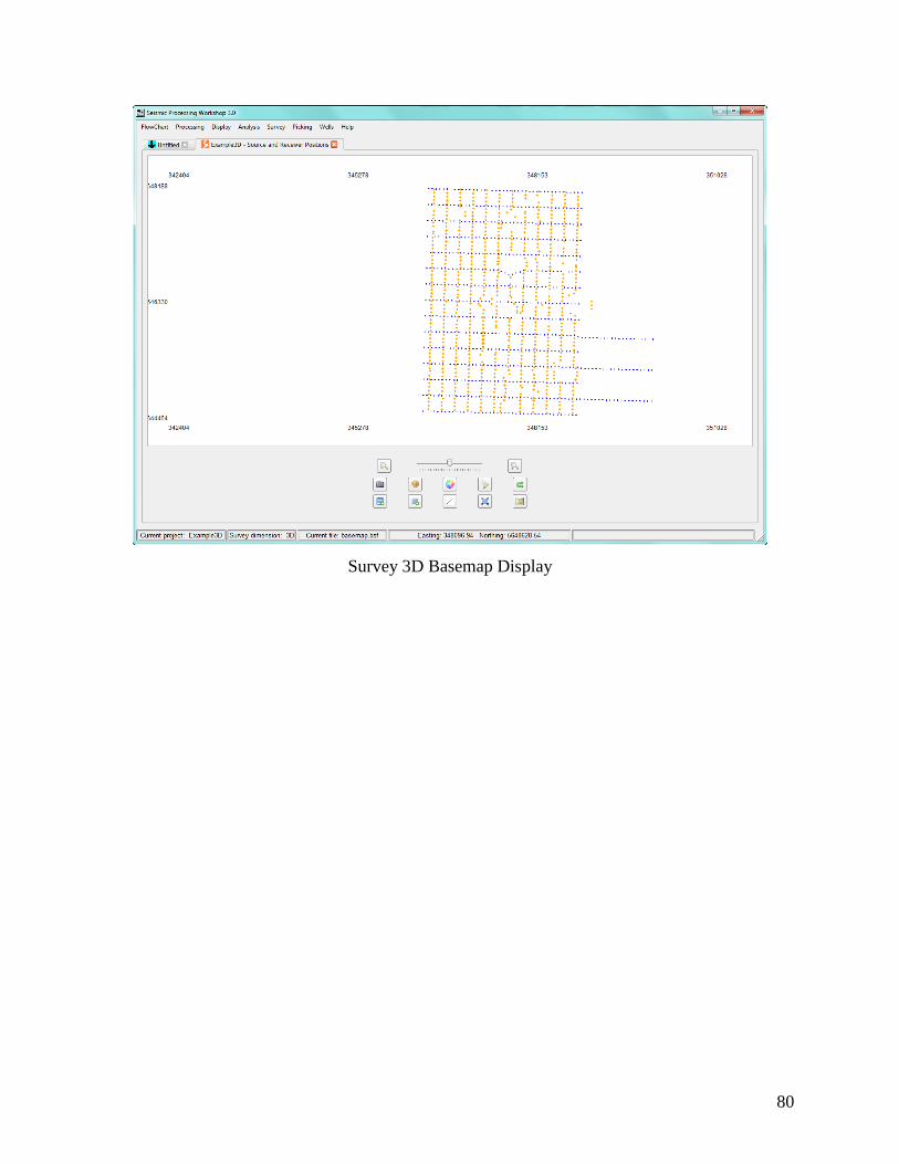
80

Survey 3D Basemap Display

81

Base Map Display Control Panel

Zoom In & Zoom Out – Click on the buttons to zoom the image in or out. Also

use the slider bar to change the level of zoom. Use the Reset to Original Scale

button to reset the zoom level. Clicking on this button changes the sort order of

your data using current sort keys. When new sort keys are selected from the right

side of the seismic display control panel, clicking on this button implements the

selection.

Capture an Image – Opens the Setup Image Dialog box (this is described along

with the seismic view description, above).

Select or View a Current Color Scale – Opens the Select Color Tool dialog from

which you can view currently available color scales and select a different scale to

view (this is described along with the seismic view description, above).

Create a New Color Scale or Edit an Existing One – Opens the Color Scale

Editor dialog (this is described along with the seismic view description, above).

Customize Map Annotations – Click to open the annotation panel where you can

configure the size, color and shape of the source and receiver points.

Reset to Original Scale – resets the zoom.

Measure Distance Between Points – Click the pointer in two places on the map

view to measure the distance and azimuth between points.

82

Measure Areas – Click, drag and then release the pointer to create an rectangular

area – the area within the shape will be displayed.

Redraw Map – Redraws the map.

83

Fold Maps

Previously computed fold maps can be selected and new ones generated from SPS geometry files.

The geometry files must be in the Survey directory of a project To generate one select “Generate

from SPS” from the Fold Maps menu:

When you select the Fold->Generate fold from SPS command, for a 3D dataset, you will see the

parameter dialog shown below for creating a fold map. The fold map is created and saved to file –

use “Select fold image” to redisplay any previously created image files.

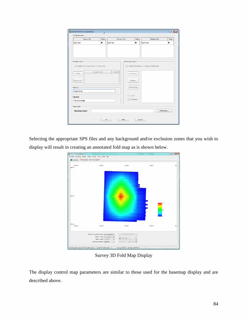
84

Selecting the appropriate SPS files and any background and/or exclusion zones that you wish to

display will result in creating an annotated fold map as is shown below.

Survey 3D Fold Map Display

The display control map parameters are similar to those used for the basemap display and are

described above.

85

Compute Fold Difference

Two fold maps can be used to create a difference map. Select “Compute fold difference” to open

the Compute Fold Difference dialog from which the difference map can be computed and saved.

Previously computed difference maps can be re-displayed using Select Fold Image.

Compute Fold Difference

Fold Difference Dialog

The Picking Menu

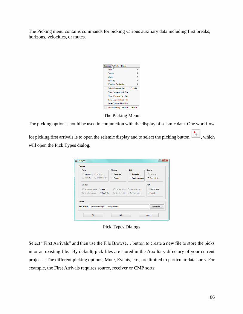
86

The Picking menu contains commands for picking various auxiliary data including first breaks,

horizons, velocities, or mutes.

The Picking Menu

The picking options should be used in conjunction with the display of seismic data. One workflow

for picking first arrivals is to open the seismic display and to select the picking button , which

will open the Pick Types dialog.

Pick Types Dialogs

Select “First Arrivals” and then use the File Browse… button to create a new file to store the picks

in or an existing file. By default, pick files are stored in the Auxiliary directory of your current

project. The different picking options, Mute, Events, etc., are limited to particular data sorts. For

example, the First Arrivals requires source, receiver or CMP sorts:

87

The Picking’s Sort Keys Dialog

When an existing file is selected for storing the pick outputs, a check is made to ensure that the

file already contains picks of the required type – for example you can’t mix velocity picks with

first break picks. While picking is progress a backup pick file (ending .bak) is created that will

contain the previously saved picks.

Picking is controlled by the options in the picking panel which is shown to the right the display:

The Picking Panel

The Picking options include:

Pick Method – select from single trace, linear guided or automatic methods.

Guide Type – used for the guided method to select rubberband or Two-Point methods.

Auto-Pick Method – used for the automatic pick methods.

Pick phase – select peaks and troughs, zero crossings or no auto selection.

88

Window length – control the search in the picking phase.

Other options control the colors, sizes and shapes of the picking markers.

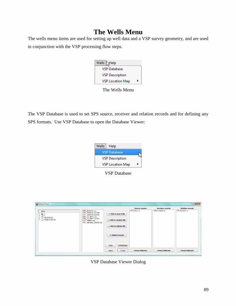
89

The Wells Menu The wells menu items are used for setting up well data and a VSP survey geometry, and are used

in conjunction with the VSP processing flow steps.

The Wells Menu

The VSP Database is used to set SPS source, receiver and relation records and for defining any

SPS formats. Use VSP Database to open the Database Viewer:

VSP Database

VSP Database Viewer Dialog

90

The VSP Database Viewer operates in a similar manner to the SPS Survey Menu, described above,

with source, receiver and relations files needed to be defined and the formats set.

A Location map can be constructed from the VSP Database and previously created location maps

opened (use VSP Location Map > Generate from VSP files and VSP Location Map > Select map

image, respectively):

VSP Location Map options

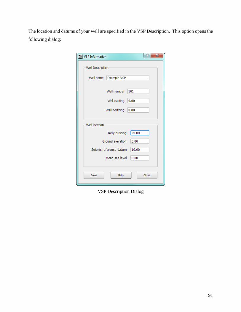
91

The location and datums of your well are specified in the VSP Description. This option opens the

following dialog:

VSP Description Dialog

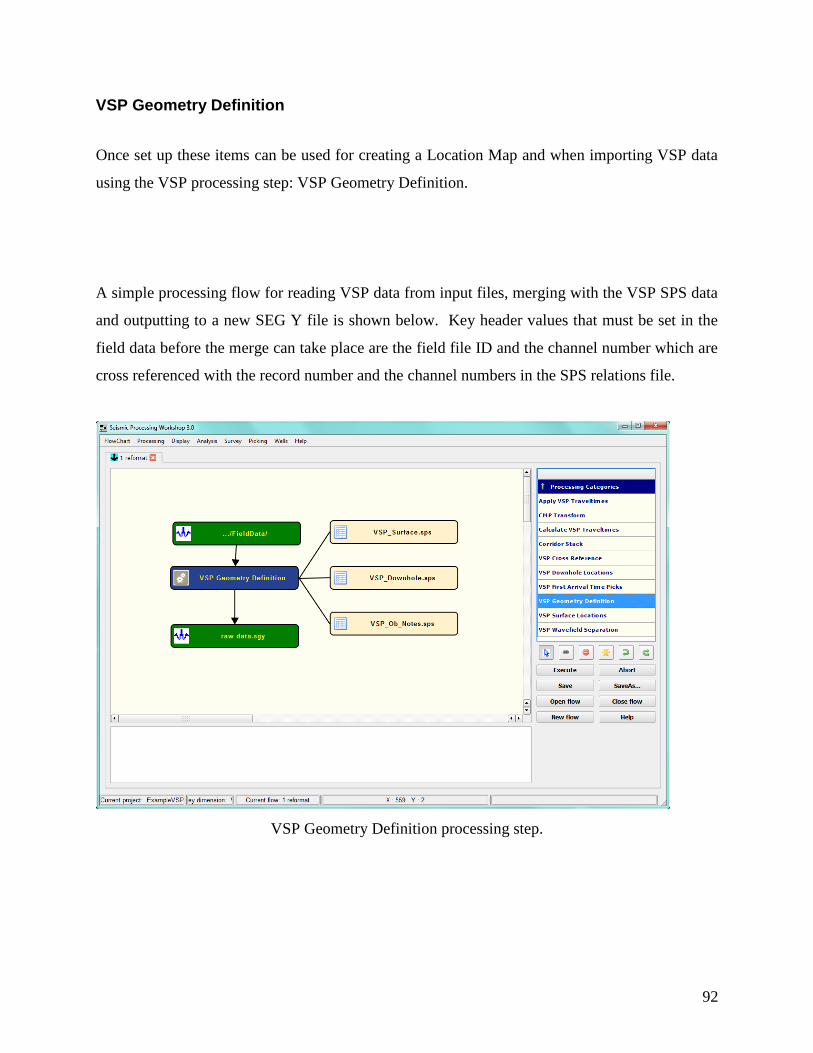
92

VSP Geometry Definition

Once set up these items can be used for creating a Location Map and when importing VSP data

using the VSP processing step: VSP Geometry Definition.

A simple processing flow for reading VSP data from input files, merging with the VSP SPS data

and outputting to a new SEG Y file is shown below. Key header values that must be set in the

field data before the merge can take place are the field file ID and the channel number which are

cross referenced with the record number and the channel numbers in the SPS relations file.

VSP Geometry Definition processing step.

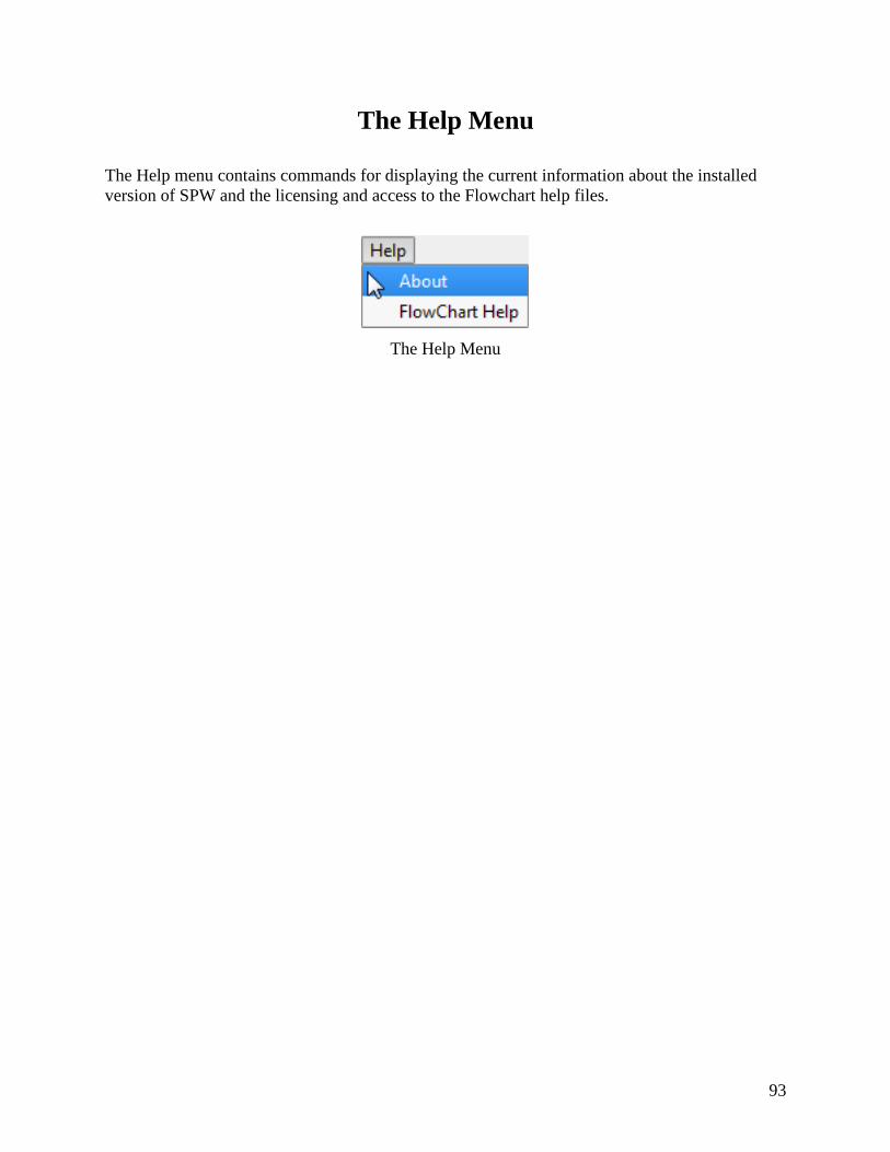
93

The Help Menu

The Help menu contains commands for displaying the current information about the installed

version of SPW and the licensing and access to the Flowchart help files.

The Help Menu

94

Displaying Spreadsheets of Auxiliary Data

Each of the Auxiliary data types has a unique display and spreadsheet view which is customized

for that spreadsheet’s specific data type and contents. The following pages show examples of the

spreadsheet views for a number of the data types. Each spreadsheet also has controls allowing you

to move between displays. For example, Velocity Functions exist in multiple locations in a 3D

survey at specific CMP Line and CMP Location positions. You can move between control points

using the control at the top of the spreadsheet where it shows the Line and Location.

To open an auxiliary dialog, you can select an appropriate Auxiliary Data step from the Flowchart

steps (double click or right click on the step to open the file selection dialog). Alternatively you

can view a dialog when you select a step in the flowchart which requires auxiliary data as input.

For example the receiver and source statics dialogs can be opened from the Statics processing

steps, time picks can be opened from the First Arrivals Statics step, velocity function files can be

opened and displayed from the Apply Normal Moveout step. These are just some of the many

examples of where auxiliary data files can be opened; the following gives examples of some of

these dialogs.

95

Early Mute Functions

Mute functions are defined by time offset pairs. They are usually picked on a few gathers in the

dataset and interpolated between these control points.

SPW Early Mute Function Spreadsheet

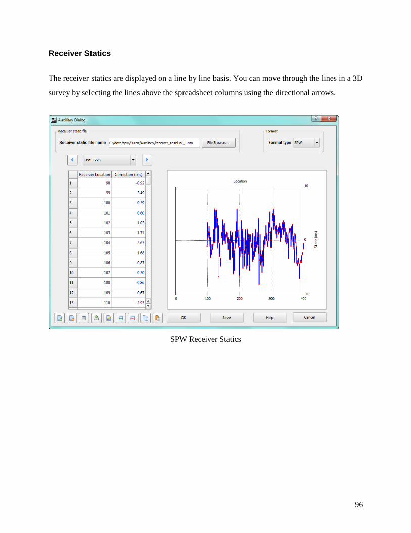
96

Receiver Statics

The receiver statics are displayed on a line by line basis. You can move through the lines in a 3D

survey by selecting the lines above the spreadsheet columns using the directional arrows.

SPW Receiver Statics

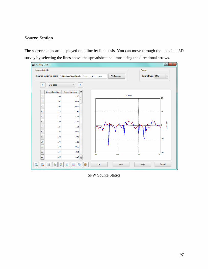
97

Source Statics

The source statics are displayed on a line by line basis. You can move through the lines in a 3D

survey by selecting the lines above the spreadsheet columns using the directional arrows.

SPW Source Statics

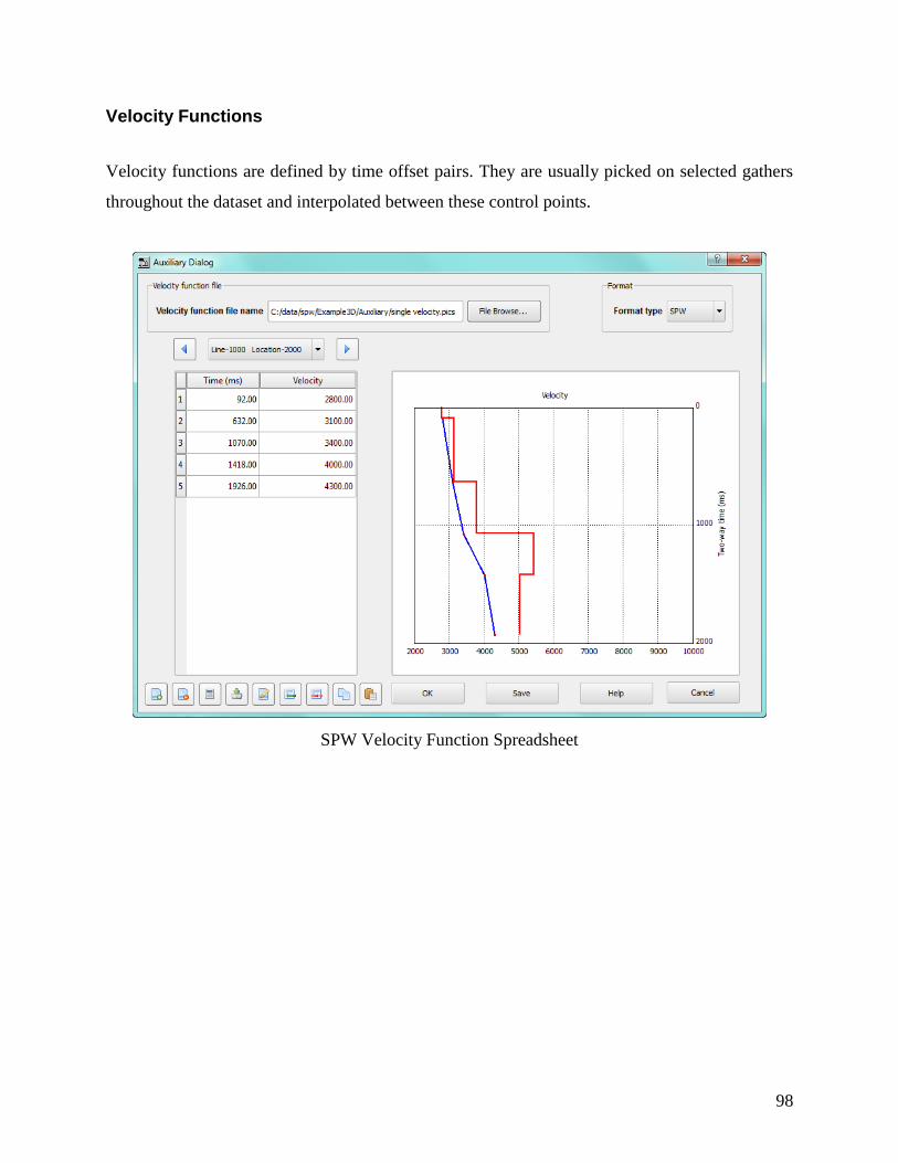
98

Velocity Functions

Velocity functions are defined by time offset pairs. They are usually picked on selected gathers

throughout the dataset and interpolated between these control points.

SPW Velocity Function Spreadsheet

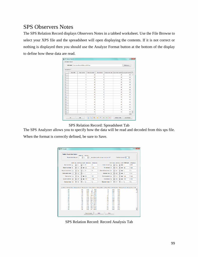
99

SPS Observers Notes The SPS Relation Record displays Observers Notes in a tabbed worksheet. Use the File Browse to

select your XPS file and the spreadsheet will open displaying the contents. If it is not correct or

nothing is displayed then you should use the Analyze Format button at the bottom of the display

to define how these data are read.

SPS Relation Record: Spreadsheet Tab

The SPS Analyzer allows you to specify how the data will be read and decoded from this sps file.

When the format is correctly defined, be sure to Save.

SPS Relation Record: Record Analysis Tab

100

SPS Receiver Locations

The SPS Point Record displays Receiver Locations in a tabbed worksheet. Use the File Browse to

select your RPS file and the spreadsheet will open displaying the contents. If it is not correct or

nothing is displayed then you should use the Analyze Format button at the bottom of the display

to define how these data are read.

SPS Receiver Record: Spreadsheet Tab

The SPS Analyzer allows you to specify how the data will be read and decoded from this sps file.

When the format is correctly defined, be sure to Save.

SPS Receiver Record: Record Analysis Tab

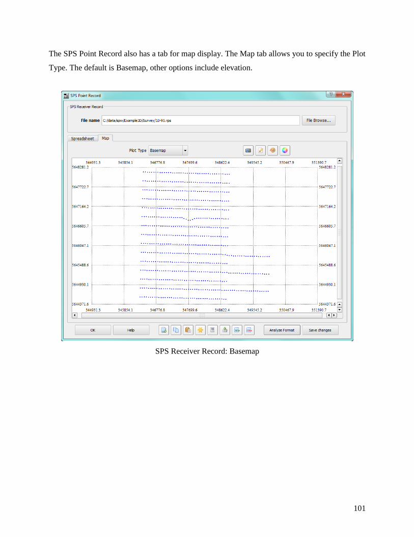
101

The SPS Point Record also has a tab for map display. The Map tab allows you to specify the Plot

Type. The default is Basemap, other options include elevation.

SPS Receiver Record: Basemap

102

SPS Source Locations

The SPS Point Record displays Source Locations in a tabbed worksheet. Use the File Browse to

select your SPS file and the spreadsheet will open displaying the contents. If it is not correct or

nothing is displayed then you should use the Analyze Format button at the bottom of the display

to define how these data are read.

SPS Source Record: Spreadsheet Tab

The SPS Analyzer allows you to specify how the data will be read and decoded from this sps file.

When the format is correctly defined, be sure to Save.

SPS Source Record: Record Analysis Tab

103

The SPS Point Record also has a tab for map display. The Map tab allows you to specify the Plot

Type. The default is Basemap, other options include elevation.

SPS Source Record: Basemap

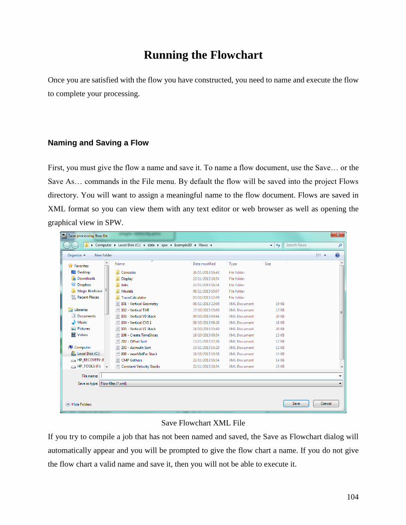
104

Running the Flowchart

Once you are satisfied with the flow you have constructed, you need to name and execute the flow

to complete your processing.

Naming and Saving a Flow

First, you must give the flow a name and save it. To name a flow document, use the Save… or the

Save As… commands in the File menu. By default the flow will be saved into the project Flows

directory. You will want to assign a meaningful name to the flow document. Flows are saved in

XML format so you can view them with any text editor or web browser as well as opening the

graphical view in SPW.

Save Flowchart XML File

If you try to compile a job that has not been named and saved, the Save as Flowchart dialog will

automatically appear and you will be prompted to give the flow chart a name. If you do not give

the flow chart a valid name and save it, then you will not be able to execute it.

105

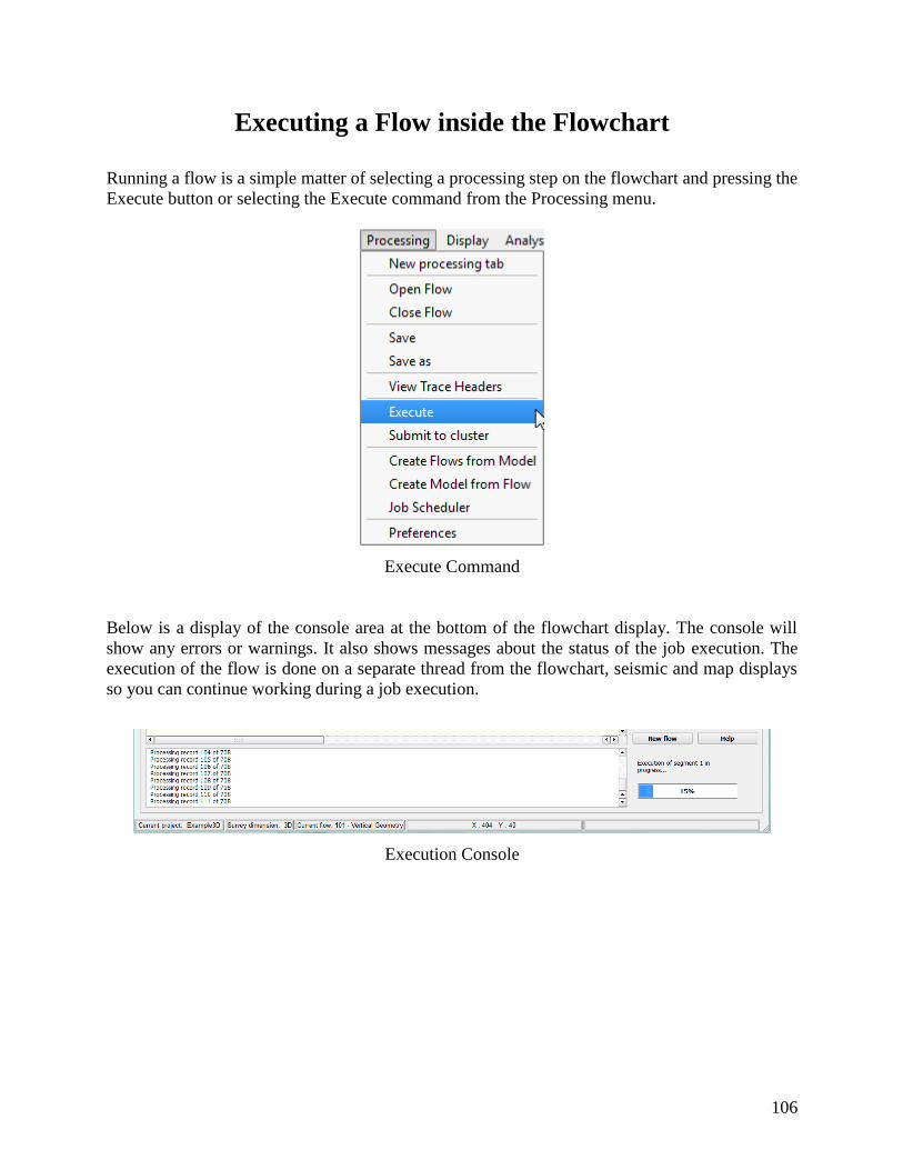
106

Executing a Flow inside the Flowchart

Running a flow is a simple matter of selecting a processing step on the flowchart and pressing the

Execute button or selecting the Execute command from the Processing menu.

Execute Command

Below is a display of the console area at the bottom of the flowchart display. The console will

show any errors or warnings. It also shows messages about the status of the job execution. The

execution of the flow is done on a separate thread from the flowchart, seismic and map displays

so you can continue working during a job execution.

Execution Console

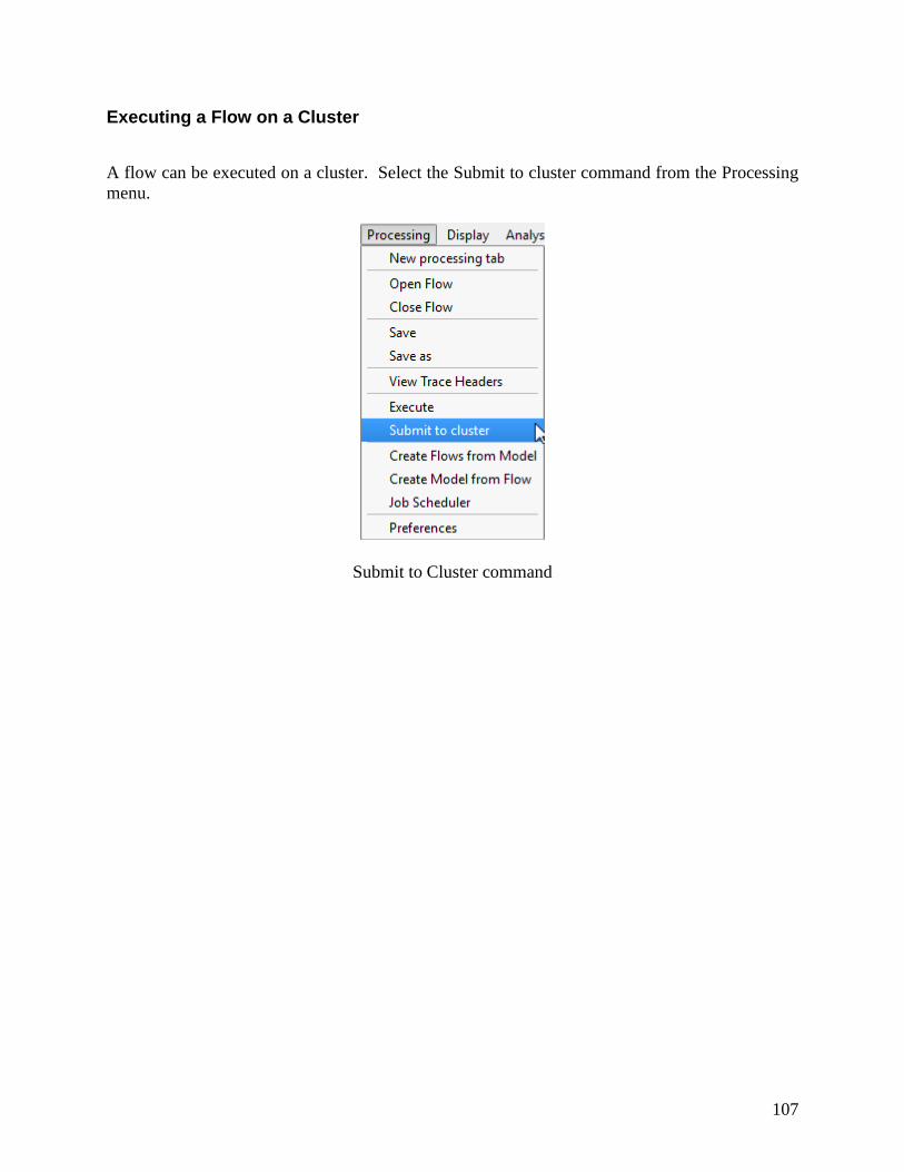
107

Executing a Flow on a Cluster

A flow can be executed on a cluster. Select the Submit to cluster command from the Processing

menu.

Submit to Cluster command

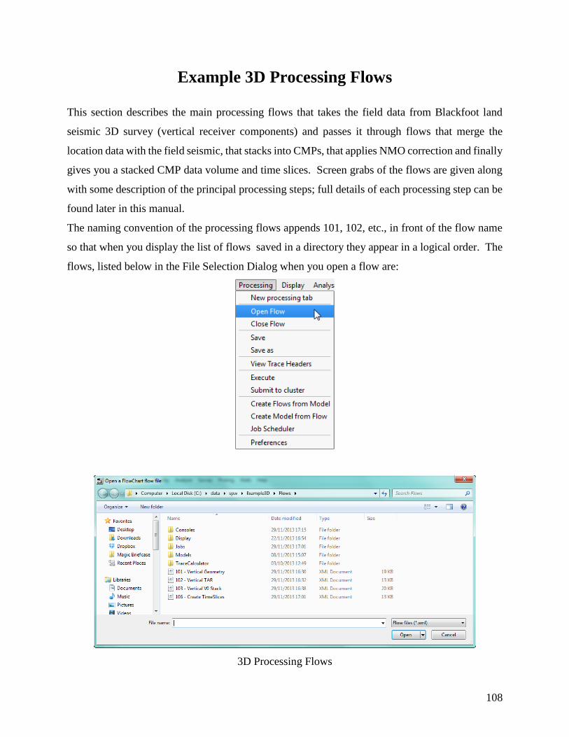
108

Example 3D Processing Flows

This section describes the main processing flows that takes the field data from Blackfoot land

seismic 3D survey (vertical receiver components) and passes it through flows that merge the

location data with the field seismic, that stacks into CMPs, that applies NMO correction and finally

gives you a stacked CMP data volume and time slices. Screen grabs of the flows are given along

with some description of the principal processing steps; full details of each processing step can be

found later in this manual.

The naming convention of the processing flows appends 101, 102, etc., in front of the flow name

so that when you display the list of flows saved in a directory they appear in a logical order. The

flows, listed below in the File Selection Dialog when you open a flow are:

3D Processing Flows

109

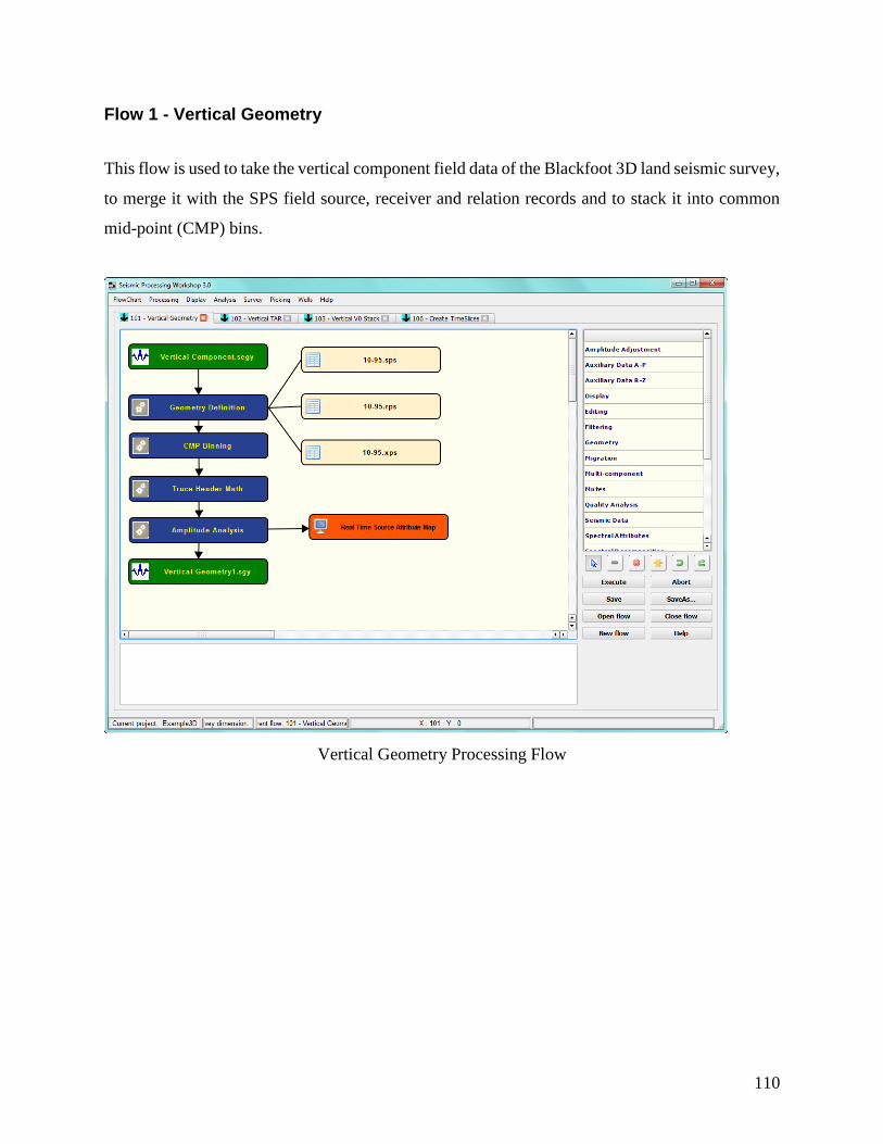
110

Flow 1 - Vertical Geometry

This flow is used to take the vertical component field data of the Blackfoot 3D land seismic survey,

to merge it with the SPS field source, receiver and relation records and to stack it into common

mid-point (CMP) bins.

Vertical Geometry Processing Flow

111

SEG Y Import

The input SEG Y file is sorted by Field File number and Channel Number, with the number and

ranges shown in the screen grab of the SEG Y Import dialog below.

SEG Y Import Dialog

Geometry Definition

The geometry is imported from the Source, Receiver and Relation components of the SPS files

which, by default, should have been stored in the project’s Survey directory. Screen grabs of each

of these, together with information about setting the format descriptions for each SPS data file are

given in the SPS section of the Display Auxiliary Data section of this manual, above. This

processing flow step will merge the SPS data and populate the trace headers of seismic data with

shot and receiver numbers. You could run a simple flow here by saving the output from the

geometry definition into a separate SEG Y file rather than passing it onto the CMP Binning flow.

This would give you a SEG Y output file, sorted by field and channel numbers, but with the shot

and receiver numbers, locations, offsets, etc., added to the headers.

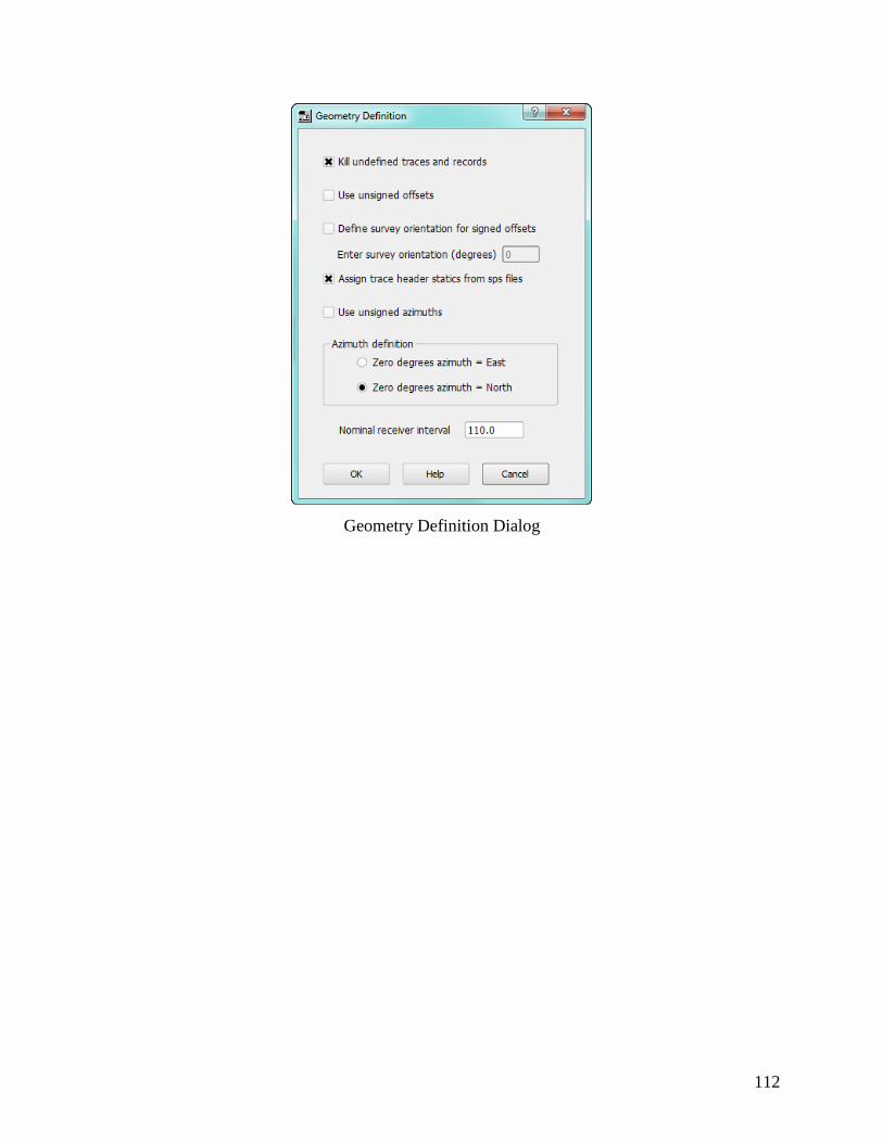
112

Geometry Definition Dialog

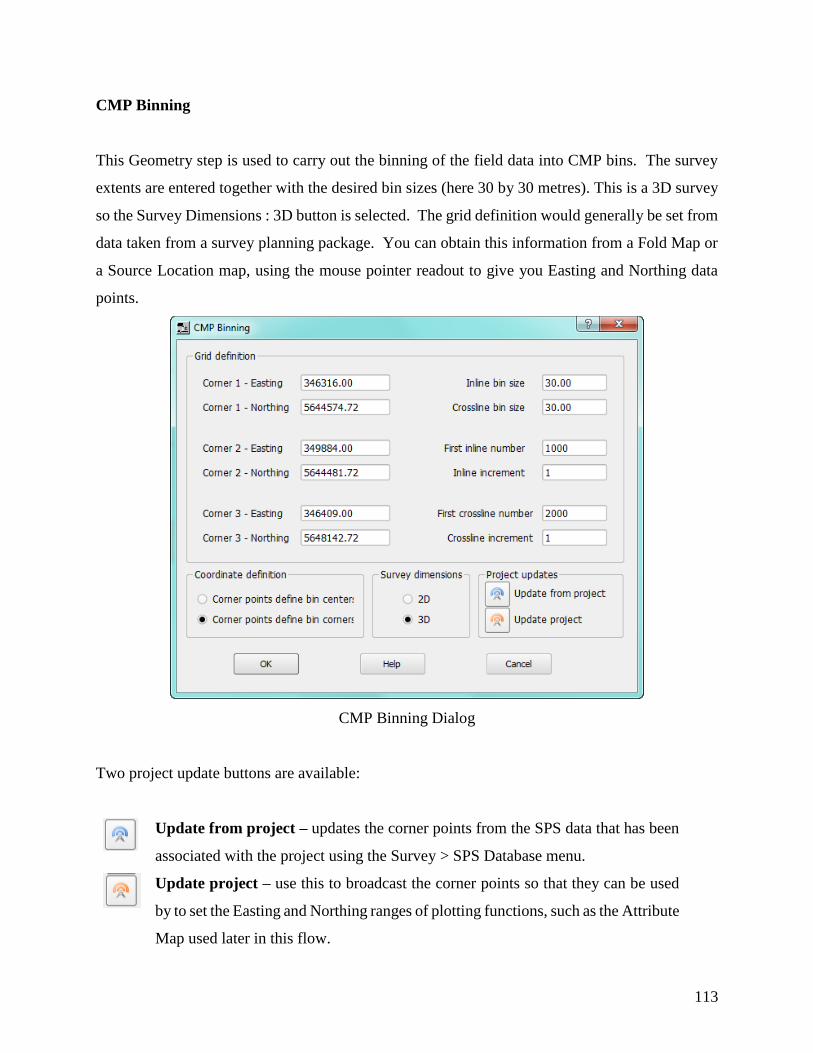
113

CMP Binning

This Geometry step is used to carry out the binning of the field data into CMP bins. The survey

extents are entered together with the desired bin sizes (here 30 by 30 metres). This is a 3D survey

so the Survey Dimensions : 3D button is selected. The grid definition would generally be set from

data taken from a survey planning package. You can obtain this information from a Fold Map or

a Source Location map, using the mouse pointer readout to give you Easting and Northing data

points.

CMP Binning Dialog

Two project update buttons are available:

Update from project – updates the corner points from the SPS data that has been

associated with the project using the Survey > SPS Database menu.

Update project – use this to broadcast the corner points so that they can be used

by to set the Easting and Northing ranges of plotting functions, such as the Attribute

Map used later in this flow.

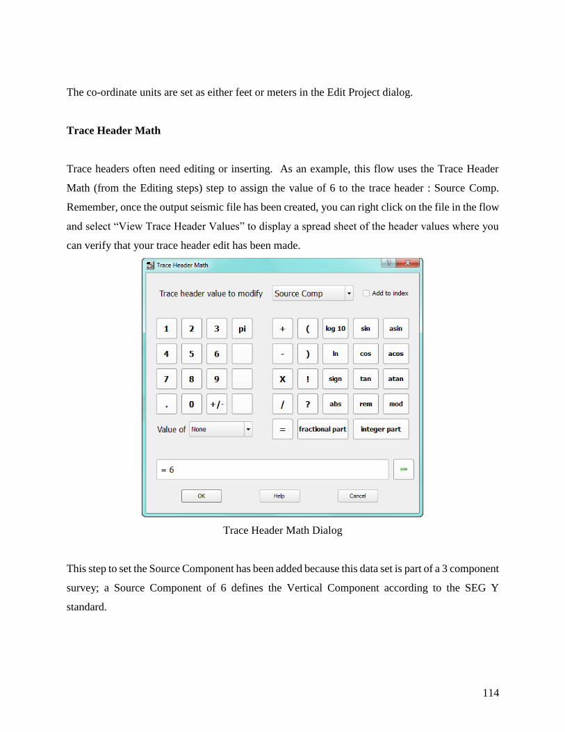
114

The co-ordinate units are set as either feet or meters in the Edit Project dialog.

Trace Header Math

Trace headers often need editing or inserting. As an example, this flow uses the Trace Header

Math (from the Editing steps) step to assign the value of 6 to the trace header : Source Comp.

Remember, once the output seismic file has been created, you can right click on the file in the flow

and select “View Trace Header Values” to display a spread sheet of the header values where you

can verify that your trace header edit has been made.

Trace Header Math Dialog

This step to set the Source Component has been added because this data set is part of a 3 component

survey; a Source Component of 6 defines the Vertical Component according to the SEG Y

standard.

115

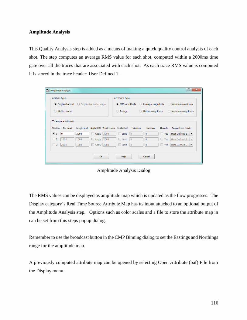
116

Amplitude Analysis

This Quality Analysis step is added as a means of making a quick quality control analysis of each

shot. The step computes an average RMS value for each shot, computed within a 2000ms time

gate over all the traces that are associated with each shot. As each trace RMS value is computed

it is stored in the trace header: User Defined 1.

Amplitude Analysis Dialog

The RMS values can be displayed as amplitude map which is updated as the flow progresses. The

Display category’s Real Time Source Attribute Map has its input attached to an optional output of

the Amplitude Analysis step. Options such as color scales and a file to store the attribute map in

can be set from this steps popup dialog.

Remember to use the broadcast button in the CMP Binning dialog to set the Eastings and Northings

range for the amplitude map.

A previously computed attribute map can be opened by selecting Open Attribute (baf) File from

the Display menu.

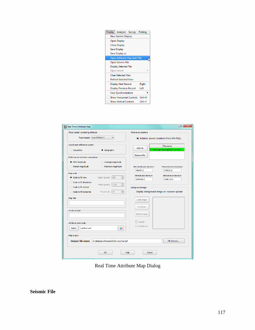
117

Real Time Attribute Map Dialog

Seismic File

118

Finally, the a Seismic File step (from the Seismic Data steps) is used to create a new SEG Y file

which is used to store the CMP binned data. The data are sorted in this file with CMP Line, CMP

Location and Offset sorts for the Primary, Secondary and Tertiary sorts, respectively.

To run the flow, use the pointer to select the flow (or use the Select All Items button) and then

press Execute. The time for the flow to execute is determined by the processor speed, number of

cores and speed of the disk access. Flows can sometimes take longer to run the first time than on

subsequent running because of how data is cached by the computer. While running, the real time

amplitude map is updated with the average RMS values for each source location.

119

Flow 2 – Bandpass Filtering and Spherical Divergence Correction

This flow gives examples of two processing steps that can be applied to the trace data: bandpass

filtering and spherical divergence correction.

Spherical Divergence Correction Flow

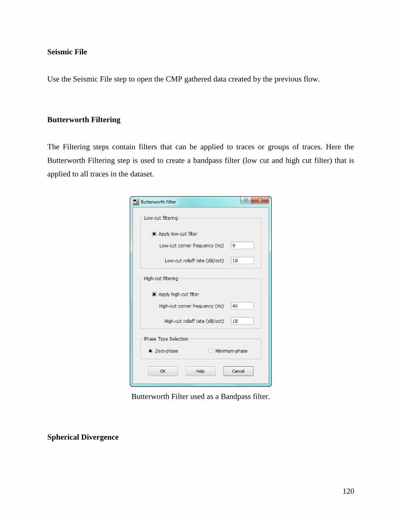
120

Seismic File

Use the Seismic File step to open the CMP gathered data created by the previous flow.

Butterworth Filtering

The Filtering steps contain filters that can be applied to traces or groups of traces. Here the

Butterworth Filtering step is used to create a bandpass filter (low cut and high cut filter) that is

applied to all traces in the dataset.

Butterworth Filter used as a Bandpass filter.

Spherical Divergence

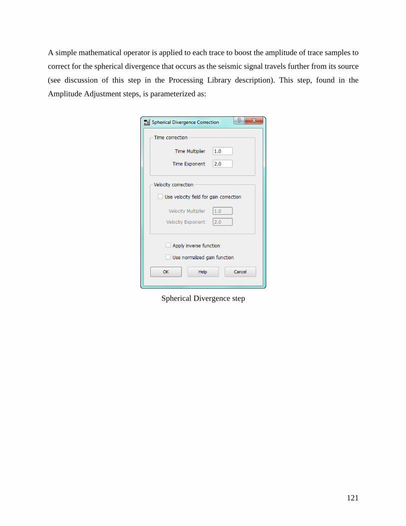
121

A simple mathematical operator is applied to each trace to boost the amplitude of trace samples to

correct for the spherical divergence that occurs as the seismic signal travels further from its source

(see discussion of this step in the Processing Library description). This step, found in the

Amplitude Adjustment steps, is parameterized as:

Spherical Divergence step

122

Seismic File

Use the Seismic File step to save the filtered and divergence corrected data set to a new seismic

file.

123

Flow 3 – Normal Moveout Correction and Vertical Stacking

This flow combines together a normal moveout correction with a simple CMP stack to produce a

file of inline and crossline stacked traces – i.e. one stacked trace per CMP location. Additional

steps to apply an Automatic Gain Control (AGC), an early mute and to kill traces are applied.

Normal Moveout Correction and Vertical Stacking Flow

Seismic File

124

Use the Seismic File step to open the filtered and spherical divergence corrected data created by

the previous flow.

Apply Normal Moveout

The normal moveout correction step is located within the Velocities group of processing steps and

is explained in more detail in the Processing Library description. In this flow it takes its input

from the CMP stacked and filtered seismic file, together with a velocity field from a data file

created using the Velocity wizard described further back in this manual.

Apply Normal Moveout processing step

The velocity field was created for a number of the CMP locations; it is interpolated for missing

CMPs. By default, the field needs only one set of velocity picks from a single CMP, but in practice

picks would be made at regular intervals across the CMP survey area.

125

The velocity fields are interpolated using Delaunay triangulation for a 3D survey or linear

interpolation for a 2D survey.

Automatic Gain Control

An Automatic Gain Control step (see Amplitude Adjustment steps) has been applied to boost lower

amplitude arrivals prior to making the brute stack in the CMP stack below. Such a step would not

be applied if any amplitude analysis was expected to be made; instead a step such as surface

consistent amplitude balancing would be used.

Automatic Gain Control Dialog

Apply Early Mute

The early mute step (from the Mute group of processing steps) is used to remove any noise or

NMO artifacts present in the data before the useful signal. The mutes are interpolated so picks can

be made at regular intervals across the survey. Mutes are read in from an early mute picked file.

126

Early Mute Dialog

Kill Traces

Because there is some ground roll evident in the near offset traces, a simple kill trace mute is

applied to any trace with an offset of between +/- 350 feet.

Kill Trace Dialog

CMP Stack

Once the CMP data has been NMO corrected, it can be stacked using the CMP Stack step (see the

Stacking group of processing steps). We could stack into various offsets (e.g. near, mid and far)

but in this step a single stack is made over the full offset range.

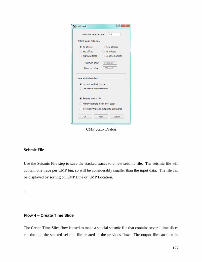
127

CMP Stack Dialog

Seismic File

Use the Seismic File step to save the stacked traces to a new seismic file. The seismic file will

contain one trace per CMP bin, so will be considerably smaller than the input data. The file can

be displayed by sorting on CMP Line or CMP Location.

.

Flow 4 – Create Time Slice

The Create Time Slice flow is used to make a special seismic file that contains several time slices

cut through the stacked seismic file created in the previous flow. The output file can then be

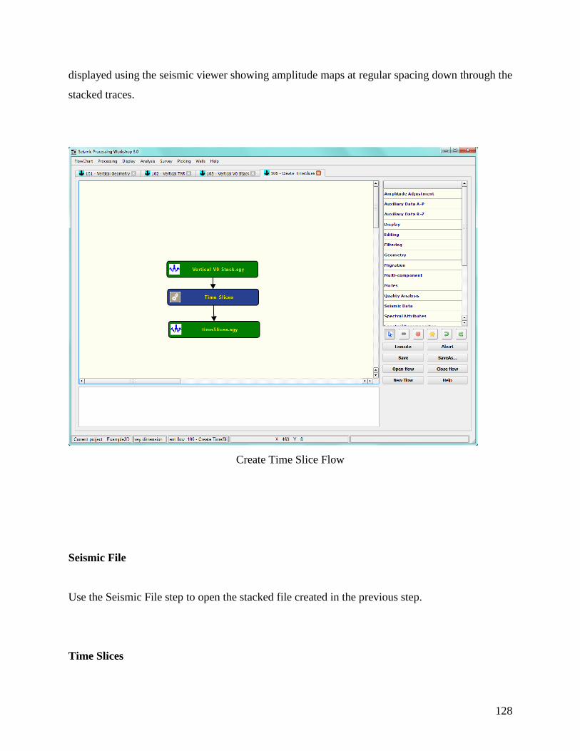
128

displayed using the seismic viewer showing amplitude maps at regular spacing down through the

stacked traces.

Create Time Slice Flow

Seismic File

Use the Seismic File step to open the stacked file created in the previous step.

Time Slices

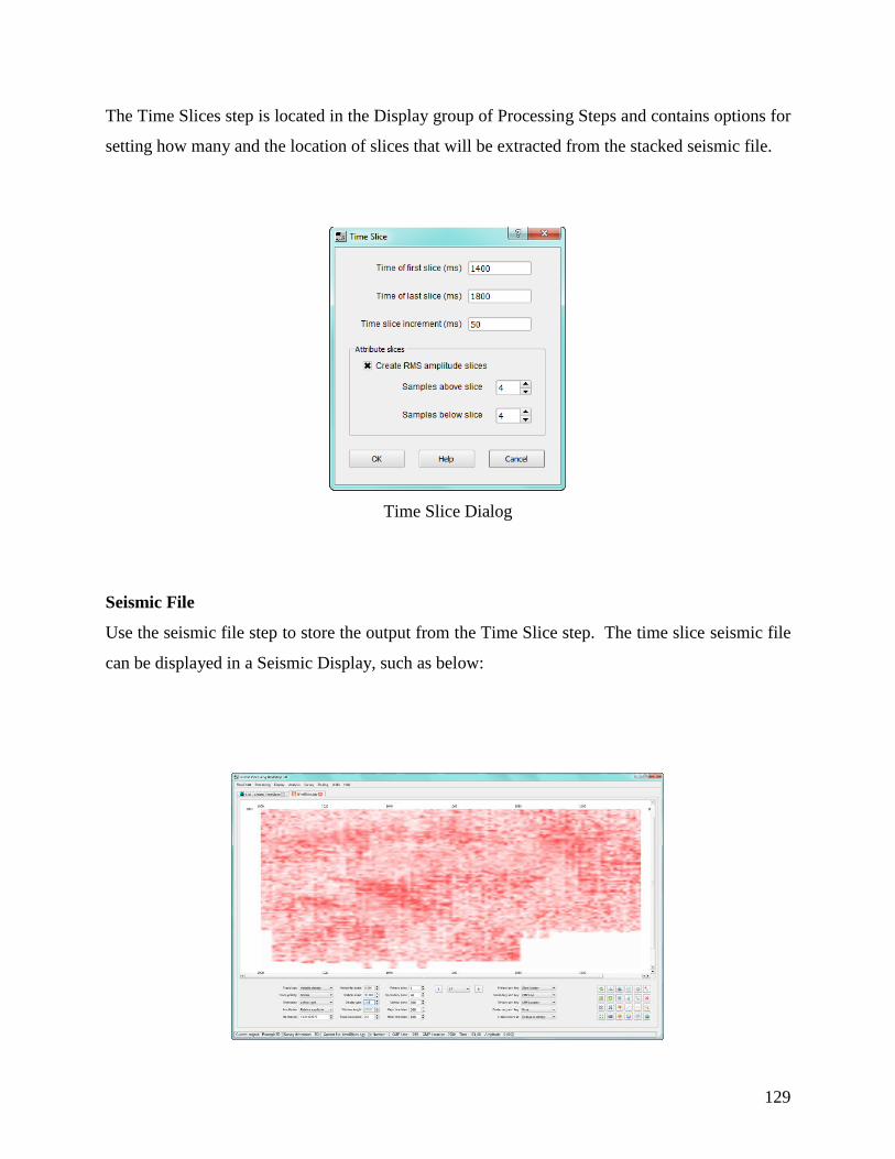
129

The Time Slices step is located in the Display group of Processing Steps and contains options for

setting how many and the location of slices that will be extracted from the stacked seismic file.

Time Slice Dialog

Seismic File

Use the seismic file step to store the output from the Time Slice step. The time slice seismic file

can be displayed in a Seismic Display, such as below:

130

Time Slice at 1600ms

As before, to run the flow, use the pointer to select the flow (or use the Select All Items button)

and then press Execute.

131

Instantaneous Field QC Capabilities and Procedures

A focus of the development of this version of SPW has been to simplify and automate field quality

control. Multiple new map displays have been implemented to enable rapid visualization of your

survey. Real time input of data direct from seismic recorders has been incorporated and simplified.

Real time displays of seismic data, attribute maps and survey information are some of the new

capabilities.

Real Time Processing

Real time processing starts with the input from the seismic recorder. SPW currently supports

ARAM SEG Y format, Sercel SEG D format, Hydroscience SEG D format, Standard SEG D

format, and SEG 2 format. Other formats and recording instrument specifications will be added as

needed in the future. The implementations of these formats read in all of the extended headers and

if the geometry information is present in the headers, it is always input.

Real Time Seismic Input Dialog

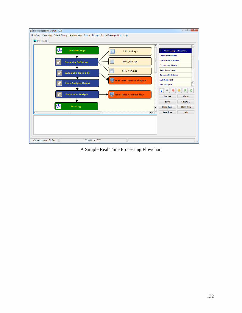
132

A Simple Real Time Processing Flowchart

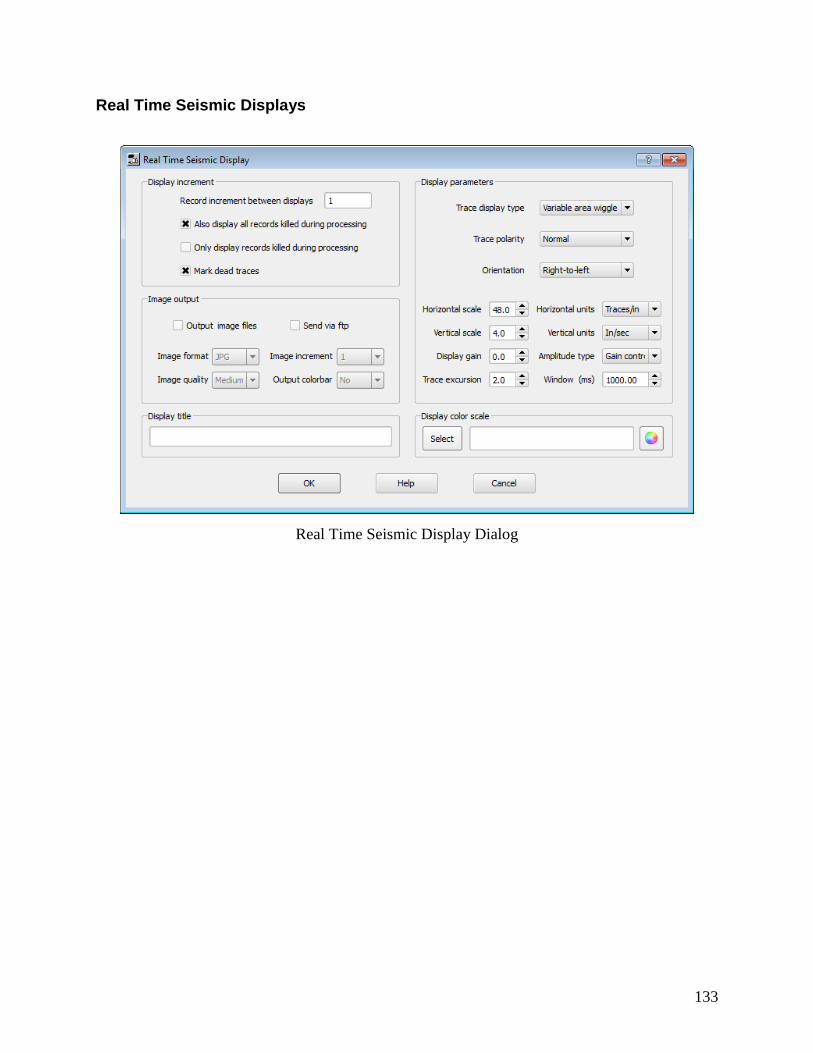
133

Real Time Seismic Displays

Real Time Seismic Display Dialog

134

Real Time Map Displays

Real Time Attribute Map Display Dialog

135

FTP Connection

***Note – FTP capability is temporarily disabled (October 2014) due to low level library changes.

Open the FTP Client

136

FTP Client Window

Using the SPW ftp client, either complete directories or single files may be sent to an ftp server.

Simply open a connection to the ftp server and then select the directory or the files to transfer.

Sending Reports via FTP in Real Time

Several reports on record and trace kills may be sent automatically to an ftp server during the

execution of a flow. This feature allows experienced personnel in the office to assist in evaluating

noisy or problem data by being able to review the same information available to the field personnel.

To enable this option, the ftp connection must be initiated using the ftp client from the Flowchart

menu. After the connection is established then selecting the Sent file via ftp option will

automatically send the report file after each record is processed.

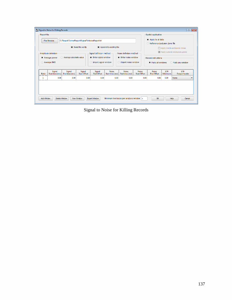
137

Signal to Noise for Killing Records

138

Send Trace Analysis Report via FTP

Sending Image Files via FTP in Real Time

139

Troubleshooting

No License Key Available

If you start the Flowchart without a valid licence key available, you may get the following popup

error message:

Check that the license key is correctly inserted into a USB port on the computer and there are

sufficient days left in the license (use the Help > About dialog for this).

Killing the Flowchart Process

Occasionally, it is necessary to close the Flowchart while a process is executing, for example if

you have started a flow by mistake that is going to take a long time to execute. Usually, the

flowchart process will be killed when the flowchart is closed, but sometimes this doesn’t happen.

In this case you can use the Windows Task Manager to “End Process” the flowchart.exe process:

Windows Task Manager showing the flowchart.exe processes highlighted.

If a flowchart process is already running, you will be prevented from opening a new Flowchart

until the previous flowchart process has ended.

Details of how to obtain support from Parallel Geocience are given at the start of this user manual.

140

141

The Processing Library:

Overview

The library of processing steps is separated into categories. The categories are as follows:

Not all processing steps from SPW 2 are available in SPW 3.

142

The standard use of each processing step will be described in the pages that follow. If the step is

enabled for only 2-D or only 3-D, it will be explicitly annotated as such; otherwise the process

may be used with both 2-D and 3-D data. Each of the Processing Step descriptions lists the

mandatory and optional input and output links required for execution, and contains an illustration

of an example flow chart. References are given for some processing steps based upon specific

published techniques or algorithms. An image of the processing step's parameter dialog is also

displayed for your reference. Finally, you will find a description of each parameter for each

processing step. At the end of each parameter description, the valid range for each parameter is

shown in brackets {}.

Abbreviations for the parameters are as follows –

• - Greater than

<= - Less than or equal to

< - Less than

>= - Greater than or equal to

#,# - Range of values from first number to last number

Parameter range checking is enabled for some of the processing step parameters. Additional

parameter range checking will be enabled in the future.

Note: For processing parameters with spatial units such as feet, meters, feet per second, meters per

second, etc., SPW assumes that you are consistent in your use of spatial units for the entire data

set. If your geometry information is in meters then you should consistently use metric units as your

unit of measure for the SPW processing parameters applied to that data set. If your geometry

information is in feet then you should consistently use English units as your unit of measure for

the SPW processing parameters applied to that data set. Combining English and metric units of

measure when processing in SPW will yield erroneous results.

Amplitude Adjustment Steps

This section documents the processing steps available for Amplitude Adjustment. Processing steps

currently available are:

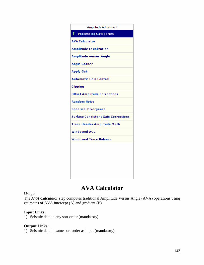
143

AVA Calculator Usage:

The AVA Calculator step computes traditional Amplitude Versus Angle (AVA) operations using

estimates of AVA intercept (A) and gradient (B)

Input Links:

1) Seismic data in any sort order (mandatory).

Output Links:

1) Seismic data in same sort order as input (mandatory).

144

Reference:

-

Example Flowchart:

Step Parameter Dialog:

Parameter Description:

Intercept (A) – If seleceted, compute AVA Intercept.

Gradient (B) – If seleceted, compute Gradient.

145

A * B – If seleceted, compute AVA Intercept and AVA Gradient and multiplies both.

B/A – If selected, compute the division between the AVA Gradient with the AVA Intercept.

B * sign(A) – If selected, compute the AVA Gradient and multiplies it by the signed AVA

Gradient.

(A+B)/2 – If selected, computes the average between AVA Intercept and Gradient.

(A-B)/2 – If selected, bomputes the difference between AVA Intercept and Gradient and divides

by two.

AB Rotation – If selected, sums AVA Intercept and Gradient after inpute traces being rotated by

the Phase rotatation angle (degrees).

Phase rotatation angle (degrees) – Enabled if AB Rotation is selected. Enter constant angle

in degress used to rotate the phase of each trace.

Amplitude Equalization Usage:

The Amplitude Equalization step allows you to balance the RMS values of your data traces to a

constant specified RMS level. You can also clip your data at a specified level. You can specify the

data window to use in calculating the RMS amplitudes, the output RMS and clipping levels, and

the method of amplitude equalization, which may be either trace constant or record constant.

Input Links:

1) Seismic data in any sort order (mandatory).

Output Links:

1) Seismic data in same sort order as input (mandatory).

Reference:

-

Example Flowchart:

146

Step Parameter Dialog:

Parameter Description:

Equalization window start (ms) — Enter the start time in milliseconds of the window to be used

in calculating the trace amplitude. {=>0}

147

Window length (ms) — Enter the length in milliseconds of the window to be used in calculating

the trace amplitude. {>0.0}

RMS level — Enter the output RMS level of the data window specified. {>0.0}

Clipping level — Enter the clipping level of the trace data. {>0.0}

Method: Specify whether to apply the equalization on a trace by trace basis or to maintain relative

amplitudes and level the RMS value of the entire record.

Trace constant equalization — If selected, your data will be equalized on a trace by trace

basis.

Record constant equalization — If selected, your data will be equalized on a record by record

basis, which will depend on the sort order of the input data.

Apply moveout to equalization window — If checked, the equalization will be performed after

linear moveout at the specified velocity. The window start time will shift by: delta time =

offset/velocity.

Linear moveout velocity — Enabled in Apply moveout to equalization window is checked.

Enter the constant moveout velocity. {>0.0}

Amplitude Versus Angle Usage:

The Amplitude Versus Angle step allows you to map seismic reflection information in the

biangular domain using various methods to interpret the amplitude values. You may also define

the velocity field, select the ray tracing type, specify the angle range, and choose the velocity curve

fit type.

Input Links:

1) Seismic data in any sort order (mandatory).

Output Links:

1) Seismic data in any sort order (mandatory).

Reference:

-

Example Flowchart:

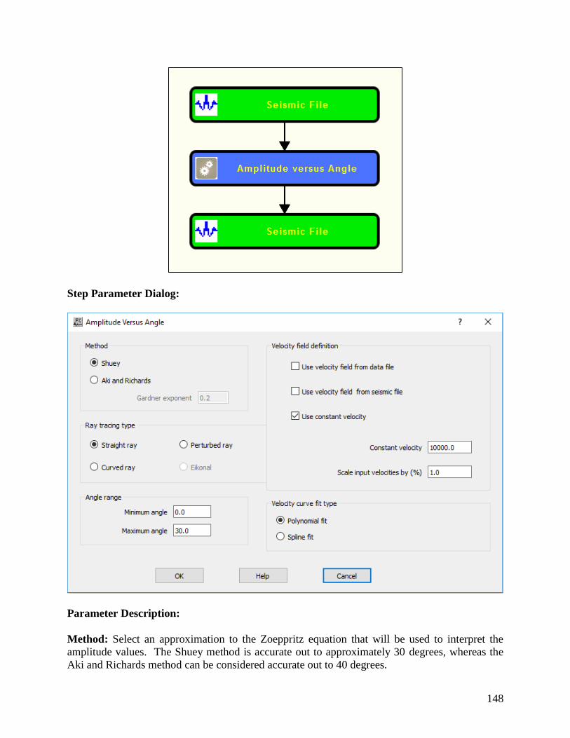
148

Step Parameter Dialog:

Parameter Description:

Method: Select an approximation to the Zoeppritz equation that will be used to interpret the

amplitude values. The Shuey method is accurate out to approximately 30 degrees, whereas the

Aki and Richards method can be considered accurate out to 40 degrees.

149

Shuey — If selected, the Shuey approximation will be used.

Aki and Richards — If selected, the Aki and Richards approximation will be used.

Gardner exponent — Enter the value to be used for the exponent in the Gardner equation. The

value may be set to 0.0 and the default (0.25) only applies if the Aki and Richards method is

selected.

Velocity field definition: Define the velocity field to be used.

Use velocity field from data file — If checked, the velocity field will be used from the data

file.

Use velocity field from seismic file — If checked, the velocity field will be used from the

seismic file.

Use constant velocity — If checked, a constant velocity will be used.

Constant velocity — If Use constant Velocity is checked, enter a constant velocity.

Scale input velocities by (%) — Enter a percentage to scale input velocities. {1.0 = 100%}

Ray tracing type: Define the ray tracing method used in the estimation of propagation angles.

Straight ray — If selected, rays will be traced using a straight ray algorithm.

Perturbed ray — If selected, rays will be traced using a perturbed ray algorithm.

Curved ray — If selected, rays will be traced using a curved ray algorithm.

Eikonal ray — If selected, rays will be traced using an eikonal ray algorithm.

Angle range: Define the minimum and maximum angles used in the calculation of AVA attributes.

Minimum angle — Enter the minimum angle.

Minimum angle — Enter the maximum angle.

Velocity curve fit type: Define the procedure to interpolate velocities between time-velocity pairs

specified in the linked velocity file.

Polynomial fit — If selected, velocities will be interpolated with a polynomial interpolator.

Spline fit — If selected, velocities will be interpolated with a spline interpolator.

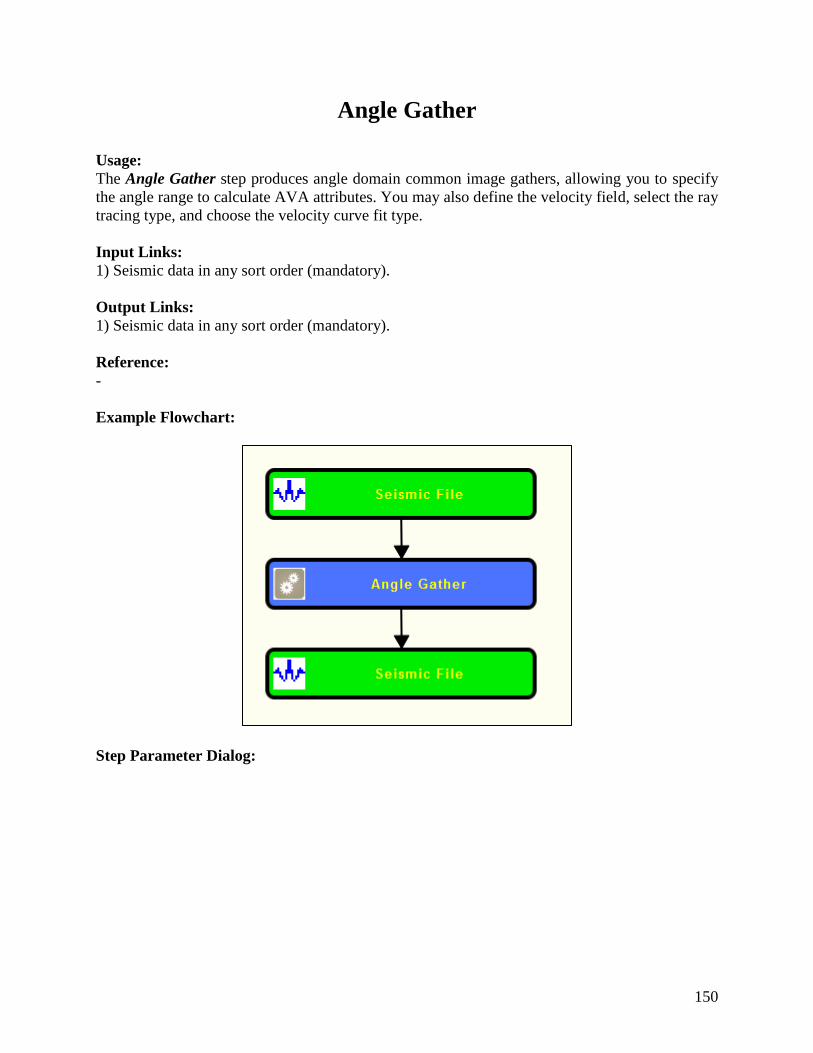
150

Angle Gather

Usage:

The Angle Gather step produces angle domain common image gathers, allowing you to specify

the angle range to calculate AVA attributes. You may also define the velocity field, select the ray

tracing type, and choose the velocity curve fit type.

Input Links:

1) Seismic data in any sort order (mandatory).

Output Links:

1) Seismic data in any sort order (mandatory).

Reference:

-

Example Flowchart:

Step Parameter Dialog:

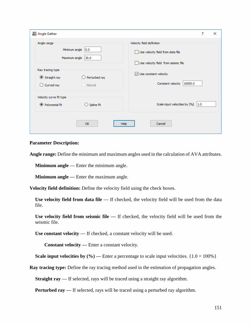
151

Parameter Description:

Angle range: Define the minimum and maximum angles used in the calculation of AVA attributes.

Minimum angle — Enter the minimum angle.

Minimum angle — Enter the maximum angle.

Velocity field definition: Define the velocity field using the check boxes.

Use velocity field from data file — If checked, the velocity field will be used from the data

file.

Use velocity field from seismic file — If checked, the velocity field will be used from the

seismic file.

Use constant velocity — If checked, a constant velocity will be used.

Constant velocity — Enter a constant velocity.

Scale input velocities by (%) — Enter a percentage to scale input velocities. {1.0 = 100%}

Ray tracing type: Define the ray tracing method used in the estimation of propagation angles.

Straight ray — If selected, rays will be traced using a straight ray algorithm.

Perturbed ray — If selected, rays will be traced using a perturbed ray algorithm.

152

Curved ray — If selected, rays will be traced using a curved ray algorithm.

Eikonal ray — If selected, rays will be traced using an eikonal ray algorithm.

Velocity curve fit type: Define the procedure to interpolate velocities between time-velocity pairs

specified in the linked velocity file.

Polynomial fit — If selected, velocities will be interpolated with a polynomial interpolator.

Spline fit — If selected, velocities will be interpolated with a spline interpolator.

Apply Gain Usage:

The Apply Gain step allows you to apply gain function curves to your seismic data. Any or all

source, receiver, offset or gain card data may be applied. Gain curves may also be applied from

the data file. Additionally, gain may be applied by entering dB/second. Gain curves are specified

as time – dB pairs and are linearly interpolated to each location along the line. A constant gain

multiplier may also be applied to the data.

Input Links:

1) Seismic data in any sort order (mandatory).

2) Source Gain Corrections cards (optional).

3) Receiver Gain Corrections cards (optional).

4) Offset Gain Corrections cards (optional).

5) Gain Curves cards (optional).

Output Links:

1) Seismic data in same sort order as input (mandatory).

Reference:

-

Example Flow chart:

153

Step Parameter Dialog:

Parameter Description:

154

Apply source gain corrections — If checked, source gain corrections will be applied to the

seismic data from a source gain correction auxiliary file.

Apply receiver gain corrections — If checked, receiver gain corrections will be applied to the

seismic data from a receiver gain correction auxiliary file.

Apply offset gain corrections — If checked, offset gain corrections will be applied to the seismic

data from an offset gain correction auxiliary file.

Apply gain curves from data file — If checked, gain curves will be applied to the seismic data

from a gain curves auxiliary file.

Apply dB/sec gain — If checked, gain will be applied to the data in decibels per second.

dB/sec gain — Enter the gain in decibels per second.

Constant gain multiplier — Enter a constant gain multiplier by which value each trace data

sample will be multiplied.

Apply any gain specified — If selected, apply specified gain to the seismic data.

Remove any gain specified — If selected, remove specified gain from the seismic data.

Automatic Gain Control Usage:

The Automatic Gain Control step allows you to apply up to five sliding window gain functions to

each data trace. You specify the number of gated windows, the overlap between the gated

windows, and the start time and length of each gate. The calculated gain functions may be output

to an optional seismic file, which allows you the option to remove the AGC functions prior to

subsequent processing steps.

Input Links:

1) Seismic data in any sort order (mandatory).

Output Links:

1) Seismic data in same sort order as input (mandatory).

Reference:

-

Example Flowcharts:

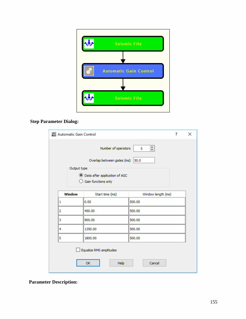
155

Step Parameter Dialog:

Parameter Description:

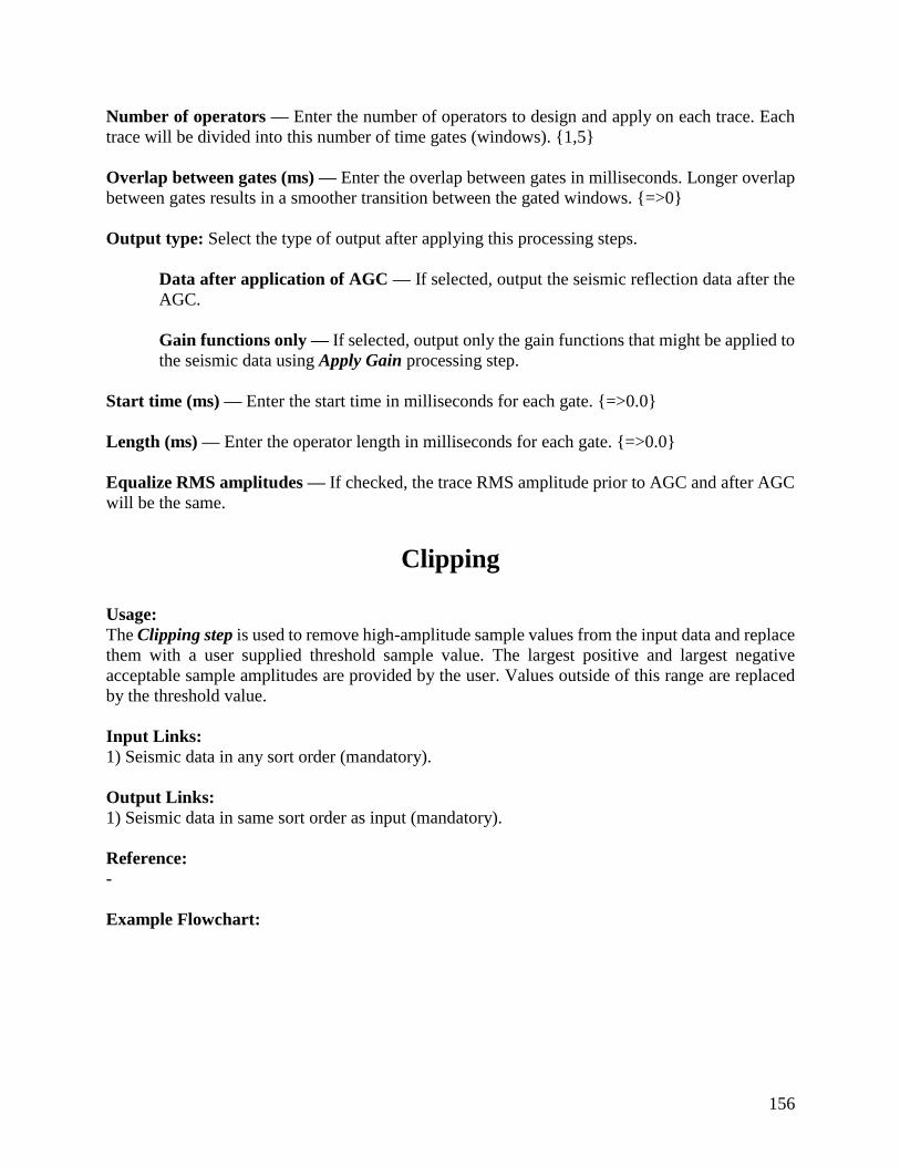
156

Number of operators — Enter the number of operators to design and apply on each trace. Each

trace will be divided into this number of time gates (windows). {1,5}

Overlap between gates (ms) — Enter the overlap between gates in milliseconds. Longer overlap

between gates results in a smoother transition between the gated windows. {=>0}

Output type: Select the type of output after applying this processing steps.

Data after application of AGC — If selected, output the seismic reflection data after the

AGC.

Gain functions only — If selected, output only the gain functions that might be applied to

the seismic data using Apply Gain processing step.

Start time (ms) — Enter the start time in milliseconds for each gate. {=>0.0}

Length (ms) — Enter the operator length in milliseconds for each gate. {=>0.0}

Equalize RMS amplitudes — If checked, the trace RMS amplitude prior to AGC and after AGC

will be the same.

Clipping

Usage:

The Clipping step is used to remove high-amplitude sample values from the input data and replace

them with a user supplied threshold sample value. The largest positive and largest negative

acceptable sample amplitudes are provided by the user. Values outside of this range are replaced

by the threshold value.

Input Links:

1) Seismic data in any sort order (mandatory).

Output Links:

1) Seismic data in same sort order as input (mandatory).

Reference:

-

Example Flowchart:

157

Step Parameter Dialog:

Parameter Description:

Clipping upper value — Specify the largest acceptable positive value. Positive values larger than

the clipping upper limit are replaced with the clipping upper limit.

Clipping lower value — Specify the largest acceptable negative value. Negative values greater

than the clipping lower limit are replaced with the clipping lower limit.

Offset Amplitude Corrections

Usage:

158

The Offset Amplitude Corrections step allows you to correct the amplitude values of your seismic

reflection data with the offset. You need to specitfy a function of gain with the offset.

Input Links:

1) Seismic data in any sort order (mandatory).

2) Offset Gains cart data (mandatory).

Output Links:

1) Seismic data in same sort order as input (mandatory).

Reference:

-

Example Flowchart:

Step Parameter Dialog:

159

Parameter Description:

Define Window: Define window configuration where the correction is going to be applied. The

window may be defined within a constant time gate, and/or by applying a linear moveout and/or

by limiting the traces in the calculation by the offset.

Used fixed window to build pilot — If checked, the pilot window is defined within a time gate.

Design window start time (ms) — Enter the start time for the design window.

Design window stop time (ms) — Enter the end time for the design window.

160

Apply Linear moveout to design window — If checked, apply a linear moveout to the design

window with a constant velocity as defined in Linear moveout velocity.

Linear moveout velocity (m/s) — Enter velocity to apply the linear moveout to the design

window.

Offset limt traces in design window — If checked, the traces considered to the design window

are limited by offset.

Minimum offset — Enter the minimum offset to be considered in the design window.

Maximum offset — Enter the maximum offset to be considered in the design window.

Offset gain calculations: Define parameters related with the gain calculation.

Offset bin size — Enter bin size to compute offset gain.

Minimum hit count per bin — Enter minimum hit count per bin.

Random Noise Usage:

The Random Noise step estimates the signal level then generates random noise to add to the data

at a specified Signal to Noise ratio. It is useful for creating noise in model data.

Input Links:

1) Seismic data in any sort order (mandatory).

Output Links:

1) Seismic data in same sort order as input (mandatory).

Reference:

-

Example Flowchart:

161

Step Parameter Dialog:

Parameter Description:

Signal amplitude estimation mode: Estimate signal amplitude either on a single channel or on

multi channel.

Signal-channel — If selected, use a single channel to estimate the signal amplitude.

162

Multi-channel — If selected, use multi-channel to estimate the signal amplitude.

Signal amplitude estimation type: Select the type of signal amplitude estimation.

RMS amplitude — Signal amplitude is estimated by RMS amplitude.

Average magnitude — Signal amplitude is estimated by average magnitude.

Max magnitude — Signal amplitude is estimated by maximum magnitude.

Power — Signal amplitude is estimated by the power of amplitude.

Average amplitude — Signal amplitude is estimated by average amplitude.

Max amplitude — Signal amplitude is estimated by maximum amplitude.

Signal-to-noise ratio — Enter the desired signal to noise ratio.

Spherical Divergence Usage:

The Spherical Divergence correction step is designed to compensate for the decrease in seismic

amplitude as a wavefront propagates away from the source location. The Spherical Divergence

Correction step allows you to apply a gain to the data traces based on the equation:

Gain = T_Multiplier * (Time ** T_Exponent) * V_Multiplier * (Velocity(Time) ** V_Exponent).

The T_Multiplier and the V_Multiplier are constant gain factors and the T_Exponent and the

V_Exponent vary the gain with time. Multipliers of one (1) and an exponent of two (2) are

commonly used for the spherical divergence correction since energy from a point source dissipates

in proportion to the square of distance traveled. To apply the spherical divergence correction as a

function of both time and velocity, you must supply the optional velocity function. Otherwise, the

velocity terms in the above equation will be ignored and the spherical divergence correction will

only be applied as a function of time. You also have the option to apply the inverse spherical

divergence correction function to your data.

Input Links:

1) Seismic data in any sort order (mandatory).

2) Velocity field card (optional).

Output Links:

1) Seismic data in same sort order as input (mandatory).

Reference:

Claerbout, Jon F., 1985, Fundamentals of Geophysical Data Processing: Blackwell Scientific

Publications.

163

Example Flowcharts:

Step Parameter Dialog:

Parameter Description:

164

The Gain equation for the following definitions is:

Gain = T_Multiplier * (Time ** T_Exponent) * V_Multiplier * (Velocity(Time) ** V_Exponent).

Time correction: Define parameters related with spherical correction based on time.

Time multiplier — Enter the time multiplier in the gain equation.

Time exponent — Enter the time exponent in the gain equation.

Velocity correction: Define parameters related with spherical correction based on velocity.

Use velocity field for gain correction — If checked, spherical correction is applied based on a

velocity field.

Velocity multiplier — Enter the velocity multiplier in the gain equation.

Velocity exponent — Enter the velocity exponent in the gain equation.

Apply inverse function — If checked, an inverse spherical divergence correction will be applied

to your data.

Use normalize gain function — Normalize the gain function to be applied.

Surface Consistent Gain Corrections Usage:

The Surface Consistent Gain Corrections step calculates source and receiver amplitude variations

in a surface consistent manner. Gain curves must be specified for source and receiver.

Input Links:

1) Seismic data in any sort order (mandatory).

2) Source Gain Corrections cards (mandatory).

3) Receiver Gain Corrections cards (mandatory).

Output Links:

1) Seismic data in same sort order as input (mandatory).

2) Source Gain Corrections cards (optional).

3) Receiver Gain Corrections cards (optional)

4) Offset Gain Corrections cards (optional).

Reference:

Taner, M. T., and Coburn, K. W., 1980, Surface consistent estimation of source and receiver

response functions: 50 th International Meeting of Soc. Expl.Geophy., Expanded Abstract.

Example Flowchart:

165

Step Parameter Dialog:

Parameter Description:

Design window:

Use window definition file — If selected, the pilot area is defined with a Window Definition

card.

166

Use fixed window to build pilot — If selected, the pilot area is defined within a fixed time gate.

Design window start time (ms) — Enter the window starting time in ms.

Design window stop time (ms) — Enter the window ending time in ms.

Apply linear moveout to desing window — If checked, the window is defined variable based on

a linear moveout with the velocity defined in Linear moveout velocity.

Linear moveout velocity — Enter the linear moveout velocity in m/s.

Offset limit traces in design window — If checked the window definition is limited by a

Minimum and Maximum offset values.

Minimum offset — Enter the minimum offset in field units to build the window.

Maximum offset — Enter the minimum offset in field units to build the window.

Surface consistent amplitude decomposition:

RMS error for termination —

Compute log amplitude —

Remove linear trend at each interation —

Compute source term —

Output source gain corrections —

Compute receiver term —

Output receiver gain corrections —

Compute offset term —

Output offset gain corrections —

Compute Structure term —

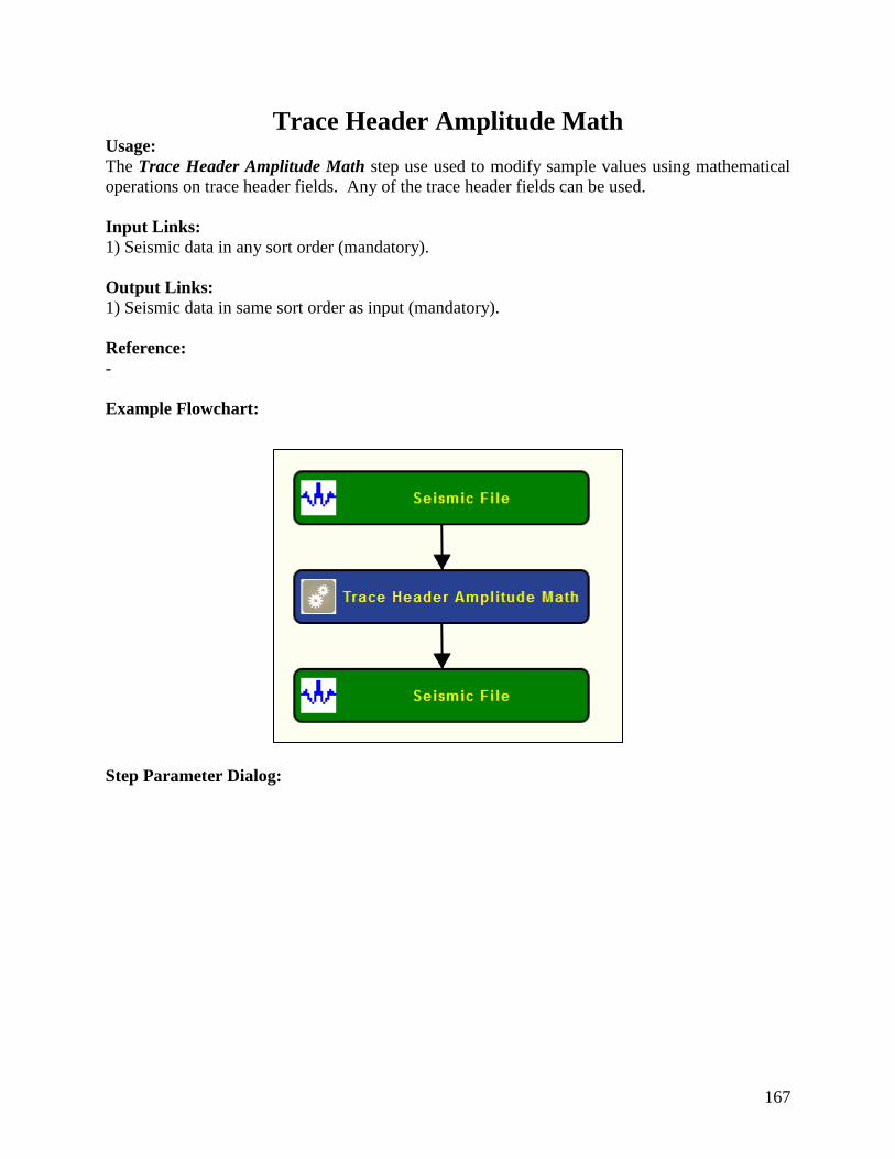
167

Trace Header Amplitude Math Usage:

The Trace Header Amplitude Math step use used to modify sample values using mathematical

operations on trace header fields. Any of the trace header fields can be used.

Input Links:

1) Seismic data in any sort order (mandatory).

Output Links:

1) Seismic data in same sort order as input (mandatory).

Reference:

-

Example Flowchart:

Step Parameter Dialog:

168

Parameter Description:

Operations: Select the mathematical operation that will modify the seismic amplitude values

based on value specified on a user-defined header.

Add header to — add header value to each seismic amplitude value.

Subtract header from — subtract header value to each seismic amplitude value.

Multiply by header — multiply each seismic amplitude value by header.

Divide by header — divide each seismic amplitude value by header.

Power of header — compute the power of each seismic amplitude value by an exponent as defined

in header.

Header Field — Select the trace header field that will modify the seismic amplitude values.

Example: If the Multiply by header operator is selected and the Header field is set to offset, then

the sample values in each input trace will be multiplied by the value of offset in the corresponding

trace header.

Windowed AGC Usage:

The Windowed AGC step step allows you to apply window gain functions to each data trace based

on user-defined windows. You specify the number of windows by setting the start time and length

169

of each gate. The calculated gain functions may be output to an optional seismic file, which allows

you the option to remove the AGC functions prior to subsequent processing steps.

Input Links:

1) Seismic data in any sort order (mandatory).

Output Links:

1) Seismic data in same sort order as input (mandatory).

2) Gain functions (optional).

Reference:

-

Example Flowchart:

Step Parameter Dialog:

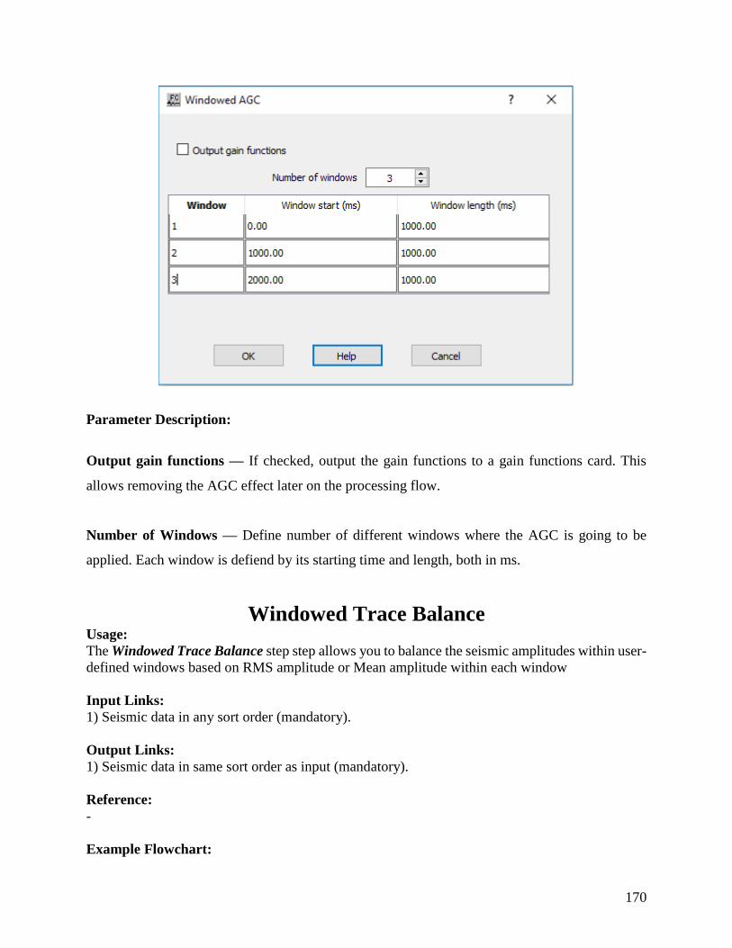
170

Parameter Description:

Output gain functions — If checked, output the gain functions to a gain functions card. This

allows removing the AGC effect later on the processing flow.

Number of Windows — Define number of different windows where the AGC is going to be

applied. Each window is defiend by its starting time and length, both in ms.

Windowed Trace Balance Usage:

The Windowed Trace Balance step step allows you to balance the seismic amplitudes within user-

defined windows based on RMS amplitude or Mean amplitude within each window

Input Links:

1) Seismic data in any sort order (mandatory).

Output Links:

1) Seismic data in same sort order as input (mandatory).

Reference:

-

Example Flowchart:

171

Step Parameter Dialog:

Parameter Description:

Reference type: Select whether the traces will be leveled according to RMS or mean amplitude.

Number of windows per trace — Enter the number of balancing windows per data trace.

Window start (ms) — Enter the start time in milliseconds for the balancing window.

172

Window length (ms) — Enter the length in milliseconds for the balancing window. The window

will extend from the start time to start time + length.

Reference level — Enter the reference level for the balancing window. On output, the RMS or

mean amplitude of the data trace will be equal to the specified value.

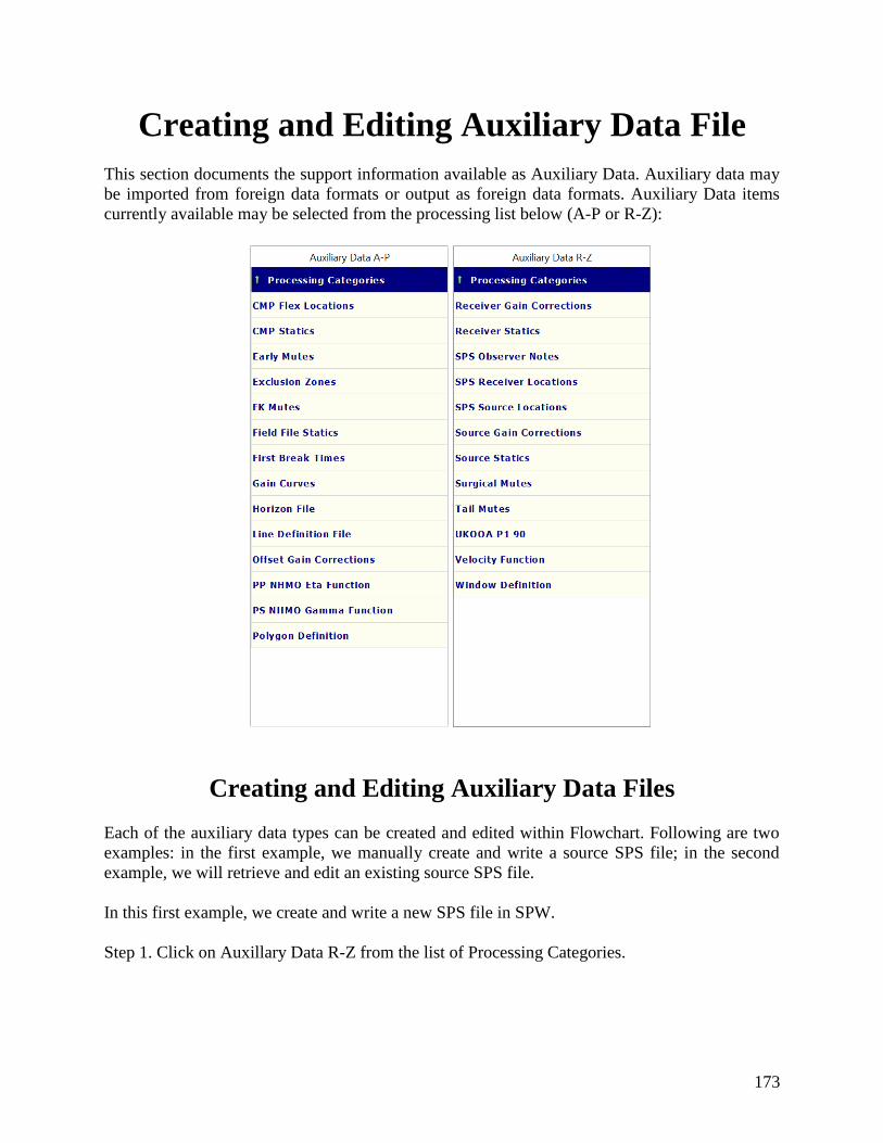
173

Creating and Editing Auxiliary Data File

This section documents the support information available as Auxiliary Data. Auxiliary data may

be imported from foreign data formats or output as foreign data formats. Auxiliary Data items

currently available may be selected from the processing list below (A-P or R-Z):

Creating and Editing Auxiliary Data Files

Each of the auxiliary data types can be created and edited within Flowchart. Following are two

examples: in the first example, we manually create and write a source SPS file; in the second

example, we will retrieve and edit an existing source SPS file.

In this first example, we create and write a new SPS file in SPW.

Step 1. Click on Auxillary Data R-Z from the list of Processing Categories.

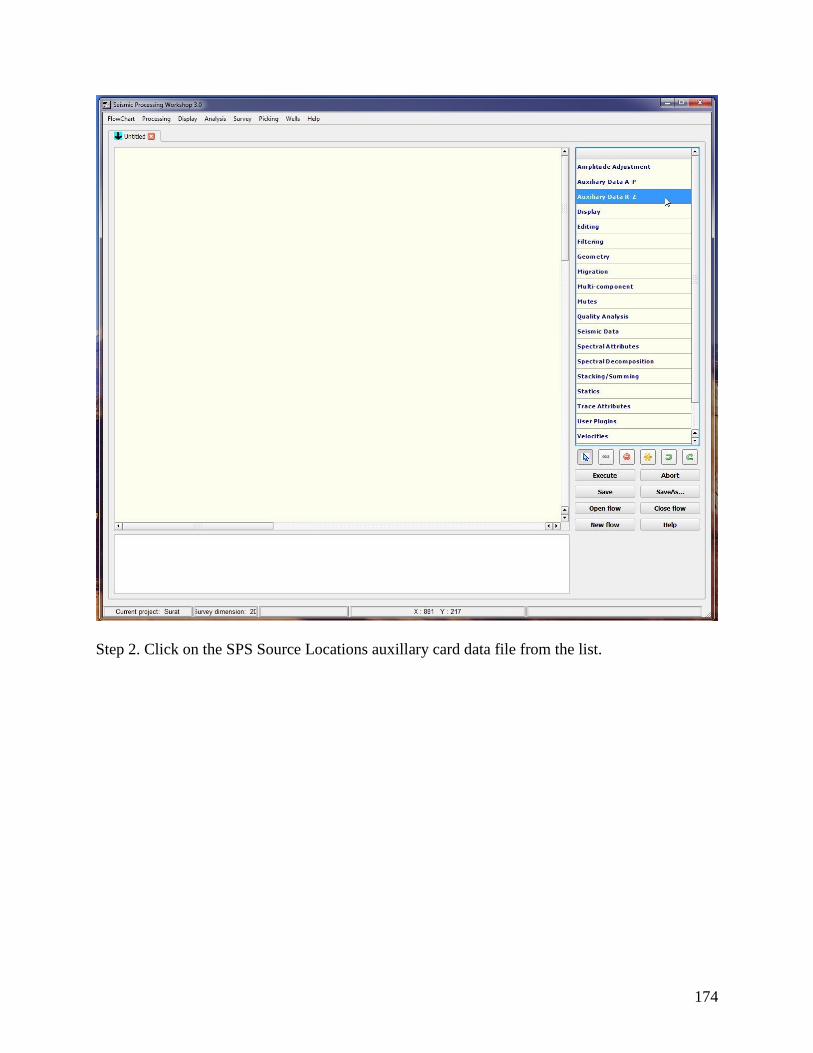
174

Step 2. Click on the SPS Source Locations auxillary card data file from the list.

175

An example of selecting the SPS Source Locations auxillary data file.

Step 3. Click on the FlowChart canvas to place the SPS Source Locations icon. You may click and

drag the icon to relocate it. Double click on the SPS Source Locations auxillary card data file to

open it.

176

Step 4. To create a new SPS Source Point Record, click on the File Browse… button. A dialog

box allows you to enter a desired name for your new file (e.g. NewFile) in the File name: text entry

box and clicking Open.

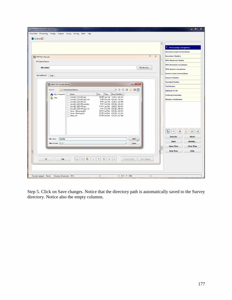
177

Step 5. Click on Save changes. Notice that the directory path is automatically saved to the Survey

directory. Notice also the empty columns.

178

Step 6. Select adds rows to create a spreadsheet for data entry. When the Add Rows dialog box

comes up, enter the number of rows desired, click OK and then Save changes.

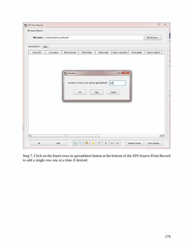
179

Step 7. Click on the Insert rows in spreadsheet button at the bottom of the SPS Source Point Record

to add a single row one at a time if desired.

180

Most values may be entered in the spreadsheet by using the fill column function.

181

If a column is not selected, an error check dialog box will prompt you to select a single column to

fill.

Step 8. Select a column to fill in the spreadsheet by clicking on the column header (e.g. Point

number).

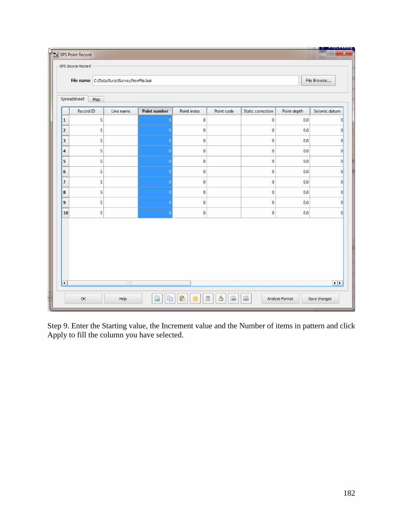
182

Step 9. Enter the Starting value, the Increment value and the Number of items in pattern and click

Apply to fill the column you have selected.

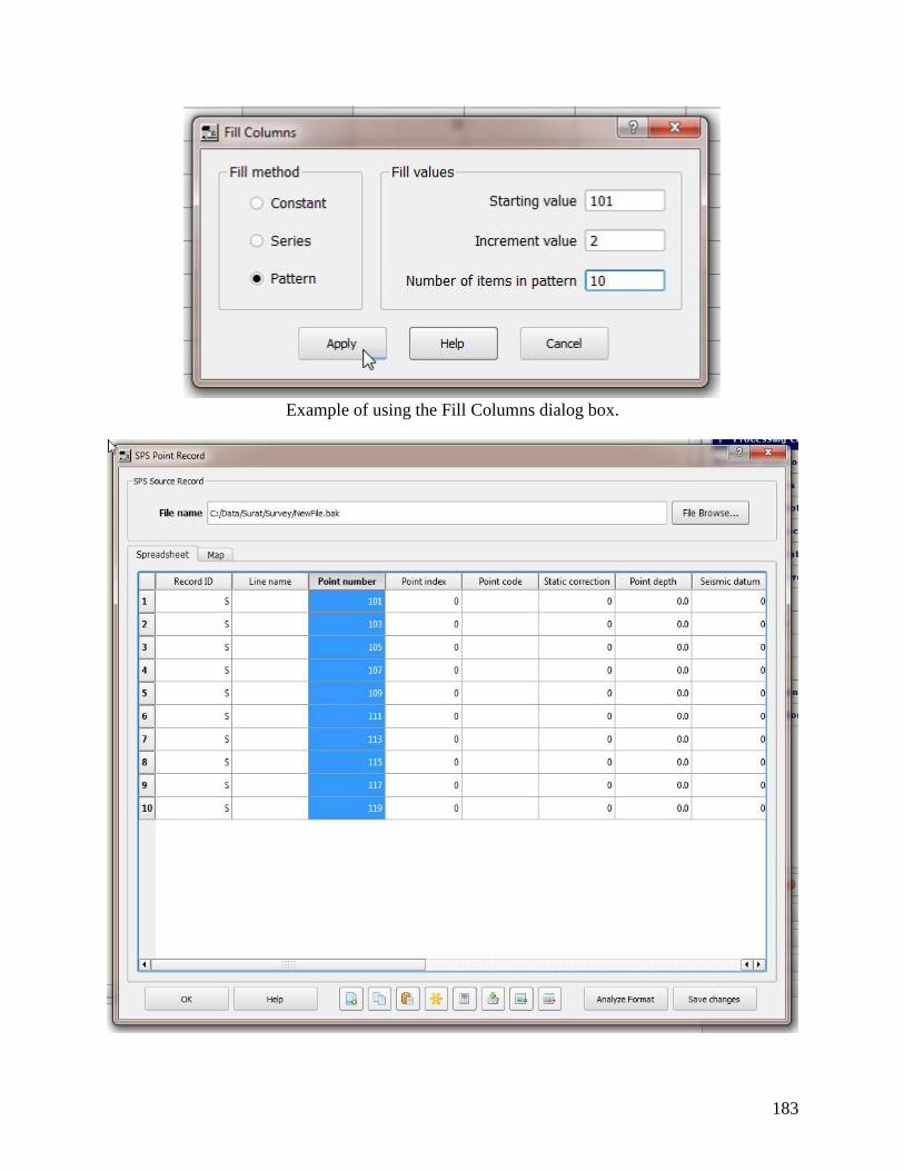
183

Example of using the Fill Columns dialog box.

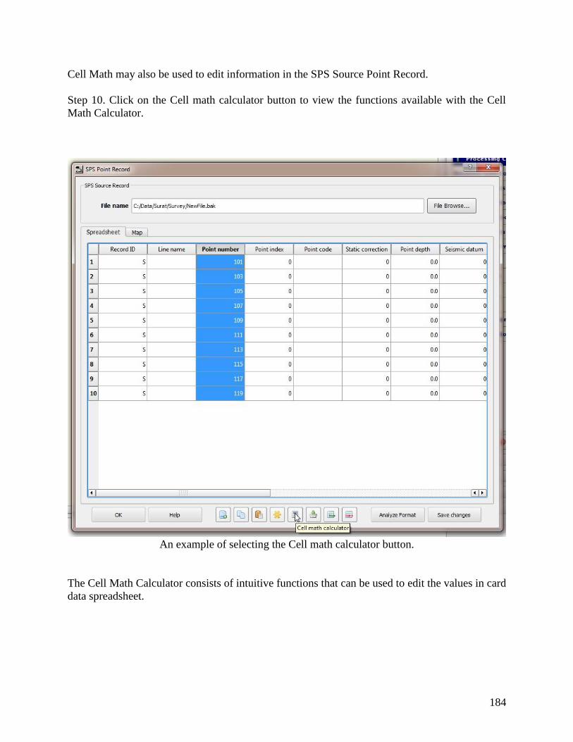
184

Cell Math may also be used to edit information in the SPS Source Point Record.

Step 10. Click on the Cell math calculator button to view the functions available with the Cell

Math Calculator.

An example of selecting the Cell math calculator button.

The Cell Math Calculator consists of intuitive functions that can be used to edit the values in card

data spreadsheet.

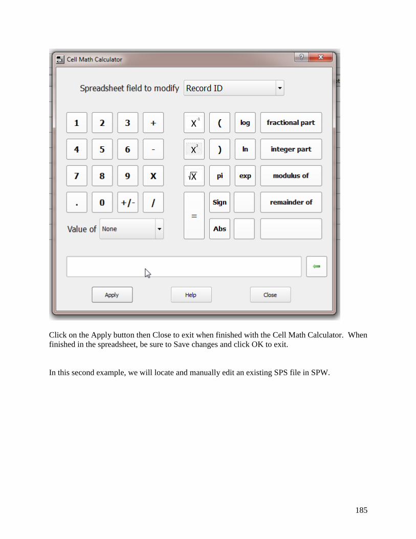
185

Click on the Apply button then Close to exit when finished with the Cell Math Calculator. When

finished in the spreadsheet, be sure to Save changes and click OK to exit.

In this second example, we will locate and manually edit an existing SPS file in SPW.

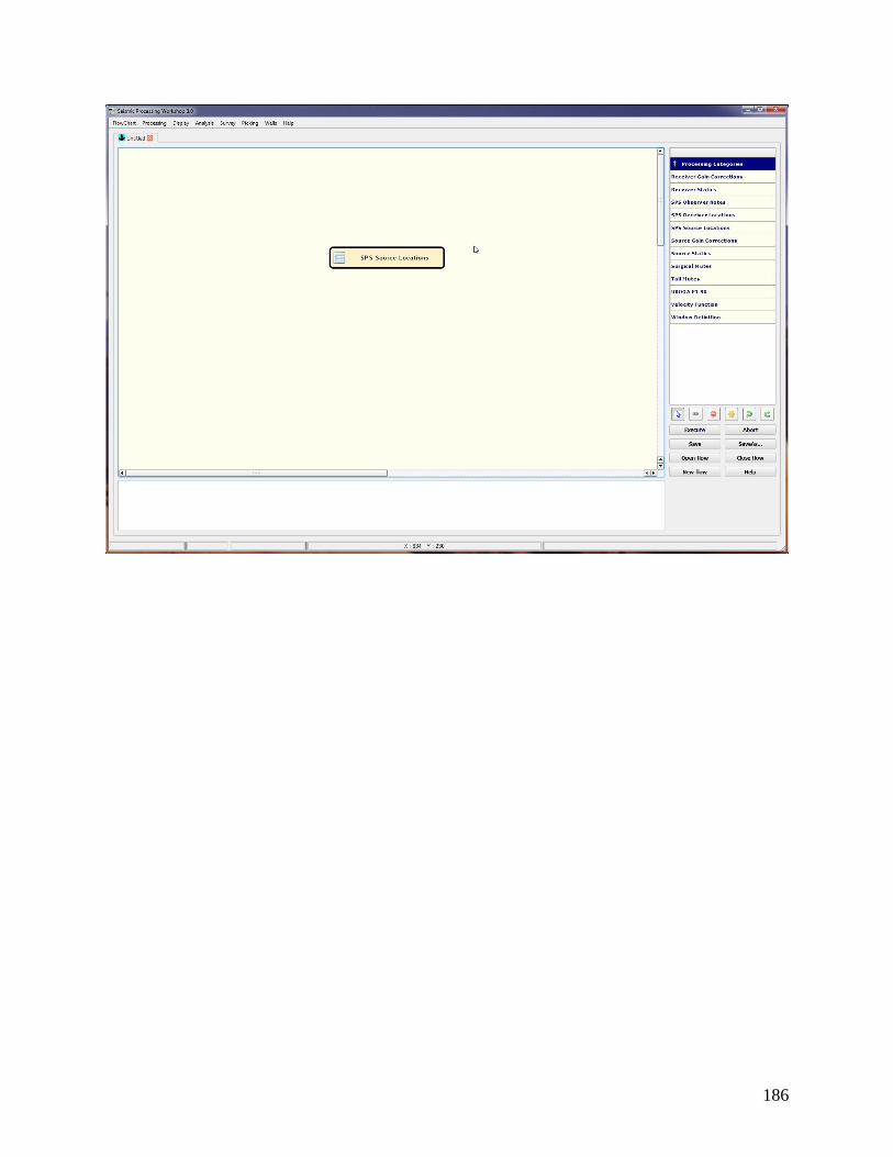
186

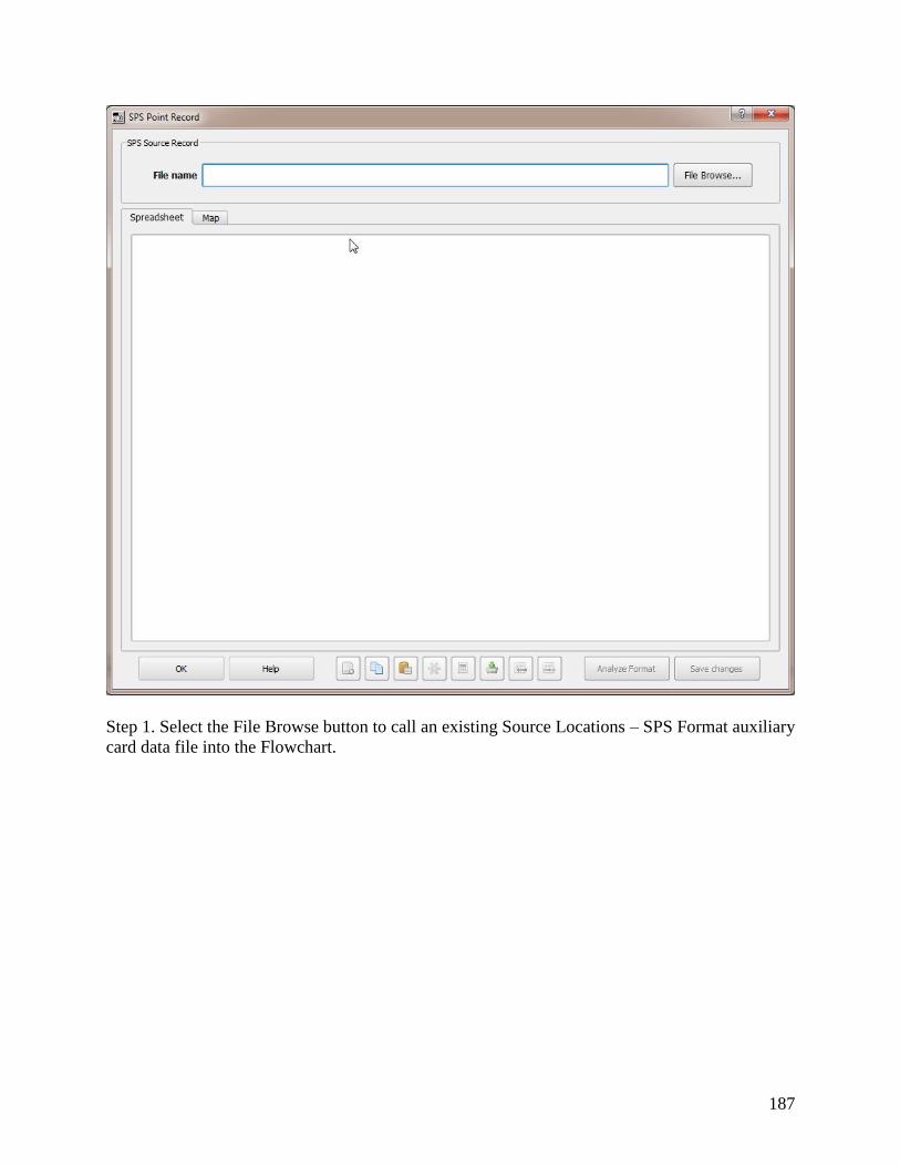
187

Step 1. Select the File Browse button to call an existing Source Locations – SPS Format auxiliary

card data file into the Flowchart.

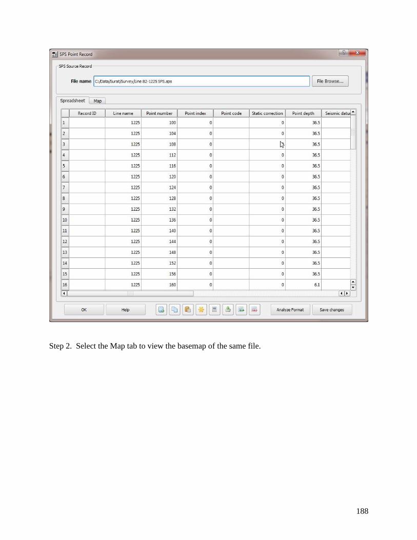
188

Step 2. Select the Map tab to view the basemap of the same file.

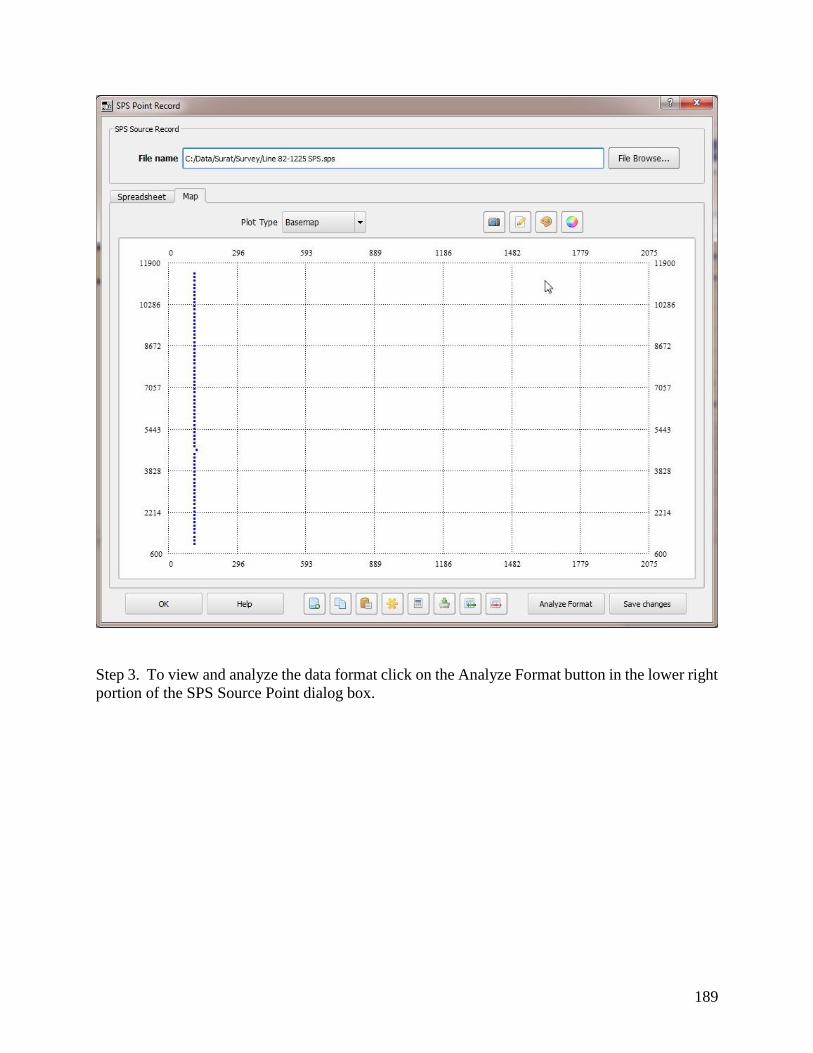
189

Step 3. To view and analyze the data format click on the Analyze Format button in the lower right

portion of the SPS Source Point dialog box.

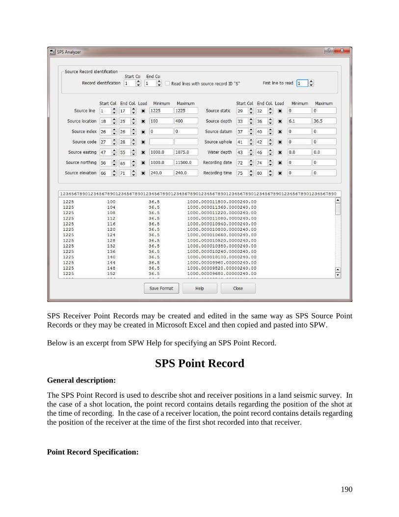
190

SPS Receiver Point Records may be created and edited in the same way as SPS Source Point

Records or they may be created in Microsoft Excel and then copied and pasted into SPW.

Below is an excerpt from SPW Help for specifying an SPS Point Record.

SPS Point Record

General description:

The SPS Point Record is used to describe shot and receiver positions in a land seismic survey. In

the case of a shot location, the point record contains details regarding the position of the shot at

the time of recording. In the case of a receiver location, the point record contains details regarding

the position of the receiver at the time of the first shot recorded into that receiver.

Point Record Specification:

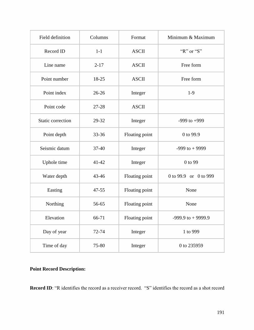
191

Field definition Columns Format Minimum & Maximum

Record ID 1-1 ASCII “R” or “S”

Line name 2-17 ASCII Free form

Point number 18-25 ASCII Free form

Point index 26-26 Integer 1-9

Point code 27-28 ASCII

Static correction 29-32 Integer -999 to +999

Point depth 33-36 Floating point 0 to 99.9

Seismic datum 37-40 Integer -999 to + 9999

Uphole time 41-42 Integer 0 to 99

Water depth 43-46 Floating point 0 to 99.9 or 0 to 999

Easting 47-55 Floating point None

Northing 56-65 Floating point None

Elevation 66-71 Floating point -999.9 to + 9999.9

Day of year 72-74 Integer 1 to 999

Time of day 75-80 Integer 0 to 235959

Point Record Description:

Record ID: “R identifies the record as a receiver record. “S” identifies the record as a shot record

192

Line name: Identifier for the shotpoint or receiver line.

Point number: Identifier for the shotpoint or receiver group number.

Point index: Index of the shotpoint or receiver number. In the case of shotpoints, 1 indicates the

first shot at the specified location. The value of the index is incremented by 1 for each additional

shot at the specified location. In the case of receivers, 1 indicates the first positioning of the

receiver at the specified location. The value of the index is incremented by 1 each time the receiver

group is moved or repositioned.

Point code: A code that characterizes the shot or receiver used at the point.

Static correction: The shot or receiver static, in units of milliseconds, that has been computed in

the field to correct the seismic recording for the effects of elevation, weathering thickness, or

weathering velocity at the point. The correction is referenced to the seismic datum specified in

field 8.

Point depth: The depth of the shot or receiver.

Seismic datum: Elevation of the seismic datum.

Uphole time: In the case of a shot, this is the vertical traveltime from the charge to surface, in

units of milliseconds. The value is always positive.

Water depth: The measured height of the water surface above the seafloor or water bottom. In

the case of shotpoints, the value should be the depth at the time of recording. In the case of

receivers, the value should be the depth at the time of recording the first shot into the receiver.

Easting: Map easting for the point. The coordinate system is defined in header H13 of the point

record.

Northing: Map northing for the point. The coordinate system is defined in header H13 of the

point record.

Elevation: Suface elevation with respect to the datum defined in header H17 of the point

record. Elevations above datum are positive. In the case of shotpoints, the value should be the

elevation at the time of recording. In the case of receivers, the value should be the elevation at the

time of recording the first shot into the receiver.

Day of year: Julian day of recording. In the case of shotpoints, the value should be the day of

recording the shot. In the case of receivers, the value should be the day of recording the first shot

into the receiver.

Creating Card Data Using Excel

In addition to calling existing files into or creating new data files within SPW, you may create data

in a Microsoft Excel spreadsheet and transfer these data into any auxulliary card data record

spreadsheet. To transfer a few data values, simply copy and paste from the Excel spreadsheet to

the SPW card data file spreadsheet. However, the array of data you cut from Exel must match in

size the area you select in the SPW spreadsheet prior to pasting.

193

To transfer an entire file, you will need to reformat the Excel file as an SPW card data file. The

following example will demonstrate how to create a SPS Receiver Point Record in Excel and

format the file for use in the SPW Flowchart.

Step 1. Open the Excel application.

Step 2. Determine or set the width of the required amount of columns. Locate the format drop-

lown list on the right side of the tool bar above the spreadsheet.

194

Step 3. The column width is set by clicking on the Format menu and selecting Column Width.

The default width of an Excel spreadsheet column is 8.43, which means you will get 8 spaces if

you save the file as a space delimited text file).

195

Step 4. You can format each column from the Point Record Specification list (see above).Since

the first column is defined for identifying the field record for either source or receiver card data

(“R” or “S”) and uses only 1 column, set the column width to 1 and click OK.

Field definition Columns Format Minimum & Maximum

Record ID 1-1 ASCII “R” or “S”

Step 5. Click on the Format dropdown menu and select Format Cells and set the format to Text

(ie. ASCII) on the Number tab. Set all text left-to-right.

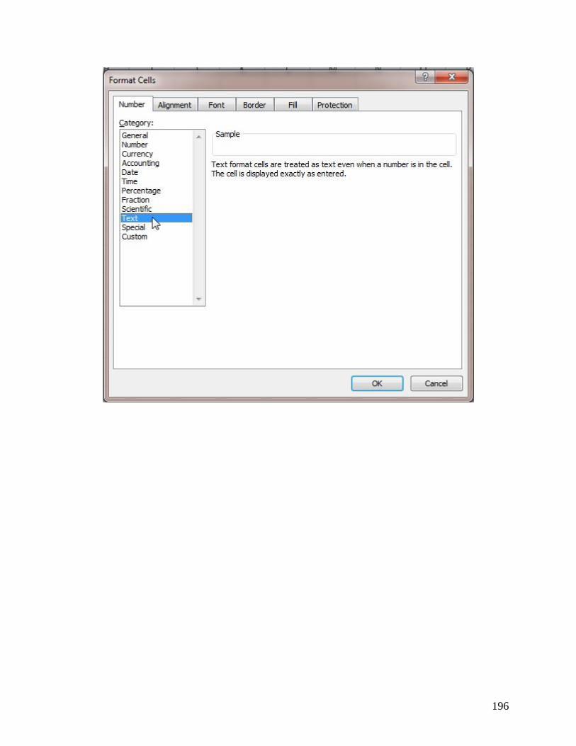
196

197

Field definition Columns Format Minimum & Maximum

Record ID 1-1 ASCII “R” or “S”

Line name 2-17 ASCII Free form

Point number 18-25 ASCII Free form

Point index 26-26 Integer 1-9

Point code 27-28 ASCII

Static correction 29-32 Integer -999 to +999

Point depth 33-36 Floating point 0 to 99.9

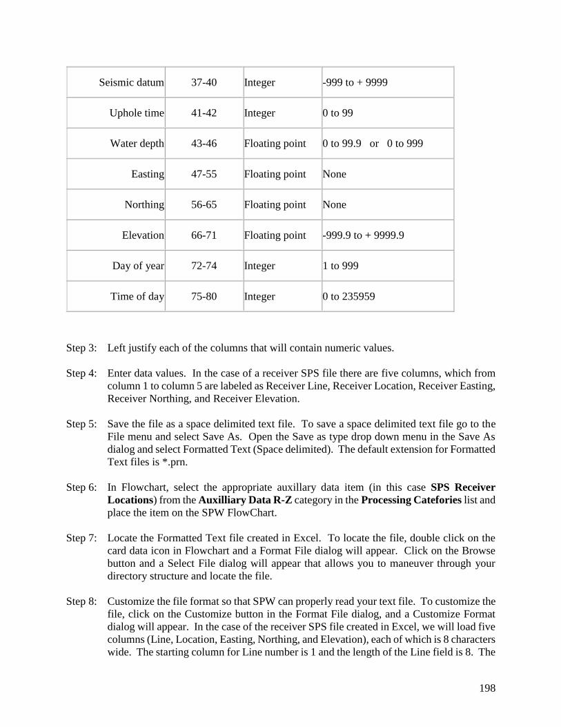
198

Seismic datum 37-40 Integer -999 to + 9999

Uphole time 41-42 Integer 0 to 99

Water depth 43-46 Floating point 0 to 99.9 or 0 to 999

Easting 47-55 Floating point None

Northing 56-65 Floating point None

Elevation 66-71 Floating point -999.9 to + 9999.9

Day of year 72-74 Integer 1 to 999

Time of day 75-80 Integer 0 to 235959

Step 3: Left justify each of the columns that will contain numeric values.

Step 4: Enter data values. In the case of a receiver SPS file there are five columns, which from

column 1 to column 5 are labeled as Receiver Line, Receiver Location, Receiver Easting,

Receiver Northing, and Receiver Elevation.

Step 5: Save the file as a space delimited text file. To save a space delimited text file go to the

File menu and select Save As. Open the Save as type drop down menu in the Save As

dialog and select Formatted Text (Space delimited). The default extension for Formatted

Text files is *.prn.

Step 6: In Flowchart, select the appropriate auxillary data item (in this case SPS Receiver

Locations) from the Auxilliary Data R-Z category in the Processing Catefories list and

place the item on the SPW FlowChart.

Step 7: Locate the Formatted Text file created in Excel. To locate the file, double click on the

card data icon in Flowchart and a Format File dialog will appear. Click on the Browse

button and a Select File dialog will appear that allows you to maneuver through your

directory structure and locate the file.

Step 8: Customize the file format so that SPW can properly read your text file. To customize the

file, click on the Customize button in the Format File dialog, and a Customize Format

dialog will appear. In the case of the receiver SPS file created in Excel, we will load five

columns (Line, Location, Easting, Northing, and Elevation), each of which is 8 characters

wide. The starting column for Line number is 1 and the length of the Line field is 8. The

199

starting column for the Location number is 9 and the length of the Location field is 8…..

The starting column for the Elevation field is 33 and the length of the Elevation field is

8. When the appropriate parameters have been entered, select OK.

Step 9: View the card data spreadsheet to verify the data values.

Auxiliary Data A-P

CMP Flex Locations Usage:

The CMP Flex Location card data item is used to store the location of flex binned location as

computed by CMP Binning processing step.

Step Parameter Dialog:

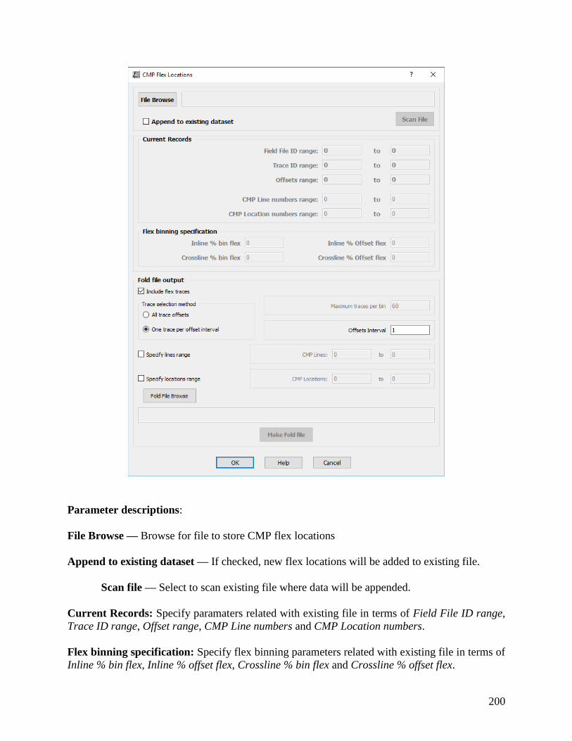
200

Parameter descriptions:

File Browse — Browse for file to store CMP flex locations

Append to existing dataset — If checked, new flex locations will be added to existing file.

Scan file — Select to scan existing file where data will be appended.

Current Records: Specify paramaters related with existing file in terms of Field File ID range,

Trace ID range, Offset range, CMP Line numbers and CMP Location numbers.

Flex binning specification: Specify flex binning parameters related with existing file in terms of

Inline % bin flex, Inline % offset flex, Crossline % bin flex and Crossline % offset flex.

201

Fold file output: Specify parameters related with fold file output.

Include flex traces — If checked, include flex traces in output file.

Trace selection method: Specify parameters for trace selections.

All trace offsets — If selected, all offsets are selected for flex binning.

Maximum traces per bin — Enter the maximum number of traces per bin.

One trace per offset interval — If selected, only one trace per offset is selected for flex binning.

Offset interval — Enter the offset interval to be considered for flex binning.

Specify line range — If checked, line range are defined manually.

CMP Lines — Enter the CMP line range to be considered for the flex binning.

Specify locations range — If checked, location range are defined manually.

CMP Locations — Enter the CMP location range to be considered for the flex binning.

Fold file browse — Select file to store fold information.

Make fold file — Not yet implemented.

CMP Statics Usage:

The CMP Statics card data item is used to store CMP based static shift values in milliseconds.

Step Parameter Dialog:

202

CMP Statics card data file may be sorted in CMP Line, Source Line, Receiver Line or Offset.

Example Card Data:

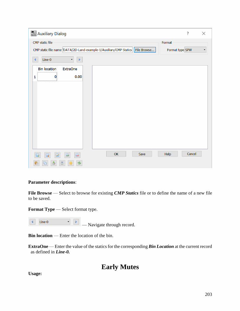
203

Parameter descriptions:

File Browse — Select to browse for existing CMP Statics file or to define the name of a new file

to be saved.

Format Type — Select format type.

— Navigate through record.

Bin location — Enter the location of the bin.

ExtraOne — Enter the value of the statics for the corresponding Bin Location at the current record

as defined in Line-0.

Early Mutes Usage:

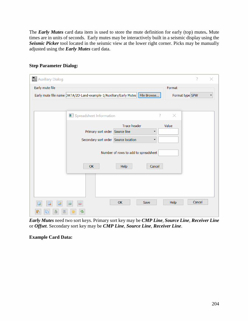
204

The Early Mutes card data item is used to store the mute definition for early (top) mutes. Mute

times are in units of seconds. Early mutes may be interactively built in a seismic display using the

Seismic Picker tool located in the seismic view at the lower right corner. Picks may be manually

adjusted using the Early Mutes card data.

Step Parameter Dialog:

Early Mutes need two sort keys. Primary sort key may be CMP Line, Source Line, Receiver Line

or Offset. Secondary sort key may be CMP Line, Source Line, Receiver Line.

Example Card Data:

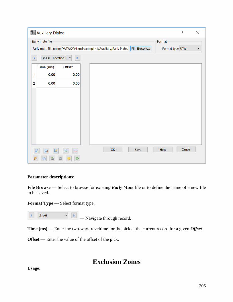
205

Parameter descriptions:

File Browse — Select to browse for existing Early Mute file or to define the name of a new file

to be saved.

Format Type — Select format type.

— Navigate through record.

Time (ms) — Enter the two-way-traveltime for the pick at the current record for a given Offset.

Offset — Enter the value of the offset of the pick.

Exclusion Zones Usage:

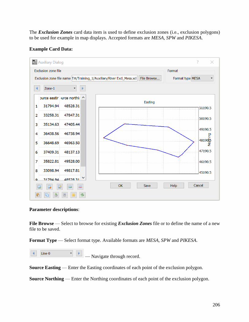
206

The Exclusion Zones card data item is used to define exclusion zones (i.e., exclusion polygons)

to be used for example in map displays. Accepted formats are MESA, SPW and PIKESA.

Example Card Data:

Parameter descriptions:

File Browse — Select to browse for existing Exclusion Zones file or to define the name of a new

file to be saved.

Format Type — Select format type. Available formats are MESA, SPW and PIKESA.

— Navigate through record.

Source Easting — Enter the Easting coordinates of each point of the exclusion polygon.

Source Northing — Enter the Northing coordinates of each point of the exclusion polygon.

207

FK Mutes Usage:

The FK Mutes card data item is used to store the mute definition for mutes in the FK domain.

Mute are defined in wavenumber (k) and velocity. FK mutes may be interactively built in a FK

spectrum display using the Seismic Picker tool located in the seismic view at the lower right

corner. Picks may be manually adjusted using the FK Mutes card data.

Step Parameter Dialog:

FK Mutes need two sort keys. Primary sort key may be CMP Line, Source Line, Receiver Line

or Offset. Secondary sort key may be CMP Line, Source Line, Receiver Line.

Example Card Data:

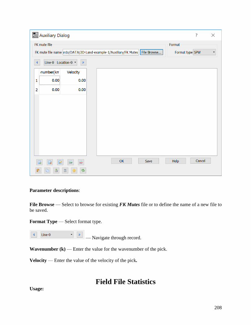
208

Parameter descriptions:

File Browse — Select to browse for existing FK Mutes file or to define the name of a new file to

be saved.

Format Type — Select format type.

— Navigate through record.

Wavenumber (k) — Enter the value for the wavenumber of the pick.

Velocity — Enter the value of the velocity of the pick.

Field File Statistics Usage:

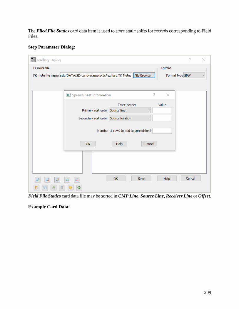
209

The Filed File Statics card data item is used to store static shifts for records corresponding to Field

Files.

Step Parameter Dialog:

Field File Statics card data file may be sorted in CMP Line, Source Line, Receiver Line or Offset.

Example Card Data:

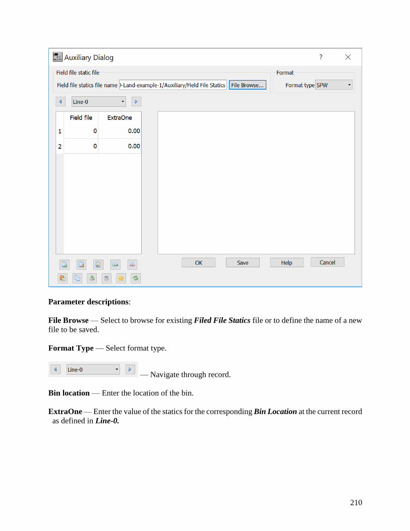
210

Parameter descriptions:

File Browse — Select to browse for existing Filed File Statics file or to define the name of a new

file to be saved.

Format Type — Select format type.

— Navigate through record.

Bin location — Enter the location of the bin.

ExtraOne — Enter the value of the statics for the corresponding Bin Location at the current record

as defined in Line-0.

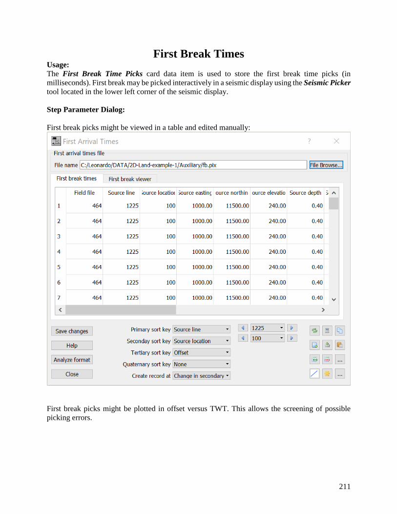
211

First Break Times Usage:

The First Break Time Picks card data item is used to store the first break time picks (in

milliseconds). First break may be picked interactively in a seismic display using the Seismic Picker

tool located in the lower left corner of the seismic display.

Step Parameter Dialog:

First break picks might be viewed in a table and edited manually:

First break picks might be plotted in offset versus TWT. This allows the screening of possible

picking errors.

212

Parameter descriptions:

File Browse — Select to browse for existing First Break Times file or to define the name of a

new file to be saved.

Primary sort key — Select the primary sort key to be used in the navigation from record to record.

Secondary sort key — Select the secondary sort key to be used in the navigation from record to

record.

Tertiary sort key — Select the tertiary sort key to be used in the navigation from record to record.

Quaternary sort key — Select the quaternary sort key to be used in the navigation from record

to record.

Create record at — Select the sort key used to create records.

213

Gain Curves Usage:

The Gain Curves card data item is used to store time-decibel gain pairs. A gain of 0 dB is

equivalent to scalar multiplication by a factor of 1, a gain of 6 dB by a factor of 2, a gain of 12 dB

by a factor of 4, a gain of 18 dB by a factor of 8, and so on. Time is in milliseconds.

Step Parameter Dialog:

Gain functions card data file may be sorted in CMP Line, Source Line, Receiver Line or Offset.

Example Card Data:

214

Parameter descriptions:

Format Type — Select format type.

— Navigate through record.

Bin location — Enter the location of the bin.

ExtraOne — Enter the value of the statics for the corresponding Bin Location at the current record

as defined in Line-0.

Time (ms) — Enter the start column and the number of columns allocated to write the two-way

time (in milliseconds) associated with a given gain value in the output gain file.

ExtraOne — Enter the start column and the number of columns allocated to write the gain in dB

associated with a given two-way travel time in the output gain file.

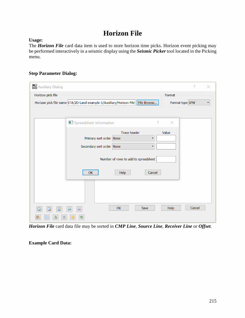
215

Horizon File Usage:

The Horizon File card data item is used to store horizon time picks. Horizon event picking may

be performed interactively in a seismic display using the Seismic Picker tool located in the Picking

menu.

Step Parameter Dialog:

Horizon File card data file may be sorted in CMP Line, Source Line, Receiver Line or Offset.

Example Card Data:

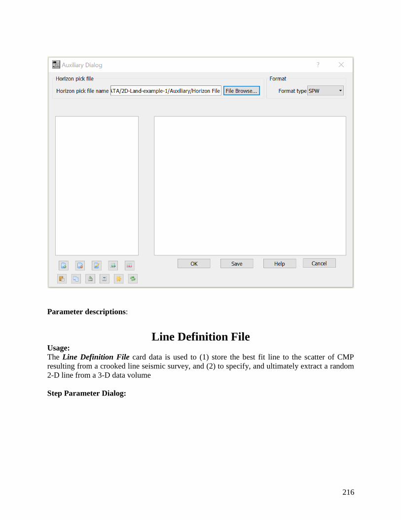
216

Parameter descriptions:

Line Definition File Usage:

The Line Definition File card data is used to (1) store the best fit line to the scatter of CMP

resulting from a crooked line seismic survey, and (2) to specify, and ultimately extract a random

2-D line from a 3-D data volume

Step Parameter Dialog:

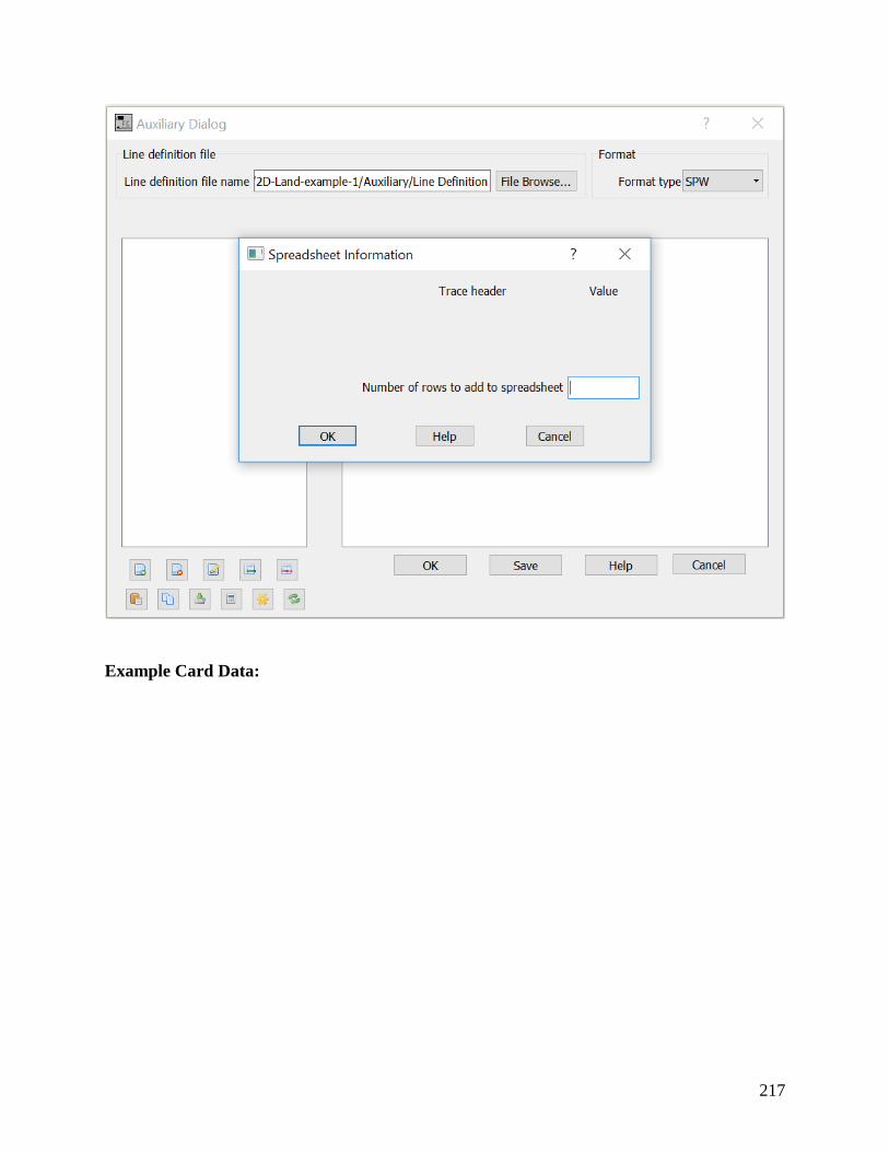
217

Example Card Data:

218

Parameter descriptions:

File Browse — Select to browse for existing Line Definition File file or to define the name of a

new file to be saved.

Format Type — Select format type.

— Navigate through record.

Bin Easting — Enter the start column and the number of columns allocated to write the easting

associated with a given coordinate pair in the output line definition file.

Bin Northing — Enter the start column and the number of columns allocated to write the northing

associated with a given coordinate pair in the output line definition file.

Offset Gain Corrections Usage:

The Offset Gain Corrections auxiliary card data allows definint offset varying functions for gain

correction.

219

Step Parameter Dialog:

Example Card Data:

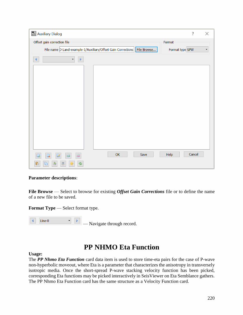
220

Parameter descriptions:

File Browse — Select to browse for existing Offset Gain Corrections file or to define the name

of a new file to be saved.

Format Type — Select format type.

— Navigate through record.

PP NHMO Eta Function Usage:

The PP Nhmo Eta Function card data item is used to store time-eta pairs for the case of P-wave

non-hyperbolic moveout, where Eta is a parameter that characterizes the anisotropy in transversely

isotropic media. Once the short-spread P-wave stacking velocity function has been picked,

corresponding Eta functions may be picked interactively in SeisViewer on Eta Semblance gathers.

The PP Nhmo Eta Function card has the same structure as a Velocity Function card.

221

Step Parameter Dialog:

Primary sort key may be CMP Line, Source Line, Receiver Line or Offset. Secondary sort key

may be CMP Line, Source Line, Receiver Line. Select outpu velocity type from RMS (Stacking)

velocity, Interval velocity or Average Velocity. Velocity field may be defined in the Two-way time

or Depth domain.

Example Card Data:

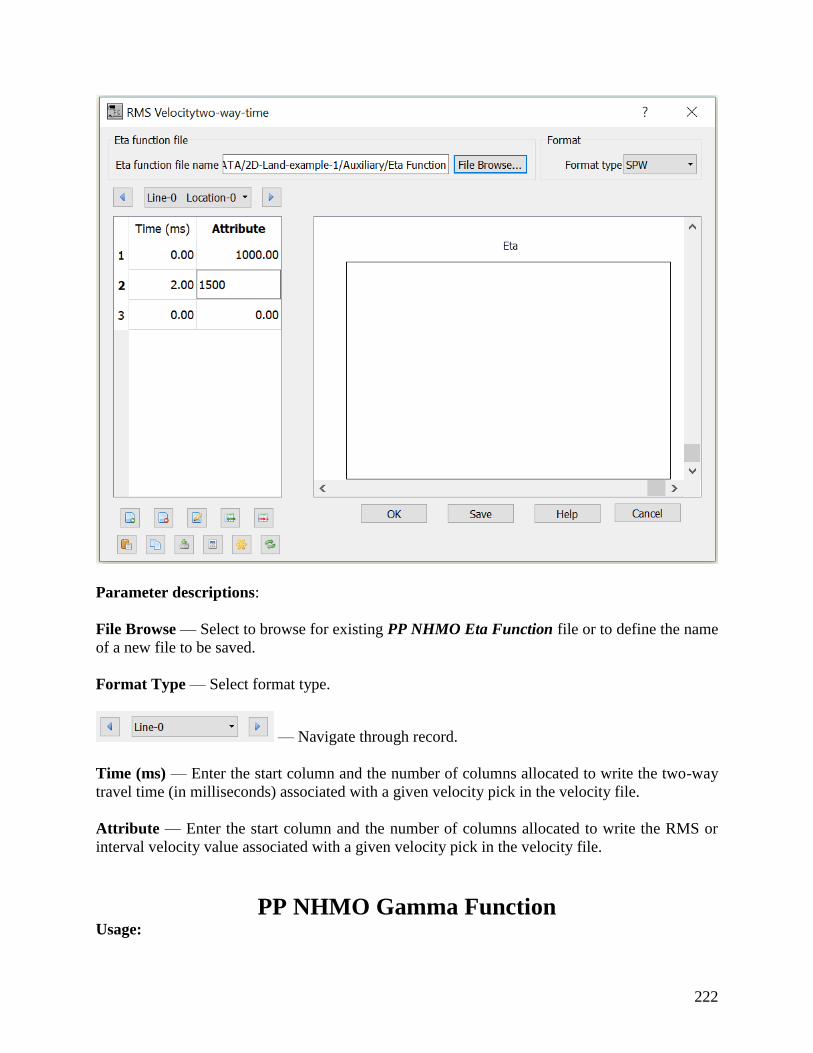
222

Parameter descriptions:

File Browse — Select to browse for existing PP NHMO Eta Function file or to define the name

of a new file to be saved.

Format Type — Select format type.

— Navigate through record.

Time (ms) — Enter the start column and the number of columns allocated to write the two-way

travel time (in milliseconds) associated with a given velocity pick in the velocity file.

Attribute — Enter the start column and the number of columns allocated to write the RMS or

interval velocity value associated with a given velocity pick in the velocity file.

PP NHMO Gamma Function Usage:

223

The PP Nhmo Gamma Function card data item is used to store time-gamma pairs for the case of

PS-wave (i.e. converted wave) non-hyperbolic moveout, where Gamma is the effective Vp/Vs ratio

down to the event being analyzed. Once the short-spread P-wave stacking velocity function has

been picked, corresponding Gamma functions may be picked interactively in SeisViewer on

Gamma Semblance gathers. The PP Nhmo Gamma Function card has the same structure as a

Velocity Function card.

Primary sort key may be CMP Line, Source Line, Receiver Line or Offset. Secondary sort key

may be CMP Line, Source Line, Receiver Line.

Polygon Definition Usage:

The Polygon Definition card data item is used to specify the coordinates of a polygon that will be

used to select data from a seismic volume. The Polygon Definition File may be used to selectively

input data in conjunction with the SPW Tape Utility or may be linked to the Select Traces

processing step for the same purpose.

Step Parameter Dialog:

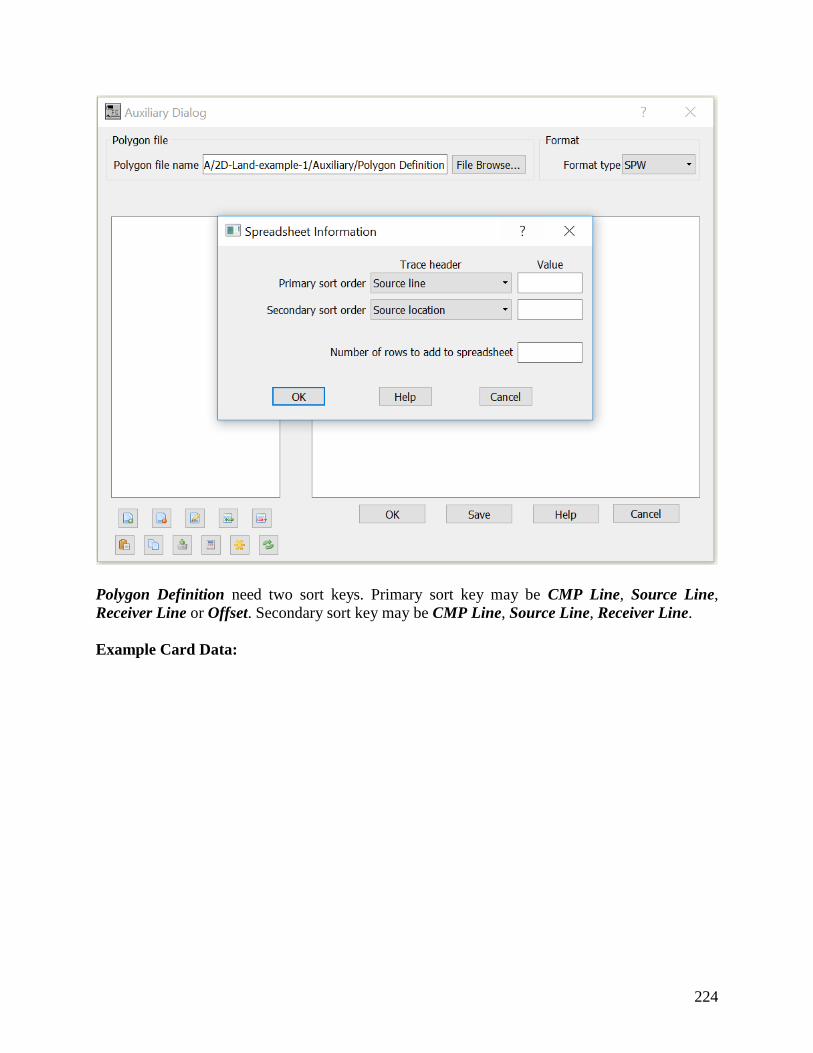
224

Polygon Definition need two sort keys. Primary sort key may be CMP Line, Source Line,

Receiver Line or Offset. Secondary sort key may be CMP Line, Source Line, Receiver Line.

Example Card Data:

225

Parameter descriptions:

File Browse — Select to browse for existing Polygon Definition file or to define the name of a

new file to be saved.

Format Type — Select format type.

— Navigate through record.

X (first key value) — Enter the start column and the number of columns allocated to write the X

coordinate associated with a given coordinate pair in the output polygon definition file.

Y (second key value) — Enter the start column and the number of columns allocated to write the

Y coordinate associated with a given coordinate pair in the output polygon definition file.

Auxiliary Data R-Z

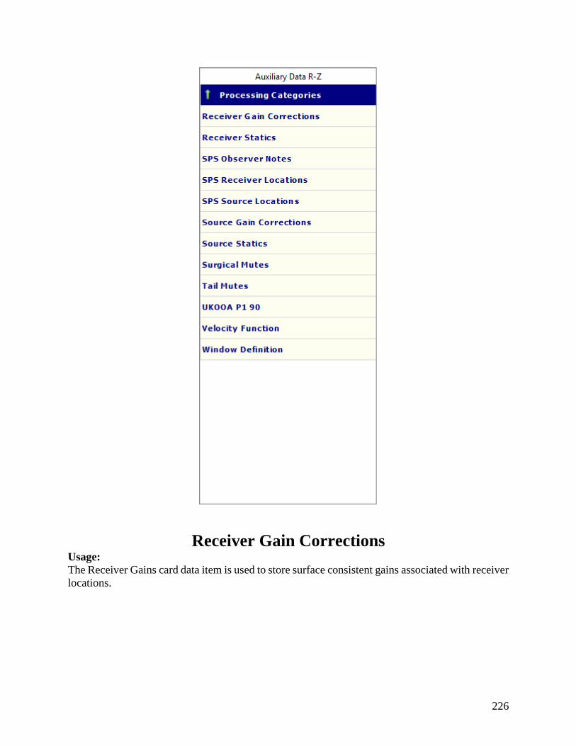
226

Receiver Gain Corrections Usage:

The Receiver Gains card data item is used to store surface consistent gains associated with receiver

locations.

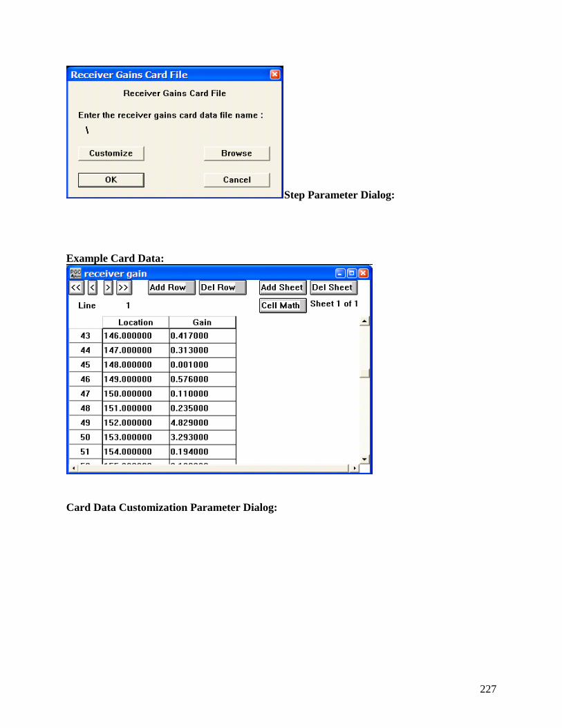
227

Step Parameter Dialog:

Example Card Data:

Card Data Customization Parameter Dialog:

228

Parameter descriptions:

Number of comment records preceding data: – Indicates the number of lines in the output file

reserved for writing comment cards. These are the first lines in the file. A minimum of one line is

required.

File Header field:

Number of lines — Enter the start column and the number of columns allocated to write the number

of receiver lines in the receiver gain file.

Sheet Header field:

Receiver line number — Enter the start column and the number of columns allocated to write the

receiver line number in the output receiver gain file.

Number of rows — Enter the start column and the number of columns allocated to write the

number of receiver positions per receiver line in the output receiver gain file.

Data header field:

Location number — Enter the start column and the number of columns allocated to write the

receiver location number in the receiver gain file.

Gain — Enter the start column and the number of columns allocated to write the receiver gain in

the receiver gain file.

229

Enter the length of each record in the file in bytes – Enter the length in bytes of one line of the

receiver gains file.

Receiver Statics Usage:

The Receiver Statics card data item is used to store receiver static information in units of

milliseconds.

Step Parameter Dialog:

Example Card Data:

230

Card Data Customization Parameter Dialog:

Parameter descriptions:

Number of comment records preceding data: – Indicates the number of lines in the output file

reserved for writing comment cards. These are the first lines in the file. A minimum of one line is

required.

File Header field:

Number of lines — Enter the start column and the number of columns allocated to write the number

of receiver lines in the receiver statics file.

Sheet Header field:

Receiver line number — Enter the start column and the number of columns allocated to write the

receiver line number in the output receiver statics file.

Number of rows — Enter the start column and the number of columns allocated to write the

number of receiver positions per receiver line in the output receiver statics file.

Data header field:

Location number — Enter the start column and the number of columns allocated to write the

receiver location number in the receiver statics file.

Time — Enter the start column and the number of columns allocated to write the receiver static

(in milliseconds) in the receiver static file.

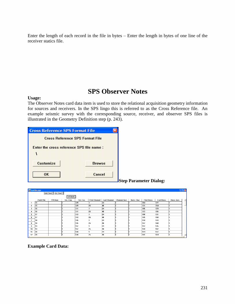
231

Enter the length of each record in the file in bytes – Enter the length in bytes of one line of the

receiver statics file.

SPS Observer Notes Usage:

The Observer Notes card data item is used to store the relational acquisition geometry information

for sources and receivers. In the SPS lingo this is referred to as the Cross Reference file. An

example seismic survey with the corresponding source, receiver, and observer SPS files is

illustrated in the Geometry Definition step (p. 243).

Step Parameter Dialog:

Example Card Data:

232

Card Data Customization Parameter Dialog:

Parameter descriptions:

Load – If checked, indicates the existence of the entity in the file.

Tape — Enter the start column and the number of columns allocated to write the tape number (disk

or physical) associated with a given record in the Cross Reference SPS file.

Field file — Enter the start column and the number of columns allocated to write the field file

number associated with a given record in the Cross Reference SPS file.

Field file incr. — Enter the start column and the number of columns allocated to write the

increment between field files in the Cross Reference SPS file.

Source line — Enter the start column and the number of columns allocated to write the source line

number associated with a given record in the Cross Reference SPS file.

Source location — Enter the start column and the number of columns allocated to write the source

location number associated with a given record in the Cross Reference SPS file.

First channel — Enter the start column and the number of columns allocated to write the first

channel associated with a given record in the Cross Reference SPS file.

233

Last channel — Enter the start column and the number of columns allocated to write the last

channel associated with a given record in the Cross Reference SPS file.

Channel incr — Enter the start column and the number of columns allocated to write the increment

between channels associated with a given record in the Cross Reference SPS file.

Receiver line — Enter the start column and the number of columns allocated to write the receiver

line number associated with a given record in the Cross Reference SPS file.

First receiver — Enter the start column and the number of columns allocated to write the first

receiver associated with a given record in the Cross Reference SPS file.

Last receiver — Enter the start column and the number of columns allocated to write the last

receiver associated with a given record in the Cross Reference SPS file.

Receiver incr — Enter the start column and the number of columns allocated to write the increment

between receivers associated with a given record in the Cross Reference SPS file.

Enter the length of each record in the file in bytes – Enter the length in bytes of one line of the SPS

Observer Notes file.

SPS Receiver Locations Usage:

The Receiver Locations – SPS Format card data item is used to store positional receiver location

information. An example seismic survey with the corresponding source, receiver, and observer

SPS files is illustrated in the Geometry Definition step (p. 243).

Step Parameter Dialog:

234

Example Card Data:

Card Data Customization Parameter Dialog:

Parameter descriptions:

Load – If checked, indicates the existence of the entity in the file.

235

Line — Enter the start column and the number of columns allocated to write the receiver line

associated with a given record in the Receiver SPS file.

Location — Enter the start column and the number of columns allocated to write the receiver

location associated with a given record in the Receiver SPS file.

Latitude — Enter the start column and the number of columns allocated to write the receiver

latitude associated with a given record in the Receiver SPS file.

Longitude — Enter the start column and the number of columns allocated to write the receiver

longitude associated with a given record in the Receiver SPS file.

Easting — Enter the start column and the number of columns allocated to write the receiver easting

associated with a given record in the Receiver SPS file.

Northing — Enter the start column and the number of columns allocated to write the receiver

northing associated with a given record in the Receiver SPS file.

Elevation — Enter the start column and the number of columns allocated to write the receiver

elevation associated with a given record in the Receiver SPS file.

Static — Enter the start column and the number of columns allocated to write the receiver static

associated with a given record in the Receiver SPS file.

Depth — Enter the start column and the number of columns allocated to write the receiver depth

associated with a given record in the Receiver SPS file.

Datum — Enter the start column and the number of columns allocated to write the elevation of the

datum at a receiver station associated with a given record in the Receiver SPS file.

Uphole — Enter the start column and the number of columns allocated to write the interpolated

uphole time (ms) at a receiver station associated with a given record in the Receiver SPS file.

Water depth — Enter the start column and the number of columns allocated to write the water

depth at a receiver station associated with a given record in the Receiver SPS file.

Date — Enter the start column and the number of columns allocated to write the Julian day on

which the receiver station was initially deployed in the Receiver SPS file.

Time — Enter the start column and the number of columns allocated to write the time of day on

which the receiver station was initially deployed in the Receiver SPS file.

Enter the length of each record in the file in bytes – Enter the length in bytes of one line of the SPS

receiver file.

236

SPS Source Locations Usage:

The Source Locations – SPW Format card data item is used to source location geometry

information. An example seismic survey with the corresponding source, receiver, and observer

SPS files is illustrated in the Geometry Definition step (p. 243).

Step Parameter Dialog:

Example Card Data:

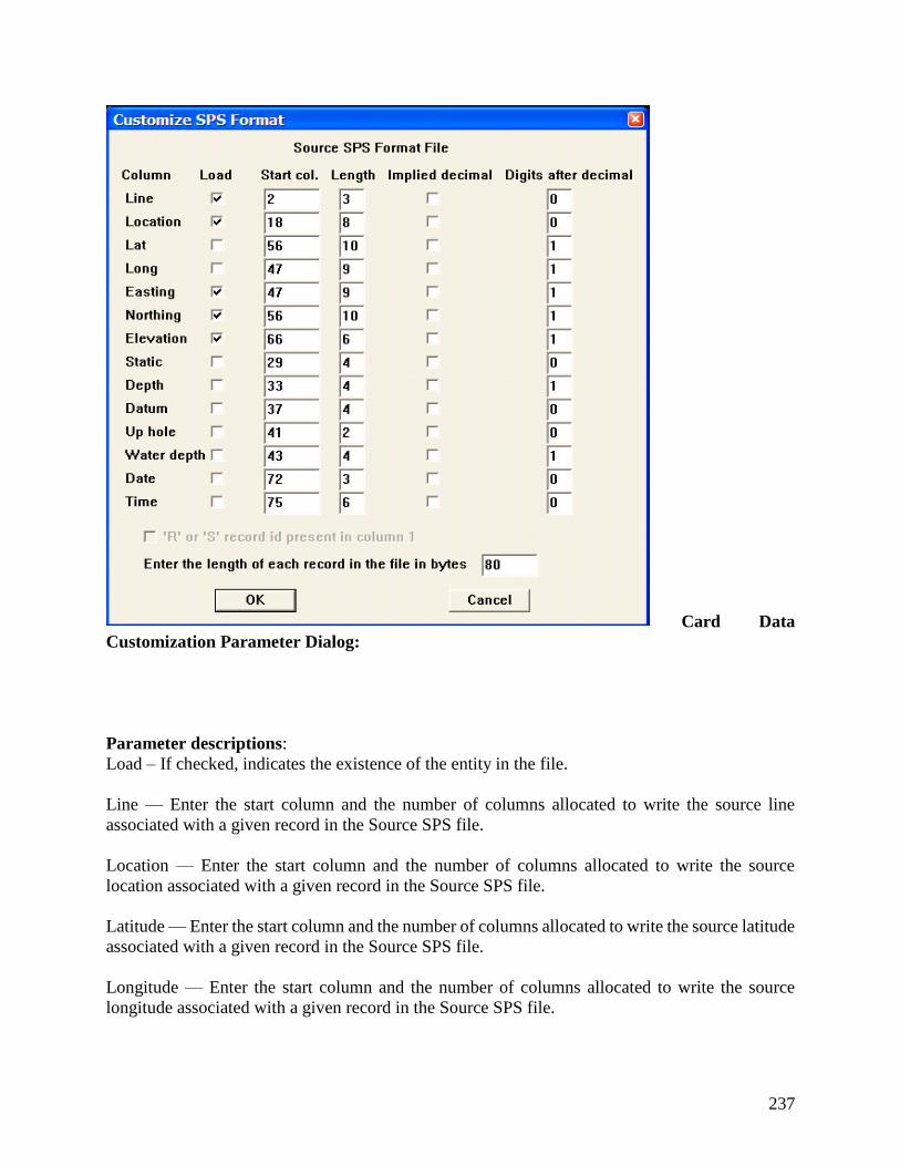
237

Card Data

Customization Parameter Dialog:

Parameter descriptions:

Load – If checked, indicates the existence of the entity in the file.

Line — Enter the start column and the number of columns allocated to write the source line

associated with a given record in the Source SPS file.

Location — Enter the start column and the number of columns allocated to write the source

location associated with a given record in the Source SPS file.

Latitude — Enter the start column and the number of columns allocated to write the source latitude

associated with a given record in the Source SPS file.

Longitude — Enter the start column and the number of columns allocated to write the source

longitude associated with a given record in the Source SPS file.

238

Easting — Enter the start column and the number of columns allocated to write the source easting

associated with a given record in the Source SPS file.

Northing — Enter the start column and the number of columns allocated to write the source

northing associated with a given record in the Source SPS file.

Elevation — Enter the start column and the number of columns allocated to write the source

elevation associated with a given record in the Source SPS file.

Static — Enter the start column and the number of columns allocated to write the source static

associated with a given record in the Source SPS file.

Depth — Enter the start column and the number of columns allocated to write the source depth

associated with a given record in the Source SPS file.

Datum — Enter the start column and the number of columns allocated to write the elevation of the

datum at the source station associated with a given record in the Source SPS file.

Uphole — Enter the start column and the number of columns allocated to write the uphole time

(ms) at a source station associated with a given record in the Source SPS file.

Water depth — Enter the start column and the number of columns allocated to write the water

depth at a source station associated with a given record in the Source SPS file.

Date — Enter the start column and the number of columns allocated to write the Julian day on

which the source station was occupied in the Source SPS file.

Enter the length of each record in the file in bytes – Enter the length in bytes of one line of the SPS

source file.

Source Gain Corrections Usage:

The Source Gains card data item is used to store gains associated with source locations.

Step Parameter Dialog:

239

Example Card Data:

Card Data Customization Parameter Dialog:

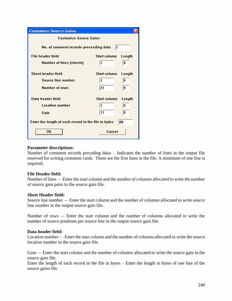
240

Parameter descriptions:

Number of comment records preceding data: – Indicates the number of lines in the output file

reserved for writing comment cards. These are the first lines in the file. A minimum of one line is

required.

File Header field:

Number of lines — Enter the start column and the number of columns allocated to write the number

of source gain pairs in the source gain file.

Sheet Header field:

Source line number — Enter the start column and the number of columns allocated to write source

line number in the output source gain file.

Number of rows — Enter the start column and the number of columns allocated to write the

number of source positions per source line in the output source gain file.

Data header field:

Location number — Enter the start column and the number of columns allocated to write the source

location number in the source gain file.

Gain — Enter the start column and the number of columns allocated to write the source gain in the

source gain file.

Enter the length of each record in the file in bytes – Enter the length in bytes of one line of the

source gains file.

241

Source Statics Usage:

The Source Statics card data item is used to store source statics information in units of

milliseconds.

Step Parameter Dialog:

Example Card Data:

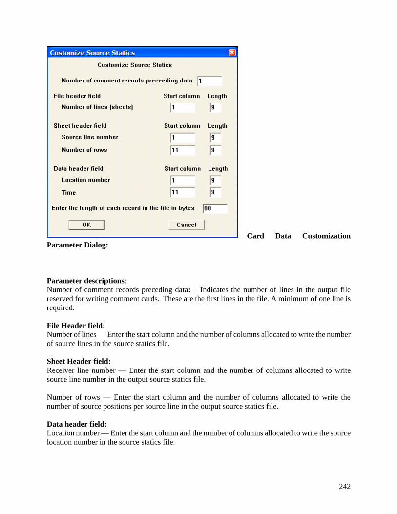
242

Card Data Customization

Parameter Dialog:

Parameter descriptions:

Number of comment records preceding data: – Indicates the number of lines in the output file

reserved for writing comment cards. These are the first lines in the file. A minimum of one line is

required.

File Header field:

Number of lines — Enter the start column and the number of columns allocated to write the number

of source lines in the source statics file.

Sheet Header field:

Receiver line number — Enter the start column and the number of columns allocated to write

source line number in the output source statics file.

Number of rows — Enter the start column and the number of columns allocated to write the

number of source positions per source line in the output source statics file.

Data header field:

Location number — Enter the start column and the number of columns allocated to write the source

location number in the source statics file.

243

Time — Enter the start column and the number of columns allocated to write the source static (in

milliseconds) in the source static file.

Enter the length of each record in the file in bytes – Enter the length in bytes of one line of the

source statics file.

Surgical Mutes Usage:

The Surgical Mutes card data item is used to store surgical mute data. Mute times are in units of

seconds. Surgical mutes may be defined interactively in SeisViewer using the Pick Traces tool

located in the Picking menu.

Step Parameter Dialog:

Example Card Data:

244

Card Data Customization Parameter Dialog:

Parameter descriptions:

Number of comment records preceding data: – Indicates the number of lines in the output file

reserved for writing comment cards. These are the first lines in the file. A minimum of one line is

required.

File Header field:

Number of mute locations — Enter the start column and the number of columns allocated to write

the number of mute locations in the output mute file.

Sheet Header field:

CMP line number — Enter the start column and the number of columns allocated to write CMP

line number in the output mute file.

CMP location number — Enter the start column and the number of columns allocated to write

CMP location number in the output mute file.

245

Number of rows — Enter the start column and the number of columns allocated to write the

number of CMP positions in the CMP line in the output mute file.

Sort — Enter the start column and the number of columns allocated to write the sort order (e.g.

common source, CMP, etc…) of the data file on which the early mute was picked.

Data header field:

Time — Enter the start column and the number of columns allocated to write the mute time (in

seconds) at a specified offset and trace number in the output mute file.

Offset — Enter the start column and the number of columns allocated to write the source receiver

offset corresponding to a specified mute time and trace number in the output mute file.

Unique trace number — Enter the start column and the number of columns allocated to write the

unique trace number corresponding to a specified mute time and source-receiver offset in the

output mute file.

Pick order index — Enter the start column and the number of columns allocated to write the pick

index corresponding to a specified mute time, source-receiver offset, and unique trace number in

the output mute file.

Enter the length of each record in the file in bytes – Enter the length in bytes of one line of the

surgical mute file.

Tail Mutes Usage:

The Tail Mutes card data item is used to store tail or end mute data. Mute times are in units of

seconds. Tail mutes may be interactively defined in SeisViewer using the Pick Traces tool located

in the Picking menu.

Step Parameter Dialog:

246

Example Card Data:

Card Data Customization Parameter Dialog:

Parameter descriptions:

Number of comment records preceding data: – Indicates the number of lines in the output file

reserved for writing comment cards. These are the first lines in the file. A minimum of one line is

required.

File Header field:

247

Number of mute locations — Enter the start column and the number of columns allocated to write

the number of mute locations in the output mute file.

Sheet Header field:

CMP line number — Enter the start column and the number of columns allocated to write CMP

line number in the output mute file.

CMP location number — Enter the start column and the number of columns allocated to write

CMP location number in the output mute file.

Number of rows — Enter the start column and the number of columns allocated to write the

number of CMP positions in the CMP line in the output mute file.

Sort — Enter the start column and the number of columns allocated to write the sort order (e.g.

common source, CMP, etc…) of the data file on which the early mute was picked.

Data header field:

Time — Enter the start column and the number of columns allocated to write the mute time (in

seconds) at a specified offset and trace number in the output mute file.

Offset — Enter the start column and the number of columns allocated to write the source receiver

offset corresponding to a specified mute time and trace number in the output mute file.

Unique trace number — Enter the start column and the number of columns allocated to write the

unique trace number corresponding to a specified mute time and source-receiver offset in the

output mute file.

Enter the length of each record in the file in bytes – Enter the length in bytes of one line of the tail

mute file.

UKOOA P1 90

Velocity Function Usage:

The Velocity Function card data item is used to store time-velocity pairs. Stacking velocities may

be picked interactively in SeisViewer using the Pick Traces tool located in the Picking menu..

Step Parameter Dialog:

248

Example Card Data:

Card Data Customization Parameter Dialog:

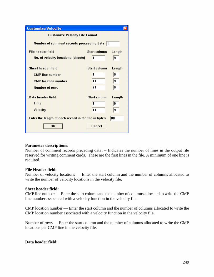
249

Parameter descriptions:

Number of comment records preceding data: – Indicates the number of lines in the output file

reserved for writing comment cards. These are the first lines in the file. A minimum of one line is

required.

File Header field:

Number of velocity locations — Enter the start column and the number of columns allocated to

write the number of velocity locations in the velocity file.

Sheet header field:

CMP line number — Enter the start column and the number of columns allocated to write the CMP

line number associated with a velocity function in the velocity file.

CMP location number — Enter the start column and the number of columns allocated to write the

CMP location number associated with a velocity function in the velocity file.

Number of rows — Enter the start column and the number of columns allocated to write the CMP

locations per CMP line in the velocity file.

Data header field:

250

Time — Enter the start column and the number of columns allocated to write the two-way travel

time (in milliseconds) associated with a given velocity pick in the velocity file.

Velocity — Enter the start column and the number of columns allocated to write the RMS or

interval velocity value associated with a given velocity pick in the velocity file.

Enter the length of each record in the file in bytes – Enter the length in bytes of one line of the

velocity function file.

Window Definition

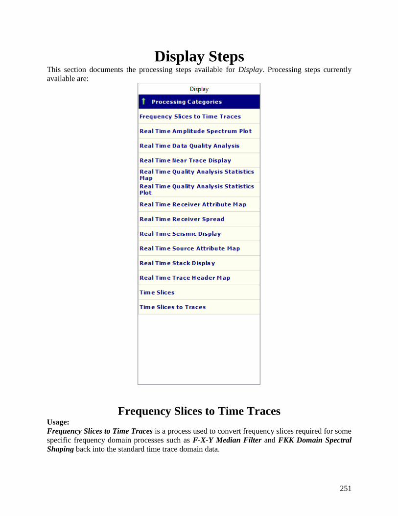
251

Display Steps This section documents the processing steps available for Display. Processing steps currently

available are:

Frequency Slices to Time Traces Usage:

Frequency Slices to Time Traces is a process used to convert frequency slices required for some

specific frequency domain processes such as F-X-Y Median Filter and FKK Domain Spectral

Shaping back into the standard time trace domain data.

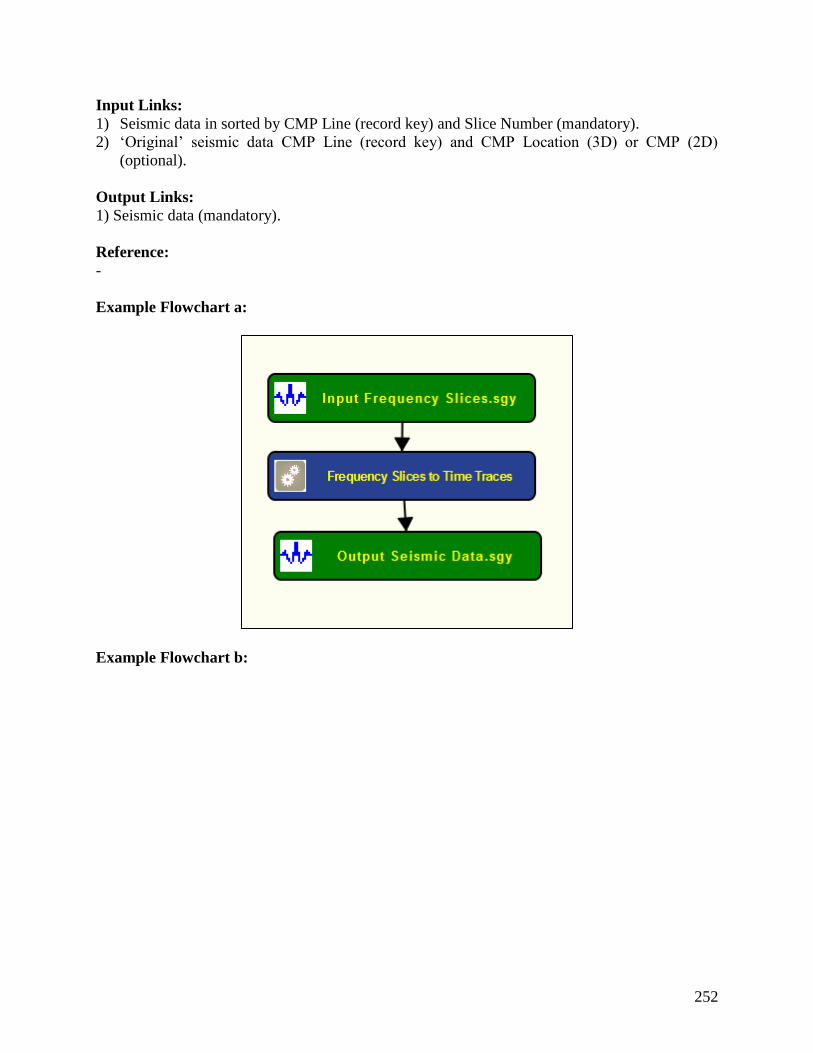
252

Input Links:

1) Seismic data in sorted by CMP Line (record key) and Slice Number (mandatory).

2) ‘Original’ seismic data CMP Line (record key) and CMP Location (3D) or CMP (2D)

(optional).

Output Links:

1) Seismic data (mandatory).

Reference:

-

Example Flowchart a:

Example Flowchart b:

253

Step Parameter Dialog:

Parameter Description:

Output maximum time (ms) — Enter maximum time of the output in time.

Restore headers from original data — If checked, a secondary input data stream will be required,

sorted by CMP Line (record key) and CMP Location (3D) or CMP (2D) (example flowchart b).

This secondary input data will be used to supply the headers to be attached to the output data, and

the data extent must be set to match the extent of the output data.

Real Time Amplitude Spectrum Plot

254

Usage: The Real Time Amplitude Spectrum Plot step is a real time plot of the amplitude spectrum

for a group traces as defined by the user. This step is not ready available yet.

Input Links:

1) Seismic data in sorted by CMP Line (record key) and Slice Number (mandatory).

Output Links:

-

Reference:

-

Example Flowchart:

Step Parameter Dialog:

Parameter Description:

Real Time Data Quality Analysis Usage:

The Real Time Data Quality step is a real time display that allows plotting the information

generated by the Spectral Comparison processing step (under Quality Analysis category). It

generates a real time map using as horizontal axis the header value defined under the Trace header

containing horizontal coordinate and as vertical axis the header value located under the Trace

header containing vertical coordinate. The map is then colored by the values defined under the

Trace header containing attribute for display. In the Spectral Comparison case, we can select

either the spectral semblance value of the dead/live flag.

Input Links:

1) Seismic file (mandatory). Normally this step is applied together with Spectral Comparison for

real time quality control.

Output Links:

-

Reference:

-

Example Flowchart:

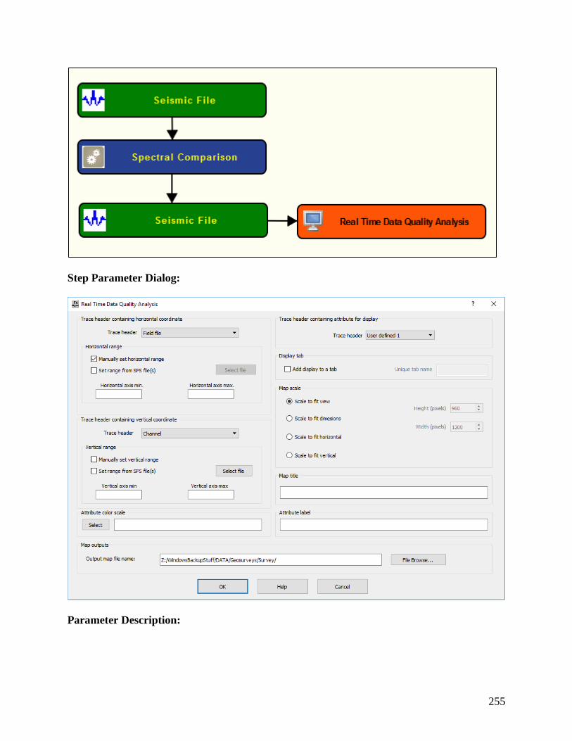
255

Step Parameter Dialog:

Parameter Description:

256

Trace header containing horizontal coordinate: It generates a real time map using as horizontal

axis the header value defined under the Trace header.

Trace header — Select trace header to be used as horizontal axis for the real time map.

Horizontal range: In the current version of this real time display, it is mandatory to define the

horizontal range of the map either by using user-defined minimum and maximum values or by

using an auxiliary SPS geometry file.

Manually set horizontal range — If checked, the minimum and maximum horizontal ranges are

used-defined and set as specified under Horizontal axis min. and Horizontal axis max.. The

maximum value for the horizontal coordinate will be automatically updated if the current

horizontal trace header value is larger than what is pre-defined.

Set range from SPS file(s) — If checked, the minimum and maximum horizontal ranges are

specified by an auxiliary SPS geometry file selected under browse button.

Horizontal axis min. — Enter minimum value of the horizontal coordinate to be displayed.

Horizontal axis max. — Enter maximum value of the horizontal coordinate to be displayed.

Trace header containing vertical coordinate: It generates a real time map using as vertical axis

the header value defined under the Trace header.

Trace header — Select trace header to be used as horizontal axis for the real time map.

Vertical range: In the current version of this real time display, it is mandatory to define the vertical

range of the map either by using user-defined minimum and maximum values or by using an

auxiliary SPS geometry file. The maximum value for the vertical coordinate will be automatically

updated if the current horizontal trace header value is larger than what is pre-defined.

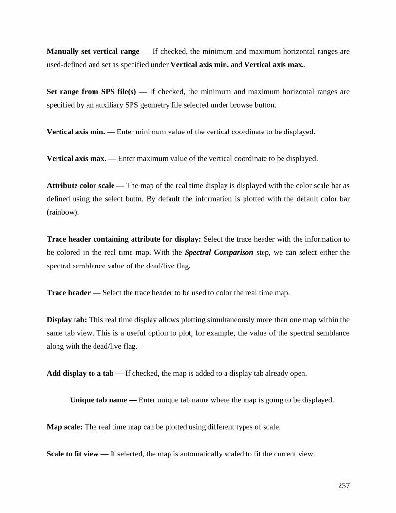
257

Manually set vertical range — If checked, the minimum and maximum horizontal ranges are

used-defined and set as specified under Vertical axis min. and Vertical axis max..

Set range from SPS file(s) — If checked, the minimum and maximum horizontal ranges are

specified by an auxiliary SPS geometry file selected under browse button.

Vertical axis min. — Enter minimum value of the vertical coordinate to be displayed.

Vertical axis max. — Enter maximum value of the vertical coordinate to be displayed.

Attribute color scale — The map of the real time display is displayed with the color scale bar as

defined using the select buttn. By default the information is plotted with the default color bar

(rainbow).

Trace header containing attribute for display: Select the trace header with the information to

be colored in the real time map. With the Spectral Comparison step, we can select either the

spectral semblance value of the dead/live flag.

Trace header — Select the trace header to be used to color the real time map.

Display tab: This real time display allows plotting simultaneously more than one map within the

same tab view. This is a useful option to plot, for example, the value of the spectral semblance

along with the dead/live flag.

Add display to a tab — If checked, the map is added to a display tab already open.

Unique tab name — Enter unique tab name where the map is going to be displayed.

Map scale: The real time map can be plotted using different types of scale.

Scale to fit view — If selected, the map is automatically scaled to fit the current view.

258

Scale to fit dimensions — If selected, the map is automatically scaled to fit the dimensions defined

by the user.

Height (in pixels) — Enter the height of the map in number of pixels.

Width (in pixels) — Enter the width of the map in number of pixels.

Scale to fit horizontal — If selected, the map is automatically scaled to fit the current view

horizontally.

Scale to fit vertical — If selected, the map is automatically scaled to fit the current view

horizontally.

Map title — Enter map title to be displayed in the display tab.

Attribute label — Enter attribute label.

Output map file name — Enter, or browse, the name of the file where the map is going to be

saved. The map final map will be stored in a .baf format.

Real Time Near Trace Display Usage:

The Real Time Near Trace Display step is a real time display that allows plotting continously the

near offset trace, as defined under Channel number of the near offset group, of the current

record from the input seismic data file.

Input Links:

1) Seismic file (mandatory). Normally this step is applied together with Spectral Comparison for

real time quality control.

Output Links:

-

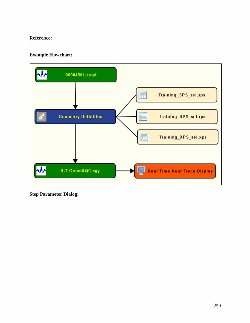
259

Reference:

-

Example Flowchart:

Step Parameter Dialog:

260

Parameter Description:

Channel number of near offset group — Enter the number of the channel number corresponding

to the near offset group to be ploted in real time.

Display tab: This real time display allows plotting simultaneously more than one diplay within

the same tab view. This is a useful option to plot simultaneously several data for QC.

261

Add display to a tab — If checked, the map is added to a display tab already open.

Unique tab name — Enter unique tab name where the map is going to be displayed.

Display paramters: Define the parameters related with the real time of the near offset trace.

Trace display type — Select the type of the seismic display. The user can select between Variable

area wiggle or Variable density.

Trace polarity — Select the type of polarity for the seismic display. The user can selecte between

Normal or Reverse.

Orientation — Select the orientation of the seismic display. The user can selecte between Right-

to-left or Left-to-right.

Horizontal scale — Enter the horizontal scale for the seismic display, with the units as specified

in Horizontal Units.

Vertical scale — Enter the vertical scale for the seismic display, with the units as specified in

Vertical Units.

Display gain — Enter the display gain of the seismic display.

Trace excursion — Enter the trace excursion gain of the seismic display

Horizontal units — Select the horizontal units to be used for the Horizontal scale. Units can be

defined in Traces per inch or Traces per cm.

Vertical units — Select the horizontal units to be used for the Vertical scale. Units can be defined

in inch per second or centimeter per second.

262

Amplitude type — Select the amplitude type for the seismic display. The near offset record may

be displayed in True amplitude, Relative amplitude or Gain control with a window size defined

in Window.

Window (ms) — Enter the window size in ms for Gain control.

Display color scale: Select the display color scale to be used in the real time plot.

Select — Use the button to select the display color bar for the real time seismic plot.

Display title — Enter display title to be displayed in the display tab.

Real Time Quality Analysis Statistics Map Usage:

The Real Time Quality Analysis Statistics Map step is a real time display that allows plotting the

information generated by the Signal to Noise Attribute (under Quality Analysis). It generates a

real time map like a bar chart where the S/N ratio and dead/live flags can be plotted simultaneously

for the three different signal-to-noise ratio estimates with the Signal to Noise Attribute.

Input Links:

1) Seismic file (mandatory). Normally this step is applied together with Signal to Noise Attribute

for real time quality control.

Output Links:

-

Reference:

-

Example Flowchart:

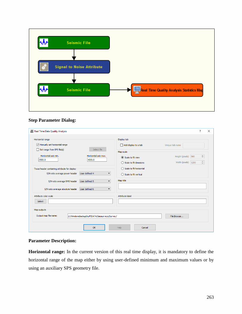
263

Step Parameter Dialog:

Parameter Description:

Horizontal range: In the current version of this real time display, it is mandatory to define the

horizontal range of the map either by using user-defined minimum and maximum values or by

using an auxiliary SPS geometry file.

264

Manually set horizontal range — If checked, the minimum and maximum horizontal ranges are

used-defined and set as specified under Horizontal axis min. and Horizontal axis max.. The

maximum value for the horizontal coordinate will be automatically updated if the current

horizontal trace header value is larger than what is pre-defined.

Set range from SPS file(s) — If checked, the minimum and maximum horizontal ranges are

specified by an auxiliary SPS geometry file selected under browse button.

Horizontal axis min. — Enter minimum value of the horizontal coordinate to be displayed.

Horizontal axis max. — Enter maximum value of the horizontal coordinate to be displayed.

Trace header containing attribute for display: Select the trace header with the information to

be colored in the real time map. With the Signal to Noise Attribute step, the user can select between

the Signal-to-Noise ration computed with the average power, average RMS and average absolute.

S/N ratio average power header — Select the trace header where the corresponding type of S/N

ratio was stored by the Signal to Noise Attribute step.

S/N ratio average RMS header — Select the trace header where the corresponding type of S/N

ratio was stored by the Signal to Noise Attribute step.

S/N ratio average absolute power — Select the trace header where the corresponding type of

S/N ratio was stored by the Signal to Noise Attribute step.

Attribute color scale — The map of the real time display is displayed with the color scale bar as

defined using the select buttn. By default the information is plotted with the default color bar

(rainbow).

265

Display tab: This real time display allows plotting simultaneously more than one map within the

same tab view. This is a useful option to plot, for example, the value of the spectral semblance

along with the dead/live flag.

Add display to a tab — If checked, the map is added to a display tab already open.

Unique tab name — Enter unique tab name where the map is going to be displayed.

Map scale: The real time map can be plotted using different types of display.

Scale to fit view — If selected, the map is automatically scaled to fit the current view.

Scale to fit dimensions — If selected, the map is automatically scaled to fit the dimensions defined

by the user.

Height (in pixels) — Enter the height of the map in number of pixels.

Width (in pixels) — Enter the width of the map in number of pixels.

Scale to fit horizontal — If selected, the map is automatically scaled to fit the current view

horizontally.

Scale to fit vertical — If selected, the map is automatically scaled to fit the current view

horizontally.

Map title — Enter map title to be displayed in the display tab.

Attribute label — Enter attribute label.

Output map file name — Enter, or browse, the name of the file where the map is going to be

saved. The map final map will be stored in a .baf format.

266

Real Time Quality Analysis Statistics Plot Usage:

The Real Time Quality Analysis Statistics Plot step is a real time display that allows plotting the

information generated by the Signal to Noise Attribute (under Quality Analysis). It generates a

real time map like a linear where the S/N ratio can be plotted simultaneously for the three different

signal-to-noise ratio estimates with the Signal to Noise Attribute with a statistical measurement of

the nth previous records as defined in the Number of records in moving window.

Input Links:

1) Seismic file (mandatory). Normally this step is applied together with Signal to Noise Attribute

for real time quality control.

Output Links:

-

Reference:

-

Example Flowchart:

Step Parameter Dialog:

267

Parameter Description:

Horizontal range: In the current version of this real time display, it is mandatory to define the

horizontal range of the map either by using user-defined minimum and maximum values or by

using an auxiliary SPS geometry file.

Manually set horizontal range — If checked, the minimum and maximum horizontal ranges are

used-defined and set as specified under Horizontal axis min. and Horizontal axis max.. The

maximum value for the horizontal coordinate will be automatically updated if the current

horizontal trace header value is larger than what is pre-defined.

Set range from SPS file(s) — If checked, the minimum and maximum horizontal ranges are

specified by an auxiliary SPS geometry file selected under browse button.

Horizontal axis min. — Enter minimum value of the horizontal coordinate to be displayed.

268

Horizontal axis max. — Enter maximum value of the horizontal coordinate to be displayed.

Trace header containing attribute for display: Select the trace header with the information to

be colored in the real time map. With the Signal to Noise Attribute step, the user can select between

the Signal-to-Noise ration computed with the average power, average RMS and average absolute.

S/N ratio average power header — Select the trace header where the corresponding type of S/N

ratio was stored by the Signal to Noise Attribute step.

S/N ratio average RMS header — Select the trace header where the corresponding type of S/N

ratio was stored by the Signal to Noise Attribute step.

S/N ratio average absolute power — Select the trace header where the corresponding type of

S/N ratio was stored by the Signal to Noise Attribute step.

Attribute color scale — The map of the real time display is displayed with the color scale bar as

defined using the select button. By default the information is plotted with the default color bar

(rainbow).

Display tab: This real time display allows plotting simultaneously more than one map within the

same tab view. This is a useful option to plot, for example, the value of the spectral semblance

along with the dead/live flag.

Add display to a tab — If checked, the map is added to a display tab already open.

Unique tab name — Enter unique tab name where the map is going to be displayed.

Map scale: The real time map can be plotted using different types of display.

269

Plot statistics: This real time display allow plotting with the current signal to noise attribute along

with the selected statistical measurement of the nth previous records as defined in the Number of

records in moving window.

Plot average S/N ratio — If selected, plot the average S/N ratio of the nth previous records as

defined in the Number of records in moving window.

Plot median S/N ratio — If selected, plot the median S/N ratio of the nth previous records as

defined in the Number of records in moving window.

Plot mode S/N ratio — If selected, plot the mode S/N ratio of the nth previous records as defined

in the Number of records in moving window.

Number of records in moving window — Enter the number of previous records in the calcularion

of the statistical measurement.

Scale to fit view — If selected, the map is automatically scaled to fit the current view.

Scale to fit dimensions — If selected, the map is automatically scaled to fit the dimensions defined

by the user.

Height (in pixels) — Enter the height of the map in number of pixels.

Width (in pixels) — Enter the width of the map in number of pixels.

Scale to fit horizontal — If selected, the map is automatically scaled to fit the current view

horizontally.

Scale to fit vertical — If selected, the map is automatically scaled to fit the current view

horizontally.

270

Map title — Enter map title to be displayed in the display tab.

Attribute label — Enter attribute label.

Output map file name — Enter, or browse, the name of the file where the map is going to be

saved. The map final map will be stored in a .baf format.

Real Time Receiver Attribute Map

Usage: The Real Time Receiver Attribute Map step builds a real time map of the locations of

receivers colored by a given receiver attribute for each record. Often this step is used with

Amplitude Analysis (under Quality Analysis).

Input Links:

1) Seismic file (mandatory). Normally this step is applied together with Amplitude Analysis for

real time quality control.

Output Links:

-

Reference:

-

Example Flowchart:

271

Step Parameter Dialog:

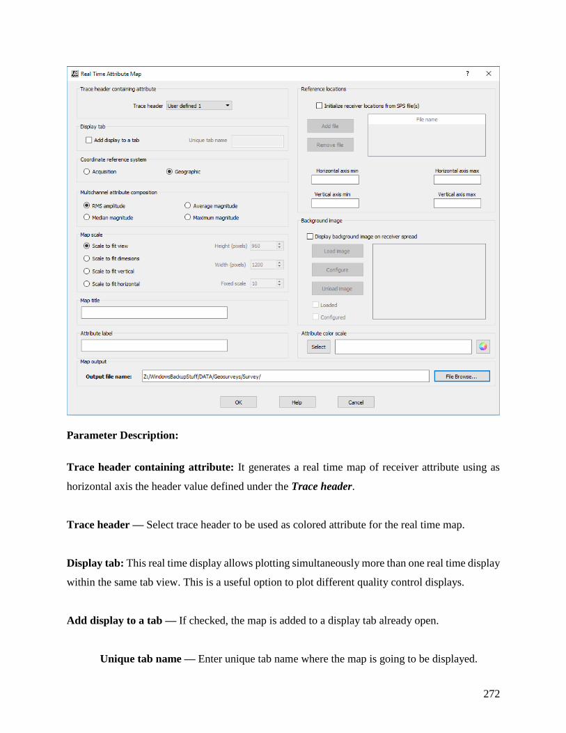
272

Parameter Description:

Trace header containing attribute: It generates a real time map of receiver attribute using as

horizontal axis the header value defined under the Trace header.

Trace header — Select trace header to be used as colored attribute for the real time map.

Display tab: This real time display allows plotting simultaneously more than one real time display

within the same tab view. This is a useful option to plot different quality control displays.

Add display to a tab — If checked, the map is added to a display tab already open.

Unique tab name — Enter unique tab name where the map is going to be displayed.

273

Coordinate reference system: Defines the coordinate systems to be used for the real time map.

Acquisition — Use relative coordinates from the acquisition geometry.

Geographic — Use real world coordinates.

Multichannel attribute composition: this real time display allow plotting different attributes

regarding the data received at each active channel group.

RMS amplitude — If selected, plots the RMS amplitude as defined in the Amplitude Analysis

step.

Median magnitude — If selected, plots the RMS amplitude as defined in the Amplitude Analysis

step.

Average magnitude — If selected, plots the RMS amplitude as defined in the Amplitude Analysis

step.

Maximum magnitude — If selected, plots the RMS amplitude as defined in the Amplitude

Analysis step.

Map scale: The real time map can be plotted using different types of scale.

Scale to fit view — If selected, the map is automatically scaled to fit the current view.

Scale to fit dimensions — If selected, the map is automatically scaled to fit the dimensions defined

by the user.

Height (in pixels) — Enter the height of the map in number of pixels.

Width (in pixels) — Enter the width of the map in number of pixels.

274

Scale to fit horizontal — If selected, the map is automatically scaled to fit the current view

horizontally.

Scale to fit vertical — If selected, the map is automatically scaled to fit the current view

horizontally.

Map title — Enter map title to be displayed in the display tab.

Attribute label — Enter attribute label.

Reference locations: The real time map needs a reference spatial location in order to plot the

location of each channel group. These reference locations are updated if during the survey the

objects to be displayed are outside the pre-defined area.

Initialize receiver locations from SPS file(s) — If cheked, the reference locations are loaded

directly from a SPS geometry file. More than one SPS files may be used to define the reference

locations.

Add file — Select to browse for a SPS file to be used as reference locations. The SPS file

will automatically be scanned and added to the nearby box. The reference location may be

defined with more than one file. In this case Horizontal axis min, Horizontal axis max,

Vertical axis min, Vertical axis max are automatically filled in according to the SPS files.

Remove file — The SPS file highlighted in the nearby box is going to be removed and the

reference locations updated accordingly.

Horizontal axis min — Enter minimum value of the horizontal coordinate to be displayed.

Horizontal axis max — Enter maximum value of the horizontal coordinate to be displayed.

275

Vertical axis min — Enter minimum value of the vertical coordinate to be displayed.

Vertical axis max — Enter maximum value of the vertical coordinate to be displayed.

Background image: The real time map may use a background image with cultural data.

Display background image on receiver spread — If checked the real time map uses a

background image of the area.

Load image — Select to browse for the image file to be used as background image. The

image file is automatically loaded and added to the box nearby.

Configure — Select to configure the coordinates of the background image.

Unload image — Select if you want to unload the background image from the real time

map.

Loaded — Automatically checked if the background image was loaded successfully.

Configured — Automatically checked if the background images was configure

successfully.

Attribute Color scale — The map of the real time display is displayed with the color scale bar as

defined using the select buttn. By default the information is plotted with the default color bar

(rainbow).

Map Output file name — Enter, or browse, the name of the file where the map is going to be

saved. The map final map will be stored in a .baf format.

Real Time Receiver Spread

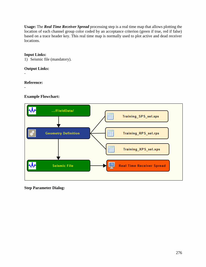
276

Usage: The Real Time Receiver Spread processing step is a real time map that allows plotting the

location of each channel group color coded by an acceptance criterion (green if true, red if false)

based on a trace header key. This real time map is normally used to plot active and dead receiver

locations.

Input Links:

1) Seismic file (mandatory).

Output Links:

-

Reference:

-

Example Flowchart:

Step Parameter Dialog:

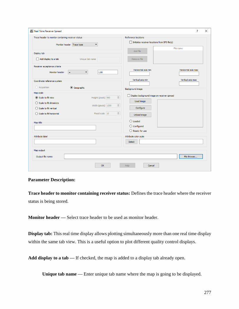
277

Parameter Description:

Trace header to monitor containing receiver status: Defines the trace header where the receiver

status is being stored.

Monitor header — Select trace header to be used as monitor header.

Display tab: This real time display allows plotting simultaneously more than one real time display

within the same tab view. This is a useful option to plot different quality control displays.

Add display to a tab — If checked, the map is added to a display tab already open.

Unique tab name — Enter unique tab name where the map is going to be displayed.

278

Receiver acceptance criteria: Select the logical operator that you want to use as acceptance

criteria. This logical operator is going to be applied to the selected monitor header.

Monitor header — Selecte trace header key to monitor. Enter the value for the acceptance criteria.

Coordinate reference system: Defines the coordinate systems to be used for the real time map.

Acquisition — Use relative coordinates from the acquisition geometry.

Geographic — Use real world coordinates.

Map scale: The real time map can be plotted using different types of scale.

Scale to fit view — If selected, the map is automatically scaled to fit the current view.

Scale to fit dimensions — If selected, the map is automatically scaled to fit the dimensions defined

by the user.

Height (in pixels) — Enter the height of the map in number of pixels.

Width (in pixels) — Enter the width of the map in number of pixels.

Scale to fit horizontal — If selected, the map is automatically scaled to fit the current view

horizontally.

Scale to fit vertical — If selected, the map is automatically scaled to fit the current view

horizontally.

Map title — Enter map title to be displayed in the display tab.

279

Reference locations: The real time map needs a reference spatial location in order to plot the

location of each channel group. These reference locations are updated if during the survey the

objects to be displayed are outside the pre-defined area.

Initialize receiver locations from SPS file(s) — If cheked, the reference locations are loaded

directly from a SPS geometry file. More than one SPS files may be used to define the reference

locations.

Add file — Select to browse for a SPS file to be used as reference locations. The SPS file

will automatically be scanned and added to the nearby box. The reference location may be

defined with more than one file. In this case Horizontal axis min, Horizontal axis max,

Vertical axis min, Vertical axis max are automatically filled in according to the SPS files.

Remove file — The SPS file highlighted in the nearby box is going to be removed and the

reference locations updated accordingly.

Horizontal axis min — Enter minimum value of the horizontal coordinate to be displayed.

Horizontal axis max — Enter maximum value of the horizontal coordinate to be displayed.

Vertical axis min — Enter minimum value of the vertical coordinate to be displayed.

Vertical axis max — Enter maximum value of the vertical coordinate to be displayed.

Display background image on receiver spread — If checked the real time map uses a

background image of the area.

Load image — Select to browse for the image file to be used as background image. The

image file is automatically loaded and added to the box nearby.

Configure — Select to configure the coordinates of the background image.

280

Unload image — Select if you want to unload the background image from the real time

map.

Loaded — Automatically checked if the background image was loaded successfully.

Configured — Automatically checked if the background images was configure

successfully.

Attribute label — Enter attribute label.

Attribute Color scale — The map of the real time display is displayed with the color scale bar as

defined using the select buttn. By default the information is plotted with the default color bar

(rainbow).

Map Output file name — Enter, or browse, the name of the file where the map is going to be

saved. The map final map will be stored in a .baf format.

Real Time Seismic Display

Usage:

The Real Time Seismic Display step is used to display seismic records during the processing flow.

It also can output image files and automatically ftp these image files to a server on an active internet

connection.

Input Links:

1) Seismic data in any sort order (mandatory).

Output Links:

-

Reference:

-

Example Flowchart:

281

Step Parameter Dialog:

282

Parameter descriptions:

Display increment: This real time display plots the input seismic data along with either killed

records during the processing selecting, using a given increment between records, or the records

killed by the processing.

Record increment between displays — Enter the increment between records to be ploted in the

real time display. If Only display records killed during processing is selected this option is

disabled.

Also display records killed during processing — If checked, plot with the input seismic file the

records killed during the processing.

Only display records killed during processing — If checked, plot only records that have been

killed by the processing.

Mark dead traces — If checked, plot dead traces in red.

Display tab: This real time display allows plotting simultaneously more than one map within the

same tab view. This is a useful option to plot, for example, the value of the spectral semblance

along with the dead/live flag.

Add display to a tab — If checked, the map is added to a display tab already open.

Unique tab name — Enter unique tab name where the map is going to be displayed.

Image output: Each plot of the real time display may be stored in an image file.

Output image files — If checked, the display of the real time display is stored in an image file.

Send via ftp — If checked, the image output is send directly via FTP.

Image format — Select the image format. The image may be stored in BMP, JPG or PNG.

Image quality — Select the quality of the output image. The output image may be saved

with Low, Medium or High quality.

Image increment — Select, from 1 to 10, the increment between records that is going to

be used to save the image.

Output colorbar — Select if the colorbar is saved within the image.

283

Real time options: A noise and/or signal window, represented by a rectangle, may be ploted

overlaying the current seismic record.

Plot signal and noise windows — If checked plot overlaying the real time seismic display a

polygon representing signal and noise windows. Signal window is ploted in green while noise

window is ploted in red.

Select signal polygon — Enter signal polygon card file location.

Select noise polygon — Enter noise polygon card file location.

Display paramters: Define the parameters related with the real time of the near offset trace.

Trace display type — Select the type of the seismic display. The user can select between Variable

area wiggle or Variable density.

Trace polarity — Select the type of polarity for the seismic display. The user can selecte between

Normal or Reverse.

Orientation — Select the orientation of the seismic display. The user can selecte between Right-

to-left or Left-to-right.

Horizontal scale — Enter the horizontal scale for the seismic display, with the units as specified

in Horizontal Units.

Vertical scale — Enter the vertical scale for the seismic display, with the units as specified in

Vertical Units.

Display gain — Enter the display gain of the seismic display.

Trace excursion — Enter the trace excursion gain of the seismic display

Horizontal units — Select the horizontal units to be used for the Horizontal scale. Units can be

defined in Traces per inch or Traces per cm.

284

Vertical units — Select the horizontal units to be used for the Vertical scale. Units can be defined

in inch per second or centimeter per second.

Amplitude type — Select the amplitude type for the seismic display. The near offset record may

be displayed in True amplitude, Relative amplitude or Gain control with a window size defined

in Window.

Window (ms) — Enter the window size in ms for Gain control.

Diplay title — Enter display title to be displayed in the display tab.

Display color scale — Select color scale bar for the display.

Real Time Source Attribute Map Usage:

The Real Time Source Attribute Map step is used to display maps of source attributes (amplitudes,

frequency attributes) during the processing flow.

Input Links:

1) Seismic data in any sort order (mandatory).

Output Links:

-

Reference:

-

Example Flowchart:

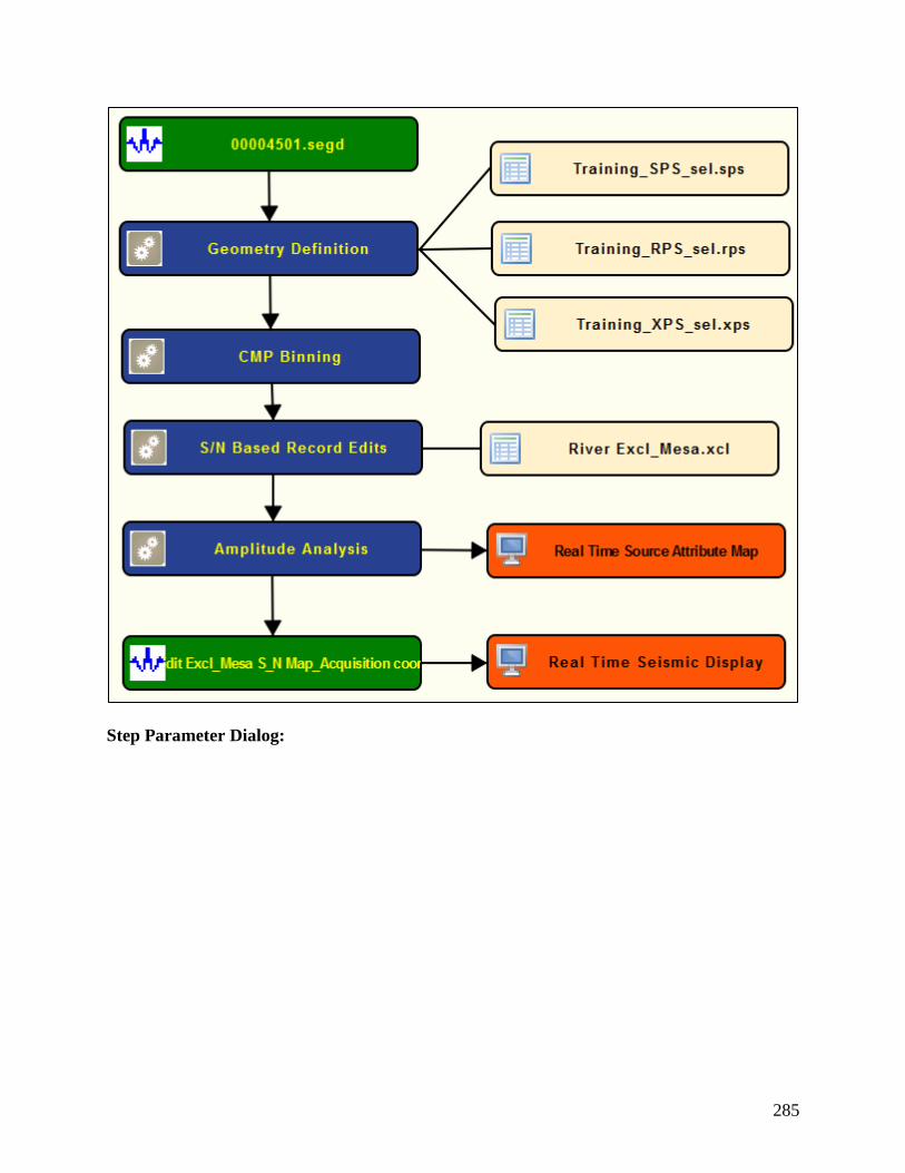
285

Step Parameter Dialog:

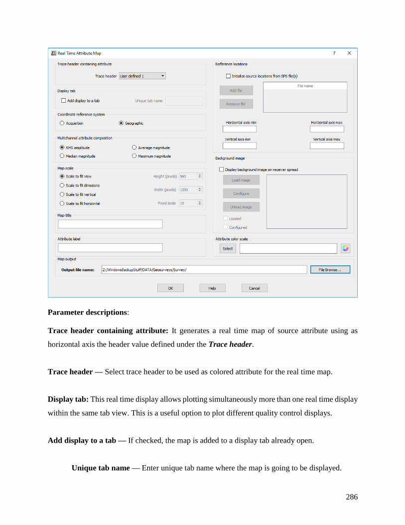
286

Parameter descriptions:

Trace header containing attribute: It generates a real time map of source attribute using as

horizontal axis the header value defined under the Trace header.

Trace header — Select trace header to be used as colored attribute for the real time map.

Display tab: This real time display allows plotting simultaneously more than one real time display

within the same tab view. This is a useful option to plot different quality control displays.

Add display to a tab — If checked, the map is added to a display tab already open.

Unique tab name — Enter unique tab name where the map is going to be displayed.

287

Coordinate reference system: Defines the coordinate systems to be used for the real time map.

Acquisition — Use relative coordinates from the acquisition geometry.

Geographic — Use real world coordinates.

Multichannel attribute composition: this real time display allow plotting different attributes

regarding the data received at each active channel group.

RMS amplitude — If selected, plots the RMS amplitude as defined in the Amplitude Analysis

step.

Median magnitude — If selected, plots the RMS amplitude as defined in the Amplitude Analysis

step.

Average magnitude — If selected, plots the RMS amplitude as defined in the Amplitude Analysis

step.

Maximum magnitude — If selected, plots the RMS amplitude as defined in the Amplitude

Analysis step.

Map scale: The real time map can be plotted using different types of scale.

Scale to fit view — If selected, the map is automatically scaled to fit the current view.

Scale to fit dimensions — If selected, the map is automatically scaled to fit the dimensions defined

by the user.

Height (in pixels) — Enter the height of the map in number of pixels.

Width (in pixels) — Enter the width of the map in number of pixels.

288

Scale to fit horizontal — If selected, the map is automatically scaled to fit the current view

horizontally.

Scale to fit vertical — If selected, the map is automatically scaled to fit the current view

horizontally.

Map title — Enter map title to be displayed in the display tab.

Attribute label — Enter attribute label.

Reference locations: The real time map needs a reference spatial location in order to plot the

location of each channel group. These reference locations are updated if during the survey the

objects to be displayed are outside the pre-defined area.

Initialize receiver locations from SPS file(s) — If cheked, the reference locations are loaded

directly from a SPS geometry file. More than one SPS files may be used to define the reference

locations.

Add file — Select to browse for a SPS file to be used as reference locations. The SPS file

will automatically be scanned and added to the nearby box. The reference location may be

defined with more than one file. In this case Horizontal axis min, Horizontal axis max,

Vertical axis min, Vertical axis max are automatically filled in according to the SPS files.

Remove file — The SPS file highlighted in the nearby box is going to be removed and the

reference locations updated accordingly.

Horizontal axis min — Enter minimum value of the horizontal coordinate to be displayed.

Horizontal axis max — Enter maximum value of the horizontal coordinate to be displayed.

289

Vertical axis min — Enter minimum value of the vertical coordinate to be displayed.

Vertical axis max — Enter maximum value of the vertical coordinate to be displayed.

Background image: The real time map may use a background image with cultural data.

Display background image on receiver spread — If checked the real time map uses a

background image of the area.

Load image — Select to browse for the image file to be used as background image. The

image file is automatically loaded and added to the box nearby.

Configure — Select to configure the coordinates of the background image.

Unload image — Select if you want to unload the background image from the real time

map.

Loaded — Automatically checked if the background image was loaded successfully.

Configured — Automatically checked if the background images was configure

successfully.

Attribute Color scale — The map of the real time display is displayed with the color scale bar as

defined using the select buttn. By default the information is plotted with the default color bar

(rainbow).

Map Output file name — Enter, or browse, the name of the file where the map is going to be

saved. The map final map will be stored in a .baf format.

Real Time Stack Display

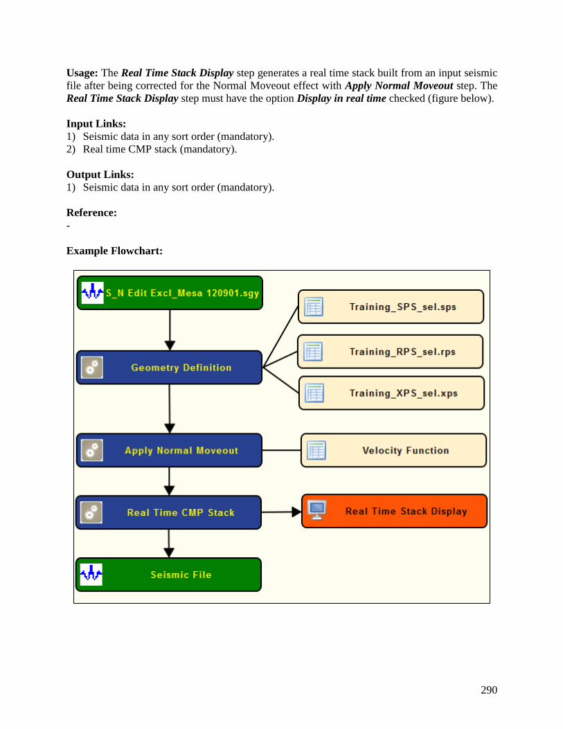
290

Usage: The Real Time Stack Display step generates a real time stack built from an input seismic

file after being corrected for the Normal Moveout effect with Apply Normal Moveout step. The

Real Time Stack Display step must have the option Display in real time checked (figure below).

Input Links:

1) Seismic data in any sort order (mandatory).

2) Real time CMP stack (mandatory).

Output Links:

1) Seismic data in any sort order (mandatory).

Reference:

-

Example Flowchart:

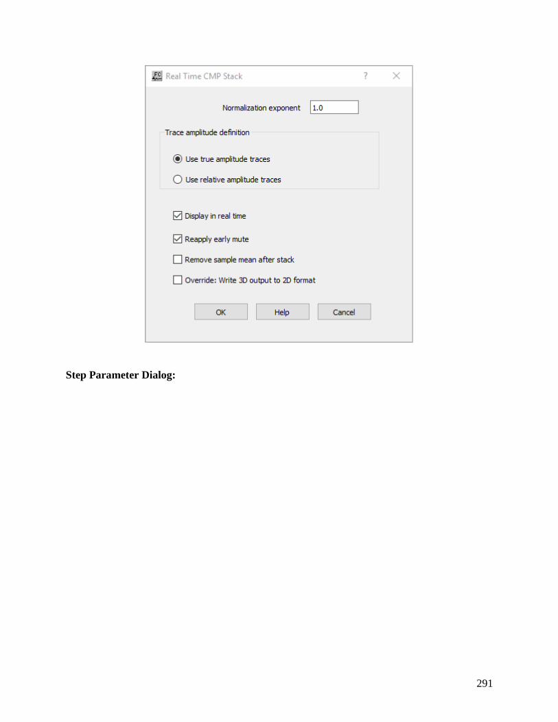
291

Step Parameter Dialog:

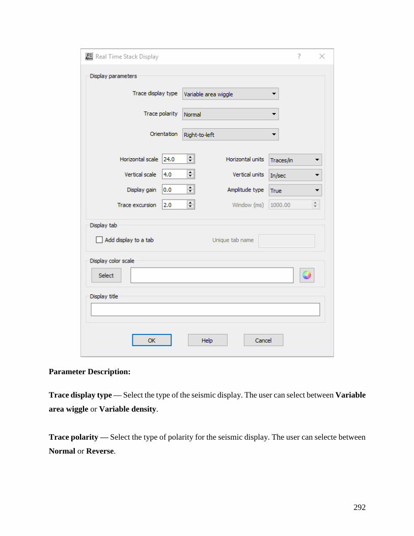
292

Parameter Description:

Trace display type — Select the type of the seismic display. The user can select between Variable

area wiggle or Variable density.

Trace polarity — Select the type of polarity for the seismic display. The user can selecte between

Normal or Reverse.

293

Orientation — Select the orientation of the seismic display. The user can selecte between Right-

to-left or Left-to-right.

Horizontal scale — Enter the horizontal scale for the seismic display, with the units as specified

in Horizontal Units.

Vertical scale — Enter the vertical scale for the seismic display, with the units as specified in

Vertical Units.

Display gain — Enter the display gain of the seismic display.

Trace excursion — Enter the trace excursion gain of the seismic display

Horizontal units — Select the horizontal units to be used for the Horizontal scale. Units can be

defined in Traces per inch or Traces per cm.

Vertical units — Select the horizontal units to be used for the Vertical scale. Units can be defined

in inch per second or centimeter per second.

Amplitude type — Select the amplitude type for the seismic display. The near offset record may

be displayed in True amplitude, Relative amplitude or Gain control with a window size defined

in Window.

Window (ms) — Enter the window size in ms for Gain control.

Diplay title — Enter display title to be displayed in the display tab.

Display color scale — Select color scale bar for the display.

Real Time Trace Header Map

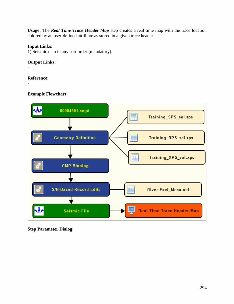
294

Usage: The Real Time Trace Header Map step creates a real time map with the trace location

colored by an user-defined attribute as stored in a given trace header.

Input Links:

1) Seismic data in any sort order (mandatory).

Output Links:

-

Reference:

-

Example Flowchart:

Step Parameter Dialog:

295

Parameter Description:

Trace header — Select trace header to be used as horizontal axis for the real time map.

Horizontal range: In the current version of this real time display, it is mandatory to define the

horizontal range of the map either by using user-defined minimum and maximum values or by

using an auxiliary SPS geometry file.

Manually set horizontal range — If checked, the minimum and maximum horizontal ranges are

used-defined and set as specified under Horizontal axis min. and Horizontal axis max.. The

maximum value for the horizontal coordinate will be automatically updated if the current

horizontal trace header value is larger than what is pre-defined.

296

Set range from SPS file(s) — If checked, the minimum and maximum horizontal ranges are

specified by an auxiliary SPS geometry file selected under browse button.

Horizontal axis min. — Enter minimum value of the horizontal coordinate to be displayed.

Horizontal axis max. — Enter maximum value of the horizontal coordinate to be displayed.

Trace header containing vertical coordinate: It generates a real time map using as vertical axis

the header value defined under the Trace header.

Trace header — Select trace header to be used as horizontal axis for the real time map.

Vertical range: In the current version of this real time display, it is mandatory to define the vertical

range of the map either by using user-defined minimum and maximum values or by using an

auxiliary SPS geometry file. The maximum value for the vertical coordinate will be automatically

updated if the current horizontal trace header value is larger than what is pre-defined.

Manually set vertical range — If checked, the minimum and maximum horizontal ranges are

used-defined and set as specified under Vertical axis min. and Vertical axis max..

Set range from SPS file(s) — If checked, the minimum and maximum horizontal ranges are

specified by an auxiliary SPS geometry file selected under browse button.

Vertical axis min. — Enter minimum value of the vertical coordinate to be displayed.

Vertical axis max. — Enter maximum value of the vertical coordinate to be displayed.

Attribute color scale — The map of the real time display is displayed with the color scale bar as

defined using the select buttn. By default the information is plotted with the default color bar

(rainbow).

297

Trace header containing attribute for display: Select the trace header with the information to

be colored in the real time map. With the Spectral Comparison step, we can select either the

spectral semblance value of the dead/live flag.

Trace header — Select the trace header to be used to color the real time map.

Display tab: This real time display allows plotting simultaneously more than one map within the

same tab view. This is a useful option to plot, for example, the value of the spectral semblance

along with the dead/live flag.

Add display to a tab — If checked, the map is added to a display tab already open.

Unique tab name — Enter unique tab name where the map is going to be displayed.

Map scale: The real time map can be plotted using different types of scale.

Scale to fit view — If selected, the map is automatically scaled to fit the current view.

Scale to fit dimensions — If selected, the map is automatically scaled to fit the dimensions defined

by the user.

Height (in pixels) — Enter the height of the map in number of pixels.

Width (in pixels) — Enter the width of the map in number of pixels.

Scale to fit horizontal — If selected, the map is automatically scaled to fit the current view

horizontally.

Scale to fit vertical — If selected, the map is automatically scaled to fit the current view

horizontally.

298

Map title — Enter map title to be displayed in the display tab.

Attribute label — Enter attribute label.

Output map file name — Enter, or browse, the name of the file where the map is going to be

saved. The map final map will be stored in a .baf format.

Time Slices Usage:

Time Slices is a process used for either display of selected time slices as a display option, or as a

tool to convert the data into a form suitable for specific processing.

Input Links:

1) Seismic data in sorted by CMP Line (record key) and CMP Location (mandatory).

Output Links:

1) Seismic data sorted by Slice Number and CMP Line (mandatory).

Reference:

-

Example Flowchart:

Step Parameter Dialog:

299

Parameter Description:

All input data — If checked, time slices will be made from all of the data. This is likely to be the

most suitable option for further processing of the data.

Selected time slices — If checked, those time slices specified by the following parameter values

will be output. This is likely to be the best data display option.

Time of first slice (ms) — The first slice output will be drawn from the data samples at the

specified time.

Time of last slice (ms) — The last slice output will be drawn from the data samples at the specified

time.

Time slice increment (ms) — Time slices will be output with the specified time increment (to the

nearest sample)..

Create RMS amplitude slices — If checked, each output time slice sample value will be the root

mean square value of all the specified samples above and below the that sample.

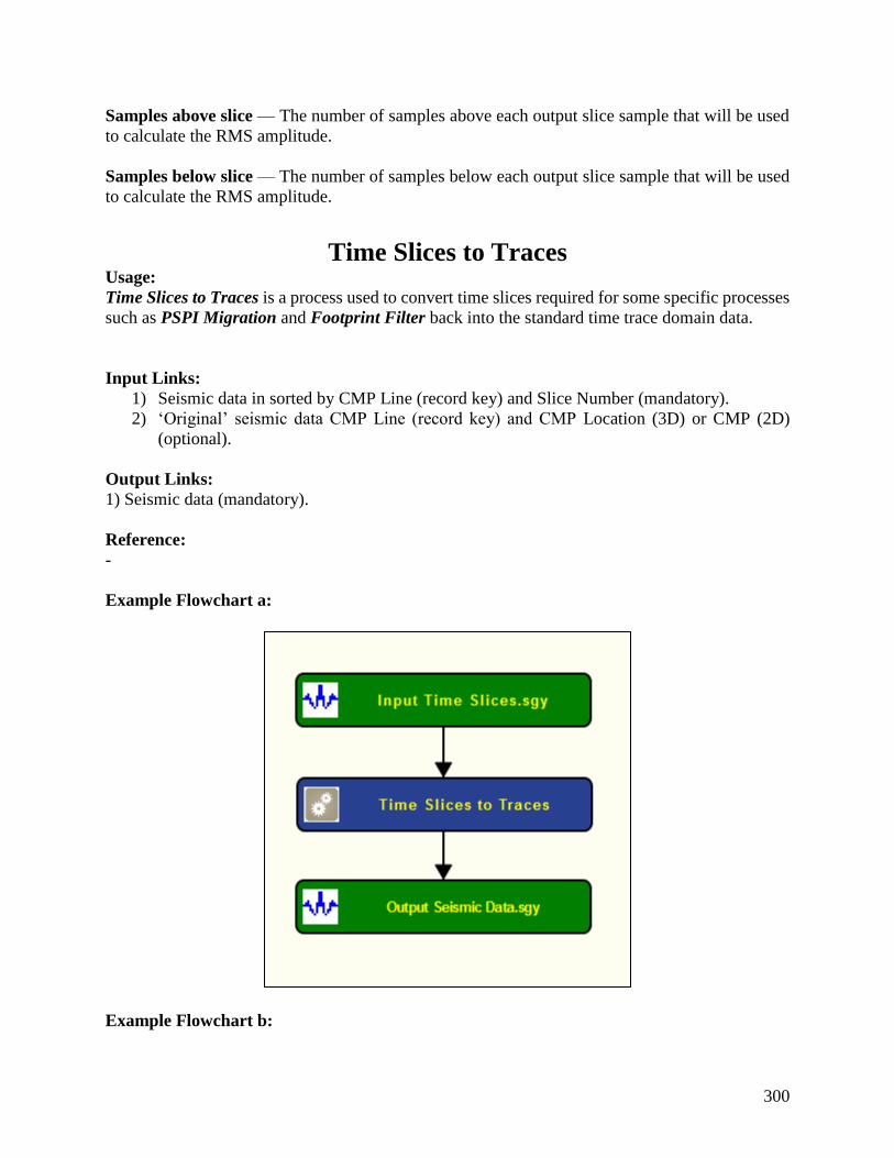
300

Samples above slice — The number of samples above each output slice sample that will be used

to calculate the RMS amplitude.

Samples below slice — The number of samples below each output slice sample that will be used

to calculate the RMS amplitude.

Time Slices to Traces Usage:

Time Slices to Traces is a process used to convert time slices required for some specific processes

such as PSPI Migration and Footprint Filter back into the standard time trace domain data.

Input Links:

1) Seismic data in sorted by CMP Line (record key) and Slice Number (mandatory).

2) ‘Original’ seismic data CMP Line (record key) and CMP Location (3D) or CMP (2D)

(optional).

Output Links:

1) Seismic data (mandatory).

Reference:

-

Example Flowchart a:

Example Flowchart b:

301

Step Parameter Dialog:

Parameter Description:

Restore headers from original data — If checked, a secondary input data stream will be required,

sorted by CMP Line (record key) and CMP Location (3D) or CMP (2D) (example flowchart b).

This secondary input data will be used to supply the headers to be attached to the output data, and

the data extent must be set to match the extent of the output data.

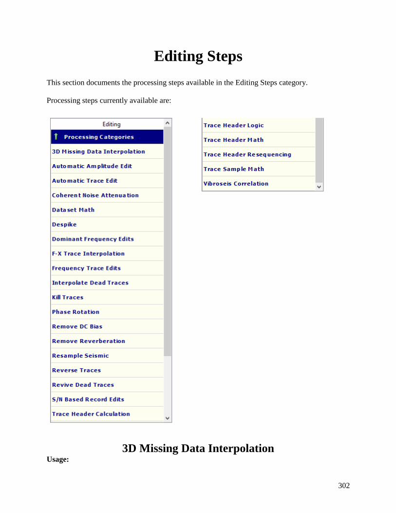
302

Editing Steps

This section documents the processing steps available in the Editing Steps category.

Processing steps currently available are:

3D Missing Data Interpolation Usage:

303

3D Missing Data Interpolation is a fast and pragmatic way to fill missing traces by means of

inverse-distance weighted interpolation from near traces.

For 3D pre-stack interpolation of missing data, the data should be ordered as 3D common offset

gathers, so that (binned) Offset is the primary key, CMP Line the secondary and record key, and

CMP location the tertiary key.

Input Links:

1) Seismic data in any sort order (mandatory).

Output Links:

1) Seismic data in any sort order (mandatory).

Reference:

-

Example Flowchart:

Step Parameter Dialog:

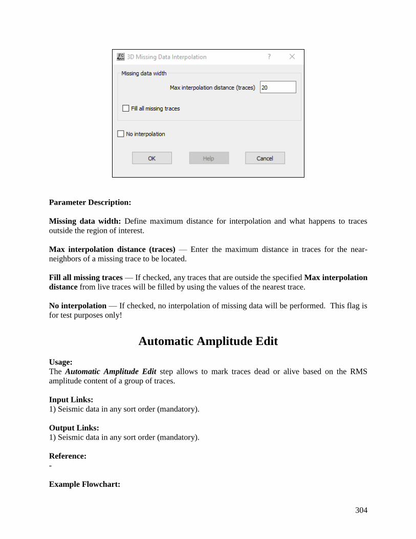
304

Parameter Description:

Missing data width: Define maximum distance for interpolation and what happens to traces

outside the region of interest.

Max interpolation distance (traces) — Enter the maximum distance in traces for the near-

neighbors of a missing trace to be located.

Fill all missing traces — If checked, any traces that are outside the specified Max interpolation

distance from live traces will be filled by using the values of the nearest trace.

No interpolation — If checked, no interpolation of missing data will be performed. This flag is

for test purposes only!

Automatic Amplitude Edit

Usage:

The Automatic Amplitude Edit step allows to mark traces dead or alive based on the RMS

amplitude content of a group of traces.

Input Links:

1) Seismic data in any sort order (mandatory).

Output Links:

1) Seismic data in any sort order (mandatory).

Reference:

-

Example Flowchart:

305

Step Parameter Dialog:

Parameter Description:

Number of traces in running average — Enter the number of traces in the moving window where

the RMS amplitude is going to be computed.

Percentage change in RMS amplitude — Enter the percentage change in RMS amplitude to

consider the traces dead of live.

306

Editing action: Select how seismic traces are marked based on the RMS amplitude content of a

group of traces within a moving window.

Only mark low amplitude traces as dead — If selected, low RMS amplitude traces are marked

as dead.

Only mark high amplitude traces as dead — If selected, high RMS amplitude traces are marked

as dead.

Mark both low and high amplitude traces as dead — If selected, both low and high RMS

amplitude traces are marked as dead.

Automatic Trace Edit Usage:

The Automatic Trace Edit step allows you to automatically remove invalid or noisy traces from

your data set based on user-defined criteria.

Input Links:

1) Seismic data in any sort order (mandatory).

Output Links:

1) Seismic data in any sort order (mandatory).

Reference:

-

Example Flowchart:

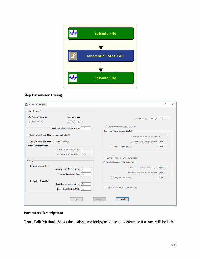
307

Step Parameter Dialog:

Parameter Description:

Trace Edit Method: Select the analysis method(s) to be used to determine if a trace will be killed.

308

Spectral semblance — The spectral semblance method uses the semblance between a single

trace’s power spectrum and the average power spectrum of the gather as the basis for killing a

trace.

Power ratio — The power ratio method uses the ratio of trace energy in the upper part of a trace

to that in the lower part of a trace as the basis for killing a trace. This is often an effective means

of editing traces that are contaminated with 60 Hz powerline noise, which does not decay as a

function of record time.

Both methods — Traces will be killed only if they fail BOTH the power ratio test AND the

spectral semblance test.

Either method — Traces will be killed if they fail EITHER the power ratio test OR the spectral

semblance test.

Calculate spectral semblance on receiver line basis — If checked, the spectral semblance will

be calculated on a receiver line basis.

Calculate spectral semblance using a time window — Enabled if Spectral Semblance option is

selected. If checked, spectral semblance is computed within a time gate defined by its top and base

in ms.

Spectral semblance window: Define the start and end time of the time window where the spectral

semblance is calculated.

Start time in ms of the window — Enter the start time of the window to compute the spectral

semblance. Time in ms.

End time in ms of the window — Enter the end time of the window to compute the spectral

semblance. Time in ms.

Power ratio decay cutoff (dB) — If you choose the power ratio method, enter the minimum decay

of trace energy in decibels that you expect between the first and second half of the trace.

Define top window for power ratio — Enabled if Power ratio option is selected. If checked,

select parameters to define the top window where the calculation is done.

Top window power ratio parameters: Define the start and end time of the top time window

where the power ratio is calculated.

Start time in ms of the window — Enter the start time of the window to compute the power ratio.

Time in ms.

End time in ms of the window — Enter the start time of the window to compute the power ratio.

Time in ms.

309

Apply moveout velocity — If selected, the normal moveout correction with a constant velocity is

applied to the record before computing the power ratio. Enter the velocity for the normal moveout

correction.

Define bottom window for power ratio — Enabled if Power ratio option is selected. If checked,

select parameters to define the bottom window where the calculation is done.

Bottom window power ratio parameters: Define the start and end time of the bottom time

window where the power ratio is calculated.

Start time in ms of the window — Enter the start time of the window to compute the power ratio.

Time in ms.

End time in ms of the window — Enter the end time of the window to compute the power ratio.

Time in ms.

Apply moveout velocity — If selected, the normal moveout correction with a constant velocity is

applied to the record before computing the power ratio. Enter the velocity for the normal moveout

correction.

Output kills to Trace Edit auxiliary file – If selected outputs killed traces based on the selected

measurement to an auxiliary file.

Spectral semblance cutoff (percent) — If you choose the spectral semblance method, enter the

minimum semblance value you expect for each trace’s power spectrum relative to the power

spectrum for the gather.

Coherent Noise Attenuation Usage:

The Coherent Noise Attenuation step edit coherent noise between adjacent traces based on

variations (in percentage) of the seismic amplitudes within a time trace window.

Input Links:

1) Seismic data in any sort order (mandatory).

Output Links:

2) Seismic data in any sort order (mandatory).

Reference:

-

Example Flowchart:

310

Step Parameter Dialog:

Parameter Description:

Trace window length (ms) — Enter the length of the window, in ms, where the estimation of the

reference amplitude is calculated.

Maximum trace amplitude variation (%) — Enter the maximum trace amplitude variation, in

percentage, to consider a given sample noise.

Gap between traces to compare — Enter the number of traces to skip for trace comparison.

Outlier replacement options: Define what happens to seismic samples considered noise.

311

Set to average of adjacent samples — If selected, the values of the seismic samples considered

noise are replaced by the average value of adjacent samples.

Set to zero — If selected, the value of the seismic samples considered noise are set to zero.

Dataset Math Usage:

The Dataset Math step will add, subtract, multiply, divide or do adaptive subtraction between the

samples of one data file from the corresponding samples of a second data file and output the result

to a seismic file.

Input Links:

1) Seismic data in any sort order (mandatory).

2) Seismic data in any sort order (mandatory) – must match the first dataset.

Output Links:

1) Seismic data in same sort order as the input (mandatory).

Example Flowchart:

Step Parameter Dialog:

312

Parameter Description:

Operation: Specify the math operation to perform between the samples of the two datasets.

Addition — If selected, perform addition between the samples of the two datasets.

Subtraction — If selected, perform subtraction between the samples of the two datasets.

Multiplication — If selected, perform multiplication between the samples of the two datasets.

Division — If selected, perform division between the samples of the two datasets.

Adaptive subtraction — If selected, perform adaptive subtraction between the samples of the two

datasets.

Despike

Usage:

The Despike step removes spikes of amplitude related with bursts of energy based on the variance

estimate of a given seismic sample when compared against its neighbours.

Input Links:

1) Seismic data in any sort order (mandatory).

Output Links:

1) Seismic data in any sort order (mandatory).

Reference:

313

-

Example Flowchart:

Step Parameter Dialog:

Parameter Description:

Variance limit — Enter the number of variance allowed for a seismic sample be considered signal.

Window length (ms) — Enter the windown length, in ms, where the statistical measures

(variance) are going to be computed and used as reference to detect spikes.

Replace spikes with interplated sample value — If checked, seismic samples marked as noise

are going to be replaced by an interpolated sampled value from its neighbours. If unchecked,

marked seismic samples are replaced by zero.

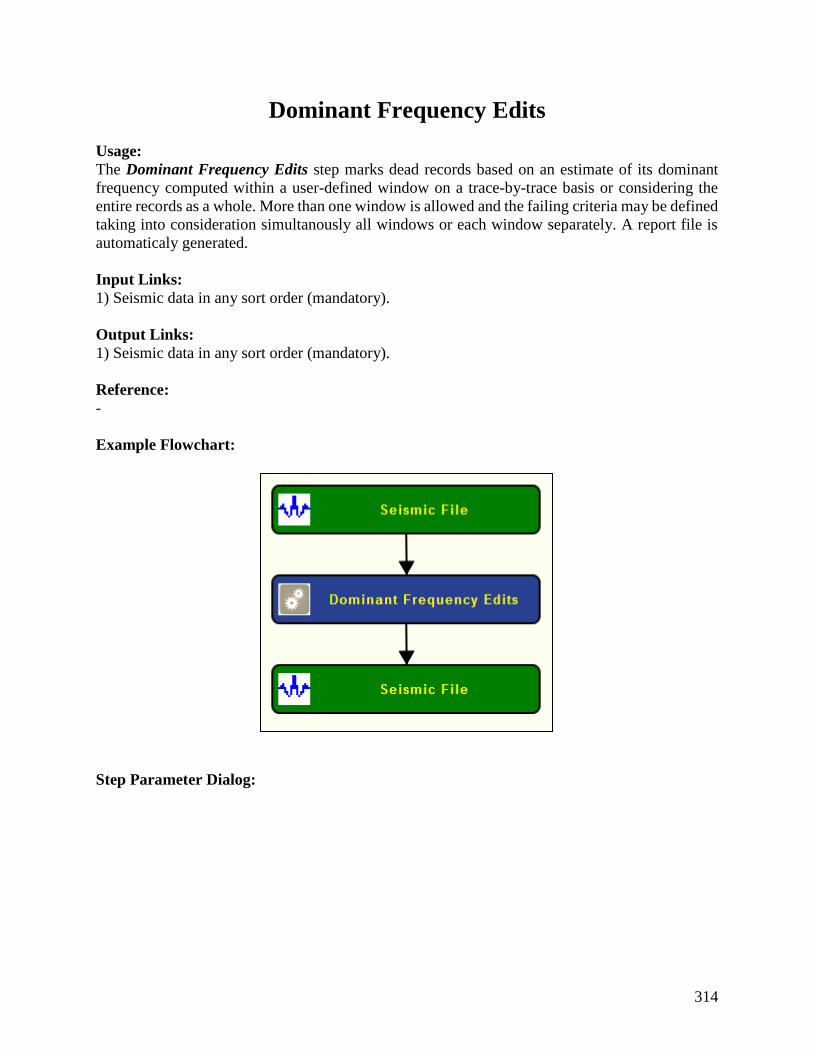
314

Dominant Frequency Edits

Usage:

The Dominant Frequency Edits step marks dead records based on an estimate of its dominant

frequency computed within a user-defined window on a trace-by-trace basis or considering the

entire records as a whole. More than one window is allowed and the failing criteria may be defined

taking into consideration simultanously all windows or each window separately. A report file is

automaticaly generated.

Input Links:

1) Seismic data in any sort order (mandatory).

Output Links:

1) Seismic data in any sort order (mandatory).

Reference:

-

Example Flowchart:

Step Parameter Dialog:

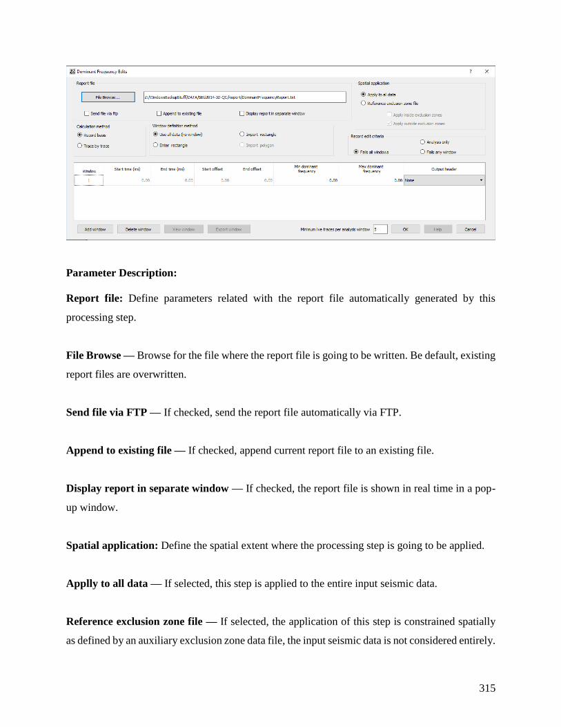
315

Parameter Description:

Report file: Define parameters related with the report file automatically generated by this

processing step.

File Browse — Browse for the file where the report file is going to be written. Be default, existing

report files are overwritten.

Send file via FTP — If checked, send the report file automatically via FTP.

Append to existing file — If checked, append current report file to an existing file.

Display report in separate window — If checked, the report file is shown in real time in a pop-

up window.

Spatial application: Define the spatial extent where the processing step is going to be applied.

Applly to all data — If selected, this step is applied to the entire input seismic data.

Reference exclusion zone file — If selected, the application of this step is constrained spatially

as defined by an auxiliary exclusion zone data file, the input seismic data is not considered entirely.

316

Apply inside exclusion zone — If checked, only the data inside the exclusion zone is

considered for the calculations.

Apply outside exclusion zone — If checked, only the data outside the exclusion zone is

considered for the calculations.

Calculation method: This processing step may be applied either on a record basis or trace-by-

trace basis.

Record basis — If selected, the dominant frequency is computed for the entire record as a whole.

Trace by trace — If selected, the dominant frequency is computed considering each trace

individually.

Window definition method: The estimate might be computed within a user-defined window, or

windows, defined by its start and end time and offset. Seismic samples outside these windows are

not considered.

Use all data (no window) — If selected, all seismic samples are considered. There are no

constraints in terms of time or offset.

Enter rectangle — If selected, enables the table below where the user can define the top, bottom,

start and end offset of each window considered.

Import rectangle — If selected, the windows are defined by an auxiliary rectangle data file.

Import polygon — Not yet available.

Record edit criteria: Define the criteria to consider a good or bad record.

317

Fails all windows — If selected, the record is considered dead if it fails in all the defined

windows simultaneously.

Analysis only — If selected, any recorded is marked as dead. This processing step is

considered just an analysis tool.

Fails any window — If selected, the record is considered dead if it fails in on of the defined

windows.

Window: Define the extent of each window where the estimate of the dominant frequency is

computed.

Start time (ms) — Enter the start time, in ms, for each window.

End time (ms) — Enter the end time, in ms, for each window.

Start offset — Enter the start offset for each window.

End offset — Enter the end offset for each window.

Min dominant frequency — Enter the minimum dominant frequency that a given window must

have for the record to be considered good.

Max dominant frequency — Enter the maximum dominant frequency that a given window must

have for the record to be considered good.

Output header — Select the header location where the flag for good/bad records is stored.

Add window — Select if more than one window per record is going to considered.

318

Delete window — Select to remove an existing window.

View window — Not yet available.

Export window — Not yet available.

Minimum live traces per analysis window — Enter the minimum number of live traces that mus

exit within each window for the estimation.

F-X Trace Interpolation

Usage:

The F-X Trace Interpolation step performs a 2-to-1 f-x domain interpolation of the input gather.

Trace headers of the interpolated traces are equal to the average of their two neighbors. The Trace

Flag header field of the interpolated traces will be equal to 28 on output.

Input Links:

1) Seismic data in any sort order (mandatory).

Output Links:

1) Seismic data with interpolated traces.

Reference:

Spitz, S., 1991 Seismic trace interpolation in the f-x domain, Geophysics, 56, p. 785.

Example Flowchart:

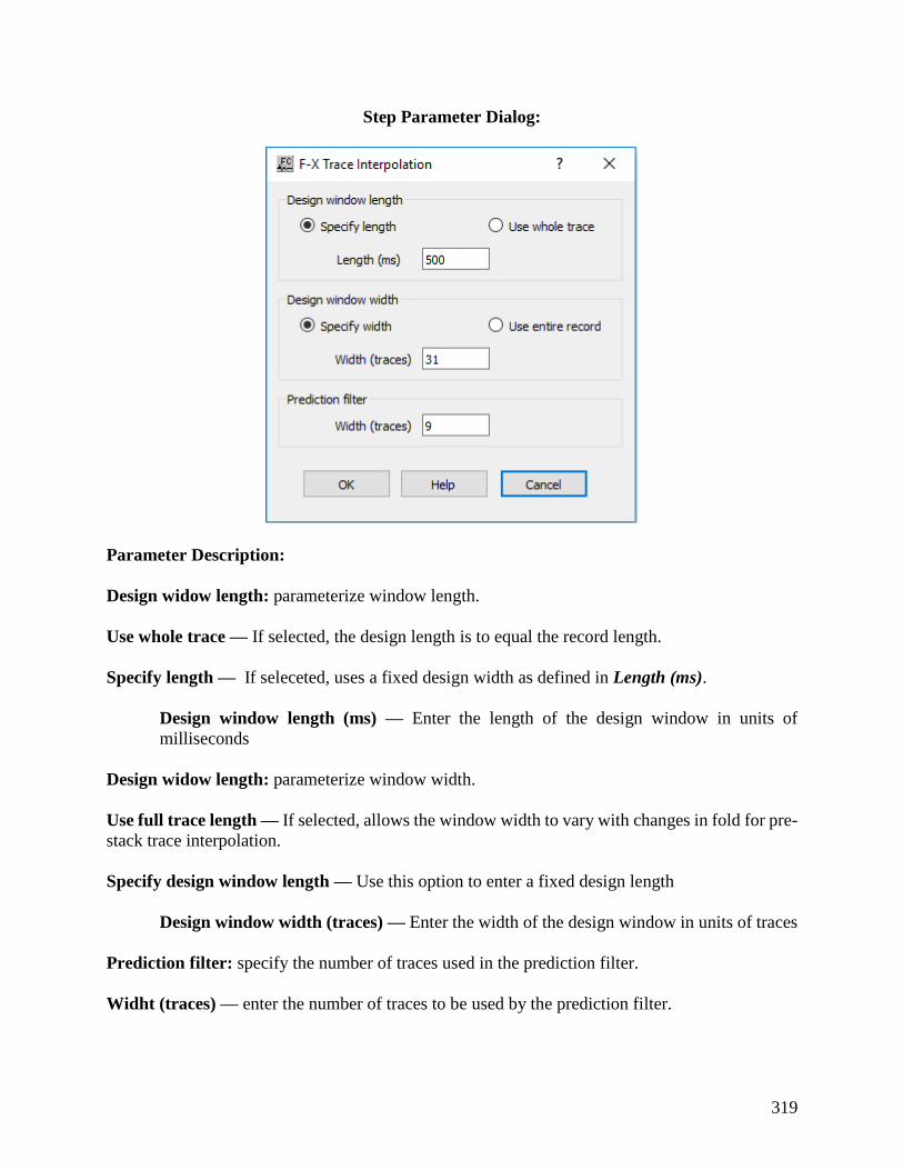
319

Step Parameter Dialog:

Parameter Description:

Design widow length: parameterize window length.

Use whole trace — If selected, the design length is to equal the record length.

Specify length — If seleceted, uses a fixed design width as defined in Length (ms).

Design window length (ms) — Enter the length of the design window in units of

milliseconds

Design widow length: parameterize window width.

Use full trace length — If selected, allows the window width to vary with changes in fold for pre-

stack trace interpolation.

Specify design window length — Use this option to enter a fixed design length

Design window width (traces) — Enter the width of the design window in units of traces

Prediction filter: specify the number of traces used in the prediction filter.

Widht (traces) — enter the number of traces to be used by the prediction filter.

320

Frequency Trace Edits

The Frequency Trace Edits step marks dead records based on an estimate of its frequency

computed content within a user-defined window on a trace-by-trace basis or considering the entire

records as a whole. More than one window is allowed and the failing criteria may be defined taking

into consideration simultanously all windows or each window separately. A report file is

automaticaly generated.

Input Links:

1) Seismic data in any sort order (mandatory).

Output Links:

1) Seismic data in any sort order (mandatory).

Reference:

-

Example Flowchart:

Step Parameter Dialog:

321

Parameter Description:

Report file: Define parameters related with the report file automatically generated by this

processing step.

File Browse — Browse for the file where the report file is going to be written. Be default, existing

report files are overwritten.

Send file via FTP — If checked, send the report file automatically via FTP.

Append to existing file — If checked, append current report file to an existing file.

Display report in separate window — If checked, the report file is shown in real time in a pop-

up window.

Spatial application: Define the spatial extent where the processing step is going to be applied.

Applly to all data — If selected, this step is applied to the entire input seismic data.

Reference exclusion zone file — If selected, the application of this step is constrained spatially

as defined by an auxiliary exclusion zone data file, the input seismic data is not considered entirely.

322

Apply inside exclusion zone — If checked, only the data inside the exclusion zone is

considered for the calculations.

Apply outside exclusion zone — If checked, only the data outside the exclusion zone is

considered for the calculations.

Calculation method: This processing step may be applied either on a record basis or trace-by-

trace basis.

Record basis — If selected, the dominant frequency is computed for the entire record as a whole.

Trace by trace — If selected, the dominant frequency is computed considering each trace

individually.

Window definition method: The estimate might be computed within a user-defined window, or

windows, defined by its start and end time and offset. Seismic samples outside these windows are

not considered.

Use full trace — If selected, all seismic samples are considered. There are no constraints in terms

of time or offset.

Enter rectangle — If selected, enables the table below where the user can define the top, bottom,

start and end offset of each window considered.

Import rectangle — If selected, the windows are defined by an auxiliary rectangle data file.

Import polygon — Not yet available.

Record edit criteria: Define the criteria to consider a good or bad record.

323

Fails all windows — If selected, the record is considered dead if it fails in all the defined

windows simultaneously.

Analysis only — If selected, any recorded is marked as dead. This processing step is

considered just an analysis tool.

Fails any window — If selected, the record is considered dead if it fails in on of the defined

windows.

Window: Define the extent of each window where the estimate of the dominant frequency is

computed.

Start time (ms) — Enter the start time, in ms, for each window.

End time (ms) — Enter the end time, in ms, for each window.

Start offset — Enter the start offset for each window.

End offset — Enter the end offset for each window.

Min frequency — Enter the minimum dominant frequency that a given window must have for the

record to be considered good.

Max frequency — Enter the maximum dominant frequency that a given window must have for

the record to be considered good.

Output header — Select the header location where the flag for good/bad records is stored.

Add window — Select if more than one window per record is going to considered.

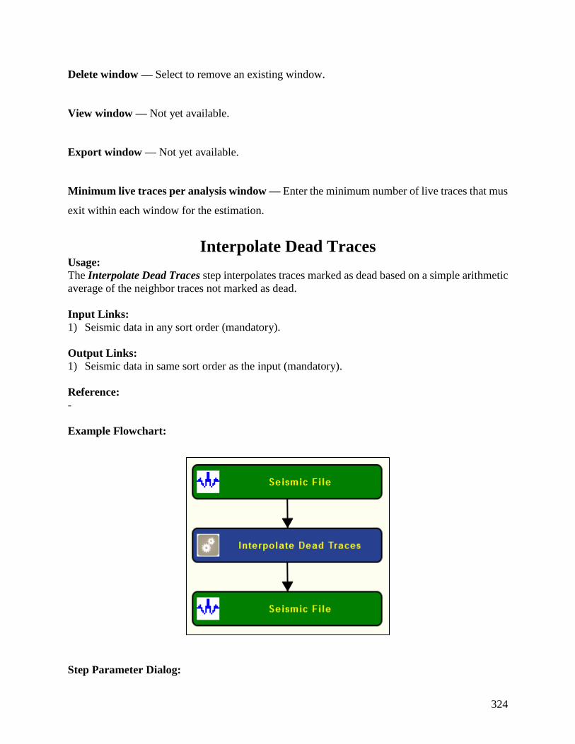
324

Delete window — Select to remove an existing window.

View window — Not yet available.

Export window — Not yet available.

Minimum live traces per analysis window — Enter the minimum number of live traces that mus

exit within each window for the estimation.

Interpolate Dead Traces Usage:

The Interpolate Dead Traces step interpolates traces marked as dead based on a simple arithmetic

average of the neighbor traces not marked as dead.

Input Links:

1) Seismic data in any sort order (mandatory).

Output Links:

1) Seismic data in same sort order as the input (mandatory).

Reference:

-

Example Flowchart:

Step Parameter Dialog:

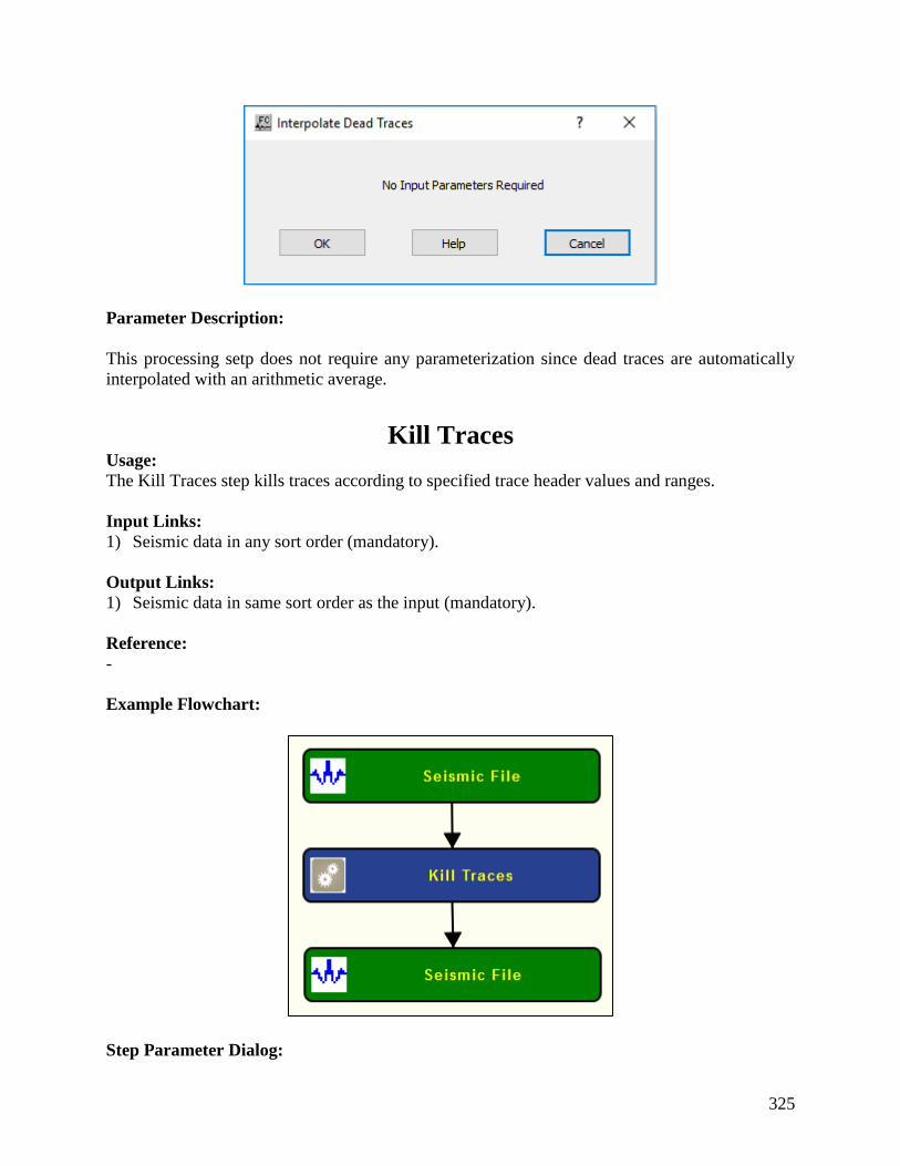
325

Parameter Description:

This processing setp does not require any parameterization since dead traces are automatically

interpolated with an arithmetic average.

Kill Traces Usage:

The Kill Traces step kills traces according to specified trace header values and ranges.

Input Links:

1) Seismic data in any sort order (mandatory).

Output Links:

1) Seismic data in same sort order as the input (mandatory).

Reference:

-

Example Flowchart:

Step Parameter Dialog:

326

Parameter Description:

Primary header — Select the first trace header field to use for killing traces. This is combined

with the other selected header key values to determine the set of traces to kill.

Primary start — Enter the start value for the first selected header field.

Primary stop — Enter the end value for the first selected header field.

Secondary header — Select the second trace header field to use for killing traces. This is

combined with the other selected header key values to determine the set of traces to kill.

Secondary start — Enter the start value for the second selected header field.

Secondary stop — Enter the end value for the second selected header field.

Tertiary header — Select the third trace header field to use for killing traces. This is combined

with the other selected header key values to determine the set of traces to kill.

Tertiary start — Enter the start value for the third selected header field.

Tertiary stop — Enter the end value for the third selected header field.

Import — Import a set of picked trace kills from a Trace Kills auxiliary dataset.

Export — Export the entered trace kills into a Trace Kills auxiliary dataset.

Add Row — Add a row to dialog.

Delete Row — Delete a row from the dialog.

Set dead trace amplitude to zero — If checked, fill dead traces with zeros.

Phase Rotation Usage:

327

The Phase Rotation step allows you to rotate your seismic traces by a constant phase angle from

–180 to +180 degrees. Values outside this range will be wrapped back into this range (i.e. 240

degrees is equivalent to –60 degrees).

Input Links:

1) Seismic data in any sort order (mandatory).

Output Links:

1) Seismic data in same sort order as the input (mandatory).

Reference:

-

Example Flowchart:

Step Parameter Dialog:

328

Parameter Description:

Rotate based on header value — If checked, the phase rotation is only applied to some traces in

the dataset, then a trace header value may be used to control which traces are rotated. An example

of where this is useful is transition zone seismic where some receivers in a line are geophones and

some are hydrophones. Rotating the hydrophone by -90 matches the data from the geophone.

If Component trace header — Select the trace header to be used for controlling the

operation.

== — Select the logic operator (<, <=, ==, >, >= or !=) to be used in determining the traces

to used in the operation and enter the value of the logical condition.

Rotate by angle stored in trace header value — If checked, does a constant phase rotation, a

header value (degrees) may be used.

Rotation angle in trace header — Select the trace header word containing the rotation

angle (degrees).

Phase rotation angle (degrees) — Enter the constant phase rotation angle to apply to all the

seismic data traces unless Rotate by angle stored in trace header value is checked.

Remove DC Bias Usage:

The Remove DC Bias step removes the average, median or mean DC bias on a trace-by-trace basis

or based on a moving average window which may run per channel or gather. The calculation

window may be limited within a userd-defined time gate.

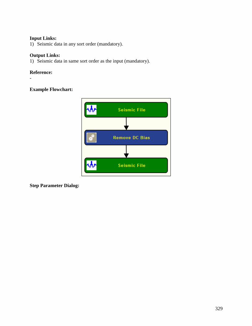
329

Input Links:

1) Seismic data in any sort order (mandatory).

Output Links:

1) Seismic data in same sort order as the input (mandatory).

Reference:

-

Example Flowchart:

Step Parameter Dialog:

330

Parameter Description:

DC calculation method: select the method to estimate the DC bias.

Mean — If selected, estimates the DC bias as the mean of the seismic samples considered.

Median — If selected, estimates the DC bias as the median of the seismic samples considered.

(Min+Max)/2 — If selected, estimates the DC bias as central value between the min and max of

the seismic samples considered.

Chanel Average: DC bias may be estimated using a moving window running through channels in

order to increase the reliability of the estimate.

Use running average across channels — If checked the DC bias is estimate taking into account

a moving window computed across channels.

331

Number of channels to average — Enter the number of channels that belong to the

moving window.

Gather Average: DC bias may be estimated using a moving window running through gathers (or

records) in order to increase the reliability of the estimate.

Use running average across prior gathers — If checked the DC bias is estimate taking into

account a moving window computed across prior gathers.

Number of gathers to average — Enter the number of gathers that belong to the moving

window.

DC calculation window: define the time gate where the calculation is going to be computed.

Calculate DC in a window — If checked, only the entered window of each trace will be used to

calculate the DC.

Minimum time (ms) — Enter the start time of the window to be used for calculating the

DC value.

Maximum time (ms) — Enter the ending time of the window to be used for calculating

the DC value.

Remove Reverberation Usage:

The Remove Reverberation step searches for reverberations in the signal and attempts to remove

these using an adaptive filtering technique.

Input Links:

1) Seismic data in any sort order (mandatory).

Output Links:

1) Seismic data in same sort order as the input (mandatory).

Reference:

-

Example Flowchart:

332

Step Parameter Dialog:

Parameter Description:

Minimum delay time — Enter the minimum delay time to use in searching for the reverberation.

Minimum offset — Enter the minimum offset to use in searching for the reverberation.

Maximum offset — Enter the maximum offset to use in searching for the reverberation.

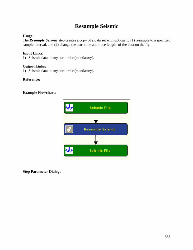
333

Resample Seismic

Usage:

The Resample Seismic step creates a copy of a data set with options to (1) resample to a specified

sample interval, and (2) change the start time and trace length of the data on the fly.

Input Links:

1) Seismic data in any sort order (mandatory).

Output Links:

1) Seismic data in any sort order (mandatory).

Reference:

-

Example Flowchart:

Step Parameter Dialog:

334

Parameter Description:

Sample interval: modify the sample interval of the input seismic data.

Change sample interval — If checked, the traces will be resampled to the specified sample

interval.

Output sample interval (ms) — Enter the new sampling interval in ms.

Anti-alias Filter: apply an anti-alias filter to the data after the resampling.

Apply anti-alias filter — If checked, apply an anti-alias filter after the resampling.

Cutoff (%Nyquist) — Enter the percentage of the Nyquist frequency at which an anti-

alias filter is applied.

Rolloff (db/Octave) — Enter the rolloff of the filter in dB/Octave.

Trace length: modify the original length of the input seismic traces.

335

Change Length — If checked, the traces will be truncated or extended to the specified length.

Start time (ms) — Enter the start time of the trace to output in milliseconds.

Length (ms) — Enter the length of the trace to output in milliseconds

Reverse Traces Usage:

The Reverse Traces step allows you to invert the polarity of traces according specified trace header

values and ranges.

Input Links:

1) Seismic data in any sort order (mandatory).

Output Links:

1) Seismic data in same sort order as the input (mandatory).

Reference:

-

Example Flowchart:

Step Parameter Dialog:

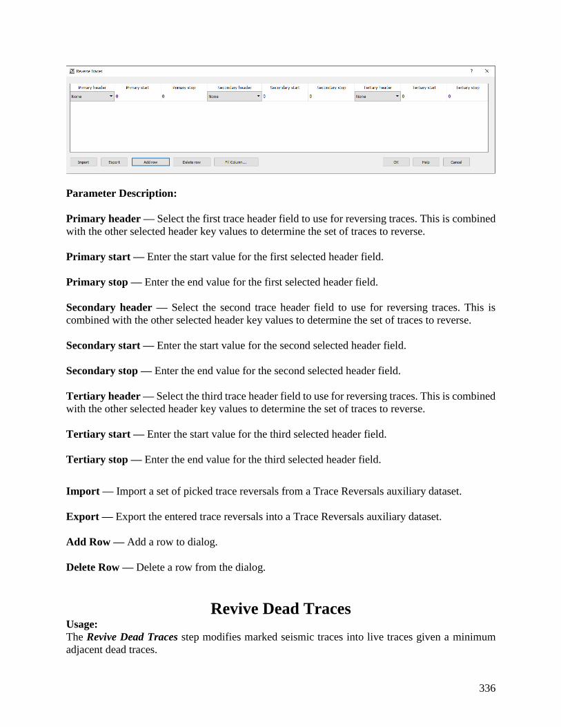
336

Parameter Description:

Primary header — Select the first trace header field to use for reversing traces. This is combined

with the other selected header key values to determine the set of traces to reverse.

Primary start — Enter the start value for the first selected header field.

Primary stop — Enter the end value for the first selected header field.

Secondary header — Select the second trace header field to use for reversing traces. This is

combined with the other selected header key values to determine the set of traces to reverse.

Secondary start — Enter the start value for the second selected header field.

Secondary stop — Enter the end value for the second selected header field.

Tertiary header — Select the third trace header field to use for reversing traces. This is combined

with the other selected header key values to determine the set of traces to reverse.

Tertiary start — Enter the start value for the third selected header field.

Tertiary stop — Enter the end value for the third selected header field.

Import — Import a set of picked trace reversals from a Trace Reversals auxiliary dataset.

Export — Export the entered trace reversals into a Trace Reversals auxiliary dataset.

Add Row — Add a row to dialog.

Delete Row — Delete a row from the dialog.

Revive Dead Traces Usage:

The Revive Dead Traces step modifies marked seismic traces into live traces given a minimum

adjacent dead traces.

337

Input Links:

1) Seismic data in any sort order (mandatory).

Output Links:

1) Seismic data in same sort order as the input (mandatory).

Reference:

-

Example Flowchart:

Step Parameter Dialog:

338

Parameter Description:

Minmum number adjacent traces — Enter the minimum number of adjacent dead traces that

must exist to be modified into live traces.

S/N Based Record Edits Usage:

The S/N Based Record Edits step marks dead records based on an estimate of its signal-to-noise

ratio computed within a user-defined window on a trace-by-trace basis or considering the entire

records as a whole. More than one window is allowed and the failing criteria may be defined taking

into consideration simultanously all windows or each window separately. A report file is

automaticaly generated.

Input Links:

1) Seismic data in any sort order (mandatory).

Output Links:

1) Seismic data in same sort order as the input (mandatory).

Reference:

-

Example Flowchart:

Step Parameter Dialog:

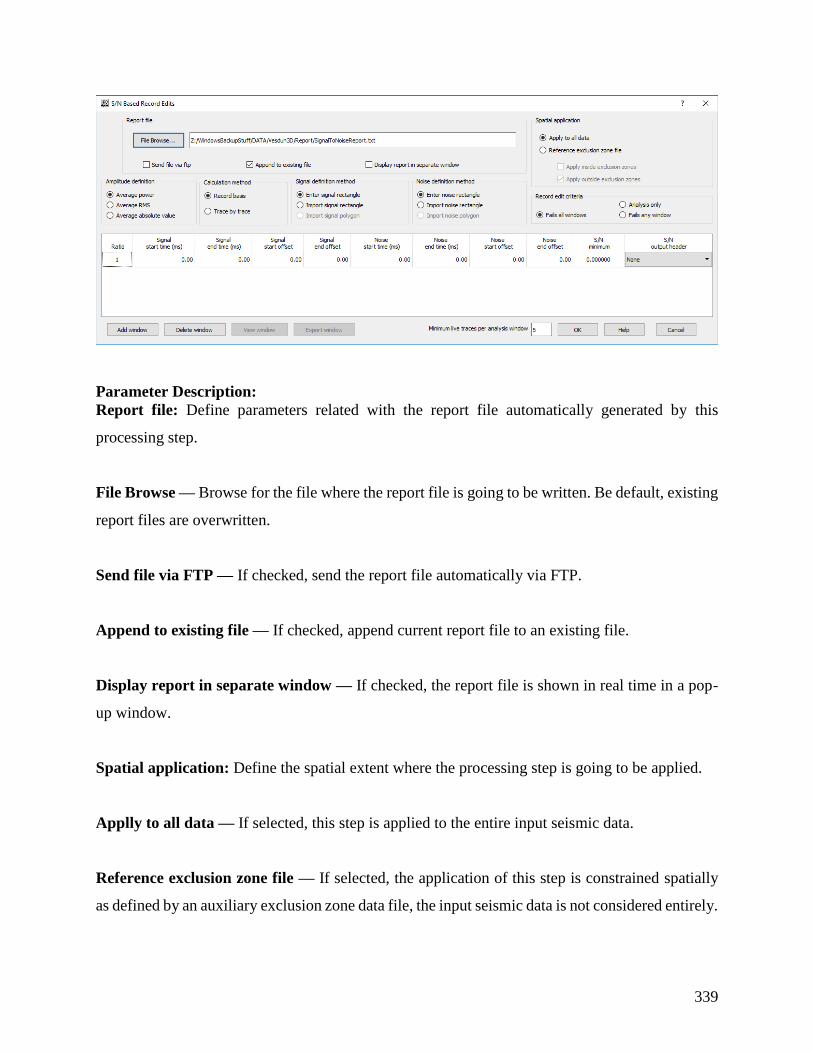
339

Parameter Description:

Report file: Define parameters related with the report file automatically generated by this

processing step.

File Browse — Browse for the file where the report file is going to be written. Be default, existing

report files are overwritten.

Send file via FTP — If checked, send the report file automatically via FTP.

Append to existing file — If checked, append current report file to an existing file.

Display report in separate window — If checked, the report file is shown in real time in a pop-

up window.

Spatial application: Define the spatial extent where the processing step is going to be applied.

Applly to all data — If selected, this step is applied to the entire input seismic data.

Reference exclusion zone file — If selected, the application of this step is constrained spatially

as defined by an auxiliary exclusion zone data file, the input seismic data is not considered entirely.

340

Apply inside exclusion zone — If checked, only the data inside the exclusion zone is

considered for the calculations.

Apply outside exclusion zone — If checked, only the data outside the exclusion zone is

considered for the calculations.

Amplitude Definition: Select the type of amplitude to be computed during this editing processing

step.

Average power — If selected, compute the average power of the input seismic amplitudes.

Average RMS — If selected, compute the average RMS of the input seismic amplitudes.

Average absolute value — If selected, compute the average of the absolute value of the input

seismic amplitudes.

Calculation method: This processing step may be applied either on a record basis or trace-by-

trace basis.

Record basis — If selected, the dominant frequency is computed for the entire record as a whole.

Trace by trace — If selected, the dominant frequency is computed considering each trace

individually.

Window definition method: The estimate might be computed within a user-defined window, or

windows, defined by its start and end time and offset. Seismic samples outside these windows are

not considered.

Use all data (no window) — If selected, all seismic samples are considered. There are no

constraints in terms of time or offset.

341

Enter rectangle — If selected, enables the table below where the user can define the top, bottom,

start and end offset of each window considered.

Import rectangle — If selected, the windows are defined by an auxiliary rectangle data file.

Import polygon — Not yet available.

Record edit criteria: Define the criteria to consider a good or bad record.

Fails all windows — If selected, the record is considered dead if it fails in all the defined

windows simultaneously.

Analysis only — If selected, any recorded is marked as dead. This processing step is

considered just an analysis tool.

Fails any window — If selected, the record is considered dead if it fails in on of the defined

windows.

Window: Define the extent of each window where the estimate of the dominant frequency is

computed.

Start time (ms) — Enter the start time, in ms, for each window.

End time (ms) — Enter the end time, in ms, for each window.

Start offset — Enter the start offset for each window.

End offset — Enter the end offset for each window.

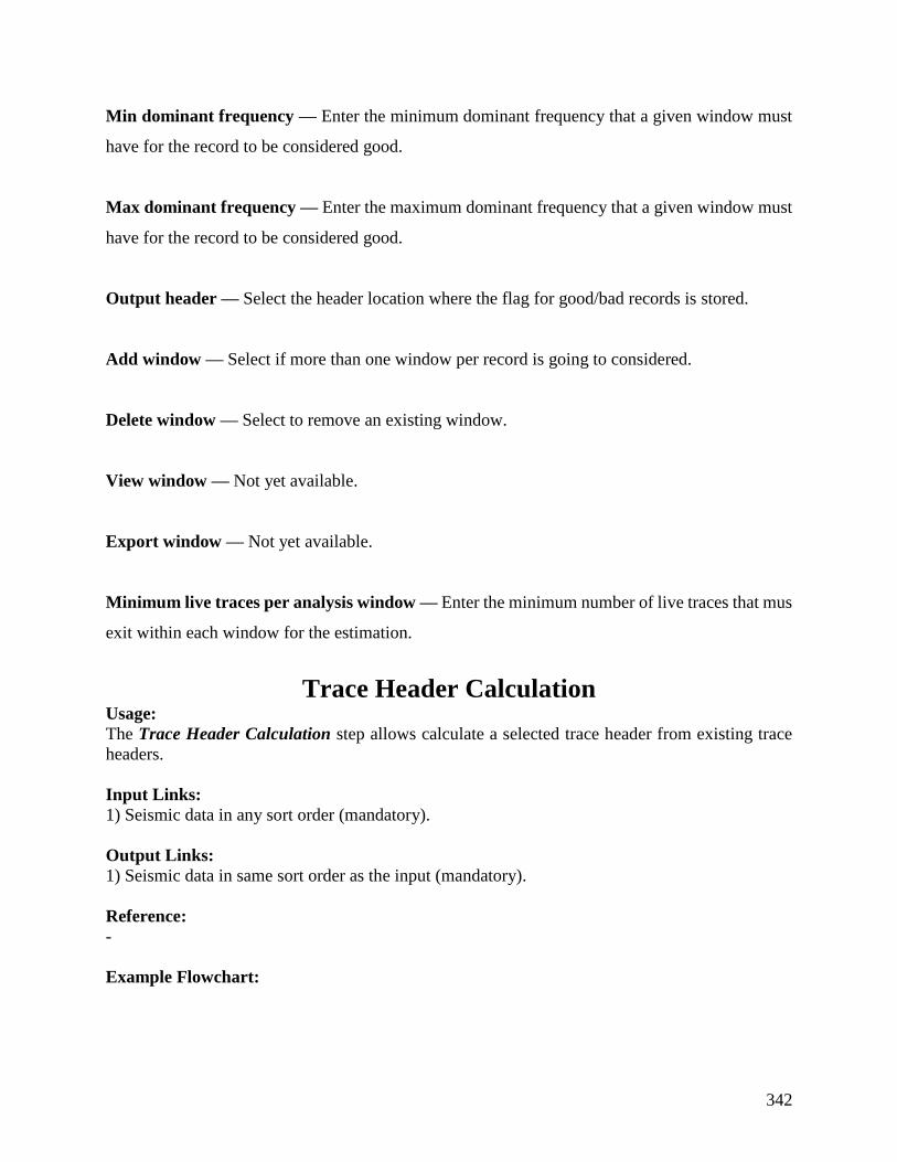
342

Min dominant frequency — Enter the minimum dominant frequency that a given window must

have for the record to be considered good.

Max dominant frequency — Enter the maximum dominant frequency that a given window must

have for the record to be considered good.

Output header — Select the header location where the flag for good/bad records is stored.

Add window — Select if more than one window per record is going to considered.

Delete window — Select to remove an existing window.

View window — Not yet available.

Export window — Not yet available.

Minimum live traces per analysis window — Enter the minimum number of live traces that mus

exit within each window for the estimation.

Trace Header Calculation Usage:

The Trace Header Calculation step allows calculate a selected trace header from existing trace

headers.

Input Links:

1) Seismic data in any sort order (mandatory).

Output Links:

1) Seismic data in same sort order as the input (mandatory).

Reference:

-

Example Flowchart:

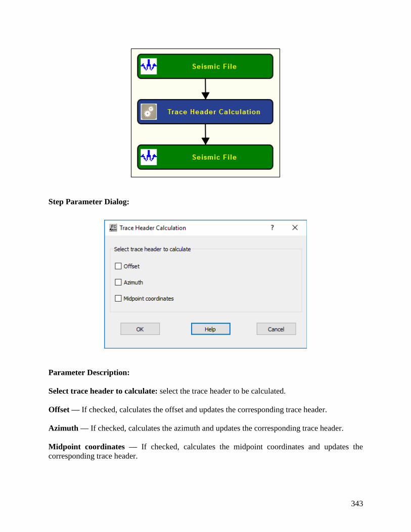
343

Step Parameter Dialog:

Parameter Description:

Select trace header to calculate: select the trace header to be calculated.

Offset — If checked, calculates the offset and updates the corresponding trace header.

Azimuth — If checked, calculates the azimuth and updates the corresponding trace header.

Midpoint coordinates — If checked, calculates the midpoint coordinates and updates the

corresponding trace header.

344

Trace Header Logic Usage:

The Trace Header Logic step allows you modify the trace header values of a seismic trace using

the relational operators and logic conditions characteristic of an If - Then – Else statement.

Input Links:

1) Seismic data in any sort order (mandatory).

Output Links:

1) Seismic data in same sort order as the input (mandatory).

Reference:

-

Example Flowchart:

Step Parameter Dialog:

345

Parameter Description:

if — Select the relational and logic conditions for which the then statement will be executed.

Header Field — Select the primary trace header field to be tested.

Relation — Select the primary relational operator

Header Field — If selected, the primary trace header field will be evaluated against the

chosen header field using the primary relational operator.

Constant — If selected, the primary trace header field will be evaluated against the user-

supplied constant using the primary relational operator.

Logic — If checked, the Logic option allows selection of a secondary header field using

and|or logic.

Header Field — Select the secondary trace header field to be tested.

Relation — Select the secondary relational operator

Header Field — If selected, the primary trace header field will be evaluated against the

chosen header field using the secondary relational operator.

Constant — If selected, the primary trace header field will be evaluated against the-user

supplied constant using the secondary relational operator.

346

then — Define the trace header operation to be performed in the case that the if conditions are

satisfied.

Header Field — Select the trace header field to be modified in the case that the if

conditions are satisfied.

Header Field — If selected, the header field selected above will be set equal to the chosen

header field.

Constant — If selected, the header field selected above will be set equal to the user-

supplied constant.

else — Define the trace header operation to be performed in the case that the if conditions are not

satisfied.

Header Field — Select the trace header field to be modified in the case that the if

conditions are not satisfied.

Header Field — If selected, the header field selected above will be set equal to the chosen

header field.

Constant — If selected, the header field selected above will be set equal to the user-

supplied constant.

Example: If the source-receiver azimuth is greater than or equal to zero, set the User Def 1 field

equal to +1. Otherwise, set the User Def 1 field equal to -1.

347

Trace Header Math Usage:

The Trace Header Math step allows you modify the trace header values of a seismic trace using

standard mathematical operations.

Input Links:

1) Seismic data in any sort order (mandatory).

Output Links:

1) Seismic data in same sort order as the input (mandatory).

Reference:

-

Example Flowchart:

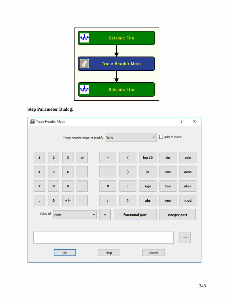
348

Step Parameter Dialog:

349

Parameter Description:

Trace header value to modify — Select trace header location to be modified.

Add to index — I checked, changed trace header is automatically updated in the index file.

The rest of the parameters are just like a regular calculator.

Example: Add 40 to the existing value of the Uphole time.

Trace Header Resequencing Usage:

The Trace Header Resequencing step is used to modify trace header values based on changes in

other trace header values.

Input Links:

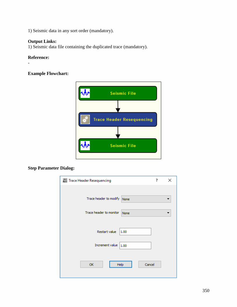
350

1) Seismic data in any sort order (mandatory).

Output Links:

1) Seismic data file containing the duplicated trace (mandatory).

Reference:

-

Example Flowchart:

Step Parameter Dialog:

351

Parameter Description:

Trace Header to Modify — Select the trace header field that will be modified.

Monitor Trace Header — Select the monitor trace header field. A change in value of the Monitor

Trace Header will result in a change in value of the Trace Header to Modify based on the following

two values:

Restart value — This value will be placed in the Trace Header to Modify whenever there is a

change in the Monitor Trace Header.

Increment value — This value will be added to the Restart value for each trace header in which

the Trace Header to Modify does not change.

Trace Sample Math Usage:

The Trace Sample Math step allows you operate at the trace seismic samples using some pre-

defined mathematical operations and two user-defined values.

Input Links:

1) Seismic data in any sort order (mandatory).

Output Links:

1) Seismic data in same sort order as the input (mandatory).

Example Flowchart:

Step Parameter Dialog:

352

Parameter Description:

Math operation: Select pre-defined mathematical operations to be applied to the trace seismic

samples of the input seismic file.

Value of a — Enter a value to be used in the selected mathematical operation replacing a.

Value of b — Enter a value to be used in the selected mathematical operation replacing b.

Vibroseis Correlation Usage:

The Vibroseis Correlation step cross correlates uncorrelated seismic data acquired with the

Vibroseis™ method with the corresponding vibroseis sweep. The correlated output data should be

considered zero phase.

Input Links:

1. Seismic data in any sort order (mandatory).

2) Seismic data — Vibroseis™ pilot sweeps (optional).

Output Links:

1) Seismic data in same sort order as the input (mandatory).

Example Flowchart:

353

Step Parameter Dialog:

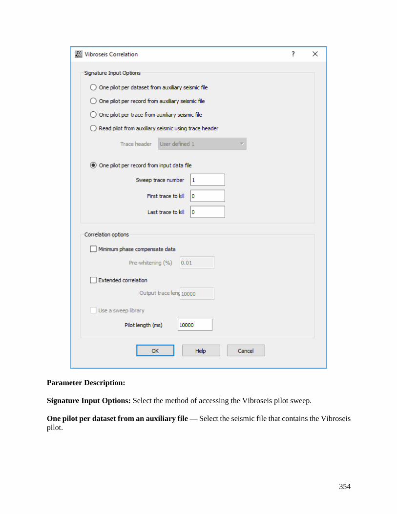
354

Parameter Description:

Signature Input Options: Select the method of accessing the Vibroseis pilot sweep.

One pilot per dataset from an auxiliary file — Select the seismic file that contains the Vibroseis

pilot.

355

One pilot per record from an auxiliary file — This option inputs one pilot trace in sequential

order from an auxiliary file and crosscorrelates that pilot signature with the respective sequential

record. Therefore, number of pilot traces should equal the number of input records.

One pilot per trace from an auxiliary file — This option inputs one pilot trace in sequential

order from an auxiliary file and crosscorrelates that pilot signature with the respective sequential

trace. Therefore, number of pilot traces should equal the number of input traces.

One pilot from auxiliary seismic using trace header — This option inputs one pilot trace based

on the selected traced heder from an auxiliary file and crosscorrelates that pilot signature with the

respective sequential trace. Therefore, number of pilot traces should equal the number of input

traces.

Trace header — Select trace header to be used to select the pilot.

One pilot per record from intput data file — This option uses one trace from the each of the

uncorrelated input records as the pilot trace for that record.

Sweep trace number — Enter the trace number to use as the pilot sweep.

First trace to kill — If you demultiplexed the data set with the auxiliary traces to recover

the pilot sweep, you may wish to kill these auxiliary traces so that the do not appear on

output. Enter the first trace number to kill.

Last trace to kill — If you demultiplexed the data set with the auxiliary traces to recover

the pilot sweep, you may wish to kill these auxiliary traces traces so that the do not appear

on output. Enter the last trace number to kill.

Pilot length (ms) — Enter the length of the pilot sweep in milliseconds.

Minimum phase compensate data —If checked, a minimum phase compensation filter will be

calculated and applied so that the correlated data will be minimum phase on output.

Extended Correlation — If checked, an extended correlation will be done using the entered trace

output length.

Output trace length (ms) — Enter the output length of the result of the cross correlation.

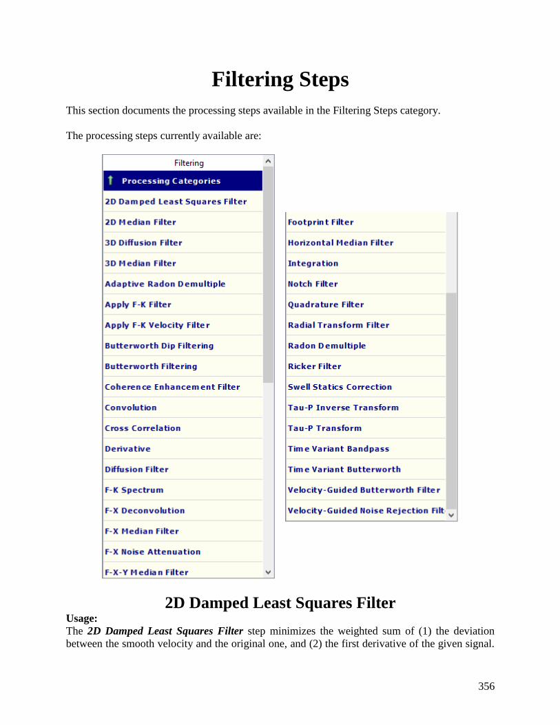
356

Filtering Steps

This section documents the processing steps available in the Filtering Steps category.

The processing steps currently available are:

2D Damped Least Squares Filter Usage:

The 2D Damped Least Squares Filter step minimizes the weighted sum of (1) the deviation

between the smooth velocity and the original one, and (2) the first derivative of the given signal.

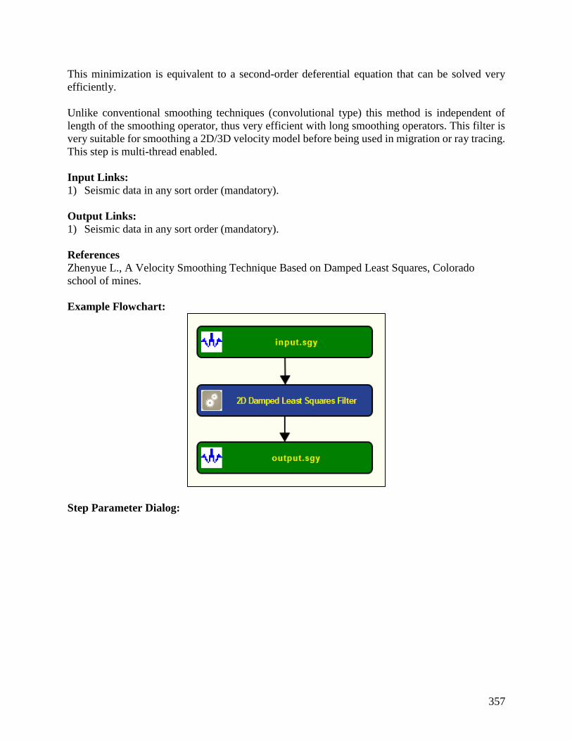
357

This minimization is equivalent to a second-order deferential equation that can be solved very

efficiently.

Unlike conventional smoothing techniques (convolutional type) this method is independent of

length of the smoothing operator, thus very efficient with long smoothing operators. This filter is

very suitable for smoothing a 2D/3D velocity model before being used in migration or ray tracing.

This step is multi-thread enabled.

Input Links:

1) Seismic data in any sort order (mandatory).

Output Links:

1) Seismic data in any sort order (mandatory).

References

Zhenyue L., A Velocity Smoothing Technique Based on Damped Least Squares, Colorado

school of mines.

Example Flowchart:

Step Parameter Dialog:

358

Parameter Description:

Apply spatially — If checked, the filter is applied in the horizontal direction.

Spatial smoothing operator — Enter the degree of the smoothing operator in the

horizontal direction.

Apply temporally (or depth) — If checked, the filter is applied in the vertical direction.

Temporal smoothing operator — Enter the degree of the smoothing operator in the

vertical direction.

Define a window — If checked, the smoothing will be applied only within the specified window

Window smoothing parameter — Enter the smoothing operator value between the

window and the rest of the record.

First trace — first trace defining the window.

Last trace — last trace defining the window.

First sample — first sample defining the window.

Last sample — last sample defining the window.

2D Median Filter

Usage:

The 2D Median Filter step is a single channel filter that may be used to remove spikes from your

data or any other features, such as the wow in radar, which may be filtered by a median operator.

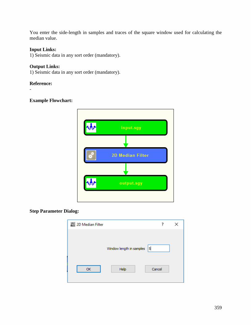
359

You enter the side-length in samples and traces of the square window used for calculating the

median value.

Input Links:

1) Seismic data in any sort order (mandatory).

Output Links:

1) Seismic data in any sort order (mandatory).

Reference:

-

Example Flowchart:

Step Parameter Dialog:

360

Parameter Description:

Window length in samples — Enter the number of samples in the window over which the median

will be calculated. The sample at the windows center will be replaced by the calculated median

value.

3D Diffusion Filter Usage:

The 3D Diffusion Filter step is an anisotropic diffusion filter which performs edge-preserving

smoothing in three dimensions. It is intended to be used to enhance post-stack 3D data.

The input data in the form of time traces does not require prior slicing or transformation.

Anisotropic diffusion is applied following structure in three dimensions using the Kuwahara filter.

For this reason, estimation of the dip field is a required integral initial step. Parameters to control

dip estimation are therefore required in addition to the diffusion parameters.

Due to parallel data handling, the output from 3D Diffusion Filter must be written directly to disk

using Seismic File without further processes in that job flow.

Input Links:

1) 3D seismic data ordered by CMP Line and CMP Location (mandatory).

Output Links:

1) 3D seismic data ordered by CMP Line and CMP Location (mandatory).

Reference:

Fehmers, G.C, and Hocker, C.F.W., 2003, Fast structural interpretation with structure-oriented

filters, Geophysics, vol. 68, no. 4, p. 1286-1293.

Example Flowchart:

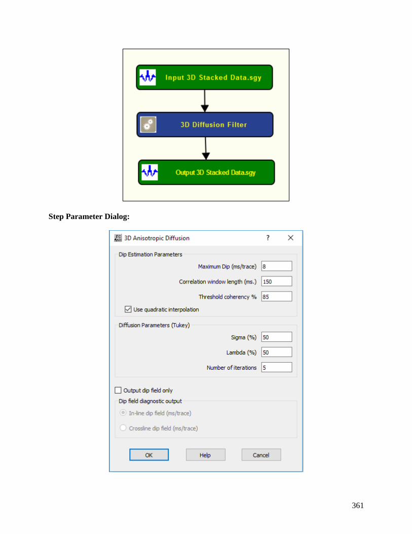
361

Step Parameter Dialog:

362

Parameter Description:

Dip estimation paramters: define the parameters for dip estimation that is used for the edge

preserving filter.

Maximum Dip (ms/trace) — Enter the maximum dip to be considered in the filter.

Correlation window length (ms.) — Enter the correlation window length for the dip scanning.

An initial stage of dip estimation is cross-correlation of adjacent traces. This length should be

sufficient to obtain stable dip estimates without being so long as to lose local structure changes.

Threshold coherency % — Enter a normalised correlation values must exceed this % for the

estimated dip at a point to be considered valid.

Use quadratic interpolation — If checked, the dips are better estimated using a quadratic

estimation formula.

Difussion parameters (Tukey): define parameters that allow distinguish noise from signal.

Sigma (%) — Enter the noise threshold as a percentage of standard deviations

Lambda (%) — Enter the percentage of new values to add on each filter iteration

Number of iterations — Enter the number of filter iteration to apply to the input data.

Output dip field only — If checked, only the estimated inline or cross-line dip field will

be output. This is for diagnostic use: If the estimated dip field output is not smooth and

contain spikes then the diffusion process will not be optimal. In this case the dip estimation

parameters should be modified until a reasonable dip field is output.

In-line dip field (ms/trace) — If checked, the dip field output will be the estimated in-line

dip field.

Crossline dip field (ms/trace) — If checked, the dip field output will be the estimated

crossline dip field.

3D Median Filter Usage:

The 3D Median Filter step is a filter with multiple uses which may be used for both single and

multi-channel processing.

The input data in the form of time traces does not require prior slicing or transformation.

In ‘Apply’ mode, 3D Median Filter replaces the input data samples with the median value of the

surrounding values as specified by the filter size. In this mode the filter may be used to enhance

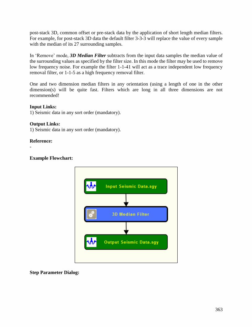
363

post-stack 3D, common offset or pre-stack data by the application of short length median filters.

For example, for post-stack 3D data the default filter 3-3-3 will replace the value of every sample

with the median of its 27 surrounding samples.

In ‘Remove’ mode, 3D Median Filter subtracts from the input data samples the median value of

the surrounding values as specified by the filter size. In this mode the filter may be used to remove

low frequency noise. For example the filter 1-1-41 will act as a trace independent low frequency

removal filter, or 1-1-5 as a high frequency removal filter.

One and two dimension median filters in any orientation (using a length of one in the other

dimension(s) will be quite fast. Filters which are long in all three dimensions are not

recommended!

Input Links:

1) Seismic data in any sort order (mandatory).

Output Links:

1) Seismic data in any sort order (mandatory).

Reference:

-

Example Flowchart:

Step Parameter Dialog:

364

Parameter Description:

Apply median filter — If selected, the data will be replaced by the median values as calculated

by the specified filter. Use to enhance the data by removing random noise with a short filter in two

or three dimensions.

Remove median filter — If selected, the median values as calculated by the specified filter will

be subtracted from the input data. Use to remove low frequency noise with a long filter in one or

two dimensions

Filter size: define the size of the filter to be applied.

Width in traces — Enter the number of traces within each record used to estimate median values.

Depth (records) in traces — Enter the number of neighboring records used to estimate median

values. Note: this assumes sufficient similarity of adjacent records such as use in post-stack 3d

data.

Height in samples — Enter the median filter length in the trace direction.

Adaptive Radon Demultiple Usage:

The Adaptive Radon Demultiple step performs parabolic radon demultiple through a modeling of

primaries, multiples, and noise in the parabolic radon domain followed by subtraction of multiples

and noise in the time domain. You specify the transform type, the range of ray parameters in the

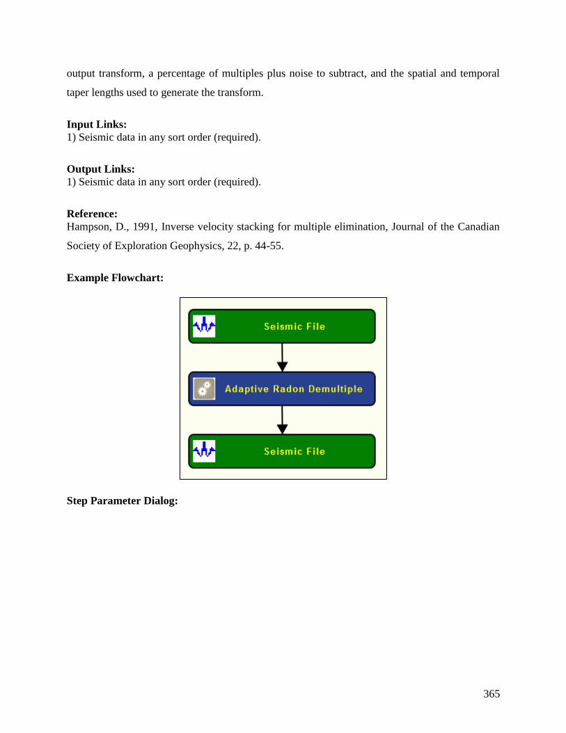
365

output transform, a percentage of multiples plus noise to subtract, and the spatial and temporal

taper lengths used to generate the transform.

Input Links:

1) Seismic data in any sort order (required).

Output Links:

1) Seismic data in any sort order (required).

Reference:

Hampson, D., 1991, Inverse velocity stacking for multiple elimination, Journal of the Canadian

Society of Exploration Geophysics, 22, p. 44-55.

Example Flowchart:

Step Parameter Dialog:

366

367

Parameter Description:

Time window: Specify time parameters.

Limit application time — If checked, the application time for the filter may be limited by using

an input horizon or by using a constant time.

Start time referenced to horizon — If selected, reference start time to a horizon for the

filter.

Multiplier for time horizon — Enter the multiplier for time horizon.

Use constant start time — If seleceted, a constant time for limiting the application zone

for the filter.

Start time (ms) — Enter the start time in milliseconds for the application window

of the filter.

Length of taper zone (ms) — Enter the taper length for the transition zone for the

windows. A Hanning taper is used.

Ray parameters: Specify ray parameters.

Set number of ray parameters — If checked, the number of ray parameters to be calculated will

be the number entered below. If not checked, the number of ray parameters will be equal to the

number of traces in the input gather.

Number of ray parameters — Enter the constant number of ray parameters to calculate

for each gather.

Bandpass filter: Specify bandpass filter parameters.

Low cut (Hz) — Enter the low cut frequency in Hertz for the bandpass filter.

Low pass (Hz) — Enter the low pass frequency in Hertz for the bandpass filter.

High pass (Hz) — Enter the high pass frequency in Hertz for the bandpass filter.

High cut (Hz) — Enter the high cut frequency in Hertz for the bandpass filter.

Model moveout: Set the range of parabolas that will generate the primary and multiple models.

Use differential moveout – If selected, specify the radon parameters in terms of differential

moveout at far offset.

368

Minimum — Enter the minimum differential moveout for calculation of the radon

transform expressed in milliseconds on the far-offset trace. The primary model is generated

with parabolas from the <minimum differential moveout> to the <minimum multiple

moveout>.

Maximum — Enter the maximum differential moveout for the calculation of the radon

transform expressed in milliseconds on the far-offset trace. The multiple model is generated

with parabolas from the <minimum multiple moveout> to the <maximum differential

moveout>.

Minimum multiple — Enter the minimum mulitple differential moveout for the radon

filter expressed in milliseconds on the far-offset trace. All data between the minimum

multiple differential moveout and the maximum differential moveout will be removed by

the filter. The multiple model is generated with parabolas from the <minimum multiple

moveout> to the <maximum differential moveout>.

Use velocity — If selected. specify the radon filter parameterization using velocities.

Minimum moveout — Enter the minimum (negative usually) velocity for the radon

transform calculation.

Maximum moveout — Enter the maximum velocity for the radon transform calculation.

Minimum multiple moveout — Enter the minimum multiple moveout velocity for the

radon filter. The filter will remove data between the minimum multiple moveout velocity

and the maximum multiple moveout velocity.

Define maximum reference offset — If checked, a constant maximum offset will be used for the

calculation of the radon transform. The differential moveouts will be the delta times at this

specified offset.

Maximum reference offset — Enter a constant maximum offset to be used for the

calculation of the radon transform. The differential moveouts will be the delta times at this

specified offset.

Reference time (sec) — Enter the reference time in seconds where the velocities are

specified. This is used to convert the velocities to differential moveout for the radon

algorithim.

Additional parameters: Specify additional parameters.

Percent add-back — Enter the percentage of the original data to be blended with the output

filtered data.

Percent pre-whitening — Enter the percentage of pre-whitening to apply to the data for

stabilizing the algorithm.

369

Minimum live traces — Enter the minimum number of live traces per gather for applying the

filter. Gathers with fewer traces will be passed through to the output with no filtering applied.

AGC window — Set the parameters for an AGC window.

Apply and remove AGC – If checked, apply an AGC before the filter and remove the same AGC

after the filter.

AGC operator length (ms) — Enter the AGC operator length in milliseconds.

Type of output — If selected, the type of output desired.

Estimated primaries — If selected, output the estimated primaries.

Multiple model – Output the multiple data.

Example of Adaptive Radon Demultiple:

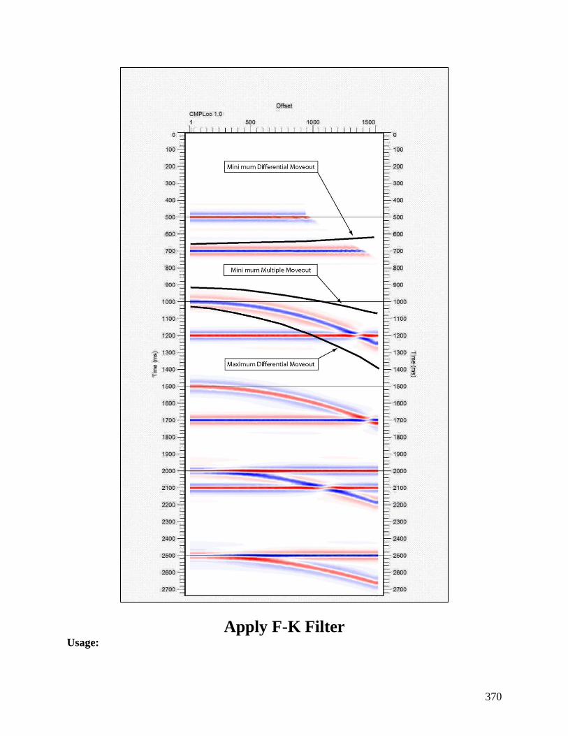
370

Apply F-K Filter Usage:

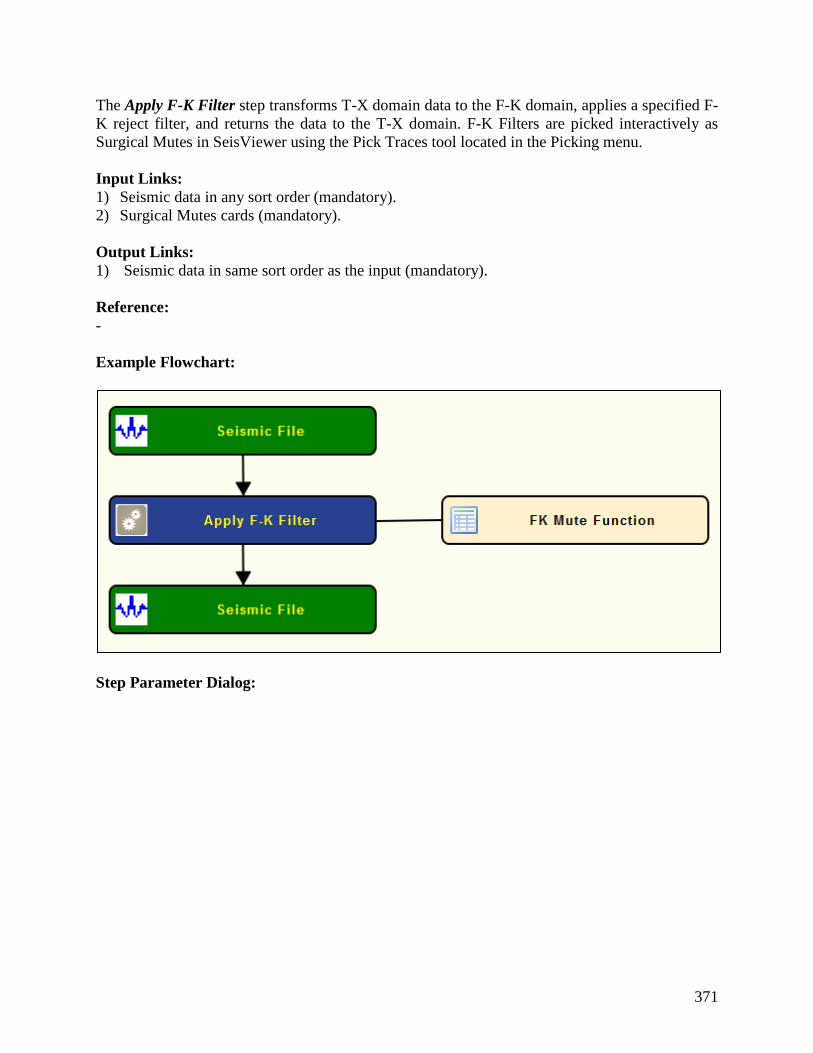
371

The Apply F-K Filter step transforms T-X domain data to the F-K domain, applies a specified F-

K reject filter, and returns the data to the T-X domain. F-K Filters are picked interactively as

Surgical Mutes in SeisViewer using the Pick Traces tool located in the Picking menu.

Input Links:

1) Seismic data in any sort order (mandatory).

2) Surgical Mutes cards (mandatory).

Output Links:

1) Seismic data in same sort order as the input (mandatory).

Reference:

-

Example Flowchart:

Step Parameter Dialog:

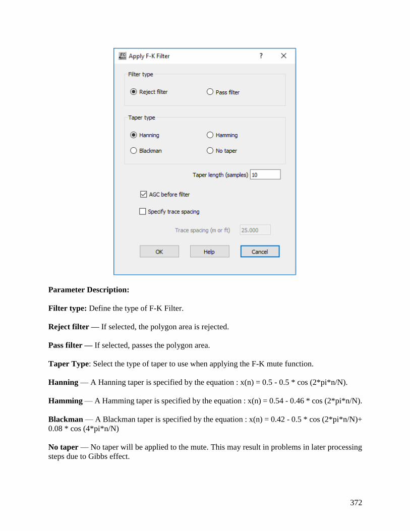
372

Parameter Description:

Filter type: Define the type of F-K Filter.

Reject filter — If selected, the polygon area is rejected.

Pass filter — If selected, passes the polygon area.

Taper Type: Select the type of taper to use when applying the F-K mute function.

Hanning — A Hanning taper is specified by the equation : x(n) = 0.5 - 0.5 * cos (2*pi*n/N).

Hamming — A Hamming taper is specified by the equation : x(n) = 0.54 - 0.46 * cos (2*pi*n/N).

Blackman — A Blackman taper is specified by the equation : x(n) = 0.42 - 0.5 * cos (2*pi*n/N)+

0.08 * cos (4*pi*n/N)

No taper — No taper will be applied to the mute. This may result in problems in later processing

steps due to Gibbs effect.

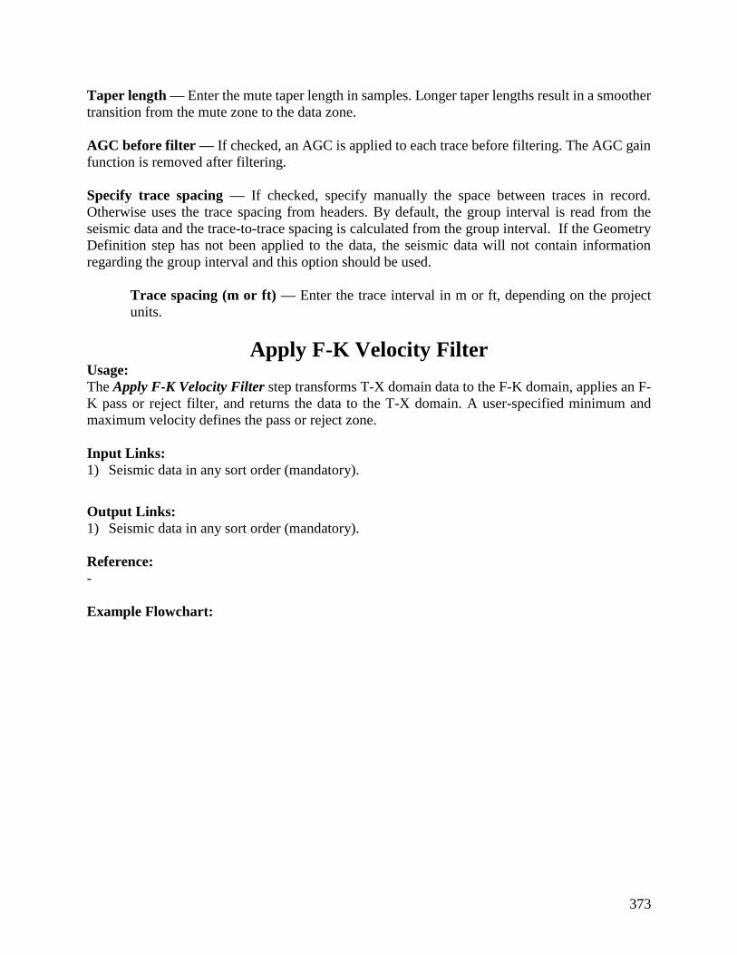
373

Taper length — Enter the mute taper length in samples. Longer taper lengths result in a smoother

transition from the mute zone to the data zone.

AGC before filter — If checked, an AGC is applied to each trace before filtering. The AGC gain

function is removed after filtering.

Specify trace spacing — If checked, specify manually the space between traces in record.

Otherwise uses the trace spacing from headers. By default, the group interval is read from the

seismic data and the trace-to-trace spacing is calculated from the group interval. If the Geometry

Definition step has not been applied to the data, the seismic data will not contain information

regarding the group interval and this option should be used.

Trace spacing (m or ft) — Enter the trace interval in m or ft, depending on the project

units.

Apply F-K Velocity Filter Usage:

The Apply F-K Velocity Filter step transforms T-X domain data to the F-K domain, applies an F-

K pass or reject filter, and returns the data to the T-X domain. A user-specified minimum and

maximum velocity defines the pass or reject zone.

Input Links:

1) Seismic data in any sort order (mandatory).

Output Links:

1) Seismic data in any sort order (mandatory).

Reference:

-

Example Flowchart:

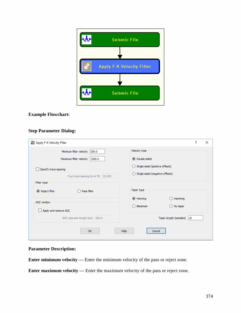
374

Example Flowchart:

Step Parameter Dialog:

Parameter Description:

Enter minimum velocity — Enter the minimum velocity of the pass or reject zone.

Enter maximum velocity — Enter the maximum velocity of the pass or reject zone.

375

Specify trace spacing — If checked, manual set the trace-to-trace spacing in the record to be

filtered. By default, the group interval is read from the seismic data and the trace-to-trace spacing

is calculated from the group interval. If the Geometry Definition step has not been applied to the

data, the seismic data will not contain information regarding the group interval and this option

should be used.

Trace spacing (m or ft) — Enter the trace interval in m or ft, depending on the project

units.

Velocity type: Specify whether the applied F-K filter will be symmetrical or asymmetrical. See

Figure below.

Double sided — If selected, the specified minimum and maximum velocities will be used to create

a double-sided, or symmetrical F-K filter.

Single sided (positive offsets) — If selected, the specified minimum and maximum velocities will

be used to pass or reject energy propagating in the direction of increasingly positive source-to-

receiver offset.

Single sided (negative offsets) — If selected, the specified minimum and maximum velocities

will be used to pass or reject energy propagating in the direction of increasingly negative source-

to-receiver offset.

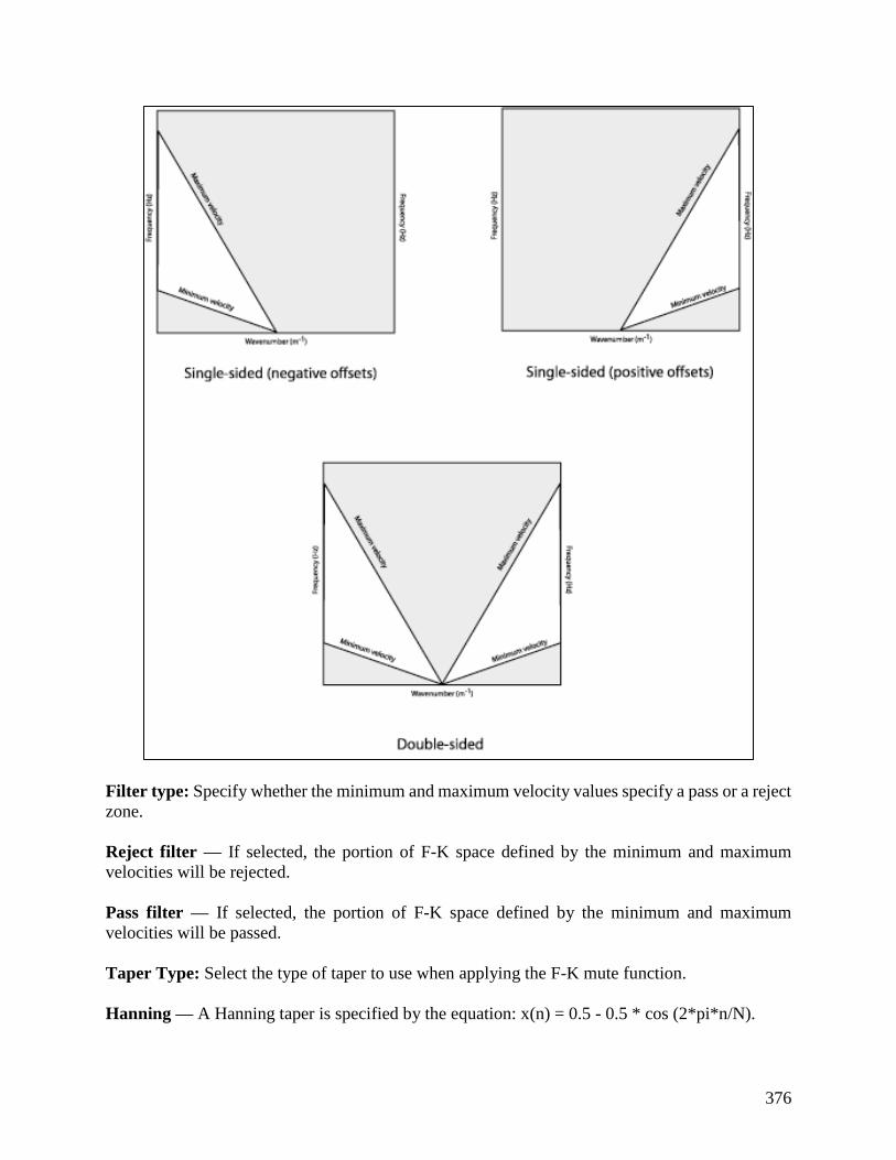
376

Filter type: Specify whether the minimum and maximum velocity values specify a pass or a reject

zone.

Reject filter — If selected, the portion of F-K space defined by the minimum and maximum

velocities will be rejected.

Pass filter — If selected, the portion of F-K space defined by the minimum and maximum

velocities will be passed.

Taper Type: Select the type of taper to use when applying the F-K mute function.

Hanning — A Hanning taper is specified by the equation: x(n) = 0.5 - 0.5 * cos (2*pi*n/N).

377

Hamming — A Hamming taper is specified by the equation: x(n) = 0.54 - 0.46 * cos (2*pi*n/N).

Blackman — A Blackman taper is specified by the equation: x(n) = 0.42 - 0.5 * cos (2*pi*n/N)+

0.08 * cos (4*pi*n/N)

No taper — No taper will be applied to the mute. This may result in problems in later processing

steps due to Gibbs effect.

AGC Window: Define parameter for AGC filter.

Apply and remove AGC — If checked, and AGC filter is applied before the F-K Velocity filter

and removed from the output seismic file. The AGC filter is used exclusively internally to improve

the performance of the F-K filter.

AGC operator length — Enter the AGC operator length in ms.

Taper length (ms) — Enter the mute taper length in samples. Longer taper lengths result in a

smoother transition from the mute zone to the data zone.

Butterworth Dip Filtering Usage:

The Butterworth Dip Filtering step is a single channel filter that may be used to pass or reject

dipping data.

The data is transformed to the frequency domain, where the Buttterworth dip filter is applied.

Common usage includes suppression of dipping noise from pre-stack data.

Input Links:

1) Seismic data in any sort order (mandatory).

Output Links:

1) Seismic data in any sort order (mandatory).

Reference:

Hale, D. and Claerbout, J.F., 1983, Butterworth dip filters, Geophysics, v. 48, p. 1033-1038.

Example Flowchart:

378

Step Parameter Dialog:

379

Parameter Description:

Filter type: Define type of filter to be applied.

Pass — If checked, the filter will pass dipping data over the specified range of dips.

Reject — If checked, the filter will reject dipping data over the specified range of dips.

Dip specification: Specify parameters related with dip estimation

Milliseconds per trace — If checked, the range of dips required must be input in terms of

milliseconds per trace.

Velocity — If checked, the range of dips required must be input in terms of apparent velocity.

Poles: Define number of poles in the filter.

Number of poles – Enter the number of poles for the Butterworth dip filter. A larger number of

poles for a sharper cut-off of the pass or reject zone.

Amplitude selection: Select type of amplitude.

Relative amplitude – If checked, the data is equalized to relative amplitude before application of

the filter.

True amplitude – If checked, the filter is directly applied to the frequency domain data.

Frequency range: Specify the frequency range of the filter.

Maximum frequency – Enter the maximum frequency to be used. The greatest frequency that is

to be maintained and dip filtered.

Butterworth Filtering Usage:

The Butterworth Filtering step allows you to apply recursively a Butterworth filter to your trace

data in the time domain. You specify the low pass, high pass and high and low rolloff rates in

decibels (dB) for the filter. You may choose to apply the filter as either a zero phase or minimum

phase filter.

Input Links:

1) Seismic data in any sort order (mandatory).

2) Seismic data or auxiliary text file with filter (mandatory).

Output Links:

1) Seismic data in any sort order (mandatory).

380

Reference:

-

Example Flowchart:

Step Parameter Dialog:

381

Parameter Description:

Low-cut filtering: Specify low-cut filter parameters.

Apply low-cut filter — If checked, a low-cut filter will be applied to your data.

Low-cut corner frequency (Hz) — Enter the low half-power frequency in Hertz to be applied

to your data. The amplitude of this frequency will be reduced by a factor of two relative to the

input.

Low-cut rolloff rate (dB/oct) — Enter the low rolloff filter slope in decibels per octave to be

applied to your data. Higher numbers give steeper rolloff.

High-cut filtering: Specify high-cut filter parameters.

Apply high-cut filter — If checked, a high-cut filter will be applied to your data.

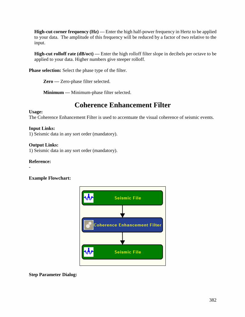
382

High-cut corner frequency (Hz) — Enter the high half-power frequency in Hertz to be applied

to your data. The amplitude of this frequency will be reduced by a factor of two relative to the

input.

High-cut rolloff rate (dB/oct) — Enter the high rolloff filter slope in decibels per octave to be

applied to your data. Higher numbers give steeper rolloff.

Phase selection: Select the phase type of the filter.

Zero — Zero-phase filter selected.

Minimum — Minimum-phase filter selected.

Coherence Enhancement Filter Usage:

The Coherence Enhancement Filter is used to accentuate the visual coherence of seismic events.

Input Links:

1) Seismic data in any sort order (mandatory).

Output Links:

1) Seismic data in any sort order (mandatory).

Reference:

-

Example Flowchart:

Step Parameter Dialog:

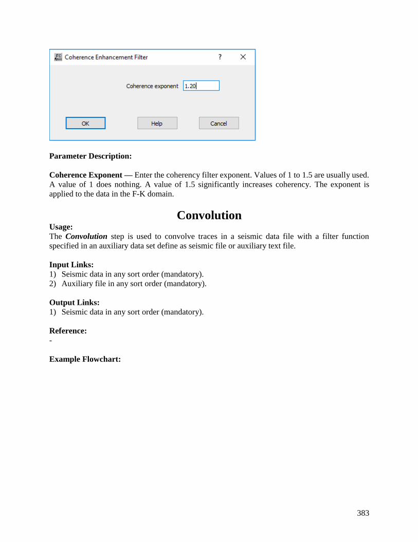
383

Parameter Description:

Coherence Exponent — Enter the coherency filter exponent. Values of 1 to 1.5 are usually used.

A value of 1 does nothing. A value of 1.5 significantly increases coherency. The exponent is

applied to the data in the F-K domain.

Convolution Usage:

The Convolution step is used to convolve traces in a seismic data file with a filter function

specified in an auxiliary data set define as seismic file or auxiliary text file.

Input Links:

1) Seismic data in any sort order (mandatory).

2) Auxiliary file in any sort order (mandatory).

Output Links:

1) Seismic data in any sort order (mandatory).

Reference:

-

Example Flowchart:

384

Step Parameter Dialog:

Parameter Description:

Filter location: Specify the location of the filter to be convolved.

Seismic file — If selected, the filter is defined in an auxiliary seismic file.

Text file — If selected, the filter is defined in an auxiliary text file.

Cross Correlation Usage:

The Cross Correlation step computes the cross correlation between an input seismic data and an

auxiliary seismic data.

Input Links:

1) Seismic data in any sort order (mandatory).

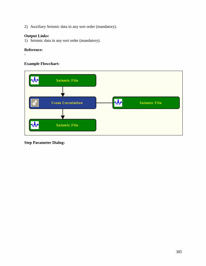
385

2) Auxiliary Seismic data in any sort order (mandatory).

Output Links:

1) Seismic data in any sort order (mandatory).

Reference:

-

Example Flowchart:

Step Parameter Dialog:

386

Parameter Description:

Input data: Specify parameters for input seismic file.

Window start time — Enter the window start time for input seismic file in milliseconds.

Window end time — Enter the window end time for input seismic file in milliseconds.

Auxiliary data: Specify parameters for input seismic file.

Window start time — Enter the window start time for auxiliary seismic file in milliseconds.

Window end time — Enter the window start time for auxiliary seismic file in milliseconds.

One input trace per record — If selected, the auxiliary data is considered to have one input trace

per record.

One input trace per dataset — If selected, the auxiliary data is considered to have one input trace

per record.

Zero lag time — Enter the zero lag time for the cross correlation.

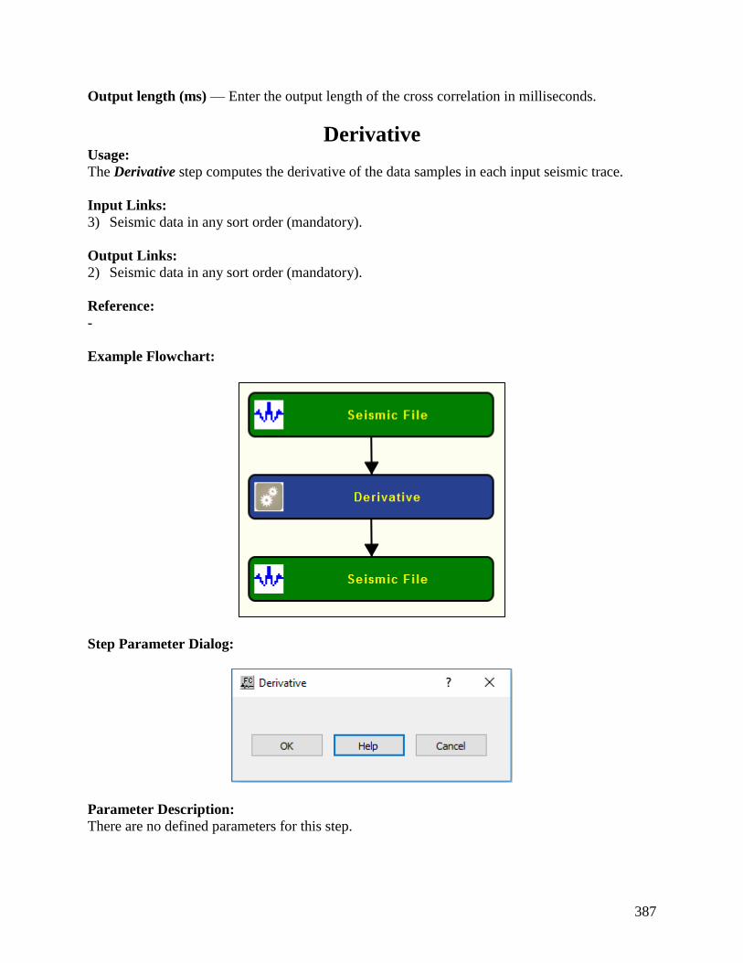
387

Output length (ms) — Enter the output length of the cross correlation in milliseconds.

Derivative Usage:

The Derivative step computes the derivative of the data samples in each input seismic trace.

Input Links:

3) Seismic data in any sort order (mandatory).

Output Links:

2) Seismic data in any sort order (mandatory).

Reference:

-

Example Flowchart:

Step Parameter Dialog:

Parameter Description:

There are no defined parameters for this step.

388

Diffusion Filter Usage:

The Diffusion Filter is a noise reduction filter based on the diffusion equation. The filter performs

both smoothing and edge preservation.

The most common usage is to enhance post-stack 3D data by applying Diffusion Filter to time

slices.

Use Time Slice (Processing Category Display) in a prior job flow to convert such data to time

slices for input to Diffusion Filter.

After Diffusion Filter, use Time Slice to Trace (Processing Category Display) in a further job

flow to revert the filtered data to normal order.

An alternative to Diffusion Filter for enhancing post-stack 3D data is use of 3D Diffusion Filter.

Input Links:

1) Seismic data in any sort order (mandatory).

Output Links:

1) Seismic data in any sort order (mandatory).

Reference:

Fehmers, G.C, and Hocker, C.F.W., 2003, Fast structural interpretation with structure-oriented

filters, Geophysics, vol. 68, no. 4, p. 1286-1293.

Example Flowchart:

Step Parameter Dialog:

389

Parameter Description:

Difussion method: Define the diffusion method.

Structure gradient diffusion — If selected, use structure-oriented filtering (Fehmers & Hocker)

Tukey diffusion — If selected, use an anisotropic diffusion using the Kuwahara filter

Structure gradient diffusion: specify the structure gradient diffusion.

Gradient scale — Enter the number of standard deviation of 2D Gaussian filter used for

smoothing the input data prior to gradient calculation.

Structure scale — Enter the number of standard deviation of 2D Gaussian filter used for

smoothing the gradient tensors prior to eigendecomposition.

Number of iterations — Enter the number of filter iteration to apply to the input data.

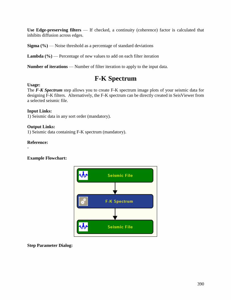
390

Use Edge-preserving filters — If checked, a continuity (coherence) factor is calculated that

inhibits diffusion across edges.

Sigma (%) — Noise threshold as a percentage of standard deviations

Lambda (%) — Percentage of new values to add on each filter iteration

Number of iterations — Number of filter iteration to apply to the input data.

F-K Spectrum Usage:

The F-K Spectrum step allows you to create F-K spectrum image plots of your seismic data for

designing F-K filters. Alternatively, the F-K spectrum can be directly created in SeisViewer from

a selected seismic file.

Input Links:

1) Seismic data in any sort order (mandatory).

Output Links:

1) Seismic data containing F-K spectrum (mandatory).

Reference:

-

Example Flowchart:

Step Parameter Dialog:

391

Parameter Description:

Input amplitude treatment: The amplitude to use as input to the F-K transform, either relative

or true amplitude

True amplitude — If selected, use the true seismic amplitude as in the input seismic traces for

the analysis. True amplitude traces are scaled by one common factor per record.

True amplitude — If selected, use relative seisimc amplitude scaled traces in the analysis.

Relative amplitude traces are scaled independently of one another.

Output amplitude scale: Select the output amplitude scale, either absolute amplitude or dB down

from the maximum.

Amplitude — If selected, the output amplitude scale is set absolute amplitude.

Decibel — If selected, the output amplitude scale is set in dB down from the maximum.

392

Specify trace spacing — If checked, specify manually the space between traces in record.

Otherwise uses the trace spacing from headers. By default, the group interval is read from the

seismic data and the trace-to-trace spacing is calculated from the group interval. If the Geometry

Definition step has not been applied to the data, the seismic data will not contain information

regarding the group interval and this option should be used.

Trace spacing (m or ft) — Enter the trace interval in m or ft, depending on the project

units.

dB scale control: Set zero dB amplitude for comparison of two dB scale iamges.

Set 0dB value — If checked, the zero dB amplitude value may be entered. Using this option allows

you to compare two dB scale images.

Zero dB value — Enter the Zero dB value and its exponent.

F-X Deconvolution Usage:

The F-X Deconvolution step is a 2D multi-channel noise filter designed to attenuate random noise.

This time-variant, adaptive filter removes the non-predictable part of the data using the assumption

that the signal portion of the data is predictable and the noise portion of the data is inherently

random, and therefore non-predictable. You specify the length of the filter window, in samples,

the width of the filter window, in traces, and the filter adaptation percent.

Input Links:

1) Seismic data in any sort order (mandatory).

Output Links:

1) Seismic data in any sort order (mandatory).

Reference:

Hornbostel, S., 1991, Spatial prediction filtering in the t-x and f-x domain, Geophysics, v. 56, no

12, p. 2019-2026.

Example Flowchart:

393

Step Parameter Dialog:

394

Parameter Description:

Design window length: Specify the length of the window of the filter.

Whole trace — If checked, the length of the filter is equal to the length of the input seismic trace.

Specify length — If checked, the length of the filter is defined manually.

Length (ms) — Enter the length of the filter in ms.

Taper length (ms) — Enter the taper length of the filter in ms.

Design window width: Specify the width of the filter.

Entire record — If checked, uses the width filter is equal to the number of traces of the input

record.

395

Specify width — If checked, uses the width filter is manually defined.

Width (traces) — Enter the width of the filter in number of traces.

Prediction filter: Specify the size of the prediction filter.

Width (traces) — Enter the width of the prediction filter in number of traces.

Processing Frequency Range: Specify the frequency band where the filter is going to be applied.

Minimum frequency (Hz.) — Enter the minimum frequency value in Hz of the frequency band.

Maximum frequency (Hz.) — Enter the maximum frequency value in Hz of the frequency band.

F-X Median Filter Usage:

The F-X Median Filter step is a single channel filter that may be used to remove spikes or other

noise from your data without damaging dipping data. The operator is applied in the temporal

frequency domain using fully overlapping cosign-tapered window panes of specified height. A

horizontal 1D median filter is applied to the frequency amplitudes whilst leaving the phase

unchanged. Either the entire dataset or a specified tapered time window may be filtered

The input data in the form of time traces and does not require prior slicing or transformation.

Input Links:

1) Seismic data in any sort order (mandatory).

Output Links:

1) Seismic data in any sort order (mandatory).

Reference:

-

Example Flowchart:

396

Step Parameter Dialog:

Parameter Description:

397

Paramters: Specify the median filter parameters.

Filter width in traces — Enter the width in number of traces of the spacial median filter to be

applied to each temporal frequency component.

Overlapping panes’ height (ms.) — Enter the height in milliseconds of each of the fully-

overlapping cosine-tapered panes from which frequency components are derived. In general,

shorter panes will exhibit more filtering, but these should be sufficiently long to allow realistic

longer frequency estimation.

Data selection: Specify the size of the data input for the median filter.

All data — If checked, the entire data length will be filtered.

Specified extent — If checked, the specified data aperture will be filtered.

Start time (ms.) — Enter the required time at which filtering is to begin.

End time (ms.) — Enter the required time at which filtering is to end.

Taper length (ms.) — Enter the length of the start and end tapers used to taper in the

filtered data to the input data.

F-X Noise Attenuation Usage:

The F-X Noise Attenuation step is a random noise attenuation technique in the frequency-space

domain. This filtering method predicts the signal with spatial changes in dir or amplitude using the

F-X domain.

Input Links:

1) Seismic data in any sort order (mandatory).

Output Links:

1) Seismic data in any sort order (mandatory).

Reference:

-

Example Flowchart:

398

Step Parameter Dialog:

Parameter Description:

Design window length (ms) —Enter the filter length in ms.

Design window width (traces) — Enter the width of the filter in number of traces.

Filter order — Enter the filter order.

Filter adaptation (%) — enter the filter adaptation in percentage.

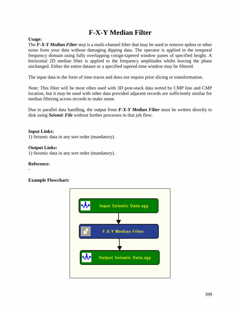
399

F-X-Y Median Filter Usage:

The F-X-Y Median Filter step is a multi-channel filter that may be used to remove spikes or other

noise from your data without damaging dipping data. The operator is applied in the temporal

frequency domain using fully overlapping cosign-tapered window panes of specified height. A

horizontal 2D median filter is applied to the frequency amplitudes whilst leaving the phase

unchanged. Either the entire dataset or a specified tapered time window may be filtered.

The input data in the form of time traces and does not require prior slicing or transformation.

Note: This filter will be most often used with 3D post-stack data sorted by CMP line and CMP

location, but it may be used with other data provided adjacent records are sufficiently similar for

median filtering across records to make sense.

Due to parallel data handling, the output from F-X-Y Median Filter must be written directly to

disk using Seismic File without further processes in that job flow.

Input Links:

1) Seismic data in any sort order (mandatory).

Output Links:

1) Seismic data in any sort order (mandatory).

Reference:

-

Example Flowchart:

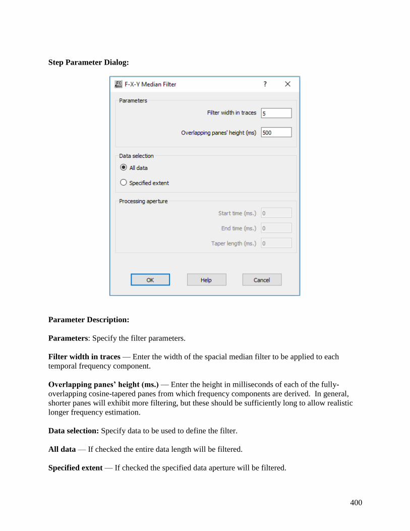
400

Step Parameter Dialog:

Parameter Description:

Parameters: Specify the filter parameters.

Filter width in traces — Enter the width of the spacial median filter to be applied to each

temporal frequency component.

Overlapping panes’ height (ms.) — Enter the height in milliseconds of each of the fully-

overlapping cosine-tapered panes from which frequency components are derived. In general,

shorter panes will exhibit more filtering, but these should be sufficiently long to allow realistic

longer frequency estimation.

Data selection: Specify data to be used to define the filter.

All data — If checked the entire data length will be filtered.

Specified extent — If checked the specified data aperture will be filtered.

401

Start time (ms.) — Enter the required time at which filtering is to begin.

End time (ms.) — Enter the required time at which filtering is to end.

Taper length (ms.) — Enter the length of the start and end tapers used to taper in the

filtered data to the input data.

Footprint Filter Usage:

The Footprint Filter step is a KK filtering technique for application to 3D post-stack data that is

focused on attenuating acquisition footprint noise.

Two techniques are available:

1) Application of a global high cut KK filter. Seismic signal generally displays most of its

energy in the KK domain close to zero, whereas the jitter sometimes seen due to acquisition

will have high KK amplitudes. This filter is then simple, effective and fast.

2) A local adaptive noise removal algorithm for when the acquisition footprint exhibits in the

KK domain as spikes. The seismic signal energy is protected with an exclusion zone

around the origin. This technique is significantly more time-consuming and should be used

only when the first technique does not address the type of acquisition noise seen.

Footprint Filter is applied to post-stack 3D data which has been converted to time slices.

Use Time Slice (Processing Category Display) in a prior job flow to convert such data to time

slices for input to Footprint Filter.

After Footprint Filter, use Time Slice to Trace (Processing Category Display) in a further job

flow to revert the filtered data to normal order.

Input Links:

1) Seismic data sorted by Slice Number (record key) and CMP Line (mandatory).

Output Links:

1) Seismic data sorted by Slice Number (record key) and CMP Line (mandatory).

Reference:

-

Example Flowchart:

402

Step Parameter Dialog:

403

Parameter Description:

Apply high-cut KK filtering — If checked, a high-cut KK cosine filter as specified will be

applied.

High-cut KK filtering: Specify the high-cut KK filter.

High pass frequency (% Nyq) — Enter the KK taper-off beginning frequency.

High cut frequency (% Nyq) — Enter the KK taper-off ending frequency.

Apply adaptive noise removal — If checked, an adaptive noise removal filter will be applied.

404

Adaptive noise removal: Specify the adaptive noise removal parameters.

Noise threshold — Enter the number of standard deviations of a sample amplitude above the

standard deviation of the sample amplitudes within a local area or ‘patch’ for that sample to be

regarded as noise.

Patch width — Enter the KK plane is divided into overlapping ‘patches’ to be analyzed for noise

spikes. This parameter is the side length of each square patch.

Number of iterations — Enter the number of iterations of the adaptive noise removal algorithm.

Removal method: Select the removal method for the KK filter.

Replace noise samples — If selected, the amplitude of a noise sample will be replaced by the

average value within the patch.

Remove noise samples — If selected, the amplitude of a noise sample will be set to zero.

Filtering signal exclusion zone: Specify a signal exclusion zone based on the percentage of the

Nyquist.

Exclusion zone size (% Nyq) — Enter the size of the area around the KK origin to be protected

from the adaptive filter so as to preserve the signal.

Mask dead areas — If checked, then input data dead zones will be masked after application of

the KK filtering.

Horizontal Median Filter Usage:

The Horizontal Median step allows you to apply a horizontal median filter across the data traces

of a gather or stack. This process is very useful in processing VSP data for separation of up-going

and down-going events.

Input Links:

1) Seismic data in any sort order (mandatory).

Output Links:

1) Seismic data in any sort order (mandatory).

References:

Hardage, B. A., 1983, Vertical Seismic Profiling, Geophysical Press.

Example Flowchart:

405

Step Parameter Dialog:

Parameter Description:

Window length in traces — Enter the number of traces in the spatial window.

Use quantile for median application — If checked, the median value is computed over the

selected quantile.

Quantile value — Enter the quantile value to calculate the median.

Apply for VSP upgoing traces only — If checked, the horizontal median filter is only applied to

seismic traces marked as VSP upgoing traces.

406

Integration Usage:

The Integration step integrates data samples in each input seismic data trace.

Input Links:

1) Seismic data in any sort order (mandatory).

Output Links:

1) Seismic data in same sort order as the input (mandatory).

Reference:

-

Example Flowchart:

Step Parameter Dialog:

Parameter Description:

There are no parameters for this step.

Notch Filter Usage:

407

The Notch Filter step applies a frequency domain notch filter to the input data. The filter is

specified by describing the frequency notch and the width of the notch. Options exist to (1) apply

the filter as a function of header word flags, (2) parameterize the notch as a function of header

word flags.

Input Links:

1) Seismic data in any sort order (mandatory).

Output Links:

1) Seismic data in any sort order (mandatory).

Reference:

-

Example Flowchart:

Step Parameter Dialog:

408

Parameter Description:

Application window: Specify the window of application for the notch filter.

Apply filter based on a trace header flag — If checked, the application of the filter is to be

controlled by the value of a trace header flag.

Trace header field — Enter the value of a trace header flag, select the trace header from

the drop down menu.

Trace header value — Enter the value of a trace header flag, set the value of the trace

header. When the value of the trace header equals the specified value, the filter will be

applied. Otherwise, the filter will not be applied.

Notch frequency is in a trace header field — If checked, the value of the notch frequency is

to be controlled by the value of a trace header field.

Trace header field — Enter the value of a trace header field, select the trace header from

the drop down menu.

409

Notch frequency (Hz) — Enter the value of the notch frequency in Hertz.

Notch width (Hz) — Enter the width of the notch frequency in Hertz.

Quadrature Filter

Usage:

The Quadrature Filter step computes the Hilbert transform of the input seismic data. Quadrature

filters are usually applied to enhance the presence of discontinuities and reveal the structure of the

seismic image.

Input Links:

1) Seismic data in any sort order (mandatory).

Output Links:

1) Seismic data in any sort order (mandatory).

Reference:

-

Example Flowchart:

Step Parameter Dialog:

410

Parameter Description:

Processing start time (ms) — Enter the processing start time in ms.

Processing end time (ms) — Enter the processing start time in ms.

Radial Transform Filter

Usage:

The Radial Transform Filter step is a 2D pre-stack single channel filter for attenuation of noise

originating from a point source with a specific apparent velocity by means of the radial transform.

For example, shot generated noise may be attenuated by application of Radial Transform Filter

to common shot gathers.

Each input record must be ordered by offset.

The input 2D record is first converted to the radial domain such that each radial trace represents a

different apparent velocity within the range of interest, radiating from a start time (usually zero) at

zero offset.

Using the output data type ‘Radial traces’, these traces may be output and displayed:

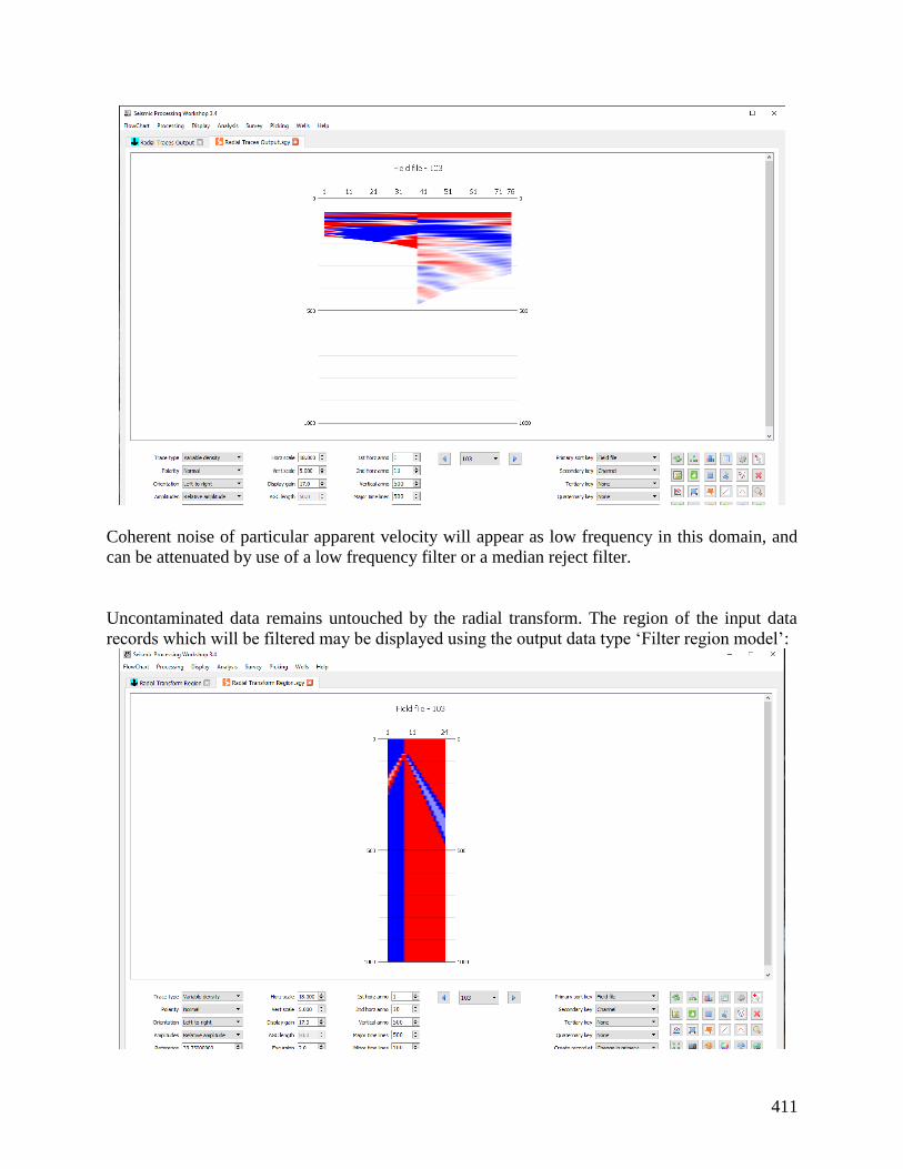
411

Coherent noise of particular apparent velocity will appear as low frequency in this domain, and

can be attenuated by use of a low frequency filter or a median reject filter.

Uncontaminated data remains untouched by the radial transform. The region of the input data

records which will be filtered may be displayed using the output data type ‘Filter region model’:

412

Input Links:

1) 2D Seismic data offset-sorted records (mandatory).

Output Links:

1) 2D Seismic data offset-sorted records (mandatory).

Reference:

Henley, D., 2008, A Convenient Truth: Radial Trace Filtering – Simple and Effective, CSEG

Recorder, vol. 34, no 1.

Example Flowchart:

Step Parameter Dialog:

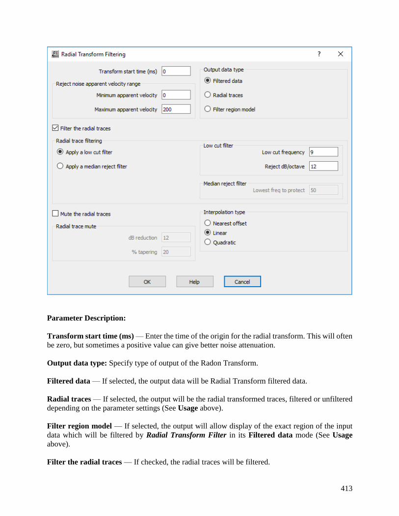
413

Parameter Description:

Transform start time (ms) — Enter the time of the origin for the radial transform. This will often

be zero, but sometimes a positive value can give better noise attenuation.

Output data type: Specify type of output of the Radon Transform.

Filtered data — If selected, the output data will be Radial Transform filtered data.

Radial traces — If selected, the output will be the radial transformed traces, filtered or unfiltered

depending on the parameter settings (See Usage above).

Filter region model — If selected, the output will allow display of the exact region of the input

data which will be filtered by Radial Transform Filter in its Filtered data mode (See Usage

above).

Filter the radial traces — If checked, the radial traces will be filtered.

414

Radial trace filtering: Specify type of rejection filter.

Apply a low cut frequency — If selected, a low cut filter will be applied.

Low cut filter: Specify low cut parameters

Low cut frequency— Specify the low cut frequency of the Butterworth filter.

Reject dB/octave — Specify the rate of fall-off of the filter.

Apply a median reject filter — If selected, a median reject filter will be applied.

Median reject filter: Specify median reject filter parameters. Low frequencies are

attenuated by subtracting the median filtered data from the data.

Lowest freq to protect — Specify the lowest frequency that will not be attenuated by the

median reject filter. The median filter length used will be the wavelength of this frequency

in samples.

Mute the radial traces — If checked, the radial traces will be attenuated.

Radial trace mute: Specify the radial trace mute parameters.

dB reduction — All data within the radial traces will be attenuated by the specified

amount.

% tapering — Specify the percentage of the radial trace zone(s) which will be tapered.

Interpolation type: Deriving the radial traces from the input data requires interpolation of the

data. Nearest offset is the fastest, while linear and quadratic interpolation may give a smoother

result and better radial domain low frequency attenuation.

Nearest offset — If selected, radial traces will be constructed by picking nearest offset samples.

Linear — If selected, linear interpolation will be used to construct radial traces.

Quadratic — If selected, quadratic interpolation will be used to construct radial traces.

The above parameters may be adjusted by trial and error to obtain the best attenuation, or by

inspection of the radial traces.

Radon Demultiple Usage:

The Radon Demultiple step performs parabolic radon demultiple through a modeling of multiples

in the parabolic radon domain followed by subtraction of those multiples in the time domain. You

415

specify the transform type, the range of ray parameters in the output transform, and the spatial and

temporal taper lengths used to generate the transform.

Input Links:

1) Seismic data in any sort order (mandatory).

Output Links:

1) Seismic data in any sort order (mandatory).

Reference:

Hampson, D., 1991, Inverse velocity stacking for multiple elimination, Journal of the Canadian

Society of Exploration Geophysics, 22, p. 44-55.

Example Flowchart:

Step Parameter Dialog:

416

Parameter Description:

Time window:

Limit application time —

Use constant start time —

Start time (ms) —

Start time referenced to horizon —

Multiplier for time horizon —

Length of taper zone (ms) —

Model moveout: Set the range of parabolas that will generate the primary and multiple models.

Minimum differential moveout — Enter the minimum differential moveout, expressed in

milliseconds on the far-offset trace. The primary model is generated with parabolas from the

<minimum differential moveout> to the <minimum multiple moveout>.

417

Maximum differential moveout — Enter the maximum differential moveout, expressed in

milliseconds on the far-offset trace. The multiple model is generated with parabolas from the

<minimum multiple moveout> to the <maximum differential moveout>.

Minimum multiple moveout — Enter the minimum multiple moveout, expressed in milliseconds

on the far-offset trace. The multiple model is generated with parabolas from the <minimum

multiple moveout> to the <maximum differential moveout>.

Ray parameters: Specify ray parameters

Set number of ray parameters — If checked, the number of ray parameters is determined

manually. By default, the number of ray parameters is determined internally.

Number of ray parameters — set the number of ray parameter.

Offset window: Speficy paramters for window definition.

Define maximum reference offset — If checked, limit the input seismic data by a maximum

reference offset

Maximum reference offset — Enter the reference maximum offset. Maximum offset of

the input record that is going to be used.

AGC Window: Define parameter for AGC filter.

Apply and remove AGC — If checked, and AGC filter is applied before the F-K Velocity filter

and removed from the output seismic file. The AGC filter is used exclusively internally to improve

the performance of the F-K filter.

AGC operator length — Enter the AGC operator length in ms.

Bandpass filter: Specify bandpass filter parameters, as defined in a trapezoid, to be applied during

the processing.

Low cut (Hz) — enter low cut frequency in Hz.

Low pass (Hz) — enter low pass frequency in Hz.

High pass (Hz) — enter high pass frequency in Hz.

High cut (Hz) — enter high cut frequency in Hz.

Aditional parameters: Specify additional parameters to stabilize the Randon Demultiple.

418

Percent pre-whitening — Enter the amount of pre-whitening used to stabilize the least-squares

inversion in the presence of noise.

Minimum live traces — Enter the minimum number of live traces that must be present in a gather

in order to transform that gather.

Type of output: Specify type of output form Radon Demultiple.

Estimated primaries — If selected, output estimated primary reflections.

Multiple model — If selected, output modelled multiple reflection. This multiple model can then

be subtracted to the input seismic data.

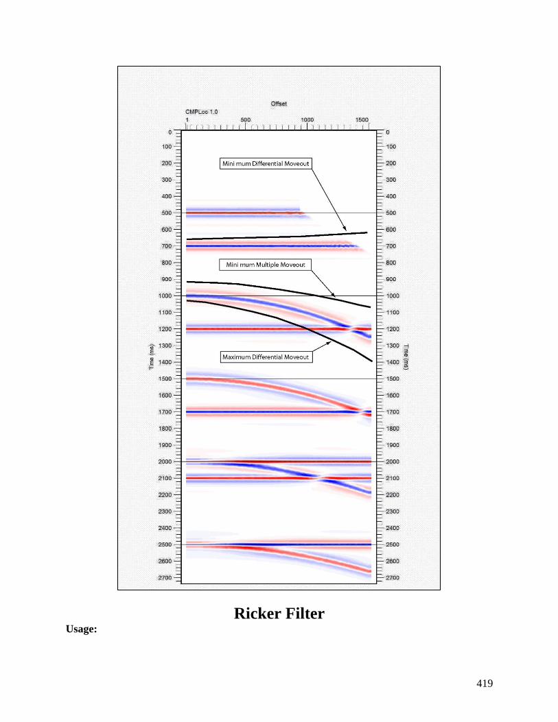
419

Ricker Filter Usage:

420

The Ricker Filter step applies a ricker filter to the input seismic file. The Ricker filter is

completely determined by the center frequency of the Ricker wavelet.

Input Links:

1) Seismic data in any sort order (mandatory).

Output Links:

1) Seismic data in any sort order (mandatory).

Reference:

-

Example Flowchart:

Step Parameter Dialog:

Parameter Description:

Center frequency (Hz) — Specify the center frequency of the Ricker wavelet.

421

Swell Statics Correction Usage:

The Swell Statics Correction step is a moving average filter designed for marine data used to

attenuate statics originated by marine swell.

Input Links:

1) Seismic data in any sort order (mandatory).

Output Links:

1) Seismic data in any sort order (mandatory).

Reference:

-

Example Flowchart:

Step Parameter Dialog:

Parameter Description:

422

Traces in design window — Enter the number of traces to be used in the window filter.

Maximum allowable shift (samples) — Enter the maximum allowable shift, in number of seismic

samples, that a sample may suffer while being filtered.

Tau-p Inverse Transform Usage:

The Tau-P Inverse Transform step transforms 2D Tau-P domain pre-stack data back to the time-

offset domain after conversion to this domain after the use of Tau-P Transform.

Input Links:

1) 2D Seismic pre-stack Tau-P domain data records ordered by Ray Parameter (mandatory).

2) Auxiliary seismic data file: the original offset-time shot records for restoration of headers to

the inverted data.

Output Links:

1) 2D Seismic pre-stack data records ordered by offset (mandatory).

Reference:

Kostov, C., 1990, Toeplitz Structure in Slant-Stack Inversion: 60th Annual Internat..Mtg., Soc.

Expl. Geophys., Expanded Abstracrs, 1618-1621.

Example Flowchart:

Step Parameter Dialog:

423

Parameter Description:

Type of Tau-P transform: Specify the function of offset used for the Tau-P transform.

Parabolic — If selected, a parabolic inverse transform will be performed. This must be the same

as was used for the forward transform.

Linear — If selected, a linear inverse transform will be performed. This must be the same as was

used for the forward transform.

Output data offsets: Specify whether to use the original t-x data to obtain the offsets to be

inverted, or to specify regular offsets.

Original t-x data offsets — If selected, an auxiliary input file will be required. This should be the

original t-x data before forward Tau-P transform. The offsets returned will match those on this file.

Regular offsets — If selected, the inverse transformed records will contain regular offsets.

Bandpass filter: A bandpass filter will be applied to the data, before inverse Tau-P transformation.

It is sensible if the same frequency range is inverted as specified for the forward transform, but not

essential. If aliasing noise is a problem on inversion, then the inversion high pass or high cut

frequencies may be decreased.

Low cut (Hz) — Enter the bandpass low cut frequency in Hz.

Low pass (Hz) — Enter the bandpass low pass frequency in Hz.

High pass (Hz) — Enter the bandpass high pass frequency in Hz.

424

High cut (Hz) — Enter the bandpass high cut frequency in Hz.

Percent pre-whitening — Enter the percentage of pre-whitening. A Toeplitz matrix inversion is

used for the Tau-P inversion of each frequency. A small amount of white noise added may be

needed to stabilize the inversion. A fraction of one percent is often sufficient, and decreases the

smearing sometimes seen when larger values are used.

Tau-p Transform Usage:

The Tau-P Transform step transforms 2D pre-stack data to the Tau-P domain for further

processing. The Tau-P domain data may be inverted to the time-offset domain by the use of Tau-

P Inverse Transform.

The input traces of each record are time-shifted according to their offsets, and then a low-cut spatial

frequency filter is applied. This will attenuate much of the noise energy at that particular apparent

velocity. The time-shifted data is then restored.

Input Links:

1) 2D Seismic pre-stack data records ordered by offset (mandatory).

Output Links:

1) 2D Seismic pre-stack Tau-P domain data records ordered by Ray Parameter (mandatory).

Reference:

Kostov, C., 1990, Toeplitz Structure in Slant-Stack Inversion: 60th Annual Internat..Mtg., Soc.

Expl. Geophys., Expanded Abstracrs, 1618-1621.

Example Flowchart:

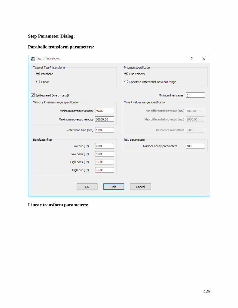
425

Step Parameter Dialog:

Parabolic transform parameters:

Linear transform parameters:

426

Parameter Description:

Type of Tau-P transform: Specify the function of offset used for the Tau-P transform.

Parabolic — If checked, a signed offset squared function will be used. This transform type yields

the best inversion back to the original domain

Linear — If checked, the function used will be offset itself.

P values specification: Specify which method will be used to specify the range of P values to be

calculated.

Use Velocity — If checked, the range of P values to be calculated will be determined by the

minimum and maximum velocities specified. In the case of the Parabolic transform, these

velocities will be moveout velocities. In the case of the Linear transform, these velocities will be

apparent velocities.

427

Specify a differential moveout range — If checked, the minimum P value will be calculated

from the maximum time shift at the specified max offset. The maximum P value will be calculated

from the minimum time shift at the specified max offset.

Split-spread (-ve offsets)? — If checked, the P-values calculated will be a negative P-value range

and a positive P-value range.

Minimum live traces — Enter the minimum number of live traces read for a record to be

transformed to the Tau-P domain.

Velocity P values range specification: Specify the range of P values to be calculated by means

of velocity.

Minimum moveout velocity (Parabolic transform) — Enter the minimum moveout velocity. The

maximum P value will be calculated from this and the specified reference time.

Maximum moveout velocity (Parabolic transform) — Enter the maximum moveout velocity. The

minimum P value will be calculated from this and the specified reference time.

Minimum apparent velocity (Linear transform) — Enter the minimum apparent velocity. The

maximum P value to calculate will be the inverse of this velocity.

Maximum apparent velocity (Linear transform) — Enter the maximum apparent velocity. The

minimum P value to calculate will be the inverse of this velocity.

Reference time (sec) — (Parabolic transform only). Enter the time in seconds at which the

moveout velocity is measured.

Time P values range specification: Specify the range of P values to be calculated by means of

differential moveout.

Min differential moveout (ms.) (Parabolic transform) — Enter the minimum differential moveout

at the specified reference time. The minimum P value to calculate will be calculated from this

value.

Max differential moveout (ms.) (Parabolic transform) — Enter the maximum differential

moveout at the specified reference time. The maximum P value to calculate will be calculated from

this value.

Min slope (ms./1000’) (Linear transform) — Enter the minimum slope in milliseconds per

thousand metres/feet. The minimum P value to calculate will be calculated from this value.

Max slope (ms./1000’) (Linear transform) — Enter the maximum slope in milliseconds per

thousand metres/feet. The maximum P value to calculate will be calculated from this value.

428

Reference max offset (Parabolic transform only) — Enter the offset for the minimum and

maximum differential moveouts specified.

Ray parameters: Specity ray parameters.

Number of ray parameters — Enter the number of P values to be calculated. If split-spread, half

of these will be used for negative P values and half for positive. The number required depends on

the total range of ray parameters. These P-values will be regularly spaced. If the increment

multiplied by the offset is greater than half a wavelength of a frequency, then aliasing noise on

inverse transform may result. The inversion execution time depends on this parameter, and testing

with a few shot records is recommended to determine the smallest value possible without undue

aliasing noise.

Bandpass filter: Both the forward and inverse Tau-P transforms perform calculation in the

frequency domain. A bandpass filter is applied to the data, and the frequency range specified here

should be based on the signal spectrum and minimization of aliasing noise.

Low cut (Hz) — Enter the bandpass low cut frequency in Hz.

Low pass (Hz) — Enter the bandpass low pass frequency in Hz.

High pass (Hz) — Enter the bandpass high pass frequency in Hz.

High cut (Hz) — Enter the bandpass high cut frequency in Hz.

Time Variant Bandpass Usage:

The Time Variant Bandpass step allows you to apply up to five (5) different time-variant bandpass

filters to your trace data. You specify the low cut, low pass, high pass and high cut, filter points

for each filter and the starting time for application of the filter. You also specify the filter taper

length, which allows you to control the smoothness of the transition between adjacent filters.

Input Links:

1) Seismic data in any sort order (mandatory).

Output Links:

1) Seismic data in any sort order (mandatory).

Reference:

-

Example Flowchart:

429

Step Parameter Dialog:

Parameter Description:

Number of filters to use — Enter the number of filters to apply.

Filter taper length — Enter the length of the filter taper in samples. The longer the filters taper

length, the smoother the transition between adjacent filters.

Low cut — Enter the low cut frequency of the bandpass filter in Hertz.

Low pass — Enter the low pass frequency of the bandpass filter in Hertz.

High pass — Enter the high pass frequency of the bandpass filter in Hertz.

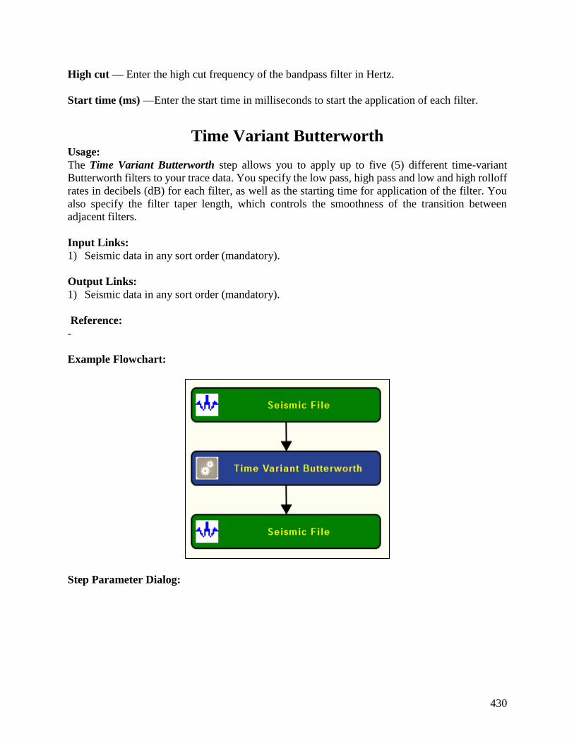
430

High cut — Enter the high cut frequency of the bandpass filter in Hertz.

Start time (ms) —Enter the start time in milliseconds to start the application of each filter.

Time Variant Butterworth Usage:

The Time Variant Butterworth step allows you to apply up to five (5) different time-variant

Butterworth filters to your trace data. You specify the low pass, high pass and low and high rolloff

rates in decibels (dB) for each filter, as well as the starting time for application of the filter. You

also specify the filter taper length, which controls the smoothness of the transition between

adjacent filters.

Input Links:

1) Seismic data in any sort order (mandatory).

Output Links:

1) Seismic data in any sort order (mandatory).

Reference:

-

Example Flowchart:

Step Parameter Dialog:

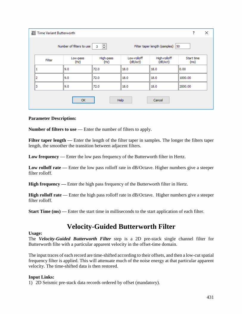
431

Parameter Description:

Number of filters to use — Enter the number of filters to apply.

Filter taper length — Enter the length of the filter taper in samples. The longer the filters taper

length, the smoother the transition between adjacent filters.

Low frequency — Enter the low pass frequency of the Butterworth filter in Hertz.

Low rolloff rate — Enter the low pass rolloff rate in dB/Octave. Higher numbers give a steeper

filter rolloff.

High frequency — Enter the high pass frequency of the Butterworth filter in Hertz.

High rolloff rate — Enter the high pass rolloff rate in dB/Octave. Higher numbers give a steeper

filter rolloff.

Start Time (ms) — Enter the start time in milliseconds to the start application of each filter.

Velocity-Guided Butterworth Filter Usage:

The Velocity-Guided Butterworth Filter step is a 2D pre-stack single channel filter for

Butterworth filte with a particular apparent velocity in the offset-time domain.

The input traces of each record are time-shifted according to their offsets, and then a low-cut spatial

frequency filter is applied. This will attenuate much of the noise energy at that particular apparent

velocity. The time-shifted data is then restored.

Input Links:

1) 2D Seismic pre-stack data records ordered by offset (mandatory).

432

Output Links:

1) 2D Seismic pre-stack data records ordered by offset (mandatory).

Reference:

-

Example Flowchart:

Step Parameter Dialog:

433

Parameter Description:

Velocity cone: Specify velocity parameters.

Linear moveout velocity filter — Enter linear moveout velocity for the Butterworth filter in m/s

or ft/s.

Start time at zero-offset (ms) — Enter the start time at zero-offset in milliseconds

434

Filter type: Specify filter type.

Apply inside cone — If selected, apply the Butterworth filter inside the defined velocity cone.

Apply outside cone — If selected, apply the Butterworth filter outside the defined velocity cone.

Low-cut filtering: Specify low-cut Butterworth filter parameters.

Apply low-cut filter — If checked, apply a Butterworth filter with a low-cut.

Low-cut corner frequency (Hz) — Enter the low pass frequency of the Butterworth filter

in Hertz.

Low-cut rollof rate (dB/oct) — Enter the low pass rolloff rate in dB/Octave. Higher

numbers give a steeper filter rolloff.

High-cut filtering: Specify high-cut Butterworth filter parameters

Apply high-cut filter — If checked, apply a Butterworth filter with a low-cut.

High-cut corner frequency (Hz) — Enter the high pass frequency of the Butterworth filter

in Hertz.

High-cut rollof rate (dB/oct) — Enter the high pass rolloff rate in dB/Octave. Higher

numbers give a steeper filter rolloff.

Velocity-Guided Noise Rejection Filter Usage:

The Velocity-Guided Noise Rejection Filter step is a 2D pre-stack single channel filter for

attenuation of noise with a particular apparent velocity in the offset-time domain.

The input traces of each record are time-shifted according to their offsets, and then a low-cut spatial

frequency filter is applied. This will attenuate much of the noise energy at that particular apparent

velocity. The time-shifted data is then restored.

Input Links:

2) 2D Seismic pre-stack data records ordered by offset (mandatory).

Output Links:

435

2) 2D Seismic pre-stack data records ordered by offset (mandatory).

Reference:

-

Example Flowchart:

Step Parameter Dialog:

Parameter Description:

Apparent velocity — Enter the apparent velocity at which the noise is to be attenuated.

436

Low cut spatial freq % Nyquist — Enter the low-cut point as a percentage of the Nyquist

frequency of the spatial frequency filter to be used.

Reject dB/octave — Enter the cut-off attenuation rate of the low-cut Butterworth filter to be used.

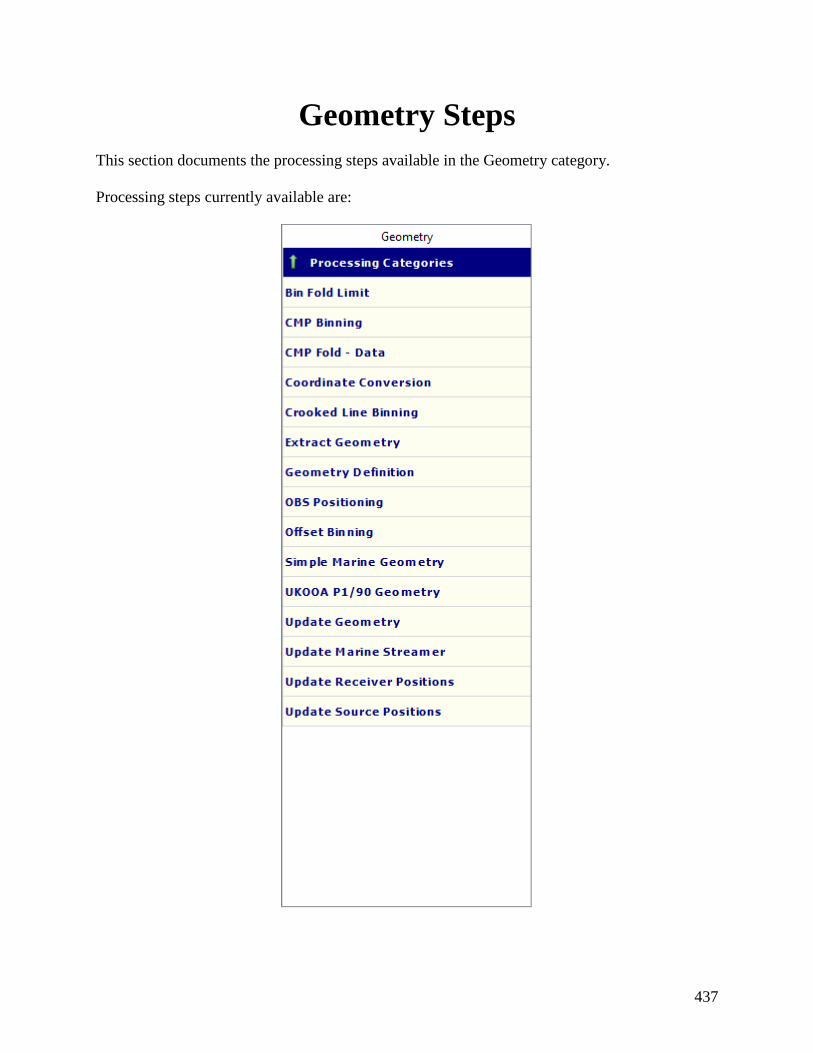
437

Geometry Steps

This section documents the processing steps available in the Geometry category.

Processing steps currently available are:

438

Note Trace Header Geometry Application

The first step in the majority of processing sequences is to update the seismic field headers with

the acquisition geometry information. This information is required to perform basic data analysis

and to execute almost all multi-channel processing steps.

There are three basic structures for the processing flow that is used to update the seismic trace

header with the acquisition geometry information. The structure you use will depend on the nature

of the seismic survey. The three seismic surveys and their associated processing flows can be

classified as follows;

1. 2D seismic. In SPW, 2D seismic surveys are those in which the sources and receivers are laid

out on the same 2D line and the CMP number can be computed as CMP = (Source Location +

Receiver Location) / 2. This implies that source location 101 and receiver location 101 are co-

located (i.e. have the same X,Y coordinates).

1. Crooked line 2D seismic. In SPW, Crooked line 2D seismic surveys are those that will be

processed as a single CMP line, though the sources and receivers are not necessarily laid out

along the same line. This implies that source location 101 and receiver location 101 need not

be co-located (i.e. are not required to have the same X,Y coordinates).

1. 3D seismic. In SPW, 3D seismic surveys are those in which the sources and receivers are laid

out areally and the data will be organized in terms of inlines and crosslines.

An example of each of these three types of processing flows can be found in the Templates library

under the Geometry category.

Example Flowchart for a 2D seismic survey:

439

Example Flowchart for a crooked line 2D seismic survey:

Example Flowchart for a 3D seismic survey:

440

Bin Fold Limit Usage:

The Bin Fold Limit step adds extra flex traces to input binned data from an input Flex Table as

output from CMP Binning in flex mode. Flex traces are selected from the flex table locations as

specified by the Bin Fold Limit parameters.

An alternative to using CMP Binning in flex mode and Bin Fold Limit to improve coverage is to

interpolate the binned data with, for example, 3D Missing Data Interpolation.

Input Links:

441

1) 3D Seismic data sorted by CMP Line and CMP Location, with CMP Location as the record

key (mandatory).

2) Flex Table as output by CMP Binning with flex trace location data.

Output Links:

1) 3D Seismic data sorted by CMP Line and CMP Location (mandatory).

Reference:

-

Example Flowchart:

Step Parameter Dialog:

442

Parameter Description:

Trace selection method: Specify the criterion by which traces are selected from both the input

data and the flex traces whose locations are specified by the input flex file.

Nearest to within bin – If selected, traces will be selected for inclusion in a bin by their distances

from the bin boundary.

Nearest to bin center – If selected, traces will be selected for inclusion in a bin by their distances

from the center of the bin.

One trace per offset interval – If selected, this option aims to provide a full range of offsets

within each bin by allowing just one trace per offset interval.

Override offset interval – If checked, the required offset interval may be overridden in the

adjacent box.

CMP maximum fold: This option does not apply when traces are selected for inclusion in a bin

by one per offset interval.

Maximum traces per bin – Specify the total number of traces that may be included in each bin.

Allow removal of non-flex traces – If checked, and there are more (non-flex) traces assigned to

a bin than the specified. Maximum traces per bin, then those furthest from the bin center will be

removed. If not checked, then only flex traces which fall within the box will be de-selected.

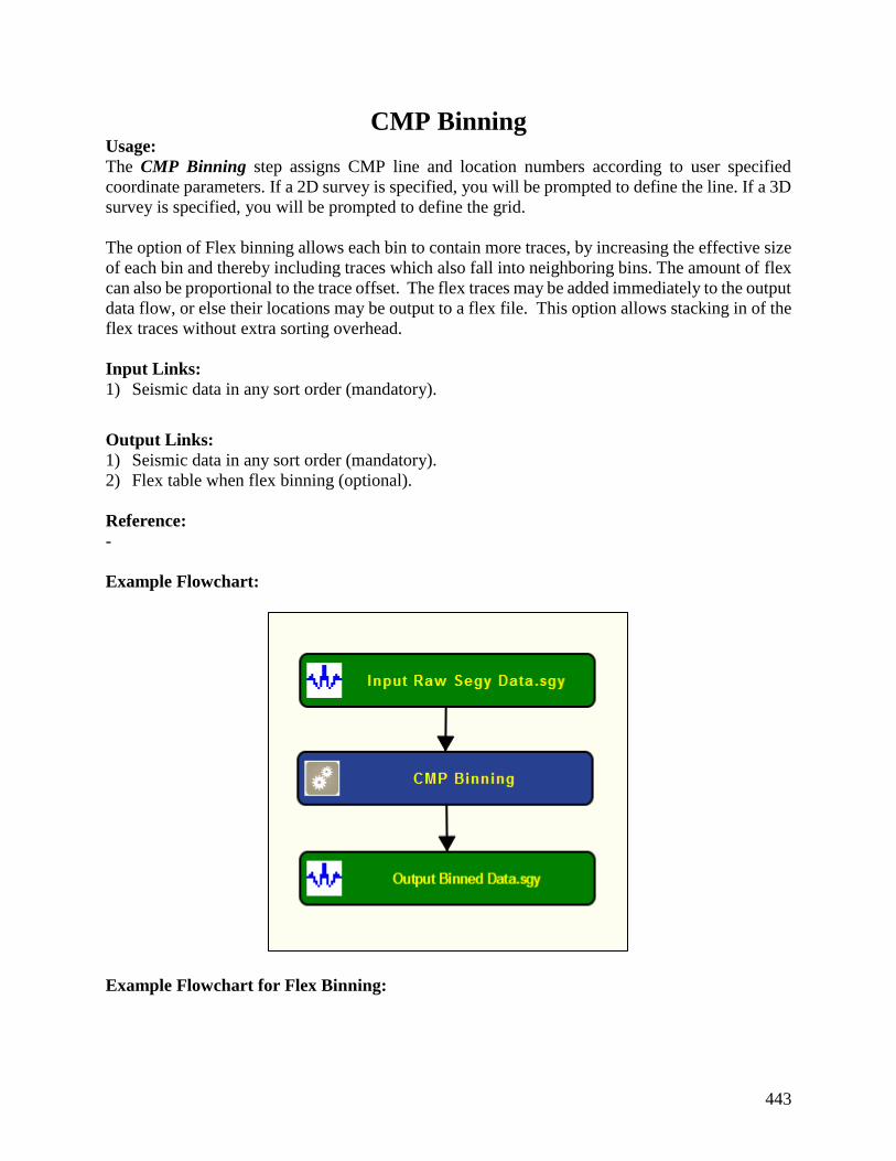
443

CMP Binning Usage:

The CMP Binning step assigns CMP line and location numbers according to user specified

coordinate parameters. If a 2D survey is specified, you will be prompted to define the line. If a 3D

survey is specified, you will be prompted to define the grid.

The option of Flex binning allows each bin to contain more traces, by increasing the effective size

of each bin and thereby including traces which also fall into neighboring bins. The amount of flex

can also be proportional to the trace offset. The flex traces may be added immediately to the output

data flow, or else their locations may be output to a flex file. This option allows stacking in of the

flex traces without extra sorting overhead.

Input Links:

1) Seismic data in any sort order (mandatory).

Output Links:

1) Seismic data in any sort order (mandatory).

2) Flex table when flex binning (optional).

Reference:

-

Example Flowchart:

Example Flowchart for Flex Binning:

444

Step Parameter Dialog for 2D:

445

Step Parameter Dialog for 3D:

446

Step Parameter Dialog for 3D Flex Binning:

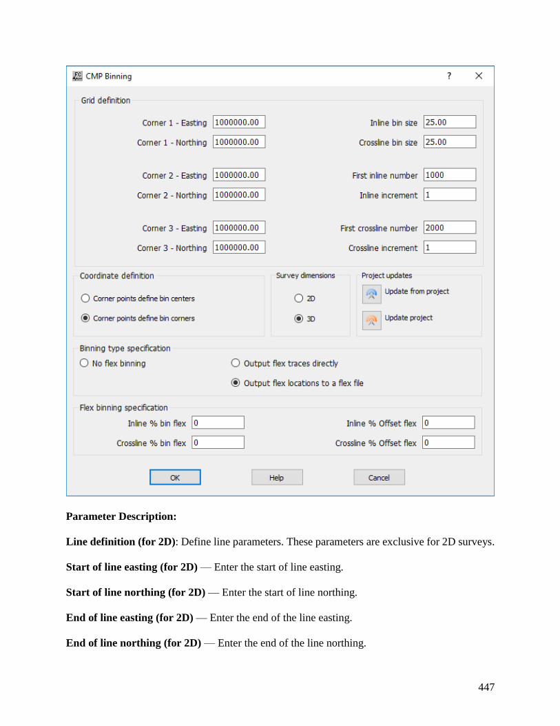
447

Parameter Description:

Line definition (for 2D): Define line parameters. These parameters are exclusive for 2D surveys.

Start of line easting (for 2D) — Enter the start of line easting.

Start of line northing (for 2D) — Enter the start of line northing.

End of line easting (for 2D) — Enter the end of the line easting.

End of line northing (for 2D) — Enter the end of the line northing.

448

Line number (for 2D) — Enter the line number.

Line azimuth (for 2D) — Enter the line azimuth.

First midpoint number (for 2D) — Enter the first midpoint number.

Common midpoint increment (for 2D) — Enter the common midpoint increment.

Common midpoint size (for 2D) — Enter the common midpoint size.

Grid definition (for 3D) — Define the 3D grid. These parameters are exclusive for 3D surveys.

Corner 1 – Easting (for 3D) — Enter the easting (x) coordinate of the first corner of your survey.

Corner 1 – Northing (for 3D) — Enter the northing (y) coordinate of the first corner of your

survey.

Corner 2 – Easting (for 3D) — Enter the easting (x) coordinate of the second corner of your

survey.

Corner 2 – Northing (for 3D) — Enter the northing (y) coordinate of the second corner of your

survey.

Corner 3 – Easting (for 3D) — Enter the easting (x) coordinate of the third corner of your survey.

Corner 3 – Northing (for 3D) — Enter the northing (y) coordinate of the third corner of your

survey.

Inline bin size (for 3D) — Enter the size in distance units of the in-line side (1 to 2) of each bin.

Crossline bin size (for 3D) — Enter the size in distance units of the cross-line side (1 to 3) of each

bin.

First inline number (for 3D) — Enter the first inline number. This line number is assigned to all

the bins along the side of the survey from corner 1 to corner 2.

Inline increment (for 3D) — Enter the increment in line numbers between adjacent CMP lines.

First crossline number (for 3D) — Enter the first crossline number. This location number is

assigned to all the bins along the side of the survey from corner 1 to corner 3.

Crossline increment (for 3D) — Enter the increment in locations between adjacent CMP

locations.

449

Coordinate definition: Specify whether the corner points define the bin centers or corners

following the figure below.

Corner points define bin centers — If selected, specify that corner points define bin centers.

Corner points define bin corners — If selected, specify that corner points define bin corners.

Survey dimensions: Specify whether the dimensions of the survey are 2D or 3D.

2D — If selected, specify 2D line survey.

3D — If selected, specify a 3D grid survey.

Project updates: Specify project updates.

Update from project — Select to update from the project.

Update project — Select to update the project.

Binning type specification: Specify standard binning or the type of flex binning.

No flex binning — If selected, a standard binning, with no extra traces added, is going to be

performed.

Output flex traces directly — If selected, add flex traces to the output binned traces.

Output flex locations to a flex file — If selected, add the locations of flex traces to an additional

output flex file. The flex traces may then be added using Bin Fold Limit at a later stage.

450

Flex binning specification: Specify standard binning or the type of flex binning.

Inline % bin flex — Enter the percentage increase of each bin size in the inline direction to include

extra ‘flex’ traces.

Crossline % bin flex — Enter the percentage increase of each bin size in the crossline direction

to include extra ‘flex’ traces.

Inline % Offset flex — Enter the increase of each bin size as the percentage increase of the trace

inline offsets.

Crossline % Offset flex — Enter the increase of each bin size as the percentage increase of the

trace crossline offsets.

Note: The bin flex and Offset flex options are additive – the bin size used will be the maximum

size of the bin flex and Offset flex options.

CMP Fold - Data Usage:

The CMP Fold – Data step extracts information related with the CMP fold from the seismic data

trace headers.

Input Links:

1) Seismic data in any sort order (mandatory).

Output Links:

None

Reference:

-

Example Flowchart:

451

.4

Step Parameter Dialog:

Parameter Description:

Bin fold file name — Select file to save the bin fold map in bsf form.

452

Specify an offset range — If checked, CMP fold map is limited by minimum and maximum offset

distance as it is written in the trace headers.

Minimum offset — Enter the minimum offset considered to build the CMP fold map.

Maximum offset — Enter the maximum offset considered to build the CMP fold map.

Specify an azimuth range — If checked, CMP fold map is limited by minimum and maximum

azimuth defined in degrees from the North.

Minimum azimuth (deg.) — Enter the minimum azimuth considered to build the CMP

fold map.

Maximum azimuth (deg.) — Enter the maximum azimuth considered to build the CMP

fold map.

Map area: Define map area either by survey of data.

Survey — If selected, the CMP fold map is built from survey geometry.

Data — If selected, the CMP fold map is built from data geometry.

Coordinate Conversion Usage:

The Coordinate Conversion step allows converting the coordinates stored in the seismic traces

headers between geographic (latitude/longitude), Transverse Mercator, UTM or UPS. This step

allows converting the source, receiver and CMP coordinates simulatenously or individually.

Input Links:

1) Seismic data in any sort order (mandatory).

Output Links:

1) Seismic data in any sort order (mandatory).

Reference:

-

Example Flowchart:

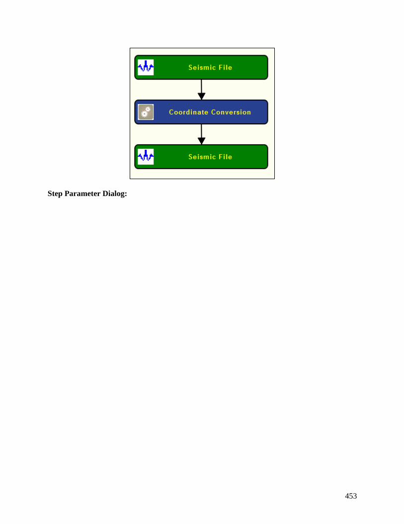
453

Step Parameter Dialog:

454

Parameter Description:

Input file coordinate system: Specify the coordinate system of the input seismic file.

Geographic (Lat-Long) — Select the coordinate system. The user may choose between

Geographic (latitude/longitude), Transverse Mercator, UTM – Universal Transverse

Mercator or UPS – Universal Polar Stereographic.

Geographic units (only for Geographic (Lat-Long)) — Select if the geographic coordinates are

in Decimal or DD MM SS.

455

Geographic datum — Select the datum of the selected coordinate system. Only available for

Transverse Mercator, UTM and UPS.

Orientation – longitude — Select between East or West.

Hemisphere – latitude — Select the hemisphere of the coordinate system.

Override input geographic datum values — If checked, overrides the standard parameters of

the selected coordinate reference system.

Equatorial radius (m) — Enter the value in meters for the user-defined equatorial radius.

Polar radius (m) — Enter the value in meters for the user-defined polar radiues.

Mean radius (m) — Enter the value in meters for the user-defined mean radius.

Flattening — Enter the value for flattening.

Flattening reciprocal — Enter the flattening reciprocal values.

Scale — Enter the scale factor.

Eccentricity — Enter the eccentricity value.

Override input central meridian — If checked, overrides the central meridian for the input

coordinate reference system.

Input central meridian — Enter the value for the user-defined central meridian.

Output file coordinate system: Specify the coordinate system of the input seismic file.

456

Geographic (Lat-Long) — Select the coordinate system. The user may choose between

Geographic (latitude/longitude), Transverse Mercator, UTM – Universal Transverse

Mercator or UPS – Universal Polar Stereographic.

Geographic units (only for Geographic (Lat-Long)) — Select if the geographic coordinates are

in Decimal or DD MM SS.

Geographic datum — Select the datum of the selected coordinate system. Only available for

Transverse Mercator, UTM and UPS.

Orientation – longitude — Select between East or West.

Hemisphere – latitude — Select the hemisphere of the coordinate system.

Override output geographic datum values — If checked, overrides the standard parameters of

the selected coordinate reference system.

Equatorial radius (m) — Enter the value in meters for the user-defined equatorial radius.

Polar radius (m) — Enter the value in meters for the user-defined polar radiues.

Mean radius (m) — Enter the value in meters for the user-defined mean radius.

Flattening — Enter the value for flattening.

Flattening reciprocal — Enter the flattening reciprocal values.

Scale — Enter the scale factor.

Eccentricity — Enter the eccentricity value.

457

Override output central meridian — If checked, overrides the central meridian for the output

coordinate reference system.

Output central meridian — Enter the value for the user-defined central meridian.

Convert source coordinates — If checked, apply coordinate conversion to source coordinates.

Convert receiver coordinates — If checked, apply coordinate conversion to receiver coordinates.

Convert CMP coordinates — If checked, apply coordinate conversion to CMP coordinates.

Crooked Line Binning Usage:

The Crooked Line Binning step selects those traces from an input 3D pre-stack seismic data file

whose source-receiver mid-points fall sufficiently close to the centers of bins following a crooked

line defined by 3D locations in a Line Definition card data file. The input data mid-points are

calculated from the source and receiver eastings and northings placed in the trace headers though

the use of SPS files by Geometry Definition. The Line Definition card data file contains the

eastings and northings of crooked line CMP positions of a best-fit line determined by Crooked

Line Fit.

Input Links:

1) 3D Seismic data in any sort order (mandatory).

2) Line Definition card data file (mandatory).

Output Links:

1) Crooked line 2D CMP binned seismic data in any sort order (mandatory).

Reference:

-

Example Flowchart:

458

Step Parameter Dialog:

459

Parameter Description:

Number of first midpoint — Enter the number of the first midpoint.

In line bin dimension (ft or m) — Enter the inline bin dimension.

Line width (ft or m) — Enter the crossline bin dimension.

Project updates: These keys allow values to be read from the project, or alternatively to update

the project.

Update from project — Select to update from the project.

Update project — Select to update the project.

Output data CMP coordinates: Specify if output coordinates are bin coordinates or source-

receiver midpoints.

Bin coordinates — If selected, those traces which fall into crooked line bins and output will be

given CMP coordinates which reflect the center points of the bins.

Source-receiver coordinates — If selected, those traces which fall into crooked line bins and

output will be given CMP coordinates equal to their source-receiver nid-points.

Source and Receiver Binning: Specify if the binning is performed at source or receiver locations.

Bin source locations — If checekd, those traces whose source locations fall into crooked line bins

will be output.

Bin receiver locations — If checked, those traces whose receiver locations fall into crooked line

bins will be output.

Flex Binning: Specify the flex binning parameters.

Use flex binning — If checekd, those traces whose source locations fall into or sufficiently close

to crooked line bins will be output.

In-line % flex — Enter the percentage distance from a trace mid-point to the boundary of a bin as

compared to the bin width for that trace to be considered valid and output as a flex trace.

Extract Geometry Usage:

The Extract Geometry step extracts geometry information from the seismic trace header and create

source, receiver SPS card data files or UKOOA P190 Locations card data file.

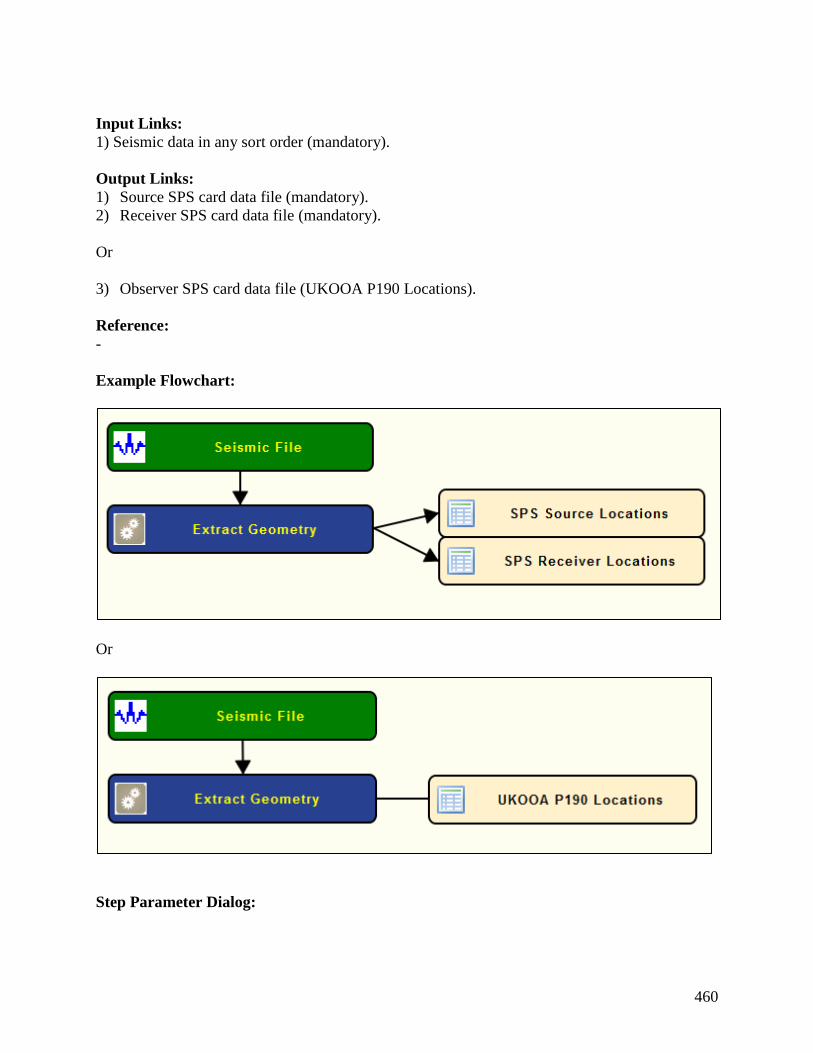
460

Input Links:

1) Seismic data in any sort order (mandatory).

Output Links:

1) Source SPS card data file (mandatory).

2) Receiver SPS card data file (mandatory).

Or

3) Observer SPS card data file (UKOOA P190 Locations).

Reference:

-

Example Flowchart:

Or

Step Parameter Dialog:

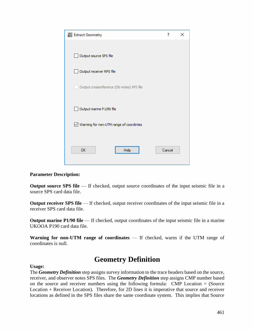
461

Parameter Description:

Output source SPS file — If checked, output source coordinates of the input seismic file in a

source SPS card data file.

Output receiver SPS file — If checked, output receiver coordinates of the input seismic file in a

receiver SPS card data file.

Output marine P1/90 file — If checked, output coordinates of the input seismic file in a marine

UKOOA P190 card data file.

Warning for non-UTM range of coordinates — If checked, warns if the UTM range of

coordinates is null.

Geometry Definition Usage:

The Geometry Definition step assigns survey information to the trace headers based on the source,

receiver, and observer notes SPS files. The Geometry Definition step assigns CMP number based

on the source and receiver numbers using the following formula: CMP Location = (Source

Location + Receiver Location). Therefore, for 2D lines it is imperative that source and receiver

locations as defined in the SPS files share the same coordinate system. This implies that Source

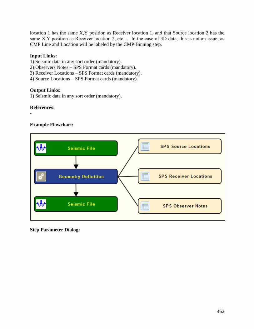
462

location 1 has the same X,Y position as Receiver location 1, and that Source location 2 has the

same X,Y position as Receiver location 2, etc… In the case of 3D data, this is not an issue, as

CMP Line and Location will be labeled by the CMP Binning step.

Input Links:

1) Seismic data in any sort order (mandatory).

2) Observers Notes – SPS Format cards (mandatory).

3) Receiver Locations – SPS Format cards (mandatory).

4) Source Locations – SPS Format cards (mandatory).

Output Links:

1) Seismic data in any sort order (mandatory).

References:

-

Example Flowchart:

Step Parameter Dialog:

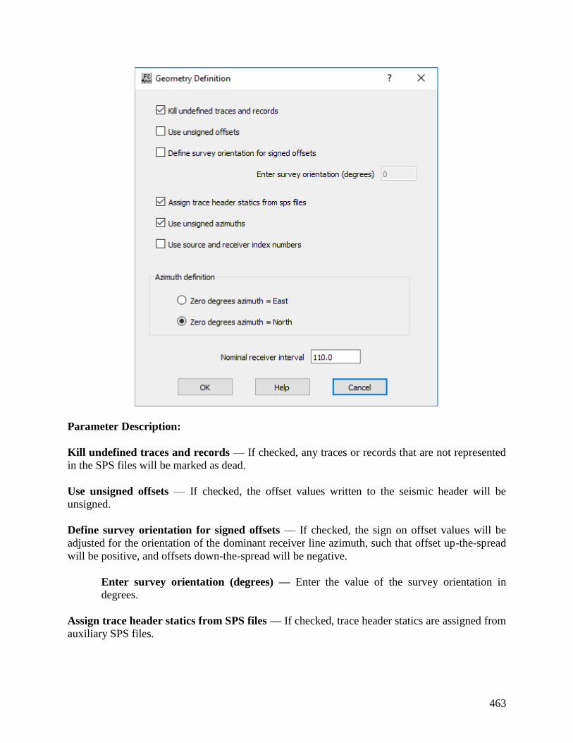
463

Parameter Description:

Kill undefined traces and records — If checked, any traces or records that are not represented

in the SPS files will be marked as dead.

Use unsigned offsets — If checked, the offset values written to the seismic header will be

unsigned.

Define survey orientation for signed offsets — If checked, the sign on offset values will be

adjusted for the orientation of the dominant receiver line azimuth, such that offset up-the-spread

will be positive, and offsets down-the-spread will be negative.

Enter survey orientation (degrees) — Enter the value of the survey orientation in

degrees.

Assign trace header statics from SPS files — If checked, trace header statics are assigned from

auxiliary SPS files.

464

Use unsigned azimuths — If checked, the azimuth values written to the seismic header will range

from 0 to 360 degrees, with zero degrees of azimuth equal to the user-specified direction. By

default, azimuth values are signed and range from 0 to +/-180 degrees, with zero degrees of

azimuth equal to the user-specified direction.

Use source and receiver index number — Define source and receiver by its index number.

Azimuth definition: Specify the origin of azimuth.

Zero degrees azimuth = East — If selected, then zero degrees of source-receiver azimuth will be

set equal to due East.

Zero degrees azimuth = North — If selected, then zero degrees of source-receiver azimuth will

be set equal to due North.

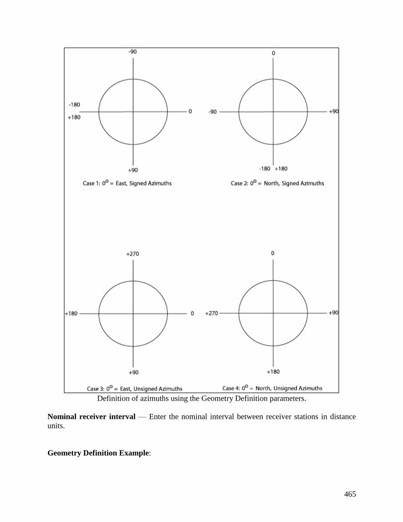
465

Definition of azimuths using the Geometry Definition parameters.

Nominal receiver interval — Enter the nominal interval between receiver stations in distance

units.

Geometry Definition Example:

466

Figure 1. 2D seismic survey consisting of a 6-channel spread and a 25-m station

interval. The spread “rolls-off” at the end of the line.

Source SPS file corresponding to the survey illustrated in figure 1.

467

Figure 3. Receiver SPS file corresponding to the survey illustrated in figure 1.

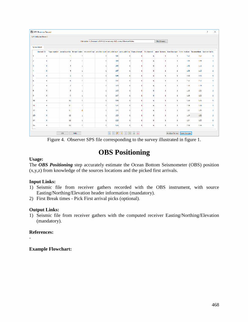
468

Figure 4. Observer SPS file corresponding to the survey illustrated in figure 1.

OBS Positioning Usage:

The OBS Positioning step accurately estimate the Ocean Bottom Seismometer (OBS) position

(x,y,z) from knowledge of the sources locations and the picked first arrivals.

Input Links:

1) Seismic file from receiver gathers recorded with the OBS instrument, with source

Easting/Northing/Elevation header information (mandatory).

2) First Break times - Pick First arrival picks (optional).

Output Links:

1) Seismic file from receiver gathers with the computed receiver Easting/Northing/Elevation

(mandatory).

References:

-

Example Flowchart:

469

Step Parameter Dialog:

Parameter Description:

First arrival picks: Specify first arrival times picks parameters.

Use first arrivals from header word — if checked select the header word containing the first

arrivals information.

Use first arrivals from card date — if checked a first arrivals card data will connect to the step.

Receiver/Source paramters: Specify source elvation parametes.

Sources are mainly at the same depth — if checked all sources are at the same depth range.

Velocity check: Specify range of water velocity.

Check range of the computed water velocity — return a warning message if the inverted velocity

exceeds a range specified by the Minimum/Maximum velocities.

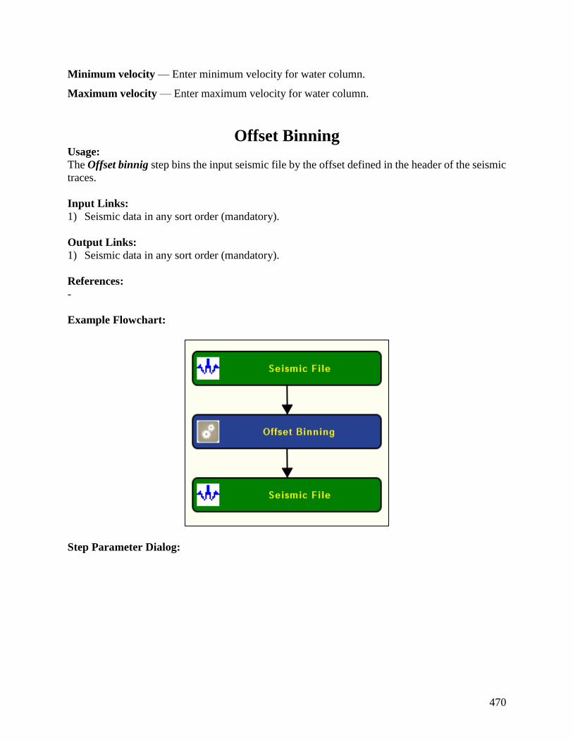
470

Minimum velocity — Enter minimum velocity for water column.

Maximum velocity — Enter maximum velocity for water column.

Offset Binning Usage:

The Offset binnig step bins the input seismic file by the offset defined in the header of the seismic

traces.

Input Links:

1) Seismic data in any sort order (mandatory).

Output Links:

1) Seismic data in any sort order (mandatory).

References:

-

Example Flowchart:

Step Parameter Dialog:

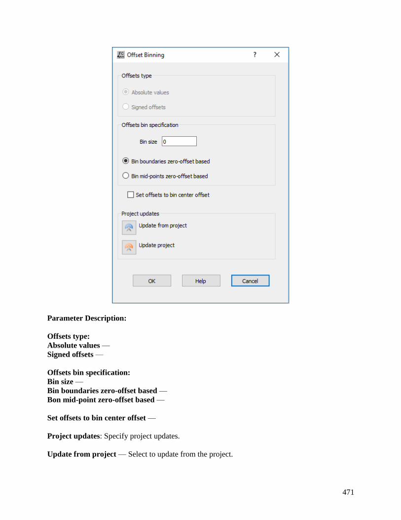
471

Parameter Description:

Offsets type:

Absolute values —

Signed offsets —

Offsets bin specification:

Bin size —

Bin boundaries zero-offset based —

Bon mid-point zero-offset based —

Set offsets to bin center offset —

Project updates: Specify project updates.

Update from project — Select to update from the project.

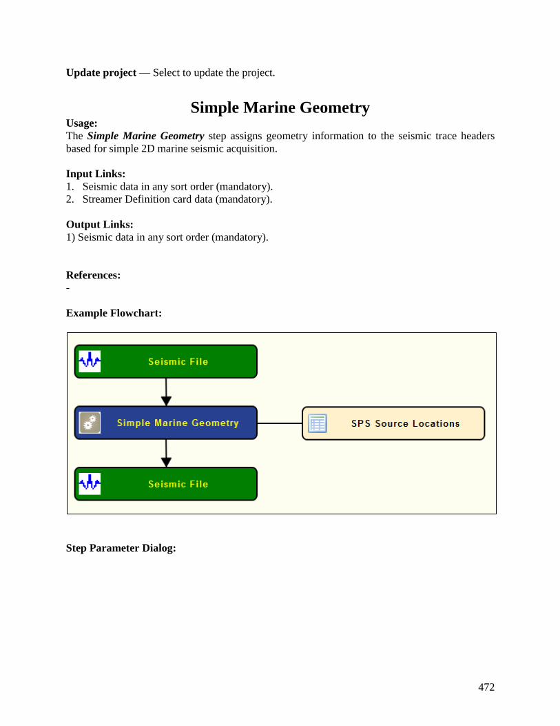
472

Update project — Select to update the project.

Simple Marine Geometry Usage:

The Simple Marine Geometry step assigns geometry information to the seismic trace headers

based for simple 2D marine seismic acquisition.

Input Links:

1. Seismic data in any sort order (mandatory).

2. Streamer Definition card data (mandatory).

Output Links:

1) Seismic data in any sort order (mandatory).

References:

-

Example Flowchart:

Step Parameter Dialog:

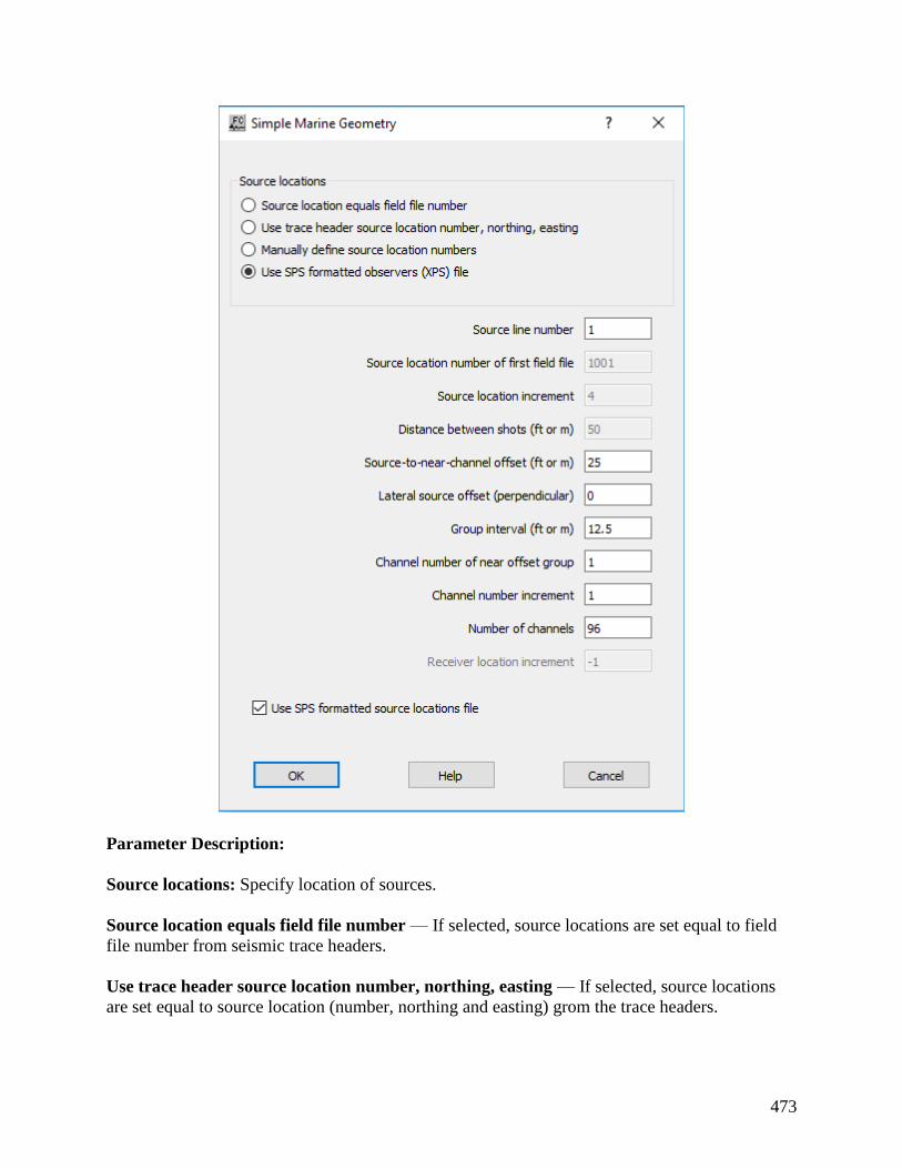
473

Parameter Description:

Source locations: Specify location of sources.

Source location equals field file number — If selected, source locations are set equal to field

file number from seismic trace headers.

Use trace header source location number, northing, easting — If selected, source locations

are set equal to source location (number, northing and easting) grom the trace headers.

474

Manually define source location numbers — If selected, source locations are defined manually

from the parameters below.

Use SPS formatted observers (XPS) file — If selected, source locations are set as defined in

the auxiliare observers (XPS) card data file.

Source line number — Enter the source location line number.

Source location number of first field file — Enter the location of the source for first field file

number.

Source location increment — Enter the source location increment. This value must be an integer

value.

Distance between shot (ft or m) — Enter the distance between shots in ft or m, depending on the

units defined for the project.

Source-to-near-channel offset (ft or m) — Enter the near offset, distance between source and the

near channel. Distance defined in ft or m, depending on the units defined for the project.

Lateral source offset (perpendicular) — Enter the offset distance in the direction perpendicular

to the streamer.

Group interval (ft or m) — Enter the distance between each group. Distance defined in ft or m,

depending on the units defined for the project.

Channel number of near offset group — Enter the number of the enear offset group.

Channel number increment — Enter the increment between channels.

Number of channles — Enter total number of channels in the streamer.

Receiver location increment — Enter the increment between receiver locations.

Use SPS formatted source locations file — If checked, source locations are extracted from an

auxiliary source SPS card data file.

UKOOA P1/90 Geometry Usage:

The UKOOA P1/90 Geometry step assigns survey information to the trace headers based on a

geometry file as defined in an auxiliary UKOOA P1/90 card data file.

Input Links:

1) Seismic data in any sort order (mandatory).

2) UKOOA P1 90 card data file (mandatory).

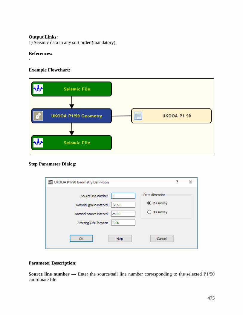
475

Output Links:

1) Seismic data in any sort order (mandatory).

References:

-

Example Flowchart:

Step Parameter Dialog:

Parameter Description:

Source line number — Enter the source/sail line number corresponding to the selected P1/90

coordinate file.

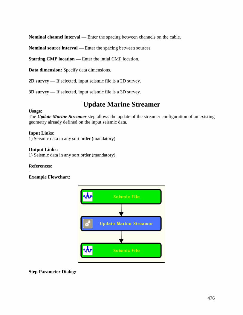
476

Nominal channel interval — Enter the spacing between channels on the cable.

Nominal source interval — Enter the spacing between sources.

Starting CMP location — Enter the intial CMP location.

Data dimension: Specify data dimensions.

2D survey — If selected, input seismic file is a 2D survey.

3D survey — If selected, input seismic file is a 3D survey.

Update Marine Streamer Usage:

The Update Marine Streamer step allows the update of the streamer configuration of an existing

geometry already defined on the input seismic data.

Input Links:

1) Seismic data in any sort order (mandatory).

Output Links:

1) Seismic data in any sort order (mandatory).

References:

-

Example Flowchart:

Step Parameter Dialog:

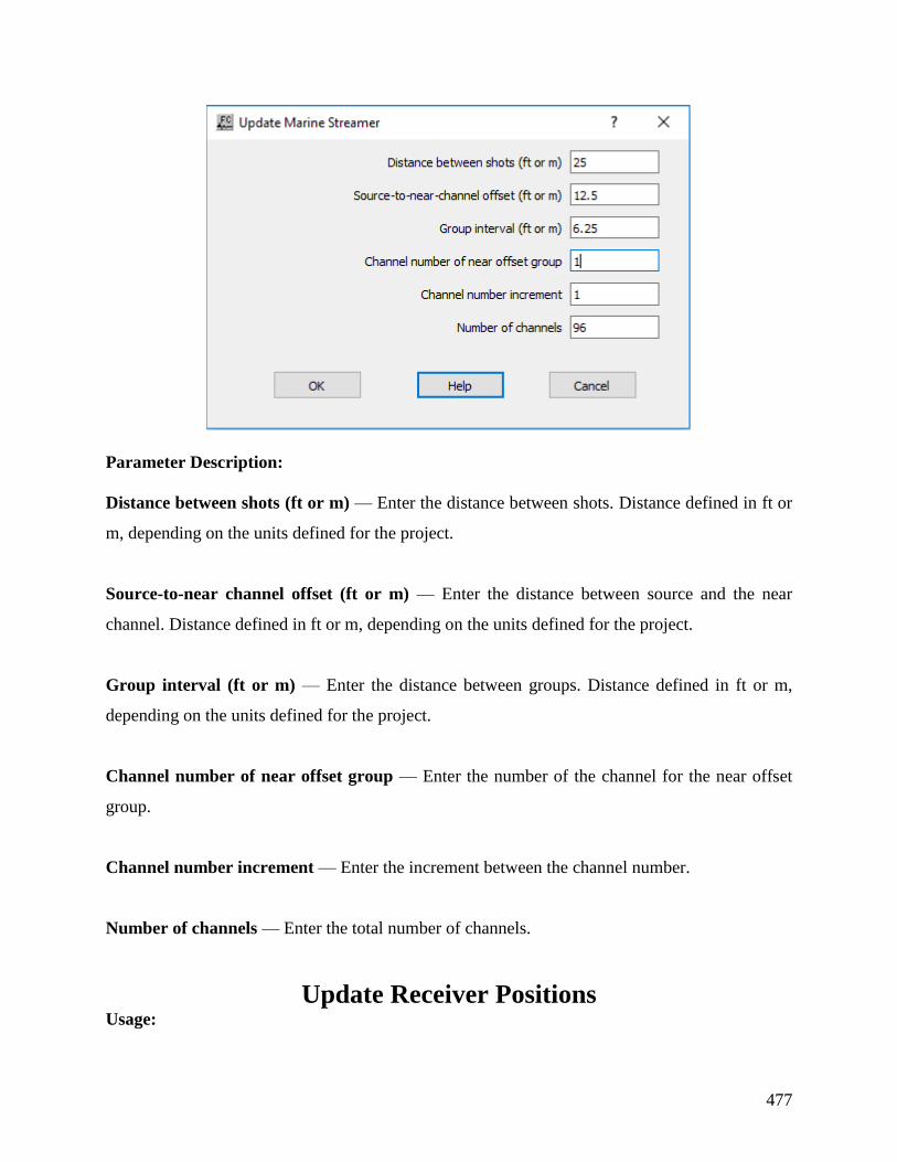
477

Parameter Description:

Distance between shots (ft or m) — Enter the distance between shots. Distance defined in ft or

m, depending on the units defined for the project.

Source-to-near channel offset (ft or m) — Enter the distance between source and the near

channel. Distance defined in ft or m, depending on the units defined for the project.

Group interval (ft or m) — Enter the distance between groups. Distance defined in ft or m,

depending on the units defined for the project.

Channel number of near offset group — Enter the number of the channel for the near offset

group.

Channel number increment — Enter the increment between the channel number.

Number of channels — Enter the total number of channels.

Update Receiver Positions Usage:

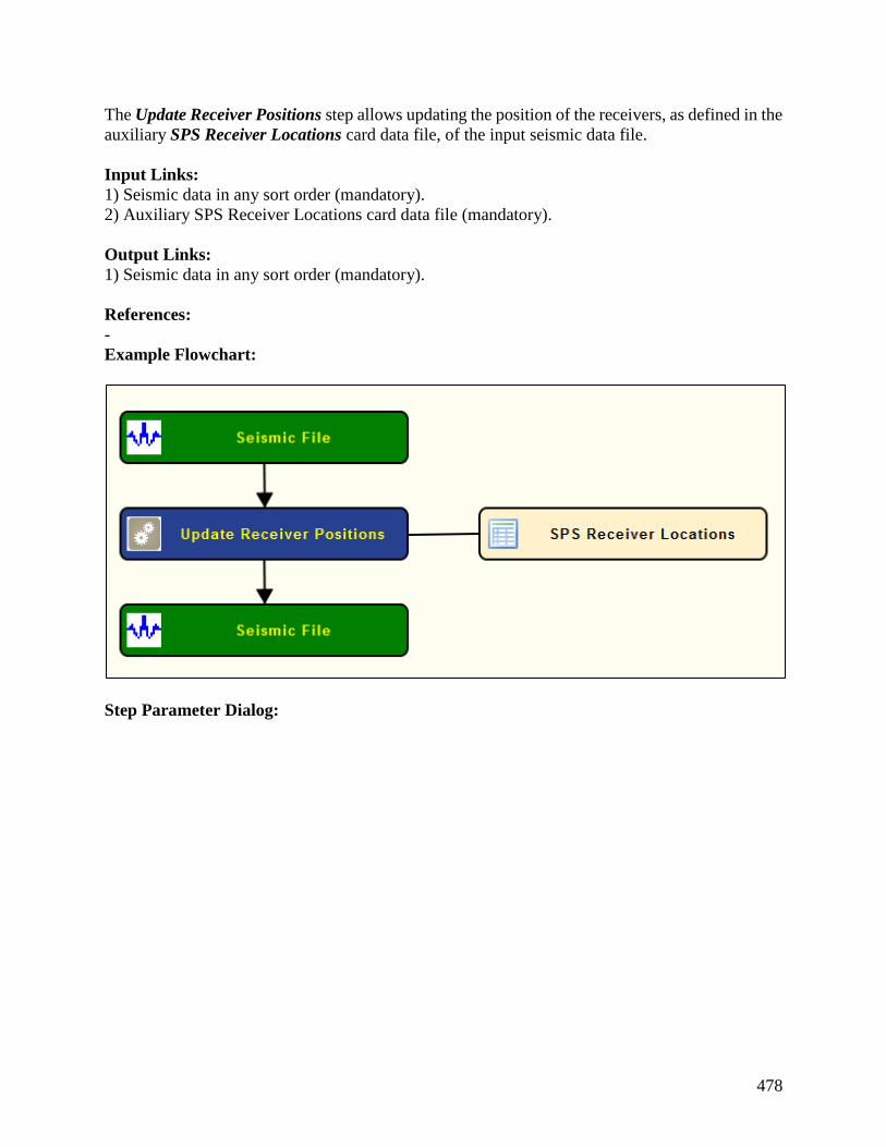
478

The Update Receiver Positions step allows updating the position of the receivers, as defined in the

auxiliary SPS Receiver Locations card data file, of the input seismic data file.

Input Links:

1) Seismic data in any sort order (mandatory).

2) Auxiliary SPS Receiver Locations card data file (mandatory).

Output Links:

1) Seismic data in any sort order (mandatory).

References:

-

Example Flowchart:

Step Parameter Dialog:

479

Parameter Description:

Use unsigned offsets — If checked, the offset values written to the seismic header will be

unsigned.

Define survey orientation for signed offsets — If checked, the sign on offset values will be

adjusted for the orientation of the dominant receiver line azimuth, such that offset up-the-spread

will be positive, and offsets down-the-spread will be negative.

Enter survey orientation (degrees) — Enter the value of the survey orientation in

degrees.

Use unsigned azimuths — If checked, the azimuth values written to the seismic header will range

from 0 to 360 degrees, with zero degrees of azimuth equal to the user-specified direction. By

default, azimuth values are signed and range from 0 to +/-180 degrees, with zero degrees of

azimuth equal to the user-specified direction.

Azimuth definition: Specify the origin of azimuth.

Zero degrees azimuth = East — If selected, then zero degrees of source-receiver azimuth will be

set equal to due East.

480

Zero degrees azimuth = North — If selected, then zero degrees of source-receiver azimuth will

be set equal to due North.

Nominal receiver interval — Enter the nominal interval between receiver stations in distance

units.

Update Source Positions

Usage:

The Update Source Positions step allows updating the position of the sources, as defined in the

auxiliary SPS Source Locations card data file, of the input seismic data file.

Input Links:

1) Seismic data in any sort order (mandatory).

2) Auxiliary SPS Source Locations card data file (mandatory).

Output Links:

1) Seismic data in any sort order (mandatory).

References:

-

Example Flowchart:

Step Parameter Dialog:

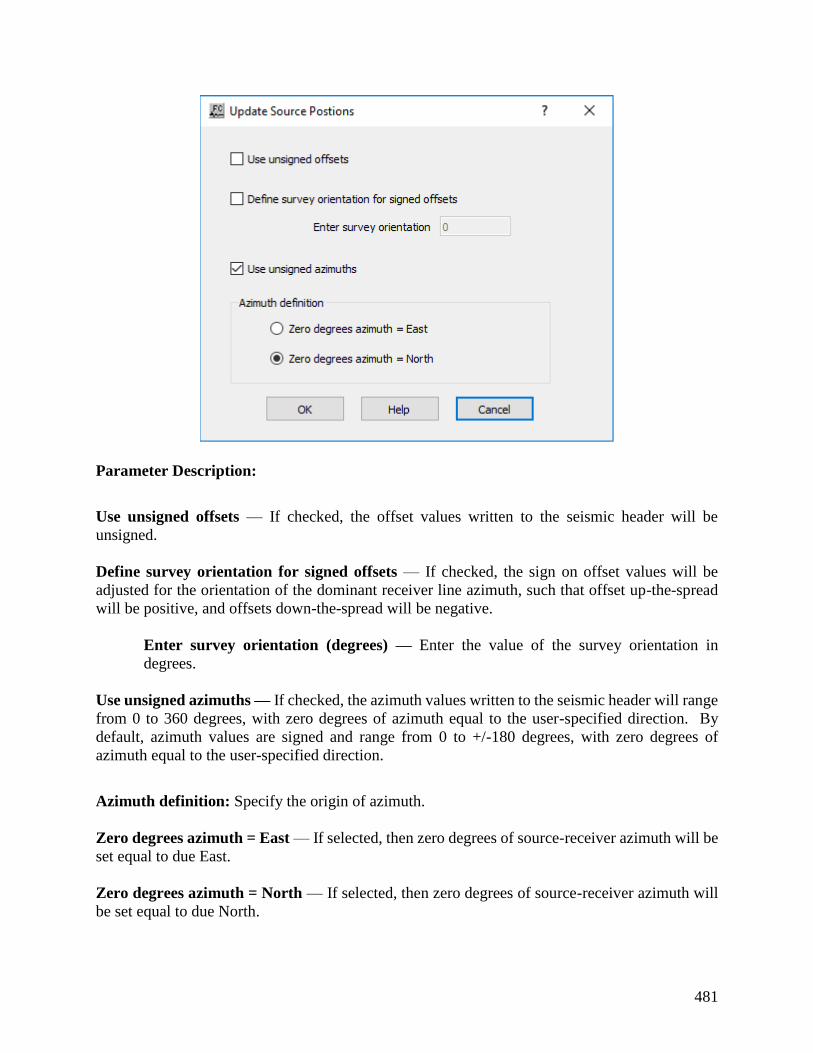
481

Parameter Description:

Use unsigned offsets — If checked, the offset values written to the seismic header will be

unsigned.

Define survey orientation for signed offsets — If checked, the sign on offset values will be

adjusted for the orientation of the dominant receiver line azimuth, such that offset up-the-spread

will be positive, and offsets down-the-spread will be negative.

Enter survey orientation (degrees) — Enter the value of the survey orientation in

degrees.

Use unsigned azimuths — If checked, the azimuth values written to the seismic header will range

from 0 to 360 degrees, with zero degrees of azimuth equal to the user-specified direction. By

default, azimuth values are signed and range from 0 to +/-180 degrees, with zero degrees of

azimuth equal to the user-specified direction.

Azimuth definition: Specify the origin of azimuth.

Zero degrees azimuth = East — If selected, then zero degrees of source-receiver azimuth will be

set equal to due East.

Zero degrees azimuth = North — If selected, then zero degrees of source-receiver azimuth will

be set equal to due North.

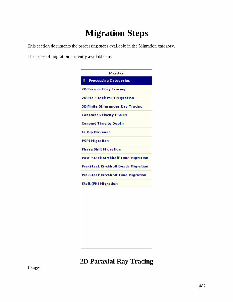
482

Migration Steps

This section documents the processing steps available in the Migration category.

The types of migration currently available are:

2D Paraxial Ray Tracing Usage:

483

The 2D Paraxial Ray Tracing step is an asymptotic wave method, which uses quantities (local

wavefront curvature and spreading information) determined along a central ray via dynamic ray

tracing, to evaluate approximately the seismic wave field in its vicinity rather then just on the ray

itself (Cerveny et al. 1984). This implementation is designed to run in single thread or in parallel,

giving it the possibility to take full advantage of multiple processors at the same time.

Input Links:

-

Auxiliary dataset:

1) Interval Velocity-Field file, created using the step Create Velocity Field under the velocity

category (mandatory).

2) Pre-stack dataset, used to get source and receivers geometry (mandatory).

Output Links:

1) Seismic file where the computed source or receiver travel-time tables will be saved (mandatory).

References:

Cerveny V, Klimes L, Psencik I (1984) Paraxial ray approximations in the computation of

seismic wavefields in inhomogeneous media. Geophys J R Astron Soc 89–104.

Example Flowchart:

Step Parameter Dialog:

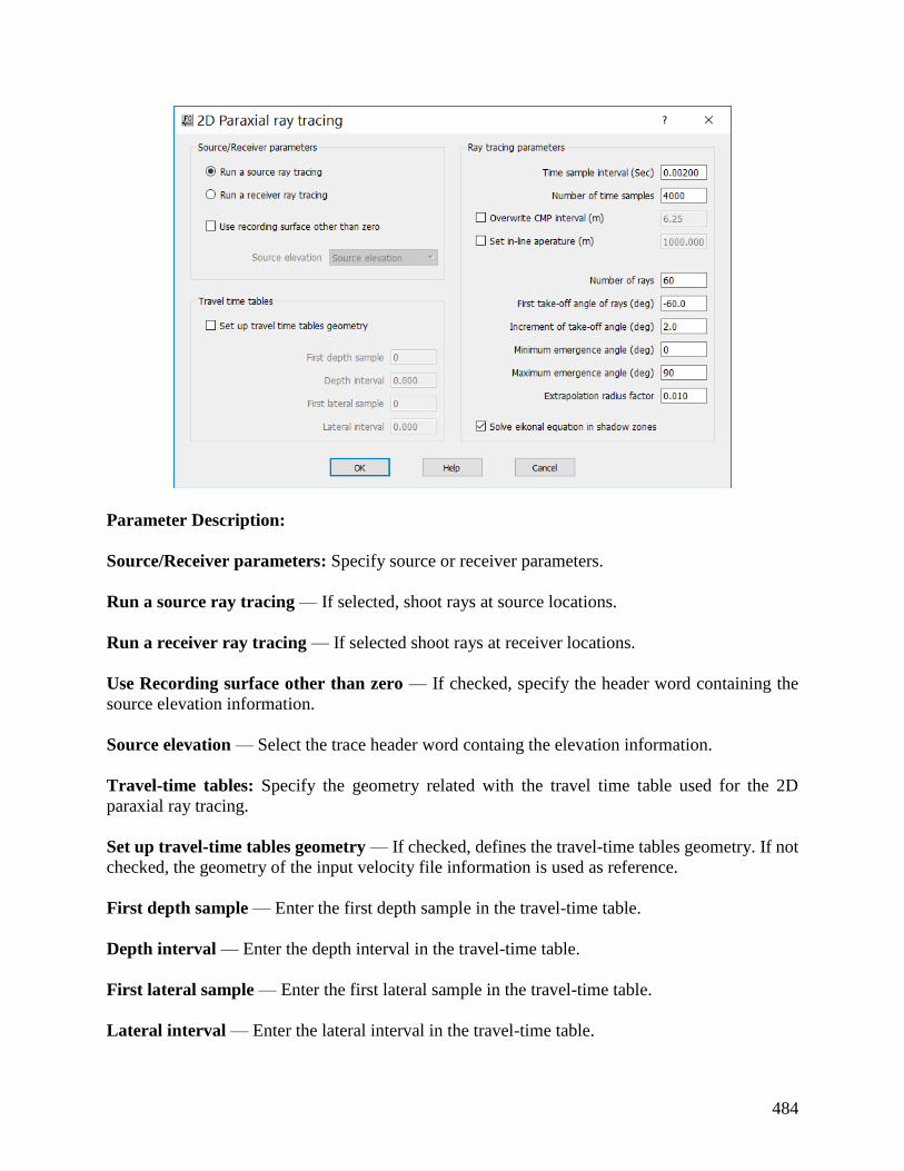
484

Parameter Description:

Source/Receiver parameters: Specify source or receiver parameters.

Run a source ray tracing — If selected, shoot rays at source locations.

Run a receiver ray tracing — If selected shoot rays at receiver locations.

Use Recording surface other than zero — If checked, specify the header word containing the

source elevation information.

Source elevation — Select the trace header word containg the elevation information.

Travel-time tables: Specify the geometry related with the travel time table used for the 2D

paraxial ray tracing.

Set up travel-time tables geometry — If checked, defines the travel-time tables geometry. If not

checked, the geometry of the input velocity file information is used as reference.

First depth sample — Enter the first depth sample in the travel-time table.

Depth interval — Enter the depth interval in the travel-time table.

First lateral sample — Enter the first lateral sample in the travel-time table.

Lateral interval — Enter the lateral interval in the travel-time table.

485

Ray tracing parameters: Specify the ray tracing parameters.

Time sample interval — Enter the time sample interval in ray tracing.

Number of time samples — Enter the number of time samples in ray tracing.

Number of rays — Enter the number of rays.

Set in-line aperture — Define the setting for the in-line aperture. If not checked, the maximum

aperture is used, which require more compute time.

In-line aperture — Enter the ray tracing aperture for the in-line direction.

First take-off angle of rays (deg.) — Enter the first take-off angle of the rays in degrees.

Increment of take-off angle — Enter the increment of the take-off angle.

Minimum emergence angle — Enter the minimum emergence angle.

Maximum emergence angle — Enter the maximum emergence angle.

Extrapolation radius factor — Enter the factor to determine the radius for extrapolation.

Solve eikonal equation in shadow zones — If checked implements the eikonal equation in the

shadow zones.

2D Pre-Stack PSPI Migration Usage:

The 2D Pre-Stack PSPI Migration step is only available for 2D seismic data and is a 2D ‘Phase

Shift Plus Interpolation’ seismic data migration. The input data must be in the form of frequency

slices of CMP v Offset. Convert the CMP and offset-sorted data to frequency slices by the use of

Frequency Slices step in a prior job flow.

The output data will be in standard trace order and not requiring further transformation.

Input Links:

1) Frequency slices ordered by Slice Number and CMP (mandatory).

Output Links:

1) Time traces sorted by CMP and Offset (mandatory).

Reference:

Gasdag, J, and Sguazzero P., 1984, Migration of seismic data by phase shift plus interpolation,

Geophysics, vol. 49, no. 2, p. 124-131.

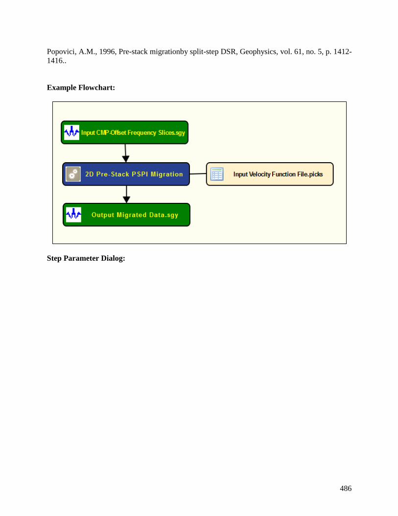
486

Popovici, A.M., 1996, Pre-stack migrationby split-step DSR, Geophysics, vol. 61, no. 5, p. 1412-

1416..

Example Flowchart:

Step Parameter Dialog:

487

Parameter Description:

488

Migration mode: Specify migration domain and output format.

Time Migration — If checked, time migration will be performed.

Output maximum time(ms) — Enter the maximum time of the output migrated data in

milliseconds. The time sampling will be the same as that of the input data.

Depth Migration — If checked, depth migration will be performed.

Output maximum depth(ft/m) — Enter the maximum depth of the output migrated data.

Output depth sampling (ft/m) — Enter the depth sampling interval of the output migrated

data.

Migration velocity field: Specify parameters related with the velocity field used for migration.

Use velocity field from data file — If checked, then the file name of an auxiliary input file must

be specified which contains the velocity field picks.

Use constant migration velocity — If checked, then the migration velocity to be used should be

specified in the adjacent box.

Scale input velocities by — The migration velocities may be scaled by a constant factor if

required.

Velocity sampling: Specify velocity sampling parameters.

Use CMP velocity — If selected, then velocity will be CMP dependent only. This is the normal

assumption when performing time migration.

[Use velocity from CMP and offset — If selected, then velocity field will be expected to be

dependent both on CMP and on offset. This is likely to be the case when performing depth

migration. This option is not currently available.]

Migration step size: Specify migration step size.

Number of output samples — Enter the number of output migration slices to be output with each

iteration of the migration. Every migration iteration takes a roughly constant execution time, so

the total execution time can be significantly reduced if several output slices are calculated at once.

There may be a degradation in the migration of dipping data if this parameter is set too high.

Consequently, this parameter is data-dependent and may require testing.

Frequency filtering: Specify filtering parameters. The output migrated data will be Hanning

(cosine) tapered.

Low cut Frequency (Hz.) — Enter the low cut frequency of the output migrated data.

489

Low pass Frequency (Hz.) — Enter the low pass frequency of the output migrated data.

High pass Frequency (Hz.) — Enter the high pass frequency of the output migrated data.

High cut Frequency (Hz.) — Enter the high cut frequency of the output migrated data.

Alias energy removal: Specify alias energy removal.

Evanescent damping factor — Enter the amount of suppression of energy which is not a real

solution of the acoustic wave equation, as a value between zero and one. A value of 0.5 is

recommended.

Spatial padding width (traces) — Enter how many additional traces are to be added (in both

CMP line and location directions in the case of 3D migration). These extra traces plus spatial

tapering help to minimize interference of migrated energy from one end of the data into migrated

data on the other side.

Override trace spacing: Specify if the original trace spacing is override by a user defined

distance. If the trace spacing cannot be read from or is incorrect in the trace headers, then it may

be specified in the following parameter fields:

Specify the CMP spacing— If checked, then the user must enter the distance between CMP

locations in the adjacent field.

3D Finite Differences Ray Tracing Usage:

The 3D Finite Differences Ray Tracing step is a wavefront tracing technique, and a robust

alternative to conventional ray tracing. This method relies on the application of Huygens’ Principle

in the finite difference approximation. That is, every point reached by a wave becomes a secondary

source; the sum of these secondary waves determines the form of the wave at any subsequent time.

This method accurately computes travel-time information even with step velocity contrast as high

as 1:10 regardless of the sharpness of the velocity anomaly. This implementation is designed to

run in single thread or in parallel, giving it the possibility to take full advantage of multiple

processors at the same time.

Input Links:

-

Auxiliary dataset:

1) 3D Interval Velocity-Field file, created using the step Create Velocity Field under the velocity

category (mandatory).

2) Pre-stack dataset, used to get source and receivers geometry (mandatory).

490

Output Links:

1) Seismic file where the computed source or receiver travel-time cubes will be saved

(mandatory).

References:

Podvin P, L. I (1991) Finite difference computation of traveltimes in very contrasted velocity

models: a massively parallel approach and its associated. Geophys J Int 105:271–284.

Huygens wavefront tracing: A robust alternative to conventional ray tracing. SEP Report, 95,

101-113 (1997)

Example Flowchart:

Step Parameter Dialog:

Parameter Description:

491

Source/Receiver parameters: Specify source or receiver parameters.

Run a source ray tracing — If selected, shoot rays at source locations.

Run a receiver ray tracing — If selected, shoot rays at receiver locations.

Define the travel time computation grid (m) — If checked, specify the grid spacing on which

the computation is carried; the output grid is exactly the same as the velocity grid.

Travel time grid spacing (m) — Enter the travel time grid spacing.

Use Recording surface other than zero — If checked, specify the header word containing the

source elevation information.

Source/Receiver elevation — Select header word with source elevation information.

Mute above the source/receiver depth — This option is only enabled if the recording

surface is other then zero.

Constant Velocity PSKTM Usage:

The Constant Velocity PSKTM step is a migration velocity analysis tool; it runs multiple Pre-

Stack Kirchhoff Migrations around the velocity model given as input to pick the velocity that

migrate best the data. This implementation is designed to run in single thread or in parallel, giving

it the possibility to take full advantage of multiple processors at the same time.

Input Links:

1) Pre-Stack seismic dataset with geometry applied to it and preferably some pre-processing as

well (mandatory).

Auxiliary dataset:

1) Velocity model/function (mandatory).

Output Links:

1) Seismic file where the Constant Velocity PSKTM will be saved (mandatory).

References:

-

Example Flowchart:

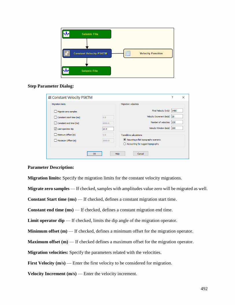
492

Step Parameter Dialog:

Parameter Description:

Migration limits: Specify the migration limits for the constant velocity migrations.

Migrate zero samples — If checked, samples with amplitudes value zero will be migrated as well.

Constant Start time (ms) — If checked, defines a constant migration start time.

Constant end time (ms) — If checked, defines a constant migration end time.

Limit operator dip — If checked, limits the dip angle of the migration operator.

Minimum offset (m) — If checked, defines a minimum offset for the migration operator.

Maximum offset (m) — If checked defines a maximum offset for the migration operator.

Migration velocities: Specify the parameters related with the velocities.

First Velocity (m/s) — Enter the first velocity to be considered for migration.

Velocity Increment (m/s) — Enter the velocity increment.

493

Number of Velocities — Enter the number of velocities to be tested.

Number of Velocities — Enter the number of velocities to be tested.

Velocity window (m/s) — Enter a window around the input velocity model.

Traveltime calculations: Specify parameters for traveltime calculations.

Assuming a flat topography scenario — If selected, assume a flat recording surface when

computing travel-time information.

Accounting for rugged topography — If selected, assume a rugged recording surface when

computing travel-time information.

Convert Time to Depth Usage:

The Convert Time to Depth step does a vertical time to depth conversion of a seismic file using

an input set of interval velocities. The input velocities are assumed to be in units of feet or meters

per second. If the input file to be depth converted is a GPR image, and the input velocity file is in

units of feet or meters per nanosecond, you must first multiply the velocity values by 1x10-9.

Input Links:

1) Seismic data in any sort order (mandatory).

2) Velocity Function cards (optional).

Output Links:

1) Seismic data in any sort order (mandatory).

References:

See Technical Note TN-DpthConv.doc

Example Flowchart:

494

Step Parameter Dialog:

495

Parameter Description:

Velocity field estimation: Specify velocity field.

Use velocity field from data file — If selected, the velocity field used for the time to depth

conversion is from an auxiliary velocity field card data.

Use smooth velocities — If selected, input velocities are smoothed horizontally and

vertically.

Use blocky velocities — If selected, input velocities are converted into interval velocities.

Correction velocity — Enter the correction velocity (ft/sec or m/sec) to be used in the conversion.

This constant velocity will be used unless a velocity function is connected to the step. In the case

of GPR data, convert this value to the appropriate units.

496

Output depth interval — Enter the depth interval in your spatial units. To obtain an estimate

of the output depth interval, first employ the formula X = VT, where X = estimated depth of

section, V = average velocity of section, and T = one-way time of the section (i.e. record length

divided by two). Second, employ the formula output depth interval = X = X/(number of

samples 1).

Number of output samples — Enter the number of samples to output.

Interpolation Type Selection — Select the type of interpolator to use. This interpolator is used

to resample the data to the specified depth interval.

Do inverse correction — If checked, a depth to time conversion will be performed.

FK Dip Moveout Usage:

Input Links:

Output Links:

Reference:

-

Example Flowchart:

Step Parameter Dialog:

Parameter Description:

PSPI Migration Usage:

The PSPI Migration step is a post-stack ‘Phase Shift Plus Interpolation’ seismic data migration.

Input data may be 2D or 3D, and both time migration and depth migration are options.

The input data must be in the form of frequency slices – data can be converted to frequency slices

by the use of Frequency Slices in a prior job flow.

The output data will be in the form of time slices – convert the time slices back to standard trace

order in a subsequent job flow after the migration with the use of Time Slices to Traces.

Input Links:

1) Frequency slices ordered by Slice Number and CMP Line (3D) or by Slice Number (2D)

(mandatory).

Output Links:

1) Time slices (or depth slices) ordered by Slice Number and CMP Line (3D) or by Slice Number

(2D) (mandatory).

Reference:

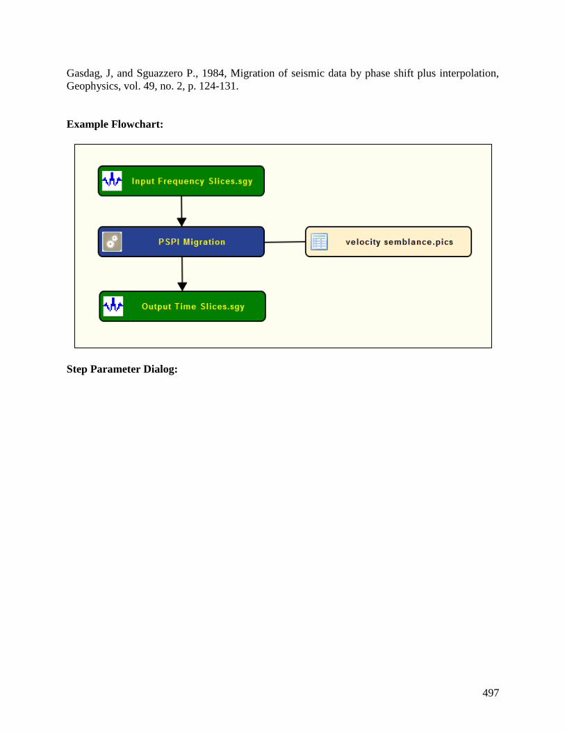
497

Gasdag, J, and Sguazzero P., 1984, Migration of seismic data by phase shift plus interpolation,

Geophysics, vol. 49, no. 2, p. 124-131.

Example Flowchart:

Step Parameter Dialog:

498

Parameter Description:

Migration mode: Define type o migration (time or depth migration) to be applied to data.

499

Time Migration — If checked, time migration will be performed.

Output maximum time(ms) — Enter the maximum time of the output migrated data in

milliseconds. The time sampling will be the same as that of the input data.

Depth Migration — If checked, depth migration will be performed.

Output maximum depth(ft/m) — Enter the maximum depth of the output migrated data.

Output depth sampling (ft/m) — Enter the depth sampling interval of the output migrated

data.

Migration velocity field: Specify the type of velocity field to be applied during the migration.

Use velocity field from data file — If checked, then the file name of an auxiliary input file must

be specified which contains the velocity field picks.

Use constant migration velocity — If checked, then the migration velocity to be used should be

specified in the adjacent box.

Scale input velocities by — The migration velocities may be scaled by a constant factor if

required.

Output velocity field only— If checked, then only the interpolated and fully sampled migration

velocity will be output. This flag is for test purposes only.

Migration step size: Specify the step size for the migration.

Number of output samples — Enter the number of output migration slices to be output with each

iteration of the migration. Every migration iteration takes a roughly constant execution time, so

the total execution time can be significantly reduced if several output slices are calculated at once.

There may be a degradation in the migration of dipping data if this parameter is set too high.

Consequently, this parameter is data-dependent and may require testing.

Frequency filtering: Specify and parameterizer the frequency filter to be applied to the migrated

data. The output migrated data will be Hanning (cosine) tapered.

Low cut Frequency (Hz.) — Enter the low cut frequency of the output migrated data.

Low pass Frequency (Hz.) — Enter the low pass frequency of the output migrated data.

High pass Frequency (Hz.) — Enter the high pass frequency of the output migrated data.

High cut Frequency (Hz.) — Enter the high cut frequency of the output migrated data.

Alias energy removal: Specify parameters related with alias energy removal.

500

Evanescent damping factor — Enter the amount of suppression of energy which is not a real

solution of the acoustic wave equation, as a value between zero and one. A value of 0.5 is

recommended.

Spatial padding width (traces) — Enter how many additional traces are to be added (in both

CMP line and location directions in the case of 3D migration). These extra traces plus spatial

tapering help to minimize interference of migrated energy from one end of the data into migrated

data on the other side.

Override trace spacing: If the trace spacing cannot be read from or is incorrect in the trace

headers, then it may be specified in the following parameter fields.

Specify the trace spacing — If checked, enter the distance between trace locations.

Specify the line spacing — If checked, enter the the distance between lines (for 3D data only).

Phase Shift Migration Usage:

The Phase Shift Migration step implements a constant velocity or a depth-variable velocity post

stack phase shift time migration in the frequency domain. The input velocity field is assumed to

be the stacking velocity field derived from velocity analysis of the pre-stack data. This step is

currently only available for 2D data.

Input Links:

1) Seismic data in stacked order (mandatory).

2) Velocity Function cards (optional).

Output Links:

1) Seismic data in stacked order (mandatory) and sampled in time.

Reference:

Gazdag, J, 1978, Wave-equation migration by phase shift, Geophysics, v. 43, p. 1342-1351.

Example Flowchart:

501

Step Parameter Dialog:

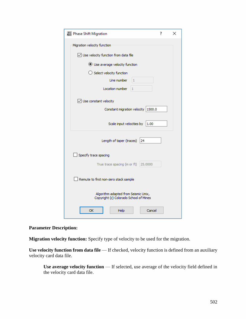
502

Parameter Description:

Migration velocity function: Specify type of velocity to be used for the migration.

Use velocity function from data file — If checked, velocity function is defined from an auxiliary

velocity card data file.

Use average velocity function — If selected, use average of the velocity field defined in

the velocity card data file.

503

Select velocity function — If selected, use a velocity function as defined in a specific

location from the input velocity card data.

Line number — Enter line number for the location of the velocity function.

Location number — Enter location number for the location of the velocity

function.

Use constant velocity — If checked, a constant velocity value will be used as the migration

velocity if no velocity cards are linked.

Constant migration velocity — Enter constant velocity value to be used for migration.

Scale input velocities by — The input velocities are multiplied by this number. This scalar is used

for adjusting the input velocities if they are interval velocities derived using Dix's equation rather

than true interval velocities.

Lenth of taper (traces) — Enter the length of the taper to be used for the migration in number of

traces.

Specify trace spacing — If checked, overwrite trace spacing by defined value.

True trace spacing (m or ft) — Enter trace spacing in ft or m to overwrite geometry.

Remute to first non-zero stack sample — If checked, mute for all traces individually all samples

before non-zero.

Post-Stack Kirchhoff Time Migration

Usage:

The Post-Stack Kirchhoff Time Migration step implements a diffraction summation migration of

the Kirchhoff type on a post-stack section, which is capable of handing vertically and laterally

varying velocity fields. The input velocity field is assumed to be the stacking velocity field derived

from velocity analysis of the pre-stack data.

Input Links:

Stacked seismic data (mandatory).

Auxiliary dataset:

Velocity Function cards (mandatory).

Output Links:

Seismic file where the migrated section will be saved (mandatory).

Reference:

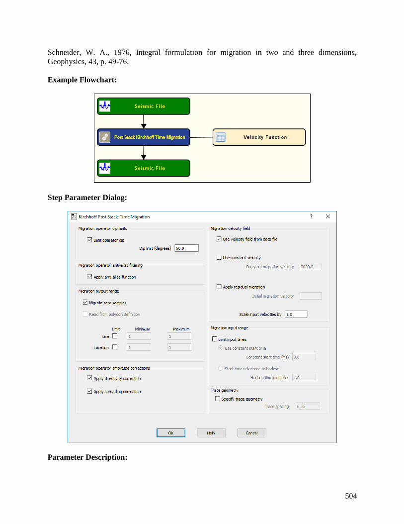
504

Schneider, W. A., 1976, Integral formulation for migration in two and three dimensions,

Geophysics, 43, p. 49-76.

Example Flowchart:

Step Parameter Dialog:

Parameter Description:

505

Migration operator dip limits: Specify if any dip limit will be used for the migration.

Limit Operator Dip — If checked, limts the dip angle to be migrated.

Dip limit (degrees) — Enter the dip angle of the migration operator.

Migration operator anti-alias filter: Specify operator of the anti-alias filter to be applied during

the migration.

Apply anti-alias function — If checked, apply an anti-aliasing measure to the migration operator.

Migration output range: Specify output range of the migrated data.

Migrate zero samples — If checked, samples with amplitudes value zero will be migrated as well.

Line (Min/Max) — If checked, allows you to limit the range of the migrated CMP lines.

Location (Min/Max) — If checked, allows you to limit the range of the migrated CMP locations.

Migration operator amplitude correction: Specify how migrated amplitudes are handled.

Apply directivity correction — If checked, applies directivity correction to the amplitudes of the

migrated data.

Apply spreading correction — If checked, applies spreading correction to the amplitudes of the

migrated data.

Migration velocity field: Specify velocity model used for migration.

Use velocity field from data file — If cheked, connect a velocity function to the migration step

as input migration RMS velocities.

Use constant velocity — If checked, uses a constant velocity model for migration.

Constant migration velocity — Enter the constant velocity value to be used for migration.

Apply residual migration — not yet implemented.

Initial migration velocity — not yet implemented.

Scale velocity input — Enter a scaling factor for the input velocities, or else 1.

Migration input range: Specify input range of the data for the migration.

Limit input times (ms) — If checked, input data is limited by time windows.

506

Use constant start time — If selected, defines a constant migration start time.

Constant start time (ms) — Enter migration start time.

Start time reference to horizon — not yet implemented.

Horizont time multiplier — not yet implemented.

Trace geometry: Specify trace spacing.

Specify trace geometry — If checked, specifies trace spacing in meters.

Trace spacing — Enter trace spacing in m or ft.

Pre-Stack Kirchhoff Depth Migration

Usage:

The Pre-Stack Kirchhoff Depth Migration step implements a diffraction summation migration

of the Kirchhoff type on a pre-stack shot gathers. As opposed to the time version, the

depth implementation of the Kirchhoff migration does not compute travel time with a

strait ray propagation assumption. Instead, it uses travel-time tables that were precomputed

using methods like the 2D Paraxial Ray Tracing or the 3D Finite Difference

wavefront tracing. This method handles more accurately vertical and lateral changes in

the velocity fields and dipping reflectors. This implementation is designed to run in single

thread or in parallel, giving it the possibility to take full advantage of multiple processors

at the same time.

Input Links:

1) Pre-Stack seismic data in shot gather order (mandatory).

2) Source travel-time tables (mandatory).

3) Receiver travel-time tables (mandatory).

Output Links:

1) Seismic file where the migrated seismic data will be saved (mandatory).

References:

-

Example Flowchart:

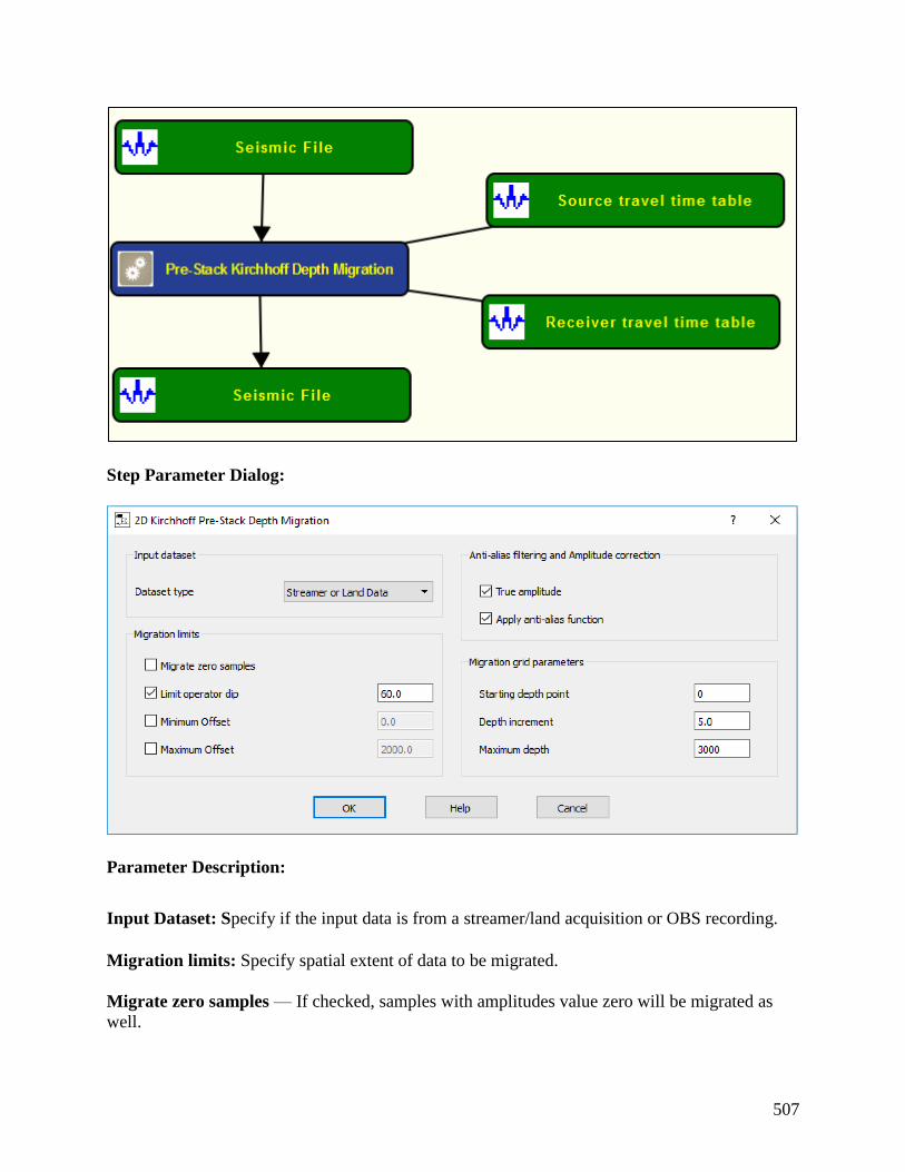
507

Step Parameter Dialog:

Parameter Description:

Input Dataset: Specify if the input data is from a streamer/land acquisition or OBS recording.

Migration limits: Specify spatial extent of data to be migrated.

Migrate zero samples — If checked, samples with amplitudes value zero will be migrated as

well.

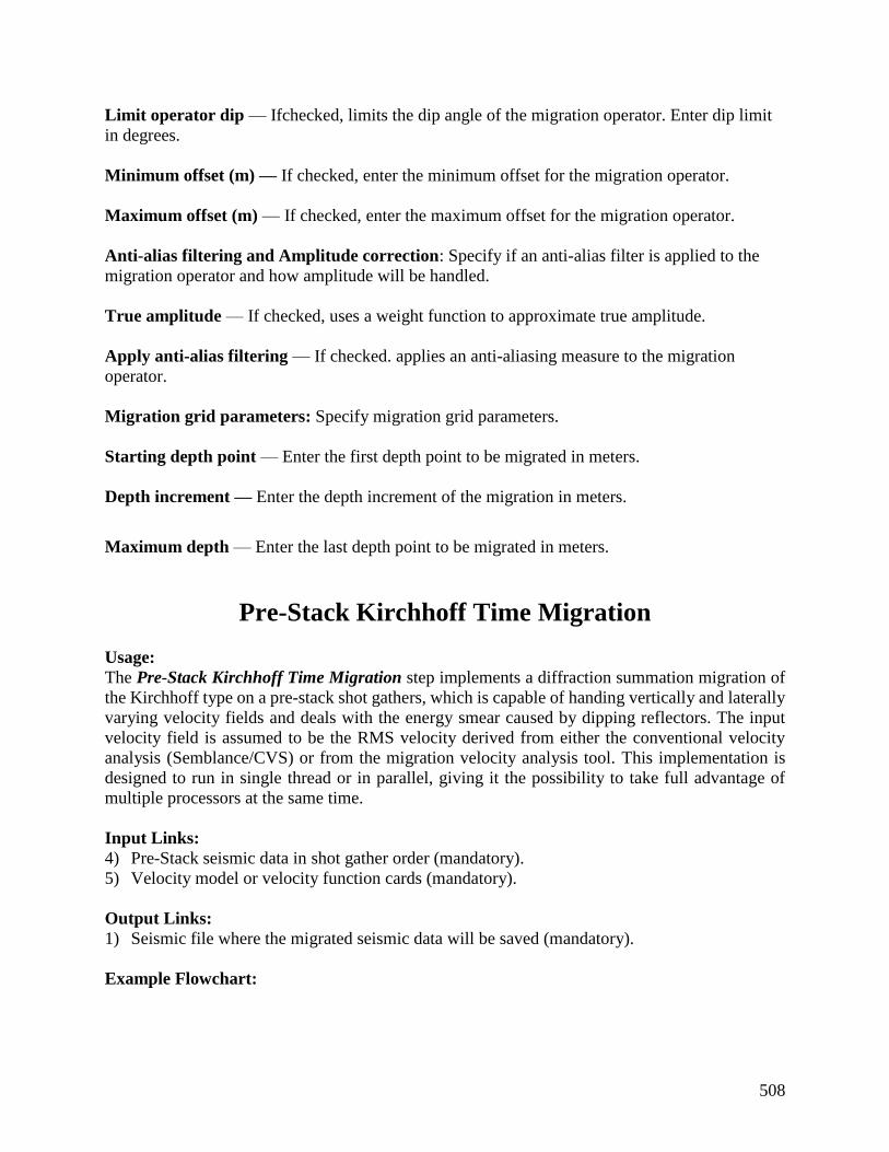
508

Limit operator dip — Ifchecked, limits the dip angle of the migration operator. Enter dip limit

in degrees.

Minimum offset (m) — If checked, enter the minimum offset for the migration operator.

Maximum offset (m) — If checked, enter the maximum offset for the migration operator.

Anti-alias filtering and Amplitude correction: Specify if an anti-alias filter is applied to the

migration operator and how amplitude will be handled.

True amplitude — If checked, uses a weight function to approximate true amplitude.

Apply anti-alias filtering — If checked. applies an anti-aliasing measure to the migration

operator.

Migration grid parameters: Specify migration grid parameters.

Starting depth point — Enter the first depth point to be migrated in meters.

Depth increment — Enter the depth increment of the migration in meters.

Maximum depth — Enter the last depth point to be migrated in meters.

Pre-Stack Kirchhoff Time Migration

Usage:

The Pre-Stack Kirchhoff Time Migration step implements a diffraction summation migration of

the Kirchhoff type on a pre-stack shot gathers, which is capable of handing vertically and laterally

varying velocity fields and deals with the energy smear caused by dipping reflectors. The input

velocity field is assumed to be the RMS velocity derived from either the conventional velocity

analysis (Semblance/CVS) or from the migration velocity analysis tool. This implementation is

designed to run in single thread or in parallel, giving it the possibility to take full advantage of

multiple processors at the same time.

Input Links:

4) Pre-Stack seismic data in shot gather order (mandatory).

5) Velocity model or velocity function cards (mandatory).

Output Links:

1) Seismic file where the migrated seismic data will be saved (mandatory).

Example Flowchart:

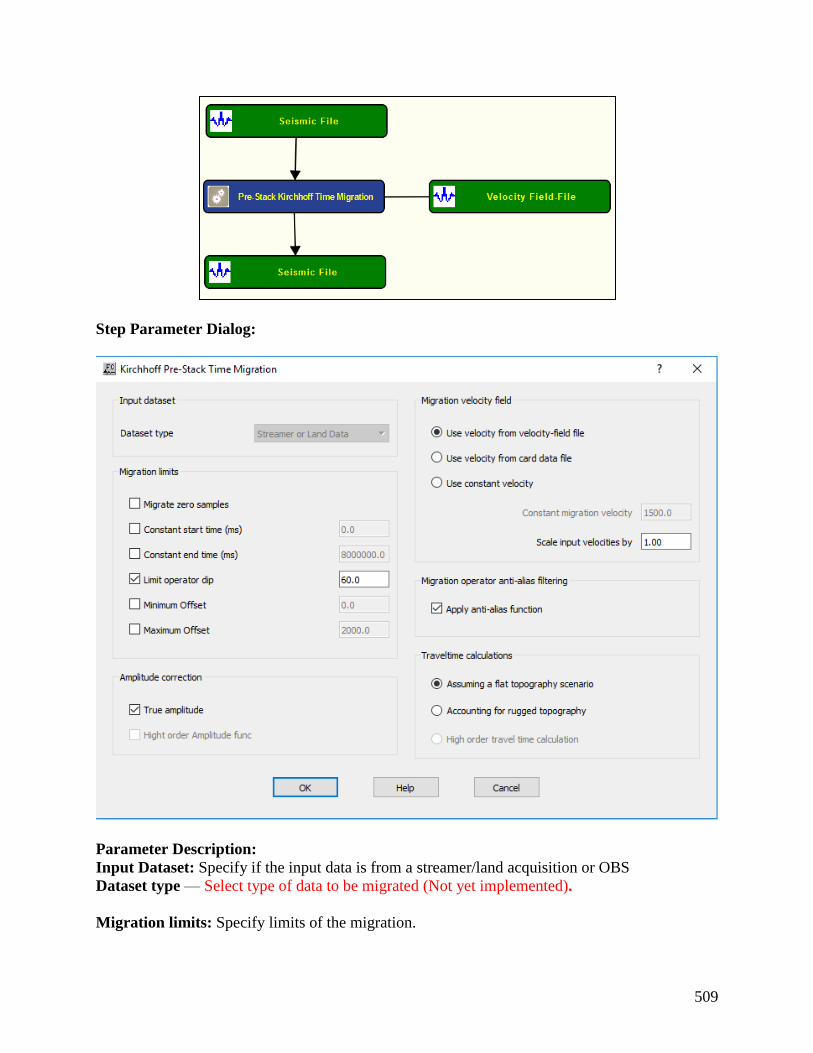
509

Step Parameter Dialog:

Parameter Description:

Input Dataset: Specify if the input data is from a streamer/land acquisition or OBS

Dataset type — Select type of data to be migrated (Not yet implemented).

Migration limits: Specify limits of the migration.

510

Migrate zero samples — If checked, samples with amplitudes value zero will be migrated as well.

Constant Start time (ms) — If checked, defines a constant migration start time.

Constant end time (ms) — If checked, defines a constant migration end time.

Limit operator dip — If checked, limits the dip angle of the migration operator.

Minimum offset (m) — If checked, defines a minimum offset for the migration operator.

Maximum offset (m) — If checked, defines a maximum offset for the migration operator.

Amplitude correction: Specifies how amplitudes are handled during migration.

True amplitude — if checked to use a weight function to approximate true amplitude.

High order amplitude function — (Not yet implemented).

Migration velocity field: Specify velocity field to be used by the migration.

Use velocity from velocity-field file — If selected, connects an auxiliary velocity-field file as

input velocity model.

Use velocity from card data file — If selected, connects an auxiliary velocity function card as

input velocity model.

Use constant velocity — If selected, uses a constant velocity migration.

Constant migration velocity — Enter constant velocity value for migration.

Scale velocity input — enter a scaling factor for the input velocities, or else 1.

Migration operator anti-alias filter: Specifies anti-alias filter parameters.

Apply anti-alias function — If checked, applies an anti-aliasing measure to the migration

operator.

Traveltime calculations: Specify how traveltimes for Kirchhoff migration are calculated.

Assuming a flat topography scenario — If selected, assume a flat recording surface when

computing travel-time information.

Accounting for rugged topography — If selected, Assume a rugged recording surface when

computing travel-time information.

High order travel-time calculation — (Not yet implemented).

511

Stolt Migration 2-D only

Usage:

The Stolt Migration step implements a constant velocity or depth variable Stolt migration

algorithm for post-stack time migration. This migration scheme can accommodate a vertically

varying velocity field in the form of one SPW velocity function card. This velocity field is assumed

to be the stacking velocity field derived from velocity analysis of the pre-stack data. The user

designates a Stolt stretch factor, a maximum frequency to migrate, and temporal and spatial tapers.

An option allows the input velocity function to be scaled. Finally, you can override the SPW

calculated trace spacing and specify the true trace spacing of your data in your spatial units of

choice. By default, SPW calculates the trace spacing for the stack as the group interval, as you

defined it in the geometry definition, divided by two (2).

Input Links:

1) Seismic data in stacked order (mandatory).

2) Velocity Function cards (optional).

Output Links:

1) Seismic data in stacked order (mandatory) and sampled in time.

Reference:

Stolt, R.H, 1978, Migration by Fourier transform, Geophysics, v. 43, no 1., p. 23-48.

Example Flowchart:

Step Parameter Dialog:

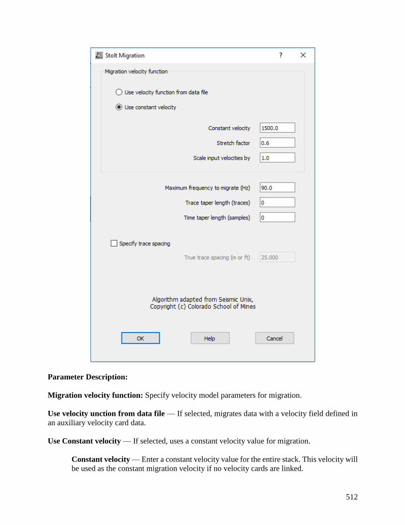
512

Parameter Description:

Migration velocity function: Specify velocity model parameters for migration.

Use velocity unction from data file — If selected, migrates data with a velocity field defined in

an auxiliary velocity card data.

Use Constant velocity — If selected, uses a constant velocity value for migration.

Constant velocity — Enter a constant velocity value for the entire stack. This velocity will

be used as the constant migration velocity if no velocity cards are linked.

513

Stretch factor — In the case of a time-variable velocity field, the Stolt stretch factor is designed

to stretch the time axis so that the data appear to have propagated through a constant-velocity earth.

Values of 0.5 to 1 are typical.

Scale input velocities by — The input velocities are multiplied by this number. This scalar may

be used for adjusting the input velocities if they are interval velocities derived using Dix's equation

rather than true interval velocities.

Maximum frequency to migrate — Enter the maximum frequency component in the data to be

migrated.

Trace taper length (traces) — Number of traces to over which to taper traces at the start and end

of the line prior to migration.

Time taper length (samples) — Number of samples to over which to taper at the start and end of

each trace prior to migration.

Specify trace spacing — If checked, allows for manual specification of the trace spacing. By

default, SPW calculates the trace spacing for the stack as the group interval, as you defined it in

the geometry definition, divided by two (2).

True trace spacing (m or ft) — Enter trace spacing. This value will overwrite the parameters in

geometry.

514

Multi-component Steps

This section documents the processing steps available in the Multi-

Component category.

The multi-component processing steps currently available are:

Note on Multi-component trace header values

Receiver types and Receiver component trace header values

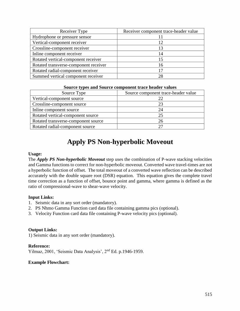
515

Receiver Type Receiver component trace-header value

Hydrophone or pressure sensor 11

Vertical-component receiver 12

Crossline-component receiver 13

Inline component receiver 14

Rotated vertical-component receiver 15

Rotated transverse-component receiver 16

Rotated radial-component receiver 17

Summed vertical component receiver 28

Source types and Source component trace header values

Source Type Source component trace-header value

Vertical-component source 22

Crossline-component source 23

Inline component source 24

Rotated vertical-component source 25

Rotated transverse-component source 26

Rotated radial-component source 27

Apply PS Non-hyperbolic Moveout

Usage:

The Apply PS Non-hyperbolic Moveout step uses the combination of P-wave stacking velocities

and Gamma functions to correct for non-hyperbolic moveout. Converted wave travel-times are not

a hyperbolic function of offset. The total moveout of a converted wave reflection can be described

accurately with the double square root (DSR) equation. This equation gives the complete travel

time correction as a function of offset, bounce point and gamma, where gamma is defined as the

ratio of compressional-wave to shear-wave velocity.

Input Links:

1. Seismic data in any sort order (mandatory).

2. PS Nhmo Gamma Function card data file containing gamma pics (optional).

3. Velocity Function card data file containing P-wave velocity pics (optional).

Output Links:

1) Seismic data in any sort order (mandatory).

Reference:

Yilmaz, 2001, ‘Seismic Data Analysis’, 2nd Ed. p.1946-1959.

Example Flowchart:

516

Step Parameter Dialog:

517

Parameter Description:

Gamma field definition: Specify gamma field description for PS nonhyperbolic moveout.

Use gamma functions from data file — If checked, an auxiliary card data file with the gamma

field description will be automatically linked into the process.

518

Use gamma field from seismic file — If checked, an auxiliary seismic file with the gamma field

description will be automatically linked into the process.

Use constant gamma — If checked, a constant gamma value will be used for the moveout

correction.

Constant gamma — Enter the constant gamma value to be used for the moveout

correction.

Scale input gamma values by (%) — Enter a value to be used to scale the input gamma field.

P-wave velocity field definition: Specify P-wave velocity field description for PS nonhyperbolic

moveout.

Use velocity functions from data file — If checked, an auxiliary card data file with the P-wave

velocity field description will be automatically linked into the process.

Use velocity field from seismic file — If checked, an auxiliary seismic file with the P-wave

velocity field description will be automatically linked into the process.

Use constant gamma — If checked, a constant P-wave velocity value will be used for the moveout

correction.

Constant gamma — Enter the constant P-wave velocity value to be used for the moveout

correction.

Scale input gamma values by (%) — Enter a value to be used to scale the input P-wave velocity

field.

Mute control: Specify stretch mute parameters.

Apply stretch mute — If checked, apply a strectch mute after the moveout correction.

Percentage — Enter the percentage of strecht mute to be applied.

Taper length (samples) — Enter the taper length for the stretch mute in number of

samples.

Interpolation Type Selection: Specify the interpolation type (linear or quadratic). The moveout

function causes trace data samples to be moved in time to new locations. Since these new time

locations of the data sample values are not usually exactly at the sample interval of the data, the

data is interpolated to be evenly sampled at the correct sample interval.

Linear — If selected, uses a linear interpolation following the equation of a line (y = mx

+ b) to interpolate data values between or beyond existing data.

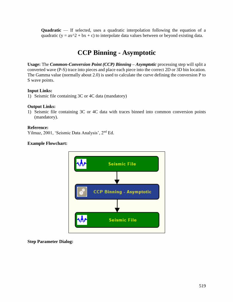
519

Quadratic — If selected, uses a quadratic interpolation following the equation of a

quadratic (y = ax^2 + bx + c) to interpolate data values between or beyond existing data.

CCP Binning - Asymptotic

Usage: The Common-Conversion Point (CCP) Binning – Asymptotic processing step will split a

converted wave (P-S) trace into pieces and place each piece into the correct 2D or 3D bin location.

The Gamma value (normally about 2.0) is used to calculate the curve defining the conversion P to

S wave points.

Input Links:

1) Seismic file containing 3C or 4C data (mandatory)

Output Links:

1) Seismic file containing 3C or 4C data with traces binned into common conversion points

(mandatory).

Reference:

Yilmaz, 2001, ‘Seismic Data Analysis’, 2nd Ed.

Example Flowchart:

Step Parameter Dialog:

520

Parameter Description:

Line definition (for 2D): Define line parameters. These parameters are exclusive for 2D surveys.

Start of line easting (for 2D) — Enter the start of line easting.

Start of line northing (for 2D) — Enter the start of line northing.

End of line easting (for 2D) — Enter the end of the line easting.

End of line northing (for 2D) — Enter the end of the line northing.

Line number (for 2D) — Enter the line number.

Line azimuth (for 2D) — Enter the line azimuth.

521

First midpoint number (for 2D) — Enter the first midpoint number.

Common midpoint increment (for 2D) — Enter the common midpoint increment.

Common midpoint size (for 2D) — Enter the common midpoint size.

Grid definition (for 3D) — Define the 3D grid. These parameters are exclusive for 3D surveys.

Corner 1 – Easting (for 3D) — Enter the easting (x) coordinate of the first corner of your survey.

Corner 1 – Northing (for 3D) — Enter the northing (y) coordinate of the first corner of your

survey.

Corner 2 – Easting (for 3D) — Enter the easting (x) coordinate of the second corner of your

survey.

Corner 2 – Northing (for 3D) — Enter the northing (y) coordinate of the second corner of your

survey.

Corner 3 – Easting (for 3D) — Enter the easting (x) coordinate of the third corner of your survey.

Corner 3 – Northing (for 3D) — Enter the northing (y) coordinate of the third corner of your

survey.

Inline bin size (for 3D) — Enter the size in distance units of the in-line side (1 to 2) of each bin.

Crossline bin size (for 3D) — Enter the size in distance units of the cross-line side (1 to 3) of each

bin.

First inline number (for 3D) — Enter the first inline number. This line number is assigned to all

the bins along the side of the survey from corner 1 to corner 2.

Inline increment (for 3D) — Enter the increment in line numbers between adjacent CMP lines.

First crossline number (for 3D) — Enter the first crossline number. This location number is

assigned to all the bins along the side of the survey from corner 1 to corner 3.

Crossline increment (for 3D) — Enter the increment in locations between adjacent CMP

locations.

Coordinate definition: Specify whether the corner points define the bin centers or corners

following the figure below.

522

Corner points define bin centers — If selected, specify that corner points define bin centers.

Corner points define bin corners — If selected, specify that corner points define bin corners.

Survey dimensions: Specify whether the dimensions of the survey are 2D or 3D.

2D — If selected, specify 2D line survey.

3D — If selected, specify a 3D grid survey.

Project updates: Specify project updates.

Update from project — Select to update from the project.

Gamma — Enter the gamma parameter value. Gamma is the ratio of Vp/Vs velocities. This

parameter defines the curve of the conversion point.

CCP Binning - Dynamic

Usage: The Common-Conversion Point (CCP) binning - Dynamic step assigns CCP numbers

to mode-converted PS data as a function of the source-receiver offset and a constant or time-

variable Vp/Vs ratio (gamma).

Input Links:

1) Converted wave data volume in any sort order (mandatory).

2) Nhmo gamma function card (optional).

Output Links:

523

1) Converted wave data volume in any sort order (mandatory).

Reference:

Yilmaz, 2001, ‘Seismic Data Analysis’, 2nd Ed.

Example Flowchart:

Step Parameter Dialog:

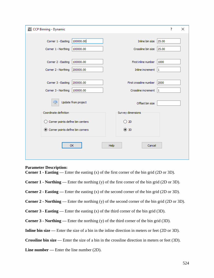
524

Parameter Description:

Corner 1 - Easting — Enter the easting (x) of the first corner of the bin grid (2D or 3D).

Corner 1 - Northing — Enter the northing (y) of the first corner of the bin grid (2D or 3D).

Corner 2 - Easting — Enter the easting (x) of the second corner of the bin grid (2D or 3D).

Corner 2 - Northing — Enter the northing (y) of the second corner of the bin grid (2D or 3D).

Corner 3 - Easting — Enter the easting (x) of the third corner of the bin grid (3D).

Corner 3 - Northing — Enter the northing (y) of the third corner of the bin grid (3D).

Inline bin size — Enter the size of a bin in the inline direction in meters or feet (2D or 3D).

Crossline bin size — Enter the size of a bin in the crossline direction in meters or feet (3D).

Line number — Enter the line number (2D).

525

First inline number — Enter the first inline number (3D).

Inline increment — Enter the inline increment (3D).

First CMP number — Enter the first CMP number (2D).

First crossline number — Enter the first crossline number (3D).

CMP increment — Enter the CMP increment (2D).

Crossline increment — Enter the crossline increment (3D).

Offset bin size – Enter the offset bin size (2D or 3D).

Corner points define bin centers — If selected, specify that corner points define bin centers.

Corner points define bin corners — If selected, specify that corner points define bin corners.

Survey dimensions: Specify whether the dimensions of the survey are 2D or 3D.

2D — If selected, specify 2D line survey.

3D — If selected, specify a 3D grid survey.

Constant Gamma Stacks Usage:

The Constant Gamma Stack step generates a file of constant gamma stack traces, where gamma

is defined as the Vp/Vs ratio. A P-wave stacking velocity field must be supplied, and you choose

the number of gammas with which to stack your data, the first gamma to apply, and the last gamma

to apply. You have the option to apply a stretch mute, if you so desire. With the series of constant

gamma stack traces, you page through these stacked panels in Display and interactively pick

gamma functions that result in the most coherent stacked sections.

Input Links:

1. Seismic data pre-stack, in CMP sort order (mandatory).

2. Velocity card data file containing p-wave stacking velocity functions (mandatory).

Output Links:

1. Seismic data pre-stack, in CMP sort order (mandatory).

Example Flowchart:

526

Step Parameter Dialog:

Parameter Description:

Gamma range: Specify the range of gammas to use in the analysis. A stacked section is calculated

for each gamma linearly interpolated between the starting and ending input gamma. The gamma

increment will be: Ginc = (last gamma – first gamma)/(Number of gammas-1).

First gamma — Enter the starting gamma for the analysis. This gamma will be used for non-

hyperbolic NMO on the first output stack. {>0.0}

Last gamma — Enter the ending gamma for the analysis. This gamma will be used for non-

hyperbolic NMO on the last output stack. {>0.0}

527

Gamma increment — Enter the number of velocities to use in the analysis. A stacked section is

calculated for each velocity linearly interpolated between the starting and ending input velocities.

The velocity increment will be: inc = (last velocity - first velocity)/(Number of velocities-1).

P-wave velocity field definition: Define the P-wave velocity field.

Use velocity functions from data file — If checked, velocity functions will be applied from a

data file.

Use velocity field from seismic file — If checked, a velocity field will be applied from a seismic

file.

Use constant velocity — If checked, a constant velocity will be applied to the data.

Constant velocity — Enter the NMO velocity. This constant velocity will be used if a set

of velocity function cards is NOT linked to the NMO correction step.

Scale input velocities by (%) — Enter the amount by which the input velocities are scaled up or

down. A value of 1.0 does not alter the velocity field.

Line range: Specify the line range.

First line to analyze — Enter the first CMP line number to analyze.

Last line to analyze — Enter the last CMP line number to analyze.

Line increment — Enter the CMP line increment between lines to analyze.

Location range: Specify the location range.

First location to analyze — Enter the first CMP location to analyze.

Last location to analyze — Enter the last CMP location to analyze.

Location increment — Enter the CMP location increment between groups of CMP locations to

analyze.

Locations per analysis — Enter the number of CMP locations in each analysis panel. At each

CMP location a range of constant velocity stacks will be generated from the first velocity to the

last velocity in increments of Vinc.

Mute Control: Specify the parameters for the stretch mute definition.

Apply mute from data file — If checked, a mute will be applied to the NHMO corrected data

from a data file.

528

Apply stretch mute — If checked, a stretch mute will be applied to the NHMO corrected data.

Stretch muting restricts the stretching of the data due to the NMO correction. If not checked, the

stretch mute must be supplied by an Early Mute card linked to the Constant Gamma Stack step.

Percentage — Enter the percent stretch mute. The smaller the percent the more severe the

mute function.

Taper length (samples) — Enter the mute taper length in samples. Longer taper lengths result

in a smoother transition from the mute zone to the data zone.

Interpolation Type Selection: Specify the interpolation type (linear or quadratic). The moveout

function causes trace data samples to be moved in time to new locations. Since these new time

locations of the data sample values are not exactly at the sample interval of the data, the data is

interpolated to the correct sample interval.

Linear — Linear interpolation uses the equation of a line (y = mx + b) to interpolate data samples

between or beyond existing data.

Quadratic — Quadratic interpolation uses the equation of a quadratic (y = ax^2 + bx + c) to

interpolate data samples between or beyond existing data.

Trace Amplitude Definition: Specify the trace amplitude definition.

Use relative amplitude traces — Relative amplitude traces will be summed in the stacking

process. Relative amplitude traces are scaled independently of one another.

Use true amplitude traces — Selects the use of true amplitude scaled traces in the analysis. True

amplitude traces are scaled by one common factor per record.

Converted Wave Receiver Statics

Usage:

The Converted Wave Receiver Statics step uses a cross correlation and least squares fitting to

calculate receiver statics for converted wave traces (P=S).

Input Links:

1) Seismic file containing converted wave data traces sorted in receiver order (mandatory).

Output Links:

1) Seismic file containing converted wave data traces sorted in receiver order (mandatory).

2) Receiver statics file containing the calculated receiver statics (mandatory).

Reference:

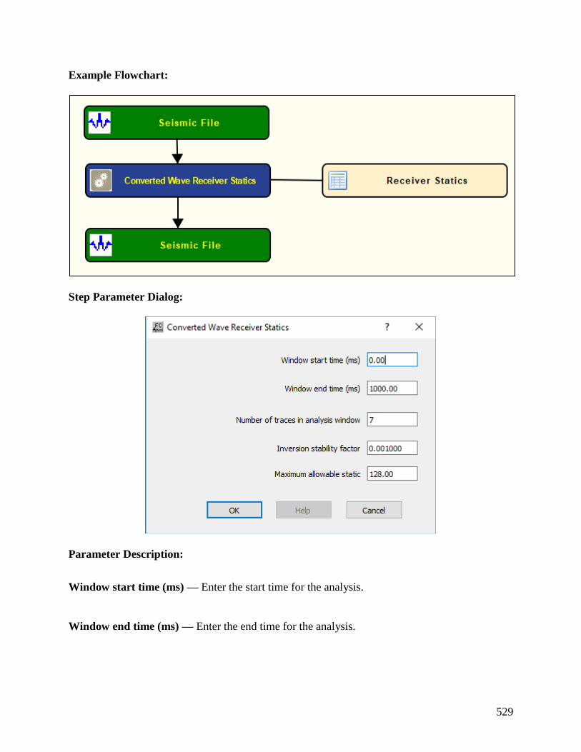
529

Example Flowchart:

Step Parameter Dialog:

Parameter Description:

Window start time (ms) — Enter the start time for the analysis.

Window end time (ms) — Enter the end time for the analysis.

530

Number of traces in analysis window — Enter the minimum number of traces considered for the

converted waver receiver statics.

Inversion stability factor — Enter a small value used to stabilize the matrix inversion and

prevent inverting zeros which causes instatility

Maximum allowable static — Enter the maximum amount of static correction.

Crooked Line Asymptotic CCP Binning Usage:

The Crooked Line Asymptotic Common-Conversion Point (CCP) Binning step will split a

converted wave (P-S) trace into pieces and place each piece into the correct crooked line bin

location. The Gamma value (normally about 2.0) is used to calculate the curve defining the

conversion P to S wave points.

Input Links:

1) Seismic file containing 3C or 4C data (mandatory)

2) Line Definition File containing the crooked line fit information (mandatory)

Output Links:

1) Seismic file containing 3C or 4C data with traces binned into common conversion points

(mandatory)

Reference:

-

Example Flowchart:

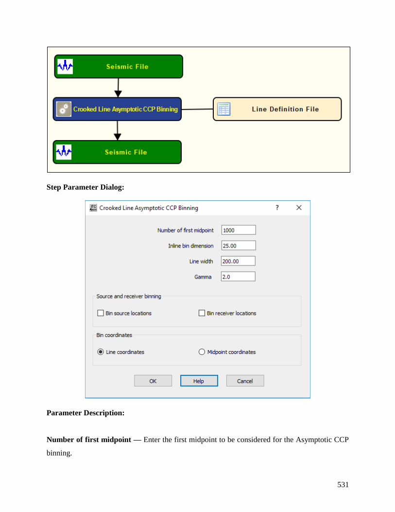
531

Step Parameter Dialog:

Parameter Description:

Number of first midpoint — Enter the first midpoint to be considered for the Asymptotic CCP

binning.

532

Inline bin dimension — Enter the bin dimension in the inline direction.

Line width — Enter the line width to be considered for the asymptotic CCP.

Gamma — Enter a value for gamma parameter as defined by Vp/Vs ratio.

Source and receiver binning: Define bin for sources and/or receiver locations.

Bin source locations — If checked, bin source locations.

Bin receiver locations — If checked, bin receiver locations.

Bin coordinates: Define bin coordinates. Bin coordinates can be either defined as line of

midpoins.

Line coordinates — If selected, bin coordinates are line coordinates.

Midpoint coordinates — If selected, bin coordinates are midpoint coordinates.

Crooked Line Dynamic CCP Binning

Usage: The Crooked Common-Conversion Point (CCP) binning - Dynamic step assigns CCP

numbers to mode-converted PS data as a function of the source-receiver offset and a constant or

time-variable Vp/Vs ratio (gamma) for 2D crooked lines.

Input Links:

1) Converted wave data volume in any sort order (mandatory).

2) Line definition file (mandatory).

3) Auxiliary gamma card data file (optional).

4) Auxiliary P-wave velocity card data file (optional).

Output Links:

1) Seismic file (mandatory).

Reference:

-

Example Flowchart:

533

Step Parameter Dialog:

534

Parameter Description:

Number of first midpoint — Enter the number of the first midpoint to be binned.

Inline bin dimension — Enter the bin dimension in the inline direction.

Line width — Enter the line width for the binning.

Offset bin size — Enter the ofsset bin size.

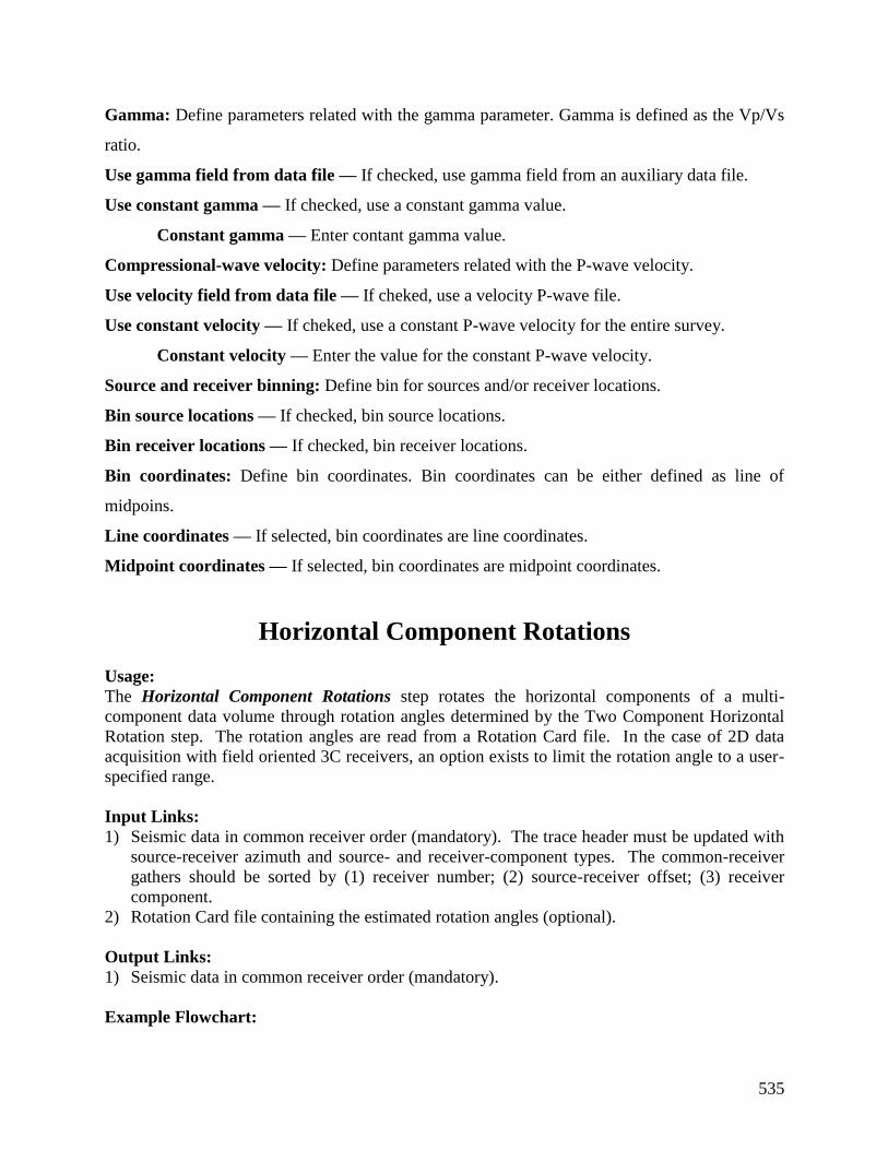
535

Gamma: Define parameters related with the gamma parameter. Gamma is defined as the Vp/Vs

ratio.

Use gamma field from data file — If checked, use gamma field from an auxiliary data file.

Use constant gamma — If checked, use a constant gamma value.

Constant gamma — Enter contant gamma value.

Compressional-wave velocity: Define parameters related with the P-wave velocity.

Use velocity field from data file — If cheked, use a velocity P-wave file.

Use constant velocity — If cheked, use a constant P-wave velocity for the entire survey.

Constant velocity — Enter the value for the constant P-wave velocity.

Source and receiver binning: Define bin for sources and/or receiver locations.

Bin source locations — If checked, bin source locations.

Bin receiver locations — If checked, bin receiver locations.

Bin coordinates: Define bin coordinates. Bin coordinates can be either defined as line of

midpoins.

Line coordinates — If selected, bin coordinates are line coordinates.

Midpoint coordinates — If selected, bin coordinates are midpoint coordinates.

Horizontal Component Rotations

Usage:

The Horizontal Component Rotations step rotates the horizontal components of a multi-

component data volume through rotation angles determined by the Two Component Horizontal

Rotation step. The rotation angles are read from a Rotation Card file. In the case of 2D data

acquisition with field oriented 3C receivers, an option exists to limit the rotation angle to a user-

specified range.

Input Links:

1) Seismic data in common receiver order (mandatory). The trace header must be updated with

source-receiver azimuth and source- and receiver-component types. The common-receiver

gathers should be sorted by (1) receiver number; (2) source-receiver offset; (3) receiver

component.

2) Rotation Card file containing the estimated rotation angles (optional).

Output Links:

1) Seismic data in common receiver order (mandatory).

Example Flowchart:

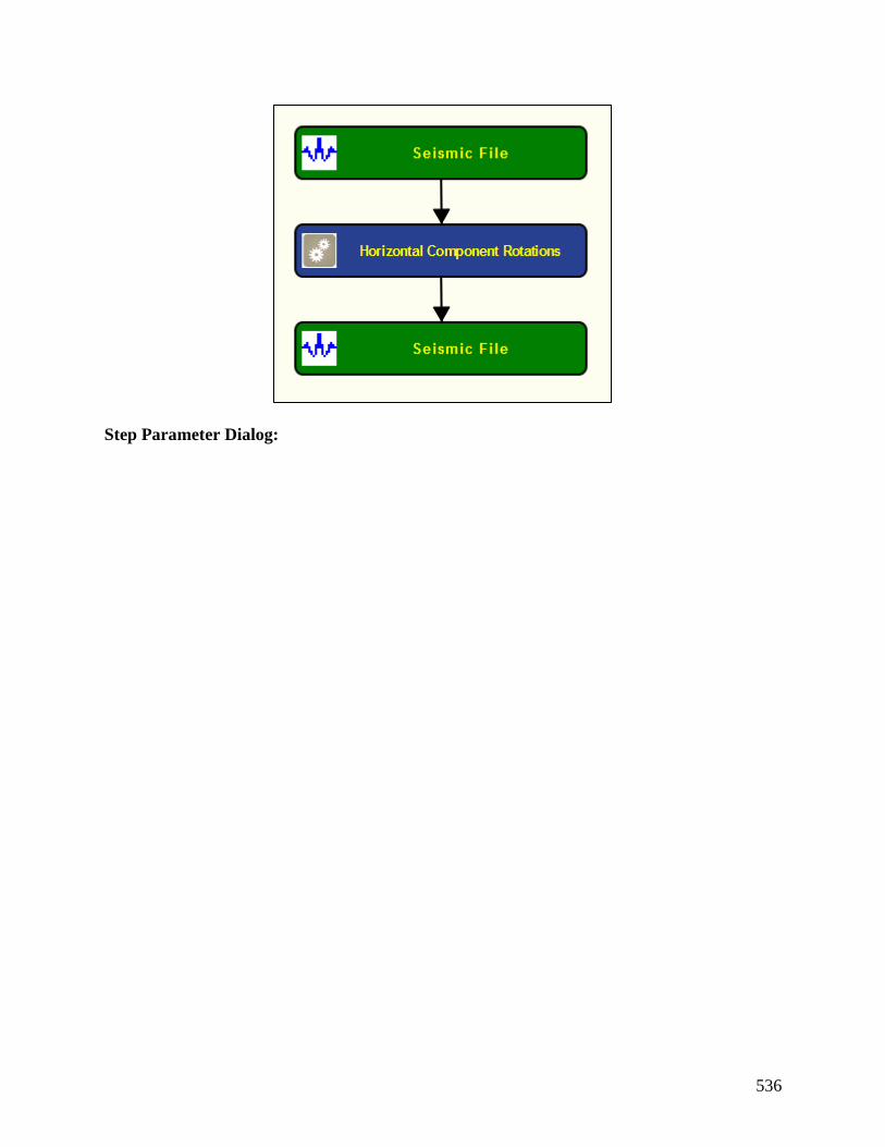
536

Step Parameter Dialog:

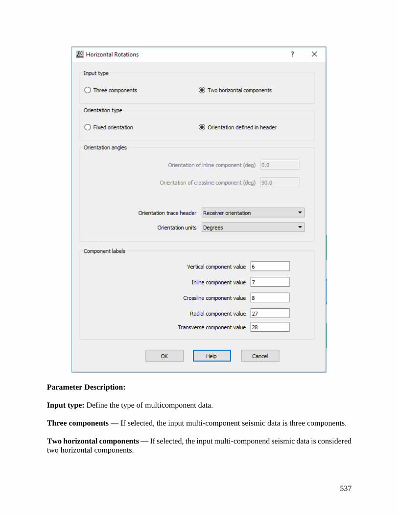
537

Parameter Description:

Input type: Define the type of multicomponent data.

Three components — If selected, the input multi-component seismic data is three components.

Two horizontal components — If selected, the input multi-componend seismic data is considered

two horizontal components.

538

Orientation type: Define the type or orientation.

Fixed orientation — If selected, entire data has a fixed orientation.

Orientation defined in header— If selected, the orientation of the data varies and must be defined

in the header.

Orientation angles: Define the orientation angles.

Orientation of inline component (deg.) — If fixed orientation, enter the orientation (azimuth) of

the inline component in degrees.

Orientation of crossline component (deg.) — If fixed orientation, enter the orientation (azimuth)

of the crossline component in degress.

Orientation trace header — If orientation defined in header, select the location of the header key

word with the orientation (azimuth) value.

Orientation units — If orientation defined in header, select the units for orientation (azimuth)

(degrees or radians)

Component labels: Define the components labels.

Vertical component value — Enter the label value corresponding to the vertical component.

Inline component value — Enter the label value corresponding to the inline component.

Crossline component value — Enter the label value corresponding to the crossline component.

Radial component value — Enter the label value corresponding to the radial component.

Transverse component value — Enter the label value corresponding to the transverse component.

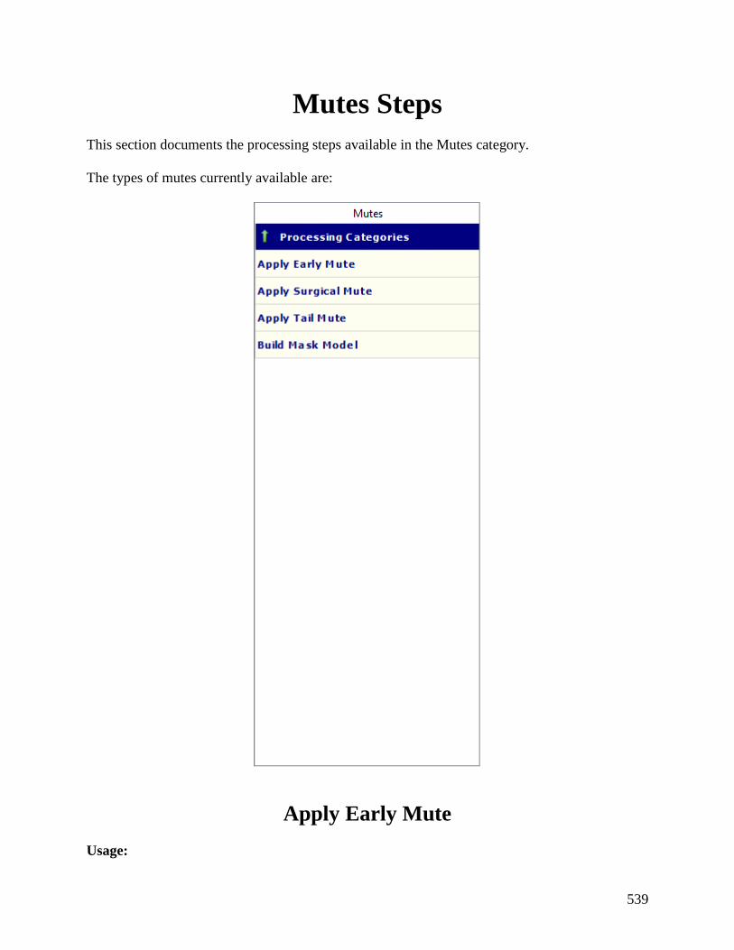
539

Mutes Steps

This section documents the processing steps available in the Mutes category.

The types of mutes currently available are:

Apply Early Mute

Usage:

540

The Apply Early Mute step allows you to apply mute definitions to your data from different

sources. You may choose to interpolate mute functions for the records between the picked mute

records or to just mute the records associated with the picked mutes. Mute function may be defined

by auxiliary mute card data file or using a constant velocity linearly versus offset. You have a

choice of applying a Hanning, Hamming, or Blackman type of mute taper, or none at all. You may

also specify in samples the length of the mute taper and scale the input offsets by a value. Early

mutes may be interactively defined using first the Display menu to select the file, then the Picking

menu to select the type of mute.

Input Links:

1) Seismic data in any sort order (mandatory).

2) Early Mute Function card (optional).

Output Links:

1) Seismic data in any sort order (mandatory).

Reference:

-

Example Flowchart:

Step Parameter Dialog:

541

Parameter Description:

Mute definition: Specify the parameterization for the mute function.

Velocity — If selected, the mute function is defined linearly with the offset using a constant

velocity.

Velocity — Enter the constant velocity value to be used to define the mute functions.

Early mute file — If selected, an auxiliary Early Mute auxiliary card data file is used to define

the mute definition.

542

First arrivals files — If selected, an auxiliary First Break Times auxiliary card data file is used

to define the mute function.

VSP first arrivals files — If selected, an auxiliary VSP First Arrival Time Picks auxiliary card

data file is used to define the mute function.

Samples shift at zero offset — Enter the number of samples to be shifted at the zero-offset when

applying the mute.

Samples shift at maximum offset — Enter the number of samples to be shifted at the maximum

offset when applying the mute.

Apply value from header — If selected, the mute function is defined by values stored in a specific

trace header locations.

Mute header — Select the location of the trace header with the mute value.

Mute Taper Type: Specify the type of taper to use when applying the mute function.

Hanning — Is selected, a Hanning taper is specified by the equation: x(n) = 0.5 - 0.5 * cos

(2*pi*n/N).

Hamming — Is selected, a Hamming taper is specified by the equation: x(n) = 0.54 - 0.46 * cos

(2*pi*n/N).

Blackman — Is selected, a Blackman taper is specified by the equation: x(n) = 0.42 - 0.5 * cos

(2*pi*n/N)+ 0.08 * cos (4*pi*n/N).

No taper — Is selected, no taper will be applied to the mute. This may result in problems in later

processing steps due to Gibbs effect.

Mute taper length (samples) — Enter the mute taper length in samples. Longer taper lengths

result in a smoother transition from the mute zone to the data zone.

Mute record interpolation: Speciy interpolation parameters of the mute function.

Mute interpolation between input records — If checked, the early mutes will be interpolated

between the control points where picks were made.

Field File order — If selected, interpolation between input records is done in the field file

order.

Receiver order — If selected, interpolation between input records is done in the receiver

order.

543

Source order — If selected, interpolation between input records is done in the source

order.

CMP order — If selected, interpolation between input records is done in the CMP order.

Scale input offsets by — Enter a value to scale the input offsets.

Apply Surgical Mute

Usage:

The Apply Surgical Mute step allows you to apply mute definitions to your data from the attached

Surgical Mute Function auxiliary card data file. You may choose to interpolate mute functions for

the records between the picked mute records or to just mute the records associated with the picked

mutes. You have a choice of applying a Hanning, Hamming, or Blackman type of mute taper, or

none at all. You may also specify in samples the length of the mute taper and scale the input offsets

by a value. Surgical mutes may be interactively defined using first the Display menu to select the

file, then the Picking menu to select the type of mute.

Input Links:

1) Seismic data in any sort order (mandatory).

2) Surgical Mute Function card (mandatory).

Output Links:

1) Seismic data in any sort order (mandatory).

Reference:

-

Example Flowchart:

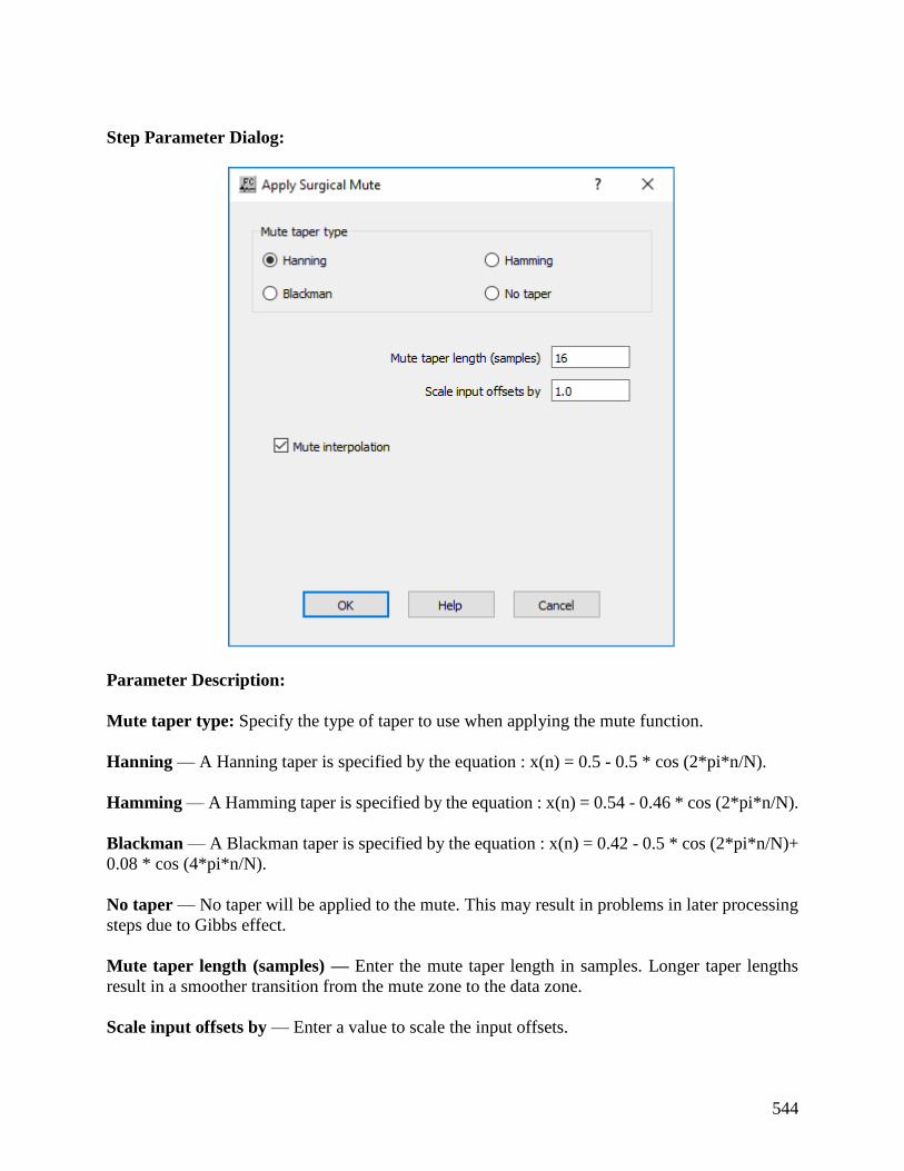
544

Step Parameter Dialog:

Parameter Description:

Mute taper type: Specify the type of taper to use when applying the mute function.

Hanning — A Hanning taper is specified by the equation : x(n) = 0.5 - 0.5 * cos (2*pi*n/N).

Hamming — A Hamming taper is specified by the equation : x(n) = 0.54 - 0.46 * cos (2*pi*n/N).

Blackman — A Blackman taper is specified by the equation : x(n) = 0.42 - 0.5 * cos (2*pi*n/N)+

0.08 * cos (4*pi*n/N).

No taper — No taper will be applied to the mute. This may result in problems in later processing

steps due to Gibbs effect.

Mute taper length (samples) — Enter the mute taper length in samples. Longer taper lengths

result in a smoother transition from the mute zone to the data zone.

Scale input offsets by — Enter a value to scale the input offsets.

545

Mute Interpolation — If checked, the surgical mutes will be interpolated between the control

points where picks were made.

Apply Tail Mute

Usage:

The Apply Tail Mute step allows you to apply mute definitions to your data from the attached Tail

Mute Function auxiliary card data file or using a linear function of constant velocity versus offset.

You may choose to interpolate mute functions for the records between the picked mute records or

to just mute the records associated with the picked mutes. You have a choice of applying a

Hanning, Hamming, or Blackman type of mute taper, or none at all. You may also specify in

samples the length of the mute taper and scale the input offsets by a value. Tail mutes may be

interactively defined using first the Display menu to select the file, then the Picking menu to select

the type of mute.

Input Links:

1) Seismic data in any sort order (mandatory).

2) Surgical Mute Function card (optional).

Output Links:

1) Seismic data in any sort order (mandatory).

Reference:

-

Example Flowchart:

Step Parameter Dialog:

546

Parameter Description:

Mute taper type: Specify the type of taper to use when applying the mute function.

Hanning — A Hanning taper is specified by the equation : x(n) = 0.5 - 0.5 * cos (2*pi*n/N).

Hamming — A Hamming taper is specified by the equation : x(n) = 0.54 - 0.46 * cos (2*pi*n/N).

Blackman — A Blackman taper is specified by the equation : x(n) = 0.42 - 0.5 * cos (2*pi*n/N)+

0.08 * cos (4*pi*n/N).

No taper — No taper will be applied to the mute. This may result in problems in later processing

steps due to Gibbs effect.

Mute taper length (samples) — Enter the mute taper length in samples. Longer taper lengths

result in a smoother transition from the mute zone to the data zone.

Scale input offsets by — Enter a value to scale the input offsets.

Mute Interpolation — If checked, the surgical mutes will be interpolated between the control

points where picks were made.

547

Velocity — If selected, the mute function is defined linearly with the offset using a constant

velocity.

Velocity — Enter the constant velocity value to be used to define the mute functions.

Build Mask Model

Usage: The Build Mask Model step allows you to build an output seismic file with zeros and ones

that can be used to set to null specific samples or as auxiliary file for the Simultaneous Iterative

Refraction Tomography (SIRT) analysis. The geometry of the output file may be defined

manually of by an auxiliary seismic file. The masked region may be defined using a surgical mute

card file.

Input Links:

1) Seismic data in any sort order (mandatory).

2) Seismic data in any sort order to define geometry (optional).

3) Surgical Mute Function card (optional).

Output Links:

1) Seismic data in any sort order (mandatory).

Reference:

-

Example Flowchart:

Step Parameter Dialog:

548

Parameter Description:

Define geometry: Specify parameters related with the geometry of the output seismic file.

Define geometry manually — If selected, the output seismic file with the mask has a geometry

as defined manually with the parameters below.

Number of lines — Enter the number of line.

Number of locations — Enter the number of locations.

549

Sampling interval (ms) — Enter the sampling interval in milliseconds.

Number of samples — Enter number of samples.

Define geometry from auxiliary seismic file — If selected, the geometry of the output seismic

file with the mask will have the geometry of an auxiliary seismic file.

Define masked interval: Specify the spatial extent of the mask (locations defined with zero

values).

Use constant time gate — If selected, masked interval is defined with a time gate defined by

constant top and bottom.

Top limit (ms) — Enter the location of the top boundary of the time gate in milliseconds.

Bottom limite (ms) — Enter the location of the bottom boundary of the time gate in

milliseconds.

Use surgical mute file — If selected, masked interval is defined with an auxiliary surgical mute

card data file.

Define masked area: Specify if mask inside or outside the are defined in the masked interval

Mask inside — If selected, mask inside the region.

Mask outside — If selected, mask outside the region.

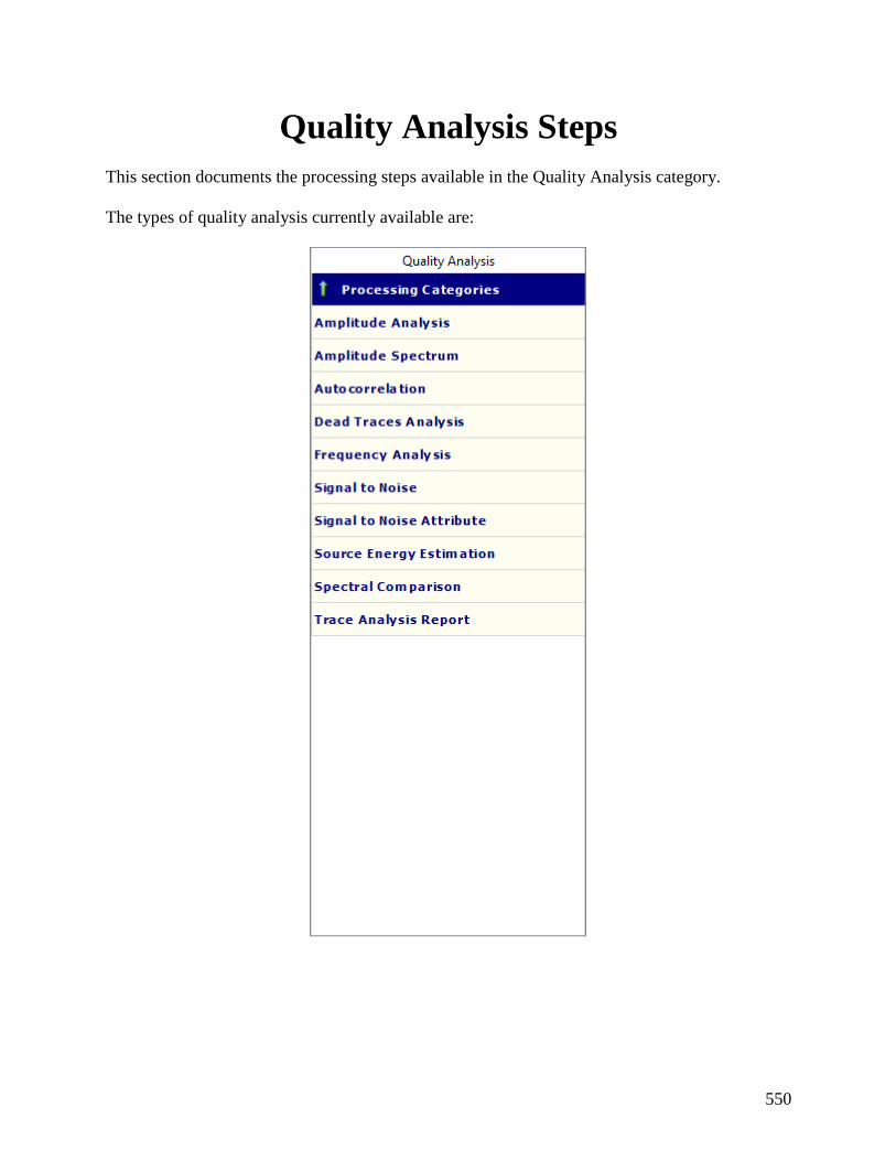
550

Quality Analysis Steps

This section documents the processing steps available in the Quality Analysis category.

The types of quality analysis currently available are:

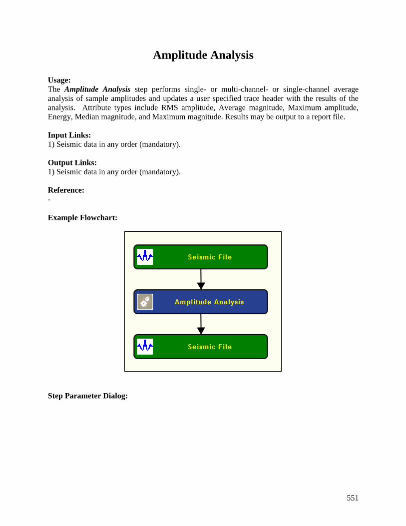
551

Amplitude Analysis

Usage:

The Amplitude Analysis step performs single- or multi-channel- or single-channel average

analysis of sample amplitudes and updates a user specified trace header with the results of the

analysis. Attribute types include RMS amplitude, Average magnitude, Maximum amplitude,

Energy, Median magnitude, and Maximum magnitude. Results may be output to a report file.

Input Links:

1) Seismic data in any order (mandatory).

Output Links:

1) Seismic data in any order (mandatory).

Reference:

-

Example Flowchart:

Step Parameter Dialog:

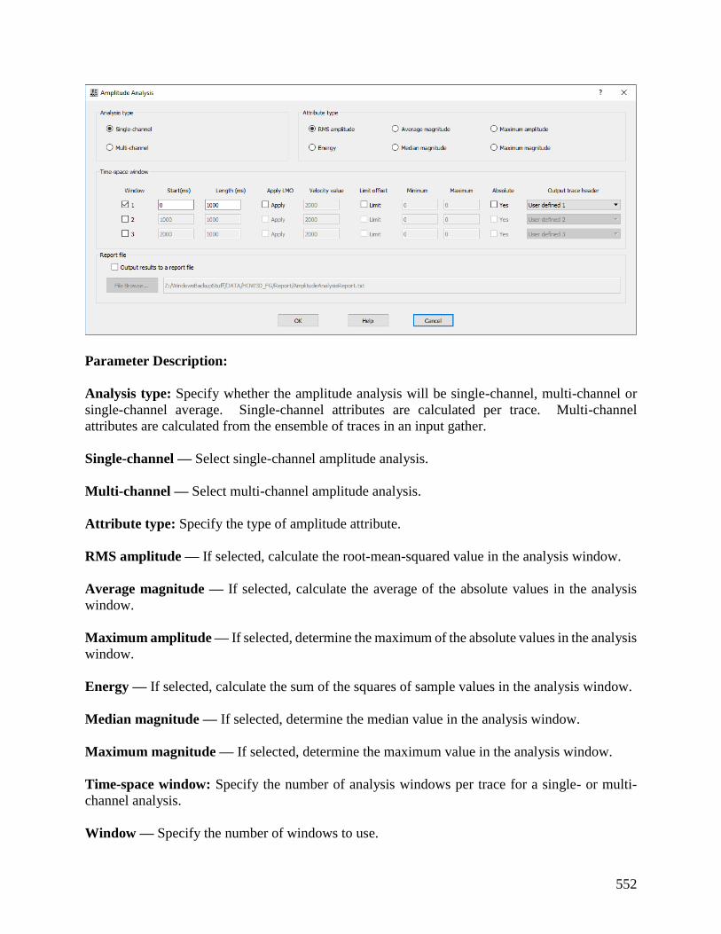
552

Parameter Description:

Analysis type: Specify whether the amplitude analysis will be single-channel, multi-channel or

single-channel average. Single-channel attributes are calculated per trace. Multi-channel

attributes are calculated from the ensemble of traces in an input gather.

Single-channel — Select single-channel amplitude analysis.

Multi-channel — Select multi-channel amplitude analysis.

Attribute type: Specify the type of amplitude attribute.

RMS amplitude — If selected, calculate the root-mean-squared value in the analysis window.

Average magnitude — If selected, calculate the average of the absolute values in the analysis

window.

Maximum amplitude — If selected, determine the maximum of the absolute values in the analysis

window.

Energy — If selected, calculate the sum of the squares of sample values in the analysis window.

Median magnitude — If selected, determine the median value in the analysis window.

Maximum magnitude — If selected, determine the maximum value in the analysis window.

Time-space window: Specify the number of analysis windows per trace for a single- or multi-

channel analysis.

Window — Specify the number of windows to use.

553

1 — The first window is checked by default for use in the calculations.

2 — Check to use a second window in the calculations.

3 — Check to use a third window in the calculations.

Start time (ms) — Enter the start time in milliseconds for the window to use.

Length (ms) — Enter the length in milliseconds for the window to use.

Apply LMO — Specify whether a linear moveout will be applied to the start time of the analysis

window.

Apply — If checked, a linear moveout will be applied to the start time of the analysis window.

Velocity value — If linear moveout is to be applied, enter the moveout velocity.

Limit offset — If offset is to be limited, specify minimum and maximum values. Absolute values

may be specified.

Limit — If checked, the offset will be limited, specify minimum and maximum values.

Minimum — Enter minimum offset value.

Maximum — Enter maximum offset value.

Absolute — Specify if absolute value is desired.

Yes — If checked, an absolute value will be used.

Output trace header — Select the trace header for each window that will be updated with the

results of the analysis.

Report file — Specify whether to save results to a report file and browse to locate or create an

amplitude analysis report file.

Output results to a report file — If checked, results will be saved to a report file.

Amplitude Spectrum

Usage:

The Amplitude Spectrum step inputs seismic data and outputs the amplitude spectrum of each

trace into the output seismic file.

Input Links:

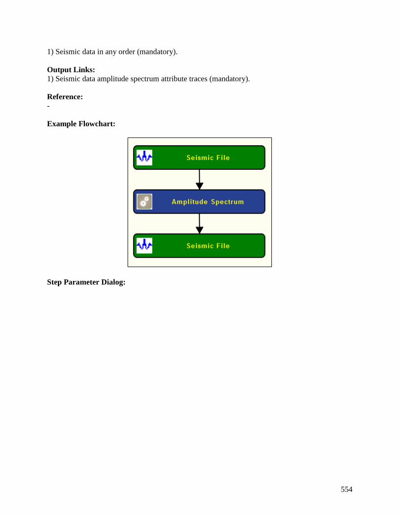
554

1) Seismic data in any order (mandatory).

Output Links:

1) Seismic data amplitude spectrum attribute traces (mandatory).

Reference:

-

Example Flowchart:

Step Parameter Dialog:

555

Parameter Description:

Trace window: Specify the parameters related with the

Specify trace window — If checked, the specified trace window will be used for calculating the

amplitude spectrum.

Start time (ms) — Enter the start time of the trace window to use in milliseconds.

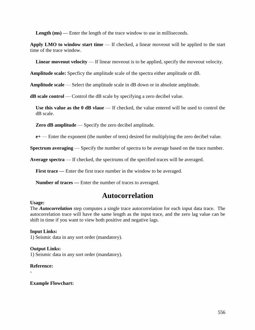
556

Length (ms) — Enter the length of the trace window to use in milliseconds.

Apply LMO to window start time — If checked, a linear moveout will be applied to the start

time of the trace window.

Linear moveout velocity — If linear moveout is to be applied, specify the moveout velocity.

Amplitude scale: Specficy the amplitude scale of the spectra either amplitude or dB.

Amplitude scale — Select the amplitude scale in dB down or in absolute amplitude.

dB scale control — Control the dB scale by specifying a zero decibel value.

Use this value as the 0 dB vlaue — If checked, the value entered will be used to control the

dB scale.

Zero dB amplitude — Specify the zero decibel amplitude.

e+ — Enter the exponent (the number of tens) desired for multiplying the zero decibel value.

Spectrum averaging — Specify the number of spectra to be average based on the trace number.

Average spectra — If checked, the spectrums of the specified traces will be averaged.

First trace — Enter the first trace number in the window to be averaged.

Number of traces — Enter the number of traces to averaged.

Autocorrelation Usage:

The Autocorrelation step computes a single trace autocorrelation for each input data trace. The

autocorrelation trace will have the same length as the input trace, and the zero lag value can be

shift in time if you want to view both positive and negative lags.

Input Links:

1) Seismic data in any sort order (mandatory).

Output Links:

1) Seismic data in any sort order (mandatory).

Reference:

-

Example Flowchart:

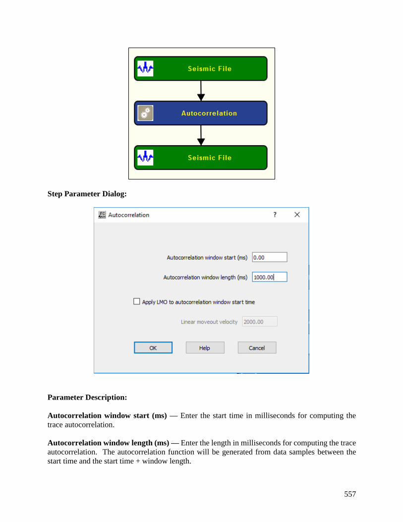
557

Step Parameter Dialog:

Parameter Description:

Autocorrelation window start (ms) — Enter the start time in milliseconds for computing the

trace autocorrelation.

Autocorrelation window length (ms) — Enter the length in milliseconds for computing the trace

autocorrelation. The autocorrelation function will be generated from data samples between the

start time and the start time + window length.

558

Apply LMO to autocorrelation window start time — If checked, the autocorrelation window

start time will be a function of offset: Start time = (source-receiver offset/ velocity) +

Autocorrelation window start time.

Linear moveout velocity — Enter the linear moveout velocity.

Dead Trace Analysis Usage:

The Dead Trace Analysis step allows to kill traces based on a user-defined trace header key word,

and receiver lines or entire records based on the number and the relative location of dead traces.

Input Links:

1) Seismic data in any sort order (mandatory).

Output Links:

1) Seismic data in any sort order (mandatory).

Reference:

-

Example Flowchart:

Step Parameter Dialog:

559

Parameter Description:

Kill traces based on header values — If checked, traces will be killed based on the value stored

on a user-defined trace header key word. Traces can be killed after some mathematical operations

are performed with the selected traces header key word.

Kill receiver lines based on adjacent dead trace limit — If checked, receiver lines will be killed

depending on a limit of consecutive dead traces.

Receiver line adjacent dead trace limit — Enter the minimum number of consecutive

dead traces a receiver line must have to be killed.

560

Kill receiver lines based on percent of dead trace per line — If checked, receiver lines will be

killed depending on the percentage of dead traces.

Dead trace limit per receiver line (%) — Enter the minimum percentage of deade traces

a receiver line must have to be killed.

Kill entire records based on number of dead receiver lines — If checked, records are killed

depending on the number of dead receiver lines.

Dead receiver line limit per record (%) — Enter the minimum percentage of dead

receiver lines a record must have to be killed.

Kill entire records based on number of adjacent traces — If checked, records are killed

depending on a limit of consecutive dead traces.

Adjacent dead trace limit — Enter the minimum number of consecutive dead traces a

record must have to be killed.

Kill entire records based on percent of dead traces per record — If checked, records are killed

depending on the percentage of dead traces per record.

Dead trace limit per record (%) — Enter the minimum percentage of dead traces a record

must have to be killed.

Frequency Analysis

Usage: The Frequency Analysis step computes frequency related seismic attributes in distinct

time windows from an input seismic file. Seismic attributes may be compute from single or multi-

channel. Avaialble seismic attribeutes are dominant frequency, center frequency, average

frequency, RMS frequency, bandwith or peak amplitude. Computed attributes can be stored in

Input Links:

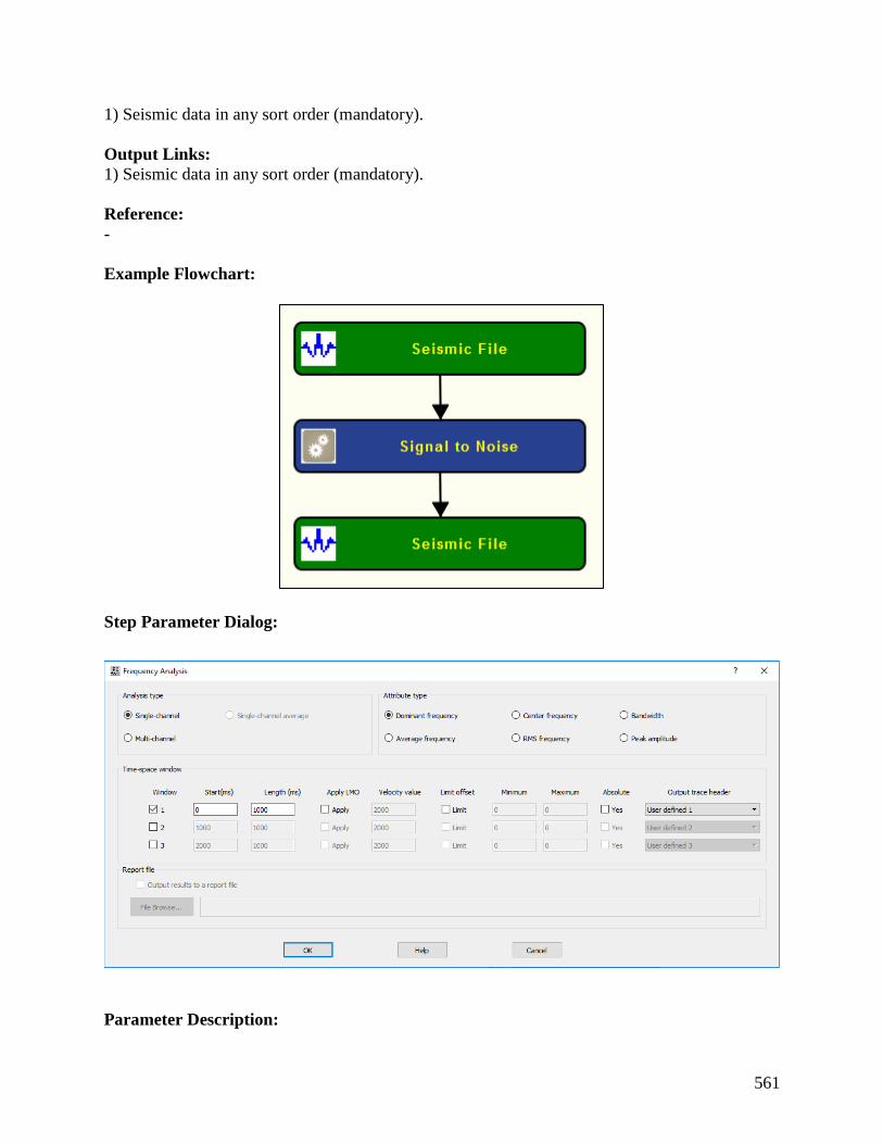
561

1) Seismic data in any sort order (mandatory).

Output Links:

1) Seismic data in any sort order (mandatory).

Reference:

-

Example Flowchart:

Step Parameter Dialog:

Parameter Description:

562

Analysis Type: Specify if the analysis is to be performed in single- or multi-channel.

Single-channel — If selected, frequency analysis attribute will be computed on each single-

channel of the current record.

Multi-channel — If selected, frequency analysis attribute will be computed on all the traces of

the current record.

Single-channel average — Not yet available.

Attribute type: Specify the type of frequency attribute to be computed for the analysis.

Dominant frequency — If selected, computes the dominant frequency of the signal.

Center frequency — If selected, computes the center frequency of the signal.

Bandwidth — If selected, computes the bandwidth the signal.

Average frequency — If selected, computes the average frequency of the signal.

RMS frequency — If selected, computes the root mean square frequency of the signal.

Peak Amplitude — If selected, computes the peak amplitude of the signal.

Time space window: Specify the spatial/time extent where the calculation of the frequency

attribute will be computed.

Window — Check how many windows will be used for the analysis. A maximum of three

windows can be used.

563

Start (ms) — Enter the start time (upper boundary) in milliseconds where the calculation will be

done.

Length (ms) — Enter the length of the time window in milliseconds where the calculation will be

done.

Apply LMO — If checked a linear moveout (LMO) will be applied to the data before computing

the analysis

Velocity value — Enter the velocity value to be used for the LMO correction.

Limit offset — If checked limit the selection of traces based on the offset.

Minimum — Enter the minimum offset where the calculation will be done.

Maximum — Enter the maximum offset where the calculation will be done.

Absolute — If checked uses the absolute value of the offset defined.

Output trace header — Select the trace header key word where the attribute calculation will be

stored.

Signal to Noise Usage:

The Signal to Noise step provides a statistical estimate of the signal to noise ratio of the selected

seismic data. The results of the process are output into a user-defined trace header key word.

Input Links:

1) Seismic data in any sort order (mandatory).

Output Links:

1) Seismic data in any sort order (mandatory).

Reference:

Hatton, L., Worthington, M.H. and Makin, J. 1986, Seismic Data Processing, Theory and Practice.

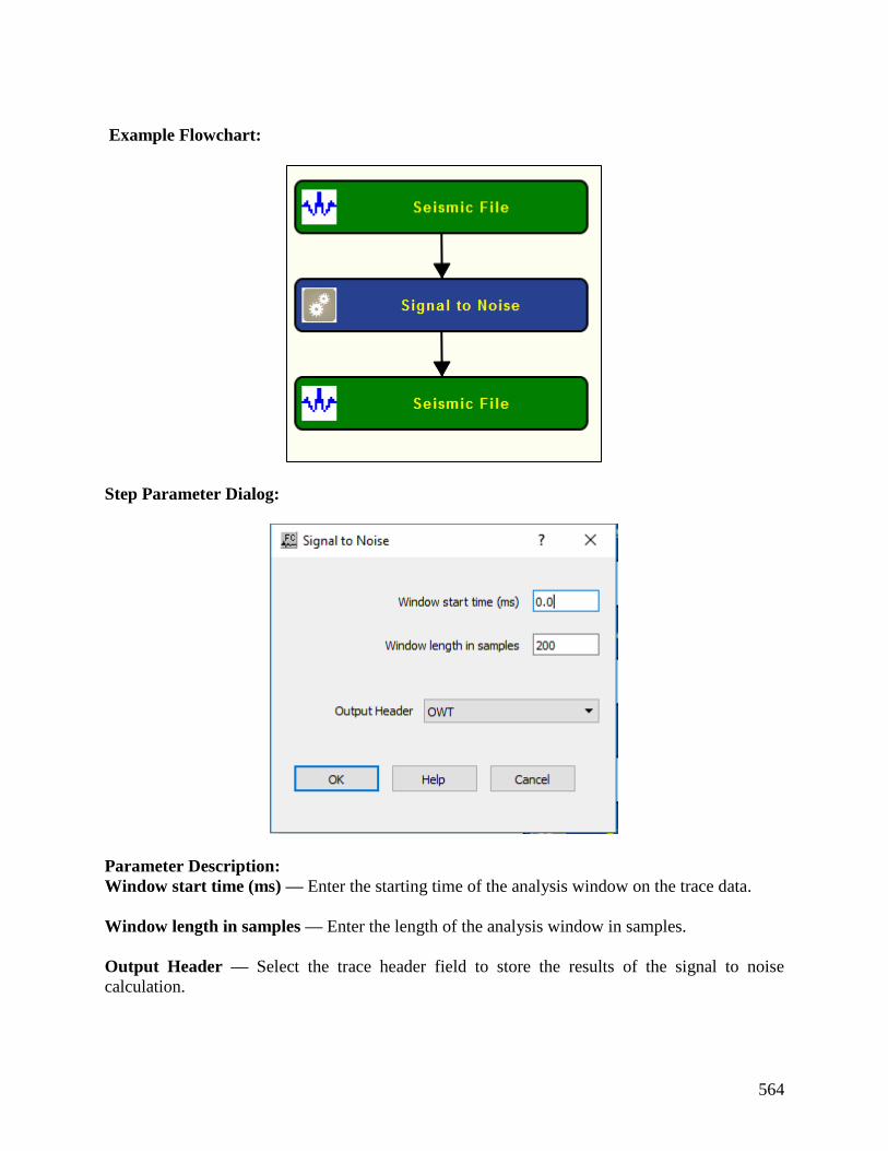
564

Example Flowchart:

Step Parameter Dialog:

Parameter Description:

Window start time (ms) — Enter the starting time of the analysis window on the trace data.

Window length in samples — Enter the length of the analysis window in samples.

Output Header — Select the trace header field to store the results of the signal to noise

calculation.

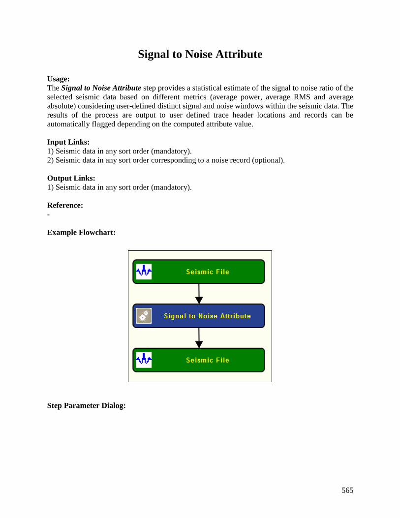
565

Signal to Noise Attribute

Usage:

The Signal to Noise Attribute step provides a statistical estimate of the signal to noise ratio of the

selected seismic data based on different metrics (average power, average RMS and average

absolute) considering user-defined distinct signal and noise windows within the seismic data. The

results of the process are output to user defined trace header locations and records can be

automatically flagged depending on the computed attribute value.

Input Links:

1) Seismic data in any sort order (mandatory).

2) Seismic data in any sort order corresponding to a noise record (optional).

Output Links:

1) Seismic data in any sort order (mandatory).

Reference:

-

Example Flowchart:

Step Parameter Dialog:

566

Parameter Description:

Parameterization method: Specify the space/time extent of signal and noise windows.

Specify windows — If selected, specify signal and noise windows manually by defining start and

end time interval and minimum and maximum channel group considered for the calculation. These

windows will be fixed for all the records in the input seismic file.

Signal window start time (ms) — Enter the signal window start time (upper boundary) in

milliseconds.

Signal window end time (ms) — Enter the signal window end time (lower boundary) in

milliseconds.

Signal window minimum channel group — Enter the minimum channel to be considered

in the signal window.

567

Signal window maximum channel group — Enter the maximum channel to be

considered in the signal window.

Noise window start time (ms) — Enter the noise window start time (upper boundary) in

milliseconds.

Noise window end time (ms) — Enter the noise window end time (lower boundary) in

milliseconds.

Noise window minimum channel group — Enter the minimum channel to be considered

in the noise window.

Noise window maximum channel group — Enter the maximum channel to be considered

in the noise window.

Use auxiliary noise record — If selected, the noise window is computed from an auxiliary seismic

file containing a single noise record. Signal window is defined manually and fixed for all input

records.

Signal window start time (ms) — Enter the signal window start time (upper boundary) in

milliseconds.

Signal window end time (ms) — Enter the signal window end time (lower boundary) in

milliseconds.

Signal window minimum channel group — Enter the minimum channel to be considered

in the signal window.

Signal window maximum channel group — Enter the maximum channel to be

considered in the signal window.

568

Compare S/N ratio in the frequency domain — If selected, the signal-to-noise ratio is estimated

from the overlap between the amplitude spectra of signal and noise windows.

% of overlapping area — Enter the percentage of overlapping area of frequency spectra

where the estimate is going to be computed.

Minimum frequency (Hz) — Enter the minimum frequency in hertz of the spectra to be

considered for the estimate.

Maximum frequency (Hz) — Enter the maximum frequency in hertz of the spectra to be

considered for the estimate.

Signal window start time (ms) — Enter the signal window start time (upper boundary) in

milliseconds.

Signal window end time (ms) — Enter the signal window end time (lower boundary) in

milliseconds.

Signal window minimum channel group — Enter the minimum channel to be considered

in the signal window.

Signal window maximum channel group — Enter the maximum channel to be

considered in the signal window.

Noise window start time (ms) — Enter the noise window start time (upper boundary) in

milliseconds.

Noise window end time (ms) — Enter the noise window end time (lower boundary) in

milliseconds.

569

Specify velocity — If selected, signal and noise windows are defined based on a reference velocity

varying linearly with the offset.

Reference velocity — Enter a reference velocity fo be used to define the location of the

start time of the signal and noise windows.

Signal window start time below velocity (ms) — Enter the start time in milliseconds

below the initial time computed from the reference velocity

Signal window length (ms) — Enter the signal window length in milliseconds

Signal window minimum channel group — Enter the minimum channel to be considered

in the signal window.

Signal window maximum channel group — Enter the maximum channel to be

considered in the signal window.

Noise window start time below velocity (ms) — Enter the start time in milliseconds

below the initial time computed from the reference velocity

Noise window length (ms) — Enter the signal window length in milliseconds

Noise window minimum channel group — Enter the minimum channel to be considered

in the noise window.

Noise window maximum channel group — Enter the maximum channel to be considered

in the noise window.

Calculation method: Specify how if the signal to noise ratio is computed either on a record or

trace-by-trace basis.

570

Record basis — If selected, estimate is based on the current record as a whole.

Trace by trace — If selected, the estimate is based on a trace-by-trace calculation.

Change noise window at each record — If checked, the noise window changes at each record.

If unchecked, noise window changes at each record.

Output headers: Specify the location of the trace header key words where the attribute will be

stored.

Top mute length (ms) — Enter the length of the top mute to be applied to both windows.

Bottom mute length (ms) — Enter the length of the bottom mute to be applied to both windows.

Minimum S/N ratio — Enter the minimum signal-to-noise ratio for a record to be consired bad.

Output average power header — Select the trace header location where the signal-to-noise ratio

computed using the average power will be stored.

Output average power flag — Select the trace header location where the record flag based on the

signal-to-noise ratio computed using the average power will be stored.

Output average RMS header — Select the trace header location where the signal-to-noise ratio

computed using the average RMS will be stored.

Output average RMS flag — Select the trace header location where the record flag based on the

signal-to-noise ratio computed using the average RMS will be stored.

Output average absolute header — Select the trace header location where the signal-to-noise

ratio computed using the average absolute will be stored.

571

Output average absolute flag — Select the trace header location where the record flag based on

the signal-to-noise ratio computed using the average RMS will be stored

Report file — Specify whether to save results to a report file and browse to locate or create an

amplitude analysis report file.

Append to existing file — If checked, append report to existing report file.

Source Energy Estimation Usage:

The Source Energy Estimation step computes an estimate of the source energy-to-noise ratio

based on an analysis of samples values prior to and following the arrival of first break energy. A

text file is output that contains, for each source location, an estimate of (1) the energy-to-noise

ratio, (2) the average energy, and (3) the average noise

Input Links:

1. Seismic data in source order (mandatory).

2. An Early Mute card containing reference times to the start of analysis. Typically, these would

be picked at the time of the first arrivals. (mandatory).

Output Links:

1) Seismic data in source order (mandatory).

References

-

Example Flowchart:

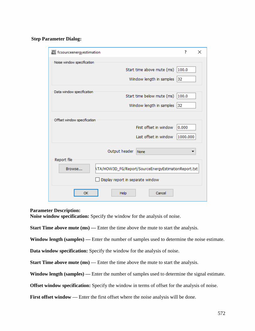
572

Step Parameter Dialog:

Parameter Description:

Noise window specification: Specify the window for the analysis of noise.

Start Time above mute (ms) — Enter the time above the mute to start the analysis.

Window length (samples) — Enter the number of samples used to determine the noise estimate.

Data window specification: Specify the window for the analysis of noise.

Start Time above mute (ms) — Enter the time above the mute to start the analysis.

Window length (samples) — Enter the number of samples used to determine the signal estimate.

Offset window specification: Specify the window in terms of offset for the analysis of noise.

First offset window — Enter the first offset where the noise analysis will be done.

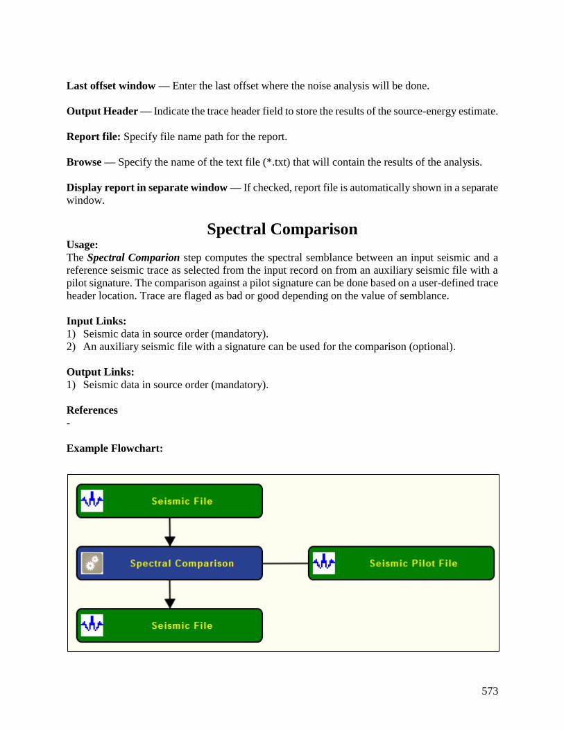
573

Last offset window — Enter the last offset where the noise analysis will be done.

Output Header — Indicate the trace header field to store the results of the source-energy estimate.

Report file: Specify file name path for the report.

Browse — Specify the name of the text file (*.txt) that will contain the results of the analysis.

Display report in separate window — If checked, report file is automatically shown in a separate

window.

Spectral Comparison Usage:

The Spectral Comparion step computes the spectral semblance between an input seismic and a

reference seismic trace as selected from the input record on from an auxiliary seismic file with a

pilot signature. The comparison against a pilot signature can be done based on a user-defined trace

header location. Trace are flaged as bad or good depending on the value of semblance.

Input Links:

1) Seismic data in source order (mandatory).

2) An auxiliary seismic file with a signature can be used for the comparison (optional).

Output Links:

1) Seismic data in source order (mandatory).

References

-

Example Flowchart:

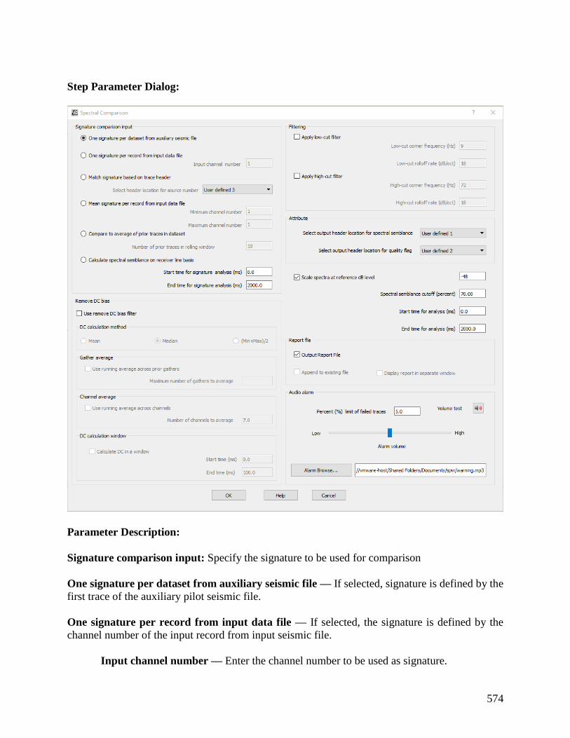
574

Step Parameter Dialog:

Parameter Description:

Signature comparison input: Specify the signature to be used for comparison

One signature per dataset from auxiliary seismic file — If selected, signature is defined by the

first trace of the auxiliary pilot seismic file.

One signature per record from input data file — If selected, the signature is defined by the

channel number of the input record from input seismic file.

Input channel number — Enter the channel number to be used as signature.

575

Match signature based on trace header — If selected, signature is from and axiliary pilot file

and matched against current record based on the value of a user-defined trace header locations.

Select header location for source number — Select the location of the header to be used

as reference between signature and input seismic file.

Mean signature per record from input data file — If selected, signature is computed as the

average of a user-defined range of traces.

Minimum channel number — Enter the minimum channel number to be used for the

mean signature.

Maximum channel number — Enter the maximum channel number to be used for the

mean signature.

Compare to average of prior traces in dataset — If selected, signature is defined as the average

of the number of prioer traces defined in a rolling window.

Number of prior traces in rolling window — Enter the number of prior traces in a rolling

window to be used for the average of the signature.

Calculate spectral semblance on receiver line basis — If selected, signature is defined as the

average along a receiver line.

Start time for signature analysis (ms) — Enter the start time (upper boundary) in milliseconds

of the time window for the signature analysis.

End time for signature analysis (ms) — Enter the end time (lower boundary) in milliseconds of

the time window for the signature analysis.

Remove DC bias: Specify if a DC remove bias filter will be applied to the input seismic file before

computing the spectral semblance.

Use remove DC bias filter — If checked applies a Remove DC bias step to the input seismic file.

The filter is not store in the output seismic file, it is only applied before the calculations of the

spectral semblance.

DC calculation method: select the method to estimate the DC bias.

Mean — If selected, estimates the DC bias as the mean of the seismic samples considered.

Median — If selected, estimates the DC bias as the median of the seismic samples

considered.

576

(Min+Max)/2 — If selected, estimates the DC bias as central value between the min and

max of the seismic samples considered.

Channel Average: DC bias may be estimated using a moving window running through

channels in order to increase the reliability of the estimate.

Use running average across channels — If checked the DC bias is estimate taking into

account a moving window computed across channels.

Number of channels to average — Enter the number of channels that belong to

the moving window.

Gather Average: DC bias may be estimated using a moving window running through

gathers (or records) in order to increase the reliability of the estimate.

Use running average across prior gathers — If checked the DC bias is estimate taking

into account a moving window computed across prior gathers.

Number of gathers to average — Enter the number of gathers that belong to the

moving window.

DC calculation window: define the time gate where the calculation is going to be

computed.

Calculate DC in a window — If checked, only the entered window of each trace will be

used to calculate the DC.

Start time (ms) — Enter the start time of the window to be used for calculating the

DC value.

End time (ms) — Enter the end time of the window to be used for calculating the

DC value.

Filtering:

Apply low-cut filter — If checked applies to the input seismic file a zero-phase Butterworth filter

to the input seismic data before computing the spectral semblance. The filter is only applied to the

input file and not store in the output seismic file.

Low-cut filtering: Specify low-cut filter parameters.

Apply low-cut filter — If checked, a low-cut filter will be applied to your data.

Low-cut corner frequency (Hz) — Enter the low half-power frequency in Hertz to be

applied to your data. The amplitude of this frequency will be reduced by a factor of two

relative to the input.

577

Low-cut rolloff rate (dB/oct) — Enter the low rolloff filter slope in decibels per octave

to be applied to your data. Higher numbers give steeper rolloff.

High-cut filtering: Specify high-cut filter parameters.

Apply high-cut filter — If checked, a high-cut filter will be applied to your data.

High-cut corner frequency (Hz) — Enter the high half-power frequency in Hertz to be

applied to your data. The amplitude of this frequency will be reduced by a factor of two

relative to the input.

High-cut rolloff rate (dB/oct) — Enter the high rolloff filter slope in decibels per

octave to be applied to your data. Higher numbers give steeper rolloff.

Attribute: Specify the trace header location where the spectral semblance and flags will be stored.

Select output header location for spectral semblance — Select the trace header location where

the value of spectral semblance will be store.

Select output header location for quality flag — Select the trace header location where the flag

of good or bad trace will be stored.

Scale spectra at reference dB level — If checked, spectra of inut and signature are scaled at a

refecence level.

Spectral semblance cutoff (percent) — Enter the semblance cutoff value in percentage to

distinguish between good and bad traces.

Start time for analysis (ms) — Enter the start time (upper boundary) in milliseconds of the time

window for the analysis of the input seismic file.

End time for analysis (ms) — Enter the end time (lower boundary) in milliseconds of the time

window for the analysis of the input seismic file.

Report file: Specifies if a report file is generated

Output Report file — If checked, outputs a report file with a unique name idenfier.

Audio alarm: Specifies alarm depending on the number of traces flagged as bad traces.

Percent (%) limit of failed traces — Enter the percent of failed traces to trigger the alarm

Alarm volume — Use slider to define the alarm volume

Alarm browse — Select an audio file to be used as alarm.

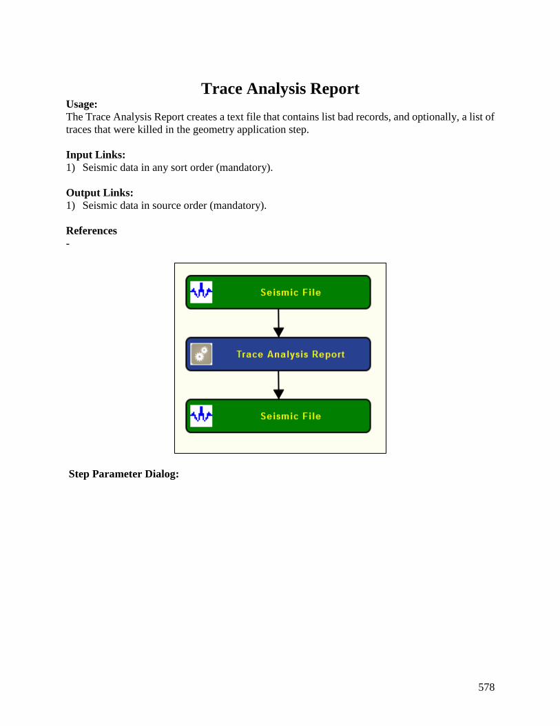
578

Trace Analysis Report Usage:

The Trace Analysis Report creates a text file that contains list bad records, and optionally, a list of

traces that were killed in the geometry application step.

Input Links:

1) Seismic data in any sort order (mandatory).

Output Links:

1) Seismic data in source order (mandatory).

References

-

Step Parameter Dialog:

579

Parameter Description:

Report traces killed by Geometry Definition step — If checked, traces killed by a previous

Geometry Definition step will be reported.

Report traces killed by processing steps — If checked, report traces killed by processing steps.

580

Use Geometry Definition dead traces in analysis — If cheked, dead traces from Geometry

Definition will be included in the analysis.

Report bad records based on adjacent dead traces — If checked, bad records are to be identified

according to the number of adjacent dead traces.

Adjacent dead trace limit — Enter the number of adjacent dead traces that will cause the

record the be considered “bad”, and therefore listed in the trace analysis report.

Report bad records based on number of dead traces per record — If checked, bad records are

to be identified according to the number of adjacent dead traces.

Dead trace limit per record — Enter the maximum percentage of dead traces that will cause

the record the be considered “bad”, and therefore listed in the trace analysis report.

Report records killed by prior process — If checked, traces killed by previous steps, e.g. by

geometry definition, will be included in the report.

Kill bad records — If checked, bad records are killed from the input seismic file.

Audio alarm: Specifies alarm depending on the number of traces flagged as bad traces.

Percent (%) limit of failed traces — Enter the percent of failed traces to trigger the alarm

Alarm volume — Use slider to define the alarm volume

Alarm browse — Select an audio file to be used as alarm.

Report file — Specify whether to save results to a report file and browse to locate or create an

amplitude analysis report file.

Append to existing file — If checked, append report to existing report file.

581

Seismic Data Steps

This section documents the seismic data types in SPW and the processes currently available for

creating those data types.

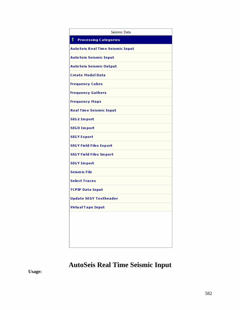
582

AutoSeis Real Time Seismic Input Usage:

583

The AutoSeis Real Time Seismic Input step allows import AutoSeis seismic data format from the

field into a single seismic file. Field data is imported automatically from a root directory. The

output seismic files are by default set for nodes (receiver order).

Input Links:

None.

Output Links:

1) Seismic data in any sort order (mandatory).

References:

-

Example Flowchart:

Step Parameter Dialog:

Parameter Description:

584

Input AutoSeis root directory: Specify AutoSeis root directory.

Input directory… — Browse for the directory where AutoSeis files are stored.

Remove auxiliary traces — If checked, auxiliary traces present in the input data are automatically

removed from the outuput seismic file.

Apply fractional time shift correction — If checked apply factional time shift correction to the

input data.

AutoSeis Seismic Input Usage:

The AutoSeis Seismic Input step allows import AutoSeis seismic data format from the field into

a single seismic file. Field data is imported automatically from a root directory. The output seismic

files are by default set for nodes (receiver order).

Input Links:

None.

Output Links:

1) Seismic data in any sort order (mandatory).

References:

-

Example Flowchart:

Step Parameter Dialog:

585

Parameter Description:

Input AutoSeis root directory: Specify AutoSeis root directory.

Input directory… — Browse for the directory where AutoSeis files are stored.

Remove auxiliary traces — If checked, auxiliary traces present in the input data are automatically

removed from the outuput seismic file.

Apply fractional time shift correction — If checked apply factional time shift correction to the

input data.

AutoSeis Seismic Ouput

Create Model Data Usage:

The Create Model Data step is a utility for testing purposes. It allows you to create synthetic data

with specific number of events per record, the wavelet type, the number of records, the number of

traces per record, the sample interval, the trace length, record and trace labeling parameters, and

wavelet parameters for setting filtering frequencies.

Input Links:

None.

Output Links:

1) Seismic data in any sort order (mandatory).

References:

-

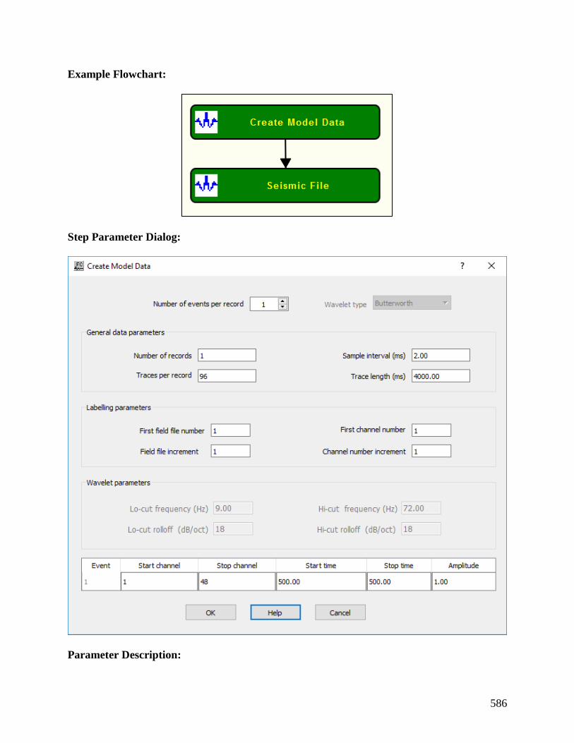
586

Example Flowchart:

Step Parameter Dialog:

Parameter Description:

587

Number of events per record — Enter the number of events per record to create.

Wavelet type — Select the wavelet type to use.

General data parameters: Specify the general data parameters.

Number of records — Enter the number of data records.

Sample interval (ms) — Enter the sample interval of the traces in milliseconds.

Traces per record — Enter the number of traces per record.

Trace length (ms) — Enter the trace length in milliseconds.

Labelling parameters: Specify labelling parameters for field files and channels.

First field file number — Enter the first field file number.

Field file increment — Enter the field file increment number.

First channel number — Enter the first channel number.

Channel number increment — Enter the channel number increment.

Wavelet parameters: Specify wavelet parameters.

Lo-cut frequency (Hz) — Enter the lo-cut filter frequency in Hertz.

Lo-pass frequency (Hz) — Enter the lo-pass filter frequency in Hertz.

Hi-pass frequency (Hz) — Enter the Hi-pass filter frequency in Hertz.

Hi-cut frequency (Hz) — Enter the Hi-cut filter frequency in Hertz.

Frequency Cubes

Usage:

The Frequency Cubes step computes frequency volumes from input seismic of SEG-Y files at

specific frequencies. The output cubes are generated at specific frequencies inferred directly from

the input seismic file or at user-defined frequencies. The output frequency volumes can also be

sorted using user-defined sort order.

Input Links:

None.

588

Output Links:

1) Seismic data in selected processing sort order (mandatory).

Example Flowchart:

Step Parameter Dialog:

589

Parameter Description:

Seismic file: Specify the location of the input seismic or SEG-Y file.

File Browse… — Select the input root file name. All the files sharing the same root name will be

used as input.

SEGY format: Specify the input SEG-Y format.

Format Browse… — Select saved SEG-Y format. Browse for format file.

590

Create new SEGY format — Select to create a new SEG-Y format.

View existing SEGY format — Select to view current SEG-Y format.

SEGY index: Specify SEG-Y index parameters. If needed index file parameterization may be

changed here.

Customize Index Map — Select to customize the index map of the input SEG-Y file.

View trace headers — Select to view the trace headers of the input SEG-Y file.

View trace header map — Select to view trace header map of the input SEG-Y file.

Save headers to a file — Select to save headers from input SEG-Y file into a file.

General dataset properties: Specify general properties of the input SEG-Y dataset. All these

properties may be overwritten by the user. User-defined parameters will be used as parameter for

the output seismic file.

Number of frequency cubes — Enter number of frequency cubes to be generated.

Number of traces per cube — Enter the number of traces per cube.

First output frequency — Enter first output frequency.

Last output frequency — Enter last ouput frequency.

Output frequency increment — Enter output frequency increment.

Sample format — Enter sample format.

591

Sample interval — Enter sample interval in milliseconds.

Samples per trace — Enter number of samples per trace.

Start time (ms) — Enter start time of the input dataset in milliseconds.

End time (ms) — Enter end time of the input dataset in milliseconds.

Processing sort order: Specify processing sort order. Ouput dataset will have selected sort order.

Primary sort key — Select primary sort key to be used during processing.

Limit Range — If checked, limit range based on primary sort key.

Minimum value — Enter minimum value to limit the range

Maximum value — Enter the maximum value to limit the range.

Secondary sort key — Select secondary sort key to be used during processing.

Limit Range — If checked, limit range based on secondary sort key.

Minimum value — Enter minimum value to limit the range

Maximum value — Enter the maximum value to limit the range.

Tertiary sort key — Select tertiary sort key to be used during processing.

Limit Range — If checked, limit range based on tertiary sort key.

592

Minimum value — Enter minimum value to limit the range

Maximum value — Enter the maximum value to limit the range.

Quaternary sort — Select quaternary sort key to be used during processing.

Limit Range — If checked, limit range based on quaternary sort key.

Minimum value — Enter minimum value to limit the range

Maximum value — Enter the maximum value to limit the range.

Create record at — Select criteria to create record.

Frequency Gathers

Usage:

The Frequency Gather step computes frequency gathers from input seismic of SEG-Y files at

specific frequencies. The output cubes are generated at specific frequencies inferred directly from

the input seismic file or at user-defined frequencies. The output frequency volumes can also be

sorted using user-defined sort order.

Input Links:

None.

Output Links:

1) Seismic data in selected processing sort order (mandatory).

Example Flowchart:

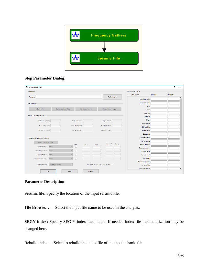
593

Step Parameter Dialog:

Parameter Description:

Seismic file: Specify the location of the input seismic file.

File Browse… — Select the input file name to be used in the analysis.

SEGY index: Specify SEG-Y index parameters. If needed index file parameterization may be

changed here.

Rebuild index — Select to rebuild the index file of the input seismic file.

594

Customize index map — Select to customize the index map of the input seismic file.

View trace header — Select to view trace headers.

Trace header ranges — Select to update trace header ranges in Trace header ranges.

Trac header ranges: Specify the trace headers map into the index files and its ranges.

General dataset properties: Specify general properties of the input dataset. All these properties

may be overwritten by the user. User-defined parameters will be used as parameter for the output

seismic file.

Number of gathers — Enter the number of gathers of input seismic file.

Freq. per gather — Enter the number of frequencies per gather.

Number of traces — Enter the number of traces of the input seismic file to be analyzed

Freq. increment — Enter the frequency increment.

First output freq. — Enter the first output frequency.

Last output freq. — Enter the last output frequency

Sample format — Enter the sample format of the input seismic file.

Sample interval — Enter the sample interval of the input seismic file.

Samples/Trace — Enter the number of samples per trace.

595

Input sort and selection option: Specify the input sort order.

Reset internal order — Select to reset the sort order to the internal sort order of th input seismic

file.

Primary sort key — Select primary sort key to be used during processing.

Limit Range — If checked, limit range based on primary sort key.

Minimum value — Enter minimum value to limit the range

Maximum value — Enter the maximum value to limit the range.

Secondary sort key — Select secondary sort key to be used during processing.

Limit Range — If checked, limit range based on secondary sort key.

Minimum value — Enter minimum value to limit the range

Maximum value — Enter the maximum value to limit the range.

Tertiary sort key — Select tertiary sort key to be used during processing.

Limit Range — If checked, limit range based on tertiary sort key.

Minimum value — Enter minimum value to limit the range

Maximum value — Enter the maximum value to limit the range.

Quaternary sort — Select quaternary sort key to be used during processing.

596

Limit Range — If checked, limit range based on quaternary sort key.

Minimum value — Enter minimum value to limit the range

Maximum value — Enter the maximum value to limit the range.

Create record at — Select criteria to create record.

Regather groups into supergathers — If checked, groups are regathers into supergathers.

Frequency Maps Usage:

The Frequency Maps step computes frequency maps from input seismic of SEG-Y files at specific

frequencies. The output cubes are generated at specific frequencies inferred directly from the input

seismic file or at user-defined frequencies. The output frequency volumes can also be sorted using

user-defined sort order.

Input Links:

None.

Output Links:

1) Seismic data in selected processing sort order (mandatory).

Example Flowchart:

Step Parameter Dialog:

597

Parameter Description:

Seismic file: Specify the location of the input seismic or SEG-Y file.

File Browse… — Select the input root file name. All the files sharing the same root name will be

used as input.

SEGY format: Specify the input SEG-Y format.

Format Browe… — Select saved SEG-Y format. Browse for format file.

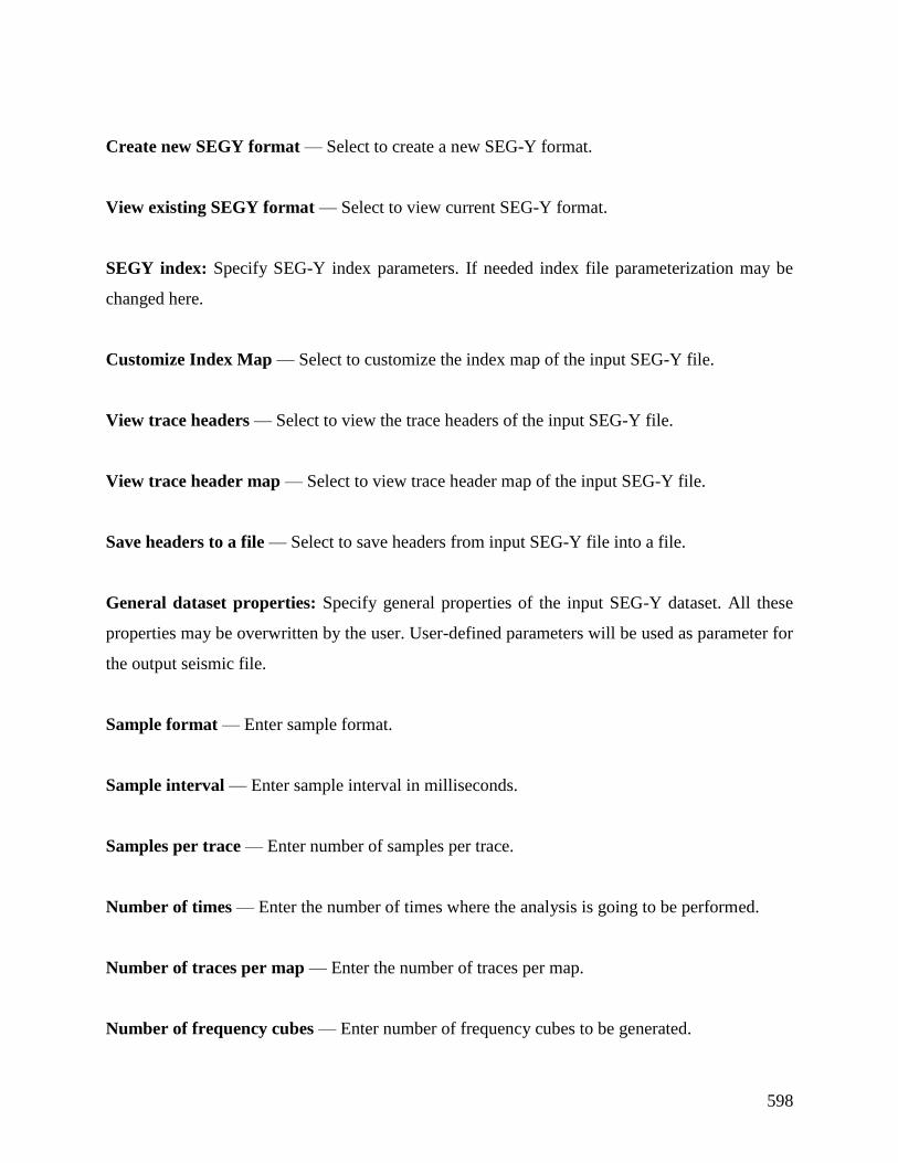
598

Create new SEGY format — Select to create a new SEG-Y format.

View existing SEGY format — Select to view current SEG-Y format.

SEGY index: Specify SEG-Y index parameters. If needed index file parameterization may be

changed here.

Customize Index Map — Select to customize the index map of the input SEG-Y file.

View trace headers — Select to view the trace headers of the input SEG-Y file.

View trace header map — Select to view trace header map of the input SEG-Y file.

Save headers to a file — Select to save headers from input SEG-Y file into a file.

General dataset properties: Specify general properties of the input SEG-Y dataset. All these

properties may be overwritten by the user. User-defined parameters will be used as parameter for

the output seismic file.

Sample format — Enter sample format.

Sample interval — Enter sample interval in milliseconds.

Samples per trace — Enter number of samples per trace.

Number of times — Enter the number of times where the analysis is going to be performed.

Number of traces per map — Enter the number of traces per map.

Number of frequency cubes — Enter number of frequency cubes to be generated.

599

First output frequency — Enter first output frequency.

Last output frequency — Enter last ouput frequency.

Processing sort order: Specify processing sort order. Ouput dataset will have selected sort order.

Primary sort key — Select primary sort key to be used during processing.

Limit Range — If checked, limit range based on primary sort key.

Minimum value — Enter minimum value to limit the range

Maximum value — Enter the maximum value to limit the range.

Secondary sort key — Select secondary sort key to be used during processing.

Limit Range — If checked, limit range based on secondary sort key.

Minimum value — Enter minimum value to limit the range

Maximum value — Enter the maximum value to limit the range.

Tertiary sort key — Select tertiary sort key to be used during processing.

Limit Range — If checked, limit range based on tertiary sort key.

Minimum value — Enter minimum value to limit the range

Maximum value — Enter the maximum value to limit the range.

600

Quaternary sort — Select quaternary sort key to be used during processing.

Limit Range — If checked, limit range based on quaternary sort key.

Minimum value — Enter minimum value to limit the range

Maximum value — Enter the maximum value to limit the range.

Create record at — Select criteria to create record.

Real Time Seismic Input Usage:

Input Links:

None.

Output Links:

1) Seismic data in any sort order (mandatory).

Example Flowchart:

Step Parameter Dialog:

601

Parameter Description:

Input source: Specify either the input seismic is all the files at a given directory or at a a specific

file within the directory

Specify input directory — If selected, input data is defined as all the seismic files in the Input

directory. Files will be loaded sequentially as defined in File ordering.

Specify input virtual tape device — Not yet implemented.

Specify starting input file — If selected, input data is defined starting from a user-defined seismic

file. Files will be loaded sequentially as defined in File ordering.

Input directory… — Browse for input directory where seismic files are stored.

File ordering: Specify the sequential order used to load the seismic files.

Order files by timestamp — If selected, seismic files will be loaded by its timestamp, from older

to newer.

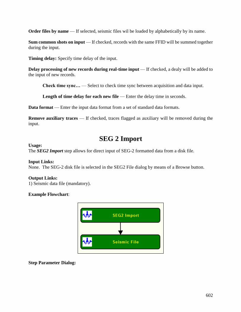
602

Order files by name — If selected, seismic files wil be loaded by alphabetically by its name.

Sum common shots on input — If checked, records with the same FFID will be summed together

during the input.

Timing delay: Specify time delay of the input.

Delay processing of new records during real-time input — If checked, a dealy will be added to

the input of new records.

Check time sync… — Select to check time sync between acquisition and data input.

Length of time delay for each new file — Enter the delay time in seconds.

Data format — Enter the input data format from a set of standard data formats.

Remove auxiliary traces — If checked, traces flagged as auxiliary will be removed during the

input.

SEG 2 Import Usage:

The SEG2 Import step allows for direct input of SEG-2 formatted data from a disk file.

Input Links:

None. The SEG-2 disk file is selected in the SEG2 File dialog by means of a Browse button.

Output Links:

1) Seismic data file (mandatory).

Example Flowchart:

Step Parameter Dialog:

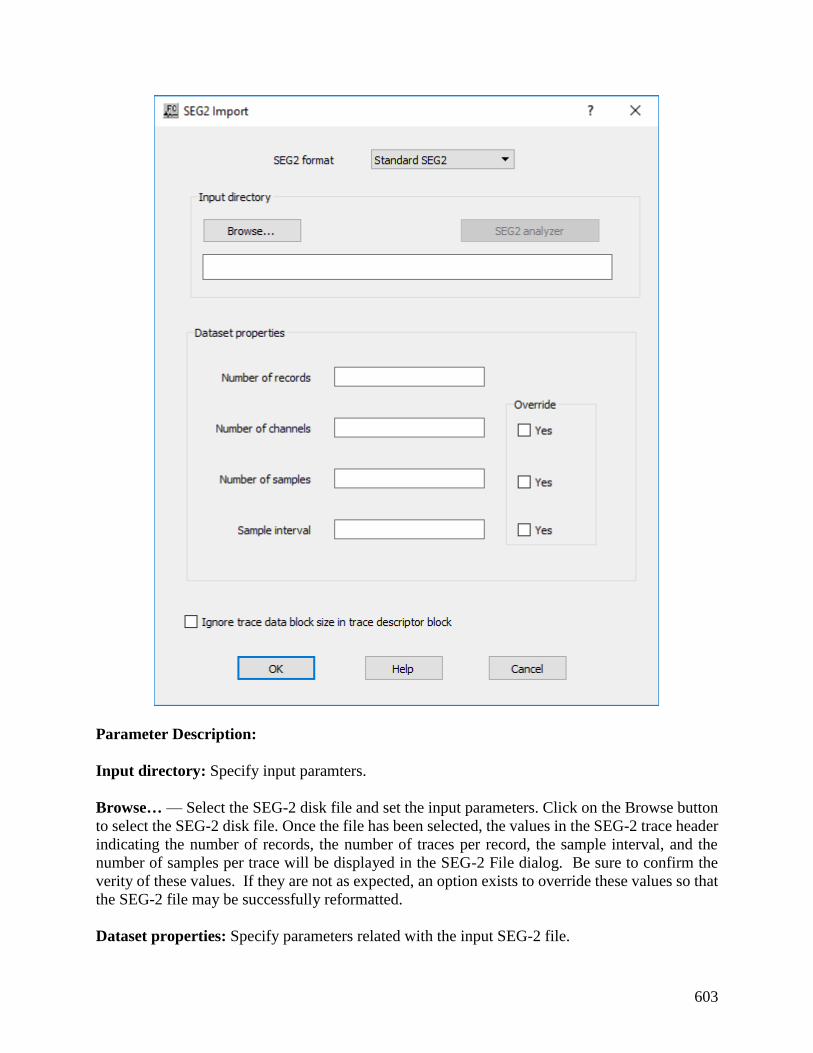
603

Parameter Description:

Input directory: Specify input paramters.

Browse… — Select the SEG-2 disk file and set the input parameters. Click on the Browse button

to select the SEG-2 disk file. Once the file has been selected, the values in the SEG-2 trace header

indicating the number of records, the number of traces per record, the sample interval, and the

number of samples per trace will be displayed in the SEG-2 File dialog. Be sure to confirm the

verity of these values. If they are not as expected, an option exists to override these values so that

the SEG-2 file may be successfully reformatted.

Dataset properties: Specify parameters related with the input SEG-2 file.

604

Number of records — Enter the number of records in the SEG-2 disk file inferred from the SEG-

2 file header.

Number of channels — Enter the number of traces per record stored in bytes 6 and 7 of the SEG-

2 file descriptor block.

Override — If checked, enter a value to overwrite the number of traces per record stored

in the input file.

Number of samples — Indicates the number of samples per trace stored in bytes 8-11 of the SEG-

2 trace descriptor block.

Override – If checked, enter a value to overwrite the number of samples per trace stored

in the input file.

Sample interval (ms) — Indicates the sample interval stored in the appropriate sub-string of the

SEG-2 file descriptor block.

Override — If checked, enter a value to overwrite the sample interval in milliseconds

stored in the input file.

Ignore trace data blocks size in trace descriptor block — If checked, ignore trace data blocks

size as defined in trace descriptor block.

SEG D Import Usage:

The SEGD Import step allows for direct input of SEG-D formatted data from a disk file. Different

standard SEG-D formats are available for import.

Input Links:

None. The SEG-2 disk file is selected in the SEG2 File dialog by means of a Browse button.

Output Links:

1) Seismic data file (mandatory).

Example Flowchart:

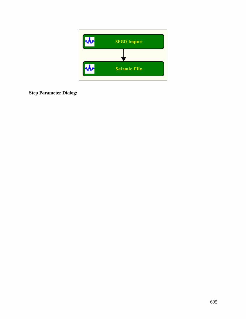
605

Step Parameter Dialog:

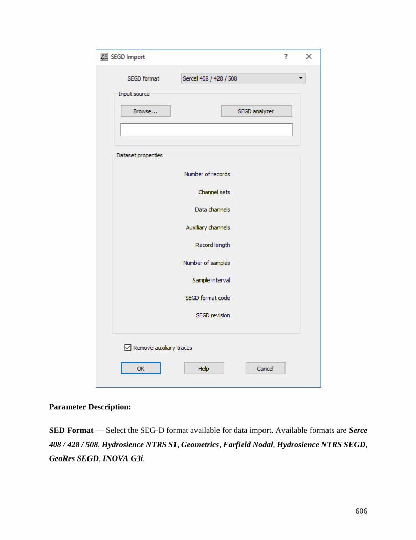
606

Parameter Description:

SED Format — Select the SEG-D format available for data import. Available formats are Serce

408 / 428 / 508, Hydrosience NTRS S1, Geometrics, Farfield Nodal, Hydrosience NTRS SEGD,

GeoRes SEGD, INOVA G3i.

607

Browse… — Select the SEG-D disk file and set the input parameters. Click on the Browse button

to select the SEG-D disk file. Once the file has been selected, the values stored in the SEG-D trace

header indicating the number of records, channel stes, data channels, auxiliary channels, record

length, number of samples, sample interval, SEG format code, SEG revision are displayed in the

Dataset properties box.

SEG Y Export

Usage:

The SEG Y Export allows for direct output of seismic files into a formatted data SEG-Y.

Input Links:

1) Seismic data file (mandatory).

Output Links:

None.

Example Flowchart

Step Parameter Dialog:

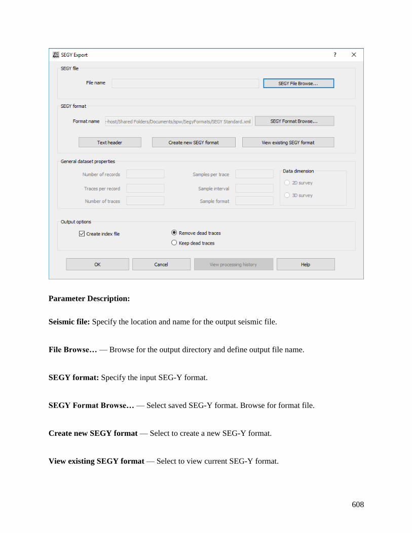
608

Parameter Description:

Seismic file: Specify the location and name for the output seismic file.

File Browse… — Browse for the output directory and define output file name.

SEGY format: Specify the input SEG-Y format.

SEGY Format Browse… — Select saved SEG-Y format. Browse for format file.

Create new SEGY format — Select to create a new SEG-Y format.

View existing SEGY format — Select to view current SEG-Y format.

609

General dataset properties: Specify general properties of the input dataset. All these properties

may be overwritten by the user. User-defined parameters will be used as parameter for the output

seismic file.

Number of records — Enter the number of records in the input seismic file.

Traces per record — Enter the number of traces per record.

Number of traces — Enter the number of traces in the input seismic file.

Samples per trace — Enter the number of samples per trace in the input seismic file.

Sample interval — Enter the sample interval of the input seismic file in milliseconds

Sample format — Enter the sample format of the input seismic file.

Data dimesion: Specify the dimension of the input data.

2D survey — If selected, input data is two-dimensional.

3D survey — If selected, input data is three-dimensional.

Output options: Specify options of the output SEG-Y file.

Create index file — If checked, create index file for output SEG-Y file.

Remove dead traces — If checked, traces flagged as dead are removed from the outpu SEG-Y

file.

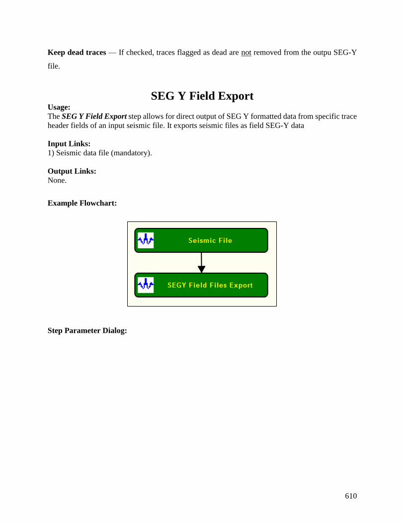
610

Keep dead traces — If checked, traces flagged as dead are not removed from the outpu SEG-Y

file.

SEG Y Field Export Usage:

The SEG Y Field Export step allows for direct output of SEG Y formatted data from specific trace

header fields of an input seismic file. It exports seismic files as field SEG-Y data

Input Links:

1) Seismic data file (mandatory).

Output Links:

None.

Example Flowchart:

Step Parameter Dialog:

611

Parameter Description:

Browse… — Browse for the directory where the output SEG-Y files will be stored.

File naming: Specify common file name for the output seismic files.

Create file name using receiver identifier of first trace in gather — If selected, file name of

the output SEG-Y files uses the receiver number of the first trace in the gather as identified.

Create file name using field file number of first trace in gather — If selected, file name of the

output SEG-Y files uses the field file number of the first trace in the gather as identified.

Create file name using frequency of first trace in gather — If selected, file name of the output

SEG-Y files uses the frequency number of the first trace in the gather as identified.

612

Create file name using data timestamp — Not yet implemented.

File name prefix — Enter the file name prefix of the output SEG-Y files that will be written in

the hard-drive.

SEG-Y Format: Specify SEG-Y format of the output SEG- files.

Browse… — Browse for an existing SEG-Y format file.

Create new SEGY format — Select to create a new SEG-Y format.

View existing SEGY format — Select to view current SEG-Y format.

SEG Y Field Import Usage:

The SEGY Filed Import step allows importing field SEG Y formatted data from a disk file into a

seismic file.

Input Links:

None.

Output Links:

1) Seismic data file (mandatory).

Example Flowchart:

Step Parameter Dialog:

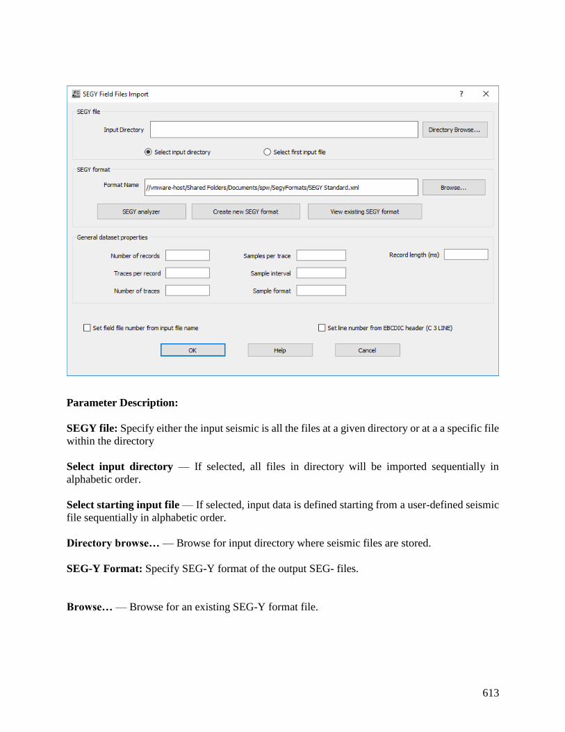
613

Parameter Description:

SEGY file: Specify either the input seismic is all the files at a given directory or at a a specific file

within the directory

Select input directory — If selected, all files in directory will be imported sequentially in

alphabetic order.

Select starting input file — If selected, input data is defined starting from a user-defined seismic

file sequentially in alphabetic order.

Directory browse… — Browse for input directory where seismic files are stored.

SEG-Y Format: Specify SEG-Y format of the output SEG- files.

Browse… — Browse for an existing SEG-Y format file.

614

SEGY analyzer — Select to access properties of the input SEG-Y file.

Create new SEGY format — Select to create a new SEG-Y format.

View existing SEGY format — Select to view current SEG-Y format.

General dataset properties: Specify general properties of the input dataset. All these properties

may be overwritten by the user. User-defined parameters will be used as parameter for the output

seismic file.

Number of records — Enter the number of records in the input seismic file.

Traces per record — Enter the number of traces per record.

Number of traces — Enter the number of traces in the input seismic file.

Samples per trace — Enter the number of samples per trace in the input seismic file.

Sample interval — Enter the sample interval of the input seismic file in milliseconds

Sample format — Enter the sample format of the input seismic file.

Sample format — Enter the record length of the input SEG-Y file in milliseconds.

Set field file number from input file name — If checked, field file number is retrieved fom the

name of the input file name.

Set line number from EBCDIC header (C 3 LINE) — If checked, line number is retrived from

the SEG-Y text header (EBCDIC header) at line position C3.

SEG Y Import Usage:

The SEGY Import step allows for direct input of SEG Y formatted seimsic data from a disk file

into a seismic file in SPW format. It allows to select the SEG-Y trace header keys to be mapped

into the index file which stores this information as part of the SPW format.

615

Input Links:

None.

Output Links:

1) Seismic data file (mandatory).

Example Flowchart:

Step Parameter Dialog:

Parameter Description:

SEGY File: Specify input SEG-Y file by browsing it.

Browse… — Browse for the input SEG-Y file.

616

SEG-Y Format: Specify the input SEG-file format Y format and map trace headers to be stored

in the SPW index file.

Browse… — Browse for an existing SEG-Y format file.

SEGY analyzer — Select to access properties of the input SEG-Y file.

Create new format — Select to creat a new SEG-Y map format.

View existing format — Select to view the existing format, SEGY index fields are automatically

updated.

SEGY index fields — Check/Uncheck SEG-Y trace headers to be mapped into the SPW

index file.

SEGY index: Specify SEG-Y index parameters. If needed index file parameterization may be

changed here.

Build SEGY index — Select to build the index filel usinf the current SEG-Y format for the

selected input SEG-Y file.

View trace headers — Select to view original trace headers from the input SEG-Y file.

Trace header ranges — Select to update Trace header ranges table

Trace header ranges — Shows the range of the input SEG-Y trace headers

General dataset properties: Specify general properties of the input dataset. All these properties

may be overwritten by the user. User-defined parameters will be used as parameter for the output

seismic file.

617

Number of records — Enter the number of records in the input seismic file.

Traces per record — Enter the number of traces per record.

Number of traces — Enter the number of traces in the input seismic file.

Samples per trace — Enter the number of samples per trace in the input seismic file.

Sample interval — Enter the sample interval of the input seismic file in milliseconds

Sample format — Enter the sample format of the input seismic file.

Dimesion: Specify the dimension of the input data.

2D survey — If selected, input data is two-dimensional.

3D survey — If selected, input data is three-dimensional

Input sort and selection option: Specify the input sort order.

Reset internal order — Select to reset the sort order to the internal sort order of th input seismic

file.

Primary sort key — Select primary sort key to be used during processing.

Limit Range — If checked, limit range based on primary sort key.

Minimum value — Enter minimum value to limit the range

Maximum value — Enter the maximum value to limit the range.

618

Secondary sort key — Select secondary sort key to be used during processing.

Limit Range — If checked, limit range based on secondary sort key.

Minimum value — Enter minimum value to limit the range

Maximum value — Enter the maximum value to limit the range.

Tertiary sort key — Select tertiary sort key to be used during processing.

Limit Range — If checked, limit range based on tertiary sort key.

Minimum value — Enter minimum value to limit the range

Maximum value — Enter the maximum value to limit the range.

Quaternary sort — Select quaternary sort key to be used during processing.

Limit Range — If checked, limit range based on quaternary sort key.

Minimum value — Enter minimum value to limit the range

Maximum value — Enter the maximum value to limit the range.

Create record at — Select criteria to create record.

Regather groups into supergathers — If checked, groups are regathers into supergathers.

Seismic File Usage:

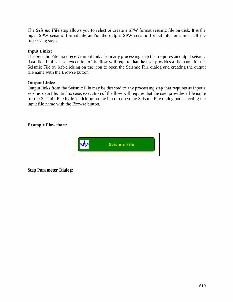
619

The Seismic File step allows you to select or create a SPW format seismic file on disk. It is the

input SPW seismic format file and/or the output SPW seismic format file for almost all the

processing steps.

Input Links:

The Seismic File may receive input links from any processing step that requires an output seismic

data file. In this case, execution of the flow will require that the user provides a file name for the

Seismic File by left-clicking on the icon to open the Seismic File dialog and creating the output

file name with the Browse button.

Output Links:

Output links from the Seismic File may be directed to any processing step that requires as input a

seismic data file. In this case, execution of the flow will require that the user provides a file name

for the Seismic File by left-clicking on the icon to open the Seismic File dialog and selecting the

input file name with the Browse button.

Example Flowchart:

Step Parameter Dialog:

620

Seismic file: Specify location and name of the seismic file. Browse for existing file if seismic file

is going to be used as input for other processing step or write select directory and write file name

if seismic file is going to be used as output fo a processing step.

File Browse… — Select to browse for input or output location and select file.

SEGY index: Specify parameters related with the index file used as part of the SPW seismic

formatl.

Rebuild index — Select to rebuild index file. Due to SPW updates there may be the need to update

an existing index file.

621

Customize Index Map — Select to customize the index file. With this option the user can select

which fields are stored in the index file.

View trace headers — Select to view trace header values with its ranges.

Trace header ranges — Select to open a table with the ranges for all the trace header in the

seismic file.

General dataset properties: Specify general properties of the input dataset. All these properties

may be overwritten by the user. User-defined parameters will be used as parameter for the output

seismic file.

Number of records — Enter the number of records in the input seismic file.

Traces per record — Enter the number of traces per record.

Number of traces — Enter the number of traces in the input seismic file.

Samples per trace — Enter the number of samples per trace in the input seismic file.

Sample interval — Enter the sample interval of the input seismic file in milliseconds

Sample format — Enter the sample format of the input seismic file.

Dimesion: Specify the dimension of the input data.

2D survey — If selected, input data is two-dimensional.

3D survey — If selected, input data is three-dimensional

Input sort and selection option: Specify the input sort order.

622

R — Select to sort the seismic file by common receiver order: Primary sort key is set to none;

Secondary sort key is set to none; Tertiary sort key is set to Offset; Quaternary sort key is set to

none; Create record at is set to Change in secondary.

O — Select to sort the seismic file by common offset order: Primary sort key is set to Offset;

Secondary sort key is set to none; Tertiary sort key is set to none; Quaternary sort key is set to

none; Create record at is set to Change in primary.

C — Select to sort the seismic file by common midpoint order: Primary sort key is set to Offset;

Secondary sort key is set to none; Tertiary sort key is set to none; Quaternary sort key is set to

none; Create record at is set to Change in primary.

S — Select to sort the seismic file by common source order: Primary sort key is set to FFID;

Secondary sort key is set to Channel; Tertiary sort key is set to none; Quaternary sort key is set

to none; Create record at is set to Change in primary.

Reset internal order — Select to reset the sort order to the internal sort order of th input seismic

file.

Primary sort key — Select primary sort key to be used during processing.

Limit Range — If checked, limit range based on primary sort key.

Minimum value — Enter minimum value to limit the range

Maximum value — Enter the maximum value to limit the range.

Secondary sort key — Select secondary sort key to be used during processing.

Limit Range — If checked, limit range based on secondary sort key.

623

Minimum value — Enter minimum value to limit the range

Maximum value — Enter the maximum value to limit the range.

Tertiary sort key — Select tertiary sort key to be used during processing.

Limit Range — If checked, limit range based on tertiary sort key.

Minimum value — Enter minimum value to limit the range

Maximum value — Enter the maximum value to limit the range.

Quaternary sort — Select quaternary sort key to be used during processing.

Limit Range — If checked, limit range based on quaternary sort key.

Minimum value — Enter minimum value to limit the range

Maximum value — Enter the maximum value to limit the range.

Create record at — Select criteria to create record.

Regather groups into supergathers — If checked, groups are regathers into supergathers.

Output options: Specfify options related with the output seismic file.

Append to exsiting dataset — If checked, current input file will be appended to existing file as

defined in Seismic file.

Do not overwrite and exisiting output file — If checked, if the output file already exists this will

not be overwritten. Instead a new name will be automatically given to the output file.

Export full input header — If checked, the full trace header information will be exported along

with the seismic data.

624

Remove dead traces — If checked, traces from the input file flagged as dead will be removed and

not written in the output seismic file.

Keep dead traces — If checked, traces from the input file flagged as dead will not be removed

and will be written in the output seismic file.

Do not write data into file — If checked, no data wil be written in the output file, only information

related with the trace headers will be written.

Do not output index file — If checked, the index file will not be written.

Select Traces Usage:

The Select Traces step allows selecting a user-defined range of traces from the input seismic file.

The selection of traces if defined based on the ranges of primary, secondary and tertiary sort keys.

Input Links:

1) Seismic file in any sort order (mandatory).

Output Links:

1) Seismic file in any sort order (mandatory).

Example Flowchart:

Step Parameter Dialog:

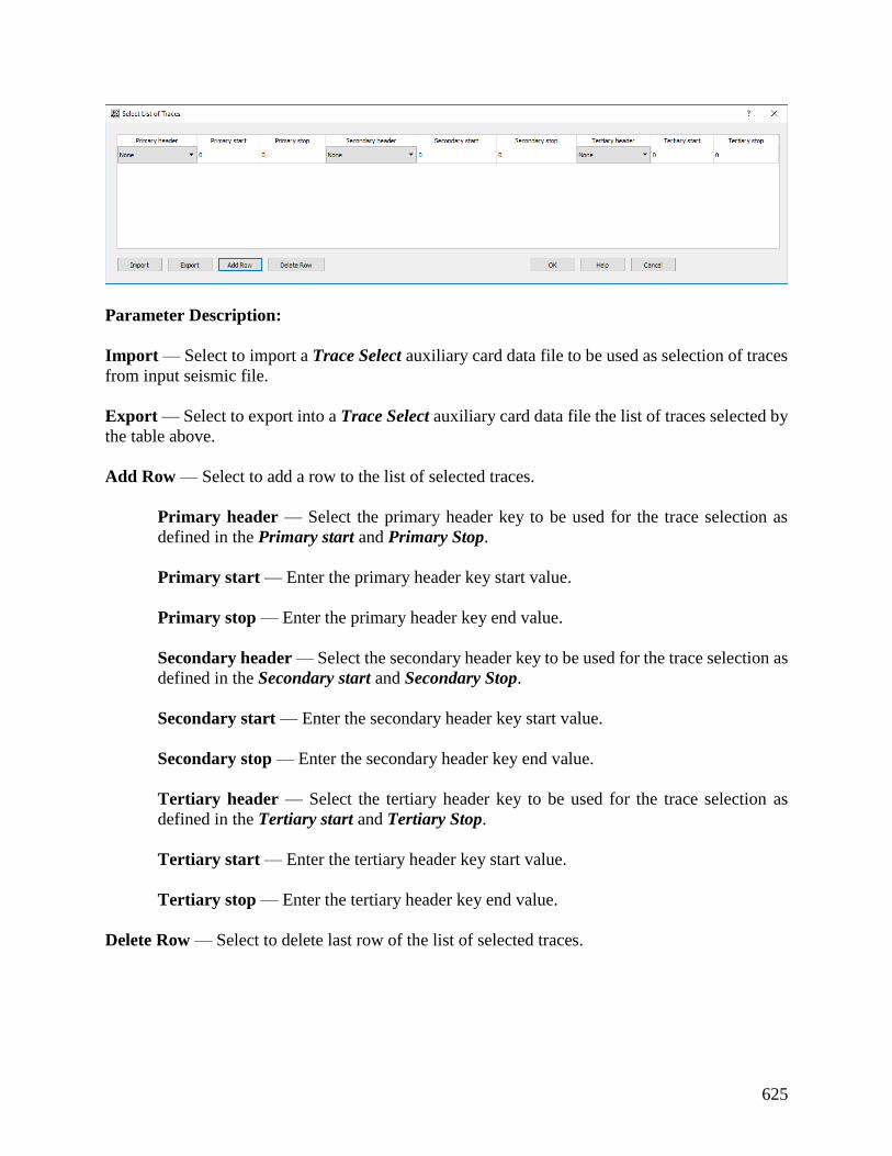
625

Parameter Description:

Import — Select to import a Trace Select auxiliary card data file to be used as selection of traces

from input seismic file.

Export — Select to export into a Trace Select auxiliary card data file the list of traces selected by

the table above.

Add Row — Select to add a row to the list of selected traces.

Primary header — Select the primary header key to be used for the trace selection as

defined in the Primary start and Primary Stop.

Primary start — Enter the primary header key start value.

Primary stop — Enter the primary header key end value.

Secondary header — Select the secondary header key to be used for the trace selection as

defined in the Secondary start and Secondary Stop.

Secondary start — Enter the secondary header key start value.

Secondary stop — Enter the secondary header key end value.

Tertiary header — Select the tertiary header key to be used for the trace selection as

defined in the Tertiary start and Tertiary Stop.

Tertiary start — Enter the tertiary header key start value.

Tertiary stop — Enter the tertiary header key end value.

Delete Row — Select to delete last row of the list of selected traces.

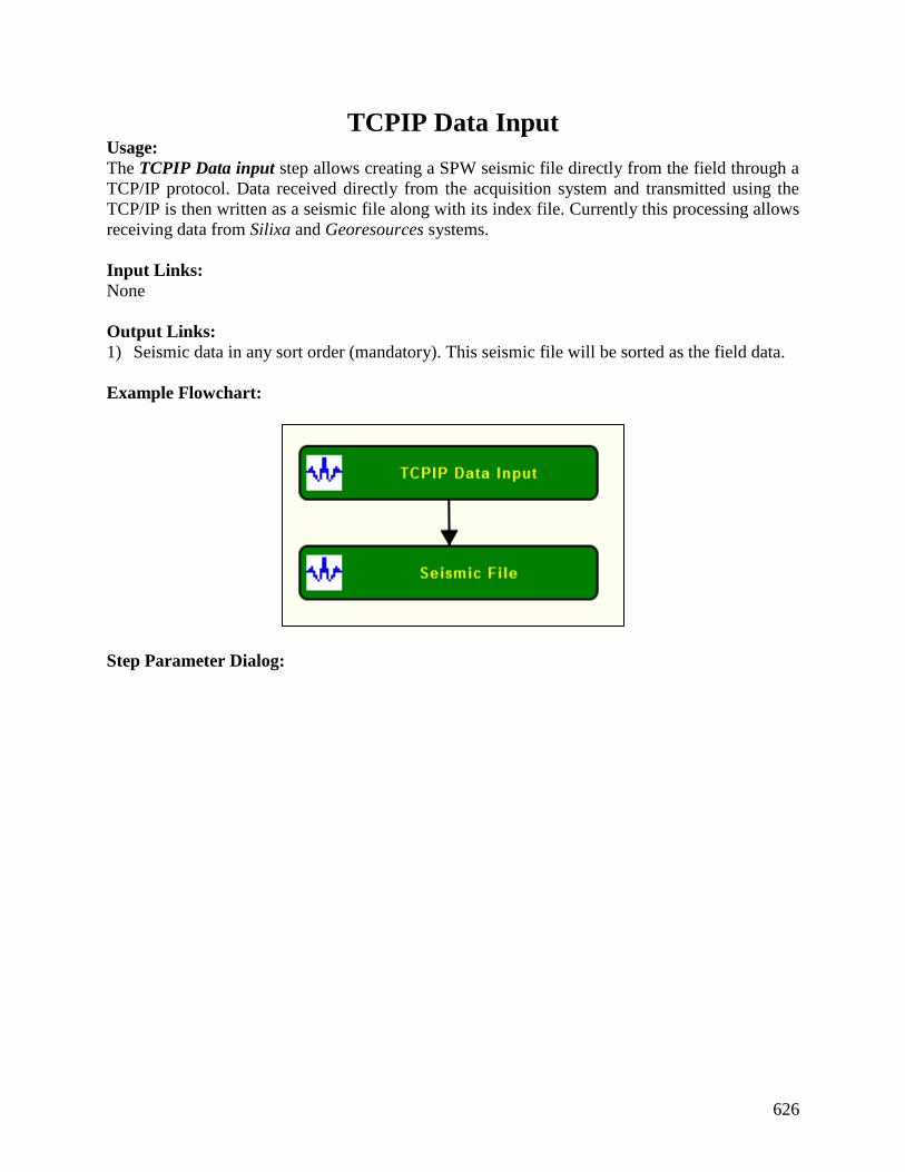
626

TCPIP Data Input Usage:

The TCPIP Data input step allows creating a SPW seismic file directly from the field through a

TCP/IP protocol. Data received directly from the acquisition system and transmitted using the

TCP/IP is then written as a seismic file along with its index file. Currently this processing allows

receiving data from Silixa and Georesources systems.

Input Links:

None

Output Links:

1) Seismic data in any sort order (mandatory). This seismic file will be sorted as the field data.

Example Flowchart:

Step Parameter Dialog:

627

628

Parameter Description:

TCP/IP address — Enter TCP/IP address where the acquired data will be transmitted.

Input from Georesources system — If selected, input data is from a Georesource system.

Georesources parameters: Specify input parameters regarding input data.

Overwrite dataset parameters — If checked, overwrite data acquisition parameters.

Sample format — Enter sample format of the input data.

Number of Samples — Enter number of samples of input data.

Keep recording when skipped shots — If checked, output seismic file will have

skipped shots.

Sample interval (ms) — Enter sample interval in milliseconds.

Number of Channels — Enter number of channels of input data.

Number of Aux. Channels — Enter number of auxiliary channels.

Continuous recording — If checked, the TCP/IP stop signal will be ignored and

the record will continue.

Incremental index start at — Enter the start value for the incremental index of

each record.

Dimiss Aux Channels — If checked, auxiliary traces are not store in output seismic

file.

629

Connection timeout (ms) — Enter a time value in milliseconds for the connection to be

considered timedout.

Data read delay (ms) — Enter a delay value in milliseconds for the data to be read.

Number of shots to skip — Enter the number of shots to skip during the recording.

Upper limit — Enter the

Lower limit —

Average water layer velocity — Enter a value im meters per second of the average water

velocity. This value will be used to automatically pick the first arrivals.

First arrivals window size — Enter the window size in milliseconds for the first arrival

picking.

Output ASCII log — If checked, as ASCII log with the acquisition report will be

generated.

Input from Silixa system — If selected, input data is from a Silixa system.

Silixa parameters: Specify Silixa real time acquisition parameters.

Apply surface geometry — If checked, applies in real time the surface geometry to the

data.

Geometry parameters… — Select to define the parameters related with the

acquisition geometry.

630

Apply VSP geometry — If checked, apply VSP geometry to the data acquired in real time.

Output SEGY files containing geometry — If selected, outputs SEG-Y files with

geometry applied.

Output directory… — Select to browse for the output directory of SEG-Y with

geometry

Perform vibroseis correlation — If checked, performs real-time vibroseis correlation of

the acquired data.

Vib parameters… — Select vibroseis related parameters.

Output correlated SEGY files — If checked, outputs vibroseis correlated SEG-Y files.

Output directory… — Select to browse for the output directory of vibroseis

correlated SEG-Y files

Sum common shot records — If checked, sum common shot records in real-time.

Summing paramters… — Select to define the parameters related with the real-

time summing.

Update SEGY Textheader

Usage:

The Update SEGY Textheader step adds a EBCIDIC text header into a SEG-Y seismic file. The

text header needs to be stored in an auxiliary text file.

Input Links:

1) Seismic data file in any sort order (mandatory).

631

Output Links:

1) Seismic data in any sort order (mandatory).

Example Flowchart:

Step Parameter Dialog:

Parameter Description:

File Browse… — Browse for the location of the text file with the EBCDIC header to be included

in the seismic file.

Virtual Tape Input

Usage:

The Virtual Tape Input step allows importing seismic data from tapes into a seismic file. In order

to access this step a tape drive must be connected using a SCSI connection.

Input Links:

None.

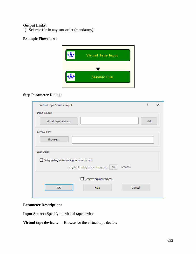
632

Output Links:

1) Seismic file in any sort order (mandatory).

Example Flowchart:

Step Parameter Dialog:

Parameter Description:

Input Source: Specify the virtual tape device.

Virtual tape device… — Browse for the virtual tape device.

633

Crtl — Select to test control parameters of the virtual tape.

Archive Files: Specify archive location.

Browse… — Browse for archive location.

Wait Delay: Specify delay during reading.

Delay polling while waiting for new record — If checked, delays polling while waiting for a

new record.

Length of polling delay during wait … seconds — Enter the length fo the polling delay in

seconds.

Remove auxiliary traces — If checked, removes auxiliary traces from the input seismic data.

634

Spectral Attributes Steps

This section documents the processing steps available in the Spectral Attributes Steps category.

The types of Spectral Attributes Steps currently available are:

Bandwidth Usage:

635

The Bandwidth step estimates the bandwith of spectrally decomposed seismic data computed for

example with Wigner-Ville Decomposition step using a user-defined time and frequency window.

Input Links:

1) Spectrally decomposed seismic data (mandatory).

Output Links:

2) Spectrally decomposed seismic data (mandatory).

Example Flowchart:

Step Parameter Dialog:

Parameter Description:

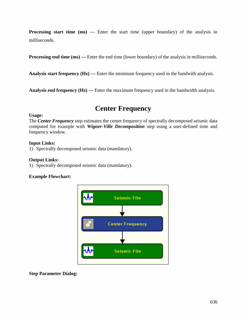
636

Processing start time (ms) — Enter the start time (upper boundary) of the analysis in

milliseconds.

Processing end time (ms) — Enter the end time (lower boundary) of the analysis in milliseconds.

Analysis start frequency (Hz) — Enter the minimum frequency used in the bandwith analysis.

Analysis end frequency (Hz) — Enter the maximum frequency used in the bandwidth analysis.

Center Frequency Usage:

The Center Frequency step estimates the center frequency of spectrally decomposed seismic data

computed for example with Wigner-Ville Decomposition step using a user-defined time and

frequency window.

Input Links:

1) Spectrally decomposed seismic data (mandatory).

Output Links:

1) Spectrally decomposed seismic data (mandatory).

Example Flowchart:

Step Parameter Dialog:

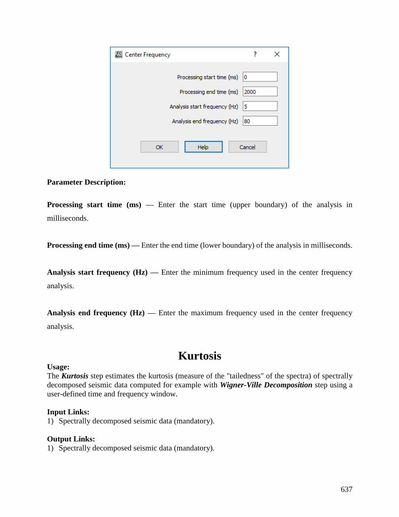
637

Parameter Description:

Processing start time (ms) — Enter the start time (upper boundary) of the analysis in

milliseconds.

Processing end time (ms) — Enter the end time (lower boundary) of the analysis in milliseconds.

Analysis start frequency (Hz) — Enter the minimum frequency used in the center frequency

analysis.

Analysis end frequency (Hz) — Enter the maximum frequency used in the center frequency

analysis.

Kurtosis Usage:

The Kurtosis step estimates the kurtosis (measure of the "tailedness" of the spectra) of spectrally

decomposed seismic data computed for example with Wigner-Ville Decomposition step using a

user-defined time and frequency window.

Input Links:

1) Spectrally decomposed seismic data (mandatory).

Output Links:

1) Spectrally decomposed seismic data (mandatory).

638

Example Flowchart:

Step Parameter Dialog:

Parameter Description:

Processing start time (ms) — Enter the start time (upper boundary) of the analysis in

milliseconds.

Processing end time (ms) — Enter the end time (lower boundary) of the analysis in milliseconds.

Analysis start frequency (Hz) — Enter the minimum frequency used in the kurtosis analysis.

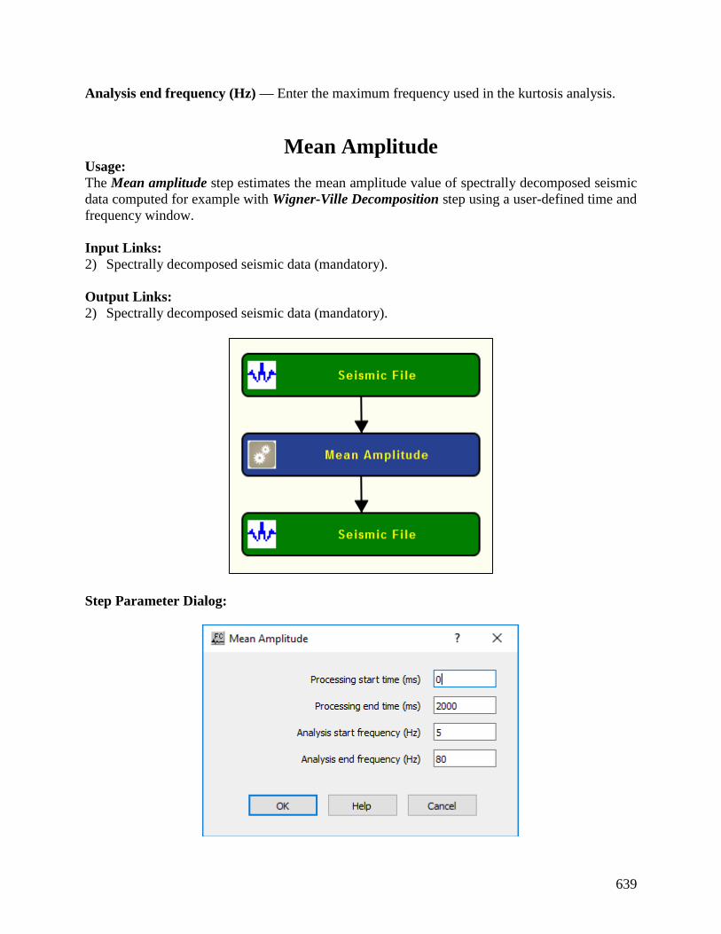
639

Analysis end frequency (Hz) — Enter the maximum frequency used in the kurtosis analysis.

Mean Amplitude Usage:

The Mean amplitude step estimates the mean amplitude value of spectrally decomposed seismic

data computed for example with Wigner-Ville Decomposition step using a user-defined time and

frequency window.

Input Links:

2) Spectrally decomposed seismic data (mandatory).

Output Links:

2) Spectrally decomposed seismic data (mandatory).

Step Parameter Dialog:

640

Parameter Description:

Processing start time (ms) — Enter the start time (upper boundary) of the analysis in

milliseconds.

Processing end time (ms) — Enter the end time (lower boundary) of the analysis in milliseconds.

Analysis start frequency (Hz) — Enter the minimum frequency used in the mean amplitude

analysis.

Analysis end frequency (Hz) — Enter the maximum frequency used in the mean amplitude

analysis.

Minimum Amplitude Usage:

The Minimum amplitude step estimates the minimum amplitude value of spectrally decomposed

seismic data computed for example with Wigner-Ville Decomposition step using a user-defined

time and frequency window.

Input Links:

1) Spectrally decomposed seismic data (mandatory).

Output Links:

1) Spectrally decomposed seismic data (mandatory).

641

Step Parameter Dialog:

Parameter Description:

Processing start time (ms) — Enter the start time (upper boundary) of the analysis in

milliseconds.

Processing end time (ms) — Enter the end time (lower boundary) of the analysis in milliseconds.

Analysis start frequency (Hz) — Enter the minimum frequency used in the minimum amplitude

analysis.

Analysis end frequency (Hz) — Enter the maximum frequency used in the minimum amplitude

analysis.

Peak Amplitude Usage:

The Peak amplitude step estimates the peak (maximum) amplitude value of spectrally

decomposed seismic data computed for example with Wigner-Ville Decomposition step using a

user-defined time and frequency window.

Input Links:

1) Spectrally decomposed seismic data (mandatory).

Output Links:

642

1) Spectrally decomposed seismic data (mandatory).

Step Parameter Dialog:

Parameter Description:

Processing start time (ms) — Enter the start time (upper boundary) of the analysis in

milliseconds.

Processing end time (ms) — Enter the end time (lower boundary) of the analysis in milliseconds.

Analysis start frequency (Hz) — Enter the minimum frequency used in the maximum amplitude

analysis.

643

Analysis end frequency (Hz) — Enter the maximum frequency used in the maximum amplitude

analysis.

Peak Amplitude Above Mean Usage:

The Peak Amplitude amplitude step estimates the maximum amplitude above the mean of

spectrally decomposed seismic data computed for example with Wigner-Ville Decomposition step

using a user-defined time and frequency window.

Input Links:

1) Spectrally decomposed seismic data (mandatory).

Output Links:

1) Spectrally decomposed seismic data (mandatory).

Example Flowchart:

Step Parameter Dialog:

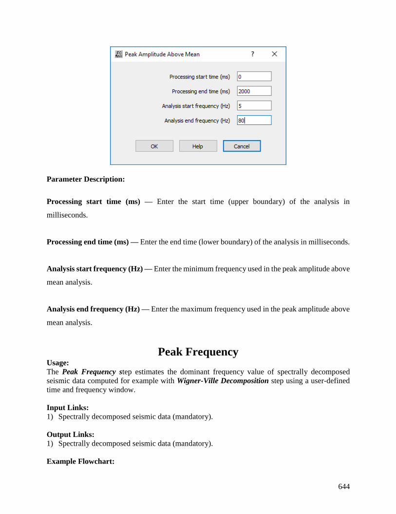
644

Parameter Description:

Processing start time (ms) — Enter the start time (upper boundary) of the analysis in

milliseconds.

Processing end time (ms) — Enter the end time (lower boundary) of the analysis in milliseconds.

Analysis start frequency (Hz) — Enter the minimum frequency used in the peak amplitude above

mean analysis.

Analysis end frequency (Hz) — Enter the maximum frequency used in the peak amplitude above

mean analysis.

Peak Frequency Usage:

The Peak Frequency step estimates the dominant frequency value of spectrally decomposed

seismic data computed for example with Wigner-Ville Decomposition step using a user-defined

time and frequency window.

Input Links:

1) Spectrally decomposed seismic data (mandatory).

Output Links:

1) Spectrally decomposed seismic data (mandatory).

Example Flowchart:

645

Step Parameter Dialog:

Parameter Description:

Processing start time (ms) — Enter the start time (upper boundary) of the analysis in

milliseconds.

Processing end time (ms) — Enter the end time (lower boundary) of the analysis in milliseconds.

Analysis start frequency (Hz) — Enter the minimum frequency used in the peak frequency

amplitude analysis.

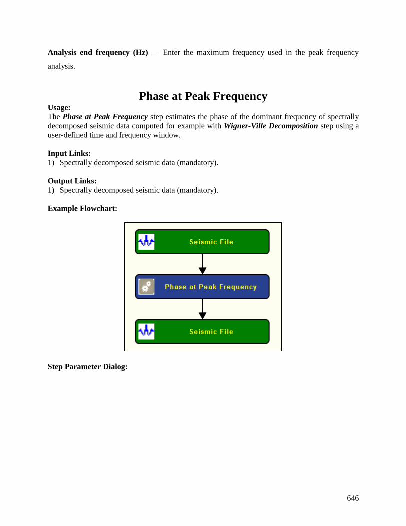
646

Analysis end frequency (Hz) — Enter the maximum frequency used in the peak frequency

analysis.

Phase at Peak Frequency Usage:

The Phase at Peak Frequency step estimates the phase of the dominant frequency of spectrally

decomposed seismic data computed for example with Wigner-Ville Decomposition step using a

user-defined time and frequency window.

Input Links:

1) Spectrally decomposed seismic data (mandatory).

Output Links:

1) Spectrally decomposed seismic data (mandatory).

Example Flowchart:

Step Parameter Dialog:

647

Parameter Description:

Processing start time (ms) — Enter the start time (upper boundary) of the analysis in

milliseconds.

Processing end time (ms) — Enter the end time (lower boundary) of the analysis in milliseconds.

Analysis start frequency (Hz) — Enter the minimum frequency used in the phase at peak

frequency analysis.

Analysis end frequency (Hz) — Enter the maximum frequency used in the phase at peak

frequency analysis.

RMS Frequency Usage:

The RMS Frequency step estimates the root mean square of spectrally decomposed seismic data

computed for example with Wigner-Ville Decomposition step using a user-defined time and

frequency window.

Input Links:

1) Spectrally decomposed seismic data (mandatory).

Output Links:

1) Spectrally decomposed seismic data (mandatory).

Example Flowchart:

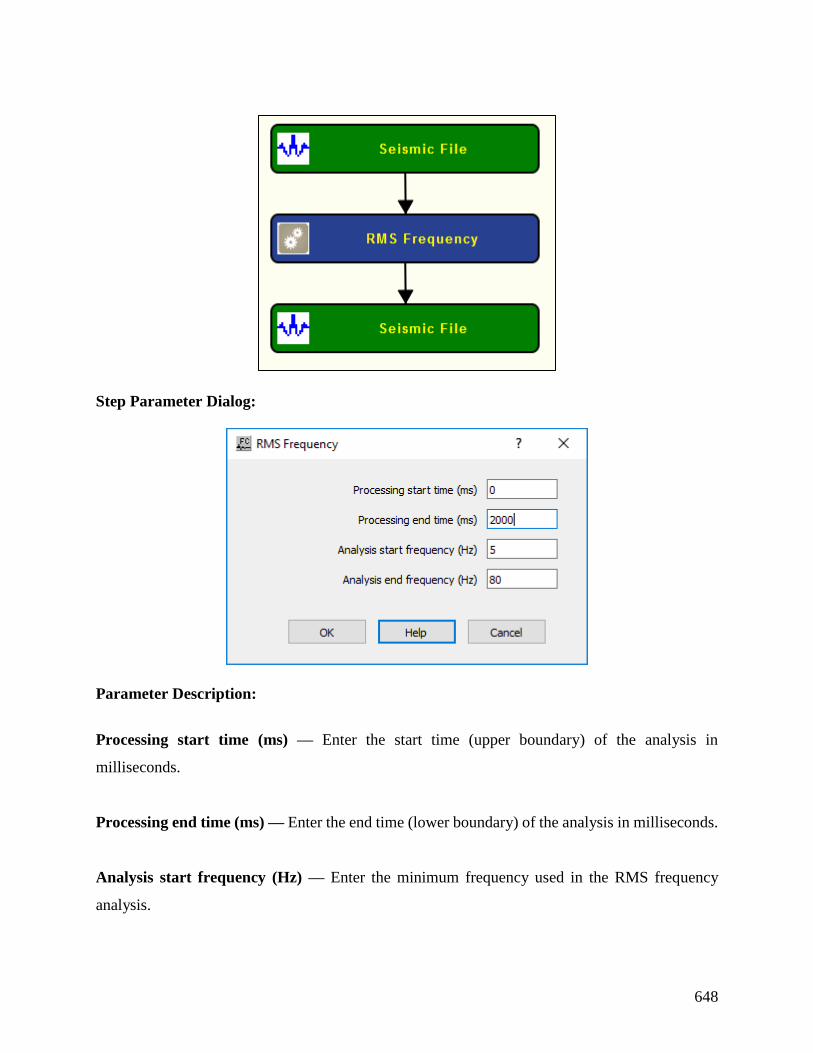
648

Step Parameter Dialog:

Parameter Description:

Processing start time (ms) — Enter the start time (upper boundary) of the analysis in

milliseconds.

Processing end time (ms) — Enter the end time (lower boundary) of the analysis in milliseconds.

Analysis start frequency (Hz) — Enter the minimum frequency used in the RMS frequency

analysis.

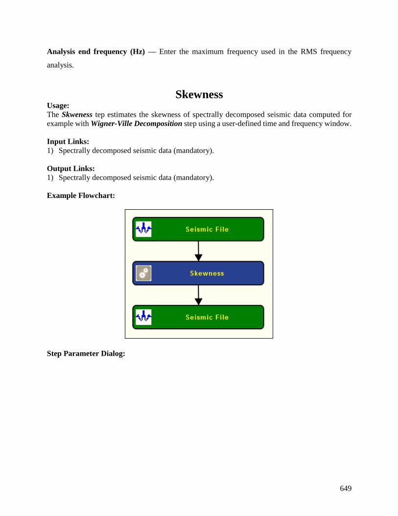
649

Analysis end frequency (Hz) — Enter the maximum frequency used in the RMS frequency

analysis.

Skewness Usage:

The Skweness tep estimates the skewness of spectrally decomposed seismic data computed for

example with Wigner-Ville Decomposition step using a user-defined time and frequency window.

Input Links:

1) Spectrally decomposed seismic data (mandatory).

Output Links:

1) Spectrally decomposed seismic data (mandatory).

Example Flowchart:

Step Parameter Dialog:

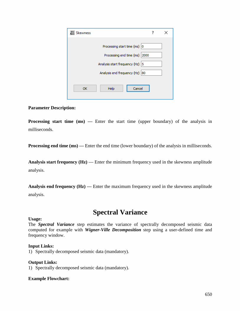
650

Parameter Description:

Processing start time (ms) — Enter the start time (upper boundary) of the analysis in

milliseconds.

Processing end time (ms) — Enter the end time (lower boundary) of the analysis in milliseconds.

Analysis start frequency (Hz) — Enter the minimum frequency used in the skewness amplitude

analysis.

Analysis end frequency (Hz) — Enter the maximum frequency used in the skewness amplitude

analysis.

Spectral Variance Usage:

The Spectral Variance step estimates the variance of spectrally decomposed seismic data

computed for example with Wigner-Ville Decomposition step using a user-defined time and

frequency window.

Input Links:

1) Spectrally decomposed seismic data (mandatory).

Output Links:

1) Spectrally decomposed seismic data (mandatory).

Example Flowchart:

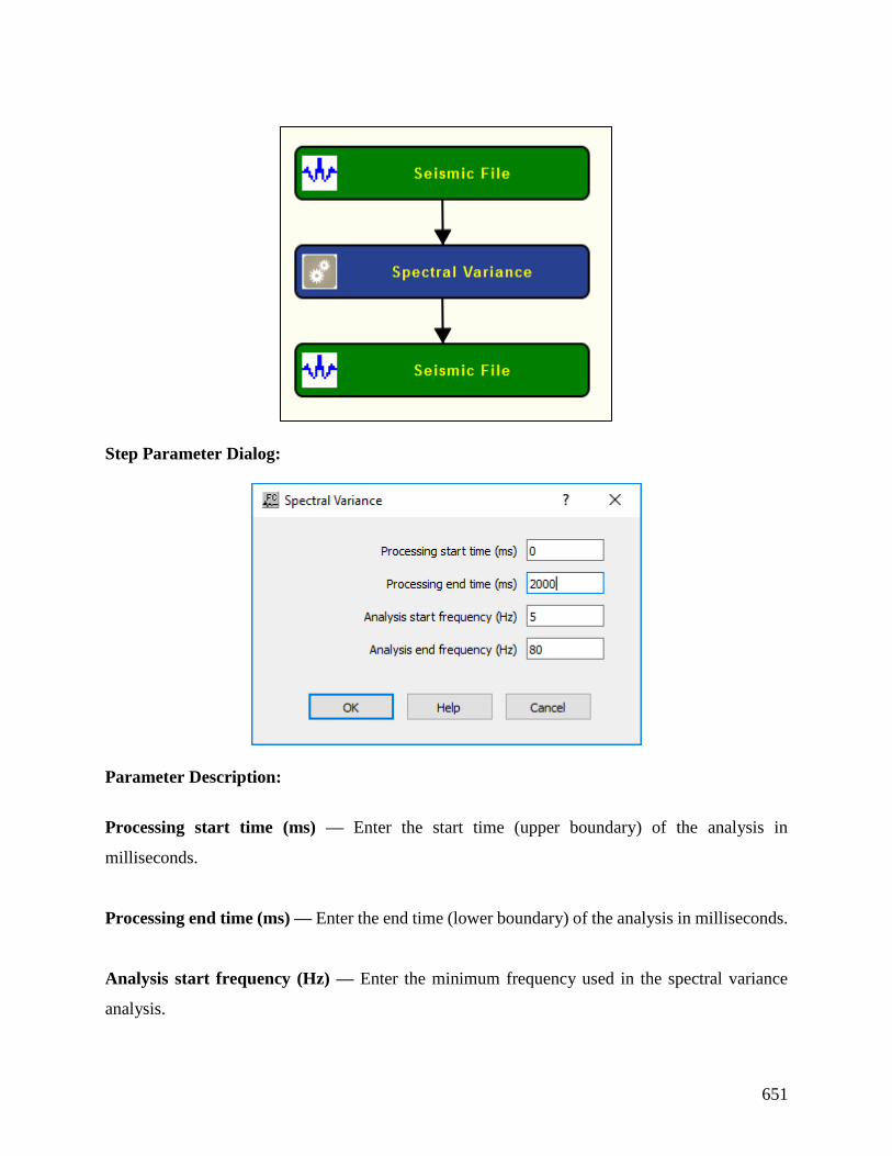
651

Step Parameter Dialog:

Parameter Description:

Processing start time (ms) — Enter the start time (upper boundary) of the analysis in

milliseconds.

Processing end time (ms) — Enter the end time (lower boundary) of the analysis in milliseconds.

Analysis start frequency (Hz) — Enter the minimum frequency used in the spectral variance

analysis.

652

Analysis end frequency (Hz) — Enter the maximum frequency used in the spectral variance

analysis.

653

Spectral Decomposition Steps

This section documents the processing steps available in the Spectral Decomposition Steps

category.

Processing steps currently available are:

654

Band Aid

Usage:

Input Links:

655

Auxiliary dataset:

Output Links:

References:

Example Flowchart:

Step Parameter Dialog:

Parameter Description:

Bandwidth Enhancement Usage:

Input Links:

Auxiliary dataset:

Output Links:

References:

Example Flowchart:

Step Parameter Dialog:

Parameter Description:

Cohen’s Class Usage:

Input Links:

Auxiliary dataset:

Output Links:

References:

Example Flowchart:

Step Parameter Dialog:

Parameter Description:

Short-Time Fourier Transform Usage:

Input Links:

Auxiliary dataset:

Output Links:

References:

Example Flowchart:

Step Parameter Dialog:

Parameter Description:

656

Stockwell Transform Usage:

Input Links:

Auxiliary dataset:

Output Links:

References:

Example Flowchart:

Step Parameter Dialog:

Parameter Description:

Wavelet Recomposition Usage:

Input Links:

Auxiliary dataset:

Output Links:

References:

Example Flowchart:

Step Parameter Dialog:

Parameter Description:

Wavelet Transform Usage:

Input Links:

Auxiliary dataset:

Output Links:

References:

Example Flowchart:

Step Parameter Dialog:

Parameter Description:

Wigner-Ville Decomposition Usage:

Input Links:

Auxiliary dataset:

Output Links:

657

References:

Example Flowchart:

Step Parameter Dialog:

Parameter Description:

Windowed Wigner-Ville Decomposition Usage:

Input Links:

Auxiliary dataset:

Output Links:

References:

Example Flowchart:

Step Parameter Dialog:

Parameter Description:

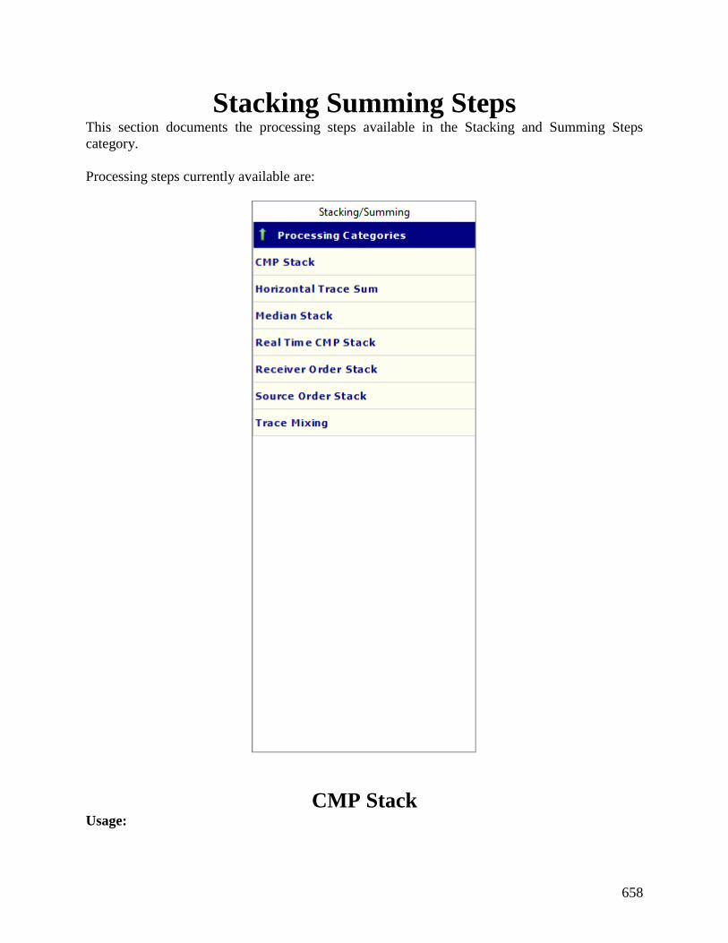
658

Stacking Summing Steps This section documents the processing steps available in the Stacking and Summing Steps

category.

Processing steps currently available are:

CMP Stack Usage:

659

The CMP Stack step generates a CMP stack seismic file from CMP sorted input data. You may

choose among stacking all offsets, the near 1/3 offsets, or the mid 1/3 offsets, the far 1/3 offsets.

You may also choose to stack signed (positive and negative) or unsigned (absolute value of

positive and negative) offsets. For the signed or unsigned offset cases you specify the minimum

and maximum offsets to stack. You may apply a scaling exponent for scaling of your traces. Traces

are scaled by the fold of your data raised to the power of the chosen exponent (i.e. fold ** EXP).

You also specify whether you want to sum relative or absolute amplitude traces.

Input Links:

1) Seismic data in any CMP order (mandatory).

Output Links:

1) Seismic data as a stack (mandatory).

Example Flowchart:

Step Parameter Dialog:

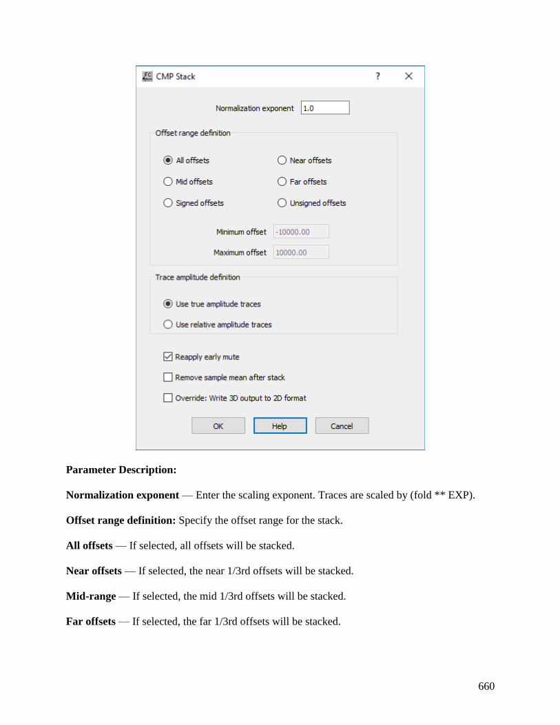
660

Parameter Description:

Normalization exponent — Enter the scaling exponent. Traces are scaled by (fold ** EXP).

Offset range definition: Specify the offset range for the stack.

All offsets — If selected, all offsets will be stacked.

Near offsets — If selected, the near 1/3rd offsets will be stacked.

Mid-range — If selected, the mid 1/3rd offsets will be stacked.

Far offsets — If selected, the far 1/3rd offsets will be stacked.

661

Signed offset — If selected, offsets in the signed (both positive and negative offsets) range will

be stacked. Specify the minimum and maximum offsets to be used.

Unsigned offset — If selected, offsets in the unsigned (absolute value of positive and negative

offsets) range will be stacked. Specify the minimum and maximum offsets to be used.

Minimum — Enter the minimum offset range to stack.

Maximum — Enter the maximum offset range to stack.

Trace amplitude definition: Specify type of amplitudes to be used for the stack.

Use true amplitude traces — If selected, the absolute amplitude will be summed in the stacking

process. True amplitude traces are scaled by one common factor per record.

Use relative amplitude traces — If selected, relative amplitude will be summed in the stacking

process. Relative amplitude traces are scaled independently of one another.

Reapply early mute — If checked, reapplies an early mute after stacking the data

Remove sample mean after stack — If checked, removes the average DC bias from each stacked

trace.

Override: Write 3D output to 2D format — If checked, writes the output as a 2D seismic file.

Horizontal Trace Sum Usage:

The Horizontal Trace Sum step is used to perform a horizontal sum of multiple input traces into

a single output trace on the basis of either the sequential or the offset order of the input traces.

Input Links:

1) Seismic data in any sort order (mandatory).

Output Links:

1) Seismic data in any sort order (mandatory).

Example Flowchart:

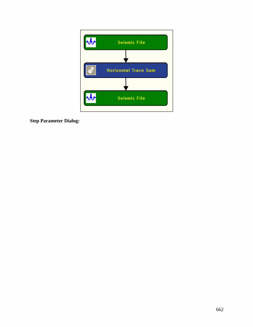
662

Step Parameter Dialog:

663

Parameter Description:

Trace Sum Operation: Specify whether to sum traces sequentially or by common offset bin.

Sum n traces into one — If selected, sum n consecutive seismic traces into a single output trace.

Number of traces to sum — Enter the number of sequential input traces to sum into a

single output trace.

Sum common offset traces — If selected, sum seismic traces within a specified offset bin size.

664

Offset bin size — Enter the offset bin size over which input traces will be summed into a

single output trace. All input trace offsets falling between (n) * offset bin size and (n+1) *

offset bin size will be summed into a single output trace.

Sum common header word — If selected, sum traces with a common header work as defined in

Header word

Header word — Selected the header word location to be used to sum traces.

Sum common receiver locations — If selected, sum traces with common receiver locations into

a single output trace.

Sum common source locations — If selected, sum traces with common source locations into a

single output trace.

Summing: Specify how selected traces are summed.

Average traces — If selected, average horizontally all traces selected with equal weights for all

traces.

Weighted diversity sum — If selected, each trace is scaled by the inverse of its average power

prior to stacking.The composite trace is then renormalized by dividing by the sum of the scalers

used.

Diversity edit — If selected, only a percentage of traces as defined in the Percentage of traces is

summed.

Percentage of traces — Enter the percentage of traces from the selected range to be

summed.

Median Stack Usage:

The Median Stack step performs a sample by sample horizontal stack using a specified percent of

the samples centered on the median sample.

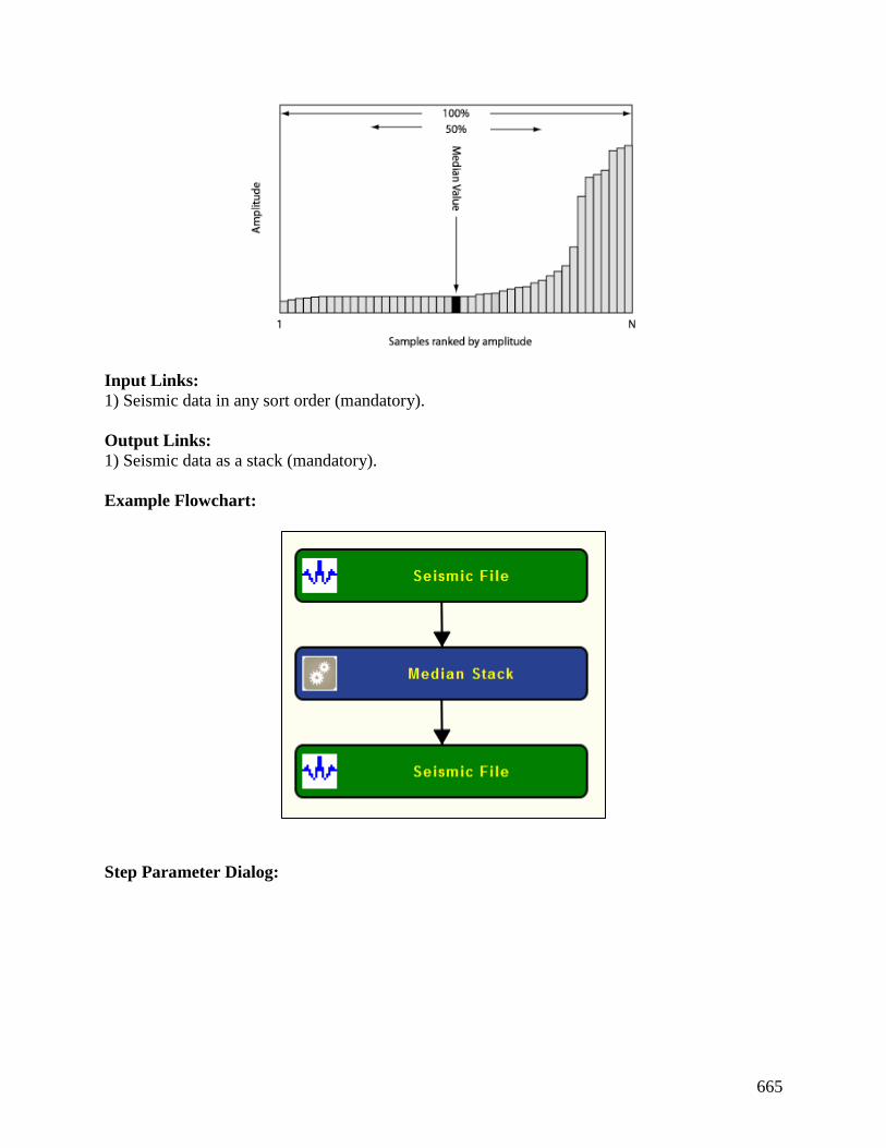
665

Input Links:

1) Seismic data in any sort order (mandatory).

Output Links:

1) Seismic data as a stack (mandatory).

Example Flowchart:

Step Parameter Dialog:

666

Parameter Description:

Percent of traces to stack — Enter the percentage of traces to sum into each resulting output

trace. A number such as 50 indicates that 50 % of the samples centered on the median sample

value will contribute to the summed output sample.

Normalization exponent — Enter the scaling exponent. Traces are scaled by (fold ** EXP).

Offset range definition: Specify the offset range for the stack.

All offsets — If selected, all offsets will be stacked.

Near offsets — If selected, the near 1/3rd offsets will be stacked.

Mid-range — If selected, the mid 1/3rd offsets will be stacked.

667

Far offsets — If selected, the far 1/3rd offsets will be stacked.

Signed offset — If selected, offsets in the signed (both positive and negative offsets) range will

be stacked. Specify the minimum and maximum offsets to be used.

Unsigned offset — If selected, offsets in the unsigned (absolute value of positive and negative

offsets) range will be stacked. Specify the minimum and maximum offsets to be used.

Minimum — Enter the minimum offset range to stack.

Maximum — Enter the maximum offset range to stack.

Trace amplitude definition: Specify type of amplitudes to be used for the stack.

Use true amplitude traces — If selected, the absolute amplitude will be summed in the stacking

process. True amplitude traces are scaled by one common factor per record.

Use relative amplitude traces — If selected, relative amplitude will be summed in the stacking

process. Relative amplitude traces are scaled independently of one another.

Reapply early mute — If checked, reapplies an early mute after stacking the data

Remove sample mean after stack — If checked, removes the average DC bias from each stacked

trace.

Browse — Select this button to set the output seismic file name.

Real Time CMP Stack Usage:

The Real Time CMP Stack step generates a CMP fullstack seismic file from CMP sorted input

data with a real time input. This step allows to display the resulting stack in real time using a Real

Time Stack Display. The output stack is stored in an output seismic file.

Input Links:

1) Seismic data in any CMP order (mandatory).

Output Links:

Example Flowchart:

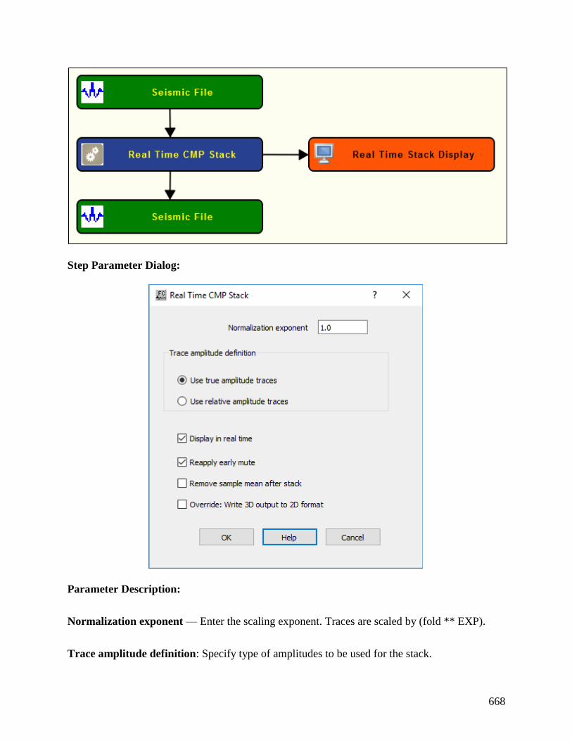
668

Step Parameter Dialog:

Parameter Description:

Normalization exponent — Enter the scaling exponent. Traces are scaled by (fold ** EXP).

Trace amplitude definition: Specify type of amplitudes to be used for the stack.

669

Use true amplitude traces — If selected, the absolute amplitude will be summed in the stacking

process. True amplitude traces are scaled by one common factor per record.

Use relative amplitude traces — If selected, relative amplitude will be summed in the stacking

process. Relative amplitude traces are scaled independently of one another.

Display in real time — If checked, the input data is stacked in real time and a real time display is

generated as defined in Real Time Stack Display step.

Reapply early mute — If checked, reapplies an early mute after stacking the data

Remove sample mean after stack — If checked, removes the average DC bias from each stacked

trace.

Override: Write 3D output to 2D format — If checked, writes the output as a 2D seismic file.

Receiver Order Stack Usage:

The Receiver Order Stack step allows you to input data sorted in common receiver order and

output a common receiver stack seismic file. You may apply a scaling exponent for scaling of your

traces. Traces are scaled by the fold of your data raised to the power of the chosen exponent (i.e.

fold ** EXP). You also specify whether you want to sum relative or absolute amplitude traces.

Input Links:

1) Seismic data in common receiver sort order (mandatory).

Output Links:

1) Seismic data as a stack (mandatory).

Example Flowchart:

670

Step Parameter Dialog:

Parameter Description:

Normalization exponent — Enter the scaling exponent. Traces are scaled by (fold ** EXP).

Offset range definition: Specify the offset range for the stack.

All offsets — If selected, all offsets will be stacked.

Near offsets — If selected, the near 1/3rd offsets will be stacked.

Mid-range — If selected, the mid 1/3rd offsets will be stacked.

671

Far offsets — If selected, the far 1/3rd offsets will be stacked.

Signed offset — If selected, offsets in the signed (both positive and negative offsets) range will

be stacked. Specify the minimum and maximum offsets to be used.

Unsigned offset — If selected, offsets in the unsigned (absolute value of positive and negative

offsets) range will be stacked. Specify the minimum and maximum offsets to be used.

Minimum — Enter the minimum offset range to stack.

Maximum — Enter the maximum offset range to stack.

Trace amplitude definition: Specify type of amplitudes to be used for the stack.

Use true amplitude traces — If selected, the absolute amplitude will be summed in the stacking

process. True amplitude traces are scaled by one common factor per record.

Use relative amplitude traces — If selected, relative amplitude will be summed in the stacking

process. Relative amplitude traces are scaled independently of one another.

Reapply early mute — If checked, reapplies an early mute after stacking the data

Remove sample mean after stack — If checked, removes the average DC bias from each stacked

trace.

Override: Write 3D output to 2D format — If checked, writes the output as a 2D seismic file.

Source Order Stack Usage:

The Source Order Stack step allows you to input data sorted in common source order and output

a common source stack seismic file. You may apply a scaling exponent for scaling of your traces.

Traces are scaled by the fold of your data raised to the power of the chosen exponent (i.e. fold **

EXP). You also specify whether you want to sum relative or absolute amplitude traces.

Input Links:

1) Seismic data in common source sort order (mandatory).

Output Links:

1) Seismic data as a stack (mandatory).

Example Flowchart:

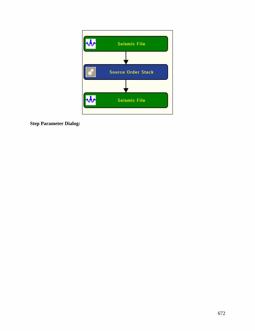
672

Step Parameter Dialog:

673

Parameter Description:

Normalization exponent — Enter the scaling exponent. Traces are scaled by (fold ** EXP).

Offset range definition: Specify the offset range for the stack.

All offsets — If selected, all offsets will be stacked.

Near offsets — If selected, the near 1/3rd offsets will be stacked.

Mid-range — If selected, the mid 1/3rd offsets will be stacked.

Far offsets — If selected, the far 1/3rd offsets will be stacked.

674

Signed offset — If selected, offsets in the signed (both positive and negative offsets) range will

be stacked. Specify the minimum and maximum offsets to be used.

Unsigned offset — If selected, offsets in the unsigned (absolute value of positive and negative

offsets) range will be stacked. Specify the minimum and maximum offsets to be used.

Minimum — Enter the minimum offset range to stack.

Maximum — Enter the maximum offset range to stack.

Trace amplitude definition: Specify type of amplitudes to be used for the stack.

Use true amplitude traces — If selected, the absolute amplitude will be summed in the stacking

process. True amplitude traces are scaled by one common factor per record.

Use relative amplitude traces — If selected, relative amplitude will be summed in the stacking

process. Relative amplitude traces are scaled independently of one another.

Reapply early mute — If checked, reapplies an early mute after stacking the data

Remove sample mean after stack — If checked, removes the average DC bias from each stacked

trace.

Override: Write 3D output to 2D format — If checked, writes the output as a 2D seismic file.

Trace Mixing Usage:

The Trace Mixing step is used to perform a weighted horizontal sum of up to fifteen (15)

sequential input traces into a single output trace.

Input Links:

1) Seismic data in any sort order (mandatory).

Output Links:

1) Seismic data in any sort order (mandatory).

Example Flowchart:

675

Step Parameter Dialog:

Parameter Description:

Number of traces to mix — Enter the number of traces to mix (blend) into each output trace.

Weight — The relative value of the weight for each trace in the m

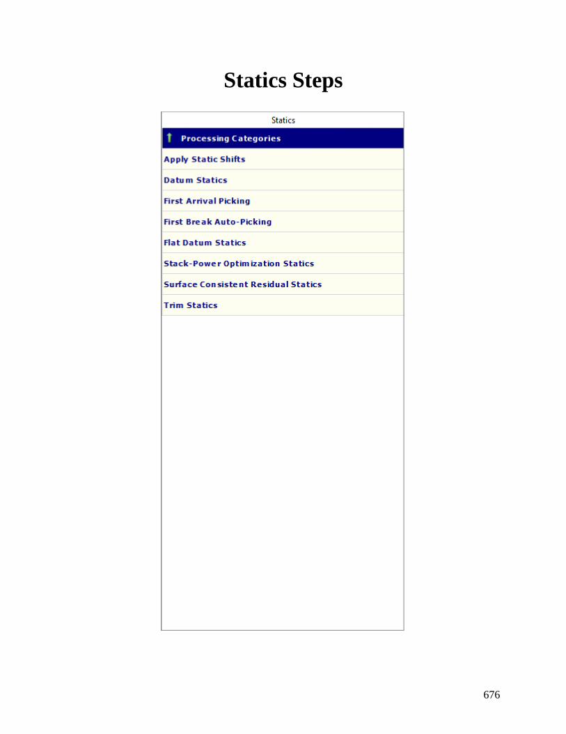
676

Statics Steps

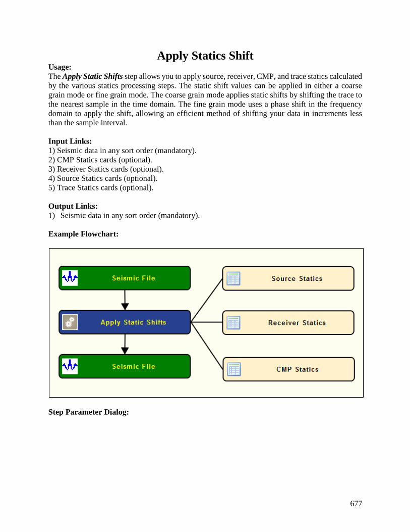
677

Apply Statics Shift Usage:

The Apply Static Shifts step allows you to apply source, receiver, CMP, and trace statics calculated

by the various statics processing steps. The static shift values can be applied in either a coarse

grain mode or fine grain mode. The coarse grain mode applies static shifts by shifting the trace to

the nearest sample in the time domain. The fine grain mode uses a phase shift in the frequency

domain to apply the shift, allowing an efficient method of shifting your data in increments less

than the sample interval.

Input Links:

1) Seismic data in any sort order (mandatory).

2) CMP Statics cards (optional).

3) Receiver Statics cards (optional).

4) Source Statics cards (optional).

5) Trace Statics cards (optional).

Output Links:

1) Seismic data in any sort order (mandatory).

Example Flowchart:

Step Parameter Dialog:

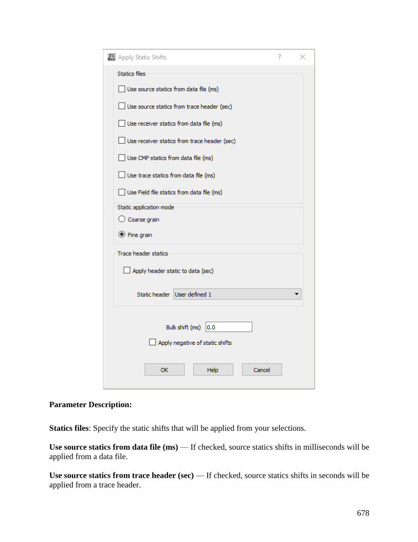
678

Parameter Description:

Statics files: Specify the static shifts that will be applied from your selections.

Use source statics from data file (ms) — If checked, source statics shifts in milliseconds will be

applied from a data file.

Use source statics from trace header (sec) — If checked, source statics shifts in seconds will be

applied from a trace header.

679

Use receiver statics from data file (ms) — If checked, receiver statics shifts in milliseconds will

be applied from a data file.

Use receiver statics from trace header (sec) — If checked, receiver statics shifts in seconds will

be applied from a trace header.

Use CMP statics from data file (ms) — If checked, CMP statics shifts in milliseconds will be

applied from a data file.

Use trace statics from data file (ms) — If checked, trace statics shifts in milliseconds will be

applied from a data file.

Static application mode: Specify the mode of statics application.

Coarse grain — Statics shifts are applied to the nearest discrete sample position.

Fine grain — Statics shifts are applied as a precise phase shift operator in the Fourier domain.

Trace header statics: Specify the header location with statics to be applied to your data.

Apply header static to data — If checked, the value in the user selected trace header field will

be applied to the seismic trace as a static shift.

Static header — Use the drop down menu to select the trace header field that will be applied to

the trace as a static shift.

Bulk shift (ms) — Enter a constant statics shift in milliseconds to apply to all the seismic data

traces.

Apply negative of static shifts — If checked, the negative of the static values will be applied.

Datum Statics Usage:

The Datum Statics step inputs the trace headers from a Seismic Data file and outputs a set of

Source and Receiver static files that adjust the data to a floating datum, and CMP static file that

asdjusts the data from the floating datum to a flat datum. Alternatively, the Source and Receiver

statics can be computed that adjust the surface data directly to a flat datum. In both cases, the

statics are applied using the Apply Statics step.

680

Input Links:

1) Seismic data file in any sort order (mandatory).

Output Links:

1) Source Statics cards (mandatory).

2) Receiver Statics cards (mandatory).

3) CMP Statics cards (optional, in the case of correction to a Floating Datum).

Example Flowchart:

Step Parameter Dialog:

681

Parameter Description:

Reference datum: Specify datum preference.

Final datum — If selected final datum is considered.

Floating datum — If selected, a floating datum is considered.

Datum definition: Specify parameters that define your datum preference.

Final datum elevation — Enter a constant value for the elevation of the flat datum.

Floating datum: Specify the parameters for a floating datum function, if Floating datum is

slected.

Mean datum static — If selected, an average operator for calculating the datum static will be

used to define the datum.

682

Median datum static — If selected, a median smoothing operator for calculating the datum

static will be used to define the datum.

Offset weighted datum static — If selected, a weighted CMP elevation function of the form

weight = multiplier*(offset **exponent ) will be used to define the datum.

Multiplier — Enter the multiplier of the weighting function.

Exponent — Enter the exponent of the weighting function.

Apply spatial smoothing — If checked, apply spatial smoothing to the floating datum.

Radius of smoothing — Enter the radius of smoothing.

Elevation correction: Specify replacement velocities to correct the elevation.

Replacement velocity (Vp) — Enter a constant value to correct the traces to the final datum using

the consolidated p-wave velocity.

Replacement velocity (Vs) — Enter a constant value to correct the traces to the final datum using

the consolidated s-wave velocity.

Upholes: Specify whether to apply the uphole time.

Apply uphole time — If checked, the uphole static will be applied.

Static output: Specify how to output flat datum statics.

Output source statics file — If checked, source statics will be output as calculated from the

surface to the flat datum.

Output receiver statics file — If checked, receiver statics will be output as calculated from the

surface to the flat datum.

Output midpoint statics file — If checked, CMP statics will be output as zero.

First Arrival Picking Usage:

Input Links:

Output Links:

Example Flowchart:

Step Parameter Dialog:

Parameter Description:

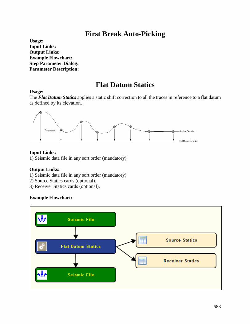
683

First Break Auto-Picking Usage:

Input Links:

Output Links:

Example Flowchart:

Step Parameter Dialog:

Parameter Description:

Flat Datum Statics Usage:

The Flat Datum Statics applies a static shift correction to all the traces in reference to a flat datum

as defined by its elevation.

Input Links:

1) Seismic data file in any sort order (mandatory).

Output Links:

1) Seismic data file in any sort order (mandatory).

2) Source Statics cards (optional).

3) Receiver Statics cards (optional).

Example Flowchart:

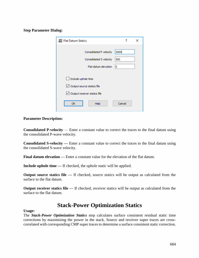
684

Step Parameter Dialog:

Parameter Description:

Consolidated P-velocity — Enter a constant value to correct the traces to the final datum using

the consolidated P-wave velocity.

Consolidated S-velocity — Enter a constant value to correct the traces to the final datum using

the consolidated S-wave velocity.

Final datum elevation — Enter a constant value for the elevation of the flat datum.

Include uphole time — If checked, the uphole static will be applied.

Output source statics file — If checked, source statics will be output as calculated from the

surface to the flat datum.

Output receiver statics file — If checked, receiver statics will be output as calculated from the

surface to the flat datum.

Stack-Power Optimization Statics Usage:

The Stack-Power Optimization Statics step calculates surface consistent residual static time

corrections by maximizing the power in the stack. Source and receiver super traces are cross-

correlated with corresponding CMP super traces to determine a surface consistent static correction.

685

For 3-D, the input seismic file is required to be a CMP binned seismic volume. For 2-D, the input

seismic file can be in any sort order, as long as Geometry Definition has been applied. Binning

geometry for 3-D surveys should include all shot and receiver locations. Set the bin origin at the

minimum source, receiver or CMP location.

Output stacks may be generated to evaluate the quality of the statics. The stacks show the sorted

input file stacked in the analysis window with static corrections applied. The stacks are

accumulated in the frequency domain and back transformed for the final stack trace. Numerical

round off may cause slight variations when compared with stacks from the CMP Stack processing

step. Stack type may be source, receiver or CMP.

Analysis stacks at specified intervals may be created to evaluate optimal convergence. The

analysis stacks are a selected subset of source, receiver or CMP lines output to a specified

directory. A unique filename suffix is assigned automatically for each iteration. Small subsets are

recommended to reduce disk storage requirements. Full volume source, receiver and CMP stacks

with user specified filename may be output for the final iteration.

An option exists to output to the console a summary of the static corrections generated at the end

of each iteration. The source and receiver statics output by the Stack-Power Optimization Statics

Step are applied with the Apply Statics Shift step.

Input Links:

1) Seismic data, 3-D binned or 2-D in any sort order with geometry applied (mandatory).

Output Links:

1) Source statics cards (mandatory).

2) Receiver statics cards (mandatory).

3) Selected stack analysis files (optional).

4) Selected stack volume (optional).

Reference:

Ronen J., and Claerbout, J., 1985, Surface-consistent residual statics estimation by stack-power

maximization, Geophysics, vol. 50, no. 12, p. 2759-2767.

Example Flowchart:

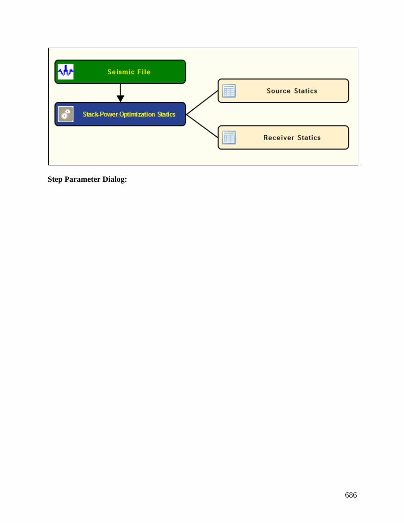
686

Step Parameter Dialog:

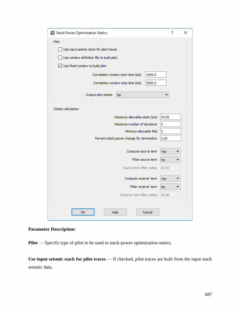
687

Parameter Description:

Pilot — Specify type of pilot to be used in stack-power optimization statics.

Use input seismic stack for pilot traces — If checked, pilot traces are built from the input stack

seismic data.

688

Use window definition file to build pilot — If checked, pilot traces are built from an auxiliary

Window definition card data from the input seismic data.

Use fixed window to build pilot —If checked, pilot traces are built from a constant time gate

from the input seismic data.

Correlation window start time (ms) — Enter the start time in milliseconds for the

correlation window used to build the pilot.

Correlation window stop time (ms) — Enter the end time in milliseconds for the

correlation window used to build the pilot.

Output pilot stacks — Select from the drop-down menu to output the pilot stacks used for the

optimization. Stacks can be from the midpoint, source, receiver or any combination of these.

Statics calculation: Specify the statics calculation parameters.

Maximum allowable static (ms) — Enter a value in milliseconds for the maximum static shifts

for each iteration. The final static is the sum of statics at each iteration. The total static may exceed

the maximum allowable static per iteration.

Maximum number of iterations — Enter the maximum number of iterations for the processing

step.

Minimum allowable fold — Enter the maximum allowable fold for the processing step.

Percent stack power change for termination — Enter the percentage value of the stack power

change to terminate the optimization process.

Compute source term — Select from the drop-down menu to compute the statics for the source

component.

Filter source term — Select from the drop-down menu to filter or not the source term component.

Source term filter radius — If filtering the source term, enter the filter radius.

689

Compute receiver term — Select from the drop-down menu to compute the statics for the

receiver component.

Filter receiver term — Select from the drop-down menu to filter or not the receiver term

component.

Receiver term filter radius — If filtering the receiver term, enter the filter radius.

Surface Consistent Residual Statics

Usage:

The Surface Consistent Residual Statics step calculates source and receiver residual statics using

a Gauss-Seidel iterative method to solve for the source static, receiver static, structure term, and

residual NMO) that provide a best fit to the linear traveltime equations in a least-squares sense.

linear inversion routine to decompose traveltime equations into source, receiver, CMP, and offset

related terms. The pick times input to the inversion are picked automatically using cross correlation

in a specified time window. You control the window of data for analysis as well as the maximum

allowable static that can be computed. A damping filter can be applied to suppress any long period

effects associated with the residual statics solution. Options exist for removing either or both the

residual normal moveout (RNMO) term and a linear trend from the statics solution. The source

and receiver statics output by the Surface Consistent Residual Statics Step are applied with the

Apply Statics step.

Input Links:

1) Seismic data - NMO corrected CMP gathers (mandatory).

Output Links:

1) Source Statics cards (mandatory).

2) Receiver Statics cards (mandatory).

Reference:

Wiggins, R. A., et al., 1976, Residual statics analysis as a general linear inverse problem:

Geophysics, vol. 50, no. 11, p. 2172ff.

See Technical Note TN-ResSt.doc

Example Flowchart:

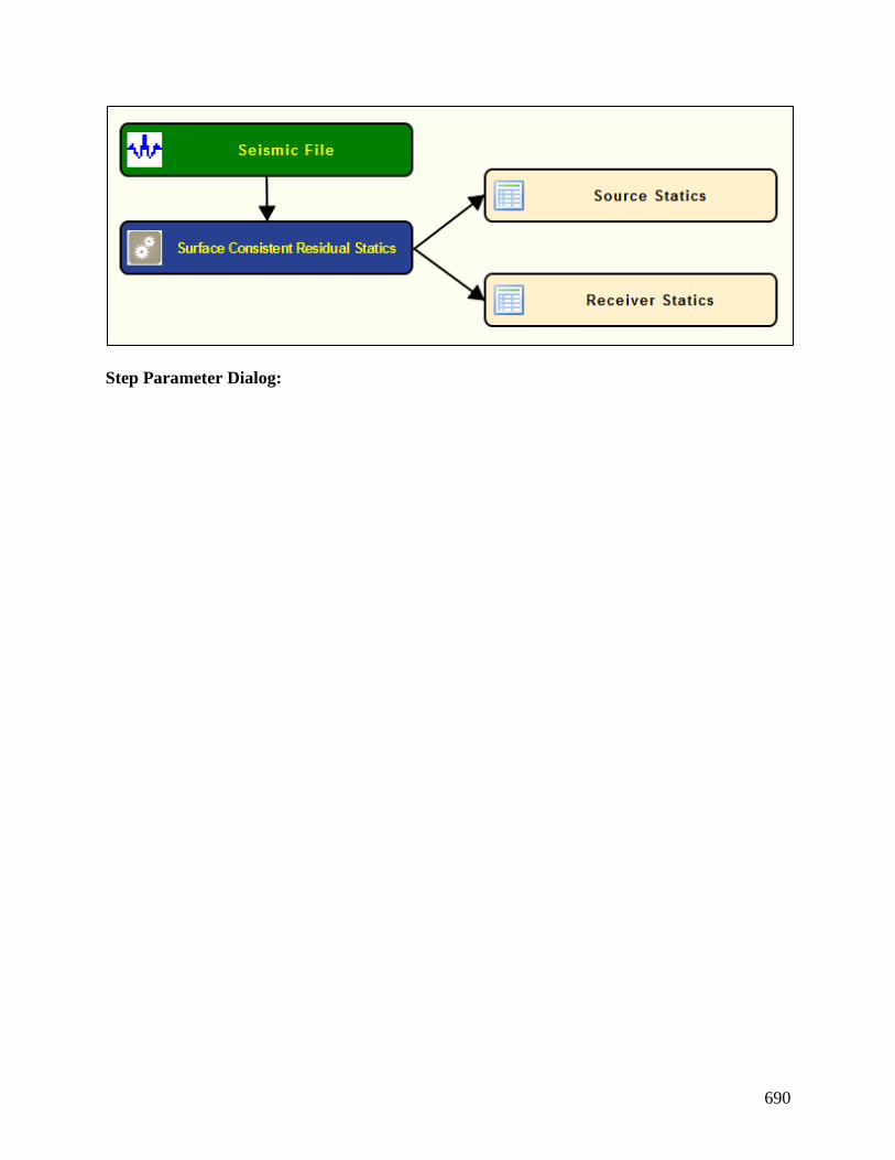
690

Step Parameter Dialog:

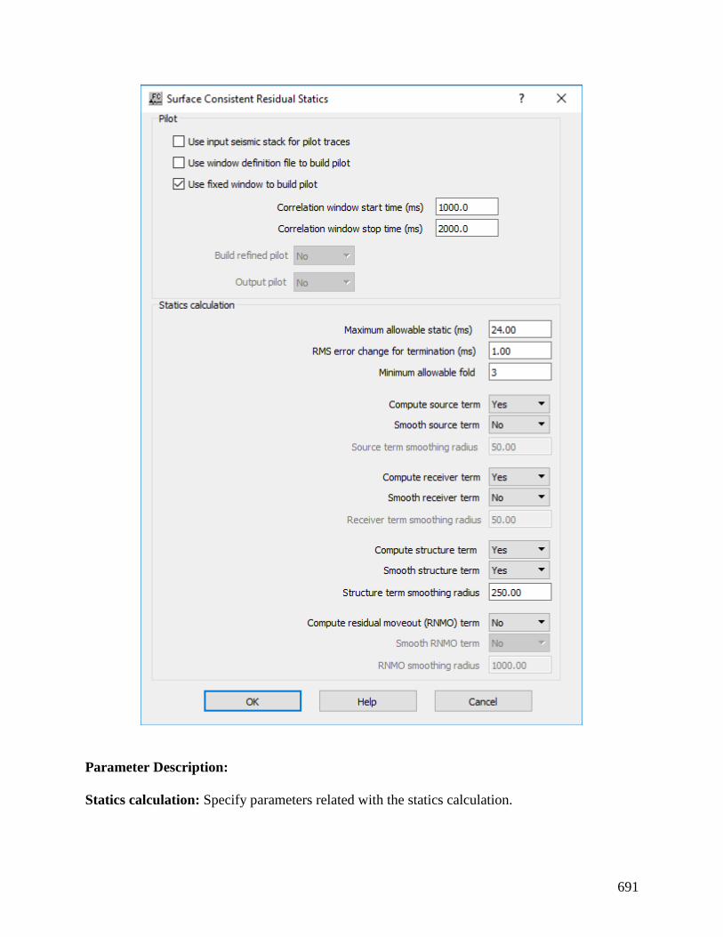
691

Parameter Description:

Statics calculation: Specify parameters related with the statics calculation.

692

Maximum allowable static (ms) — Enter the maximum allowable static shift in milliseconds.

RMS error change for termination (ms) — Error the minium RMS error change from iteration

to iteration for the optimization to be considered finished.

Minimum allowable fold — Enter the minimum fold allowable for the optimization.

Compute source term — Select from the drop-down menu to compute the statics for the source

term.

Smooth source term — Select from the drop-down menu to filter or not the source term.

Smooth source term — If filtering the source term, enter the filter radius.

Compute receiver term — Select from the drop-down menu to compute the statics for the

receiver term.

Smooth receiver term — Select from the drop-down menu to filter or not the receiver term

component.

Receiver term smoothing radius — If filtering the receiver term, enter the filter radius.

Compute structure term — Select from the drop-down menu to compute the statics for the

receiver component.

Smooth structure term — Select from the drop-down menu to filter or not the receiver term

component.

Structure term smoothing radius — If filtering the structure term, enter the filter radius.

Compute residual moveout (RNMO) term — If checked, a least squares linear fit will be

removed from the final statics solution.

Smooth RNMO term — Select from the drop-down menu to filter or not the RNMO term

component.

RNMO smoothing radius — If filtering the RNMO term, enter the filter radius

Trim Statics Usage:

The Trim Statics step calculates small CMP statics shifts for the data based on alignment of events

within the specified window. You specify the start time and the length of the analysis window for

693

calculation and the maximum allowed static shift. The step finds the static shift within these limits

using automatic picking of the peak of the cross-correlation amplitude between the trace and the

stacked trace for the gather.

Input Links:

1) Seismic data in CMP sort order (mandatory).

Output Links:

1) Seismic data in CMP sort order (mandatory).

Example Flowchart:

Step Parameter Dialog:

Parameter Description:

694

Window start time (ms) — Enter the window start time in milliseconds for trim statics analysis.

Window length (ms) — Enter the length of the window in milliseconds for trim statics analysis.

Max static shift +/- (ms) — Enter the largest allowable static shift in milliseconds for trim statics

analysis.

Use auxiliary stack trace as pilot — Not yet implemented.

695

Trace Attributes Steps

696

Instantaneous Amplitude Usage:

The Instantaneous Amplitude step calculates instantaneous amplitude attributes for each trace and

outputs each as a seismic trace in the output seismic file. Instantaneous amplitude is a measure of

the reflectivity strength of events on a seismic section.

Input Links:

1) Seismic data in any sort order (mandatory).

Output Links:

1) Seismic attribute data in any sort order (mandatory).

Reference:

Taner, M.T., Koehler, F., Sheriff, R.E., 1979, Complex Seismic Trace Analysis: Geophysics, v.

44, no. 6, p. 1041-1063.

Example Flowchart:

Step Parameter Dialog:

697

Parameter Description:

Processing start time (ms) — Enter the start time (upper boundary) in milliseconds of the time

gate where the calculation will start.

Processing end time (ms) — Enter the end time (lower boundary) in milliseconds of the time gate

where the calculation will end.

Instantaneous Frequency Usage:

The Instantaneous Frequency step calculates instantaneous frequency attribute for each trace and

outputs each as a seismic trace in the output seismic file. This attribute is a measure of the

frequency of events on a seismic section.

Input Links:

1) Seismic data in any sort order (mandatory).

Output Links:

1) Seismic attribute data in any sort order (mandatory).

Reference:

Taner, M.T., Koehler, F., Sheriff, R.E., 1979, Complex Seismic Trace Analysis: Geophysics, v.

44, no. 6, p. 1041-1063.

Example Flowchart:

698

Step Parameter Dialog:

Parameter Description:

Processing start time (ms) — Enter the start time (upper boundary) in milliseconds of the time

gate where the calculation will start.

Processing end time (ms) — Enter the end time (lower boundary) in milliseconds of the time gate

where the calculation will end.

Number of samples to average — Enter the number of seismic samples to be averaged during

the calculation of the Instataneous Frequency step.

Instantaneous Phase Usage:

699

The Instantaneous Phase step calculates instantaneous phase attribute for each trace and outputs

each as a seismic trace in the output seismic file. This attribute is a measure of the continuity of

events on a seismic section.

Input Links:

1) Seismic data in any sort order (mandatory).

Output Links:

1) Seismic attribute data in any sort order (mandatory).

Reference:

Taner, M.T., Koehler, F., Sheriff, R.E., 1979, Complex Seismic Trace Analysis: Geophysics, v.

44, no. 6, p. 1041-1063.

Example Flowchart:

Step Parameter Dialog:

700

Parameter Description:

Processing start time (ms) — Enter the start time (upper boundary) in milliseconds of the time

gate where the calculation will start.

Processing end time (ms) — Enter the end time (lower boundary) in milliseconds of the time gate

where the calculation will end.

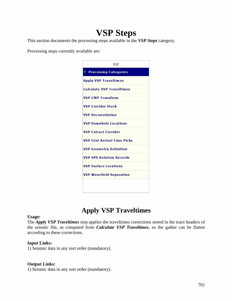
701

VSP Steps This section documents the processing steps available in the VSP Steps category.

Processing steps currently available are:

Apply VSP Traveltimes Usage:

The Apply VSP Traveltimes step applies the traveltimes corrections stored in the trace headers of

the seismic file, as computed from Calculate VSP Traveltimes, so the gather can be flatten

according to these corrections.

Input Links:

1) Seismic data in any sort order (mandatory).

Output Links:

1) Seismic data in any sort order (mandatory).

702

Example Flowchart:

Step Parameter Dialog:

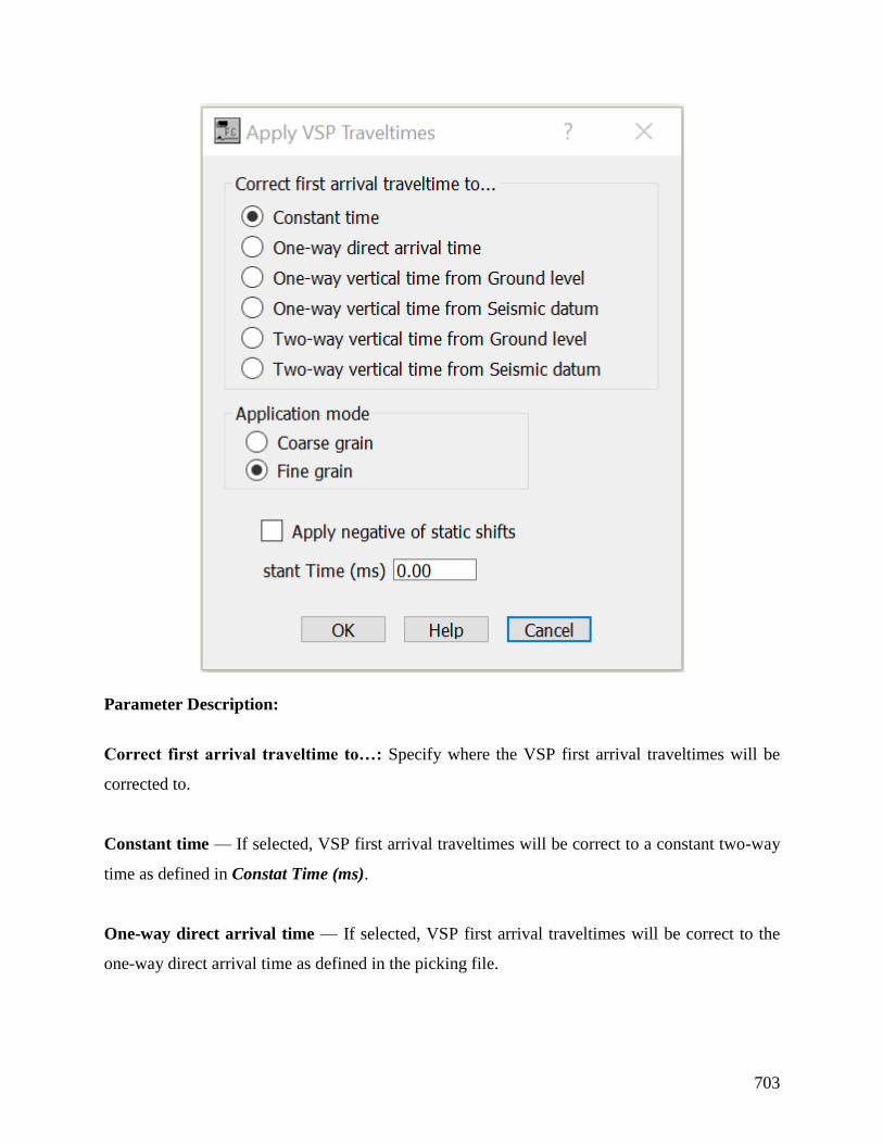
703

Parameter Description:

Correct first arrival traveltime to…: Specify where the VSP first arrival traveltimes will be

corrected to.

Constant time — If selected, VSP first arrival traveltimes will be correct to a constant two-way

time as defined in Constat Time (ms).

One-way direct arrival time — If selected, VSP first arrival traveltimes will be correct to the

one-way direct arrival time as defined in the picking file.

704

One-way vertical time from Ground level — If selected, VSP first arrival traveltimes will be

corrected vertically to the one-way time corresponding to the ground level location.

One-way vertical time from Seismic datum — If selected, VSP first arrival traveltimes will be

corrected vertically to the one-way time corresponding to the ground seismic reference datum.

Two-way vertical time from Ground level — If selected, VSP first arrival traveltimes will be

corrected vertically to the two-way time corresponding to the ground level location.

Two-way vertical time from Seismic datum — If selected, VSP first arrival traveltimes will be

corrected vertically to the two-way time corresponding to the seismic reference datum.

Application mode: Specify the mode of statics application.

Coarse grain — If selected, statics shifts are applied to the nearest discrete sample position.

Fine grain — If selected, statics shifts are applied as a precise phase shift operator in the Fourier

domain.

Apply negative static shifts — If, checked apply a negative of the static shifts.

Constant time (ms)/ Bulk shift (ms) — Enter the constant time in millisecond to be used as

reference if Constant time is selected. Enter a bulk shift value in milliseconds to shift all the data

simultaneously with this value.

Calculate VSP Traveltimes Usage:

The Calculate VSP Traveltimes step computes corrections for the travel times based on the

picking of the first arrivals (auxiliary VSP Frist Arrivals card data). The output seismic file has

the trace headers corresponding to VSP depths, times and velocities update accordingly. This file

can then be used as input for the Apply VSP Traveltimes step in order to flatten the record.

Input Links:

1) Seismic data in any sort order (mandatory).

2) VSP First arrivals card data (mandatory).

705

Output Links:

1) Seismic data in any sort order (mandatory).

Example Flowchart:

Step Parameter Dialog:

706

Parameter Description:

Well location: Specify general parameter related with the well corresponding to the VSP.

Kelly bushing — Enter a value for the Kelly bushing (KB) of the well corresponding to the VSP.

KB is defined in project units (m or ft).

Seismic reference datum — Enter a value for the seismic reference datum (SRD). SRD is defined

in project units (m or ft).

Ground elevation — Enter a value for the ground elevation/level (GL). GL is defind in project

units (m or ft).

707

Mean sea level — Enter a value for the mean sea level (MSL). MSL is defined in project units (m

or ft).

Project updates: Specify either if the geometry is updated from the project or if the project settings

will be updated with current parameterization.

Update from project — Updates the corner points from the SPS data that has been associated

with the project using the Survey > SPS Database menu.

Update project — Use this to broadcast the corner points so that they can be used by to set the

Easting and Northing ranges of plotting functions, such as the Attribute Map used later in this

flow.

Near surface model: Specify parameters related with the near surface model.

Weathering depth — Enter a value for the total depth of the weathering layer. Depth defined in

project units (m or ft).

Weathering velocity — Enter a value for the velocity of the weathering layer.

Replacement velocity — Enter a value for the replacement velocity to be used to comput the VSP

traveltime correcitons.

Marine VSP — If checked, VSP is assumed to be acquired in marine environment.

Fluid velocity — Enter the fluid velocity if VSP was acquired in marine environment.

VSP CMP Transform Usage:

The VSP CMP Transform step moves offset VSP data to the reflecting point location

(approximately half the distance for the largest offset) assuming that there is no dip.

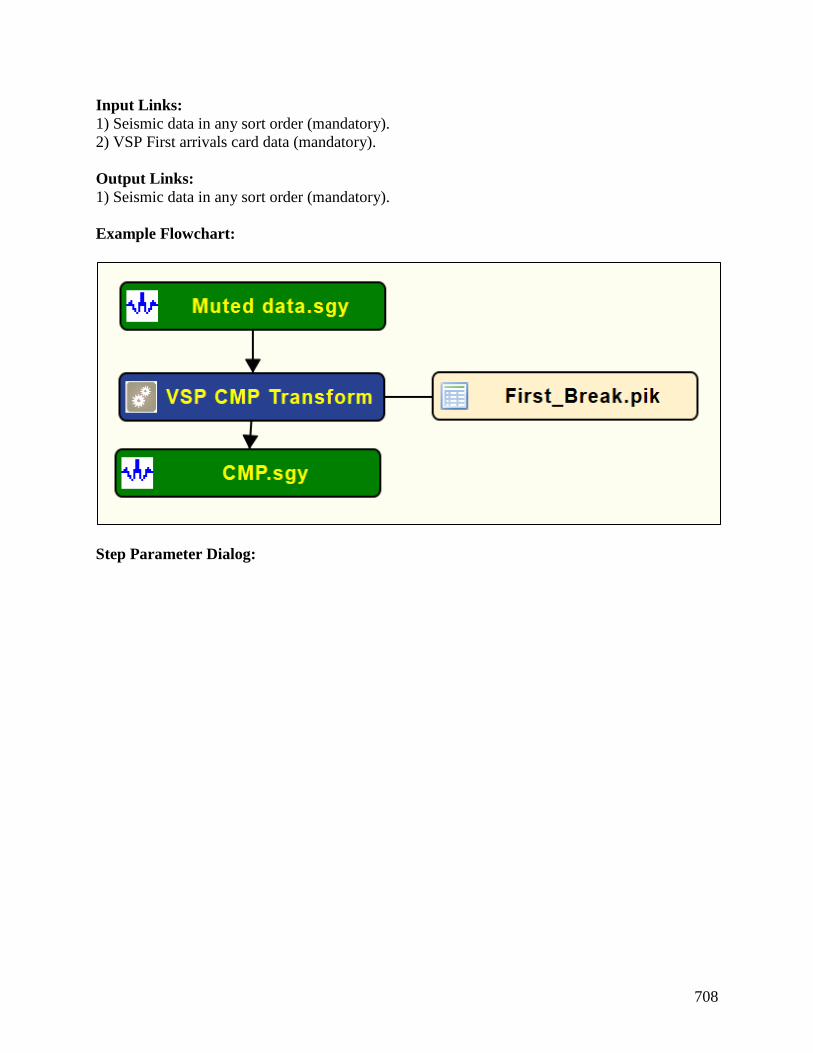
708

Input Links:

1) Seismic data in any sort order (mandatory).

2) VSP First arrivals card data (mandatory).

Output Links:

1) Seismic data in any sort order (mandatory).

Example Flowchart:

Step Parameter Dialog:

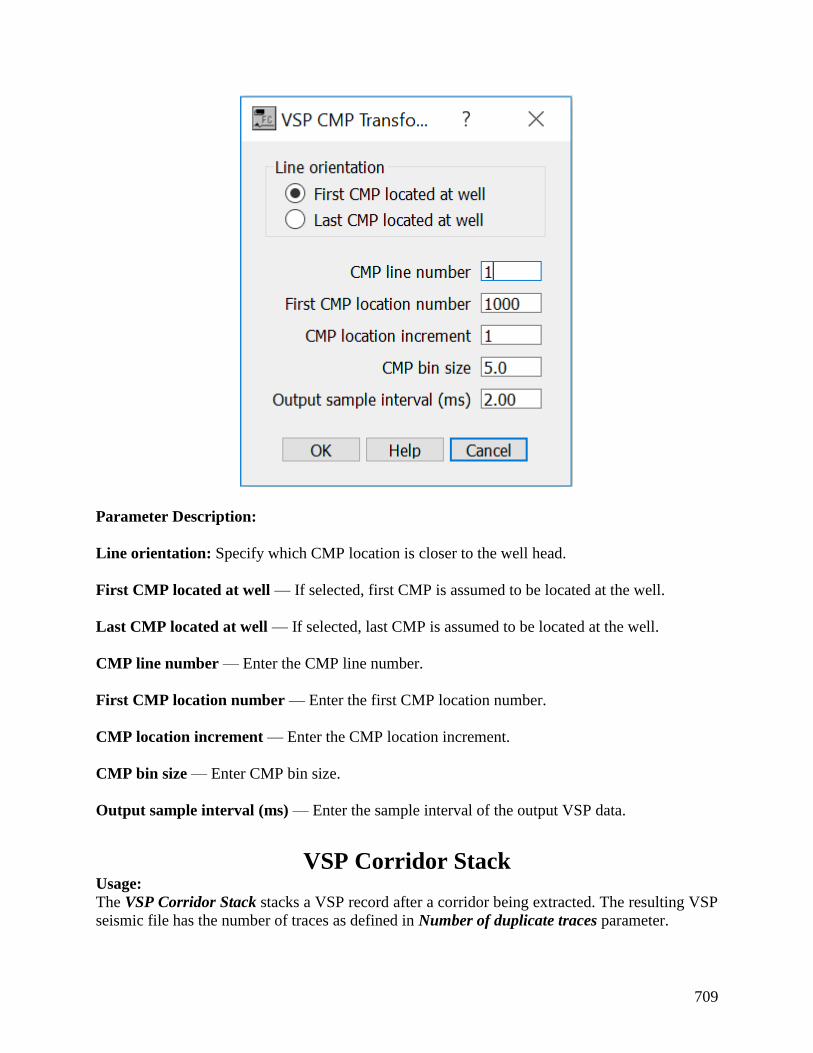
709

Parameter Description:

Line orientation: Specify which CMP location is closer to the well head.

First CMP located at well — If selected, first CMP is assumed to be located at the well.

Last CMP located at well — If selected, last CMP is assumed to be located at the well.

CMP line number — Enter the CMP line number.

First CMP location number — Enter the first CMP location number.

CMP location increment — Enter the CMP location increment.

CMP bin size — Enter CMP bin size.

Output sample interval (ms) — Enter the sample interval of the output VSP data.

VSP Corridor Stack Usage:

The VSP Corridor Stack stacks a VSP record after a corridor being extracted. The resulting VSP

seismic file has the number of traces as defined in Number of duplicate traces parameter.

710

Input Links:

1) Seismic data in any sort order (mandatory).

Output Links:

1) Seismic data in any sort order (mandatory).

Example Flowchart:

Step Parameter Dialog:

Parameter Description:

Corridor length (ms) — Enter the length of the corridor of data to be extracted in milliseconds.

Number of duplicate traces — Enter the number of duplicated traces in the corridor stack.

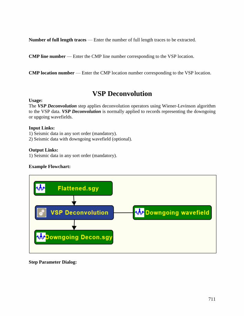
711

Number of full length traces — Enter the number of full length traces to be extracted.

CMP line number — Enter the CMP line number corresponding to the VSP location.

CMP location number — Enter the CMP location number corresponding to the VSP location.

VSP Deconvolution Usage:

The VSP Deconvolution step applies deconvolution operators using Wiener-Levinson algorithm

to the VSP data. VSP Deconvolution is normally applied to records representing the downgoing

or upgoing wavefields.

Input Links:

1) Seismic data in any sort order (mandatory).

2) Seismic data with downgoing wavefield (optional).

Output Links:

1) Seismic data in any sort order (mandatory).

Example Flowchart:

Step Parameter Dialog:

712

Parameter Description:

Operator type selection:

Spiking — If selected, applies a spiking deconvolution to the VSP data.

Predictive — If selected, applies a predictive deconvolution to the data.

Prediction length (ms) — Enter the prediction length of the predictive deconvolution operator.

Pre-whitening % — Enter the amount of white noise to add. The zero lag of the autocorrelation

function is increased by this amount to induce stability in the matrix solution.

Operator length (ms) — Enter the length of the operator to be calculated and applied in

milliseconds.

713

Window start (ms) — Enter the start time in milliseconds of the deconvolution design window.

Window length (ms) — Enter the length in milliseconds of the deconvolution design window.

Input downgoing data and apply operators — If selected, an auxiliary seismic file with the

downgoing field is used as auxiliary data.

VSP Downhole Locations Usage:

The VSP Downhole Locations carda data is used to store the positional downhole receiver

locations to be used by VSP Geometry Definition step.

Step Parameter Dialog:

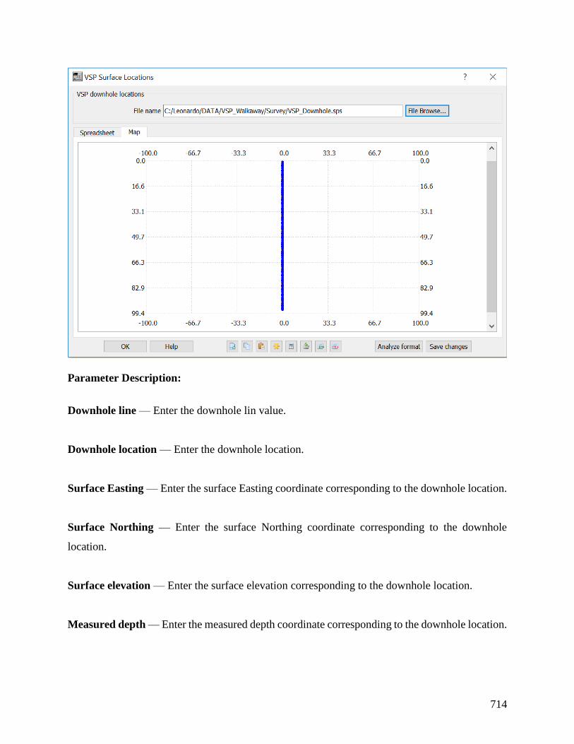
714

Parameter Description:

Downhole line — Enter the downhole lin value.

Downhole location — Enter the downhole location.

Surface Easting — Enter the surface Easting coordinate corresponding to the downhole location.

Surface Northing — Enter the surface Northing coordinate corresponding to the downhole

location.

Surface elevation — Enter the surface elevation corresponding to the downhole location.

Measured depth — Enter the measured depth coordinate corresponding to the downhole location.

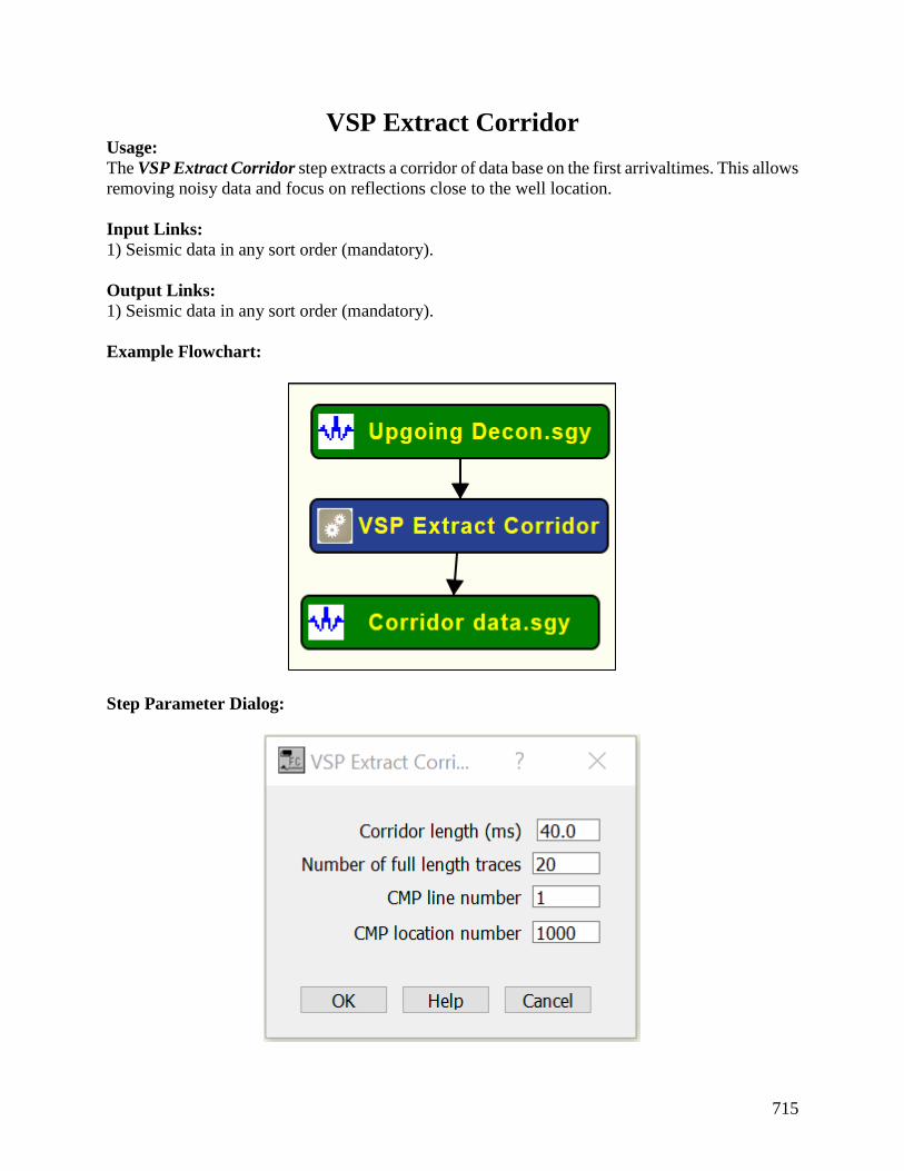
715

VSP Extract Corridor Usage:

The VSP Extract Corridor step extracts a corridor of data base on the first arrivaltimes. This allows

removing noisy data and focus on reflections close to the well location.

Input Links:

1) Seismic data in any sort order (mandatory).

Output Links:

1) Seismic data in any sort order (mandatory).

Example Flowchart:

Step Parameter Dialog:

716

Parameter Description:

Corridor length (ms) — Enter the length of the corridor of data to be extracted in milliseconds.

Number of full length traces — Enter the number of full length traces to be extracted.

CMP line number — Enter the CMP line number corresponding to the VSP location.

CMP location number — Enter the CMP location number corresponding to the VSP location.

VSP First Arrival Time Picks Usage:

Input Links:

Output Links:

Example Flowchart:

Step Parameter Dialog:

Parameter Description:

VSP Geometry Definition Usage:

The VSP Geometry Definition step assigns survey information to the VSP trace headers based on

the source, receiver, and observer notes SPS files. The VSP Geometry Definition step assigns

CMP number based on the source and receiver numbers using the following formula: CMP

Location = (Source Location + Receiver Location) / 2. Therefore, for 2D lines it is imperative that

source and receiver locations as defined in the SPS files share the same coordinate system. This

implies that Source location 1 has the same X,Y position as Receiver location 1, and that Source

location 2 has the same X,Y position as Receiver location 2, etc….

Input Links:

1) Seismic data in any sort order (mandatory).

2) Observers Notes – SPS Format cards (mandatory).

3) Receiver Locations – SPS Format cards (mandatory).

4) Source Locations – SPS Format cards (mandatory).

Output Links:

1) Seismic data in any sort order (mandatory).

Example Flowchart:

717

Step Parameter Dialog:

718

Parameter Description:

Well description: Specify general parameters related with the well.

Well name — Enter the name of the well corresponding to the VSP.

719

Well number — Enter well number corresponding to the VSP. Well number can be defined as

the UWI.

Well Easting — Enter Easting coordinates of well head.

Well Northing — Enter Northing coordinates of well head.

Project updates: Specify either if the geometry is updated from the project or if the project settings

will be updated with current parameterization.

Update from project — Updates the corner points from the SPS data that has been associated

with the project using the Survey > SPS Database menu.

Update project — Use this to broadcast the corner points so that they can be used by to set the

Easting and Northing ranges of plotting functions, such as the Attribute Map used later in this

flow.Azimuth definition: Specify the origin of azimuth.

Zero degrees azimuth = East — If selected, then zero degrees of source-receiver azimuth will be

set equal to due East.

Zero degrees azimuth = North — If selected, then zero degrees of source-receiver azimuth will

be set equal to due North.

Kill undefined traces and records — If checked, traces undefined after applying the geometry

will be flagged as dead.

Reverse VSP (source in Well) — If checked, reverse VSP source location in well.

Norminal receiver spacing — Enter the nominal (in m or ft) distance between receivers within

the well.

VSP SPS Relation Records Usage:

The VSP SPS Relation Locations carda data is used to store the relationship between surface and

downhole receiver locations to be used by VSP Geometry Definition step.

Step Parameter Dialog:

720

Parameter Description:

Record number — Enter the record number. This value should correspond to the FFID store in

the VSP seismic file.

Source line — Enter the source line as defined in VSP Surface Locations.

721

Source location — Enter the source location as defined in VSP Surface Locations.

From channel — Enter the number of the first active channel.

To channel — Enter the number of the last active channel.

Channel increment — Enter the channel increment.

Receiver line — Enter the receiver line as defined in VSP Downhole Locations.

From receiver — Enter the number of first receiver.

To receiver — Enter the number of last receiver.

Receiver increment — Enter the receiver number increment.

VSP Surface Locations Usage:

The VSP surface Locations carda data is used to store the positional surface locations to be used

by VSP Geometry Definition step.

Step Parameter Dialog:

722

723

Parameter Description:

Surface line — Enter the point lin value.

Surface location — Enter the point location.

Surface Easting — Enter the surface Easting coordinate corresponding to the point location.

Surface Northing — Enter the surface Northing coordinate corresponding to the point location.

Surface elevation — Enter the surface elevation corresponding to the point location.

Point depth — Enter the measured depth coordinate corresponding to the point location.

Uphole time — Enter the uphole time.

VSP Wavefield Separation Usage:

The VSP Wavefield Separation steps allows filtering the downgoing or the upgoing wavefields

by applying a moving average, a median or a F-K filter.

Input Links:

1) Seismic data in any sort order (mandatory).

Output Links:

1) Seismic data in any sort order (mandatory).

Example Flowchart:

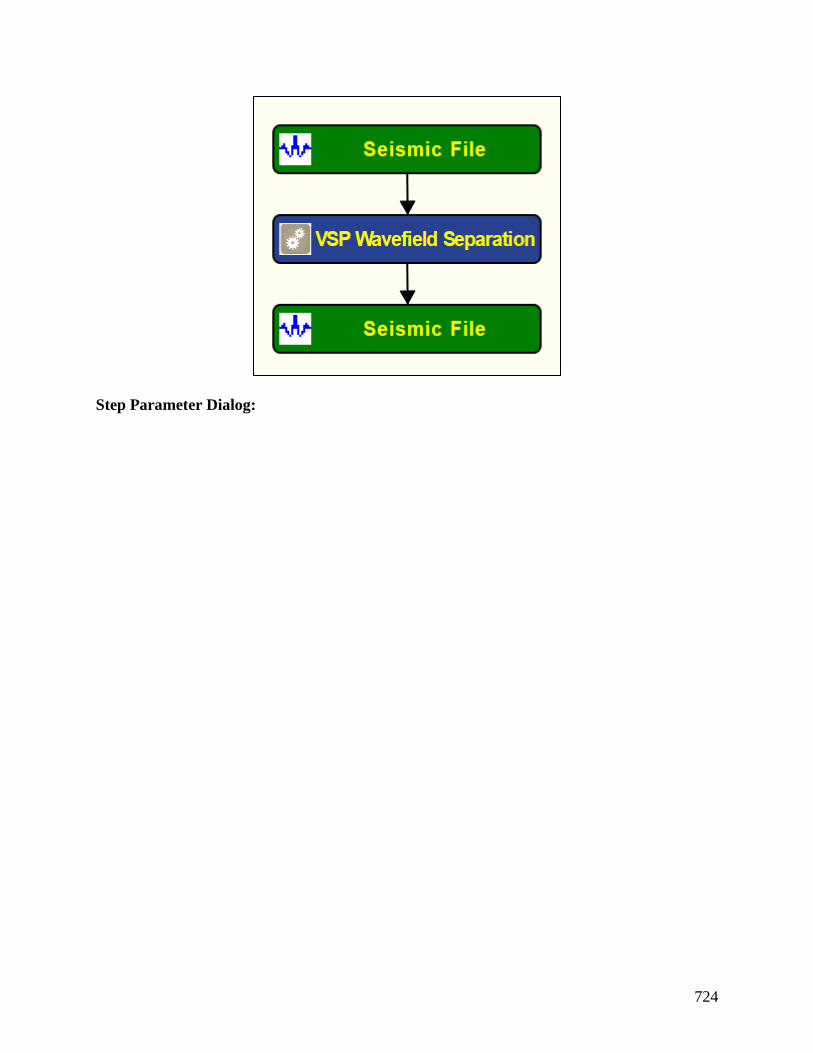
724

Step Parameter Dialog:

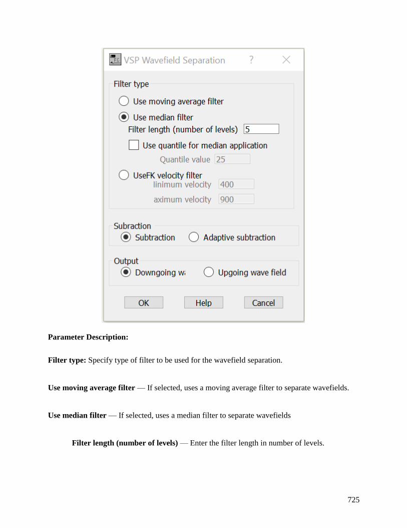
725

Parameter Description:

Filter type: Specify type of filter to be used for the wavefield separation.

Use moving average filter — If selected, uses a moving average filter to separate wavefields.

Use median filter — If selected, uses a median filter to separate wavefields

Filter length (number of levels) — Enter the filter length in number of levels.

726

Use quantile for median application — If checked, uses a quantile as defined in Quantile

value to do the filtering.

Quantile value — Enter the quantilie value.

Use FK velocity filter — If selected, uses a F-K velocity filter to separate wavefields.

Maximum velocity — Enter the maximum velocity to be considered in the FK velocity

filter

Minimum velocity — Enter the minimum velocity to be considered in the FK velocity

filter.

Subtraction: Specify type of subtraction between model and data.

Subtraction — If selected, applies a conventional sample-by-sample subtraction.

Adaptive subtraction — If selected, applies a subtractration as defined in Dataset Math step.

Output: Specify type of output.

Downgoing wavefield — If selected, outputs downgoing wavefield (filter upgoing wavefield).

Upgoing wavefield — If selected, outputs upgoing wavefield (filter downgoing wavefield).

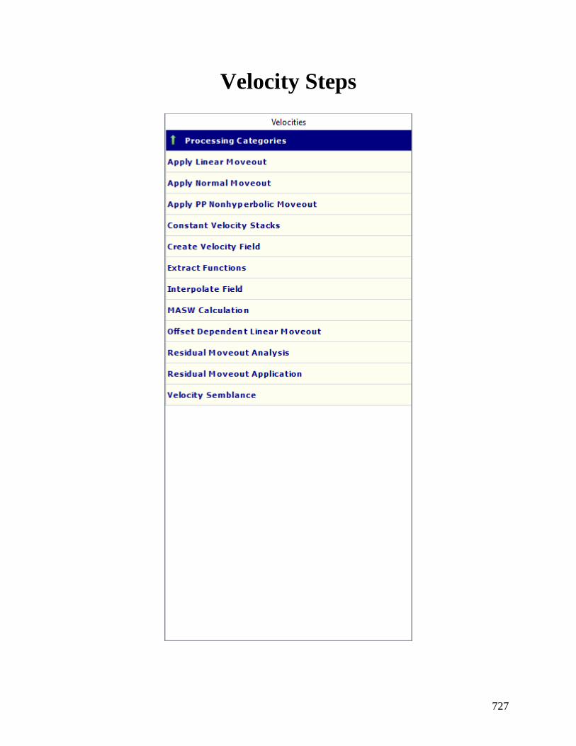
727

Velocity Steps

728

Apply Linear Moveout Usage:

The Apply Linear Moveout step allows you to apply a linear moveout function in either the

forward or inverse direction. You specify the moveout velocity. You may also apply a constant

static shift to your data. The moveout correction may be applied in a coarse or fine-grained

application mode. A coarse grained static shift is applied to the nearest sample. Fine-grained static

shifts are applied in the frequency domain by phase shifting your data.

Input Links:

1) Seismic data in any sort order (mandatory).

Output Links:

1) Seismic data in any sort order (mandatory).

Reference:

-

Example Flowchart:

Step Parameter Dialog:

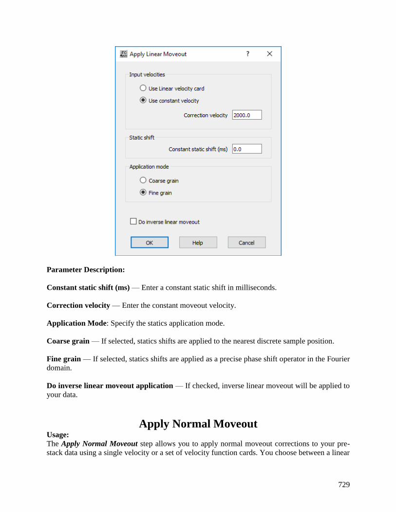
729

Parameter Description:

Constant static shift (ms) — Enter a constant static shift in milliseconds.

Correction velocity — Enter the constant moveout velocity.

Application Mode: Specify the statics application mode.

Coarse grain — If selected, statics shifts are applied to the nearest discrete sample position.

Fine grain — If selected, statics shifts are applied as a precise phase shift operator in the Fourier

domain.

Do inverse linear moveout application — If checked, inverse linear moveout will be applied to

your data.

Apply Normal Moveout Usage:

The Apply Normal Moveout step allows you to apply normal moveout corrections to your pre-

stack data using a single velocity or a set of velocity function cards. You choose between a linear

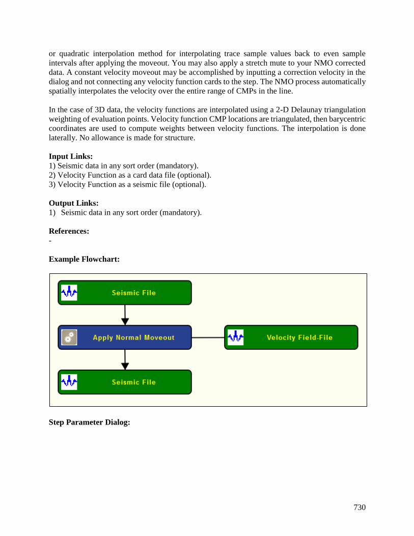
730

or quadratic interpolation method for interpolating trace sample values back to even sample

intervals after applying the moveout. You may also apply a stretch mute to your NMO corrected

data. A constant velocity moveout may be accomplished by inputting a correction velocity in the

dialog and not connecting any velocity function cards to the step. The NMO process automatically

spatially interpolates the velocity over the entire range of CMPs in the line.

In the case of 3D data, the velocity functions are interpolated using a 2-D Delaunay triangulation

weighting of evaluation points. Velocity function CMP locations are triangulated, then barycentric

coordinates are used to compute weights between velocity functions. The interpolation is done

laterally. No allowance is made for structure.

Input Links:

1) Seismic data in any sort order (mandatory).

2) Velocity Function as a card data file (optional).

3) Velocity Function as a seismic file (optional).

Output Links:

1) Seismic data in any sort order (mandatory).

References:

-

Example Flowchart:

Step Parameter Dialog:

731

Parameter Description:

Velocity field definition: Specify velocity field to be used to correct for hyperbolic moveout.

Use velocity field from data file — If checked, the velocity field from a card data file will be

used.

Use velocity field from seismic file — If checked, the velocity field from a seismic file will be

used.

Use constant velocity — If checked, a constant velocity will be used.

732

Constant velocity — Enter a constant NMO velocity. This constant velocity will be used

if a set of velocity function cards is NOT linked to the NMO correction step.

Scale input velocities by (%) — Enter the amount by which the input velocities are scaled up or

down. A value of 1.0 does not alter the velocity field.

Mute control: Specify the parameters for the stretch mute definition.

Apply mute from data file — If checked, a mute will be applied to the NMO corrected data from

a data file.

Apply stretch mute — If checked, a stretch mute will be applied to the NMO corrected data.

Stretch muting removes the stretching of the data due to the NMO correction.

Percentage — Enter the stretch mute percentage. The smaller the percent the more severe the

mute function.

Taper length — Enter the mute taper length in samples. Longer taper lengths result in a

smoother transition from the mute zone to the data zone.

Interpolation type selection: Specify the interpolation type (linear or quadratic). The moveout

function causes trace data samples to be moved in time to new locations. Since these new time

locations of the data sample values are not usually exactly at the sample interval of the data, the

data is interpolated to be evenly sampled at the correct sample interval.

Linear — Linear interpolation uses the equation of a line (y = mx + b) to interpolate data values

between or beyond existing data.

Quadratic — Quadratic interpolation uses the equation of a quadratic (y = ax^2 + bx + c) to

interpolate data values between or beyond existing data.

Do inverse moveout application — If checked, the inverse NMO correction will be applied,

instead of the usual forward NMO.

Apply PP Non-hyperbolic Moveout

Usage:

The Apply PP Non-hyperbolic Moveout step uses the travel-time equation for transversly isotropic

(TI) media described by Alkhalifah and Tsvankin (1997). Non-hyperbolic P-wave moveout may

become significant when source-receiver offsets are approximately equal to or greater than the

depth of reflection. The resulting deviations from the hyperbolic traveltime equation may be

attributed to one or more phenomena: (1) The standard hyperbolic travel-time equation is only a

two-term, short-offset approximation of the full travel-time equation for P-wave reflections in

layered media; (2) the earth media may be anisotropic. The resulting moveout is a function of the

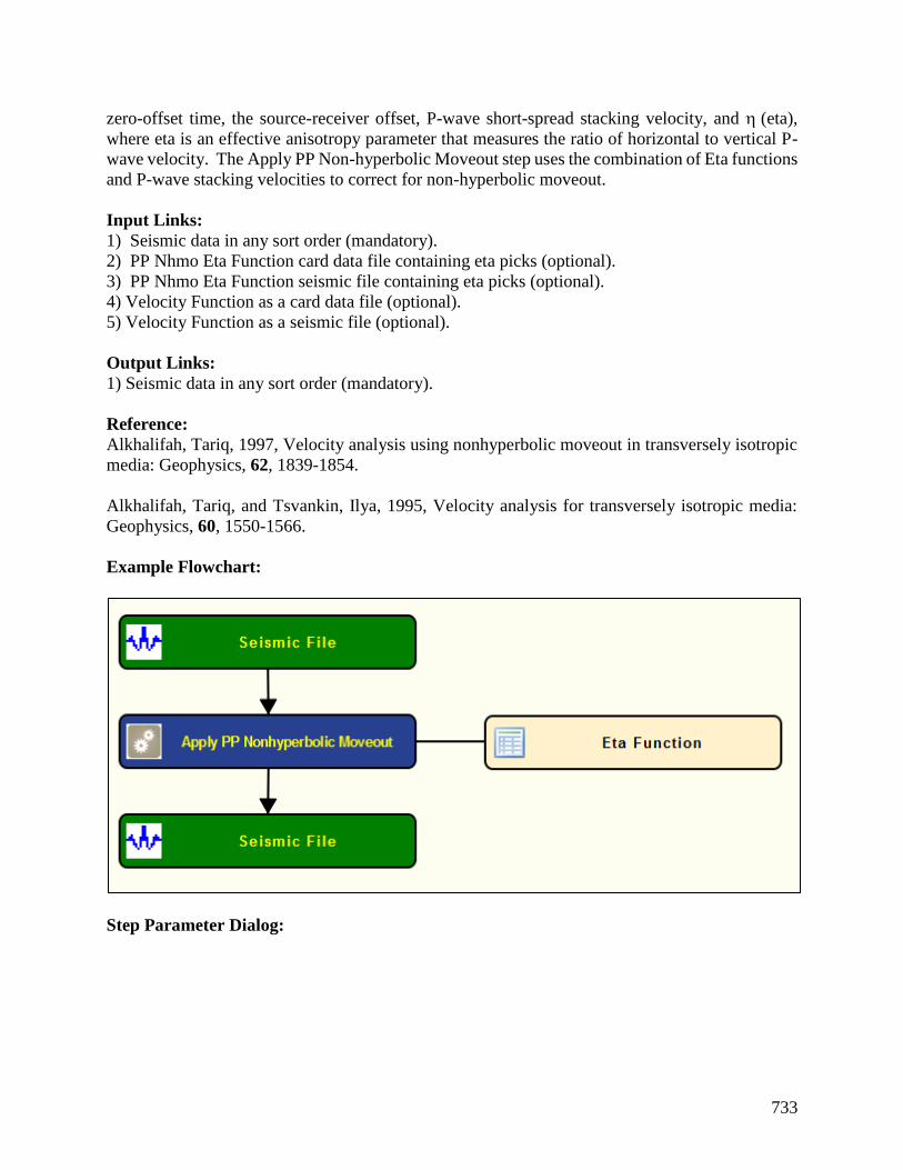
733

zero-offset time, the source-receiver offset, P-wave short-spread stacking velocity, and (eta),

where eta is an effective anisotropy parameter that measures the ratio of horizontal to vertical P-

wave velocity. The Apply PP Non-hyperbolic Moveout step uses the combination of Eta functions

and P-wave stacking velocities to correct for non-hyperbolic moveout.

Input Links:

1) Seismic data in any sort order (mandatory).

2) PP Nhmo Eta Function card data file containing eta picks (optional).

3) PP Nhmo Eta Function seismic file containing eta picks (optional).

4) Velocity Function as a card data file (optional).

5) Velocity Function as a seismic file (optional).

Output Links:

1) Seismic data in any sort order (mandatory).

Reference:

Alkhalifah, Tariq, 1997, Velocity analysis using nonhyperbolic moveout in transversely isotropic

media: Geophysics, 62, 1839-1854.

Alkhalifah, Tariq, and Tsvankin, Ilya, 1995, Velocity analysis for transversely isotropic media:

Geophysics, 60, 1550-1566.

Example Flowchart:

Step Parameter Dialog:

734

Parameter Description:

Eta field definition: Specify how the Eta field will be defined by your selections and entries to

correct for non-hyperbolic moveout.

Use eta functions from data file — If checked, the eta functions from a data file will be used.

Use eta field from seismic file — If checked, the eta field from a seismic file will be used.

Use constant eta — If checked, a constant eta will be used.

735

Constant eta — Enter constant eta value.

Scale input eta values by (%) — Enter a percentage to scale input eta values.

P-wave velocity field definition: Specify how the P-wave velocity field will be defined by your

selections and entries to correct for non-hyperbolic moveout.

Use velocity functions from data file — If checked, the velocity functions from a data file will

be used.

Use velocity field from seismic file — If checked, the velocity field from a seismic file will be

used.

Use constant velocity — If checked, a constant velocity will be used.

Constant velocity — Enter the short-spread P-wave NMO velocity. This constant velocity will

be used if a P-wave stacking velocity function is NOT selected.

Scale input velocities by (%) — Enter the amount by which the input velocities are scaled up

or down. A value of 1.0 does not alter the velocity field.

Mute control: Specify the parameters for the stretch mute definition.

Apply stretch mute — If checked, a stretch mute will be applied to the NMO corrected data.

Stretch muting removes the stretching of the data due to the NMO correction.

Percentage — Enter the stretch mute percentage. The smaller the percent the more severe the

mute function.

Taper length — Enter the mute taper length in samples. Longer taper lengths result in a

smoother transition from the mute zone to the data zone.

Interpolation type selection: Specify the the interpolation type (linear or quadratic). The moveout

function causes trace data samples to be moved in time to new locations. Since these new time

locations of the data sample values are not usually exactly at the sample interval of the data, the

data is interpolated to be evenly sampled at the correct sample interval.

Linear — Linear interpolation uses the equation of a line (y = mx + b) to interpolate data values

between or beyond existing data.

Quadratic — Quadratic interpolation uses the equation of a quadratic (y = ax^2 + bx + c) to

interpolate data values between or beyond existing data.

Do inverse moveout application — If checked, the inverse NMO correction will be applied,

instead of the usual forward NMO.

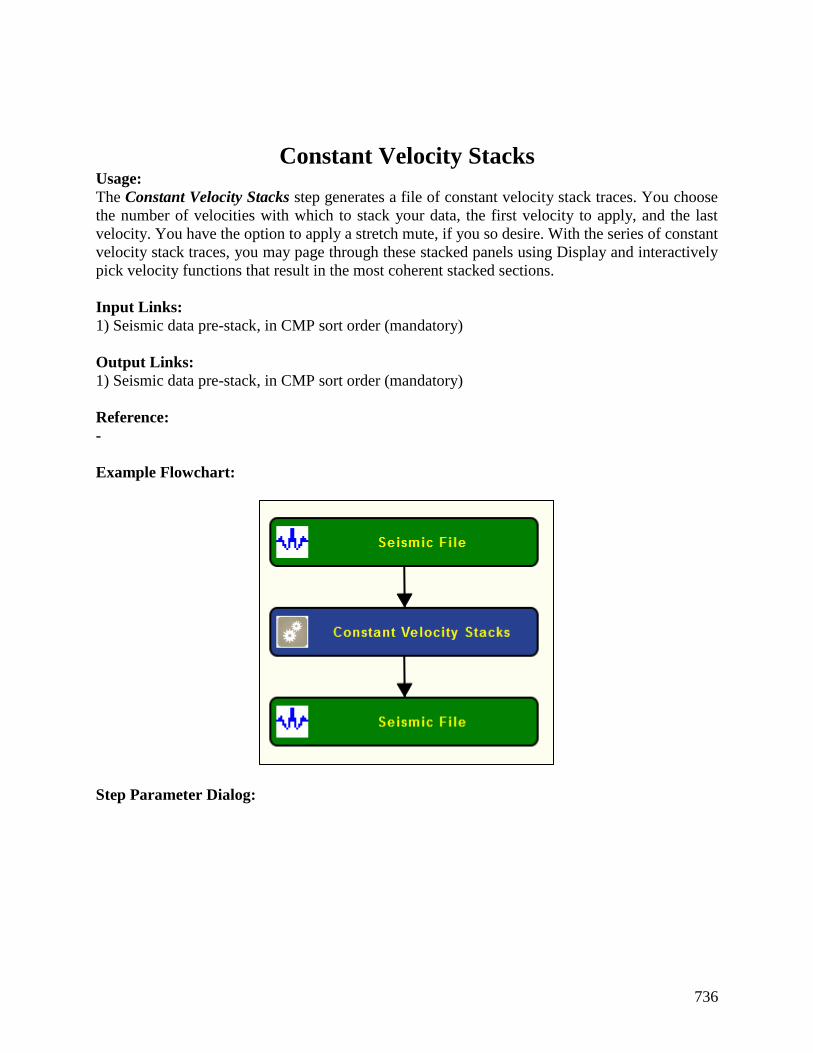
736

Constant Velocity Stacks Usage:

The Constant Velocity Stacks step generates a file of constant velocity stack traces. You choose

the number of velocities with which to stack your data, the first velocity to apply, and the last

velocity. You have the option to apply a stretch mute, if you so desire. With the series of constant

velocity stack traces, you may page through these stacked panels using Display and interactively

pick velocity functions that result in the most coherent stacked sections.

Input Links:

1) Seismic data pre-stack, in CMP sort order (mandatory)

Output Links:

1) Seismic data pre-stack, in CMP sort order (mandatory)

Reference:

-

Example Flowchart:

Step Parameter Dialog:

737

Parameter Description:

Velocity range: Specify the first and last velocities along with the velocity increment to calculate

the number of velocities to use in the analysis. A stacked section is calculated for each velocity

linearly interpolated between the starting and ending input velocities. The velocity increment will

be:

Vinc = (last velocity – first velocity)/ (Number of velocities-1).

First velocity — Enter the starting velocity for the analysis. This velocity will be used for NMO

on the first output stack. {>0.0}

Last velocity — Enter the ending velocity for the analysis. This velocity will be used for NMO

on the last output stack. {>0.0}

Velocity increment — Enter the velocity increment number. This number will be used to linearly

interpolate between the first and last velocities.

Line range: Specify the first and last lines along with the line increment to calculate the number

of lines to use in the analysis.

First line to analyze — Enter the first CMP line number to analyze.

738

Last line to analyze — Enter the last CMP line number to analyze.

Line increment — Enter the CMP line increment between lines to analyze.

Location range: Specify the first and last locations along with the location increment to calculate

the number of locations to use in the analysis. At each CMP location a range of constant velocity

stacks will be generated from the first velocity to the last velocity in increments of Vinc.

First location to analyze — Enter the first CMP location number to analyze.

Last location to analyze — Enter the last CMP location number to analyze.

Location increment — Enter the CMP location increment between groups of CMP locations to

analyze.

Locations per analysis — Enter the number of CMP locations in each analysis panel.

Mute control: Specify how the mute will be defined.

Apply mute from data file — If checked, a mute will be applied to the NMO corrected data.

Apply stretch mute — If checked, a stretch mute will be applied to the NMO corrected data.

Stretch muting restricts the stretching of the data due to the NMO correction.

Percentage — Enter the stretch mute percentage. The smaller the percent the more severe the

mute function.

Taper length (samples) — Enter the mute taper length in samples. Longer taper lengths result in

a smoother transition from the mute zone to the data zone.

Interpolation type selection — Specify the interpolation type (linear or quadratic). The moveout

function causes trace data samples to be moved in time to new locations. Since these new time

locations of the data sample values are not exactly at the sample interval of the data, the data is

interpolated to the correct sample interval.

Linear — Linear interpolation uses the equation of a line (y = mx + b) to interpolate data samples

between or beyond existing data.

Quadratic — Quadratic interpolation uses the equation of a quadratic (y = ax^2 + bx + c) to

interpolate data samples between or beyond existing data.

Trace amplitude definition — Specify the trace amplitude definition for relative or true

amplitude.

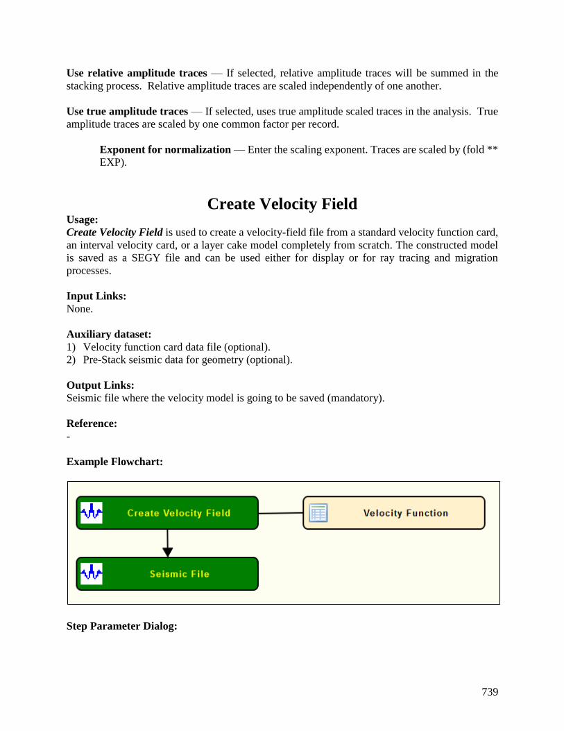
739

Use relative amplitude traces — If selected, relative amplitude traces will be summed in the

stacking process. Relative amplitude traces are scaled independently of one another.

Use true amplitude traces — If selected, uses true amplitude scaled traces in the analysis. True

amplitude traces are scaled by one common factor per record.

Exponent for normalization — Enter the scaling exponent. Traces are scaled by (fold **

EXP).

Create Velocity Field Usage:

Create Velocity Field is used to create a velocity-field file from a standard velocity function card,

an interval velocity card, or a layer cake model completely from scratch. The constructed model

is saved as a SEGY file and can be used either for display or for ray tracing and migration

processes.

Input Links:

None.

Auxiliary dataset:

1) Velocity function card data file (optional).

2) Pre-Stack seismic data for geometry (optional).

Output Links:

Seismic file where the velocity model is going to be saved (mandatory).

Reference:

-

Example Flowchart:

Step Parameter Dialog:

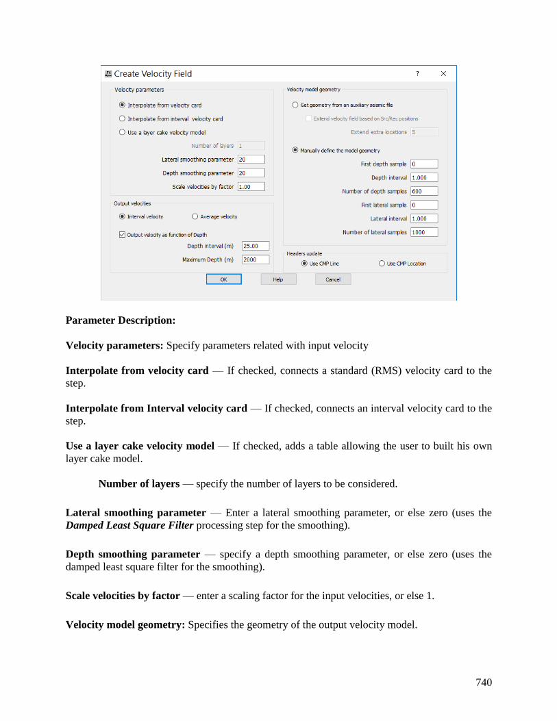
740

Parameter Description:

Velocity parameters: Specify parameters related with input velocity

Interpolate from velocity card — If checked, connects a standard (RMS) velocity card to the

step.

Interpolate from Interval velocity card — If checked, connects an interval velocity card to the

step.

Use a layer cake velocity model — If checked, adds a table allowing the user to built his own

layer cake model.

Number of layers — specify the number of layers to be considered.

Lateral smoothing parameter — Enter a lateral smoothing parameter, or else zero (uses the

Damped Least Square Filter processing step for the smoothing).

Depth smoothing parameter — specify a depth smoothing parameter, or else zero (uses the

damped least square filter for the smoothing).

Scale velocities by factor — enter a scaling factor for the input velocities, or else 1.

Velocity model geometry: Specifies the geometry of the output velocity model.

741

Get geometry from an auxiliary seismic file — If selected, get the geometry of the velocity

model from an auxiliary seismic file.

Extend velocity field based on Src/Rec positions — If checked, extends the

velocity model to cover all Src/Rec locations instead of just CMP locations.

Extend extra locations — Enter extra locations to extend.

Manually define model geometry — If selected, defines the velocity model geometry manually.

First depth sample — Enter the first depth sample of the model.

Depth interval — Enter the depth interval of the model.

Number of depth samples — Enter the last depth sample of the model.

First lateral sample — Enter the first lateral sample of the model.

Lateral interval — Enter the lateral interval of the model.

Number of lateral samples — Enter the last lateral sample of the model.

Headers Updates: Specifies each headers of the output velocity model will be updated.

Use CMP line — Update CMP line header word.

Use CMP location — Update CMP location header word.

Extract Functions Usage:

The Extract Functions step extracts velocity, Eta or Gamma functions from auxiliary card data

files at specific locations as user-defined along an existing seismic data file sorted by CMP.

Input Links:

1) Seismic file in CMP sort order (mandatory).

2) One of the following card data files: Velocity card data file, Eta card data file, Gamma card

data file (mandatory).

Output Links:

1) Seismic file with extracted functions (mandatory).

References:

-

Example Flowchart:

742

Step Parameter Dialog:

743

Parameter Description:

Input seismic field file: Specify type of auxiliary data type from where functions are going to be

extracted.

Velocity — If selected, an auxiliary velocity card data type will be used.

Eta — If selected, an auxiliary Eta card data type will be used.

Gamma — If selected, an auxiliary Gamma card data type will be used.

Input velocity field type: Specify type of input velocities in the auxiliary card data file. Only

available if Input seismic field file is set to Velocity.

RMS — If selected, input velocities are RMS velocities.

Interval — If selected, input velocities are Interval velocities.

Average — If selected, input velocities are average velocities.

Output auxiliary velocity type: Specify type of output velocities that will be written in output

seismic file. Only available if Input seismic field file is set to Velocity.

RMS — If selected, input velocities are RMS velocities.

Interval — If selected, input velocities are Interval velocities.

Average — If selected, input velocities are average velocities.

Function selection: Specify how auxiliary card data files will be sampled.

744

Regularly spaced locations — If selected, auxiliary field will be sampled at regularly spaced

locations as user-defined.

All trace locations — If selected, auxiliary field will be sampled for all the locations available.

Line Range: Specify the locations to be extract in the Line direction. Only available if Function

selection is set to Regularly spaced locations.

First line to extract — Enter the value for the first line to be extracted.

Last line to extract — Enter the value for the last line to be extracted.

Line increment — Enter the value for the increment of the sampling in the line direction.

Location range: Specify the locations to be extract in the Location direction. Only available if

Function selection is set to Regularly spaced locations.

First location to extract — Enter the value for the first location to be extracted.

Last location to extract — Enter the value for the last location to be extracted.

Location increment — Enter the value for the increment of the sampling in the location direction.

Vertical point selections: Specify how auxiliary fields are sampled vertically.

Interface ‘kneepoint’ — If selected, auxiliary fields will be sampled at the same vertical locations

as the picking.

Average points per functions — Enter the desired average number of points per function

in the vertical direction.

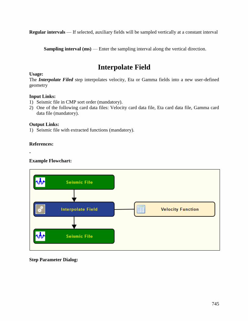
745

Regular intervals — If selected, auxiliary fields will be sampled vertically at a constant interval

Sampling interval (ms) — Enter the sampling interval along the vertical direction.

Interpolate Field Usage:

The Interpolate Filed step interpolates velocity, Eta or Gamma fields into a new user-defined

geometry

Input Links:

1) Seismic file in CMP sort order (mandatory).

2) One of the following card data files: Velocity card data file, Eta card data file, Gamma card

data file (mandatory).

Output Links:

1) Seismic file with extracted functions (mandatory).

References:

-

Example Flowchart:

Step Parameter Dialog:

746

Parameter Description:

Input parameter: Specify type of auxiliary data type from where functions are going to be

extracted.

Velocity — If selected, an auxiliary velocity card data type will be used.

Eta — If selected, an auxiliary Eta card data type will be used.

Gamma — If selected, an auxiliary Gamma card data type will be used.

747

Output velocity field type: Specify type of output velocities in the auxiliary card data file. Only

available if Input parameter is set to Velocity.

RMS — If selected, input velocities are RMS velocities.

Interval — If selected, input velocities are Interval velocities.

Average — If selected, input velocities are average velocities.

Output sampling: Specify sampling rate of output seismic file with interpolated field.

As input data — If selected, output seismic file will have the same sampling rate as input seismic

file.

Specified — If selected, output seismic file will have user-defined sampling rate.

Sampling (ms) — Enter output sampling rate in milliseconds.

Maximum time (ms) — Enter maximum time of output in milliseconds.

Smoohting: Specify vertical smoothing of the input field.

Apply vertical smoothing — If checked applies a vertical smoothing to the input field.

Smoothing length (ms) — Enter smoothing length in milliseconds.

Vertical interpolation type: Specify type of vertical interpolation of the inut field.

Linear — If selected, input field is vertically linearly interpolated.

Quadratic — If selected, input field is interpolated following a quadratic function.

748

MASW Calculation Usage:

The Multichannel analysis of surface waves (MASW) step creates multi modal dispersion images,

which shows a frequency vs. phase velocity space with pattern of energy accumulation that

represents the actual dispersion curve. This implementation is designed to run in single thread or

in parallel, giving it the possibility to take full advantage of multiple processors at the same time.

Input Links:

1) Multichannel seismic record.

Output Links:

1) Seismic file where the Dispersion images are going to be stored.

Example Flowchart:

Step Parameter Dialog:

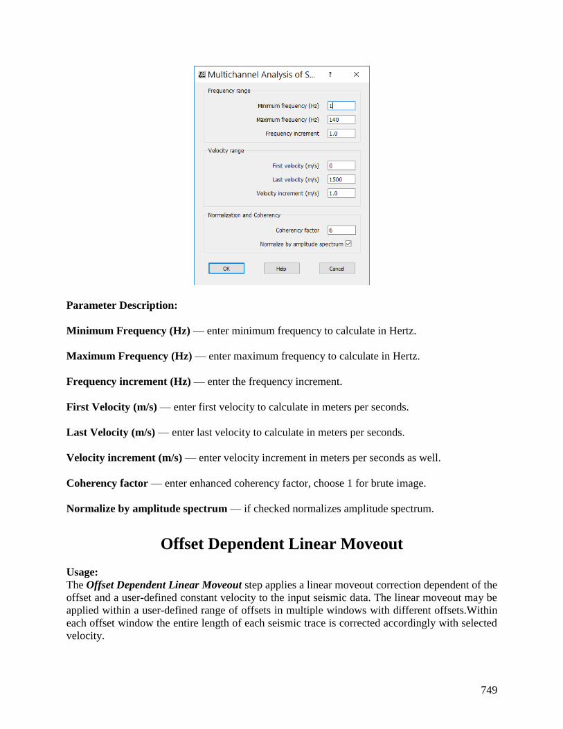
749

Parameter Description:

Minimum Frequency (Hz) — enter minimum frequency to calculate in Hertz.

Maximum Frequency (Hz) — enter maximum frequency to calculate in Hertz.

Frequency increment (Hz) — enter the frequency increment.

First Velocity (m/s) — enter first velocity to calculate in meters per seconds.

Last Velocity (m/s) — enter last velocity to calculate in meters per seconds.

Velocity increment (m/s) — enter velocity increment in meters per seconds as well.

Coherency factor — enter enhanced coherency factor, choose 1 for brute image.

Normalize by amplitude spectrum — if checked normalizes amplitude spectrum.

Offset Dependent Linear Moveout

Usage:

The Offset Dependent Linear Moveout step applies a linear moveout correction dependent of the

offset and a user-defined constant velocity to the input seismic data. The linear moveout may be

applied within a user-defined range of offsets in multiple windows with different offsets.Within

each offset window the entire length of each seismic trace is corrected accordingly with selected

velocity.

750

Input Links:

1) Seismic data in any sort order (mandatory).

Output Links:

1) Seismic data in any sort order (mandatory).

Reference:

-

Example Flowchart:

Step Parameter Dialog:

751

Parameter Description:

Do inverse linear moveout — If checked, applies an inverse linear moveout as defined below in

the window table.

Bulk shit (ms) — Enter a value in milliseconds corresponding to a vertical bulk shift of the entire

data. If no bulk shift is desired use zero.

Window — Sequential number of the offset window where the offset dependent linear moveout

will be applied.

Start offset — Enter the offset from where the linear moveout will be applied for that specific

time window.

Stop offset — Enter the last offset where the linear moveout will be applied for that specific time

window.

Velocity — Enter the velocity to be used in the offset depedent linear moveout for that specific

time window.

Add window — Add a new offset window.

Delete window — Delete the last offset window in the table.

Residual Moveout Analysis

Usage:

Residual Moveout Analysis analyses pre-stack 2D or 3D CMP NMO-corrected gathers for errors

in the moveout applied. The required residual moveout is parameterized as a CMP-varying ‘alpha’

function, using either a standard or a long offset moveout assumption. This parameter is

determined fully-sampled using a fast semblance analysis and output as a segy file. A velocity

field is not required for the analysis. The output parameter field may then be smoothed as required,

using for example, 3D Median with a 5-5-1 filter or similar.

752

As a final step use Residual Moveout Application with the derived or the smoothed parameter

field as auxiliary input to correct the residual moveout errors.

Input Links:

1) CMP records of offset-sorted moveout-applied seismic data (mandatory).

Output Links:

1) CMP-sorted ‘alpha’ parameter field (mandatory).

Reference:

Castle, R. J. 1994. A theory of normal moveout, Geophysics, Vol 59, No 6, June 1994, pp 983-

999.

Example Flowchart:

Step Parameter Dialog:

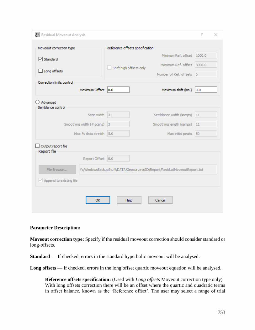
753

Parameter Description:

Moveout correction type: Specify if the residual moveout correction should consider standard or

long-offsets.

Standard — If checked, errors in the standard hyperbolic moveout will be analysed.

Long offsets — If checked, errors in the long offset quartic moveout equation will be analysed.

Reference offsets specification: (Used with Long offsets Moveout correction type only)

With long offsets correction there will be an offset where the quartic and quadratic terms

in offset balance, known as the ‘Reference offset’. The user may select a range of trial

754

reference offsets. The correction parameter will be optimized for each reference offset. The

reference offset with best optimization will then be adopted.

To save execution time, the analysis of the best Reference offset could be carried out using

a limited number of records, and then this Reference offset used with the entire dataset.

Minimum Ref. offset — Enter the smallest offset to use as a reference offset.

Maximum Ref. offset — Enter the largest offset to use as a reference offset.

Number of ref. offsets — Enter the number of reference offsets to try.

Shift high offsets only — If checked, then only offsets greater than the Reference offset

will be shifted by the residual moveout. This can be useful when it is only the high offsets

that need correction.

Correction limits control: Specify the maximum offset to be used in the analysis and the

maximum vertical shift allowed.

Maximum offset — Enter the maximum offset to be used to determine the residual moveout to

apply.

Maximum shift (ms.) — Enter the maximum trace shift in milliseconds that will be allowed at

the specified Maximum offset.

Advanced — If selected, the semblance control parameters may be modified. This is set as an

‘advanced’ option as the default parameters are usually fine to use

Scan width — Enter the width of the scan for the semblance calculation.

Smoothing width (# scans) — Enter the number of scans to be smoothed together.

Max % data stretch — Enter the maximum percentage of data stretch allowed.

Semblance width (samps) — Enter the semblance width in number of samples.

Smoothing length (samps) — Enter the vertical smoothing length in number of samples.

Max initial peaks — Enter the maximum initial peaks values.

Output report file — If checked, a text report file will be generated giving a few statistics on

residual moveout analysis of the specified offset.

Report file: Specify parameters regarding the report file.

Report Offset — Enter the offset for which statistics will be generated in the report file.

755

File Browse… — Click to specify a Report file location.

Append to existing file — If checked, the statistics for the specified offset will be tagged on to

the end of any text already in the specified file. Otherwise, the contents of the file specified, if

already existing, will be overwritten by the current text output.

Residual Moveout Applications

Usage:

Residual Moveout Application applies residual moveout to normal moveout-corrected gathers to

correct for moveout errors due to use of incorrect velocities or the use of standard hyperbolic

moveout when long offset moveout would have been better used.

To perform residual moveout, the Residual Moveout Functions file generated by Residual

Moveout Analysis is required as auxiliary input. This fully-sampled parameter file with one time

trace per CMP should be inspected and smoothed if necessary before used as auxiliary file to

Residual Moveout Application.

Input Links:

1) CMP records of offset-sorted moveout-applied seismic data (mandatory).

2) Auxiliary Residual Moveout Functions file as generated by Residual Moveout Analysis

(mandatory).

Output Links:

1) CMP-sorted ‘alpha’ parameter field (mandatory).

Reference:

Castle, R. J. 1994. A theory of normal moveout, Geophysics, Vol 59, No 6, June 1994, pp 983-

999.

Example Flowchart:

Residual Moveout Correction:

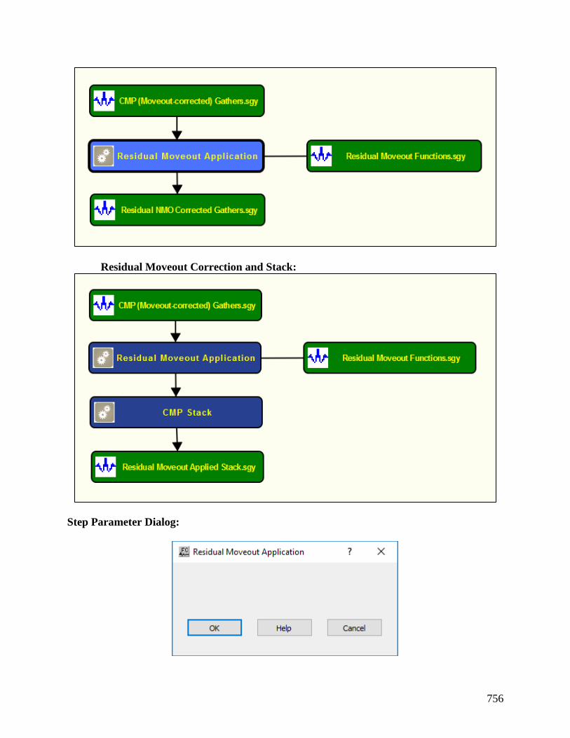
756

Residual Moveout Correction and Stack:

Step Parameter Dialog:

757

Parameter Description:

No parameters – All parameterization is specified in the prior analysis step Residual Moveout

Analysis.

Velocity Semblance Usage:

The Velocity Semblance step creates velocity semblance displays for the input CMP records.

Stacking velocities may be picked interactively from this semblance display in SeisViewer. For

semblance display generation, you designate the velocity range for semblance calculation by

choosing the number of velocities, the starting velocity for this range, and the velocity increment.

You may generate only one CMP semblance display for each input CMP gather. You may also

control the time gate length around hyperbolic velocity paths for CMP summing in the semblance

calculation using the “Semblance length” input parameter. Finally, the output semblance display

may be windowed, and a stretch mute may be applied if so desired.

Input Links:

1) Seismic data in CMP sort order (mandatory).

Output Links:

1) Seismic File (mandatory).

Reference:

Taner, M. and Kohler, 1969, Velocity spectra — digital computer derivation and applications of

velocity functions, Geophysics, v. 34, no. 6, p. 859ff.

Example Flowchart:

Step Parameter Dialog:

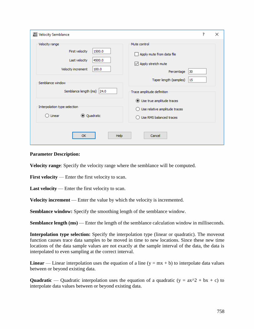
758

Parameter Description:

Velocity range: Specify the velocity range where the semblance will be computed.

First velocity — Enter the first velocity to scan.

Last velocity — Enter the first velocity to scan.

Velocity increment — Enter the value by which the velocity is incremented.

Semblance window: Specify the smoothing length of the semblance window.

Semblance length (ms) — Enter the length of the semblance calculation window in milliseconds.

Interpolation type selection: Specify the interpolation type (linear or quadratic). The moveout

function causes trace data samples to be moved in time to new locations. Since these new time

locations of the data sample values are not exactly at the sample interval of the data, the data is

interpolated to even sampling at the correct interval.

Linear — Linear interpolation uses the equation of a line (y = mx + b) to interpolate data values

between or beyond existing data.

Quadratic — Quadratic interpolation uses the equation of a quadratic (y = ax^2 + bx + c) to

interpolate data values between or beyond existing data.

759

Mute Control: Specify the stretch mute control parameters.

Apply mute from data file — If checked, a stretch mute card data will be added to the flow and

applied to the NMO corrected data

Apply stretch mute — If checked ,apply strectch mute as defined below.

Percentage — Enter the percent stretch mute. The smaller the percent the more severe the

mute function.

Taper length — Enter the mute tape length in samples. Longer taper lengths result in a

smoother transition from the mute zone to the data zone.

Trace Amplitude Definition: Specify amplitude summing selection.

Use relative amplitude traces — Selects the use of relative amplitude scaled traces in the analysis.

Relative amplitude traces are scaled independently of one another.

Use true amplitude traces — Absolute amplitude traces will be summed in the stacking process.

True amplitude traces are scaled by one common factor per record.

Use RMS balanced traces — Amplitude traces will be balanced using RMS.

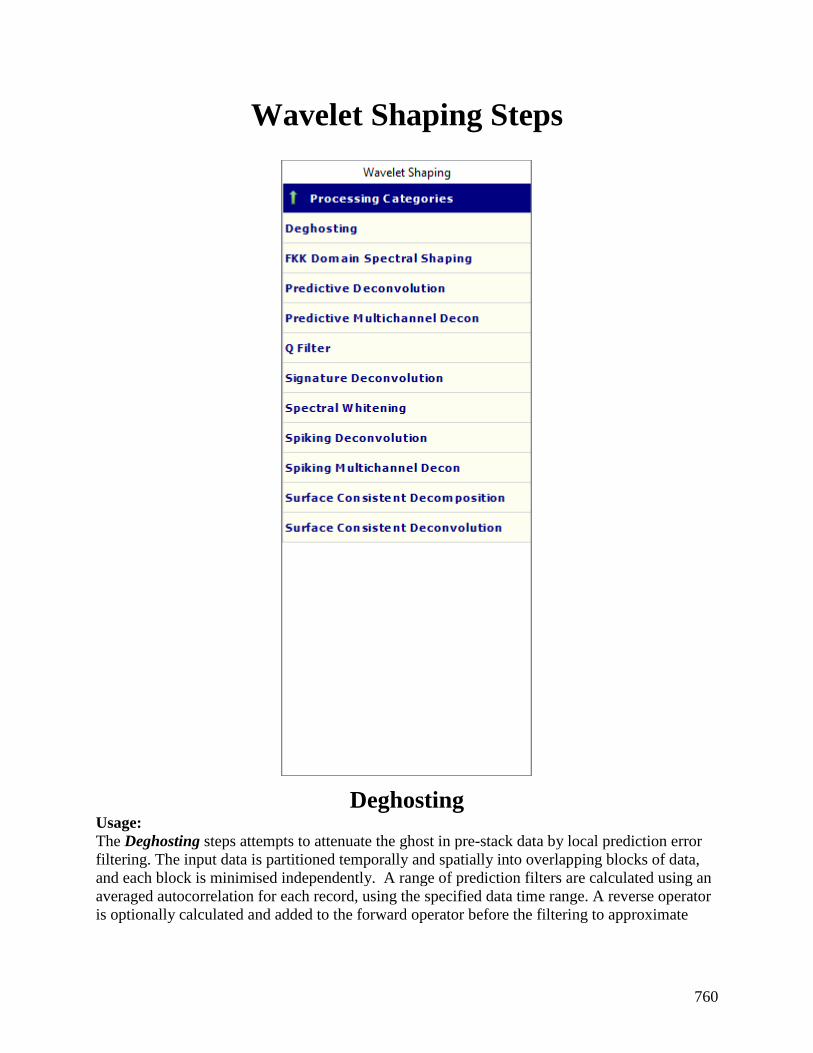
760

Wavelet Shaping Steps

Deghosting Usage:

The Deghosting steps attempts to attenuate the ghost in pre-stack data by local prediction error

filtering. The input data is partitioned temporally and spatially into overlapping blocks of data,

and each block is minimised independently. A range of prediction filters are calculated using an

averaged autocorrelation for each record, using the specified data time range. A reverse operator

is optionally calculated and added to the forward operator before the filtering to approximate

761

zero phase filtering. The prediction filters with increasing gap lengths are applied to the data

within each block. The o/p is minimised in the L1 sense.

Input Links:

1) Seismic data in any sort order (mandatory).

Output Links:

1) Seismic data in any sort order (mandatory).

Reference:

-

Example Flowchart:

Step Parameter Dialog:

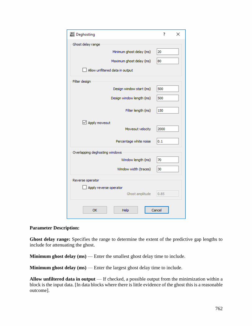
762

Parameter Description:

Ghost delay range: Specifies the range to determine the extent of the predictive gap lengths to

include for attenuating the ghost.

Minimum ghost delay (ms) — Enter the smallest ghost delay time to include.

Minimum ghost delay (ms) — Enter the largest ghost delay time to include.

Allow unfiltered data in output — If checked, a possible output from the minimization within a

block is the input data. [In data blocks where there is little evidence of the ghost this is a reasonable

outcome].

763

Filter Design: Specifies the parameters from which the predictive gap operators will be calculated

are specified here.

Design window start (ms) — Enter the initial data time to be used to extract data used to calculate

the predictive gap operators from the data autocorrelation.

Design window length (ms) — Enter the data window length to be used as above.

Filter length (ms) — Enter the lengths of the filters to calculate in milliseconds (not including the

predictive gaps).

Apply moveout – If checked, the moveout velocity may be overridden in the adjacent box. A

moveout correction corresponding to the trace offset will then be applied before windowing the

data according to the parameters above.

Percentage white noise – Specify amount of white noise (as a % of the autocorrelation zero lag )

to add to stabilize the solution of the Toeplitz matrix in estimation of the filter.

Overlapping deghosting windows: Specify the overlap of blocks is set to 50%, using Hanning

tapering between the blocks.

Window length (ms) — Enter the length in milliseconds of each deghosting window.

Window width (traces) — Enter the width in traces of each deghosting window.

Reverse Operator: Specifies if the operation adds in a time-reversed and scaled copy of the

operator to act like a zero-phase filter.

Apply reverse Operator — If checked, a reverse operator will be added.

Ghost amplitude — Enter the scaling of the reverse operator to approximate the relative

amplitude of the ghost.

FKK Domain Spectral Shaping Usage:

The FKK Domain Spectral Shaping step is a spectral shaping filter primarily for application to

post-stack and 3D migrated seismic data. The operator is applied in the 3D Fourier transformed

FKK domain.

The process applies an integration filter to the data with an optional 90 degrees phase shift rotation

to simulate acoustic impedance data. Applying such a process to migrated data can cause severe

amplitude distortions, excessively amplifying dipping events, signal or noise. Therefore, in

replace mode, this process simulates de-migration of the data, application of the integration filter

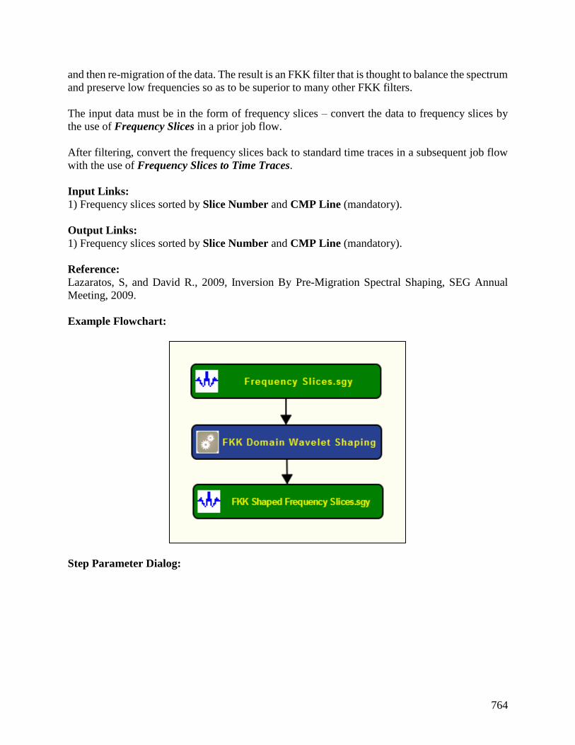
764

and then re-migration of the data. The result is an FKK filter that is thought to balance the spectrum

and preserve low frequencies so as to be superior to many other FKK filters.

The input data must be in the form of frequency slices – convert the data to frequency slices by

the use of Frequency Slices in a prior job flow.

After filtering, convert the frequency slices back to standard time traces in a subsequent job flow

with the use of Frequency Slices to Time Traces.

Input Links:

1) Frequency slices sorted by Slice Number and CMP Line (mandatory).

Output Links:

1) Frequency slices sorted by Slice Number and CMP Line (mandatory).

Reference:

Lazaratos, S, and David R., 2009, Inversion By Pre-Migration Spectral Shaping, SEG Annual

Meeting, 2009.

Example Flowchart:

Step Parameter Dialog:

765

Parameter Description:

Integrating filter application mode: Specify filter application mode.

Replace — If checked, simulates de-migration of the data, application of the integration filter

and then re-migration of the data

Apply — If checked, apply the FKK spectral shaping to the data.

Apply pre-migration —If checked, applies the FKK spectral shaping before migration.

Remove — If checked, removes the FKK filter to the data

Migration velocity — Enter constant velocity to be used in the migration step.

Start frequency — Enter the start frequency to be analyzed.

Apply 90 deg. Phase shift — If checked, applies a 90 degrees phase shift to the input data to

simulate acoustic impedance.

Override trace spacing: Specify if ones wishes to override trace space as defined in input

seismic file.

766

Specify trace spacing — If checked, specify trace spacing entering the corresponding value.

Specigy line spacing (3D) — If checked, specify line spacing entering the corresponding value.

This option is only valid for three-dimensional dataset.

Predictive Deconvolution Usage:

The Predictive Deconvolution step is a Wiener-Levinson algorithm for applying a predictive

multi-gate deconvolution to your data. You choose the percent pre-whitening, filter length, number

of operators, the overlap of the operator design windows, start time of each operator design

window, and the design window lengths. For the predictive deconvolution method, you must

specify the predictive length of your wavelet. You may also apply a linear moveout to your

deconvolution design windows to allow a sliding window whose start time varies with offset.

Input Links:

1) Seismic data in any sort order (mandatory).

Output Links:

1) Seismic data in any sort order (mandatory).

Reference:

-

Example Flowchart:

Step Parameter Dialog:

767

Parameter Description:

Number of operators — Enter the number of deconvolutin operators to be used.

Overlap between operators (ms) — Enter the overlap in milliseconds between operators. This is

the amount of the previous and/or next window to include in the calculation of the inverse filter

for the current window.

Apply reverse operator — If checked, applies the reverse deconvolution operator to the data.

Ghost amplitude — Enter the amplitude value for the deconvolved ghost.

Operator — Sequential number of the operator to be used.

Prewhiten % — Enter the amount of white noise to add. The zero lag of the autocorrelation

function is increased by this amount to induce stability in the matrix solution.

Operator length (ms) — Enter the length of the operator to be calculated and applied in

milliseconds.

Moveout — If checked, a linear moveout will be applied to the deconvolution design window.

The window start time will shift by: delta time = offset / velocity.

Velocity — Enter the velocity to be applied in the linear moveout.

Window start (ms) — Enter the start time in milliseconds of the deconvolution design window.

768

Window length (ms) — Enter the length in milliseconds of the deconvolution design window.

Predicitve Multichannel Deconvolution Usage:

The Predicitve Multichannel Deconvolution step is a Wiener-Levinson algorithm for applying a

multi-channel predictive multi-gate deconvolution to your data. You choose the percent pre-

whitening, filter length, number of operators, the overlap of the operator design windows, start

time of each operator design window, and the design window lengths. For the predictive

deconvolution method, you must specify the predictive length of your wavelet. You may also apply

a linear moveout to your deconvolution design windows to allow a sliding window whose start

time varies with offset.

Input Links:

1) Seismic data in any sort order (mandatory).

Output Links:

1) Seismic data in any sort order (mandatory).

Reference:

-

Example Flowchart:

Step Parameter Dialog:

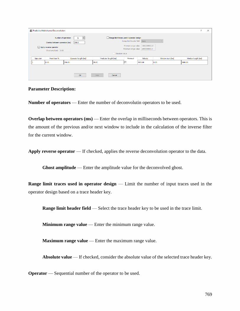
769

Parameter Description:

Number of operators — Enter the number of deconvolutin operators to be used.

Overlap between operators (ms) — Enter the overlap in milliseconds between operators. This is

the amount of the previous and/or next window to include in the calculation of the inverse filter

for the current window.

Apply reverse operator — If checked, applies the reverse deconvolution operator to the data.

Ghost amplitude — Enter the amplitude value for the deconvolved ghost.

Range limit traces used in operator design — Limit the number of input traces used in the

operator design based on a trace header key.

Range limit header field — Select the trace header key to be used in the trace limit.

Minimum range value — Enter the minimum range value.

Maximum range value — Enter the maximum range value.

Absolute value — If checked, consider the absolute value of the selected trace header key.

Operator — Sequential number of the operator to be used.

770

Prewhiten % — Enter the amount of white noise to add. The zero lag of the autocorrelation

function is increased by this amount to induce stability in the matrix solution.

Operator length (ms) — Enter the length of the operator to be calculated and applied in

milliseconds.

Moveout — If checked, a linear moveout will be applied to the deconvolution design window.

The window start time will shift by: delta time = offset / velocity.

Velocity — Enter the velocity to be applied in the linear moveout.

Window start (ms) — Enter the start time in milliseconds of the deconvolution design window.

Window length (ms) — Enter the length in milliseconds of the deconvolution design window.

Q Filter

Usage:

The Q Filter step applies a frequency dependent “Q” attenuation compensation filter or an

attenuation modeling filter to the input file. For both attenuation and modeling options, phase only

or phase and amplitude filters may be applied.

Input Links:

1) Seismic data in any sort order (mandatory).

Output Links:

1) Seismic data in any sort order (mandatory).

Reference:

Hargreaves, N. D., Calvert A. J., 1991, Inverse Q filtering by Fourier Transform, Geophysics, 56,

p. 519.

Hargreaves, N., 1992, Similarity and the inverse Q filter: Some simple algorithms for inverse Q

filtering, Geophysics, 57, p. 994.

Wang, Y., 2002, A stable and efficient approach of inverse Q filtering, Geophysics, 67, p. 657.

Example Flowchart:

771

Step Parameter Dialog:

Parameter Description:

772

Operator type: Specify the type of operator.

Inverse Q - compensation — If checked, attenuation will be removed from the input seismic

traces.

Forward Q - modelling — If checked, the input seismic traces will have attenuation is to be

introduced to.

Compensation type: Specify the compensation type.

Phase only — If selected, an allpass, phase-only filter is to be applied for forward or inverse Q

filtering. This is a computationally efficient option.

Phase and amplitude — If selected, a phase and amplitude type filter is to be applied for forward

or inverse Q filtering. This option is computer intensive.

Constant Q — Enter the value of Q for forward or inverse Q filtering.

Reference frequency (Hz) — Enter the reference frequency for forward or inverse Q filtering.

There will be slight frequency dependent phase shifts with respect to this frequency.

Gain limit (dB) — Enter the maximum gain limit per frequency in the case of inverse Q filtering.

Signature Deconvolution Usage:

The Signature Deconvolution step removes a seismic signature from your data traces by

calculating the inverse of a supplied signature trace and then filtering your data by this signature

inverse. This is a common technique for use in processing marine data to remove the signature of

the airguns.

Input Links:

1) Seismic data in any sort order (mandatory).

Output Links:

1) Seismic data in any sort order (mandatory).

Example Flowchart:

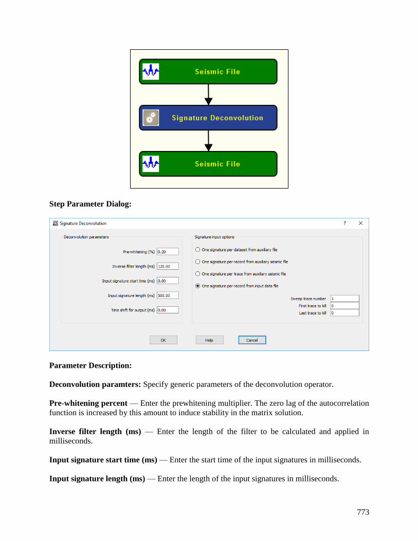
773

Step Parameter Dialog:

Parameter Description:

Deconvolution paramters: Specify generic parameters of the deconvolution operator.

Pre-whitening percent — Enter the prewhitening multiplier. The zero lag of the autocorrelation

function is increased by this amount to induce stability in the matrix solution.

Inverse filter length (ms) — Enter the length of the filter to be calculated and applied in

milliseconds.

Input signature start time (ms) — Enter the start time of the input signatures in milliseconds.

Input signature length (ms) — Enter the length of the input signatures in milliseconds.

774

Time shift for output (ms) – Enter the time shift for the output trace following signature

deconvolution

Signature Input Options: Specify the data input source of the signature trace or traces.

One signature from an auxiliary file — This option inputs one signature trace from an auxiliary

input data and uses that trace as the signature trace for the entire data set.

One signature per record from an auxiliary data file — This option inputs one signature trace

per record from an auxiliary input data set and uses that trace as the signature trace for all traces

in the record in the signature deconvolution calculation.

One signature per trace from an auxiliary data file — This option inputs one signature trace

from an auxiliary input data set per data trace and uses that trace as the signature trace for the

corresponding data trace in the signature deconvolution calculation.

One signature per record in the data file — This option uses one trace from each data record

and uses that trace as the signature trace for all seismic traces in the record in the signature

deconvolution calculation.

Signature trace number — Enter the trace number to use as the signature trace.

Sweep trace number — Enter the number of traces in the sweep.

First trace to kill — If you demultiplexed the data set with the auxiliary traces to recover the

signature trace, you may wish to kill the these auxiliary traces. Enter the first trace number to kill.

Last trace to kill — If you demultiplexed the data set with the auxiliary traces to recover the

signature trace, you may wish to kill the these auxiliary traces. Enter the last trace number to kill.

Spectral Whitening Usage:

The Spectral Whitening step is a multi-banded spectral whitening method for balancing the energy

of the selected frequency bands of your data. You specify the beginning and ending frequencies in

the pass zone, the number of bands within this zone, and the length of the AGC operator. The

individual band-pass filter cut off values are linearly interpolated based on the low and high pass

frequencies and the number of bands that you choose. Each band is given a Butterworth third order

slope with the midpoints of each slope being the half power points. Within each band every trace

is AGC’ed with respect to the maximum amplitude in the window. All AGC’ed bands are then

summed. Optionally, you may specify the Low Cut / Low Pass / High Pass / High Cut

(LC,LP,HP,HC) filter points and associated weights for summing of up to ten filter bands. For

optimal balancing of the energy of your frequency bands, your filters should be designed such that

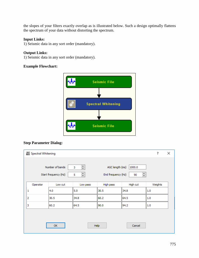
775

the slopes of your filters exactly overlap as is illustrated below. Such a design optimally flattens

the spectrum of your data without distorting the spectrum.

Input Links:

1) Seismic data in any sort order (mandatory).

Output Links:

1) Seismic data in any sort order (mandatory).

Example Flowchart:

Step Parameter Dialog:

776

Parameter Description:

Number of bands — Enter the number of frequency bands. Each trace is split into this number of

frequency bands which are AGC'ed and then summed to create the output trace.

Start frequency (Hz) — Enter the low frequency pass band limit in hertz (Hz). This is the lowest

frequency in the pass band.

End frequency (Hz) — Enter the high frequency pass band limit in hertz (Hz). This is the highest

frequency in the pass band. It may not exceed one-half the Nyquist frequency.

AGC length — Enter the AGC operator length. This is the length of the AGC operator, which is

applied to each frequency band.

Operator — Sequential number of the operator to be used.

Low Cut — Enter the filter low frequency cutoff point in hertz (Hz).

Low Pass — Enter the filter low frequency pass point in hertz (Hz).

High Pass — Enter the filter high frequency pass point in hertz (Hz).

High Cut — Enter the filter high frequency cutoff point in hertz (Hz).

Weights — Enter the filter band relative weight.

Spiking Deconvolution Usage:

The Spiking Deconvolution step is a Wiener-Levinson algorithm for applying a spiking multi-gate

deconvolution to your data. You choose the percent pre-whitening, filter length, number of

operators, the overlap of the operator design windows, start time of each operator design window,

and the design window lengths. For the predictive deconvolution method, you must specify the

predictive length of your wavelet. You may also apply a linear moveout to your deconvolution

design windows to allow a sliding window whose start time varies with offset.

Input Links:

1) Seismic data in any sort order (mandatory).

Output Links:

1) Seismic data in any sort order (mandatory).

Reference:

-

Example Flowchart:

777

Step Parameter Dialog:

Parameter Description:

Number of operators — Enter the number of deconvolutin operators to be used.

Overlap between operators (ms) — Enter the overlap in milliseconds between operators. This is

the amount of the previous and/or next window to include in the calculation of the inverse filter

for the current window.

Apply reverse operator — If checked, applies the reverse deconvolution operator to the data.

Ghost amplitude — Enter the amplitude value for the deconvolved ghost.

778

Operator — Sequential number of the operator to be used.

Prewhiten % — Enter the amount of white noise to add. The zero lag of the autocorrelation

function is increased by this amount to induce stability in the matrix solution.

Operator length (ms) — Enter the length of the operator to be calculated and applied in

milliseconds.

Moveout — If checked, a linear moveout will be applied to the deconvolution design window.

The window start time will shift by: delta time = offset / velocity.

Velocity — Enter the velocity to be applied in the linear moveout.

Window start (ms) — Enter the start time in milliseconds of the deconvolution design window.

Window length (ms) — Enter the length in milliseconds of the deconvolution design window.

Spiking Multichannel Deconvolution Usage:

The Spiking Multichannel Deconvolution step is a Wiener-Levinson algorithm for applying a

multi-channel spiking multi-gate deconvolution to your data. You choose the percent pre-

whitening, filter length, number of operators, the overlap of the operator design windows, start

time of each operator design window, and the design window lengths. For the predictive

deconvolution method, you must specify the predictive length of your wavelet. You may also apply

a linear moveout to your deconvolution design windows to allow a sliding window whose start

time varies with offset.

Input Links:

1) Seismic data in any sort order (mandatory).

Output Links:

1) Seismic data in any sort order (mandatory).

Reference:

-

Example Flowchart:

779

Step Parameter Dialog:

Parameter Description:

Number of operators — Enter the number of deconvolutin operators to be used.

Overlap between operators (ms) — Enter the overlap in milliseconds between operators. This is

the amount of the previous and/or next window to include in the calculation of the inverse filter

for the current window.

Apply reverse operator — If checked, applies the reverse deconvolution operator to the data.

Ghost amplitude — Enter the amplitude value for the deconvolved ghost.

780

Range limit traces used in operator design — Limit the number of input traces used in the

operator design based on a trace header key.

Range limit header field — Select the trace header key to be used in the trace limit.

Minimum range value — Enter the minimum range value.

Maximum range value — Enter the maximum range value.

Absolute value — If checked, consider the absolute value of the selected trace header key.

Operator — Sequential number of the operator to be used.

Prewhiten % — Enter the amount of white noise to add. The zero lag of the autocorrelation

function is increased by this amount to induce stability in the matrix solution.

Operator length (ms) — Enter the length of the operator to be calculated and applied in

milliseconds.

Moveout — If checked, a linear moveout will be applied to the deconvolution design window.

The window start time will shift by: delta time = offset / velocity.

Velocity — Enter the velocity to be applied in the linear moveout.

Window start (ms) — Enter the start time in milliseconds of the deconvolution design window.

Window length (ms) — Enter the length in milliseconds of the deconvolution design window.

Surface Consistent Decomposition Usage:

The Surface Consistent Decomposition step uses a Gauss-Seidel iterative method to perform a

four-component surface-consistent decomposition of the amplitude spectra of the input seismic

data into source, receiver, offset, and CMP components. Output component spectra can then be

used as input to Surface Consistent Deconvolution step.

781

Input Links:

1) Seismic data in any sort order (mandatory).

Output Links:

1) Seismic data in any sort order (mandatory).

Reference:

-

Example Flowchart:

Step Parameter Dialog:

782

Parameter Description:

Design window: Specify window where surface-consitent decomposition will be performed.

Use fixed window to built pilot — If checked, use a fixed time window to build a pilot.

Design window start time (ms) — Enter start time of the pilot window in millieseconds.

Design window end time (ms) — Enter the end time of the pilot window in milliseconds.

Apply linear moveout to design window — If checked, design window is defined as an offset-

dependent linear moveout.

Linear moveout velocity — Enter the linear moveout velocity.

Offset limit traces in design window — If checked, traces for the analysis are limited in terms of

offset.

Minimum offset — Enter the minimum offset to be considered.

Maximum offset — Enter the maximum offset to be considered.

Surface consistent spectral decomposition: Specify consistent spectra decomposition

parameters.

783

RMS error change for termination — Enter the minimum RMS error for the iterative procedure

to be considered finished.

Midpoint smoothing radius (bin) — Enter the radius (in number of bins) of the midpoint

smoothing operator.

Compute source spectra — Select yes to compute source spectra.

Compute receiver spectra — Select yes to compute receiver spectra.

Compute midpoint spectra — Select yes to compute midpoint spectra.

Compute offset spectra — Select yes to compute offset spectra.

Residual spectra output: Specify type of output.

Output source spectra — Select yes to output source spectra.

Output receiver spectra — Select yes to output receiver spectra.

Output midpoint spectra — Select yes to output midpoint spectra.

Output offset spectra — Select yes to output offset spectra.

Surface Consistent Deconvolution Usage:

The Surface Consistent Deconvolution step uses a Gauss-Seidel iterative method to perform a

four-component surface-consistent decomposition of the amplitude spectra of the input seismic

data into source, receiver, offset, and CMP components. Deconvolution operators are constructed

from the source and receiver components of this decomposition. The user specifies whether the

deconvolution will be of the spiking or predictive type, the design window, operator length, and

percent white noise.

Input Links:

1) data in any sort order (mandatory).

Output Links:

1) Seismic data in any sort order (mandatory).

Reference:

Cary, P. M., and Lorentz, G. A., 1993, Four-component surface-consistent deconvolution:

Geophysics, 58, 383-392.

Example Flowchart:

784

Step Parameter Dialog:

785

Parameter Description:

Deconvolution parameters: Specifyvtype of deconvolution to perform: Spiking or Predictive.

Spiking — If selected, use a spiking deconvolution.

Predictive — If selected, use a predictive or gapped deconvolution.

Prediction length (ms) — Enter the prediction length in milliseconds.

Pre-whitening percent — Enter the pre-whitening multiplier. The zero lag of the autocorrelation

function is increased by this amount to induce stability in the matrix solution.

786

Inverse filter length (ms) — Enter the length of the filter to be calculated and applied in

milliseconds.

Deconvolution operator application: Specify type of deconvolution operators to be applied to

the data.

Compute and apply source operators — Select yes, to compute and apply source deconvolution

operators.

Compute and apply receiver operators — Select yes, to compute and apply receiver

deconvolution operators.

Compute and apply midpoint operators — Select yes, to compute and apply midpoint

deconvolution operators.

Compute and apply offset operators — Select yes, to compute and apply offset deconvolution

operators.

Output type: Specify type of output.

Output deconvolved trace data — If selected, deconvolution operators are applied to the output

data.

Output deconvolution operators — If selected, deconvolution operators are the output and can

be used in other processing steps. No deconvolution is applied to input data.