ORIGINAL PAPER

Climatology of extratropical cyclones over the SouthAmerican–southern oceans sector

David Mendes & Enio P. Souza & José A. Marengo &

Monica C. D. Mendes

Received: 24 October 2007 /Accepted: 27 May 2009# Springer-Verlag 2009

Abstract A climatology of extratropical cyclones is pre-sented. Extratropical cyclones, their main characteristics andtheir predominant tracks, as well as their interannualvariability, affect weather in South America. For thatpurpose, a storm track database has been compiled byapplying a cyclone tracking scheme to six-hourly sea levelpressure fields, available from the National Center forEnvironmental Prediction–National Center for AtmosphericResearch reanalyses II for the 1979–2003 period. The spatialdistribution of the cyclogenesis frequency shows two maincenters: one around Northern Argentina, Uruguay, andSouthern Brazil in all seasons and the other near to theNorth Antarctic Peninsula. The lifetime of extratropicalcyclones in the South American sector exhibits smallseasonality, being typically of the order of 3.0 days duringmost of the year and slightly higher (3.5 days) in australsummer. The distance travelled by the cyclones formed in theSouth American sector tends to be smaller than the totalpaths found in other areas of the Southern Hemisphere. A k-mean clustering technique is used to summarize theanalysis of the 25-year climatology of cyclone tracks.Three clusters were found: one storm-track cluster in

Northeast Argentina; a second one west of the AndesCordillera; and a third cluster located to the north of theAntarctic Peninsula (around the Weddell Sea). The influ-ence of the Antarctic Oscillation (AAO) in the variability ofextratropical cyclones is explored, and some signals of theimpacts of the variability of the AAO can be observed inthe position of the extratropical cyclones around 40°S,while the impacts on the intensity is detected around 55°S.

1 Introduction

The conventional Lagrangian approach used to definestorm track involves tracking the displacement of pre-defined features usually in near surface charts, such asminima (maxima) in sea level pressure (SLP), geopotentialheight, or vorticity fields. There are several studies onclimatology of storms over the Northern Hemisphere (NH),based on the visual inspection of sea level pressure charts,from the earlier work by Petterssen (1950) to the mostrecent studies relying on automatic methods to detectingand tracking storms over gridded-reanalysis data (e.g.,Blender et al. 1997; Trigo et al. 1999; Gulev et al. 2001).

Among the studies dedicated to storm track over thesouthern oceans, the first one based on an automatic schemewas developed and applied to the Southern Hemisphere (SH)by Murray and Simmonds (1991a,b). In monitoring cycloneand anticyclone tracks, it is important to notice that, in thepast, this process used to demand a lot of work time becauseof its manual nature. Nowadays, however, the situation iscompletely different due to recent developments on auto-matic tracking schemes such as those described in Murrayand Simmonds (1991a,b) and Sinclair (1994). Murray andSimmonds (1991a,b) developed an automatic procedureto find and track surface pressure systems. Jones and

D. Mendes : J. A. MarengoCentro de Ciência do Sistema Terrestre/Instituto Nacional dePesquisas Espaciais, Rod. Pres. Dutra, Km 40,12630-000 Cachoeira Paulista, São Paulo, Brazil

E. P. SouzaDepartamento de Ciências Atmosféricas,Universidade Federal de Campina Grande,Paraíba, Brazil

D. Mendes (*) :M. C. D. MendesCentro de Previsão de Tempo e Estudos Climáticos—CPTEC/INPE, Cachoeira Paulista, São Paulo, Brazile-mail: dmendes@cptec.inpe.br

Theor Appl ClimatolDOI 10.1007/s00704-009-0161-6

Simmonds (1993a) evaluated the performance of thisparticular tracking scheme through different datasets andconcluded that it is a very useful tool for meteorologicalapplications. They were able to reproduce and complementsome previous results found in the literature. In recent years,a relatively large number of studies using cyclone/anticy-clone tracking schemes have shown this tool’s reliability(e.g., Sinclair 1994; Sinclair et al. 1997; Simmonds andKeay 2000a,b; and Pezza and Ambrizzi 2003).

Sinclair (1994), using vorticity fields derived from theEuropean Centre for Medium-Range Weather Forecasts datafor the 1980–1986 period, found fairly uniformly distributedstorm tracks, but with a maximum in the 45°S–55°S band.Part of this equatorward displacement of cyclone activitymay be attributed to vorticity maxima, associated withorographic effects (Kidson and Sinclair 1995). More recently,Simmonds and Keay (2000a), using an updated version ofthe Melbourne University cyclone finding and trackingscheme (Simmonds et al. 1999) found that the annual meannumber of extratropical cyclones in the Southern Hemisphere(SH), as those analyzed for the 1958–1997 period, arecharacterized by a year-round frequency maximum in thecircumpolar trough between 50°S and 70°S.

Despite the overall symmetry of southern storm tracks, itis possible to identify regions of enhanced cyclonic activity,such as the maximum off East Antarctica, a region wherethe well-known katabatic outflows occur, and the secondarymaximum located to the east of New Zealand during thewinter-spring time, associated with the subtropical westerlyjet stream near 40°S (Sinclair 1997).

Gan and Rao (1991) developed one of the first studies ofcyclogenesis over the South American sector (SA). Theydetected and tracked cyclonic systems by visual inspection ofsurface pressure charts, available four times per day for the1979–1988 period. The method used by Gan and Rao (1991)for identifying extratropical cyclones required that at least oneclosed isobar around a low pressure center should be foundfor an analysis of 2-mb intervals. Gan and Rao (1991) foundthat the extratropical cyclones over the South America sector(SA) are more frequent in winter than in any other season.

Previously, Satyamurty et al. (1990) did a similaranalyses based on satellite imagery for the 1980–1986period, covering South America and a wider area over theSouthern Atlantic. They found that the highest cyclogenesisfrequency was obtained for the summer season.

The abovementioned studies using different horizontaldomains show conflicting results. Nevertheless, both studiesagreed on one of the most active cyclogenetic areas, namelythe Gulf of San Mathias (42.5°S, 62°W) during summer andover Uruguay (around 31°S, 55°W) during winter (Table 1).

In the mid-to-high latitudes of the Southern Hemisphere(SH), the Antarctic Oscillation (AAO) is the leading mode ofatmospheric variability, corresponding to the transfer ofatmospheric mass between higher and lower latitudes(Thompson and Wallace 2000). The phase of the AAO atupper levels is strongly associated with the location andintensity of the polar jet stream and, thus, directly influencingthe developing regions and the steering of extratropical lows.

Recently, Pezza et al. (2007) suggested a robust link ofthese trends of number of extratropical cyclones with thePacific Decadal Oscillation, especially with the last majorclimate shift in the Pacific Basin by the middle-lateseventies. This view goes beyond the traditional study oflarge-scale influences related to interannual variabilitylinked to El Niño-Southern Oscillation (ENSO).

Therefore, the objectives of the present work are toanalyze the spatial distribution of cyclogenesis and cyclonetracks in the Southern American sector (SA), and also tocharacterize storm events, taking into account measures ofintensity (minimum central pressure and the pressure deepen-ing rate), lifetime, and total distance travelled by cyclones. Theinter-annual variability of cyclone activity in the SouthAmerica sector (SA) is also analyzed, with particular emphasison possible links with the main mode of low frequencyvariability in the Southern Hemisphere (SH), the AntarcticOscillation (AAO).

2 Data and methodology

This work is based on the analysis of a 25-year (1979–2003)database of cyclone tracks derived for the whole SouthernHemisphere (SH), for latitudes south of 20°S. The dataset wasbuilt by applying an automated scheme to detecting andtracking lows in sea level pressure (SLP) fields, available fromthe National Center for Environmental Prediction/NationalCenter for Atmospheric Research (NCEP/NCAR) reanalysisII (2.5°×2.5° horizontal and six-hourly temporal resolution;Kistler et al. 2001; Kanamitsu et al. 2002). The year 1979 is aturning point in the sense of increasing the data coverage.

Authors Period Number of season Data

Winter Summer

Satyamurty et al. (1990) 1980–1986 ~20 ~32 Satellite

Gan and Rao (1991) 1979–1988 ~31 ~21 Surface data

Mendes et al. (2007) 1949–2003 ~35 ~28 NCEP/NCAR reanalysis

Table 1 Summary of applica-tions of extratropical studyover the South American sector

D. Mendes et al.

That was the year of the First Global Atmospheric ResearchProgram (GARP) Global Experiment, and it is also the startof the “modern” satellite era.

Although the storm track database covers most of theSouthern Hemisphere (SH), the analysis carried out herefocuses on the area from 70°S to 20° and from 120°W to 0°,encompassing most of South America and surroundingregions (Fig. 1). Hereafter, this area will be referred to asthe South American sector (SA).

The algorithm implemented for detecting cyclones in theSA sector follows quite closely that described by Blender et al.(1997) and Trigo et al. (1999) and later adapted to theSouthern Hemisphere (SH) by Mendes et al. (2007).

A cyclone candidate is identified as a local sea levelpressure (SLP) minimum over a 3°×3° grid point area, whichhas to fulfill the following conditions to be considered as acyclone:

1. the central sea level pressure cannot be higher than1,010 hPa; and

2. the mean pressure gradient, estimated for an area of 9°lat×11°lon (approximately 1,000 km×1,000 km) around theminimum pressure, has to be of at least 0.55 hPa/250 km.

The cyclone tracking algorithm is based on a nearest-neighbor search procedure (e.g., Blender et al. 1997; Serrezeet al. 1997; Mendes et al. 2007): a cyclone’s trajectory isdetermined by computing the distance to cyclones detectedin the previous chart and assuming the cyclone has taken thepath of minimum distance. If the nearest neighbor in theprevious chart is not within an area determined by imposinga maximum cyclone velocity of 33 km/h in the westward

direction and of 90 km/h in any other, then cyclogenesis isassumed to have occurred. We stress that these thresholdswere determined empirically by observing cyclone behaviorin sea level pressure (SLP) charts.

3 Cyclones in South America

3.1 Cyclogenesis

Figure 2 shows the average amount of cyclogenesis events,estimated for 3°×3° grid boxes. During winter (Fig. 2a), twomain regions of maximum quantity of cyclogenesis are found.This is in good agreement with previous studies bySatyamurty et al. (1990), Gan and Rao (1991), and Simmondsand Keay (2000). The first cyclogenetic area is located overthe coastal region of Argentina, Uruguay, and South Brazil,reaching average values of about 18 events per winter,whereas the second and wider area is located next to theAntarctic Peninsula over the Weddell Sea. For the remainingseasons, the geographical position of the most active regionsremains fairly constant, although cyclogenesis events off theArgentinean coast tend to concentrate closer to the continentand slightly further south (particularly during the summer).Spring (Fig. 2b) and autumn (Fig. 2d) exhibit the lowestcyclogenesis activity, with average values within the mostactive area lesser than 15 events per season. In particular, theWeddell Sea area, which remains fairly active throughout thewhole year, presents a pronounced minimum during autumn.In contrast with spring and autumn, summer (Fig. 2c) is veryactive in terms of cyclogenesis. Although the average values

Fig. 1 Domain of study, limitedbetween 70° and 0° andbetween 120° and 0°

Cyclones over the South American–southern oceans sector

per grid cell are in most cases similar to those observedduring winter, the summer season is characterized by a highconcentration of events over relatively smaller areas.

Despite using different methodology and/or different data,the results presented here generally agree with those obtainedby Gan and Rao (1991) and Simmonds and Keay (2000a,b).Moreover, the spatial distribution and inter-seasonal variabil-ity of cyclogenesis are consistent with the main mechanismsassociated with cyclone development frequently suggestedfor this area, namely baroclinic instability of the westerliesand orographic-induced cyclone development in the lee sideof the Andes Cordillera (Gan and Rao 1991; Gan and Rao1994; Sinclair 1995; Bonatti and Rao 1987). Recently,Mendes et al. (2007) showed that cyclone formation overthe Southern American sector (SA) is characterized by someremarkable features: (1) this large number of events originatesin a rather localized area; (2) the cyclogenesis process ispreceded by an anomalous flow over the continent, associatedwith the transport of warm and moist air into the cyclogenesisregion; and (3) cyclogenesis occurs in all seasons with similarmean anomalies but with somewhat different statistics.

3.2 Cyclones lifetime and total travelled distance

The strong zonal behavior (orientation) of storm tracks inthe Southern Hemisphere (SH), associated with the lack oforographic barriers over large portions of the southern

middle and high latitudes, leads to relatively longer-lastingsystems traveling over larger distances, in comparison withthe corresponding synoptic disturbances in the NorthernHemisphere (NH), which have modal lifetimes between 2and 3 days (Gulev et al. 2001).

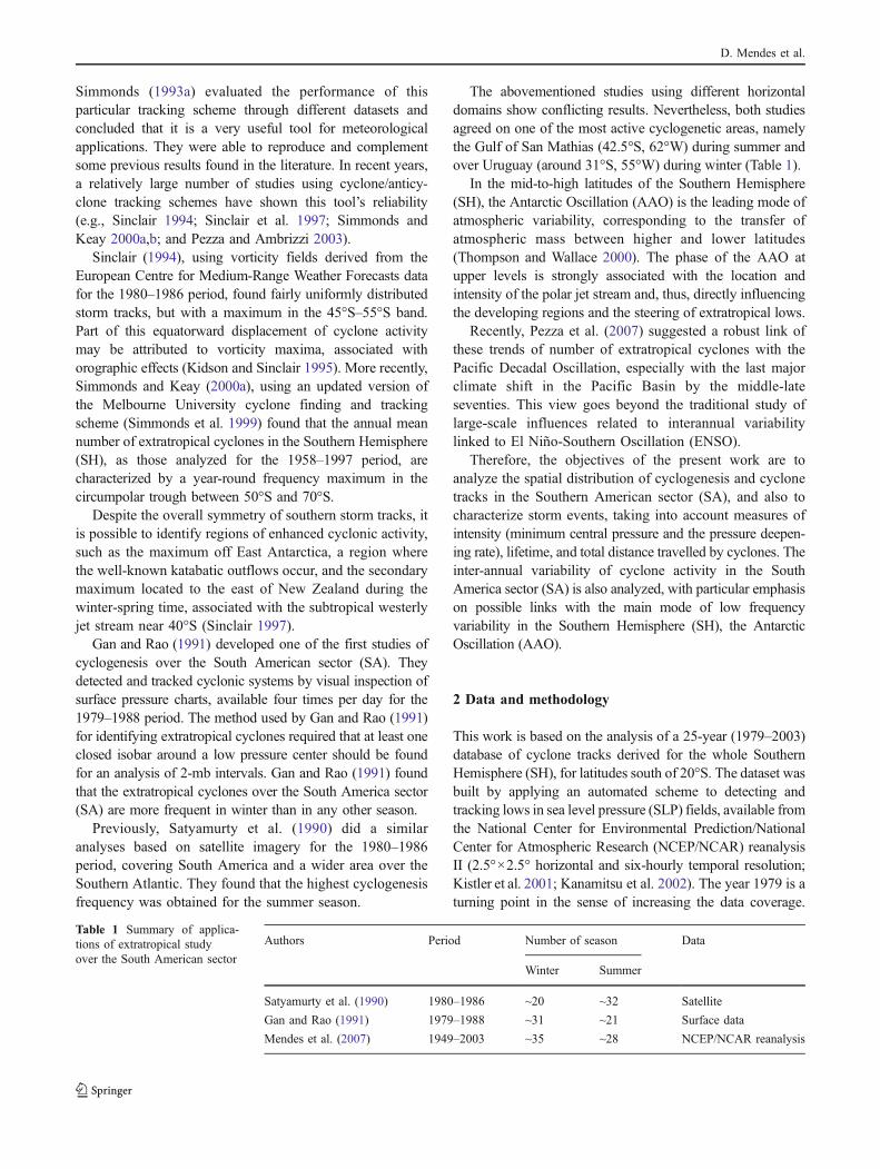
Figures 3 and 4 show, respectively, histograms of cyclone’slifetime and total distance travelled for systems originatedwithin the South American sector (SA) (light bars) and forsystems detected in the whole Southern Hemisphere (SH)(dark bars).

The highest frequency of cyclone lifetime is found with 2–3 days total duration, for both the South America sector andfor the whole Southern Hemisphere (SH). The latter, however,tends to have lower relative frequencies associated with thosemodal values and larger upper tails. This is particularly thecase of the winter and the spring distributions (Fig. 3a, b),where the fraction of lows lasting 8 days or more is about76% to 70%, compared with 85% to 80% in the vicinity ofSouth Hemisphere (SH). Many of these long-lasting systemsoccur over the circumpolar ocean, where they can also travelfor long distances (Simmonds and Keay 2000a,b).

Accordingly, the distribution of cyclone total-traveledpaths for the whole Southern Hemisphere (Fig. 4) presentslonger left tails, with secondary maxima between 2,600 and3,000 km, while the corresponding histograms for theSouthern American sector (SA) exhibit considerably lessskewness. Indeed, the extratropical cyclones generated over

Fig. 2 Number of cyclogenesis events detected per 3°×3° cell, for each season for the whole 25-year period

D. Mendes et al.

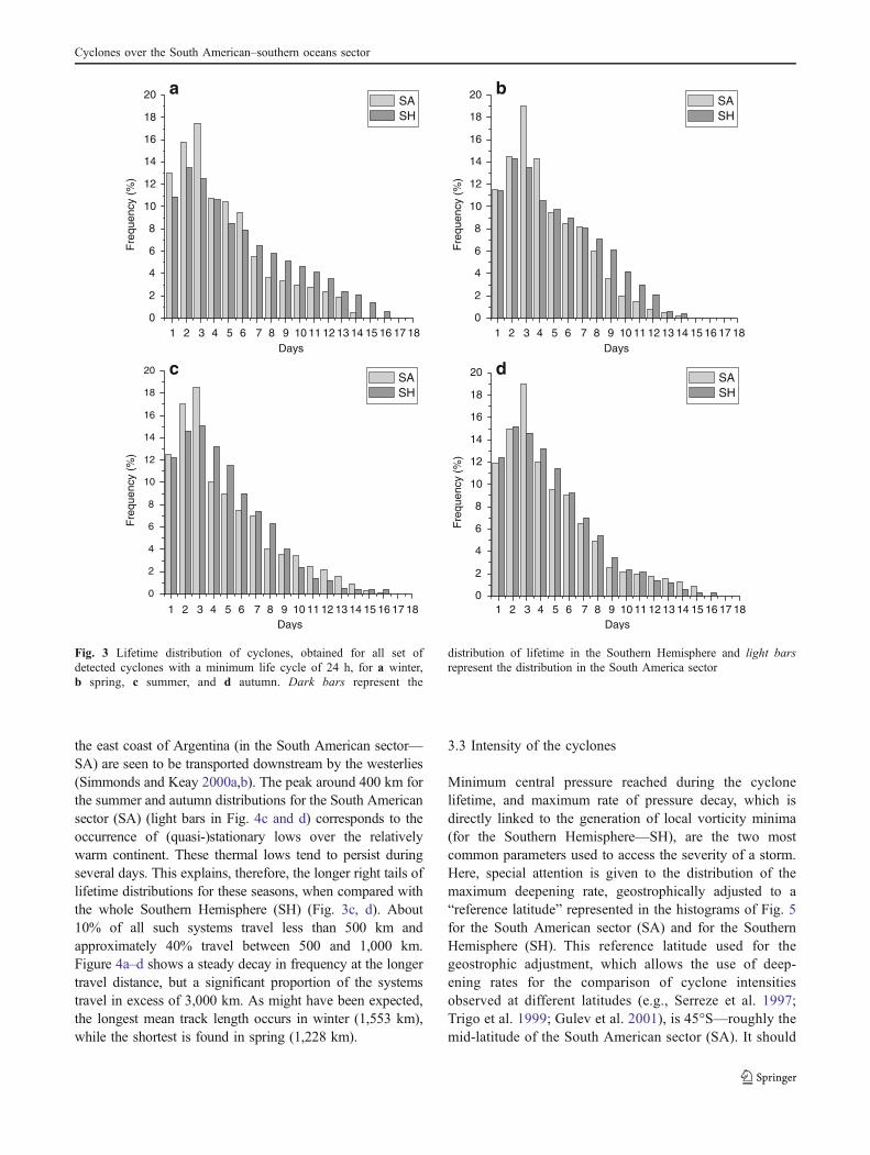
the east coast of Argentina (in the South American sector—SA) are seen to be transported downstream by the westerlies(Simmonds and Keay 2000a,b). The peak around 400 km forthe summer and autumn distributions for the South Americansector (SA) (light bars in Fig. 4c and d) corresponds to theoccurrence of (quasi-)stationary lows over the relativelywarm continent. These thermal lows tend to persist duringseveral days. This explains, therefore, the longer right tails oflifetime distributions for these seasons, when compared withthe whole Southern Hemisphere (SH) (Fig. 3c, d). About10% of all such systems travel less than 500 km andapproximately 40% travel between 500 and 1,000 km.Figure 4a–d shows a steady decay in frequency at the longertravel distance, but a significant proportion of the systemstravel in excess of 3,000 km. As might have been expected,the longest mean track length occurs in winter (1,553 km),while the shortest is found in spring (1,228 km).

3.3 Intensity of the cyclones

Minimum central pressure reached during the cyclonelifetime, and maximum rate of pressure decay, which isdirectly linked to the generation of local vorticity minima(for the Southern Hemisphere—SH), are the two mostcommon parameters used to access the severity of a storm.Here, special attention is given to the distribution of themaximum deepening rate, geostrophically adjusted to a“reference latitude” represented in the histograms of Fig. 5for the South American sector (SA) and for the SouthernHemisphere (SH). This reference latitude used for thegeostrophic adjustment, which allows the use of deep-ening rates for the comparison of cyclone intensitiesobserved at different latitudes (e.g., Serreze et al. 1997;Trigo et al. 1999; Gulev et al. 2001), is 45°S—roughly themid-latitude of the South American sector (SA). It should

1 2 3 4 5 6 7 8 9 10 11 12 13 14 15 16 17 18 1 2 3 4 5 6 7 8 9 10 11 12 13 14 15 16 17 18

1 2 3 4 5 6 7 8 9 10 11 12 13 14 15 16 17 181 2 3 4 5 6 7 8 9 10 11 12 13 14 15 16 17 18

0

2

4

6

8

10

12

14

16

18

20

Fre

quen

cy (

%)

Days

SA SH

0

2

4

6

8

10

12

14

16

18

20

Fre

quen

cy (

%)

Days

SA SH

0

2

4

6

8

10

12

14

16

18

20

Fre

quen

cy (

%)

Days

SA SH

0

2

4

6

8

10

12

14

16

18

20

Fre

quen

cy (

%)

Days

SA SH

a b

c d

Fig. 3 Lifetime distribution of cyclones, obtained for all set ofdetected cyclones with a minimum life cycle of 24 h, for a winter,b spring, c summer, and d autumn. Dark bars represent the

distribution of lifetime in the Southern Hemisphere and light barsrepresent the distribution in the South America sector

Cyclones over the South American–southern oceans sector

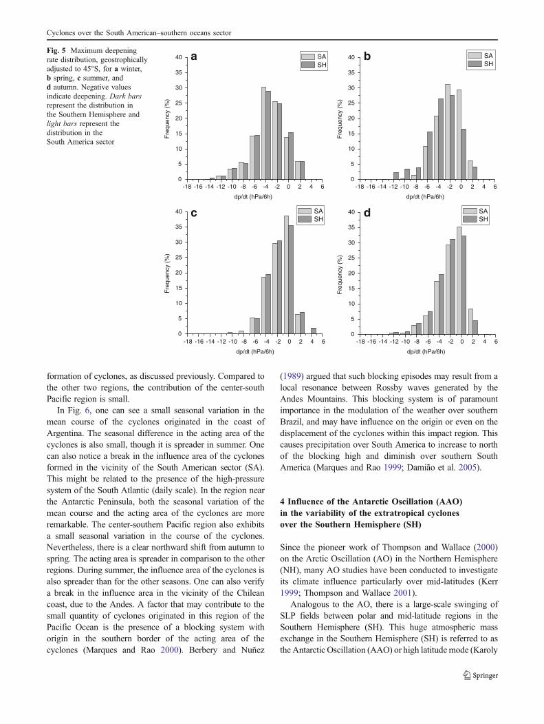
be pointed out that positive values correspond to eventsdetected when their minimum central pressure has alreadybeen reached.

The storm intensity, as measured by the maximumdeepening rate (hPa) (in order to analyze deepening forindividual cyclones, it is more effective to consider meanand extreme deepening rates during the phase of cycloneintensification rather than the overall statistics of deepeningrates) does not differ significantly between the SouthAmerican sector (SA) cases and the whole cyclonepopulation in the Southern Hemisphere (SH). Springpresents the distribution with the longest left tail (Fig. 5b),although the most extreme cases of very rapidly developingsystems, or explosive cyclones, tend to occur in winter.When compared with the Northern Hemisphere (NH),deepening rates are generally smoother in the SouthernHemisphere (SH), with a lower number of explosivecyclogenesis cases (e.g., Lim and Simmonds 2002).

3.4 Cyclone tracks

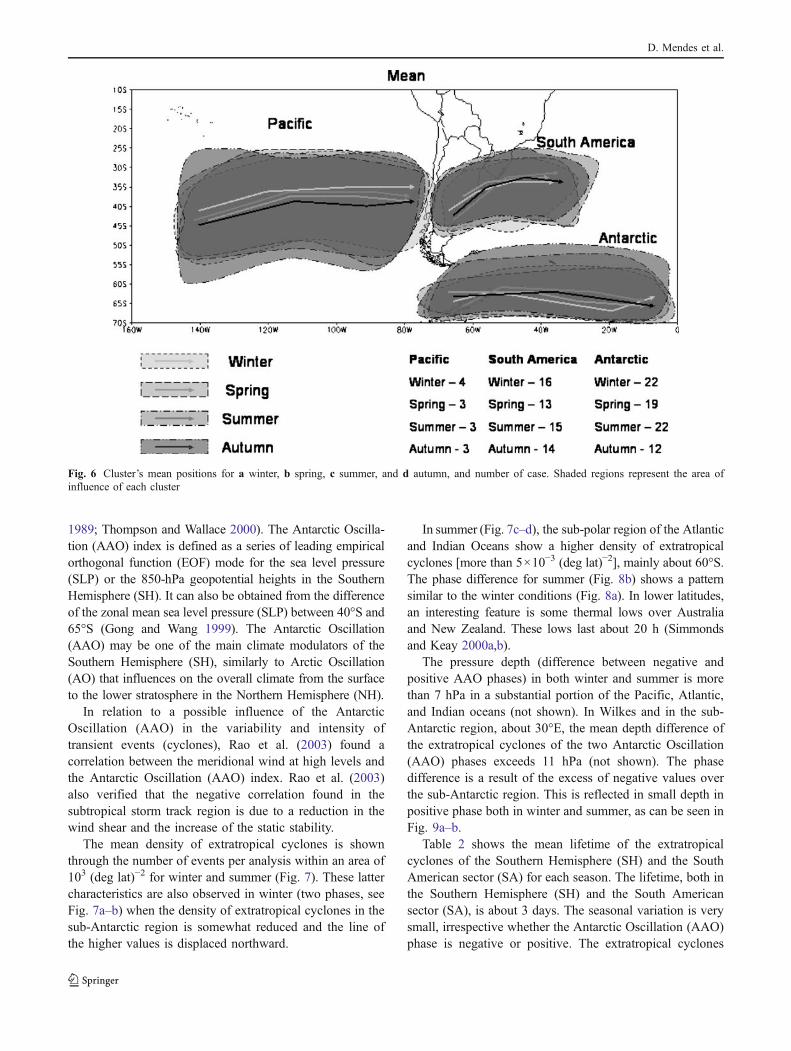
In order to identify the main paths of the cyclones originatedin the vicinity of the South American sector (SA), the stormtracks within the South American sector were subject to a k-mean cluster analysis. The goal of the k-mean algorithm is toget k clusters, which minimize the variability within theclusters, and maximize the variability among them (Mirkin1996). In the present case, the k-mean cluster analysis isapplied to the standardized vectors containing the six-hourly(latitude/longitude) positions of each cyclone. For a betterdefinition of the acting area of the cyclones in this study, weuse a value of one standard deviation to delimitate this areaof storm tracks. Figure 6 shows three regions with well-defined paths: the first one includes the coast of Argentina,Uruguay, and Southern Brazil; the second one is in theregion near the Antarctic Peninsula; and the third one is theSouth Central Pacific. The first two regions are regions of

0

2

4

6

8

10

12

14

16

18

20

Fre

quen

cy (

%)

SA SH

0

2

4

6

8

10

12

14

16

18

20

Fre

quen

cy (

%)

SA SH

1000 2000 3000 4000 5000 6000 1000 2000 3000 4000 5000 60000

2

4

6

8

10

12

14

16

18

20

Fre

quen

cy (

%)

Total Distance (km)

1000 2000 3000 4000 5000 6000

Total Distance (km)

1000 2000 3000 4000 5000 6000

Total Distance (km)

SA SH

0

2

4

6

8

10

12

14

16

18

20

Fre

quen

cy (

%)

Total Distance (km)

SA SH

a b

c d

Fig. 4 Distribution of total distance travelled by cyclones during the time life, for a winter, b spring, c summer, and d autumn. Dark barsrepresent the distribution in the Southern Hemisphere and light bars represent the distribution in the South America sector

D. Mendes et al.

formation of cyclones, as discussed previously. Compared tothe other two regions, the contribution of the center-southPacific region is small.

In Fig. 6, one can see a small seasonal variation in themean course of the cyclones originated in the coast ofArgentina. The seasonal difference in the acting area of thecyclones is also small, though it is spreader in summer. Onecan also notice a break in the influence area of the cyclonesformed in the vicinity of the South American sector (SA).This might be related to the presence of the high-pressuresystem of the South Atlantic (daily scale). In the region nearthe Antarctic Peninsula, both the seasonal variation of themean course and the acting area of the cyclones are moreremarkable. The center-southern Pacific region also exhibitsa small seasonal variation in the course of the cyclones.Nevertheless, there is a clear northward shift from autumn tospring. The acting area is spreader in comparison to the otherregions. During summer, the influence area of the cyclones isalso spreader than for the other seasons. One can also verifya break in the influence area in the vicinity of the Chileancoast, due to the Andes. A factor that may contribute to thesmall quantity of cyclones originated in this region of thePacific Ocean is the presence of a blocking system withorigin in the southern border of the acting area of thecyclones (Marques and Rao 2000). Berbery and Nuñez

(1989) argued that such blocking episodes may result from alocal resonance between Rossby waves generated by theAndes Mountains. This blocking system is of paramountimportance in the modulation of the weather over southernBrazil, and may have influence on the origin or even on thedisplacement of the cyclones within this impact region. Thiscauses precipitation over South America to increase to northof the blocking high and diminish over southern SouthAmerica (Marques and Rao 1999; Damião et al. 2005).

4 Influence of the Antarctic Oscillation (AAO)in the variability of the extratropical cyclonesover the Southern Hemisphere (SH)

Since the pioneer work of Thompson and Wallace (2000)on the Arctic Oscillation (AO) in the Northern Hemisphere(NH), many AO studies have been conducted to investigateits climate influence particularly over mid-latitudes (Kerr1999; Thompson and Wallace 2001).

Analogous to the AO, there is a large-scale swinging ofSLP fields between polar and mid-latitude regions in theSouthern Hemisphere (SH). This huge atmospheric massexchange in the Southern Hemisphere (SH) is referred to asthe Antarctic Oscillation (AAO) or high latitudemode (Karoly

-18 -16 -14 -12 -10 -8 -6 -4 -2 0 2 4 6 -18 -16 -14 -12 -10 -8 -6 -4 -2 0 2 4 60

5

10

15

20

25

30

35

40

Fre

quen

cy (

%)

dp/dt (hPa/6h) dp/dt (hPa/6h)

-18 -16 -14 -12 -10 -8 -6 -4 -2 0 2 4 6 -18 -16 -14 -12 -10 -8 -6 -4 -2 0 2 4 6

dp/dt (hPa/6h) dp/dt (hPa/6h)

SA SH

0

5

10

15

20

25

30

35

40

Fre

quen

cy (

%)

SA SH

0

5

10

15

20

25

30

35

40

Fre

quen

cy (

%)

SA SH

0

5

10

15

20

25

30

35

40

Fre

quen

cy (

%)

SA SH

a b

c d

Fig. 5 Maximum deepeningrate distribution, geostrophicallyadjusted to 45°S, for a winter,b spring, c summer, andd autumn. Negative valuesindicate deepening. Dark barsrepresent the distribution inthe Southern Hemisphere andlight bars represent thedistribution in theSouth America sector

Cyclones over the South American–southern oceans sector

1989; Thompson and Wallace 2000). The Antarctic Oscilla-tion (AAO) index is defined as a series of leading empiricalorthogonal function (EOF) mode for the sea level pressure(SLP) or the 850-hPa geopotential heights in the SouthernHemisphere (SH). It can also be obtained from the differenceof the zonal mean sea level pressure (SLP) between 40°S and65°S (Gong and Wang 1999). The Antarctic Oscillation(AAO) may be one of the main climate modulators of theSouthern Hemisphere (SH), similarly to Arctic Oscillation(AO) that influences on the overall climate from the surfaceto the lower stratosphere in the Northern Hemisphere (NH).

In relation to a possible influence of the AntarcticOscillation (AAO) in the variability and intensity oftransient events (cyclones), Rao et al. (2003) found acorrelation between the meridional wind at high levels andthe Antarctic Oscillation (AAO) index. Rao et al. (2003)also verified that the negative correlation found in thesubtropical storm track region is due to a reduction in thewind shear and the increase of the static stability.

The mean density of extratropical cyclones is shownthrough the number of events per analysis within an area of103 (deg lat)−2 for winter and summer (Fig. 7). These lattercharacteristics are also observed in winter (two phases, seeFig. 7a–b) when the density of extratropical cyclones in thesub-Antarctic region is somewhat reduced and the line ofthe higher values is displaced northward.

In summer (Fig. 7c–d), the sub-polar region of the Atlanticand Indian Oceans show a higher density of extratropicalcyclones [more than 5×10−3 (deg lat)−2], mainly about 60°S.The phase difference for summer (Fig. 8b) shows a patternsimilar to the winter conditions (Fig. 8a). In lower latitudes,an interesting feature is some thermal lows over Australiaand New Zealand. These lows last about 20 h (Simmondsand Keay 2000a,b).

The pressure depth (difference between negative andpositive AAO phases) in both winter and summer is morethan 7 hPa in a substantial portion of the Pacific, Atlantic,and Indian oceans (not shown). In Wilkes and in the sub-Antarctic region, about 30°E, the mean depth difference ofthe extratropical cyclones of the two Antarctic Oscillation(AAO) phases exceeds 11 hPa (not shown). The phasedifference is a result of the excess of negative values overthe sub-Antarctic region. This is reflected in small depth inpositive phase both in winter and summer, as can be seen inFig. 9a–b.

Table 2 shows the mean lifetime of the extratropicalcyclones of the Southern Hemisphere (SH) and the SouthAmerican sector (SA) for each season. The lifetime, both inthe Southern Hemisphere (SH) and the South Americansector (SA), is about 3 days. The seasonal variation is verysmall, irrespective whether the Antarctic Oscillation (AAO)phase is negative or positive. The extratropical cyclones

Fig. 6 Cluster’s mean positions for a winter, b spring, c summer, and d autumn, and number of case. Shaded regions represent the area ofinfluence of each cluster

D. Mendes et al.

whose cyclogenesis occurs between 45° and 75°S are morelong lasting than those originated in lower latitudes. Thelifetime of extratropical cyclones originated in the sub-polarregion exhibits a moderate seasonality in both phases.

5 Summary and concluding remarks

Cyclones are of major importance in the modulation ofweather and climate in South America. In the Southern

Fig. 7 Extratropical cyclonesmeasurement means number peranalysis found in a 103 (deg lat)2

in a winter and b summer.Contour interval is 2×10−3

(deg lat)−2 in positive andnegative phase

4.5

3.5

2.5

1.5

0.5

–0.5

–1.5

–2.5

–3.5

–4.5

4.5

3.5

2.5

1.5

0.5

–0.5

–1.5

–2.5

–3.5

–4.5

WINTERDif (Neg – Pos)

SUMMERDif (Neg – Pos)

(a) (b)

Fig. 8 Difference between extratropical cyclones density in negative and positive phase in a winter and b summer. Contour interval is 0.5×10−3

(deg lat)−3day−1

Cyclones over the South American–southern oceans sector

Hemisphere (SH), few studies have focused on thecharacteristics and frequencies, as well as possible variabil-ity of cyclones in ENSO years (Sinclair 1994; Simmondsand Keay 2000a,b; Solman and Menéndez 2001; Pezza andAmbrizzi 2003). Previous studies in southern SouthAmerica have used short-term data for First GARP GlobalExperiment (FGGE) to investigate the characteristics andvariability of cyclones. Necco (1982) used 1 year of datafrom the FGGE. Satyamurty et al. (1990) used satelliteimages to diagnose cyclones for a period of 7 years. Ganand Rao (1991) developed a short-term climatology using10 years of data of surface observations for 1979–1988. Inthis paper, we developed an analysis of the quantity ofcyclones for the four seasons, and verified some character-istics of the cyclones, such as lifetime, maximum deepen-ing, and overall distance traveled using the 1979–2003NCEP/NCAR reanalyses II. We also verified the spacevariability through clusters for seasons with negative andpositive Antarctic Oscillation (AAO) phases.

It was found a characteristic region for formation ofcyclones, located near the coast of Argentina, Uruguay, andSouthern Brazil. This region is characterized as a cyclo-genesis one for cyclones that form in the vicinity of the

South American sector (SA). Winter and summer are theseasons with the largest quantity of cyclones formed in thisregion. These results are in agreement with those obtainedby Satyamurty et al. (1990) and Gan and Rao (1991), aswell as those obtained by Simmonds and Keay (2000a,b)from their 40-year climatology of cyclones for the SouthernHemisphere (SH).

In relation to lifetime (life cycle), there is a strikingsimilarity between the extratropical cyclones formed in theregion of the South American sector (SA) and the cyclonesin the entire Southern Hemisphere (SH). In the distributionof the frequency of the lifetime, we verified a smallvariability between seasons, not only for the cyclonesformed in the region of the South American sector (SA) butalso for the Southern Hemisphere (SH). In relation to thefrequency of the maximum deepening, winter is the seasonwith more different characteristics, being verified a largeskewness (intensification of extratropical cyclones). For theoverall distance traveled by the cyclones, as well as for themaximum deepening, the winter cyclones exhibited differ-ent characteristics in relation to those of the other seasons.In winter, the frequency of distance is better distributed, andin spring and in autumn the cyclones rarely travel distances

Table 2 Mean extratropical cyclones tracks duration (days) for at least 24 h

Summer Autumn Winter Spring

POS NEG ALL POS NEG ALL POS NEG ALL POS NEG ALL

SH 3.06 3.04 3.04 3.11 3.08 3.10 3.15 3.11 3.14 3.05 3.01 3.02

SA 3.05 3.01 3.03 2.92 2.86 2.99 3.05 3.02 3.07 3.0 2.98 3.01

15°–45°S 2.65 2.58 2.61 2.61 2.57 2.60 2.42 2.40 2.42 2.48 2.46 2.48

45°–75°S 3.19 3.11 3.15 3.19 3.14 3.20 3.22 3.21 3.25 3.27 3.25 3.24

75°–90°S 2.19 2.18 2.19 2.66 2.65 2.66 2.55 2.50 2.54 2.31 2.31 2.35

An extratropical cyclone track is allocated to the latitude band and phase of the Antarctic Oscillation (AAO). POS means positive, NEG meansnegative, and ALL means positive, negative, and neutral phases

5

4

3

2

1

–1

–2

–3

–4

–5

5

4

3

2

1

–1

–2

–3

–4

–5

WINTERDif (Neg – Pos)

SUMMERDif (Neg – Pos)

(a) (b)

Fig. 9 Difference betweenextratropical cyclones depth in awinter and b summer fornegative and positive phase ofthe Antarctic Oscillation (AAO).Contour interval is 1 hPa

D. Mendes et al.

larger than 3,000 km. These results compared well withthose of Simmonds and Keay (2000a,b). To gain insightabout the acting area, as well as the average course of thecyclones, we used a cluster analysis that gave three regionslocated on the coast of Argentina, Uruguay, and southernBrazil, near the Antarctic Peninsula and in the SoutheasternPacific, for the same period of analysis of the cyclones(25 years of data). These results show little variability in theregion of influence of the cyclones for the three areasstudied, and also for their mean trajectories.

Effects of variation in the Antarctic Oscillation (AAO)phase were observed in the extratropical cyclones (~40°S).The higher extratropical cyclone density is found south of45°S in all seasons, with values exceeding 5×10−3 extra-tropical cyclones (deg lat)−2 over the Indian and PacificOceans. This is more remarkable in winter of the positiveAntarctic Oscillation (AAO) period. In summer, the structureis similar, but with less density for extratropical cyclones.

The largest variation of extratropical cyclone depth isfound about 55°S, north of the Antarctic region that presentshigh density of extratropical cyclones, both in winter andsummer, despite the Antarctic Oscillation (AAO) phase.

Acknowledgements The present work was supported by the POCTIprogram (Portuguese Office for Science and Technology), Grant BD/8482/2002 and FAPESP grant 07/50145-4, and Enio P. Souza andJose A. Marengo were funded by the Brazilian Conselho Nacional deDesenvolvimento Cientifico e Tecnologico—CNPq. The authorswould like to thank Dr. Isabel F. Trigo and Dr. Pedro A. Mirandafor their helpful suggestions. We are also grateful for the helpfulcomments made by two anonymous reviewers.

References

Berbery EH, Núñez MN (1989) An observational and numerical studyof blocking episodes near South America. J Climate 2:1352–1361

Blender R, Fraedrich K, Lunkeit F (1997) Identification of cyclonetrack regimes in North Atlantic. Quart J Roy Meteor Soc 123:727–741

Bonatti JP, Rao VB (1987) Moist baroclinic instability in thedevelopment of the North Pacific and South Americanintermediate-scale disturbances. J Atmos Sci 44:2657–2667

Damião MCM, Trigo RM, Cavalcanti IF, DaCamara CC (2005)Bloqueios armosféricos de 1960 a 2000 sobre o Oceano PacíficoSul: Impactos climáticos e Mecanismos Físicos Associados. RevBras Meteor 20(2):175–190

Gan MA, Rao VB (1991) Surface cyclogenesis over South America.Mon Wea Rev 119:1293–1302

Gan MA, Rao VB (1994) The influence of the Andes Cordillera ontransient disturbances. Mon Wea Rev 122:1141–1157

Gong D, Wang S (1999) Definition of Antarctic oscillation index.Geophys Res Lett 26:459–462

Gulev SK, Zolina O, Grigoriev S (2001) Extratropical cyclonevariability in the Northern Hemisphere winter from the NCEP/NCAR reanalysis data. Climate Dyn 17:795–809

Jones DA, Simmonds I (1993) A climatology of Southern Hemisphereextratropical cyclones. Climate Dyn 9:131–145

Kanamitsu M, Ebisuzaki W, Woollen J, Yang S-K, Hnilo JJ, Fiorino M,Potter GL (2002) NCEP-DEO AMIP-II Reanalysis (R-2) BullAtmos 1631–1643

Karoly DJ (1989) Southern Hemisphere circulation features associatedwith El Niño-Southern Oscillation events. J Climate 2:1239–1252

Kerr RA (1999) Big El Niños ride the back of slower climate change.Science 283:1108–1109

Kidson JW, Sinclair MR (1995) The influence of persistent anomalieson Southern Hemisphere storm tracks. J Climate 8:1938–1950

Lim E-P, Simmonds I (2002) Explosive cyclone development in theSouthern Hemisphere and a comparison with Northern Hemi-sphere events. Mon Wea Rev 130:2188–2209

Marques RFC, Rao VB (2000) Inter-annual variations of blocking inthe Southern Hemisphere and their energetic. J Geophys Res105:4628–4636

Marques RFC, Rao VB (1999) A diagnosis of a long-lastingblocking event over the southeast Pacific Ocean. Mon WeaRev 127:1761–1775

Kistler R et al (2001) The NCEP-NCAR 50-year reanalysis: monthlymeans CD-ROM and documentation. Bull Amer Meteor Soc82:247–267

Mendes D, Souza EP, Trigo IF, Miranda PMA (2007) On precursorsof South-American cyclogenesis. Tellus A 59:114–121

Mirkin, B., 1996: Mathematical classification and clustering. Kluwer,Dordrecht 428 pp.

Murray RJ, Simmonds I (1991a) A numerical scheme for trackingcyclone centres from digital data. Part I: Development andoperation of the scheme. Aust Meteorol Mag 39:155–166

Murray RJ, Simmonds I (1991b) A numerical scheme for trackingcyclone centres from digital data. Part II: Application to Januaryand July general circulation model simulations. Aust MeteorolMag 39:167–180

Necco GV (1982) Comportamiento de vortices ciclónicos en el áreasudamericana durante el FGGE: ciclogénesis. Meteorológica 13(1):7–20

Petterssen S (1950) Some aspects of the general circulation. Centen.Proc Roy Met Soc, Roy Meteor Soc 120–155

Pezza AB, Ambrizzi T (2003) Variability of Southern Hemispherecyclone and anticyclone behavior: further analysis. J Climate16:1075–1083

Pezza AB, Simmonds I, Renwick JA (2007) Southern Hemispherecyclones and anticyclones: recent trends and links with decadalvariability in the Pacific Ocean. Int J Climatol 27:1403–1419

Rao VB, Do Carmo AMC, Franchito SH (2003) Inter-annualvariations of storm tracks in the Southern Hemisphere and theirconnections with the Antarctic Oscillation. Int J Climatol23:1537–1545

Satyamurty P, Ferreira CC, Gan MA (1990) Cyclonic vortices overSouth America. Tellus 42A:194–201

Serreze MC, Carse F, Barry RG, Rogers JC (1997) Icelandic lowcyclone activity: climatological features, linkages with the NAO,and relationships with recent changes in the Northern Hemi-sphere circulation. J Climate 10:453–464

Simmonds I, Keay K (2000a) Variability of Southern HemisphereExtratropical Cyclone Behavior, 1958–1997. J Climate 13:550–561

Simmonds I, Keay K (2000b) Mean southern extratropical cyclonebehavior in the 40-year NCEP–NCAR reanalysis. J Climate13:873–885

Simmonds I, Murray RJ, Leighton RM (1999) A refinement ofcyclone tracking methods with data from FROST. Aust MeteorMag, Special Issue, 35–49

Sinclair MR (1994) An objective cyclone climatology for the SouthernHemisphere. Mon Wea Rev 122:2239–2256

Sinclair MR (1995) A climatology of cyclogenesis for the SouthernHemisphere. Mon Wea Rev 123:1601–1619

Cyclones over the South American–southern oceans sector

Sinclair MR (1997) Objective identification of cyclones and theircirculation intensity, and climatology. Weather Forecast 12:595–612

Sinclair MR, Renwick JA, Kidson JW (1997) Low-frequencyvariability of Southern pressure and weather system activity.Mon Wea Rev 127:2531–2542

Solman SA, Menéndez CG (2001) ENSO-related variability of theSouthern Hemisphere winter storm tracks over the EasternPacific–Atlantic Sector. J Atmos Sci 59:2128–2140

Thompson DWJ, Wallace JM (2000) Annular modes in the extra-tropical circulation. Part I: Month-to-month variability. J Climate13:1000–1016

Thompson DWJ, Wallace JM (2001) Regional climate impacts of theNorthern Hemisphere annular mode. Science 293:85–89

Trigo IF, Davies TD, Bigg GR (1999) Objective climatologyof cyclones in the Mediterranean region. J Climate 12:1685–1696

D. Mendes et al.