Ozone and UV Radiation over Southern South America: Climatology and Anomalies
10
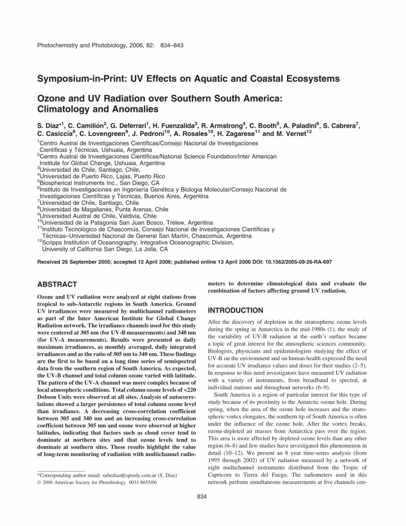
Photochemistry and Photobiology, 2006, 82: 834–843 Symposium-in-Print: UV Effects on Aquatic and Coastal Ecosystems Ozone and UV Radiation over Southern South America: Climatology and Anomalies S. Diaz* 1 , C. Camilio ´n 2 , G. Deferrari 1 , H. Fuenzalida 3 , R. Armstrong 4 , C. Booth 5 , A. Paladini 6 , S. Cabrera 7 , C. Casiccia 8 , C. Lovengreen 9 , J. Pedroni 10 , A. Rosales 10 , H. Zagarese 11 and M. Vernet 12 1 Centro Austral de Investigaciones Cientı ´ficas/Consejo Nacional de Investigaciones Cientı ´ficas y Te ´ cnicas, Ushuaia, Argentina 2 Centro Austral de Investigaciones Cientı ´ficas/National Science Foundation/Inter American Institute for Global Change, Ushuaia, Argentina 3 Universidad de Chile, Santiago, Chile, 4 Universidad de Puerto Rico, Lajas, Puerto Rico 5 Biospherical Instruments Inc., San Diego, CA 6 Instituto de Investigaciones en Ingenierı ´a Gene ´ tica y Biologı ´a Molecular/Consejo Nacional de Investigaciones Cientı ´ficas y Te ´ cnicas, Buenos Aires, Argentina 7 Universidad de Chile, Santiago, Chile 8 Universidad de Magallanes, Punta Arenas, Chile 9 Universidad Austral de Chile, Valdivia, Chile 10 Universidad de la Patagonia San Juan Bosco, Trelew, Argentina 11 Instituto Tecnolo ´ gico de Chascom us, Consejo Nacional de Investigaciones Cientı ´ficas y Te ´ cnicas–Universidad Nacional de General San Martı ´n, Chascom us, Argentina 12 Scripps Institution of Oceanography, Integrative Oceanographic Division, University of California San Diego, La Jolla, CA Received 26 September 2005; accepted 12 April 2006; published online 13 April 2006 DOI: 10.1562/2005-09-26-RA-697 ABSTRACT Ozone and UV radiation were analyzed at eight stations from tropical to sub-Antarctic regions in South America. Ground UV irradiances were measured by multichannel radiometers as part of the Inter American Institute for Global Change Radiation network. The irradiance channels used for this study were centered at 305 nm (for UV-B measurements) and 340 nm (for UV-A measurements). Results were presented as daily maximum irradiances, as monthly averaged, daily integrated irradiances and as the ratio of 305 nm to 340 nm. These findings are the first to be based on a long time series of semispectral data from the southern region of South America. As expected, the UV-B channel and total column ozone varied with latitude. The pattern of the UV-A channel was more complex because of local atmospheric conditions. Total column ozone levels of <220 Dobson Units were observed at all sites. Analysis of autocorre- lations showed a larger persistence of total column ozone level than irradiance. A decreasing cross-correlation coefficient between 305 and 340 nm and an increasing cross-correlation coefficient between 305 nm and ozone were observed at higher latitudes, indicating that factors such as cloud cover tend to dominate at northern sites and that ozone levels tend to dominate at southern sites. These results highlight the value of long-term monitoring of radiation with multichannel radio- meters to determine climatological data and evaluate the combination of factors affecting ground UV radiation. INTRODUCTION After the discovery of depletion in the stratospheric ozone levels during the spring in Antarctica in the mid-1980s (1), the study of the variability of UV-B radiation at the earth’s surface became a topic of great interest for the atmospheric sciences community. Biologists, physicians and epidemiologists studying the effect of UV-B on the environment and on human health expressed the need for accurate UV irradiance values and doses for their studies (2–5). In response to this need investigators have measured UV radiation with a variety of instruments, from broadband to spectral, at individual stations and throughout networks (6–9). South America is a region of particular interest for this type of study because of its proximity to the Antarctic ozone hole. During spring, when the area of the ozone hole increases and the strato- spheric vortex elongates, the southern tip of South America is often under the influence of the ozone hole. After the vortex breaks, ozone-depleted air masses from Antarctica pass over the region. This area is more affected by depleted ozone levels than any other region (6–8) and few studies have investigated this phenomenon in detail (10–12). We present an 8 year time-series analysis (from 1995 through 2002) of UV radiation measured by a network of eight multichannel instruments distributed from the Tropic of Capricorn to Tierra del Fuego. The radiometers used in this network perform simultaneous measurements at five channels cen- *Corresponding author email: [email protected] (S. Diaz) Ó 2006 American Society for Photobiology 0031-8655/06 834
-
Upload
independent -
Category
Documents
-
view
3 -
download
0
Transcript of Ozone and UV Radiation over Southern South America: Climatology and Anomalies
Photochemistry and Photobiology, 2006, 82: 834–843
Symposium-in-Print: UV Effects on Aquatic and Coastal Ecosystems
Ozone and UV Radiation over Southern South America:Climatology and Anomalies
S. Diaz*1, C. Camilion2, G. Deferrari1, H. Fuenzalida3, R. Armstrong4, C. Booth5, A. Paladini6, S. Cabrera7,C. Casiccia8, C. Lovengreen9, J. Pedroni10, A. Rosales10, H. Zagarese11 and M. Vernet12
1Centro Austral de Investigaciones Cientıficas/Consejo Nacional de InvestigacionesCientıficas y Tecnicas, Ushuaia, Argentina
2Centro Austral de Investigaciones Cientıficas/National Science Foundation/Inter AmericanInstitute for Global Change, Ushuaia, Argentina
3Universidad de Chile, Santiago, Chile,4Universidad de Puerto Rico, Lajas, Puerto Rico5Biospherical Instruments Inc., San Diego, CA6Instituto de Investigaciones en Ingenierıa Genetica y Biologıa Molecular/Consejo Nacional deInvestigaciones Cientıficas y Tecnicas, Buenos Aires, Argentina
7Universidad de Chile, Santiago, Chile8Universidad de Magallanes, Punta Arenas, Chile9Universidad Austral de Chile, Valdivia, Chile10Universidad de la Patagonia San Juan Bosco, Trelew, Argentina11Instituto Tecnologico de Chascom�us, Consejo Nacional de Investigaciones Cientıficas y
Tecnicas–Universidad Nacional de General San Martın, Chascom�us, Argentina12Scripps Institution of Oceanography, Integrative Oceanographic Division,
University of California San Diego, La Jolla, CA
Received 26 September 2005; accepted 12 April 2006; published online 13 April 2006 DOI: 10.1562/2005-09-26-RA-697
ABSTRACT
Ozone and UV radiation were analyzed at eight stations fromtropical to sub-Antarctic regions in South America. GroundUV irradiances were measured by multichannel radiometersas part of the Inter American Institute for Global ChangeRadiation network. The irradiance channels used for this studywere centered at 305 nm (for UV-B measurements) and 340 nm(for UV-A measurements). Results were presented as dailymaximum irradiances, as monthly averaged, daily integratedirradiances and as the ratio of 305 nm to 340 nm. These findingsare the first to be based on a long time series of semispectraldata from the southern region of South America. As expected,the UV-B channel and total column ozone varied with latitude.The pattern of the UV-A channel was more complex because oflocal atmospheric conditions. Total column ozone levels of <220Dobson Units were observed at all sites. Analysis of autocorre-lations showed a larger persistence of total column ozone levelthan irradiance. A decreasing cross-correlation coefficientbetween 305 and 340 nm and an increasing cross-correlationcoefficient between 305 nm and ozone were observed at higherlatitudes, indicating that factors such as cloud cover tend todominate at northern sites and that ozone levels tend todominate at southern sites. These results highlight the valueof long-term monitoring of radiation with multichannel radio-
meters to determine climatological data and evaluate thecombination of factors affecting ground UV radiation.
INTRODUCTION
After the discovery of depletion in the stratospheric ozone levels
during the spring in Antarctica in the mid-1980s (1), the study of
the variability of UV-B radiation at the earth’s surface became
a topic of great interest for the atmospheric sciences community.
Biologists, physicians and epidemiologists studying the effect of
UV-B on the environment and on human health expressed the need
for accurate UV irradiance values and doses for their studies (2–5).
In response to this need investigators have measured UV radiation
with a variety of instruments, from broadband to spectral, at
individual stations and throughout networks (6–9).
South America is a region of particular interest for this type of
study because of its proximity to the Antarctic ozone hole. During
spring, when the area of the ozone hole increases and the strato-
spheric vortex elongates, the southern tip of South America is often
under the influence of the ozone hole. After the vortex breaks,
ozone-depleted air masses from Antarctica pass over the region.
This area is more affected by depleted ozone levels than any other
region (6–8) and few studies have investigated this phenomenon in
detail (10–12). We present an 8 year time-series analysis (from
1995 through 2002) of UV radiation measured by a network of
eight multichannel instruments distributed from the Tropic of
Capricorn to Tierra del Fuego. The radiometers used in this
network perform simultaneous measurements at five channels cen-*Corresponding author email: [email protected] (S. Diaz)
� 2006 American Society for Photobiology 0031-8655/06
834

tered at 305 nm and 320 nm (UV-B), 340 nm and 380 nm (UV-A)
and 400–700 nm (photosynthetically active radiation [PAR]). They
provide valuable information on the spectral distribution of the
solar radiation as it relates to ozone dynamics and other factors.
MATERIALS AND METHODS
Surface UV radiation is a function of several factors, such as the distancebetween the earth and sun, the levels of atmospheric gases and aerosols, thesolar zenith angle (SZA), the cloud cover, the altitude and the surfacealbedo. Geometric factors (i.e. the SZA and the distance between the earthand sun) are responsible for pronounced and systematic variations inirradiance. For example, variation in the distance between the earth andsun produces an alteration in extraterrestrial radiation of 7% between themaximum distance at the beginning of July and the minimum distance atthe beginning of January (23). Irradiance variation with respect to time ofthe day, latitude and season result from changes in the SZA. Cloud cover isan important factor to which short-term variability is attributed. Cloudsattenuate the level of UV irradiance, although partly cloudy conditionshave been associated with increases of up to 27% over levels for clearskies (24,25).
Ozone. Total column ozone levels were measured by Total OzoneMapping Spectrometers, version 8, on Nimbus-7, Meteor-3, and EarthProbe satellites and data were provided by the North American SpaceAdministration (NASA) Goddard Space Flight Center (13,14). Weexamined data obtained from January 1979 through December 2004;historical maximum, minimum and mean values for each Julian Day andannual cycle were determined. The mean annual total column level and itsinterannual variation were also determined. The global ultraviolet (GUV),which was originally located in Puerto Madryn, was moved to Trelewduring 1998. Both cities are very close to each other (50 km apart);therefore, ozone data for Trelew were used in the analysis of the dataobtained at both sites. Because NASA does not provide overpass values forBariloche (41.018S, 71.428W), the closest grid point (lat 41.58S, long71.8758W) was selected.
To determine the annual cycle we used a procedure described in Wilks(15), which is a more general version of the Fast Fourier Transform (FFT)spectral analysis. FTT has the advantage that equidistant data are notneeded because coefficients and phases corresponding to the harmoniccomponents are obtained via multivariate analysis.
The annual component of a time series may be represented by thefollowing cosine function:
yt ¼ �yþ C1 cos2pt
n� u1
� �ðEq: 1Þ
where yt is the value obtained on day t, �y : is the mean value of the annualcycle, t is time, n is number of days in the annual cycle (in this case, 365days), C1 is amplitude of the annual cycle and u1 is the phase.
Equation 1 may be reformulated by taking into account that
cosða� u1Þ ¼ cosðu1Þ cosðaÞ þ sinðu1Þ sinðaÞ ðEq: 2Þ
Also, after performing the following replacement
A1 ¼ C1 cosðu1ÞB1 ¼ C1 sinðu1Þ
and the following change of variable
x1 ¼ cosðaÞx2 ¼ sinðaÞ
where
a ¼ ð2pt=nÞ
(Eq. 1) is transformed into a regressive equation with two predictors,as follows:
yt ¼ �yþ A1x1 þ B1x2 ðEq: 3Þ
Usually, the annual cycle is not a pure cosine function. It is rather the sumof the first (n5 365), second (n 5180) and third (n5120) harmonics. If thisis taken into account and the procedure explained above is followed,a multivariate equation with six predictors is obtained that, when solved,provides the annual cycle. The independent term of (Eq. 3) corresponds tothe mean of the annual cycle or continuous component in the FFT. Toconfirm that the first three harmonics were enough to represent the annualcycle, we performed a spectral analysis of the residuals (i.e. historical meanvalue minus the annual cycle value), which showed that the annual cyclehad been totally removed. Also, we added a fourth harmonic and confirmedthat it did not improve the annual cycle (data not shown).
To complete the analysis the mean annual total column ozone level wascalculated. Also, we determined the mean (6SD) of the annual mean timeseries and the maximum and minimum values (and the years in which theyoccurred). The mean value of the annual means for 1980–1986 wasincluded as reference. This period was selected as reference because itincludes data from years in which the first satellite measurements wereperformed, when total column ozone levels were less affected by strato-spheric depletion, and because it covers half a solar cycle (from a maximumto a minimum).
UV irradiances. In order to study irradiance climatologies, we analyzedthe measurements provided by the Inter American Institute for GlobalChange Radiation Network (IAI RadNet). At present this network is com-posed of 10 multichannel radiometers (GUV 511, Biospherical InstrumentsInc.), located in Chile, Argentina and Puerto Rico (Table 1). The instrumentsof the IAI RadNet were installed during the 1990s through the efforts ofdifferent nations and are still in operation. The geographical distributionof the stations allowed comparisons between tropical and sub-Antarcticregions. Data from 1995 to 2002 are presented in this analysis. Data fromall stations except those in Puerto Rico and Trelew 2 are included.
The GUV511 is a temperature-stabilized multichannel radiometer thatmeasures downwelling irradiances with moderately narrow bandwidth
Table 1. Sites, geographic coordinates, altitude, date of starting operation or period considered in this study and total number of days in the period.*
Region (country) Lat, long; elevation Study periodDuration of study
period (days)
La Parguera (Puerto Rico) 17858.2249N, 67802.7239W; 16 m Since 1 January 1995 —San Salvador de Jujuy (Argentina) 24.178S, 65.028W; 1300 m 1 January 1995–31 December 2002 2574Buenos Aires (Argentina) 34.588S, 58.478W; sea level 1 January 1995–31 December 2002 2840Santiago de Chile (Chile) 33.418S, 70.658W; sea level 1 January 1995–31 December 2002 (Except 1997) 1473San Carlos de Bariloche (Argentina) 41.018S, 71.428W; 700 m 7 August 1998–31 December 2002 1307Valdivia (Chile) 39.818S, 73.258W; sea level 1 January 1995–31 December 2002 2536Puerto Madryn–Playa Union (Argentina) 43.38S, 65.058W; sea level 1 January 1995–31 December 2002 2492Trelew (Argentina) 43.258S, 65.318W; sea level 1 January 1995–31 December 2002 2492Trelew 2 (Argentina) 43.258S, 65.318W; sea level Since 1 January 1999 —Punta Arenas (Chile) 53.098S, 70.558W; sea level 1 January 1995–31 December 2002 (except 1997) 2014Ushuaia (Argentina) 548509S, 688189W; sea level 1 January 1995–31 December 2002 2492
*This article includes data from all stations except Puerto Rico and Trelew 2.
Photochemistry and Photobiology, 2006, 82 835
channels (near 10 nm), centered at approximately 305, 320, 340 and380 nm, plus PAR (400–700 nm) (16).
All instruments collected one measurement each minute 24 h per day.Raw data were processed by means of software provided by BiosphericalInstruments and were modified by the Laboratory of UV and Ozone,CADIC, Ushuaia. During data processing the quality and consistency of thedata were checked, night values (comprising instrument internal noise) weresubtracted and calibration constants were applied. When the temperaturecontroller failed or the operational temperature of the instrument differedfrom the temperature at the moment of the calibration, temperaturecorrections were applied to the calibration constants (17). Any observedchanges in radiometric data were assumed to be linear. Therefore, cal-ibration constants applied between two calibrations dates were calculatedby linear interpolation between the two closest calibrations, unless anabrupt known change (e.g. during filter replacement) had occurred.
The GUV-511 apparatus were periodically sun calibrated, usually onceper year, with a traveling reference GUV (RGUV) (16). The referenceradiometer was calibrated under solar light (before and after movement)against the spectroradiometer SUV100 of the US National ScienceFoundation UV Radiation Monitoring Network (San Diego, CA) (18).During RGUV calibration the output voltage from each channel of theradiometer was related to the calibrated irradiance measured by thespectroradiometer at the nominal central wavelength of the channel. As a re-sult, a calibrated monochromatic irradiance was obtained. Because of thebandwidth of the radiometer (10 nm), changes in the SZA and the ozonelevel introduce an error in the measurements performed by the RGUV,mainly in the 305 nm channel. These errors may be addressed by in-troducing the total column ozone level and the SZA in the calculation of thecalibrated irradiance (19). In this way the calibration would be representedby a function rather than by a constant. Data from all calibrations during theperiod included in the present article were not available in order to back-calculate calibrations with the new improved procedure. Thus, the ozoneand SZA corrections were not used in the analysis presented here. Testsperformed during the calibration in 2000 indicated that the GUVs of thenetwork had an error of 8–13%, based on the 305 channel and a SZA of,608, with respect to the SUV-100 at San Diego, where the correctionsfor SZA and ozone were not applied. For channel 340, the error was ,5%for all SZAs.
Irradiances were presented for channels 305 and 340 of the GUV-511.The first channel was chosen because it is the most sensitive to ozonechanges and the second because it is independent of ozone variations anda good proxy for factors like cloud cover (20). Time-series analyses werebased on daily maximum irradiance values. When no clouds are present,maximum irradiance occurs at solar noon; when clouds are present, largerirradiance values may occur at other times of the day. For each JulianDay we determined the historical maximum, minimum and mean irradiancevalues; the annual cycle was inferred on the basis of these values. Theprocedure for calculating the total column ozone annual cycle was slightlymodified for irradiances. Because the seasonal variability in UV radiation isvery pronounced, the annual cycle calculated for irradiance would presentlarge errors in the winter, owing to the small weight that winter irradiancepresents when solving the multivariate equation by means of the leastsquares method. In order to avoid this problem, the irradiance values werelogarithmically transformed before solving the multivariate equation. Theirradiance annual cycle is the result of the annual variation of several factors(e.g. the SZA, the distance between the earth and the sun and the ozonelevel). If, in (Eq. 1), yt is expressed as the sum of the annual cycles (cosinefunctions) of two or more factors with different amplitude and phase andthen they are decomposed as explained in the equations following (Eq. 1),the resulting multiregressive equation will have the same number of termsas (Eq. 3) but coefficients A1 and B1 and the independent term of theequation will vary, as a result of the amplitude and phase of the consideredannual cycles. The methodology described by Wilks (15) and used in thisstudy for the calculation of the irradiance annual cycle provided the annualcycle resulting from all of the parameters affecting the irradiance. As forozone, the first three harmonics were used to construct the annual cycle andtests were performed to confirm that the annual cycle was well represented.
The monthly averaged daily integrated irradiance was calculated formonths with data from �26 days. Cross-checking with data for equivalentmonths (without gaps) from different years revealed that the errors for theincomplete months would be ,10%, compared with the months withoutdata gaps. This error is smaller than the dispersion observed between datawithout gaps from different years for a given month and site. To avoidinconveniences produced by the existence of small gaps in the irradiance
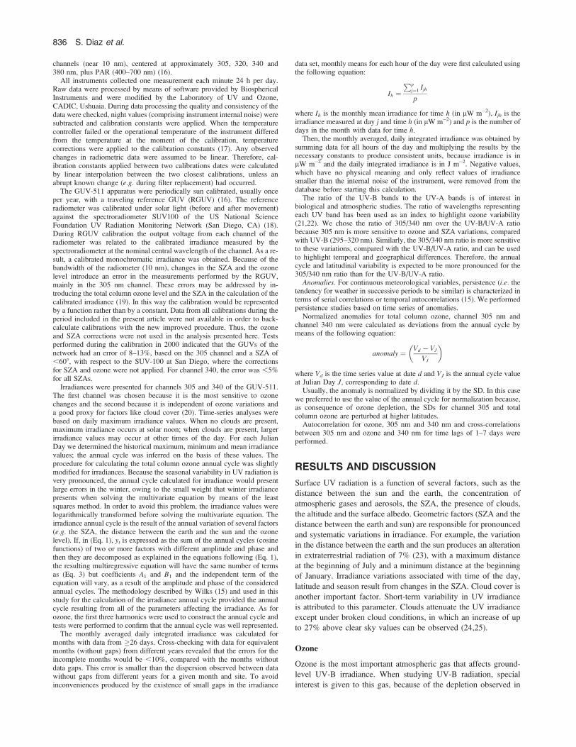
data set, monthly means for each hour of the day were first calculated usingthe following equation:
Ih ¼Pp
j¼1 Ijh
p
where Ih is the monthly mean irradiance for time h (in lW m�2), Ijh is theirradiance measured at day j and time h (in lW m�2) and p is the number ofdays in the month with data for time h.
Then, the monthly averaged, daily integrated irradiance was obtained bysumming data for all hours of the day and multiplying the results by thenecessary constants to produce consistent units, because irradiance is inlW m�2 and the daily integrated irradiance is in J m�2. Negative values,which have no physical meaning and only reflect values of irradiancesmaller than the internal noise of the instrument, were removed from thedatabase before starting this calculation.
The ratio of the UV-B bands to the UV-A bands is of interest inbiological and atmospheric studies. The ratio of wavelengths representingeach UV band has been used as an index to highlight ozone variability(21,22). We chose the ratio of 305/340 nm over the UV-B/UV-A ratiobecause 305 nm is more sensitive to ozone and SZA variations, comparedwith UV-B (295–320 nm). Similarly, the 305/340 nm ratio is more sensitiveto these variations, compared with the UV-B/UV-A ratio, and can be usedto highlight temporal and geographical differences. Therefore, the annualcycle and latitudinal variability is expected to be more pronounced for the305/340 nm ratio than for the UV-B/UV-A ratio.
Anomalies. For continuous meteorological variables, persistence (i.e. thetendency for weather in successive periods to be similar) is characterized interms of serial correlations or temporal autocorrelations (15). We performedpersistence studies based on time series of anomalies.
Normalized anomalies for total column ozone, channel 305 nm andchannel 340 nm were calculated as deviations from the annual cycle bymeans of the following equation:
anomaly ¼ Vd � VJ
VJ
� �
where Vd is the time series value at date d and VJ is the annual cycle valueat Julian Day J, corresponding to date d.
Usually, the anomaly is normalized by dividing it by the SD. In this casewe preferred to use the value of the annual cycle for normalization because,as consequence of ozone depletion, the SDs for channel 305 and totalcolumn ozone are perturbed at higher latitudes.
Autocorrelation for ozone, 305 nm and 340 nm and cross-correlationsbetween 305 nm and ozone and 340 nm for time lags of 1–7 days wereperformed.
RESULTS AND DISCUSSION
Surface UV radiation is a function of several factors, such as the
distance between the sun and the earth, the concentration of
atmospheric gases and aerosols, the SZA, the presence of clouds,
the altitude and the surface albedo. Geometric factors (SZA and the
distance between the earth and sun) are responsible for pronounced
and systematic variations in irradiance. For example, the variation
in the distance between the earth and the sun produces an alteration
in extraterrestrial radiation of 7% (23), with a maximum distance
at the beginning of July and a minimum distance at the beginning
of January. Irradiance variations associated with time of the day,
latitude and season result from changes in the SZA. Cloud cover is
another important factor. Short-term variability in UV irradiance
is attributed to this parameter. Clouds attenuate the UV irradiance
except under broken cloud conditions, in which an increase of up
to 27% above clear sky values can be observed (24,25).
Ozone
Ozone is the most important atmospheric gas that affects ground-
level UV-B irradiance. When studying UV-B radiation, special
interest is given to this gas, because of the depletion observed in
836 S. Diaz et al.

recent decades (6–9). Ozone presents important temporal and
geographical variations. Higher total column ozone is usually
observed at higher latitudes and lower values are observed at the
tropical regions (6). Main temporal variations of this parameter are
based on season, which is more pronounced at high latitudes, and
time of day. Other temporal changes are related to the quasi-
biennial oscillation (QBO) (26–28), the 11 year sun spot cycle and
the 27 day sun rotation (29–33).
Historical maximum, minimum and mean and annual cycle of
total column ozone for each Julian Day between 1 January 1979
and 31 December 2004 are presented in Figure 1. In general, the
annual cycle showed a maximum in late winter and spring, a
minimum in late summer and autumn and a larger amplitude at
higher latitudes, as expected. Several interesting points are worth
highlighting. The seasonal and day-to-day variability were con-
siderably smaller at Jujuy than at the other sites. At Punta Arenas
and Ushuaia the sinusoidal pattern of the annual cycle looked
broken. We attributed this to the overpass of the ozone hole and
to low ozone air masses from Antarctica passing over the region.
Furthermore, the ozone hole effect shifted the maximum value
during the annual cycle in these 2 localities.
The mean annual total column ozone level showed the expected
increase from tropical to high latitudes (Table 2). The difference
between the mean for the series 1979–2004 and the mean for 1980–
1986 (the reference period) was consistent with the observed
latitudinal variation in ozone depletion. In general, the maximum
total column ozone of the time series occurred during or close to the
years of maximum solar activity and/or at the beginning of the time
series, whereas the minimum level occurred during or close to years
of minimum solar activity and/or towards the end of the time series.
Data from Punta Arenas were exceptions, because 2000 corre-
sponded to a maximum value of the solar cycle. The SD increased
with latitude. Maximum and minimum values increased and
decreased, respectively, with latitude. For all sites, the minimum
values were ,220 Dobson Units (DU) (which is considered as the
limit of the spring Antarctic ozone hole over high latitudes, although
the hole may be present over other regions or seasons, mainly during
autumn, when the minimum value of the ozone annual cycle
occurs). Jujuy had minimum annual total column ozone ,220 DU
Figure 1. Total column ozone levels. Historical maximum(upper full grey line), minimum (lower full grey line), mean(dotted line) and annual cycle (full black line), calculatedfrom maximum daily irradiance values, based on (Eq. 3), forthe period 1979–2004.
Table 2. Total ozone column. Mean and standard deviation of yearmean for the period 1979–2004; maximum and minimum values of thetime series, and year when they occurred; and mean of year mean 1980–1986, as a reference, are presented.
Site
Annual meanlevel 6 SD,1979–2004
(DU)Maximum level
(DU); yearMinimum level
(DU); year
Mean level,1980–1986
(DU)
Jujuy 267.36 6 6.27 334.70; 1991 217.00; 2004 268.99Buenos
Aires 288.94 6 8.71 433.80; 1979 216.40; 1997 291.85Santiago 281.07 6 8.01 391.00; 1983 200.40; 2004 283.37Bariloche 296.83 6 9.37 423.00; 1979 204.00; 2004 302.77Valdiva 299.64 6 8.89 421.30; 1979 209.80; 1997 304.92Trelew 299.12 6 9.23 451.40; 1979 208.30; 2004 305.31Punta
Arenas 302.98 6 10.63 461.00; 1979 155.50; 2000 313.47Ushuaia 302.42 6 11.35 469.10; 1979 136.1; 2003 314.50
Photochemistry and Photobiology, 2006, 82 837
in 1992, 1998 and 2004. These minima occurred during different
seasons. Buenos Aires showed values ,220 DU in1997; Santiago
in 1986, 1996, 1997, 1998, 2002 and 2004; and Valdivia, Bariloche
and Trelew in 1997 and 2004. In all these cases the minimum levels
were recorded during autumn. Interestingly, in the last three
stations, the minima did not coincide with the occurrence of the
Antarctic Ozone hole. It was observed that values in 1997 were
,220 DU at most stations. Fioletov et al. (34) reported record large
negative deviations from pre-1980 for 1997 at 35–608S latitude,
which persisted once the QBO and the solar cycle were removed.
Observations of the Halogen Occultation Experiment determined
that record low ozone level observed in 1997 (at 20–408S latitude)
was mainly confined to the lower stratosphere (35).
The locations affected by the ozone hole presented different
dynamics (6–9). Ushuaia showed values ,220 DU every spring,
starting in 1990; Punta Arenas had similar conditions except in
1993. Before 1990 Ushuaia had values of ,220 DU almost every
year, during winter or autumn, and such values were observed for
Punta Arenas on a few occasions during the same seasons.
Irradiance
The irradiances in the UV-B and UV-A bands present differences
in latitudinal and seasonal distribution. In addition, parameters
affecting UV showed a large variety of combinations at the studied
sites, which were reflected in the variability patterns.
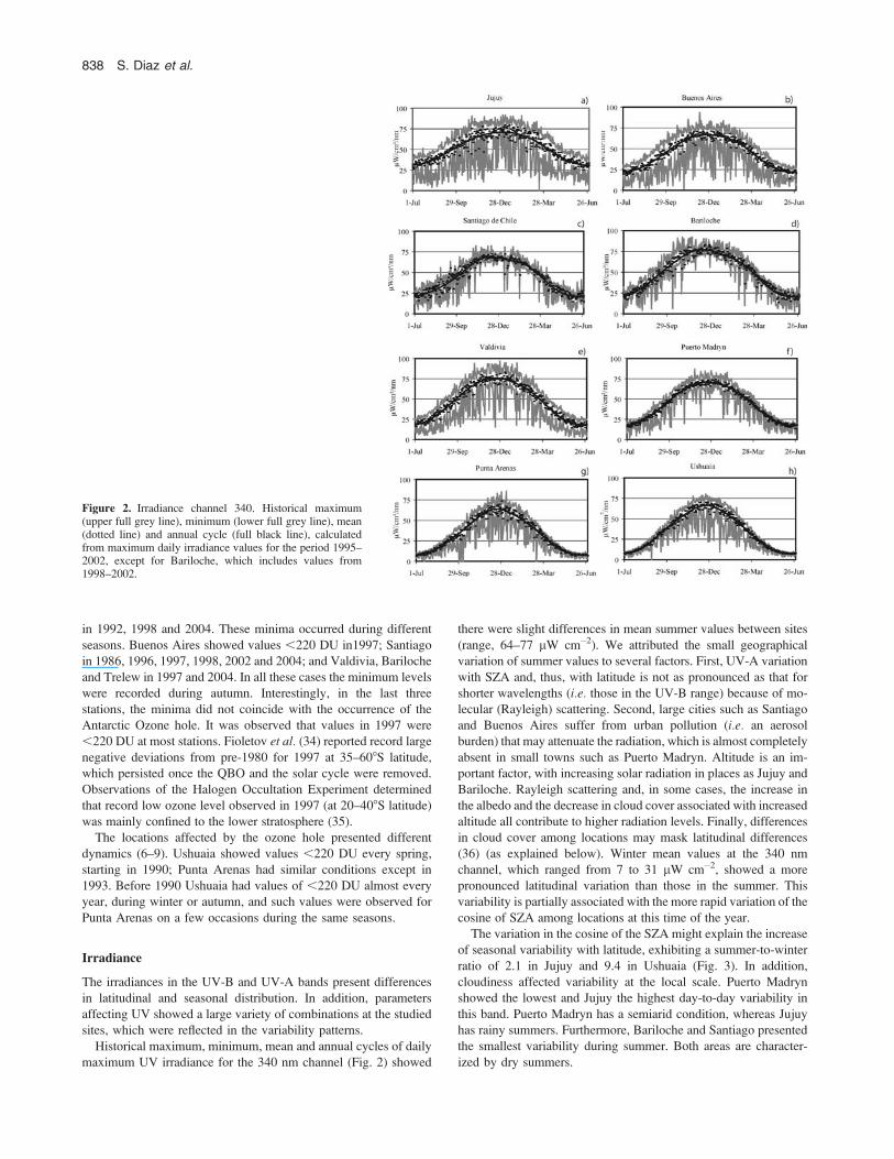
Historical maximum, minimum, mean and annual cycles of daily
maximum UV irradiance for the 340 nm channel (Fig. 2) showed
there were slight differences in mean summer values between sites
(range, 64–77 lW cm�2). We attributed the small geographical
variation of summer values to several factors. First, UV-A variation
with SZA and, thus, with latitude is not as pronounced as that for
shorter wavelengths (i.e. those in the UV-B range) because of mo-
lecular (Rayleigh) scattering. Second, large cities such as Santiago
and Buenos Aires suffer from urban pollution (i.e. an aerosol
burden) that may attenuate the radiation, which is almost completely
absent in small towns such as Puerto Madryn. Altitude is an im-
portant factor, with increasing solar radiation in places as Jujuy and
Bariloche. Rayleigh scattering and, in some cases, the increase in
the albedo and the decrease in cloud cover associated with increased
altitude all contribute to higher radiation levels. Finally, differences
in cloud cover among locations may mask latitudinal differences
(36) (as explained below). Winter mean values at the 340 nm
channel, which ranged from 7 to 31 lW cm�2, showed a more
pronounced latitudinal variation than those in the summer. This
variability is partially associated with the more rapid variation of the
cosine of SZA among locations at this time of the year.
The variation in the cosine of the SZA might explain the increase
of seasonal variability with latitude, exhibiting a summer-to-winter
ratio of 2.1 in Jujuy and 9.4 in Ushuaia (Fig. 3). In addition,
cloudiness affected variability at the local scale. Puerto Madryn
showed the lowest and Jujuy the highest day-to-day variability in
this band. Puerto Madryn has a semiarid condition, whereas Jujuy
has rainy summers. Furthermore, Bariloche and Santiago presented
the smallest variability during summer. Both areas are character-
ized by dry summers.
Figure 2. Irradiance channel 340. Historical maximum(upper full grey line), minimum (lower full grey line), mean(dotted line) and annual cycle (full black line), calculatedfrom maximum daily irradiance values for the period 1995–2002, except for Bariloche, which includes values from1998–2002.
838 S. Diaz et al.

Geographical differences and the annual cycle amplitude were
more pronounced at the 305 nm channel than at the 340 nm
channel, as expected (Fig. 4). Summer mean values varied from 5
lW cm�2 at Ushuaia to 10 lW cm�2 at Jujuy, and winter mean
values ranged from 0.04 lW cm�2 at Ushuaia to 2.3 lW cm�2 at
Jujuy. As a direct consequence of variations associated with SZA
and ozone level, lower latitudes had larger values during all seasons
and a smaller amplitude of the annual cycle. Mean values for the
summer-to-winter ratio were 4.4 at Jujuy and 125 at Ushuaia.
The 305 nm channel is affected by all of the factors mentioned
for the 340 nm band and, in addition, by total column ozone. In
some cases these factors may compete or result in additive effects.
For example, the presence of clouds can mask the effect of ozone
depletion. Strong ozone depletion produced while the ozone hole
was passing overhead, during cloudy conditions and in conjunc-
tion with high SZAs can, on clear days, produce lower irradiances
than weaker ozone depletions near the summer solstice (37). To
determine which factors were responsible for the variability
observed with the 305 nm channel, we compared the irradiance
at both wavelengths with the ozone level during the same period.
We observed that the springtime variability at the historical
maximum in Punta Arenas and Ushuaia was mainly the result of
low total column ozone associated with the presence of the ozone
hole vortex (Figs. 1–3). Similarly, places such as Valdivia, Puerto
Madryn and Bariloche showed spring irradiance values affected by
low ozone amounts. This may be inferred by the fact that the
maximum and mean values showed an increase at the 305 nm
channel but not the 340 nm channel.
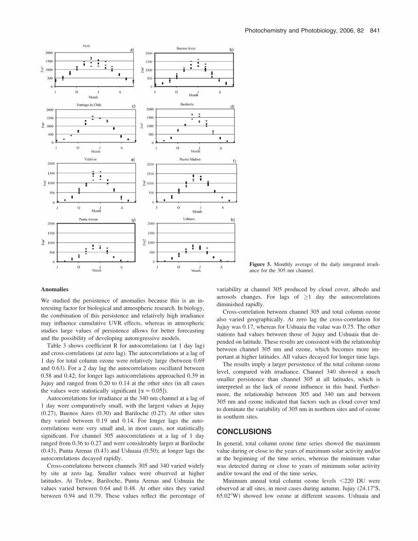
Monthly averaged, daily integrated irradiance values for channel
305 (Fig. 5) were extreme in December and January and in June
and July, as expected. All sites except Punta Arenas and Ushuaia
showed similar summer values, which oscillated between 1 and
1.7 kJ/m2; daily integrated values at Punta Arenas and Ushuaia
during the summer were ca 50% less (0.6–0.9 kJ m�2). To explain
this variability we first need to consider that the duration of day-
light varies considerably among stations. At Jujuy the duration
varies from 10.5 h in June to 13.5 h in December. At Ushuaia the
duration varies from 7 to 17 h. Second, analysis of channel 340 nm
and total column ozone showed that the observed interannual
variability was related to both ozone and cloud cover variations,
Figure 3. Cloud cover during summer and winter in SouthAmerican region, where data from the GUV-511 radio-meters analyzed in this study were obtained.
Photochemistry and Photobiology, 2006, 82 839

although the effect of ozone was less pronounced than that
observed for instantaneous values (as explained below). Other
factors, such as aerosols, could have influenced the interannual
variability but this could not be confirmed in the present analysis.
In contrast to summer values there was a larger latitudinal varia-
tion in daily integrated values during the winter (ranging from
0.2 kJ m�2 at Jujuy to 0.004 kJ m�2 at Ushuaia), because of the
effect of SZA, ozone and duration of daylight. This resulted in
a seasonal ratio of 7 at Jujuy and of .150 at Ushuaia.
Monthly averages mask some interesting features in the data.
Instantaneous values at the 305 nm channel showed that, during
spring, the irradiance was highly affected by ozone depletion at the
southern stations. When monthly values were considered, the effect
vanished at Ushuaia and Punta Arenas (Fig. 5).
Ratio 305/340
The ratio of a wavelength or narrow band in the UV-B and in the
UV-A is of interest for biological studies. In some organisms UV-
A contributes to the recovery from the damage produced by UV-B
(38,39). Also, this ratio is relevant for atmospheric research,
because the parameters that affect UV irradiance have different
spectral patterns. For example, 305 nm presents a more pronounced
variation with SZA than 340 nm (compare seasonal cycles in Fig. 2
with Fig. 3). The ratio of 305 to 340 is then a function of SZA,
resulting in a systematic variability with latitude and seasons (22).
Cloud cover has a slight spectral dependence; the ratio removes
most of the cloud effect (21). Furthermore, changes in total column
ozone produce abrupt changes in the ratio as consequence of ozone
absorption spectral pattern (21). Therefore, this ratio can highlight
variations in ozone levels, and the effects of cloud cover can be
minimized (21,22).
Historical maximum, minimum, mean and annual cycle of the
305/340 nm ratio at solar noon are shown in Figure 6. Solar noon
values were considered, because use of the ratio removed most of
the effects due to clouds.
Latitudinal variation showed a doubling of the ratio between
Jujuy and Ushuaia in summer, and the ratio was even higher in
winter. At Jujuy the extreme values of the annual cycle were 0.15
and 0.07 and at Ushuaia the extreme values were 0.08 and 0.005.
Another interesting feature can be seen during springtime, when
anomalously large values were observed in Ushuaia and Punta
Arenas that showed good agreement with the presence of low
ozone levels. At Punta Arenas the largest value was 0.14 on 21
November 1999, with a total column ozone level of 216.4 DU.
Slightly lower values (0.13) were present on 18 December 1996
(237.3 DU), 22 October 1998 (203.6 DU), 8 December 1998
(229.1 DU), 12 October 2000 (155.5 DU) and 1 November 2002
(215 DU). At Ushuaia the maximum was 0.17 and was detected on
12 October 2000 (139 DU) and 0.16 was detected on 14 November
1997 (207 DU). It may be observed that a mild ozone depletion
at the end of springtime can produce high ratios similar to those
associated with pronounced ozone depletion at the midpoint of
springtime. This is a consequence of the increase in the ratio
associated with SZA as the season progresses.
Figure 4. Irradiance channel 305. Historical maximum(upper full grey line), minimum (lower full grey line), mean(dotted line) and annual cycle (full black line), calculatedfrom maximum daily irradiance values for the period 1995–2002, except for Bariloche, which includes values from1998–2002.
840 S. Diaz et al.
Anomalies
We studied the persistence of anomalies because this is an in-
teresting factor for biological and atmospheric research. In biology,
the combination of this persistence and relatively high irradiance
may influence cumulative UVR effects, whereas in atmospheric
studies large values of persistence allows for better forecasting
and the possibility of developing autoregressive models.
Table 3 shows coefficient R for autocorrelations (at 1 day lag)
and cross-correlations (at zero lag). The autocorrelations at a lag of
1 day for total column ozone were relatively large (between 0.69
and 0.63). For a 2 day lag the autocorrelations oscillated between
0.58 and 0.42; for longer lags autocorrelations approached 0.39 in
Jujuy and ranged from 0.20 to 0.14 at the other sites (in all cases
the values were statistically significant [a 5 0.05]).
Autocorrelations for irradiance at the 340 nm channel at a lag of
1 day were comparatively small, with the largest values at Jujuy
(0.27), Buenos Aires (0.30) and Bariloche (0.27). At other sites
they varied between 0.19 and 0.14. For longer lags the auto-
correlations were very small and, in most cases, not statistically
significant. For channel 305 autocorrelations at a lag of 1 day
ranged from 0.36 to 0.27 and were considerably larger at Bariloche
(0.43), Punta Arenas (0.43) and Ushuaia (0.50); at longer lags the
autocorrelations decayed rapidly.
Cross-correlations between channels 305 and 340 varied widely
by site at zero lag. Smaller values were observed at higher
latitudes. At Trelew, Bariloche, Punta Arenas and Ushuaia the
values varied between 0.64 and 0.48. At other sites they varied
between 0.94 and 0.79. These values reflect the percentage of
variability at channel 305 produced by cloud cover, albedo and
aerosols changes. For lags of �1 day the autocorrelations
diminished rapidly.
Cross-correlation between channel 305 and total column ozone
also varied geographically. At zero lag the cross-correlation for
Jujuy was 0.17, whereas for Ushuaia the value was 0.75. The other
stations had values between those of Jujuy and Ushuaia that de-
pended on latitude. These results are consistent with the relationship
between channel 305 nm and ozone, which becomes more im-
portant at higher latitudes. All values decayed for longer time lags.
The results imply a larger persistence of the total column ozone
level, compared with irradiance. Channel 340 showed a much
smaller persistence than channel 305 at all latitudes, which is
interpreted as the lack of ozone influence in this band. Further-
more, the relationship between 305 and 340 nm and between
305 nm and ozone indicated that factors such as cloud cover tend
to dominate the variability of 305 nm in northern sites and of ozone
in southern sites.
CONCLUSIONS
In general, total column ozone time series showed the maximum
value during or close to the years of maximum solar activity and/or
at the beginning of the time series, whereas the minimum value
was detected during or close to years of minimum solar activity
and/or toward the end of the time series.
Minimum annual total column ozone levels ,220 DU were
observed at all sites, in most cases during autumn. Jujuy (24.178S,
65.028W) showed low ozone at different seasons. Ushuaia and
Figure 5. Monthly average of the daily integrated irradi-ance for the 305 nm channel.
Photochemistry and Photobiology, 2006, 82 841

Punta Arenas presented minima of ,220 DU every spring,
beginning in 1990; before 1990 these levels were present in winter
and autumn.
Irradiance in the UV-B channel and total column ozone varied
with latitude, as expected. The UV-A channel showed a more
complex geographical pattern, because it was affected by local
atmospheric conditions.
Latitudinal differences and the amplitude of the annual cycle
were more pronounced in the 305 nm channel, compared with the
340 nm channel, as consequence of the effect of SZA and ozone.
Monthly averaged daily integrated irradiance for channel 305
showed similar values at all sites except Punta Arenas and Ushuaia,
whereas winter values showed a larger latitudinal variation. These
results were a consequence of the effect of SZA, ozone and
daylight duration.
Mild ozone depletion at the end of spring can produce similar
305/340 ratios than those under pronounced ozone depletion in the
middle of spring. This results from the increase in the ratio as the
SZA diminishes.
Total column ozone anomalies showed a larger persistence than
did irradiance at 305 and 340 nm. Irradiance at 340 nm showed the
smallest persistence. The relationships between 305 and 340 nm
anomalies and between 305 nm and ozone anomalies indicated that
factors such as cloud cover tend to dominate 305 nm variability in
northern sites and ozone variability in southern sites.
Acknowledgements—This study was funded by a grant from the Inter-American Institute for Global Change (CRN-026). We thank Dr. LuisOrce for leading the installation of and operating the instruments at Jujuy,Buenos Aires, Puerto Madryn and Ushuaia when the Argentinean net-work was first created; Drs. McPeters and Herman, NASA/GSFC, forproviding total column ozone data; Jim Ehramjian, James Robertson andthe UV group (Biospherical Instruments Inc.) for calibrating the GUVsand RGUV; Dr. Paula Vigliarolo for contributing to the extraction of to-tal column ozone for Bariloche; Drs. San Roman, Buitrago, Labraga, He-bling and Dieguez for collaborating in data collection at Ushuaia, Jujuy,Puerto Madryn, Playa Union and Bariloche; and Centro Austral de Inves-tigaciones Cientificas, Consejo Nacional de Investigaciones Cientıficas yTecnicas, Argentina.
Table 3. Autocorrelation (Auto) and cross-correlation (Cross) R coeffi-cients for anomalies.*
Site
Autoozone(lag ¼1 day)
Auto340 nm(lag ¼1 day)
Auto305 nm(lag ¼1 day)
Cross305–340(lag ¼0 days)
Cross305–Oz(lag ¼0 days)
Jujuy 0.69 0.27 0.33 0.94 0.17Buenos
Aires 0.69 0.30 0.36 0.87 0.32Santiago 0.69 0.15 0.27 0.83 0.28Bariloche 0.64 0.27 0.43 0.64 0.55Valdiva 0.64 0.11 0.27 0.79 0.34Trelew 0.63 0.14 0.36 0.60 0.62Punta
Arenas 0.67 0.19 0.43 0.58 0.61Ushuaia 0.67 0.07 0.50 0.48 0.75
*a 5 0.05.
Figure 6. Ratio channel 305/channel 340. Historicalmaximum (upper full grey line), minimum (lower full greyline), mean (dotted line) and annual cycle (full black line),calculated from maximum daily irradiance values for theperiod 1995–2002, except for Bariloche, which includesvalues from 1998–2002.
842 S. Diaz et al.
REFERENCES
1. Farman, J. C., B. G. Gardiner and J. D. Shanklin (1985) Large lossesof total ozone in Antarctica reveals seasonal ClOx/NOx interaction.Nature 315, 207–210.
2. United Nations Environmental Program (1991) Environmental Effectsof Ozone Depletion: 1991 (Edited by J. C. van der Leun, X. Tang andM. Tevini). United Nations Environmental Programme, Nairobi, Kenya.
3. United Nations Environmental Program (1994) Environmental Effectsof Ozone Depletion: 1994 (Edited by J. C. van der Leun, X. Tangand M. Tevini). United Nations Environmental Programme, Nairobi,Kenya.
4. United Nations Environmental Program (1998) Environmental Effectsof Ozone Depletion: 1998 (Edited by J. C. van der Leun, X. Tang andM. Tevini). United Nations Environmental Programme, Nairobi, Kenya.
5. United Nations Environmental Program (2002) Environmental effects ofozone Depletion: 2002 (Edited by J. C. van der Leun, X. Tang and M.Tevini). United Nations Environmental Programme, Nairobi, Kenya.
6. World Meteorological Organization (1992). Scientific Assessment ofOzone Depletion: 1991. United Nations Environment Program, WorldMeteorological Organization. Global Ozone Research and MonitoringProject (Edited by D. L. Albritton, R. T. Watson and P. J. Aucamp).WMO/UNEP, Nairobi, Kenya.
7. World Meteorological Organization (1995) Scientific Assessment ofOzone Depletion: 1994. United Nations Environment Program, WorldMeteorological Organization. Global Ozone Research and MonitoringProject (Edited by D. L. Albritton, R. T. Watson and P. J. Aucamp).WMO/UNEP, Nairobi, Kenya.
8. World Meteorological Organization (1999) Scientific Assessment ofOzone Depletion: 1998. United Nations Environment Program, WorldMeteorological Organization. Global Ozone Research and MonitoringProject (Edited by D. L. Albritton, R. T. Watson and P. J. Aucamp).WMO/UNEP, Nairobi, Kenya.
9. World Meteorological Organization (2003) Scientific Assessment ofOzone Depletion: 2002. United Nations Environment Program, WorldMeteorological Organization. Global Ozone Research and MonitoringProject (Edited by D. L. Albritton, R. T. Watson and P. J. Aucamp).WMO/UNEP, Nairobi, Kenya.
10. Cede, A., M. Blumthaler, E. Luccini, R. Piacentini and L. Nunez(2002) Effects of clouds on erythemal and total irradiance as derivedfrom data of the Argentine Network. Geophys. Res. Lett. 29, 2223(DOI:10.1029/2002GL015708).
11. Cede, A., E. Luccini, L. Nunez, R. Piacentini and M. Blumthaler(2002) Monitoring of erythemal irradiance in the Argentine ultravioletnetwork. J. Geophys. Res. 107, 4165 (DOI:10.1029/2001JD001206).
12. Pazmino, A., S. Godin-Beekmann, M. Ginzburg, S. Bekki, A.Hauchecorne, R. Piacentini and E. Quel (2005) Impact of Antarcticpolar vortex occurrences on total ozone and UVB radiation at southernArgentinean and Antarctic stations during 1997–2003 period. J.Geophys. Res. 110 (DOI:10.1029/2004JD005304).
13. Herman, J. (2004) TOMS ADEOS. NASA/GSFC, Version 8. Availableat: http://toms.gsfc.nasa.gov/ozone/ozoneother.html. Accessed on 8March 2005.
14. Mc Peters, R., and E. Beach (2004) TOMS Nimbus 7, Meteor 3 andEarth Probe. NASA/GSFC, Version 8. Available at: http://toms.gsfc.nasa.gov. Accessed on 8 March 2005.
15. Wilks, D. S. (1995) Time series. In Statistical Methods in theAtmospheric Sciences, International Geophysics Series, Vol. 59(Edited by R. Dmowska and J. R. Holton). Academic Press, San Diego.
16. Booth, R., T. Mestechkina and J. H. Morrow (1994) Errors in the re-porting of solar spectral irradiance using moderate band-width radio-meters and experimental investigation. In Ocean Optics, Vol. XII, 13–15June, 1994, Bergen, Norway (Edited by J. S. Jaffe), pp. 654–663.Proceedings of SPIE. Bellingham, Washington, USA.
17. Booth, R. (1998) Application Note: Temperature Coefficients in PUVand GUV Radiometers and Suggested Compensation Methods. Bio-spherical Instruments Inc., San Diego, CA.
18. Booth, C. R., T. B. Lucas, J. H. Morrow, C. S. Weiler and P. A.Penhale (1994) The United States National Science Foundation’s PolarNetwork for monitoring ultraviolet radiation. In Ultraviolet Radiationin Antarctica Measurements and Biological Effects. Antarctic ResearchSeries, Vol. 62 (Edited by C. Susan Weiler and Polly A. Penhale),pp. 17–37. American Geophysical Union, Washington, DC.
19. Diaz S. B., C. R. Booth, R. Armstrong, C. Brunat, S. Cabrera, C.Camilion, C. Cassiccia, G. Deferrari, H. Fuenzalida, C. Lovengreen, A.Paladini, J. Pedroni, A. Rosales, H. Zagarese and M. Vernet (2005)Multi-channel radiometers calibration: A new approach. Appl. Opt. 44,5374–5380.
20. Dıaz S., G. Deferrari, D. Martinioni and A. Oberto (2000) Regressionanalysis of biologically effective integrated irradiances versus ozone,clouds and geometric factors. J. Atmos.-Solar Terr. Phys. 62, 629–638.
21. Lubin, D. and J. Frederick (1989) Measurements of EnhancedSpringtime Ultraviolet Springtime Radiation at Palmer Station. Geo-phys. Res. Lett. 16, 783–785.
22. Frederick, J. E., S. B. Diaz, I. Smolskaia, W. Esposito, T. Lucas andC. R. Booth (1994) Ultraviolet solar radiation in the high latitudes ofSouth America. Photochem. Photobiol. 60, 356–362.
23. Frolich, C. (1987) Variability of the solar ‘‘constant’’ on time scales ofminutes to years. J. Geophys. Res. 92, 796–800.
24. Estupinan, J. G., S. Raman, G. H. Crescenti, J. J. Streitcher and W. F.Barnard (1996) The effects of clouds and haze on UV-B radiation.J. Geophys. Res. 101, 807–816.
25. Frederick, J. and H. Steele (1995) The transmission of sunlight throughcloudy skies: An analysis based on standard meteorological in-formation. J. Appl. Meteorol. 34, 2755–2761.
26. Huang, T. Y. W. (1986) The impact of solar radiation on the quasi-biennial oscillation of the ozone in the tropical stratosphere. Geophys.Res. Lett. 23, 3211–3214.
27. Randell, W. J. and F. Wu (1996) Isolation of the ozone QBO in SAGEII data by singular-value decomposition. J. Atmos. Sci. 53, 2546–2559.
28. Zerefos, C, C. Meleti, D. Balis, K. Tourpali and A. F. Bais (1998)Quasi-biennial and longer-term changes in clear sky UV-B solar irra-diance. Geophys. Res. Lett. 25, 4345–4348.
29. Callis, L. B., M. Natarajan and J. D. Lambeth (2000) Calculated upperstratospheric effects of solar UV flux and NOY variations during the11-year solar cycle. Geophys. Res. Lett. 27, 3869–3872.
30. Chandra, S. and R. D. Mc Peters (1994) The solar cycle variation ofozone in the stratosphere inferred from Nimbus 7 and NOAA 11satellites. J. Geophys. Res. 99, 20 665–20 671.
31. Lean, J. L., G. J. Rottman, H. L. Kyle, T. N. Woods, J. R. Hickey andL. C. Puga (1997) Detection and parameterization of variations in solarmid- and near-ultraviolet radiation (200–400 nm). J. Geophys. Res.102, 29 939–29 956.
32. Zhou, S., G. J. Rottman and A. J. Miller (1997) Stratospheric ozoneresponse to short- and intermediate-term variations of solar UV flux.J. Geophys. Res. 102, 9003–9011.
33. Zhou, S., A. J. Miller and L. L. Hood (2000) A partial correlationanalysis of the stratospheric ozone response to 12-day solar UVvariations with temperature effect removed. J. Geophys. Res. 105,4491–4500.
34. Fioletov, V., G. Bodeker, A. Miller, R. Mc Peters and R. Stolarski(2002) Global and zonal total ozone variations estimated from ground-based and satellite measurements: 1964–2000. J. Geophys. Res. 107,4647 (DOI:10.1029/2001JD001350).
35. Cordero, E. and T. Nathan (2002) An examination of anomalously lowcolumn ozone in the Southern Hemisphere midlatitudes during 1997.Geophys. Res. Lett. 29, 1123 (DOI:0.1029/2001GL013948).
36. Dıaz, S. B., G. Deferrari, R. Booth, D. Martinioni and A. Oberto (2001)Solar irradiances over ushuaia (54.498S, 68.198W) and San Diego(32.458N, 117.118W) geographical and seasonal variation. J. Atmos.Solar Terr. Phys. 63, 310–320.
37. Dıaz, S. B., C. R. Booth, T. B. Lucas and I. Smolskaia (1994) Effectsof ozone depletion on irradiances and biological doses over Ushuaia. InImpact of UV-B Radiation on Pelagic Freshwater Ecosystems (Editedby C. E. Williamson and H. E. Zagarese). Archiv. Fur Hydrobiologie.Ergebnisse de Limnologie 43, 115–122.
38. Caldwell, M. M., L. B. Camp, C. W. Warner and S. D. Flint (1986)Action spectra and their key role in assessing biological consequencesof solar UV-B radiation change. In Strartospheric Ozone Reduction,Solar Ultraviolet Radiation and Plant Life (Edited by R. C. Worrestand M. M. Caldwell), pp. 87–111. Springer-Verlag, Berlin.
39. Neal, P. and D. Kieber (2000) Assessing biological and chemicaleffects of UV in the marine environment spectral weighting functions.In Causes and Environmental Implications of Increase UV-B Radiation(Edited by R. E. Hester and R. M. Harrison). Issues in EnvironmentalScience and Technology, No. 14. The Royal Society of Chemistry,Cambridge, UK, 61–83.
Photochemistry and Photobiology, 2006, 82 843