Photochemical ozone creation potentials

L C A C a s e S t u d i e s P h o t o c h e m i c a l O z o n e C r e a t i o n P o t e n t i a l s

LCA Case Studies [

Photochemical Ozone Creation Potentials A n e w s e t o f c h a r a c t e r i z a t i o n f a c t o r s f o r d i f f e r e n t g a s s p e c i e s o n t h e s c a l e o f W e s t e r n E u r o p e

Eric L a b o u z e 1., C6cile Honor62 , L a m y a M o u l a y 1, B6n4dicte C o u f f i g n a P and M a t t h i a s B e e k m a n n 2

1 BIO Intelligence Service S.A., Ivry-sur-Seine, France 2 Service d'A4ronomie du CNRS, Institut Pierre Simon Laplace, Universit6 Pierre et Marie Curie, Paris, France 3 Association RECORD (R6seau Coop6ratif de Recherche sur les D&hets), Villeurbanne, France

* Corresponding author ([email protected])

DOh http:lldx.doi.oro/10.1065flca2004.04.155

Abstract

Goal, Scope and Background. Photochemical ozone creation potentials (POCPs) typically used in life cycle impact assessment (LCIA) to address the impact category 'photo-oxidant formation' only provide factors for particular volatile organic compounds and do not take into account background concentrations and meteorological conditions. However, the formation of ozone from volatile organic compounds (VOCs), carbon monoxide (CO) and nitrogen oxides (NOx) is highly dependent on the background pollutant concentrations and meteorological conditions. Some LCIA manuals therefore recommend working with potentials for high background concentrations of NO x (Derwent 1998 ), and potentials for low background concentrations of NO X (Andersson-Sk61d 1992). Objectives. This study has introduced an improved set of POCPs independently of meteorological and emission conditions specific to a given period or location. Whereas current POCP values may be relevant to estimate the photo-oxidant formation over a certain (temporally and spatially well-defined) domain, this study has further introduced more relevant values with respect to potential impacts of ozone on human health and environment. Methods. For the computation of POCP values on the scale of Western Europe, independently of meteorological and emission conditions specific to a given period or location, a Eulerian chemistry-transport numerical model (CHIMERE-continental) has been implemented over three summer seasons. POCPs have been evaluated for ten VOC species (including the whole VOC group), CO and NO x. The coherence of this new set of POCP values with previous studies has been checked. The spatial representativity of POCP values over the simulation domain in Europe has also been addressed. The robustness of these POCP values to changes in the implemented chemical mechanism used in our model has been checked. Results and Discussion. The POCPs computed in this study were generally lower than the POCPs calculated in previous studies. In the previous studies, but not here, the POCPs have been calculated with particular meteorological conditions (during anticyclonic, fair weather conditions) or emission levels (high polluted backgrounds) known to be optimal with respect to ozone formation. Despite the quantitative variations in the POCP values, we have found a good agreement in the relative ranking of the pollutant species between this study and previous studies. It was also shown that POCP values display significant spatial variability over Western Europe (the largest spatial differences were obtained for NO X where the sign of the POCP value even changes from region to region).

II

Conclusions. Finally, the temporally and spatially averaged values obtained here for the POCP index update previous values and represent an attempt to generate the most appropriate and accurate scale for European conditions independently of meteorological and emission conditions specific to a given period or location.

Recommendations and Outlook. These new PCOPs should be useful to LCIA-practitioners in further life cycle impact assessment. However, for the NO x species, we do not recommend the use of the POCP value for LCIA.

Keywords: Characterization factors; life cycle impact assessment (LCIA); photochemical atmospheric model; photochemical ozone creation potentials (POCP); photo-oxidant formation

1 Goal, Scope and Background

A life cycle impact assessment (LCIA) has been defined by the Society of Envi ronmenta l Toxicology and Chemistry (SETAC 1993a, 1993b and 1997) and the Internat ional Standard Organiza t ion (ISO 1999) as a relative approach based on a functional unit for characterizing and assessing the potential effects of the environmental burdens (resources used and emissions released) identified in a life cycle inventory (LCI). As stated by ISO (1999), an LCIA consists of three manda to ry elements (scoping including impact category and model selection, classification, and characterization), which can be followed by four optional elements (normalization, grouping, weighting, and data quality analysis). This paper deals with the characterization element of LCIA, which in- cludes modelling, quantification, and aggregation of inventory data within a particular impact category. The aim of this paper is to improve the characterization of photo-oxidant for- mat ion (i.e. tropospheric ozone formation) in LCIA.

The study presented was initiated by RE.CO.R.D (French research network on solid waste) for suggesting an improved set of characterization factors for photo-oxidant formation in LCIA to industry members of RE.CO.R.D (RECORD 2002).

1.1 Tropospheric ozone

Photo-oxidant formation, also k n o w n as summer smog since about 50 years (McCabe 1952), is generally regarded as one of the impact categories to be considered in impact assess-

Int J LCA 9 (3) 187- 195 (2004) �9 ecomed publishers, D-86899 Landsberg, Germany and Ft. Worthfi-X �9 Tokyo ~ Mumbai �9 Seoul ~ Melbourne �9 Paris

1 8 7

Photochemical Ozone Creation Potentials LCA Case Studies

ment. Photo-oxidant formation is the formation of reactive chemical compounds such as ozone by the action of sun- light on certain primary pollutants. On the regional scale, these reactive compounds may be injurious to human health and ecosystems and may also damage crops. Efforts are made all over Europe to deal with the tropospheric ozone problem both on a European and a local scale. Within the framework of the Convention on Long Range Transboundary Air Pollu- tion of the United Nations Economic Commission for Europe (UNECE/CLRTAP nitrogen protocols), the ozone problem is a topic of highest priority together with acidification.

1.2 On photo-oxidant formation

Photo-oxidants such as ozone may be formed in the troposphere under the influence of ultraviolet light, through photochemical oxidation of Volatile Organic compounds (VOCs) and carbon monoxide (CO) in the presence of nitrogen oxides (NOx), in addition to a smaller natural background transported downwards f rom the stratospheric reservoir. It is the combinat ion of the three essential factors (UV radiation, reactive volatile organic compounds and CO, and reactive nitrogen oxides) which makes a real environmental p rob lem and a threat to human health and the environment.

Photo-oxidant formation is a difficult impact category for several reasons. Many VOCs undergo rather similar reactions in the atmosphere, but each individual species has its own reaction path. The production of ozone caused by a certain VOC depends on the chemical and meteorological conditions of the environment into which the VOC is emit- ted. The very same VOC may give a high ozone production under conditions with higher N O x concentrations, and a low ozone product ion where the availability of NOx is critical (Carter 1994, Bowman and Seinfeld 1994ab). Atmospheric NO• levels depend on many factors, including the emission patterns, the strength of dispersion and on chemical loss. Furthermore, VOCs which produce many radicals during their photolytic degradation will speed up the oxidation of all other VOC present and thus increase the ozone production. Thus, high radiation intensity will increase the efficiency of VOCs to produce ozone. Therefore, a large spatial and temporal variability in the ozone creation potential of each V O C is expected.

1.3 State of art in LCIA

The numerous atmospheric species of VOCs vary widely in their contr ibution to photo-oxidant formation. Today, two basic methods are available for comparing the ozone crea- t ion potential of different species of VOCs, based on: 1. Photochemical Ozone Creation Potentials (POCPs, e.g. Derwent

and Jenkin 1991, updated in Derwent 1998), which are developed for the European situation, taking into account average concentration levels of the relevant substances concerned.

2. Incremental Reactivity (Carter 1994), developed in the US, adapted to conditions of maximum oxidant creation.

Note a third method used in Eco-indicator 99 (Goedkoop and Spriensma 1999) has also been proposed (Hofstetter 1998), but it is directly derived from the current POCP approach.

The two methods above include the use of atmospheric models. Atmospheric photochemical models describe the chemical and meteorological features of the atmosphere and are used to study atmospheric processes. In LCIA, the POCPs of Derwent (1998) are widely used all over the world as a char- acterisation factor to assess and aggregate the emissions for the impact category photo-oxidant formation (Heijungs 1992):

Photo-oxidant formation = X x POCP x �9 m x (1)

where m~ (kg) is the mass of substance X released, POCP x the photochemical ozone creation potential of the substance and Photo-oxidant formation is the indicator result, which is expressed in kg ethylene-equivalents.

Photochemical Ozone Creation Potentials (POCPs) were originally developed to assess various emission scenarios for VOCs (Derwent and Jenkin 1991). A UN protocol defined the POCP of a VOC as the ratio between the change in ozone concentration due to a change in the emission of that VOC and the change in the ozone concentration due to an equally relative change in the emission of ethylene (UNECE 1990). Expressed as a formula:

POCP x = 100 �9 [a x / bx] / [a C2H4 / b C2H4] (2)

where a x is the change in ozone concentration due to a change in the emission of compound X and bx the integrated emission of X up to that time, with the denominator containing these parameters for ethylene, the reference substance.

Practically, the numerator and the denominator are calculated as follows: when atmospheric models are used to de- termine the ozone production from a certain substance X emission, two separate simulations are run, one with and one without an extra emission of that substance; the amount of ozone which is produced through the additional emission of X is then calculated as the difference in ozone concentration between the two scenarios, divided by the amount of extra X added.

1.4 Current limitations of the POCP concept used in LCIA and scope of our study

The POCP concept as currently used in LCIA suffers from several limitations:

1) First, recent POCPs were developed on the basis of regional European scenarios (Derwent 1998, Andersson-Sk61d 1992 and 2000), but the atmospheric photochemical model which has been used is a Lagrangian one, i.e. considering a column of air with several layers (mixing layer, residual layer) moving along an air mass trajectory. This approach neglects horizontal mixing and dilution of pollutants, due to the vertical differences in the wind speed and direction. In this study, we therefore propose to extend this approach in the framework of a numerical Eulerian model (i.e. a three-dimensional atmospheric model) which permits one to describe the pollutant t ransport above West-Europe in a best way.

2) Second, the current POCP values are based on a typical 5-day trajectory describing air mass transport above Europe (note the Incremental Reactivity approach is based on a time

188 Int J LCA 9 (3) 2004

LCA Case Studies Photochemical Ozone Creation Potentials

span of one day at most). This short time scale is very sensi- tive to the chosen initial conditions whereas it is well known that emission values (NO x and VOCs) and meteorological conditions are able to completely modify the photochemical pathway of the atmospheric system under study. Meteoro- logical conditions (winds, temperature, height of the mixing layer, radiation) and initial conditions for pollutants (namely for NO x and ozone) are chosen to represent typical values during anticyclonic, fair weather conditions. As the efficiency of ozone build-up from VOCs strongly depends on all these factors, the POCP values obtained in such a way are therefore difficult to generalize. With respect to the LeA con- text, a longer term may also be more relevant because emissions which are aggregated in the inventory may occur at different place and time locations. In this study, we therefore propose to compute POCPs over a much longer time scale, namely over a time period of 3 summer seasons, taking into account the whole range of emission patterns and meteorological conditions occurring above Western Europe.

3) As shown in equation 2, the POCP values are presented as relative values where the change in ozone concentration due to a certain pollutant is divided with the change in ozone concentration due to an equally large emission of ethylene. Actually, this notion of 'change in ozone concentration' re- fers to a variable (let us say AO 3) which can be defined in several manners. Generally, in the methods currently used, this variable (AO3) is based on the difference in daily maximum ozone concentration along the air mass trajectory or on the difference at a certain hour (always between a reference simulation and one with extra emissions of VOC). In this study, we introduce other definitions for the target variable AO3, more relevant with respect to potential impacts of ozone on human health and ecosystem health.

2 Model Description

For the estimation of POCPs in Western Europe, we have used the European-scale CHIMERE model (Schmidt 2001, Vautard 2001) which is primarily designed to produce daily forecasts of ozone and other pollutants over Western Eu- rope and make long-term simulations. It is a 3-dimensional chemistry-transport model (CTM), simplified enough to allow for long simulations, but realistic enough to allow for quantitative simulations of the large-scale ozone distribution over continental areas, without the use of super-com- puters. This model (version 200108) is fully described on the internet at: http://euler.lmd.polytechnique.fr/chimere/ CONT200108. Developments required for the computation of POCPs are presented hereafter.

CHIMERE is based on the mass continuity equation for the concentrations of chemical species in every box of a given grid:

8c 8-[ + V(uc) = V (KVc) + P - L (3)

In this equation, characteristic for the Eulerian approach (see Seinfeld and Pandis 1998), c is a vector containing the concentrations of all model species for every grid box, u is the three dimensional wind vector, K the tensor of eddy dif- fusivity and P and L represent production and loss terms

due to chemical reactions, emissions and deposition. In the following sections, the main features of the model are presented. To keep the description brief, the reader is referred to existing literature wherever possible.

2.1 Model domain and grid

In the horizontal, the model uses a Cartesian latitude-longi- tude grid. The grid size of the model is 1/2 degree (both zonal and meridional). The number of zonal cells is 65 and the number of meridional cells is 33. The centre of the Southernmost+Westernmost cell is located at 10 degree W and 40.5 degree N. The Northernmost+Easternmost cell is located at 22E and 56.5N. Horizontal resolution is approxi- mately corresponding to EMEP emissions resolution and most large-scale, numerical, meteorological models' resolution. In the vertical, the model uses 5 layers covering the boundary layer and the lower part of the free troposphere, from 0 to about 2500 m (the model top is a pressure level, namely the 750 hPa level). For the present study, the total number of grid points is thus: 65x33x5 = 10725 points, as shown in Fig. 1.

Fig.1 : The horizontal domain resolution covered by the CHIMERE model

2.2 Production and loss fluxes

Chemical mechanism. The chemical mechanism used in CHIMERE is MELCHIOR (Lattuati 1997) the original scheme of which describes more than 300 reactions of 80 gaseous species; it is adapted from the original EMEP mechanism (Simpson 1992). All rate constants are updated according to Atkinson (1997) and DeMore (1997). In order to re- duce the computing time for long-time simulations, a reduced mechanism with 44 species and 116 reactions is derived from MELCHIOR (Derognat 1998 and 2002). A list of the model species and of the complete set of chemical reactions of this reduced mechanism, which is applied in the long-term simulation under study, is presented on the Internet (http:Neuler. lmd.pol~echnique.fr/chimere/CONT200108/; then click on the section 'chemical mechanism').

Int J LCA 9 (3) 2004 189


Transport. All the considerations related to horizontal transport, vertical transport, turbulent mixing and dry deposition are detailed in Schmidt (2001). Let us say briefly that advection is performed by the PPM (Piecewise Parabolic Method) 3d order scheme. Vertical mixing is parameterised by a diffusion depending only on the height of the boundary layer, which is calculated from Richardson number profiles. Photolytic rates are attenuated as a function of cloudiness.

Numerical resolution. The numerical method for the temporal solution of the stiff system of partial differential equa- tions (3) is adapted from the second-order, TWOSTEP algo- rithm originally proposed by Verwer (1994) for gas phase chemistry only. In this study, the time step (i.e. the value of At in equation 3) between two reactualisations of the concentrations of all model species for every grid box is 300 seconds; the same time step (300 s) was used to reactualise the meteorological data.

2.3 Input data into the model

Meteorological input. The CHIMERE model requires meteorological input variables; these are 3D data: Horizontal wind (transport), Temperature (chemistry), Density (chemistry and transport), Specific humidity (chemistry), Height of model layers (model geometry); and 2D data: Tempera- ture at 2m (deposition, biogenic emissions), Photolysis at- tenuation due to clouds (chemistry/photolysis), Low cloud fraction (mixing), Richardson number (deposition), Convec- tive precipitation (mixing), Boundary layer heights for urban and non-urban cases.

It was decided to use operationally available meteorological forecast data as an input. For the present study, data from the European Center for Medium Range Weather Forecast (ECMWF) are used, which are calculated by a model available on the same 0.5 ~ x 0.5 ~ horizontal grid that is used in CHIMERE. The number of vertical levels of ECMWF model between 0 and 2500 m is about 10. The data are averaged within the CHIMERE model layers, except for the first layer where data from the first ECMWF layer are used without interpolation. The time resolution of the data which are used is six hours. An exception is made for the temperature fields (three hours) in order to avoid an insufficient determination of stability parameters encountered with 6-hourly data.

Emission data. CHIMERE requires input emission for 15 model species (13 anthropic emissions and 2 biogenic emissions). These model species are. NO, NO2, SO2, CO, CH 4 (methane), C2H 6 (ethane), NC4H10 (n-butane), C2H 4 (ethene), C3H 6 (propene), CsH 8 (isoprene), OXYL (o-xylene), HCHO (formaldehyde), CH3CHO (acetaldehyde), CH3COE (me- thyl ethyl ketone), and APINEN (c~-pinene). Annual data of anthropogenic emissions for the four classes NOx, SO2, CO and non-methane volatile organic compounds (NMVOC) are taken from the EMEP data base for 1998 <http://www. emep.int> NMVOC emissions then have to be split into 10 classes represented within the models chemical mechanism. To this purpose, they are first distributed for each country into different broad activity sectors (traffic, solvents, indus-

trial and residential combustion, others), according to data prepared by IER (Institute for Energy Economics and Ra- tional Use of Energy, University of Stuttgart) in the framework of the EUROTRAC/GENEMIS project (GENEMIS 1994). Second, for each sector, NMVOC emissions are split into 32 classes with similar structures and reactivity, following a classification of Middleton et al. 1990, and using VOC profiles again from IER. Third, VOCs from these 32 classes are aggregated into the 10 classes represented within CHIMERE, by applying mass and reactivity weighting as proposed by Middleton et al., 1990. Four monthly, daily and hourly variations of the emissions are modelled by im- posing respective variations available from the GENEMIS (1994) data base.

Biogenic emissions of isoprene and terpenes (affected to ~- pinene in the chemical mechanism) are estimated from the SEI (Stockholm Environment Institute) land cover data base which details the fraction of different tree species over Eu- rope on a 50 km grid (EMEP type), by using the spatial species distribution described in Simpson (1999). The dependence on temperature and insulation is parameterised (Guenther 1997).

Boundary and initial values. Boundary concentrations are prescribed for fourteen species relevant for photo-oxidant formation and with longer lifetime (O3, NO2, CO, PAN, CH4, C2H4, C2H~, C3H6, NC4H10, CH3CHO, HCHO, HNO3, H202, CH302H ) using a climatology with monthly mean data from the global MOZART CTM (Hauglustaine 1998) with a horizontal resolution of 2.8 ~ x 2.8 ~ and about 10 vertical layers up to the model top of CHIMERE. The same climatological data are also used to initialise the model. The initial value problem is not of importance for the present study since the simulation is continuous and model results are used after a spin-off time of ten days, when the initial values do not affect the results anymore.

3 POCP Values for 15 Gas Species

In this study, the POCPs have been computed for 12 pollutant species: the 10 VOCs classes represented within CHIMERE (i.e. APINEN, C2H4, C2H6, C3H6, C5H8, CH3CHO, CH3COE, HCHO, NC4Hi0 and OXYL) plus CO and NO x. The readers are referred to Table 1 to see for which broader classes of VOC compounds these model species stand for. These POCPs have been computed for a long period of time, namely the three extended summer seasons 1997 to 1999, from May to August, with the aim of estimating temporally and spatially averaged POCPs for Western Europe, independently of meteorological and emission conditions specific to a given short period. The period from May to Au- gust generally corresponds to the time when large ozone concentrations can present an environmental problem for Europe. Emission data were those from the EMEP data base for 1998; we have considered that emission data stay constant during this 3-year period.

A first run of the CHIMERE model was implemented to calculate the ozone concentration baseline across the entire model domain. For instance, the values obtained for the near

190 Int J LCA 9 (3) 2004


Fig. 2: Ozone peak (in ppb) average during 3 summer seasons (1997, 1998, 1999) at the ground level of the CHIMERE-continental model

surface (at 25 m height) daily ozone peak in this base case scenario are given in Fig. 2 and show a high spatial variability. A similar mapping has been obtained for daily average ozone concentrations. The POCP value for a particular pollutant X (one out of the twelve under study) was then calculated by running a separate simulation with an extra emission of X. For that purpose, a relative incremental change of 0.1% was employed in the emission pattern for X across the entire model domain. A further simulation (called hereafter TOTVOC) has been performed where the emission pattern of every VOC species has been increased in the same proportion (0.1%): this simulation has permitted the computation of a POCP value for the entire VOC class. Note the choice of the magnitude of this extra emission increment was entirely arbitrary and does not affect the results as long as ozone changes induced by the extra emissions are in a linear range (which was verified to be true). We draw the reader's attention to the fact that relative increments of emission changes have been applied rather than absolute ones. The underlying hypothesis is that a given additional VOC source will most probably be spatially distributed in a similar pattern as already existing VOC sources. Additional VOC emissions due to gasoline reformulation, for example, should closely follow the distribution of already existing traffic emissions.

This increased pol lutant emission st imulated additional ozone formation with respect to the base case and this incremental ozone amount is first calculated for each grid point within the model domain and each time step. In order to obtain temporally and spatially averaged POCP values representative for Western Europe, these ozone increments were then averaged over the entire model domain and averaged or accumulated over the entire simulation period. These averaged ozone increments were compared with the corresponding increments for a reference hydrocarbon, taken to be ethylene (ethene). The POCPx for a particular pollutant, X, was accordingly defined in equation (4) as:

POCPx -- Ozone increment with the pollutant X �9 100 (4) Ozone increment with ethylene (ethene)

for an incremental change of 0.1% in the emission pattern of X and ethylene.

In this study, we have used several baselines for ozone amount in order to define an ozone increment as used in equation (4). Two of them are classical:

1) the average daily ozone concentrat ion (vertically integrated f rom the ground level to 750 hPa, e.g. about 2.5 km);

2) the max imum daily ozone concentration (ozone peak), at the ground level (25 m height).

These quantities are calculated for each grid point of the model domain and each day, and may be relevant to estimate the photo-oxidant formation over this domain. We have also introduced new definitions, more relevant with respect to potential impacts of ozone on human health and ecosystem health. In Europe, several threshold values for ozone concentration have been defined in Directive 92/72/EEC 1 on air pollution by ozone. For instance, the so called critical level AOT40 a (Accumulated Ozone exposure over a Thresh- old of 40 ppb) is used to describe ozone damage to vegeta- tion. Because such a quantity can be associated to an ozone concentration (at the ground level), we have then decided to use the quantity AOT40 as a baseline for the calculation of ozone increment in equation (4). We can derive two other variables f rom the EU legislation which can be used to describe ozone damages to health: AOT60 and A O T 90 (AOT60 corresponds to a long-term health protection threshold, and AOT90 corresponds more or less to the threshold in ozone concentration for information to the public for short-term ozone exceedability). Thus, the following variables have also been used to define an ozone increment as used in equation (4):

3) the AOT40 value associated to ozone concentration (at the ground level),

4) the AOT60 value associated to ozone concentration (at the ground level),

5) the AOT90 value associated to ozone concentration (at the ground level).

Hereafter, we use the generic term 'target variable' to refer to the employed ozone amount baseline (5 types of target variables are thus described in this study). Please note that target values 1 and 2 are averaged over the simulation period, whereas target variables 3, 4 and 5 are accumulated during this period. For each separate target variable we have defined the corresponding POCP values for each of the 12 pollutant species under study, namely: POCPmean , POCPpeak , POCPAoT4o, POCPAoT6o, POCPAoTgo-

Council Directive 92/72/EEC of 21 September 1992 on air pollution by ozone [Official Journal L 297, 13.10.1992].

2 AOTx is an accumulated value given in ppb.hours and is calculated over a certain period of time as the sum of the exceedance of the ozone concentration above x ppb for daylight hours (from 8h00 to 20h00). Ozone levels below x ppb are not included in AOTx. (at 20~ and 1013 mb pression, 1 ppb of ozone is equivalent to 2 pg / m3).

Int J LCA 9 (3) 2004 191


Table 1: Spatially and temporally averaged values for POCPs on Western Europe

Pol lutant s p e c i e s ( M E L C H I O R c o m p o u n d ) �9

CO Carbon monoxide

C2He Ethane

NC4Hlo Other alkanes

02H4 Ethane (ethylene)

03H6 Other alkenes

C5H8 Isoprene

APINEN Terpenes

Oxyl Aromatics HC, phel

HCHO Formaldehyde

CH3CH0 Other aldehydes

CH3COE Ketones

TOTVOC Total VOC

NOx Nitrogen oxides

Finally, the values obtained for the POCP index are given in Table 1 and are discussed in some detail in the paragraph below. The spatially and temporally averaged POCPs in this table are complementary to previous values (Derwent et al. 1998) and represent an attempt to generate the most appropriate and accurate scale for European conditions independently of meteorological and emission conditions specific to a given period.

4 D i s c u s s i o n

4.1 E n v i r o n m e n t a l r e l e v a n c e of P O C P s

As discussed earlier, we have used several baselines for ozone amount in order to define an ozone increment as used in

equation (4). Table 2 gives an overlook of the environmental impact which could be associated with each of the five baselines considered in this study. The first two baselines are directly related to physical variables (mean or daily maximum ozone value).The other three are more complicated, as they correspond to the accumulated amount above certain threshold values which have been defined for plant and for health damage (AOT40 and AOT60, respectively). The last POCP is related to the accumulated ozone above 90 ppb (AOT90), knowing that 90 ppb is the threshold level for information of the public with respect to short-term ozone pollution.

Table 2: Interpretation of the different POCP values introduced in this study

P O C P values Method o f calculat ion o f the o z o n e increment Related envi ronmenta l irnpact :

POCPmean Average daily ozone concentration (vertically - Marginal change in the atmospheric composition Physical impact integrated from the ground level to 750 hPa, - No direct relation with either environmental or health e.g. about 2.5 km) problems

POCPpeak Maximum daily ozone concentration (ozone peak), again at the ground level (25 m height)

POCPAoT4O

POCPAoT6O

POCPAoTg0

Cumulative hourly ozone concentration above a threshold of 40 ppb at the ground level (25 m height), all over one summer period



- Marginal change in the atmospheric composition at daily pollution maximum

- Hypothetical health impact (not proven) - No direct relation with either environmental or health

problems short-term exposure to a very polluted period (peak of pollution)

- Cumulative marginal change (above threshold) in the atmospheric composition

- Threshold defined in relation with damage to plants and crops

- Long-term exposure (one summer period) to a low polluted period (above 40 ppb)

- Cumulative marginal change (above threshold) in the atmospheric composition

- Threshold defined in relation with damage to health - Long-term exposure (one summer period) to a mid

polluted period (above 60 ppb) - Cumulative marginal change (above threshold) in the

atmospheric composition - Threshold defined in relation with damage to health - Long-term exposure (one summer period) to a high

polluted period (above 90 ppb)

Physical impact with hypothetical health impacts in the short- term

Environmental impact

Health impact

Health impact

192 Int J LCA 9 (3) 2004


4.2 Spatially and temporally averaged POCPs

The POCPs for a particular VOC exhibit significant variations depending upon the ozone variable chosen (ozone concentration, ozone peak, AOT40, AOT60 or AOT90) for calculating the ozone increment: the POCPs for alkanes, for instance, cover the range 10-22, from a lower value (10) for POCPmean to a higher value (22) for POCPAoTg0; this range is indeed much higher for NO~ (27 to 95). Despite the ampli- tude of these variations between the different approaches used to compute POCPs (namely POCPmean , POCPp~k, POCPAoT40, POCPAoT60 and POCPAoTg0), all these approaches generate POCPs which show the same progression: CO < C2H 6 < APINEN < CH3CHO < CH3COE < NC4Hi0 < CsH 8 < HCHO < OXYL < C3H 6 < C2H 4. Much more difficult is the position- ing of NO~ within this scale, because it is highly dependent upon the ozone variable considered.

Although values given in Table 1 have been computed over three extended summer seasons, we also have analysed individual summers. For most of the VOC species, the POCPs values obtained for each summer season were generally similar to the POCPs values over the whole three seasons. Interestingly, for some species (C3H6, CH3CHO , HCHO, NO x and OXYL), the POCPs values obtained for a particular season (1999) were very different as compared to the POCPs calculated over the three seasons; the most important variation was obtained for NO~ the POCPAoT90 of which was negative in 1999 while its average value over the three seasons was 27. We must therefore accept the need to consider a pattern of several years for the computation of truly representative POCPs (at least three years).

4.3 Dependence of POCPs on chemical mechanism

We have checked that POCPs values obtained here for VOCs are, for the most part, increasing with their reactivity towards the OH radical (which performs their chemical degradation)

(Darnall et al. 1976) - except for AP1NEN, C2H4, CsHs, CH3CHO , but the variations can be explained by the spatial differentiation of NO X emission over the entire model domain (APINEN, CsHs) in these cases; the competition between PAN and ozone formation (CH3CHO); the high ozone yield in comparison to other species (C2H4). Furthermore, there are a number of reasons to check whether the POCPs generated in this study are dependent on the implemented chemical mechanism. The calculation of the POCPs has therefore been repeated with the complete version of MELCHIOR (instead of the reduced one) over a short period of time (5 days, from 06 / 08 / 1998, 00h to 11 / 08 / 1998, 23h). Except for NO x, the POCPs calculated with the complete version of MELCHIOR were very similar to those calculated with the reduced version; the maximum difference was below 20 in an absolute scale for the POCP AOT90 and in general below 10 for the other POCPs. For NOx, however; the differences were up to 40 between the reduced and the complete mechanism. Therefore, with the exception of NOr, the POCP values can be considered to be quite robust with respect to the tested chemical mechanisms.

4.4 Dependence of POCPs on local emissions of NO x and VOCs (spatial variability)

Next, we address the spatial representativity of POCP values over the simulation domain in Europe. We limit the discussion here to the POCP values relative to daily ozone peaks (POCPp~k), but the major conclusions are similar for other target values (POCP . . . . POCPAoT40, POCPAoT60 and POCPAoTg0). For all compounds, Fig. 3 shows a more or less pronounced spatial variability in the POCP values, proving that the POCP values given in Table 1, which are spatially averaged over the entire domain model (Western Europe), are not representative of the local POCPs. In the following, these distri- butions are commented and tentative explanations given with respect to some pollutant species.

Fig. 3: Spatial variability of POCP values for ozone peaks (in ppb) over Europe

Int J LCA 9 (3) 2004 1 9 3


NC4H10 shows maximal POCPs, up to over 30, in the Adrian and Ligurian Sea. These enhanced values can be explained by the fact that NC4H10 is less reactive than ethene, thus its POCP tends to be maximal off-wind of large emission sources like the Po valley (Northern Italy), where ethene is already consumed, but where still enough NO x is present to form ozone. On the contrary, over a large part of Western and Central Europe, NC4H10 shows rather constant average values close to its average POCP of 14 (see Table 1).

OXYL, C3H 6 and H C H O show rather similar spatial patterns. They all are more reactive than ethene, thus, in con- trast to NC4H10 , they tend to show larger POCP values near strong emission sources present in Southern and Middle England, Benelux, Northern France, Western Germany and Northern Italy. Also more localised maxima are seen as in the Marseille region, Rome, Naples, Barcelona and Madrid.

POCPs for isoprene (CsHs) are largest where its emissions are large with respect to anthropogenic emissions. This is the case especially for France and for parts of the Mediter- ranean area. Enhanced POCP values are also exported in a way over the sea (Western Atlantic or Mediterranean Sea) even without isoprene emissions being there, Indeed, while the isoprene atmospheric lifetime is very short (less than I h for OH attack during day-time), that of its oxidation products is larger (in the range of hours to days) and thus still affects areas at some distance from the emission sources.

NO~ is the only compound showing negative POCP (see Fig. 3) over large areas, especially in the high emission regions in Northwest Europe. There, additional NO~ emissions lead to smaller ozone peak values indeed, mainly because NO 2 inhibits ozone production by trapping the OH radical (Sillman 1999, Honor6 2000). This effect is comparatively less pronounced over the Po valley, where radiation and thus radical production is larger than over Northwestern Europe. In the emission poor regions in the southern part of the model domain, POCP values above 100 are frequently calculated. This large spatial variability in the POCP values for NO~ shows that this concept is particularly difficult to apply for NO~.

4.5 Comparison with previous studies

Table 3 gives the values obtained for the POCP index in previous studies and the values obtained in this study (in the last columns).

The POCPs computed in this study were generally lower than the POCPs calculated in previous studies. In the previous studies, but not here, the POCPs have been calculated with particular meteorological conditions (during anticyclonic, fair weather conditions) or emission levels (for the most cases, large emission levels, i.e. highly polluted backgrounds), known to be optimal with respect to ozone formation. Despite the quantitative variations in the POCP values, it is important to underline the good agreement in the relative ranking of the pollutant species between this study and previous studies.

5 Conclusion and Outlook

This paper proposes a new set of characterization factors for quantifying the photo-oxidant formation impact category in LCIA. As a baseline it could be recommended to use the spatially and temporally averaged POCP values computed in this study. These values are representative for the average distribution of meteorological and emission patterns all over West- ern Europe, independently of meteorological and emission conditions specific to a given period or location. We therefore propose to name the POCPs obtained in this study 'climatological POCPs' as these values represent an attempt to be in- dependent of meteorological and emission conditions specific to a given period or location. Note that relative increments rather than absolute ones have been used to calculate the POCP values, making the underlying hypothesis that new emission sources would most probably follow the spatial pattern of already existing ones. Another advantage of the POCPAoT40, POCPAoT60 and POCPAoT90 values introduced in this study may be their relevance with respect to potential impacts of ozone on human health and ecosystem health. A further so- phistication of this concept, but probably beyond the scope of LCIA, would have consisted in weighting the calculated indi-

Table 3- POCPs values from (1) Derwent and Jenkins 1991 (European ozone concentration over three air trajectories, average over 5 days; (2) Derwent 1996 (UK ozone concentration, average over 5 days; (3) Derwent 1998 (UK ozone concentration, average over 5 days); (4) Andersson-Sk61d and Holmberg 2000; (London, ozone concentration, average over 36h); (5) Andersson-SkSId and Holmberg 2000; (European background, ozone concentration, average over 96h); POCPr.ea n, POCPpea~, and POGPAoT~0: this study (European background, average over 3 summer seasons)

Pollutant specie Corresponding item! n ( 1 ) ( 2 ) : ( 3 ) ( 4 ) ( 5 ) P O C P ~ (MELCHIOR l i fe cyc le i . ~ : ~ : ~

CO Carbon monoxide

C2H6 Ethane

NC4H~0 Other alkanes C2H4 Ethene (ethylene)

C3H6 Other alkenes CsH8 Isoprene APINEN Terpenes

Oxyl Aromatics HC, phenols HCHO Formaldehyde CH3CH0 Other aldehydes

CH3COE Ketones TOTCOV Total VOC

NOx Nitrogen oxides

- - 3 m _ _

8 14 12 3 6

41 60 35 16 32

100 100 100 100 100 103 108 112 139 90

- 118 109 - - . . . . .

67 83 105 67 75 42 55 52 115 53

53 65 64 68 56 42 51 37 49 44

. . . . ~ ~ .....

194 Int J LCA 9 (3) 2004


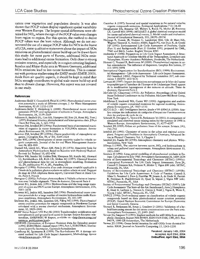
cators over v e g e t a t i o n and p o p u l a t i o n density. It was also s h o w n that P O C P va lues d i sp lay significant spatial var iab i l i ty over Western E u r o p e . The la rges t spatial differences were ob- ta ined for N O x , w h e r e the s ign of the P O C P value even changes f r o m region to reg ion . For this species, the m e t h o d to der ive P O C P values was the least robus t . M t h o u g h we do n o t rec- o m m e n d the use o f a un ique P O C P value for N O x in the f l a m e of LCIA, some qual i ta t ive s ta tements abou t the impac t of N O x emissions on p h o t o c h e m i c a l ozone build-up can be d r a w n f r o m this study: for m o s t par ts o f Europe , addi t iona l N O x emissions lead to a d d i t i o n a l o z o n e fo rmat ion . O n l y close to s t rong emission sources , a n d especial ly in a reg ion cover ing England , Benelux and R h i n e - R u h r a rea in Western Germany, add i t iona l N O x emissions l ead to less o z o n e fo rmat ion . This is consis t - ent wi th previous studies using the EMEP mode l (EMEP, 2003). Aside f rom air qua l i t y aspects, it should be kep t in m i n d t h a t N O x st rongly con t r ibu te s to g loba l scale ozone bui ld-up a n d thus to c l imate change . H o w e v e r , this aspect was no t cove red in ou r study.

References

Andersson-Sk61d Y, Grennfelt P, Pleijel K (1992): Photochemical ozone creation potentials: a study of different concepts. J. Air Waste Management Association, 42 (9) 1152-1158

Andersson-Sk61d Y, Holmberg L (2000): Photochemical ozone creation potentials (POCP) and replacement of solvents in Europe. Atmospheric Environment, 34, 3159-3169

Atkinson R, Baulsch DL, Cox RA, Hampton RF, Kerr JA, Rossi MJ, Troe J (1997): Evaluated kinetics, photochemical and heterogeneous data. J Phys Chem Ref Data 26, 3, 521-1012

Bowman FM, Seinfled JH (1994a): Fundamental basis of incremental reacti- vities of organics in ozone formation in VOC/NOx mixture. Atmos- pheric Environment 28, 3359-3368

Bowman FM, Seinfled JH (1994b): Ozone productivity of atmospheric organics. J Geophys Res. 99, n ~ D3, 5309-5324

Carter WPL (1994): Development of ozone reactivity scales for volatile organic compounds. Journal of the Air and Waste Management Associa- tion 44, 881-899

Darnall KR, Lloyd AC, Winer AM, Pitts Jr JN (1976): Reactivity Scale for Atmospheric Hydrocarbons Based on Reaction with Hydroxyl Radical. Environ Sci Technol 10, 692-696

DeMore WB, Sander SP, Golden DM, Hampson RF, Kurylo MJ, Howard CJ, Ravishankara AR, Kolb CE, Molina MJ (1997): Chemical kinetics and photochemical data for use in stratospheric modeling. Evaluation 12, JPL publication 97, 4, JPL, Pasadena, US

Derognat C (1998): Elaboration d'un code chimique simplifi6 applicable ~t l'&ude de la pollution photooxydante en milieu urbain et rural. Rapport de stage de DEA (diploma thesis report), Universit6 Pierre et Marie Cu- rie, Paris 6, France

Derognat C (2002): Pollution photooxydante & l'&helle urbaine et interac- tion avec l'&helle rtgionale. Th~se de doctorat, Universit6 Paris 6

Derwent RG, Jenkin ME (1991): Hydrocarbons and the long-range transport of ozone and PAN across Europe. Atmospheric Environment, 25A, 1661-1678

Derwent RG, Jenkin ME, Saunders SM (1996): Photochemical ozone creation potentials for a large number of reactive hydrocarbons under Euro- pean conditions, Atmospheric Environment, 30, 181-199

Derwent RG, Jenkin ME, Saunders SM, Pilling MJ (1998): Photochemical ozone creation potentials for organic compounds in Northwest Europe calculated with a master chemical mechanism. Atmospheric Environ- ment, 32, 2429-2441

EMEP Status Report 1/03 Part III (2003) Transboundary acidification and eutrophication and ground level ozone in Europe: Source-Receptor rela- tionships, EMEP/MSC-W Report, available on <httn://www.emen.ind common tmblications.html>

GENEMIS (Generation of European Emission Data for Episodes) project (1994): EUROTRAC Annual report 1993, Part 5, EUROTRAC Interna- tional Scientific Secretariat, Garmisch-Partenkirchen

Goedkoop M, Spriensma R (1999): The Eco-Indicator 99. A damage ori- ented method for Life Cycle Impact Assessment, Methodology Annex <http://www.pre.nl>, 108 pp.

Guenther A (1997): Seasonal and spatial variations in the natural volatiles organic compounds emissions. Ecological Applications 7 (1) 34-45

Hauglustaine DA, Brasseur GP, Wakers S, Rasch PJ, Muller JF, Emmons LK, Carroll MA (1998): MOZART: A global chemical transport model for ozone and related chemical tracers, 2. Model results and evaluation. Journal of Geophysical Research, 103, 28291-28336

Heijungs R, Guin& JB, Huppes G, Lamkreijer RM, Udo de Haes HA, Wegener Sleeswijk A, Ansems AMM, Eggels PG, van Duin R, de Goede liP (1992): Environmental Life Cycle Assessment of Products. Guide (Part 1) and Backgrounds (Part 2) October 1992, prepared by CML, TNO and B&G. Leiden. English Version 1993

Hofstetter P (1998): Perspectives in Life Cycle Impact Assessment; A Struc- tured Approach to Combine Models of the Technosphere, Ecosphere and Valuesphere. Kluwer Academic Publishers, Dordrecht, The Netherlands

Honor6 C, Vautard R, Beekmann M (2000): Photochemical regimes in urban atmospheres: The influence of dispersion. Geophys Res Letters, 27 (13) 1895-1898

International Organization for Standardization (ISO) (1999): Environmen- tal Management - Life cycle Assessment - Life cycle Impact Assessment. ISO Standard 14042. Prepared by Technical committee 207, sub committee 5 (ISO/TC 205/SC5)

Lattuati M (1997): Impact des ~missions europ~ennes sur le bilan de l'ozone tropospMrique ~ l'interface de l'Europe et de l'Atlantique Nord: apport de la mod~lisation lagrangienne et des mesures en altitude. Th~se de doctorat, Universit~ Paris 6

McCabe LC (Chairman) (1952): Air Pollution. Proceedings of the United States Technical Conference on Air Pollution. McGraw-Hill Book Comp, New York

Middleton P, Stockwell WR, Carter WP (1990): Aggregation and analysis of volatile organic compound emissions for regional modeling. Atmos- pheric Environment, 24, 1107-1133

RE.CO.R.D. - BIO Intelligence Service, Etude n~ (2000): Ana- lyse critique des indicateurs de categories d'impact sur l'environnement dans les analyses de cycle de vie

Schmidt H, Derognat C, Vautard R, Beekmann M (2001): A comparison of simulated and observed ozone mixing ratios for the summer of 1998 in Western Europe. Atmospheric Environment, 35, 6277-6297

Seinfeld JH (1989): Urban air pollution: State of the science. Science, 243, 745-752

Seinfeld JH (1995): Chemistry of ozone in the urban and regional atmosphere. Progress and Problems in Atmospheric Chemistry, Advanced Se- ries in Physical Chemistry Vol. 3, Chapter 2

Seinfeld JH, Pandis SN (1998): Atmospheric chemistry and physics. Wiley- Interscience, New York

Sillman S (1999), The relation between ozone, NO x and hydrocarbons in urban and polluted rural environments. Atmospheric Environment 33, 1821-1845

Simpson D (1992): Long period modelling of photochemical oxidants in Eu- rope. Calculations for July 1985. Atmospheric Environment 26, 1609-1634

Society of Environmental Toxicology and Chemistry (SETAC) (1993a): Conceptual Framework for Life Cycle Impact Assessment. Fava JA, Consoli F, Denison RA, Dickson K, Mohin T, Vigon BW (eds). SETAC, Pensacola, FL, USA

Society of Environmental Toxicology and Chemistry (SETAC) (1993b): Guidelines for Life Cycle Assessment: A Code of Practice. Consoli F, Allen D, Boustead I, Fava J, Franklin W, Jensen A, de Oude N, Parrish R, Perriman R, Postlethwaite D, Quay B, S~guin J, V-lgon BW (eds). SETAC, Pensacola, FL, USA

Society of Environmental Toxicology and Chemistry (SETAC) (1997): Life Cycle Assessment: The State-of-the-Art. Barnthouse L, Fava J, Humphreys K, Hunt R, Laibson L, Noesen S, Owens J, Todd J, Vigon B, Weitz K, Young J (eds). SETAC, Pensacola, FL, USA

UNECE (1990): Draft technical annex on classification of volatile organic compounds based on their photochemical ozone creation potential (POCP). United Nations Economic Commission for Europe (Economic and Social Council), Geneva

Vautard R, Beekmann M, Roux J, Gombert D (2001): Validation of a hy- brid forecasting system for the ozone concentrations over the Paris area. Atmospheric Environment, 35, 2449-2461

Verwer JG, Simpson D (1991): Explicit methods for stiff ODEs from atmospheric chemistry, Report NM-R9409, ISSN 0169-0388, CWI, P.O. Box 94079, 1090 GB Amsterdam, The Netherlands

Verwer JG (1994): Gauss-Seidel iteration for stiff ODEs from chemical kinetics. SIAM. Journal on Scientific Computing 15, 1243-1250

Received: January 14th, 2004 Accepted: April 23rd, 2004

OnlineFirst: April 23rd, 2004

Int J LCA 9 (3) 2004 195

Photochemical ozone creation potentials

Documents

Transcript of Photochemical ozone creation potentials