Ozone and Stratospheric Chemistry
29
309 EOS Science Plan Ozone and Stratospheric Chemistry Lead Author Contributing Authors M. R. Schoeberl A. R. Douglass J. C. Gille J. A. Gleason W. R. Grose C. H. Jackman S. T. Massie M. P. McCormick A. J. Miller P. A. Newman L. R. Poole R. B. Rood G. J. Rottman R. S. Stolarski J. W. Waters Chapter 7
-
Upload
khangminh22 -
Category
Documents
-
view
3 -
download
0
Transcript of Ozone and Stratospheric Chemistry

309EOS Science Plan
Ozone andStratospheric
Chemistry
Lead Author
Contributing Authors
M. R. Schoeberl
A. R. DouglassJ. C. GilleJ. A. GleasonW. R. GroseC. H. JackmanS. T. MassieM. P. McCormickA. J. MillerP. A. NewmanL. R. PooleR. B. RoodG. J. RottmanR. S. StolarskiJ. W. Waters
Chapter 7

CHAPTER 7 CONTENTS
7.1 Stratospheric ozone - background 3117.1.1 Why is understanding stratospheric ozone important? 311
7.1.1.1 Location of the ozone layer and climatology 3117.1.1.2 Ozone and UV—biological threat 3117.1.1.3 Ozone and climate change 311
7.1.2 Observed ozone changes 3127.1.2.1 Polar ozone changes 3127.1.2.2 Mid-latitude ozone loss 313
7.1.3 The stratospheric ozone distribution 3147.1.3.1 Chemical processes 3147.1.3.2 Transport 3157.1.3.3 Aerosols and Polar Stratospheric Clouds (PSCs) 315
7.1.3.3.1 Aerosols 3167.1.3.3.2 Polar stratospheric clouds 316
7.1.3.4 Solar ultraviolet and energetic particles 3167.1.4 Modeling the ozone distribution, assessments 317
7.1.4.1 Two-dimensional models 3177.1.4.2 Three-dimensional models
3187.2 Major scientific issues and measurement needs 319
7.2.1 Natural changes 3197.2.1.1 Interannual and long-term variability of the stratospheric circulation3197.2.1.2 External influences (solar and energetic particle effects) 3197.2.1.3 Natural aerosols and PSCs 319
7.2.2 Man-made changes 3207.2.2.1 Trends in chlorine source gases 320
7.2.2.1.1 Historical trends in chlorine source gases 3207.2.2.1.2 Stratospheric chlorine 3217.2.2.1.3 Depletion of ozone by stratospheric chlorine 321
7.2.2.2 Effects of aircraft exhaust 3227.2.3 Summary of science issues 322
7.3 Required measurements and data sets 3227.3.1 Meteorological requirements 3237.3.2 Chemical measurement requirements 324
7.3.2.1 Science questions 3247.3.2.2 Key trace gas measurements 325
7.3.3 Stratospheric aerosols and PSCs 3267.3.4 Solar ultraviolet flux 3277.3.5 Validation of satellite measurements 327
7.4 EOS contributions 3287.4.1 Improvements in meteorological measurements 328
7.4.1.1 Global limb temperature measurements 3287.4.1.2 Higher horizontal resolution temperature profiles 328
7.4.2 Improvements in chemical measurements in the stratosphere 3287.4.3 Improvements in measurements of aerosols 3307.4.4 Improvements in measurements of the solar ultraviolet flux 3317.4.5 Advanced chemical/dynamical/radiative models 3317.4.6 Full meteorological and chemical assimilation of EOS data sets 333
7.5 Foreign partners and other measurement sources 333
References 334
Chapter 7 Index 337

OZONE AND STRATOSPHERIC CHEMISTRY 311
7.1 Stratospheric ozone - background
primarily occurs in the tropical upper stratosphere, whereit is transported poleward and downward by the large-scale Brewer-Dobson circulation. The global distributionof total ozone is shown in Figure 7.2 (pg. 312). This fig-ure represents the 13-year average of the total ozonemeasurements taken by the Nimbus-7 Total Ozone Map-ping Spectrometer (TOMS) instrument.
The formation of ozone by the photolysis of mo-lecular oxygen removes most of the incident sunlight withwavelengths shorter than 200 nm. The wavelengths be-
tween 200 and 310 nm are removedby the photolysis of ozone itself. Thisphotolysis of ozone in the stratosphereis the process by which most of thebiologically damaging ultraviolet sun-light (UV-B) is filtered out.
As this filtering process occurs,the stratosphere is heated. This heat-ing is responsible for the temperaturestructure of the stratosphere, where thetemperature increases as the altitudeincreases. Without this filtering, largeramounts of UV-B would reach the sur-face. Numerous studies have shownthat excessive exposure to UV-B isharmful to plants, animals, and hu-mans (WMO 1992).
7.1.1.3 Ozone and climate changeIf ozone in the stratosphere were to be
removed, the stratosphere would cool. How a cooler strato-sphere affects radiative balance in the rest of theatmosphere has been the subject of many detailed stud-ies. These studies have been reanalyzed and integratedinto the latest Intergovernmental Panel on Climate Change(IPCC) report, “Climate Change 1994: Radiative Forc-ing of Climate Change” (1995). The conclusion of thatreport is that stratospheric ozone loss leads to a “smallbut non-negligible offset to the total greenhouse forcingfrom CO2, N2O, CH4, CFCs....” It is ironic that the size ofthe negative radiative forcing from ozone loss is nearlyequal to the positive radiative forcing from chlorofluoro-carbons (CFCs), the source of the stratospheric ozone loss.The size of the radiative forcing due to stratospheric ozoneloss has also been shown to be very sensitive to the pro-file shape assumed for that loss.
FIGURE 7.1
The distribution of atmospheric ozone in partial pressure as a function of altitude.
• Contains 90% of atmosphericozone
• Beneficial role: Acts as primaryUV radiation shield
• Current issues:- Long-term global down-
ward trends- Springtime Antarctic ozone hole each year
• Contains 10% of atmosphericozone
• Harmful impact: Toxic effectson humans and vegetation
• Current issues:- Episodes of high surface
ozone in urban and ruralareas
Atmospheric Ozone
“Smog” Ozone
Stratospheric Ozone(The Ozone Layer)
Tropospheric Ozone
0 5 10 15 20 25Ozone Amount (pressure, mP)
35
30
25
20
15
10
5
Alti
tude
(ki
lom
eter
s)
7.1.1 Why is understanding stratospheric ozone im-portant?
Ozone is one of the most important trace species in theatmosphere. Ozone plays two critical roles: it removesmost of the biologically harmful ultraviolet light beforethe light reaches the surface, and it plays an essential rolein setting up the temperature structure and therefore theradiative heating/cooling balance in the atmosphere, es-pecially the stratosphere (the region between about 10and 60 km).
7.1.1.1 Location of the ozone layer and climatologyOzone is mainly found in two regions of the atmosphere.Most of the ozone can be found in a layer between 10 and60 km above the Earth’s surface (Figure 7.1). This ozoneregion located in the stratosphere is known as the “ozonelayer.” Some ozone can also be found in the lower atmo-sphere (below 10 km) in the region known as thetroposphere. Although chemically identical to strato-spheric ozone, tropospheric ozone is quite distinct andgeophysically different from stratospheric ozone, and thescience issues concerning tropospheric ozone are dis-cussed in Chapter 4.
7.1.1.2 Ozone and UV—biological threatOzone is produced by the photolysis of molecular oxy-gen, O2. The oxygen atom, O, produced by this photolysisrecombines with O2 to form ozone, O3. Ozone formation

312 EOS SCIENCE PLAN - CHAPTER 7
7.1.2 Observed ozone changesWhile the global amount of ozone is fairly constant, thereare significant local, seasonal, and long-term changes. Thecauses of these changes are discussed in detail in Section7.1.3.
The seasonal ozone changes are basically deter-mined by the winter-summer changes in the stratosphericcirculation. Since ozone has a lifetime of weeks to monthsin the lower stratosphere, the amount of ozone can stronglyvary due to transport by stratospheric wind systems. Sinceweather conditions in the stratosphere, as in the tropo-sphere, vary from year to year, there is also interannualvariability in ozone amounts. Interseasonal changes inozone are also linked to the 11-year solar cycle in UVoutput and the amount of volcanic aerosols in the strato-sphere. Changes in ozone have also been linked toanthropogenic pollutants, especially the release of man-made chemicals containing chlorine. In the section belowwe describe the more-significant recent global changesin ozone observed by a variety of instruments.
7.1.2.1 Polar ozone changesThe first ozone measurements in the Antarctic were madeduring the 1950s. A Dobson instrument was installed atHalley Bay in late 1956 in preparation for the Interna-
tional Geophysical Year in 1957.One of the first discoveries madeby this instrument was that theseasonal cycle of ozone in thesouth polar region is very differ-ent from that which had beenobserved in the north. This wasnoted in a review article by Dob-son (1966), which pointed out thatits cause was a difference in thecirculation patterns of the Antarc-tic relative to the Arctic. In theArctic, the total ozone amountgrew rapidly in the late winter andearly spring to about 500 DobsonUnits (DU). (A DU is onemilliatmosphere-cm of pureozone; a layer of pure ozone thatwould be 0.001-cm thick underconditions of Standard Tempera-ture and Pressure [STP].) Incontrast, the Antarctic earlyspringtime amounts remainednear 300 DU.
The Dobson instrument at Halley Bay continuedto make measurements each year. Farman et al. (1985)showed that the springtime ozone amounts over HalleyBay had declined from nearly 300 DU in the early 1960sto about 180 DU in the early-to-mid 1980s. This resulthas been confirmed at a number of other stations andshown using satellite data to occur over an area largerthan the Antarctic continent (Stolarski et al. 1986). Theselarge ozone changes implied that losses must be takingplace in the lower stratosphere where most of the ozoneexists. This was shown to be true in a series of ozonesondemeasurements (see, e.g., Hofmann et al. 1989 and Figure7.3). More-recent sonde measurements have shown in-stances of near-zero concentrations of ozone over a 5-kmaltitude range (Hofmann et al. 1994). Aircraft measure-ments (Proffitt et al. 1989) and satellite measurements(McCormick et al. 1988) confirm and show further de-tails of these ozone changes.
The 1996-1997 Northern Hemisphere winter ex-perienced a significant ozone depletion over the Arcticand subsequent total ozone values achieved record lowvalues in the spring. Long term records of the Total OzoneMapping Spectrometer (TOMS) (Newman et al., 1997)and ground based observations (Fioletov et al., 1997) showa downward change over the past several years occurringmostly in February and March and confined to the lower
The global distribution of column or total ozone averaged over the 13 years of Nimbus-7 TOMSdata in Dobson Units (DU).
FIGURE 7.2

OZONE AND STRATOSPHERIC CHEMISTRY 313
FIGURE 7.3
Balloonsonde ozone measurements made at McMurdo and SAGE II measurementsfor 1987.
(a) (b)
stratosphere (Manney et al. 1997) similar to the depletionover the Antarctic. Total ozone changes for both polarregions are shown in Figure 7.4 (pg. 314) (Newman, Pri-vate communication). Chlorine radicals have beenconclusively identified as the causes of ozone depletionnow in both hemispheres. Measurements of ClO by theUARS MLS instrument (Santee et al., 1997) observedelevated levels in late February over Northern Hemispherepolar regions. The winter of 1996-1997, showed extremelylow temperatures in the Stratosphere. These cold tempera-tures led to the formation of polar stratospheric cloudswhose particles shift chlorine gas away from its HCl res-ervoir to active ClO through heterogeneous chemistry.This is the primary mechanism producing the Antarctic
ozone hole (Anderson et al., 1991,Solomon, 1990, and others). Althoughthe buildup of chlorine has occurredapproximately uniformly in both hemi-sphere the unusually low temperaturesreached in high northern latitudesmostly likely precipitated the concur-rent ozone losses over the Arctic.
7.1.2.2 Midlatitude ozone lossMidlatitude ozone loss estimates mustbe extracted from long time series us-ing statistical models (see, e.g., Reportof the International Ozone TrendsPanel 1990). The longest time seriesof total ozone data is from Arosa inSwitzerland. This time series, whichdates back to 1926, is shown in Figure7.5 (pg. 314). The Arosa data show arelatively constant amount of ozone forover 4 decades and a decrease in thelast decade and a half. Analysis of amore-extensive network of 30+ sta-tions which have been in operation forabout 35 years shows negative trendsover the last 1.5 decades, especially inthe winter and early spring (see, e.g.,Reinsel et al. 1994).
High-quality global satellitedata records began in November 1978with the launch of the Nimbus-7 SolarBackscatter Ultraviolet (SBUV) radi-ometer and TOMS instruments. Thesedata show midlatitude trends in theNorthern Hemisphere which are larg-est in the winter and early spring,peaking at about 6-8% per decade at
40˚-50° N in February (see, e.g., Randel and Cobb 1994;Hollandsworth et al. 1995). These satellite trends are inthe process of being updated with a version 7 algorithmfor the TOMS and SBUV instruments.
Changes in the profile of ozone with altitude canbe deduced from sonde data or from the StratosphericAerosol and Gas Experiment (SAGE) satellite measure-ments. Analyses of sonde data (e.g., Logan 1994) showozone decreases between the tropopause and about 24-km altitude. Analyses of SAGE data show larger decreasesthan those derived from sondes. SAGE results show nega-tive ozone trends in the lower stratosphere in the tropics.Column ozone changes deduced from SBUV and TOMSshow only small downward trends. Hollandsworth et al.

314 EOS SCIENCE PLAN - CHAPTER 7
(1995) used SBUV profile and total ozone trends to de-duce that ozone in the tropics below 32 hPa has increasedslightly over the last decade. The resolution of the uncer-tainty in the magnitude of lower stratospheric and uppertropospheric ozone trends is an important measurementand analysis issue for the coming years.
7.1.3 The stratospheric ozonedistribution
7.1.3.1 Chemical processesOzone is being continuously created and de-stroyed by the action of ultraviolet sunlight.The overall amount of ozone in the globalstratosphere is determined by the magnitudeof the production and loss processes and bythe rate at which air is transported from re-gions of net production to those of net loss.
Production of ozone requires thebreaking of an O2 bond, with the extra or“odd” oxygen atom attaching to another O2
to form O3. This most frequently occurs viathe photodissociation of O2 by solar ultra-violet radiation. In the lower stratosphere andtroposphere ozone can also be produced byphotochemical smog-like reactions. In thesereactions H or CH3 or higher hydrocarbon
radicals attach to an O2 forming HO2 or CH3O2, etc., whichthen react with NO. This reaction breaks the O2 bond byforming NO2 (which is really ONO). When NO2 is pho-tolyzed an O atom is formed which reacts with O2 to formO3. Loss of ozone occurs when an O atom reacts with O3
to re-form the O2 bond. More importantly, this loss pro-cess is catalyzed by the oxides of hydrogen, nitrogen,chlorine, and bromine. These oxides are produced in the
stratosphere from long-lived, unreactive moleculesreleased at the surface ofthe Earth. The major sourcemolecules for HOx (HOx ischemical shorthand for thesum of all the hydrogenradicals—OH and HO2,mostly) are methane (CH4)and water vapor (H2O). Themain source of NOx (NOx
is chemical shorthand forthe sum of all nitrogen radi-cals—NO, NO2, N2O5,NO3, mostly) is nitrous ox-ide (N2O). The majorsources of chlorine are in-dustrially-produced CFCs(such as CFC-11, which isCFCl3, and CFC-12, whichis CF2Cl2) and naturally-occurring methyl chloride(CH3Cl). The major
FIGURE 7.5
one year smoothed
TOMS ozone
trend: 1926-1973+0.1%/decade
trend: 1973-1993-2.9%/decade
360
340
320
300
Ozo
ne (
DU
)
30 40 50 60 70 80 90Year
Time series of column ozone measurements at Arosa, Switzerland, in DU.
63˚ - 90˚ total ozone average
FIGURE 7.4

OZONE AND STRATOSPHERIC CHEMISTRY 315
sources of bromine are methyl bromide (CH3Br) and thehalons (CF3Br and CF2ClBr). These source molecules aretransported to the stratosphere where they react or are pho-todissociated to produce the catalytically-active oxideradicals.
The catalytic efficiency of hydrogen, nitrogen,chlorine, and bromine oxides is determined by a set ofinterlocking reactions which convert the active oxides tocatalytically-inactive temporary reservoirs, such as HNO3,HCl, ClONO2, H2O, HOCl, HOBr, and BrONO2, and viceversa. In the lower stratosphere, the balance between cata-lytic oxides and temporary reservoirs is strongly affectedby reactions on the surfaces of stratospheric aerosols. Thebalance is even more profoundly affected in the polarwinter by reactions on the surface of Polar StratosphericCloud (PSC) particles. In the early spring, the chlorinebalance is shifted to almost 100% ClOx (ClOx is short-hand for the sum of all chlorine radicals, C1O, Cl2O2, Cl)(Brune et al. 1989; Waters et al. 1993). This shift in thechemical balance results in a large calculated chemicalsensitivity of ozone towards chlorine perturbations and arelatively small calculated sensitivity of ozone towardsnitrogen oxide perturbations.
Although the basic outline of the chemistry con-trolling stratospheric ozone is now known, many importantaspects of the problem remain to be solved. The primarydifference between the Northern and Southern Hemi-spheric polar ozone loss regions appears to be a result ofthe “denitrification” that occurs in the Antarctic winter.Denitrification means the removal of nitrogen oxides andHNO3 by large particles which fall into the troposphere.Denitrification takes place when temperatures are coldenough to form large stratospheric ice crystals.
When springtime comes there are no nitrogen ox-ides to convert ClOx to ClONO2 and slow down the rateof ozone depletion. There is some evidence for denitrifi-cation when temperatures are not cold enough to formice crystals. Under those conditions the mechanism fordenitrification is not completely understood.
7.1.3.2 TransportMuch of the currently-observed ozone interannual vari-ability in the stratosphere is controlled by dynamicalprocesses. In particular, this variability is driven by suchprocesses as the quasi-biennial oscillation (QBO), ElNiño-Southern Oscillation, tropospheric weather systemswhich extend into the stratosphere, and long-term fluc-tuations in planetary wave activity. The annual cycle oftotal ozone is largely driven by transport effects. As shownin Figure 7.2, relatively low values of ozone are observedin the tropics and high values are observed in theextratropics. These low tropical ozone values occur in spite
of the large ozone production rates in the tropics. If ozoneproduction were precisely balanced by ozone loss every-where, total ozone would have extremely high values inthe tropics. The observed tropical low values result fromvertical advection of low-ozone air from the tropical tro-posphere into the tropical stratosphere, and the subsequenttransport of this air poleward and downward into theextratropics and polar regions. This advective circulationis known as the Brewer-Dobson circulation.
The redistribution of ozone from the productionregion at low latitudes to extratropical latitudes is modu-lated by a variety of processes. Foremost among theseprocesses is the annual cycle in the circulation. It is nowrecognized that the Brewer-Dobson circulation is prima-rily controlled by large-scale waves in the winterstratosphere. As these waves propagate through the west-erly winds that dominate the winter stratosphere, they exerta westward zonal drag, which through the Coriolis forceleads to a poleward and downward transport circulation,which in turn drives the temperatures away from radia-tive equilibrium. The large-scale waves breaking in thewinter upper stratosphere also produce lifting in the trop-ics. Since the lifetime of ozone increases with pressure,the poleward downward circulation causes ozone to ac-cumulate in the lower stratosphere over the course of thewinter. Since the large-scale waves are not present in thesummer, the poleward and downward circulation is sig-nificantly weakened, and ozone amounts which have builtup during winter begin to decrease due both to transportinto the troposphere and to photochemistry.
The exchange of mass between the troposphere andthe stratosphere is the focus of considerable current re-search (Holton et al. 1995). Stratosphere-troposphereexchange is important for the budget of ozone in the lowerstratosphere as well as the ozone budget in the troposphere.Upward transport occurs in the tropics, but the exactmechanism controlling the transport is not clear. Currentresearch is focussing on the role of subvisible cirrus andthe radiative impact of infrared (IR) heating of subvisiblecirrus (Jensen et al. 1997). Downward transport (strato-sphere to troposphere) takes place in midlatitudes throughjet stream folds—but the frequency and amount of massirreversibly moving through these folds is still not under-stood (Holton et al. 1995).
7.1.3.3 Aerosols and Polar Stratospheric Clouds (PSCs)It is now known that knowledge of stratospheric aerosolsand PSCs is very important to our understanding of strato-spheric ozone. The surfaces of aerosols and PSCs are sitesfor heterogeneous reactions which can convert chlorinefrom reservoir to radical forms. Likewise, radical nitro-

316 EOS SCIENCE PLAN - CHAPTER 7
gen forms can be sequestered as nitric acid to shift thechemical loss process (WMO 1995).
7.1.3.3.1 AerosolsThe long-term stratospheric aerosol record reveals at leastthree components: episodic volcanic enhancements, PSCsand clouds just above the tropical tropopause, and a back-ground aerosol level. At normal stratospherictemperatures, aerosols are most likely super-cooled solu-tion droplets of H2SO4-H2O, with an acid weight fractionof 55 to 80%. The primary source of stratospheric aero-sols is volcanic eruptions that are strong enough to injectSO2 buoyantly into the stratosphere. Aerosol sizes rangefrom hundredths of a micrometer to several micrometers.Although there is some variability, especially just after avolcanic eruption, a log-normal size distribution of spheri-cal particles appears to aptly describe the aerosol. Justafter an eruption, the size distribution becomes bimodal,and some particles are nonspherical because of the addi-tion of crustal material. After an eruption, the SO2 isconverted to H2SO4, which condenses to form strato-spheric sulfuric acid aerosols, with a time scale of about30 days. Subsequently, aerosol loading decreases due toa combination of sedimentation, subsidence, and exchangethrough tropopause folds. The loading decreases with ane-folding time of 9-to-12 months, although this appearsquite variable with altitude and latitude.
The net effect of this post-volcanic dispersion andnatural cleansing is a greatly enhanced aerosol concen-tration in the upper troposphere after a major eruption,especially poleward of about 30° latitude. Except imme-diately after an eruption, stratospheric aerosol dropletstend to be concentrated into 3 distinct latitudinal bands—one over the equatorial region (to 30°) and the other overeach high-latitude region, 50˚ to 90° N and S. Followinga low-latitude eruption, aerosol is dispersed into bothhemispheres, whereas following a mid-to-high-latitudeeruption, aerosols tend to stay primarily in the hemisphereof the eruption. Potential sources of a background aero-sol component include carbonyl sulfide (OCS) from theoceans, low-level SO2 emissions from volcanoes, andvarious anthropogenic sources, including industrial andaircraft emissions. Also, it is not clear whether there is anupward trend in this background aerosol, as has been hy-pothesized and linked to increasing aircraft emissions,since any increase may be due to incomplete removal ofpast volcanic aerosol.
Stratospheric aerosol loading in 1979 was approxi-mately 0.5 × 10¹²g (0.5 Mt), thought to be representativeof background aerosol conditions. The present status ofthe aerosol is one of enhancement due to the June 1991eruption of Pinatubo (15.1° N, 120.4° E), which produced
on the order of 30 × 1012g (30 Mt) of new aerosol in thestratosphere, about 3 times that of the 1982 eruption of ElChichón. This perturbation appears to be the largest ofthe century, perhaps the largest since the 1883 eruptionof Krakatoa. By early 1993, stratospheric loading de-creased to approximately 13 Mt, about equal to the peakloading values after El Chichón (McCormick et al. 1995).Measurements in 1995 showed that the aerosol levels wereapproaching background levels.
7.1.3.3.2 Polar Stratospheric Clouds (PSCs)The interannual variability in PSC sightings has
been addressed by Poole and Pitts (1994), who analyzedmore than a decade of data from the spaceborne Strato-spheric Aerosol Measurement (SAM) II sensor (Figure7.6). They found noticeable variability in PSC sightingsin the Antarctic from year to year, even though the south-ern polar vortex is typically quite stable and long-lived.This variability was found to occur late in the season andcan be explained qualitatively by temperature differences.Poole and Pitts found even more year-to-year variabilityin SAM II Arctic PSC sighting probabilities. This wasexpected since the characteristics and longevity of thenorthern polar vortex vary greatly from one year to thenext. The year-to-year variability in Arctic sighting prob-abilities can also be explained qualitatively by differencesin temperature, e.g., zonal mean lower stratospheric tem-peratures in February 1988 were as much as 20 K colderthan those one year earlier.
7.1.3.4 Solar ultraviolet and energetic particlesSince ozone formation is fundamentally linked to the lev-els of ultraviolet radiation reaching the Earth, naturalvariations in that radiation must be understood in order todetect trends. The ultraviolet comprises only one-to-twopercent of the total solar radiation, but it displays consid-erably more variation than the longer wavelength visibleradiation. For example, from 1986 to 1990 the solar UVincreased with onset of the 11-year solar cycle and re-sulted in an increase of global total ozone of almost 2%.This natural increase in ozone is comparable to the sus-pected anthropogenic decrease and needs to be understoodin order to totally separate the anthropogenic decreasefrom this natural change. Studies of total ozone trendstypically subtract solar cycle and other natural changesfrom the total ozone record in trend resolution (see WMO1992; WMO 1995; Stolarski et al. 1991; and Hood andMcCormack 1992). Thus, more-quantitative knowledgeof this natural solar-cycle-induced total ozone changewould be especially valuable.
Changes in energetic particle flux from the sunpenetrate into the middle atmosphere and may also drive

OZONE AND STRATOSPHERIC CHEMISTRY 317
the natural ozone variations. A series of solar flares in1989 spewed solar particles into the Earth’s polar cap re-gions (greater than 60° geomagnetic latitude) and led topolar ozone depletion (Jackman et al. 1993). Further stud-ies related to the very large solar particle events (SPEs)of October 1989 have predicted ozone depletions lastingfor several months after the SPEs (Reid et al. 1991;Jackman et al. 1995). Although SPEs of this magnitudeoccur infrequently (only two have been observed in thepast 25 years), they need to be understood more com-pletely to be able to separate natural from anthropogenicozone effects.
Relativistic electron precipitations (REPs) havebeen predicted to contribute substantially to the odd ni-trogen budget of the stratosphere and, therefore, have beenpredicted to play a large role in controlling ozone in thisregion (Callis et al. 1991a, 1991b). Another investigation(Aikin 1992) has failed to find any REP-caused ozonedepletion. Further work (Gaines et al. 1995) determinedthat REPs in May 1992, the largest measured relativisticelectron flux precipitating in the atmosphere between Oc-tober 1991 and July 1994, added only about 0.5 to 1% ofthe global annual source of odd nitrogen to the strato-sphere and mesosphere. The actual importance of REPsin regulating ozone is thus not well understood nor char-acterized, and further work on REPs is required tothoroughly determine their importance regarding modu-lation of stratospheric ozone.
7.1.4 Modeling the ozone distribution, assessmentsModels of the stratosphere provide the only means to at-tempt quantitative prediction of global change, or toevaluate the impact of natural or anthropogenic changesin composition on the stratospheric ozone and climate. Inaddition, models provide a means to integrate observa-tions and theory, to provide tests of mechanisms forchemical, dynamical, or radiative changes, and to enableinterpretation of observations from different platforms.
7.1.4.1 Two-dimensional modelsTwo-dimensional (2-D) models are used by several re-search groups. The models predict the behavior of ozoneand other trace gases in reasonable agreement with mea-surements (WMO 1992; WMO 1995). Because of thesefavorable comparisons to measurements, these modelshave been utilized recently in many atmospheric studies,for example: 1) the response of the middle atmospheredue to solar variability was studied by Brasseur (1993),Huang and Brasseur (1993), and Fleming et al. (1995); 2)the influence of the Mt. Pinatubo eruption on the strato-sphere was studied by Kinnison et al. (1994a, b) and Tieet al. (1994); and 3) the effects of proposed stratosphericaircraft on atmospheric constituents were studied by Pitariet al. (1993), Weisenstein et al. (1993), Considine et al.(1994), and Considine et al. (1995).
SAM II measurements of vertical optical depth data in the stratosphere over the Arctic and Antarctic. The measurementsshow the impact of volcanic eruptions over the period 1979-1992 along with seasonal effects in the local winters due toPolar Stratospheric Clouds (PSCs). The data are weekly averages at a wavelength of 1000 nm.
FIGURE 7.6
10-1
10-2
10-3
10-4
Opt
ical
Dep
th
1979 1981 1983 1985 1987 1989 1991Year
El C
hich
on
Mt.
Pin
atub
o
Arctic
Antarctic
318 EOS SCIENCE PLAN - CHAPTER 7
These 2-D models have also been used to producemulti-year simulations of the response of stratosphericozone to perturbations of the source gases such as CFCsfrom which chlorine radicals are produced (WMO 1992;WMO 1995). An outstanding issue regarding simulationsof the stratospheric ozone response to chlorine increasesis the lack of ability of 2-D models to accurately predictthe ozone trend in the middle and high northern latitudesover the 1980-to-1990 time period. Since the 2-D modelspredict a smaller trend than observed, it is believed thatthe models do not adequately model all of the relevantprocesses and thus require further development.
7.1.4.2 Three-dimensional modelsThe three-dimensional (3-D) (or general circulation)model with full interaction between chemical, dynami-cal, and radiative processes remains elusive. The presentgeneration of general circulation models (GCMs) gener-ates unrealistic temperature fields which, in turn, alter thephotochemistry. The unrealistic temperatures are relatedto problems with the model transport circulation. For ex-ample, the polar regions are persistently cold in GCMs,which suggests that there is insufficient adiabatic heating(or descent) in the winter polar region. Correspondingly,there will be insufficient ascent in the tropics, which weak-ens the transport from the troposphere into thestratosphere.
Subtle changes in the general circulation of the at-mosphere in 3-D models can alter and distort the chemicalfeedbacks. For example, Rasch et al. (1995) report on atwo-year simulation using version 2 of the National Cen-ter for Atmospheric Research (NCAR) MiddleAtmosphere Community Climate Model (MACCM2). Achemical scheme for 24 reactive species, or families, isrun as part of this simulation. This model is partiallycoupled in that the water vapor predicted by MACCM2is connected to the chemical source of water through oxi-dation of methane. Prescribed ozone is used in the radiativecalculation. In this simulation, the calculated upper strato-spheric ozone is substantially lower than is observed; muchof the difference is attributed to the lower CH4, comparedto observations by the UARS Halogen Occultation Ex-periment (HALOE). This bias leads to excessive ClO andexcessive destruction of O3. In effect, the error in this long-lived trace gas, which results from the weak transportcirculation, leads to noticeable errors in ozone.
The difficulties described above show why most3-D modeling efforts have focused on “off-line” calcula-tions, i.e., use of chemistry and transport models (CTMs)in which the wind and temperature fields are input from aGCM (e.g., Eckman et al. 1995) or from a data assimila-
tion system (e.g., Rood et al. 1991; Lefevre et al. 1994).For either approach, there are computational advantages,as the same set of winds and temperatures is used manytimes. Furthermore, the effects of modifications to thechemical scheme can be isolated, and their effects under-stood, without the complications caused by feedbackprocesses. A further advantage of the use of assimilatedwinds and temperatures is that the results of constituentsimulations may be compared directly with observationswith no temperature biases such as those found in GCMs.This is particularly important for the study of processeswhich have a temperature threshold, such as heteroge-neous reactions on PSC surfaces. The most informationis gleaned when the model is sampled in a manner con-sistent with the satellite sampling (Geller et al. 1993).
The “off-line” approach has been used successfullyfor many years and is used to test chemical and transportmechanisms, as well as to interpret observations. Thesetests include:
1) assessment of the importance of transport of air withhigh levels of reactive chlorine to middle latitudes(Douglass et al. 1991);
2) assessment of the rate of ozone loss within the North-ern Hemisphere vortex and identification of thevariables to which the calculation is sensitive(Chipperfield et al.1993);
3) determination of the importance of upper troposphericsynoptic-scale systems on the vortex temperature, aswell as their influence on the transport and mixing ofair which has experienced temperatures cold enoughfor PSC formation (Douglass et al. 1993); and
4) examination of the impact of ozone transport follow-ing the breakup of the Antarctic polar vortex on theglobal ozone budget (the “ozone dilution” effect).
These 3-D studies provide a picture of the impor-tant physical processes which control polar ozone loss.However, because of computer resource restrictions, it isnot yet possible to make full 3-D model long-range pre-dictions, including possible influence of the ozone losson lower stratospheric temperature and climate. For ex-ample, future temperature changes may have a significantimpact on the Northern Hemisphere vortex. The full 3-Dmodel, with all relevant chemical, dynamical, and radia-tive processes and feedbacks among them, has yet to bedeveloped.

OZONE AND STRATOSPHERIC CHEMISTRY 319
7.2 Major scientific issues and measurement needs
Changes in the ozone layer can be divided into two cat-egories: natural changes and man-made changes.Separating these components is the goal of much ozoneand trace gas research. Since ozone can be transported bystratospheric winds, there is significant interannual vari-ability in column ozone amounts. Ozone is likewiseinfluenced by aerosol amounts (through heterogeneouschemistry) (Solomon et al. 1996), the formation of nitro-gen radicals associated with high-energy particles, andvariations in the ultraviolet radiation from the sun. Man-made changes generally include increased chlorine andhydrogen amounts from industrial gases and increasedaerosols and nitrogen radicals from airplane exhaust.Many of our current scientific issues and future measure-ment needs center around the interaction of the ozone layerwith these pollutants and separating natural changes inthe ozone layer from man-made processes.
7.2.1 Natural changes
7.2.1.1 Interannual and long-term variability of thestratospheric circulation
Because the stratospheric circulation is strongly depen-dent on the dissipation of large-scale waves in thestratosphere, interannual variability of the wave ampli-tudes has an important impact on ozone transport (seeSection 7.1.3.2). Winds and temperatures derived from3-D GCMs and assimilation models include suchinterannual variability and can be used to assess the im-pact on ozone transport. 2-D models can incorporateprescribed variability to simulate interannual ozone trans-port (see Section 7.1.4.1). Accurate assessment of thelarge-scale waves and the transport circulation is neces-sary for understanding the variability of ozone trends.
One of the failures of the 3-D models is inadequatesimulation of the QBO. The QBO is a 24-30-month os-cillation of the zonal wind in the tropical lowerstratosphere that is driven by tropical waves. The QBOaffects the stratospheric temperature distribution and pro-duces a secondary circulation which transports trace gasesand aerosols. For ozone, the QBO can generate variationsfrom the climatological mean of 5-10 DU in the tropics.There is also a QBO-ozone signal outside the tropics of10-20 DU.
The QBO provides one of the largest componentsof the interannual variability of the column ozone values.Because the geostrophic relationship breaks down in thetropics, direct tropical wind measurements are critical toprecisely measuring the QBO and for understanding the
effects of the QBO on the circulation. Data-sparse regionsand infrequent sampling of wind fields all preclude goodquantitative studies of the tropical circulation and its ef-fect on ozone.
7.2.1.2 External influences (solar and energetic particleeffects)
As discussed in Section 7.1.3.4 solar ultraviolet radiationand precipitating energetic particles can strongly influ-ence ozone amounts. In order to understand theanthropogenic changes in ozone, we must maintain reli-able measurements of the solar ultraviolet input to themiddle atmosphere. Solar variations in the UV produceozone changes on the same order of magnitude as thecurrent observed midlatitude changes. Proxies for the UVchanges have been historically used to estimate the re-sponse of ozone to solar ultraviolet changes. With directmeasurements from UARS, these proxies have beenshown to inadequately represent changes in ultravioletflux.
Particle events generate NOx compounds whichcatalytically destroy ozone, but these events tend to beconfined to the upper stratosphere. Large events, whichtend to be more episodic, may affect polar ozone at lowerlevels. The impact of NOx generation through particleprecipitation on the natural ozone layer is a major scien-tific question.
7.2.1.3 Natural aerosols and PSCsAs discussed in Section 7.1.3.3, aerosols and PSCs arebelieved to play a major (although indirect) role in ozoneloss. Irregular volcanic inputs of SO2 with the subsequentformation of sulfate aerosols have an impact on the ozonelayer. There is some evidence suggesting that increasingamounts of background aerosols are a result of subsonicaircraft emissions in the lower stratosphere. A major sci-entific question is whether the background amounts ofthese aerosols are increasing and, if so, determining theirorigin. Monitoring the aerosol amounts within the strato-sphere and determining their trend is a primarymeasurement requirement to understand ozone loss.
During the 1980s it became apparent that aerosolsplay an important role in the chemistry of the stratosphere.Observations of large decreases in ozone over Antarcticaduring the Southern Hemisphere spring were not ac-counted for by theory, until several researchershypothesized that heterogeneous reactions on PSCs mightbe converting inactive chlorine compounds into reactiveforms (Solomon et al. 1986; McElroy et al. 1986; Toon et
320 EOS SCIENCE PLAN - CHAPTER 7
al. 1986). In a similar fashion to PSCs, heterogeneousreactions upon sulfuric acid droplets at midlatitudes con-vert N2O5 into HNO3 and shift the ratio of HNO3 to NO2
normally present in the stratosphere. Throughout thestratosphere, reactions on and inside aerosol particles aretherefore important.
To understand the effectiveness of the heteroge-neous (gas phase/aerosol phase) reactions, it is importantto know:
a) the temperatures of the aerosol particles;b) the surface and volume densities of the aerosol par-
ticles, which are derived from the aerosol extinction,and a knowledge of the size distribution;
c) the composition (the mixing ratios of H2O, H2SO4,and HNO3 in ppbv) and phase (liquid/solid/amorphoussolid solution) of the aerosol particles;
d) the concentration of the reactants in the aerosol (e.g.,the concentration of HCl); and
e) the duration of time over which the heterogeneous re-actions occur.
A theoretical framework, by which heterogeneousrates of reaction are quantified, is given in Hanson et al.(1994).
An important research goal is the ability to observethe yearly episodes of ozone loss in the polar regions (e.g.,the Antarctic ozone hole), to measure this loss as reser-voir chlorine levels change with time, and to be able torelate the changes in observed ozone to a quantitativeunderstanding of heterogeneous processes.
In principle, one should be able to identify the com-position of stratospheric aerosol from multi-wavelengthextinction data. Multi-wavelength observations ofmidlatitude sulfuric acid droplets have an extensive his-tory. Observations of El Chichón aerosol (Pollack et al.l991), post El Chichón aerosol (Osborn et al. 1989;Oberbeck et al. 1989), and of Mt. Pinatubo aerosol(Grainger et al. 1993; Massie et al. 1994; and Rinsland etal. l994) yield spectral data consistent with theoreticalexpectation. Analysis of multi-wavelength observationsof PSCs is a developing research topic. Recent attemptsto use spectra to determine PSC composition are illus-trated by Toon and Tolbert (1995).
Several years ago, ice and nitric acid trihydrate(NAT) particles were thought to be the primary composi-tion of PSCs. Recent studies have shown that some PSCparticles are liquid (the ternary solution of HNO3/H2O/H2SO4), and not that of crystalline NAT (Carslaw et al.l994; Drdla et al. l994). As additional laboratory cold-temperature measurements of the indices of refraction of
PSC composition candidates become available, the abil-ity to classify PSC composition from spectra will improve.
Although PSCs are now known to be instrumentalin polar ozone loss, their amounts and types must be moni-tored. The major difference between the Antarctic ozonedepletion and the less-severe Arctic depletion appears tobe the result of a lack of denitrification in the Arctic(Schoeberl et al. 1993). Fundamentally, denitrification isa function of temperature and the size of PSCs. Abovefrost point the PSC size is generally too small to precipi-tate nitric acid from the stratosphere. If temperatures reachfrost point, larger PSCs form, which are able to removenitrogen acid from the lower stratosphere. The tempera-ture history of the air parcel may play an important rolein the PSC size distribution as well (e.g., Murphy andGary 1995). Photolysis of the nitric acid is key to haltingthe ozone depletion during winter.
With the increase of greenhouse gases, the strato-sphere is expected to cool and thus increase the probabilityof PSC formation as well as increase the surface area andheterogeneous reaction rates on sulfate aerosols. Prelimi-nary studies (Austin et al. 1992) suggest greenhouse gasincrease could have a major role in polar ozone depletionthrough increased probability of PSC formation. Moni-toring stratospheric aerosol loading and PSC amounts iscritical for understanding ozone loss.
7.2.2 Man-made changesMan-made changes in ozone mostly arise from the manu-facture of unreactive chlorine-containing compounds suchas the CFCs (chlorine source gases). These compoundsreach stratospheric altitudes where photolysis by ultra-violet radiation releases chlorine with subsequentdestruction of ozone through catalytic cycles. Aviationalso has an impact on ozone through the release of nitro-gen radicals in aircraft exhaust. Both of theseanthropogenic effects are discussed below.
7.2.2.1 Trends in chlorine source gasesAs mentioned earlier, chlorine source gases and their re-spective trends are the major drivers behind decreases instratospheric ozone. A comprehensive discussion of chlo-rine source gases is contained in WMO (1995). This reportmay be consulted for more detail and appropriate refer-ences.
7.2.2.1.1 Historical trends in chlorine source gasesAll chlorine in the stratosphere comes from troposphericsources, predominantly the man-made CFCs andchlorocarbons. The man-made sources account for about7/8th of the total stratospheric chlorine. CFCs are cur-

OZONE AND STRATOSPHERIC CHEMISTRY 321
rently being phased out in favor of thehydrochlorofluorocarbons (HCFCs). Extensive measure-ments of the chlorofluorocarbons CFC-11 (CCl3F),CFC-12 (CCl2F2), and CFC-113 (CCl2FCClF2) have in-dicated a steady increase in their tropospheric mixingratios for more than a decade. Most recent data suggestthat the growth rate for these species has begun to de-crease. Measurements taken from Tasmania suggest thatlevels of the important chlorocarbon CCl4 in the tropo-sphere are also decreasing.
As HCFCs are introduced as substitutes for CFCs,it may be expected that their mixing ratios in the tropo-sphere will increase well into the next century. HCFC-22(CHClF2) data show a near-linear growth rate in recentyears. HCFC-141b and HCFC-142b have been availableonly recently as CFC replacements. These species areclearly increasing in the troposphere, but further data isrequired to get reliable growth rates for long-term stud-ies.
CH3CCl3 data also indicate a reduced growth ratethat is a result of recently-reduced emissions, but also pos-sibly due in part to increasing hydroxyl (OH) levels. Datafor dichloromethane (CH2Cl2), methyl chloride (CH3Cl),and chloroform (CHCl3) currently exhibit no long-termtrends. Continued tropospheric measurements of thesegases are required to estimate ozone depletion potential.
7.2.2.1.2 Stratospheric chlorineAn extensive compilation of measurements of chlorinesource gases in the stratosphere can be found in Fraser etal. (1994). The most comprehensive suites of simultaneousmeasurements of chlorine constituents in the stratosphereinclude the Atmospheric Trace Molecule Spectroscopy(ATMOS) experiments of 1985, 1992, and 1993, and theAirborne Arctic Stratospheric Expedition II (AASE II)measurements of 1991, 1992. The data from these mis-sions have provided invaluable information on thestratospheric chlorine burden and the partitioning amongthe various chlorine species.
Based upon the 1985 ATMOS data, Zander et al.(1992) determined a total stratospheric chlorine level of2.55 ± 0.28 ppbv. Further, they concluded that above 50km most of the inorganic chlorine was in the form of hy-drogen chloride (HCl), and that the partitioning of thechlorine among sources, sinks, and reservoir species wasconsistent with that level of total chlorine.
From the 1992 ATMOS flights, total stratosphericchlorine (based upon HCl data above 50 km) was esti-mated to be 3.4 ± 0.3 ppbv, an increase of approximately35% in seven years (Gunson et al. 1994). This increase isconsistent with that predicted by models (e.g., WMO1992). Schauffler et al. (1993) inferred total chlorine lev-
els of 3.50 ± 0.06 ppbv from the AASE II data near thetropopause, a value which is in excellent agreement withthe 1992 ATMOS values.
Recent HCl data (55 km) from HALOE on UARS(see Russell et al. 1996) reveal a trend in HCl versus timeat 55 km (v18) compared with the estimated total Cl trendbased on tropospheric emissions (Figure 7.7).
Of the total stratospheric burden, only about 0.5ppbv is estimated to arise from natural sources in the tro-posphere (WMO 1995), but these estimates have yet tobe confirmed by direct or remote observations. HCl emis-sions from major volcanic eruptions (El Chichón, 1982,and Mt. Pinatubo, 1991) provided negligible perturbationsto the levels of HCl in the stratosphere (Mankin and Coffey1984; Wallace and Livingston 1992; and Mankin et al.1992).
7.2.2.1.3 Depletion of ozone by stratospheric chlorineEstimates of the severity of ozone depletion in the futurecan only be determined by atmospheric model simula-tions. The level of confidence in these models is basedupon their ability to simulate present atmospheric distri-butions and their ability to simulate recent (decadal)trends. A discussion of the strengths and weaknesses ofcurrent assessment models is contained in WMO (1995)and Section 7.1.4.1.
Model simulations of ozone change spanning theperiod 1980 to 2050 were conducted as part of the WMO(1995) assessment process. Two scenarios were adoptedfor the assessment studies: 1) the emissions of halocar-bons follow the guidelines in the Amendments to theMontreal Protocol, Scenario I; and 2) partial compliancewith the guidelines, Scenario II (see WMO [1995] forspecific details of the scenarios and models).
Figure 7.8 (pg. 324) summarizes the results of themodel calculations for Scenario I. This figure shows thepercent change (relative to 1980) in the ozone column at50° N in March for each of the models participating inthe assessment. Decreases of up to approximately 6.5%are seen to occur just prior to 2000. The recovery time to1980 levels varies widely for the different models, fromas early as 2020 to well past 2050. The individual modelsall showed reasonable agreement among themselves forthe present-day ozone distributions, but begin to differsubstantially as the atmosphere is perturbed away fromits existing state by increasing levels of nitrous oxide,methane, halocarbons, and other influences.
Uncertainties in the absolute levels of depletionpredicted by the models are difficult to evaluate for theselong-term scenario calculations. The trends in the sourcegases are changing, and the trends in the stratosphericreservoir gases, which are dependent on transport into the

322 EOS SCIENCE PLAN - CHAPTER 7
stratosphere, will respond. Thus, measurements of thechlorine source and stratospheric reservoir gases must bemade to test models against observations. Critical gasesin the suite of required measurements are the reservoirsHCl and ClONO2. The predictive capability of these as-sessment models directly rests on additional measurementsof chlorine source gases, reservoir gases, and gases whichare sensitive to transport processes.
7.2.2.2 Effects of aircraft exhaustLong-lived source gases (e.g., N2O, CH4) are unreactivein the troposphere and hence can enter the stratosphere atthe ambient tropospheric concentrations. In the strato-sphere, these gases undergo photolysis or react withradicals to release their potential ozone-destroying cata-lytic agents. In contrast, aircraft flying in the stratospherewill directly inject catalytic agents into the stratosphere.The primary agents for potential ozone change which havebeen considered in studies of aircraft exhaust are the ni-trogen oxides (NOx) and water vapor (which leads to HOx).Now that heterogeneous reactions on background aero-sols and PSCs are known to play an important role in theozone balance of the stratosphere, the evaluation of theeffects on ozone of NOx from supersonic aircraft flying inthe stratosphere has changed significantly.
The impact on column ozone of a fleet of super-sonic transports (now referred to as High Speed CivilTransports [HSCTs]) is now calculated to be of the orderof 1% or less. An important possibility is that the sulfur inthe exhaust will lead to the generation of numerous smallparticles which will add to the aerosol surface area. Anincrease in surface area will enhance the conversion ofchlorine from its reservoirs to ClOx and thus could lead toan increased loss rate for ozone. Another possibility isthat the other condensibles in the exhaust, water vapor,and nitric acid (from NOx) could impact the formation orduration of PSCs. Initial calculations show this effect tobe small (Considine et al. 1995), and transport studies showthat injection into the polar vortex is unlikely (Sparling etal. 1995), but there is still uncertainty about what willhappen as the stratosphere cools with increasing CO2 con-centrations.
All of the chemical effects of HSCT exhaust de-pend on how much of the exhaust products accumulate inthe stratosphere and where they accumulate. The same istrue for the exhaust of the subsonic fleet, which is releasedin the upper troposphere and lower stratosphere. The threemajor potential effects of the subsonic fleet of aircraft areozone increase due to the smog-like photochemistry ofNOx, CO2 increase due to fuel consumption, and cirruscloud formation from the water vapor. The importance ofaircraft NOx to ozone generation in the upper troposphere
and lower stratosphere is not completely understood. Air-craft NOx sources have to be compared to the NOx sourcesdue to lightning, stratospheric intrusions, and the loftingof ground-level pollution in cumulus clouds. Thus therole of aircraft as a source of upper tropospheric NOx andits impact on lower stratospheric ozone is uncertain. Alsouncertain is whether heterogeneous chemistry on ice crys-tals plays a significant role in the NOx budget.
Understanding the impact of supersonic and sub-sonic aircraft exhaust on the stratospheric chemicalbalance is a complex problem. Knowledge of meteoro-logical conditions is required to compute exhaustdispersion. Knowledge of aerosol chemistry is requiredto understand the aerosol formation process (from sulfurin fuels) and its impact on the background conditions.Finally, a good understanding of the lower stratospherechemistry is required to understand the direct impact ofthe NOx pollutants.
7.2.3 Summary of science issuesThe investment by the scientific community in instru-ment and model development has produced a significantincrease in the understanding of stratospheric chemicaland dynamical processes. Although some fundamentalquestions of ozone loss have been answered, new ques-tions have arisen. For example, the long-term responseof the ozone layer to natural fluctuations (QBO, El Niño,volcanoes) is still not well understood (Section 7.2.1.1).The secular decrease in ozone following the eruption ofMt. Pinatubo was clearly associated with aerosol loadingof the stratosphere—but the nearly one-year delay in theappearance of maximum ozone loss is still not explained.More fundamentally, the midlatitude trend in columnozone loss reported by Stolarski et al. (1991) is still notexplained (although it is probably connected with the in-crease in stratospheric chlorine and the stratosphericchemistry associated with aerosols, see Section 7.1.3.3).Our understanding of the more-subtle chemical processesis still quite incomplete, which increases our uncertaintyin the forecast predictions.
Under the Atmospheric Effects of Aviation Pro-gram (AEAP) the impact of stratospheric and troposphericaircraft pollution on stratospheric ozone is now being in-vestigated (Section 7.2.2.2). The research studies havereemphasized that our understanding of stratospherictransport is not complete with regard to transport, espe-cially the containment of the pollutants within themidlatitude release regions and the distribution and mag-nitude of stratosphere-troposphere exchange, especiallyexchange of ozone. Many of the issues associated withthe stratospheric circulation (Section 7.2.1.1) are abovethe observing range of current stratospheric aircraft (i.e.,

OZONE AND STRATOSPHERIC CHEMISTRY 323
above 70 hPa). The analysis ofUARS measurements has also re-vealed the tremendous advantagesof global chemical data sets.
Finally, the most extensiveobservations of solar UV and en-ergetic particle impact on ozonehave been made recently byUARS. Unfortunately, these obser-vations have been made during thedeclining phase of the solar cycle,and we have not developed a long-enough baseline of measurementsto quantify the impacts of chang-ing solar conditions. Long-termmeasurements of solar UV and to-tal solar irradiance are neededduring the waxing phase of thesolar cycle.
The National Plan for Stratospheric Monitoring1988-1997 (1989) set down the minimum requirementsfor meteorological variables between 1000 and 0.1 hPa.Their requirements were: 2.7-km vertical resolution; 12-hour time resolution; 1-K precision for temperature, and5 m s-1 precision for winds.
Current radiosonde and rawinsonde measurementshave precisions of a few tenths of a kelvin and 1-4 m s-1
wind speed in precision (Nash and Schmidlin 1987). Un-fortunately, the balloon-borne rawinsonde system is lim-ited to altitudes below 30 km. For higher altitudes, themeteorological rocket network provided some data, butthe network has been effectively discontinued. Satellitesystems are now relied upon to provide all of the meteo-rological information above 30 km.
The National Oceanographic and AtmosphericAdministration (NOAA) TIROS Operational VerticalSounder (TOVS) (Microwave Sounding Unit [MSU],Stratospheric Sounding Unit [SSU], and High-ResolutionInfrared Sounder [HIRS]) SSU instrument has an error of2 K at 10 hPa rising to 4 K at 1 hPa. The TOVS weightingfunctions are about 10-12-km deep. Later NOAA sound-ers use the Advanced Microwave Sounding Unit (AMSU)instead of MSU/SSU. The AMSU weighting functionsare about half the depth of the TOVS functions. AMSUtemperature measurements are limited to the atmospherebelow 50 hPa.
Trend in HALOE HCl versus time at 55 km (v18) compared with the estimated total Cl trendbased on tropospheric emissions. Note that HCl represents ~95% of the total Cl at this altitude(see Russell et al., 1996) .
1992 1993 1994 1995 1998Year
4.0
3.5
3.0
2.5
2.0
HC
l Mix
ing
Rat
io (
ppbv
)
FIGURE 7.7
7.3 Required measurements and data sets
The measurement requirements are discussed below. Table7.1 (pg. 326) summarizes the minimum measurements,their accuracies, and the instruments which will make themeasurements. Often, key measurements will be madeby more than one instrument, which gives the whole mea-surement suite a level of robustness in case of instrumentfailure.
7.3.1 Meteorological requirementsAn understanding of the photochemistry of the strato-sphere is clearly contingent on high-quality observationsof temperature. The temperature field affects stratosphericphysical processes in a number of ways. First, tempera-ture fields are used to calculate geopotential heights andwinds via the hydrostatic and geostrophic approximations.Second, temperatures affect the radiation field, particu-larly in relation to the longwave cooling in the stratosphere.Third, temperatures affect the chemistry via temperature-dependent reaction rates, and via the formation of PSCs(the indirect cause of the ozone hole). Hence, accurateand precise temperatures provide a basic foundation forstratospheric chemistry, radiation, dynamics, and trans-port.
As stated in section 7.2.1.1 low-quality tropical me-teorological observations are an impediment to ourunderstanding of the interaction of the tropics and themiddle latitudes.
HALOE HCl rate 117.10 pptv yr -1
Tropospheric Cl rate 116.00 pptv yr -1

324 EOS SCIENCE PLAN - CHAPTER 7
The UARS Microwave Limb Sounder (MLS) hasa vertical resolution of a few km, although its horizontalcoverage is inferior to nadir-sounding TOVS and AMSUinstruments. Improved understanding of stratosphericchemistry and heterogeneous processing suggests that im-provement of temperature measurements will have animpact on our ability to predict where the heterogeneousreactions will take place.
Lower stratospheric temperature measurementsmade during the numerous polar aircraft missions sug-gest that the meteorological analyses (based upon TOVS)in the Southern Hemisphere are warm biased by about 2K. This suggests that the Earth EOS stratospheric tem-perature accuracy requirements should be less than 0.5K. It is also important that good temperature measure-ments be made near the tropical tropopause, especially incloudy regions where air is entering the stratospherethrough the tropopause.
Direct stratospheric wind data are needed wherethe divergence fields are significant (e.g., the tropics). Thecurrent wind requirement for assimilation models is anunbiased horizontal wind field accuracy of 2-5 m s-1. Theseshould be global measurements with a vertical resolutionof a few kilometers. Presently, the UARS High Resolu-tion Doppler Imager (HRDI) satellite wind instrumentmakes these measurements at the upper end of the limit.
A joint effort betweenNOAA, the Department of De-fense, and NASA will producethe National Polar OrbitingEnvironmental Satellite Sys-tem. This system will takeneeded operational data andcertain long term observationsfor climate studies (IntegratedProgram Office, IPO, 1996,1998). This system will be inplace after 2008. The require-ments for meteorologicalvariables between 1000 and 1mb include the following: tem-peratures accuracys of betterthan 1.5 K with vertical reso-lutions of 1 to 5 km from theground to the mesosphere. Thelocal revisit time is 6 hours andhorizontal cell size of about 50km. The NPOESS also has op-erational requirements fortotal column and profileozone, aerosols and winds
(IPO, 1996, 1998).
7.3.2 Chemical measurement requirementsAtmospheric composition measurements form a corner-stone of any global change strategy. Chemical and dy-namical measurements must be made in both thestratosphere and the troposphere. Indeed, chemical mea-surements around the upper troposphere and lower strato-sphere should be among those with the highest priority.
7.3.2.1 Science questionsThe science questions for stratospheric processes aremostly focused on the changes in the stratosphere expectedto take place as anthropogenic pollutants accumulate inthe middle atmosphere. Greenhouse gases are expectedto substantially increase during the EOS period. Strato-spheric halogens are expected to increase until 1999, thenlevel off and slowly decline as a result of internationalregulations. The increases in these gases should producechemical and dynamical changes. The magnitude of thestratospheric cooling in response to increasing greenhousegases should far exceed the tropospheric warming becausethere are fewer feedback mechanisms (such as clouds)which buffer the radiative interaction. Increases in chlo-rine and bromine will cause decreases in stratosphericozone. The ozone decrease could be exacerbated by colder
AER
CAMBRIDGE
GSFC
ITALY
MPIC
MRI
OSLO
1980 1990 2000 2010 2020 2030 2040 2050Year
2
1
0
-1
-2
-3
-4
-5
-6
-7
-8
-9
Per
cent
Diff
eren
ce
A summary of model calculations of the percent change in column ozone versus time for March at 50°N for Scenario 1 (reproduced from Fig. 6-12 of WMO 1995).
FIGURE 7.8
OZONE AND STRATOSPHERIC CHEMISTRY 325
lower stratospheric temperatures caused by increasinggreenhouse gas concentrations. For example, the colderstratospheric temperatures may lead to an expansion ofthe extent of PSCs and, hence, polar ozone depletion.
The complex chemistry of the stratosphere can onlybe understood in detail by measuring a broad range ofspecies over varying conditions with global coverage andover at least an annual cycle. The first area which meritsfurther observational and theoretical study is polar chem-istry processes. Direct, simultaneous measurements ofHOCl (or a proxy such as ClO), HNO3, and N2O5 are criti-cal since these gases are believed to be involved in PSCsurface chemistry. Also, polar night observations, above20 km, of the chemically-active species, along with PSCmeasurements, are needed in understanding polar ozonedepletion. These regions are not presently accessible withballoons and aircraft.
In order to understand the large ozone depletion atmidlatitudes (see Section 7.1.2.2), simultaneous measure-ments of N2O5, HOCl, HNO3, and HCl are needed toassess the role of heterogeneous chemistry on backgroundaerosols. Since OH and HO2 drive the chemistry of thelower stratosphere, global measurements of these gasesare required to evaluate ozone losses, especially any zonalasymmetries. Also, lower mesosphere observations of OHand HO2, along with O3 and temperature, are likely to bekey links in understanding the large O3 decrease expectedto occur near 40 km as chlorine levels continue to rise. Itis clear that full understanding of these changes requiresnot just O3 and ClO measurements, but HOx and NOx
measurements as well. Measurements in the lower meso-sphere, where the chemistry is more simple, may providethe best data set for this analysis.
7.3.2.2 Key trace gas measurementsThere are several scientific requirements to addressmiddle-atmosphere chemistry issues:
1) The self-consistency between the source gases and theresulting active reservoir gases needs to be tested forthe four major families that are important to ozonechemistry. The four families and most important spe-cies measurements required are: oxygen family (O3),hydrogen family (H2O, CH4, OH, HO2, H2O2), nitro-gen family (N2O, NO2, HNO3, N2O5), and chlorinefamily (CFCl3, CF2Cl2, HCl, ClO, ClONO2). Strato-spheric chlorine is predicted by atmospheric modelsto increase by 20% in the next five years; thus, ourunderstanding of the production and partitioningamong the individual family constituents needs to beverified.
2) The changes in the Antarctic/Arctic lower stratosphereconstituents (O3, H2O, ClO, OClO, HCl, BrO, N2O,NO2, HNO3, N2O5, and aerosols) during the ozone holeperiod in the winter and spring need to be monitored.Since significant changes have been detected duringthe 1980s and 1990s in the polar regions, these geo-graphical areas require special attention andmonitoring.
3) There are a few chemical process studies which re-quire investigation as indicated below.
a. The HOx family (OH, HO2, H2O2) is fundamen-tally important in stratospheric chemistry, but thedatabase for that group remains one of the poorestin the atmosphere. Global measurements of thelatitudinal, seasonal, and diurnal variation in theHOx family and related species, H2O and O3, areneeded to address this deficiency.
b. Models for the past decade have predicted lessozone in the upper stratosphere than is measured.Several species (O3, O, NO2, OH, and ClO) needto be measured in the upper stratosphere to helpresolve this difficulty (see Section 7.1.4.1).
c. Models, in general, predict less odd nitrogen in thelower stratosphere than observed. Measurementsof odd nitrogen species, NO2, HNO3, N2O5, andClONO2 in the lower stratosphere will help to dealwith this problem.
d. Another odd nitrogen species, HNO3, is not mod-eled accurately in the wintertime in the mid-to-highlatitudes. A measurement of HNO3, N2O5, H2O, andaerosols should help confront this problem.
4) Global observations of ozone in the lowermost strato-sphere (tropopause to about 20 km) with highhorizontal, vertical, and temporal resolution are neededin order to quantify the ozone budget in that region ofthe atmosphere and, in particular, to determine thespatial and temporal distribution of ozone fluxes fromthe lowermost stratosphere to the troposphere. Thesefluxes, which are presently known only to within abouta factor of two, are important for the ozone budget ofthe lowermost stratosphere and are crucial for under-standing the ozone budget of the upper troposphere.
The measurement requirements to attack these sci-ence questions are outlined in Table 7.1. Generally, the

326 EOS SCIENCE PLAN - CHAPTER 7
accuracies needed are 5-10% of the ambient concentra-tions found in the lower stratosphere.
7.3.3 Stratospheric aerosols and PSCsThe remote sensing of the composition of aerosol atmidlatitudes is fairly straightforward. However, remotesensing of the composition and phase of the aerosol par-ticles, for the case of the PSCs, is a developing topic ofresearch. One research goal is to see to what extent it ispossible to estimate the composition, phase, area, and vol-ume densities from orbital observations. It is known thatthe volume densities of NAT and ternary particles are dif-ferent. Carslaw et al. (l994) and Drdla et al. (1994) haveshown that ternary solutions best describe some of theNASA High-Altitude Research Aircraft (ER-2) data. For
example, Figure 7.9 shows a graph of temperature ver-sus volume density for several aerosol compositions.Beginning with a sulfuric acid droplet core, the volumedensity of the aerosol increases as temperatures becomecolder. These equilibrium curves were calculated usingdifferent amounts of ambient HNO3 (5, 10, and 15 ppbv).Remote-sensing observations of temperature versus vol-ume density (and/or aerosol extinction) will likely helpclassify the composition and phase of the PSC particles.It is also known that HNO3 is incorporated in ternary,nitric acid dihydrate (NAD), and NAT particles as a func-tion of temperature (i.e., curves of temperature versusthe equilibrium gas phase of HNO3 differ for the threecompounds). Therefore, the simultaneous observation ofaerosol extinction and HNO3 gas mixing ratios should
O3 (column) 15 milli-atm-cm TOMS, OMI
O3 (profile) 0.2 ppm MLS, HIRDLS, SAGE III
H2O 0.5 ppm MLS, HIRDLS, SAGE III
CFC-11 / 12 0.2 ppb HIRDLS
N2O 20 ppb MLS, HIRDLS
CH4
0.1 ppm HIRDLS
HCl 0.1 ppb MLS
C1ONO2
0.1 ppb HIRDLS
HNO3
1.0 ppb HIRDLS, MLS
NO2 / NO 0.2 ppb HIRDLS, SAGE III
C1O 50 ppt MLS
BrO 5 ppt MLS
OH 0.5 ppt MLS
N2O
50.2 ppb HIRDLS
Aerosols Surface area within 10% SAGE III, HIRDLS
Solar Flux 100-400 nm to 4% SOLSTICE
Meteorology
TABLE 7.1
Stratospheric chemical and dynamical measurement requirements. Requirements include vertical resolution of 1-2 km through thetropopause into the lower stratosphere. Horizontal resolution is minimally that of UARS (2700 km), but increased horizontal res olu-tion vastly improves the science. HIRDLS scanning will achieve a horizontal resolution of 400 km. AMLS may achieve a horizontalresolution of 100 km with MMIC array technology.
MEASUREMENT ACCURACY EOS INSTRUMENT
Temperature 1K MLS, HIRDLS, SAGE III
Winds 2-5 m/s (none)
Chemistry

OZONE AND STRATOSPHERIC CHEMISTRY 327
help one to classify regions of PSCs as to compositionand phase.
Since the microphysics of PSC particles is verytemperature sensitive, absolute temperatures need to bemeasured to plus-or-minus 2 K, since curves of tempera-ture versus volume density for NAT, ternary, and NADparticles (Figure 7.9, pg. 329) differ by only a few kelvins.Remote-sensing observations also average over many ki-lometers along a horizontal ray path. Vertical coverage isusually on the order of several km. Thus, the fine-scalestructure of PSCs, as sampled by ER-2 instruments, can-not be resolved by the remote sounder. Anothercomplication is due to present limitations in the theoreti-cal understanding of how PSCs form, which compositionsare formed, and the need for additional laboratory workto quantify at cold stratospheric temperatures the rates atwhich realistic PSC particles convert inactive to activechlorine compounds, and the need for additional labora-tory measurements of the refractive indices of PSC andsulfuric droplets. Current research will see to what extentit is possible to refine present capability to quantify themechanisms of PSC chemistry, as observed from orbit.
7.3.4 Solar ultraviolet fluxSolar radiation at wavelengths below about 300 nm iscompletely absorbed by the Earth’s atmosphere and be-comes the dominant direct energy input, establishing thecomposition and temperature through photodissociation,and driving much of the dynamics as well. Even smallchanges in this ultraviolet irradiance will have importantand demonstrable effects on atmospheric ozone. Radia-tion between roughly 200 and 300 nm is absorbed byozone and becomes the major loss mechanism for ozonein the middle atmosphere. Likewise, solar radiation < 200nm is absorbed predominantly by molecular oxygen andbecomes a dominant source of ozone in the middle atmo-sphere, so changes in these ultraviolet wavelengths willhave, to first order, an inverse influence on ozone. Thesetwo atmospheric processes, driven by solar radiation, be-come the major natural control for ozone in the Earth’sstratosphere and lower thermosphere. To fully understandthe ozone distribution will require many coordinated ob-servations and, in particular, a precise measurement ofthe solar ultraviolet flux.
The visible portion of solar radiation originates inthe solar photosphere and has been accurately measuredfor about fifteen years (Willson and Hudson 1991). Ap-parently, this radiation varies by only small fractions ofone percent over the 11-year activity cycle of the sun,with comparable variation over time scales of a few days.The ultraviolet portion of the solar spectrum comprisesonly about 1% (approximately 10 W m-2) and originates
from higher layers of the photosphere. As we move toshorter and shorter wavelengths, the emission comes fromhigher and higher layers of the solar atmosphere. Unlikethe solar photosphere, these higher levels are much moreunder the influence of solar activity, as manifested, forexample, by increasing magnetic field strength. As themagnetic activity increases or disappears, the solar radia-tion, especially the ultraviolet, undergoes dramatic varia-tions modulated by the 27-day rotation period of the sun.Near 120 nm the variation over time periods of days toweeks can be as large as 50%, and over the longer 11-year solar cycle the variation can be as large as a factor oftwo (Rottman 1993). Toward longer wavelengths, the so-lar variability decreases to levels of about 10% at 200 nm(Figure 7.10) and finally to only about 1% at 300 nm.Longward of 300 nm, the intrinsic solar variability is prob-ably only on the order 0.1%, roughly commensurate withmeasurements of total solar radiation.
The challenge during the EOS time period is toprovide measurements of the solar ultraviolet with a pre-cision and accuracy capable of tracking the changes inthe solar output. Ideally, the instrument will be capableof measuring changes as small as one percent throughoutthe EOS mission. This requirement is extremely challeng-ing for solar instruments, especially those makingobservations at the ultraviolet wavelengths, which are no-toriously variable. The harsh environment of space,coupled with the energetic solar radiation, rapidly de-grades optical surfaces and usually makes the observationssuspect. Some manner of in-flight calibration is requiredto unambiguously separate changes in the instrument re-sponse from true solar changes.
7.3.5 Validation of satellite measurementsThe role of validation of satellite-based chemical mea-surements cannot be over stressed. Validationmeasurements, especially measurements of the same spe-cies using two different techniques, have proved to beinvaluable for understanding satellite trace species mea-surements. The very successful UARS validationcampaign has contributed a great deal to understandingthe individual UARS measurements. The validation cam-paigns perform two major functions. First, they test theability of a satellite instrument to make a measurementby giving an independent data point to compare against.Second, if the validation measurements are performed aspart of a larger, coordinated campaign, the validationmeasurements done using aircraft and ground-based mea-surements can be used to link the small-scale geophysicalfeatures that they can observe with the large-scale geo-physical features observable from space.
328 EOS SCIENCE PLAN - CHAPTER 7
7.4 EOS contributions
7.4.1 Improvements in meteorological measure-ments
7.4.1.1 Global limb temperature measurementsThe tropopause, the boundary between the upper tropo-sphere (UT) and lower stratosphere (LS), is critical forunderstanding many important processes in the atmo-sphere. The tropopause is defined by a sharp change inthe vertical temperature gradient, taking place over a fewhundred meters at most. Below the tropopause, the tropo-sphere is a region of active vertical mixing. Above thetropopause, the stratosphere is very stable with little ver-tical mixing. The match between these dissimilar regions,troposphere and stratosphere, modulates the processes thatpermit the exchange of mass, trace gases, momentum,potential vorticity, and energy between the two regions.
Unfortunately, present observing systems do notobserve the UT-LS region with sufficient detail. TheNOAA operational temperature sensors are characterizedby vertical resolution of the retrievals of the order of 10-12 km. The detailed structure of the tropopause is muchtoo thin to be seen by operational systems. However, theircross-track scanning capability gives them the ability toobserve horizontal scales of about 100 km (Figure 7.11,pg. 381).
Temperature profiles with much higher verticalresolution can be obtained by observing the atmosphericlimb, or horizon. The improvement results from the ge-ometry, since most of the ray path through the atmosphereis within 1-2 km of the lowest, or tangent, point. In addi-tion, the atmospheric signal is seen against the coldbackground of space. These factors can reduce the heightof the vertical weighting functions to 3-4 km, and the ef-fective resolution to ~ 5 km.
EOS limb sounders (MLS and the High-Resolu-tion Dynamics Limb Sounder [HIRDLS] on the EOSChemistry Mission [CHEM]) will greatly improve theaccuracy, precision, and resolution of temperature mea-surements in the tropopause region. HIRDLS willdetermine temperatures with a resolution of 1-1.5 km,through a combination of a narrow (1 km) vertical fieldof view (FOV), low noise, and oversampling. MLS willmake limb temperature measurements with a resolutionof 2-3 km.
7.4.1.2 Higher horizontal resolution temperature pro-files
Previous limb scanners have retrieved temperatures withhigher vertical resolution, but, because the vertical scansare made at a single azimuth relative to the orbital plane,the horizontal resolution was limited to the orbital spac-
ing, or about 25°. This is sufficient to resolve only about6 longitudinal waves. However, the UT-LS is a region inwhich smaller-scale waves from the troposphere arepresent. The horizontal resolution of previous limb sound-ers did not allow these smaller-scale systems to bemeasured. Figure 7.11 shows that the consistent scalingbetween vertical and horizontal scales suggests that higherhorizontal resolution is required to sample geostrophicmotions. The figure shows that HIRDLS has the abilityto observe and retrieve with a 1-km vertical resolutionand 4° horizontal resolution by scanning from side to side.This resolution allows all horizontal waves, up to~ wavenumber 45, to be observed with the appropriatevertical resolution. Furthermore, the high vertical resolu-tion of HIRDLS together with the high horizontalresolution and daily observations will for the first timeprovide accurate global mapping of the distribution ofozone in the lowermost stratosphere, a measurement thatis crucial for determining the distribution of the flux ofozone to the troposphere, which in turn is crucial for un-derstanding the budget of tropospheric ozone.
Recently a technological innovation has been pro-posed for the MLS instrument. Instead of a singleheterodyne receiver, Microwave Monolithic IntegratedCircuit (MMIC) arrays have been proposed at two fre-quencies. The array system (Array MLS [AMLS]) wouldallow 100-km × 100-km horizontal resolution tempera-ture, ozone, N2O, and water with lower power and weight.This proposed system is currently being studied by NASA.
7.4.2 Improvements in chemical measurements inthe stratosphere
EOS instruments will give significantly improved strato-spheric chemical measurements by having bettermeasurement precision, particularly in the lower strato-sphere, and a more-complete suite of collocatedmeasurements, especially chemical radicals. The accu-racy of the proposed instruments is close to that set downin Table 7.1. The major improvements in these chemicalmeasurements are from MLS and HIRDLS. These twoinstruments (especially AMLS) are very synergistic in thatHIRDLS will have high resolution in longitude as well aslatitude (discussed in the previous section) while MLSwill be able to make measurements in high-aerosol orcloudy regions. In addition, high-latitude coverage willbe obtained on each orbit from both HIRDLS and MLS,a significant improvement from UARS, which hadmonthly gaps in high-latitude coverage and did not sampleimportant periods.

OZONE AND STRATOSPHERIC CHEMISTRY 329
The high-verticaland horizontal-resolutioncoverage in the upper tro-posphere and lowerstratosphere by HIRDLS(and AMLS) is extremelyimportant because atmo-spheric waves with smallerhorizontal scales can pen-etrate to these altitudes,creating variations on smallscales that are critical to ourunderstanding of wavebreaking, mixing, strato-s p h e r e - t r o p o s p h e r eexchange of mass constitu-ents, and perhaps chemicalprocessing.
Compared withUARS, EOS MLS has tre-mendous improvements inprecision of lower strato-spheric measurements dueto its increased spectral bandwidth and choice of strongerspectral lines. Whereas UARS MLS was designed prima-rily for the middle and upper stratosphere, EOS MLSemphasizes the lower stratosphere. Improvements overUARS are summarized in Table 7.2.
Inclusion of the OH measurement in MLS is amajor qualitative improvement in the suite of global strato-spheric measurements which EOS will provide. Thismeasurement is possible because of recent submillime-ter-wavelength technology advances, which were notavailable for UARS. The OH measurement will extend tothe lowest and the highest regions of the stratosphere,where HOx chemistry is thought to be the dominant ozoneloss mechanism on a global scale. It will cover regionswhere OH is thought to control the conversion of CH4 toH2O, to control the rates of SO2 and OCS oxidation tosulfate aerosol, and to be an essential player in control-ling the balance between radical and reservoir species inthe nitrogen and chlorine families. The global OH mea-surements over the complete stratosphere by EOS willgive unprecedented new information on stratosphericchemistry, and are especially valuable in being made si-multaneously with that of the many other EOS chemistrymeasurements. MLS will also likely be able to measureHO2 in the upper stratosphere, further testing and improv-ing our understanding of stratospheric hydrogenchemistry.
HIRDLS NO2 measurements provide an importantcomponent of NOx, and, because of its reactions with ClO
(measured by MLS), the formation of ClONO2, also mea-sured by HIRDLS. HIRDLS measurements of N2O5 andHNO3, along with the ClONO2, provide a fairly completeset of measurements of the NOy (NOy is chemical short-hand for the sum of all nitrogen reservoir and radicalspecies, NOx plus HNO3, mostly) species. Note that theratio of NO2/HNO3 provides an additional way of deriv-ing the OH concentration.
MLS will also measure middle- and upper-strato-spheric BrO, the dominant radical in the bromine chemicalfamily. No global stratospheric bromine measurementshave been made to date, and the BrO measurement willbe important to test our understanding of this chemistry.
Other important improvements in the suite ofchemical measurements include the simultaneous andcommonly-calibrated measurement of HCl and ClO byMLS. This allows very accurate monitoring of the ClO/HCl ratio, which provides a sensitive indicator of our un-derstanding of chlorine chemistry and early detection ofchanges. The MLS and HIRDLS N2O measurements willallow much more accurate distinction between chemicaland dynamical changes in the atmosphere.
Total ozone measurements using TOMS will con-tinue with a flight on a Russian Meteor satellite in 2000.Total ozone measurements will continue with an advancedOzone Monitoring Instrument (OMI) contributed to EOSChem by the Netherlands. OMI is a hyperspectral imag-ing spectrometer operating in the ultraviolet and visible.Its hyperspectral capabilities will improve the precision
Ternary, 15 ppbv HNO3
10 ppbv
5 ppbv NAD, 15 ppbv HNO3
NAT, 15 ppbv HNO3
Temperature (K)185 190 195 200 205 210
15
10
5
0
Vol
ume
Den
sity
(um
3 cm
-3)
FIGURE 7.9
Temperature versus volume density for several aerosol compositions expected in the stratosphere.
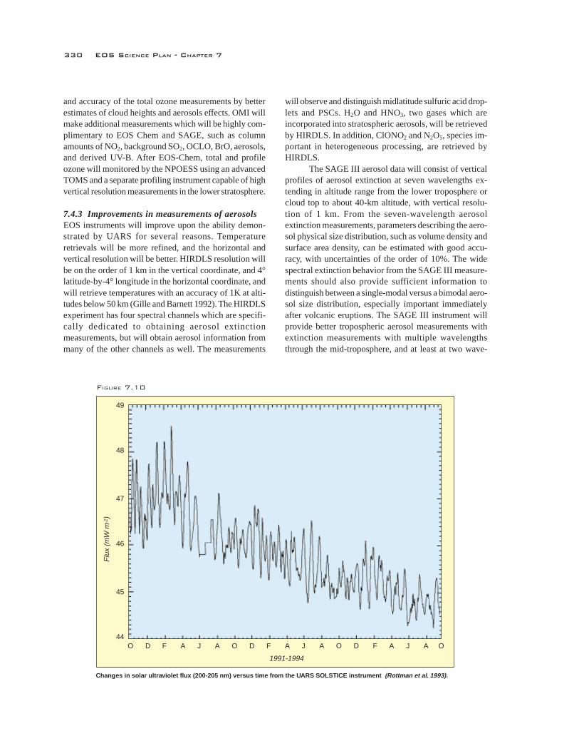
330 EOS SCIENCE PLAN - CHAPTER 7
and accuracy of the total ozone measurements by betterestimates of cloud heights and aerosols effects. OMI willmake additional measurements which will be highly com-plimentary to EOS Chem and SAGE, such as columnamounts of NO2, background SO2, OCLO, BrO, aerosols,and derived UV-B. After EOS-Chem, total and profileozone will monitored by the NPOESS using an advancedTOMS and a separate profiling instrument capable of highvertical resolution measurements in the lower stratosphere.
7.4.3 Improvements in measurements of aerosolsEOS instruments will improve upon the ability demon-strated by UARS for several reasons. Temperatureretrievals will be more refined, and the horizontal andvertical resolution will be better. HIRDLS resolution willbe on the order of 1 km in the vertical coordinate, and 4°latitude-by-4° longitude in the horizontal coordinate, andwill retrieve temperatures with an accuracy of 1K at alti-tudes below 50 km (Gille and Barnett 1992). The HIRDLSexperiment has four spectral channels which are specifi-cally dedicated to obtaining aerosol extinctionmeasurements, but will obtain aerosol information frommany of the other channels as well. The measurements
will observe and distinguish midlatitude sulfuric acid drop-lets and PSCs. H2O and HNO3, two gases which areincorporated into stratospheric aerosols, will be retrievedby HIRDLS. In addition, ClONO2 and N2O5, species im-portant in heterogeneous processing, are retrieved byHIRDLS.
The SAGE III aerosol data will consist of verticalprofiles of aerosol extinction at seven wavelengths ex-tending in altitude range from the lower troposphere orcloud top to about 40-km altitude, with vertical resolu-tion of 1 km. From the seven-wavelength aerosolextinction measurements, parameters describing the aero-sol physical size distribution, such as volume density andsurface area density, can be estimated with good accu-racy, with uncertainties of the order of 10%. The widespectral extinction behavior from the SAGE III measure-ments should also provide sufficient information todistinguish between a single-modal versus a bimodal aero-sol size distribution, especially important immediatelyafter volcanic eruptions. The SAGE III instrument willprovide better tropospheric aerosol measurements withextinction measurements with multiple wavelengthsthrough the mid-troposphere, and at least at two wave-
O D F A J A O D F A J A O D F A J A O
1991-1994
49
48
47
46
45
44
Flu
x (m
W m
-2)
FIGURE 7.10
Changes in solar ultraviolet flux (200-205 nm) versus time from the UARS SOLSTICE instrument (Rottman et al. 1993).

OZONE AND STRATOSPHERIC CHEMISTRY 331
lengths down to sea level. For the measurements of PSCs,SAGE III will be the first satellite instrument to providesize distribution information.
The SAGE III aerosol information will be key tounderstanding the role played by stratospheric aerosolsand PSCs in heterogeneous chemical reactions and ozonedepletion and will be indispensable for understandingaerosol radiative forcing.
7.4.4 Improvements in measurements of the solarultraviolet flux
The EOS Solar Stellar Irradiance Comparison Experiment(SOLSTICE) has the unique capability of observingbright, blue stars employing the very same optics anddetectors used for the solar observations. With the assump-tion that these stars are extremely stable, the response ofSOLSTICE could be accurately monitored by observinga single star. However the calibration plan uses twenty ormore of these reference stars, and it is the average fluxfrom the entire ensemble of stars that provides an evenmore reliable reference for the solar observations. Re-peated observation of the stars should yield an averageflux level that is unchanging in time. A decrease in the
level is an indication of loss in instrument sensitivity andadjustments are made accordingly. Since the same opticsand detectors are used for the solar observations, the samecorrections apply, and the resulting solar measurement isreliable and free of any instrumental effects. The largedynamic range between the stellar and solar signals is onthe order of eight to nine orders of magnitude, and is eas-ily accommodated by changing the entrance apertures,spectral bandpass, and integration times (Rottman et al.1993).
7.4.5 Advanced chemical/dynamical/radiativemodels
EOS is currently funding a U.S. effort and cooperates witha foreign effort to build fully interactive chemical/dynami-cal models for interpretation of EOS data. The first effort,the Schoeberl Interdisciplinary Science Investigation(IDS), currently uses data assimilation winds and tem-peratures (see Section 7.4.6) along with a chemicaltransport model to simulate the stratospheric system. Theresults of this model are then used to compare with ob-servations such as those from UARS, SAGE, and TOMS.Full coupling and feedback between the meteorology and
+ +
+
+
+
+
+
++
+
+ +++
TIROS-N TOVSStratospheric Channels
HIS 30 kmSimulation
HIS 15 kmSimulation
HIRDLS
Ideal scaling for Rossby-typedisturbances at different latitudes
NIMBUS 5,6 SCR, PMR
NIMBUS 7SAMS
45°
22.5°
equa
tor
Other EOS LimbSounders
UARS MLS
UARS CLAES
UARS ISAMS
NIMBUS 6 LRIR
NIMBUS 7 LIMS
0 6 12 18 24 30
12
9
6
3
0
Horizontal Resolution (Deg)
Vert
ical
Res
olut
ion
(km
)
FIGURE 7.11
A comparison of the vertical and horizontal resolutions of various limb- and nadir-sounding satellite instruments. Lines indica tethe ideal observation scale for Rossby waves.
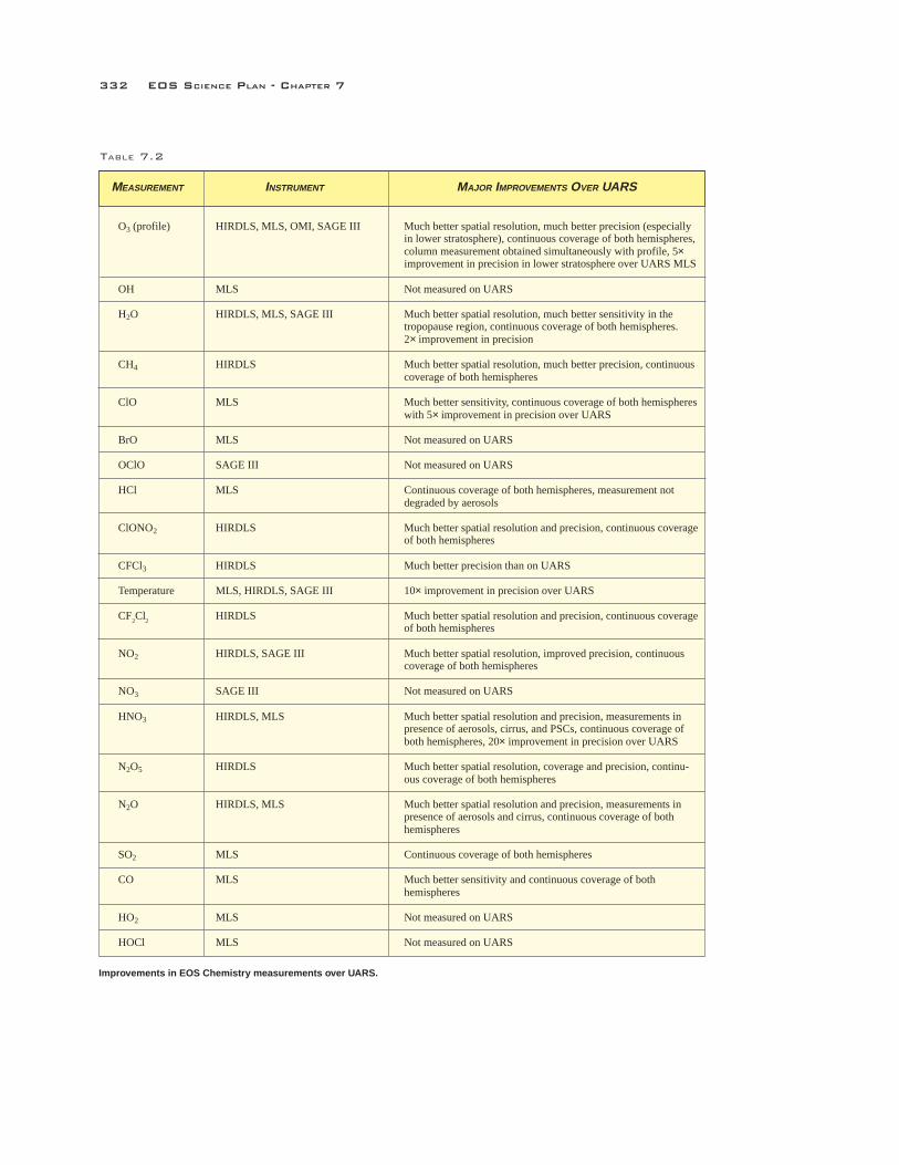
332 EOS SCIENCE PLAN - CHAPTER 7
O3 (profile) HIRDLS, MLS, OMI, SAGE III Much better spatial resolution, much better precision (especiallyin lower stratosphere), continuous coverage of both hemispheres,column measurement obtained simultaneously with profile, 5×improvement in precision in lower stratosphere over UARS MLS
OH MLS Not measured on UARS
H2O HIRDLS, MLS, SAGE III Much better spatial resolution, much better sensitivity in thetropopause region, continuous coverage of both hemispheres.2× improvement in precision
CH4 HIRDLS Much better spatial resolution, much better precision, continuouscoverage of both hemispheres
ClO MLS Much better sensitivity, continuous coverage of both hemisphereswith 5× improvement in precision over UARS
BrO MLS Not measured on UARS
OClO SAGE III Not measured on UARS
HCl MLS Continuous coverage of both hemispheres, measurement notdegraded by aerosols
ClONO2 HIRDLS Much better spatial resolution and precision, continuous coverageof both hemispheres
CFCl3 HIRDLS Much better precision than on UARS
Temperature MLS, HIRDLS, SAGE III 10× improvement in precision over UARS
CF2Cl
2HIRDLS Much better spatial resolution and precision, continuous coverage
of both hemispheres
NO2 HIRDLS, SAGE III Much better spatial resolution, improved precision, continuouscoverage of both hemispheres
NO3 SAGE III Not measured on UARS
HNO3 HIRDLS, MLS Much better spatial resolution and precision, measurements inpresence of aerosols, cirrus, and PSCs, continuous coverage ofboth hemispheres, 20× improvement in precision over UARS
N2O5 HIRDLS Much better spatial resolution, coverage and precision, continu-ous coverage of both hemispheres
N2O HIRDLS, MLS Much better spatial resolution and precision, measurements inpresence of aerosols and cirrus, continuous coverage of bothhemispheres
SO2 MLS Continuous coverage of both hemispheres
CO MLS Much better sensitivity and continuous coverage of bothhemispheres
HO2 MLS Not measured on UARS
HOCl MLS Not measured on UARS
TABLE 7.2
Improvements in EOS Chemistry measurements over UARS.
MEASUREMENT INSTRUMENT MAJOR IMPROVEMENTS OVER UARS

OZONE AND STRATOSPHERIC CHEMISTRY 333
chemistry do not occur at this stage. Later, the chemical/transport model will be used along with the EOS chemi-cal data to produce an assimilated chemical data set. Thefull coupling will occur through the assimilation system.The observations of motion of long-lived trace speciescan be inverted to make better estimates of stratosphericwinds. The forecast of temperatures from the assimila-tion modeling effort will increase the accuracy of theretrieved trace gases.
The second effort, the Pyle IDS (United Kingdom),uses a full GCM and chemical package. The GCM andchemical/radiation/transport system will be fully linked.The objectives are to examine the sensitivity of the atmo-sphere to the chemical/radiative/dynamical feedbacksystems. This foreign effort consists of a full-fledged EOSIDS team but is not funded by NASA.
7.4.6 Full meteorological and chemical assimilationof EOS data sets
The Data Assimilation Office (DAO) at NASA/GoddardSpace Flight Center (GSFC) already provides routine sup-port to the stratospheric aircraft missions planned to studystratospheric ozone. Daily analyses are produced for theStratospheric Tracers of Atmospheric Transport (STRAT)mission, and, given the duration of this mission, this willevolve into the operational support of the EOS MorningPlatform (AM-1). During the aircraft deployment peri-ods, forecasts are produced to aid in-flight planning. Theseforecasts enhance the ability of the mission planners totarget air of specific chemical characteristics.
The current DAO meteorological analyses have alarge impact on stratospheric chemistry studies. The windfields are of sufficient quality to remove the dynamicaluncertainty from trace observations. This allows a high-caliber examination of chemical processes, a benefit thathas been realized for satellite, balloon, and aircraft data.There are active efforts of the DAO to improve the sub-tropical winds and the deep vertical motions that link thestratosphere and mesosphere.
Future plans call for a straightforward extensionof the application of winds from the DAO assimilation tomore-general problems. This includes stratospheric-tro-pospheric exchange, as well as broader issues oftropospheric chemistry. Advanced assimilation systemswill directly assimilate constituent observations. First,long-lived tracers will be assimilated. Initial studies ofN2O from UARS show that assimilation can in fact pro-vide verifiable global information from the non-globalUARS coverage pattern. An important goal of the DAOconstituent effort is to improve wind estimates, especiallyin the tropics. Wind inversion techniques are being ac-tively investigated. In addition, at least two universityproposals have been recently submitted to attempt to as-similate aerosol observations within the DAO system.These proposals are examples of the long-term efforts toassimilate the complete chemical suite of measurements,with the goal of bringing to bear the quantitative analysisof data assimilation on the internal consistency of thechemical observations of UARS and CHEM.
7.5 Foreign partners and other measurement sources
Foreign partners are critical to the scientific success ofthe global stratospheric measurements program. The scaleof collaboration ranges from individual science teams, tocollaborative instruments, to reciprocal flights of instru-ments, to mission planning. The timing of the EOS CHEMmission has been structured to follow the launch of theEuropean Space Agency’s (ESA’s) Environmental Satel-lite I (ENVISAT I). This mission, to be launched in 2000,follows the successful NASA UARS mission. ENVISATwill make many critical trace species measurements inthe time period of maximum stratospheric chlorine. Thislong-term data set, UARS-ENVISAT-CHEM, will be ab-
solutely critical to our understanding of the role of tracespecies in controlling ozone in the stratosphere.
Other international space platforms will carry a fewstratospheric instruments: The French Systeme pourl’Observation de la Terre (SPOT) satellite will carry thePolar Ozone Aerosol Measurements II (POAM II) aero-sol and ozone measuring system. The Russian MIR spacestation will fly the Fourier Transform Spectrometer, DOPI.
In addition to these space instruments, severalstratospheric aircraft campaigns are planned for the nextfew years (e.g., the STRAT campaign).

334 EOS SCIENCE PLAN - CHAPTER 7
References
Aikin, A. C., 1992: Stratospheric evidence of relativistic electron pre-cipitation. Planet. Space Sci., 40, 413–431.
Anderson, J.G., D.W. Toohey, and W.H. Brune, 1991: Free radicals withinthe Antarctic vortex: The role of CFC's in the Antarctic ozoneloss. Science, 251, 39-46.
Austin, J., R. R. Garcia, J. M. Russell III, S. Solomon, and A. F. Tuck,1986: On the atmospheric photochemistry of nitric acid. J.Geophys. Res., 91, 5477–5485.
Austin, J., N. Butchart, and K. P. Shine, 1992: Possibility of an Arcticozone hole in a doubled-CO2 climate. Nature, 360, 221–225.
Brasseur, G., 1993: The response of the middle atmosphere to long-term and short-term solar variability: A two-dimensional model.J. Geophys. Res., 98, 23,079–23,090.
Brune, W. H., J. G. Anderson, and K. R. Chan, 1989: In situ observa-tions ClO in the Antarctic: ER-2 aircraft results from 54 S to 72S latitude. J. Geophys. Res., 94, 16649-16663.
Callis, L. B., D. N. Baker, J. B. Blake, J. D. Lambeth, R. E. Boughner,M. Natarajan, R. W. Klebesadel, and D. J. Gorney, 1991a: Pre-cipitating relativistic electrons: Their long-term effect on strato-spheric odd nitrogen levels. J. Geophys. Res., 96, 2939–2976.
Callis, L. B., R. E. Boughner, M. Natarajan, J. D. Lambeth, D. N. Baker,and J. B. Blake, 1991b: Ozone depletion in the high latitude lowerstratosphere: 1979-1990. J. Geophys. Res., 96, 2921–2937.
Carslaw, K. S., B. P. Luo, S. L. Clegg, Th. Peter, P. Brimblecombe, andP. J. Crutzen, 1994: Stratospheric aerosol growth and HNO3 gasdepletion from coupled HNO3 and water uptake by liquid par-ticles. Geophys. Res. Lett., 21, 2479–2482.
Chipperfield, M. P., D. Cariolle, P. Simon, R. Ramaroson, and D. J.Lary, 1993: A three-dimensional modeling study of trace speciesin the Arctic lower stratosphere during winter 1989-1990. J.Geophys. Res., 98, 7199–7218.
Considine, D. B., A. R. Douglass, and C. H. Jackman, 1994: Effects ofa PSC parameterization on ozone depletion due to stratosphericaircraft in a 2-D model. J. Geophys. Res., 99, 18,879–18,894.
Considine, D. B., A. R. Douglass, and C. H. Jackman, 1995: Sensitivityof two-dimensional model predictions of ozone response to strato-spheric aircraft: An update. J. Geophys. Res., 100, 3075–3090.
Dobson, G. M. B., 1966: Annual variation of ozone in Antarctica. Quart.J. Roy. Met. Soc., 92, 546–550.
Douglass, A. R., R. B. Rood, J. A. Kaye, R. S. Stolarski, D. J. Allen, andE. M. Larson, 1991: The influence of polar heterogeneous pro-cesses on reactive chlorine at middle latitudes: Three-dimensionalmodel implications. Geophys. Res. Lett., 18, 25–28.
Douglass, A. R., R. B. Rood, J. W. Waters, L. Froidevaux, W. Read, L.Elson, M. Geller, Y. Chi, M. Cerniglia, S. Steenrod, 1993: A 3-Dsimulation of the early winter distribution of reactive chlorine inthe north polar vortex. Geophys. Res. Lett., 20, 1271–1274.
Drdla, K., A. Tabazadeh, R. P. Turco, M. Z. Jacobson, J. E. Dye, C.Twohy, and D. Baumgardner, 1994: Analysis of the physical stateof one Arctic polar stratospheric cloud based on observations.Geophys. Res. Lett., 21, 2475–2478.
Eckman, R. S., W. L. Grose, R. E. Turner, W. T. Blackshear, J. M. RussellIII, L. Froidevaux, J. W. Waters, J. B. Kumer, and A. E. Roche,1995: Stratospheric trace constituents simulated by a three-di-mensional general circulation model: comparison with UARSdata. J. Geophys. Res., 100, 13,951–13,966.
Farman, J. C., B. B. Bardiner, and J. D. Shanklin, 1985: Large losses oftotal ozone in Antarctica reveal seasonal ClOx/NOx interaction.Nature, 315, 207–210.
Fioletov, V.E. J.B. Kerr, D.I. Wardle, J. Davies, E.W. Hare, C.T. McElroy,and D.W. Tarasick, 1997: Long term decline over the Canadianarctic to early 1997 from ground based and balloon observations.Geophys. Res. Lett., 24, 2705-2708.
Fleming, E. L., S. Chandra, C. H. Jackman, D. B. Considine, and A. R.Douglass, 1995: The middle atmospheric response to short- andlong-term solar UV variations: Analysis of observations and 2-D model results. J. Atmos. Terr. Phys., 57, 333–365.
Fraser, P., S. Penkett, M. Gunson, R. Weiss, and F. S. Rowland, 1994:Measurements, Chapter 1 in “NASA Report on Concentrations,Lifetimes, and Trends of CFC’s, Halons, and Related Species,”edited by J. Kaye, S. Penkett, and F. Ormond, NASA ReferencePublication 1339, Washington, D. C., 1.1–1.68.
Gaines, E. E., D. L. Chenette, W. L. Imhof, C. H. Jackman, and J. D.Winningham, 1995: Relativistic electron fluxes in May 1992 andtheir effect on the middle atmosphere. J. Geophys. Res., 100,1027–1033.
Geller, M. A., Y. Chi, R. B. Rood, A. R. Douglass, J. A. Kaye, and D. J.Allen, 1993: Satellite observation and mapping of wintertimeozone variability in the lower stratosphere. J. Atmos. and Terr.Phys., 55, 1081–1088.
Gille, J. C., and J. J. Barnett, 1992: The high resolution dynamics limbsounder (HIRDLS). An instrument for the study of global change,in “The Use of EOS for Studies of Atmospheric Physics,” J. C.Gille and G. Visconti, editors, 433–450.
Grainger, R. G., A. Lambert, F. W. Taylor, J. J. Remedios, C. D. Rodgers,M. Corney, and B. J. Kerridge, 1993: Infrared absorption by vol-canic stratospheric aerosols observed by ISAMS. Geophy. Res.Lett., 20, 1283–1286.
Gunson, M. R., et al., Increase in levels of stratospheric chlorine andfluorine loading between 1985 and 1992, 1994: Geophys. Res.Lett., 21, 2223-2226.
Hanson, D. R., A. R. Ravishankara, and S. Solomon, 1994: Heteroge-neous reactions in sulfuric acid aerosols: A framework for modelcalculations. J. Geophy. Res., 99, 3615–3629.
Hofmann, D. J., J. W. Harder, J. M. Rosen, J. V. Hereford, and J. R.Carpenter, 1989: Ozone profile measurements at McMurdo Sta-tion, Antarctica, during the spring of 1987. J. Geophys. Res., 94,16,527–16,536.
Hofmann, D. J., S. J. Oltmans, J. A. Lathrop, J. M. Harris, and H. Vomel,1994: Record low ozone at the south pole in spring. Geophys.Res. Lett., 21, 421-424.
Hollandswarth, S. M., R. D. McPeters, L. E. Flynn, W. Planet, A. J.Miller, and S. Chandra, 1995: Ozone trends deduced from com-bined Nimbus 7 SBUV and NOAA 11 SBUV/2 data. Geophys.Res. Lett., 22, 905–908.
Holton, J. R., P. H. Haynes, M. E. McIntyre, A. R. Douglass, R. B.Rood, and L. Pfister, 1995: Stratosphere-troposphere exchange.Reviews of Geophys., 33, 403-439.
Hood, L. L., and J. P. McCormack, 1992: “Components of interannualozone change based on NIMBUS 7 TOMS data.” Geophys. Res.Lett., 19, 2309–2312.
Huang, T. Y. W., and G. P. Brasseur, 1993: Effect of long-term solarvariability in a two-dimensional interactive model of the middleatmosphere. J. Geophys. Res., 98, 20,413–20,427.
IPCC, “Climate Change, 1994,” 1995: (J. Houghton, L. Filho, J. Bruce,H. Lee, B. Callander, E. Haites, N. Harris, and K. Maskell, Eds.)Cambridge University Press, Cambridge, U.K., 339 pp.
IPO, Integrated Operational Requirements Document (IORD) I, March,1996 IPO, Technical Requirements Document (TRD), Appen-dix D, NPOESS System EDR Requirements, June, 1998.

OZONE AND STRATOSPHERIC CHEMISTRY 335
Jackman, C. H., J. E. Nielsen, D. J. Allen, M. C. Cerniglia, R. D.McPeters, A. R. Douglass, and R. B. Rood, 1993: The effects ofthe October 1989 solar proton events on the stratosphere as com-puted using a three-dimensional model. Geophys. Res. Lett., 20,459–462.
Jackman, C. H., M. C. Cerniglia, J. E. Nielsen, D. J. Allen, J. M.Zawodny, R. D. McPeters, A. R. Douglass, J. E. Rosenfield, andR. B. Rood, 1995: Two-dimensional and three-dimensional modelsimulations, measurements, and interpretation of the influenceof the October 1989 solar proton events on the middle atmo-sphere. J. Geophys. Res., 100, 11,641–11,660.
Jensen, E. J., O. B. Toon, J. D. Spinhirne, and H. B. Selkirk, 1997: Onthe formation and persistence of subvisible cirrus clouds nearthe tropical tropopause, J. Geophys. Res., in press.
Kinnison, D. E., H. S. Johnston, and D. J. Wuebbles, 1994a: Modelstudy of atmospheric transport using carbon 14 and strontium 90as inert tracers. J. Geophys. Res., 99, 20,647–20,664.
Kinnison, D. E., K. E. Grant, P. S. Connell, D. A. Rotman, and D. J.Wuebbles, 1994b: The chemical and radiative effects of theMount Pinatubo eruption. J. Geophys. Res., 99, 25,705–25,731.
Lefevre, F., G. P. Brasseur, I. Folkins, A. K. Smith, and P. Simon, 1994:Chemistry of the 1991-1992 stratospheric winter: three dimen-sional model simulations. J. Geophys. Res., 99, 8183–8197.
Logan, J. A., 1994: Trends in the vertical distribution of ozone: An analy-sis of ozonesonde data. J. Geophys. Res., 99, 25,553–25,585.
Mankin, W. G., and M. T. Coffey, 1984: Increased stratospheric hydro-gen chloride in the El Chichon cloud, Nature, 226, 170-174.
Mankin, W. G., M. T. Coffey, and A. Goldman, Airborne observationsof SO2, HCl, and O3 in the stratospheric plume of the Pinatubovolcano in July 1991. J. Geophys. Res., 100, 2953-2972.
Manney, G.L., L. Froidevaux, M.L. Santee, R.W. Zurek, and J.W. Wa-ters, 1997: MLS observations of the Arctic ozone loss in 1996-1997. Geophys. Res. Lett., 24, 2697-2700.
Manney, G. L., L. Froidevaux, J. W. Waters, and R. W. Zurek, 1995:Evolution of microwave limb sounder ozone and the polar vor-tex during winter. J. Geophys. Res., 100, 2953–2972.
Massie, S. T., P. L. Bailey, J. C. Gille, E. C. Lee, J. L. Mergenthaler, A.E. Roche, J. B. Kumer, E. F. Fishbein, J. W. Waters, and W. A.Lahoz, 1994: Spectral signatures of polar stratospheric cloudsand sulfate aerosol. J. Atmos. Sci., 51, 3027–3044.
McCormick, M. P., and J. C. Larsen, 1988: Antarctic measurements ofozone by SAGE II in the spring of 1985, 1986, and 1987.Geophys. Res. Lett., 15, 906–910.
McCormick, M. P., L. W. Thomason, and C. R. Trepte, 1995: Atmo-spheric effects of the Mt. Pinatubo eruption. Nature, 373, 399–404.
McElroy, M. B., R. J. Salawitch, and S. C. Wofsy, 1986: Antarctic O3:Chemical mechanisms for the spring decrease. Geophys. Res.Lett., 13, 1296–1297.
Murphy, D., and G. B. Gary, 1995: Mesoscale temperature fluctuationsand polar stratospheric clouds. J. Atmos. Sci., 52, 1753–1760.
Nash, J., and F. Schmidlin, 1987: Final report of the WMO interna-tional radiosonde intercomparisons, WMO Report No. 30.
National Plan for Stratospheric Monitoring 1988–1997, 1989: Dept. ofCommerce/NOAA, FCM-P17-1989.
Newman, P.A., J.F. Gleason, R.D. McPeters, and R.S. Stolarski, 1997:Anomalously low ozone over the Arctic. Geophys. Res. Lett.,24, 2689- 2692.
Oberbeck, V. R., J. M. Livingston, P. B. Russell, R. F. Pueschel, J. N.Rosen, M. T. Osborn, M. A. Kritz, K. G. Snetsinger, and G. V.Ferry, 1989: SAGE II aerosol validation: Selected altitude mea-surements, including particle micromeasurements. J. Geophys.Res., 94, 8367–8380.
Osborn, M. T., J. M. Rosen, M. P. McCormick, P.-H. Wang, J. M.Livingston, and T. J. Swissler, 1989: SAGE II aerosol correla-tive observations: Profile measurements. J. Geophys. Res., 94,8353–8366.
Pitari, G., V. Rizi, L. Ricciardulli, and G. Visconti, 1993: High speedcivil transport impact: Role of sulfate, nitric acid trihydrate andice aerosols studied with a two-dimensional model including aero-sol physics. J. Geophys. Res., 98, 23,141–23,164.
Pollack, J. B., F. C. Witteborn, K. O’Brien, and B. Flynn, 1991: A deter-mination of the infrared optical depth of the El Chichón volcaniccloud. J. Geophys. Res., 97, 3115–3122.
Poole, L. R., and M. C. Pitts, 1994: Polar stratospheric cloud climatol-ogy based on Stratospheric Aerosol Measurement II observa-tions from 1978-1989. J. Geophys. Res., 99, 13,083–13,089.
Proffitt, M. H., J. A. Powell, A. F. Tuck, D. W. Fahey, K. K. Kelly, A. J.Drueger, M. R. Schoeberl, B. L. Gary, J. J. Margitan, K. R. Chan,M. Loewenstein, and J. R. Podolske, 1989: A chemical defini-tion of the boundary of the Antarctic ozone hole. J. Geophys.Res., 94, 11,437–11,448.
Randel, W. J., and J. B. Cobb, 1994: Coherent variations of monthlymean total ozone and lower stratospheric temperature. J. Geophys.Res., 99, 5433–5448.
Rasch, P. J., B. A. Boville, and G. P. Brasseur, 1995: A three-dimen-sional general circulation model with coupled chemistry for themiddle atmosphere. J. Geophys. Res., 100, 9041–9071.
Reid, G. C., S. Solomon, and R. R. Garcia, 1991: Response of the middleatmosphere to the solar proton events of August-December 1989.Geophys. Res. Lett., 18, 1019–1022.
Reinsel, G. C., G. C. Tiao, D. J. Wuebbles, J. B. Kerr, A. J. Miller, R. M.Nagatani, L. Bishop, and L. H. Ying, 1994: Seasonal trend analy-sis of published ground-based and TOMS total ozone data through1991. J. Geophys. Res., 99, 5449–5464.
Report of the International Ozone Trends Panel 1988. 1990: WMO Re-port 18.
Rinsland, C. P., G. K. Yue, M. R. Gunson, R. Zander, and M. C. Abrams,1994: Mid-infrared extinction by sulfate aerosols from the Mt.Pinatubo eruption. J. Quant. Spectrosc. Radiat. Transfer, 52, 241–252.
Rood, R. B., A. R. Douglass, J. A. Kaye, M. A. Geller, Y. Chi, D. J.Allen, E. M. Larson, E. R. Nash, and J. E. Nielsen, 1991: Three-dimensional simulations of wintertime ozone variability in thelower stratosphere. J. Geophys. Res., 96, 5055–5071.
Rottman, G. J., T. N. Woods, and T. P. Sparn, 1993: Solar Stellar Irradi-ance Comparison Experiment 1: 1. Instrument design and op-eration. J. Geophys. Res., 98, 10,667–10,678.
Russell, J. M., M. Luo, R. J. Cicerone, and L. E. Deaver, 1996: Satelliteconfirmation of the dominance of chlorofluorocarbons in the glo-bal stratospheric chlorine budget. Nature, 379, 526–529.
Santee, M.L., G.L. Manney, L. Froidevaux, R.W. Zurek, and J.W. Wa-ters, 1997: MLS Observations of ClO and HNO3 in the 1996-1997 Arctic polar vortex. Geophys. Res. Lett., 24, 2713-2716.
Schauffler, S. M., L. E. Heidt, W. H. Pollack, T. M. Gilpin, J. F. Vedder,S. Solomon, R. A. Lueb, and E. L. Atlas, 1993: Measurements ofhalogenated organic compounds near the tropical tropopause,Geophys. Res. Lett., 20, 2567-2570.
Schoeberl, M. R., et al., 1993: The evolution of ClO and NO along airparcel trajectories. Geophys. Res. Lett., 20, 2511–1514.
Solomon, S., 1990: Progress towards a quantitative understanding ofthe Antarctic ozone depletion. Nature, 347, 347-354.
Solomon, S., R. R. Garcia, F. S. Rowland, and D. J. Wuebbles, 1986:On the depletion of Antarctic ozone. Nature, 321, 755–758.

336 EOS SCIENCE PLAN - CHAPTER 7
Solomon, S., R. W. Portmann, R. R. Garcia, L. W. Thomason, L. Poole,and M. P. McCormick, 1996: The role of aerosol variations inanthropogenic ozone depletion at northern midlatitudes. J.Geophys. Res., 101, 6713–6727.
Sparling, L., et al., 1995: Trajectory modeling of emissions from lowerstratospheric aircraft. J. Geophys. Res., 100, 1427–1438.
Stolarski, R. S., A. J. Drueger, M. R. Schoeberl, R. D. McPeters, P. A.Newman, and J. C. Alpert, 1986: Nimbus 7 satellite measure-ments of the springtime Antarctic ozone decrease. Nature, 322,808–811.
Stolarski, R. S., P. Bloomfield, R. D. McPeters, and J. R. Herman, 1991:Total ozone trends deduced from Nimbus 7 TOMS data. Geophys.Res. Lett., 18, 1015–1018.
Tie, X. X., G. P. Brasseur, and C. Granier, 1994: Two-dimensional simu-lation of Pinatubo aerosol and its effect on stratospheric ozone.J. Geophys. Res., 99, 20,545–20,562.
Toon, O. B., P. Hamill, R. P. Turco, and J. Pinto, 1986: Condensation ofHNO3 and HCl in the winter polar stratosphere. Geophys. Res.Lett., 13, 1284–1287.
Toon, O. B., and M. Tolbert, 1995: Spectroscopic evidence against ni-tric acid trihydrate in polar stratospheric clouds. Nature, 375,218–221.
Wallace, L., and W. Livingston, 1992: The effect of the Pinatubo cloudon hydrogen chloride and hydrogen fluoride, Geophys. Res. Lett.,19, 1209.
Waters, J. W., L. Froidevaux, W. G. Read, G. L. Manney, L. S. Elson, D.A. Flower, R. F. Jarnot, and R. S. Harwood, 1993: StratosphericClO and ozone from the microwave limb sounder on the upperatmosphere research satellite. Nature, 362, 597–602.
Weisenstein, D. K., M. K. W. Ko, J. M. Rodriguez, and N. D. Sze, 1993:Effects on stratospheric ozone from high-speed civil transport:Sensitivity to stratospheric aerosol loading. J. Geophys. Res., 98,23,133–23,140.
Willson, R. C., and H. S. Hudson, 1991: “A solar cycle of measured andmodeled total irradiance.” Nature, 351, 42–44.
World Meteorological Organization (WMO), 1992: Scientific assess-ment of ozone depletion: 1991, Global Ozone Res. and Monit.Proj., World Meteorol. Org., Rep. 25.
World Meteorological Organization (WMO), 1995: Scientific assess-ment of ozone depletion: 1994, Global Ozone Res. and Monit.Proj., World Meteorol. Org., Rep. 37.
Zander, R., M. R. Gunson, C. B. Farmer, C. P. Rinsland, F. W. Irion, andE. Mahieu, 1992: The 1985 chlorine and fluorine inventories inthe stratosphere based upon ATMOS observations at 30 N lati-tude. J. Atm. Chem., 15, 171-186.

OZONE AND STRATOSPHERIC CHEMISTRY 337
Chapter 7 Index
2-D models 317-318
3-D models 318-319
AASE II 321
AEAP 322
aerosols 315-316, 322, 325, 328, 330
aircraft exhaust 320, 322
AMLS 326-329
ATMOS 321
biological threat 311
bromine 314-315, 324, 329
calibration 327, 331
carbon dioxide (CO2) 311, 322
carbon monoxide (CO) 332
CFC 314, 321, 326
CH2Cl2 321
CH3Cl 314, 321
CHCl3 321
chlorine 312-327, 333
CLAES 331
climate change 311
Clx 315, 322
DAO 333
Dobson units 312
DU 312, 314, 319
El Niño 315, 322
energetic particles 316-317, 319
ER-2 327
foreign partners 333
greenhouse forcing 311
GSFC 324, 333
H2SO4 316, 320
HALOE 318, 321, 323
HCFC 321
HIRDLS 326-332
HIRS 323
HOx 314, 322, 325, 329
HSCT 322
IDS 331, 333
interannual variability 315-316, 319
IPCC 311
IR 315
ISAMS 331
lightning 322
man-made changes 320-322
measurement requirements 323-333
METEOR-3 329
methane (CH4) 314, 318, 322, 325,329, 332
MLS 313, 324-332
MMIC 326-328
modeling 317, 333
MSU 323
NAD 326-329
NASA 324, 326, 328, 333
NAT 320, 326-329
natural changes 319-320
NCAR 318
Nimbus-7 311
NOAA 323-324, 328
NOx 314, 319, 322, 325, 329
NPOESS 324, 330
OCS 316, 329
OH 314, 321, 325-326, 329, 332
OMI 326, 329-332
ozone changes 312-315
ozone chemistry 314-315
ozone distribution 314, 317, 319-320
ozone transport 315
precipitation 319
PSC 315-316, 318-322, 325, 327, 331
QBO 315, 319, 322
REP 317
SAGE 313, 331
SAGE III 313, 330-332
SAM 316-317
SBUV 313-314
SOLSTICE 326, 330-331
SPOT 333
STP 312
sulfate 319-320, 329
sulfur 322
sulfur dioxide (SO2) 316, 319, 329-332
sulfuric acid 316, 320
TOMS 311-314, 326, 329-331
TOVS 323-324, 331
trace gases 317, 319, 328, 333
UARS 313, 318-321, 323, 326-332
UT 328
UV 311, 327, 330-331
UV-B 311, 330
validation 327
volcanoes 316, 322
wind 312, 319, 323-324, 333
WMO 311, 316-318, 320-321, 324
WSR 316