Stratospheric Nudging And Predictable Surface Impacts ...

Stratospheric Nudging And Predictable Surface Impacts (SNAPSI):A Protocol for Investigating the Role of the Stratospheric PolarVortex in Subseasonal to Seasonal ForecastsPeter Hitchcock1, Amy Butler2, Andrew Charlton-Perez3, Chaim Garfinkel4, Tim Stockdale5,James Anstey6, Dann Mitchell7, Daniela I. V. Domeisen8,9, Tongwen Wu10, Yixiong Lu10,Daniele Mastrangelo11, Piero Malguzzi11, Hai Lin12, Ryan Muncaster12, Bill Merryfield6,Michael Sigmond6, Baoqiang Xiang13,14, Liwei Jia13, Yu-Kyung Hyun15, Jiyoung Oh16, Damien Specq17,Isla R. Simpson18, Jadwiga H. Richter18, Cory Barton19, Jeff Knight20, Eun-Pa Lim21, andHarry Hendon21

1Dept. Earth and Atmospheric Sciences, Cornell University, Ithaca, NY, USA2NOAA Chemical Sciences Laboratory, Boulder, CO, USA3Department of Meteorology, University of Reading, UK4Fredy and Nadine Herrmann Institute of Earth Sciences, The Hebrew University of Jerusalem, Jerusalem, Israel5European Centre for Medium-range Weather Forecasts, Reading, UK6Canadian Centre for Climate Modelling and Analysis, Environment and Climate Change Canada, Victoria, BC, Canada7School of Geographical Sciences, University of Bristol, Bristol, United Kingdom8University of Lausanne, Lausanne, Switzerland9ETH Zürich, Zürich, Switzerland10Beijing Climate Center, China Meteorological Administration, Beijing, China11CNR-ISAC, Bologna, Italy12Recherche en prévision numérique atmosphérique, Environment and Climate Change Canada, Dorval, QC, Canada13Geophysical Fluid Dynamics Laboratory, NOAA, Princeton, NJ, USA14University Corporation for Atmospheric Research, Boulder, CO, USA15National Institute of Meteorological Sciences, Korea Meteorological Administration, Jeju, Korea16School of Earth and Environmental Sciences, Seoul National University, Seoul, Korea17Centre National de Recherches Météorologiques, Université de Toulouse, Météo-France, CNRS, Toulouse, France18Climate and Global Dynamics Laboratory, National Center for Atmospheric Research, Boulder, CO, USA19Space Science Division, US Naval Research Laboratory, Washington, DC, USA20Hadley Centre, Met Office, Exeter, United Kingdom21Bureau of Meteorology, Melbourne, Victoria, Australia

Correspondence: Peter Hitchcock ([email protected])

Abstract. Major disruptions of the winter season, high-latitude, stratospheric polar vortices can result in stratospheric anoma-

lies that persist for months. These sudden stratospheric warming events are recognized as an important potential source of

forecast skill for surface climate on subseasonal to seasonal timescales. Realizing this skill in operational subseasonal forecast

models remains a challenge, as models must capture both the evolution of the stratospheric polar vortices in addition to their

coupling to the troposphere. The processes involved in this coupling remain a topic of open research.5

We present here the Stratospheric Nudging And Predictable Surface Impacts (SNAPSI) project. SNAPSI is a new model

intercomparison protocol designed to study the role of the Arctic and Antarctic stratospheric polar vortices in sub-seasonal to

1

https://doi.org/10.5194/gmd-2021-394Preprint. Discussion started: 4 January 2022c© Author(s) 2022. CC BY 4.0 License.

seasonal forecast models. Based on a set of controlled, subseasonal, ensemble forecasts of three recent events, the protocol aims

to address four main scientific goals. First, to quantify the impact of improved stratospheric forecasts on near-surface forecast

skill. Second, to attribute specific extreme events to stratospheric variability. Third, to assess the mechanisms by which the10

stratosphere influences the troposphere in the forecast models, and fourth, to investigate the wave processes that lead to the

stratospheric anomalies themselves. Although not a primary focus, the experiments are furthermore expected to shed light on

coupling between the tropical stratosphere and troposphere. The output requested will allow for a more detailed, process-based

community analysis than has been possible with existing databases of subseasonal forecasts.

1 Introduction15

Sudden stratospheric warmings are dramatic manifestations of dynamical variability in the polar vortices that form each winter

in both hemispheres (Scherhag, 1952; Baldwin et al., 2021). They are known to lead to equatorward shifts of the tropospheric

eddy-driven jets that can persist for several months (Kidston et al., 2015), and to increase the likelihood and severity of a variety

of high-impact extreme events (Domeisen and Butler, 2020). Capturing these surface impacts is thus of growing concern for

operational centers interested in improving their extended range forecasts on subseasonal to seasonal timescales.20

A number of recent studies have explored the role of major or minor stratospheric warmings in the Subseasonal-to-Seasonal

Prediction (S2S) database (Butler et al., 2019; Karpechko et al., 2018; Domeisen et al., 2020a, b; Rao et al., 2019, 2020a, b; Lee

et al., 2019; Butler et al., 2020) or in individual models (Kautz et al., 2020; Knight et al., 2020; Lim et al., 2021; Noguchi et al.,

2020). These studies confirm that operational models can to some extent capture the surface impacts of such stratospheric

variability, and have demonstrated regionally enhanced skill at subseasonal timescales in the weeks following stratospheric25

warmings. However, studies based on existing databases of subseasonal forecasts are hampered by the diversity of forecast

initialization dates and ensemble generation strategies, limited availability of detailed model output, and the varying ability

of operational models to capture the stratospheric variability itself. Moreover, such studies must ultimately rely on correlative

analyses, making causal inferences difficult to assess. Single-model studies have been extremely valuable in providing a more

detailed understanding, but cannot be as robust as a controlled, multi-model intercomparison. There is a clear need at this point30

to more carefully evaluate and compare the relevant coupling mechanisms across operational models in order to fully exploit

this important source of skill on timescales of weeks to months.

The purpose of this paper is to propose and describe a common protocol for numerical experiments to isolate and evaluate

the representation of stratospheric influence on near-surface weather in subseasonal to seasonal forecast models. The intent

is that by outlining and motivating a single protocol that can be adopted by multiple operational centers, such efforts can be35

directly compared, increasing their collective value.

The protocol presented here is primarily based on a zonally-symmetric nudging technique that has been used successfully

to identify stratospheric influences on the tropospheric circulation in both hemispheres (Simpson et al., 2011; Hitchcock and

Simpson, 2014; Zhang et al., 2018; Jiménez-Esteve and Domeisen, 2020). In essence, by comparing an ensemble hindcast in

which the stratosphere is constrained to the observed evolution, to a second hindcast in which the stratospheric circulation is40

2


constrained to climatology, the tropospheric impacts of the stratospheric anomalies can be isolated. Moreover, the protocol will

request a more complete set of output than is typically available from existing databases of subseasonal forecasts. The requested

variables are relevant to understanding both the coupling processes and the surface impacts themselves. The experiments

described here will thus represent a significant step forward from the previous intercomparisons of operational forecasts both by

allowing deeper investigations into the relevant coupling processes, and by removing the confounding influence of differences45

in stratospheric forecast skill.

Although the zonally-symmetric nudging is related to other nudging approaches (Jia et al., 2017; Kautz et al., 2020; Knight

et al., 2020), in this case stratospheric circulation anomalies are imposed through a linear relaxation term that acts only on

the zonally symmetric component of the stratospheric circulation. The purpose of this technique is to permit eddies to vary in

a dynamically consistent way across the tropopause. This is particularly relevant for the planetary waves that play a central50

role coupling the stratosphere and troposphere. This approach has been shown theoretically (Hitchcock and Haynes, 2014) and

practically (Hitchcock and Simpson, 2014) to avoid any significant artifacts.

While the protocol as outlined is intended to be applicable to any stratospheric event of interest, we suggest that it be initially

applied to three specific recent events: the boreal sudden warmings that occurred in February 2018 and January 2019, and the

austral sudden warming that occurred in September 2019. Each of these was followed by surface extremes that studies have55

suggested arise in part because of the stratospheric event.

This project is coordinated by the Stratospheric Network for the Assessment of Predictability (SNAP) working group that

is a joint activity of the World Climate Research Programme (WCRP) Stratosphere-troposphere Processes and their Role in

Climate (SPARC) project and of the Subseasonal-to-Seasonal Prediction (S2S) project that is supported by both the WCRP

and the World Weather Research Programme (WWRP).60

This paper describes the overall experimental design as well as details of the nudging approach. Data produced by this

project will be made available to the community through the Center for Environmental Data Analysis (CEDA), with the aim

of providing researchers with a resource to investigate the dynamics of stratosphere-troposphere coupling. While not a central

goal of the experiments, the case studies span periods with several distinct phases of the quasi-biennial oscillation (QBO) and

the occurrence of several large-amplitude Madden-Julian Oscillation (MJO) events. As such these experiments are expected to65

be valuable to several other SPARC and S2S projects, including the S2S MJO and Teleconnections group, the QBO initiative

(QBOi), and Stratospheric And Tropospheric Influences On Tropical Convective Systems (SATIO-TCS).

This paper is outlined as follows. The next section describes four specific goals that the proposed experiments are intended

to achieve. The third section describes in detail the general experimental protocol that can be applied to study any stratospheric

event of interest, and specifies details of the nudging, including the reference states towards which the nudged experiments70

are relaxed. In the fourth section the three target events of interest are described in further detail. The fifth section lays out the

model output requested from the forecasts, and the final section includes a list of participating models and a brief concluding

outlook.

3


2 Overview and Motivations

The basic experimental design proposes to focus on the evolution of specific events of interest, using the following sets of75

forecast ensembles:

free A standard forecast ensemble in which the atmosphere evolves freely after initialization. The method of initialization and

of generating ensemble members is not specified and can be determined by the participating modeling groups.

nudged A nudged ensemble in which the zonally symmetric stratospheric state is nudged globally to the observed time evo-

lution of the stratospheric event of interest.80

control A nudged control ensemble in which the zonally symmetric stratospheric state is nudged globally to a time-evolving

climatological state.

As discussed in the introduction, the free ensembles along with the zonally symmetric nudged and control ensembles are

of highest priority. However, particularly for models with grids that are not aligned along fixed latitudes, the zonally symmetric

nudging is difficult to realize. Thus two additional ensembles are requested at lower priority:85

nudged-full A nudged ensemble in which the full stratospheric state (including zonally asymmetric components) is nudged

globally to the observed time evolution of the stratospheric event of interest.

control-full A nudged control ensemble in which the full stratospheric state (including zonally asymmetric components) is

nudged globally to a time-evolving climatological state.

The reference states for the nudged and control ensembles are computed from ERA5 reanalysis output (Hersbach et al.,90

2020) on native model levels. These coincide with isobaric surfaces at the stratospheric levels where the nudging is applied.

Details of how the climatological state is computed are given in the Methods section below.

The protocol targets forecast integrations of 45 days, and an ensemble size of 50 to 100 members. For each of the three

case studies, two specific initialization dates for each type of integration are proposed; these are discussed in the context of the

specific target events described in Section 3.95

The impact of the stratosphere on the troposphere can be confounded by unrelated dynamical variability within the tropo-

sphere. Hence the choice to emphasize ensemble size over the number of initialization dates is intended to allow for statistically

and dynamically meaningful comparisons of these specific events across participating models.

There are four central motivations for the proposed forecast experiments, presented in the following subsections. In addition,

these experiments are expected to provide useful insights into coupling between the tropical stratosphere and troposphere.100

These secondary motivations are discussed following the four primary goals.

2.1 Quantify stratospheric contributions to surface predictability

Through nudging the stratosphere to observations, the nudged ensemble will provide a ‘perfect’ forecast of the stratosphere’s

zonal mean state. The forecast skill attained can be compared to that attained by the control ensemble (amounting to a ‘clima-

4


tological’ stratospheric forecast) and the free ensemble to quantify the contribution of a successful forecast of the stratosphere.105

These experiments will provide a multi-model assessment of the potential increase in skill associated with an improved rep-

resentation of the stratospheric state, and an up to date assessment of the present skill that is achieved by each model. By

including multiple case studies of interest, this suite of experiments also makes it possible to study the dependence of the

tropospheric response to stratospheric anomalies on the tropospheric state itself.

2.2 Attribute extreme events to stratospheric variability110

The proposed protocol will also provide a means of assessing or formally attributing the contribution of the stratosphere to an

extreme event of interest (Domeisen and Butler, 2020). Extremes that have been associated with sudden warmings in recent

years include cold air outbreaks in the Northern Hemisphere (Kolstad et al., 2010; Afargan-Gerstman et al., 2020; Huang

et al., 2021; Charlton-Perez et al., 2021) and hot, dry extremes over Australia (Lim et al., 2019). This goal is closely related to

the growing sub-discipline that focuses on attributing the occurrence of particular extremes to climate change and variability115

(National Academies of Sciences, Engineering, and Medicine, 2016).

Consider some extreme eventA that is thought to have been associated with a specific sudden stratospheric warming (SSW),

for instance the cold air outbreak (CAO) that occurred in Europe following the sudden warming in February 2018. The proba-

bility of such an event occurring p0 = p(A) might be estimated from the observed climatological frequency of similar events,

or from a set of forecasts that sufficiently represent the variability of the climate system from a given subseasonal forecast120

model, or from a combination of both (Sippel et al., 2015). Given the nudged ensemble, one can then estimate the probability

of a similar event occurring given the weakened state of the stratospheric polar vortex p1 = p(A|V −). The Relative Risk (see,

e.g. Paciorek et al., 2018) of this CAO might then be calculated as RR = p1/p0. Relative Risk values of RR> 1 would then

imply an increased risk of a CAO under a weakened vortex state, whereas RR< 1 would imply the opposite. This can also be

compared to the probability of such an event occurring in the counterfactual situation that the sudden warming did not occur,125

p′0 = p(A|V 0), computed from the control ensemble, allowing further for the calculation of necessary or sufficient causation

probabilities (Hannart et al., 2016). In the context used here, the RR is the most appropriate measure of risk because the data

are likely to be non-Gaussian (Christiansen, 2015).

As an example, Fig. 1 shows monthly mean NAO indices (from Hitchcock and Simpson, 2014). The probability of occur-

rence of a strongly negative monthly mean NAO state is much more likely in the aftermath of a sudden stratospheric warming130

than under a ‘counterfactual’ scenario during which the stratosphere was close to its climatological state.

The interpretation of the Relative Risk becomes more challenging in a forecast context, since the probability of an extreme

event is strongly conditional on the initial conditions known at the time of the forecast. As the forecast initialization date

grows closer to the event of interest, the forecast ensembles will begin to forecast the event with increasing fidelity; that is, the

probability of occurrence conditional on initial conditions n days prior to an event, p(A|IC(n)) will grow.135

One practical way to frame this question is to ask whether improving the forecast of the stratospheric state can lead to earlier

accurate forecasts of the event in question. Alternately, one may ask whether degrading the forecast of the stratosphere leads

to degraded forecasts of the event. Both framings are enabled by the proposed experiments.

5


Figure 1. Monthly mean NAO indices from a set of nudged integrations similar to those described in this protocol. The zonally symmetric

component of the stratosphere in the CTRL run is nudged to the model climatology, while those of SSWs and SSWd are nudged, respectively,

to the evolution of a vortex split and a vortex displacement event simulated by a free-running configuration of the same model. (Fig. 12a

from Hitchcock and Simpson, 2014, copyright American Meteorological Society. Used with permission.)

Figure 2 provides an example from NCEP CFSv2 monthly forecasts of March 2018 temperatures over Europe for different

initialization dates. A sudden stratospheric warming occurred on 12 February 2018. The forecast model did not predict the140

SSW with any certainty until the initializations in the 1-10 February period. There is a significant change in the March surface

temperatures over Europe for initializations before and after the stratospheric event was captured in the prediction system,

with forecasts initialized with the SSW information more closely capturing the observed March temperatures. But do these

differences arise solely because the forecast model finally captured the SSW, or because the lead-time had decreased? With

the three experiments proposed and applying this to multiple initializations before the event, it would be clear whether or145

not having the “perfect” stratosphere (nudged ensemble) for runs initialized in mid-January would have given more accurate

forecasts at longer leads.

A very similar approach has been adopted by Kautz et al. (2020) who made the distinction between ‘probabilistic’ and

‘deterministic’ forecasts of the extreme event in question. They presented evidence from the ECMWF model that a perfect

forecast of the stratospheric anomalies in early 2018 would increase the predicted odds of extreme cold weather over Europe150

from 5% to 45%. These odds then increase further as forecasts are made closer to the event.

The common and comparable set of integrations from a range of operational centers made available by this project will

allow this finding to be extended to other extreme events and will allow further development of this methodology. We aim

to have a large enough ensemble size to allow for the direct study of well-constrained extreme events, but if necessary may

also supplement the model data with extreme value statistics (e.g. Sippel et al., 2015). Ensemble sizes of 50-100 are sufficient155

to understand large-spatial scale and persistent (weekly) extremes, such as cold or NAO events, but the latter method will be

required for ‘noisier’ fields such as precipitation.

6


Figure 2. Forecast and observed monthly averaged temperature anomalies for March 2018 over Europe from NCEP CFSv2.

2.3 Assess the mechanisms underlying stratospheric coupling in individual models

Imposing stratospheric anomalies through a nudging procedure has been shown to significantly impact the near surface flow

(e.g. Douville, 2009), even if only the zonally symmetric component is imposed (e.g. Simpson et al., 2011; Hitchcock and160

Simpson, 2014; Zhang et al., 2018; Jiménez-Esteve and Domeisen, 2020). By comparing the difference between the nudged

and control ensembles, the processes that drive this downward coupling can be diagnosed in each model for a variety of

events of interest. It is of particular interest to better understand why some specific stratospheric events are followed by the

‘canonical’ equatorward shift of the tropospheric eddy driven jets, while others are not. The two boreal and one austral case

studies proposed were followed by a diversity of tropospheric responses, including two cases which exhibited the ‘canonical’165

response (the 2018 boreal and 2019 austral cases) and one which did not (the 2019 boreal case). This set of experiments will

thus shed light on whether these diverse responses were determined by stratospheric causes, or whether they are determined by

competing effects such as tropical tropospheric variability or independent mid-latitude dynamical processes (e.g. Knight et al.,

2020). In either case, the statistical sampling afforded by a multi-model set of forecast ensembles with detailed diagnostics

will allow for new and deeper insights into the mechanisms responsible for the tropospheric response. Moreover, each event170

also coincided with specific surface extremes that produced significant societal impacts. This set of experiments will provide

quantitative insight into the mechanisms responsible for these surface extremes. The data request has been designed to allow for

7


a more detailed analysis of these processes than has been possible with existing databases of subseasonal forecasts. Ultimately

this understanding will help both future operational system design and practical use of subseasonal forecasts.

2.4 Quantify the role of the stratosphere in upward wave propagation175

The onset of a sudden stratospheric warming is marked by the reversal of the climatologically westerly zonal mean zonal

winds in the mid stratosphere. Operational forecasts can, on average, successfully forecast this reversal starting about two

weeks prior, but this depends strongly on the specifics of the event in question (Tripathi et al., 2015; Domeisen et al., 2020a;

Rao et al., 2020a, b). A key issue is the successful forecasting of the rapid growth in planetary-scale Rossby waves that drives

the breakdown of the stratospheric polar vortex. This requires capturing both tropospheric precursors for these waves (e.g.180

Garfinkel et al., 2010), as well as their interaction with the stratospheric flow (e.g. Hitchcock and Haynes, 2016; de la Cámara

et al., 2018; Lim et al., 2021; Weinberger et al., 2021).

A fourth goal for this protocol is to determine how well forecast systems capture this initial amplification of planetary waves.

In particular, the first of the initialization dates has been chosen just prior to the periods of enhanced wave driving that lead

to the breakdown of the stratospheric polar vortex (as discussed in section 4 below). By comparing the evolution of the wave185

field in the control and nudged ensembles, the role of the stratospheric state in determining the wave amplification can be

isolated and compared with the importance of capturing specific tropospheric precursors. This will reveal how well forecast

models can predict the evolution of the planetary waves on a given zonally symmetric background, allowing for quantitative

intercomparison. Further comparison with the free ensemble will provide detailed insight into the ability of individual models

to forecast the complex interactions responsible for the amplification of the wave field.190

2.5 Secondary Science Questions

Although the emphasis in the design of SNAPSI has been on extratropical coupling between the stratosphere and troposphere,

the experiments are expected to provide further insights into coupling between the tropical stratosphere and troposphere, and

between the tropics and extratropics in both the troposphere and stratosphere. We outline in this section several potential

questions that may be addressed with these experiments.195

2.5.1 Representation of the Quasibiennial Oscillation

These experiments may be useful for examining the model representation of the QBO. Since the QBO is a nonlinear oscillation

driven by wave-mean flow interactions, the waves and the mean flow are tightly coupled: the waves influence the evolution

of the mean flow, and vice versa. In the nudged ensemble, upward-propagating equatorial waves that force the QBO (both

resolved and parameterized) will encounter essentially identical zonal-mean zonal wind profiles in all models. This allows200

wave forcing to be directly compared between models absent the complication of differing background zonal-mean winds.

This approach has been used previously to assess the response of wave forcing to changing vertical resolution in a single model

(Anstey et al., 2016). In the free experiment, equatorial winds can respond to the wave forcing. To the extent that model biases

8


have time to develop over the 45-day hindcast period, results from the nudged ensemble may yield insight into the origin of

biases in the free runs. In particular, current QBO-resolving models are typically unable to maintain realistic QBO amplitude205

in the lowermost tropical stratosphere (Stockdale et al., 2020; Richter et al., 2020), and some S2S models lose nearly the entire

QBO signal within a typical 40 day reforecast (Garfinkel et al., 2018).

2.5.2 Stratospheric influences on tropical convection

Recent work has highlighted a variety of potential stratospheric impacts on organized tropical convection (Haynes et al., in

press). Notably, the phase of the QBO has been shown to have a significant impact on the strength and persistence of the210

MJO (Son et al., 2017). This impact has an apparent effect on the predictive skill of the MJO, in that forecasts of the MJO

remain skillful at longer lead times during the easterly phase of the QBO (Martin et al., 2021b). Sudden stratospheric warmings

have also been shown to shift and enhance regions of tropical convection (Kodera, 2006; Noguchi et al., 2020). A wide range

of coupling pathways and mechanisms have been proposed, but fundamental understanding remains limited, in part due to

the large scale separation between the planetary scales of the stratospheric variability and the mesoscale to synoptic scale of215

tropical convection (Haynes et al., in press).

Imposing stratospheric variability through nudging as is proposed here can isolate the importance of the stratospheric state

on convection in the forecast models. Nudging techniques similar to those adopted by SNAPSI have been used to study both

tropical (Martin et al., 2021a) and extratropical (Noguchi et al., 2020) pathways in single-model contexts; SNAPSI will allow

for a multi-model investigation of these effects.220

2.5.3 Stratospheric pathways for teleconnections

The stratosphere is thought to modulate the remote impacts of a variety of climate drivers, spanning from shorter time-scale

blocking events and seasonal snow-cover anomalies to ENSO and sources of decadal variability such as the solar cycle (for a

more complete list, see Butler et al., 2019). Thus the stratosphere may play an important role in correctly capturing the response

to a broad range of subseasonal predictors. In many cases the detailed mechanisms responsible for the modulation remains an225

open area of study. Comparisons between the nudged and control ensembles will provide a clear means of assessing the

stratospheric pathway at play for those teleconnections that are active during the selected case studies. An analysis of the

teleconnection in the free ensemble may then provide an assessment of the skill of each model in capturing the relevant

pathway. It may also yield insight into specific model biases or deficiencies that prevent skill arising from the stratospheric

pathways from being realized.230

9


3 Methodology

3.1 Reference states

The reference states have been prepared from the ERA5 reanalysis (Hersbach et al., 2020). The zonally symmetric reference

states used for the nudged and control ensembles are the instantaneous zonal mean temperature and zonal wind output from

ERA5 at the native 137 model levels at six hourly intervals, interpolated to a 1 degree horizontal grid. No relaxation is imposed235

on the meridional (or vertical) winds in these two ensembles. For the full ensembles which require zonally varying information,

the zonal and meridional wind fields are provided along with the temperatures, again on a 1 degree horizontal grid at the native

vertical resolution of ERA5.

The climatological state for the control ensemble is computed based on the 40-year period from 00:00 UTC 1 July 1979

to 18:00 UTC 30 June 2019. Leap years are handled by using the 365 consecutive days following 1 July, omitting 30 June;240

thus 29 February is treated as 1 March for leap years. Thus any discontinuities from the end points of the climatology or from

omitting leap days are introduced between 30 June and 1 July, outside forecast periods of interest. The climatological state

is then further smoothed in time by a 121-point (30-day) triangular filter to reduce residual high-frequency features from the

limited sampling of the climatological state. A further modification to the reference state for the control ensemble is discussed

in the next section.245

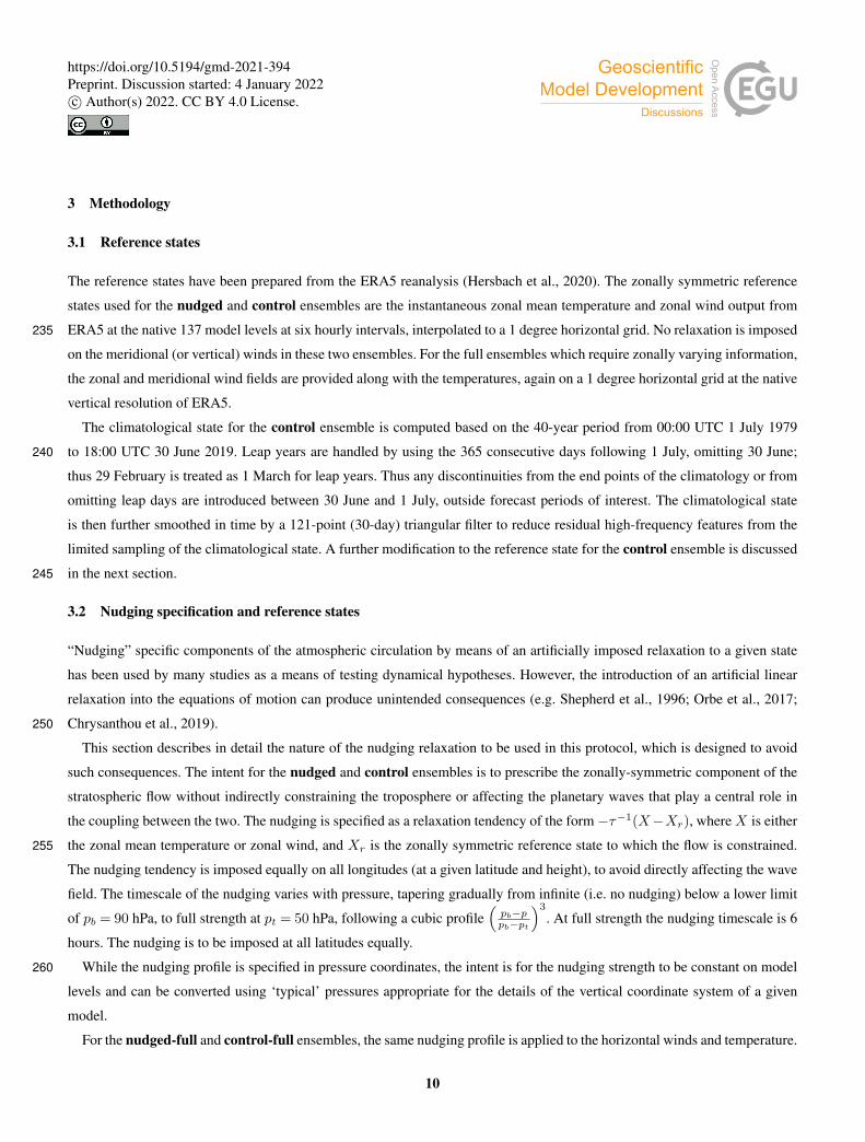
3.2 Nudging specification and reference states

“Nudging” specific components of the atmospheric circulation by means of an artificially imposed relaxation to a given state

has been used by many studies as a means of testing dynamical hypotheses. However, the introduction of an artificial linear

relaxation into the equations of motion can produce unintended consequences (e.g. Shepherd et al., 1996; Orbe et al., 2017;

Chrysanthou et al., 2019).250

This section describes in detail the nature of the nudging relaxation to be used in this protocol, which is designed to avoid

such consequences. The intent for the nudged and control ensembles is to prescribe the zonally-symmetric component of the

stratospheric flow without indirectly constraining the troposphere or affecting the planetary waves that play a central role in

the coupling between the two. The nudging is specified as a relaxation tendency of the form−τ−1(X−Xr), where X is either

the zonal mean temperature or zonal wind, and Xr is the zonally symmetric reference state to which the flow is constrained.255

The nudging tendency is imposed equally on all longitudes (at a given latitude and height), to avoid directly affecting the wave

field. The timescale of the nudging varies with pressure, tapering gradually from infinite (i.e. no nudging) below a lower limit

of pb = 90 hPa, to full strength at pt = 50 hPa, following a cubic profile(pb−ppb−pt

)3

. At full strength the nudging timescale is 6

hours. The nudging is to be imposed at all latitudes equally.

While the nudging profile is specified in pressure coordinates, the intent is for the nudging strength to be constant on model260

levels and can be converted using ‘typical’ pressures appropriate for the details of the vertical coordinate system of a given

model.

For the nudged-full and control-full ensembles, the same nudging profile is applied to the horizontal winds and temperature.

10


For the control ensemble, the protocol specifies nudging the zonally symmetric components of the stratosphere towards the

climatology. Since the initial conditions are in some cases some ways away from the climatology, nudging at full strength to265

the climatology will generate undesirable transients as the stratosphere adjusts towards the climatological state.

In order to reduce this initial shock, the reference state for the control ensemble is interpolated smoothly from the observed

evolution to the climatology over the first 5 days of the forecast period. For instance, the temperatures is relaxed towards a state

Tr defined by

Tr(t) = To(t)(1− f(t− ti)) +Tc(t)f(t− ti)270

where To is the instantaneous reference state, Tc is the reference climatology computed as described in the previous section, t

is the time, ti is the starting time of the forecast, and f is an interpolating function given by

f(t− ti) =

0 if t− ti < 0

sin2(π2

(t−ti)∆t

)if 0≤ t− ti <∆t

1 if t− ti ≥∆t

with ∆t= 5 days. A similar adjustment should be adopted for the control-full ensemble.

The zonally symmetric nudging approach has been successfully applied by a number of studies to explore aspects of275

stratosphere-troposphere interactions (Simpson et al., 2011; Hitchcock and Simpson, 2014; Simpson et al., 2018). The ap-

proach has also been used to impose a QBO in models that do not internally generate one, and to study the dynamics of the

QBO and its teleconnections (Anstey et al., 2016; Martin et al., 2021a). However, these studies have been carried out either in

uninitialized climate models or in idealized general circulation models, not in the context of operational forecasting, and the

technique in general can produce undesirable artifacts, particularly with regards to transport effects (Chrysanthou et al., 2019;280

Hitchcock and Haynes, 2014).

The nudging specification in the nudged and control runs is intended not to directly impact the zonally asymmetric compo-

nent of the flow. The statistics of the planetary waves in particular are found in test experiments to be largely unaffected by the

constraint on the zonal mean. One exception is that wave amplitudes in the upper stratosphere can grow larger in the presence

of nudging; this is in part because the nudging prevents the wave transience from decelerating the mean flow, allowing plane-285

tary waves to propagate higher before they encounter critical levels. In some cases this can result in unusually strong winds in

the upper stratosphere and lower mesosphere; however this is not expected to influence the evolution of the lower stratosphere

or its interactions with the troposphere.

Because the wave field is not directly controlled by the nudging, the zonal mean forcing produced by the internally-generated

wave field can differ substantially from that consistent with the evolution of the reference state, particularly for the control290

ensemble. Since the meridional circulation is largely determined by the forcing associated with the waves (e.g. Plumb, 1982;

Haynes et al., 1991), misrepresentation of the wave field can result in spurious meridional circulations and the potential for un-

intended remote effects. However, Hitchcock and Haynes (2014) has shown that the spurious circulations are largely confined

to within the region of nudging, while the non-local circulation below the region of the nudging associated with ‘downward

11


Table 1. Case studies and forecast initialization dates. The nudged-full and control-full ensembles are requested only for the later of the

two initialization dates for a given event.

(Hemisphere) Event Initialization Dates

(NH) 12 Feb 2018 25 Jan 2018 8 Feb 2018

(NH) 2 Jan 2019 13 Dec 2018 8 Jan 2019

(SH) 18 Sep 2019 29 Aug 2019 1 Oct 2019

control’ is to a close approximation consistent with the forcings that produced the reference state. This implies that any down-295

ward influence associated with these circulations can be expected to be present in the nudged ensemble, and absent in the

control ensemble. Spurious circulations within the nudging region may give rise to anomalous transport of constituents within

the stratosphere, but this is not expected to be of concern on the subseasonal timescales relevant to the present protocol.

The presence of a nudging layer can also give rise to a ‘sponge-layer feedback’ like response (Shepherd et al., 1996), which

is characterized by spurious zonal mean temperature and wind anomalies generated just below the layer of nudging in response300

to tropospheric torques that differ from the reference state. These effects have also been shown to be negligible on these

timescales (Hitchcock and Haynes, 2014).

4 Case Studies

The ensemble forecasts just described will be applied to three recent events: the major sudden stratospheric warmings of

2018 and 2019 in the Northern Hemisphere, and the near-major warming of 2019 in the Southern Hemisphere. This section305

reviews the evolution of these three events, highlighting the evolution of the stratospheric polar vortex and the response of

the tropospheric Northern and Southern annular modes (NAM and SAM, respectively) along with the closely related North

Atlantic Oscillation (NAO) and Arctic Oscillation (AO). Notable high-impact events that may be related to the stratospheric

anomalies are also discussed. Finally, the state of other modes of climate variability that have important teleconnections relevant

to the stratosphere and to the surface impact itself are briefly summarized, including the Quasi-biennial oscillation (QBO), El310

Niño-Southern Oscillation (ENSO), and the Madden-Julian Oscillation (MJO).

Two initialization dates are requested for each event (Table 1). One date is chosen about three weeks prior to the surface

extreme of interest, in order to identify the contribution of the stratosphere to its forecast on subseasonal timescales (motivations

1, 2, and 3). A second date is chosen prior to the onset of the stratospheric warming in order to assess the representation

of the onset of the event (motivations 1, 3, and 4). The former has higher priority than the latter, although they are listed315

chronologically in Table 1. Thursdays are chosen since nearly all models that contributed to the S2S database contributed

forecasts initialized on Thursdays, making it easier to compare the two datasets. Further justification for the initialization dates

selected are provided in the case-by-case discussion below.

12


16 Jan 1 Feb 16 Feb 1 Mar 16 Mar 1 Apr 16 Apr

1

10

100

1000

Pres

sure

[hPa

]2018 NAM

4321

01234

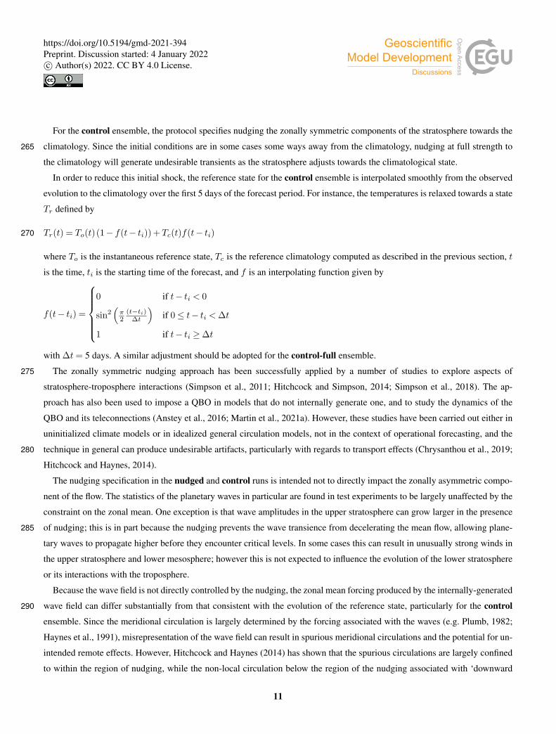
Figure 3. Northern Annular mode during the February 2018 boreal major warming. The NAM indices are computed from ERA5 geopotential

height anomalies following the methodology of Butler et al. (2020). The vertical black dash-dotted line indicates the date of the wind reversal

at 10 hPa, 60◦ N. The green and orange vertical lines indicate the requested initialization dates.

4.1 Boreal Major Warming of 12 February 2018

The Arctic polar vortex split in early February of 2018, leading to a reversal of the zonal mean zonal wind at 60 N, 10 hPa on 12320

February 2018. Prior to the event (Fig.3) the vortex was near to its climatological strength; it weakened rapidly throughout the

depth of the stratosphere, coincident with large-amplitude vertical fluxes of wavenumber-two wave activity. Lower stratospheric

anomalies persisted into late March of 2018.

The tropospheric NAM responded strongly to these stratospheric anomalies, exhibiting a shift to negative values from mid-

February through mid-March, consistent with the composite mean response to sudden stratospheric warmings. The NAO index325

was strongly negative in late February, coinciding with unusually cold weather over much of Europe and Asia during the

last two weeks of Feb. (Lü et al., 2020), bringing, for example, snow to Rome and several notable winter storms to the UK.

Precipitation patterns also shifted, bringing persistent rain to the Iberian peninsula, ending an extended period of drought

(Ayarzagüena et al., 2018).

Of the three proposed case studies, this first case has been the most actively studied to date. In a study of the S2S database,330

Rao et al. (2020a) showed that those ensemble members that capture the amplitude of the lower stratospheric anomalies during

this event (and the 2019 case considered next) were also more successful in forecasting the surface extremes; they also showed

that this was more relevant than whether the model forecasted a split or displacement of the vortex. As discussed above, Kautz

et al. (2020) explicitly identified the increased risk of extreme cold over Europe arising from the stratospheric anomalies. This

was also the case in the nudging experiments of Knight et al. (2020), who examined the impacts of relaxing the stratospheric335

flow in seasonal forecasts initialized at the beginning of the winter season. The nudged ensemble reproduced a tropospheric

response following the SSW in close agreement with observational composites.

The MJO reached near-record strength in phase 6 and 7 prior to the stratospheric wind reversal in February of 2018, i.e,

the MJO phase which has been linked to enhanced SSW frequency and predictability for earlier events (Garfinkel et al., 2012;

13


3

10

30

100

300

1000

Pres

sure

[hPa

](a) 2018 U 60 N, Fz 50 -70 N: wave number 1

16 Jan 1 Feb 16 Feb 1 Mar 16 Mar 1 Apr 16 Apr

3

10

30

100

300

1000

Pres

sure

[hPa

]

(b) 2018 U 60 N, Fz 50 -70 N: wave number 2

-1× 106

-1× 105

-1× 104

0

1× 104

1× 105

1× 106

kg s 2

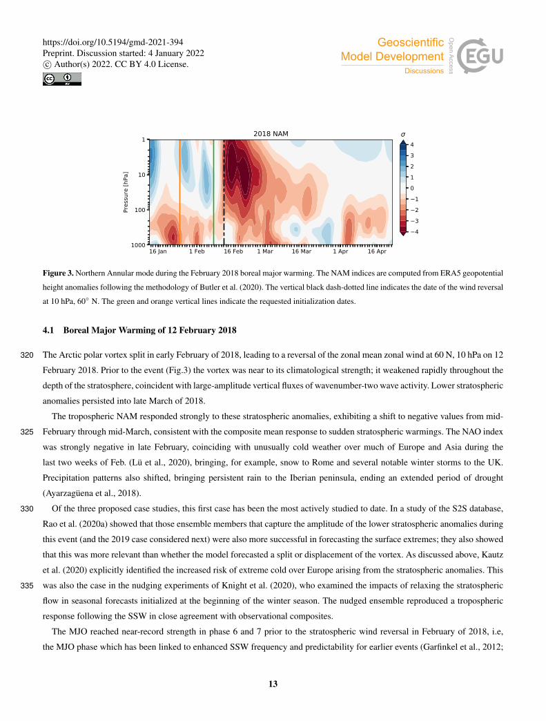
Figure 4. Wave forcing during the February 2018 boreal major warming. Shading shows the vertical component of the Eliassen Palm flux

averaged from 50◦-70◦ N from zonal wavenumber (a) one and (b) two. Contour lines show zonal mean zonal wind at 60◦ N. The vertical

black dash-dotted line indicates the date of the wind reversal at 10 hPa, 60◦ N. The green and orange vertical lines indicate the requested

initialization dates.

Garfinkel and Schwartz, 2017). A week after the event the MJO entered phase 8, which is linked to a negative NAO pattern.340

While Butler et al. (2020) do not find a correlation between forecast errors in the MJO and those in the NAM, Knight et al.

(2020) do find that nudging the tropical evolution produces a negative NAO response in late February, suggesting that tropical

circulation anomalies contributed to the anomalous European weather regimes.

The S2S prediction systems forecast the event about 11 days in advance (Karpechko et al., 2018; Rao et al., 2020a), making

this event less predictable than some other sudden warmings. Proximately, this is likely due to the nature of the relevant wave345

driving which amplified rapidly during the week prior to the stratospheric wind reversal (Fig. 4). Subseasonal forecasts that

captured this wave event were more successful in forecasting the vortex breakdown. The difficulty in forecasting the pulse of

wave activity has in turn been tied to both anomalous blocking over Siberia (Karpechko et al., 2018) as well as to an episode

of anticyclonic Rossby wave breaking in the North Atlantic (Lee et al., 2019).

On longer timescales, Knight et al. (2020) further suggest a role for the large-amplitude MJO event that preceded the350

stratospheric wind reversal, and Lü et al. (2020) suggest that several large snowfall events over Siberia in early and late January

contributed to the wave driving responsible for the vortex breakdown. On seasonal timescales, the tropical Pacific was in a

14


16 Dec 1 Jan 16 Jan 1 Feb 16 Feb 1 Mar 16 Mar

1

10

100

1000

Pres

sure

[hPa

]2018-19 NAM

4321

01234

Figure 5. Northern Annular mode during the January 2019 boreal major warming. The vertical black dash-dotted line indicates the date of

the wind reversal at 10 hPa, 60◦ N. The green and orange vertical lines indicate the requested initialization dates.

moderate La Niña state, and the QBO winds were persistently westerly at 50 hPa and easterly at 30 hPa throughout the winter.

Thus the state of both ENSO and the QBO may have also contributed.

The first initialization date proposed is 25 Jan 2018, just prior to the first pulse of wave activity leading to the vortex split.355

The ensembles will thus produce some diversity in the tropospheric precursors outlined above. By considering the ensemble

spread, the relative roles of tropospheric precursors and the stratospheric state in the amplification of the planetary waves

can thus be isolated. These integrations may also capture some of the development of the European cold air outbreak in late

February. The second date, 8 Feb 2018, is chosen to be closer to the development of the tropospheric extreme event, after the

full development of the stratospheric anomalies.360

4.2 Boreal Major Warming of 2 January 2019

In late December 2018, the Arctic vortex was displaced off of the pole, prior to splitting. The 10 hPa winds reversed on 2 Jan

2019. In contrast to the 2018 event, the stratospheric vortex anomalies developed much more gradually through late December

and early January of the 2018-19 winter (Lee and Butler, 2020). The vortex remained split for several weeks. Anomalies in the

lower stratosphere persisted nearly to March of 2019. The gradual weakening of the vortex was due to persistent wavenumber-365

one forcing that was well predicted even from mid-December (Rao et al., 2020a).

In strong contrast to the 2018 case, the tropospheric NAM did not respond strongly to the stratospheric anomalies, remaining

near neutral or even slightly positive through much of the troposphere until early February (Fig.5). However, an extensive cold

snap occurred over North America in late January (roughly 23-29 Jan) in a region vertically aligned with one of the daughter

vortices generated by the split.370

This event was also considered by Rao et al. (2020a), who found that the surface temperatures and precipitation patterns

20 days following the onset date were generally not well forecast by the S2S models. Note, however, that they did not focus

specifically on the cold air outbreak over North America. Knight et al. (2020) also performed nudging experiments to explore

the impacts of the stratospheric anomalies on the surface. They found that the ensemble mean again reproduced the ‘canonical’

15


3

10

30

100

300

1000

Pres

sure

[hPa

](a) 2018-19 U 60 N, Fz 50 -70 N: wave number 1

16 Dec 1 Jan 16 Jan 1 Feb 16 Feb 1 Mar 16 Mar

3

10

30

100

300

1000

Pres

sure

[hPa

]

(b) 2018-19 U 60 N, Fz 50 -70 N: wave number 2

-1× 106

-1× 105

-1× 104

0

1× 104

1× 105

1× 106

kg s 2

Figure 6. Wave forcing during the January 2019 boreal major warming (quantities the same as Fig. 4). The vertical black dash-dotted line

indicates the date of the wind reversal at 10 hPa, 60◦ N. The green and orange vertical lines indicate the requested initialization dates.

tropospheric response, with an anomalously persistent negative AO pattern coinciding with NAM anomalies in the lower375

stratosphere, implying that the lack of tropospheric signal in observations was due to some competing effect(s). One possibility

is that these competing effects arise from the tropics; the tropical nudging experiments of Knight et al. (2020) gave rise to

North Atlantic mean sea-level pressure anomalies that more closely resembled observations in January. For instance, the MJO

also progressed through phase 6 and 7 in early January 2019, but at amplitudes considerably weaker than in 2018.

The S2S prediction systems forecast the stratospheric wind reversal more than 18 days prior to the central date in some380

cases (Rao et al., 2020a), but did not predict the vortex would split more than a few days in advance (Butler et al., 2020). The

longer forecast horizon in this case seems to be related to the persistent wavenumber-one forcing from mid-December 2018

that displaced the vortex off the pole, prior to its ultimate splitting (see Fig.6).

Rao et al. (2020a) propose a range of contributing factors for the wave amplification, including the state of ENSO, the QBO,

the solar cycle, and the MJO. In the fall of 2018, the QBO at 50 hPa was strongly easterly, below a westerly shear zone that385

stretched from 40 hPa to 20 hPa. This shear zone descended through the winter. At the time of the wind reversal, the winds

at 50 hPa were easterly and those at 30 hPa were westerly. Since the vertical wind shear in the 30-50 hPa layer was easterly

in February 2018 and westerly in January 2019, these two start dates provide contrasting case studies of how model biases in

wave forcing and QBO amplitude develop in the lower stratosphere for both easterly and westerly QBO phases.

16


16 Aug 1 Sep 16 Sep 1 Oct 16 Oct 1 Nov 16 Nov 1 Dec

1

10

100

1000

Pres

sure

[hPa

]2019 SAM

4321

01234

Figure 7. Southern Annular Mode during the September 2019 austral minor warming. The SAM indices are computed from ERA5 geopo-

tential height anomalies averaged over 65◦ to 90◦ S, analogously to the NAM indices shown in Figs. 3 and 5. The vertical black dash-dotted

line indicates the date of minimum zonal mean zonal wind at 10 hPa, 60◦ S. The green and orange vertical lines indicate the requested

initialization dates.

The first suggested initialization date is 13 Dec 2018, just prior to the onset of the wavenumber-one pulse, again motivated390

by the goal of producing some diversity in the tropospheric wave source in order to distinguish tropospheric and stratospheric

contributions to the wave amplification. The second suggested initialization date is 8 Jan 2019, several weeks prior to the North

American cold air outbreak.

4.3 Austral Minor Warming of September 2019

The final event of interest is the minor warming that occurred in the Southern Hemisphere in September of 2019. Significant395

Southern Annular Mode anomalies began to emerge in the upper stratosphere towards the end of August (Fig. 7). However, in

contrast to the first two cases, the zonal mean winds at 10 hPa, 60◦S did not reverse. However, they did decelerate dramatically,

reaching their minimum value on 18 Sep 2019, which can be considered as the ‘central’ date for the event (Fig. 8). This was

slightly earlier in the spring than the major austral warming event that occurred in 2002, during which the Antarctic polar

vortex westerlies did fully reverse. In late August the mid-stratospheric winds were near their climatological values, before400

a series of wavenumber-one pulses of upward wave activity flux weakened the vortex from the stratopause downwards (Lim

et al., 2021, see also Fig. 8).

The tropospheric Southern Annular Mode did not initially shift to negative values following the event. However, negative

anomalies were observed in late October and November, during which conditions over Australia were hot and dry; severe

wildfires were widespread in October through December, potentially due in part to the stratospheric anomalies (Lim et al.,405

2019, 2021).

Noguchi et al. (2020) studied the effects of this event on tropical convection though a nudging experiment constraining the

full stratospheric flow. They demonstrated that the stratospheric anomalies led to a systematic enhancement of convection in

the Northern Hemisphere tropics, centered over Southeast Asia and the Western Pacific.

17


3

10

30

100

300

1000

Pres

sure

[hPa

](a) 2019 U 60 S, Fz 50 -70 S: wave number 1

16 Aug 1 Sep 16 Sep 1 Oct 16 Oct 1 Nov 16 Nov 1 Dec

3

10

30

100

300

1000

Pres

sure

[hPa

]

(b) 2019 U 60 S, Fz 50 -70 S: wave number 2

-1× 106

-1× 105

-1× 104

0

1× 104

1× 105

1× 106

kg s 2

Figure 8. Wave forcing during the September 2019 austral minor warming. Shading shows the vertical component of the Eliassen Palm flux

averaged from 50◦-70◦ S from zonal wavenumber (a) one and (b) two. Contour lines show zonal mean zonal wind at 60◦ S. The vertical

black dash-dotted line indicates the date of minimum zonal mean zonal wind at 10 hPa, 60◦ S. The green and orange vertical lines indicate

the requested initialization dates.

The event was forecast nearly 18 days prior by models with a reasonably resolved stratosphere (Rao et al., 2020b), including410

the persistent stratospheric wavenumber-one flux anomalies (Fig. 8). A number of tropospheric precursors have been linked

to this wave activity pulse, including a persistent blocking high over the Antarctic Peninsula and a region of anomalously low

pressure over the Southern Indian Ocean (Rao et al., 2020b; Lim et al., 2021). The first suggested initialization date is 29

August 2019, early in the development of the wave activity pulse responsible for the stratospheric event. The second suggested

initialization date is 1 October 2019, after the stratospheric anomalies are established, two to three weeks prior to the onset of415

the tropospheric SAM response.

5 Data Request

In order to meet the scientific goals of this project, we request output from the forecast models that includes both surface

quantities needed for identifying and quantifying high-impact surface extremes, as well as dynamical quantities needed to

diagnose the processes that couple the stratosphere and troposphere. Given the relatively short integration periods and small420

number of initialization dates, data is requested at relatively high temporal and vertical resolution to enable more detailed

18


comparisons of the relevant processes than has been possible with existing subseasonal forecast databases. The data request is

closely related to the DynVarMIP request (Gerber and Manzini, 2016), including a request for quantities required to close the

zonally averaged zonal momentum and thermodynamic budgets.

Quantities are requested on a horizontal grid at no finer resolution than 1◦× 1◦, and at a time resolution of 6 hours. At-425

mospheric quantities that depend on a vertical coordinate are requested on a slightly non-standard grid “snap34” of pressure

levels: 1000, 925, 850, 700, 600, 500, 400, 300, 250, 200, 170, 150, 130, 115, 100, 90, 80, 70, 60, 50, 40, 30, 20, 15, 10, 7, 5,

3, 2, 1.5, 1, 0.7, 0.5, and 0.4 hPa. This includes some additional levels in the lower stratosphere relative to the CMIP6 “plev39”

grid, and fewer levels above the stratopause. Variable names follow CMIP6 standard naming conventions where possible. The

requested variables are summarized in four tables.430

6hr Surface quantities and fluxes averaged, maximized, or minimized over the 6 hours preceding the timestep (Table 2).

6hrZ Zonally-averaged atmospheric quantities averaged over the 6 hours preceding the timestep (Table 3). Includes quantities

needed to close atmospheric momentum and thermodynamic budgets. These follow closely the DynVarMIP request

(Gerber and Manzini, 2016), but include the imposed tendencies from the nudging as well.

6hrPt Instantaneous basic meteorological and surface quantities output every 6 hours (Table 4).435

6hrPtZ Instantaneous Transformed Eulerian Mean dynamical quantities output every 6 hours, following the DynVarMIP

request (Table 5).

There are two levels of priority for the requested variables. The higher priority variables (1) are considered necessary to meet

the primary science goals, and include meteorological quantities (winds, temperatures, specific humidity, and geopotential

height) required to compute commonly used dynamical diagnostics, measures of precipitation, and surface quantities including440

pressure, temperature, and horizontal winds. Variables at the lower priority level (2) include zonally averaged quantities that

would permit closing the zonally averaged momentum and thermodynamic budgets, as well as surface quantities that would

permit a more detailed analysis of surface processes. The zonal mean stratospheric ozone field is also requested at this lower

priority level to allow for some assessment of the importance of ozone anomalies in forecasting the evolution of the polar

vortex over subseasonal timescales.445

6 Summary and Outlook

The SNAPSI project aims to produce a set of controlled ensemble forecasts, initialized around several recent sudden strato-

spheric warmings. This dataset will allow for an unprecedentedly thorough, multi-model assessment of the contribution of

stratospheric extreme events to surface predictability on subseasonal timescales. The proposed forecast ensembles include

standard, free-running ensembles, in addition to ‘nudged’ ensembles in which the evolution of the stratosphere is constrained450

either to the observed or to climatological conditions. The use of zonally symmetric nudging will enable detailed investigations

of the representation of planetary waves that play a central role in the evolution of the events.

19


Table 2. Requested variables in table 6hr. Surface (XYT) output averaged over 6 hourly intervals. See text for meaning of priority levels.

Name (Priority) Long name Unit

pr (1) Precipitation kg m−2 s−1

prc (1) Convective Precipitation kg m−2 s−1

clt (2) Total Cloud Cover Percentage %

hfds (2) Downward Heat Flux at Sea Water Surface W m−2

tauu (2) Surface Downward Eastward Wind Stress Pa

tauv (2) Surface Downward Northward Wind Stress Pa

tasmaxa (2) 6 hourly Maximum Near-Surface Air Temperature K

tasmina (2) 6 hourly Minimum Near-Surface Air Temperature K

a Maximum/minimum computed over preceding 6 hours.

Table 3. Requested variables in table 6hrZ. Zonal mean output averaged over 6 hourly intervals (YPT). See text for meaning of priority

levels.


tntnda (1) Tendency of Air Temperature Due to Imposed Relaxation K s−1

utendnda (1) Tendency of Eastward Wind Due to Imposed Relaxation m s−2

tntmp (2) Tendency of Air Temperature Due to Model Physics K s−1

tntrl (2) Tendency of Air Temperature Due to Longwave Radiative Heating K s−1

tntrs (2) Tendency of Air Temperature Due to Shortwave Radiative Heating K s−1

utendepfd (2) Tendency of Eastward Wind Due to Eliassen-Palm Flux Divergence m s−2

utendmpa (2) Tendency of Eastward Wind Due to Model Physics m s−2

utendnogw (2) Eastward Acceleration Due to Non-Orographic Gravity Wave Drag m s−2

utendogw (2) Eastward Acceleration Due to Orographic Gravity Wave Drag m s−2

utendvtem (2) Tendency of Eastward Wind Due to TEM Northward Advection and Coriolis Term m s−2

utendwtem (2) Tendency of Eastward Wind Due to TEM Upward Advection m s−2

vtendnogw (2) Northward Acceleration Due to Non-Orographic Gravity Wave Drag m s−2

vtendogw (2) Northward Acceleration Due to Orographic Gravity Wave Drag m s−2

xgwdparam (2) Eastward Gravity Wave Drag Pa

ygwdparam (2) Northward Gravity Wave Drag Pa

a These variables are not defined by the CMIP 6 standard.

Three case studies have been chosen to apply the experimental methodology: the major boreal sudden stratospheric warmings

of February 2018 and January 2019, and the austral minor sudden stratospheric warming of September 2019. The atmosphere

20


Table 4. Requested variables in table ‘6hrPt’. Instantaneous atmospheric (XYPT) and surface (XYT) quantities output at 6 hourly intervals.

See text for meaning of priority levels.


ta (1) Air Temperature K

ua (1) Eastward Wind m s−1

va (1) Northward Wind m s−1

wap (1) Omega (vertical pressure velocity) Pa s−1

zg (1) Geopotential Height m

hus (1) Specific Humidity kg kg−1

ps (1) Surface Air Pressure Pa

psl (1) Sea Level Pressure Pa

tas (1) Near-Surface Air Temperature K

uas (1) Eastward Near-Surface Wind m s−1

vas (1) Northward Near-Surface Wind m s−1

rlut (1) TOA Outgoing Longwave Radiation W m−2

tos (2) Sea Surface Temperature degC

siconca (2) Sea-Ice Area Percentage %

sithick (2) Sea Ice Thickness m

snd (2) Snow Depth m

snw (2) Surface Snow Amount kg m−2

mrso (2) Total Soil Moisture Content kg m−2

mrsos (2) Moisture in Upper Portion of Soil Column kg m−2

Table 5. Requested variables in table ‘6hrPtZ’. Zonal mean, instantaneous atmospheric (YPT) output at 6 hourly intervals. See text for

meaning of priority levels.


epfy (2) Northward Component of the Eliassen-Palm Flux m3 s−2

epfz (2) Upward Component of the Eliassen-Palm Flux m3 s−2

o3a (2) Mole Fraction of O3 mol mol−1

vtem (2) Transformed Eulerian Mean Northward Wind m s−1

wtem (2) Transformed Eulerian Mean Upward Wind m s−1

a Climatological if necessary

exhibited a range of tropospheric responses, but in each case, an extreme event with significant societal impacts followed the455

stratospheric perturbation.

21


Table 6. Participating Centres, models, and reference publications.

Participating Centre Model Reference Publication(s)

Beijing Climate Center (BCC), China MeteorologicalAdministration

BCC-CSM2-HR Wu et al. (2019, 2021)

Institute of Atmospheric Sciences and Climate of theNational Council of Research of Italy (CNR-ISAC)

GLOBOMalguzzi et al. (2011); Mastrangelo andMalguzzi (2019)

Environment and Climate Change Canada (ECCC) GEM-NEMO Smith et al. (2018); Lin et al. (2020)

Environment and Climate Change Canada (ECCC) CanESM5Swart et al. (2019); Sospedra-Alfonso et al.(2021)

European Centre for Mid-range Weather Forecasting(ECMWF)

IFS ECMWF (2020)

Geophysical Fluid Dynamics Laboratory, NOAA(GFDL)

SPEAR Delworth et al. (2020)

Korean Meteorological Administration (KMA) GloSea5-GC2MacLachlan et al. (2014); Williams et al. (2015);Walters et al. (2017)

Météo-France CNRM-CM 6.1 Voldoire et al. (2019)

National Center for Atmospheric Research (NCAR) CESM2(CAM6) Danabasoglu et al. (2020); Richter et al. (2021)

Naval Research Laboratory (NRL) NAVGEMHogan et al. (2014); McCormack et al. (2017);Eckermann et al. (2018)

United Kingdom Met Office (UKMO) GloSea5 MacLachlan et al. (2014)

The experiments have been designed with four primary scientific motivations. First, as outlined above to assess the con-

tribution of the stratosphere to subseasonal forecast skill. Second, to develop methods of formally attributing specific surface

extremes to this stratospheric variability. Third, to quantify in detail mechanisms responsible for the surface impacts across the

forecast models, controlling for the magnitude and nature of the zonally symmetric stratospheric anomalies that are thought460

to be most directly responsible for the surface impacts. Fourth, and finally, to improve understanding of the upward coupling

from the troposphere to the stratosphere. The experimental design, specific case studies and forecast initialization dates have

been chosen to meet these four goals.

Beyond these central goals, the experiments are further expected to shed light on a number of other aspects of dynamical

coupling on subseasonal timescales between the stratosphere and troposphere, and between the tropics and extratropics. No-465

tably, both the 2018 and 2019 boreal sudden warming case studies span periods with significant MJO activity and differing

22


phases of the QBO, and the 2019 austral sudden warming case spans the development phase of a disruption to the QBO that

occurred in early 2020.

At the time of submission, eleven modeling groups from ten modeling centers are participating in this project (Table 6).

Output from the contributing models will be stored in a central archive hosted by CEDA. Initial analysis of the output will be470

carried out by community working groups organized through the SNAP project; following an initial embargo period intended

to allow time for this analysis to be carried out, the data will be made available to the broader community.

Data availability. The reference states for all nudging runs and all model output will be made available through the CEDA archive. At time

of submission this archive is not operational.

Author contributions. The protocol was initially designed by Peter Hitchcock, Amy Butler, Andrew Charlton-Perez, Tim Stockdale, and475

Chaim Garfinkel. James Anstey, Dann Mitchell, and Daniela Domeisen contributed to the text of the paper. The remaining authors contributed

to the experimental design from the perspective of contributing operational centers and edited the manuscript.

Competing interests. The authors declare no competing interests are present.

Acknowledgements. We acknowledge the support of SPARC and the S2S Prediction Project. CIG is supported by the European Research

Council starting grant under the European Union’s Horizon 2020 research and innovation program (Grant Agreement 677756). DD gratefully480

acknowledges support from the Swiss National Science Foundation through projects PP00P2_170523 and PP00P2_198896.

23


References

Afargan-Gerstman, H., Polkova, I., Papritz, L., Ruggieri, P., King, M. P., Athanasiadis, P. J., Baehr, J., and Domeisen, D. I. V.: Stratospheric

influence on North Atlantic marine cold air outbreaks following sudden stratospheric warming events, Weather Clim. Dynam., 1, 541–553,

https://doi.org/10.5194/wcd-1-541-2020, 2020.485

Anstey, J. A., Scinocca, J. F., and Keller, M.: Simulating the QBO in an Atmospheric General Circulation Model: Sensitivity to Resolved

and Parameterized Forcing, J. Atmos. Sci., 73, 1649–1665, https://doi.org/10.1175/JAS-D-15-0099.1, 2016.

Ayarzagüena, B., Barriopedro, D., Garrido-Perez, J. M., Abalos, M., de la Cámara, A., García-Herrera, R., Calvo, N., and Or-

dóñez, C.: Stratospheric Connection to the Abrupt End of the 2016/2017 Iberian Drought, Geophys. Res. Lett., 45, 12 639–12 646,

https://doi.org/10.1029/2018GL079802, 2018.490

Baldwin, M. P., Ayarzagüena, B., Birner, T., Butchart, N., Butler, A. H., Charlton-Perez, A. J., Domeisen, D. I. V., Garfinkel, C. I., Garny, H.,

Gerber, E. P., Hegglin, M. I., Langematz, U., and Pedatella, N. M.: Sudden Stratospheric Warmings, Rev. Geophys., 59, e2020RG000 708,

https://doi.org/10.1029/2020RG000708, 2021.

Butler, A., Charlton-Perez, A., Domeisen, D. I., Garfinkel, C., Gerber, E. P., Hitchcock, P., Karpechko, A. Y., Maycock, A. C., Sigmond,

M., Simpson, I., and Son, S.-W.: Chapter 11 - Sub-seasonal Predictability and the Stratosphere, in: Sub-Seasonal to Seasonal Prediction,495

edited by Robertson, A. W. and Vitart, F., pp. 223 – 241, Elsevier, https://doi.org/https://doi.org/10.1016/B978-0-12-811714-9.00011-5,

2019.

Butler, A. H., Lawrence, Z. D., Lee, S. H., Lillo, S. P., and Long, C. S.: Differences between the 2018 and 2019 stratospheric polar vortex

split events, Q. J. R. Meteorol. Soc., 146, 3503–3521, https://doi.org/10.1002/qj.3858, 2020.

Charlton-Perez, A. J., Huang, W. T. K., and Lee, S. H.: Impact of sudden stratospheric warmings on United Kingdom mortality, Atmos. Sci.500

Let., 22, e1013, https://doi.org/10.1002/asl.1013, 2021.

Christiansen, B.: The Role of the Selection Problem and Non-Gaussianity in Attribution of Single Events to Climate Change, J. Clim., 28,

9873–9891, https://doi.org/10.1175/JCLI-D-15-0318.1, 2015.

Chrysanthou, A., Maycock, A. C., Chipperfield, M. P., Dhomse, S., Garny, H., Kinnison, D., Akiyoshi, H., Deushi, M., Garcia, R. R., Jöckel,

P., Kirner, O., Pitari, G., Plummer, D. A., Revell, L., Rozanov, E., Stenke, A., Tanaka, T. Y., Visioni, D., and Yamashita, Y.: The effect505

of atmospheric nudging on the stratospheric residual circulation in chemistry–climate models, Atmos. Chem. Phys., 19, 11 559–11 586,

https://doi.org/10.5194/acp-19-11559-2019, 2019.

Danabasoglu, G., Lamarque, J.-F., Bacmeister, J., Bailey, D. A., DuVivier, A. K., Edwards, J., Emmons, L. K., Fasullo, J., Garcia, R.,

Gettelman, A., Hannay, C., Holland, M. M., Large, W. G., Lauritzen, P. H., Lawrence, D. M., Lenaerts, J. T. M., Lindsay, K., Lipscomb,

W. H., Mills, M. J., Neale, R., Oleson, K. W., Otto-Bliesner, B., Phillips, A. S., Sacks, W., Tilmes, S., van Kampenhout, L., Vertenstein,510

M., Bertini, A., Dennis, J., Deser, C., Fischer, C., Fox-Kemper, B., Kay, J. E., Kinnison, D., Kushner, P. J., Larson, V. E., Long, M. C.,

Mickelson, S., Moore, J. K., Nienhouse, E., Polvani, L., Rasch, P. J., and Strand, W. G.: The Community Earth System Model Version 2

(CESM2), J. Adv. Model Earth Sy., 12, e2019MS001 916, https://doi.org/10.1029/2019MS001916, 2020.

de la Cámara, A., Abalos, M., and Hitchcock, P.: Changes in stratospheric transport and mixing during sudden stratospheric warmings, J.

Geophys. Res., 123, 3356–3373, https://doi.org/10.1002/2017JD028007, 2018.515

Delworth, T. L., Cooke, W. F., Adcroft, A., Bushuk, M., Chen, J.-H., Dunne, K. A., Ginoux, P., Gudgel, R., Hallberg, R. W., Harris, L.,

Harrison, M. J., Johnson, N., Kapnick, S. B., Lin, S.-J., Lu, F., Malyshev, S., Milly, P. C., Murakami, H., Naik, V., Pascale, S., Paynter, D.,

Rosati, A., Schwarzkopf, M., Shevliakova, E., Underwood, S., Wittenberg, A. T., Xiang, B., Yang, X., Zeng, F., Zhang, H., Zhang, L., and

24


Zhao, M.: SPEAR: The Next Generation GFDL Modeling System for Seasonal to Multidecadal Prediction and Projection, J. Adv. Model

Earth Sy., 12, e2019MS001 895, https://doi.org/10.1029/2019MS001895, 2020.520

Domeisen, D. I. V. and Butler, A. H.: Stratospheric drivers of extreme events at the Earth’s surface, Commun. Earth Environ., 1, 59,

https://doi.org/10.1038/s43247-020-00060-z, 2020.

Domeisen, D. I. V., Butler, A. H., Charlton-Perez, A. J., Ayarzagüena, B., Baldwin, M. P., Dunn-Sigouin, E., Furtado, J. C., Garfinkel, C. I.,

Hitchcock, P., Karpechko, A. Y., Kim, H., Knight, J., Lang, A. L., Lim, E., Marshall, A., Roff, G., Schwartz, C., Simpson, I. R., Son, S.,

and Taguchi, M.: The Role of the Stratosphere in Subseasonal to Seasonal Prediction: 1. Predictability of the Stratosphere, J. Geophys.525

Res., 125, e2019JD030 920, https://doi.org/10.1029/2019JD030920, 2020a.

Domeisen, D. I. V., Butler, A. H., Charlton-Perez, A. J., Ayarzagüena, B., Baldwin, M. P., Dunn-Sigouin, E., Furtado, J. C., Garfinkel, C. I.,

Hitchcock, P., Karpechko, A. Y., Kim, H., Knight, J., Lang, A. L., Lim, E., Marshall, A., Roff, G., Schwartz, C., Simpson, I. R., Son, S., and

Taguchi, M.: The Role of the Stratosphere in Subseasonal to Seasonal Prediction: 2. Predictability Arising From Stratosphere-Troposphere

Coupling, J. Geophys. Res., 125, e2019JD030 923, https://doi.org/10.1029/2019JD030923, 2020b.530

Douville, H.: Stratospheric polar vortex influence on Northern Hemisphere winter climate variability, Geophys. Res. Lett., 36, L18 703,

https://doi.org/10.1029/2009GL039334, 2009.

Eckermann, S. D., Ma, J., Hoppel, K. W., Kuhl, D. D., Allen, D. R., Doyle, J. A., Viner, K. C., Ruston, B. C., Baker, N. L., Swadley, S. D.,

Whitcomb, T. R., Reynolds, C. A., Xu, L., Kaifler, N., Kaifler, B., Reid, I. M., Murphy, D. J., , and Love, P. T.: High-Altitude (0–100 km)

Global Atmospheric Reanalysis System: Description and Application to the 2014 Austral Winter of the Deep Propagating Gravity Wave535

Experiment (DEEPWAVE), Mon. Wea. Rev., 146, 2639–2666, https://doi.org/10.1175/MWR-D-17-0386.1, 2018.

ECMWF: IFS Documentation CY47R1 - Part V: Ensemble Prediction System, no. 5 in IFS Documentation, ECMWF,

https://doi.org/10.21957/d7e3hrb, 2020.

Garfinkel, C., Schwartz, C., Domeisen, D., Son, S., Butler, A., and White, I.: Extratropical atmospheric predictability from the quasi-biennial

oscillation in subseasonal forecast models, Geophys. Res. Lett., 123, 7855–7866, https://doi.org/10.1029/2018JD028724, 2018.540

Garfinkel, C. I. and Schwartz, C.: MJO-related tropical convection anomalies lead to more accurate stratospheric vortex variability in sub-

seasonal forecast models, Geophys. Res. Lett., 44, 10 054–10 062, https://doi.org/10.1002/2017GL074470, 2017.

Garfinkel, C. I., Hartmann, D. L., and Sassi, F.: Tropospheric precursors of anomalous Northern Hemisphere stratospheric polar vortices, J.

Clim., 23, 3282–3299, https://doi.org/10.1175/2010JCLI3010.1, 2010.

Garfinkel, C. I., Feldstein, S. B., Waugh, D. W., Yoo, C., and Lee, S.: Observed connection between stratospheric sudden warmings and the545

Madden-Julian Oscillation, Geophys. Res. Lett., 39, L18 807, https://doi.org/10.1029/2012GL053144, 2012.

Gerber, E. P. and Manzini, E.: The Dynamics and Variability Model Intercomparison Project (DynVarMIP) for CMIP6: assessing the strato-

sphere–troposphere system, Geosci. Model Dev., 9, 3413–3425, https://doi.org/10.5194/gmd-9-3413-2016, 2016.

Hannart, A., Pearl, J., Otto, F. E. L., Naveau, P., and Ghil, M.: Causal counterfactual theory for the attribution of weather and climate-related

events, Bull. Amer. Meteor. Soc., 97, 99–110, https://doi.org/10.1175/BAMS-D-14-00034.1, 2016.550

Haynes, P., Hitchcock, P., Hitchman, M., Yoden, S., Hendon, H., Kiladis, G., Kodera, K., and Simpson, I. R.: The Influence of the Stratosphere

on the Tropical Troposphere, J. Meteor. Soc. Japan, https://doi.org/10.2151/jmsj.2021-040, in press.

Haynes, P. H., Marks, C. J., McIntyre, M. E., Shepherd, T. G., and Shine, K. P.: On the “downward control” of extratropical diabatic

circulations by eddy-induced mean zonal forces, J. Atmos. Sci., 48, 651–678, 1991.

Hersbach, H., Bell, B., Berrisford, P., Hirahara, S., Horányi, A., Muñoz-Sabater, J., Nicolas, J., Peubey, C., Radu, R., Schepers, D., Simmons,555

A., Soci, C., Abdalla, S., Abellan, X., Balsamo, G., Bechtold, P., Biavati, G., Bidlot, J., Bonavita, M., De Chiara, G., Dahlgren, P., Dee,

25


D., Diamantakis, M., Dragani, R., Flemming, J., Forbes, R., Fuentes, M., Geer, A., Haimberger, L., Healy, S., Hogan, R. J., Hólm, E.,

Janisková, M., Keeley, S., Laloyaux, P., Lopez, P., Lupu, C., Radnoti, G., de Rosnay, P., Rozum, I., Vamborg, F., Villaume, S., and Thépaut,

J.-N.: The ERA5 global reanalysis, Q. J. R. Meteorol. Soc., 146, 1999–2049, https://doi.org/10.1002/qj.3803, 2020.

Hitchcock, P. and Haynes, P. H.: Zonally symmetric adjustment in the presence of artificial relaxation, J. Atmos. Sci., 71, 4349–4368,560

https://doi.org/10.1175/JAS-D-14-0013.1, 2014.

Hitchcock, P. and Haynes, P. H.: Stratospheric control of planetary waves, Geophys. Res. Lett., 43, 11 884–11 892,

https://doi.org/10.1002/2016GL071372, 2016.

Hitchcock, P. and Simpson, I. R.: The downward influence of stratospheric sudden warmings, J. Atmos. Sci., 71, 3856–3876,

https://doi.org/10.1175/JAS-D-14-0012.1, 2014.565

Hogan, T. F., Liu, M., Ridout, J. A., Peng, M. S., Whitcomb, T. R., Ruston, B. C., Reynolds, C. A., Eckermann, S. D., Moskaitis, J. R., Baker,

N. L., McCormack, J. P., Viner, K. C., McLay, J. G., Flatau, M. K., Xu, L., Chen, C., and Chang, S. W.: The Navy Global Environmental

Model, Oceanography, 27, 116–125, https://doi.org/10.5670/oceanog.2014.73, 2014.

Huang, J., Hitchcock, P., Maycock, A. C., McKenna, C. M., and Tian, W.: Northern hemisphere cold air outbreaks are more likely to be

severe during weak polar vortex conditions, Commun. Earth Environ., 2, 147, https://doi.org/10.1038/s43247-021-00215-6, 2021.570

Jia, L., Yang, X., Vecchi, G., Gudgel, R., Delworth, T., Fueglistaler, S., Lin, P., Scaife, A. A., Underwood, S., and Lin, S.-J.:

Seasonal Prediction Skill of Northern Extratropical Surface Temperature Driven by the Stratosphere, J. Clim., 30, 4463–4475,

https://doi.org/10.1175/JCLI-D-16-0475.1, 2017.

Jiménez-Esteve, B. and Domeisen, D. I. V.: Nonlinearity in the tropospheric pathway of ENSO to the North Atlantic, Weather Clim. Dynam.,

1, 225–245, https://doi.org/10.5194/wcd-1-225-2020, 2020.575

Karpechko, A. Y., Charlton-Perez, A., Balmaseda, M., Tyrrell, N., and Vitart, F.: Predicting sudden stratospheric warming 2018 and its

climate impacts with a multimodel ensemble, Geophys. Res. Lett., 45, 13 538–13 546, 2018.

Kautz, L.-A., Polichtchouk, I., Birner, T., Garny, H., and Pinto, J. G.: Enhanced extended-range predictability of the 2018 late-winter Eurasian

cold spell due to the stratosphere, Q. J. R. Meteorol. Soc., 146, 1040–1055, https://doi.org/10.1002/qj.3724, 2020.

Kidston, J., Scaife, A. A., Hardiman, S. C., Mitchell, D. M., Butchart, N., Baldwin, M. P., and Gray, L. J.: Stratospheric influence on580

tropospheric jet streams, storm tracks and surface weather, Nat. Geosci., 8, 433–440, https://doi.org/10.1038/NGEO2424, 2015.

Knight, J., Scaife, A., Bett, P. E., Collier, T., Dunstone, N., Gordon, M., Hardiman, S., Hermanson, L., Ineson, S., Kay, G., McLean, P., Pilling,

C., Smith, D., Stringer, N., Thornton, H., and Walker, B.: Predictability of European Winters 2017/2018 and 2018/2019: Contrasting

influences from the Tropics and stratosphere, Atmos. Sci. Let., p. e1009, https://doi.org/10.1002/asl.1009, 2020.

Kodera, K.: Influence of stratospheric sudden warming on the equatorial troposphere, Geophys. Res. Lett., 33, L06 804,585

https://doi.org/10.1029/2005GL024510, 2006.

Kolstad, E. W., Breitig, T., and Scaife, A. A.: The association between stratospheric weak polar vortex events and cold air outbreaks in the

Northern Hemisphere, Q. J. R. Meteorol. Soc., 136, 886–893, https://doi.org/10.1002/qj.620, 2010.

Lee, S. H. and Butler, A. H.: The 2018–2019 Arctic stratospheric polar vortex, Weather, 75, 52–57, https://doi.org/10.1002/wea.3643, 2020.

Lee, S. H., Charlton-Perez, A. J., Furtado, J. C., and Woolnough, S. J.: Abrupt stratospheric vortex weakening associated with North Atlantic590

anticyclonic wave breaking, J. Geophys. Res., 124, 8563–8575, https://doi.org/10.1029/2019JD030940, 2019.

Lim, E.-P., Hendon, H. H., Boschat, G., Hudson, D., Thompson, D. W. J., Dowdy, A. J., and Arblaster, J. M.: Australian hot and dry extremes

induced by weakenings of the stratospheric polar vortex, Nat. Geosci., 12, 896–901, https://doi.org/10.1038/s41561-019-0456-x, 2019.

26


Lim, E.-P., Hendon, H. H., Butler, A. H., Thompson, D. W. J., Lawrence, Z. D., Scaife, A. A., Shepherd, T. G., Polichtchouk, I., Nakamura,

H., Kobayashi, C., Comer, R., Coy, L., Dowdy, A., Garreaud, R. D., Newman, P. A., and Wang, G.: The 2019 Southern Hemisphere595

Stratospheric Polar Vortex Weakening and Its Impacts, Bull. Amer. Meteor. Soc., 102, E1150–E1171, https://doi.org/10.1175/BAMS-D-

20-0112.1, 2021.

Lin, H., Merryfield, W. J., Muncaster, R., Smith, G. C., Markovic, M., Dupont, F., Roy, F., Lemieux, J.-F., Dirkson, A., Kharin, V. V.,

Lee, W.-S., Charron, M., and Erfani, A.: The Canadian Seasonal to Interannual Prediction System Version 2 (CanSIPSv2), Weather and

Forecasting, 35, 1317–1343, https://doi.org/10.1175/WAF-D-19-0259.1, 2020.600

Lü, Z., Li, F., Orsolini, Y. J., Gao, Y., and He, S.: Understanding of European Cold Extremes, Sudden Stratospheric Warming, and Siberian

Snow Accumulation in the Winter of 2017/18, J. Clim., 33, 527–545, https://doi.org/10.1175/JCLI-D-18-0861.1, 2020.

MacLachlan, C., Arribas, A., Peterson, K. A., Maidens, A., Fereday, D., Scaife, A. A., Gordon, M., Vellinga, M., Williams, A., Comer, R. E.,

Camp, J., Xavier, P., and Madec, G.: Global Seasonal forecast system version 5 (GloSea5): a high-resolution seasonal forecast system, Q.

J. R. Meteorol. Soc., 141, 1072–1084, https://doi.org/10.1002/qj.2396, 2014.605

Malguzzi, P., Buzzi, A., and Drofa, O.: The Meteorological Global Model GLOBO at the ISAC-CNR of Italy Assessment of 1.5 Yr of

Experimental Use for Medium-Range Weather Forecasts, Weather Forecast., 26, 1045–1055, https://doi.org/10.1175/WAF-D-11-00027.1,

2011.

Martin, Z., Orbe, C., Wang, S., and Sobel, A.: The MJO–QBO Relationship in a GCM with Stratospheric Nudging, J. Clim., 34, 4603–4624,

https://doi.org/10.1175/JCLI-D-20-0636.1, 2021a.610

Martin, Z., Son, S.-W., Butler, A., Hendon, H., Kim, H., Sobel, A., Yoden, S., and Zhang, C.: The influence of the quasi-biennial oscillation

on the Madden–Julian oscillation, Nat. Rev. Earth Environ., 2, 477–489, https://doi.org/10.1038/s43017-021-00173-9, 2021b.

Mastrangelo, D. and Malguzzi, P.: Verification of Two Years of CNR-ISAC Subseasonal Forecasts, Weather and Forecasting, 34, 331–344,

https://doi.org/10.1175/WAF-D-18-0091.1, 2019.

McCormack, J., Hoppel, K., Kuhl, D., de Wit, R., Stober, G., Espy, P., Baker, N., Brown, P., Fritts, D., Jacobi, C., Janches, D., Mitchell, N.,615

Ruston, B., Swadley, S., Viner, K., Whitcomb, T., and Hibbins, R.: Comparison of mesospheric winds from a high-altitude meteorological

analysis system and meteor radar observations during the boreal winters of 2009–2010 and 2012–2013, J. Atmos. Sol.-Terres. Phys., 154,

132–166, https://doi.org/10.1016/j.jastp.2016.12.007, 2017.

National Academies of Sciences, Engineering, and Medicine: Attribution of Extreme Weather Events in the Context of Climate Change, The

National Academies Press, Washington, DC., https://doi.org/10.17226/21852, 2016.620

Noguchi, S., Kuroda, Y., Kodera, K., , and Watanabe, S.: Robust Enhancement of Tropical Convective Activity by the 2019 Antarctic Sudden

Stratospheric Warming, Geophys. Res. Lett., 47, e2020GL088 743, https://doi.org/10.1029/2020GL088743, 2020.

Orbe, C., Waugh, D., Yang, H., Lamarque, J.-F., Tilmes, S., and Kinnison, D.: Tropospheric transport differences between models using the

same large-scale meteorological fields, Geophys. Res. Lett., 44, 1068–1078, https://doi.org/10.1002/2016GL071339, 2017.

Paciorek, C. J., Stone, D. A., and Wehner, M. F.: Quantifying statistical uncertainty in the attribution of human influence on severe weather,625

Weather. Clim. Extremes, 20, 69–80, https://doi.org/10.1016/j.wace.2018.01.002, 2018.

Plumb, R. A.: Zonally symmetric Hough modes and meridional circulations in the middle atmosphere, J. Atmos. Sci., 39, 983–991, 1982.

Rao, J., Garfinkel, C. I., Chen, H., and White, I. P.: The 2019 new year stratospheric sudden warming and its real-time predictions in multiple

S2S models, J. Geophys. Res., 124, 11,155–11,174, https://doi.org/10.1029/2019JD030826, 2019.

27


Rao, J., Garfinkel, C. I., and White, I. P.: Predicting the downward and surface influence of the February 2018 and January630

2019 sudden stratospheric warming events in subseasonal to seasonal (S2S) models, J. Geophys. Res., 125, e2019JD031 919,

https://doi.org/10.1029/2019JD031919, 2020a.

Rao, J., Garfinkel, C. I., White, I. P., and Schwartz, C.: The Southern Hemisphere Minor Sudden Stratospheric Warming in September 2019

and its Predictions in S2S Models, J. Geophys. Res., 125, e2020JD032 723, https://doi.org/10.1029/2020JD032723, 2020b.

Richter, J. H., Anstey, J. A., Butchart, N., Kawatani, Y., Meehl, G. A., Osprey, S., and Simpson, I. R.: Progress in simulating the quasi-biennial635

oscillation in CMIP models, J. Geophys. Res., 125, e2019JD032 362, https://doi.org/10.1029/2019JD032362, 2020.

Richter, J. H., Glanville, A. A., Edwards, J., Kauffman, B., Davis, N. A., Jaye, A., Kim, H., Pedatella, N. M., Sun, L., Berner, J., Kim, W. M.,

Yeager, S. G., Danabasoglu, G., Caron, J. M., and Oleson, K. W.: Subseasonal Earth system prediction with CESM2, J. Adv. Model Earth

Sy., (in review), 2021.

Scherhag, R.: Die explosionsartigen Stratosphärenerwärmungen des Spätwinters, Ber. Deut. Wetterdienst (US Zone), 38, 51–63, 1952.640

Shepherd, T. G., Semeniuk, K., and Koshyk, J. N.: Sponge layer feedbacks in middle-atmosphere models, J. Geophys. Res., 101, 23 447–

23 464, 1996.

Simpson, I. R., Hitchcock, P., Shepherd, T. G., and Scinocca, J. F.: Stratospheric variability and tropospheric annular-mode timescales,

Geophys. Res. Lett., 38, L20 806, https://doi.org/10.1029/2011GL049304, 2011.

Simpson, I. R., Hitchcock, P., Seager, R., Wu, Y., and Callaghan, P.: The downward influence of uncertainty in the Northern Hemisphere645

stratospheric polar vortex response to climate change, J. Clim., 31, 6371–6391, https://doi.org/10.1175/JCLI-D-18-0041.1, 2018.

Sippel, S., Mitchell, D., Black, M. T., Dittus, A. J., Harrington, L., Schaller, N., and Otto, F. E. L.: Combining large model

ensembles with extreme value statistics to improve attribution statements of rare events, Weather. Clim. Extremes, 9, 25–35,

https://doi.org/10.1016/j.wace.2015.06.004, 2015.

Smith, G. C., Bélanger, J.-M., Roy, F., Pellerin, P., Ritchie, H., Onu, K., Roch, M., Zadra, A., Colan, D. S., Winter, B., Fontecilla, J.-S.,650

and Deacu., D.: Impact of Coupling with an Ice–Ocean Model on Global Medium-Range NWP Forecast Skill, Mon. Wea. Rev., 146,

1157–1180, https://doi.org/10.1175/MWR-D-17-0157.1, 2018.

Son, S.-W., Lim, Y., Yoo, C., Hendon, H. H., and Kim, J.: Stratospheric Control of the Madden–Julian Oscillation, J. Clim., 30, 1909–1922,

https://doi.org/10.1175/JCLI-D-16-0620.1, 2017.

Sospedra-Alfonso, R., Merryfield, W. J., Boer, G. J., Kharin, V. V., Lee, W.-S., Seiler, C., and Christian, J. R.: Decadal climate predictions655

with the Canadian Earth System Model version 5 (CanESM5), Geosci. Model Dev., (in press), https://doi.org/10.5194/gmd-2021-1, 2021.

Stockdale, T. N., Kim, Y.-H., Anstey, J. A., Palmeiro, F. M., Butchart, N., Scaife, A. A., Andrews, M., Bushell, A. C., Dobrynin, M.,

Garcia-Serrano, J., Hamilton, K., Kawatani, Y., Lott, F., McLandress, C., Naoe, H., Osprey, S., Pohlmann, H., Scinocca, J., Watanabe, S.,

Yoshida, K., and Yukimoto, S.: Prediction of the quasi-biennial oscillation with a multi-model ensemble of QBO-resolving models, Q. J.

R. Meteorol. Soc., pp. 1–22, https://doi.org/10.1002/qj.3919, 2020.660

Swart, N. C., Cole, J. N. S., Kharin, V. V., Lazare, M., Scinocca, J. F., Gillett, N. P., Anstey, J., Arora, V., Christian, J. R., Hanna, S., Jiao, Y.,

Lee, W. G., Majaess, F., Saenko, O. A., Seiler, C., Seinen, C., Shao, A., Sigmond, M., Solheim, L., von Salzen, K., Yang, D., and Winter,

B.: The Canadian Earth System Model version 5 (CanESM5.0.3), Geosci. Model Dev., 12, 4823–4873, https://doi.org/10.5194/gmd-2019-

177, 2019.

Tripathi, O. P., Baldwin, M., Charlton-Perez, A., Charron, M., Eckermann, S. D., Gerber, E., Harrison, R. G., Jackson, D. R., Kim, B.-665

M., Kuroda, Y., Lang, A., Mahmood, S., Mizuta, R., Roff, G., Sigmond, M., and Son, S.-W.: The predictability of the extra-tropical

28


stratosphere on monthly time-scales and its impact on the skill of tropospheric forecasts, Q. J. R. Meteorol. Soc., 141, 987–1003,

https://doi.org/10.1002/qj.2432, 2015.

Voldoire, A., Saint-Martin, D., Sénési, S., Decharme, B., Alias, A., Chevallier, M., Colin, J., Guérémy, J.-F., Michou, M., Moine, M.-P.,

Nabat, P., Roehrig, R., y Mélia, D. S., Séférian, R., Valcke, S., Beau, I., Belamari, S., Berthet, S., Cassou, C., Cattiaux, J., Deshayes, J.,670

Douville, H., Ethé, C., Franchistéguy, L., Geoffroy, O., Lévy, C., Madec, G., Meurdesoif, Y., Msadek, R., Ribes, A., Sanchez-Gomez, E.,

Terray, L., and Waldman, R.: Evaluation of CMIP6 DECK experiments with CNRM-CM6-1, J. Adv. Model Earth Sy., 11, 2177–2213,

https://doi.org/10.1029/2019MS001683, 2019.

Walters, D., Boutle, I., Brooks, M., Melvin, T., Stratton, R., Vosper, S., Wells, H., Williams, K., Wood, N., Allen, T., Bushell, A., Copsey, D.,

Earnshaw, P., Edwards, J., Gross, M., Hardiman, S., Harris, C., Heming, J., Klingaman, N., Levine, R., Manners, J., Martin, G., Milton, S.,675

Mittermaier, M., Morcrette, C., Riddick, T., , Roberts, M., Sanchez, C., Selwood, P., Stirling, A., Smith, C., Suri, D., Tennant, W., Vidale,

P. L., Wilkinson, J., Willett, M., Woolnough, S., and Xavier, P.: The Met Office Unified Model Global Atmosphere 6.0/6.1 and JULES

Global Land 6.0/6.1 configurations, Geosci. Model Dev., 10, 1487–1520, https://doi.org/10.5194/gmd-10-1487-2017, 2017.

Weinberger, I., Garfinkel, C. I., White, I. P., and Birner, T.: The efficiency of upward wave propagation near the tropopause: importance of

the form of the refractive index, J. Atmos. Sci., 78, 2605–2617, https://doi.org/10.1175/JAS-D-20-0267.1, 2021.680

Williams, K. D., Harris, C. M., Bodas-Salcedo, A., Camp, J., Comer, R. E., Copsey, D., Fereday, D., Graham, T., Hill, R., Hinton, T.,

Hyder, P., Ineson, S., Masato, G., Milton, S. F., Roberts, M. J., Rowell, D. P., Sanchez, C., Shelly, A., Sinha, B., Walters, D. N., West,

A., Woollings, T., and Xavier, P. K.: The Met Office Global Coupled model 2.0 (GC2) configuration, Geosci. Model Dev., 8, 1509–1524,

https://doi.org/10.5194/gmd-8-1509-2015, 2015.

Wu, T., Lu, Y., Fang, Y., Xin, X., Li, L., Li, W., Jie, W., Zhang, J., Liu, Y., Zhang, L., Zhang, F., Zhang, Y., Wu, F., Li, J., Chu, M., Wang, Z.,685

Shi, X., Liu, X., Wei, M., Huang, A., Zhang, Y., and Liu, X.: The Beijing Climate Center Climate System Model (BCC-CSM): the main

progress from CMIP5 to CMIP6, Geosci. Model Dev., 12, 1573–1600, https://doi.org/10.5194/gmd-12-1573-2019, 2019.

Wu, T., Yu, R., Lu, Y., Jie, W., Fang, Y., Zhang, J., Zhang, L., Xin, X., Li, L., Wang, Z., Liu, Y., Zhang, F., Wu, F., Chu, M., Li, J., Li, W.,

Zhang, Y., Shi, X., Zhou, W., Yao, J., Liu, X., Zhao, H., Yan, J., Wei, M., Xue, W., Huang, A., Zhang, Y., Zhang, Y., Shu, Q., and Hu, A.:

BCC-CSM2-HR: a high-resolution version of the Beijing Climate Center Climate System Model, Geosci. Model Dev., 14, 2977–3006,690

https://doi.org/10.5194/gmd-14-2977-2021, 2021.

Zhang, P., Wu, Y., Simpson, I. R., Smith, K. L., Zhang, X., De, B., and Callaghan, P.: A stratospheric pathway linking a colder Siberia to

Barents-Kara Sea sea ice loss, Sci. Adv., 4, eaat6025, https://doi.org/10.1126/sciadv.aat6025, 2018.

29


Stratospheric Nudging And Predictable Surface Impacts ...

Documents

Transcript of Stratospheric Nudging And Predictable Surface Impacts ...