remote sensing

Article

Variations in Stratospheric Gravity Waves Derived fromTemperature Observations of Multi-GNSS RadioOccultation Missions

Jia Luo 1,2 , Jialiang Hou 1 and Xiaohua Xu 1,3,*

�����������������

Citation: Luo, J.; Hou, J.; Xu, X.

Variations in Stratospheric Gravity

Waves Derived from Temperature

Observations of Multi-GNSS Radio

Occultation Missions. Remote Sens.

2021, 13, 4835. https://doi.org/

10.3390/rs13234835

Academic Editor: Vagner G. Ferreira

Received: 10 September 2021

Accepted: 25 November 2021

Published: 28 November 2021

Publisher’s Note: MDPI stays neutral

with regard to jurisdictional claims in

published maps and institutional affil-

iations.

Copyright: © 2021 by the authors.

Licensee MDPI, Basel, Switzerland.

This article is an open access article

distributed under the terms and

conditions of the Creative Commons

Attribution (CC BY) license (https://

creativecommons.org/licenses/by/

4.0/).

1 School of Geodesy and Geomatics, Wuhan University, 129 Luoyu Road, Wuhan 430079, China;jialuo@whu.edu.cn (J.L.); JialiangHou@whu.edu.cn (J.H.)

2 Key Laboratory of Geospace Environment and Geodesy, Ministry of Education, 129 Luoyu Road,Wuhan 430079, China

3 Collaborative Innovation Center for Geospatial Technology, 129 Luoyu Road, Wuhan 430079, China* Correspondence: xhxu@sgg.whu.edu.cn

Abstract: The spatial–temporal distribution of the global gravity wave (GW) potential energy (Ep) atthe lower stratosphere of 20–35 km is studied using the dry temperature profiles from multi- GlobalNavigation Satellite System (GNSS) radio occultation (RO) missions, including CHAMP, COSMIC,GRACE, and METOP-A/B/C, during the 14 years from 2007 to 2020, based on which the lineartrends of the GW Ep and the responses of GW Ep to solar activity, quasi biennial oscillation (QBO),and El Niño-Southern Oscillation (ENSO) are analyzed using the multivariate linear regression (MLR)method. It is found that the signs and the magnitudes of the trends of GW Ep during each monthvary at different altitude ranges and over different latitudes. At 25–35 km of the middle and highlatitudes, GW Ep values generally show significant negative trends in almost all months, and thevalues of the negative trends become smaller in the regions closer to the poles. The distribution of thedeseasonalized trends in the monthly zonal-mean GW Ep demonstrates that the GW activities aregenerally declining from 2007 to 2020 over the globe. The responses of GW Ep to solar activity arefound to be mostly positive at 20–35 km over the globe, and the comparison between the distributionpattern of the deseasonalized trends in the GW activities and that of the responses of GWs to solaractivity indicates that the sharp decline in solar activity from 2015 to 2017 might contribute to theoverall attenuation of gravity wave activity during the 14 years. Significant negative responses of GWEp to QBO are found at 30–35 km over 30◦ S–25◦ N, and the negative responses extend to the midand high latitudes in the southern hemisphere at 20–30 km. The responses of GW Ep to QBO changeto be significantly positive at 20–30 km over 15◦ S–15◦ N, which demonstrates that the zonal windfield should be the main factor affecting the GW activities at 20–30 km over the tropics. The responsesof GW Ep at 20–35 km to ENSO are found to be positive over 15◦ S–15◦ N, while at 30–35 km over15◦ N–30◦ N and at 20–35 km near 50◦ N, significant negative responses of GW Ep to ENSO exist.

Keywords: gravity wave (GW); potential energy (Ep); Radio Occultation (RO); linear trend; solaractivity; quasi biennial oscillation (QBO); El Niño–Southern Oscillation (ENSO)

1. Introduction

Gravity waves (GWs), which are fluctuations generated by buoyancy and gravity un-der stable stratification in the atmosphere, are an important component of the atmosphericsystem and a critical driving mechanism in the lower and middle atmosphere through dragand diffusion processes [1,2]. The sources for generating GWs include deep convection,jet stream, flow over topography, and wind shear, etc. [1,3]. Energy and momentum inthe troposphere can be transported by the GWs to the middle atmosphere due to theeffect of background wind [4]. Meanwhile, the break in GWs can enhance the local eddydiffusions, which will have impacts on the local distribution of atmospheric species [5,6].

Remote Sens. 2021, 13, 4835. https://doi.org/10.3390/rs13234835 https://www.mdpi.com/journal/remotesensing

Remote Sens. 2021, 13, 4835 2 of 20

To reproduce realistic atmospheric structure in the general circulation models (GCMs), itis necessary to include the GW effects [7,8]. Nowadays, it is still difficult to resolve GWsand the associated eddy diffusions explicitly in a GCM due to the high computationalcost [9–12]. Therefore, it is of great significance to obtain the relevant parameters of gravitywaves through observation methods, which will improve the accuracy and the reliabilityof GCMs forecasts. Being valuable complements to conventional ground-based measure-ments of GWs, satellite observations can provide realistic information on the spatial andtemporal distributions of GWs over the globe and can contribute to some constraints onGW parameterizations in GCMs [9].

As a satellite-based observation technology developed rapidly in recent twenty years,the Global Navigation Satellite System (GNSS) radio occultation (RO) can provide at-mospheric and ionospheric products with global coverage, all-weather capability, andlong-term stability. RO temperature profiles are of vertical resolution better than 1 kmand temperature accuracy higher than 1K in the upper troposphere and lower strato-sphere [13–15], which are ideal data sources for the study of gravity wave activities inthis altitude range [2,13,16–25]. Using the RO temperature data from the ChallengingMinisatellite Payload (CHAMP) mission during 2001 to 2003, Ratnam et al. [18] studiedthe stratospheric GW activities over the globe and the properties of GW activity duringthe major sudden stratospheric warming (SSW) events. Alexander et al. [19,20] used thetemperature profiles from the Constellation Observing System for Meteorology, Ionosphereand Climate (COSMIC) RO mission to investigate the spatial and temporal variations ofGW potential energy (Ep) over the northern hemisphere (NH) during the winter seasonsand analyzed the interaction of GW Ep with wind and convection. Using the COSMIC ROtemperatures, Hindley et al. [2] investigated the GW activities above the Southern Andesmountains and Antarctic peninsula during 2006 to 2012. Some other studies concernedthe practicability and the methods for deriving the GW momentum flux (MF) from ROdata [21,23,25]. In these previous GW-related studies based on RO data, the length of thetime period is generally less than ten years and the trends in the GW activities were notfocused on.

On the other hand, using ground-based observations, the long-term (e.g., decadal)variations in GW activities and the possible related impact factors have been studied.Hoffmann et al. [26] studied the relationship between the variations of GWs and zonalwind trends using MF radar wind data at juliusruh (55◦ N, 13◦ E) during the twenty yearsfrom 1990 to 2010. Using the MF radar winds at Hawaii (22◦ N, 160◦ W), Gavrilov et al. [27]investigated the GW activities during the ten years from 1990 to 2000 and analyzed theinfluence of strong El Niño events on the variations of GW activities. The correlationsbetween GW activities and the solar cycles have also been investigated using long-termground-based observations [28–31]. In these studies, only specific regions are focused ondue to the limited geographic coverage of the ground-based observations.

For a long time, studying the trends of GWs over the globe was challenging due to thelimited temporal extension of the satellite observation data. Liu et al. [9], for the first time,studied the trends in GW activities over the globe during 2002 to 2015, and the responsesof GW activities to solar activity, quasi-biennial oscillation (QBO), and El Niño–SouthernOscillation (ENSO) based on the temperature data provided by the satellite mission ofSounding of the Atmosphere using Broadband Emission Radiometry (SABER). Accordingto the characteristics of the SABER data, the GW activities in the altitude range from 30 kmto 100 km are highlighted in their work. Until now, the trends of the GW activities overthe globe at a height lower than 30 km have not yet been investigated. The observationsfrom multi-GNSS RO missions, which are of longer than one decade duration now, can beused for the study of the long-term variabilities of GW activities at the lower and middlestratosphere over the globe. The present work is aimed to derive the trends of the globalGW activities at the altitude range of 20–35 km and their responses to solar activity, QBO,and ENSO using GNSS RO data.

Remote Sens. 2021, 13, 4835 3 of 20

The remainder of this paper is organized as follows. Section 2 introduces the data andmethods, including the GNSS RO missions used for our study, the method for deriving theGW Ep from RO temperature profiles, the quality control scheme in the data processing,and the multivariate linear regression (MLR) method applied for the trend analysis ofGW activities. The results and analyses are presented in Section 3, including the spatialand temporal variations of GW activities at 20–35 km, the distributions of the trends ofGW activities, and the responses of GW activities to solar activity, QBO, and ENSO. Ourdiscussion on the responses of GW activities at 20–35 km to solar activity, QBO, and ENSOis given in Section 4. Section 5 presents the conclusions.

2. Data and Methods2.1. Datasets

GNSS RO measurements from the following satellite missions are used in the presentwork: CHAMP [32], COSMIC [33], Gravity Recovery and Climate Experiment (GRACE) [34],METeorological Operational satellites (METOP) -A [35], and the successive METOP-B/C [36]. The post-processed level two dry temperature profiles (atmPrf files) for theyears 2007–2020, which are provided by the COSMIC Data Analysis and Archive Center(CDAAC, https://cdaac-www.cosmic.ucar.edu/cdaac/products.html, last accessed on27 August 2021), are used to study the long-term changes in global GW activities in thelower stratosphere, i.e., at the altitude range of 20–35 km. Temperature profiles from nearthe ground up to about 60 km, which are with a vertical resolution better than 1 km, areavailable in these atmPrf files. The RO dry temperature data are with sub-Kelvin accuracyin the lower stratosphere, while their errors increase significantly at altitudes higher than35 km due to the a priori information used in the inversion process and residual ionosphericeffects [37,38]. The consistency, mission independence, and good precision among the dataproducts from different GNSS RO missions, as well as compared to radiosonde data, havebeen revealed in many previous studies [33,39–42].

In addition, the monthly zonal wind data from the European Centre for Medium-Range Weather Forecasts (ECMWF) Reanalysis v5 (ERA5) dataset, which is the latestproduct of the ECMWF, are used to present in detail the relationship between the temporalvariations of GW Ep and QBO over the tropics in Section 4. The detailed informationabout the ERA5 dataset is available on the web site https://www.ecmwf.int/en/forecasts/datasets/reanalysis-datasets/era5 (last accessed on 27 August 2021).

2.2. Method for Extracting GW Activities from RO Temperature Profiles

In the research on the characteristics and distribution patterns of GW activities basedon satellite observation data, GW activities are often measured by GW energy (e.g., [2,9,16]),which includes kinetic energy (Ek) and potential energy (Ep). According to the linear wavetheory, the ratio of the kinetic energy to the potential energy, Ek/Ep, is approximate to aconstant in the atmosphere. Therefore, the characteristics of GW activities can be directlycharacterized by Ep [16,43], and Ep is calculated by the formulas below:

Ep =12

g2

N2

(T′

T

)2

(1)

N2 =gT

(∂T∂z

+gcp

)(2)

T′ = T − T (3)

where, g, N, cp, z are respectively the gravitational acceleration, the Brunt-Väisälä frequency,the isobaric heating capacity, and the altitude. T represents the background temperature,and T′ represents the temperature perturbation caused by the GWs. In the present study,for each original atmPrf profile, the corresponding GW Ep profile is derived using the

Remote Sens. 2021, 13, 4835 4 of 20

horizontal detrending method brought forward by Wang and Alexander [21,37], and itsflow chart is shown in Figure 1.

Remote Sens. 2021, 13, 4835 4 of 21

where, 𝑔, N, 𝑐 , 𝑧 are respectively the gravitational acceleration, the Brunt-Väisälä fre-quency, the isobaric heating capacity, and the altitude. 𝑇 represents the background tem-perature, and T′ represents the temperature perturbation caused by the GWs. In the pre-sent study, for each original atmPrf profile, the corresponding GW Ep profile is derived using the horizontal detrending method brought forward by Wang and Alexander [21,37], and its flow chart is shown in Figure 1.

Figure 1. Flow chart for calculating GW Ep.

The original RO dry temperature profile is of the vertical resolution varying from tens of meters to around a hundred meters, and in the data processing, each temperature profile is interpolated with a height interval of 0.1 km between 20 and 35 km, at first. Then, the daily dry temperature profiles are binned into 15°× 10° longitude–latitude grids, and the mean temperature profile of each grid is derived and then used to construct a three-dimensional single day global temperature grid data. Next, at each height level, S-trans-form is applied on each zonal component in the global temperature grid data of the single day to derive the zonal wavenumbers, 0–6 of the corresponding latitude band, which are used to construct the three-dimensional background temperature’s grid data. By interpo-lating back to the positions of the raw temperature profiles in the background tempera-ture’s grid data, the background temperature profiles 𝑇 corresponding to the raw tem-perature profiles are obtained. The profiles of temperature perturbations, T′, are further extracted by subtracting the background temperatures from the raw temperatures using Equation (3). In the next step, S-transform is applied the second time to filter out the 0–3 wavenumber in T′, which aims to remove the residual background information in the temperature perturbations. Finally, the GW Ep is calculated using Equations (1) and (2). What needs to be mentioned is that, theoretically, the GWs with vertical wavelengths longer than twice the vertical resolution of the GNSS RO data (~1km), can be resolved in the present analyses [37].

Figure 1. Flow chart for calculating GW Ep.

The original RO dry temperature profile is of the vertical resolution varying fromtens of meters to around a hundred meters, and in the data processing, each temperatureprofile is interpolated with a height interval of 0.1 km between 20 and 35 km, at first. Then,the daily dry temperature profiles are binned into 15◦ × 10◦ longitude–latitude grids,and the mean temperature profile of each grid is derived and then used to construct athree-dimensional single day global temperature grid data. Next, at each height level,S-transform is applied on each zonal component in the global temperature grid data ofthe single day to derive the zonal wavenumbers, 0–6 of the corresponding latitude band,which are used to construct the three-dimensional background temperature’s grid data.By interpolating back to the positions of the raw temperature profiles in the backgroundtemperature’s grid data, the background temperature profiles T corresponding to the rawtemperature profiles are obtained. The profiles of temperature perturbations, T′, are furtherextracted by subtracting the background temperatures from the raw temperatures usingEquation (3). In the next step, S-transform is applied the second time to filter out the0–3 wavenumber in T′, which aims to remove the residual background information in thetemperature perturbations. Finally, the GW Ep is calculated using Equations (1) and (2).What needs to be mentioned is that, theoretically, the GWs with vertical wavelengths longerthan twice the vertical resolution of the GNSS RO data (~1km), can be resolved in thepresent analyses [37].

2.3. Data Quality Check

In our experiment, each atmPrf profile undergoes a two-step quality check. In the firststep, the “global attribute” of the original atmPrf profile is checked to eliminate the errorprofiles which are marked as “bad” by CDAAC. In the next step, the corresponding GWEp profile is further checked by its maximal and minimal values in the altitude range of

Remote Sens. 2021, 13, 4835 5 of 20

20–35 km. Specifically, if the maximal value in an Ep profile is higher than 50 J/kg or theminimal value is lower than 0 J/kg, this profile is considered to be non-physical, and is thuseliminated [44]. Table 1 presents the number of the original atmPrf profiles, the number ofthe profiles remained after the global attribute check, and the number of the qualified GWEp profiles finally obtained from each of the RO missions during 2007 to 2020. A total of12,247,106 dry temperature profiles from all GNSS RO missions are used in the experiment,among which 10,767,609 profiles remained after the global attribute check and are then usedto calculate the GW Ep profiles. Finally, 10,736,341 qualified GW Ep profiles pass throughthe threshold check of Ep values. In the quality check step 1 and 2, 1,479,497 (12.08%) errorprofiles and 31,268 (0.26%) non-physical profiles are eliminated, respectively.

Table 1. The statistics on the numbers of the original RO temperature profiles and the numbers of qualified GW Ep profiles.

RO Mission Number of the Temperature Profiles Number of the Profiles afterGlobal Attribute Check

Number of the QualifiedGW Ep Profiles

COSMIC 6,669,523 5,521,060 5,507,018CHAMP 114,161 106,567 106,242GRACE 565,012 523,529 520,389

METOP-A/B/C 4,898,410 4,616,453 4,602,692Total 12,247,106 10,767,609 10,736,341

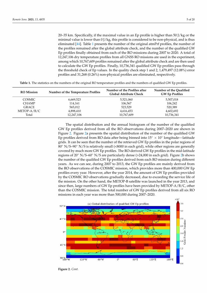
The spatial distribution and the annual histogram of the number of the qualifiedGW Ep profiles derived from all the RO observations during 2007–2020 are shown inFigure 2. Figure 2a presents the spatial distribution of the number of the qualified GWEp profiles derived from RO data after being binned into 15◦ × 10◦ longitude—latitudegrids. It can be seen that the number of the retrieved GW Ep profiles in the polar regions of80◦ N/S–90◦ N/S is relatively small (<8000 in each grid), while other regions are generallycovered by much more GW Ep profiles. The RO-derived GW Ep profiles in the mid-latituderegions of 20◦ N/S–60◦ N/S are particularly dense (>24,000 in each grid). Figure 2b showsthe number of the qualified GW Ep profiles derived from each RO mission during differentyears. As we can see, during 2007 to 2013, the GW Ep profiles are mainly derived fromthe RO observations of the COSMIC mission, which provides more than 400,000 GW Epprofiles every year. However, after the year 2014, the amount of GW Ep profiles providedby the COSMIC RO observations gradually decreased, due to exceeding the service life ofthe mission. On the other hand, the METOP-B satellite was launched in the year 2013, andsince then, large numbers of GW Ep profiles have been provided by METOP-A/B/C, otherthan the COSMIC mission. The total number of GW Ep profiles derived from all six ROmissions in each year was more than 500,000 during 2007–2020.

Remote Sens. 2021, 13, 4835 6 of 21

𝐸 𝑡 , = 𝜇 + 𝛼𝑡 , + 𝛽𝑠𝑜𝑙𝑎𝑟 𝑡 , + 𝛾𝑄𝐵𝑂 𝑡 , + 𝜅𝐸𝑁𝑆𝑂 𝑡 , + 𝑅𝑒𝑠𝑖𝑑𝑢𝑎𝑙 With I = 2007, 2008, …, 2020; j = 1,2, …, 12

(4)

In Equation (4), 𝐸 𝑡 , represents the monthly zonal-mean value of GW Ep at month (j) and year number (i) and the quantity μ represents a constant Ep value. The parameter α, which reflects the change in GW Ep with time, represents the linear trend of monthly zonal-mean Ep during 2007–2020. The parameters β, γ, and κ, which demonstrate the cor-relation between the time series of GW Ep and the time series of the three indices, repre-sent the responses of the monthly zonal-mean Ep to solar activity, to QBO, and to ENSO. The variance–covariance matrix and student t-test can be used to evaluate whether the estimated regression coefficients are significant at a given confidence level. Giving a sig-nificance level s, which means that the corresponding confidence level is set as 1 − 𝑠 × 100%, then the corresponding critical value of the t distribution can be ob-tained in the look-up table. If the absolute value of the ratio between the regression coef-ficient and its corresponding standard deviation is larger than the critical value of the t distribution at the given significance level s, then it is claimed that the regression coeffi-cient is significant at the confidence level 1 − 𝑠 × 100% [46]. In the present study, the confidence level for the t-test is set as 90%.

Figure 2. (a) Global distribution and (b) yearly number of qualified GW Ep profiles derived from the RO observations during 2007–2020.

Figure 2. Cont.

Remote Sens. 2021, 13, 4835 6 of 20

Remote Sens. 2021, 13, 4835 6 of 21

𝐸 𝑡 , = 𝜇 + 𝛼𝑡 , + 𝛽𝑠𝑜𝑙𝑎𝑟 𝑡 , + 𝛾𝑄𝐵𝑂 𝑡 , + 𝜅𝐸𝑁𝑆𝑂 𝑡 , + 𝑅𝑒𝑠𝑖𝑑𝑢𝑎𝑙 With I = 2007, 2008, …, 2020; j = 1,2, …, 12

(4)

In Equation (4), 𝐸 𝑡 , represents the monthly zonal-mean value of GW Ep at month (j) and year number (i) and the quantity μ represents a constant Ep value. The parameter α, which reflects the change in GW Ep with time, represents the linear trend of monthly zonal-mean Ep during 2007–2020. The parameters β, γ, and κ, which demonstrate the cor-relation between the time series of GW Ep and the time series of the three indices, repre-sent the responses of the monthly zonal-mean Ep to solar activity, to QBO, and to ENSO. The variance–covariance matrix and student t-test can be used to evaluate whether the estimated regression coefficients are significant at a given confidence level. Giving a sig-nificance level s, which means that the corresponding confidence level is set as 1 − 𝑠 × 100%, then the corresponding critical value of the t distribution can be ob-tained in the look-up table. If the absolute value of the ratio between the regression coef-ficient and its corresponding standard deviation is larger than the critical value of the t distribution at the given significance level s, then it is claimed that the regression coeffi-cient is significant at the confidence level 1 − 𝑠 × 100% [46]. In the present study, the confidence level for the t-test is set as 90%.

Figure 2. (a) Global distribution and (b) yearly number of qualified GW Ep profiles derived from the RO observations during 2007–2020.

Figure 2. (a) Global distribution and (b) yearly number of qualified GW Ep profiles derived from theRO observations during 2007–2020.

2.4. Method for Extracting Long-Term Changes of GW Activities

After obtaining all the qualified GW Ep profiles through the steps introduced in theprevious two subsections, these GW Ep profiles are averaged within a single month andbinned into 360◦ × 5◦ longitude[—-]latitude grids, with an overlap of 2.5◦ in latitude tocalculate the monthly and zonal-mean Ep for each height level at the altitude range of20–35 km. For each latitude band and each height level, the linear trend in monthly zonal-mean Ep time series and the responses of the monthly zonal-mean Ep to solar activity, QBOwind, and ENSO are derived by the method of multivariate linear regression (MLR) [9,45].The equation for the MLR method is expressed as:

Ep(ti,j

)= µ + αti,j + βsolar

(ti,j

)+ γQBO

(ti,j

)+ κENSO

(ti,j

)+ Residual

With I = 2007, 2008, . . . , 2020; j = 1, 2, . . . , 12(4)

In Equation (4), Ep(ti,j

)represents the monthly zonal-mean value of GW Ep at month (j)

and year number (i) and the quantity µ represents a constant Ep value. The parameter α,which reflects the change in GW Ep with time, represents the linear trend of monthlyzonal-mean Ep during 2007–2020. The parameters β, γ, and κ, which demonstrate thecorrelation between the time series of GW Ep and the time series of the three indices,represent the responses of the monthly zonal-mean Ep to solar activity, to QBO, andto ENSO. The variance–covariance matrix and student t-test can be used to evaluatewhether the estimated regression coefficients are significant at a given confidence level.Giving a significance level s, which means that the corresponding confidence level is set as(1− s)× 100%, then the corresponding critical value of the t distribution can be obtainedin the look-up table. If the absolute value of the ratio between the regression coefficient andits corresponding standard deviation is larger than the critical value of the t distribution atthe given significance level s, then it is claimed that the regression coefficient is significantat the confidence level (1− s)× 100% [46]. In the present study, the confidence level forthe t-test is set as 90%.

Figure 3 presents the reference time series of solar activity, QBO, and ENSO during2007 to 2020. The monthly mean values of radio emissions from the sun at a wavelength of10.7 centimetres (the 10.7 cm solar flux, F10.7) are used to represent the solar activity [47],and F10.7 is given in solar flux units (sfu, 1 s f u = 10−22 W m−2 Hz−1) in Figure 3a. It shouldbe noted that during the studied time period, the solar activity was the most intensiveduring 2014 to 2015, and declined after the year 2015. In Figure 3b, the temporal variationof 30 hPa zonal-mean zonal wind over the equator is used as the reference time series forQBO [48]. In Figure 3c, the temporal variations of the ENSO phases are shown by the

Remote Sens. 2021, 13, 4835 7 of 20

values of the bi-monthly Multivariate El Niño/Southern Oscillation (ENSO) index (MEI),which is the time series of the leading combined Empirical Orthogonal Function (EOF) offive different variables (sea level pressure (SLP), sea surface temperature (SST), zonal andmeridional components of the surface wind, and outgoing longwave radiation (OLR)) overthe tropical Pacific basin (30◦ S–30◦ N and 100◦ E–70◦ W) [49–51].

Remote Sens. 2021, 13, 4835 7 of 21

Figure 3 presents the reference time series of solar activity, QBO, and ENSO during 2007 to 2020. The monthly mean values of radio emissions from the sun at a wavelength of 10.7 centimetres (the 10.7 cm solar flux, F10.7) are used to represent the solar activity [47], and F10.7 is given in solar flux units (sfu, 1 𝑠𝑓𝑢 = 10 𝑊 𝑚 𝐻𝑧 ) in Figure 3a. It should be noted that during the studied time period, the solar activity was the most intensive during 2014 to 2015, and declined after the year 2015. In Figure 3b, the temporal variation of 30 hPa zonal-mean zonal wind over the equator is used as the reference time series for QBO [48]. In Figure 3c, the temporal variations of the ENSO phases are shown by the values of the bi-monthly Multivariate El Niño/Southern Oscillation (ENSO) index (MEI), which is the time series of the leading combined Empirical Orthogonal Function (EOF) of five different variables (sea level pressure (SLP), sea surface temperature (SST), zonal and meridional components of the surface wind, and outgoing longwave radiation (OLR)) over the tropical Pacific basin (30° S–30° N and 100° E–70° W) [49–51].

Figure 3. Variations in the monthly values for (a) Solar radio flux at 10.7 cm (F10.7) index, (b) 30 hPa zonal winds over the equator, used as QBO index, and (c) Multivariate ENSO Index (MEI)

Figure 3. Variations in the monthly values for (a) Solar radio flux at 10.7 cm (F10.7) index, (b) 30 hPazonal winds over the equator, used as QBO index, and (c) Multivariate ENSO Index (MEI).

3. Results and Analyses3.1. Comparisons of the Global Distributions of GW Ep Derived from Different RO Datasets

In order to verify the validity of our procedure for deriving the GW Ep values, and toinvestigate the consistency of the GW Ep values extracted from different RO missions, theseasonal variations of the global distributions of GW Ep at 20–35 km during the periodfrom February 2013 to January 2016 are derived from different datasets and are compared,as shown in Figure 4. Here, the four seasons are categorized as MAM (March to May),JJA (June to August), SON (September to November), and DJF (December to February).

Remote Sens. 2021, 13, 4835 8 of 20

The statistics in the subgraphs of the first column are calculated from the profiles of all themissions available for the experiment’s time period (including COSMIC, METOP-A/B, andGRACE), and the subgraphs of the second and third columns are derived from the profilesof COSMIC and METOP-A/B, respectively. The reason why the datasets from February2013 to January 2016 are selected in this validation experiment is that the Metop-B dataseries started in February 2013, and COSMIC still provided a sufficient number of profilesevery day over the next three years for the statistics of global GW Ep heat map, as shown inFigure 2. The GW Ep seasonal variations derived independently from the GRACE missionare not listed here due to the limited number of temperature profiles provided by GRACE,which is a disadvantage for constructing the single-day geographic grid data to derive thebackground temperature when applying the horizontal detrending method.

Remote Sens. 2021, 13, 4835 8 of 21

3. Results and Analyses 3.1. Comparisons of the Global Distributions of GW Ep Derived from Different RO Datasets

In order to verify the validity of our procedure for deriving the GW Ep values, and to investigate the consistency of the GW Ep values extracted from different RO missions, the seasonal variations of the global distributions of GW Ep at 20–35 km during the period from February 2013 to January 2016 are derived from different datasets and are compared, as shown in Figure 4. Here, the four seasons are categorized as MAM (March to May), JJA (June to August), SON (September to November), and DJF (December to February). The statistics in the subgraphs of the first column are calculated from the profiles of all the missions available for the experiment’s time period (including COSMIC, METOP-A/B, and GRACE), and the subgraphs of the second and third columns are derived from the profiles of COSMIC and METOP-A/B, respectively. The reason why the datasets from February 2013 to January 2016 are selected in this validation experiment is that the Metop-B data series started in February 2013, and COSMIC still provided a sufficient number of profiles every day over the next three years for the statistics of global GW Ep heat map, as shown in Figure 2. The GW Ep seasonal variations derived independently from the GRACE mission are not listed here due to the limited number of temperature profiles provided by GRACE, which is a disadvantage for constructing the single-day geographic grid data to derive the background temperature when applying the horizontal detrending method.

Figure 4. Global distribution of 3 years (from February 2013 to January 2016) GW Ep averaged seasonal means (row 1: MAM, row 2: JJA, row 3: SON, and row 4: DJF) over 20–35 km derived from different datasets.

Figure 4 suggests that the magnitudes and the distribution patterns of the GW Ep values derived from the three different datasets, i.e., data of all missions, COSMIC, and METOP-A/B, are of high consistency and the seasonal distribution patterns of the GW values derived from all the three datasets agree well with previous studies [2,52–57]. Spe-cifically, the GW Ep values derived from all the three datasets mainly vary between 0.2 to 2 J/kg, and with each of the three datasets, the GW Ep derived is generally higher over the tropical latitude bands than over other regions during all four seasons, and is almost equa-torial symmetric in MAM and SON in the tropics. Over the tropics, the distribution of GW

Figure 4. Global distribution of 3 years (from February 2013 to January 2016) GW Ep averaged seasonal means (row 1: MAM,row 2: JJA, row 3: SON, and row 4: DJF) over 20–35 km derived from different datasets.

Figure 4 suggests that the magnitudes and the distribution patterns of the GW Epvalues derived from the three different datasets, i.e., data of all missions, COSMIC, andMETOP-A/B, are of high consistency and the seasonal distribution patterns of the GWvalues derived from all the three datasets agree well with previous studies [2,52–57].Specifically, the GW Ep values derived from all the three datasets mainly vary between0.2 to 2 J/kg, and with each of the three datasets, the GW Ep derived is generally higherover the tropical latitude bands than over other regions during all four seasons, andis almost equatorial symmetric in MAM and SON in the tropics. Over the tropics, thedistribution of GW Ep is consistent with that of deep convection [17]. In addition, due tothe influences of orography and zonal wind, during JJA (the second row)/DJF (the fourthrow) in the extratropical regions, the GW Ep values are generally higher over the winterhemisphere than the summer hemisphere [2,9,53,54,57]. Furthermore, for all three datasets,in JJA (the second row) and SON (the third row) we can see a long leeward region of highEp values exists, which stretches eastward from 70◦ W to around 180◦ E, covering theSouthern Andes, Drake Passage, and the Antarctic Peninsula. The Ep values over thisregion reach the maximum in the southern hemisphere (SH) winter and weaken slightlyin the SH spring. The eastward propagation of the orographic mountain waves, which is

Remote Sens. 2021, 13, 4835 9 of 20

generated by the north–south distribution of the Andes, should contribute to the formationof this specific GW Ep distribution pattern [2,58,59].

The results shown in Figure 4 verify the validity of the procedure for deriving the GWEp and the feasibility of combining the data from different RO missions in the present study.Moreover, a mixture of datasets from different RO missions was widely used for studyingthe GW activities in previous studies [21,25,37]. Leroy et al. [60] found that the temperaturetrends during 2003 to 2014 produced by the combined RO datasets from CHAMP andCOSMIC missions and by other satellite observations and model data agree to within0.02K/year in the lower stratosphere. Therefore, the following analyses of the present workwill be carried out using the data from multi-GNSS RO missions simultaneously, and willnot differentiate among the data from different RO missions.

3.2. Time-Latitude Distributions of the Monthly and Zonal-Mean GW Ep

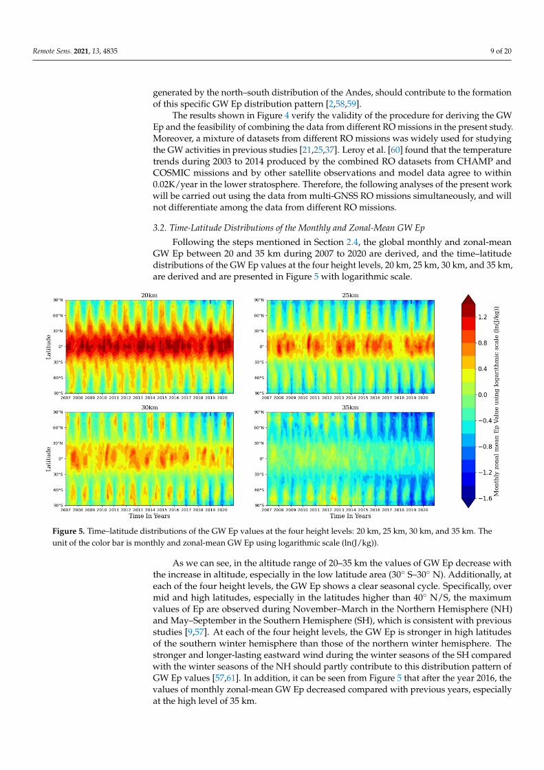
Following the steps mentioned in Section 2.4, the global monthly and zonal-meanGW Ep between 20 and 35 km during 2007 to 2020 are derived, and the time–latitudedistributions of the GW Ep values at the four height levels, 20 km, 25 km, 30 km, and 35 km,are derived and are presented in Figure 5 with logarithmic scale.

Remote Sens. 2021, 13, 4835 9 of 21

Ep is consistent with that of deep convection [17]. In addition, due to the influences of orography and zonal wind, during JJA (the second row)/DJF (the fourth row) in the extra-tropical regions, the GW Ep values are generally higher over the winter hemisphere than the summer hemisphere [2,9,53,54,57]. Furthermore, for all three datasets, in JJA (the sec-ond row) and SON (the third row) we can see a long leeward region of high Ep values exists, which stretches eastward from 70° W to around 180° E, covering the Southern An-des, Drake Passage, and the Antarctic Peninsula. The Ep values over this region reach the maximum in the southern hemisphere (SH) winter and weaken slightly in the SH spring. The eastward propagation of the orographic mountain waves, which is generated by the north–south distribution of the Andes, should contribute to the formation of this specific GW Ep distribution pattern [2,58,59].

The results shown in Figure 4 verify the validity of the procedure for deriving the GW Ep and the feasibility of combining the data from different RO missions in the present study. Moreover, a mixture of datasets from different RO missions was widely used for studying the GW activities in previous studies [21,25,37]. Leroy et al. [60] found that the temperature trends during 2003 to 2014 produced by the combined RO datasets from CHAMP and COSMIC missions and by other satellite observations and model data agree to within 0.02K/year in the lower stratosphere. Therefore, the following analyses of the present work will be carried out using the data from multi-GNSS RO missions simultane-ously, and will not differentiate among the data from different RO missions.

3.2. Time-Latitude Distributions of the Monthly and Zonal-Mean GW Ep Following the steps mentioned in Section 2.4, the global monthly and zonal-mean

GW Ep between 20 and 35 km during 2007 to 2020 are derived, and the time–latitude distributions of the GW Ep values at the four height levels, 20 km, 25 km, 30 km, and 35 km, are derived and are presented in Figure 5 with logarithmic scale.

Figure 5. Time–latitude distributions of the GW Ep values at the four height levels: 20 km, 25 km, 30 km, and 35 km. The unit of the color bar is monthly and zonal-mean GW Ep using logarithmic scale (ln(J/kg)).

As we can see, in the altitude range of 20–35 km the values of GW Ep decrease with the increase in altitude, especially in the low latitude area (30° S–30° N). Additionally, at each of the four height levels, the GW Ep shows a clear seasonal cycle. Specifically, over

Figure 5. Time–latitude distributions of the GW Ep values at the four height levels: 20 km, 25 km, 30 km, and 35 km. Theunit of the color bar is monthly and zonal-mean GW Ep using logarithmic scale (ln(J/kg)).

As we can see, in the altitude range of 20–35 km the values of GW Ep decrease withthe increase in altitude, especially in the low latitude area (30◦ S–30◦ N). Additionally, ateach of the four height levels, the GW Ep shows a clear seasonal cycle. Specifically, overmid and high latitudes, especially in the latitudes higher than 40◦ N/S, the maximumvalues of Ep are observed during November–March in the Northern Hemisphere (NH)and May–September in the Southern Hemisphere (SH), which is consistent with previousstudies [9,57]. At each of the four height levels, the GW Ep is stronger in high latitudesof the southern winter hemisphere than those of the northern winter hemisphere. Thestronger and longer-lasting eastward wind during the winter seasons of the SH comparedwith the winter seasons of the NH should partly contribute to this distribution pattern ofGW Ep values [57,61]. In addition, it can be seen from Figure 5 that after the year 2016, thevalues of monthly zonal-mean GW Ep decreased compared with previous years, especiallyat the high level of 35 km.

Remote Sens. 2021, 13, 4835 10 of 20

3.3. Time–Height Distributions of the Monthly and Zonal-Mean GW Ep

To investigate the temporal variations of the global GW activities, the time–heightdistributions of the monthly and global/zonal-mean GW Ep from 2007 to 2020 at 20–35 kmheight are drawn and are presented using logarithmic scale in Figures 6 and 7, respectively.In these heat maps, the horizontal axis is the time series with the step length of one month,and the vertical axis is the altitude.

Remote Sens. 2021, 13, 4835 10 of 21

mid and high latitudes, especially in the latitudes higher than 40° N/S, the maximum val-ues of Ep are observed during November–March in the Northern Hemisphere (NH) and May–September in the Southern Hemisphere (SH), which is consistent with previous studies [9,57]. At each of the four height levels, the GW Ep is stronger in high latitudes of the southern winter hemisphere than those of the northern winter hemisphere. The stronger and longer-lasting eastward wind during the winter seasons of the SH compared with the winter seasons of the NH should partly contribute to this distribution pattern of GW Ep values [57,61]. In addition, it can be seen from Figure 5 that after the year 2016, the values of monthly zonal-mean GW Ep decreased compared with previous years, espe-cially at the high level of 35 km.

3.3. Time–Height Distributions of the Monthly and Zonal-Mean GW Ep To investigate the temporal variations of the global GW activities, the time–height

distributions of the monthly and global/zonal-mean GW Ep from 2007 to 2020 at 20–35 km height are drawn and are presented using logarithmic scale in Figures 6 and 7, respec-tively. In these heat maps, the horizontal axis is the time series with the step length of one month, and the vertical axis is the altitude.

As we can see in Figure 6, in general, the magnitudes of the monthly global-mean GW Ep in 20–30 km are greater than those in 30–35 km. The maximum values of the global mean GW Ep appear in the summer solstice and the winter solstice every year, which is the most distinct in 25–30 km. This is consistent with Liu et al. [9], although the altitude range of the GW activity they were concerned about was 30–100 km. Moreover, Figure 6 presents that the magnitudes of GW Ep values before 2016 were significantly larger than those after 2016, which may be related to the sharp weakening in the solar activity during 2015–2017 (shown in Figure 3c), and will be discussed later.

Figure 6. Time–altitude distribution of the monthly and global-mean GW Ep at 20–35 km during 2007 to 2020. Logarithmic scale is used.

Figure 6. Time–altitude distribution of the monthly and global-mean GW Ep at 20–35 km during2007 to 2020. Logarithmic scale is used.

As we can see in Figure 6, in general, the magnitudes of the monthly global-mean GWEp in 20–30 km are greater than those in 30–35 km. The maximum values of the globalmean GW Ep appear in the summer solstice and the winter solstice every year, which isthe most distinct in 25–30 km. This is consistent with Liu et al. [9], although the altituderange of the GW activity they were concerned about was 30–100 km. Moreover, Figure 6presents that the magnitudes of GW Ep values before 2016 were significantly larger thanthose after 2016, which may be related to the sharp weakening in the solar activity during2015–2017 (shown in Figure 3c), and will be discussed later.

Figure 7 presents the time–height distributions of the monthly zonal-mean GW Epat different latitudes of the NH (left column) and the SH (right column). The QBO windtime series presented in Figure 3b are overlapped on the Ep distribution at the latitudebands of 10◦ N/S and the equator. It can be seen that at the latitudes higher than 30◦ N/Sthe monthly zonal-mean GW Ep exhibits distinct annual variations, with GW Ep peaksappearing in the winter months of the corresponding hemisphere, which is consistent withthe findings of Wilson et al. [62], by using lidar observations in southern France (44◦ N),and those of Liu et al. [9], by using 14 years of SABER data. The monthly zonal-mean GWEp exhibits semiannual variations at 20◦ N/S and 30◦ N/S, with GW Ep peaks appearingin both the winter and summer months, just similar to the global-mean GW Ep shownin Figure 6.

The QBO signals can be identified in the time variations of GW Ep at 10◦ N/S andover the equator. The monthly zonal-mean GW Ep at 20–30 km over the tropics peakswhen the QBO eastward wind phase reaches its peak too, which is consistent with someprevious studies [57,61,63,64]. What needs to be mentioned is that during January 2007to September 2013, the variation of Ep over the equator shown in Figure 7 is similar toFigure 6 of Xu et al. [57]. By comparing the temporal variations in the GW Ep with those ofthe zonal wind field, Xu et al. [57] pointed out that, due to the selective filtering effect ofstratospheric wind systems on GWs, maximum GW Ep values generally appear where the

Remote Sens. 2021, 13, 4835 11 of 20

direction of the wind changes from westward to eastward [63]. The detailed relationshipbetween Ep and zonal wind field over the tropics will be further discussed in Section 4.

Remote Sens. 2021, 13, 4835 11 of 21

Figure 7. Time–height distributions of the monthly and zonal-mean GW Ep at 20–35 km over different latitude bands during 2007 to 2020. The unit of color bar is monthly and zonal-mean GW Ep using logarithmic scale (ln(J/kg)). The black dotted lines overlapped on the Ep distributions at 10° N/S and the equator present the QBO wind time series (label at the right y-axis).

Figure 7 presents the time–height distributions of the monthly zonal-mean GW Ep at different latitudes of the NH (left column) and the SH (right column). The QBO wind time series presented in Figure 3b are overlapped on the Ep distribution at the latitude bands of 10° N/S and the equator. It can be seen that at the latitudes higher than 30° N/S the monthly zonal-mean GW Ep exhibits distinct annual variations, with GW Ep peaks ap-pearing in the winter months of the corresponding hemisphere, which is consistent with the findings of Wilson et al. [62], by using lidar observations in southern France (44° N), and those of Liu et al. [9], by using 14 years of SABER data. The monthly zonal-mean GW Ep exhibits semiannual variations at 20° N/S and 30° N/S, with GW Ep peaks appearing in both the winter and summer months, just similar to the global-mean GW Ep shown in Figure 6.

Figure 7. Time–height distributions of the monthly and zonal-mean GW Ep at 20–35 km over different latitude bandsduring 2007 to 2020. The unit of color bar is monthly and zonal-mean GW Ep using logarithmic scale (ln(J/kg)). The blackdotted lines overlapped on the Ep distributions at 10◦ N/S and the equator present the QBO wind time series (label at theright y-axis).

At 10◦ N/S and 20◦ N/S, the GW Ep has larger values in the summer months than inthe winter months, which is consistent with the results of Zhang et al. [64] and Liu et al. [9].Moreover, at 20◦ N/S, 30◦ N/S, and 40◦ N/S, the zonal-mean GW Ep values at the zonalbands of the NH are larger than those of the corresponding zonal bands of the SH. Usingeight-year SABER/TIMED data, Zhang et al. [64] also found that the GW Ep at 10◦ N–30◦ Nwas larger than at 10◦ S–30◦ S in 21–26 km height. However, in the latitudes at and higherthan 60◦ N/S, GW activities over the zonal bands of the SH are stronger than those overthe corresponding zonal bands of the NH, which has already been described in Section 3.2.In the high latitudes of 70◦ N/S, 80◦ N/S, and 90◦ N/S, GW Ep decreases significantly

Remote Sens. 2021, 13, 4835 12 of 20

after 2016, which is shown by the distinct attenuation of the global GW Ep values after2016 shown in Figure 6.

Figures 6 and 7 present that the temporal variations in the GW Ep change with heightsand latitudes. For the altitude range of 20–35 km, in general, the annual variations of GWEp are prominent at the latitudes higher than 40◦ N/S, getting peak values in the wintermonths, while the semiannual variations of GW Ep are distinct at 20–30◦ N/S, gettingpeaks both in the winter and the summer months. QBO signals are distinct in the timevariations of GW Ep between 10◦ S–10◦ N. The above analyses also illustrate that theclimatology of GW activities derived above is reliable, based on which the global trends ofGWs and the responses of GWs to solar activity, QBO, and ENSO can be further analyzed.

3.4. Global Trends in GWsDuring 2007 to 2020

Following the procedure introduced in Section 2.4, by analyzing the time series of themonthly zonal-mean GW Ep values from 2007 to 2020 with the MLR method, the lineartrend (α in Equation (4)) in the GW Ep values for each 2.5◦× 0.1 km (latitude× height)grid cell is obtained for each month. For a certain month, if the value of the coefficientα of a grid cell is greater than 0, then the GW Ep of the corresponding cell has a positivetrend. Otherwise, the GW Ep of the corresponding cell has a negative trend. The finallatitude–height distributions of the GW linear trends for each month are presented inFigure 8. In each subfigure of Figure 8, the regions covering the cells with the trendspassing the student t-test with a confidence level of 90% are shown as protuberance.

It can be seen from Figure 8 that in the middle and high latitudes, GW Ep valuesgenerally show significant negative trends (<−0.02 J/kg per year) in almost all months,especially in the altitude range of 25–35 km, which is consistent with the phenomena,shown in Figures 5 and 7, that the GW Ep decreases significantly in middle and highlatitudes after 2016. Over the tropics, positive trends appear from March to August, whilethese trends are mostly not significant. Besides, relatively large positive trends appearin the latitudes of 25◦ N–45◦ N in November and December, and these trends are notsignificant either, which is consistent with Liu et al. [9]. The low confidence level of thetrends over these latitudes might be partly due to the strong planetary wave activity andthe impacts of SSWs in the northern high latitudes. It should be noted that due to the strongextension and subsequent division of the polar vortex, almost the whole NH to the north ofabout 30◦ N will be influenced by the enhanced GW activities induced by SSWs [65]. Thepositive trends occurring in 40◦ N–70◦ N during March and April are also consistent withthe findings of Liu et al. [9]. In addition, the significant negative trends over 5◦ N–30◦ N inJanuary and the negative trends over 25◦ N–40◦ N in February in the range of 30–35 km,which were presented in Figure 5 of Liu et al. [9], are also shown here in Figure 8.

Considering that a half-year shift exists in the atmospheric conditions between thetwo hemispheres, some distinct characteristics of GW trends can be determined, whichare almost symmetrical between the SH and the NH. For example, in the altitude range of30–35 km, both the high latitudes of the SH during June, July, and August and the highlatitudes of the NH during December, January, and February have significant negativetrends, which are generally lower than –0.03 J/kg per year. In the NH from June toSeptember and in the SH from December to March, the GW Ep values at 25–35 km overthe mid-high latitudes generally show significantly negative trends, which are of themagnitudes of –0.01 to –0.03 J/kg per year. Whether for the more active winter monthsor for the relatively less active summer months of the gravity waves, the GW Ep trendsgenerally show a consistent symmetry over the two hemispheres. Furthermore, the GWactivities in 20–35 km are generally declining from 2007 to 2020.

The latitude–height distributions of the deseasonalized trends in the monthly zonal-mean GW Ep values at 20–35 km during 2007 to 2020 and the responses of GW Ep to solarflux, QBO, and ENSO are presented in Figure 9. Similar to Figure 8, in each subfigure ofFigure 9, the regions where the results are statistically significant at the confidence level of90% are shown as protuberance.

Remote Sens. 2021, 13, 4835 13 of 20Remote Sens. 2021, 13, 4835 13 of 21

Figure 8. Latitude–height distributions of the linear trends in the monthly zonal-mean GW Ep at 20–35 km for each month during 2007 to 2020. The regions where the trends are statistically significant at the confidence level of 90% are shown as protuberance.

It can be seen from Figure 8 that in the middle and high latitudes, GW Ep values generally show significant negative trends (<−0.02 J/kg per year) in almost all months, especially in the altitude range of 25–35 km, which is consistent with the phenomena, shown in Figures 5 and Figure 7, that the GW Ep decreases significantly in middle and high latitudes after 2016. Over the tropics, positive trends appear from March to August, while these trends are mostly not significant. Besides, relatively large positive trends ap-pear in the latitudes of 25° N–45° N in November and December, and these trends are not significant either, which is consistent with Liu et al. [9]. The low confidence level of the trends over these latitudes might be partly due to the strong planetary wave activity and the impacts of SSWs in the northern high latitudes. It should be noted that due to the

Figure 8. Latitude–height distributions of the linear trends in the monthly zonal-mean GW Ep at 20–35 km for each monthduring 2007 to 2020. The regions where the trends are statistically significant at the confidence level of 90% are shownas protuberance.

The deseasonalized trends shown in Figure 9a are derived by analyzing the deseason-alized monthly zonal-mean GW Ep time series using the MLR method [46,66]. As we cansee from Figure 9a, except for a few locations, GW Ep values generally show significantnegative trends at most latitudes and altitudes, especially in the middle and high latitudesof the two hemispheres. In addition, in the low latitudes of 30◦ S–30◦ N, significant neg-ative trends exist above 30 km. The values of the negative trends become smaller in theregions closer to the poles, which is consistent with what is shown in Figure 8. In thefollowing subsection, we will further analyze the responses of GW to solar activity, QBOwind, and ENSO.

Remote Sens. 2021, 13, 4835 14 of 20

Remote Sens. 2021, 13, 4835 14 of 21

strong extension and subsequent division of the polar vortex, almost the whole NH to the north of about 30° N will be influenced by the enhanced GW activities induced by SSWs [65]. The positive trends occurring in 40° N–70° N during March and April are also con-sistent with the findings of Liu et al. [9]. In addition, the significant negative trends over 5° N–30° N in January and the negative trends over 25° N–40° N in February in the range of 30–35 km, which were presented in Figure 5 of Liu et al. [9], are also shown here in Figure 8.

Considering that a half-year shift exists in the atmospheric conditions between the two hemispheres, some distinct characteristics of GW trends can be determined, which are almost symmetrical between the SH and the NH. For example, in the altitude range of 30–35 km, both the high latitudes of the SH during June, July, and August and the high latitudes of the NH during December, January, and February have significant negative trends, which are generally lower than –0.03 J/kg per year. In the NH from June to Sep-tember and in the SH from December to March, the GW Ep values at 25–35 km over the mid-high latitudes generally show significantly negative trends, which are of the magni-tudes of –0.01 to –0.03 J/kg per year. Whether for the more active winter months or for the relatively less active summer months of the gravity waves, the GW Ep trends generally show a consistent symmetry over the two hemispheres. Furthermore, the GW activities in 20–35 km are generally declining from 2007 to 2020.

The latitude–height distributions of the deseasonalized trends in the monthly zonal-mean GW Ep values at 20–35 km during 2007 to 2020 and the responses of GW Ep to solar flux, QBO, and ENSO are presented in Figure 9. Similar to Figure 8, in each subfigure of Figure 9, the regions where the results are statistically significant at the confidence level of 90% are shown as protuberance.

Figure 9. Latitude–height distributions of the deseasonalized trends of GW Ep at 20–35 km during the 14 years from 2007 to 2020 (a) and the responses of GW Ep to solar activity (b), to QBO (c), and to ENSO (d). The regions where the results are statistically significant at the confidence level of 90% are shown as protuberance.

Figure 9. Latitude–height distributions of the deseasonalized trends of GW Ep at 20–35 km during the 14 years from 2007 to2020 (a) and the responses of GW Ep to solar activity (b), to QBO (c), and to ENSO (d). The regions where the results arestatistically significant at the confidence level of 90% are shown as protuberance.

3.5. Responses of GW Activities to Solar Activity, QBO Wind, and ENSO over the Globe

The response of the variation in GW Ep at 20–35 km to that of the solar activityrepresented by the F10.7 indexes is shown in Figure 9b. Contrary to the GW Ep trendsduring the 14 years, which are mainly negative, GW Ep in the mid and high latitudes of thetwo hemispheres generally show significant positive responses to the solar activity withinthe altitude range of 20–35 km. In the low latitudes of 30◦ S–30◦ N, significant positiveresponses of GW Ep to solar activity also exist at 30–35 km. Additionally, in terms of themagnitudes of the responses, the positive responses of the GW Ep to the solar activitybecome stronger in the region closer to the poles. Our results are consistent with Jacobiet al. [30], who got positive correlations of GWs with the solar activities by using the radiodrift observations at 52◦ N.

Figure 9c presents the responses of GW activities to QBO at 20–35 km over the globe.It can be seen that at the latitude range of 20–35 km, the responses of GW Ep values to theQBO eastward wind phases are mainly negative at most latitudes. At the altitude rangeof 30–35 km, significant negative responses of GW Ep to the QBO eastward wind phasesoccur at the latitudes of 30◦ S–25◦ N, and the negative responses at 0◦–25◦ N are smallerthan those at 0◦–30◦ S, which is basically consistent with Liu et al. [9]. At the altitude rangeof 20–30 km, the significant negative responses extend to the mid and high latitudes in theSH, while at the low latitudes of 15◦ S–15◦ N, the responses of GW Ep values to the QBOeastward wind phases are significantly positive.

The response of the GW Ep at 20–35 km to ENSO, which is represented by the MEIindex, is shown in Figure 9d. It can be seen that over low latitudes of 15◦ S–15◦ N, GW Epvalues are of positive responses to ENSO in 20–35 km, which is consistent with Liu et al. [9].In addition, the response of the GW Ep to ENSO is significantly negative in 30–35 km over

Remote Sens. 2021, 13, 4835 15 of 20

the latitudes of 15◦ N–30◦ N, which is also consistent with the findings of Liu et al. [9].The significant negative response near 50◦ N in our results should be partly due to theweakening in GW activity after 2016.

4. Discussion

The comparison between Figure 9a,b demonstrates that the height–latitude distribu-tion pattern of the trends in the GW Ep and that of the response of GW Ep to the solaractivity show distinct correlations, i.e., the overall negative trends in GWs correspond tothe overall positive responses of the GW Ep to the solar activity. Considering that thesolar activity weakened significantly after the year 2015, as shown in Figure 3a, it can bededuced that the sharp decline in the solar activity after the year 2015, together with thepositive response of the GW Ep to the solar activity, might have contributed significantlyto the overall attenuation of the gravity wave activity during the 14 years from 2007 to2020. What needs to be mentioned is that Ern et al. [67] and Liu et al. [9] both observednegative responses in GW Ep to F10.7 indexes at the altitude range of 30–35 km abovelow and middle latitudes by using the SABER temperature data, which are different fromour results, while the time periods researched by Ern et al. [67] and by Liu et al. [9] are2002–2011 and 2002–2015, respectively, and the F10.7 data after the year 2015 were not usedin their studies. Moreover, Gavrilov et al. [29] pointed out that differences in GW sources, inconditions of wave propagations, and in measurement methods might all have impacts onthe analyses concerning the responses of GW to solar activities. We suggest that a possiblereason why our results are inconsistent with those of Ern et al. [67] and Liu et al. [9] is thatthe solar activity weakened sharply during 2015 to 2017 (as shown in Figure 3a), whichpartially contributed to the general weakening of GW activities after 2016.

The specific dynamic mechanisms which directly lead to the negative trend in globalGW Ep are still unclear. Considering that the significant negative trend is particularlynotable in the polar regions, these background dynamic mechanisms might be related tothe enhancement/weakening of polar circulations or the expansion and break in polarvortexes. On the other hand, as shown in Figures 5 and 7, the GW Ep at high latitudes hasbeen declining extremely rapidly since 2016, accompanied by a decrease in solar activity.Taking into consideration the strong positive correlation between GW Ep and solar activityrevealed in the present study, it is speculated that the dynamic mechanisms which lead tothe negative trend in global GW Ep should also be strongly affected by the solar activity.More work will be done on this issue in our future work.

The comparisons of the QBO time series, the time–height distributions of the monthlyand zonal-mean GW Ep over the equator, and the latitudes of 10◦ N and 10◦ S, whichare presented in Figure 7, reveal that during the time periods when peak values appearin the QBO eastward wind phase time series, the monthly zonal-mean GW Ep values in20–30 km also reach peak values over the equator and over 10◦ N/S, where the value ofln(Ep) is larger than 0.6 ln(J/kg) and is shown with red color in Figure 7. Figure 10 furtherpresents the time–height cross section of Ep and zonal wind field at 20–35 km over theequator during 2007 and 2020. As mentioned in Section 3.3, due to the selective filteringeffect of stratospheric wind systems on GWs, the GW Ep value above the 0 m s−1 windlevel line is usually significantly attenuated compared with the value below it. We also cansee that the Ep value at 20–30 km is generally large (>1.8 J/kg) in the eastward wind timeperiod and small (<1.8 J/kg) in the westward wind time period. This is a manifestation ofthe significant positive correlation between the GW Ep in the altitude range of 20–30 kmand the QBO over the tropics, and is consistent with the significant positive responses ofGW Ep below 30 km over 15◦ S–15◦ N, as shown in Figure 9c. This indicates that GW Epactivity in 20–30 km over the tropics is mainly affected by the variation in the zonal windfield. In addition, Figure 7 also shows that during the two peak periods of QBO east windphases from March 2015 to June 2017 and from June 2018 to December 2020, the valuesof GW Ep at 30–35 km over the equator and over 10◦ N/S are at a lower level compared

Remote Sens. 2021, 13, 4835 16 of 20

with other peak periods, which might lead to the negative response of GW activity to QBOwithin 30–35 km height over the tropics.

Remote Sens. 2021, 13, 4835 17 of 21

Figure 10. Time–height distributions of GW Ep and zonal wind at 20–35 km over the equator during the 14 years from 2007 to 2020. The eastward and westward winds, with the unit of m s−1, are represented by the black solid lines and the black dashed lines, respectively. The 0 m s−1 wind level is represented by the red solid lines. Zonal wind data from ERA5 are used.

5. Conclusions By using multi-mission GNSS RO data from 2007 to 2020, the present study studies

the variations in the gravity waves at the lower stratosphere of 20–35 km over the globe. The dry temperature profiles (atmPrf files) from six different RO missions provided by CDAAC, after a two-step quality check, are used to retrieve the GW Ep profiles, based on which the temporal variations of the GW activities are derived and the linear trends of the GWs and the responses of GW activities to solar activity, QBO, and ENSO are further analyzed using the MLR method.

To verify the validity of our procedure for extracting the GW Ep profiles with the horizontal detrending method and to understand the consistency of the GWs derived from different RO missions, firstly, the global distributions of the seasonal means of GW Ep values at the altitude range of 20–35 km, derived respectively from three RO datasets, i.e., data of all the missions, COSMIC data only, and METOP-A/B data only, during the period from February 2013 to January 2016, are compared. It is found that the distribution patterns of the seasonal means of GW Ep values derived from the three datasets are all consistent with previous works, and there are no significant differences among the mag-nitudes of the Ep values derived from different RO datasets, which confirms the feasibility of the method for extracting the GW Ep and suggests that it is statistically reasonable to use the data from multi-GNSS RO missions to study the trend in the GW activities.

By analyzing the time–latitude and the time–height distributions of the GW Ep val-ues during the 14 years from 2007 to 2020, we found that GW activities in 20–35 km show distinct annual variations in mid and high latitude regions with latitudes higher than 40° in both of the two hemispheres, reaching the peaks during winter months of the corre-sponding hemisphere. The stronger and longer-lasting eastward wind during the winter seasons of the SH compared with the winter seasons of the NH should partly contribute to the GW Ep distribution pattern that GW activities are stronger in winter months at high latitudes of the SH than that of the NH. At lower latitudes of 20° N/S and 30° N/S, GW activities at the altitudes of 20–35 km exhibit semiannual variations, with Ep values peak-ing in both winter and summer months. At the equator and the latitudes of 10° N/S, QBO

Figure 10. Time–height distributions of GW Ep and zonal wind at 20–35 km over the equator during the 14 years from2007 to 2020. The eastward and westward winds, with the unit of m s−1, are represented by the black solid lines and theblack dashed lines, respectively. The 0 m s−1 wind level is represented by the red solid lines. Zonal wind data from ERA5are used.

A possible mechanism for explaining the positive response of GW activities to ENSOover the low latitudes is that convective GW sources in the tropical region may be strength-ened by the El Niño events, which change the atmospheric wind and temperature struc-tures [68,69]. What needs to be mentioned is that, at the altitude range of 30–35 km overthe latitudes near 50◦ N, GW Ep has a significant negative response to ENSO in our results,while in the work of Liu et al. [9], significant positive responses are found at the sameregion. The difference between ours and Liu et al.’s results should be mainly attributed tothe different time periods of the two studies. The time period focused on by Liu et al. [9]was 2002–2015, while our work focused on the period from 2007 to 2020.

5. Conclusions

By using multi-mission GNSS RO data from 2007 to 2020, the present study studiesthe variations in the gravity waves at the lower stratosphere of 20–35 km over the globe.The dry temperature profiles (atmPrf files) from six different RO missions provided byCDAAC, after a two-step quality check, are used to retrieve the GW Ep profiles, based onwhich the temporal variations of the GW activities are derived and the linear trends ofthe GWs and the responses of GW activities to solar activity, QBO, and ENSO are furtheranalyzed using the MLR method.

To verify the validity of our procedure for extracting the GW Ep profiles with thehorizontal detrending method and to understand the consistency of the GWs derived fromdifferent RO missions, firstly, the global distributions of the seasonal means of GW Ep val-ues at the altitude range of 20–35 km, derived respectively from three RO datasets, i.e., dataof all the missions, COSMIC data only, and METOP-A/B data only, during the period fromFebruary 2013 to January 2016, are compared. It is found that the distribution patterns ofthe seasonal means of GW Ep values derived from the three datasets are all consistent withprevious works, and there are no significant differences among the magnitudes of the Ep

Remote Sens. 2021, 13, 4835 17 of 20

values derived from different RO datasets, which confirms the feasibility of the method forextracting the GW Ep and suggests that it is statistically reasonable to use the data frommulti-GNSS RO missions to study the trend in the GW activities.

By analyzing the time–latitude and the time–height distributions of the GW Ep valuesduring the 14 years from 2007 to 2020, we found that GW activities in 20–35 km showdistinct annual variations in mid and high latitude regions with latitudes higher than40◦ in both of the two hemispheres, reaching the peaks during winter months of thecorresponding hemisphere. The stronger and longer-lasting eastward wind during thewinter seasons of the SH compared with the winter seasons of the NH should partlycontribute to the GW Ep distribution pattern that GW activities are stronger in wintermonths at high latitudes of the SH than that of the NH. At lower latitudes of 20◦ N/S and30◦ N/S, GW activities at the altitudes of 20–35 km exhibit semiannual variations, withEp values peaking in both winter and summer months. At the equator and the latitudesof 10◦ N/S, QBO signals of GW Ep are observed, which should be related to the selectivefiltration of gravity waves by the stratospheric wind system. Moreover, the zonal-meanGW activities over the latitudes of 20◦ N, 30◦ N, and 40◦ N are generally larger than thoseof the same latitude bands of the SH, which is contrary to the comparison between thehigh latitudes of the two hemispheres. In addition, in both the time–latitude and thetime–altitude distributions of the GW Ep values, it is clearly observed that in high latituderegions, there has been a significant decrease in the strength of the GW activities since 2016.

From the latitude–height distributions of the trends in the GW Ep values during eachmonth, it is found that positive, while not significant, trends appear from March to Augustover the tropics. Being consistent with Liu et al. [9], relatively large positive trends whichare not significant appear in the latitudes of 25◦ N–45◦ N in November and December,and positive trends also occur in the latitudes of 40◦ N–70◦ N during March and April.Moreover, in the altitude range of 25–35 km of the middle and high latitudes, GW Ep valuesgenerally show significant negative trends in almost all months, and the values of thenegative trends become smaller in the region closer to the poles. A similar pattern is alsoshown in the distribution of the deseasonalized trends of monthly zonal-mean GW Ep timeseries during the 14 years from 2007 to 2020. Furthermore, some prominent features, whichare almost symmetric between the NH and the SH, can be figured out in the distributions ofthe GW Ep trends of different months when taking into consideration the six months shiftin the atmospheric conditions between the two hemispheres. On the whole, the gravitywave activities are declining from 2007 to 2020 over the globe.

The analyses concerning the responses of the global GW activities in 20–35 km tosolar activity, QBO, and ENSO during 2007 to 2020 reveal that the responses of GW Epvalues to solar activity are mostly positive. The latitude–height distribution of the areaswith significant responses are very similar to that of the deseasonalized trends of theGW Ep, and the positive responses of the GW Ep to solar activity become stronger inthe regions closer to the poles. The comparison between the distribution pattern of thedeseasonalized trends of the GW activities and that of the response of GW activities tosolar activity indicates that the sharp decline in solar activity from 2015 to 2017 mightcontribute to the overall attenuation of gravity wave activity during the 14 years from 2007to 2020. Furthermore, significant negative responses of the GW activities to QBO are foundin 30–35 km over the latitudes of 30◦ S–25◦ N, and the negative responses extend to themid and high latitudes in the SH at 20–30 km. Meanwhile, the responses of GW activitiesto QBO change to be significantly positive in 20–30 km over the latitudes of 15◦ S–15◦ N,which demonstrates that the variation in the zonal wind field should be the main factoraffecting the GW activities in 20–30 km over the tropics. The responses of GW activitiesto ENSO at 20–35 km are found to be positive over the latitudes of 15◦ S–15◦ N, while at30–35 km over 15◦ N–30◦ N and at 20–35 km near the latitude of 50◦ N, significant negativeresponses of GW activities to ENSO exist.

Remote Sens. 2021, 13, 4835 18 of 20

Author Contributions: Conceptualization, X.X.; Investigation, J.L. and J.H.; Methodology, J.H.;Project administration, J.L. and X.X.; Supervision, J.L. and X.X.; Writing—original draft, J.L. and J.H.;Writing—review and editing, X.X. All authors have read and agreed to the published version ofthe manuscript.

Funding: This work is supported by the National Natural Science Foundation of China (Grant Nos.41774033, 41774032, and 42074027).

Data Availability Statement: The data used in the manuscript are all public data. The atmPrf data ofthe RO missions, including CHAMP, COSMIC, GRACE, and METOP-A/B/C, were downloaded fromthe CDAAC Data Center: https://cdaac-www.cosmic.ucar.edu/cdaac/products.html (last accessedon 27 August 2021). The F10.7 data were downloaded from the Canadian Space Weather ForecastCentre: https://www.spaceweather.gc.ca/solarflux/sx-5-en.php (last accessed on 27 August 2021),QBO data were downloaded from the Institute of Meteorology of Freie Universität Berlin: http://www.geo.fu-berlin.de/en/met/ag/strat/produkte/qbo/ (last accessed on 27 August 2021), and MEIdata were downloaded from the NOAA Physical Sciences Laboratory http://www.esrl.noaa.gov/psd/enso/mei/ (last accessed on 27 August 2021). The ERA5 reanalysis dataset was downloadedfrom the ECMWF: https://www.ecmwf.int/en/forecasts/datasets/reanalysis-datasets/era5 (lastaccessed on 27 August 2021).

Acknowledgments: The authors would like to express their gratitude to University Corporation forAtmospheric Research (UCAR) for providing the GNSS RO data. We are also very grateful to theCanadian Space Weather Forecast Centre, the Institute of Meteorology of Freie Universität Berlin, theNOAA Physical Sciences Laboratory, and the ECMWF for providing the data of F10.7, QBO, MEI,and the ERA5 reanalysis dataset, respectively.

Conflicts of Interest: The authors declare no conflict of interest.

References1. Fritts, D.C.; Alexander, M.J. Gravity wave dynamics and effects in the middle atmosphere. Rev. Geophys. 2003, 41, 1003. [CrossRef]2. Hindley, N.P.; Wright, C.J.; Smith, N.D.; Mitchell, N.J. The southern stratospheric gravity wave hot spot: Individual waves and

their momentum fluxes measured by COSMIC GPS-RO. Atmos. Chem. Phys. 2015, 15, 7797–7818. [CrossRef]3. Uccellini, L.W.; Koch, S.E. The synoptic setting and possible energy sources for mesoscale wave disturbances. Mon. Weather Rev.

1987, 115, 721–729. [CrossRef]4. Manzini, E.; McFarlance, N.A. The effect of varying the source spectrum of a gravity wave parameterization in a middle

atmosphere general circulation model. J. Geophys. Res. 1998, 103, 31523–31540. [CrossRef]5. Liu, H.L.; Hays, P.B.; Roble, R.G. A numerical study of gravity wave breaking and impacts on turbulence and mean state. J.

Atmos. Sci. 1999, 56, 2152–2177. [CrossRef]6. Xu, J.; Smith, A.K.; Collins, R.L.; She, C.Y. Signature of an overturning gravity wave in the mesospheric sodium layer: Comparison

of a nonlinear photochemical-dynamical model and lidar observations. J. Geophys. Res. 2006, 111, D17301. [CrossRef]7. Kim, Y.; Eckermann, S.D.; Chun, H. An overview of the past, present and future of gravity-wave drag parametrization for

numerical climate and weather prediction models. Atmos. Ocean 2003, 41, 65–98. [CrossRef]8. Alexander, S.P.; Shepherd, M.G. Planetary wave activity in the polar lower stratosphere. Atmos. Chem. Phys. 2010, 10, 707–718.

[CrossRef]9. Liu, X.; Yue, J.; Xu, J.; Garcia, R.R.; Russell III, J.M.; Mlynczak, M.; Wu, D.L.; Nakamura, T. Variations of global gravity waves

derived from 14 years of SABER temperature observations. J. Geophys. Res. Atmos. 2017, 122, 6231–6249. [CrossRef]10. Watanabe, S.; Kawatani, Y.; Tomikawa, Y.; Miyazaki, K.; Takahashi, M.; Sato, K. General aspects of a T213L256 middle atmosphere

general circulation model. J. Geophys. Res. 2008, 113, D12110. [CrossRef]11. Liu, H.L.; McInerney, J.M.; Santos, S.; Lauritzen, P.H.; Taylor, M.A.; Pedatella, N.M. Gravity waves simulated by high-resolution

Whole Atmosphere Community Climate Model. Geophys. Res. Lett. 2014, 41, 9106–9112. [CrossRef]12. Holt, L.A.; Alexander, M.J.; Coy, L.; Molod, A.; Putman, W.; Pawson, S. Tropical waves and the quasi-biennial oscillation in a

7-km global climate simulation. J. Atmos. Sci. 2016, 73, 3771–3783. [CrossRef]13. Kursinski, E.R.; Hajj, G.A.; Schofield, J.T.; Linfield, R.P.; Hardy, K.R. Observing Earth’s atmosphere with radio occultation

measurements using the Global Positioning System. J. Geophys. Res. Atmos. 1997, 102, 23429–23465. [CrossRef]14. Steiner, A.K.; Kirchengast, G. Error analysis for GNSS radio occultation data based on ensembles of profiles from end-to-end

simulations. J. Geophys. Res. 2005, 110, D15307. [CrossRef]15. Horinouchi, T.; Tsuda, T. Spatial structures and statistics of atmospheric gravity waves derived using a heuristic vertical

cross-section extraction from COSMIC GPS radio occultation data. J. Geophys. Res. Atmos. 2009, 114, D16. [CrossRef]16. Tsuda, T.; Nishida, M.; Rocken, C.; Ware, R.H. A global morphology of gravity wave activity in the stratosphere revealed by the

GPS occultation data (GPS/MET). J. Geophys. Res. 2000, 105, 7257–7273. [CrossRef]

Remote Sens. 2021, 13, 4835 19 of 20

17. Ratnam, M.V.; Tetzlaff, G.; Jacobi, C. Global and seasonal variations of stratospheric gravity wave activity deduced from theCHAMP/GPS satellite. J. Atmos. Sci. 2004, 61, 1610–1620. [CrossRef]

18. Ratnam, M.V.; Tsuda, T.; Jacobi, C.; Aoyama, Y. Enhancement of gravity wave activity observed during a major southernhemisphere stratospheric warming by CHAMP/GPS measurements. Geophys. Res. Lett. 2004, 31, 171–184.

19. Alexander, S.P.; Tsuda, T.; Kawatani, Y. COSMIC GPS observations of northern hemisphere winter stratospheric gravity wavesand comparisons with an atmospheric general circulation model. Geophys. Res. Lett. 2008, 35, 156–167. [CrossRef]

20. Alexander, S.P.; Tsuda, T.; Kawatani, Y.; Takahashi, M. Global distribution of atmospheric waves in the equatorial uppertroposphere and lower stratosphere: COSMIC observations of wave mean flow interactions. J. Geophys. Res. 2008, 113, D24115.[CrossRef]

21. Wang, L.; Alexander, M.J. Global estimates of gravity wave parameters from GPS radio occultation temperature data. J. Geophys.Res. Atmos. 2010, 115, D21122. [CrossRef]

22. Kohma, M.; Sato, K. The effects of atmospheric waves on the amounts of polar stratospheric clouds. Atmos. Chem. Phys. 2011,11, 11535–11552. [CrossRef]

23. Faber, A.; Llamedo, P.; Schmidt, T.; De, L.; Wickert, J. A new approach to global gravity wave momentum flux determinationfrom GPS radio occultation data. Atmos. Meas. Tech. Discuss. 2013, 6, 2907–2933. [CrossRef]

24. Tsuda, T. Characteristics of atmospheric gravity waves observed using the MU (Middle and Upper atmosphere) radar and GPS(Global Positioning System) radio occultation. Proc. Jpn. Acad. Ser. B 2014, 90, 12–27. [CrossRef]

25. Schmidt, T.; Alexander, P.; de la Torre, A. Stratospheric gravity wave momentum flux from radio occultations. J. Geophys. Res.Atmos. 2016, 121, 4443–4467. [CrossRef]

26. Hoffmann, P.; Rapp, M.; Singer, W.; Keuer, D. Trends of mesospheric gravity waves at northern middle latitudes during summer.J. Geophys. Res. 2011, 116, D00P08. [CrossRef]

27. Gavrilov, N.M.; Riggin, D.M.; Fritts, D.C. Interannual variations of the mean wind and gravity wave variances in the middleatmosphere over Hawaii. J. Atmos. Sol. Terr. Phys. 2004, 66, 637–645. [CrossRef]

28. Gavrilov, N.M.; Manson, A.H.; Meek, C.E. Climatological monthly characteristics of middle atmosphere gravity waves(10 min-10 h) during 1979–1993 at Saskatoon. Ann. Geophys. 1995, 13, 285–295.

29. Gavrilov, N.M.; Fukao, S.; Nakamura, T.; Jacobi, C.; Kürschner, D.; Manson, A.H.; Meek, C.E. Comparative study of interannualchanges of the mean winds and gravity wave activity in the middle atmosphere over Japan, Central Europe and Canada. J. Atmos.Sol. Terr. Phys. 2002, 64, 1003–1010. [CrossRef]

30. Jacobi, C.; Gavrilov, N.M.; Kürschner, D.; Fröhlich, K. Gravity wave climatology and trends in the mesosphere/lower thermo-sphere region deduced from low-frequency drift measurements 1984–2003 (52.1◦ N, 13.2◦ E). J. Atmos. Sol. Terr. Phys. 2006,68, 1913–1923. [CrossRef]

31. Li, T.; Leblanc, T.; McDermid, I.S.; Wu, D.L.; Dou, X.; Wang, S. Seasonal and interannual variability of gravity wave activityrevealed by long-term lidar observations over Mauna Loa Observatory, Hawaii. J. Geophys. Res. 2010, 115, D13103. [CrossRef]

32. Wickert, J.; Reigber, C.; Beyerle, G.; König, R.; Marquardt, C.; Schmidt, T.; Grunwaldt, L.; Galas, R.; Meehan, T.K.;Melbourne, W.G.; et al. Atmosphere sounding by GPS radio occultation: First results from CHAMP. Geophys. Res. Lett. 2001,28, 3263–3266. [CrossRef]

33. Anthes, R.A.; Bernhardt, P.A.; Chen, Y.; Cucurull, L.; Dymond, K.F.; Ector, D.; Healy, S.B.; Ho, S.P.; Hunt, D.C.; Kuo, Y.H.; et al.The COSMIC/FORMOSAT-3 mission: Early results. Bull. Am. Meteorol. Soc. 2008, 89, 313–334. [CrossRef]

34. Beyerle, G.; Schmidt, T.; Michalak, G.; Heise, S.; Wickert, J.; Reigber, C. GPS radio occultation with GRACE: Atmospheric profilingutilizing the zero difference technique. Geophys. Res. Lett. 2005, 32, L13806. [CrossRef]

35. Von Engeln, A.; Andres, Y.; Marquardt, C.; Sancho, F. GRAS radio occultation on-board of Metop. Adv. Space Res. 2011, 47, 336–347.[CrossRef]

36. Righetti, P.L.; de Juana Gamo, J.M.; Sancho, F. Metop-C deployment and start of three-satellite operations. Aeronaut. J. 2020,124, 902–916. [CrossRef]

37. Wang, L.; Alexander, M.J. Gravity wave activity during stratospheric sudden warmings in the 2007–2008 Northern Hemispherewinter. J. Geophys. Res. 2009, 114, D18108. [CrossRef]

38. Tsuda, T.; Lin, X.; Hayashi, H.; Noersomadi. Analysis of vertical wave number spectrum of atmospheric gravity waves in thestratosphere using COSMIC GPS radio occultation data. Atmos. Meas. Tech. 2011, 4, 1627–1636. [CrossRef]

39. Hajj, G.A.; Ao, C.O.; Iijima, B.A.; Kuang, D.; Kursinski, E.R.; Mannucci, A.J.; Meehan, T.K.; Romans, L.J.; de la Torre Juarez, M.;Yunck, T.P. CHAMP and SAC-C atmospheric occultation results and intercomparisons. J. Geophys. Res. Atmos. 2004, 109, D06109.[CrossRef]

40. Wickert, J.; Michalak, G.; Schmidt, T.; Beyerle, G.; Cheng, C.Z.; Healy, S.B.; Heise, S.; Huang, C.Y.; Jakowski, N.; Köhler, W.; et al.GPS radio occultation: Results from CHAMP, GRACE and FORMOSAT-3/COSMIC. Terr. Atmos. Ocean. Sci. 2009, 20, 35–50.[CrossRef]

41. Schreiner, W.; Sokolovskiy, S.; Hunt, D.; Rocken, C.; Kuo, Y.H. Analysis of GPS radio occultation data from the FORMOSAT-3/COSMIC and Metop/GRAS missions at CDAAC. Atmos. Meas. Tech. 2011, 4, 2255–2272. [CrossRef]

42. Ho, S.P.; Peng, L.; Vömel, H. Characterization of the longterm radiosonde temperature biases in the upper troposphere and lowerstratosphere using COSMIC and Metop-A/GRAS data from 2006 to 2014. Atmos. Chem. Phys. 2017, 17, 4493–4511. [CrossRef]

Remote Sens. 2021, 13, 4835 20 of 20

43. Fritts, D.C.; VanZandt, T.E. Spectral estimates of gravity wave energy and momentum fluxes. Part I: Energy dissipation,acceleration, and constraints. J. Atmos. Sci. 1993, 50, 3685–3694. [CrossRef]

44. Xu, X.; Yu, D.; Luo, J. Seasonal variations of global stratospheric gravity wave activity revealed by COSMIC RO data. InProceedings of the CPGPS 2017 Forum on Cooperative Positioning and Service, Harbin, China, 19–21 May 2017.

45. Gao, P.; Xu, X.; Zhang, X. Characteristics of the trends in the global tropopause estimated from cosmic radio occultation data.IEEE Trans. Geosci. Remote. Sens. 2015, 53, 6813–6822. [CrossRef]

46. Kutner, M.H.; Nachtsheim, C.J.; Neter, J.; Li, W. Applied Linear Statistical Models, 5th ed.; Mcgraw-Hill/Irwin: San Francisco, CA,USA, 2004; pp. 40–88 and pp. 214–247.

47. Tapping, K.F. The 10.7 cm solar radio flux (F10.7). Space Weather 2013, 11, 394–406. [CrossRef]48. Baldwin, M.P.; Gray, L.J.; Dunkerton, T.J.; Hamilton, K.; Haynes, P.H.; Randel, W.J.; Holton, J.R.; Alexander, M.J.; Hirota, I.;

Horinouchi, T. The quasi-biennial oscillation. Rev. Geophys. 2001, 39, 179–229. [CrossRef]49. Randel, W.J.; Garcia, R.R.; Calvo, N.; Marsh, D. ENSO influence on zonal mean temperature and ozone in the tropical lower

stratosphere. Geophys. Res. Lett. 2009, 36, L15822. [CrossRef]50. Wolter, K.; Timlin, M.S. El Niño/Southern Oscillation behaviour since 1871 as diagnosed in an extended multivariate ENSO

index (MEI.ext). Int. J. Climatol. 2011, 31, 1074–1087. [CrossRef]51. Li, T.; Calvo, N.; Yue, J.; Dou, X.; Russell, J.M., III; Mlynczak, M.G.; She, C.Y.; Xue, X. Influence of El Niño-Southern Oscillation in

the mesosphere. Geophys. Res. Lett. 2013, 40, 3292–3296. [CrossRef]52. Ern, M.; Preusse, P.; Alexander, M.J.; Warner, C.D. Absolute values of gravity wave momentum flux derived from satellite data. J.

Geophys. Res. 2004, 109, D20103. [CrossRef]53. Hei, H.; Tsuda, T.; Hirooka, T. Characteristics of atmospheric gravity wave activity in the polar regions revealed by GPS radio

occultation data with CHAMP. J. Geophys. Res. 2008, 113, D04107. [CrossRef]54. Alexander, S.P.; Klekociuk, A.R.; Tsuda, T. Gravity wave and orographic wave activity observed around the Antarctic and Arctic

stratospheric vortices by the COSMIC GPSRO satellite constellation. J. Geophys. Res. 2009, 114, D17103. [CrossRef]55. Yan, X.; Arnold, N.; Remedios, J. Global observations of gravity waves from high resolution dynamics limb sounder temperature

measurements: A year-long record of temperature amplitude. J. Geophys. Res. 2010, 115, D10113. [CrossRef]56. Hoffmann, L.; Xue, X.; Alexander, M.J. A global view of stratospheric gravity wave hotspots located with Atmospheric Infrared

Sounder observations. J. Geophys. Res. Atmos. 2013, 118, 416–434. [CrossRef]57. Xu, X.H.; Yu, D.H.; Luo, J. The spatial and temporal variability of global stratospheric gravity waves and their activity during

sudden stratospheric warming revealed by COSMIC measurements. Adv. Atmos. Sci. 2018, 35, 1533–1546. [CrossRef]58. Alexander, P.; de la Torre, A. A method to infer the three Cartesian wavelengths of a mountain wave from three soundings. J.

Appl. Meteorol. Climatol. 2010, 49, 2069–2074. [CrossRef]59. Sato, K.; Tateno, S.; Watanabe, S.; Kawatani, Y. Gravity wave characteristics in the southern hemisphere revealed by a high-

resolution middle-atmosphere general circulation model. J. Atmos. Sci. 2012, 69, 1378–1396. [CrossRef]60. Leroy, S.S.; Ao, C.O.; Verkhoglyadova, O.P. Temperature trends and anomalies in modern satellite data: Infrared sounding and

GPS radio occultation. J. Geophys. Res. Atmos. 2018, 123, 11431–11444. [CrossRef]61. De la Torre, A.; Schmidt, T.; Wickert, J. A global analysis of wave potential energy in the lower stratosphere derived from 5 years

of GPS radio occultation data with CHAMP. Geophys. Res. Lett. 2006, 33, L24809. [CrossRef]62. Wilson, R.; Chanin, M.L.; Hauchecorne, A. Gravity waves in the middle atmosphere observed by Rayleigh lidar. Part 2.

Climatology. J. Geophys. Res. 1991, 96, 5169–5183. [CrossRef]63. John, S.R.; Kumar, K.K. TIMED/SABER observations of global gravity wave climatology and their interannual variability from

stratosphere to mesosphere lower thermosphere. Clim. Dyn. 2012, 39, 1489–1505. [CrossRef]64. Zhang, Y.; Xiong, J.; Liu, L.; Wan, W. A global morphology of gravity wave activity in the stratosphere revealed by the 8-year

SABER/TIMED data. J. Geophys. Res. 2012, 117, D21101. [CrossRef]65. Ern, M.; Trinh, Q.T.; Kaufmann, M.; Krisch, I.; Preusse, P.; Ungermann, J.; Zhu, Y.; Gille, J.C.; Mlynczak, M.G.; Russel III, J.M.; et al.

Satellite observations of middle atmosphere gravity wave absolute momentum flux and of its vertical gradient during recentstratospheric warmings. Atmos. Chem. Phys. 2016, 16, 9983–10019. [CrossRef]

66. Randel, W.J.; Cobb, J.B. Coherent variations of monthly mean total ozone and lower stratospheric temperature. J. Geophys. Res.1994, 99, 5433–5447. [CrossRef]

67. Ern, M.; Preusse, P.; Gille, J.C.; Hepplewhite, C.L.; Mlynczak, M.G.; Russell, J.M., III; Riese, M. Implications for atmosphericdynamics derived from global observations of gravity wave momentum flux in stratosphere and mesosphere. J. Geophys. Res.2011, 116, D19107. [CrossRef]

68. Geller, M.A.; Zhou, T.; Yuan, W. The QBO, gravity waves forced by tropical convection, and ENSO. J. Geophys. Res. Atmos. 2016,121, 8886–8895. [CrossRef]

69. Sato, K.; Tsuchiya, C.; Alexander, M.J.; Hoffmann, L. Climatology and ENSO-related interannual variability of gravity waves inthe Southern Hemisphere subtropical stratosphere revealed by high-resolution AIRS observations. J. Geophys. Res. Atmos. 2016,121, 7622–7640. [CrossRef]