Journal of Atmospheric and Solar-Terrestrial Physics 122 (2015) 75–85

Contents lists available at ScienceDirect

Journal of Atmospheric and Solar-Terrestrial Physics

http://d1364-68

n CorrE-m

journal homepage: www.elsevier.com/locate/jastp

A model study of the plasma chemistry of stratospheric Blue Jets

Holger Winkler n, Justus NotholtInstitute of Environmental Physics, University of Bremen, Germany

a r t i c l e i n f o

Article history:Received 12 March 2014Received in revised form23 October 2014Accepted 29 October 2014Available online 6 November 2014

Keywords:Blue JetsPlasma chemistryStreamerLeader

x.doi.org/10.1016/j.jastp.2014.10.01526/& 2014 Elsevier Ltd. All rights reserved.

esponding author.ail address: hwinkler@iup.physik.uni-bremen.

a b s t r a c t

A numerical plasma chemistry model has been used to simulate the chemical processes in stratosphericBlue Jets. It was applied to Blue Jet streamers in the altitude range 18–38 km. Additionally, the chemicalprocesses in the leader part of a Blue Jet have been simulated for the first time. The model results indicatethat there is considerable impact on nitrogen species and ozone. The chemical effects of the streamerspredicted by our model are by orders of magnitude larger than in previous model studies. In the leaderchannel, driven by high-temperature reactions, the concentration of N2O and NO increases by severalorders of magnitude, and there is a significant depletion of ozone.

& 2014 Elsevier Ltd. All rights reserved.

1. Introduction

Stratospheric Blue Jets (BJs) are upward propagating dischargesin the altitude range 15–40 km above thunderstorms. Such eventshave been observed from aircraft (Wescott et al., 1995, 2001),space (Boeck et al., 1995), and ground (Lyons et al., 2003). Theyappear as conical bodies of blue light originating at the top ofthunderclouds and proceed upward with velocities of the order of100 km/s. Typically, the diameters of BJs are a few hundred metresat their base and increase with altitude, e.g. Mishin and Milikh(2008).

Early theories related BJs to conventional electric breakdownabove charged thunderclouds, and the propagation of streamers ofpositive (Pasko et al., 1996) or negative (Sukhorukov et al., 1996a)polarity. Also runaway electron breakdown was proposed to causeBJ discharges (Roussel-Dupré and Gurevich, 1996). Petrov andPetrova (1999) suggested that BJs are similar to the streamer zoneof a leader (streamer corona). Three-dimensional model studies ofstreamer coronas in the stratosphere are in good agreement withBJ observations (Pasko and George, 2002). The currently mostaccepted theory of BJs was proposed by Raizer et al. (2007). Itassociates BJs to the development of a bi-leader which consists oftwo leaders of positive and negative polarity growing in oppositedirections. Streamers emitted from the upward propagating part ofa bi-leader can be sustained by relatively moderate cloud charges(Raizer et al., 2006, 2007, 2010). Streamers are ionised channelswhich propagate in relatively weak ambient electric fields. Theygrow due to ionisation caused by the strong electric fields at their

de (H. Winkler).

tips. In developed BJs, the streamers can travel for a few tens ofkilometres predominantly in the vertical direction (Raizer et al.,2006). For more details on the underlying mechanisms of BJs seee.g. Siingh et al. (2012) and Pasko et al. (2012).

The terminal altitude of an upward propagating leader abovethunderstorms increases with the electric current carried by theleader (Milikh et al., 2014). From the results of da Silva and Pasko(2013a) it can be concluded that the maximum terminal altitude ofa stratospheric BJ is about 30 km. Streamers emitted from leadersat higher altitudes connect to the lower ionosphere, and lead tothe development of the so-called Gigantic Jets, for details see e.g.da Silva and Pasko (2013a), Milikh et al. (2014), and referencestherein.

Electric discharges in the atmosphere are known to have che-mical effects. Energetic electrons cause ionisation, dissociation andexcitation mainly of the highly abundant N2 and O2. As a result,reactive nitrogen and oxygen species are produced which initiaterapid ion-neutral reactions, see e.g. Kossyi et al. (1992). Of parti-cular interest from the atmospheric chemistry point of view is theformation of ozone, and the production of ozone depleting nitricoxide (NO). In recent years, the chemical effects of electric dis-charges occurring in the mesosphere (so-called sprites) have beeninvestigated in a number of model studies, e.g. Enell et al. (2008),Gordillo-Vázquez (2008),Hiraki et al. (2008), Sentman et al.(2008), Evtushenko et al. (2013), and Parra-Rojas et al. (2013). Onthe other hand, there are only a few investigations on the chem-istry of BJs. However, chemical perturbations due to BJs are ofinterest as they might influence the stratospheric ozone layer.

To the authors' best knowledge, there are only two publicationson the plasma chemistry of BJ streamers: Mishin (1997) has esti-mated the chemical impact of a single Blue Jet by means of a basic

Table 2Electric field driven processes in the model.

IonisationeþN2 → N2

þþ2eeþN2 → NþþN(4S)þ2eeþN2 → NþþN(2D)þ2eeþO2 → O2

þþ2eeþO2 → OþþO(3P)þ2e

AttachmenteþO2 → O� þ O(3P)

DissociationeþN2 → N(4S)þN(4S)þeeþN2 → N(4S)þN(2D)þeeþN2 → N(4S)þN(2P)þeeþO2 → O(3P)þO(3P)þeeþO2 → O(3P)þO(1D)þeeþO2 → O(3P)þO(1S)þe

Excitation

eþN2 → Σ ++N (A ) eu23

eþN2 → Π +N (B ) eg23

eþN2 → ′ Σ +−N (a ) eu21

eþN2 → Π +N (a ) eg21

eþN2 → Π +N (C ) eu23

eþO2 → O2(a)þeeþO2 → O2(b)þe

Detachment+−O N2 → N2Oþe

H. Winkler, J. Notholt / Journal of Atmospheric and Solar-Terrestrial Physics 122 (2015) 75–8576

nitrogen and oxygen plasma chemistry model. For an altitude of30 km, the model indicates a 10% increase of nitric oxide, and a0.5% increase of ozone (peak values within 100 s of model time).Smirnova et al. (2003) used a more detailed chemistry model of 33species together with modified electron impact rate coefficients tostudy BJ discharges. Their simulations predict a larger increase ofNO, and a smaller relative increase of O3 compared to the values ofMishin (1997).

The streamer parameters used by Mishin (1997) and Smirnovaet al. (2003) were based on an early BJ model (Sukhorukov et al.,1996b). It was pointed out by Mishin and Milikh (2008) that thestrength of the streamer tip electric field was unrealistically small.As a result, ionisation, dissociation and excitation processes weresignificantly underestimated. Therefore, also the calculated che-mical effects of BJ streamers might be underestimated.

Furthermore, it is expected that the high temperatures in theleader channel give rise to additional chemical perturbations(Mishin and Milikh, 2008). As far as the authors know, the che-mical processes in BJ leaders have not been simulated before.

In this paper, the chemical effects of BJs are investigated bymeans of a plasma chemistry model. Single BJ streamers are si-mulated using realistic electric field parameters based on Raizeret al. (2007). Additionally, a first attempt is made to simulate theprocesses in a BJ leader. For this purpose, leader parameters areestimated from the model results of da Silva and Pasko (2013b).The aim of this study is to investigate the short-term impact ofboth streamers and leader. The longer-term effects including themixing of the BJ body with ambient air are not addressed here.

2. Approach

In order to simulate the chemical processes in BJs, a numericalplasma chemistry model is used. It accounts for more than 1000reactions and calculates the evolution of the 88 species listed inTable 1. The model is similar to the one described in Winkler andNotholt (2014). The only difference of the chemical scheme is thatthe chlorine ion clusters Cl�(H2O), Cl�(CO2), and Cl�(HCl) are notsimulated because of the uncertainties concerning these species(Winkler and Notholt, 2013). This is of minor importance for thepresent study because the negative ion chemistry of the strato-sphere is dominated by HCO3

� , and CO3� , NO3

� and their hy-drates, see e.g. Winkler and Notholt (2013), and references therein.

The model considers the electric field driven processes given inTable 2. The reaction rate coefficients have been calculated withthe Boltzmann solver BOLSIGþ (Hagelaar and Pitchford, 2005)

Table 1Modelled species.

Negative speciese, O� ,O�

2 , O�3 ,O�

4 ,NO� , NO�2 , NO�

3 ,CO�3 ,CO�

4 ,O�(H2O), O�

2 (H2O), O�3 (H2O), OH� , HCO�

3 , Cl� , ClO�

Positive speciesNþ , N2

þ , N3þ , N4

þ ,Oþ , O2þ ,O4

þ ,NOþ ,NO2þ ,N2Oþ , N2O2

þ , NOþ(N2), NOþ(O2),H2Oþ , OHþ , Hþ(H2O)n¼1–7, Hþ(H2O)(OH), Hþ(H2O)(CO2), Hþ(H2O)2(CO2),Hþ(H2O)(N2), Hþ(H2O)2(N2), O2

þ(H2O), NOþ(H2O)n¼1–3,NOþ(CO2), NOþ(H2O)(CO2), NOþ(H2O)2(CO2),NOþ(H2O)(N2), NOþ(H2O)2(N2)

Neutral speciesN(4S), N(2D), N(2P), O(3P), O(1D), O(1S), O3, NO, NO2, NO3,N2O, N2O5, HNO3, HNO2, HNO, H2O2,

N2( Σ +A u3 ), N2( ΠB g

3 ), N2( ΠC u3 ), N2( Πa g

1 ), N2( ′ Σ −a u1 ), O2(a), O2(b),

H2O, HO2, OH, OH(v), H,HCl, Cl, ClO,N2, O2, H2, CO2

dependent on the reduced electric field E/N, where E is the electricfield strength, and N the number density of air molecules. A de-tailed description of the model, including the full reaction schemeand the rate coefficients, can be found in Winkler and Notholt(2014).

2.1. Initialisation

The model is applied at seven altitude levels between 18 kmand 38 km, the typical BJ altitude range. It is initialised with results(pressure, temperature, and trace gas concentrations) of the two-dimensional atmospheric chemistry and transport model B2dM(Winkler et al., 2009) for mid-solar activity conditions. For moreinformation on the B2dM and its performance see Funke et al.(2011), and references therein. The model was applied to tropicalconditions (latitude 10°N; March 1) as Blue Jets might be favouredin the tropics in comparison with mid-latitudes (Pasko et al.,2002).

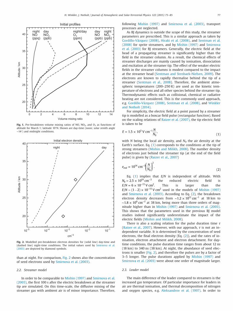
After initialisation, the model is run for five days withoutelectric fields applied in order to achieve a stable (repeating)diurnal cycle of all chemical species. Loss and production termshave been added to the model to avoid a slow drift of the modeldue to missing atmospheric transport processes. Fig. 1 shows thepre-breakdown profiles of O3, NO, and NO2 which are of interestfor the BJ simulations. While there are considerable differencesbetween the night-time and day-time values of the nitrogenspecies, the diurnal changes of ozone in the considered altituderange are small.

In a next step, the model is used to calculate the pre-break-down electron and ion composition, i.e. the steady state con-centrations due to galactic cosmic ray ionisation. This is the sameapproach as in Winkler and Notholt (2014). It provides the at-mospheric background profiles of electrons and ions for the BJsimulations. The pre-breakdown concentration of the free elec-trons (seed electrons) is shown in Fig. 2. Due to photo-electrondetachment, the day-time concentration of free electrons is higher

Initial profiles

0 2 4 6 8 10 12 14Volume mixing ratio

20

25

30

35

40

Alti

tude

/ km

Fig. 1. Pre-breakdown volume mixing ratios of NO, NO2, and O3 as functions ofaltitude for March 1; latitude 10°N. Shown are day-time (noon; solar zenith angle∼14°) and midnight conditions.

Initial electron density

10−5 10−4 10−3 10−2 10−1

cm−3

20

25

30

35

40

Alti

tude

/ km

daynight

Fig. 2. Modelled pre-breakdown electron densities for (solid line) day-time and(dashed line) night-time conditions. The initial values used by Smirnova et al.(2003) are depicted by diamond symbols.

H. Winkler, J. Notholt / Journal of Atmospheric and Solar-Terrestrial Physics 122 (2015) 75–85 77

than at night. For comparison, Fig. 2 shows also the concentrationof seed electrons used by Smirnova et al. (2003).

2.2. Streamer model

In order to be comparable to Mishin (1997) and Smirnova et al.(2003), the first 100 s after the electric breakdown at the streamertip are simulated. On this time-scale, the diffusive mixing of thestreamer gas with ambient air is of minor importance. Therefore,

following Mishin (1997) and Smirnova et al. (2003), transportprocesses are neglected.

As BJ dynamics is outside the scope of this study, the streamerparameters are prescribed. This is a similar approach as taken byGordillo-Vázquez (2008), Hiraki et al. (2008), and Sentman et al.(2008) for sprite streamers, and by Mishin (1997) and Smirnovaet al. (2003) for BJ streamers. Generally, the electric field at thehead of a propagating streamer is significantly higher than thefield in the streamer column. As a result, the chemical effects ofstreamer discharges are mainly caused by ionisation, dissociationand excitation at the streamer tip. The effect of the weaker electricfields in the streamer columns is modest compared to the impactat the streamer head (Sentman and Stenbaek-Nielsen, 2009). Theelectrons are known to rapidly thermalise behind the tip of astreamer (Sentman et al., 2008). Therefore, the ambient atmo-spheric temperatures (200–250 K) are used as the kinetic tem-perature of electrons and all other species behind the streamer tip.Thermodynamic effects such as collisional, chemical or radiativeheating are not considered. This is the commonly used approach,e.g. Gordillo-Vázquez (2008), Sentman et al. (2008), and Winklerand Notholt (2014).

For simplicity, the electric field at a point passed by a streamertip is modelled as a boxcar field pulse (rectangular function). Basedon the scaling relations of Raizer et al. (2007), the tip electric fieldis taken to be

= × −ENN

1.5 10 V cm ,(1)

5 1

0

with N being the local air density, and N0 the air density at theEarth's surface. Eq. (1) corresponds to the conditions at the tip ofstrong streamers (Mishin and Milikh, 2008). The number densityof electrons just behind the streamer tip (at the end of the fieldpulse) is given by (Raizer et al., 2007)

⎛⎝⎜

⎞⎠⎟= −e

NN

10 cm .(2)

end14 3

0

2

Eq. (1) implies that E/N is independent of altitude. With= × −N 2.5 10 cm0

19 3 the reduced electric field is= × −E N/ 6 10 V cm15 2. This is larger than the∼ – × −E N/ (1 2) 10 V cm15 2 used in the models of Mishin (1997)

and Smirnova et al. (2003). According to Eq. (2), the breakdownelectron density decreases from ∼ × −1.2 10 cm12 3 at 18 km to∼ × −1.8 10 cm9 3 at 38 km, being more than three orders of mag-nitude higher than in Mishin (1997) and Smirnova et al. (2003).This shows that the parameters used in the previous BJ modelstudies indeed significantly underestimate the impact of theelectric fields (Mishin and Milikh, 2008).

There is also a scaling relation for the pulse duration time τ(Raizer et al., 2007). However, with our approach, τ is not an in-dependent variable. It is determined by the concentration of seedelectrons, the final electron density (Eq. (2)), and the rates of io-nisation, electron attachment and electron detachment. For day-time conditions, the pulse duration time ranges from about 12 ns(18 km) to 340 ns (38 km). At night, the abundance of seed elec-trons is smaller (Fig. 2), and therefore the pulses are by a factor of3–5 longer. The pulse durations applied by Mishin (1997) andSmirnova et al. (2003) were about one order of magnitude larger.

2.3. Leader model

The main difference of the leader compared to streamers is theincreased gas temperature. Of particular importance for leaders inair are thermal ionisation, and thermal decomposition of nitrogenand oxygen species, e.g. Aleksandrov et al. (1997). In order to

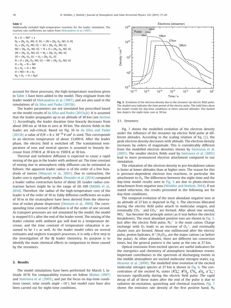
Table 3Additionally included high-temperature reactions for the leader simulation. Thereaction rate coefficients are taken from Aleksandrov et al. (1997).

+N O → ++NO e+N {N , O , NO, O, N}2 2 2 → +2N {N , O , NO, O, N}2 2

+O {N , O , NO, O}2 2 2 → +2O {N , O , NO, O}2 2

+NO {N , O , NO, O}2 2 → + +N O {N , O , NO, O}2 2

+2N {N , O , NO, O}2 2 → +N {N , O , NO, O}2 2 2

+2O {N , O , O}2 2 → +O {N , O , O}2 2 2

+ +N O {N , O , NO, O}2 2 → +NO {N , O , NO, O}2 2

+O N2 → +N NO+N O2 → +O NO+O NO→ +N O2

+N O2 2 → +O N O2

Electrons (streamer)

10−10 10−8 10−6 10−4 10−2 100 102

Time / s

10−5

100

105

1010

1015

Den

sity

/ cm

−3

Pulse18km

27km38km

18km27km

38km

Fig. 3. Evolution of the electron density due to the streamer tip electric field pulse.The shaded area indicates the time period of the electric pulse. The solid lines showthe model results for day-time conditions at three selected altitudes. The dashedline depicts the night-time case at 38 km.

H. Winkler, J. Notholt / Journal of Atmospheric and Solar-Terrestrial Physics 122 (2015) 75–8578

account for these processes, the high-temperature reactions givenin Table 3 have been added to the model. They originate from theleader model of Aleksandrov et al. (1997), and are also used in thesimulations of da Silva and Pasko (2013b).

The leader parameters are not simulated but prescribed basedon the model results of da Silva and Pasko (2013a,b): It is assumedthat the leader propagates up to an altitude of 30 km (see Section1). Accordingly, the leader duration time linearly decreases fromabout 200 ms at 18 km to zero at 30 km. The electric fields in theleader are sub-critical. Based on Fig. 16 in da Silva and Pasko(2013b) a value of = × −E N/ 6 10 V cm16 2 is used. This correspondsto an electron temperature of about 13,000 K. After the leaderphase, the electric field is switched off. The translational tem-perature of ions and neutral species is assumed to linearly de-crease from 2700 K at 18 km to 1500 K at 30 km.

Thermal and turbulent diffusion is expected to cause a rapidmixing of the gas in the leader with ambient air. The time constantof mixing due to atmospheric eddy diffusion can be estimated asfollows: the apparent leader radius is of the order of a few hun-dreds of metres (Wescott et al., 2001). Due to contraction, theleader core is significantly smaller. Shneider et al. (2014) computeda leader radius contraction factor of about 20. Leader radius con-traction factors might be in the range of 20–100 (Milikh et al.,2014). Therefore, the radius of the high-temperature core of theleader is of the order of 10 m. Eddy diffusion coefficients on scalesof 10 m in the stratosphere have been derived from the observa-tion of rocket plume dispersion (Denison et al., 1994). The corre-sponding time constant of diffusion is of the order of one second.As transport processes are not simulated by the model, the modelis stopped 0.5 s after the end of the leader event. The mixing of theleader column with ambient gas will lead to a temperature de-crease, and the time constant of temperature relaxation is as-sumed to be 1 s as well. As the leader model relies on severalestimates and neglects transport processes, it is only a first step inthe investigation of the BJ leader chemistry. Its purpose is toidentify the main chemical effects in comparison to those causedby the streamers.

3. Results

The model simulations have been performed for March 1, la-titude 10°N. For comparability reasons we follow Mishin (1997)and Smirnova et al. (2003), and put the focus on day-time condi-tions (noon; solar zenith angle ∼14°), but model runs have alsobeen carried out for night-time conditions.

3.1. Streamers

Fig. 3 shows the modelled evolution of the electron densityunder the influence of the streamer tip electric field pulse at dif-ferent altitudes. According to the scaling relation of Eq. (2), thepeak electron density decreases with altitude. The electron densityincreases by orders of magnitude. This is considerably differentfrom the modelled electron densities shown by Smirnova et al.(2003). The smaller electric fields used by Smirnova et al. (2003)lead to more pronounced electron attachment compared to oursimulation.

The relaxation of the electron density to pre-breakdown valuesis faster at lower altitudes than at higher ones. The reason for thisis pressure-dependent electron loss reactions, in particular theattachment to O2. The differences between the night-time and theday-time model results seen in Fig. 3 are due to photo-electrondetachment from negative ions (Winkler and Notholt, 2014). If notstated otherwise, the results presented in the following are forday-time conditions.

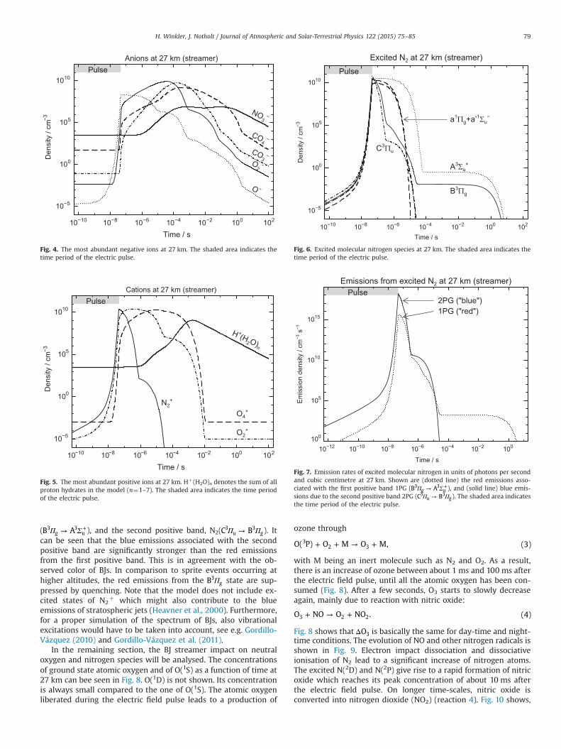
The temporal evolution of the most abundant negative ions atan altitude of 27 km is depicted in Fig. 4. The electrons liberatedduring the electric field pulse attach to molecular oxygen, andeventually CO3

� and CO4� are formed. After about one second,

NO3� has become the principle anion (as it was before the electric

breakdown). The most abundant positive ions are shown in Fig. 5.Just after the electric field pulse, N2

þ is the main cation. Chargeexchange with O2 leads to an increase of O2

þ , and eventuallycluster ions are formed. About one millisecond after the electricpulse, proton hydrates, Hþ(H2O)n, are the major cations (as beforethe pulse). At other altitudes, there are different ion conversiontimes, but the general pattern is the same as the one at 27 km.

Optical emissions from excited species are useful indicators forthe energetics and chemistry of atmospheric breakdown events.Important contributors to the spectrum of discharging events inthe middle atmosphere are excited molecular nitrogen states, e.g.Heavner et al. (2000). The modelled time evolution of the excitedmolecular nitrogen species at 27 km is shown in Fig. 6. The con-centration of the excited N2 states ( Σ +A u

3 , ΠB g3 , ΠC u

3 , Πa g1 , Σ′ −a u

1 )increases significantly during the electric field pulse. The rapiddecay of all of these states after the end of the pulse is due toradiative de-excitation, quenching and chemical reactions. Fig. 7shows the emission rate density of the first positive band, N2

Anions at 27 km (streamer)

10−10 10−8 10−6 10−4 10−2 100 102

Time / s

10−5

100

105

1010

Den

sity

/ cm

−3

Fig. 4. The most abundant negative ions at 27 km. The shaded area indicates thetime period of the electric pulse.

Cations at 27 km (streamer)

10−10 10−8 10−6 10−4 10−2 100 102

Time / s

10−5

100

105

1010

Den

sity

/ cm

−3

Fig. 5. The most abundant positive ions at 27 km. Hþ(H2O)n denotes the sum of allproton hydrates in the model (n¼1–7). The shaded area indicates the time periodof the electric pulse.

Fig. 6. Excited molecular nitrogen species at 27 km. The shaded area indicates thetime period of the electric pulse.

Fig. 7. Emission rates of excited molecular nitrogen in units of photons per secondand cubic centimetre at 27 km. Shown are (dotted line) the red emissions asso-ciated with the first positive band 1PG ( Π Σ→ +B Ag u

3 3 ), and (solid line) blue emis-sions due to the second positive band 2PG ( Π Π→C Bu g

3 3 ). The shaded area indicatesthe time period of the electric pulse.

H. Winkler, J. Notholt / Journal of Atmospheric and Solar-Terrestrial Physics 122 (2015) 75–85 79

( Π Σ→ +B Ag u3 3 ), and the second positive band, N2( Π Π→C Bu g

3 3 ). Itcan be seen that the blue emissions associated with the secondpositive band are significantly stronger than the red emissionsfrom the first positive band. This is in agreement with the ob-served color of BJs. In comparison to sprite events occurring athigher altitudes, the red emissions from the ΠB g

3 state are sup-pressed by quenching. Note that the model does not include ex-cited states of N2

þ which might also contribute to the blueemissions of stratospheric jets (Heavner et al., 2000). Furthermore,for a proper simulation of the spectrum of BJs, also vibrationalexcitations would have to be taken into account, see e.g. Gordillo-Vázquez (2010) and Gordillo-Vázquez et al. (2011).

In the remaining section, the BJ streamer impact on neutraloxygen and nitrogen species will be analysed. The concentrationsof ground state atomic oxygen and of O(1S) as a function of time at27 km can bee seen in Fig. 8. O(1D) is not shown. Its concentrationis always small compared to the one of O(1S). The atomic oxygenliberated during the electric field pulse leads to a production of

ozone through

+ + → +O( P) O M O M, (3)32 3

with M being an inert molecule such as N2 and O2. As a result,there is an increase of ozone between about 1 ms and 100 ms afterthe electric field pulse, until all the atomic oxygen has been con-sumed (Fig. 8). After a few seconds, O3 starts to slowly decreaseagain, mainly due to reaction with nitric oxide:

+ → +O NO O NO . (4)3 2 2

Fig. 8 shows that ΔO3 is basically the same for day-time and night-time conditions. The evolution of NO and other nitrogen radicals isshown in Fig. 9. Electron impact dissociation and dissociativeionisation of N2 lead to a significant increase of nitrogen atoms.The excited N(2D) and N(2P) give rise to a rapid formation of nitricoxide which reaches its peak concentration of about 10 ms afterthe electric field pulse. On longer time-scales, nitric oxide isconverted into nitrogen dioxide (NO2) (reaction 4). Fig. 10 shows,

Fig. 8. Evolution of ground state atomic oxygen O(3P) and excited O(1S) as well asthe ozone change with respect to the pre-breakdown ozone value at 27 km. Theshaded area indicates the time period of the electric pulse.

Fig. 9. Evolution of nitrogen species at 27 km. The shaded area indicates the timeperiod of the electric pulse.

Day and night Nitrogen at 27 km (streamer)

0 20 40 60 80 100 120

Time / s

0

1

2

3

4

5

6

NO day2

NO night

Fig. 10. Evolution of NO and NO2 for both day-time and night-time conditions at27 km.

Ozone (streamer)

1 2 3 4 5 6 7 8 9

20

25

30

35

Alti

tude

/ km

Fig. 11. Ozone concentration as a function of altitude. Shown are (dashed line) theinitial atmospheric profile, and (solid line) the ozone profile 100 s after the electricbreakdown.

H. Winkler, J. Notholt / Journal of Atmospheric and Solar-Terrestrial Physics 122 (2015) 75–8580

in linear scale, the concentrations of NO and NO2 for both day-timeand night-time conditions. It can be seen that during day thetransformation of NO into NO2 is slower than at night. This is dueto reactions in the sunlit atmosphere which convert NO2 back intonitric oxide (Winkler and Notholt, 2014). The sum NOx¼NOþNO2

(odd nitrogen) is basically the same for day-time and night-timemodel runs. It is virtually constant until the end of the simulation100 s after the electric pulse.

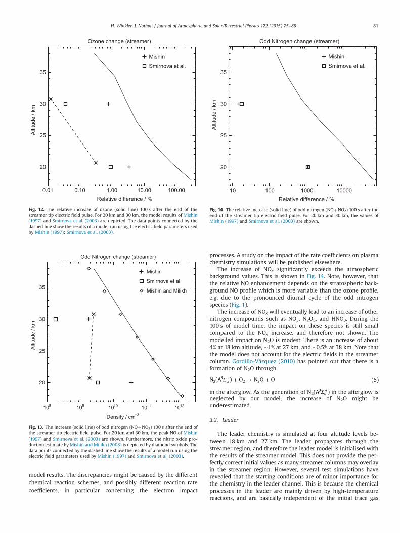
Finally, we consider the height-dependence of the BJ streamerimpact on ozone and on odd nitrogen. Fig. 11 shows the con-centration of O3 as a function of altitude before and after theelectric breakdown pulse. While the increase of ozone is small athigher altitudes, there is a significant production of ozone at loweraltitudes. The relative O3 enhancement is displayed in Fig. 12.Ozone is increased by about 3% at an altitude of 30 km, and bymore than 300% at 18 km. These values are much larger than themodel predictions of Mishin (1997) and Smirnova et al. (2003)which are also shown in Fig. 12.

The streamer induced NOx increase as a function of altitude isshown in Fig. 13. Again, the effect is most pronounced at loweraltitudes, and by orders of magnitude larger than in Mishin (1997)and Smirnova et al. (2003). There is good agreement of the mod-elled NOx increase with the NO production estimate based onenergetic considerations by Mishin and Milikh (2008), see Fig. 13.

The modelled increase of NOx and O3 gets significantly smallerif the pulse parameters of Mishin (1997) and Smirnova et al.(2003) are used, and it is different from the results of Mishin(1997) or Smirnova et al. (2003), see Figs. 12 and 13. Note that alsothe results of Mishin (1997) and Smirnova et al. (2003) do notagree with each other. On the other hand, using the seed electrondensity of Smirnova et al. (2003) instead of our values (Fig. 2) doesbasically not change the results (not shown). Therefore, the dif-ferent amounts of seed electrons do not explain the different

Ozone change (streamer)

0.01 0.10 1.00 10.00 100.00Relative difference / %

20

25

30

35

Alti

tude

/ km

Mishin

Smirnova et al.

Fig. 12. The relative increase of ozone (solid line) 100 s after the end of thestreamer tip electric field pulse. For 20 km and 30 km, the model results of Mishin(1997) and Smirnova et al. (2003) are depicted. The data points connected by thedashed line show the results of a model run using the electric field parameters usedby Mishin (1997); Smirnova et al. (2003).

Odd Nitrogen change (streamer)

108 109 1010 1011 1012

Density / cm−3

20

25

30

35

Alti

tude

/ km

Mishin

Smirnova et al.

Mishin and Milikh

Fig. 13. The increase (solid line) of odd nitrogen (NOþNO2) 100 s after the end ofthe streamer tip electric field pulse. For 20 km and 30 km, the peak NO of Mishin(1997) and Smirnova et al. (2003) are shown. Furthermore, the nitric oxide pro-duction estimate by Mishin and Milikh (2008) is depicted by diamond symbols. Thedata points connected by the dashed line show the results of a model run using theelectric field parameters used by Mishin (1997) and Smirnova et al. (2003).

Odd Nitrogen change (streamer)

10 100 1000 10000Relative difference / %

20

25

30

35

Alti

tude

/ km

Mishin

Smirnova et al.

Fig. 14. The relative increase (solid line) of odd nitrogen (NOþNO2) 100 s after theend of the streamer tip electric field pulse. For 20 km and 30 km, the values ofMishin (1997) and Smirnova et al. (2003) are shown.

H. Winkler, J. Notholt / Journal of Atmospheric and Solar-Terrestrial Physics 122 (2015) 75–85 81

model results. The discrepancies might be caused by the differentchemical reaction schemes, and possibly different reaction ratecoefficients, in particular concerning the electron impact

processes. A study on the impact of the rate coefficients on plasmachemistry simulations will be published elsewhere.

The increase of NOx significantly exceeds the atmosphericbackground values. This is shown in Fig. 14. Note, however, thatthe relative NO enhancement depends on the stratospheric back-ground NO profile which is more variable than the ozone profile,e.g. due to the pronounced diurnal cycle of the odd nitrogenspecies (Fig. 1).

The increase of NOx will eventually lead to an increase of othernitrogen compounds such as NO3, N2O5, and HNO3. During the100 s of model time, the impact on these species is still smallcompared to the NOx increase, and therefore not shown. Themodelled impact on N2O is modest. There is an increase of about4% at 18 km altitude, ∼1% at 27 km, and ∼0.5% at 38 km. Note thatthe model does not account for the electric fields in the streamercolumn. Gordillo-Vázquez (2010) has pointed out that there is aformation of N2O through

Σ + → ++N (A ) O N O O (5)23

u 2 2

in the afterglow. As the generation of N2( Σ +A u3 ) in the afterglow is

neglected by our model, the increase of N2O might beunderestimated.

3.2. Leader

The leader chemistry is simulated at four altitude levels be-tween 18 km and 27 km. The leader propagates through thestreamer region, and therefore the leader model is initialised withthe results of the streamer model. This does not provide the per-fectly correct initial values as many streamer columns may overlayin the streamer region. However, several test simulations haverevealed that the starting conditions are of minor importance forthe chemistry in the leader channel. This is because the chemicalprocesses in the leader are mainly driven by high-temperaturereactions, and are basically independent of the initial trace gas

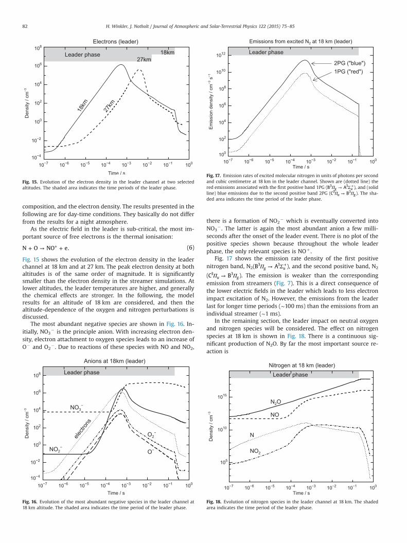
Fig. 15. Evolution of the electron density in the leader channel at two selectedaltitudes. The shaded area indicates the time periods of the leader phase.

Fig. 17. Emission rates of excited molecular nitrogen in units of photons per secondand cubic centimetre at 18 km in the leader channel. Shown are (dotted line) thered emissions associated with the first positive band 1PG ( Π Σ→ +B Ag u

3 3 ), and (solidline) blue emissions due to the second positive band 2PG ( Π Π→C Bu g

3 3 ). The sha-ded area indicates the time period of the leader phase.

H. Winkler, J. Notholt / Journal of Atmospheric and Solar-Terrestrial Physics 122 (2015) 75–8582

composition, and the electron density. The results presented in thefollowing are for day-time conditions. They basically do not differfrom the results for a night atmosphere.

As the electric field in the leader is sub-critical, the most im-portant source of free electrons is the thermal ionisation:

+ → ++N O NO e. (6)

Fig. 15 shows the evolution of the electron density in the leaderchannel at 18 km and at 27 km. The peak electron density at bothaltitudes is of the same order of magnitude. It is significantlysmaller than the electron density in the streamer simulations. Atlower altitudes, the leader temperatures are higher, and generallythe chemical effects are stronger. In the following, the modelresults for an altitude of 18 km are considered, and then thealtitude-dependence of the oxygen and nitrogen perturbations isdiscussed.

The most abundant negative species are shown in Fig. 16. In-itially, NO3

� is the principle anion. With increasing electron den-sity, electron attachment to oxygen species leads to an increase ofO� and O2

� . Due to reactions of these species with NO and NO2,

Fig. 16. Evolution of the most abundant negative species in the leader channel at18 km altitude. The shaded area indicates the time period of the leader phase.

there is a formation of NO2� which is eventually converted into

NO3� . The latter is again the most abundant anion a few milli-

seconds after the onset of the leader event. There is no plot of thepositive species shown because throughout the whole leaderphase, the only relevant species is NOþ .

Fig. 17 shows the emission rate density of the first positivenitrogen band, N2( Π Σ→ +B Ag u

3 3 ), and the second positive band, N2

( Π Π→C Bu g3 3 ). The emission is weaker than the corresponding

emission from streamers (Fig. 7). This is a direct consequence ofthe lower electric fields in the leader which leads to less electronimpact excitation of N2. However, the emissions from the leaderlast for longer time periods (∼100 ms) than the emissions from anindividual streamer (∼1 ms).

In the remaining section, the leader impact on neutral oxygenand nitrogen species will be considered. The effect on nitrogenspecies at 18 km is shown in Fig. 18. There is a continuous sig-nificant production of N2O. By far the most important source re-action is

Fig. 18. Evolution of nitrogen species in the leader channel at 18 km. The shadedarea indicates the time period of the leader phase.

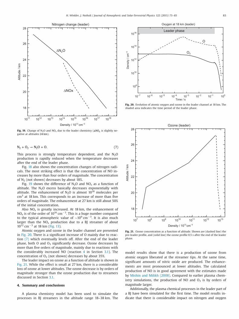
Fig. 19. Change of N2O and NOx due to the leader chemistry (ΔNOx is slightly ne-gative at altitudes 24 km).

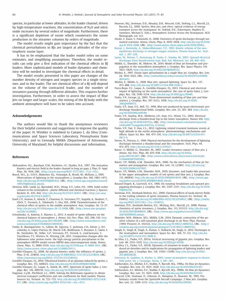
Fig. 20. Evolution of atomic oxygen and ozone in the leader channel at 18 km. Theshaded area indicates the time period of the leader phase.

Fig. 21. Ozone concentration as a function of altitude. Shown are (dashed line) thepre-leader profile, and (solid line) the ozone profile 0.5 s after the end of the leaderphase.

H. Winkler, J. Notholt / Journal of Atmospheric and Solar-Terrestrial Physics 122 (2015) 75–85 83

+ → +N O N O O. (7)2 2 2

This process is strongly temperature dependent, and the N2Oproduction is rapidly reduced when the temperature decreasesafter the end of the leader phase.

Fig. 18 also shows the concentration changes of nitrogen radi-cals. The most striking effect is that the concentration of NO in-creases by more than four orders of magnitude. The concentrationof N2 (not shown) decreases by about 18%.

Fig. 19 shows the difference of N2O and NOx as a function ofaltitude. The N2O excess basically decreases exponentially withaltitude. The enhancement of N2O is almost 1018 molecules percm3 at 18 km. This corresponds to an increase of more than fiveorders of magnitude. The enhancement at 27 km is still about 50%of the initial concentration.

Also NOx is greatly increased. At 18 km, the enhancement ofNOx is of the order of 1016 cm�3. This is a huge number comparedto the typical atmospheric value of ∼109 cm�3. It is also muchlarger than the NOx production due to a BJ streamer of about1012 cm�3 at 18 km (Fig. 13).

Atomic oxygen and ozone in the leader channel are presentedin Fig. 20. There is a significant increase of O mainly due to reac-tion (7) which eventually levels off. After the end of the leaderphase, both O and O3 significantly decrease. Ozone decreases bymore than five orders of magnitude, mainly due to reactions withthe considerably increased NO (reaction 4 in Section 3.1). Theconcentration of O2 (not shown) decreases by about 35%.

The leader impact on ozone as a function of altitude is shown inFig. 21. While the effect is small at 27 km, there is a considerableloss of ozone at lower altitudes. The ozone decrease is by orders ofmagnitude stronger than the ozone production due to streamersdiscussed in Section 3.1.

4. Summary and conclusions

A plasma chemistry model has been used to simulate theprocesses in BJ streamers in the altitude range 18–38 km. The

model results show that there is a production of ozone fromatomic oxygen liberated at the streamer tips. At the same time,significant amounts of nitric oxide are produced. The enhance-ments are most pronounced at lower altitudes. The calculatedproduction of NO is in good agreement with the estimates madeby Mishin and Milikh (2008). Compared to earlier plasma chem-istry simulations, the production of NO and O3 is by orders ofmagnitude larger.

Additionally, the plasma chemical processes in the leader part ofa BJ have been simulated for the first time. The model results in-dicate that there is considerable impact on nitrogen and oxygen

H. Winkler, J. Notholt / Journal of Atmospheric and Solar-Terrestrial Physics 122 (2015) 75–8584

species, in particular at lower altitudes. In the leader channel, drivenby high-temperature reactions, the concentration of N2O and nitricoxide increases by several orders of magnitude. Furthermore, thereis a significant depletion of ozone which counteracts the ozoneproduction in the streamer columns by orders of magnitude.

The model results might gain importance by the fact that thechemical perturbations in BJs are largest at altitudes of the stra-tospheric ozone layer.

It has to be emphasized that the leader model relies on someestimates, and simplifying assumptions. Therefore, the model re-sults can only give a first indication of the chemical effects in BJleaders. More sophisticated models of leader dynamics and chem-istry will be needed to investigate the chemical effects in detail.

The model results presented in this paper are changes of thenumber density of nitrogen and oxygen species in a single strea-mer, and in the leader. The net chemical effect of a BJ will dependon the volume of the contracted leader, and the number ofstreamers passing through different altitudes. This requires furtherinvestigation. Furthermore, in order to assess the impact of BlueJets on longer and larger scales, the mixing of the BJ body with theambient atmosphere will have to be taken into account.

Acknowledgements

The authors would like to thank the anonymous reviewersfor their helpful comments and suggestions to improve the qualityof the paper. H. Winkler is indebted to Caitano L. da Silva (Com-munications and Space Sciences Laboratory, Pennsylvania StateUniversity), and to Gennady Milikh (Department of Astronomy,University of Maryland) for helpful discussions and information.

References

Aleksandrov, N.L., Bazelyan, E.M., Kochetov, I.V., Dyatko, N.A., 1997. The ionizationkinetics and electric field in the leader channel in long air gaps. J. Phys. D: Appl.Phys. 30, 1616, URL: ⟨http://stacks.iop.org/0022-3727/30/i¼11/a¼011⟩.

Boeck, W.L., Jr., O.H.V., Blakeslee, R.J., Vonnegut, B., Brook, M., McKune, J., 1995.Observations of lightning in the stratosphere. J. Geophys Res. 100, 1465–1475,http://dx.doi.org/10.1029/94JD02432. URL: ⟨http://www.agu.org/pubs/crossref/1995/94JD02432.shtml⟩.

Denison, M.R., Lamb, J.J., Bjorndahl, W.D., Wong, E.Y., Lohn, P.D., 1994. Solid rocketexhaust in the stratosphere - plume diffusion and chemical reactions. J. Spacecr.Rockets 31, 435–442. http://dx.doi.org/10.2514/3.26457, URL: ⟨http://arc.aiaa.org/doi/abs/10.2514/3.26457⟩.

Enell, C.F., Arnone, E., Adachi, T., Chanrion, O., Verronen, P.T., Seppälä, A., Neubert, T.,Ulich, T., Turunen, E., Takahashi, Y., Hsu, R.R., 2008. Parameterisation of thechemical effect of sprites in the middle atmosphere. Ann. Geophys. 26, 13–27.http://dx.doi.org/10.5194/angeo-26-13-2008, URL: ⟨http://www.ann-geophys.net/26/13/2008/⟩.

Evtushenko, A., Kuterin, F., Mareev, E., 2013. A model of sprite influence on thechemical balance of mesosphere. J. Atmos. Sol.-Terr. Phys. 102, 298–310. http://dx.doi.org/10.1016/j.jastp.2013.06.005, URL: ⟨http://www.sciencedirect.com/science/article/pii/S1364682613001818⟩.

Funke, B., Baumgaertner, A., Calisto, M., Egorova, T., Jackman, C.H., Kieser, J., Kri-volutsky, A., López-Puertas, M., Marsh, D.R., Reddmann, T., Rozanov, E., Salmi, S.M., Sinnhuber, M., Stiller, G.P., Verronen, P.T., Versick, S., vonClarmann, T.,Vyushkova, T.Y., Wieters, N., Wissing, J.M., 2011. Composition changes after thehalloween solar proton event: the high energy particle precipitation in theatmosphere HEPPA model versus MIPAS data intercomparison study. Atmos.Chem. Phys. 11, 9089–9139. http://dx.doi.org/10.5194/acp-11-9089-2011, URL:⟨http://www.atmos-chem-phys.net/11/9089/2011/⟩.

Gordillo-Vázquez, F.J., 2008. Air plasma kinetics under the influence of sprites. J.Phys. D 41, 234016. http://dx.doi.org/10.1088/0022-3727/41/23/234016, URL:⟨http://iopscience.iop.org/0022-3727/41/23/234016/⟩.

Gordillo-Vázquez, F.J., 2010. Vibrational kinetics of air plasmas induced by sprites. J.Geophys. Res. 115, A00E25. http://dx.doi.org/10.1029/2009JA014688.

Gordillo-Vázquez, F.J., Luque, A., Simek, M., 2011. Spectrum of sprite halos. J. Geo-phys. Res. 116, A09319. http://dx.doi.org/10.1029/2011JA016652.

Hagelaar, G.J.M., Pitchford, L.C., 2005. Solving the Boltzmann equation to obtainelectron transport coefficients and rate coefficients for fluid models. PlasmaSources Sci. Technol. 14, 722–733. http://dx.doi.org/10.1088/0963-0252/14/4/011, URL: ⟨http://stacks.iop.org/0963-0252/14/i¼4/a¼011⟩.

Heavner, M.J., Sentman, D.D., Moudry, D.R., Wescott, E.M., Siefring, C.L., Morrill, J.S.,Bucsela, E.J., 2000. Sprites, blue jets, and elves: optical evidence of energytransport across the stratopause. In: Siskind, D.E., Eckermann, Stephen D.,Summers, Michael E. (Eds.), Atmospheric Science Across the Stratopause. AGUMonograph, vol. 123.

Hiraki, Y., Kasai, Y., Fukunishi, H., 2008. Chemistry of sprite discharges through ion-neutral reactions. Atmos. Chem. Phys. 8, 3919–3928. http://dx.doi.org/10.5194/acp-8-3919-2008, URL: ⟨http://www.atmos-chem-phys.net/8/3919/2008/⟩.

Kossyi, I., Kostinsky, A., SilakovMatveyev, V.P., 1992. Kinetic scheme of the non-equlibrium discharge in nitrogen-oxygen mixtures. Plasma Sources Sci. Tech-nol. 1, 207–220.

Lyons, W., Nelson, T., Armstrong, R., Pasko, V., Stanley, M., 2003. Upward electricaldischarges from thunderstorm tops. Bull. Am. Meteorol. Soc. 84, 445–454.

Milikh, G., Shneider, M., Mokrov, M., 2014. Model of blue jet formation and pro-pagation in the nonuniform atmosphere. J. Geophys. Res. Space Physics 119,5821–5829, http://dx.doi.org/10.1002/2014JA020123.

Mishin, E., 1997. Ozone layer perturbation by a single blue jet. Geophys. Res. Lett.24, 1919–1922, URL: ⟨http://onlinelibrary.wiley.com/doi/10.1029/97GL01890/abstract⟩.

Mishin, E., Milikh, G., 2008. Blue jets: upward lightning. Space Sci. Rev. 137,473–488. http://dx.doi.org/10.1007/s11214-008-9346-z.

Parra-Rojas, F.C., Luque, A., Gordillo-Vázquez, F.J., 2013. Chemical and electricalimpact of lightning on the earth mesosphere: the case of sprite halos. J. Geo-phys. Res. 118, 5190–5214. http://dx.doi.org/10.1002/jgra.50449.

Pasko, V.P., George, J.J., 2002. Three-dimensional modeling of blue jets and bluestarters. J. Geophys. Res. 107 (A12), 1458, http://dx.doi.org/10.1029/2002JA009473.

Pasko, V.P., Inan, U.S., Bell, T.F., 1996. Blue jets produced by quasi-electrostatic pre-discharge thundercloud fields. Geophys. Res. Lett. 23, 301–304. http://dx.doi.org/10.1029/96GL00149.

Pasko, V.P., Stanley, M.A., Mathews, J.D., Inan, U.S., Wood, T.G., 2002. Electricaldischarge from a thundercloud top to the lower ionosphere. Nature 416, http://dx.doi.org/10.1038/416152a, URL: ⟨http://www.nature.com/nature/journal/v416/n6877/suppinfo/416152a_S1.html⟩.

Pasko, V.P., Yair, Y., Kuo, C.L., 2012. Lightning related transient luminous events athigh altitude in the earths atmosphere: phenomenology, mechanisms andeffects. Space Sci. Rev. 168, 475–516. http://dx.doi.org/10.1007/s11214-011-9813-9.

Petrov, N., Petrova, G., 1999. Physical mechanisms for the development of lightningdischarges between a thundercloud and the ionosphere. Tech. Phys. 44,472–475. http://dx.doi.org/10.1134/1.1259327.

Raizer, Y., Milikh, G., Shneider, M., 2007. Leader-streamers nature of blue jets. J.Atmos. Sol.-Terr. Phys. 69, 925–938. http://dx.doi.org/10.1016/j.jastp.2007.02.007, URL: ⟨http://www.sciencedirect.com/science/article/pii/S1364682607000302⟩.

Raizer, Y.P., Milikh, G.M., Shneider, M.N., 2006. On the mechanism of blue jet for-mation and propagation. Geophys. Res. Lett. 33, L23801. http://dx.doi.org/10.1029/2006GL027697.

Raizer, Y.P., Milikh, G.M., Shneider, M.N., 2010. Streamer- and leader-like processesin the upper atmosphere: models of red sprites and blue jets. J. Geophys. Res.115, A00E42. http://dx.doi.org/10.1029/2009JA014645, URL: ⟨http://www.agu.org/pubs/crossref/2010/2009JA014645.shtml⟩.

Roussel-Dupré, R., Gurevich, A.V., 1996. On runaway breakdown and upward pro-pagating discharges. J. Geophys. Res. 101, 2297–2311. http://dx.doi.org/10.1029/95JA03278.

Sentman, D.D., Stenbaek-Nielsen, H.C., 2009. Chemical effects of weak electric fieldsin the trailing columns of sprite streamers. Plasma Sources Sci. Technol. 18,034012. http://dx.doi.org/10.1088/0963-0252/18/3/034012, URL: ⟨http://stacks.iop.org/0963-0252/18/i¼3/a¼034012⟩.

Sentman, D.D., Stenbaek-Nielsen, H.C., McHarg, M.G., Morrill, J.S., 2008. Plasmachemistry of sprite streamers. J. Geophys. Res. 113, D11112. http://dx.doi.org/10.1029/2007JD008941, URL: ⟨http://www.agu.org/pubs/crossref/2008/2007JD008941.shtml⟩.

Shneider, M.N., Mokrov, M.S., Milikh, G.M., 2014. Dynamic contraction of the po-sitive column of a self-sustained glow discharge in air flow. Phys. Plasmas(1994–Present) 21, 032122. http://dx.doi.org/10.1063/1.4869332, URL: ⟨http://scitation.aip.org/content/aip/journal/pop/21/3/10.1063/1.4869332⟩.

Siingh, D., Singh, R., Singh, A., Kumar, S., Kulkarni, M., Singh, A., 2012. Discharges inthe stratosphere and mesosphere. Space Sci. Rev. 169, 73–121. http://dx.doi.org/10.1007/s11214-012-9906-0.

da Silva, C.L., Pasko, V.P., 2013a. Vertical structuring of gigantic jets. Geophys. Res.Lett. 40, 3315–3319. http://dx.doi.org/10.1002/grl.50596.

da Silva, C.L., Pasko, V.P., 2013b. Dynamics of streamer-to-leader transition at re-duced air densities and its implications for propagation of lightning leaders andgigantic jets. J. Geophys. Res. 118, 13561–13590. http://dx.doi.org/10.1002/2013JD020618.

Smirnova, N., Lyakhov, A., Kozlov, S., 2003. Lower stratosphere response to electricfield pulse. Int. J. Geomagn. Aeron. 3, 281–287.

Sukhorukov, A.I., Mishin, E.V., Stubbe, P., Rycroft, M.J., 1996a. On blue jet dynamics.Geophys. Res. Lett. 23, 1625–1628. http://dx.doi.org/10.1029/96GL01367.

Sukhorukov, A.I., Mishin, E.V., Stubbe, P., Rycroft, M.J., 1996b. On blue jet dynamics.Geophys. Res. Lett. 23, 1625–1628. http://dx.doi.org/10.1029/96GL01367.

Wescott, E.M., Sentman, D., Osborne, D., Hampton, D., Heavner, M., 1995. Pre-liminary results from the Sprites94 Aircraft Campaign: 2 blue jets. Geophys.Res. Lett. 22, 1209–1212. http://dx.doi.org/10.1029/95GL00582.

H. Winkler, J. Notholt / Journal of Atmospheric and Solar-Terrestrial Physics 122 (2015) 75–85 85

Wescott, E.M., Sentman, D.D., Stenbaek-Nielsen, H.C., Huet, P., Heavner, M.J., Mou-dry, D.R., 2001. New evidence for the brightness and ionization of blue startersand blue jets. J. Geophys. Res. 106, 21549–21554. http://dx.doi.org/10.1029/2000JA000429.

Winkler, H., Kazeminejad, S., Sinnhuber, M., Kallenrode, M.B., Notholt, J., 2009.Conversion of mesospheric HCl into active chlorine during the solar protonevent in July 2000 in the northern polar region. J. Geophys. Res. 114, D00I03,http://dx.doi.org/10.1029/2008JD011587.

Winkler, H., Notholt, J., 2013. A model study of the negative chlorine ion chemistryin the Earth's mesosphere. Adv. Space Res. 51, 2342–2352. http://dx.doi.org/10.1016/j.asr.2013.02.013, URL: ⟨http://www.sciencedirect.com/science/article/pii/S0273117713001191⟩.

Winkler, H., Notholt, J., 2014. The chemistry of daytime sprite streamers—a modelstudy. Atmos. Chem. Phys. 14, 3545–3556. http://dx.doi.org/10.5194/acp-14-3545-2014, URL: ⟨http://www.atmos-chem-phys.net/14/3545/2014/⟩.