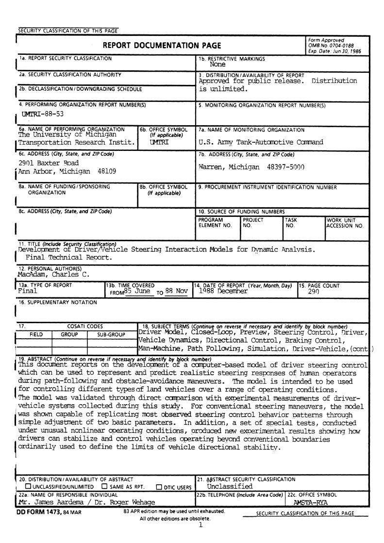
SECURITY CLASSIFICATION OF THlS PAGE

I - - - -

REPORT DOCUMENTATION PAGE Form Approved OMB NO 0704-01ae Exp Oate l un 30, 1986

4. PERFORMING ORGANIZATION REPORT NUMBER(S)

I UMPRT-8R-53

2901 Eaxter %ad ' Ann Arbor , Vichigan 48109 I

5. MONITORING ORGANIZATION REPORT NUMBER(S)

t

I Warren, Michigan 48397-5000

I la . REPORT SECURITY CLASSIFICATION

2a. SECURITY CLASSIFICATION AUTHORITY

I 2b. DECLASSIFICATION I DOWNGRADING SCHEDULE

6a. NAME, OF PEqFORMlNG OPGANIZATION The Unlverslty of mchigan Transportation Research Instit,

1 b. RESTRICTIVE MARKINGS None

3 DISTRIBUTION /AVAILABILITY OF REPORT Approved for public release. Distribution is unlimited.

6b. OFFICE SYMBOL (If applicable) TNTlU

I t

11. TITLE (Include Security ,C/arsifi ation) , Mvelopnent of ~rlver/teh~cle Steerinq Interaction Mcdels for Jlynamic Analvsis . I

7a. NAME OF MONITORING ORGANIZATION

U .S. AnrTJ Tank-Autmtive Ccg-cnnand 6c. ADDRESS (City, State, and ZIPCode)

9. PROCUREMENT INSTRUMENT IDENTIFICATION NUMBER 8a. NAME OF FUNDING /SPONSORING ORGANIZATION

I t

8c. ADDRESS (City, State, and ZIP Code)

I I Final Technical Report. I

7 b. ADDRESS (City, State, and ZIP Code)

8b. OFFICE SYMBOL (If applicable)

I L . ~ C N ~ U I Y A L AU I n u n \ > )

MacAdam. Charles C .

10. SOURCE OF FUNDING NUMBERS

13a. TYPE OF REPORT 13b. TIME COVERED 14. DATE OF REPORT (Year, Month, Day) Final FROM85 June 88N0v 1 9 8 8 Decemher TO-

16. SUPPLEMENTARY NOTATION

I

PROGRAM ELEMENT NO.

I I I

19. PBSTRACT (Continue on reverse if necessary and identify by block number) 1 Thls document reports on the devel-t of a ccmputer-based model of driver steerinq control

PROJECT NO.

"which can he used to represent and predict realistic steering responses of human oGators during path-follwing and obstacle-avoidance maneuvers. The mdel is intended to he used

I for controlling different types af land vehicles over a range of operating conditions. The model was validated through direct canparison with experimental measurements of driver- vehicle systems collected during this study. For conventional steering maneuvers, the model

i was shwn capable of replicating mst observed steering control behavior wtterns through simple adjustment of two basic parameters. In addition, a set of special tests, conducted under unusual nonlinear operating conditions, produced new exwrimental results shwinq hcw drivers can stabilize and control vehicles operating beyond conventional bounclaries ordinarily used to define the limits of vehicle directional stability.

18,. SUBJECT TERMS (Continue on reverse if neceuary and identify by block number) Drlver .Model, Closed-bop , Preview , Steerlng Control, r)river , Vehicle Evnamics, Directional Control, Braking Control, Man-Machine , Path Follaving , Simulation, Driver-Vehicle , (cont

17. COSATI CODES I

TASK NO.

I FIELD

t

WORK UNIT ACCESSION NO.

20. DISTRIBUTION /AVAILABILITY OF ABSTRACT UNCLASSIFIED/UNLIMITED O SAME AS RPT. DTIC USERS

22a. NAME OF RESPONSIBLE INDIVIDUAL

Mr. James Aardm / Dr. Roger Wehage

GROUP SUB-GROUP

*

DD FORM 1 4 7 3 , 8 4 MAR 83 APR edltlon may be used untli exhausted. SECURITY CLASSIFICATION OF THIS PAGE All other editions are obsolete.

1

21. 4JSTRACT SECURITY CLASSIFICATION Unclassified

22b. TELEPHONE (Include Area Code) 22c. OFFICE SYMBOL

AMSTA-WA

Block 18 (continued): Vehicle, Yeasurement, H m Operator, Bifurcation, Optimal Control, Handling, Braking, marnics .

PREFACE

The author gratefully acknowledges the assistance and cooperation of several key people who contributed to the success and support of this work. Mr. Michael Campbell of UMTM deserves special credit for his technical expertise and strong contributions to the test program conducted during this project. Mr. Campbell not only served as the principal test driver during that program, but also supervised the technical aspects and instrumentation of the HMMWV and trailer test vehicles. Mr. Campbell also assisted in the data processing activities and acted as chief liaison with the Chrysler Proving Grounds staff. His cooperative efforts are greatly appreciated.

At TACOM, the cooperation and support of Mr. Cedric Mousseau, Dr. Roger Wehage, and Mr. James Aardema are gratefully acknowledged. Mr. Mousseau served as the primary technical representative for most of the project. Dr. Wehage and Mr. Aardema served in this same capacity during alternate periods. Messrs. Mousseau and Aardema provided the principal support for interfacing the developed driver model within the DADS simulation model at TACOM.

An unexpected but interesting development during the course of this project was the establishment of frequent cooperative efforts between the staff members at UMTRI and TACOM, not only on a level of technical exchange, but also on levels of mutual professional interest as well. A transfer of technology and expertise has flowed in both directions during this project, covering such topics as vehicle dynamics, field testing practices, and specialized vehicle simulation programs, with both organizations having benefited.

TABLE OF CONTENTS

Section Page

........................................................................ 1 . 0. INTRODUCTION 15

................................................ 2.0. OBJECTIVE .................... ........... 15

......................................................................... 3.0. CONCLUSIONS 16

................................................................. 4.0. RECOMMENDATIONS 17

5.0. DISCUSSION ............................................................................ 19

.............................................................. 5.1. Background and Overview 19

............................................................ . 5 .2 The Preview Model Concept 23

5.3, The Preview Model vs . Experimental Observations of Man/Machine

Systems .................................................................................... 24

5.4. Mathematical Formulation of the Preview Control Model ........................... 27

5.5. Application of the Preview Control Model to Steering of Basic Land

Vehicles ............................................................................... 36

......................................... ...................... 5.6. Driver / Vehicle Tests .. 57 ........................................ 5.6.1. Inertial Parameter Measurements 57

5.6.2. T i Measurements ........................................................ 57 5.6.3. HMMWV Test Maneuvers ............................................... 63

........................................... 5.6.4. Data Acquisition Equipment 77

5.6.5. VehicleDriver Measurements ......................... ... ................ 77

................................................................ 5.7. Driver Model Validation 79

Section Page

5.8 . Implementation of the Driver Model in DADS ........................................ 108

5.9. Path Planning and Obstacle Detection Algorithm .................................... 120

....................................... 5.10. Driver Model Option for Closed-Loop Braking 132

5.10.1. Closed-Loop Brake Application Strategy .............................. 132

5.1 0.2. Closed-Loop Brake Release Strategy ................................... 137

......................................................................... LIST OF REFERENCES 141

APPENDIX A . ARTICULATED VEHICLE EQUATIONS .............................. .A. 1

APPENDIXB . HMMWV TEST DATA ...................................................... B-1

APPENDIX C . HMMWV-TRAILER TEST DATA ........................................ C- 1

APPENDIX D . FORTRAN DRIVER MODEL SOURCE CODE ......................... D.1

APPENDIX E . FORTRAN DADS / DRIVER MODEL INTERFACE CODE .......... E. 1

APPENDIX F . PATH PLANNING / OBSTACLE DETECTION CODE ............... F. 1

APPENDIX G . BACKGROUND REFERENCES .......................................... G-1

DISTRIBUTION LIST ........................................................................ Dist-1

LIST OF 1LLUSTRATIONS

Figure Title Page

................... . Figure 5- 1 Driver Control Strategy: Minimize Previewed Path Error 20

..................... Figure 5.2 . Driver Model Structure and Interface to Vehicle Model 21

Figure 5.3 . Typical Laboratory "Cross-Over Model" Measurements of Human ................... Operators in Compensatory Tracking Task Experiments 25

Figure 5.4 . Typical Full Scale Road measurements of DriverNehicle Systems .......... and Comparison with Laboratory Tracking Task Measurements 26

............................................ Figure 5.5 . TACOM Driver Model Predictions 28

....................................... Figure 5.6 . Sequence of Driver Model Calculations 30

Figure 5.7 . The Driver Model Shown in a Conventional Block Diagram Format ...... 34

.......................... . Figure 5.8 The "Single-Point" Version of the Driver Model 37

Figure 5.9 . Three Control Schemes ......................................................... 39

................................... Figure 5- 10 . The Linearized Single-Unit Vehicle Model 41

Figure 5- 1 1 . Interpretation of the Single-Unit Model Parameters when Steering an Articulated Vehicle ............................................................... 45

Figure 5- 12 . Parameter Values for Example Calculations .................................. 46

Figure 5- 13 . Driver Model Controlled Lane-Change Maneuver. front wheel only

..................................................................... steering; k 4 48

Figure 5.14 . Driver Model Controlled Lane-Change Maneuver. front wheel only

..................................................................... steering; k 4 49

Figure 5- 15 . Driver Model Controlled Lane-Change Maneuver. front wheel and

rear wheel steering; k4.75 .................................................... 50

Figure 5- 16 . Driver Model Controlled Lane-Change Maneuver. front wheel and rear wheel steering; k4.75 .................................................... 51

Figure 5- 17 . Driver Model Controlled Lane-Change Maneuver. Steering via an

Applied Yaw Control Moment ................................................. 53

Figure 5- 18 . Driver Model Controlled Lane-Change Maneuver. Steering via an ................................................. Applied Yaw Control Moment 54

Figure 5.19 . Driver Model Controlled Lane-Change Maneuver. Steering via an .................................................. Applied Lateral Control Force 55

Figure 5.20 . Driver Model Controlled Lane-Change Maneuver. Steering via an .................................................. Applied Lateral Control Force 56

................................................. . Figure 5.21 The M1037 Truck (HMMWV) 58

................................................................ Figure 5.22 . The MlOl T d e r 59

Figure 5.23 . HMMWV Tire: Influence of Tire Inflation Pressure ....................... 61

Figure 5.24 . HMMWV Lateral Tire Force Measurements ................................ 62

............................ . Figure 5.25 Driver Controlled Constant Radius Turning Test 64

.................................... Figure 5.26 . Path-Constrained Lane Change Maneuver 66

....................................... Figure 5.27 . Unconstrained Lane Change Maneuver 67

Figure 5.28 . Basic Obstacle Course Layout ................................................. .68

............................. Figure 5.29 . Baseline Obstacle Course Layout Used in Tests 69

........................ Figure 5.30 . Driver Model Validation, Constrained Lane-Change 81

........................ Figure 5-3 1 . Driver Model Validation. Constrained Lane-Change 82

.......................... Figure 5.32 . Constrained vs . Unconstrained Lane Change Test 85

.......................... Figure 5.33 . Constrained vs . Unconstrained Lane-Change Test 86

......................... Figure 5.34 . Driver Model Validation, Obstacle Course. 40 mph 88

......................... Figure 5.35 . Driver Model Validation. Obstacle Course. 40 mph 89

.......................... ........... Figure 5.36 . HMMWV Entering the Obstacle Course : 91

..................................... Figure 5.37 . HMMWV Negotiating the F i t Obstacle 92

.................................. Figure 5.38 . HMMWV Negotiating the Second Obstacle 93

Figure 5.39 . HMMWV Exiting the Obstacle Course ..................................... 94

........................... Figure 5.40 . Driver Model Validation, 500' Radius, 24.5 mph 96

Figure 5.41 . Figure 5.42 . Figure 5.43 . Figure 5.44 . Figure 5.45 . Figure 5.46 . Figure 5.47 . Figure 5.48 . Figure 5.49 . Figure 5.50 . Figure 5.51 .

Figure 5.52 .

Figure 5.53 .

Figure 5.54 .

Figure 5.55 .

Figure 5.56 .

Figure 5.57 . Figure 5.58 . Figure 5.59 .

........................... Driver Model Validation. 500' Radius. 24.5 mph 97

............................ Driver Model Validation. 500' Radius. 49 mph 98

.............................. Driver Model Validation. 500' Radius. 49 mph 99

.............................. Driver Model Validation. 500' Radius. 47 mph 101

.............................. Driver Model Validation. 500' Radius. 47 mph 102

.............................. Driver Model Validation. 500' Radius. 57 mph 103

............................. Driver Model Validation. 500' Radius. 57 mph 104

...................... Block Diagram of the DADS /Driver Model Interface 109

......................... Initialization Sequence of Driver Model at Time = 0 112

......................... Driver Model Calculations During Integration Loop 113

Example Lane-Change from DADS Simulation using the TACOM

Driver Model ..................................................................... 114

Example Lane-Change from DADS Simulation using the TACOM Driver Model ..................................................................... 115

Example Circular Turn itom DADS Simulation using the TACOM

Driver Model ..................................................................... 117

DADS / TACOM Driver Model for HMMWV Along Circular Turn

at 50 mph ......................................................................... 118

DADS / TACOM Driver Model for HMMWV Along Circular Turn at 50 mph ......................................................................... 119

Example Path Planning Algorithm for the Driver Model (during

.................... integration loop) .. ....................................... 121

Vehicle Entering Field of Obstacles and Corresponding Profile ........... 123

Vehicle at Advanced Position and Corresponding Profile .................. 124

Lane-Change Geometry for the Example Calculation using the Path

Planning Algorithm .............................................................. 126

Figure 5.60 .

Figure 5.61 .

Figure 5.62 .

Figure 5.63 .

Figure 5.64 .

Figure 5.65 .

Figure 5.66 .

Figure 5.67 .

Figure A- 1 . Figure A.2 . Figure B.1 . Figure B.2 . Figure B.3 . Figure B.4 . Figure B.5 . Figure B.6 . Figure B.7 . Figure B.8 . Figure B.9 .

Example Calculation using the Path Planning Algorithm . Lane ................................................................ Change Maneuver 127

Example Calculation using the Path Planning Algorithm . Lane ................................................................ Change Maneuver 128

Obstacle Course Geometry for the Example Calculation using the ........................................................ Path Planning Algorithm 129

Example Calculation using the Path Planning Algorithm . Obstacle ................................................................ Course Maneuver 130

Example Calculation using the Path Planning Algorithm . Obstacle ................................................................ Course Maneuver 13 1

Example Prediction of Command Pressure from the Closed-Loop

Driver Braking Model During a Controlled Stop ............................. 135

Comparison of Simple Driver Model Braking Expectation with .................................................. Actual Retardation Properties 136

Command Pressure Modulation by the Driver Braking Model in ............................................. Response to Front Axle Lock-ups 139

Articulated Vehicle Model ....................................................... A-4

Example Calculations for a Simulated LVS ................................... A-11

HMMWV Test 50 mph Steady Turn ............................... .. ...... B.5

............................... HMMWV Test 50 mph Steady Turn ... ..... B.6

.......................................... HMMWV Test 25 mph Steady Turn B.7

.......................................... HMMWV Test 25 mph Steady Turn B.8

HMMWV Test Braking.in.a.Turn, 132 ft ..................................... B-9

HMMWV Test Braking.in.a.Turn. 132 ft .................................... B. 10

.................................... HMMWV Test Braking4n.a.Tw-n. 195 ft B. 11

.................. ... ...... HMMWV Test Braking.in.a.Turn. 195 ft .,.. .. B. 12

........................................ HMMWV Test Lane.Change. 60 mph B. 13

........................................ . Figure B.10 HMMWV Test Lane.Change. 60 mph B. 14

........................................ . Figure B- 1 1 HMMWV Test Lane.Change. 30 mph B. 15

. ........................................ Figure B- 12 HMMWV Test Lane.Change, 30 mph B. 16

. . ................................. Figure B 13 HMMWV Test Obstacle Course, shodshort B. 17

. ................................. Figure B- 14 HMMWV Test Obstacle Course. shodshort B. 18

.................................. . Figure B.15 HMMWV Test Obstacle Course. longllong B.19

.................................. . Figure B.16 HMMWV Test Obstacle Course, longllong B.20

................................ . Figure B- 17 HMMWV Test Straight-Line Braking, 200 ft B.21

................................ . Figure B.18 HMMWV Test Straight-Line Braking, 145 ft B.22

................................ . Figure B- 19 HMMWV Test Straight-Line Braking, 125 ft B.23

.................................... . Figure B.20 HMMWV Test Random Steer Application B-24

. ......................................... Figure C- 1 HMMWV / Trailer Lane-Change Test C-4

......................................... Figure C.2 . HMMWV / Trailer Lane-Change Test C.5

Figure C.3 . HMMWV / Trailer Lane-Change Test ......................................... C.6

Figure C.4 . HMMWV / Trailer Steady Turning Test ...................................... C.7

Figure C.5 . HMMWV / Trailer Steady Turning Test ...................................... C.8

Figure C.6 . HMMWV / Trailer Braking-in-a-Turn Test ................................... C.9

Figure C.7 . HMMWV / Trailer Braking-in-a-Turn Test ................................... C. 10

Figure C.8 . HMMWV /Trailer Braking-in-a-Turn Test ................................... C. 11

Figure C.9 . HMMWV / Trailer "Divergence" Test ......................................... C. 12

Figure C.10 . HMMWV / Trailer "Oscillation" Test .......................................... (2-13

. Figure C-1 1 HMMWV / Trailer "Oscillation" Test .................. .... ............ C. 14

Figure C- 12 . HMMWV / Trailer "Oscillation" Test .......................................... C. 15

Figure C- 13 . HMMWV / Trailer "Oscillation" Test .......................................... C. 16

Table

LIST OF TABLES

Title Page

Table 5- 1 . Parameter Measurements and Estimates for the HMMWV in ................................................................ its Test Condition 60

Table 5.2 . Log Sheet Summary of Driver-Vehicle Tests ............................... 70

...... Table 5.3 . Baseline DriverNehicle Parameters Used in Validation Calculations 80

Table A.1 . Articulated Vehicle Model . Parameter Definitions ........................... A-5

...................................................... . Table A.2 LVS Parameter Estimates .A. 10

1.0. INTRODUCTION

This document constitutes the final technical report for the U.S. Army Tank-Automotive Command (TACOM) project entitled "Development of DriverRehicle Steering Interaction Models for Dynamic Analysis" conducted by the University of Michigan Transportation Research Institute (UMTRI) under contract DAAE07-85-C-R069. The purpose of the research conducted under this project was to develop a computer-based steering control model (or "driver model") of the human operator for use by TACOM within its large-scale vehicle simulation program. The model was to realistically represent steering control behavior of actual drivers during path-following and obstacle avoidance maneuvers. Predictions of driver steering control behavior by the model were to be subsequently validated by comparison with direct measurements of driverivehicle tests conducted during the latter course of the project. The validation testing took place at the Chrysler Proving Grounds and involved a number of test maneuvers including negotiation of obstacle courses, lane-change maneuvers, steady turning along circular paths, and braking maneuvers. Data collected from these tests were used to correct any observed deficiencies in the initial model and to select parameter values for the driver model for representing realistic driver steering behavior.

The basis of the driver modelling effort was an UMTRI steering control model used previously to represent steering control behavior of passenger car drivers. It was proposed that the UMTRI model be modified and extended under this project to represent the steering behavior of drivers when controlling a broader and more unusual class of vehicles of interest to TACOM.

The principal goal of this work was to develop a practical model of driver steering control which could be used to represent and predict realistic steering responses of human operators during path-following and obstacle-avoidance maneuvers. The model was intended to be used with a variety of different vehicle configurations and for a reasonable range of vehicle operating conditions.

An equally important objective was to validate the developed model through direct comparison with full-scale test data collected during the project. The test data would involve selected vehicles and drivers performing a variety of path-following and obstacle avoidance maneuvers. The initial project plan called for testing several different vehicle types including a steered-wheel vehicle (e.g. the HMMWV), an articulated vehicle (e.g. the LVS), and a tracked vehicle. However, because of the unavailability of the latter two

vehicle types during the proposed project testing, the HMMWV and a HMMWV-Trailer (M101) combination vehicle served as the primary test vehicles for the model validation.

3.0. CONCLUSIONS

A computer-based model used to steer, in a human-like manner, a wide variety of land vehicles was successfully developed and demonstrated under this work. Test data, collected to validate the driver model predictions, provided convincing evidence of the capabilities of the new model. Significant agreement between test track measurements and corresponding model predictions was demonstrated for a variety of path tracking and obstacle avoidance maneuvers.

A sequence of specialized tests, conducted under unusual nonlinear operating conditions, produced new experimental results clearly showing how drivers can stabilize and control vehicles operating beyond the conventional boundaries used to define the limits of vehicle directional stability. Investigation of this same phenomena during the project with the developed driver model produced a nearly identical result. This finding provided further evidence of the capabilities of the new model for predicting likely human operator steering responses under unusual maneuvering conditions.

With respect to the conventional steering maneuvers conducted under this project:

The test drivers used in this test program reacted more quickly than what has been traditionally reported in the technical literature as typical for "average" drivers of passenger cars. The conclusion was that such differences in driver response characteristics can be attributed to differences in the directional response qualities of the controlled vehicles (i.e. a HMMWV versus most passenger cars). The observed change in driver responsiveness is assumed to represent typical human operator adaptation/compensation behavior frequently observed in most man- machine systems.

A simplified vehicle representation was generally sufficient for describing the dhctional dynamics of the internal reference vehicle used by the driver model for estimating its future position.

Adaptation by the driver model to changes in the controlled vehicle dynamics during more demanding ("high-g") maneuvers was found to be necessary, provided the changes to the vehicle dynamics lasted for an

extended period of time during the maneuver. Compensation by the driver model was less critical for maneuvers producing similar, but short-term, variations in the same vehicle properties.

Regardless of the observed variations exhibited in driver steering behavior during this test program, or in what has been reported previously by others in the technical literature, the TACOM model appears to be quite capable of replicating most of these observed driver steering control behavior patterns through simple adjustment of two basic parameters.

Secondary tasks which were undertaken to supplement the basic features present in the steering control model, and which hold promise for further enhancing the present model capabilities, include the following:

development of a path planning/obstacle avoidance algorithm for generating a path input to the steering control model based upon a simplified geometric description of the surrounding landscape

development of a driver braking model to represent how human operators apply brake pedal force and control to vehicles during deceleration and stopping maneuvers

Lastly, a sequence of handling tests conducted with the HMMWV and MlOl trailer produced no special problems for the test driver in controlling and stabilizing the combination vehicle, despite some significant payload alterations to the trailer and its dynamic behavior. Limiting the vehicle speed was the most effective means for controlling the more severe types of trailer oscillations introduced by extreme rearward placement of the trailer payload.'

4.0. RECOMMENDATIONS

Further tests involving a small group of vehicles are recommended to clarify certain interesting fmdings from this project which seem to suggest that a peculiar relationship may exist between the directional response of the controlled vehicle and the steering response of the driver. The two test drivers used in this test program responded m m quickly during most of the steering maneuvers with the HMMWV test vehicle than that traditionally reported in the technical literature for similar tests with drivers of passenger cars. The relatively slow directional response of the HMMWV test vehicle,

when compared with a typical passenger car, may be the principal reason. However, without conducting a sequence of side-by-side tests with the same driver(s) and a group of vehicles having significantly different directional response qualities, this hypothesis will remain unproven. It is suggested that a brief follow-up test program be conducted to address this matter using the following group of three vehicles: 1) a directionally sluggish vehicle, 2) an empty HMMWV with directional response properties faster than those used in this test program, and 3) a directionally "quick" passenger car or comparable vehicle. The data collected should be analyzed in the same manner as performed under this project to clarify the results and observations reported here. This infoxmation would improve TACOM's ability to choose appropriate values of parameters for the developed driver model when used to steer vehicles having more unusual directional control properties.

The path planning / obstacle detection model begun under this project should be extended and refined further to provide additional capabilities for TACOM in using the developed driver model with its present land vehicle simulations. Ideas and algorithms initiated here could also be combined with similar concepts residing in other navigation models, such as the NATO Mobility Model, to develop a more sophisticated computer-based land navigation capability. Specialized tests could be designed and conducted to help develop and validate such a model.

The driver braking model concepts proposed in this report should be pursued further by TACOM to provide an enhanced capability for simulating representative driver braking behavior during vehicle stops or maneuvers involving controlled deceleration. Much of the test data collected under this project can be used as a good starting point for initial validation efforts.

Lastly, use of the driver model developed here should be considered as a key ingredient for a basic research program involving autonomous vehicle and tele-operated vehicle applications. An on-board, silicon-based extension of this work appears as an obvious candidate for steering control of both autonomous and (a special class of) tele-operated land vehicles. Combined with existing remote sensing capabilities, a high performance "driver model on a chip" concept is very promising. Although previous research efforts have been hampered by time delays in remote sensing and image processing, improvements in the on-board steering controller and use of "image prediction" schemes can improve overall system performance for such vehicles.

5.0. DISCUSSION

Backmound and Overview

The starting point for the driver modelling research conducted under this project was a linear preview control model originally proposed by MacAdam in 198 1. The primary conclusion from that work was that automobile driver steering control could be represented and modelled quite accurately as an optimal preview control strategy which attempts to minimize errors between a desired previewed path and the predicted future position of the vehicle being controlled. See Figure 5-1. The driver model incorporated knowledge of the vehicle dynamics (i.e. the vehicle being controlled) within its structure and could therefore project into the future an estimate of the vehicle position at an advanced point in time. Simultaneously, the use of preview permitted the driver model to observe directly (i.e. "look ahead at") the corresponding desired path to follow. See Figure 5-2. The difference between these two future projections (predicted vehicle position and previewed desired path) corresponded to the previewed error signal minimized by the steering controller. However, one additional refinement was proposed and found necessary in that original model to account for human operator limitations in reacting to external stimuli. This other ingredient was the presence of a pure time delay accounting primarily for the neuro- muscular transport delay of average human operators and generally observed in most tracking control task experiments of man-machine systems?, 49 5 9 When the proposed time delay property was added to the optimal preview control strategy outlined above, agreement between model predictions and actual driverlvehicle measurements for several different validations was found to be remarkably good.

Since that original paper, the driver model has been implemented in a number of UMTRI computer programs used to primaril simulate vehicle handling performance of passenger cars and commercial vehicles. 7 9 $ A number of technical papers have also been published since that time which utilized the original model to study problems associated with "closed-loop" or driver steering control of various vehicles. 10, 11, 12, 13, 14, 15

In 1985, the research described within this report was begun and was aimed at extending the original UMTRI driver model to the TACOM vehicle simulation environment while simultaneously adding other features and capabilities not present in the original model. One primary goal of this research was to "generalize" the internal vehicle dynamics module of the driver model so that use of it with different vehicle configurations would be possible. That is, the driver model would be capable of representing, within its own internal vehicle dynamics structure, the dynamics of a four-wheel-steered vehicle or a tracked vehicle, for

\\\\\\\F - Previewed Path Error

Desired Previewed Path (from direct observation)

Predicted Future Vehicle Position (based on driver's "understanding" or "internal model" of vehicle being steered)

Steering Angle (Selected by Driver to Minimize - - ' previewed path Error)

# Vehicle at Current Position I

Figure 5-1. Drlver Control Strategy: Minimize Previewed Path Error.

Figure 5-2. Driver Model Structure and Interface to Vehicle Model.

example, rather than just a basic passenger car with front-wheel-only steering. In addition, it was important that the resulting steering control predictions made by the driver model be representative of what actual drivers would likely produce under similar maneuvering scenarios.

Consequently, it was decided at the start of the project that an initial investigation would be first conducted to look at how the original UMTRI preview model could be adapted to a wider variety of vehicles than just passenger cars and conventional trucks - the type of vehicle it had been primarily used for up until that time. Because of the UMTRI model's demonstrated capability of accurately representing steering control behavior of passenger car drivers, it was reasoned that if its internal vehicle dynamics module could be generalized to account for a wider class of vehicles, it might also do a good job of simulating more diverse driver/vehicle systems as well. The results from that initial project task showed that generalization of the vehicle dynamics module for the UMTRI model would be possible and that doing so was a relatively straightforward process. Section 5.5 reports on that work.

Having found a means for adapting the driver model to a wider class of vehicles, the remaining basic goal was to validate the extended model through direct comparison with measurements from driverlvehicle tests. Testing was accomplished by performing a sequence of "closed-loop" drivertvehicle tests at the Chrysler Proving Grounds. Results from those tests and the subsequent model validation are reported on in Sections 5.6 and 5.7 respectively.

During the course of the project a number of additional topics arose which contributed to the further extension and refinement of the final model. These included:

adaptation by the driver model to lateral acceleration due to maneuvering

adaptation by the driver model to forward speed

study of roll motion as an additional degree of freedom "sensed" by the driver model

development of an optional "path planning / obstacle avoidance" algorithm capable of generating path inputs for the driver model based upon a previewed field of obstacles and terrain boundaries

consideration of a proposed closed-loop braking model for future extensions to this work.

These topics are covered further within the discussion sections of 5.8 to 5.10.

Finally, installation of the developed driver model into the DADS simulation program used by TACOM is described in section 5.8. Computer code illustrating the interface procedure is listed in Appendices D and E.

5.2. The Preview Model Concat

The importance of utilizing a preview-based control concept to model the steering control strategy used by drivers of land-based vehicles cannot be over emphasized. Researchers and laymen alike know from simple observation and experience that path control of typical land vehicles relies heavily upon "looking ahead" to observe a desired path or direction of travel. 1 7 9 l9 Accordingly, preview or "look ahead" characteristics should seemingly be an inherent part of any mathematical model which attempts to represent the basic steering control characteristics of human operators. Thus, three key reasons are seen as arguments for a preview-based control approach to modelling the driver steering control process:

Human operators are known to employ preview in their steering control strategy and therefore any corresponding model should include it.

The use of preview allows the "physics" of the driving control process to be explained simply and directly in texms of regulating previewed path errors alone - something that anyone who has driven an automobile can relate to and understand.

future extension of a preview-based model to incorporate path planning and navigation algorithms/models within a single overall driver model structure is a natural extension (physically and mathematically) of the project work reported on here.

References 20 - 23, 49 provide additional examples of preview-based driver modelling which have been published previously in the technical literature.

5.3. The Preview Model vs. Ex~erimental Observations of ManfMachine Svstem~

A pertinent question is whether or not the developed preview control model is in fundamental agreement with known experimental measurements and findings regarding manlmachine systems and their interactions. A well-known principle within the madmachine arena, and one used to describe the compensation 1 adaptation properties of human operators when interacting with different machines, is the so-called "cross-over model" principle.4 This principle is really an ex~erimental observation that when human subjects attempt to regulate simple first and second order plant dynamics during laboratory tracking task experiments, the measured transfer function of the combined madmachine system exhibits an invariant property within a certain range of frequencies. (The term "cross-over model" derives from the fact that a simple mathematical expression, CIIC e-jm/ jw, can be used to frequently curve fit the experimental measurements collected from such laboratory tests.) This invariant form of the combined madmachine transfer function is seen in Figure 5-3. The top portion of Figure 5-3 shows a block diagram depicting the typical laboratory tracking task experimental arrangement. In these experiments, human subjects are instructed to maintain an enor signal, e, at a small or zero value by movement of a "joystickt' controller, u. The error signal presented to the subject is simply the difference between a random input waveform, f, and the output of the plant, x, the subject is being asked to regulate.

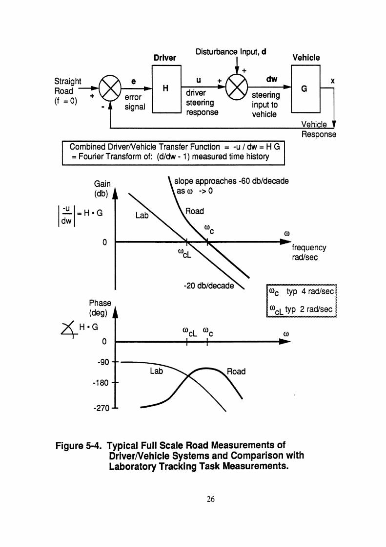
When similar experiments are conducted with drivers in full-scale vehicle tests or sophisticated moving-base simulators, 24, 25, 26, 27 the complexity of the plant (vehicle) dynamics is now increased. Measurements then show that the same madmachine transfer function becomes altered to that seen in Figure 5-4. From this we note several things. First, the slope of the gain function at low frequencies is significantly increased from that of the laboratory tests; second, the low frequency phase lag is also increased, thereby producing a characteristic parabolic-like shape of the total phase plot; and finally, the cross- over frequency, %, is increased. (The basic laboratory cross-over model result is included in the figure for direct comparison.) However, even though the frequency responses become altered and shifted, the shape of all the curves the vicinity of their res~ective cross-over freauencies, %, remains unchanped, with each maintaining a slope of -20 dbldecade. The key point to be made here is that unless a driver model, regardless of its origin, can pass at least the elementary validation test of exhibiting "cross-over modelu-like- behavior in the vicinity of its cross-over frequency, the model's legitimacy in terns of its ability to mimic human operator behavior will generally be held in question. Obviously, if a particular model can not only exhibit "cross-over model" behavior within the vicinity of its cross-over frequency, but can fit experimental measurements at other frequencies as well, its validity is further enhanced.

Human Plant f Operator Dynamics

U X G - Plant

joystick Output position Response

Gain

ManIMachine Transfer

Figure 5-3. Typical Laboratory "Cross-Over Model" Measurements of Human Operators in Compensatory Tracking Task Experiments

Phase (deg) A

3 H O G 0

-180

o , c o I

--1 ,

I Vehicle t Response

Disturbance Input, d Driver Vehicle

Combined DriverNehicle Transfer Function = -u 1 dw = H G = Fourier Transform of: (dldw - 1) measured time history

dw

steering input to

slope approaches -60 dbldecade

0

)frequency radlsec

Phase (deg) A

vehicle

G

Road

-270

x -

Figure 5-4. Typical Full Scale Road Measurements of DriverNehicle Systems and Comparison with Laboratory Tracking Task Measurements.

The importance of these observations for the TACOM driver model is that the very same transfer function characteristics seen for these full-scale experimental measurements are predicted by the TACOM model. To demonstrate, corresponding example calculations from the model are shown in Figure 5-5 using 1) a large passenger car (4000 lb), and 2) a loaded HMMWV (7500 lb) to represent the dynamics of the controlled vehicle in each case.

It can be shown l , that adjustment of the transfer function characteristics seen in Figure 5-5 is easily controlled through two basic driver model parameters. The first parameter which determines the amount of preview or "look ahead time used by the model, controls the slope of the low frequency end of the combined transfer function. Increasing the preview time decreases the slope at low frequencies and simultaneously decreases the corresponding phase lag as well. The other basic parameter determines the amount of neuromuscular time delay in the driver model and adjustment of it controls the frequency at which cross-over occurs in the combined transfer function plot. Consequently, a wide variety of basic man- machine behavior, as defined by such experimental measurements, can be accurately represented with this model through simple adjustment of only two basic parameters. Not surprisingly, the two model parameters that are key to controlling these adjustments are also parameters which represent the two central assumptions used in the development of the model: 1) recognition and use of preview within the model, and 2) presence of a driver time delay.

Prior to leaving this discussion, it should be noted that an analogous time-domain validation of the model is presented in Section 5.7 where driverlvehicle test track measurements for the HMMWV are compared with model predictions. Furthermore, a portion of those tesvmodel comparisons show new results for a driverlvehicle system operating under unusual nonlinear operating conditions and which heretofore have not been reported in the general literature. The measurements presented there offer further experimental confirmation of the validity of the driver model in predicting steering control behavior of drivers operating at or near limit maneuvering conditions.

5.4. Mathematical Formulation of the Preview Control Model

Tne material in this section shows the mathematical development of the preview control model and closely follows that of reference 1. The basic "computational mechanics" of the model is to first calculate, at each point in time, the steering control, uo, which will minimize the mean squared error between a desired path input, f, and the projected future lateral displacement of the vehicle, y, over a specified preview time interval, T. The "optimal" control, uO, is then delayed in time by an amount .r seconds. The time delay is used to represent the effective neuromuscular lag and characteristic limitation of the human

-=A=&- Passenger Car -d4- HMMWV Gain - db

2 3 4 5 6 7 8 9 10 Frequency - radlsec

Phase - deg

. . . . . 5 6 7 8 9 1 2 3 4 5 6 7 8 9

Frequency - radlsec 10

Figure 5-5. TACOM Driver Model Predictions.

operator in responding to external stimuli. The delayed steering control, u, is then used to steer the vehicle. This basic sequence is outlined in Figure 5-6.

As will be seen in the development which follows, the model is able to estimate the future response of the vehicle being controlled by utilizing an internal linearized dynamical representation of that vehicle within its own structure. Consequently, the driver model includes an internal "understanding" or "mapping" of the likely vehicle response resulting from a particular steering control input. Obviously, the better the internal linearized model is in representing the vehicle being controlled, the better will be the es- of the projected vehicle response.

The resulting driver model then has certain basic features. First, the model incorporates preview to "look ahead" and anticipate the desired path to follow. Second, the driver model possesses an internal linearized representation of the vehicle being controlled and uses that dynamical representation to predict/estimate the vehicle position and response at future times. Third, the control strategy used by the model is to minimize the previewed error between the desired path input and the future estimated vehicle position. And finally, the steering control obtained kom the error minimization calculation is delayed in time to account for human operator neurornuscular limitations in reacting to external stimuli.

These basic notions can all be expressed mathematically within the context of linear system theory. Following the mathematical formulation of the problem from references 1 and 2, we have for a given linear system,*

where,

X is the n x 1 state vector y is the scalar output related to the state by the n x 1 mT constant observer vector

-spa= F is the constant n x n system matrix g is the constant n x 1 control coefficient vector

and u is the scalar control variable.

-- -

I Bold face type denotes matrices and vectors.

optimal control, uo(t)

final steering control, u(t) = uo(t - D)

Figure 5-6. Sequence of Driver Model Calculations

We would like to find the control, uO(t), which minimizes a local performance index,

over the the current preview time interval (t, t + T) where,

W is an arbitrary weighting function over the preview interval (selected as a constant 1.0 for all of this discussion)

and, f is the previewed input.

The previewed output, y(q), is related to the current state, x(t), and fixed control, u(t), over the preview interval (t, t+T), by

y(q) = mT [I + x F"q-t)"/ n!] x(t)

+ (q-t) mT [I + Fyq- t tn I (n+l)!] g u(t) n=l (5.4-4)

The matrix, m

I + I?" (q-t)"/n! n= 1

is simply the state transition matrix for the linear system, F, and is frequently denoted as @(v,t)-

When the above general formulation is applied to the driver/vehicle path following problem, F and g represent the dynamics of the controlled vehicle, f is associated with the desired path input, and y with the lateral displacement of the vehicle.

Returning to the general formulation, the necessary condition that the derivative of J with respect to the control variable, u, be zero, leads to the equation for the optimal control, uO, given by,

00 { (q-t) mT [I + x F"q-t)'/ (n+l)!] g n=l

Because of the need to subsequently apply this formulation to systems containing "imperfect" human operators which possess known reaction time limitations and cannot therefore be expected to exhibit optimal control behavior, an alternate but mathematically equivalent formulation of equation (5.4-5) is shown below. This alternate formulation directly involves the previewed error quantity, e(q), which is being minimized in the original performance index of equation (5.4-3). The same optimal solution, uO(t), can therefore be expressed in terms of any current nonoptimal control, u(t), and the previewed error, e(q), as, rT oh) A(n) w(q-t)

uo (t) = u (t) +

where, 00

n=l and,

E(q) = f(q) - mT [I + x Fn (q-t)" / n!] x(t) - u(t) A(q) n=l

In this particular formulation, the current control is modified only in response to a nonzero function of the previewed output error, and thereby, is analogous to an integral controller. Note that the generality of the mathematics presented above allows it to be applied to a variety of control problems, assuming the controlled dynamical system can be expressed in tenns of equations (5.4-1) and (5.4-2).

In order to apply this generalized formulation to the driverhehicle path following problem, the F and g matrices must be associated with the directional dynamics of the vehicle being controlled. (In reference 1, F and g represent the directional dynamics of a two-degree-of- freedom automobile.) In addition, the resulting optimal control, uO(t), is assumed to be delayed an amount z seconds to account for the known neuromuscular delay of the driver. From this, the steering control for the driver model finally becomes,

u (t) = uO (t) e-ST (5.4-7)

where, e-ST, is the driver time delay, and uO (t) is given by equation (5.4-5 or 5.4-6).

The final steering control law is noteworthy for several reasons. First, it shows a direct dependence upon the dynamics of the controlled system (vehicle) through the presence of F and g in equation (5.4-5). This is important for driverhehicle systems since we know from experimental evidence that human operators, as part of man/machine systems, demonstrate great capacity for sensin and adapting to changes in the dynamics of the machine being controlled. 39 22, 26, 2\, 29, 30, 31, 32 Thus, when the driver model is used to steer different types of vehicles, or, when changes in the dynamics of the vehicle occur due to operating conditions, those vehicle-related effects arc nflected directly in the driver model through the F and g matrices appearing in the control law. (For applications involving significant nonlinearitits, or, paramem in the F and g matrices that may vary significantly over time, the F and g matrices may be updated continuously or intermittently to account for and represent the adaptive control behavior of drivers.) Secondly, the characteristic behavior of human operators to utilize preview as part of their control strategy, and the fact that human operators also have limited reaction times, are both incorporated in the model through the presence of the preview time parameter, T, and time delay parameter, z, appearing in equation (5.4-5) and (5.4-7). Variations in these two paramem can markedly affect the response and stability propexties of the closed-loop driver/vehicle system. F u r t h e m , as noted in section 5.3, adjustment of these same two parameters facilitates curve fitting the frequency response characteristics of the driverhehicle model to experimental data in the frequency domain,

The driver model equations, (5.4-6) and (5.4-7), can also be expressed in terns of a conventional control system block diagram as seen in Figure 5-7. In this diagram, H

Previewed Path Previewed Input Error

Predicted Driver Vehicle Driver Lateral Lag Dynamics Prediction Displacement

~p ' t ) *

Driver Gain

Driver Prediction

+ I

Figure 5-7. The Driver Model Shown in a Conventional Block Diagram Format

represents the time delay block of the human operator and is given by H = e-ST. The block (vector) denoted as G represents the directional dynamics of the vehicle (internal to the driver model) and relates the vehicle state response, x, to the driver steering output, u. The scalar constant, a, appearing in two of the blocks is given by,

and the constant gain vector, b, is given by the expression,

mT [I + Fn (q-t)" / n!]

The scalar, a, npnsents the driver's ability to predict that component of the future response of the vehicle deriving only from the current steering control input. The constant gain vector, b, represents the driver's ability to predict that component of the future vehicle response deriving only from the present state of the vehicle.

The dw history input to the block diagram, fp(t), is given by,

00

f(q) (q-t) mT [I + Fn (q-t)"l (n+l)!] g drl m1 (5.4- 10)

The quantities yo(t), yu(t), yp(t), ep(t), and fp(t) appearing in this diagram can then be interprcttd as:

fp(t) a weighted average of the previewed input (forcing function) over the preview interval (t, t+T)

y~(t) a weighted average of the predicted output response over the preview interval due to the current system state, x(t)

yU(t) a weighted average of the predicted output response over the preview interval due to the current control, u(t)

yp(t) a weighted average of the total predicted output response over the preview interval

ep(t) a weighted average of the previewed error over the preview interval

Note that the above block diagram and associated variables apply to the complete preview control fondation, wherein the minimization of the previewed error signal is occurring over the entire preview interval. If a simplification is introduced, so that the previewed error signal is being minimized or nulled out only at a single point, T* seconds ahead in time, the so-called "single-point" version of the preview model, as described in reference 1, is obtained. See the similar block diagram of Figure 5-8 for this model.

The "single-point" model is derived from the previous mathematical formulation by letting the arbitrary weight function, W(q-t), be equal to the Dirac delta function, 6(T*). In this diagram, the corresponding quantities y(t+T*), f(t+T*), and e(t+T*) are more directly and easily understood as the previewed plant output T* seconds ahead, the previewed input T* seconds ahead, and the previewed error signal T* seconds ahead, respectively. The corresponding constant gain, a*, is then provided by the somewhat simpler expression,

a* = (T*) mT [I + Fn (T*)" 1 (n+ 1 )!] g ml

and the constant feedback gain vector, b*, is seen to be,

b* = mT [I + Fn (T*)"/ n!]

The "single-point" model of Figure 5-8 is shown here primarily to present a simpler and mon obvious version of the analogous diagram in Figure 5-7. Reference 1 also includes a similar version of the "single-point" model in its discussion.

5.5. B t h e P r e v i e . . w Control Model to Steering of Basic Land Vehicla

Attention is now turned to applying the generalized results of section 5.4 to the problem of directional and path control of land vehicles by human drivers. The vehicle directional dynamics equations (F and g matrices of section 5.4) appearing in the original UMTRI driver model arc extended here to provide for single-unit vehicles controlled by three possible schemes: a) control through steering of the h n t andlor rear wheels, b) control by

'El E a - 8 i 2 2 p a Q L ;ii .si & A n

application of a pure yaw moment input, and c) control by means of both an applied lateral force and accompanying yaw moment. See Figure 5-9. Case a) applies to the conventional passenger car and single-unit vehicles such as the HMMWV. Case b) is primarily intended for applications involving tracked vehicles wherein the control torque, Mc, is applied by means of side-to-side longitudinal forces deriving from differential track speeds. Case c) is a generalized formulation intended to cover a broader range of future control possibilities as well as those represented by Cases a) and b).

For example, Case c) can duplicate a steered-wheel vehicle response by simply defining the control force as the product of the control variable and the tire cornering stiffness and then applying the control force at the forward non-steered wheel location. (The force control variable is in fact the steering magnitude, scaled by the cornering stiffness of the tire, of a an equivalent steerable wheel.) Likewise, Case c) can be used to duplicate a yaw moment control scheme, as given by Case b), by using a control force located at a very large forward distance, d, ahead of the mass center. This results in a sizeable yaw moment control accomplished through use of a very small lateral control force.

hoking first at the case of a single-unit vehicle having both front and rear wheel steering, the linemized vehicle dynamic equations are shown here:

where,

' denotes differentiation with respect to time

y is the inertial lateral displacement of the vehicle mass center

v is the lateral velocity in the vehicle body axis system

r is the yaw rate about the vertical body axis

y is the vehicle heading (yaw) angle

6f is the front tire steer angle, control variable

6, is the rear tire steer angle, control variable

and the parameters appearing in equations (5.5-1) -> (5.5-4) are:

U forward vehicle velocity

Caf, ar front and rear tire cornering stiffnesses

a, b forward and rearward locations of tires from the vehicle mass center

m, I vehicle mass and yaw inertia

The diagram of Figure 5- 10 further supplements these definitions.

The above equations can be simplified somewhat to represent rear wheel steering system implementations in which the rear wheels are proportionately slaved to the front wheel angle by a gain constant, k,

and thereby eliminating 6, as a second independent control input,

By also adding lateral force, B / m, and yaw moment, D / I, control terms, the equations (5.5-1) -> (5.5-4) can be written in a more general fom that now encompasses all the cases shown in Figure 5-9:

Figure 5-10. The Linearized Single-Unit Vehicle Model

41

where now,

u, takes on the role of the general purpose control variable (uc may be interpreted as either front wheel steer angle, lateral control force, or yaw moment control, depending upon the values of the control parameters A , B , C , a n d D ) .

and, A , B , C , and D are "control coefficients" specified to allow various types of

control schemes to be represented in the above equations.

For example, by specifying A and C as 1.0 and k = B = D = 0, the conventional front wheel steered vehicle is represented with uc interpreted as the front wheel steer angle control variable.

By specifying A = B = C = 0 and D as 1.0, a vehicle controlled by a pure yaw moment control (e.g., a tracked vehicle) is represented with uc now interpreted as the yaw moment control variable. In the case of the tracked vehicle, the sum of Caf and Ca would be interpreted as an equivalent lateral force "cornering stiffness" of the track element due to track sideslip. Different fore-aft values of Caf and Car could be designated to move the center of track side force forward or r e w a r d from the mid-wheelbase position, or equivalently, assign different levels of "front" and "rear" (single point) track side forces. The a and b parameters would be used to locate the tracked vehicle's fore-aft mass center location with respect to the equivalent "front" and "rear" side force locations. The resulting yaw moment control variable, u,, calculated by the steering model could then be expressed, if desired, in terms of a driver steering control movement through knowledge of the steering control gain (e.g., inches or degrees of stick movement per differential longitudinal track force) and the lateral spacing of the tracks.

The last control option, for representing a lateral force control scheme, A and C are selected as 0, B = 1.0, and D is the distance forward of the vehicle mass center at which the lateral control force, uc, acts.

Equations (5.5-6) -> (5.5-9) represent the internal set of vehicle dynamics utilized by the driver model for the category of single-unit vehicles. (The FORTRAN driver model code appearing in Appendix D utilizes these equations as the basis for its internal vehicle dynamics model.) The above equations can be expressed in state space terminology by defining the F, g, x, and m matrices of section 5.4 as,

For the case of an articulated vehicle, a similar but lengthier set of equations is produced and is shown in Appendix A. The equations in Appendix A are for a linear, constant velocity articulated vehicle having front steerable wheels as well as an articulation joint torque as control variables - similar in concept to a simplified LVS (MK48 Series). These equations could be used in a manner identical to those just presented to represent the internal vehicle model of the driver if greater accuracy was required, for example, to study driver steering interactions with, or dependencies upon, the dynamics of the rear unit. In this way, the more extensive set of articulated vehicle equations could be used to represent a driver's more complete "understanding" of the contributions of the rear unit (or even the articulation controller torque) to the directional control of the total vehicle.

In general though, driver steering control of most articulated vehicles can be adequately represented by the single-unit equations presented above. When doing so, the following interpretations and modifications of the vehicle parameters in the single-unit equations need to be applied:

the mass, m, and yaw inertia, I, now represent the mass and inertia of the lead unit plus that "contributed by the static vertical hitch load from the second unit

the a and b parameters locating the forelaft positions of the front and rear suspension centerlines, must now be altered to reflect the additional static vertical hitch load h r n the second unit

the tire cornering stiffness parameters need to reflect any changes resulting h r n the increased vertical loads

Refening to Figure 5-1 1, we see that the nominal single-unit parameters appearing at the top of the figure, become altered to those in the bottom portion of the figure due to the presence of the vertical hitch load contributed from the second unit. The driver model is then viewed as steering a single-unit vehicle having a total mass, mg + Fh, with a new "total c.g." location given by the modified parameters a' and b'. The tire cornering stiffnesses that now apply should also correspond to the new vertical tire loads Fzl' and Fz2'. (A more sophisticated and accurate method for representing the coupled inertial effects of multiple masses is described by ~ e h a ~ e . ~ ~ )

If a vehicle has more than one tire per side at a front or rear suspension location, the particular Eronflrear cornering stiffness parameter used in the model (Caf or Car ) should represent the sum of all the tire cornering stiffnesses per side at the fronthear suspension location. Similarly, the a and b parameters locating the total mass center of the vehicle should be from the centerline of the axle set for a particular front or rear suspension.

To illustrate the types of responses that are representative of the driver model when steering a single unit vehicle, a sequence of example calculations are now presented for two single unit vehicles having sigmficantly different sets of vehicle directional dynamics. The first vehicle is a conventional compact passenger car weighing 3000 lb; the other vehicle is a HMMWV loaded to a total gross weight of 7500 lb. The baseline maneuver for the examples that follow is a conventional 12-foot lane-change performed at a speed of 50 mph (73.3 ftlsec) over a forward travel distance of 100 feet. The driver model was used to steer the vehicle over this desired course and utilized a preview parameter of 1.50 seconds. The driver time delay parameter was fixed at 0.25 seconds. Figure 5-12 lists each of these parameters and shows a diagram of the desired path used in the example calculations. The vehicle parameter values seen in Figure 5-12 are based upon measurements and reasonable estimates.34

Identical calculations were performed for each vehicle for four different control cases comsponding to the following: A) control through front wheel steering only, A) control through h n t and rear wheel steering, with the front- to-rear-wheel ratio parameter, k, set at 0.75, C) control by means of an applied yaw control torque, and D) control through means

Single Unit Vehicle

I I I I mass

A rticula fed Vehicle

Fz2'=a'/(a'+p) (mg +Fh)

Figure 5-1 1. Interpretation of the Single-Unit Model Parameters when Steering an Articulated Vehicle.

"Desired" Path Input for Example Lane-Change Maneuver:

I vv

end

Baseline Vehicle Parameter Values

m 93.17 slugs

Caf 1 1,460 lblradian

Car 14,327 Iblradian

m 232.9 slugs

Caf 14,325 lblradian t

Car 19,196 lblradian

U 73.3 ftlsec

Figure 5-12. Parameter Values for Example Calculations

46

of an applied lateral control force. In cases C and D, none of the wheels are steered. The above cases correspond closely with those seen earlier in Figure 5-9. (The HMMWV is a specific hnt-only steering vehicle and reference to it in these other example cases is for the purpose of only providing a distinctly different set of directional dynamics for comparison with the passenger car directional dynamics.) Additional analyses appear in the 1986 Interim Technical Repurt 35 for this project.

The example calculations which follow utilize equations (5.5-6) - (5.5-9) for simulating the vehicle directional dynamics, and equations (5.4-6) - (5.4-7) for simulating the driver steering control. The equations were implemented in a digital simulation. Referring to Figures 5-13 and 5-14, example time history results are seen for the case of conventional front wheel only steering. The earlier "control coefficients" (A, B, C, D) seen in the vehicle dynamics equations have the values here of 1.0, 0.0, 1.0, and 0.0 respectively. Also, the front-to-rear-wheel steering ratio, k, is set equal to 0.0 in this fust example. As seen in Figure 5-13, the trajectories of both simulated driverlvehicle systems track the desired path quite well (bottom portion of the figure), even though significantly different steering control waveforms a- r e q w by the driver model for each vehicle (top portion). This is characteristic of the adaptive properties of the driver model (and most drivers) since the directional dynamics of each vehicle are completely different but still accounted for by the driver model. The corresponding time histories of Figure 5-14 show lateral acceleration and heading (yaw) angle results for each vehicle during the course of the simulated maneuver. The reduced level of damping exhibited by the HMMWV-driver system, in comparison to the passenger car-driver system, is not unusual since the HMMWV directional dynamics are significantly more oversteer (-3 deg/g) than the passenger car (1.2 deg/g), and such tendencies are frequently observed in closed-loop experimental tests. In practice, a driver could add more damping to the system by extending hisher preview time to a larger value.

In Figures 5-15 and 5-16 the same maneuver is repeated for both vehicles, with each now modified to include rear wheel steering (k = 0.75). In the top portion of Figure 5-15, the front wheel steering commands calculated by the driver model are seen for each vehicle, along with the corresponding rear wheel steering values (slaved at 751, in this example, of the front wheel steer commands). The calculated vehicle trajectories are seen on the lower portion of the figure. Again, as in Figure 5-13, the driver model manages to track the desired path quite accurately, even though significantly different steering control inputs are required for each vehicle by the driver model. The use of rear wheel steering is seen to increase the required level of steering from the previous example, while decreasing the peak amplitudes of vehicle yaw angle and lateral acceleration (Figure 5-16). Both driver-vehicle systems also exhibit a greater degree of damping when rear wheel steering is present. This

4,- Passenger Car * Loaded HMMWV Front Steer Angle - deg

4 Time - sec

Y Position - f t 14

200 300 400 X Position - ft

Figure 5-1 3. Driver Model Controlled Lane-Change Maneuver, front wheel only steering; k= 0

4-0- Passenger Car * Loaded HMMWV Lateral Acceleration cg - g's

.3

Yaw - deg 8

4 Time - sec

4 Time - sec

Figure 5-1 4. Driver Model Controlled Lane-Change Maneuver, front wheel only steering; k= 0

-04- Passenger Car front * Loaded HMMWV front -h-6 Passenger Car rear +++ Loaded HMMWV rear

Steer Angles - deg 3

4 Time - sec

Y Position - ft 14

200 300 400 X Position - ft

Figure 5-15. Driver Model Controlled Lane-Change Maneuver, front and rear wheel steering; k = 0.75

44- Passenger Car * Loaded HMMWV

Lateral Acceleration cg - g's

4 Time - sec

Yaw - deg 6

4 Time - sec

Figure 5-16. Driver Model Controlled Lane-Change Maneuver, front and rear wheel steering; k 0.75

observation is also supported by recent experimental tests of four wheel steering passenger cars. 36, 37, 38, 39

The next example calculation, seen in Figures 5-17 and 5-18 are for the same maneuver, but the two vehicles are now steered by means of an applied yaw moment control torque. Neither the front nor the rear wheels are steered in this example. Lateral motion is instead accomplished, as it is for a tracked vehicle, by rotating the vehicle in yaw through application of an applied moment to a certain sideslip condition, whereupon the non-steered wheels (or tracks) generate side force in reponse to sideslip. In this example, it is assumed that a physical mechanism is available (such as differential track speeds) which can generate an applied yaw control torque. The "control coefficients" in the previous equations then become: A = 0, B = 0, C = 0, and D = 1 with the control variable, uc, now interpreted as torque, instead of steer angle.

The calculations show that the preview model is quite capable of steering each of the example vehicles along the desired trajectory by means of the applied control torque. Time histories for the required yaw control torques for each vehicle are seen in the upper portion of Figure 5-17 and the corresponding trajectories in the lower portion of the figure. The difference in control torque magnitudes is due to the difference in mass and dynamics of the two vehicles. The results seen here are quite similar to those seen earlier in Figures 5-13 and 5-14 for the front steer only example calculations.

The fmal example calculation, seen in Figures 5-19 and 5-20, is similar to the previous one but employs a lateral control force, instead of a yaw control torque, for steering each vehicle, In this example, the control force is applied at a distance of 2 feet ahead of the mass center of each vehicle. Consequently the "control coefficients" become: A = 0, B = 1, C = 0, and D = 2. Again, the control force magnitude differences seen in the top portion of Figure 5-19 are primarily due to the mass and inertia differences of the two vehicles and the placement of the control force relative to the vehicle mass center. Locating the applied control force further ahead of the vehicle mass center scales down the required control force. Placing it very far ahead results in a near zero applied control force accompanied by an increased yaw moment, thereby approximating the previous case of control by means of an applied yaw moment only.

If the control force is applied right at the front axle position, the case of front wheel only steering is duplicated. The required control force in that case is equal to the product of the front tire cornering stiffness and the steering angle required from a steerable front wheel.

Regardless of the particular vehicle control mechanism used, the above examples demonstrate that as long as the preview control driver model has a simple means of

4 - Passenger Car +h+ Loaded HMMWV Yaw Control Torque - ft-lb

4 Time - see

Y Position - ft 14

200 300 400 X Position - ft

Figure 5-1 7. Driver Model Controlled Lane-Change Maneuver, Steering via an Applied Yaw Control Moment

44- Passenger Car * Loaded HMMWV Lateral Acceleration cg - g's

Yaw - deg 8

4 Time - sec

4 Time - sec

Figure 5-1 8. Driver Model Controlled Lane-Change Maneuver, Steering via an Applied Yaw Control Moment

44- Passenger Car * Loaded HMMWV Lateral Force Control - Ib

1 500

Y Position - ft 14

4 Time - sec

200 300 400 X Position - ft

Figure 5-1 9. Driver Model Controlled Lane-Change Maneuver, Steering via an Applied Lateral Control Force

44- Passenger Car * Loaded HMMWV Lateral Acceleration cg - g's

4 Time - sec

Yaw - deg 7

4 Time - sec

Figure 5-20. Driver Model Controlled Lane-Change Maneuver, Steering via an Applied Lateral Control Force

representing the dynamics of the vehicle and its control mechanism (via an internal vehicle model), it is capable of calculating an appropriate control variable time history which causes the vehicle to follow a prescribed path - and do so in a manner consistent with how actual human operators would steer a similar vehicle. To underscore this latter point, the following two sections of the report will present test data collected during the project, as well as direct comparisons between selected examples of that test data and corresponding predictions from the driver model.

5.6. Driver I Vehicle T e s ~

Closed-loop driverlvehicle tests were conducted during the project at the Chrysler Corporation Proving Grounds in Chelsea, Michigan. The primary vehicle used in these tests was an M1057 Truck also known as the HMMWV. The HMMWV was carrying a 3000 lb payload bringing its total weight to 7500 lb. Figure 5-21 shows a sketch of the basic HMMWV used in these tests, The 3000 lb payload was located directly over the rear axle thereby positioning the total mass center (of the vehicle and payload) at a point approximately 4 ft ahead of the rear axle and 4 ft above the ground.

A short sequence of additional tests were conducted with the same HMMWV pulling an MlOl trailer. In these tests, the HMMWV's weight remained at 7500 lb and the total trailer weight was 3160 lb (1600 lb of payload). The trailer mass center was slightly ahead of its axle, producing a vertical hitch load of 176 lb on to the HMMWV. Figure 5-22 shows a sketch of the MlOl trailer.

5.6.1. Inertial Parameter Measurements. The HMMWV was weighed in its test condition (with instrumentation and driver) to obtain front and rear tire loads and total weight. Estimates of yaw, pitch, and roll inertias were estimated or obtained from previous inertial measurements of the same vehicle at UMTRI. Likewise, total center of gravity height was estimated from previous empty vehicle inertial measurements and the known payload location. Measurements of wheelbase, wheel track, suspension locations, and overall geometry were also performed. Table 5-1 shows the parameter measurements and estimates for the HMMWV in its test condition.

5.6.2. Tire Measurements. One tire (size: 36 x 12.50 - 16.5 LT) from the HMMWV test vehicle was tested on the UMTRI flat-bed tire test machine to obtain lateral tire force measurements at four different nominal loads (1000,2000,3000, and 4000 Ib) and eight slip angles (-1, 0, +1, 2, 3, 4, 6, and 12 degrees). See Figures 5-23 and 5-24. Tire cornering stiffness parameters needed by the driver model in subsequent modeljtest

Figure 5-21. The MI037 Truck (HMMWV)

Figure 5-22. The M l O l Trailer 59

Table 5-1. Parameter Measurements and Estimates for the HMMWV in its Test Condition

Total Weight

Wheel base

Front Axle Load

Rear Axle Load

Distance from Total c.g Location to Rear Axle

Total Yaw Moment of lnertia

Total Pitch Moment of Inertia

Total Roll Moment of lnertia

Front Tire Cornering Stiffness (@ static load)

Rear Tire Cornering Stiffness (@ static load)

Total c.g. Height Above Ground

50.9 i n

70000 in-lb-sec2

60000 in-lb-sec2

13200 in-lb-sec2

270 lbldeg

335 lbldeg

Vertical Load (lb)

Figure 5-23. HMMWV Tire: Influence of Tire Inflation Pressure.

HMMWV Tire @ 20 psi

* 1OOOlbLoad * 2000 1b Load + 3000 1b Load * 40001bLoad

Slip Angle (deg)

HMMWV Tire @ 28 psi

* 1000 lb Load * 2000 1b Load * 3000 1b Load * 4000 1b Load

-400 - 1 0 1 2 3 4 5 6 7 8 9 1 0 1 1 1 2

Slip Angle (deg)

Figure 5-24. HMMWV Lateral Tire Force Measurements

validation activities, as well as complete lateral tire force representation within the DADS model 40, were based upon these measurements.

5.6.3. HMMWV Test Maneuvers. Three basic sets of driverhehicle maneuvers were conducted during the test program with the HMMWV test vehicle. (1) The first test maneuver was simple steady turning by a driver along a circular path . The purpose of this test was to obtain estimates of the vehicle understeer and basic cornering properties, as well as, driver closed-loop steering control behavior into and during the steady turning maneuver under different conditions. (2) The second maneuver was similar to the first, but braking was applied during the turning maneuver by the driver so as to bring the vehicle to a stop at randomly selected points along the curve. (3) The third type of maneuver was to drive through a set of different obstacle courses, as defined by a pattern of traffic cones. These tests are explained more fully in the following.

Driver-Controlled Constant Radius Turning Tests. The turning tests were conducted at 25, 50, and 60 mph with the test driver attempting to track a cone-marked turn of fixed radius (500 '). (A radius of 500 feet produces a lateral acceleration of 0.33 g's at 50 mph and was easily accommodated on the 800' x 800' Chrysler skid pad area) The maneuver was begun by having the driver approach the circular turn along a straight tangent and, then, track the curve at constant speed. See Figure 5-25. Transient driver/vehicle response information due to entering the curve, as well as steady-state driverlvehicle response information due to tracking the curve, was gathered from these tests. Influence of forward speed and lateral acceleration upon system damping was obtained by conducting the same tests at the three different speeds. Vehicle turning properties, such as understeer level and steering control gains, were also derived from the steady turning data in these tests. Further, since both front wheel angles and steering wheel angle were being measured, estimates of the effective steering gear ratio and steering system compliance properties were available from these tests.

Driver-Controlled Braking-in-a-Turn Tests. The braking-in-a-turn tests were all conducted from an initial speed of 50 mph with the test driver attempting to stop the vehicle in a fned distance. The stopping distances were varied randomly, thereby requiring the driver to achieve different deceleration levels during each stop. This type of test served as a closed-loop braking control task for the driver, while simultaneously, yielding information on the basic braking performance capabilities of the test vehicle. Wheel lock-up occurrences were recorded for the shorter stopping distance cases. The driver brake pressure responses and corresponding deceleration time histories would be used to evaluate and outline a proposed closed- loop braking algorithm for the driver, augmenting the driver steering control model.

cones

0 Steady Turning 0 Portion

Figure 5-25. Driver Controlled Constant Radius Turning Test

64

Obstacle Course Tests. The purpose of these tests was to gather transient driver/vehicle response data for both path-following and obstacle avoidance maneuvers. The basic type of maneuver consisted of performing various lane-to- lane movements with the vehicle as it traverses a cone-marked course. Tests were conducted at different speeds from 30 to 60 mph. Three basic obstacle course patterns were layed out and are shown in Figures 5-26 through 5-28:

A) Simple Path-Constrained Lane Change (Figure 5-26)

B) Simple Unconstrained Lane Change (Figure 5-27)

C) Obstacle Course (Figure 5-28)

The first two cases were included primarily to evaluate the influence of path constraints on driver steering control behavior. The constrained lane width in each of these tests was maintained at 12 feet, leaving the driver with about 2.5 feet of lateral maneuvering space with the vehicle centered in the lane. The remainder of the obstacle course tests took place with the layout shown in Figure 5-28. In these tests, the fore-aft distances between the 12' x 12' square obstacles were varied randomly from test to test.

In the lane-change tests, the baseline geometry, with the shoot-to-shoot forward travel distance (L) set at 100 feet, produced approximately 0.30 g's of peak lateral acceleration during the 60 mph maneuvers. The same course geometry was used for the 30 mph tests in order to evaluate the influence of forward speed upon driver preview and system damping.

In the obstacle course tests, the baseline geometry seen in Figure 5-29 produced peak lateral acceleration levels of about 0.4 g's with the obstacles located in their normal baseline positions. Tests were repeated several times, with the distances L1, L2, and L3 varied in a random-like sequence. The values of L1, L2, and L3 were set to 100 feet in the baseline course geometry. L1 and L2 were then varied forward or rearward by 20 feet to produce a 'short' or 'long' variation respectively from the nominal baseline geometry. The test driver continuously drove the vehicle dynamics oval - encountering a different obstacle course layout each time around the track. Data collection began several seconds prior to the beginning of the obstacle course and ended several seconds after the end of the obstacle course.

Table 5-2 is a listing of the log sheets from the test program. Run numbers and speeds are seen in the frst two columns. Column 3 defines the test maneuver. Column 4 contains

nes

(not to scale)

Figure 5-26. Path-Constrained Lane Change Maneuver

66

/ Cones

(not to scale)

Figure 5-27. Unconstrained Lane Change Maneuver

67

to provide lateral accel.

L1, L2, L3 varied randomly from test to test

(not to scale)

Figure 5-28. Basic Obstacle Course Layout

68

Figure 5-29. Baseline Obstacle Course Layout Used in Tests

69

Table 5-2. Log Sheet Summary of Driver-Vehicle Tests

Run

101 1 0 2 103 1 0 4 1 0 5 1 0 6 1 0 7 1 0 8 1 0 9

, 1 1 0 111 1 1 2 1 1 3

1 1 4 1 1 5 1 1 6 1 1 7 1 1 8

, 1 1 9 1 2 0 1 2 1 1 2 2 1 2 3 1 2 4

1 2 5 . 1 2 6

1 2 7 , 1 2 8 , 1 2 9 . 1 3 0

131 1 3 2 1 3 3

, 1 3 4 1 3 5 1 3 6 1 3 7 1 3 8 1 3 9

Maneuver

Steady Turning n

n

11

n

I

n

n

n

n

n

n

n

Braking in a Turn n

n

7 n

H

n

n

n

I'

I,

Constrained Lane Change M

n

n

n

n

I(

n

n

n

n

n

n

ll

n

&peed (mph)

5 0 5 0 5 0 5 0 5 0 2 5 2 5 2 5 2 5 2 5 5 5 5 5 5 5

5 0 5 0 5 0 5 0 5 0 5 0 5 0 5 0 5 0 5 0 5 0

5 0 6 0 "

" " " " " "

3 0 " " " "

Comments

28 psi tire pressures, driver #1

sign of Ay changed to proper SAE convention

some swerving 5 mph fast at end

lost velocity signal during run lost yaw rate during run

21 5' stopping distance 170 ' 195 ' ,

145 ' 132 ' 195 ' 195 '

130', left rear wheel locked, 37' of skid 140 ' 130 '

125', left rear wheel locked, 34' of skid

12' x 100' , 28 psi tire pressures

lost velocity siqnal at end of run

re-fueled

A

Table 5-2. Log Sheet Summary of Driver-Vehicle Tests (continued)

Run #

. 1 4 0 141 1 4 2 143 144 1 4 5 1 4 6 1 4 7 148 149 1 5 0 151 1 5 2 1 5 3 1 5 4 1 5 5 156 1 5 7 1 5 8 1 5 9 160 161 1 6 2 1

, 1 6 3 1 1 6 4

. I 6 5 1 1 6 6 1

, 1 6 7 1 6 8 1 1 6 9 1 1 7 0 171 1 7 2 1 7 3 1 7 4 1 7 5 1 7 6

, 1 7 7 1 7 8 179 1 8 0

Speed (mph)

3 0 " "

4 0 5 0 6 0 3 0 3 0 3 0 6 0 6 0 6 0 6 0 6 0 3 0 3 0 3 0

1 3 0 4 0

1 5 0 1 4 0

4 0 " "

1 " " " " " " " " " " " " " " " " "

Maneuver

Constrained Lane Change I

" II

" "

Jnconstrained Lane-Change " " w

I

" I

"

Temporary Obst Course

II

Obstacle Course Obstacle Course

" " a

a

I 4

(I

tl

I

I!

I

" " " " I

" " I

e l

" I

Comments

driver #2 driver #2 driver #2 driver #2 driver #2

12' x 1 OO', driver # I , no cones hit " " " W

n

driver #2, hit numerous cones driver #2, no cones hit

driver #1 n

n

see Fig 5.6-6, driver #1, centerlcenter n

n

11

n

centerlcenter, hit obstacle #2 on right centerlshort centerllona centerllong

centerlshort centerlcenter shortlcenter

longlshort, hit second obstacle lonalcenter

s h o r t l l ~ n ~ , (obst #2 width=9.5') centerllong (obst #2 width=9.5') longllonq, (obst #2 width=9.5')

longllong centerlshort

shortlshort, clipped obst #2 centerlcenter

longlcenter, clipped obst #2 lon(l/short, hit obst #2

Table 5-2. Log Sheet Summary of Driver-Vehicle Tests (continued)

Comments

longtshort, hit obst #2, clipped cone on exit centertcenter, c l i p~ed obst #2

centerlcenter shortlshort

longllong

driver #2 w

I(

" w

n

w

n

w

w

speed low w

w

w

w

(I

143' stopping distance 120', short lockup F & R

170' 195'

130', all locked, slight drift to right 140' 150'

200', short lock at end 170' 150' 200'

125', F & R lock 145' 150' 175'

Maneuver

Obstacle Course II

Il

H

I(

Random Steer Tests " w

w

" n

w

" w

I

w

Il

w

w

a

w

w

Straight-Line Braking tl

w

a

I

w

w

Il

w

w

w

w

w

I'

n

Run

- 181 182 183 184 185

186 187 188 189 190 191 192 193 194

, 195 196 197 198 199 200 201 202

20 3 204 205 206 207 208

.209 , 210 211 212

, 213 214 215 216

; 217

#'Speed (mph)

40 " " " "

30 30 30 50 60 " " " "

30 30 60 60 45 45 30 60

5 0 " " " " " " " " " " " " " "

Table 5-2. Log Sheet Summary of Driver-Vehicle Tests (continued)

Run #

218 219

, 220 . 2 2 1 , 222

223 224

225 , 226

2 2 7 228 229 230 231

232 233

, 234 235 236 237 238 239

240 241 242 243 244

, 245 246 247 248

, 249 250 251 2 5 2 253

Maneuver

Steady Turnina I

I

I

I

I

I

Random Steer Test I

I

I

I

I

I

Random Steer tests I

I

I

I

I

I

I

Steady Turnina I

I

I

I

I

I

" I

I

(I

I

n

I

Speed (mph)

2 5 " " "

5 0 " "

3 0 3 0 3 0 6 0 6 0 6 0 6 0

3 0 3 0 3 0 5 5 6 0 6 0 6 0 6 0

2 5 2 5 2 5 5 0 5 0 5 0 6 0 6 0 " " " " " "

Comments

all tires at 28 psi I

I

I

I

I

I

all tires at 28 psi n

I

I

" (start tape seg 5) I

I

all tires set to 22 psi HOT (were 29-32) I

I

" I

I

I

I

all tires set at 20 psi HOT

oradual heating of tires during this sequence.

I

tire pressures up to 24-26 psi rear tire pressures set back to 22 psi HOT

Table 5-2. Log Sheet Summary of Driver-Vehicle Tests (continued)

Run

2 5 4 255 256 257 258 259 260

. 261 262 263 264 265 266 267

- 271 272

- 273 274 275

, 276 , 2 7 7

278 279

, 280 . 281

282 283 284

, 285 286 2 8 7 288 289 290

Maneuver

Constrained Lane-Change I

I

I

H

I

I(

H

I

I

I

I

I

ConstrainedLaneChange I

I

H

I

I

I

I

I

I

I

I

I

I

I

I

I

H

H

dSpeed (mph)

-- 3 0 3 0 3 0 6 0 6 0 6 0 3 0 3 0 3 0 3 0 6 0 6 0 6 0 6 0

2 5 2 5 2 5 2 5 3 5 4 3 4 8 4 8 4 6 4 ? 5 0 4 8 4 8 2 5 2 5 2 5 4 5 4 8 4 6 4 8

Comments

all tires set at 28 psi I

H

I

I

tires up to 32 psi HOT all tires reduced to 20 psi HOT

I

H

u

H

" (tape segment 6) W

H

HMMWV & Trailer, 30 psi / 82 psi H

I

H

n

I

H

H

H

I(

I

H

21 psi / 30 psi / 82 psi I

I

I

I 8

I

I

I

Table 5-2. Log Sheet Summary of Driver-Vehicle Tests (continued)

Run #

291 292 293 294

, 295 296 297 298 299 3 0 0 301 3 0 2

. 303 304

. 305 3 0 6

, 3 0 7 . 308

3 0 9 3 1 0

Speed (mph)

2 5 2 5 2 5 3 5 3 8 4 2 4 1 4 5 4 3 4 4 4 5 4 6

4 5 4 5

, 5 0 5 0 5 0 5 0 5 0 4 8

Maneuver

Steady Turning n

n

n

n

n

n

n

n

I

n

n

Braking in a Turn n

I

I

n

n

I

n

Comments

HMMWV 81 Trailer, 30 psi1 82 psi . n

I

n

n

n

n

hit some cones II

n

n

n

180' stoppina distance, wheel lock 220 ' 170 '

180', hummer locked all, 50' skid marks 143 ' 169 '

147, intermittent lockups, 25' skid marks. 145 '

,

Table 5-2. Log Sheet Summary of Driver-Vehicle Tests (continued)

Run

320 321 322 323 324 325 326 327 328 329 330 331 332 333 334 335 336 337

, 338 339 340 341 342 343

.344 345 346 347 34 8

#Speed (mph)

45 45 48 x 45 50 50 55 55 58 60 57 58 62 63 63 40 40 40 40 45 40 40 40 35 35 35

accel accel

Maneuver

Divergence Tests " " "

" " " " " " II

u

I

I

Oscillation tests u

n

"

R

W

" " W

" " a

Comments

HMMWV & Trailer, Divergence Tests, ", video #3 ", video #4

u

" u

" " W

" W

n

", video #8 " I

I

HMMWV & Trailer, Oscillation Tests

speed not constant

"small" steer input disturbance "medium" steer input disturbance

"large" steer input disturbance "small" steer input disturbance

"medium" steer input disturbance "large" steer input disturbance

u

a

additional comments specific to each test. Two additional test maneuvers for the HMMWV arc listed in the log sheets of Table 5-2 as "Random Steer Tests" and "S traight-line Braking". These tests were conducted initially as "additional" tests to provide further data onsthe directional dynamics and braking characteristics of the HMMWV. It turned out that the information provided by these additional tests was not subsequently needed in the model validation. However, the data from these additional tests are available as part of the entire collection of test data being delivered to TACOM and can be used as a source of additional information. The "Straight-line Braking" tests were conducted in the same manner as the braking-in-a-turn baseline tests (but without any turning) with the stopping point varied in a random manner. The stopping distances are noted in the log sheets of Table 5-2. The "Random Steer" tests wen conducted during straight-line driving with the test driver producing a random-like steering input to purposely excite the vehicle directional dynamics across a range of steering input frequencies. Fourier transforms can be performed on these measured vehicle responses and the steering input to obtain frequency response characteristics for the open-loop directional dynamics of the vehicle.

Example measurements from each of these basic tcst maneuvers appear in Appendix B. The total set of data collected during the tcst program are being delivered to TACOM on floppy disks in a standardized UMTRI format

5.6.4. Data Acquisition Equipment Test data was collected using the UMTRI portable data acquisition system. The system consists of a Texas Instruments 'I'M 990 microprocessor, signal-conditioning units, p r o ~ ~ b l e filters, and analog/digital converters. A CRT unit and keyboard were used to operate and control the system. Data were stored on high capacity digital tape cartridges for subsequent post-processing. Simple statistical calculations and background calibrations could be performed in the field. Spot checks of the collected data would occur periodically throughout the duration of the test program to guard against undetected instnunentation failures. AU of the test data collected during the program were transferred to hatd disks and floppies in an UMTRI standard fonnat for subsequent plotting and analysis.

5.6.5. Vehicle / Driver Measurements. The vehicle was instrumented with appropriate transducers and the UMTRI data acquisition package to measure the following signals and vehicle responses:

Lateral Accelexation

Longitudinal Acceleration

Vehicle Velocity

Yaw Rate

Roll Angle

Eront Wheel Steer Angles (left and right)

Steexing Wheel Angle

* Brake Pedal Pressure

The UMTRI stable platform was used to measure the vehicle lateral and longitudinal accelerations, as well as the yaw rate and roll angle, relative to a horizontal plane oriented normal to the gravity vector. A conventional fifth wheel was used to measure forward velocity. Front wheel angles were measured with linear potentiometers, driver steering wheel angle with a rotary potentiometer, and driver brake pedal force with a hydraulic pressure transducer.

5.6.6. Special HMMWV-Trailer Tests. A sequence of baseline articulated vehicle tests were also conducted using the single-axle MlOl trailer attached to the HMMWV via its rear pintle-hook. The trailer load was located approximately over the trailer axle, producing a vertical hitch load of 176 lbs at the HMMWV pintle hook. The dynamics of the trailer, and its possible effect upon driver steering control activity, were evaluated during a repeat of several of the lane-change and circular turning tests. Using the test data collected under this project, Mousseau in a TACOM technical report,41 fully analyzed the HMMWV-trailer combination vehicle using the DADS simulati~n.~

In addition to the baseline tests studied by Mousseau, a short series of straight-line stability tests were also conducted with the trailer payload located in an adverse rearward location, thereby exciting a limit-cycle response in the articulation motion. The resulting driver steering action in response to the limit cycle motion was later analyzed and compared with results h m comparable simulation runs. A short tahnical paper 42 reporting on some of these special tests appears in Appendix G of this report.

Example measurements from the HMMWV-Trailer test program appear in Appendix C. As in the case of the HMMWV data, all the trailer test results are being delivered to TACOM on floppy disks in a standardized format.

During all of these tests, the MlOl trailer was instrumented with three additional transducers to measure the following vehicle responses:

Trailer Lataai Acceleration

HMMWV-Trailer Articulation Angle

and Trailer Roll Angle

The last portion of Table 5-2 lists the HMMWV-trailer tests. Tests 27 1-310 correspond to the HMMWV-trailer in its normal loading state as reported on by ~ o u s s e a u . ~ ~ Tests 336- 348 ("Oscillation Tests") correspond to the straight-line stability tests with the trailer loaded in an adverse rearward manner in order to excite the limit cycle trailer oscillations. Tests 320-335 ("Divergence Tests") had the trailer payload located in the far forward position, but produced no significant instability or difficulty for the driver. A video tape was also produced at the time of these tests to record several of the trailer oscillation responses for later analysis.

5.7. Driver Model Validation

The material presented in this section of the report validates the developed steering control model by comparing example test results directly with corresponding predictions from the model. In most of these comparisons, the driver model is used in conjunction with a linear vehicle In cases involving significant nonlinearities, fully nonlinear vehicle models 79 40 are used with the same driver model to represent the vehicle. The parameters selected for the vehicle model were based upon the measured and estimated values obtained during the course of the project as reported in the previous section and by Mousseau. 4 1 Table 5-3 lists the basic vehicle and driver parameters used in most of these validation calculations. Any changes in speed, tire properties, or driver parameters for the individual comparisons that follow are noted and explained in the corresponding discussions for each case.

The fast series of tests examined are for the constrained lane-change maneuver at the nominal speed of 60 mph. Figures 5-30 and 5-31 show a comparison between experimental measurements and predictions from the TACOM driver model. Tests 126, 127, 129, and 130 represent four repeated runs by the test driver through the constrained lane-change test course seen in Figure 5-26 at 60 mph, The driver steering wheel angle and lateral acceleration signals seen in these two figures are direct measurements. The experimental lateral displacement and yaw angle signals are obtained from the measured data by doubly integrating the lateral acceleration and singly integrating the yaw rate measurements respectively over the time interval shown. The thick dark line represents the output from the model using an identical 1 2 4 by 100-ft lane-change course as that used in the tests for its desired path input. Preview time and driver lag values were selected as 1.1

Table 5-3. Baseline DriverlVehicle Parameters Used in Validation Calculations

Driver Model Preview Time

Driver Model Delay Time

Total Vehicle Weight

Wheelbase

Front Axle Load

Rear Axle Load

Distance from Total c.g Location to Rear Axle

Total Yaw Moment of lnertia

Total Pitch Moment of Inertia

Total Roll Moment of lnertia

Front Tire Cornering Stiffness (@ static load)

Rear Tire Cornering Stiffness (@ static load)

Total c.g. Height Above Ground

1 .I sec

0.1 sec

50.8 i n

70000 in-lb-sec2

60000 in-lb-sec2

1 3200 in-lb-sec2

270 lbldeg

335 lbldeg

Driver Steering Wheel Angle - deg

4 time - sec

Lateral I

4 time - sec

Figure 5-30. Driver Model Validation, Constrained Lane-Change

Lateral Acceleration - g's

0 2 4 6 8 time - sec

Heading Angle - deg

2 4 6 time - sec

Figure 5-31. Driver Model Validation, Constrained Lane-Change

seconds and 0.1 seconds respectively to provide the degree of matching observed in Figures 5-30 and 5-31.

The relatively small value of the driver time delay parameter (0.1 seconds) is an interesting result. Recall from section 5.3 that most previous research involving random excitation of driver vehicle systems suggests that the TACOM driver model can best match such data by using a value of approximately 0.25 seconds ( l l q , or, 114 radlsec) for this parameter. However, these results are based upon closed-loop tests involving passenger cars. One explanation of this apparent conflict may be that because the HMMWV is more sluggish in its directional dynamics than a conventional passenger car, the driver of a HMMWV is required to provide more lead time and anticipation in order to perform a comparable maneuver. Another explanation may be that the lane-change tests conducted here were highly repeatable and easily predicted by the driver. Consequently, the "processing time" required by the driver to obtain an appropriate steering input for these tests may be considerably less than if the path input was less predictable. A reduction in driver processing time would then be reflected in the driver model by a smaller value of the driver time lag parameter. However, a previous study 44 which examined lane-change tests with drivers of passenger cars and then represented the results with a similar version of the TACOM model, concluded that values of 0.2 to 0.3 seconds were appropriate in representing driver steering control time delay characteristics for that vehicle in a nearly identical lane-change maneuver. This would then seem to suggest that the differences raised here in driver time delay characteristics are somehow related to the directional dynamics of the controlled vehicle.

To illustrate this point further by example, if a driver model time lag value of 0.25 seconds is used instead of the 0.1 second value for the same HMMWV calculation just presented, the preview time parameter must correspondingly be increased to maintain the same degree of damping shown in the test data. This then results in a somewhat more sluggish response from the model with most of the resulting waveforms having a longer period than that seen in the test data. Figures 5-13 and 5-14, for example, previously showed a calculation for the HMMWV using a larger set of time delay and preview time parameters. The result was a considerably more sluggish response than that seen in Figures 5-30 and 5- 31.

The suggestion that the TACOM driver model time delay parameter should be reduced in certain cases to values less than those previously suggested by random disturbance tests 24, 259 26 is an important result. This finding may suggest that drivers of land vehicles having more sluggish directional dynamics are required to be more responsive during typical steering maneuvers in order to compensate for the increased lag of the vehicle. Intuitively, this makes sense, but heretofore, this observation about the responsiveness of

drivers and the directional responsiveness of vehicles has not been adequately established and linked to experimental evidence from full-scale tests of driverhehicle systems.

A less obvious suggestion that driverlvehicle systems are not necessarily any more stable with shortened driver lags follows from the observation that the preview time is apparently reduced "in step" with the driver lag for the lanechange data collected here. (Ordinarily, experimental measurements obtained fiom random disturbance tests 26 of passenger car / driver systems would suggest values of the time delay parameter on the order of 0.25 seconds, and values of the preview time on the order of 1.5 to 3.0 sec0nds.l) Recall that reductions in stability' occur in the model for either an increased driver time lag or a reduced driver preview time. Consequently, similar stability margins can be maintained in the model to some extent by compensating increases in one parameter with increases in the other parameter. Any such apparent "correlation" between driver time delay and preview time thereby allows the driver to maintain approximately the same level of closed-loop system stability as a corresponding, but less responsive, driverlvehicle system having a larger time delay and longer preview time. It may be that drivers, under tight maneuvering conditions, only look far enough ahead to negotiate the next immediate "obstacle," thereby requiring a shortening of their preview time during such maneuvers. In order to maintain a desired level of stability, drivers may then decrease their time delay cycle through faster information processing under such circumstances.

Along this line, MacAdam in 1983 hypothesized that drivers could possibly "trade off' directional stability for improved path tracking capabilities, This work however assumed that the driver time delay parameter (e.g. 0.25 seconds) was largely invariant based upon the measurements of the previous research using random disturbance input testing. The findings reported here, however, seem to suggest instead, that depending upon the vehicle being controlled, drivers have more control over their time delay characteristics than previously observed, and, that no such "trade off' between directional stability and path tracking performance need necessarily occur.

To further support the observation linking reduced driver time lag characteristics and the HMMWV test vehicle, the unconstrained lane-change maneuvers also conducted during this testing clearly demonstrated that both test drivers (during the sequence of lane-change tests 125 through 153; constrained and unconstrained) exhibited even more responsive behavior when the lane-change course was unconstrained than when the course was constrained. The basic observation was that the test drivers acted with more of an "open- loop" steering manner in initiating the unconstrained lane-change maneuver, moving quickly from the initial lane to the second lane. This was then followed by a more apparent "closed-loop" steering control pattern to stabilize the vehicle in the second lane. To illustrate this point, Figure 5-32 shows a comparison of steering and lateral displacement

Driver Steering Wheel Angle - deg

0 1 2 3 4 5 6 7 time - sec

-4- Test ID 126, constrained & Test ID 149, unconstrained

Lateral Displacement - ft

2 3 4 time - sec

Figure 5-32. Constrained vs. Unconstrained Lane-Change Test

Lateral Acceleration - g's

2 3 4 time - sec

-a*- Test ID 126, constrained 111&.6 Test ID 149, unconstrained

Heading Angle - deg

2 3 4 time - sec

Figure 5-33. Constrained vs. Unconstrained Lane-Change Test

time histories for test 126 (constrained) and test 149 (unconstrained). Note the more responsive and aggressive behavior exhibited d u b g the unconsuained test. This appeared to be a typical trend for most of the constrained vs. unconstrained comparisons. Figure 5- 33 shows carresponding lateral acceleration and yaw angle comparisons from the same two tests. Again, the unconstrained response is more rapid, particulariy during the reversal and correction phase of the maneuver. It was also visually apparent to observers at the time of these experiments that the test drivers were performing the unconstrained lane-changes more quickly and aggressively.

This observed behavior pattern during the unconstrained lane-change maneuvers seems to raise the question for users of the driver model as to what an "appropriate" desired path input should be in cases where portions of the desired trajectory are illdefined. In the case of the constrained lane-change manewer, the 12-ft x 100-ft trajectory is quite obvious since it represents the centerline of the constrained course. However, when the middle of the course is opened up, as in the unconstrained case, a corresponding desired path is not as obvious. Based on the above test results though, it appears that a more rapid lane-change path input is appropriate in such cases, for example, a 1 2 4 x 75-ft, or possibly, a 12-ft x 5Gft trajectory. In any event, a "bandwidth limit" for the driver-vehicle system will eventually be reached as the trajectory approaches a step-like input with the corresponding driver-vehicle reponse representing the bound for the system. Ordinarily, matching of the model with such data can be accommodated by selecting appropriate path inputs in combination with a representative set of driver time lag and preview time parameters. In the unconstrained example just seen, a 1 2 4 x 50-ft trajectory would better permit the model to reproduce the responses observed in the test data.

The next example of validating the driver model predictions is presented in Figures 5-34 and 5-35 for the baseline obstacle course maneuver of Figure 5-29. In this maneuver, the vehicle speed is maintained at 40 mph as the driver steers the vehicle from the left lane to the right lane around the first obstacle. The vehicle is then steered back to the left, around the second obstacle, and then to the right lane again to exit the course (positive values of lateral displacement in Figure 5-34 arc to the right on the test course). In this example comparison, runs for the "centerlcenter" positioning of the obstacles were selected (test numbers 168, 178, 182, and 183 from the log sheets of Table 5-2). The "centerlcenter" obstacle arrangement had equal longitudinal gaps of 100 ft between each of the obstacles, as well as at the entrance and exit portions of the course (i.e., L1 = L2 = L3 = 100' in Figure 5-28). Figures 5-34 and 5-35 show an overlay of the four "centerfcenter" tests and the predicted response from the drivu model. Also seen in the trajectory overlay portion of Figure 5-34 are the locations of the two obstacles.

Driver Steering Wheel Angle - deg 80

4 6 time - sec

8

Lateral Displacement - ft Tests 168, 178, 182, 183

100 200 300 400 500 600 700 Longitudinal Displacement - ft

Figure 434. Driver Model Validation, Obstacle Course, 40 mph

Lateral Acceleration - g's .6

4 6 8 time - sec

Heading E 15

4 6 time - sec

Tests 168, 178, 182, 183 - TACOM Driver Model

I VI I I

Figure 5-35. Driver Model Validation, Obstacle Course, 40 mph

Unlike the previous lane-change tests in which the course geometry remained static, the geometry of the obstacle course was varied to some extent from test to test by random longitudinal placement of the two obstacles. The exact placement of the obstacles was unknown to the test driver until the vehicle entered the obstacle course. Despite this, the test driver was still able to replicate with some accuracy the same basic response during each of the tests seen in Figures 5-34 and 5-35.

The driver model preview time and time delay parameters used for the obstacle course validation calculations were the same values used in the previous lanechange validation (1.1 and 0.1 seconds respectively). The desired path used as the input to the driver model was simply taken as the "center-line" of the course and defined here as seven straight-line segments:

C- 175' straight-line to entrance of course c- entrance point of course c- 100' gap to first obstacle c- 12' width of first obstacle <- 100' gap to second obstacle c- 12' width of second obstacle <- 100' gap to exit of course C- straight-line exit out of course

As seen in these figures, the model predictions are in very good agreement with the measured responses. Again, as in the previous comparison, the lateral displacement and yaw angle measurements were obtained from integration of the lateral acceleration and yaw rate measurements over the length of the course. The longitudinal displacement signal (Figure 5-34) was obtained by integration of the fifth-wheel forward speed measurement.

In the "Comments" field of the log sheets (Table 5-2) for run #182, it is noted that obstacle #2 was "clipped" during this test. This can be seen as well in the test &ta of Figure 5-34 in which one of the test trajectories (from run #182) records a value of lateral displacement of about 3.5-ft at the 390-ft mark of longitudinal displacement. Since the half-width of the HMMWV is about 3.25-ft at the outside of the tires and an indicated clearance of only 2.5 is seen at the point shown, this particular trajectory would produce wheel or body contact with obstacle #2.

Finally, a sequence of frames from a simplified computer animation program is shown in Figures 5-36 through 5-39 to illustrate the response and trajectory of the vehicle during the obstacle course maneuver. The frame number and time (corresponding to that in Rgures 5- 34 and 5-35) are noted in the upper left comer of each frame. The locattion and orientation

of the vehicle at each of the animation positions can be coordinated with the time histories of Figures 5-34 and 5-35 through the time parameter shown in each frame. The observer during this animation sequence is at a forward position of 400 ft, a lateral position of 200 ft, and an elevation of 100 ft.

The next maneuver examined during the validation exercise is that of steady turning (to the left) along a circular arc of 500 ft radius. As noted in section 5.6, tests were conducted at different speeds and tire inflation pressures in order to study the response of the driverlvehicle system under different lateral acceleration conditions and for different sets of vehicle directional dynamics, A sequence of figures is presented in the following discussion which compares the predicted response of the TACOM driver model and simulated vehicle with corresponding measurements from a number of steady turning tests.

The first comparison, shown in Figures 5-40 and 5-41, is for a low speed (24.5 mph), low lateral acceleration operating condition. Figure 5-40 shows the steering wheel angle input from the driver and the left front wheel angle at the road. Figure 5-41 shows the corresponding lateral acceleration and yaw rate relative to a stable platform oriented normal to the gravity vector. The HMMWV was loaded as before in its baseline configuration with all tires inflated to 28 psi. Measured signals from tests 219, 220, and 221 are shown overlayed . ,. with the prediction £?om the TACOM driver model. The same linear vehicle model 4j was used to represent the HMMWV dynamics. As seen in these two figures, the three test results and the model predictions are in close agreement. Since, the vehicle is turning on a circular arc and at low lateral acceleration, the front wheel angles should be close to the Ackerman steer angle, L/R, equal here to (130112) / (500) 57.3 degrees, or, 1.24 degrees. The test data and the model both indicate measured values in that range. The measured and predicted values are slightly smaller than the Ackerman value due to the modest oversteer condition of the vehicle and the 0.08 g's of lateral acceleration present during the test.

The next comparison is for the driverlvehicle system performing the same maneuver at a higher speed and lateral acceleration condition. Figures 5-42 and 5-43 show the same four driverivehicle responses compared for the driver model and tests 223 and 224. The speed was maintained at an approximately constant value of 49 mph during these tests. Again, the basic predicted and measured responses are in good agreement. Note that despite the increase in lateral acceleration level for this maneuver, the driver input at the steering wheel is about the same. This is a direct result of the steering system compliance. The vehicle, with respect to the steering wheel input, could then be considered to be approximately neutral steer with the steering system compliance contributing about 2 degg of understeer, thereby cancelling out the opposite buy equal oversteer condition of the vehicle at the road wheels. Since the road wheel steer angle requirement decreased by approximately 0.5

Driver Steering Wheel Angle - deg 10

-40 0 time - sec 10 15

5 time - sec

10

Figure 5-40. Driver Model Validation, 500' Radius, 24.5 mph

Lateral Acceleration - g's 4x1 0-2

2x10-~ -

0

-2x10-*

-4x1 0-2

-6~10"

-8x1 o ' ~

- I

Yaw Rate - degls

5 time - sec 10 15

5 10 time - sec

Figure 5-41. Driver Model Validation, 500' Radius, 24.5 mph

Driver Steering Wheel Angle - deg

Time - sec 10

Left Front Wheel Angle - deg .5

5 Time - sec

10

Figure 5-42. Driver Model Validation, 500' Radius, 49 mph

Lateral Acceleration - g's

Yaw Rate - deglsec 2

5 10 15 Time - sec

Figure 5-43. Driver Model Validation, 500' Radius, 49 mph

degrees when going from 0.08 g's of lateral acceleration to 0.32 g's of lateral acceleration along the same turn radius, the observed oversteer level of the vehicle is 0.5 / (0.32 - 0.08) or about 2 dedg with respect to the road wheels.

A final set of steady turn tests were conducted with reduced tire inflation pressures and at elevated speeds in order to produce an unstable set of directional vehicle dynamics for the driver to contend with during the steady turning maneuver. The idea was to introduce an increased level of oversteer into the directional dynamics through controlled reductions in tire inflation pressures. The vehicle would then be steered along the same circular turn at inmmented speeds and corresponding lateral acceleration conditions. Provided that 3 to 4 degrees of oversteer could be introduced by appropriate selection of front and rear tire inflation pressures, a critical velocity in the vicinity of 50 mph could be obtained at which point the directional dynamics of the vehicle become unstable. This would then produce a requirement on the part of the test driver to stabilize the vehicle by appropriate steering control actions which would be measured and recorded for subsequent analysis. The next two sets of figures show example results from this experimental approach.

Based upon the tire data shown in Figure 5-23, reduced tire pressures will affect the relative front and nat tire cornering stiffhesses, thereby altering the directional dynamics of the vehicle through a change in understeer level. Referring to Figures 5-44 and 5-45, simulated and measured responses are shown for the condition of reduced tire pressures and an average test speed of 47 mph. When compared with the previous 28 psi, 49 mph, steady turn maneuver, the results do not look extremely different. This is apparently a result of nearly proportional reductions occurring in the front and rear tire cornering stiffhesses, thereby causing little net change in the oversteer condition of the vehicle. Tire heating was also occurring during this sequence of tests causing the tire inflation pressures to rise to approximately 24-26 psi, offsetting somewhat the anticipated increase in oversteer. Further alteration of tire inflation pressures were made at this point in the testing to provide a stronger front/rear bias in tire properties, and in turn, a correspondingly increased oversteer condition of the vehicle.

As speeds were increased to nearly 60 mph with additional side-to-side load transfer also conhbuting to a greater oversteer condition, unusual driver steering control waveforms charactcriztd by long period oscillations were recorded in several of the tests. At the same time, the tire inflation pressures were gradually increasing again due to further heating of the tires. In test 253, the rear tire pressures were set back to 22 psi in order to maintain an elevated oversteer condition of the vehicle and the nominal 60 mph test was repeated. The result from this test, similar to some of the previous 60 mph tests, is shown in Figures 5- 46 and 5-47. The unusual long period steering waveform produced by the driver is a result of controlling the vehicle above its critical velocity and during which the directional

Tires @ 22 psi Driver Steering Wheel Angle - deg 10

Left Front Wheel Angle - deg

5 Time - sec 10

5 10 15 Time - sec

Figure 5-44. Driver Model Validation, 500' Radius, 47 mph

Tires @ 22 psi Lateral Acceleration - g's .1

Time - sec 10

Yaw Rate - deg/sec

Tests 243, 244, 245 - TACOM Driver Model

5 10 Time - sec

Figure 5-45. Driver Model Validation, 500' Radius, 47 mph

Driver Steering Wheel Angle - deg

5 10 15 time - sec

Left Front Wheel Angle - deg - TACOM Driver Model

5 10 time - sec

Figure 5-46. Driver Model Validation, 500' Radius, 57 mph

103

Lateral Acceleration - g's .I

0

-. 1

-.2

-.3

5 time - sec 10

Yaw Rate - deglsec 5

time-sec 10

Figure 5-47. Driver Model Validation, 500' Radius, 57 mph

104

dynamics are unstable. Obvious counter-steering at the front wheels can be seen in the lower portion Figure 5-46, where the left-turning vehicle is being steered by means of an average front wheel angle which is positive, or, steered to the right. The average driver input at the steering wheel is slightly negative, or to the! left, due to the compliance in the steering system. The actual average speed recorded during this test was 57 mph.

Also seen in Figures 5-46 and 5-47 is a prediction from the TACOM driver model. In order to obtain the degree of matching seen here between the driver model predictions and the measured test data seen in Figures 5-46 and 5-47, the driver model time delay parameter had to be increased significantly from 0.1 seconds, used during previous validation comparisons, to 0.30 seconds. Also, because of the elevated lateral acceleration condition being experienced during this test maneuver and the likelihood of nonlinear tire properties playing a more signifcant role, a nonlinear vehicle model was used with the TACOM driver model for this validation comparison. Aside from an initial steering wheel fluctuation not produced in the model result, a reasonably good match occurs between the test results and the model prediction for both amplitude and osciUatory period of each of the responses. Several simulation runs were performed initially with smaller values of driver time delay, all resulting in more well damped and less oscillatory behavior. It was not until the driver time delay was increased beyond 0.25 seconds that the level of agreement seen here was established. As the driver time delay is increased to even larger values, such as 0.35 sec, the basic response of the driver/vehicle system tends to become unstable with each of the successive oxillations growing slowly in magnitude.

The test and model results seen h a for the driver-controlled steady turning maneuver and a directionally unstable vehicle, seem to suggest that the driver workload is significantly increased under such circumstances. Not only is the level of steering activity increased markedly for the driver, but the response time of the driver is also increased (as indicated by the larger driver model time delay parameter requid to suitably match the test result). Ordinarily, increases in either one of these erformance indices would be a sign of P increased task difficulty for a human operator. Prior to even conducting any such tests, it would seem that the anticipated change in directional dynamics would present a greater prediction problem for the driver in tenns of being able to judge how and to what degree the vehicle would respond to the Qivds steering control input. This indeed appeared to be the case based upon the actual test results and the model predictions.

This discussion also raises the question as to how closed-loop tests involving random disturbance inputs may be related to, or interpreted in ttrms of, these test results - if at all. Since most disturbance testing is n d y conducted during straight-line running, or along mild circular curves, the predictability of the path input is very high. However, the response of the vehicle, because it is being disturbed in a random-like manner by the

excitation input, is clearly less pmEcsabie during such tests than if no disturbance input is present. This type of test would then seem to fall into a category of test procedures that introduces uncertainty into the vehicle response, and may be viewed as a form of closed- loop testing which tasks the ability of human operators to predict and control the response of an "uncertaintt vehicle. In this sense then, the last sequence of high oversteer tests conducted during this study may be more closely related to random disturbance tests than initially thought. In fact, the unstable directional dynamics encountered during such tests can be viewed as the disturbing mechanism to the vehicle motion, causing the driver to continuously counteract it with corrective steering thughout the duration of the test maneuver.

Recalling the earlier results from the lane-change and obstacle avoidance maneuvers, questions also arise regarding the mechanism by which drivers may adjust preview and time delay characteristics according to task difficulty associated with the predictability of a desired path. Previously, the same driver preview and time delay parameters were required for the obstacle course maneuver and the lane-change maneuvers in order to match the corresponding test results. Since the obstacle course geometry was expected to be less predictable during each test than the static geometry of the lanechange maneuver, it seemed reasonable that the driver would requirt additional "processing time" for the obstacle course tests. However, this did not seem to occur. One possibility may be that additional time was in fact available to the driver during the obstacle course tests since they were conducted at a slower speed. Another possibility may be that the obstacle course geometry was still highly predictable because of the known left-right required movements as well as their required sequence. Without additional testing to carefully sort out various alternative explanations, the actual mechanism by which drivers may possibly be affected by different path geometry is not clear. However, fiom the limited data collected here, it appears that modest changes in path geometry and its corresponding degree of predictability, does not have a primary influence on driver steering behavior,

Finally, the matter of how parameters for the TACOM driver model should be selected is an important issue, particularly if test data is not readily available to directly guide the parameter selection process. Based upon the above discussion, it appears that the TACOM driver model time &lay parameter should be selected primarily on the basis of task difficulty, as defined by how well behaved and nsponsive, the controlled vehicle directional dynamics are expected to be. On the one hand, we have experimental evidence from this study that a driver time lag value of 0.1 seconds is reasonable for the HMMWV and, presumably, a similar class of vehicles having relatively sluggish but predictable directional dynamics. On the other hand, previous experimental studies using passenger cars (differentiated from the HMMWV primarily by considerably faster directional dynamics) have identified appropriate values of the same driver model time lag in the range

of 0.2 to 0.3 seconds. These @as d t s have been obtained using both random disturbance tests and lane-change manamrs similar to those used in this project. Based upon these observations for vehidcs baving predictable directional response characteristics, but differing in their relative responsiveness, the following recommendations can be made regarding the selection of reasonahk ddva model time lag and preview time parameters:

For maneuvers prhady involving straight-line driving or mild turning with no obstacles in the i m d a t e path, a value for the driver model time delay parameter of approximately 0.25 seconds is reasonable. Values for the driver model preview time parameter ranging from about 1.50 seconds to 3.0 seconds is likewise reasonable for this class of maneuvers and most vehicles, depending upon the level of desired damping and path error control. Larger values of preview time add more damping, but sacrifice path tracldng acnnvy and system responsiveness.

For transient type maneuvers involving lane-changes or maneuvering around obstacles in tight quarters, a value for the driver model time delay parameter of approximately 0.10 seconds is recommended for vehicles having sluggish directional dynamics, such as the HMMWV. For vehicles having quicker directional dynamics, such as conventional passenger cars, values in the range of 0.15 to 0.3 seconds for this parameter are recommended. Appropriate values for the driver model preview time parameter here typically would range from about 0.8 seconds to 1.5 seconds, again, depending upon the level of desired damping, path error control, and the g a i m c t ~ ~ of the course.

For vehicles having poor or unconventional handling qualities (e.g., heavily oversteer vehicles, or vehicles having directional control properties not well understood by a driver):

A value of 0.25 seconds or greater is estimated for the driver model time delay parameter unAa these conditions to represent likely difficulties human operators may have in controlling such vehicles . A reasonable range of preview times would be 1.0 to 3.0 seconds, depending upon system damping and path control considerations.

Summari.r;ng the primary conclusions from the validation testing and model predictions, it does appear from the validation exercise results that:

1) The drivers used in this test program did react more quickly than what has been traditionally npoTttd in the technical literature as typical of "average" drivers of passenger cars evaluated with "random disturbance" tests and

similar lane-change test procedures. The conclusion here is that such differences in driver response characteristics are attributable to differences in the directional response qualities of the controlled vehicles (i.e. a HMMWV versus most passenger cars). The observed change in driver time delay property is assumed to represent typical human operator adaptation/compensation behavior frequently observed in most madmachine systems.

2) A two degree-of-freedom vehicle model was generally sufficient for representing the directional dynamics of the controlled vehicle within the driver model itself for the types of maneuvers examined in this validation exercise.

and,

3) Regardless of the observed variations exhibited in driver steering behavior during this test program, or in what has been reported previously by others in the technical litaature, the TACOM model appears to be quite capable of replicating most of these observed driver steering control behavior patterns through simple adjustment of two basic parameters.

5.8. w l e m e of the Driver Model in DADS

The material presented in this section of the repart describes how the TACOM driver model was implemented in a recent version of the DADS (Dynamic Analysis and Design System) 40 computer software developed by CADS1 (Computer Aided Design Software, hc.) of Oakdale, Iowa. Reference will be made during this discussion to a number of FORTRAN code subroutines which are part of either the DADS program or the code developed as part of this project. Most of this code appears in Appendices D and E.

Figure 5-48 provides an overview of the interaction between the DADS program, which would normally be used in this context to represent the dynamics of a particular vehicle, and the TACOM driver model. The driver model software (represented here in part by subroutines DRIVER, TRANS, and TRAJ) and most other user-defined programs, interface with the DADS software through a subroutine entitled USER49 seen in the center of the figure. (Depending upon the installation, "USER49" may have a different name.) USER49 is used to place FORTRAN "CALLS" to the driver model subroutines and to update DADS with results from the driver model calculations during the course of a simulation run. The USER49 subroutine therefore acts as communication interface between DADS and other external programs not inherently part of the DADS package.

Provides Current steering Tire Information control

(Interface to DADS)

Passes current vehicle position, velocity, and Vehicle mass & other vehicle state

. information to the Properties; Speed driver model & Operating

Calculates Transition

DRIVER I) Matrix of Internal Vehicle Model Used

(Driver Model) by Driver Model

Calculates Closed- Loop Steering

steering Control TRAJ control x-y Coordinates of

Desired Path

Figure 5-48. Block Diagram of the DADS I Driver Model Interface

109

A typical sequence of events related to the driver model calculations during an integration time step would be as follows:

DADS updates its tire forces through calls to the tire model in subroutine

TrREF

DADS calls USER49 to handle any external user-defined calculations (such

as the driver model)

USER49 calls the primary driver model subroutine DRIVER to calculate a

new steering control. Information such as current vehicle position,

velocity, and steering angle are passed to DRIVER.

DRIVER updates its information on vehicle speed and tire properties available in the COMMON BLOCKS

DRIVER calls driver model subroutine TRANS to update the transition

matrix of the internal linear vehicle model used by DRIVER to predict future

positions within the preview interval

DRIVER then calls subroutine TRAJ to obtain "desired path" information

and compares it with its own predicted position calculations to obtain an

estimate of previewed path error

DRIVER then calculates the time lagged optimal preview steering control and returns it to subroutine USER49

Prior to the start of the simulation, a number of initializations have to first occur in the driver model software. Parameters describing the basic features of the vehicle being simulated by the DADS program must be passed to the driver model or read in from external Nes. These parameters include such items as the vehicle weight, its yaw moment of inertia, vehicle speed, front and rear tire cornering stiffnesses, and the vehicle c.g. location with respect to the front and rear suspensions. The vehicle parameters passed to the driver model at this point are used to define its own internal simplified representation of the complete vehicle being represented by the DADS code. Each of these parameters appeared earlier as part of the section 5.5 discussion and a sample list appears in Figure 5- 12. In addition to these basic vehicle parameters, the driver model time delay and preview time parameters must also be made available to the driver model either through USER49 or from an external frle. The only remaining item to enter is the set of x-y coordinates

defining the desired path for the driver model to follow. Figure 5-49 outlines this initialization process for the start of a simulation run.

Once the DADS simulation begins, USER49 is called at each integration time step and in turn calls the driver model software. Figure 5-50 shows the sequence of driver model calculations occurring during each integration time step. For most nonlinear vehicle calculations for which large programs such as DADS would ordinarily be used, speed changes due to cornering or braking are kept track of in the driver model by ~~mmunication with the DRIVER MODEL COMMON BLOCKS. Similarly, front and rear tire cornering stiffness alterations are communicated to the driver model from DADS through these same common blocks. Updating of the transition matrix of the internal vehicle model can then be performed continuously or in an intermittent fashion by the driver model to maintain a " c m t " representation of the controlled vehicle under changing operating conditions.

The driver model common blocks must be updated periodically by an appropriate DADS subroutine, depending upon the particular parameter in question. For example, tire cornering stiffness values can most easily be updated by the DADS tire model subroutine. In this application, the DADS tire model subroutine is called TIREF, as seen in Figure 5- 48, and cornering stiffness calculations for each of the HMMWV tires is performed within this subroutine at each time step of the simulation. A routine was written by TACOM to obtain a local slope from the nonlinear tire data tables ordinarily entered as part of the DADS input. Under low lateral acceleration operating conditions, where a tire experiences only a small range of sideslip and the cornering stiffness remains approximately constant, the effect of updating the tire cornering stiffness obviously has little effect. However, undex higher lateral acceleration conditions where the tire properties are normally changing si@icantly, such updating can be important in terms of keeping the driver model "informed" about current operating conditions and enabling it to better predict future vehicle states.

Example calculations from the DADS / TACOM driver model implementation are seen in Figures 5-51 and 5-52 for a simulated HMMWV performing a 12-ft by 100-ft lane-change mancuvc~ at a speed of 50 mph. The plots seen here were produced by the DADS post processor softwan. Figure 5-51 shows the average front wheel steer angle (radians) versus time (scc) calculated by the TACOM driver model during the DADS run. The corrcqonding vehicle trajectory, in units of inches of lateral and longitudinal displacement of the vehicle c.g., is seen in the lower portion of the same figure. Figure 5-52 shows time histories of lateral acceleration (inches/sec/sec) and yaw rate (radiandsec) for the same maneuver. As seen, the predicted responses are quite similar to previous examples and test data for comparable lane-change maneuvers. Continuous updating of the driver model transition matrix (for changes in speed and tire cornering stiffnesses) was occurring

Driver Model Code

DADS ( Initial Call to USER49 )

Figure 5-49. Initialization Sequence of Driver Model at Time = 0

0 , USER49

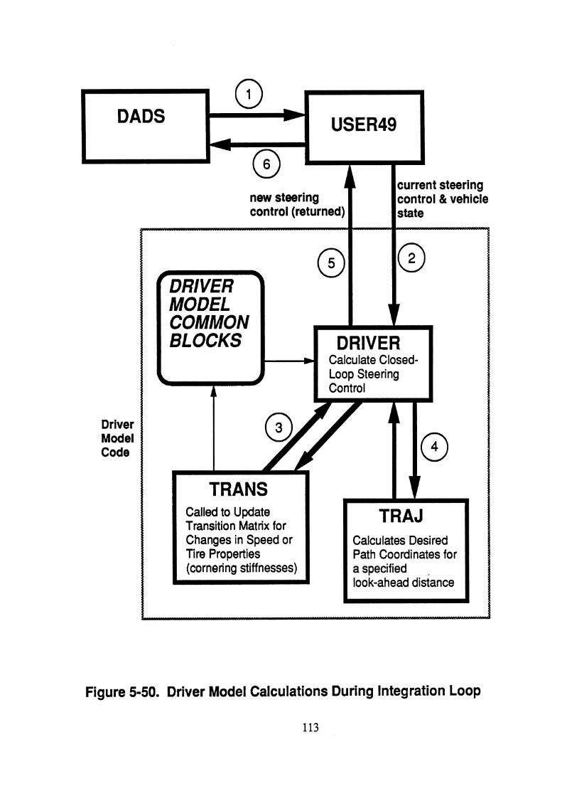
Calculate Closed-

Calculates Desired Path Coordinates for

(cornering stiffnesses)

Figure 5-50. Driver Model Calculations During lnteg ration Loop

113

- 1 . - 0 , 3 7 5 0 . 2 5 0 . 8 7 5 1 . 5 2 . 1 2 5 2 . 7 5 3 . 3 7 5 4 . 4 . 6 2 5 5 . 2 5 X E 3

T O R W A R D D I S T A W C I ( I N )

Figure 5-51. Example Lane-Change from DADS Simulation using the TACOM Driver Model

i i ~ l

Figure 5-52. Example Lane-Change from DADS Simulation using the TACOM Driver Model

throughout this run. However, because the peak lateral accelerations of approximately 70 in/sec/sec or, 0.18 g's, seen here would categorize this run as a relatively low lateral acceleration manewer, such updating of the driver model transition matrix would have little beneficial effect in this particular example.

Another example from the DADS 1 TACOM driver model simulation is seen in Figure 5-53 for a circular turning maneuver along a 500-ft radius path at a speed of 35 mph. Time histories of the average front wheel steering angle (radians) and the corresponding lateral acceleration (g's) are shown. A slight amount of overshoot is seen at about the 4-second point in the run as the vehicle "transitions" from the 100-ft straight approach tangent in to the circular curve.

Lastly, a sequence of animation frames are shown in Figures 5-54 and 5-55, illustrating the same DADS maneuver performed at a higher speed of 50 mph. During this run, the simulated HMMWV is experiencing a significant amount of sideslip and diminished directional stability because of reduced tire traction capabilities and a large rearward- positioned payload. The tires are operating under highly variable sideslip conditions during this maneuver and continuous updating of the localized tire cornering stiffnesses assists the driver model in better maintaining the desired path and directional stability in this example case.

If the transition mtrix is not updated, unlike the previous example run, the driver model would use the initial values of tire cornering stiffness and vehicle speed prevailing at the start of the simulation to calculate the transition matrix. As the simulation progresses and significant side-to-side load transfer and vehicle sideslip occurs, the tire properties and localized cornering stiffness values would depart from their initial values prevailing at the start of the maneuver. The change in directional dynamics in this case would not be sensed by the driver model and the vehicle would be steered differently. A preliminary test run performed with no transition matrix updating (for the same 50 mph case) produced a directionally stable nsult, but large path enms showing the vehicle off-tracking several feet to the outside of the lane during the cornering maneuver.

In most nonlinear simulations, the driver model can still be used effectively without use of transition matrix updating provided that large changes in tire properties or speed do not occur for extended periods of time during the maneuver. Examples of this might be lane- change maneuvers which may have large peak levels of lateral acceleration (e.g. above 0.4 g's) but which are relatively short in duration. The driver model may be temporarily less accurate during these peak acceleration periods in predicting the future position of the vehicle, but the net effect will generally be small when compared to an identical run having continuous transition manix updating. For some users, the additional execution time and

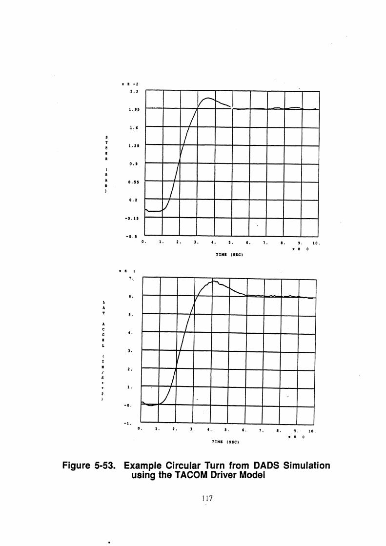
Figure 5-53. Example Circular Turn from DADS Simulation using the TACOM Driver Model

computational requirements of continuously updating the driver model transition matrix may be of concern and not actually needed for most of their maneuvers. In this case, the call to the TRANS subroutine from within the DRIVER subroutine may be removed or temporarily commented out.

It should also be remarked here that the "notion" of updating the transition matrix is in a sense analogous to human operator adaptation behavior observed during experimental tests of man/machine systems durin which the d namics of the controlled element is being altered. Previous research 3, 2q, 28, 299 309 $13 32 has shown that human operators can adapt quite quickly to large changes in the dynamics of the controlled plant during the course of a tracking task experiment. Very often this adaptation or "re-identification" process by the human subject can occur within less than a second of time. Consequently, including or removing this call to the TRANS subroutine can be a way of representing (or not) the ability of drivers to adapt to changing vehicle dynamics properties during the course of a maneuver. The code that appears in Appendix D for the driver model shows the call from within the DRIVER subroutine to the TRANS subroutine enabled as the default.

5.9. Path Plannin~ and Obstacle Detection Al~orithrq

This and the next section of the report describe two secondary tasks undertaken during the project which were intended to supplement the basic driver steering model described in earlier sections of the report. The first option, discussed in this section, describes a path planning algorithm which could be used to generate a "desired path" input for the basic steering control model. Instead of the program user specifying a set of x-y coordinates for the vehicle to follow (such as the center-line of a road), the program user would instead provide a more general scene description of the road geometry and any obstacles. The path planning algorithm would then select the specific desired path input for the steering control model to follow based upon an analysis of the scene data.

Initially, several approaches were considered for implementing a "path planning" capability within the driver model. The method described here is based upon compromises between computational efficiency and assumed capabilities of human operators in visually detecting obstacles and selecting paths. The basic outline of the algorithm used to represent a possible path planning capability for the driver model is seen in Figures 5-56 and 5-57. The basic idea of the algorithm is to sweep a forward radial area ahead of the vehicle with radial lines (or rays) originating at the vehicle. A radial profile of any obstacles or left/right boundary lines detected during a sweep is then constructed. A "centroid-like" point from

1. Transform specified left and right boundary lines from (x-y) cartesian inertial coordinates to (r-theta) polar coordinates (centered in the vehicle body axes).

2. Transform circular obstacle definitions, similarly, fiom cartesian to polar coordinates.

3 . Obstacle &tection and path selection:

a. generate radial rays from - to +thetamax in increments of &lth i. step along ray until impact with boundary or obstacle or r-

exceeded ii. record r and theta values at impact & store as part of r(theta)

profile

b. from stored.r(theta) profde: i. calculate I9 {e.g. sum[r(i)] 1 i ) ii. calculate theta* {e.g. [r(i) theta(i)] I sum[r(i)] }

c. check to see if f lies within r(theta) profile i. if yes, proceed to step d. ii. if no, (left-right choice possible), then perform steps a and b.

twice: A. once from -theta- to 0 B. once from 0 to +thetamax C. compare I9 and theta* from A. and B. D. select r* having largest value

d. transform ?(theta*) point to cartesian point and pass to steering model as input

e. if f is less than a defined rmin, activate closed-loop driver braking control model to stop in distance r*.

4. End of integration loop. Increment position and repeat

Figure 5-56. Example Path Planning Algorithm for the Driver Model (during integration loop)

this profle is calculated which acts as the target point for the steering control model to then follow.

Figures 5-57 and 5-58 show a hypothetical driverhehicle system approaching a field of obstacles. The fmt figure shows the vehicle just entering the field and detecting the h t

obstacle. The second figure shows the vehicle at an advanced position now detecting all obstacles and moved somewhat to the right of the first obstacle. The r* and 8* quantities appearing in these figures represent "centroid-like" coordinates of the driver field of view. At any point in time, the (r*,8*) coordinate (or some variation of it) would be used as a point located on and, over time, defining the desired path to be followed by the driver steering control modeL The r(8) vs 8 graph simply represents unobstructed sight distance in the driver's field of view out to some finite maximum distance. The (r*,8*) point moves to the left or right based upon the particular r(8) profiles generated in the field of view.

As the scene becomes more crowded or the maneuvering field limited, the centroid-like quantity r*(8*) will move closer to the driver thereby resulting in a shortening of the preview distance used in the steering control strategy. This is a desirable effect since most drivers will reflect this same basic behavior pattern under similar circumstances.

The same preview distance "shortening mechanism" can be used to trigger the start of a closed-loop braking model such as the one described in the next section 5.10. For example, if r*(O*) becomes less than some rmi, level needed for moderate braking under the prevailing tire/surface friction conditions, the brakes would be applied in a closed-loop manner so as to bring the vehicle to a stop in a distance of rmb. During the course of the braking maneuver, the obstacle detectiordpath planning algorithm would still be active, so that, if an "opening" in the obstacle field was detected prior to the stop, the braking could be abandoned and the vehicle steered out through the "opening." Acceleration and speed control of the vehicle could be controlled by a counter-strategy.

A simple computer program (shown listed in Appendix F) was written to implement and test the basic path planning algorithm outlined here. The algorithm provides for a set of left and right boundaries in addition to a number of obstacles in the driver field of view. The left and right boundaries are represented as arbitrary x-y tabular data (with respect to an inertial h m e of reference) and the obstacles as circular objects of arbitrary radii centered at designated x-y (inertial frame) locations. The computer code that was written to test the described algorithm requires input of those basic items, in addition to such things as driver location, orientation, field of view, and maximum sight distance. At each position, the program then calculates the r(8) profile and the centroid-like location, r*(8*), for that particular scene. By performing these calculations in a sequential fashion with the driver moving forward toward the desired cenuoid-like location, a path is generated (as defined

Figure 5-57. Vehicle Entering Field of Obstacles and Corresponding Profile

Figure 5-58. Vehicle at Advanced Position and Corresponding Profile

by the sequential locations of that quantity). This path then represents the output of the path planning module and acts as an input to the driver steering control module.

Two examples are presented next which illustrate the operation of the path planning algorithm used in conjunction with the steering control model. Figure 5-59 shows a lane- change course using left and right boundaries (instead of a desired x-y path) to guide the driverhehicle system during the path-following maneuver. No obstacles are present in this run. Results in the form of time histories are shown in Figures 5-60 and 5-61. The simulated vehicle is a loaded HMMWV travelling at 60 mph. The specified field of view is +I- 0.3 radians. The maximum look-ahead distance, r,,, is 150 ft.

As a second example, Figure 5-62 shows a course layout in which the left and right boundaries are straight line segments defining the left and right road boundaries of an obstacle course similar to that used during the test program. Centered in the left-hand lane and directly in front of the vehicle at the start of the run is a circular obstacle with a diameter of 12 ft. An identical second obstacle is located centered in the right-hand lane 112 ft beyond the first obstacle. Results from this ,run are also seen as a sequence of time histories in Figures 5-63 and 5-64. After the start of the run, the vehicle is steered to the right away from and around the first obstacle. As the vehicle moves forward beyond the first obstacle, it is steered back to the left around the second obstacle. The vehicle then encounters the leftfight road boundaries which guide it out the exit in the right-hand lane.

Note that the only information provided to the path planning algorithm are the left and right boundaries (located with respect to an inertial reference frame) and location and size of any obstacles. The model thus decides "where to go" (by means of the path planning module) as well as "how to get there" (by means of the steering control model). The algorithm continuously adjusts the driver preview parameter and its "transition matrix" based upon the obstacles or boundary constraints present in the field-of-view. For example, in the obstacle course run seen in Figure 5-62, the preview distance was shortened by the model to a value of about 25 feet when the vehicle was nearing an obstaclelgap, and was lengthened to approximately 100 ft (up to the maximum sight-distance specified) at the start and end of the course where no obstacles were immediately present. This version of the the path planning model uses a single point in the preview interval to guide and steer the vehicle in order to minimize the computational requirements of the algorithm. Consequently, the steering responses seen with this type of model will be somewhat more variable than one in which an average of several points over the preview interval are used in the computation (as, for example, the type of calculation performed by the basic version of the TACOM stkring control model presented earlier).

No Obstacles Present in this Example

start A

t

finish

(not to scale)

Figure 5-59. Lane-Change Geometry for the Example Calculation using the Path Planning Algorithm

126

Front Wheel Angle - deg

Lateral Position - ft 14

2 3 4 Time - sec

200 300 400 Longitudinal Position - ft

Figure 5-60. Example Calculation using the Path Planning Algorithm - Lane Change Maneuver

Lateral Acceleration - g's

0 1 2 3 4 5 6 Time - see

Yaw Angle - deg 8

- 2 0 1 2 3 4 5 6

Time - sec

Figure 5-61. Example Calculation using the Path Planning Algorithm - Lane Change Maneuver

t'77 Left Boundary

(not to scale)

Figure 5-62. Obstacle Course Geometry for the Example Calculation using the Path Planning Algorithm

Front Wheel Angle - deg

0 2 4 6 8 10 12 Time - sec

Lateral Position - ft

V

0 100 200 300 400 500 600 700 Longitudinal Position - ft

Figure 5-63. Example Calculation using the Path Planning Algorithm - Obstacle Course Maneuver

Lateral Acceleration - g's

0 2

Yaw Angle - deg

4 6 8 Time - sec

4 6 8 Time - sec

Figure 5-64. Example Calculation using the Path Planning Algorithm - Obstacle Course Maneuver

The advantages of using a path planning feature in combination with the driver steering control model are: 1) geometric desniptions of the roadway or obstacle course can often be supplied in a simple manner, and 2) the path planning module automatically determines the path to be followed based upon the boundary and obstacle data. The chief disadvantage is the large increase in computational effort used by such algorithms in determining the path. More efficient computational schemes could no doubt be offered to improve upon the basic concept described in this repart. In general, use of a path planning model is probably best suited to driving scenarios involving arbitrary obstade courses for which tracking of a particular pre-determined path is not required, or, a likely path is not obvious from simple examination of the course geometry.

5.1 0. Driver Model Option for Closed- loo^ Braking

The TACOM driver model discussed in the previous sections of the report is obviously aimed at simulating the closed-loop steering behavior of drivers. No consideration of how drivers might also control or modulate brake pressure during braking maneuvers was initially included in that model. However, in order to study the effects of active driver modulation of brake pressure during vehicle deceleration maneuvers, it will ultimately be necessary to augment and extend the capabilities of the driver steering control model in future studies. This section describes, in general terms, one possible method by which closed-loop braking behavior of drivers could be modelled. Much of the proposed closed- loop braking model discussion that follows was initially suggested in a small study performed by Uh4TlU for the Rockwell International ~orporat ion.~~

The test data collected under this project for the H M M S W was intended, in part, to support future development and validation of closed-loop braking models by TACOM. Those braking tests, as discussed previously in setion 5.6, were all conducted intentionally as closed-loop braking tasks during which the driver applied braking so as to bring the vehicle to a uniform stop at a specified point on the test track. Recall that the requested stopping distances were varied in a random-like manner h m test to test to prevent the test drivers from "automating" their brake pressure control strategy. Data was collected for braking-in- a-turn as well as for straight-line braking maneuvers.

5.10.1. Closed-Loop Brake Application Strategy. The basic idea underlying the proposed model of driver braking behavior is for the model to apply appropriate levels of brake pressure to bring the vehicle to rest at a future position in space. The driver is assumed to be equipped with a simple "understanding" of the longitudinal dynamics of the vehicle in response to command pressure inputs. In addition, the driver is presumed to act in a time-delayed fashion so that the command pressure calculated by the model is applied

to the brake system after some inherent driver delay. In the model, the simple "understanding" is represented by the longitudinal dynamics of a point-mass subject to a braking or retardation force. In essence, the driver model has a simplified "internal model" of the longitudinal dynamics of the vehicle being operated, and can, therefore, predict or estimate future vehicle position in response to command pressure inputs. (This is essentially an extension of the same basic optimal control approach applied successfully during this project for the lateral steering control of vehicles.)

Without presenting the mathematical derivation here, the equation that results from this model is one that relates an ideal driver command pressure, ~ * ( t ) , to current longitudinal vehicle position, speed, and desired stopping point:

where,

t is time from the start of the braking maneuver

~ ' ( t ) is the calculated ideal driver command pressure (brake pedal) at each point in time during the braking stop (the calculated "control variable" here)

m is the total mass of the vehicle

V(t) is the forward speed of the vehicle at each point in time during the braking stop

K is a linear gain factor relating driver command pressure to total retardation force (lbs / psi)

xd is the desired stopping distance from the point of brake application and,

x(t) is the vehicle longitudinal position at each point in time during the braking stop

The ideal command pressure, ~ * ( t ) , is then delayed an amount seconds (driver time delay for braking), resulting in the final equation for the driver modulated command pressure, P(t), which is the actual pressure applied to the brake system:

As seen, the closed-loop equation (5.10-1) is quite simple and, in fact, is a rearrangement of the well known physics formula (applied on a point-in-time by point-in-time basis) relating stopping distance, x, to initial speed, V, and subject to a constant deceleration, D. [ x = ~2 I (2 D) ] The driver model, in effect, selects deceleration at each point in time using this formula, translates it to a command pressure equivalent, based upon brake gains and vehicle weight, and then delays it in time to account for an assumed driver lag. Although equation (5.10-1) was not derived from this particular viewpoint, it is helpful to see an analogy between it and a simple explanation in basic physics.

Figure 5-65 shows an example time history for the closed-loop driver command pressure predicted by the model for a braking stop from 30 mph and a desired stopping distance of 150 feet. The calculation is for a 5-axle tractor-semitrailer and was simulated using a modified version of the UMTRI Phase 4 commercial vehicle model? Since the driver braking model approximates the deceleration gain of the braking system by a simple gain constant, K, noted above, differences can exist between the driver "understanding" of the pressure-retardation force relationship and that of the actual brake system. This would be particularly true for vehicles having highly nonlinear torque-pressure relationships and significant levels of hysteresis, or, for cases of low road surface friction where the available retardation torque is limited by the surface friction. Since the vehicle used in this example possessed fairly linear-like brakes (aside from the usual push-out pressure characteristic) and only modest levels of brake hysteresis, reasonable predictions of command pressure would be expected by the model when sufficient tire-road friction is available. Figure 5-65 seems to suggest this. The continued "drooping" of treadle (command) pressure at the end of the stop is attributable to brake hysteresis, which causes a lagging of brake torque requested by the model during the pressure reduction phase. As indicated in the next section, 5.10.2 Closed-Loop Brake Release Strategy, this basic form of brake application will normally be interrupted in the model by front-axle wheel locks andlor vehicle instabilities with more demanding stops attempted for shorter distances.

Figure 5-66 illustrates the differences between the simple linear retardation function expected by the driver model and that experienced by an actual vehicle. For the high friction surface (top diagram) where the retardation forces primarily derive from the torque limitation of the brake (summed over the vehicle), the primary differences lie in the nonlinearities present in the brake system itself. For the case of the low friction surface (bottom diagram), additional saturation-type nonlinearities are introduced because of the tire-surface friction limitations, Consequently, mild over- or under-estimations of total brake retardation forces by the driver model under conditions of high surface friction, can become exaggerated under low friction conditions. This would especially be true for a loaded vehicle and low friction surface combination since the command pressure "expectation" requested by the driver model will be scaled up by the weight of the vehicle

time - sec

5-axle Tr -Semi; 30 mph; Braking-in-a-Tur n; Driver Control;

Figure 5-65. Example Prediction of Command Pressure from the Closed-Loop Driver Braking Model during a Controlled Stop

High Friction Surface

Available under-estimation

Torque

Simple Driver Model "Expectation Function"

Driver Command Pressure

under-estimation by driver rodel

I

Low Friction Surface

Available Retardation Torque

Simple Driver Model "Expectation Function"

Driver Command Pressure

Figure 5-66. Comparison of Simple Driver Model Braking Expectation with Actual Retardation Properties

136

from the empty vehicle condition on the same surface. This will, in turn, result in a significant over-estimation of the available retardation torque on the part of the model as indicated in Figure 5-66 (lower diagram).

In spite of this, even in cases of significant over-estimation of the available retardation torque by the model, reasonable predictions of command pressure demand can still be obtained from the model. Much of this "success" can be attributed to the other half of the driver model behavior, discussed in the next section, which models how brake pressure is released under various conditions, thereby preventing the model from operating for extended periods of time in modes of mismatch or over-estimation. Further refinement or improvements to the driver "expectation function" of retardation torque are of course possible, such as accounting for the brake system push-out pressure (dead-zone), or, introducing nonlinearities into the expectation function.

5.10.2. Closed-Loop Brake Release Strategy. In order to represent a basic response to loss of steering due to front axle lock-up and/or various forms of vehicle directional instability that can occur during heavy braking, the closed-loop braking model may have'a number of programmable "rules" for temporarily releasing driver commanded pressure during a braking maneuver. The following "rules" define conditions for possible pressure release by the driver model:

left and right axle wheel slip values both exceed value of Smax, (front -axle lock)

absolute value of path error exceeds value of Ymax, (vehicle 1 2-foot lane exceedance)

absolute value of vehicle sideslip angle exceeds value of Bmax, (yaw instability)

absolute value of tractor-semi articulation angle exceeds value of Gmax, (jackknife and/or trailer swing for an articulated vehicle)

forward speed greater than Vmin. (ignore brake release "rules" at very low speeds)

Example values for these parameters for a tractor-semitrailer might be:

Smax = 0.5 Bmax = 10 degrees

Ymax = 4.0 feet Gmax = 10 degrees. Vmin = 10 ftfsec

Figure 5-67 shows a time history of driver command pressure from the closed-loop driver model for a braking stop on a low friction surface in which front-axle lock-up is occuning and causing interruption of the applied command pressure based upon "rule" A) above. A by-product of this "brake pumping" activity by the driver model is that following each interruption, the next application by the model is successively higher in order to meet the increased stopping demand caused by the previous brake releases. The increasing command pressure, or upward ramping, seen during the first two application cycles by the driver model also reflects "over-estimation" behavior of the model as discussed in the previous section and Figure 5-66. The "over estimation" is caused by insufficient tire- surface fiction (semitrailer and tractor rear lock-ups are occurring prior to a tractor front- axle lock-up during these two application cycles).

Overall, the basic command pressure modulation by the closed-loop driver model seems to behave reasonably given the simplicity of the model. Refinements of this model are certainly possible based upon some of the braking data collected under this project. Additional driver-vehicle experiments could also be designed and conducted to extract information useful to a more comprehensive modelling effort.

In summary, it is assumed that the closed-loop braking model outlined above possesses certain capabilities and inherent properties. First, the ability to select, in at least a simple manner, an appropriate value of command pressure to bring the vehicle to a stopping point. This suggests an ability of drivers to "calibrate" themselves to the vehicle being controlled and to, therefore, account for changes in basic vehicle dynamics or operating conditions (estimation of retardation as a function of command pressure; prediction of future vehicle position; adaptation to gross vehicle weight changes). Secondly, it is assumed that the simulated driver does not react in an instantaneous manner to an elected brake control strategy. Consequently, a simple transport time delay property can be assigned to the driver to represent this basic limitation. The value used for this delay was 0.1 second in the calculations seen above (for a'very responsive driver), but a value more representative of "average" drivers would probably be somewhat greater 469 47, 48. Simulations performed in reference 45 with varying values of this driver model time delay parameter suggested a strong sensitivity between closed-loop stopping performance and this basic driver lag property.

5-axle Tr-Semi; 30 rnph; Braking-in-a-Turn: Driver Control:

Figure 5-67. Command Pressure Modulation by the Driver Braking Model in Response to Front Axle Lock-ups

LIST OF REFERENCES

MacAdam, C. C. "Application of an Optimal Review Control for Simulation of Closed-Loop Automobile Driving." IEEE Transactions on Systems, Man, and Cybernetics, SMC-11, June (1981). 393-399.

MacAdam, C.C. "An Optimal Preview Control for Linear Systems." Journal of Dynamic System, Measurement, and Control, 102, September (1980). 188-190.

Elkind, J. I. "A Survey of the Development of Models for the Human Controller." Progress in Astronautics and Aeronautics. (1964). 13: 623-643.

McRuer, D. T., et al. "New Approaches to Human-Pilot/Vehicle Dynamic Analysis." Tech. Report AFFDL-TR-67-150, WPAFB. (1968).

Henderson, R. L. (Editor). "Driver Performance Data Book." Final Report DOT HS 807 126, NHTSA. (1987).

Johannsen, G. "Man-Machine Systems - Introduction and Background." Proceedings of IFAC Man-Machine Systems, Baden-Baden, Federal Republic of Germany, (1982).

MacAdam, C. C., et al. "A Computerized Model for Simulating the Braking and Steering Dynamics of Trucks, Tractor-Semitrailers, Doubles, and Triples Combinations." User's Manual - Phase 4, UM-HSRI-80-58. (1980).

Gillespie, T., and MacAdam, C. C. "Constant Velocity Yaw/Roll Rogram - User's Manual." UMTRI-82-39. (1982).

MacAdam, C. C. "A Microcomputer-Based Model for Studying Open- and Closed- Loop Steering Response of Automobile/Driver Systems." Proceedings of the Society for Computer Simulation Conference on Modeling and Simulation on Microcomputers: 1983, Ed. R. Martinez. San Diego, California, SCS, (1983).

lo MacAdam, C. C. "A Computer-Based Study of the Yaw/Roll Stability of Heavy Trucks Characterized by High Centers of Gravity." SAE Transactions, SAE, paper no. 821260, (1982).

l1 MacAdam, C. C. "Frequency Domain Methods for Analyzing the Closed-Loop Directional Stability and Maneuverability of Driver/Vehicle Systems." Proceedings of the Conference on Modern Vehicle Design Analysis, Ed. M. Dorgharn. London, U.K., (1983).

l2 MacAdam, C. C. "A Computer Simulation Study of the Closed-Loop Stability and Maneuverability of Articulated CoachDriver Systems. " Proceedings of the 8th IAVSD Symposium of the Dynamics of Vehicles on Roads and Tracks, Ed. K. Hedrick. Cambridge, Massachussetts, Swets & Zeitlinger B.V. - Lisse, (1983).

l3 MacAdam, C. C. "Computer Model Predictions of the Directional Response and Stability of Driver Vehicle Systems During Anti-Skid Braking." Proceedings of the IMech E Conference on Antilock Braking Systems for Road Vehicles, Ed, P. Newcomb. London, U.K., IMech E, (1985).

l4 MacAdarn, C. C., and Fancher, P. S. "A Study of the Closed-Loop Directional Stability of Various Commercial Vehicle Configurations." Proceedings of the 9th IAVSD Symposium of the Dynamics of Vehicles on Roads and Tracks, Ed. 0. Nordstrom. Linkoping, Sweden, Swets & Zeitlinger B.V. - Lisse, (1985).

l5 Fancher, P. S. "Integrating Anti-Lock Braking Systems with the Directional Control Properties of Heavy Trucks." Proceedings of the IMech E Conference on Antilock Braking Systems for Road Vehicles, Ed. P. Newcomb. London, U.K., IMech E, (1985).

l6 Rashevsky, N. "Mathematical Biology of Automobile Driving." Bull. Mathematical Biophysics, 30, (1968). p 153.

l7 Sheridan, T. B., et al. "Control Models of Creatures Which Look Ahead." Proceedings of the 5th National Symposium on Human Factors in Electronics, (1964).

l8 Kondo, M., and Ajimine, A. "Driver's Sight Point and Dynamics of the Driver- Vehicle System Related to It." SAE Automotive Engineering Congress. Detroit, Michigan, SAE, paper no. 680104, (1968).

l9 Mortimer, R. G., and Jorgeson, C. M. "Eye Fixations of Drivers as Affected by Highway and Traffic Characteristics and Moderate Doses of Alcohol." Proceedings of the Sixteenth Annual Meeting, Human Factors Society, (1972).

20 Baron, S. "A Model for Human Control and Monitoring Based on Modern Control Theory." Journal of Cybernetics and Infonnation Science, 1, January (1976).

21 Hatwal, A., and Mikulcik, E. C. "An Optimal Control Approach to the Path Tracking Problem for an Automobile." Transactions of the Canadian Society for Mechanical Engineering, 10,4 (1986). 233-241.

22 Nagai, M., and Mitschke, M. "Adaptive Behavior of Driver-Car Systems in Critical Situations: Analysis by Adaptive Model." JSAE Review, December (1985). 82-89.

23 Tomiruka, M. "The Optimal Finite Preview Problem and Its Application to Man- Machine Systems." PhD Dissertation. MIT, (1973).

24 McRuer, D. T., and Klein, R. "Comparison of Human Driver Dynamics in Simulators with Complex and Simple Visual Displays and in an Automobile on the Road." 1 lth Annual Conference on Manual Control. (1975).

25 McRuer, D. T., Allen, R. W., and Klein, R. H. "New Results in Driver Steering Control Models." Human Factors, 19,4 (1977). 38 1-397.

26 Weir, D., DiMarco, R. J., and McRuer, D. T. "Evaluation and Correlation of Driver/Vehicle Data, Vol 11." Final Technical Report, NHTSA, DOT-HS-803-246. (1977).

27 Hosman, R. J. A. W, and van der Vaart, J. C. "Laboratory and Moving-Base Simulator Experiments on Speed and Accuracy of Visual and Whole-Body Motion Perception." Proceedings of IFAC Man-Machine Systems, Varese, Italy, (1985).

28 Young, L. R. and Stark, L. "Biological Control Systems - A Critical Review and Evaluation." NASA Contractor Report, NASA CR-190. (1965).

29 Weir, D. and Phatak, A. V. "Model of Human Response to Step Transitions in Controlled Element Dynamics." Technical Report NASA CR-671. (1968).

30 Phatak, A. V., Bekey, G. A. "Model of the Adaptive Behavior." IEEE Tamactions on Man-Machine Systems, MMS-10, September (1969). 72-80.

31 Miller, D. C. and Elkind, J. I. 'The Adaptive Response of the Human Controller to Sudden Changes in Controlled Process Dynamics." IEEE Transactions on Hman Factors in Electronics, HFE-8,3 (1967).

32 Li, Y.T., Young, L.R., and Meiry, J.L. "Adaptive Functions of Man in Vehicle Control Systems." Proceedings of the International Federation of Automatic Control Symposium, Paddington, England, (1965).

33 Wehage, R. A. "Application of Matrix Partioning and Recursive Projection to O(n) Solution of Constrained Equations of Motion." ASME Journal, (in review).

34 Riede, P. M., Leffert, R. L., and Cobb, W. A. "Typical Vehicle Parameters for Dynamics Studies Revised for the 1980's." SAE Automotive Engineering Congress. Detroit, Michigan, SAE, paper no. 840561, (1984).

35 MacAdam, C. C. "Development of DriverNehicle Steering Interaction Models for Dynamic Analysis." Interim Technical Report, UMTRI-86-41. TACOM Contract DAAE07-85-C-R069. (1986).

36 Fukunaga, Y. et al. "Improved Handling and Stability Using Four-Wheel Steering." Proceedings of the 11th International Conference on Experimental Technical Safety Vehicles, Washington, D. C., (1987).

37 Sano, S., Furukawa, Y., and Shiraishi, S. "Four Wheel Steering System with Rear Wheel Steer' Angle Controlled as a Function of Steering Angle." SAE International Congress and Exposition. Detroit, Michigan, SAE, paper no. 860625, (1986).

38 Takiguchi, T. et al. "Improvement of Vehicle Dynamics by Vehicle-Speed-Sensing Four Wheel Steering System." SAE International Congress and Exposition. Detroit, Michigan, SAE, paper no. 860624, (1986).

39 Hay ashi, Y. "Optimum Control of a Driver/Four-Wheel S teered-Vehicle System." Proceedings of the 10th IAVSD Symposium of the Dynamics of Vehicles on Roads and Tracks, Prague, Cz, (1987).

40 "DADS User's Manual - Rev 4.0." Computer Aided Design Software, Inc. (1986).

41 Mousseau, R. "An Investigation Into the Lateral Stability of the M1037 Truck Pulling the MlOl Trailer." U.S. Army Tank Automotive Command, Systems Simulation and Technology Division, Final Report. (1 988).

42 Stribersky, A., and MacAdam, C. C. "Lateral Stability of a Controlled Articulated Vehicle - An Application of Bifurcation Theory in Vehicle Dynamics." Proceedings of the 12th Canadian Congress of Applied Mechanics, Ottawa, Canada, (1989).

43 Sayers, M., MacAdam, C. C., and Guy, Y. "Chrysler Wind-Steer Vehicle Simulation." User's Manual. (1988).

44 "Comparison of Vehicle Test Procedures." Contract DRDA 781433, Highway Safety Research Institute, University of Michigan. (1978).

45 MacAdam, C. C. et al. "Computer Study of the Braking Performance of a Tractor- Semitrailer." Technical Report for the Rockwell International Corporation. (1987).

46 Newcomb, T. P. "Driver Behavior During Braking." SAE I I. Mech. E. Exchange Lecture. SAE, paper no. 810832, (1981).

47 Rompe, K., Schindler, A., and Wallrich, M. "Comparison of the Braking Performance Achieved by Average Drivers in Vehicles with Standard and Anti Wheel Lock Brake Systems." SAE International Congress and Exposition. Detroit, Michigan, SAE, paper no. 870335, (1987).

48 McLean, D., Newcornb, T. P., and Spurr, R. T. "Simulation of Driver Behavior During Braking." I, Mech. E. Conference on Braking of Road Vehicles, IME, paper no. C411176, (1976).

49 Sheridan, T. B. "Three Models of Preview Control." IEEE Transactions on Human Factors in Electronics, HFE-7, June (1966).

Appendix A

Articulated Vehicle Equations

As noted in section 5.5 of the report, the internal single-unit model used throughout much of this report as the "reference" vehicle used by the driver model, can also be used for steering many articulated vehicles, provided the lead-unit vehicle parameters reflect the presence of the hitch load as described in that section. The alternate approach for steering an articulated vehicle is to apply a more complete set of articulated vehicle equations, such as those appearing in this appendix, as a substitute for the single-unit equations presented earlier.

The equations in this appendix apply to the articulated vehicle model shown in Figure A-1 and Table A-1. This basic model is intended to serve as a "simplified articulated vehicle with front wheel steering and a provision for an articulation control torque, patterned after the LVS vehicle. These equations would be used to represent the internal vehicle model employed by the driver control algorithm when steering an articulated vehicle, if a fuller treatment of ~ossible driverfvehicle interactions is required. The controlled system dynamics, now represented by an articulated vehicle having one additional degree of freedom in its simplest form, is extended beyond that of the single-unit vehicle assumed by the baseline driver model of section 5.5.

A diagram of the proposed articulated vehicle used by the driver model is seen in Figure A- 1. A list of corresponding variable and parameter definitions appears in Table A- 1. The model has two control inputs: the front wheel steer angle, 6 , and the articulation torque, . (A later simplification slaves the articulation control torque to the front wheel steer angle by a proportional gain factor, thereby resulting in essentially one control input and a gain parameter for controlling the front-wheel-steer / articulation-torque "mixture.") The linearized equations representing the articulated vehicle model now follow.

The sum of lateral forces and sum of yaw torques acting on each of the two articulated masses produces the following four dynamical equations (primes denoting differentiation with respect to time):

ml vl' = Fy1 + Fy2 - ml U rl + fy (A-1) (fy is the lateral hitch constraint force)

I1 rl' = a1 Fyl - bl Fy2 - cl fy + M, (A-2)

Figure A-1 . Articulated Vehicle Model

Table A-I . Articulated Vehicle Model - Parameter Definitions

(Internal Driver Model Representation)

Parameter Description

mass of front unit

mass of rear unit

lateral sideslip velocity of unit 1

lateral sideslip velocity of unit 2

yaw rate of unit 1

yaw rate of unit 2

distance form c.g. of unit 1 to axle 1

distance form c.g. of unit 1 to axle 2

distance form c.g. of unit 2 to axle 3

distance form c.g. of unit 1 to hitch

distance form c.g. of unit 2 to hitch

forward velocity component in x-body axis

front axle steer angle - control variable

articulation angle tire sideslip angle (axle i)

tire cornering stiffness (axle i)

articulation torque - control variable

lateral tire force (axle i)

The kinematic constraint for the articulation joint produces the following algebraic relationship between the lateral displacement, yi, and heading angle variables, yi :

y1 - cl sin ~1 = y2 + c2 sin ~2 (A-5)

Differentiating twice and assuming small angles for the heading angles results in the equivalent constraint equation expressed in terms of the associated accelerations:

The tire forces Fyi can be expressed in terms of the tire cornering stiffnesses and tire sideslip angles as:

where,

Assuming small tire sideslip angles for the ai (replacing the arctan by the angle), Equations (A-1) -> (A-4) become after these substitutions:

ml vl' = - Cal (vi+alri) / U - Ca (vl-blrl) / U + Gal 6 - ml U rl + fy (A- 11)

11 rl' = -a1 Cal (vl+alrl) / U + bl C d (vl-blrl) I U - cl fy + a1 Gal 8 + Mc (A-12)

m2 v2' = - Ca3 (v2-br2) / U - m2 U r2 - fy (A- 13)

I2 r2' = b2 ca3 (v2-br2) / U - c2 fy - M, (A- 14)

Expressed in matrix algebra terminology, the equations of motion (A-11) -> (A-14) become:

M v ' = A V + G 6 + Nfy +EM, (A- 15)

and the kinematic constraint equation (A-6) becomes:

C V ' = D v (A- 16)

where, v = { vl, rl, v2, r2 IT.

Solving (A-15) and (A-16) for the constraint force, fy, and upon back substitution, results in the following set of dynamical equations free of the constraint force:

v' = F * v + g * 6 + h M , (A- 17)

For a powered articulation scheme with Mc = K [ 6 - q ( ~ 1 -y2) ] , where the parameter K controls the degree to which the articulation torque is slaved to the front wheel steer angle, 6, and q provides an optional torsional spring effect about the articulation joint, equations (A- 17) become:

v' = F * v + ( g * + K h ) 6 + yi terms (A- 18)

Addition of the lead unit lateral displacement, yl, and heading angle state variable, vi,

equations, results in the final set of seven linear dynarnical equations:

(A- 1 9)

or in matrix algebra notation:

where,

D - - 0, -u, 0, u }

and,

To use these equations in the driver model, the F and g matrices appearing in Equation (A- 20) would replace the corresponding F and g matrices presented earlier in section 5.4, to now represent the internal vehicle dynamics within the driver model.

As indicated above, the LVS vehicle was used as a guide for defining the characteristics of the articulated model. General estimates of the LVS mass and geometric parameters are listed in Table A-2. These parameters were used in an example calculation demonstrating the operation of the equations just presented for steering an LVS-like articulated vehicle.

Example time histories are seen in Figure A-2 for the simulated LVS articulated vehicle, controlled by the extended driver model, performing a 12-foot lane-change maneuver at 60 mph. The input path was a standard 12-ft by 100-ft lane-change. The first four plots correspond to the lead unit. The second four plots apply to the trailing unit. The last group of time histories show lateral acceleration traces for the lead and trailing units, the control variable (degrees of front wheel angle), and the calculated mean squared path error within the preview interval "MSE Preview Path Error." In this particular example, the articulation control torque was active and was slaved to the front wheel steer angle (10,000 ft-lb of articulation control torque / degree of front steer angle). The results seen here were calculated with a modified UMTRI vehicle model (to incorporate the articulation control torque) and used the extended driver model equations from this Appendix.

Table A-2. LVS Parameter Estimates

Parameter

c2

c3 TF

Tau

RKMOM

Value

750 slugs

5 15 slugs

9,000 ft2-slug (lead unit yaw inertia)

20,000 a I1 (rear unlt " > 2.5 ft 2.5 ft 5.3 ft 2.0 ft 14.25 ft 88 ftlsec 42,000 Ib/rad/suspension-side (tire cornering

stiffness)

1.5 sec (driver preview time)

0.25 sec (driver transport lag)

570,000 ft-lblrad (articulation control

moment-front steer gain)

a

u,

*- e n V) cn w w

M \ M

\

E .- E .- c u k cu

I-

C

0 0

st 01 S 0 01 S 0 S- (14) / ~uauaaolds!a l o ~ a 1 ~ 1 (6ap) al6uy 6u!poa~

Figure A-2. Example Calculations for a Simulated LVS

A-1 1

(u) z - ) u a u a ~ o ~ d ~ ~ I ~ ~ i ) ~ l

Figure A-2. Example Calculations

02 0 OZ- ( s / B a ~ ) / ZaPt) MoA

for a Simulated LVS

Figure A-2. Example Calculations for a Simulated LVS

Appendix B

HMMWV Test Data

The material contained in this Appendix supplements the test data appearing in earlier sections of the report and helps document the types of test maneuvers performed. Example time histories are provided here for each test maneuver conducted during the test program. The complete set of data collected during the project are being supplied to TACOM on floppy disks with corresponding UMTRI software used to graphically view the time history data. Log sheets for all of the test data collected during the test program appear in Table 5-2 of section 5.6.

The first set of Figures B-1 to B-4 apply to the steady turning maneuver performed at 50 and 25 mph respectively (tests 105 and 110 from Table 5-2). Measurements of forward speed, driver steering wheel angle, and lateral acceleration are seen in Figures B- 1 and B-3, Figures B-2 and B-4 show corresponding measurements of roll angle, yaw rate, and left front wheel angle. The "spikes" seen in the roll angle measurement data are due to faulty contacts occuring within the roll angle transducer wiper assembly. Irregular drifting of the roll angle measurement was also encountered with this same transducer. For most of the tests performed in this study, this particular measurement was of secondary importance and is only shown here to provide a "ballpark estimate of the vehicle roll response.

Figures B-5 to B-8 show example test results from the braking-in-a-turn maneuver from an initial speed of 50 mph and along a curve of 500-ft radius. Figures B-5 and B-6 correspond to a short stopping distance of 132 ft (test 118); Figures B-7 and B-8 show comparable results for a longer stopping distance of 195 ft (test 120). Driver brake pressure, longitudinal acceleration, and forward speed are seen in Figures B-5 and B-7. Figure B-6 and B-8 show the corresponding driver steering wheel angle and lateral acceleration measurements.

Example results from the constrained lane-change maneuver at 60 and 30 mph are seen in Figures B-9 through B-12. The 60 mph results are from test 127; the 30 mph results are from test 137.

Two example runs from the obstacle course tests are seen in Figure B-13 to B-16. The first example, seen in Figures B-13 and B-14, are from test 184 and correspond to a "short/short" obstacle placement (L=80 ft; L2=100; L3=120 ft) as discussed in section 5.6. Figures B- 15 and B- 16 are from run 185 and correspond to a "longil~ng" obstacle placement (L1=120 ft; L2=100; L3=80 ft). The previous results seen for the obstacle course in section 5.7 were for a "center/centerM setting of the two obstacles.

Figures B- 17 to B- 19 correspond to three different straight-line braking tests (213, 2 15, and 214). Figure B-17 is for a relatively long stopping distance showing the driver clearly modulating the brake pressure about an approximate value of 350 psi. Figure B-18 is for a

realtively short stopping distance of 145 ft. The driver brake pressure application is considerably larger and noticeably different. In fact, this particular trace closely resembles the shape of the time history prediction from the closed-loop braking model seen in Figure 5-65. The last straight-line braking test result seen in Figure B-19 is for a stopping distance of 125 ft but included wheel lock occurences at both the front and rear axles. Midway through this stop, the driver is seen releasing the brake pressure temporarily to regain directional control of the vehicle. Sharp steering to the right by the driver is also seen at the 7-second mark in response to the directional disturbance to the vehicle motion caused by the wheel locks.

Lastly, Figure B-20 shows a sample result from a "Random Steer Test" initially conducted to obtain open-loop frequency response characteristics on the HMMWV directional dynamics. These were subsequently not needed but are available for future studies as part of the HMMWV test data library being delivered to TACOM. A typical random steer test would last from 45 to 75 seconds depending upon the test speed. Shown in Figure B-20 are the first 20 seconds from test 202 conducted at 60 mph. The driver is simply applying a "random-like" steering input to the vehicle while travelling along a straight-line course. The intent of this test is to excite the directional dynamics with a wide variety of steering frequencies, thereby allowing a subsequent Fourier analysis to be applied to the recorded data. The Fourier analysis then produces the frequency response of the vehicle directional dynamics due to the steering input.

Forward Velocity - mph

time - sec 06/01/88 16:15:35 STEADY TURN

15 20

WMPH

Driver Steering Wheel Angle - deg

time - sec 06/01/88 16:15:35 STEADY TURN 50MPH

Lateral Acceleration - g's 5x1 o ' ~

lime - sec 06/01/88 16:15:35 STEADY TURN WMPH

Figure B-1. HMMWV TegG 50 mph Steady Turn

Roll Angle - deg 2

time - sec 06/01/88 16:15:35 STEADY TURN 50MPH

Yaw Rate - degs 2

time - sec 06/01/88 16:15:35 m A D Y TURN

Left Front Wheel Angle - deg .6

time - sec 06/01/88 16:15:35 STEADY TURN 50MPH

Figure B-2. HMMWV Test: 50 mph Steady Turn

Forward Velocity - rnph 26.5

time - sec 06101128 16:44:38 STEADY TURN 25MPH

Driver Steering Wheel Angle - deg 10

time - sec 06fl1188 16:44:38 STEADY TURN 25MPH

Lateral Acceleration g's 2x1 o ' ~

-. I2 0 5 10 15 20

time - sec 06fl1188 16:44:38 !YEADY TURN 25MPH

Figure B-3. HMMWV Test: 35 mph Steady Turn

Roll Angle - deg

time - sec 06/01/88 16:44:38 STEADY TURN 25MPH

Yaw Rate - degs

0 5 10 15 20

time - sec 06/01/88 16:44:38 STEADY TURN 25MPH

Left Front Wheel Angle - deg

time - sec 06/01/88 16:44:38 STEADY TURN 25MPH

Figure 8-4. HMMWV Test: 25 mph Steady Turn

Driver Brake Pressure - psi

time - sec 06/01/88 17:3331 BRAKING IN A TURN 132 FEET

Longitudinal Acceleration - g's

-.8 0 2 4 6 8 10 12

time - sec 06/01/88 17:33:31 BRAKING IN A TURN 132 FEET

Forward Velocity - rnph 60

time - sec 06/01lB8 17:33:31 BRAKING IN A TURN 132 FEET

Figure 8-5. HMMWV Test: Braking-in-a-Turn, 132 ft

Driver Steering Wheel Angle - deg 10

time - sec 06/01/88 17:33:31 BRAKING IN ATURN 132 FEET

Lateral Acceleration - g's 5x1 om2

time - sec 06/01/88 17:33:31 BRAKING IN A TURN 132 FEET

Figure B-6. HMMWV Test: Braking-in-a-Turn, 132 ft

Driver Brake Pressure - psi 1200

time - sec 06/01 B8 17:4200 BRAKING IN A TURN 195 FEET

Longitudinal Acceleration - g's

0 2 4 6 8 10 12

Ume-sec 06/01M 17:4208 BRAKING IN A TURN 195 FEET

Forward Velocity - mph 60

time - sec 06/01/88 1742.08 BRAKING IN ATURN 195 FEET

Figure B-7. HMMWV Test: Braking-in-a-Turn, 195 ft

Driver Steering Wheel Angle - deg 10

5

0

time - sec 06/01/88 17:42.98 BRAKING IN A TURN

8 10

195 FEET

Lateral Acceleration - g's

lime - sec 06/01/88 17:42.08 BRAKING IN A TURN 195 FEET

Figure 8-8. HMMWV Test: Braking-in-a-Turn, 195 ft

Driver Steering Wheel Angle - deg

0 2 4 6 8 10 12

time - sec 06103188 10:30:46 CON. LANE CHANGE GOMPH

Lateral Acceleration - g's

time - sec 06/03/88 10:30:46 CON. LANE CHANGE GOMPH

Forward Velocity - mph

0 2 4 6 8 10 12

time - sec 061U3-188 10:30:46 CON. LANE CHANGE GOMPH

Figure B-9. HMMWV Test: Lane-Change, 60 rnph

B-13

Roll Angle - deg

0 2 4 6 8 10 12

time - sec 06/03/88 10:30:46 CON. LANE CHANGE GOMPH

Yaw Rate - deg/s

time - sec 06/03/88 10:30:46 CON. LANE CHANGE GOMPH

Lefl Front Wheel Angle - deg 3

time - sec 06/03/88 10:30:46 CON. LANE CHANGE GOMPH

Figure B-10. HMMWV Test: Lane-Change, 60 mph

Driver Steering Wheel Angle - deg

time - sec 06m6188 15:5324 CON. LANE CHANGE

Lateral Acceleration - g's .15

time - sec 06/06/88 15:5324 CON. LANE CHANGE 30MPH

Forward Velocity - mph 32.5

time - sec 0 6 M 8 15:5324 CON. LANE CHANGE 30MPH

Figure B-11. HMMWV Test: Lane-Change, 30 mph

Roll Angle - deg

time - sec 06/06/88 15:53:24 CON. LANE CHANGE 30MPH

Yaw Rate - degls

0 2 4 6 8 10 12

time - sec 06106188 155324 CON. LANE CHANGE 30MPH

Left Front Wheel Angle - deg 2

lime - sec 06- 15:5324 CON. LANE CHANGE 30MPH

Figure B-12. HMMWV Test: Lane-Change, 30 mph

Fotward Velocity - mph 41.5

time - sec 06/07/88 16:01:47 OBST. COURSE 2 40MPH SHORT1 SHORT2

Driver Steering Wheel Angle - deg 60

time - sec 06/07/88 16:01:47 O W . COURSE 2 40MPH SHORT1 SHORT2

Lateral Acceleration - g's

0 2 4 6 8 10 12

time - sec 06/07/88 1691 :47 O W . COURSE 2 40MPH SHORT1 SHORT2

Figure 8-13, HMMWV Test: Obstacle Course, shortlshort

Rdl Angle - deg

lime - sec 06/07/88 16:01:47 O M . COURSE 2 40MPH SHORT1 SHORT2

Yaw Rate - degs 15

time - sec 06/07/88 16:01:47 OBST. COURSE 2 40MPH SHORT1 SHORT2

Lefl Front Wheel Angle - deg 3

time - sec 06/07/88 16:01:47 OBST. COURSE 2 40MPH SHORT1 SHORT2

Figure B-14. HMMWV Test: Obstacle Course, shortlshort

Forward Velocity - rnph 43

time - sec 06/07/8816.96:11OBST.COURSE2 40MPHLONGlLONG2

Driier Steering Wheel Angle - deg

0 2 4 6 8 10 12

time - sec 06/07/88 16D6:ll OBST. COURSE 2 4OMPH LONG 1 LONG 2

Lateral Acceleration - g's .4

time - sec 06/07/88 16:06:11 OBST. COURSE 2 40MPH LONG 1 LONG 2

Figure 8-1 5. HMMWV Test: Obstacle Course, longllong

Roll Angle - deg

time - sac 06/07/88 1606:ll OBST. COURSE 2 M P H LONG 1 LONG 2

Yaw Rate - degs

time - sec 06/07/88 1696:ll OBST. COURSE 2 40MPH LONG 1 LONG 2

LeH Front Wheel Angle - deg

0 2 4 6 8 10 12

time - sec 06/07/88 1606:ll OBST. COURSE 2 4OMPH LONG 1 LONG 2

Figure B-16. HMMWV Test: Obstacle Course, longllong

Driver Brake Pressure - psi

0 2 4 6 8 10 12

time-sec 06/10/88 13:19:12 STRAIGHT BRAKING QMPH 200 FOOT

Longitudinal Acceleration - g's

0 2 4 6 8 10 12

time - sec 0 6 l l W 13:19:12 STRAIGHT BRAKING SOMPH 200 FOOT

Driver Steering Wheel Angle - deg 8

6

time - sec 06/10/88 13:19:12 STRAIGHT BRAKING 50MPH 200 FOOT

Figure 8-17. HMMWV Test: Straight-Line Braking, 200 ft

Driver Brake Pressure - psi

0 2 4 6 8 10 12

time - sec C6/l0/88 132632 STRAIGHT BRAKING 50MPH 145 FOOT

Longitudinal Acceleration - g's

time - sec 06/10/881326:12STRAlGKTBRAKlNG SOMPH145FOOT

Driver Steering Wheel Angle - deg

0 2 4 6 8 10 12

time-sec 06/10/88 132632 STRAIGHT BRAKING 50MPH 145 FOOT

Figure 8-18. HMMWV Test: Straight-Line Braking, 145 ft

Driver Brake Pressure - psi

time - sec 0611 0188 1322:27 STRAIGHT BRAKING SOMPH 125F FtR LOCK

Longitudinal Acceleration - g's

0 2 4 6 8 10 12

time - sec 06110188 13.2227 STRAIGHT BRAKING SOMPH 125F FtR LOCK

Driver Steering Wheel Angle - deg

0 2 4 6 8 10 12

time - sec 0611 O M 132227 STRAlGKT BRAKING SOMPH 125F F+R LOCK

Figure 8-19. HMMWV Test: Straight-Line Braking, 125 ft

Driver Steering Wheel Angle - deg 100

time - sec 06/10/88 12:01:09 RANDOM STEER TEST 60 MPH

Lateral Acceleration - g's .4

time - sec 06/10/88 12:01:09 RANDOM STEER TEST 60 MPH

Yaw Rate - degs 20

time - sac 06/10/88 12:01:09 RANDOM STEER TEST 60 MPH

Figure 8-20, HMMWV TW.. Random Steer Application

Appendix C

HMMWV-Trailer Test Data

The test data appearing in this appendix are for the combined HMMWV-Trailer vehicle tests. Mousseau, in reference 41, utilized these data in validating a DADS computer model of the HMMWV-Trailer combination and in further studying the dynamic response of that system. The log sheets appearing as Table 5-2 in section 5.6 list these data as tests 271- 310. During this sequence of tests, the trailer payload of approximately 1600 lb was located directly over the trailer axle. This loading resulted in a vertical hitch load of 176 lb on the HMMWV. Three different types of handling tests were conducted for the combination vehicle and an example of each appears in Figures C-1 through C-8.

Figures C-1 to C-3 cornspond to a nominal 50 mph lane-change maneuver (test 28 1). The first two figures, C-1 and C-2, apply to the lead unit (HMMWV). Figure C-3 shows the HMMWV-trailer articulation angle and the lateral acceleration experienced by the trailer. The trailer lateral accelerometer was body-mounted (as opposed to the stable platform mounting in the HMMWV). Consequently, its measurement includes a small component of gravity due to trailer roll angle which should be accounted for in any subsequent analyses.

Figures C-4 and C-5 show measured results from steady turning test 296.

The data seen in Figures C-6 through C-8 are from the braking-in-a-turn test 308.

A sequence of additional HMMWV-Trailer tests having unusual (forelaft) trailer loadings are listed as tests 320-348 in Table 5-2. During these tests, the same 1600 lb trailer payload as used in the previous test series was moved either (a) all the way forward in the trailer ("Divergence Tests" 320-335), or, (b) all the way rearward (Oscillation Tests" 336- 348). These tests were part of a special trailer stability study reported on in reference 42 by S tribersky, and were intended to help validate the application of "bifurcation" theory to non-linear vehicle systems. That reference is included as part of Appendix G.

An example divergence test is seen in Figure C-9. In general, these tests proved to be largely uneventful, with the test driver having no dificulty in maintaining directional stablity of the vehicle.

Two examples of the trailer oscillation tests are seen in Figures C-10 through C-13. Figures C-10 and C-11 correspond to test 342 showing the response of the combination vehicle to a sinusoidal-like steering wheel disturbance applied by the driver in order to excite the system. Following this initial steering input, the driver only attempted to stabilize the lead HMMWV unit along a straight-line path. The resulting vehicle oscillations that build up due to the adverse rearward loading of the trailer are clearly seen in the accompanying figures. Figures C-12 and C-13 conespond to test 343 in which the same test was repeated but with a larger initial steering wheel input. In both of these tests, the loss of forward speed during the tests helps to eventually damp out the limit cycle oscillations that are initially excited by the steering inputs.

Forward Velocity - mph

0 2 4 6 8 10 12

time - sec 07/08/88 1 2 3 7 : s 5OMPH

Driver Steering Wheel Angle - deg

0 2 4 6 8 10 12

time - sec 07/08/88 1237:s SOMPH

Lateral Acceleration - g's

0 2 4 6 8 10 12

time - sec 07/08/88 1237:s 50MPH

Figure C-I. HMMWV I Trailer Lane-Change Test

Yaw Rate - deg's

0 2 4 6 8 10 12

time - sec 07/08/88 12:37:06 5OMPH

Lefl Front Wheel Angle - deg

0 2 4 6 8 10 12

time - sec 07/08/88 123796 50MPH

Right Front Wheel Angle - deg

time - sec 07/08/88 12:37:06 SOM P H

Figure C-2. HMMWV / Trailer Lane-Change Test

Articulation Angle - deg

0 2 4 6 8 10 12

time - sec 07/08/88 12:37:ffi 50MPH

Trailer Lateral Acceleration - g's

time - sec 07/08/88 1237% SOMPH

Figure C-3. HMMWV 1 Trailer Lane-Change Test

Forward Velocity - mph 44

time-sec 07/OBrg8 1627:43 STEADY TURNING 42MPH

Driver Steering Wheel Angle - deg 20

time-sec 07/08/88 1627:43 STEADY TURNING 42MPH

Lateral Acceleration - g's 5x1 o ' ~

0

-5x1 oe2

-. 1

-.I5

-.2

-25

-.3 0 5 10 15

time-sec 07108188 16:27:43 STEADY TURNING 42MPH

Figure C-4. HMMWV I Trailer Steady Turning Test

Yaw Rate - degs

time - sec 07/08/88 16:27:43 STEADY TURNING 42MPH

Articulation Angle - deg 1

time - sec 07/08/88 16:27:43 STEADY TURNING 42MPH

Trailer Lateral Acceleration - g's .1

time - sec

17/08/88 1627:43 STEADY TURNING 42MPH

Figure C-5. HMMWV / Trailer Steady Turning Test

Driver Brake Pressure - psi

0 5 10 15

time - sec 07/08/88 17:32:48 BRAKING IN A TURN SOMPH 169FOOT

Longitudinal Acceleration - g's .1

time - sec 07/08/88 17:32:48 BRAKING IN A TURN

Forward Velocity - mph 50

time - sec 07/08/88 17:32:48 BRAKING IN A TURN WMPH 169WOT

Figure C-6. HMMWV I Trailer Braking-in-a-Turn Test

Yaw Rate - degs 4

time - sec 07/08/88 17:32:48 BRAKING IN A N R N SOMPH 1 6 9 W T

Articulation Angle - deg 1

time - sec 07/08/88 17:32:48 BRAKING IN A TURN SOMPH 169FOOT

Driver Steering Wheel Angle - deg 5

0 5 10 15

time-sec 07/08/88 17:32:48 BRAKING IN ANRN 5OMPH 1 6 Q W T

Figure C-7. HMMWV I Trailer Braking-in-a-Turn Test

Lateral Acceleration - g's 5x1 0"

time - sec 07/08/86 173248 BRAKING IN A TURN 50MPH 169FOOT

Trailer Lateral Acceleration - g's 5x1 0.'

0 5 10 15

lime - sec 07108/88 17:32:48 BRAKING IN ATURN 50MPH 169F00T

Figure C-8. HMMWV I Trailer Braking-in-a-Turn Test

Driver Steering Wheel Angle - deg

0 5 10 15

time - sec 07R6188 1727:OO DIVERGENCE TEST 63MPH

Lateral Acceleration - g's

time - sec 07R6/88 1727:OO DIVERGENCE TEST 63MPH

Yaw Rate - degs

-15

-20 0 5 10 15

time - sec 07/26/88 1727:OO DIVERGENCE TEST 63MPH

Figure C-9. HMMWV I Trailer "Divergence" Test

FOIWW~ Velocity - wh

0 5 10 15 20

time-sec 07R6/88 1855:46 TRAILER OSCY. QMPH

Driver Steering Wheel Angle - deg

0 5 10 15 20

time-sec 07/26/88 1855:46 TRAILER OSCY. 40MPH

Lateral Acceleration - g's

0 5 10 15 20

time - sec 07R6/88 18:55:46 TRAILER OSCY. QMPH

Figure C-10. HMMWV I Trailer "Oscillation" Test

Yaw Rate - degs 10

-15 0 5 10 15 20

time - sec 07/26/88 18:55:46 TRAILER OSCY. 40MPH

Articulation Angle - deg 6

time - sec 07/26/88 18:55:46 TRAILER OSCY. 40MPH

Trailer Lateral Acceleration - g's .6

time - sec 07/26/88 18:55:46 TRAILER OSCY. 40MPH

Figure C-1 I . HMMWV I Trailer "Oscillation" Test

Fonnard Velocity - rnph

10 15 20 25

time - sec 07/26/86 18:59:05 TRAILER OSCY. 40MPH

Driver Steering Wheel Angle - deg

10 15 20 25

Ume - sec 07/26/68 185Q:05 TRAILER OSCY. 40MPH

Lateral Acceleration - g's

10 15 20 25

time - sec 07/26/88 1859:05 TRAILER OSCY. (IOMPH

Figure C-12. HMMWV I Trailer "Oscillation" Test

Yaw Rate - degs

10 15 20 25

time-sec 07/26/86 18:59:05 TRAILER OSCY. 40MPH

Articulation Angle - deg 20

time - sec 07126/88 18:59:05 TRAILER OSCY. 40MPH

Trailer Lateral Acceleration - g's 1

time-sec 07R6/80 18:59:05 TRAILER OSCY. 40MPH

Figure C-13. HMMWV / Trailer "Oscillation" Test C-16

Appendix D

FORTRAN Driver Model Code

This appendix contains FORTRAN code defining the basic single-unit driver steering control model interfaced to the CADS1 1 DADS program used at TACOM. Other DADS subroutines such as USER49, TIREF, and FILTER that were used to call the driver model or calculate information for the model are contained in Appendix E.

The following subroutine are listed in this appendix:

DRIVGO called once by DADS at time zero OUT (optional) called by DADS for reporting out DRIVE1 called by DRIVGO TRANS called by DRIVGO & DRIVER DRIVER called by USER49 (DADS) each time step TRAJ called by DRIVER GMPRD called by DRIVER

C The following FORTRAN code documents the basic driver model C subroutines used with the DADS program to simulate a closed-loop C vehicle-driver system. Most portions of this code, not specific to C DADS, may be used to represent the driver model within other vehicle C simulation programs. The code listed here utilizes a 2-DOF vehicle C model for the driver's internal vehicle representation. C C C*********************************************************************** C**************** * * * * * * * * * * * * * * * * * * * * * * * * * ****************************** C C * * * DADS3D Initialization Entry for the Driver Model *** C C DRNGO: Intializes driver model variables and opens driver model C files C C Author and Modification Section C C Author: C. C. MacAdam C C Date written: 01/01/88 C C Written on: C C Modifications: C C C C Algorithm Description C C Purpose and use: C C Error conditions: C C References : C C [I] MacAdam, C.C. "Development of DriverNehicle Steering C Interaction Models for Dynamic Analysis," Final C Technical Report, U.S. Army Tank Automotive Command C Contract No. DAAE07-85-C-R069, The University of C Michigan Transportatln Research Inst, December 1988 C C [ 2 1 MacAdam, C.C. nApplication of an Optimal Preview Control c . for Simulation of Closed-Loop Automobile Driving," C IEEE Transactions on Systems, Man, and Cybernetics, C Vol. 11, June 1981. C C [31 MacAdam, C.C. "An Optimal Preview Control for Linear C Systems, " Journal of Dynamic Systems, Measurement, C and Control, ASME, Vol. 102, No. 3, September 1980. C C C Machine dependencies : none C C Called By: USER49.F77

C C C

SUBROUTINE DRIVGO C C Variable Descriptions C C---Arguments passed: None C

INTEGER R, W C C--- COMMON blocks------------------------------------------------------- C

COMMON /DRIV/ CAF, CAR, WHBS, WF, WR, U SAVE /DRIV/ COMMON /INOUT/ R, W SAVE / INOUT/

C C---COMMON Variables--------------------------------------------------- C R.....Driver Model Input 1/0 unit ("DMINPUT.INPW) - optional C W.....Driver Model Output 1/0 unit ("DMOUTPUT.OUTW) - optional C C---DRIV.BLK cornon block C C CAF...total cornering stiffness of tires on left front susp (lb/rad) C CAR...total cornering stiffness of tires on left rear susp (lb/rad) C WHBS. .wheelbase of vehicle (center-line of front & rear susp) (ft) C WF.. ..static load on front suspension (lb) C WR.... static load on rear suspension (lb) C U.. . . .initial velocity (ft/sec) C

C A.....distance from c.g, to front suspension center-line (ft) C B.....distance from c.g. to rear suspension center-line (ft) C WGHT. .total static weight on front and rear suspsensions (lb) C RM. . . .total static mass (slug) C DFW...steer angle of front tires [or average] (rad) C C---Functions and subroutines------------------------------------------- C

EXTERNAL DRIVE1, TRANS C

C Process Block C C

R=3 3 w=34 GRAV = 32.16666 OPEN (R,FILE='DMINPUT.INPr,STATUS=lUNKNOWN1) OPEN ( W, FILE='DMOUTPUT.OUT',STATUS=IUNKNOWN1)

C C Driver model internal vehicle model parameters can be read in from

C external files, as here, or passed from DADS through common blocks C

READ (R,10) CAF, CAR, WGHT, U, A, B, RI 10 FORMAT (7F10.3) 11 FORMAT (3F10.3)

RM = WGHT / GRAV WHBS = A + B WE' = WGHT * B / WHBS WR = WGHT * A / WHBS

C C Call DRIVE1 to read driver model parameters & initialize C

CALL DRIVE1 (DFW) C C Call TRANS to Calculate Transition Matrix at time zero C

CALL TRANS C

RETURN END

........................................................................

........................................................................ C C *** Out Subroutine *** *** OPTIONAL SUBROUTINE *** C C OUT: Writes driver model calculations on unit W C C Author and Modification Section - - C C Author: C. C. MacAdam C C Date written: 01/01/88 C C Written on: C C Modifications: C C - C C Algorithm Description C C Purpose and use: C C Error conditions: C C Machine dependencies: none C C Called By: DRIVGO C C C

SUBROUTINE OUT (T, Y, YD, DFW) C C Variable Descriptions

C C---Arguments passed: C T.....current time in simulation (sec) C Y.. ... driver model state vector of dimension 5 comprised of the C following physical quantities: [I] inertial lateral C displacement (ft), [2] lateral veloc in body frame (ft/s), C [3] yaw rate global (rad/s), [4] SAE global yaw angle (rad), C [5] global forward displacent (ft) . C YD....rates of change of Y C DFW. . . steer angle of front tires [or average] (rad) C

INTEGER R, W DIMENSION Y (5), YD (5) , YOUT (5) , YDOUT (5)

C C---COmN blocks------------------------------------------------------- C

COMMON /DRIV/ CAF, CAR, WHBS, WF, WR, U SAVE /DRIV/ COMMON /INOUT/ R, W SAVE / INOUT /

C C---COmN Vari&les--------------------------------------------------- C C R. .... Driver Model Input 1/0 unit ("DMINPUT.INPW) C W. . . . .Driver Model Output 1/0 unit ("DMOUTPUT .OUT1') C C---Dm.BLK common block variables------------------------------------- -- C C CAF... total cornering stiffness of tires on left front susp (lb/rad) C CAR... total cornering stiffness of tires on left rear susp (lb/rad) C WHBS..wheelbase of vehicle (center-line of front & rear susp) (ft) C WF....static load on front suspension (lb) C WR.... static load on rear suspension (lb) C U.....initial velocity (ft/sec) C C---Local variables----------------------------------------------------- C C YOUT .... output buffer in engineering / english units for Y vector C YDOUT... " I1 YD I' C DFWPRT..steer angle in degrees C RADIAN..radian to degree conversion factor (deg/rad) C C---Functions and subroutines------------------------------------------- C C None C

C Process Block C C

DATA RADIAN /57.3/ C

DO 10 I = 1, 5

YOUT (I) = Y (I) YDOUT (I) = YD (I)

10 CONTINUE YOUT (2) = Y (2) / U * RADIAN YOUT (3) = Y (3) * RADIAN YOUT(4) = Y (4) * RADIAN YDOUT(2) = YD(2) / U * RADIAN YDOUT(3) = YD (3) * 57.3 YDOUT(4) = YD (4) * RADIAN DEWPRT = DFW * RADIAN WRITE (W, 20) T, DFWPRT, (YOUT (I), 1=1,5), (YDOUT (I), I=1,5)

20 FORMAT (12F8 -2) RETURN END

........................................................................ C***********************************************************************

C C *** Initialization Subroutine *** C C DFUVE1: Intializes variables and echoes driver model parameters on W C C Author and Modification Section C C Author: C. C. MacAdam C C Date written: 01/01/88 C C Written on: C C Modifications: C C C C Algorithm Description C C Purpose and use: C C Error conditions: C C Machine dependencies: none C C Called By: DRIVGO C

SUBROUTINE DRIVE1 (DFW)

C Variable Descriptions C c--- Arguments passed: f l

C DEW...steer angle of front tires [or average] (rad) C

INTEGER R, W C

C COMMON /DRvST~/ GRAV, TICYCL, TSS, DMAX, W (loo), YP (loo), TAIMEM,

TE'F, RM, A, Bf RI, PSIO, NTF, NP, TLAST, DFWLST, TILAST, DMEM (1000,2) , XT (loo), YT (100)

SAVE/DRVST~ / COMMON /DRIV/ CAF, CAR, WHBS, WF, WR, U SAVE / DRIV/ COMMON /INOUT/ Rf W SAVE / INOUT/

C C---COMMON Variables--------------------------------------------------- C R. . . . .Driver Model Input 1/0 unit ("DMINPUT. INP") C W.....Driver Model Output 1/0 unit ("DMOUTPUT.OUT1') C C---DRIV,BLK common block variables-------------------------------------

CAF... total cornering stiffness of tires on left front susp (lb/rad) CAR..,total cornering stiffness of tires on left rear susp (lb/rad) WHBS,.wheelbase of vehicle (center-line of front & rear susp) (ft) WF .... static load on front suspension (lb) WR.... static load on rear suspension (lb) U.. . . .initial velocity (ft/sec) --DRVST1.BLK common block variables

GRAV .....gr avitational constant TICYCL...driver model sample time (sec) TSS... ... minimum preview time (sec) DMAX ..... upper bound on front wheel angle steer (rad) XP,Y P.... x-y path coords(SAE) wrt inertial coords [input] (ft) TAUMEM.. .driver transport time dealy [input parameter] (sec) TE'F......driver model preview time [input parameter] (sec) RM.. . . . . ,vehicle mass (slug) A......,.distance from c.g. to front suspension center-line (ft) B........distance from c.g. to rear suspension center-line (ft) FU....... total vehicle yaw inertia (slug-ft) PSIO.....current yaw angle reference value (rad) NTF......number of points in the preview time interval NP.......n&er of points in the x-y trajectory table TLAST....last time driver model calulated a steer value (sec) DFWLST...last value of steer calculated by driver model (rad) TILAST...last sample time driver model calulated a steer value (sec) DMEM.....2-dim array (time & steer history) used in delay calculat'n XT,YT....transfomation of XP,YP in vehicle body axes (ftj

C---Local vai&les----------------------------------------------------- C C WGHT..total static weight on front and rear suspsensions (lb) C DFW...steer angle of front tires [or average] (rad) C C---Functions and subroutines------------------------------------------- C C None

up------ - -

C C Process Block C C C

GRAV = 32.16666 TICYCL = 0.000001 TSS = 0.0 DMAX = 0.2

C C Read & Echo Driver Model Path, Time Delay, and Preview Parameters C - OPTIONAL. May be passed instead from DADS through common blocks C and echoed as part of DADS standard 1/0 C

WRITE (W,10) 10 FORMAT (lo', T20, 'CLOSED-LOOP PATH FOLLOWING MODE', /, l o ' , T20, 1 'X-Y ', 'PATH', ' COORDINATES : I , /, lo', T50, 'XI, T60, 2 'Y', /, /'Of, T47, '(FEET)', T57, '(FEET)')

C READ (R,20) NP

20 FORMAT (13) DO 40 J = 1, NP

READ (R,30) XP(J), YP(J) 30 FORMAT (2F10.2)

WRITE (W, 50) XP (J) , YP (J) 40 CONTINUE 50 FORMAT ( ' ', T43, 2F10.2)

READ (R, 60) T A M , TFF 60 FORMAT (F10.4)

WRITE (W, 70 ) TAUMEM, TFF 70 FORMAT (I I , /, , T20, DRIVER TRANSPORT LAG (SEC) : , T60, 1 F4.2, /, ' ', T20, 'END OF PREVIEW INTERVAL (SEC) : I , T60, 2 F4.2/) RM = (WF + WR) / GRAV B = WHBS * WE' / (WE' + WR) A = WHBS - B R I = A * B k R M PSIO = 0.0 NTF = 10 DO 80 J = 1, NP XT (J) = XP (J) * COS (PSIO) + YP (J) * SIN (PSIO YT (J) = -XP (J) * SIN (PSIO) + YP (J) * COS (PSIO)

80 CONTINUE TLAST = 0. DFWLST = 0. TILAST = 0. DFW = 0. DO 90 I = 1, 1000 DMEM(1,l) = 0.

90 DMEM(I,2) = -1. RETURN END

........................................................................

C C *** Transition Matrix Calculation Subroutine *** C C C TRANS: Computes transition matrix (and integral) of the linearized C system, F, described in references. Result stored in common C arrays TTT and TTTl repectively. 10 pts per preview interval. C C Author and Modification Section C C Author: C. C. MacAdam C C Date written: 01/01/88 C C Written on: C C ~odif ications : C C C C Algorithm Description C C Purpose and use: Used by the driver model in predicting future states rr L

C Error conditions: C C Machine dependencies: none C C Called By: DRIVGO C C C

SUBROUTINE TRANS C C Variable Descriptions C C---Arguments passed: None C

INTEGER R, W DIMENSION SV(4), SD (4), SVI (4)

C C---COMMON blocks------------------------------------------------------- C

COMMON /DRVSTl/ GRAV, TICYCL, TSS, DMAX, XP (100) YP (100) TAUMEMI 1 TFF, MI A, Bf RI, PSIO, NTF, NP, TLAST, DFWLST, 'TILAST, 2 DMEM(1000, 2), XT (loo), YT (100) SAVE/DRVSTl/ COMMoN /DRIV/ CAF, CAR, WHBS, WFf WR, U SAVE /DRIV/ COMMON /INOUT/ Rf W SAVE/ INOUT/ COMMON /TRSSTR/ TTT (4,4, lo), TTT1(4,4, lo), G (4) SAVE/TRSSTR/

C

C Control Coefficients A, B, C, D defined in section 5 . 5 of C reference [I] and passed from DADS through common block VEHTYP C ( A = 1, C=l; B = D = k = 0 defines a conventional front steer C vehicle, etc. ) C

COMMON /VEHTYP/ AAA, BBB, CCC, DDD, RATIO SAVE /VEHTYP /

C C---COMMON Vari&les--------------------------------------------------- C R.....Driver Model Input 1/0 unit ("DMINPUT.INPV) C W.. ... Driver Model Output 1/0 unit ("DMOUTPUT.OUT1') C C--- DRIV,BLK common block C

... C CAF total cornering stiffness of tires on left front susp (lb/rad) C CAR...total cornering stiffness of tires on left rear susp (lb/rad) C WHBS..wheelbase of vehicle (center-line of front & rear susp) (ft) C WF.... static load on front suspension (lb) C WR....static load on rear suspension (lb) .. C U.. .initial velocity (ft/sec) C C---DRVST1.BLK common block variables C C GRAV .....g ravitational constant C TICYCL . . . driver model sample time (sec) C TSS......minimum preview time (sec) ..... C DMAX upper bound on front wheel angle steer (rad) .. C XP, YP. .x-y path coords (SAE) wrt inertial coords [input] (ft) C T A M . . .driver transport time dealy [input parameter] (sec)

...... C TFF driver model preview time [input parameter] (sec) C RM....... vehicle mass (slug) ..... C A.. .distance from c.g. to front suspension center-line (ft) C B....... .distance from c.g. to rear suspension center-line (ft) C R I . . . , . . . total vehicle yaw inertia (slug-ft) C PSIO.....current yaw angle reference value (rad) C NTF......number of points in the preview time interval C NP.......number of points in the x-y trajectory table C TLAST....last time driver model calulated a steer value (sec) C DFWLST...last value of steer calculated by driver model (rad) C TILAST...last sample time driver model calulated a steer value (sec) C DMEM.....2-dim =ray (time & steer history) used in delay calculat'n C XT,YT .... transformation of XP,YP in vehicle body axes (ft) C C--- TRSSTR.BLK common block variables---------------------------------- C C TTT..... ..transition matrix at 10 discrete points in preview interval C TTTl ...... integral of trans matrix wrt preview time C G. ........ vector of control gain coefficients C C--- VEHTYp common block variables--------------------------------------- C C AAA....Control coefficient A defined in section 5 . 5 of ref [l] C BBB....Control coefficient B defined in section 5 . 5 of ref [I] C CCC....Control coefficient C defined in section 5 . 5 of ref [l] C DDD....Control coefficient D defined in section 5 . 5 of ref [I]

C RATIO..rear steer / front steer ratio, k, defined in section 5 .5 C C---Local variables----------------------------------------------------- C .... C DELT. time step in local Euler integration (sec) C A 1 ....... l a t accel coefficient of sideslip veloc i n linearizd system C B l . . n yaw rate 11 ..... C A2. .yaw accel " sideslip vel I1 ..... C B 2 . . n yaw rate I* ..... ...... C C l . steer control gain coefficient for la tera l accel C C2 ....... steer control gain coefficient for yaw moment C ULAST. ... l a s t value of forward velocity (f t /sec) ..... C NBEG integer s tar t in counter value C NENDl....integer ending counter value

.... C NENDV integer ending counter value C J . . . . . . . . in teger counter ..... C SV. .s tate vector: y, v, r, yaw,x [SAE] C S V l ...... integral of s tate vector C SD.......state vector derivative C C---Functions and subroutines------------------------------------------- C C None C C C C Process Block

DELT = 0 . 0 1 A l = - 2 . * ( C A F t C A R ) / W / U B 1 - 2 . * (CAR*B-CAF*A) / m / u - U A 2 = 2 . * (CAR*B-CAF*A) / R I / U B 2 = - 2 . * (CAR*B*B+CAE'*A*A) / R I / U C 1 = 2. * (CAF + RATIO * CAR) / RM * AAA t BBB / RM C2 = 2. * (A * CAF - RATIO * B * CAR) / R I * CCC + DDD / RI ULAST = U G ( 1 ) = 0. G ( 2 ) = C 1 G(3) = C2 G ( 4 ) = 0 . DO 70 J = 1, 4

NBEG = TSS / DELT t 1 NENDl = (TFF + .001 - TSS) / NTF / DELT NENDV = NENDl DO 1 0 L = 1, 4

SV(L) = 0.0 S v I ( L ) = 0.0

1 0 CONTINUE TIME = 0.

C C In i t ia l ize each s ta te in turn t o 1 . 0 and integrate. C

SV(J) = 1.0 DO 60 I = 1, NTF DO 40 K = NBEG, NENDV SD(1) = SV(2) + U * SV(4) SD (2) = A1 * SV(2) + B1 * SV (3) SD (3) = A2 * SV (2) + B2 * SV (3) SD (4) = SV(3) DO 20 L = 1, 4 SV (L) = SV (L) + SD (L) * DELT

20 CONTINUE TIME = TIME + DELT DO 30 L = 1, 4 SVI(L) = SVI(L) + SV(L) * DELT

30 CONTINUE 4 0 CONTINUE

Store "impulsen responses in TTT columns, integral in TTT1. TTT is a NPT-point tabular transition matrix, TTTl is its integral. (See References 2 & 3. )

C DO 50 L = 1, 4 TTT(L, J,I) = SV(L) TTT1 (L, J, I ) = SVI (L)

5 0 CONTINUE NBEG = NBEG + NENDl NENDV = NENDV + NEND1

60 CONTINUE 70 CONTINUE

RETURN END

C*********************************************************************** ........................................................................ C C *** Closed-Loop Steer Calculation Subroutine *** C C DRIVER: Computes closed-loop steering control during the simulation C C Author and Modification Section - C C Author: C. C. MacAdam C C Date written: 01/01/88 C C Written on: C C Modifications: C

C Algorithm Description --- I, L.

C Purpose and use: C C Error conditions: C

C References : C C [I] MacAdam, C . C . "Development of Driver/Vehicle Steering C Interaction Models for Dynamic Analysis," Final C Technical Report, U.S. Army Tank Automotive Command C Contract No. DAAE07-85-C-R069, The University of C Michigan Transportat'n Research Inst, December 1988 C C [ 2 1 MacAdam, C.C. "Application of an Optimal Preview Control C for Simulation of Closed-Loop Automobile Driving," C IEEE Transactions on Systems, Man, and Cybernetics, C Vol. 11, June 1981. C C [31 MacAdam, C.C. "An Optimal Preview Control for Linear C Systems," Journal of Dynamic Systems, Measurement, C and Control, ASME, Vol. 102, No. 3, September 1980. C C C Machine dependencies: none C C Called By: USER49.F77 C C C

SUBROUTINE DRIVER ( X I Y, DEW, DFWNOW) C C Variable Descriptions C C---Arguments passed: C C -> X.....time in the simulation (sec) C -> Y.....current driver model state vector obtained from DADS. C Driver model state vector of dimension 5 comprised of the C following physical quantities: [I] inertial lateral C displacement (ft), [2] lateral veloc in body frame (ft/s), C [3] yaw rate global (rad/s) , [4] SAE global yaw angle (rad) , C [5] global forward displacement (ft) . C C <- DFW ...... closed-loop steering control returned to DADS (returned) C -> DFWNOW...current steering angle [average] of front wheels, passed C in after effects of roll-steer, compliance, etc. C

INTEGER RI W DIMENSION Y (5), YC (5) DIMENSION DUMV11(4) DIMENSION D M (4) , VECM (4) DIMENSION DUMI.(4,4), DUMM2(4,4)

C C--- COMMON blocks------------------------------------------------------- C

COMMON /DRVSTl/ GRAV, TICYCL, TSS, DMAX, XP (loo), YP(100), TAUMEM, 1 TFF, RM, A, B, RI, PSIO, NTF, NP, TLAST, DFWLST, TILAST, 2 DMEM(1000, 2), XT (loo), YT(100) SAVE/DRVSTl/ C W N / D m / CAF, CAR, WHBS, WF, WR, U

SAVE /DRIV/ COMMON /INOUT/ R, w SAVE/INOUT/ COMMON /TRSSTR/ TTT(4,4 , l o ) , TTT1(4,4,10), G ( 4 ) SAVE /TRSSTR/

C C Get Tire Cornering Stiffnesses, Vertical Tire Loads, and Speed C from DADS Through Common Block DWIR C

COMMON/DMTIR/CCAFl, C U P 2 CCARl , CCAR2 , FFZLl , FFZL2 , F'FZL3 , FFZL4 , + DMVELC

C C--- COMMON Variables--------------------------------------------------- C R. . . . .Driver Model Input 1/0 unit ("DMINPUT. INP") C W. . . . .Driver Model Output I / O unit ("DMOUTPUT. OUTw) C C---DmV,BLK common block variables------------------------------------ C C In i t i a l Values from Time Zero: C C CAF...total cornering stiffness of t i r e s on l e f t front susp (lb/rad) C CAR...total cornering s t i f fness of t i r e s on l e f t rear susp (lb/rad) C WHBS. .wheelbase of vehicle (center-line of front ti rear susp) ( f t ) C WF.... s ta t ic load on front suspension ( lb) C WR .... s ta t ic load on rear suspension ( lb) C U . . . . . i n i t i a l velocity (ft /sec) C c--- DMTIR.BLK common block variables ................................. C C Updates during simulation run: m

CCAFl...Left front t i r e cornering stiffness from DADS during run CCAF2 ...Rig h t front t i r e cornering s t i f fness from DADS during run CCARl...Left rear t i r e cornering s t i f fness from DADS during run CCAR2 ... Right rear t i r e cornering s t i f fness from DADS during run FFZLl...Left front t i r e vertical load from DADS during run FFZL2 ...Rig h t front t i r e vertical load from DADS during run FFZL3 ... Left rear t i r e vertical load from DADS during run FFZL4 . . . a 9 h t rear t i r e vertical load from DADS during run DMVELC . . . Forward speed f ran DADS

GRAV .....g ravitational constant TICYCL. . .driver model sample time (sec) TSS.. . . . .minimum preview time (sec) DMAX. . . . . upper bound on front wheel angle steer (rad) XI?, YP . . . . x-y path coords (SAE) w r t iner t ia l coords [input] ( f t ) TAUMEM. . ,driver transport time dealy [input parameter] (sec) TFF . . . . . . driver model preview time [input parameter] (sec) RM.. . . . . .vehicle mass (slug) A........distance from c.g. t o front suspension center-line ( f t ) B. ....... distance from c.g. t o rear suspension center-line ( f t ) RI.. . . . . . total vehicle yaw inert ia (slug-ft) PSIO.....current yaw angle reference value (rad)

C NTF......number of points in the preview time interval C NP....... number of points in the x-y trajectory table C TLAST....last time driver model calulated a steer value (sec) C DEWLST...last value of steer calculated by driver model (rad) C TILAST...last sample time driver model calulated a steer value (sec) C DMEM.. ... 2-dim array (time & steer history) used in delay calculatln C XT,YT .... transformation of XP,YP in vehicle body axes (ft) C C--- TRSSTR-BLK common block variables ................................. C C TTT ....... transition matrix at 10 discrete points in preview interval C TTTl ...... integral of trans matrix wrt preview time C G.........vector of control gain coefficients C C---Local vari&les----------------------------------------------------- C C YC.......local (body-axis based) copy of state vector Y C VECM.....observer vector - lateral displacement from state vector C DUMVl....work vector C DUMVll... I1

C D M . ... work matrix C DUMM2.. .. n

C T...... ..time in the simulation (sec) C EPSI .....y aw angle between body axis and current index value, PSIO C PSIO.....current nominal value of yaw angle used for linearization C NP....... number of points in x-y path table C XP,YP .... x-y inertial path table [input] (ft) C XT,YT .... x-y path table transformed to body axis [PSIO] system (ft) C EPSY2 .... cumulative preview path error squared C EPSY.....mean squared value of cumulative preview path error C TSUM.....scalar work quantity C SSUM.....scalar work quantity C DFWLST ... steering control from last calculation (rad)

TJI ..... .preview- time ahead from present time value (sec) I,J,K .... integer counters XCAR .....p review distance ahead in feet (ft) XO .......p resent forward postion of vehicle c.g. (ft) TTAB.....current time less the driver delay, TAUMEM. Used to access

the delayed driver response stored in DMEM array. (sec) Sl..... ..scalar work quantity Tl.......scalar work quantity

C EP. ..... .previewed path error (ft) C C---Functfons and subroutines------------------------------------------- C

EXTERNAL TRAJ, GMPRD C

C Process Block C C

DATA VECM /1.0, 3*0.0/ C

1 T = X

EPSI = ABS (Y (4) - PSIO) DO 10 I = 1, 5

10 YC(1) = Y (I) IF (EPSI .LE. .0002) GO TO 30

Update Coordinate Transformation

PSI0 = Y (4) DO 20 J = 1, NP XT (J) = XP (J) * COS (PSIO) + YP (J) * SIN (PSIO)

20 YT (J) = -XP (J) * SIN(PSI0) + YP (J) * COS (PSIO)

30 YO = -Y (5) * SIN (PSIO) + Y (1) * COS (PSIO) XO = Y (5) * COS (PSIO) + Y (1) * SIN(PSI0) YC(1) = 1'0 YC(4) = Y (4) - PSI0 EPSY2 = 0. TSUM = 0. SSUM = 0. DFW = DFWLST

Return if time from last calculation less than sample interval

IF (T - TILAST .LE. TICYCL) RETURN The next 6 l i nes o f executable code may be commented out t o bypass continuous updating o f the transition matrices, i f not required. See section 5.8 o f reference 1.

Update tire cornering stiffnesses and vehicle velocity and recalculate transition matrix:

CAFTEM = (CCAFl*FFZLl+CCAF2*FFZL2) / (FFZLl+FFZL2) CARTEM = (CCARl*FFZL3+CCAR2*FFZL4) / (FFZL3+FFZL4) CAF = CAE'TEM CAR = CARTEM U = DMVELC

Update Transition Matrices

CALL TRANS

Loop to calculate optimal preview control per References 2 C 3: (NTF points within the preview interval)

DO 50 I = 1, NTF TJI = (TFF - TSS) / NTF * I + TSS DO 40 J = 1, 4 DO 40 K = 1, 4 D U W (J,K) = TTT1 (J,K,I)

40 D W ( J , K ) =TTT(J,K,I) CALL WFUl(VECM, D U N , DUMV11, 1, 4, 4) CALL WRD(VECM, D W , DUMV1, 1, 4, 4) CALL WRD(DUMV1, YC, TI, 1, 4, 1)

Get observed pa th input , YPATH, wi th in preview i n t e r v a l a t XCAR f t :

XCAR = XO + U * TJI CALL TRAJ(XCAR, XT, YT, YPATH)

CALL W'fID(DUMV11, G I S I I 1, 4, 1)

EP i s t h e previewed pa th e r r o r a t t h i s preview po in t .

EP = T1 + S1 * DFWNOW - YPATH TSUM = TSUM + EP * S1 SSUM = SSUM + S1 * S1

Cumulative preview e r r o r c a l c u l a t i o n (un re l a t ed t o con t ro l )

EPSY2 = EPSY2 + EP * EP * (TFF - TSS) / NTF

50 CONTINUE

Cumulative preview e r r o r c a l c u l a t i o n (unre la ted t o con t ro l )

EPSY = SQRT (EPSY2) / (TFF - TSS)

Optimal va lue - no delay y e t .

DFW = -TSUM / SSUM + DFWNOW

Maximum steer bound set a t DMAX ( a r b i t r a r y )

IF (ABS(DFW) .GT. DMAX) DEW = DMAX * SIGN(l.,DFW)

S to re steer h i s t o r y and corresponding times i n DMEM. Ret r ieve steer delayed by TAUMEM sec and r e t u r n as delayed driver steer cont ro l , DFW.

DO 60 J = 1, 2 DO 60 I = 1, 999

60 DMEM(1001 - I, J) = DMEM(1000 - I, J) D M E M ( 1 , l ) = DFW DMEM(1,2) = T TTAB = T - TAUMEM DO 70 I = 1, 999

IF (DMEM(1 + 1,2) .LE. TTAB .AND. DMEM(I,2) .GE. TTAB) 1 GO TO 90

70 CONTINUE WRITE (W, 80) TAUMEMI DFWI X

80 FORMAT ( ' 0 1 , I***** TAUMEM PROBABLY TOO LARGE *****I, & /, 3 (1XIG12. 6) ) CALL EXIT

90 DFW = D M E M ( 1 , l )

Save steer and time values f o r next c a l u l a t i o n .

DFWLST = DFW TLAST = X

TILAST = X RETURN END

C***********************************************************************

C C *** Trajectory Subroutine *** C C T W : Cqmputes lateral displacement of previewed path as a table C look-up C C Author and Modification Section C C Author: C. C. MacAdam C C Date written: 01/01/88 C C Written on: C C Modifications: C "

C C Algorithm Description - C C Purpose and use: C C Error conditions: C C Machine dependencies: none C C Called By: DRIVER C C C

SUBROUTINE TRAJ(X, XT, YT, YPATH) C C Variable Descriptions C C--- Arguments passed: C C ->X.......forward displacement (ft) C ->XT......longitudinal path coordinates (ft) C ->YT......lateral path coordinated corresponding to XT values (ft) C <-YPATH...lateral displacement of path corresponding to X, (ft) C C

INTEGER R, W DIMENSION XT (* ) , YT ( * )

C C---COMMON blocks------------------------------------------------------- C

COMMON /INOUT/ R, W SAVE / INOUT/

C

C---COMMON Variables--------------------------------------------------- C R.....Driver Model Input 1/0 unit ("DMINPUT.INPn) C W.....DriverModelOutputI/Ounit ("DMOUTPUT.OUT1') C C--- Local variables----------------------------------------------------- C C J.......integer counter C SLOPE ... dYT/dXT of path at X C C---Functions and subroutines------------------------------------------- C C None C - C C Process Block C C SEARCH FOR XI,XI+l:

DO 10 J = 1, 99 IF (X .GE. XT(J) .AND. X .LT. XT(J + 1)) GO TO 30

10 CONTINUE WRITE (W,20)

20 FORMAT ('O', 'X-SEARCH IN SUB. TRAJ FAILED.') CALL EXIT

30 SLOPE = (YT(J + 1) - YT(J)) / (XT(J + 1) - XT(J)) YPATH = YT (J) + SLOPE * (X - XT (J) ) RETURN END

C*********************************************************************** ........................................................................ C C *** Matrix Product Subroutine *** C C GMPRD: Computes matrix product C C Author and Modification Section C C Author: IBM Scientific Subroutine C C Date written: C C Written on: C C Modifications: C. MacAdam C C - C C Algorithm Description C C Purpose and use: R = A B C C Error conditions: C C Machine dependencies: none C

C Called By: DRIVER C C C

SUBROUTINE GMPRD(A, B, R, N, M, L) C C Variable Descriptions C c--- Arguments passed: C C A.....N x M matrix C B.....M x L matrix C R.....N x L resultant matrix = A B product C N.....integer row dimension of A C M.....integer column dimension of A (or row dimension of B ) C L.....integer column dimension of B C

DIMENSION A (N*M) , B (M*L) , R (N* L) C C--- COMMON blocks------------------------------------------------------- C C None C C---COMMON Vari&les--------------------------------------------------- C C None C C---Local variables----------------------------------------------------- C C IR, IK, M, K, L, IR, JI, J, N, IB, IK, etc . . . . . .integer counters C C---Functions and subr~~tines------------------------------------------- C C None C

--- -- - C C Process Block C

IR = 0 IK = -M DO 10 K = 1, L IK = IK + M DO 10 J = 1, N IR = IR + 1 J I = J - N IB = IK R(IR) = 0. DO 10 I = 1, M JI = JI + N IB = IB + 1

10 R(1R) = R(1R) + A ( J I ) * B(1B) RETURN END

........................................................................

Appendix E

FORTRAN DADS I Driver Model Interface Code

This appendix contains FORTRAN code that was used by the CADS1 / DADS program at TACOM to call the driver model code appearing in Appendix D or to calculate information for its use with DADS. Most of this code was developed by TACOM personnel and is included here to illustrate the calling mechanisms used to interface the DADS code to the driver model of Appendix D.

The following subroutines are listed in this appendix:

USE R4 9 called by DADS; USER49 calls DRIVER of Appendix D TIREF called by DADS for tire forces / comering stiffnesses FILTER called by USER49 EULANG called by USER49

USER49 is the primary interface between DADS and the driver model and is used to control external calls to user-defined functions. TIREF is included to show how the tire cornering stiffnesses are calculated and stored in a common block for use by the driver model routine DRIVER.

The subroutine FILTER is a second order filter called by USER49 to obtain first and second order derivatives of the driver steering control returned by DRIVER. These derivatives were required by DADS for the constraint calculations associated with the pitman arm steering mechanism. An additional FILTER call was used to further smooth the derivative time histories. Small delays introduced by the filtering were compensated by reducing the driver model time delay parameter.

EULANG is an auxilliary subroutine used to calcuate and write out to an external file Euler angle and position information for subsequent animation processing at UMTRI. (optional)

C C USER49: Calcula tes User suppl ied va lues f o r t h e d r i v i n g funct ion C C Author and Modification Section C C Author: James A. Aardema, C . MacAdam C C Date wr i t ten: 07/01/87, 02/01/88 C C Written on: C C Modifications: C

C Algorithm Description - -- C C Purpose and use: C C Error condit ions: C C Machine dependencies: none C C Called By: FUN49.FOR C

SUBROUTINE USER49 ( IRE, FN, A J , ND, DRV, IDRV, Q, QD, A, I A , & MPTRS, NPTRS, RB, NPRB, QDR, QDDR, NB, RVLT, & TRAN, CYL, NPRT, NPTRN, NPCYL, QDD, & CST, CSTD, CSTDD, IDRIVER )

C Variable Descriptions -- C C--- Arguments passed---------------------------------------------------- C C ND ................ number of d r iv ing cons t ra in t C I A ................ t o t a l in t ege r a r ray C A ................ t o t a l real array C IDRV . . . IA(MP(12)) ... i n t ege r a r ray f o r t h e d r iv ing cons t ra in t C NPTRS ............... real data item per cons t ra in t C TRAN ............... Real data f o r t h e t r a n s l a t i o n a l jo in t . C CYL ................ Real data f o r t h e cy l indr ica l jo in t . C RVLT ............... Real data f o r t h e revolute jo in t . . C NPTRN .............. Number of real da ta per t r a n s l a t i o n a l jo in t . C NPCYL .............. Number of real data per c y l i n d r i c a l jo in t . C NPRT ............... Number of real da ta per revolute jo in t . C DRV .... A(NP(12)) ... r e a l da ta f o r d r iv ing cons t ra in t C Q .... A ( N1 ) . . . . pos i t ion C QD ... . A ( N2 ) . ... ve loc i ty C QDD .... A ( N3 ) . . . . accelera t ion C QDR .... Q (IQ (MM) ) . . . pos i t ion C QDDR .... Q D ( I Q ( M M ) ) . . ve loc i ty

C A J , . . .A ( N5 ) . . , . Jacobian matrix C FN .... A ( N8 ).... temporary array for the constraint equation C r.h.s. of velocity or acceleration equation C IRE . . .El( M7 ) . . .. f lag for redundant constraint C NB ................ number of r ig id bodies i n the model C CST ... driving function C CSTD ... f i r s t derivative of driving function C CSTDD . . . second derivative of driving function C IDRIVER...Current driver being analyzed

INTEGER MPTRS, NPTRS, ND, IDRV(MPTRS,ND), I A ( O : l ) , & I R E ( 1 ) ,NPRB; NB, NPTFW, NPCYL, NPRT, IDRIVER

DOUBLE PRECISION F N ( 1 ) r A J ( l ) , DRV(NPTRS,ND), Q ( 7 r l ) r Q D ( 7 f l ) f & RB(NPRB,NB), Q D R ( 1 ) t Q D D R ( 1 ) r A ( O : l ) r & TRAN (NPTRN, I ) , CYL (NPCYL, I ) , RVLT (NPRT, 1) & QDD (7r1) CST, CSTD, CSTDD

C C---COMMON blocks-------------------------------------------------------

C--- COMMON Vari&les--------------------------------------------------- C C---STEpHT common block variables--------------------------------------- C C H.... . . . .Integration predictor step size. C HMAX.. . ..Maximum integration predictor step size. C TSTART...Time a t the s t a r t of the simulation. C TEND.....Tirne when simulation i s t o stop. C TSTEP .... Integration step size. C T... . . . . .Current time durina the simulation.

HSTLEN HSTPTR HSTCNT

Length of the hist6ry arrays. Pointer t o the l a s t used location Count of the number of time steps

i n the history arrays. for which integration

C history was saved. C HSTH ..... Past history of the integration time step. C HSTK.....Past history of the integration order. C HSTERR...Past history of the integration error estimate. yr

C---UpLOT,BLK Common Variables------------------------------------------ C C UPLOT .... Array for storing user variables C NPLOT....Number of plot variables used n L C---Local vari&les----------------------------------------------------- C C K l l . . . . EQ.0 : do not evaluate Jacobian matr ix C E Q . l : evaluate Jacobian matrix C K22.... E Q . l : evaluate Jacobian matrix C EQ.2 : evaluate constraint equation C EQ.3 : evaluate r .h . s . of the velocity equation C EQ.4 : evaluate r.h.s. of the acceleration equation

JB1 ... f i r s t body number of driving constraint i s imposed JB2 ... second body number of driving constraint i s imposed JTYPE .. type of driving constraint joint.

=1 Revolute joint =2 Cylindrical joint =3 Translational joint

FTYPE .. Driving function. EQ.1 : polynomial driving function

coeffl + coeff2*T + coeff3*T**2 + coeff4*T**3 EQ.2 : harmonic driving function

coeffl + coeff2 * SIN ( coeff3*T - coeff4 ) EQ.3 : general driving function

coefficients of the driving functions polynomial harmonic general

coeffl: constant term constant term not used coeff2: 1st order coef. amplitude not used coeff3: 2nd order coef. frequency not used coeff4: 3rd order coef. phase sh i f t not used

DTYPE ... Type of constraint defined: EQ.1 : constrain Xpi EQ.2 : constrain Ypi EQ.3 : constrain Zpi EQ.4 : constrain Xpj - Xpi EQ.5 : constrain Ypj - Ypi EQ.6 : constrain Zpj - Zpi EQ.7 : constrain distance between two position EQ.8 : relat ive angle constraint on revolute or cylin-

dr ical joint EQ.9 : constrain relat ive position on translational or

cylindrical joint FT ... value of general curve NZHS ... pointer for Jacobian array ITEMP ... temporary value PNTR ... pointer into the input data array DNAME ... name of a distance driver JN . . . joint number. ICHS ... Body number of the chassis

INTEGER JB1, JB2, DTYPE, JTYPE, K 1 1 , K22, NZHS, ITEMP, & PNTR, FTYPE, JN, ICHS

DOUBLE PRECISION ACHS(3,3), PHI, STEER, DSTEER, DDSTEER

REAL*4 Y(5)I DFWOUT, DFWOLD, DF, DFVEL, DFACC, DFF REAL TDRIV

CHARACTER*20 DNAME

EXTERNAL FSPLIN, SIMDR, ELMDR, DISTDR, TRANDR, SINE, COSINE, & TRULEN, DRIVER, FILTER EXTERNAL EULANG

INTEGER TRULEN

DOUBLE PRECISION FSPLIN DOUBLE PRECISION YANIM (3)

INTRINSIC DCOS, MOD, DSIN, DABS, DATAN, DSIGN, DATAN2, & SNGL, DBLE SAVE DFWOLD SAVE A1LST,B1LSTfC1LST,D1LST,E1LST,A2LST,B2LST, 1 C2LST,D2LSTtE2LST

C C

C Process Block - C C Initalize filter varaibles to zero at start. C

IF(T .LE. 0.001) THEN DFWOUT = 0.0 STEER = 0.0 AlLST=O. 0 BlLS*O. 0 ClLST=O. 0 DlLST-0.0 E1LSPO.O A2LST=O. 0 B2LS-0.0 C2LSl=O. 0 D2LST=O.O E2LSP0.0

ENDIF

C---Get the chassis body number

ICHS = IDRV(1,IDRNER) /* IDRIVER is the current driver being analyzed

C---Get the chassis transformation matrix

ACHS (1,l) = RE (38, ICHS) ACHS (2,l) = RB(39,ICHS) ACHS (3,l) = RB (40, ICHS) ACHS(1,2) = RB(41,ICHS) ACHS (2,2) = RB (42, ICHS) ACHS (3,2) = RE (43, ICHS) ACHS(1,3) = RB(44,ICHS) ACHS (2,3) = RE (45, ICHS) ACHS (3,3) = RE (46,ICHS)

C Call to EulAng for Animation Output C

YANIM(1) = Q(2, ICHS) / 12. YANIM(2) = Q (1, ICHS) / 12. YANIM(3) = - (Q(3,ICHS) - RB (20, ICHS) ) / 12. CALL EULANG (TI YANIM, ACHS)

Y(2) = SNGL( ACHS(l,l)*QD(l,ICHS) + & ACHS(2,1)*QD(2,ICHS) + & ACHS (3,l) *QD (3, ICHS) ) /12.0 / * lateral velocity in

body cs

--Get the current vehicle global position

SAE conventions used to define position and orientation for driver model arguments passed in:

Y(1) lateral SAE global position (DADS global X) Y(2) SAE body sideslip velocity component (see above) Y (3) SAE yaw rate (DADS : minus llPHIDOTll) Y (4) SAE Yaw angle (DADS: minus "PHI") Y (5) forward SAE global position (DADS global Y)

Y(1) =SNGL(Q(l,ICHS))/12.0 / * LATERALDISPLACEMENT - SAE Y(5) =SNGL(Q(2,ICHS))/12.0 /*FORWARD DISPLACEMENT - SAE Y ( 3 ) = -SNGL (RB (34, ICHS) ) / * SAE YAW RATE - GLOBAL PHI = DATAN2 (ACHS (1,2) , ACHS (2,2) ) / * SAE YAW ANGLE Y (4) = SNGL(PH1)

C C Plot variables: C

UPLOT (NPLOTtl ) = DBLE (Y (1 ) ) UPLOT (NPLOTt2) = DBLE (Y (2) ) UPLOT(NPLOTt3) = DBLE(Y (3) ) UPLOT (NPLOT+4 ) = DBLE (Y (4 ) ) UPLOT(NPLOTt5) = DBLE(Y (5) )

C---Calculate the steering control from the steering model C If STEER > 0.0 Turn Right C If STEER < 0.0 Turn Left

TDRIV = SNGL (T) C C Call to Driver Model: C

CALL DRIVER ( TDRIV, Y, DFWOUT, DFWOLD ) C C Filter DFWOUT steering control from DRIVER for derivatives DFVEL C and DFACC: C

CALL FILTER (TDRIV, DFWOUT, DF, DFVEL, DFACC, AlLST, BlLST, ClLST, 1 DlLST, ElLST)

C Plot variables: C

UPLOT (NPLOT+ 6) = DBLE (DFWOUT) UPLOT (NPLOT+7) = DBLE (DFWOLD ) UPLOT (NPLOT+8) = DBLE (0.0 )

VPLOT (NPLOTt 9) = DBLE (DF) UPLOT (NPLOT+lO) = DBLE (DFVEL) UPLOT (NPLOTt11) = DBLE (DFACC)

Further smoothing (optional) :

CALL FILTER(TDRIV,DF,DFF,DFVEL,DFACC,A2LST,B2LST,C2LST, 1 D2LST,E2LST) DFWOLD = DFF

STEER = DBLE (DFF) DSTEER = DBLE (DFVEL) DDSTEER = DBLE (DFACC)

Plot variables:

UPLOT (NPLOT+12 ) = STEER UPLOT (NPLOT+13) = DSTEER UPLOT(NPLOTt14) = DDSTEER

C---Calculate the pitman arm angle from the tire steering angle C The ratio between steering angle and pitman arm angle is 1.166DO

CST = 1.166DO * STEER CSTD = 1.166DO * DSTEER CSTDD = 1.166DO * DDSTEER

C CST = FSPLIN(T, 0.0, IDRV(S,IDRIVER), 1, A, IA, 0, 0) C IF ( ERRCOD .NE. 0 ) RETURN C CSTD = FSPLIN(T, 0.0, IDRV(S,IDRIVER), 1, A, IA, 1, 0) C IF ( ERRCOD .NE. 0 ) RETURN C CSTDD = FSPLIN(T, 0.0, IDRV(S,IDRIVER), 1, A, IA, 2, 0) C IF ( ERRCOD .NE. 0 ) RETURN

C---Pitman arm travel is limited to 38.25 degrees or 0.668 radians

IF ( DABS (CST) .GE. 0.668DO ) THEN CST = DSIGN (0.668D0, CST) CSTD = O.ODO CSTDD = O.ODO

ENDIF

C PRINT*, ' ' C PRINT*, 'H...Integration predictor step size', H

RETURN END

C

C C---TIREF: Calculates the forces exerted on the tire through the road.

C Author and Modification Section -- C C Author: James A. Aardema, Rick Mousseau, Roger Weahage C C Date written: Unknown C C Written on: C C Modifications: C

C Algorithm Description C C Purpose and use: Calculates the slip angle, lateral, C longitudinal, and normal tire forces for a C point follower tire model. C C

SUBROUTINE TIREF ( I, Q, QD, QDD, FRC, ITIR, TIR, RB, A, IA, & NB, NTR, MPTRS, NPTRS, NPRB, UDE, DUDE, NWHDE )

IMPLICIT DOUBLE PRECISION (A-H,P-Z)

C Variable Descriptions - C C---&-gaents passed---------------------------------------------------- C C I......Current tire being calculated C Q......Array of generalized coordinates. C QD ..... Array of velocities. C QDD .... Array of acceleration values. C FRC .... Array of generalized forces. C ITIR ... Array of integer data from this module. C TIR .... Array of real data from this module. C RB.....Array of rigid body real data. C A......Vector of all real data. C IA.....Vector of all integer data. C NB . . . . . Number of rigid bodies. C NTR....Number of tire elements. C NPTRS..Number of real data per element. C MPTRS..Number of integer data per element. C NPRB...Number of real data per rigid body. C UDE . . . . Array of user differential equations, Position terms C DUDE ... Array of user differential equations, Velocity terms

INTEGER NTR, MPTRS, NPTRS, NPRB, NWHDE,

& NB, IA(O:l), ITIR(MPTRS,NTR), I

DOUBLE PRECISION A(O:l), Q(7,1), QD(7,l) , QDD(7,I)t FRC(7,l) & TIR (NPTRS, NTR) , RB (NPRB, NB) , & UDE (NWHDE) , DUDE (NWHDE)

$INSERT CADSI>HMfrlWV>STEER>COMMON>ALTORl.BLK $INSERT CADSI~HMfrlWV>STEER>COMMON>ALTOR2.BLK $INSERT CADSI>HMfrlWV>STEER>COMMON>RUNFLAT.BLK $INSERT CADSI~HMfrlWV>STEER>COMMON>SDFRCl. BLK $INSERT CADSI>HMfrlWV>STEER>COMMON>SDFRC2. BLK C C Used to pass tire cornering stiffnesses and loads to driver model: C $INSERT CADSI>HMMWV>STEER>COMMON>D~IR.BLK

H........Integration predictor step size. HMAX..... Maximum integration predictor step size. TSTART...Time at the start of the simulation. TEND.....Time when simulation is to stop. TSTEP .... Integration step size. T........Current time during the simulation. HSTLEN ... Length of the history arrays. HSTPTR...Pointer to the last used location in the history arrays. HSTCNT..,Count of the number of time steps for which integration

history was saved. HSTH.. . . HSTK.. . . HSTERR. .

.Past . Past

.Past

history history history

of the of the of the

integration integration integration

time step. order. error estimate.

L

C C----pm.BLK Common Vari&les---------------------------------------- C C This file contains a number of constants which are used in various C subroutines throughout the code and are stored here to insure C accuracy and make any changes easier. rr

PI .......p i TWOPI....two times pi DEG RAD... degrees per radian MCHEPS. ..machine epsilon BODMOD ... number of the rigid body module CRVMOD...number of the curve module INPEPS . . . epsilon value used to check error in normalized input

values

C---POmN Common Vari&les-------------------------------------------- C C MSTAT ..... Flag contro l ing whether t o t a l energy i s t o be ca lcula ted . C V . . . . . . . . . S c a l a r of p o t e n t i a l energies. C VBGN ...... Working vector . C F . . . ...... Function value working vector . C C---ALTORl,BLK Common Vari&les----------------------------------------- -- C C NSA1. ..... Number of s l i p angle po in t s C N F Z 1 . ..... Number of v e r t i c a l force po in t s C SANGLEI ... Array containing t h e s l i p angle po in t s C FZ1 ....... Array containing t h e v e r t i c a l po in t s C ALTOR1 .... Grid a r ray containing t h e a l ign ing torque values C IPSA1 ..... Array containg s l i p angle po in te r s C IPFZ1 ..... Array containg v e r t i c a l force pointers C C---ALTORZ.BLK Common Variables----------------------------------------- -- C C NSA2 ...... Number of s l i p angle po in t s C NFZ2... ... Number of v e r t i c a l force po in t s ... C SANGLE2 Array containing t h e s l i p angle po in t s C FZ2 ....... Array containing t h e v e r t i c a l po in t s C ALTOR2....Grid a r ray containing t h e a l ign ing torque values C IPSA2 ..... Array containg s l i p angle po in te r s C IPFZ2 ..... Array containg v e r t i c a l force po in te r s C C---RUNFLAT,BLK Common Vari&les-------------------------------------- C C RFRAD.... Run F l a t Radius C RFSTIF...Run F l a t S t i f f n e s s C RFDAMP...Run F l a t Damping C C--- SDFRCl Common Vari&les--------------------------------------------- C C SFRC1(20,20) . C ALREFl(20) ... C FZREFl(20) ... C IPAl(20) ..... C IPF l (20) . .... C NAPNTl....... ..... C NE'PNTl,. C C--- SDFRCl Common Vari&les--------------------------------------------- C C SFRC2 (20,20) . C ALREF2 (20) ... C FZREF2 (20) ... C IPA2(20). .... C IPF2(20). .... C WNT2 ....... C NFPNT~. . . .... C

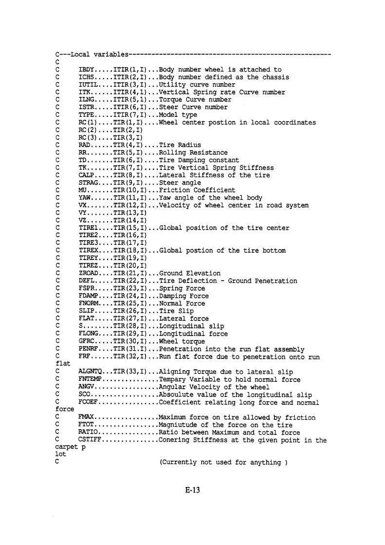
C---Local variables----------------------------------------------------- C ..... C IBDY I T I R ( 1 , I ) ...Body number wheel i s attached t o ..... ... C ICHS I T I R ( 2 , I ) Body number defined as the chassis .... ... C IUTIL ITIR(3,I) Uti l i ty curve number ...... C ITK I T I R ( 4 , l ) ... Vertical Spring ra te Curve number C ILNG ..... ITIR(5,l) ... Torque Curve number C ISTR ..... I T I R ( 6 , I ) , , .S teer Curve number .... .. C TYPE. I T I R (7, I) .Model type .... .... C R C ( 1 ) T I R ( 1 , I ) Wheel center postion i n local coordinates C RC (2) ... . T I R ( 2 , I) .. C RC(3). . T I R ( 3 , I ) ..... .... C RAD. T I R ( 4 , I) Tire Radius ....... C RR TIR(5,I) .... Rolling Resistance ....... .... C TD T I R ( 6 , I ) Tire Damping constant C TK....... TIR(7,1).. . .Tire Vertical Spring Stiffness ..... .... C CALP TIR(8,I) Lateral Stiffness of the t i r e .... .. . . C STRAG T I R ( 9 , I ) Steer angle ....... ... C MU T I R ( 1 0 , I ) Friction Coefficient ...... C YAW T I R ( 1 1 , I ) . ..Yaw angle of the wheel body ....... C VX TIR(12,I)..,Velocity of wheel center i n road system C VY.. .... .TIR(13, I) C a,. .... . T I R ( ~ ~ , I ) .... C TIRE1 TIR(15,I). ..Global position of the t i r e center C TIRE2.. . . T I R ( 1 6 , I) C TIRl33.. . . T I R ( 1 7 , I) C TIREX .... T I R ( 1 8 , I ) ... Global postion of the t i r e bottom C TIREY.. . . T I R ( 1 9 , 1 ) C TIREZ. .. .TIR(20 , I) C ZROAD .... T I R (21, I) .. .Ground Elevation C DEFL ..... TIR(22,I) ... Tire Deflection - Ground Penetration C FSPR. .... T I R (23, I) ... Spring Force C FDAMP .... T I R (24, I ) ... Damping Force C FNORM. ... TIR (25, I) ... Normal Force C SLIP. .... T I R (26, I ) .. .Tire Slip C FLAT ..... TIR(27,I) ... Lateral force C S........TIR(28,I)...Longitudinal s l i p C FLONG .... TIR(29,I) ... Longitudinal force C GFRC.. ... TIR(30,I).,.Wheel torque C PENRF .... TIR(31.1) ... Penetration into the run f l a t assembly C FRF ...... TIR(32,I) ... Run f l a t force due t o penetration onto run f l a t C AZIGNTQ. .. TIR(33, I) .. .Aligning Torque due t o l a t e ra l s l i p C FN T E M P . . . . . . . . . . . . . . . Tmpary Variable t o hold normal force C ANGV ................. Angular Velocity of the wheel C SCO..................Absoulute value of the longitudinal s l i p C FCOEF............. ... Coefficient re lat ing long force and normal force C FMAX ................. Maximum force on t i r e allowed by f r ic t ion C FTOT ................. Magniutude of the force on the t i r e C RATIO... ............. Ratio between Maximum and t o t a l force C CSTIFF .............. .Conering Stiffness a t the given point i n the carpet P lo t C (Currently not used for anything )

INTEGER IBDY, ICHS, IUTIL, ITK, ILNG, ISTR, TYPE

DOUBLE PRECISION RC(3), RAD, RR, TD, TK, CALP, STRAGL, MU, & YAW, VX, VY, VZ, TIRE1, TIRE2, TIRE3, & TIREX, TIREY, TIREZ, ZROAD, & DEFL, FSPR, FDAMP, FNORM, SLIP, FLAT, & Sf FLONG, GFRC, FW, P E W , & FNTEMP, ANW, SCO, FCOEF, FMAX, FTOT, & RATIO, ALGNTQ, CSTIFF

DOUBLE PRECISION

EXTERNAL

FSPLIN, CUBIC, CARPET

FSPLIN, CUBIC, CUBIC1, CARPET

INTRINSIC DABS, DSIGN, DCOS, DSIN, DATAN2, & DSQRT, DMAXl

C--- I n i t i a l i z e t h e ou tput q u a n i t i e s t o zero i n case wheel i s o f f ground

FLONG = O . O D O GFRC = O.ODO FLAT = O.ODO ALGNTQ = O.ODO

FSPR = O.ODO FDAMP = 0 . OD0 FNORM = O . O D O FRF = O.ODO P E W = O.ODO SLIP = O.ODO S = 0.ODO

/* T i r e Longi tudinal f o r c e /* t u r n i n g wheel t o rque /* T i r e L a t e r a l f o r c e / * Aligning Torque

/* T i r e Spr ing Force / * T i r e Damping Force /* Tota l Normal Force /* Run F l a t Force /* P e n e t r a t i o n i n t o run f l a t /* L a t e r a l S l i p /* Longintudinal S l i p

C--- Ca l cu l a t e t h e t i r e - s p r i n g d e f l e c t i o n . C Difference between road elevation and t i r e bottom e l e v a t i o n C Ground p e n e t r a t i o n i f DEFL > 0.0 C Wheel o f f t h e ground i f DEFL <= 0.0

TIREZ = TIR(20, I) ZROAD = TIR(21, I) DEFL = ZROAD - TIREZ

C---Calculate t h e normal f o r c e from ground i f t h e wheel ha s d e f l e c t e d C i n t o t h e ground. If t h e t i r e is no t d e f l e c t e d t h e r e are no C f o r c e s on t h e t i re , s k i p t o t h e end

I F ( DEFL .LE. O.ODO ) THEN DEFL = O.ODO GOT0 1000

ENDIF

C---The wheel has penetrated the ground so we must calculate t i r e forces

C---Get variables from I T I R and T I R arrays

C IBDY = I T I R ( 1 , I) /* Body number w h e e l is a t t a c h e d t o ICHS = I T I R ( 2 , I) /* Body number defined as the c h a s s i s IUTIL = I T I R ( 3, I ) /* U t i l i t y curve number ITK = I T I R ( 4 , l ) /* V e r t i c a l S p r i n g rate C u r v e number ILNG = I T I R ( 5 , l ) /* T o r q u e C u r v e number ISTR = I T I R ( 6 , I ) / * S t e e r C u r v e number

C TYPE = I T I R ( 7 , I ) /* Model type

C R C ( 1 ) = T I R ( 1 , I ) / * Wheel center postion i n local coordinates C RC(2) = T I R ( 2 , I ) C R C ( 3 ) = T I R ( 3 , I )

RAD = T I R ( 4 , I ) /* T i r e R a d i u s RR = T I R ( 5 , I ) /* R o l l i n g R e s i s t a n c e TD = T I R ( 6 , I ) / * T i r e Damping constant TK = T I R ( 7 , I ) /* T i r e V e r t i c a l S p r i n g S t i f f n e s s CALP = T I R ( 8 , I ) /* L a t e r a l S t i f f n e s s of t h e t i re

C STRAGL= T I R (9, I ) /* S t e e r angle MU = T I R ( l O , I ) /* F r i c t i o n C o e f f i c i e n t

C YAW = T I R (11, I) / * Yaw angle of the w h e e l b o d y VX = T I R ( 1 2 , 1 ) /* V e l o c i t y of wheel center i n road

s y s t e m VY = T I R ( 1 3 , I ) VZ = T I R ( 1 4 , I )

C TIRE1 = T I R ( 1 5 , I ) /* G l o b a l pos i t ion of the t i r e center C TIRE2 = T I R ( 1 6 , I ) C TIRE3 = T I R ( 1 7 , I ) C TIREX = T I R ( 1 8 , I ) /* G l o b a l postion of the t i r e bottom C TIREY = T I R ( 1 9 , I ) C TIREZ = T I R ( 2 0 , I) C ZROAD = T I R ( 2 1 , I ) /* G r o u n d E l e v a t i o n

C---Define the normal force, t e s t for a constant spring or curve d a t a

I F ( ITK .EQ. 0 ) THEN defined

J / * No S p r i n g C u r v e

FSPR = TK * DEFL /* T i r e S t i f f n e s s ELSE

FSPR = FSPLIN ( DEFL, O.DO, ITK, 1, A, IA, O, 0 ) ENDIF

C---Define potential energy for s ta t ic analysis

I F ( MSTAT .LE. 1 ) THEN I F ( ITK .EQ. 0 ) THEN

V = V + TK * DEFL**2 / 2.ODO ELSE V = V + FSPLIN ( DEFL, O.DO, ITK, 1, A, IA, -1, 0 )

ENDIF ENDIF

c--- Define t h e normal fo rce r e s u l t i n g from t i r e damping

FDAMP = -VZ * TD * CUBIC1 (DEFL) / * Ti re Damping fo rce

C--- The r a d i u s of t h e run f l a t assembly is given by (RFRAD) C Add 1 inch t o t h i s r ad ius t o account f o r t i r e carcuss th ickness C Check t o see i f t h e t i r e has de f l ec ted i n t o t h e run f l a t assembly C I f TRUE, then add add i t iona l fo rces C Run f l a t s t i f f n e s s is s t o r e d i n RFSTIF C Run f l a t damping i s s t o r e d i n RFDAMP C Use cubic1 with a to le rance of p l u s on minus 1 / 1 6 inch

PENRE' = RFRAD + 1 . O D O + 0.0625D0 - (RAD-DEFL) / * Run f l a t penet ra t ion

IF ( PENRE' .GT. O.ODO ) THEN FRF = RFSTIF * PENRE' * CUBIC1 (8.0DO*PENRF)

& + RFDAMP * (-VZ) * CUBIC1(8,0DO*PENRF) /* Run f l a t force

FRF = DMAXl(O.OD0,FRF) ELSE

PENRF = O.ODO /* Reset f o r r epor t ing

FRF = O . O D O ENDIF

C--- Sum up a l l t h e fo rces t h a t may act on t h e t i r e C Limit t h e normal fo rce so t h a t it can not go negative

FNORM = FSPR + FDAMP + FRF t i r e

FNORM = DMAX1 (O.ODO,FNORM)

/* Normal fo rce on

C---If t h e t i r e i s off t h e ground t h e r e are no longi tudinal forces , C la tera l forces , or torques tu rn ing t h e wheel. C else i f t h e t i r e has penet ra ted t h e ground then c a l c u l a t e t h e C t i r e s l i p angle.

IF ( DSQRT ( VX*VX + W*VY ) . GT. 1 .D-2 ) THEN SLIP = -DATAN2 (VX, VY)

ELSE SLIP = O.DO

ENDIF C C Veloci ty i n X Y plane f o r d r i v e r model: - C

DMVELC = SNGL(DSQRT(QD(l,ICHS)**2 + QD(2,ICHS)**2) / 12. ) C

c--- For t h e Front t i r e s use t h e La te ra l Force Data and Aligning Torque C Date from t h e f i r s t d a t a a r rays

IF ( I .EQ. 1 .OR. I .EQ. 2 ) THEN / * Front Ti res

c--- Save t h e normal fo rce i n a temporary va r i ab le

C Calculate lateral f o r c e from t h e carpet p lo t C Carpe t p lo t is a fami ly o f normal f o r c e Curves versus s l i p angle

FNTEMp = E'NORM FLAT = CARPET ( DABS (SLIP) , DABS (FNTEBP) , I , SFRCl(1, l ) ,

& ALREFl(1) , FZREFl(1) , IPA1 (I) , I P F l ( 1 ) & NAPNTl, NE'PNTl, NTR, CSTIFF )

F U T = DSIGN (FLAT, SLIP)

Corner ing S t i f f n e s s and vertical t i r e load updates ( f r o n t axle) : ( f o r driver model)

I F (I. EQ -1) THEN CCAFl = SNGL(CST1FF) FFZLl = SNGL (FNORM)

ELSE CCAF2 = SNGL (CSTIFF) FFZL2 = SNGL(FNORM1

ENDIF

C---Calculate a l i n g i n g torque from carpet p l o t

ALGNTQ = CARPET ( DABS (SLIP) , DABS (FNTEMP ) , I, ALTOR1(1,1) , & SANGLEI (1) , FZl (1) , IPSA1 (1) , IPFZl (1) & NSA1, NFZ1, NTR, CSTIFF )

ALGNTQ = DSIGN(ALGNTQ,SLIP) END I F

C---For t h e Rear t i res use t h e L a t e r a l Force Data and A l ign ing Torque C Date from t h e second d a t a a r r a y s

I F ( I .EQ. 3 .OR. I .EQ. 4 ) THEN /* Rear T i r e s

C---Save t h e normal f o r c e i n a temporary variable C Calculate lateral f o r c e from t h e carpet p lo t C Carpet p lo t i s a fami ly o f normal f o r c e Curves versus s l i p ang l e

FNTEMP = F'NORM FLAT = CARPET ( DABS (SLIP) I DABS (E'NTEW) I II SFRC2 (1, I)

& ALREF2 (1) , FZREF2 (I) , IPA2 ( 1 1 , IPF2 (1) I & NAPNT2, NE'PNT2, NTR, CSTIFF )

FLAT = DSIGN (FLAT, SLIP)

Corner ing S t i f f n e s s and vertical t i r e load updates (rear axle) : ( f o r driver model)

I F (I. EQ -3) THEN CCARl = SNGL (CSTIFF) FFZL3 = SNGL (FNORM)

ELSE CCA.2 = SNGL (CSTIFF) FFZL4 = SNGL (E'NORM)

ENDIF

C---Calculate alinging torque from carpet plot

ALGNTQ = CARPET ( DABS (SLIP) , DABS (FNTEMP) , I, ALTOR2 (1,l) , & SANGLE2 (I), FZ2 (I), IPSA2 (I), IPFZ2 (I), & NSA2, NFZ2, NTR, CSTIFF )

ALGNTQ = DSIGN (ALGNTQ, SLIP ) END IF

C---Define the longitudinal force for the turning wheel model C Get local velocity in the steer direction C Get the angular velocity of the wheel; Postive velocity is in the C the negative Y direction

C Defn: Long Slip = ( Velocity - R*W ) / Velocity

C if Vel > R*w then slip > 0.0 Wheel is turning to slow causing slip C if Vel = R*w then slip = 0.0 C if Vel < R*w then slip < 0.0 Wheel is turning to fast causing slip

ANGV = UDE ( ItNTR ) / * Angular velocity of wheel

IF ( DABS (VY) .GT. 0.0001DO ) THEN S = ( VY + ANGV* (RAD-DEFL) ) / VY / * Definition of Long.

Slip ELSE S = O.DO

END IF SCO = DABS ( S ) / * temporary variable IF ( SCO .GT. 1.DO ) SCO=l.DO / * Limit slip

C--- The Utility spline curve is used for calculating slip. C Longitudinal force = Fcoef * Fnorm

FCOEF = FSPLIN ( SCO, O.DO, IUTIL, 1, A, IA, 0, 0 ) FLONG = -DSIGN ( FCOEF*FNORM, S )

C---Limit the long. and lateral forces using the friction ellipse (circle).

FMAX = MU*DABS (FNORM) FTOT = DSQRT(FLONG**2 + FLATf*2) IF ( FTOT . GT. FMAX ) THEN RATIO = FMAX/FTOT FLAT = RATIO*FLAT FLONG = RATIO*FLONG

END IF

C--- Calculate the torque due to the longitudinal force causing the wheel C to turn

GFRC = FLONG * ( RAD-DEFL )

C--- S a v e v a l u e s i n I T I R and TIR a r r a y s

T I R ( 2 2 , I ) = DEFL P e n e t r a t i o n

TIR ( 2 3 , I) = FSPR T I R ( 2 4 , I ) = FDAMP T I R ( 2 5 , I ) = FNORM T I R ( 2 6 , I ) = SLIP TIR (27 , I) = FLAT T I R ( 2 8 , I) = S T I R ( 2 9 , I) = FLONG T I R ( 3 0 , I ) = GFRC T I R ( 3 1 , I ) = PENRF T I R ( 3 2 , I ) = FRJ? T I R ( 3 3 , I ) = ALGNTQ

/ * T i r e D e f l e c t i o n - Ground

/* S p r i n g F o r c e /* Damping F o r c e /* Normal F o r c e /* T i r e S l i p /* L a t e r a l force /* L o n g i t u d i n a l s l i p / * L o n g i t u d i n a l force / * Wheel torque /* P e n e t r a t i o n i n t o r u n f l a t / * Force due t o r u n f l a t /* A l i g n i n g T o r q u e

RETURN END

C

SUBROUTINE FILTER(TIME, XNOW, YNOW, VNOW, ANOW, YLAST, VLAST, 1 ALAST, XLAST, TLAST)

Second Order Filter:

TIME.....current time (sec) XNOW.....current input signal to be filtered (input) YNOW ..... filtered value of XNOW signal (output) VNOW..... first derivative of YNOW (output) ANOW ..... second derivative of YNOW (output) YLAST....value of YNOW at last filter computation (input) VLAST....value of VNOW at last filter computation (input) ALAST .... value of ANOW at last filter computation (input) XLAST....value of XNOW at last filter computation (input) TLAST. ... value of TIME at last filter computation (input) Set Filter cutoff frequency and damping:

WN = 25.0 ZETA = 0.707

UPDATE RETURN VALUES FROM LAST ENTRY IN CASE OF T<=O RETURN

YNOW = YLAST VNOW = VLAST ANOW = ALAST

INITIALIZE FOR TIME ZERO

IF(TIME .LE. 0.0) THEN YLAST = XNOW VLAST = 0.0 XLAST = XNOW TLAST = 0.0 YNOW = XNOW VNOW = 0.0 ANOW = 0.0

END IF

T = TIME - TLAST IF(T .LE. 0.0) RETURN

COMPUTE CONSTANTS IN RECURSION EXPRESSIONS

C1 = 4.+ 4.*T*ZETA*WN - T*T*WN*WN C2 = 4.*T C3 = T*TfWN*WN DET = 4.*(l+T*ZETA*WN)+WN*WN*T*T C4 = -4.*T*WNfWN C5 = 4.-4.*T*ZETA*WN-TfT*WN*WN C6 = 2.*ThWN*WN

* CALCULATE FILTERED VALUES OF DISPLACEMENT, VELOCITY, AND ACCEL: *

YNOW = ( Cl*YLAST + C2*VLAST + C3*(XNOW+XLAST) ) / DET VNOW = ( CQ*YLAST + CS*VLAST + CG*(XNOW+XLAST) ) / DET ANOW =: (WN*WN) * (XNOW - YNOW) - (2.0*ZETA*WN) *WOW *

* * UPDATE VALUES FOR NEXT ENTRY PRIOR TO RETURNING *

YLAST = YNOW VLAST = VNOW XLAST = XNOW ALAST = ANOW TLAST = TIME

RETURN

END

C C Auxilliary routine used to calculate Euler angles & position C information and write results to an external file. Output used by C by post processing software for animation. C

SUBROUTINE EULANG(T, Y, A)

DOUBLE PRECISION A (3,3) , Y (3) , T, BOT, TLAST DOUBLE PRECISION PSI, THETA, PHI SAVE IOPEN, TLAST

IF(T .LE. 0.02) THEN TLAST = 0.0 IOPEN = 0

ENDIF C

IF (T-TLAST . LE . 0.0495) RETURN C C Heading Angle

PSI = DATAN2( A(1,2), A(2,2) ) C Pitch Angle

BOT = DSQRT( A(1,2)*A(lf2) + A(2,2)*A(2,2) ) THETA = DATAN2( A(3,2), BOT)

C Roll Angle BOT = DSQRT( A(l,l)*A(l,l) + A(2,1)*A(2,1) ) PHI = -DATAN2( A(3,1), BOT)

C IF (IOPEN . EQ. 0) OPEN (35, FILE=IDADS .ANIM1, STATUS=IUNKN0WN1 ) IOPEN = 1 WRITE (35,100) Y,PSI,THETA,PHI

100 FORMAT(6F12.4) C

TLAST = T RETURN END

Appendix F

Path Planning 1 Obstacle Detection Example Code

This appendix contains example FORTRAN code that was used to demonstrate the path planning and obstacle detection algorithm discussed in section 5.9. The code is only minimally documented but may be helpful as an outline and starting point for other studies interested in using and interfacing the driver model code.

The code also contains a linear vehicle model with 3 degrees of freedom which may be instructive, by example, for persons interested in altering or extending the vehicle dynamics portion of the driver model to other types of vehicles or applications.

Below is a brief outline of the code that follows:

read in vehicle parameters for a 3-DOF vehicle model (yaw, lateral displacement, and roll motion)

read in left / right boundary tables and obstacle positions

within the integration loop:

calculate @eta) profiles relative to current vehicle position and orientation

calculate r*, theta* & transform to x*, y* inertial coordinates as the "input path" (target point) for the single-point driver model

calculate a new preview time based upon r* and forward speed

update the transition matrix for the new preview time

pass x*,y* to the driver model and obtain a steering command

I integrate the linear equations of motion and obtain a new state

I end of the integration loop

I stop

C *** Driver Model - Main Call ing Program *** C *** Path Planning / Obstacle Detection Example Code *** C

PROGRAM MAIN SAVE INTEGER R, W

C REAL OBST(3,3) REAZ; LB (99,2), RB (99,2) REAL RLB(99), THLB(99) REAL RRB(99), THRB(99) REAL RD (200), TH (200) REAL PHICOF (3,3)

C CHARACTER*80 TITLE CoMMoN /ERDINE'/ TITLE SAVE /ERDINE'/ COMMON /DRIV/ CAF, CAR, WHBS, WF, WR, U SAVE /DRIV/ COMMON /ROLL/ HRC, ROLLK, ROLLC, RIROU SAVE /ROLL/ COMMON /INOUT/ R, W SAVE /INOUT/ COMMON /TIRE/ FYlL,FYlR,FY2L,FY2R SAVE /TIRE/ COMMON /DRVSTl/ GRAV, TICYCL, TSS, DMAX, XP (100) , YP (100) , TAUMEM, 1 TFF, RM, A, B, RI, PSIO, NTF, NP, TLAST, DFWLST, TILAST, 2 DMEM(100,2), XT (loo), YT (100) SAVE /DRVSTl/ DIMENSION Y (7), YD (7) DATA IERD/8/

C GRAV = 32.16666 R = 1 w = 2 OPEN (R, FILE=' DMOBST. INf ) OPEN (W, FILE=' DMOBST. OUT ' )

C OPEN (G,FILE='OUT.6') C OPEN (7,FILE='OUT.7') C

READ (R,3) TITLE 3 FORMAT (A80)

C C Read vehicle & simulation parameters: C

READ (R,10) CAF, CAR, WGHT, U, A, B, RI READ (R, 10) HRC, ROLLK, ROLLC, RIROLL READ (R,10) TEND, DT, DTPR

10 FORMAT (7F10.3) C C

RM = WGHT / GRAV WHBS = A + B WE' = WGHT * B / WHBS WR = WGHT * A / WHBS

C C C a l l DRIVE1 t o read driver m o d e l parameters & i n i t i a l i z e C

CALL DRIVE1 ( D m ) C C R e a d i n l e f t & r i gh t boundary tables, obstacle positions, C and i n i t i a l vehicle location C

CALL GETBOU (LB, RB, NLBO, NRBO, VEHWID) CALL GETOBS (NOBST, OBST, VEHWID) CALL GETPAR(THMAX, WAX, DELTH, DELR, NPOWER)

C C C C a l l TRANS t o C a l c u l a t e I n i t i a l T r a n s i t i o n Matrix C

CALL TRANS C

A l = - 2 . * ( C A F t C A R ) / R M / U B 1 = 2 . * (CAR*B - CAF*A) / RM / U - U A2 = 2 . * (CAR*B - CAF*A) / RI / U B2 = -2. * (CAR*B*B + CAF*A*A) / R I / U C 1 = 2 . * w / m C 2 = 2 . * C A F / R I * A A0 = HRC D l = HRC B3 = (WFtWR) /GRAV*HRC*U/RIROLL B4 = (- (WFtWR) *HRC t ROLLK) / R I R O U B5 = ROUC / RIROLL

C C I n i t i a l i z a t i o n of state (3-DOF vehicle model: lateral, yaw, r o l l ) -> C C Y ( 1 ) lateral inert ial posi t ion C Y ( 2 ) lateral veloci ty i n body axis system C Y (3) yaw rate C Y ( 4 ) yaw angle C Y(5) longitudinal iner t ia l posi t ion C Y (6 ) r o l l rate C Y (7) r o l l angle C

DO 2 0 I = 1, 7 Y ( 1 ) = 0.0 YD(1) = 0 . 0

2 0 CONTINUE YD(5) = u

C DFWOLD = 0 . 0 DFWOUT = 0 . 0 IEND = INT (TEND/DT t 0 . 0 0 0 0 1 )

C C S t a r t of Integration Loop: C

DO 3 0 I = 0, IEND T = I * D T

C C S t a t e V e l o c i t y : YD(1)

Current vehicle position and heading:

XV = Y (5) W = Y (1) PSI = Y ( 4 )

No of p t s i n l e f t and right boundary tables

NLB = NLBO NRB=NRBO

Transform x,y boundary and obstacle data t o polar coords:

CALL TRPOLR(XV, W, PSI, LB, NLB, RLB, THLB, CALL MONO (NLB , THLB RLB) CALL TRPOLR(XV, W, PSI, RB, NRB, RRB, THRB, CALL MONO (NRB, THRB, RRB)

DO 25 J=1, NOBST CALL TRANOB (XV, W, PSI, OBST, PHICOF, J)

25 CONTINUE

Ray tracing t o calculate boundary/obstacle intersects :

CALL GENRAY (XV, W, PSI, NLB, RLB, THLB, NRB, RRB, THRB, + NOBST, PHICOF, THMAX, RMAX, DELTH, DELR, RD, TH)

Calculate r* from r ( t h e t a ) profi le returned by GENRAY:

CALL CALCRS (RD, TH, THMAX, DELTH, RSTAR)

Calculate theta*:

CALL CALCTH(RD, THf THMAX, DELTH, NPOWER, THSTAR)

Transform polar r*, theta* coords t o i n e r t i a l x*, y* coords: (save x*,yf as single-point target for driver model)

CALL TRANXY (XV, W, PSI, RSTAR, THSTAR, XSTAR, YSTAR)

Adjust driver model preview time based upon r* and forward speed:

TFF = RSTAR / U

Update driver model t ransi t ion matrix for current preview time:

CALL TRANS

Call t o Driver Model: returns calculated s teer angle, DFW.

CALL STEER(Tf Y f DFWOUT, DFWOLD, XSTAR, YSTAR)

Optional screen output:

WRITE(9,999) T, (Y(JK),JK=1,7),DFWOLD,DFWOUT 999 FORMAT (10F8.2)

DFW = DFWOUT DFWOLD = DFWOUT

State Derivatives:

YD(2) = Al * Y (2) + B1 * Y (3) + C1 * DFW YD(3) = A2 * Y (2) + B2 * Y (3) + C2 * DFW YD(4) = Y (3) YD (5) = U YD(6) = Y (7) YD (7) = -B3* (Y (3) + YD (2) /U) - B4*Y (6) - B5*Y (7)

State Position: Y (i)

FYlL a -CAI?* ( (Y (2)+Y (3) *A) /U - DFW ) FYlR a -CAI?* ( (Y (2) +Y (3) *A) /U - DFW ) FY2L = -CAI?* (Y (2) -Y (3) *B) /U FY2R = -CAE'* (Y (2) -Y (3) *B) /U

Call Output Subroutine to Print Results (optional)

CALL OUT(T, Y, YD, DFW)

Call ERD plotter routines: (optional)

IF(T .EQ. 0.0) THEN CALL SETERD (IERD, NBYTES) CALL OUTERD (IERD, NBYTES, TI Y, YD, DFWOUT, DFW, DFVEL, DFACC) ELSE CALL OUTERD (IERD, NBYTES, T, Y, YD, DFWOUT, DFW, DFVEL, DFACC) ENDIF

End of Integration Loop:

30 CONTINUE

CLOSE (R) CLOSE (W) CLOSE (6) CLOSE (7)

READ (9,40) ISTOP

40 FORMAT (11) STOP END

* * End of Main Calling Program ***

*** Output Subroutine ***

SUBROUTINE OUT (T, Y, YD, DFW) SAVE INTEGER R, W COMMON /INOUT/ R, W SAVE /INOUT/ COMMON /DRIV/ CAF, CAR, WHBS, WF, WR, U SAVE /DRIV/ DIMENSION Y (7), YD (7), YOUT(7), YDOUT(7) DATA RADIAN /57.3/ DO 10 I = 1, 7 YOUT (I) = Y (I) YDOUT(1) = YD (I)

10 CONTINUE YOUT (2) = Y (2) / U * RADIAN YOUT(3) = Y(3) * RADIAN YOUT (4) = Y (4) * RADIAN YOUT (6) = Y (6) *RADIAN YOUT(7) = Y (7)*RADIAN YDOUT(2) = YD(2) / U * RADIAN YDOUT(3) = YD (3) * 57.3 YDOUT(4) = YD (4) * RADIAN DFWPRT = DFW * RADIAN WRITE (W, 20) TI DFWPRT, (YOUT (I) , I=1,7) , (YDOUT (I) , I=1,5)

20 FORMAT (14F8.2) RE- END

*** Start of Driver Model Routines ***

*** Driver Model Subroutine ***

Initialization

SUBROUTINE DRIVE1 (DFW) SAVE INTEGER RI W COMMON /INOUT/ R, w SAVE /INOUT/ COMMoN /DRIV/ CAF, CAR, WHBS, WF, WR, U SAVE /DRIV/ COMMON /DRVSTl/ GRAV, TICYCL, TSS, DMAX, XP (100) , YP (100) , TAUMEM, 1 TFF, RM, A, B, RI, PSIO, NTF, NP, TLAST, DEWLST, TILAST, 2 DMEM(100,2) , XT (loo), YT (100) SAVE /DRVSTl/

GRAV = 32.16666 TICYCL = 0.0001 TSS = 0.0 DMAX = 0.2

WRITE (W,lO) 10 FORMAT ('O', T20, 'CLOSED-LOOP PATH FOLLOWING MODE', /, 'of, T20, 1 'X-Y ', 'PATH', ' COORDINATES :', /, 'Of, TSO, 'XI, T60, 2 'Y1, /, /'ol, T47, '(FEET)', T57, ' (FEET)')

READ (R,20) NP 20 FORMAT (13)

DO 40 J = 1, NP READ (Rr30) XP(J), YP(J)

30 FORMAT (2F10.2) WRITE (W, 50) XP (J) , YP (J)

40 CONTINUE 50 FORMAT ( ' ', T43, 2F10.2)

READ (R, 60) TAUMEMI TFF 60 FORMAT (F10.4)

WRITE (W, 70) TAUMEMI TFF 70 FORMAT (I I , /, I , T20, 'DRIVER TRANSPORT LAG (SEC) : I , T60, 1 F4.2, /, I , T20, 'END OF PREVIEW INTERVAL (SEC) : I , T60, 2 F4.2/) RM = (WF t WR) / GRAV B = WHBS * WF / (WE' + WR) A = WHBS - B R I = A * B * R M PSI0 = 0.0

NTF = 1

DO 80 J = 1, NP XT(J) = XP(J) * COS(PSI0) t YP(J) * SIN(PSI0) YT(J) = -XP(J) * SIN(PSI0) t YP (J) * COS (PSIO)

80 CONTINUE TLAsT= 0. DFWLST = 0. TILAST = 0. DFW = 0. DO 90 I = 1, 100 DMEM(1,l) = 0.

90 DMEM(I,2) = -1. R e m END

Transition Matrix Calculation

SUBROUTINE TRANS SAVE INTEGER R, W COMMON /INOUT/ R, W

SAVE /INOUT/ COMMON /DRIV/ CAE', CAR, WHBS, WF, WR, U SAVE /DRIV/ COMMON /ROLL/ HRC, ROLLK, ROLLC, RIROLL SAVE /ROLL/ COMMON /DRVSTI/ GRAV, TICYCL, TSS, DMAX, ~ ~ ( 1 0 0 1 , YP( IOO) , TAUMEM,

1 TFF, RM, A, B, R I , PSIO, NTF, NP, TLAST, DE'WLST, TILAST, 2 DMEM(100,2), XT ( l o o ) , YT ( 1 0 0 )

SAVE /DRVST~/ COMMON /TRSSTR/ T T T ( 6 , 6 , 1 0 ) , T T T 1 ( 6 , 6 , 1 0 ) , G ( 6 ) SAVE /TRSSTR/ DIMENSION SV ( 6 ) , SD ( 6 ) , SVI ( 6 )

C DELT = 0 . 0 1 GRAV = 3 2 . 1 6 6 6 6 A 1 = -2 . * (CAE' + C A R ) / RM / U B 1 = 2 . * (CARfB - CAF*A) / RM / U - U A2 = 2 . * (CAR*B - CAF*A) / RI / U B2 = -2. * (CAR*B*B + CAF*A*A) / RI / U C1 = 2 . * CAF / RM C 2 = 2 . * C A F / R I * A A0 = HRC D l = HRC B3 = (WF+WR)'/GRAV*HRC*U/RIROLL B4 = (-(WF+WR)*HRC + ROLLK) / RIROLL B5 = ROLLC / RIROLL ULAST = U G ( 1 ) = 0 . G ( 2 ) = C1 G ( 3 ) = C2 G ( 4 ) = 0 . G ( 5 ) = 0. G ( 6 ) = 0 . DO 70 J = 1, 6

NBEG = TSS / DELT t 1 NENDl = (TFF t . 0 0 1 - TSS) / NTF / DELT NENDV = NENDl DO 1 0 L = 1, 6

SV(L) = 0 . 0 S v I ( L ) = 0 . 0

1 0 CONTINUE TIME = 0 . S V ( J ) = 1 . 0 DO 6 0 I = 1, NTF

DO 4 0 K = NBEG, NENDV S D ( 1 ) = S V ( 2 ) + U * S V ( 4 ) t AO*SV(6) S D ( 2 ) = A 1 * S V ( 2 ) t B 1 * S V ( 3 ) S D ( 3 ) = A2 * S V ( 2 ) + B2 * S V ( 3 ) S D ( 4 ) = S V ( 3 ) S D ( 5 ) = S V ( 6 ) SD (6 ) = -B3 * ( S V ( 3 ) + SD ( 2 ) /U) - B4*SV(5) - B5*SV(6) DO 2 0 L = 1, 6

SV(L) = SV(L) t SD(L) * DELT 2 0 CONTINUE

TIME = TIME t DELT

DO 30 L = 1, 6 SVI (L) = SV;C (L) + SV(L) * DELT

30 CONTINUE 4 0 CONTINUE

DO 50 L = 1, 6 TTT (L, JI I) = SV (L) TTT1 (L, J, I) = SVI (L)

50 CONTINUE NBEG = NBEG t NENDl NENDV = NENDV t NENDl

60 CONTINUE 70 CONTINUE

RETURN END

Closed-Loop Steer Calculation

SUBROUTINE STEER(XI Y I DFW, DFWNOW, XSTAR, YSTAR)

(Subroutine "DRIVERn in other versions)

SAVE INTEGER R, W COMMON /INOUT/ RI W SAVE /INOUT/ COMMON /DRIV/ C A F , CAR, WHBS, WF, WR, U SAVE /DRIV/ COMMON /DRVSTI/ GRAV, TICYCL, TSS, DMAX, XP (100 , YP (100 , TAUMEM,

TFF, MI A, BI R I , PSIO, NTF, NP, TLAST, DFWLST, TILAST, DMEM(100,2), XT(100), YT (100)

SAVE /DRVSTl/ COMMON /TRSSTR/ TTT (6,6, lo), TTT1(6,6, lo), G (6) SAVE /TRSSTR/ DIMENSION Y (7), YC(7) DIMENSION D M 1 (6) DIMENSION D M ( 6 ) , VECM(6) DIMENSION D W (6,6), DUMM2 (6,6) DATA VECM /1.0, 5*0.0/

N P = 1 XP(1) = XSTAR YP (1) = YSTAR T = X EPSI = ABS (Y (4) - PSIO) DO 10 I = 1, 4

10 YC(1) = Y (I) YC(5) = Y (6) YC(6) = Y (7) YC(7) = Y (5)

IF (EPSI .LE. .002) GO TO 30

Update Coordinate Transformation

XT(J) = XP(J) * COS(PSI0) + YP(J) * SIN(PSI0) 20 YT (J) = -W (J) * SIN (PSIO) + YP (J) * COS (PSIO)

C 30 YO = -YC (7) * SIN(PSI0) t YC (1) * COS (PSIO)

XO = YC (7) * COS (PSIO) t YC (1) * SIN(PSI0) YC(1) = YO YC (4) = YC (4) - PSI0 EPSY2 = 0. TSUM = 0. SSUM = 0. IF (T - TILAST .LE. TICYCL) RETURN DO 50 I = 1, NTF TJI = (TFF - TSS) / NTF * I t TSS DO 40 J = i, 6 DO 40 K = 1, 6 DUMMl ( J , K ) = TTT1 (J,K, I)

40 DUMM2(J,K) =TTT(J,K,I) CALL GMPRD(VECM, D M , DUMV11, 1, 6, 6) CALL GMPRD (VECM, D U W , DUMV1, 1, 6, 6 ) CALL GMPRD(DUMV1, YC, TI, 1, 6, 1) XCAR = XO t U * TJI

CAU TRAJ(XCAR, XT, YT, YPATH)

YPATH = YT (1)

CALL GMPRD(DUMVl1, G, S1, 1, 6, 1) EP = T1 t S1 * DFWNOW - YPATH TSUM = TSUM + EP * S1 SSUM = SSUM + S1 * Si EPSY2 = EPSY2 + EP * EP * (TFF - TSS) / NTF

50 CONTINUE EPSY = SQRT (EPSY2) / (TFF - TSS) DFW = -TSUM / SSUM + DEWNOW IF (ABS (DEW) . GT. DMAX) DEW = DMAX * SIGN(1. ,DFW) DO 60 J = 1, 2 DO 60 I = 1, 99

60 DMEM(101 - 1,J) = DMEM(100 - 1,J) DMEM(1,l) = DEW DMEM(1,2) = T TTAB = T - TAUMEM DO 70 I = 1, 99 IF (DMEM(1 t 1,2) .LE. TTAB .AND. DMEM(I,2) .GE. TTAB)

1 GO TO 90 70 CONTINUE

WRITE (W,80) 80 FORMAT ('01, I***** TAUMEM PROBABLY TOO LARGE *****I )

CALL EXIT C 90 DFW =DMEM(I-2,1)+DMEM(I-1,1)+DMEM(I,1)+DMEM(If1l1)+DMEM(I+~ll) C DFW = DFW/5.

90 DEW = 0.0 IF(T .GE. TAUMEM) DEW = DMEM(1,l) TLAST = X TILAST = X RETURN

END

*** T r a j e c t o r y S u b r o u t i n e *** SUBROUTINE TRAJ (XI XT, YT, YPATH) SAVE INTEGER R, W COMMON /INOUT/ R, w SAVE /INOUT/ COMMON /DRIV/ CAE', CAR, WHBSr WF, WRI U SAVE /DRIV/ DIMENSION XT (* ) , YT (* )

SEARCH FOR X I , X I + l : DO 1 0 J = 1, 99

I F (X .GE. X T ( J ) .AND. X .LT. X T ( J + 1)) GO TO 3 0 1 0 CONTINUE

WRITE (W,20) 2 0 FORMAT ( ' O ' , 'X-SEARCH I N SUB. TRAJ FAILED. ' )

CALL EXIT 30 SLOPE ( Y T ( J + 1) - Y T ( J ) ) / ( X T ( J + 1) - X T ( J ) )

Y2 = Y T ( J ) + SLOPE * (X - X T ( J ) ) YPATH = Y2 RETURN END

*** Matrix P r o d u c t S u b r o u t i n e ***

SUBROUTINE --(A, B, R, N, M, L ) DIMENSION A(N*M), B(M*L), R(N*L) I R = 0 I K = -M DO 1 0 K = 1, L

I K = I K + M DO 1 0 J = 1, N

I R = I R + 1 J I = J - N I B = I K R ( 1 R ) = 0 . DO 1 0 I = 1, M JI = JI + N I B = I B + 1

1 0 R ( 1 R ) = R(1R) + A ( J 1 ) * B ( 1 B ) RETURN END

*** End of Driver Model Code ***

*** Start of Path Planning / Obstacle Detection Code * * *

SUBROUTINE GETBOU(LB, RBI NLB, NRB, VEHWID) SAVE INTEGER RI W

COMMON /INOUT/ R, W SAVE /INOUT/

REAL LB (99,2), RE (99,2), VEHWID

READ(R,100) VEHWID 100 FORMAT (F10.3)

READ (R, 150) NLB 150 FORMAT(I.2)

DO 200 I=l,NLB READ (R, 50) LB(I,l) tLB(If2)

50 FORMAT (2F10.3) LB(I,2) = LB(I,2) + VEHWID/2.

200 CONTINUE

READ(R,150) NRB DO 300 I=l,NRB READ(Rt50) RE(I,l) rRB(Ir2) RB(I,2) = RB(If2) - VEHWID/2.

300 CONTINUE RETURN END

C C C

SUBROUTINE GETOBS (NOBST, OBST, VEHWID) SAVE INTEGER R, W COMMON /INOUT/ R, w SAVE /INOUT/

REAL OBST(3,3)

READ(R,100) NOBST 100 FORMAT (12)

DO 200 I=l,NOBST READ (R, 3ooj (OBST (I, J) , J=I, 3) OBST (I, 3) = OBST (I, 3) + VEHWID/2.

200 CONTINUE 300 FORMAT(3F10.3)

RETURN END

SUBROUTINE GETPAR (THMAX, RMAX, DELTH, DELR, NPOWER) SAVE INTEGER R, W COMMON /INOUT/ R, W SAVE /INOUT/

READ (R, 100) THMAX, RMAX, DELTH, DELR, NPOWER 100 FORMAT (4F10.3,12)

RETURN END

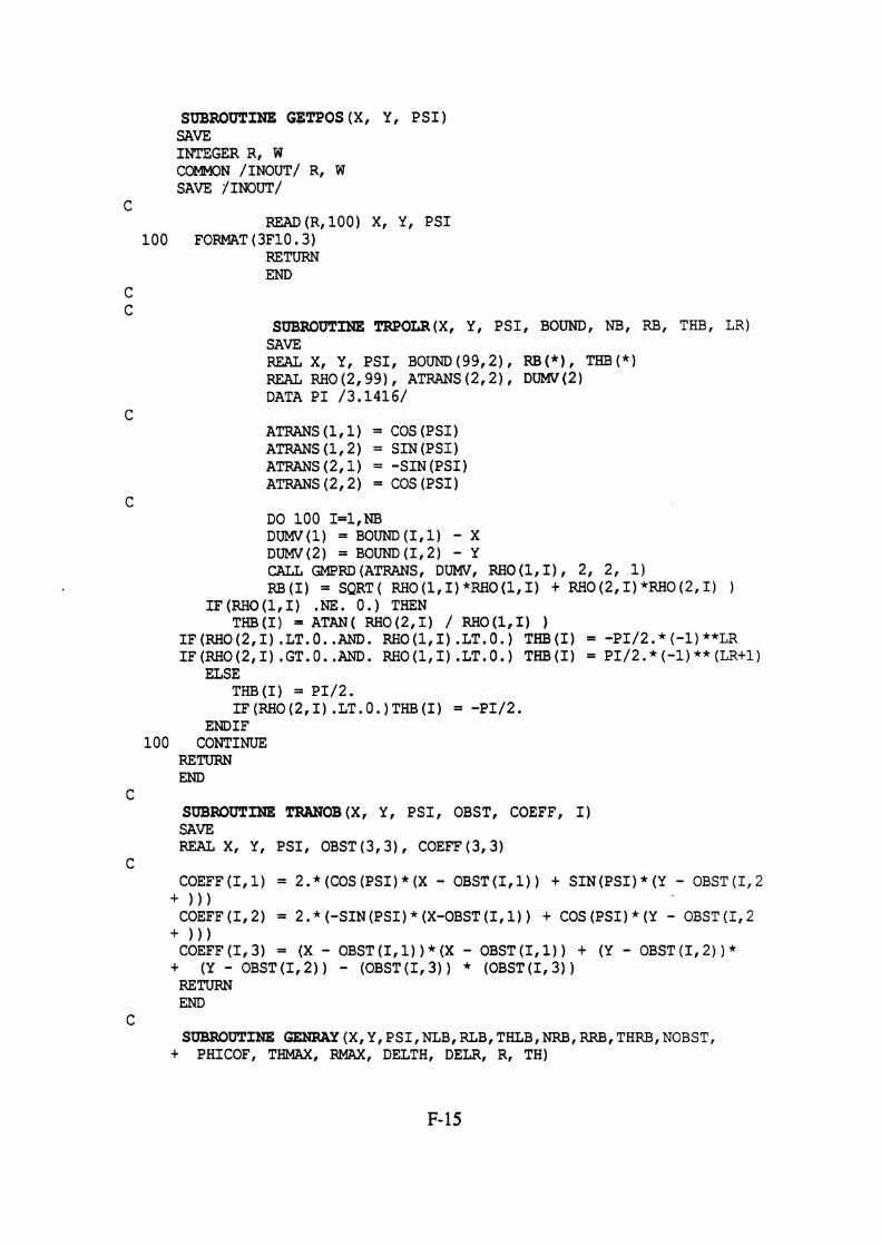
SUBROUTINE GETPOS (XI Y, PSI ) SAVE INTEGER R, W COMMON /INOUT/ R, W SAVE ;/INOUT/

C READ(R,100) XI Y, PSI

100 FORMAT (3F10.3) RETURN END

C C

SUBROUTINE TRPOLR(X, Y, PSI, BOUND, NB, RB, THB, LR) SAVE REAL XI Y, PSI, BOUND(99,2), RB(*), THB(*) REAL RH0(2,99), ATPANS(2,2), DUMV(2) DATA PI /3.1416/

ATPANS (Ill) = COS (PSI) ATRANS (1,2) = SIN (PSI) ATRANS (2,l) = -SIN (PSI) ATRANS(2,2) = COS(PS1)

DO 100 I=l,NB DUMV(1) = BOUND (Ill) - X DUMV(2) = BOUND(I,2) - Y CAU GMPRD(ATRANS, DUMV, RHO(l,I), 2, 2, 1) RB(1) = SQRT( RHO(l,I)*RHO(l,I) + RH0(2,1)*RH0(2,1) )

IF(RHO(1,I) .NE. 0.) THEN THB(1) = ATAN( RHO(2,I) / RHO(1,I) )

IF (RHO(2,I) .LT.O. .AND. RHO(1,I) .LT.O.) THB(1) = -PI/2.* (-1) **LR IF(RHO(2,I) .GT.O. .AND. RHO(1,I) .LT.O.) THB(1) = PI/2.* (-I)** ( L R t 1 )

ELSE THB (I) = PI/2. IF(RHO(2,I) .LT.O.)THB(I) = -PI/2.

ENDIF 100 CONTIMJE

RETURN END

C SUBROUTINE TRANOB (XI Y l PSI, OBST, COEFF, I) SAVE REAL X, Y, PSI, OBST(3,3), COEFF (3,3)

C COEFF(1,l) = 2.*(COS(PSI)*(X - OBST(1,l)) + SIN(PSI)*(Y - OBST(I,2

+ 1 ) ) COEFF (I, 2) = 2. * (-SIN (PSI) * (X-OBST (I, 1) ) + COS (PSI) * (Y - OBST (I, 2

+ 1 ) ) COEFF(I,3) = (X - OBST(I,l))*(X - OBST(1,l)) t (Y - OBST(I,2))*

+ (Y - OBST (I, 2) ) - (OBST (I, 3) ) * (OBST(I,3) ) RETURN END

C SUBROUTINE GENRAY (X,Y,PSI,NLB,RLB,THLBINRB,RRB,THRB,NOBSTf

+ PHICOF, THMAX, MI DELTH, DELR, Rl TH)

SAVE REAL XI Y f P S I , RLB(*) , THLB(*), RRB(*) T.YRB(*), PHICOF(3 ,3 )

+ , R ( * ) f TH(*) REAL RADLST(200) SAVE RADLST

C JMAX = 2*THMAX/DELTHtl THETA = -THMAX - DELTH DO 1 0 0 J=l, JMAX

THETA = THETA t DELTH CALL SEARCH(1, NLB, THLB, RLB, THETA, RNOWL, 1) CALL SEARCH (1, NRB, THRB, RRB, THETA, RNOWR, 1) R ( J ) = FNOWR IF(RN0WL .LT. RNOWR) R ( J ) = RNOWL

I F (NOBST .GT. 0 ) THEN RADIUS = 0 . 0 ISTART = RADIUS/DELR IEND = RMAX/DELR

DO 90 I=ISTART, IEND RADIUS = RADIUS + DELR CALL EVALOB (RADIUS THETA, PHICOF , NOBST , VALUE)

IF(VALUE .LT. 0 ) THEN I F ( RADIUS .LT. R ( J ) ) R ( J ) = RADIUS GO TO 95

ENDIF 90 CONTINUE 9 5 CONTINUE

ENDIF C

I F ( RMAX .LT. R ( J ) ) R(J) = RMAX TH (J) = THETA

C RADLST (J) = R ( J )

C 1 0 0 CONTINUE

C RETURN END

C C

SUBROUT1 NE CALCRS (R, TH, THMAX, DELTH , RSTAR) SAVE REAL R (*) , TH (*) , THMAX, DELTH, RSTAR

C SUM = 0 . 0

C IMAX = 2*THMAX/DELTHtl DO 1 0 0 I=l,IMAX

SUM = SUM t R ( 1 ) 100 CONTINUE

S T A R = SUM / IMAX C

RETURN END

C

SUBROUTINE CALCTH (R, TH, THMAX, DELTH NPOWER, THSTAR) SAVE REAL R(*) TH(*) I TIMAX, DELTH, THSTAR

IMAX = 2*THMAX/DELTHtl DO 100 I=l,IMAX

SUMl = SUMl + (R (I) **NPOWER) * TH (I) SUM2 = SUM2 + (R(I)**NPOWER)

100 CONTINUE

THSTAR = SUMl / SUM2

RETURN END

SUBROUTINE EVALOB (R, THETA, PHICOF NOBST VALUE) SAVE REAL Rf THETA, PHICOF (3,3) VALUE DIMENSION VAL (3)

DO 100 1-1, NOBST VAL (I) =R*R+ ( PHICOF (I, 1) *COS (THETA) + PHICOF (I, 2) *SIN(THETA) ) t * R + PHICOF(I,3)

100 CONTINUE

VALUE = VAL(1) DO 90 1-1, NOBST

IF(VAL(1) .LT. VALUE) VALUE = VAL(1) 90 CONTINlTE

RETURN END

SUBROUTINE TRAlUY (XI Y, PSI, RSTAR, THSTAR, XSTAR, YSTAR) SAVE REAL XI Y, PSI, RSTAR, THSTAR, XSTAR, YSTAR XSTAR = X + RSTAR*COS(PSI+THSTAR) YSTAR = Y + RSTAR*SIN(PSI+THSTAR) RETURN END

SUBROUTINE SEARCH(Mf N, XI Yf A, Bf IDIR) SAVE DIMENSION X (* ) , Y (*)

IDIR = 1 => FORWARD SEARCH; IDIR = -1 => REVERSE SEARCH.

4 0 0 CONTINUE C

DO 1 0 0 I = M, N-1 B = Y ( I )

IF ( A . E Q . X ( I ) ) RETURN I F ( A .GE. X ( 1 ) .AND. A . L T . X ( I t 1 ) ) THEN

B = Y ( I ) t (Y (14-1) -Y ( I ) ) / (X ( I t l ) -X ( I ) ) * (A-X ( I ) ) RETURN

ENDIF C -

I F ( A .LE. X ( 1 ) .AND. A .GT. X ( I t 1 ) ) THEN B = Y ( I ) t (Y ( I t l ) -Y ( I ) ) / (X ( I t l ) -X (I) ) * (A-X (I) ) RETURN

ENDIF 1 0 0 CONTINUE

B = Y (N) I F ( ( A . L E . X ( M ) ) .AND. ( X ( M ) . L E . X ( N ) ) ) B = Y(M) RETURN

C C REVERSE SEARCH: C

8 0 0 CONTINUE C

DO 2 0 0 I = N,M+l,-1 B = Y ( I )

I F ( A . E Q . X ( I ) ) RETURN I F ( A .GE. X ( 1 ) .AND. A .LT. X ( 1 - 1 ) ) THEN

B = Y ( 1 ) t (Y(1-1)-Y(I))/(X(I-1)-X(I))*(A-X(1)) RETURN

ENDIF C

I F ( A .LE. X ( 1 ) .AND. A .GT. X ( 1 - 1 ) ) THEN B = Y (I) t (Y ( 1 - 1 ) -Y ( I ) ) / (X ( 1 - 1 ) -X ( I ) ) * (A-X ( I ) ) RETURN

ENDIF 2 0 0 CONTINUE

B = Y (M) I F ( ( A .LE. X ( N ) ) .AND. (X(N) . L E . X ( M ) ) ) B = Y ( N ) RETURN END

C C

SUBROUTINE MONO (N, X, Y ) SAVE DIMENSION X ( * ) , Y (*)

C I F ( X ( 1 ) . L T . X ( N ) ) RETURN

C M = N / 2

C DO 1 0 0 I = l , M

DUM = X ( 1 ) X ( 1 ) = X ( N - I t l ) X ( N - I t l ) = DUM

1 0 0 CONTINUE

DO 200 I=l,M DUM = Y (I) Y (I) = Y (N-It1) Y (N-Itl) = DUM

200 CONTINUE C

RETURN END

Appendix G

Background References

The first two technical papers included in this appendix (references 1 and 2 from the List of References) provide principal background material for much of the work initially undertalcen in this project and are included here as a convenience. The third technical paper appearing in this appendix reports on analyses performed by Stribersky (reference 42) using the HMMWV-Trailer combination vehicle test data from this project to confirm findings predicted by the application of bifurcation theory to vehicle dynamic systems.

The material is reproduced here by permission of the IEEE Transactions on Sytems, Man, and Cybernetics journal (Copyright IEEE ), and, the ASME Journal of Dynamic Systems, Measurement, and Control (Copyright ASME).

IFXE TRANSACTIONS ON SYSTEMS. M A h . 4ND CYBEXNETICS, V O L SMC-11. NO. 6, IUNE 1981

Application of an Optimal Preview Control for Simulation of Closed-Loop

Automobile Driving CHARLES C. MACADAM

AbsM-An oprimal preview control method is applied to the automo- automobile path following problem produces substantive bile path fouowing problem. The technique is first used to examine the agreement when driv&/vehicle straight-line regulatory driving task and results compared with similar es- perimental measurements. The method is further demonstrated by closed- tal measurements for both straight-line regulatory driving loop simulation of an automobile driver~vehicle system during transient and transient lane-change lane-change maneuvers. The computer simulation results are compared uith equivalent vehicle test measurements. 11. THE OPTIMAL PREVIEW CONTROL

I. INTRODUCTION

I T HIS PAPER presents example applications (to the

automobile path following problem) of a general method of control synthesis presented in [I]. The method is

I demonstrated here by simulation of a closed-loop automo- I I bile/driver system and the results compared with

driver/vehicle test measurements. Results for the optimal preview control are also discussed within the context of manual control pursuit tracking task findings.

The control technique demonstrated herein is designed for application to linear time-invariant systems utilizing preview control strategies for regulation or tracking tasks. A common example of this type of control strategy occurs during normal automobile path following in which drivers "look-ahead" to follow a desired path. Human operators, as part of various man-machine systems, typically employ preview control struzgies to control and stabilize such systems. It is widely recognized that human operators are capable of controlling and adapting to a wide variety of dynamical sy&ems. many of which are vehicles with pre- view-oriented control requirements such as automobiles, bicycles, and complex aircraft [2]-[8]. Clearly human con- trol of most vehicles would not be possible without some training by the operator to acquire an understanding of the vehicle response to various control inputs. While a certain portion of this training serves to identify and reinforce learned open-loop responses for repeated and familiar con- trol task scenarios, the remainder frequently serves to idenufy and reinforce the operator's understanding or "feel" of the vehicle response to control inputs continually in use for closed-loop regulation and/or pursuit n~xds. It is in this latter control category for general linear system representations capable of preview control strategies, that the method presented in [ I ] can find particular application. As will be demonstrated in this paper, application to the

Before applying the optimal preview control of [I] to the automobile path following problem, the main results and symbol definitions contained therein are briefly reviewed in this section for later reference. As derived in [I], for the linear system

x = F x + g u (1)

y = mTx where

(2)

x n X 1 state vector, y scalar output related to the state by the n X lmT

constant observer vector transpose, F constant n X n system matrix,

and g constant n X 1 control coefficient vector,

the optimal control u O ( t ) which minimizes a special form of the local performance index,

over the current preview interval (t, t + T) where

W arbitrary weighting function over the preview inter- val

and

f previewed input,

is given by

Manuscript reccived October 10. 1980; revised March 2. 198 1. Tbe author is with the Highway Safety Research Institute of the W ( V - t ) d ?

University of Michigan, Ann Arbor, MI 48109. 1

3'94 lEEE TRANSACTIONS ON SYSTEMS. MAN. AND ~7aERNmc$ VOL. SMC-I I , NO. 6, JUNE 1981

where I is the identity matrix. For the special case of characteristic roots of the constant matrix M'( 7 - t ) = S(F). the Dirac delta function for 0 < Tt < T. ( 4 ) simplifies to [F- dl (9)

where

the single-point preview control version of (4). where For the special case of W ( 7 ) = S ( T * ) , ( 9 ) becomes

(,n - I ) ! n !

Equation ( 6 ) represents a proportional controller with gain inversely related to the preview interval P and oper- ating on the error between the previewed input f ( t + TC) 111. APPLICATION TO MANUAL CONTROL PURSUIT and y,(t + T I ) , that portion of the previewed output deriv- TRACKING TASKS AS REPRESENTED BY

ing from the state vector's current initial condition. Like- STRAIGHT-LINE AUTOMOBILE DRNING wise (4) be interpreted as a proportional controller me most weU&nOwn and propeq a- operating on a similar error averaged and weighted over hibited by human operators in tracking m~ is the trans- the p r e ~ e w interval ( t , + T) by the additional terms po, delay deriving from pmccptual and neuromuscular appearing in (4). mechanisms. By introducing this inherent delay property a

It is also shorn in 11 1 that the optimal solution uO( l ) can pos,,on in the optimal previm control formulation, s x ~ l - be expressed in terms of any current nonoptimal u ( t ) and lent agreement can be dcmonsvated between typical man- correspondingly nonzero preview output error c ( t ) as ual control pursuit tracking task results and the resulting

I" : ( 1 ) ~ ( n ) w ( t l - t ) drt optimal preview controller modified to include the inherent transport delay (heretofore referred to as the "modified"

u O ( t ) = u ( t ) + , ( ' " ~ ~ ( n ) ~ ( r - t ) d n

(') optimal preview control). For reasons of clarity and notational simplicity, the

discussion in this section will make use only of (8), the where single-point preview control version of (7). Equation (8)

I can be represented by the block diagram of Fig. 1, where G(s) = [ I s - F ] ' 'g represents the controlled element vec- tor transfer function, and u(r), the current control, is

4 7 ) -- mT+(l) , t ) ~ ( t ) - ~ ( t ) A ( 7 ) ) related to the optimal control uO( t ) by a transfer function H(s) (previously assumed equal to one in the derivation of

F n ( q - t ) n the optimal control uO( t ) ) . The introduction of the H ( s ) + ( T , ~ ) ~ I + 2 n ! transfer function is useful in describing systems which

n= l function (or are presumed to do so) in an error minimiza- For the special case of W7(q - t ) = 6(T"). as before, (7) tion fashion, but fail to achieve the precise optimal control reduces to due to an inherent limitation within the controller or

c ( t + Tt) control process itself. e.g.. delays resulting from processor u O ( t ) = u ( t ) +

7"sK ' (8) calculations and sample hold operations in digital systems,

or perceptual/neuromuscular lags in the case of a human The formulation expressed by (7) can be useful in describ- ,troller. B~ letting H($) = -", tho% actual delay limi- ing systems which do not achieve, thou% closely aP- tations displayed by human operators during tracking tasks proximate. the defined optimal system behavior. Such cases ,, be approGmated by the parameter r , an .affective may arise from limitations in achieving the precise optimal transport lag. B~ incorporating this approximatjon and control due to time lags or dynamic properties inherent in ,,ting then that the vansfn function relating u ( t ) and the controller and not accounted for a prior1 in the optirni- , i t + T I ) is -'?/(I - -")KT, Fig. 1 reduces to Fig. 2, mtion. The next two sections adopt this view for the a sin@e-loop pursuit tracking formulation, The open-loop car/driver man-machine system in an attempt to describe transfer function Yo($) relating y(r + T.) and c(t + p) is and explain actual closed-loop driving behavior. given by

Finally, i t was also shown in [ I ] that information con- cerning stability of the closed-loop system utilizing the e-sT

+ mT+(t + F, l ) G ( s )

optimal preview control of (4) or (7) is provided by the Yd5)= I - e - , T KT*

MACADAM: OPTIMAL PREVIEW CONTROL

Fig. 1. Block diagram for the single-pt preview control.

Fig. 2. Equivalent block diagram for the sinde-point preview control, H(s) = e -".

The stability of this system is determined by the char- acteristic roots of 1 +. y,(~), or equivalently,

To test the utility of this model by comparison with experimental findings, open-loop gain/phase frequency re- sponse results measured by Weir et al. [9, Fig. 12-C] for an automobile straight-line regulatory control task are pre- sented in Figs. 3 and 4. These experimental results repre- sent the open-loop frequency response relating the driver's output (presumably an estimate of future lateral position) to an assumed error, derived by the driver, between the previewed inpuf (straight road ahead) and the driver's output. Since this may be categorized as a form of linear pursuit tracking, the formulation of (I 1) is accommodated. Also shown in Figs. 3 and 4 is the frequency response calculation for (1 1) with parameters T* = 3.0 (s) and T = 0.26 (s). The model output y(t + F) is the estimated vehicle lateral position at time t + T"; the input f ( t + 71) m 0 is the lateral displacement of the previewed path. The automobile (F, g) dynamics used in (1 1) appear in Ap- pendix I-A and duplicate those identified in [9 ] , The values of F and 7 were selected to fit the experimental data as closely as the single-point model would permit. As can be seen, the model and experimental results display excellent agreement. Not only does the preview model reproduce the - 6 db/octave slope of the familiar manual control "cross- over" model [2], [8] gain characteristic, but also the peaking phase characteristic usually displayed in manual control task experimental data of this kind.

The model parameters F and 7 appearing in ( I 1) repre- sent the average preview time used by the driver and

b P ' k n' FREO.' (RAO/SECI

Fig. 3. Frequency response gain comparison.

his,/her effective transport lag associated with this particu- lar control task. The values of F and 7 used here fall well within the range identified by other investigators studying straight-line automobile driving [lo]-[ 121 and human oper- ator tracking performance [2], [4], [9].

Interestingly, for the relatively simple control task of typical straight-line automobile regulation as discussed here,

E E E TRANSACTIONS ON SYSTEMS. MAN. AND CYBERNETICS. VOL. SMC-I I , NO. 6. JUNE 1981

Fig. 4. Frequency response phase comparison.

Fig. 5. Lane-change test course.

the vehicle dynamics portion of the total transfer function (1 1 ) does not play a dominant role except at very low frequencies. As a result, the open-loop transfer function gain characteristic (11) is closely approximated by the human operator term, e --"/(I - e -") * e -"/Ts. Such a result would support the well-known fact that tracking task test results for simple automobile regulation [8]. (91 can generally be approximated by the "cross-over" model form Ce-"/s (C being the "cross-over" gain constant) in the vicinity of the cross-over frequency. Moreover, in such cases where the above approximation docs hold, 1/7 be- comes C in the "cross-over" model representation.

For the simple manual control pursuit tracking task. as represented here by straight-line automobile regulation, the modified optimal preview controller, even employed in only a single-point form [W(q - t ) = S ( I I * ) ] , appears to accurately mimic human control behablor. It might. there- fore, seem reasonable to conjecture that human operator strategy during simple pursuit tracking (or at least straight- line automobile regulation) is closely akin to an optimal preview error minimization process which ignores or is unaware of transport delay mechanisms inherent in the control processor. A more stringent test of this hypothesis is offered in the following section wherein transient auto- mobile path following is examined using the modified optimal preview control model in its complete form.

APPLICATION OF THE OPTIMAL PREVIEW C O ~ O L FOR SIMULATION OF CLOSED-LOOP TRANSIENT

AUTOMOBILE PATH FOLLOWING

The previous section addressed the applicability of the optimal preview control to the problem of preview regula- tion and the effects of an inherent transport delay within

* - 5 -i 1 - + SITULRTEO

i -+ MEASURED - 1

Fig. 6. Closed-loop simdation/test result comparison.

the controller. Using straight-line automobile regulation as an example, the single-point preview model was compared with experimental results within the frequency domain. In this section application to the tracking problem is demon- strated using the general preview control model (7), with an inherent transport time delay to simulate a closed-loop automobile/driver path following maneuver. Results from the model are compared with time history measurements from corresponding full-scale vehicle tests.

The specific closed-loop maneuver examined here re- quired an automobile driver to perform a standard 3.66 m (12-ft) lane-change within a distance of 30.5 m (100 ft) at a vehicle speed of approximately 26.8 m/s (60 mi/h). The initiation and completion of the lane change was con- strained by 3.05-m wide (10 ft) cone-marked lanes (Fig. 5). The test vehicle was a standard American compact with measured parameter values shown in Appendix I-B. A representative test result for this vehicle/driver combina- tion appears in Fig. 6, showing recorded-time histories of lateral acceleration, yaw rate, and front-wheel steer angle (1 31.

MACADAM: OPTIMAL PREVIEW CONTROL

Also shown in Fig. 6 are computer srmulation results using the optimal preview control (7) with an assumed human operator transport delay term e-" relating u G ( t ) and u(r). The transport lag term is included here. as in the previous section, to approximate the principal human oper- ator lag effects. The calculation of (7). steer angle, seen in Fig. 6 is for values of 7 = 0.2 (s) and T = 1.3 (s) using ten equally spaced points in the preview interval to approxi- mate the integral. The values of T and 7 were selected to closely fit the test measurements. The (F, g ) automobile dynamics model is the same two-degree-of-freedom model appearing in Appendix I-A, evaluaied for the parameter values identified in Appendix I-B. The previewed input f ( q ) appearing in (7) represents the desired lateral path deviation and was obtained dunng the s~mulation using the simple straight-line path segments shown in Fig. 5 as input.

I As seen from Fig. 6, excellent agreement can be obtained between the experimental results and simulation predic- tions using the two numerical parameters (7, T) and a simple straight-line path input. Variations in the value of r primarily influenced the closed-loop system damping; larger

! 1 values producing reduced damping. Variations in the value I of T influenced control (steering) amplitude as well as I ! damping; larger values of T producing lower control am-

plitude and increased damping. Finally, Fig. 7 shows a comparison of the preview model

predictions and measured test results for a modified set of vehicle dynamics (F, g). The same vehicle was employed but with modifications to its mass center and rear tires so

I as to produce a new set of parameter values listed in Appendix I-C. As shown in Fig. 7 the principal change in the closed-loop response from Fig. 6 is an increased steer- ing gain (lower steering amplitude for the same nominal maneuver) and decreased damping. Larger values of T (0.3) and T (1.55) were required in the calculation of (7), shown as steer angle in Fig. 7, to better approximate the reduced damping and smaller amplitude steering control. A com- parison of computed vehicle path trajectories, correspond- ing to the baseline and modified vehicle responses shown in Figs. 6 and 7, appears in Fig. 8.

characteristic roots for each of the closed-loop systems, as calculated from the constant matrix (13), are shown in Fig. 9. The matrix (13) (see Appendix I-D) is similar to that given by (9) but includes the influence of the transport lag term e-" approximated by the first-order Pade poly- nomial

7 1 --s 2 -

7 1 + j s

- -

Note that the reduced damping in the driver/vehicle responses, displayed in Figs. 7 and 8, is equivalently repre- sented by the corresponding closed-loop characteristic root locations shown in Fig. 9.

Fig. 7. Closed-loop slmulation/test result comparison- modified vehicle.

G

9 * BASELINE VEHICLE t lOCIF IE3 VEHICLE

8 88 I 3 t x

0.00 30.00 60.00 90.00 120.00 150.00 LONGITUOINRL POSITION [lll

Fig. 8. Simulated path trajectories.

m BASELINE VEHICLE f lOGIF IE0 VEHICLE

Fig. 9. Characteristic roots of the baseline and modified closed-loop systems.

398 IELE TRANSACTIONS ON SYSIWS, MAN, A h D CYBERNETICS, VOL. SMC- 11, NO. 6, JUNE 1981

These results and those of the previous section demon- strate useful application of the optimal preview model in simuiation of closed-loop automobile driving. The pnn- cipal conclusion concerning these results is that driver steering control strategy during path following can be accurately represented as a time-lagged optimal preview control. Similar applications and extensions to problems in other fields are clearly suggested by the results shown here.

The optimal preview control model, applied here to the closed-loop automobile path following problem, offers a useful and direct method for representing closed-loop be- havior of linear dnver /vehicle systems. It is suggested that drive: automobile steering control strategj dunng path following can be viewed as a time-lagged optimal preview control process.

The general linear system formulation of the preview control methodology, demonstrated here, pennits appli- cation to a broad range of problems relating to man- machine systems.

APPENDIX I

A. Vehicle Dynamics

The linear dynamical equations of an automobile for lateral and yaw motions are

where

r inertial lateral displacement of the vehicle mass center,

1; lateral velocity in the vehicle body axis system, r yaw rate about the vertical body axis,

vehicle heading angle, and 6,.,. front tire steer angle, control variable.

The parameters appearing in (A1)-(A4) are

U forward vehicle velocity, CaF, Call front and rear tire cornering coefficients, a, b forward and rearward locations of tires from

the vehicle mass center, and m, 1 vehicle mass and rotational inertia.

The above equations can be expressed in matrix notation as

x = FX + gaFH, ( A 9

where

and

A , = -2(c(,, + C , , ) / ~ L J

B , = 2 ( b ~ , , - aCaF)/rnu - Ci

C, = 2CkF/m

A2 = 2(bcafi - aCaF)/IU

B, = -2(a2ca, + ~'c,,,)/Iu C2 = 2aCaF/I.

The calculation of (11) appearing in Figs. 3 and 3 used the following parameter values identified in (91 for ve- hicle D

a = 1.41 m (4.63 ft) b = 1.41 m (4.63 ft) rn = 2016 kg (138 slug) I = 4013 r n . ~ . s ~ (2960 f t * l b ~ s 2 ) U = 22.3 m/s (73.3 ft/s) CaF = 25 266 N/rad (5 680 lb /rad) C,, = 70 933 N/rad (I5 960 lb/rad).

The constant observer vector mr = (1,0,0,0) provided the vehicle lateral position y.

B. Baseline Vehicle Parameter Values

The vehicle parameter values listed below and used in the calculations appearing in Fig. 6 were derived from vehicle wheelbase/weight measurements and steady-state, constant-steer vehicle test results [13]

a = 1.37 m (4.5 ft) b = 1.22 m (4.0 ft) m = 1563 kg (107 slug) I = 2712 m.N*s2 (2 000 ft.lb.s2) U = 25.9 m/s (85 ft/s) CaF= 19 438 N/rad (4 370 lb/rad) C,, = 33 628 N/rad (7 560 lb/rad).

The weighting function W appearing in (7) was selected as constant 1.0 over the ten-point preview interval.

C. Modified Vehicle Parameter Values

The vehicle parameters of Appendix I-B were altered to those values shown in this section by a rearward shift in the vehicle mass center and a decrease in rear tire inflation

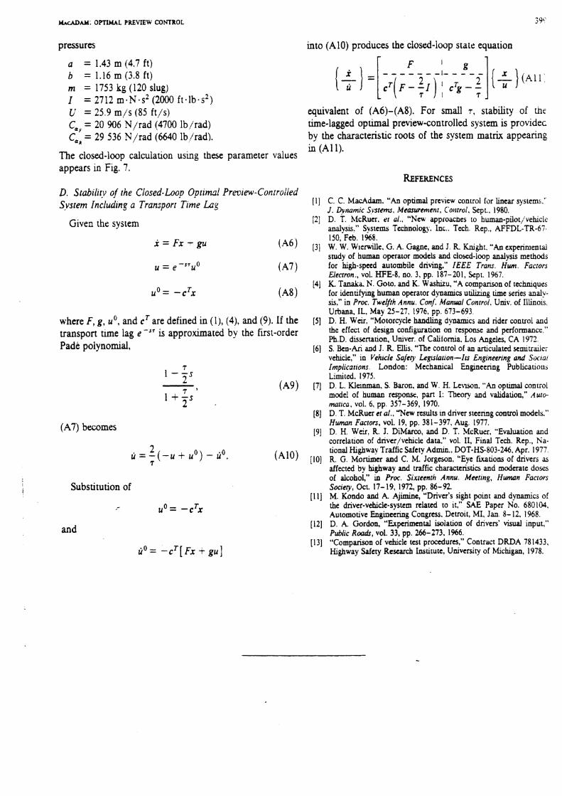
MACADAM: OPTIMAL PREVIEW COMROL

pressures into (A10) produces the closed-loop state equation f- -I

a = 1.43 m (4.7 ft) b = 1.16 m (3.8 ft) m = 1753 kg (120 slug) I = 2712 m.N.s2 (2000 ft.lb.s2) L; = 25.9 m j s (85 ft/s)

C a ~ = 20 906 N/rad (4700 lb/rad) CUR = 29 536 N/rad (6640 lb/rad).

The closed-loop calculation using these parameter values appears in Fig. 7.

D. Stabilitv of the Closed-Loo? Optimal Preview-Conrroiled S.vsrem Including a Transport Time L a g

Given the system

where F, g, uO, and cT are defined in ( I ) , (4), and (9). If the transport time lag e -" is approximated by the first-order Pade polynomial,

7 1 - 7 s -

7 ' (A9) 1 + r s

(A7) becomes

Substitution of

u O = -cTx

and

ti0 = -cT[Fx + gu]

F ' i? - _ - _ - _ - I - - - -

c r F 7 I i C g - T T i][+) ( A N :

equivalent of (A6)-(AS). For small 7, stability of tne time-lagged optimal preview-controlled system is providec by the characteristic roots of the system matrix appearing in (A1 1).

[ I ] C. C. MacAdarn. "An optimal preview control for linear systems.' J. Dynamic 5,vsremc. Mearurenlettt, C'otrrrol. Scpt.. 1980.

[2] D. T. McRuer. et al. . "New approacnes to human-pilotjvehlcle analysis." Systems Technology. Inc.. Tech. Rep., AFFDL-TR-67. 150, Feb. I%S.

[3] W. W. Wlerwille. G. A. Gagne, and J. R. Knight. "An experimental study of human operator models and closed-loop analysis methods for high-speed autombile dri\ing." IEEE Trans. Hwn. Facrors Electron., vol. HFE-8, no, 3, pp. 187- 201, Sept. 1967.

(41 K. T a d a N. Goto. and K. Washizu, "A comparison of techniques for identifying human operator dynamics u t h g time series anal? sis," in Proc. Twelfih Annu. Conf. Manual Conrrol. Univ. of Illinois. Urbana, IL, May 25-27, 1976, pp. 673-693.

[5] D. H. Weir. "Motorcycle handling dynamics and rider control and the effect of destgn configuration on response and performance," Ph.D. dissemtion, Univer. of California. Los Angeles, CA 1972.

[6] S. Ben-Ari and J. R. Ellis, "The control of an articulated xmitraiiei vehicle," in Vehicle Safcp Legrslauon-Ils Engineering and Soc~ai Implicanons. London: Mechanical Engineering Publicatious Limited. 1975.

(71 D. L. Klemman, S. Baron, and W. H. Lewon. "An optitnal control model of human response, part I: Theory and validation," Aulo- mutlca, vol. 6 , pp. 357-369, 1970.

[8] D. T. McRuer et ul., "New results m driver steering control model5." Hwnan Factors, vol. 19, pp. 381-397, Aug. 1977.

[9] D. H. Wek, R. J. DiMarco, and D. T. McRuer, "Evaluation and correlation of driver/vehicle data." vol. 11, Final Tech. Rep., Na- tional Highway Traffic Safety Admin., DOT-HS-803-246, Apr. 1977.

[lo] R. G. Monimer and C. M. Jorgeson, "Eye fixations of drivers as affected by highway and traffic characteristics and moderate doses of alcohol," in Proc. Sixteenth Annu. Meetlng, Human Factors Society, Oct. 17- 19, 1972, pp. 86-92.

[I I] M. Kondo and A. Ajimine, "Driver's sight point and dynamics of the driver-vehicle-system related to it," SAE Paper No. 680104, Automotive Engiieering Congress, Detroit, MI, Jan. 8- 12, 1968.

[I21 D. A. Gordon, "Experimental isolation of drivers' visual input," Public R d , vol. 33, pp. 266-273, 1966.

[I31 "Comparison of vehicle test procedures," Contract DRDA 781433, Highway Safety Research Institute, University of Michigan, 1978.

An Optimal Previ~w Control for Linear Systems u n a e ,

\ is then x 1 state vector C. C. MacAdam' j. is the scalar output related to tne state by the n x 1 mT

constant observer vector transpose A technique for synthesizing closed-loop conrrol of linear is the system matrix time-invariant systems during tracking of previewed inputs is and presenred. The derived control is directly dependent upon the properries of the controlled system and is obtained by g is the constant n x 1 control coefficient vector minimization of a defined previewed output error. find the control, u ( t ) , which minimizes a local performance

index,

I Introduction This paper presents a general method of control synthesis applicable to linear time-invariant systems utilizing preview control strategies for regulation or tracking tasks. A common example of this type of dynamical behavior occurs during normal automobile path following in which drivers "look- ahead" to follow a desired path. A frequent source of preview control strategies in various man-machine systems is, of course, the human operator. It is widely recognized !hat human operators are capable of controlling and adapting to a wide variety of dynamical systems, macy of which are vehicles with preview-oriented control requirements such as automobiles, bicycles, and complex aircraft (1-71. Although this paper does not offer evidence as to the utility of the proposed control synthesis for man-machine systems in- volving preview strategies, i t is suggested that the method presented here can be applied to such problems. Portions of the work by Tomizuka [8], which treated a similar problem, indicated useful application of optimal preview control methods in representing man-machine dynamical behavior.

The particular method presented in this paper is directly applicable to general linear system representations assumed to incorporate preview control strategies that depend only upon knowledge of the current values of the state and control. The optimal control is derived by minimization of a performance index that is defined as a mean squared preview output error. It will be shown that the derived control function is not ar- bitrary or independent but depends directly upon the dynamical properties of the controlled system.

11 Statement of the Problem Given the linear system

x=Fk+gu y = m r x

over the current preview interval (r,t+ r) , where,

W is an arbitrary weighting function over the preview interval and! is the previewed input.

The performance index given by (3) represents the weighted mean squared error between the previewed input and the previewed output as defined below.

The previewed output, y ( $ , is related to the present state, ~ ( t ) , by

u( , )=mTrncn.r ,x ( t , + j :mrmc?. t ) ru(€ ,d t (4 )

where,

6 t q.t)'= exp[F( q- 01 is the transition matrix of the system F [9].

If u ( t ) is assumed selected on the basis of a constant previewed control, u (0 = u ( t 1, equation (4 ) simplifies to

and the performance index, (3), can be written as

The above assumption simply requires the resulting o p (1) timization to reflect a control strategy dependent only upon

current values of the state and control. This assumption is, in (2) part, motivated by the potential application to those man-

machine systems, wherein, it is assumed the human oDerator 'Research Associate, Urliversity of Michigan. Highway Safety Research limited i n &riling or having knowledge a priori if more

Institute, Ann Arbor, Mich. 48109 Contributed by the Dynamic Systems and Control Division of THE AMERICAS complex or optimal control waveforms over the preview

SOCIETY OF MECHAN~CAL ESGINEERS. ~ ~ P I I I I S C T I ~ ~ received at ASME if',terva" Hcadquarlers, ~ u i y 9 , 1980. The necessary condition for minimization of J, defined by

1881Vol. 102, SEPTEMBER 1980 Transactions of the ASME

equation (6). with respect to the control, u ( t ) , is provided by dJldu = 0, or

where I is the identity matrix, and performing the d t in- tegrations, ( 7 ) becomes

Solving (8) for u ( t ) yields

Equation (1 1) represents a proportional controller with gain ~nversely related t o the preview interval, T , and operating on the error between the previewed input, f ( r + T ) , and ).( ( I + T I , that portion o f the previewed output deriving from the state vector's current initial condition. Likewise, equation (9 ) can be interpreted as a proportional controller operating on a similar error averaged and weighted over the preview interval ( t , t 7) by the additional terms appearing in equation (9) .

The optimal solution, u0 ( t ) , can also be expressed in terms of any current nonspt imal u ( t ) and correspondingly nonzero preview output error, e ( t ) , by writing equation (9) as

n 1 -7

u 6 , r ) = [I' [ f ( v ) - m T ~ ( q , O x ( t ) - u ( O ~ ( q ) ]

* I - -

* A i 7 ) w ( q - O d n + u ( O / A .1) ~ ( n - O d q ] . '

Jg j W ( ? - [ ) a ? J For the special case of W ( 7 - t ) = b( T ) , as before, equation .

where u0 (0 represents the optimal solution. For the special case of W ( q - t ) = 6(T), the Dirac delta function for 0 c 7' s T, (9) simplifies to

= v ( t + r ) - y , ( t + r ) ] / ( r K ) ( 1 1 )

where

( 13) reduces to

The formulation expressed by equation (13) can be useful in describing systems which do not achieve, though closely approximate, the optimal system behavior. Such cases may arise from limitations in achieving the precise optimal control due to time lags or dynamic properties inherent in the con- troller and not accounted for apriori in the optimization.

While equations (9) and (13) are equivalent mathematically, the latter deomonstrates an explicit relationship between the derived optimal control and the previewed output error function appearing in the performance index of the original problem formulation. Simply stated, the current control level is modified only in response to a nonzero function of the previewed output error, and, in this sense, analogous to an integral controller.

Finally, dependence of the derived optimal control upon the system (F, g ) properties is clearly demonstrated by the explicit presence of F and g in equations (9) and (13). Furthermore, information concerning stability of the closed-loop system utilizing the optimal preview control of equation (9 ) or (13) is provided by the characteristic roots of the constant matrix

Journal of Dynamic Systems, Measurement, and Control SEPTEMBER 1980, Vol. 102 1189

or

where

Introduction

(15) The purpose of the present paper is twofold. The first is to obtain an analytic expression for the critical speed of a

resulting from the substitution of (9, into ( 1 ) . For the special caseof W ( 7 ) = 6 ( F ) , (15 ) becomes

Ill Summary The optimal preview control model presented here offers a

useful and direct method for representing closed-loop behavior of linear systems utiiizlng preview control strategies. The derived control is directly related to the properties of the linear system and the previewed input. Further, the method is formulated in terms of general linear system representations, thereby permitting applications to a wide variety of problems.

References I McRuer, D . T . . et al . . "Neu Approaches to Human-Pilol/Vehicle

Analysis," Systems Technolog), Inc.. Tech. Rept. AFFDL-TR-67.150. Fcb. 1968.

? Wierwille, W . W . , Gagne. G.A. , and Knight, J.R.. "An Exper~mental Study of Human Operator Models and Closed-Loop Analys~s Methods for High-Speed Au~omobile Driving." I E E E Trons. on Human Factors in Elec- lronrcs. Vol. HFE-8. No. 3. Sept. I%', pp. 187-201.

3 Tanaka, K.. Goto. N., and H'ashizu. K.. "A Comparison of Techniques for ldentify~ng Human Operator 3ynamlcs Citiilzlng Time Series Anaiysls," Proceedtngs o j t h e Twelfth .4nnuol Conjercnce on Atanual Confrol, bniversity of Illinois, Urbana. 1 1 1 . . Ma) 3-2'. :916. pp. 6 7 - 6 9 3 .

4 Weir, D.H., "Motorcycle Handling D!lnam~cs and Rider Control and the Effect of Design Configurauon on Response and Performance," Ph.D. thesis, University of California, Lor Angeles, 1972.

5 Ben-Ari, S . , and Ellis, J.R.. "Thc Control of an Antculated Semitrailer Vehicle," Vehicle Snjety Lepislarion-11s Engineerrng and Socml Implrcaltons, Mechanical Engineering Publicat~ons L~mited, London. 19'5.

6 Klelnman, D.L.. Baron, S.. and Levison. W.H.. "An Optimal Control Model of Human Response, Part I: Theory and Validation." Auromorica, Vol. 6. 1970, pp. 357-369.

7 McRuer, D.T., e? al., "New Results In Driver Steering Control Models." Human Facrors, Vol. 19, Aug. 1977, pp. 381-397.

8 Tomizuka, M., "The Optimal Finite Preview Problem and Its Application to Man-Machine Systems," Dissertation, MIT, Cambridge. Mass.. Sept.. 1973.

9 D'Angelo, H., Linear Time-Varying Sysrems: Analvsir ond Synlhesis, Allyn and Bacon, Boston, 1970.

Asymptotic Theory of Freight Car Hunting

A simple formula is derived for the hunting speed of a freight car from an 8 degree of freedom linear model using asymp- totic techniques. A comparison is made between the ap- proximation and exact (numerical) solutions. The two agree within 10 percent for parameter values typical of present designs.

'Director of Research, Railroad Dynamics, Inc., Ardmore, Pa. Present Address: Assoclaw Professor. University of Pennsylvania,

Philadelphia, Pa. Contributed by the Dynamic Systems and Control Division of THE M N C A N

S o c ~ r u OF MECHANICAL ENGMEERS. Manuscript reccived at ASIME Headquarters, July 9, 1980.

multidegree of freedom model of a freight car which is simpie enough to convey physical insight into the hunting problem while at the same time complex enough to have validity for realistic vehicles. The second is to illustrate the simplification which can be effected in problems of this type by employing asymptotic mtrhods. These methods are model independent and rely on tne fact that the creep forces dominate the motion.

Previous work has included analytical studies of simple vehicles (1-21 and numerical solutions for realistic vehicles [3- 41. The present work can be viewed as a generalization and formal mathematical justification o i the former, which although cleverly done are ad hoc by nature and seem to be restricted to systems with few degrees of freedom, and a specialization of the lattcr, giving the same results in the region of validity of the expansion but being restricted by nature to specific regions in parameter space. The utility of the present work is in the simple result which it yields. From this one can obtain physical insight into the phenomenon as well as easily calculable answers.

Model Description We consider a model of the lateral dynamics of a freight car

composed cf a rigid car body pinned at either end to a truck. The pin connection transmits a linear damping moment (constant c',) between the car body and the truck. Each truck, see Fig. 1, is composed of 2 wheelsets, two rigid sideframes connected by ball joints to each wheelset, and a bolster, which contains the car connection (centerplate) at its midpoint, is constrained to move parallel to each wheelset by means of frictionless slotted pins in each sideframe, and is restrained from moving freely in that direction by 2 linear springs (constant k each) and dampers (constant c each) at each end. In the real systcrn this restraint is provided by the shear stiffness of the bolster springs, whose primary function is to support the car weight, and the sliding of the friction wedges laterally. Further, because the springs and dampers are separated by a distance d , there is a moment tending to square the truck due to both the springs (constant 4kdz) and the dampers constant 4cdZ). In addition, the bolster has mounted symmetrically with respect to_ the centerplarc, constant contact sidebearings (constant kB each) whose function is to provide a torsional spring restraint for the bolster relative to the car body (constant 2kB d). Actually the sidebearings also transmit a damping moment between the bolster and the car body (constant 2cBd); however, this has the same form as the centerplate moment and can be combined with it. There are eight degrees of freedom in this model and we will take as our independent coordinates 9, f, bF, uF, 9, p, BR, uR . Here the superscripts represent the front and rear truck coordinates, x is the axial dispiacement of the truck centroid relative to the track center line, 3, the yaw angle of each wheelset of the truck as a result of the kinematic constraint, 8 the trail angle of the truck, and u the bolster displacement relative to the truck centroid. The equations of motion, which have been derived elsewhere [ 5 ] and which are quite similar to others which have been discussed in the literature [4], are written here in dimensionless form in terms of sum and difference coordinates,

190 1 Vol. 102. SEPTEMBER 1980 Transactions of the ASME

L A W S T A B W OF A CONTROLLED ARTICULATED VEHICLE - AN APPLICATION OF BIFURCATION THEORY IN VEHICLE DYNAMICS

Anton S t r ibersky and Charles C. Mac- The Universi ty of Michigan Transportat ion Research I n s t i t u t e

2901 Baxter Road - Ann Arbor, Uichigan 48109, U.S.A.

MANY ACCIDENTS OF TRUCK-TRAILER COMBINATIONS a r e caused by l o s s of c o n t r o l of t h e veh ic le . Therefore inves t iga t ions of t h e dynamic l a t e r a l s t a b i l i t y of such a r t i c u l a t e d v e h i c l e s a r e important . In t h e p a s t , most of t h e engineering a n a l y s e s of s t a b i l i t y problems have on ly u t i l ~ z e d l i n e a r s t a b i l i t y t h e o r y . However, l i n e a r s t a b i l i t y theory can be overly generous

4 zn i d e n t i f y i n g regions of s t a b i l i t y f o r dynamic s y s t e m containing n o n l i n e a r i t i e s , such a s t h e a r t i c r r l a t e d v e h i c l e dynamics problem be ing considered here. In b r i e f , t h e physical phenom- enon of i n t e r e s t i n t h i s paper i s one i n which t h e l a t e r a l s t a b i l i t y th reshold of t h e a r t i c - u l a t e d v e h i c l e is reduced and caused t o occur a t s eeds below t h a t o r d i n a r i l y p red ic ted by a purery l i n e a r a n a l y s i s . For example, i f a r t x - u l a t e d v e h i c l e s a r e d r iven under high forward speeds, a f i n i t e d i s tu rb ing e f f e c t of a s teady s t a t e s t r a i g h t - l i n e motion can r e s u l t i n a s t a r t i n g of o s c i l l a t i o n s with c a t a s t r o p h i c a l l y increas ing amplitudes. The experimental r e s u l t s i n F ig . 2 ( I ) show an example ( c ) of unstable veh ic le behavior, caused from a f i n i t e s t e e r i n g d i s tu rbance , f o r a speed V much lower then t h e c r i t i c a l speed V c . Thus, t h e need f o r a n o n l i n e a r a n a l y s i s i s c l e a r l y ev iden t h e r e . Recent a p l i c a t i o n of n o n l i n e a r s t a b i l i t y theory [I,!] t o veh ic le engineering prob lem is provided i n references [ 4,5,7 I .

, r;;l

Fig.1: Mechanical model with t k c dew of fnedan y, 7, and + This paper a p p l i e s a nonl inear s t a b i l i t y

i n v e s t i g a t i o n t o a t r u c k , which is towing a s ingle-axle u t i l i t y t r a i l e r v i a i t s rear ' p i n t l e hook on a f l a t hor izon ta l road. The geometry of t h i s a r t i c u l a t e d veh ic le is shown i n Fig. 1. We cons ider a s y m e t r i c veh ic le . The l o c a t i o n of t h e v e h i c l e is described by t h e var iab les$ , TI and 4. The cons tan t forward speed, V, an t h e loading condi t ion of t h e t r a i l e r , measured by d, a r e t h e main parameters of t h e system. The l a t e r a l t i r e fo rces Si, which a r e of p a r t i c u l a r importance f o r t h e s t a b i l i t y a n a l y s e s , a r e c a l c u l a t e d a p p l y i n g an a d h e s i o n / s l i d i n g approach i n t h e con tac t a rea between t i r e and road [71. In o rder t o perform an inves t iga t ion of a veh ic le -dr iver system (closed-loop system) a l i n e a r , preview-based d r i v e r model [ 6 1 is employed i n t h e control led-vehicle analyses.

I n F i g . 2 ( I) ex e r i m e n t a l r e s u l t s from t h r e e a h o s t i d e n t i c a r f i e l d t e s t s a r e shown, d i f f e r i n g only i n t h e amplitude of t h e i n i t i a l s t e e r i n g d i s t u r b a n c e . Corresponding r e s u l t s from s i m u l a t i o n s of t h e s e t r a n s i e n t v e h i c l e responses a r e a l s o drawn i n Fig. 2 (11) f o r cornparision. The s imula t ions were done using t h e n o n l i n e a r Yaw/Roll Program [31. Shown is t h e articulation angle, 0, between t ruck and t r a i l e r . Following a s h o r t s t e e r i n g d i s t u r - bance, t h e v e h i c l e should fol low a s t r a i g h t - l i n e path (y - 0).

But t h i s i s only p o s s i b l e f o r a s u f f i c i e n t l y s m a l l d i s t u r b a n c e . I f t h e magnitude of t h e d i s tu rbance becomes t o o l a r g e , t h e amplitudes of t h e o s c i l l a t i o n s fo l lowin t h e d i s tu rbance i o c r e a s e , and t h e v e h i c l e t e h a v i o r becomes unstable ( i n con t ras t t o s t a b i l i t y p red ic ted by a purely l i n e a r a n a l y s i s ) . Detennrnation of t h e magnitude of d i s tu rbance needed t o produce an u n s t a b l e system response - f o r d i f f e r e n t forward speed3 - can be performed u s i n g a nonl inear s t a b i l i t y ana lys i s .

$,deP

R 2 Comparison of.measlmnent (I) and computn simulation (11) o?msicnt vehicle re nses of an equally loaded truck-der caubirrPrton (d = 0 . 4 g for a driving speed (V117.9 m/s) much ,,,~~ (VC-~WS).

Applying Newton's law, we can w r i t e t h e non- l i n e a r equations of motion

u ( x ) x - f ( x , 8 ) I , (1)

where xT - (yIv,7, OD,$,$) i s t h e s t a t e vector , 6 is t h e s t e e r i n g aeg le , and W(x) is a (non- l i n e a r ) 6 x 6 matr ix. The s t r a i g h t - l i n e motion i s given by 80 = 0 and x = 0. It is obvious t h a t t h e s t r a i g h t - l i n e motton i s an e q u i l i b r i u m p o s i t i o n of system (1). After i n v e r t i n g t h e matr ix U(x1, which can be done by power s e r i e s expansion with r e s p e c t t o t h i s e q u i l i b r i u m pos j t ion , we ob ta in

x - T x + g 8 + aa(x,8) (21

where a (= ,& c o n t a b t h e nonl inear terms.

Due t o t h e s t e e r i n g of t h e d r i v e r , any dev ia t ion from t h e s t ra1ght: l ine motion of t h e t r u c k l e a d s t o a s t e e r i n g response 8. Tha p o s i t i o n of the d r i v e r from t h e t ruck c . g . is l o c a t e d by t h e parameter e . The d r i v e r is modelled mathamatical ly by an optimal preview c o n t r o l approach [ 6 ] , whzch uses t h e l i n e a r p a r t of equ. (2) . The optimal con t ro l , Gept ( t ) , minimizes t h e e r r o r between t h e d e s i r e d s t r a i g h t - l i n e motion and t h e pred ic ted veh ic le p o s i t i o n , T seconds ahead i n t ime . The p r e d i c t e d l a t e r a l p o s i t i o n of t h e d r i v e r , yd(t+T), T seconds ahead, is derived from t h e observer vec tor mT - ( 1 , 0 , e , 0 , 0 , 0 ) , t h e s t a t e v e c t o r ' s cur ren t i r i i t i a l condit ion, x ( t 1 , and the s t a t e t r a n s i . i o n matr ix.

1 1

I f t h e d r i v e r delay t i s modelled with a Pad6 polynomial, t h e s t e e r r n g input f a p p l i e d by t h e

i a r r v e r can be a p p r o x m t e d by (s i s t h e Laplace v a r i a b l e )

5 l - y s 6 - 6,

t ( 4 ) l + - s

2 This l i n e a r d r i v e r model has been shown t o be an e f f e c t i v e means f o r r e p r e s e n t i n g a c t u a l human behavior dur ing d r i v r n g t a s k s . A t ime d e l a y value 5 of approximately 0.25 seconds i s !rdinari;)y used i n t h i s model t o r e p r e s e n t

average d r i v e r behavior . Equ. ( 2 ) t o g e t h e r w i t h e q u . ( 4 ) p r o d u c e s t h e c l o s e d - l o o p equa t iovs of motion:

1

where 6

With yT = (xT,f) we can w r i t e equ. (5 ) i n t h e ,form

y = A ( X ) y + m(y,X) , (7) where we have now a l s o in t roduced t h e para- meter v e c t o r k? = (Y,d) . The s t a b i l i t y of t h e e q u i l i b r i u m p o s i t i o n y = 0 i s guaranteed by a theorem of L~apunov, LP a l l e igenvalues of t h e m a t r i x A(1) have nega t ive r e a l p a r t s . To f i n d t h e c r i t i c a l forward speed, VF, we c a l c u l a t e f o r a f i x e d l o a d i n g c o n d i t ~ o n , d , and a q u a s i s t a t i c i n c r e a s i n g speed, V, t h e eigen- v a l u e s of t h e m a t r i x ~ ( 1 ) . The s t a b i l i t y boundary is reached, i f one o r more eigenvalues c r o s s t h e imaginary a x i s .

Vc, IS m ~ h

0 I 1 0 -0.5 0 0.5

d ,m Fig.3: Sfabiity boundary in the panvneta for the opm-loop

' . 9 s m (- . -1 and the ckwii-lmp system Z 1. see w ~ g . 5. Fig . 3 shows'.the s t a b i l i t y boundaries f o r t h e open-loop and t h e closed-loop system. For t h e v e h i c l e with a f i x e d s t e e r i n g wheel (8 * 01,

yT = (vtw,$,$) t a rearward l o c a t e d load can l e a d t o an o s c i l - l a t o r y t y p e of i n s t a b i l i t y , due t o a p u r e l y

p a i r of e igenva lues . The reason is a 2 $ 8 2 : 3 o n of a l i m i t cyc le , which is c a l l e d Hopi b i f u r c a t i o n . On t h e o t h e r s i d e , p o s i t i v e v a l u e s of d can l e a d t o a d ivergen t typa of i n s t a b i l i t y , caused by a s imple ze ro eigen- va lue . Fig.4 shows a t ime h i s t o r y of t h e a r t i - c u l a t i o n angle , 0 , f o r a d i v e r g e n t u n s t a b l e b e h a v i o r of t h e v e h i c l e a f t e r a s t e e r i n g d i s tu rbance .

For t h e c o n t r o l l e d veh ic le , a Bopf b i f u r - c a t i o n ( o s c i l l a t o r y type) is t h e only mannar t n which l o s s of s t a b i l i t y of t h e s t r a i g h t - l i n e motion can occur . The rnf luence of t h e d r i v e r t ime lag , t, upon c r i t i c a l speed is seen t o be almost insignificant f o r t h e l e f t branch of t h e s t a b i l i t y c h a r t (Fig. 3 1 , i n d i c a t i n g t h a t t h e d r i v e r has l i t t l e c o n t r o l over t h e o s c i l l a t o r y t r a i l e r motion, which dominates d u r i n g t h i s mode. However, on t h e r i g h t branch, t h e d r i v e r t ime l a g i s seen t o p lay a very important r o l e i n a e t e h n i n g t h e c r i t i c a l speed.

I \' ' -4

Timc,s 0 10 20

(1) (11)

Fig. 4: Divapat thy vetwle n* a

of the articulation angle for the (d = posmve) - (I) rncasuranenk

(Xi) C O ~ P U ~ Q

For one t o i n v e s t i g a t e t h e n o n l i n e a r be- havlor , a change i n coord ina tes y + r by y-Tr 2s necessary a s a f i r s t s t e p i n o rder t o t rans - form t h e mat r ix A(X) i n t o d iagona l form. The m a t r i x T i s g iven by t h e e igenvec tors of t h e matrrx h ( k ) . Center manifold theory [ I ] allows us t o reduce t h e system (7) t o b i f u r c a t l o n ecruatzons (71. (For t h e c o n t r o l l e d veh ic le a ~ 6 p f b i f u r c a t i o n always appears and leads t o a two-Cimensional b i f u r c a t l o n sys tem. ) I n t h e c a s e of a Bopf b i f u r c a t i o n , by i n t r o d u c i n g p o l a r c o o r d i n a t e s and apply ing t h e a v e r a ~ i n g p r i n c i p l e [ 2 ] , t h e two-dimensional b i f u r c a t i o n system can be transformed i n t o t h e norrnal form

3 ; = vl r + K3 r + ~ ( / r i ) ) . ( 8 ) Equ. (8 ) i s an equa t ion f o r t h e amplitude r of a limit c y c l e ( r = 0 ) . The mathematical para- mete r v l i s p r o p o r t i o n a l t o t h e p h y s i c a l parameter 711 - (V-Vc), and K j i s a constant f o r a given loaded veh ic le . Fig. 5 shows amplitudes of t h e b i f u r c a t i n g u n s t a b l e l i m i t c y c l e f o r d i f f e r e n t load ing c o n d i t r o n s (1 ,2 ,3 , and 4 ) , f o l l o w i n g from equ . ( 8 ) . The limit c y c l e s border t h e a t t r a c t i o n domains of t h e s t a b l e s t r a i g h t - l i n e motion. As soon a s a d i s tu rbance causes a c r o s s i n g of t h e u n s t a b l e linut c c l e , an uns tab le v e h i c l e response occurs . The fimit cyc les of Fig.5 r e s u l t from an i n v e s t i g a t i o n of t h e system near t h e c r i t i c a l e q u i l i b r ~ w poin t ( V c ) . I n t e r e s t i n g l y , t h e t h e o r e t i c a l r e s u l t of Frg.5 ( l i m i t c y c l e 3 ) , when e x t r a p o l a t e d t o even lower forward speeds, shows good agree- ment with t h e corresponding measurements of t h e t r a n s i e n t veh ic le responses seen i n Fig.2.

-i !@I, rad

Fig5 Am lifudes of unstable Limit c le solutions. The numbers c a m p o d t o ~ g . 3. (- mbc--- unstable )

ACKNO- This work has been suppor ted by t h e Aus t r ian "Fonds z u r Foerderung d e r wissenschaf t l i chen Forschungw (J0260T), and b t h e "U.S. Army Tank &utomot:ve Co-nd" (DAAEoT-8 5-C-~069) .

mas Can J. A Fcations of Centre Manifold Theory, A lied

cer JS. &mga-va% New Y& Heidrrmg !9$ nheimer J.. P. olmes, Nonl~near Osclllauons,

and Bihrcation of Vecpr Welds, lied Math. =92-!* -V=h New York, H e m 19?f Gill ie%., c.E. MacAdam, Consrant Velocity Yaw /

!ill Progd%stir MaPL UMIRI-82-39, October 1982. [41 Xaqni V., A. Sribeqky, H. Troger, IC w a n , and Bifurcations m the Mobon of Tracm-Semrmler ehlcles. Co erence Proceed. Canadiy Math. Soc., Vol. 8 (F.V. AIkinson, W . f h n f o r d A.B. hrknpanh. cds3.1987.485499.

in h i V.. A. Skibcrsky. I& Trogir. Maneuverability of a mk-Tda Combination after Loss of Latrral Stab& Proceed. of

the 10th AVSD-Sjmposium. Pm e. (h4. Apetam. 23, S- and Zcillinger B.V.. Use. 1988, 186-!$8

Macpdam C.C., A lication'of an timal Preview Conml j!r Simuiauon of C l o r ~ - h o p Autorno "% ile Drivin l E E E Trwoctionr on ~vstemr. on. mi Cvtwmtics. VOI. SME-11. NO. 6, June 1981.393399.

Smkaky A,. P.S: Fqcher. ,me Nonlinear Behavior, of caw-Duty T ~ c k Combrnauons wrth Respect to Stmghrline

Stabiliw ASME Journal of D namic S stems, Measurement, and conno(. boi. 11 1, Nr. 4, k e m L 1989 [to appear)

DISTRIBUTION LIST Copies

Commander U.S . Army Tank- Automotive Command ATIN ASNC-TAC-DIT (Technical Library)

AMSTA-CF (Dir. RDE center) AMSTA-CR (Technical Director) AMSTA-R (Dir. Tank-Automotive Technology) AMSTA-RY (System Simulation and Tech. Div.)

Warren, MI 48397-5000

Commander Defense Technical Information Center Bldg. 5, Cameron Station ATI'N: DDAC Alexandria, VA 22304-9990

Manager Defense Logistics Studies Information Exchange A m AMXMC-D Fort Lee, V A 2380 1-6044

Commander U.S. Army Operational Test and Evaluation Agency A m : CSTE-CS (Combat Support Div.) 5600 Columbia Pike Falls Church, VA 22041-51 15

Deputy Commander U.S. Army Strategic Defense Command P.O. Box 1500 ATIN DASD-H-S (Systems Anal./Battle Management Dir.)

DASD-H-V (Advanced Technology Dir.) Huntsville, AL 35807-3801

Commander U.S. Army Foreign Science & Tech Center 220 Seventh Street NE ATIN: ALQST-RA (Research and Analysis Dir.) Charlottesfle, VA 22901-5396

Director U.S. Axmy Cold Regions Research & Engineering Lab P.O. Box 282 A T W CECRL-IC (Technical Library) Hanover, NH 03755- 1290

Dist- 1

DISTRIBUTION LIST Copies

Director U.S. Army Corps of Engineers Waterways Experiment Station P.O. Box 631 A m : WESGV-Z (Geotechnical Laboratory) Vicksburg, MS 39 180-063 1

U. S. Army Laboratory Command Army Research Office P.O. Box 1221 1 ATTN: SLCRO-EG (Engineering Division)

SLCRO-TS (Library Services) Research Triangle Park, NC 27709-221 1

Director U.S. Army Ballistic Research Lab ATTN: SLCBR-D (Office of Director) Aberdeen Proving Grounds, MD 2 1005-5066

Director Harry Diamond Laboratories A'ITN: SLCHD-IT (Eng. & Tech Support Div.)

SLCHD-TA (Tech. Applications Div.) 2800 Powder Mill Road Adelphi, MD 20783-1197

Director U.S. Army Human Engineering Laboratory A'ITN: SLCHE-D (Office of Director )

SLCHE-SS -TS (Library) Aberdeen Proving Grounds, MD 2 1005-500 1

Commander U.S. Army Material Command A'ITN: AMCDE (Development, Eng, & Acqusition)

AMCDMA-ML (Library) 500 1 Eisenhower Avenue Alexandria, VA 22333-001

Commander 1 U.S. Army Armament Munitions and Chemical Command ATTN: SMCAR-MS (Information Management Dir. - Tech Library) Picatinny Arsenal, NJ 07806-5000

Commander 1 St. Louis Support Command A'ITN: DAWASMC-STL-DACL (Library/Information Center) Granite City, IL 62040- 1801

DISTRIBUTION LIST

Director CECOM Research Development & Engineering Center A m : AMSEL-RD (Director) Fort Monmouth, NJ '07703-5b01

Commander U.S. Army Missile Command ATTN: AMCPM (Land Combat Systems)

AMSMI-CG (Reference Library) AMSMI-RD (Research, Dev. and Eng. Center)

Redstone Arsenal, AL 35898-5000

Commander U.S. Army Cold Regions Test Center A m STECR-MT (Materiel Test Dir.) Fort Greenly, AL

Commander U.S. Army Combat Systems Test Activity A m Axmament Systems Directorate

Close Combat Systems Directorate Engineering Directorate Development & Analysis Directorate

Aberdeen Proving Grounds, MA 21005-5059

Commander U.S . Army Y uma Proving Ground ATTN: STEYP-MT (Material Test Dir.) Yuma, AX 85364

Director TRAC-FLVN A'ITN: ATRC-F Fort Leavenworth, KS 66027-5200

Director TRAC-WSMR A m : ATRC-W White Sands Missile Range, NM 88002-5502

Commander U.S. Army Center and Fort Knox A m : ATZK-DOTD (USAARMS Library)

ATZK-CD @ire of Combat Developments) ATZK-AE-A0 (Library)

Fort &OX, KY 40121-5000

Copies

1

DISTRIBUTION LIST

President U.S. Army Armor and Engineer Board Fort Knox, KY 40121-5470

President US Army Aviation Board A m : AlZQ-OTC (Technical/Operations Div.) Fort Rucker, AL 36362-5064

Director U.S. Amy Combat Developments Experimentation Center A'lTN: Technical Library; Bldg 2925 Fort Ord, CA 93941-7000

Commander U.S. Army Combined Arms Center and Fort Leavenworth A m : ATOR-CT (Scientific and Tech. Support Dir.)

ATZL-CA (Combined Arms Combat Devl. Activity) Fort Leavenworth, KS 66027-5 130

Commander TRADOC Combined Arms Test Activity A m : ATCT-MA (Methodology & Analysis Dir.)

ATCT-SPT (Technical Library) Fort Hood, TX 76544-5065

President U.S. Army Communications-Electronics Board ATIN: ATZH-BDS (Analysis & Tech. Support Div.) Fort Gordon, GA 30905-5350

Commander U.S. Army Engineer Center and Fort Belvoir AlTN: ATZA-SS-LIB (Library) Fort Belvoir, VA 22060-5000

President U.S. Army Field Artillery Board A'ITN: A'IZR-BDS (Analysis and Tech. Support Div.) Fort Sill, OK 73503-6100

Copies

1

President U.S. Army Infantry Board A m : ATZB-IB-PR-T (TechfScience Dir.) Fort Benning, GA 3 1905-5800

DISTRIBUTION LIST

Commander U.S. Army Infantry School A'ITN: ATSH-CD (Dir. of Combat Development) Fort Benning, GA 31905-5000

Commander U.S. Army Intelligence Center and School ATTN: ATSI-CD (Dir. of Combat Developments) Fort Huachuca, AZ 85613-7000

PresidentKommander U.S. Army Intelligence and Security Board ATIN: ATSI-BD-A (Analysis & Tech. Support Div.) Fort Huachuca, AZ 85613-7000

Commander U.S. Army Ordance Center and School A'ITN: ATSL-CD (Dir. of Combat Development)

ATSL-SE-LI (Library) Aberdeen Proving Ground, MD 2 1005-520 1

Commander U.S. A m y Ordance Missile and Munitions Center and School A'ITN: ATSK-C (Dir. of Combat Developments)

ATS K- AB (Library) Redstone Arsenal, AL 35897-6500

Headquarters U. S. Army Quartermaster Center and Fort Lee A'ITN: ATSM-CD @ire of Combat Developments) Fort Lee, VA 23801-500095,96

Headquarters U.S. Army Troop Support Command A m : AMSTR-B (Systems Analysis Office)

AMSTR-E (Research & Development Integration Office) 4300 Goodfellow Blvd. St. Louis, MO 63 120- 1798

Copies

1

Commander 1 US Army Belvoir Research, Development, & Engineering Center A'ITN: STRBE-BT (Technical Library Div) Fort Belvoir, VA 22060-5606

DISTRIBUTION LIST

Commander U.S. A m y Natic Research, Development, and Engineering Center A T I N STRNC-ML (Technical Library) Natick, MA 01760-5000

Commander U.S. Army Development and Readiness Command 5001 Eisenhower Avenue A m : Dr. R. S. Wiseman Alexandria, VA 22333

Commander US Army Soldier Support Center National Capitol Region A1ITN: ATNC-NMM-A 200 S tovall Street Alexandria, VA 22332-0400

HQDA Office of Dep Chief of Staff for Rsch Dev & Acquisition A'lTN: ARZ-A Dr. Lasser - Dir. of Army Research

DAMA-AR Washington, D.C. 203 10

Commander U.S. Army Military Equipment R&D Command A m . DRDME-T Fort Belvoir, VA 22060

Commandant U.S. Army Engineer School A'ITN: ATZA-CDT Fort Belvoir, VA 22060-528 1

Commander Rock Island Arsenal ATIN: SARRI-LR Rock Island, IL 61201

Director U.S. Army Material Systems Analysis Agency ATTN: AMXSY-DD

AMXSY-C (Mr. Harold Burke) AMXSY-CM (Mr. Fordyce) AMXSY-MP (Mr. Cohen)

Aberdeen Proving Ground, MD 21005-507 1

Copies

1

DISTRIBUTION LIST

Director Keweenaw Research Center Michigan Technological University Houghton, MI 4993 1

Director Defense Advanced Research Projects Agency 1400 Wilson Boulevard Arlington, VA 22209

Commander U.S. Army Materials and Mechanics Research Center A T I N Mr. Adachi Watertown, MA 02172

Director U.S.D. A. Forest Service Equipment Development Center 444 East Bonita Avenue San Dimes, CA 9 1773

Engineering Society Library 345 East 47th Street New York, NY 10017

Commander U.S. Army Armament Research and Development Command AlTN: Mr. Rubin Dover, NJ 07801

Commander USAMC Material Readiness Support Activity ATTN: AMXMD-ED (Equip Develop/Deploy Anal Br) Lexington, KY 405 1 1-5 10 1

Commander U.S. Army Logistics Center ATIN: ATCL-M Fort Lee, VA 23801-6000

Director TRADOC Systems Analysis Activity A T I N ATOR-TF White Sands Missile Range, NM 88002-5502

Copies

1

DISTRIBUTION LIST

Commander U.S. Army Test Evaluation Command

AMSTE-BB AMSTE-TA AMSTE-TE AMSTE-TD-T

Aberdeen Proving Ground, MD 21005-5055

Commanding General U.S. Marine Corps Mobility & Logistics Division Development and Education Command A'ITN: Mr. Hickson

MCOTEA Quantico, VA 22134

Commander U.S. Air Force Tactical Air Warfare Center ATTN: TE Eglin AFB, FL 32542

Commandant U.S. Army Armor School A m : ATSB

PERI-IK Fort Knox, KY 40121-5000

Commander US Army Transportation School A m : ATSP-TD Fort Eustis, VA 23604-5361

Commander US Army Training Support Center A m : ATIC-DM Fort Eustis, VA 23604-5 166

President CDED Test Board A m : ATEC-B Fort Lewis, WA 98433-5000

Copies

4

Superintendent U.S. Military Academy ATI'N: Dept. of Engineering West Point, NY 10996