Data-Driven Operations Management

by

Manqi Li

A dissertation submitted in partial fulfillmentof the requirements for the degree of

Doctor of Philosophy(Business Administration)

in The University of Michigan2021

Doctoral Committee:Assistant Professor Shima Nassiri, ChairAssistant Professor Yan HuangAssociate Professor Cong ShiAssistant Professor Joline UichancoAssociate Professor Brian Wu

Manqi Li

manqili@umich.edu

ORCID iD: 0000-0002-5210-4368

ACKNOWLEDGEMENTS

The journey of academic research is full of challenges. Along the way, there are

lots of people that I want to acknowledge, without whom I can never come to where

I am.

First, I would like to acknowledge Dr. Amitabh Sinha for leading me to the world

of academic research. He is not only my advisor in research but also my lifetime

mentor. He is always supportive to all the decisions I made and all the paths I chose.

Second, I would like to thank Professor Yan Huang for all the support throughout

my Ph.D. She showed me a great example of how to become a researcher full of

enthusiasm. She put a huge amount of effort in guiding me through the process

of finishing a complete research project. Her profession, hardworking, and sense of

responsibility will always inspire me in my future career.

Third, I would like to thank Professor Shima Nassiri. During the difficult times,

she gives me the hope and confidence to continue my academic journey. She always

encourages me to explore new topics and try new methodologies, which is extremely

important for me as an independent researcher.

I would like to also thank my dissertation committee members Professor Cong

Shi, Professor Joline Uichanco, and Professor Brian Wu, who give me great support

toward the completion of my degree.

Finally, I am grateful for my family and friends. Special thanks to my husband

Xiang Liu and my daughter Andrea Liu. Xiang: thank you! I know I will always have

you by my side. Andrea: You are such an angle and I can’t love you more! I would

ii

also like to thank my parents Liying Gu and Ruiliang Li: You are the best parents in

the world! I would also like to thank my parents in law Chunsheng Liu and Yayun

Li: thank you for all the support. I can not imagine my life without your help. Last

but not least, thanks to my dogs Playdoh and Hunio: love you forever.

iii

TABLE OF CONTENTS

ACKNOWLEDGEMENTS . . . . . . . . . . . . . . . . . . . . . . . . . . ii

LIST OF TABLES . . . . . . . . . . . . . . . . . . . . . . . . . . . . . . . . vii

LIST OF FIGURES . . . . . . . . . . . . . . . . . . . . . . . . . . . . . . . x

ABSTRACT . . . . . . . . . . . . . . . . . . . . . . . . . . . . . . . . . . . xiii

CHAPTER

I. Introduction . . . . . . . . . . . . . . . . . . . . . . . . . . . . . . 1

II. Data-Driven Promotion Planning for Paid Mobile Applications 5

2.1 Introduction . . . . . . . . . . . . . . . . . . . . . . . . . . . 52.2 Literature Review . . . . . . . . . . . . . . . . . . . . . . . . 92.3 Data and Descriptive Analysis . . . . . . . . . . . . . . . . . 132.4 Empirical Model and Estimation . . . . . . . . . . . . . . . 18

2.4.1 Empirical Model . . . . . . . . . . . . . . . . . . . 182.4.2 Instrumental Variables . . . . . . . . . . . . . . . . 212.4.3 Estimation Results . . . . . . . . . . . . . . . . . . 272.4.4 Robustness Checks . . . . . . . . . . . . . . . . . . 382.4.5 Heterogeneity . . . . . . . . . . . . . . . . . . . . . 60

2.5 Prediction Accuracy . . . . . . . . . . . . . . . . . . . . . . 632.6 Promotion Planning Problem . . . . . . . . . . . . . . . . . . 64

2.6.1 PPP Model Formulation . . . . . . . . . . . . . . . 642.7 Promotion Planning Result . . . . . . . . . . . . . . . . . . . 70

2.7.1 Window Size Sensitivity . . . . . . . . . . . . . . . 702.7.2 Performance Comparison among Alternative Policies 712.7.3 Significance of the Visibility Effect and Dynamic

Promotion Effect . . . . . . . . . . . . . . . . . . . 752.8 Conclusion . . . . . . . . . . . . . . . . . . . . . . . . . . . . 76

iv

III. How Does Telemedicine Shape Physician’s Practice in Men-tal Health? . . . . . . . . . . . . . . . . . . . . . . . . . . . . . . . 88

3.1 Introduction . . . . . . . . . . . . . . . . . . . . . . . . . . . 883.2 Literature Review . . . . . . . . . . . . . . . . . . . . . . . . 913.3 Problem Setting . . . . . . . . . . . . . . . . . . . . . . . . . 94

3.3.1 Definitions . . . . . . . . . . . . . . . . . . . . . . . 943.3.2 Telemedicine Effects . . . . . . . . . . . . . . . . . 973.3.3 Dynamic Effects . . . . . . . . . . . . . . . . . . . . 101

3.4 Data Description . . . . . . . . . . . . . . . . . . . . . . . . . 1023.4.1 Data Sources and General Inclusion Criteria . . . . 1023.4.2 Identifying the Adopter and Non-Adopter Groups . 1043.4.3 Variables Description . . . . . . . . . . . . . . . . . 109

3.5 Econometric Model . . . . . . . . . . . . . . . . . . . . . . . 1103.5.1 Heterogeneous Adoption Time CIC Model in Athey

and Imbens (2006) . . . . . . . . . . . . . . . . . . 1133.5.2 Controlling for Observable Covariates . . . . . . . . 1183.5.3 Effect Estimation . . . . . . . . . . . . . . . . . . . 119

3.6 Results . . . . . . . . . . . . . . . . . . . . . . . . . . . . . . 1213.6.1 Controlling for Observable Covariates: Regression

Results . . . . . . . . . . . . . . . . . . . . . . . . . 1213.6.2 Telemedicine Adoption and Spillover Effects . . . . 1223.6.3 Explanation of the Observations . . . . . . . . . . . 124

3.7 Additional Analysis and Robustness Checks . . . . . . . . . . 1293.7.1 New Patient Visits Vs. Established Patient Visits . 1293.7.2 Linear Difference-in-Difference Model . . . . . . . . 129

3.8 Conclusion . . . . . . . . . . . . . . . . . . . . . . . . . . . . 131

IV. Search Page Personalization: A Consider-then-choose Model 134

4.1 Introduction . . . . . . . . . . . . . . . . . . . . . . . . . . . 1344.2 Literature Review . . . . . . . . . . . . . . . . . . . . . . . . 138

4.2.1 Consider-then-Choose Model . . . . . . . . . . . . . 1384.2.2 Assortment Planning . . . . . . . . . . . . . . . . . 140

4.3 A Consider-then-Choose Model . . . . . . . . . . . . . . . . . 1434.3.1 Consideration Set Formation (The “Consider” Stage) 1444.3.2 Purchase Decision Given a Consideration Set (The

“Choose” Stage) . . . . . . . . . . . . . . . . . . . 1474.3.3 Estimation Strategy . . . . . . . . . . . . . . . . . 148

4.4 Assortment Personalization via Consideration Set Induction . 1524.4.1 Max-Revenue Assortment Planning . . . . . . . . . 1534.4.2 Optimal Consideration Set Induction Optimization 155

4.5 A Case Study . . . . . . . . . . . . . . . . . . . . . . . . . . 1674.5.1 Data Description . . . . . . . . . . . . . . . . . . . 1674.5.2 Estimation Result and Discussion . . . . . . . . . . 168

v

4.5.3 Comparison of OCSIO Heuristic and OCSIO . . . . 1714.5.4 Revenue Increase using the OCSIO Heuristic . . . . 1724.5.5 Performance of OCSIO Given Imperfect Taste Infor-

mation . . . . . . . . . . . . . . . . . . . . . . . . . 1734.6 Conclusion . . . . . . . . . . . . . . . . . . . . . . . . . . . . 174

V. Future Work . . . . . . . . . . . . . . . . . . . . . . . . . . . . . . 177

BIBLIOGRAPHY . . . . . . . . . . . . . . . . . . . . . . . . . . . . . . . . 180

APPENDICES . . . . . . . . . . . . . . . . . . . . . . . . . . . . . . . . . . 192A.1 Procedure Codes Included in the Study . . . . . . . . . . . . 193A.2 Data Generating Process . . . . . . . . . . . . . . . . . . . . 195

vi

LIST OF TABLES

Table

2.1 Summary Statistics . . . . . . . . . . . . . . . . . . . . . . . . . . . 14

2.2 Price Tiers in iOS App Store . . . . . . . . . . . . . . . . . . . . . . 14

2.3 Summary Statistics of Promotion Depth and Promotion Length . . 16

2.4 Variable Description . . . . . . . . . . . . . . . . . . . . . . . . . . 21

2.5 Main Model Full Result . . . . . . . . . . . . . . . . . . . . . . . . 28

2.6 Regression Results of Ranking Function (Equation (2.3)) . . . . . . 29

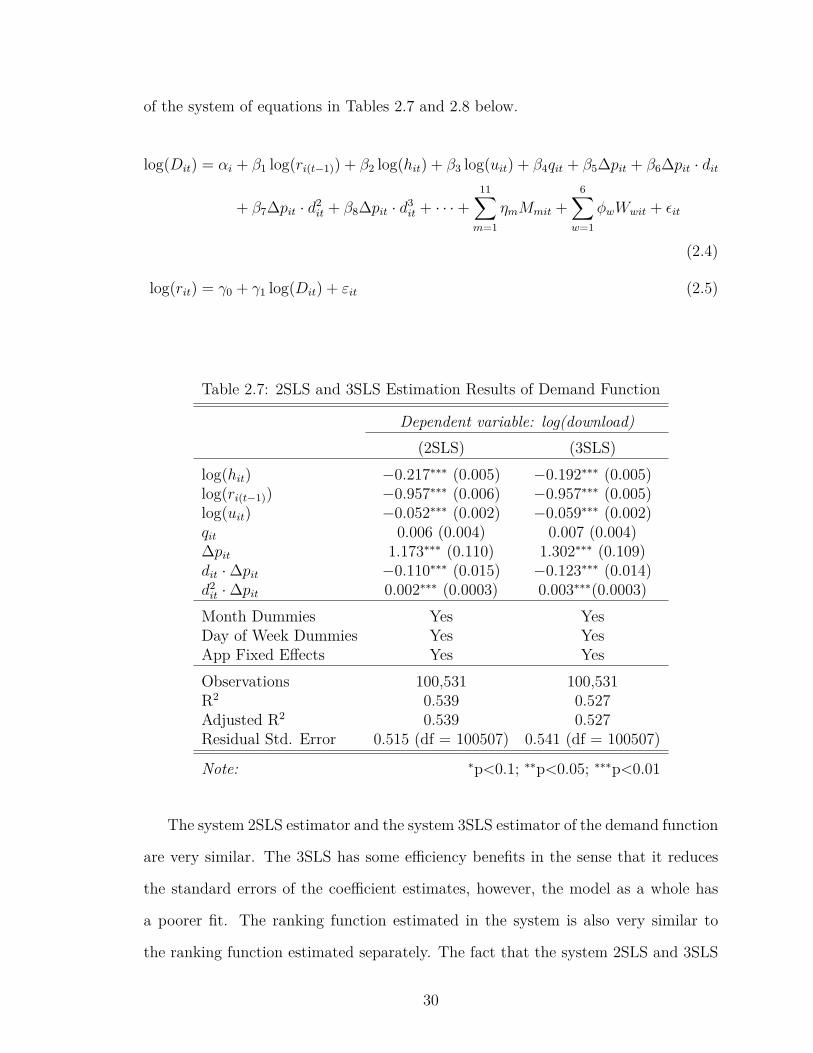
2.7 2SLS and 3SLS Estimation Results of Demand Function . . . . . . 30

2.8 2SLS and 3SLS Estimation Results of Ranking Function . . . . . . 31

2.9 Regression Results of Alternative Demand Specifications . . . . . . 33

2.10 Estimation Results of Main Model with Different Missing Data Im-putation Methods . . . . . . . . . . . . . . . . . . . . . . . . . . . . 39

2.11 Estimatin Results of the Demand Function with Different SampleCutoff Values . . . . . . . . . . . . . . . . . . . . . . . . . . . . . . 40

2.12 Estimation Results of Demand Function under Alternative Specifi-cations of Promotion effect . . . . . . . . . . . . . . . . . . . . . . . 41

2.14 Estimation Results of Demand Function with App Age Dummies (byMonth) . . . . . . . . . . . . . . . . . . . . . . . . . . . . . . . . . . 42

2.13 Estimation Results of Demand Function with ds Dummy Variables . 45

2.15 Estimation Results of Demand Function with More Lagged Ranks . 46

vii

2.16 Estimation Results of Demand Function with Lagged Download . . 47

2.17 In-sample and Out-of-sample MSE . . . . . . . . . . . . . . . . . . 47

2.18 Estimation Results of Demand Function with log(avg_rpromotionit ) ·

dpostit . . . . . . . . . . . . . . . . . . . . . . . . . . . . . . . . . . . 48

2.19 Regression Results for Cumulative Number of Ratings . . . . . . . . 49

2.20 Estimation Results of Demand Function with Fitted Rating Counts 50

2.21 Main Model vs. Choice Model: Out-of-Sample Mean Squared Errorfor Each Cross-validation Round . . . . . . . . . . . . . . . . . . . . 53

2.22 Effect of Number of Other Apps on Promotion . . . . . . . . . . . . 54

2.23 Estimation Results of Demand Function for Top 100 Apps . . . . . 55

2.24 Main Model vs. Choice Model: Out-of-Sample Mean Squared Errorfor Each Cross-validation Round . . . . . . . . . . . . . . . . . . . . 55

2.25 Summary Statistics of Data for Network Effect Test . . . . . . . . . 57

2.26 Estimation Results of Demand Function with Visibility Effect and/orNetwork Effect . . . . . . . . . . . . . . . . . . . . . . . . . . . . . 58

2.27 Estimation Results of Demand Function with Past 10 Days’ Cumu-lative Download . . . . . . . . . . . . . . . . . . . . . . . . . . . . . 59

2.28 Effect of Short vs Long Promotions . . . . . . . . . . . . . . . . . . 81

2.29 Estimation Results of Demand Function by App Rating . . . . . . 82

2.30 Estimation Results of Demand Function by Original Price . . . . . 82

2.31 Estimation Results of Demand Function – Apps with vs withoutFreemium Version . . . . . . . . . . . . . . . . . . . . . . . . . . . . 83

2.32 Estimation Results of Demand Function with Interaction Effect be-tween Promotion and Rank Prior to Promotion . . . . . . . . . . . 84

2.33 Estimation Results of Demand Function with Interaction Effect be-tween Promotion and log(hit) . . . . . . . . . . . . . . . . . . . . . 85

viii

2.34 Estimation Results of Demand Function with Interaction Effect be-tween Promotion and log(uit) . . . . . . . . . . . . . . . . . . . . . 86

2.35 Prediction Accuracy . . . . . . . . . . . . . . . . . . . . . . . . . . 86

2.36 Performance Comparison with Real App Data . . . . . . . . . . . . 86

2.37 Total Revenue of Different Pricing Policies Relative to Revenue underConstant Price Policy . . . . . . . . . . . . . . . . . . . . . . . . . . 87

3.1 Claim-level summary statistics . . . . . . . . . . . . . . . . . . . . . 104

3.2 Physicians’ characteristics comparison between the adopters and non-adopters (before matching) . . . . . . . . . . . . . . . . . . . . . . . 107

3.3 Physicians’ characteristics comparison between the adopters and matchednon-adopters . . . . . . . . . . . . . . . . . . . . . . . . . . . . . . 108

3.4 Summary of visit-, patient-, and physician-related variables . . . . . 111

3.5 RVI Summary Statistics . . . . . . . . . . . . . . . . . . . . . . . . 112

3.6 Linear regression result of controlling for observable characteristics . 122

3.7 CIC model estimation results over the entire horizon . . . . . . . . 123

3.8 Telemedicine Adoption Effect on New Patient Visits V.S. EstablishedPatient Visits . . . . . . . . . . . . . . . . . . . . . . . . . . . . . . 129

3.9 Linear DID Model Result . . . . . . . . . . . . . . . . . . . . . . . 131

4.1 Table of notations . . . . . . . . . . . . . . . . . . . . . . . . . . . . 144

4.2 Summary Statistics . . . . . . . . . . . . . . . . . . . . . . . . . . 169

4.3 Estimation Result . . . . . . . . . . . . . . . . . . . . . . . . . . . . 170

4.4 Revenue Increase Under Imperfect Taste Information . . . . . . . . 174

ix

LIST OF FIGURES

Figure

2.1 Histogram of No. Promotions . . . . . . . . . . . . . . . . . . . . . 15

2.2 Distributions of Promotion Depth and Promotion Length . . . . . . 15

2.3 Relationship between Sales Rank and Download Volume and SampleApps: Left Panel: Log(Sales Rank) vs. Log(Download Volume);Middle and Right Panels: Sample App Promotions . . . . . . . . . 17

2.4 Evidence of Promotion Effects in Data: Left Panel: Coefficients ofDays-on(after)-Promotion Dummies; Right Panel: Cumulative Rev-enue Over Time: Apps with and without Promotions . . . . . . . . 18

2.5 Number of promotions against number of apps published by its de-veloper, average app rating and app fixed effect . . . . . . . . . . . 24

2.6 Promotion depth against rating, download, rank, and app fixed effect 25

2.7 Daily rank improvement against the number of days being on promotion 27

2.8 Immediate and Total Effect of a 25-Day Promotion (Promotion Depth= 0.5) . . . . . . . . . . . . . . . . . . . . . . . . . . . . . . . . . . 32

2.9 Total Effect Resulting from a 5-, 10- or 15-day Promotion . . . . . . 37

2.10 Total Effect by Quality and Rank . . . . . . . . . . . . . . . . . . . 37

2.11 Out-of-sample prediction accuracy for sample apps: Left Panel: Modelpredicted and observed log(download) values for a sample app with-out promotions; Right Panel: Sample app with promotion. . . . . . 63

2.12 Sample graph for PPP . . . . . . . . . . . . . . . . . . . . . . . . . 66

x

2.13 Fatigue values for sample fatigue functions with fatigue scale1.173

log(1 + 1),

1.173

log(1 + 16)

. . . . . . . . . . . . . . . . . . . . . . . . . . 69

2.14 Performance of the MPW with various window sizes (T = 12); LeftPanel: Average revenue from MPW as window size increases; RightPanel: Number of possible pricing trajectories need to be evaluatedas window size increases . . . . . . . . . . . . . . . . . . . . . . . . 71

2.15 Performance Comparison between MPW, Random Policy and Cur-rent Practice for an App with p0 = $2.99. Fatigue scale ζ = β5

log(2),

plan window TW = 10 . . . . . . . . . . . . . . . . . . . . . . . . . 72

2.16 Average daily revenue with initial state (r0, h0, p0) : r0 ∈ {10, 20, · · · , 100};h0 ∈{100, 150, · · · , 600}, p0 = {1.99, · · · , 8.99}; Planning horizon: T =50 days. Left Panel: average total revenue vs. initial rank; RightPanel: average total revenue vs. initial app age . . . . . . . . . . . 73

2.17 Performance comparison between different values of fixed effect fora sample app with p0 = 2.99, fatigue scale ζ = β5

log(2), and planning

window TW = 10 . . . . . . . . . . . . . . . . . . . . . . . . . . . . 76

2.18 Performance comparison between different values of fixed effect for asample app with a 20% additional revenue from in-app features foreach download . . . . . . . . . . . . . . . . . . . . . . . . . . . . . . 77

2.19 Performance comparison between different values of fixed effect for asample app with a 50% additional revenue from in-app features foreach download . . . . . . . . . . . . . . . . . . . . . . . . . . . . . . 77

2.20 Comparison among MPW, MPW w/o Visibility Effect (ConstantPrice), and MPW w/o Dynamic Promotion Effect for an App withr0 = 20, h0 = 200, p0 = $2.99. Fatigue scale ζ = β5

log(2), plan window

TW = 10 . . . . . . . . . . . . . . . . . . . . . . . . . . . . . . . . . 78

3.1 RVI definition illustration . . . . . . . . . . . . . . . . . . . . . . . 96

3.2 Examples of an adopter, two weak users, and an established userphysician . . . . . . . . . . . . . . . . . . . . . . . . . . . . . . . . . 106

3.3 Estimation of the effects of interest at different times after adoption 123

3.4 Telemedicine Usage Effect Estimation Result . . . . . . . . . . . . . 126

4.1 Example of Thumbnail (Left Panel) and Item Page (Right Panel) . 135

xi

4.2 Example of Search Page Results . . . . . . . . . . . . . . . . . . . . 136

4.3 Overview of the Assortment Personalization Approach . . . . . . . 153

4.4 Potential Covariates that can be Incorporated into the Utility Function156

4.5 Point Estimates of the Mean Thumbnail Utility Vit (Left Panel) andthe Mean Item-Page Utility Vit (Right Panel) . . . . . . . . . . . . 169

4.6 The Optimality Gap and the Perturbation Produced by the OCSIOHeuristic . . . . . . . . . . . . . . . . . . . . . . . . . . . . . . . . . 172

4.7 Revenue Improvement under Different Utility Adjustment Budget . 173

xii

ABSTRACT

Digitization of the world has made available tons of data to operations researchers.

In this dissertation, we discuss three projects in the fields of mobile app market,

telemedicine in healthcare, and E-commerce platforms, where real data are utilized to

answer operations management questions. In the first project, we propose a two-step

data analytic model for mobile apps’ promotion planning. We show that estimating

the demand function from real data will significantly increase the total revenue. In

the second project, we propose a changes-in-changes model to identify the effect

of adopting telemedicine on physicians’ scheduling of followup visits. In the third

project, we model consumers’ purchasing behavior on E-commerce platforms as a

consider-then-choose model. The model is then used to solve for the optimal search

page assortment on E-commerce platforms. We close this dissertation by discussing

several future research directions of data-driven analysis.

xiii

CHAPTER I

Introduction

By 2019, about 81% of adults in the U.S. own a smartphone and 75% own at

least one personal computer (PRC , 2019). This digital revolution has fundamentally

changed the way people do business in many industries. For example, in retail, tra-

ditional brick-and-mortar retailers are now offering their apps and online shopping

websites to maintain their competitiveness in the new wave of technology revolu-

tion. Consumers are more used to omni-channel shopping and using mobile apps

to deal with their daily tasks. In the healthcare industry, electronic health records

and telemedicine granted providers and patients more access to health information

and care. Huge amount of data, generated by digital devices, provide opportunities

for researchers to better optimize the efficiency of operations in virtually all indus-

tries. In this dissertation, we study three different fields where digital technology was

adopted. We empirically identify the behavior change due to the unique character-

istics of the technology and uncover users’ cognitive reasoning behind their behavior

change. Specifically, we leverage real-world data in three highly digitized yet distinct

fields: mobile app market, telemedicine, and E-commerce platforms. We then analyze

the data to study consumers’(users’) behavior. Additionally, we provide mathemati-

cal models raised from the available data that can optimize companies’ revenue and

consumers’ experience.

1

In the second chapter, we study consumers’ purchasing behavior in a market

where visibility effect exists. We propose a two-step data analytic approach to the

promotion planning for paid mobile applications (apps). In the first step, we use

historical sales data to empirically estimate the app demand model and quantify the

effect of price promotions on download volume. The estimation results reveal two

interesting characteristics of the relationship between price promotion and download

volume of mobile apps: (1) the magnitude of the direct immediate promotion effect

is changing within a multi-day promotion; and (2) due to the visibility effect (i.e.,

apps ranked high on the download chart are more visible to consumers), a price

promotion also has an indirect effect on download volume by affecting app rank, and

this effect can persist after the promotion ends. Based on the empirically estimated

demand model, we formulate the app promotion optimization problem into a Longest

Path Problem, which takes into account the direct and indirect effects of promotions.

To deal with the tractability of the Longest Path Problem, we propose a Moving

Planning Window heuristic, which sequentially solves a series of sub-problems with a

shorter time horizon, to construct a promotion policy. Our heuristic promotion policy

consists of shorter and more frequent promotions. We show that the proposed policy

can increase the app lifetime revenue by around 10%.

In the third chapter, we study the effect of adopting telemedicine, where patients

visit physicians through online video chat, on physicians’ scheduling of followup vis-

its. With the prevalence of digital devices and internet access, telemedicine is be-

coming an important mode of service. In this work, we study whether the adoption

of telemedicine has an impact on physicians’ behavior in terms of scheduling related

follow-up visits. To answer this question, we use a changes-in-changes (CIC) model

to estimate the effect of adopting telemedicine on the length of the interval between

two related visits, namely, the related visit interval (RVI). Our results show that

physicians schedule related visits with shorter RVIs in the short term after adopting

2

telemedicine. As a result, physicians can admit more patients to their panel as they

adopt telemedicine for a longer time. Thus, in the long run, adoption of telemedicine

results in experiencing a heavier workload and scheduling related visits with longer

RVIs. The adoption effect is also spilled over to the scheduling decision made during

the in-office visits with a decrease in RVI length in the short term and an increase

in the long term. Furthermore, we show that physicians tend to schedule more fre-

quent follow-up visits after a telemedicine visit due to the uncertainty in patient’s

health status in a remote visit. This study sheds light on the benefits and unintended

consequences of adopting telemedicine as this mode of service becomes more widely

utilized.

In the fourth chapter, We develop a new approach that integrates empirical estima-

tion and assortment optimization to achieve display personalization for e-commerce

platforms. We propose a two-stage Multinomial Logit (MNL) based consider-then-

choose model, which accurately captures the two stages of a consumer’s decision-

making process – consideration set formation and purchase decision given a consider-

ation set. To calibrate our model, we develop an empirical estimation method using

viewing and sales data at the aggregate level. The accurate predictions of both view

counts and sales numbers provide a solid basis for our assortment optimization. To

maximize the expected revenue, we compute the optimal target assortment set based

on each consumer’s taste. Then we adjust the display of items to induce this con-

sumer to form her consideration set that coincides with the target assortment set.

We formulate this consideration set induction process as a nonconvex optimization,

for which we provide the sufficient and necessary condition for feasibility. This con-

dition reveals that a consumer is willing to consider at most K(C) items given the

viewing cost C incurred by considering and evaluating an item, which is intrinsic to

consumers’ online shopping behavior. As such, we argue that the assortment capacity

should not be imposed by the platform, but rather comes from the consumers due

3

to limited time and cognitive capacity. We provide a simple closed-form relationship

between the viewing cost and the number of items a consumer is willing to consider.

To mitigate computational difficulties associated with nonconvexity, we develop an

efficient heuristic to induce the optimal consideration set. We test the heuristic and

show that it yields near-optimal solutions. Given accurate taste information, our ap-

proach can increase the revenue by up to 35%. Under noisy predictions of consumer

taste, the revenue can still be increased by 1% to 2%. Our approach does not require

a designated space within a webpage, and can be applied to virtually all webpages

thereby generating site-wise revenue improvement.

Through these three projects, we show the advantage of utilizing the real data

in operations management. The investigation into the dataset uncovers the mecha-

nisms behind users’ behavior in a digital world. The insights from real data further

guide both researchers and practitioners to solve real world problems with practical

solutions.

4

CHAPTER II

Data-Driven Promotion Planning for Paid Mobile

Applications

2.1 Introduction

With the prevalence of mobile devices and widespread Internet access, mobile

applications (apps) increasingly play essential roles in people’s daily lives. In 2018,

global mobile app revenues reached $365 billion (including revenues via paid down-

loads and in-app features), and are projected to exceed $935 billion in 2023 (Statista,

2019). Among all mobile apps, some can be downloaded for free (free apps), and oth-

ers can be purchased at a price (paid apps). Free apps generate revenue mostly from

in-app features and/or charges for exclusive features, functionality, or virtual goods.

For paid apps, the focus of this study, customers pay the price to download the app,

and the majority of paid apps’ revenue is from the initial purchases (Priceonomics,

2016).

As in many other markets, price promotions are one of the widely used tools

to boost sales for paid apps (e.g., Loadown 2014). Price promotions are easy to

implement in mobile app markets – app developers can update the price of their apps

in their online account with a few clicks, and the new price will be in effect within

hours. In practice, developers of paid apps typically follow a simple pricing strategy.

5

There is a regular price, which is in effect for most of the time in the app’s life cycle;

for specific periods of time (promotion periods), the price of the app temporarily drops

to a lower level, then returns to the normal level. To be effective, such promotions,

including their timing, length, and depth (discount percentage), need to be carefully

planned. Although there is extensive literature on price promotions, the majority of

the existing studies are about physical, non-durable goods that are sold in brick-and-

mortar stores and involve repeat purchases. Mobile apps (like other digital goods,

such as digital music and software products) exhibit unique features, including zero

marginal cost1 and a very large number of highly differentiated products from which

consumers can choose, which raises questions about the applicability of the existing

knowledge and practices about price promotions for mobile apps.

Because mobile app consumers have so many apps to choose from, mobile app

platforms (e.g., Apple App Store, Google Play, and Amazon App Store) provide

them with tools to assist product discovery. One of the most noticeable tools is

the sales charts (ranking). On the one hand, sales rank reflects the current sales

performance of an app; on the other hand, apps in higher positions enjoy a higher

degree of exposure to potential customers, which, in turn, can lead to higher future

sales. In the literature on the demand for mobile apps (e.g., Ghose and Han 2014),

price is typically considered as a factor affecting demand; however, it is often assumed

to have a fixed, immediate effect on demand. Little research looks specifically at

temporary price promotions and their possible dynamic effects on the demand for

mobile apps, for example, through the visibility effect (i.e., the potential impact of an

app’s sales rank on its future demand). The existence of the visibility effect leads to

inter-temporal dependence on product demand, which significantly complicates the

pricing and promotion planning decisions for apps.

This paper aims to examine the dynamic promotion effects and address the promo-1That is, once created, there is practically no recurring manufacturing, shipping, and storage

cost.

6

tion planning problem for paid apps. Specifically, we intend to answer the following

research questions. First, how do price promotions affect paid apps’ sales; is the ef-

fect of price promotions constant over time; is there any inter-temporal dependence

in product demand (e.g., via visibility effect)? Second, how can app developers design

an effective promotion schedule to maximize the lifetime revenue of their products

based on the empirically estimated demand function, especially in the presence of the

visibility effect? We first formulate a system of equations consisting of (1) an app de-

mand function that considers the potential visibility effect and the direct promotion

effect (in addition to other observable app characteristics) and (2) a rank function

that maps daily download volume to app rank. The system of equations is then esti-

mated with a dataset containing the daily records of 377 mobile apps that appeared

in the Apple iOS top 500 action game chart for at least five days from September

2014 to December 2015, which is merged from two data sets obtained from two third-

party market research companies in the mobile apps industry. A unique feature of

our dataset is that it contains direct information on download volume. Possibly due

to the lack of data on download volume, most existing studies of mobile apps use app

rank as a proxy for app sales (Ghose et al., 2012a; Carare, 2012; Garg and Telang,

2013). The download data allows us to more accurately examine the characteristics

of app demand and directly estimate the rank function. We then formulate the Pro-

motion Planning Problem (PPP hereafter) into a Longest Path Problem. Due to

the NP-hardness of the problem, we propose a Moving Planning Window heuristic

consisting of a sequence of sub-problems with a size that is polynomial in the length

of the planning horizon.

Our empirical results confirm that price promotions have a significant direct, im-

mediate positive effect on app download volume; however, the magnitude of this effect

is much smaller on later days in a promotion. Besides, an app’s download volume is

significantly affected by its position on the sales chart, indicating the presence of vis-

7

ibility effect. Through this visibility effect, promotions also exert an indirect impact

on future sales. The numerical results of our proposed heuristic promotion policy

show that developers can benefit from offering shorter price promotions at a higher

frequency. Compared with the constant price policy,2 our proposed promotion policy

improves an app’s lifetime revenue by around 10% regardless of the initial state (e.g.,

rank, app age, and normal price) of the app.

Our paper makes several contributions. First, we use a unique dataset to empiri-

cally examine the time-varying immediate promotion effect and the effect of ranking

on next-period demand (visibility effect) and quantify the short-term and long-term

effects of price promotions on app demand. We find that the positive impact of pro-

motion is amplified during the promotion period by the visibility effect, and may

persist even after the promotion ends. These findings provide novel insights into the

characteristics of app demand where the visibility effect is present, and extend the

empirical literature of the demand for mobile apps; they also contribute to the litera-

ture of price promotions by introducing a new mechanism for the long-term effect of

promotions – the visibility effect. Second, we take the empirical finding as inputs and

close the loop of data-driven decision making by formulating the app PPP based on a

flexible demand function estimated from historical sales data. We provide a heuristic

for the app PPP that significantly improves the app lifetime revenue. This part of

our research contributes to the literature of dynamic pricing and promotion planning

in two ways: (1) instead of assuming a highly stylized demand model, our PPP is

formulated based on a sophisticated, empirically estimated demand model; (2) our

PPP considers the inter-temporal dependence in the demand for mobile apps through

the visibility effect, a mechanism that has not been studied in the literature. Third,

the proposed heuristic (with a reasonable amount of customization in the calibration

of the demand model and parameter re-tuning) can be readily applied to mobile apps’2More than 60% of the apps in our sample use a constant pricing policy.

8

promotion planning, and the two-step data analytic approach can serve as a general

framework for the promotion planning for other digital goods.

2.2 Literature Review

In this section, we review the multiple streams of literature relevant to this pa-

per. This paper is related to the large and continuously growing literature, especially

the empirical literature, on product pricing and promotion strategies in the fields of

information systems, economics, and marketing. In the economics literature, price

has been considered one of the most important factors affecting product demand

(e.g., Pashigian 1988; Berry et al. 1995; Bils and Klenow 2004). In the marketing

literature, price promotions have been extensively studied; researchers have examined

the effects of price promotions on the demand for the promoted product, category

demand, store performance, brand evaluation, etc., and the mechanisms underlying

these effects (e.g., Raju 1992; Blattberg et al. 1995; Raghubir and Corfman 1999; Nijs

et al. 2001; Horváth and Fok 2013). Most studies find a positive immediate effect of

price promotions on the sales of the product being promoted. Some papers document

the longer-term effects of promotions (see Pauwels et al. (2002) for a comprehen-

sive review), including the post-promotion trough, the mere purchase effect, and the

promotion usage effect. These long-term effects of promotions are modeled through

consumer stockpiling, promotion-induced consumer trial and learning, reference price

effect, etc. Since the majority of these studies concern physical, non-durable goods

that are sold in brick-and-mortar stores and involve repeat purchases, mechanisms

identified are more relevant to this type of product.

In this paper, we study the promotion strategies for mobile apps. Mobile apps

differ from physical, non-durable goods in that they are typically purchased only

once, there are usually a large number of highly differentiated product for consumers

to choose from, and online retailers provide sales rankings to assist consumers with

9

product discovery. Given these differences, the demand for mobile apps may exhibit

some unique characteristics, and the short- and long-term effects of promotions on

mobile apps and the underlying mechanism may be different from those for physical

non-durable goods documented in the marketing literature.

There is also an emerging stream of literature specifically on the demand for

mobile apps. For example, Ghose and Han (2014) build a BLP-style (Berry et al.,

1995) econometric model to analyze the demand for apps in iOS and Google Play

app stores. Ghose and Han (2014) consider app price as one of the covariates in the

demand model and briefly discuss the implications of their empirical results for price

discounts. Their model assumes that price promotion has a constant effect on demand

and does not account for the inter-temporal dependence of app demand through the

visibility effect. Our demand model explicitly captures the time-varying immediate

promotion effect and visibility effect. Based on our model, we provide a framework for

the app promotion planning problem that accounts for these nuanced effects and show

the revenue improvement our proposed promotion policy can achieve over promotion

policies that do not account for these effects. Lee and Raghu (2014) examine key

seller- and app-level characteristics that affect the survival of apps in the top-grossing

chart. Garg and Telang (2013) introduce a novel method to infer download volume,

which is rarely available to researchers, from rank data. Han et al. (2015) jointly

study consumer app choices and usage patterns, and demonstrate the applications

of their model and findings to mobile competitive analysis, mobile user targeting,

and mobile media planning. Mendelson and Moon (2016) investigate customers’ app

adoption, usage, and retention. Wang et al. (2018) develop a machine learning model

to detect copycats. Our empirical analysis of mobile app demand builds upon these

studies and extends them by incorporating two unique characteristics of app demand

– the time-varying immediate promotion effect and the visibility effect.

An increasing number of papers also examine non-content decisions made by de-

10

velopers, including choices of the revenue model, pricing, and promotion strategies

that affect app revenue. Among these factors, the choice of apps’ revenue model has

been extensively studied in the literature (Liu et al., 2014; Lambrecht et al., 2014;

Ragaglia and Roma, 2014; Appel et al., 2016; Nan et al., 2016; Oh et al., 2016; Ri-

etveld, 2016; Roma and Ragaglia, 2016). Several other studies look into app pricing

problems: Roma et al. (2016) and Roma and Dominici (2016) analyze how platform

choices and app age affect app developers’ pricing decisions. To our best knowledge,

three papers study apps’ promotion strategies. Among them, Askalidis (2015) and Lee

et al. (2017) focus on cross-app promotions, in which one app is featured/promoted

in another app. In contrast, our work focuses on app promotions in the form of

temporary price changes, which apply to all paid apps. Chaudhari and Byers (2017)

examine a unique feature once available in Amazon App Store, called “free app of the

day”, and document the effects of the free promotion on app sales in the focal market,

app sales in other app markets, and app ratings. App rank is the dependent variable

in their empirical models as a proxy for app download volume. Our paper focuses on

the within-platform effect of price promotions, considering the time-varying immedi-

ate promotion effect on current demand, the effect of app rank on future demand,

and the mechanism behind the long-term effect of price promotions.

Many online retailers provide sales rank to make it easier for consumers to find

best-selling products from the broard set of products (Garg and Telang, 2013). There-

fore, a product’s sales rank (or more broadly, position in any rankings) may affect

the product’s subsequent sales. Several empirical studies of online marketplaces and

sponsor search advertising have documented this effect, which we call “visibility ef-

fect” (Sorensen 2007; Agarwal et al. 2011; Ghose et al. 2012b, 2014); several papers

also document the existence of the visibility effect in mobile app markets (Ifrach and

Johari, 2014; Carare, 2012). However, due to the lack of download volume data,

Ifrach and Johari (2014) and Carare (2012) have not been able to quantify the mag-

11

nitude of the visibility effect accurately. For our study, we obtain a unique data set

that records actual download volume, which enables us to quantify the magnitude.

Moreover, these papers focus on documenting the impact of rank on sales, whereas

our paper focuses on the promotion planning of mobile apps in the presence of this

visibility effect. Ours is the first paper to connect the promotion effect and the vis-

ibility effect in a closed loop – price promotions as a tool to boost sales rank and

visibility effect as the mechanism for the dynamic, long-term effects of price promo-

tions. In addition to estimating the visibility effect, we provide prescriptive solutions

for apps’ promotion policies that account for the visibility effect.

Finally, this paper is also related to the stream of research on dynamic pric-

ing/promotion planning in the operations management literature. Traditionally,

PPPs are formulated and solved as a special case of dynamic pricing problems (see

Talluri and van Ryzin (2006) and the references therein). Most of the previous studies

on PPP consider promotion planning for physical goods. The main trade-off exam-

ined in these studies is between the demand increase during the promotion and the

post-promotion demand dip (Assuncao and Meyer, 1993; Popescu and Wu, 2007; Su,

2010; Cohen et al., 2017). In contrast, due to the existence of the visibility effect, for

mobile apps, the download volume often stays at a relatively high level, as opposed to

experiencing an immediate drop, after a promotion. Therefore, the promotion poli-

cies proposed in the existing literature, which are designed for physical goods, cannot

be applied directly to mobile apps. In addition, to ensure tractability, most existing

papers in the dynamic pricing literature assume demand functions have specific prop-

erties (e.g., linearity or diffusion property; see Bitran and Caldentey (2003) and the

references therein for a detailed review). In practice, these demand properties often

are not satisfied. We formulate the PPP based on a realistic demand function em-

pirically estimated using real-world data. Since the demand function we face is much

more complicated than those studied in the dynamic pricing literature, we propose

12

a Moving Planning Window heuristic to approximate the optimal promotion policy.

We show that the proposed heuristic can significantly improve the app lifetime rev-

enue and that it is important to consider the visibility effect in price promotions for

mobile apps – ignoring the visibility effect will lead to a significant revenue loss.

2.3 Data and Descriptive Analysis

The dataset we use comes from two major market research companies in the mo-

bile app industry. We obtain a panel dataset containing apps’ daily download volume,

rank, rating score, and price from one of the companies, and augment the data by

collecting static information (e.g., app release date, developer information, and cu-

mulative update history) from the other company. Our dataset contains information

on the top 500 apps in the paid action game category in the U.S. iOS App Store

from September 1, 2014 to December 31, 2015. The top 500 list is updated daily,

and apps frequently move on to and off the list.3 We remove 25 games that ever

offered temporary free downloading during the study period because free promotions

will disrupt apps’ ranking on the sales chart.4 In addition, apps with less than five

observations (i.e., appear in the top 500 paid chart on less than five days)5 are also

excluded because there are not enough observations to make meaningful inferences

about these apps. There are 377 unique apps in our final dataset. The app-day level

summary statistics of the key variables in our data are reported in Table 2.1.3An important implication of this sample selection is that the demand function estimated in

this paper is directly applicable to apps in the top 500 chart in the paid action game category; itsprediction of the demand for apps ranked below 500 is subject to extrapolation. It also implies thatwe do not have data for the days on which an app is not on the top 500 chart. We examine howmuch the missing observations affect the estimation results, and find the effect is small. The detailsof this test can be found in Section 2.4.4.1.

4Apple iOS App Store’s ranking is unique for free and paid apps. If a paid app’s price drops tozero, it will be moved from the paid category to the free category and lose its ranking in the paidchart. (If the price of a paid app drops but the app remains a paid app, it will not lose its rankingin the paid chart.)

5We try two alternative cutoffs, 10 and 15 observations, and show that the empirical results arerobust to the selection of the cutoff value. See Section 2.4.4.2 for the detailed estimation results.

13

Table 2.1: Summary StatisticsVariable Mean Std. Dev. Min MaxPrice 2.82 1.90 0.99 7.99Daily download 209.46 1373.36 1 59773App age 933.11 622.70 2 2643Rank 180.11 125.18 1 500Note: N = 100, 531

Table 2.2: Price Tiers in iOS App StorePrice Range Increment$0-$49.99 $1$49.99-$99.99 $5$99.99-$249.99 $10$249.99-$499.99 $50$499.99-$999.99 $100

Compared with suppliers in many other markets, suppliers in mobile app markets

(i.e., app developers) have less flexibility in setting the price for their products, as

they have a limited set of price choices. In the iOS App Store, app developers are

provided with a menu of price choices ranging from $0 to $999.99. In the U.S.,

specifically, there are 87 prices on the menu from which app developers can choose

(see Table 2.3 for details).6 In Table 2.1 we can see that the observed prices of the

action games represented in our data fall in a relatively small range – from $0.99 to

$7.99. Therefore, in the rest of the paper, we consider only the eight candidate prices

from $0.99 to $7.99 with $1 steps. Although developers can change their app’s price

at any time, price changes are relatively infrequent in the data. Out of the 377 apps

in our sample, only 138 apps experienced at least one price change, and 80 apps had

multiple price changes in the time window spanned by the data. These price changes

took the form of promotions, where the app price dropped to a lower level for a short

period (e.g., several days). Among the apps in our sample, on average, each app

experienced 0.824 such promotions during our study period (min = 0 and max = 8;6The price tier for other countries can be found at http://www.equinux.com/us/appdevelopers/pricematrix.html.

14

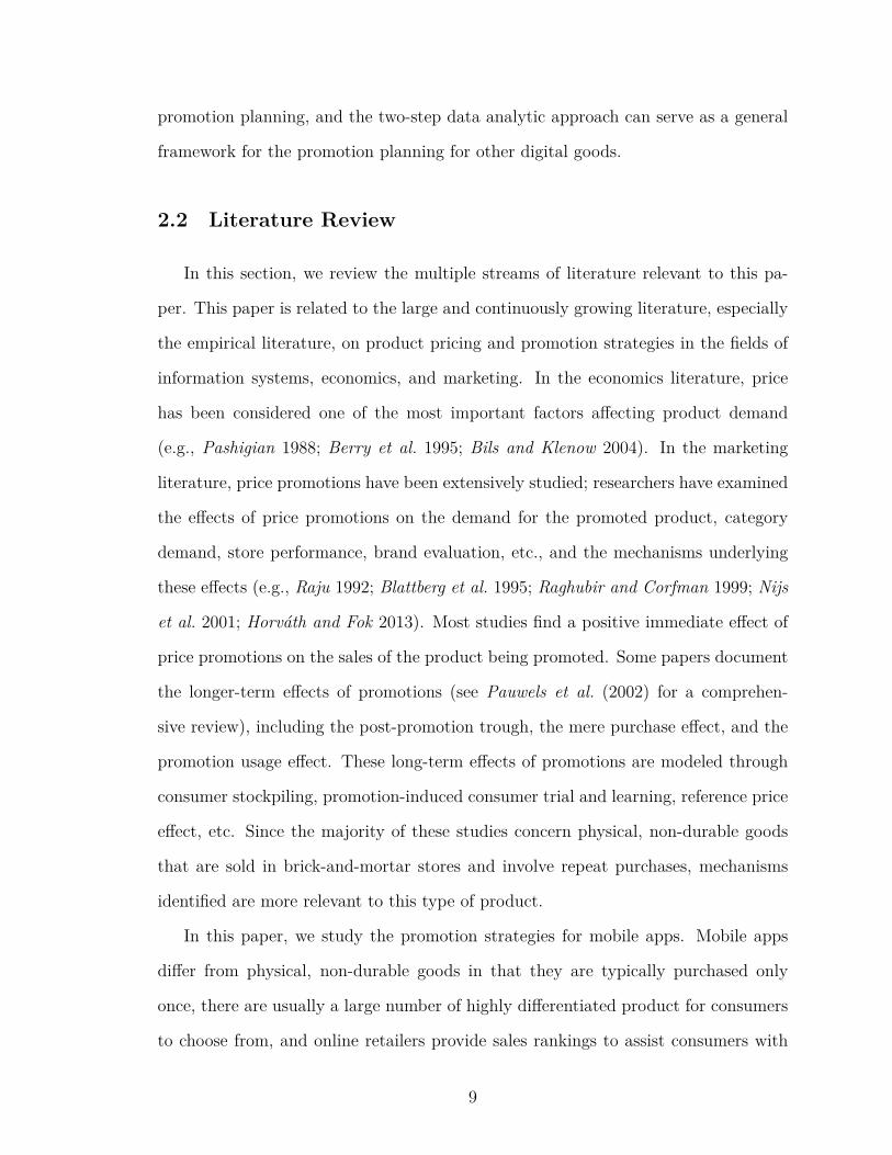
Figure 2.1 displays the histogram of the number of promotions each app experienced

in our sample).

Figure 2.1: Histogram of No. Promotions

0 1 2 3 4 5 6 7 8 9

Number of Promotions per App

0

50

100

150

200

250

Freq

uenc

y

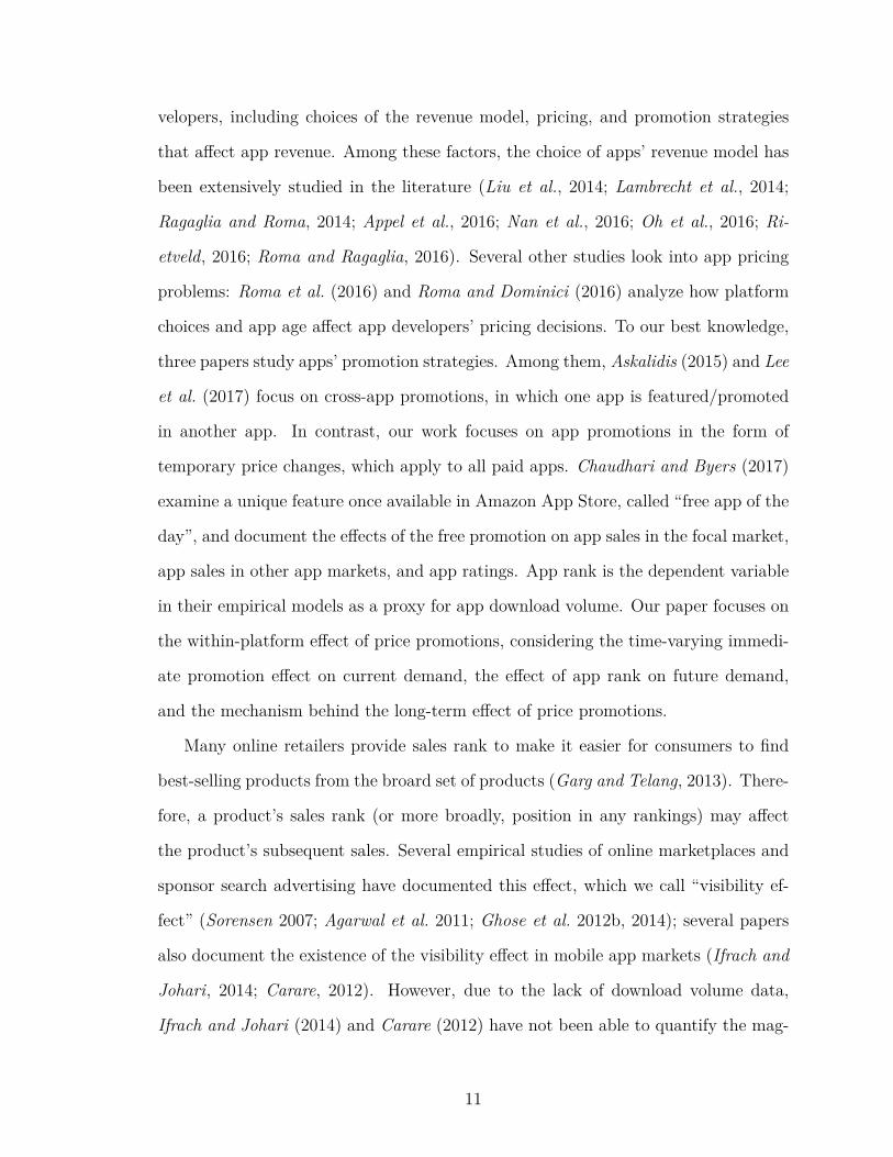
Figure 2.2: Distributions of Promotion Depth and Promotion Length

0.1 0.2 0.3 0.4 0.5 0.6 0.7 0.8

Promotion price discount depth

0

10

20

30

40

50

60

70

80

Num

ber o

f pro

mot

ions

0 5 10 15 20 25 30 35 40 45 50

Promotion length (day)

0

5

10

15

20

25

30

35

40

45

Num

ber o

f pro

mot

ions

Each price promotion can be characterized by two parameters: promotion depth

and promotion length. Let poriginal be the original price of an app and ppromotion be

the discounted price effective during the promotion; the promotion depth is then

defined as the percentage price decrease during the promotion(

poriginal−ppromotion

poriginal

),

and promotion length is measured by the number of days the promotion lasts. The

distributions of the depth and length of the promotions observed in our data are

shown in Figure 2.2: the majority of promotions observed in our sample involved

a 50%-70% discount and lasted 1 to 20 days. The detailed summary statistics of

promotion depth and promotion length are provided in Table 2.3.

We first visualize the relationship between daily rank and daily download volume

on the log-scale in the left panel of Figure 2.3. Consistent with Chevalier and Goolsbee

(2003); Ghose and Han (2014), and Garg and Telang (2013), our data suggests a linear

relationship between the logarithm of rank and the logarithm of download volume.

15

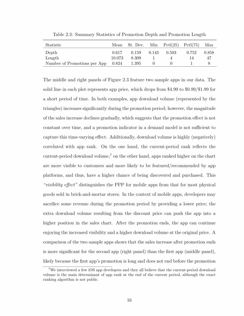
Table 2.3: Summary Statistics of Promotion Depth and Promotion Length

Statistic Mean St. Dev. Min Pctl(25) Pctl(75) MaxDepth 0.617 0.159 0.143 0.503 0.752 0.858Length 10.073 8.309 1 4 14 47Number of Promotions per App 0.824 1.395 0 0 1 8

The middle and right panels of Figure 2.3 feature two sample apps in our data. The

solid line in each plot represents app price, which drops from $4.99 to $0.99/$1.99 for

a short period of time. In both examples, app download volume (represented by the

triangles) increases significantly during the promotion period; however, the magnitude

of the sales increase declines gradually, which suggests that the promotion effect is not

constant over time, and a promotion indicator in a demand model is not sufficient to

capture this time-varying effect. Additionally, download volume is highly (negatively)

correlated with app rank. On the one hand, the current-period rank reflects the

current-period download volume,7 on the other hand, apps ranked higher on the chart

are more visible to customers and more likely to be featured/recommended by app

platforms, and thus, have a higher chance of being discovered and purchased. This

“visibility effect” distinguishes the PPP for mobile apps from that for most physical

goods sold in brick-and-mortar stores. In the context of mobile apps, developers may

sacrifice some revenue during the promotion period by providing a lower price; the

extra download volume resulting from the discount price can push the app into a

higher position in the sales chart. After the promotion ends, the app can continue

enjoying the increased visibility and a higher download volume at the original price. A

comparison of the two sample apps shows that the sales increase after promotion ends

is more significant for the second app (right panel) than the first app (middle panel),

likely because the first app’s promotion is long and does not end before the promotion7We interviewed a few iOS app developers and they all believe that the current-period download

volume is the main determinant of app rank at the end of the current period, although the exactranking algorithm is not public.

16

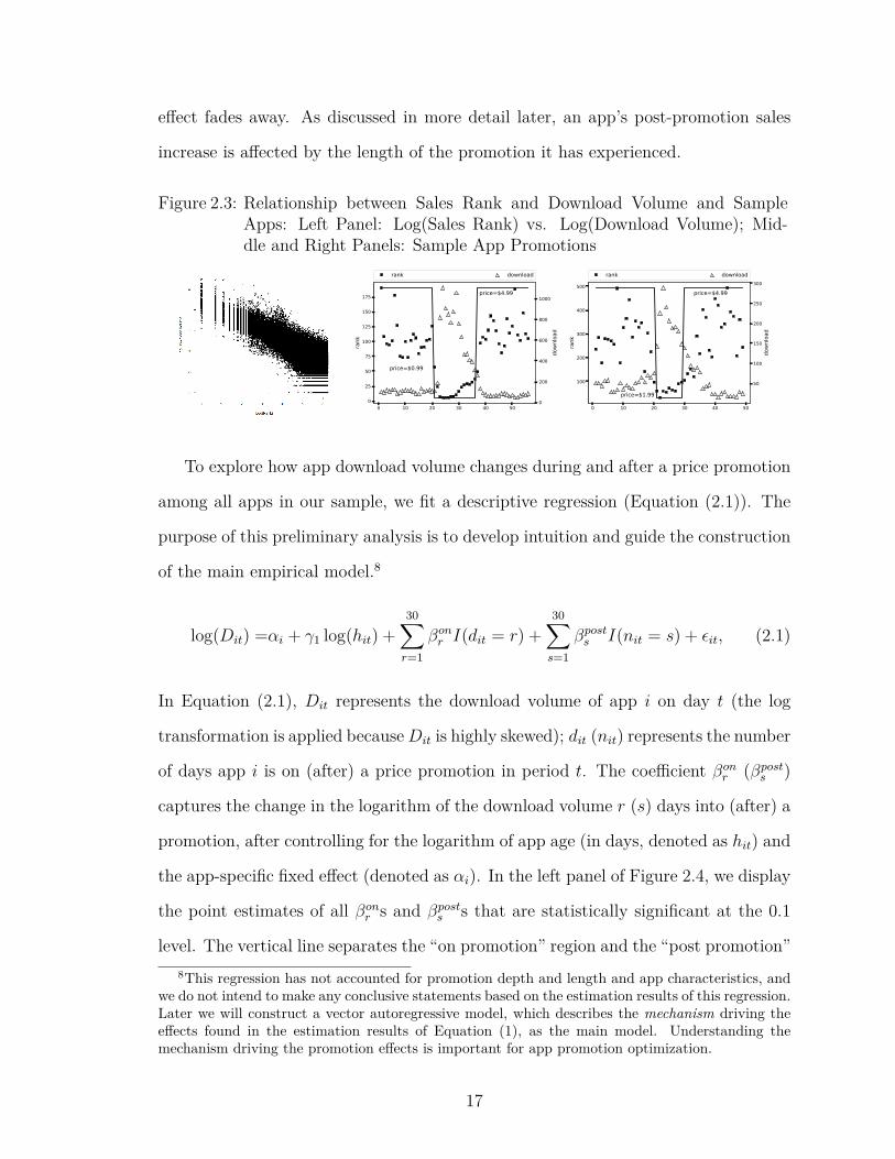
effect fades away. As discussed in more detail later, an app’s post-promotion sales

increase is affected by the length of the promotion it has experienced.

Figure 2.3: Relationship between Sales Rank and Download Volume and SampleApps: Left Panel: Log(Sales Rank) vs. Log(Download Volume); Mid-dle and Right Panels: Sample App Promotions

0 10 20 30 40 500

25

50

75

100

125

150

175

rank

0

200

400

600

800

1000

down

load

0.99

4.99

rank download

price=$0.99

price=$4.99

0 10 20 30 40 50

100

200

300

400

500

rank

50

100

150

200

250

300

down

load

2.0

2.5

3.0

3.5

4.0

4.5

5.0

rank download

price=$1.99

price=$4.99

To explore how app download volume changes during and after a price promotion

among all apps in our sample, we fit a descriptive regression (Equation (2.1)). The

purpose of this preliminary analysis is to develop intuition and guide the construction

of the main empirical model.8

log(Dit) =αi + γ1 log(hit) +30∑r=1

βonr I(dit = r) +

30∑s=1

βposts I(nit = s) + ϵit, (2.1)

In Equation (2.1), Dit represents the download volume of app i on day t (the log

transformation is applied because Dit is highly skewed); dit (nit) represents the number

of days app i is on (after) a price promotion in period t. The coefficient βonr (βpost

s )

captures the change in the logarithm of the download volume r (s) days into (after) a

promotion, after controlling for the logarithm of app age (in days, denoted as hit) and

the app-specific fixed effect (denoted as αi). In the left panel of Figure 2.4, we display

the point estimates of all βonr s and βpost

s s that are statistically significant at the 0.1

level. The vertical line separates the “on promotion” region and the “post promotion”8This regression has not accounted for promotion depth and length and app characteristics, and

we do not intend to make any conclusive statements based on the estimation results of this regression.Later we will construct a vector autoregressive model, which describes the mechanism driving theeffects found in the estimation results of Equation (1), as the main model. Understanding themechanism driving the promotion effects is important for app promotion optimization.

17

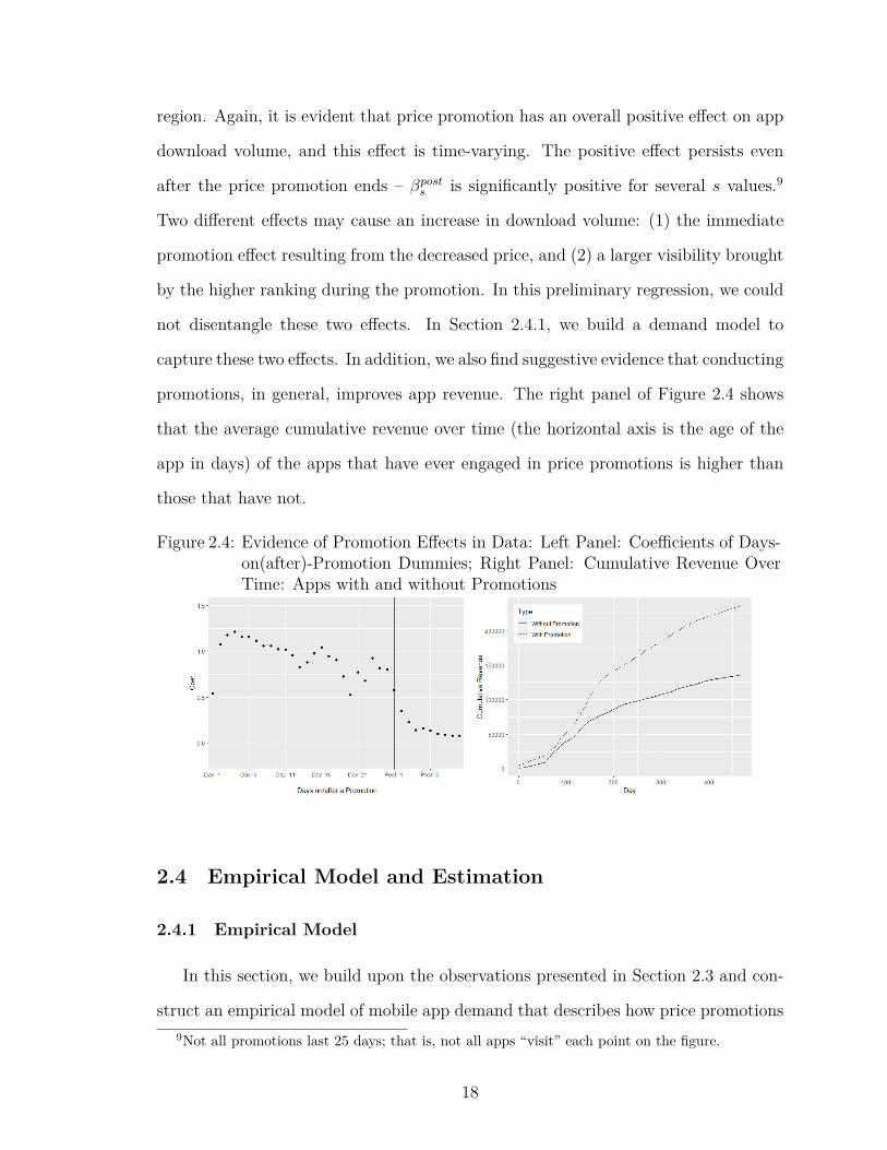
region. Again, it is evident that price promotion has an overall positive effect on app

download volume, and this effect is time-varying. The positive effect persists even

after the price promotion ends – βposts is significantly positive for several s values.9

Two different effects may cause an increase in download volume: (1) the immediate

promotion effect resulting from the decreased price, and (2) a larger visibility brought

by the higher ranking during the promotion. In this preliminary regression, we could

not disentangle these two effects. In Section 2.4.1, we build a demand model to

capture these two effects. In addition, we also find suggestive evidence that conducting

promotions, in general, improves app revenue. The right panel of Figure 2.4 shows

that the average cumulative revenue over time (the horizontal axis is the age of the

app in days) of the apps that have ever engaged in price promotions is higher than

those that have not.

Figure 2.4: Evidence of Promotion Effects in Data: Left Panel: Coefficients of Days-on(after)-Promotion Dummies; Right Panel: Cumulative Revenue OverTime: Apps with and without Promotions

2.4 Empirical Model and Estimation

2.4.1 Empirical Model

In this section, we build upon the observations presented in Section 2.3 and con-

struct an empirical model of mobile app demand that describes how price promotions9Not all promotions last 25 days; that is, not all apps “visit” each point on the figure.

18

affect download volume.

We formulate a system of equations consisting of Equations (2.2) and (2.3), where

Equation (2.2) is the demand function capturing how price promotions, last-period

rank, and other app characteristics affect download volume. Equation (2.3) is the

ranking function characterizing how download volume is reflected by rank. This

model describes the mechanism driving the promotion effects shown in the left panel

of Figure 2.4; it captures the inter-period dependence of rank and download volume,

and allows us to tease apart the visibility effect and the immediate promotion effect.

log(Dit) =αi + β1 log(ri(t−1)) + β2 log(hit) + β3 log(uit) + β4qit + β5∆pit + β6∆pit · dit

+ β7∆pit · d2it + β8∆pit · d3it + · · ·+11∑

m=1

ηmMmit +6∑

w=1

ϕwWwit + ϵit, (2.2)

log(rit) =γ0 + γ1 log(Dit) + εit. (2.3)

In the equations, i is the index for mobile apps and t is the index for time (day).

The notation and description of the variables in the model are summarized in Table

2.4. The dependent variable of the demand function is the logarithm of the download

volume of an app on a day (Dit). To account for the effect of unobserved time-

invariant app-specific characteristics (e.g., story-line and playability, which constitute

each app’s base quality) on download volume, we include app-specific fixed effect αi

in our model. To capture the visibility effect evident in the data, we follow Carare

(2012) and include the one-period lagged rank (log(ri(t−1))) as one of the independent

variables.1011 We then include the logarithm of app i’s age by days (log(hit)) and the10The coefficient of lagged rank captures not only the direct visibility benefits brought by moving

from a lower to a higher position on the app store’s download chart, but also the indirect visibilitybenefits resulting from being featured in app stores. App store editors periodically select popularapps and display them on the app stores’ homepage as “featured apps” or “editor’s choices”andrecommend them on social media platforms. Additionally, since log(ri(t−1)) and log(Di(t−1)) arehighly correlated, the visibility effect, reflected by the coefficient of log(ri(t−1)), may also capturethe effect of log(Di(t−1)) through non-ranking-related channels.

11We considered a few alternative specifications, including one that contains more lagged values oflog(rit), one that uses log(Di(t−1)) to replace log(ri(t−1)), and one that incorporates both log(Di(t−1))

19

logarithm of the number of days since the last version update (log(uit)) to account for

the possible effects of app age and version age on app demand. Following Ghose and

Han (2014), we also incorporate app ratings (ranging from 1 to 5 stars, denoted as qit)

in the demand equation. We use ∆pit to represent the depth of the promotion app i is

experiencing on day t.12 (For all t’s at which app i is not on promotion, dit equals 0.)

The coefficient of ∆pit, denoted by β5, captures the baseline effect of a promotion with

a depth of 1 on the logarithm of download volume. To capture the possibility that

the size of the promotion effect varies on different days in the promotion period, we

interact ∆pit with polynomial terms of dit, with dit representing the number of days

into the current promotion. For example, if the price of app i drops on day τ , then

diτ = 1, di(τ+1) = 2, di(τ+2) = 3, and so on. The promotion effect app i experiences

on day t is then β5∆pit + β6∆pit · dit + β7∆pit · d2it + · · · . (We discuss later in this

section how we determine the number of polynomial terms of dit to keep.) Finally,

we include a series of month dummies (Mmit) and a series of day-of-week dummies to

control for seasonality and weekday/weekend effects, respectively.

For the ranking function, we follow Chevalier and Goolsbee (2003), Garg and

Telang (2013), and Ghose and Han (2014) and assume a Pareto distribution between

rank (rit) and download volume (Dit), i.e., rit = a·D−bit . Here b is the shape parameter

and a is the scale parameter. Taking the logarithm of both sides of the equation and

adding noise terms to the mapping, we can re-write the ranking function as Equation

(2.3). The effect of a promotion captured by “β5∆pit+β6∆pit ·dit+β7∆pit ·d2it+ · · · ”

in Equation (2.2) is the immediate promotion effect, which corresponds to the direct

effect of a price drop on the current-period download volume. In addition to this direct

effect, price promotions have an indirect effect on demand through the visibility effect

and log(ri(t−1)). The estimation results of these alternative models and the model comparison arebriefly discussed in Section 2.4.4

12We consider an alternative demand function that includes the absolute price change instead ofthe fractional price change. The model has a slightly worse fit as compared with the main demandmodel (Equation (2.2)); see Section 2.4.4 for details of this analysis.

20

– the direct effect of the promotion in period t on the period-t demand will lead to

changes in the focal app’s sales rank, and the period-t app rank can further affect

the period-(t + 1) download volume. In fact, Equations (2.2) and (2.3) constitute a

general form of a vector autoregressive (VAR) model. The total effect of a promotion

on current and future app demand should be evaluated using an approach similar to

the impulse response function, which will be elaborated in Section 4.3.

Table 2.4: Variable DescriptionDit Download volume of app i on day tri(t−1) Rank of app i on day t− 1hit The number of days since app i’s releaseuit The number of days since app i’s last updateqit Current rating (on a scale of 1-5 stars) of app i

on day t∆pit =(poriginal

i − ppromotionit )/poriginal

i

Depth of the promotion for app i on day t

dit Days in promotion for app i on day tMmit Month dummiesWwit Day-of-week dummies

In the current model, we do not explicitly consider substitution between apps

because mobile games are highly differentiated (in terms of story-line, graphic de-

sign, game mechanisms, and game-play experience). Therefore, there is likely little

substitution between games, as compared to physical, non-durable products (e.g.,

detergents and cereal). Similar assumptions are made in studies of other sectors of

the media and entertainment industry: Chen et al. (2018) consider each book as a

monopolistic product and Danaher et al. (2014) treat each music album as a monop-

olistic product. In Section 2.4.4, we compare alternative models with/without this

assumption.

2.4.2 Instrumental Variables

Endogeneity is a known common challenge in demand estimation. In our demand

model, the timing, depth, and length of promotions are potentially endogenous be-

21

cause developers’ promotion decisions may be based on the expected demand. Not

only the depth but also the timing and length of promotions are reflected in the series

of ∆pit in our model – in periods when app i is not on promotion, ∆pit = 0; in periods

when app i is on promotion, ∆pit takes a positive value.13 To address the endogeneity

with respect to developers’ promotion decisions, we instrument for ∆pit.

We follow Ghose and Han (2014) and consider the average price of all apps pro-

duced by the focal app’s developer in the Google Play store on the same day as an

instrument. The prices of Android apps (sold in the Google Play store) produced by

the same developer are likely to be correlated with the focal iOS app’s price. How-

ever, the demand shock to the focal iOS app is unlikely to be correlated with the

prices and download volumes of apps sold in the Google Play store because the two

stores have different customer bases.14 This is a BLP-style instrument (Berry et al.,

1995). Since the price of an app is affected by the production and maintenance costs

of the app and those costs are shared by the Android apps and iOS apps produced

by the same developer, the prices of apps sold in the iOS and Google Play app stores

are also likely to be correlated. It is common for a mobile game developer to publish

the same game in both iOS and Google Play stores. Although the iOS version and

Android version (sold in the Google Play store) of the same app may be written in

different programming languages, they share common graphical modules and story-

lines. Therefore, the development costs of the iOS and Android versions of the same

app tend to correlate with each other. Mobile games typically make major updates in

both stores at the same time to ensure similar customer experiences across platforms.

Furthermore, the iOS and Android versions of the same game are maintained by the13For example, consider a 7-day window and fix the promotion depth to 0.5. A promotion that

starts on day 2 and lasts for 3 days would result in a sequence of ∆pit of {0, 0.5, 0.5, 0.5, 0, 0, 0};a promotion that starts on day 3 and lasts for 5 days would result in a sequence of ∆pit of{0, 0, 0.5, 0.5, 0.5, 0.5, 0.5}. dit is simply the natural day count for days on which ∆pit > 0.

14Like Ghose and Han (2014), we do not consider cross-platform demand correlation throughmedia channels shared by users of both platforms, which is possible to exist in reality. In addition,we do not explicitly consider any marketing campaigns that app developers conduct in conjunctionwith price promotions.

22

same development team, and the two platforms usually share the same database;

therefore, the maintenance costs associated with the iOS and Android versions of the

same game are likely to be correlated. We further use a set of 13 version indicator

variables (referred to as Version Number) to instrument for ∆pit. For example, the

kth indicator variable takes the value of 1 when the current version is the kth version,

and 0 otherwise. This set of indicator variables is likely to be correlated with ∆pit

because the maintenance cost may vary with app version. Indeed, the first-stage F-

test strongly rejects (p-value=0.000) the hypothesis that the set of version indicator

variables are jointly uncorrelated with ∆pit. If the number of version updates affects

demand, it does so by affecting app quality (Ghose and Han, 2014); since we have

already controlled for app quality by incorporating app fixed effects and app rating,

app version is unlikely to be correlated with demand shocks.

One plausible mechanism causing the endogeneity of promotion length is that app

developers may dynamically determine the length of promotion after observing the

realized promotion effect. That is, if a promotion is effective immediately after it is

turned on, the developer may end it early; if not, the developer may let it run for a

more extensive period. If this is true, we will find that shorter promotions tend to

be more effective early on. To test if this mechanism is active, we explore what kind

of apps engage in price promotions, and whether decisions on promotion depth and

length are correlated with app features.

Promotion adoption. It is possible that more experienced developers can plan for

more effective promotions and at the same time conduct more promotions than the

developers who are less experienced. Figure 2.5 shows the relationship between the

number of promotions conducted during the study period and (1) developer experi-

ence (measured by the number of apps published by the focal app’s developer) and

(2) app quality (measured by the app rating and the magnitude of the app-specific

fixed effect). The figure suggests that apps whose developer is less experienced tend

23

to experience more price promotions, while the correlation between the number of

promotions and app quality is weak.

We further perform two-sample T-tests on the difference in developer experience

and that in app quality (both measures) between apps that ever engaged in price

promotions and those that never did. We find that the differences in the number of

apps published by the focal app’s developer, app rating and app fixed effect between

these two groups of apps, are all statistically insignificant (p-value = 0.997, 0.966 and

0.991, respectively). These results indicate there is no strong select in the adoption

and usage of price promotions in the data.

Figure 2.5: Number of promotions against number of apps published by its developer,average app rating and app fixed effect

Promotion depth. We then explore the relationship between promotion depth

and apps’ rating, download volume, rank, and the magnitude of the app-specific

24

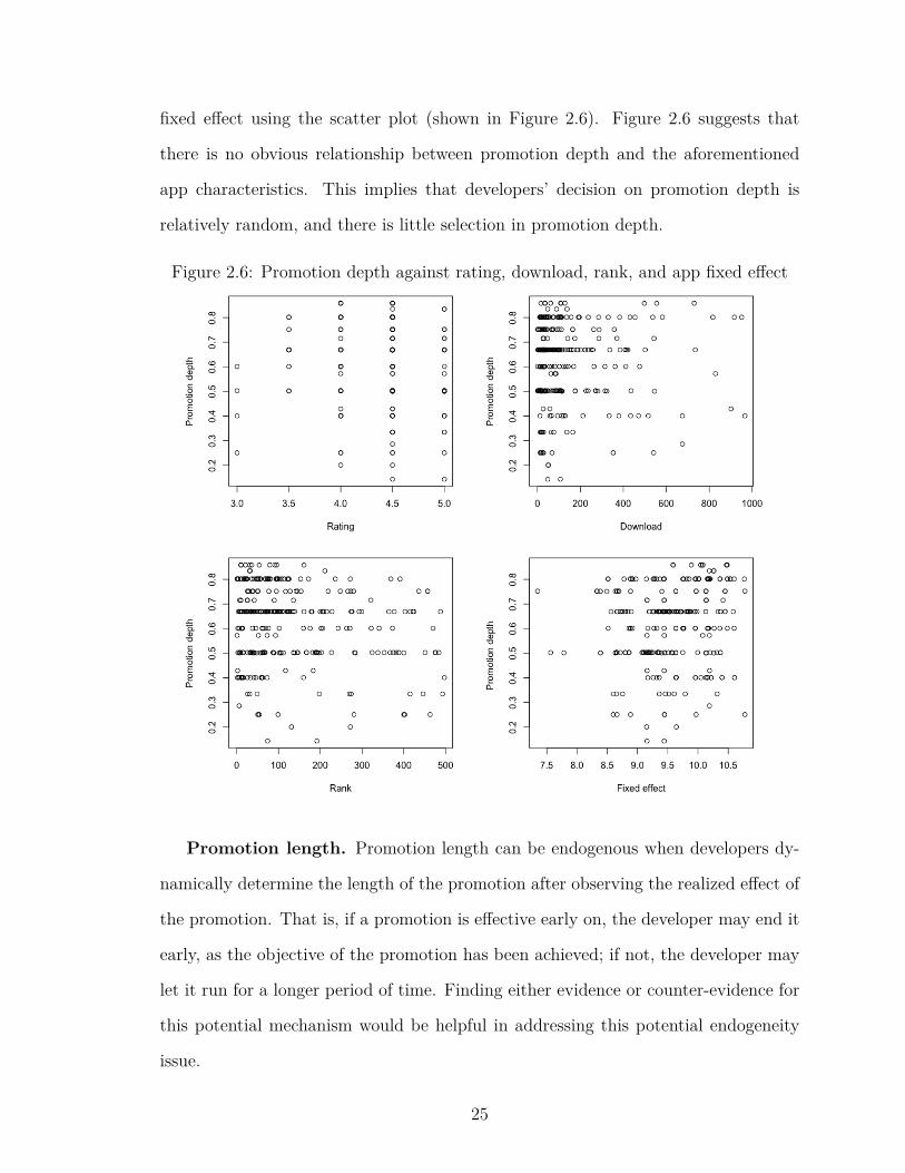
fixed effect using the scatter plot (shown in Figure 2.6). Figure 2.6 suggests that

there is no obvious relationship between promotion depth and the aforementioned

app characteristics. This implies that developers’ decision on promotion depth is

relatively random, and there is little selection in promotion depth.

Figure 2.6: Promotion depth against rating, download, rank, and app fixed effect

Promotion length. Promotion length can be endogenous when developers dy-

namically determine the length of the promotion after observing the realized effect of

the promotion. That is, if a promotion is effective early on, the developer may end it

early, as the objective of the promotion has been achieved; if not, the developer may

let it run for a longer period of time. Finding either evidence or counter-evidence for

this potential mechanism would be helpful in addressing this potential endogeneity

issue.

25

Therefore, we first explore if rank improvement (current-day app rank minus app

rank on the day prior to the promotion) on each day of the promotion is significantly

different for short and long promotions. Short promotions are defined as those that

last less than or equal to 10 days, which is the median of the promotion length in

the data. Note that in this analysis, each promotion, rather than each app, is an

observation. In Figure 2.7, we plot the rank improvement against the number of

days on promotion (dit in Equation 2.2). The solid line and the dashed line represent

the mean rank improvement among long promotions and among short promotions,

respectively. The figure shows a small difference between long promotions and short

promotions in terms of rank improvement. It is in fact the short promotions that

are slightly less effective on the first several days of the promotion. In other words,

short promotions lead to a less negative change in rank, or equivalently, a smaller

rank improvement.

We also perform a two-sample T-test on the difference in length between pro-

motions that got apps into top positions of the ranking chart, i.e., top 20 (top 30),

and those that did not. The results are consistent with what is shown in Figure 2.7:

Promotions that helped apps reach a top 20 (top 30) position is slightly longer (about

two days) than those that were not able to (p-value=0.049 for the top 20 cutoff and

0.003 for the top 30 cutoff).

In summary, there is no evidence for the endogeneity of promotion length. Even

if such endogeneity exists, instrumenting for ∆pit can still address it.

Another endogeneity issue we need to address is with log(ri(t−1)). Although the

last-period rank cannot be influenced by unobservables that affect the current-period

demand, demand shocks for the same app may be correlated from period to period.

Following the same rationale in Carare (2012), we use the logged two- and three-period

lagged ranks as instruments for log(ri(t−1)). We carry out tests for weak instruments

and overidentifying restrictions on the instruments for the two potentially endogenous

26

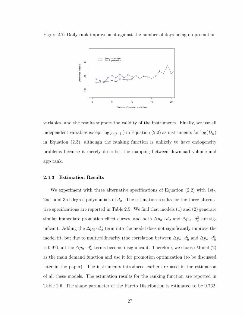
Figure 2.7: Daily rank improvement against the number of days being on promotion

0 5 10 15 20

-100

-50

0

Number of days on promotion

Diff

eren

ce in

rank

Long promotionShort promotion

variables, and the results support the validity of the instruments. Finally, we use all

independent variables except log(ri(t−1)) in Equation (2.2) as instruments for log(Dit)

in Equation (2.3), although the ranking function is unlikely to have endogeneity

problems because it merely describes the mapping between download volume and

app rank.

2.4.3 Estimation Results

We experiment with three alternative specifications of Equation (2.2) with 1st-,

2nd- and 3rd-degree polynomials of dit. The estimation results for the three alterna-

tive specifications are reported in Table 2.5. We find that models (1) and (2) generate

similar immediate promotion effect curves, and both ∆pit · dit and ∆pit · d2it are sig-

nificant. Adding the ∆pit · d3it term into the model does not significantly improve the

model fit, but due to multicollinearity (the correlation between ∆pit ·d2it and ∆pit ·d3it

is 0.97), all the ∆pit · dkit terms become insignificant. Therefore, we choose Model (2)

as the main demand function and use it for promotion optimization (to be discussed

later in the paper). The instruments introduced earlier are used in the estimation

of all these models. The estimation results for the ranking function are reported in

Table 2.6. The shape parameter of the Pareto Distribution is estimated to be 0.762,

27

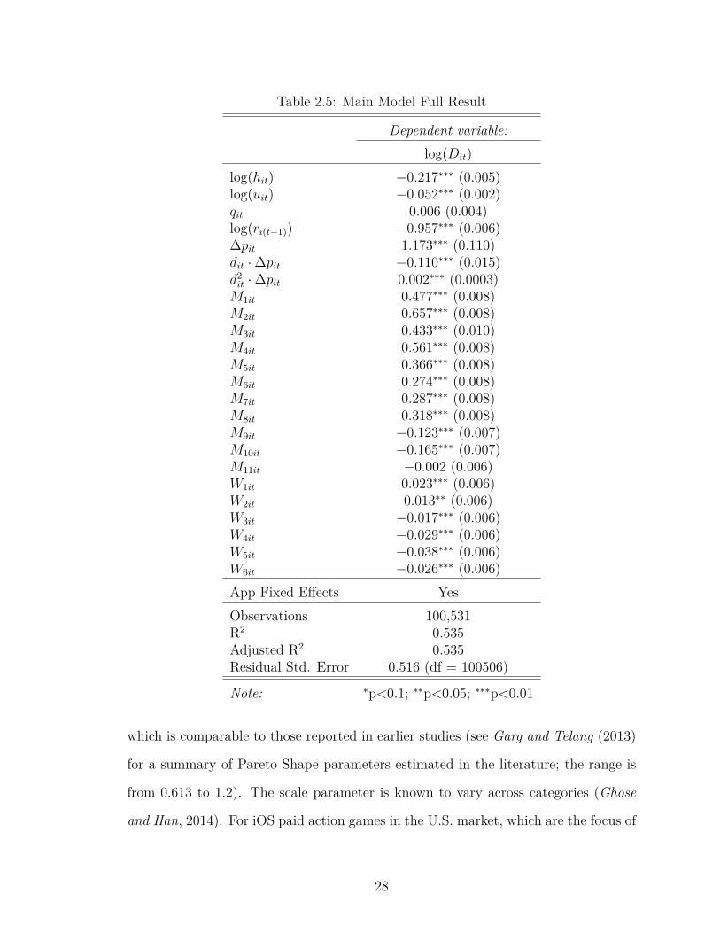
Table 2.5: Main Model Full Result

Dependent variable:log(Dit)

log(hit) −0.217∗∗∗ (0.005)log(uit) −0.052∗∗∗ (0.002)qit 0.006 (0.004)log(ri(t−1)) −0.957∗∗∗ (0.006)∆pit 1.173∗∗∗ (0.110)dit ·∆pit −0.110∗∗∗ (0.015)d2it ·∆pit 0.002∗∗∗ (0.0003)M1it 0.477∗∗∗ (0.008)M2it 0.657∗∗∗ (0.008)M3it 0.433∗∗∗ (0.010)M4it 0.561∗∗∗ (0.008)M5it 0.366∗∗∗ (0.008)M6it 0.274∗∗∗ (0.008)M7it 0.287∗∗∗ (0.008)M8it 0.318∗∗∗ (0.008)M9it −0.123∗∗∗ (0.007)M10it −0.165∗∗∗ (0.007)M11it −0.002 (0.006)W1it 0.023∗∗∗ (0.006)W2it 0.013∗∗ (0.006)W3it −0.017∗∗∗ (0.006)W4it −0.029∗∗∗ (0.006)W5it −0.038∗∗∗ (0.006)W6it −0.026∗∗∗ (0.006)App Fixed Effects YesObservations 100,531R2 0.535Adjusted R2 0.535Residual Std. Error 0.516 (df = 100506)

Note: ∗p<0.1; ∗∗p<0.05; ∗∗∗p<0.01

which is comparable to those reported in earlier studies (see Garg and Telang (2013)

for a summary of Pareto Shape parameters estimated in the literature; the range is

from 0.613 to 1.2). The scale parameter is known to vary across categories (Ghose

and Han, 2014). For iOS paid action games in the U.S. market, which are the focus of

28

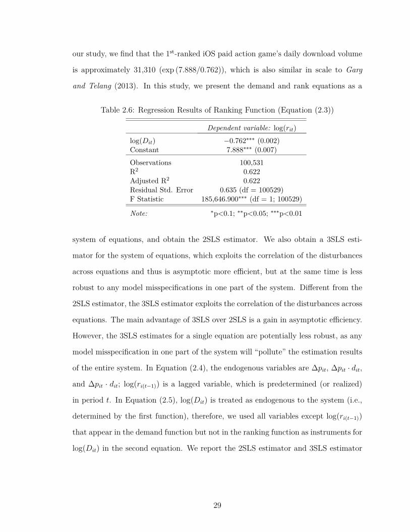
our study, we find that the 1st-ranked iOS paid action game’s daily download volume

is approximately 31,310 (exp (7.888/0.762)), which is also similar in scale to Garg

and Telang (2013). In this study, we present the demand and rank equations as a

Table 2.6: Regression Results of Ranking Function (Equation (2.3))

Dependent variable: log(rit)

log(Dit) −0.762∗∗∗ (0.002)Constant 7.888∗∗∗ (0.007)Observations 100,531R2 0.622Adjusted R2 0.622Residual Std. Error 0.635 (df = 100529)F Statistic 185,646.900∗∗∗ (df = 1; 100529)

Note: ∗p<0.1; ∗∗p<0.05; ∗∗∗p<0.01

system of equations, and obtain the 2SLS estimator. We also obtain a 3SLS esti-

mator for the system of equations, which exploits the correlation of the disturbances

across equations and thus is asymptotic more efficient, but at the same time is less

robust to any model misspecifications in one part of the system. Different from the

2SLS estimator, the 3SLS estimator exploits the correlation of the disturbances across

equations. The main advantage of 3SLS over 2SLS is a gain in asymptotic efficiency.

However, the 3SLS estimates for a single equation are potentially less robust, as any

model misspecification in one part of the system will “pollute” the estimation results

of the entire system. In Equation (2.4), the endogenous variables are ∆pit, ∆pit · dit,

and ∆pit · dit; log(ri(t−1)) is a lagged variable, which is predetermined (or realized)

in period t. In Equation (2.5), log(Dit) is treated as endogenous to the system (i.e.,

determined by the first function), therefore, we used all variables except log(ri(t−1))

that appear in the demand function but not in the ranking function as instruments for

log(Dit) in the second equation. We report the 2SLS estimator and 3SLS estimator

29

of the system of equations in Tables 2.7 and 2.8 below.

log(Dit) = αi + β1 log(ri(t−1)) + β2 log(hit) + β3 log(uit) + β4qit + β5∆pit + β6∆pit · dit

+ β7∆pit · d2it + β8∆pit · d3it + · · ·+11∑

m=1

ηmMmit +6∑

w=1

ϕwWwit + ϵit

(2.4)

log(rit) = γ0 + γ1 log(Dit) + εit (2.5)

Table 2.7: 2SLS and 3SLS Estimation Results of Demand Function

Dependent variable: log(download)(2SLS) (3SLS)

log(hit) −0.217∗∗∗ (0.005) −0.192∗∗∗ (0.005)log(ri(t−1)) −0.957∗∗∗ (0.006) −0.957∗∗∗ (0.005)log(uit) −0.052∗∗∗ (0.002) −0.059∗∗∗ (0.002)qit 0.006 (0.004) 0.007 (0.004)∆pit 1.173∗∗∗ (0.110) 1.302∗∗∗ (0.109)dit ·∆pit −0.110∗∗∗ (0.015) −0.123∗∗∗ (0.014)d2it ·∆pit 0.002∗∗∗ (0.0003) 0.003∗∗∗(0.0003)Month Dummies Yes YesDay of Week Dummies Yes YesApp Fixed Effects Yes YesObservations 100,531 100,531R2 0.539 0.527Adjusted R2 0.539 0.527Residual Std. Error 0.515 (df = 100507) 0.541 (df = 100507)

Note: ∗p<0.1; ∗∗p<0.05; ∗∗∗p<0.01

The system 2SLS estimator and the system 3SLS estimator of the demand function

are very similar. The 3SLS has some efficiency benefits in the sense that it reduces

the standard errors of the coefficient estimates, however, the model as a whole has

a poorer fit. The ranking function estimated in the system is also very similar to

the ranking function estimated separately. The fact that the system 2SLS and 3SLS

30

Table 2.8: 2SLS and 3SLS Estimation Results of Ranking Function

Dependent variable: log(Rank)(2SLS) (3SLS)

log(Dit) 7.888∗∗∗ (0.007) 7.888∗∗∗ (0.007)Constant −0.762∗∗∗ (0.002) −0.762∗∗∗ (0.002)Observations 100,531 100,531R2 0.622 0.622Adjusted R2 0.622 0.622Residual Std. Error 0.635 (df = 100529) 0.635 (df = 100529)

Note: ∗p<0.1; ∗∗p<0.05; ∗∗∗p<0.01

estimators are similar indicates that the cross-equation correlation in the error terms

is weak. Therefore we use 2SLS estimator in the rest of the analyses.

2.4.3.1 Immediate Promotion Effect.

The estimation results confirm that price promotions have a significant immediate

positive impact on app download volume. If we plug the estimated β5, β6 and β7

into Equation (2.2), we can calculate the daily immediate effect of a promotion as

1.173∆pit − 0.110∆pit · dit + 0.002∆pit · d2it. The dashed line in Figure 2.8 shows the

daily immediate effect of a promotion with a depth of 0.5 and over a 25-day promotion

period. We can see that the immediate promotion effect generally decreases over time.

(Figure 2.2 shows 95% of the promotions in the data last no more than 25 days,

therefore, we are only able to accurately estimate the promotion effect for dit ≤ 25.

The estimated promotion effect for dit > 25 is subject to extrapolation.)

The promotion effect is negative for dit ≥ 15. One possible explanation is that in

each period, a number of new consumers are exposed to the focal app, and the number

of such customers is affected by app rank. The consumers who have a willingness-

to-pay higher than the normal app price will purchase the app immediately, while

those whose willingness-to-pay is below the normal app price become aware of the

31

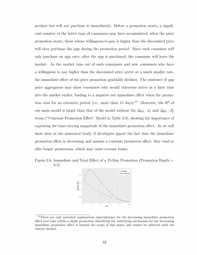
product but will not purchase it immediately. Before a promotion starts, a signifi-

cant number of the latter type of consumers may have accumulated; when the price

promotion starts, those whose willingness-to-pay is higher than the discounted price

will then purchase the app during the promotion period. Since each consumer will

only purchase an app once, after the app is purchased, the consumer will leave the

market. As the market runs out of such consumers and new consumers who have

a willingness to pay higher than the discounted price arrive at a much smaller rate,

the immediate effect of the price promotion gradually declines. The existence of app

price aggregators may draw consumers who would otherwise arrive at a later time

into the market earlier, leading to a negative net immediate effect when the promo-

tion runs for an extensive period (i.e., more than 15 days).15 Moreover, the R2 of

our main model is larger than that of the model without the ∆pit · dit and ∆pit · d2it

terms (“Constant Promotion Effect” Model in Table 2.9), showing the importance of

capturing the time-varying magnitude of the immediate promotion effect. As we will

show later in the numerical study, if developers ignore the fact that the immediate

promotion effect is decreasing and assume a constant promotion effect, they tend to

offer longer promotions, which may cause revenue losses.

Figure 2.8: Immediate and Total Effect of a 25-Day Promotion (Promotion Depth =0.5)

15These are only potential explanations (speculations) for the decreasing immediate promotioneffect over time within a single promotion; identifying the underlying mechanism for the decreasingimmediate promotion effect is beyond the scope of this paper and cannot be achieved with ourcurrent dataset.

32

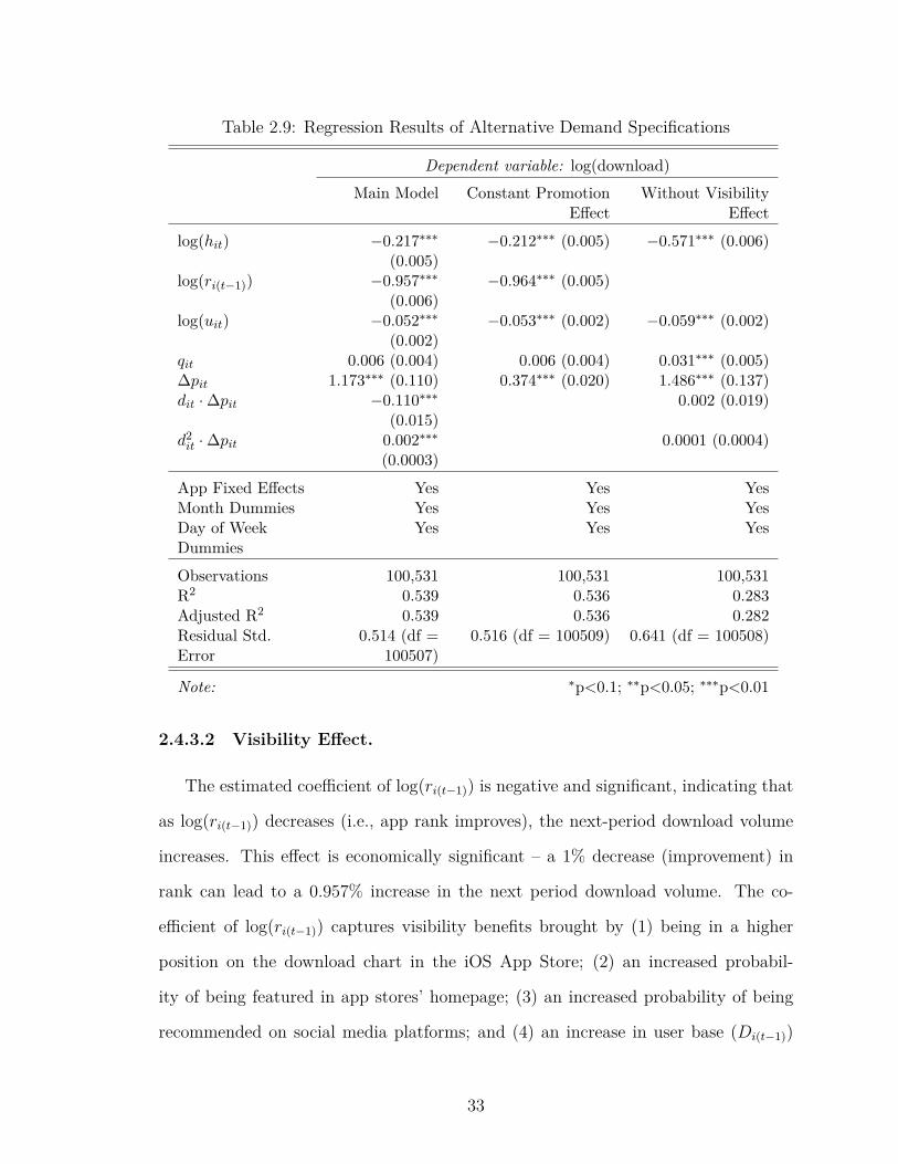
Table 2.9: Regression Results of Alternative Demand Specifications

Dependent variable: log(download)Main Model Constant Promotion

EffectWithout Visibility

Effectlog(hit) −0.217∗∗∗

(0.005)−0.212∗∗∗ (0.005) −0.571∗∗∗ (0.006)

log(ri(t−1)) −0.957∗∗∗(0.006)

−0.964∗∗∗ (0.005)

log(uit) −0.052∗∗∗(0.002)

−0.053∗∗∗ (0.002) −0.059∗∗∗ (0.002)

qit 0.006 (0.004) 0.006 (0.004) 0.031∗∗∗ (0.005)∆pit 1.173∗∗∗ (0.110) 0.374∗∗∗ (0.020) 1.486∗∗∗ (0.137)dit ·∆pit −0.110∗∗∗

(0.015)0.002 (0.019)

d2it ·∆pit 0.002∗∗∗(0.0003)

0.0001 (0.0004)

App Fixed Effects Yes Yes YesMonth Dummies Yes Yes YesDay of WeekDummies

Yes Yes Yes

Observations 100,531 100,531 100,531R2 0.539 0.536 0.283Adjusted R2 0.539 0.536 0.282Residual Std.Error

0.514 (df =100507)

0.516 (df = 100509) 0.641 (df = 100508)

Note: ∗p<0.1; ∗∗p<0.05; ∗∗∗p<0.01

2.4.3.2 Visibility Effect.

The estimated coefficient of log(ri(t−1)) is negative and significant, indicating that

as log(ri(t−1)) decreases (i.e., app rank improves), the next-period download volume

increases. This effect is economically significant – a 1% decrease (improvement) in

rank can lead to a 0.957% increase in the next period download volume. The co-

efficient of log(ri(t−1)) captures visibility benefits brought by (1) being in a higher

position on the download chart in the iOS App Store; (2) an increased probabil-

ity of being featured in app stores’ homepage; (3) an increased probability of being

recommended on social media platforms; and (4) an increase in user base (Di(t−1))

33

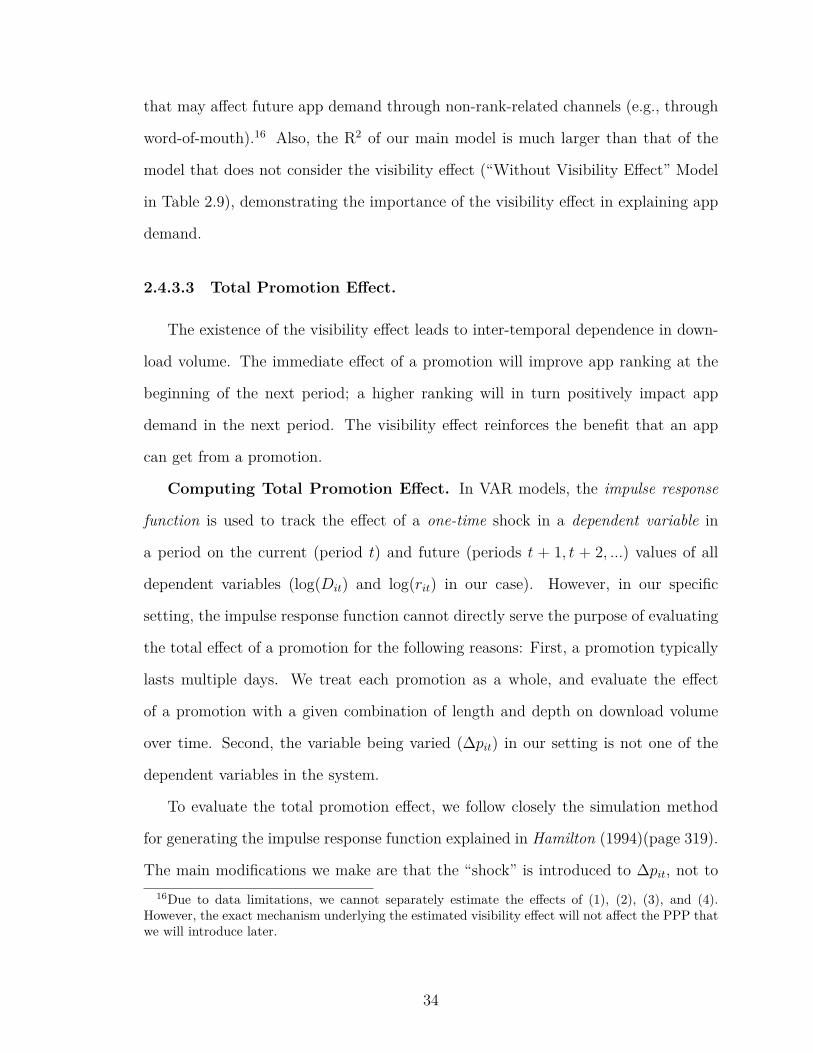
that may affect future app demand through non-rank-related channels (e.g., through

word-of-mouth).16 Also, the R2 of our main model is much larger than that of the

model that does not consider the visibility effect (“Without Visibility Effect” Model

in Table 2.9), demonstrating the importance of the visibility effect in explaining app

demand.

2.4.3.3 Total Promotion Effect.

The existence of the visibility effect leads to inter-temporal dependence in down-

load volume. The immediate effect of a promotion will improve app ranking at the

beginning of the next period; a higher ranking will in turn positively impact app

demand in the next period. The visibility effect reinforces the benefit that an app

can get from a promotion.

Computing Total Promotion Effect. In VAR models, the impulse response

function is used to track the effect of a one-time shock in a dependent variable in

a period on the current (period t) and future (periods t + 1, t + 2, ...) values of all

dependent variables (log(Dit) and log(rit) in our case). However, in our specific

setting, the impulse response function cannot directly serve the purpose of evaluating

the total effect of a promotion for the following reasons: First, a promotion typically

lasts multiple days. We treat each promotion as a whole, and evaluate the effect

of a promotion with a given combination of length and depth on download volume

over time. Second, the variable being varied (∆pit) in our setting is not one of the

dependent variables in the system.

To evaluate the total promotion effect, we follow closely the simulation method

for generating the impulse response function explained in Hamilton (1994)(page 319).

The main modifications we make are that the “shock” is introduced to ∆pit, not to16Due to data limitations, we cannot separately estimate the effects of (1), (2), (3), and (4).

However, the exact mechanism underlying the estimated visibility effect will not affect the PPP thatwe will introduce later.

34

one of the dependent variables, and that the shock is not one-time, but lasts for a few

days. Specifically, to evaluate the total effect of a promotion starting on day τ with a

depth of g and a length of l days on app i whose day τ−1 rank was w, we carry out the

following steps: First, we fix log(ri(τ−1)) to log(w). Since the promotion starts on day

τ and lasts for l days, in the simulation, ∆pit for all t ∈ {τ, τ +1, ..., τ + l−1} is set to

g, and ∆pit for all t ≥ τ+l is set to 0; dit is set to 1+t−τ for t ∈ {τ, τ+1, ..., τ+l−1},

and 0 for t ≥ τ+ l. Following Hamilton (1994), we set all ϵt and εt to zero. hiτ and uiτ

are set to their respective average values in the sample, and evolve deterministically

as hi(t+1) = hit +1, and ui(t+1) = uit +1. The month dummies, day-of-week dummies

and rating score qit are omitted. We then simulate the daily download volume and

app rank from day τ onward. That is, starting from t = τ , for each day, we plug the

values of the right-hand side variables into the estimated Equation (2.2) to simulate

log(Dit); then plug the simulated log(Dit) into the estimated Equation (3) to simulate

log(rit). We use the same method to simulate the daily download volume and app

rank for the same period of time without the promotion (where ∆pit and dit are set

to 0 throughout). Finally, we take the pairwise difference in log(Dit) between the

with- and without-promotion cases; the difference represents the total effect of the

promotion on each day.

Discussion. The solid line in Figure 2.8 visualizes the total promotion effect. The

gap between the solid and dashed lines represents the indirect effect of promotions

reinforced by the visibility effect. The increasing total promotion effect that occurs

in the first few days of a promotion is due to the larger immediate positive effect of

the promotion and its resulting higher app rank, which generates more visibility and

boosts demand significantly in the subsequent periods. As the promotion lasts longer,

the decrease in the immediate promotion effect dominates the visibility effect; thus

the total promotion effect also declines. Figure 2.9 shows how the total promotion

effect varies with promotion depth (0.25, 0.5, or 0.75) and length (5 days, 10 days, or

35

15 days). The first observation on each curve corresponds to the first promotion day.

The figure indicates that the size of the total promotion effect and whether it persists

after a promotion ends are affected by promotion length and depth. For example,

the solid curve in the left panel corresponds to a promotion with a depth of 0.25 and

a length of 5 days, whose total promotion effect is fairly large and remains positive

after day 12 (7 days after the promotion ends). This promotion ends when the total

promotion effect is still strong; therefore, the app enters the post-promotion period

with a high rank (visibility). The inter-temporal dependence of download volume and

app rank, as captured by our VAR model, keeps the download volume at a relatively

high level for several days, before it drops back to the normal level. If the promotion

lasts for 15 days (the dotted line in the same plot), the persistent promotion effect

(after day 15) is quite small.

Note that even under the homogeneous-effect demand function estimated using

the full data set (Column 2 in Table 2.5), the total long-term effect of a promotion on

the absolute download volume (Dit as opposed to log(Dit)) varies with app quality

(captured in the app-specific fixed effect) and the log(rit) at the beginning of the

promotion. Figure 2.10 shows the total long-term effect of a 10-day 50%-discount

promotion on the absolute download volume in the following four cases: (1) high

quality and high rank; (2) high quality and low rank; (3) low quality and high rank;

and (4) low quality and low rank.17 As we can see from the figure, a promotion of the

same length and depth has a larger total effect on the absolute download volume for

higher-quality and higher ranked apps. The total promotion effect remains positive

after the promotion ends (i.e., after Day 10), and the promotion effect persists for a

longer period for apps of a higher quality.17The low-(high-) quality app is defined as an app with a fixed effect that equals the 1st (3rd)

quartile of the estimated app fixed effects across all apps. The calculation of the app fixed effect isdiscussed in Section 2.4.3.4. In reality, the “low quality and high rank” case is unlikely to exist, asa low-quality app is unlikely to reach a high rank.

36

Figure 2.9: Total Effect Resulting from a 5-, 10- or 15-day Promotion

Figure 2.10: Total Effect by Quality and Rank

2.4.3.4 Other Coefficient Estimates.

The estimation results also indicate a significant decay in download volume as

apps become older – the estimated coefficient for log(hit) is negative and significant.

(In Section 2.4.4, we will show that this result holds when we replace log(hit) with a

series of app age dummies by month.) This is not surprising because a sales decay

is commonly observed in markets for digital and creative products. The estimated

coefficient for log(uit) is also negative and significant, suggesting that the download

volume gradually drops after an update. The estimated coefficient for average app

rating of the current version is insignificant, likely due to the small within-app rat-

ing variation (a variance of 0.15). The estimation result of the month dummies and

day-of-week dummies (see Table 2.5) indicates a strong seasonality effect and a week-

end effect – the download volume is significantly higher in the first half of the year

37

and during weekends. Finally, after all the coefficients in the demand function are

estimated, the app-specific fixed effect for app i (αi) can be calculated by taking the

average of log(Dit)− (Xitβ+∑11

m=1 ηmMmit+∑6

w=1 ϕwWwit), where Xit is the vector

of all covariates in Equation (2.2) except Mmit and Wwit, across different periods (t’s)

for that app. The estimated app-specific fixed effects (αi’s) have a mean of 9.73 and a

standard deviation of 0.50 across different apps. As mentioned earlier, an app’s fixed

effect captures all time-invariant characteristics of the app that drive its demand,

which could includes the time-invariant part of app quality (i.e., base quality). The

time-varying part of app quality is largely reflected in changes in app’s rating over

time. As we will show later, the magnitude of the app fixed effect plays an important

role in the PPP.

2.4.4 Robustness Checks

We perform a series of robustness checks to ensure that our empirical results are

robust to our data sampling, modeling assumptions and choices.

2.4.4.1 Discussion on Missing Observations for Cases Where Rank > 500

The dataset for this study does not contain observations for apps ranked over

500 on the sales chart. To test how these missing observations affect the estimated

promotion effect, we perform the following analysis. We first look for apps that drop

out of the Top 500 Chart when they are on promotion. We find one such app and

remove it from the dataset. Note that the difference in download volume among

the top 450-500 apps is very small: apps with a rank of 450 have an average daily

download volume of 27.65 and an average daily logged download volume of 2.99,

whereas apps with a rank of 500 have an average daily download volume of 20.84 and

an average daily logged download volume of 2.81. This is not surprising because the

download distribution is flat in the right tail. We then estimate our main model under

38

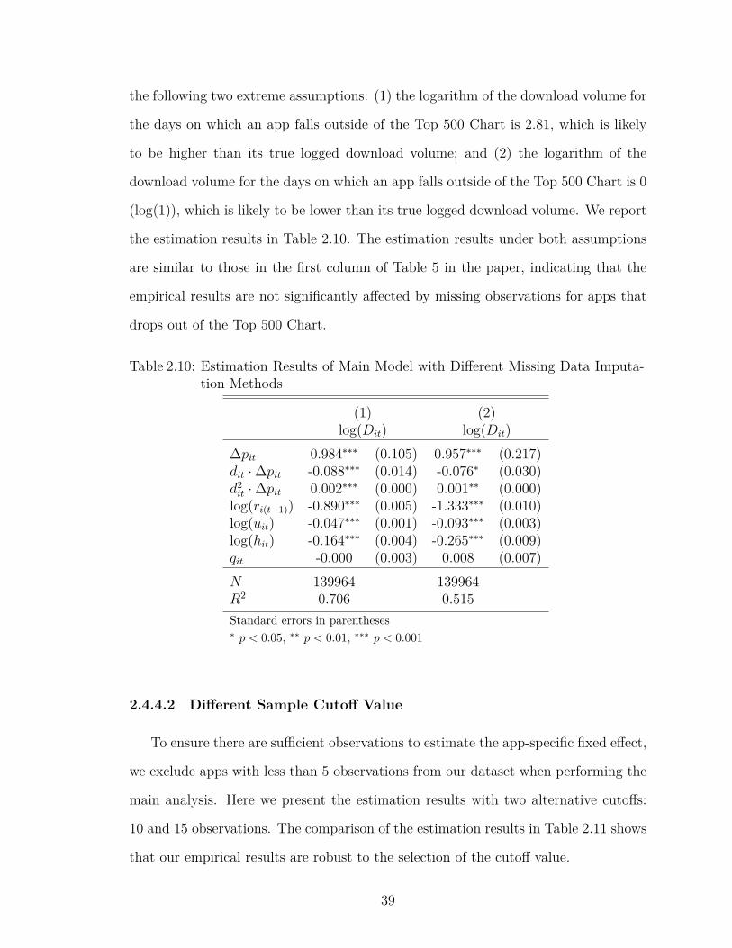
the following two extreme assumptions: (1) the logarithm of the download volume for

the days on which an app falls outside of the Top 500 Chart is 2.81, which is likely

to be higher than its true logged download volume; and (2) the logarithm of the

download volume for the days on which an app falls outside of the Top 500 Chart is 0

(log(1)), which is likely to be lower than its true logged download volume. We report

the estimation results in Table 2.10. The estimation results under both assumptions

are similar to those in the first column of Table 5 in the paper, indicating that the

empirical results are not significantly affected by missing observations for apps that

drops out of the Top 500 Chart.

Table 2.10: Estimation Results of Main Model with Different Missing Data Imputa-tion Methods

(1) (2)log(Dit) log(Dit)

∆pit 0.984∗∗∗ (0.105) 0.957∗∗∗ (0.217)dit ·∆pit -0.088∗∗∗ (0.014) -0.076∗ (0.030)d2it ·∆pit 0.002∗∗∗ (0.000) 0.001∗∗ (0.000)log(ri(t−1)) -0.890∗∗∗ (0.005) -1.333∗∗∗ (0.010)log(uit) -0.047∗∗∗ (0.001) -0.093∗∗∗ (0.003)log(hit) -0.164∗∗∗ (0.004) -0.265∗∗∗ (0.009)qit -0.000 (0.003) 0.008 (0.007)N 139964 139964R2 0.706 0.515Standard errors in parentheses∗ p < 0.05, ∗∗ p < 0.01, ∗∗∗ p < 0.001

2.4.4.2 Different Sample Cutoff Value

To ensure there are sufficient observations to estimate the app-specific fixed effect,

we exclude apps with less than 5 observations from our dataset when performing the

main analysis. Here we present the estimation results with two alternative cutoffs:

10 and 15 observations. The comparison of the estimation results in Table 2.11 shows

that our empirical results are robust to the selection of the cutoff value.

39

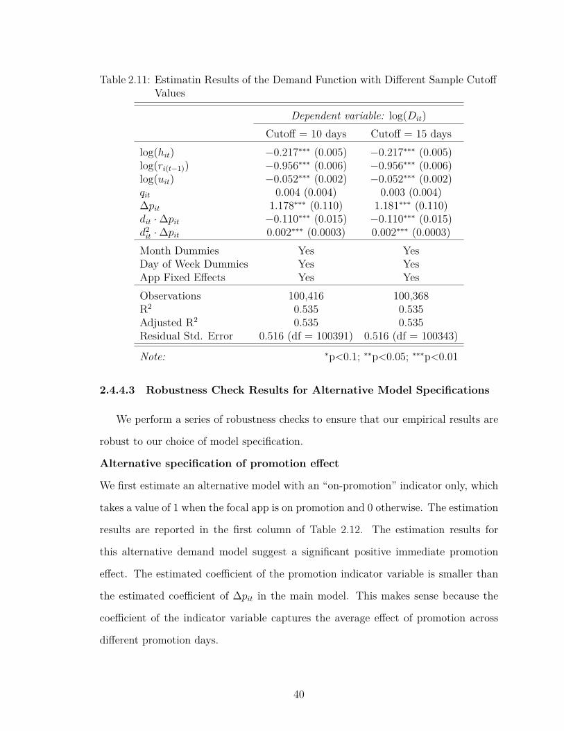
Table 2.11: Estimatin Results of the Demand Function with Different Sample CutoffValues

Dependent variable: log(Dit)

Cutoff = 10 days Cutoff = 15 dayslog(hit) −0.217∗∗∗ (0.005) −0.217∗∗∗ (0.005)log(ri(t−1)) −0.956∗∗∗ (0.006) −0.956∗∗∗ (0.006)log(uit) −0.052∗∗∗ (0.002) −0.052∗∗∗ (0.002)qit 0.004 (0.004) 0.003 (0.004)∆pit 1.178∗∗∗ (0.110) 1.181∗∗∗ (0.110)dit ·∆pit −0.110∗∗∗ (0.015) −0.110∗∗∗ (0.015)d2it ·∆pit 0.002∗∗∗ (0.0003) 0.002∗∗∗ (0.0003)Month Dummies Yes YesDay of Week Dummies Yes YesApp Fixed Effects Yes YesObservations 100,416 100,368R2 0.535 0.535Adjusted R2 0.535 0.535Residual Std. Error 0.516 (df = 100391) 0.516 (df = 100343)

Note: ∗p<0.1; ∗∗p<0.05; ∗∗∗p<0.01

2.4.4.3 Robustness Check Results for Alternative Model Specifications

We perform a series of robustness checks to ensure that our empirical results are

robust to our choice of model specification.

Alternative specification of promotion effect

We first estimate an alternative model with an “on-promotion” indicator only, which

takes a value of 1 when the focal app is on promotion and 0 otherwise. The estimation

results are reported in the first column of Table 2.12. The estimation results for

this alternative demand model suggest a significant positive immediate promotion

effect. The estimated coefficient of the promotion indicator variable is smaller than

the estimated coefficient of ∆pit in the main model. This makes sense because the

coefficient of the indicator variable captures the average effect of promotion across

different promotion days.

40

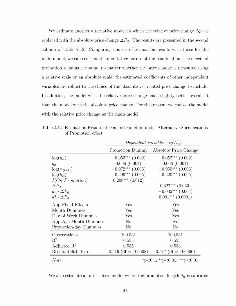
We estimate another alternative model in which the relative price change ∆pit is

replaced with the absolute price change ∆Pit. The results are presented in the second

column of Table 2.12. Comparing this set of estimation results with those for the

main model, we can see that the qualitative nature of the results about the effects of

promotion remains the same, no matter whether the price change is measured using

a relative scale or an absolute scale; the estimated coefficients of other independent

variables are robust to the choice of the absolute vs. related price change to include.

In addition, the model with the relative price change has a slightly better overall fit

than the model with the absolute price change. For this reason, we choose the model

with the relative price change as the main model.

Table 2.12: Estimation Results of Demand Function under Alternative Specificationsof Promotion effect

Dependent variable: log(Dit)

Promotion Dummy Absolute Price Changelog(uit) −0.053∗∗∗ (0.002) −0.052∗∗∗ (0.002)qit 0.006 (0.004) 0.006 (0.004)log(ri(t−1)) −0.972∗∗∗ (0.005) −0.950∗∗∗ (0.006)log(hit) −0.209∗∗∗ (0.005) −0.220∗∗∗ (0.005)I(On Promotion) 0.208∗∗∗ (0.012)∆Pit 0.327∗∗∗ (0.030)dit ·∆Pit −0.032∗∗∗ (0.004)d2it ·∆Pit 0.001∗∗∗ (0.0001)App Fixed Effects Yes YesMonth Dummies Yes YesDay of Week Dummies Yes YesApp Age Month Dummies No NoPromotion-day Dummies No NoObservations 100,531 100,531R2 0.535 0.533Adjusted R2 0.535 0.533Residual Std. Error 0.516 (df = 100508) 0.517 (df = 100506)

Note: ∗p<0.1; ∗∗p<0.05; ∗∗∗p<0.01

We also estimate an alternative model where the promotion length dit is captured

41

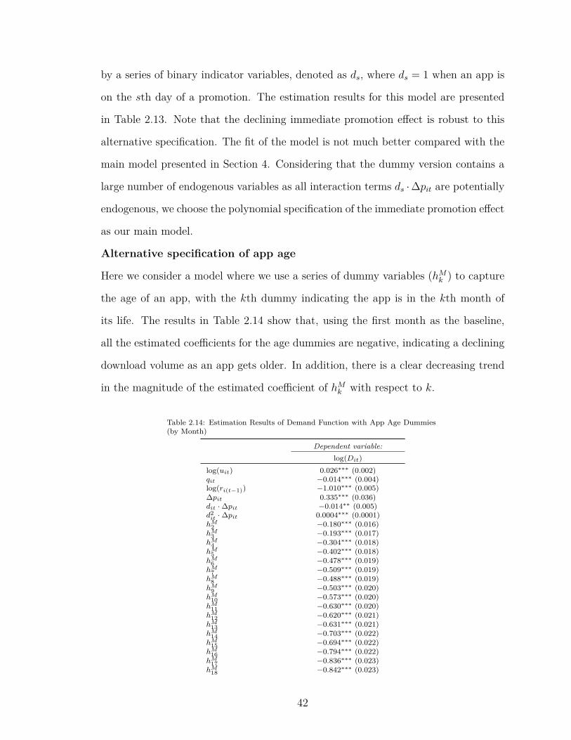
by a series of binary indicator variables, denoted as ds, where ds = 1 when an app is

on the sth day of a promotion. The estimation results for this model are presented

in Table 2.13. Note that the declining immediate promotion effect is robust to this

alternative specification. The fit of the model is not much better compared with the

main model presented in Section 4. Considering that the dummy version contains a

large number of endogenous variables as all interaction terms ds ·∆pit are potentially

endogenous, we choose the polynomial specification of the immediate promotion effect

as our main model.

Alternative specification of app age

Here we consider a model where we use a series of dummy variables (hMk ) to capture

the age of an app, with the kth dummy indicating the app is in the kth month of

its life. The results in Table 2.14 show that, using the first month as the baseline,

all the estimated coefficients for the age dummies are negative, indicating a declining

download volume as an app gets older. In addition, there is a clear decreasing trend

in the magnitude of the estimated coefficient of hMk with respect to k.

Table 2.14: Estimation Results of Demand Function with App Age Dummies(by Month)

Dependent variable:log(Dit)

log(uit) 0.026∗∗∗ (0.002)qit −0.014∗∗∗ (0.004)log(ri(t−1)) −1.010∗∗∗ (0.005)∆pit 0.335∗∗∗ (0.036)dit ·∆pit −0.014∗∗ (0.005)d2it ·∆pit 0.0004∗∗∗ (0.0001)hM2 −0.180∗∗∗ (0.016)

hM3 −0.193∗∗∗ (0.017)

hM4 −0.304∗∗∗ (0.018)

hM5 −0.402∗∗∗ (0.018)

hM6 −0.478∗∗∗ (0.019)

hM7 −0.509∗∗∗ (0.019)

hM8 −0.488∗∗∗ (0.019)

hM9 −0.503∗∗∗ (0.020)

hM10 −0.573∗∗∗ (0.020)

hM11 −0.630∗∗∗ (0.020)

hM12 −0.620∗∗∗ (0.021)

hM13 −0.631∗∗∗ (0.021)

hM14 −0.703∗∗∗ (0.022)

hM15 −0.694∗∗∗ (0.022)

hM16 −0.794∗∗∗ (0.022)

hM17 −0.836∗∗∗ (0.023)

hM18 −0.842∗∗∗ (0.023)

42

hM19 −0.889∗∗∗ (0.023)

hM20 −0.916∗∗∗ (0.024)

hM21 −0.947∗∗∗ (0.024)

hM22 −0.978∗∗∗ (0.025)

hM23 −1.049∗∗∗ (0.025)

hM24 −1.143∗∗∗ (0.025)

hM25 −1.209∗∗∗ (0.025)

hM26 −1.227∗∗∗ (0.026)

hM27 −1.300∗∗∗ (0.026)

hM28 −1.349∗∗∗ (0.026)

hM29 −1.320∗∗∗ (0.026)

hM30 −1.335∗∗∗ (0.026)

hM31 −1.375∗∗∗ (0.027)

hM32 −1.411∗∗∗ (0.027)

hM33 −1.424∗∗∗ (0.028)

hM34 −1.528∗∗∗ (0.028)

hM35 −1.598∗∗∗ (0.028)

hM36 −1.642∗∗∗ (0.029)

hM37 −1.596∗∗∗ (0.029)

hM38 −1.613∗∗∗ (0.029)

hM39 −1.684∗∗∗ (0.030)

hM40 −1.754∗∗∗ (0.030)

hM41 −1.846∗∗∗ (0.031)

hM42 −1.895∗∗∗ (0.031)

hM43 −1.968∗∗∗ (0.032)

hM44 −1.951∗∗∗ (0.032)

hM45 −1.894∗∗∗ (0.033)

hM46 −1.904∗∗∗ (0.033)

hM47 −1.999∗∗∗ (0.034)

hM48 −2.070∗∗∗ (0.034)

hM49 −2.147∗∗∗ (0.034)

hM50 −2.250∗∗∗ (0.035)

hM51 −2.346∗∗∗ (0.036)

hM52 −2.300∗∗∗ (0.037)

hM53 −2.268∗∗∗ (0.037)

hM54 −2.295∗∗∗ (0.037)

hM55 −2.384∗∗∗ (0.038)

hM56 −2.382∗∗∗ (0.039)

hM57 −2.391∗∗∗ (0.040)

hM58 −2.490∗∗∗ (0.040)

hM59 −2.592∗∗∗ (0.040)

hM60 −2.540∗∗∗ (0.041)

hM61 −2.513∗∗∗ (0.041)

hM62 −2.514∗∗∗ (0.041)

hM63 −2.597∗∗∗ (0.042)

hM64 −2.643∗∗∗ (0.043)

hM65 −2.644∗∗∗ (0.043)

hM66 −2.808∗∗∗ (0.044)

hM67 −2.822∗∗∗ (0.044)

hM68 −2.738∗∗∗ (0.045)

hM69 −2.748∗∗∗ (0.046)

hM70 −2.794∗∗∗ (0.046)

hM71 −2.904∗∗∗ (0.047)

hM72 −2.946∗∗∗ (0.047)

hM73 −3.002∗∗∗ (0.047)

hM74 −2.948∗∗∗ (0.048)

hM75 −2.981∗∗∗ (0.050)

hM76 −3.071∗∗∗ (0.052)

hM77 −3.212∗∗∗ (0.053)

hM78 −3.189∗∗∗ (0.054)

hM79 −3.267∗∗∗ (0.057)

hM80 −3.379∗∗∗ (0.059)

hM81 −3.354∗∗∗ (0.061)

hM82 −3.401∗∗∗ (0.064)

hM83 −3.446∗∗∗ (0.070)

hM84 −3.699∗∗∗ (0.084)

43

hM85 −3.504∗∗∗ (0.098)

hM86 −3.312∗∗∗ (0.103)

hM87 −3.829∗∗∗ (0.108)

hM88 −3.842∗∗∗ (0.108)

hM89 −3.661∗∗∗ (0.298)

Month Dummies YesDay of Week Dummies YesApp Fixed Effects YesObservations 100,531R2 0.552Adjusted R2 0.552Residual Std. Error 0.507 (df = 100419)Note: ∗p<0.1; ∗∗p<0.05; ∗∗∗p<0.01

Alternative specification of visibility effect

Here we present a set of alternative models with more than one period lagged ranks.

Table 2.15 tabulates the estimation results of models with 1-4, 1-6, and 1-8 period

lagged ranks. The results show that the effect of lagged ranks declines quickly with

the number of periods lagged. The magnitude of the logarithm of two-day lagged rank

(log(ri(t−2))) is significantly smaller than that of one-day lagged rank (log(ri(t−1))).

The coefficient of log(ri(t−2)) is only about one ninth of the coefficient of log(ri(t−1)),

and the coefficients of log(ri(t−s)) for s > 2 are even smaller than that of log(ri(t−2)).

In addition, including more lagged rank variables does not meaningfully affect the

estimated coefficient of log(ri(t−1)), indicating that the main visibility effect is driven

by the one-period lagged rank. Since including more lagged rank variables will sig-

nificantly complicate the promotion planning problem, we use the model with only

the one-period lagged rank (log(ri(t−1))) as the main model.

Another possible specification is to substitute log(ri(t−1)) with log(Di(t−1)). Here

we present two alternative specifications for Equation 2.2: 1) replacing log(ri(t−1))

with log(Di(t−1)); and 2) including both log(Di(t−1)) and log(ri,t−1). The estimation

results of these two alternative models, as well as those of the main model, are reported

in Table 2.16. The results in the third column show that when both log(ri,t−1) and

log(Di,t−1) are included in the model, multicollinearity is present: the sign of the

coefficient of log(ri(t−1)) is flipped. A positive coefficient of log(ri,(t−1)) implies that

44

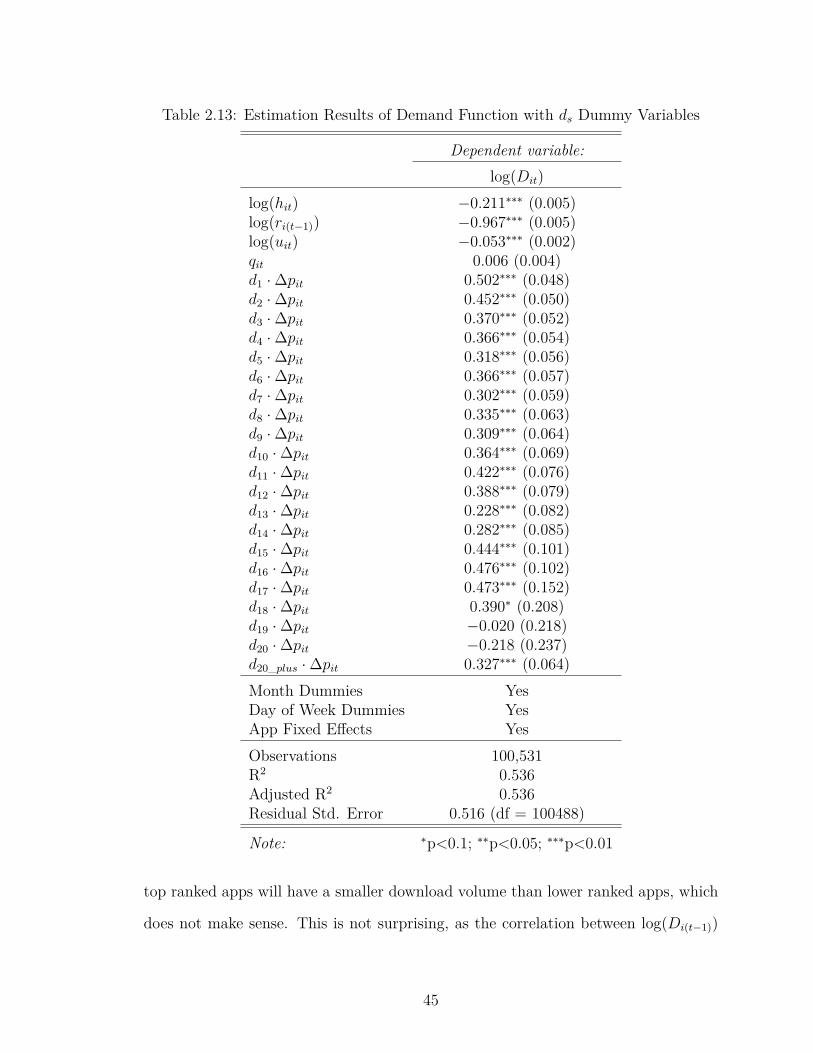
Table 2.13: Estimation Results of Demand Function with ds Dummy Variables

Dependent variable:log(Dit)

log(hit) −0.211∗∗∗ (0.005)log(ri(t−1)) −0.967∗∗∗ (0.005)log(uit) −0.053∗∗∗ (0.002)qit 0.006 (0.004)d1 ·∆pit 0.502∗∗∗ (0.048)d2 ·∆pit 0.452∗∗∗ (0.050)d3 ·∆pit 0.370∗∗∗ (0.052)d4 ·∆pit 0.366∗∗∗ (0.054)d5 ·∆pit 0.318∗∗∗ (0.056)d6 ·∆pit 0.366∗∗∗ (0.057)d7 ·∆pit 0.302∗∗∗ (0.059)d8 ·∆pit 0.335∗∗∗ (0.063)d9 ·∆pit 0.309∗∗∗ (0.064)d10 ·∆pit 0.364∗∗∗ (0.069)d11 ·∆pit 0.422∗∗∗ (0.076)d12 ·∆pit 0.388∗∗∗ (0.079)d13 ·∆pit 0.228∗∗∗ (0.082)d14 ·∆pit 0.282∗∗∗ (0.085)d15 ·∆pit 0.444∗∗∗ (0.101)d16 ·∆pit 0.476∗∗∗ (0.102)d17 ·∆pit 0.473∗∗∗ (0.152)d18 ·∆pit 0.390∗ (0.208)d19 ·∆pit −0.020 (0.218)d20 ·∆pit −0.218 (0.237)d20_plus ·∆pit 0.327∗∗∗ (0.064)Month Dummies YesDay of Week Dummies YesApp Fixed Effects YesObservations 100,531R2 0.536Adjusted R2 0.536Residual Std. Error 0.516 (df = 100488)

Note: ∗p<0.1; ∗∗p<0.05; ∗∗∗p<0.01

top ranked apps will have a smaller download volume than lower ranked apps, which

does not make sense. This is not surprising, as the correlation between log(Di(t−1))

45

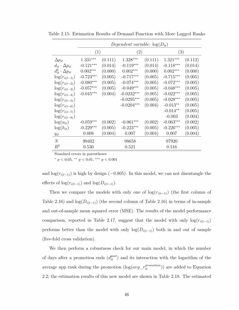
Table 2.15: Estimation Results of Demand Function with More Lagged Ranks

Dependent variable: log(Dit)

(1) (2) (3)∆pit 1.331∗∗∗ (0.111) 1.328∗∗∗ (0.111) 1.321∗∗∗ (0.112)dit ·∆pit -0.121∗∗∗ (0.014) -0.119∗∗∗ (0.014) -0.118∗∗∗ (0.014)d2it ·∆pit 0.002∗∗∗ (0.000) 0.002∗∗∗ (0.000) 0.002∗∗∗ (0.000)log(ri(t−1)) -0.723∗∗∗ (0.005) -0.717∗∗∗ (0.005) -0.715∗∗∗ (0.005)log(ri(t−2)) -0.080∗∗∗ (0.005) -0.074∗∗∗ (0.005) -0.072∗∗∗ (0.005)log(ri(t−3)) -0.057∗∗∗ (0.005) -0.049∗∗∗ (0.005) -0.048∗∗∗ (0.005)log(ri(t−4)) -0.045∗∗∗ (0.004) -0.0232∗∗∗ (0.005) -0.022∗∗∗ (0.005)log(ri(t−5)) -0.0295∗∗∗ (0.005) -0.028∗∗∗ (0.005)log(ri(t−6)) -0.0204∗∗∗ (0.004) -0.013∗∗ (0.005)log(ri(t−7)) -0.014∗∗ (0.005)log(ri(t−8)) -0.003 (0.004)log(uit) -0.059∗∗∗ (0.002) -0.061∗∗∗ (0.002) -0.063∗∗∗ (0.002)log(hit) -0.229∗∗∗ (0.005) -0.223∗∗∗ (0.005) -0.226∗∗∗ (0.005)qit 0.008 (0.004) 0.007 (0.004) 0.007 (0.004)N 99402 98658 97920R2 0.530 0.521 0.516Standard errors in parentheses∗ p < 0.05, ∗∗ p < 0.01, ∗∗∗ p < 0.001

and log(ri(t−1)) is high by design (−0.805). In this model, we can not disentangle the

effects of log(ri(t−1)) and log(Di(t−1)).

Then we compare the models with only one of log(ri(t−1)) (the first column of

Table 2.16) and log(Di(t−1)) (the second column of Table 2.16) in terms of in-sample

and out-of-sample mean squared error (MSE). The results of the model performance

comparison, reported in Table 2.17, suggest that the model with only log(ri(t−1))

performs better than the model with only log(Di(t−1)) both in and out of sample

(five-fold cross validation).

We then perform a robustness check for our main model, in which the number

of days after a promotion ends (dpostit ) and its interaction with the logarithm of the

average app rank during the promotion (log(avg_rpromotionit )) are added to Equation

2.2; the estimation results of this new model are shown in Table 2.18. The estimated

46

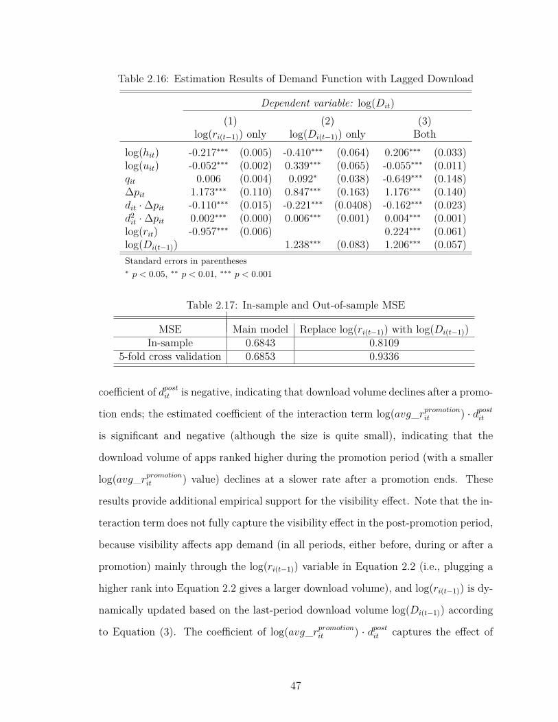
Table 2.16: Estimation Results of Demand Function with Lagged Download

Dependent variable: log(Dit)

(1) (2) (3)log(ri(t−1)) only log(Di(t−1)) only Both

log(hit) -0.217∗∗∗ (0.005) -0.410∗∗∗ (0.064) 0.206∗∗∗ (0.033)log(uit) -0.052∗∗∗ (0.002) 0.339∗∗∗ (0.065) -0.055∗∗∗ (0.011)qit 0.006 (0.004) 0.092∗ (0.038) -0.649∗∗∗ (0.148)∆pit 1.173∗∗∗ (0.110) 0.847∗∗∗ (0.163) 1.176∗∗∗ (0.140)dit ·∆pit -0.110∗∗∗ (0.015) -0.221∗∗∗ (0.0408) -0.162∗∗∗ (0.023)d2it ·∆pit 0.002∗∗∗ (0.000) 0.006∗∗∗ (0.001) 0.004∗∗∗ (0.001)log(rit) -0.957∗∗∗ (0.006) 0.224∗∗∗ (0.061)log(Di(t−1)) 1.238∗∗∗ (0.083) 1.206∗∗∗ (0.057)Standard errors in parentheses∗ p < 0.05, ∗∗ p < 0.01, ∗∗∗ p < 0.001

Table 2.17: In-sample and Out-of-sample MSE

MSE Main model Replace log(ri(t−1)) with log(Di(t−1))In-sample 0.6843 0.8109

5-fold cross validation 0.6853 0.9336

coefficient of dpostit is negative, indicating that download volume declines after a promo-

tion ends; the estimated coefficient of the interaction term log(avg_rpromotionit ) · dpostit

is significant and negative (although the size is quite small), indicating that the

download volume of apps ranked higher during the promotion period (with a smaller

log(avg_rpromotionit ) value) declines at a slower rate after a promotion ends. These

results provide additional empirical support for the visibility effect. Note that the in-

teraction term does not fully capture the visibility effect in the post-promotion period,

because visibility affects app demand (in all periods, either before, during or after a

promotion) mainly through the log(ri(t−1)) variable in Equation 2.2 (i.e., plugging a

higher rank into Equation 2.2 gives a larger download volume), and log(ri(t−1)) is dy-

namically updated based on the last-period download volume log(Di(t−1)) according

to Equation (3). The coefficient of log(avg_rpromotionit ) · dpostit captures the effect of

47

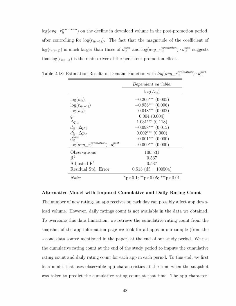
log(avg_rpromotionit ) on the decline in download volume in the post-promotion period,

after controlling for log(ri(t−1)). The fact that the magnitude of the coefficient of

log(ri(t−1)) is much larger than those of dpostit and log(avg_rpromotionit ) · dpostit suggests

that log(ri(t−1)) is the main driver of the persistent promotion effect.

Table 2.18: Estimation Results of Demand Function with log(avg_rpromotionit ) · dpostit

Dependent variable:log(Dit)

log(hit) −0.206∗∗∗ (0.005)log(ri(t−1)) −0.958∗∗∗ (0.006)log(uit) −0.048∗∗∗ (0.002)qit 0.004 (0.004)∆pit 1.031∗∗∗ (0.118)dit ·∆pit −0.098∗∗∗ (0.015)d2it ·∆pit 0.002∗∗∗ (0.000)dpostit −0.001∗∗∗ (0.000)log(avg_rpromotion

it ) · dpostit −0.000∗∗∗ (0.000)Observations 100,531R2 0.537Adjusted R2 0.537Residual Std. Error 0.515 (df = 100504)

Note: ∗p<0.1; ∗∗p<0.05; ∗∗∗p<0.01

Alternative Model with Imputed Cumulative and Daily Rating Count

The number of new ratings an app receives on each day can possibly affect app down-

load volume. However, daily ratings count is not available in the data we obtained.

To overcome this data limitation, we retrieve the cumulative rating count from the

snapshot of the app information page we took for all apps in our sample (from the

second data source mentioned in the paper) at the end of our study period. We use

the cumulative rating count at the end of the study period to impute the cumulative

rating count and daily rating count for each app in each period. To this end, we first

fit a model that uses observable app characteristics at the time when the snapshot

was taken to predict the cumulative rating count at that time. The app character-

48

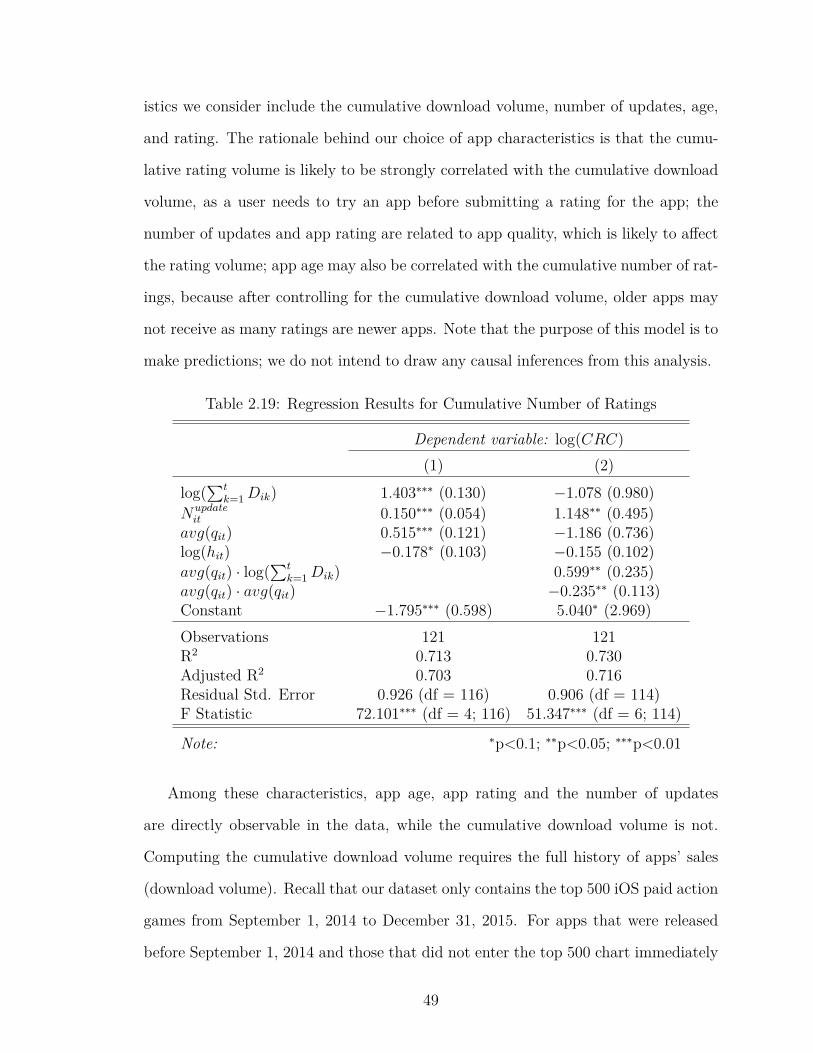
istics we consider include the cumulative download volume, number of updates, age,

and rating. The rationale behind our choice of app characteristics is that the cumu-

lative rating volume is likely to be strongly correlated with the cumulative download

volume, as a user needs to try an app before submitting a rating for the app; the

number of updates and app rating are related to app quality, which is likely to affect

the rating volume; app age may also be correlated with the cumulative number of rat-

ings, because after controlling for the cumulative download volume, older apps may

not receive as many ratings are newer apps. Note that the purpose of this model is to

make predictions; we do not intend to draw any causal inferences from this analysis.

Table 2.19: Regression Results for Cumulative Number of Ratings

Dependent variable: log(CRC)

(1) (2)log(

∑tk=1Dik) 1.403∗∗∗ (0.130) −1.078 (0.980)

Nupdateit 0.150∗∗∗ (0.054) 1.148∗∗ (0.495)

avg(qit) 0.515∗∗∗ (0.121) −1.186 (0.736)log(hit) −0.178∗ (0.103) −0.155 (0.102)avg(qit) · log(

∑tk=1Dik) 0.599∗∗ (0.235)

avg(qit) · avg(qit) −0.235∗∗ (0.113)Constant −1.795∗∗∗ (0.598) 5.040∗ (2.969)Observations 121 121R2 0.713 0.730Adjusted R2 0.703 0.716Residual Std. Error 0.926 (df = 116) 0.906 (df = 114)F Statistic 72.101∗∗∗ (df = 4; 116) 51.347∗∗∗ (df = 6; 114)

Note: ∗p<0.1; ∗∗p<0.05; ∗∗∗p<0.01

Among these characteristics, app age, app rating and the number of updates

are directly observable in the data, while the cumulative download volume is not.

Computing the cumulative download volume requires the full history of apps’ sales

(download volume). Recall that our dataset only contains the top 500 iOS paid action

games from September 1, 2014 to December 31, 2015. For apps that were released

before September 1, 2014 and those that did not enter the top 500 chart immediately

49

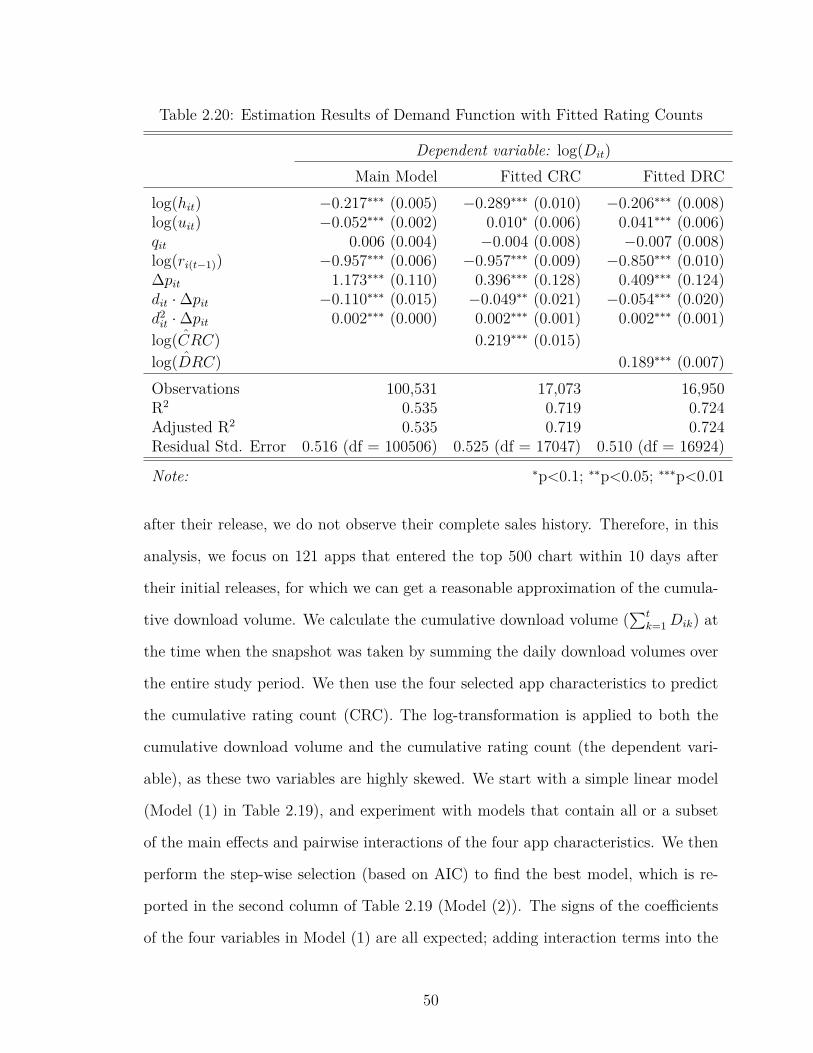
Table 2.20: Estimation Results of Demand Function with Fitted Rating Counts

Dependent variable: log(Dit)

Main Model Fitted CRC Fitted DRClog(hit) −0.217∗∗∗ (0.005) −0.289∗∗∗ (0.010) −0.206∗∗∗ (0.008)log(uit) −0.052∗∗∗ (0.002) 0.010∗ (0.006) 0.041∗∗∗ (0.006)qit 0.006 (0.004) −0.004 (0.008) −0.007 (0.008)log(ri(t−1)) −0.957∗∗∗ (0.006) −0.957∗∗∗ (0.009) −0.850∗∗∗ (0.010)∆pit 1.173∗∗∗ (0.110) 0.396∗∗∗ (0.128) 0.409∗∗∗ (0.124)dit ·∆pit −0.110∗∗∗ (0.015) −0.049∗∗ (0.021) −0.054∗∗∗ (0.020)d2it ·∆pit 0.002∗∗∗ (0.000) 0.002∗∗∗ (0.001) 0.002∗∗∗ (0.001)

ˆlog(CRC) 0.219∗∗∗ (0.015)ˆlog(DRC) 0.189∗∗∗ (0.007)

Observations 100,531 17,073 16,950R2 0.535 0.719 0.724Adjusted R2 0.535 0.719 0.724Residual Std. Error 0.516 (df = 100506) 0.525 (df = 17047) 0.510 (df = 16924)

Note: ∗p<0.1; ∗∗p<0.05; ∗∗∗p<0.01

after their release, we do not observe their complete sales history. Therefore, in this

analysis, we focus on 121 apps that entered the top 500 chart within 10 days after

their initial releases, for which we can get a reasonable approximation of the cumula-

tive download volume. We calculate the cumulative download volume (∑t

k=1Dik) at

the time when the snapshot was taken by summing the daily download volumes over

the entire study period. We then use the four selected app characteristics to predict

the cumulative rating count (CRC). The log-transformation is applied to both the

cumulative download volume and the cumulative rating count (the dependent vari-

able), as these two variables are highly skewed. We start with a simple linear model

(Model (1) in Table 2.19), and experiment with models that contain all or a subset

of the main effects and pairwise interactions of the four app characteristics. We then

perform the step-wise selection (based on AIC) to find the best model, which is re-

ported in the second column of Table 2.19 (Model (2)). The signs of the coefficients

of the four variables in Model (1) are all expected; adding interaction terms into the

50

model causes collinearity and changes the sign and significance of a few coefficients,

however, Model (2) has a better overall model fit and out-of-sample prediction accu-

racy than Model (1). Since our goal is to accurately predict the cumulative rating

count and derive the daily rating count, we use Model (2) to predict the cumulative

rating count.

With the predicted CRC for each app in each period, we can calculate the daily

new rating count (DRC), which is the difference in the fitted cumulative rating count

between two consecutive days. Then we add the fitted CRC or the fitted DRC to our

main model and re-estimate the revised model. The estimation results are shown in

the second and third columns of Table 2.20. (We also perform the same analysis using

the fitted CRC/DRC predicted by the linear model (Model (1)), and find the results

are almost identical to those reported in Table 2.20. For brevity, we do not report

them here. This analysis demonstrates the robustness of the estimation results with

respect to our choices of the prediction model.) The respective coefficients of the fitted

CRC and DRC are positive and statistically significant, indicating that they have a

positive impact on app download volume. These results are consistent with those from

the model with the cumulative download volume added (i.e., robustness checks about

the potential network effect), which is not surprising because the cumulative download

volume and the cumulative rating count are strongly correlated. The coefficients of

other independent variables in the model remain largely unchanged, indicating the

robustness of our results with respect to the inclusion/exclusion of the fitted CRC

and DRC. But we caution that these results are suggestive, not conclusive, because

this analysis is conducted on a small subsample of apps, and the fitted CRC and DRC

contain prediction errors.

2.4.4.4 Robustness Check Results and Details for Correlated Demand

Discrete Choice Model

51

In the discrete choice model (similar to Ghose and Han (2014)), we assume that the

utility an individual consumer (indexed by j) receives from purchasing app i in period

t is

Uijt = αi + β1 log(ri(t−1)) + β2 log(hit) + β3 log(uit) + β4qit + β5∆pit + β6∆pit · dit

+ β7∆pit · d2it +11∑

m=1

ηmMmit +6∑

w=1

ϕwWwit + ξit + ϵijt (2.6)

Uijt = δit + ϵijt (2.7)

where ξit represents the unobserved (to researchers) product characteristic, ϵijt is

a zero-mean stochastic individual-level preference shock, and δit can be interpreted

as the mean utility level. Under the assumption that the options (including the

no-purchase option) are mutually exclusive, ϵijt follows i.i.d Type-I Extreme Value

distribution, and consumers are homogeneous, the market share of app i in period

t can be written as sit = exp (δit)1+

∑i′ exp (δi′t)

. Given a market size, we can compute the

observed market share for each app (Sit). By matching the observed shares (Sit) and

the model predicted shares (sit), we can estimate the parameters in consumers’ utility

function. Note that αi and βk in the model (with abuse of notation) are parameters

in consumers’ utility function (at the individual level), and have different meanings

from those in Equation 2.2, which are coefficients in the demand function (at the

aggregate level). Therefore, the estimated parameters in the individual-level utility

function cannot be directly compared with those in the demand function. Also note

that one important assumption of the discrete choice model is that in each period, a

consumer can choose zero or one app from the set of apps available in the choice set

(all iOS action games); whereas the main model in the paper does not impose any

assumption on how many apps an individual consumer can purchase at a time, but

assumes that the demand for the apps are not correlated. We then use the estimated

choice model and the main model in the paper to perform out-of-sample prediction

52

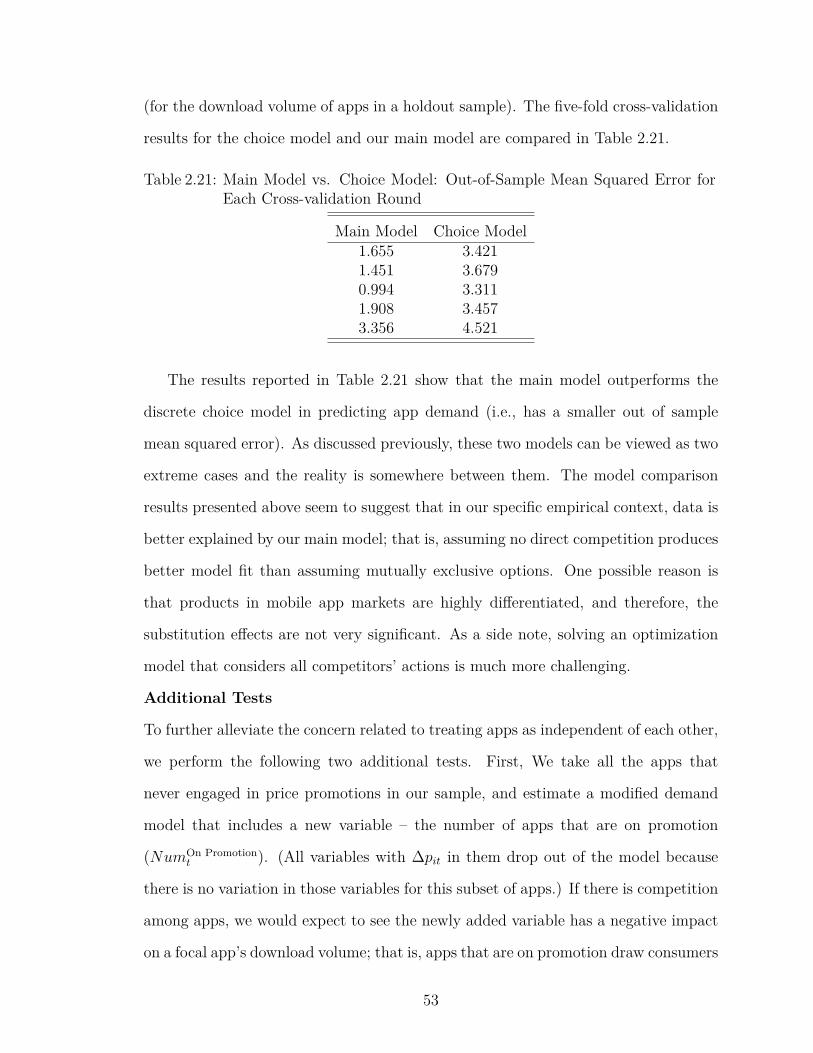
(for the download volume of apps in a holdout sample). The five-fold cross-validation

results for the choice model and our main model are compared in Table 2.21.

Table 2.21: Main Model vs. Choice Model: Out-of-Sample Mean Squared Error forEach Cross-validation Round

Main Model Choice Model1.655 3.4211.451 3.6790.994 3.3111.908 3.4573.356 4.521

The results reported in Table 2.21 show that the main model outperforms the

discrete choice model in predicting app demand (i.e., has a smaller out of sample

mean squared error). As discussed previously, these two models can be viewed as two

extreme cases and the reality is somewhere between them. The model comparison

results presented above seem to suggest that in our specific empirical context, data is

better explained by our main model; that is, assuming no direct competition produces

better model fit than assuming mutually exclusive options. One possible reason is

that products in mobile app markets are highly differentiated, and therefore, the

substitution effects are not very significant. As a side note, solving an optimization

model that considers all competitors’ actions is much more challenging.

Additional Tests

To further alleviate the concern related to treating apps as independent of each other,

we perform the following two additional tests. First, We take all the apps that

never engaged in price promotions in our sample, and estimate a modified demand

model that includes a new variable – the number of apps that are on promotion

(NumOn Promotiont ). (All variables with ∆pit in them drop out of the model because

there is no variation in those variables for this subset of apps.) If there is competition

among apps, we would expect to see the newly added variable has a negative impact

on a focal app’s download volume; that is, apps that are on promotion draw consumers

53

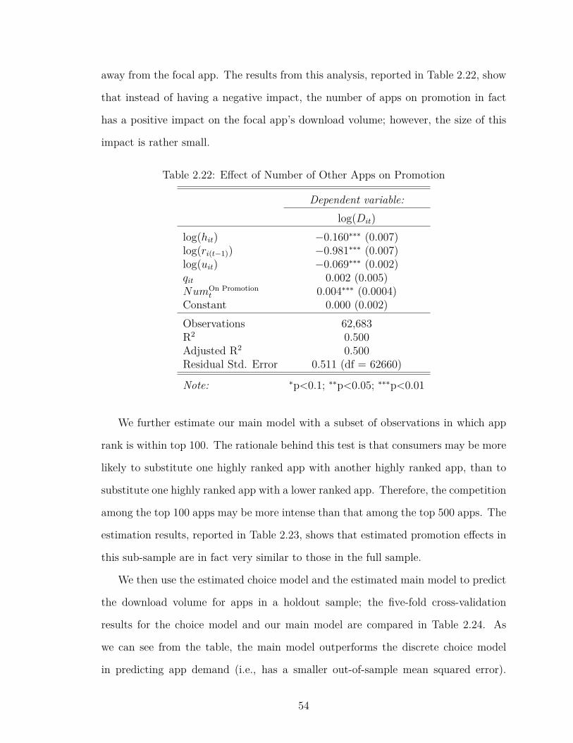
away from the focal app. The results from this analysis, reported in Table 2.22, show

that instead of having a negative impact, the number of apps on promotion in fact

has a positive impact on the focal app’s download volume; however, the size of this

impact is rather small.

Table 2.22: Effect of Number of Other Apps on Promotion

Dependent variable:log(Dit)

log(hit) −0.160∗∗∗ (0.007)log(ri(t−1)) −0.981∗∗∗ (0.007)log(uit) −0.069∗∗∗ (0.002)qit 0.002 (0.005)NumOn Promotion

t 0.004∗∗∗ (0.0004)Constant 0.000 (0.002)Observations 62,683R2 0.500Adjusted R2 0.500Residual Std. Error 0.511 (df = 62660)

Note: ∗p<0.1; ∗∗p<0.05; ∗∗∗p<0.01

We further estimate our main model with a subset of observations in which app

rank is within top 100. The rationale behind this test is that consumers may be more

likely to substitute one highly ranked app with another highly ranked app, than to

substitute one highly ranked app with a lower ranked app. Therefore, the competition

among the top 100 apps may be more intense than that among the top 500 apps. The

estimation results, reported in Table 2.23, shows that estimated promotion effects in

this sub-sample are in fact very similar to those in the full sample.

We then use the estimated choice model and the estimated main model to predict

the download volume for apps in a holdout sample; the five-fold cross-validation

results for the choice model and our main model are compared in Table 2.24. As

we can see from the table, the main model outperforms the discrete choice model

in predicting app demand (i.e., has a smaller out-of-sample mean squared error).

54

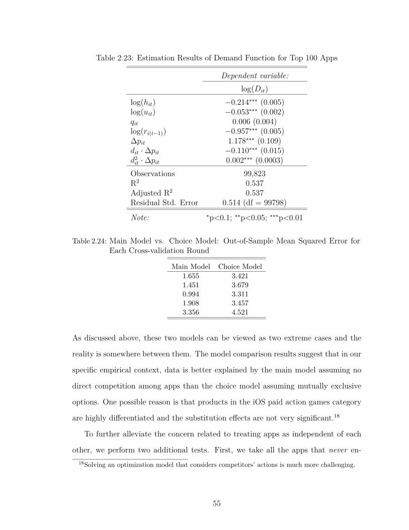
Table 2.23: Estimation Results of Demand Function for Top 100 Apps

Dependent variable:log(Dit)

log(hit) −0.214∗∗∗ (0.005)log(uit) −0.053∗∗∗ (0.002)qit 0.006 (0.004)log(ri(t−1)) −0.957∗∗∗ (0.005)∆pit 1.178∗∗∗ (0.109)dit ·∆pit −0.110∗∗∗ (0.015)d2it ·∆pit 0.002∗∗∗ (0.0003)Observations 99,823R2 0.537Adjusted R2 0.537Residual Std. Error 0.514 (df = 99798)

Note: ∗p<0.1; ∗∗p<0.05; ∗∗∗p<0.01

Table 2.24: Main Model vs. Choice Model: Out-of-Sample Mean Squared Error forEach Cross-validation Round

Main Model Choice Model1.655 3.4211.451 3.6790.994 3.3111.908 3.4573.356 4.521

As discussed above, these two models can be viewed as two extreme cases and the

reality is somewhere between them. The model comparison results suggest that in our

specific empirical context, data is better explained by the main model assuming no

direct competition among apps than the choice model assuming mutually exclusive

options. One possible reason is that products in the iOS paid action games category

are highly differentiated and the substitution effects are not very significant.18

To further alleviate the concern related to treating apps as independent of each

other, we perform two additional tests. First, we take all the apps that never en-18Solving an optimization model that considers competitors’ actions is much more challenging.

55

gaged in price promotions in our sample, and estimate a modified demand model

that includes a new variable, the number of apps that are currently on promotion

(NumOnPromotiont ). (All variables with dit in them drop out of the model because

there is no variation in those variables for this subset of apps.) If there is any com-

petition among apps, we would expect the newly added variable to have a negative

impact on the focal app’s download volume; that is, apps that are on promotions draw

consumers away from the focal app. The estimation results suggest that the number

of apps on promotion, in fact, has a positive effect on the focal app’s download vol-

ume, but the size of this effect is rather small. Second, we estimate our main model

with a subset of observations in which app rank is within the top 100. The rationale

behind this test is that consumers may be more likely to substitute one highly ranked

app with another highly ranked app, than with a lower-ranked app, hence, the com-

petition among this subset of apps may be more intense. The estimated promotion

effects in this subsample are very similar to those reported in Table 2.5. This set of

analyses shows that there is little evidence for the substitution effect among apps in

our dataset. Future studies can consider similar tests and decide whether a correlated

or uncorrelated demand assumption is more appropriate in their research contexts.

Developing methods that explicitly incorporate the competition among products is a

direction for future research.

2.4.4.5 Robustness Checks for Alternative Mechanism

There are a few alternative models that could also capture the inter-temporal

dependence in demand. One of them is a model that considers the network effect

(Economides, 1996). The network effect refers to the positive effect that additional

users of a good or service have on the value of that product or service to others, i.e.,

the value of a product or service increases in the number of others using it. Empirical

studies of network effects typically examine the relationship between additional sales

56

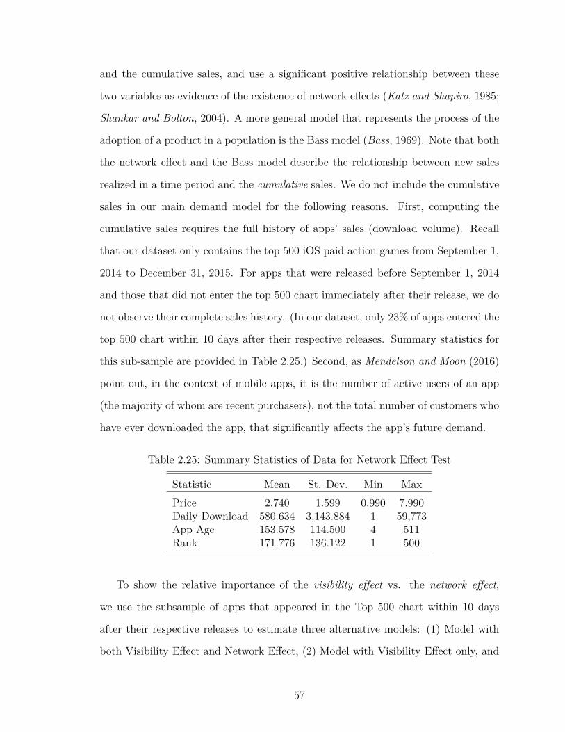
and the cumulative sales, and use a significant positive relationship between these

two variables as evidence of the existence of network effects (Katz and Shapiro, 1985;

Shankar and Bolton, 2004). A more general model that represents the process of the

adoption of a product in a population is the Bass model (Bass, 1969). Note that both

the network effect and the Bass model describe the relationship between new sales

realized in a time period and the cumulative sales. We do not include the cumulative

sales in our main demand model for the following reasons. First, computing the

cumulative sales requires the full history of apps’ sales (download volume). Recall

that our dataset only contains the top 500 iOS paid action games from September 1,

2014 to December 31, 2015. For apps that were released before September 1, 2014

and those that did not enter the top 500 chart immediately after their release, we do

not observe their complete sales history. (In our dataset, only 23% of apps entered the

top 500 chart within 10 days after their respective releases. Summary statistics for

this sub-sample are provided in Table 2.25.) Second, as Mendelson and Moon (2016)

point out, in the context of mobile apps, it is the number of active users of an app

(the majority of whom are recent purchasers), not the total number of customers who

have ever downloaded the app, that significantly affects the app’s future demand.

Table 2.25: Summary Statistics of Data for Network Effect Test

Statistic Mean St. Dev. Min MaxPrice 2.740 1.599 0.990 7.990Daily Download 580.634 3,143.884 1 59,773App Age 153.578 114.500 4 511Rank 171.776 136.122 1 500

To show the relative importance of the visibility effect vs. the network effect,

we use the subsample of apps that appeared in the Top 500 chart within 10 days

after their respective releases to estimate three alternative models: (1) Model with

both Visibility Effect and Network Effect, (2) Model with Visibility Effect only, and

57

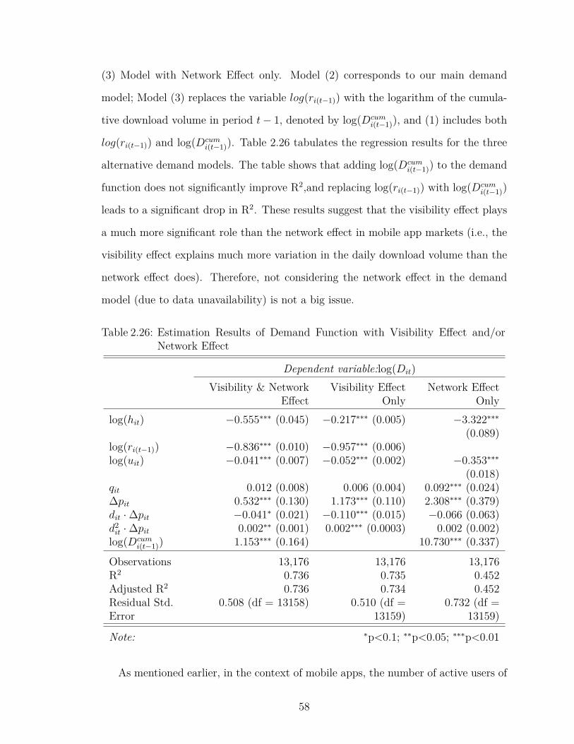
(3) Model with Network Effect only. Model (2) corresponds to our main demand

model; Model (3) replaces the variable log(ri(t−1)) with the logarithm of the cumula-

tive download volume in period t− 1, denoted by log(Dcumi(t−1)), and (1) includes both

log(ri(t−1)) and log(Dcumi(t−1)). Table 2.26 tabulates the regression results for the three

alternative demand models. The table shows that adding log(Dcumi(t−1)) to the demand

function does not significantly improve R2,and replacing log(ri(t−1)) with log(Dcumi(t−1))

leads to a significant drop in R2. These results suggest that the visibility effect plays

a much more significant role than the network effect in mobile app markets (i.e., the

visibility effect explains much more variation in the daily download volume than the

network effect does). Therefore, not considering the network effect in the demand

model (due to data unavailability) is not a big issue.

Table 2.26: Estimation Results of Demand Function with Visibility Effect and/orNetwork Effect

Dependent variable:log(Dit)

Visibility & NetworkEffect

Visibility EffectOnly

Network EffectOnly

log(hit) −0.555∗∗∗ (0.045) −0.217∗∗∗ (0.005) −3.322∗∗∗

(0.089)log(ri(t−1)) −0.836∗∗∗ (0.010) −0.957∗∗∗ (0.006)log(uit) −0.041∗∗∗ (0.007) −0.052∗∗∗ (0.002) −0.353∗∗∗

(0.018)qit 0.012 (0.008) 0.006 (0.004) 0.092∗∗∗ (0.024)∆pit 0.532∗∗∗ (0.130) 1.173∗∗∗ (0.110) 2.308∗∗∗ (0.379)dit ·∆pit −0.041∗ (0.021) −0.110∗∗∗ (0.015) −0.066 (0.063)d2it ·∆pit 0.002∗∗ (0.001) 0.002∗∗∗ (0.0003) 0.002 (0.002)log(Dcum

i(t−1)) 1.153∗∗∗ (0.164) 10.730∗∗∗ (0.337)

Observations 13,176 13,176 13,176R2 0.736 0.735 0.452Adjusted R2 0.736 0.734 0.452Residual Std.Error

0.508 (df = 13158) 0.510 (df =13159)

0.732 (df =13159)

Note: ∗p<0.1; ∗∗p<0.05; ∗∗∗p<0.01

As mentioned earlier, in the context of mobile apps, the number of active users of

58

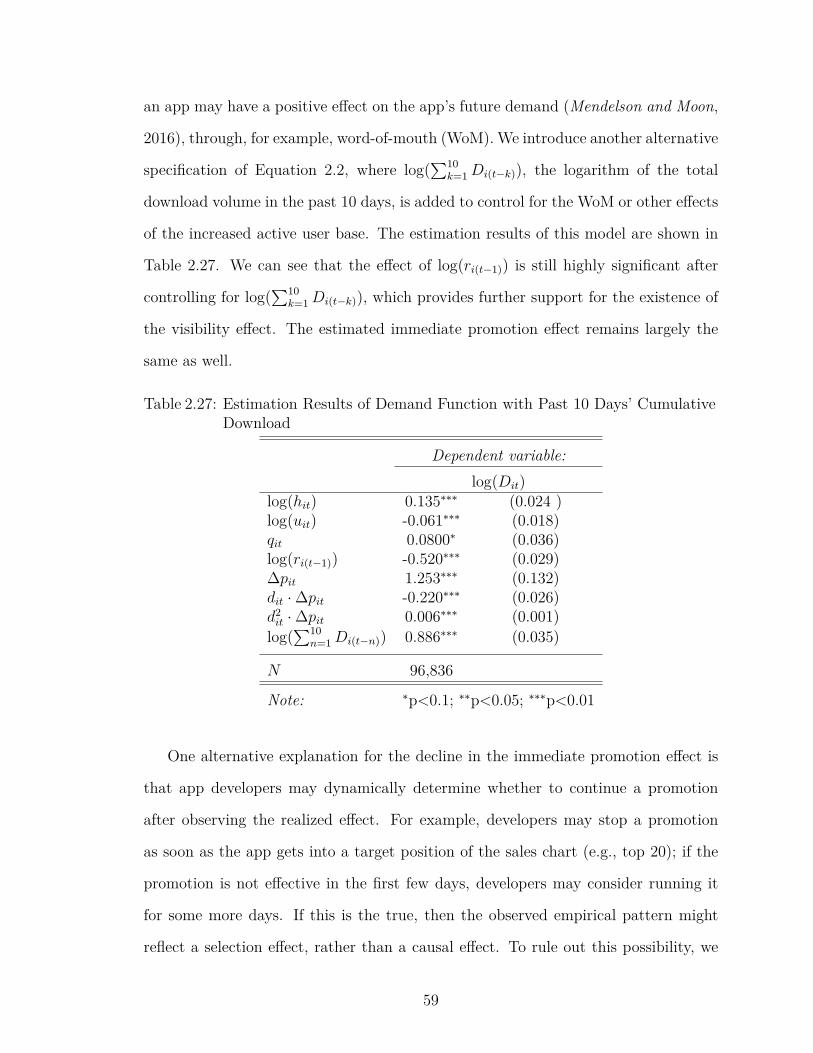
an app may have a positive effect on the app’s future demand (Mendelson and Moon,

2016), through, for example, word-of-mouth (WoM). We introduce another alternative

specification of Equation 2.2, where log(∑10

k=1Di(t−k)), the logarithm of the total

download volume in the past 10 days, is added to control for the WoM or other effects

of the increased active user base. The estimation results of this model are shown in

Table 2.27. We can see that the effect of log(ri(t−1)) is still highly significant after

controlling for log(∑10

k=1Di(t−k)), which provides further support for the existence of

the visibility effect. The estimated immediate promotion effect remains largely the

same as well.

Table 2.27: Estimation Results of Demand Function with Past 10 Days’ CumulativeDownload

Dependent variable:log(Dit)

log(hit) 0.135∗∗∗ (0.024 )log(uit) -0.061∗∗∗ (0.018)qit 0.0800∗ (0.036)log(ri(t−1)) -0.520∗∗∗ (0.029)∆pit 1.253∗∗∗ (0.132)dit ·∆pit -0.220∗∗∗ (0.026)d2it ·∆pit 0.006∗∗∗ (0.001)log(

∑10n=1Di(t−n)) 0.886∗∗∗ (0.035)

N 96,836

Note: ∗p<0.1; ∗∗p<0.05; ∗∗∗p<0.01

One alternative explanation for the decline in the immediate promotion effect is

that app developers may dynamically determine whether to continue a promotion

after observing the realized effect. For example, developers may stop a promotion

as soon as the app gets into a target position of the sales chart (e.g., top 20); if the

promotion is not effective in the first few days, developers may consider running it

for some more days. If this is the true, then the observed empirical pattern might

reflect a selection effect, rather than a causal effect. To rule out this possibility, we

59

estimate the following modified demand model:

log(Dit) = αi + β1 log(ri(t−1)) + β2 log(hit) + β3 log(uit) + β4qit

+20∑j=1

β(4+j)∆pit · I(dit = j) +10∑k=1

θk∆pit · I(dit = k) · IShortit

+12∑

m=2

ηmMmit +7∑

w=2

ϕwWwit + ϵit

(2.8)

where the newly added variable I(dit = j) is a binary variable indicating that app i is

on the jth day of the promotion in period t, and IShortit is a binary variable indicating

that the promotion that app i experiences in period t is a short promotion (shorter

than or exactly 10 days, which is the median of the promotion length observed in the

data). If the aforementioned selection effect exists, then we would expect to see a

larger positive effect of the promotion in the first few days of the promotion in shorter

promotions than in the longer promotions. However, as shown in Table 2.28, most

of the estimated coefficients of the interaction terms are insignificant, which is not

consistent with the conjecture. In other words, there is no evidence in the data to

support the selection effect.

2.4.5 Heterogeneity

In the main model, we assume that promotions of the same depth have a ho-

mogeneous immediate effect on log(Dit).19 It is possible that the magnitude of the

immediate promotion effect is different for apps with different characteristics. To

test this possibility, we perform the following analyses to explore the potential het-

erogeneity in the immediate effect of promotion on log(Dit) with respect to (i) a set

of time-invariant app characteristics and (ii) a set of time-varying app characteris-

tics. The former set includes app quality (proxied by app all-time average rating19As shown in Figure 2.10, it does not imply that the total effect of promotions on the absolute

download volume is homogeneous.

60

and ranking), original price, and whether the app has a free version available or not;

the latter set includes the average app rank 7 days prior to the promotion, app age

at the time of the promotion, and the time since the last update at the time of the

promotion. We explore the potential heterogeneity in the immediate promotion effect

with respect to (i) using stratified analysis to allow for the maximum flexibility, and

that with respect to (ii) by including interaction effects.20 Finally, to see whether the

immediate promotion effect varies with calendar time, we divide the sample period

into four equal-length intervals and estimate the main model with data falling in each

interval separately.

To test if the promotion effect is different for apps with different levels of quality,

we classify all apps into “high-quality” (with a rating ≥ 4) and “low-quality” (with

a rating < 4”) groups, and estimate the demand model with these two sub-samples,

separately. The estimation results reported in Table 2.29 suggest that the immediate

promotion effect is similar between the two sub-samples of apps – the effect is only

slightly larger for high quality apps (≥ 4 stars).

We also classify the apps in our sample into “expensive apps” and “inexpensive

apps” (original price is greater than or equal to vs. less than the median original

price among the apps in the sample, which is $2.99), and estimate the demand model

using the two subsamples separately. The estimation results, reported in Table 2.30,

suggest that the immediate promotion effect is significantly higher for apps that have

a higher original price, which is not surprising because given the same discount depth,

the absolute decrease in price is larger for apps that have a higher original price.

It is possible that the promotion effect is different for apps with a freemium

version and those without. Therefore, we try to estimate the demand model using

the following two sub-samples of apps separately – (1) those that have a freemium

version available and (2) those that do not. It turns out that only 12 apps in our20Because ∆pit is potentially endogenous, any interaction terms that contain ∆pit are also poten-

tially endogenous.

61

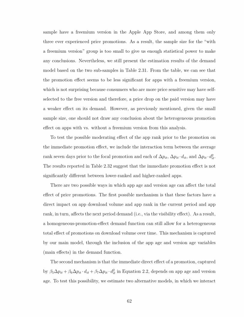
sample have a freemium version in the Apple App Store, and among them only

three ever experienced price promotions. As a result, the sample size for the “with

a freemium version” group is too small to give us enough statistical power to make

any conclusions. Nevertheless, we still present the estimation results of the demand

model based on the two sub-samples in Table 2.31. From the table, we can see that

the promotion effect seems to be less significant for apps with a freemium version,

which is not surprising because consumers who are more price sensitive may have self-

selected to the free version and therefore, a price drop on the paid version may have

a weaker effect on its demand. However, as previously mentioned, given the small

sample size, one should not draw any conclusion about the heterogeneous promotion

effect on apps with vs. without a freemium version from this analysis.

To test the possible moderating effect of the app rank prior to the promotion on

the immediate promotion effect, we include the interaction term between the average

rank seven days prior to the focal promotion and each of ∆pit, ∆pit ·dit, and ∆pit ·d2it.

The results reported in Table 2.32 suggest that the immediate promotion effect is not

significantly different between lower-ranked and higher-ranked apps.

There are two possible ways in which app age and version age can affect the total

effect of price promotions. The first possible mechanism is that these factors have a

direct impact on app download volume and app rank in the current period and app

rank, in turn, affects the next period demand (i.e., via the visibility effect). As a result,

a homogeneous-promotion-effect demand function can still allow for a heterogeneous

total effect of promotions on download volume over time. This mechanism is captured

by our main model, through the inclusion of the app age and version age variables

(main effects) in the demand function.

The second mechanism is that the immediate direct effect of a promotion, captured

by β5∆pit+β6∆pit · dit+β7∆pit · d2it in Equation 2.2, depends on app age and version

age. To test this possibility, we estimate two alternative models, in which we interact

62

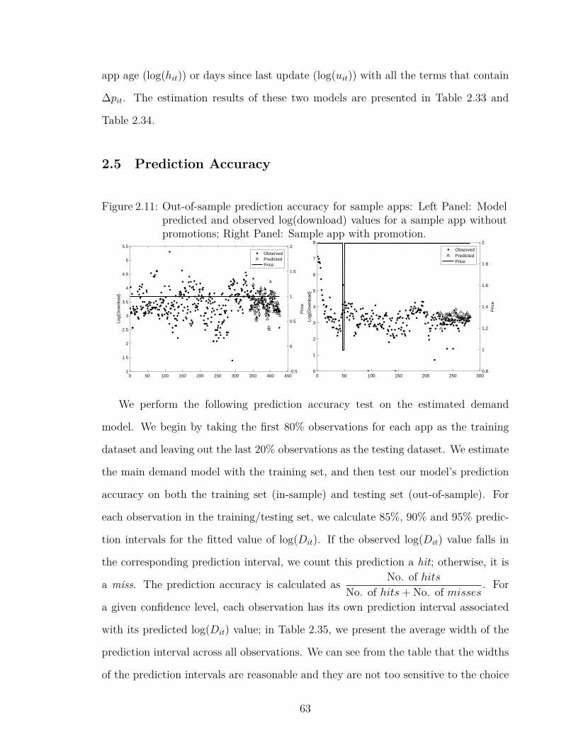
app age (log(hit)) or days since last update (log(uit)) with all the terms that contain

∆pit. The estimation results of these two models are presented in Table 2.33 and

Table 2.34.

2.5 Prediction Accuracy

Figure 2.11: Out-of-sample prediction accuracy for sample apps: Left Panel: Modelpredicted and observed log(download) values for a sample app withoutpromotions; Right Panel: Sample app with promotion.

0 50 100 150 200 250 300 350 400 4501

1.5

2

2.5

3

3.5

4

4.5

5

5.5

Log(

Dow

nloa

d)

-0.5

0

0.5

1

1.5

2

Pric

e

ObservedPredictedPrice

0 50 100 150 200 250 3000

1

2

3

4

5

6

7

8

Log(

Dow

nloa

d)

0.8

1

1.2

1.4

1.6

1.8

2

Pric

e

ObservedPredictedPrice

We perform the following prediction accuracy test on the estimated demand

model. We begin by taking the first 80% observations for each app as the training

dataset and leaving out the last 20% observations as the testing dataset. We estimate

the main demand model with the training set, and then test our model’s prediction

accuracy on both the training set (in-sample) and testing set (out-of-sample). For

each observation in the training/testing set, we calculate 85%, 90% and 95% predic-

tion intervals for the fitted value of log(Dit). If the observed log(Dit) value falls in

the corresponding prediction interval, we count this prediction a hit; otherwise, it is

a miss. The prediction accuracy is calculated as No. of hitsNo. of hits+ No. of misses

. For

a given confidence level, each observation has its own prediction interval associated

with its predicted log(Dit) value; in Table 2.35, we present the average width of the

prediction interval across all observations. We can see from the table that the widths

of the prediction intervals are reasonable and they are not too sensitive to the choice

63

of the confidence level. In addition, we observe that the interval widths in the in-

sample and out-of-sample tests are very close, indicating that there is no significant

difference between the training data and the testing data. In Figure 2.11, we show

the observed and predicted download volumes for two sample apps. We can see that

the model-predicted download volumes are close to the observed download volumes.

In Table 2.24, we also present the MSE of a five-fold cross validation for our main

model. Note that accurately predicting download volume is difficult for apps with a

small number of observations. In spite of that, our model still achieves a good level of

accuracy in both in-sample and out-of-sample prediction tests. These results together

suggest that our model performs well in predicting download volume.

2.6 Promotion Planning Problem

In this section, we apply the empirical results to the optimization of price pro-

motions for mobile apps. Our goal is to optimize the promotion schedule (including

starting time and duration) as well as the promotion depth.21 We formulate the PPP

based on the demand system estimated in Section 2.4.1. The PPP is then transformed

into a Longest Path Problem (LPP). Due to the NP-hardness of the LPP, we further

propose a Moving Planning Window (MPW) heuristic that can effectively find near-

optimal solutions to the LPP. Finally, we numerically show the performance of the

proposed heuristic for apps with different initial ranks, ages, and original prices.

2.6.1 PPP Model Formulation

For notational simplicity, we drop the app index i and simplify the demand func-tion and ranking function estimated in Section 2.4.1.22 The PPP can be formulated

21Since all price changes in our dataset take the form of price promotions, we do not have datato empirically examine the effect of an increase in app price that goes beyond the original price.Therefore, our PPP formulation does not allow increasing app price beyond the original price. Wealso assume that the original price for each app is pre-determined. Determining an app’s originalprice requires a different analysis and is outside the scope of this study.

22We also drop the error term from both models for the PPP formulation. Including the errorterm in the demand model does not significantly affect the proposed heuristic.

64

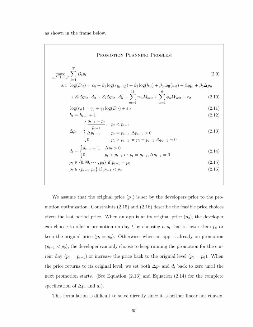
as shown in the frame below.

Promotion Planning Problem

maxpt,t=1,··· ,T

T∑t=1

Dtpt (2.9)

s.t. log(Dit) = αi + β1 log(ri(t−1)) + β2 log(hit) + β3 log(uit) + β4qit + β5∆pit

+ β6∆pit · dit + β7∆pit · d2it +11∑

m=1

ηmMmit +

6∑w=1

ϕwWwit + ϵit (2.10)

log(rit) = γ0 + γ1 log(Dit) + εit (2.11)ht = ht−1 + 1 (2.12)

∆pt =

pt−1 − pt

pt−1, pt < pt−1

∆pt−1, pt = pt−1,∆pt−1 > 0

0, pt > pt−1 or pt = pt−1,∆pt−1 = 0

(2.13)

dt =

{dt−1 + 1, ∆pt > 0

0, pt > pt−1 or pt = pt−1,∆pt−1 = 0(2.14)

pt ∈ {0.99, · · · , p0} if pt−1 = p0 (2.15)pt ∈ {pt−1, p0} if pt−1 < p0 (2.16)

We assume that the original price (p0) is set by the developers prior to the pro-

motion optimization. Constraints (2.15) and (2.16) describe the feasible price choices

given the last period price. When an app is at its original price (p0), the developer

can choose to offer a promotion on day t by choosing a pt that is lower than p0 or

keep the original price (pt = p0). Otherwise, when an app is already on promotion

(pt−1 < p0), the developer can only choose to keep running the promotion for the cur-

rent day (pt = pt−1) or increase the price back to the original level (pt = p0). When

the price returns to its original level, we set both ∆pt and dt back to zero until the

next promotion starts. (See Equation (2.13) and Equation (2.14) for the complete

specification of ∆pt and dt).

This formulation is difficult to solve directly since it is neither linear nor convex.

65

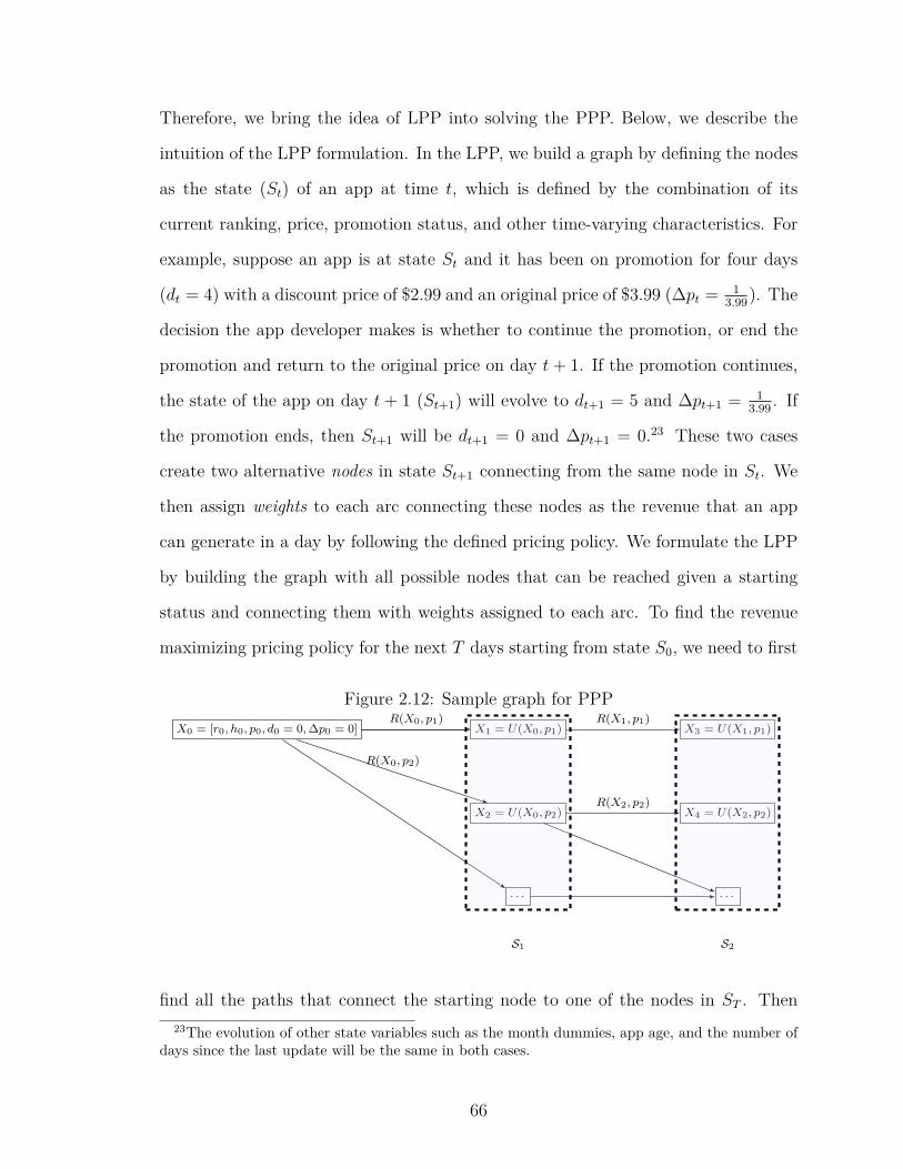
Therefore, we bring the idea of LPP into solving the PPP. Below, we describe the

intuition of the LPP formulation. In the LPP, we build a graph by defining the nodes

as the state (St) of an app at time t, which is defined by the combination of its

current ranking, price, promotion status, and other time-varying characteristics. For

example, suppose an app is at state St and it has been on promotion for four days

(dt = 4) with a discount price of $2.99 and an original price of $3.99 (∆pt =1

3.99). The

decision the app developer makes is whether to continue the promotion, or end the

promotion and return to the original price on day t+ 1. If the promotion continues,

the state of the app on day t + 1 (St+1) will evolve to dt+1 = 5 and ∆pt+1 =1

3.99. If

the promotion ends, then St+1 will be dt+1 = 0 and ∆pt+1 = 0.23 These two cases

create two alternative nodes in state St+1 connecting from the same node in St. We

then assign weights to each arc connecting these nodes as the revenue that an app

can generate in a day by following the defined pricing policy. We formulate the LPP

by building the graph with all possible nodes that can be reached given a starting

status and connecting them with weights assigned to each arc. To find the revenue

maximizing pricing policy for the next T days starting from state S0, we need to first

Figure 2.12: Sample graph for PPPX0 = [r0, h0, p0, d0 = 0,∆p0 = 0] X1 = U(X0, p1)

X2 = U(X0, p2)

· · ·

X4 = U(X2, p2)

X3 = U(X1, p1)

· · ·

R(X0, p1)

R(X0, p2)

R(X1, p1)

R(X2, p2)

S1 S2

find all the paths that connect the starting node to one of the nodes in ST . Then23The evolution of other state variables such as the month dummies, app age, and the number of

days since the last update will be the same in both cases.

66

we sum all the weights along each path and find the path with the maximum total

weight. The total weight is equal to the total revenue the app can get by following

that price trajectory. On any given day we can keep the current price or change it

(either raise or drop), hence, at least two nodes in the next time period connect from

the current node. Therefore, the number of nodes in state ST grows exponentially as

T gets larger.

With limited computational power, we cannot build the full graph with every

single possible price trajectory for a large T and solve the problem exactly. To ef-

ficiently find a near-optimal pricing policy, we propose a Moving Planning Window

(MPW) heuristic. For a PPP within the planning horizon of T days,24 the MPW

heuristic deals with sub-problems of a small planning window of TW days. We then

solve the sub-problems sequentially by moving the planning window forward with a

step size of n (n < TW ) days each time. We assume that the developer will follow

the optimal pricing policy solved from the sub-problem for the next n days. We can

then get the initial point of the next sub-problem using Equations (2.10) and (2.11).25

The next sub-problem will then be solved given the new initial state for the next TW

days. These steps are repeated until the planning window covers day T , which is

predetermined by the developer. The pricing policy from the heuristic is the price

trajectory that the developer follows along the way of solving these sub-problems.

For a PPP with a planning horizon of T days (i.e., developers ignore the sales from

day T + 1 onwards in the PPP), the moving planning window (MPW) heuristic we

propose deals with sub-problems of a small planning window of TW days. We then

solve the sub-problems sequentially by moving the planning window forward with a

step size of n (n < TW ) days at a time. For each sub-problem, we generate the graph

only focusing on the next TW days given an initial state. We assume that the app24We assume that developers will ignore the sales from day T + 1 onwards in the PPP.25We focus on the rank and the download volume here since all the other variables can be updated

automatically without considering the promotion policy.

67

will keep a constant original (pre-promotion) price for all the remaining days of the

planning horizon after the TW -day window. Suppose the promotion planning starts

on day t and the app’s initial state is Xt = (rt, ht, pt, dt,∆pt). We first generate the

directed graph of possible pricing choices for the periods from t to t+ TW . Then the

optimal pricing policy (p∗t+1, p∗t+1, · · · , p∗t+TW

) for this TW -day planning window can

be found by solving the LPP on the directed graph using Dijkstra Algorithm. The

resulting optimal pricing policy is adopted for the next n days. Along the longest

path, we can get the realized states Xt+1, · · · , Xt+n. We then move the planning

window n days forward and start the next planning horizon at day t + n with the

initial state of Xt+n. This process is repeated until the end of planning horizon T is

reached. In our numerical results, we show that the MPW can get a near-optimal

objective value while significantly saving the computational time.

Fatigue. In our basic LPP, every promotion is assumed to be independent of

each other, even if one promotion immediately follows another (i.e., two promotions

are offered within a short period of time). Under this assumption, the optimal promo-

tion plan will suggest that developers conduct promotions as frequently as possible,

increasing the price back to its original level for one day and then immediately con-

ducting the next promotion to exploit the largest promotion effect on the first day of

each promotion.

In practice, however, when two promotions are offered back to back, the second

one may not be as effective as the first (Kumar and Pereira, 1995; Blattberg et al.,

1995). The reduced effectiveness of the second promotion is often referred to as

fatigue. As shown in the empirical analysis (Figure 2.8), the promotion effect drops

with dit. When two promotions are offered back to back, the second promotion is

effectively an extension of the first; therefore, its promotion effect may be smaller in

magnitude. To make our model more realistic, we introduce fatigue into our model.

Let F(∫⊔) denote the decrease in the second promotion’s baseline effect (β5) if it

68

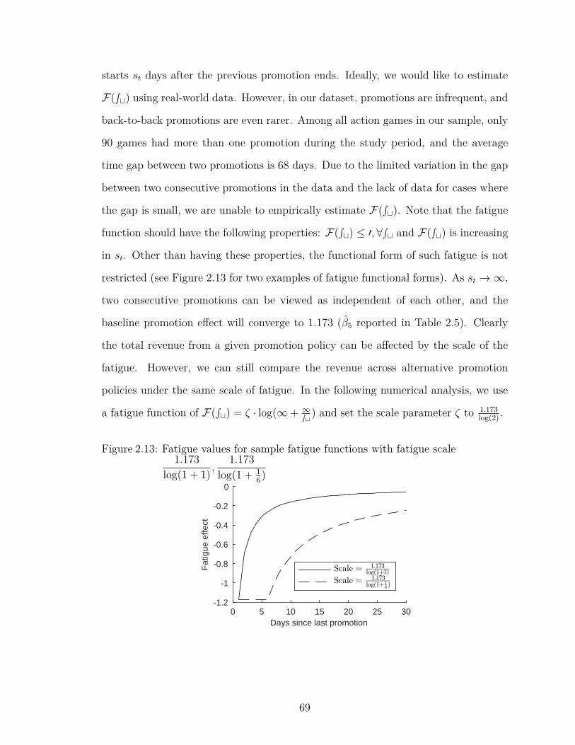
starts st days after the previous promotion ends. Ideally, we would like to estimate

F(∫⊔) using real-world data. However, in our dataset, promotions are infrequent, and

back-to-back promotions are even rarer. Among all action games in our sample, only

90 games had more than one promotion during the study period, and the average

time gap between two promotions is 68 days. Due to the limited variation in the gap

between two consecutive promotions in the data and the lack of data for cases where

the gap is small, we are unable to empirically estimate F(∫⊔). Note that the fatigue

function should have the following properties: F(∫⊔) ≤ ′,∀∫⊔ and F(∫⊔) is increasing

in st. Other than having these properties, the functional form of such fatigue is not

restricted (see Figure 2.13 for two examples of fatigue functional forms). As st → ∞,

two consecutive promotions can be viewed as independent of each other, and the

baseline promotion effect will converge to 1.173 (β5 reported in Table 2.5). Clearly

the total revenue from a given promotion policy can be affected by the scale of the

fatigue. However, we can still compare the revenue across alternative promotion

policies under the same scale of fatigue. In the following numerical analysis, we use

a fatigue function of F(∫⊔) = ζ · log(∞+ ∞∫⊔ ) and set the scale parameter ζ to 1.173

log(2).

Figure 2.13: Fatigue values for sample fatigue functions with fatigue scale1.173

log(1 + 1),

1.173

log(1 + 16)

0 5 10 15 20 25 30Days since last promotion

-1.2

-1

-0.8

-0.6

-0.4

-0.2

0

Fat

igue

effe

ct

69

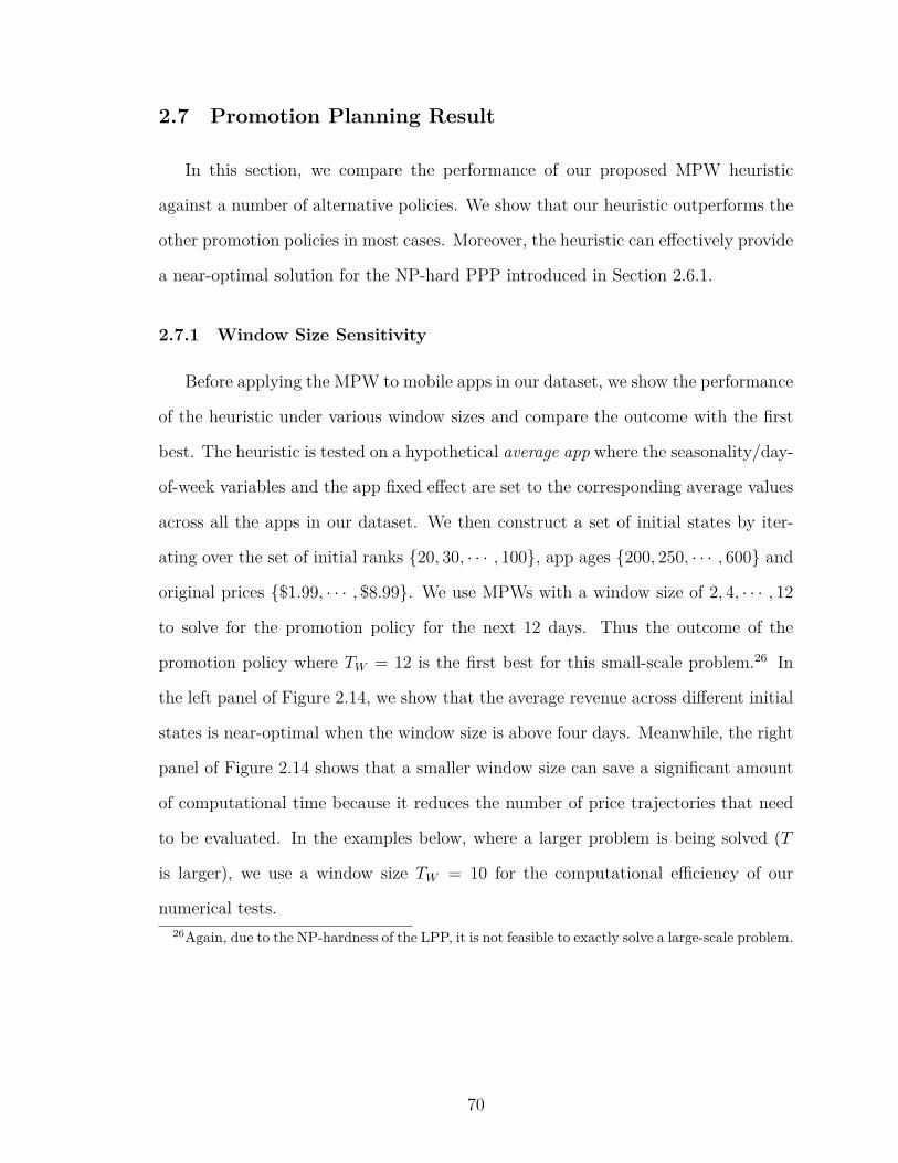
2.7 Promotion Planning Result

In this section, we compare the performance of our proposed MPW heuristic

against a number of alternative policies. We show that our heuristic outperforms the

other promotion policies in most cases. Moreover, the heuristic can effectively provide

a near-optimal solution for the NP-hard PPP introduced in Section 2.6.1.

2.7.1 Window Size Sensitivity

Before applying the MPW to mobile apps in our dataset, we show the performance

of the heuristic under various window sizes and compare the outcome with the first

best. The heuristic is tested on a hypothetical average app where the seasonality/day-

of-week variables and the app fixed effect are set to the corresponding average values

across all the apps in our dataset. We then construct a set of initial states by iter-

ating over the set of initial ranks {20, 30, · · · , 100}, app ages {200, 250, · · · , 600} and

original prices {$1.99, · · · , $8.99}. We use MPWs with a window size of 2, 4, · · · , 12

to solve for the promotion policy for the next 12 days. Thus the outcome of the

promotion policy where TW = 12 is the first best for this small-scale problem.26 In

the left panel of Figure 2.14, we show that the average revenue across different initial

states is near-optimal when the window size is above four days. Meanwhile, the right

panel of Figure 2.14 shows that a smaller window size can save a significant amount

of computational time because it reduces the number of price trajectories that need

to be evaluated. In the examples below, where a larger problem is being solved (T

is larger), we use a window size TW = 10 for the computational efficiency of our

numerical tests.26Again, due to the NP-hardness of the LPP, it is not feasible to exactly solve a large-scale problem.

70

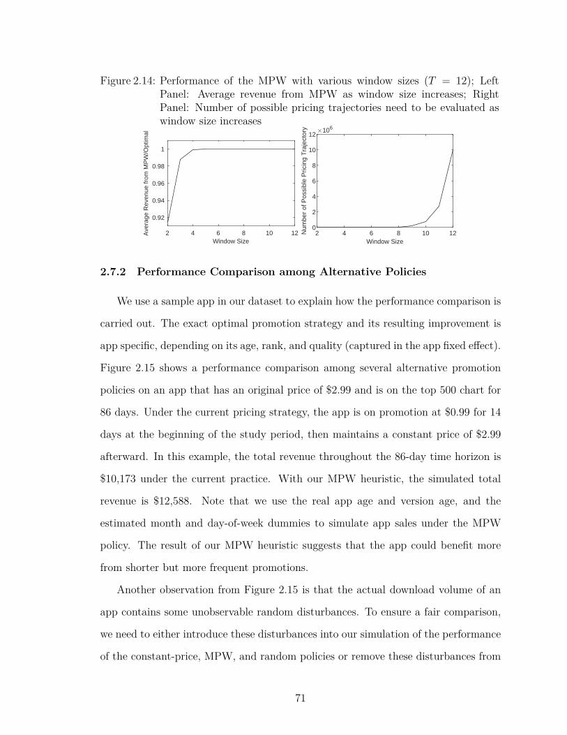
Figure 2.14: Performance of the MPW with various window sizes (T = 12); LeftPanel: Average revenue from MPW as window size increases; RightPanel: Number of possible pricing trajectories need to be evaluated aswindow size increases

2 4 6 8 10 12Window Size

0.92

0.94

0.96

0.98

1A

vera

ge R

even

ue fr

om M

PW

/Opt

imal

2 4 6 8 10 12Window Size

0

2

4

6

8

10

12

Num

ber

of P

ossi

ble

Pric

ing

Tra

ject

ory 106

2.7.2 Performance Comparison among Alternative Policies

We use a sample app in our dataset to explain how the performance comparison is

carried out. The exact optimal promotion strategy and its resulting improvement is

app specific, depending on its age, rank, and quality (captured in the app fixed effect).

Figure 2.15 shows a performance comparison among several alternative promotion

policies on an app that has an original price of $2.99 and is on the top 500 chart for

86 days. Under the current pricing strategy, the app is on promotion at $0.99 for 14

days at the beginning of the study period, then maintains a constant price of $2.99

afterward. In this example, the total revenue throughout the 86-day time horizon is

$10,173 under the current practice. With our MPW heuristic, the simulated total

revenue is $12,588. Note that we use the real app age and version age, and the

estimated month and day-of-week dummies to simulate app sales under the MPW

policy. The result of our MPW heuristic suggests that the app could benefit more

from shorter but more frequent promotions.

Another observation from Figure 2.15 is that the actual download volume of an

app contains some unobservable random disturbances. To ensure a fair comparison,

we need to either introduce these disturbances into our simulation of the performance

of the constant-price, MPW, and random policies or remove these disturbances from

71

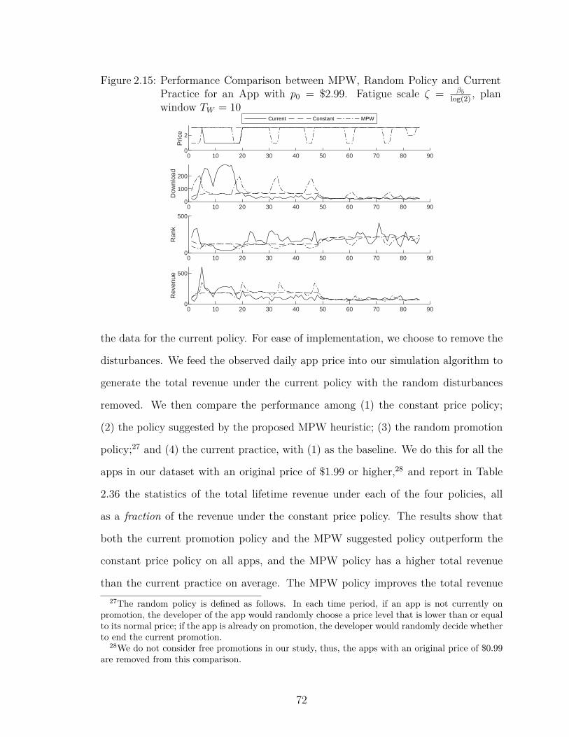
Figure 2.15: Performance Comparison between MPW, Random Policy and CurrentPractice for an App with p0 = $2.99. Fatigue scale ζ = β5

log(2), plan

window TW = 10

0 10 20 30 40 50 60 70 80 900

100

200D

ownl

oad

0 10 20 30 40 50 60 70 80 900

500

Ran

k

0 10 20 30 40 50 60 70 80 900

500

Rev

enue

0 10 20 30 40 50 60 70 80 900

2

Pric

e

Current Constant MPW

the data for the current policy. For ease of implementation, we choose to remove the

disturbances. We feed the observed daily app price into our simulation algorithm to

generate the total revenue under the current policy with the random disturbances

removed. We then compare the performance among (1) the constant price policy;

(2) the policy suggested by the proposed MPW heuristic; (3) the random promotion

policy;27 and (4) the current practice, with (1) as the baseline. We do this for all the

apps in our dataset with an original price of $1.99 or higher,28 and report in Table

2.36 the statistics of the total lifetime revenue under each of the four policies, all

as a fraction of the revenue under the constant price policy. The results show that

both the current promotion policy and the MPW suggested policy outperform the

constant price policy on all apps, and the MPW policy has a higher total revenue

than the current practice on average. The MPW policy improves the total revenue27The random policy is defined as follows. In each time period, if an app is not currently on

promotion, the developer of the app would randomly choose a price level that is lower than or equalto its normal price; if the app is already on promotion, the developer would randomly decide whetherto end the current promotion.

28We do not consider free promotions in our study, thus, the apps with an original price of $0.99are removed from this comparison.

72

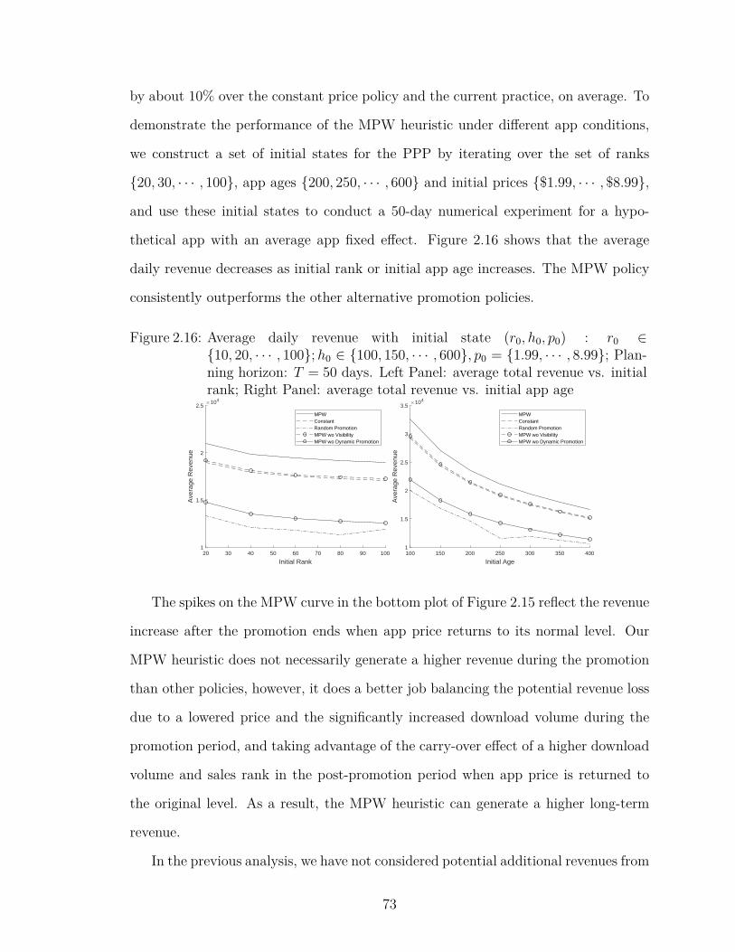
by about 10% over the constant price policy and the current practice, on average. To

demonstrate the performance of the MPW heuristic under different app conditions,

we construct a set of initial states for the PPP by iterating over the set of ranks

{20, 30, · · · , 100}, app ages {200, 250, · · · , 600} and initial prices {$1.99, · · · , $8.99},

and use these initial states to conduct a 50-day numerical experiment for a hypo-

thetical app with an average app fixed effect. Figure 2.16 shows that the average

daily revenue decreases as initial rank or initial app age increases. The MPW policy

consistently outperforms the other alternative promotion policies.

Figure 2.16: Average daily revenue with initial state (r0, h0, p0) : r0 ∈{10, 20, · · · , 100};h0 ∈ {100, 150, · · · , 600}, p0 = {1.99, · · · , 8.99}; Plan-ning horizon: T = 50 days. Left Panel: average total revenue vs. initialrank; Right Panel: average total revenue vs. initial app age

20 30 40 50 60 70 80 90 100

Initial Rank

1

1.5

2

2.5

Ave

rage

Rev

enue

104

MPWConstantRandom PromotionMPW wo VisibilityMPW wo Dynamic Promotion

100 150 200 250 300 350 400

Initial Age

1

1.5

2

2.5

3

3.5

Ave

rage

Rev

enue

104

MPWConstantRandom PromotionMPW wo VisibilityMPW wo Dynamic Promotion

The spikes on the MPW curve in the bottom plot of Figure 2.15 reflect the revenue

increase after the promotion ends when app price returns to its normal level. Our

MPW heuristic does not necessarily generate a higher revenue during the promotion

than other policies, however, it does a better job balancing the potential revenue loss

due to a lowered price and the significantly increased download volume during the

promotion period, and taking advantage of the carry-over effect of a higher download

volume and sales rank in the post-promotion period when app price is returned to

the original level. As a result, the MPW heuristic can generate a higher long-term

revenue.

In the previous analysis, we have not considered potential additional revenues from

73

in-app purchases or in-app advertising. Ghose and Han (2014) find that“providing

in-app purchases directly increases the demand of an app”, and it also has an indi-

rect positive effect on app demand because apps with in-app purchase features tend

to charge a lower price. They also find that in-app advertising “is likely to cause

annoyance and hence decrease app demand”. Note that the decisions about whether

to provide in-app purchase or in-app advertising features are typically made before

an app is released and an app’s revenue model usually does not change afterwards.

Therefore, the direct effects of in-app purchase and in-app advertising features on

demand can be captured by the app-specific fixed effect in our model.

As a first step, we analyze how in-app purchase and in-app advertising features

affect app demand and revenue from initial purchases. According to Ghose and Han

(2014), providing in-app purchases increases the download volume, which is equivalent

to having an increased app fixed effect; including in-app advertising decreases the

download volume, which is equivalent to having a decreased app fixed effect. Note that

both in-app purchase and in-app advertising can increase the revenue app developers

collect from an additional unit of download (on top of the price they charge for the

initial purchase); we will consider revenue from in-app purchase/advertising later.

We consider the app that was used for the analysis presented in Section 6.2, and

slightly increase (decrease) the app fixed effect to reflect the scenario in which in-app

purchase (in-app advertising) features are introduced into the app. We then use our

proposed Moving Planning Window (MPW) heuristic to find the optimal promotion

schedule under the following three conditions: original (without in-app purchase or

in-app advertising, same as shown in Figure 9 in the paper), with in-app purchase, and

with in-app advertising. The optimal promotion policy and the resulting download

volume, rank and revenue under these three conditions are compared in Figure 2.17.

It is evident in the figure that the optimal promotion schedule is identical under the

three conditions; however, the app with in-app purchase (in-app advertising) features

74

benefits more (less) from promotions than the app without in-app purchase or in-app

advertising. This result suggests that in-app purchase and in-app advertising do not

significantly affect the optimal promotion policy if we only consider revenue from

initial downloads.

We then bring the additional revenue generated from in-app purchases and in-

app advertising to the PPP. We consider two cases – (1) in-app purchase/advertising

brings a small amount of additional revenue, which is 20% of p0, and (2) in-app

purchase/advertising brings a large amount of additional revenue, which is 50% of

p0. That is, the revenue per download is p0(1 + 20%+∆pit) and p0(1 + 50%+∆pit)

for cases (1) and (2) respectively. In Figure 2.18 (2.19), we compare the promotion

schedule generated by our proposed MPW and the resulting download volume, rank

and revenue under three conditions – original, with in-app purchase, and with in-app

advertising. The results from the comparisons suggest that the optimal promotion

policy is not significantly affected by the inclusion of the additional revenue from

in-app purchase/advertising. Only in the case where in-app purchase/advertising

brings a large amount of additional revenue (50% of the original price), we observe a

slightly different promotion timing (a slight delay) for the app with in-app purchase

features (the dash-dotted line in the top panel of Figure 2.19); the promotion length

and depth for this app are not significantly different from those for the app without

in-app purchase or advertising features.

2.7.3 Significance of the Visibility Effect and Dynamic Promotion Effect

Next, we discuss the characteristics of the promotion schedule prescribed by our

MPW heuristic. Figure 2.20 shows a 50-day promotion schedule generated by the

MPW heuristic for a hypothetical app released 200 days ago with an initial rank of 20

and an original price of $2.99. A few observations about the optimal promotion policy

are worth noting. First, the MPW heuristic suggests that promotions be offered more

75

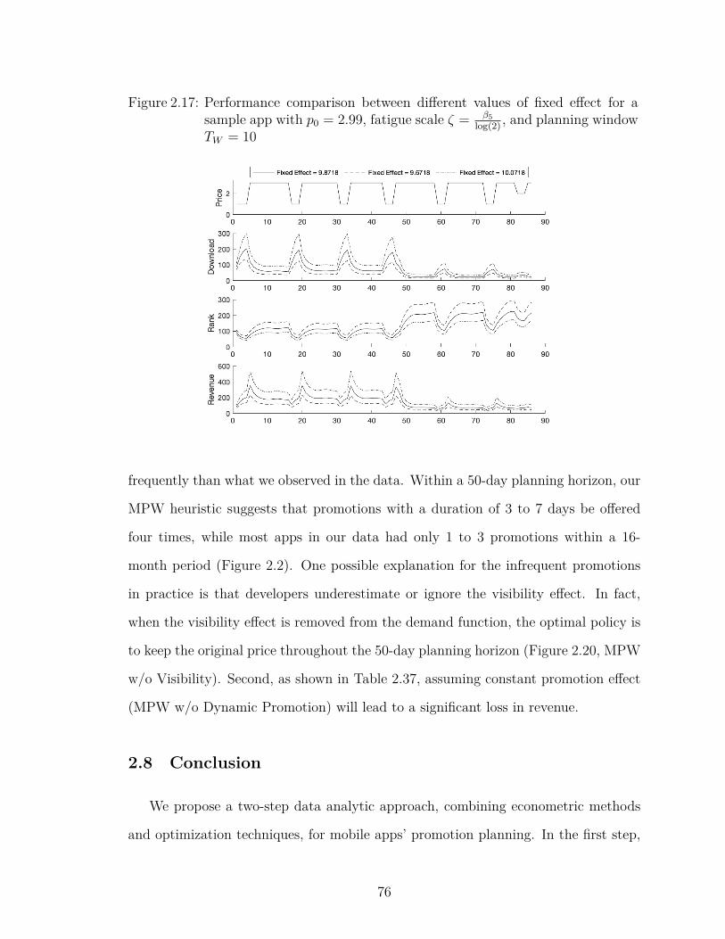
Figure 2.17: Performance comparison between different values of fixed effect for asample app with p0 = 2.99, fatigue scale ζ = β5

log(2), and planning window

TW = 10

frequently than what we observed in the data. Within a 50-day planning horizon, our

MPW heuristic suggests that promotions with a duration of 3 to 7 days be offered

four times, while most apps in our data had only 1 to 3 promotions within a 16-

month period (Figure 2.2). One possible explanation for the infrequent promotions

in practice is that developers underestimate or ignore the visibility effect. In fact,

when the visibility effect is removed from the demand function, the optimal policy is

to keep the original price throughout the 50-day planning horizon (Figure 2.20, MPW

w/o Visibility). Second, as shown in Table 2.37, assuming constant promotion effect

(MPW w/o Dynamic Promotion) will lead to a significant loss in revenue.

2.8 Conclusion

We propose a two-step data analytic approach, combining econometric methods

and optimization techniques, for mobile apps’ promotion planning. In the first step,

76

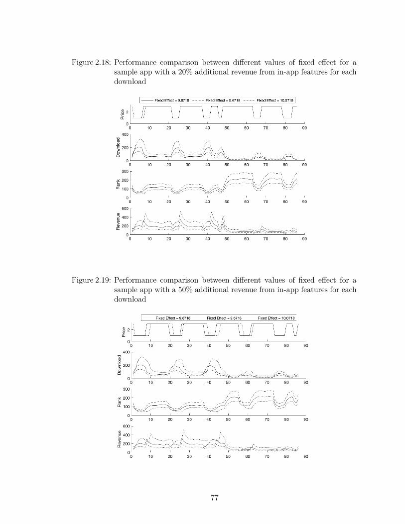
Figure 2.18: Performance comparison between different values of fixed effect for asample app with a 20% additional revenue from in-app features for eachdownload

Figure 2.19: Performance comparison between different values of fixed effect for asample app with a 50% additional revenue from in-app features for eachdownload

77

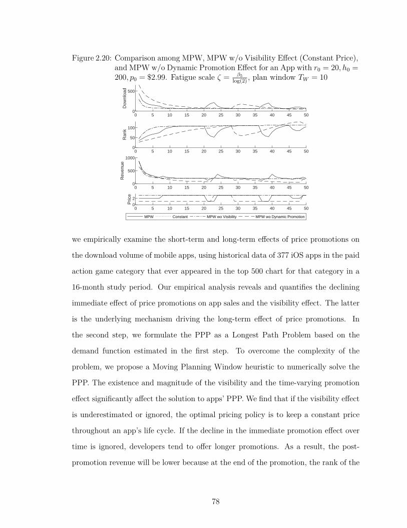
Figure 2.20: Comparison among MPW, MPW w/o Visibility Effect (Constant Price),and MPW w/o Dynamic Promotion Effect for an App with r0 = 20, h0 =200, p0 = $2.99. Fatigue scale ζ = β5

log(2), plan window TW = 10

0 5 10 15 20 25 30 35 40 45 500

500

Dow

nloa

d

0 5 10 15 20 25 30 35 40 45 500

50

100R

ank

0 5 10 15 20 25 30 35 40 45 500

500

1000

Rev

enue

0 5 10 15 20 25 30 35 40 45 500

2

Pric

e

MPW Constant MPW wo Visibility MPW wo Dynamic Promotion

we empirically examine the short-term and long-term effects of price promotions on

the download volume of mobile apps, using historical data of 377 iOS apps in the paid

action game category that ever appeared in the top 500 chart for that category in a

16-month study period. Our empirical analysis reveals and quantifies the declining

immediate effect of price promotions on app sales and the visibility effect. The latter

is the underlying mechanism driving the long-term effect of price promotions. In

the second step, we formulate the PPP as a Longest Path Problem based on the

demand function estimated in the first step. To overcome the complexity of the

problem, we propose a Moving Planning Window heuristic to numerically solve the

PPP. The existence and magnitude of the visibility and the time-varying promotion

effect significantly affect the solution to apps’ PPP. We find that if the visibility effect

is underestimated or ignored, the optimal pricing policy is to keep a constant price

throughout an app’s life cycle. If the decline in the immediate promotion effect over

time is ignored, developers tend to offer longer promotions. As a result, the post-

promotion revenue will be lower because at the end of the promotion, the rank of the

78

app is not as high as it would have been if the promotion were shorter. In this case,

the visibility effect is not taken advantage of in the post-promotion period.

Our study makes significant contributions to both theory and practice. First, our

work is among the first to study the promotion planning problem for (paid) mobile

apps. We show that shorter and more frequent promotions work better for mobile

apps due to the declining immediate promotion effect and the existence of the visi-

bility effect. Second, our data-driven promotion planning policy outperforms current

common practice in the industry, demonstrating the power of combining econometric

analysis and optimization techniques to design effective price promotions. Our mod-

eling framework (including the demand estimation and PPP) is completely driven

by real data, and imposes minimal assumptions on the demand function. The pro-

posed heuristic can be conveniently used by app developers29 to achieve real-time

promotion planning. Our proposed framework is readily applicable to the promo-

tion planning for other digital products that exhibit similar promotion effects and

visibility effects, such as desktop software. It may also be applied to physical goods

sold on E-commerce platforms where sales rank affects the position on the platform’s

website in which products are displayed, especially those that can be considered one-

time purchase products. We caution that the specific empirical model needs to be

updated and re-estimated when the framework is applied to other digital goods or

physical goods sold on E-commerce platforms whose demand is affected by a different

set of factors, and that our algorithm assumes changing price is costless and has an

objective of maximizing revenue (which is equivalent to maximizing profit when the29App developers can update their estimate of the demand function using data on their own

apps (or the data that they believe is the most relevant). The ranking function is not app specific,but category specific; app developers can directly use the estimated ranking function in this paperif the app for which they are designing the promotion plan is in the paid action game category.To estimate the effect of promotions, app developers can also use historical data, or experimentwith different promotion depths and lengths to get their app-specific estimate. Note that even if abetter-calibrated model is found, the formulation and solution for the PPP and the structure of theheuristic proposed in the paper remain valid; the parameters or the demand model simply need tobe re-tuned or modified.

79

marginal cost is zero). In contexts where these assumptions/objectives do not apply

(e.g., producers/retailers have limited flexibility to make price changes, pricing deci-

sions are jointly made by multiple parties with different objectives, or the marginal

cost is not zero), modifications to the setup of PPP are also necessary.

Our study has several limitations. First, due to data unavailability, the fatigue

function used in the PPP is based on prior theoretical work, but not directly estimated

from the real-world data. Future research could consider collecting relevant data or

running field experiments to estimate a more realistic fatigue function, or test the

proposed promotion planning heuristic in the field.30 Second, since the range of

prices observed in our dataset is from $0.99 to $7.99, the estimated demand function

may be unable to describe the relationship between price promotions and app demand

when app price is higher than $7.99. Although we do not expect dramatic differences

in the shape of the app demand function in the price range of ($7.99, +∞), the

estimated demand function is worth additional empirical validation. Third, we are

not able to pinpoint the exact mechanism for the decreasing immediate effect of

promotions on app demand with current data. Finally, we do not have information

about when apps are featured or recommended, and for this reason we interpret the

estimated visibility effect as a combination of direct visibility effect from moving to a

higher position in the sales chart and the possible indirect visibility effect through the

increased chance of being featured or recommended (and perhaps even the positive

effect of an increased user base through non-ranking-related channels). In spite of

these limitations, our study generates important insights into the design of effective

price promotions for mobile apps, and shows the advantages of using data-driven

models for solving PPPs, especially for products in markets that exhibit the visibility

effect, where future demand depends on past sales rank.

30The procedure to solve for the optimal promotion policy will remain the same regardless of thechanges in the fatigue function.

80

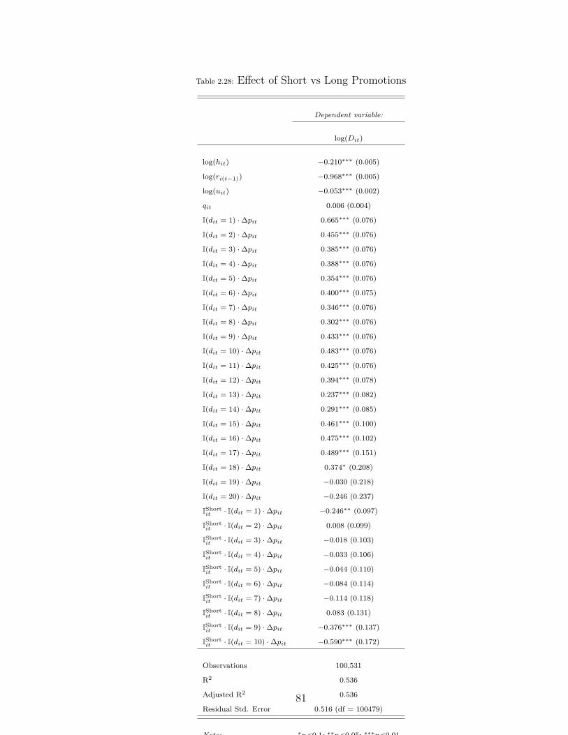
Table 2.28: Effect of Short vs Long Promotions

Dependent variable:

log(Dit)

log(hit) −0.210∗∗∗ (0.005)

log(ri(t−1)) −0.968∗∗∗ (0.005)

log(uit) −0.053∗∗∗ (0.002)

qit 0.006 (0.004)

I(dit = 1) ·∆pit 0.665∗∗∗ (0.076)

I(dit = 2) ·∆pit 0.455∗∗∗ (0.076)

I(dit = 3) ·∆pit 0.385∗∗∗ (0.076)

I(dit = 4) ·∆pit 0.388∗∗∗ (0.076)

I(dit = 5) ·∆pit 0.354∗∗∗ (0.076)

I(dit = 6) ·∆pit 0.400∗∗∗ (0.075)

I(dit = 7) ·∆pit 0.346∗∗∗ (0.076)

I(dit = 8) ·∆pit 0.302∗∗∗ (0.076)

I(dit = 9) ·∆pit 0.433∗∗∗ (0.076)

I(dit = 10) ·∆pit 0.483∗∗∗ (0.076)

I(dit = 11) ·∆pit 0.425∗∗∗ (0.076)

I(dit = 12) ·∆pit 0.394∗∗∗ (0.078)

I(dit = 13) ·∆pit 0.237∗∗∗ (0.082)

I(dit = 14) ·∆pit 0.291∗∗∗ (0.085)

I(dit = 15) ·∆pit 0.461∗∗∗ (0.100)

I(dit = 16) ·∆pit 0.475∗∗∗ (0.102)

I(dit = 17) ·∆pit 0.489∗∗∗ (0.151)

I(dit = 18) ·∆pit 0.374∗ (0.208)

I(dit = 19) ·∆pit −0.030 (0.218)

I(dit = 20) ·∆pit −0.246 (0.237)

IShortit · I(dit = 1) ·∆pit −0.246∗∗ (0.097)

IShortit · I(dit = 2) ·∆pit 0.008 (0.099)

IShortit · I(dit = 3) ·∆pit −0.018 (0.103)

IShortit · I(dit = 4) ·∆pit −0.033 (0.106)

IShortit · I(dit = 5) ·∆pit −0.044 (0.110)

IShortit · I(dit = 6) ·∆pit −0.084 (0.114)

IShortit · I(dit = 7) ·∆pit −0.114 (0.118)

IShortit · I(dit = 8) ·∆pit 0.083 (0.131)

IShortit · I(dit = 9) ·∆pit −0.376∗∗∗ (0.137)

IShortit · I(dit = 10) ·∆pit −0.590∗∗∗ (0.172)

Observations 100,531

R2 0.536

Adjusted R2 0.536

Residual Std. Error 0.516 (df = 100479)

Note: ∗p<0.1; ∗∗p<0.05; ∗∗∗p<0.01

81

Table 2.29: Estimation Results of Demand Function by App Rating

Dependent variable: log(Dit)

Rating < 4.0 Rating ≥ 4.0log(hit) −0.204∗∗∗ (0.006) −0.232∗∗∗ (0.009)log(ri(t−1)) −0.958∗∗∗ (0.006) −0.960∗∗∗ (0.010)log(uit) −0.059∗∗∗ (0.002) −0.042∗∗∗ (0.003)qit 0.010∗ (0.005) 0.002 (0.007)∆pit 0.847∗∗∗ (0.117) 0.973∗∗∗ (0.129)dit ·∆pit −0.079∗∗∗ (0.016) −0.066∗∗∗ (0.017)d2it ·∆pit 0.002∗∗∗ (0.0004) 0.002∗∗∗ (0.0004)Month Dummies Yes YesDay of Week Dummies Yes YesApp Fixed Effects Yes YesObservations 61,908 38,623R2 0.556 0.503Adjusted R2 0.556 0.503Residual Std. Error 0.510 (df = 61883) 0.523 (df = 38598)

Note: ∗p<0.1; ∗∗p<0.05; ∗∗∗p<0.01

Table 2.30: Estimation Results of Demand Function by Original Price

Dependent variable: log(Dit)

Original Price ≤ $2.99 Original Price > $2.99

log(hit) −0.179∗∗∗ (0.008) −0.260∗∗∗ (0.007)log(ri(t−1)) −0.998∗∗∗ (0.008) −0.919∗∗∗ (0.008)log(uit) −0.062∗∗∗ (0.003) −0.044∗∗∗ (0.003)qit 0.011∗∗ (0.006) 0.001 (0.006)∆pit 0.224 (0.289) 1.118∗∗∗ (0.109)dit ·∆pit 0.023 (0.070) −0.098∗∗∗ (0.014)d2it ·∆pit −0.0001 (0.003) 0.002∗∗∗ (0.0003)Month Dummies Yes YesDay of Week Dummies Yes YesApp Fixed Effects Yes YesObservations 46,712 53,819R2 0.492 0.575Adjusted R2 0.492 0.574Residual Std. Error 0.516 (df = 46687) 0.511 (df = 53794)

Note: ∗p<0.1; ∗∗p<0.05; ∗∗∗p<0.01

82

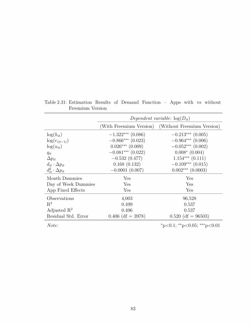
Table 2.31: Estimation Results of Demand Function – Apps with vs withoutFreemium Version

Dependent variable: log(Dit)

(With Freemium Version) (Without Freemium Version)log(hit) −1.322∗∗∗ (0.086) −0.213∗∗∗ (0.005)log(ri(t−1)) −0.866∗∗∗ (0.023) −0.964∗∗∗ (0.006)log(uit) 0.026∗∗∗ (0.009) −0.052∗∗∗ (0.002)qit −0.081∗∗∗ (0.022) 0.008∗ (0.004)∆pit −0.532 (0.477) 1.154∗∗∗ (0.111)dit ·∆pit 0.168 (0.132) −0.109∗∗∗ (0.015)d2it ·∆pit −0.0001 (0.007) 0.002∗∗∗ (0.0003)Month Dummies Yes YesDay of Week Dummies Yes YesApp Fixed Effects Yes YesObservations 4,003 96,528R2 0.499 0.537Adjusted R2 0.496 0.537Residual Std. Error 0.406 (df = 3978) 0.520 (df = 96503)

Note: ∗p<0.1; ∗∗p<0.05; ∗∗∗p<0.01

83

Table 2.32: Estimation Results of Demand Function with Interaction Effect betweenPromotion and Rank Prior to Promotion

Dependent variable:log(Dit)

log(hit) −0.259∗∗∗ (0.005)log(ri(t−1)) −0.839∗∗∗ (0.004)log(uit) −0.053∗∗∗ (0.002)qit 0.009∗∗ (0.004)∆pit 0.804∗∗∗ (0.138)dit ·∆pit −0.052∗∗∗ (0.020)d2it ·∆pit 0.002∗∗∗ (0.0005)Average 7-day Rank·∆pit 0.001 (0.001)Average 7-day Rank·dit ·∆pit −0.00005 (0.0001)Average 7-day Rank·d2it ·∆pit −0.00000 (0.00000)Month Dummies YesDay of Week Dummies YesApp Fixed Effects YesObservations 100,531R2 0.541Adjusted R2 0.541Residual Std. Error 0.513 (df = 100503)

Note: ∗p<0.1; ∗∗p<0.05; ∗∗∗p<0.01

84

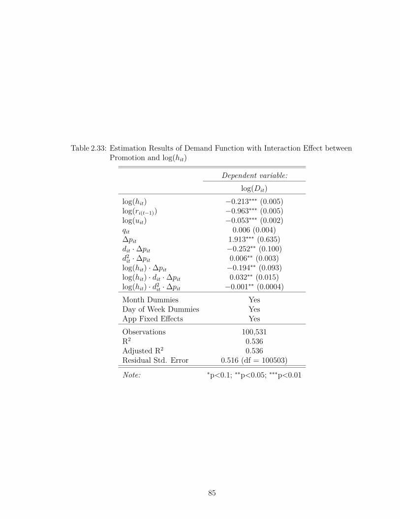
Table 2.33: Estimation Results of Demand Function with Interaction Effect betweenPromotion and log(hit)

Dependent variable:log(Dit)

log(hit) −0.213∗∗∗ (0.005)log(ri(t−1)) −0.963∗∗∗ (0.005)log(uit) −0.053∗∗∗ (0.002)qit 0.006 (0.004)∆pit 1.913∗∗∗ (0.635)dit ·∆pit −0.252∗∗ (0.100)d2it ·∆pit 0.006∗∗ (0.003)log(hit) ·∆pit −0.194∗∗ (0.093)log(hit) · dit ·∆pit 0.032∗∗ (0.015)log(hit) · d2it ·∆pit −0.001∗∗ (0.0004)Month Dummies YesDay of Week Dummies YesApp Fixed Effects YesObservations 100,531R2 0.536Adjusted R2 0.536Residual Std. Error 0.516 (df = 100503)

Note: ∗p<0.1; ∗∗p<0.05; ∗∗∗p<0.01

85

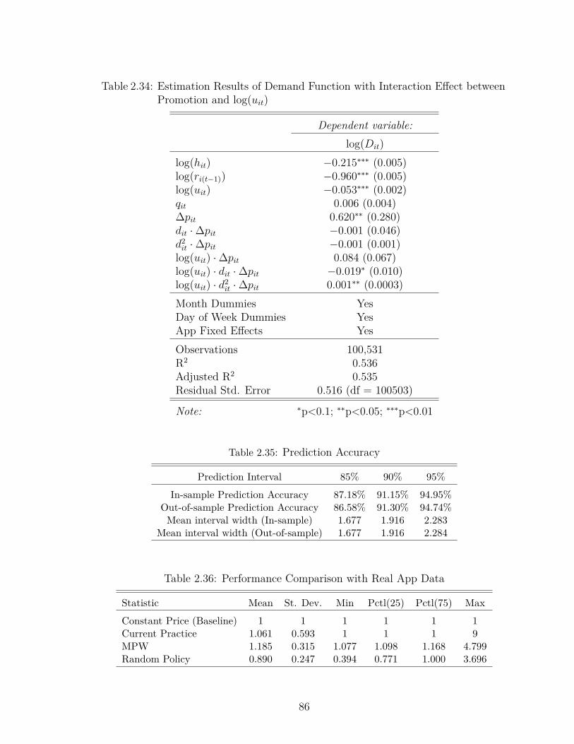
Table 2.34: Estimation Results of Demand Function with Interaction Effect betweenPromotion and log(uit)

Dependent variable:log(Dit)

log(hit) −0.215∗∗∗ (0.005)log(ri(t−1)) −0.960∗∗∗ (0.005)log(uit) −0.053∗∗∗ (0.002)qit 0.006 (0.004)∆pit 0.620∗∗ (0.280)dit ·∆pit −0.001 (0.046)d2it ·∆pit −0.001 (0.001)log(uit) ·∆pit 0.084 (0.067)log(uit) · dit ·∆pit −0.019∗ (0.010)log(uit) · d2it ·∆pit 0.001∗∗ (0.0003)Month Dummies YesDay of Week Dummies YesApp Fixed Effects YesObservations 100,531R2 0.536Adjusted R2 0.535Residual Std. Error 0.516 (df = 100503)

Note: ∗p<0.1; ∗∗p<0.05; ∗∗∗p<0.01

Table 2.35: Prediction Accuracy

Prediction Interval 85% 90% 95%In-sample Prediction Accuracy 87.18% 91.15% 94.95%

Out-of-sample Prediction Accuracy 86.58% 91.30% 94.74%Mean interval width (In-sample) 1.677 1.916 2.283

Mean interval width (Out-of-sample) 1.677 1.916 2.284

Table 2.36: Performance Comparison with Real App Data

Statistic Mean St. Dev. Min Pctl(25) Pctl(75) MaxConstant Price (Baseline) 1 1 1 1 1 1Current Practice 1.061 0.593 1 1 1 9MPW 1.185 0.315 1.077 1.098 1.168 4.799Random Policy 0.890 0.247 0.394 0.771 1.000 3.696

86

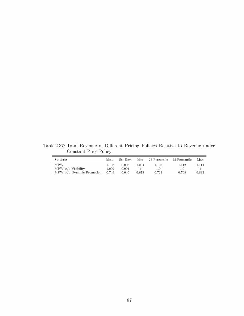
Table 2.37: Total Revenue of Different Pricing Policies Relative to Revenue underConstant Price Policy

Statistic Mean St. Dev. Min 25 Percentile 75 Percentile MaxMPW 1.108 0.005 1.094 1.105 1.112 1.114MPW w/o Visibility 1.009 0.004 1 1.0 1.0 1MPW w/o Dynamic Promotion 0.749 0.040 0.678 0.723 0.768 0.832

87

CHAPTER III

How Does Telemedicine Shape Physician’s

Practice in Mental Health?

3.1 Introduction

The adoption of telemedicine is considered as one of the most important changes

that is currently happening in healthcare delivery. The global telemedicine market

size has been on the rise year after year over the past decade and is estimated at over

$40 billion in 2019 (Grand View Research, 2020). By interacting with patients through

a telecommunication system, providers can deliver care remotely, which improves the

access to care, especially for the patients living in underprivileged areas with limited

healthcare resources. During the COVID-19 pandemic, the usage of telemedicine has

skyrocketed around the world. Iyengar (2020) report that a virtual health platform

based in Alexandria, VA saw a 3,600% increase in its virtual visits over an 11-day

period. As more providers and more patients adopt telemedicine, it is believed that

the boost in using telemedicine will sustain even after the crisis passes.

Telemedicine is known to be one of the key enablers to create better health ex-

perience for patients by providing high quality, easy to access care (Totten et al.,

2016). Healthcare providers also benefit from telemedicine by expanding their reach

to new patients and by avoiding overcrowding their facilities. It is reported that

88

telemedicine can result in lower per capita cost of healthcare as a result of the im-

proved efficiency in the healthcare system (New York Times, 2021). Despite these

benefits, telemedicine can have some downsides. Adopting telemedicine requires tech-

nical training and (expensive) infrastructure. Some telemedicine models may reduce

care continuity. For example, a patient may opt to see an online physician on com-

mercial telemedicine platforms instead of seeing her own primary care physicians.

For providers, telemedicine could mean extra administrative work, since navigating

the changing law, policy, and reimbursement landscape can be difficult (Fanburg

and Walzman, 2018). Finally, telemedicine can expand the provider’s coverage and

panel size and may overburden the provider, resulting in the postponing of necessary

follow-up visits. Understanding how the adoption of telemedicine affects the physi-

cians’ practice and access to care is of significant importance that this study sheds

light on.

In this paper we use claims and enrollment data from a major insurer in Michi-

gan, namely Blue Cross Blue Shield of Michigan (BCBSM), in conjuncture with the

American Medical Association (AMA) Physician Master File to empirically study the

impact of telemedicine adoption on the frequency of follow-up visits. In particular, we

focus on a subset of telemedicine visits in outpatient settings that are conducted via

real-time (synchronous) audio-video telecommunication systems. These telemedicine

visits may substitute their in-office counterparts to achieve similar diagnostic and

therapeutic functions. This distinguishes us from existing work such as Bavafa et al.

(2018, 2019); Bavafa and Terwiesch (2019); Sun et al. (2020), where they focus on

asynchronous encounters or non-outpatient settings. This study focuses on mental

health visits since mental health is one of the largest and most promising application

domains of telemedicine (Bashshur et al., 2016). Moreover, by the clinical nature of

mental health visits, less hands-on procedures (e.g., blood tests, imaging, physical

exams, IV treatments) are involved (BCBSM , 2018a,b). Therefore, mental health

89

telemedicine visits, if used appropriately, may have the potential to substitute for a

face-to-face and hands-on encounter to achieve the same diagnostic and therapeutic

functionalities.

The key question we answer in this study is how physicians’ scheduling of re-

lated visits changes after adopting telemedicine. This question is motivated by the

fact that the adoption and usage of alternative communication modes could poten-

tially shape how physicians make treatment and follow-up decisions thereby leading

to unintended consequences. This study adopts a novel changes-in-changes (CIC)

approach (Athey and Imbens, 2006), which non-parametrically estimates the effect of

telemedicine adoption on the frequency of scheduling follow-up related visits. To cap-

ture the frequency of follow-up visits, we focus on the related visit intervals (RVIs),

which is defined to be the number of days elapsed between a patient’s visiting a

physician for a concern and her next visit with the same physician for the same con-

cern. This definition of related visits and intervals are widely used in the medical

and operations literature (Hertzog et al., 2019; Santillanes et al., 2020; Bavafa et al.,

2019).

Our estimation results show that, telemedicine adoption on average decreases the

length of RVIs in the short term and increases it in the long term. Interestingly, such

an adoption effect is also spilled over to the in-office visits as we observe a similar

pattern in the in-office initiated RVI length (a decrease in the short term and an in-

crease in the long term). We find adopting telemedicine results in more new patients

admitted into the physicians’ panel. Over time, this increase in panel size (caused

by telemedicine adoption) leads to a heavier workload and occupies the physicians’

capacity. As a result, the physicians in the long term schedule visits with longer RVIs.

Nonetheless, the physicians who adopt telemedicine (i.e., the adopter group) with a

lighter workload would still schedule related visits with shorter RVIs. Focusing on

the effect of the initiating visit’s mode for each RVI, we find that the telemedicine

90

initiated RVIs are consistently shorter than in-office RVIs at different stages of adop-

tion. Finally, comparing the RVI length following a new vs. an established patient

indicates no heterogeneous impact of adoption across these two groups of patients.

Focusing on real-time telemedicine visits that fulfil diagnostic and therapeutic

purposes as their in-office counterparts, the results in this paper uncover valuable

managerial insights on telemedicine’s short- and long-term effects on healthcare de-

livery. First, telemedicine may not be treated as a perfect substitute for the in-office

visits. Second, physicians who adopt telemedicine may need to re-evaluate their ca-

pacity and availability under the new practice scheme. Third, since our results suggest

that telemedicine visits are relatively inadequate, practitioners may need to schedule

more visits periodically to resolve the uncertainty arisen during telemedicine visits.

This study also contributes to the empirical research literature, as to the best of our

knowledge, we are the first application of a CIC model to estimate the effect of an

intervention with heterogeneous adoption time.

3.2 Literature Review

Our work is related to three main streams of research: 1) telehealth related studies

in the medical field; 2) empirical and analytical research that studies the operational

problems related to telehealth; and 3) research that focuses on nonparametrical iden-

tification and estimation especially in a difference-in-differences (DID) setting.

The first stream is the medical literature that studies telehealth in general. Nu-

merous medical papers can be found in this stream, we review some of the most rel-

evant ones. In recent years, Medicare and other commercial insurances have started

to broaden the coverage of telemedicine services (Clay et al., 2018; BCBSM , 2018a).

Consequently, there has been an increasing trend in the adoption of telemedicine vis-

its as they are believed to be cost-effective alternatives to office visits. Gordon et al.

(2017) found that telemedicine encounters are cheaper than many other face-to-face

91

encounters. A survey conducted by Viers et al. (2015) on urological patients showed

that most patients are willing to accept telemedicine. Bashshur et al. (2016) reviews

numerous randomized clinical trials of telemedicine usage in mental health and found

that telemedicine improves the quality, access, cost, and adherence. Telemedicine may

have unintended (and sometimes negative) consequences. Shaw et al. (2018) found

that some physicians are reluctant to adopting telemedicine. Dr. Rashid Bashshur,

a pioneering public health researcher in the field of telemedicine, has pointed out in

(Bashshur, 1995) that telemedicine could have the effect of increasing the intensity

of care (provision of more diagnostic tests and procedures). This issue still remains

unsolved to date. Mehrotra et al. (2013); Uscher-Pines et al. (2015, 2016) found that

physicians tend to prescribe antibiotics more frequently in telemedicine visits than

they do in office visits.

A handful of articles investigate the factors that affect telemedicine adoption

and diffusion. A recent paper (Harst et al., 2019) gives a comprehensive summary.

Spaulding et al. (2005) surveys 356 providers on the core characteristics in Roger’s

innovation-diffusion theory to study how these characteristics affect telemedicine

adoption. They find that telemedicine adopters tend to make more referrals to

telemedicine when they recognize the benefits of telemedicine. This indicates a po-

tential over-utilization of telemedicine.

The second stream of research are empirical and analytical studies in the op-

erations management literature. Pertaining to empirical research on the impact of

telemedicine on physician’s practice, we review a few recent papers. Bavafa et al.

(2018); Bavafa and Terwiesch (2019) are most relevant to our study. The authors

empirically investigate the impact of adopting an asynchronous messaging system (e-

visits) on the frequency of in-office visits and physician workload. Their results show

that the messaging system leads to more visits and a heavier workload. Closely re-

lated to our study, Sun et al. (2020) empirically investigates the effect of telemedicine

92

adoption on emergency room (ER) congestion. Our work differs from these two pa-

pers in the following aspects. First and foremost, we focus on 1) the synchronous

video-audio communications unlike Bavafa et al. (2018), and 2) the visits that could

potentially be a substitute for in-office visits unlike Sun et al. (2020). Second, instead

of a linear DID model, we adopt the nonparametric CIC model proposed by Athey

and Imbens (2006), which estimates the entire counterfactual distribution of outcomes

for the treated group in the absence of treatment. Additionally, the CIC model al-

lows for multiple groups and adoption time periods, and assumptions invariant to the

scaling of the outcome. There are several other studies that investigate the usage of

telemedicine from different aspects. Hwang et al. (2017) builds an exponential ran-

dom graph model to study how distance affects the usage of telemedicine. Bavafa and

Terwiesch (2019) studies how e-visits could burden the provider by introducing extra

workload. Delana et al. (2019) uses a quasi-experimental difference-in-differences ap-

proach to estimate the impact of the introduction of telemedicine centers in different

areas.

A few papers study the management of telemedicine visits with analytical models.

Zhong et al. (2018) takes a queuing approach and shows that variations in e-visit

service time could offset the efficiency edge of using e-visits. Zhong (2018) studies

how the rejoining probability of the service queues (e-visits and office visits) impacts

the queuing performance metrics. Bayram et al. (2020) study the sequential decision

of which subset of patients should be seen by office visits or virtual visits to maximize

the quality adjusted life year of the entire panel. Wang et al. (2019) takes a queuing

approach and studies the e-consultations between providers. Li et al. (2019) also

analyzes a queuing game and show that if patients are sensitive to delays, introducing

telemedicine can increase the total cost of care. Sun et al. (2020) focus on the impact

of telemedicine adoption in emergency care delivery and show that ER telemedicine

adoption significantly reduces patients’ waiting time.

93

Finally, as mentioned above, in this paper, we adopt a nonparametric changes-

in-changes approach to estimate the telemedicine adoption effect on the physicians

who adopted telemedicine as proposed by Athey and Imbens (2006). This method

has been adopted in empirical studies that aim to estimate the effect of a policy

change or an intervention (Reza et al., 2020; Borah et al., 2011; Asteriou et al., 2019;

Pieroni and Salmasi, 2016). In these works, the authors adopt the CIC model with

two time periods and two groups to estimate the target effect. To the best of our

knowledge, our paper is the first application of a CIC model with multiple periods

and heterogeneous intervention time.

3.3 Problem Setting

The adoption of telemedicine can impact the physician behavior as captured by

the length of the interval between two consecutive visits that are scheduled for a

given patient (RVI). In what follows, we first describe our problem setting by defining

telemedicine visits and describing the main variable of interest (i.e., RVIs). We then

describe different effects of telemedicine and the potential mechanisms leading to such

effects.

3.3.1 Definitions

3.3.1.1 Telemedicine visits.

The terms telemedicine and telehealth are often used interchangeably with various

definitions, depending on the insurer and the provider. In what follows, We clarify

the definition of telemedicine in this study.

According to the policies established by the insurer in our dataset (BCBSM), tele-

health is a broad concept that includes all health care services and education, using

telecommunications (synchronous or asynchronous) for 1) diagnosis, 2) treatment, and

94

3) health management. Examples of such telehealth services include: telemedicine

(which is the scope of this study, and will be further defined in the next paragraph),

telemonitoring, healthcare education, patient portal communications (the e-visits con-

sidered in Bavafa et al. (2018); Bavafa and Terwiesch (2019) fall into this category),

email and text messages, and administrative services (BCBSM , 2018a).

Telemedicine is a subset of telehealth that is 1) synchronous and real-time (for

example, video chatting or telephone call); and 2) for medical diagnostic and ther-

apeutic purposes. Therefore, portal messages or emails, patient education, health

management visits do not qualify as telemedicine by this definition. It is important

to highlight that the telemedicine visits considered in this paper are recognized as

formal clinical encounters that are reimbursed by most insurers at the same rate as

their in-office counterparts (eVisit, 2021).

Within telemedicine visits, we focus on the evaluation and management (E&M)

visits for mental health patients. In these E&M visits, physicians perform medical

evaluations on the patient and make medical decisions such as prescriptions, referrals,

and follow-up scheduling. The billing codes of the E&M visits directly reflect the com-

plexity of a patient visit and the duration of the visit. The reasons for focusing only

on the mental health E&M visits are threefold. First, mental health is one of the most

promising fields of telemedicine (Bashshur et al., 2016). Second, by the clinical nature

of mental health E&M visits, if telemedicine visits are used appropriately, they may

have the potential to substitute for a face-to-face and hands-on encounter to achieve

the same functionality1. Third, each procedure billing code of these telemedicine

E&M visits has a one-to-one in-office counterpart procedure code2. This allows us to

identify the set of telemedicine and its in-office counterparts to better understand the1In BCBSM policy’s own words: “making decisions regarding diagnosis and/or treatment of

telemedicine visits, the physician does not require face-to-face contact to make an optimal decision.”(BCBSM , 2018a,b).

2For example, procedure code 99211 is for a 5-minute in-office E&M, and procedure code 99211with a modifier GT or GQ is for a 5-minute telemedicine E&M, and both are reimbursed at thesame rate.

95

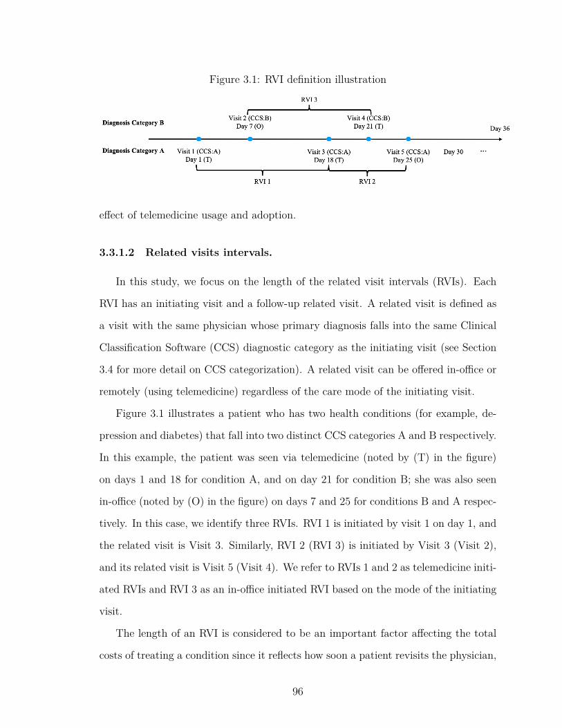
Figure 3.1: RVI definition illustration

effect of telemedicine usage and adoption.

3.3.1.2 Related visits intervals.

In this study, we focus on the length of the related visit intervals (RVIs). Each

RVI has an initiating visit and a follow-up related visit. A related visit is defined as

a visit with the same physician whose primary diagnosis falls into the same Clinical

Classification Software (CCS) diagnostic category as the initiating visit (see Section

3.4 for more detail on CCS categorization). A related visit can be offered in-office or

remotely (using telemedicine) regardless of the care mode of the initiating visit.

Figure 3.1 illustrates a patient who has two health conditions (for example, de-

pression and diabetes) that fall into two distinct CCS categories A and B respectively.

In this example, the patient was seen via telemedicine (noted by (T) in the figure)

on days 1 and 18 for condition A, and on day 21 for condition B; she was also seen

in-office (noted by (O) in the figure) on days 7 and 25 for conditions B and A respec-

tively. In this case, we identify three RVIs. RVI 1 is initiated by visit 1 on day 1, and

the related visit is Visit 3. Similarly, RVI 2 (RVI 3) is initiated by Visit 3 (Visit 2),

and its related visit is Visit 5 (Visit 4). We refer to RVIs 1 and 2 as telemedicine initi-

ated RVIs and RVI 3 as an in-office initiated RVI based on the mode of the initiating

visit.

The length of an RVI is considered to be an important factor affecting the total

costs of treating a condition since it reflects how soon a patient revisits the physician,

96

which itself may be affected by the adoption of telemedicine (LORIG et al., 2001).

We investigate the effect of telemedicine adoption on this measure in the remainder

of the paper.

3.3.2 Telemedicine Effects

We present two main effects of telemedicine here: the telemedicine adoption effect,

and the spillover effect. A detailed discussion of the mechanisms behind these effects

is also provided in what follows.

3.3.2.1 Telemedicine adoption effect.

The main research question of this study is whether physicians schedule related

visits differently after adopting telemedicine. To answer this question, we estimate the

effect of telemedicine adoption on RVI lengths, which is referred to as the telemedicine

adoption effect in the rest of the paper. For a given diagnosis, there is usually some es-

tablished protocols for the physicians to follow when scheduling related visits (Mitchell

et al., 2013). Nonetheless, in practice, physicians have discretion over the scheduling

of visits and may thus choose to see patients more (or less) frequently depending on

their availability and the mode of the initiating visit. After adopting telemedicine,

physicians may experience efficiency improvement or deterioration, technical difficul-

ties, capacity issues, etc. Given these changes, we believe that the length of RVIs

can move in either direction. In what follows, we discuss the possible changes in the

length of RVIs and the potential underlying mechanisms for these changes.

Positive telemedicine adoption effect.

Below are the mechanisms that can contribute to an increase in the length of RVIs

for the adopter group after the adoption.

97

• Operational inefficiency: The adoption of telemedicine may introduce opera-

tional inefficiencies due to the changeover time between the telemedicine and

in-office visits (e.g., switching between the telemedicine platform and the regular

in-office visit system). To guarantee privacy and security of the conversation,

physicians may need an extra telecommunication system during a telemedicine

visit, which may be different from the original system for in-office visits. Such

switching between systems could lead to interruptions and changeover time.

Previous studies have shown that resuming a preempted task after switching

out is cognitively costly (Pashler, 1994; Rubinstein et al., 2001; Czerwinski

et al., 2004; Salvucci et al., 2009). Furthermore, the potential technical issues

in telemedicine visits can lead to interruptions and thus cause inefficiencies in

the visiting time (Gurvich et al., 2020). Cayirli and Veral (2003) points out

that in the implementation of telemedicine, “Little knowledge currently exists

among medical practitioners on how to effectively and practically use various

forms of telemedicine.” The operational inefficiencies caused by the adoption of

telemedicine can then reduce physician’s availability. As a result, the related

visits are scheduled with longer intervals in between.

• Heavier workload: Physicians who adopt telemedicine may admit more new

patients (who are otherwise unable to be seen through in-office visits) after the

adoption. This increase in panel size may increase the physician’s workload and

make him/her less available. As a result, the physicians may schedule related

visits with longer intervals in between.

Negative telemedicine adoption effect.

Below are the mechanisms that can contribute to a decrease in the length of RVIs

for the adopter group after the adoption.

98

• Operational efficiency: Telemedicine visits can have several advantages in terms

of operational efficiency. One such advantage is reducing or eliminating patient’s

travel time, especially for rural patients.

In addition to the reduced travel cost, telemedicine is also believed to be more

efficient than in-office visits since it virtualizes and shortens the check-in, check-

out, and paperwork processes. For a typical in-office visit, a patient needs to go

through a multi-stage process of check-in, vital measurement, nurse examina-

tion, physician visit, labs and tests (if any), and check-out (Cayirli and Veral,

2003). Conversation with practitioners at our partner hospital suggests that

patients and physicians could connect to the secured telecommunication sys-

tem at the scheduled time and begin the visit much more quickly since many of

the aforementioned stages are virtualized and shortened with the help of tech-

nology. With fewer number of stages in a visit, the mean and variance of the

service time are likely decreased. This can ultimately increase the availability

of the physicians to schedule more frequent follow-ups so long as they have ca-

pacity available to do so. As a result, this may lead to a decrease in the length

of RVIs for the adopter group after the intervention (adoption of telemedicine).

• Telemedicine inadequacy: Telemedicine visits have some unique characteristics

that can potentially reduce the length of telemedicine initiated RVIs. Although

a telemedicine visit may have an edge in convenience and cost, it may also

give rise to uncertainty about patients’ health conditions. First, seeing a physi-

cian through telemedicine is psychologically different from a face-to-face visit.

A telemedicine visit may feel unreal since the physician is “depersonalized”

(Hjelm, 2005). In some cases, if the connection is poor, physicians may not

hear or see the patient as clearly as they do in an in-office visit, and some sub-

tle expressions of the patient may not be observed. This may lead to a weaker

relationship between patients and physicians which is important for diagnosis,

99

treatment, and continuity of care, especially for mental health visits. Second,

the consultation may be interrupted by technical issues in telemedicine visits.

As Cayirli and Veral (2003) points out, when physicians or patients are not fa-

miliar with the telemedicine communication system, technical difficulties may

arise. Third, telemedicine may only provide limited information about the pa-

tient. Particularly, physicians are not able to perform physical examinations

or lab tests in telemedicine visits (at least not in a timely manner, since the

patient may not be in a medical facility during the telemedicine visit). Given

these uncertainties in telemedicine visits, physicians may schedule additional

follow-up visits to resolve the uncertainty and closely monitor patients’ condi-

tions. Consequently, the telemedicine inadequacy will result in a shorter RVI

after adoption.

3.3.2.2 Spillover effect.

Another effect that we are interested in is the spillover effect. As we introduced

above, some mechanisms may only impact the length of telemedicine initiated RVIs

but not the in-office initiated ones. For example, if there is an improvement or a

deterioration in the operational efficiency, then both telemedicine initiated RVIs and

in-office initiated RVIs are going to be impacted because the operational efficiency

affects the physicians’ day-to-day practice in general. Nevertheless, some mechanisms

may also impact the length of in-office initiated RVIs. We refer to this kind of effect

on in-office RVIs as the spillover effect.

One of such mechanisms that may have an spillover effect is telemedicine inade-

quacy. Due to telemedicine inadequacy, physicians are seeing patients with shorter

RVIs. If the physicians find out that the quality of care is improved after using the

more frequent visiting schedule, they may then adopt a similar practice for their in-

office visits. As a result, the length of in-office initiated RVIs is also going to decrease.

100

If such a behavioral spillover effect exists, we should observe a similar pattern in the

effect of adoption on both telemedicine and in-office initiated RVIs for the adopter

group.

3.3.3 Dynamic Effects

The telemedicine adoption and spillover effects can also dynamically change as

the physicians adopt telemedicine for a longer time. There are several mechanisms

that can explain such dynamic change:

• Familiarity with the telemedicine system: Within a short period after adopting

telemedicine, physicians may not be familiar with the telecommunication system

and the administrative and billing process, which may cause inefficiency. As

they use telemedicine for a longer time, they become more familiar with the

tools and process for telemedicine visits, therefore the changeover time will be

reduced. As such, the inefficiency caused by technical issues will diminish. As a

result, we may observe a positive telemedicine adoption effect in the short term

after adoption, followed by a decreasing trend.

• Panel expansion and capacity limit: Alternatively, if the adoption of telemedicine

brings an improvement in efficiency, the physicians will be able to admit more

new patients to their panel and schedule more frequent visits with the existing

patients. The remote nature of telemedicine also allows the physicians to reach

patients in a wider geographical area. Since the mental health patients usually

need to be followed regularly, the physicians may accumulate more patients in

their panel as they adopt telemedicine for a longer time. Consequently, the

adopter physicians may reach their capacity limit and become less available in

the long run after adoption. In this case, we will observe a negative telemedicine

adoption effect in the short period of time after adoption, followed by an in-

creasing trend in the long term.

101

In this study, we first estimate the telemedicine adoption effect and spillover effect

over the whole horizon and then perform additional analyses on the dynamic change

of such an effect.

3.4 Data Description

In this section we describe the sources of our dataset and the inclusion/exclusion

criteria. We provide a description of the physician variables to illustrate how we form

the treatment and control groups using a propensity score matching (PSM) technique.

Finally, we provide a detailed description of all the variables we use in our study.

3.4.1 Data Sources and General Inclusion Criteria

For this study, we use two datasets. The first is the Blue Cross Blue Shield

of Michigan (BCBSM) claims and enrollments dataset, which includes professional

claims and demographics of all BCBSM beneficiaries between January 2014 and De-

cember 2019, and contains 25.83 million claims of 4.16 million beneficiaries. The

second is the American Medical Association (AMA) physician master file, which con-

tains physician characteristics such as demographics, education and training, as well

as practice and specialty.

Since we focus on the telemedicine visits and their in-office counterparts, we select

the evaluation and management (E&M) visits (identified by the healthcare common

procedure coding system (HCPCS)). Appendix A.1 lists the codes that we include in

our analysis. These procedure codes are identified per the telemedicine reimbursement

policies and rules used by BCBSM (BCBSM , 2018a,b). We then apply a series of

inclusion and exclusion criteria on the dataset. First, we exclude inpatient claims

since inpatient claims tend to appear back-to-back for days during the hospitalization,

which generate very short RVIs. These back-to-back inpatient visits should not be

considered as a related visit decision made by the physician in the context of our

102

analysis. Besides, the inpatient visits can not be substituted with telemedicine visits

and hence do not have a remote counterpart. We exclude emergency room visits since

they are typically initiated by the patient and cannot be addressed remotely. We also

exclude visits that have telemedicine exclusive HCPCS codes, since these codes do not

have in-office counterparts.3 We only include telemedicine visits that are conducted

via real-time interactive audio and video telecommunications systems4. We exclude

patients and physicians who are not Michigan residence. To guarantee the power

of estimation, we further exclude the physicians with less than 5 observations over

the study period from our dataset. Furthermore, we exclude observations from the

last two months (Nov. and Dec. 2019) of our dataset because of the few numbers

of observations in these periods and the limited time in our data for observing their

follow-ups.

For each visit, we identify the primary and secondary diagnosis codes (in the form

of International Classification of Diseases (ICD) codes). We classify these codes to

one of 285 clinical categories using the clinical classifications software (CCS) (Elix-

hauser et al., 2015), which is a classification scheme that maps an ICD code to one

of 285 categories of diagnoses. Since mental health conditions are one of the largest

application areas of telemedicine, we include CCS categories 650 through 670 (14

categories in total) within mental health in this study. Table 3.1 shows the name of

each CCS category and the number of visits in each CCS category by year.

As medical studies show, physicians’ characteristics can play an important role

in the adoption of telemedicine (Peabody et al., 2019). We include physicians whose

primary or secondary specialty is internal medicine, family/general practice, or psy-

chiatry, since these specialty groups handle most of the mental health conditions.3An example of such a code is HCPCS code 99444 (online evaluative and management service),

which are use by commercial telemedicine visit providers such as American Well and Teladoc (thiscode falls into the online visits category defined by BCBSM policy, which is intended for non-chronicand low-complexity one-time visits).

4(identified by a GT or 95 procedure code modifiers — both are used interchangeably (Jimenez,2018) to indicate such audio-video telecommunication systems).

103

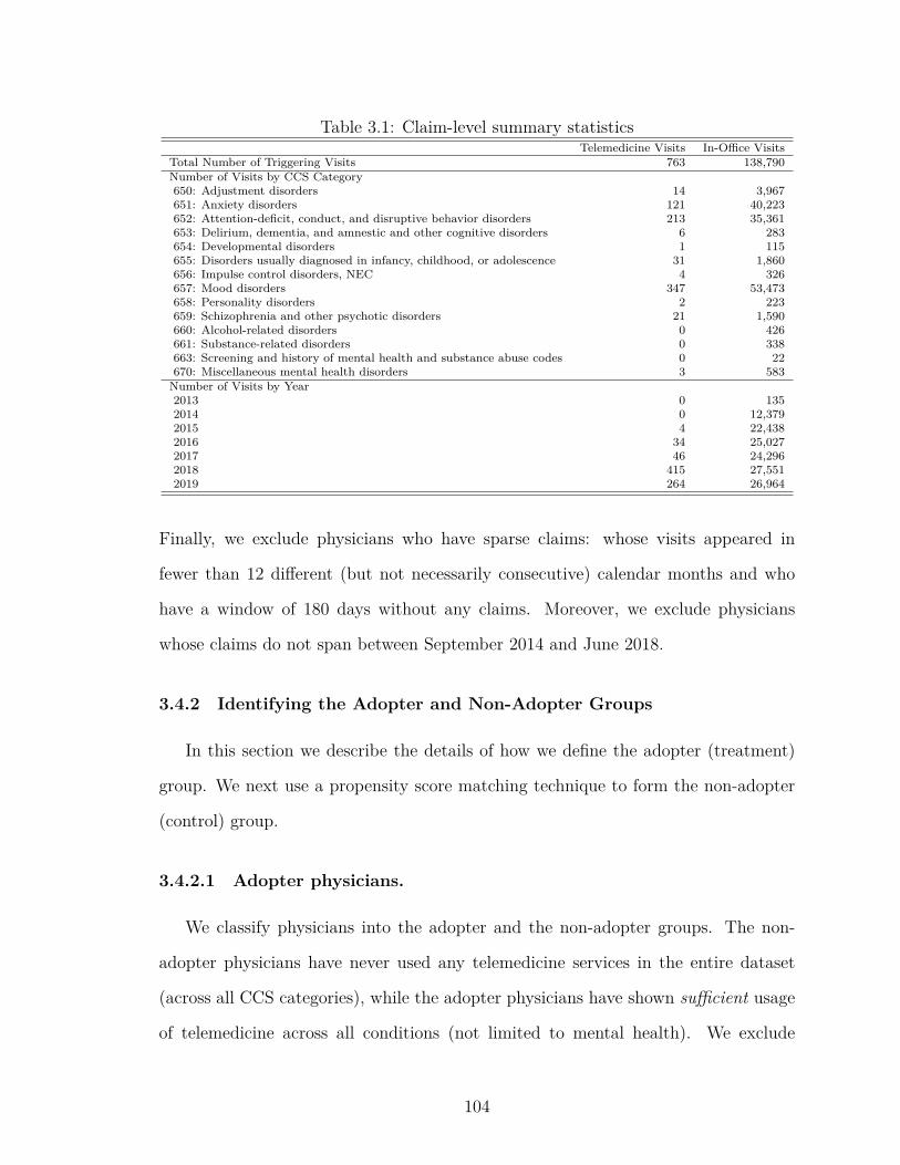
Table 3.1: Claim-level summary statisticsTelemedicine Visits In-Office Visits

Total Number of Triggering Visits 763 138,790Number of Visits by CCS Category650: Adjustment disorders 14 3,967651: Anxiety disorders 121 40,223652: Attention-deficit, conduct, and disruptive behavior disorders 213 35,361653: Delirium, dementia, and amnestic and other cognitive disorders 6 283654: Developmental disorders 1 115655: Disorders usually diagnosed in infancy, childhood, or adolescence 31 1,860656: Impulse control disorders, NEC 4 326657: Mood disorders 347 53,473658: Personality disorders 2 223659: Schizophrenia and other psychotic disorders 21 1,590660: Alcohol-related disorders 0 426661: Substance-related disorders 0 338663: Screening and history of mental health and substance abuse codes 0 22670: Miscellaneous mental health disorders 3 583

Number of Visits by Year2013 0 1352014 0 12,3792015 4 22,4382016 34 25,0272017 46 24,2962018 415 27,5512019 264 26,964

Finally, we exclude physicians who have sparse claims: whose visits appeared in

fewer than 12 different (but not necessarily consecutive) calendar months and who

have a window of 180 days without any claims. Moreover, we exclude physicians

whose claims do not span between September 2014 and June 2018.

3.4.2 Identifying the Adopter and Non-Adopter Groups

In this section we describe the details of how we define the adopter (treatment)

group. We next use a propensity score matching technique to form the non-adopter

(control) group.

3.4.2.1 Adopter physicians.

We classify physicians into the adopter and the non-adopter groups. The non-

adopter physicians have never used any telemedicine services in the entire dataset

(across all CCS categories), while the adopter physicians have shown sufficient usage

of telemedicine across all conditions (not limited to mental health). We exclude

104

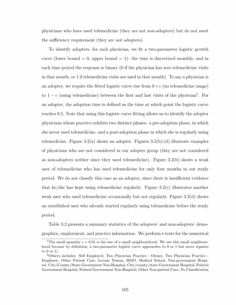
physicians who have used telemedicine (they are not non-adopters) but do not meet

the sufficiency requirement (they are not adopters).

To identify adopters, for each physician, we fit a two-parameter logistic growth

curve (lower bound = 0, upper bound = 1): the time is discretized monthly, and in

each time period the response is binary (0 if the physician has zero telemedicine visits

in that month, or 1 if telemedicine visits are used in that month). To say a physician is

an adopter, we require the fitted logistic curve rise from 0+ ϵ (no telemedicine usage)

to 1 − ϵ (using telemedicine) between the first and last visits of the physician5. For

an adopter, the adoption time is defined as the time at which point the logistic curve

reaches 0.5. Note that using this logistic curve fitting allows us to identify the adopter

physicians whose practice exhibits two distinct phases: a pre-adoption phase, in which

she never used telemedicine, and a post-adoption phase in which she is regularly using

telemedicine. Figure 3.2(a) shows an adopter. Figures 3.2(b)-(d) illustrate examples

of physicians who are not considered in our adopter group (they are not considered

as non-adopters neither since they used telemedicine). Figure 3.2(b) shows a weak

user of telemedicine who has used telemedicine for only four months in our study

period. We do not classify this case as an adopter, since there is insufficient evidence

that he/she has kept using telemedicine regularly. Figure 3.2(c) illustrates another

weak user who used telemedicine occasionally but not regularly. Figure 3.2(d) shows

an established user who already started regularly using telemedicine before the study

period.

Table 3.2 presents a summary statistics of the adopters’ and non-adopters’ demo-

graphics, employment, and practice information. We perform t-tests for the numerical5The small quantity ϵ = 0.01 is the size of a small neighbourhood. We use this small neighbour-

hood because by definition, a two-parameter logistic curve approaches to 0 or 1 but never equatesto 0 or 1).

6Others includes: Self Employed, Two Physician Practice - Owner, Two Physician Practice -Employee, Other Patient Care, Locum Tenens, HMO, Medical School, Non-government Hospi-tal, City/County/State Government Non-Hospital, City/county/state Government Hospital, FederalGovernment Hospital, Federal Government Non-Hospital, Other Non-patient Care, No Classification

105

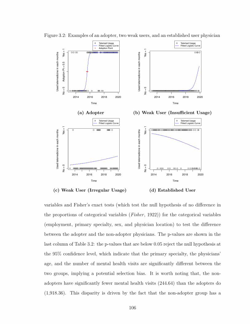
Figure 3.2: Examples of an adopter, two weak users, and an established user physician

2014 2016 2018 2020

Time

Use

d t

ele

me

dic

ine in

ea

ch

mo

nth

s

No

= 0

Ad

op

tio

n P

t =

0.5

Ye

s =

1

o

+

Telemed UsageFitted Logistic CurveAdoption Point

2014 2016 2018 2020

Time

Use

d t

ele

me

dic

ine in

ea

ch

mo

nth

s

No

= 0

Ye

s =

1

o Telemed UsageFitted Logistic Curve

(a) Adopter (b) Weak User (Insufficient Usage)

2014 2016 2018 2020

Time

Use

d te

lem

ed

icin

e in

each

mon

ths

No

= 0

Ye

s =

1

o Telemed UsageFitted Logistic Curve

2014 2016 2018 2020

Time

Use

d te

lem

ed

icin

e in

each

mon

ths

No

= 0

Ye

s =

1

o Telemed UsageFitted Logistic Curve

(c) Weak User (Irregular Usage) (d) Established User

variables and Fisher’s exact tests (which test the null hypothesis of no difference in

the proportions of categorical variables (Fisher, 1922)) for the categorical variables

(employment, primary specialty, sex, and physician location) to test the difference

between the adopter and the non-adopter physicians. The p-values are shown in the

last column of Table 3.2: the p-values that are below 0.05 reject the null hypothesis at

the 95% confidence level, which indicate that the primary specialty, the physicians’

age, and the number of mental health visits are significantly different between the

two groups, implying a potential selection bias. It is worth noting that, the non-

adopters have significantly fewer mental health visits (244.64) than the adopters do

(1,918.36). This disparity is driven by the fact that the non-adopter group has a

106

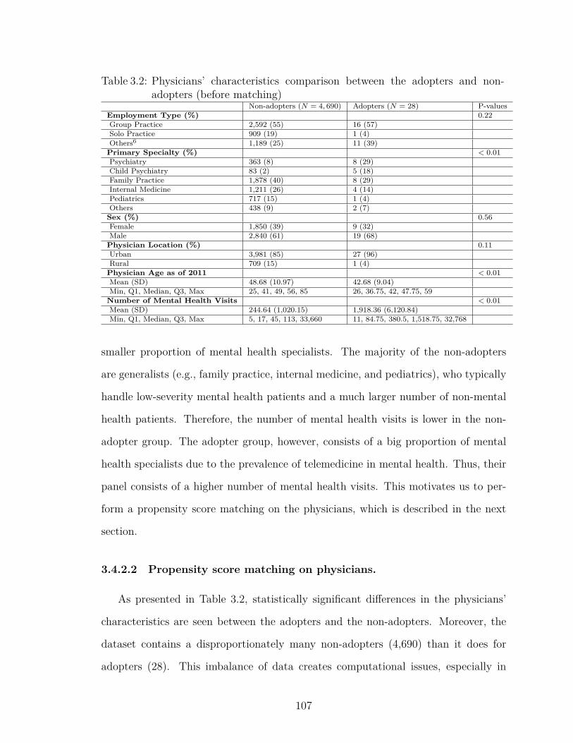
Table 3.2: Physicians’ characteristics comparison between the adopters and non-adopters (before matching)

Non-adopters (N = 4, 690) Adopters (N = 28) P-valuesEmployment Type (%) 0.22Group Practice 2,592 (55) 16 (57)Solo Practice 909 (19) 1 (4)Others6 1,189 (25) 11 (39)

Primary Specialty (%) < 0.01Psychiatry 363 (8) 8 (29)Child Psychiatry 83 (2) 5 (18)Family Practice 1,878 (40) 8 (29)Internal Medicine 1,211 (26) 4 (14)Pediatrics 717 (15) 1 (4)Others 438 (9) 2 (7)

Sex (%) 0.56Female 1,850 (39) 9 (32)Male 2,840 (61) 19 (68)

Physician Location (%) 0.11Urban 3,981 (85) 27 (96)Rural 709 (15) 1 (4)

Physician Age as of 2011 < 0.01Mean (SD) 48.68 (10.97) 42.68 (9.04)Min, Q1, Median, Q3, Max 25, 41, 49, 56, 85 26, 36.75, 42, 47.75, 59

Number of Mental Health Visits < 0.01Mean (SD) 244.64 (1,020.15) 1,918.36 (6,120.84)Min, Q1, Median, Q3, Max 5, 17, 45, 113, 33,660 11, 84.75, 380.5, 1,518.75, 32,768

smaller proportion of mental health specialists. The majority of the non-adopters

are generalists (e.g., family practice, internal medicine, and pediatrics), who typically

handle low-severity mental health patients and a much larger number of non-mental

health patients. Therefore, the number of mental health visits is lower in the non-

adopter group. The adopter group, however, consists of a big proportion of mental

health specialists due to the prevalence of telemedicine in mental health. Thus, their

panel consists of a higher number of mental health visits. This motivates us to per-

form a propensity score matching on the physicians, which is described in the next

section.

3.4.2.2 Propensity score matching on physicians.

As presented in Table 3.2, statistically significant differences in the physicians’

characteristics are seen between the adopters and the non-adopters. Moreover, the

dataset contains a disproportionately many non-adopters (4,690) than it does for

adopters (28). This imbalance of data creates computational issues, especially in

107

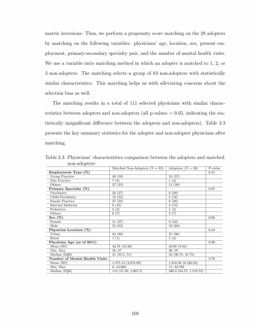
matrix inversions. Thus, we perform a propensity score matching on the 28 adopters

by matching on the following variables: physicians’ age, location, sex, present em-

ployment, primary-secondary specialty pair, and the number of mental health visits.

We use a variable ratio matching method in which an adopter is matched to 1, 2, or

3 non-adopters. The matching selects a group of 83 non-adopters with statistically

similar characteristics. This matching helps us with alleviating concerns about the

selection bias as well.

The matching results in a total of 111 selected physicians with similar charac-

teristics between adopters and non-adopters (all p-values > 0.05, indicating the sta-

tistically insignificant difference between the adopters and non-adopters). Table 3.3

presents the key summary statistics for the adopter and non-adopter physicians after

matching.

Table 3.3: Physicians’ characteristics comparison between the adopters and matchednon-adopters

Matched Non-Adopters (N = 83) Adopters (N = 28) P-valueEmployment Type (%) 0.31Group Practice 49 (59) 16 (57)Solo Practice 7 (8) 1 (4)Others 27 (33) 11 (39)

Primary Specialty (%) 0.97Psychiatry 22 (27) 8 (29)Child Psychiatry 18 (22) 5 (18)Family Practice 27 (33) 8 (29)Internal Medicine 8 (10) 4 (14)Pediatrics 2 (2) 1 (4)Others 6 (7) 2 (7)

Sex (%) 0.66Female 31 (37) 9 (32)Male 52 (63) 19 (68)

Physician Location (%) 0.44Urban 82 (99) 27 (96)Rural 1 (1) 1 (4)

Physician Age (as of 2011) 0.96Mean (SD) 42.78 (10.26) 42.68 (9.04)Min, Max 28, 67 26, 59Median (IQR) 41 (33.5, 51) 42 (36.75, 47.75)

Number of Mental Health Visits 0.70Mean (SD) 1,475.13 (4,872.89) 1,918.36 (6,120.84)Min, Max 6, 33,660 11, 32,768Median (IQR) 113 (31.50, 1,001.5) 380.5 (84.75, 1,518.75)

108

3.4.3 Variables Description

As stated previously, we focus on the effect of telemedicine adoption on the fre-

quency of visits. To do so, we first calculate the revisit interval length (RVI).

To capture the clinical nature and severity of each visit, we create two variables.

First, we pair the CCS category and the procedure code of each visit together as an

interaction categorical variable, which we call the severity variable (Severity). Then,

we compute the comorbidity score (Comorbidity) of each interval by counting the

number of unique CCS categories that are associated with the diagnosis codes (up to

25) of the triggering visit. This method of measuring comorbidity is consistent with

studies and tools using CCS (Machnicki et al., 2009; Radley et al., 2008; Magnan,

2015).

To capture the patient’s historical healthcare utilization, we calculate the number

of emergency department visits and the total charges within the past 90 days of each

visit.

Next, for each visit, we calculate the distance between the patient’s and the physi-

cian’s zipcodes using the Haversine (the great circle) distance in miles.

We also propose a proxy variable to measure the patient’s tech-savviness, which

measures how likely it is for a patient to accept telemedicine. To account for the tech-

savviness of a patient at the time of visit, which is unobservable, we created a variable

named PanelTechSavviness. For each visit, we first identify the annual panel size of

the physician, which is the number of patients who have been seen by the physician

over the past 365 days. Within this panel, we count the number of patients who

have used telemedicine before their first visit with the physician. These patients are

considered tech-savvy and therefore are capable of using telemedicine again, since they

have used telemedicine already. To calculate PanelTechSavviness, we compute the

ratio as number of tech-savvy patientsannual panel size . This ratio measures the overall patients’ acceptance

of telemedicine within a physician’s panel prior to the first visit. Therefore, a larger

109

PanelTechSavviness value implies that a physician wanting to adopt telemedicine may

face less friction from her patients. Note that this variable calculates the number of

tech-savvy patients before their first visit with the physicians. Hence, it will not

impact the physician’s adoption.

Finally, for each interval, we calculate the number of visits (across all CCS cat-

egories) generated by the physician in the calendar month as the variable VisitPer-

Month. This captures the overall workload of the physician.

We apply two exclusion filters on the RVIs. First, we exclude intervals longer

than 180 days since the distant visit may not be related to the first visit as physicians

typically do not schedule follow-up visits so far apart (clinical guidelines recommend

following up within three months for patients with mental health conditions (Mitchell

et al., 2013)). Next, to assure that the RVIs length decisions are made by the physi-

cians instead of patients, we exclude RVIs that are either too short or too long for

each severity group (CCS-procedure code pair). The short RVIs are excluded since

they are likely scheduled by the patients due to insufficient treatment in the last visit.

The long RVIs are exlucded since they may not be related to the initiating visit any-

more and can be scheduled by patients instead of physicians. To do this, we calculate

the RVI standard deviation (SD) and only kept the intervals that are within ± 1.5

SD from the mean RVI for each severity group.

In Table 3.4, we provide the list of variables used for the models we present in

this work. We index the visits by t, the physicians by j, and the patients by i.

The final dataset contains 138,790 in-office visits and 763 telemedicine visits. Ta-

ble 3.5 shows the summary statistics of the RVIs.

3.5 Econometric Model

In this study, we aim to estimate the effect of telemedicine adoption on physi-

cians’ decisions of the length of RVIs. We then further investigate whether such an

110

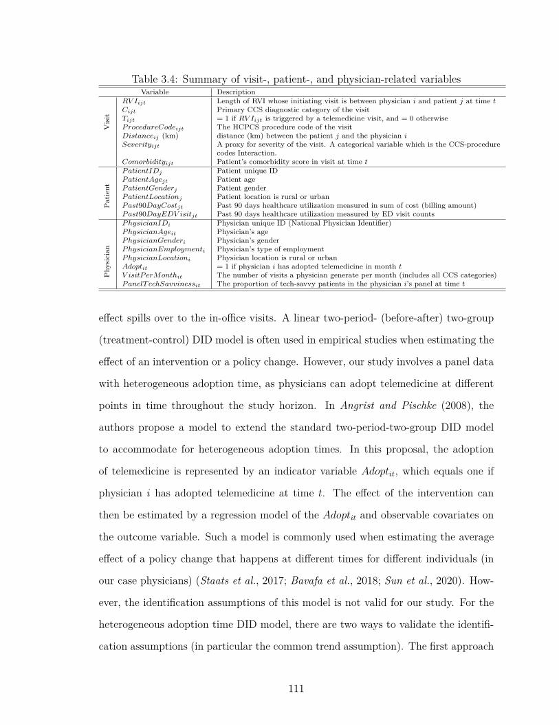
Table 3.4: Summary of visit-, patient-, and physician-related variablesVariable Description

Vis

itRV Iijt Length of RVI whose initiating visit is between physician i and patient j at time tCijt Primary CCS diagnostic category of the visitTijt = 1 if RV Iijt is triggered by a telemedicine visit, and = 0 otherwiseProcedureCodeijt The HCPCS procedure code of the visitDistanceij (km) distance (km) between the patient j and the physician iSeverityijt A proxy for severity of the visit. A categorical variable which is the CCS-procedure

codes Interaction.Comorbidityijt Patient’s comorbidity score in visit at time t

Patie

nt

PatientIDj Patient unique IDPatientAgejt Patient agePatientGenderj Patient genderPatientLocationj Patient location is rural or urbanPast90DayCostjt Past 90 days healthcare utilization measured in sum of cost (billing amount)Past90DayEDV isitjt Past 90 days healthcare utilization measured by ED visit counts

Phy

sici

an

PhysicianIDi Physician unique ID (National Physician Identifier)PhysicianAgeit Physician’s agePhysicianGenderi Physician’s genderPhysicianEmploymenti Physician’s type of employmentPhysicianLocationi Physician location is rural or urbanAdoptit = 1 if physician i has adopted telemedicine in month tV isitPerMonthit The number of visits a physician generate per month (includes all CCS categories)PanelTechSavvinessit The proportion of tech-savvy patients in the physician i’s panel at time t

effect spills over to the in-office visits. A linear two-period- (before-after) two-group

(treatment-control) DID model is often used in empirical studies when estimating the

effect of an intervention or a policy change. However, our study involves a panel data

with heterogeneous adoption time, as physicians can adopt telemedicine at different

points in time throughout the study horizon. In Angrist and Pischke (2008), the

authors propose a model to extend the standard two-period-two-group DID model

to accommodate for heterogeneous adoption times. In this proposal, the adoption

of telemedicine is represented by an indicator variable Adoptit, which equals one if

physician i has adopted telemedicine at time t. The effect of the intervention can

then be estimated by a regression model of the Adoptit and observable covariates on

the outcome variable. Such a model is commonly used when estimating the average

effect of a policy change that happens at different times for different individuals (in

our case physicians) (Staats et al., 2017; Bavafa et al., 2018; Sun et al., 2020). How-

ever, the identification assumptions of this model is not valid for our study. For the

heterogeneous adoption time DID model, there are two ways to validate the identifi-

cation assumptions (in particular the common trend assumption). The first approach

111

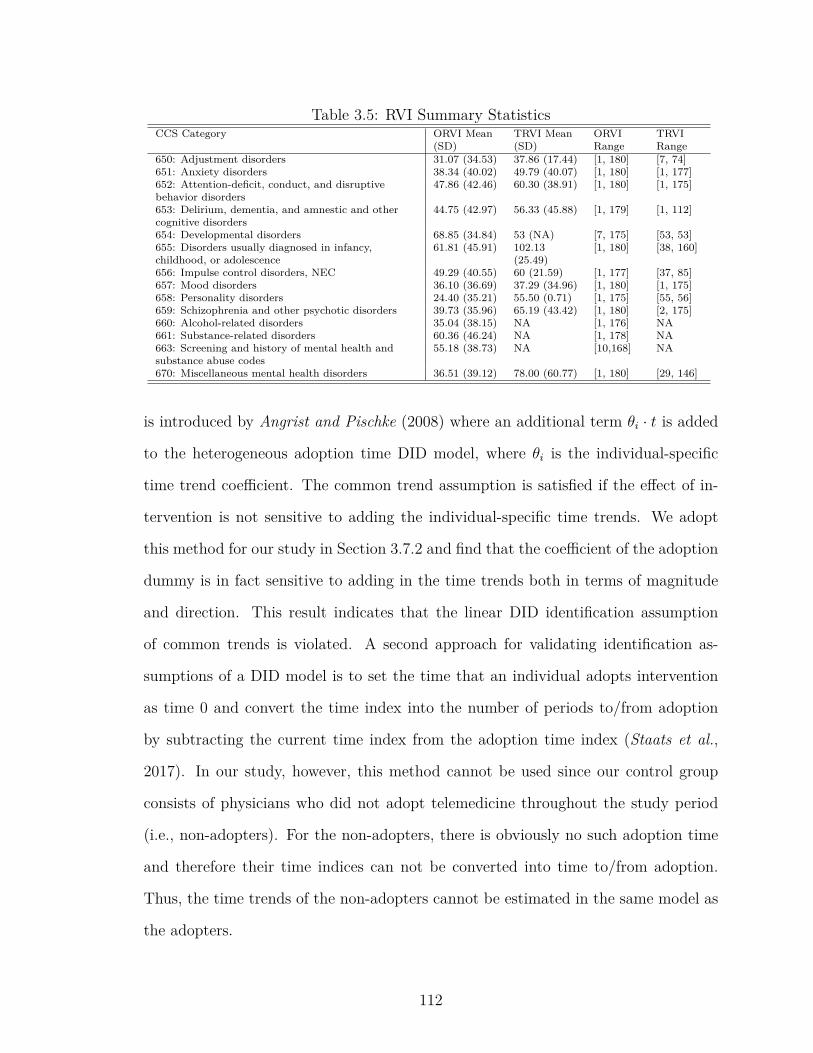
Table 3.5: RVI Summary StatisticsCCS Category ORVI Mean

(SD)TRVI Mean(SD)

ORVIRange

TRVIRange

650: Adjustment disorders 31.07 (34.53) 37.86 (17.44) [1, 180] [7, 74]651: Anxiety disorders 38.34 (40.02) 49.79 (40.07) [1, 180] [1, 177]652: Attention-deficit, conduct, and disruptivebehavior disorders

47.86 (42.46) 60.30 (38.91) [1, 180] [1, 175]

653: Delirium, dementia, and amnestic and othercognitive disorders

44.75 (42.97) 56.33 (45.88) [1, 179] [1, 112]

654: Developmental disorders 68.85 (34.84) 53 (NA) [7, 175] [53, 53]655: Disorders usually diagnosed in infancy,childhood, or adolescence

61.81 (45.91) 102.13(25.49)

[1, 180] [38, 160]

656: Impulse control disorders, NEC 49.29 (40.55) 60 (21.59) [1, 177] [37, 85]657: Mood disorders 36.10 (36.69) 37.29 (34.96) [1, 180] [1, 175]658: Personality disorders 24.40 (35.21) 55.50 (0.71) [1, 175] [55, 56]659: Schizophrenia and other psychotic disorders 39.73 (35.96) 65.19 (43.42) [1, 180] [2, 175]660: Alcohol-related disorders 35.04 (38.15) NA [1, 176] NA661: Substance-related disorders 60.36 (46.24) NA [1, 178] NA663: Screening and history of mental health andsubstance abuse codes

55.18 (38.73) NA [10,168] NA

670: Miscellaneous mental health disorders 36.51 (39.12) 78.00 (60.77) [1, 180] [29, 146]

is introduced by Angrist and Pischke (2008) where an additional term θi · t is added

to the heterogeneous adoption time DID model, where θi is the individual-specific

time trend coefficient. The common trend assumption is satisfied if the effect of in-

tervention is not sensitive to adding the individual-specific time trends. We adopt

this method for our study in Section 3.7.2 and find that the coefficient of the adoption

dummy is in fact sensitive to adding in the time trends both in terms of magnitude

and direction. This result indicates that the linear DID identification assumption

of common trends is violated. A second approach for validating identification as-

sumptions of a DID model is to set the time that an individual adopts intervention

as time 0 and convert the time index into the number of periods to/from adoption

by subtracting the current time index from the adoption time index (Staats et al.,

2017). In our study, however, this method cannot be used since our control group

consists of physicians who did not adopt telemedicine throughout the study period

(i.e., non-adopters). For the non-adopters, there is obviously no such adoption time

and therefore their time indices can not be converted into time to/from adoption.

Thus, the time trends of the non-adopters cannot be estimated in the same model as

the adopters.

112

For the aforementioned reasons, we adopt the nonparametric changes-in-changes

(CIC) model proposed by Athey and Imbens (2006) to estimate the average effect of

adoption. The CIC model has several advantages for this study. First, it allows for

heterogeneous adoption times, which is essential in our problem setting. Second, it

does not impose the common trend assumption as in a DID model. We will later

discuss the assumptions of the CIC model, which are all satisfied with our problem

setting and dataset. Furthermore, the CIC model allows for capturing nonlinear treat-

ment effects due to its non-parametric nature, which generates additional flexibility

for our model.

In what follows, we first describe the CIC model and then detail the application

of this model to test the two main effects of our study.

3.5.1 Heterogeneous Adoption Time CIC Model in Athey and Imbens

(2006)

In this section, we briefly review the CIC model introduced in Athey and Imbens

(2006), the key assumptions, formulation, and its application in a heterogeneous

adoption time setting. CIC models have been used to estimate the average treatment

effect when a linear DID model does not apply (Reza et al., 2020; Borah et al.,

2011; Asteriou et al., 2019; Pieroni and Salmasi, 2016). However, to the best of our

knowledge, all the previous studies focus on the applications of a CIC model in a

two-period-two-group case where the treatment group experiences an intervention in

the second period while the control group does not. In our study, the final dataset

contains 70 months where a physician can adopt telemedicine at anytime. Therefore

we apply the CIC model with multiple adoption periods as introduced in Section 6

of Athey and Imbens (2006), which we briefly describe here.

Let G = {0, 1} and T = {0, 1, . . . , 69} be the set of group and time indices7. Let7The CIC model also allows for multiple groups, but in this study, we only consider the case with

two groups (i.e., treatment and control) and multiple time periods.

113

Y denote the outcome variable where Y Igt and Y N

gt are the outcomes with and without

receiving the treatment in group g at time t respectively. The realized outcome is

then given by Ygt = IY Igt + (1 − I)Y N

gt , where I = 1 if an individual is treated and

I = 0 otherwise.

We start with a two-period-two-group case where g = 1 represents the treatment

group and g = 0 represents the control group. All the individuals in the treatment

group receive an intervention in period t = 1 and the control group remains untreated

in both periods. The average treatment effect on the treated (ATT) is hence ATT =

E[Y I11]−E[Y N

11 ]. Here Y N11 is the counterfactual outcome of the treated group assuming

the treatment does not exist.

In a multi-period case, let I denote the set of group-time pairs (g1, t), where the

individuals in group g1 have been treated at time t ∈ T −{0}. Notice that we consider

no individual receives treatment in the initial period. We can then form a quadruple

for a given adoption period t as (g0, g1, t0, t). Here g0 is an index for observations

that do not receive intervention in either t0 < t or at t, while g1 is an index for

observations that receive an intervention by or at t. In other words, we assume that

after receiving the treatment, an individual continues receiving treatment in all the

remaining periods. That is, if (g1, t) ∈ I, then (g1, t + 1) ∈ I. Our control group

consists of (g0, t0), (g0, t), and (g1, t0) /∈ I for t0 < t. This is similar to dividing the

multi-period case into several two by two subproblems. For each (g1, t) pair, there

exists a treatment effect τg1,t. We then rewrite the average treatment effect of group

g1 at time t as τg1,t = E[Y Ig1,t

]−E[Y Ng1,t

]. Note that the treatment group g1 has received

intervention in period t, so Y Ig1,t

is observable in the data, and the expectation E[Y Ig1,t

]

can be calculated by taking the mean value of Yg1,t. The main challenge here is the

estimation of E[Y Ng1,t

], which requires the counterfactual distribution of Yg1,t in the

absence of intervention. Next we introduce the method to estimate such distribution

proposed by Athey and Imbens (2006).

114

First, we assume that the outcome (RVI length) is determined by the function

h(U, T ), where U is the unobservable characteristics of physicians such as physician

conservativeness in scheduling follow-up visits, and T is the time variable. Note that

such unobservable characteristics is different from the fixed effect that is commonly

used in empirical models. As we will introduce in the assumptions, the value of

U in our model can be time-varying as long as its marginal distribution is time-

invariant, which is different from the fixed effect model. Let hN(U, T ) be the out-

come function without telemedicine adoption, and hI(U, T ) be the outcome function

with telemedicine adoption, we have Yq,g1t0 = hN(Uq, t0), Yq,g1t = hI(Uq, t), Yr,g0t0 =

hN(Ur, t0), and Yr,g0t = hN(Ur, t). Here q and r are the indices of physicians. Note

that the unobservable characteristics can vary across physicians and over time and the

observable characteristics are controlled for by a set of covariates before the estima-

tion of the counterfactual distribution (we will discuss this in more detail in Section

3.5.2). Furthermore, the outcome function is assumed to be strictly increasing in

U . Besides, the unobservable characteristics U is time-invariant within each group.

Finally, we assume that the support of the unobservable characteristics is the same

for all the groups. Let U be the support of the variable U and recall that T is the

set of all the time periods, we now formally introduce these assumptions.

Assumption III.1. The outcome of an individual, in the absence of intervention,

satisfies the relationship: Y N = hN(U, T ).

Assumption III.2. Strict Monotonicity: The outcome function h(., .), where h :

U× T → R, is strictly increasing in U ∈ U for a given t ∈ T .

Assumption III.3. Distribution Time Invariance Within Groups: the marginal dis-

tribution of U is time-invariant conditional on a given group.

Assumption III.4. Support in the Multiple Group and Multiple Time Period Case:

The support of U |G = g, denoted by Ug, is the same for all g ∈ G.

115

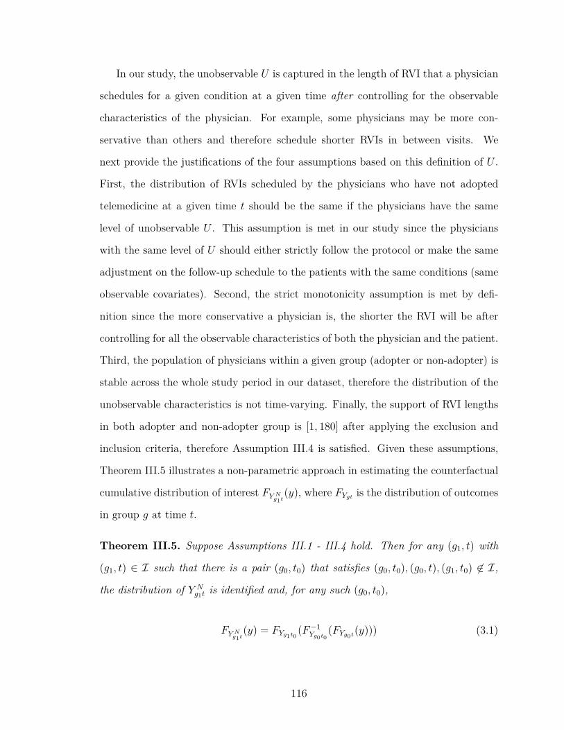
In our study, the unobservable U is captured in the length of RVI that a physician

schedules for a given condition at a given time after controlling for the observable

characteristics of the physician. For example, some physicians may be more con-

servative than others and therefore schedule shorter RVIs in between visits. We

next provide the justifications of the four assumptions based on this definition of U .

First, the distribution of RVIs scheduled by the physicians who have not adopted

telemedicine at a given time t should be the same if the physicians have the same

level of unobservable U . This assumption is met in our study since the physicians

with the same level of U should either strictly follow the protocol or make the same

adjustment on the follow-up schedule to the patients with the same conditions (same

observable covariates). Second, the strict monotonicity assumption is met by defi-

nition since the more conservative a physician is, the shorter the RVI will be after

controlling for all the observable characteristics of both the physician and the patient.

Third, the population of physicians within a given group (adopter or non-adopter) is

stable across the whole study period in our dataset, therefore the distribution of the

unobservable characteristics is not time-varying. Finally, the support of RVI lengths

in both adopter and non-adopter group is [1, 180] after applying the exclusion and

inclusion criteria, therefore Assumption III.4 is satisfied. Given these assumptions,

Theorem III.5 illustrates a non-parametric approach in estimating the counterfactual

cumulative distribution of interest FY Ng1t(y), where FYgt is the distribution of outcomes

in group g at time t.

Theorem III.5. Suppose Assumptions III.1 - III.4 hold. Then for any (g1, t) with

(g1, t) ∈ I such that there is a pair (g0, t0) that satisfies (g0, t0), (g0, t), (g1, t0) ∈ I,

the distribution of Y Ng1t

is identified and, for any such (g0, t0),

FY Ng1t(y) = FYg1t0

(F−1Yg0t0

(FYg0t(y))) (3.1)

116

Please refer to Section 6 of Athey and Imbens (2006) for the proof of Theorem

III.5. Leveraging this result, we can then write the counterfactual value of the outcome

variable Yg1t. Suppose there’s no adoption of telemedicine, then the counterfactual

outcomes for the treated group at time t can be expressed as F−1Yg0t

(FYg0t0(Yg1t0,m)).

The estimated ATT of g1 at time t with the observations in the control group for

each quadruple is:

κg0,g1,t0,t =1

Ng1t

Ng1t∑m=1

Yg1t,m − 1

Ng1t0

Ng1t0∑m=1

F−1Yg0t

(FYg0t0(Yg1t0,m)). (3.2)

In this equation, Ngt represents the number of observations in group g at time t.

The variable Yg1t,m is the mth observation from the physicians who have adopted

telemedicine at time t and Yg1t0,m is the mth observation from the adopter physicians

who have not adopted telemedicine yet at time t0. The function F−1Yg0t

is the inverse

function of the estimated cdf function from Yg0t, which consists of the observations

in the non-adopter group at time t. The function FYg0t0is the estimated cdf function

from Yg0t0 , which consists of the observations in the non-adopter group at time t0.

Now let J be the set of all possible quadruples (g0, g1, t0, t), the full set of estimated

ATT can be then written as κJ . In Athey and Imbens (2006), the authors show that√N(κJ − κJ )

d−→ N (0, VJ ) and VJp−→ VJ , where VJ is the normalized covariance

matrix of√N · κJ under the conditions that: 1) the data is generated following the

procedure introduced in Section 5 of Athey and Imbens (2006) (see Appendix A.2 for

more details), and 2) Assumption III.4 holds.

Note that the estimated effects for κg0,g1,t0,t are different from the estimates of the

average effect τg1t. We then aggregate these estimates through the following equation

for each (g1, t) ∈ I:

τI = (A′V −J A)−1(A′V −

J κJ ), (3.3)

117

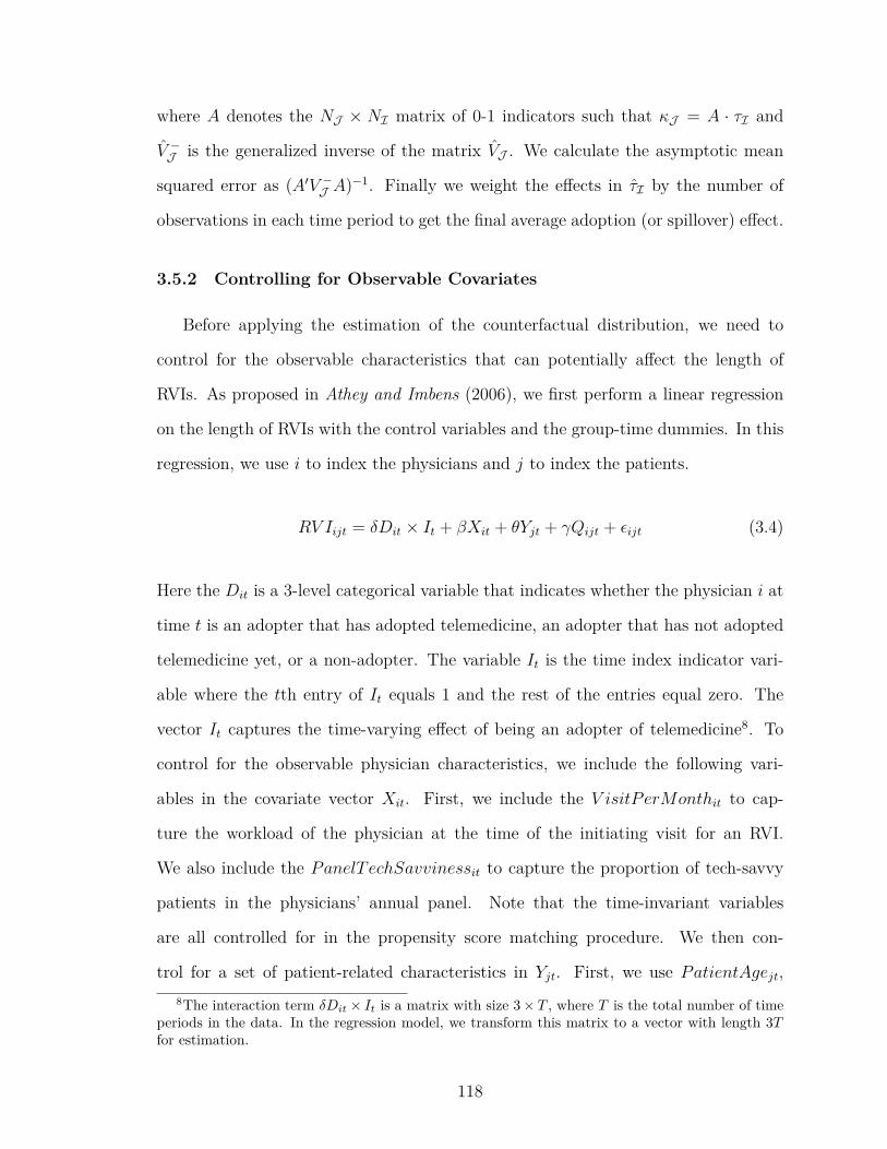
where A denotes the NJ × NI matrix of 0-1 indicators such that κJ = A · τI and

V −J is the generalized inverse of the matrix VJ . We calculate the asymptotic mean

squared error as (A′V −J A)−1. Finally we weight the effects in τI by the number of

observations in each time period to get the final average adoption (or spillover) effect.

3.5.2 Controlling for Observable Covariates

Before applying the estimation of the counterfactual distribution, we need to

control for the observable characteristics that can potentially affect the length of

RVIs. As proposed in Athey and Imbens (2006), we first perform a linear regression

on the length of RVIs with the control variables and the group-time dummies. In this

regression, we use i to index the physicians and j to index the patients.

RV Iijt = δDit × It + βXit + θYjt + γQijt + ϵijt (3.4)

Here the Dit is a 3-level categorical variable that indicates whether the physician i at

time t is an adopter that has adopted telemedicine, an adopter that has not adopted

telemedicine yet, or a non-adopter. The variable It is the time index indicator vari-

able where the tth entry of It equals 1 and the rest of the entries equal zero. The

vector It captures the time-varying effect of being an adopter of telemedicine8. To

control for the observable physician characteristics, we include the following vari-

ables in the covariate vector Xit. First, we include the V isitPerMonthit to cap-

ture the workload of the physician at the time of the initiating visit for an RVI.

We also include the PanelTechSavvinessit to capture the proportion of tech-savvy

patients in the physicians’ annual panel. Note that the time-invariant variables

are all controlled for in the propensity score matching procedure. We then con-

trol for a set of patient-related characteristics in Yjt. First, we use PatientAgejt,8The interaction term δDit × It is a matrix with size 3× T , where T is the total number of time

periods in the data. In the regression model, we transform this matrix to a vector with length 3Tfor estimation.

118

PatientGenderj, and PatientLocationj to capture the demographic characteristics.

Furthermore, we use the patient’s total number of visits to the emergency depart-

ment (Past90DayEDV isitjt) and the total cost of healthcare in the past 90 days

(Past90DayCostjt) to capture his/her utilization of healthcare resources. Finally,

we include visit-specific variables in the vector Qijt: Distanceij, Comorbidityijt and

Severityijt. We include the distance between physician and patient (Distanceij)

since the travel time may affect the visiting frequency. We then include the patients’

Comorbidityijt measured by the total number of diagnosis categories the patient has

in the initiating visit of the RVI to measure the health condition of the patient. Since

physicians may hope to follow-up sooner with the patients under more severe condi-

tions, we also include Severityijt in the regression, which is the CCS-Procedure Code

pair at the initiating visit.

After performing the regression estimation, we then obtain a new outcome variable˜RV I ijt by subtracting the effect of the observable characteristics from the original

outcome variable RV Iijt. Specifically, we now have ˜RV I ijt = RV Iijt − βXit − θYjt −

γQijt, where ˜RV I ijt is used in all the CIC estimations below as the outcome variable.

3.5.3 Effect Estimation

As mentioned above, our model differs from a standard DID model, in each time

period t, we have three types of physicians: 1) those who have adopted telemedicine,

2) those who have not adopted telemedicine but will adopt in the future, and 3) those

who do not adopt throughout the study period. In each CIC model, we will include

different observations from these three types of physicians in the estimation. Next,

we introduce the details in the estimation procedures for the telemedicine adoption

effect, the spillover effect, and the dynamics in both effects.

119

3.5.3.1 Telemedicine adoption effect.

In the estimation for telemedicine adoption effect, we have four groups of obser-

vations for a given quadruple (g0, g1, t0, t) (in the estimation of κg0,g1,t0,t): Yg0t0 , Yg0t,

Yg1,t0 , and Yg1t. Explicitly, Yg0t0 contains all the observations from the non-adopter

physicians at time t0; Yg0t contains all the observations from non-adopters at time

t; Yg1t0 includes all the observations from the adopter physicians who have not yet

adopted telemedicine at t0; and Yg1t includes observations at time t from the physi-

cians who have adopted telemedicine by t. These four sets of observations will be

combined to estimate the effect κg0,g1,t0,t for this given quadruple.

3.5.3.2 Spillover effect.

The spillover effect focuses on the impact of telemedicine adoption on the in-office

initiated RVIs for the adopters. Therefore we exclude the telemedicine initiated RVIs

from the adopters in the treatment group in this test. Specifically, we have the same

set of Yg0t0 , Yg0t, and Yg1t0 as those in the telemedicine adoption effect estimation, but

exclude the telemedicine initiated RVIs from the Yg1t and only focus on the in-office

initiated visits.

3.5.3.3 Dynamic effect.

To assess the short- and long-term effects of the adoption of telemedicine and

the spillover, we perform a sub-sample analysis with the following steps. First, we

compute the adoption time length as the number of months between the time of the

initiated visit and the adoption time of the visited physician for all the post-adoption

observations in the data. We then select all the observations with an adoption time

length less than t, where t takes values of {6, 9, 12, · · · , 36} months9. These observa-9In our dataset, most of the adopter physicians have adopted telemedicine for less than 36 months

at the end of the study period.

120

tions are then combined with all the observations from the non-adopter group and the

pre-adoption observations from the adopter group to form a sub-sample. This sub-

sample is fed into the CIC model to estimate the telemedicine adoption and in-office

spillover effects after adopting telemedicine for t months.

3.6 Results

In this section, we present the estimation results for the telemedicine adoption

and the spillover effects.

3.6.1 Controlling for Observable Covariates: Regression Results

Before applying the CIC method, we first control for the observable characteristics

of both patients and physicians as introduced in Section 3.5.2 in a linear regression

model. Recall that, in the propensity score matching analysis we conducted earlier,

we controlled for the time-invariant characteristics of the physicians.

Table 3.6 presents the observable covariates’ coefficients estimation results based

on a linear regression model. There are several variables that are worth paying at-

tention to. First, as the patient’s comorbidity increases, the length of RVIs increases.

Here, a larger comorbidity indicates that the patient has multiple medical concerns

across all CCS categories at the same time. In this case, they may need to sched-

ule visits with multiple physicians within a short period and therefore may have

less availability. Hence the mental health visit may not receive the highest priority in

their treatment plan and the physicians may schedule the mental health visits further

apart. Second, we observe that larger medical cost and more Emergency Department

visits in the past 90 days result in shorter RVIs. The reason is that high utilization

of healthcare services indicates a need for close monitoring of their health status.

Third, if the patient is visiting a physician with more scheduled visits per month (i.e.,

higher V isitPerMonth), then the RVI length is going to be shorter. The physicians

121

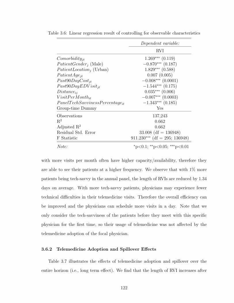
Table 3.6: Linear regression result of controlling for observable characteristics

Dependent variable:RVI

Comorbidityjt 1.269∗∗∗ (0.119)PatientGenderj (Male) −0.870∗∗∗ (0.187)PatientLocationj (Urban) 1.829∗∗∗ (0.588)PatientAgejt 0.007 (0.005)Past90DayCostjt −0.008∗∗∗ (0.0001)Past90DayEDV isitjt −1.544∗∗∗ (0.175)Distanceij 0.035∗∗∗ (0.006)V isitPerMonthit −0.007∗∗∗ (0.0003)PanelTechSavvinessPercentageit −1.343∗∗∗ (0.185)Group-time Dummy YesObservations 137,243R2 0.662Adjusted R2 0.662Residual Std. Error 33.008 (df = 136948)F Statistic 911.230∗∗∗ (df = 295; 136948)

Note: ∗p<0.1; ∗∗p<0.05; ∗∗∗p<0.01

with more visits per month often have higher capacity/availability, therefore they

are able to see their patients at a higher frequency. We observe that with 1% more

patients being tech-savvy in the annual panel, the length of RVIs are reduced by 1.34

days on average. With more tech-savvy patients, physicians may experience fewer

technical difficulties in their telemedicine visits. Therefore the overall efficiency can

be improved and the physicians can schedule more visits in a day. Note that we

only consider the tech-savviness of the patients before they meet with this specific

physician for the first time, so their usage of telemedicine was not affected by the

telemedicine adoption of the focal physician.

3.6.2 Telemedicine Adoption and Spillover Effects

Table 3.7 illustrates the effects of telemedicine adoption and spillover over the

entire horizon (i.e., long term effect). We find that the length of RVI increases after

122

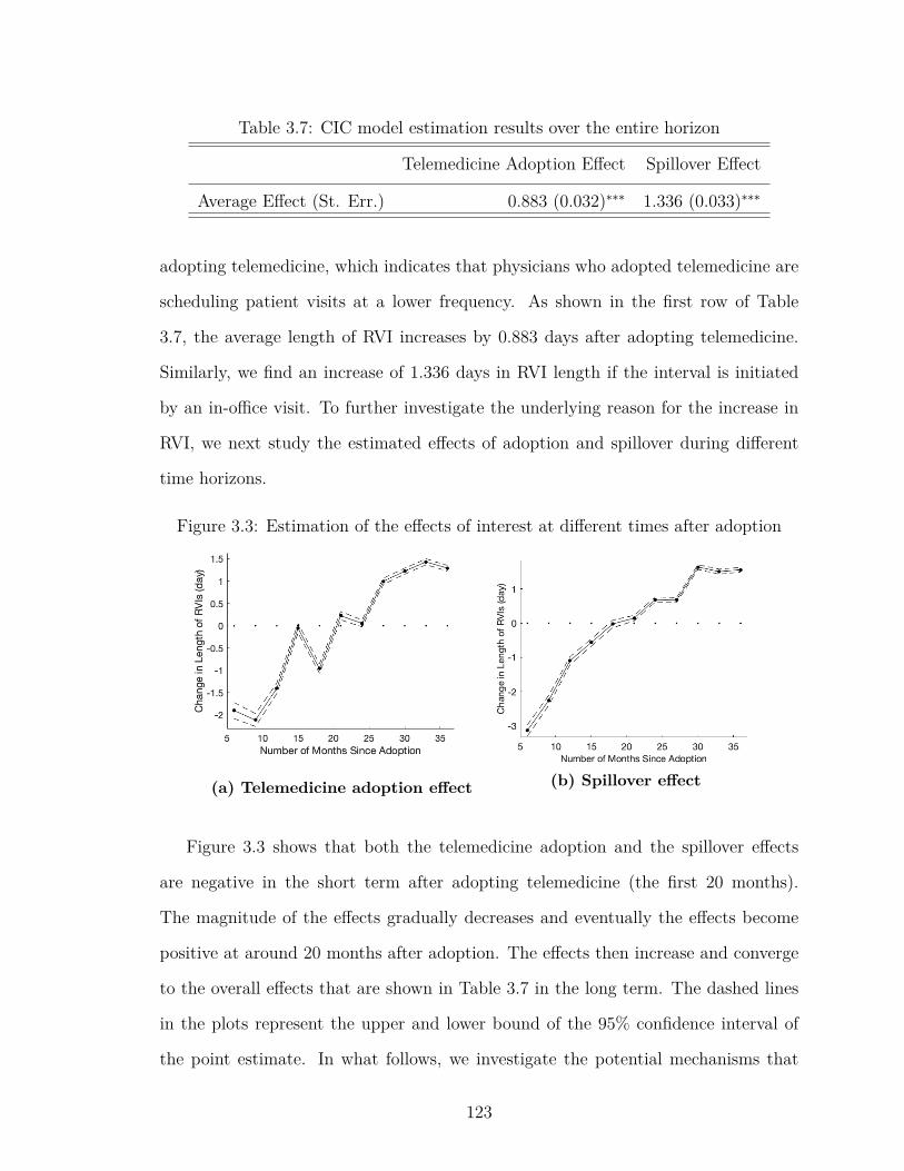
Table 3.7: CIC model estimation results over the entire horizon

Telemedicine Adoption Effect Spillover Effect

Average Effect (St. Err.) 0.883 (0.032)∗∗∗ 1.336 (0.033)∗∗∗

adopting telemedicine, which indicates that physicians who adopted telemedicine are

scheduling patient visits at a lower frequency. As shown in the first row of Table

3.7, the average length of RVI increases by 0.883 days after adopting telemedicine.

Similarly, we find an increase of 1.336 days in RVI length if the interval is initiated

by an in-office visit. To further investigate the underlying reason for the increase in

RVI, we next study the estimated effects of adoption and spillover during different

time horizons.

Figure 3.3: Estimation of the effects of interest at different times after adoption

(a) Telemedicine adoption effect (b) Spillover effect

Figure 3.3 shows that both the telemedicine adoption and the spillover effects

are negative in the short term after adopting telemedicine (the first 20 months).

The magnitude of the effects gradually decreases and eventually the effects become

positive at around 20 months after adoption. The effects then increase and converge

to the overall effects that are shown in Table 3.7 in the long term. The dashed lines

in the plots represent the upper and lower bound of the 95% confidence interval of

the point estimate. In what follows, we investigate the potential mechanisms that

123

can lead to these observations.

3.6.3 Explanation of the Observations

As introduced in Section 3.3.2.1, there are two mechanisms that can lead to pos-

itive long-term telemedicine adoption and spillover effects: operational inefficiency

and heavy workload. The negative telemedicine adoption and spillover effects in the

short term, indicate that the operational inefficiency did not significantly impact the

RVIs in the short-term and as a result should not be an active mechanism in ex-

plaining the positive long-term telemedicine adoption and spillover effects. If there

is a significant inefficiency introduced by telemedicine mode of service, we should

have observed an increase in length of RVIs, including the in-office initiated RVIs,

right after the adoption of telemedicine. We next test if the increase in RVI length

is due to increased workload. As mentioned before, telemedicine allows physicians

to admit patients from a broader geographical area, which can lead to an increase

in the physicians’ panel size. The expanded panel size may reduce the availability

of the physicians and therefore lead to an increase in the RVI length. To test if this

mechanism is active, we performed a sub-sample analysis by selecting the physicians

with a low workload to re-estimate the telemedicine adoption and the spillover effects.

These physicians are less likely to have fully utilized their availability and hence are

not impacted by the high workload. Specifically, we select the RVIs scheduled by

physicians who have less than 500 visits that month, which is the mean number of

visits per month in our dataset. With the low workload physicians, the adoption

of telemedicine leads to a decrease in RVI length by 1.84 days over the entire hori-

zon (St. Err.: 0.047). When we focus on the in-office initiated RVIs, the adoption

of telemedicine has a spillover effect of -0.016 days (St. Err.: 0.00039) on the low

workload physicians. These results further confirm that the increase in RVI length is

caused by the increased workload accumulated as the physicians adopt telemedicine

124

for a longer time. Besides, the negative adoption effect in this analysis suggests that

the physicians are able to schedule more frequent visits with a lower workload. As

we will discuss in more detail below, this decrease in RVI length is likely caused by

an efficiency improvement.

The negative short-term telemedicine adoption effect can be caused by efficiency

improvement or telemedicine inadequacy. In the short term after adoption, the physi-

cians are scheduling more frequent visits following both in-office and telemedicine

visits. Such negative short-term adoption and spillover effects suggest that there can

be an operational efficiency improvement after adopting telemedicine.

To test if physicians are scheduling more frequent visits with their patients due to

inadequate information during telemedicine visits, we need to test if physicians behave

differently during telemedicine visits vs in-office visits. Note that the spillover effect

result shows that the in-office initiated RVIs are impacted by the telemedicine visits,

hence we can not directly take the difference between the empirical distributions of

telemedicine and in-office initiated visits’ RVI lengths. Here, we follow the same logic

as in the CIC estimation to estimate the difference in the distribution of telemedicine

initiated RVI length and the counterfactual distribution of in-office initiated RVI

length within the adopter group. Let Y T be the observations of telemedicine initiated

visits’ RVIs and Y O be the RVIs initiated by in-office visits. Using the observations

in the non-adopter group and the adopter group before adoption at time t0 as the

control group, the average effect of using a telemedicine visit on the length of RVIs

at a given time t can be expressed as:

γg0,g1,t0,t =1

NTg1t

NTg1t∑

k=1

Y Tg1t,k

− 1

NOg1t

NOg1t∑

k=1

F−1Y Og0t(FY O

g0t0(Y O

g1t,k)) (3.5)

Note that although we use Y Og0t0

and Y Og0t

in this equation, there are actually no

telemedicine visits in the group g0. The first term in the equation calculates the

125

Figure 3.4: Telemedicine Usage Effect Estimation Result

mean of all the telemedicine initiated RVIs in g1 at time t and the second term

gives the mean value of the transformed in-office initiated RVIs in g1 through the

counterfactual distribution function estimated from g0. Note that in this estimation,

we are not computing the difference in the length of RVIs before and after adoption.

Instead, we are computing the difference between the telemedicine initiated and the

in-office initiated RVIs within the adopter group in the post-adoption periods. As

suggested by the result of spillover effect, the length of in-office initiated RVIs are also

impacted by the adoption of telemedicine. Hence in the second term of this equation,

we compute the mean of the counterfactual distribution of in-office initiated RVIs in

the post-adoption period (Y Og1t,k

) supposing that there’s no adoption of telemedicine.

The counterfactual distribution allows us to estimate the telemedicine usage effect

free of the potential impact from spillover effect. The aggregation of γg0,g1,t0,t follows

the same logic as in the CIC model introduced above. Finally, we get a set of average

telemedicine usage effects θI , similar to the τI in the estimation of the previous two

effects. We then aggregate θI by weighting it over the number of observations.

We follow the same procedure introduced in Section 3.5.3.3 to estimate the telemedicine

usage effect at different times after the adoption. The results in Figure 3.4 show that

the telemedicine initiated RVIs are constantly smaller than the in-office initiated RVIs

at different stages of adoption. In this figure, the dashed lines are the upper and lower

bound of the 95% confidence interval of the point estimates. When the physicians

have just adopted telemedicine, the length of telemedicine initiated RVIs are signifi-

126

cantly shorter than the in-office initiated ones by over 20 days. Such a significantly

negative telemedicine usage effect suggests that the physicians are likely to be uncer-

tain about the patients’ health status after a telemedicine visit when they had just

adopted telemedicine. As a result, they need to schedule a related visit within a short

time to check their patients again. As the physicians use telemedicine for a longer

time, they accumulate more knowledge and skills in telemedicine and therefore sched-

ule related visits with relatively longer intervals. However, compared to the in-office

initiated RVIs, those initiated by telemedicine still have shorter RVIs on average. In

the long term, adopter physicians’ telemedicine initiated RVIs were on average 3 to 4

days shorter than in-office initiated RVIs. Unlike the telemedicine adoption effect or

the spillover effect, the telemedicine usage effect is constantly negative. Such a con-

stant negative effect suggests that telemedicine visits are inadequate compared to the

in-office visits. As a result, the physicians need to adjust the follow-up visits’ schedule

to accommodate for the missing information during telemedicine visits which results

in an overutilization of the healthcare system. We also need to point out that as the

physicians adopt telemedicine for a longer time, the magnitude of the effect shrinks

and gradually converges to a stable level. As we discussed before, the physician’s be-

havioral change in scheduling follow up visits due to the adoption of telemedicine can

spill over to in-office visits. However, since we observe a positive long-term spillover

effect and a negative telemedicine usage effect, we have evidence that such behavioral

change in telemedicine visits is not significantly impacting the in-office visits. Note

that although the in-office initiated RVIs are not impacted by the adopters’ behav-

ioral change in scheduling follow up visits, they are still impacted by the efficiency

improvement and limited capacity of the adopters. The negative telemedicine usage

effect also explains the difference in magnitude of the telemedicine adoption effect

(0.883) and the spillover effect (1.336). Notice that the telemedicine adoption effect

captures the combination of spillover and telemedicine usage effects resulting in a

127

lower magnitude for the adoption effect.

Next, we continue to explain the increasing trend in telemedicine adoption

and spillover effects over time, which can potentially be caused by the patient panel

expansion and limited availability of the physician. We perform a CIC estimation

with the number of new patients admitted every month as our outcome variable10.

Similar to the CIC estimation of the adoption effects, we also control for the physician

observable characteristics before conducting the CIC method in this analysis. The

result shows that physicians admit 1.358 (with St. Err. of 0.013) more patients per

month after adopting telemedicine on average. In the field of mental health, patients

usually need to have repeated visits with the physicians for a relatively long period.

Therefore, the additional new patients will be accumulated in the long term and cause

a significant amount of extra visits for the adopter physicians. As the physicians’

availability is reduced, the length of RVIs is going to increase, especially for in-office

initiated RVIs. Using this result combined with the sub-sample analysis for low

workload physicians, we can conclude that the increasing trend in both telemedicine

adoption and spillover effects are caused by the patient panel expansion and limited

availability of physicians.

In summary, we observe an increase in RVI length after the physicians adopt

telemedicine over the long run. The additional analyses suggest that such an increase

is not due to operational inefficiencies of adopting telemedicine and is caused by the

increased workload and limited availability of physicians after adopting telemedicine

over a long horizon. In fact, we show that adopting telemedicine can potentially im-

prove the operational efficiency. Compared with in-office visits, physicians schedule

visits with shorter RVIs to accommodate for the uncertainty arisen during telemedicine

visits.10Here we use the continuous multi-period CIC model to approximate the effect of telemedicine

adoption on the new patient admission.

128

3.7 Additional Analysis and Robustness Checks

We extend our study to estimate the effect of telemedicine adoption on the quality

of care. We then test if the effect is different between new patient visits and estab-

lished patient visits. Finally, we test the validity of an alternative linear difference-

in-difference model.

3.7.1 New Patient Visits Vs. Established Patient Visits

In the previous section, we show that physicians admit more patient after adopting

telemedicine. In this analysis, we hope to test whether physicians treat the new

patients and established patients differently. We perform the test by a sub-sample

analysis where the first sample only contains the new patient visits initiated RVIs

and the second dataset contains the rest of the RVIs. The results in Table 3.8 show

that physicians do not behave differently during the new patient visits.

Table 3.8: Telemedicine Adoption Effect on New Patient Visits V.S. Established Pa-tient Visits

New Patient Visit Established Patient Visit

Average Effect (St. Err.) 3.396 (0.164) 3.403 (0.030)

3.7.2 Linear Difference-in-Difference Model

Besides the CIC model, a linear difference-in-difference model is often used to

estimate the effect of an intervention. In this section, we estimate the telemedicine

adoption effect with the linear difference-in-difference (DID) model as a robustness

check. We estimate the effect of telemedicine adoption on the length of RVIs following

the regression DID method for multiple periods in Angrist and Pischke (2008). Since

our original outcome is skewed, we use the logarithm transformation of the RVI length

to fit the linear form of the regression model. We then estimate the adoption effect

129

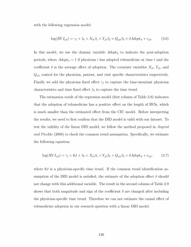
with the following regression model:

log(RV Iijt) = γi + λt +Xitβ1 + Yjtβ2 +Qijtβ3 + δAdoptit + ϵijt (3.6)

In this model, we use the dummy variable Adoptit to indicate the post-adoption

periods, where Adoptit = 1 if physician i has adopted telemedicine at time t and the

coefficient δ is the average effect of adoption. The covariate variables Xit, Yjt, and

Qijt control for the physician, patient, and visit specific characteristics respectively.

Finally we add the physician fixed effect γi to capture the time-invariant physician

characteristics and time fixed effect λt to capture the time trend.

The estimation result of the regression model (first column of Table 3.9) indicates

that the adoption of telemedicine has a positive effect on the length of RVIs, which

is much smaller than the estimated effect from the CIC model. Before interpreting

the results, we need to first confirm that the DID model is valid with our dataset. To

test the validity of the linear DID model, we follow the method proposed in Angrist

and Pischke (2008) to check the common trend assumption. Specifically, we estimate

the following equation:

log(RV Iijt) = γi + θit+ λt +Xitβ1 + Yjtβ2 +Qijtβ3 + δAdoptit + ϵijt, (3.7)

where θit is a physician-specific time trend. If the common trend identification as-

sumption of the DID model is satisfied, the estimate of the adoption effect δ should

not change with this additional variable. The result in the second column of Table 3.9

shows that both magnitude and sign of the coefficient δ are changed after including

the physician-specific time trend. Therefore we can not estimate the causal effect of

telemedicine adoption in our research question with a linear DID model.

130

Table 3.9: Linear DID Model ResultDependent variable:

log(RVI)DID Model Common Trend Assumption Check

PatientGenderj (Male) −0.025∗∗∗ (0.005) −0.024∗∗∗ (0.005)PatientLocationj (Urban) 0.022 (0.016) 0.018 (0.016)PatientAgejt 0.0001 (0.0001) 0.0003∗ (0.0001)Comorbidityjt 0.006 (0.003) 0.004 (0.003)Past90DayCostjt −0.0003∗∗∗ (0.00000) −0.0003∗∗∗ (0.00000)Past90DayEDV isitjt −0.017∗∗∗ (0.005) −0.018∗∗∗ (0.005)Distanceij 0.001∗∗∗ (0.0002) 0.001∗∗∗ (0.0002)V isitPerMonthit −0.0001∗∗∗ (0.00002) −0.0002∗∗∗ (0.00002)PanelTechSavvinessPercentageit 0.079∗∗∗ (0.009) 0.010 (0.011)Adoptit 0.051∗∗∗ (0.010) −0.042∗∗ (0.018)Time Dummy Yes YesPhysician Fixed Effect Yes YesPhysician-specific Time Trend No YesObservations 137,243 137,243R2 0.937 0.937Adjusted R2 0.937 0.937Residual Std. Error 0.846 (df = 136972) 0.843 (df = 136875)F Statistic 7,502.284∗∗∗ (df = 271; 136972) 5,565.149∗∗∗ (df = 368; 136875)

Note: ∗p<0.1; ∗∗p<0.05; ∗∗∗p<0.01

3.8 Conclusion

In this study, we aim to answer the question of whether physicians schedule

related visits differently after adopting telemedicine. To answer this question, we

use a changes-in-changes model with the claims data from BCBSM to estimate the

telemedicine adoption effect. Specifically, we estimate the effect of telemedicine adop-

tion at different stages after the initial adoption. Our results show that the length of

RVIs increases after telemedicine adoption in the long term while it decreases in the

short term after adoption (about 20 months). Moreover, this effect of telemedicine

adoption is spilled over to the in-office initiated RVIs and leads to an increase in

their length as well over the long run. When the physicians first adopt telemedicine,

they schedule shorter RVIs with their patients, regardless of the service mode of the

initiating visit. As physicians adopt telemedicine over a longer horizon, the in-office

initiated RVIs becomes longer (even longer than the pre-adoption RVIs).

We discuss several mechanisms that can explain these effects. First, the opera-

tional efficiency improves initially after the adoption, which causes a decrease in RVI

131

length. The improvement in efficiency then allows physicians to schedule more visits

in a day and admit more new patients. In the long term, the adopter physicians

will reach their capacity limit and need to schedule visits with longer RVIs for the

in-office patients. The telemedicine initiated visits, however, still need to be followed

up with shorter RVIs due to the missing information and uncertainty in health sta-

tus of the patients. In addition, we provide several extensions to the main analysis.

We compare the effect of adoption on the new vs. established patients, and observe

no heterogeneity. We also estimate the effects using a linear difference-in-differences

model and show that the common trend assumption is not valid with our dataset and

problem setting. Therefore we can not use a linear DID model to estimate the effect

of telemedicine adoption.

This paper makes contributions to both literature and practice. Our paper is

among the first that studies the effect of adopting and using real-time reimbursable

telemedicine on the physicians’ decision to schedule follow-up visits. To the best

of our knowledge, we are the first paper that applies the changes-in-changes model

under a multiple-period setting. We provide theoretical and empirical evidence for the

potential problems of using a linear DID model under our setting. Finally, we provide

an extension to the CIC model for comparing the difference between telemedicine and

in-office initiated RVIs within the adopter group in the post-adoption periods.

This paper provides several important managerial insights to healthcare providers

and policy makers. First, telemedicine may not be treated as a perfect substi-

tute for the in-office visits. Our results show that physicians schedule related visits

with significantly shorter RVIs after a telemedicine visit. Second, physicians who

adopt telemedicine may need to re-evaluate their capacity under the new practice

scheme. At the beginning of adopting telemedicine, physicians may observe a promi-

nent efficiency improvement and begin to admit more new patients. Physicians need

to correctly estimate the new capacity limit and their availability after adopting

132

telemedicine and then control their new patient admission rate to avoid the potential

overwhelm of workload. Finally, since our result suggests that telemedicine visits are

relatively inadequate, practitioners may need to schedule in-office visits periodically

to resolve the uncertainty of telemedicine visits.

133

CHAPTER IV

Search Page Personalization: A

Consider-then-choose Model

4.1 Introduction

In the past decade, the emergence of e-commerce has revolutionized the way mer-

chants sell and the way consumers shop. Today, e-commerce is one of the fastest

growing sectors across the globe. For example, as one of the biggest e-commerce

companies in the world, Alibaba owns and operates several C2C, B2C, and B2B

e-commerce platforms (Taobao, Tmall, Aliexpress, etc). In Q2 of 2018, Alibaba’s

revenue from e-commerce has increased 61% year-over-year to RMB 69,188 million

(equivalent to US $10,456 million). This large and fast-growing market faces a unique

set of opportunities and challenges.

Compared to brick-and-mortar stores, E-commerce has several unique features,

which necessitate novel models to accurately capture users’ shopping experience.

Shopping on an e-commerce platform is a two-stage process. In stage one (forming a

consideration set), a consumer typically search for a keyword or select a category and

browses the search result page. On this page, items’ thumbnails pictures along with

the price, rating scores (stars), historical sales, banners, and some seller information

are presented. The customer will browse through these thumbnails and select a subset

134

Figure 4.1: Example of Thumbnail (Left Panel) and Item Page (Right Panel)

of items of interests. In stage two (choose from the consideration set), the consumer

will click the thumbnail and browse the item page to obtain additional information of

the item (e.g., specifications, detailed reviews, warranty, etc). Note that consumers

need to spend some viewing cost (time and effort) to browse through the item pages.

Through the two stages, the consumer will make her purchase decision. By contrast,

in a brick-and-mortar store, it is generally a one stage process: the actual products

are physically presented to the consumer for her to choose from.

Although in some special cases, we may see a two-stage process in brick-and-

mortar stores too, for example, browsing and select a subset of apparel products

(stage one), then go to the fitting room to try them on. Nonetheless, it is worth

highlighting that on an e-commerce platform, consumers are presented with two sets

of information that may differ drastically. Therefore, the utilities from the two stages

may also differ drastically. For example, the left panel of Figure 4.1 is one of the

thumbnails a user will see when they search for “wireless headset” (in Chinese) on

Tmall. The texts on the picture read “HIFI lossless audio quality” and “theatre-level

surrounding sound”. When she goes into the item page, she sees the right panel of

Figure 4.1, which differs drastically. Such examples are not uncommon on e-commerce

platforms across the globe.

One of the reasons that causes this disparity of information and utility is that

sellers have the freedom to design what are displayed in the thumbnail picture, and

135

Figure 4.2: Example of Search Page Results

sellers strive to capture the consumer’s attention at the first glance. In fact, we see

huge degree of freedom and variability in the way sellers design the thumbnails. Figure

4.2 shows the top eight product on the “wireless headset” search page. The thumbnail

utility can be impacted by both sellers and E-commerce platforms. The individual

sellers can provide different designs of the thumbnail picture and the keywords in

the item title to the consumers. Besides, e-commerce platforms can also adjust the

ranking of products and adding badges (such as “best seller” or “editor’s pick”), which

can also change consumers’ expectation on the products when they browse through

the search result page.

To model the two-stage shopping process that accounts for the information dispar-

ity, we adopt a consider-then-choose model in this study. The consider-then-choose

model has been widely used in marketing and operations management literature

(Morrow et al., 2012; Gallego and Li, 2017; Liu and Arora, 2011). Since the pro-

cess of forming consideration sets is often unobservable to the researchers, previous

studies have been focusing on inferring the consideration sets from sales/transaction

data(Jagabathula et al., 2019). Thanks to the emergence of E-commerce platforms,

136

we are now able to observe the full shopping process by tracking consumers’ click-

ing trajectory. In this study, we use click- and transaction-level data from Tmall

(an E-commerce platform of Alibaba) between Jan. and July 2017 to estimate the

thumbnail utility consumers have when forming their consideration sets, the item

page utility when consumers make their purchasing decision, and the viewing cost

that consumers incur when browsing through the items. Our consider-then-choose

model provides more complete information on how consumers form consideration sets

and make purchase decisions.

Furthermore, we utilize the estimated consider-then-choose model to develop an

optimization framework for e-commerce platforms to better design the search result

page and maximize the revenue. Leveraging our analytical results, we propose a

heuristic that provides a “target” thumbnail utility for the platform to adjust how

the items are displayed within a search result page and induce the consumer to con-

sider only the “best” subset of items that generate the highest expected revenue from

a customer. Such an assortment problem on e-commerce platform differs from the

one in brick-and-mortar stores since e-commerce platforms do not have a hard phys-

ical capacity constraint. In previous studies, assortment problems for E-commerce

platforms are often solved under a capacity limit (Feldman et al., 2018; Wang and

Sahin, 2018).1 We believe that e-commerce platforms should lift the limitation of

enforcing a stringent cardinality constraint on how many items to be displayed. How-

ever, this does not mean that the problem of assortment planning or product display

is “uncapacitated”. We argue that an e-commerce platform’s assortment capacity

constraint comes from the consumers – they can only consider a subset with limited

cardinality of all available products due to their limited time and cognitive capacity.1On some websites, however, a portion of the webpage is designated to display recommendations,

which has a capacity constraint because there are a fixed number of slots in this space. For example,recent work by Feldman et al. (2018) considered a six-item space on the webpage and studied howto optimize the assortment for this space. Nonetheless, such an assortment planning approach stillresembles more the traditional brick-and-mortar store approach, in that their designated six-itemspace on the webpage is similar to a physical “six-item shelf” within a brick-and-mortar store.

137

In this study, we seek to develop a novel assortment planning approach specifically

for e-commerce platforms based on a “consider-then-choose” model, which explicitly

considers the above-mentioned unique feature of e-commerce platforms.

4.2 Literature Review

This study is related to two streams of literature: the empirical estimation of a

consider-then-choose model and assortment problem in E-commerce platforms.

4.2.1 Consider-then-Choose Model

The modeling of consideration set formation can be divided into two streams:

item attribute screening and total expected utility maximization. The first stream

assumes that consumers form consideration sets by screening in (out) items based

on items’ desired (undesired) attributes (Gilbride and Allenby, 2003, 2004; Bettman

et al., 1998). For example, Bettman et al. (1998) gave an overview of the different

consumer decision strategies and Gilbride and Allenby (2004) investigated a discrete-

choice model under conjunctive, disjunctive, and compensatory screening rules. The

attribute screening approach usually assumes that consumers have observed most, if

not all, of the attributes of the product before they form the consideration set, and

screen out products that do not pass the required threshold for certain attributes

(e.g., a consumer looking to purchase a laptop requires that the screen size be at

least 14 inches; therefore, all laptops smaller than 14 inches are excluded from her

consideration set). However, in an e-commerce setting, consumers can only observe

limited information on the front page, and they rely on clicking into the item page

for further evaluation to learn about the attributes of the products. In addition, the

screening rules are good to capture “hard requirements”, but not “prefererences” (e.g.,

a consumer prefers laptops larger than 14 inches, but is willing to consider smaller

laptops if there is a significant price difference.)

138

Alternatively, the consideration set formation can be modeled as an expected util-

ity maximization problem (Mehta et al., 2003; Roberts and Lattin, 1991; Hauser and

Wernerfelt, 1990; Palazzolo and Feinberg, 2015; van Nierop et al., 2010). In most

studies that use a utility maximization approach, the optimal set is decided by max-

imizing the expected utility from purchasing a product in the set minus the cost of

acquiring more information about the products in the set (Palazzolo and Feinberg,

2015; van Nierop et al., 2010). In our paper, consumers can only observe partial in-

formation on the front page. As a result, they are not certain about the utility of each

item. Therefore, they will choose a set of items that look promising to them based on

the limited information, and invest their time and effort to learn the full information.

To this point, Mehta et al. (2003) is the closest work to ours regarding the consumer

choice model. In this study, the authors proposed a structural model of the consid-

eration set formation process with price uncertainty, where consumers incur costs to

confirm the prices of the items in their consideration set, assuming consumers shop

in a brick-and-mortar store. In the e-commerce setting we study, consumers typically

obtain the precise price information from the front page, and their uncertainties about

the product are mainly on the quality side. In addition, Mehta et al. (2003) studied

experience goods (specifically, liquid detergents and ketchup) and therefore assumed

that consumers update their belief of product quality through repeated shopping ex-

periences. However, in our dataset, the majority of consumers only purchase the same

item once during the half-year study period. In our setting, consumers learn about

the products’ quality mostly through reviews, product popularity, past sales, and the

description provided by the merchants on the item page.

Our consider-then-choose model takes a structural approach and has the following

advantages: 1) the two-stage formulation is more realistic for our e-commerce setting

and potentially provides more accurate predictions than simple choice models (Aouad

et al., 2015); 2) the structural modeling approach allows for policy testing without

139

changing the underlying utility model in consumers’ decision processes, which is cru-

cial for our assortment planning problem; 3) as we will introduce in detail in Section

4.3, our model allows for flexible specification of the utility functions, and the first

stage utility as well as the resulting consideration set can be adjusted by leveraging

the platform-specific features.

Additional to the formulation of consider-then-choose model, our study also has

its novelty in the estimation of the model. Due to the limited data, previous studies

focus on inferring consideration sets from sales data. (Jagabathula et al., 2019; Mehta

et al., 2003) In this study, we utilize the aggregated clicking (viewing) data to more

accurately infer the consideration set formed by each consumer.

4.2.2 Assortment Planning

Assortment planning problems have been extensively studied in the revenue man-

agement literature (see the survey paper by Kök et al. (2008) and the book by Talluri

and van Ryzin (2006) for an extensive overview). For this class of problems, the re-

tailer has to determine the subset of products to display/offer from a much larger set,

so as to maximize the expected revenue subject to operational constraints. The core

for studying such problems is how to characterize customers’ choice behaviors (among

differentiated products), build appropriate optimization models, and prescribe effi-

cient and effective algorithms.

Pertaining to customers’ choice behaviors, the MNL model, proposed indepen-

dently by Luce (1959) and Plackett (1975), is arguably the most widespread ap-

proach for modeling choice among practitioners (McFadden, 1980; Ben-Akiva et al.,

1985; Guadagni and Little, 2008; Grover and Vriens, 2006; Chandukala et al., 2008;

Feldman et al., 2018). The MNL model describes the probabilistic choice outcomes

of a customer who maximizes her utility over different alternatives, via a noisy evalu-

ation of the utility they procure. In the context of static assortment planning, MNL

140

choices preferences have been well studied, and by now well understood. For the

uncapacitated model (where any number of products can be offered), Talluri and van

Ryzin (2004) showed that the optimal assortment can be obtained by greedily adding

products with the largest revenues into the offered assortment. Rusmevichientong

et al. (2010) designed a polynomial-time algorithm for the case with a cardinality

constraint (that limits the total number of offered products). These results were fur-

ther advanced to handle more general settings with totally-unimodular constraints

(Davis et al., 2013), random choice parameters (Rusmevichientong et al., 2014), and

robust optimization settings (Rusmevichientong and Topaloglu, 2012). There also

has been a stream of literature addressing the positioning or product framing effects

of assortment planning (Davis et al., 2013; Aouad and Segev, 2015; Gallego et al.,

2016; Abeliuk et al., 2016), where the choice probability of a product is affected by

its relative position in the offered set.

The models above place very general conditions on the customer’s decision-making

process, effectively requiring a customer to sift through all products and then to pick

her favorite one. However, it is arguable that in reality, customers typically form

a quick belief over a small subset of candidate products (thereby disregarding the

vast majority of choices), and then choose her favorite only from this subset. This

is referred to as the consider-then-choose model, which was rooted in the marketing

literature briefly reviewed earlier. Aouad et al. (2015) and Golrezaei et al. (2018)

are perhaps the closest to our work. Aouad et al. (2015) studied the computational

tractability of assortment problems under a family of preference-list based choice

models. They proposed the so-called induced intervals consideration set, based on

some simple screening rules (e.g., budget constraint, perceived quality cut-off). They

then devised polynomial-time dynamic programming algorithms for very sparse dis-

tributions, when the number of preference-lists grows logarithmically in the number

of products. By contrast, our MNL-based consider-then-choose model is different.

141

The empirically estimated structural model predicts the consideration set that a con-

sumer will form given any assortment. Therefore, We first solve the second stage (the

choose stage) problem to find out the revenue-maximizing target assortment, and

then, by adjusting the thumbnail utilities, induce the customer to form her consid-

eration set the same as the target set in the first stage (the consider stage). During

the course of preparing this manuscript, we learned that Golrezaei et al. (2018) also,

independently, considered a similar two-stage model, in which product ranking is

optimized to maximize consumer welfare or revenue. However, the consideration set

formation process is fundamentally different – their first stage used a stylized Pan-

dora Box model, which assumes that consumers click into each product page and form

consideration sets sequentially according to the ranking order. Our model is more

flexible as we allow a consumer to form any consideration set arbitrarily based on

the perceived utility (thumbnail utility in our paper) of each item (and product rank-

ing is only one of the factors affecting the perceived utility). Moreover, their main

analytical results assumed homogeneous consumers. In contrast, our framework is

driven by an empirically estimated consider-then-choose model that allows for het-

erogeneity. A more obvious high-level difference is that each and every parameter

in our model is empirically identified and estimated using real data. Given sufficient

data, our integrated empirical and operational approach has the potential to help

e-commerce platforms optimize and personalize not only product rankings but also

other assortment decisions and item display options.

On bridging theory and practice, a very recent related work was done by Feld-

man et al. (2018), where they implemented a large-scale product recommendation

system on Alibaba’s two online marketplaces (Tmall and Taobao), based on solv-

ing a cardinality-constrained assortment planning problem under the classic MNL

choice model using historical sales data. Their fieldwork showed an increase of 28%

in revenue per visit compared to the current all-feature machine learning algorithm.

142

The MNL-based approach outperformed the machine learning approach because the

MNL model is capable of capturing the substitution behavior. By contrast, we study

a consider-then-choose model, where both stages (the consideration set formulation

and the assortment planning) involve an MNL choice model. This two-stage model

arguably better depicts the purchasing behaviors of online e-commerce customers.

Moreover, we leverage the item view data to calibrate the consideration formation

model, whereas Feldman et al. (2018) does not use this information in their experi-

mental design.

4.3 A Consider-then-Choose Model

As introduced in Section 4.1, in the context of e-commerce platforms, consumer

experience typically starts with entering a search keyword, selecting a product cate-

gory the consumer is interested in, or clicking on a tag of interests, any of which will

take the consumer to a front page with a list of similar products in the same category.

On the front page, the consumer is provided with preliminary information about each

item, such as a photo of the item, the current price and the recent sales.2 The recent

sales can serve as a signal of the item quality, but the consumer needs to visit the

so-called item page to collect more detailed information about the item, such as item

description and consumer ratings of the item quality and merchandiser service, to

better evaluate the item. However, reading through item pages and evaluating the

items take time and effort. Hence, it is unlikely that the consumer will consider all

available items and visit each item’s page; instead, she will select only a subset of

items and review their pages to collect more information. Based on the additional

information, she will decide which item to purchase, or not to purchase any item.

(The choices are mutually exclusive.)2Note that the same product sold by different merchants is displayed as different entries on the

front page, hence we refer to an “item” as a unique “product-merchant” combination from now onin this paper.

143

In this section, we construct a structural model of consumer choice, which ex-

plicitly captures the two stages of their decision-making process: (1) consideration

set formation and (2) purchase decision within the chosen consideration set. The

notations used in this model are summarized in Table 4.1.

Table 4.1: Table of notationsi, k =1, ..., N

Item index

j Consumer indext = 1, ..., T Time index

It Set of all available items (nonzero inventory) in period t

Uijt The thumbnail utility of item i to consumer j in period tUijt The item-page utility of item i to consumer j in period tαi The fixed effect in the thumbnail utilityαi The fixed effect in the item-page utility

xij , β Covariates of item i’s thumbnail in period t and its effectxij , β Covariates of item i’s item page in period t and its effectρit Unobserved time-varying attributes that affects the thumbnail utilityρit Unobserved time-varying attributes that affects the item-page utilityξijt Consumer j’s taste towards item i in period t

ξijt The noisy prediction/observation of the taste of consumer j’s towards item i in period tηijt Consumer j’s uncertainty in item i’s quality due to incompleteness of the information in period t

Vit The mean thumbnail utility item i in period tS, |S| A consideration set and its cardinalityyijt An indicator variable: yijt = 1 if consumer j purchases item i in period t

EUjt The expected front-page utilityCt The viewing costBjt The expected benefit of a consideration set S to consumer j in period tS∗jt Optimal consideration set2S Powerset of S

UV it, UV it The predicted and true unique view counts of item i in period t respectivelyMt Market size in period t

sit, sit The predicted and true sales of item i in period t respectivelyγ Mismatch toleranceRit Revenue generated by item i in period tpit Sales price of item i in period tA∗

t Max-revenue target assortment setK(C) Assortment set capacity

K−1(n) The maximum viewing cost such that a consumer is willing to consider n itemsb Utility adjustment budget

Popt, PH Perturbation required by OCSIO and OCSIO heuristic respectivelyu Noise bandwidth

4.3.1 Consideration Set Formation (The “Consider” Stage)

We denote the utility consumer j derives from item i at time t conditional on

the limited information presented on the search result page as Uijt, which we call the

144

thumbnail utility. Uijt is expressed as:

Uijt = αi + xitβ + ρit + ξijt + ηijt = Vit + ξijt + ηijt. (4.1)

The mean thumbnail utility of item i in period t across all consumers is denoted as

Vit, and Vit = αi + xitβ+ ρit. The covariates xit (assumed to be a row vector) include

the information that is presented on the front page, such as the price, the past sales,

the ranking position, whether it is editorially recommended (e.g. Amazon’s Choice),

etc. Each element in β (assumed to be a column vector) measures the effect of the

corresponding covariate in xit. Both αi and ρit capture item-specific effect that cannot

be explained by the covariates in xit and thus unobservable to researchers; the former

captures time-invariant unobserved attributes (i.e., item fixed effect), whereas the

latter captures time-varying unobserved attributes that affect the mean thumbnail

utility. The deviation of consumer j’s utility from the mean utility is reflected in ξijt

and ηijt. Both of them are unobserved random variables, however, their economic

meanings are different: ξijt is the difference in consumer j’s idiosyncratic preferences

towards the photos, description, and other item information presented on the front

page; ηijt, on the other hand, is the shock to the utility consumer j receives from

consuming item i in period t, reflecting the uncertainty the consumer faces at the

stage of the consideration set formation due to the incompleteness of the information

available on the front page. For tractability, we assume ξijt follows a standard normal

distribution, and ηijt follows a Type-I Extreme Value distribution. It is important

to note that ξijt is observed by consumer j herself at the stage of consideration

set formation, but unobservable to researchers; ηijt is not observable to either the

consumer or researchers. Consumers are assumed to know the distribution of ηijt

when forming their consideration set, and the value of ηijt is realized after consumers

visit the item page (i.e., in the second stage of the consumer decision-making process,

145

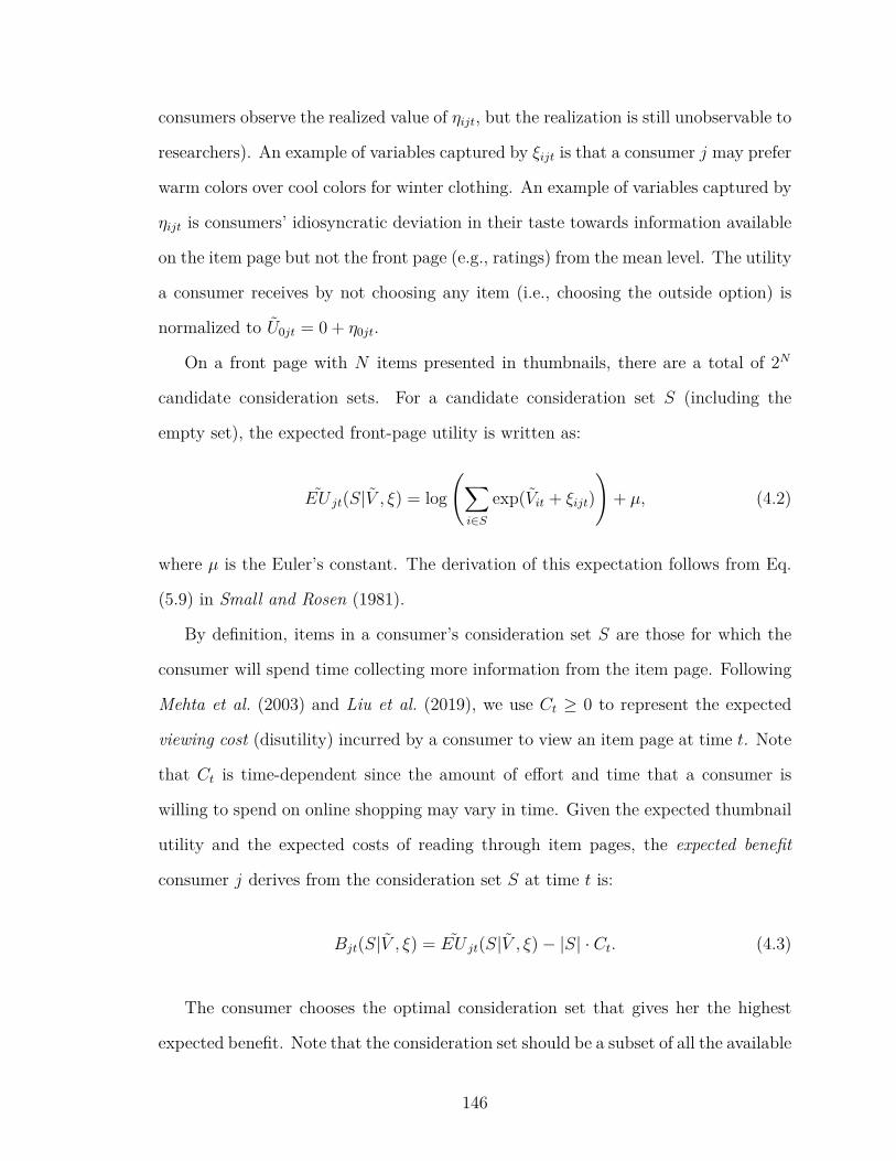
consumers observe the realized value of ηijt, but the realization is still unobservable to

researchers). An example of variables captured by ξijt is that a consumer j may prefer

warm colors over cool colors for winter clothing. An example of variables captured by

ηijt is consumers’ idiosyncratic deviation in their taste towards information available

on the item page but not the front page (e.g., ratings) from the mean level. The utility

a consumer receives by not choosing any item (i.e., choosing the outside option) is

normalized to U0jt = 0 + η0jt.

On a front page with N items presented in thumbnails, there are a total of 2N

candidate consideration sets. For a candidate consideration set S (including the

empty set), the expected front-page utility is written as:

EU jt(S|V , ξ) = log

(∑i∈S

exp(Vit + ξijt)

)+ µ, (4.2)

where µ is the Euler’s constant. The derivation of this expectation follows from Eq.

(5.9) in Small and Rosen (1981).

By definition, items in a consumer’s consideration set S are those for which the

consumer will spend time collecting more information from the item page. Following

Mehta et al. (2003) and Liu et al. (2019), we use Ct ≥ 0 to represent the expected

viewing cost (disutility) incurred by a consumer to view an item page at time t. Note

that Ct is time-dependent since the amount of effort and time that a consumer is

willing to spend on online shopping may vary in time. Given the expected thumbnail

utility and the expected costs of reading through item pages, the expected benefit

consumer j derives from the consideration set S at time t is:

Bjt(S|V , ξ) = EU jt(S|V , ξ)− |S| · Ct. (4.3)

The consumer chooses the optimal consideration set that gives her the highest

expected benefit. Note that the consideration set should be a subset of all the available

146

items, i.e. the inventory level of each item in the set is positive. Let It denote the set

of items that are available at time t, a consumer’s optimal consideration set is formed

by solving:

S∗jt(V , ξ) = argmax

S∈2ItBjt(S|V , ξ), (4.4)

where 2It is the powerset of It.

4.3.2 Purchase Decision Given a Consideration Set (The “Choose” Stage)

Once a consumer has formed a consideration set, she will visit the page of all the

items in the set and then makes a purchase decision. The item page contains addi-

tional information, including the review scores of the item quality, merchant’s service

(responsiveness of the merchant), logistics service (delivery speed and reliability), etc.

We specify another MNL model for item choice within the optimal consideration set.

Consider a consumer j with consideration set S∗jt. The utility for this consumer

to purchase item i ∈ S∗jt is given as:

Uijt = αi + xitβ + ρit + ξijt + ϵijt = Vit + ξijt + ϵijt. (4.5)

This utility function is similar to the thumbnail utility function (Eq. (4.1)). The

term αi is the fixed effect of item i. The covariates xit include the information that

is presented on the item page, and each element of β captures the effect of each

covariate in xit. The mean utility (across all consumers) of item i in period t is Vit =

αi+xitβ+ρit. The error term ρit is a normally distributed error that captures the part

of the mean utility that is not explained by xit and αi. The tildes are dropped from

the notations to indicate that these variables capture consumer utility/information

in the second stage in which a consumer collects further information about items in

her consideration set and makes a purchase decision. Note that the covariates in xit

147

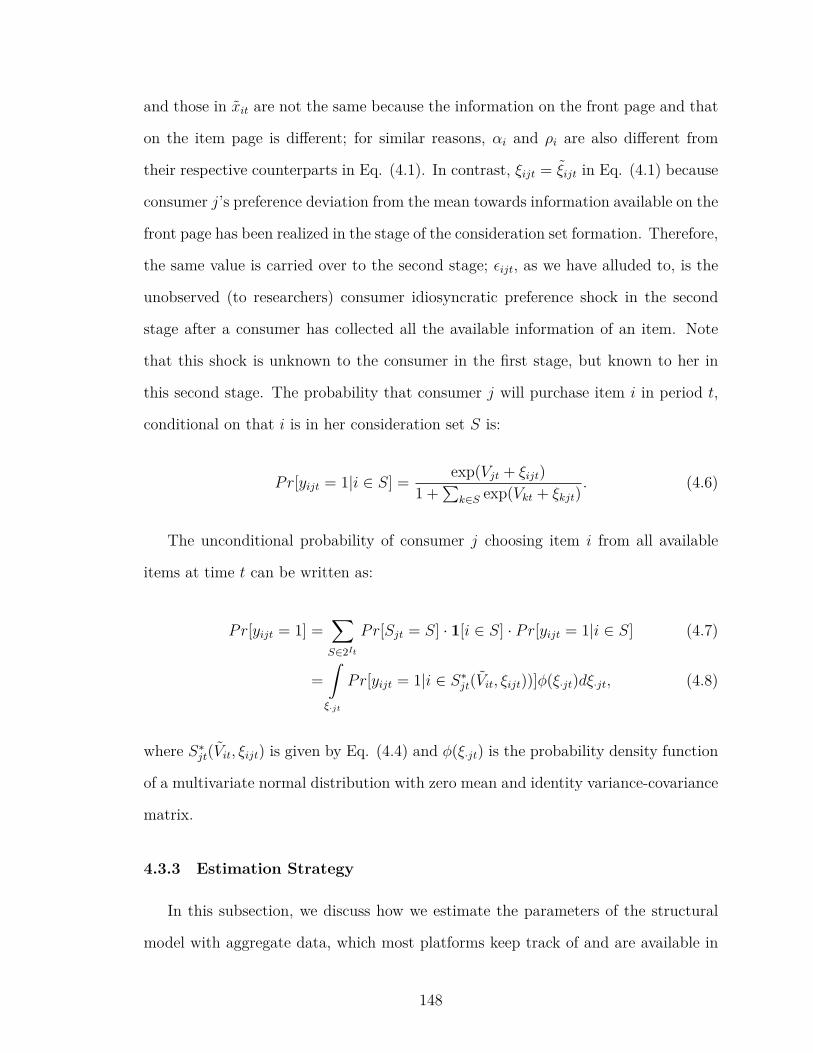
and those in xit are not the same because the information on the front page and that

on the item page is different; for similar reasons, αi and ρi are also different from

their respective counterparts in Eq. (4.1). In contrast, ξijt = ξijt in Eq. (4.1) because

consumer j’s preference deviation from the mean towards information available on the

front page has been realized in the stage of the consideration set formation. Therefore,

the same value is carried over to the second stage; ϵijt, as we have alluded to, is the

unobserved (to researchers) consumer idiosyncratic preference shock in the second

stage after a consumer has collected all the available information of an item. Note

that this shock is unknown to the consumer in the first stage, but known to her in

this second stage. The probability that consumer j will purchase item i in period t,

conditional on that i is in her consideration set S is:

Pr[yijt = 1|i ∈ S] =exp(Vjt + ξijt)

1 +∑

k∈S exp(Vkt + ξkjt). (4.6)

The unconditional probability of consumer j choosing item i from all available

items at time t can be written as:

Pr[yijt = 1] =∑S∈2It

Pr[Sjt = S] · 1[i ∈ S] · Pr[yijt = 1|i ∈ S] (4.7)

=

∫ξ·jt

Pr[yijt = 1|i ∈ S∗jt(Vit, ξijt))]ϕ(ξ·jt)dξ·jt, (4.8)

where S∗jt(Vit, ξijt) is given by Eq. (4.4) and ϕ(ξ·jt) is the probability density function

of a multivariate normal distribution with zero mean and identity variance-covariance

matrix.

4.3.3 Estimation Strategy

In this subsection, we discuss how we estimate the parameters of the structural

model with aggregate data, which most platforms keep track of and are available in

148

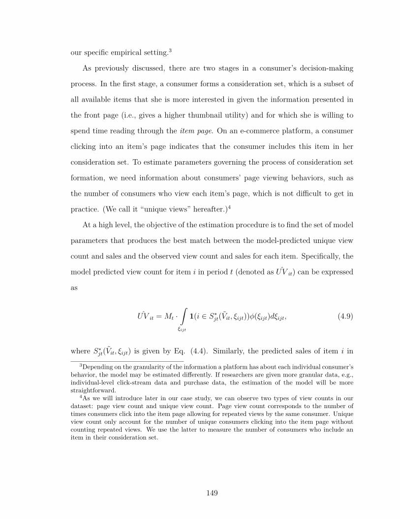
our specific empirical setting.3

As previously discussed, there are two stages in a consumer’s decision-making

process. In the first stage, a consumer forms a consideration set, which is a subset of

all available items that she is more interested in given the information presented in

the front page (i.e., gives a higher thumbnail utility) and for which she is willing to

spend time reading through the item page. On an e-commerce platform, a consumer

clicking into an item’s page indicates that the consumer includes this item in her

consideration set. To estimate parameters governing the process of consideration set

formation, we need information about consumers’ page viewing behaviors, such as

the number of consumers who view each item’s page, which is not difficult to get in

practice. (We call it “unique views” hereafter.)4

At a high level, the objective of the estimation procedure is to find the set of model

parameters that produces the best match between the model-predicted unique view

count and sales and the observed view count and sales for each item. Specifically, the

model predicted view count for item i in period t (denoted as UV it) can be expressed

as

UV it = Mt ·∫ξijt

1(i ∈ S∗jt(Vit, ξijt))ϕ(ξijt)dξijt, (4.9)

where S∗jt(Vit, ξijt) is given by Eq. (4.4). Similarly, the predicted sales of item i in

3Depending on the granularity of the information a platform has about each individual consumer’sbehavior, the model may be estimated differently. If researchers are given more granular data, e.g.,individual-level click-stream data and purchase data, the estimation of the model will be morestraightforward.

4As we will introduce later in our case study, we can observe two types of view counts in ourdataset: page view count and unique view count. Page view count corresponds to the number oftimes consumers click into the item page allowing for repeated views by the same consumer. Uniqueview count only account for the number of unique consumers clicking into the item page withoutcounting repeated views. We use the latter to measure the number of consumers who include anitem in their consideration set.

149

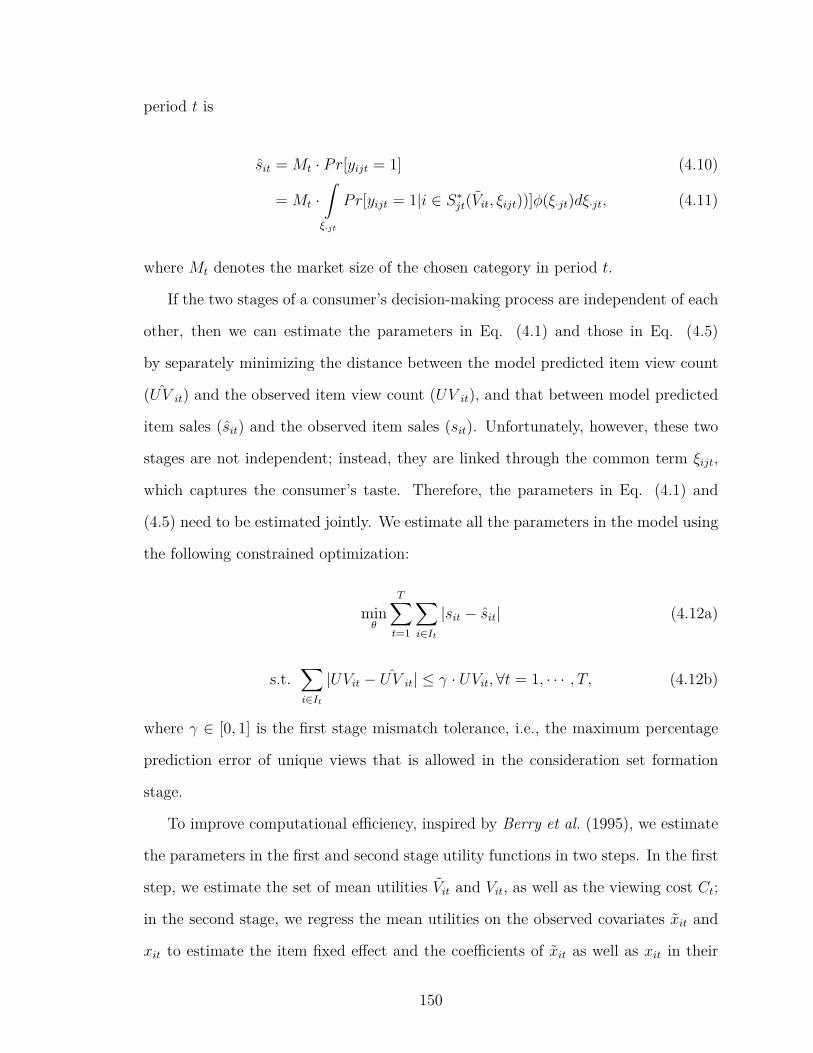
period t is

sit = Mt · Pr[yijt = 1] (4.10)

= Mt ·∫ξ·jt

Pr[yijt = 1|i ∈ S∗jt(Vit, ξijt))]ϕ(ξ·jt)dξ·jt, (4.11)

where Mt denotes the market size of the chosen category in period t.

If the two stages of a consumer’s decision-making process are independent of each

other, then we can estimate the parameters in Eq. (4.1) and those in Eq. (4.5)

by separately minimizing the distance between the model predicted item view count

(UV it) and the observed item view count (UV it), and that between model predicted

item sales (sit) and the observed item sales (sit). Unfortunately, however, these two

stages are not independent; instead, they are linked through the common term ξijt,

which captures the consumer’s taste. Therefore, the parameters in Eq. (4.1) and

(4.5) need to be estimated jointly. We estimate all the parameters in the model using

the following constrained optimization:

minθ

T∑t=1

∑i∈It

|sit − sit| (4.12a)

s.t.∑i∈It

|UVit − UV it| ≤ γ · UVit,∀t = 1, · · · , T, (4.12b)

where γ ∈ [0, 1] is the first stage mismatch tolerance, i.e., the maximum percentage

prediction error of unique views that is allowed in the consideration set formation

stage.

To improve computational efficiency, inspired by Berry et al. (1995), we estimate

the parameters in the first and second stage utility functions in two steps. In the first

step, we estimate the set of mean utilities Vit and Vit, as well as the viewing cost Ct;

in the second stage, we regress the mean utilities on the observed covariates xit and

xit to estimate the item fixed effect and the coefficients of xit as well as xit in their

150

respective functions. Following Berry et al. (1995), we estimate the mean utilities for

different periods separately. Given the above, in the first step, we solve the following

problem for each time t = 1, · · · , T as follows

minVit,Vit,Cit

∑i∈It

|sit − sit| (4.13a)

s.t.∑i∈It

|UVit − UV it| ≤ γ · UVit. (4.13b)

Once we obtain the estimates of Vit, Ct, and Vit, coefficients β, α, β, and α can be

estimated by regressing the mean utilities Vit and Vit on the item features consumers

can observe in the corresponding stage. Note that the available item features are

different on the front page and the item page, therefore we need to estimate the two

fixed-effect regressions for the two stages separately.

There are a few important details of the estimation procedure worth pointing

out. First, in our model, choices are mutually exclusive, i.e., each consumer chooses

at most one item from the set. Therefore, the data we apply this model to should

contain a set of substitutable items. For example, one can consider the set of items

in the same category as the choice set from which consumers can choose. Second, for

any item to be considered by consumers in a period, the item needs to be available (in

stock) in that period. Therefore, the choice set in period t (denoted as It) is defined as

the set of items with beginning inventory level greater than zero in the period. Third,

we use the total number of unique views of all items in the category to approximate

the market size of that category. Fourth, in the consideration set formation stage,

we allow consumers to form an empty consideration set (i.e., decide not to visit any

item page) and exit the market directly.

151

4.4 Assortment Personalization via Consideration Set Induc-

tion

In this section, we propose a novel approach to assortment planning that allows

for personalization based on each consumer’s taste. The main idea of our approach

is as follows. For each consumer, we (the platform) first find a target assortment

set that generates the maximum expected revenue. Then, we adjust the thumbnail

utility (by adjusting the display of items in the front page) to induce a consumer to

form her optimal consideration set that coincides with the target assortment set.

In the remainder of this section, we drop the time index t and the consumer

index j for convenience, without loss of generality. For a consumer with taste ξ =

(ξ1, ξ2, ..., ξN), we first formulate and solve the max-revenue capacitated assortment

planning problem given the estimated viewing cost C and item-page utility V =

(V1, V2, ..., VN). This problem is well-studied in the literature. The optimal assortment

set A∗(V, ξ) can be computed efficiently using the StaticMNL algorithm developed

by Rusmevichientong et al. (2010). Then, we prove that for any assortment set

A : |A| < K(C) and any taste vector ξ, there exists a set of V = (V1, V2, ...., VN)

such that the consumer’s optimal consideration set S∗(V , ξ) coincides with A. The

capacity K(C) is a mental capacity of a consumer – it is the maximum number of

items a consumer is willing to consider (and evaluate) regardless of the item utilities.

This is determined by the viewing cost, which is empirically estimated (see Section

4.3.3). Given the existence of such a utility vector V , we show that a minimally-

perturbed solution can be found by solving the Optimal Consideration Set Induction

Optimization (OCSIO) that has linearly many constraints in the number of items.

We provide a sufficient and necessary condition for the feasibility of OCSIO. Due to

nonconvexity of OCSIO, solving a large instance might be challenging. We propose

an efficient heuristic for solving OCSIO. Using the proposed approach, we generate

152

personalized assortment plans based on each consumer’s taste. Figure 4.3 provides

an overview of our approach.

Figure 4.3: Overview of the Assortment Personalization Approach

Thumbnail Utility ViewingCost Item-PageUtility𝑉" 𝐶 𝑉

Consumer formsconsideration setStomaximize utility

Platform finds targetassortment setA tomaximize revenue

Platformadjusts 𝑉"toinduce 𝑆 = 𝐴

(OCSIO)

AssortmentPersonalization

Empirical Estimation

SetCapacity𝐾(𝐶)

Taste𝜉

4.4.1 Max-Revenue Assortment Planning

Following the consider-then-choose model proposed in Section 4.3, we now for-

mulate the assortment planning problem to maximize the expected total revenue.5

Given the item-page utility V (estimated using the proposed empirical method), the

expected revenue of an assortment set A, for a consumer whose taste is ξ, is given by:

Ri(A|V, ξ) =exp(Vi + ξi)

1 +∑

k∈A exp(Vk + ξk)· pi, (4.14)

where pi is the price of item i.

To maximize the expected revenue, a capacitated assortment planning problem is5Revenue from each item equals the quantity sold × unit price. E-commerce platforms’ main

revenue sources are the revenue from items they themselves sell and the service fee they charge themerchants, which is typically a fraction of the transaction amount). As such, we consider maximizingthe total revenue as our objective.

153

formulated as follows:

A∗(V, ξ) = argmaxA∈2I

∑i∈A

Ri(A|V, ξ) (4.15a)

s.t. |A| < K(C). (4.15b)

The capacity constraint is imposed to ensure any assortment set A with cardinality

|A| < K(C) can be optimally induced (in the consideration set formation stage). The

capacity K(C) is a mental capacity of a consumer – it is the maximum number of

items a consumer is willing to consider (and compare) regardless of the item utilities.

This is determined by the viewing cost, which is empirically estimated (see Section

4.3.3). As viewing cost per item page increases, viewing and comparing items become

more costly, the maximum number of items a consumer is willing to consider will

consequently decreases. Later in Section 4.4.2, we provide a simple closed-form lower

bound for K−1(n), which is the inverse function of K(C). The functions K(C) and

K−1(n) tell us the number of items a consumer will consider (n) given the viewing

cost (C) and vice-versa.

Thanks to the seminal work by Rusmevichientong et al. (2010), this problem can

be solved efficiently using their StaticMNL algorithm. The optimal assortment set

A∗ will later be used as a target assortment/consideration set. On the front page,

we would like to induce the consumer to naturally form her optimal consideration

set that aligns with A∗. We do so by adjusting how the items are displayed on the

front page (i.e., by changing the thumbnail utility of each item V ). Note that this

adjustment only affects V but not C, because C is intrinsic to the consumer’s online

shopping behavior.

Remark IV.1 (Assortment Personalization Based on Taste). So far, we have assumed

that the taste vector of each consumer ξ is known prior to solving the assortment

planning problem. In practice, this can be achieved by learning from the consumer’s

154

purchase history, the items in her wish list, her favorite’d items, the reviews she has

previously written, etc. Given sufficient data, one can estimate the taste ξ using var-

ious statistical and machine learning techniques. In fact, many websites have already

implemented such a taste/preference prediction/learning mechanism very successfully

(the history goes back a decade, see, for example, Schafer et al. 2001). However, the

limited data on hand do not allow us to develop such a prediction model. We leave

the prediction of ξ for future work. In Section 4.5, we conduct numerical tests and

demonstrate that our approach can still increase the total revenue given imperfect

taste information.

4.4.2 Optimal Consideration Set Induction Optimization

From the platform’s perspective, our goal is to induce the consumer to form her

optimal consideration set that coincides with the target assortment set. We formulate

this induction process as an optimization problem. We provide feasibility conditions

for this optimization — if the cardinality of the target set is sufficiently small (i.e., A∗ :

|A∗| < K(C)), then there exists a mean utility vector V such that the consideration

set and the target assortment set coincide.

Remark IV.2 (Thumbnail Utility Adjustment). In practice, to induce the optimal

consideration set, the platform adjusts the thumbnail utility V (x) by adjusting the

covariates x (e.g., ranking, editorial promotion tag, and etc). Figure 4.4 illustrates

the potential covariates that can be incorporated and adjusted. We consider the

adjustment of the variable V and impose a budgetary constraint ||V − V ′||2 ≤ b to

ensure the level of adjustment can be realized by adjusting x.

In order to minimize the marketing and webpage redesign efforts, we minimally

perturb V (which is empirically estimated using the method developed in Section

4.3.3) to V ′ so that ||V − V ′||2 is minimized.

To induce the optimal consideration set S∗(V , ξ) that coincides with the target

155

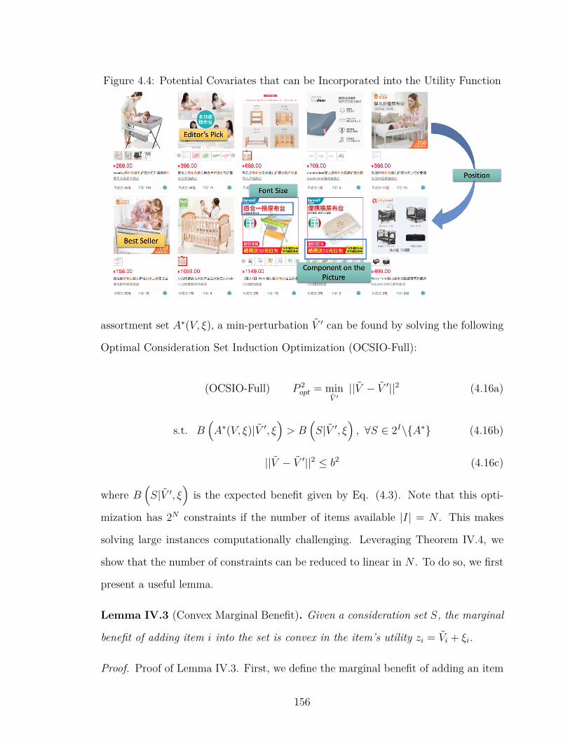
Figure 4.4: Potential Covariates that can be Incorporated into the Utility Function

assortment set A∗(V, ξ), a min-perturbation V ′ can be found by solving the following

Optimal Consideration Set Induction Optimization (OCSIO-Full):

(OCSIO-Full) P 2opt = min

V ′||V − V ′||2 (4.16a)

s.t. B(A∗(V, ξ)|V ′, ξ

)> B

(S|V ′, ξ

), ∀S ∈ 2I\{A∗} (4.16b)

||V − V ′||2 ≤ b2 (4.16c)

where B(S|V ′, ξ

)is the expected benefit given by Eq. (4.3). Note that this opti-

mization has 2N constraints if the number of items available |I| = N . This makes

solving large instances computationally challenging. Leveraging Theorem IV.4, we

show that the number of constraints can be reduced to linear in N . To do so, we first

present a useful lemma.

Lemma IV.3 (Convex Marginal Benefit). Given a consideration set S, the marginal

benefit of adding item i into the set is convex in the item’s utility zi = Vi + ξi.

Proof. Proof of Lemma IV.3. First, we define the marginal benefit of adding an item

156

with utility zi := Vi + ξi to the set S = {1, 2, ..., i − 1}. Let Si = S ∪ {i}, we can

compute the difference in the expected benefits between sets Si and S. The marginal

benefit is given by:

h(zi|S) = B(S ∪ {i}|(V1, ..., Vi), (ξ1, ..., ξi)

)−B

(S|(V1, ..., Vi−1), (ξ1, ..., ξi−1)

)(4.17)

= log

(∑k∈S

exp(zk) + exp(zi)

)− log

(∑k∈S

exp(zk)

)− C (4.18)

= log

(1 +

exp(zi)∑k∈S exp(zk)

)− C. (4.19)

Convexity follows from the fact that the second derivative is positive:

h′′(zi|S) =ES exp(zi)

(ES + exp(zi))2> 0, (4.20)

where ES =∑

k∈S exp(zk) > 0.

Next, we leverage Lemma IV.3 to show an intuitive theorem: the optimal con-

sideration set is always a popular set. Within the assortment planning literature, the

optimality of a popular set has been studied by Cachon et al. (2005) in a different

setting. The idea of a popular set is quite intuitive – a consumer forms her optimal

consideration set that consists of the items with the largest expected utility.

Theorem IV.4 (Optimality of Popular Sets). If the items are ordered such that

z1 ≥ z2 ≥ · · · ≥ zN , for all i = 0, ..., N−1, if item i+1 is in the optimal consideration

set, item i must also be in the optimal consideration set. The empty set is denoted by

i = 0.

Proof. Proof of Theorem IV.4. The proof follows a similar process in the proof of

Theorem 1 in van Ryzin and Mahajan (1999). The idea of the proof is as follows: the

convexity of the marginal benefit (Lemma IV.3) implies that the maximum marginal

157

benefit is attained by either adding the item with the largest utility or adding nothing

to the set.

Since all optimal consideration sets are popular sets, we can reduce the number

of constraints to linearly many in the number of items. This is formally given by

Corollary IV.5.

Corollary IV.5. Without loss of generality, reindex the items such that A∗(V, ξ) =

{1, 2, ..., |A∗(V, ξ)|}. OCSIO-Full is equivalent to the following optimization (OCSIO):

(OCSIO) P 2opt = min

V ′||V − V ′||2 (4.21a)

s.t. B(A∗|V ′, ξ

)> B

(S|V ′, ξ

), ∀S ∈ {∅, {1}, {1, 2}, {1, 2, 3}, ..., I}\{A∗}

(4.21b)

z1 ≥ z2 ≥ · · · ≥ zN , (4.21c)

||V − V ′||2 ≤ b2 (4.21d)

which has at most 2N = 2|I| constraints, where zi = V ′i + ξi.

Proof. Proof of Corollary IV.5. The equivalence follows from Theorem IV.4.

Despite only having linearly many constraints, OCSIO is nonetheless a challenging

problem to solve. We remark that OCSIO is not always a convex optimization.

Remark IV.6 (OCSIO is Not Necessarily Convex). The feasible region of OCSIO is

not necessarily a convex set. A counter-example is provided below.

For example, consider a two-item case. A∗ = {1, 2}. Let b = ∞. The feasible

158

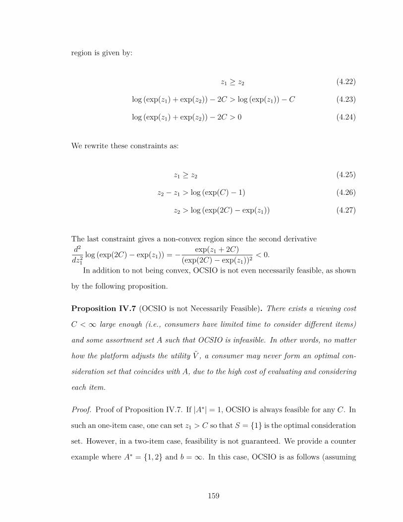
region is given by:

z1 ≥ z2 (4.22)

log (exp(z1) + exp(z2))− 2C > log (exp(z1))− C (4.23)

log (exp(z1) + exp(z2))− 2C > 0 (4.24)

We rewrite these constraints as:

z1 ≥ z2 (4.25)

z2 − z1 > log (exp(C)− 1) (4.26)

z2 > log (exp(2C)− exp(z1)) (4.27)

The last constraint gives a non-convex region since the second derivatived2

dz21log (exp(2C)− exp(z1)) = − exp(z1 + 2C)

(exp(2C)− exp(z1))2< 0.

In addition to not being convex, OCSIO is not even necessarily feasible, as shown

by the following proposition.

Proposition IV.7 (OCSIO is not Necessarily Feasible). There exists a viewing cost

C < ∞ large enough (i.e., consumers have limited time to consider different items)

and some assortment set A such that OCSIO is infeasible. In other words, no matter

how the platform adjusts the utility V , a consumer may never form an optimal con-

sideration set that coincides with A, due to the high cost of evaluating and considering

each item.

Proof. Proof of Proposition IV.7. If |A∗| = 1, OCSIO is always feasible for any C. In

such an one-item case, one can set z1 > C so that S = {1} is the optimal consideration

set. However, in a two-item case, feasibility is not guaranteed. We provide a counter

example where A∗ = {1, 2} and b = ∞. In this case, OCSIO is as follows (assuming

159

b = ∞):

minz1,z2

(z1 − z1)2 + (z2 − z2)

2 (4.28)

s.t. z2 − z1 > log (exp(C)− 1) (4.29)

z2 > log (exp(2C)− exp(z1)) (4.30)

z1 ≥ z2 (4.31)

Observe that constraints (4.29) and (4.31) cannot be satisfied at the same time if

we let C > log 2.

To ensure a target assortment set can be induced as an optimal consideration set,

the viewing cost has to be sufficiently small. Intuitively, this means that viewing

and evaluating items in such a set should not be too burdensome for a consumer. To

quantify the relationship between the viewing cost and the number of items a con-

sumer will consider, we present a theorem that provides the sufficient-and-necessary

condition for the feasibility of OCSIO.

Theorem IV.8 (Sufficient and Necessary Condition for OCSIO Feasibility). Suppose

b = ∞, for any given assortment set A∗ with cardinality |A∗| = n ≤ N , if n = 1,

OCSIO is always feasible. For n ≥ 2, OCSIO is feasible if and only if C < K−1(n) =

log

(n

n− 1

).

Proof. Proof of Theorem IV.8. First, we prove the sufficiency. For the one-item case

A∗ = {1} and n = 1, we set z1 = z > C and set z2, ..., zN = x. OCSIO is feasible if

160

the following holds:

z − C > log(exp(z) + k exp(x))− (k + 1)C, ∀k = 1, ..., n− 1

z − C > 0

z ≥ x

(4.32)

⇔

kC > log

(1 +

k exp(x)

exp(z)

),∀k = 1, ..., n− 1

z > C

z ≥ x

(4.33)

Observe that if we set z large enough, the constraints will be met.

For n ≥ 2, reindex the items such that A∗ = {1, 2, ..., n}. Let zi = z, ∀i = 1, ..., n

and let zi = x,∀i = n+1, ..., N . If there exists C > 0 and z, x such that the following

constraints can be satisfied simultaneously, then OCSIO is feasible.

log(n exp(z))− nC > log((n− k) exp(z))− (n− k)C, ∀k = 1, ..., n− 1

log(n exp(z))− nC > 0

log(n exp(z))− nC > log(n exp(z) + l exp(x))− (n+ l)C, ∀l = 1, ..., N − n

z ≥ x

(4.34)

⇔

log

(n

n− k

)− kC > 0,∀k = 1, ..., n− 1

n exp(z) > exp(nC)

lC > log

(1 +

l

nexp(x− z)

),∀l = 1, ..., N − n

z ≥ x

(4.35)

Let us first focus on the first set of constraints (∀k). Our goal is to let the tightest

161

constraint k∗ hold (minimum across k, LHS > 0). Since log

(n

n− k

)− kC is convex

in k, the stationary point is k∗ = n− 1/C.

Three cases must be considered:

1. The stationary point k∗ is left of the interval [1, ..., n− 1]. This means that 0 <

C ≤ 1n−1

. The minimum is attained at k = 1. Hence, we need log( nn−1

)−C > 0.

Therefore, we have C < log( nn−1

). Note that log( nn−1

) < 1n−1

for n ≥ 2, so the

stationary point is still left of the interval.

2. The stationary point k∗ is right of the interval [1, ..., n − 1]. This means that

C ≥ 1. The minimum is attained at k = n− 1. We need log(n)− (n− 1)C > 0.

However, this is impossible for any C ≥ 1 and n ≥ 2.

3. The stationary point k∗ is in the interval [1, ..., n− 1]. This means that 1n−1

<

C < 1. This case is also infeasible because the constraint’s value at k = 1 is

negative as log( nn−1

)− C < log( nn−1

)− 1n−1

< 0 for n ≥ 2.

Therefore if we set C < log( nn−1

), then the first set of constraints (∀k) holds.

Now we shall move on to the third and fourth sets of constraints (∀l). We can

always find z large enough and x small enough such that the constraints are satisfied.

If 0 < C < log

(n

n− 1

), then we can find such x and z that satisfy all constraints

by setting:

z = zin >nC − log(n) (4.36)

x = zout <min

{x ≤ zin

∣∣∣lC − log

(1 +

l

nexp(x− zin)

)> 0,∀l = 1, ..., N − n

}(4.37)

≤ minl=1,...,N−n

{log (exp(lC)− 1) + nC − log(l)} (4.38)

162

Now we prove the necessity by contradiction. Suppose (for contradiction) ∃C ≥

log(n/(n− 1)) and OCSIO is feasible.

Let us define

U(z1, z2, ..., zk|k) = log

(k∑

i=1

exp(zk)

)− kC (4.39)

The feasible region of OCSIO thereby becomes

U(z1, ..., zn|n) > U(z1, ..., zk|k),∀k = 1, ..., n− 1, n+ 1, ..., N (4.40)

U(z1, ..., zn|n) > 0 (4.41)

z1 ≥ z2 ≥ · · · ≥ zN (4.42)

Our goal is to show that U(z1, ..., zn|n) − U(z1, ..., zn−1|n − 1) > 0 is not feasible.

Recall the definition of the marginal benefit function h, it follows that U(z1, ..., zk|k)−

U(z1, ..., zk−1|k − 1) = h(zk|{1, 2, ..., k − 1}). We show that, under the constraint of

z1 ≥ z2 ≥ · · · ≥ zN , h(zk|{1, 2, ..., k − 1}) attains its maximum for all k ≥ 2 at

z1 = z2 = · · · = zk.

Consider the following maximization:

maxzk≤zk−1≤···≤z1

log (exp(zk) + exp(zk−1) + · · ·+ exp(z1))− log (exp(zk−1) + · · ·+ exp(z1))− C

(4.43)

Let z = zk and E = exp(zk−1) + · · ·+exp(z1), then the optimization is equivalent to:

maxz,E

log(exp(z) + E)− log(E)− C (4.44)

s.t. E ≥ (k − 1) exp(z) (4.45)

The objective function is increasing in z and decreasing in E. Hence, the maximum

163

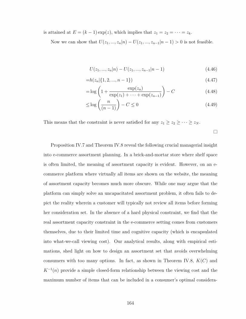
is attained at E = (k − 1) exp(z), which implies that z1 = z2 = · · · = zk.

Now we can show that U(z1, ..., zn|n)− U(z1, ..., zn−1|n− 1) > 0 is not feasible.

U(z1, ..., zn|n)− U(z1, ..., zn−1|n− 1) (4.46)

=h(zn|{1, 2, ..., n− 1}) (4.47)

= log

(1 +

exp(zn)

exp(z1) + · · ·+ exp(zn−1)

)− C (4.48)

≤ log

(n

(n− 1)

)− C ≤ 0 (4.49)

This means that the constraint is never satisfied for any z1 ≥ z2 ≥ · · · ≥ zN .

Proposition IV.7 and Theorem IV.8 reveal the following crucial managerial insight

into e-commerce assortment planning. In a brick-and-mortar store where shelf space

is often limited, the meaning of assortment capacity is evident. However, on an e-

commerce platform where virtually all items are shown on the website, the meaning

of assortment capacity becomes much more obscure. While one may argue that the

platform can simply solve an uncapacitated assortment problem, it often fails to de-

pict the reality wherein a customer will typically not review all items before forming

her consideration set. In the absence of a hard physical constraint, we find that the

real assortment capacity constraint in the e-commerce setting comes from customers

themselves, due to their limited time and cognitive capacity (which is encapsulated

into what-we-call viewing cost). Our analytical results, along with empirical esti-

mations, shed light on how to design an assortment set that avoids overwhelming

consumers with too many options. In fact, as shown in Theorem IV.8, K(C) and

K−1(n) provide a simple closed-form relationship between the viewing cost and the

maximum number of items that can be included in a consumer’s optimal considera-

164

tion set. We would like to emphasize that this capacity is not a “physical” capacity.

Instead, it is the “mental” capacity that consumers impose on themselves. To the

best of our knowledge, this is the first attempt at linking the viewing cost to the

cognitive constraint on consideration set formation in a quantitative way.

Remark IV.9 (Assortment Set Capacity). Given an empirically estimated viewing

cost C > 0, K(C) =exp(C)

exp(C)− 1is the maximum number of items a consumer is

willing to consider (and compare), regardless of the item utilities. We set K(C) as

the assortment set capacity. As a result, if there is a sufficient utility adjustment

budget (b = ∞), then OCSIO is always feasible for any target assortment set A∗ :

|A∗| < K(C).

So far we have shown that OCSIO, despite only having 2N constraints, is nev-

ertheless a challenging problem (not necessarily convex and not necessarily feasible).

Leveraging Theorem IV.8, we can set a capacity constraint in the max-revenue as-

sortment planing stage to guarantee OCSIO feasibility. Given a feasible OCSIO, to

solve such a non-convex optimization, we develop the following intuitive and efficient

heuristic.

Proposition IV.10 (OCSIO Heuristic). For a feasible n-item OCSIO (|A∗| = n ≥

2), suppose the original utility is V = V1, ..., VN , and the consumer’s taste is given by

ξ (N is the number of items available in the category). Given some accuracy tolerance

ϵ > 0, we construct V ′ in the following fashion:

We denote the OCSIO heuristic operation as (PH , V′) = OCSIO-H(V , ξ, A), where

P 2H = ||V ′ − V ||2. The computational complexity of OCSIO-H is O(N log(N)).

Proof. Proof of Proposition IV.10. The feasibility of the output follows from the suf-

ficiency proof of Theorem IV.8. The computational complexity is O(N log(N)) since

the operations before the while loop take at most O(N log(N)) (driven by sorting)

165

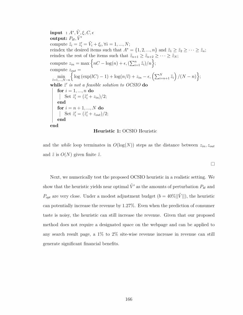
input : A∗, V , ξ, C, ϵoutput: PH , V

′

compute zi = z′i = Vi + ξi,∀i = 1, ..., N ;reindex the desired items such that A∗ = {1, 2, ..., n} and z1 ≥ z2 ≥ · · · ≥ zn;reindex the rest of the items such that zn+1 ≥ zn+2 ≥ · · · ≥ zN ;compute zin = max

{nC − log(n) + ϵ, (

∑ni=1 zi)/n

};

compute zout =

minl=1,...,N−n

{log (exp(lC)− 1) + log(n/l) + zin − ϵ,

(∑Ni=n+1 zi

)/(N − n)

};

while z′ is not a feasible solution to OCSIO dofor i = 1, ..., n do

Set z′i = (z′i + zin)/2;endfor i = n+ 1, ..., N do

Set z′i = (z′i + zout)/2;end

endHeuristic 1: OCSIO Heuristic

and the while loop terminates in O(log(N)) steps as the distance between zin, zout

and z is O(N) given finite z.

Next, we numerically test the proposed OCSIO heuristic in a realistic setting. We

show that the heuristic yields near optimal V ′ as the amounts of perturbation PH and

Popt are very close. Under a modest adjustment budget (b = 40%||V ||), the heuristic

can potentially increase the revenue by 1.27%. Even when the prediction of consumer

taste is noisy, the heuristic can still increase the revenue. Given that our proposed

method does not require a designated space on the webpage and can be applied to

any search result page, a 1% to 2% site-wise revenue increase in revenue can still

generate significant financial benefits.

166

4.5 A Case Study

In this section, we put the developed framework into practice and demonstrate how

it can be implemented to increase revenue. We first estimate the structural model for a

category of substitutable items using data from Tmall, a major e-commerce platform

operated by Alibaba. We then demonstrate that the proposed OCSIO heuristic is

near optimal and it can increase the revenue by up to 35%. We test the heuristic

under imperfect taste information and show that it can still increase the revenue

under a limited utility adjustment budget.

4.5.1 Data Description

For illustration purposes, we choose an item category on the platform that consists

of six different items (recall that we define an item as a product-merchant combina-

tion). Our dataset contains daily sales, price, number of (unique) views, and inventory

information of each item in the chosen category for 182 days.6 Table 4.2 shows the

summary statistics of the main variables used in our model. These variables include

information available to consumers in both stages of their decision-making process.

In the consideration set formation stage, a consumer forms her consideration set

based on the information provided on the front page, including the price of each

item sold by each merchant, the past-month sales, and a photo of each item. The

price and past sales information is available in our dataset, while the item photo is

not. However, since the photo of an item does not frequently change, its impact on

the consumer utility can be captured by the item-level fixed effect αi. This fixed

effect also captures any other unobserved time-invariant item features that affect the

thumbnail utility. Note that one item can be sold at different prices during a day6The original dataset contains 212 days of records. However, the first 30 days of sales data

are used to calculate the “past-month sales” (information displayed on the summary page on thisplatform but not directly recorded in the dataset) on day 31. Therefore, we are only able to estimatethe model from day 31 onwards.

167

and we use the average price throughout the day as the price that is observed by the

consumers on both the front page and the item page.

In the stage of making a purchase decision, the consumer clicks into an item page,

where she sees the ratings of the merchant’s service quality, the quality of all items

sold by the merchant, and the quality of the logistics (shipment services) provided

by this merchant. As discussed in Section 4.3.3, the market size of each day is

computed using the number of unique views. Note that the daily number of unique

views varies from a minimum of 116 to a maximum of 63,944, while the daily sales

number is in the range between 1 and 807. This large variation further supports the

need for incorporating the consideration set formation stage into consumer purchase

decision making-process. An implicit assumption made in the standard single-stage

logit choice model (that includes all item attributes displayed on the item page as

independent variables) is that all the available items are “considered/viewed”. If this

were true, there would not be much variation in view counts across items. Besides,

in practice, the platform only displays the items that have at least one unit in stock.

Therefore, when estimating the consider-then-choose model, one should only include

items with a positive inventory level. We check and ensure that in the category that

we choose in this illustration, there was no stock-out throughout the whole study

period. In fact, we observe that stock-outs rarely happen on the Tmall platform in

the half-year study period.

4.5.2 Estimation Result and Discussion

As discussed previously, in the first step of our two-step estimation process, we

estimate a set of mean utilities (Vit and Vit) of all available items in the category in

each day separately. In Figure 4.5 , we plot the point estimates of Vit and Vit of the

six items over time. In addition, we also estimate the viewing cost Ct for each t. The

estimated costs have an average value of 0.68 and a standard deviation of 0.004 over

168

Table 4.2: Summary Statistics

Statistic N Mean St.Dev.

Min Max

Item Daily Sales 1,092 63.34 67.00 1.00 807.00Unique View on Item Page (App and PC)

(ItemUV )1,092 6,457.94 7,657.16 116.00 63,944.00

*Price 1,092 202.07 245.11 7.01 577.81*Past (30 days) Sales 1,092 2,247.67 1,901.53 136.00 8,461.00

Merchant Logistics Review Score (out of5)

1,092 4.85 0.06 4.37 5.00

Merchant Service Review Score (out of 5) 1,092 4.86 0.06 4.48 5.00Merchant Quality Review Score (out of 5) 1,092 4.89 0.05 4.56 5.00Inventory Level at the Beginning of the

Day1,092 4,678.57 4,596.84 94.00 19,572.00

Note: The variables with * in the front are the information available to the consumerson the front page.

Figure 4.5: Point Estimates of the Mean Thumbnail Utility Vit (Left Panel) and theMean Item-Page Utility Vit (Right Panel)

0 5 10 15 20 25

Item 1 Item 2 Item 3 Item 4 Item 5 Item 6

50 100 150-1.5

-1

-0.5

0

0.5

1

1.5

2

50 100 150-10

-9

-8

-7

-6

-5

-4

-3

the 182 days.

The estimation results for parameters in Eq. (4.1) and Eq. (4.5) are reported

169

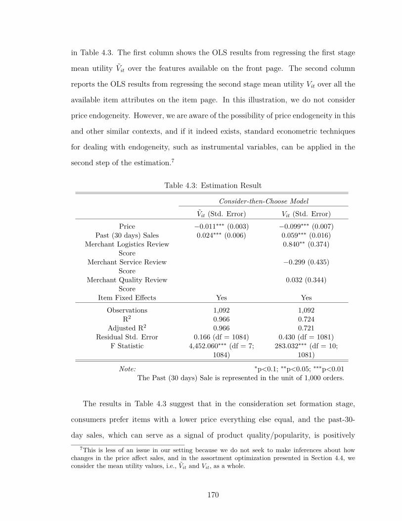
in Table 4.3. The first column shows the OLS results from regressing the first stage

mean utility Vit over the features available on the front page. The second column

reports the OLS results from regressing the second stage mean utility Vit over all the

available item attributes on the item page. In this illustration, we do not consider

price endogeneity. However, we are aware of the possibility of price endogeneity in this

and other similar contexts, and if it indeed exists, standard econometric techniques

for dealing with endogeneity, such as instrumental variables, can be applied in the

second step of the estimation.7

Table 4.3: Estimation Result

Consider-then-Choose ModelVit (Std. Error) Vit (Std. Error)

Price −0.011∗∗∗ (0.003) −0.099∗∗∗ (0.007)Past (30 days) Sales 0.024∗∗∗ (0.006) 0.059∗∗∗ (0.016)

Merchant Logistics ReviewScore

0.840∗∗ (0.374)

Merchant Service ReviewScore

−0.299 (0.435)

Merchant Quality ReviewScore

0.032 (0.344)

Item Fixed Effects Yes YesObservations 1,092 1,092

R2 0.966 0.724Adjusted R2 0.966 0.721

Residual Std. Error 0.166 (df = 1084) 0.430 (df = 1081)F Statistic 4,452.060∗∗∗ (df = 7;

1084)283.032∗∗∗ (df = 10;

1081)

Note: ∗p<0.1; ∗∗p<0.05; ∗∗∗p<0.01The Past (30 days) Sale is represented in the unit of 1,000 orders.

The results in Table 4.3 suggest that in the consideration set formation stage,

consumers prefer items with a lower price everything else equal, and the past-30-

day sales, which can serve as a signal of product quality/popularity, is positively7This is less of an issue in our setting because we do not seek to make inferences about how

changes in the price affect sales, and in the assortment optimization presented in Section 4.4, weconsider the mean utility values, i.e., Vit and Vit, as a whole.

170

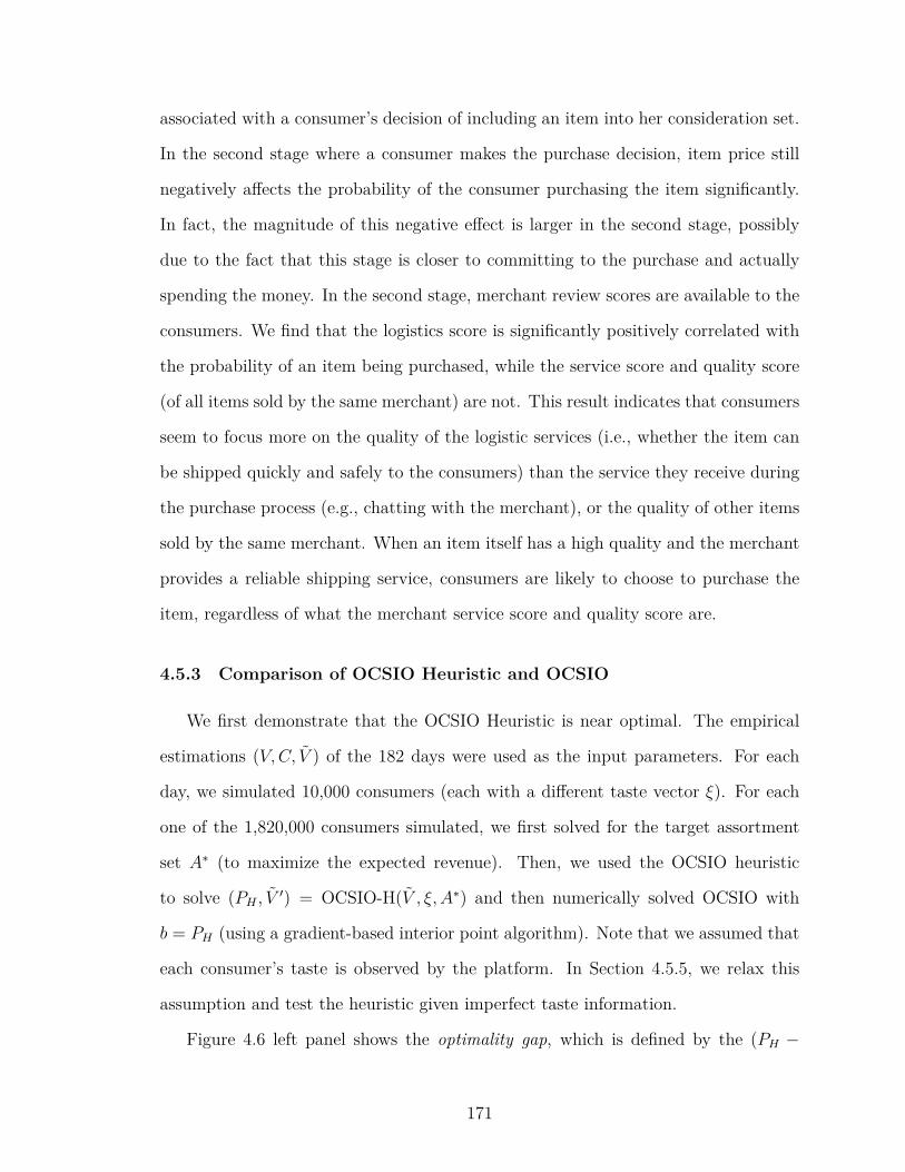
associated with a consumer’s decision of including an item into her consideration set.

In the second stage where a consumer makes the purchase decision, item price still

negatively affects the probability of the consumer purchasing the item significantly.

In fact, the magnitude of this negative effect is larger in the second stage, possibly

due to the fact that this stage is closer to committing to the purchase and actually

spending the money. In the second stage, merchant review scores are available to the

consumers. We find that the logistics score is significantly positively correlated with

the probability of an item being purchased, while the service score and quality score

(of all items sold by the same merchant) are not. This result indicates that consumers

seem to focus more on the quality of the logistic services (i.e., whether the item can

be shipped quickly and safely to the consumers) than the service they receive during

the purchase process (e.g., chatting with the merchant), or the quality of other items

sold by the same merchant. When an item itself has a high quality and the merchant

provides a reliable shipping service, consumers are likely to choose to purchase the

item, regardless of what the merchant service score and quality score are.

4.5.3 Comparison of OCSIO Heuristic and OCSIO

We first demonstrate that the OCSIO Heuristic is near optimal. The empirical

estimations (V,C, V ) of the 182 days were used as the input parameters. For each

day, we simulated 10,000 consumers (each with a different taste vector ξ). For each

one of the 1,820,000 consumers simulated, we first solved for the target assortment

set A∗ (to maximize the expected revenue). Then, we used the OCSIO heuristic

to solve (PH , V′) = OCSIO-H(V , ξ, A∗) and then numerically solved OCSIO with

b = PH (using a gradient-based interior point algorithm). Note that we assumed that

each consumer’s taste is observed by the platform. In Section 4.5.5, we relax this

assumption and test the heuristic given imperfect taste information.

Figure 4.6 left panel shows the optimality gap, which is defined by the (PH −

171

Figure 4.6: The Optimality Gap and the Perturbation Produced by the OCSIOHeuristic

0%

20%

40%

60%

80%

100%

0% 50% 100%0

0.5

1

1.5

2

2.5105

0%

20%

40%

60%

80%

100%

0% 50% 100% 150%0

5

10

104

Popt)/||V ||, where PH is the required perturbation by the heuristic and Popt is the

minimal perturbation (obtained by solving OCSIO). For 80% of the simulated con-

sumers, the optimality gap is within 45% of the magnitude (norm) of the original V .

Figure 4.6 right panel shows that the distribution of the required perturbations (pro-

duced by the OCSIO heuristic). On average, the required perturbation is 98%×||V ||

(standard deviation = 31%× ||V ||).

4.5.4 Revenue Increase using the OCSIO Heuristic

In this experiment, we varied the budget b between 0 and 150%× ||V ||. For each

one of the 182×10, 000 consumer, the heuristic produces (PH , V′) = OCSIO-H(V , ξ, A∗).

If the OCSIO heuristic required perturbation is within the adjustment budget (PH ≤

b), the utility V is adjusted to V ′. Otherwise, the original utility V is unchanged.

We compared the total expected revenue with the historical revenue (over the

182-day period) under different utility adjustment budgets. Figure 4.7 shows that a

maximum revenue improvement of 35% is achieved when the budget is set to b =

150%||V ||. As the budget for utility adjustment increases, the revenue improvement

ramps up in a linear fashion (until it hits the 35% maximum).

Given data on hand, it is difficult to accurately estimate a practical budget con-

straint. Nonetheless, a budget would stem from the regression result should more

172

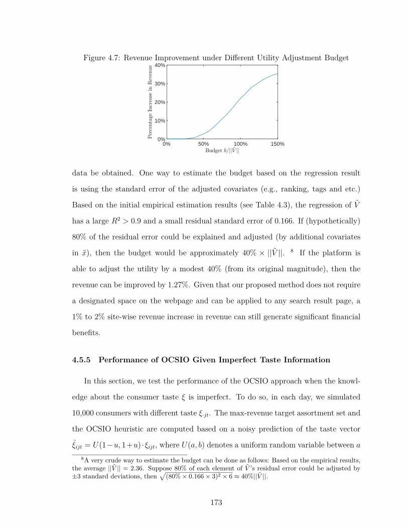
Figure 4.7: Revenue Improvement under Different Utility Adjustment Budget

0% 50% 100% 150%0%

10%

20%

30%

40%

data be obtained. One way to estimate the budget based on the regression result

is using the standard error of the adjusted covariates (e.g., ranking, tags and etc.)

Based on the initial empirical estimation results (see Table 4.3), the regression of V

has a large R2 > 0.9 and a small residual standard error of 0.166. If (hypothetically)

80% of the residual error could be explained and adjusted (by additional covariates

in x), then the budget would be approximately 40% × ||V ||. 8 If the platform is

able to adjust the utility by a modest 40% (from its original magnitude), then the

revenue can be improved by 1.27%. Given that our proposed method does not require

a designated space on the webpage and can be applied to any search result page, a

1% to 2% site-wise revenue increase in revenue can still generate significant financial

benefits.

4.5.5 Performance of OCSIO Given Imperfect Taste Information

In this section, we test the performance of the OCSIO approach when the knowl-

edge about the consumer taste ξ is imperfect. To do so, in each day, we simulated

10,000 consumers with different taste ξ·jt. The max-revenue target assortment set and

the OCSIO heuristic are computed based on a noisy prediction of the taste vector

ξijt = U(1−u, 1+u) ·ξijt, where U(a, b) denotes a uniform random variable between a

8A very crude way to estimate the budget can be done as follows: Based on the empirical results,the average ||V || = 2.36. Suppose 80% of each element of V ’s residual error could be adjusted by±3 standard deviations, then

√(80%× 0.166× 3)2 × 6 ≈ 40%||V ||.

173

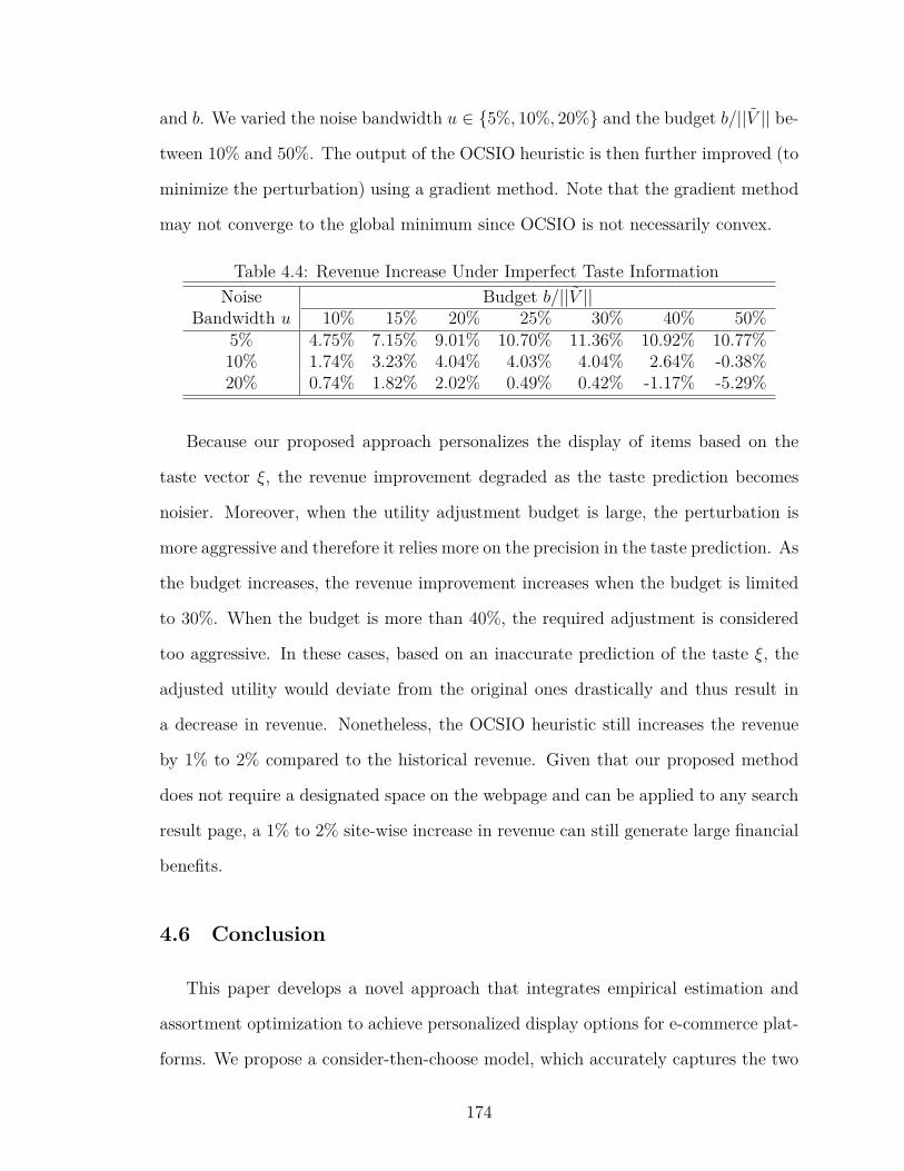
and b. We varied the noise bandwidth u ∈ {5%, 10%, 20%} and the budget b/||V || be-

tween 10% and 50%. The output of the OCSIO heuristic is then further improved (to

minimize the perturbation) using a gradient method. Note that the gradient method

may not converge to the global minimum since OCSIO is not necessarily convex.

Table 4.4: Revenue Increase Under Imperfect Taste InformationNoise Budget b/||V ||

Bandwidth u 10% 15% 20% 25% 30% 40% 50%5% 4.75% 7.15% 9.01% 10.70% 11.36% 10.92% 10.77%10% 1.74% 3.23% 4.04% 4.03% 4.04% 2.64% -0.38%20% 0.74% 1.82% 2.02% 0.49% 0.42% -1.17% -5.29%

Because our proposed approach personalizes the display of items based on the

taste vector ξ, the revenue improvement degraded as the taste prediction becomes

noisier. Moreover, when the utility adjustment budget is large, the perturbation is

more aggressive and therefore it relies more on the precision in the taste prediction. As

the budget increases, the revenue improvement increases when the budget is limited

to 30%. When the budget is more than 40%, the required adjustment is considered

too aggressive. In these cases, based on an inaccurate prediction of the taste ξ, the

adjusted utility would deviate from the original ones drastically and thus result in

a decrease in revenue. Nonetheless, the OCSIO heuristic still increases the revenue

by 1% to 2% compared to the historical revenue. Given that our proposed method

does not require a designated space on the webpage and can be applied to any search

result page, a 1% to 2% site-wise increase in revenue can still generate large financial

benefits.

4.6 Conclusion

This paper develops a novel approach that integrates empirical estimation and

assortment optimization to achieve personalized display options for e-commerce plat-

forms. We propose a consider-then-choose model, which accurately captures the two

174

stages of a consumer’s decision-making process, using two Multinomial Logit (MNL)

choice models interlinked by the heterogeneity in consumers’ taste. To calibrate this

two-stage model, we develop an estimation strategy to estimate the parameters in

consumers’ utility function, using aggregated view and order data. Based on the

estimated consider-then-choose model, we propose a novel approach to assortment

personalization. This approach achieves a “virtual” assortment planning by adjust-

ing how the items are displayed within a search result page (or on the front page).

As such, we induce the consumer to form a consideration set that coincides with the

revenue-maximizing target assortment set. Our approach does not require a capacity

constraint exogenously imposed by the platform nor a designated space for assort-

ment/recommendation display within a webpage. It can be applied to virtually all

search results, thereby generating potential site-wise revenue improvement.

To achieve assortment personalization, we develop an optimization procedure for

inducing a consumer to form a consideration set that coincides with the revenue-

maximizing target assortment set. We derive the feasibility conditions and propose

an efficient heuristic for solving large instances of the problem. Moreover, our an-

alytical results suggest that when a consumer forms her consideration set, she will

consider at most K(C) items given the cost/disutility (C) associated with the effort

of viewing and considering an item. Even when the utilities of some items are very

high (attractive) to the consumer, she will still consider at most K(C) items to avoid

incurring an unnecessarily high viewing cost. The functions K(C) and K−1(n) tell us

the number of items a consumer will consider (n) given the viewing cost (C) and vice-

versa. Tested on real-world data, our heuristic yields near-optimal solutions. Given

precise information of consumer taste, the proposed approach can increase the rev-

enue by up to 35% (compared with the historical revenue). Given moderately noisy

taste predictions, the heuristic can still increase the revenue by 1% to 2%. Since our

approach does not require a designated space on the webpage and could be applied

175

to any search result page, a 1% to 2% site-wise increase in revenue is substantial.

We close our paper by discussing some of the limitations and future directions

of this work. First, due to the limited data on hand, we are unable to incorporate

the desired covariates that can be leveraged to adjust the utility. These covariates

include, but are not limited to 1) whether an item has any editorial recommendation

tags (e.g., Amazon’s Choice), 2) item ranking and position within a search result

webpage, 3) picture size, font size, and other display features. Should more data

be provided, one can incorporate these features into the utility function. Second,

our heuristic relies on the sufficiently accurate predictions of each consumer’s taste

towards different items. Although the infrastructure of taste/preference learning is

already in place on many e-commerce websites, we, unfortunately, do not have access

to this type of data. Future research, where detailed data on user purchasing and

browsing history are available, can consider integrating the estimation of consumer

taste heterogeneity into the assortment personalization algorithm. Third, this model

assumed that the viewing cost Ct incurred by considering and evaluating an item

is homogeneous across all consumers. A sensible future extension is to incorporate

viewing cost heterogeneity. While many aspects of our modeling framework require

further data for empirical estimation and analytical investigation, we believe that

our integrated empirical and operational approach points out a new direction for

assortment and product display personalization for e-commerce platforms.

176

CHAPTER V

Future Work

In this chapter, we discuss some potential future research directions in the digi-

tal world. In the mobile app market, we can explore consumers’ in-app purchasing

behavior for different categories of apps. In the field of E-commerce platform, I wish

to explore the underlying mechanisms of consumers’ consideration set formation. I

plan to also continue study the effect of adopting telemedicine on patients’ quality of

care. I also raise two new fields that are live streaming media and fan economy.

Free downloading with in-app purchase option has been a popular revenue model

for mobile app developers. There are mainly two types of in-app purchases. The

first kind is subscription or premium membership. Consumers can either use part of

the app’s function for free, or they can use all functions for a limited time. To use

the more advanced functions or to extend the functional time of the app, consumers

need to make in-app purchases. The in-app purchase can be a subscription where

consumers make payment periodically or a one-time purchase where the consumers

pay a fixed amount of money for the lifetime usage of the app. The second kind of

in-app purchase is the option to purchase digital items, which is commonly seen in

mobile games. Developers create different virtual products in their apps that can

provide the consumers with better gaming experiences. Consumers can pay for these

items just like purchasing physical goods.

177

There are several research questions that are particularly interesting for us:

• How does the in-app purchase model (subscription vs. lifetime membership)

affect the apps total revenue? Does it impact the user loyalty?

• How does the in-app purchase items (price, variety, availability) impact app

users’ loyalty?

The research project introduced in Chapter IV empirically studies the impact of

thumbnail utility on consumers’ choices. In the future, I wish to use experiment-based

data to further explore the underlying mechanism of consideration set formation and

how different components of thumbnail page impact consumers’ choices.

Telemedicine has been widely used during the pandemic. In the future, I plan to

study the impact of telemedicine on the quality of care. Besides, I also plan to study

the adoption of telemedicine during the COVID period and whether the physicians

continue using telemedicine after the pandemic ends.

Livestream platforms are popular among young people. On these platforms, peo-

ple can broadcast their life in front of the camera. One interesting feature of some

livestream platforms is its virtual gifting system. This gifting system is similar to

the aforementioned in-app purchase option. The audience can buy virtual gifts and

send it to the broadcaster as a reward. The platform then transform the gifts back

to cash, deduct certain percentage of transaction fee, and send it to the broadcasters’

account. For most broadcasters, this is their main source of income. It is worth notic-

ing that these virtual gifts can be as expensive as more than a hundred dollars each,

yet lots of the broadcasters can get hundreds of them within several hours. Here we

are interested in the characteristics of the broadcaster and the content that attracts

the most audience and gifts. As a platform, how can it choose the broadcaster to

display on the front page to transfer the most traffic into gift purchasing?

Social media has become the main channel for fans to get information about the

178

celebrities that they follow. One interesting phenomenon is that fans tend to buy

the products that the celebrities use. Therefore some companies would send products

to the celebrities so that they may show up on their Instagram or Weibo as a form

of advertising. Other companies may take one step further and cooperate with the

celebrities and let them become the brand ambassador. While some celebrities can

get the products sold out within a few minutes after posting a photo of it on his social

media, some may not be able to boost the sales because his fan group does not overlap

with the products’ targeting consumers. In fact, there have been cases where the fans

refuse to accept their idol becoming the ambassador of certain products because they

thought the brand image does not match with their idol. Under such situation, the

sales may even decrease since the fans might even spread negative comments of the

brand on social media to force the company to terminate the cooperation. We are

interested in the relationship among the celebrities’ characteristics, the distribution

of his fans’ demographics, and the characteristics of the products. By empirically

combining the data from social media, product information, and product historical

sales, we can try to find the optimal match of products and celebrities when companies

are trying to invest in this form of advertising.

179

BIBLIOGRAPHY

180

BIBLIOGRAPHY

Abeliuk, A., G. Berbeglia, M. Cebrian, and P. Van Hentenryck (2016), Assortmentoptimization under a multinomial logit model with position bias and social influ-ence, 4OR, 14(1), 57–75.

Agarwal, A., K. Hosanagar, and M. D. Smith (2011), Location, location, location:An analysis of profitability of position in online advertising markets, Journal ofmarketing research, 48(6), 1057–1073.

Angrist, J. D., and J.-S. Pischke (2008), Mostly harmless econometrics: An empiri-cist’s companion, Princeton university press.

Aouad, A., and D. Segev (2015), Display optimization for vertically differentiatedlocations under multinomial logit choice preferences, Working Paper, MassachusettsInstitute of Technology, Cambridge, MA, doi:10.2139/ssrn.2709652.

Aouad, A., V. F. Farias, and R. Levi (2015), Assortment optimization under consider-then-choose choice models, Working Paper, Massachusetts Institute of Technology,Cambridge, MA, doi:10.2139/ssrn.2618823.

Appel, G., B. Libai, E. Muller, and R. Shachar (2016), Stickiness and the monetizationof apps, Available at SSRN 2652213.

Askalidis, G. (2015), The impact of large scale promotions on the sales and ratingsof mobile apps: Evidence from Apple’s app storeapple’s app store, arXiv preprintarXiv:1506.06857.

Assuncao, J. L., and R. J. Meyer (1993), The rational effect of price promotions onsales and consumption, Management Science, 39(5), 517–535.

Asteriou, D., K. Pilbeam, and A. Sarantidis (2019), The Behaviour of Banking StocksDuring the Financial Crisis and Recessions. Evidence from Changes-in-ChangesPanel Data Estimations, Scottish Journal of Political Economy, 66(1), 154–179,doi:10.1111/sjpe.12191.

Athey, S., and G. W. Imbens (2006), Identification and inference in nonlineardifference-in-differences models, Econometrica, 74(2), 431–497.

Bashshur, R. L. (1995), Telemedicine effects: cost, quality, and access, Journal ofmedical systems, 19(2), 81–91.

181

Bashshur, R. L., G. W. Shannon, N. Bashshur, and P. M. Yellowlees (2016), Theempirical evidence for telemedicine interventions in mental disorders, Telemedicineand e-Health, 22(2), 87–113.

Bass, F. M. (1969), A new product growth for model consumer durables, ManagementScience, 15(5), 215–227.

Bavafa, H., and C. Terwiesch (2019), Work after work: The impact of new servicedelivery models on work hours, Journal of Operations Management, 65(7), 636–658.

Bavafa, H., L. M. Hitt, and C. Terwiesch (2018), The impact of e-visits on visitfrequencies and patient health: Evidence from primary care, Management Science,doi:10.1287/mnsc.2017.2900.

Bavafa, H., S. Savin, and C. Terwiesch (2019), Managing patient panels with non-physician providers, Production and Operations Management, 28(6), 1577–1593.

Bayram, A., S. Deo, S. Iravani, and K. Smilowitz (2020), Managing virtual appoint-ments in chronic care, IISE Transactions on Healthcare Systems Engineering, 10(1),1–17.

BCBSM (2018a), Blue cross blue shield of michigan medical policy: Telemedicine,accessed on 9/24/2019.

BCBSM (2018b), Clarification: Telephone sessions as part of telemedicine for behav-ioral health providers, accessed on 9/24/2019.

Ben-Akiva, M. E., S. R. Lerman, and S. R. Lerman (1985), Discrete choice analysis:theory and application to travel demand, vol. 9, MIT Press, Cambridge, MA.

Berry, S., J. Levinsohn, and A. Pakes (1995), Automobile prices in market equilib-rium, Econometrica: Journal of the Econometric Society, pp. 841–890.

Bettman, J. R., M. F. Luce, and J. W. Payne (1998), Constructive consumer choiceprocesses, Journal of consumer research, 25(3), 187–217.

Bils, M., and P. J. Klenow (2004), Some evidence on the importance of sticky prices,Journal of political economy, 112(5), 947–985.

Bitran, G., and R. Caldentey (2003), An overview of pricing models for revenuemanagement, Manufacturing & Service Operations Management, 5(3), 203–229.

Blattberg, R. C., R. Briesch, and E. J. Fox (1995), How promotions work, Marketingscience, 14(3), G122–G132.

Borah, B. J., M. E. Burns, and N. D. Shah (2011), Assessing the impact of highdeductible health plans on health-care utilization and cost: a changes-in-changesapproach., Health economics, 20(9), 1025–42, doi:10.1002/hec.1757.

182

Cachon, G. P., C. Terwiesch, and Y. Xu (2005), Retail assortment planning in thepresence of consumer search, Manufacturing & Service Operations Management,7(4), 330–346.

Carare, O. (2012), The impact of bestseller rank on demand: Evidence from the appmarket, International Economic Review, 53(3), 717–742.

Cayirli, T., and E. Veral (2003), Outpatient scheduling in health care: a review ofliterature, Prod and oper manag, 12(4), 519–549.

Chandukala, S. R., J. Kim, T. Otter, P. E. Rossi, G. M. Allenby, et al. (2008), Choicemodels in marketing: Economic assumptions, challenges and trends, Foundationsand Trends® in Marketing, 2(2), 97–184.

Chaudhari, H., and J. Byers (2017), Impact of free app promotion on future sales: Acase study on amazon appstore, Available at SSRN 3078067.

Chen, H., Y. J. Hu, and M. D. Smith (2018), The impact of e-book distribution onprint sales: analysis of a natural experiment, Management Science, 65(1), 19–31.

Chevalier, J., and A. Goolsbee (2003), Measuring prices and price competition online:Amazon. com and barnes and noble.com, Quantitative marketing and Economics,1(2), 203–222.

Clay, S., M. Ross, and Z. Doolin (2018), New payments for non-face-to-face servicesin the 2019 medicare physician fee schedule proposed rule, accessed on 9/24/2019.

Cohen, M. C., N.-H. Z. Leung, K. Panchamgam, G. Perakis, and A. Smith (2017),The impact of linear optimization on promotion planning, Operations Research,65(2), 446–468.

Czerwinski, M., M. Czerwinski, E. Horvitz, and S. Wilhite (2004), A diary studyof task switching and interruptions, in Proceedings of the SIGCHI conference onHuman factors in computing systems, pp. 175–182, ACM.

Danaher, B., Y. Huang, M. D. Smith, and R. Telang (2014), An empirical analysis ofdigital music bundling strategies, Management Science, 60(6), 1413–1433.

Davis, J., G. Gallego, and H. Topaloglu (2013), Assortment planning under the multi-nomial logit model with totally unimodular constraint structures, Working Paper,Cornell University, Ithaca, NY.

Delana, K., S. Deo, K. Ramdas, G. Babu, and T. Ravilla (2019), Multichannel deliveryin healthcare: The impact of telemedicine centers in southern india, Available atSSRN 3505318.

Economides, N. (1996), The economics of networks, International Journal of Indus-trial Organization, 14(6), 673–699.

183

Elixhauser, A., C. Steiner, and L. Palmer (2015), Clinical classifications software(ccs).

eVisit (2021), Telemedicine reimbursement guide, accessed on 1/1/2021.

Fanburg, J., and J. Walzman (2018), Telehealth and the law: the challenge of reim-bursement, Psychiatric Times, 35(10), 12.

Feldman, J., D. Zhang, X. Liu, and N. Zhang (2018), Taking assortment opti-mization from theory to practice: Evidence from large field experiments on al-ibaba, Working Paper, Washington University in St. Louis, St. Louis, MO, doi:10.2139/ssrn.3232059.

Fisher, R. A. (1922), On the interpretation of χ 2 from contingency tables, and thecalculation of p, Journal of the Royal Statistical Society, 85(1), 87–94.

Gallego, G., and A. Li (2017), Attention, Consideration then Selection Choice Model,SSRN Electronic Journal, doi:10.2139/ssrn.2926942.

Gallego, G., A. Li, V.-A. Truong, and X. Wang (2016), Approximation algorithmsfor product framing and pricing, Working Paper, Columbia University, New York,NY.

Garg, R., and R. Telang (2013), Inferring app demand from publicly available data,MIS Quarterly, pp. 1253–1264.

Ghose, A., and S. P. Han (2014), Estimating demand for mobile applications in thenew economy, Management Science, 60(6), 1470–1488.

Ghose, A., A. Goldfarb, and S. P. Han (2012a), How is the mobile internet different?search costs and local activities, Information Systems Research, 24(3), 613–631.

Ghose, A., P. G. Ipeirotis, and B. Li (2012b), Designing ranking systems for ho-tels on travel search engines by mining user-generated and crowdsourced content,Marketing Science, 31(3), 493–520.

Ghose, A., P. G. Ipeirotis, and B. Li (2014), Examining the impact of ranking onconsumer behavior and search engine revenue, Management Science, 60(7), 1632–1654.

Gilbride, T. J., and G. M. Allenby (2003), Attribute-based consideration sets, Work-ing Paper, University of Notre Dame, Notre Dame, IN.

Gilbride, T. J., and G. M. Allenby (2004), A choice model with conjunctive, disjunc-tive, and compensatory screening rules, Marketing Science, 23(3), 391–406.

Golrezaei, N., V. Manshadi, and V. Mirrokni (2018), Two-stage pandora’s box forproduct ranking, Working Paper, Massachusetts Institute of Technology, Cam-bridge, MA, doi:10.2139/ssrn.3130378.

184

Gordon, A. S., W. C. Adamson, and A. R. DeVries (2017), Virtual visits for acute,nonurgent care: a claims analysis of episode-level utilization, Journal of medicalInternet research, 19(2).

Grand View Research (2020), Telemedicine market size, share & trends analysis reportby component, by delivery model, by technology, by application (teleradiology,telepsychiatry), by type, by end use, by region, and segment forecasts, 2020 - 2027,(Accessed on 05/21/2018).

Grover, R., and M. Vriens (2006), The handbook of marketing research: uses, misuses,and future advances, Sage.

Guadagni, P. M., and J. D. Little (2008), A logit model of brand choice calibratedon scanner data, Marketing Science, 27(1), 29–48.

Gurvich, I., K. J. O’Leary, L. Wang, and J. A. Van Mieghem (2020), Collabora-tion, interruptions, and changeover times: Workflow model and empirical studyof hospitalist charting, Manufacturing & Service Operations Management, 22(4),754–774.

Hamilton, J. (1994), Time Series Analysis, Princeton University Press.

Han, S. P., S. Park, and W. Oh (2015), Mobile app analytics: A multiple discrete-continuous choice framework, Available at SSRN 2676823.

Harst, L., H. Lantzsch, and M. Scheibe (2019), Theories predicting end-user accep-tance of telemedicine use: systematic review, Journal of medical Internet research,21(5), e13,117.

Hauser, J. R., and B. Wernerfelt (1990), An evaluation cost model of considerationsets, Journal of consumer research, 16(4), 393–408.

Hertzog, R., J. Johnson, J. Smith, F. W. McStay, B. da Graca, T. Haneke, T. Heav-ener, and G. R. Couchman (2019), Diagnostic accuracy in primary care e-visits:evaluation of a large integrated health care delivery system’s experience, in MayoClinic Proceedings, vol. 94, pp. 976–984, Elsevier.

Hjelm, N. (2005), Benefits and drawbacks of telemedicine, Journal of telemedicineand telecare, 11(2), 60–70.

Horváth, C., and D. Fok (2013), Moderating factors of immediate, gross, and netcross-brand effects of price promotions, Marketing Science, 32(1), 127–152.

Hwang, E. H., X. Guo, Y. Tan, and Y. Dang (2017), Delivering healthcare throughteleconsultations: Implication on offline healthcare disparity, Available at SSRN2988340.

Ifrach, B., and R. Johari (2014), The impact of visibility on demand in the marketfor mobile apps, Available at SSRN 2444542.

185

Iyengar, R. (2020), The coronavirus pandemic could push telemedicine into the main-stream, CNN Business.

Jagabathula, S., D. Mitrofanov, and G. Vulcano (2019), Inferring Consideration Setsfrom Sales Transaction Data, SSRN Electronic Journal, doi:10.2139/ssrn.3410019.

Jimenez, R. (2018), Coding corner: Telehealth coding nuances, For The Record, 9(4),8–8.

Katz, M. L., and C. Shapiro (1985), Network externalities, competition, and compat-ibility, The American Economic Review, 75(3), 424–440.

Kök, A. G., M. L. Fisher, and R. Vaidyanathan (2008), Assortment planning: Reviewof literature and industry practice, in Retail supply chain management, pp. 99–153,Springer.

Kumar, V., and A. Pereira (1995), Explaining the variation in short-term sales re-sponse to retail price promotions, Journal of the Academy of Marketing Science,23(3), 155–169.

Lambrecht, A., A. Goldfarb, A. Bonatti, A. Ghose, D. G. Goldstein, R. Lewis, A. Rao,N. Sahni, and S. Yao (2014), How do firms make money selling digital goods online?,Marketing Letters, 25(3), 331–341.

Lee, G., and T. S. Raghu (2014), Determinants of mobile apps’ success: evidencefrom the app store market, Journal of Management Information Systems, 31(2),133–170.

Lee, G. M., S. He, J. Lee, and A. B. Whinston (2017), Matching mobile applicationsfor cross promotion, Available at SSRN 2893338.

Li, X., W. Huang, Y. Chen, and W. Zhou (2019), The effects of an online inquiry ser-vice on gatekeeping systems with heterogeneous patients, Journal of ManagementScience and Engineering, 4(4), 211–227.

Liu, C. Z., Y. A. Au, and H. S. Choi (2014), Effects of freemium strategy in themobile app market: an empirical study of google play, Journal of ManagementInformation Systems, 31(3), 326–354.

Liu, Q., and N. Arora (2011), Efficient Choice Designs for a Consider-Then-ChooseModel, Marketing Science, 30(2), 321–338, doi:10.1287/mksc.1100.0629.

Liu, Y., W. L. Cooper, and Z. Wang (2019), Information Provision and Pricing inthe Presence of Consumer Search Costs, Production and Operations Management,28(7), 1603–1620, doi:10.1111/poms.13003, whether to withhold information.

Loadown, T. (2014), Using version updates and price changes to im-prove mobile app discovery, Available at https://docs.google.com/file/d/0B9Pjy-KrfwRCZ1VwZFpxZHZIN2c/edit.

186

LORIG, K. R., P. RITTER, A. L. STEWART, D. S. SOBEL, B. W. BROWN JR,A. BANDURA, V. M. GONZALEZ, D. D. LAURENT, and H. R. HOLMAN(2001), Chronic disease self-management program, MEDICAL CARE, 39(11),1217–1223.

Luce, R. D. (1959), Individual Choice Behavior a Theoretical Analysis, John Wileyand sons.

Machnicki, G., et al. (2009), Predictive ability of pretransplant comorbidities to pre-dict long-term graft loss and death, American Journal of Transplantation, 9(3),494–505.

Magnan, E. (2015), Algorithm for identifying patients with multiple chronic condi-tions (multimorbidity).

McFadden, D. (1980), Econometric models for probabilistic choice among products,Journal of Business, pp. S13–S29.

Mehrotra, A., S. Paone, G. D. Martich, S. M. Albert, and G. J. Shevchik (2013), Acomparison of care at e-visits and physician office visits for sinusitis and urinarytract infection, JAMA internal medicine, 173(1), 72–74.

Mehta, N., S. Rajiv, and K. Srinivasan (2003), Price uncertainty and consumer search:A structural model of consideration set formation, Marketing science, 22(1), 58–84.

Mendelson, H., and K. Moon (2016), Growth and customer loyalty: Evidence fromthe app economy, Stanford University Graduate School of Business Research PaperNo. 16-24. Available at SSRN: https://ssrn.com/abstract=2777764.

Mitchell, J., et al. (2013), Adult depression in primary care, Institute for clinicalsystems improvement.

Morrow, W. R., M. Long, and E. F. MacDonald (2012), Consider-Then-ChooseModels in Decision-Based Design Optimization, pp. 405–422, doi:10.1115/detc2012-71176.

Nan, G., D. Wu, M. Li, and Y. Tan (2016), Optimal pricing of information goodsunder the freemium strategy in the presence of piracy and network effects.

New York Times (2021), Is telehealth the future of health care?, New York Times,accessed on 1/1/2021.

Nijs, V. R., M. G. Dekimpe, J.-B. E. Steenkamps, and D. M. Hanssens (2001), Thecategory-demand effects of price promotions, Marketing science, 20(1), 1–22.

Oh, H., A. Animesh, and A. Pinsonneault (2016), Free versus for-a-fee: The impactof a paywall on the pattern and effectiveness of word-of-mouth via social media.,MIS Quarterly, 40(1).

187

Palazzolo, M., and F. Feinberg (2015), Modeling consideration set substitution, Work-ing Paper, University of Michigan, Ann Arbor, MI.

Pashigian, B. P. (1988), Demand uncertainty and sales: A study of fashion andmarkdown pricing, The American Economic Review, pp. 936–953.

Pashler, H. (1994), Dual-task interference in simple tasks: data and theory., Psycho-logical bulletin, 116(2), 220.

Pauwels, K., D. M. Hanssens, and S. Siddarth (2002), The long-term effects of pricepromotions on category incidence, brand choice, and purchase quantity, Journal ofmarketing research, 39(4), 421–439.

Peabody, M. R., M. Dai, K. Turner, L. E. Peterson, and A. G. Mainous (2019),Prevalence and factors associated with family physicians providing e-visits, TheJournal of the American Board of Family Medicine, 32(6), 868–875.

Pieroni, L., and L. Salmasi (2016), The effect of smoking habit changes on bodyweight: Evidence from the UK, Economics & Human Biology, 20, 1–13, doi:10.1016/j.ehb.2015.11.002.

Plackett, R. L. (1975), The analysis of permutations, Applied Statistics, pp. 193–202.

Popescu, I., and Y. Wu (2007), Dynamic pricing strategies with reference effects,Operations Research, 55(3), 413–429.

PRC (2019), Demographics of mobile device ownership and adoption in theunited states | pew research center, https://www.pewinternet.org/fact-sheet/mobile/, accessed: 2019-04-26.

Priceonomics (2016), Mobile app industry revenue statistics: Where’s the moneycome from?

Radley, D. C., D. J. Gottlieb, E. S. Fisher, and A. N. Tosteson (2008), Comorbidityrisk-adjustment strategies are comparable among persons with hip fracture, Journalof clinical epidemiology, 61(6), 580–587.

Ragaglia, D., and P. Roma (2014), Understanding the drivers of the daily app rank:The role of revenue models, in Proceedings of the 26th annual conference of theproductions and operations management society, pp. 8–11.

Raghubir, P., and K. Corfman (1999), When do price promotions affect pretrial brandevaluations?, Journal of Marketing Research, 36(2), 211–222.

Raju, J. S. (1992), The effect of price promotions on variability in product categorysales, Marketing Science, 11(3), 207–220.

Reza, S., H. Ho, R. Ling, and H. Shi (2020), Experience Effect in the Impact of FreeTrial Promotions, Management Science, doi:10.1287/mnsc.2020.3613.

188

Rietveld, J. (2016), Creating value through the freemium business model: A consumerperspectivea consumer perspective, in Academy of Management Proceedings, vol.2016, p. 11073, Academy of Management.

Roberts, J. H., and J. M. Lattin (1991), Development and testing of a model ofconsideration set composition, Journal of Marketing Research, pp. 429–440.

Roma, P., and G. Dominici (2016), Understanding the price drivers of successfulapps in the mobile app market, International Journal of Electronic Marketing andRetailing, 7(2), 159–185.

Roma, P., and D. Ragaglia (2016), Revenue models, in-app purchase, and the appperformance: Evidence from Apple’s app store and Google Play, Electronic Com-merce Research and Applications, 17, 173–190.

Roma, P., F. Zambuto, and G. Perrone (2016), The role of the distribution platformin price formation of paid apps, Decision Support Systems, 91, 13–24.

Rubinstein, J. S., D. E. Meyer, and J. E. Evans (2001), Executive control of cognitiveprocesses in task switching., Journal of experimental psychology: human perceptionand performance, 27(4), 763.

Rusmevichientong, P., and H. Topaloglu (2012), Robust assortment optimization inrevenue management under the multinomial logit choice model, Operations Re-search, 60(4), 865–882.

Rusmevichientong, P., Z.-J. M. Shen, and D. B. Shmoys (2010), Dynamic assort-ment optimization with a multinomial logit choice model and capacity constraint,Operations research, 58(6), 1666–1680.

Rusmevichientong, P., D. Shmoys, C. Tong, and H. Topaloglu (2014), Assortmentoptimization under the multinomial logit model with random choice parameters,Production and Operations Management, 23(11), 2023–2039.

Salvucci, D. D., N. A. Taatgen, and J. P. Borst (2009), Toward a unified theoryof the multitasking continuum: From concurrent performance to task switching,interruption, and resumption, in Proceedings of the SIGCHI conference on humanfactors in computing systems, pp. 1819–1828.

Santillanes, G., S. Axeen, C. N. Lam, and M. Menchine (2020), National trends inmental health-related emergency department visits by children and adults, 2009–2015, The American journal of emergency medicine, 38(12), 2536–2544.

Schafer, J. B., J. A. Konstan, and J. Riedl (2001), E-commerce recommendationapplications, Data mining and knowledge discovery, 5(1-2), 115–153.

Shankar, V., and R. N. Bolton (2004), An empirical analysis of determinants ofretailer pricing strategy, Marketing Science, 23(1), 28–49.

189

Shaw, S. E., D. Cameron, J. Wherton, L. M. Seuren, S. Vijayaraghavan, S. Bhat-tacharya, C. A’Court, J. Morris, and T. Greenhalgh (2018), Technology-enhancedconsultations in diabetes, cancer, and heart failure: Protocol for the qualitativeanalysis of remote consultations (QuARC) project, JMIR Research Protocols, 7(7),e10,913–e10,913.

Small, K. A., and H. S. Rosen (1981), Applied welfare economics with discrete choicemodels, Econometrica: Journal of the Econometric Society, pp. 105–130.

Sorensen, A. T. (2007), Bestseller lists and product variety, The journal of industrialeconomics, 55(4), 715–738.

Spaulding, R. J., T. Russo, D. J. Cook, and G. C. Doolittle (2005), Diffusion the-ory and telemedicine adoption by kansas health-care providers: critical factorsin telemedicine adoption for improved patient access, J TELEMED TELECARE,11(1_suppl), 107–109.

Staats, B. R., H. Dai, D. Hofmann, and K. L. Milkman (2017), Motivating processcompliance through individual electronic monitoring: An empirical examination ofhand hygiene in healthcare, Management Science, 63(5), 1563–1585.

Statista (2019), Worldwide mobile app revenues in 2014 to 2023 (in billion u.s. dol-lars).

Su, X. (2010), Intertemporal pricing and consumer stockpiling, Operations Research,58(4-part-2), 1133–1147.

Sun, S., S. F. Lu, and H. Rui (2020), Does telemedicine reduce emergency roomcongestion? evidence from new york state, Information Systems Research, 31(3),972–986.

Talluri, K. T., and G. J. van Ryzin (2004), Revenue management under a generaldiscrete choice model of consumer behavior, Management Science, 50(1), 15–33.

Talluri, K. T., and G. J. van Ryzin (2006), The theory and practice of revenue man-agement, vol. 68, Springer Science & Business Media.

Totten, A. M., D. M. Womack, K. B. Eden, M. S. McDonagh, J. C. Griffin, S. Grusing,and W. R. Hersh (2016), Telehealth: Mapping the evidence for patient outcomesfrom systematic reviews, Agency for Healthcare Research and Quality Report No.:16-EHC034-EF. PMID: 27536752.

Uscher-Pines, L., A. Mulcahy, D. Cowling, G. Hunter, R. Burns, and A. Mehrotra(2015), Antibiotic prescribing for acute respiratory infections in direct-to-consumertelemedicine visits, JAMA internal medicine, 175(7), 1234–1235.

Uscher-Pines, L., A. Mulcahy, D. Cowling, G. Hunter, R. Burns, and A. Mehrotra(2016), Access and quality of care in direct-to-consumer telemedicine, Telemedicineand e-Health, 22(4), 282–287.

190

van Nierop, E., B. Bronnenberg, R. Paap, M. Wedel, and P. H. Franses (2010),Retrieving unobserved consideration sets from household panel data, Journal ofMarketing Research, 47(1), 63–74.

van Ryzin, G. J., and S. Mahajan (1999), On the relationship between inventory costsand variety benefits in retail assortments, Management Science, 45(11), 1496–1509.

Viers, B. R., S. Pruthi, M. E. Rivera, D. A. O’Neil, M. R. Gardner, S. M. Jenkins, D. J.Lightner, and M. T. Gettman (2015), Are patients willing to engage in telemedicinefor their care: a survey of preuse perceptions and acceptance of remote video visitsin a urological patient population, Urology, 85(6), 1233–1240.

Wang, Q., B. Li, and P. V. Singh (2018), Copycats versus original mobile apps: Amachine learning copycat detection method and empirical analysis, InformationSystems Research,, Articles in Advance.

Wang, R., and O. Sahin (2018), The Impact of Consumer Search Cost on AssortmentPlanning and Pricing, Management Science, 64(8), 3649–3666, doi:10.1287/mnsc.2017.2790.

Wang, X., Y. Guan, and X. Zhong (2019), Design of video-based clinical visits withnurse assistant for chronic diseases management, in 2019 IEEE 15th InternationalConference on Automation Science and Engineering (CASE), pp. 709–714.

Zhong, X. (2018), A queueing approach for appointment capacity planning in primarycare clinics with electronic visits, IISE Transactions, 50(11), 970–988.

Zhong, X., P. Hoonakker, P. A. Bain, A. J. Musa, and J. Li (2018), The impact ofe-visits on patient access to primary care, Health care management science, 21(4),475–491.

191

APPENDICES

192

APPENDIX A

Supplemental Material for Chapter III

A.1 Procedure Codes Included in the Study

In this section, we list all the procedure codes that are included in the study.

• 90791, 90792, 90801, 90802 : Psychiatric diagnostic services

• 90804-90819, 90821-90824, 90826-90829, 90832, 90834, 90837, 90839, 90845,

90847: Psychotherapeutic services

• 90862 : Pharmacologic management

• 96116, 96510, 96151 : Neurobehavioral/behaviorial assesment

• 96152-96154 : Health and behavior intervention

• 97802-90834 : Medical nutrition therapy

• 99201-99205 : Office or other outpatient visit for the evaluation and manage-

ment of a new patient

• 99211-99215 : Office or other outpatient visit for the evaluation and manage-

ment of an established patient

193

• 99406, 99047, G0396, G0397, G0436, G0437, G0442, G0443 : substances abuse

counseling and screening

• G0444 : Annual depression screening

194

A.2 Data Generating Process

In Section 5 of Athey and Imbens (2006), they describe the assumption for the data

generating process for the two-period-two-group case. Here we restate the assumption

with the notation used in a multi-period setting as follows:

(i) Conditional on time Tijt = t and group Gi = g, Yijt is a random draw from the

subpopulation with Gi = g during period t

(ii) For all t ∈ {0, 1, 2, · · · }, g ∈ {g0, g1}, αgt = Pr(Tijt = t, Gi = g) > 0.

(iii) The four random variables Ygt ( Yg0t0 , Yg0t, Yg1t0 , and Yg1t) are continuous with

densities fY,gt(y) that are continuously differentiable,m bounded from above by fgt,

and bounded from below by fgt> 0 with support Ygt = [f

gt, fgt].

(iv) We have the support Yg1t0 ⊆ Yg0t0

In our study, we have a large enough dataset that condition (i) is satisfied. Condi-

tion (ii) is also satisfied since we only include the quadruple (g0, g1, t0, t) with at least

10 observations in each Ygt. Next, we have a bounded set for the support of each Ygt

and in the estimation procedures, we take all the distinct observations in the union

of the variables Ygt as the support of the density functions.1 Therefore the conditions

(iii) and (iv) are also satisfied.

1This procedure is used in the estimation MATLAB code provided by the authors, we follow thesame steps to form the support and density functions in our study.

195