Geomagnetic perturbations on stratospheric circulation in late winter

and spring

Hua Lu,1 Mark A. Clilverd,1 Annika Seppala,1,2 and Lon L. Hood3

Received 4 May 2007; revised 4 June 2008; accepted 11 June 2008; published 22 August 2008.

[1] This study investigates if the descent of odd nitrogen, generated in the thermosphereand the upper mesosphere by energetic particle precipitation (EPP-NOx), has a detectableimpact on stratospheric wind and temperature in late winter and spring presumablythrough the loss of ozone and reduction of absorption of solar UV. In both hemispheres,similar downward propagating geomagnetic signals in the extratropical stratosphere arefound in spring for those years when no stratospheric sudden warming occurred inmid-winter. Anomalous easterly winds and warmer polar regions are found when the4-month averaged winter Ap index (Ap) is high, and the signals become clearer when solarF10.7 is low. In May, significant geomagnetic signals are obtained in the NorthernHemisphere when the data are grouped according to the phase of the stratosphericequatorial QBO. The magnitudes of changes in spring stratospheric wind and temperaturesassociated with Ap signals are in the range of 10–20 m s�1 and 5–10 K, which arecomparable with those of the 11-yr SC signals typically found in late winter. The spring Ap

signals show the opposite sign to that expected due to in situ cooling effects causedby catalytic destruction of stratospheric ozone by descending EPP-NOx. Thus it is unlikelythat the in situ chemical effect of descending EPP-NOx on stratospheric ozone would havea dominant influence on stratospheric circulation. Instead, we suggest that the detected Ap

signals in the extratropical spring stratosphere may be an indirect consequence ofgeomagnetic and solar activity, dynamically induced by changes in wave ductingconditions.

Citation: Lu, H., M. A. Clilverd, A. Seppala, and L. L. Hood (2008), Geomagnetic perturbations on stratospheric circulation in late

winter and spring, J. Geophys. Res., 113, D16106, doi:10.1029/2007JD008915.

1. Introduction

[2] There is growing evidence that the Sun may affectEarth’s climate by multiple means. Apart from well reportedcorrelations between the 11-year solar cycle (11-yr SC) andatmospheric temperature [Labitzke and van Loon, 2000;Crooks and Gray, 2005], statistical correlations have beenestablished between geomagnetic activity and atmosphericvariables such as the North Atlantic Oscillation (NAO) andgeopotential height [Thejll et al., 2003; Bochnicek andHejda, 2005]. Boberg and Lundstedt [2002, 2003] foundthat the variation of the winter NAO index is correlated withthe electric field strength of the solar wind, and suggested asolar wind generated electromagnetic disturbance in theionosphere may dynamically propagate downward throughthe atmosphere. GCM studies have suggested that thestratospheric temperature response to the enhancement ofsolar wind driven magnetic flux is through the coupling ofchanges in atmospheric mean flow and planetary waves

[Arnold and Robinson, 2001]. The solar wind may alsoinduce heating in the middle stratosphere and thus influenceatmospheric circulation [Zubov et al., 2005].[3] The physical processes by which the effects of geo-

magnetic variability may propagate to the lower atmosphereare yet to be understood. One possible mechanism ofdownward transfer of geomagnetic influences is throughenergy deposition and changes in chemical constituents viaenergetic particle precipitation (EPP), which may potentiallyinfluence the atmospheric circulation through dynamical–chemical coupling [Solomon et al., 1982]. EPP leads toproduction of odd nitrogen NOx (NO + NO2) in the meso-sphere and the lower thermosphere, and to sporadic NOx

production in the stratosphere via high-energy particle pre-cipitation. During polar winter and spring, the EPP inducedNOx (EPP-NOx) may descend into the upper stratosphere,perturbing stratospheric ozone (O3) chemistry throughcatalytic reactions, which in turn will affect the stratospher-ic radiative balance and thus may affect the circulation[Brasseur and Solomon, 2005].[4] Although the recent observational studies have estab-

lished an apparent linkage between descending polar NOx

and upper stratospheric O3 depletions [Randall et al., 2005;Clilverd et al., 2006; Hauchecorne et al., 2007; Seppala etal., 2007], the net impact of EPP-NOx on stratospheric O3

and the consequent effects on the stratospheric circulation

JOURNAL OF GEOPHYSICAL RESEARCH, VOL. 113, D16106, doi:10.1029/2007JD008915, 2008ClickHere

for

FullArticle

1Physical Sciences Division, British Antarctic Survey, Cambridge, UK.2Earth Observation, Finnish Meteorological Institute, Helsinki, Finland.3Lunar and Planetary Laboratory, University of Arizona, Tuczon,

Arizona, USA.

Copyright 2008 by the American Geophysical Union.0148-0227/08/2007JD008915$09.00

D16106 1 of 16

remain poorly quantified. A major difficulty is that theproduction altitude of NOx depends on the energy spectrumof the particles and thus the stratospheric NOx enhancementcan originate from a wide range of processes [Seppala et al.,2007]. Impulsive episodes of Solar Proton Events (SPEs)which are rather sporadic and are able to directly penetrateinto the stratosphere to generate stratospheric NOx in situ,should be considered as a additional cause of stratospherichigh-latitude NOx [Jackman and McPeters, 2004]. High-energy relativistic electron precipitation (REP) producesNOx in the high latitude mesosphere at altitudes of �60–80 km, and tends to peak around solar minimum [Callis etal., 1991, 2001]. Medium-energy auroral EPP, which peakspreferentially in the descending phase of the 11-yr SC[Vennerstrøm and Friis-Christensen, 1996], produces NOx

routinely in the mesosphere and the thermosphere (�90–120 km) [Brasseur and Solomon, 2005]. Also, galacticcosmic rays that peak at solar minimum can lead tosecondary NOx production in the lower stratosphere.[5] A few modeling studies have been undertaken to

understand stratospheric responses to the NOx enhancement.As different assumptions have been made for differentmodels, the modeled temperature responses differ widelyfrom one model to another in both magnitude and spatialpatterns. By using the Whole Atmosphere CommunityClimate Model (WACCM3), Jackman et al. [2008] pre-dicted >20% O3 loss in the polar middle to upper strato-sphere due to downward transport of induced NOx

following extremely large SPEs. For the well-documentedSPEs during October–November 2003 (4th largest since1963), it was estimated that 10–60% O3 depletion lasteddays beyond the events in the polar upper stratosphere and1–10% O3 loss lasted for a few months [Seppala etal., 2004; Jackman et al., 2005]. Using the Thermo-sphere Ionosphere Mesosphere Electrodynamics-GCM(TIME-GCM), Jackman et al. [2007] further showed thattemperature changes associated with 2003 SPEs were main-ly concentrated in the sunlit Southern Hemisphere (SH)mesosphere as temperature changes in the winter hemispherewould be small due to the lack of sunlight to be absorbed bythe O3. The O3 loss led to up to 2.6 K decreases in zonal-mean temperature in the high latitude middle mesosphere,while modest temperature increases (<1 K, <1%) were foundin the stratosphere. Rozanov et al. [2005] studied REPinduced NOy(= NOx + NO3 + HNO3 + CINO3 + 2N2O5 +HNO4) during 1987, a year with relatively low geomagneticactivity, on stratospheric O3 and temperature using a 3Dchemistry-climate model. They found that REP induced NOy

led to 3–5% of annual O3 loss outside the polar stratosphereand up to 30% in the polar latitudes with higher O3 lossoccurring during spring. Mean annual temperature waspredicted to decrease by up to 1 K in the upper and middlestratosphere outside the polar latitudes, and up to 5 K in theSH polar latitudes. An intensification of the polar vortex andsmall perturbations to the surface air temperature were alsopredicted. They concluded that the magnitude of the atmo-spheric response to the EPP could exceed the effects fromvarying solar UV flux.[6] Langematz et al. [2005] also modeled atmospheric

responses to REP by using the Freie Universitat BerlinClimate Middle Atmosphere Model with interactive chem-istry (FUB-CMAM-CHEM). They found that doubling the

NOx source in the polar region between 73 and 84 km atsolar minimum led to 40–50% less O3 throughout the polarstratosphere and 30–40% less O3 in the lower equatorialstratosphere between solar maximum and solar minimum.Marsh et al. [2007] used WACCM3 to simulate 11-yr SCinfluences on the atmospheric circulation by imposing ahigher geomagnetic Ap index (i.e., increased NO produc-tion in the thermosphere) under solar maximum. Theyfound that effects on stratospheric O3 via downward trans-port of thermospheric NO are indirect in the polar middleand upper stratosphere. The estimated changes associatedwith O3 and temperature are at least one order of magnitudesmaller than those reported by Rozanov et al. [2005] andLangematz et al. [2005].[7] By using homogeneous radiosonde measurements

over 1968–2004 and from the surface to 30 hPa (�23 kmaltitude), the statistical inferences of Lu et al. [2007]reported positive temperature responses to the geomagneticAp index in the high-latitude Northern Hemisphere (NH)lower stratosphere when the data were treated by filteringout the periods shorter than 12 months. The authors reportedup to 0.6 K increases in the temperature anomalies in theArctic lower stratosphere, though the filtering window wastoo long to detect a seasonal distribution. They also foundthat those positive geomagnetic activity signatures in theNH polar annual temperature were preferably associatedwith low solar activity. They suggested that those geo-magnetic signals are likely due to indirect or dynamicalresponses instead of in situ cooling caused by O3 depletionby EPP-NOx. The GCM modeling study of Arnold andRobinson [1998] showed that planetary waves can couplesolar-induced changes in the thermosphere down to thestratosphere. They demonstrated that, in the winter hemi-sphere, the 11-yr SC modulation of planetary wave prop-agation reinforces small but persistent perturbations in thethermosphere. This leads to changes in middle atmospherecirculation with a significantly weakened winter strato-spheric vortex under high solar activity. Arnold andRobinson [2001] extended this work to show that geo-magnetic variability could produce a similar stratosphericresponse when no stratospheric in situ forcing, such asthat associated with increases in solar ultraviolet (UV)irradiance, was applied.[8] The current literature suggests that the route by which

geomagnetic variability might affect climate remains aprovocative question that warrants further examination.The modeled stratospheric temperature responses to NOx

enhancement include both direct and localized heating andcooling caused by photochemical reactions, and indirect andnonlocal responses to changes induced by atmosphericdynamical conditions. It remains unclear whether or notEPP-NOx plays a major role in the variability of strato-spheric O3 and circulation, and whether the in situ ornonlocal mechanism dominates. Questions also remainabout if and how changes occurring in the upper atmospherecould interact with upward propagating waves, and conse-quently alter the dynamical condition of the stratosphere.[9] This study makes a statistical assessment of possible

geomagnetic activity influences on atmospheric circulationon a month-by-month basis. By using the longest possibleatmospheric reanalysis data set available, we aim to addressthree research questions: 1) Can we detect geomagnetic Ap

D16106 LU ET AL.: GEOMAGNETIC SIGNALS IN THE STRATOSPHERE

2 of 16

D16106

signals in stratospheric dynamical variables in late winterand spring? 2) Does geomagnetic variability affect theextratropical stratosphere primarily through the mechanismof the descending EPP-NOx? 3) Are atmospheric responsesto geomagnetic activity modulated by the 11-yr SC or theQBO?

2. Data and Methods

[10] After sunset, chemical processes within the NOx

family lead to rapid conversion of NO to NO2. Hencenighttime NO2 measurements represent the overall levelsof NOx reasonably well. Vertical profiles of several chem-ical species including NO2 (20–50/70 km) and O3 (10–100 km) have been retrieved from the Global OzoneMonitoring by Occultation of Stars (GOMOS) instrumenton board the Envisat satellite since 2002 [Bertaux et al.,2000; Kyrola et al., 2004; Hauchecorne et al., 2005, 2007].The stellar occultation technique allows NO2 measurementsto be made in the dark wintertime polar latitudes. NighttimeGOMOS (GOPR version 6.0f) NO2 measurements arepresented here to show the descent of NOx in the polarregion and its possible relation to geomagnetic activity. Themeasurement selection criteria are the same as that ofSeppala et al. [2007]. The analysis is further complementedwith measurements made by SAGE III (version 3, sunsetevents, available at http://eosweb.larc.nasa.gov) and POAMIII (version 4, available at http://wvms.nrl.navy.mil). BothSAGE III and POAM III instruments use the solar occul-tation technique and are thus unable to make measurementsin the polar night region [Randall et al., 2002]. As theGOMOS measurements represent nighttime NO2 whilePOAM/SAGE data represent the daytime NO2, there is anexpected difference between the amount of NO2 observedby GOMOS and SAGE/POAM. This is due to the diurnalvariation of NO2, reflecting the differences in the day andnighttime NOx partitioning.[11] The atmospheric data used here are monthly-mean

zonal wind and temperatures from ECMWF (EuropeanCentre for Medium Range Weather Forecasting) ERA-40Reanalysis (September 1957 to August 2002) and ECMWFOperational analyses (September 2002 to December 2006).The ERA-40 Reanalysis has a spectral resolution of T159,corresponding to a 1.125� horizontal resolution in latitudeand longitude. The data are available at 23 standard pressuresurfaces from 1000 hPa to 1 hPa, which were assimilatedusing direct radiosonde and satellite measurements [Uppalaet al., 2005]. The ECMWF Operational data were outputfrom the ongoing analyses produced by the most recentECMWF Integrated Forecasting System (IFS) model. Datafrom September 2002 to the present day are available on thesame 1.125� grid and 21 pressure levels, which are identicalto the ERA-40 data except without the 600 and 775 hPalevels. Data below 300 hPa are excluded from this study sothose missing levels have no effect here. It is known thatlarger uncertainty in the ERA-40 reanalysis exists in the SHthan in the NH. The scarcity of SH radiosonde measure-ments results in unreliable estimations before the satelliteera (i.e., pre-1979) due to poorly constrained model output.For this reason, we use the full data length for the NH butdata since 1979 for the SH.

[12] The Ap index is a measure of the global levels ofgeomagnetic disturbance [Mayaud, 1980], and is a goodproxy for the energy deposited in the Earth’s upper atmo-sphere by EPP [Siskind et al., 2000]. The monthly averagedAp index ranges typically from 4–44, and 4-month aver-ages range from 6 to 30 for the period of 1958–2006. LowAp values indicate a quiescent interplanetary medium aswell as low solar wind speed [Garrett et al., 1974]. Weobtain the monthly averaged Ap index from the NationalGeophysical Data Center (NGDC) website (www.ncdc.noaa.gov/stp). The 10.7-cm solar radio flux data (F10.7)are also downloaded from the NGDC website and are usedhere to represent variations of solar irradiance over the 11-yrSC.[13] A list of major sudden stratospheric warming (SSW)

events over the period of 1958–2001 was compiled byCharlton and Polvani [2007]. It is used here to identifythose years when the NH polar vortex was dynamicallydisrupted during the middle to late winter. Excluding thoseyears affected by the major SSWs may provide a statisti-cally more suitable condition for EPP-NOx to descend intothe lower atmosphere [Randall et al., 2005]. Similarly, datafor 2002 are excluded from the SH analyses to account forthe unprecedented major SSW event which occurred inSeptember 2002. To avoid contamination by the warmingcaused by volcanic aerosols in the stratosphere, two years ofdata following three major eruptions (i.e., Agung in March,1963, El Chichon in April, 1982, and Pinatubo in June,1991) are also excluded from our analysis.[14] The main diagnostic tools employed are composite

analysis and linear correlation. The significance of thecorrelations is tested by using the method of Davis[1976], which is based on the concept of Effective SampleSize (ESS). The same Monte Carlo significance test used byLu et al. [2007] is used to test the statistical significance ofthe composite differences.

3. Observations of Descending NOx

[15] In this Section, we summarize the essential featuresof EPP-NOx using satellite observations. These features willhelp us to set up a benchmark that facilitates a comparisonwith the geomagnetic signals found in the stratosphericwind and temperature. The upper panels of Figure 1 showGOMOS and SAGE III observations of descending NOx inthe NH winter/spring (December 2003–May 2004, left) andGOMOS and POAM III observations in the SH winter/spring (May–October, 2003, right). These two winters werechosen as examples of significant NOx descent events thathave taken place in recent years. The plots show the NO2

mixing ratio from 30–70 km. Above these altitudes thechemical lifetime of NO2 is short and the abundance too lowfor NO2 to be detectable to the satellite instruments and thusthe NO2 measurements are no longer available for theapproximation of the nighttime NOx, although EPP-NOx

can be detected at altitudes of 70–90 km by radio propa-gation techniques [Clilverd et al., 2006]. The transition fromGOMOS to SAGE III data in the NH panel occurs at the endof February when GOMOS nighttime measurements in theArctic end. In the SH panel POAM III data are also used tosupplement GOMOS data gaps. Note that different NOx

mixing ratio color scales are used for the GOMOS, SAGE

D16106 LU ET AL.: GEOMAGNETIC SIGNALS IN THE STRATOSPHERE

3 of 16

D16106

III and POAM III, in order to maximize the details of theNO2 descent.[16] In the event shown in the upper panels of Figure 1,

the descent of NO2 takes up to four months in both hemi-spheres. The lowest altitude that the NOx enhancementreaches in the NH is �40 km, while in the SH it is

noticeably lower, at �30 km. At the lowest altitudes, theNOx persists for another month or so before the NO2

enhancement features become indistinct. The lower panelsof Figure 1 show the column density of NO2 between 46–56 km in both the NH (left) and SH (right), for each winter/spring since 2002 estimated using GOMOS measurements

Figure 1. (top row) GOMOS (data for 30–70 km, nighttime NO2) and SAGE III (data for 30–50 km,sunset NO2) observations of descending NO2 in the NH winter/spring (left panel, December 2003–May2004) and GOMOS (data for 30–70 km) and POAM III (data for 30–40 km, sunset NO2) observations inthe SH winter/spring (right panel, May 2003–October 2003). The NO2 values have been averaged overtwo days. The panels show the NO2 mixing ratio from 30 to 70 km and in the latitude range of 60�–90�with the time series of 7-day running mean Ap for the periods of interest shown above. The SAGE andPOAM measurements are shown simply to indicate the progress of the descent. NO2 has a strong diurnalvariation and therefore we have adopted different color scales for the different measurements. (bottomrow). The column density of NO2 between 46 and 56 km in both the NH (left panel, October–January)and the SH (right panel, May–August), for each winter/spring since 2002 using GOMOS data, plottedagainst the 4-month average Ap index (Ap) [from Seppala et al., 2007]. Additional data points in red takenfrom Siskind [2000] show NO2 column density at altitudes 22–32 km in the SH.

D16106 LU ET AL.: GEOMAGNETIC SIGNALS IN THE STRATOSPHERE

4 of 16

D16106

only, plotted against the 4-month average Ap index (Ap)[Seppala et al., 2007]. The SH panel also shows the NO2

column density for �22–32 km in red stars from Siskind etal. [2000] during 1991–1996. The months used in produc-ing the NO2 column and the Ap were: October–January forthe NH, and May–August for the SH. The panels show thatsimilar amounts of NO2 are observed in each hemisphereand that there is a nearly linear relationship between theupper stratospheric NO2 and Ap [Seppala et al., 2007]. Notethat the event of descending NOx such as the one thatoccurred in 2003/2004 late winter and spring was rare in theNH, while the event shown in right-hand panel of Figure 1were observed more regularly in the SH. In summary, theGOMOS observations suggest that, in late winter and springand in the latitude region of 60�–90�, the NOx is likely toreach the upper stratosphere (�40–50 km, or 3–0.5 hPa),where the average stratospheric NOx column density is

shown to be correlated to the 4-month averaged geomag-netic Ap index (referred as Ap hereinafter).[17] In section 4, we search for the signature of the

descending NOx in atmospheric reanalysis data. We assumethat EPP-NOx will reduce stratospheric O3 through catalyticreaction cycles and therefore decrease the in situ tempera-ture and produce more westerly winds in the extratropicalregion. We use Ap as a proxy to account for the accumu-lative effects of EPP-NOx in our statistical analyses. In orderto account for the delayed stratospheric response to EPP-NOx, a 1–3 month backward lag is applied to Ap as well. Asthe time series of Ap obeys a log-normal distribution, Ap

greater or smaller than its median is defined as high and lowgeomagnetic activity, while high and low solar activity aredefined by the monthly mean values of F10.7. For simplic-ity, hereinafter, high and low Ap are shorthanded as HG andLG, and high and low F10.7 are shorthanded as HS and

Figure 2. Composite differences between HG and LG for zonal-mean zonal wind DU (m s�1, left-handpanels) and for temperature DT (K, right-hand panels) for the months from March to May (top tobottom), displayed in the NH meridional-vertical cross section. The years in which a major SSWoccurredor affected by a major volcanic eruption are excluded, and the data are grouped into � and < median(Ap),where Ap is the 4-month averaged Ap index with Nov–Feb, Dec–Mar and January–April mean forMarch, April and May, respectively, for March to May analyses. The areas enclosed within the grey linesindicate that the differences are statistically significant from zero with a confidence level of 90% orabove, calculated using a Monte Carlo trial based non-parametric test.

D16106 LU ET AL.: GEOMAGNETIC SIGNALS IN THE STRATOSPHERE

5 of 16

D16106

LS, respectively. Note that the separation of HG and LG ismade by using the median value of Ap for individualcalendar months rather than by that of all months. Similarly,the separation of HS and LS is made by using the meanvalue of F10.7 for each calendar month as well. The medianvalues of Ap range from 12.33 for January to 15.33 forApril, and the mean values of F10.7 range from 127 inDecember to 131 in January in the unit of solar flux units(1 sfu = 10�22 Wm�2 Hz�1).

4. Ap Signatures in Zonal-Mean Zonal Windand Temperature

[18] In this section, composite and linear correlationanalyses are performed to detect geomagnetic signals inthe atmospheric data for late winter and spring months. Foreach hemisphere, composite analyses are first performed.Linear correlation is then used to check whether similargeomagnetic signals also exist if different analytical meth-ods are applied and whether either the 11-yr SC or the QBOmodulates the geomagnetic signals.[19] As the descent of EPP-NOx is facilitated by confine-

ment of descending air within the polar vortex, which detershorizontal transport to lower latitudes where EPP-NOxwouldbe more efficiently dissociated, a stronger, more stable polarvortex is expected to lead to more efficient downwardtransport of EPP-NOx to the stratosphere [Randall et al.,2005]. To maximize the chance of detecting the coolingeffects due to loss of stratospheric O3 through the catalyticNOx cycle, we minimize the possibility of NOx loss byexcluding from our statistical analyses those years in which

major SSWs occurred inmiddle to late winter. Effectively, weassume that there is a steady downward transport of NOx

provided that there is a stable polar vortex. This allows us toexamine the stratospheric dynamical variables in relation tothe production rate of EPP-NOx in the upper mesosphere andlower thermosphere.[20] All our analyses are performed using monthly mean

of zonally averaged values for both wind and temperature,covering mid-latitude to polar stratospheric region in themeridional–vertical cross section of 20�–90�, 1–300 hPa.For either the NH or the SH, it is always possible to find Ap

signals within a small confined region which are statisticallysignificant, such ‘‘signals’’ are likely to have been causedby statistical fluctuations and are excluded from our reportbelow.

4.1. Ap Signals in the NH

[21] In the NH, excluding those years in which majorSSWs occurred during January to March, Figure 2 showsthe composite differences of wind (left panels) and temper-ature (right panels) from March to May (from top to bottom)between HG and LG, which is determined by the medianvalues of November–February, December–March, andJanuary–April Ap index, respectively. In total, there are18 years (1959, 1961, 1962, 1967, 1972, 1974, 1975, 1976,1978, 1986, 1990, 1991, 1994, 1995, 1996, 1997, 1998, and2006) in which no major SSW occurred during January toMarch, of those years there are 9 with HG and 9 with LG. InMarch, the averaged Arctic stratospheric zonal winds are upto 15 m s�1 less westerly under HG than under LG, whilethe temperature is up to 10 K warmer. Similar patterns

Figure 3. Correlations between Ap Nov–Feb and May (the 1st row), and April (the 2nd row) zonal wind,for all data (the 1st column), under HS (the 2nd column), and under LS (the 3rd column), displayed in theNH meridional-vertical cross section. The number of data points (i.e., years) used to calculate thecorrelation coefficients (r) are indicated on the top of each panel. The contour interval is ±0.1. Solid anddotted lines are positive and negative correlations, respectively. Shaded areas denote confidence levelsabove 90% (light shaded), and above 95% (dark shaded), respectively, calculated using the method ofDavis [1976].

D16106 LU ET AL.: GEOMAGNETIC SIGNALS IN THE STRATOSPHERE

6 of 16

D16106

appear in April and May except the maximum differenceshave transferred down from the upper stratosphere to themiddle, and then to the lower stratosphere. In May, themagnitudes of the composite differences reduce consider-ably. No significant differences can be found in wind andonly a shallow ledge in temperature near 5–10 hPa whichshows �2 K decrease. From March to May, the upperstratosphere (>10 hPa) is generally warmer under HG thanunder LG. The primary feature of geomagnetic Ap signalswe see in extratropical stratospheric temperatures is adescent of alternating warming and cooling cells throughthe winter and spring. In spring, we see a dominantwarming cell descending with a cooling cell above.4.1.1. Possible Modulation by the 11-yr SC[22] A similar spatial pattern of the Ap signals can also be

produced using linear correlations. Figure 3 shows thecorrelation between Ap and zonal wind and Figure 4 showsthe same but between Ap and temperature for March (upperpanels) and April (lower panels), where Ap is equal to theNovember–February, December–March mean Ap index,respectively. The 1st column shows the case when the datafor the years in which no major SSW occurred duringJanuary–March were included and the 2nd and 3rd columnsseparate those years into HS and LS conditions, respectively.The label on the top of the panels shows the number ofsamples (i.e., n years) used for each condition. The correla-tion patterns shown in the 1st column of Figure 3 and the 1stcolumn of Figure 4 resemble those of Figures 2a, 2c andFigures 2b, 2d, respectively. The linear correlation resultsimply that, if the Ap signals in zonal wind and temperature arephysically real, these mid- and high latitude responses togeomagnetic forcing are likely to be linear. Figures 3 and 4also suggest that the same correlation patterns are maintainedfor both wind and temperature under LS but fail to hold underHS.

[23] We have tested the robustness of the Ap signalsshown in Figures 2–4 by changing the time lag by1–2 months between Ap and the atmospheric variables, or/and by subsampling the data randomly. Similar spatialpatterns emerge in the Arctic stratosphere though the absolutevalues of composite differences and correlation coefficientsalter. When those years in which major SSWs occurred wereincluded, similar spatial patterns can be produced, though themagnitudes of the composite differences reduce and thepatterns are not significant. Both composite and correlationanalyses suggest that a warmer rather than cooler uppermiddle Arctic stratosphere is more likely to be associatedwith HG from March to April in the NH, while apparentcooling of the upper stratosphere appears only in May.Possible contamination due to the 11-yr SC signals can beruled out, as the Ap signals are preferably associated with LSrather than HS. It can also be shown that a very low positivecorrelation exists between Ap and F10.7 (r � 0.3) in the NHspring months (March–April) during 1958–2006.[24] To examine more closely if the 11-yr SC does

modulate the Ap signals, we have analyzed the data usingscatter plots for a few selected locations. Results for a fewrepresentative locations (i.e., locations of highest correla-tion) are shown in Figures 5 and 6. For each of theselocations, similar statistics can be obtained if the time seriesare extracted from a nearby locations within a radius of�20� in latitude and �10 km in altitude. Figure 5 showsthat, when all the years are included, no significant corre-lation between Ap Nov–Feb and March zonal wind at 55�N,5 hPa and between Ap Nov–Feb and March temperature at65�N, 20 hPa can be established (Figures 5a and 5d). Notethat, for the upper to mid-stratospheric polar region, inMarch, approximately the same zonal wind speeds andtemperatures were found in the Arctic upper stratospherein 2004 and 2006, and that they were among only a fewextremely cold years since 1958. In both years, substantial

Figure 4. Same as Figure 3 but the zonal winds are replaced by the temperatures.

D16106 LU ET AL.: GEOMAGNETIC SIGNALS IN THE STRATOSPHERE

7 of 16

D16106

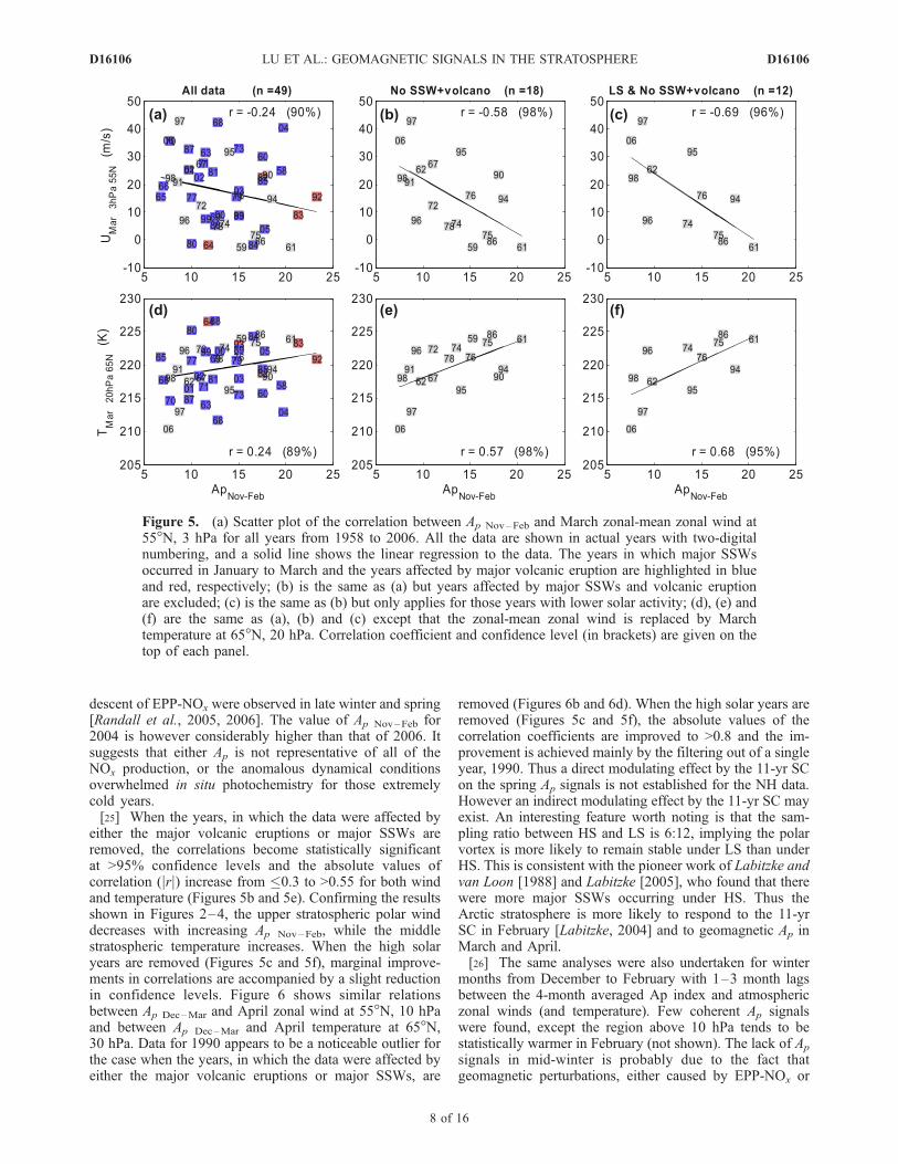
descent of EPP-NOx were observed in late winter and spring[Randall et al., 2005, 2006]. The value of Ap Nov–Feb for2004 is however considerably higher than that of 2006. Itsuggests that either Ap is not representative of all of theNOx production, or the anomalous dynamical conditionsoverwhelmed in situ photochemistry for those extremelycold years.[25] When the years, in which the data were affected by

either the major volcanic eruptions or major SSWs areremoved, the correlations become statistically significantat >95% confidence levels and the absolute values ofcorrelation (jrj) increase from �0.3 to >0.55 for both windand temperature (Figures 5b and 5e). Confirming the resultsshown in Figures 2–4, the upper stratospheric polar winddecreases with increasing Ap Nov–Feb, while the middlestratospheric temperature increases. When the high solaryears are removed (Figures 5c and 5f), marginal improve-ments in correlations are accompanied by a slight reductionin confidence levels. Figure 6 shows similar relationsbetween Ap Dec–Mar and April zonal wind at 55�N, 10 hPaand between Ap Dec–Mar and April temperature at 65�N,30 hPa. Data for 1990 appears to be a noticeable outlier forthe case when the years, in which the data were affected byeither the major volcanic eruptions or major SSWs, are

removed (Figures 6b and 6d). When the high solar years areremoved (Figures 5c and 5f), the absolute values of thecorrelation coefficients are improved to >0.8 and the im-provement is achieved mainly by the filtering out of a singleyear, 1990. Thus a direct modulating effect by the 11-yr SCon the spring Ap signals is not established for the NH data.However an indirect modulating effect by the 11-yr SC mayexist. An interesting feature worth noting is that the sam-pling ratio between HS and LS is 6:12, implying the polarvortex is more likely to remain stable under LS than underHS. This is consistent with the pioneer work of Labitzke andvan Loon [1988] and Labitzke [2005], who found that therewere more major SSWs occurring under HS. Thus theArctic stratosphere is more likely to respond to the 11-yrSC in February [Labitzke, 2004] and to geomagnetic Ap inMarch and April.[26] The same analyses were also undertaken for winter

months from December to February with 1–3 month lagsbetween the 4-month averaged Ap index and atmosphericzonal winds (and temperature). Few coherent Ap signalswere found, except the region above 10 hPa tends to bestatistically warmer in February (not shown). The lack of Ap

signals in mid-winter is probably due to the fact thatgeomagnetic perturbations, either caused by EPP-NOx or

Figure 5. (a) Scatter plot of the correlation between Ap Nov–Feb and March zonal-mean zonal wind at55�N, 3 hPa for all years from 1958 to 2006. All the data are shown in actual years with two-digitalnumbering, and a solid line shows the linear regression to the data. The years in which major SSWsoccurred in January to March and the years affected by major volcanic eruption are highlighted in blueand red, respectively; (b) is the same as (a) but years affected by major SSWs and volcanic eruptionare excluded; (c) is the same as (b) but only applies for those years with lower solar activity; (d), (e) and(f) are the same as (a), (b) and (c) except that the zonal-mean zonal wind is replaced by Marchtemperature at 65�N, 20 hPa. Correlation coefficient and confidence level (in brackets) are given on thetop of each panel.

D16106 LU ET AL.: GEOMAGNETIC SIGNALS IN THE STRATOSPHERE

8 of 16

D16106

through dynamic forcing, have not yet taken effect in thestratosphere. It is also likely that geomagnetic perturbationsare overpowered by the dominant effects of other processessuch as the stratospheric equatorial quasi-biennial oscilla-tion (QBO) in early winter [Holton and Tan, 1980; Lu et al.,2008], and the 11-yr SC in late winter [Labitzke, 2005].4.1.2. Possible Modulation by the QBO[27] Linear correlations were performed to investigate

whether the observed Ap signals are also modulated bythe QBO. We extract the equatorial (0.56�N) zonal winds ata range of pressure levels from 10 hPa to 50 hPa from thecombined ERA-40 and Operational records. The westerlyand easterly phases were defined as the deseasonalizedmonthly zonal-mean zonal wind �2 m s�1 and ��2 m s�1,and are hereinafter respectively referred to as wQBO andeQBO. In the NH, we did not find large-scale robust Ap

signals in both zonal wind and temperature, except forMay and when the 50 hPa deseasonalized equatorial zonalwind is used to present the QBO.[28] Figure 7 shows linear correlations between Ap Jan–Apr

and May zonal wind (upper panels) and between Ap Jan–Apr

and May temperature (lower panels). The data included inthe analysis are those years in which no major SSWsoccurred in late winter (i.e., in February–March) and nomajor volcanic eruption had occurred in the past 2 years.The plots in Figure 7 indicate that, when the data are notgrouped by the phases of the QBO, there is little or nocorrelation between Ap Jan –Apr and the zonal wind andbetween Ap Jan–Apr and the temperature in the extratropicalstratosphere (r = ±0.2). Apart from a small region near theequator and at low altitude, where the correlation between

Ap Jan–Apr and the zonal wind is 0.4 with confidence levelsabove 95%.[29] The middle and right-most panels of Figure 7 show

the same as the left panels but the data are groupedaccording to wQBO and eQBO phases. Under wQBO,positive Ap Jan–Apr signals in zonal wind are shown in alarge region of the stratospheric extratropics, where r � 0.8can be found. These Ap Jan–Apr signals in zonal-mean zonalwinds under wQBO are highly significant with confidencelevels above 99%. The mid-latitude NH polar temperature isnegatively correlated with Ap Jan–Apr under wQBO, imply-ing a colder NH polar region when Ap Jan–Apr is high. UndereQBO, no Ap Jan –Apr signals can be found except anoscillating positive–negative correlation pattern in the zonalwind from the sub-tropical to mid-latitudes, associated withan cold region in the sub-tropical mid-stratosphere covering20�–45�N, and 100–10 hPa (18–32 km altitudes), whichare rather stable and become statistically significant atconfidence levels of 95% when the volcanic eruptioneffected years were excluded but major SSWs years wereincluded (not shown).[30] The scatter plots for those locations with peak

correlations for wind and temperature under wQBO (see2nd column of Figure 7) are shown in Figure 8, in whichonly the volcanic eruption affected years were excluded.Figure 8a shows that the upper stratospheric polar windincreases with increasing Ap Jan–Apr, while Figure 8c showsthat the temperature decreases with increasing Ap Jan–Apr

under wQBO. The magnitude of the changes in windanomaly is up to 15 m s�1, and the corresponding decreasein temperature is �5 K. Figures 8b and 8d show that the

Figure 6. Same as Figure 5 except that Ap is December–March mean and zonal wind and temperatureare replaced by April mean values at 55�N, 10 hPa and at 65�N, 30 hPa, respectively.

D16106 LU ET AL.: GEOMAGNETIC SIGNALS IN THE STRATOSPHERE

9 of 16

D16106

Figure 7. Correlations between Ap Jan–Apr and May zonal-mean zonal wind (1st row) and Maytemperature (2nd row) for all data (1st column), when the QBO is westerly (2nd column), and when theQBO is easterly (3rd column), displayed in the NH extratropical meridional–vertical cross section. TheQBO phases are defined by May zonal-mean zonal wind anomalies at 0.56�N, 50 hPa. The contours andshadings are the same as those in Figure 3.

Figure 8. Scatter plots of correlations between the zonal-mean zonal wind at 64�N, 2 hPa and Ap Jan–Apr

(a) and May F10.7 fluxes (b) under wQBO. (c) and (d) are the same as (a) and (b) but for the zonal-meantemperature at 80�N, 20 hPa. The data are shown in actual years with two-digital numbering with a solidline showing the linear regression to the data. Correlation coefficient and confidence level (in bracket) areshown on the top of each panel.

D16106 LU ET AL.: GEOMAGNETIC SIGNALS IN THE STRATOSPHERE

10 of 16

D16106

correlations between both the wind and temperature and theproxy of the 11-yr SC, F10.7 in May, are rather weak.

4.2. Ap Signals in the SH

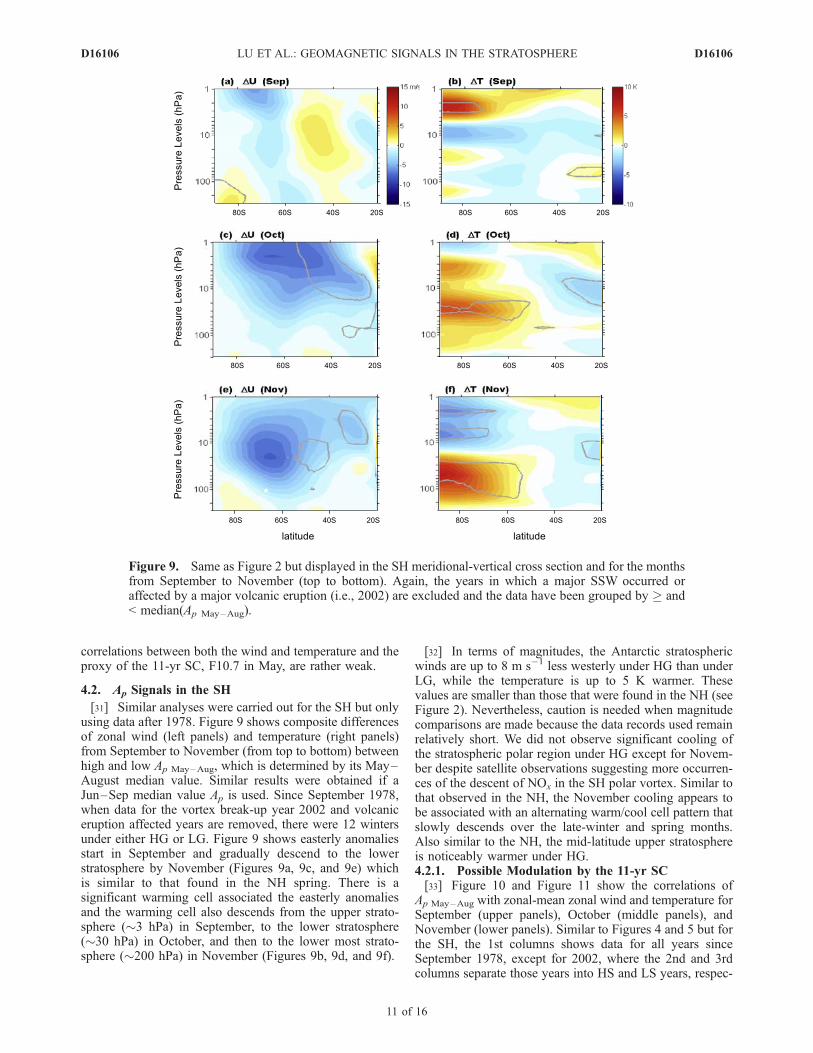
[31] Similar analyses were carried out for the SH but onlyusing data after 1978. Figure 9 shows composite differencesof zonal wind (left panels) and temperature (right panels)from September to November (from top to bottom) betweenhigh and low Ap May–Aug, which is determined by its May–August median value. Similar results were obtained if aJun–Sep median value Ap is used. Since September 1978,when data for the vortex break-up year 2002 and volcaniceruption affected years are removed, there were 12 wintersunder either HG or LG. Figure 9 shows easterly anomaliesstart in September and gradually descend to the lowerstratosphere by November (Figures 9a, 9c, and 9e) whichis similar to that found in the NH spring. There is asignificant warming cell associated the easterly anomaliesand the warming cell also descends from the upper strato-sphere (�3 hPa) in September, to the lower stratosphere(�30 hPa) in October, and then to the lower most strato-sphere (�200 hPa) in November (Figures 9b, 9d, and 9f).

[32] In terms of magnitudes, the Antarctic stratosphericwinds are up to 8 m s�1 less westerly under HG than underLG, while the temperature is up to 5 K warmer. Thesevalues are smaller than those that were found in the NH (seeFigure 2). Nevertheless, caution is needed when magnitudecomparisons are made because the data records used remainrelatively short. We did not observe significant cooling ofthe stratospheric polar region under HG except for Novem-ber despite satellite observations suggesting more occurren-ces of the descent of NOx in the SH polar vortex. Similar tothat observed in the NH, the November cooling appears tobe associated with an alternating warm/cool cell pattern thatslowly descends over the late-winter and spring months.Also similar to the NH, the mid-latitude upper stratosphereis noticeably warmer under HG.4.2.1. Possible Modulation by the 11-yr SC[33] Figure 10 and Figure 11 show the correlations of

Ap May–Aug with zonal-mean zonal wind and temperature forSeptember (upper panels), October (middle panels), andNovember (lower panels). Similar to Figures 4 and 5 but forthe SH, the 1st columns shows data for all years sinceSeptember 1978, except for 2002, where the 2nd and 3rdcolumns separate those years into HS and LS years, respec-

Figure 9. Same as Figure 2 but displayed in the SH meridional-vertical cross section and for the monthsfrom September to November (top to bottom). Again, the years in which a major SSW occurred oraffected by a major volcanic eruption (i.e., 2002) are excluded and the data have been grouped by � and< median(Ap May–Aug).

D16106 LU ET AL.: GEOMAGNETIC SIGNALS IN THE STRATOSPHERE

11 of 16

D16106

tively. In the 1st columns, the correlation patterns for bothzonal wind (Figure 10) and temperature (Figure 11) resem-ble those shown in Figure 9 and the correlations becomestatistically significant in October. In October, similar Ap

signals in both wind and temperature are maintained underLS, generally with a warmer Antarctic stratosphere withnegative correlations shown in the extratropics. Under HS,the correlations are no longer significant though the signs ofthe correlations remain the same. In September and No-vember however the linear correlations are not significantfor all three cases (all data, HS, and LS) though the signs ofthe correlations remain similar to those in October. For allthree months, there are nearly equal amounts of datasamples under HS and LS.[34] Similar analyses were also conducted for winter

months from June to August. Only localized or weak Ap

signals were found. During those SH winter months, we, onthe other hand, found that strong signatures of the 11-yr SC,similar to those shown in Crooks and Gray [2005], domi-nate the extratropical stratosphere (not shown). Thus, sim-ilar to the NH, it is apparent that the extratropicalstratosphere responds to the 11-yr SC in middle to latewinter while it responds to geomagnetic activity in spring.[35] To examine if the 11-yr SC indeed modulates the Ap

signals in the SH, the October data were analyzed usingscatter plots. Figure 12 shows the correlations between

Ap May–Aug and October stratospheric wind and tempera-ture at two selected locations. The values of jrj betweenAp May–Aug and October zonal wind at 40�N, 5 hPa andbetween Ap May–Aug and October temperature at 65�N,30 hPa are <0.5 when all the years since 1979 are selected(Figures 12a and 12c). When the HS years are removed(Figures 12b and 12d), significant increases in the values ofjrj are accompanied with marginal increases in confidencelevels. Due to the marginal increases in confidence levelsand the critical influence of the data point for 2003,Figure 12 does not suggest an indisputable modulation ofthe 11-yr SC. Note that for the period from 1979 to 2006,the Ap May–Aug and F10.7May–Aug are positively correlatedwith r = 0.48. Thus it is possible that the Ap signals weobtained here may be contaminated by that of the 11-yr SC.Longer data records are needed to further test if thereis indeed a significant 11-yr SC modulation on atmo-spheric responses to geomagnetic forcing in the extra-tropical stratosphere.[36] We found no significant QBO modulated Ap May–Aug

signals for the SH late winter and spring. Apparent positivecorrelations were found only in zonal winds during Augustand September under wQBO at the altitudes around 20 hPaand 100 hPa in the Antarctic stratosphere (not shown).However these SH zonal wind correlations are only mar-ginally significant and confined within a rather small area. It

Figure 10. Same as Figure 3 but for September to November, displayed in the SH meridional–verticalcross section of 300-1 hPa and 20�–90�N.

D16106 LU ET AL.: GEOMAGNETIC SIGNALS IN THE STRATOSPHERE

12 of 16

D16106

is likely because that the SH vortex is less dynamicallydisturbed and therefore less influenced by the QBO than theNH vortex that is forced by stronger planetary wave activity.

5. Discussion and Conclusions

[37] Enhancement of upper stratospheric NOx accompa-nied by a simultaneous reduction in O3 has been observedby various satellites [Siskind et al., 2000; Natarajan et al.,2004; Randall et al., 2005; Rinsland et al., 2005; Seppala etal., 2007]. Using data from the Halogen Occultation Ex-periment (UARS/HALOE), Siskind and Russell [1996]found that, in the SH, downward transport of thermosphericNOx was a regular feature of the winter high-latitudemesosphere and the enhancements of NOx were seen aslow as 35 km. The average SH stratospheric NOx columndensity with an altitude range of 23–32 km during May–August, 1991–1996 were found to be correlated with the4-month averaged geomagnetic Ap index, implying a geo-magnetic origin of EPP-NOx [Siskind et al., 2000]. Howeverthe enhancements did not seem to persist until spring whenthe O3 depletion would be more efficient. Using solaroccultation (SO) data from 1992 to 2005, Randall et al.[2007] estimate that NOx descended from the thermosphereand the upper mesosphere contributed up to 40% of theannual SH polar stratospheric NOx, and the interannual

variability of the SH polar stratospheric NOx is stronglycorrelated with low and medium energy EPP fluxes.[38] Until the winter of 2003/2004 however the SO data

sets used to investigate long-term EPP impacts showed littleevidence of descending EPP-NOx in the NH compared withthe SH. The unprecedented event of descending NOx in latewinter to spring of 2003/2004 was explained as a result ofan accumulative effect of low to medium energy EPPtogether with an exceptionally strong late winter polarvortex [Orsolini et al., 2005; Randall et al., 2005; Clilverdet al., 2006]. However, in February and March 2006, asubstantial polar upper stratospheric NOx enhancement inthe NH was observed by the Atmospheric ChemistryExperiment (ACE) during a period of minimal geomagneticactivity [Randall et al., 2006]. NO2 mixing ratios in theupper stratosphere were 3–6 times larger than observedpreviously in either the Arctic or Antarctic, apart from theextraordinary winter of 2003/2004, when the observed NOx

mixing ratio were yet an order of magnitude larger. Suchobservations raise the question about how significant is theeffect of geomagnetic activity on the magnitude of NOx

enhancements in the stratospheric polar region in compar-ison with dynamical forcing [Hauchecorne et al., 2007;Siskind et al., 2007].[39] To answer the three research questions raised in the

introduction, we have investigated possible stratosphericresponses to geomagnetic activity in late winter and spring

Figure 11. Same as Figure 10 but the zonal-mean zonal winds are replaced by temperature.

D16106 LU ET AL.: GEOMAGNETIC SIGNALS IN THE STRATOSPHERE

13 of 16

D16106

of both hemispheres. Using the combined ERA-40 andOperational records for the periods of 1958–2006 for theNH and 1979–2006 for the SH, we have found apparentlysignificant spring geomagnetic signals in zonal-mean zonalwind and temperature in the extratropical stratosphere. Acommon feature of the spring geomagnetic Ap signals in thestratospheric mid- to high latitudes is less anomalouswesterly wind, and warmer polar regions, associated withhigher winter time geomagnetic activity when there was astable winter vortex. Such spring geomagnetic Ap signalsare, in general, consistent with the findings of Lu et al.[2007], who filtered out the periods below 12 months fromthe radiosonde temperature data. In the spring months whenthe descent of EPP-NOx may have a detectable impact, wefind here that the geomagnetic Ap signals seem to descendfrom the upper stratosphere to the lower stratosphere. Thesignals become more statistically significant when thewinter polar vortex is stable without major stratosphericsudden warming (SSW) occurring in middle to late winter.[40] The spring Ap signals we have found here appear to

be inconsistent with a simple local cooling effect of in situchemistry between stratospheric O3 and descending high-altitude EPP-NOx. Firstly, the Ap signals in both wind andtemperature have the opposite signs to those expected fromcooling effects due to catalytic destruction of stratosphericO3 by EPP-NOx. Secondly, we found stronger and more

significant geomagnetic signals in the NH than in the SHeven though the satellite observations suggest more frequentdescent of EPP-NOx to the stratosphere in the SH. Thirdly,the observed geomagnetic Ap signals in both stratosphericwind and temperature have much larger magnitudes thanwould be expected from in situ chemical reactions alone[Jackman et al., 2005, 2008]. It is however important tostress that our results here neither rule out the possibilitythat descending EPP-NOx may have played a role instratospheric circulation on an irregular basis, nor show thatEPP-NOx does not affect stratospheric ozone. Further mod-eling of descending EPP-NOx and its radiative feedback isrequired to clarify the detailed situation.[41] Possible modulations of the spring geomagnetic Ap

signals by the 11-yr SC and the QBO were found in thisstudy, although more data are needed to test the significanceof such modulations. In spring, atmospheric responses togeomagnetic activity are preferentially clearer when solarirradiance is low. Only in the NH during May are the Ap

signals found to be modulated by the QBO. The results mayrule out the possibility that the detected geomagnetic signalsare caused by solar UV radiative heating, but do not rule outthe possibility of its relation to solar UV induced effectselsewhere in the atmosphere. The results also imply thatthere is a possible inter-modulating relationship among theQBO, the 11-yr SC and geomagnetic activity. The strato-

Figure 12. (a) Scatter plot of the correlation between Ap May–Aug and October zonal-mean zonal wind at40�S, 5 hPa for all years since 1979 to 2006, 2002 and the years affected by the major volcanic eruptionare highlighted in blue and red, respectively; (b) is the same as (a) but only for those years with lowersolar activity; (c) and (d) are the same as (a) and (b) but for October temperature at 65�S, 30 hPa.Correlation coefficient and confidence level (in bracket) are given on the top of each panel.

D16106 LU ET AL.: GEOMAGNETIC SIGNALS IN THE STRATOSPHERE

14 of 16

D16106

spheric polar region may respond to both solar originatedperturbations through dynamical interactions. The questionremains as to what mechanism is behind such modulations.A possible mechanism for the QBO modulated Ap signalsmight be that suggested by Naito and Yoden [2006], whofound that poleward and downward anomalous extratropicalwave forcing was associated with the wQBO, while equa-tor-ward wave forcing was associated with the eQBO. Thatmight point to a possible mechanism explaining why polarAp signals are associated with the wQBO, and subtropicalAp signals are associated with the eQBO.[42] During northern winters as well as northern sum-

mers, the 11-yr SC signal in atmospheric temperature andgeopotential height have been found when subdividedaccording to the QBO phases [Labitzke and van Loon,1988; Salby and Callaghan, 2006]. Similar to the 11-yrSC signals, which were found to be broadly symmetricabout the equator, here we found that spring geomagneticsignatures in the extratropical stratosphere are also approx-imately symmetric about the equator. However such Ap

signals have only been obtained by using the years whenno major SSWs occurred in middle to late winter. Themagnitudes of changes in spring stratospheric wind andtemperatures associated with the geomagnetic Ap signals arein the range of 10–20 m s�1 and 5–10 K. They arecomparable with those of the 11-yr SC signals typicallyfound in late winter [Labitzke, 2004; Crooks and Gray,2005]. Together with those previous findings, we suggestthat those solar or geomagnetic signals in the extratropicalstratosphere are not consistent with a direct or in situconsequence of radiative heating by UV–ozone interaction,or EPP-NOx effects on ozone.[43] We suggest that there might be an indirect chemical–

dynamic connection to the stratosphere, with geomagneticand solar far-UV perturbations in the mesosphere and thelower thermosphere, where routine production of NOx isformed by the dissociation of N2 by far-UV solar radiationand EPP in the auroral zone. It is likely that the geomagneticAp signals found in this study result from a couplingbetween mean flow and atmospheric waves, includingplanetary and gravity waves, as suggested earlier by Arnoldand Robinson [2001]. In the stratosphere, vertically propa-gating planetary waves from the troposphere control theintensity of the equator-to-pole transport of O3 by theBrewer–Dobson circulation. In the mesosphere, the inter-action between gravity waves and zonal winds controls thetransport strength from summer pole to winter pole. Tem-perature changes induced by either EPP or far-UV solarradiation in the mesosphere or the thermosphere may causechanges in vertical propagating wave ducting. It is alsopossible that EPP-NOx may cause changes of mesosphericO3, which lead to anomalous changes of the temperaturegradient between the two poles, consequently altering themesospheric pole-to-pole circulation. Such a change wouldmodify the refraction or ducting condition of planetary andgravity waves. By either suppressing or enhancing thepropagation/reflection of planetary waves into the strato-spheric polar region, it leads to anomalous warming orcooling in the stratospheric polar regions. Nevertheless, thedetailed mechanism that produces the spring geomagneticsignals found in this study and drives their downwardpropagation remains unclear. More data and modeling

exercises are needed in order to answer this intriguingquestion, as our statistical analyses have not been able toprovide an unequivocal answer to it.

[44] Acknowledgments. We would like to thank Martin J. Jarvis forhis useful discussions and guidance. The SAGE III data were obtained fromthe NASA Langley Research Center Atmospheric Science Data Center. Weare very grateful to two anonymous referees whose comments significantlyimproved the paper.

ReferencesArnold, N. F., and T. R. Robinson (1998), Solar cycle changes to planetarywave propagation and their influence on the middle atmosphere circula-tion, Ann. Geophys., 16(1), 69–76.

Arnold, N. F., and T. R. Robinson (2001), Solar magnetic flux influences onthe dynamics of the winter middle atmosphere, Geophys. Res. Lett.,28(12), 2381–2384.

Bertaux, J. L., E. Kyrola, and T. Wehr (2000), Stellar occultation techniquefor atmospheric ozone monitoring: GOMOS on Envisat, Earth Observ.Quart., 67, 17–20.

Boberg, F., and H. Lundstedt (2002), Solar wind variations related to fluc-tuations of the North Atlantic Oscillation, Geophys. Res. Lett., 29(15),1718, doi:10.1029/2002GL014903.

Boberg, F., and H. Lundstedt (2003), Solar wind electric field modulationof the NAO: A correlation analysis in the lower atmosphere, Geophys.Res. Lett., 30(15), 1825, doi:10.1029/2003GL017360.

Bochnicek, J., and P. Hejda (2005), The winter NAO pattern changes inassociation with solar and geomagnetic activity, J. Atmos. Sol. Terr.Phys., 67, 17–32.

Brasseur, G. P., and S. Solomon (2005),Aeronomy of theMiddle Atmosphere,3rd ed., Springer, Dordrecht.

Callis, L. B., R. E. Boughner, M. Natarajan, J. D. Lambeth, D. N. Baker,and J. B. Blake (1991), Ozone depletion in the high-latitude lower strato-sphere-1979–1990, J. Geophys. Res., 96(D2), 2921–2937.

Callis, L. B., M. Natarajan, and J. D. Lambeth (2001), Solar-atmosphericcoupling by electrons (SOLACE) 3. Comparisons of simulations andobservations, 1979–1997, issues and implications, J. Geophys. Res.,106(D7), 7523–7539.

Charlton, A. J., and L. M. Polvani (2007), A new look at stratosphericsudden warmings. part I. Climatology and modelling benchmarks,J. Clim., 20, 449–469.

Clilverd, M. A., A. Seppala, C. J. Rodger, P. T. Verronen, and N. R.Thomson (2006), Ionospheric evidence of thermosphere-to-stratospheredescent of polar NOx, Geophys. Res. Lett., 33, L19811, doi:10.1029/2006GL026727.

Crooks, S. A., and L. J. Gray (2005), Characterization of the 11-year solarsignal using a multiple regression analysis of the ERA-40 dataset,J. Clim., 18(7), 996–1015.

Davis, R. E. (1976), Predictability of sea surface temperature and sea levelpressure anomalies over the North Pacific Ocean, J. Phys. Oceangr., 6,249–266.

Garrett, H. B., A. J. Dessler, and T. W. Hill (1974), I. Influence of solar windvariability on geomagnetic activity, J. Geophys. Res., 79(31), 4603–4610.

Hauchecorne, A., et al. (2005), First simultaneous global measurements ofnighttime stratospheric NO2 and NO3 observed by global ozone monitor-ing by Occultation of Stars (GOMOS)/Envisat in 2003, J. Geophys. Res.,110, D18301, doi:10.1029/2004JD005711.

Hauchecorne, A., J.-L. Bertaux, F. Dalaudier, J. M. Russell, M. G.Mlynczak,E. Kyrola, and D. Fussen (2007), Large increase of NO2 in the north polarmesosphere in January–February 2004: Evidence of a dynamical originfrom GOMOS/ENVISAT and SABER/TIMED data, Geophys. Res. Lett.,34, L03810, doi:10.1029/2006GL027628.

Holton, J. R., and H. C. Tan (1980), The influence of the equatorial quasi-biennial oscillation on the global circulation at 50 mb, J. Atmos. Sci., 37,2200–2208.

Jackman, C. H., and R. D. McPeters (2004), The effect of solar protonevents on ozone and other constituents, in Solar Variability and Its Effecton the Earth’s Atmosphere and Climate System, edited by J. Pap et al.,AGU Monogr. Ser., Washington D. C.

Jackman, C. H., M. T. DeLand, G. J. Labow, E. L. Fleming, D. K.Weisenstein, M. K. W. Ko, M. Sinnhuber, and J. M. Russell III (2005),Neutral atmospheric influences of the solar proton events in October–November 2003, J. Geophys. Res., 110, A09S27, doi:10.1029/2004JA010888.

Jackman, C. H., R. G. Roble, and E. L. Fleming (2007), Mesosphericdynamical changes induced by the solar proton events in October –November 2003, Geophys. Res. Lett., 34, L04812, doi:10.1029/2006GL028328.

D16106 LU ET AL.: GEOMAGNETIC SIGNALS IN THE STRATOSPHERE

15 of 16

D16106

Jackman, C. H., et al. (2008), Short- and medium-term atmospheric effectsof very large solar proton events, Atmos. Chem. Phys., 8, 765–785.

Kyrola, E., et al. (2004), GOMOS on Envisat: An overview, Adv. SpaceRes., 33, 1020–1028.

Labitzke, K. (2004), On the signal of the 11-year sunspot cycle in thestratosphere and its modulation by the quasi-biennial oscillation, J. At-mos. Sol. Terr. Phys., 66(13–14), 1151–1157.

Labitzke, K. (2005), On the solar cycle-QBO relationship: A summary,J. Atmos. Sol. Terr. Phys., 67(1–2), 45–54.

Labitzke, K., and H. van Loon (1988), Associations between the 11-yearsolar-cycle, the QBO and the atmosphere 1. The troposphere and strato-sphere in the Northern Hemisphere in winter, J. Atmos. Terr. Phys., 50(3),197–206.

Labitzke, K., and H. van Loon (2000), The QBO effect on the solar signalin the global stratosphere in the winter of the Northern Hemisphere,J. Atmos. Sol. Terr. Phys., 62(8), 621–628.

Langematz, U., J. L. Grenfell, K. Matthes, P. Mieth, M. Kunze, B. Steil, andC. Bruhl (2005), Chemical effects in 11-year solar cycle simulations withthe Freie Universitat Berlin Climate Middle Atmosphere Model withonline chemistry (FUB-CMAM-CHEM), Geophys. Res. Lett., 32,L13803, doi:10.1029/2005GL022686.

Lu, H., M. J. Jarvis, H. F. Graf, P. C. Young, and R. B. Horne (2007),Atmospheric temperature response to solar irradiance and geomagneticactivity, J. Geophys. Res., 112, D11109, doi:10.1029/2006JD007864.

Lu, H., M. Bladwin, L. Gray, and M. J. Jarvis (2008), Decadal-scalechanges in the effect of the QBO on the northern stratospheric polarvortex, J. Geophys. Res., 113, D10114, doi:10.1029/2007JD009647.

Marsh, D. R., R. R. Garcia, D. E. Kinnison, B. A. Boville, F. Sassi, S. C.Solomon, and K. Matthes (2007), Modeling the whole atmosphereresponse to solar cycle changes in radiative and geomagnetic forcing,J. Geophys. Res., 112, D23306, doi:10.1029/2006JD008306.

Mayaud, P. N. (1980), Derivation, Meaning, and Use of GeomagneticIndices, AGU, Washington, D. C.

Naito, Y., and S. Yoden (2006), Behavior of planetary waves before andafter stratospheric sudden warming events in several phases of the equa-torial QBO, J. Atmos. Sci., 63(6), 1637–1649.

Natarajan, M., E. E. Remsberg, L. E. Deaver, and J. M. Russell III (2004),Anomalously high levels of NOx in the polar upper stratosphere duringApril, 2004: Photochemical consistency of HALOE observations, Geo-phys. Res. Lett., 31, L15113, doi:10.1029/2004GL020566.

Orsolini, Y. J., G. L. Manney, M. L. Santee, and C. E. Randall (2005),An upper stratospheric layer of enhanced HNO3 following exceptionalsolar storms, Geophys. Res. Lett., 32, L12S01, doi:10.1029/2004GL021588.

Randall, C. E., et al. (2002), Validation of POAM III NO2 measurements,J. Geophys. Res., 107(D20), 8299, doi:10.1029/2001JD000471.

Randall, C. E., et al. (2005), Stratospheric effects of energetic particleprecipitation in 2003 – 2004, Geophys. Res. Lett., 32, L05802,doi:10.1029/2004GL022003.

Randall, C. E., V. L. Harvey, C. S. Singleton, P. F. Bernath, C. D. Boone,and J. U. Kozyra (2006), Enhanced NOx in 2006 linked to strong upperstratospheric Arctic vortex, Geophys. Res. Lett., 33, L18811, doi:10.1029/2006GL027160.

Randall, C. E., V. L. Harvey, C. S. Singleton, S. M. Bailey, P. F. Bernath,M. Codrescu, H. Nakajima, and J. M. Russell III (2007), Energeticparticle precipitation effects on the Southern Hemisphere stratospherein 1992 – 2005, J. Geophys. Res., 112, D08308, doi:10.1029/2006JD007696.

Rinsland, C. P., C. Boone, R. Nassar, K.Walker, P. Bernath, J. C.McConnell,and L. Chiou (2005), Atmospheric Chemistry Experiment (ACE) Arctic

stratospheric measurements of NOx during February and March 2004:Impact of intense solar flares, Geophys. Res. Lett., 32, L16S05,doi:10.1029/2005GL022425.

Rozanov, E., L. Callis, M. Schlesinger, F. Yang, N. Andronova, andV. Zubov (2005), Atmospheric response to NOy source due to energeticelectron precipitation, Geophys. Res. Lett., 32, L14811, doi:10.1029/2005GL023041.

Salby, M. L., and P. F. Callaghan (2006), Relationship of the quasi-biennialoscillation to the stratospheric signature of the solar cycle, J. Geophys.Res., 111, D06110, doi:10.1029/2005JD006012.

Seppala, A., P. T. Verronen, E. Kyrola, S. Hassinen, L. Backman,A. Hauchecorne, J. L. Bertaux, and D. Fussen (2004), Solar proton eventsof October –November 2003: Ozone depletion in the Northern Hemi-sphere polar winter as seen by GOMOS/Envisat, Geophys. Res. Lett.,31, L19107, doi:10.1029/2004GL021042.

Seppala, A., P. T. Verronen, M. A. Clilverd, C. E. Randall, J. Tamminen,V. Sofieva, L. Backman, and E. Kyrola (2007), Arctic and Antarcticpolar winter NOx and energetic particle precipitation in 2002–2006,Geophys. Res. Lett., 34, L12810, doi:10.1029/2007GL029733.

Siskind, D. E. (2000), On the coupling between the middle and upper atmo-spheric odd nitrogen, in Atmospheric Science Across the Stratopause,Geophys. Monogr. Ser., vol. 123, pp. 101–116, AGU, Washington, D. C.

Siskind, D. E., and J. M. Russell III (1996), Coupling between middle andupper atmospheric NO: Constraints from HALOE observations, Geo-phys. Res. Lett., 23(2), 137–140.

Siskind, D. E., G. E. Nedoluha, C. E. Randall, M. Fromm, and J. M. Russell(2000), An assessment of Southern Hemisphere stratospheric NOx

enhancements due to transport from the upper atmosphere, Geophys.Res. Lett., 27(3), 329–332.

Siskind, D. E., S. D. Eckermann, L. Coy, J. P. McCormack, and C. E.Randall (2007), On recent interannual variability of the Arctic wintermesosphere: Implications for tracer descent, Geophys. Res. Lett., 34,L09806, doi:10.1029/2007GL029293.

Solomon, S., P. J. Crutzen, and R. G. Roble (1982), Photochemical cou-pling between the thermosphere and the lower atmosphere: 1. Odd nitro-gen from 50 to 120 km, J. Geophys. Res., 87(C9), 7206–7220.

Thejll, P., B. Christiansen, and H. Gleisner (2003), On correlations betweenthe North Atlantic Oscillation, geopotential heights, and geomagneticactivity, Geophys. Res. Lett., 30(6), 1347, doi:10.1029/2002GL016598.

Uppala, S. M., et al. (2005), The ERA-40 reanalysis, Q. J. R. Meteorol.Soc., 131(612), 2961–3012.

Vennerstrøm, S., and E. Friis-Christensen (1996), Long-term and solarcycle variation of the ring current, J. Geophys. Res., 101(A11),24,727–24,735.

Zubov, V., E. Rozanov, A. Shirochkov, L. N. Makarova, T. Egorova,A. Kiselev, Y. Ozolin, I. Karol, and W. Schmutz (2005), Modeling of theJoule heating influence on the circulation and ozone concentration in themiddle atmosphere, J. Atmos. Terr. Phys., 67, 155–162, doi:10.1016/j.jastp.2004.07.024.

�����������������������M. A. Clilverd and H. Lu, Physical Sciences Division, British Antarctic

Survey, High Cross, Madingley Road, Cambridge CB3 0ET, UK.(macl@bas.ac.uk; hlu@bas.ac.uk)L. Hood, Lunar and Planetary Laboratory, University of Arizona, Tuczon,

AZ 85721, USA. (lon@lpl.arizona.edu)A. Seppala, Earth Observation, Finnish Meteorological Institute, P.O.

Box 503, FI-00101 Helsinki, Finland. (annika.seppala@fmi.fi)

D16106 LU ET AL.: GEOMAGNETIC SIGNALS IN THE STRATOSPHERE

16 of 16

D16106