arX

iv:0

809.

3374

v2 [

astr

o-ph

] 1

Mar

200

9

The growth of matter perturbations in f(R) models

R. Gannouji∗, B. Moraes†and D. Polarski‡

Lab. de Physique Theorique et Astroparticules, CNRSUniversite Montpellier II, France

March 1, 2009

Abstract

We consider the linear growth of matter perturbations on low redshiftsin some f(R) dark energy (DE) models. We discuss the definition of darkenergy (DE) in these models and show the differences with scalar-tensor DEmodels. For the f(R) model recently proposed by Starobinsky we show thatthe growth parameter γ0 ≡ γ(z = 0) takes the value γ0 ≃ 0.4 for Ωm,0 = 0.32and γ0 ≃ 0.43 for Ωm,0 = 0.23, allowing for a clear distinction from ΛCDM.Though a scale-dependence appears in the growth of perturbations on higherredshifts, we find no dispersion for γ(z) on low redshifts up to z ∼ 0.3, γ(z)is also quasi-linear in this interval. At redshift z = 0.5, the dispersion is stillsmall with ∆γ ≃ 0.01. As for some scalar-tensor models, we find here too alarge value for γ′

0 ≡ dγdz

(z = 0), γ′

0 ≃ −0.25 for Ωm,0 = 0.32 and γ′

0 ≃ −0.18 forΩm,0 = 0.23. These values are largely outside the range found for DE modelsin General Relativity (GR). This clear signature provides a powerful constrainton these models.

PACS Numbers: 04.62.+v, 98.80.Cq

∗email:gannouji@lpta.univ-montp2.fr†email:moraes@lpta.univ-montp2.fr‡email:polarski@lpta.univ-montp2.fr

1

1 Introduction

The present stage of accelerated expansion of the universe [1] is a major challenge forcosmology. There are basically two main roads one can take: either to introduce anew (approximately) smooth component or to modify the laws of gravity on cosmicscales. In the first class of models, the new component dubbed dark energy (DE)must have a sufficiently negative pressure in order to induce a late-time acceleratedexpansion. One typically adds a new isotropic perfect fluid with negative pressureable to accelerate the expansion. In the second class of models one is trying to explainthe accelerated expansion by modifying gravity, after all the universe expansion is alarge-scale gravitational effect. It is far from clear at the present time which class ofDE models will finally prevail and one must study carefully all possibilities. Whileall models are called DE models [2], the models of the second class are called morespecifically modified gravity DE models.

It is clear that in both classes we have many models able to reproduce a late-timeaccelerated expansion in agreement with the present data probing the backgroundexpansion like luminosity distances from SNIa. Probably this will remain the caseeven with more accurate data. However the evolution of matter perturbations will beaffected differently depending on the class of models we are dealing with. This can beused for a consistency check in order to find out whether a DE model is inside GeneralRelativity (GR) or not [3]. Therefore the evolution of matter perturbations seemsto be a powerful tool to discriminate between models inside and outside GR [4]. Inparticular, the growth of matter perturbations on small redshifts seems a promisingtool and it has been the subject of intensive investigations recently [5].

A particular class of modified gravity DE models are f(R) models where R isreplaced by some function f(R) in the gravitational Lagrangian density [6] (for arecent review, see [7]). The idea of producing an accelerated stage in such modelswas first successfully implemented in Starobinsky’s inflationary model [8]. In somesense it was rather natural to try explaining the late-time accelerated expansion by thesame kind of mechanism, a modification of gravity but now at much lower energies.Some problems arising in these f(R) DE models were quickly pointed out, relatedto solar-system constraints [9] and instabilities [10]. It was then found that a veryserious problem arises where it was not expected: many of these models are unableto produce the late-time acceleration together with a viable cosmic expansion history[11]. It was shown that many popular f(R) models, like those containing a R−1 term[12], are unable to account for a viable expansion history because of the absence of a

standard matter-dominated stage a ∝ t2

3 which is replaced instead by the behavioura ∝ t

1

2 [13].However some interesting cosmological models remain viable like the model re-

cently suggested by Starobinsky [14], (for another interesting viable model see also[15]). It is interesting in the first place because of its non-trivial ability to allowfor a standard matter-dominated stage. This goes together with the appearance oflarge oscillations in the past and the overproduction of massive scalar particles in thevery early universe which, as noted already in [14], can be a serious problem of allviable f(R) DE models. Another interesting property is the scale dependence of the

1

growth of matter perturbations deep inside the Hubble radius [16],[17]. This scaledependence was actually used in [14] in order to constrain one of the parameters ofthe model. Of course this model also satisfies the local gravity constraints for certainparameter values. In the end a window in parameter space remains where the modelis in principle physically acceptable.

In this letter we want to assess the viability of this model with respect to thegrowth of matter perturbations (see e.g. [18] for other possible constraints and ap-proaches). Some viable f(R) DE models have their free parameters constrained insuch a way that they cannot be distinguished observationally from ΛCDM. The situa-tion is different in this case. Our results show that the growth of matter perturbationson low redshifts z . 1 provides a discriminating signature of these models, able toclearly differentiate it from ΛCDM and also from any other DE model inside GR.These results confirm that the growth of matter perturbations can be used efficientlyto track the nature of DE models.

2 f(R) modified gravity cosmology

We consider now f(R) models and discuss some general properties in connection withtheir observational viability. Many f(R) models have the surprising property thatthey cannot account simultaneously for a viable cosmic expansion history and a late-time accelerated expansion. This severely constraints viable f(R) modified gravityDE models. We consider a universe where gravity and the content of the universe aredescribed by the following action

S =

∫

d4x√−g

[

1

16πG∗

f(R) + Lm

]

. (1)

For the time being, G∗ is a bare gravitational constant, its connection with obser-vations depends on the theory under consideration. We concentrate on spatially flatFriedman-Lemaıtre-Robertson-Walker (FLRW) universes with a time-dependent scalefactor a(t) and a metric

ds2 = −dt2 + a2(t) dx2 . (2)

For this metric the Ricci scalar R is given by

R = 6(

2H2 + H)

, (3)

where H ≡ aa

is the Hubble rate while a dot stands for a derivative with respect tothe cosmic time t. DE models have a > 0 on low redshifts. The following equationsare obtained

3FH2 = 8πG∗ (ρm + ρrad) +1

2(FR − f) − 3HF , (4)

−2FH = 8πG∗

(

ρm +4

3ρrad

)

+ F − HF , (5)

2

where

F ≡ df

dR. (6)

In standard Einstein gravity (f = R) one has F = 1. The densities ρm and ρrad satisfythe usual conservation equations ρi = −3H(1 + wi)ρi with wm = 0 and wrad = 1

3.

We summarize briefly the way in which the dynamics of f(R) models can be ana-lyzed. For a general f(R) model we introduce the following (dimensionless) variables

x1 = − F

HF, (7)

x2 = − f

6FH2, (8)

x3 =R

6H2=

H

H2+ 2 , (9)

x4 =8πG∗ρrad

3FH2. (10)

From Eq. (4) we have the algebraic identity

Ωm =8πG∗ ρm

3FH2= 1 − x1 − x2 − x3 − x4 . (11)

It is then possible to write down the following autonomous system

dx1

dN= −1 − x3 − 3x2 + x2

1 − x1x3 + x4 , (12)

dx2

dN=

x1x3

m− x2(2x3 − 4 − x1) , (13)

dx3

dN= −x1x3

m− 2x3(x3 − 2) , (14)

dx4

dN= −2x3x4 + x1 x4 , (15)

where N ≡ ln a. In eqs(13,14), the quantity m corresponds to

m ≡ d log F

d logR=

RF ′

F, (16)

(a prime stands for derivative with respect to R) hence m is a priori a function of R.However it is easy to see that R can in turn be expressed in function of the variablesof our autonomous system. Indeed we have

x3

x2≡ r = −RF

f= − d log f

d log R. (17)

Inverting (17) we can in principle express R as a function of x3

x2≡ r and so m becomes

in turn a function of r, m = m(r) which closes our system.

3

It was found in [13] that when radiation is negligible (x4 = 0) there exists a criticalpoint x1 = 0, x2 = −1

2, x3 = 1

2corresponding to an exact matter phase

weff = −1 − 2H

3H2=

1

3(1 − 2x3) = 0 (18)

Ωm = 1 . (19)

This is the critical point called P5(m = 0) in [13], it satisfies r = −1.Let us comment about the physical meaning of these conditions. For r = −1 or

x2 + x3 = 0, eq.(4) reduces to

3FH2 = 8πG∗ ρm − 3HF . (20)

Then we clearly have an exact matter phase (a ∼ t2

3 ) for F = 0 or x1 = 0. We notefurther from eqs.(13,14) that x2 + x3 remains zero for x1 = 0.

The condition m = 0 is more subtle. From eq.(14) a stable matter phase requires

x1 = 3 m . (21)

It is straightforward to generalize (21) for arbitrary scaling behaviour of the back-ground

x1 = 3 m(1 + weff) . (22)

Actually neither x1 nor m can be exactly zero during a matter phase (which corre-sponds to a critical point of the system). This would require F ′ = 0, which reducesto General Relativity plus a cosmological constant. The system can only come inthe vicinity of P5 and trajectories with an acceptable matter phase have x1 ≈ 0 andm ≈ 0 with x1 ≈ 3 m. In addition, from F ′ > 0 both x1 and m should be positiveduring the matter phase. Finally, it is easy to check that (21) implies

R ∝ a−3 . (23)

The situation is very different in scalar-tensor models where a standard matter phaseis possible with F ≈ 0 because the energy density associated with the dilaton φ canmimic the behaviour of dustlike matter for a particular type of potential U(φ) [19].It is this property which is used in [20]. More explicitly, for the Lagrangian density

L =1

16πG∗

(

F (Φ) R − gµν∂µΦ∂νΦ − 2U(Φ))

+ Lm(gµν) , (24)

we have the Friedmann equations (in flat space)

3FH2 = 8πG∗ ρm +Φ2

2+ U − 3HF , (25)

−2FH = 8πG∗ ρm + Φ2 + F − HF . (26)

It is possible to have a solution with F = 0 and Φ2

2+ U ∝ a−3 by a suitable choice

of the potential U [19]. Because of this property it is possible in the matter phase

4

to have a nonvanishing DE energy density ρDE . The definition of ρDE requires somecare. If we want ρDE to obey the usual energy conservation for perfect fluids, certainlya desirable property, then the choice is not unique. The Friedmann equations (4,5)and also (25,26) can be recast in the form

3A H2 = 8πG∗ (ρm + ρDE(A)) (27)

−2A H = 8πG∗ (ρm + ρDE(A) + pDE(A)) . (28)

where A is some arbitrary constant. We have written ρDE(A) (and pDE(A)) as thesequantities depend on the choice of A. For example from (4,5), neglecting radiation,we obtain

8πG∗ ρDE(A) =1

2(FR − f) − 3HF + 3(A − F ) H2 (29)

8πG∗ (ρDE(A) + pDE(A)) = F − HF − 2(A − F ) H (30)

Obviously, whatever choice is adopted the corresponding DE component obeys theusual conservation law of an isotropic perfect fluid. For the representation (27), it isnatural to introduce the cosmic relative densities

Ωi ≡8πG∗ρi

3AH2. (31)

A natural choice, especially if we are willing to compare modified gravity theorieswith General Relativity (GR), is to take

G∗

A≃ GN , (32)

to very high accuracy, where GN is Newton’s constant found in textbooks. In GR, it isthe bare gravitational constant appearing in the action and it corresponds to the valueof the gravitational constant obtained in a Cavendish-type experiment measuring theNewtonian force between two close test masses. As is well-known, this identificationno longer holds outside GR. For modified gravity theories it is the quantity Geff , apriori different from G∗, which plays the role of gravitational constant and whichis measured in a Cavendish-type experiment and clearly all acceptable models musthave the same Geff today to very high precision.

For scalar-tensor models we can make the choice A = F0 [19] as G∗F0

≃ Geff,0 to

very high accuracy because ωBD,0 > 4×104 from solar system constraints. As we willsee later, in our f(R) model a Cavendish-type experiment corresponds to the limitGeff = G∗ (see [14] and eq. (50) below). It is therefore natural to take A = 1 in sucha model.

As noted in [14] a consequence of the arbitrariness in the choice of A is that itintroduces an arbitrariness in the sign of ρDE as well. In a model where F0 > F inthe past, ρDE remains positive if we take A = F0. In our f(R) models however, wehave F0 < F (z > 0) in an expanding universe with F → 1 at high redshifts. Hence

5

ρDE(A) defined from (27) can become negative in the past if we take A = F0. Thisproblem is avoided if we define ρDE from (27,28) putting A = 1

3H2 = 8πG∗ (ρm + ρDE) (33)

−2H = 8πG∗ (ρm + ρDE + pDE) . (34)

The corresponding relative densities become Ωi ≡ 8πG∗ρi

3H2 and actually ΩDE → 0 inthe past. Note that though it is always possible to write the Friedmann equations inthe form (33,34) this should not conceal the fact that we are dealing with a genuinelymodified gravity theory obeying eqs.(4,5). The difference is absorbed in the micro-scopic definitions of the DE component. This shows again the need to go beyond thebackground expansion in order to discriminate modified gravity DE models from GR.

3 Starobinsky’s model

It was shown that a viable cosmic expansion is rather problematic in f(R) models.As already mentioned in the Introduction problems related to instabilities [10] andsolar-system constraints [9] were pointed out soon after the first attempts to producef(R) DE models. An even more unexpected problem was found later related to thebackground expansion as many f(R) models, including popular ones containing aninverse power of R, are unable to reproduce a viable expansion history containinga standard matter-dominated stage [11]. The viability of these models was thensystematically studied in [13]. All this shows that the construction of a viable f(R)DE model is something highly non-trivial. Still there are some f(R) DE models leftthat can account for a viable expansion history and still depart from ΛCDM. Onesuch interesting model was suggested recently by Starobinsky

f(R) = R + λRc

(

(

1 +R2

R2c

)

−n

− 1

)

, (35)

with λ, n > 0. We see that f(R) → R for R → 0 in contrast to models containing aninverse power of R, in addition in flat space the correction term to Einstein gravitydisappears. The quantity Rc has the dimension of R and is a free parameter of themodel, it corresponds essentially to the present cosmic value of R. Recently problemsrelated to the high-curvature regime of this model were pointed out [21] but it seemsthis could be cured by the addition of a term R2

m2 as noted in [14]. However the massm is required to be very high with m ≫ 1 GeV hence this term is negligible in thelow curvature regime. In the present work we will show that it is the low curvaturelimit of this model, through the growth of matter perturbations on small redshifts,that could severely constrain this model. It is convenient to introduce the reduceddimensionless curvature R ≡ R

Rc. We have for this model

r(R) =2nλR

(

R2 + 1)

−n−1

− 1

1 + λR−1

(

(

R2 + 1)

−n

− 1

) (36)

6

This is hardly inversible but fortunately the situation improves for R ≫ 1. In thisregime we have

f(R) ≃ R − λ Rc ≡ R − 2Λ(∞) (37)

F ≃ 1 (38)

r ≃ −1 − λR−1 (39)

m(r) ≃ 2n(2n + 1)

λ2n(−r − 1)2n+1 ≃ 2n(2n + 1)

λ

R2n+1≈ 0, m > 0 (40)

M2 ≃ 1

3F ′=

R

3mF≫ R . (41)

It is clear that when f(R) satisfies (37), x2 + x3 comes close to zero as FR − f ≃2Λ(∞) ≪ 6H2. We see that M2, the scalaron mass introduced in [8], becomes verylarge in the past. As noted in [14], one should find a mechanism to avoid M2 becomingtoo large in the early universe. We get also strong oscillations δR in the past and weillustrate this with the oscillations induced in the behaviour of weff on high redshiftsalready during the matter phase as displayed on Figure 1a. These oscillations couldlead to overproduction of scalarons in the very early universe [14]. While the cosmicbackground today corresponds to R ∼ 1, the regime R ≫ 1, eqs.(37)-(41), is quicklyreached as we go back in time. In this regime r ≈ −1 and m ≈ 0 so that a viablematter phase is possible followed by a late-time accelerated stage. We have also inthis regime F ≈ 1 to very high accuracy. One finds that in this model acceleratedexpansion starts at za ≃ (0.5− 1) depending on the value of Ωm,0, in agreement withobservations [22].

In order to be viable, this theory should not be in conflict with gravity constraints.On scales satisfying today k ≪ 2πM , one will not feel the presence of a “fifth force”caused by the scalar part of the gravitational interaction. Hence provided the scalaronmass M corresponding to some experiment is large enough, the “fifth force” will onlybe felt on scales that are much smaller than those probed by this experiment. Inparticular one will not see it in a Cavendish-type experiment on scales larger than5 × 10−2cm provided n ≥ 1, and this range can be increased to even lower scalesfor larger n [14]. We refer the interested reader to the reference [14] for a thoroughdiscussion of the properties of this model and of its potential problems.

The evolution and growth of matter perturbations can also be seen as an exper-iment probing gravity. In this case the scalaron mass can be much smaller so thatdeviations from GR and the appearance of a “fifth force”can be felt on larger scalesand even on cosmic scales. We will consider this in more detail in the next section.

4 Linear growth of matter perturbations

In a way analogous to scalar-tensor DE models, the equation governing the growthof matter perturbations on subhorizon scales is of the form [23]

δm + 2Hδm − 4πGeff ρm δm = 0 . (42)

7

0.0 0.2 0.4 0.6 0.8 1.0 1.2

-0.6

-0.5

-0.4

-0.3

-0.2

-0.1

0.0

Log @1+zD

wef

f

0.0 0.5 1.0 1.5 2.0

10

20

30

40

50

60

70

z

aH

a 0H

0

Figure 1: a) On the left panel the effective (total) equation of state parameter weff

is shown for n = 2. We see that large oscillations appear in the past, already inthe matter-dominated stage at rather low redshifts. b) On the right panel, the

behaviour of the quantity aHa0 H0

is displayed. It is seen that some subhorizon scales

satisfying k ≪ aH in the past will gradually shift to the regime k ≫ aH as theuniverse expands. In this asymptotic regime, the scalaron corresponding to the cosmicbackgroung curvature is nearly massless and a fifth-force is felt on these cosmic scales.Note that today H0 ∼ 7 H0.

The expression for Geff in f(R) models is given below, see eq.(42). Many DE modelsoutside GR have a modified equation of this type describing the growth of matterperturbations. For the models where it is valid, this equation includes all perturba-tions, the assumption is that we are in a regime deep inside the Hubble radius wherethe leading terms result in (42). One can also have in principle more elaborate DEmodels yielding a different equation (see e.g. [24]). It is convenient to rewrite thecorresponding equation satisfied by the quantity f = d ln δ

d ln a1[25]

df

dN+ f 2 +

1

2

(

1 − d lnΩm

dN

)

f =3

2

Geff

G∗

Ωm , (43)

where Ωm is defined from (31) with A = 1, and [16]

Geff =G∗

F

1 + 4k2F ′

a2F

1 + 3k2F ′

a2F

. (44)

The r.h.s. of (43) is given by the expression 4πGeffρm

H2 which obviously does notdepend on (the constant) A so that the evolution of f does not depend on A either.If we write this r.h.s. using the definition (29) Ωm = 8πG∗ρm

3AH2 with A 6= 1, we will have

4πGeffρm

H2 = 32

AGeff

G∗Ωm and we have in particular 3

2A Geff

G∗Ωm = 3

2

1+4k2F ′

a2F

1+3k2F ′

a2F

Ωm, with

Ωm defined in eq.(11). When gravity is described by GR eq.(43) reduces to eq.(B7)given in [26].

1The reader should not confuse this quantity with the quantity f(R), we believe such confusionwill be easily avoided from the context where they appear.

8

A crucial point in this model is that Geff is scale dependent

Geff = Geff(z, k) . (45)

In other words, the driving force in eq.(43) introduces a scale dependence in thegrowth of perturbations. The spatial variation on cosmic scales of Geff increasesthe growth of matter perturbations as is seen very clearly from Figure 2a. As thisincrease is rather tightly constrained by observations, so will the model parameter n

on which this increase depends [14]. We will return in more details to this importantpoint below.

We can rewrite Geff in the suggestive way

Geff =G∗

F

1 + 4 k2

a2H2

1 + 3 k2

a2H2

(46)

=G∗

F

(

1 +k2

a2H2

1 + 3 k2

a2H2

)

, (47)

where

H2 =F

F ′≡ 3FM2 =

R

m. (48)

In equation (43), Geff depends on the cosmic curvature R taken from (3). In the limitR ≫ 1 satisfied by the cosmic curvature R at high redshifts, we have

Geff = G∗

(

1 +1

3

k2

a2M2

1 + k2

a2M2

)

R ≫ 1 . (49)

Taking the (inverse) Fourier transform of (49) it is straightforward to recover thecorresponding gravitational potential per unit mass V (r). Remembering that a po-tential ∝ 1

rin real space yields a k−2 term in Fourier space, we recognize in (49) the

gravitational potential in real space (per unit mass)

V (r) = −G∗

r

(

1 +1

3e−Mr

)

. (50)

The quantity H (and M(R)) can become small enough with the universe expansion,see Figure 1b, so that some cosmic subhorizon scales can feel a significant fifth-force.As the universe expands, H is rapidly decreasing so that these deviations are felt inPoisson’s equation on ever increasing scales. While in the past only scales very muchsmaller than those corresponding to cosmic scales today could feel deviations fromGR, today H0 ∼ H0 and deviations can be felt on essentially all subhorizon scales.

We can distinguish two basic asymptotic regimes

Geff =4

3

G∗

Fk ≫ aH , (51)

=G∗

Fk ≪ aH . (52)

9

The quantity aH is rapidly increasing in the past. Hence some cosmic subhorizonscales (k ≫ aH) will satisfy k ≪ aH in earlier times (large redshifts) and switch intothe regime k ≫ aH on lower redshifts as the universe expands, see Figure 1b. Forcosmic scales that are in this regime (51), the scalaron mass appears negligible and afifth force does appear which results in the factor 4

3.

An accurate evolution of f or δm for arbitrary r.h.s. of eq.(43) requires numericalcalculations. But it is possible to find analytically the solutions in the two asymptoticregimes (51,52) during the matter stage when Ωm ≈ 1 and F ≈ 1. This regime isstill valid until low redshifts. When C ≡ Geff

G∗Ωm = constant we get constant growing

mode solutions f = p with (see e.g.[20])

p =1

4

(

−1 +√

1 + 24C)

. (53)

A similar result can also be obtained in the framework of chameleon models (see e.g.[27]) and inside GR (see e.g. [28]). We have C ≈ 1 for k ≪ aH and C ≈ 4

3for

k ≫ aH , so that we obtain [14]

δm ∝ a k ≪ aH (54)

δm ∝ a√

33−1

4 k ≫ aH . (55)

For subhorizon scales that go from the first into the second regime, this can yield ascale-dependent increase (see Figure 2a) in the growth of matter perturbations. Notethat this increase takes place on small cosmic scales. This increase in the growth ofmatter perturbations will induce a change of shape of the matter power spectrumP (k) inferred from galaxy surveys with a subsequent change of its spectral index ngal

s ,

P (k) ∝ kngals . This can then be compared with the spectral index nCMB

s derived fromthe CMB anisotropy data resulting in a possible discrepancy between both spectralindices. No significant discrepancy between the two values is allowed by presentobservations and we have the conservative bound (see e.g. [29])

ngals − nCMB

s < 0.05 (56)

So this difference is rather tightly constrained and so is the model parameter n onwhich it depends. This results in the constraint n ≥ 2. Because increasing the modelparameter n will decrease this discrepancy according to the analytical estimate [14]

ngals − nCMB

s =

√33 − 5

2(3n + 2), (57)

which is accurate for a wide range of n values (only for large values one should resortto a more accurate numerical estimate), (56,57) result in the constraint n ≥ 2.

Let us emphasize again at this point the differences with scalar-tensor DE models.In scalar-tensor DE models Geff does not depend on k (or on r in real space), at agiven time it is the same Geff that enters the equation for the growth of perturbationsand the gravitational constant measured in a Cavendish-type experiment. These

10

DE models have further a negligible dilaton mass but they can comply with solar-system constraints if they satisfy ωBD,0 > 4 × 104, where ωBD,0 is the value today ofthe Brans-Dicke parameter, which yields γPN ≈ 1 [23],[30]. Indeed for scalar-tensormodels one has for the Post-Newtonian parameter today γPN =

ωBD,0+1

ωBD,0+2and solar-

system constraints point at γPN ≈ 1 close to its GR value γPN = 1. As f(R) modelscorrespond to scalar-tensor models with ωBD = 0 they have γPN = 1

2which requires

a high scalaron mass to comply with solar-system constraints.In asymptotically stable scalar-tensor DE models the matter perturbations grow

slowlier than a in the matter stage and this growth is scale-independent.The growth of matter perturbations could provide an efficient way to discriminate

between modified gravity DE models and DE models inside GR. One can characterizethe growth of matter perturbations on small redshifts using the quantity γ(z)

f = Ωm(z)γ(z) . (58)

In the pioneering papers on this approach γ was taken constant [31]. But it is impor-tant to realize that γ(z) is a function of z which is generically not constant, and thatits variation can contain crucial information about the underlying model. As wasshown earlier, for a wide class of models inside GR one has |γ′

0 ≡ dγ

dz(z = 0)| . 0.02

so that γ(z) is approximately constant [25]. In ΛCDM we have γ0 ≈ 0.55 (with aslight dependence on Ωm,0) and γ′

0 ≃ −0.015. However, γ′

0 can be significantly largerin models outside GR [20]. From the growth of matter perturbations we can calculateγ(z) and dγ

dzand in particular their value at z = 0. As we can see from Figure 2a, we

find that f is scale-independent on low redshifts z . 0.5. This means that the growthof matter perturbations is the same on all relevant scales in this redshift interval.This is easily understood as H0 ∼ H0 so that all subhorizon scales, and certainlythe relevant scales that are deep inside the Hubble radius today, satisfy k ≫ H0 (wetake a0 = 1). Some scale dependence can appear in the growth of matter perturba-tions today for scales that are so large that the original equation (43) (or (42)) nolonger provides an accurate approximation. Therefore the quantity γ(z) is essentiallyscale independent too on low redshifts z ≤ 0.3 in our model. On higher redshiftssome restricted dispersion appears which could be another signature of this model,for example at z = 0.5 we can have a difference ∆γ ∼ 0.04 between various scales,see Figure 2b. On even higher redshifts the growth is of course scale-dependent andwe can see from Figures 2a that the relative increase is damped with increasing n

in accordance with earlier analytical estimates. As mentioned earlier, this increaseis constrained by the observations and cannot be large. We find further that inthis f(R) model γ0 ≡ γ(z = 0) ≈ 0.41 which is much lower than in ΛCDM whereγ0 ≈ 0.55 (and γ′

0 ≈ −0.015). This is an interesting property which clearly allowsto discriminate this model from ΛCDM. It is also significantly lower than the valuefound in some scalar-tensor DE models. This value seems essentially independentof the model parameter n. So a measurement of γ0 could allow to discriminate thismodel from ΛCDM, but also possibly from other modified gravity DE models. As γ0

is scale independent this is a clear signature of this f(R) model.These conclusions remain the same if we let Ωm,0 vary in the viable range of Ωm,0

values. As we can see on Figures 3, there is some variation of γ0 and γ′

0 in function

11

0 2 4 6 8

0.5

0.6

0.7

0.8

0.9

1.0

1.1

z

f

LCDM

Λ=1h-1 Mpc

Λ=5h-1 Mpc

Λ=10h-1 Mpc

Λ=30h-1 Mpc

0.0 0.1 0.2 0.3 0.4 0.50.25

0.30

0.35

0.40

0.45

0.50

0.55

z

Γ

LCDM

Λ=1h-1 Mpc

Λ=5h-1 Mpc

Λ=10h-1 Mpc

Λ=30h-1 Mpc

0.0 0.1 0.2 0.3 0.4 0.50.65

0.70

0.75

0.80

0.85

0.90

0.95

1.00

z

∆m

∆m

,0

LCDM

Λ=1 h-1 Mpc

Λ=5 h-1 Mpc

Λ=10 h-1 Mpc

Λ=30 h-1 Mpc

Figure 2: a) On the left, the growth factor f is shown for the model with n = 2and the dimensionless model parameter λ has the value λ = 0.94. We see the scaledependent behaviour of f . On low redshifts all the cosmic scales displayed hereare in the regime (51),and matter perturbations obey (55) in the matter-dominatedstage. A significant fifth-force is felt in the deviation of Poisson’s equation for matterperturbations on these cosmic scales. Note that on higher redshifts these scales willeventually be in the opposite regime (52), so that perturbations follow the evolution(54). This is the origin of the bumps seen on the figure. b) On the right, the quantityγ(z) is displayed for the same model parameters as on the left panel. We find a lowvalue for the growth parameter γ0, substantially lower than in ΛCDM. It is seen thatthe dispersion of γ(z) is very small, while that of γ0 is negigible. We find also a valuefor γ′

0 ≡ dγ

dz(z = 0), γ′

0 ∼ 0.2 which is much larger than the value found for DE models

inside GR. c) On the bottom figure, the quantity δm(z)δm,0

is displayed up to z = 0.5.

This quantity does not depend explicitly on the background quantity Ωm. At z = 0.5,a difference of about 6% is found with ΛCDM.

12

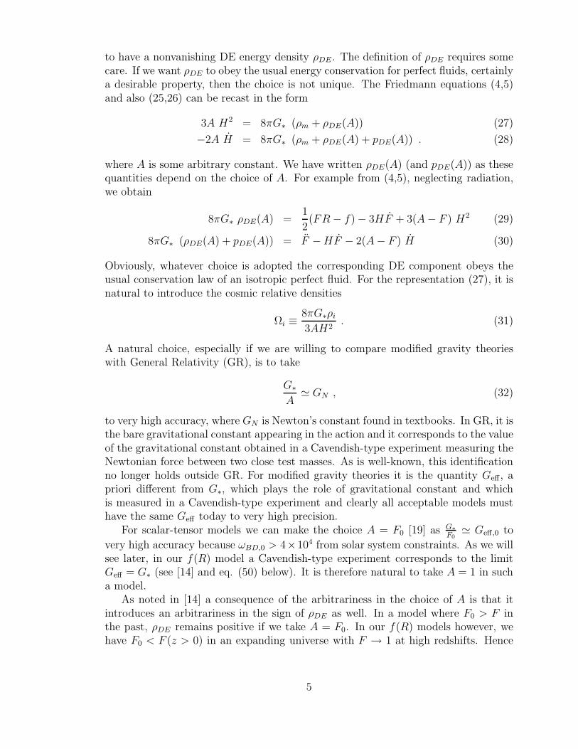
Ωm,0 0.322 0.315 0.302 0.289 0.273 0.263 0.254 0.245 0.238 0.227γ0 0.396 0.399 0.404 0.409 0.415 0.419 0.422 0.425 0.428 0.432γ′

0 -0.253 -0.246 -0.234 -0.224 -0.210 -0.202 -0.195 -0.189 -0.183 -0.175za 0.654 0.673 0.711 0.747 0.798 0.830 0.862 0.893 0.922 0.965

δm(z=0.5)δm,0

0.731 0.733 0.737 0.742 0.747 0.751 0.754 0.758 0.761 0.765

Table 1: This table summarizes the value of the growth parameters γ0, γ′

0 and of za,the redshift when accelerated expansion starts. All these values correspond to n = 2and λ = 0.94.

0.20 0.22 0.24 0.26 0.28 0.30 0.32 0.340.36

0.38

0.40

0.42

0.44

Wm,0

Γ0

n=2.5

n=2

n=1

0.20 0.22 0.24 0.26 0.28 0.30 0.32 0.34-0.28

-0.26

-0.24

-0.22

-0.20

-0.18

-0.16

Wm,0Γ

’ 0

n=2.5

n=2

n=1

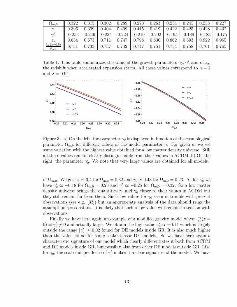
Figure 3: a) On the left, the parameter γ0 is displayed in function of the cosmologicalparameter Ωm,0 for different values of the model parameter n. For given n, we seesome variation with the highest value obtained for a low matter density universe. Stillall these values remain clearly distinguishable from their values in ΛCDM. b) On theright, the parameter γ′

0. We note that very large values are obtained for all models.

of Ωm,0. We get γ0 ≃ 0.4 for Ωm,0 = 0.32 and γ0 ≃ 0.43 for Ωm,0 = 0.23. As for γ′

0 wehave γ′

0 ≃ −0.18 for Ωm,0 = 0.23 and γ′

0 ≃ −0.25 for Ωm,0 = 0.32. So a low matterdensity universe brings the quantities γ0 and γ′

0 closer to their values in ΛCDM butthey still remain far from them. Such low values for γ0 seem in trouble with presentobservations (see e.g. [33]) but an appropriate analysis of the data should relax theassumption γ= constant. It is likely that such a low value will remain in tension withobservations.

Finally we have here again an example of a modified gravity model where dγ

dz(z =

0) ≡ γ′

0 6= 0 and actually large. We obtain the high value γ′

0 ≈ −0.14 which is largelyoutside the range |γ′

0| ≤ 0.02 found for DE models inside GR. It is also much higherthan the value found for some scalar-tensor DE models. So we have here again acharacteristic signature of our model which clearly differentiates it both from ΛCDMand DE models inside GR, but possibly also from other DE models outside GR. Likefor γ0, the scale independence of γ′

0 makes it a clear signature of the model. We have

13

checked that γ′

0 obeys the constraint

γ′

0 =[

ln Ω−1m,0

]

−1[

−Ωγ0

m,0 − 3(γ0 −1

2)weff,0 +

3

2

Geff(R0)

G∗

Ω1−γ0

m,0 − 1

2

]

, (59)

where we have to include the factor Geff (R0)G∗

≃ 43F0

6= 1. As for the scalar-tensor modelsconsidered earlier, we obtain a nearly linear behaviour on low redshifts z ≤ 0.3.

In conclusion we find that the growth of matter perturbations on small redshiftsprovides a powerful constraint on our f(R) model. We find low values for the pa-rameter γ0 with γ0 ≈ 0.4, and high values for γ′

0 with γ′

0 ≃ −0.2. These values arenot scale dependent and provide therefore a clear signature. The growth parametersγ0 and γ′

0 are mainly affected by the cosmological parameter Ωm,0, in particular γ′

0 isless negative for low Ωm,0 values. But in all cases, characteristic values very far fromΛCDM and from all DE models inside GR are found.

There are still very large uncertainties on the quantity f(z) or on β ≡ f

bwhere b

is the bias factor (see e.g. [33],[32]). One should further keep in mind that a preciseobservational determination of both f(z) and Ωm is needed in order to measure γ(z)accurately. Hence to get precise values for the couple γ0, γ

′

0 we need to determineaccurately both f(z) and Ωm(z) around z = 0. If future surveys will constrain γ0, γ

′

0

to be close to their values for ΛCDM then the models we have investigated here will beruled out. Though a systematic numerical exploration in the model parameter spaceis very hard to achieve, the model for n = 2 shows already a very large deviation fromΛCDM if one considers the growth of matter perturbations while this model meetsall other constraints. So either the model will be ruled out for any value of n or thegrowth of matter perturbations will at least significantly restrict the viable intervalin the model parameter n.

We conjecture that many if not all viable f(R) models will have similar obser-vational signatures. A precise determination of the parameters γ0 and γ′

0 could bedecisive in the quest for the true DE model especially if it is an f(R) modified gravityDE model.

References

[1] S.J. Perlmutter et al., Ap. J. 483 565 (1997), Nature 391 51 (1998); A. G. Riess,A. V. Filippenko, P. Challis et al., Astron. J. 116, 1009 (1998); S. J. Perlmut-ter, G. Aldering, G. Goldhaber et al., Astroph. J. 517, 565 (1999); P. Astier,J. Guy, N. Regnault et al., Astron. Astroph. 447, 31 (2006); Adam G. Riess et

al. e-Print astro-ph/0611572.

[2] V. Sahni, A. A. Starobinsky, Int. J. Mod. Phys. D9, 373 (2000); T. Padmanab-han, Phys. Rep. 380, 235 (2003); E. J. Copeland, M. Sami and S. Tsujikawa,hep-th/0603057 (2006); V. Sahni, A. A. Starobinsky, Int. J. Mod. Phys. D15,2105 (2006).

[3] A. A. Starobinsky, JETP Lett.68, 757 (1998).

14

[4] S. Bludman, e-Print astro-ph/0702085. D. Polarski, AIP Conf. Proc. 861,1013 (2006), e-Print astro-ph/0605532; M. Ishak, A. Upadhye, D. N. Spergel,Phys. Rev. D 74, 043513 (2006).

[5] D. Huterer, E. Linder, astro-ph/0608681; E. Linder, R. Cahn,astro-ph/0701317; A. F. Heavens, T. D. Kitching, L. Verde, e-Print

astro-ph/0703191; C. Di Porto, L. Amendola, arXiv:0707.2686; V.Acquaviva, L. Verde, arXiv:0709.0082; A. Kiakotou, O. Elgaroy, O. La-hav, arXiv:0709.0253; Y. Wang, arXiv:0710.3885; L. Hui, K. Parfree,arXiv:0712.1162; J.B. Dent, S. Dutta, arXiv:0808.2689; H. Zhang, H. Yu,H. Noh, Z.-H. Zhu, Phys. Lett. B665 (2008); Hao Wei, S. N. Zhang, Phys. Rev.D78, 023011 (2008); V. Acquaviva, A. Hajian, D. N. Spergel, S. Das, Phys.Rev.D78, 043514 (2008); Yungui Gong, arXiv:0808.1316.

[6] S. Capozziello, Int. J. Mod. Phys. D 11, 483 (2002).

[7] T. P. Sotiriou, V. Faraoni, arXiv:0805.1726.

[8] A. A. Starobinsky, Phys. Lett. B91, 99 (1980).

[9] T. Chiba, Phys. Lett. B 575, 1 (2003).

[10] A. D. Dolgov and M. Kawasaki, Phys. Lett. B 573, 1 (2003).

[11] L. Amendola, D. Polarski, S. Tsujikawa, Phys. Rev. Lett. 98, 131302 (2007).

[12] S. M. Carroll, V. Duvvuri, M. Trodden, M. S. Turner, Phys. Rev. D70, 043528(2004).

[13] L. Amendola, R. Gannouji, D. Polarski, S. Tsujikawa, Phys. Rev. D75, 083504(2007); L. Amendola, D. Polarski, S. Tsujikawa, Int. J. Mod. Phys.D16, 1555(2007).

[14] A. A. Starobinsky, JETP Lett.86, 157 (2007).

[15] W. Hu, I. Sawicki, Phys. Rev. D76, 064004 (2007).

[16] S. Tsujikawa, Phys.Rev.D76, 023514 (2007).

[17] E. Bertschinger, P. Zukin, Phys. Rev. D78, 024015 (2008).

[18] A. Dev, D. Jain, S. Jhingan, S. Nojiri, M. Sami, I. Thongkool, arXiv:0807.3445;L. Pogosian, A. Silvestri, Phys. Rev. D 77, 023503 (2008)

[19] R. Gannouji, D. Polarski, A. Ranquet, A. A. Starobinsky, JCAP 0609, 016(2006).

[20] R. Gannouji, D. Polarski, JCAP 0805, 018 (2008).

[21] V. A. Frolov Phys. Rev. Lett. 101, 061103 (2008); T. Kobayashi, Kei-ichi Maeda,Phys. Rev. D78, 064019 (2008).

15

[22] A. Melchiorri, L. Pagano, S. Pandolfi, Phys. Rev. D76, 041301 (2007).

[23] B. Boisseau, G. Esposito-Farese, D. Polarski and A.A. Starobinsky, Phys. Rev.Lett. 85, 2236 (2000).

[24] M. Kunz, D. Sapone, Phys. Rev. Lett. 98, 121301 (2007).

[25] D. Polarski, R. Gannouji, Phys. Lett.B660, 439 (2008).

[26] L. Wang, P. J. Steinhardt, Astrophys. J.508, 483 (1998).

[27] P. Brax, C. van de Bruck, A.-C. Davis, Phys. Rev. D70, 123518 (2004).

[28] J. Lesgourgues, S. Pastor, Phys. Rept. 429, 307 (2006).

[29] M. Tegmark, D. Eisenstein, M. Strauss, et al, Phys. Rev. D74, 123507 (2006).

[30] G. Esposito-Farese and D. Polarski, Phys. Rev. D63, 063504 (2001).

[31] P. J. E. Peebles, Astrophys. J.284, 439 (1984); O. Lahav, P. B. Lilje, J. R.Primack, M. J. Rees, MNRAS 251, 128 (1991).

[32] S. Nesseris and L. Perivolaropoulos, Phys. Rev. D77, 023504 (2008).

[33] K. Yamamoto, T. Sato, G. Huetsi, arXiv:0805.4789.

16