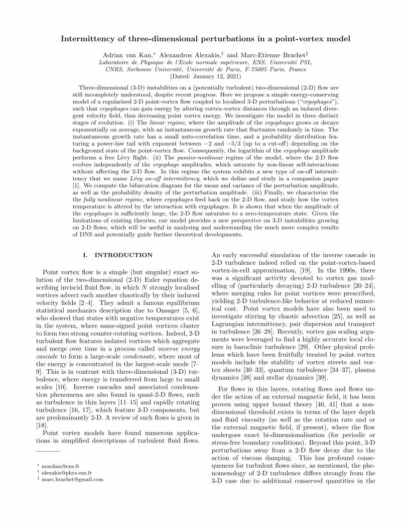
Intermittency of three-dimensional perturbations in a point-vortex model

Adrian van Kan,∗ Alexandros Alexakis,† and Marc-Etienne Brachet‡

Laboratoire de Physique de l’Ecole normale superieure, ENS, Universite PSL,CNRS, Sorbonne Universite, Universite de Paris, F-75005 Paris, France

(Dated: January 12, 2021)

Three-dimensional (3-D) instabilities on a (potentially turbulent) two-dimensional (2-D) flow arestill incompletely understood, despite recent progress. Here we propose a simple energy-conservingmodel of a regularised 2-D point-vortex flow coupled to localised 3-D perturbations (“ergophages”),such that ergophages can gain energy by altering vortex-vortex distances through an induced diver-gent velocity field, thus decreasing point vortex energy. We investigate the model in three distinctstages of evolution: (i) The linear regime, where the amplitude of the ergophages grows or decaysexponentially on average, with an instantaneous growth rate that fluctuates randomly in time. Theinstantaneous growth rate has a small auto-correlation time, and a probability distribution fea-turing a power-law tail with exponent between −2 and −5/3 (up to a cut-off) depending on thebackground state of the point-vortex flow. Consequently, the logarithm of the ergophage amplitudeperforms a free Levy flight. (ii) The passive-nonlinear regime of the model, where the 2-D flowevolves independently of the ergophage amplitudes, which saturate by non-linear self-interactionswithout affecting the 2-D flow. In this regime the system exhibits a new type of on-off intermit-tency that we name Levy on-off intermittency, which we define and study in a companion paper[1]. We compute the bifurcation diagram for the mean and variance of the perturbation amplitude,as well as the probability density of the perturbation amplitude. (iii) Finally, we characterise thethe fully nonlinear regime, where ergophages feed back on the 2-D flow, and study how the vortextemperature is altered by the interaction with ergophages. It is shown that when the amplitude ofthe ergophages is sufficiently large, the 2-D flow saturates to a zero-temperature state. Given thelimitations of existing theories, our model provides a new perspective on 3-D instabilities growingon 2-D flows, which will be useful in analysing and understanding the much more complex resultsof DNS and potentially guide further theoretical developments.

I. INTRODUCTION

Point vortex flow is a simple (but singular) exact so-lution of the two-dimensional (2-D) Euler equation de-scribing inviscid fluid flow, in which N strongly localisedvortices advect each another chaotically by their inducedvelocity fields [2–4]. They admit a famous equilibriumstatistical mechanics description due to Onsager [5, 6],who showed that states with negative temperatures existin the system, where same-signed point vortices clusterto form two strong counter-rotating vortices. Indeed, 2-Dturbulent flow features isolated vortices which aggregateand merge over time in a process called inverse energycascade to form a large-scale condensate, where most ofthe energy is concentrated in the largest-scale mode [7–9]. This is in contrast with three-dimensional (3-D) tur-bulence, where energy is transferred from large to smallscales [10]. Inverse cascades and associated condensa-tion phenomena are also found in quasi-2-D flows, suchas turbulence in thin layers [11–15] and rapidly rotatingturbulence [16, 17], which feature 3-D components, butare predominantly 2-D. A review of such flows is given in[18].

Point vortex models have found numerous applica-tions in simplified descriptions of turbulent fluid flows.

∗ avankan@ens.fr† alexakis@phys.ens.fr‡ marc.brachet@gmail.com

An early successful simulation of the inverse cascade in2-D turbulence indeed relied on the point-vortex-basedvortex-in-cell approximation, [19]. In the 1990s, therewas a significant activity devoted to vortex gas mod-elling of (particularly decaying) 2-D turbulence [20–24],where merging rules for point vortices were prescribed,yielding 2-D turbulence-like behavior at reduced numer-ical cost. Point vortex models have also been used toinvestigate stirring by chaotic advection [25], as well asLagrangian intermittency, pair dispersion and transportin turbulence [26–28]. Recently, vortex gas scaling argu-ments were leveraged to find a highly accurate local clo-sure in baroclinic turbulence [29]. Other physical prob-lems which have been fruitfully treated by point vortexmodels include the stability of vortex streets and vor-tex sheets [30–33], quantum turbulence [34–37], plasmadynamics [38] and stellar dynamics [39].

For flows in thin layers, rotating flows and flows un-der the action of an external magnetic field, it has beenproven using upper bound theory [40, 41] that a non-dimensional threshold exists in terms of the layer depthand fluid viscosity (as well as the rotation rate and orthe external magnetic field, if present), where the flowundergoes exact bi-dimensionalisation (for periodic orstress-free boundary conditions). Beyond this point, 3-Dperturbations away from a 2-D flow decay due to theaction of viscous damping. This has profound conse-quences for turbulent flows since, as mentioned, the phe-nomenology of 2-D turbulence differs strongly from the3-D case due to additional conserved quantities in the

2

2-D case [9, 10]. Therefore, it is important to under-stand quasi-two-dimensional flows close to the onset ofthree-dimensionality. The bounding theory only estab-lishes the existence of a threshold, but since it is builton rather conservative estimates, it cannot capture thephysics occurring near the threshold. Very recently, in anextensive numerical study [42], Seshasayanan and Galletinvestigated the linear stability of 3-D perturbations ona 2-D turbulent condensate background flow at the onsetof three-dimensionality. The authors showed that wheninstability is present, the time evolution of the energy oflinear 3-D modes involves phases of jump-like exponen-tial growth occurring randomly in time, inter-spaced byplateau-like phases where growth is absent. Here, in thespirit of the wide range of applications of point vorticesdescribed above, we present and analyse a point vortexmodel of localised 3-D perturbations in quasi-2-D tur-bulence, whose dynamics are qualitatively similar to theexponential growth and decay evolution found in [42].

The remainder of this article is structured as follows.In section II, we provide a brief introduction to the con-cept of point vortex temperature, in section III, we for-mulate the model to be studied. In section IV, we de-scribe the method of our investigation. Then, in sectionV we present the results of our numerical simulationsand finally in section VI we discuss the implications ofour results and remaining open questions.

II. BACKGROUND: TEMPERATURE OFPOINT VORTEX STATES

We briefly summarise the concept of the temperatureof point vortex flow, which was introduced in 1949 by On-sager [5]. The energy of a set of point vortices is given bythe HamiltonianH, which only depends on the vortex po-sitions (x, y). These positions are the conjugate variablesof the point vortex Hamiltonian. In bounded domains,the total phase space volume is therefore finite. We de-note by Ω(E) the phase space volume occupied by stateswhose energies H lie in the interval [E,E + dE]. Thenthe thermodynamic entropy is kB ln(Ω(E)/Ω0), where kBis the Boltzmann constant and Ω0 is a reference volumerequired for dimensional reasons. In the extreme situa-tion where vortex dipoles (vortex-antivortex pairs) col-lapse, which corresponds to negative energies E < 0,the available phase space volume is vanishingly small,

Ω(E)E→−∞−→ 0. The opposite limit of large positive ener-

gies occurs when like-sign vortices concentrate at a point,

in which case also Ω(E)E→∞−→ 0. Since the total volume

is non-zero, the non-negative function Ω(E) must reacha maximum at an intermediate energy −∞ < Em < ∞.The associated microcanonical inverse temperature,

β(E) ≡ ∂ ln(Ω(E))

∂E(1)

is thus positive for E < Em, but vanishes at E = Em andis negative for E > Em. Negative-temperature states

FIG. 1. Overview of point vortex states at negative, zeroand positive inverse temperatures β. Clustering occurs forβ < βc < 0, a homogeneous state is found at β = 0, and paircondensation occurs for β > βpc.

can generally arise in both classical and quantum sys-tems with a finite number of degrees of freedom whosestate space is bounded, such as localized spin systems[43–45]. In the point vortex system, high-energy states atnegative temperatures, corresponding to condensates fea-turing same-sign vortex clusters, have been extensivelystudied since Onsager’s initial contribution [5, 6, 46]. Inparticular, there is a negative clustering temperature βc,which marks the onset of same-sign vortex clustering.Similarly, there is a positive pair condensation tempera-ture βpc, at which opposite-sign vortices form dipole pairswhich propagate through the domain, see [47]. The van-ishing inverse temperature at E = Em corresponds toa homogeneous state with positive and negative vorticesspread out evenly over the domain. The point vortexstates at different temperatures are summarised in fig-ure 1. Such point vortex states at a given inverse tem-perature β may be generated using the noisy gradientmethod presented in appendix B, which was previouslyintroduced in [48]. Specifically, once a statistically sta-tionary state is reached, this numerical method generatesrandom point-vortex states according to the canonicaldistribution associated with the inverse temperature β.For a given value of β, the mean energy in the statis-tically stationary state can be measured from the timeseries. Thus, like every microcanonical temperature cor-responds to an energy E according to (1), in the noisygradient method every value of β corresponds to a meanenergy 〈E〉 in steady state. The resulting mean energyas a function of temperature is shown in figure 2.

III. THE MODEL

We now describe the simplified model of the interac-tion of 2-D and 3-D flow studied in this paper. Forthe sake of simplicity and clarity, the theoretical for-malism is presented in the infinite domain. The corre-sponding equations for the 2-D doubly periodic domain[0, 2πL]×[0, 2πL], where the statistical point vortex tem-perature from section II is well-defined, are given in ap-pendix A.

Consider an even number Nv of point vortices with

3

−1 0 1 2β

0

500

1000

1500〈E〉

FIG. 2. Mean point vortex energy 〈E〉 of Nv = 32 vorticesversus β, computed using the method described in appendixB in the periodic domain [0, 2π]× [0, 2π] (with a truncation atdistances smaller than ε = 0.1, cf. appendix B). This curveallows a translation from vortex energies at steady state tocorresponding temperatures.

circulations Γi located at positions x(i)v = (x

(i)v , y

(i)v ).

In addition to the point vortices, we introduce localised3-D perturbations (“ergophages”). Motivated by thestrong localisation of 3-D motions (spatial intermittency)observed close to the onset of three-dimensionality insimulations [13, 14, 42] we also model 3-D motions as

Np point-like pertubations located at positions x(k)p =

(x(k)p , y

(k)p ). We do not resolve the spatial structure of

the perturbations, but rather assign to every ergophagean effective perturbation amplitude Ak (with dimensionsof circulation), which measures its intensity. This simpli-fies the formalism and makes the mathematical structureof the model effectively 2-D.

Point vortices and 3-D point perturbations induce ve-locity fields that advect each other following the equa-tions

d

dtx(i)v = U′(i)v + U(i)

p + u(i)f (2)

and

d

dtx(k)p = U(k)

v + v(k)f (3)

where U′(i)v is the velocity induced on vortex i by all point

vortices i 6= j, U(i)p is the velocity induced on vortex i

by the 3-D ergophages and U(k)v is the velocity induced

on ergophage k by all Nv point vortices. Finally, u(i)f

and v(k)f are externally imposed velocity fields that could

inject energy to the system. Note that ergophages do notadvect each other.

In the absence of ergophages and external velocities,point vortices move due to their mutual advection, fol-

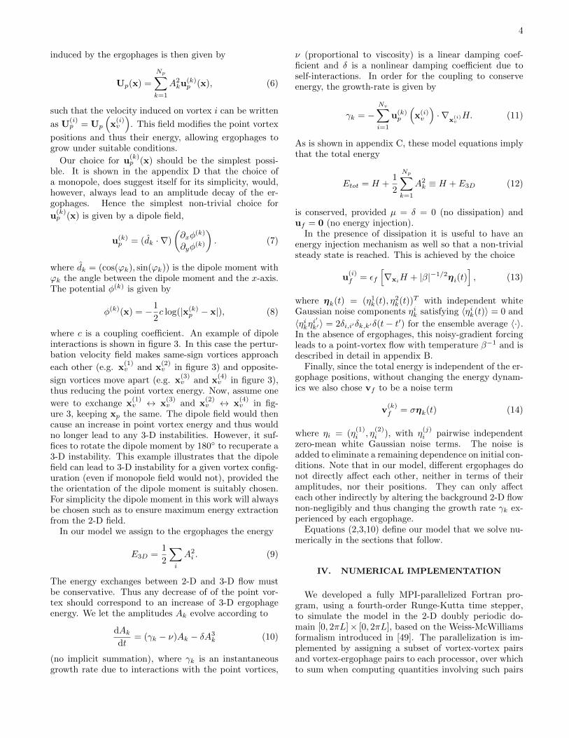
FIG. 3. Illustration of how a velocity field up (steam lines)due to a 3-D perturbation at xp, can reduce point vortexenergy. This is done by increasing the distance between the

same-sign vortices at x(1)v ,x

(2)v and/or decreasing the distance

between opposite-sign vortices at x(3)v ,x

(4)v . The bold black

arrow passing through xp represents the dipole moment.

lowing Hamiltonian dynamics so that the velocity field

U′(i)v can be written as

U′(i)v = Γ−1i

(∂y(i)vH

−∂x(i)vH

), (4)

corresponding to the advection of the i-th vortex by allvortices j 6= i. The Hamiltonian H in R2 is given by

H(x(1)v , . . . , x(Nv)v ) = −1

2

Nv∑i,j=1i6=j

ΓiΓj log(|x(i)v −x(j)

v |), (5)

which is a sum over pairs depending on the vortex-vortex

distances alone. The velocity field U(k)v closely resembles

U′(i)v , but it includes the advection due to all Nv vor-

tices, formally omitting the condition i 6= j in H before

differentiating in (4) and evaluating at x(i)v → x

(k)p . The

Hamiltonian also gives the kinetic energy of the flow (upto a factor of (2π)−1 and an additive infinite constantdue to self-energy), which is conserved. The point vor-tex energy increases when same-sign vortices approacheach other and when opposite-sign vortices move apart,while it decreases when same-sign vortices move apartand when opposite-sign vortices approach each other.

In the presence of ergophages, energy of the 2-D fieldcan be transferred to the 3-D field perturbations. Thus,in order to gain energy, an ergophage must reduce theenergy of a given point vortex configuration on which itis superimposed. Each ergophage induces a 3-D pertur-bation velocity field ukp(x) of amplitude A2

k, which hasnon-zero divergence in the plane. The total velocity field

4

induced by the ergophages is then given by

Up(x) =

Np∑k=1

A2ku

(k)p (x), (6)

such that the velocity induced on vortex i can be written

as U(i)p = Up

(x(i)v

). This field modifies the point vortex

positions and thus their energy, allowing ergophages togrow under suitable conditions.

Our choice for u(k)p (x) should be the simplest possi-

ble. It is shown in the appendix D that the choice ofa monopole, does suggest itself for its simplicity, would,however, always lead to an amplitude decay of the er-gophages. Hence the simplest non-trivial choice for

u(k)p (x) is given by a dipole field,

u(k)p = (dk · ∇)

(∂xφ

(k)

∂yφ(k)

). (7)

where dk = (cos(ϕk), sin(ϕk)) is the dipole moment withϕk the angle between the dipole moment and the x-axis.The potential φ(k) is given by

φ(k)(x) = −1

2c log(|x(k)

p − x|), (8)

where c is a coupling coefficient. An example of dipoleinteractions is shown in figure 3. In this case the pertur-bation velocity field makes same-sign vortices approach

each other (e.g. x(1)v and x

(2)v in figure 3) and opposite-

sign vortices move apart (e.g. x(3)v and x

(4)v in figure 3),

thus reducing the point vortex energy. Now, assume one

were to exchange x(1)v ↔ x

(3)v and x

(2)v ↔ x

(4)v in fig-

ure 3, keeping xp the same. The dipole field would thencause an increase in point vortex energy and thus wouldno longer lead to any 3-D instabilities. However, it suf-fices to rotate the dipole moment by 180 to recuperate a3-D instability. This example illustrates that the dipolefield can lead to 3-D instability for a given vortex config-uration (even if monopole field would not), provided thethe orientation of the dipole moment is suitably chosen.For simplicity the dipole moment in this work will alwaysbe chosen such as to ensure maximum energy extractionfrom the 2-D field.

In our model we assign to the ergophages the energy

E3D =1

2

∑i

A2i . (9)

The energy exchanges between 2-D and 3-D flow mustbe conservative. Thus any decrease of of the point vor-tex should correspond to an increase of 3-D ergophageenergy. We let the amplitudes Ak evolve according to

dAkdt

= (γk − ν)Ak − δA3k (10)

(no implicit summation), where γk is an instantaneousgrowth rate due to interactions with the point vortices,

ν (proportional to viscosity) is a linear damping coef-ficient and δ is a nonlinear damping coefficient due toself-interactions. In order for the coupling to conserveenergy, the growth-rate is given by

γk = −Nv∑i=1

u(k)p

(x(i)v

)· ∇

x(i)vH. (11)

As is shown in appendix C, these model equations implythat the total energy

Etot = H +1

2

Np∑k=1

A2k ≡ H + E3D (12)

is conserved, provided µ = δ = 0 (no dissipation) anduf = 0 (no energy injection).

In the presence of dissipation it is useful to have anenergy injection mechanism as well so that a non-trivialsteady state is reached. This is achieved by the choice

u(i)f = εf

[∇xiH + |β|−1/2ηi(t)

], (13)

where ηk(t) = (η1k(t), η2k(t))T with independent whiteGaussian noise components ηik satisfying 〈ηik(t)〉 = 0 and

〈ηikηi′

k′〉 = 2δi,i′δk,k′δ(t− t′) for the ensemble average 〈·〉.In the absence of ergophages, this noisy-gradient forcingleads to a point-vortex flow with temperature β−1 and isdescribed in detail in appendix B.

Finally, since the total energy is independent of the er-gophage positions, without changing the energy dynam-ics we also chose vf to be a noise term

v(k)f = σηk(t) (14)

where ηi = (η(1)i , η

(2)i ), with η

(j)i pairwise independent

zero-mean white Gaussian noise terms. The noise isadded to eliminate a remaining dependence on initial con-ditions. Note that in our model, different ergophages donot directly affect each other, neither in terms of theiramplitudes, nor their positions. They can only affecteach other indirectly by altering the background 2-D flownon-negligibly and thus changing the growth rate γk ex-perienced by each ergophage.

Equations (2,3,10) define our model that we solve nu-merically in the sections that follow.

IV. NUMERICAL IMPLEMENTATION

We developed a fully MPI-parallelized Fortran pro-gram, using a fourth-order Runge-Kutta time stepper,to simulate the model in the 2-D doubly periodic do-main [0, 2πL]× [0, 2πL], based on the Weiss-McWilliamsformalism introduced in [49]. The parallelization is im-plemented by assigning a subset of vortex-vortex pairsand vortex-ergophage pairs to each processor, over whichto sum when computing quantities involving such pairs

5

such as Ui)v ,U

(i)p , H and γk. The specific model equa-

tions for the periodic domain are given in appendix A.Since the periodic domain has a finite area, the statis-tical point vortex temperature introduced in section IIis well-defined here and no vortices can escape to infin-ity. A regularisation was introduced at distances smallerthan a positive cut-off ε 2πL (we set ε/L = 0.1),similarly as in [33]. The time step ∆t is dictated bythe maximum growth rate γk, which is associated withclose encounters where some distances are of the order ofO(ε). For highly condensed configurations, where Nv/2vortices form a cluster for each sign of circulation, eachcluster comprises approximately N2

v /8 vortex pairs con-tributing to γk. At small distances up = O(ε−2) and∇

x(i)vH = O(ε−1), such that the time step thus bounded

above by

∆t . (max(γk))−1 ∼ 8ε3

N2v

. (15)

For dilute vortex configurations, the largest growth ratesstem from encounters between a single ergophage and asingle vortex, such that ∆t . ε3. This strong dependenceof the required time step on ε, and Nv for dense config-urations, is an important limiting factor in computationcost. The operation of the highest numerical complex-ity at every time step is the evaluation of γk since itrequires summing O(N2

v ) vortex-vortex pairs for everyk = 1, . . . , Np.

V. SIMULATION RESULTS

To study the model introduced in section III, we firstuse the noisy gradient method described in appendix Bto generate point vortex states with Nv = 32 vortices atboth positive and negative temperatures. This relativelysmall number of vortices is chosen in order to be able torun simulations for long times in order to obtain satis-factory statistics. The energy of the resulting equilibriaas a function of their inverse temperature β is as shownin figure 2. We note that at this relatively low numberof vortices, the transitions to a condensate and to paircondensation are not sharp. Using these states as initialconditions for the point vortices, we proceed in the threefollowing steps:

(A) The passive, linear regime: perturbation ampli-tudes Ak/Γ 1 and δ → 0 for a given backgroundpoint-vortex flow. In this limit, the evolution equa-tion (10) of Ak is linear and the point vortex energyH is constant in time since Up = O(A2

k) is negli-gible with respect to the conservative Hamiltonianadvection terms. To investigate this limit we setUp = 0 in (3) and δ = 0 in 10. Since there is nodissipation in the system we also set uf = 0.

(B) The passive, nonlinear regime: still Ak/Γ 1, suchthat H still remains unaffected by the 3-D instabil-ities, but we include saturation of the amplitude

0 1 2 3 4 5 6x

0

1

2

3

4

5

6

y

++++++++++++++++

----------------

0 1 2 3 4 5 6x

0

1

2

3

4

5

6

y++

++

++

+

+

+

+

++

+++

+

-

-

-

-

-

-

--

-

-

-

- -

- -

-

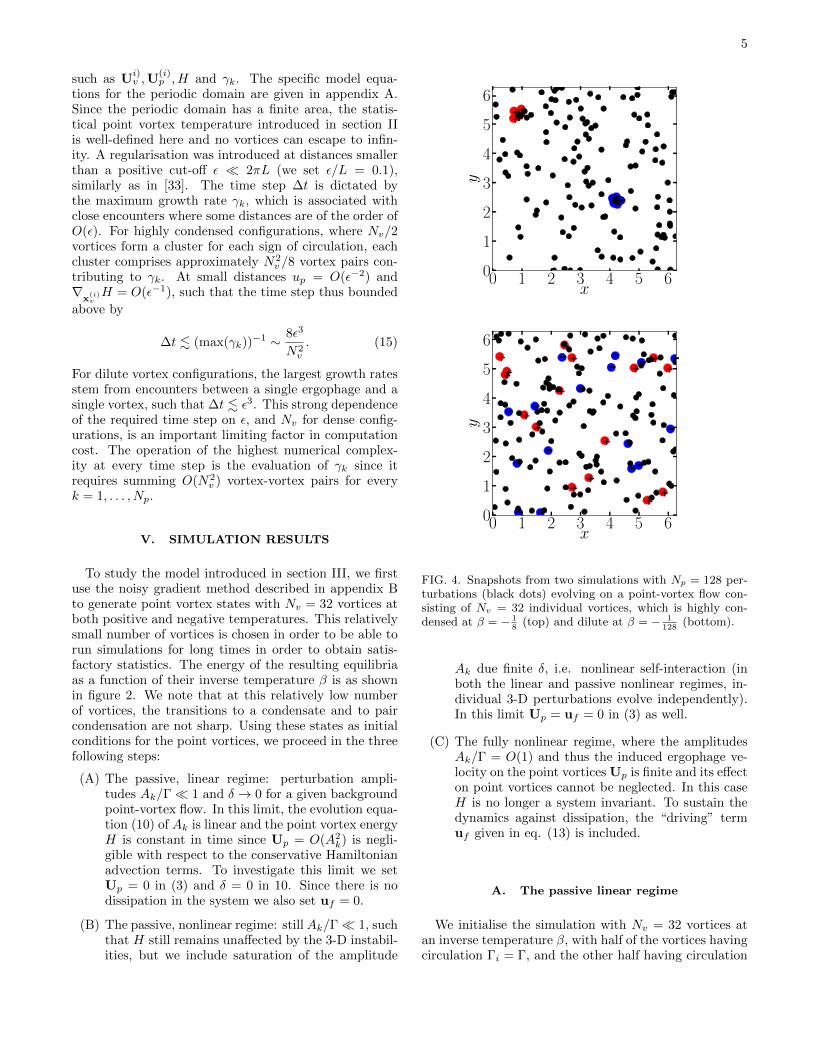
FIG. 4. Snapshots from two simulations with Np = 128 per-turbations (black dots) evolving on a point-vortex flow con-sisting of Nv = 32 individual vortices, which is highly con-densed at β = − 1

8(top) and dilute at β = − 1

128(bottom).

Ak due finite δ, i.e. nonlinear self-interaction (inboth the linear and passive nonlinear regimes, in-dividual 3-D perturbations evolve independently).In this limit Up = uf = 0 in (3) as well.

(C) The fully nonlinear regime, where the amplitudesAk/Γ = O(1) and thus the induced ergophage ve-locity on the point vortices Up is finite and its effecton point vortices cannot be neglected. In this caseH is no longer a system invariant. To sustain thedynamics against dissipation, the “driving” termuf given in eq. (13) is included.

A. The passive linear regime

We initialise the simulation with Nv = 32 vortices atan inverse temperature β, with half of the vortices havingcirculation Γi = Γ, and the other half having circulation

6

0.000 0.010 0.020 0.030t

10−102

10−36

1030

1096

10162E

3D

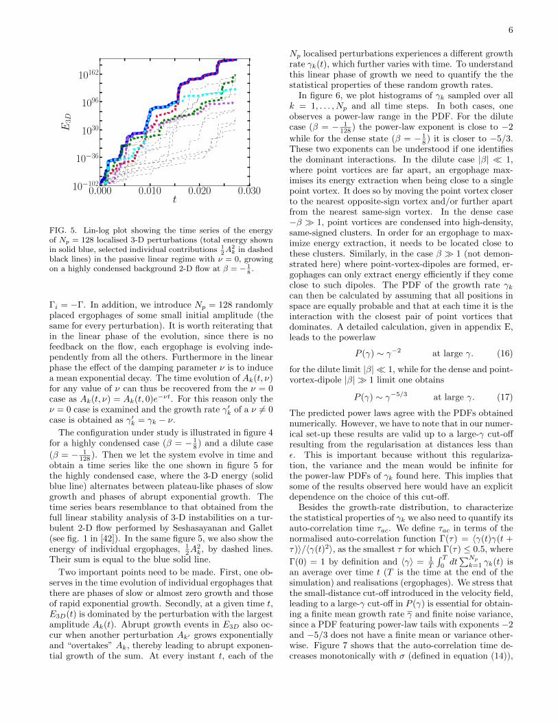
FIG. 5. Lin-log plot showing the time series of the energyof Np = 128 localised 3-D perturbations (total energy shownin solid blue, selected individual contributions 1

2A2

k in dashedblack lines) in the passive linear regime with ν = 0, growingon a highly condensed background 2-D flow at β = − 1

8.

Γi = −Γ. In addition, we introduce Np = 128 randomlyplaced ergophages of some small initial amplitude (thesame for every perturbation). It is worth reiterating thatin the linear phase of the evolution, since there is nofeedback on the flow, each ergophage is evolving inde-pendently from all the others. Furthermore in the linearphase the effect of the damping parameter ν is to inducea mean exponential decay. The time evolution of Ak(t, ν)for any value of ν can thus be recovered from the ν = 0case as Ak(t, ν) = Ak(t, 0)e−νt. For this reason only theν = 0 case is examined and the growth rate γ′k of a ν 6= 0case is obtained as γ′k = γk − ν.

The configuration under study is illustrated in figure 4for a highly condensed case (β = − 1

8 ) and a dilute case

(β = − 1128 ). Then we let the system evolve in time and

obtain a time series like the one shown in figure 5 forthe highly condensed case, where the 3-D energy (solidblue line) alternates between plateau-like phases of slowgrowth and phases of abrupt exponential growth. Thetime series bears resemblance to that obtained from thefull linear stability analysis of 3-D instabilities on a tur-bulent 2-D flow performed by Seshasayanan and Gallet(see fig. 1 in [42]). In the same figure 5, we also show theenergy of individual ergophages, 1

2A2k, by dashed lines.

Their sum is equal to the blue solid line.

Two important points need to be made. First, one ob-serves in the time evolution of individual ergophages thatthere are phases of slow or almost zero growth and thoseof rapid exponential growth. Secondly, at a given time t,E3D(t) is dominated by the perturbation with the largestamplitude Ak(t). Abrupt growth events in E3D also oc-cur when another perturbation Ak′ grows exponentiallyand “overtakes” Ak, thereby leading to abrupt exponen-tial growth of the sum. At every instant t, each of the

Np localised perturbations experiences a different growthrate γk(t), which further varies with time. To understandthis linear phase of growth we need to quantify the thestatistical properties of these random growth rates.

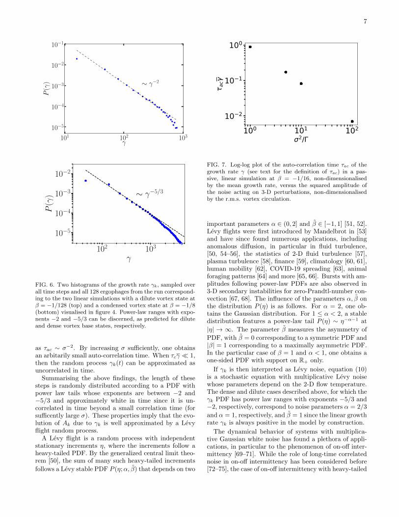
In figure 6, we plot histograms of γk sampled over allk = 1, . . . , Np and all time steps. In both cases, oneobserves a power-law range in the PDF. For the dilutecase (β = − 1

128 ) the power-law exponent is close to −2

while for the dense state (β = − 18 ) it is closer to −5/3.

These two exponents can be understood if one identifiesthe dominant interactions. In the dilute case |β| 1,where point vortices are far apart, an ergophage max-imises its energy extraction when being close to a singlepoint vortex. It does so by moving the point vortex closerto the nearest opposite-sign vortex and/or further apartfrom the nearest same-sign vortex. In the dense case−β 1, point vortices are condensed into high-density,same-signed clusters. In order for an ergophage to max-imize energy extraction, it needs to be located close tothese clusters. Similarly, in the case β 1 (not demon-strated here) where point-vortex-dipoles are formed, er-gophages can only extract energy efficiently if they comeclose to such dipoles. The PDF of the growth rate γkcan then be calculated by assuming that all positions inspace are equally probable and that at each time it is theinteraction with the closest pair of point vortices thatdominates. A detailed calculation, given in appendix E,leads to the powerlaw

P (γ) ∼ γ−2 at large γ. (16)

for the dilute limit |β| 1, while for the dense and point-vortex-dipole |β| 1 limit one obtains

P (γ) ∼ γ−5/3 at large γ. (17)

The predicted power laws agree with the PDFs obtainednumerically. However, we have to note that in our numer-ical set-up these results are valid up to a large-γ cut-offresulting from the regularisation at distances less thanε. This is important because without this regulariza-tion, the variance and the mean would be infinite forthe power-law PDFs of γk found here. This implies thatsome of the results observed here would have an explicitdependence on the choice of this cut-off.

Besides the growth-rate distribution, to characterizethe statistical properties of γk we also need to quantify itsauto-correlation time τac. We define τac in terms of thenormalised auto-correlation function Γ(τ) = 〈γ(t)γ(t +τ)〉/〈γ(t)2〉, as the smallest τ for which Γ(τ) ≤ 0.5, where

Γ(0) = 1 by definition and 〈γ〉 = 1T

∫ T0dt∑Np

k=1 γk(t) isan average over time t (T is the time at the end of thesimulation) and realisations (ergophages). We stress thatthe small-distance cut-off introduced in the velocity field,leading to a large-γ cut-off in P (γ) is essential for obtain-ing a finite mean growth rate γ and finite noise variance,since a PDF featuring power-law tails with exponents −2and −5/3 does not have a finite mean or variance other-wise. Figure 7 shows that the auto-correlation time de-creases monotonically with σ (defined in equation (14)),

7

101 102 103

γ

10−5

10−4

10−3

10−2

10−1P

(γ) ∼ γ−2

102 103

γ

10−5

10−4

10−3

10−2

P(γ

) ∼ γ−5/3

FIG. 6. Two histograms of the growth rate γk, sampled overall time steps and all 128 ergophages from the run correspond-ing to the two linear simulations with a dilute vortex state atβ = −1/128 (top) and a condensed vortex state at β = −1/8(bottom) visualised in figure 4. Power-law ranges with expo-nents −2 and −5/3 can be discerned, as predicted for diluteand dense vortex base states, respectively.

as τac ∼ σ−2. By increasing σ sufficiently, one obtainsan arbitarily small auto-correlation time. When τcγ 1,then the random process γk(t) can be approximated asuncorrelated in time.

Summarising the above findings, the length of thesesteps is randomly distributed according to a PDF withpower law tails whose exponents are between −2 and−5/3 and approximately white in time since it is un-correlated in time beyond a small correlation time (forsufficently large σ). These properties imply that the evo-lution of Ak due to γk is well approximated by a Levyflight random process.

A Levy flight is a random process with independentstationary increments η, where the increments follow aheavy-tailed PDF. By the generalized central limit theo-rem [50], the sum of many such heavy-tailed increments

follows a Levy stable PDF P (η;α, β) that depends on two

100 101 1022/

10 2

10 1

100

ac

FIG. 7. Log-log plot of the auto-correlation time τac of thegrowth rate γ (see text for the definition of τac) in a pas-sive, linear simulation at β = −1/16, non-dimensionalisedby the mean growth rate, versus the squared amplitude ofthe noise acting on 3-D perturbations, non-dimensionalisedby the r.m.s. vortex circulation.

important parameters α ∈ (0, 2] and β ∈ [−1, 1] [51, 52].Levy flights were first introduced by Mandelbrot in [53]and have since found numerous applications, includinganomalous diffusion, in particular in fluid turbulence,[50, 54–56], the statistics of 2-D fluid turbulence [57],plasma turbulence [58], finance [59], climatology [60, 61],human mobility [62], COVID-19 spreading [63], animalforaging patterns [64] and more [65, 66]. Bursts with am-plitudes following power-law PDFs are also observed in3-D secondary instabilities for zero-Prandtl-number con-vection [67, 68]. The influence of the parameters α, β onthe distribution P (η) is as follows. For α = 2, one ob-tains the Gaussian distribution. For 1 ≤ α < 2, a stabledistribution features a power-law tail P (η) ∼ η−α−1 at

|η| → ∞. The parameter β measures the asymmetry of

PDF, with β = 0 corresponding to a symmetric PDF and|β| = 1 corresponding to a maximally asymmetric PDF.In the particular case of β = 1 and α < 1, one obtains aone-sided PDF with support on R+ only.

If γk is then interpreted as Levy noise, equation (10)is a stochastic equation with multiplicative Levy noisewhose parameters depend on the 2-D flow temperature.The dense and dilute cases described above, for which theγk PDF has power law ranges with exponents −5/3 and−2, respectively, correspond to noise parameters α = 2/3

and α = 1, respectively, and β = 1 since the linear growthrate γk is always positive in the model by construction.

The dynamical behavior of systems with multiplica-tive Gaussian white noise has found a plethora of appli-cations, in particular to the phenomenon of on-off inter-mittency [69–71]. While the role of long-time correlatednoise in on-off intermittency has been considered before[72–75], the case of on-off intermittency with heavy-tailed

8

noise has not previously been studied explicitly, to ourknowledge. Our companion paper [1] is devoted to thistopic. Here we summarize only the relevant results. It isshown in [1] that in the case α < 1 and β = 1 which ap-plies here, the system (10), with γk interpreted as whiteLevy noise, is unstable for all values of ν: since the meanvalue of 〈γk〉 → +∞, viscosity ν, no matter how large,cannot stop the growth of Ak. If, however, the attainedvalues of γk are truncated, so that a finite value of 〈γk〉exists, then there is a critical value of viscosity νc abovewhich all trajectories converge to zero Ak → 0. However,this critical value depends on the truncation value of γk,which in the problem at hand implies that the νc will de-pend on the regularization cut-off ε. At long time scalesthe system displays on-off intermittency.

B. The passive nonlinear regime

We solve the model equations for Np = 32 passive non-linear dipole ergophages evolving on a highly condensedbackground flow of Nv = 32 point vortices at tempera-ture β = −1/8, fixing the nonlinear damping coefficientat δ = 1. For a given ν, we initialise the ergophagesat random positions and with small amplitudes. Welet the system evolve for long times, such that the per-turbation amplitude either decays or reaches a statisti-cally steady state. We then measure the steady-statetime average of the moments Mn = 〈An〉, in terms of

〈f(A)〉 = limT→∞1

TNp

∫ T0

∑Np

k=1 f(Ak)dt. We also define

the “zeroth” moment as M0 = exp(〈log(A)〉), By the in-equality of arithmetic and geometric means the moments

are ordered M0 ≤ M1 ≤ M1/22 ≤ M

1/33 ≤ . . . . The re-

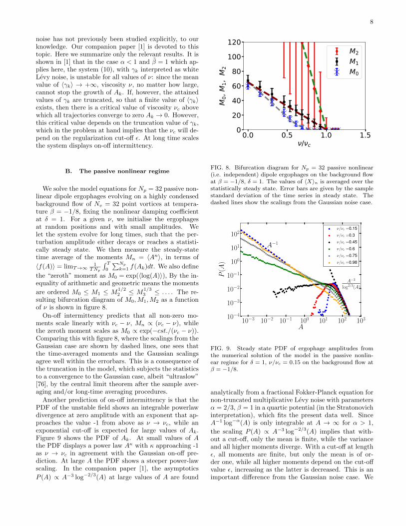
sulting bifurcation diagram of M0,M1,M2 as a functionof ν is shown in figure 8.

On-off intermittency predicts that all non-zero mo-ments scale linearly with νc − ν, Mn ∝ (νc − ν), whilethe zeroth moment scales as M0 ∝ exp(−cst./(νc − ν)).Comparing this with figure 8, where the scalings from theGaussian case are shown by dashed lines, one sees thatthe time-averaged moments and the Gaussian scalingsagree well within the errorbars. This is a consequence ofthe truncation in the model, which subjects the statisticsto a convergence to the Gaussian case, albeit “ultraslow”[76], by the central limit theorem after the sample aver-aging and/or long-time averaging procedures.

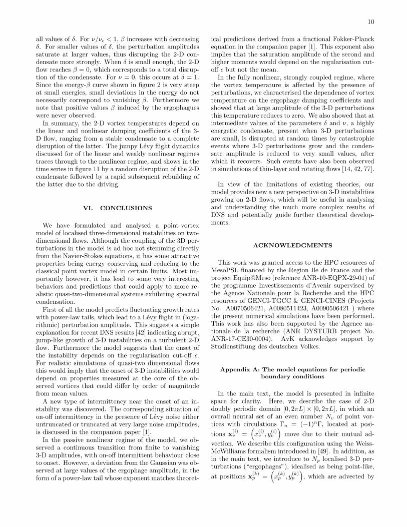
Another prediction of on-off intermittency is that thePDF of the unstable field shows an integrable powerlawdivergence at zero amplitude with an exponent that ap-proaches the value -1 from above as ν → νc, while anexponential cut-off is expected for large values of Ak.Figure 9 shows the PDF of Ak. At small values of Athe PDF displays a power law Aκ with κ approaching -1as ν → νc in agreement with the Gaussian on-off pre-diction. At large A the PDF shows a steeper power-lawscaling. In the companion paper [1], the asymptotics

P (A) ∝ A−3 log−2/3(A) at large values of A are found

0.0 0.5 1.0 1.5/ c

020406080

100120

M0,

M1,

M2

M2M1M0

FIG. 8. Bifurcation diagram for Np = 32 passive nonlinear(i.e. independent) dipole ergophages on the background flowat β = −1/8, δ = 1. The values of 〈X〉n is averaged over thestatistically steady state. Error bars are given by the samplestandard deviation of the time series in steady state. Thedashed lines show the scalings from the Gaussian noise case.

10−3 10−2 10−1 100 101 102 103

A

10−4

10−3

10−2

10−1

100

101

102

P(A

)

A−1

A−3

log2/3(A)

ν/νc =0.15

ν/νc =0.3

ν/νc =0.45

ν/νc =0.6

ν/νc =0.75

ν/νc =0.98

FIG. 9. Steady state PDF of ergophage amplitudes fromthe numerical solution of the model in the passive nonlin-ear regime for δ = 1, ν/νc = 0.15 on the background flow atβ = −1/8.

analytically from a fractional Fokker-Planck equation fornon-truncated multiplicative Levy noise with parametersα = 2/3, β = 1 in a quartic potential (in the Stratonovichinterpretation), which fits the present data well. SinceA−1 log−α(A) is only integrable at A → ∞ for α > 1,

the scaling P (A) ∝ A−3 log−2/3(A) implies that with-out a cut-off, only the mean is finite, while the varianceand all higher moments diverge. With a cut-off at lengthε, all moments are finite, but only the mean is of or-der one, while all higher moments depend on the cut-offvalue ε, increasing as the latter is decreased. This is animportant difference from the Gaussian noise case. We

9

101 102

〈A〉

10−4

10−3

10−2

10−1

P(〈A〉)

〈A〉−3

log2/3(〈A〉)

nsample =32

nsample =16

nsample =8

nsample =4

nsample =2

nsample =1

FIG. 10. PDF of sample mean 〈A〉, over nsample realisations(independent ergophages) from the passive nonlinear pointvortex model with parameters δ = 1, ν/νc = 0.15. Fornsample = 1, the PDF is close to the theoretical predictionfor the non-truncated system, and converges to a GaussianPDF (thin dashed line) as nsample is increased.

note, however, that this difference is diminished as largersamples are used due to the imposed truncation and thelaw of large numbers. This is demonstrated in figure 10which focuses on this power-law tail far from thresholdν/νc = 0.15, and averaging A over independent samplesleads to a convergence towards a Gaussian distribution.For a single realisation, however, we observe a form closeto the theoretical prediction for the non-truncated Levyprocess.

C. The fully nonlinear regime

We now enable ergophages to feed back on the point-vortex flow and include the driving velocity uf . Ini-tialising a simulation at a condensed vortex state withβ = −1/8, Np = 32 ergophages at random locations withsmall initial amplitudes Ak for given values of ν, δ andusing a forcing temperature βf = −1/8, we let the sys-tem evolve in time and measure the mean energy aroundwhich the energy fluctuates at late times.

Figure 11 shows time series of the 2-D energy H in thefully nonlinear regime for ν/νc = 0.15 for different val-ues of δ. For large δ = 106, the 3-D instabilities cannotgrow to large amplitudes and therefore do not disrupt thehighly energetic condensate. For δ = 105, a slightly lessenergetic condensate persists, but is disrupted at ran-dom times by catastrophic events that bring the 2-Dflow energy close to zero, just to rebuild again thanksto the driving. These are the traces of the jumps dueto Levy flight dynamics remaining present in the nonlin-ear regime. Disruptive events occur when an ergophagecomes very close to the point vortex clusters shown inthe top panel of figure 4, extracting the cluster’s energy

0.0 0.1 0.2 0.3 0.4t

0

500

1000

1500

H

δ = 10−2

δ = 6× 104

δ = 105

δ = 106

FIG. 11. Time series of the 2-D energy H in the fully non-linear regime at ν/νc = 0.15 for different values of δ. Atδ = 105, the flow is close to a 2-D condensate, up to abruptevents when the condensate is disrupted. For decreasing val-ues of δ, ergophages grow to larger amplitudes and lower theenergy of the 2-D flow further.

−6 −5 −4 −3 −2 −1 0 1 2log10(1/δ)

−1.0

−0.8

−0.6

−0.4

−0.2

0.0

β/|β

f|

ν/νc = 0

ν/νc = 0.15

ν/νc = 0.37

ν/νc = 0.67

ν/νc = 1.04

FIG. 12. Plot of mean temperature of the point vortex flow ina fully nonlinear regime in the presence of a single perturba-tion Np = 1 for varying δ, different curves show different ν. Atν/νc > 1, the flow temperature is exactly that of the forcing,i.e. β = βf = −1/8, since all 3-D perturbations decay.

by partially breaking it up. With decreasing values of δ,the ergophages disrupt the condensate further and fur-ther until they reduce its energy to close to zero drivingall point vortices apart.

For each simulation, we use the correspondence be-tween mean energy and inverse temperature visualisedin figure 2 to assign a vortex temperature based on themeasured average point-vortex energy at late times. Werepeat this procedure for several values of ν and δ to ob-tain the diagram shown in figure 12. For ν/νc > 1, 3-Dperturbations decay and the 2-D condensate is stable for

10

all values of δ. For ν/νc < 1, β increases with decreasingδ. For smaller values of δ, the perturbation amplitudessaturate at larger values, thus disrupting the 2-D con-densate more strongly. When δ is small enough, the 2-Dflow reaches β = 0, which corresponds to a total disrup-tion of the condensate. For ν = 0, this occurs at δ = 1.Since the energy-β curve shown in figure 2 is very steepat small energies, small deviations in the energy do notnecessarily correspond to vanishing β. Furthermore wenote that positive values β induced by the ergophagueswere never observed.

In summary, the 2-D vortex temperatures depend onthe linear and nonlinear damping coefficients of the 3-D flow, ranging from a stable condensate to a completedisruption of the latter. The jumpy Levy flight dynamicsdiscussed for of the linear and weakly nonlinear regimestraces through to the nonlinear regime, and shows in thetime series in figure 11 by a random disruption of the 2-Dcondensate followed by a rapid subsequent rebuilding ofthe latter due to the driving.

VI. CONCLUSIONS

We have formulated and analysed a point-vortexmodel of localised three-dimensional instabilities on two-dimensional flows. Although the coupling of the 3D per-turbations in the model is ad-hoc not stemming directlyfrom the Navier-Stokes equations, it has some attractiveproperties being energy conserving and reducing to theclassical point vortex model in certain limits. Most im-portantly however, it has lead to some very interestingbehaviors and predictions that could apply to more re-alistic quasi-two-dimensional systems exhibiting spectralcondensation.

First of all the model predicts fluctuating growth rateswith power-law tails, which lead to a Levy flight in (loga-rithmic) perturbation amplitude. This suggests a simpleexplanation for recent DNS results [42] indicating abrupt,jump-like growth of 3-D instabilities on a turbulent 2-Dflow. Furthermore the model suggests that the onset ofthe instability depends on the regularisation cut-off ε.For realistic simulations of quasi-two dimensional flowsthis would imply that the onset of 3-D instabilities woulddepend on properties measured at the core of the ob-served vortices that could differ by order of magnitudefrom mean values.

A new type of intermittency near the onset of an in-stability was discovered. The corresponding situation ofon-off intermittency in the presence of Levy noise eitheruntruncated or truncated at very large noise amplitudes,is discussed in the companion paper [1].

In the passive nonlinear regime of the model, we ob-served a continuous transition from finite to vanishing3-D amplitudes, with on-off intermittent behaviour closeto onset. However, a deviation from the Gaussian was ob-served at large values of the ergophage amplitude, in theform of a power-law tail whose exponent matches theoret-

ical predictions derived from a fractional Fokker-Planckequation in the companion paper [1]. This exponent alsoimplies that the saturation amplitude of the second andhigher moments would depend on the regularisation cut-off ε but not the mean.

In the fully nonlinear, strongly coupled regime, wherethe vortex temperature is affected by the presence ofperturbations, we characterised the dependence of vortextemperature on the ergophage damping coefficients andshowed that at large amplitude of the 3-D perturbationsthis temperature reduces to zero. We also showed that atintermediate values of the parameters δ and ν, a highlyenergetic condensate, present when 3-D perturbationsare small, is disrupted at random times by catastrophicevents where 3-D perturbations grow and the conden-sate amplitude is reduced to very small values, afterwhich it recovers. Such events have also been observedin simulations of thin-layer and rotating flows [14, 42, 77].

In view of the limitations of existing theories, ourmodel provides new a new perspective on 3-D instabilitiesgrowing on 2-D flows, which will be useful in analysingand understanding the much more complex results ofDNS and potentially guide further theoretical develop-ments.

ACKNOWLEDGMENTS

This work was granted access to the HPC resources ofMesoPSL financed by the Region Ile de France and theproject Equip@Meso (reference ANR-10-EQPX-29-01) ofthe programme Investissements d’Avenir supervised bythe Agence Nationale pour la Recherche and the HPCresources of GENCI-TGCC & GENCI-CINES (ProjectsNo. A0070506421, A0080511423, A0090506421 ) wherethe present numerical simulations have been performed.This work has also been supported by the Agence na-tionale de la recherche (ANR DYSTURB project No.ANR-17-CE30-0004). AvK acknowledges support byStudienstiftung des deutschen Volkes.

Appendix A: The model equations for periodicboundary conditions

In the main text, the model is presented in infinitespace for clarity. Here, we describe the case of 2-Ddoubly periodic domain [0, 2πL] × [0, 2πL], in which anoverall neutral set of an even number Nv of point vor-tices with circulations Γn = (−1)nΓ, located at posi-

tions x(i)v =

(x(i)v , y

(i)v

)move due to their mutual ad-

vection. We describe this configuration using the Weiss-McWilliams formalism introduced in [49]. In addition, asin the main text, we introduce to Np localised 3-D per-turbations (“ergophages”), idealised as being point-like,

at positions x(k)p =

(x(k)p , y

(k)p

), which are advected by

11

the 2-D point vortex motions through the 2-D domain,and whose amplitude Ak may grow by extracting energyfrom the 2-D flow.

1. Equations of motion and Hamiltonian

The equations of motion of the point vortices and er-gophages in the periodic domain are given by the sameequations as in the infinite space, (2) and (3) along with(4). The Hamiltonian in the periodic domain differs fromthat in the infinite plane, and is given by

H(x(i)v − x(j)

v ) = −1

2

Nv∑i,j=1i6=j

ΓiΓjh(x(i)v − x(j)

v ), (A1)

with xijvv ≡ x(i)v − x

(j)v ≡ (xijvv, y

ijvv) and the vortex-pair

energy function in the periodic domain given by

h(x, y) =

∞∑m=−∞

ln

(cosh(x/L− 2πm)− cos(y/L)

cosh(2πm)

)− x2

2πL2,

(A2)where the infinite sum over m stems from the sum over allcopies of the periodic domain, as shown in [49]. A usefulalternative notation for the 2-D point vortex advectionis given in [49] as

Γ−1i

(+∂

y(i)vH

−∂x(i)vH

)=

Nv∑j=1j 6=i

Γj

(−S

(yijvv, x

ijvv

)+S

(xijvv, y

ijvv

)) , (A3)

in terms of the rapidly converging series

S(x, y) =

∞∑m=−∞

sin(x/L)

cosh(y/L− 2πm)− cos(x/L). (A4)

Equation (A3) relies on the identities ∂h/∂x(x, y) =S(x, y) = ∂h/∂y(y, x). We note that at small distances,the periodic copies are negligible and one recovers theresults valid in the infinite plane. In particular, forx, y 1, S(x, y) ≈ xL/(x2 + y2). This enables us totransfer all results pertaining to small distances in theinfinite plane to the periodic case.

2. Interactions

As in the main text, each of the localised 3-D pertur-bations is assigned an amplitude Ak ≥ 0, k = 1, . . . , Np,with an associated energy A2

k/2, such that the total en-ergy is again given by (12), with H given by (A1). For

the velocity U(i)p induced by the ergophages on the point

vortices, we choose again the form given in equation (6).The expression for the dipole field given in equations (7)and (8) must be adapted to satisfy the periodic boundaryconditions. This is done by tiling R2 with infinitely many

copies of the domain [0, 2πL]×[0, 2πL] and summing overall copies. For a periodic monopole, one obtains

u(k)p,monopole(x) = ∇φk(x), (A5)

where the potential φk, is given by

φk(x) = h(x− x(k)p , y − y(k)p

), (A6)

in terms of the vortex-pair energy function h(x, y) definedin (A2). The dipole field arises from the difference be-tween two monopoles at small distances, and it is there-fore equal to the derivative of the monopole field along

the dipole moment dk = (cos(ϕk), sin(ϕk)),

u(k)p (x) = (d · ∇x)u

(k)p,monopole(x) (A7)

As in the main text, if the Ak obey (10) with γk givenby (11), then the total energy is conserved in time forarbitrary up, provided that µ = δ = 0 (no dissipation),and uf = 0.

The dipole phase ϕk is an important degree of freedom,which can be adjusted for sustained growth of ergophageamplitude. Indeed, one can rewrite the growth rate as

γk = Θk cos(ϕk) + Σk sin(ϕk), (A8)

with

Θk =−Nv∑i=1

∂2φk(x(i)v )(

∂x(i)v

)2 ∂H

∂x(i)v

+∂2φk(x

(i)v )

∂x(i)v ∂y

(i)v

∂H

∂y(i)v

(A9)

and

Σk =−Nv∑i=1

∂2φk(x(i)v )

∂x(i)v ∂y

(i)v

∂H

∂x(i)v

+∂2φk(x

(i)v )(

∂y(i)v

)2 ∂H

∂y(i)v

.

(A10)

The form of (A8) implies that for any vortex configu-ration, there is an optimum value of the phases ϕk, forwhich the growth rate γk is at its (positive) maximum,is given by

ϕ∗k = arctan (|Σk/Ωk|) , (A11)

The above formulae also apply to dipole ergophages inthe infinite domain with the potential (8). We let ϕk =ϕ∗k for all k at every instant, implying growth of 3-Dinstabilities in the inviscid case.

3. Numerical implementation of the model

We implemented the equations corresponding to (2,3, 10) with (A7) and (A11) in a fully MPI-parallelized

12

Fortran program using a fourth-order Runge-Kutta timestepper. For the numerical implementation, a regularisa-tion was introduced at distances smaller than ε 2πL,for ε > 0, in a manner inspired by [33]. Specifically, wereplace

h(x, y)→∞∑

m=−∞ln

(cosh

(x−2πmL

L

)− cos

(yL

)+ ε2

cosh(2πm)

)− x2

2πL2

(A12)and

S(x, y)→∞∑

m=−∞

sin(x/L)

cosh(y/L− 2πm)− cos(y/L) + ε2.

(A13)As mentioned in the main text, the parallelization isimplemented straightforwardly by splitting up the sumsover vortex-vortex pairs and vortex-parasite pairs intochunks, each of which is assigned to one processor. Thechoice of the time step is discussed in the main text.

Appendix B: Method for generating point vortexconfigurations at a given temperature

Consider N point vortices located at positions (xi, yi),i = 1, . . . , N in a given finite domain, with associatedHamiltonian H. Pick a positive or negative temperatureT ∈ R. Consider the stochastic gradient dynamics de-fined by

dxidt

= −sgn(T )∂H

∂xi+√kB |T |η(1)i (t), (B1)

dyidt

= −sgn(T )∂H

∂yi+√kB |T |η(2)i (t). (B2)

where η(1)i (t) and η

(2)i (t) are pairwise independent delta

correlated Gaussian noise terms, i.e. 〈η(1)i 〉 = 〈η(2)i 〉 = 0

and 〈η(j)i (t)η(j′)i′ (t′)〉 = 2δ(t − t′)δi,i′δj,j′ , in terms of the

ensemble average 〈·〉. Denote by X the state vector withentries X2n−1 = xn, X2n = yn for n = 1, . . . , N . Fur-ther, let ∇X denote the 2N -dimensional gradient opera-tor with respect to X, then the Fokker-Planck equationfor the probability density P (X, t) associated with thegiven gradient dynamics reads

∂tP = ∇X·F, where F = sgn(T )(∇XH)P+kB |T |∇XP.(B3)

In steady state, the flux of probability vanishes if thereis no absorption or injection of probability at the bound-aries. Solving the zero-flux condition gives the stationaryprobability density Ps(X)

Ps(X) =1

Zexp

(−H(X)

kBT

), (B4)

which is the Boltzmann equilibrium distribution of thesystem at temperature T . Thus, solving equations (B1,

B2) numerically, the system reaches a steady state whichis precisely the equilibrium at temperature T . Impor-

tantly, adding the Hamiltonian advection term U(i)v as in

(2) does not change this equilibrium, since the associatedterms in the Fokker-Planck equation cancel for every in-dex i (being the divergence of a curl).

Appendix C: Conservaton of energy

For the evolution equations (2, 10, 11), for µ = δ = 0and no forcing, one finds that the total energy is con-served, since

dEtotdt

=dH

dt+

Np∑k=1

AkdAkdt

(C1)

=

Nv∑i=1

U(i)p · ∇x

(i)vH +

Np∑k=1

Ak(γkAk) (C2)

=

Nv∑i=1

Np∑k=1

A2ku

(k)p (x(i)

v ) · ∇x(i)vH

−Np∑k=1

Nv∑i=1

A2ku

(k)p (x(i)

v ) · ∇x(i)vH (C3)

=0 (C4)

This conservation of energy is independent of the mod-elling choice of the velocity field up and of the particularform of the Hamiltonian. Hence the conservation holdsfor arbitrary boundary conditions.

Appendix D: Vanishing mean growth rate formonopole 3-D perturbations and derivation of

dipole formulas

The simplest possible choice for the velocity induced by3-D perturbations, up(x), in infinite space is an isotropicradial profile,

u(k)p (x) =

x− x(k)p

|x− x(k)p |2

, (D1)

i.e. a monopole profile. Since it decays at infinity, it isadmissible in the infinite plane. In a periodic domain,however, it needs to be adapted to the boundary condi-tions by summing over an infinite grid of images:

up(x)(k) =

∞∑n,m=−∞

x− x(k)p −

(2πn2πm

)∣∣∣∣x− x

(k)p −

(2πnL2πmL

)∣∣∣∣2=

(S(x− x(k)p , y − y(k)p )

S(y − y(k)p , x− x(k)p )

), (D2)

13

where S(x, y) is as defined by the rapidly converging se-ries given in (A4) and regularised in (A13). Equation(D2) provides an alternative expression for the periodicmonopole field, equivalent to that in (A6) We note thatthe infinite sum is exactly the double series calculated byWeiss and McWilliams in [49]. The corresponding growthrate of perturbation k given in (11) can be rewritten as

γk =c

2

Np∑i,j=1i6=j

ΓiΓj∇h|xijvv·(∇h|xik

vp− ∇h|xjk

vp

)(D3)

with xijvv = x(i)v − x

(j)v and xikvp = x

(i)v − x

(k)p . It has been

used that from eq. (A4) that ∂h/∂x(x, y) = S(x, y) =∂h/∂y(y, x). For simplicity, since the sum is over vortexpairs, consider a single such pair with circulations Γ1,Γ2

at arbitrary positions x1,x2. Place a single ergophageat position (x, y). The sum over i, j in (D3) reduces toa single term. Applying the averaging operator over er-gophage positions,

F ≡ 1

4π2L2

∫ 2πL

0

∫ 2πL

0

F (x, y)dxdy,

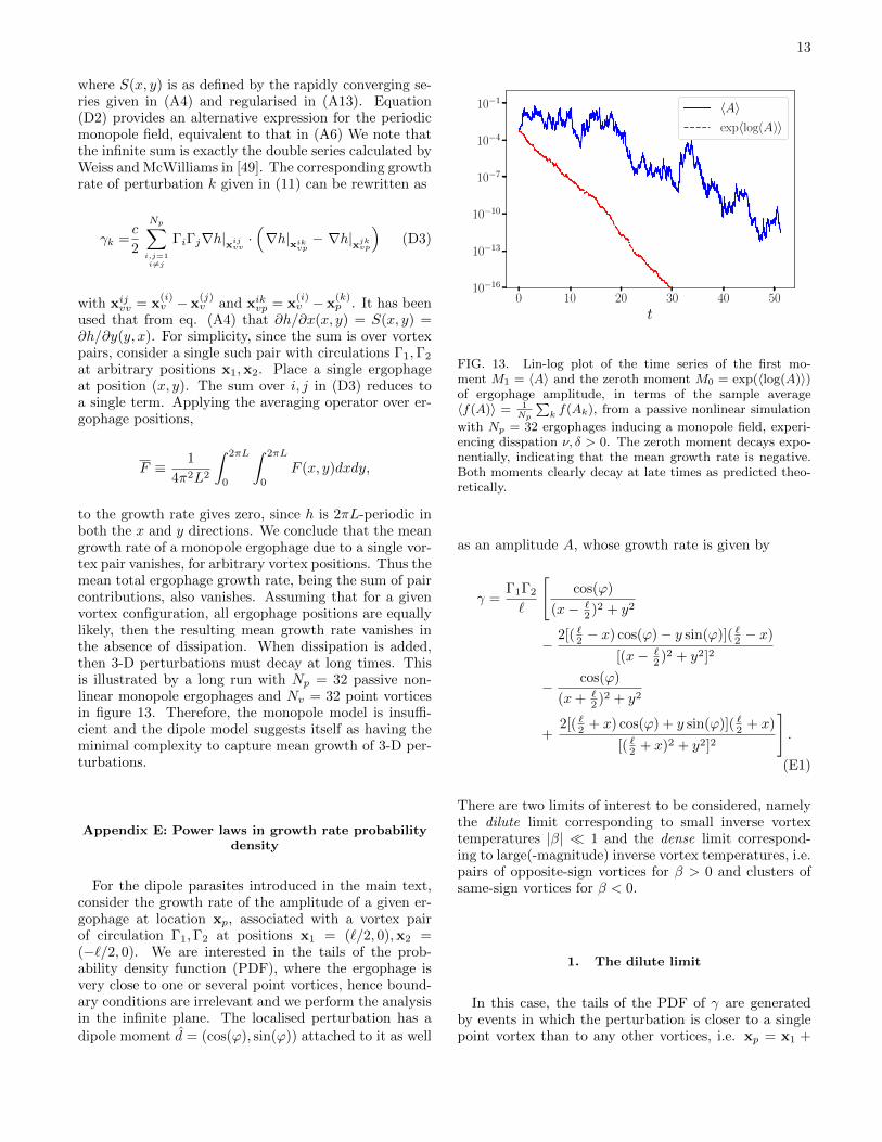
to the growth rate gives zero, since h is 2πL-periodic inboth the x and y directions. We conclude that the meangrowth rate of a monopole ergophage due to a single vor-tex pair vanishes, for arbitrary vortex positions. Thus themean total ergophage growth rate, being the sum of paircontributions, also vanishes. Assuming that for a givenvortex configuration, all ergophage positions are equallylikely, then the resulting mean growth rate vanishes inthe absence of dissipation. When dissipation is added,then 3-D perturbations must decay at long times. Thisis illustrated by a long run with Np = 32 passive non-linear monopole ergophages and Nv = 32 point vorticesin figure 13. Therefore, the monopole model is insuffi-cient and the dipole model suggests itself as having theminimal complexity to capture mean growth of 3-D per-turbations.

Appendix E: Power laws in growth rate probabilitydensity

For the dipole parasites introduced in the main text,consider the growth rate of the amplitude of a given er-gophage at location xp, associated with a vortex pairof circulation Γ1,Γ2 at positions x1 = (`/2, 0),x2 =(−`/2, 0). We are interested in the tails of the prob-ability density function (PDF), where the ergophage isvery close to one or several point vortices, hence bound-ary conditions are irrelevant and we perform the analysisin the infinite plane. The localised perturbation has a

dipole moment d = (cos(ϕ), sin(ϕ)) attached to it as well

0 10 20 30 40 50

t

10−16

10−13

10−10

10−7

10−4

10−1 〈A〉exp〈log(A)〉

FIG. 13. Lin-log plot of the time series of the first mo-ment M1 = 〈A〉 and the zeroth moment M0 = exp(〈log(A)〉)of ergophage amplitude, in terms of the sample average〈f(A)〉 = 1

Np

∑k f(Ak), from a passive nonlinear simulation

with Np = 32 ergophages inducing a monopole field, experi-encing disspation ν, δ > 0. The zeroth moment decays expo-nentially, indicating that the mean growth rate is negative.Both moments clearly decay at late times as predicted theo-retically.

as an amplitude A, whose growth rate is given by

γ =Γ1Γ2

`

[cos(ϕ)

(x− `2 )2 + y2

− 2[( `2 − x) cos(ϕ)− y sin(ϕ)]( `2 − x)

[(x− `2 )2 + y2]2

− cos(ϕ)

(x+ `2 )2 + y2

+2[( `2 + x) cos(ϕ) + y sin(ϕ)]( `2 + x)

[( `2 + x)2 + y2]2

].

(E1)

There are two limits of interest to be considered, namelythe dilute limit corresponding to small inverse vortextemperatures |β| 1 and the dense limit correspond-ing to large(-magnitude) inverse vortex temperatures, i.e.pairs of opposite-sign vortices for β > 0 and clusters ofsame-sign vortices for β < 0.

1. The dilute limit

In this case, the tails of the PDF of γ are generatedby events in which the perturbation is closer to a singlepoint vortex than to any other vortices, i.e. xp = x1 +

14

r(cos(φ), sin(φ)), r `. In this case,

γ ∼ Γ1Γ2

`r2[sin(ϕ) sin(2θ)− cos(ϕ) cos(2θ)]

= −Γ1Γ2

`r2cos(2θ + ϕ). (E2)

Since we consider the case where ϕ is optimal at everyposition, one finds ϕ = −2θ + nπ, n ∈ N and

γ ∼ |Γ1Γ2|`r2

⇔ r(γ) ∼√

γ`

|Γ1Γ2|(E3)

Assuming that all ergophage positions are equally proba-ble, then the probability of of being at distance betwennr and r+ dr is proportional to the ring area 2πrdr. Thiscan be inverted using (E3) to obtain a prediction for thePDF of γ, namely

P (γ) = r(γ)dr(γ)

dγ∝ 1

γ2(E4)

2. The dense limit

In this case, the tails of the PDF of the growth ratestem from encounters of the localised perturbation with

pairs of vortices, i.e. xp = r(cos(θ), sin(θ)), r `. Then,one finds at leading order in ` that

γ ∼Γ1Γ2

`

(−2`

cos(ϕ) cos(θ)

r3

+2`y sin(ϕ)(y2 − 3x2)− 2x cos(ϕ)(x2 − x2)

r6

)∼ −2Γ1Γ2

r3cos(3θ − ϕ)

Again assuming that ϕ is optimal, then ϕ = −3θ + nπ,n ∈ N, such that

γ ∼ 2|Γ1Γ2|r3

,

which leads to the growth rate PDF, again under the as-sumption that all ergophage positions are equally prob-able

P (γ) = r(γ)dr(γ)

dγ∝ 1

γ13+

43

=1

γ5/3,

with an exponent −5/3, whose magnitude is less than 2,hence there is neither a finite mean nor a finite variancefor this distribution. However, this −5/3 bears no rela-tion to Kolmogorov’s spectral exponent, it is merely adirect consequence of the modelling choices made here.

[1] A. van Kan, A. Alexakis, and M. E. Brachet, Extremeon-off intermittency, In preparation (2020).

[2] H. v. Helmholtz, LXIII. On integrals of the hydrodynam-ical equations, which express vortex-motion, The Lon-don, Edinburgh, and Dublin Philosophical Magazine andJournal of Science 33, 485 (1867).

[3] G. Kirchhoff, Vorlesungen uber mathematische Physik:Mechanik, Vol. 1 (BG Teubner, 1876).

[4] J. Goodman, T. Y. Hou, and J. Lowengrub, Convergenceof the point vortex method for the 2-D Euler equations,Communications on Pure and Applied Mathematics 43,415 (1990).

[5] L. Onsager, Statistical hydrodynamics, Il Nuovo Cimento(1943-1954) 6, 279 (1949).

[6] G. L. Eyink and K. R. Sreenivasan, Onsager and thetheory of hydrodynamic turbulence, Reviews of ModernPhysics 78, 87 (2006).

[7] R. H. Kraichnan and D. Montgomery, Two-dimensionalturbulence, Reports on Progress in Physics 43, 547(1980).

[8] P. Tabeling, Two-dimensional turbulence: a physicist ap-proach, Physics Reports 362, 1 (2002).

[9] G. Boffetta and R. E. Ecke, Two-dimensional turbulence,Annual Review of Fluid Mechanics 44, 427 (2012).

[10] U. Frisch and A. N. Kolmogorov, Turbulence: the legacyof AN Kolmogorov (Cambridge University Press, 1995).

[11] A. Celani, S. Musacchio, and D. Vincenzi, Turbulence inmore than two and less than three dimensions, Physicalreview letters 104, 184506 (2010).

[12] H. Xia, D. Byrne, G. Falkovich, and M. Shats, Upscaleenergy transfer in thick turbulent fluid layers, NaturePhysics 7, 321 (2011).

[13] S. J. Benavides and A. Alexakis, Critical transitions inthin layer turbulence, Journal of Fluid Mechanics 822,364 (2017).

[14] A. van Kan and A. Alexakis, Condensates in thin-layerturbulence, Journal of Fluid Mechanics 864, 490 (2019).

[15] S. Musacchio and G. Boffetta, Condensate in quasi-two-dimensional turbulence, Physical Review Fluids 4,022602 (2019).

[16] L. M. Smith, J. R. Chasnov, and F. Waleffe, Crossoverfrom two-to three-dimensional turbulence, Physical re-view letters 77, 2467 (1996).

[17] E. Deusebio, G. Boffetta, E. Lindborg, and S. Musacchio,Dimensional transition in rotating turbulence, PhysicalReview E 90, 023005 (2014).

[18] A. Alexakis and L. Biferale, Cascades and transitions inturbulent flows, Physics Reports 767, 1 (2018).

[19] E. D. Siggia and H. Aref, Point-vortex simulation of theinverse energy cascade in two-dimensional turbulence,The Physics of Fluids 24, 171 (1981).

[20] G. Carnevale, J. McWilliams, Y. Pomeau, J. Weiss,and W. Young, Evolution of vortex statistics in two-dimensional turbulence, Physical review letters 66, 2735(1991).

[21] R. Benzi, M. Colella, M. Briscolini, and P. Santangelo, Asimple point vortex model for two-dimensional decayingturbulence, Physics of Fluids A: Fluid Dynamics 4, 1036

15

(1992).[22] J. B. Weiss and J. C. McWilliams, Temporal scaling be-

havior of decaying two-dimensional turbulence, Physicsof Fluids A: Fluid Dynamics 5, 608 (1993).

[23] E. Trizac, A coalescence model for freely decaying two-dimensional turbulence, EPL (Europhysics Letters) 43,671 (1998).

[24] J. B. Weiss, Punctuated hamiltonian models of struc-tured turbulence, Semi-Analytic Methods for the Navier–Stokes Equations (Montreal, Canada, 1995)(ed. K.Coughlin). CRM Proc. Lecture Notes 20, 109 (1999).

[25] H. Aref, Stirring by chaotic advection, Journal of fluidmechanics 143, 1 (1984).

[26] M. P. Rast and J.-F. Pinton, Point-vortex model for la-grangian intermittency in turbulence, Physical Review E79, 046314 (2009).

[27] M. P. Rast and J.-F. Pinton, Pair dispersion in turbu-lence: the subdominant role of scaling, Physical reviewletters 107, 214501 (2011).

[28] M. P. Rast, J.-F. Pinton, and P. D. Mininni, Turbulenttransport with intermittency: Expectation of a scalarconcentration, Physical Review E 93, 043120 (2016).

[29] B. Gallet and R. Ferrari, The vortex gas scaling regimeof baroclinic turbulence, Proceedings of the NationalAcademy of Sciences 117, 4491 (2020).

[30] L. Horace, Hydrodynamics, 6th ed. (Dover, New York,1945).

[31] H. Aref and E. D. Siggia, Evolution and breakdown ofa vortex street in two dimensions, Journal of Fluid Me-chanics 109, 435 (1981).

[32] R. Krasny, A study of singularity formation in a vor-tex sheet by the point-vortex approximation, Journal ofFluid Mechanics 167, 65 (1986).

[33] R. Krasny, Desingularization of periodic vortex sheet roll-up, Journal of Computational Physics 65, 292 (1986).

[34] B. Nowak, J. Schole, D. Sexty, and T. Gasenzer, Nonther-mal fixed points, vortex statistics, and superfluid turbu-lence in an ultracold bose gas, Physical Review A 85,043627 (2012).

[35] M. T. Reeves, T. P. Billam, B. P. Anderson, andA. S. Bradley, Inverse energy cascade in forced two-dimensional quantum turbulence, Physical review letters110, 104501 (2013).

[36] T. P. Billam, M. T. Reeves, B. P. Anderson, and A. S.Bradley, Onsager-kraichnan condensation in decayingtwo-dimensional quantum turbulence, Physical reviewletters 112, 145301 (2014).

[37] A. Griffin, V. Shukla, M.-E. Brachet, and S. Nazarenko,Magnus-force model for active particles trapped on su-perfluid vortices, Physical Review A 101, 053601 (2020).

[38] G. Joyce and D. Montgomery, Negative temperaturestates for the two-dimensional guiding-centre plasma,Journal of Plasma Physics 10, 107 (1973).

[39] P.-H. Chavanis, J. Sommeria, and R. Robert, Statisti-cal mechanics of two-dimensional vortices and collision-less stellar systems, The Astrophysical Journal 471, 385(1996).

[40] B. Gallet, Exact two-dimensionalization of rapidly rotat-ing large-reynolds-number flows, Journal of Fluid Me-chanics 783, 412 (2015).

[41] B. Gallet and C. R. Doering, Exact two-dimensionalization of low-magnetic-reynolds-numberflows subject to a strong magnetic field, Journal of FluidMechanics 773, 154 (2015).

[42] K. Seshasayanan and B. Gallet, Onset of three-dimensionality in rapidly rotating turbulent flows, Jour-nal of Fluid Mechanics 901, R5 (2020).

[43] E. M. Purcell and R. V. Pound, A nuclear spin system atnegative temperature, Physical Review 81, 279 (1951).

[44] A. Oja and O. Lounasmaa, Nuclear magnetic ordering insimple metals at positive and negative nanokelvin tem-peratures, Reviews of Modern Physics 69, 1 (1997).

[45] P. Medley, D. M. Weld, H. Miyake, D. E. Pritchard,and W. Ketterle, Spin gradient demagnetization coolingof ultracold atoms, Physical review letters 106, 195301(2011).

[46] X. Yu, T. P. Billam, J. Nian, M. T. Reeves, and A. S.Bradley, Theory of the vortex-clustering transition in aconfined two-dimensional quantum fluid, Physical Re-view A 94, 023602 (2016).

[47] F. Cornu and B. Jancovici, On the two-dimensionalcoulomb gas, Journal of statistical physics 49, 33 (1987).

[48] G. Krstulovic, C. Cartes, M. Brachet, and E. Tirapegui,Generation and characterization of absolute equilibriumof compressible flows, International Journal of Bifurca-tion and Chaos 19, 3445 (2009).

[49] J. B. Weiss and J. C. McWilliams, Nonergodicity of pointvortices, Physics of Fluids A: Fluid Dynamics 3, 835(1991).

[50] A. A. Dubkov, B. Spagnolo, and V. V. Uchaikin, Levyflight superdiffusion: an introduction, International Jour-nal of Bifurcation and Chaos 18, 2649 (2008).

[51] M. F. Shlesinger, G. M. Zaslavsky, and U. Frisch, Levyflights and related topics in physics (Springer, 1995).

[52] A. V. Chechkin, R. Metzler, J. Klafter, V. Y. Gonchar,et al., Introduction to the theory of levy flights, Anoma-lous Transport , 129 (2008).

[53] B. B. Mandelbrot, The fractal geometry of nature, Vol.173 (WH freeman New York, 1983).

[54] M. Shlesinger, B. West, and J. Klafter, Levy dynamics ofenhanced diffusion: Application to turbulence, PhysicalReview Letters 58, 1100 (1987).

[55] T. Solomon, E. R. Weeks, and H. L. Swinney, Obser-vation of anomalous diffusion and levy flights in a two-dimensional rotating flow, Physical Review Letters 71,3975 (1993).

[56] R. Metzler and J. Klafter, The random walk’s guide toanomalous diffusion: a fractional dynamics approach,Physics reports 339, 1 (2000).

[57] B. Dubrulle and J.-P. Laval, Truncated levy lawsand 2d turbulence, The European Physical Journal B-Condensed Matter and Complex Systems 4, 143 (1998).

[58] D. del Castillo-Negrete, B. Carreras, and V. Lynch, Non-diffusive transport in plasma turbulence: a fractionaldiffusion approach, Physical review letters 94, 065003(2005).

[59] C. Schinckus, How physicists made stable levy processesphysically plausible, Brazilian Journal of Physics 43, 281(2013).

[60] P. D. Ditlevsen, Anomalous jumping in a double-well po-tential, Physical Review E 60, 172 (1999).

[61] P. D. Ditlevsen, Observation of α-stable noise inducedmillennial climate changes from an ice-core record, Geo-physical Research Letters 26, 1441 (1999).

[62] I. Rhee, M. Shin, S. Hong, K. Lee, S. J. Kim, andS. Chong, On the levy-walk nature of human mobility,IEEE/ACM transactions on networking 19, 630 (2011).

16

[63] B. Gross, Z. Zheng, S. Liu, X. Chen, A. Sela, J. Li, D. Li,and S. Havlin, Spatio-temporal propagation of covid-19pandemics, medRxiv (2020).

[64] G. M. Viswanathan, V. Afanasyev, S. Buldyrev, E. Mur-phy, P. Prince, and H. E. Stanley, Levy flight search pat-terns of wandering albatrosses, Nature 381, 413 (1996).

[65] R. Metzler and J. Klafter, The restaurant at the end ofthe random walk: recent developments in the descriptionof anomalous transport by fractional dynamics, Jour-nal of Physics A: Mathematical and General 37, R161(2004).

[66] D. Applebaum, Levy processes-from probability to fi-nance and quantum groups, Notices of the AMS 51, 1336(2004).

[67] K. Kumar, S. Fauve, and O. Thual, Critical self-tuning:the example of zero prandtl number convection, Journalde Physique II 6, 945 (1996).

[68] K. Kumar, P. Pal, and S. Fauve, Critical bursting, EPL(Europhysics Letters) 74, 1020 (2006).

[69] N. Platt, E. Spiegel, and C. Tresser, On-off intermittency:A mechanism for bursting, Physical Review Letters 70,279 (1993).

[70] S. Aumaıtre, K. Mallick, and F. Petrelis, Noise-inducedbifurcations, multiscaling and on–off intermittency, Jour-

nal of Statistical Mechanics: Theory and Experiment2007, P07016 (2007).

[71] S. Benavides, E. Deal, J. Perron, J. Venditti, Q. Zhang,and K. Kamrin, Multiplicative noise and intermittency inbedload sediment transport (2020).

[72] M. Ding and W. Yang, Distribution of the first returntime in fractional brownian motion and its applicationto the study of on-off intermittency, Physical Review E52, 207 (1995).

[73] A. Alexakis and F. Petrelis, Planar bifurcation subject tomultiplicative noise: Role of symmetry, Physical ReviewE 80, 041134 (2009).

[74] A. Alexakis and F. Petrelis, Critical exponents in zero di-mensions, Journal of Statistical Physics 149, 738 (2012).

[75] F. Petrelis and A. Alexakis, Anomalous exponents atthe onset of an instability, Physical Review Letters 108,014501 (2012).

[76] R. N. Mantegna and H. E. Stanley, Stochastic processwith ultraslow convergence to a gaussian: the truncatedlevy flight, Physical Review Letters 73, 2946 (1994).

[77] A. van Kan, T. Nemoto, and A. Alexakis, Rare tran-sitions to thin-layer turbulent condensates, Journal ofFluid Mechanics 878, 356 (2019).