Can heterogeneous core–mantle electromagnetic coupling control geomagnetic reversals?
Upload
independentCategory
view
1download
0
Four centuries of geomagnetic secularvariation from historical records
By And rew Jackson1 Art R T Jonkers2
a n d Matthew R Walker1
1School of Earth Sciences Leeds University Leeds LS2 9JT UK2Department of History Vrije Universiteit Amsterdam The Netherlands
We present a new model of the magnetic shy eld at the coremantle boundary for theinterval 15901990 The model called gufm1 is based on a massive new compilationof historical observations of the magnetic shy eld The greater part of the new datasetoriginates from unpublished observations taken by mariners engaged in merchantand naval shipping Considerable attention is given to both correction of data forpossible mislocation (originating from poor knowledge of longitude) and to properallocation of error in the data We adopt a stochastic model for uncorrected positionalerrors that properly accounts for the nature of the noise process based on a Brownianmotion model The variability of navigational errors as a function of the duration ofthe voyages that we have analysed is consistent with this model For the period before1800 more than 83 000 individual observations of magnetic declination were recordedat more than 64 000 locations more than 8000 new observations are for the 17thcentury alone The time-dependent shy eld model that we construct from the dataset isparametrized spatially in terms of spherical harmonics and temporally in B-splinesusing a total of 36 512 parameters The model has improved the resolution of the coreshy eld and represents the longest continuous model of the shy eld available However fullexploitation of the database may demand a new modelling methodology
Keywords Earthrsquos core geomagnetic secular variationmagnetic macreld maritime history
1 Introduction
The Earth has possessed a magnetic shy eld for more than 4 billion years generated inthe reguid core Although considerable progress has been made in elucidating the gener-ation process (summaries can be found in this issue) much remains to be understoodnot least why the shy eld appears to be so stable for long periods of time punctuatedby occasional reversals Since humans have been observing the magnetic shy eld for thepast thousand years or so and geographically diverse observations are available forthe last 500 years it is likely that there is much to be learned from an analysis of theshy eld morphology and evolution deduced from direct measurements To this end weaim to construct the most accurate model of the magnetic shy eld to date from originalobservations
The models we create are specishy cally designed to examine the shy eld at the coremantle boundary (CMB) and our results are presented as maps of the radial compo-nent of the magnetic shy eld at the surface of the core Fortunately the mathematical
Phil Trans R Soc Lond A (2000) 358 957990
957
c 2000 The Royal Society
958 A Jackson A R T Jonkers and M R Walker
tools for doing this (Whaler amp Gubbins 1981 Shure et al 1982 Gubbins 1983Gubbins amp Bloxham 1985) are well developed It is now commonplace for dynam-ical simulations of the dynamo to plot maps of the radial shy eld at the CMB to aidcomparison with observation
The historical record is very short compared with the time-scales used in palaeo-magnetic analyses or indeed compared with the life of the magnetic shy eld itself It isour opinion that it is important to try to push the analysis of historical observationsback in time as far as possible and secondly to improve the shy delity of our knowledgeof the shy eld in the recent past In this paper we focus on our enotorts to address theseissues
In terms of methodology our work builds on that of Bloxham et al (1989) andBloxham amp Jackson (1992) we omit describing their work noting that it was theshy rst systematic analysis of the core magnetic shy eld morphology through time andthat it was entirely based on published data sources As described in Bloxham et al (1989) virtually all of the previous work on modelling the historical magnetic shy eldhad been designed to describe the shy eld at the Earthrsquos surface Such models are notdesigned to be nor are they optimal for describing the conshy guration of shy eld at theCMB
A review of the previous compilations of magnetic data that have been pro-duced over time can be found in Barraclough (1982) The earliest catalogues|ofStevin (1599) Kircher (1641) and Wright (1657)|are deshy cient in that they con-tain undated observations Around 1705 the French hydrographer Guillaume Delislecompiled some 10 000 observations (mostly of declination) in his notebooks tryingto establish regularity in secular acceleration these were never published but stillexist in the Archives Nationales in Paris The next important compilation of mag-netic data was made by Mountaine amp Dodson (1757) who claimed to have basedtheir tables of declination at dinoterent points on the Earth on over 50 000 origi-nal observations of the shy eld It was this claim that partly provided the stimulusfor our work This claim was treated with some scepticism by some (eg Bloxham1985) on the grounds that such large numbers of observations almost certainly didnot exist at that time since such a number was more than an order of magnitudelarger than the number of observations in published works Although they did notreference their data sources in a modern manner nor publish the actual observa-tions Mountaine amp Dodson (1757) do explicitly state the sources they used for theirdata which are very similar to those we have used We are therefore conshy dent thattheir claim for the number of data that they used is true as our own data col-lection activities show that such numbers of data clearly exist It is also the casethat we have used only a tiny fraction of the data that reside in the India Omacr ceof the British Library (we have used 325 out of the estimated 1500 pre-19th cen-tury logs that are held there however we have processed all of the 17th centurylogs) The early work of Mountaine amp Dodson (1757) should almost certainly receivemore prominence than it does representing probably the shy rst large-scale attemptto describe the morphology of the shy eld Maps based on the data were subsequentlyproduced
The catalogues that were produced after the work of Mountaine amp Dodson (1757)have been the basis for the data compilation described in the study of Bloxham et al (1989) and will not be discussed here save for the remarks regarding the catalogueof Sabine given in x 2 b
Phil Trans R Soc Lond A (2000)
Geomagnetic secular variation 959
The plan of the paper is as follows General aspects of the data that contributeto the new model are described in x 2 a more detailed account will be forthcomingThe methodology that has been applied to the dataset is described in x 3 along withthe deterministic corrections that are made to the data The stochastic model fornavigational errors and assignments of other errors are described in x 4 The resultsare discussed in a geophysical context in x 5 for results of this analysis applied tothe history of navigation and science see Jonkers (2000)
2 Data
The major problem anotecting early maritime observations is that of navigationalimprecision By far the most important and potentially the most accurate obser-vation on board ship was that of latitude Even for the very shy rst long-distance voy-ages latitude could be found quite accurately its determination had been a long-established practice by land-based astronomers and it was initially their instrumentsquadrant and astrolabe that were adapted for use at sea A more practical device ondeck was the cross-stanot a stick with separate transoms of dinoterent dimensions slidingalong its length The problem of having to look directly into the sun was obviatedby the backstanot invented by John Davis in 1594 working with cast shadow insteadof direct sighting Thus the problem of determining latitude has been rather wellsolved for the last 400 years
As is well known the problem of determining longitude at sea was not adequatelysolved until the 1760s (and gradually implemented in merchant shipping from the1780s) the story of the battle of John Harrison to gain acceptance of his timekeepershas been oft told and we will not dwell on the issue (see for example Andrewes1996) Before the use of accurate chronometers or the competing lunar methodlongitude was found by the method known as dead reckoning At the beginningof each new shiprsquos day (at noon) the `dayrsquos workrsquo was performed either with orwithout an observation of latitude The calculation of the change in longitude wasbased on simple trigonometry using an estimate of the distance run by the ship(based on assessment of the shiprsquos speed taking into account currents and leeway)and the shiprsquos heading The result of ill-founded estimates of speed leeway and driftwere able to produce longitudinal errors of up to several degrees after months ofunchecked progress Much of our enotort has been directed towards properly accountingfor or statistically representing the enotects of this poor knowledge of longitude Wehave made independent estimates of the accuracy of dead-reckoning estimates usingestimated and measured latitudes (see x 4 a)
The measurements of the magnetic shy eld that were made most commonly in his-torical times were the declination (or angle between true north and magnetic north)denoted D and the inclination or dip (or angle between the horizontal and magneticshy eld vector) denoted I After Gaussrsquos development of a method for measuring abso-lute intensities in 1832 the horizontal intensity (H) and the total intensity (F ) wereobserved In more recent times X Y and Z the northward eastward and downwardcomponents of the magnetic shy eld respectively are reported Exact deshy nitions canbe found in Langel (1987)
Awareness of magnetic declination dates back to the shy rst half of the 15th cen-tury at least in Europe These shy rst measurements take the form of scattered landobservations More importantly for our purpose the oceans have been traversed
Phil Trans R Soc Lond A (2000)
960 A Jackson A R T Jonkers and M R Walker
by ships from many nations since the 16th century In marked contrast to coastalnavigation negotiating an ocean relied on astronomical observation for a daily lat-itudinal shy x (accurate using a backstanot to about ten minutes of arc eg Andrewes(1996 p 400)) and a compass to maintain course in the absence of landmarks andsoundings to steer by In addition compass bearings were used in dead-reckoning cal-culations (see below) and to chart coastlines All of these applications necessitatedan adequate correction for local declination Navigational practice thus frequentlyincluded magnetic observations as is evinced in thousands of logbooks kept by cap-tains masters and mates Although many of these manuscripts have since been losta sumacr ciently large number has been preserved to warrant a substantial sample to beextracted for geomagnetic modelling purposes In the following we will brieregy out-line the shipping companies we investigated their routes and some characteristicsof the measurements
(a) Pre-19th century data sources
Our archival research took place in Great Britain France the Netherlands Den-mark and Spain Three main categories of shipping have been analysed East-IndiaCompanies naval expeditions and smaller merchant organizations The shy rst cate-gory provided about twice as many readings as each of the other two and representsthe earliest and longest record The English East India Company (EIC) obtaineda royal charter in 1600 while its Dutch counterpart the VOC (Vereenigde Oost-Indische Compagnie) followed two years later Both eventually sunotered shy nancialruin on account of war losses and an ever-growing administrative burden due to ter-ritorial management Three French state-sponsored `Compagnie des Indesrsquo (CDI)were launched in 1664 (by Colbert) 1717 (Law) and 1785 (Calonne) None provedcommercially viable and only the second left any data An even smaller player wasthe Danish `Asiatiske Kompagnirsquo founded in 1732 after a pioneering trading expe-dition to Canton
All of the above ventures had both standardized instruments and a highly devel-oped infrastructure which allowed the processing and communication of nauticalinformation (in logbooks charts and sailing directions) The same can be said to alesser degree of these countriesrsquo navies During the 17th century their peace-time rulewas mainly conshy ned to patrolling the Channel the North Atlantic and the Mediter-ranean Eighteenth-century convoy duties however expanded their actions acrossthe Atlantic to the Americas (especially the West Indies) destinations eventuallycame to include the East Indies as well The Danes maintained a military presencealong the coasts of Greenland where they collected a series of magnetic dip mea-surements in 1736 Of particular interest for the present studies are scientishy c voyagesperformed under naval command Exploration was usually accompanied by partic-ular attention to instruments and the observations obtained therewith resulting indense high-quality records of otherwise sparsely visited regions We merely recall inpassing the Dutch exploits in the Pacishy c by the Nassau regeet Edmond Halleyrsquos twomagnetic surveys Ansonrsquos and Cookrsquos circumnavigations and French expeditions byBougainville Crozet Laperouse and drsquoEntrecasteaux
Of the merchant navies Dutch slavers (foremost the `Midddelburgsche CommercieCompagniersquo or MCC) and the English `Hudsonrsquos Bay Companyrsquo (trading in furs)deserve mention Both were active in the 18th century records of small shipping com-panies tend to be extremely scarce before that time and indeed the largest Dutch
Phil Trans R Soc Lond A (2000)
Geomagnetic secular variation 961
slaver company (the West Indian Company) left very few shiprsquos logs in contrast tothe MCC A triangular route was pursued by the MCC from Europe down to theWest-African coasts (to buy slaves) then across the ocean to South America and theCaribbean (to sell slaves and buy agricultural produce) and homeward bound alongmore northerly latitudes This triangular trade in combination with direct tramacr cby Europeans to the West Indies and North-American colonies generated magneticshy eld observations that covered much of the North Atlantic even though the aver-age number of measurements taken per voyage was lower than on ships bound forAsia Relatively few measurements were taken on each voyage along the high-latitudetrack towards Hudsonrsquos Bay but the regularity of the shipsrsquo annual crossings whichcontinued well into the 19th century actually generates excellent data coverage
The data that we have amassed for the period to 1800 is shown in shy gure 1af Note that even in the shy rst 50 years of the 17th century (shy gure 1a) there were somePacishy c crossings exhibiting the technique of `running down the latitudersquo Many ofthese data originated in the compilation of Hutcheson amp Gubbins (1990) which waslargely based on the work of Van Bemmelen (1899) In contrast the last 50 years ofthe 17th century (shy gure 1b) are somewhat devoid of Pacishy c crossings save for thedata near the Aleutians Between 1700 and 1750 (shy gure 1c) there is a tremendousincrease in tra c around Cape Horn and the voyages of Middleton into HudsonrsquosBay can clearly be seen The latter part of the 18th century witnessed the tremendousexplosion in voyages of exploration generating a very even geographical coverage ofthe world (shy gure 1d) Note that there are data stretching from the Bering Straits inthe north almost to the edges of the Antarctic continent in the south The distributionof inclinations for the 17th century shown in shy gure 1e has been greatly improvedfrom that of Hutcheson amp Gubbins (1990) whose data were entirely in the NorthernHemisphere consisting of observations in Europe and the Barents Sea HudsonrsquosBay and a single observation at Cape Comorin India Our dataset has inclinationsin South Africa the Philippines Japan and along the east coasts of North and SouthAmerica
In all of 2398 logs processed 1633 contained a grand total of 83 861 magneticdeclination observations gathered on 64 386 days For the 17th century alone theformer compilation of 2715 measurements was boosted with 8282 new readings Inextremely rare instances inclination was also measured on board the existing set of1721 inclinations has grown with an additional 266 measurements
(b) 19th and 20th century data sources
Our data-compilation work has focused on improving the collections of Bloxham(1985) and Jackson (1989) Bloxhamrsquos 19th century data came entirely from thecompilations of Sabine (1868 1872 1875 1877) Jacksonrsquos data came from a varietyof sources documented in Bloxham et al (1989) as no previous catalogue for thisperiod had been made We have made a number of improvements to this databaseWe have added the 12 post-1790 voyages contained in Hansteen (1819) which hadnot been previously used Sabinersquos compilations of data cover the period 18201870They are based on both published accounts of expeditions British and foreign andmanuscripts to which Sabine had access Fortunately the sources of data are alllisted It is perhaps inevitable that the compilation is incomplete and we have com-piled many data from this period that were omitted from Sabine A more serious
Phil Trans R Soc Lond A (2000)
962 A Jackson A R T Jonkers and M R Walker
(a)
(b)
(c)
Figure 1 Data distributions in time (a) Declinations 16001649(b) Declinations 16501699 (c) Declinations 17001749
Phil Trans R Soc Lond A (2000)
Geomagnetic secular variation 963
(d )
(e)
( f )
Figure 1 (Cont) (d) Declinations 17501799 (e) Inclinations 16001699 Stars areused here to allow the few locations to be seen (f ) Inclinations 17001799
Phil Trans R Soc Lond A (2000)
964 A Jackson A R T Jonkers and M R Walker
(g)
(h)
Figure 1 (Cont) (g) All data 18001849 (h) All data 18501899
shortcoming of the compilation is the fact that data were omitted by Sabine whenforming his compilation from the original sources Since the world compilations areby region rather than by voyage and are only for the zones 4085 N 040 N and040 S data from greater than 40 S have been omitted (notwithstanding the dataoriginating in the Magnetic Survey of the South Polar Regions undertaken between1840 and 1845 reported in Sabine (1868)) We used Sabinersquos dataset as the basisfor creating a new dataset in which individual voyages are represented and we usedthe original sources to reinstate missing data from the voyages A more completeaccount will be forthcoming
A major source of data for the early 19th century originates as two manuscriptcompilations held in the Archives Nationales and the Bibliotheque Nationale in ParisThe majority of the data are observations of declination made on board FrenchNaval and Hydrographic Service ships Since the data were not recorded in theiroriginal manuscript form but had been transcribed onto a geographical grid there
Phil Trans R Soc Lond A (2000)
Geomagnetic secular variation 965
20 000
16 000
8000
4000
12 000
0
date
freq
uenc
y
1600 1650 1700 1750 1800 1850
Figure 2 Histogram showing the temporal distribution of the new data collected (black)compared with the previous historical collection (grey) used in Bloxham amp Jackson (1992)
is a quantization error in the observation positions that must be taken into accountSome observations are given on a 1 1 grid while others are on a 100 100 gridWe have accounted for the positional imprecision in the same way as for pre-19thcentury data
For the 20th century we have used the same dataset as was used by Bloxham etal (1989) which includes survey data observatory data (which runs back to themid-19th century) and data from the POGO and Magsat satellites The temporaldistribution of the shy nal dataset up to 1860 is shown in shy gure 2 showing the largeincrease in data over that used in the production of the models ufm1 and ufm2 ofBloxham amp Jackson (1992)
3 Method
(a) Demacrnitions and notation
We begin by reviewing the concepts and notation necessary for our analysis Muchis standard and can be found for example in the texts of Langel (1987) or Backuset al (1996) We adopt a spherical coordinate system (r ) where r is radiusis colatitude and is longitude We denote the Earthrsquos radius and core radius by aand c respectively and take a = 63712 km and c = 3485 km We assume the mantleis an insulator so that for r gt c
B = rV (31)
where V is the magnetic potential Although other methodologies are possible someof which are attractive for certain applications (eg Shure et al 1982 Constable et al 1993 OrsquoBrien amp Parker 1994) we use the spherical harmonic expansion of V as theunderlying parametrization of the radial magnetic shy eld at the CMB Br = rV jr = c
Phil Trans R Soc Lond A (2000)
966 A Jackson A R T Jonkers and M R Walker
which as we stated in x 1 is the quantity in which we are ultimately interested Atany time t the potential can be written
V = a1X
l = 1
lX
m = 0
a
r
l + 1
(gml (t) cos m + hm
l (t) sin m )P ml (cos ) (32)
where fgml (t) hm
l (t)g are the so-called Gauss coemacr cients and P ml (cos ) are Schmidt
quasi-normalized associated Legendre functions The choice of parametrization thusfar has proceeded without loss of generality the spherical harmonics represent acomplete set Computational considerations require that we truncate the sphericalharmonic expansion at degree L in this paper as in previous work (eg Bloxhamamp Jackson 1992) we take L = 14 This choice is beyond the point in the sphericalharmonic power spectrum measured at the Earthrsquos surface at which the core shy eldis overwhelmed by the crustal magnetic shy eld We also require a parametric represen-tation for the time-varying Gauss coemacr cients Here we make a choice that restrictsthe class of functions that can be represented With one eye on the regularizationthat we will introduce in equation (37) below we choose the B-splines (eg Lan-caster amp Salkauskas 1986) of order 4 as basis functions for the expansion of the gm
land hm
l exactly as in Bloxham amp Jackson (1992) wherein a rationalization can befound
gml (t) =
X
n
ngml Bn(t) (33)
with a similar expansion for the hml (t) We choose to use T B-splines for the time
period [t s te] erected on a set of T + 4 regularly spaced knots The fngml nhm
l gwhen suitably ordered (we chose to let n increase the most slowly then l then m)constitute what we will call the model vector m with dimension P = T L(L + 2)and components mj
Each component of the shy eld constitutes a datum j with an associated forwardfunction fj(m) that makes a prediction from the model Because many of our data arenonlinear functionals of the model m our methodology for shy nding a model from theobservations proceeds by an iterative method whereby we calculate small incrementsm to the model at the ith iterate We will frequently require the sensitivity of the
jth synthesized datum with respect to a change in the kth model parameter mkthis is simply the derivative fj(m)=mk We store these derivatives in the matrixA with Ajk = fj(m)=mk
We group the data into a data vector of length N with an associated errorvector e It is necessary to assign the ei for each datum depending on the methodsof acquisition and the likely sources of error this is given considerable attentionin x 4 Of particular importance is the correlation in the errors described by thecovariance matrix Ce with elements
[Ce]ij = Efeiejg (34)
where E signishy es expectation For most sources the errors are independent so thatCe is diagonal this is the situation that is most commonly assumed in geophysicsHowever one source of error namely that due to imprecise navigation is proneto lead to correlated errors because navigational errors made on a particular daycompound errors made on previous days We have developed a stochastic formalism
Phil Trans R Soc Lond A (2000)
Geomagnetic secular variation 967
to account for this in our attribution of error it leads to a non-diagonal Ce althoughthe correlation only anotects data between landfalls within each individual voyage thisis described in x 4 a
(b) The continuous timespace model
Before describing our solution methodology it is pertinent to discuss the issue ofuniqueness of our inverse problem given perfect continuous knowledge of a propertyof the magnetic shy eld on the surface of the Earth we must consider if this is sumacr cientto reconstruct the magnetic shy eld everywhere We shy x attention on one particularepoch It is well known that perfect knowledge of the vertical component of themagnetic shy eld is sumacr cient to determine the magnetic shy eld everywhere as a result ofthe uniqueness theorem for Laplacersquos equation with Neumann boundary conditions(eg Kellogg 1929) Indeed knowledge of the horizontal shy eld will sumacr ce equally wellA dinoterent issue relates to whether shy eld directions are sumacr cient to determine themagnetic shy eld everywhere This is particularly relevant since our dataset is heavilybiased towards declination measurements in the earliest years and there are noabsolute intensities prior to Gaussrsquos invention of a method for determining intensityin 1832 The question has been recently addressed by Hulot et al (1997) who foundthat perfect knowledge of the shy eld direction on a surface is sumacr cient to determinethe magnetic shy eld everywhere provided that the magnetic shy eld has no more thantwo dip poles An ambiguity that remains is that before 1832 our model can giveonly the shy eld morphology and requires a scale factor to shy x its intensity We adoptthe dipole decay with time suggested by the extrapolation of Barraclough (1974)this shy xes g0
1(t) to decay at a rate of 15 nT yr 1 for t lt 1840 (essentially the rate ofBarraclough (1974)) with the value in 1840 being determined by the intensities inthe dataset
A second and possibly more pertinent issue is that of non-uniqueness resultingfrom the shy niteness of the dataset being analysed It is well known (Backus amp Gilbert1970) that there are many models of a continuous function such as Br that arecapable of shy tting a shy nite dataset Therefore we stress that in the methodology thatfollows we choose a model that satisshy es our prejudices of being smooth in timeand space while still shy tting the data We do not claim any sort of uniqueness forthe images that we present Nevertheless it is useful at this stage to mention theway that observations sample the core shy eld Figure 3 shows a cross-section of the(two-dimensional) kernel that dictates the sensitivity of a declination observation todepartures of the core shy eld from an axial dipole state The point to note from thisis that a declination observation is sensitive to perturbations in the core shy eld overa large angular distance and we can tolerate some gaps in our geographical datadistribution without losing sensitivity to the core shy eld entirely (see for exampleJohnson amp Constable (1997) for more details)
Our methodology for regularizing the timespace model is the same as that pre-sented in Bloxham amp Jackson (1992) We shy nd the smoothest model for a given shy t tothe data by seeking as our estimate the model vector m that minimizes the misshy t tothe data and two model norms one measuring roughness in the spatial domain andthe other roughness in the temporal domain For the spatial norm we seek the solu-tion with minimum ohmic dissipation based on the ohmic heating bound of Gubbins
Phil Trans R Soc Lond A (2000)
968 A Jackson A R T Jonkers and M R Walker
- 180 - 90 0
angular distance (great circle)
006
004
002
000
- 002
- 004
- 00690 180
Figure 3 The kernel describing the sensitivity of a declination observation to the radial coremacreld when linearized about the macreld of an axial dipole The ordinate shows the distance fromthe observation site measured along the great circle passing through the site in an eastwestdirection
(1975) we minimize the integral
=1
(te t s )
Z te
ts
F (Br) dt = mTS 1m (35)
where F(Br) is the quadratic norm associated with the minimum ohmic heating ofa shy eld parametrized by fgm
l hml g
F (Br) = 4
1X
l = 1
(l + 1)(2l + 1)(2l + 3)
l
a
c
2l + 4 lX
m = 0
[(gml )2 + (hm
l )2] (36)
For the temporal model norm we use
=1
(te t s )
Z te
ts
I
CM B
(2t Br)2 d dt = mTT 1m (37)
where [t s te] is the time-interval over which we solve for the shy eldWe have assumed that the errors contaminating our dataset are Gaussian with
known covariance matrix Ce this assumption leads naturally to the use of least-squares in the estimate of the model m We caution the reader that there is accu-mulating evidence that the distribution of errors that contaminate geomagnetic datamay be far from Gaussian therefore we make our estimate robust to the presenceof outliers by the use of a clamping scheme whereby large residuals are gradu-ally rejected from the estimation process until only data whose residuals are less
Phil Trans R Soc Lond A (2000)
Geomagnetic secular variation 969
than three standard deviations away from the current prediction for that datum areretained (as used in Bloxham et al (1989)) Our model estimate m is that whichminimizes the objective function
(m) = [ f (m)]TC 1e [ f (m)] + mTC 1
m m (38)
where Ce is the data error covariance matrix (specishy ed in x 4) and C 1m = S S 1 +
TT 1 with damping parameters S and T The solution is sought iteratively usingthe scheme
m i+ 1 = m i + (ATC 1e A + C 1
m ) 1[ATC 1e ( f (m i)) C 1
m m i] (39)
A consequence of these regularization conditions is that the expansions (32)and (33) converge so that with appropriately large values for the truncation points Land T the solution is insensitive to truncation We have used L = 14 and T = 163 inour calculations with knots every 25 years In addition to the regularization providedby (35) and (37) we have found it advantageous to impose boundary conditionsat ts and te The so-called natural boundary condition of vanishing second (time)derivative has been applied at t s so that B(t s ) = 0 The equivalent condition at te
has not been applied doing so creates a large misshy t primarily to the observatorydata In enotect the observatory data supply a boundary condition on B themselves(recall that we use shy rst dinoterences of observatory data) and the pre-1990 secularvariation is strongly at variance with the B (te) = 0 assumption We have thereforerefrained from applying this boundary condition at te
Since the error covariance matrix is sparse (it is block diagonal) we can computethe contribution to the total misshy t M from any subset of the data of size Ns witherrors e(s) as
Ms =
r1
Ns
(e(s))T[C(s)e ] 1(e(s)) (310)
where C(s)e is the Ns Ns submatrix of Ce associated with the data sample neces-
sarily it must encompass all correlations The total misshy t clearly satisshy es
M 2 =1
N
X
s
NsM 2s (311)
a weighted sum over all the subset misshy ts
(c) Data correction
After archival data conversion to machine-readable form and correction of obvi-ous typographical errors all of our new pre-19th century data have been manuallyexamined by plotting in a purpose-built `voyage editorrsquo an interactive graphical userinterface built around the GMT plotting package (Wessel amp Smith 1991) designedfor us by Dr N Barber The identishy cation of geographical locations mentioned inthe log is invaluable in enabling a reconstruction of the actual course plots thevoyage editor provided instant visual feedback on land sightings and allowed posi-tional adjustments of three kinds single-point editing translation of voyage legs andstretching of voyage legs
Phil Trans R Soc Lond A (2000)
970 A Jackson A R T Jonkers and M R Walker
Figure 4 Example of a voyage loaded into the voyage editorrsquo
Translation and stretching operations acted on multiple points which we refer toas a `legrsquo of a voyage a start and end point were chosen to deshy ne the leg boundariesand either could be lifted and transported elsewhere This displacement could then beenotected uniformly for each point shifting the whole leg to the right or left while main-taining latitude Alternatively in the case of stretching one end of a leg remainedshy xed while the other points were longitudinally stretched to meet the translatedother end For example when a ship travelling eastward from Tristan da Cunhashy nally spotted the Cape of Good Hope the westerly winds and currents carrying theship along may have been underestimated or overestimated to such an extent that thereckoning put the vessel either far ahead or far before the longitude of Capetown Thelast land previously sighted (the islands of Tristan) could then be shy xed as a startingpoint and the entry containing the comment `seen the Cape of Good Hopersquo or `atanchor in Simons Bayrsquo moved to the appropriate location The stretch was distributedequally over time and all longitudes recalculated to proportionally reregect the changethrough linear transformation This assumption namely that the dead-reckoned errorin longitude had been accumulated at an equal rate is the same assumption as madeby Bloxham (1986) An example of a voyage in the data editor is shown in shy gure 4
4 Error estimates
A careful analysis of the sources of error in our data is essential if the data areto be used optimally There are three major sources of error navigational errors
Phil Trans R Soc Lond A (2000)
Geomagnetic secular variation 971
observational errors and crustal magnetic shy elds we estimate the covariance matricesrespectively as Cn Co and Cc The shy nal errors associated with the observations aregiven by the covariance matrix Ce which is the sum of all the contributing covariancematrices
Ce = Cn + Co + Cc (41)
(a) Navigational errors
Beginning with navigational errors we turn to the issue of estimating the errors inthe data that originate from the fact that prior to the use of the marine chronometerat sea longitudes were estimated by the process of dead reckoning As a resultnavigational errors are often serially correlated The estimate of longitude on dayti is obtained by adding an estimated increment i to the longitudinal estimatefrom the previous day
(ti) = (ti 1) + i (42)
The error in the daily increment denoted i is responsible for the serial correlationWe assume that i is a zero-mean Gaussian random variable Therefore
Ef ig = 0 (43)
and the variance of the daily error is
Ef i jg = 2ij (44)
Here is measured in degreesThe covariance matrix of the longitudinal errors is
[C ]ij = Ef (ti) (tj)g (45)
Usually in addition to the dead-reckoned longitudes we know the initial and shy nal portlongitude and often have intermediate land sightings In the case of land sightingshaving been made the voyage is divided into legs with each leg treated separatelyAt each positional shy x we can compare the known position with the dead-reckonedposition giving an estimate of the accumulated error in a leg These errors can beused to check the consistency of our random-walk model of navigation errors
Two situations arise in the logs The shy rst is a leg that starts from a known positionand a number of observations are made before the leg shy nishes with no geographicalshy x only dead-reckoned longitudes are given We will refer to this shy rst class as aclassical random walk (for the continuous time case) or Brownian motion The secondclass comprises legs with a known initial position and a known shy nal position withintervening observations This second case is the so-called Brownian bridge (egBhattacharya amp Waymire 1990 ch 1)
We begin by considering the case of the classical random walk As is well knownthe walk is a stochastic process resulting from the accumulation of independent incre-ments This is applicable because it is the error in the dead reckoning that contributescumulatively to the positional uncertainty For the random walk beginning at timet0 and ending at time tn + 1 we have the result
[Crw]ij = Ef (ti) (tj)g = 2 min(ti tj) (46)
Phil Trans R Soc Lond A (2000)
972 A Jackson A R T Jonkers and M R Walker
simply because
(ti) = (tj) +iX
k = j + 1
k (for ti gt tj) (47)
and all the errors in the increments k are uncorrelated We note that the varianceof the process increases as
Var( (t)) = Ef (t)2g = 2t (48)
which encapsulates the well-known result that the root-mean square deviation of arandom walk increases as
pt Clearly
[Crw]0j = [Crw]j0 = 0 8j (49)
since the position is known perfectly at time t0 without any other sources of errorthis covariance matrix is improper in as far as it is non-positive deshy nite Howeverthe full covariance matrix is the sum of the covariance matrices of all the contributingsources of error which removes this problem
In the second case of the Brownian bridge (a known arrival point exists) the datafrom each leg are corrected in the manner described in x 3 c using the purpose-built`voyage editorrsquo The error at time T = tn + 1 is annihilated by bringing the longitude
(T ) into agreement with the known longitude all intervening dead-reckoned lon-gitudes are corrected by linear interpolation in time This transformation generatesthe so-called Brownian bridge More specishy cally following Bhattacharya amp Waymire(1990) let (t) be the error in longitude resulting from a standard Brownian motionstarting at = 0 at t = 0 We deshy ne
e(t) = (t)t
T(T ) (410)
giving e(0) = e(T ) = 0 as required We have
Ef e(t)g = 0 (411)
and (for ti tj to make the issue deshy nite) it follows from (410) that
Ef e(ti) e(tj)g = Ef (ti) (tj)g tj
TEf (ti) (T )g
ti
TEf (tj) (T )g +
titj
T 2Ef (T ) (T )g
= 2 titj
Tti
ti
Ttj +
titj
T 2T
= 2ti(1 tj=T ) for ti tj (412)
and thus we deshy ne the Brownian bridge covariance matrix Cb b as
[Cb b ]ij = Ef e(ti) e(tj)g = 2ti(1 tj=T ) for ti tj (413)
Equation (413) shows that
[Cb b ]0j = [Cb b ]j0 = [Cb b ]j(n+ 1) = [Cb b ](n+ 1)j = 0 8j (414)
Phil Trans R Soc Lond A (2000)
Geomagnetic secular variation 973
since the position is known perfectly at both the start and end points It should alsobe noted that the variance of the error varies like 2T ~t(1 ~t) where ~t = t=T Thevariance is maximum at the mid-point of the journey just as it should logically benote however that the amplitude of the maximum error has been reduced comparedwith the ordinary random walk (which scales as 2T ~t) by a factor of two when thestandard deviations are compared the knowledge of the correct end point is valuable
To convert these positional errors into errors in the observation we multiply bythe gradient of the shy eld in the longitudinal direction D= then the contributionof the navigational errors to the total covariance matrix reads
[Cn ]ij = [C ]ijD( i)
D( j)
(415)
where C is either of Cb b or Crw depending on whether the leg ended at a landfallor not We compute the gradients using the estimate of the magnetic shy eld model atthe current iteration In general D= is somewhat less than a degree per degreeof longitude although of course errors in longitude near to the magnetic poles cantranslate into considerable errors in D because of the huge gradients there
This simple method of converting positional errors into the equivalent error inthe datum is a pragmatic approach to what would otherwise be a very complicatedproblem Of the other approaches to dealing with errors in the independent ratherthan the dependent variable the approach of treating the positions as parametersto be determined along with the geomagnetic shy eld model has `the makings of avery poorly determined inverse problemrsquo according to Bloxham (1985) a secondapproach designed to deal with errors in the design matrix (which is exactly the casehere) is termed the `total least-squares problemrsquo and remains a subject of research(see for example Van Hunotel amp Vandewalle 1991) Sumacr ce it to say that we do notbelieve that the computational obstacles that would have to be overcome would leadto radically dinoterent solutions to those determined here
We can use the voyages themselves to test the validity of the random-walk modelAt the shy rst landfall after the start of a leg we estimate the accumulated error inlongitude according to the model each of these errors is a sample from (t) aftertime t A plot of (t) as determined from the voyages is given in shy gure 5a thedata contributing to this plot are those corrections that were manually performedusing the voyage editor based on objective information regarding the shy nal positionWe have omitted those voyages whose legs had no corrections a necessity forced onus by the fact that some logs have been left uncorrected merely because we lackedany information on their recorded landfall If included these logs would create anunduly large peak at zero error completely biasing the analysis It is thereforean unfortunate state of anotairs that we cannot separate logs with perfect navigation(which must occur on a small number of occasions) from those for which navigationalcorrection was impossible
We would like to check that some of the underlying features of the random-walkmodel are exhibited by the data bearing in mind that exact correspondence isunlikely The random-walk model requires that Ef (t)g = 0 which is reasonablywell satisshy ed by the errors this is important as it suggests that systematic errorsare probably not present in the data We recall that there was at least rudimentaryknowledge of ocean currents that might well have been accounted for by the navi-gators We can also check that the width of the distribution increases with time as
Phil Trans R Soc Lond A (2000)
974 A Jackson A R T Jonkers and M R Walker
15
5
time to land-fix (days) voyage duration (days)
erro
r (d
eg)
Rm
s na
viga
tiona
l err
or (
deg)
(a) (b)
101 102 102101100
100
101
10 - 1
103
- 5
- 15
- 25
Figure 5 (a) Scatterplot showing the individual errors in longitude accumulated as a functionof time for the voyages we corrected using land sighting information (b) The data in (a) asa function of time for all days with two or more samples The dotted line is the theoreticalprediction for a
pt increase with time t if = 04
predicted by the random-walk model To illustrate this we analyse the data as afunction of the length of the voyage using days on which two or more samples arepresent Figure 5b shows the RMS deviation as a function of the length of the voyagein days Reassuringly we shy nd that the variance increases as a function of time andthere is a reasonable agreement with the square-root-of-time model predicted by therandom-walk model although it is unfortunate that there are few long voyages (orlegs) and thus there is considerable scatter for t gt 100 days The statistics arebiased upwards by the lack of voyages with zero or small corrections and we mustlook for another indicator of the rate at which longitudinal error is accumulated Weturn to the dead-reckoned latitudes
It is not uncommon for both dead-reckoned latitudes and astronomically deter-mined latitudes to be recorded in a log and we have a considerable number of theseduplicate positional estimates in our database We have used Dutch logs containingboth dead-reckoned and astronomical latitudes to determine the latitudinal errorsfrom the dinoterence in the two readings The dinoterence between the errors in lati-tude and the corresponding errors in longitude is in the frequency of the accuratedeterminations of position (ie astronomical determinations of latitude and land-fallssightings in the case of longitudes) It was common for astronomical latitudesto be found daily weather permitting and although there are instances of stormsor overcast weather obscuring the sky for up to a week it was rare for a ship togo for more than a few days without a latitudinal shy x either the sun or the starscould almost always be observed to enable a shy x to be made The errors in latituderepresent overwhelmingly errors accumulated over one day with a few representingerrors over a handful of days (From the records it is dimacr cult for us to determinethe time since the navigator made his last astronomical shy x because we only recorddays on which magnetic data are recorded to do otherwise could have increased
Phil Trans R Soc Lond A (2000)
Geomagnetic secular variation 975
6
0
200
400
600
800
1000
4
2
0 100 200
azimuth (deg)
- 20 - 10 00
Nmean
s
===
6160- 965 10 - 4
02052
10 20
error (deg)
erro
r (d
eg)
freq
uenc
y
(b)
(a)
300
0
- 2
- 4
- 6
- 8
- 10
Figure 6 (a) Direg erences in dead-reckoned and astronomically determined latitudes(b) Same as (a) but as a function of heading
the data-entry task by up to an order of magnitude) Figure 6a shows a histogramof the latitude errors from our dataset that have been taken within one day of aprevious magnetic measurement We can see that the errors in latitude are equallydistributed about zero and have a standard deviation of approximately 02 Part of
Phil Trans R Soc Lond A (2000)
976 A Jackson A R T Jonkers and M R Walker
this error distribution originates in inaccuracies in the dead-reckoned latitudes andpart originates in errors in the astronomical determinations We estimate that theastronomical determinations are good to about 100 of arc so it is possible that half ofthe variance observed comes from this source This shy gure is extremely robust whenall available dead-reckoned latitudes are analysed (including those which may havebeen made after an interval of more than one day had passed) we shy nd a standarddeviation of 023 from a total of 11 670 observations
We have examined the distribution of these errors as a function of the course onwhich the ship was sailing but found no signishy cant variation (shy gure 6b) If the mainsource of error was due to inaccuracy in the estimated distance that the ship had runwe would expect larger errors on northsouth voyages than on eastwest voyagesThe null result suggests that errors originate from the combination of misestimatesof distance run combined with drift The fact that the errors are isotropic means thatwe can reasonably make the assumption that they are a good estimate of the dailyerror in dead-reckoned longitudes The biased shy gure for the daily error obtainedfrom the analysis of the navigational corrections was of the order of 04 We havegood grounds for rejecting this shy gure as too large and instead consider the analysisof the latitudinal dead reckoning to be a more useful indicator However we areloathed to reduce it to a shy gure of 016 which would be appropriate if we assignpart of the observed errors to astronomical error Therefore we use the standarddeviation obtained here to shy x = 02 This shy gure is used in our assignment of Cn
via (415)
(b) Observational errors
We have been able to quantify observational errors in pre-19th century data Con-temporary accounts suggest that defects seem to have plagued the instruments usedby mariners of all nations sampled In addition to technical limitations and a hostof secondary ills there were three major complaints the needle being too weaklymagnetized the card not being properly oriented (skewed or warped) and the capand pin being subject to friction and wear Observational error constituted a secondcategory comprising atmospheric conditions (unclear sighting refraction) parallax(both in sighting and reading onot the dial) shiprsquos movement deviation and humanerror in performing the task As a rule discrepancies between consecutive or simul-taneous measurements of D with a magnitude perceived to be large enough to meritspecial mention in logs decreased through time from a couple of degrees early inthe 17th century to a few minutes late in the 18th On several ships careful analysiswas made of performance dinoterences mostly between the omacr cial issue compass (bythe Admiralty or EIC) and an alternative in the personal possession of the observerwhich often proved superior
Repeated observations on one day can be used to determine the observationalerror For any day on which there are n repeated observations f ig we calculate thesample mean ^ and sample variance s2 of the observations
^ =1
n
nX
i= 1
i (416)
s2 =1
n 1
nX
i= 1
( i ^)2 =1
n 1
nX
i = 1
r2i (417)
Phil Trans R Soc Lond A (2000)
Geomagnetic secular variation 977
1400
1200
1000
800
600
400
200
10
08
06
04
02
00
0
- 3 - 2 - 1 0
error (deg)
- 10 - 5 0
sample size = 18 940s = 046deg
5 10
normalized residual
cum
ulat
ive
prob
abil
ityfr
eque
ncy
(a)
(b)
1 2 3
Figure 7 (a) Errors in repeated observations of declination made on the same day plotted asa histogram Also plotted (dashed) is the theoretical probability density function (PDF) for aLaplace distribution with parameter = 032 (b) Same as (a) but the cumulative densityfunction (CDF) is plotted Also plotted is the theoretical CDF for a Laplace distribution withparameter = 032 since the standard deviation of this distribution is
p2 = 045 the sample
standard deviation s (046 ) and theoretical standard deviation agree almost exactly
Phil Trans R Soc Lond A (2000)
978 A Jackson A R T Jonkers and M R Walker
ndash1000 ndash800 10008006004002000ndash200ndash600 ndash400
(a)
(b)
(c)
Figure 8 The radial macreld at the CMB on an Aitoreg equal-area projection The contour intervalis 100 T Blue shades represent deg ux into the core red shades deg ux out of the core (a) 1590(b) 1690 (c) 1790
Phil Trans R Soc Lond A (2000)
Geomagnetic secular variation 979
- 1000 - 800 - 600 - 400 - 200 0
(d)
(e)
200 400 600 800 1000
Figure 8 (Cont) (d) 1890 (e) 1990
where frig are the residuals from the calculated mean ^ We are interested in theerror on the true mean of the observations this is well known to be given by
2 = Ef( ^)2g = s2=n (418)
We use ^ as the single datum for each day and assign it an error s=p
n but wedetermine a single value for s to apply for all the observations as follows From theobservations database a total of 18 918 residuals ri from their daily mean can bederived from days on which 24 measurements (or measurement sessions) were takenat dinoterent times during a single day From these we shy nd s = 046
Figure 7a shows a histogram of the observed errors The errors are distinctly non-Gaussian we have no explanation for this at present Indeed the data are verywell represented by a Laplace or double-exponential distribution with probability
Phil Trans R Soc Lond A (2000)
980 A Jackson A R T Jonkers and M R Walker
distribution function
p(x) =1
2e jxj= (419)
When the cumulative distribution functions are compared (shy gure 7b) the agreementis spectacular Despite this non-Gaussian behaviour we have taken the value ofs = 046 as representative of observational error before 1800 this value then formsthe (diagonal) entry in the covariance matrix Co
(c) Crustal magnetic macreld errors
The presence of magnetized rocks at the Earthrsquos surface constitutes for our pur-poses a source of noise in imaging the core shy eld Over the last ten years some progresshas been made in characterizing this noise by assuming that the crustal shy eld is astationary isotropic random process (Jackson 1990 1994 1996 Backus 1988 1996Ma 1998) Such statistical models are useful for our purposes because it is almost cer-tainly impossible to develop a deterministic model of the crustal shy eld with sumacr cientshy delity that every magnetic anomaly is represented down to sub-kilometre scalesEven if such a model existed it would be dimacr cult to use with our historical datasetbecause of the possibility of navigational inaccuracy Without precise positional cer-tainty the subtraction of a global crustal model could actually have the enotect ofincreasing the noise in the data as a result of subtracting the wrong anomaly astatistical model is much more suitable for our purposes In the spatial domain thestatistical models describe a covariance function giving the expected value of thecorrelation of the dinoterent magnetic shy eld components (or equivalently the magneticpotential) at dinoterent positions on the Earthrsquos surface Such a covariance functioncan be used in the pre-whitening of the data in a way analogous to the treatmentof the navigational errors The covariance function can in principle be discoveredfrom the power spectrum of the magnetic shy eld this is equivalent to the idea that ina plane geometry a white power spectrum results from random noise that is purelyuncorrelated or has a delta function as its covariance function Despite considerableprogress in the theory it remains dimacr cult to determine the covariance function Byfar the most useful observations must come from close to ground level because ofthe superior resolving power of the data compared with satellite observations Ourgeological prejudices dictate that the half-width of the correlation function must berather small of the order of a few tens of kilometres possibly a few hundreds of kilo-metres at the very most Calculations that take the correlation function into accountin the analysis of satellite (Magsat) data (Rygaard-Hjalsted et al 1997) found verysmall changes in the model estimated mainly because the random errors in the dataare signishy cantly larger than the crustal errors (Jackson 1990) making the matrixdiagonally dominant This may not be the case for the new generation of satellitessuch as Agraversted and therefore the enotect may be required to be re-analysed A covari-ance matrix designed to account for the correlation caused by the crust has neverbeen applied to surface data To do so would be a massive computational under-taking It is not clear to what extent we may be susceptible to aliasing the possiblycorrelated noise into long-wavelength core magnetic shy elds
Amongst the observational constraints that appear indisputable is the fact thaton average the vertical magnetic shy eld has a larger magnitude than the horizontal
Phil Trans R Soc Lond A (2000)
Geomagnetic secular variation 981
Table 1 Statistics of the model
number of data retained 365 694
number of data rejected 26 893
mismacrt 116
damping parameter s (nT 2 ) 1 10 12
damping parameter T (nT 2 yr4 ) 5 10 4
spatial norm (nT2 ) 35 1012
temporal norm (nT2 yr 4 ) 68 104
RMS secular variation (at CMB) (nT yr 1 ) 1817
components of the shy eld The stochastic model predicts a value ofp
2 for the ratio ofthe RMS value of the Z component to the RMS values of H X or Y and we haveadopted values for the amplitudes that exhibit this so-called anisotropy (Holme ampJackson 1997) of 200 nT (for H
cr) and 300 nT (for Zcr) the theoretical value is not
exactly reproduced but the applicability of the isotropic model is not undisputedWith these values of the crustal amplitudes we generate the well-known standard
deviations for the D and I measurements of
Dcr = H
cr=H Icr = Z
cr=F (420)
The values form the appropriate diagonal elements of Cc when the required valuesof H and F are calculated at the desired location from the current iterate of m
We note here that the treatment of observatory data must take into account thepresence of the crust because otherwise the errors are liable to be correlated in timeWe adopt the same approach as in Bloxham amp Jackson (1992) namely that of usingshy rst dinoterences of the data which should be free of the enotects of the crust if it isstrictly constant in time
5 Results
We present our results as a series of snapshots of the shy eld at the coremantle bound-ary through time and give statistics of model gufm1 in table 1
Figure 8ae shows the evolution of the shy eld at 100 year intervals from 15901990The results show good consistency with those produced previously from much smallerdatasets although there are some dinoterences The solutions exhibit the long-termfeatures of the shy eld that have become familiar since the work of Bloxham amp Gub-bins (1985) for example the four large regux lobes at high latitudes over Canadaand Siberia and their counterparts almost symmetrically placed to the south of theEquator and the low intensity of regux at the North Pole commonly believed to beindicative of the dynamical enotect of the inner core We appear to have imaged theIndian Ocean core spot that is visible in 1590 and which gradually drifts west overtime to a shy nal situation in Central Africa in 1990 particularly well Additionally thetime dependency of the Canadian regux lobe should be noted this is far from a staticfeature splitting into two parts by the mid-19th century and exhibiting wave-likemotion that is most easily viewed in the form of a movie made from a series ofimages
In order to see the similarities and dinoterences between this model and the previousmodels ufm1 and ufm2 in shy gure 9ac we show three comparisons with the model
Phil Trans R Soc Lond A (2000)
982 A Jackson A R T Jonkers and M R Walker
- 1000 - 800 - 600 - 400 - 200 0
(ii)
(i)(a)
200 400 600 800 1000
Figure 9 Comparisons of the radial macreld at the coremantle boundary from the new modeland model ufm2 of Bloxham amp Jackson (1992) (a) For 1690 gufm1 (top) and ufm2 (bottom)
ufm2 for the years 1690 1765 and 1840 In 1690 (shy gure 9a) the regux lobe over Siberiawhich had diminished amplitude in ufm2 is present In 1765 (shy gure 9b) the reverseregux patch at the North Pole is slightly more prominent Note that the splittingof the Canadian regux lobe is highly evident in shy gure 9c This surprising similaritybetween the solutions probably results from the fact that the solutions we presentare smoother than they should be a problem that we discuss below
Our model solves the optimization problem posed by (38) with the data covariancematrix Ce and the regularization matrix Cm prescribed by the preceding discussionThe solution is therefore `optimalrsquo in this sense It is well known that the regu-larized solution can be interpreted in a Bayesian sense as being the mode of the
Phil Trans R Soc Lond A (2000)
Geomagnetic secular variation 983
- 1000 - 800 - 600 - 400 - 200 0
(ii)
(i)(b)
200 400 600 800 1000
Figure 9 (Cont) (b) For 1765 gufm1 (top) and ufm2 (bottom)
posterior probability density function a discussion can be found in Bloxham et al (1989) We caution the reader that this methodology for generating a solution hassome features that we consider mildly undesirable Figure 10a shows the misshy t Ms of5 year subsets of data as a function of time The misshy t increases slightly on averageback in time indicating that the solution shy ts the more recent data more closely Thisenotect is clearly linked to the number of data contributing to the solution as a func-tion of time shown in shy gure 10b We also shy nd that the spatial norm of the solutionexhibits a similar increase with time linked to the increase in the number of data(shy gure 10c) In a Bayesian sense this is precisely what is to be expected increasedinformation content maps into more complex solutions and when there is little infor-mation injected from the data the solution is controlled by the prior informationThis state of anotairs is not tremendously satisfying as discussed in Bloxham et al
Phil Trans R Soc Lond A (2000)
984 A Jackson A R T Jonkers and M R Walker
- 1000 - 800 - 600 - 400 - 200 0
(ii)
(i)(c)
200 400 600 800 1000
Figure 9 (Cont) (c) For 1840 gufm1 (top) and ufm2 (bottom)
(1989) there is much to be said for retaining a similar number of degrees of freedomin the model as a function of time although even this must be done at the expenseof increased variance of the model estimate back in time The alternative strategyof actually winnowing the dataset to give poorer resolution in this century by usingsimilar numbers of data to other times does not look particularly attractive
It would be possible to pose an optimization problem that would be capable ofovercoming some of these `undesirablersquo properties of the solution the approach ofshy xing the spatial norm in time by using time-varying damping parameters comesto mind and the approach developed by Love amp Gubbins (1996) for the `optimizeddynamo problemrsquo would certainly be a useful approach We plan to look at thisapproach and others in the future
Phil Trans R Soc Lond A (2000)
Geomagnetic secular variation 985
25
20
15
10
05
00
date
(a)
mis
fit
1600 20001800
25 000
15 000
5000
0
date
(b)
freq
uenc
y
1600 20001800
60
50
40
30
20
date
(c)
norm
(10
12)
1600 20001800
Figure 10 (a) Root-mean-square weighted mismacrt Ms between the model and the data for 5 yearsubsets of data (b) The overall number of data in the model in 5 year bins (c) Spatial normF (Br ) given by equation (36) as a function of time
Despite our comments above we would like to stress that gufm1 does represent anexcellent representation of the secular variation over the last four centuries As anexample in shy gure 11 we show the shy t of the model to the declination and inclinationin London taken from the compilation of Malin amp Bullard (1981) This data serieshas not contributed to the model instead we use it as an external quality checkWe do not use the data in the modelling because of the problem of error correlationdue to the presence of the magnetic crust For observatories that have measuredthe linear elements X Y and Z it is possible to account for the crustal anomalyor bias since it adds linearly to the shy eld at any one time (see x 4 c) The Londondata consist of direction measurements only so it is not possible to solve for biasesin the same way hence our omission of the data Recall that the use of dinoterentobservation sites is expected to generate a little over half a degree of noise in theobservations The overall misshy t of the model to the 26 731 observatory annual meansused in its construction is 121 slightly better than the misshy t of ufm1 which is 132These shy gures are calculated using the a priori errors estimates for each observatorydescribed in Bloxham amp Jackson (1992)
Phil Trans R Soc Lond A (2000)
986 A Jackson A R T Jonkers and M R Walker
10
0
- 10
- 20
1600
decl
inat
ion
(deg
)
74
72
70
68
66
incl
inat
ion
(deg
)1800
year
(a) (b)
2000 1600 1800
year
2000
Figure 11 Fit of the model to the dataset of declination and inclination measurementscompiled by Malin amp Bullard (1981) (a) declination and (b) inclination
6 Discussion
It seems increasingly likely from palaeomagnetic studies that the mantle inreguencesthe shy eld-generation process Analyses of both sedimentary (Laj et al 1991 Clement1991) and volcanic (Love 1998) recordings of the last reversals suggest geographicalbiasing in the reversal paths of virtual geomagnetic poles (VGPs) an enotect thatwould be predicted to be absent in the presence of homogeneous boundary conditionsThe interpretation of the data is not incontrovertible however (eg Prevot amp Camps1993 Merrill amp McFadden 1999) Similarly when examining the long-term stablemagnetic shy eld over the last few million years persistent features can be found insome authorsrsquo models (Gubbins amp Kelly 1993 Johnson amp Constable 1995) althoughagain the results are refuted by other authors (McElhinney et al 1996 Carlut ampCourtillot 1998)
The problem of deducing the pattern of regow at the surface of the core from geo-magnetic observations is one that demands a high-quality model of the magnetic shy eldin the past Under the frozen regux approximation (Roberts amp Scott 1965) all secularvariation is ascribed to rearrangement of regux by surface motions no dinotusion of shy eldis allowed Recent work by Rau et al (2000) has assessed this idea by examiningits application to the output of numerical dynamo simulations The study indicatesthat the approximation in conjunction with the hypothesis of tangential geostrophyworks well with the proviso that the calculation works at the scales appropriate tothe underlying dynamo It is imperative that the secular variation is known as accu-rately as possible and in our view models that are based primarily on observatorydata such as the secular variation models of the IGRF can be improved by a contin-uous representation of the shy eld such as that used both here and in constructing ufm1and ufm2 of Bloxham amp Jackson (1992) which allows all types of data to contributeto the estimate of shy eld and its dinoterent rates of change Models ufm1 and ufm2 havebeen used to investigate coupling mechanisms that could be responsible for changesin the length of day and the model described here is equally suited for such studies
Phil Trans R Soc Lond A (2000)
Geomagnetic secular variation 987
The goals that spurred the data collection exercise on which we embarked in themid 1990s were threefold
(i) Firstly we wanted to quantify properly the errors present in historical magneticdata more fully through a thorough analysis
(ii) Secondly we wanted to exploit the vast amounts of data that remain availablein national libraries to improve the resolution of the core shy eld back in time
(iii) Thirdly our aim was to develop a core shy eld model that was suitable for studiesof the regow at the top of the core in particular for looking at large excitationevents such as that which occurred at the end of the 19th century
The work described here demonstrates that these goals have been met A majordisappointment has been the tiny amount of data that we found in the Spanisharchives we had hope of shy nding Pacishy c voyages to improve early coverage in thisarea Our proper quantishy cation of the observational errors in the data as well asthe determination of the accuracy of navigation in the pre-chronometer era hasnot previously been described in the literature Both of these enotects determine theaccuracy of the magnetic data and in taking account of the navigational errors wehave developed a new formalism to account for the error correlation that this enotectis likely to generate
Our model of the shy eld at the core surface represents the shy eld for the 400 year span15901990 It improves on the models of Bloxham amp Jackson (1992) by extendingthe time-span represented and by being a single solution it removes any artefactsfrom the point at which the two models ufm1 and ufm2 join (1840) Our future workwill centre around the testing of physical hypotheses regarding the shy eld at the coresurface and the derivation of core motions from the database
We have benemacrted from the help of a large number of colleagues in the course of this work Weare particularly indebted to Anne Murray for her fastidious work in various archives MioaraAlexandrescu Jose Luque and Stuart Humber have all helped with data collection verimacrcationand homogenization We thank Nick Barber for his development of the voyage editor softwareDavid Barraclough Ken Hutcheson and Jeremy Bloxham have shared their data and expertisewith us for which we are grateful We thank Gary Egbert for supplying references to theBrownian motion literature and Jereg Love David Gubbins Cathy Constable and George Helfrichfor useful discussions regarding the problem of navigational errors This work was supported byNERC grants GR901848 GR310581 and The Royal Society ARTJ is supported by theFoundation for Historical Sciences with macrnancial aid from The Netherlands Organisation forScientimacrc Research (NWO)
References
Andrewes W J H (ed) 1996 The quest for longitude Cambridge MA Harvard UniversityCollection of Historical Scientimacrc Instruments
Backus G E 1988 Bayesian inference in geomagnetism Geophys J 92 125142
Backus G E 1996 Trimming and procrastination as inversion techniques Phys Earth PlanetInteriors 98 101142
Backus G E amp Gilbert F 1970 Uniqueness in the inversion of inaccurate gross Earth dataPhil Trans R Soc Lond A 266 123192
Backus G E Parker R L amp Constable C G 1996 Foundations of geomagnetism CambridgeUniversity Press
Phil Trans R Soc Lond A (2000)
988 A Jackson A R T Jonkers and M R Walker
Barraclough D R 1974 Spherical harmonic models of the geomagnetic macreld for eight epochsbetween 1600 and 1910 Geophys J R Astr Soc 36 497513
Barraclough D R 1982 Historical observations of the geomagnetic macreld Phil Trans R SocLond A 306 7178
Bhattacharya R N amp Waymire E C 1990 Stochastic processes with applications Wiley
Bloxham J 1985 Geomagnetic secular variation PhD thesis University of Cambridge
Bloxham J 1986 Models of the magnetic macreld at the coremantle boundary for 1715 1777 and1842 J Geophys Res 91 13 95413 966
Bloxham J amp Gubbins D 1985 The secular variation of Earthrsquo s magnetic macreld Nature 317777781
Bloxham J amp Jackson A 1992 Time-dependent mapping of the magnetic macreld at the coremantle boundary J Geophys Res 97 19 53719 563
Bloxham J Gubbins D amp Jackson A 1989 Geomagnetic secular variation Phil Trans RSoc Lond A 329 415502
Carlut J amp Courtillot V 1998 How complex is the time-averaged geomagnetic macreld over thepast 5 Myr Geophys J Int 134 527544
Clement B 1991 Geographical distribution of transitional VGPs evidence for non-zonal equato-rial symmetry during the MatuyamaBrunhes geomagnetic reversal Earth Planet Sci Lett104 4858
Constable C Parker R amp Stark P B 1993 Geomagnetic macreld models incorporating frozendeg ux constraints Geophys J Int 113 419433
Gubbins D 1975 Can the Earthrsquo s magnetic macreld be sustained by core oscillations GeophysRes Lett 2 409412
Gubbins D 1983 Geomagnetic macreld analysis I Stochastic inversion Geophys J R Astr Soc73 641652
Gubbins D amp Bloxham J 1985 Geomagnetic macreld analysis III Magnetic macrelds on the coremantle boundary Geophys J R Astr Soc 80 695713
Gubbins D amp Kelly P 1993 Persistent patterns in the geomagnetic macreld during the last 25 Myr Nature 365 829832
Hansteen C 1819 Untersuchungen uber den Magnetismus der Erde Christiania NorwayLehmann amp Grondahl
Holme R amp Jackson A 1997 The cause and treatment of anisotropic errors in geomagnetismPhys Earth Planet Interiors 103 375388
Hulot G Khokhlov A amp LeMouel J-L 1997 Uniqueness of mainly dipolar magnetic macreldsrecovered from directional data Geophys J Int 129 347354
Hutcheson K A amp Gubbins D 1990 Earthrsquo s magnetic macreld in the seventeenth century JGeophys Res 95 10 76910 781
Jackson A 1989 The Earthrsquo s magnetic macreld at the coremantle boundary PhD thesis Universityof Cambridge
Jackson A 1990 Accounting for crustal magnetization in models of the core magnetic macreldGeophys J Int 103 657673
Jackson A 1994 Statistical treatment of crustal magnetization Geophys J Int 119 991998
Jackson A 1996 Bounding the long-wavelength crustal magnetic macreld Phys Earth PlanetInteriors 98 283302
Johnson C L amp Constable C G 1995 The time-averaged geomagnetic macreld as recorded bylava deg ows over the past 5 Myr Geophys J Int 122 489519
Johnson C L amp Constable C G 1997 The time-averaged geomagnetic macreld global and regionalbiases for 05 Ma Geophys J Int 131 643666
Jonkers A R T 2000 North by Northwest seafaring science and the Earthrsquo s magnetic macreldPhD thesis Vrije Universiteit Amsterdam
Phil Trans R Soc Lond A (2000)
Geomagnetic secular variation 989
Kellogg O D 1929 Foundations of potential theory Springer
Kircher A 1641 Magnes sive de arte magnetica Coloniae Agrippinae
Laj C Mazaud A Weeks R Fuller M amp Herrero-Bervera E 1991 Geomagnetic reversalpaths Nature 351 447
Lancaster P amp Salkauskas K 1986 Curve and surface macrtting an introduction Academic
Langel R A 1987 The main macreld In Geomagnetism (ed J A Jacobs) vol I pp 249512Academic
Love J J 1998 Paleomagnetic volcanic data and geometric regularity of reversals and excur-sions J Geophys Res 103 12 43512 452
Love J J amp Gubbins D 1996 Optimized kinematic dynamos Geophys J Int 124 787800
Ma S-Z 1998 Spherical isotropic stochastic vector macreld in geomagnetism Chinese J Geophys40 575585
McElhinney M W McFadden P L amp Merrill R T 1996 The time-averaged paleomagneticmacreld J Geophys Res 101 25 00725 028
Malin S R C amp Bullard E C 1981 The direction of the Earthrsquo s magnetic macreld at London15701975 Phil Trans R Soc Lond A 299 357423
Merrill R T amp McFadden P L 1999 Geomagnetic polarity transitions Rev Geophys 37201226
Mountaine W amp Dodson J 1757 A letter to the Right Honourable the Earl of MacclesmacreldPresident of the Council and Fellow of the Royal Society concerning the variation of themagnetic needle with a set of tables annexed which exhibit the results of upwards of macrftythousand observations in six periodic reviews from the year 1700 to the year 1756 bothinclusive and are adapted to every 5 degrees of latitude and longitude in the more frequentedoceans Phil Trans R Soc Lond 50 329350
Orsquo Brien M S amp Parker R L 1994 Regularized geomagnetic macreld modelling using monopolesGeophys J Int 118 566578
Prparaevot M amp Camps P 1993 Absence of preferred longitude sectors for poles from volcanicrecords of geomagnetic reversals Nature 366 5357
Rau S Christensen U Jackson A amp Wicht J 2000 Core deg ow inversion tested with numericaldynamo models Geophys J Int (In the press)
Roberts P H amp Scott S 1965 On the analysis of the secular variation I A hydrodynamicconstraint theory J Geomagn Geoelect 17 137151
Rygaard-Hjalsted C Constable C G amp Parker R L 1997 The indeg uence of correlated crustalsignals in modelling the main geomagnetic macreld Geophys J Int 130 717726
Sabine E 1868 Contributions to terrestrial magnetism No XI Phil Trans R Soc LondA 158 371416
Sabine E 1872 Contributions to terrestrial magnetism No XIII Phil Trans R Soc LondA 162 353433
Sabine E 1875 Contributions to terrestrial magnetism No XIV Phil Trans R Soc LondA 165 161203
Sabine E 1877 Contributions to terrestrial magnetism No XV Phil Trans R Soc LondA 167 461508
Shure L Parker R L amp Backus G E 1982 Harmonic splines for geomagnetic macreld modellingPhys Earth Planet Interiors 28 215229
Stevin S 1599 De havenvinding Leiden Plantiin
Van Bemmelen W 1899 Die Abweichung der Magnetnadel Beobachtungen Sacular-VariationWert- und Isogonensysteme bis zur Mitte des XVIIIten Jahrhunderts Supplement to ObsnsR Mag Met Observatory Batavia 21 1109
Van Hureg el S amp Vandewalle J 1991 The total least squares problem computational aspects andanalysis SIAM
Phil Trans R Soc Lond A (2000)
990 A Jackson A R T Jonkers and M R Walker
Wessel P amp Smith W H F 1991 Free software helps map and display data Eos 72 445446
Whaler K A amp Gubbins D 1981 Spherical harmonic analysis of the geomagnetic macreld anexample of a linear inverse problem Geophys J R Astr Soc 65 645693
Wright E 1657 Certaine errors in navigation detected and corrected London Joseph Moxton
Phil Trans R Soc Lond A (2000)
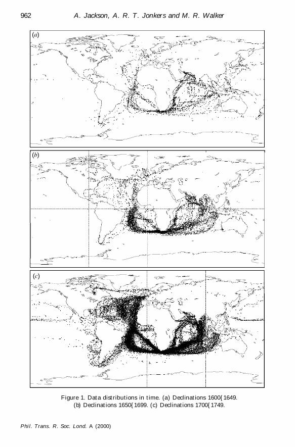
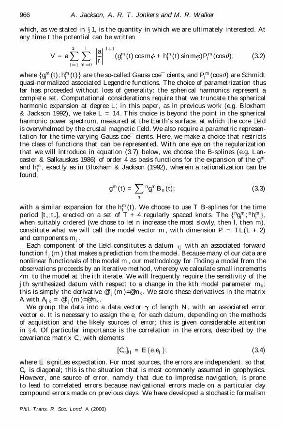
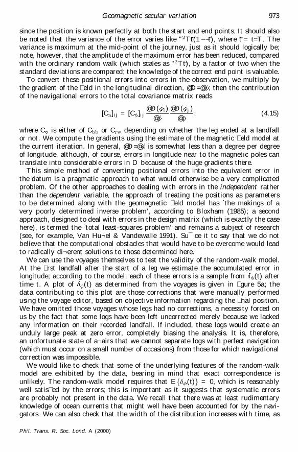
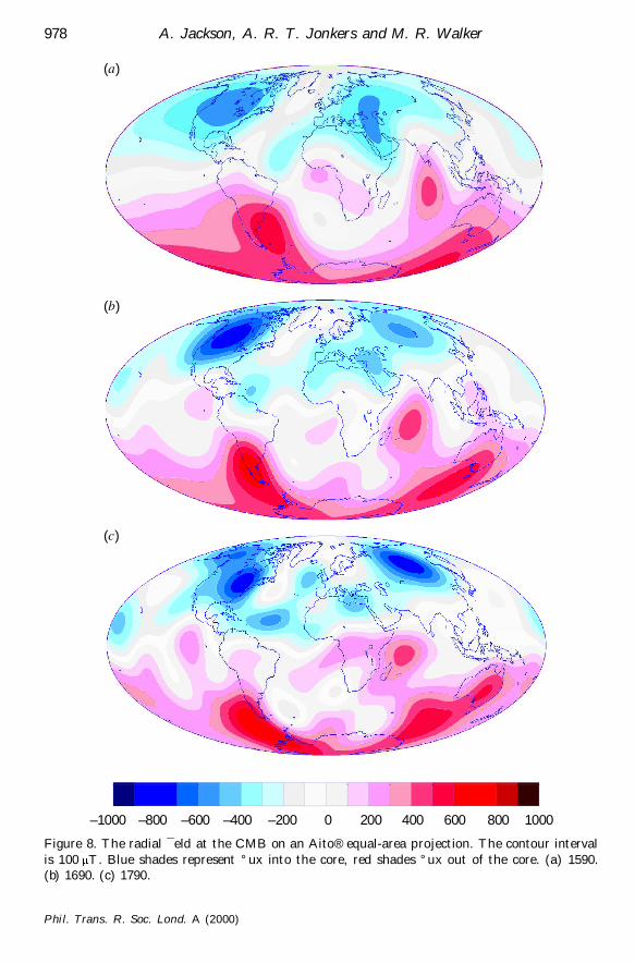
Copyright © 2022 FDOKUMEN