C Finite Element Analysis for Mechanical and Aerospace Design

CCOORRNNEELLLL U N I V E R S I T Y 1

MAE 4700 – FE Analysis for Mechanical & Aerospace Design N. Zabaras (02/20/2014)

Finite Element Analysis for Mechanical and Aerospace

Design

Prof. Nicholas Zabaras Materials Process Design and Control Laboratory

Sibley School of Mechanical and Aerospace Engineering 101 Rhodes Hall

Cornell University Ithaca, NY 14853-3801 [email protected]

http://mpdc.mae.cornell.edu

mailto:[email protected]

http://mpdc.mae.cornell.edu/



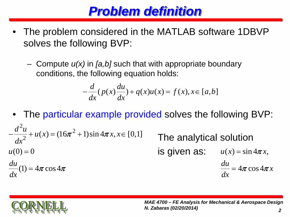
Problem definition • The problem considered in the MATLAB software 1DBVP

solves the following BVP:

– Compute u(x) in [a,b] such that with appropriate boundary conditions, the following equation holds:

• The particular example provided solves the following BVP:

The analytical solution is given as:

( ( ) ) ( ) ( ) ( ), [ , ]d dup x q x u x f x x a bdx dx

− + = ∈

22

2 ( ) (16 1)sin 4 , [0,1]

(0) 0

(1) 4 cos4

d u u x x xdx

ududx

π π

π π

− + = + ∈

=

=

( ) sin 4 ,

4 cos4

u x xdu xdx

π

π π

=

=



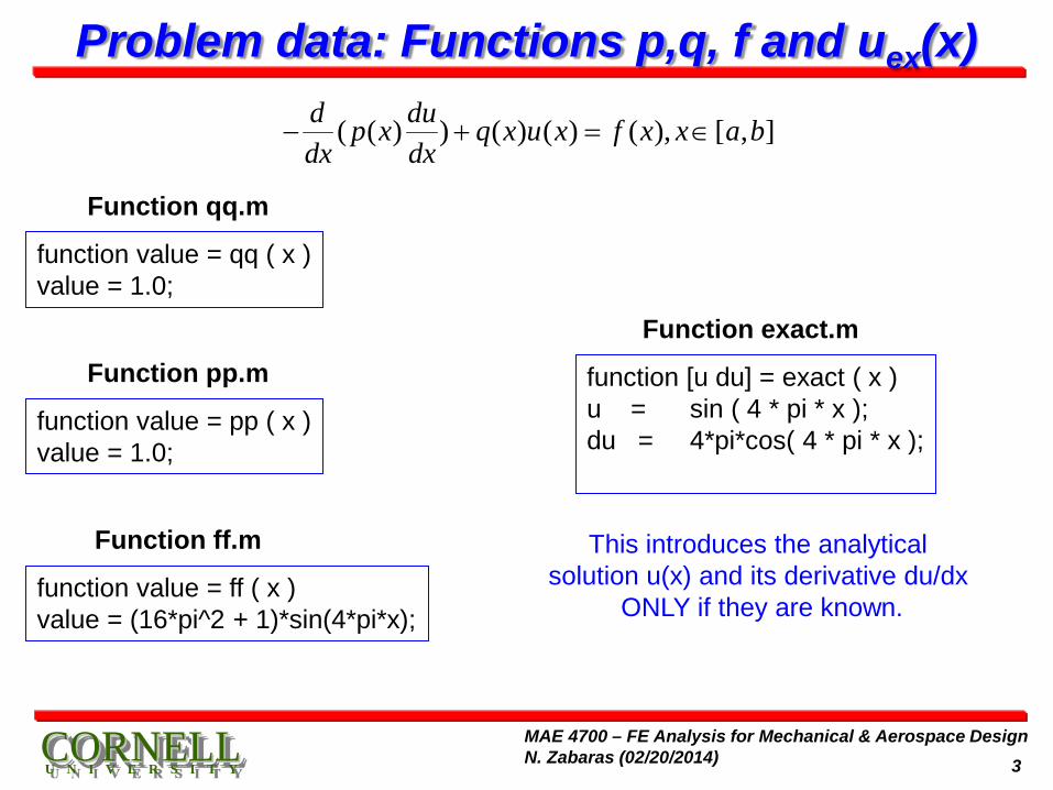
Problem data: Functions p,q, f and uex(x)


− + = ∈

function value = qq ( x ) value = 1.0;

Function qq.m

function value = pp ( x ) value = 1.0;

Function pp.m

function value = ff ( x ) value = (16*pi^2 + 1)*sin(4*pi*x);

Function ff.m

function [u du] = exact ( x ) u = sin ( 4 * pi * x ); du = 4*pi*cos( 4 * pi * x );

Function exact.m

This introduces the analytical solution u(x) and its derivative du/dx

ONLY if they are known.



Introducing the geometry and FE discretization

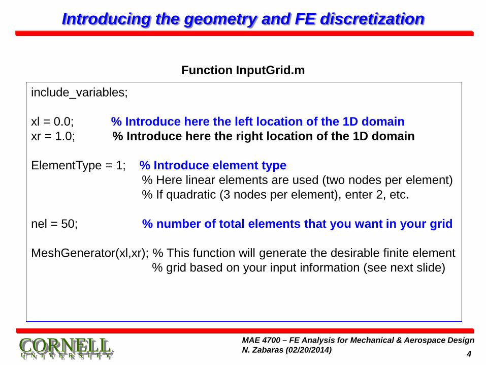
include_variables; xl = 0.0; % Introduce here the left location of the 1D domain xr = 1.0; % Introduce here the right location of the 1D domain ElementType = 1; % Introduce element type % Here linear elements are used (two nodes per element) % If quadratic (3 nodes per element), enter 2, etc. nel = 50; % number of total elements that you want in your grid MeshGenerator(xl,xr); % This function will generate the desirable finite element % grid based on your input information (see next slide)

Function InputGrid.m



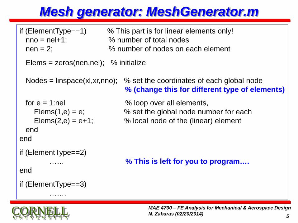
Mesh generator: MeshGenerator.m if (ElementType==1) % This part is for linear elements only! nno = nel+1; % number of total nodes nen = 2; % number of nodes on each element

Elems = zeros(nen,nel); % initialize Nodes = linspace(xl,xr,nno); % set the coordinates of each global node % (change this for different type of elements)

for e = 1:nel % loop over all elements, Elems(1,e) = e; % set the global node number for each Elems(2,e) = e+1; % local node of the (linear) element end end

if (ElementType==2) …… % This is left for you to program…. end

if (ElementType==3) …….



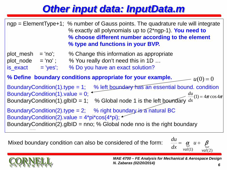
Other input data: InputData.m ngp = ElementType+1; % number of Gauss points. The quadrature rule will integrate % exactly all polynomials up to (2*ngp-1). You need to % choose different number according to the element % type and functions in your BVP.

plot_mesh = 'no'; % Change this information as appropriate plot_node = 'no' ; % You really don’t need this in 1D … is_exact = 'yes'; % Do you have an exact solution?

% Define boundary conditions appropriate for your example.

BoundaryCondition(1).type = 1; % left boundary has an essential bound. condition BoundaryCondition(1).value = 0; BoundaryCondition(1).glbID = 1; % Global node 1 is the left boundary

BoundaryCondition(2).type = 2; % right boundary is a natural BC BoundaryCondition(2).value = 4*pi*cos(4*pi); BoundaryCondition(2).glbID = nno; % Global node nno is the right boundary …….

(1) 4 cos4dudx

π π=

(0) 0u =

Mixed boundary condition can also be considered of the form:

(1) (2)val val

du udx

= +α β



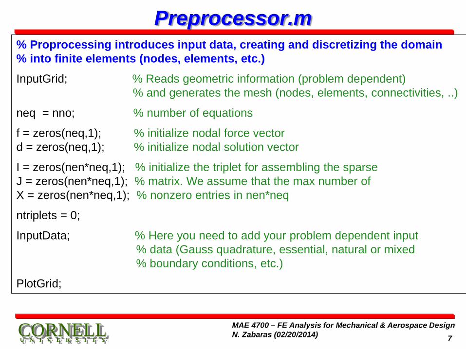
Preprocessor.m % Proprocessing introduces input data, creating and discretizing the domain % into finite elements (nodes, elements, etc.)

InputGrid; % Reads geometric information (problem dependent) % and generates the mesh (nodes, elements, connectivities, ..)

neq = nno; % number of equations

f = zeros(neq,1); % initialize nodal force vector d = zeros(neq,1); % initialize nodal solution vector

I = zeros(nen*neq,1); % initialize the triplet for assembling the sparse J = zeros(nen*neq,1); % matrix. We assume that the max number of X = zeros(nen*neq,1); % nonzero entries in nen*neq

ntriplets = 0;

InputData; % Here you need to add your problem dependent input % data (Gauss quadrature, essential, natural or mixed % boundary conditions, etc.)

PlotGrid;



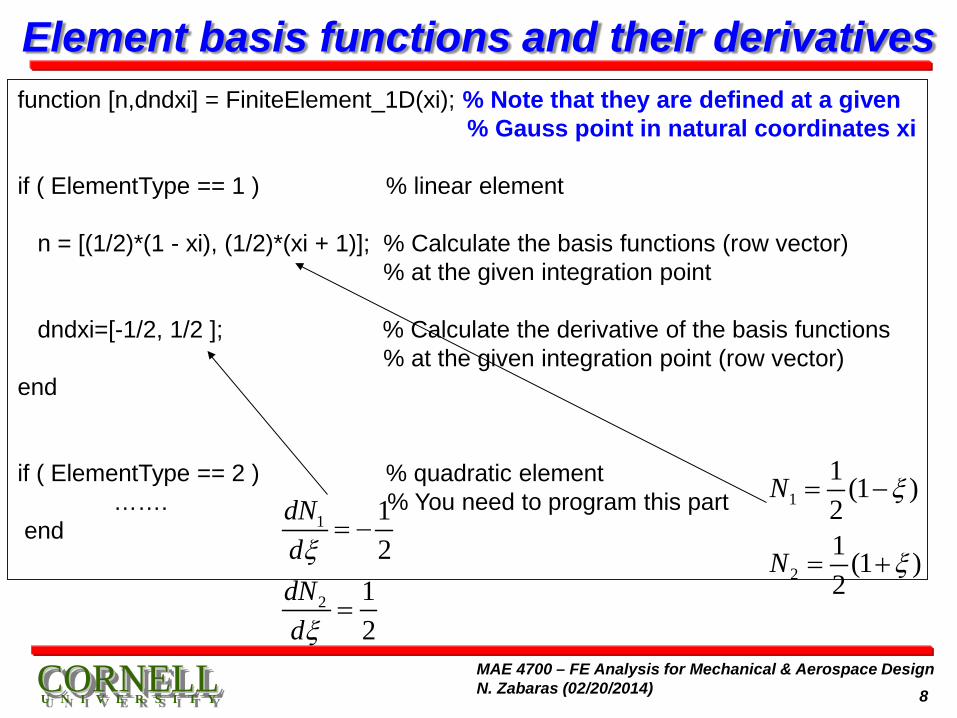
Element basis functions and their derivatives function [n,dndxi] = FiniteElement_1D(xi); % Note that they are defined at a given % Gauss point in natural coordinates xi if ( ElementType == 1 ) % linear element n = [(1/2)*(1 - xi), (1/2)*(xi + 1)]; % Calculate the basis functions (row vector) % at the given integration point dndxi=[-1/2, 1/2 ]; % Calculate the derivative of the basis functions % at the given integration point (row vector) end if ( ElementType == 2 ) % quadratic element ……. % You need to program this part end

1

2

1 (1 )21 (1 )2

N

N

ξ

ξ

= −

= +

1

2

12

12

dNddNd

= −

=

ξ

ξ



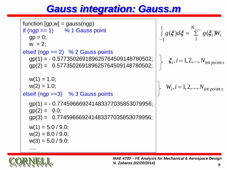
Gauss integration: Gauss.m function [gp,w] = gauss(ngp) if (ngp == 1) % 1 Gauss point gp = 0; w = 2;

elseif (ngp == 2) % 2 Gauss points gp(1) = - 0.577350269189625764509148780502; gp(2) = 0.577350269189625764509148780502; w(1) = 1.0; w(2) = 1.0;

elseif (ngp ==3) % 3 Gauss points

gp(1) = - 0.774596669241483377035853079956; gp(2) = 0.0; gp(3) = 0.774596669241483377035853079956;

w(1) = 5.0 / 9.0; w(2) = 8.0 / 9.0; w(3) = 5.0 / 9.0; ….

int int1

11( ) ( )

po sN

i ig d g Wξ ξ ξ−

∑∫ =

int int, 1,2,...,i po si Nξ =

int int, 1,2,...,i po sW i N=



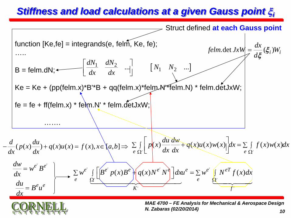
Stiffness and load calculations at a given Gauss point ξi

function [Ke,fe] = integrands(e, felm, Ke, fe); ….. B = felm.dN; Ke = Ke + (pp(felm.x)*B'*B + qq(felm.x)*felm.N'*felm.N) * felm.detJxW; fe = fe + ff(felm.x) * felm.N' * felm.detJxW; …….


− + = ∈ ⇒ ( ) ( ) ( ) ( ) ( ) ( )e ee e

du dwp x q x u x w x dx f x w x dxdx dxΩ Ω

∑ ∑∫ ∫ + =

T Te edw w Bdx

=

e edu B udx

=

( ) ( ) ( )T T T T

e e

e e

e e e e e e e eT

e e

K f

w B p x B q x N N dxu w N f x dxΩ Ω

∑ ∑∫ ∫ + =

.det ( )i idxfelm JxW Wd

ξξ

=

1 2 ...dN dNdx dx

Struct defined at each Gauss point

[ ]1 2 ...N N



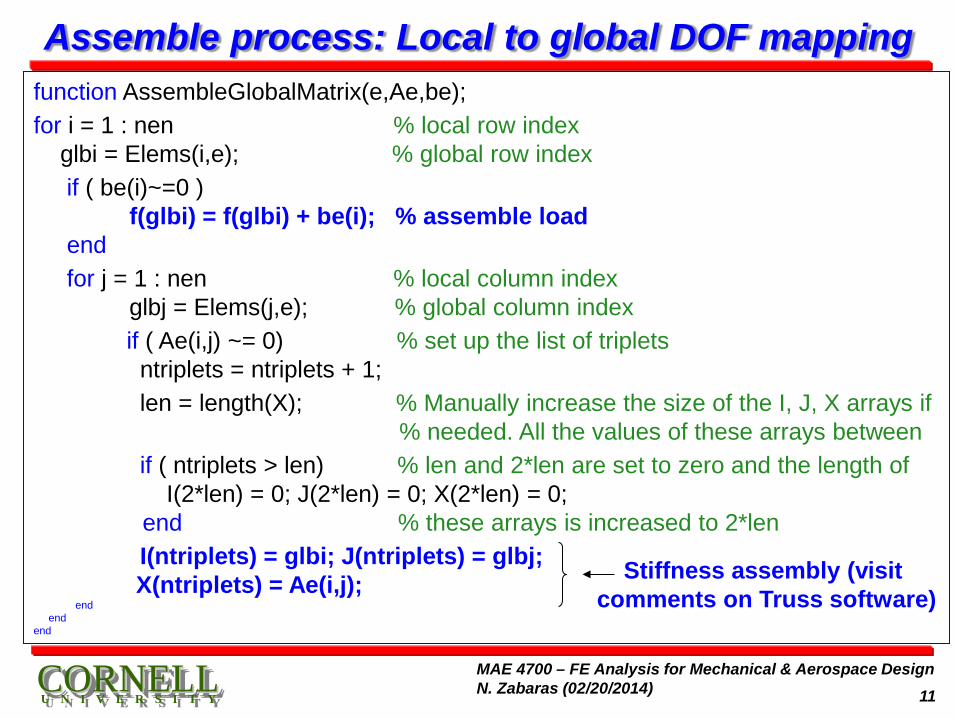
Assemble process: Local to global DOF mapping function AssembleGlobalMatrix(e,Ae,be);

for i = 1 : nen % local row index glbi = Elems(i,e); % global row index

if ( be(i)~=0 ) f(glbi) = f(glbi) + be(i); % assemble load end

for j = 1 : nen % local column index glbj = Elems(j,e); % global column index

if ( Ae(i,j) ~= 0) % set up the list of triplets ntriplets = ntriplets + 1;

len = length(X); % Manually increase the size of the I, J, X arrays if % needed. All the values of these arrays between

if ( ntriplets > len) % len and 2*len are set to zero and the length of I(2*len) = 0; J(2*len) = 0; X(2*len) = 0; end % these arrays is increased to 2*len

I(ntriplets) = glbi; J(ntriplets) = glbj; X(ntriplets) = Ae(i,j); end end end

Stiffness assembly (visit comments on Truss software)



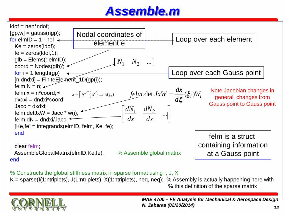
Assemble.m ldof = nen*ndof; [gp,w] = gauss(ngp); for elmID = 1 : nel Ke = zeros(ldof); fe = zeros(ldof,1); glb = Elems(:,elmID); coord = Nodes(glb)'; for i = 1:length(gp) [n,dndxi] = FiniteElement_1D(gp(i)); felm.N = n; felm.x = n*coord; dxdxi = dndxi*coord; Jacc = dxdxi; felm.detJxW = Jacc * w(i); felm.dN = dndxi/Jacc; [Ke,fe] = integrands(elmID, felm, Ke, fe); end clear felm; AssembleGlobalMatrix(elmID,Ke,fe); % Assemble global matrix end % Constructs the global stiffness matrix in sparse format using I, J, X K = sparse(I(1:ntriplets), J(1:ntriplets), X(1:ntriplets), neq, neq); % Assembly is actually happening here with % this definition of the sparse matrix

1 2 ...dN dNdx dx

.det ( )i idxfelm JxW Wd

ξξ

=

[ ]1 2 ...N N

Nodal coordinates of element e

Loop over each Gauss point

Loop over each element

felm is a struct containing information

at a Gauss point

( )e eix N x x ξ = ⇒

Note Jacobian changes in general changes from

Gauss point to Gauss point



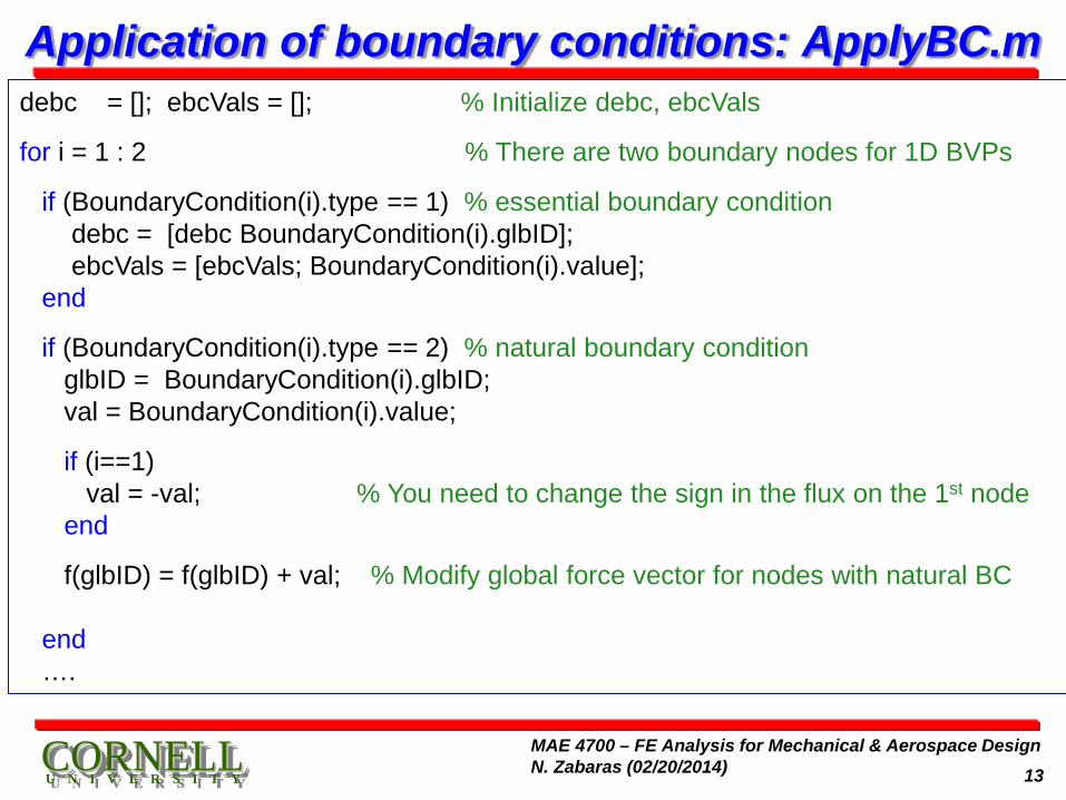
Application of boundary conditions: ApplyBC.m debc = []; ebcVals = []; % Initialize debc, ebcVals

for i = 1 : 2 % There are two boundary nodes for 1D BVPs

if (BoundaryCondition(i).type == 1) % essential boundary condition debc = [debc BoundaryCondition(i).glbID]; ebcVals = [ebcVals; BoundaryCondition(i).value]; end

if (BoundaryCondition(i).type == 2) % natural boundary condition glbID = BoundaryCondition(i).glbID; val = BoundaryCondition(i).value;

if (i==1) val = -val; % You need to change the sign in the flux on the 1st node end

f(glbID) = f(glbID) + val; % Modify global force vector for nodes with natural BC end ….



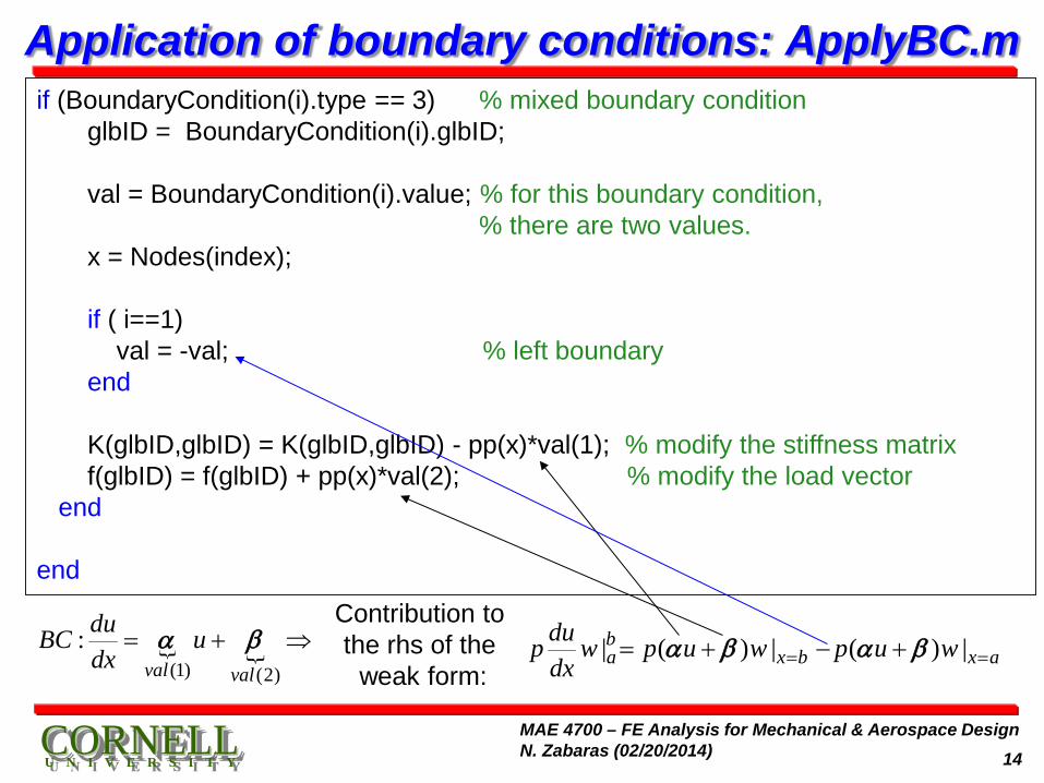
Application of boundary conditions: ApplyBC.m if (BoundaryCondition(i).type == 3) % mixed boundary condition glbID = BoundaryCondition(i).glbID; val = BoundaryCondition(i).value; % for this boundary condition, % there are two values. x = Nodes(index); if ( i==1) val = -val; % left boundary end K(glbID,glbID) = K(glbID,glbID) - pp(x)*val(1); % modify the stiffness matrix f(glbID) = f(glbID) + pp(x)*val(2); % modify the load vector end end

(1) (2)

:val val

duBC udx

= + ⇒α β | ( ) | ( ) |ba x b x a

dup w p u w p u wdx = == + − +α β α β

Contribution to the rhs of the

weak form:



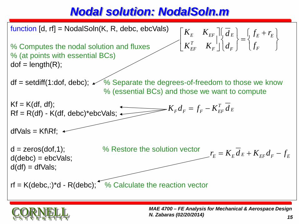
Nodal solution: NodalSoln.m function [d, rf] = NodalSoln(K, R, debc, ebcVals) % Computes the nodal solution and fluxes % (at points with essential BCs) dof = length(R); df = setdiff(1:dof, debc); % Separate the degrees-of-freedom to those we know

% (essential BCs) and those we want to compute

Kf = K(df, df); Rf = R(df) - K(df, debc)*ebcVals; dfVals = Kf\Rf; d = zeros(dof,1); % Restore the solution vector d(debc) = ebcVals; d(df) = dfVals; rf = K(debc,:)*d - R(debc); % Calculate the reaction vector

EE EF E ET

FEF F F

K K f rdfK K d

+ =

TEF F F EFK d f K d= −

EE E EF F Er K d K d f= + −



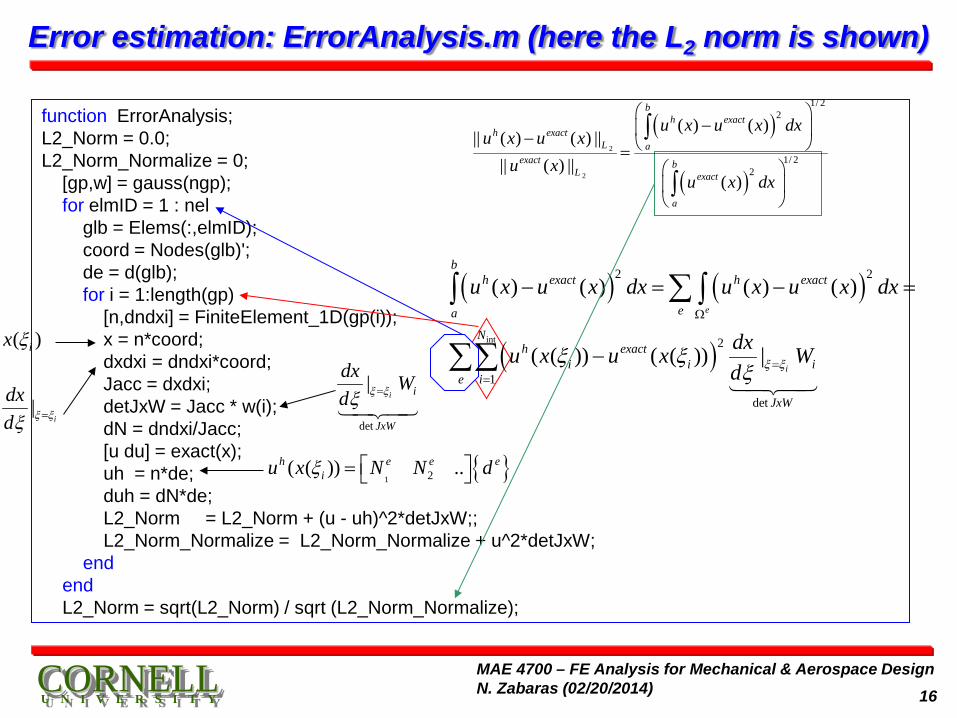
Error estimation: ErrorAnalysis.m (here the L2 norm is shown)

function ErrorAnalysis; L2_Norm = 0.0; L2_Norm_Normalize = 0; [gp,w] = gauss(ngp); for elmID = 1 : nel glb = Elems(:,elmID); coord = Nodes(glb)'; de = d(glb); for i = 1:length(gp) [n,dndxi] = FiniteElement_1D(gp(i)); x = n*coord; dxdxi = dndxi*coord; Jacc = dxdxi; detJxW = Jacc * w(i); dN = dndxi/Jacc; [u du] = exact(x); uh = n*de; duh = dN*de; L2_Norm = L2_Norm + (u - uh)^2*detJxW;; L2_Norm_Normalize = L2_Norm_Normalize + u^2*detJxW; end end L2_Norm = sqrt(L2_Norm) / sqrt (L2_Norm_Normalize);

( )

( )2

2

1/ 22

1/ 22

( ) ( )|| ( ) ( ) ||

|| ( ) ||( )

bh exact

h exactL a

exact bL exact

a

u x u x dxu x u x

u xu x dx

− − =

∫

∫

( ) ( )

( )int

2 2

2

1

det

( ) ( ) ( ) ( )

( ( )) ( ( )) |

e

i

bh exact h exact

ea

Nh exact

i i ie i

JxW

u x u x dx u x u x dx

dxu x u x Wd ξ ξξ ξξ

Ω

==

− = − =

−

∑∫ ∫

∑∑

( )ix ξ

|i

dxd =ξ ξξ det

|i i

JxW

dx Wd =

ξ ξξ

1 2( ( )) ..h e e e

iu x N N d = ξ



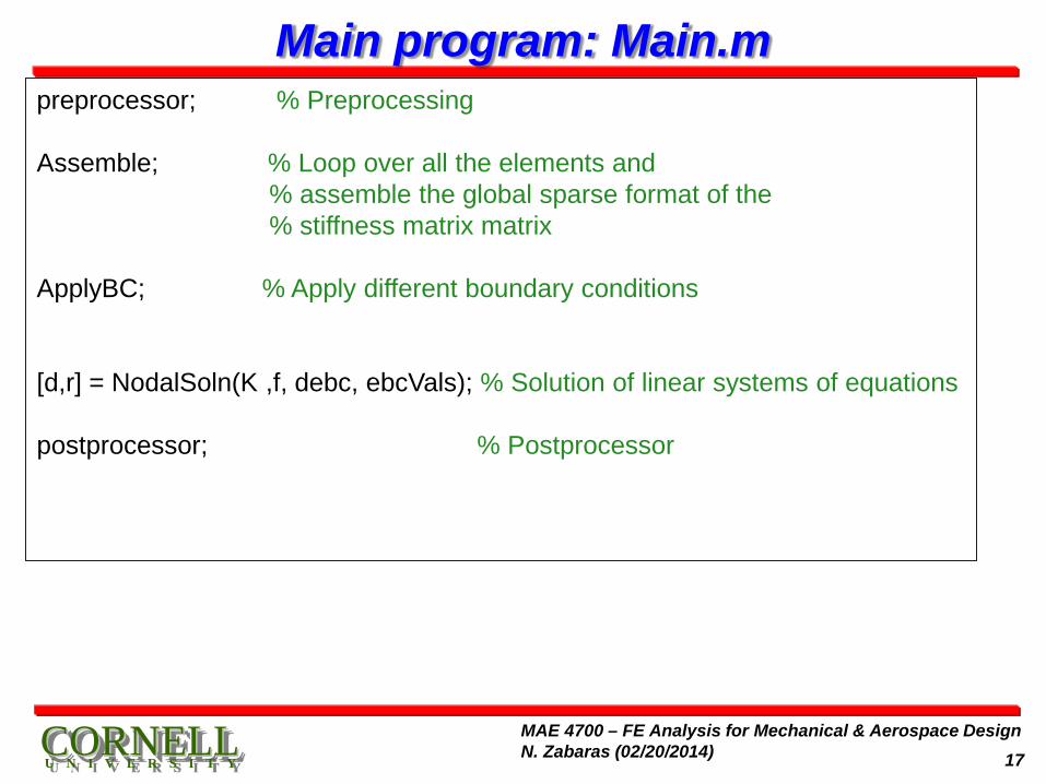
Main program: Main.m preprocessor; % Preprocessing Assemble; % Loop over all the elements and % assemble the global sparse format of the % stiffness matrix matrix ApplyBC; % Apply different boundary conditions [d,r] = NodalSoln(K ,f, debc, ebcVals); % Solution of linear systems of equations postprocessor; % Postprocessor

C Finite Element Analysis for Mechanical and Aerospace Design

Documents

Transcript of C Finite Element Analysis for Mechanical and Aerospace Design