Biophysical characterisation of biopharmaceuticals under defined flow fields

John Andrew Dobson

Submitted in accordance with the requirements for the degree of

Doctor of Philosophy

The University of Leeds

School of Mechanical Engineering

November, 2017

- ii -

The candidate confirms that the work submitted is his own, except where work

which has formed part of jointly-authored publications has been included. The

contribution of the candidate and the other authors to this work has been

explicitly indicated below. The candidate confirms that appropriate credit has

been given within the thesis where reference has been made to the work of

others.

The publication Inducing protein aggregation by extensional flow was jointly-

authored by John Dobson (JD), Amit Kumar (AK), Leon F. Willis (LFW),

Roman Tuma (RT), Daniel R. Higazi (DRH), Richard Turner (RTurner), David

C. Lowe (DCL), Alison E. Ashcroft (AEA), Sheena E. Radford (SER), Nikil

Kapur (NK), and David J. Brockwell (DJB). The publication was approved for

publication in Proceedings of the National Academy of Sciences of the United

States of America on March 28, 2017.

Author contributions as recorded in the publication: J.D., A.K., L.F.W., A.E.A.,

S.E.R., N.K., and D.J.B. designed research; J.D., A.K., and L.F.W. performed

research; R. Tuma, D.R.H., R. Turner, and D.C.L. contributed new

reagents/analytic tools.; J.D., A.K., L.F.W., R. Tuma, D.R.H., R. Turner,

D.C.L., A.E.A., S.E.R., N.K., and D.J.B. analysed data; and J.D., A.K., L.F.W.,

A.E.A., S.E.R., N.K., and D.J.B. wrote the paper.

Specific contribution by JD within “designing and performing research”:

Design and analysis of flow field simulations. Design and construction of

hardware for testing proteins. Joint analysis and interpretation of results

including energy analysis.

This copy has been supplied on the understanding that it is copyright material

and that no quotation from the thesis may be published without proper

acknowledgement.

© 2017 The University of Leeds and John Andrew Dobson

- iii -

Acknowledgements

I would like to thank all of my colleagues who have contributed to this research

and supported me throughout. I am grateful for the invaluable guidance and

genuine enthusiasm expressed by my lead supervisor Prof Nikil Kapur. No

matter what the situation, I always left a meeting with a feeling of motivation,

and a clear sense of direction.

I would also like to convey my gratitude to the amazing team from the Astbury

Centre. Prof Alison Ashcroft, Dr David Brockwell, and Prof Sheena Radford

worked tirelessly to guide this lowly engineer through the world of molecular

biology, and patiently endured countless discussions on fluid mechanics.

My special thanks go to Dr Amit Kumar and Leon Willis for their supervision,

assistance, and friendship during the long hours in the lab – and for their

fathomless patience with regard to a certain temperamental experimental flow

device.

I’d like to say a massive thank you to all of my friends, many of whom were in

similar situations and gave valuable advice. And to my family, for being

supportive throughout my entire educational journey, alleviating my worries

and always brightening my mood.

Finally, particular thanks should go to the women in my life, my partner, my

mother and my grandmother. They have been a constant source of strength

and support, and whilst sometimes mildly irritating, I truly could not have this

without them!

- iv -

Abstract

Flow induced aggregation occurs during the manufacturing process of

biopharmaceuticals. An understanding of the effects of extensional flow is

required as a means of predicting the response of experimental protein

molecules to flow conditions during the down-stream manufacturing

operations. Adequate prediction methods allow for elimination of proteins

susceptible to flow induced aggregation, reducing development costs.

An experimental device is designed and implemented to subject the proteins

BSA, β2-microglobulin (β2m), granulocyte colony stimulating factor (G-CSF),

and three monoclonal antibodies (mAbs) to a defined and quantified flow field

dominated by extensional flow. CFD analysis is used to accurately

characterise the flow field throughout the geometry. Through simulation and

bespoke post-processing it is possible to determine the magnitude of

extensional strain which the fluid is subjected to. The device is then modified

to allow for a comparison to be made between the strain and shear which is

inherent in any flow device.

The work shows that the device induces protein aggregation after exposure

to an extensional flow field for 0.36 – 1.8 ms, at concentrations as low as 0.5

mg ml−1. Correlation is drawn between the extent of aggregation and the

applied strain rate, as well as protein concentration, structural properties, and

sequence of the protein.

A method of equating the forces present within the flow to those experienced

by a single molecule within the fluid continuum are also presented.

- v -

Table of Contents

Acknowledgements .................................................................................... iii

Abstract ....................................................................................................... iv

Table of Contents ........................................................................................ v

List of Tables .............................................................................................. xi

List of Figures ........................................................................................... xii

1. Introduction ......................................................................................... 1

1.1. Aims 2

1.2. Objectives ..................................................................................... 2

1.3. Thesis Structure ............................................................................ 3

2. Literature Review ................................................................................ 4

2.1. Protein modelling for fluid mechanics ............................................ 4

2.2. Protein Aggregation and Pathways ............................................... 5

2.3. Introduction to biopharma.............................................................. 7

2.4. Current perspectives ................................................................... 11

2.5. Previous flow studies .................................................................. 14

2.5.1. Coaxial (Weissenberg Couette) Viscometer ............... 17

2.5.2. Parallel plate rheometer .............................................. 18

2.5.3. Four roll mill ................................................................ 19

2.5.4. Opposed jets ............................................................... 21

2.5.5. Capillary Rheometer ................................................... 22

2.5.6. Microchannel devices .................................................. 22

2.6. Frequently used proteins ............................................................. 24

2.7. Protein characterisation methods ................................................ 25

2.7.1. Light obscuration ......................................................... 25

2.7.2. Circular dichroism spectroscopy ................................. 26

2.7.3. UV/visible spectroscopy .............................................. 26

2.7.4. Light scattering spectroscopy ...................................... 28

2.7.5. Size-exclusion chromatography and multi-angle laser-light scattering ............................................................ 28

2.7.6. In situ characterisation methods.................................. 28

2.8. Summary ..................................................................................... 29

3. Theory ................................................................................................ 30

3.1. Fluid mechanics .......................................................................... 31

3.1.1. Shear vs. extensional flow within biopharmaceutical manufacture .......................................... 32

- vi -

3.1.2. Rate of Deformation .................................................... 34

Deformation tensor .............................................................. 36

3.1.3. Numerical solvers and Navier-Stokes Equations ........ 38

3.1.4. Pressure ................................................................. 38

3.2. Proteins ....................................................................................... 42

Aggregation ......................................................................... 44

3.2.1. ........................................................................................... 44

3.2.2. Aggregation characterisation ...................................... 45

Analytical Ultra-Centrifugation ............................................. 46

Nanoparticle Tracking Analysis ........................................... 46

Absorbance spectroscopy ................................................... 47

3.3. Summary ..................................................................................... 48

4. Numerical Modelling and Computational Fluid Dynamics ............ 49

4.1. Introduction ................................................................................. 49

4.2. Theory and Methodology ............................................................ 50

4.3. Problem Brief .............................................................................. 51

4.4. Software ...................................................................................... 52

4.4.1. COMSOL Multiphysics ................................................ 52

4.4.2. MATLAB ...................................................................... 53

4.5. Pre-Processor ............................................................................. 53

4.5.1. Universal assumptions ................................................ 53

4.5.2. Single constriction open model ................................... 55

4.5.2.1. Geometry ............................................................. 55

4.5.2.2. Boundary conditions ............................................ 56

4.5.2.3. Mesh .................................................................... 56

4.5.2.4. Model summary and conclusions ......................... 57

4.5.3. Constriction-expansion closed model .......................... 57

4.5.3.1. Geometry ............................................................. 58

4.5.3.2. Boundary conditions ............................................ 58

4.5.3.3. Mesh .................................................................... 59

4.6. Post-Processor ............................................................................ 61

4.7. Plan of Numerical Experiments ................................................... 62

4.7.1. Mesh dependence study ............................................. 62

4.7.2. Validation of model ...................................................... 62

4.7.3. Numerical experimental plan ....................................... 62

- vii -

4.7.3.1. Characterisation of an abrupt 90° constriction ..... 62

4.7.3.2. Effects of constriction angle on strain rate ........... 63

4.7.3.3. Downstream syringe investigation ....................... 63

4.8. Summary ..................................................................................... 63

5. Computational Results ..................................................................... 64

5.1. Validation ..................................................................................... 65

5.1.1. Single constriction open model mesh dependence study ................................................................................... 65

5.1.2. Constriction-expansion closed model mesh dependence study ............................................................... 66

5.2. Flow profile for an abrupt 90° constriction .................................... 68

5.2.1. Streamline plots for 90° constriction .................................. 69

5.2.2. Velocity magnitude for 90° constriction ............................. 70

5.2.3. Pressure profiles for 90° constriction ................................. 71

5.2.4. Strain rate profiles for 90° constriction .............................. 74

5.3. Flow profile for reduced-angle constrictions ................................. 75

5.3.1. Streamline plots for reduced-angle constrictions ............... 75

5.3.2. Velocity profiles for reduced angle constriction ................. 76

5.3.3. Pressure profiles for reduced-angle constrictions ............. 78

5.3.4. Strain rate profiles for reduced-angle constrictions ........... 79

5.4. Quantifying strain rate data .......................................................... 81

5.4.1. Strain rate as a function of displacement .......................... 81

5.4.2. Strain rate as a function of plunger velocity ....................... 84

5.5. Transition from extension- to shear-dominated flow .................... 84

5.5.2. Stagnation point within the downstream syringe ............... 89

6. Experimental Design, Methods and Materials ................................ 96

6.1. Design of experimental equipment .............................................. 97

6.1.1. Design Scope .............................................................. 97

6.1.2. Device Specification .................................................... 98

6.1.3. Design review of previous experimental methods ..... 101

Taylor-Couette Flow Cell ................................................... 101

Four-Roll Mill ..................................................................... 101

Opposed Jets .................................................................... 102

Stenotic Indentation Microchannel .................................... 102

High Viscosity Cylindrical Tubing ...................................... 102

Etched Elongational Microchannel .................................... 102

- viii -

6.1.4. Design of Experimental Equipment ........................... 105

Initial concept .................................................................... 105

Open-Source and Off-The-Shelf Equipment ..................... 107

Syringes ...................................................................................... 108

Capillaries ................................................................................... 108

Mounting Board ........................................................................... 108

Computer Aided Design .................................................... 109

Bracket Design ............................................................................ 110

Angled geometry design ............................................................. 110

6.1.5. Control theory............................................................ 111

Linear actuators ................................................................ 112

Stepper motors .................................................................. 112

Integrated micro-controllers............................................... 113

6.2. Final specification of experimental equipment & method of use 113

6.2.1. Experimental equipment ........................................... 113

6.2.2. Method ...................................................................... 114

6.3. Limitations and considerations .................................................. 115

6.3.1. High shear in capillary ............................................... 115

6.3.2. Geometry accuracy ................................................... 115

6.3.3. Downstream stagnation point .................................... 116

6.4. Protein Selection, Specification and Formulation ...................... 117

6.4.1. Bovine Serum Albumin .............................................. 117

6.4.2. β2-Microglobulin ........................................................ 118

6.4.3. Granulocyte Colony-Stimulating Factor ..................... 119

6.4.4. Model Antibodies ....................................................... 120

6.4.5. Summary of proteins ................................................. 122

6.5. Characterisation of Aggregated Protein .................................... 122

6.5.1. Nanoparticle Tracking Analysis (NTA) ...................... 122

6.5.2. Transmission Electron Microscopy ............................ 123

6.5.3. Insoluble Protein Pelleting Assay .............................. 123

6.6. Experimental Plan ..................................................................... 124

6.6.1. The Effects of Extensional Flow on Bovine Serum Albumin ............................................................................. 125

BSA aggregation dependence on exposure time to extensional flow and concentration ........................... 125

- ix -

BSA aggregation dependence on strain-rate .................... 125

6.6.2. The Effects of Extensional Flow on Therapeutic Proteins ............................................................................. 125

mAb aggregation dependence on exposure time to extensional flow......................................................... 125

6.6.3. Contraction Angle Experiments ................................. 127

6.6.4. Control Experiments .................................................. 127

Shear dependence experiment ......................................... 127

Dead volume experiment .................................................. 128

6.7. Summary ................................................................................... 128

7. Experimental Results ...................................................................... 130

7.1. Introduction ............................................................................... 130

7.2. The Effects of Extensional Flow on Bovine Serum Albumin ...... 130

7.2.1. BSA Aggregation Dependence on Exposure Time and Concentration ............................................................. 130

Insoluble protein pelleting method ..................................... 130

Qualitative analysis of BSA ............................................... 132

7.2.2. BSA Aggregation Dependence on Strain-Rate ......... 136

7.3. The Effects of Extensional Flow on Therapeutic Proteins ......... 137

7.3.1. Comparison of therapeutic proteins .......................... 137

7.3.2. mAb Aggregation dependence on velocity ................ 139

7.3.3. Further study of WFL ................................................ 141

7.4. Results from contraction angle experiments ............................. 142

7.5. Results from control experiments .............................................. 143

7.5.1. Shear dependence of BSA aggregation .................... 143

7.5.2. Stagnation point dependence of STT aggregation .... 144

8. Discussion ....................................................................................... 146

8.1. Tensile stress ............................................................................. 146

8.2. Aggregation in terms of energy ................................................. 148

8.3. Strain rate distribution at the capillary inlet ................................ 150

9. Conclusions ..................................................................................... 155

9.2. Summary ................................................................................... 155

9.2.1. Extensional flow induced aggregation in BSA ........... 155

9.2.2. Extensional flow induced aggregation in therapeutic proteins ........................................................... 155

9.2.3. Antibody conformation affects flow sensitivity ................... 155

9.2.4. Strain trumps shear ........................................................... 156

- x -

9.1.5. Successful validation ......................................................... 156

9.3. Future Work .............................................................................. 157

List of References ................................................................................... 159

- xi -

List of Tables

Table 3-1: summary of pressure loss equations for validating numerical methods. .......................................................................... 41

Table 4-1: Fluid properties applied to CFD modelling in this section ............................................................................................... 54

Table 5-1: CFD validation comparing hand calculated pressure losses to those obtained from CFD modelling ... Error! Bookmark not defined.

Table 6-1: Design specification matrix for the experimental method ............................................................................................. 100

Table 6-2: Design review summary of previous methods ................... 104

Table 6-3: Stepper motor relation to flow velocity ............................... 113

Table 6-4: Summary of proteins for use in experiments ...................... 122

Table 7-1: Accumulative time samples were exposed to strain and shear environment .......................................................................... 131

- xii -

List of Figures

Figure 2-1: “A good conformational match shown in (a) can change if the receptor deforms under force (b).”[1] ........................ 5

Figure 2-2: Many physical degradation pathways of proteins are made possible through exposure to interfaces, foreign particulates, or leachables. This figure shows a vial as one example [5]. ......................................................................................... 6

Figure 2-3: An example of a funnel device for high strain rate flows with a superimposed graphic of DNA responding to extensional flow. (B) graphic of DNA stretching in a pure elongational flow with a strong strain rate along the polymer [9]. ....................................................................................................... 16

Figure 2-4: Viscometers produce high shear flows. (a) Narrow gap coaxial cylinder viscometer. (b) Cone-and-plate viscometers. [2] ........................................................................................................ 19

Figure 2-5: “Velocity profile for the different flow configurations (a) elongation (b) hybrid and (c) rotation for water (Re 155) in the four-roll apparatus calculated with CFD. Arrows indicate the rotation direction of the rollers.” [8] ......................................... 20

Figure 2-6: Example of an opposed jets experiment schematic (left) and photograph showing extended polymer chains (right) [64]. Note that in this instance, fluid is being drawn into the jets as opposed to being sprayed out; both are common arrangements. ................................................................... 21

Figure 2-7: An experimental setup of a flow cell similar to a coaxial viscometer with in situ Raman spectroscopy laser and optics. [1] .................................................................................... 29

Figure 3-1: Shear flow in a pipe or tube with a characteristic velocity profile. Notice how any two fluid elements on adjacent streamlines are never travelling at the same velocity. .............................................................................................. 32

Figure 3-2: (Top) Contraction in a flow geometry resulting in acceleration and therefore extensional flow. The arrow lengths are proportional to fluid velocity. (Bottom) Average fluid velocity v is plotted against position z, demonstrating the acceleration of the fluid.............................................................. 33

Figure 3-4: location of vena contracta circulations resulting in pressure losses in a sudden contraction. ...................................... 40

- xiii -

Figure 3-5: Schematic of an IgG-type monoclonal antibody. Each block represents a β-sheet rich immunoglobulin domain. The heavy chains are in dark blue, whilst the light chains are represented in light blue. The two halves of the antibody are connected by disulfide bridges. The Fc domain is the ‘crystallisable’ region as it is readily crystallised. Most glycosylation takes place in this region. The Fab domain is the antigen-binding domain, with the antigen binding represented by the convex end sections. The two domains are connected by a flexible hinge region, which gives these molecules conformational flexibility, facilitating target binding [7]. ......................................................................................... 42

Figure 3-6: Schematic of upstream and downstream processing of a typical mAb-based biopharmaceutical. Throughout the manufacture, hydrodynamic processes are involved. Fermentation steps lead to the over-expression of the product. Primary recovery steps (centrifugation and depth filtration) separate the product from cell debris, DNA and other contaminants. Protein A chromatography is used as the capture step. Ion-exchange chromatography is then used to polish the product. A viral inactivation step is used for products derived from mammalian cell lines. The product is then concentrated, formulated and packaged [3]. ..................... 43

Figure 3-7: Schematic of a protein aggregation mechanism. The native (folded) protein can oligomerise into its native quaternary structure. Alternatively, stresses such as temperature and pH can perturb the native protein, causing it to unfold. Unfolded protein can form dimers and trimers before forming multimeric species or soluble aggregates. Both types of oligomeric species can precipitate as an amorphous aggregate or fibril [3]. ................................................... 45

Figure 3-8: NanoSight instrument configuration [6] .............................. 47

Figure 4-1: Schematic of problem to be modelled. Two pipes of diameter 4.61 mm are connected with a narrow pipe of 0.3 mm which form abrupt step up and step down constrictions. ..... 52

Figure 4-2: Schematic of the single contraction open model to be modelled in CFD ................................................................................ 55

Figure 4-3: A “slice” of the flow field that can be modelled in a 2D axisymmetric domain for efficient computation. ............................ 55

Figure 4-4: COMSOL CFD package 2D axisymmetric model of two long rectangles representing a sudden and substantial constriction in a pipe flow. The axis of symmetry is marked as the dashed red line. ..................................................................... 56

Figure 4-5: Free quadratic mesh used for single constriction open CFD model. Flow direction from top to bottom, units in mm. ....... 57

Figure 4-6: A “slice” of the flow field that can be modelled in a 2D axisymmetric domain for efficient computation. ............................ 58

- xiv -

Figure 4-7: Schematic of the constriction-expansion model. In this instance the upstream syringe plunger is fully receded and so the upstream syringe barrel (left) is near its full capacity, represented by the domain being very long. The downstream syringe plunger is almost completely compressed resulting in the downstream syringe barrel (right) domain being very short. The blue lines represent the plungers which are configured as moving walls. These move left to right simultaneously. Units are in mm. .................................................... 59

Figure 4-8: the domain was divided into sections to allow for meshing density to be skewed to better reflect the flow complexity of different regions. ....................................................... 60

Figure 4-9: Free triangular mesh used in the constriction-expansion closed model CFD simulation. i) The upstream syringe feeding into the capillary inlet. ii) Increased mesh density at the corner of the constriction at the capillary inlet. iii) Increased mesh density at the location of a stagnation point on the downstream syringe plunger. iv) increased mesh density at the capillary outlet. Units in mm. ................................... 60

Figure 5-1: Mesh density refinement study for model 1. The mesh was systematically refined whilst all mesh-independent parameters were held constant. The model was then solved and the maximum strain rate along the axis of symmetry was reported. This was correlated to the number of domain elements used to construct the mesh. ............................................ 66

Figure 5-2: Mesh density refinement study for the extensional flow and capillary domains of model-2. Elements required to mesh this section only were recorded, a coarser mesh was then constructed in the remaining regions and the model was solved for a characteristic strain rate. ............................................ 67

Figure 5-3: Strain rate profiles along the axis of symmetry in the z direction for inlet velocity of 8mms-1. A comparison is made between simulation results for models with 10322 and 3673 discrete elements. It can be seen that although the values of maximum strain rate are in agreement, the lower element count is still resulting in mesh-dependent artefacts which disappear with increased mesh density. ........................................ 68

Figure 5-4: 2D axisymmetric streamline plot for various plunger velocities (as stated) showing path of fluid as it approaches the narrow capillary producing an abrupt 90° constriction. Note (i) the small recirculation occurring in the corner adjacent to the capillary inlet, and (ii) the extended path-length for fluid traveling along the peripheries of the syringe barrel. ................................................................................................. 69

- xv -

Figure 5-5: 2D axisymmetric velocity profile for 90° constriction for various plunger velocities (as stated). Note the high velocity in the corner which forms the capillary inlet. Note also, the length of capillary required for the flow along the axis to reach maximum velocity. ..................................................... 70

Figure 5-6: 2D axisymmetric pressure profile at the 90° constriction for various plunger velocities. .................................... 71

Figure 5-7: Pressure profile along the axis of rotation in the z direction for various plunger velocities as stated. In this instance, the positive z direction indicates the direction of flow with negative values indicating a location upstream of the contraction within the syringe barrel. The capillary is 16 mm in length, starting from z = 0 mm. ............................................. 73

Figure 5-8: 2D axisymmetric strain rate profile for 90° constriction for various plunger velocities (as stated). Not the high strain rate around the corner forming the inlet to the capillary. .............. 74

Figure 5-9: 2D axisymmetric streamline plot for 45° and 30° constrictions for plunger velocities 8 and 16 mms-1. ..................... 75

Figure 5-10: 2D axisymmetric velocity profile for 45° constriction for various plunger velocities (as stated). ...................................... 77

Figure 5-11: 2D axisymmetric velocity profile for 30° constriction for various plunger velocities (as stated). ...................................... 77

Figure 5-12: 2D axisymmetric pressure profile for 45° constriction for various plunger velocities (as stated). ...................................... 78

Figure 5-13: 2D axisymmetric pressure profile for 30° constriction for various plunger velocities (as stated). ...................................... 78

Figure 5-14: 2D axisymmetric strain rate profile for 45° constriction for various plunger velocities (as stated). ................. 80

Figure 5-15: 2D axisymmetric strain rate profile for 30° constriction for various plunger velocities (as stated). ................. 80

Figure 5-16: i) Schematic of flow profile with contraction located the Z = 0 coordinate. ii) Velocity and strain rate profile in the z-direction for a 90° contraction with plunger velocity 8 mms-1. The velocity profile along the axis of symmetry in the z-direction is plotted in blue (measured against the left axis) whilst the corresponding strain rate along the axis is plotted in orange (in relation to the right axis). The horizontal axis measures the distance from the capillary inlet with the positive direction indicating the direction of flow (i.e. negative z position represents flow within the syringe barrel immediately upstream of the capillary). .......................................... 83

Figure 5-17: Characteristic strain rate plotted for constriction angles of 90°, 45° and 30°. ................................................................ 84

- xvi -

Figure 5-18: Absolute velocity U profile with respect to radial displacement from the axis of symmetry at the capillary inlet, given for increasing values of upstream velocity U∞. .................... 85

Figure 5-19: Absolute velocity U profile with respect to radial displacement from the axis of symmetry Sr taken at incremental distances (given in legend) from the capillary inlet. Average inlet velocity U∞ = 8 mms-1. Sr = 0 lies on the axis of symmetry, and Sr = 0.15 indicates the capillary wall. ........ 86

Figure 5-20: Radial velocity profile immediately after capillary inlet at distances 0, 0.4 and 4mm following a i) 45° and ii) 30° inlet angle. Flow inlet velocity 8 mms-1. The transition from extension-dominated to shear-dominate regimes produce very similar velocity profiles over the same length scales as for the 90° inlet angle. The only noticeable differences are the maximum and minimum velocities at 0mm. ................................... 87

Figure 5-21: 2D axisymmetric streamline plot showing the flow field development as the downstream syringe plunger recedes at 2 mms-1. Measurements are given in mm. .................... 91

Figure 5-22: Streamline plots showing the development of the flow fields for various plunger velocities for a given downstream plunger position (60 mm). .......................................... 92

Figure 5-23: 2D axisymmetric velocity profile of the jet of fluid leaving the capillary outlet and impacting the downstream syringe plunger, before turning through 90°. In this instance, the downstream plunger is located 5mm from the capillary outlet. Profiles are shown for a range of plunger velocities (as stated). ......................................................................................... 93

Figure 5-24: 2D axisymmetric strain rate profile of the jet of fluid leaving the capillary outlet and impacting the downstream syringe plunger, resulting in the formation of a stagnation point. In this instance, the downstream plunger is located 1 mm from the capillary outlet. Profiles are shown for a range of plunger velocities (as stated). ..................................................... 94

Figure 5-25: A comparison of the maximum strain rates experienced by a fluid particle as it travels along a streamline that passes through the capillary inlet at a given radial position. The particle experiences a transitory strain rate as it passes through the extensional flow region, and a stagnation strain rate as it passes near to stagnation point on the downstream plunger. The maximum stagnation strain rates are given for varying distances of downstream plunger. Inlet velocity generated by the upstream plunger moving at 8 mms-1. ................................................................................................ 95

Figure 6-1: Schematic of equipment setup for the proposed experimental method. The fluid sample is shuttled between two syringes. ................................................................................... 106

- xvii -

Figure 6-2: CAD image showing location of dovetail rail, rail carrier and V-clamps on Thor Labs optics breadboard with syringes in place for reference. ..................................................... 109

Figure 6-3: CAD image of bracket designed the secure the syringe plunger to the linear carriage and transmit the work done by the linear actuator to the plungers ................................................ 110

Figure 6-4: Designs for an angled contraction. a) used an interference fit to form a seal. b) used a threaded collar section to compress a PTFE ferrule to form a seal. b-i) shows half of the angled section with the threaded attachment and modified syringe in place. the cut-through in b-ii) shows the location of the PTFE ferrule. .......................................................... 111

Figure 6-5: A computer model of the experimental rig configured for extensional flow using glass capillaries ................................. 114

Figure 6-6: Bovine serum albumin (BSA) topology diagram from the RCSB Protein Data Bank. ID code 3V03. Hydrodynamic radius of 3.5 nm. .............................................................................. 117

Figure 6-7: β2-microglobulin (β2m) topology diagram from the RCSB Protein Data Bank. ID code: 1LDS. Hydrodynamic radius 1.9 nm. .................................................................................. 118

Figure 6-8: Granulocyte colony-stimulating factor (GCSF) topology diagram from the RCSB Protein Data Bank. ID code: 5GW9. Hydrodynamic radius 2 nm. ............................................... 119

Figure 6-9: Example of a monoclonal antibody topology diagram from the RCSB Protein Data Bank. ID code: 1HZH. Hydrodynamic radius 3.5 nm. ........................................................ 121

Figure 7-1: percentage of BSA remaining in solution after 500, 1000, 1500 and 2,000 passes at 8 mm s−1 at a protein concentration of 1 (black), 2 (red), 5 (blue), or 10 (magenta) mg·ml−1 [1]. ...................................................................................... 132

Figure 7-2: BSA aggregation analysed by NTA. The experiments were performed at the number of passes indicated at different BSA concentrations. The plunger velocity in all cases was 8 mm s-1 (strain rate = 11750 s-1 and shear rate = 55200 s-1). (A) and (B) at 1mg·mL-1, (C) and (D) at 2 mg·mL-1, (E) and (F) at 5 mg·mL-1 and (G) and (H) at 10mg·mL-1 of BSA. Note: very few or no aggregates (< 5 particles) were observed for BSA when fewer than 50 passes were applied, rendering the particle tracking analysis statistically invalid [1]. .................. 134

Figure 7-3: Total number of 10–2,000 nm particles tracked by NTA in 1, 2, 5, and 10 mg·mL−1 BSA solutions after 50–2,000 passes at 8 mm·s−1. Error bars represent the error from two independent experiments [1]. ........................................................ 135

- xviii -

Figure 7-4: TEM images of BSA after extensional flow at the protein concentration and pass number stated. The plunger velocity in all experiments above was 8 mm s-1 (strain rate = 11750 s-1, shear rate = 52000 s-1). Images taken at 10000× magnification, scale bar = 500 nm [1]............................................ 135

Figure 7-5: Percentage of insoluble aggregate after 500 passes of BSA in solution at concentrations of 2.5 and 5 mg·ml-1 for plunger speeds from 2 – 16 mms-1. ............................................... 136

Figure 7-6: A) Percentage of protein remaining in solution after 0, 20, or 100 passes at a plunger velocity of 8 mm·s−1. B–E) TEM images of β2m, G-CSF C3, mAb1, and WFL after 100 passes. The grids were imaged at 10,000× magnification. (Scale bar = 500 nm) [1]. ...................................................................................... 138

Figure 7-7: Speed dependent studies of STT (a, b) and WFL (c, d), both at 0.5 mg·ml-1. ......................................................................... 140

Figure 7-8: percentage of insoluble aggregation of WFL for a concentration of 0.5 mg·ml-1 solution exposed to varying pass number at 8 mm·s-1. ............................................................... 141

Figure 7-9: Percentage of in soluble aggregate in WFL 0.5 mg·ml-1 samples after being subjected to various contraction angles at 8 mm·s-1 plunger speeds. ........................................................... 142

Figure 7-10: BSA 5 mg·ml-1 stressed for 1000 passes at 8 mm·s-1 and 100 passes at 16 mm·s-1. Halving the exposure time to shear flow using a 37.5-mm instead of a 75-mm capillary for the control experiment [1]. ............................................................. 143

Figure 7-11: STT 0.5 mg·ml-1 subjected to 200 passes with a standard volume, and an excess volume normalised to take into account the different sample volumes. This is the ratio of mass of insoluble aggregate. ......................................................... 145

Figure 7-12: STT 0.5 mg·ml-1 subjected to 200 passes with a standard volume, and an excess volume. .................................... 145

Figure 8-1: Model for denaturation of a protein by an elongational flow: a protein of N residues (depicted as spheres, with centre-to-centre separation d) divides into two clusters, separated by a linker of ~n residues and length ~nd. The velocity field v leads to a tension in the linker which can be calculated [4] ................................................................................... 148

Figure 8-2: Energy distribution in the extensional flow device. (A) The average energy dissipated within the extensional region (red line) versus that within the shear region (black line) for a single pass for a protein with a diameter of 3.5 nm as a function of plunger velocity. (B) Average rate of energy dissipation within the extensional region (red line) and within the shear region (black line) per protein volume as a function of plunger velocity . ........................................................................ 149

- xix -

Figure 8-3: Radial velocity profile for undisturbed flow thorough the upstream syringe, typical of a syringe moving at 8 mms-1. .. 151

Figure 8-4: Cumulative flow rate distribution with respect to radial position for undisturbed flow through the upstream syringe. .... 152

Figure 8-5: Flow rate distribution with respect to radial position for undisturbed flow through the upstream syringe normalised to the maximum value. ............................................... 153

- 1 -

1. Introduction

Protein aggregation due to flow induced shear is a widely debated topic and

despite a lengthy history of debate, a satisfactory conclusion has yet to be

produced. The question is largely based around whether the body forces in a

fluid flow act upon the protein molecules in the solvent in such a way as to

alter their structure and, therefore, their biological performance. The body

forces discussed widely in current literature are referred to collectively as

“shear” forces. The ambiguous use of the term “shear” has led to some

confusion around the topic as, within the discipline of fluid mechanics, “shear”

has a very specific definition which fails to include the vast majority of flow

conditions which theoretically could provide the necessary forces to damage

proteins. Whatever the mechanism, degradation of protein stock during

processing has a major influence on manufacturing costs. A means of

predicting the behaviour of a protein throughout the manufacturing procedure

would allow manufacturers to modify/ tune their machinery or, in the case of

biopharma development, select a molecule which is more likely to survive.

Such a method could use a well-defined flow in a microfluidic device to induce

forces similar to those present in manufacturing equipment.

- 2 -

1.1. Aims

Determine the effects of fluid forces on protein molecules during the

manufacturing and processing stages of biopharmaceutical development and

production. Develop a method of screening proteins for susceptibility to

aggregation and/or deactivation during the manufacturing procedure.

1.2. Objectives

Develop a model understanding for flow induced protein deformation

using CFD, experimental and biological methods.

Determine what aspects of flow are likely to result in the deactivation

of protein in solution.

Perform a detailed CFD study to model types of flow present in protein

manufacture:

Gain an understanding of protein characterisation methods and select

the appropriate methods to assess the effects of flow on proteins.

Develop and test an experimental method to produce predictable and

repeatable aggregation/ inactivation in protein samples and draw a

comparison to predictions from CFD as a validation method.

Go on to develop a method for screening a range of proteins from the

formula development stage of a biotic drug to assess which strands are

likely to survive the manufacture process as a means to reduce costs

of development and production.

- 3 -

1.3. Thesis Structure

The problem will be identified from a comprehensive literature review which

will form the background section of the thesis. From this, it will be clear what

specific questions need to be asked. The theory required to address these

questions with then be presented. This will include information about

characterisation methods and previous flow devices.

The design of an experimental device will then be documented. A CFD study

will be conducted to validate the applicability of the device and explore the

limitations of the device. The results of which will be presented here and will

be used to inform the experimental method.

Due to the nature of the current work, the computational characterisation of

the flow cell device will happen in parallel with the device design and

development. This stage will include the selection of a suitable control system

as well as off-the-shelf components.

In the current work, the computational methods are presented first, followed

by the results from the computational study. The computational results are

then used as the validation and basis for the experimental design. Although in

reality, these two sections are conducted in tandem. They are presented in

this order to emphasise the importance of understanding the fluid forces

present during the experimental study.

The comprehensive experimental method follows. This will document which

variables are being investigated, what the limitations are, what

characterisation methods will be used and what can and cannot be obtained

from the results. A series of control experiments will also be carried out to

address any issues raised during the CFD study.

The results from the experimental work will then be presented and discussed

in light of what is known from the CFD study. Concluding remarks will then be

made with suggestions for future work.

- 4 -

2. Literature Review This review is aimed at the engineer. It is the opinion of the writer that the

relatively young world of the biopharmaceutical industry may appear

somewhat abstract from an engineering (particularly a fluid dynamics)

perspective. The structure is therefore as follows: a broad introduction will give

an overview of the field and a summary of the problem at hand. The

background of the pharmaceuticals industry will then be presented to give

context to the current work. The development and manufacturing procedures,

of protein-based biopharmaceutical products will then be covered during

which attention will be paid to the fluid mechanics at play and the current

perspectives within the literature. From this, certain inherent shortcomings

within the literature will become apparent from a fluid mechanics context.

Finally, a solution will be explored which takes inspiration from the related field

of DNA analysis, and the more obscure field of polymer processing.

2.1. Protein modelling for fluid mechanics

Proteins are long chain-like molecules of “links” called amino acids. There are

twenty-two amino acids which are assembled in specific orders to create

bespoke proteins. An amino acid within a protein sequence is referred to as a

residue. As such, the “size” or length of a protein can be given in terms of the

number of residues. A protein has a specific job in an organic system, and as

such, it has a specific shape, often suited to adhere to a unique bonding site.

This is known as a conformational match and is often likened to a key fitting a

lock. Proteins are usually globular, in that they fold, and curl up to give a

minimal surface area. The folding pattern is mostly controlled by the

hydrophobic effect which acts to contain the reactive, hydrophilic region on

the inside of the fold to minimise contact with the solvent. However, some

proteins can in fact form highly elongated structures [10]. These structures are

deformable and can be manipulated by mechanical forces which are often

present within the protein’s native environment. If a mechanical force is

applied to a ligand or receptor (the active part of the protein) the resulting

deformation can alter the conformational match, weakening the functionality

of the protein, as illustrated in Figure 2-1 [11].

- 5 -

Even with the relatively advanced position that DNA modelling in flow seems

to be in, there are still large assumptions being applied. Two models of note

are the bead-spring and bead-rod assumption [12]. The bead-rod assumption

takes each monomer as a “mass point” attached together by freely jointed

rigid links [13]. The term “free-draining” was used to describe the models. The

definition of “free-draining” molecule, Schroeder states that it is one that “does

not induce perturbations in the solvent velocity”, though it is probable that a

long polymer chain would have a notable effect on the flow field. This is a

reasonable concept when the structure of an organic molecule is considered.

The natural state of a long-chain molecule is coiled up, in a flow the interior

monomer units would be protected or “shielded”[12] from the forces of the

flow. As the molecule is extended, however, it unravels and more units

become susceptible to fluid forces.

2.2. Protein Aggregation and Pathways

The pathways to protein deactivation and aggregation have been researched,

with sensitivities to environmental factors such as temperature and pH well

documented [14]. Aggregation has been found to propagate through the

partial unfolding of the complex native structure of any given protein [15]. The

native structure is largely driven by the order of hydrophilic and hydrophobic

regions, with hydrophobic section confined to the centre of the protein [16,

17]. The partial unfolding of the native structure exposes the hydrophobic core

Figure 2-1: “A good conformational match shown in (a) can change if the receptor deforms under force (b).”[1]

- 6 -

regions which can then bond with exposed regions in neighbouring proteins

[18]. The agglomerated proteins likely become inactive, and insoluble [19, 20].

The aggregated mass of protein, when exposed to harsh fluid processing

environments such as stirring, pumping or filtering, can then be broken up into

protein fragments [21]. These fragments then form nucleation sites for the

basis of aggregation seeding, where functional proteins adhere to protein

fragments to form new agglomerates.

The effects of fragment seeding is documented in the formation of amyloid

fibrils [22] and is particularly topical in the study of neurodegenerative

diseases [23].

Bee et. al. 2011 summarised, also, the effects of materials and surfaces on

proteins in solution. This is evident particularly in the field of

biopharmaceuticals, where proteins are exposed to a wide variety of materials

Figure 2-2: Many physical degradation pathways of proteins are made possible through exposure to interfaces, foreign particulates, or leachables. This figure shows a vial as one example [5].

- 7 -

throughout their manufacture and storage [24]. One such concern is the action

of adsorption, where a protein may become attached to a solid surface [25].

The surface may be the side of a vessel, a pipe, or a stirring or pumping

impellor. Adsorption may be driven by the same hydrophobic forces which

dominate protein-protein aggregation [26]. The associated protein could bind

to the surface reversibly or irreversibly. An irreversibly bonded protein would

then be subject to the same possibilities of nucleating further aggregation, or

fragmenting and seeding agglomeration in the wider fluid environment. These

aggregation pathways are well demonstrated by Error! Reference source

not found. [5].

2.3. Introduction to biopharma

Traditional pharmaceuticals are organic chemicals such as acetaminophen

(Paracetamol) or ketamine with relatively low molar masses. For example, the

fore mentioned drugs have molecular masses of 151Da and 238Da

respectively. Some drugs were discovered in nature, such as aspirin (salicylic

acid) which was derived from willow tree bark around 200 years ago[27], and

are now mass produced by chemical synthesis. These drugs make up the

chemical-based pharmaceutical industry [28].

Another branch of pharmaceuticals uses pre-existing biological sources such

as hormones or blood products as raw materials for manufacturing

therapeutics. An historic example of this is Insulin; first successfully

demonstrated as a subcutaneous injection in a human patient in 1923,

Insuline, as it was then known, was a slightly acidic alcohol solution of raw

beef pancreas which was harvested from a fresh bovine sample and injected

into the arm of a severely diabetic 14-year-old boy. Although the effects of

diabetes had been well known for some time and the search for a method of

alleviating the symptoms had been ongoing for 30 years prior to this

successful trial, the mechanism and structure of insulin was not fully

understood until the late 1950’s with radically new formulations being

introduced to market as late as the 1970’s [29].

- 8 -

Vaccines and immunology form another example of biological therapeutics.

By the late 1700’s it had been recognised that survivors of Smallpox were

protected against re-contracting the disease. It was becoming understood that

exposure to a somehow “weakened” virus could grant patients immunity

against a potentially lethal strain. The earliest medical practice of exposure to

infected material to ward off Smallpox, practiced in Asia, was to inhale pox

material as a form of controlled inoculation known as variolation which was

shown to dramatically reduce fatalities. The practice became well established

in the UK throughout the 18th century. The term vaccine was first coined By

Edward Jenner in his 1801 publication “the Origin of the Vaccine Inoculation”

in which he documents his administering of the non-lethal virus, cowpox, as a

preventative method to the contraction of smallpox [30].

The success and subsequent distribution of smallpox vaccine across the

globe is now legend, but despite that monumental leap forward in human

pathology, the science of immunology was still considered to be in its infancy

until the late 1970’s. The subsequent eradication of Smallpox and birth of

Molecular Immunology in 1980 marked the revolution [31] in biological

therapeutics which paved the way for modern day biotechnology.

Products of biotechnology such as insulin and vaccine, as well as any

therapeutic derived from blood, toxins or allergens are termed “biologics” (or

“biological medicinal product”). This label encompasses most (but not all)

biopharmaceuticals [28].

The first major steps into Genetic Engineering (GE) were taken in 1971 with

the proposal from Stanford researcher Paul Berg to combine genes from a

tumour virus SV40 with E-coli DNA using a complex prototype method which

would combine the features of both organisms into one strand. The potential

of what was intended to be nothing more than an academic exercise was

realised almost immediately as Berg’s proposal triggers a series of

discussions regarding ethics and safety implications around the study of

recombinant DNA (rDNA). It was known that the small animal tumour virus

SV40 could also act upon individual human cells. If its genes could be

attached to the DNA of E-coli, a bacteria which can thrive in the human gut, it

- 9 -

was thought that the tumour virus could then replicate in humans. Berg

postponed his research and published a series of guidelines for the use of

rDNA technology [32].

Since the 1950’s, a large number of biomolecules which occur naturally within

the body have been discovered to have medicinal properties, but because of

the relatively small quantities in which they are produced in nature, their large

scale therapeutic application was rendered impractical [28]. A means of mass

production was required if these antibodies were to become a practical form

of therapeutic treatment. The answer was given over the following years with

the discovery of rDNA and monoclonal/ hybridoma technologies.

In 1972 Herbert Boyer from the University of California, San Francisco and

Stanley Cohen, another Stanford researcher, successfully tested a simple

method for producing rDNA using E-coli plasmids to produce a strain of E-coli

that was immune to both tetracycline and kanamycin antibiotics [33]. This is

recorded as the advent of Genetic Engineering and rDNA technology.

The potential of rDNA flourished when it was combined with the development

of monoclonal antibodies (mAbs) and hybridoma technology. Lymphocytes

are white blood cells, capable of producing the antibodies which make up the

immune system. The existence of antibodies, the immune system and the role

it plays was discovered during the 1890’s but it wasn’t until the 1960’s that the

importance of lymphocytes was understood. The average human possesses

~1×1012 lymphocytes making up approximately 1% of our body mass [34].

The ability to manufacture antibodies from adapted B-lymphocytes (or B-cells,

an antibody with a binding area specific to a single antigen) to produce

monoclonal antibodies (mAb) was realised by the development of hybridoma

technology [35].

The first mAb, produced in 1975 by Georges Köhler via hybridoma, was the

result of combining a B-cell which produced a known antibody, with a

myeloma cell [34], a mutation which results in the myeloma plasma producing

only a single antibody as opposed to the many antibodies produced by regular

plasma cells. The result was an “immortalised” B-cell which output only a

single type antibody [34]. This paved the way for the mass production of

- 10 -

antibody based biopharmaceuticals with the first FDA approved antibody

entering the market in 1986 [35].

In 2009 the number of mAbs produced made up more than 30% of all

biopharmaceuticals manufactured [36] and represented a market value of

over $30 billion, with growth figures far in excess of any other therapeutic on

the market [35]. Currently, therapies of biopharmaceuticals are taken over a

relatively large treatment time, and at high dosages, with any one consumable

mAb requiring a production rate of 100-1000kg/yr [36].

There is a clear requirement, therefore, for a method of screening potential

candidates for manufacturability early in the development stages. This would,

at the very least, provide an estimate of processing viability. At best, potential

candidates could be rated on their likelihood to survive the plant; information

which could be used along with efficacy studies to identify ideal market

candidates.

Pharmaceutical development and manufacture is now a recognised industry

and the steps from formula to marketing have become very well defined. A

detailed account can be found in any number of texts[28, 37]. With

biopharmaceuticals, the game changes substantially with the cultivation and

processing of biologically active raw material and the need for the final product

to adhere to all of the previous quality requirements of classical

pharmaceuticals. The production cycle of a biopharmaceutical varies from

drug to drug. Again, for a fuller understanding, the reader is directed to texts

such as Crommelin [37]. But for the purposes of the current work, a generic

summary will be made with the assumption that it can be applied universally.

The production of biopharmaceuticals can be separated into two stages, the

first of which is the development stage. Various different compounds of the

drug are optimised and tested against a range of requirements including

clinical trials. A therapeutic compound can exist in many different variations of

the same chemical formula. Each version could carry a subtle alteration on

others such as a unique chiral centre. The same variations occur in the

proteins used for biopharmaceuticals. As such, each small change may

produce a different efficacy or a variation on a desired outcome. These subtle

- 11 -

characteristics also affect the structure of the protein and its ability to fold

easily or resist physical stress. To that end, a number of variations need to be

explored with every new drug to establish which are the most effective, the

least evasive and the easiest to manufacture. During this stage only a limited

amount of the various lines are required and so production is on a scale much

smaller than that required for commercial purposes.

The second stage is the manufacture stage. This only takes place on a single

variant of the protein after all other development lines have been ruled out.

The scale of production is much larger than that required for development;

however the overall scale varies from drug to drug depending on demand,

complexity, raw materials, etc.

Carrying many variations of compound from stage one, all showing medical

efficacy, but having different structures, through all the different levels of

testing is very cost intensive. As yet, no method of testing multiple compounds

for their response to flow induced aggregation exists. It is currently the industry

norm to take the most medically viable variants forward to testing without

considering the manufacturability of the drug until the scale-up phase. At this

point it can become clear that the most effective drug may in fact be extremely

temperamental to mass production due to its response to adverse flow

conditions. It may be a viable option to select a variant with less stringent

manufacture requirements.

2.4. Current perspectives

Protein aggregation is a general term used to describe denaturation, or the

loss of biological activity due to mis-folded protein molecules. Mis-folded

proteins can become inactive or accumulate and clump together, often

irreversibly [38]. Flow induced protein aggregation during the manufacture

and processing of protein-based biopharmaceuticals, on an industrial scale,

has been widely reported since the introduction of biotechnological drugs into

mainstream therapeutics [39-41]. However the mechanism by which flow

induced aggregation occurs is still unclear. A large body of experimental

research [2, 42] has been presented by the biopharma and biotech fields

- 12 -

around the effects of fluid-mechanical shear on the performance of protein

solutions. A sizable range of findings have been produced for a substantial

number of protein-based products; stretching from naturally occurring, and

relatively common, proteins such as albumin [8] and enzymes such as

lysozyme [8, 43] and alcohol dehydrogenase (ADH) [44], to bioengineered

antibodies such as immunoglobulin G, (IgG) destined to become bio-

therapeutics [24]. The results presented over time have often proved

contradictory with little correlation drawn between protein composition,

mechanical structure, mechanical forces, energy dissipation or absorption

within the fluid medium. The only flow characteristic of interest in previous

work is maximum shear stress or shear rate. For example, Tirrell and

Middleman proposed in 1975 that enzymes could be temporarily deactivated

be exposure to shear, and demonstrated both permanent and temporary

inactivation of urea [2, 45]. Whereas, in 1979, Thomas and Dunnill [44]

demonstrated a distinct lack of deactivation after exposure to shear for up to

5 hours. The experiment was carried out on urease, as well as catalase and

ADH. This is typical of previous work, as reviewed recently by Thomas and

Geer [2].

Performance of proteins in the aforementioned work was measured in various

ways. In studies related to enzymes, the performance was measured by

comparing the ability of the stressed samples to perform their biological

function with that of a native, unaltered molecule. Similarly in studies

concerning therapeutic proteins, the performance was measured by

assessing the efficacy of the drug, where efficacy is defined as the maximum

response that can achieved during clinical testing [46]. In terms of protein

performance to adverse environments however, a measure of performance

can achieved by gauging the amount of protein that survives the given

conditions. These could be pH, temperature or physical stress, amongst

others. In this instance, performance is measured by assessing the amount of

monomeric protein that remains in solution after stressing. For the current

work, it is the latter method that is used to evaluate the performance of protein.

- 13 -

An identifiable cause for contention within the literature lies with some

considerable margins for error introduced within the experimental procedure

or with the application/ interpretation of fluid-mechanical engineering theory.

Work has been criticised for the inclusion of air-liquid interfaces when

conducting rheological shear experiments. It is known that surface tension can

induce aggregation in presence of shear or mixing. Bee et al. [5] noted that

aggregation of β-lactoglobulin and human serum albumin, reported to have

been induced by agitation in a 2003 paper [47] was observed in the presence

of an air-liquid interface and therefore cannot be attributed to shear. The

values of shear quoted in the bulk of reviewed literature are generally the

maximum shear, occurring at the walls of the experimental device. It is

important to note that the shear in this region is not typical of shear values in

the bulk of the flow and the overall contribution of maximum shear to the fluid

depends on the volume of fluid and the geometry of the test device.

It seems that the cause of aggregation during processing may well lie within

the characteristics of the flows induced by manufacturing procedure coupled

with the properties of the individual proteins; either their mechanical (tertiary-

quaternary) structure or their chemical composition. But to date, the emphasis

has been largely directed toward the nature of the proteins with only a brief

summary of the flow conditions provided; usually defining the maximum shear

stress or shear strain and the exposure time of the solution to an applied load.

In fact, understanding the effects of flow on biological material is proving

problematic across a range of fields. Damage to blood (haemolysis) flow

through ventricular assist devices is known to induce aggregation in the blood

(thrombosis). Yet, the mechanism by which this occurs in complex flow is still

under investigation[48]. Furthermore, thrombus formation has been linked to

the aggregation of blood platelets which is exacerbated by the presence of a

contraction in the flow, such as a build-up of arterial plaque [49]. A contraction

introduces a particular phenomenon into the flow mechanics. Due to

conservation of mass a fluid must accelerate at a contraction. This causes an

extension of the fluid element within the flow. A considerable body of work [9,

50] around the application of extensional flow fields to DNA molecules has

been presented in which the characteristics of the flow are well defined,

- 14 -

controllable and repeatable to the extent where a single DNA molecule can

be non-destructively unravelled and scrutinised down to the individual

nucleotides [9]. In order to achieve this, the destructive capability of

extensional flow in relation to long-chain/ polymer-like molecules had to be

understood in order for it to be mitigated. The use of extensional flow to control

protein aggregation has been touched on before with success [51]. This raises

questions around whether the types of flow used to analyse proteins in

solution, which are historically based around viscometric [43] and rheological

[24] studies, are truly the best approach to stressing proteins.

Gaps in the current understanding of flow induced protein aggregation

therefore appear to be located around the characterisation of flow of the

protein solution and how the flow interacts with the protein molecules. The

models used to characterise these flows seem to be invariably Newtonian with

no discussion around the possibility of non-Newtonian phenomena occurring,

either universally throughout the solution or locally at points where the flow

tends to converge, typically around filters or filling operations. Studies into the

effects of convergent flow on proteins are scarce and far from comprehensive,

but do suggest a trend toward increased aggregation. A large body of work

has however been done around the effects of having particles suspended in

fluids in relation to Stokes number and Brownian motion which could be drawn

upon in this area.

2.5. Previous flow studies

The current debate within the literature is whether the likelihood of a protein

to undergo activity loss during production can be related to magnitude of

activity loss within a high-shear environment.

A review of previous work, published in 2010 by Thomas and Geer [2],

summarises a large body of research dating back to work as early as 1970

where the first mention of shear relating to activity loss is reported by Charm

and Wong [52]. The precedent is discussed whereby fluid mechanics within

protein manufacture equipment is commonly examined by way of the shear

rate or shear stress [2]. These properties will be discussed in full at a later

- 15 -

section but it is worth noting at this point that a typical shear rate has yet to be

identified within the industrial process [2]. Furthermore, the experimental

application of shear to proteins is somewhat abstract when considered from a

manufacture perspective. Manufacture involves pumps, filters and stir tanks;

all of which possess extremely random, non-uniform “shear” environments.

Whereas the experimental shear devices are uniform in nature. Some

examples of high-shear devices are given below.

Thomas and Geer came to the conclusion that “shear” (in this case referring

to a wide range of hydrodynamic phenomena which will be discussed in detail

later) is unlikely to be the sole cause of protein denaturation, proposing a

series of alternative mechanisms for activity loss in proteins. This conclusion

does hold based on the reviewed literature. Examples include the reviewed

work conducted by Lencki et al. [2, 53] which concluded that denaturation

caused by shear may enhance coagulation. But the presence of a moving

gas-liquid interface allows for the possibility that proteins were denatured at

the surface and mixed back into the solution. The conclusion was drawn that

fluid shear plays a negligible role in protein aggregation, as proved by an

extensive number of experimental studies.

Thomas and Geer fall short with the assumption that shear related effects

encompass all interfacial and hydrodynamic phenomena whilst failing to

present a proper definition of a high-shear environment [2]. Distinction must

be made between mechanical shear forces and interfacial phenomena.

Effects of interfacial phenomena are well documented and surfactants can be

used to control them, either to prevent adsorption at a filter interface or to

relieve hydrophobic effects and surface tension at a gas-liquid boundary [54].

Despite the long line of evidence presented for and against the effects of shear

and its link to protein production, no clear consensus has yet been reached

within the field of biologics and biopharmacology. A number of models have

been presented in an attempt to apply some emphasis on the mechanical

properties of long chain molecules in flow and some predictions have been

made (see chapter Error! Reference source not found.) but even with these

- 16 -

predictions, the effects of shear on protein in solution is still a cause for

contention.

This is particularly interesting when studied in a broader context,

encompassing the use of similar biological products such as DNA

characterisation. The requirement of a method for analysing individual strands

of DNA resulted in a solution which utilises extensional flow to unravel the

long-chain molecule without incurring any damage to the strand whilst passing

it under a laser at a controlled, steady speed. A schematic is shown in Figure

2-3. This allowed each individual nucleotide to be read and sequenced in real-

time [9]. It is interesting to note that the work by Larson et al. [9] devotes a

section to specifying the flow conditions that gives the maximum extension to

the molecule without resulting in denaturation due to scission. This implies a

substantial understanding of the stresses required to cause irreparable

damage to long-chain molecules which is very much of interest in the current

work. Similar experiments on DNA in extensional flow fields can be seen in

the work by Schroeder [12] in which the link between hydrodynamic

Figure 2-3: An example of a funnel device for high strain rate flows with a superimposed graphic of DNA responding to extensional flow. (B) graphic of DNA stretching in a pure elongational flow with a strong strain rate along the polymer [9].

- 17 -

interactions and molecule characteristic length was explored. The ability to

accurately predict unfolding and extension was demonstrated with success.

What follows is a description of popular methods used in the study of flow

induced aggregation in proteins and enzymes. The section gives an overview

of the types of work which have been carried out. In later sections the theory

required to adequately critique these methods will be presented. Following on

from that, a critical discussion of previous methods will be presented as part

of the design process for the bespoke experimental setup used in the current

work.

2.5.1. Coaxial (Weissenberg Couette) Viscometer

A coaxial viscometer is a rotating cylinder within a loosely fitting housing. The

sample is placed in the gap between the cylinder and the housing. When the

cylinder in rotated a shear force is applied to the sample proportional to the

radial velocity. The device is used predominantly in rheology to test the

viscosity of fluids such as lubricants. The intensity of the shear force is

measure as the shear rate, which is the rate of deformation in the sample. The

units of shear rate are reciprocal seconds (s-1). In coaxial viscometer studies,

samples are often exposed to a shearing environment for extended,

continuous lengths of time. The exposer time is often varied and reported as

an experimental variable. An example of a coaxial viscometer is shown in

Figure 2-4a.

Charm and Wong [52] subjected the three enzymes catalase, rennet and

carboxypeptidase, to shear in a coaxial viscometer. It was determined that

these enzymes lose activity with respect to shear rate and exposure time. It

was even reported that activity loss due to laminar flow through a tube could

be predicted for these enzymes using viscometric data alone.

In contrast, Thomas et. al. [44] used a coaxial viscometer to determine the

effects of shear on alcohol dehydrogenase (ADH) at shear rate of 683 to 744

s-1, with an exposure time of 5 hours. This study reported no loss of activity in

the supernatant, whilst a precipitate formed at the surface of the sample. The

precipitate was found the contain a small percentage of the original protein.

The results were compared to those of a lower concentration sample of ADH

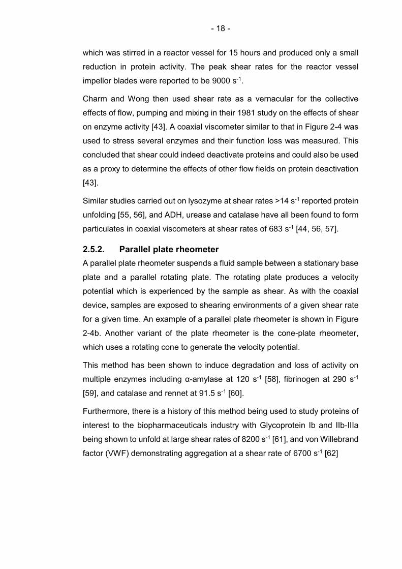
- 18 -

which was stirred in a reactor vessel for 15 hours and produced only a small

reduction in protein activity. The peak shear rates for the reactor vessel

impellor blades were reported to be 9000 s-1.

Charm and Wong then used shear rate as a vernacular for the collective

effects of flow, pumping and mixing in their 1981 study on the effects of shear

on enzyme activity [43]. A coaxial viscometer similar to that in Figure 2-4 was

used to stress several enzymes and their function loss was measured. This

concluded that shear could indeed deactivate proteins and could also be used

as a proxy to determine the effects of other flow fields on protein deactivation

[43].

Similar studies carried out on lysozyme at shear rates >14 s-1 reported protein

unfolding [55, 56], and ADH, urease and catalase have all been found to form

particulates in coaxial viscometers at shear rates of 683 s-1 [44, 56, 57].

2.5.2. Parallel plate rheometer

A parallel plate rheometer suspends a fluid sample between a stationary base

plate and a parallel rotating plate. The rotating plate produces a velocity

potential which is experienced by the sample as shear. As with the coaxial

device, samples are exposed to shearing environments of a given shear rate

for a given time. An example of a parallel plate rheometer is shown in Figure

2-4b. Another variant of the plate rheometer is the cone-plate rheometer,

which uses a rotating cone to generate the velocity potential.

This method has been shown to induce degradation and loss of activity on

multiple enzymes including α-amylase at 120 s-1 [58], fibrinogen at 290 s-1

[59], and catalase and rennet at 91.5 s-1 [60].

Furthermore, there is a history of this method being used to study proteins of

interest to the biopharmaceuticals industry with Glycoprotein Ib and IIb-IIIa

being shown to unfold at large shear rates of 8200 s-1 [61], and von Willebrand

factor (VWF) demonstrating aggregation at a shear rate of 6700 s-1 [62]

- 19 -

Examples of plate rheometer studies with antibodies include subjecting

antistreptavidin immunoglobulin (IgG1), a humanised monoclonal antibody, to

shear rates of 2000s-1 for up to 300s [24]. At concentrations greater than

100mg/mL a small increase (0.3%) of aggregation was observed directly after

exposure. After 1 week of storage, however, the level of aggregation was

undetectable.

2.5.3. Four roll mill

The four roll mill comprises four cylinders, or rollers which are submerged

vertically in a reservoir containing the sample fluid. The rollers can be rotated

in different directions to control the type of flow field induced in the sample

[63].

The four roll mill is presented as an extensional flow device. In fact the four

roll mill combines the boundary layer shear of the rotating cylinders which

propagate in such a way as to generate the velocity potential required to

produce a stagnation point. As a result, comparatively large volumes of fluid

are commuted though high shear environments compared to the limited

volume of fluid which typically passes through the slow moving fluid region in

and around the stagnation point [8, 63]. A comprehensive CFD study of the

flow profile is shown in Figure 2-5 [8].

This apparatus in the study that produced Figure 2-5 was used to stress three

proteins; Hen egg-white lysozyme, Bovine serum albumin, Alcohol

dehydrogenase (ADH). Shear and strain rates as high as 400 s-1 were

Figure 2-4: Viscometers produce high shear flows. (a) Narrow gap coaxial cylinder viscometer. (b) Cone-and-plate viscometers. [2]

- 20 -

generated, although the study is careful to point out that the average stress

rates throughout the sample do not exceed 30 s-1 [8]. Solutions of the proteins

were tested in relatively high sample sizes, as befitting the nature of the

device. Aggregation, detected using absorbance at a range of wavelengths,

was seen to increase with roller rotational speed, and hence, with stress rate.

Formation of larger particles was seen to correlate with speed. ADH, the

largest of the three, was shown to be the most affected.

Figure 2-5: “Velocity profile for the different flow configurations (a) elongation (b) hybrid and (c) rotation for water (Re 155) in the four-roll apparatus calculated with CFD. Arrows indicate the rotation direction of the rollers.” [8]

- 21 -

2.5.4. Opposed jets

An opposed jets device primarily consists of two identical fluid inlets facing

each other over a short distance. Both inlets expel or draw in jets of fluid at

the same rate so that a stagnation point forms where the jets meet at the

centre of the breach. An example is shown in Figure 2-6. The fluid is then

forced to turn through 90° and travel away from the stagnation point in a

perpendicular direction to the axis of the jets. This produces a velocity gradient

tangential to the direction of flow, otherwise known as an extensional flow field

[64].

Opposed jets are often submerged in a reservoir of the fluid to be studied. A

two-dimensional variation on the opposed jets is the cross-slot device. This

device consists of a plate with four channels etched into it which meet to form

a cross. As with the opposed jet device, two of the channels facing each other

provide the incoming mass flux. The fluid is required to turn a right-angle to

exit through either remaining channel resulting in a stagnation point at the

centre [65].

Figure 2-6: Example of an opposed jets experiment schematic (left) and photograph showing extended polymer chains (right) [64]. Note that in this instance, fluid is being drawn into the jets as opposed to being sprayed out; both are common arrangements.

The cross slot device is not widely used in protein or enzyme studies.

Examples are largely limited to polymer investigations. Haward et al. [66] used

such a device to generate an extensional region measuring 435 s-1 to

manipulate polymers in solution.

- 22 -

Examples closer to bioprocessing include the novel use of a nanofluidic cross

slot device to trap a single strand of DNA in the stagnation point and unfurl it

using the extensional flow region using a strain rate no grater that 1 s-1 [67].

2.5.5. Capillary Rheometer

Capillary devices subject fluid to shear by forcing it though a narrow tube, or

capillary. The pressure differential across the capillary and the cross sectional

dimensions are required to calculate the shear [56, 68]. Capillary rheometers

operate at Re Numbers typically in the laminar region, below Re = 3000. Shear

rates in excess of 105 s-1 are achievable for short time periods [4, 56]. Short

residence times have been linked to partial protein unfolding [56, 69] with

multiple passes through said devices used to increase the residence time [59].

This however, is a point of contention in the current work which will be

explored in later sections.

The capillary rheometer has been used to demonstrate shear induced activity

loss in catalase at shear rates of 67 s-1 [52] and also at 4600 s-1 [57].

No loss in activity was recorded when cytochrome C was subjected to 20,000

s-1, however [4].

More recently, the capillary rheometer has been employed as a method of

characterising high concentration biopharmaceuticals in terms of

“Syringeability”, or usability by the end user. Such devices are also concerned

with assessing any non-Newtonian effects that syringing might incur [70]. The

effects of soluble aggregates and reversible self-association on high

concentration monoclonal antibodies have also been investigated using

capillary rheometers [71].

2.5.6. Microchannel devices

Microchannel, or microfluidic, devices include any device that have a

characteristic or defining dimension ≤1000 µm. Typically, microchannel

devices are made by molding or etching a series of pathways into a glass or

polymer substrate. This allows for flexibility in the geometries which can be

produced, although generally speaking, many of the devices discussed

earlier, particularly cross slot devices, could also fit into this category.

- 23 -

A prime example of a microchannel device designed to manipulate molecules

using fluid flow is given by Larson et al. [9] who present a 2D funnel etched

into a plate. The funnel employs mass conservation to cause fluid to

accelerate downstream, producing an extensional flow profile as it goes. This

extensional region is used to unfurl a DNA molecule in a similar manner to

that seen with the cross slot example.

A similar example in the field of protein aggregation within extensional flows

is presented in which spider silk is spun from artificially produced spider

dragline silk proteins [51]. The work discusses, rather elementarily, how

convergent micro-channels cause unfolding and irreversible aggregation

resulting in fibre formation. What is particularly noteworthy is that these

examples do not deal in earnest with the relationship between flow and the

denaturation, but simply focus on applications of seemingly well-defined

phenomena of long-chain biological molecules in extensional flow fields. To

move on from this, a sound understanding of the mechanics within shear and

extensional flow is required, which will now be discussed. Interestingly

however, only a small number of studies within the biopharma field explore

the fluid mechanical theory in any great detail, with the emphasis being placed

mainly on the folding kinetics of the proteins themselves.

- 24 -

2.6. Frequently used proteins

Cytochrome c is a small protein of only 104 residues and contains natural

fluorophores. This makes it a useful protein to study for unfolding as the

flourophores only fluoresce when the hydrophilic centre of the structure is

revealed, indicating unfolding. In a study by Jaspe & Hagan [4] a solution of

cytochrome c was passed through a narrow capillary of inner diameter 150µm

at speeds of up to 10ms-1 to induce shear. No evidence of shear induced

aggregation was detected on any timescale. The findings were reviewed by

Ashton et al. [55] in which the findings were compared to a similar globular

protein, lysozyme with a viscous fluid medium, glycerol. In this case

conformational change (unfolding) was witnessed under simple, laminar shear

flow, although this change was reversible.

Lysozyme is also reported to have been exposed to well defined extensional

flow fields in a paper by Simon et al. [8]. Lysozyme was chosen as a “model

protein” in this case, no doubt due to the ease and repeatability demonstrated

by Ashton et al. Under extensional flow, an increase in particles of size >1µm

was detected indicating denaturation in the form of agglomeration. The

population of large particles increased with extensional intensity and

interfacial effects (both solid-liquid and liquid-gas) were ruled out. The time

dependency of the aggregate population is not discussed although the nature

of large particle aggregates is commonly stable and therefore time

independent. The same experiment was conducted with two larger proteins;

bovine serum albumin and alcohol dehydrogenase (ADH). In this instance the

results were similar to those observed for lysozyme only the population of

larger particles was higher for the larger molecules indicating aggregation due

to extension is more prevalent in longer chain proteins. Aggregation was

highest in the case of ADH.

- 25 -

2.7. Protein characterisation methods

In the study of proteins, the term “characterisation” describes a means of

analysing or probing an aspect or structural arrangement which portrays some

property or function of the molecule. A vast array of characterisation methods

exist for protein analysis. In this study we are interested in detecting whether

a protein is in its native, folded state or if it has undergone some structural

deformation, reducing its functionality or rendering it inactive. As previously

mentioned, for the purpose of this study the characterisation methods can be

divided into two types.

Type one will be classified as “ex situ”, where a protein solution is subjected

to an adverse flow field, is extracted, and sometime later is scrutinised by

some characterisation method. Therefore type one can only detect time

independent, irreversible changes, or reversible changes with relatively long

timescales – typically in excess of 30 minutes for current methods.

Type two characterisation methods are classified as “in situ” as they are

designed to probe the space within the flow field as the experiment is in

progress. In this situation it is possible to measure time dependent, reversible

conformational changes, either in real-time or in a timeframe which would be

unachievable using ex situ methods.

Primarily, a selection of ex situ characterisation methods will be presented.

These methods are generally less complicated to apply as the techniques are

well documented, standardised and the equipment is stand-alone and readily

available. In comparison, in situ methods require custom equipment and

techniques. The current experiments, as previously mentioned, are tailored

towards ex situ characterisation as a means of testing for severe levels of

damage or inactivation as a proof of concept.

2.7.1. Light obscuration

Denaturation of proteins can occur as aggregation resulting in the formation

of relatively large particles. These can be detected in a sample using light

obscuration. Light obscuration measures the amount of light detected after it

passes through a sample. The detector is calibrated using a set of polymer

- 26 -

beads of a known size and concentration. In the previously mentioned study

by Simon et al. [8] this method was used to identify particles larger than 1µm

indicating denaturation for 3 types of proteins commonly studied in flow

induced aggregation experiments.

2.7.2. Circular dichroism spectroscopy

Circular dichroism (CD) spectroscopy measures changes in protein

secondary structure by use of far UV absorbance. Proteins absorb left and

right circular polarised UV light at different affinities based on their structures.

Therefore, a protein can be identified by analysing the difference in

absorbance between the two types of polarised light. As the absorbance is

based on structure, a denatured protein will produce a difference to spectra to

its naturally folded counterpart. Strong signals are typically associated with

commonly seen structural properties such as α-helices and β-sheets. Analysis

of tertiary structure and binding sites is also possible. CD spectroscopy is

often compared to techniques such as X-ray crystallography and NMR by

which CD boasts several advantages such as smaller sample sizes, no limits

on protein sizes and the non-destructive nature of the analysis [72].

2.7.3. UV/visible spectroscopy

UV/visible spectrophotometry is used to measure the concentration of

proteins in the solution. Light is produced by a deuterium (near-UV, 150-

400nm) or tungsten-halogen (visible, 400-800nm) light source and passed

through a monochromator. Light that passes through sample is detected by a

photomultiplier/ photodiode. A reference (produced by analysing the buffer

alone) is subtracted from the final result to measure the absorbance of the

protein. The technique can be used to measure aggregation by taking a

measurement before and after stressing to draw a comparison. A stressed

sample may need centrifuging to remove non-soluble aggregates. UV/visible

spectrophotometry is only applicable to proteins with aromatic residues [73].

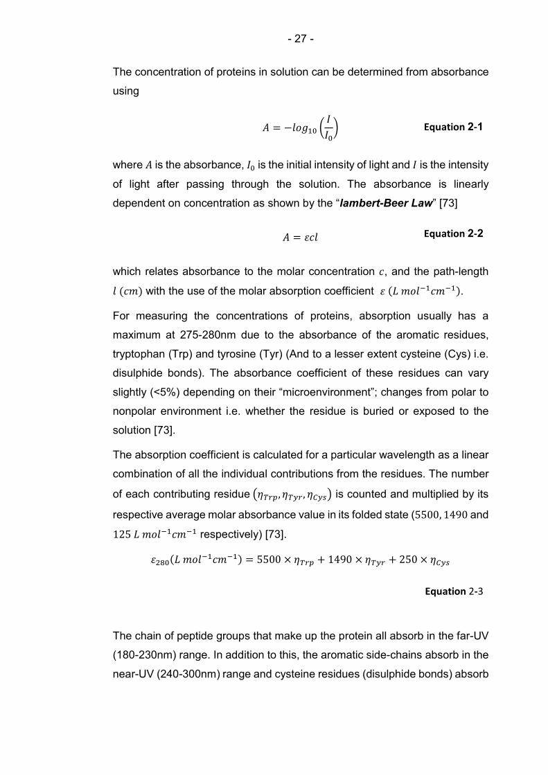
- 27 -

The concentration of proteins in solution can be determined from absorbance

using

𝐴 = −𝑙𝑜𝑔𝐼

𝐼 Equation 2-1

where 𝐴 is the absorbance, 𝐼 is the initial intensity of light and 𝐼 is the intensity

of light after passing through the solution. The absorbance is linearly

dependent on concentration as shown by the “lambert-Beer Law” [73]

𝐴 = 𝜀𝑐𝑙 Equation 2-2

which relates absorbance to the molar concentration 𝑐, and the path-length

𝑙 (𝑐𝑚) with the use of the molar absorption coefficient 𝜀 (𝐿 𝑚𝑜𝑙 𝑐𝑚 ).

For measuring the concentrations of proteins, absorption usually has a

maximum at 275-280nm due to the absorbance of the aromatic residues,

tryptophan (Trp) and tyrosine (Tyr) (And to a lesser extent cysteine (Cys) i.e.

disulphide bonds). The absorbance coefficient of these residues can vary

slightly (<5%) depending on their “microenvironment”; changes from polar to

nonpolar environment i.e. whether the residue is buried or exposed to the

solution [73].

The absorption coefficient is calculated for a particular wavelength as a linear

combination of all the individual contributions from the residues. The number

of each contributing residue 𝜂 , 𝜂 , 𝜂 is counted and multiplied by its

respective average molar absorbance value in its folded state (5500, 1490 and

125 𝐿 𝑚𝑜𝑙 𝑐𝑚 respectively) [73].

𝜀 (𝐿 𝑚𝑜𝑙 𝑐𝑚 ) = 5500 × 𝜂 + 1490 × 𝜂 + 250 × 𝜂

Equation 2-3

The chain of peptide groups that make up the protein all absorb in the far-UV

(180-230nm) range. In addition to this, the aromatic side-chains absorb in the

near-UV (240-300nm) range and cysteine residues (disulphide bonds) absorb

- 28 -

at around 260nm. Peptides present in a folded protein are in an immobilised

asymmetric structure. In this state, residues are seen to demonstrate circular

dichroism; a phenomena by which left- and right-handed circularly polarised

light are absorbed differently [73].

2.7.4. Light scattering spectroscopy

Light scattering (LS) spectroscopy, dynamic light scattering (DLS), light

scattering by particles (LSP) or Rayleigh scattering (RS) spectroscopy is used

to determine the hydrodynamic radius of protein from measuring its diffusion

coefficient in solution. It is capable of measuring the actual change in average

macromolecule size whereas other techniques look for localised markers

within the structure e.g. UV spec [74].

2.7.5. Size-exclusion chromatography and multi-angle laser-light scattering

Size-exclusion chromatography and laser-light scattering (SEC MALLS) is a

technique for relative molecular weight determination based on UV/Vis

detection. It consists of a chromatographic column with multi-wavelength

detector and light-scattering with refractive index detection [75].

2.7.6. In situ characterisation methods

Ultimately, in situ methods are a target for the current research and some of

the work reviewed has presented some techniques worth consideration. The

cytochrome c visited in the previous section shows increased fluorescence

upon unfolding. In the case of Jaspe & Hagen [4] the solution was illuminated

with an ultraviolet laser which was incident on the silica, i.e. transparent,

capillary. In this setup the unfolding was measured whilst protein was

travelling through the high-shear environment. In situ UV/visible spectroscopy

measurements was performed during stress testing in a four-roll mill [8].

Raman spectroscopy is increasingly being applied to protein conformational

studies as it is sensitive to changes in secondary structure, hydrophilic

exposure of side-chains and able to identify disordered structures. The

technique also allows protein to be continuously exposed to stress

environments as shown in Figure 2-7 [55].

- 29 -

Figure 2-7: An experimental setup of a flow cell similar to a coaxial viscometer with in situ Raman spectroscopy laser and optics. [1]

2.8. Summary

Proteins are highly sensitive to a range of variables. Many studies have been

carried out to identify the effects of environmental changes such as

temperature, pH and concentration. As a result, thesis conditions are now well

understood. The same is not yet true of flow. in this chapter, the efforts made

to quantify the effects of fluid forces on long-chain molecules have been found

to be insightful, but not yet complete. A number of techniques have been

applied to investigate the response of a range of proteins to various flow

profiles. The following sections of this thesis will further develop on the ideas

that have been introduced so far, drawing inspiration from previous studies.

- 30 -

3. Theory

The theory section consists of two separate parts; 1) fluid mechanics and

corresponding analytical methods including CFD, and 2) protein aggregation

theory with characterisation methods which includes particle tracking and

absorption/emission spectroscopy. In previous studies attempts have been

made to combine the two with varying degrees of success [76-78]. In the

following sections, a formal introduction will be made to both subjects.

In the first section, the knowledge required to make a detailed fluid mechanical

model will be discussed. Due to the nature of filters and fill-finish operations

as discussed in the literature review, this will centre around the idea of slow,

laminar flows in viscous-dominated regimes. Previous studies exploring the

relationship between flow and protein aggregation have shown a propensity

toward shear dominated flow. The properties of shear will, therefore, be

discussed here.

Further afield in studies related to fluid effects on longer, less structured

molecules, such a DNA and polymers, an interest has been raised in

extensional, strain-dominated regimes in laminar flow. The properties of

extensional flow will also be discussed.

It will be seen that both shear and extension are present in some form in the

majority of laminar flow systems. The deformation of an incompressible fluid

element in a continuum can be described by a single function which can

simultaneously describe the combined effects of both shear and strain, and

also allow the two effects to be uncoupled to measure their individual

contributions towards protein aggregation.

The methods used to calculate and model fluid behaviour will also be

introduced, although further detail will be presented on this in the dedicated

Numerical Modelling and Computational Fluid Dynamics chapter.

In the second part of this chapter protein aggregation theory will be presented.

The mechanisms which make proteins susceptible to aggregation are

explored, and detection and characterisation methods will be described.

- 31 -

3.1. Fluid mechanics

This chapter provides a detailed discussion into the fluid mechanics used

within this thesis. A classical definition of both shear and extension dominated

flows are given and a literature review of fluid mechanics and long-chain

molecules is presented.

A large body of work based around the effects of shear on proteins has been

presented by previous literature. Thomas and Geer [2] present a definition for

“shear” (expressed in inverted commas) as any mechanical or hydrodynamic

force, and in some broader cases, it even extends to interfacial phenomena.

This trend of using the term “shear” synonymously with any fluid force is still

prevalent in 2016 [79]. According to Rathore [42], “shear” is prevalent

throughout the manufacture process (“Shear” in this instance referring to any,

and all, hydrodynamic forces!). From formulation and filtration, drug product

filling, through to delivery devices. “Shear” is considered to drastically affect

proteins during manufacture, to the extent where a characterisation method is

called for to evaluate the structural stability of proteins under processing

conditions [80]. Currently, rheometers are used to conduct shear

characterisation over comparable exposure times as a means of assessing

whether a drug is suitable for manufacture [81-83]. But it is becoming

increasingly evident that the response of a long-chain molecule to shear alone

is not necessarily indicative of manufacturability.

The terms “strong” and “weak” were coined in field of polymer processing

(1975-76) as a means of classification of flows by their ability to stretch and

align macromolecules suspended in solution or fibres in suspension

corresponding to extension or simple shear respectively [84, 85]. In fact,

extensional flow has been a widely researched topic to the point where it has

almost fallen under the category of “classical” fluid mechanics. It is

understandable to assume that it has failed to attract the attention of

researchers from biopharmaceutical backgrounds over the past few decades.

- 32 -

3.1.1. Shear vs. extensional flow within biopharmaceutical manufacture

Shear flow is present in all laminar flow pipes and tubes, for instance, in blood

vessels and arteries, or the pipes used to pump biological materials around

during a manufacturing procedure. It is a phenomenon caused by the no slip

condition observed between the fluid and the fluid boundary at the pipe wall

as shown in Figure 3-1. This no slip condition was observed experimentally in

the early days of fluid mechanics and holds for all fluids, with the exception of

rarefied gas and conditions where the molecular path is similar or smaller than

the pipe diameter. Since we are pumping fluid we know that the velocity of the

fluid cannot be zero across the whole pipe cross-section, in fact the velocity

of the fluid increases the further away from the wall the fluid is. This produces

a velocity profile where two adjacent streamlines are never carrying fluid at

the same velocity. This difference in velocity between two adjacent fluid

elements is known as shear.

Shear stress is at its maximum at the capillary wall. Denoted as 𝜏 , this is

calculated as

𝜏 =𝑑∆𝑝

4𝐿 Equation 3-1

where 𝑑 is the capillary diameter, ∆𝑝 is the change in pressure, and 𝐿 is

capillary length.

𝑉𝑒𝑙𝑜𝑐𝑖𝑡𝑦 𝑝𝑟𝑜𝑓𝑖𝑙𝑒

Figure 3-1: Shear flow in a pipe or tube with a characteristic velocity profile. Notice how any two fluid elements on adjacent streamlines are never travelling at the same velocity.

- 33 -

Pressure drop in a laminar flow regime is calculated by

∆𝑝 =32𝜇∆𝐿𝑢

𝐷 Equation 3-2

Extensional flow is caused by a contraction in the flow geometry. If the fluid is

assumed to be incompressible it must accelerate to satisfy mass

conservation. As the fluid accelerates, the fluid element will be subjected to a

velocity profile as part of the front of the element will always be traveling faster

than the rear. This causes the fluid element to stretch out as it passes through

a contraction. The phenomenon exerts strain on any fluid element passing

through the extensional region. In its simplest form, fluid strain can be

expressed in the same fashion as its solid mechanical counterpart. After time,

𝑡, strain, 𝜀 , is the ratio of the increased length due to stretching, 𝐿 − 𝐿 , over

the original length 𝐿 .

𝜀 =𝐿 − 𝐿 ,

𝐿 , Equation 3-3

Figure 3-2: (Top) Contraction in a flow geometry resulting in acceleration and therefore extensional flow. The arrow lengths are proportional to fluid velocity. (Bottom) Average fluid velocity v is plotted against position z, demonstrating the acceleration of the fluid.

v

z

- 34 -

3.1.2. Rate of Deformation

The intensity of a shear or strain region is often presented in terms of rate of

deformation, these are termed the shear rate and strain rate. These can both

be expressed as a ratio of deformation to the size of the deformed fluid

element

𝛾 =𝑑𝑥

𝑑𝑦 Equation 3-4

For an extensional flow, the strain rate is then defined as

�̇� =𝑠ℎ𝑒𝑎𝑟 𝑠𝑡𝑟𝑎𝑖𝑛

𝑡𝑖𝑚𝑒 𝑡𝑎𝑘𝑒𝑛=

𝛾

𝑑𝑡=

𝑑𝑥

𝑑𝑡𝑑𝑦=

𝑑𝑢

𝑑𝑦 Equation 3-5

The formal definition for an extensional flow is then

𝑭(𝑡) = 𝑹(𝑡)𝑼(𝑡) Equation 3-6

Where 𝑭 is the deformation tensor, 𝑹 the (orthogonal) rotation tensor and 𝑼

the (positive definite symmetric) right stretch tensor. The flow is defined as

extensional when there is a fixed orthogonal coordinate system in which 𝑼(𝑡)

has diagonal components.

Alignment is seen to be of relative importance to the strength of the flow as

any confined flow is going to have a shear, and therefore a rotational

component regardless of the size of contraction [84].

Strain 𝜀 is a measure of mechanical extension. Therefore rate of strain 𝜀̇ is the

time derivative of 𝜀. A 3-dimensional fluid element undergoing strain in one

direction, much like an elastic solid, will experience proportional elongations

in the remaining directions. To describe this in 3-dimensions, the rate of strain

tensor is used:

𝑑 =1

2𝑢 + 𝑢 Equation 3-7

Where 𝑢 is the scalar component of velocities. This can be expanded such

that

- 35 -

𝑑 =

⎣⎢⎢⎢⎢⎢⎡

𝜕𝑢

𝜕𝑥

1

2

𝜕𝑢

𝜕𝑥+

𝜕𝑢

𝜕𝑥

1

2

𝜕𝑢

𝜕𝑥+

𝜕𝑢

𝜕𝑥1

2

𝜕𝑢

𝜕𝑥+

𝜕𝑢

𝜕𝑥

𝜕𝑢

𝜕𝑥

1

2

𝜕𝑢

𝜕𝑥+

𝜕𝑢

𝜕𝑥1

2

𝜕𝑢

𝜕𝑥+

𝜕𝑢

𝜕𝑥

1

2

𝜕𝑢

𝜕𝑥+

𝜕𝑢

𝜕𝑥

𝜕𝑢

𝜕𝑥 ⎦⎥⎥⎥⎥⎥⎤

Equation 3-8

where 𝑥 denote a specific direction. For uniaxial, homogenous, simple

extension the flow is assumed to have no vorticity. If 𝑥 is taken to be the

direction of maximum 𝜀̇ i.e. the frame of reference is such that the deformation

is purely symmetric in that direction, the rate of strain tensor 𝐷 is becomes

𝑑 =

⎣⎢⎢⎢⎡𝜀̇ 0 0

0 −1

2𝜀̇ 0

0 0 −1

2𝜀̇⎦

⎥⎥⎥⎤

Equation 3-9

where the rate of strain 𝜀̇ can be expressed as extension over time:

𝜀̇ =𝑑𝜀

𝑑𝑡 Equation 3-10

or as change in velocity over change in position:

𝜀̇ =𝑑𝑢

𝑑𝑥 Equation 3-11

By taking the latter and by assuming that flow down the central axis of an

axisymmetric sudden constriction in a pipe consists predominantly of uniaxial

extension, it is possible to calculate the maximum rate of strain in the region

in the flow where the ratio of extension to shear is at a maximum. A

comparison can then be drawn between rate of strain and aggregation in

proteins in solution.

- 36 -

Deformation tensor

The deformation tensor 𝑑 is a 2nd order tensor that determines how a fluid

element deforms as it travels along a flow.

𝑑 =1

2𝑢 + 𝑢 Equation 3-12

𝑜𝑟

𝑑 =

⎣⎢⎢⎢⎢⎢⎡

𝜕𝑢

𝜕𝑥

1

2

𝜕𝑢

𝜕𝑥−

𝜕𝑢

𝜕𝑥

1

2

𝜕𝑢

𝜕𝑥−

𝜕𝑢

𝜕𝑥1

2

𝜕𝑢

𝜕𝑥−

𝜕𝑢

𝜕𝑥

𝜕𝑢

𝜕𝑥

1

2

𝜕𝑢

𝜕𝑥−

𝜕𝑢

𝜕𝑥1

2

𝜕𝑢

𝜕𝑥−

𝜕𝑢

𝜕𝑥

1

2

𝜕𝑢

𝜕𝑥−

𝜕𝑢

𝜕𝑥

𝜕𝑢

𝜕𝑥 ⎦⎥⎥⎥⎥⎥⎤

Equation 3-13

A 2nd order tensor can be decomposed into two parts; a symmetric and an

anti-symmetric part as discussed by Jaspe and Hagen [4]:

𝜕𝑢

𝜕𝑥=

𝜀̇

2+

Ω̇

2=

1

2

𝜕𝑢

𝜕𝑥+

𝜕𝑢

𝜕𝑥+

1

2

𝜕𝑢

𝜕𝑥−

𝜕𝑢

𝜕𝑥 Equation 3-14

The symmetric part is the rate of strain tensor:

𝜀̇ =1

2

𝜕𝑢

𝜕𝑥+

𝜕𝑢

𝜕𝑥

𝜀̇ =

⎣⎢⎢⎢⎢⎢⎡

𝜕𝑢

𝜕𝑥

1

2

𝜕𝑢

𝜕𝑥+

𝜕𝑢

𝜕𝑥

1

2

𝜕𝑢

𝜕𝑥+

𝜕𝑢

𝜕𝑥1

2

𝜕𝑢

𝜕𝑥+

𝜕𝑢

𝜕𝑥

𝜕𝑢

𝜕𝑥

1

2

𝜕𝑢

𝜕𝑥+

𝜕𝑢

𝜕𝑥1

2

𝜕𝑢

𝜕𝑥+

𝜕𝑢

𝜕𝑥

1

2

𝜕𝑢

𝜕𝑥+

𝜕𝑢

𝜕𝑥

𝜕𝑢

𝜕𝑥 ⎦⎥⎥⎥⎥⎥⎤

Equation 3-15

- 37 -

And the asymmetric part is the vorticity tensor:

Ω̇ =1

2

𝜕𝑢

𝜕𝑥−

𝜕𝑢

𝜕𝑥

Ω̇ =

⎣⎢⎢⎢⎢⎢⎡ 0

1

2

𝜕𝑢

𝜕𝑥−

𝜕𝑢

𝜕𝑥

1

2

𝜕𝑢

𝜕𝑥−

𝜕𝑢

𝜕𝑥1

2

𝜕𝑢

𝜕𝑥−

𝜕𝑢

𝜕𝑥0

1

2

𝜕𝑢

𝜕𝑥−

𝜕𝑢

𝜕𝑥1

2

𝜕𝑢

𝜕𝑥−

𝜕𝑢

𝜕𝑥

1

2

𝜕𝑢

𝜕𝑥−

𝜕𝑢

𝜕𝑥0

⎦⎥⎥⎥⎥⎥⎤

Equation 3-16

𝑜𝑟

Ω̇ =1

2

0 𝜔 𝜔

−𝜔 0 𝜔

−𝜔 −𝜔 0 Equation 3-17

As 𝜔 are all components of the vorticity vector, such that

𝝎 = 𝛁 × 𝐮 =𝝏𝒖𝟑

𝝏𝒙𝟐−

𝝏𝒖𝟐

𝝏𝒙𝟑̂ +

𝝏𝒖𝟏

𝝏𝒙𝟑−

𝝏𝒖𝟑

𝝏𝒙𝟏̂ +

𝝏𝒖𝟐

𝝏𝒙𝟏−

𝝏𝒖𝟏

𝝏𝒙𝟐𝒌

𝝎 = 𝜔 𝚤̂ + 𝜔 𝚥̂ + 𝜔 𝑘 Equation 3-18

A flow is considered to be deforming due to shear if the off-diagonal

components are non-zero.

To interpret this in the form of a 2D axisymmetric flow simulation, we use the

coordinate system and corresponding velocities 𝑥 = 𝑟, 𝑥 = 𝑧, 𝑥 = 𝜑, 𝑢 =

𝑢, 𝑢 = 𝑤 𝑎𝑛𝑑 𝑢 = 𝑣 = 0. Therefore our 2D problem becomes

𝑑 =

𝜕𝑢

𝜕𝑟

1

2

𝜕𝑢

𝜕𝑧−

𝜕𝑤

𝜕𝑟1

2

𝜕𝑤

𝜕𝑟−

𝜕𝑢

𝜕𝑧

𝜕𝑤

𝜕𝑧

Equation 3-19

- 38 -

By using CFD to calculate the rate of strain in a fluid of known viscosity, it is

then possible to relate this to proteins in solution. Assuming that a protein

molecule can be aligned with the direction of extension, the extensional force

can be compared to that applied by an atomic force microscope (AFM)

experiments. These have been used to unfold protein molecules with the an

unfolding force requirement of about 20 to 150 pN for α-helical and β-sheet

proteins, respectively [24].

3.1.3. Numerical solvers and Navier-Stokes Equations

Numerical solvers are increasingly used to approximate complex flow systems

with ever improving accuracy and computational efficiency. Such solvers

include the finite element method (FEM) and the finite difference method

(FDM). FEM has the advantage of solving for arbitrarily unstructured

subdivisions whilst providing approximations for self-adjoint problems, usually

in advance of a comparative FDM solver [86]. FEM is employed by

computational fluid dynamics (CFD) packages such as COMSOL.

Numerical solvers exist to provide approximations based on conservation of

momentum. This is achieved by solving the Navier-Stokes equations

(Equation 3-20) for an incompressible fluid [87] in tandem with the continuity

equation (Equation 3-21) [88].

𝜌𝜕𝒖

𝜕𝑡+ (𝒖. ∇)𝒖 = −∇𝑃 + 𝜌𝑔 + 𝜇∇ 𝒖 Equation 3-20

∇ ∙ 𝒖 = 0 Equation 3-21

Navier-Stokes give the equations of motion for a Newtonian fluid taking into

account viscosity, 𝜇, which can be a function of the fluid’s thermodynamic

conditions but in this case is assumed a constant. Numerical solutions will be

covered in greater detail in later chapters.

3.1.4. Pressure It is appropriate to provide validation for a numerical study. In this case, the

numerical method will be performed alongside an experimental method. For

a flow to be fully defined, it is important to know which features in the flow are

- 39 -

dominant. For example, a slow, Newtonian flow will have a low Reynolds

number therefore viscous forces will be dominant over inertial forces. Along a

similar argument, in this flow setup it is evident that there will be a number of

characteristic conditions which will become dominant in different regions; the

acceleration and extensional forces will dominate in the rapid contraction, and

viscous shear forces will become dominant in the capillary tube. To determine

the relative effects these two flow conditions have on the flow in relation to

each other, the drop in pressure can be measured across each region and

compared directly.

Pressure drop along the capillary tube is proportional to the length of the tube

section therefore the ratio of pressure drops across the two regions can be

controlled. Calculated using the Hagan-Poiseuille equation

∆𝑃 =128𝜇𝐿𝑄

𝜋𝑑 Equation 3-22

The pressure drop through a capillary can be calculated and be further backed

up using CFD by probing the pressures at different lengths along the capillary.

Determining the pressure drop across the sharp contraction, however, proves

to be slightly more problematic. Astarita and Greco [89] review Equation 3-23

from Holmes, Sylvester and Rosen [90]

∆𝑝 = 𝐾 +𝑘

𝑅𝑒

𝜌𝑈

2 Equation 3-23

where 𝐾 is the Hagenbach correction and is referred to as the coquette

correction. 𝑈 is taken as the average downstream velocity. A range of

numbers are taken from literature ranging from 2.16 − 2.34, with the most

prominent being quoted as 2.24.

Astarita and Greco [89] go on to suggest the modification of the Holmes [90]

equation with the experimentally derived values specifically for a sudden

contraction which yield the equations:

- 40 -

𝑅𝑒 < 146; ∆𝑝 =795

𝑅𝑒

𝜌𝑈

2 Equation 3-24

𝑅𝑒 > 146; ∆𝑝 = 5.48𝜌𝑈

2 Equation 3-25

Another equation proposed for the pressure drop across a sharp contraction

which apparently takes into account the development of a vena contracta

directly after the contraction is accredited to Lighthill [91]. The equation is as

follows

∆𝑝 = −�̇�

2𝜌𝑆

1

𝐶− 1 + (𝑆 − 1) Equation 3-26

�̇� is the mass flow rate or mass flux, 𝑆 is the ratio of upstream and

downstream areas, and 𝐶 is stated as the contraction coefficient which is

the ratio of areas between the vena contracta and the downstream section

and can be calculated using Equation 3-27 and empirically derived

constants.

𝐶 =𝐴

𝐴= 1 −

1 − 𝜎

2.08(1 − 𝜎) + 0.5371 Equation 3-27

𝜎 =𝐴

𝐴 Equation 3-28

Circulation 2 (Vena Contracta) Circulation 1

Figure 3-3: location of vena contracta circulations resulting in pressure losses in a sudden contraction.

- 41 -

A diagram of the vena contracta can be seen in Error! Reference source not

found..

The pressure equations are summarised in Error! Reference source not

found. and will be used to validate the numerical study with hand calculations.

Pressure equation Reference

∆𝑝 = 𝐾 +𝑘′

𝑅𝑒

𝜌𝑈

2

𝑅𝑒 < 146; ∆𝑝 = , 𝑅𝑒 < 146; ∆𝑝 = 5.48

Equation 3-23, 3-

24, 3-25 [89, 90]

∆𝒑 =⟨𝒖𝟏⟩𝟐

𝟐𝟏 −

𝟏

𝑪𝒄

𝟐

+ 𝟏 − 𝝈𝟐

𝐶 =𝐴

𝐴= 1 −

1 − 𝜎

2.08(1 − 𝜎) + 0.5371

𝜎 =𝐴

𝐴

Equation 3-27, 3-

28 [92]

∆𝑝 = −�̇�

2𝜌𝑆

1

𝐶− 1 + (𝑆 − 1) Equation 3-26 [91]

Table 3-1: summary of pressure loss equations for validating numerical methods.

- 42 -

3.2. Proteins

A major barrier to the development of biopharmaceuticals is their challenging

manufacture process. Monoclonal antibodies are often expressed in

mammalian cell lines, such as Chinese Hamster Ovary (CHO), to allow for the

correct post-translational modifications to be made [93]. A typical mAb is

shown in Figure 3-4.

Throughout the manufacture cycle, to purification and formulation, biologics

are susceptible to degradation through temperature, chemical modifications

and mechanical processes, resulting in the formation of aggregates [5, 38, 94,

95]. A typical expression and purification profile for a mAb-based

biopharmaceutical is shown in Figure 3-5.

Figure 3-4: Schematic of an IgG-type monoclonal antibody. Each block represents a β-sheet rich immunoglobulin domain. The heavy chains are in dark blue, whilst the light chains are represented in light blue. The two halves of the antibody are connected by disulfide bridges. The Fc domain is the ‘crystallisable’ region as it is readily crystallised. Most glycosylation takes place in this region. The Fab domain is the antigen-binding domain, with the antigen binding represented by the convex end sections. The two domains are connected by a flexible hinge region, which gives these molecules conformational flexibility, facilitating target binding [7].

- 43 -

Fig

ure

3-5

: S

ch

em

ati

c o

f u

ps

tre

am

an

d d

ow

ns

tre

am

pro

ce

ssin

g o

f a

typ

ica

l m

Ab

-ba

se

d b

iop

ha

rma

ce

uti

cal.

T

hro

ug

ho

ut

the

ma

nu

fac

ture

, h

ydro

dyn

am

ic p

roce

sse

s a

re in

volv

ed

. F

erm

en

tati

on

ste

ps

lea

d t

o t

he

ove

r-e

xp

res

sio

n o

f th

e p

rod

uc

t. P

rim

ary

re

co

very

ste

ps

(c

en

trif

ug

ati

on

an

d d

ep

th f

iltr

ati

on

) s

ep

ara

te t

he

pro

du

ct

fro

m c

ell

de

bri

s, D

NA

an

d o

the

r c

on

tam

inan

ts.

Pro

tein

A c

hro

ma

tog

rap

hy

is u

se

d a

s t

he

ca

ptu

re s

tep

. I

on

-e

xc

ha

ng

e c

hro

ma

tog

rap

hy

is t

he

n u

se

d t

o p

oli

sh

th

e p

rod

uc

t. A

vir

al

ina

cti

vati

on

ste

p i

s u

se

d f

or

pro

du

cts

d

eri

ved

fro

m m

am

ma

lia

n c

ell

lin

es.

Th

e p

rod

uc

t is

th

en

co

nc

en

tra

ted

, fo

rmu

late

d a

nd

pa

cka

ge

d [

3].

- 44 -

3.2.1. Aggregation

The presence of aggregates or particulates in a finished biopharmaceutical

product is indicative of degradation [95, 96]. Regulators specify the threshold

of impurities that can be present in biopharmaceutical formulations, with

aggregate levels typically lower than 1% [97]. It is suggested that

biopharmaceutical aggregates, particularly those in the sub-visible range of

0.1-10µm, could potentially trigger immunological responses in the patient.

The severity of this response in vivo could range from loss of efficacy to mild

allergic reactions and even anaphylaxis [3, 95]. The exact mechanisms of the

immunogenicity, nor its extent, are known for all biologics. They are often

identified in clinical trials [97].

Aggregates are defined as any multimeric species made up of partially

unfolded protein monomers [3]. Aggregates range in size up to limit, typically,

of 100 nm. Aggregates of this size are often soluble and can form either

reversibly or irreversibly, depending on the monomer properties and its

environment [54, 95, 98]. The larger an aggregate grows, the greater its

propensity to drop out of solution. Insoluble aggregates are termed

particulates in order to differentiate them from their smaller, soluble

counterparts [94]. Many proteins, including biopharmaceuticals, are widely

thought to aggregate according to established models such as the Lumry-

Eyring Model. These models attempt to explain aggregate formation and

growth through kinetics. A schematic of how a biopharmaceutical could

aggregate is shown in Figure 3-6.

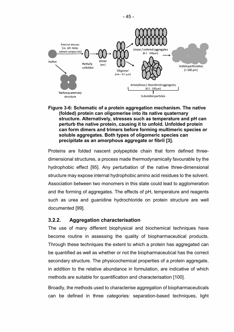
- 45 -

Proteins are folded nascent polypeptide chain that form defined three-

dimensional structures, a process made thermodynamically favourable by the

hydrophobic effect [95]. Any perturbation of the native three-dimensional

structure may expose internal hydrophobic amino acid residues to the solvent.

Association between two monomers in this state could lead to agglomeration

and the forming of aggregates. The effects of pH, temperature and reagents

such as urea and guanidine hydrochloride on protein structure are well

documented [99].

3.2.2. Aggregation characterisation

The use of many different biophysical and biochemical techniques have

become routine in assessing the quality of biopharmaceutical products.

Through these techniques the extent to which a protein has aggregated can

be quantified as well as whether or not the biopharmaceutical has the correct

secondary structure. The physicochemical properties of a protein aggregate,

in addition to the relative abundance in formulation, are indicative of which

methods are suitable for quantification and characterisation [100].

Broadly, the methods used to characterise aggregation of biopharmaceuticals

can be defined in three categories: separation-based techniques, light

Figure 3-6: Schematic of a protein aggregation mechanism. The native (folded) protein can oligomerise into its native quaternary structure. Alternatively, stresses such as temperature and pH can perturb the native protein, causing it to unfold. Unfolded protein can form dimers and trimers before forming multimeric species or soluble aggregates. Both types of oligomeric species can precipitate as an amorphous aggregate or fibril [3].

- 46 -

scattering/obscuration techniques and spectroscopic/spectrometric

techniques. All three methods are used in assessing the effects of extensional

flow on aggregation. Specifically, the techniques used in this study are

analytical ultra-centrifugation (AUC), nanoparticle tracking analysis (NTA),

and absorbance spectroscopy at the 280 nm wavelength (A280), respectively.

These will be described in further detail here.

Analytical Ultra-Centrifugation

Analytical Ultra Centrifugation (AUC) is used to separate monomeric proteins

from their oligomers/aggregates to quantify species and is applicable to those

of biopharmaceutical importance [101].

In AUC, a centripetal force is used to accelerate the sedimentation of very

small particles in a precipitate [102]. The technique separates the insoluble

material and concentrates it into a pellet, leaving a supernatant sample in

solution.

AUC is a routine method of determining the molecular weight and size of

proteins, requiring little sample preparation [100]. The concentration of protein

is then detected with UV absorbance spectroscopy measurement (seen in

later sections). However, the technique is not without with issue; the operator

requires a high level of training, the data analysis is complex [102], the

equipment is expensive, and process is time consuming [100, 103].

Nanoparticle Tracking Analysis

Many new techniques have been developed in recent years to aid the

quantification of nanoparticles. Nanoparticle Tracking Analysis (NTA) is a

technique which utilises camera images to visualise and track the motion of

particles which dynamically scatter laser light within the confines of a defined

field of view [104, 105].

For proteins, the lower limit of resolution for the technique is 40 nm [104].

Though this appears disadvantageous in comparison to DLS, where the

scatter from an incoming beam is used to infer the size distribution of the

particles [106], NTA is capable of distinguishing between particles in a

polydisperse sample with greater sensitivity. Where DLS can only distinguish

- 47 -

between particles that have a three-fold size difference, NTA can distinguish

between particles which have a 1.25-fold size difference [6].

Furthermore, the instrument will determine the concentration of each size of

particle based on the defined sample size illuminated by its laser [104]. This

is useful for capturing any smaller aggregates present in the sample that may

be missed using DLS. Finally, NTA tracks particles individually, whereas DLS

is an ensemble technique; hence the latter may not fully represent the

aggregated nature of the sample [104]. A schematic of the apparatus is shown

in Figure 3-7.

However, NTA cannot visualise or quantify native protein monomers due to

their size, although new techniques such as Taylor-Dispersion Analysis are

being developed to address this [107]. The use of NTA as an orthogonal

method for the detection and quantification of protein nanoparticles has been

used effectively by many in previous studies [104, 108, 109].

Absorbance spectroscopy

Absorbance spectroscopy is often used as a convenient and time effective

method for quantifying the concentration of protein in a solution. Concentration

is determined through measuring the absorbance of UV light at a wavelength

of 280 nm, referred to as A280. More specifically, the technique measures the

Figure 3-7: NanoSight instrument configuration [6]

- 48 -

concentration of the aromatic residues tryptophan and tyrosine, and

disulphide bonded cystine with in the solution [110]. Relating this to a

concentration requires a knowledge of the protein structure. i.e. the number

of UV light absorbing bonds in the protein. This property is often expressed as

a value termed absorptivity [111] or, more commonly, as the protein’s mass

extinction coefficient (ε280) which expresses absorbance in terms of the path

length of light passing through a sample [112].

The absorbance (A) is logarithmic relationship between the intensities of light

transmitted (I) and received (I0) though the sample, noted previously in

Equation 2-1 and Equation 2-2:

𝐴 = −𝑙𝑜𝑔𝐼

𝐼

When conducting A280 spectroscopy, the mass extinction coefficient (ε280), the

light source intensity (I), and the pathlength (l) though the sample are known,

so the absorbance can be calculated using the Beer-Lambert law:

𝐴 = 𝜀 𝑐 𝑙

Where c in the protein concentration [113].

3.3. Summary

In order to explore the effects of fluid flow on protein aggregation, a range of

theory is required. The mechanics that govern fluid flow through laminar

systems has be presented, along with the mathematics that governs fluid

element deformation and numerical methods for flow simulation.

A discussion around the physical properties of proteins has also been

presented, with an emphasis on aggregation pathways. The means to

characterise aggregation has also been explored.

The following sections will rely on the information presented in this chapter,

beginning with the development of a numerical model to characterise an

experimental flow device.

- 49 -

4. Numerical Modelling and Computational Fluid Dynamics

4.1. Introduction

The purpose of this section is to document the design and implementation of

the computational model used to characterise the experimental flow device.

As discussed in previous sections, this thesis is presented such that a

computational fluid dynamics (CFD) model was used to determine the design

of a device. In practice, the development of the device occurred in tandem

with the CFD study, with the CFD results heavily influencing design choices

and device usage. As a result, some aspects of the CFD model, such as

capillary and syringe geometries, are assumed in this section. The design

methodology behind these choices is covered as part of Chapter 6. The

decision to structure this thesis in such a way is to highlight the importance of

having a fully defined flow system in order to address the question of how

protein molecules interact with a given flow field. It is also to emphasise the

point that flow analysis is a critical part of this study as opposed to a mere

discussion point.

The CFD chapter is separated into two sections; the theory section and the

application section. CFD theory is concerned with CFD as a tool. The

concepts of conservation are dealt with here. Conservation of mass,

conservation of momentum and conservation of energy.

In the application section the use of CFD is discussed in relation to the current

problem. The CFD solver is scrutinised for applicability and a post-process

method designed for use alongside physical experimentation is discussed.

The current problem is then introduced. The geometry is developed, and

assumptions are made and justified.

Finally, post processing is discussed. This concerns with how the data that

the CFD solver produces is manipulated into useable results.

It is worth noting that the molecular level is not modelled in CFD. This section

is applicable only on the fluid bulk; the fluid matter is dealt with as a continuum.

During the discussion in Chapter 8, a case will be made to bridge the gap

- 50 -

between the interaction of long-chain molecules and the fluid continuum, as it

is treated here.

4.2. Theory and Methodology

A finite element numerical solution in CFD is found by discretizing a problem

into a finite number of volumes or nodes and assigning discrete values to each

node. A solver is then used to give an approximate solution a set of

fundamental equations with respect to the values of each node, together with

information from neighbouring nodes. An error is calculated, each node is

updated, and another iteration is carried out until a solution is obtained within

an acceptable error. A problem can be based in one, two or three dimensions.

The problem can be steady state or time dependent depending on the model.

CFD is governed by three fundamentals, conservation of mass, conservation

of energy and Newton’s second law. These fundamentals of fluid dynamics

are expressed by the Navier Stokes equations, which incorporate viscosity,

heating and mass transfer.

Newton’s second law constitutes the theory of momentum. The momentum of

an object remains constant unless acted upon by an external force, or 𝐹 =

𝑚𝑎. Newton’s second law is applied to the fluid to govern the conservation of

momentum. Mass is conserved whilst taking compressibility into account.

These characteristics form the continuity equation.

The continuity equation is expressed as the application of Reynold’s transport

theorem and divergence theorem to a fixed arbitrary control volume. The mass

flux at the volume control surface is taken into account to allow for matter

flowing into and out of a control volume.

𝜕𝜌

𝜕𝑡+ ∇ ∙ (𝜌𝒖) = 0

For an incompressible fluid, the density 𝜌 does not change, and so the

continuity equation simplifies to

∇ ∙ 𝒖 = 0

- 51 -

Forces or stresses acting on a fluid element result in changing the momentum

of the fluid by accelerating or warping it. A fluid element can be accelerated

and warped along multiple axes simultaneously.

There are two types of force that can act to change the momentum of a fluid

element; a body (or mass) force, which acts on the entire control volume, and

a surface force, which acts on the fluid via a boundary of a surface. Examples

of body or surface forces are gravity and pressure, respectively.

This is expressed as the Navier-Stokes equation, reiterated here:

𝜌𝜕𝒖

𝜕𝑡+ (𝒖. ∇)𝒖 = −∇𝑃 + 𝜌𝑔 + 𝜇∇ 𝒖 Equation 3-20

where 𝒖 determines the change of velocity with time, (𝒖. ∇)𝒖 governs

convective transport, ∇𝑃 is the pressure gradient term, 𝜌𝑔 is the body force

term, and 𝜇∇ 𝒖 is the viscous diffusion term.

4.3. Problem Brief

The purpose of the computational method is to produce and test a model with

an extensional flow region that would be easily reproduced or represented

experimentally. An extensional flow can be created with a sudden contraction.

A contraction can be constructed by attaching a narrow bore capillary to a

relatively wide bore syringe. The syringe plunger then provides the pressure

differential required to drive the flow profile.

- 52 -

Through a systematic design process (Chapter 6), the syringe chosen was the

Hamilton 1001 RN Valco gastight borosilicate syringe with a maximum volume

of 1 ml and a bore diameter of 4.61 mm. This was to be mated to a 75 mm

borosilicate capillary with a bore diameter of 0.3 mm. A second identical

syringe will be mated to the downstream end of the capillary to capture the

sample after stressing, and to return the fluid in the opposite direction if

required. The maximum plunger velocity to be modelled is 24 mms-1, whilst

the fluid conditions can match those of water. The glass walls and plungers

can be considered smooth. This can be modelled by connecting two wide tube

sections via an abruptly narrower section of tube, as shown in Figure 4-1.

4.4. Software

4.4.1. COMSOL Multiphysics

COMSOL Multiphysics is a simulation platform designed for engineering

analysis of a range of different problems. Its CFD module consists of a high

level user interface which allows for step-by-step design of complex models.

The package pre-processor is used to create geometries, define the flow

parameters and build the mesh. The CFD solver uses a finite element method

(FEM) to approximate and solve complex flow problems. A built-in post-

processer is available to support some data analysis. The data can also be

extracted for use in other post-processor applications. The package used for

this model was COMSOL Multiphysics 5.3.

Sudden contraction causing acceleration and extension

Direction of flow

Figure 4-1: Schematic of problem to be modelled. Two pipes of diameter 4.61 mm are connected with a narrow pipe of 0.3 mm which form abrupt step up and step down constrictions.

Syringe 1 Syringe 2

Capillary

- 53 -

4.4.2. MATLAB

MATLAB is a numerical programming environment developed for data

manipulation and visualisation, matrix manipulation, algorithm implementation

and the creation of user interfaces. COMSOL has been designed to link with

MATLAB so that it can be controlled using script. It is also useful for extracting

data post-process to allow for more involved data processing. In the current

work, a post-processer was written in MATLAB R2017a to allow for

visualisation of the strain-rate profiles in the 2D models.

4.5. Pre-Processor

Two CFD models were compiled; the first was an open pipe system with the

step-down constriction, the second model was a closed system with an

additional expansion to simulate the down-stream syringe, and moving

boundaries to simulate the syringe plungers. The models will be referred to as

the open model and the closed model respectively.

The open model was designed to solve problems that only arise as a product

of the contraction, such as calculating strain rate, measuring the propagation

of the extensional flow field. It then became apparent that the expansion

region into the downstream syringe combined with the proximity of the

downstream syringe plunger face could potentially have an effect on

aggregation propensity. The closed model was produced to investigate this

potential.

Both models share some properties and as such, the assumptions,

approximations and simplifications can be combined for both.

4.5.1. Universal assumptions

Each computer model will have its own unique properties, but for the majority

of work some universal assumptions and simplifications can be defined. The

properties of the fluid are defined in Table 4-1 from both models and remain

constant for the duration of the testing. These properties will be recognisable

as those of water at 25 °C. These were used because the protein samples to

- 54 -

be tested will be of such low concentration that the rheological properties will

be indistinguishable from water.

Both geometries are comprised of axially symmetric sections which allows for

both problems to be solved as 2D axisymmetric models. This reduces

complexity, computation and post-processing time without compromising the

fundamental physics of the problem.

The fluid will be assumed to be incompressible and isothermal. These are

justified because the pressures and speed involved are small enough for any

changes in density of temperature to be negligible.

Property Value Units

Temperature 25 °C

Density 997 kgm-3

Viscosity 8.9 x10-4 Pa·s

Table 4-1: Fluid properties applied to CFD modelling in this section

The problem is assumed to remain laminar throughout. The fact that it is

laminar is demonstrated by the low Reynolds Number (Re), given by Equation

4-1.

𝑅𝑒 = 𝜌𝑢𝐿

𝜇 Equation 4-1

where the density 𝜌 and viscosity 𝜇 are defined in Table 4-1, the characteristic

length scale 𝐿 is taken as the diameter of the section, and the velocity 𝑢 in the

average flow velocity at that section. For a syringe plunger velocity of 8 mms-

1, Re varies from as low as 41.31 in the syringe barrel up to 634.86 in the

capillary. Throughout the device Re remains below 2000 up to plunger speeds

of 25 mms-1 which satisfies the laminar flow assumption for the current

application.

- 55 -

The surface finish on all of the geometry walls are polished glass with the

exception of the plungers which are PTFE, a smooth, dense polymer. All walls

will be approximated to a smooth, no slip boundary condition.

4.5.2. Single constriction open model

To characterise the extensional flow field at the constriction, a simplified model

was created to exclude the downstream syringe barrel or plunger surface. The

pressure differential of the plunger was modelled as a fully developed laminar

flow with a constrained average velocity equal to that of the desired plunger

velocity.

4.5.2.1. Geometry

The geometry was modelled as two rectangles which represent a 2D slice

though the flow profile, as shown in Figure 4-3. The height of the large

rectangle was equal to the radius of a syringe barrel, while the narrow

rectangle was set to the height and length equal to the radius and length of

the capillary.

Figure 4-2: Schematic of the single contraction open model to be modelled in CFD

Figure 4-3: A “slice” of the flow field that can be modelled in a 2D axisymmetric domain for efficient computation.

- 56 -

4.5.2.2. Boundary conditions

The boundaries that simulate the glass walls of the flow channel were imposed

with a no slip condition. This constrains flow velocity at this boundary to zero

as is true in any real sold surface. The boundary that simulates the symmetric

axis, however, does not constrain the fluid velocity, it simply imposes zero

mass flux; no fluid may move across this boundary. This flow outlet is located

at the downstream end of the capillary. This boundary consists of a zero

pressure outlet; fluid may flow out of the channel if the pressure gradient is

positive. The inlet is defined as an established laminar flow inlet. This means

that the fluid passing into the channel is conditioned to travel parallel with the

axis of symmetry. This is not true of fluid at the pace of the upstream plunger

in the real condition, but is a fair approximation given that this problem is only

concerned with the region of flow around the constriction. The boundaries to

the model were define as in Figure 4-4.

4.5.2.3. Mesh

The mesh used for the single constriction open model is a free quadratic

mesh. This meshing parameter divides the flow profile into a series of

rectangles of varying sizes. The mesh was globally restricted to elements with

dimensions of 0.9 – 65 µm with a maximum size ratio of 1:1.1 between any

neighbouring elements. This is defined as the maximum element growth rate

[114]. As the geometry is relatively elongated, the elements’ dimensions were

scaled into rectangles to the ratio 2:5 (axial : radial). This allows for increased

accuracy though the narrow capillary section at low computation cost.

Figure 4-4: COMSOL CFD package 2D axisymmetric model of two long rectangles representing a sudden and substantial constriction in a pipe flow. The axis of symmetry is marked as the dashed red line.

Lamina inflow

boundary

No-slip wall boundary

Symmetric axis

Pressure outlet

boundary Flow

direction

- 57 -

The boundary layers were constructed of 5 elements with the element growth

rate increased to 1:1.2 to allow for denser meshing in areas of greater velocity

gradients. The mesh can be seen in Figure 4-5.

4.5.2.4. Model summary and conclusions

The open model delivered some success in that it highlighted regions of high

strain rate around the constriction region. Details of the findings are presented

in chapter 5. It was found however, that improvements could be made around

skewing the mesh so that a greater number of elements could be employed

around in the corners which form the constriction region. This will be taken

into account in the closed model.

4.5.3. Constriction-expansion closed model

The previous open model was a useful tool in highlighting regions of high

strain that are present at an abrupt constriction. In the constriction-expansion

closed model, the effects of expansion region into the downstream syringe will

now be modelled. The pressure differential used to drive the flow profile will

also be improved by introducing a moving wall to simulate an advancing

plunger. the receding downstream plunger will also be modelled. Analysis

Figure 4-5: Free quadratic mesh used for single constriction open CFD model. Flow direction from top to bottom, units in mm.

- 58 -

from the initial open model will also be used to make improvements to the

constriction region.

4.5.3.1. Geometry

The geometry was modelled from two large rectangles with a height equal to

the radius of a syringe barrel. The length of the rectangles was then varied to

simulate the effect of advancing and receding syringe plungers. A third narrow

rectangle of a height and length equal to the radius and length of the capillary

was used to connect the two syringe rectangles. A schematic of the section

can be seen in Figure 4-6.

4.5.3.2. Boundary conditions

As with the open model, the boundaries that simulate the glass walls of the

syringe and capillary are set as no slip to constrain the velocity at the walls to

zero. The axis of symmetry is set to allow zero mass flux without constraining

velocity. In terms of boundary conditions, the only dramatic change between

the models in the inlet and outlet; or in this case, the lack of. The volume of

the closed model is fixed, with a moving wall in place of the laminar flow inlet

seen in the open model. A second moving wall is applied to the downstream

wall of the downstream syringe. Both walls are set to allow zero mass flux

across the boundaries and have a no slip condition enforced. Both walls are

set to move at the same velocity to ensure volume is conserved. In this

instance, both moving walls act as advancing and receding syringe plungers.

To model the moving boundaries, each was given a set velocity and solved

for the instantaneous case. As such, the model used was quasi-steady as

opposed to fully transient. This decreased computation time and reduced the

Figure 4-6: A “slice” of the flow field that can be modelled in a 2D axisymmetric domain for efficient computation.

- 59 -

model complexity whilst maintaining validity. To obtain a stable solution, the

simulation was solved for 1 mms-1 and the speed was incrementally increased

by 1 mms-1 using the result from the previous iteration as an initial solution for

the increased velocity. This allowed for convergent results up to plunger

speeds of 25 mms-1. For a closed model, pressure needs to be constrained at

a point inside the domain for gauge pressure throughout the system to be

calculated against. A point on the advancing moving wall was selected for the

reference pressure point constraint such that all pressures calculated in the

domain would be relative to this point. The boundary conditions are illustrated

in Figure 4-7.

4.5.3.3. Mesh

For the closed model an unstructured triangular mesh was implemented. This

allowed for smoother application of mesh density skewing. To aid in meshing,

the domains were separated into smaller regions as shown in Figure 4-8.

Globally, mesh element dimensions were limited to between 460 nm and 156

µm, with a maximum element growth factor of 1.05. The mesh density in the

capillary and at the capillary inlet was increased by 50% while the mesh

density at the downstream syringe plunger stagnation point was increased by

300%. The corners that form the capillary inlet and outlet were also given an

Moving wall and pressure point constraint

Moving wall No slip boundary wall Axis of symmetry

Flow direction

Figure 4-7: Schematic of the constriction-expansion model. In this instance the upstream syringe plunger is fully receded and so the upstream syringe barrel (left) is near its full capacity, represented by the domain being very long. The downstream syringe plunger is almost completely compressed resulting in the downstream syringe barrel (right) domain being very short. The blue lines represent the plungers which are configured as moving walls. These move left to right simultaneously. Units are in mm.

- 60 -

additional increase in element density by decreasing the minimum element

size by a factor of 0.15 in these regions. These areas of increased mesh

density are highlighted in Figure 4-9 i) – iv).

Figure 4-8: the domain was divided into sections to allow for meshing density to be skewed to better reflect the flow complexity of different regions.

Upstream syringe Downstream syringe

Domain segregated into areas of varying complexity

Flow

direction

Flow

Direction

i) ii)

iii)

iv)

Capillary inlet

Capillary outlet

Figure 4-9: Free triangular mesh used in the constriction-expansion closed model CFD simulation. i) The upstream syringe feeding into the capillary inlet. ii) Increased mesh density at the corner of the constriction at the capillary inlet. iii) Increased mesh density at the location of a stagnation point on the downstream syringe plunger. iv) increased mesh density at the capillary outlet. Units in mm.

- 61 -

4.6. Post-Processor

The post-processor refers to the method of data manipulation used to present

the solver data. The CFD package in COMSOL has a built in post-processor

which is sufficient for presenting and extracting data that is generic to most

CFD applications. These data include flow direction and streamlines, velocity

contours, and pressure fields. As such, COMSOL was used to acquire these

data. In the current study, however, much emphasis has been placed on strain

rate, which COMSOL does not readily provide. The data required to produce

strain rate contour plots is available, as it is a displacement derivative of

velocity. As such, MATLAB was utilised to extract and process the necessary

data and produce graphics for use in post-process analysis.

To analyse the strain rate in MATLAB, data pertaining to the direction and

velocity of flow was extracted for each coordinate point in the domain. At each

point the frame of reference was then aligned with direction of travel such that

the anti-symmetric part of the deformation tensor in Equation 3-13 equated to

zero. This allowed for the deformation tensor to be solved for extensional flow

only using the symmetric part of the deformation tensor given in Equation

3-15. By translating the coordinate system to the direction of travel, the strain

rate was calculated along a streamline such that the differential equation could

be calculated in one dimension at each point using Equation 3-11 reiterated

below.

𝜀̇ =𝑑𝑢

𝑑𝑥 Equation 3-11

The point strain rates were then plotted as a strain rate contour diagram. To

quantify the results so that different scenarios could be compared, a

characteristic strain rate needed to be selected. To do this, the maximum

strain rate along the axis of symmetry was used. This was chosen because

flow travelling along the axis of symmetry is irrotational, as such the universal

coordinal system could be used to analyse the strain rate through the

contraction, allowing for direct comparison between scenarios.

- 62 -

4.7. Plan of Numerical Experiments

The numerical investigation to be carried out is outlined in this section. Before

the model can be used for investigation it must first be validated. Validation of

a numerical model incorporates two stages; the first stage requires that the

model performs independently of its numerical approximation, the second

stage requires that the model conforms with current fluid mechanical theory.

Once the validity of the model has be confirmed, it will be used to characterise

the flow field of the proposed experimental device via a range of numerical

experiments.

4.7.1. Mesh dependence study

The accuracy of any numerical model is dependent on the resolution of the

approximation used to simulate a physical system. In this instance a fluid flow

is approximated by a number of finite fluid elements. To ascertain whether the

numerical solution is independent of the mesh density, a series of numerical

studies will be carried out. In each study, the mesh density will be increased.

The number of mesh elements will be recorded along with the maximum strain

rate along the symmetric axis. Mesh independence will have been achieved

when maximum strain rate no longer varies with mesh density. The results will

be presented in Chapter 5.

4.7.2. Validation of model

To validate the model, the pressure drop at the constriction and along the

capillary will be calculated in accordance with current fluid mechanical theory.

A comparison will be drawn between the numerical and theoretical values.

The findings will be presented in Chapter 5.

4.7.3. Numerical experimental plan

4.7.3.1. Characterisation of an abrupt 90° constriction

The flow field at a 90° constriction will be characterised for a range of inlet

velocities. Streamline plots will be used to analyse the direction of flow, whilst

velocity contour and strain rate contour plots will be produced to identify

regions of high strain rate. Maximum strain rate will be plotted against plunger

velocity.

- 63 -

4.7.3.2. Effects of constriction angle on strain rate

The flow field of constriction angles of 45°, 30°, and 15° will be characterised

for a range of inlet velocities. Streamline plots will be used to analyse the

direction of flow, whilst velocity contour and strain rate contour plots will be

produced to identify regions of high strain rate. Maximum strain rate will be

plotted against plunger velocity for the various angles.

4.7.3.3. Downstream syringe investigation

An investigation into the flow profile generated in the downstream syringe is

to be carried out. The investigation will include the characterisation of the flow

field using streamline plots and velocity contour plots. An analysis of how the

stagnation point at the downstream syringe plunger varies with displacement

from the syringe outlet will be presented. This will utilise strain rate contour

plots.

4.8. Summary

Two CFD models have been created to characterise and define the flow

profiles generated in an experimental flow device. The device has been

designed to determine the effects of extensional flow on protein molecules in

dilute solution. As such, the importance of quantifying the forces present within

the flow have been addressed in this section. These include gaining

information on the magnitude of strain rate at the constriction as well as

understanding the flow properties present in the downstream section of the

device.

- 64 -

5. Computational Results

Prior to this chapter, the theory of CFD was discussed along with a

methodology that would be used to analyse and validate the experimental

setup. Two CFD models were compiled; the first was an open system with a

single constriction, the second model was a closed system with an additional

expansion to simulate the down-stream syringe, and moving boundaries to

simulate the syringe plungers. The models will be referred to as the open

model and the closed model respectively.

The section will begin with validation and mesh dependence studies to

address the issue of error inherent within any numerical approximation.

The abrupt 90° constriction profile will then be analysed in terms of 2D

axisymmetric streamline and velocity contour profiles. The flow profile will then

be examined in terms of acceleration and strain rate.

A variation on the model will be used to introduce inlet/outlet angles to the flow

geometry. This is proposed as an experimental method of reducing strain rate

whilst holding shear constant within the capillary and offers a way of

decoupling the effects of strain and shear. 2D axisymmetric plots of

streamlines, velocity contours and strain rate contours will be presented for

constriction angles of 45° and 30°.

A quantitative measure of strain rate will be used to examine the relationship

between plunger (inlet) velocity and strain rate. A characteristic measure of

strain rate will be recorded for the 90°, 45° and 30° inlet angles for

comparison. The effect of the angle reduction on the capillary outlet will also

be addressed.

The transition region from extension-dominated to shear-dominated flow will

be evaluated in terms of velocity profiles with respect to the radial direction.

The resultant impact this has on shear within the capillary will then be

presented.

The model will then be used to address phenomena downstream of the

capillary outlet. The 2D axisymmetric flow profile will be presented in terms of

streamline and velocity contour plots for the downstream syringe. It will be

- 65 -

shown how this flow region develops over time, and as a function of plunger

velocity. The effects of a stagnation point on the boundary representing the

downstream syringe plunger will be assessed in terms of strain rate. The

impact of the stagnation point on the total fluid bulk will be analysed by

measuring the volumetric flow rate associated with regions of high strain at

varying distances from the stagnation point.

5.1. Validation

CFD is a numerical approximation to a physical fluid system build upon

several carefully considered assumptions and simplifications, and solved

through a methodical numerical approach. Large fluid domains are discretised

into many smaller elements, whose properties are determined largely by the

properties of their neighbours. Dividing a fluid element into fewer elements will

reduce computational time required to solve the global model. This may,

however, reduce the accuracy of the approximation. By systematically

increasing the number of elements within the model, and reporting a value of

interest to the study, it is possible to determine an appropriate mesh density

that optimises computational time without compromising on model accuracy.

In this model, strain rate is an important feature. Strain rate is also subject to

large gradients and sudden gradient changes due to its relation to

acceleration, making it highly sensitive to model resolution. For these reasons,

it was chosen as a suitable parameter for a mesh dependence study.

5.1.1. Single constriction open model mesh dependence study

The single constriction open model was an early “proof of concept” model, the

density of the mesh was incrementally increased and solved for maximum

strain rate. The number of domain elements was recorded and plotted against

the maximum strain rate within the model.

The results of the mesh refinement study for model-1 can be seen in Figure

5-1. The mesh density was varied from 1635 to 65905 domain elements over

eighteen independent approximations. For coarse meshes, reported values

for maximum strain rate along the axis varied from 8341s-1 to 15029s-1. Strain

rate values appeared to converge around 12700s-1 between domain element

- 66 -

counts of 13000 and 30000 before shifting suddenly to values around 11700s-

1 for element counts more than 30000. Seven approximations returned

maximum strain values between 11684s-1 and 11762-1 for domain element

counts between 42312 and 65905. The percentage error in this region is

therefore 0.66%.

This model indicated that the numerical approach converged on a solution

and produced an initial estimate for a characteristic maximum strain rate along

the axis of 11700s-1.

5.1.2. Constriction-expansion closed model mesh dependence study

The second, closed system model, was built to include the effects of moving

walls, as a result of the motion of the syringe plunger. The domain was

constructed in sections to allow for regions of complex flow formations to be

meshed with greater density than areas of slow or uniform flow. Tuning the

mesh in such a way allows for greater accuracy without excessive

computational cost.

8000

9000

10000

11000

12000

13000

14000

15000

0 10000 20000 30000 40000 50000 60000

Stra

in ra

te/

s-1

Domain elements

Figure 5-1: Mesh density refinement study for model 1. The mesh was systematically refined whilst all mesh-independent parameters were held constant. The model was then solved and the maximum strain rate along the axis of symmetry was reported. This was correlated to the number of domain elements used to construct the mesh.

- 67 -

Areas of high mesh density include the extensional flow region around the

capillary inlet, the relatively narrow capillary, and the downstream syringe face

on which a stagnation point forms. A mesh dependence study was carried out

for the closed model by systematically increasing the mesh density in the

extensional flow and capillary regions and solving for maximum strain rate in

the extensional region along the axis. The number of elements required to

mesh the high density regions were recorded only. A coarser mesh was then

constructed outside of the refined regions and solved, with maximum strain

rate being recorded.

Figure 5-2 shows the results from the model-2 mesh refinement study. Strain

rates were seen to be erratic for mesh elements below 5000 and converge

from 10000 onward. A typical value for strain rate was given as 10300s-1 with

a range of +/- 110s-1 for element counts between 10- and 40-thousand. This

accounts for an error of 1.07%. The disparity between models 1 and 2 is

approximately 1400s-1 which equates to 12%.

Mesh refinement continued past apparent convergence due to discrepancies

seen in other aspects of the model. Figure 5-3 shows a plot of strain rate along

10000

11000

12000

13000

0 10000 20000 30000 40000

Stra

in ra

te (s

-1)

Domain elements

Figure 5-2: Mesh density refinement study for the extensional flow and capillary domains of model-2. Elements required to mesh this section only were recorded, a coarser mesh was then constructed in the remaining regions and the model was solved for a characteristic strain rate.

- 68 -

the axis of symmetry within the capillary for two mesh densities, both of which

fall within the apparent region of convergence. Yet the plot for lower mesh

density shows a series of artefacts within the capillary which appear to be the

subject of mesh dependence. Increasing the element count across this region

has ensured mesh independence.

5.2. Flow profile for an abrupt 90° constriction

Post processing of CFD data allows for a visual representation of the flow

field. Streamline plots show the direction and path of a given fluid element

while velocity profiles show relative velocities anywhere within the fluid

domain. Pressure is also an important characteristic and will be plotted in 2D.

This information defines the fluid properties anywhere in the domain, and

allows for more complex information, such as strain rate, to be derived

mathematically and visualised by the reader.

11823

0

5000

10000

-5 0 5 10

Stra

in ra

te/ s

-1

11472

0

5000

10000

-5 0 5 10

Z location mm

3673 elements 10322 elements

Figure 5-3: Strain rate profiles along the axis of symmetry in the z direction for inlet velocity of 8mms-1. A comparison is made between simulation results for models with 10322 and 3673 discrete elements. It can be seen that although the values of maximum strain rate are in agreement, the lower element count is still resulting in mesh-dependent artefacts which disappear with increased mesh density.

- 69 -

5.2.1. Streamline plots for 90° constriction

From Figure 5-4 the streamlines are seen to be even, equidistant and present

all characteristics of laminar flow. The bulk of fluid travels parallel to the

domain boundary along the majority of the syringe barrel as well as along the

capillary. No great variation in streamline profile can be seen for plunger

velocities between 8 mms-1 and 16 mms-1. Fluid close to the axis of symmetry

travels along a largely straight path. The streamlines become more tortuous

with greater free-stream radial displacement. Fluid near the syringe barrel wall

is forced to make a near-90° turn as it approaches the end of the barrel. The

fluid remains within close proximity of a no-slip boundary as it travels near-

parallel to wall of the syringe hub section. The fluid then makes another, small

radius 90° turn in order to enter the capillary. A recirculation can be seen in

the corner adjacent to the capillary inlet, common with a forward-facing step

geometry .This will contribute to pressure losses over the total system as

energy is required to drive the recirculation with no useful gain to the system.

A smaller recirculation, a vena contracta, is also present just downstream of

the capillary inlet, on the outer boundary.

8mms-1 10mms-1 12mms-1 14mms-1 16mms-1

mm

mm

Dire

ction

of flow

Figure 5-4: 2D axisymmetric streamline plot for various plunger velocities (as stated) showing path of fluid as it approaches the narrow capillary producing an abrupt 90° constriction. Note (i) the small recirculation occurring in the corner adjacent to the capillary inlet, and (ii) the extended path-length for fluid traveling along the peripheries of the syringe barrel.

- 70 -

5.2.2. Velocity magnitude for 90° constriction

Although the average syringe velocity (upstream of the capillary) in Figure 5-5

(16 mms-1) is twice that of Figure 5-5 (8 mms-1), this disparity is invisible on

the current scale as inlet velocity is an order of magnitude smaller than the

average velocity in the capillary. Maximum velocity increases with plunger

velocity while velocity at the wall remains zero, as expected. Velocity gradient

is therefore greater for higher plunger velocities, resulting in larger shear

stress. Noticeable velocity increase ahead of the capillary inlet can be seen to

protrude further upstream with increased plunger velocity.

A region of high velocity fluid can be seen (especially clearly in Figure

5-5(16mms-1)) just within the corner which forms the capillary inlet. This region

is in stark contrast to the relatively slow moving fluid immediately upstream,

and either side of it. When considered alongside the corresponding streamline

plot in Figure 5-4(16mms-1) it can be seen that this fluid is travelling almost

10mms-1 12mms-1 16mms-1 14mms-1 8mms-1

mm

Dire

ction

of flow

ms-1

Figure 5-5: 2D axisymmetric velocity profile for 90° constriction for various plunger velocities (as stated). Note the high velocity in the corner which forms the capillary inlet. Note also, the length of capillary required for the flow along the axis to reach maximum velocity.

- 71 -

perpendicular to the capillary before abruptly changing direction to flow near

parallel with the capillary. It is clear than this sudden change in direction

occurs in tandem with an abrupt change in velocity.

5.2.3. Pressure profiles for 90° constriction

Figure 5-6 gives the pressure distribution across a 2D sectional view of the

90° constriction. A large drop in pressure occurs over the abrupt constriction.

In Figure 5-6 a region of low pressure can be seen immediately downstream

of the corner which forms the inlet of the capillary. This is due to the

momentum of the fluid travelling thought the inlet preventing it from changing

direction and flowing into this region readily. This is consistent with laminar

flow theory discussed in the theory chapter.

Pressure was measured in the CFD model for comparison to hand

calculations as a means of validation. In Chapter 3 a number of equations

were identified to calculate the pressure loss of flow through a contraction and

along a capillary. Given the dimensions of the flow geometry, the velocities

kPa 8mms

-1 10mms

-1 12mms

-1 14mms

-1 16mms

-1

mm

Direction of

flow

Figure 5-6: 2D axisymmetric pressure profile at the 90° constriction for various plunger velocities.

- 72 -

used, and the resultant Reynolds Number, it was decided that Equation 3-23

is the most applicable. The equations in reiterated below.

∆𝑃 = 𝐾 +𝑘

𝑅𝑒

𝜌𝑈

2 Equation 3-23

For the Hagenbach correction 𝐾, the value of 2.24 was used as according to

Sparrow and Lin [115]. The value used for the Couette correction 𝑘 was 38.3

as given by Weissberg [116] and Holmes [117].

The pressure loss in the capillary was calculated using the Hagan-Poiseuille

equation reiterated below.

∆𝑃 =128𝜇𝐿𝑄

𝜋𝑑 Equation 3-22

The total pressure loss over the contraction and the 16 mm capillary section

in the model is given by the sum of these two losses such that

∆𝑃 = 𝐾 +𝑘

𝑅𝑒

𝜌𝑈

2+

128𝜇𝐿𝑄

𝜋𝑑 Equation 5-1

The calculated values for each plunger velocity plotted in Figure 5-7 are

presented in Error! Reference source not found. along with the

corresponding Reynold numbers and pressure losses from CFD predictions.

Comparing these two results in terms of percentage difference show good

agreement between calculated and modelled pressure losses with error

ranging from 1.57% for low speeds down to 0.44% for the highest plunger

speeds.

It can be seen in these results that the pressure loss at the contraction and

along the capillary are concurrent with theoretical findings, thus validating the

CFD model.

- 73 -

Plunger velocity (mms-1)

Syringe Reynolds Number

Hand calculated

pressure loss (kPa)

Pressure loss from CFD (kPa)

Error (%)

8 41.31 15.20 14.96 1.57

10 51.64 20.24 20.01 1.15

12 61.97 25.79 25.57 0.84

14 72.30 31.83 31.64 0.59

16 82.63 38.37 38.2 0.44

Table 5-1: CFD validation comparing hand calculated pressure losses to those obtained from CFD modelling

Figure 5-7: Pressure profile along the axis of rotation in the z direction for various plunger velocities as stated. In this instance, the positive z direction indicates the direction of flow with negative values indicating a location upstream of the contraction within the syringe barrel. The capillary is 16 mm in length, starting from z = 0 mm.

- 74 -

5.2.4. Strain rate profiles for 90° constriction

Figure 5-8 shows the magnitude of strain rate in 2-dimensions as fluid passes

through the transient extensional flow region at the 90° capillary inlet. The

visualised range has been limited to 2.5x104 s-1 to highlight the relevant strain

rates for the majority of flow without being skewed by uncharacteristically high

strain regions located at the corner around the capillary inlet. High strain can

be seen in the corner, with a distinct streak extruding along the capillary in the

direction of flow. The high strain region is also seen to balloon out toward the

axis of symmetry with decreasing, yet still considerably high strain rates at the

geometric centre. A discussion concerning the formation of the high strain rate

region follows in later sections.

s-1

8mms-1 10mms- 12mms- 14mms- 16mms-

mm

Dire

ction

of flow

Figure 5-8: 2D axisymmetric strain rate profile for 90° constriction for various plunger velocities (as stated). Not the high strain rate around the corner forming the inlet to the capillary.

- 75 -

5.3. Flow profile for reduced-angle constrictions

The angle of the capillary inlet was varied to explore strain rate as a variable

independent of shear rate. The angled inlets are characterised below in terms

of streamline plots, velocity contours plots, and strain rate contour plots.

5.3.1. Streamline plots for reduced-angle constrictions

Figure 5-9 shows the streamline plots of capillary inlets with various angles at

velocities of 8 and 16 mms-1. The reduction in capillary inlet angle removes

the recirculation from the outside corner. This shows the gradual change in

direction, and the lack of any recirculation.

8 mms-1 16 mms-1

8 mms-1 16 mms-1

Figure 5-9: 2D axisymmetric streamline plot for 45° and 30° constrictions for plunger velocities 8 and 16 mms-1.

- 76 -

5.3.2. Velocity profiles for reduced angle constriction

Figure 5-10 and Figure 5-11 show the velocity contour profiles for capillary

inlet angles of 45° and 30°. Plunger velocities of 8, 12, and 16 mms-1 are

plotted. When compared to the 90° constriction, the higher velocities (>1ms-1)

are seen to be present further upstream of the capillary inlet. This is due to

the reducing cross-sectional area which requires the average velocity over the

cross-section to increase gradually with axial displacement to satisfy mass

conservation. Velocity is low (~0ms-1) at the angled inlet wall due to the no-

slip friction condition. The high contrast region near the corner of the capillary

inlet is still present as with the 90° constriction.

There is a high contrast between the near-zero velocity along the angled wall

and the corner at the capillary inlet. From the streamline plots, it can be seen

that fluid traverses from the slow region directly into the fast region. High strain

rate can be expected in the region.

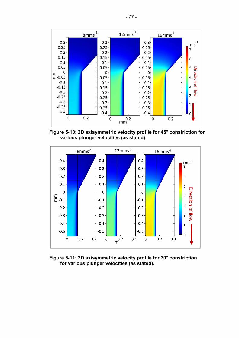
- 77 -

Figure 5-10: 2D axisymmetric velocity profile for 45° constriction for various plunger velocities (as stated).

8mms-1 12mms

-1 16mms

-1

ms-1

mm

mm

Direction of flow

8mms-1 12mms-1 16mms-1

ms-1

mm

m

Dire

ction

of flow

Figure 5-11: 2D axisymmetric velocity profile for 30° constriction for various plunger velocities (as stated).

- 78 -

5.3.3. Pressure profiles for reduced-angle constrictions

Figure 5-12 and Figure 5-13 show the pressure contour plots for capillary

inlet angles of 45° and 30°. Plunger velocities of 8, 12, and 16 mms-1 are

plotted.

8mm/s 12mm/s 16mm/s

mm

mm

Direction of flow

kPa

Figure 5-12: 2D axisymmetric pressure profile for 45° constriction for various plunger velocities (as stated).

8mm/s 12mm/s 16mm/s

mm

mm

Direction of flow

kPa

Figure 5-13: 2D axisymmetric pressure profile for 30° constriction for various plunger velocities (as stated).

- 79 -

5.3.4. Strain rate profiles for reduced-angle constrictions

Figure 5-14 and Figure 5-15 show the strain rate contour plots for capillary

inlet angles of 45° and 30°. Plots were produced for inlet velocities of 8, 12,

and 16 mms-1.

As with the 90° constriction, strain rate is highest in the corner that forms the

capillary inlet. Maximum strain rates in this area are ~20% lower for the 45°

angled constriction when compared with the 90° constriction in Figure 5-8.

Maximum strain rate at the corner of the capillary inlet are ~40% lower for the

30° angled constriction when compared with the 90° constriction in Figure 5-8.

High strain can be seen at the angled inlet wall which increased with velocity.

- 80 -

8mms-1 12mms-1 16mms-1

s-1

mm

mm

Dire

ction

of flow

Figure 5-14: 2D axisymmetric strain rate profile for 45° constriction for various plunger velocities (as stated).

8 mms-1 12 mms-1 16 mms-1

s-1

mm

Dire

ction

of flow

Figure 5-15: 2D axisymmetric strain rate profile for 30° constriction for various plunger velocities (as stated).

- 81 -

5.4. Quantifying strain rate data

A characteristic strain rate should be defined to allow for comparison between

different geometries. The maximum strain rate anywhere in a given field is not

necessarily representative of the strain experienced by the fluid bulk. The

maximum strain rate may occur at a boundary or corner. Due to the nature of

laminar flow, this region of high strain rate will have very low flow rate through,

or near it.

A measure of the maximum strain rate along the centre of the channel is used

as a characteristic strain rate of the device. This would be informative as the

velocity will be at its highest in, and around, this part of the channel, which

would account for the majority of mass transit through the domain. There is

no shear present in this region, nor has the fluid had to deviate far from its

initial direction, resulting in a largely irrotational flow. These make for good

conditions to measure extensional flow. Furthermore, because the current

model is axisymmetric, the centre of the channel lies on the axis of symmetry.

This makes for simple recording of accurate data as the fluid properties are

easily accessible at the boundaries with minimal post-processing.

5.4.1. Strain rate as a function of displacement

It is clear from the work presented in this chapter that analysing strain rate

and its effects requires a well-defined method in order for multiple geometries

or devices to be examined and compared. It would not be appropriate to

simply take the maximum reported strain rate from a CFD post processor as

this is evidenced to occur in some extremity of the flow field in a region of

small mass flux which would have little to no bearing on the response of the

fluid bulk. It is also the case that such high strain rates in extremely localised

regions are often numerical artefacts, the products of approximate velocity

gradients at imposed boundary conditions.

It would be possible to define a characteristic strain rate as the strain rate

associated with a region of high volumetric flow rate or a mass transit

weighted-average across a particular cross-section. A method for calculating

this is discussed in a later section.

- 82 -

For the current work a characteristic strain rate is taken as the maximum strain

rate experienced along a streamline located on the axis of rotational

symmetry. This was chosen because the flow through this region is irrotational

and void of shear effects. The average velocity along the axis is also higher

than for any other region in the domain, indicating that acceleration, and

therefore strain, will be present and predictable. The axis of symmetry also

corresponds with a domain boundary on the model, which allows for

straightforward data extraction without complex post-process manipulation.

Figure 5-16 shows a graph of total velocity (u) plotted against displacement

along the device in the z-direction (Sz). As the flow is laminar along an

axisymmetric geometry, the fluid along the centreline does not vary from a

straight path and so total velocity is equal to the x component of velocity only

(u = uz). The strain rate along this same streamline is plotted below, also with

respect to Sz. Strain rate is proportional to acceleration and so the magnitude

of strain rate is seen to map the gradient of velocity. The maximum strain rate

along the axis of symmetry occurs when the velocity gradient (i.e. the

acceleration) is greatest. This will be referred to as the characteristic strain

rate here-in.

- 83 -

Figure 5-16: i) Schematic of flow profile with contraction located the Z = 0 coordinate. ii) Velocity and strain rate profile in the z-direction for a 90° contraction with plunger velocity 8 mms-1. The velocity profile along the axis of symmetry in the z-direction is plotted in blue (measured against the left axis) whilst the corresponding strain rate along the axis is plotted in orange (in relation to the right axis). The horizontal axis measures the distance from the capillary inlet with the positive direction indicating the direction of flow (i.e. negative z position represents flow within the syringe barrel immediately upstream of the capillary).

Direction of flow

i)

ii)

- 84 -

5.4.2. Strain rate as a function of plunger velocity

In Figure 5-17 the maximum value of strain rate along the axis of symmetry is

plotted against plunger velocity. The characteristic strain rate increases

linearly with plunger velocity, producing values in excess of 104 for plunger

velocities above 6 mms-1. This is compared to the characteristic strain rate

verses plunger velocity for the two reduced angle inlet geometries. As

expected, a reduction in strain rate is observed with decreasing inlet angle.

Figure 5-17: Characteristic strain rate plotted for constriction angles of 90°, 45° and 30°.

5.5. Transition from extension- to shear-dominated flow

Shear invariably plays an integral role in any laminar flow regime. With regard

to this, it is important to investigate shear in this device. In order to understand

shear, the velocity profile will be analysed. In a converging extensional flow

regime, there is an overall acceleration in the fluid bulk as the mass flow rate

must be conserved. It is also known that laminar flow through a capillary is

expected to generate a familiar parabolic velocity profile with respect to radial

position 𝑆 . These two effects are, however, contradictory as upstream of the

constriction the fluid which must be travelling at the highest velocity is that

which is located at greater values of 𝑆𝑟. This discrepancy results in a

transitionary phase at the capillary inlet where a fluid is initially seen to be

- 85 -

travelling faster nearer to the wall. This results in a region where shear is

higher than that which is expected in an established capillary flow.

Figure 5-18 shows the radial velocity profile at the capillary inlet for various

plunger velocities. For a plunger velocity of 2 mms-1 there is a subtle increase

in velocity with radial displacement before velocity gradually curves off to zero

at the boundary. With increased plunger velocity, the gain in fluid velocity with

radial displacement becomes more apparent. The reduction to zero at the

boundary also becomes steeper. This is evident of high shear.

Figure 5-18: Absolute velocity U profile with respect to radial displacement from the axis of symmetry at the capillary inlet, given for increasing values of upstream velocity U∞.

Figure 5-19 takes a plunger velocity of 8 mms-1 and measures the resulting

radial velocity profile at various positions along the capillary. The graph shares

one set of data with Figure 5-18; plunger velocity of 8 mms-1 at Sz = 0 mm.

It can be seen from Figure 5-19 that at the entrance to the capillary, the highest

velocity fluid, travelling at 2.3ms-1, is located over 0.13 mm away from the axis

where fluid is only travelling at 1.8ms-1. This discrepancy is seen to reduce as

fluid travels along the capillary, and the no-slip condition begins to exert its

- 86 -

influence. As the fluid travels through the first 0.2mm, the discrepancy

between velocities at the axis and near the boundary reduces. After the fluid

has travelled 0.2mm along the capillary, it can be seen that the fluid located

at the axis now has the greatest velocity. Shear forces are now dominating

the flow regime. It is not until 4mm along the capillary, however, that a truly

parabolic velocity profile has developed.

Figure 5-19: Absolute velocity U profile with respect to radial displacement from the axis of symmetry Sr taken at incremental distances (given in legend) from the capillary inlet. Average inlet velocity U∞ = 8 mms-1. Sr = 0 lies on the axis of symmetry, and Sr = 0.15 indicates the capillary wall.

Figure 5-20 shows the radial velocity profile immediately after capillary inlet at

distances 0, 0.4 and 4 mm following (i) 45° and (ii) 30° inlet angle. For 45°, at

0 mm the velocity highest velocity fluid, located near the wall at 𝑆𝑟 = 0.125 is

2.198 ms-1 and the velocity at the axis is 0.185 ms-1, whereas, for 30° the

respective velocities are 2.133 ms-1 and 0.191 ms-1. The percentage

disparities between 45° and 30° with respect to 90° maximum and axis flow

velocities are 7.66% and 10.9% respectively.

- 87 -

Examining the velocity profile for the inlet, shown in Figure 5-19 at 0mm, it is

seen that the highest velocity flow 𝑢0𝑚𝑎𝑥 = 2.198𝑚𝑠−1is located at 0.125𝑚𝑚

from the axis. The velocity at the axis is 𝑢0𝑟=0 = 0.181𝑚𝑠−1. From Figure 5-19

it can be seen that the important locations are 0mm where the transition phase

begins, 0.02mm where shear begins to dominate and location of maximum

velocity shifts to the axis, and 4mm where the velocity profile takes on the

characteristic parabola and stabilises for the duration of the capillary.

0

1

2

3

0 0.05 0.1 0.15

U (m

s-1)

Sr (mm)

4mm

0.2mm

0mm

Figure 5-20: Radial velocity profile immediately after capillary inlet at distances 0, 0.4 and 4mm following a i) 45° and ii) 30° inlet angle. Flow inlet velocity 8 mms-1. The transition from extension-dominated to shear-dominate regimes produce very similar velocity profiles over the same length scales as for the 90° inlet angle. The only noticeable differences are the maximum and minimum velocities at 0mm.

0

1

2

3

0 0.05 0.1 0.15

U (m

s-1)

Sr (mm)

4mm

0.2mm

0mm

ii)

i)

- 88 -

Interestingly, the distance required for shear to dominate does not vary with

inlet angle or plunger velocity.

It is important to note that these graphs do not start at zero z-displacement.

This is because there is a numerical artefact at the Sz = 0 which produces an

unrealistic spike in shear which is only present for the first 10’s of microns.

The high shear at the inlet is in agreement with the steep velocity profile seen

near the boundary in Figure 5-18. The steady reduction to a constant shear

value with respect to z-displacement is in agreement with the reduction in

gradient of the velocity profiles seen in Figure 5-19.

- 89 -

5.5.2. Stagnation point within the downstream syringe

As this study is aimed at assessing the effects of flow on a biological material,

it is important to note that, in the current study, it is not possible to assess the

state of the material in-situ. This means that the bulk material is required to

experience the entirety of the conditions within the fluidic device before it can

be analysed. Therefore, any other potentially adverse flow conditions need

examined to assess whether they will have any effect on protein stability. One

such region of concern is the fluid exiting the capillary and impacting the

plunger. The following results explore this.

Figure 5-21 shows the development of the flow field in the downstream syringe

as it recedes from the capillary outlet. The flow profile is depicted for a plunger

velocity of 2 mms-1. It can be seen that as the fluid leaves the capillary it

continues in a straight line until it encounters the syringe plunger, where it is

forced to make an abrupt right-angled turn. At this point, a stagnation point

develops.

In Figure 5-22 the same plunger position is repeated for increasing plunger

velocities. It can be seen that the complexity of the flow profile grows with

velocity. This is indicative of the increased energy present in the flow field,

and the growing intensity of the stagnation point with plunger velocity.

As fluid leaves the capillary it is travelling two orders of magnitude faster than

anything else in the region, including the receding plunger face. The incoming

fluid forms a jet along the centre of the downstream syringe which impacts on

the downstream syringe plunger, causing it to turn through 90° and flow

radially out toward the syringe walls. The high speed jet flow combined with

the radial flow sets up a series of recirculations driven by viscous interaction.

As the plunger recedes and the cavity volume increases, the elongated

geometry causes the recirculating flow to deform in order to fill the available

space.

As the jet velocity increases with plunger velocity, the kinetic energy drives

stronger recirculations and a second region of recirculation is seen to develop

at the syringe wall. Size and definition grow with increased plunger velocity.

- 90 -

When the plunger in the downstream syringe is near the capillary outlet, this

effectively causes a second extensional flow region around the stagnation

point which has formed on the on the plunger face exactly opposite the

capillary outlet. The phenomena can be thought of as a fluid jet meeting a

perpendicular, flat target.

- 91 -

Figure 5-21: 2D axisymmetric streamline plot showing the flow field development as the downstream syringe plunger recedes at 2 mms-1. Measurements are given in mm.

- 92 -

6 mms-1 8 mms-1 4 mms-1 2 mms-1

Figure 5-22: Streamline plots showing the development of the flow fields for various plunger velocities for a given downstream plunger position (60 mm).

- 93 -

mm

ms-1

Dire

ction

of flow

Figure 5-23: 2D axisymmetric velocity profile of the jet of fluid leaving the capillary outlet and impacting the downstream syringe plunger, before turning through 90°. In this instance, the downstream plunger is located 5mm from the capillary outlet. Profiles are shown for a range of plunger velocities (as stated).

6 mms-1

16 mms-1 14 mms-1 12 mms-1

8 mms-1 10 mms-1

- 94 -

It is important to note that the streamline positions in Figure 5-25 are

measured in the radial direction at the capillary outlet only. The path naturally

deviates radially up- and downstream of this point. For the transitory

extensional flow region, maximum strain rate is shown to increase with

distance from the axis. For the stagnation point region, maximum strain rate

decreases with distance from the axis. The intensity of strain around the

stagnation point also decreases universally as distance from the outlet jet

increases.

By comparing the flow rates at varying distances from the axis, it can be seen

that the highest throughput occurs at 1 mm from the origin. Stagnation strain

rates drop below transitory strain rates universally for radii greater than 0.06

mm. This accounts for approximately 67% of the flow at any given time. For

downstream plunger distances within 8 mm of the outlet jet, 27.9% of fluid

experiences greater strain at the stagnation point than through the transitory

m

m

Dire

ction

of flow

8 mms-1 10mm s-1 12 mms-1 14 mms-1 16 mms-1

Figure 5-24: 2D axisymmetric strain rate profile of the jet of fluid leaving the capillary outlet and impacting the downstream syringe plunger, resulting in the formation of a stagnation point. In this instance, the downstream plunger is located 1 mm from the capillary outlet. Profiles are shown for a range of plunger velocities (as stated).

s-1

- 95 -

extension region. This drops to below 3.3% for distances of 16 mm as shown

by the graph in Figure 5-25.

Figure 5-25: A comparison of the maximum strain rates experienced by a fluid particle as it travels along a streamline that passes through the capillary inlet at a given radial position. The particle experiences a transitory strain rate as it passes through the extensional flow region, and a stagnation strain rate as it passes near to stagnation point on the downstream plunger. The maximum stagnation strain rates are given for varying distances of downstream plunger. Inlet velocity generated by the upstream plunger moving at 8 mms-1.

- 96 -

6. Experimental Design, Methods and Materials

In the preceding chapters a computational study was described drawing on

previous literature and fluid dynamic theory. The computational model

explored the effects of extensional flow in an axisymmetric geometry with a

step constriction, together with investigating the effects of angled constrictions

with angles of 45° and 30°. The purpose of these studies was to assess the

validity of an experimental setup capable of exposing protein in solution to an

extensional flow field, and to allow an assessment the effects of extensional

flow on protein aggregation. To do this, the presence of other flow

characteristics were also documented; (i) the presence and magnitude of

shear, (ii) the transition of extension to shear and (iii) the presence of a

stagnation point in the downstream syringe barrel.

From these simulations, it was possible to produce a methodology for testing

the effects of extensional flow on protein aggregation, taking into account

other factors present in the flow.

To achieve this, the development of a bespoke extensional flow cell is

presented in this chapter. This will include the production of a specification

which is used to further analyse existing methodologies from previous studies.

Using the information from this methodology review, combined with data

presented in the computational results chapter, a bespoke flow-cell is

designed. The design includes a mechatronic control strategy as well as

mechanical and fluid mechanical consideration.

A standard procedure for using the device is explained in order to remove a

degree of experimental error. This includes details about assembly as well as

sample loading and unloading. The formulation of samples is detailed for each

protein.

A plan of experiments is also presented in this chapter. This includes a

justification for each test case. The plan includes a series of experimental

controls. These were included to satisfy the requirement of decoupling strain

from shear and downstream factors.

- 97 -

The techniques used for measuring and characterising the magnitude of

aggregation are then be described.

6.1. Design of experimental equipment

A method of subjecting soluble protein to clearly defined flow fields was

required for the current work. The method had to satisfy a number of

requirements in order to be scientifically relevant and practically justifiable.

Several previous methods have been reviewed in earlier sections in terms of

the work produced; what follows is a brief review of these methods in terms of

specification in order to assess their viability to the current work.

6.1.1. Design Scope

The design scope of the experimental methodology is explained here. Design

scope is used to define exactly what areas were to be investigated and by

what means. In the Literature Review section a formal research proposition

was presented. This section is aimed at adding the necessary boundaries and

restrictions around that to give the research a defined focus.

As previously stated, this work was concerned with the contentious topic

around the effects of extensional flow on proteins. Experimental equipment

and methodologies were designed in keeping with previously presented

computational studies. A design specification was developed, with the

originality of the specification being validated against previous work.

Equipment and methodologies proposed took into account the complex nature

of fluid mechanical theory and drew upon the results of the computational

study. The equipment and methods inevitably had limitations; these were

understood, discussed and mitigated wherever possible. A selection of

proteins was made for experimentation; these included well documented

proteins which have been used in previous studies as well as clinically

relevant proteins so as to provide correlation with the biopharmaceutical

industry. Methods of analysing and characterising protein aggregation ex-situ

were defined and used. Experiments were carried out using the bespoke

equipment and samples were characterised using the proposed methods. The

current method does not include a process for characterising the unfolding

- 98 -

and aggregation process in real-time within the flow cell. Nor did the current

method work toward integration within an ‘online’ characterisation technique.

The current work did, however, draw conclusions from the ex-situ results as

the nature of aggregation pathways within the device. Potential methods and

benefits of in-situ and online characterisation techniques were addressed as

a topic of potential future study.

6.1.2. Device Specification

Presented in this section is a table of requirements for the current method.

Each specification point is presented in terms of a parameter, the

requirements of that parameter, and a justification for the stated requirements.

Definitions of the parameters can be found in the Theory section.

Parameter: an experimental control, a variable, or a dependent which can be

held constant, adjusted, or measured as part of the experimental method.

Requirement: the limits of the parameter which were deemed acceptable to

the experimental method.

Justification: the argument as to why a parameter has be specified to fall

within defined values.

The flow profile had to contain an extensional, strain-dominated region

capable of producing a strain-rate in the magnitude of ≥104 s-1. This value is

typical of shear- and strain-rates presented in previous work [2, 4, 24, 79] as

well as the forces present in manufacturing equipment [118-122].

The maximum Reynolds Number (Re) had to be no greater than Re = 3000.

This number represents the upper bound of a fully laminar flow regime and

laminar flow had to be maintained so as to allow for accurate tracking of

streamlines for statistical analysis.

The current work also had to include a technique to vary strain independently

of shear. This was necessary because shear is present in all extensional flows

and has previously been presented as a major contributor to protein

aggregation.

The experimental flow method had to limit sample exposure to gas-liquid

interfaces during setup and sample recovery, and remove all such interfaces

- 99 -

during flow cell operation. Gas-liquid interfaces are well documented in

producing the necessary surface energies to unfold a protein [123] and as

such, should not be present in a purely fluid mechanical study.

The proposed method had to be fully repeatable with flow rates and sample

volumes being precisely controlled. Strain and shear magnitudes are often

coupled to flow rate such that accurate control over the device speed will allow

for detailed mapping of aggregation response against fluid force.

Protein samples had to only come into contact with materials which were

chemically inert and hardened against polymer leaching. Failure to achieve

this may result in proteins adhering to surfaces within the flow cell and change

the surface energy, resulting in increased aggregation propensity.

The method requires a sample volume in the region of 0.5 – 1 ml per

experiment with a protein concentration in the region of 0.5 – 10 mg·ml-1.

Experimental therapeutic antibodies are often expensive and time consuming

to produce prior to plant-scale production. As such, a flow device aimed at

pre-upscale analysis had to be sympathetic to these limitations.

The method had to allow for exposure time to extensional flow to be varied

experimentally without the need to expose the sample to other factors such

as external materials, gas-liquid interfaces or long periods of time between

exposures. Such factors were likely to affect aggregation propensity and had

to be excluded from test procedures. The methodology specification is

summarised below in Table 6-1.

- 100 -

Parameter Requirement Justification

Flow Profile

Must have a strain-dominated region within in the flow geometry.

To expose the majority of the fluid sample to predominantly extensional flow.

Reynold’s Number

Laminar; typically, Re <3000 A development on the previous point; Re further defines the flow profile.

Strain rate ≥ 104 s-1 Industrial processes often produce strain values of this magnitude [118-122].

Shear dependence

The ability to modify the amount of extension without changing shear

To demonstrate shear independent aggregation.

Liquid-gas interfaces

Must be limited during setup with minimal agitation during sample loading. No liquid-gas interfaces should be present during flow-cell operation.

Interfacial phenomena introduce surface energies which are capable of inducing aggregation.

Repeatability Must have a control system that allows for precise control of flow rate across multiple experiments.

To ensure repeatability and direct comparison between experiments.

Materials Must be chemically inert and resistant to leaching.

To reduce the addition of interfacial effects into the flow profile results.

Sample volume

0.5 ml < Volume < 1 ml per experiment.

Sample size is restricted by cost of pharmaceutical antibodies as well as characteristic techniques which require a minimum volume.

Exposure time or exposure counts

Flexible without exposing sample to gas interfaces/ external materials or factors

To allow exposure time to be used as an experimental control without the addition of other external factors which may also lead to aggregation.

Table 6-1: Design specification matrix for the experimental method

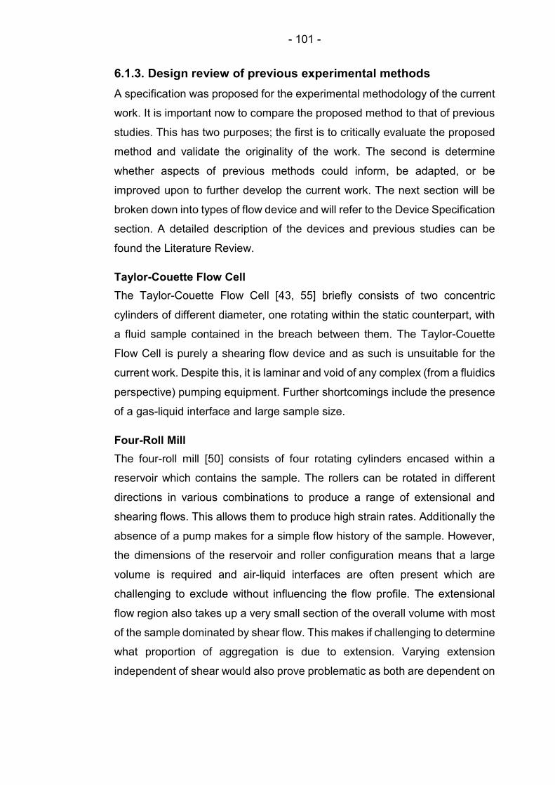
- 101 -

6.1.3. Design review of previous experimental methods

A specification was proposed for the experimental methodology of the current

work. It is important now to compare the proposed method to that of previous

studies. This has two purposes; the first is to critically evaluate the proposed

method and validate the originality of the work. The second is determine

whether aspects of previous methods could inform, be adapted, or be

improved upon to further develop the current work. The next section will be

broken down into types of flow device and will refer to the Device Specification

section. A detailed description of the devices and previous studies can be

found the Literature Review.

Taylor-Couette Flow Cell

The Taylor-Couette Flow Cell [43, 55] briefly consists of two concentric

cylinders of different diameter, one rotating within the static counterpart, with

a fluid sample contained in the breach between them. The Taylor-Couette

Flow Cell is purely a shearing flow device and as such is unsuitable for the

current work. Despite this, it is laminar and void of any complex (from a fluidics

perspective) pumping equipment. Further shortcomings include the presence

of a gas-liquid interface and large sample size.

Four-Roll Mill

The four-roll mill [50] consists of four rotating cylinders encased within a

reservoir which contains the sample. The rollers can be rotated in different

directions in various combinations to produce a range of extensional and

shearing flows. This allows them to produce high strain rates. Additionally the

absence of a pump makes for a simple flow history of the sample. However,

the dimensions of the reservoir and roller configuration means that a large

volume is required and air-liquid interfaces are often present which are

challenging to exclude without influencing the flow profile. The extensional

flow region also takes up a very small section of the overall volume with most

of the sample dominated by shear flow. This makes if challenging to determine

what proportion of aggregation is due to extension. Varying extension

independent of shear would also prove problematic as both are dependent on

- 102 -

roller speed. Device geometries would have to be adjustable which introduces

new variables such as sample volume.

Opposed Jets

Opposed jet devices [50] place two nozzles opposite each other and pump a

sample out of both simultaneously such that a stagnation point is formed

where the streams converge. This method can produce very high strain rates.

The sample had to however, be passed through a pump which adds

complexity the flow history of the sample. Large volume reservoirs are also

used the store the sample, making this device unsuitable for the current

method.

Stenotic Indentation Microchannel

The stenotic indentation microchannel [49] is an etched 2D path with a

constriction introduced on one wall. By producing multiple versions of the

geometry, the strain rate is made to vary. Although, in this instance, varying

the constriction size alters the minimum cross sectional area, resulting in

increased strain. The design of the device does lend itself to small sample

sizes. In this instance, the device is driven by a pump, but could be adapted

to run from a syringe driver.

High Viscosity Cylindrical Tubing

By applying a high mass flux across a narrow, constant cross sectional area

[43] a region of high shear can be produced. Although this is a simple shear

device, extensional flow could be achieved with a modified flow geometry.

Noteworthy aspects of this device include the cylindrical cross section which

is conducive of a laminar flow regime, and the potential for a small sample

size. This device does require an external pump, although it could also be

adapted to use a syringe driver.

Etched Elongational Microchannel

Etched elongational microchannels [9] are microns-deep pathways sintered

into PEEK or glass substrate. Such devices can produce complex geometries,

and as such can be used to develop varying degrees of extensional flow

independent of shear. The dimensions involved also accommodate for small

- 103 -

sample sizes. The flow cell does, however, require the use of a pump and

lengths of tubing for the sample to be driven through the device. The

manufacturing technique of these devices also limits the cross sectional shape

to a rectangular form. This could complicate the flow profile, and increase

modelling and simulation time. Following this review of currently available

defined flow field devices, it is clear that the requirements of this work are not

met by previous methods.

A summary of the specifications of the above devices is presented in Table

6-2. It is worth noting that some factors, such as pumps, are external to the

devices themselves and could potentially be mitigated with the correct choice

of external factors, but this is beyond the scope of the current work.

- 104 -

Device/ method Satisfies specification Fails specification

Taylor-Couette flow cell [43, 55]

- Low Reynolds number; typically, in the region of 330-1618.

- Flow cell is self-contained with no pumps.

- Capable of high shear rates.

- Air-liquid interface present in the flow cell.

- Not possible to vary strain rate independent of shear rate.

- 390ml per sample, although smaller cells could be adapted from this method.

Four-roll mill [50]

- Strain rate up to 15x103. - Flow cell is self-contained

with no pumps.

- Air-liquid interface present in the flow cell.

- Large volume. - Residence time dependent

on location relative to stagnation point.

- Large amount of dead space in reservoir around rollers.

Opposed jets [50]

- Strain rate up to 15x103. - Hydrophobic siloxane to

prevent sample adsorption.

- Fluid moved through device via a pump.

- Large volume stored in two reservoirs with air-liquid interfaces.

PDMS Stenotic indentation microchannel [49]

- Variable strain rate independent of shear by changing flow cell geometry.

- Small sample size.

- High shear and complex flow profile due to shallow channel.

- Driven by a pump.

High viscosity cylindrical tubing [43]

- Simple, cylindrical flow profile.

- Small sample requirement.

- Driven by a pump - other features present which

are not accounted for, i.e. contractions and nozzles.

- No function to vary strain rate independent of shear.

Etched elongational Micro-channels [9]

- Small sample sizes. - Various geometries allow

for strain rate to be varied independent of shear.

- Requires a pump or syringe to drive fluid across the flow cell.

- Shallow, rectangular cross section produces high-shear, complex flow profile.

Table 6-2: Design review summary of previous methods

- 105 -

Arising from this study was the requirement for a method of producing the

pressure differential required to drive a flow cell without introducing the

complex flow regimes associated with pumps. Atkins & Taylor [50] drive an

opposed jets apparatus with a peristaltic pump which at low speeds would

maintain the laminar low in a tube, but still required a reservoir which reduces

the certainty of flow history across the whole sample.

Smaller samples with exact precise flow histories could be achieved using a

syringe driver attached to a flow cell. But again, the sample would likely pass

through a series of high-shear tubes or expanding - contracting regions before

reaching the flow cell. After traversing the flow cell the sample would then

have to be collected. This would be challenging without exposing the sample

to a liquid-gas interface.

A concept for an extensional flow device is presented in the following sections

taking into account these considerations.

6.1.4. Design of Experimental Equipment

A solution to the specification laid out for this experiment will now be

presented.

Initial concept

It was proposed that two opposing syringes mated by a single glass capillary

and driven by a bespoke syringe pump would satisfy the specification

requirements. A schematic of the initial concept can be seen in Figure 6-1.

The solution was loaded into one syringe through the capillary by means of

drawing up the syringe plunger. The free end of the capillary was then

attached to the nozzle of a fully depressed syringe and sealed. This ensures

all gas was expelled from the system. The sudden reduction in cross-sectional

area between the syringe barrel and the capillary produces the abrupt

contraction necessary to induce extensional flow as discussed in the Theory

chapter.

The opposed syringes were then be placed in a bracket which will hold the

syringes at a fixed distance apart while the plungers were driven by a

computer-controlled actuator. This ensures accurate and consistent speed.

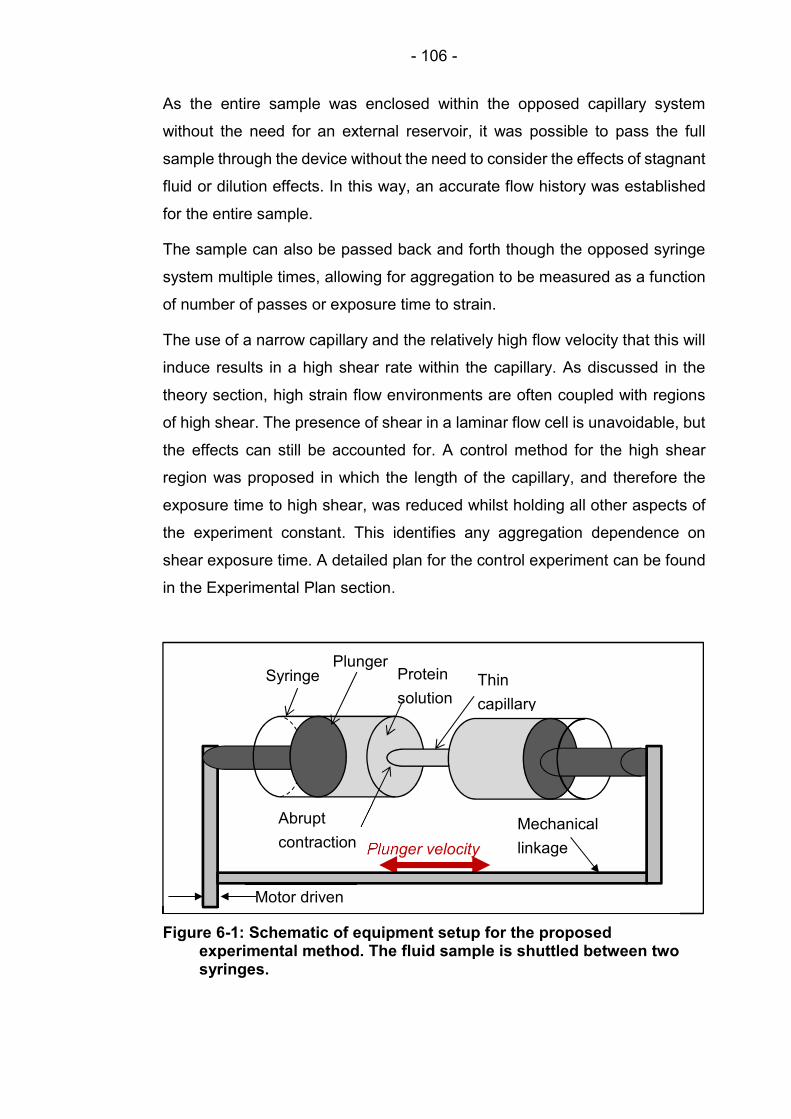
- 106 -

As the entire sample was enclosed within the opposed capillary system

without the need for an external reservoir, it was possible to pass the full

sample through the device without the need to consider the effects of stagnant

fluid or dilution effects. In this way, an accurate flow history was established

for the entire sample.

The sample can also be passed back and forth though the opposed syringe

system multiple times, allowing for aggregation to be measured as a function

of number of passes or exposure time to strain.

The use of a narrow capillary and the relatively high flow velocity that this will

induce results in a high shear rate within the capillary. As discussed in the

theory section, high strain flow environments are often coupled with regions

of high shear. The presence of shear in a laminar flow cell is unavoidable, but

the effects can still be accounted for. A control method for the high shear

region was proposed in which the length of the capillary, and therefore the

exposure time to high shear, was reduced whilst holding all other aspects of

the experiment constant. This identifies any aggregation dependence on

shear exposure time. A detailed plan for the control experiment can be found

in the Experimental Plan section.

Plunger velocity

Syringe Plunger

Protein

solution Thin

capillary

Abrupt

contraction

Figure 6-1: Schematic of equipment setup for the proposed experimental method. The fluid sample is shuttled between two syringes.

Motor driven

Mechanical

linkage

- 107 -

The capillary length control experiment answers the question of shear

exposure, but does not cover the topic of magnitude. I.e. is aggregation

triggered by a particular value of shear or strain rate irrespective of exposure

time? To explore this an experiment was proposed which varies the geometry

of the inlet angle of the contraction from the syringe barrel to the capillary. To

do this, a series of bespoke capillary sections were manufactured with angled

nozzles at either end resulting in a gradual reduction in the flow profile cross-

sectional area. If the length of the capillary section and flow rate remain

constant, the maximum shear value will stay the same whilst the various

angles will give different maximum strain-rate values. This identifies whether

aggregation increases with strain-rate in the presence of constant shear. The

design of these parts is presented in the Computer Aided Design section of

this chapter, the experiment itself is explained fully in the Experimental Plan

section.

With the use of a computerised control system, the effects of flow rate can be

explored with high accuracy. The higher plunger velocities results in higher

strain and shear values which were correlated against aggregation propensity.

The control system will be discussed in the Control theory section.

Open-Source and Off-The-Shelf Equipment

Off-the-shelf (OTS) components have the advantage over custom

components in that they are readily available, produced to predetermined

standard, and require only a working understanding of the part by the user.

The disadvantage of OTS is that the component specification is often based

on a generic case. This means that the most suitable OTS part will likely be in

excess of the assembly specification requirement, or may even drive the

assembly specification. A compromise can be found in the after-market

modification of OTS components, though it is advisable to limit the complexity

of after-market modifications.

Open-source often refers to software which is released for public use as well

as further development. It also refers to component design. For instance, the

design of programmable logic controllers (PLC), microcomputers, and other

areas of mechatronics. The value of open-source electronic hardware design

- 108 -

is in the availability of low-cost products which have had countless human-

hours of development, accompanied with many readily available examples of

how best to use such products.

Syringes

A critical part of the design of the rig was the syringes. The syringes were

required to be gas-tight, but with low a low-friction plunger. The materials had

to also be chemically inert.

The syringe chosen for this was the 1 mL model 1001 RN Valco gastight

syringe produced by Hamilton Syringes. The syringe has a 1 mL capacity and

a 4.61 mm inner barrel diameter. The fluid path within this syringe encounters

borosilicate glass and a PTFE coated syringe plunger [124]. The orifice

diameter was enlarged to take a 1 mm outer diameter borosilicate capillary.

Capillaries

Once a syringe has been selected, a capillary can be selected based on the

relative diameter. The material should be chemically inert with a smooth finish.

Borosilicate glass is a common material for laboratory glassware due to its

high thermal shock resistance and, more importantly in this application, its

high chemical stability and resistance to leaching [125]. A borosilicate capillary

of length 75 mm, outer diameter 1 mm and inner diameter 0.3 mm was

selected. This produced a reduction in cross sectional area with a ratio of

238:1.

To form a seal around the capillary, a 1 mm compression fitting, Hamilton

55750-01, consisting of a stainless steel nut, a PEEK cup ferrule and a PFA

cone ferrule were used to secure the capillary to the syringe.

Mounting Board

To secure the two syringes in place, a Thor Labs aluminium optics

breadboard, MB1560/M, dimensions 150 mm x 600 mm x 12.7 mm was

selected. A Thor Labs dovetail optical rail, RLA300/M, with two extended

dovetail rail carriers, RC2/M, were used to locate the syringes. The syringes

were clamped in place with two small V-clamps with clamping arm, VC1/M

and PM3/M respectively. This assembly can be seen in Figure 6-2.

- 109 -

Bespoke Syringe Driver

In order to drive the syringe plungers in both directions, a bespoke syringe

driver was integrated on to the mounting board. The syringe driver requires a

linear actuator which is covered in the Control theory section, and a purpose-

designed bracket to connect the linear actuator to both syringe plunger which

is covered in the Computer Aided Design section. The syringe driver also

requires a linear rail to ensure that all motion was constrained to a single

direction. To achieve this, an NSK PU series, linear guide rail,

P1U090600SKN-PCT, was mounted to the optics board. Two corresponding

NSK linear guide carriages, PAU09TRS, were selected to connect the plunger

brackets to the rail.

Computer Aided Design

Computer aided design (CAD) was used to design the bespoke parts

necessary for the current work. These include the brackets used to mount the

syringe plungers to the linear actuator and linear rail, and the varied angle

contractions.

Optics breadboard

Dovetail rail

Dovetail rail carrier

V-clamp

Figure 6-2: CAD image showing location of dovetail rail, rail carrier and V-clamps on Thor Labs optics breadboard with syringes in place for reference.

- 110 -

Bracket Design

A bracket was required to transmit the work done by the linear actuator to the

syringe plunger. Both syringes were mechanically secured to each other via

a studded steel shaft of 6 mm diameter. The bracket was secured to the shaft

using a grub screw. Four screws mount the brackets to the linear carriages. A

threaded hole allows for the drive nut on the linear actuator to attach to the

bracket. The syringe plunger was secured by clamping the handle between a

flat plate and two prongs. The brackets was machined from stock aluminium.

An image of the model can be seen in Figure 6-3.

Angled geometry design

The method requires a device that can vary strain rate independently of shear.

This was achieved by removing the end from a pair of syringes to produce a

straight, glass tube, and designing a series of fitted funnels to attach the two

syringes together. The funnels all have different contraction angles but share

the same capillary diameter and length.

The first design for an angled flow geometry, shown in Figure 6-4(a) used an

interference fit and was dependent on the firm clamping of the two opposed

Location for shaft

connecting two

brackets

Mounting points for

linear carriage

Location for

lead screw nut

Grub screw to

secure connecting

shaft

Syringe plunger

handle clamped

between plate

and prongs

Figure 6-3: CAD image of bracket designed the secure the syringe plunger to the linear carriage and transmit the work done by the linear actuator to the plungers

- 111 -

syringes to form a seal. The material chosen was nylon. The part was

machined from stock bar. The capillary was drilled using a precision 0.3mm

cutter. The fine diameter of the cutter limits the length of the capillary section

to 12mm. This was considerably shorter than the capillary proposed for the

abrupt contraction experiments so a control piece with a right-angled, abrupt

contraction was proposed to be manufactured in the same fashion.

The interference fit did not provide an adequate seal, however the material

and flow channel cutting techniques were both successful and were carried

forward onto the next design.

A clearance was added between the interior wall and the capillary, as seen in

Figure 6-4(b-i) and a flexible PTFE ferrule was added to the end of the syringe.

A thread was cut into the wall and a collar with a corresponding thread was

added to a pipe fitting. As the pipe fitting was screwed into the nylon section

the PTFE ferrule deforms and grips to the syringe, producing a seal, Figure

6-4b-ii).

6.1.5. Control theory

With the flow-cell fully defined, a suitable actuator and control system needs

to be developed. The actuator requires between 50 and 120mm of linear

Figure 6-4: Designs for an angled contraction. a) used an interference fit to form a seal. b) used a threaded collar section to compress a PTFE ferrule to form a seal. b-i) shows half of the angled section with the threaded attachment and modified syringe in place. the cut-through in b-ii) shows the location of the PTFE ferrule.

a)

b-ii)

b-i) 0.3 mm capillary

Angled contraction

PTFE ferrule

Threaded collar

- 112 -

motion, with enough force to drive the fluid in the plunger through the narrow

constriction as well as overcome the friction of the two plungers. The linear

actuator had to also produce the motion in a consistent and repeatable

fashion, including acceleration and deceleration at the end of each pass. The

distance travelled in each pass had to also be identical.

Linear actuators

Linear actuators are available in many forms such as electric, pneumatic,

hydraulic or a combination of these [126]. Pneumatic linear actuators provide

fast motion over an accurate displacement but are not good for controlling

speed. Hydraulic actuators provide good speed control and accurate motion

but are designed for application requiring large amounts of force and often

require complex ancillaries such as fluid reservoirs, accumulators and pumps.

Electric linear actuators have been designed for a wide range of applications

with most using a brushless motor to drive a leadscrew. The simplest way to

drive an electric linear actuator is to do so without sensor feedback, requiring

a highly accurate motor. This was best achieved with a stepper motor.

Stepper motors

A stepper motor is a brushless DC electric motor designed for applications

requiring precise angular positioning and velocity. Stepper motors typically

have slow rotational speeds with high holding torque. Precise motion was

achieved using a high number of permanent magnets and coils which allow

the motor to be actuated and held to an accuracy typically of 1.8°. This

resolution can be increased to 0.35° at the cost of reduced angular velocity

and holding torque.

The rotational motion of a stepper motor was transmitted to a linear actuator

with a studded lead screw. The pitch of the lead screw determines the linear

velocity of the actuator, with higher velocities delivering reduced driving force.

The stepper motor used was the Haydon E28H4. The motor has a step angle

of 1.8° which corresponds to 225 steps per revolution. The lead screw has a

thread pitch of 2.8125mm. This translates to a linear displacement of

0.0125mm per 1.6° step. In order to drive the syringe plunger at 8mms-1, for

example, the stepper motor must rotate 1024° which requires 640 steps.

- 113 -

A stepper motor is a permanent magnet electric motor designed for highly

accurate rotational speed and position. There is a compromise between speed

and accuracy, as well as speed and power.

No. Steps per second

Plunger velocity/ x10-3 ms-1

Average capillary flow velocity/ ms-1

Flow rate/ mls-1

640 8 1.889 0.134

800 10 2.361 0.167

960 12 2.834 0.200

1120 14 3.306 0.234

1280 16 3.778 0.267

Table 6-3: Stepper motor relation to flow velocity

Integrated micro-controllers

A computer system was required to control the stepper motor that powers the

linear actuator. The system selected for this was that Arduino Uno R3. The

Uno is an open source, single board microcontroller [127]. It has a single

16MHz 8-bit ATmega328/p processor with 32 KB of flash memory [128], 14

digital input/output pins and a maximum operating voltage of 20 V [129].

The microcontroller controls the stepper motor through a stepper motor driver

board. The driver board used here was the EasyDriver Stepper Motor Driver

v4.3 [130]. The driver board connects to a 4-wire bi-polar stepper motor,

converting a digital 5 V pulse signal from the microcontroller to precise

rotational motion. The driver board requires a 6 – 30 V power supply, and so,

can share a 20 V bus with the Uno R3.

6.2. Final specification of experimental equipment & method

of use

6.2.1. Experimental equipment

The final specification has been modelled in CAD in Figure 6-5. The position

of the two syringes can be adjusted using the dovetail rail. This allows for

shorter capillaries to be fitted as well as modified syringes with bespoke flow

geometry connectors.

- 114 -

The placement of the stepper motor with lead screw allows for the full bore of

the syringe to be utilised, giving a maximum sample volume of 1 ml.

The linear rail with carriage system counteracts the torque from the stepper

motor to effectively convert the rotational motion into a smooth linear motion

with enough force to drive the syringes.

6.2.2. Method

The capillary was fitted to a single syringe using a compression fitting. The

protein solution was drawn into the single syringe very slowly by hand through

the capillary so as not to damage the protein prematurely. The loaded syringe

was then positioned in a V-clamp and the empty syringe was placed in the

opposite V-clamp with the plunger full depressed. A second compression

fitting was used to secure the empty syringe to the capillary, forming a gas-

tight seal.

The microcontroller was then programmed to move a set linear distance at a

constant speed with a small acceleration time so as to fully depress the

plunger of the loaded syringe, transporting the entire sample to the second

syringe via the capillary and the extensional flow region. The syringe plungers

were linked hydraulically through the protein solution such that, as one syringe

plunger was depressed, the fluid forces cause the other to be expelled from

Figure 6-5: A computer model of the experimental rig configured for extensional flow using glass capillaries

- 115 -

its syringe jacket. The syringes were flushed with 2 % (v/v) Hellmanex-III

solution and MilliQ-grade H2O prior to each run, followed by a final wash with

0.22 µm-filtered (Merck Millipore) and de-gassed buffer.

A new capillary was used for each experiment. The capillary was filled with

buffer from the recently washed syringe so as to remove any air. Due to the

dimensions of the capillary relative to syringe, the effect on sample

concentration was negligible.

In using the angled contraction pieces, the same preparation was applied to

the modified syringes. The modified syringes, however, have a wider orifice

allowing for the sample to be pipetted into the barrel with the plunger set to

the correct displacement. The threaded collar was placed around syringe with

the PTFE ferrule located around the end of the syringe. The angled

contraction piece was then screwed in place, compressing the ferrule to form

a seal.

The plunger was compressed allowing the sample to flood the flow cell and

the second syringe was attached with the plunger fully depressed to expel any

air.

6.3. Limitations and considerations

6.3.1. High shear in capillary

It has been stated that the capillary in the device produces a high shear region

which could be contribute to the aggregation of protein. To explore this

possibility, a control experiment was proposed to measure the effects of

capillary length on aggregation.

6.3.2. Geometry accuracy

It was important to draw a comparison between the computer model and the

experimental device in terms of the experimental flow cell geometry. In the

capillary configuration , the 90° step contraction was formed by the edge of

the capillary. The capillaries used in this experiment were etch-cut and fire

finished. This produces a sharp 90° angle with a slight fillet with a radius in

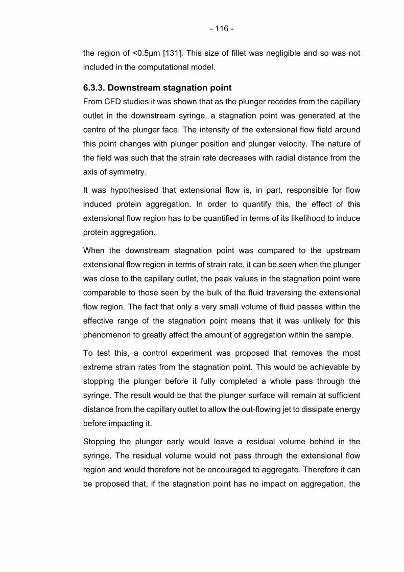
- 116 -

the region of <0.5µm [131]. This size of fillet was negligible and so was not

included in the computational model.

6.3.3. Downstream stagnation point

From CFD studies it was shown that as the plunger recedes from the capillary

outlet in the downstream syringe, a stagnation point was generated at the

centre of the plunger face. The intensity of the extensional flow field around

this point changes with plunger position and plunger velocity. The nature of

the field was such that the strain rate decreases with radial distance from the

axis of symmetry.

It was hypothesised that extensional flow is, in part, responsible for flow

induced protein aggregation. In order to quantify this, the effect of this

extensional flow region has to be quantified in terms of its likelihood to induce

protein aggregation.

When the downstream stagnation point was compared to the upstream

extensional flow region in terms of strain rate, it can be seen when the plunger

was close to the capillary outlet, the peak values in the stagnation point were

comparable to those seen by the bulk of the fluid traversing the extensional

flow region. The fact that only a very small volume of fluid passes within the

effective range of the stagnation point means that it was unlikely for this

phenomenon to greatly affect the amount of aggregation within the sample.

To test this, a control experiment was proposed that removes the most

extreme strain rates from the stagnation point. This would be achievable by

stopping the plunger before it fully completed a whole pass through the

syringe. The result would be that the plunger surface will remain at sufficient

distance from the capillary outlet to allow the out-flowing jet to dissipate energy

before impacting it.

Stopping the plunger early would leave a residual volume behind in the

syringe. The residual volume would not pass through the extensional flow

region and would therefore not be encouraged to aggregate. Therefore it can

be proposed that, if the stagnation point has no impact on aggregation, the

- 117 -

percentage of insoluble aggregate will be linearly proportional to the size of

the dead volume.

6.4. Protein Selection, Specification and Formulation

Credit is due to L. F. Willis and A. Kumar at the School of Molecular and

Cellular Biology, and the Astbury Centre for Structural Molecular Biology,

University of Leeds, for their respective roles in the expression, purification

and formulation of proteins and samples as outlined in the following steps.

6.4.1. Bovine Serum Albumin

Serum albumin is a blood plasma protein produced in abundance by the liver.

In humans, serum album constitutes approximately 50% of all blood plasma

protein [132]. Bovine serum albumin (BSA) is a serum albumin derived from

cows. It is very well documented and understood [133, 134] and has been

used in many previous flow studies [8, 135, 136] making it ideal to test the

effectiveness of the current device.

BSA is predominantly α-helical with 583 amino acids. It has a molecular weight

of 66 kDa and a hydrodynamic radius of 3.5 nm. Figure 6-6 shows the tertiary

structure of BSA.

BSA was purified though a Superdex 200 (26/60) gel filtration column (GE

Heathcare) equilibrated with 25 mM ammonium acetate buffer at pH 5.1 and

stored in aliquots at −20 °C. The protein solution was then concentrated using

Figure 6-6: Bovine serum albumin (BSA) topology diagram from the RCSB Protein Data Bank. ID code 3V03. Hydrodynamic radius of 3.5 nm.

- 118 -

a centrifugal concentrator with a 30kDa cutoff filter (Merck Millipore). The

solution was then filtered through a 0.22μm membrane (Merck Millipore) for

the concentration to be determined using UV spectroscopy. The concentration

was adjusted as necessary for the experiment.

6.4.2. β2-Microglobulin

Human β2-microglobulin (β2m) is a protein found on the surface of all

nucleated cells and platelets in the human body [137]. It is a small protein,

consisting only of 100 amino acids with a molecular mass of 11.86 kDa. It

measures a mere 2.3nm in diameter with a hydrodynamic radius of 1.9 nm

[138]. Figure 6-7 shows the tertiary structure of β2m. β2m is clinically

significant as it is a constituent factor in in the formation of amyloid fibril

aggregates during long-term courses of haemodialysis; a common

complication known as dialysis-associated amyloidosis [139]. Dialysis is the

extraction of whole blood from a patient, to be pumped through a series of

filters, before being returning to the patient. It is therefore, the processing of

biological material with multiple flow profiles resulting in the formation of

unwanted aggregates. Hence, the flow induced aggregation of β2m will be

studied here.

Figure 6-7: β2-microglobulin (β2m) topology diagram from the RCSB Protein Data Bank. ID code: 1LDS. Hydrodynamic radius 1.9 nm.

- 119 -

The expression and purification of recombinant human β2m from a strain of

Escherichia coli and has previously been described [140, 141]. Extensional

flow experiments were performed on β2m in filtered (0.22μm) and degassed

25mM sodium phosphate buffer at pH 7.2 [1].

6.4.3. Granulocyte Colony-Stimulating Factor

Granulocyte colony-stimulating factor (GCSF) is a hormone consisting of 175

residues. It measures 2.5 nm with a molecular weight of 18.8 kDa ad a

hydrodynamic radius of 2 nm [142]. Its role as a hormone is to trigger bone

marrow to produce stem cells and granulocytes, a type of white blood cell.

Pharmacologically, GCSF is used to boost the number of white blood cells in

patients undergoing chemotherapy to counter the effects of reduced immunity

and low for more intensive treatment. Figure 6-8 shows the tertiary structure

of GCSF.

GCSF C3 [143] was overexpressed in BL21[DE3]pLysS cells transformed

with a pET23a_G-CSF C3 vector and purified. The purification method can be

found in the literature [1] and is reiterated below.

Cell pellets were resuspended in lysis buffer (50mM TrisHCl, 5mM EDTA,

2mM phenylmethanesulphonyl fluoride (PMSF) and 2mM benzamidine

hydrochloride hydrate pH 8) at a ratio of 1g of cell pellet to 10mL of buffer and

lysed by 5× 30 second periods of sonication on ice at 75% amplitude, using a

Sonics Vibra-CellTM VCX-130PB sonicator with a 6mm diameter probe.

Inclusion bodies were harvested by centrifugation at 15000rpm, 4°C for 30

minutes, using a Beckman Coulter Avanti J-26 XP centrifuge with JLA 16.250

Figure 6-8: Granulocyte colony-stimulating factor (GCSF) topology diagram from the RCSB Protein Data Bank. ID code: 5GW9. Hydrodynamic radius 2 nm.

- 120 -

rotor. Inclusion bodies were then washed by re-suspending in wash buffer 1

(50mM TrisHCl, 5mM EDTA, 1% (v/v) triton X-100 pH 8) at a ratio of 1g of

inclusion body pellet to 20mL of buffer and harvesting inclusion bodies by

centrifugation as before. This wash step was repeated using wash buffer 2

(50mM TrisHCl, 5mM EDTA, 4M urea pH 8). Washed inclusion bodies were

resuspended in unfolding buffer (50mM TrisHCl, 5mM EDTA, 6M GdnHCl,

10mM DTT pH 8) at a ratio of 1g of inclusion body pellet to 5mL of buffer and

left to agitate overnight. The resuspended pellet was then centrifuged at

15000rpm, 4°C for 1h, using a Beckman Coulter Avanti J-26 XP centrifuge

with JA 25.50 rotor. The supernatant was diluted 1 in 10 with refolding buffer

(50mM TrisHCl, 5mM EDTA, 0.9M L-arginine pH 8) and immediately dialysed

into 5L of 20mM sodium phosphate, 20mM sodium acetate pH 4. After three

dialysis 6 changes refolded G-CSF was centrifuged at 15000rpm for 30

minutes and the supernatant was filtered through a 0.22μm filter. The filtrate

was loaded onto a 5 mL HiTrapTM SP HP cation exchange column (GE

Healthcare) at a flow rate of 5mL min-1 using an Äktaprime plus (GE

Healthcare) system. A gradient of 0-100% elution buffer (20mM sodium

phosphate, 20mM sodium acetate, 1M NaCl pH 4) was then run over 100mL,

with 2mL fractions being collected. Fractions were pooled based on the results

of SDS-PAGE analysis and desalted by dialysis. After desalting, pools were

concentrated using Vivaspin 20 centrifugal concentrators with 5kDa MWCO

PES membrane (Sartorius Stedim) until the protein concentration was approx.

8-10mg mL-1 and snap frozen using dry ice and ethanol for storage at -80°C.

Extensional flow experiments with G-CSF C3 were performed in filtered

(0.22μm) and degassed 25mM sodium phosphate, 25mM sodium acetate

buffer, pH 7.0.

6.4.4. Model Antibodies

Three model antibodies with known, yet varying propensities to aggregation

were supplied by Medimmune. The typical tertiary structure of a monoclonal

antibody is shown in Figure 6-9.

- 121 -

Two proteins were identical to each other with the exception of only six

residues. The antibody designated MEDI1912_WFL was shown to possess

three exposed hydrophobic binding sites at the locations W30 and F31 in the

complementarity-determining region (CDR) -1, and L56 in CDR-2 of each

variable heavy domain. These sites were seen to be largely responsible for

the protein’s high affinity for self-association and aggregation. To alleviate this

effect, the three hydrophobic residues (W30, F31 and L56) were replaced

systematically with other combinations of residues. The variant with the lowest

aggregation propensity, MEDI1912_STT had mutated the tryptophan residue,

W30, with serine, and both the phenylamine and leucine, F31 & L56, with

threonine [144]. Both MEDI1912_WFL and MEDI1912_STT were selected for

extensional flow analysis to determine whether the differing aggregation

affinities of these two proteins could be detected.

The third antibody supplied by Medimmune, designated mAb1, was selected

for its low sequence identity with MEDI1912_WFL. mAb1 was representative

of a protein which has been deemed fit for full-scale manufacture, having

Figure 6-9: Example of a monoclonal antibody topology diagram from the RCSB Protein Data Bank. ID code: 1HZH. Hydrodynamic radius 3.5 nm.

- 122 -

demonstrated greater than 95% monomeric purity post-process and a

degradation rate of less than 2% per year in solution [1, 144].

The three IgGs were prepared by dialyzing into 0.22μm filtered and degassed

150mM ammonium acetate buffer at pH 6.0, and diluting to a concentration of

0.5mgmL-1.

6.4.5. Summary of proteins

The proteins to be used for flow induced aggregation are summarised in Table

6-4.

Protein BSA mAbs GCSF Β2m

Amino Acids 583 ~1400 175 100

Molecular weight (kDa)

66 148 18.8 11.86

Molar concentration at 1 mg·ml-1 (µMol·ml-1)

1.52x10-5 6.76x10-6 5.32x10-5 1.19x10-5

Hydrodynamic radius (nm)

3.5 6 2 1.9

Extinction coefficient at 280nm (M-1·cm-1)

43824 mAb1 = 207360

WFL = 239440

STT = 228440

10220 20065

Table 6-4: Summary of proteins for use in experiments

6.5. Characterisation of Aggregated Protein

6.5.1. Nanoparticle Tracking Analysis (NTA)

Native and stressed protein samples at a range of concentrations (1-10 mg·ml-

1) were diluted in the ratios 1:2 and 1:5 for sample concentrations ≤5 mg·ml-

1 and >5 mg·ml-1 respectively. A Nanosight® LM10 (Malvern Instruments)

equipped with a 642 nm laser was used and the resultant data analysed using

NTA 2.3 software. 250 μL protein solution was injected into the sample

chamber, ensuring no air enters the system. Three 90 second videos were

recorded, analysed and averaged in the software for each sample. The

- 123 -

instrument parameters were set as follows: screen gain = 1, detection

threshold = 10 nm, T=22 °C, viscosity = 0.95 cP and camera brightness = 4 -

12 to minimise background noise. Particle size in NTA corresponds to the

hydrodynamic diameter of the particles in nanometres. A 70% (v/v) ethanol

solution was used to clean the device between samples and an air-duster was

used to remove residual traces of ethanol from the inlets and O-ring followed

by a buffer wash of the sample chamber prior to sample loading. The data

was processed using Microsoft Excel® 2010 and plotted using Origin Pro®

8.6 [1].

6.5.2. Transmission Electron Microscopy

Transmission Electron Microscopy (TEM) is the technique of using “cathode

rays”, i.e. beams of electrons, to excite a sample into producing a signal which

can be recorded as an image. The advantage of using an electron as opposed

to photons in the visible light spectrum (the excitation method of optical

microscopy) is in the highly increased resolution available. The effective

wavelength of an electron excited to 60 kV is 0.005 nm; one hundred-

thousandth that of green light [145].

20 μL protein solution, 5 and 10 mg·mL-1 samples were diluted 1:2 or 1:5 with

their respective buffers was deposited onto carbon-coated EM grids for 45

seconds at room temperature. Excess sample was blotted onto filter paper

and the grid was washed with 3 × 20 μL of H2O, followed by staining in 10 μL

of 2 % (w/v) uranyl acetate solution. Excess stain was removed by blotting

and the grid allowed to air-dry. The grids were imaged using a JEOL

JEM1400® transmission electron microscope at 120 kV. Images were

recorded at 1000× and 10,000× magnification for each specimen using the

AMT Image Capture Engine software Version 6.02 supplied with the

instrument [1].

6.5.3. Insoluble Protein Pelleting Assay

After subjecting the protein solution to the desired number of passes, the

apparatus will be disassembled and 200 μL of protein solution will be

subjected to ultracentrifugation using a Beckmann Coulter Optima TLX

Ultracentrifuge equipped with a TLA100 rotor at 30,000 rpm for 30 min at 4

- 124 -

°C. 150 μL of supernatant will then be removed and diluted to 2 mL for BSA

or 250 μL for all other proteins in 6 M guanidine hydrochloride (Gdn HCl) 25

mM TrisHCl buffer, pH 6. The pellet and remaining supernatant will be diluted

in the same buffer to 2 mL (BSA) or 250 μL (all other proteins) and incubated

overnight. The amount of protein in the pellet will then be calculated by

measuring the protein concentration of this solution, the supernatant after

ultracentrifugation, and the protein solution in the absence of extensional flow

using UV-visible spectroscopy. This procedure will be performed in duplicate.

UV-visible spectroscopy will provide a dimensionless measure of absorbance

for the resuspended pellet and supernatant, 𝐴. By dividing the absorbance by

the extinction coefficient, 𝜀 of units M-1·cm-1, and the path length, which was

1 cm in the current work, the molecular concentration was obtained. As the

concentration of the original sample was known, the percentage of insoluble

protein contained within the pellet can be calculated.

𝑐 =𝐴 − 𝐴

𝜀 ∙ 𝑐

Where 𝑐 is the fraction of protein from the original sample which has

aggregated and collected in the pellet, 𝐴 and 𝐴 are the absorbance of the

resuspended pellet and the supernatant respectively, 𝜀 is the extinction

coefficient of the protein, and 𝑐 is the original concentration of the sample.

6.6. Experimental Plan

A range of experiments are presented to test the effects of predominantly

extensional flow on a range of proteins in solution in their native, folded state.

The extensional flow will be produced by pumping the solution through an

abrupt contraction, which will be modelled from a wide bore syringe flowing

into a narrow capillary at a rate accurately controlled by an embedded micro

controller. In-keeping with the aim of the project, this experiment was a step

towards screening the structural stability of proteins. To that end these

experiments will first attempt to impart a large amount of damage to the

samples as a proof of concept.

- 125 -

The purpose of the extensional flow device was to explore the relationship

between protein aggregation and extensional flow. The intensity of

extensional flow was measured by the strain rate. The strain rate was shown

to increase with flow rate. The amount of protein aggregation can then be

related to strain rate by varying the flow rate for each sample.

The protein was exposed to an extensional flow region every time it passes

from a syringe barrel into the capillary. The number of passes is synonymous

with exposure time to extensional flow. The effects of increased exposure time

on aggregation can be explored by varying the number of passes per sample.

The effects of strain rate magnitude on aggregation can be explored by

varying plunger velocity.

6.6.1. The Effects of Extensional Flow on Bovine Serum Albumin

BSA aggregation dependence on exposure time to extensional flow

and concentration

BSA was prepared in samples of 1, 2, 5 and 10 mg·ml-1 and exposed to 500,

1000, 1500 and 2000 passes through the extensional flow device at a plunger

speed of 8 mms-1 for each concentration. Aggregation was quantified using

the insoluble protein pelleting method.

further samples were made up of the same concentrations and subjected to

50, 100, 500, 1000 and 2000 passes. These samples were analysed by NTA

and TEM.

BSA aggregation dependence on strain-rate

Samples were prepared at concentrations of 2.5 and 5 mg·ml-1 and subjected

to 500 passes at plunger speeds of 2 – 16mms-1. Aggregation was quantified

using the insoluble protein pelleting method.

6.6.2. The Effects of Extensional Flow on Therapeutic Proteins

mAb aggregation dependence on exposure time to extensional flow

β2m and BSA will be prepared at 5 mg·ml-1. WFL, STT and mAb1 will be

prepared at 0.5 mg·ml-1. All four therapeutic proteins, and BSA, will be

subjected to 20 and 100 passes at plunger speed 8 mms-1. Aggregation was

quantified using the insoluble protein pelleting method as well as TEM.

- 126 -

WFL was prepared at 0.5 mg·ml-1 and subjected to 10, 20, 50, 80 and 100

passes at 8 mms-1 plunger velocity. Aggregation was quantified using the

insoluble protein pelleting method.

- 127 -

6.6.3. Contraction Angle Experiments

At this point it is still apparent that the increase in strain rate (i.e. extension)

was applied by increasing the plunger velocity, and thus, increasing the flow

rate. An increase in strain rate is, therefore, coupled to an increase in shear

rate, as conservation of mass requires.

A method was required that allows for extension to be varied independently

of shear. To achieve this, a capillary was designed with an angled inlet to

reduce the extensional flow, whist maintaining the maximum shear value

within the capillary. The angled inlet geometry was produced out of stock

nylon bar in two angles; 45° and 30°, relative to the axial flow direction. A 90°

section was also produced to as a control, to eliminate the possibility that the

material was responsible for any change in aggregation propensity.

WFL was prepared at 0.5 mg·ml-1 and subjected to 50 passes at 8 mms-1

plunger velocity through each contraction angle. Aggregation was quantified

using the insoluble protein pelleting method.

6.6.4. Control Experiments

Shear dependence experiment

As previously stated, an extensional flow field cannot exist without a

component of shear. This was true within the extensional region of the current

extensional flow device and cannot be avoided. Downstream of the

extensional flow region, however, the sudden acceleration responsible for the

extensional region was no longer acting and the flow becomes dominated by

shear as the relatively high velocity fluid travels down a narrow capillary.

The nature of the current device was such that the maximum shear cannot be

altered without changing the maximum strain or device cross-sectional

geometry. This presents a challenge for conducting a shear control

experiment.

One solution was to measure the magnitude of protein aggregation in

response to exposure time to high-shear within the device. In the capillary the

fluid was moving at a constant velocity, so time exposed to high-shear was

proportional to the length of the capillary. A shear control experiment was

- 128 -

proposed to measure the extent of protein aggregation in relation to capillary

length. If the protein was sensitive to shear, aggregation was seen to increase

with capillary length. If the protein was unaffected by shear, and aggregation

in shown to be independent of shear, it can be deduced that aggregation was

dominated by the intensity of strain rate within the extensional flow region.

BSA was prepared in samples of 5 mg·ml-1 and exposed to 1000 passes

through the extensional flow device at a plunger speed of 8 mms-1 through

capillaries of lengths 70 mm and 37.5 mm. Aggregation was quantified using

the insoluble protein pelleting method.

Dead volume experiment

The same concentration of sample was made up to a larger volume. The

excess volume of sample was distributed evenly between both syringes. The

syringe plungers will travel the exact same distance as they did for other

experiments, but the extra volume of sample will always remain in the syringe.

This means that there will always be a greater distance between the inlet and

the stagnation point that forms at the downstream syringe plunger face.

STT was prepared in samples of 0.5 mg·ml-1 and exposed to 200 passes

through the extensional flow device at a plunger speed of 8 mms-1. The

experiment was carried out with the standard volume, allowing the entire

sample to pass from one capillary to the other 200 times, and again with

excess sample volume, leaving a 10 mm gap (approx. 0.08 ml) in the syringe

after each pass. Aggregation was quantified using the insoluble protein

pelleting method.

6.7. Summary

From previous work it is clear that extensional flow has been considered and

explored experimentally. However, analysis of the papers suggest that the

presence of external factors have not been satisfactorily controlled. To that

end, equipment and a methodology have been designed to minimise non-

extensional fluid stresses where possible, and to take account of non-

extensional flow profiles where they were unavoidable. Initial tests were

- 129 -

carried out to assess the suitability of the equipment. The results from which

were used to inform the final design and methodology.

A number of limitations have been identified in the current methodology.

These have been fully explored and mitigated where possible with the use of

control experiments.

- 130 -

7. Experimental Results

7.1. Introduction

Preceding this chapter is a detailed experimental methodology. In that section,

an experimental plan was laid out to test the validity of the device and the

theory surrounding it. A number of experiments were proposed; some were

intended to test the applicability of a technique whilst others were carried out

extensively to provide comparisons between experimental variables.

Credit is due to L. F. Willis and A. Kumar at the School of Molecular and

Cellular Biology, and the Astbury Centre for Structural Molecular Biology,

University of Leeds, for their respective roles in processing and preparing the

necessary data for this chapter.

7.2. The Effects of Extensional Flow on Bovine Serum Albumin

7.2.1. BSA Aggregation Dependence on Exposure Time and Concentration

As discussed in the Experimental Design, Methods and Materials section,

BSA is a well characterised and understood protein, having been involved in

multiple flow studies. The heritage of BSA makes it an ideal protein for initial

assessment of the device, and its ability to induce protein aggregation through

extensional flow.

Insoluble protein pelleting method

BSA was prepared in samples of 1, 2, 5 and 10 mg·ml-1 as detailed in the

Protein Selection, Specification and Formulation section and exposed to 500,

1000, 1500 and 2000 passes through the extensional flow device at a plunger

speed of 8 mms-1 for each concentration. These number of passes equate to

the total exposure times to the extensional flow region of 9, 18, 27, and 36 ms

respectively, at a centreline strain-rate of 11,750 s−1 as shown in Table 7-1.

The sample was also exposed to a maximum shear rate of 52,000 s−1 during

every pass [1]. The total times of exposure were equivalent to 19.9, 39.7,

- 131 -

59.55 and 79.4 s for the four pass number respectively. These are presented

in Table 7-1.

Table 7-1: Accumulative time samples were exposed to strain and shear environment

Aggregation was quantified using the insoluble protein pelleting method and

the percentage of protein left in solution after stressing was plotted in Figure

7-1. These data show that the extensional flow device can induce protein

aggregation. The percentage amount of insoluble material increases with

pass number and with concentration [1].

For concentrations of 1 mg·ml-1, the percentage of soluble BSA remains within

error of 100% until it was exposed to 2000 passes. Concentrations of 2 mg·ml-

1 show a slightly higher sensitivity to lower number of passes with a steady

downward trend in the averaged data, although results for 500, 1000 and 1500

passes were in error of each other. This suggests a downward trend for

exposures in excess of 1000 passes for concentrations of 2 mg·ml-1.

For concentrations of 5 mg·ml-1, a consistent, steady decrease in soluble BSA

can be seen as pass number increases, whereas for the 10 mg·ml-1

concentration the rate of aggregation was seen to increase with pass number.

Number of

passes

Exposure time to 11,750 s-1

strain-rate (ms)

Exposure time to 52,000 s-1

sheer-rate (s)

500 9 19.9

1000 18 39.7

1500 27 59.55

2000 36 79.4

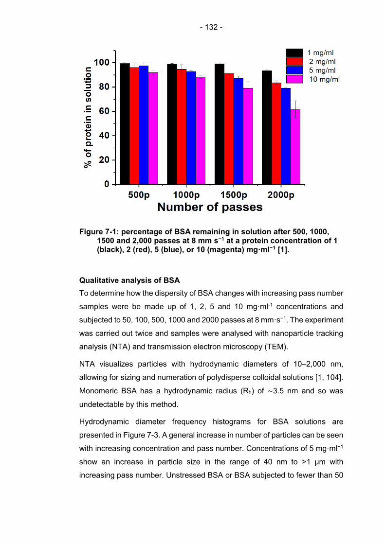
- 132 -

Qualitative analysis of BSA

To determine how the dispersity of BSA changes with increasing pass number

samples were be made up of 1, 2, 5 and 10 mg·ml-1 concentrations and

subjected to 50, 100, 500, 1000 and 2000 passes at 8 mm·s−1. The experiment

was carried out twice and samples were analysed with nanoparticle tracking

analysis (NTA) and transmission electron microscopy (TEM).

NTA visualizes particles with hydrodynamic diameters of 10–2,000 nm,

allowing for sizing and numeration of polydisperse colloidal solutions [1, 104].

Monomeric BSA has a hydrodynamic radius (Rh) of ∼3.5 nm and so was

undetectable by this method.

Hydrodynamic diameter frequency histograms for BSA solutions are

presented in Figure 7-3. A general increase in number of particles can be seen

with increasing concentration and pass number. Concentrations of 5 mg·ml−1

show an increase in particle size in the range of 40 nm to >1 μm with

increasing pass number. Unstressed BSA or BSA subjected to fewer than 50

Figure 7-1: percentage of BSA remaining in solution after 500, 1000, 1500 and 2,000 passes at 8 mm s−1 at a protein concentration of 1 (black), 2 (red), 5 (blue), or 10 (magenta) mg·ml−1 [1].

- 133 -

passes, yielded no detectable particles. The total number of aggregates was

also found to increase with increasing pass number and with increasing BSA

concentration. The width of the error bars also increases with the number of

passes, suggesting an increase in sample dispersity [1].

Figure 7-4 shows the TEM images taken of BSA concentrations ranging from

1 – 10 mg·ml-1, and from 50 – 2000 passes. The images support the data

collected from NTA experiments in Figure 7-2 and Figure 7-3 in that larger

particles were present after increased numbers of passes and at higher

concentrations, and that their frequency also appears to increase [1].

- 134 -

Figure 7-2: BSA aggregation analysed by NTA. The experiments were performed at the number of passes indicated at different BSA concentrations. The plunger velocity in all cases was 8 mm s-1 (strain rate = 11750 s-1 and shear rate = 55200 s-1). (A) and (B) at 1mg·mL-1, (C) and (D) at 2 mg·mL-1, (E) and (F) at 5 mg·mL-1 and (G) and (H) at 10mg·mL-1 of BSA. Note: very few or no aggregates (< 5 particles) were observed for BSA when fewer than 50 passes were applied, rendering the particle tracking analysis statistically invalid [1].

- 135 -

Figure 7-4: TEM images of BSA after extensional flow at the protein concentration and pass number stated. The plunger velocity in all experiments above was 8 mm s-1 (strain rate = 11750 s-1, shear rate = 52000 s-1). Images taken at 10000× magnification, scale bar = 500 nm [1].

Figure 7-3: Total number of 10–2,000 nm particles tracked by NTA in 1, 2, 5, and 10 mg·mL−1 BSA solutions after 50–2,000 passes at 8 mm·s−1. Error bars represent the error from two independent experiments [1].

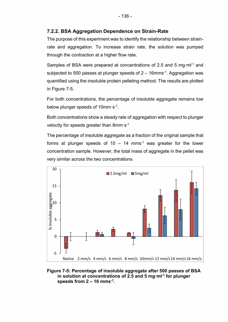
- 136 -

7.2.2. BSA Aggregation Dependence on Strain-Rate

The purpose of this experiment was to identify the relationship between strain-

rate and aggregation. To increase strain rate, the solution was pumped

through the contraction at a higher flow rate.

Samples of BSA were prepared at concentrations of 2.5 and 5 mg·ml-1 and

subjected to 500 passes at plunger speeds of 2 – 16mms-1. Aggregation was

quantified using the insoluble protein pelleting method. The results are plotted

in Figure 7-5.

For both concentrations, the percentage of insoluble aggregate remains low

below plunger speeds of 10mm·s-1.

Both concentrations show a steady rate of aggregation with respect to plunger

velocity for speeds greater than 8mm·s-1

The percentage of insoluble aggregate as a fraction of the original sample that

forms at plunger speeds of 10 – 14 mms-1 was greater for the lower

concentration sample. However, the total mass of aggregate in the pellet was

very similar across the two concentrations.

-5

0

5

10

15

20

Native 2 mm/s 4 mm/s 6 mm/s 8 mm/s 10mm/s 12 mm/s 14 mm/s16 mm/s

% In

solu

ble

aggr

egat

e

2.5mg/ml 5mg/ml

Figure 7-5: Percentage of insoluble aggregate after 500 passes of BSA in solution at concentrations of 2.5 and 5 mg·ml-1 for plunger speeds from 2 – 16 mms-1.

- 137 -

7.3. The Effects of Extensional Flow on Therapeutic Proteins

7.3.1. Comparison of therapeutic proteins

β2m and BSA were prepared at 5 mg·ml-1. WFL, STT and mAb1 was prepared

at 0.5 mg·ml-1. All four therapeutic proteins, and BSA, were subjected to 20

and 100 passes at plunger speed 8 mms-1. Aggregation was quantified using

the insoluble protein pelleting method as well as TEM.

β2m at 5 mg·ml−1 was found to be more sensitive than BSA yielding 2 % and

10 % insoluble after 20 or 100 passes, respectively, compared with 1% and

1.5% of BSA [Figure 7-6 A)]. Visualization of these aggregates by TEM

revealed short, needle-like fibrils, similar to those found in the joints of patients

undergoing long-term dialysis [1, 146].

GCSF [143] was found to be extremely sensitive to the effects of extensional

flow. After 20 passes of GCSF C3 at a concentration of 0.5 mg·ml−1 through

the device, 20% of the sample rendered insoluble [Figure 7-6 A) and C)],

increasing to 40% after 100 passes. The aggregation-prone WFL was reduced

to ∼45% and ∼15% of soluble protein after 20 and 100 passes, respectively

[Figure 7-6]. This was noteworthy given the low concentration of protein used

(0.5 mg mL−1). mAb1 yielded significantly less insoluble material with ∼15%

and ∼25% in the pellet after 20 and 100 passes respectively. STT exhibited

even less susceptibility, yielding only ∼2% and ∼5% insoluble material after

20 and 100 passes, respectively. It was evident that biopharmaceuticals with

diverse structures, such as the α-helical G-CSF C3 and the β-sheet mAbs,

were all prone to extensional flow-induced aggregation. It also shows that

aggregation propensity of IgGs that differ only at three positions in the CDR

loops of each VH domain show remarkably different responses to

hydrodynamic flow [1].

- 138 -

Figure 7-6: A) Percentage of protein remaining in solution after 0, 20, or 100 passes at a plunger velocity of 8 mm·s−1. B–E) TEM images of β2m, G-CSF C3, mAb1, and WFL after 100 passes. The grids were imaged at 10,000× magnification. (Scale bar = 500 nm) [1].

A

- 139 -

7.3.2. mAb Aggregation dependence on velocity

STT and WFL were almost identical versions of the same IgG, with only six

differing residues between them. WFL is known to be sensitive to flow

whereas STT shows more resilience to processing. In previous experiments,

both proteins showed pass-number dependent aggregation to different

degrees, as expected.

In the current experiment, samples of WFL and STT were prepared at 0.5

mg·ml-1. The IgGs were subjected to a number of passes, STT to 100 and 200

passes, and the more sensitive WFL to 50 and 80 passes [Figure 7-7 a)–d)

respectively]. For all experiments, plunger speeds were varied from 2 - 16

mms-1 to identify any relationship between flow rate and aggregation.

Aggregation was quantified using the insoluble protein pelleting method.

STT demonstrated flow rate dependent aggregation for both 100 and 200

passes [Figure 7-7 a), b) respectively]. In both instances, the protein showed

a very gradual increase in average aggregation with flow rate up to plunger

speeds of 10 mm·s-1. So gradual in fact, that with error taken into account, this

trend was almost statistically irrelevant. As plunger speed increases beyond

10 mm·s-1, however, aggregation shows a stronger correlation with plunger

speed up to 16 mm·s-1. For STT after 200 passes [Figure 7-7 b)] the rate of

aggregation with respect to plunger speed decreases for the highest speed.

This was due to the percentage of soluble aggregate tending to zero, hence

there was little more aggregation to occur.

Contrary to STT, WFL shows no sign of flow rate dependent aggregation. After

50 passes [Figure 7-7 c)] WFL consistently returns between 40 – 60 %

insoluble aggregate irrespective of plunger velocity. Similarly after 80 passes

[Figure 7-7 d)] WFL consistently produces a pellet containing 65 – 75 %

insoluble aggregate.

To study this further, WFL was subjected to a pass number experiment as

follows.

- 140 -

Figure 7-7: Speed dependent studies of STT (a, b) and WFL (c, d), both at 0.5 mg·ml-1.

- 141 -

7.3.3. Further study of WFL

In the previous experiment, WFL aggregation was seen to be independent of

plunger velocity whilst showing some dependence on the number of passes

through the device. To explore this further, WFL was prepared at 0.5 mg·ml-1

and subjected to 10, 20, 50, 80 and 100 passes at 8 mms-1 plunger velocity.

Aggregation was quantified using the insoluble protein pelleting method.

As before, aggregation was seen to increase with the number of passes as

shown in Figure 7-8. This differs, however, from previous pass number

dependent aggregation seen in BSA [Figure 7-1 and Figure 7-5] in that BSA

aggregation was only pass number dependent above a certain number of

passes, whereas WFL shows pass number dependence from 10 passes.

0

10

20

30

40

50

60

70

80

90

0 20 40 60 80 100

% In

solu

ble

aggr

egat

e

Number of passes

Figure 7-8: percentage of insoluble aggregation of WFL for a concentration of 0.5 mg·ml-1 solution exposed to varying pass number at 8 mm·s-1.

- 142 -

7.4. Results from contraction angle experiments

In the previous experiment, WFL was shown to be independent of plunger

velocity, with aggregation shown to vary with number of passes only. In the

experiment WFL was subjected to 50 passes through varying contraction

angles. By varying the contraction angle and maintain the plunger speed, the

maximum strain-rate was varied whilst maximum shear remains constant.

WFL was prepared at 0.5 mg·ml-1 and subjected to 50 passes at 8 mms-1

plunger velocity through contraction angles of 90°, 45° and 30°. Aggregation

was quantified using the insoluble protein pelleting method.

For the 90° contraction, identical to that formed by the glass capillary and

syringe barrel in previous experiments, the percentage of insoluble aggregate

present after 50 passes [Figure 7-9] is similar to that seen in the previous WFL

pass number dependent experiments [Figure 7-7 c), Figure 7-8]. As

contraction angle, and strain rate, were reduced, the percentage of insoluble

aggregate decreases proportionally.

-5

5

15

25

35

45

55

Native 90° 45° 30°

% In

solu

ble

aggr

egat

e

Figure 7-9: Percentage of in soluble aggregate in WFL 0.5 mg·ml-1 samples after being subjected to various contraction angles at 8 mm·s-1 plunger speeds.

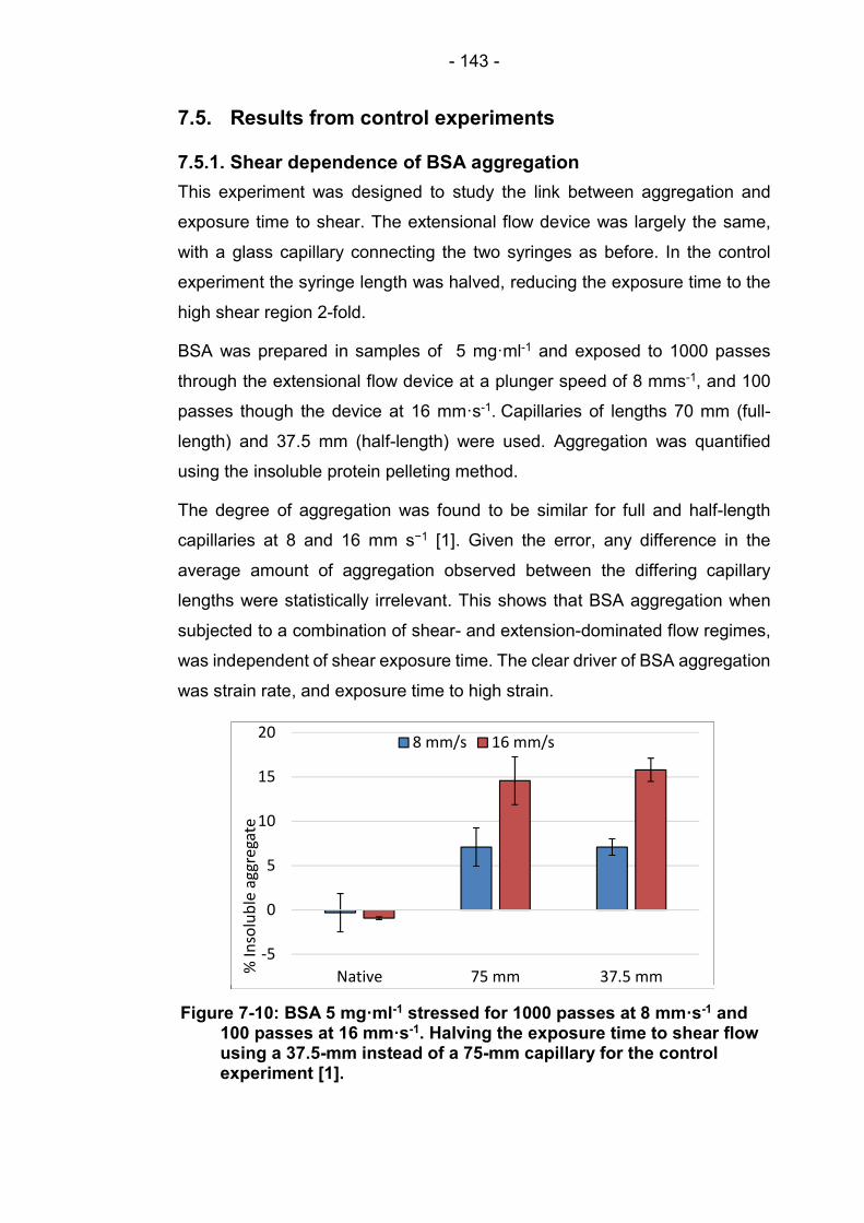
- 143 -

7.5. Results from control experiments

7.5.1. Shear dependence of BSA aggregation

This experiment was designed to study the link between aggregation and

exposure time to shear. The extensional flow device was largely the same,

with a glass capillary connecting the two syringes as before. In the control

experiment the syringe length was halved, reducing the exposure time to the

high shear region 2-fold.

BSA was prepared in samples of 5 mg·ml-1 and exposed to 1000 passes

through the extensional flow device at a plunger speed of 8 mms-1, and 100

passes though the device at 16 mm·s-1. Capillaries of lengths 70 mm (full-

length) and 37.5 mm (half-length) were used. Aggregation was quantified

using the insoluble protein pelleting method.

The degree of aggregation was found to be similar for full and half-length

capillaries at 8 and 16 mm s−1 [1]. Given the error, any difference in the

average amount of aggregation observed between the differing capillary

lengths were statistically irrelevant. This shows that BSA aggregation when

subjected to a combination of shear- and extension-dominated flow regimes,

was independent of shear exposure time. The clear driver of BSA aggregation

was strain rate, and exposure time to high strain.

-5

0

5

10

15

20

Native 75 mm 37.5 mm% In

solu

ble

aggr

egat

e

8 mm/s 16 mm/s

Figure 7-10: BSA 5 mg·ml-1 stressed for 1000 passes at 8 mm·s-1 and 100 passes at 16 mm·s-1. Halving the exposure time to shear flow using a 37.5-mm instead of a 75-mm capillary for the control experiment [1].

- 144 -

7.5.2. Stagnation point dependence of STT aggregation

It was determined through CFD simulation of the device, that a region of

extensional flow exists within the downstream syringe. This was the result of

a stagnation point forming on the receding plunger face as it was impacted by

a jet of fluid exiting the capillary. The extensional strength was shown to be

proportional to the plunger distance from the jet outlet, i.e. the capillary exit.

The control experiment to discount the effects of stagnation on aggregation

was, therefore, to repeat the conventional reciprocating experiment whilst

maintaining a 10 mm fluid-filled gap between the jet outlet and the plunger

face. The sample size was increased to accommodate an extra 10 mm of

sample in both syringes. The same volume of sample was passed through the

extensional flow device as for the conventional experiments. If the mass of

aggregate per unit sample volume was greater for the standard volume

experiment, this would suggest that the stagnation point was a factor in

aggregation. In order to measure this, the measured pellet concentration was

corrected to take into account the excess volume. Therefore, it was purely

mass of insoluble aggregate that was important here, not percentage of total

sample.

STT was prepared in samples of 0.5 mg·ml-1 and exposed to 200 passes

through the extensional flow device at a plunger speed of 8 mms-1. The

experiment was carried out with the standard volume, allowing the entire

sample to pass from one syringe to the other 200 times. The experiment was

repeated with excess sample volume, leaving a 10 mm gap (approx. 0.08 ml)

in the syringe after each pass. Aggregation was quantified using the insoluble

protein pelleting method.

By percentage, the amount of aggregate in the smaller, standard volume was

higher [Figure 7-12]. When the data was normalised to take into account the

difference in volume [Figure 7-11], the data shows that, on average, the

excess volume experiment produced more aggregated material than the

standard volume experiment, although the standard volume result does fall

within the error of the excess volume result.

- 145 -

If the stagnation point was responsible for increasing aggregation, the excess

volume sample would be expected to show a reduction in aggregation as the

strain rate weakens with distance from the jet. The evidence suggests that the

presence of a stagnation point in the downstream syringe has negligible effect

on protein aggregation within the current device.

0

0.2

0.4

0.6

0.8

1

1.2

1.4

Standard volume Excess volume

Nor

mal

ised

scal

e

Figure 7-11: STT 0.5 mg·ml-1 subjected to 200 passes with a standard volume, and an excess volume normalised to take into account the different sample volumes. This is the ratio of mass of insoluble aggregate.

-10

0

10

20

30

Native Standardvolume

Excessvolume

% In

solu

ble

aggr

egat

e

Figure 7-12: STT 0.5 mg·ml-1 subjected to 200 passes with a standard volume, and an excess volume.

- 146 -

8. Discussion

Work prior to this study has demonstrated that hydrodynamic forces were

capable of inducing unfolding in long chain molecules such as DNA [147, 148],

polymers [149], von Willebrand factor (VWF) [150], as well as other proteins

[8]. The specific flow mechanism which causes unfolding however, has not

been made clear. To investigate this, a device was designed to vary different

aspects of the fluid profile, namely shear and extensional flow. The device

was used to subject natively folded globular proteins to well-defined shear and

extensional flows at high strain rates. The device successfully demonstrated

that the protein bovine serum albumin (BSA) will aggregate when exposed to

extensional flow. The device also demonstrated that the degree of

aggregation of BSA was independent of exposure time to shear dominated

environments over the time periods used in our study.

In other studies it has been shown that over extended periods of time (10s of

minutes), exposure to high shear environments will result in BSA aggregation

[151]. This is not surprising when we consider other globular proteins, such as

VWF and spider silk, have evolved to aggregate readily under relatively low

exposure times to shear stress [51, 152]. Although such proteins can be

considered atypical of globular molecules, it is compelling evidence to suggest

that the mechanisms which allow sensitivity to shear are likely to be present

in a range of proteins, albeit at a much more subtle level [1].

8.1. Tensile stress

Experiments carried out on a range of proteins has demonstrated that the

magnitude of aggregation is dependent on a variety of factors. These include

size and concentration, as well as the structure and surface topology of the

folded molecule. Experiments comparing the sensitivity of WFL and STT also

demonstrated the importance of the precise sequence of the protein [1].

Further work by L. F. Willis and A. Kumar [1] using in situ cystine labelling has

demonstrated that extensional flow likely catalyses the unfolding process,

subject to a critical energy transfer rate that had to be overcome for partial

unfolding to result in irreversible aggregation.

- 147 -

It follows then, that hydrodynamic unfolding of proteins through extensional

flow shares some common ground with mechanical protein unfolding through

means such as optical tweezers and atomic force microscopy which can

induce conformational changes, modify stability, and stimulate biochemical

responses [153]. In such methods, the tensile force required to “pull apart”

specific structures within a molecule are quantifiable. Typically, full unfolding

of a particularly “strong” β-sheet region occurs in the region of 50 – 200 pN of

directly applied force [154].

To allow for engineering analysis, one study [4], discusses the model

approximation of a bead necklace, shown in Figure 8-1, consisting of 𝑁

residues where each residue is represented as a bead separated from its

neighbours by an average centre-to-centre distance 𝑑. The protein is

assumed to form two approximately equal bunches with a linking chain of 𝑛

beads between them. The protein is subjected to tension caused by an

extensional flow characterised by �̇� = 𝑑𝑣 𝑑𝑥⁄ , where 𝑥 is taken to be the

direction parallel to the linking chain. An equation for tensile stress is

presented for the linking chain of length ~𝑛𝑑 between the two equally sized

clusters of radius 𝑎. The extensional flow can be expressed as the difference

between the flow velocities experienced by the two clusters at their relative

locations (𝑣 − 𝑣 ) = �̇� 𝑛𝑑. Tension can be calculated as

where 𝜂 is the dynamic viscosity of the fluid, which can be taken as that of

water ~1 mPa·s.

The maximum strain rate �̇� has been solved for the extensional flow device

using CFD analysis. For a typical plunger velocity of 8 mm·s, �̇� ≈ 12000 s-1. If

a typical mAb molecule were to be crudely approximated into a dumb-bell

model, the values of a and nd could be approximated to 5 and 10 nm

respectively. Using these values in Equation 8-1 a tensile force of the order 5

fN; four orders of magnitude below the 50 pN required to fully unfold a

structurally sound β-sheet structure. This implies that the aggregation

witnessed during experiments is the product of partial unfolding of native

protein.

𝑇 ≈ 6𝜋𝜂𝑎(𝑣 − 𝑣 ) 2⁄ = 3𝜋𝜂𝑎 �̇� 𝑛𝑑 Equation 8-1

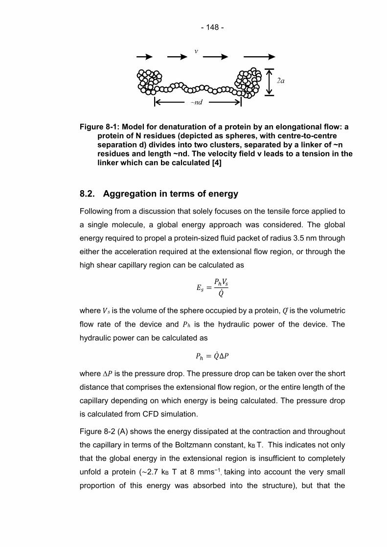
- 148 -

8.2. Aggregation in terms of energy

Following from a discussion that solely focuses on the tensile force applied to

a single molecule, a global energy approach was considered. The global

energy required to propel a protein-sized fluid packet of radius 3.5 nm through

either the acceleration required at the extensional flow region, or through the

high shear capillary region can be calculated as

𝐸 =𝑃 𝑉

�̇�

where 𝑉𝑠 is the volume of the sphere occupied by a protein, �̇� is the volumetric

flow rate of the device and 𝑃ℎ is the hydraulic power of the device. The

hydraulic power can be calculated as

𝑃 = �̇�∆𝑃

where ∆𝑃 is the pressure drop. The pressure drop can be taken over the short

distance that comprises the extensional flow region, or the entire length of the

capillary depending on which energy is being calculated. The pressure drop

is calculated from CFD simulation.

Figure 8-2 (A) shows the energy dissipated at the contraction and throughout

the capillary in terms of the Boltzmann constant, kB T. This indicates not only

that the global energy in the extensional region is insufficient to completely

unfold a protein (∼2.7 kB T at 8 mms−1, taking into account the very small

proportion of this energy was absorbed into the structure), but that the

Figure 8-1: Model for denaturation of a protein by an elongational flow: a protein of N residues (depicted as spheres, with centre-to-centre separation d) divides into two clusters, separated by a linker of ~n residues and length ~nd. The velocity field v leads to a tension in the linker which can be calculated [4]

- 149 -

energies in the shear and extensional region are relatively similar. This is

interesting, given the experimental findings that suggest large disparities in

the abilities for these different regions to induce aggregation.

The time over which these respective energies were imparted to the flow was

then considered. The rate of energy transfer as the fluid passes through the

extensional flow region is high, given that it is proportional to the gradient of

the pressure drop. Figure 8-2 (B) shows the energy transfer rate E/(kB T·t) in

reciprocal seconds (s−1), where t is the time taken to traverse the capillary or

the extensional flow regions. This shows the rate at which energy is introduced

to the protein solution. This is especially relevant as a perturbed structure will

only be able to dissipate energy at a finite rate. This analysis demonstrates

that the rate of energy transfer by extensional flow is in fact orders of

magnitude larger than that of shear [1].

Figure 8-2: Energy distribution in the extensional flow device. (A) The average energy dissipated within the extensional region (red line) versus that within the shear region (black line) for a single pass for a protein with a diameter of 3.5 nm as a function of plunger velocity. (B) Average rate of energy dissipation within the extensional region (red line) and within the shear region (black line) per protein volume as a function of plunger velocity .

- 150 -

8.3. Strain rate distribution at the capillary inlet

The lack of evidence relating aggregation to extensional flow in-and-around

the stagnation point may seem counterintuitive to the premise of this work. An

explanation as to why the transitory extensional flow region is seen to drive

aggregation, whilst a stagnating extensional flow region is not, can be found

with further analysis of their respective flow fields. More specifically, the

answer is found by identifying the regions with greatest mass flow rate.

Starting with the transitory extensional flow region around the capillary

entrance; from the computational study it is clear that there is a wide range in

strain rate magnitudes occurring across the capillary inlet radius. The highest

of which, seen in an extremely localised point at the inlet corner can be

dismissed as an erroneous artefact; the product of post-process arithmetic

applied to numerical results at an extremity. This analysis does not, however,

carry into the bulk of the flow. The strain rate is seen to increase with radial

(sr) displacement from the axis of symmetry. Strain rate is related to regions

of high acceleration and, comparing the strain profiles in Figure 5-8 to the

velocity profiles in Figure 5-5, it is clear that the region of high strain

correspond with areas of high contrast in the velocity plots.

To explain this phenomena, the flow through the capillary inlet should be

examined in terms of the upstream flow that feeds into it.

It is clear that the fluid velocity in the syringe region is relatively slow; a plunger

moving at 8 mms-1 produces a maximum fluid velocity of 16 mms-1 in the

syringe compared with 3500 mms-1 along the capillary. Despite this the

capillary inlet profile is heavily influenced by the conditions upstream in the

syringe barrel.

Figure 8-3 shows the velocity profile inside the barrel of a syringe, 100mm

upstream of the capillary inlet. The profile is taken at a location such that there

is sufficient distance from the upstream plunger for uniform, laminar flow to

fully develop. The profile is also sufficiently upstream of the capillary inlet so

as to avoid regions of perturbed flow. The velocity profile spans the radius of

the syringe, with radial position (Sr) =0mm located at the axis of symmetry (i.e.

- 151 -

the centre of the syringe barrel) and Sr =2.305mm representing the syringe

wall. Velocity (uz) is the fluid velocity parallel to the syringe wall (z-direction).

A parabolic velocity profile is produced with maximum velocity occurring at the

centre of the syringe barrel, with velocity reducing quadratically to zero at the

wall. This is in keeping with laminar flow conditions and is not in any way

exceptional until it is considered in its 3-dimensional form. In 3D, a velocity

profile sketches out an area through which a volume of fluid travels per unit

time, producing a volumetric flow rate (Q) measured in cubic meters per

second or litres per second.

𝑄 = 𝑢𝑎

Because the current problem is axisymmetric, it follows that the radial section

that carries the largest flow rate (i.e. the region of maximum mass flux (rQ,max))

is not the same as the region of maximum velocity.

This is because the circular area through which the maximum velocity material

travels is very small, resulting in a low mass flux for that region.

If the syringe radius were divided into increments of equal length, then the

area swept out by each increment length would increase. To calculate the flow

0

0.002

0.004

0.006

0.008

0.01

0.012

0.014

0.016

0 0.5 1 1.5 2

Velo

city

(uz)

ms-1

Radial position (sr) mm

Figure 8-3: Radial velocity profile for undisturbed flow thorough the upstream syringe, typical of a syringe moving at 8 mms-1.

- 152 -

rate associated with each radial increment, the corresponding area is

multiplied by the average flow velocity across that increment.

Figure 8-4 shows the cumulative flow rate distribution with respect to radial

position within the syringe. The total flow rate from the graph is 132.6 µLs-1.

Calculating the mass flow rate using equation # gives a flow rate of 133.5 µLs-

1. The discrepancy is due to stationary fluid confined to the pipe wall by friction,

slightly reducing the “effective” radius and the total mass freely flowing through

the section.

The region near the centre of the syringe (Sr = 0mm) can be seen to make

little contribution to the total flow rate despite the high speeds associated with

it. For radial positions 1mm<Sr<1.5mm, contributions to the total flow rate are

high as fluid is relatively free to move and cross-sectional area is large enough

to accommodate substantial mass flux. Near the wall (Sr=2.305mm) the

available area is at its largest but frictional effects drastically reduce the fluid

velocity, resulting in minimal contributions to mass flux.

Figure 8-5 shows the standard distribution of Q with respect to Sr normalised

to the maximum incremental value of flow rate. From Figure 8-5, the region of

maximum mass flux, rQ,max, is located at Sr=1.342mm, or at 57.45% across

0

20

40

60

80

100

120

140

0 0.5 1 1.5 2

Cum

ulat

ive

flow

rate

dis

trib

utio

n µL

s-1

Radial position (Sr) mm

Figure 8-4: Cumulative flow rate distribution with respect to radial position for undisturbed flow through the upstream syringe.

- 153 -

the radius. This indicates that mass flux is skewed towards the lower velocity

region.

This explains why the capillary inlet is seen to have such high velocity regions

near the extremities. To satisfy conservation of mass, the mass flux across

any two cross-sectional areas had to equate. The ratio of cross-sectional

areas from the syringe to capillary is 538:1, meaning that the average velocity

had to increase by 538 times. The fluid at the centre of the syringe is readily

available, traveling faster than its radially displaced neighbours and in the right

direction. But, as Figure 8-5 show, there isn’t enough material at the axis to

satisfy mass conservation. In order to supply the capillary with the amount of

fluid necessary to maintain this flow rate the slow moving fluid in the outer

42.55%- radius, which constitutes the majority of material in the continuum, is

drawn inward toward the capillary where is experiences the sudden

acceleration required to fulfil the need for mass conservation.

This is further evidenced when the streamline paths are taken into account. A

streamline that passes through the region of maximum mass flux at Sr=1.324

mm along the syringe can be followed until it reaches the capillary inlet. The

same streamline crosses the inlet at a radial position of 0.111mm; just 14

0

0.1

0.2

0.3

0.4

0.5

0.6

0.7

0.8

0.9

1

0 0.5 1 1.5 2

Nor

mal

ised

flow

rate

dis

trib

utio

n

Radial position mm

Figure 8-5: Flow rate distribution with respect to radial position for undisturbed flow through the upstream syringe normalised to the maximum value.

- 154 -

microns from the inlet peak velocity region at 0.125 mm. Furthermore, if the

highest velocity point at the inlet Sr = 0.125 mm is traced back along a

streamline to a region of unperturbed flow within the syringe, it is found to

travel at a distance of 1.575 mm from the axis. A region with 94% of the

maximum mass flux.

In conclusion, evidence suggests that the regions of high strain at the

peripheries of the capillary inlet are caused by the requirement of slow-moving

fluid in the outer regions of the syringe, responsible for the majority of total

mass flux, to accelerate suddenly in order to continue supplying the large

volumes required to satisfy mass conservation.

- 155 -

9. Conclusions

9.2. Summary

9.2.1. Extensional flow induced aggregation in BSA

BSA aggregation correlated with concentration and exposure time to

extensional flow. At a concentration of 1 mg·ml-1, BSA remained in solution

until exposed to 2000 passes. Concentrations of 2 mg·ml-1 showed higher

sensitivity to pass number, with a steady downward trend in the averaged

data. For concentrations of 5 mg·ml-1 a steady decrease in soluble BSA was

seen as pass number increased. 10 mg·ml-1 concentration saw greatest rate

of aggregation with pass number.

BSA aggregation also correlated with strain rate. Samples of BSA at

concentrations of 2.5 and 5 mg·ml-1 subjected to 500 passes at plunger

speeds of 2 – 16mms-1 both resulted in aggregation. The percentage of

insoluble aggregate remains low below plunger speeds of 10mms-1, this

indicated an energy threshold needed to be overcome to trigger flow induced

aggregation.

9.2.2. Extensional flow induced aggregation in therapeutic proteins

5 mg·ml−1 β2m produced 2% and 10% insoluble aggregated after 20 or 100

passes, respectively. TEM images showed short, needle-like fibrils. 0.5

mg·ml−1 GCSF C3 produced 20% insoluble aggregate after 20 passes. This

increased to 40% after 100 passes. 0.5 mg mL−1 WFL produced ∼55% and

∼85% aggregate after 20 and 100 passes, respectively. 0.5 mg mL−1 mAb1

yielded ∼15% and ∼25% insoluble protein after 20 and 100 passes. STT

produced only ∼2% and ∼5% insoluble material.

9.2.3. Antibody conformation affects flow sensitivity

STT demonstrated flow rate dependent aggregation for both 100 and 200

passes in flow rates up to plunger speeds of 10 mms-1. Plunger speeds greater

than 10 mms-1, showed a stronger correlation with aggregation up to 16 mms-

1. WFL, however, did not demonstrate flow rate dependent aggregation. After

- 156 -

50 passes, WFL consistently produced between 40 – 60 % insoluble

aggregate irrespective of plunger velocity. This trend was repeated at 80

passes.

Further investigation into WFL presented aggregation increase with number

of passes. the behaviour was different to BSA in that BSA aggregation was

only pass number dependent above a certain number of passes, whereas

WFL showed pass number dependence from 10 passes.

These findings are important because STT and WFL differ by only six residues

in some 1400.

9.2.4. Strain trumps shear

0.5 mg·ml-1 WFL subjected to 50 passes at 8 mms-1 plunger velocity through

the 90° nylon constriction returned identical results to the longer, glass

capillary experiments with longer shear exposure times. As the contraction

angle and, therefore, the strain rate were reduced through 45° and 30°, the

percentage of insoluble aggregate decreased proportionally. This

demonstrated a strain rate dependence over a shear rate dependence.

9.1.5. Successful validation

5 mg·ml-1 BSA exposed to 1000 passes at a plunger speed of 8 mms-1, and

100 passes at 16 mms-1 through capillaries of lengths 70 mm and 37.5 mm.

The degree of aggregation was within error for both full and half-length

capillaries at 8 and 16 mm s−1.This showed that BSA aggregation when

subjected to a combination of shear- and extension-dominated flow regimes,

is independent of shear exposure time. BSA aggregation was therefore driven

by strain rate.

0.5 mg·ml-1 STT exposed to 200 passes at a plunger speed of 8 mms-1 was

carried out with the standard experimental volume, and repeated with an

excess sample volume, leaving a 10 mm gap in the syringe after each pass.

Normalised data taking into account the difference in volume showed that, on

average, the excess volume experiment produced more aggregated material

- 157 -

than the standard volume experiment. Therefore, the intensity of the

stagnation point was not responsible for increasing aggregation.

9.3. Future Work

The extensional flow device presented in the current work has successfully

proved the concept of a benchtop application that is capable of probing the

stability of proteins in the presence of fluid forces. It has highlighted the

necessity for detailed characterisation of the flow field when interpreting the

behaviour of proteins in flow, and has demonstrated the importance of

extensional flow in the production of aggregation in hydrodynamic systems.

The device did however present some drawbacks which had to be taken into

account during the experimental campaign. One of which was the presence

of the high shear region within the capillary. A control experiment was

implemented to address this, however, this only reduced the exposure time to

high shear without reducing the magnitude of shear itself.

Another hindrance was the inclusion of a stagnation point that varied in

intensity with time during each pass through the device. Again, a control

procedure was built into the experimental procedure and aggregation was

found to be independent of the stagnation point. This however, is almost

certainly not the case for all proteins.

A further shortcoming of the device, and indeed, the methodology, stems from

limited information the user can extract about the pathways to aggregation. It

was seen that a 0.8 ml sample of some protein or another will, over time,

undergo some conformational change over a series of passes back and forth

through a region of high stress. In between stress events, the sample dwells

in a relatively spacious reservoir where it is free to disperse and mix. This

allows for aggregated particles to seed further aggregation. information about

this pathway is not captured in the current methodology.

A more subtle event is also left unexplored; the presence of reversible

conformational changes. If the flow field is indeed imparting enough energy to

partially unfold a molecule, it stands to reason that a proportion of these will

- 158 -

revert to their native state after the stress is removed. This event remains

uncaptured by the current methodology.

To address these issues, a further study into the effects of extensional flow on

conformation change and aggregation of proteins would require a

fundamentally different device. Such a device would expose a solution to a

high strain environment whilst reducing exposure time to high shear to a

minimum. The device would have to perform without the presence of a

stagnation point, and ideally subject the sample to multiple passes though an

extensional flow profile without allowing it to dwell in a reservoir so as to

prevent the effects of seeding. The device would also allow for revisable

conformational changes to be probed; this would require the use of in-situ

characterisation techniques. Such a device would greatly improve upon the

progress made in the current work.

- 159 -

List of References

1. Dobson, J., et al., Inducing protein aggregation by extensional flow. Proceedings of the National Academy of Sciences, 2017. 114(18): p. 4673-4678.

2. Thomas, C.R. and D. Geer, Effects of shear on proteins in solution. Biotechnology Letters, 2011. 33(3): p. 443-56.

3. Ratanji, K.D., et al., Immunogenicity of therapeutic proteins: Influence of aggregation. Journal of Immunotoxicology, 2014. 11(2): p. 99-109.

4. Jaspe, J. and S.J. Hagen, Do protein molecules unfold in a simple shear flow? Biophysical Journal, 2006. 91(9): p. 3415-24.

5. Bee, J.S., et al., Effects of surfaces and leachables on the stability of biopharmaceuticals. Journal of Pharmaceutical Sciences, 2011. 100(10): p. 4158-4170.

6. Dragovic, R.A., et al., Sizing and phenotyping of cellular vesicles using Nanoparticle Tracking Analysis. Nanomedicine: Nanotechnology, Biology and Medicine, 2011. 7(6): p. 780-788.

7. Buss, N.A.P.S., et al., Monoclonal antibody therapeutics: history and future. Current Opinion in Pharmacology, 2012. 12(5): p. 615-622.

8. Simon, S., et al., Physical degradation of proteins in well-defined fluid flows studied within a four-roll apparatus. Biotechnology and Bioengineering, 2011. 108(12): p. 2914-2922.

9. Larson, J.W., et al., Single DNA molecule stretching in sudden mixed shear and elongational microflows. Lab Chip, 2006. 6(9): p. 1187-99.

10. Erickson, H.P., Size and Shape of Protein Molecules at the Nanometer Level Determined by Sedimentation, Gel Filtration, and Electron Microscopy. 2009. 11: p. 32-51.

11. Zhu, C., G. Bao, and N. Wang, CELL MECHANICS: Mechanical Response, Cell Adhesion, and Molecular Deformation. Annual Review of Biomedical Engineering, 2000. 2(1): p. 189-226.

12. Schroeder, C.M., E.S.G. Shaqfeh, and S. Chu, Effect of Hydrodynamic Interactions on DNA Dynamics in Extensional Flow:  Simulation and Single Molecule Experiment. Macromolecules, 2004. 37(24): p. 9242-9256.

13. Hassager, O., Kinetic theory and rheology of bead‐rod models for macromolecular solutions. I. Equilibrium and steady flow properties. The Journal of Chemical Physics, 1974. 60(5): p. 2111-2124.

14. Jahn, T.R. and S.E. Radford, The Yin and Yang of protein folding. FEBS Journal, 2005. 272(23): p. 5962-5970.

15. Tipping, K.W., et al., Amyloid Fibres: Inert End-Stage Aggregates or Key Players in Disease? Trends in Biochemical Sciences, 2015. 40(12): p. 719-727.

16. Pace, C.N., et al., Forces contributing to the conformational stability of proteins. The FASEB Journal, 1996. 10(1): p. 75-83.

17. Farber, P.J. and A. Mittermaier, Side chain burial and hydrophobic core packing in protein folding transition states. Protein Science : A Publication of the Protein Society, 2008. 17(4): p. 644-651.

18. Fink, A.L., Protein aggregation: folding aggregates, inclusion bodies and amyloid. Folding and Design, 1998. 3(1): p. R9-R23.

- 160 -

19. Deng, H.-X., et al., Conversion to the amyotrophic lateral sclerosis phenotype is associated with intermolecular linked insoluble aggregates of SOD1 in mitochondria. Proceedings of the National Academy of Sciences, 2006. 103(18): p. 7142-7147.

20. Lee, R.E.C., et al., Metacaspase Yca1 is required for clearance of insoluble protein aggregates. Proceedings of the National Academy of Sciences, 2010. 107(30): p. 13348-13353.

21. Ayazi Shamlou, P., et al., Turbulent breakage of protein precipitates in mechanically stirred bioreactors. Bioprocess Engineering, 1996. 14(5): p. 237-243.

22. Krebs, M.R.H., et al., Formation and seeding of amyloid fibrils from wild-type hen lysozyme and a peptide fragment from the β-domain 11Edited by P. E. Wright. Journal of Molecular Biology, 2000. 300(3): p. 541-549.

23. Han, H., P.H. Weinreb, and P.T. Lansbury, The core Alzheimer's peptide NAC forms amyloid fibrils which seed and are seeded by β-amyloid: is NAC a common trigger or target in neurodegenerative disease? Chemistry & Biology, 1995. 2(3): p. 163-169.

24. Bee, J.S., et al., Response of a concentrated monoclonal antibody formulation to high shear. Biotechnology and Bioengineering, 2009. 103(5): p. 936-943.

25. Haynes, C.A. and W. Norde, Globular proteins at solid/liquid interfaces. Colloids and Surfaces B: Biointerfaces, 1994. 2(6): p. 517-566.

26. Norde, W., My voyage of discovery to proteins in flatland …and beyond. Colloids and Surfaces B: Biointerfaces, 2008. 61(1): p. 1-9.

27. Mahdi, J.G., et al., The historical analysis of aspirin discovery, its relation to the willow tree and antiproliferative and anticancer potential. Cell Proliferation, 2006. 39(2): p. 147-155.

28. Walsh, G., Biopharmaceuticals : biochemistry and biotechnology. 1st ed. 1998, Chichester: Wiley. 431.

29. Bliss, M., The history of insulin. Diabetes Care, 1993. 16(Supplement 3): p. 4-7.

30. Smith, K.A., Edward Jenner and the small pox vaccine. Frontiers in Immunology, 2011. 2.

31. Smith, K.A., <Smallpox can we still learn from the journey to eradication.pdf>. Indian Journal of Medical Research, 2013. 137(1): p. 895 - 899.

32. Swazey, J.P., J.R. Sorenson, and C.B. Wong, Risks and Benefits, Rights and Responsibilities - History of the Recombinant DNA Research Controversy. Southern California Law Review, 1978. 51(6): p. 1019-1078.

33. Cohen, S.N., A.C.Y. Chang, and L. Hsu, Nonchromosomal Antibiotic Resistance in Bacteria: Genetic Transformation of Escherichia coli by R-Factor DNA. Proceedings of the National Academy of Sciences, 1972. 69(8): p. 2110-2114.

34. Sefik, S.A., Monoclonal antibodies: the story of a discovery that revolutionized science and medicine. Nature Reviews Immunology, 2004. 4(2): p. 153-156.

- 161 -

35. Jing, L. and Z. Zhenping, Research and development of next generation of antibody-based therapeutics. Acta Pharmacologica Sinica, 2010. 31(9): p. 1198-1207.

36. Rodrigues, M.E., et al., Technological progresses in monoclonal antibody production systems. Biotechnology Progress, 2010. 26(2): p. 332-351.

37. Crommelin, D.J.A. and R.D. Sindelar, Pharmaceutical biotechnology: an introduction for pharmacists and pharmaceutical scientists. 2002, London: Taylor & Francis.

38. Cromwell, M.M., E. Hilario, and F. Jacobson, Protein aggregation and bioprocessing. The AAPS Journal, 2006. 8(3): p. E572-E579.

39. Magnin, A.A., P.S. Wah, and P. Dennis, Pasteurization of immunoglobulin solutions. 1989, Google Patents.

40. Tolbert, W. and C. Prior, Perfusion Culture, in Advanced Research on Animal Cell Technology, A.A. Miller, Editor. 1989, Springer Netherlands. p. 119-145.

41. Hung, C.H., et al., Process for purifying recombinant proteins, and products thereof. 1988, Google Patents.

42. Rathore, N. and R.S. Rajan. Current perspectives on stability of protein drug products during formulation, fill and finish operations. 2008. 2540 Olentangy River Road, P.O. Box 3337, Columbus, OH 43210-3337, United States: American Chemical Society.

43. Charm, S.E. and B.L. Wong, Shear effects on enzymes. Enzyme and Microbial Technology, 1981. 3(2): p. 111-118.

44. Thomas, C.R., A.W. Nienow, and P. Dunnill, Action of shear on enzymes: Studies with alcohol dehydrogenase. Biotechnology and Bioengineering, 1979. 21(12): p. 2263-2278.

45. Tirrell, M. and S. Middleman, Shear modification of enzyme kinetics. Biotechnology and Bioengineering, 1975. 17(2): p. 299-303.

46. Holford, N.H. and L.B. Sheiner, Understanding the dose-effect relationship: clinical application of pharmacokinetic-pharmacodynamic models. Clin Pharmacokinet, 1981. 6(6): p. 429-53.

47. Oliva, A., et al., Effect of high shear rate on stability of proteins: kinetic study. Journal of Pharmaceutical and Biomedical Analysis, 2003. 33(2): p. 145-155.

48. Arora, D., M. Behr, and M. Pasquali, A Tensor-based Measure for Estimating Blood Damage. Artificial Organs, 2004. 28(11): p. 1002-1015.

49. Westein, E., et al., Atherosclerotic geometries exacerbate pathological thrombus formation poststenosis in a von Willebrand factor-dependent manner. Proc Natl Acad Sci U S A, 2013. 110(4): p. 1357-62.

50. Atkins, E.D.T. and M.A. Taylor, Elongational flow studies on DNA in aqueous solution and stress-induced scission of the double helix. Biopolymers, 1992. 32(8): p. 911-923.

51. Rammensee, S., et al., Assembly mechanism of recombinant spider silk proteins. Proc Natl Acad Sci U S A, 2008. 105(18): p. 6590-5.

52. Charm, S.E. and B.L. Wong, Enzyme inactivation with shearing. Biotechnology and Bioengineering, 1970. 12(6): p. 1103-1109.

- 162 -

53. Lencki, R.W., A. Tecante, and L. Choplin, Effect of shear on the inactivation kinetics of the enzyme dextransucrase. Biotechnology and Bioengineering, 1993. 42(9): p. 1061-1067.

54. Chi, E., et al., Physical Stability of Proteins in Aqueous Solution: Mechanism and Driving Forces in Nonnative Protein Aggregation. Pharmaceutical Research, 2003. 20(9): p. 1325-1336.

55. Ashton, L., et al., Shear-Induced Unfolding of Lysozyme Monitored In Situ. Biophysical Journal, 2009. 96(10): p. 4231-4236.

56. Bekard, I.B., et al., The effects of shear flow on protein structure and function. Biopolymers, 2011. 95(11): p. 733-745.

57. Thomas, C.R. and P. Dunnill, Action of shear on enzymes: Studies with catalase and urease. Biotechnology and Bioengineering, 1979. 21(12): p. 2279-2302.

58. van der Veen, M.E., et al., Shear-Induced Inactivation of α-Amylase in a Plain Shear Field. Biotechnology Progress, 2004. 20(4): p. 1140-1145.

59. Charm, S.E. and B.L. Wong, Shear Degradation of Fibrinogen in the Circulation. Science, 1970. 170(3956): p. 466-468.

60. Charm, S.E. and C.J. Lai, Comparison of ultrafiltration systems for concentration of biologicals. Biotechnology and Bioengineering, 1971. 13(2): p. 185-202.

61. Peterson, D.M., et al., Shear-Induced Platelet-Aggregation Requires Vonwillebrand-Factor And Platelet Membrane Glycoprotein-Ib And Glycoprotein-IIB-IIIA. Blood, 1987. 69(2): p. 625-628.

62. Ikeda, Y., et al., The role of von Willebrand factor and fibrinogen in platelet aggregation under varying shear stress. The Journal of Clinical Investigation, 1991. 87(4): p. 1234-1240.

63. Higdon, J.J.L., The Kinematics of the 4-Roll Mill. Physics of Fluids a-Fluid Dynamics, 1993. 5(1): p. 274-276.

64. Müller, A.J., J.A. Odell, and A. Keller, Elongational flow and rheology of monodisperse polymers in solution. Journal of Non-Newtonian Fluid Mechanics, 1988. 30(2): p. 99-118.

65. Janssen, J.M.H., G.W.M. Peters, and H.E.H. Meijer, An opposed jets device for studying the breakup of dispersed liquid drops. Chemical Engineering Science, 1993. 48(2): p. 255-265.

66. Haward, S.J., et al., Optimized Cross-Slot Flow Geometry for Microfluidic Extensional Rheometry. Physical Review Letters, 2012. 109(12): p. 128301.

67. Balducci, A.G., J. Tang, and P.S. Doyle, Electrophoretic Stretching of DNA Molecules in Cross-Slot Nanoslit Channels. Macromolecules, 2008. 41(24): p. 9914-9918.

68. Skalak, R. and S. Chien, Capillary-Flow - History, Experiments and Theory. Biorheology, 1981. 18(3-6): p. 307-330.

69. Cathey, C.A. and G.G. Fuller, The optical and mechanical response of flexible polymer solutions to extensional flow. Journal of Non-Newtonian Fluid Mechanics, 1990. 34(1): p. 63-88.

70. Hudson, S.D., et al., A Microliter Capillary Rheometer for Characterization of Protein Solutions. Journal of Pharmaceutical Sciences, 2015. 104(2): p. 678-685.

- 163 -

71. Liu, J., et al., Reversible self-association increases the viscosity of a concentrated monoclonal antibody in aqueous solution. Journal of Pharmaceutical Sciences, 2005. 94(9): p. 1928-1940.

72. Kelly, S.M., T.J. Jess, and N.C. Price, How to study proteins by circular dichroism. Biochimica et Biophysica Acta (BBA) - Proteins and Proteomics, 2005. 1751(2): p. 119-139.

73. Schmid, F.-X., Biological Macromolecules: UV-visible Spectrophotometry, in eLS. 2001, John Wiley & Sons, Ltd.

74. Nicoli, D.F. and G.B. Benedek, Study of thermal denaturation of lysozyme and other globular proteins by light-scattering spectroscopy. Biopolymers, 1976. 15(12): p. 2421-2437.

75. Oliva, A., M.a. Llabrés, and J.B. Fariña, Comparative study of protein molecular weights by size-exclusion chromatography and laser-light scattering. Journal of Pharmaceutical and Biomedical Analysis, 2001. 25(5–6): p. 833-841.

76. Wang, L., R.D. Vigil, and R.O. Fox, CFD simulation of shear-induced aggregation and breakage in turbulent Taylor–Couette flow. Journal of Colloid and Interface Science, 2005. 285(1): p. 167-178.

77. Nesbitt, W.S., et al., A shear gradient-dependent platelet aggregation mechanism drives thrombus formation. Nat Med, 2009. 15(6): p. 665-673.

78. Delaunay, D., et al., Mapping of protein fouling by FTIR-ATR as experimental tool to study membrane fouling and fluid velocity profile in various geometries and validation by CFD simulation. Chemical Engineering and Processing: Process Intensification, 2008. 47(7): p. 1106-1117.

79. Brückl, L., et al., The Effect of Shear on the Structural Conformation of rhGH and IgG1 in Free Solution. Journal of Pharmaceutical Sciences. 105(6): p. 1810-1818.

80. Wang, W., Protein aggregation and its inhibition in biopharmaceutics. International Journal of Pharmaceutics, 2005. 289(1–2): p. 1-30.

81. S Hartmann, H.K., Best practices in assessment of developability of biopharmaceutical candidates, in Developability of Biotherapeutics: Computational Approaches, S.K.S. Sandeep Kumar, Editor. 2015, CRC Press.

82. Schermeyer, M.-T., et al., Squeeze flow rheometry as a novel tool for the characterization of highly concentrated protein solutions. Biotechnology and Bioengineering, 2016. 113(3): p. 576-587.

83. Negrini, R., S. Aleandri, and M. Kuentz, Study of Rheology and Polymer Adsorption Onto Drug Nanoparticles in Pharmaceutical Suspensions Produced by Nanomilling. Journal of Pharmaceutical Sciences, 2017. 106(11): p. 3395-3401.

84. Petrie, C.J.S., One hundred years of extensional flow. Journal of Non-Newtonian Fluid Mechanics, 2006. 137(1–3): p. 1-14.

85. Tanner, R.I. and R.R. Huilgol, On a classification scheme for flow fields. Rheologica Acta, 1975. 14(11): p. 959-962.

86. Zienkiewicz, O.C., R.L. Taylor, and P. Nithiarasu, Finite Element Method for Fluid Dynamics (6th Edition). Elsevier.

- 164 -

87. Falkovich, G., Fluid Mechanics - A Short Course for Physicists. Cambridge University Press.

88. Kundu, P.K. and I.M. Cohen, Fluid Mechanics (4th Edition). Elsevier. 89. Astarita, G. and G. Greco, Excess Pressure Drop in Laminar Flow

through Sudden Contraction. Newtonian Liquids. Industrial & Engineering Chemistry Fundamentals, 1968. 7(1): p. 27-31.

90. Sylvester, N.D. and S.L. Rosen, Laminar flow in the entrance region of a cylindrical tube: Part I. Newtonian fluids. AIChE Journal, 1970. 16(6): p. 964-966.

91. Lighthill, J., An informal introduction to theoretical fluid mechanics. 1986: Oxford University Press,New York, NY; None. Medium: X; Size: Pages: 260.

92. Abdelall, F.F., et al., Pressure drop caused by abrupt flow area changes in small channels. Experimental Thermal and Fluid Science, 2005. 29(4): p. 425-434.

93. Spadiut, O., et al., Microbials for the production of monoclonal antibodies and antibody fragments. Trends in Biotechnology, 2014. 32(1): p. 54-60.

94. Wang, W., S. Nema, and D. Teagarden, Protein aggregation—Pathways and influencing factors. International Journal of Pharmaceutics, 2010. 390(2): p. 89-99.

95. Roberts, C.J., Protein aggregation and its impact on product quality. Current Opinion in Biotechnology, 2014. 30: p. 211-217.

96. Carpenter, J.F., et al., Overlooking subvisible particles in therapeutic protein products: Gaps that may compromise product quality. Journal of Pharmaceutical Sciences, 2009. 98(4): p. 1201-1205.

97. Randolph, T.W. and J.F. Carpenter, Engineering challenges of protein formulations. AIChE Journal, 2007. 53(8): p. 1902-1907.

98. Li, Y. and C.J. Roberts, Lumry−Eyring Nucleated-Polymerization Model of Protein Aggregation Kinetics. 2. Competing Growth via Condensation and Chain Polymerization. The Journal of Physical Chemistry B, 2009. 113(19): p. 7020-7032.

99. Wang, W., Instability, stabilization, and formulation of liquid protein pharmaceuticals. International Journal of Pharmaceutics, 1999. 185(2): p. 129-188.

100. Mahler, H.-C., et al., Protein aggregation: Pathways, induction factors and analysis. Journal of Pharmaceutical Sciences. 98(9): p. 2909-2934.

101. Scott, D.J., et al., Low resolution solution structure of the apo form of Escherichia coli haemoglobin protease Hbp11Edited by M. F. Moody. Journal of Molecular Biology, 2002. 315(5): p. 1179-1187.

102. Tsutomu Arakawa, J.S.P., Daisuke Ejima, Kouhei Tsumoto, and Fumio Arisaka, Aggregation Analysis of Therapeutic Proteins, Part 2 Analytical Ultracentrifugation and Dynamic Light Scattering. BioProcess International, 2007. 5(4): p. 36 - 47.

103. Liu, J., J.D. Andya, and S.J. Shire, A critical review of analytical ultracentrifugation and field flow fractionation methods for measuring protein aggregation. The AAPS Journal, 2006. 8(3): p. E580-E589.

- 165 -

104. Filipe, V., A. Hawe, and W. Jiskoot, Critical Evaluation of Nanoparticle Tracking Analysis (NTA) by NanoSight for the Measurement of Nanoparticles and Protein Aggregates. Pharmaceutical Research, 2010. 27(5): p. 796-810.

105. Wright, B.C.M., NanoparticleTracking AnalysisA Review of Applications and Usage 2010 – 2012. 2012, NanoSight Ltd: Minton Park, London Road,

Amesbury, Wiltshire, SP4 7RT. 106. Chan, M.Y., et al., Particle Sizing of Nanoparticle Adjuvant

Formulations by Dynamic Light Scattering (DLS) and Nanoparticle Tracking Analysis (NTA), in Vaccine Adjuvants: Methods and Protocols, C.B. Fox, Editor. 2017, Springer New York: New York, NY. p. 239-252.

107. Hawe, A., et al., Taylor Dispersion Analysis Compared to Dynamic Light Scattering for the Size Analysis of Therapeutic Peptides and Proteins and Their Aggregates. Pharmaceutical Research, 2011. 28(9): p. 2302-2310.

108. Joubert, M.K., et al., Classification and Characterization of Therapeutic Antibody Aggregates. Journal of Biological Chemistry, 2011. 286(28): p. 25118-25133.

109. Vasudev, R., S. Mathew, and N. Afonina, Characterization of Submicron (0.1–1 μm) Particles in Therapeutic Proteins by Nanoparticle Tracking Analysis. Journal of Pharmaceutical Sciences, 2015. 104(5): p. 1622-1631.

110. Simonian, M.H., Spectrophotometric Determination of Protein Concentration, in Current Protocols in Food Analytical Chemistry. 2001, John Wiley & Sons, Inc.

111. Layne, E., [73] Spectrophotometric and turbidimetric methods for measuring proteins, in Methods in Enzymology. 1957, Academic Press. p. 447-454.

112. Gill, S.C. and P.H. von Hippel, Calculation of protein extinction coefficients from amino acid sequence data. Analytical Biochemistry, 1989. 182(2): p. 319-326.

113. Mayerhöfer, T.G., H. Mutschke, and J. Popp, Employing Theories Far beyond Their Limits—The Case of the (Boguer-) Beer–Lambert Law. ChemPhysChem, 2016. 17(13): p. 1948-1955.

114. COMSOL, COMSOL Multiphysics Users Guide. 2012. 115. Sparrow, E.M., S.H. Lin, and T.S. Lundgren, Flow Development in the

Hydrodynamic Entrance Region of Tubes and Ducts. The Physics of Fluids, 1964. 7(3): p. 338-347.

116. Weissberg, H.L., End Correction for Slow Viscous Flow through Long Tubes. The Physics of Fluids, 1962. 5(9): p. 1033-1036.

117. Holmes, D.B., Experimental studies on laminar flows in ducts, in Applied Sciences. 1967, Delftsche Uitgevers Maatschappij

118. Steinhauer, T., et al., Membrane fouling during ultra- and microfiltration of whey and whey proteins at different environmental conditions: The role of aggregated whey proteins as fouling initiators. Journal of Membrane Science, 2015. 489: p. 20-27.

- 166 -

119. Kelly, S.T. and A.L. Zydney, Mechanisms for BSA fouling during microfiltration. Journal of Membrane Science, 1995. 107(1): p. 115-127.

120. Narendranathan, T.J. and P. Dunnill, The effect of shear on globular proteins during ultrafiltration: Studies of alcohol dehydrogenase. Biotechnology and Bioengineering, 1982. 24(9): p. 2103-2107.

121. Hung, J.J., et al., High concentration tangential flow ultrafiltration of stable monoclonal antibody solutions with low viscosities. Journal of Membrane Science, 2016. 508: p. 113-126.

122. G., B.J., et al., Determining Antibody Stability: Creation of Solid‐Liquid Interfacial Effects within a High Shear Environment. Biotechnology Progress, 2007. 23(5): p. 1218-1222.

123. Gleason, C., et al., Probing Shear Thinning Behaviors of IgG Molecules at the Air–Water Interface via Rheological Methods. Langmuir, 2016. 32(2): p. 496-504.

124. Company, H. 1 mL, Model 1001 RN Valco VISF-1 SYR, Large Removable NDL, 22 ga, 0.75 in, point style 3. 2016 2016 [cited 2017 25/08/2017]; Available from: https://www.hamiltoncompany.com/search/search_results/1-mL-Model-1001-RN-Valco-f-VISF1-SYR-Large-Removable-NDL-22-ga-075-in-point-style-3.

125. Bunker, B.C., et al., The effect of molecular structure on borosilicate glass leaching. Journal of Non-Crystalline Solids, 1986. 87(1): p. 226-253.

126. Budig, P.K. The application of linear motors. in Proceedings IPEMC 2000. Third International Power Electronics and Motion Control Conference (IEEE Cat. No.00EX435). 2000.

127. Kushner, D., The making of arduino. IEEE Spectrum, 2011. 26. 128. Corporation, A., 8-bit AVR Microcontrollers ATmega328/P

DATASHEET COMPLETE, Atmel, Editor. 2016. 129. Arduino. ARDUINO UNO REV3 Code: A000066. 2017 2017 [cited

2017 25/08/2017]; Available from: https://store.arduino.cc/arduino-uno-rev3.

130. Schmalz, B. Easy Driver Stepper Motor Driver. 25/08/2017]; An Open Source Hardware Stepper Motor Drive Project]. Available from: http://www.schmalzhaus.com/EasyDriver/.

131. Roeraade, J., Cutting of glass and fused silica capillaries. Journal of High Resolution Chromatography, 1983. 6(3): p. 140-144.

132. Farrugia, A., Albumin Usage in Clinical Medicine: Tradition or Therapeutic? Transfusion Medicine Reviews, 2010. 24(1): p. 53-63.

133. Wright, A.K. and M.R. Thompson, Hydrodynamic structure of bovine serum albumin determined by transient electric birefringence. Biophysical Journal, 1975. 15(2): p. 137-141.

134. Bloomfield, V., The structure of bovine serum albumin at low pH. Biochemistry, 1966. 5(2): p. 684-689.

135. Ueki, T., et al., Aggregation of bovine serum albumin upon cleavage of its disulfide bonds, studied by the time-resolved small-angle x-ray scattering technique with synchrotron radiation. Biophysical Chemistry, 1985. 23(1): p. 115-124.

- 167 -

136. Maruyama, T., et al., Mechanism of bovine serum albumin aggregation during ultrafiltration. Biotechnology and Bioengineering, 2001. 75(2): p. 233-238.

137. Hewitt, E.W., The MHC class I antigen presentation pathway: strategies for viral immune evasion. Immunology, 2003. 110(2): p. 163-169.

138. Narang, D., A. Singh, and S. Mukhopadhyay, Stepwise unfolding of human β2-microglobulin into a disordered amyloidogenic precursor at low pH. European Biophysics Journal, 2017. 46(1): p. 65-76.

139. Miyata, T., et al., beta 2-Microglobulin modified with advanced glycation end products is a major component of hemodialysis-associated amyloidosis. Journal of Clinical Investigation, 1993. 92(3): p. 1243-1252.

140. Tipping, K.W., et al., pH-induced molecular shedding drives the formation of amyloid fibril-derived oligomers. Proceedings of the National Academy of Sciences, 2015. 112(18): p. 5691-5696.

141. Kad, N.M., et al., β2-microglobulin and its deamidated variant, N17D form amyloid fibrils with a range of morphologies in vitro11Edited by J. Thornton. Journal of Molecular Biology, 2001. 313(3): p. 559-571.

142. Jing, W., et al., Synthesis and characterization of heparosan-granulocyte-colony stimulating factor conjugates: a natural sugar-based drug delivery system to treat neutropenia. Glycobiology, 2017. 27(11): p. 1052-1061.

143. Buchanan, A., et al., Improved drug-like properties of therapeutic proteins by directed evolution. Protein Engineering, Design and Selection, 2012. 25(10): p. 631-638.

144. Dobson, C.L., et al., Engineering the surface properties of a human monoclonal antibody prevents self-association and rapid clearance in vivo. 2016. 6: p. 38644.

145. Brian J. Ford, S.B., David C. Joy. electron microscope. January 16, 2014 [cited 2017 August 06, 2017]; Available from: https://www.britannica.com/technology/electron-microscope.

146. Mangione, P.P., et al., Structure, Folding Dynamics, and Amyloidogenesis of D76N β2-Microglobulin: roles of shear flow, hydrophobic surfaces, and α-crystallin. Journal of Biological Chemistry, 2013. 288(43): p. 30917-30930.

147. Zhang, H., et al., Prediction of Shear Damage of Plasmid DNA in Pump and Centrifuge Operations Using an Ultra Scale-Down Device. Biotechnology Progress, 2007. 23(4): p. 858-865.

148. Meacle, F.J., et al., Degradation of supercoiled plasmid DNA within a capillary device. Biotechnology and Bioengineering, 2007. 97(5): p. 1148-1157.

149. Odell, J.A., et al., Degradation of polymer solutions in extensional flows. Macromolecules, 1990. 23(12): p. 3092-3103.

150. Springer, T.A., von Willebrand factor, Jedi knight of the bloodstream. Blood, 2014. 124(9): p. 1412-1425.

151. Bekard, I.B., et al., Bovine serum albumin unfolds in Couette flow. Soft Matter, 2012. 8(2): p. 385-389.

- 168 -

152. Sing, C.E. and A. Alexander-Katz, Elongational Flow Induces the Unfolding of von Willebrand Factor at Physiological Flow Rates. Biophysical Journal, 2010. 98(9): p. L35-L37.

153. Chen, Y., S.E. Radford, and D.J. Brockwell, Force-induced remodelling of proteins and their complexes. Current Opinion in Structural Biology, 2015. 30(Supplement C): p. 89-99.

154. Best, R.B., et al., Force mode atomic force microscopy as a tool for protein folding studies. Analytica Chimica Acta, 2003. 479(1): p. 87-105.