Application and Significance of Geological, Geochemical, and ...
Upload
khangminh22Category
view
3download
0
I
“Geochemical characterisation of the Pliensbachian-Toarcian
boundary during the onset of the Toarcian Oceanic Anoxic Event.
North Yorkshire, UK”
Najm-Eddin Salem
A thesis submitted to Newcastle University
In partial fulfilment of the requirements for the degree of
Doctor of Philosophy in the Faculty of Science and Agriculture
School of Civil Engineering and Geosciences,
Newcastle University, UK.
February 2013

II
ABSTRACT
The lower Whitby Mudstone Formation of the Cleveland Basin in North Yorkshire
(UK) is a world renowned location for the Early Toarcian (T-OAE). Detailed climate records
of the event have been reported from this location that shed new light on the forcing and
timing of climate perturbations and associated development of ocean anoxia. Despite this
extensive previous work, few studies have explored the well-preserved sediments below the
event that document different phases finally leading to large-scale (global) anoxia, which is
the focus of this project. We resampled the underlying Grey Shale Member at cm-scale
resolution and conducted a detailed multi-proxy geochemical approach to reconstruct the
redox history prior to the Toarcian OAE.
The lower Whitby Mudstone Formation, subdivided into the Grey Shale Member
overlain by the Jet Rock (T-OAE), is a cyclic transgressive succession that evolved from the
relatively shallow water sediments of the Cleveland Ironstone Formation. The Grey Shale
Member is characterised by three distinct layers of organic rich shales (~10-60 cm thick),
locally named as the ‘sulphur bands’. Directly above and below these conspicuous beds, the
sediments represent more normal marine mudstones. Further upwards the sequence sediments
become increasingly laminated and organic carbon rich (up to 14 wt %) representing a period
of maximum flooding that culminated in the deposition of the Jet Rock (T-OAE).
Detailed analyses of the Grey Shale Member, with a focus on the sulphur bands, for
TOC and total sulfur concentrations, microscopy, iron speciation (FeHR/FeT,
FePyrite/FeHR), trace element concentrations, molecular biomarkers, and bulk carbon and
sulphur isotopes confirm highly variable redox conditions prior to the Toarcian OAE, with
repeated anoxia/euxinia during periods of sulphur band deposition. Cm-scale geochemical
records from the lower sulphur band actually suggest significant, short term variations in
redox within the bed, with one full cycle from anoxia/euxinia to oxic conditions and back.
We speculate that these cyclic variations in redox during and possibly also between sulphur
band formation were driven by orbital forcing, however, better chronological information is
necessary to validate this interpretation. The bioturbated mudstones between and below the
sulphur bands show less enrichment of TOC, reactive iron and trace elements, but still
suggest conditions close to the Fe-proxy threshold characteristic of anoxia (FeHR/FeT =
0.38). Further up the section in the bioturbated mudstones, highly reactive iron and trace
elements are significantly depleted, indicating a return to more oxic conditions, which
persisted up the top laminated unit of the Grey Shale. This observation challenges the general
concept that anoxia/euxinia was limited to the Toarcian OAE, at least in the Cleveland Basin
of North Yorkshire.
This thesis discusses the detailed dynamics of redox variations and biogeochemical
elemental cycling in the run-up to this major event in Earth history. The mechanisms behind
the short redox events documented in the sulphur bands may have had some similarities to
those proposed for the small hyperthermals post-dating the Paleocene-Eocene thermal
maximum (PETM) and other OAE’s. Enhancement of run off from land via enhanced
hydrological cycling could have temporarily created conditions in the Jurassic Cleveland

III
Basin that favoured stratification, high productivity, and development of extreme (euxinic)
redox condition with high sulphur and carbon burial. The increasing amplitude of
perturbations from the first sulphur band to the T-OAE, and their progressive spatial
expansion from proximal to global, may argue for a unifying causal connection, orbital
forcing. Further work will have to validate these conclusions and assumption.

IV
DECLARATION
I hereby certify that the work described in this thesis is my own, except where otherwise
acknowledged, and has not been submitted previously for a degree at this or any other
university.
Najm-Eddin Salem

V
ACKNOWLEDGEMENTS
I thank family and friends who have been very supportive throughout the entire PhD. Without
you all, it would not have been possible to juggle the extensive work which this PhD entailed.
I especially thank my parents and my lovely wife for their unfailing support throughout the
duration of this PhD.
I would like to express my appreciation and gratitude to my supervisors, Professor Simon
Poulton and Professor Tom Wagner, for their guidance during the entire PhD. I would also
like to thank Al-Zawia University and the Libyan Cultural affairs department (London) for
their funding and support of this project.
I would like to acknowledge the technical assistance provided by several people at Newcastle
University, namely Phil Green, Paul Donohoe, Ian Harrison, Bernie Bowler and Rob Hunter

VI
TABLE OF CONTENTS
CHAPTER 1 – INTRODUCTION
1.1 General Overview .......................................................................................................................... 1
1.2 Overview of the Lower Jurassic .................................................................................................. 6
1.2.1 Paleogeography and Geological Framework ................................................................ 6
1.3 Toarcian Oceanic Anoxic Event ................................................................................................ 11
1.3.1 Causes and mechanisms for the Toarcian Carbon Isotopic Excursions ...................... 15
1.3.1.2 Locally driven mechanisms .................................................................................. 15
1.3.1.1 Globally driven mechanisms. ............................................................................... 16
1.4 Aims and Objectives ................................................................................................................... 18
CHAPTER 2 – TRACKING OCEANIC REDOX CONDITIONS
2.1 Overview ....................................................................................................................................... 19
2.2 Existing models for anoxia ......................................................................................................... 22
2.2.1 The silled basin model................................................................................................. 22
2.2.2 The upwelling model ................................................................................................... 27
2.3 Characteristics of euxinic environments ................................................................................... 28
2.4 An overview of palaeoredox indicators .................................................................................... 30
2.4.1 Sedimentological and palaeoecological indicators of anoxia ..................................... 30
2.4.2 Carbon–sulphur relationships ...................................................................................... 33
2.4.3 Framboidal pyrite distributions ................................................................................... 34
2.4.4 Iron geochemistry ........................................................................................................ 36
2.4.4.1 Determining highly reactive iron content (FeHR) ................................................ 38
2.4.4.2 Iron recycling, enrichment, and the shelf-to-basin iron shuttle ............................ 39
2.4.5 Redox-sensitive trace metals ....................................................................................... 45

VII
2.4.5.1 Trace metal sources and fixation mechanisms ..................................................... 45
2.4.5.1 Mo geochemistry .................................................................................................. 46
2.4.6 Molecular palaeoredox indicators ............................................................................... 47
2.4.6.1 Pristane/Phytane ratio ........................................................................................... 47
2.4.6.2 Isorenieratane ........................................................................................................ 48
CHAPTER 3 – GEOLOGICAL SETTING, MATERIALS AND METHODS
3.1 Geological setting ........................................................................................................................ 51
3.2 Sampling ....................................................................................................................................... 58
3.3 Analytical Methods ..................................................................................................................... 61
3.3.1 Bulk Geochemistry ...................................................................................................... 63
3.3.1.1 Total Organic Carbon (TOC) Determination ....................................................... 63
3.3.1.2 Total Carbon and Total Sulphur (TC & TS) Determination ................................ 63
3.3.1.3 Isotopic analysis ................................................................................................... 64
3.3.1.4 Rock- Eval Pyrolysis ............................................................................................ 66
Procedure ......................................................................................................................... 66
3.3.2 Microscopy .................................................................................................................. 66
3.3.2.1 Palynological Preparation Technique ................................................................... 66
3.3.2.2 Transmitted White Light (TWL) analysis ............................................................ 67
3.3.2.3 Fluorescence Microscopy ..................................................................................... 68
3.3.3 Organic molecular chemistry ................................................................................. 68
3.3.3.1 Bitumen Extraction ............................................................................................... 68
3.3.3.2 Thin Layer Chromatography (TLC) ..................................................................... 68
3.3.4 Sequential Extraction Procedure for Iron Speciation .................................................. 70
3.3.4.1 Pyrite extraction .................................................................................................... 71
3.3.4.2 Sequential iron extractions ................................................................................... 72
3.3.4.3 Boiling HCl extractable iron................................................................................. 73

VIII
3.3.5 Total Sediment Dissolutions ....................................................................................... 73
CHAPTER 4 - AN ORGANIC GEOCHEMICAL PROFILE OF THE
PLIENSBACHIAN-EARLY TOARCIAN OF STAITHES AND PORT MULGRAVE
(NORTH EAST YORKSHIRE, UK)
4.1 Introduction .................................................................................................................................. 75
4.2 Results ........................................................................................................................................... 75
4.2.1 Bulk Geochemistry ...................................................................................................... 76
4.2.1.1 Total Organic Carbon (TOC), Total Carbon (TC) and Total Sulphur (TS). ........ 76
4.2.1.2 Rock- Eval pyrolysis ............................................................................................ 84
Rock-Eval Quality Indices ................................................................................................ 87
4.2.2 Molecular biomarkers ................................................................................................. 89
4.2.2.1 n-alkanes distribution ........................................................................................... 89
4.2.2.2 Acyclic isoprenoids .............................................................................................. 93
4.2.2.3 Steranes and diasteranes biomarkers .................................................................... 95
4.2.2.4 Hopane biomarkers ............................................................................................... 97
4.2.2.5 Homohopane Index ............................................................................................... 99
4.2.2.6 Isorenieratane ...................................................................................................... 103
4.2.3 Organic petrological results ...................................................................................... 106
4.2.3.1 Transmitted light microscopy ............................................................................. 106
4.2.3.2 Blue light fluorescent microscopy ...................................................................... 108
4.2.4 Detailed geochemical profile across the Sulphur Band at the Pliensbachian-Toarcian
boundary ............................................................................................................................. 115
4.2.4.1 Sold bitumen assemblages within the Lower Sulphur Band. ............................. 117
4.3.1 Thermal maturity of the organic matter .................................................................... 122
4.3.2 Source of Organic Matter .......................................................................................... 124
4.3.3 The palaeoenvironment of deposition ....................................................................... 127

IX
4.3.4 Comparison of Sulphur Bands (Grey Shale Member) basal transgressive black shales
and Jet Rock (maximum flooding) black shales ................................................................ 130
4.3.5 Hydrocarbon potential ............................................................................................... 133
4.4 Conclusions ................................................................................................................................ 134
CHAPTER 5 - WATER COLUMN REDOX DYNAMICS DURING THE ONSET OF
THE TOARCIAN OCEANIC ANOXIC EVENT
5.1 Introduction ................................................................................................................................ 135
5.2 Results ......................................................................................................................................... 136
Lateral geochemical variation of the Sulphur Bands. ........................................................ 147
5.3 Discussion ................................................................................................................................... 151
5.3.1 Redox dynamic throughout the study section ........................................................... 151
5.3.1.1 Iron data .............................................................................................................. 151
5.3.1.2 Biomarkers.......................................................................................................... 155
5.3.1.3 Sulphur isotope record ........................................................................................ 155
5.3.1.4 Trace elements .................................................................................................... 156
5.3.2 Detailed iron geochemistry across the Sulphur Bands .............................................. 162
5.3.3 Regional redox of the Sulphur Bands ....................................................................... 169
5.3.4 Carbon isotopic excursion before the T-OAE ........................................................... 170
5.3.5 Conceptual model ...................................................................................................... 173
5.4 Conclusions ................................................................................................................................ 175
CHAPTER 6 - FT-NIRS ANALYSIS OF MARINE ROCK SAMPLES FROM A
RANGE OF DEPOSITIONAL ENVIRONMENTS
6.1 Introduction ................................................................................................................................ 176
6.1.1 Principles of Near Infra-Red Spectroscopy ............................................................... 177
6.1.2 Fourier Transform Infrared Spectroscopy ................................................................. 181

X
6.1.3 Partial Least Square Regression ................................................................................ 184
6.1.4 Sample material ......................................................................................................... 184
6.1.5 Aims of the study ...................................................................................................... 186
6.2 Methodology .............................................................................................................................. 186
6.2.1 Sample Preparation ................................................................................................... 187
6.2.2 Instrumentation and Analyses ................................................................................... 187
6.2.3 NIR Data Pre-Treatment ...................................................................................... 188
6.2.3.1 Multiplicative Scatter Correction ....................................................................... 188
6.2.3.2 Savitzky-Golay smoothing ................................................................................. 188
6.2.4 Development of the calibration models .................................................................... 189
6.3 ...................................................................................................................... Results and discussion
............................................................................................................................................................ 192
6.3.1 Sediment TOC, TS and Organic S Distribution ........................................................ 192
6.3.2 PCA Score plots ........................................................................................................ 195
6.3.3 Calibrated Validation Models. .................................................................................. 196
6.3.4 External Cross Validation ......................................................................................... 200
6.4 Conclusion .................................................................................................................................. 205
CHAPTER 7 – SUMMARY AND OUTLOOK
Future work ................................................................................................................................... 209

XI
LIST OF FIGURES
Figure 1.1: Early Toarcian black shale distribution (dark grey colour) in Western Europe
epicontinental basins. ................................................................................................................. 3
Figure 1.2: Stratigraphic distribution of the Oceanic Anoxic Events (OAE) with some
examples of organic rich formation ........................................................................................... 4
Figure 1.3: Early Jurassic palaeogeographical map illustrating the global distribution of
previously reported lower Toarcian bituminous black shales.................................................... 5
Figure 1.4: A) Global lower Toarcian paleogeography. B) Lower Toarcian paleogography of
Northwest European region. ...................................................................................................... 7
Figure 1.5: A) map shows the reconstruction of the extent of organic-rich sedimentation for
the Lower Toarcian of north-western Europe .......................................................................... 10
Figure 1.6: Ammonite zonal schemes (after Howarth, 1992; Jakobs et al., 1994), and
generalized isotope profiles (after Hesselbo et al., 2007; McArthur et al., 2000) for the Early
and Middle Toarcian. ............................................................................................................... 12
Figure 1.7: Comparison of the PETM and Toarcian CIEs. .................................................... 14
Figure 2. 1: depth distribution of common electron accetors, chemical zonation which
accompanies respiration processes in the environmen ............................................................ 21
Figure 2.2: Conceptual models for the formation of basin anoxia in the silled basin setting.
after Armstrong et al. (2005) ................................................................................................... 24
Figure 2.3: Schematic diagram of the main features of the dissolved and particulate inorganic
Fe and S chemical structure of the Black Sea .......................................................................... 25
Figure 2.4: Chemical data from the Black Sea. ...................................................................... 26
Figure 2.5: An oxygen profile at an oceanic location with an oxygen minimum zone. ......... 27
Figure 2.6: A classification scheme for black shale biofacies derived from data on the fauna
and lithologies of the British Jurassic. ..................................................................................... 32
Figure 2.7: TOC and TS relationship by Berner, 1984.. ........................................................ 33
Figure 2.8: SEM images for samples from the Grey shale member at North Yorkshire
(Newton, 2001).. ...................................................................................................................... 35
Figure 2.9: Diagramatic representation of the overall process of sedimentary pyrite formation
(after Berner et al., 1984) ......................................................................................................... 37

XII
Figure 2.10: Schematic of the shelf-to-basin shuttle that results in iron enrichment in
sediments deposited under euxinic conditions. ........................................................................ 40
Figure 2.11: Conceptualization of the iron-speciation parameters for evaluating ocean redox
condition. ................................................................................................................................. 43
Figure 2.12: The most reliable redox trace element parameters (Ni/Co, V/Cr, U/Th and
authigenic uranium) calibrated against DOP (After Jones and Manning, 1994). .................... 44
Figure 2.13: The mean and range of molybdenum concentrations observed at a large number
of modern oxic, suboxic, and euxinic environments, Euxinic settings are subdivided as a
function of persistence of euxinia and Mo availability in the basin (After Loyns and Anbar,
2009). ....................................................................................................................................... 46
Figure 2.14: A schematic diagram of the diagenesis of the phytol side chain of chlorophyll
(IGI Ltd, 2009) ......................................................................................................................... 48
Figure 2.15: Schematic diagram of the isorenieratane produced by green-pigmented bacteria
that thrive in presence of sun light and free hydrogen sulphide (After Summons and Powell,
1987). ....................................................................................................................................... 49
Figure 3. 1: A) North Yorkshire coast, view ESE towards Port Mulgrave , B) the three
laminated sulphur beds at the base of Gray shale Member, C) Zooming in to show the lower
Sulphur Bed. ............................................................................................................................ 53
Figure 3.2: Boundary beds between the Cleveland Ironstone and Grey shales Formations,
Port Mulgrave, North Yorkshire .............................................................................................. 53
Figure 3.3: Photographic picture of the LSB illustrating it yellowish appearance at Staithes
outcrop. .................................................................................................................................... 54
Figure 3.4: Chondrites and Diplocraterion burrows developed in the top of the Sulphur Band
at Brachenberryt Wytke, Norh Yorkshire.. .............................................................................. 55
Figure 3.5: Areal extent of the LSB (yellow band) along the coastal exposures of Staithes,
Kettleness and the Hawsker Bottoms. Not that the LSB does not grade into any near-shore
facies (after Howard, 1985) ..................................................................................................... 57
Figure 3.6: Location map of the north Yorkshire coast fieldwork sites ................................. 59
Figure 3.7: Lithological column of the studied section at Port Mulgrave showing the position
and heights of the analysed samples from the base of the Grey Shale Member. ..................... 60
Figure 3.8: Flow chart showing the order of methods ............................................................ 62

XIII
Figure 4. 1: Variation of total organic carbon content throughout the study section at Port-
Mulgrave section. LSB = Lower Sulphur Band; MSB= Middle Sulphur Band; USB= Middle
Sulphur Band ........................................................................................................................... 78
Figure 4. 2: Variation of total sulphur TS content throughout the study section at Port
Mulgrave section. ..................................................................................................................... 79
Figure 4. 3: Cross plot of the TOC% versus the TS% of the studied samples. Regression
lines for the average S and C relationships in sediments deposited under normal marine and
euxinic conditions, supplied by Berner (1984) and Leventhal (1995), are shown. ................. 80
Figure 4. 4: Variation of the δ13
C and δ34
S values through the study section at Port
Mulgrave. ................................................................................................................................. 81
Figure 4. 5: Cross plot between δ13
CTOC and % TOC for the study section at Port Mulgrave
.................................................................................................................................................. 82
Figure 4. 6: S2 and Tmax variation throughout the study section at Staithes. Note the
suppressed Tmax values for the Sulphur Bands ........................................................................ 84
Figure 4. 7: S2 versus TOC relationship for the Port Mulgrave samples ............................... 85
Figure 4.8: HI versus TOC % wt for the study section at Port Mulgrave .............................. 87
Figure 4.9: Production index profile cross the study section at Port Mulgrave. PI=S1/(S1+S2
.................................................................................................................................................. 88
Figure 4.10: Variation of the Carbon Preference index CPI and ∑ (C21 – C31)/ (C15 – C20)
ratio throughout the study section at Port Mulgrave. ............................................................... 90
Figure 4.11: Chromatograms showing n-alkanes and isoprenoids of two representative
samples. Number by the peaks give the number of carbon atoms in n-alkanes (Pr = Pristane,
Ph = Phytane) ........................................................................................................................... 92
Figure 4.12: showing the relationship between degree of waxiness and Pr/Ph ratio for the
study section............................................................................................................................. 93
Figure 4. 13: Variation of Pr/C17, Ph/C18 and Pr/Ph ratio throughout the study section at
Port Mulgrave. ......................................................................................................................... 94
Figure 4.14: Mass chromatograms showing the distributions of steranes and diasteranes (m/z
217) for a representative sample from the Lower Sulfur Band at Port Mulgrave section. ...... 95
Figure 4.15: Mass chromatograms showing the distribution of steranes and diasteranes (m/z
217) for selected samples from Jet Rock and Grey shale at Port Mulgrave (note the relative
abundance of C29 5α(H) 14α(H) 17α(H) 20R-sterance). Refer to figure 4.14 for peak label. 96
Figure 4.16: Mass chromatograms (m/z 191) showing the hopanoid hydrocarbon distribution
for representative sample from the Lower Sulfur Band at Port Mulgrave section. ................. 97
XIV
Figure 4.17: Mass chromatograms (m/z 191) showing the hopanoid hydrocarbon distribution
for selected samples from Jet Rock and Grey shale at Port Mulgrave section. ....................... 98
Figure 4.18: Homohopane index and 22S/22(S+R) AB hopanes cross the study section at
Port Mulgrave. ......................................................................................................................... 99
Figure 4.19: Sterane/hopane plotted against the height (Cm) above the base of the Grey
Shale at Port Mulgrave section showing the inferred changes in organic matter input. ........ 101
Figure 4.20: A ternary diagram showing the distributions of C27, C28 and C29 ααα(20R)
steranes within the studied samples at Port Mulgrave section. .............................................. 101
Figure 4.21: A ternary diagram showing the distribution of C31, C33 and C35 αβ(22 S&R)
homohopanes within the studied samples at Port Mulgrave section. .................................... 102
Figure 4.22: (A) GC-MS ion chromatogram of m/z 133 of aromatic hydrocarbon fraction of
representative sample (from the Jet Rock Shale) showing presence of a diagenetic product of
isorenieretane (first identified by Koopmans et al. 1996). (B) Is mass spectrum of
isorenieratane from sample JET4. .......................................................................................... 103
Figure 4.23: Stratigraphic records of isorenieratane abundances in µg/g TOC across the
study section........................................................................................................................... 104
Figure 4.24: Stratigraphical variation of % Phytoclasts and the fluorescent scale throughout
the study section at Port Mulgrave......................................................................................... 107
Figure 4.25: Amorphous organic matter-Palynomorphs-Phytoclast "APP" ternary diagram of
relative abundance of palynofoacies parameters after Tyson (1995).. .................................. 109
Figure 4.26: Stratigraphic variation in the character of the woody phytoclast fraction and of
TOC........................................................................................................................................ 110
Figure 4.27: Well preserved ‘AOM’ seen in transmitted white light, amorphous matrix rich
in small unidentifiable fragments (fluorescent under the blue light; equivalent to the maceral
liptodetrinite) plus other inclusions (palynomorphs, pyrite and small phytoclasts)
(Magnification X20). ............................................................................................................. 111
Figure 4.28: relative dominance of phytoclast mixed with poorly preserved AOM and
Palynomorous. (Magnification X20). .................................................................................... 111
Figure 4.29: stratigraphic variation in the bulk geochemistry parameters: depth versus TOC
wt% and HI of the lower Grey shale member at Port Mulgrave (Staithes) and Hawsker
Bottom outcrops. .................................................................................................................... 115
Figure 4.30: Cm-scale analysis of the TOC, TS and isotopic analysis for the organic carbon
and pyrite sulfur cross the Lower Sulfur Bed at Port Mulgrave section ................................ 116
XV
Figure 4.31: Cm-scale molecular biomarker analysis cross the Lower Sulfur Band at Port
Mulgrave section includes Pr/Ph, Isorenaraten concentration (µg/gTOC), Steranes over
Hopanes ration and the Homohopanes index......................................................................... 116
Figure 4.32: Thin layer of bitumen within the Lower sulfur band at Port Mulgrave section.
................................................................................................................................................ 117
Figure 4.33: bitumen accumulation within the Lower Sulfur Bed. The picture shows the
elongated structure casted on the shale rock. ......................................................................... 118
Figure 4.34: GC trace of the bitumen from the Lower sulfur Bed at Port Mulgrave. .......... 119
Figure 4.35: Cross plot of Pr/n-C17 versus Ph/n-C18 ratios from extracted bitumen gas
chromatograms showing organic matter type, biodegradation and maturation conditions for
the Lower Sulfur Band and the bitumen layer included compare to the Jet Rock Shale. ...... 120
Figure 4. 36: Ternary diagram showing the relative abundances of C31, C33and C35 17α (H)
21β (H) hopanes 22R + 22S isomers. .................................................................................... 121
Figure 4.37: Ternary diagram showing the relative abundances of C27, C28 and C29-regular
steranes 5α (H) 14α (H) 17α (H) 20 R isomer. ...................................................................... 121
Figure 4.38: Cross plot of HI and Tmax showing the thermal maturity state of the samples at
Port Mulgrave section. ........................................................................................................... 123
Figure 4.39: S2 versus TOC diagram with Kerogen type fields indicating that all of the Jet
Rock samples do fall in Kerogen type II while the Grey shale fall in Kerogen types II and III
region. .................................................................................................................................... 125
Figure 5. 1: Outline lithostratigrapy, and profile of concentrations TOC, TS, δ13C of the
organic matter and δ34S of the pyrite sulphur through the Lower Toarcian strata of Port
Mulgrave section. ................................................................................................................... 136
Figure 5.2: Cross plot of δ13CTOC and TOC wt% show negative correlation. Samples from
the Jet Rock shale and Lower sulphur bands are the most depleted in δ13CTOC. ............... 137
Figure 5. 3: Ternary TOC-TS-FeT diagram showing the relative distribution of the three
elements. Construction and principles of interpretation of the diagram based on Dean and
Arthur (1989) and Arthur and Sageman (1994). .................................................................... 138
Figure 5.4: Composite stratigraphy with iron speciation data. The total Fe content (in wt%)
and the relative proportion of Fe residing in unreactive and reactive phases at Port Mulgrave
section .................................................................................................................................... 139
Figure 5.5: Composite stratigraphy with iron speciation data of the Port Mulgrave section140

XVI
Figure 5.6: Stratigraphic records of isorenieratane abundaces in µg/g TOC across the study
section at Port Mulgrave. ....................................................................................................... 141
Figure 5.7: Sedimentary content of Mo/Al (104), V/Al (10
4) and Zn (10
4) plotted versus
height from base of Gray Shale Members at Port Mulgrave section. .................................... 143
Figure 5.8: Mean enrichment factors (E.F) of Cu, Zn, Mn, V and Mo relative to average
shale for the study section at Port Mulgrave. ......................................................................... 144
Figure 5.9: Mean enrichment factors (E.F) of Cu, Zn, Mn, V and Mo relative to average
shale for the Sulphur bands at Port Mulgrave. ....................................................................... 144
Figure 5.10: Cross-plots of element/Al against TOC for the study section at Port Mulgrave.
................................................................................................................................................ 146
Figure 5. 11: TOC and Iron speciation profile of section at Hawsker Bottoms. .................. 147
Figure 5. 12: iron speciation of section at Hawsker Bottoms. .............................................. 148
Figure 5. 13: Cross-plot of MO ppm and TOC %wt for the Lower Sulphur Band at Port-
Mulgrave (empty tringels) and the Hawsker Bottoms (grey squares). .................................. 150
Figure 5. 14: TOC and Iron redox proxies of the lower Grey Shale at Hawsker Bottoms
section. ................................................................................................................................... 150
Figure 5.15: Composite stratigraphy with iron Paleoredox indicators for the study section at
Port Mulgrave. ....................................................................................................................... 152
Figure 5.16: Composite stratigraphy with iron speciation data at Port Mulgrave section. ... 153
Figure 5.17: A) Cross-plot of MO ppm and TOC %wt from this study; B) Cross-plot of MO
ppm and TOC %wt from McArthur et al., 2008 . .................................................................. 159
Figure 5.18: Mo/TOC versus FePy/FeHR for the study section at Port Mulgrave. ............ 160
Figure 5.19: Detailed iron speciation profile across the Lower Sulphur Band at Port
Mulgrave ................................................................................................................................ 162
Figure 5.20: Detailed chemostratigraphic plots of δ34S(Pyrite) and δ13C isotopes, Mo/Al
ratio and maxima of isorenieratane abundances across the Lower Sulphur Band at Port
Mulgrave section. ................................................................................................................... 163
Figure 5.21: Cross plot of Mo/TOC versus FePy/FeHR through the three sulphur beds at Port
Mulgrave section. ................................................................................................................... 164
Figure 5. 22: Detailed iron speciation profile across the Middle sulphur Band at Port
Mulgrave. ............................................................................................................................... 165
Figure 5.23: Detailed chemostratigraphic plots of δ34
S(Pyrite) and δ13
C isotopes , Mo/Al ratio
and maxima of isorenieratane abundances across the Middle Sulphur Band. ....................... 166
Figure 5.24: Detailed iron speciation profile across the USB at Port Mulgrave section. ..... 167

XVII
Figure 5.25: Detailed chemostratigraphic plots of δ34S(Pyrite) and δ13C isotopes , Mo/Al
ration and maxima of isorenieratane abundances across the Upper Sulphur Band at Port
Mulgrave section. ................................................................................................................... 168
Figure 5. 26: Cross-plot of MO ppm and TOC %wt for the Sulphur Bands at Port Mulgrave
section showing the different Mo/TOC of the Lower Sulphur Bands compare to the Upper
and Middle once ..................................................................................................................... 168
Figure 5.27: Schematic W-E cross section of the Cleveland Ironstone Formation and the
lowest part of the overlying Grey Shale (Rob Newton PhD thesis, after Howard, 1985). .... 169
Figure 5.28: Comparison between carbon-isotope records of Port Mulgrave section in North
Yorkshire and Peniche section in Portugal. ........................................................................... 172
Figure 5.29: Schematic paleoceanopraphic model of the lowermost Early Toarcian. Showing
the development of the driving mechanism for the Sulphur Bands which then accumulates in
the T-OAE. Biozone duration from McArthur et al. (2000). ................................................. 174
Figure 6. 1: the vibrational behaviour of bond stretching and bending in a molecule ......... 178
Figure 6. 2: Internal workings of an FT-IR/NIR spectrometer ((www.chromatography-
online.org) .............................................................................................................................. 180
Figure 6. 3: Schematic illustration of FTIR system (www.norhtwestern.edu) ..................... 182
Figure 6. 4: schematic map of the sampling locations: D = Lyme Regis outcrop at Dorset, P=
Port Mulgrave ........................................................................................................................ 185
Figure 6. 5: A flow chart summarizing the 3 major steps used for the NIRS-PLSR calibration
and validation procedures in this study .................................................................................. 191
Figure 6. 6: Histogram representing all analyzed sediment TOC concentrations ................ 192
Figure 6. 7: Histogram representing the analyzed sediment TS wt % concentrations. ........ 194
Figure 6. 8: Histogram representing the analysed sediment TOS %wt concentrations ........ 194
Figure 6. 9: PCA scores plot of NIR spectra of all samples ................................................. 195
Figure 6. 10: Combustion technique measured and FT-NIRS predicted TOC for the Blue
Lias samples plotted against the stratigraphic height at the study section ............................. 196
Figure 6. 11: The predicted and measured TOC %wt PLSR relationship for the Blue Lais
samples. .................................................................................................................................. 197
Figure 6. 12: The predicted and measured TS %wt PLSR relationship for the Whitby
samples. .................................................................................................................................. 198

XVIII
Figure 6. 13: The predicted and measured TOS %wt PLSR relationship for the Whitby
samples. .................................................................................................................................. 199
Figure 6. 14: Plot of Leco measured TOC against PLS regressed TOC for the test (validation)
set (96 samples) for the Whitby samples. .............................................................................. 200
Figure 6. 15: Plot of Leco measured TOC against PLS regressed TOC for the test (validation)
set (144 samples) for the School archived samples ............................................................... 201
Figure 6. 16: Plot of Leco measured TS against PLS regressed T for the test (validation) set
(97 samples) for the Blue Lias samples. ................................................................................ 202
Figure 6. 17: Combustion technique measured and FT-NIRS predicted TS for the Blue Lias
samples plotted against the stratigraphic height at the study section ..................................... 202
Figure 6. 18: Plot of Leco measured TOS against PLS regressed T for the test (validation) set
(97 samples) for the Blue Lias samples. ................................................................................ 203

XIX
LIST OF TABLES
Table 2. 1: Redox classification of depositional environments, after Tyson and Pearson
(1991); the values for O2 concentrations in bottom waters are valid for present-day ocean.
Fepy= pyrite iron, FeHR= highly reactive iron (Poulton & Canfield, 2011) .............................. 19
Table 2.2: Characteristics of modern euxinic basins (After Meyer and Kump, 2008) ........... 29
Table 2.3: summary of most used paleoredox indicators Wignall and Hallam, 1991; Berner,
1984; Koopmans et al. 1996a; Zheng et al., 2000; Poulton and Raiswell, 2002. .................... 32
Table 3. 1: shows the accuracy and precision of the analytical motheds................................ 64
Table 3.2: Summary of fluorescence scale, where the 1 represents the lowest preservation
stat of the organic matter and 6 the highest (after Tyson, 1995, p.347) .................................. 68
Table 3.3: Details of the Fe extraction scheme, with target phases (After Poulton and
Canfield, 2005). ....................................................................................................................... 71
Table 3.4: Shows the accuracy and precision of the analytical method ................................. 72
Table 3.5: Shows the accuracy and precision of the iron speciation analytical method ......... 73
Table 3.6: shows the accuracy and precision of the trace element analytical method ............ 74
Table 4.1: Stratigraphic summary for the Lower Whitby Mudstone Formation modified from
Salen et al. (2000); d (m) is the cumulative distance from the top of bed to base of the Grey
Shale Member. The bed numbers are from Howarth (1962, 1973). ........................................ 76
Table 4.2: Summary table of the bulk geochemistry data: TOC= total organic carbon; TC=
total carbon; TIC= total inorganic carbon; TS= total sulphur. ................................................ 83
Table 4. 3: Summary table for the Rock-Eval data. ................................................................ 86
Table 4.4: showing the obtained normal alkanes and acyclic isoprenoids relative abundance
and the calculated CPI values for the study section. ................................................................ 91
Table 4.5: Biomarker-based parameters for organic matter thermal maturity and Paleoredox
indicators. Homohopane index = percentage of αβ-C35 Homohopane in ∑C31 – C35 αβ
homohopanes (Peters & Moldowan, 1991). +/- = presence/absence of isorenieratane. ........ 105
Table 4.6: informal kerogen categories used in this study. ................................................... 109
Table 4.7: Summary of bulk geochemical data from the Jet Rock and Sulphur Bands. ....... 131

XX
Table 4.8: Summary table show the similarities and the differences between MFS and basal
black shales. ........................................................................................................................... 132
Table 4.9: Petroleum generative potential from combined Rock-Eval and TOC values (after
Baskin, 1997) ......................................................................................................................... 133
Table 5. 1: Averages of element enrichment factor values for each interval through the study
section. MST = Mudstone, LSB= Lower sulphur bed, MSB=Middle sulphur bed,
USB=Upper sulphur bed, TL=Top Laminated unit, and the bed numbers follow those of
Howarth (1962, 1973). ........................................................................................................... 142
Table 5. 2: Averages values for individual units showing a comparison of the elemental
distribution and ratios at both Hawsker Bottoms and Port Mulgrave section. ...................... 149
Table 6. 1: Abbreviated table of group frequencies for Organic Groups (www.cem.msu.edu)
................................................................................................................................................ 179
Table 6. 2: TOC characteristic of all analyzed sediments samples. ...................................... 193
Table 6. 3: Summary of correlated results ............................................................................ 199

1
CHAPTER 1 - INTRODUCTION
1.1 General Overview
An increasing number of studies are devoted to the nature of black shale facies and
assessing the changing redox and palaeoxygenation conditions in the geological record
(Demaison and Moore, 1980; Pedersen and Calvert, 1990; Wignall, 1994; Tyson, 2005; Negri
et al 2009). The concentration of dissolved oxygen and other oxidants in the bottom water
and the uppermost part of the sediment have a great influence on the preservation and thus
geochemical quality of organic matter. Therefore, understanding the frequency, amplitude
and rates of past changes in marine redox conditions and carbon burial is important and
critical for examining links between ocean chemistry and the evolution of the biosphere and
atmosphere in the past.
The deficiency of free oxygen has been a major driver of evolution and extinction
throughout Earth history. Examples of oceanic anoxia and euxinia are frequently found in the
geologic record. The anoxic settings defined as those with less than 0.2 ml O2/l H2O (Tyson
and Pearson, 1991), while the euxinic settings are those without oxygen (anoxic) and have
free hydrogen sulfide (H2S) within the water column.
Anoxia and euxinia typically go hand in hand because anoxia is a prerequisite for the
bacterial metabolism that generates H2S through reduction of sulfate, which is the second
most abundant anion in seawater today (Meyer and Kump, 2008). Euxinic settings comprise
less than 0.5% of the deep ocean today, with the Black Sea and Cariaco Basin off the coast of
Venezuela being the largest and second largest examples, respectively. But in the geological
record oxygen deficiency and euxinia occurred on a larger scale at times dominating entire
ocean basins. Examples are the so-called Oceanic Anoxic Events (OAEs), intervals known
most famously from the Mesozoic for abundant, widespread, organic-rich black shales that
are shown to be euxinic (Schlanger and Jenkyns, 1976).
This study is devoted towards an understanding of changing palaeoredox condition
across the lower Jurassic, which was accompanied by the deposition of black shales during
the Lower Toarcian (early Jurassic, 183 Ma) OAE in Cleveland Basin in North Yorkshire
(UK) (Jenkyns, 1988). Detailed climate records of the event have been reported from this
location that shed new light on the forcing and timing of climate perturbations and associated

2
development of ocean anoxia. In discussing Early Toarcian events recorded in the Cleveland
Basin, the focus of others has been largely on the 3 m interval in the lower exaratum Subzone
where TOC concentrations are highest (the putative T-OAE in the strict sense), or the 7 m of
the exaratum Subzone itself (the putative OAE in the wider sense). Moreover the start of this
global event could have been earlier but at regional scale. In Cleveland Basin for small
repeated intervals of anoxic conditions are developed at the Pliensbachian-Toarcian boundary
preceding the main T-OAE. These events are characterised with smaller negative excursions
in δ13
Corg trend. Here the focus is to explore and understand these small events at the
Pliensbachian-Toarcian transition boundary and highlighting any possible like to the major T-
OAE above.
The Jurassic stratigraphic record of Britain contains several black shale horizons, of
which the Whitby Mudstone Formation in the Cleveland Basin (North Yorkshire, NE
England) is amongst the best studied (Wignall and Hallam, 1991; Hallam, 2001; Simms et
al., 2004; Powell, 2010). A lot of work has already been published providing a clear
lithostratigraphic, biostratigraphic and sedimentological framework for further studies.
These units, and the lateral time and facies equivalents of the Whitby Mudstone, are actual
petroleum source rocks in France, SW-Germany, and the Dutch North Sea (Schouten et al,
2000) (figure 1.1)

3
Figure 1.1: Early Toarcian black shale distribution (dark grey colour) in Western Europe epicontinental
basins. YB= Yorkshire Basin, SWGB= South West Germany Basin, NWGB= North West Germany Basin
and PB= Paris Basin (after McArthur et al., 2008)

4
Figure 1.2: Stratigraphic distribution of the Oceanic Anoxic Events (OAE) with some examples of organic
rich formation including the study section for this study (after Tribovillard et al., 2011)

5
In the Cleveland basin (UK), these organic-rich rocks span the upper Dactylioceras
semicelatum ammonite Subzone and Cleviceras exaratum ammonite Subzone (Howarth
1992), and their presence is accompanied by major geochemical and biotic changes
(Jenkyns and Clayton, 1997; McArthur et al., 2000; Little and Benton, 2005; Caswell et al.,
2008).
Figure 1.3: Early Jurassic palaeogeographical map illustrating the global distribution of previously
reported lower Toarcian bituminous black shales (black symbols) (after Jenkyns 1988).
Subsequent work, however, revealed that the geochemical signature of the T-OAE is
not so straightforward. Carbonate records show both negative and positive excurions in the
δ13
C trend, while the organic carbon record demonstrates a negative carbon-isotope
excursion (CIE) of -7‰ reported in the falciferum zone (Jenkyns and Clayton, 1997;
Hesselbo et al., 2002; Cohen et al., 2004; Kemp et al., 2005). The conflicting carbonate
signals and the large and rapid nature of the organic carbon excursion have caused much
speculation as to the causes, consequences and extent of this event.
These isotopic changes possibly resulted from widespread anoxia, coinciding with a
brief interval of global warming and biotic extinction (Jenkyns and Clayton, 1997) and
possibly linked to a third order sea-level rise (Frimmel et al., 2004). The T-OAE is marked
by a pronounced negative carbon isotope (δ13
C) excursion in marine organic and inorganic

6
carbon of ~5 - 7‰ (Kemp et al, 2005) which has been widely, but not universally (e.g., van
de Schootbrugge et al., 2005a; Wignall et al., 2006), interpreted to represent a major
perturbation in Early Jurassic carbon cycling. This shift to lower δ13
C values also affected
the atmospheric and continental carbon reservoirs because the Carbon Isotopic Excursion
(CIE) has also been observed in samples of fossil wood extracted from sedimentrary rocks
of early Toarcian age in northwest Europe (Hesselbo et al., 2000; Hesselbo et al., 2007a).
This project addresses the short term redox changes associated with enhanced carbon
burial (black shale formation) in the Lower Toarcian from two well known lower Jurassic
sections in UK (The Staithes to Port Mulgrave and Hawsker Bottoms outcrops) within the
Cleveland Basin (North Yorkshire, NE England). The intent of this project is to apply a
multi-proxy geochemical approach, using a combination of robust techniques, in order to
produce high resolution records of ocean redox covering the transition into the T-OAE.
1.2 Overview of the Lower Jurassic
1.2.1 Paleogeography and Geological Framework
The early Jurassic paleogeography and environment were fundamentally different from
the modern world (Jenkyns and Clayton, 1997). This period witnessed the continued
breakup of Pangea that began with the emplacement of the Central Atlantic Magmatic
Province at the Triassic-Jurassic boundary (Palfy and Smith, 2000; Powell et al., 2010). The
Tethys Ocean was enclosed on the north and south by a single, arid supercontinent,
Pangaea, linked to the global ocean to the east (Powell et al., 2010). The western side of the
Tethys Ocean bordered what is now northern Europe. The region had broad, shallow
epicontinental seas containing numerous small islands (Figure 1.4). Climate changes during
Lower Jurassic are extensively documented by chemical proxy data from sedimentary
rocks, commonly demonstrating 5–10 °C global warming lasting a few hundred thousand
years (Svensen et al., 2007). Lower Jurassic oceans had an average carbonate δ13
C isotopic
composition of approximately +2‰, compared to 0‰ today (Veizer et al., 1999). Organic
carbon was significantly depleted in 13
C, averaging -30‰, for typical marine organic
carbon, compared to -22‰ today (Hayes et al., 1999). Thus, the average fractionation
between inorganic and organic carbon was about 32‰ compared to 25‰ today.

7
Figure 1.4: A) Global lower Toarcian paleogeography. B) Lower Toarcian paleogography of Northwest
European region (after Bailey et al., 2003).
Widespread deposition of marine organic-rich rocks known as black shales, over
specific time intervals, has long received much attention in the geologic community. Such
deposition of organic rich sediments, when occuring globally and accompanied by global
disturbance in the carbon cycle, led to the development of the concept of Oceanic anoxic
events (Schlanger and Jenkyns, 1976).
During the lower Jurassic these organic rich sediments have been found in many
localities around the world in both the northern and southern hemispheres (Jenkyns 1988).
Their recognition provides evidence for globally enhanced accumulation of marine organic
matter during a relatively brief interval of time. The development of these organic matter-
rich black shales has been a matter of intense geological, paleontological, and geochemical
studies (Demaison and Moore, 1980; Pedersen and Calvert, 1990; Calvert and Pedersen,
1992, Bordenave, 1993, among many others). This is due to their often very good
preservation of fossils but also because of their economic potential as hydrocarbon source
rocks (Murphy et al., 1995).
8
Amongst the Mesozoic black shales in central Europe, those deposited during the lower
Jurassic (Upper Lias), the Whitby Mudstone of Yorkshire, the Posidonia Shale in Germany,
and the Schistes Cartons in France, have received special attention. The richest interval is
most precisely dated in Yorkshire as belonging to the falciferum ammonite biozone,
exaratum subzone. The thickest, most widespread, and most organic-rich sequences of the
British Jurassic occur in the lower part of the Whitby Mudstone Formation (Jet Rock
member; Lower Toarcian), the Lower Oxford Clay (Callovian) (Hudson and Martill, 1991)
and the Kimmeridge Clay (Kimmeridgian) (Scotchman, 1989). In addition, minor sequences
of organic rich units are found in the Blue Lias Formation and the Shales with Beef
Formation (Hettangian-Sinemurian).
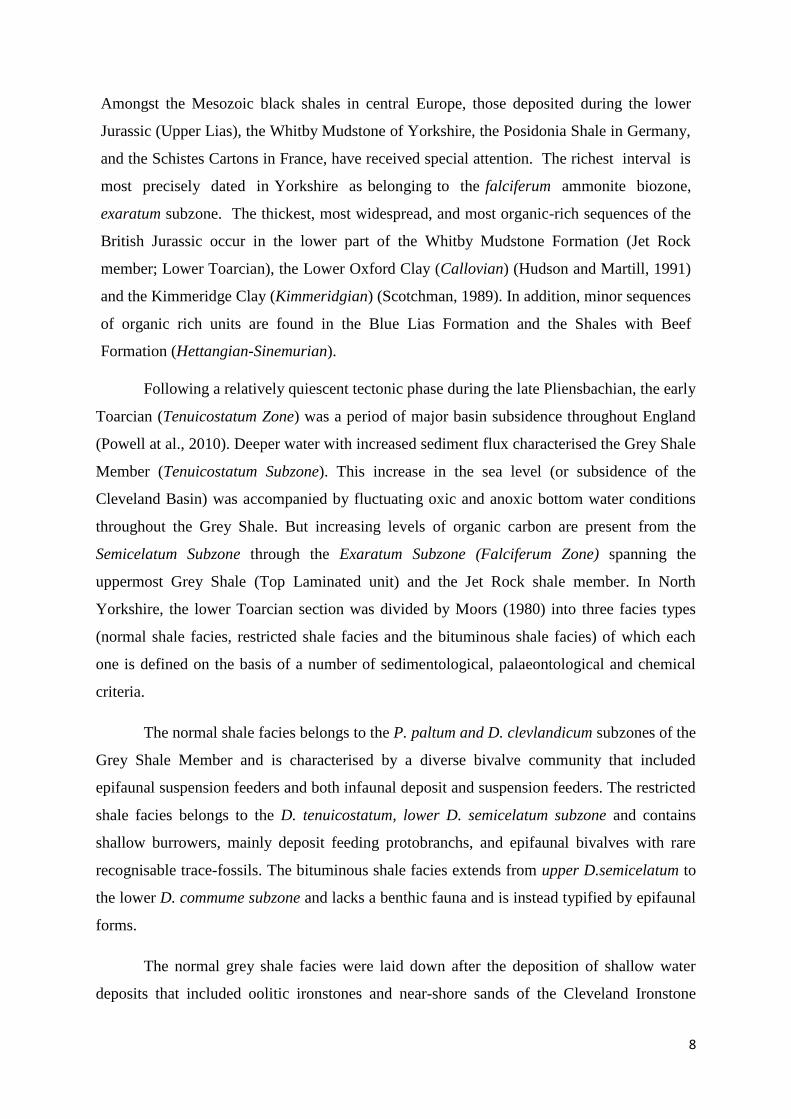
Following a relatively quiescent tectonic phase during the late Pliensbachian, the early
Toarcian (Tenuicostatum Zone) was a period of major basin subsidence throughout England
(Powell at al., 2010). Deeper water with increased sediment flux characterised the Grey Shale
Member (Tenuicostatum Subzone). This increase in the sea level (or subsidence of the
Cleveland Basin) was accompanied by fluctuating oxic and anoxic bottom water conditions
throughout the Grey Shale. But increasing levels of organic carbon are present from the
Semicelatum Subzone through the Exaratum Subzone (Falciferum Zone) spanning the
uppermost Grey Shale (Top Laminated unit) and the Jet Rock shale member. In North
Yorkshire, the lower Toarcian section was divided by Moors (1980) into three facies types
(normal shale facies, restricted shale facies and the bituminous shale facies) of which each
one is defined on the basis of a number of sedimentological, palaeontological and chemical
criteria.
The normal shale facies belongs to the P. paltum and D. clevlandicum subzones of the
Grey Shale Member and is characterised by a diverse bivalve community that included
epifaunal suspension feeders and both infaunal deposit and suspension feeders. The restricted
shale facies belongs to the D. tenuicostatum, lower D. semicelatum subzone and contains
shallow burrowers, mainly deposit feeding protobranchs, and epifaunal bivalves with rare
recognisable trace-fossils. The bituminous shale facies extends from upper D.semicelatum to
the lower D. commume subzone and lacks a benthic fauna and is instead typified by epifaunal
forms.
The normal grey shale facies were laid down after the deposition of shallow water
deposits that included oolitic ironstones and near-shore sands of the Cleveland Ironstone

9
Formation. Then organic-rich laminated shales developed during the deposition of sediments
from the overlying D. Semicelatum and H. Exaratum subzones, where benthic fauna is
entirely absent. At this time, the most organic-rich section of the Whitby Mudstone
Formation, the Jet Rock Shale was deposited in the distal part of an epicontinental sea that
covered much of NW Europe. This abrupt change to deeper-water sedimentation has been
linked to a rapid sea level rise during the early Toarcian (Ivimey-Cook and Powell, 1991).
Sediments become progressively less bituminous towards the top of the H. falcifer
subzone that overlies the H. Exaratum subzone, with the transition from bituminous to
restricted mudstones being marked by a lenticular band of limestone composed of belemnites,
bivalves, fish debris and bones (Morris, 1979).
Correlation between sections of Lower Toarcian strata on the Yorkshire coast is
possible at the decimeter level over a distance of several kilometers, due to numerous
distinctive marker beds of (mostly) carbonate and (rare) sideritic concretions, illustrating the
lateral continuity of the facies. Much of the Lower Toarcian sediment contains calcite, either
cryptically as nannofossil debris and dispersed diagenetic cement, or as large discrete
carbonate concretions (commonly > 15 cm diameter) commonly occurring along discrete
horizons. The section is well exposed along Port Mulgrave and predominantly composed of
pale to dark-grey mudstone that was deposited in fully marine conditions below storm wave-
base (Salen et al. 2000).

10
Figure 1.5: A) map shows the reconstruction of the extent of organic-rich sedimentation for the Lower Toarcian of north-western Europe, 51o 50´N, 6o 15´E. B)
map shows the location of sampling site at Port Mulgrave section in North Yorkshire, UK.
11
1.3 Toarcian Oceanic Anoxic Event
The earliest of the OAEs occurred in the Lower Jurassic (Jenkyns, 1988).
Geochemical, sedimentological and paleontological data indicate that the Early Toarcian was
a period of sudden and severe global environmental change, marked by the start of a major
marine transgression and global warming (Morris, 1980; Hallam, 1981, Jenkyns, 1985).
These global trends were accompanied by widespread development of marine black shale
characterized by a significant perturbation to the global carbon cycle (Hesselbo et al., 2000;
Schouten et al., 2000; Jenkyns et al., 2001; Cohen et al., 2007) and mass extinctions (Caswell
et al., 2009; Courtillot and Renne, 2003; Wignall, 2005).
Organic-rich marine rocks that are early Toarcian in age have been found in many
localities in both the northern and southern hemispheres (Jenkyns 1988; Jenkyns et al. 2002).
Their recognition provides a compelling case for the enhanced accumulation worldwide of
marine organic matter during a relatively brief interval of time, which is now known as the
Toarcian Oceanic Anoxic Event (T-OAE) (Jenkyns 1985; Jenkyns 1988). The major
perturbation to the global carbon cycle during the Toarcian is marked by a substantial and
abrupt carbon isotopic excursion (CIE) in organic C (δ13
C (org)) of about -6‰ to -7‰), that
is observed in rocks of early Toarcian age from throughout Europe (Kuspert 1982; Hesselbo
et al., 2000; Kemp et al., 2005).
Carbon cycle perturbations are globally recorded in sediments as carbon isotope
excursions irrespective of lithology and depositional environment. Although such a globally
significant organic carbon burial event apparently resulted in an overall positive excursion of
the carbon isotope ratio in seawater (figure 1.6), the T-OAE is also punctuated by one of the
largest negative carbon isotope excursions (CIE) of the Mesozoic, which occurred over a
short period estimated to be between 300 and 1000 ka (Kemp et al., 2005; Suan et al., 2008a).
This CIE is recorded in marine organic matter, marine carbonate and terrestrial material in
several localities around the world (Jenkyns and Clayton, 1986, Hesselbo et al., 2000, 2007;
Schouten et al., 2000; Jenkyns et al., 2001; Kemp et al., 2005).

12
Figure 1.6: Ammonite zonal schemes (after Howarth, 1992; Jakobs et al., 1994), absolute U-Pb age data
(after Palfy et al., 2000), and generalized isotope profiles (after Hesselbo et al., 2007; McArthur et al.,
2000) for the Early and Middle Toarcian. B) Palaeogeographical map for the Toarcian showing the
location of lower Toarcian sections with organic-rich facies (from Cohen et al., 2007).
Over the last two decades, there has been increased effort to unravel the causes and
consequences of the T-OAE. These new records have documented sharp and pronounced
carbon isotope excursions δ13
C (org) values which decrease abruptly from -26 to -33 ‰ (Kemp
et al., 2005). The T-OAE is associated with major changes which include a threefold
increase in atmospheric CO2 levels (McElwain et al., 2005), a rise in seawater
palaeotemperatures (Rosales et al., 2004; van de Schootbrugge et al., 2005), an increase in
silicate weathering rates (Cohen et al., 2004; Waltham and Grocke, 2006), and a biotic crisis
affecting marine invertebrates and biocalcifying microorganisms (Little and Benton, 1995;
Tremolada et al., 2005).

13
The lithological expression of the T-OAE may be locally very different (Hesselbo et
al., 2004). It has been found that the development of anoxic, organic matter rich facies did not
occur everywhere in the European Neotethyan realm and, where developed, the lithology,
petrology and organic matter richness of the sediments is variable. The lithological variation
of the T-OAE at different localities illustrates the importance of local environmental
conditions, which are ultimately more important in determining the lithology of deposits
formed during an OAE (Trabucho-Alexandre et al., 2011).
It has been suggested by Hesselbo et al. (2000), that the associated perturbations in
seawater temperature and chemistry, and marine and terrestrial biota were characteristic of all
surficial reservoirs, and the cause of the negative carbon isotope excursion concurrent with
the T-OAE was the dissociation, release and consequent oxidation of methane derived from
continental slope hydrates. More recently, a high-resolution δ13
C(org) record across the T-OAE
obtained from mudstones exposed in northeast England was generated by Kemp et al. (2005).
These data (figure 1.7) suggest that the negative δ13
C excursion was not one single event, but
was actually small multi events, the timing of which was interpreted as having been paced by
astronomically forced climate-ocean cycles.
The sudden and major perturbations to the global carbon cycle occurred during the T-
OAE is observed as well in Palaeocene–Eocene thermal maximum (PETM) about 56 million
year ago (Bowen and Zachos, 2010). This sharp negative carbon isotope excursions (CIE)
record at both T-OAE and PETM are globally recognized in the (marine and terrestrial)
sedimentary record and characterised with decreases in the δ13
C(org) values by up to7‰ and
show broadly similar patterns of initiation and recovery (Figure 1.7).
The records of the CIEs are accompanied by other isotopic, geochemical and biotic
records that show that both events were associated with the extinction of marine invertebrate
species (Suan et al., 2008b), with a crisis in primary producers, with major changes in
terrestrial species distributions and with sudden and substantial warming of marine surface
waters as a direct physical response to atmospheric warming (Morten and Twitchett, 2009).
The overall shift in δ13
C that defines the Carbon isotopic excursion at the two events
was almost -2‰ (Ccarb) for the PETM and about -7‰ (Corg) for the T-OAE. Moreover, the
negative shifts in δ13
C for both events appear to have been paced by astronomical precession,
where the peaks of the abrupt excursions (stage 2 in figure 1.7) lasted almost 100 ka and

14
involved several sudden shifts in δ13
C of between -1‰ to -3 ‰ within about 650 years (T-
OAE) and 1 ka (PETM) (Cohen et al., 2007).
Figure 1.7: Comparison of the PETM and Toarcian CIEs. The coloured bands indicate the three distinct
stages of the CIEs that can be recognized using the same criteria in each case. The A,B.C and D on the
right hand column indicate the astronomical precession cycles . From Cohen et al,. 2007.
The two events are associated with repetitive short lived and catastrophic event. In the
case of T-OAE these small events are recorded at the Pliensbachian-Toarcian boundary
preceding the main event, and characterised with negative carbon isotope excursion, that
were observed at the stage boundary in the SW European section at Peniche, Portugal in
δ13
Ccarbonate, δ13
Cwood and δ13
Cbrachiopod (Hesselbo et al., 2007). The environmental change at
the Pliensbachian-Toarcian boundary shares some characteristics with the T-OAE including a
major drop of platform-derived carbonate accumulation, reduction in size of the pelagic
carbonate producer Schizospharerella, and major rise in bottom seawater temperatures as
evidenced by brachiopod δ18
O values in Lusitanian Basin (Suan et al., 2008). This and its

15
widespread nature is suggested by a contemporaneous excursion of about -1.5‰ close to the
Pliensbachian-Toarcian boundary recorded in belemnite and bulk carbonate in England
(McArthur et al., 2000; van de Schootbrugge et al., 2005; Suan et al., 2008).
In the PETM case the repetitive short lived carbon excursions are documented
following the Paleocene-Eocene thermal maximum (PETM) event, where the main PETM
event is linked to four brief events recorded in marl-rich horizons characterised by low δ13
C
and elevated sedimentation rates. The characteristics of these small events are believed to
constrain explanations for the PETM as a dynamic source must have repeatedly injected large
quantities of 13
C-depleted carbon into the ocean or atmosphere (Nicolo et al., 2007).
1.3.1 Causes and mechanisms for the Toarcian Carbon Isotopic Excursions
Across Europe, the Lower Toarcian negative carbon isotopic excursion is expressed in
bulk organic matter including jet wood, organic biomarkers and in bulk nanofossil carbonate
(Kuspert, 1982; Schouten et al., 2000; Hesselbo et al., 2001). Records of the Toarcian CIE
based on δ13
C(org) and δ13
C(carb) analyses from a number of sections across Europe show
remarkably similar patterns. All records show an overall CIE of c. -6‰ (Jenkyns et al., 2001).
At Dotterhausen Quarry (Southern Germany) for instance, the δ13
C (org) and δ13
C (carb) records
a decrease in the carbon isotope value of -6‰ (Rohl et al., 2001). Similarly, at the Mochras
Farm borehole (Wales, UK), records of both δ13
C (org) and δ13
C (carb) show a CIE of -6‰
(Jenkyns et al., 2001). Samples from the Belluno Trough, Italy, also show a CIE of -6‰ in
δ13
C (org) and -4‰ in δ13
C (carb) (Jenkyns et al., 2001). However, the causes of the carbon
isotope perturbation and synchronicity in its record remain controversial. Two explanations
have been given for the cause of the negative C isotope excursion, which are discussed below.
1.3.1.2 Locally driven mechanisms
The negative C isotope excursion has been attributed to the recycling of re-
mineralized light carbon from the lower levels of an intermittently stratified water column
into the euphotic zone and its subsequent incorporation into photosynthetic phytoplankton
(Kuspert, 1982). This suggestion was made by way of comparison with the present-day Black
Sea. Profiles of δ13
C (bel) through the Lower Toarcian OAE in Germany and the UK presented
by Van de Schootbrugge et al. (2005) supported a local driver mechanism for the CIE,
whereby their data shows that the values of δ13
C in belemnite carbonate were actually

16
increase by 1.5 ‰, with no record of a negative C isotope excursion. However, the Kuspert
(1982) model fails to explain more recent observations which include contemporaneous CIEs
in the terrestrial and atmospheric carbon reservoirs, changes in marine and terrestrial biota,
and the widespread geographical extent of the Toarcian OAE.
1.3.1.1 Globally driven mechanisms.
The methane hydrate dissociation hypothesis
More recently it has been suggested by Hesselbo et al (2000) that the negative C
isotope excursion resulted from the rapid release to the ocean and atmosphere of (biogenic)
methane from methane hydrate in sediments. This arises because biogenic methane is
depleted in 13
C by ~60 ‰, and thus its oxidation to CO2 in the oceans and atmosphere
imparts a light carbon signal on dissolved inorganic carbon (DIC).
Although large-scale methane hydrate dissociation can explain many of the features of
the Toarcian CIE as well as many of the contemporaneous environmental effects (Hesselbo et
al., 2007; Cohen et al., 2004; Kemp et al., 2005), the mass of methane hydrate required to
produce a global CIE does not match the mass of CO2 required to produce the temperature
increases as inferred from Mg/Ca determinations (Schmidt & Shindell 2003; Zachos et al.,
2003; Higgins & Schrag 2006). A much larger mass of CO2 (involving approximately c.4 x
103 Gt of carbon) would have been required to produce the postulated increase in tropical sea
surface temperatures.
However, it is unreasonable to reject a role for methane hydrate dissociation in the
past based on the possibility that an insufficient mass was available, due to considerable
uncertainty surrounding estimates for today’s methane hydrate reserves, plus the fact that
areas of continental shelf and epicontinental seas were substantially greater in the past
(Cohen et al., 2007). Moreover, the recognition that the δ13
C(org) shifts were paced by
astronomical precession (Kemp et al., 2005) provides strong support for the suggestion that a
precessional trigger may have been responsible for the release of the isotopically light carbon.
Thermogenic methane release
Another hypothesis recently put forward for the cause of the T-OAE is that 12
C-
enriched thermogenic gas (mainly methane) was released into the ocean-atmosphere system
due to an igneous intrusion into coaly organic matter-rich facies in the Karro Basin, South

17
Africa (McElwain et al., 2005; Svensen et al., 2007). High-precision radiometric dating has
established that the emplacement of the Karoo-Ferrar igneous provinces overlapped in time
the Toarcian CIEs (Palfy & Smith 2000). A major issue with this mechanism is whether
methane production would have been of the magnitude and rapidity required to produce the
observed global CIEs and associated environmental effects (Kemp et al., 2005; Bowen et al.,
2006). Gröcke et al. (2009) studied the contacts between the intrusions and organic matter
facies in the Karoo Basin and indicated that the geochemical patterns within these facies
suggest little or no thermogenic methane generation, which makes the thermogenic methane
hypothesis questionable.
Widespread burning of terrestrial biomass
Kurtz et al. (2003) suggested that the subsequent burning and oxidation of a large
proportion of terrestrial organic carbon (which is isotopically light) could have caused the
CIE of the Palaeocene-Eocene thermal maximum (PETM) through the release of a large
quantity of light carbon over short period of time (Cohen et al., 2007). This mechanism has
also been suggested by Finkelstein et al. (2006) as a potential cause for the generation of the
CIE during the Toarcian. However, Higgins & Schrag (2006) argued that insufficient biomass
would have been available to produce the CIE at the PETM through burning, and that the
time scales of the abrupt decreases in δ13
C were too short to have been compatible with this
mechanism.

18
1.4 Aims and Objectives
This project aims to study the black shale cycles, reflecting variable redox conditions
through the Lower Toarcian (Grey Shale and Jet Rock Members of the Whitby Mudstone
Formation) in Cleveland Basin. In discussing Early Toarcian events recorded in the
Cleveland Basin, the focus of others has been largely on the 3 m interval in the lower
exaratum Subzone where TOC concentrations are highest (the putative T-OAE in the strict
sense), or the 7 m of the exaratum Subzone itself (the putative T-OAE in the wider sense).
Despite the extensive previous work on the T-OAE, few studies have explored the well-
preserved sediments below the event that document different phases finally leading to large-
scale (global) anoxia, which is the focus of this project. High-resolution multi-proxy
geochemical approach (organic and inorganic) is undertaken in order to better understand the
biogeochemical processes, which occurred during this event by investigating the following:
To identify variability in organic matter composition within a small interval of the
Sulphur Band at the base of the Grey Shale Member and compare with the Jet Rock
shale (T-OAE interval).
The sudden change in the nature of the depositional environment that produced the
laminated Sulphur Bands at the base of the transgressive systems tract, and how the
nature and geochemistry of the organic matter varies relative to that of the bituminous
facies higher up the section. How the palaeo-oxygenation condition influences the
quality of the organic matter within the Sulphur Bands (high organic carbon but
relatively low hydrogen index).
Understanding the trigger mechanisms that produced the laminated Sulphur Bands
and to investigate whether it can be linked to the same long-lasting process that
generated the T-OAE.
To determine whether data generated by FT-NIRS can be used to estimate bulk
geochemical contents of ancient sediments, such that the technique can be used to
either replace or complement data measured by conventional methods. Successful
application would mean that future studies on marine rocks could benefit from time
and cost savings offered by FT-NIRS in comparison to other, more complex
geochemical analyses.
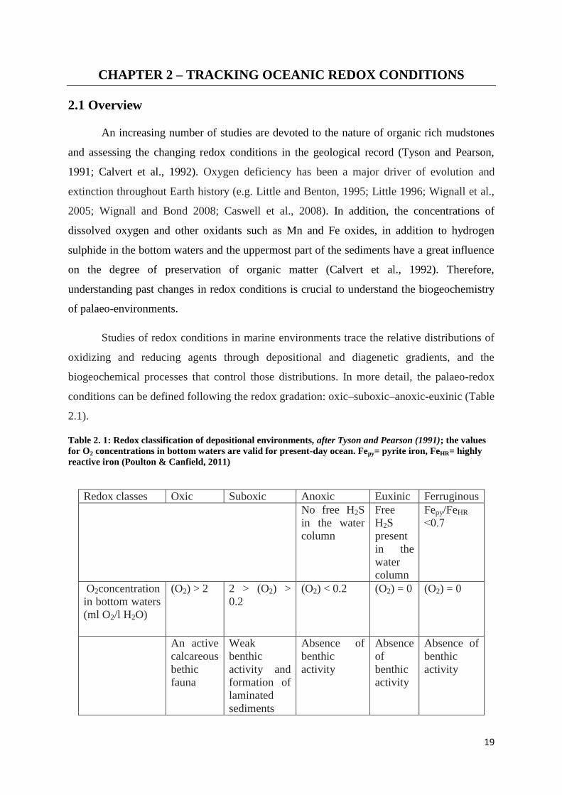
19
CHAPTER 2 – TRACKING OCEANIC REDOX CONDITIONS
2.1 Overview
An increasing number of studies are devoted to the nature of organic rich mudstones
and assessing the changing redox conditions in the geological record (Tyson and Pearson,
1991; Calvert et al., 1992). Oxygen deficiency has been a major driver of evolution and
extinction throughout Earth history (e.g. Little and Benton, 1995; Little 1996; Wignall et al.,
2005; Wignall and Bond 2008; Caswell et al., 2008). In addition, the concentrations of
dissolved oxygen and other oxidants such as Mn and Fe oxides, in addition to hydrogen
sulphide in the bottom waters and the uppermost part of the sediments have a great influence
on the degree of preservation of organic matter (Calvert et al., 1992). Therefore,
understanding past changes in redox conditions is crucial to understand the biogeochemistry
of palaeo-environments.
Studies of redox conditions in marine environments trace the relative distributions of
oxidizing and reducing agents through depositional and diagenetic gradients, and the
biogeochemical processes that control those distributions. In more detail, the palaeo-redox
conditions can be defined following the redox gradation: oxic–suboxic–anoxic-euxinic (Table
2.1).
Table 2. 1: Redox classification of depositional environments, after Tyson and Pearson (1991); the values
for O2 concentrations in bottom waters are valid for present-day ocean. Fepy= pyrite iron, FeHR= highly
reactive iron (Poulton & Canfield, 2011)
Redox classes Oxic Suboxic Anoxic Euxinic Ferruginous
No free H2S
in the water
column
Free
H2S
present
in the
water
column
Fepy/FeHR
˂0.7
O2concentration
in bottom waters
(ml O2/l H2O)
(O2) > 2 2 > (O2) >
0.2
(O2) < 0.2 (O2) = 0 (O2) = 0
An active
calcareous
bethic
fauna
Weak
benthic
activity and
formation of
laminated
sediments
Absence of
benthic
activity
Absence
of
benthic
activity
Absence of
benthic
activity

20
Anoxic conditions may be non-sulphidic or sulphidic (sulphidic conditions also being
referred to as euxinic). Euxinic water conditions develop when free H2S occurs within the
water column. In the modern world, euxinic conditions in the water column are usually
restricted to semi-enclosed basins like the Black Sea (Meyer & Kump, 2008). The H2S is
produced by sulphate-reducing bacteria. In some cases, as in the Black Sea, euxinic
conditions may reach the photic zone, where photosynthetic sulfide-oxidizing bacteria may
develop (Koopmans et al. 1996a). However, the redox state of the ocean can vary widely
(both temporally and spatially), from various levels of oxygen depletion, through anoxic and
non-sulfidic (ferruginous) conditions, to fully euxinic. Anoxic, iron-rich (ferruginous)
oceanic conditions are recognised recently as a dominant feature of anoxic oceanic intervals
throughout much of Earth’s history (Poulton and Canfield, 2011). Ferruginous conditions
describe the intermediate state between the oxic and euxinic end-members, that the
environmental behaviour of iron takes central stage.
Suboxic settings are characterized by extremely low but generally non-zero oxygen
concentrations in the water column, where H2S is limited to interstitial waters below the
sediment–water interface. Transitional settings can occur wherein the first appearance of H2S
coincides with the sediment water interface.
Under oxic conditions, aerobic organisms utilise dissolved O2 from the overlying and
interstitial waters for their metabolism. As dissolved oxygen becomes depleted, organic
matter decomposition continues via micro-organisms using secondary oxidant sources
(e.g.nitrate, iron hydroxides, manganese oxides and sulphate). Ultimately, when all free
oxidants are exhausted, methanogenesis takes place (Froelich et al., 1979).
This classical early diagenetic sequence is illustrated in Figure 2.1, with the following
equations representing the principle respirator pathways of organic matter mineralization:
1- Oxic respiration
O2+1/2C2H3O2- → HCO3- + 1/2H+
2- Denitrification
4/5NO3- + 3/5H+ + 1/2C2H3O2 → 2/5N2 + +HCO3 + 1/5H2O
3- Dissimilatory Mn reduction
7/2H+ + 2 MnO2 + 1/2 C2H3O2− → 2Mn2+ + HCO3- + 2H2O
4- Dissmilatory Fe reduction
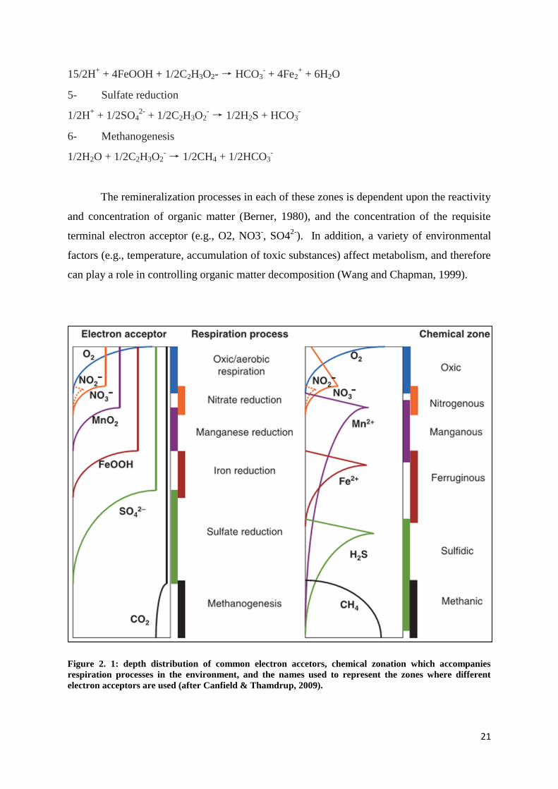
21
15/2H+ + 4FeOOH + 1/2C2H3O2- → HCO3
- + 4Fe2
+ + 6H2O
5- Sulfate reduction
1/2H+ + 1/2SO4
2- + 1/2C2H3O2
- → 1/2H2S + HCO3
-
6- Methanogenesis
1/2H2O + 1/2C2H3O2- → 1/2CH4 + 1/2HCO3
-
The remineralization processes in each of these zones is dependent upon the reactivity
and concentration of organic matter (Berner, 1980), and the concentration of the requisite
terminal electron acceptor (e.g., O2, NO3-, SO4
2-). In addition, a variety of environmental
factors (e.g., temperature, accumulation of toxic substances) affect metabolism, and therefore
can play a role in controlling organic matter decomposition (Wang and Chapman, 1999).
Figure 2. 1: depth distribution of common electron accetors, chemical zonation which accompanies
respiration processes in the environment, and the names used to represent the zones where different
electron acceptors are used (after Canfield & Thamdrup, 2009).

22
Oxygen-limited conditions and ultimately anoxia may develop when the oxygen
demand exceeds the supply. In the water column, anoxia may develop in stagnant or confined
water masses where insufficient circulation prevents O2 renewal, or in places where intense
OM degradation consumes O2 faster than it is replenished, even in open-marine conditions
(Demaison and Moore, 1980; Pedersen and Calvert, 1990).
Euxinic settings comprise less than 0.5% of the deep ocean today, with the Black Sea and
Cariaco Basin off the coast of Venezuela being the largest and second largest examples,
respectively (see recent review by Meyer & Kump, 2008). In the geologic record, however,
oxygen deficiencies and even euxinia occurred on much wider scales, as demonstrated by the
so-called OAEs, intervals known most famously from the Mesozoic for abundant, widespread,
organic-rich black shales deposited under anoxic to euxinic conditions.
2.2 Existing models for anoxia
Studies of modern oxygen-poor environments have shown that oxygen deficiency
may be due to decreased oxygen supply or increased oxygen demand beneath areas of high
productivity (Demaison and Moore, 1980; Jenkyns, 1988). Most models of palaeo-redox
conditions are based upon observations of modern anoxic environments, which are currently
limited in comparison to the much wider distribution of anoxic environments in other periods
of geological time. The Black Sea is the largest landlocked body of permanently anoxic water
in the world, covering roughly 4.4 × 10⁵ km
2 (Meyer & Kump, 2008), and as such has been
the focus of numerous studies (e.g. Vinogradov et al., 1962; Sweeney and Kaplan, 1980;
Leventhal, 1983; Canfield et al., 1996; Wilkin and Arthur, 2001). Most of the formation of
black shales in the present day occurs in two distinct settings, the upwelling zones and silled
basins (Wignall, 1994).
2.2.1 The silled basin model
This model uses the influx of fresh water into a basin to produce a halocline that is
produced due to the different water densities. The halocline restricts oxygen rich water to
lower depths in the water column. The lack of water movement and low oxygen demand due
to the decaying organic matter, results in anoxia (Wignall, 1994). There are two contrasting
models for the silled basin, both of which rely on the influx of marine water (Figure 2.2), and

23
the two models are part of the productivity versus preservation argument (Armstrong et al.,
2005).
In the Deuser (1974) model, marine water fills the deeper parts of the basin and
gradually expands upwards. Enhanced preservation beneath the anoxic water column causes a
high accumulation of organic carbon, while changes in photic zone productivity do not play
an essential role in this model. Progressive restriction of the size of the oxygenated upper
layer (mixolimnion) gradually prevents nutrient supply and thus leads to a decrease in
productivity and hence sedimentary organic carbon production.
In contrast, the Strakhov (1971) model, invokes elevated primary productivity.
During the initial stages of marine incursion, nutrients in the lower anoxic layer
(monimolimnion) remain isolated from the euphotic zone by the halocline. The gradually
rising monimolimnion then releases nutrients to the mixolimnion and triggers a high
productivity episode, which is sustained by organic matter production in the euphotic zone.
Thus, the restricted circulation characteristic in this model is important because it promotes
nutrient trapping, not because it slows circulation rates which interprets the high flux of
organic matter to the sediment at a time when much of the water column was fully
oxygenated.

24
Figure 2.2: Conceptual models for the formation of basin anoxia in the silled basin setting. after
Armstrong et al. (2005)
In the Black Sea case, continental runoff from Eastern Europe provides a vast amount
of fresh water that enters the basin via the narrow Bosporus Strait to the south and by large
rivers directly drain to the basin. These two inputs generate strong density stratification in the
Black Sea, with a deep-water residence time of ∼300 years (Murray et al. 2007). Therefore,
the freshwater forms a layer at the surface approximately 50m thick that restricts oxygen
transfer into the deep water below. An intermediate zone (free of oxygen, dissolved Fe and
H2S), separates the oxic surface fresh water from deep sulfidic waters (>100 m depth) (Figure
2.3). Dissolved H2S is only abundant below the layer containing dissolved Fe.

25
Figure 2.3: Schematic diagram of the main features of the dissolved and particulate inorganic Fe and S
chemical structure of the Black Sea (after Brewer and Spencer, 1974, Cutter and Kluckhohn, 1999)
As seen in Figure 2.3, the distribution of Iron phases follows an ordered pattern. The
intermediate anoxic layer contains the highest concentration of greigite (Fe3S4) than
anywhere in the water column, and the boundary between the intermediate and Fe bearing
anoxic layer is characterised by a peak in pyrite (Cutter and Kluckhohn, 1999).
The expanded suboxic zone has both low oxygen and low sulfide concentrations (<10
μM). Abiotic and microbial processes cycle nitrogen and trace metals across the chemocline.
Based on Murray et al.(1989) and Murray and Izdar (1989), Canfield and Thamdrup (2009)
produced depth distribution profiles of chemical zones and respiration processes deduced
from the chemical data (Figure 2.4). The nitrogenous zone is restricted to the zone containing
a nitrite maximum, and below this a manganous zone is designated, as here manganese
begins to accumulate in the absence of other anaerobic metabolic products. The sulfidic zone
is located immediately below. These respiration processes follow very closely the chemical
zonations in the case of the Black Sea (Canfield & Thamdrup, 2009).

26
Among the chemocline microbial population there are the photosynthetic green sulfur
bacteria (GSB, Chlorobiaceae) (Overmann, 2006). These anoxygenic sulfide-oxidizers can
use irradiance that is just 0.0005% of the light available in surface waters (Overmann et al.
1992). Derivatives of the GSB light-harvesting carotenoid, isorenieratene, are preserved in
anoxic sapropels of the Black Sea. The distribution of this molecular fossil in sediment cores
from near the modern chemocline is thought to record chemocline depth oscillations over the
past 8 kyr (Huang et al. 2000). Sediments accumulating at the current time in the deepest part
of the Black Sea basin consist of laminated CaCO3 rich muds (up to 80 wt%) with typically 2-
5% total organic carbon (TOC) and 1-2.5 wt% pyrite (Calver and Karlin, 1991; Wilkin and
Arthur, 2001).
Figure 2.4: Chemical data from the Black Sea. Listed are the depth distribution of chemical zones and
respiration processes deduced from the chemical data (after Canfield and Thamdrup, 2009).

27
2.2.2 The upwelling model
The upwelling model is where cold water from below the thermocline is moved up to
compensate for the seaward movement of surface water. The water from below the
thermocline is nutrient rich and, when enter the euphotic zone, high productivity stimulate or
maintain in the photic zone (Demaison and Moore 1980). This high productivity allows for
accumulation of organic rich shales (Armstrong et al., 2005).
At the present time, anoxic and dysoxic conditions are restricted to the coastal
upwelling zones at the intersection of intensified oxygen minimum zones (OMZ) and the
upper slope or continental shelf break, in water depths typically >50m (e.g., the Peru Current)
(Wignall, 1994). Organic rich sediment accumulation in upwelling zones is a result of
elevated productivity in a region of strong circulation and high organic loading. These zones
occur at water depths of about 200 to 1,000 metres, and have the potential to affect much
wider areas as they develop in the open ocean, depending on local circumstances. This
intensity of bio-accumulation and regeneration play an important role for trace matels
accumulation, where the upwelling sediments are often enriched in Cd and P and depleted in
Co and Mn (Brumsack, 2006)
Figure 2.5: An oxygen profile at an oceanic location with an oxygen minimum zone.

28
One of the best studied examples is the Arabian Sea. In this case oxygen falls to
below 1 mL/L between about 150 and 1500 m (Schulte et al., 1999), but no free sulphide is
present. Where the oxygen minimum zone overlaps the continental margin, sediments are
often laminated, and higher levels of organic carbon are preserved (Weijden et al., 1999).
Geochemical proxy data, combined with microfossil analysis, indicates that the
oxygen minimum zone in the Arabian Sea has varied considerably on orbital and suborbital
timescales over the past 225 Ka (Reichart et al., 1998). These changes are apparently driven
by surface productivity and winter mixing patterns, whilst productivity is in turn regulated by
freshwater input during the monsoon (Schulte et al., 1999). Oxygen minimum layers can be
enhanced by upwelling zones at continental margins, where nutrient rich deep waters are
brought to the surface by wind action. The increased oxygen demand resulting from high
productivity in surface waters can lead to severe oxygen depletion. Upwelling can, itself,
cause oxygen minimum zones without any pre-existing oceanic oxygen depleted layer, as is
the case on the Peru margin between 12° and 13.5°S (Arthur et al., 1998). Here, the oxygen
levels are lower than 0.1 mL/L in a zone between 70 and 400m depth, and sediments
accumulating in this zone are frequently laminated and comparatively organic-rich (Emeis et
al., 1991).
2.3 Characteristics of euxinic environments
Euxinic settings share many physical and biogeochemical characteristics (Table 2.2).
Often these euxinic settings exhibit restricted circulation, deep water and high primary
productivity thrived by elevated nutrient supply. Although it is conventionally agreed that
sluggish circulation is a primary reason for euxinia, the argument can be made that nutrient
trapping is another fundamental characteristic that promotes euxinia in such settings (Murphy
et al., 2000; Meyers, 2007). Therefore, the restricted circulation characteristic of many
modern euxinic basins is important because it promotes nutrient trapping, not because it
slows circulation rates. In modern euxinic setting there is a strong positive correlation
between deep water PO4 and sulphide concentration (Table 2.2; Meyer and Kump, 2008).
This relationship is understandable from biogeochemical relationships as decomposition of
the organic matter by sulphate reducing bacteria proceeds in deep waters, oxidants are
consumed and equivalent amounts of waste product (including H2S and organic-bound N and
P) are released.

29
Table 2.2: Characteristics of modern euxinic basins (After Meyer and Kump, 2008)
In silled basin settings, anoxia is favoured when riverine input of nutrients is high, and
recycling of P during diagenesis is high (P burial efficiency low), and when the rate of
vertical mixing within the basin is suppressed relative to the deep inflow rate (Shen et al.,
2002) .
Silled basins with estuarine circulation, such as the Black Sea and some fjords, are
efficient nutrient traps. The estuarine flow occurs in stagnant water bodies that experience a
positive water balance (where the input rates exceed that lost by evaporation) (Demaison and
Moore 1980). Low salinity and nutrient-depleted surface water flows out of the basin, while
salty and nutrient-rich waters enter the basin at relatively deeper depths. These nutrient-rich
deep waters are mixed upward, promoting biological productivity and creating high demand
on oxygen as the organic matter falls through the water column (Armstrong et al., 2005).
Once estuarine circulation is absent, other factors could aid to develop sulphidic conditions.
For instance, the groundwater supply to meromictic lakes is sulphur replete which in such
case the sulphide source allows H2S accumulation independent of phosphate concentration
(Meyer and Kump, 2008). Moreover, sulphide flux from sediments into bottom waters could
play an essential role in shallow eutrophied environments, as in the Mariager Fjord, the
process of sulphate reduction during the degradation of the sedimentary organic matter
produces the sulphide which then diffuses upward into the water column (Weeks et al., 2004).

30
2.4 An overview of palaeoredox indicators
Indices which accurately record the levels of oxygen present at the time of deposition of
ancient marine sediments are important for a number of reasons. In the first place the
characterisation of depositional conditions is fundamental to the study of sedimentary rocks.
Accurate indices of redox can also contribute to the debate on the role of redox in the
preservation of organic carbon (which is still hotly contested) and the understanding of
variations in oceanic oxygen levels. The latter has implications for both the timing and nature
of mass extinction events as well as providing information on interactions between global
climate and the oceans.
2.4.1 Sedimentological and palaeoecological indicators of anoxia
Historically, the most commonly cited fingerprints of anoxia have been organic
richness and sedimentary fabrics undisturbed by burrowing organisms (Savrda and Bottjer,
1987). However, this organic enrichment is a product of complex factors, in addition to
anoxia. Sedimentation rate, levels of organic input from primary production, and
mineralogical controls such as clay contents that can impact organic preservation are all
factors which could control organic enrichment (Pedersen and Calvert 1990). Similarly, the
preservation of lamination, often but not always reflecting seasonal patterns of deposition,
may not be reliable to explore the palaeo-oxgenation conditions as brief episodes of
oxygenation can be marked by high-abundance, low-diversity populations of shelly
pavements within otherwise microlaminated sediments (Tyson, 2005). In other words,
undisturbed sediments can reveal complex histories of more or less hospitable conditions
despite a preponderance of generally laminated material (Rohl et al., 2001).
Morris (1979) produced a detailed shale classification based on field analysis using
sedimentological and trace-fossil observations of Toarcian sediments from North Yorkshire.
He subdivided the sequence into three facies, normal, restricted and bituminous.
Normal Shale Facies
This facies is represented by the lower beds of the Grey Shale Member, and is
characterised by homogeneous, bioturbated sediment with abundant benthic body-fossils and
common sideritic nodules, and was deposited in an oxygenated shallow marine environment.
This facies is charaterised by a mixed assemblage of infaunal and epifaunal types, the
infaunal bivalves being represented by both shallow and deep burrowing types (Morris, 1979).

31
This facies is organic-poor (TOC 0.6 to 3 wt %) with low Hydrogen Index values ranging
from 83 to 134 (mg HC/g TOC).
Restricted Facies
This facies is represented by much of the Alum Shale Formation and the upper half of
Grey Shale Member. The disappearance of siderite and the abundance of calcareous
concretions suggest the loss of oxic layers in the sediment with reducing conditions extending
close to the sediment water interface. Reducing conditions within the sediments led to an
increase in the organic carbon content of the sediments. At levels of high organic carbon
content (> 3% TOC; Demaison and Morris, 1980) a decrease in the diversity of the bivalves
is observed with infaunal deposit-feeding ecoming increasingly abundant
Bituminous Shale Facies
The bituminous shales, also commonly named bituminous mudstones, are
characterized by the abundance of wavy thin lamination. According to O’Brien (1990), the
laminae are commonly less than 1 mm and have smooth, parallel contacts. The
microlamination indicates quiet environmental conditions and short-term alternations in the
predominance of terrigenous sediment supply and plankton productivity (Oschmann, 1991;
O’Brien, 1990). This facies is limited to the Jet Rock Member. The abundance of pyritic
calcareous concretions and the lack of infauna suggest that reducing conditions extended up
to sediment surface or even higher into the bottom waters. The Jet Rock Member at North
Yorkshire is one of the most organic rich rocks in Britain (Farrimond 1988). It represents a
bituminous (“inhospitable bottom”) shale facies containing high values of weight percent
total organic carbon (TOC) of around 20%, which occur towards the base of the Jet Rock and
decline upwards to the contact with the overlying Alum Shales (Myers and Wignall 1987).
Moreover, the Palaeoecological techniques were used to derive evidence for palaeo-
oxygen levels. The oxygen restricted biofacies (ORB) scheme of Wignall and Hallam (1991)
is one of the well-known indicators of Palaeo-oxygen levels of ancient sediments. This
scheme uses species diversity combined with sedimentological data to define 6 zones of
increasing oxygenation (figure 2.1)

32
Figure 2.6: A classification scheme for black shale biofacies derived from data on the fauna and
lithologies of the British Jurassic. The transition from biofacies 1-6 is interpreted to reflect an increase in
both the levels of bottom water oxygenation and the longevity of oxygenation events (Wignall and Hallam,
1991)
Because organic richness and benthic ecologies can fail to point uniquely to the
benthic oxygen condition at the time of deposition, researchers have turned increasingly to
geochemical methods (Table 2.3).
Table 2.3: summary of most used paleoredox indicators Wignall and Hallam, 1991; Berner, 1984;
Koopmans et al. 1996a; Zheng et al., 2000; Poulton and Raiswell, 2002.
Levels of oxygen Fepy/FeHR FeHR/FeT C/S Mo (µg/g) Isoren-
ieratane
Oxic (0.8-1 ml/l O2) <~0.22 Zero S
intercept
TOC:TS >
5.0
Terrestrial
background
values
Absent
Dysoxic (0.2-1.0
ml/l O2) <5 ppm Absent
Deep water anoxia;
a. non-sulphidic
(ferruginous)
b. euxinic
a. <0.7
b. >0.7
≥0.38 Non-zero S
intercept
TOC:TC <
1.5
>25 ppm Absent
Photic zone euxinia >0.7 ≥0.38 Non-zero S
intercept
TOC:TC <
1.5
>25 ppm Present

33
2.4.2 Carbon–sulphur relationships
Several approaches for evaluating the development of anoxic bottom waters are based
on C/S ratios, Fe-TOC-S relationships, and framboidal pyrite size distributions (Berner, 1984;
Brumsack, 1988; Wilkin et al., 1996; Raiswell and Canfield (1998); Poulton and Raiswell,
2002). These techniques are used to evaluate the role of sulfate reduction in marine
environments. The development of sulfate reduction is a sign of redox and occurs only under
anoxic conditions, where it is mediated by bacterial reactions utilizing dissolved sulphate and
organic matter as reactants, and yielding H2S. The output of this process (H2S) in the
presence of reactive iron can be fixed in the sediments in the form of pyrite (Berner, 1984).
Cross-plots of organic carbon and sulphur (figure 2.7) are commonly assigned to palaeoredox
conditions in the depositional environment (Berner, 1984; Jackson and Raiswell, 1991).
Figure 2.7: TOC and TS relationship by Berner, 1984. the dashed and solid lines are regression lines for
normal marine (oxygenated bottom water) and freshwater respectively.

34
Sediments deposited under oxic marine conditions generally tend to display S/C ratios
of less than 0.4 (Berner and Raiswell, 1984). On the other hand, euxinic environments are
either characterized by S/C ratios higher than 0.4 with positive intercepts on the S axis
(Leventhal, 1983), or by a fairly constant sulfur content independent of the organic carbon
content. The latter case occurs mainly in euxinic environments where sulfur fixation via
pyrite formation is limited by the availability of reactive iron and, hence, pyrite formation
ceases after the reactive iron reservoir is exhausted, even though sulfate reduction continues
(Raiswell and Berner, 1985). Moreover, the relationship between carbon and sulphur alters
with increasing burial due to preferential carbon loss during diagenesis and thermal maturity
(Jones and Manning, 1994).
The degree of pyritisation (DOP), which is defined as DOP = (Fepyrite)/(Fepyrite +
Fereactive), eliminates the effect of variations in Fe content, and Raiswell et al. (1988) suggest
that DOP may be used to distinguish between sediments deposited under different conditions,
where values of DOP less than 0.42 indicate oxic conditions, and DOP more than 0.75
indicates anoxic conditions. Reactive iron was defined by Raiswell et al. (1988) as the
fraction of iron that is HCl-soluble. Dean and Arthur (1989) plotted Fe, S, and TOC values in
a ternary diagram, where the limiting factors for pyrite formation can be distinguished. This
means that the dilution effects caused by biogenic (carbonate and opal) or siliciclastic sources
are eliminated. Based on the process of pyrite formation in organic bearing sediments, a
refinement of DOP has been defined, termed the Indicator of Anoxicity (IA) (Raiswell et al.,
2001). Here, the ratio (FeD+FeP)/FeT is used, where FeD represents the iron soluble in
dithionite, FeP the iron present as pyrite, and FeT represents total iron. Values of IA above
0.38 suggest anoxic conditions, while values of IA < 0.38 indicate oxic conditions (Raiswell
et al., 2001).
2.4.3 Framboidal pyrite distributions
Framboids are densely-packed, raspberry-like, spherical aggregates of equigranular,
micron-sized crystals or microcrysts (Rickard, 1970). They are a common diagenetic feature
in many shales, and are particularly abundant in strata formed under oxygen-poor
depositional conditions (Raiswell and Berner, 1985; Wilkin et al., 1997; Wignall and Newton,
1998). They occur within the surface layers of sediments formed beneath oxygen-poor
(dysoxic) bottom waters, where the redox boundary is located close to the sediment surface,
and can occur in a range of sizes typically between 4 and 50 m diameter (Wilkin et al.,

35
1997). As oxygen restriction intensifies the redox boundary may move above the sediment
water interface into the lower water column which creates right conditions for pyrite
framboids to form syngenetically (Wilkin et al., 1997).
Figure 2.8: SEM images for samples from the Grey shale member at North Yorkshire (Newton, 2001).
Image A (top laminated unit) showing narrow range of framboid size distribution dominated with type 1
framboids, and just one type 2 framboid appears at the centre. Image B (bioturbated mudstone) showing
a mixed cluster of framboids and euhedral crystals.
36
A clear distinction was noted between syngenetic pyrite (pyrite formed in the water
column) and diagenetic pyrite (formed within the sediment), where there are distinct
differences between the average diameters and the degree of size variability of framboidal
pyrites, depending on the oxygenation state of the environment of formation. In euxinic
environments, framboid nucleation and growth occurs within an anoxic water column, and
because of hydrodynamic effects, growth times are generally shorter than when framboid
nucleation and growth occur within anoxic sediment pore waters underlying oxic water
columns. As a result, syngenetic framboid populations formed in euxinic environments are
characteristically small (5.0 +/- 1.7 µm) and have a narrow size distribution (Wilkin et al.,
1997), while those framboid crystals formed in oxic or dysoxic are characteristically larger
and have wider size range distribution (7.7 +/- 4.1µm) (Wilkin et al., 1996; Wignall et al.,
2005).
2.4.4 Iron geochemistry
The iron-based paleoredox proxies are an important inorganic indicators of redox
conditions in ancient sediments ((Raiswell and Berner, 1987; Raiswell et al., 1994; Suits and
Wilkin, 1998; Wilkin et al., 1997; Poulton and Raiswell, 2002). Its application has sharply
increased in recent years as researchers have unlocked their underlying mechanisms (Rickard,
1974; Berner, 1980; Canfield et al., 1992; Yao and Millero, 1996; Poulton, 2003; Poulton et
al., 2004).
Under sulphidic conditions where free hydrogen sulphide is available as output of
sulphate reduction by sulphur reducing bacteria (equation 1), reactive iron associated with
detrital sediments reacts with hydrogen sulfide and forms pyrite as in equation 2 (Berner,
1970). The initial product of this reaction is not, in fact, pyrite but rather a series of
metastable iron monosulfides which during early, diagenesis readily transform to pyrite under
most conditions.
2CH2O + SO4- → H2S+ 2HCO3
- (1)
Fe2+
+ H2S → FeS + 2H+ (2)

37
Figure 2.9: Diagramatic representation of the overall process of sedimentary pyrite formation (after
Berner et al., 1984)
This iron can limit the formation of sedimentary pyrite when abundant supplies of
organic carbon and sulphate are available. Berner (1970) proposed that one minute extraction
with boiling, concentrated hydrochloric acid can approximate the amount of iron remaining
in sediment that is reactive to hydrogen sulphide on early diagenetic time scales, and argued
that the method efficiently extracts those phases most readily reactive to H2S (e.g., iron
(oxyhydr) oxides). Berner then expanded this concept by introducing the degree of
pyritization (DOP) parameter, defined as pyrite-Fe/(pyrite-Fe + HCl-extractable Fe). From
this definition, it followes that sediments with ample remaining supplies of reactive iron
38
would have low DOP values, and degrees of pyritization for those with limited iron
availability should approach one. Raiswell et al (1988) calibrated the DOP parameter using
ancient shales with independent paleoecological indications, and showed that <0.42 DOP
points to oxic facies, 0.46 < DOP < 0.80 suggests dysoxic facies, while 0.55 < DOP < 0.93
corresponds to euxinic facies, with the possibility of some overlapping. They argued that
pyrite forms in euxinic environments with higher DOP due to long exposure to high levels of
H2S, resulting in sulfidation of the less reactive iron minerals. Canfield et al. (1992) found
that in some settings DOP is intermediate (~0.4) despite exposure to pore water sulphide
concentrations of up to 6 mM on time scales of 103 years. Therefore high DOP values that
characterize the euxinic sediments must stem from another factors rather than the duration of
exposure to high concentration of dissolved sulphide.
In fact, Canfield (1989) recognised that the Fe extracted during the DOP procedure
did not accurately reflect the Fe reacting in marine systems. The challenge was a precise
definition and efficient quantification of the reactive iron portion, particularly given that in
many types of sediment only a portion of the total reactive iron pool is converted to iron
sulfide. The most highly reactive iron phases in sediments, dominantly oxides and
oxyhydroxides, are reactive toward H2S on time scales of only days to weeks or less
(Canfield et al., 1992; Poulton et al., 2004a).
2.4.4.1 Determining highly reactive iron content (FeHR)
A buffered citrate-dithionite technique was used by Raiswell and Canfield (1996) to
avoid including the poorly reactive Fe that can be leached from recalcitrant phases under the
boiling HCl treatment, the approach earlier used to define reactive iron for DOP (Berner,
1970). Therefore, the highly reactive iron (FeHR) was originally redefined as the sum of pyrite
Fe, iron present as acid volatile sulfide (AVS), and residual, unsulfidized dithionite-
extractable Fe (representing Fe oxides, but not including magnetite; Raiswell and Canfield,
1996; 1998; Raiswell et al., 2001; Poulton and Raiswell, 2002).
However, Poulton and Canfield (2005) then refined the analytical characterization of
reactive iron by introducing a new sequential extraction technique for iron, based on a
refinement of existing redox proxies centred on the mineralogy and biogeochemical
behaviour of iron. This technique allows full evaluation of the iron minerals that are
considered to be highly reactive (FeHR) towards biological and abiological reduction under
anoxic conditions. The FeHR includes four different pools of iron;

39
1) Iron associated with carbonate minerals (Fecarb; siderite FeCO3, ankerite Ca(Fe, Mg,
Mn)(CO3))
2) Ferric (oxyhydr)oxide minerals (Feox; ferrihydrite Fe2O3.0.5H2O, lepidocrocite γ-
FeOOH, goethite α-FeOOH, hematite Fe2O3, α-Fe2O3)
3) Magnetite (Femag) iron(II,III) oxide (Fe3O4)
4) Fe pyrite (Fepy) irondisulfide (FeS2)
Thus, in contrast to the older technique for defining FeHR (Raiswell et al., 1994), the
new scheme includes carbonate Fe and magnetite, which also react rapidly with dissolved
sulphide (Poulton et al., 2004; Poulton and Canfield, 2011). The sum of these pools therefore
gives the total concentration of highly reactive Fe (FeHR = Fecarb + Feox + Femag + Fepy).
2.4.4.2 Iron recycling, enrichment, and the shelf-to-basin iron shuttle
Canfield et al. (1996) provided the first detailed insight into how high concentrations
of pyrite are produced under euxinic water column conditions. The very high enrichments of
highly reactive iron (defined as Fe (oxyhydr) oxides plus pyrite) in the deep part of the Black
Sea occur due to the scavenging of dissolved iron in the water column during syngenetic
pyrite formation under euxinic conditions (Canfield et al., 1996; Raiswell and Canfield,
1998). By contrast, in oxic to suboxic bottom water conditions, such iron enrichment cannot
occur, and this enrichment forms the basis for all Fe redox indicators (also explaining how
the DOP parameter works).
The remobilization of Fe in shelf settings and its transfer to the deep part of the basin
increases the ratio of highly reactive portion relative to the total Fe (FeHR/FeT) and the total
Fe to Al (FeT/Al) in basinal sediments (Lyons and Severmann 2006). This and other
mechanisms (including enhanced hydrothermal inputs) can enhance highly reactive iron
contents of sediments. Thus, elevated FeHR/FeT may be considered a characteristic indicator
of anoxic conditions.
More recent work has explored in detail how the enrichments in FeHR are generated
under anoxic conditions. This relates to how reactive iron is distributed and transported
within sedimentary basins. Export of reactive iron from shelf sediments (Figure 2.10) results
from solubilization of iron (oxyhydr) oxides during diagenesis and release of dissolved Fe(II)
into the water column (Lyons and Severmann, 2007).
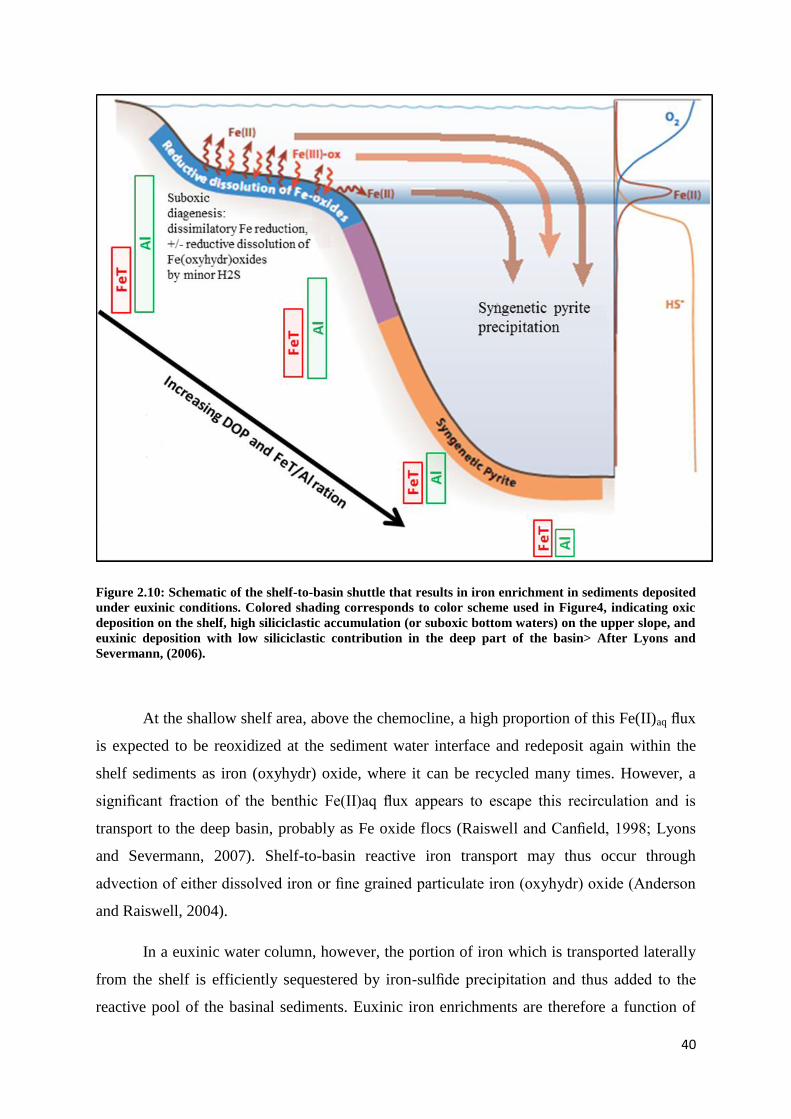
40
Figure 2.10: Schematic of the shelf-to-basin shuttle that results in iron enrichment in sediments deposited
under euxinic conditions. Colored shading corresponds to color scheme used in Figure4, indicating oxic
deposition on the shelf, high siliciclastic accumulation (or suboxic bottom waters) on the upper slope, and
euxinic deposition with low siliciclastic contribution in the deep part of the basin> After Lyons and
Severmann, (2006).
At the shallow shelf area, above the chemocline, a high proportion of this Fe(II)aq flux
is expected to be reoxidized at the sediment water interface and redeposit again within the
shelf sediments as iron (oxyhydr) oxide, where it can be recycled many times. However, a
significant fraction of the benthic Fe(II)aq flux appears to escape this recirculation and is
transport to the deep basin, probably as Fe oxide flocs (Raiswell and Canfield, 1998; Lyons
and Severmann, 2007). Shelf-to-basin reactive iron transport may thus occur through
advection of either dissolved iron or fine grained particulate iron (oxyhydr) oxide (Anderson
and Raiswell, 2004).
In a euxinic water column, however, the portion of iron which is transported laterally
from the shelf is efficiently sequestered by iron-sulfide precipitation and thus added to the
reactive pool of the basinal sediments. Euxinic iron enrichments are therefore a function of

41
the escape efficiency of iron from benthic shelf-recycling, as well as the relative proportions
of shelf area to basin area, the source to sink ratio (Raiswell and Anderson, 2005). The net
escape efficiency from a continental shelf must take into account repeated cycles of benthic
release (reduction) and re-deposition (oxidation) of reactive iron during its lateral advection
across the shelf. Moreover, release of reactive iron from the zone where the chemocline
intersects the sea floor (Figure 2.10) is an important mechanism for shelf-to-basin transport.
It is also possible that the reactivity of particulate iron in the deep basin is enhanced by other
mechanisms, potentially involving microbial activity or grazing by heterotrophic organism as
particles settle through the sulfidic water (Lyons and Severmann, 2006).

42

43
Figure 2.11: Conceptualization of the iron-speciation parameters for evaluating ocean redox condition. FeHR = highly reactive iron; FeT = total iron; FeP = pyrite
iron (after Poulton and Canfield, 2011).

44
Based on studies of modern and ancient marine sediments, it has been found that
FeHR/FeT ration do not exceed 0.38 in sediment deposited under oxygenated water column
condition (Poulton and Raiswell 2002). On the other hand, values above this threshold are
commonly indicative of deposition under anoxic conditions. Observations by Poulton and
Raiswell (2002) have shown that ancient sediments deposited from an oxic ocean have
average FeHR/FeT ratios of 014 ± 0.08. This allows distinguishing anoxic condition where
FeHR/FeT ratios ≥ 0.38 (figure 2.11) and oxic condition where FeHR/FeT ratios ≤ 0.22.
Figure 2.12: The most reliable redox trace element parameters (Ni/Co, V/Cr, U/Th and authigenic
uranium) calibrated against DOP (After Jones and Manning, 1994).
Moreover, the recent iron extraction scheme enables distinguishing ferruginous
conditions from euxinic condition. Observations on the extent of highly reactive iron
pyritization in Black Sea sediments suggest that Fepy/FeHR = 0.8 characterizes the upper limit
for ferruginous deposition (Anderson and Raiswell 2004). This threshold could drop down to
0.7 when applying Poulton and Canfield (2005) extraction scheme which includes the Fecarb
and Femag in its quantification of the highly reactive iron pool (Figure 2.11; Poulton and
Canfield 2011).

45
2.4.5 Redox-sensitive trace metals
Redox-sensitive trace element (TE) concentrations or ratios are among the most
widely used indicators of redox conditions in modern and ancient sedimentary systems (e.g.,
Calvert and Pedersen, 1993, Jones and Manning, 1994, Wignall, 1994). Elements providing
good potential for palaeo-redox determination are those which are predicted or observed as
being more insoluble in anoxic water, which can be expected to be enriched relative to
detrital inputs to normal oxic sediments. Algeo and Maynard (2004) describe strong
enrichments in Mo, U, V, and Zn from sediments deposited under euxinic bottom waters.
Brumsack (2006) extends this list to include Cd, Cu, Tl, Ni, and Sb. These metals all have in
common the tendency to form insoluble phases under anoxic sulfidic conditions.
2.4.5.1 Trace metal sources and fixation mechanisms
Under anoxic conditions, the flux and transfer rates of certain trace metals (TM) are
high, and can result in significant drawdown of TM in seawater. Chemostratigraphic
variations are a result of efficient organo-metallic complexation or precipitation of authigenic
mineral phases (Morford and Emerson, 1999).
Suitable fixation mechanisms form an important prerequisite for any trace metal
enrichment in organic rich sediments. The exposure time versus molecular oxygen seems to
be an important factor determining the transfer of trace metals from the bio-cycle towards the
sedimentary pool (Brumsack, 2006). Next to oxygen availability, the presence of hydrogen
sulphide is an important factor (Vernadsky et al., 1998). Following the catabolic pathway of
organic matter degradation, bacterial sulfate reduction and the associated presence of H2S
close to the sediment water interface or even higher up in the water column forms an
important factor for trace metal fixation, as many trace metals are immobilized as sulphides
(Zheng et al., 2000). The source and mediation of trace metals are difficult to differentiate
due to the interrelated mechanisms through which trace metals are concentrated in fine
grained sediments. Thus geochemical investigations of organic-rich sediments also require an
understanding of major element (ME) distribution, which are not affected by biological or
diagenetic processes and stable during thermal diagenesis. Brumsack (2006) used Al for
quantifying the terrigenous-detrital fraction in near shore environments. Any deviation from
average shale composition (either enrichment or depletion) can be seen in element/Al-ratios.
Brumsack (2006) calculated the enrichment factor (EF) using average shale to represent

46
terrigenous detrital background concentrations. Any relative enrichment is then expressed by
an EF>1, whereas depleted elements have an EF<1.
2.4.5.1 Mo geochemistry
Mo is a particularly useful redox proxy, and along with many other redox-sensitive
metals, Mo enrichment occurs in sediments overlain by euxinic waters, since it is strongly
affected and reduced in the presence of free hydrogen sulphide (H2S) (Crusius et al., 1996).
The enrichment of Mo occurs in sediments deposited in settings with significant free
hydrogen sulfide (H2S). Beyond a threshold concentration of ~11 μM, direct Mo-sulfide
precipitation or the switching of Mo behavior from the conservative molybdate anion
(MoO42-
) to particle reactive oxythiomolybdate ions (MoOxS4-x2-
) occurs (Helz et al., 1996;
Erickson and Helz, 2000). Mo is then sequestered by sulphide minerals or organic matter, and
as concentrations of H2S get higher (~100 µM), near quantitative removal of dissolved Mo
can occur from the water column (Zheng et al., 2000; Barling et al., 2001; Nägler et al., 2005;
Neubert et al., 2008). However, Helz et al. (2011) have suggested that the near-quantitative
removal of dissolved Mo observed in some modern euxinic basins is actually due to a
fortuitous combination of pH and H2S concentration, raising doubt as to whether complete
drawdown of Mo would necessarily be expected under euxinic conditions. Nevertheless, high
and variable Mo concentrations are often diagnostic of deposition under euxinic conditions
(figure 2.13).
Figure 2.13: The mean and range of molybdenum concentrations observed at a large number of modern
oxic, suboxic, and euxinic environments, Euxinic settings are subdivided as a function of persistence of
euxinia and Mo availability in the basin (After Loyns and Anbar, 2009).

47
Molybdenum enrichment in sediments often tracks the organic carbon flux and availability of
Mo in the basin of deposition (Lyons and Anbar, 2009). However, persistent or widespread
euxinia would be expected to gradually lower the Mo concentration of seawater as expanded
sinks exceed input from riverine sources (McArthur et al., 2008). Subsequent studies of
modern euxinic basins have confirmed the generalization that with time, euxinic basins
become depleted in Mo. For instance, the Mo contents of black shales decline with time as
other indicators of euxinia (e.g., DOP) increase (Algeo, 2004).
2.4.6 Molecular palaeoredox indicators
Organic molecular geochemistry using the advanced technology of gas
chromatography mass spectroscopy (GC-MS) has been used to generate biomarker data that
can indicate the depositional environment. Molecular biological markers, or biomarkers, are
natural products that can be assigned to a particular biosynthetic origin. For environmental
and geological studies, the most useful molecular biomarkers are organic compounds with
high taxonomic specificity and potential for preservation. Thus they can be used to identify
organic matter inputs, as well as indicating the condition of deposition (Mackenzie, 1984a).
2.4.6.1 Pristane/Phytane ratio
Pristane/Phytane (Pr/Ph) ratio is the most common and widely used biomarker
parameter for the assessment of redox conditions during sediment accumulation. According
to Didyk et al. (1978), sediments deposited under an anoxic water column condition display
low Pr/Ph ratios, with values less than 1.0, while values greater than 1.0 are observed under
oxic conditions. The underlying rationale behind the application of Pr/Ph ratio as an indicator
of oxicity is that both compounds are derived from phytol (mainly derived from the side
chain of chlorophylls), with oxidation tending to promote a decarboxylation reaction (to form
the C19isoprenoid skeleton), and reduction tending to form phytane in preference (Figure 2.14)

48
Figure 2.14: A schematic diagram of the diagenesis of the phytol side chain of chlorophyll (IGI Ltd, 2009)
Indeed, Pr/Ph is likely to become less definitive as additional data are acquired, since
there are a number of influences that impact on the Pr/Ph ratio, the most important being (1)
additional biological inputs of precursors of either pristane or phytane, and (2) the tendency
for the ratio to increase with maturity. As a consequence, the ratio should be used with
caution and in association with other indicators of redox conditions. Peters et al. (2005)
recommend that the Pr/Ph ratio is not used in immature samples, and that even within the oil
window, values between 0.8 and 3 are equivocal. High Pr/Ph values (>3) are common in
samples with abundant terrestrial organic matter deposited under oxic conditions, whilst very
low values (<0.8) are common in hypersaline environments, where anoxic conditions
typically prevail.
2.4.6.2 Isorenieratane
Organic geochemical tools have recently been developed that can diagnose the
occurrence of photic zone euxinia, based on specific bacterio-plankton biomarkers such as
isorenieratane (Koopmans et al. 1996). These biomarkers are exclusively or primarily
derived from the photosynthetic pigments of the phototrophic sulphur bacteria that
proliferate in the upper part of the water column where light, nutrients and dissolved H2S are

49
available (Figure 2.15). This type of bacteria produces unique and distinctive photosynthetic
pigments that can be traced in ancient sediments. For instance, the Chlorobiaceae (Green
Sulphur Bacteria; GSB) contains the carotenoid isorenieratene (the precursor of
isorenieratane). In fact, isorenieratane is part of the carotenoid group, which are widely
distributed in nature as well as ancient and modern sediments (Hartgers et al., 1994a).
During diagenesis, isorenieratene is reduced to isorenieratane which is a diaromatic
C40 hydrocarbon (Figure 2.15 with both aromatic rings having a 2,3,6-trimethyl substitution
pattern (Hays et al., 1999). The burial products of isorenieratene, including diagenesis or
catagenesis have been isolated from sedimentary rocks as old as approximately 1.64 billion
years (Gyr) (Brocks et al., 2005), but they do not give any information on the duration of
these conditions as they remain intact even when the conditions above the sediment have
become oxic (photic zone euxinia could occur for a very short period of time).
Figure 2.15: Schematic diagram of the isorenieratane produced by green-pigmented bacteria that thrive
in presence of sun light and free hydrogen sulphide (After Summons and Powell, 1987).
The utility of isorenieratane is confirmed by δ13
C values, which are characteristically
low due to the fact that Chlorobiaceae fix carbon by the reverse tricarboxylic acid cycle
(Hays et al., 1999). The presence of isorenieratane, derivatives and δ13
C values have been
used in many studies to reconstruct chemocline conditions (van Breugel et al., 2005), and for

50
the identification of potential source rocks (Pancost et al., 2001), as well as for evidence of
euxinic conditions during Mesozoic oceanic anoxic events (Bowden et al., 2006; Van Breugel
et al., 2006; Caswell et al., 2008).

51
CHAPTER 3 – GEOLOGICAL SETTING, MATERIALS AND
METHODS
3.1 Geological setting
During Late Triassic - Early Jurassic time a shallow epicontinental sea extended
throughout most of northwest Europe, following deposition of the brackish to shallow marine
Penarth Group (Powell et al.1992). The Lower Jurassic was deposited as two major, upward
shoaling cycles: the first cycle is Redcar Mudstone to Staithes Sandstone cycle and the
second is Cleveland Ironstone to Blea Wyke Sandstone cycle (Knox et al. 1991). The first
cycle has been subdivided into 3 second-order cycles by van Buchem and Knox (1998), each
of the second order cycles representing a significant rise in sea-level. Hesselbo and Jenkyns
(1995, 1998) recognized smaller, third-order cycles of about 300–500 Ka duration, which
approximate to the estimated duration of many ammonite zones and subzones, and suggest a
link between cyclicity, sea-level change and extinction or faunal turn over. Each of the third-
order cycles was further subdivided into a number of smaller scale cycles or parasequences
that were deposited in response to tectonic control and sediment flux.
The second major shoaling cycle represented by the Toarcian (Upper Lias) succession
comprises the Whitby Mudstone to Blea Wyke Sandstone formations (Knox 1991).
Following a relatively quiescent tectonic phase during the late Pliensbachian, the early
Toarcian (Tenuicostatum zone) was a period of major basin subsidence throughout England
(Powell, 2010). The rise of sea level across the Pliensbachian-Toarcian boundary,
culminating in the Falciferum zone of the Lower Toarcian, is one of the best documented
eustatic events in the Jurassic, marked by evident deepening in marine succession and marine
transgression in extensive parts of the world (Hallam 1988). The period was also marked by
an Early Toarcian Oceanic Anoxic Event, signified by a sharp negative excursion in the
carbon isotope curve at the base of the event followed by a positive excursion (Hesselbo et al.,
2000), the latter being associated with the widespread deposition of organic rich shale in the
ocean (Jenkyns 1988).
The Toarcian successions of Northwest Europe comprise a well-marked cycle of sea
level transgression and regression. The Early Toarcian section represents a strong
transgressive system (Tenuicostatum tile end of Falciferum zone) while the Late Toarcian is
strongly regressive (Bifrons tile Levesquei zone) producing pronounced large scale cyclicity

52
in the sediment sequences. Different from that, at the medium scale, sedimentary cycles are
not well expressed (Hallam, 1997; Hesselbo and Jenkyns, 1998).
At the smaller (second order cycling) scale, sediments were deposited in progressively
deeper water as manifested in the Early Toarcian section exposed on the Yorkshire coast,
where the succession grades from sandstone at the top of the Cleveland Ironstone Formation,
through silty mudstones to organic-rich laminated shales in a fining upward sequence (Jet
Rock Shale and Alum Shale members). This trend of prominent sea level rise (deepening of
the depositional environment) was interrupted by periods of slight relative sea level fall as
indicated by the occurrence of hummocky cross stratified beds within the upper
tenuicostatum zone (Wignall et al., 2005).
The bulk characteristics of each cycle indicate an upward increase in water energy and
its transporting capability; such characteristics are usually attributed to an initial phase of
marine transgression and deepening followed by a progressive regression and consequently
shallow sea water level (Powell 2010). Sea level change or local basin subsidence
fluctuations or a combination of the two are possibly the main factors explaining the observed
sediment cycles (Hallam, 1981).
In most areas of north-west Europe the boundary between the Pliensbachian and
Toarcian Stages of the Early Jurassic is a sequence boundary that marks the base of a major
transgressive (Jenkyns, 1985). The Grey Shale Member, the Jet Rock Member and much of
the overlying Alum Shale Member were deposited during this period of marine transgression
(Hallam 1981). The sediments fine upwards from the base of the sequence with the deepest
water conditions occurring in the middle of the Jet Rock Member. This phase of long term
sea level rise resulted in the development of two distinct types of black shale. (1) A basal
transgressive black shale representing in the earliest stages of transgression associated with
the flooding surface, also covering the Sulphur Bands. (2) Condensed maximum flooding
black shales of the Jet Rock type which sit on top of the transgressive system tract, and pass
laterally into more oxygenated facies near shore (Wignall, 1994). Above this level there is a
rapid increase in quartz silt content suggesting dropping down of the sea level. The overlying
Peak Mudstone and Fox Cliff Siltstone Members are predominantly silty. The coarsening of
the sequence probably reflects a marine regression that started toward the end of the Toarcian
(Hallam 1981).

53
Figure 3. 1: A) North Yorkshire coast, view ESE towards Port Mulgrave , B) the three laminated sulphur
beds at the base of Gray shale Member, C) Zooming in to show the lower Sulphur Bed.
Figure 3.2: Boundary beds between the Cleveland Ironstone and Grey shales Formations, Port Mulgrave,
North Yorkshire

54
At the base of this transgressive and half a metre from the top of the Cleveland
Ironstone Formation a 15 cm thick, silty laminated black shale layer (Lower Sulphur Band)
sits sharply on a siltstone with a large and diverse benthic fauna (figure 3.2). The layer
corresponds to the Sulphur Band of the mining vernacular (Howard 1985). Chowns (1968)
demonstrated that its formation was related to a brief episode of anoxic bottom water
conditions which affected the entire area at the beginning of Toarcian times. The band gained
its name from its appearance at outcrop (Figure 3.3) caused by the weathering of its abundant
pyrite content.
Figure 3.3: Photographic picture of the LSB illustrating it yellowish appearance at Staithes outcrop.
The term Sulphur Band was introduced for the first time by Chowns (1968) to define
this thin bed of fissile bituminous shale which corresponds to Bed 58 at Staithes, Bed 26 at
Kettleness and part of Bed 43 at Hawsker Bottoms (Figure 3.4). The silty laminations
towards the top of the Sulphur Band become gently disturbed and exhibit very low angle
cross lamination along with broad scour-and-fill structures (Wignall, 1994). Both pelagic and
benthic fauna are absent, implying anoxic conditions extending from the sea floor into the
water column but, curiously, this shale unit is not enriched in authigenic U, possibly implying
oxic conditions. Chondrites and Diplocraterion penetrate the top of the Sulphur Band and the

55
overlying mudstones show vestiges of silt-lamination between the dense burrows of these two
ichnogenera. There is no sequential development of burrow types and so it would appear that
Sulphur Band deposition was terminated by a sudden onset of oxygenated sea floor
conditions. The presence of scour and fill lamination in the Sulphur Bands, which indicate
their formation above storm wave base, also suggests a more dynamic environment that was
characterised by a significant degree of water column mixing. Moreover, Rob Newton (Leeds
University, unpublished data) reported high DOP, contradicted by anomalously wide range of
framboid sizes, suggesting that for at least some part of the sulphur band deposition the redox
interface must have been located at the sediment surface. These observations provide the first
evidence from ancient black shales of this mode of formation, one which has previously gone
undocumented in the literature.
Figure 3.4: Chondrites and Diplocraterion burrows developed in the top of the Sulphur Band at
Brachenberryt Wytke, Norh Yorkshire. Coin is 2cm in diameter (after Wingall, 1994).
A second, two decimetre-thick, pyritic unit with similar lithology to the Sulphur Band
occurs at 2.3 and 5.6 m above the base of the Grey Shale. In this study, the three pyritic units
are termed collectively the Lower, the Middle and the Upper Sulphur Bands, from the base
upward.
The Pliensbachian–Toarcian boundary preceding the T-OAE has received less
attention, but it is quite an important interval with regards to changes in carbon cycling, sea
level, faunal turn-over, and, more generally, evolving Early Jurassic climate. A sea-level rise
across the stage boundary of several tens of metres (Hallam, 1981) coincides with a relative
minimum in seawater strontium-isotope values at this boundary interval where the 87
Sr/86
Sr
ratios fall to the least radiogenic values seen throughout the Early Jurassic (Jones and Jenkyns,

56
2001). Moreover, the transition from the Pliensbachian into the Toarcian is marked by the
initiation of a mass extinction event, suggesting that changes in climate and
palaeoceanography started to occur well before the onset of the OAE (Little and Benton,
1995; Wignall and Bond, 2008). It has been observed that most of the well-known mass
extinction events in the geological record were accompanied by perturbations to the global
carbon cycle (Keller and Lindinger, 1989; Arens and Jahren, 2000; Payne et al. 2004;
Hesselbo et al. 2002; Riccardi et al. 2007).
Since the Sulphur Bands at the Pliensbachian–Toarcian boundary preceding the T-
OAE are interbedded as thin dark laminated shale layers in more or less normal light-colored
bioturbated mudstones sediments, the formation of these layers record short-lived but
catastrophic alterations in oceanographic conditions that were probably caused by a repeated
mechanise that operated regionally at small scale and then developed to a major process that
effected the whole ocean on a global scale. Our current understanding of these pre-TOAE
small events is unconstrained. Here we present new and comprehensive geochemical analysis
across the Pliensbachian-Toarcian and extending throughout the T-OAE to shade more light
on these events and how could they like to the main event that linked to the T-OAE. The very
high resolution (cm scale) geochemical analysis scanning this interval is the scope of this
study to shade light any possible short-lived changes in the paleoredox history which may
have gone undocumented before.

57
Figure 3.5: Areal extent of the LSB (yellow band) along the coastal exposures of Staithes, Kettleness and the Hawsker Bottoms. Not that the LSB does not grade
into any near-shore facies (after Howard, 1985)

58
3.2 Sampling
Samples used in this study were collected from two lower Jurassic exposures in the
UK. The main station is at the costal exposure between Staithes and Port Mulgrave, where
the sampled and logged section covers the Lower part of the Whitby Mudstone Formation.
The sampled lithostratigraphic units are, in ascending order, the Grey Shale Member (beds
1 to 32) between 0 and 13.60 m above the top of the Mushroom Concretions bed which is
taken as reference (all sample heights were measured from the top of this unit) and the Jet
Rock Shale Member (beds 33 to 40) between 13.60 and 18.23 m. The entire section is well
exposed along the coastal cliffs between Staithes and Port Mulgrave on the north east coast
of Yorkshire. The other location used in this study was Hawsker Bottoms (figure 3.6),
where the lower Grey Shale was sampled to investigate the geochemical variation of the
Sulphur Beds.
A total of 131 rock samples were collected at decimetre and centimetre scale from
both outcrops using either, a geological hammer and chisel or for some laminated units (e.g
the Sulphur Bands) an electrical saw was used to cut whole sections of rock which could then
be subdivided later to obtain very detailed samples at sub-cm scale. Particular attention was
taken to avoid weathered material.
Samples were labelled in the field and the top and bottom of each sample were
marked. Back in the lab, more detailed sub-sampling was carried out on the larger rock
samples. Then samples were trimmed to remove the outer edges (about 0.5 cm or more).
Prior to any geochemical and palynological analyses, the whole rock samples were described
in terms of laminations, banding, bioturbation, heterogeneity, mica content and the presence
of macrofossil material. The sections were sub-sampled and powdered in a Tema mill. The
colour of the powdered samples was recorded using a Geological Society of America Rock
Color Chart (Goddard et al., 1970).
Most of the collected samples are carbon-rich, laminated black shales that are inter-bedded
with layers of calcite concretions, and which are stratigraphically equivalent to similar
organic-rich deposits throughout Central and Western Europe (e.g. the ‘Schistes Carton’ from
the Paris Basin, France, and the ‘Posidonia Shale’ from the Posidonienschiefer Basin,
Germany; Jenkyns, 1988; Röhl et al., 2001).

59
Figure 3.6: Location map of the north Yorkshire coast fieldwork sites
At the Port Mulgrave section, a total of 98 samples were collected over almost 20 m
of the study interval, starting at the base of the Grey Shale Member, and ending at bed 40 of
the Jet Rock Shale Member (Figure 3.7). All samples were collected from outcrop, but from a
horizontal depth of > 10 cm in order to minimize the oxidative influence of subaerial
weathering. Sampling was at decimetre-scale within the bioturbated mudstone of the Grey
Shale and throughout the Jet Rock shale (exaratum subzone). The Sulphur Bands at the
Pleninsbachian-Toarcian boundary were sampled at higher resolution (mm-scale).
In order to evaluate the lateral geochemical characterization of the Sulphur Bands
within Cleveland basin, Lower Toarcian section at Hawsker bottoms was chosen as it
represents more distal site. At Hawsker bottoms 26 samples were taken spanning the Paltum
and Clevelandian subzones, which represent the stratigraphic interval of the Sulphur Beds.

60
Figure 3.7: Lithological column of the studied section at Port Mulgrave showing the position and heights
of the analysed samples from the base of the Grey Shale Member.

61
3.3 Analytical Methods
During the course of this study a variety of techniques were applied. These techniques
vary from commonly applied geochemical analyses (where the whole set of samples were
analysed), to some more detailed and advanced techniques (where selected samples were
analysed, based on the previous results). The order of analysis is described in Figure 3.8.

62
NIR
Spectroscopy
WHOLE ROCK SAMPLE
ICP-MS
GC&GC-MS
•Isorenieratane
•Mo
•Zn
•Cu
•Al
•V
•IA
•FeP/FeHR
•DOP
Blue UV light
microscopy
Transmitted light
microscopy
Fluorescence
Scale analysis
300 count:
AOM, Phytoclasts
& Palynomorphs
•TOC
•TS
•CaCO3
•S2
•HI
Bitumen
extraction
Rock-Eval
LECO
TLC
Crush to
cutting< 4mm
Non-oxidative
Palynological
Treatment using
HF & HCL
Molecular
Biomarkers
Very fine Powdered
(Retsch Mortar
Grinder)
Fe speciation & FeS2
(Chromous chloride)
Lithological
description
and observation
δ13CTOC (‰)
δ 34S (‰)
Figure 3.8: Flow chart showing the order of methods

63
3.3.1 Bulk Geochemistry
3.3.1.1 Total Organic Carbon (TOC) Determination
To determine total organic carbon, approximately 100 mg of the powdered rock
sample was placed in a porous crucible and treated with 5 ml of 40% HCl to remove
carbonate phases. The samples were washed thoroughly six times with distilled water, and
placed in an oven overnight at a temperature of 60 oC. TOC was then measured using a
LECO® HF-100 induction furnace attached to a LECO® LS-244 Carbon Sulphur
Determinator. Prior to analysis, copper metal and iron chips were added to each crucible.
Then the crucible was inserted into a furnace and combusted at 1500ºC for 30 – 50 seconds.
The apparatus was calibrated to known standards before any analyses were conducted, and to
ensure the performance of the machine some samples were run in duplicate and some
additional standards were run after every ten samples. Table 3.2 shows the results for
triplicate analyses of a rock sample from the Whitby Mudstone Formation for an internal
standard. The accuracy relative to the internal standard falls within 2% of certified standard
value. Based on triplicate measures, the relative standard deviation (RSD) was less than 1%.
3.3.1.2 Total Carbon and Total Sulphur (TC & TS) Determination
The samples were prepared for TC and TS analysis by weighing 0.1 gram of each
powdered rock sample into a crucible, and some copper metal and iron chips were added to
each crucible and inserted into the LECO CS- 244 Carbon/Sulphur Analyser. Within a few
seconds the oxidising reaction takes place producing CO2 and SO2, and these gases were
quantified by a LECO® LS-244 Carbon Sulphur Determinator, as for TOC. The accuracy
relative to the internal standard falls within 2% of certified standard value. Based on triplicate
measures, high precision was achieved with relative standard deviation (RSD) of 0.51%.

64
Sample TOC T C
MSB24 1.722 2.166
MSB24 1.744 2.161
MSB24 1.726 2.182
Mean 1.731 2.170
%RSD 0.67 0.51
Internal Std 1.723 2.807
Internal Std 1.736 2.803
Internal Std 1.727 2.798
Mean 1.729 2.803
% RSD 0.39 0.16
Table 3. 1: shows the accuracy and precision of the analytical motheds
3.3.1.3 Isotopic analysis
3.3.1.3.1 Organic carbon isotopes
Sample Preparation
Prior to carbon-13 analysis, the sediment samples were treated with hydrochloric acid
to remove inorganic carbon (carbonate) as follows. About 200 mg of sample was treated with
1 M HCl. The sample and acid were mixed and left for 24 hours to allow the carbonate
content of samples to be liberated as CO2. The acid was decanted and the sediment washed
several times with distilled water. The samples were completely dried at 60°C and re-ground
to a powder. The sample was then weighed into a tin capsule (8 x 5 mm) and sealed ready for
analysis.
Carbon-13 Analysis
The technique used for analysis was EA-IRMS (elemental analyzer isotope ratio mass
spectrometry), which was performed by Iso-Analytical Ltd., UK. In this technique, samples
and references are loaded into an auto-sampler on a Europa Scientific elemental analyzer.
The samples are then combusted at 1000°C in the presence of oxygen. The tin capsules flash
combust, raising the temperature in the region of the sample to ~1700°C. The combusted
gases are swept in a helium stream over a combustion catalyst (Cr2O3), copper oxide wires (to
oxidize hydrocarbons), and silver wool (to remove sulfur and halides). The resultant gases,

65
N2, NOx, H2O, O2, and CO2 are swept through a reduction stage of pure copper wires held at
600°C. This removes any oxygen and converts NOx species to N2. A magnesium perchlorate
chemical trap is used to remove water. Nitrogen and carbon dioxide are separated using a
packed column gas chromatograph held at a constant temperature of 100 °C. The resultant
carbon dioxide peak enters the ion source of the Europa Scientific 20-20 IRMS where it is
ionised and accelerated. Gas species of different mass are separated in a magnetic field then
simultaneously measured using a Faraday cup collector array to measure the isotopomers of
CO2 at m/z 44, 45, and 46. The reference material used during analysis of the samples was
IA-R001 (Iso-Analytical working standard Flour, 40.2% Carbon), with a 13
C value of -
26.43‰ (relative to V-PDB).
3.3.1.3.2 Sulphur isotopes analysis
Sulphur was collected for analysis in form of silver sulphide that was produced during
the pyrite extraction process (look at 3.3.2.1 section for details). Tiny amount of the silver
sulphide were placed in tin capsules and processed using continuous flow isotope ratio mass
spectrometry (EA-IRMS). The tin capsules containing reference or sample material plus
vanadium pentoxide catalyst were loaded into an automatic sampler. From where they were
dropped, in sequence, into a furnace held at 1080° C and combusted in the presence of
oxygen. Tin capsules flash combust, raising the temperature in the region of the sample to ~
1700° C. The combusted gases are then swept in a helium stream over combustion catalysts
(tungstic oxide/zirconium oxide) and through a reduction stage of high purity copper wires to
produce SO2, N2, CO2, and water. Water is removed using a Nafion™ membrane. Sulfur
dioxide is resolved from N2 and CO2 on a packed GC column at a temperature of 45 °C. The
resultant SO2 peak enters the ion source of the IRMS where upon it is ionized and accelerated.
Gas species of different mass are separated in a magnetic field then simultaneously measured
on a Faraday cup universal collector array. Analysis was based on monitoring of m/z 48, 49
and 50 of SO+ produced from SO2 in the ion source.
Reference Standards and Quality Control: The reference material used for analysis
was IA-R061 (Iso-Analytical working standard barium sulphate, 34
SCDT = +20.33 ‰). IA-
R025 (Iso-Analytical working standard barium sulphate, 34
SV-CDT = +8.53 ‰), IA-R026
(Iso-Analytical working standard silver sulphide, 34
SV-CDT = +3.96 ‰) and IA-R061 were
used for calibration and correction of the 18
O contribution to the SO+ ion beam.

66
3.3.1.4 Rock- Eval Pyrolysis
Procedure
About 0.1g of powdered rock sample was added to a stainless steel crucible, mounted
in a carousel and progressively heated up to 550°C for about 20 min. A standard source rock
sample was also analysed to enable calibration of the results. A stream of helium was passed
over the sample (oxygen was excluded), then the temperature was gradually increased until
100°C and the temperature was held constant for one minute to release the free gaseous
hydrocarbon (S0 mg/g sediments). This was detected by a Flame Ionization Detector (FID),
and is known as peak one (1). In the second stage, the temperature was increased by
25°C/min until 300°C, and the hydrocarbons released were quantified as peak 2, which is
known as S1 (mg/g). During the last stage the temperature was increased at a rate of
25°C/min until 550°C. This reflects the temperature where kerogen breaks down and the
hydrocarbons are generated (Peak 3), and is quantified as S2 (mg/g). Tmax is recorded at the
maximum of the S2 peak, which is a function of thermal maturity of the organic matter.
Petroleum yield (PY) of a source rock is defined as the sum of hydrocarbons present in the rock
sample and those generated during pyrolysis (S1+S2).
Hydrogen index (HI) corresponds to the quantity of pyrolyzable organic compound or hydrocarbons
from S2 relative to TOC (S2/TOC).
Production Index (PI) distinguishes between the HC present in the rock and those generated by
cracking during analysis (S1/ (S1+S2)).
3.3.2 Microscopy
3.3.2.1 Palynological Preparation Technique
Based on the measured values of HI and TOC, samples were selected for
palynological analysis. The selected samples represent the full range of variations in
geochemical profile (not just the richest samples). Following the standard non-oxidative
palynological preparation method (Barss and Williams, 1973), samples were cleaned of any
contamination and gently crushed to a cutting size of >2.0 mm (wrapped in foil and hit by
geological hammer, and excusive grinding was avoided). The fragments were then sieved to
<2.0 mm. Then the samples were processed as follows:
About 1 g of the crushed cutting was placed in a 600 ml plastic beaker.

67
100 ml of 40% hydrochloric acid was added to dissolve any carbonate minerals.
Sample was left for four hours or until any reaction had stopped.
Distilled water was added up to the rim of the beaker and then decanted after four
hours; repeated three times.
100 ml of 40% hydrofluoric acid was added to remove any silicate material, and the
beaker was allowed to stand for at least 24 hours.
Water was added and then decanted after more than four hours or until the sediment
settled; repeated two times.
Lycopodium tablets were then added to each sample (the number of tablets based
upon HI and TOC values).
The residue was treated with 20% hydrochloric acid to dilute and remove any silico-
fluoride compounds precipitated during the course of the treatment, and to aid
dissolution of the lycopodium tablets, then washed three times with distilled water.
About 2 L of distilled water was added to wash the residue through a ten micron sieve,
and then the residue was transferred into vials.
A thin layer of suspended kerogen was then pipetted onto a cover slip and left
overnight to dry. This was then mounted on a microscope slide using Elvacite TM
2044 (ICI) and xylene mounting medium, which was produced by slowly adding 65 g
of Elvacite to 100 ml xylene in a beaker, stirring occasionally until the solution was
completely clear.
The cover slip was mounted on a glass slide using 2044 acrylic resin and left
overnight.
3.3.2.2 Transmitted White Light (TWL) analysis
An Olympus BH2 microscope was used for petrographic examination, with the
objective to identify the source of organic matter (OM) by counting the percentages of
amorphous organic matter (AOM), palynomorphs and phytoclasts, based on 300 counts per
sample.

68
3.3.2.3 Fluorescence Microscopy
The preservation state of the kerogen was determined using blue light fluorescence
microscopy, relative to the scale of Tyson (1995; see Table 3.1).
Table 3.2: Summary of fluorescence scale, where the 1 represents the lowest preservation stat of the
organic matter and 6 the highest (after Tyson, 1995, p.347)
Scale
point
Description Relative
preservation
1
2
3
4
5
6
Nothing fluoresces (except rare palynomorphs or contaminants)
Only palynomorphs fluoresce
AOM fluoresces but just detectable
As 3 but AOM shows moderate fluorescence
As 3 but AOM shows strong but heterogeneous fluorescence
Matrix AOM shows very strong and homogeneous fluorescence
Poor
High
3.3.3 Organic molecular chemistry
3.3.3.1 Bitumen Extraction
43 samples, representing a range of Rock-Eval parameters, TOC and depositional
redox conditions (see below), were selected for detailed biomarker investigation. Aliquots of
powdered rock (15 g) were extracted for 6 hours with 93:7 dichloromethane/methanol
(DCM/MeOH) in a Dionex ASE 200 Accelerated Solvent Extraction System at 1000 psi and
100°C. Yields of extractable organic matter (EOM) were obtained.
3.3.3.2 Thin Layer Chromatography (TLC)
The extracted bitumen was concentrated by removal of solvents using a rotary
evaporator, and the extract was transferred to a small vial and bellowed down under a
nitrogen stream to result in slightly viscous bitumen. The traditional thin layer
chromatography technique was used to separate the bitumen mixtures into the three main
groups of compounds (aliphatic, aromatic and NSO compounds). The separation process
was performed on a plate of unreactive glass that was coated with a thin layer (0.5 mm

69
thick) of silica gel as adsorbent material (stationary phase). The TLC plates were prepared
by mixing the adsorbent (silica gel of standard particle size range) with a small amount of
water to improve reproducibility (2 ml of water to each gram of silica gel). Then the
mixture was spread as thick slurry on the glass plate. The plate was then dried and activated
by heating in an oven for 24 hour at 70 °C.
About 10 mg of the extracted bitumen sample was applied to the plate using a
capillary tube and spotted along a horizontal line about two centimeters from the base. The
plate was then dipped in a glass jar containing light petroleum ether and placed in a sealed
container. The solvent moved up the plate by capillary action and carried the sample mixture.
Different compounds in the sample mixture travel at different rates due to the differences in
their attraction to the stationary phase and because of differences in solubility in the solvent.
Therefore, the aliphatic and aromatic fractions were separated from the bitumen and marked
on the plate by the aid of a standard (squalane and anthracene). The plate was then spread
with Rhodamine 6 and viewed under UV light to help identify the aliphatic and aromatic
bands. These aliphatic and aromatic bands were then separately scratched out of the plate.
The sample tubes were then set by adding some activated alumina, and 30 ml of DCM was
used to flush the scratched sample through and the fractions were collected in small round
flasks.
The saturated hydrocarbon samples were diluted to 1 mg/100 µL in DCM and
transferred to a GC vial. Injections were made using an HP6890 autosampler. The column
was a 60 m Chrompack CP8744 CPsil-5CB with an internal diameter of 0.32 mm and a film
thickness of 0.25 µm. The carrier gas was helium with a volumetric flow rate of 1.6 mL/min.
Samples were analyzed using both full scans and selected-ion monitoring methods for a more
detailed analysis of specific compounds. Aromatic fractions were spiked with squalane as a
standard to facilitate quantification of aromatic hydrocarbons such as isorenieratane.
Samples were analysed by gas chromatography coupled to tandem mass spectrometry
using a Hewlett-Packard 6890 gas chromatograph and a Micromass Autospec Ultima
operated in the metastable-reaction-monitoring (MRM) mode. A 60 m Scientific DB-1 fused
silica capillary column (0.25 mm i.d.; 0.25 mm film thickness) was used with helium as the
carrier gas. Samples were injected in pulsed splitless mode. The column temperature was
programmed from 60 ºC (held for 2 min) to 150 ºC at 10 ºC/min, then at 3ºC/min to 250 ºC,
with 70 eV ionization energy and 8000 kV acceleration voltage. Peaks were identified using

70
previously published elution times and mass spectra. Isorenieratane peaks were identified by
comparison of elution time with an authentic standard (squalene), as well as previously
published mass spectra.
Quantification of GC-MS peaks
The quantification of the GC peaks was established using the integrated peaks from
the GSMS and the following equation;
Wx = RRF * Ax * Ws/As
Where;
Wx = weight of unknown sample
RRF = is the relative response factor taken here as 1
Ax = area of unknown sample
As = area of known standard
Ws = weight of known standard
3.3.4 Sequential Extraction Procedure for Iron Speciation
Fe speciation is one of the most robust redox indicators currently available. It has
been extensively calibrated to allow identification of oxic, anoxic non-sulfidic, and euxinic
bottom water conditions. The technique is based on the reactivity of different Fe minerals
towards dissolved sulphide (Canfeld et al., 1992; Poulton et al., 2004). The recently
developed sequential extraction technique of Poulton and Canfeld (2005) allows
identification of three pools of iron species of differing reactivity to dissolved sulphide, when
combined with the Fe sulphide extraction procedure of Canfield et al. (1986); highly reactive
Fe (FeHR), poorly reactive Fe (FePR) and unreactive Fe (FeU) (Raiswell and Canfield, 1998;
Poulton and Raiswell, 2002). Together, these techniques allow the recognition of five
operationally-defined Fe fractions, listed in Table 3.3.

71
Table 3.3: Details of the Fe extraction scheme, with target phases (After Poulton and Canfield, 2005).
Extraction Target phases Terminology
Na Acetate, PH 4.5, 48h, 50ºC Carbonate Fe, including siderite
and ankerite
Fecarb
Dithionite, 2 h Goethite, akaganeite, hematite Feox
Oxalate, 6h Magnetite Femag
Boiling 12 N HCL Poorly reactive sheet silicate Fe FePRS
Chromous chloride distillation Pyrite Fe Fepy
Total Fe Unreactive silicate Fe (Total Fe –
sum of first 5 stages plus pyrite Fe)
FeU
3.3.4.1 Pyrite extraction
Sulphur geochemistry and sulphur isotopic distributions are one of the most useful
techniques for elucidating depositional conditions and diagenetic histories of recent and
ancient sediments and rocks. The chromium reduction method (Canfield et al., 1986) was
used for the determination of total reduced S (dominantly pyrite). In this study pyrite sulphur
was extracted from the rock powder using a modified version of the chromium reduction
method described by Canfield et al. (1986). Approximately 300 to 1000 mg of rock powder
from each sample was first treated with 8 ml of boiling 50% HCL to extract any acid volatile
sulphur (AVS). Sulphur from the liberated H2S was precipitated as Ag2S after bubbling
through a 0.1 M AgNO3 trap (AVS-S was always below detection; <0.001 wt% S). The
extraction was performed in a sealed reaction vessel and processed for 1 h under a flow of N2
gas. The samples were then sequentially treated with a boiling CrCl2 solution. Then the Ag2S
precipitates were filtered under vacuum, and dried overnight. The concentrations of sulphide
S and Fe were then determined stoichiometrically. Based on repeated measures (five runs),
acceptable precision was achieved with relative standard deviation (RSD) of 4.25 %.

72
Table 3.4: Shows the accuracy and precision of the analytical method
Sample Fe as FeS2 wt%
MSB16 1.89
MSB16 2.08
MSB16 2.11
MSB16 2.09
MSB16 2.14
Mean 2.062
% RSD 4.25
3.3.4.2 Sequential iron extractions
3.3.4.2.1 Sodium acetate
Carbonate iron in these samples is expected to be mainly present in the form of
siderite (FeCO3) and ankerite (Fe,Mg(CO3)), with minor amounts potentially substituted
within the CaCO3 mineral lattice (Poulton and Canfield, 2005). This fraction of iron was
extracted using 1 M sodium acetate solution adjusted to PH 4.5 with acetic acid. The air
dried powdered sediments were packed into plastic centrifuge tubes, and 10 ml of the sodium
acetate solution was carefully added to each sample to avoid any potential strong reaction due
to the high carbonate contents of some samples. The tubes were left to stand for a while to
release any gases. Then, sealed tubes were placed on a shaking table at 50 °C for 48 h. After
that samples were centrifuged and an aliquot of the solution was diluted for subsequent
analysis by flame atomic absorption spectroscopy (AAS). The remaining solution was
carefully discarded and the sediment was then subjected to the next stage of the extraction.
3.3.4.2.2 Sodium dithionite
Immediately after the first pool of iron was extracted, the remaining sediment was
treated with 10 ml sodium dithionite solution (50 g/L) that was buffered to pH 4.8 with 0.35
M acetic acid/0.2 M sodium citrate (the dithionite solution was always used immediately after
preparation). The extraction process continued for two hours at room temperature to
selectively extract highly reactive iron oxides (e.g. ferrihydrite, lepidocrocite, goethite,
hematite and akaganite) and this pool is termed Feox. Samples were then treated and analysed
as above.

73
3.3.4.2.3 Ammonium oxalate
The third step extracts magnetite Fe (Femag). This iron fraction was extracted using a
0.2 M ammonium oxalate/0.17 M oxalic acid solution, with 10 ml of the solution added to the
remaining sediment and shaken for 6 hours, followed by treatment and analysis as described
above.
3.3.4.3 Boiling HCl extractable iron
The hot HCl extraction method of Berner (1970) and Raiswell et al. (1994) was used
to extract and determine the poorly reactive iron fraction. The remaining sediments after the
first three sequential extractions were washed into clean quartz test tubes using distilled water
and left to dry in an oven at 50˚C for several days. 5 ml of concentrated HCl (12 M) was
added and heated to near-boiling for the first minute and then boiled vigorously for the
second minute with care to avoid any spillage during boiling. Samples were then quenched
with distilled water straight away and transferred to 100 ml volumetric flasks and filled with
distilled water. Prior to analysis by AAS, samples were shaken well and allowed to stand
overnight.
Table 3.5: Shows the accuracy and precision of the iron speciation analytical method
sampe Fecarb wt% Feox wt% Femag wt% FePRS wt%
LSB4 1.01 0.83 0.33 1.49
1.14 0.79 0.27 1.32
1.16 0.83 0.30 1.50
1.12 0.80 0.24 1.48
mean 1.11 0.81 0.29 1.45
std 0.07 0.02 0.04 0.08
%RSD 6.03 2.50 13.77 5.78
3.3.5 Total Sediment Dissolutions
Approximately 300 mg of powdered whole-rock material was initially ashed at 550 ºC
overnight in porcelain crucibles. After combustion, samples were transferred into teflon
beakers where the sample was completely dissolved using near-boiling hydrofluoric
acid/perchloric acid/nitric acid. Once the acids had evaporated (usually overnight), 5 ml of
concentrated boric acid was add to redissolve any aluminium hexafluorates that may have
formed, and the samples were heated to dryness. Then 5 ml of 50% HCl was added and
heated to dissolve all salts. The sample was transferred to a volumetric flask and diluted with
distilled water to the required volume (100 mL). Measurement of total iron was carried out

74
using atomic adsorption spectroscopy (AAS). Contents of major and minor elements (Al, P,
Cu, Mo, V, Zn and Mn) were measured by Inductive Coupled Plasma Optical Emission
Spectrometry (ICP-OES, Perkin-Elmer Optima 3300RL), equipped with a cross-flow
nebulizer for major, and with an ultra-sonic nebulizer for minor element measurements.
Standard reference materials (table 2.4) were run parallel to the samples. Based on triplicate
measures, very high precision was achieved with low relatively standard deviation (RSD) for
the (Al, Fe, Mn, V, Zn and Cu) that is less than 1. The P and Mo showed less accuracy but
still good with RSD slightly above 1.
Table 3.6: shows the accuracy and precision of the trace element analytical method
Sample Cu µg/g Zn µg/g Mo µg/g V µg/g Mn µg/g Al µg/g P µg/g Fe wt%
MSB20 26.27 99.85 4.12 127.47 295.74 100915.25 526.98 7.30
MSB20 27.16 100.11 3.24 122.87 282.65 96478.32 511.11 6.98
MSB20 25.75 98.68 4.61 128.81 296.65 101147.32 529.37 7.29
Mean 26.39 99.55 3.99 126.38 291.68 99513.63 522.49 7.19
SD 0.71 0.76 0.69 3.11 7.83 2631.21 9.92 0.18
%RSD 2.69 0.76 17.40 2.46 2.69 2.64 1.90 2.53
St 05-10 172.90 285.40 32.46 242.25 168.91 75648.06 453.37 7.76
St 05-10 171.39 285.96 32.01 243.48 168.55 75606.08 439.13 7.71
St 05-10 174.81 287.41 31.74 242.52 167.60 75591.98 460.28 7.61
Mean 173.03 286.26 32.07 242.75 168.35 75615.37 450.93 7.69
SD 1.72 1.03 0.37 0.65 0.68 29.17 10.78 0.08
%RSD 0.99 0.36 1.15 0.27 0.40 0.04 2.39 0.99

75
CHAPTER 4 - AN ORGANIC GEOCHEMICAL PROFILE OF THE
PLIENSBACHIAN-EARLY TOARCIAN OF STAITHES AND PORT
MULGRAVE (NORTH EAST YORKSHIRE, UK)
4.1 Introduction
The development of marine organic matter-rich black shales has been a focus of geological,
paleontological, and geochemical studies for many decades. This relates to their unique
significance for preserving fossils and for providing economic potential as source rocks for
hydrocarbons. Among the Mesozoic black shales in Central Europe, those deposited during
the Early Toarcian during the Toarcian Oceanic Anoxic Event (T-OAE) have received special
attention (Jenkyns, 1988; Oschmann, 1995; Baudin, 1995) in order to investigate the origins
of the T-OAE and the extinction episodes associated with this event (Hesselbo and Jenkyns
1995; Salen et al 2000; Kemp et al., 2005; Wignall et al 2005; McArthur et al., 2008: Caswell
et al., 2009). However, in terms of controls on source rock potential and biogeochemical
processes during deposition, the nature and preservation of the organic matter in the
sediments is clearly of major interest. Furthermore, organic biomarker distributions within
the sediment can provide fundamental information on depositional redox conditions, allowing
consideration of links between redox and organic matter quality and preservation. Thus, the
geochemical properties of the organic matter deposited during the Early Toarcian on the
North Yorkshire coast, and its dependence on paleoenvironmental conditions of
sedimentation, are the focus of this chapter.
4.2 Results
Apart from the approximately 20 - 50 cm thick, three organic-rich, laminated silty ‘sulphur
beds’ at its base, the lower part of the Grey Shale Member is characterised by a relatively
normal benthic fauna (Salen et al., 2000). The topmost part of the Grey Shale Member is an
organic rich shale that is lithologically, palaeoecologically, and geochemically more similar
to the overlying Jet Rock Member. The lower 8 m of the Jet Rock Member (H. exaratum
Subzone) is composed of the most finely, continuously laminated and most organic and
sulphur-rich shales with the highest hydrogen indices and the lowest δ13
CTOC values
(Demaison and Moore, 1980)

76
Table 4.1: Stratigraphic summary for the Lower Whitby Mudstone Formation modified from Salen et al.
(2000); d (m) is the cumulative distance from the top of bed to base of the Grey Shale Member. The bed
numbers are from Howarth (1962, 1973).
Ag
e
Su
bzo
nes
Mb
r.
Bed
No
Lithological description
Low
er T
oac
ian
H.e
xart
um
Jet
Rock
Mem
ber
39 Top Jet Dogger, laminated, grey limestone
38 Shale, grey,bituminous with scattered calcitic nodules
37 The Curling stones
36 Shale, grey, bituminous
35 The Whale stones, thin-bedded bituminous shale
34 Shale, grey, bituminous
33 The Cannon ball doggers
D.t
enuco
statu
m
Gre
y S
hal
e M
emb
er 32 Shale, grey, bituminous
1-31 Shale, grey, not bituminous with occasional calcareous nodules
Upper
P
lien
sbac
hia
n
P.a
pyr
enum
Ket
tlen
ess
Mem
ber
38-
56
Shale, grey, not bituminous with regular intervals of ironstones
(Two foot, pecten and the mainseam)
4.2.1 Bulk Geochemistry
4.2.1.1 Total Organic Carbon (TOC), Total Carbon (TC) and Total Sulphur (TS).
The concentration of total organic carbon (TOC) of the samples is shown in Figure
4.1 as weight percent (wt %). Samples of the Falciferum zone contain significantly more
organic material than those in the underlying and overlying zones. Geochemical analyses
reveal that shales in the (lower) Exaratum Subzone contain more organic material than the
(underlying) tenuicostatum zone. These results are consistent with previously reported trends
(Morris 1980; Salen et.al, 2000; Jenkyns and Clayton 1997) from the same section.
Overall, the study section is characterized by fluctuating organic carbon content.
Moderate to low organic matter contents of <1.5% TOC characterise the bioturbated

77
mudstone of the middle and lower part of the Grey shale (upper Hawskerense to middle
Semicelatum) with exceptions for the laminated organic rich horizons of the Sulphur Bands,
where organic carbon contents increases up to 7%. Further up section, throughout the
uppermost part of the tenuicostatum zone and the entire exartum subzone (T-OAE interval),
TOC tends to be consistently high with an average value of 7%. The TOC reaches its
maximum values of 14% at the interval of the whale stones within the exartum subzone (top
of Bed 34 and throughout Bed 35) beyond which TOC tends to decrease into the Falciferum
subzone.
The higher resolution data at the Pliensbachian-Toarcian boundary interval displays
repeated intervals (Sulphur Bands) where the TOC suddenly increases from background of
around 1 wt% to above 3 wt% with spacing of more or less 2 m between peaks in TOC.
Detailed analysis of these Sulphur Bands reveals variation in the organic carbon content at
the cm scale. The Lower Sulphur Band shows the highest variation in the organic carbon. The
approximately lower 8 cm have moderate TOC averaging around 1.5 wt%. TOC then
increases to 6.8 wt% and decreases back to less than 1 wt% before it increases again to 6 wt%
in the top part of the Lower Sulphur Band.
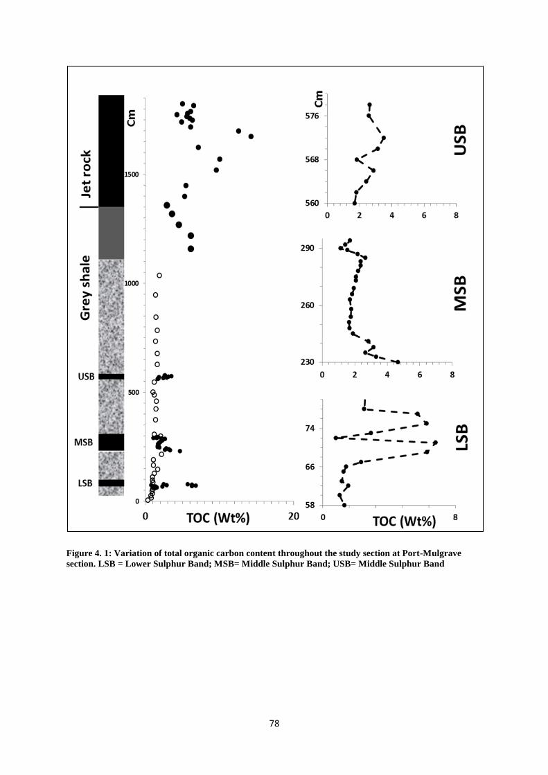
78
Figure 4. 1: Variation of total organic carbon content throughout the study section at Port-Mulgrave
section. LSB = Lower Sulphur Band; MSB= Middle Sulphur Band; USB= Middle Sulphur Band

79
Figure 4. 2: Variation of total sulphur TS content throughout the study section at Port Mulgrave section.
The sulphur content fluctuates throughout the study section (Figure 4.2). The TS data
behave similar to the TOC where it tends to be consistently high (TS >7 wt %) throughout the
uppermost part of the tenuicostatum zone and the entire of exartum subzone. A cross plot of
TOC versus TS (Figure 4.2.3) shows weak correlation (r2=0.4). The organic content tends to
decrease above the whale stone horizon (Bed 35) from values around 14 wt% to less than 5

80
wt%. On the other hand the TS profile shows less variation with high concentrations of TS
that continues above 10 wt% throughout the Jet Rock Shale.
The bioturbated mudstones of the Grey shales are characterized by relatively low TS
content with an average of 3.8 wt %. The Sulphur Bands are characterized by exceptionally
high values of up to 18%, in stark contrast to less than 2% measured in the bioturbated
mudstones directly above and below.
Figure 4. 3: Cross plot of the TOC% versus the TS% of the studied samples. Regression lines for the
average S and C relationships in sediments deposited under normal marine and euxinic conditions,
supplied by Berner (1984) and Leventhal (1995), are shown.
The δ13
CTOC values of the study section range from about -26‰ to -32‰, clearly
showing the diagnostic negative C excursions at the onset of the Toarcian-OAE (Figure 4.4).
At the study site the main negative C excursion has a magnitude of approximately -7‰,
consistent with previous studies (Kuspert 1982; Hesselbo et al., 2000; Cohen et al. 2004;
Kemp et al. 2005). The δ13
CTOC profile fluctuates through the section and shows a mirror
image to TOC. Notably, there are three small scale negative excursions with a magnitude of
almost -4‰ spanning the sulphur bands. The first peak occurs in the upper P. hawskerense
Subzone in the latest Pliensbachian, where δ13
CTOC culminates in values of approximately -
29.5‰ within the lower sulphur band. Above, δ13
CTOC returns to pre-excursion values of

81
about -25.5‰ within the base of the P. paltum Subzone, followed by a second peak of -28‰
at the Middle Sulphur bed. After the third peak that responds to the upper sulphur band the
δ13
CTOC returns to pre-excursion values until the onset of the larger negative carbon-isotope
excursion marking the Early Toarcian OAE, in the D. tenuicostatum Zone.
Figure 4. 4: Variation of the δ13
C and δ34
S values through the study section at Port Mulgrave.
The sulphur isotope record (δ34
S) ranges from -46.9‰ to -20.8‰ (Figure 4.4). The
Grey Shale samples including the Sulphur Beds shows lighter δ34
S values compare to the Jet
Rock Shale with broader range of variation from -23.2 to -46.9‰ (averaging at -34.9). On the
other hand, the Jet Rock Shale samples showed heaver values clustering over a narrow range
from -20.8 to -27.4‰ with an average of -24.7‰.
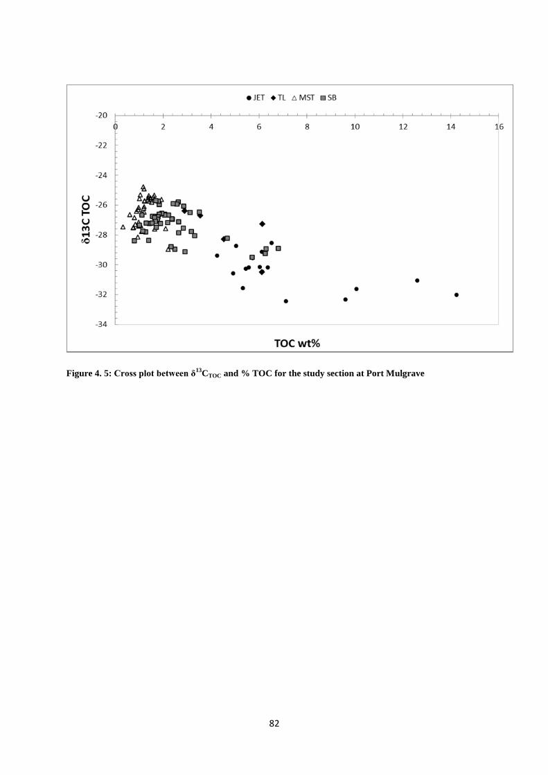
82
Figure 4. 5: Cross plot between δ13
CTOC and % TOC for the study section at Port Mulgrave

83
Table 4.2: Summary table of the bulk geochemistry data: TOC= total organic carbon; TC= total carbon;
TIC= total inorganic carbon; TS= total sulphur.
Stratigraphic unit
TOC
wt % TC wt % TIC
CaCO3
wt% TS (wt%)
JET (17
samples)
Range 14.3 - 2.8 6.1 - 16.1 0.7 - 5.8 6.1 - 49.1 9.6 - 15.1
Mean 7.1 9.2 2.0 16.5 12.2
SD 2.8 2.9 1.3 10.9 1.6
TL (5 samples)
Range 6.1 - 1.5 3.3 - 6.7 0.2 - 0.8 1.9 - 6.7 7.1 - 12.3
Mean 4.7 5.1 0.4 3.7 10.1
SD 1.5 1.6 0.2 1.9 2.2
4-MST (7
samples)
Range 1.9 - 0.2 1.9 - 2.2 0.2 - 0.8 2.0 - 6.3 3.3 -5.7
Mean 1.6 2.1 0.5 4.0 4.1
SD 0.2 0.1 0.2 1.4 0.8
USB (9
samples)
Range 1.7 - 3.5 1.9 - 4.1 0.1 - 0.6 0.9 - 4.9 5.5 -17.8
Mean 2.5 2.9 0.3 2.8 9.7
SD 0.6 0.8 0.2 1.4 4.3
3-MST (8
samples)
Range 1.0 - 2.1 1.3 - 3.8 0.1 - 1.7 0.5 - 14 1.9 - 5
Mean 1.4 1.8 0.3 2.8 3.1
SD 0.3 0.8 0.5 4.5 1.0
MSB (24
samples)
Range 1.1 - 4.7 1.7 - 5.0 0.04 - 0.6 0.3 - 4.9 3.2 - 10.1
Mean 2.2 2.5 0.3 2.1 5.7
SD 0.8 0.8 0.2 1.3 1.8
2-MST (8
samples)
Range 0.9 - 2.2 1.3 - 4.7 0.2 - 3.6 1.8 - 30.3 0.9 - 13.3
Mean 1.3 2.5 1.1 9.0 6.8
SD 0.4 1.3 1.2 9.8 4.0
LSB (14
samples)
Range 0.8 - 6.8 0.8 - 7.1 0.1 - 1.6 0.7 - 13.7 5.1 - 15.5
Mean 2.3 3.6 0.6 5.0 10.3
SD 2.3 2.3 0.5 4.0 4.2
1-MST (6
samples)
Range 0.3 - 0.1 0.8 - 1.1 0.01 - 0.7 0.1 - 5.9 3.9 - 5.8
Mean 0.81 0.99 0.16 1.31 4.64
SD 0.25 0.09 0.27 2.23 0.72

84
4.2.1.2 Rock- Eval pyrolysis
Rock-Eval pyrolysis is the one of the standard petroleum industry screening methods
to assess the source rock potential and quality of rocks. As is the case with TOC analysis,
Rock-Eval pyrolysis is quick and easy to carry out, but there are also problems which must be
addressed when interpreting the data, such as the mineral matrix effect, especially when
dealing with organic poor sediments with TOC less than 0.3wt% (Bordenave et al., 1993).
The data collected from Rock-Eval show mobile hydrocarbons as S1. The lowest S1 value of
0.08 (mg HC/g rock) was recorded within the bioturbated mudstone units, whereas the
highest value is 88 (mg HC/g rock) recorded in the Lower Sulphur Bed.
Figure 4. 6: S2 and Tmax variation throughout the study section at Staithes. Note the suppressed Tmax
values for the Sulphur Bands

85
The second parameter from Rock Eval Pyrolysis is the hydrocarbon potential from the
kerogen fraction (S2) as result of increasing temperature. The data is summarised in Table 4.3
Excluding the bioturbated mudstone samples, the samples show good generative potential
(Peters 1986) with a S2 average of 12.9 mg HC/g Rock. The Jet Rock and the top laminated
unit of the Grey shale also show consistently good source potential (10-20 mg HC/g Rock.
The crossplot of S2 versus TOC shows that the Sulphur Band samples tend to segregate from
the rest of the samples with a relatively higher slope of S2/TOC (corrected HI index). On the
other hand, the most organically rich part of the Jet Rock (Bed 35; Whale stone) is
characterized by relatively lower S2/TOC values (figure 4.7). A similar variation of the
generative potential parameters is recorded at the cm scale within the Sulphur Bands.
The Tmax values from Rock Eval pyrolyses range between 420 0C and 440
0C with an average
of 435 0C. Notably, the sulphur beds have low mean Tmax values of 430
0C. The relatively
low Tmax within the Sulphur Bands and the Jet Rock Shale are associated with higher
contents of organic sulphur.
Figure 4. 7: S2 versus TOC relationship for the Port Mulgrave samples

86
Table 4. 3: Summary table for the Rock-Eval data.
Sampled interval
S1 mgHC/g S2 mgHC/g
PI
Tmax
HI mgHC/g
TOC
JET (17
samples)
Range 2.1 - 7.9 17.6 - 42.4 18.6 – 43 420 - 436 297.4 - 483.5
Mean 4.6 26.9 27.9 431.2 392.0
SD 1.5 7.1 7.7 3.4 55.0
TL (5
samples)
Range 0.7 - 3.8 9.2 -23.4 10.2 – 24.4 431 - 436 316.9 - 415.5
Mean 2.2 16.8 17.8 434.0 356.7
SD 1.3 6.1 6.1 2.1 41.2
4-MST (7
samples)
Range 0.2 - 0.4 2.3 - 4.0 3.3 – 4.98 437 - 440 146.4 - 206.5
Mean 0.2 2.8 3.8 438.4 173.7
SD 0.1 0.6 0.6 1.1 20.9
USB (9
samples)
Range 0.2 - 1.0 2.2 - 12.2 3.2 – 13.2 427 - 440 131.4 - 464
Mean 0.6 6.5 7.5 434.0 255.1
SD 0.2 3.2 3.2 3.9 98.0
3-MST (8
samples)
Range 0.2 - 0.5 1.6 - 5.2 2.6 - -6.2 436 - 441 127.6 - 301.4
Mean 0.3 2.8 3.8 438.5 200.9
SD 0.1 1.1 1.1 1.8 53.6
MSB (24
samples)
Range 0.3 - 3.0 4.0 - 35.8 5.1 – 36.8 427 - 438 162.0 - 765.2
Mean 0.9 10.9 11.8 432.7 460.7
SD 0.6 7.3 7.3 2.7 133.9
2-MST (8
samples)
Range 0.1 - 0.5 1.3 - 5.6 2.3 – 6.6 432 - 439 116.4 - 252.5
Mean 0.3 2.6 3.6 436.8 180.0
SD 0.1 1.6 1.6 2.3 48.4
LSB (14
samples)
Range 0.2 - 88.0 0.6 - 27.9 1.6 – 28.9 424 - 437 72.3 - 444.3
Mean 7.1 9.6 10.6 431.1 247.1
SD 23.3 10.5 10.5 4.6 124.2
1-MST (6
samples)
Range 0.1 - 0.3 1.0 - 1.6 2 – 2.6 426 - 437 131.2 - 387.9
Mean 0.2 1.4 2.4 434.8 189.3
SD 0.1 0.2 0.2 4.4 98.3

87
Rock-Eval Quality Indices
The Hydrogen indices (HI) range between 42 and 765 (mg HC/g TOC). Hydrogen
index values over 100 indicate that organic matter is of kerogen type II and III (Tyson, 1995).
The bioturbated mudstone of the Grey shale are characterized by low HI values (less than 100
mg HC/g TOC) whereas most of the low HI values occur within bioturbated mudstone. The
highest HI values were recorded within the Middle sulphur bed while the Jet Rock samples
characterized with relatively suppressed HI values. Figure 4.8 illustrates the relationship
between HI and TOC. HI exhibits a positive linear correlation for the Sulphur Beds but a
negative correlation for the Jet Rock samples where the HI values tend to be suppressed
relative to TOC.
Figure 4.8: HI versus TOC % wt for the study section at Port Mulgrave
The Production index (PI) transformation ratio was calculated by using the formula
S1/ (S1+S2), often used as a maturation parameter (Peters, 1986). The highest values were
recorded within the Jet Rock shale with a mean PI value of 27.9 and a total range between
18.6 and 43. The PI is plotted in Figure 4.9 and shows low PI for the Grey Shale, except for
the Sulphur beds, which show distinctly higher values.
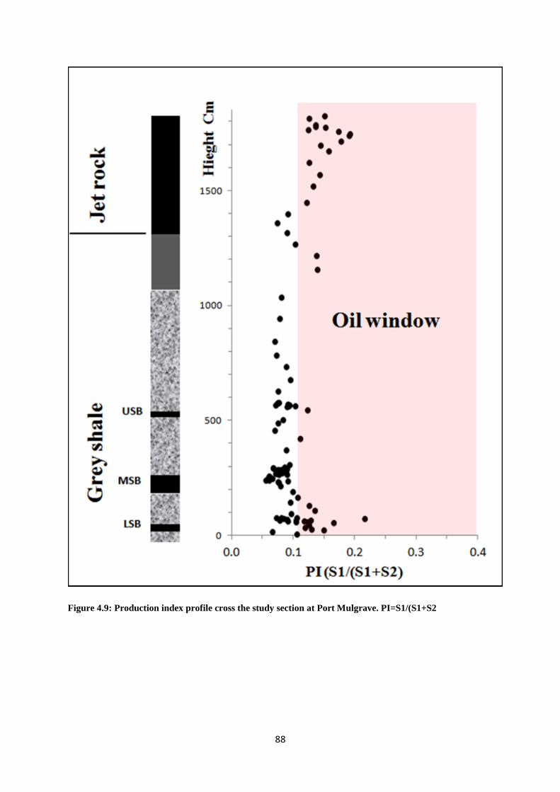
88
Figure 4.9: Production index profile cross the study section at Port Mulgrave. PI=S1/(S1+S2

89
4.2.2 Molecular biomarkers
Molecular biomarker analysis of aliphatic fractions focused on three groups, normal
alkanes, steranes and diasteranes, and pentacyclic triterpanes and their derivatives (Hopanes).
The results based on integration of peaks in various ion chromatograms are summarized in
Tables 4.4 and 4.5.
4.2.2.1 n-alkanes distribution
The aliphatic fractions of the extracted bitumen of 50 selected samples were analysed
using Gas Chromatography (GC) in order to show the molecular variation across the study
section. Figure 4.2.10 shows the aliphatic GCs of samples from the Lower sulphur, the
bioturbated mudstones and the Jet Rock shale. Whole gas chromatograms show a distribution
of normal alkane from n-C11 to n-C33 and more with maximum peak heights being n-C15. The
GC traces show similar relative abundance of n-alkanes distributions throughout the section.
Unimodal distribution of n-alkanes characterizes most samples. Normal alkanes
ranging from n-C11 to n-C33 are present in most samples. No visible signs of an undeveloped
hump or loss of n-C15 to n-C25 indicates that significant biodegradation has not occurred.
There is an odd/even predominance in most samples.
The carbon preference index CPI represents an odd carbon preference over even, and
occurs in response to chemistry in higher plant of surface waxes (an important precursor of
waxy components in sedimentary organic matter). Moldowan et al. (1985) concluded that an
odd carbon preference is characteristic of oils derived from source rocks deposited in non-
marine depositional environment. Therefore, if the total even and odd numbers of paraffins
are equally abundant the value of the CPI will be equal to one, and it goes above one with
more higher plant contribution to the organic matter, but causation must be taken when
interpreting the CPI as it changes with thermal maturity (Tissot and Welte, 1984). CPI values
in this study were obtained using the relationship proposed by Bray and Evans (1961)
formula:
All CPI values obtained are greater than 1.0 and in the range between 1.0 and 1.5 with
exception for the base of the Lower Sulphur Band where a 0.75 CPI value is recorded (table
4.4). Although there is small variation in the CPI values within the Sulphur bands it can be

90
observed that the Sulphur Bands have relatively lower CPI values compared to the
bioturbated mudstone units above and below. Moreover, the calculated ratio of ∑(C21 –
C31)/(C15 – C20) is used as degree of waxiness indication (Roushdy et al., 2010). There is an
upward decrease in the ∑(C21 – C31)/(C15 – C20) ratio (Figure 4.10). Apart from the Lower
Sulphur Band, the Middle and lower part of the Grey shale are characterised by higher ∑(C21
– C31)/(C15 – C20) ratios (consistently above 1) with an average of 1.58, while there is
variation across the Sulphur band fluctuating between 0.71 to 4.14.
Figure 4.10: Variation of the Carbon Preference index CPI and ∑ (C21 – C31)/ (C15 – C20) ratio throughout
the study section at Port Mulgrave.

91
Table 4.4: showing the obtained normal alkanes and acyclic isoprenoids relative abundance and the
calculated CPI values for the study section.
Sample Height (Cm) Pr/Ph Pr/c17 Ph/c18 ∑(C21-C31) /∑(C15-C20) CPI
Jet 17 1823 1.4 1.0 1.0 0.8 1.1
Jet15 1787 1.4 1.4 1.4 1.0 1.1
Jet 13 1774 1.3 1.3 1.3 1.2 1.1
Jet 11 1756 1.5 1.4 1.5 0.9 1.1
Jet 8 1716 1.3 1.4 1.4 0.9 1.1
Jet 6 1673 1.2 0.8 0.9 0.5 1.1
Jet 4 1568 1.3 1.3 1.3 0.6 1.1
Jet 1 1398 1.4 1.6 1.5 1.2 1.1
TL.5 1358 2.7 1.1 0.6 1.1 1.2
TL.4 1158 2.1 1.3 0.8 0.8 1.2
TL.1 1158 1.7 1.3 1.1 0.7 1.0
4-MST 6 945 4.4 0.9 0.3 1.3 1.3
4-MST 5 843 4.0 0.9 0.3 1.8 1.4
4-MST 2 678 4.3 0.9 0.2 1.5 1.3
4-MST 1 628 3.9 0.9 0.3 1.6 1.4
USB10 578 3.3 2.7 1.0 1.6 1.2
USB6 570 3.4 2.5 1.1 1.0 1.2
USB5 568 3.2 2.3 1.0 1.0 1.2
USB4 566 3.4 2.2 0.9 1.1 1.2
USB3 564 3.7 2.0 0.8 2.4 1.1
3-MST 7 501 4.6 0.9 0.2 1.7 1.3
3-MST 5 458 5.5 1.6 0.3 1.4 1.3
3-MST 1 297 3.7 1.7 0.6 1.1 1.2
MSB24 294 3.9 1.6 0.6 2.5 1.2
MSB 20 287 3.9 1.9 0.6 1.3 1.3
MSB18 283 3.3 2.0 0.9 2.9 1.2
MSB 16 278 3.5 1.9 0.7 1.4 1.3
MSB 9 254 4.1 1.5 0.5 1.4 1.3
MSB8 251 4.2 1.6 0.5 4.0 1.1
MSB 4 238 3.0 2.0 0.9 1.2 1.6
MSB2 233 2.9 2.8 1.0 2.1 1.2
2-MST 8 215 3.0 2.7 1.2 1.0 1.2
2-MST 4 128 5.0 1.2 0.3 1.7 1.4
2-MST 1 85 3.7 1.7 0.6 1.5 1.3
LSB14 78 2.9 2.7 1.2 0.9 1.4
LSB13 77 2.7 2.7 1.2 0.8 1.2
LSB11 73 2.7 2.8 1.3 0.9 1.3
LSB10 72 2.8 2.9 1.4 1.1 1.4
LSB9 71 2.9 2.8 1.3 0.7 1.3
LSB8 69 2.9 3.3 1.8 4.1 1.0
LSB4 63 1.0 2.6 1.3 0.1 0.8
1-MST 4 35 4.4 1.3 0.3 2.2 1.4

92
Figure 4.11: Chromatograms showing n-alkanes and isoprenoids of two representative samples. Number
by the peaks give the number of carbon atoms in n-alkanes (Pr = Pristane, Ph = Phytane)

93
4.2.2.2 Acyclic isoprenoids
Pristane (Pr) and Phytane (Ph) were both present in all samples, the Pr/Ph ratio
gradually decreases up section overall. The bioturbated mudstones and the Sulphur Bands
show relatively higher Pr/Ph ratios with values above 3, while the Jet Rock samples have
Pr/Ph values clustering around 1 (Figure 4.12).
Figure 4.12: showing the relationship between degree of waxiness and Pr/Ph ratio for the study section
As shown in Figure 4.12, the Pr/n-C17 and Ph/n-C18 profiles follow the same pattern
through the bioturbated mudstones. At the top laminated unit of the Grey shale and above the
Pr/Ph ratio continues to decline, while the Pr/n-C17 and Ph/n-C18 tend to slightly increase.

94
Figure 4. 13: Variation of Pr/C17, Ph/C18 and Pr/Ph ratio throughout the study section at Port Mulgrave.

95
4.2.2.3 Steranes and diasteranes biomarkers
The tetracyclic molecular biomarker steranes are derived from sterols in eukaryotic
organisms. The distribution of steranes is best studied by monitoring the ion m/z 217, which
is the characteristic fragment in the sterane series. A mass chromatogram for a representative
sample is shown in Figure 4.14. The sample shows a consistent sterane pattern throughout the
section, with the most abundant peak being the C27 5α (H) 14α (H) 17α (H) isomer.
Figure 4.14: Mass chromatograms showing the distributions of steranes and diasteranes (m/z 217) for a
representative sample from the Lower Sulfur Band at Port Mulgrave section.
Despite the general similarities that exist among the m/z 217 traces of the samples
(Figure 4.14), some marked differences are observed. Samples from the Grey Shale zone
show higher abundances of diasteranes relative to steranes, compared to samples from the Jet
Rock Shale. Other main steranes present are C27 and C28 5α (H) 14α (H) 17α (H) isomers
as well as C29, C28 and C27 5β (H) 14α (H) 17α (H) stereoisomers. The C30 steranes were
also present in all samples. Higher proportion of steranes R isomers relative to the S isomers
was observed in all samples. The ratio 20S/(20S+20R) of C27 13β(H), 17α(H) diasterane is
around 0.6 throughout the study section (Table 4.5). The isomer distributions of the C29
steranes show some variation through the section. Whilst the 20S/(20S+20R) parameter for
the 5α (H) 14α (H) 17α (H) steranes remains relatively fixed at around 50%. A triangular plot
shows the relative abundances of C27, C28 and C29 5α (H) 14α (H) 17α (H), (20R) sterane
isomers, with close grouping of all samples (Figure 4.20).

96
Figure 4.15: Mass chromatograms showing the distribution of steranes and diasteranes (m/z 217) for
selected samples from Jet Rock and Grey shale at Port Mulgrave (note the relative abundance of C29
5α(H) 14α(H) 17α(H) 20R-sterance). Refer to figure 4.14 for peak label.

97
4.2.2.4 Hopane biomarkers
Together with steranes, the triterpanes are the most important petroleum hydrocarbons
that retain the characteristic structure of the original biological compounds (Peter and
Moldowan, 1993). Tricyclics, tetracyclics, hopanes and other compounds contribute to the
terpane fingerprint (mass chromatogram m/z 191), which is commonly used to relate oils and
source rocks (Peters et al., 2005). Individual components were identified by comparison of
their retention times and mass spectra with a standard (North Sea oil) and published data
(Peters and Moldowan, 1993; Bowden et al., 2006). The fragmentograms m/z 191 was used
to detect the presence of triterpanes in the saturated hydrocarbon fractions (Figure 4.16 and
4.17). The hopane distribution pattern is similar for most samples with C30 17α (H) 21β (H)
hopane being the dominant peak (Figure 4.16). The C29 hopane peak is generally half, or less
than that of the C30 Hopane leading to a C29/C30 17α (H) hopane ratio of one or less. This
ratio and homologues of hopanes were prominent throughout the sediments analysed. The S
epimers and the 17β (H) 21β (H) and 17α (H) 21β (H) isomers are present, indicating
sufficient heating had occurred to isomerise the biological isomer 17β (H) 21β (H) to the
precursor isomer 17α (H) 21β (H) (Mackenzie et al., 1980). As a maturity parameter the
relative abundance of S and R epimers of C31 17α (H) 21β (H) was used (Peters and
Moldowan, 1993). The average maturity (22S/(22S + 22R) in %) was 52.5 with the standard
deviation of 4.8, suggesting maturity below the oil window (60% threshold).
Figure 4.16: Mass chromatograms (m/z 191) showing the hopanoid hydrocarbon distribution for
representative sample from the Lower Sulfur Band at Port Mulgrave section.
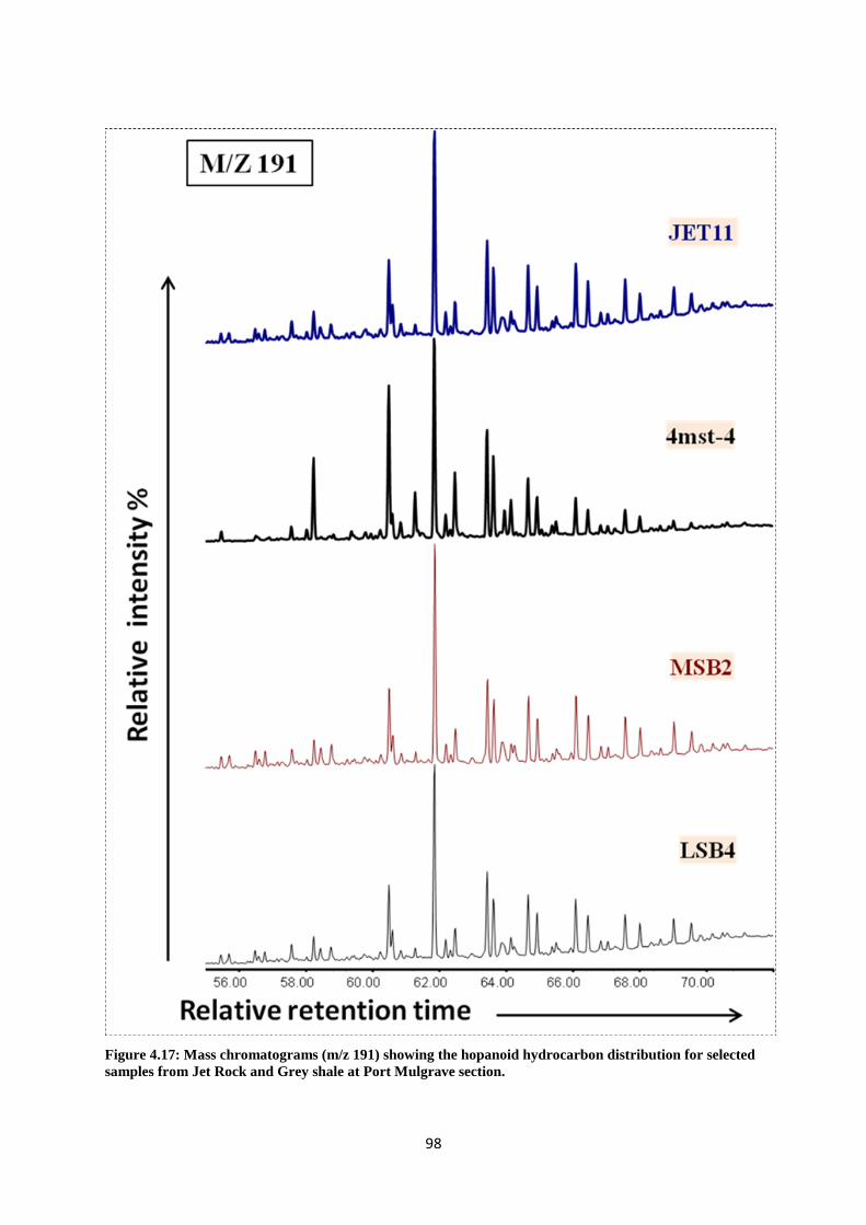
98
Figure 4.17: Mass chromatograms (m/z 191) showing the hopanoid hydrocarbon distribution for selected
samples from Jet Rock and Grey shale at Port Mulgrave section.

99
4.2.2.5 Homohopane Index
The relative distribution of C31 to C35 17α (H) 21β (H) 22S and 22R introduced as
Homohopane Index (C35/(C31-C35) αβ-hopanes) is often applied as an indicator of redox
conditions during and immediately after deposition (Peter and Moldowan, 1991). Although
high C35 homohopanes are commonly associated with marine carbonates or evaporates
(Boon et al., 1983; Clark and Philp, 1989), it is widely used as a general indicator of highly
reducing (low Eh) marine conditions during deposition (Peter and Moldowan, 1991). Values
of Homohopane Index above 7% are regarded as high and indicative of anoxic conditions.
The homohopane index values decreased slightly up section from 6.7 at the Lower sulphur
bed to 2.7 in the bioturbated mudstones right below the top laminated unit of the Grey shale,
after that the values sharply increase to approximately 11.0 above the Cannon Ball Doggers
horizon and continue at the same level throughout the Jet Rock shale (Figure 4.18).
Figure 4.18: Homohopane index and 22S/22(S+R) AB hopanes cross the study section at Port Mulgrave.

100
Steranes commonly found in mature sediments and crude oils are derived via
diagenesis from sterols which are widely dispersed in plants and microorganism, with the
C27 and C28 sterols most abundanct in marine organisms and the C29 sterols in higher plants.
Therefore, the relative distribution of C27, C28 and C29 steranes (20S & 20R epimers) is
used as indicators of depositional environment (Peters and Moldowan, 1993)
It has been proposed that the relative concentration of the diasteranes reflect the
presence of clay minerals and their ability to catalyze sterane rearrangement reactions.
However, it has become clear that the redox condition has an effect (Philip, 1994). Highly
anoxic conditions reduces the steranes, hence reducing the amount of steranes availble for the
rearrangements reactions (therefore, low diasteranes to steranes ratio).
The steranes / hopanes ratio reflects input of eukaryotic (algae and higher plants)
versus prokaryotic (bacteria) organisms to the source rock. To establish any changes in the
organic matter input the ratio of sterane over hopanes was assessed using the following
equation
Sterane/hopane = (C27ααα 20R+20S) + (C28ααα 20R+20S) + (C29ααα 20R+20S) /
C29 + C30 + (C31αβ 22 R+22S) + (C32αβ 22 R+22S) (Peters and Moldowan, 1993)
This ratio was then plotted against the height above the base of the Grey Shale Member as
shown in Figure 4.19.

101
Figure 4.19: Sterane/hopane plotted against the height (Cm) above the base of the Grey Shale at Port
Mulgrave section showing the inferred changes in organic matter input.
Figure 4.20: A ternary diagram showing the distributions of C27, C28 and C29 ααα(20R) steranes within
the studied samples at Port Mulgrave section.

102
Figure 4.21: A ternary diagram showing the distribution of C31, C33 and C35 αβ(22 S&R) homohopanes
within the studied samples at Port Mulgrave section.

103
4.2.2.6 Isorenieratane
Isorenieratane was confirmed using its diagnostic ions m/z 133, 134 and 546.5 (figure 4.22).
A typical 133 chromotogram trace bearing the characteristic relative abundace pattern
confirms Isorenieratane appearing at retention time of 76.1 mins.
Figure 4.22: (A) GC-MS ion chromatogram of m/z 133 of aromatic hydrocarbon fraction of
representative sample (from the Jet Rock Shale) showing presence of a diagenetic product of
isorenieretane (first identified by Koopmans et al. 1996). (B) Is mass spectrum of isorenieratane from
sample JET4.

104
Figure 4.23: Stratigraphic records of isorenieratane abundances in µg/g TOC across the study section
When normalised to TOC it becomes evident that samples above the boundary into
the Jet Rock shale (Exaratum subzone) have persistently high concentrations of up to 93.1
µg/gTOC (figure 4.23). The presence of isorenieratane within the bioturbated mudstone is
negligable where it was recorded in only one sample directly above the Middle Sulphur bed
(1.82 µg/gTOC). Notably, the Lower and Upper Sulphur Beds are characterized by prominent
peaks in isorenieratane with an average concentration of 12.98 µg/gTOC. The Middle
Sulphur bed is characterized by less isorenieratane (on average 5.57 µg/gTOC ) especically in
its central part where this compound was not detected at all.

105
Table 4.5: Biomarker-based parameters for organic matter thermal maturity and Paleoredox indicators.
Homohopane index = percentage of αβ-C35 Homohopane in ∑C31 – C35 αβ homohopanes (Peters &
Moldowan, 1991). +/- = presence/absence of isorenieratane.
Samples
Extract yield (mg/gTOC)
Maturity parameters Paleo-Redox parameters
22(S/S+R) C32 Hopane
20(S/S+R) C29 Sterane
Dia/Reg.steranes
Homohopanes index
Sterane/ hopanes
Isorenieratane
JET17 172.7 59.2 43.4 0.37 11.8 1.3 +
JET15 165.9 58.6 87.7 0.37 13.0
+
JET13 185.2 61.0 42.5 0.41 12.3 1.3 +
JET11 166.5 58.8 80.0 0.34 11.7
+
JET8 221.7 59.8 45.1 0.38 12.6 1.2 +
JET6 108 58.5 44.6 0.39 11.7 1.1 +
JET4 92.3 59.7 44.3 0.38 12.2 1.1 +
JET1 40.1 60.0 87.1 0.37 13.6
+
TL.5 86.1 59.6 45.8 0.45 9.8 0.4 +
TL.1 140.2 59.1 44.3 0.43 11.6 1.0 +
4-MST6 48.4 59.7 44.9 0.49 4.2 0.2 +
4-MST5 52.3 59.8 42.0 0.41 4.9 0.2 -
4-MST2 48.7 59.7 44.2 0.44 5.4 0.0 -
4-MST1 59.9 58.7 47.0 0.52 3.7 0.2 -
USB10 94.8 59.9 44.5 0.36 7.8 0.5 +
USB6 57.5 60.5 44.1 0.34 8.1 2.7 +
USB5 100.1 60.9 45.2 0.43 7.2 1.7 +
USB4 74.6 60.2 45.0 0.36 8.3 2.4 +
3-MST7 66.2 59.6 49.4 0.42 5.6 0.2 -
3-MST5 52.2 60.4 48.2 0.42 5.2 0.2 -
3-MST1 103.2 61.1 46.0 0.39 7.1 0.7 -
MSB20 92.9 62.1 43.6 0.39 7.2 0.4 +
MSB16 102.1 60.2 44.4 0.40 7.9 0.5 +
MSB9 80.8 59.9 48.0 0.35 7.6 0.4 +
MSB2 112.8 60.1
0.38 8.7 0.0 +
2-MST8 110.8 59.6 39.5 0.55 6.3 0.5 -
2-MST4 71.8 57.3 45.5 0.49 5.6 0.2 -
2-MST1 72.8 58.1 45.2 0.44 8.7 0.4 -
LSB14 175.1 61.1 46.2 0.62 8.4 2.4 +
LSB13 87.1 59.6 43.3 0.57 8.8 2.9 +
LSB11 167.5 59.5 42.9 0.53 9.0 2.9 +
LSB10 161.8 61.0 42.2 0.64 7.8 2.4 +
LSB9 95.6 60.4 44.5 0.58 8.8 2.5 +
LSB8 102.3 60.0
7.7 0.0 +
LSB7 118.5 59.6 44.5 0.57 8.8 2.6 +
LSB6 160.9 59.9 48.3 0.65 8.9 1.3 +
LSB5 145.6 60.3 55.1 0.57 7.5 1.2 +
LSB4 30.8 60.9 42.7 0.41 5.1 0.3 +
1-MST4 53.0 58.9 45.5 0.47 4.9 0.2 -

106
4.2.3 Organic petrological results
Although not a geochemical technique itself, the visual identification of kerogen
particles (macerals) in slides can provide an independent means of determining the source of
organic matter and corroborating bulk organic geochemical analyses. Kerogen is mostly
derived from microscopic dispersed particles derived from terrestrial and aquatic organic
matter and their degradation products (Vandenbroucke and Largeau, 2007). Kerogen
sometimes preserves a specific morphology (structure of particles) that allows its source to be
identified, and this in turn allows a better understanding of the depositional environment of
the sediments in which it is found (e.g. marine or freshwater, onshore or offshore, oxidising
or reducing, etc.) (Tyson, 1995). The aim of the optical examination was to give a general
characterization of the organic matter composition with regard to the terrigenous, marine and
amorphous origin, and to investigate whether this composition changes over the sequence.
Several optical classification schemes are available for the description of kerogen under
the microscope (e.g Hutton et al,. 1980: Waples, 1985). All classifications distinguish
between oxidized, carbon-rich organic matter (inertinite), humic organic matter (vitrinite),
and the lipid-rich particles of membranous material (exinite) or amorphous organic matter
(liptinite). Tyson (1995) revised and revaluated the palynofacies terms and presented a more
simplified classification (Tyson, 1995, p.350).
4.2.3.1 Transmitted light microscopy
A relatively quick qualitative, semi-quantitative approach is transmitted light
microspcopy. The total kerogen assemblage was divided into major components phytoclasts,
amorphous organic matter (AOM) and palynomorphs (Tyson, 1995). The stratigraphic
distribution of these components is shown in Figure 4.24.
A selected set of samples shows a dominance of AOM over phytoclasts assemblages.
The AOM forms more than 75% of the total kerogen apart of some mudstone samples where
the AOM drops to approximately 65%. The overall trend shows that the amount of
terrigenous input in the kerogen is extremely low in the Jet Rock (Exaratum subzone)
contributing less than 2%. At the lower part of the Grey Shale member (including the Sulphur
Bands) the contributions of terrigenous material are higher, especially within the bioturbated
mudstone horizons where the phytoclasts form up to 25% of the total kerogen with
dominance of black over brown woody materials.

107
Figure 4.24: Stratigraphical variation of % Phytoclasts and the fluorescent scale throughout the study
section at Port Mulgrave.

108
4.2.3.2 Blue light fluorescent microscopy
The palynomorphs in all samples show quite high fluorescence (e.g Plate E&F), while
AOM kerogens show fluctuated fluorescence intensity from moderate to low throughout the
studied section. Applying the fluorescence scale from Tyson (1995), the data shows moderate
fluorescence within the Grey Shale Member which passes into very strong fluorescence in the
upper part of the Grey shale and the Jet Rock member.
Total Kerogen plots
Tyson (1989) uses an AOM-phytoclast-palynomorph plot of percentage particle
abundances (i.e. relative numerical particle frequency) to characterise kerogen assemblages
into eleven (independently sedimentologically-defined) marine shale facies. The plot picks
out differences in relative proximity to terrestrial organic matter sources, and the redox status
of the depositional subenvironments that control AOM preservation. As the emphasis is on
palaeoenvironment rather than source rock potential, cuticle is incorporated within the
phytoclast group, not the palynomorph group.
The relative abundance of palynofacies components was plotted in an AOM-
phytoclasts-palynomorphs (APP) ternary diagram to investigate the organic matter type
through the section in order to determine the oxygen content of the bottom water column and
the quantity of terrestrial input. In order to demonstrate correlations between different data
sets, the percentage of various palynomorph categories, or geochemical values, were plotted
on to this diagram (Figure 4.25)

109
Figure 4.25: Amorphous organic matter-Palynomorphs-Phytoclast "APP" ternary diagram of relative
abundance of palynofoacies parameters after Tyson (1995). The percentage of each parameter is
calculated in relation to the total particulate organic matter counting.
Table 4.6: informal kerogen categories used in this study.
Main category Sub category presence
Phytoclasts Black wood common
Dark brown wood common
Light brown wood common
Cuticle rare
Fungal hyphae rare
Amorphous AOM (derived from phytoplankton and bacteria)
Dominant
Palynomorphs Sporomorphs Pollen (common)
Spores (common)
Marine miroplankton Tasmanite
Non-marine microplankton absent
Marine zoomorphs

110
Figure 4.26: Stratigraphic variation in the character of the woody phytoclast fraction and of TOC.
Connection of sample points is for diagrammatic purposes only and does not imply interpolated values.
Phytoclast data are based on relative numeric particle frequencies.

111
Figure 4.27: Well preserved ‘AOM’ seen in transmitted white light, amorphous matrix rich in small
unidentifiable fragments (fluorescent under the blue light; equivalent to the maceral liptodetrinite) plus
other inclusions (palynomorphs, pyrite and small phytoclasts) (Magnification X20).
Figure 4.28: relative dominance of phytoclast mixed with poorly preserved AOM and Palynomorous.
Biostructured phytoclast (the term biostructure refers to definitive biologically-derived structure)
composed of wood tissue such as gymnosperm tracheids and gymnosperm xylem ray tissue or dispersed
cuticle phytoclast (Magnification X20).

112
Plate A (Magnification X40)
Plate B (Magnification X40)
Plate C (Magnification X40)

113
Plate D (Magnification X40)
Plate E (Magnification X40)
Plate F (Magnification X40)

114
A: Well preserved ‘AOM’ seen under transmitted white light. Note the diffuse edged
particles. The form of the edge and the presence of the pyrite inclusions (the black spots)
indicate that the particle is structureless and therefore not a phytoclast. The sample lithology
is laminated black shale (Jet Rock shale; sample JET 15)
B1: Biostructured phytoclast (the term biostructure refers to definitive biologically-derived
structure). The phytoclast is composed of at least two adjacent gymnosperm tracheid
fragments
C: Structured phytoclast. The cross-hatch structure of the phytoclast, with thickened ribs
arranged approximately at right angles to each other, indicates a derivation from ray tissues
(Tyson, 1995). These are similar to cuticle tissues and distinguished by their regularly
arranged columns and rows of squares or rectangles and showing no fluorescence under blue
light.
D: Dispersed leaf cuticle phytoclast (Liptinite-cutinite) showing regular rectangulare cell
outlines (probably gymnosperm in origin). The relatively dark brownish matte colour and
lack of fluorescence mainly indicate partial oxidation before or during final deposition
E: Tasmanites algae belonging to the Prasinophyte phycomata, one of the major subdivisions
of the Palynomorph group. It shows intense fluorescence under the blue light.
F: Spore (Deltoidospora) with diagnostic trilete mark (Y-shaped mark) on one side, which reflects where it was joined to three neighbours on the inside of a pyramid-shaped tetrad.

115
4.2.4 Detailed geochemical profile across the Sulphur Band at the Pliensbachian-
Toarcian boundary
The Pliensbachian–Toarcian boundary preceding the T-OAE has received special
attention in this study. Intense geochemical analyses were carried out in order to understand
the geochemical systematics of the Sulfur Band intervals at the base of the Grey Shale
Member. Although the Sulphur Bands appears to be well laminated and generally have high
organic carbon contents (average TOC ~ 2.5 wt%, Figure 4.29), the very detailed analysis at
cm-scale shows that the organic content varies substantially across the Sulphur Bands.
Despite the similar geochemical pattern of the Sulfur Bands of the lower Grey shale member
at the Hawsker Bottoms and Staithes sections, the Hasker Bottoms section shows weaker
lamination and poor organic contents (TOC average of 0.93 wt% compared with 3.0 wt% at
Staithes). Moreover, the quality of the organic mattter of the Lower Sulphur Band is different
at both locations as suggested by moderate Hydrogen Index (HI) with an average of 280 wt%
at Staithes and lower values at at Hawsker Bottoms 191 wt%.
Figure 4.29: stratigraphic variation in the bulk geochemistry parameters: depth versus TOC wt% and HI
of the lower Grey shale member at Port Mulgrave (Staithes) and Hawsker Bottom outcrops.
Although the Lower Sulpur Band has been described in previous studies (Wignall,
1994) as representing an anoxic environment, the new cm-scale multiproxy records reveal a
more dynamic system, with distinct fluctuation in the geochemical parameters (Figure 4.30
and Figure 4.31).

116
Figure 4.30: Cm-scale analysis of the TOC, TS and isotopic analysis for the organic carbon and pyrite
sulfur cross the Lower Sulfur Bed at Port Mulgrave section
Figure 4.31: Cm-scale molecular biomarker analysis cross the Lower Sulfur Band at Port Mulgrave
section includes Pr/Ph, Isorenaraten concentration (µg/gTOC), Steranes over Hopanes ration and the
Homohopanes index.

117
4.2.4.1 Sold bitumen assemblages within the Lower Sulphur Band.
A thin layer of black material was found within the upper part of the Lower Sulphur
Bed. It looks like a coal with its light weight and shiny appearance. It was traced almost 25
meters along the outcrop, is about 0.5 cm thick and extends deep in the outcrop (Figure 4.32).
It is positioned between the shale laminas (Figure 4.33)
Figure 4.32: Thin layer of bitumen within the Lower sulfur band at Port Mulgrave section.
The black material was collected and subjected to hydrocarbon extraction using hot solvent
(isotropic mixture of 93% DCM and 7% methanol). The hydrocarbon extractability of this
material is extremely high (>95% of its weight is extractable bitumen) compare to an average
hydrocarbon extractability of 1.4% for the surrounding shale of the Lower Sulphur Band and
10% for the Jet rock shale. When studied under the transmitted white light microscope no
clear sings of woody material was found.

118
Figure 4.33: bitumen accumulation within the Lower Sulfur Bed. The picture shows the elongated
structure casted on the shale rock.

119
4.2.4.1.1 Molecular biomarker characterisation of the bitumen layer
Normal alkanes
The distribution of normal alkane in the bitumen layer is similar to the extracted
bitumen from the surrounded rocks. Normal alkane from n-C11) and n-C36 were identified
(figure 4.34). The GC trace displays a unimodel distribution with a very weak predominance
of odd carbon over the even carbon numbers and a low CPI of 1.9.
Figure 4.34: GC trace of the bitumen from the Lower sulfur Bed at Port Mulgrave.
Acyclic isoprenoids
Pristane (Pr) and Phytane (Ph) were both present in the samples, with a high Pr/Ph
ratio of 3.0. The Pr/C17 versus Ph/C18 relationship for the whole set of samples displays that
the Grey shale including the Sulphur Beds and the bitumen sample were segregated from the
Jet Rock sample as seeing in figure 4.35.

120
Figure 4.35: Cross plot of Pr/n-C17 versus Ph/n-C18 ratios from extracted bitumen gas chromatograms
showing organic matter type, biodegradation and maturation conditions for the Lower Sulfur Band and
the bitumen layer included compare to the Jet Rock Shale.
Hopanes and steranes distribution
Ternary plot of the 17α (H) 21β (H) S and R isomers for C31, C33 and C35 αβ hopanes
as well as the regular 27, 28 and 29 ααα20R Steranes (Figures 4.36 and 4.37) show a clear
separation of the bitumen sample from the rest of the extracted rock samples with a
dominance of C31αβ hopanes.

121
Figure 4. 36: Ternary diagram showing the relative abundances of C31, C33and C35 17α (H) 21β (H)
hopanes 22R + 22S isomers.
Figure 4.37: Ternary diagram showing the relative abundances of C27, C28 and C29-regular steranes 5α
(H) 14α (H) 17α (H) 20 R isomer.
122
4.3 Discussion
Several processes must be considered to explain the origin, preservation and
distribution of organic matter. Actually the development of organic matter-rich black shales
has been a matter of many geochemical studies for decades. This is due to their often perfect
preservation of vital information about the geologic history and because of economic
potential.
4.3.1 Thermal maturity of the organic matter
From the petroleum geochemical point of view the study section would be classified
as marginally mature. The maximum burial of the Lower Toarcian section of the Cleveland
basin is inferred to have been 2.2 to 2.5 km (Hemingway and Riddler, 1982). Reflectance
microscopy of isolated kerogens revealed few vitrinite particles, with a consistent reflectance
in the range 0.55 – 0.65% Ro (Raiswell et al., 1993; Ibrahim, 1995). Oil shows are often
found in the ammonite chambers, especially the Canon ball doggers (Bed 33, sensu Howarth,
1962 and 1973) (Salen et al., 2000).
The Rock Eval data from this study confirm this maturity interpretation from previous
studies, as indicated by low Tmax ranging from 420 to 441 (an average of 434 ºC) and
Production index (PI) ranging from 0.05 to 0.9 (an average of 0.11) reveals that early stage of
thermal maturity had been achieved. Moreover, the relatively low and uniform PI that ranges
between 0.06 to 0.51 and averaging around 0.13 indicates that any migrated hydrocarbons
could have not indeed affected the geochemical signals (Table 4.3)

123
Figure 4.38: Cross plot of HI and Tmax showing the thermal maturity state of the samples at Port
Mulgrave section.
Tmax values for some samples fall below the oil window (Tmax ≥ 430 ºC is the
maturity threshold for type II according to Hunt, 1995). This suppression in the Tmax is
found in the organic sulphur rich samples (e.g Sulphur bands). The low Tmax in those
samples could be due to the high content of organic sulphur where the oil window for Type
II-S kerogen begins earlier as the result of the breakage of weak sulphur bonds at lower
temperatures (Tmax 390–420°C).
Molecular geochemical data also confirm an immature/marginally mature thermal
maturity level. The hopanes (C29 to C35) are dominated by the more stable 17α(H), 21β(H)
isomers with much lesser amounts of the 17β(H), 21α(H) isomer. The biologically inherited
17β(H), 21β(H) isomers are completely absent. These isomer distributions are consistent with
a relatively high thermal maturity level of the organic matter in the section (Raiswell et al.,
1993). Moreover, all the samples show complete isomerisation of the 17α(H), 21β(H) isomer
at C-22 (Figure 4.18) with the 22S/(22S+22R) ratio corresponding to the equilibrium value of
around 60 % (Peters and Moldowan, 1993). Sterane and diasterane isomerisation reactions
further testify to the maturity of the organic matter of the study section as marginally mature.
The 20S/(20S+20R) ratio for the C29 5α(H), 14α(H), 17α(H) sterane isomers is around 50%

124
for almost all samples, pointing to early matured organic matter (Peters and Moldowan,
1993).
Although most of the thermal maturity indicators used here point to thermally mature
source rock, the PI are relatively low for most of the samples, particularly for the Grey Shale
including the Upper and Middle Sulphur Bed (Figure 4.9). Most of these samples fall below
the value of 0.1 which is the threshold of the oil window (Peters et al., 1986). This could be
explained as the result of the mineral matrix effects as the Grey Shale is characterized by
relatively low organic matter contents coupled with relatively high clay contents (Morris,
1979) which can retain some of the S1 and consequently lower the production indices
(Espitalie et al., 1980).
4.3.2 Source of Organic Matter
Organic matter type is an important factor in evaluating source rock potential and has
an important influence on the nature of the hydrocarbon products (Tissot and Welte, 1984;
Hunt, 1995 and Tyson, 1995).
Rock-Eval pyrolysis characterizes the organic matter of the tenuicostatum and lower
Falciferum zone (Exaratum Subzone) as being mainly of marine origin when plotted on a S2
vs. TOC scattered plot (Figure 4.39). The graph of S2 versus TOC is an informative way of
displaying Rock-Eval data (Langford and Valleron, 1990). The graph of S2 vs. TOC also
permits determination of the type of Kerogen without using S3 data. The plotted data indicate
that most of the samples are Kerogen type II, a part of few samples belonging to bioturbated
mudstones at the lower part of the section (Grey Shale Member), which do indicate kerogen
Type III OM. Moreover, the use of a linear regression curve on the S2 versus TOC plot is the
best way of calculating HI which allows identification and correction for any effects of the
rock matrix (Langford and Valleron, 1990; Tyson, 1995). Despite the relatively high TOC
content and the well laminated structure of the Sulphur bands, very detailed analysis across
these units indicates a mixed kerogen Type II/III.

125
Figure 4.39: S2 versus TOC diagram with Kerogen type fields indicating that all of the Jet Rock samples
do fall in Kerogen type II while the Grey shale fall in Kerogen types II and III region.
Hydrogen index (HI) values range from 116 mg/g TOC within the bioturbated
mudstones of the Grey Shale (Tencostatum zone) to a maximum of 484 mg/g TOC within the
Jet Rock Shlae (Exartum subzone). Despite the indication of Kerogen type II of the Jet rock
samples the HI values are relatively moderate to low, especially within bed 35 where the HI
values cluster around an average of 351 mg/g TOC. Generally, marine algal organic matter
has higher HI values (≥ 400; Tyson, 1995), whereas lower values could be caused by some
contribution of dispersed terrestrial material, with low hydrocarbon yields. However,
microscopic examination disapproved any substantial contribution of dispersed terrestrial
organic matter in the Jet Rock samples. Instead, the organic matter of the Jet Rock consists
mainly of fine grained algal AOM with very rare phytoclasts (not exceeding 5%) with
moderate to strong fluorescence (4-5 on the preservation scale of Tyson, 1995). These
observations indicate only a minor input from higher plants. The high preservation of marine
organic matter under anoxic conditions results in kerogen assemblages overwhelmingly
dominated by amorphous organic matter (70-90%). On the other hand, the bioturbated
mudstones (Tencostatum zone) apparently displayed less abundance of fine grained algal
amorphous material with slightly more contribution of woody material. Therefore from
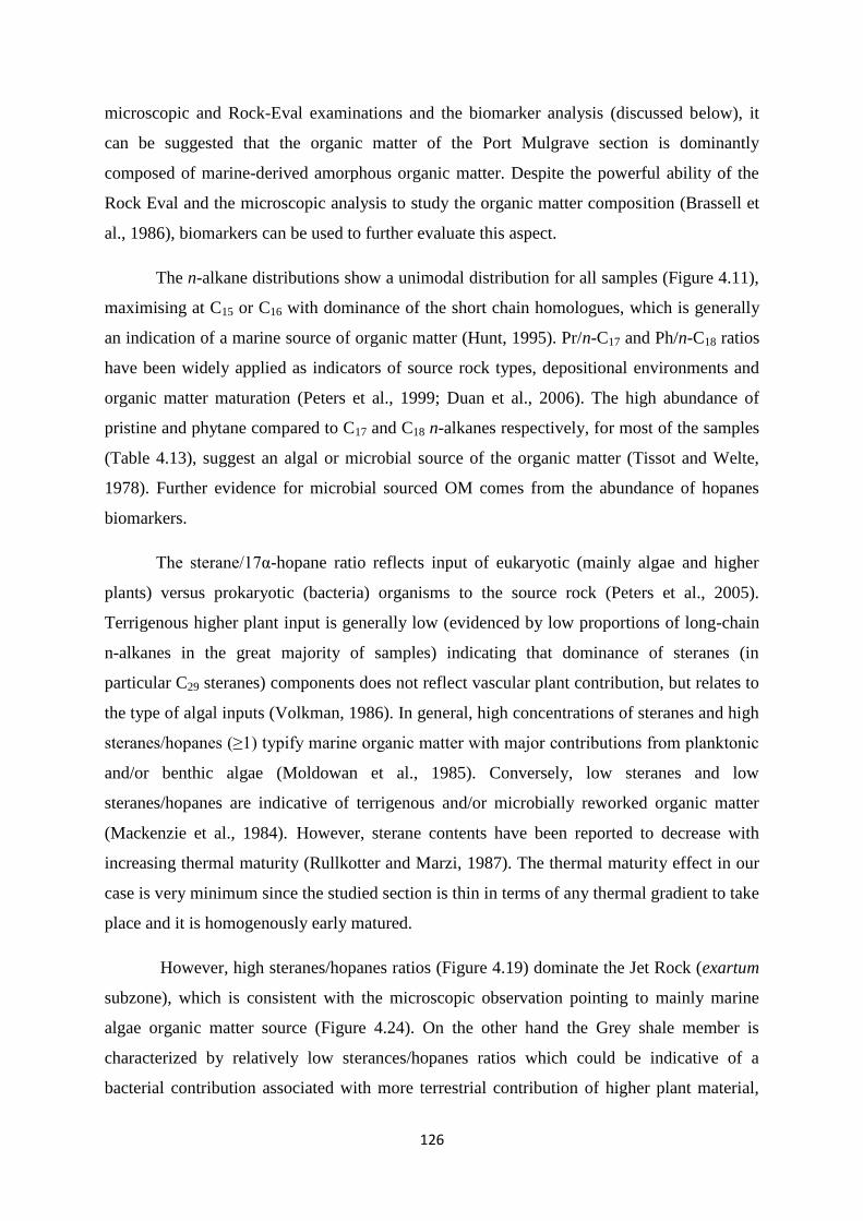
126
microscopic and Rock-Eval examinations and the biomarker analysis (discussed below), it
can be suggested that the organic matter of the Port Mulgrave section is dominantly
composed of marine-derived amorphous organic matter. Despite the powerful ability of the
Rock Eval and the microscopic analysis to study the organic matter composition (Brassell et
al., 1986), biomarkers can be used to further evaluate this aspect.
The n-alkane distributions show a unimodal distribution for all samples (Figure 4.11),
maximising at C15 or C16 with dominance of the short chain homologues, which is generally
an indication of a marine source of organic matter (Hunt, 1995). Pr/n-C17 and Ph/n-C18 ratios
have been widely applied as indicators of source rock types, depositional environments and
organic matter maturation (Peters et al., 1999; Duan et al., 2006). The high abundance of
pristine and phytane compared to C17 and C18 n-alkanes respectively, for most of the samples
(Table 4.13), suggest an algal or microbial source of the organic matter (Tissot and Welte,
1978). Further evidence for microbial sourced OM comes from the abundance of hopanes
biomarkers.
The sterane/17α-hopane ratio reflects input of eukaryotic (mainly algae and higher
plants) versus prokaryotic (bacteria) organisms to the source rock (Peters et al., 2005).
Terrigenous higher plant input is generally low (evidenced by low proportions of long-chain
n-alkanes in the great majority of samples) indicating that dominance of steranes (in
particular C29 steranes) components does not reflect vascular plant contribution, but relates to
the type of algal inputs (Volkman, 1986). In general, high concentrations of steranes and high
steranes/hopanes (≥1) typify marine organic matter with major contributions from planktonic
and/or benthic algae (Moldowan et al., 1985). Conversely, low steranes and low
steranes/hopanes are indicative of terrigenous and/or microbially reworked organic matter
(Mackenzie et al., 1984). However, sterane contents have been reported to decrease with
increasing thermal maturity (Rullkotter and Marzi, 1987). The thermal maturity effect in our
case is very minimum since the studied section is thin in terms of any thermal gradient to take
place and it is homogenously early matured.
However, high steranes/hopanes ratios (Figure 4.19) dominate the Jet Rock (exartum
subzone), which is consistent with the microscopic observation pointing to mainly marine
algae organic matter source (Figure 4.24). On the other hand the Grey shale member is
characterized by relatively low sterances/hopanes ratios which could be indicative of a
bacterial contribution associated with more terrestrial contribution of higher plant material,

127
which is supported by visual evidence (Figure 4.25) and higher degree of waxiness (Figure
4.10).
The relatively higher contribution of hopanes relative to steranes in the Grey Shale
member may also arise from greater bacterial breakdown of the autochthonous algal material
during deposition (Farrimond et al. 1986) with an associated increase in the relative
proportion of bacterial biomass.
Characterisation of the organic matter source can be extracted from the distribution of
regular steranes (Moldowan et al., 1985 and Philip et al., 1991). In our studied samples the
distribution of regular steranes as shown in Figure 4.15 is similar throughout the section,
suggesting a constant marine organic matter source with a slight preference of C29 steranes
ratios over C28 and C27 for the Grey shale samples, a feature commonly seen in marine
black shales with contribution of terrestrial organic matter (Peters et al,. 2005). Moreover,
The marine source of organic matter can be inferred (but not proven) by the ternary diagram
which reflects the distributions of C27, C28 and C29, 5α(H), 14α(H), 17α(H), (20R)
seteranes for the different shale samples of the section. All the samples, including the Grey
Shale samples, show very close grouping (Figure 4.20) suggesting a constant marine source
throughout the section.
Based on the above discussed parameters, a distinction can be made between the
dominant types of organic matter present in the shales. It can be said that the Grey shale
member seems to have received some contribution of land-derived organic matter that has
been transported into a marine depositional setting and was deposited in a photosynthetic
organisms-dominated environment (thereby suggesting a mixed Kerogen type II & III).
Moreover, the Sulphur Bands are characterised by marine sourced organic matter with some
contribution of terrestrial input. On the other hand, the Jet Rock Shale (exartum subzone) is
characterised by a dominance of marine organic matter sourced mainly from planktonic
and/or benthic algae.
4.3.3 The palaeoenvironment of deposition
The paleoenvironmental conditions during organic matter (OM)-rich black shale
formation have been an important scientific issue to understand/reconstruct global and
regional biogeochemical element cycling. The interpretation of organic matter source for any
sedimentary sequence usually provides some clues for the palaeoenvironment of deposition

128
(Brassell et al., 1986). The well preserved, dominantly amorphous organic material, the
relatively high hydrogen indices which indicate type II kerogen and the high TOC contents
(Tables 4.2 and 4.3), are indicative of a dysoxic to anoxic condition of deposition (Tyson,
1995). This assumption is confirmed by the high sulphate content which shows a degree of
correlation with the relatively high TOC content (Figure 4.3). All samples lie above the
normal marine line and mostly fall into the euxinic consistent with euxinic condition of
deposition (Raiswell and Berner, 1985) especially for those belonging to the Exartum
subzone and the Sulphur band horizons. The well-developed lamination, which is rarely
interrupted, exhibited by the shales of the Bituminous Shale zone, especially by the Jet Rock
Shale of the Exaratum subzone (Morris, 1979), is consistent with the inferred anoxic
conditions. The fluctuating TOC within the Exaratum subzone (Table 4.2 and Figure 4.1)
might suggest that the degree of anoxia has been variable although fluctuations in
productivity may be an alternative cause. The Grey Shale zone, on the other hand, consists of
poorly laminated dark grey shale, but there has been inconclusive of bioturbation which
suggests that during the deposition of the Grey Shale anoxic conditions prevailed below the
sediment-water interface and the water column remained oxic, whereas anoxic conditions
extended into the water column during the deposition of the Sulphur bands. In the present
study, Pristane/Phytane ratios are greater than unity, frequently interpreted as evidence for
oxic conditions prevailing during sediment deposition (Didyk et al., 1978). However, these
relatively high values of pristane/phytane ratios throughout the study section (Table 4.2.4) are
more likely the result of the elevated thermal maturity of the samples (Didyk et al., 1987)
rather than an indication of the degree of oxicity. Although it is difficult to interpret absolute
Pristane/Phytane values in terms of redox conditions, it is obvious that the ratio is higher for
the Grey Shale zone than the overlying Jet rock Shale zone suggesting that more oxic
conditions could have been prevailing during the deposition of the Grey Shale. Also the
relatively abundant steranes compared to hopanes within the Bituminous Shale zones of the
Sulphur Bands, could be interpreted as a result of less oxic conditions (Volkman, 1986)
prevailing during the deposition of these shales, which is further confirmed by the low C31
content compared to the C35 or C34 content of the 17α(H), 21β(H) (S+R) hopanes (Peters and
Moldowan, 1991).
The presence and widespread distribution of isorenieratane indicates that a sulfidic
photic zone was a common occurrence, within the Sulphur Bands at the base of the Grey
Shale, and as well throughout the Jet rock shale spanning the T-OAE. Isorenieratane

129
maximum abundance is near the maximum in TOC, implying that strengthening euxina was
responsible for increasing in organic carbon burial. Isorenieratane signature in Toarcian black
shales has been regarded as supporting evidence to point out to strong stratification during the
deposition of Jet Rock shale (Kuspert, 1982). The presence of isorenieratane within short
intervals of the sulphur bands before the main T-OAE indicates that euxinia was developed
during short periods at the Pliensbachian-Toarcian.
The high TOC content and the distribution of the Jet Rock of Western Europe, has led
Jenkyns (1985, 1988), to infer a widespread oxygen minimum zone associated with a so
called Toarcian Oceanic Anoxic Event (OAE), which may have resulted from high surface
productivity. In the case of the Port Mulgrave section, the well preserved algal (marine-
derived) organic matter of the Jet Rock Shale, coupled with the relatively high proportion of
regular steranes (table 4.5), could be consistent with high surface productivity (Farrimond et
al., 1988).
The geochemical characteristics of the Exartum subzone reflect global geochemical
change (T-OAE) and fit well with the model for deposition of the Jet Rock and its equivalents
in Western Europe and elsewhere in the world. Jenkyns (1988) proposed that certain regions
of the world ocean, in particular the oxygen minimum zones (OMZ) were particularly poorly
ventilated due to the topographic restriction (e.g block-faulted margin) and deposition of
organic-rich shales was widespread during the early part of the Falciferum zone (Exaratum
subzone). This model implies high surface productivity in shallow waters rich in nutrients.
The high oxygen demand, through partial microbial degradation of large quantities of the
autochthonous organic matter, led to oxygen depletion in bottom waters resulting in anoxic
conditions and the subsequent preservation of large quantities of the organic matter.

130
4.3.4 Comparison of Sulphur Bands (Grey Shale Member) basal transgressive black
shales and Jet Rock (maximum flooding) black shales
It is well documented that in many epicontinental seas, the distal basin settings
(settings of low and slow sedimentation rate) accumulate intervals of organic rich condensed
black shales (Demaison and Moore, 1980). In such deep-water settings the benthic
environment is poorly oxygenated (anoxic or suboxic) due to isolation of the bottom waters
from dynamic effects such as the wind-driven vertical advection of oxygen-rich surface
waters. The establishment of a very rapid density gradient in the water column and
development of a pyconcline can be a factor for isolating bottom waters and therefore
developing a more static state that led to water column stratification (Wignall, 1993).
Condensed sections can also extend into marginal settings at times of rapid sea level
rise where they form on the maximum flooding surface, separating the transgressive from the
high stand system tracts (e.g jet rock shale). This is an important mechanism for introducing
black shales into areas normally characterized by shallow deposition and at the same time
connecting deep and shallow water black shales. Many types of black shale are associated
with sites of greatest subsidence, leading Hallam and Bradshaw (1979) to propose the model
of irregular bottom topography (known as the “puddle model”). In this model the deep-water
conditions essential for black shales are achieved by rapid subsidence only and potential
exists for black shale formation throughout the sea level cycle. However, black shales were
most likely to form on sites of rapid subsidence at the inflexion point of relative sea level rise.
Thin black shales extending from basinal into marginal settings fall into two
categories: The first category is basal transgressive (BT) black shales, which show no
obvious lateral facies variation and normally pass proximally into sediment-starved marginal
facies (e.g the Sulphur Bands at the base of Whitby Mudstone formation at the Pliensbachian-
Toarcian boundary). BT black shales are distinguished by resting directly on a transgressive
surface which may coincide with a sequence boundary or it correlative conformity as is
probably the case with the Sulphur Band and Lower Oxford Clay examples with no time-
equivalent shoreline facies, as they most probably formed during times of non-deposition on
the basin margin (Grabowski and Glaser, 1990).
The second category are maximum flooding surface black shales, which are
distinguished by passing proximally into thicker sections of shallower marginal marine facies.
These exhibit the most oxygen-restricted facies in the basin centre and represent a deep-water

131
sediment-starved condensed section. They often rest conformably on sediments of the
transgressive system tract. Examples are the black shales of the Jet Rock, the G. cumbriense
and G. listeri Marine Bands.
Previous studies have been concerned with boundary intervals at the Late
Pliensbachian to Early Toarcian as it relates to sea level change (Hallam, 1997),
paleoceanographic change (Bailey et al., 2003), as well as contrasting water mass and basinal
restriction (Sælen et al., 2000; McArthur et al., 2008). All these may have affected deposition
of both the Grey Shale and the overlying Jet Rock during the period of major basin
subsidence characterised by deep open waters (Powell, 2010).
Despite its name, and the presence of small carbonaceous flakes and jet, the
geochemical and optical analysis of this study indicate that the Jet Rock shale organic matter
has been mainly derived from marine algae and comprises mostly amorphous organic matter
with relatively minor terrestrial contributions (This study and Farrimond et al., 1989; Ibrahim,
1995; Sælen et al., 2000). The Jet Rock having higher TOC and HI compare with the
Sulphur Bands (Table 4.8) also, the mean values of the Sulphur Beds are slightly different
from the Jet Rock. The geochemical and optical data of the Jet Rock black shale show a good
source rock potential and Type II kerogen, while the Sulphur Beds data indicate a lower
quantity of OM and quality of kerogen.
Table 4.7: Summary of bulk geochemical data from the Jet Rock and Sulphur Bands.
Jet
Rock TOC % S1 S2 Tmax HI PI
No. 17 17 17 17 17 17
Range 4.26 - 14.26 2.07 - 7.87 17.62 - 42.39 420 - 436 297 - 484 0.09 - 0.19
Mean 7.13 4.29 26.89 431 392 0.15
SD 2.82 1.48 7.06 3.43 55.01 0.03
Sulphur
Beds
No. 47 47 47 47 47 47
Range 0.80 - 6.81 0.16 - 88 0.58 - 35.81 424 - 440 72 - 765 0.06 - 0.90
Mean 2.49 2.67 9.66 432 357 0.1
SD 1.38 12.73 7.88 3.68 162 0.12
The kerogen assemblages of both samples are shown in the APP diagram (Figure
4.25). Despite the very high AOM in both intervals, the Sulphur Beds samples are clearly

132
separated from the Jet Rock samples with higher woody material and palynomorphs which
could indicate more proximal setting and more dynamic environments relative to the Jet Rock
interval. Table 4.3 summarizes the similarities and differences between the deposition
conditions of the sediments in both members; the percentage of phytoclasts input in Jet Rock
is either masked by AOM, or the formation was deposited further from shoreline.
Table 4.8: Summary table show the similarities and the differences between MFS and basal black shales.
Similarities Differences
All samples deposited in reducing
environments.
Both have dominantly marine
Amorphous Organic Matter (AOM)
Both are organic-rich shale.
Kerogen assemblages show better
preserved in Jet Rock
Sulphur Bands have more variable
properties and interbedded with more
oxic layers.
Overall thickness of Jet Rock is much
greater.

133
4.3.5 Hydrocarbon potential
The existing dataset indicates that the lower Toarcian sediments from the
Tenuicostatum - Falciferum zones have a good source rock potential. The shale and mudstone
units frequently contain above average TOC with an average of 1.3 for the mudstone units
and 3.4 wt% for the laminated shales, and an average of pyrolysis S2 yields of up to 10.9
mg/g (up to 42.4 mg/g within the bituminous shale) have been recorded pointing to very good
source rock potential (table 4.2).
Table 4.9: Petroleum generative potential from combined Rock-Eval and TOC values (after Baskin, 1997)
Potential TOC (wt %) S1 (mg HC/g rock) S2 (mg HC/g rock)
Poor <0.5 <0.5 <1
Fair 0.5-1 0.5-1 1-5
good 1-2 1-2 5-10
very good >2-4 2-4 10-20
excellent >4 >4 >20
Kerogen is mainly oil-prone type II (marine dominant) with minor contribution of
Type III kerogen. This variation in organic matter quality is also reflected in hydrogen index
values which range from less than 100 to more than 480 mgHC/mgTOC; the bituminous
shale (Exartum subzone) represent the richest horizon and the most oil-prone. Thermal
maturity indicators (e.g Tmax and C29 steranes biomarkers isomerisation) show that the lower
Toarcian section at the study area ranges from marginally mature to peak maturity for oil. Oil
and gas shows are common and are interpreted to represent hydrocarbon generation and
expulsions.

134
4.4 Conclusions
The application of CPI values and measurement of the stereo-isometric ratios
(22S/22S+22R for C32 hopanes and 20S/20S+20R for regular steranes) of the extended
hopanes and steranes series indicate that the sediments studied have reached a level of
thermal maturity that approaches the oil window.
Overall, the amorphous and fluorescent nature of the organic matter of these shales,
coupled with the high hydrogen indices point to a dominantly marine (algal and bacterial)
origin of the organic matter. However, a slight variable terrestrial input is evidenced by a
fluctuating the percentage of woody material (Phytoclasts) is observed at the base of the
Grey Shale between the Sulphur Bands and the bioturbated mudstones. The terrestrial
input is declined upward where very clear dominant of AOM is characterising the Jet
Rock shale reflecting proximal distal trend initiated by sea level change.
The organic matter sources do not vary significantly across the T-OAE interval (Jet Rock
Shale), where it is fairly homogenous. The high TOC contents coupled with the well-
developed lamination, well fluorescent nature of the organic matter and low
pristane/Phytane ratios and generally consistence Isoreneratine presence are indicative of
anoxic stratified water condition that prevailed during the deposition of these shales, with
free sulphide being present in the photic zone.
Despite the well laminated appearance of the Sulphur Bands, very detailed analysis
indicates that there are fluctuations in the paleoredox conditions across these units, cycling
between severe anoxic and sulphidic conditions extending into the photic zone and to
dysoxic conditions.
Maximum flooding black shales of the Jet Rock and the basal black shales of the Sulphur
Beds both are showing to be anoxic facieses deposited in distal setting. Although both
shales are characterised by relatively high level of HI, the Jet Rock shale seems to have
been more stagnant with more permanent stratification perhaps because it was deposited in
deeper water at the peak of the transgression.
The bioturbated mudstone intervals surrounding the Sulphur bands, are characterized by
low hydrogen index despite the relatively moderate to high AOM. The fluorescence
indicates that AOM is poorly preserved in these bioturbated sediments suggesting oxic
degradation with originally Type II kerogen degraded to a Type III.

135
CHAPTER 5 - WATER COLUMN REDOX DYNAMICS DURING THE
ONSET OF THE TOARCIAN OCEANIC ANOXIC EVENT
5.1 Introduction
The North Yorkshire succession documents a gradual transition from a well-
oxygenated marine environment during sea level lowstand, to a more stable, stratified water
column with anoxic or even sulfidic bottom waters during the maximum flooding phase,
represented by the Jet Rock Shale. Based on δ18O and Mg/Ca analyses (McArthur et al. 2000;
Bailey et al. 2003; van de Schootbrugge et al. 2005) it has been proposed that this transition
was driven by a gradual global warming accompanied by a significant mass extinction event
in the ocean (Caswell et al 2008).
The Pliensbachian–Toarcian boundary preceding the OAE has received less attention,
but is quite an important interval with regards to paleoenvironmental change, including
changes in carbon cycling, changes in sea level, faunal turn-over and evolving palaeoclimate.
A sea-level rise across the stage boundary of several tens of metres (Hallam, 1981) coincides
with a relative minimum in seawater strontium-isotope values at this boundary interval,
where the 87
Sr/86
Sr ratios fall to the least radiogenic values seen throughout the Early Jurassic
(Jones and Jenkyns, 2001).
The transition from the Pliensbachian into the Toarcian is also marked by the
initiation of the mass extinction event, suggesting that changes in climate and
paleoceanography started to occur well before the onset of the OAE (Little and Benton, 1995;
Wignall and Bond, 2008). Moreover, an abrupt paleotemperature increase in bottom sea
water is recorded at the Pliensbachian–Toarcian boundary. The changes in δ18
Obrachiopod
isotope suggest approximately 6°C shift in the bottom water paleotemperature from 14°C at
the late Pliensbachian to about 20°C in the earliest Early Toarcian (Suan et al., 2008a). It has
been observed that most of the well-known mass extinction events in the geological record
were routinely accompanied by perturbations to the global carbon cycle (Keller and
Lindinger, 1989; Arens and Jahren, 2000; Payne et al. 2004; Hesselbo et al. 2002; Riccardi et
al. 2007).
Our current understanding of the small events before the main T-OAE is, however,
largely unconstrained. Thus this chapter focuses on new and comprehensive geochemical
analyses across the Pliensbachian-Toarcian and extending throughout the T-OAE. Using a

136
combination of organic and inorganic geochemical techniques, including iron speciation
(Poulton and Canfield, 2005), trace element enrichments, molecular biomarkers for photic
zone euxinia, and bulk geochemical and isotopic analyses, new insight is provided into the
detailed dynamics of depositional redox variations. This, in turn, allows consideration of the
biogeochemical processes driving these rapid redox variations, and the significance of the
Sulphur Bands to the T-OAE.
5.2 Results
The concentration of total organic carbon is shown in Figure 5.1. These results are
consistent with previously reported trends (Salen et.al, 2000; Jenkyns and Clayton 1997).
Moderate to low organic matter contents of <1.5% TOC occur in the middle and lower part of
the Grey shale (upper Hawskerense to middle Semicelatum), except for the laminated organic
rich horizons of the Sulphur Bands where concentrations reach up to 7%. Further up-section
throughout the uppermost part of the tenuicostatum zone, TOC gradually increases to reach
maximum values exceeding 14% within the exartum subzone (top of Bed 34 and throughout
Bed 35) beyond which TOC tends to decrease into the Falciferum subzone.
Figure 5. 1: Outline lithostratigrapy, and profile of concentrations TOC, TS, δ13C of the organic matter
and δ34S of the pyrite sulphur through the Lower Toarcian strata of Port Mulgrave section.

137
The sulphur content in general changes proportional to TOC with peaks in the sulphur
bands and the Jet Rock unit. Here total S approaches up to 18%, in stark contrast to less than
2% measured in the bioturbated mudstones directly above and below. Upwards in the section
towards the laminated units, total S gradually increases to exceed 12% in Bed 31-32 before it
decreases to less than 7% near the base of the Jet Rock unit. Within the Jet Rock, total S
remains high and reaches up to 15% within bed 38, whereas TOC starts to decline above bed
35 to values of around 6%.
Figure 5.2: Cross plot of δ13CTOC and TOC wt% show negative correlation. Samples from the Jet Rock
shale and Lower sulphur bands are the most depleted in δ13CTOC.
The δ13
CTOC values of the study section range from about -26‰ to -32‰ clearly
showing the diagnostic negative C excursions marking the onset of the Toarcian-OAE. At the
study site the main negative C excursion has a magnitude of approximately -7‰. Notably,
there are three smaller scale negative excursions with a magnitude of almost -4‰ spanning
the sulphur bands. The first peak occurs in the upper P. hawskerense Subzone in the latest
Pliensbachian, where the δ13
CTOC culminating in values of approximately -29.5‰ within the
lower sulphur bed. Above, δ13
CTOC returns to pre-excursion values of about – 25.5‰ within
the base of the P. paltum Subzone, and is then followed by a second peak of -28‰ at the
middle sulphur bed. After the third peak that responds to the upper sulphur bed the δ13
CTOC

138
returns to pre-excursion values again and persists until the onset of the larger negative
carbon-isotope excursion in the D. tenuicostatum Zone that is associated with the Early
Toarcian OAE. TOC is negatively correlated to δ13
CTOC with higher TOC having the most
negative δ13
CTOC signatures (Figure 5.2).
The sulphur isotope record (δ34
S) ranges from -46.96‰ to -20.85‰ (Figure 5.1). The
variability is greatest in the bioturbated mudstones and the sulphur bands in comparison to
the Jet Rock unit where values cluster around a mean of -24.79‰.
Figure 5. 3: Ternary TOC-TS-FeT diagram showing the relative distribution of the three elements.
Construction and principles of interpretation of the diagram based on Dean and Arthur (1989) and
Arthur and Sageman (1994).

139
Figure 5.4: Composite stratigraphy with iron speciation data. The total Fe content (in wt%) and
the relative proportion of Fe residing in unreactive and reactive phases at Port Mulgrave section

140
Figure 5.5: Composite stratigraphy with iron speciation data of the Port Mulgrave section
The Fe data confirm that the study section is overall enriched in iron. The average
value of total iron (FeT) is 6.7 wt% which is significantly higher than average shale (4.7 wt%,
Turekian and Wedepohl, 1961).
The Chlorobactane and Isorenieratane records, derived from photosynthetic green
sulfur bacteria indicating photic zone euxinia (PZE), identify sulfidic conditions in the
shallow ocean during deposition of most of the sulphur beds and the entire exartum subzone
(Jet Rock). Concentrations of PZE markers fluctuate strongly, from zero to 93.1 μg g-1
TOC
for Isorenieratane (Figure 5.6). Below the Toarc-OAE interval, PZE markers are restricted to
the dark laminated units of the sulphur beds with highest quantities (19.01 µg/g TOC) in the
lower Sulphur Band. The mm-scale analysis of the lower sulphur bed reveals substantial
variation in shallow water redox conditions during times of deposition. Moreover, the top
laminated unit of the Grey shale (bed 31 and 32 of the semicelatum subzone) and the entire
Exartum subzone reveals consistent high levels of PZE markers.

141
Figure 5.6: Stratigraphic records of isorenieratane abundaces in µg/g TOC across the study
section at Port Mulgrave.
Transition metal concentrations are shown as depth profiles in Figure 5.7. To evaluate
metal enrichment relative to the detrital fraction, and to avoid complications associated with
dilution by biogenic fluxes such as calcium carbonate and organic matter, metal
concentrations have been normalized to Al. Any deviation from average shale composition
(from Taylor, 1964) is readily seen in element/Al-ratio records. In addition, enrichment
factors (EF) (EF= [element/Al]sample / [element/Al]shale) for individual elements are shown
(Table 5.1).

142
Table 5. 1: Averages of element enrichment factor values for each interval through the study section.
MST = Mudstone, LSB= Lower sulphur bed, MSB=Middle sulphur bed, USB=Upper sulphur bed,
TL=Top Laminated unit, and the bed numbers follow those of Howarth (1962, 1973).
Stratigraphic
interval
Cu
(E.F)
SD Zn
(E.F)
SD Mo
(E.F)
SD V
(E.F)
SD Mn
(E.F)
SD
Jet Rock (bed 37-39) 1.22 0.20 1.36 0.44 6.88 1.53 1.20 0.09 1.17 0.10
Jet Rock (bed 34-36) 1.93 0.72 1.32 0.50 7.99 3.09 1.44 0.30 0.84 0.45
Top laminated unit 0.91 0.28 0.89 0.18 4.01 0.79 1.01 0.10 0.84 0.22
4-MST 0.52 0.02 0.96 0.06 2.57 0.53 0.89 0.03 1 0.10
USB 1.42 0.59 1.23 0.61 3.98 0.87 0.94 0.06 1.09 0.10
3-MST 0.63 0.16 0.88 0.08 2.35 0.70 0.91 0.08 1.02 0.16
MSB 0.80 0.34 0.94 0.20 3.32 1.11 0.91 0.07 0.96 0.06
2-MST 0.73 0.61 1.09 0.50 5.70 6.16 1.00 0.07 1.02 0.09
LSB 0.95 0.70 0.87 0.21 17.38 10.43 0.98 0.13 1.11 0.22
1-MST 0.84 0.61 0.95 0.27 6.98 1.53 0.97 0.16 2.59 3.81

143
Figure 5.7: Sedimentary content of Mo/Al (104), V/Al (10
4) and Zn (10
4) plotted versus height from base of
Gray Shale Members at Port Mulgrave section.

144
Figure 5.8: Mean enrichment factors (E.F) of Cu, Zn, Mn, V and Mo relative to average shale for the
study section at Port Mulgrave.
Figure 5.9: Mean enrichment factors (E.F) of Cu, Zn, Mn, V and Mo relative to average shale for the
Sulphur bands at Port Mulgrave.

145
The element/Al records of Cu, Mo, V and Zn fluctuate throughout the study section
(Figure 5.7). The concentration of Mo ranges between 42 ppm and 0.9 ppm with a mean of 8
ppm. Generally the Mo is low within the bioturbated mudstones intervals (< 4 ppm) apart
from the first bioturbated interval at the base of the section where Mo fluctuates between 7 to
10 ppm. Within the Sulphur Bands, Mo concentrations increase sharply, especially at the
lower sulphur bed where it exceeds 30 ppm. The maximum Mo concentration is recorded in
the Exartum subzone of the Jet Rock unit reaching 42 ppm. This depth trend in Mo
concentration is followed by other trace elements, such as zinc and vanadium. Tracing the
trace metal concentration within the Lower Sulphur bed at mm-scale sampling resolution,
reveals systematic variation coupled with TOC concentration. The middle part of the Lower
sulphur bed shows relative depletion in the trace metal concentration corresponded with low
TOC and a spike in the δ13
Corg and δ34
Spyrite towards heavy values.

146
Figure 5.10: Cross-plots of element/Al against TOC for the study section at Port Mulgrave.

147
Lateral geochemical variation of the Sulphur Bands.
The Lower Sulphur Band at Hawsker Bottoms section is characterised by consistently
low organic carbon content with an average of 0.9 wt.%. The middle Sulphur Band showed
the similar trend of TOC at the both location. At Hawsker Bottoms the TOC ranges between
1.6 to 3.6 with an average of 2.3 wt.% while at Port Mulgrave section the TOC ranges
between 1.13 to 4.68 with an average of 2.5. TOC profile across the Middle Sulphur Band at
both locations shows high TOC content at the base that decrease in the central part and
increases again at the top part. On the other hand, the Upper Sulphur Band has the same TOC
profile at both locations with an average TOC of 2.0 and 2.5 at Hawsker Bottoms and Port
Mulgrave respectively.
Figure 5. 11: TOC and Iron speciation profile of section at Hawsker Bottoms.
Moreover, the Lower Sulphur Band at Hawsker Bottom site is characterised with
lower total iron content that ranges between 3.8 to 5.0 with an average of 4.6 wt%, compare
with and average FeT of 8.05 recorded at Port Mulgrave site. The Middle and Upper Sulphur
Bands show very similar iron content at both locations. Highly reactive iron (FeHR) on
average accounts for approximately 42% of the total iron for the Lower Sulphur Band at
Hawsker compare to more than 64% at Port Mulgrave site.

148
Figure 5. 12: iron speciation of section at Hawsker Bottoms.
Over the sampled interval at Hawsker Bottom, FePyrite/FeHR ratios also vary along the
section (Figure 5.20) with values ranging between 0.12 and 0.77 (average value of 0.61). The
Lower Sulphur Band is characterised with variable FePyrite/FeHR ratios ranging from 0.28 to
0.79 (average of 0.56). Middle and Upper Sulphur Bands are characterised with relatively
higher FePyrite/FeHR ratios averaging at 0.61 and 0.62 respectively.
Averages of the element composition, Mo/TOC, as well as element/Al ratio
concentrations of the Sulphur Bands and the interbedded bioturbated mudstones at both
locations are presented in Table 5.2. Despite the very similar trace metal enrichment at the
two sites, Lower Sulphur Band shows different Mo enrichment between the two locations. At
more proximal setting in the Port Mulgrave section the Lower Sulphur Band is very enriched
in Mo that fluctuate between 5.87 to 33.63 ppm (average of 19.27 ppm) which is far above
the average shale value (2.6 ppm) that recorded by Turekian and Wedepohl (1961). Towards
more distal setting at Hawsker Bottoms, the the Lower Sulphur Band is characterised with
lower enrichment of Mo that ranges between 4.4 to 6.2 ppm (average of 5.20 ppm).
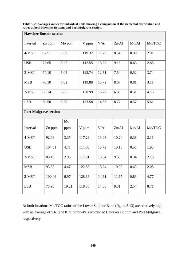
149
Table 5. 2: Averages values for individual units showing a comparison of the elemental distribution and
ratios at both Hawsker Bottoms and Port Mulgrave section.
Hawsker Bottom section
Interval Zn ppm Mo ppm V ppm V/Al Zn/Al Mo/Al Mo/TOC
4-MST 87.51 3.07 119.32 11.78 8.64 0.30 2.01
USB 77.65 5.22 112.55 13.29 9.13 0.63 2.86
3-MST 74.10 5.05 122.74 12.51 7.54 0.52 3.74
MSB 76.10 7.02 119.88 13.72 8.67 0.81 3.11
2-MST 68.14 5.05 130.99 13.22 6.88 0.51 4.15
LSB 80.58 5.20 133.58 14.63 8.77 0.57 5.61
Port Mulgrave section
Interval Zn ppm
Mo
ppm V ppm V/Al Zn/Al Mo/Al Mo/TOC
4-MST 92.09 3.35 117.29 13.03 10.24 0.38 2.11
USB 104.51 4.71 111.88 13.72 13.16 0.58 1.93
3-MST 83.19 2.95 117.31 13.34 9.39 0.34 2.18
MSB 93.68 4.47 122.88 13.24 10.09 0.49 2.08
2-MST 100.46 6.97 128.36 14.61 11.67 0.83 4.77
LSB 75.90 19.21 118.85 14.36 9.31 2.54 8.71
At both locations Mo/TOC ratios of the Lower Sulphur Band (figure 5.13) are relatively high
with an average of 5.61 and 8.71 ppm/wt% recorded at Hawsker Bottom and Port Mulgrave
respectively.

150
Figure 5. 13: Cross-plot of MO ppm and TOC %wt for the Lower Sulphur Band at Port-Mulgrave
(empty tringels) and the Hawsker Bottoms (grey squares).
Figure 5. 14: TOC and Iron redox proxies of the lower Grey Shale at Hawsker Bottoms section.

151
5.3 Discussion
5.3.1 Redox dynamic throughout the study section
The geochemical data including iron, sulphur and carbon chemistry through the
Lower Toarcian section of the lower Whitby mudstone formation reveals a marine basin
dominated by anoxic and ferrous iron-rich (ferruginous) conditions. The redox indices
indicate fluctuating redox conditions throughout the studied section, where the iron speciation
data, Trace metals concentrations and molecular biomarkers reveals various and more
dynamic palaeoxgenation conditions.
5.3.1.1 Iron data
The recent modification of iron speciation techniques has allowed the calculation of
relative iron phases more precisely (regarding its biogeochemical reactivity). It has become
one of the most valuable tools for investigating redox conditions in a variety of modern and
ancient marine environments (Poulton and Raiswell, 2002; Lyons and Severmann 2006;
Canfield et al., 2007). The distinctive feature of iron speciation as a paleoredox indicator
from other parameters is its unique ability to differentiate between oxic, anoxic sulfidic, and
anoxic non-sulfidic (ferruginous) water column conditions (Poulton et al., 2004b; Canfield et
al., 2007), allowing a detailed evaluation of ocean redox.
Anoxia was common in subsurface water masses of lower Toarcian oceans
(Farrimond et al., 1988; Jenkyns et al., 2001) and in this respect the Cleveland basin appears
typical. The results of the iron speciation data (Figure 5.4) shows that total iron (FeT wt %)
concentrations are slightly higher than average shale composition (Turekian and Wedepohl,
1961), but consistent with the ranges reported by McArthur et al. (2008) for the North
Yorkshire section. Empirically, values of FeHR/FeT above 0.38 indicate anoxic bottom water
conditions, whereas significantly lower values generally suggest oxic bottom water condition
(Raiswell et al., 2001; Poulton and Raiswell, 2002).
FeHR enrichments relative to total Fe occur due to the water column formation of
either pyrite in sulfidic basins, or non-sulfidized minerals (ferric oxides, magnetite or siderite)
in anoxic ferruginous basins. The ratio Fepy/FeHR can then be used to distinguish between
deposition in sulfidic and anoxic non-sulfidic basins, where sulfidic marine waters commonly
have FePy /FeHR ratios that approach >0.7-0.8 (Marz et al., 2008).

152
As our analyses are on outcrop samples (Staithes to Port Mulgrave section), a
consideration for possible contributions from secondary alteration by oxidative weathering
must be taken to the account. However, samples were obtained from fresh surfaces and any
visible surface staining was avoided. Oxidation by post depositional weathering would cause
the speciation within the actual highly reactive iron pool to change and as a consequence the
FeOX fraction of the highly reactive iron will be increased. In our samples, FeOX contents are
generally very low (Figure 5.5), indicating that we can readily discount any significant
influence of secondary oxidative weathering for most of the succession.
Figure 5.15: Composite stratigraphy with iron Paleoredox indicators for the study section at Port
Mulgrave.

153
Figure 5.16: Composite stratigraphy with iron speciation data at Port Mulgrave section. The
total Fe content in Wt. % and the relative proportion of Fe residing in unreactive and reactive
phases, reduced phases and oxidized phases.
As Figure 5.15 shows, FeHR/FeT is variable throughout the section. Apart from the
bioturbated mudstones, the rest of the section is fluctuating above the threshold value (0.38).
The entire data set falls in the range above the modern oxic water column average of 0.26
(Poulton and Raiswell, 2002). At the Pliensbachian-Toarcian boundary (paltum subzone till
clevelandian subzone) values of the FeHR/FeT regularly fall in the definitive anoxia region.
At the Upper Sulphur band and above proceeding to the interval of Jet Rock Shale
(tenuicostatum tile middle semicelatum subzone) FeHR/FeT fluctuates above and under the
threshold value (0.38) and at some points falls in the equivocal range between definitive
anoxia and modern oxic sediment (0.26). Moreover the Fpy/FeHR values documented in this
interval have an average of 0.42 which is far below the threshold value for euxinic condition

154
(Fpy/FeHR ≥ 0.7), pointing to anoxic ferruginous water column conditions (Poulton and
Canfield, 2001). Anoxia is more intense and permanent in the deepest waters, represented by
the Jet Rock member where the FeHR/FeT values are consistently far above the threshold
value.
Although the biomarker and trace elements data indicates that the bioturbated
mudstones at ht ebase of the study section represent oxic to dysoxic condition, the iron
speciation data suggest that the lower third of the study section at the base of the Grey shales
is a transition zone that was characterized by anoxic ferruginous condition which shows very
high enrichment of FeHR. This enrichment of iron could be sourced from the ironstones on the
basin margin or from the underneath sediment through the advication of the underground
water (Newton, 2001) and riverine flux (lateritic weathering of the hinterland). This
Ferruginous condition was punctuated with short-lived periods of euxinic conditions
indicated by high FePy/FeHR ratio (> 0.8) which could be interpreted as more sulphur was
added to the system to shift the anoxic (ferruginous) condition to euxinic condition. Above
this interval and below the T-OAE (upper clevelandian tile middle semicelatum subzone) the
system was pulled back towards suboxic-oxic condition indicated by the sedimentary fabric
of the bioturbated mudstones which record presence of benthic fossils (Caswell et al., 2008)
and very low FeHR/FeT (<0.38). The system then progressed from ferruginous non-sulfidic to
sulfidic condition through the T-OAE zone (Exeratum subzone), where the Fe speciation data
showed consistently high FePyrite/FeHR ratio suggesting periods of pronounced sulphidic
conditions in bottom waters.
The presence and fluctuation of both ferruginous and euxinic conditions recorded in
the study section indicates how dynamic the palaeoredox condition was. At the
Pliensbachian-Toarcian boundary (paltum subzone till clevelandian subzone) ferruginous
waters were persistent and sulfidic waters transient lasting for a short period of time spanning
the sulphur bands, which is estimated to last 5 – 10 Ka (McArthur et al., 2008). These
perturbations which pushed the water masses toward euxinia are the mechanisms behind the
formation of the sulpur bands at the base of the Gray shale. The dominance of sulfidic or non-
sulfidic (ferruginous) condition must be related to the equilibrium between sulphur and iron
in seawater (Poulton et al., 2004a). Enrichment of these elements is controlled by
hydrothermal fluxes and seawater sulphate level (Kump and Seyfried, 2005)
155
5.3.1.2 Biomarkers
Photic zone anoxia (PZA) during the early Toarcian is indicated by biomarkers derived from
green sulphur bacteria, such as isorenieratane and its diagenetic products, aryl isoprenoids
(Schouten et al., 2000; Bowden et al., 2006). The diaryl isoprenoids are derived from
isorenieratene, which is an undisputed biomarker for Chlorobiaceae (green sulphur bacteria).
In contradiction to previous work by Sælen et al., 2000, this study has found isorenieratane in
every sample of the Jet Rock. The occurrence of isorenieratane throughout the Jet Rock
indicates that recurrent euxinia had extended into the euphotic zone (Koopman et al., 1996).
Consistent isorenieratane presence was recorded in the equivalent interval of lower Toarcian
in Germany (Posidonia Black Shale) by Schouten et al. (2000).
The presence and widespread distribution of isorenieratane indicates that a sulfidic photic
zone was a common occurrence, before and during the T-OAE at North Yorkshire section.
Isorenieratane maximum abundance is near the maximum in TOC, implying that
strengthening euxina was responsible for increasing organic carbon burial. This occurrence of
diagenetic products of the carotenoid isorenieratene (isorenieratane and other aryl isoprenoids)
in Toarcian black shales has been regarded as supporting evidence for the Kuspert hypothesis
as they point to strong stratification of the epicontinental seas (van de Schootbrugge et al.,
2005). The presence of isorenieratane within short intervals of the sulphur bands before the
main T-OAE indicates that euxinia was developed during short periods at the Pliensbachian-
Toarcian. This is in agreement with the iron speciation data and the isotopic data suggesting
severe environmental changes triggered by repeated mechanisms.
5.3.1.3 Sulphur isotope record
The sulphur isotopic composition of pyrite from the study section is quite variable (Figure
5.6). It ranges from -20 ‰ to almost -47‰. Such a significant isotopic variation in sulphur
isotopes always tend to develop in association with extensive processes of sulphate reduction,
with the product sulphide being depleted in the heavier isotope by approximately 30‰ as
long as sulphate is available (Habicht et al. 2002).
Sulphur is removed from the oceanic sulphate pool in two ways. Firstly as evaporated
sulphate minerals, which is episodic and less important, the second process is by biological
reduction of sulphate to sulphide in organic-rich marine sediments. Most of the sulphide gets
reoxidized and the rest reacts with iron to form pyrite, which is buried in the sediments
(Berner 1970). The lighter 32
S isotope forms slightly weaker bonds than the heavier isotope

156
and therefore has a more rapid rate of reduction and thus pyrite sulphur (produced by
sulphide) is thus depleted in 34
S relative to the sea water sulphate (Newton and Bottrell, 2007).
In a closed system, sulphate becomes extensively depleted and therefore the isotopic
difference between sulphide and sulphate diminishes. Therefore pyrite formed in euxinic
water columns, should be isotopically light relative to diagenetic pyrite formed in sediments,
which tend to more closely represent closed systems. While in open system, where there is
supply of sulphate from the open ocean the isotopic differences between the sulphide and
sulphate says high and therefor isotopically heavier.
Sulphur isotope analyses of sedimentary sulfides within the studied section display a
distinctive stratigraphic pattern of variability, with the lower part at the Pliensbachian-
Toarcian boundary (paltum subzone till clevelandian subzone) preserving a large range of
isotopic compositions (fluctuating between -20‰ and -47‰), and represents the most
depleted interval with the most negative value. The overlying Jet Rock Shale (Exartum
subzone) contains much more pyrite and preserves sulphur isotope compositions that cluster
toward more enriched values where δ34
Spyrite clustered around -21‰. Although the
paleoredox proxies clearly suggest persistent euxinic condition for the Jet Rock Shale, the
relatively heavier δ34
Spyrite values compare to the Grey shale could suggest mass-balance
effect of local sulphate limitation.
5.3.1.4 Trace elements
Redox conditions control the mobility of many trace elements, and the relative
enrichment or depletion of these redox-sensitive trace elements in the sediments is used as a
redox indicator of the overlying water. Certain trace metals (e.g Mo, V, and Zn) have proven
to be particularly diagnostic for anoxic/sulfidic conditions during deposition of organic
matter-rich sediments (Jones and Manning, 1994; Brumsack, 2006; Tribovillard et al., 2006
Chris et al., 2008). In many examples of organic rich sediments deposited under such extreme
conditions, redox-sensitive trace metals such as Molybdenum and Zinc may be strongly
enriched (by factors of >100) in comparison to average marine shale (März et al., 2008). The
elements Mo, V and Zn are regarded as particularly reliable as paleoredox indicators as these
metals all have in common the tendency to form insoluble phases under anoxic and sulfidic
depositional conditions (Brumsack, 2006; Tribovillard et al., 2006).

157
Overall, element/Al ratios of Mo and V show enrichments that fluctuate throughout
the study section, with highest values recorded in the Jet rock shales (figure 5.7). Notable
trace metal enrichments occur with molybdenum (Mo), which is relatively enriched (8 ppm)
and above the average shale value which is about 1 ppm (Brumsack, 2006). Basically,
molybdenum displays much stronger enrichments under sulphidic conditions (Algeo and
Maynard, 2004; Algeo and Lyons, 2006) where it is transformed to thiomolybdate, and
becomes particle reactive under sulphidic conditions allowing its drawdown into sediments.
This only occurs when sulphide reaches a critical level, which has been estimated to be about
11 µM (Zheng et al., 2000). Under sulphidic conditions, sorption of Mo to sinking organic
matter and transport to the sediment surface is expected to be much more effective than under
anoxic non-sulphidic conditions, resulting in higher enrichments.
According to Tribovillard et al. (2006), Vanadium can be reduced and accumulated
under denitrifying conditions while Zn and Mo are enriched mainly under sulphate-reducing
conditions. Thus, in the case of V enrichment without Mo enrichment, the authors postulate
suboxic/anoxic depositional conditions without free H2S, whereas sediments exhibiting
concurrent enrichments in V and Mo reflect euxinic conditions at the sediments-water
interface or in the water column (Algeo and Maynard, 2004: Tribovillard et al., 2004). At the
Pliensbachian-Toarcian boundary (paltum subzone till clevelandian subzone) Mo and Zn
fluctuate between relatively high enrichment within the sulphur bands and relatively lower
enrichment within the bioturbated mudstone units. This suggests fluctuated palaeoredox
condition as also indicated by the iron speciation and biomarkers data. This shift in ocean
redox resulted in the rapid and extensive removal of Mo and Zn from the water column (in
the form of sulfides), leading to the observed sharp peaks (Figure 5.11). On the other hand, V
in this interval shows no particular enrichment responding to the Sulphur bands, which
reflects the negligible role for the sulfidic condition to drawdown of V. At the base of T-
OAE zone in the Jet rock shale (bed 33 &34) there is relatively higher enrichment of trace
elements. This enrichment decreases towards the top of the T-OAE. Taking seawater as the
dominant source for Mo, V and Zn, the relative depletion in trace elements may reflect the
global onset of the black shale deposition and the widespread development of anoxia, or it
may reflect hydrographic factors where the water mass restriction developed and slowed the
deepwater renewal of trace metals. Both of these mechanisms would have resulted in
depletion of redox sensitive trace metals in the water column.
Mo versus TOC

158
Recent studies have identified a range of new applications of trace-metal
concentration data in the analysis of paleoceanographic systems. In restricted anoxic marine
systems, trace metal /TOC ratios can provide insight into the degree of water mass restriction
and estimates of deepwater renewal times (Algeo and Rowe 2011).The transition from
weakly sulfidic to strongly sulfidic facies is commonly accompanied by a decline in trace
metal accumulation rates, because hydrographic factors (i.e., limited deepwater renewal)
come to dominate over redox influences. Ultimately, deepwater renewal and aqueous
molybdenum depends on basin geometry where the sub pycnoclinal water mass is renewed
less readily in larger basins with shallower sills, such as the Black Sea, than in smaller basins
with deeper sills (Algeo and Lyons, 2006).

159
Figure 5.17: A) Cross-plot of MO ppm and TOC %wt from this study; B) Cross-plot of MO ppm
and TOC %wt from McArthur et al., 2008 . Samples from the Jet rock suggest widespread
euxinia, while the underlying Sulphur Beds indicate more local euxinic conditions
The Mo versus TOC cross plot (Figure 5.23), displays a similar plot to that generated
by McArthur et al. (2008). The upper half of the semicelatum Subzone and most of the
exaratum Subzone (Bed 31 to 38) are characterized by relatively lower ratios of Mo/TOC
(low regression slop) and as this interval encompasses the Early Toarcian OAE, and is
superimposed on the main negative excursion in δ13
CTOC, it could be suggested to indicate

160
that complete restriction occurred during this interval, which was termed the interval of
maximum restriction (IMR) by McArhur et al. (2008). However, persistent euxinia would be
expected to gradually lower the Mo concentration of seawater as expanded sinks exceeded
riverine sources (Algeo and Lyons, 2006). On the other hand the bioturbated mudstones
including the intervals of the sulphur bands are characterized with higher ratios of Mo/TOC
(high regression slop), which could suggest lesser water restriction and a more dynamic
scenario.
Figure 5.18: Mo/TOC versus FePy/FeHR for the study section at Port Mulgrave.
The role of redox versus hydrographic influences on trace metal accumulation in
marine systems can be investigated through cross-plots of Mo/TOC versus paleoredox
parameters that are highly sensitive to euxinic conditions (e.g DOP) (Algeo and Rowe, 2011).
In this study the ratio of FePy/FeHR which is a powerful redox proxy for indicating sulfidic
deposition condition is used (Figure 5.18). Mo/TOC is potentially subject to both redox and
hydrographic influences (McArthur, et al., 2008) and its relationship to FePy/FeHR can assist
in identifying the relative importance of both factors.

161
Uniform Mo/TOC values within a marine system that shows spatial or temporal
variation in redox conditions are evidence for control of trace metal accumulation by
hydrographic factors. Stratigraphic variation in Mo/TOC values independent of FePy/FeHR is
evidence for changes in aqueous Mo concentrations. On the other hand, covariation between
Mo/TOC and FePy/FeHR is evidence for either a direct or indirect redox control on trace metal
accumulation. A direct redox control results in increasing Mo/TOC with more reducing
conditions (Zheng et al., 2000), but such an effect generally should be manifested only in the
oxic to weakly sulphidic part of the redox spectrum (Algeo and Rowe, 2011). Under more
reducing conditions, hydrographic controls tend to become dominant (Algeo and Lyons,
2006).
As can be seen in Figure 5.13, the cross plots of Mo versus TOC through the T-OAE
zone (upper semicelatum - Exeratum subzone) exhibits uniformly low Mo/TOC ratios. This is
indicative of extreme water mass restriction, while from McArthur et al. (2008), the overlying
Falciferum zone exhibits higher Mo/TOC ratios that covary positively with the degree of
pyritization (DOP). On the other hand, the underlying Grey shale at the Pliensbachian-
Toarcian boundary (paltum subzone till semicelatum subzone) has Mo/TOC values that are
higher. Although most of this interval is considered to represent anoxic to dysoxic conditions
(apart of the Sulphur beds where periodic euxinia was clearly detected), higher Mo/TOC
could suggest more ventilation and less restriction in the water column. The lower sulphur
bed at the Pliensbachian-Toarcian boundary showed exceptionally high Mo/TOC values. The
very high Mo content in this bed could suggest a different scenario that developed over short
a period of time. The drawdown and replenishment of Mo must have occurred within a small
and local reservoir where elevated Mo/TOC indicates brief periods of euxinia.

162
5.3.2 Detailed iron geochemistry across the Sulphur Bands
The Sulphur Bands represent three brief periods of restriction and pyrite formation in
the earliest Toarcian. They are deposited over a wide area and their lateral equivalent were
recorded in at Dotternhausen section in Germany, where four thin units of organic-rich shale
occur in the paltum and uppermost clevelandicum Subzone (Rohl et al., 2001).
At Port Mulgrave detailed (Cm-scale) multiproxy records from of the Lower Sulphur
Band (Figure 5.19) reveal a dynamic system, with sulfidic water conditions that were
intermittently interrupted by anoxic non-sulfidic water column conditions. Over all, the three
sulphur beds are enriched in reactive iron, much of which is in form of pyrite. This high
enrichment of iron is believed to be sourced from the Main Seam unit of Cleveland Ironstone
Formation that lies directly underneath the Lower Sulphur bed (Newton, 2001). The
Cleveland basin marginal sediments in the early Torcian consisted of ooidal ironstones
providing a huge reservoir of highly reactive iron (Powell, 2010).
Figure 5.19: Detailed iron speciation profile across the Lower Sulphur Band at Port Mulgrave

163
The particular enrichment of the Lower sulphur band may reflect its position at the
beginning of the transgression and therefore its relative proximity to the sediment source. All
the sulphur bands show evidence of storm activity in the form of small scale hummocky cross
stratification (Wignall, 1994). This storm activity could have played a role in redistributing
the weathered marginal ironstones to the deeper parts of the basin and provided an initial
input of iron oxides to the basin. Moreover, the anoxic bottom water reduced and released the
iron oxides into solution as Fe+2
at the sea floor and then diffused along the layer of anoxic
bottom waters to distribute extra reactive iron over a wider area.
Figure 5.20: Detailed chemostratigraphic plots of δ34S(Pyrite) and δ13C isotopes, Mo/Al ratio
and maxima of isorenieratane abundances across the Lower Sulphur Band at Port Mulgrave
section.

164
Figure 5.21: Cross plot of Mo/TOC versus FePy/FeHR through the three sulphur beds at Port
Mulgrave section.
Based on the Sr isotope analysis by McArthur et al., (2000) and the cyclostratigraphic
timescale of Suan et al., (2008), the Sulphur Bands at north Yorkshire are estimated to last
from 5 to 10 Ka (McArthur et al., 2008). Working up from the base of the Lower Sulphur
Band, the first 5 cm is characterised by high FePyrite/FeHR, high Mo enrichment and
intensive presence of Isorenieratane (9.47µg/gTOC) suggesting sulfidic water condition that
lasted approximately 2.5 Ka (based on McArthur et al., 2000 estimation). Then the system
was pushed back to non-sulfidic anoxic water column conditions lasted for approximately 2
Ka indicated by a decrease in the FePyrite/FeHR ratio to less than 0.6 over the central 4 cm.
Afterwards, the system turned to extreme euxinia with higher FeHR/FeT where the sulfidic
water condition also extended to the photic zone, which is indicated by the presence of the
isoreineratene biomarker. Despite this fluctuation between ferruginous and sulfidic condition
throughout the Lower Sulphur Band, the FeHR/FeT continued above the threshold of anoxic
water condition (0.38) throughout.
The middle part of the Lower sulphur bed witnesses major change, where the
concentration of Mo dropped below the threshold of euxinic condition (H2S <11μM), and

165
transition from sulfidic bottom water to anoxic ferruginous non-sulfidic bottom water. This
was associated with distinctive short-lived δ34
S excursion (~10‰) suggesting limited
sulphate availability and hence a decrease in sulphide in the water column.
Despite the bioturbated central 15 cm of the Middle Sulphur Band (Figure 5.28 and
5.29), the detailed geochemical analyses across it revealed consistent anoxic sulfidic
conditions. The FeHR/FeT remains high (above 0.38) in all sample (24 samples) as can be
seeing in Figure 5.23 (> 0.38).
Figure 5. 22: Detailed iron speciation profile across the Middle sulphur Band at Port Mulgrave.

166
Figure 5.23: Detailed chemostratigraphic plots of δ34
S(Pyrite) and δ13
C isotopes , Mo/Al ratio and
maxima of isorenieratane abundances across the Middle Sulphur Band.
The basal 10 cm of the MSB is characterised by high FeHR which could be linked to
the availability of the reducible iron at the beginning of the event. Overall the Fepyrit/FeHR
profile across the MSB is above 0.7 which is the upper limit of the ferruginous condition and
suggesting that dominant anoxic sulfidic condition prevailed throughout the MSB and no
cycling between sulfidic and non-sulfidic (ferruginous) is observed unlike the case of LSB.
Moreover, Isorenieratane was observed throughout the band suggesting sulfidic water
conditions that extended to the euphotic zone. Lower Mo enrichment is recorded in MSB
compared to LSB which could be related to decrease supply from content source or reflect
deeper water column and thus the Mo deposited over wider area and not concentrate on
shallower shelf zone as could be the case with the LSB.

167
Figure 5.24: Detailed iron speciation profile across the USB at Port Mulgrave section.
Similar scenario to the LSB is observed in the USB. At the start of deposition of the
USB (Figure 5.24 and 5.25), and within the lower 5 cm the FeHR/FeT ratios are higher than
0.38 and the Fepyrite/FeHR ratios above 0.7 indicating that bottom waters were anoxic sulfidic.
Then both of the FeHR/FeT and Fepyrite/FeHR ratios were decreased in the central 3 cm of the
USB to less than the threshold of anoxia and thus anoxic-dysoxic condition is suggested for
this interval. Then the anoxic sulfidic water condition dominates the upper 6 cm. Unlike the
LSB the USB has lower Mo enrichment. Moreover, the Mo/TOC ratios for the USB and
MSB are different from the LSB (Figure 5.26) and resample that for the Jet Rock shale,
which could suggest that there is stronger stratification over regional area during the
deposition compare to less stratified and more local condition for the LSB.

168
Figure 5.25: Detailed chemostratigraphic plots of δ34S(Pyrite) and δ13C isotopes , Mo/Al ration
and maxima of isorenieratane abundances across the Upper Sulphur Band at Port Mulgrave
section.
Figure 5. 26: Cross-plot of MO ppm and TOC %wt for the Sulphur Bands at Port Mulgrave
section showing the different Mo/TOC of the Lower Sulphur Bands compare to the Upper and
Middle once

169
5.3.3 Regional redox of the Sulphur Bands
The Sulphur Bands represent basal transgressive black shales that deposited in shallow shelf
setting. Despite the very thin and short lived nature of the Sulphur Band, its development at
the Piensbachian-Toarcian boundary is recorded over wide area within the European Epeiric
Sea. At Dotternhausen in Germany four thin units of organic-rich shale occur in the paltum
and uppermost clevelandicum Subzones which tempting to equate those units of Sulphur
Bands of North Yorkshire. Stratigraphically the Sulphur Bands shows no thickness or
variations (Figure 5.27).
Figure 5.27: Schematic W-E cross section of the Cleveland Ironstone Formation and the lowest part of
the overlying Grey Shale (Rob Newton PhD thesis, after Howard, 1985).
Previous studies have been concerned with boundary intervals at Late Piensbachian as
it relates to sea level change (Hallam, 1997), as well as contrasting water mass and basinal
restriction (Sælen et al., 2000: McArthur et al., 2008). The Piensbachian-Toarcian boundary
represents significant increase of bottom water temperatures from about 14°C in the late
Piensbachian to about 20°C in the earliest Early Toarcian, as seen in abrupt shift toward
lower values of the δ18
Obrachiopod (Suan et al., 2008).
Important environmental change in paleo-climate warming and enhanced
hydrological cycle across this interval is also suggested by 87
Sr/86
Sr, δ18
O and Mg/Ca ratios
of belemnite rosta, from England, Spain and Germany (Bailey et al., 2003; Rosales et al.,
2004; van de Schootbrugge et al., 2005a). All of these may have affected deposition of the
Grey Shales and the overlying Jet Rock shale during the period of major basin subsidence
170
characterised by deep open waters (Powell, 2010). However, the fluctuating redox condition
at the base of Grey Shale still needs to be more understood, particularly in terms of the spatial
extension of these small cyclic redox conditions within the Sulphur Bands.
As redox conditions at Port Mulgrave indicate that the bottom water during deposition
of the sulphur bands were anoxic, non-sulfidic to sulfidic (Figure 5.15), iron speciation data
from the Sulphur Bands at Hawsker Bottoms, a more distal site in Cleveland Basin, indicate
that bottom water conditions were mainly anoxic (FeHR/FeT, > 0.38), to sulfidic
(Fepyrite/FeHR, >0.7) throughout their deposition (Figure 5.14).
The profile indicates that the LSB has variable redox condition between the two sites.
At Port Mulgrave the LSB deposited under more sulfidic condition as can be suggested from
the iron speciation data and the presence of Isorieneratane (Figure 5.19 and 5.20). On the
other hand, the lateral extent of the LSB at the more distal setting in Hawsker Bottom is
characterised by oxic-dysoxic to anoxic non-sulfidic (ferruginous) condition through its lower
and middle part, while possibly sulfidic condition developed at its upper section. There was
no Isorieneratane detected in the LSB at Hawsker Bottoms indicating that water column
anoxia did not extend into the photic zone as is the case in Port-Mulgrave section. Moreover,
the LSB at Port-Mulgrave is highly enriched in Mo compared to its lateral extent at Hawsker
Bottoms which could be due to geographical position at more proximal setting close to the
terrestrial flux from land where higher flux of organic matter gives rise to more transition
elements under more reducing condition (Tribovillard et al., 1994).
Despite the lateral variation in the redox condition of the LSB at both localities, the
MSB and LSB shows similar paleoredox trend at both locations with fluctuation between
anoxic ferruginous to sulfidic.
5.3.4 Carbon isotopic excursion before the T-OAE
The δ13
Corg profile (Figure 5.38) displays a complex excursion developed at the
Pliensbachian-Toarcian boundary. This complex negative δ13
Corg excursion consists of three
peaks corresponding to the three sulphur bands at the base of the Gray Shale Member. The
first component of the CIE occurs in the upper P. hawskerense Subzone at the Pliensbachian-
Toarcian boundary, culminating in a value of ∼−29.6‰ within the Lower Sulphur Band and
magnitude of approximately -4‰. The earliest Toarcian samples (base of Paltum Subzone)
are characterized by sudden return to pre-excursion values of ∼−26.1‰, which are then

171
gradually decreased again forming the second and third negative CIE spanning the Middle
and Upper Sulphur Bands with weaker excursion with magnitude of ∼−3‰ and ∼−1‰,
respectively. The return to pre-excursion values after the Upper Sulphur Band persists until
the onset of the larger negative carbon-isotope excursion in the Late D. tenuicostatum zone
that is associated with the Early Toarcian OAE. This complex excursion at the Pliensbachian-
Toarcian boundary has similar characters to the main negative CIE that is well known from
the Early Toarcian OAE, so that the proposed mechanisms to explain its presence would be
similar.
The Paleocence-Eocene thermal maximum (PETM) is a globally brief interval that in
some respects shares similar characteristic features to the Early Toarcian OAE (Cohen et al.,
2007). Both events are characterized by a massive influx of isotopically light carbon, benthic
faunal extinctions, extensive carbonate dissolution and evidence for a large and rapid global
warming event (Bowen et al. 2006). There were at least five significant and similar events
between 56 and 53 Ma, of which the PETM is the most pronounced. The five events are
characterized by elevated sedimentation rates and marl-rich horizon with low δ13
C (Nicolo
etal., 2010). They therefore may have had a similar generic cause and could represent
massive inputs of isotopically light carbon during a long-term warming trend and accelerated
hydrologic cycle that increased continental erosion and development of expanded condensed
clay layers and marl rich horizons spanning the multiple excursions. Similarly, the repeated
carbon isotopic excursion at the Pliensbachian-Toarcian boundary but prior to the main
carbon isotopic excursion of the T-OAE seems to represent a comparable scenario. The
repetitive nature of these excursions suggests a dynamic source must have repeatedly injected
large quantities of 13
C depleted carbon into the ocean or atmosphere.
The carbon-isotope perturbation at the Pliensbachian-Toarcian boundary is coincident
with the first phase of extinction in marine benthos at the stage boundary (Caswell et al.,
2008) well before the main phase of anoxia associated with the Early Toarcian OAE, which
could suggests the event was not simply a localized event. The apparent abrupt onset of the
stage boundary CIE, and the initiation of an extinction step near the same level, supports the
idea of a catastrophic event such as release of methane hydrate.

172
Figure 5.28: Comparison between carbon-isotope records of Port Mulgrave section in North
Yorkshire and Peniche section in Portugal.
The identification of multiple perturbations with similar causes and consequences
would lead us to think of a source that is capable of repeated carbon injections. A similar
pattern of negative carbon-isotope excursions has been observed at the stage boundary in the
SW European section at Peniche, Portugal (Figure 5.28). The isotopic excursion is of interest
when considering the genesis and development of the later Toarcian Oceanic Anoxic Event
(OAE), as well as the second-order global extinction event that spans the stage boundary.
The carbon isotopic excusions which represent sudden environment change that
produced the Sulphur bands will likely provide a sueful chemostratigraphic marker for the
Pliensbachian-Toarcian boundary. Moreover, the gradual increase of the sulphidic condition
for the middle and upper sulfure bands suggests more global condition and that the carbon
perturbation could have affected the entire ocean system and should be registered in
appropriate material in coeval strata in all parts of the world.

173
5.3.5 Conceptual model
The paleogeography of black shale depositional environments during T-OAE is a
matter of discussion. Most of the Toarcian black shales were deposited on epi- and
pericontinental shelves in environments proximal to Pangaea. In this study, two phases of
important paleoenvironmental changes occurred at the Lower Toarcian, both of which are
characterized with enhanced organic carbon accumulation, negative shift in the carbon
isotopes and development of anoxic and euxinic bottom water condition. These two
stratigraphic limited intervals also correlate with periods of high extinction rates of benthic
marine fauna (Little and Benton, 1995; Caswell et al., 2008) and are associated with an
increase in paleotemperature of bottom waters (Suane et al., 2008).
The possible trend for this mode of redox state observed could be as a result of local
processes, which were triggered by changes in global climate. In this context a higher influx
of organic matter from accelerated hydrological cycle delivered more nutrients and
freshwater to shallow shelf-seas during continental weathering and runoff (Bailey et al.,
2003), which is supported by very high TOC (> 3wt%), Mo (21 ppm) and high HI throughout
the LSB in more proximal settings within the Claveland Basin. In contrast to the low TOC,
Mo and HI characterising the LSB at more distal setting which suggest possible distance from
source, low productivity, and residence time of organic materials (Demaison & Moore, 1980).
Results of this study fit a model as showing in Figure (5.28). During the early
Toarcian in Cleveland Basin, development of density stratification starts to occur at local
extent at proximal setting, as a result of increased fresh water inputs by enhanced
hydrological cycle, and thus combined with periodic high productivity, led to local expansion
of anoxic-euxinic conditions. This anoxic condition prevailed during the deposition of the
LSB and then the system fluctuates back to more oxic dysoxic condition represented in the
bioturbated mudstones above the LSB. The second anoxic event derived by the same
mechanise were stronger and tend to be more regional where the euxinic waters covered most
of the Cleveland Basin which again lasted for short period of time before the system switch
again to oxic-dysoxic condition.

174
Figure 5.29: Schematic paleoceanopraphic model of the lowermost Early Toarcian. Showing the
development of the driving mechanism for the Sulphur Bands which then accumulates in the T-
OAE. Biozone duration from McArthur et al. (2000).
The development of and intensity of redox conditions across the Basin preceding the
T-OAE could have been caused by a combination of restriction on circulation, coupled with
local density stratification. Wide spreading of anoxia higher up across the T-OAE could
represent more global forcing mechanisms which were capable of driving global
environmental change. These mechanisms may have included; the eruption of the Karoo-
Ferrar continental flood basalt and/or the massive dissociation of continental margin
clathrates with a resulting increased hydrological cycle and a transient greenhouse climate
with increased CO2 concentrations and paleotemperatures.

175
5.4 Conclusions
The Grey Shale Member represents an important marine sedimentary record of a gradual
transition from an oxygenated sea to one characterized by anoxic bottom waters. These
intervals of oxic and anoxic deposition for the Grey Shale are characterized by the
deposition of three pyrite rich black shales, known as the sulphur bands, and indicating
deposition under anoxic bottom water conditions.
The bioturbated mudstone intervals surrounding the Sulphur bands, are characterized with
FePy/FeHR less than the upper limit of ferruginous condition and FeHR/FeT above the
threshold of anoxic condition. The presence of bioturbation indicates that bottom waters
were periodically oxic, with strong mixing of water column signals for FeHR and trace
metals. Therefore the sequence of mudstone and Sulphur Band deposition throughout the
Grey Shales can be described by a seasonal oxic/dysoxic fluctuation model coupled to
gradual climatic warming and fluctuations in sediment supply.
Repetitive, short periods of intense oceanic anoxia (often euxinic) occurred preceding the
global T-OAE. These short periods of anoxia were localised in occurrence, with
potentially catastrophic effects on marine biology.
Despite the well laminated appearance of the Sulphur Bands, very detailed analysis
indicates that there are fluctuation in the paleoredox condition across these units cycling
between euxinic to anoxic non sulfidic to dysoxic condition.
There is lateral variation in the redox condition of the Lower Sulphur Band between Port-
Mulgrave and Hawsker Bottom section, where bottom water condition at Hawsker
Bottoms were mainly dysoxic to anoxic, with less sulphide in contrast to a more sulfidic
condition at more proximal setting in Port-Mulgrave.
The style of anoxia in the Jet Rock is fundamentally different from that in the Grey Shales.
A peak in global temperatures, a long period of sediment starvation and a greater water
depth, all combined to create a stratified anoxic water column with organic rich sediments
beneath.
The results highlight that the Earth system was highly dynamic during even the early
stages of global warming, with extreme periods of localised anoxia occurring well-before
the global OAE.

176
CHAPTER 6 - FT-NIRS ANALYSIS OF MARINE ROCK SAMPLES
FROM A RANGE OF DEPOSITIONAL ENVIRONMENTS
6.1 Introduction
Marine sedimentary rocks and sediments preserve abundant environmental
information for reconstructing the climatic and oceanic history. One tendency in the current
biogeochemical and pala-oceanographic studies is to investigate long sediment sections at
very high resolution in order to unlock internal details of the long term record, such as small
events that may hold vital information about the evolution and forcing mechanisms of
environmental change in the past. This inevitably increases the number of samples to be
analysed, significantly increasing the amount of resources and time needed. Another related
challenge for multi-component analysis is the limited coring material available. Therefore,
there is an urgent demand for new fast, non-destructive, and inexpensive analytical tools,
such as core scanner systems (Chang et al., 2005; Leach et al., 2008).
Near infrared reflectance spectroscopy (NIRS) is one rapid and non-destructive
analytical technique for characterization and quantification of material property, and it has
been widely used to monitor the quality of raw material in agricultural, pharmaceutical, and
other industries (Williams and Norris, 1987; McClure, 1994). NIRS measures the interactions
between incident near-IR light and the material’s surface. Multivariate calibration techniques,
including principle components regression (PCR) and partial least squares regression (PLSR),
are often used to relate near-IR spectra with measured properties of material (Martens and
Naes, 1989).
The conventional bulk geochemical methods to determine the OC richness nd
hydrocarbon potential of source rocks is the Rock Eval analytical pyrolysis (Tissot and Welte,
1978) combined with Carbon-Sulphur Analyser (e.g LECO CS- 244). Despite progress in
scanning technologies some of the most fundamental parameters in marine research and
petroleum geology, total organic carbon (TOC), total sulphur (TS), is still not routinely
determined. This comes as a surprise as scanning techniques have been shown to provide
high accuracy data (e.g Balsam and Deaton, 1996; Chang et al., 2005; Leach et al., 2008),
providing scope for further research.

177
Furthermore, scanning techniques pose no health and safety issues unlike some conventional
methods that require the use of concentrated acids and carcinogenic indicators . An analytical
scanning technique that has been used extensively with high success, including non-
destructive quantification of organic compounds, is Infrared (IR) spectroscopy (Mckelvy et
al., 1996). Further advancement in IR spectroscopy gave rise to a quicker and more sensitive
Fourier Transform Infrared (FT-IR) Spectrometer (Rintoul et al., 1998). Many researchers
have combined spectra from FT-IR with Partial Least Squares Regression (PLSR) to obtain
accurate and useful information. Ballard (2007) demonstrated the adaptability of the
technique to real-time logging by using it construct mineralogical log for shale gas reservoir.
This alongside portability and non-destructive ability of the technique is an advantage over
the convectional combustion technique (LECO CS- 244). Breen et al. (2008) used the
technique for bulk mineralogical characterisation of oil field reservoir rocks and sandstones
and described the method as suitable for analysing complex multi-component spectra.
This study further demonstrates that FT-NIRS can be applied to old marine sediments to
accurately determinate TOC, total sulphur (TS) and potentially even total organic sulphur
(TOS).
6.1.1 Principles of Near Infra-Red Spectroscopy
Infra-red (IR) spectroscopy is traditionally used to provide characteristic information
on the structure of a sample, by measuring the energy (from light) absorbed by molecules as
they vibrate (Bokobza, 2002). The IR analysis of a molecular structure can describe both
simple diatomic molecules, and more complicated polyatomic compounds, which represent
different functional group structures by individual characteristic absorptions (Duckett and
Gilbert, 2000). Therefore, vibrations can either describe the movement of atomic bonds and
interactions of functional groups, or describe the vibrations of a whole molecular structure
(Williams and Fleming, 1995).
The near infra-red region of the electromagnetic spectrum ranges between
wavelengths of 700-2500nm (4000-12500cm-1
). To understand the fundamental basis of
NIRS, the concept and theory of vibrational energy must be introduced. For absorption to
take place, the molecules from a structure must have a dipole moment where the atoms of a
molecule have an unequal share of electrons (Duckett & Gilbert, 2000). Within a linear or

178
branched molecule (figure 6.1), atomic bonds behave like springs constantly displacing the
shared electrons between the equilibrium positions (Hollas, 2004).
Figure 6. 1: the vibrational behaviour of bond stretching and bending in a molecule
These skeletal vibrations vary in oscillating wave function (intensity and frequency)
depending upon the quantity or radiation light emitted from the source, and absorbed as each
bond stretched or bends (McMillian and Hofmeister, 1988).
Linear diatomic molecules are the simplest group to describe by vibrational theory, as
they have fast dipole moment changes and strong vibrational systems. Examples of these
compounds include C-H, N-H and O-H, which are found in both the Near IR and Mid IR
regions (Williams & Fleming 1995). These covalent bonds each have individual and
characteristic wavelength absorption bands, found in the fingerprint region of the spectrum.
Polyatomic group vibrations occur from functional groups, which are characterised by their
position on the spectrum (McMillian & Hofmeister, 1988). The localized vibrational
frequencies are found above or below the fundamental skeletal modes with lighter groups of

179
lower atomic mass having higher frequencies than those groups, which are heavier (Duckett
and Gilbert, 2000).
Table 6. 1: Abbreviated table of group frequencies for Organic Groups (www.cem.msu.edu)
Bond Wavenumber/
Cm-1
Type of Compound Intensity
C-H 2850-2970
1340-1470
Saturated alkanes, limited value as most
organic compounds contain C-H
Strong
C-H 3010-3095 Unsaturated alkenes or aromatic Medium
C-H 3300 Terminal Alkynes Strong
C-H 3010-3100
690-900
Aromatic rings
Aromatic rings
Medium
Strong
O=C-H 2800 and 2700 Aldehyde, two weak peaks Variable
O-H
O-H (free)
3400-3000
~ 3600
Alcohols and Phenols. If hydrogen bonding
present peak will be broad 3000-2500 (e.g.
carboxylic acids)
Variable,
sometimes
broad
N-H 3300 - 3500 Amines: Primary-several peaks, Secondary-
one peak, tertiary-no peaks
Medium
C=C 1610-1680
1500-1600
Alkenes
Aromatic rings
Variable
Variable
C-O 1050-1300 Alcohols, ethers, carboxylic acids and esters strong
As energy from each transition corresponds to individual spectrum peaks
(characterised in Table 6.1), IR spectroscopy is therefore a very strong tool for identifying
unknown compounds within a sample. However when used in NIRS, the spectral information
obtained often requires quantitative analysis for calibration (Kawata, 2002). A strong
mathematically model must be developed, due to aromatic overtone and combination
vibrations which lower the intensity of fundamental frequencies and absorption.

180
Figure 6. 2: Internal workings of an FT-IR/NIR spectrometer ((www.chromatography-online.org)
The configuration of the apparatus used in IR spectroscopy is shown in Figure 6.2.
Instruments used to measure the vibrational properties of the sample structure in basic IR
spectrometers include a source lamp filament, which is used to emit a continuous beam of
radiation over a range of wavelengths (Smith, 1979). A radiation beam of uniform intensity is
focussed through a monochromator which splits the beam into component wavelengths using
a dispersion grating, or beam-splitting mirror which is half reflective and half transmitting
(Smith, 1979). Each constituent wavelength is then focused on the sample, which is held in a
cell that will not absorb radiation or cause light scatter due to the particulate nature of the
sample. When the reflected radiation has passed the sample, it is collected, amplified and
interpreted as a spectrum by the detector as a function of absorbance (Kawata, 2002).

181
6.1.2 Fourier Transform Infrared Spectroscopy
Fourier Transform infrared (FT-IR) spectroscopy was developed in order to overcome
the limitations encountered with dispersive instruments. The significant speed and high
sensitivity of FT-IRS over the use of dispersive instruments stemmed from its multiplex
advantage that permits the entire wave number range to be measured at once, and its
throughput effect that allows all infrared radiation that passed through a sample to reach the
detector at once (Griffiths and De Haseth, 2007).
The FTIR spectrometer obtains infrared spectra by first collecting an interferogram of
a sample signal with an interferometer, which measures all of infrared frequencies
simultaneously. An FTIR spectrometer acquires and digitizes the interferogram (figure 6.3),
performs the FT function, and outputs the spectrum. In addition, the “interferometric”
approach of FT-IR allows it to routinely characterise and analyse complex samples in
milligram quantities (Rintoul et al., 1998; Griffiths and De Haseth, 2007).
When the interferogram signal is transmitted through or reflected from the sample
surface, the specific frequencies of energy are adsorbed by the sample due to the excited
vibration of function groups in molecules. The infrared signal after interaction with the
sample is uniquely characteristic of the sample. The beam finally arrives at the detector and is
measure by the detector. Then the detected interferogram has to be “decoded” with a well-
known mathematical technique in term of Fourier Transformation. The computer can perform
the Fourier transformation calculation and present an infrared spectrum, which plots
adsorbance (or transmittance) versus wavenumber.

182
Figure 6. 3: Schematic illustration of FTIR system (www.norhtwestern.edu)
FT-IRS improved on the traditional transmission method employed in IR
Spectroscopy with the development of reflection and emission techniques (Madejova, 2003;
Griffiths and De Haseth, 2007). Reflectance techniques such as Diffuse Reflectance Infra-red
Fourier Transform (DRIFT), Attenuated Total Reflectance (ATR) and Specular Reflectance
have since been applied to many analytical studies. The preferential use of Reflection-FT-IR
over other methods resulted from the little time and effort required for sample preparation
(Madejova and Komadel, 2001; Madejova, 2003). Other advantages of FTIR over
conventional IR analyses include the high level of photon flux, or “optical throughput”
(Kawata, 2002) collected by the detector, and the high detection efficiency of the
spectrometer due to the simultaneous detection of a wide range of mid-IR wavelengths
(Kawata, 2002). As the wavelengths do not need to be scanned in order, the entire
wavelength interval can be measured in a few seconds at most (Williams and Fleming, 1995).
FTIR can also be used to measure wavelengths detectable with low energies due to the highly
scattering or absorbing nature of the samples being analysed (Griffiths, 1978)
Madejova (2003) used transmission and reflection (DRIFT and ATR) techniques in
the NIR and MIR region to characterise clay minerals and discovered that the various
techniques can help distinguish clay minerals. Ballard (2007) realised the accuracy and
swiftness of FT-IRS in predicting mineralogy for numerous data points within a wellbore and
used it to produce instantaneous mineralogy log for a shale gas well: a principle which can be

183
applied to produce automated logging system for TOC concentration in sedimentary sections
or wellbore if accurate calibrations can be developed from the analyses of several sample sets.
FT-IRS has been successfully used for both qualitative and quantitative analysis.
Quantitative analysis in FT-IR is based on Beer’s law, which states that the absorbance of a
substance in a sample has a direct relationship with its concentration (Smith, 1996; Griffiths
and De Haseth, 2007). While few workers have employed DRIFT technique in the
quantification of TOC in sediment, ATR has rarely been used despite the comparative
advantage it poses over DRIFT in terms of sample size and sample preparation. This could
possibly be attributed to the poor signal to noise ratio (SNR) as observed for ATR relative to
DRIFT during investigation of combination bands in some Kaolin samples (Frost and
Johansson, 1998). Chang et al. (2005) explained the need for further investigation after NIR-
DRIFT failed to accurately predict TOC concentration during geochemical analyses of some
marine sediment. MIR-DRIFT spectroscopy was successfully used for quantitative
reconstruction of TOC, total inorganic carbon (TIC), total nitrogen (TN) and opal in lake
sediment (Vogel et al., 2008). Leach et al. (2008) demonstrated that FT-IR in the NIR region
can be used for routine determination of TOC in marine sediments from different
environments and suggested a possible transformation of the technique into an automated
well logging system. A diffuse reflectance method called “Updrift” was adopted for the study
to minimise scatter and specular reflectance from powders during the scanning process.
NIR has been preferentially used for quantitative analysis as MIR sometimes requires
KBr dilution to mitigate strong absorptions present in the MIR region which could lead to
poor results (Olinger and Griffiths, 1993: Reeves et al., 2001). The spectral distortion and
non-linearities that result from the strong absorption probably makes quantification without
KBr dilution of samples difficult in the MIR region (Reeves et al., 2001). Furthermore, NIR
has more intense and highly sensitive detectors relative to MIR and does not require
mounting of samples on salt cells (Griffiths and De Haseth, 2007). Griffiths and De Haseth,
(2007) also revealed that the ease of interpretation of MIR spectra is limited by its lesser
amenability to multivariate statistical analysis.

184
6.1.3 Partial Least Square Regression
Partial Least Squares (PLS) (also called Projection to Latent Structures) technique for
modelling blocks of complicated data sets was first developed by Herman Wold in 1975
(Wold et al., 2001). The word “Partial” implies the method is a partial regression (Wold et
al., 2001). Svante Wold and Herald Martens in 1980 came up with modification of the
multivariate analysis called PLSR that uses PLS model with two blocks (X and Y) which is
suitable for science and technology data (Wold et al., 2001).
The combination of FT-IRS with multivariate statistical analysis such as PLSR has
helped solved many analytical problems (Rintoul et al., 1998). PLSR models the structure
and relationship between two matrices X and Y using two-block predictive PLS model to
give better results relative to conventional multiple regression methods (Wold et al., 2001).
The analyte components of IR spectra are usually quantified using PLSR: a process
during which PLSR analyses the spectra and detects variations caused by changing
component concentration in the investigated system (Wold et al., 2001; Breen et al., 2008).
PLSR is a factor analysis method that calculates a weighted average spectrum by using
concentration information from sample components (Smith, 1996). Moreover, construction of
predictive models during computation that involves numerous complex collinear
measurements (factors) has been successfully carried out using PLSR, and such models can
be used to predict properties of samples that fall within the property domain of the “source”
calibration set (population of samples whose properties were used for model construction)
during future analyses ( McCarty et al., 2002; Leach et al., 2008).
The application of PLSR in many analytical studies has proved effective in extracting
information from spectra (Rintoul et al., 1998) and making more accurate predictions from
calibration models (Janik et al., 1995; Reeves et al., 2001; Breen et al., 2008, Leach et al.,
2008; Vogel et al., 2008).
6.1.4 Sample material
A total of 337 marine rock samples were collected from several locations. 193
samples are outcrop samples collected from two geologically and geographically different
locations in England: Wessex Basin in the South West and Cleveland Basin in the North East

185
of England. Another 144 mudstone and shale samples were archived at CEG Newcastle
covering different ages and a wide range of depositional settings.
Figure 6. 4: schematic map of the sampling locations: D = Lyme Regis outcrop at Dorset, P= Port
Mulgrave
The 97 samples obtained from the Lower Jurassic Blue Lias Formation of Wessex
Basin were collected from Lyme Regis, Dorset while the remaining 96 from Lower Toarcian
Whitby Mudstone Formation of Cleveland Basin were collected from the North Yorkshire,
Staithes. The Whitby Mudstone and Blue Lias Formations form part of the British Jurassic
rocks with the former containing major organic-rich shale sequences and the latter containing
minor sequences (Morris, 1980). The sediments of these Formations are thermally immature,
marine in origin with mixed type II kerogen (Peters, 1986; Bowden et al., 2006; West and
Gallois, 2011) and TOC values vary between 0.5 to 12.2% for Blue Lias in Dorset area

186
(Deconinck et al., 2003) and 1.5 to 14.5% for Whitby Mudstone in North Yorkshire
(Helsebbo et al., 2000).
All of the samples were subject to various geochemical analyses, including colour,
total organic carbon (TOC), and total sulphur (TS). Additionally, the grey shale and Blue
Lias samples were analysed for the determination of total reduced S (100% pyrite Sulphur as
no AVS were detected).
6.1.5 Aims of the study
The main aim of this study was to determine whether data generated by FT-NIRS
could be used to either replace or complement data generated by standard Leco analyses.
Successful application would mean that future studies on marine rocks could benefit from
time and cost savings offered by FT-NIRS in comparison to other, more complex
geochemical analyses.
The project focuses on the development of FT-NIRS techniques that can be used for
routine determination of TOC, TS and TOS in sediment. The aim of the project is to produce
and compare calibrations from the FT-IR reflectance techniques using Near Infrared (NIR)
(700-2500 nm) region of the electromagnetic spectrum, and measure their accuracy in
quantifying the TOC, TS and TOS in sediment. This was achieved by scanning 373 outcrop
samples through the FT-IR spectrometer in the reflection mode to obtain spectra. The spectra
were combined with a multivariate statistical analysis (partial least squares regression) on
statistical software (Unscrambler X) to construct the calibration models.
6.2 Methodology
This work was carried out using 337 rock samples. The samples selected offer a wide
range of variability in TOC (0.3 to 19), TS (0.53 to 17.9) and TOS (0.13 to 14.05). The TOC
and TS values for the samples as measured using a Leco CS-244 analyser, while the TOS is
calculated as the difference between the TS and the pyrite Sulphur (Spyrite). The Spyrite is
measured using the chromium reduction method of Canfield et al. (1986) as part of this study
(See chapter 3 for more details). Most of the samples are mudstones and shales. The TOC
ranges between 0.4 to19 wt. % for the Blue Lias Formation in Lyme Regis and 0.3 to 14 wt. %
for the Whitby Mudstone Formation in North Yorkshire. The school samples are from a

187
range of different basins and have TOC that ranges between 0.33 to 13.20 wt. % with an
average of 3.15 wt. %.
Although FT-IR is capable of analysing samples using transmission and emission
spectroscopy, these methods require more effort and time for sample preparation than the
reflection techniques (Madejova, 2003). Hence, the project was restricted to the reflection
techniques (DRIFT) that would satisfy the intent of developing a more rapid technique for
quantification within the stipulated time frame for this study.
6.2.1 Sample Preparation
By using NIR spectroscopy, little preparation of the powdered rock samples was
required due to the use of Updrift Diffuse Reflectance apparatus, which allows easy loading
of very small quantities of sample (approximately 0.1 g) onto the instrument. These
procedures were partly extracted from the work of Leach et al. (2008). Every sample was
crushed in an agate pestle and mortar and sieved to < 100 microns to ensure full
homogenisation and allow reproducibility of spectra during analysis. The powdered samples
were then weighed, freeze dried and subsequently stored in air-tight glass vials prior to
analysis.
Aliquots of the homogenised samples were consecutively transferred to the sample
compartment for scanning.
6.2.2 Instrumentation and Analyses
A Thermo Nicolet Nexus 870 FT-IR spectrometer was used to scan the powdered
samples. The instrumental set up included a diffuse reflectance NIRS sampling accessory
which covers a near infrared wavelength range of 850-2500 nm. The samples were placed on
the Updrift diffuse reflectance apparatus, covering a small quartz window which minimises
scatter from heterogeneous powdered samples. After analysis the window was thoroughly
cleaned to avoid cross contamination of samples, which could be kept for further analysis due
to the non-destructive nature of the analyses.
The spectrometer contained a standard white light source, which passed light through
a quartz beam-splitter. In turn each wavelength was passed through the sample and onto the
InGaAs (Indium Gallium Arsenide) detector. The data was collected at 1nm resolution and
each spectrum was the result of 64 co-added scans. In order to calibrate the spectrometer, a
background spectrum was collected at 30 minute intervals to compensate for background

188
moisture and CO2 concentration variation within each sample run. A Spectrolon disk was
used as a background material during calibration as it is resistant to hygroscopic atmospheric
changes. Once the samples are scanned, all spectra were transferred and stored as GRAMS 32
files to be statistically treated using the Camo ‘Unscrambler X’ software.
6.2.3 NIR Data Pre-Treatment
6.2.3.1 Multiplicative Scatter Correction
Multiplicative scatter correction (MSC) is a transformation method used to
compensate for additive and/or multiplicative effects in spectral data. Due to the nature of
light scattering associated with the analysis of powders whilst using NIRS and DRIFT (Fuller
and Griffiths, 1978), the correction of scatter is based on reducing noise produced from
sample particles of different sizes (Matrens and Naes, 1989). An adjusted spectrum can be
produced by correcting a spectral area, which contains no peaks, and is therefore only
affected by the light beam (Naes et al, 2004). By comparing a reference spectra to a measured
plot, the baseline and slope of the spectrum can be adjusted, whilst maintaining useful
chemical information (Andres and Bona, 2005). However, because a background signal is
always present, which usually contains a poor signal to noise ratio, it is difficult to obtain the
“ideal” spectra.
6.2.3.2 Savitzky-Golay smoothing
The Savitzky-Golay algorithm is used as first order derivative to reduce and smooth
the data points of the spectrum. The Savitzky-Golay algorithm fits a polynomial to each
successive curve segment, thus replacing the original values with more regular variations.
Using derivatives as a means of data pre-treatment will correct for the spectral baseline and
scatter from samples (Andres and Bona, 2005). By deriving new spectra, any additional
baseline will be removed from the original spectrum, with the possibility of the new data
creating an image very different to that of the original (Andres & Bona, 2005). However by
measuring the tangent of the new curve the spectral signal is smoothed, effectively removing
spectral noise, while keeping chemical information.

189
6.2.4 Development of the calibration models
The production of multivariate calibration and prediction models are highly specific
for data produced from NIRS, due to the multi-component nature of data described by the
spectral output (Lewi, 1992). Computated mathematical models are based on multiple
independent variables, which construct a matrix equation used to predict a range of dependant
variables (Hawthorn and Waychunas, 1988). Although there are a vast number of statistical
methods, which can be used to develop, calibrate and validate the models produced, this
study uses Partial Least Squares Regression (PLSR) and Root Mean Squared Error of
Prediction (RMSEP) to create a model which will identify the predictive powers of NIRS for
the TOC, TS and TOS. This is achieved by validating these models both internally by leave-
one-out cross validation and externally by the prediction of ‘unknown’ values.
Numerical calibration models were constructed using partial least squares regression
(PLSR). In PLSR computation, the complex relationship between a very large number of X
variables (in this case numerous wavelengths of a spectrum) and one single Y variable (in
this case a geochemical parameter of interest) is compressed into a small number of linear
combinations of the original X variables, and only these components are used in the
calibration (Naes et al., 2004). Possibly the most important advantage of PLSR in comparison
to simpler regression methods (e.g. Multiple Liner Regression) is that many co-linear,
independent X variables can be handled, which is essential in NIRS analysis because of the
large number of spectral data points which often correlate with each other (Martens and Naes,
1989).
The relationship between FT-NIR spectra and geochemical composition of samples
was tested using four steps. The first step was to use a partial least squares regression
between a geochemical component of interest (e.g. TOC) and spectra for all rock samples for
which data was known (e.g. for which TOC had been measured using traditional geochemical
techniques). This first step determined whether there was any underlying relationship
between FT-NIR spectra and geochemical composition of the sample. This initial PLSR
calibration model was validated using a leave-one-out internal cross validation. Following
this initial calibration, the data set was split into three groups. Two thirds of the samples were
then used as a smaller calibration set and the remaining third used as a validation set. This
smaller calibration set was then subject to further PLSR with full internal cross validation.
The smaller calibration set was then used to independently predict the remaining one third of

190
the data as if their geochemistry was not known. Because the data for the ‘unknown’ samples
were, in fact available, the prediction ability could be tested for accuracy by regression of the
FT-NIRS predicted values for ‘unknown’ samples against their measured values, and by
using the determination coefficient (r2) value between the values.
All calibration steps were assessed for accuracy using the correlation (r2 between
measured and FT-NIRS predicted geochemistry) and the root mean squared error of
prediction (RMSEP) which gives an assessment of how calibrations are likely to perform for
the prediction of the geochemical parameters in samples with unknown values (See Naes et
al., 2004 for a review). In a final step, the calibration model generated in step 1 (using all
available data) was used to predict the geochemistry of any samples, which were truly
‘unknowns’ (e.g. which had no available previously measured geochemistry.

191
Figure 6. 5: A flow chart summarizing the 3 major steps used for the NIRS-PLSR calibration and
validation procedures in this study

192
Calibration models were built between FT-NIR spectra and the following
geochemical parameters:
Total organic carbon (TOC)
Total sulphur (TS)
Total organic sulphur (TOS)
6.3 Results and discussion
6.3.1 Sediment TOC, TS and Organic S Distribution
A total of 373 rock samples have been subjected to TOC analysis using LECO. The
TOC data set shows an uneven distribution of TOC that ranges from 0.03 to 18.7 wt%. The
TOC values of individual samples with sampled Formations and corresponding locations are
given in Appendix A. Figure 6.6 is a histogram of the TOC distribution of all samples. The
distribution skewed to the left with most samples plotting in the 1- 3 wt. % range. There are
sparse and intermittent distribution between 12 and 19 wt. %.
Figure 6. 6: Histogram representing all analyzed sediment TOC concentrations

193
Table 6. 2: TOC characteristic of all analyzed sediments samples.
ELEMENTARY STATISTICS OF SEDIMENT TOC
Type
Populatio
n
Mean
(wt. %)
Standard
Deviation
(wt. %) Range (wt. %)
Median
(wt. %)
All Samples 337 3.50 2.52 0.30-18.71 2.40
Blue Lias 97 3.92 3.19 0.36-18.71 1.90
Whitby mudstone 96 3.06 2.57 0.30-14.26 2.77
School archive 144 3.1 2.55 0.33- 18.20 2.04
The statistical description of the TS and Pyrite S analysed sediment samples (n=193
excluding the school archived samples) illustrates an uneven distribution of TS wt% with
major distribution tilting to the left. Most of the samples plotting in the 3-7 wt% range (figure
6.7). Pyrite S data ranges from 0.00 to 8.25 wt% clustering around the range of 0 to 3 wt%.

194
Figure 6. 7: Histogram representing the analyzed sediment TS wt % concentrations.
Figure 6. 8: Histogram representing the analysed sediment TOS %wt concentrations

195
6.3.2 PCA Score plots
Principle Component Analysis was used to construct score plots from all samples
provided. The samples are shown in Figure 9 to be mainly distributed along the first Principle
Component axis. 16 samples of the archived school set tend to behave differently and are
plotted out of the main population.
Figure 6.9: PCA scores plot of NIR spectra of all samples

196
6.3.3 Calibrated Validation Models.
TOC Model
The validation models in Figures 6.11 were produced using PLSR of the TOC %wt
data set, developed by selecting the Blue Lias samples as calibration set. It has been tested by
“leave on out” cross validation and one sample has been removed as it exceptionally has got
very high TOC (sample 26-S2). Any outliers found within the data series were automatically
removed from the set by the computer package, and the model refined.
Figure 6. 10: Combustion technique measured and FT-NIRS predicted TOC for the Blue Lias samples
plotted against the stratigraphic height at the study section
Figure 6.11 shows that the relationship between measuring and predicting the
TOC %wt data set provides very strong calibrated validation model with determination
coefficient of 93%. Cross validating the data set gives an RMSE of 0.55%.

197
Figure 6. 11: The predicted and measured TOC %wt PLSR relationship for the Blue Lais samples.
TS Model
For the Total sulphur (TS), the Whitby samples were chosen to produce the
calibration model. After testing the model by “leave on out” cross validation the XY plot of
the measured versus predicted TS% values (figure 6.12) provides very strong calibrated
validation model (R2 = 0.91).

198
Figure 6. 12: The predicted and measured TS %wt PLSR relationship for the Whitby samples.
TOS Model
The Whitby samples were chosen again to build up the calibration model for
predicting Total organic sulphur in the samples. The calibration and validation model for the
prediction of TOS wt% is less strongly correlating than that of the other parameters. The
relationship between measured and predicted TOS %wt data set provides determination
coefficient of 86%.

199
Figure 6. 13: The predicted and measured TOS %wt PLSR relationship for the Whitby samples.
The preliminary calibration models obtained for the individual data set were subjected
to PLSR using leave-one out internal cross validation. Overall, the calibrated models suggests
a strong relationship between the TOC content of the sample and the information collected
from the NIR Spectroscopy indicated from high determination coefficient (r2 = 97) and low
root mean square error of the calibration (RMSE = 0.634). The calibration model for the TS
and TOS shows good calibration with the NIR Spectra with slightly higher errors (table 6.3).
Table 6. 3: Summary of correlated results
Constituent Number of
samples R2 RMSE Data pre-treatment
Outliers removed from
model
TOC (%wt) 97 0.939 0.634 1st order derivative 13
TS (%wt) 96 0.906 0.643 1st order derivative 7
TOS (%wt) 96 0.864 1.063 1st order derivative 7

200
6.3.4 External Cross Validation
TOC prediction-validation model;
The external cross validation for the optimised calibration model was carried out by
splitting the data set (n = 193) into one calibration set (97 sample of the Blue Lias samples)
and one validation set (96 samples of the Whitby samples). The latter were selected and
predicted as “unknown” samples using the model obtained after subjecting the calibration set
to leave-one-out Internal cross validation (Figures 6.14)
Figure 6. 14: Plot of Leco measured TOC against PLS regressed TOC for the test (validation) set (96
samples) for the Whitby samples.
Using external cross validation, the model shows good prediction for the measured
TOC %wt of the Whitby set. Therefore, the determination coefficient of 0.77 indicates that
the FT-NIR scanning method has potential for determining the TOC, at least in this case.
Applying the same calibration model to predict various samples (variation in term of
lighology, richness and geological age) showed poor prediction with determination
coefficient of 0.50 (Figure 6.16), suggesting weaker ability of the FT-NIR scanning method
to predict TOC values for ancient sediment samples despite being of similar range of TOC.

201
Figure 6. 15: Plot of Leco measured TOC against PLS regressed TOC for the test (validation) set (144
samples) for the School archived samples
TS prediction-validation model;
The optimised calibration model for TS is used to predict the 97 samples of the Blue
Lias. The predicted values for the TS from this model are good indicated from the
determination coefficient of 0.77 between the measured and predicted values.
The Whitby samples set is charachterised with high TS values where most of the the
TS values are above 2% wt. Therefor, when the model is used to predict the Blue lias set of
sample which has some very low TS values (<2%wt) the predicted results show consist higer
values compare to the real measurments using the traditional techniques. In order to minimise
this effect a linear equation for the measured and predicted values is obtained
(y=0.9093x+6.0364) and the offsect is minimized (Figure 6.16).

202
Figure 6.16: Plot of Leco measured TS against PLS regressed T for the test (validation) set (97 samples)
for the Blue Lias samples.
Figure 6.17: Combustion technique measured and FT-NIRS predicted TS for the Blue Lias samples
plotted against the stratigraphic height at the study section

203
TOS prediction-validation model;
The prediction of the TOS using the optimized calibrated model showed very poor
results, where the predicted TOS values which obtained using this model dose not correlation
well with the measured values giving a determination coefficient of 0.35 (Figure 6.18)
Figure 6.18: Plot of Leco measured TOS against PLS regressed T for the test (validation) set (97 samples)
for the Blue Lias samples.
Figure 6.19: Combustion technique measured and FT-NIRS predicted TOS for the Blue Lias samples
plotted against the stratigrahic height at the study section.

204
In general, the evaluation of FT-NIR calibration models was based on the correlation
coefficient (r2) and RMSE. For industry applications, calibrations are expected to generate r
2
of 0.98 or more, but the criteria for evaluating the success of sediment or soil samples have
not been developed (Cheng et al., 2005). However, due to the complicated nature of the
sediment samples, the evaluating criteria for r2 are expected to be lower than industry
application. The results showed that FT-NIR was able to predict the TOC (r2 = 0.76) when it
applied to similar set of sediment samples. Although TOC is a primary property (holding
direct response to the NIR) in soils and sediments (Leach et al., 2008), it could not be
accurately estimated for ancient sediment samples from different locations (r2 = 0.50).
Acceptable cross-validation results were also obtained in the prediction of TS (r2 = 0.77). On
the other hand, the FT-NIR could not be able to estimate the TOS accuratly in this study (r2 =
0.35).
This study focused on the development of a tool for routine characterisation of TOC,
TS and TOS in sediment which was achieved with DRIFT technique using the NIR region of
electromagnetic spectrum. Despite the successful optimisation of a NIR-DRIFT-PLS model
for the TOC data when applied on similar set of samples, some low areas were observed
where further development would be required to achieve sesirable results. Firstly, the
optimised model for the TOC used data set with highest value of about 12 wt. % because of
the scanty nature of the data above this value. This impacted the predictive ability of the
model, as values above this threshold were poorly predicted. For the TS optimised model, the
TS values for the Whitby samples set were all above 2 wt. %. Therefor using this model to
predict lower values will not be very accurat.

205
6.4 CONCLUSION
This study has demonstrates the robustness of the combination of Reflection-FT-IRS and
PLSR as a viable replacement technique for Leco analytical method in the quantification
of sediment TOC concentration and could be potential to measure TS as well. By
analysing a large set of shale and mudstones sample using NIRS, and comparing the
spectral output with the same data provided by conventional methods, the level of
correlation between the predicted NIR values and the conventionally measured known
values was quantified.
The evaluation of the calibration models constructed from the spectral data obtained from
the analysis of 193 Shale samples collected from Dorset and Staithes using FT-NIR-PLS
assured that this technique could be potential screening tool to predict organic carbon
content of ancient sediments.
Although FT-NIR estimated the TS with acceptable accuracy, there is not direct affect for
the TS on the NIR spectra and more study is needed to understand it.
Despite that, TOC has been successfully estimated by FT-NIR in soils and sediments, it
application to estimate the TOC on ancient sediments characterised with different
geological and geochemical properties could not be accurately estimated in this study. To
improve the models, the number of samples analysed could be increased, or the range over
which they preside reduced
206
CHAPTER 7 – SUMMARY AND OUTLOOK
The overall aim of the research presented in this thesis has been to increase knowledge and
understanding of the paleoredox changes at the Lower Whitby Mudstone Formation of the
Cleveland Basin in North Yorkshire, which is a world renowned location for the Early
Toarcian (T-OAE). Most previous work has been on the Upper semicelatum and exaratum
subzone where TOC concentrations are highest (the putative T-OAE). Few studies have
explored the well-preserved sediments below this event that document the interval leading to
large-scale (global) anoxia, which is the focus of this project. Very intensive geochemical
analysis was carried out to investigate in details the underlying Grey Shale Member at cm-
scale resolution and concluded the following:
The lower and middle part of the Grey Shale Member were deposited during marine
transgression and represent change in the shale facies from normal facies that
dominated the Cleveland Ironstone Formations below to restricted shale facies with
higher organic content (average TOC = 1.63 wt%). The kerogen has a mixed type II
and type III composition, with a mean Hydrogen Index value of 243.8
(mgHC/gTOC). Optically this interval is characterised by some terrestrial contribution
up to 25% of the total kerogen assemblage. Despite the different TOC values
observed in the sulphur bands compare to the surrounding bioturbated mudstone units,
the relative ratio of the main kerogen categories are similar compare to that observed
in the Jet Rock Shale.
The Upper part of the Grey Shale (top laminated unit) and the Jet Rock Shale (the
putative T-OAE) were characterised by very high TOC content (up to 14.3) with an
average of 7.1 (wt%). The kerogen has Type II composition, with a mean Hydrogen
Index of 392 (mgHC/gTOC). Optically this interval is characterised by a dominance
of AOM (almost 95% of the total kerogen content), terrestrial components
(phytoclasts and palynomorphs) are consistently very low. According to the blue light
fluorescence study, the organic matter within the Upper semicelatum and exaratum
subzone is well preserved while below this interval the organic matter is biodegraded

207
and poorly preserved except within the Sulphur bands where the organic matter is less
biodegraded and shows a moderate degree of fluorescence.
The biomarker analysis of the saturated hydrocarbon showed that the Carbon
Preference Index (CPI) values and the measurements of the stereoisomertic ratios
(22S/22S+22R for C32 hopanes and 20S/20S+20R for regular steranes) of the
extended hopanes and steranes series indicate that the sediments studied have reached
a level of thermal maturity that approaches the oil window.
The high TOC contents of the exaratum subzone (Jet Rock Shale) is coupled with the
well-developed lamination, very fluorescent nature of the organic matter and low
pristane/Phytane ratios and consistence Isorenieratane presence with relatively high
concentration (up to 93 ng/µgTOC) suggesting anoxic stratified water condition that
prevailed during the deposition of these shales, with free sulphide being present in the
photic zone (Photic Zone Anoxia).
The Grey Shale Member represents an important marine sedimentary record of a
gradual transition from an oxygenated sea to one characterized by anoxic bottom
waters. These intervals of oxic and anoxic deposition for the Grey Shale are
characterized by the deposition of three pyrite rich black shales of the Sulphur Bands,
which indicates deposition under anoxic bottom water conditions. Despite the well
laminated appearance of these Sulphur Bands, very detailed analysis indicates that
there are fluctuations in the paleoredox conditions across these units, cycling between
dysoxic, anoxic and euxinic conditions.
At the lower part of the Grey shale, the bioturbated mudstone intervals surrounding
the Sulphur Bands are characterized with FePy/FeHR less than the Upper limit of
ferruginous condition (≤ 0.7) and FeHR/FeT above the threshold of anoxic condition
(0.38). The presence of bioturbation indicates that bottom waters were periodically
oxic, with strong mixing of water column signals for FeHR and trace metals.
Therefore the sequence of mudstone and Sulphur Band deposition throughout the
Grey Shales can be described by a seasonal oxic/dysoxic fluctuation model coupled to
gradual climatic warming and fluctuations in sediment supply.

208
The Sulphur Bands represent repetitive short periods of intense oceanic anoxia (often
euxinic) occurred preceding the global T-OAE. These short periods of anoxia were
localised in occurrence, with potentially catastrophic effects on marine biology. There
is lateral variation in the redox condition of the Lower Sulphur Band between Port
Mulgrave and Hawsker Bottom section.
The transition boundary of the Pleinsbachian-Toarcian in this study characterised
with a sharp negative δ13
Corg isotope excursions of somewhat complex character and
with a magnitude of up to ∼− 4 ‰. These excursions are recorded in the Sulphur
Bands which could suggest stages of increased plaeotemperature which of course
needs further investigations. This excursion across the Pliensbachian–Toarcian
boundary at North Yorkshire in Cleveland Basin can be correlated with a similar
phenomenon of lesser magnitude in the carbonate sedimentary record from coastal
Portugal, suggesting a perturbation in the carbon cycle synchronous on at least a
regional scale.
The patterns of enrichments of trace elements in black shales have been described
based on their reactivity under different redox conditions, with notable trace metal
enrichments (Mo) and presence of isorenieratane recorded for the LSB at Port
Mulgrave due to more sulphide in the water column, in contrast to lower enrichment
of these trace metals and the absence of isorenieratane at Hawsker Bottoms.
The Sulphur Bands are characterised with high ratio of Mo/TOC compare to the Jet
Rock Shales. Plotting the Mo (ppm) values against the TOC (wt%) suggesting that
the Sulphur Bands was associated with less restriction while the Jet Rock Shale
represent a time of maximum restriction.
. The development of and intensity of redox conditions across the Basin preceding the
T-OAE could have been caused by a combination of restriction on circulation,
coupled with local density stratification. Wide spreading of anoxia higher up across

209
the T-OAE could represent more global forcing mechanisms which were capable of
driving global environmental change. These mechanisms may have included; the
eruption of the Karoo-Ferrar continental flood basalt and/or the massive dissociation
of continental margin clathrates with a resulting increased hydrological cycle and a
transient greenhouse climate with increased CO2 concentrations and
paleotemperatures.
Despite the successful application of FT-NIR Spectroscopy to measure the total
organic content (TOC), this study showed relatively poor results. Especially when
applying the technique on ancient sediments from wider range of depositional
environments.
Future work
One of the future goals to integrate this thesis is to study the Pleinsbachian-Toarcian
boundary in details at another locations at more regional scale in order to understand
more any influence of any global processes that could triggered the carbon cycle at
this transition boundary
Reconstructing the palaeotemperature record from the Late Pliensbachian–Early
Toarcian interval could be used to decipher which mechanism is the most applicable
to this carbon isotopic excursion at the stage boundary, since massive methane
dissociation should be associated with a temperature maximum (as is seen at the
Palaeocene–Eocene Thermal Maximum). There for intensive study applying
plaeotempreature parameters (e.g Oxygen-isotope analysis) is recommended.

210
REFERENCES
Alaoui G., Leger M. N., Gagne J. and Tremblay L. (2011) Assessment of Estuarine Sediment
and Sedimentary Organic Matter Properties by Infrared Reflectance Spectroscopy.
Chemical Geology 286, 290-300
Algeo T. J. and Maynard J. B. (2004) Trace-element behaviour and redox facies in core
shales of Upper Pennsylvanian Kansas-type cyclotherms. Chemical Geology 206,
289-318
Algeo T. J. and Lyons T. W. (2006) Mo-total organic carbon covariation in modern anoxic
marine environments: Implication for analysis of paleoredox and paleohydrographic
conditions. Paleoceanography 21, 1016-1029
Algeo T. J. and Rowe H. (2011) Paleoceanographic applications of trace-metal concentration
data. Chemical Geology 325, 6-18
Aller R. C., Mackin J. E. and Cox R. T. (1986) Diagenesis of Fe and S in Amazon inner shelf
muds - apparent dominance of Fe reduction and implications for the genesis of
ironstones. Continental Shelf Research 6, 263-289
Al-suwaidi A. H., Angelozzi G. N., Baudin F., Damborenea S. E., Hesselbo S. P., Jenkyns H.
C., Mancenido M. O. and Riccardi A. C. (2010) First record of the Early Toarcian
Oceanic Anoxic Event from the Southern Hemisphere, Neuquen Basin, Argentina.
Journal of the Geological Society London 167, 633-636
Andres J. M. and Bona M. T. (2005) Analysis of coal by diffuse reflectance near-infrared
spectroscopy. Analytica Chimica Acta 535, 123-132
Anderson T. F. and Raiswell R. (2004) Sources and mechanisms for the enrichment of highly
reactive iron in euxinic Black Sea sediments. American Journal of Science 304, 203–
233
Arens N. C. and Jahre A. H. (2000) Carbon isotope excursion in atmospheric CO2 at the
Cretaceous-Tertiary Boundary: Evidence from terrestrial sediments. Palaios 15, 314–
322
Armstrong H. A., Turner B. R., Makhlouf I. M., Weedon G. P., Williams M., Al Smadi A.
and Abu Salah A. (2005) Origin, sequence straigraphy and depositional environment
of an upper Ordovician (Hirnantian) deglacial black shale, Jordan. Palaeogeography,
Palaeoclimatology, Palaeoecology 220, 273–289
Arthur M. A. and Sageman B. B. (1994) Marine black shales – depositional mechanisms and
environments of ancient-deposits. Annual Review of Earth and Planetary Sciences 22,
499-551
Bailey T. R., Rosenthal Y., Mcarthur J. M., van dea Schootbrugge B. and Thirlwall M. F.
(2003) Paleoceanographic changes of the late Pliensbachian-Early Toarican interval: a
possible link to the genesis of an Oceanic Anoxic Event. Earth and Planetary science
letters 212, 307-320
211
Ballard B. D. (2007) Quantitative Mineralogy of Reservoir Rocks using Fourier Transform
Infrared Spectroscopy. Society of Petroleum Engineers- 113023-STU
Balsam W. L. and Deaton B. C. (1996) Determining the composition of late Quaternary
marine sediments from NUV, VIS, and NIR diffuse reflectance spectra. Marine
Geology 134, 31-55
Barling J., Arnold G. L. and Anbar A. D. (2001) Natural mass-dependent varia-tions in the
isotopic composition of molybdenum. Earth and Planetary Science Letters 193, 447–
457
Berner R. A. and Raiswell R. (1983) Burial of organic-carbon and pyrite sulfur in sediments
over Phanerozoic time - a new theory. Geochimica et Cosmochimica Acta 47, 855-
862
Berner R. A. (1980) Early diagenesis: A theoretical approach. Princeton University Press,
Princeton, NJ
Berner R. A. and Raiswell R. (1984) C/S Method for distinguishing fresh-water from marine
sedimentary rocks. Geology 12, 365-368
Bertrand P. and Lallierverges E. (1993) Past sedimentary organic-matter accumulation and
degradation controlled by productivity. Nature 364, 786-788
Bokobza L. (2002) Origins of Near- Infrared Absorption Bands. In:SIESLER, H.W., OZAKI,
Y., KAWATA, S. & HEISE, H.M (eds) Near Infrared Spectroscopy: Principles,
Instruments, Applications, WILEY-VCH, Weinheim, p11-39
Boon J. J., Hines H., Burlingame A. L., Klok J., Rijpstra W. I. C., Leeuw J. W. Edmunds K.
E. and Eglinton G. (1983) Organic geochemical studies of Solar Lake laminated
cyanobacterial mats. In Advances in Organic Geochemistry, 207-227
Bordenave M. L. (1993) Applied petroleum geochemistry, Imprimerie Nouvelle, Paris,
524
Bottcher M. E. and Lepland A. (2000) Biogeochemistry of sulfur in a sediment core from the
west-central Baltic Sea: Evidence from stable isotopes and pyrite textures. Journal of
Marine Systems 25, 299-312
Bowden S. A., Farrimond P., Snape C. E.and Love G. D. (2006) Compositional differences in
biomarker constituents of the hydrocarbon, resin, asphaltene and kerogen fractions:
An Example from the Jet Rock (Yorkshire, UK). Organic Geochemistry 37, 369 –
383
Brassell S. C., Eglinton G., Marlowe I. T., Ptlaumann U. and Samthein M. (1986) Molecular
stratigraphy: A new tool for climatic assessment. Nature 320, 129-133
Breen C., Clegg F., Herron M. M., Hild G. P., Hillier S., Hughes T. L., Jones T. G. J.,
Matteson A. and Yarwood J. (2008) Bulk Mineralogical Characterisation of Oil field

212
Reservoir Rocks and Sandstone using Diffuse Reflectance Infrared Transform Fourier
Spectroscopy and Partial Least Square analysis. Journal of petroleum science and
engineering 60, 1-17
Brocks J. J., Love G. D., Summons R. E., Knoll A. H., Logan G. A. and Bowden S. A. (2005)
Biomarker evidence for green and purple sulphur bacteria in a stratified
Palaeoproterozoic sea. Nature, 437, 866-870
Brumsack H. J. (2006) The trace metal content of recent organic carbon-rich sediments:
implications for Cretaceous black shale formation. Palaeogeography.,
palaeoclimatology, palaeoecology 232, 344-361
Buesseler K. O., Livingston H. D., and Casso S. A. (1991) Mixing between oxic and anoxic
waters of the Black Sea as traced by Chernobyl caesium isotopes. Deep-Sea Research
Part A - Oceanographic Research Papers 38, 725-745
Butler I. B. and Rickard D. (2000) Framboidal pyrite formation via the oxidation of iron (II)
monosulfide by hydrogen sulphide. Geochimica et Cosmochimica Acta 64, 2665-2672
Calvert S. E. and Karlin R. E. (1991) Relationships between sulfur, organic carbon, and iron
in the modern sediments of the Black Sea. Geochimica et Cosmochimica Acta 55,
2483-2490
Calvert S. E. and Pedersen T. F. (1993) Geochemistry of recent oxic and anoxic marine
sediments: Implications for the geological record. Marine Geology 133, 67-88
Calvert S. E., Pedersen T. F., Naidu P. D. and von Stackelberg U. (1995) On the organic-
carbon maximum on the continental slope of the eastern Arabian Sea. Journal of
Marine Research 53, 269-296
Canfield D. E. (1989a) Sulfate reduction and oxic respiration in marine-sediments -
Implications for organic-carbon preservation in euxinic environments. Deep-Sea
Research Part A - Oceanographic Research Papers 36, 121-138
Canfield D. E. (1989b) Reactive iron in marine sediments. Geochimica et Cosmochimica
Acta 53, 619-632
Canfield D. E., Lyons T.W. and Raiswell R.(1996) A model for iron deposition to euxinic
Black Sea sediments. American Journal of Science 296, 818-834
Canfield D. E., Poulton S. W., and Narbonne G. M. (2007) Late-Neoproterozoic deep-ocean
oxygenation and the rise of animal life. Sciences 315, 92-95
Canfield D. E., Poulton S. W., Knoll A. H., Narbonne G. M., Ross G., Goldberg T. and
Strauss H. (2008) Ferruginous conditions dominated later Neoproterozoic deep-water
chemistry. Science 321, 949-952
Canfield D. E., Raiswell R. and Bottrell S. (1992) The reactivity of sedimentary iron mineral
toward sulphide. American Journal of Science 292, 659-683
213
Canfield D. E., Raiswell R. Westrich J. T., Reaves C. M. and Berner R. A. (1986) The use of
Chromium reduction in the analysis of reduced inorganic sulfur in sediments and
shales. Chemical Geology 54, 149-155
Canfield D. E. and Thamdrup B. (2009) Towards a consistent classification scheme for
geochemical environments, or, why we wish the term ‘suboxic’ would go away.
Geobiology 7, 385-392
Caswell B. A., Coe A. L. and Cohen A. S. (2008) New range data for marine invertebrate
species across the early Toarcian (Early Jurassic) mass extinction. Journal of the
Geological Society, London 166, 859-872
Chang C., You C., Huang C. and Lee T. (2005) Rapid determination of chemical and
physical properties in marine sediment using a near-infrared reflectance spectroscopic
technique. Applied Geochemistry 20, 1637-1647
Chen J., Luo P. and Li J. (1986) Using kerogen FTIR parameters for determination of organic
facies. Chinese Science Bulletin 43, 681 – 684
Chowns T. M. (1966) Depositional environment of the Cleveland Ironstone series. Nature 21,
1286-1287
Clark J. P. and Philp R. P. (1989) Geochemical characterisation of evaporite and carbonate
depositional environments and correlation of associated crude oils in the Black Creek
Basin, Alberta. Bulletin of Canadian Petroleum Geology 37, 401–416
Cohen A. S., Coe A. L. and Kemp D. B. (2007) The Late Palaeocene_Early Eocene and
Toarcian (Early Jurassic) carbon isotope excursions: a comparison of their time scales,
associated environmental changes, causes and consequences. Journal of the
Geological Society 164, 1093-1108
Crusius J., Calvert S., PedersenT. and Sage D. (1996) Rhenium and molybdenum
enrichments in sediments as indicators of oxic, suboxic, and sulfidic conditions of
deposition. Earth and Planetary Science Letters 145, 65–78
Cutter G. A. and Kluckhohn R. S. (1999) The cycling of particulate carbon, nitrogen, sulfur,
and sulfur species (iron monosulfide, greigite, pyrite, and organic sulfur) in the water
columns of Framvaren Fjord and the Black Sea. Marine Chemistry 67, 149-160
Emeis K. C., Angelo C., McKenzie J. A., Rio D. and Sprovieri R. (1991) The occurrence and
significance of Pleistocene and Upper Pliocene sapropels in the Tyrrhenian Sea.
Marine Geology 100, 155-182
Deconinck J., Helsebbo S. P., Debuisser N., Averbuch O., Baudin F. and Bessa J. (2003)
Environmental Controls on Clay Mineralogy of an Early Jurassic Mudrock (Blue Lias
Formation, Southern England). International Journal of Earth Science 92, 255-266
Demaison G. J. and Moore G. T. (1980) Anoxic environments and oil source bed genesis.
The American Association of Petroleum Geologists Bulletin 64, 1179-1209.

214
Dickens G. R., Oneil J. R., Rea D. K. and Owen R. M. (1995) Dissociation of oceanic
methane hydrate as a cause of the carbon-isotope excursion at the end of the
Paleocene. Paleoceanography 10, 965-971
Didyk B. M., Simoneit B. R. T., Brassell S. C. and Eglinton G. (1978) Organic geochemical
indicators of palaeoenvironmental conditions of sedimentation. Nature 272, 216-222
Duan Y., Wang Z. P., Zhang H., Zhang X. B., Qian Y. R. and Zheng G. D. (2006) Biomarker
geochemistry of crude oils from Qaidam basin, northwestern China. Journal of
Petroleum Geology 29, 175–188
Duckett S. and Gilbert B. (2000) Foundations of Spectroscopy. Oxford Science Publications,
Oxford, p 23-33
Ebukanson E. J. and Kinghorn R. R. F. (1985) Kerogen facies in the major Jurassic mudrock
formations of southern England and the implications on the depositional environments
of their precursors. Journal of Petroleum Geology 8, 435-462
Erickson B. E. and Helz G. R. (2000) Molybdenum(VI) speciation in sulfidic waters: stability
and lability of thiomolybdates. Geochimica et Cosmochimica Acta 64, 1149–1158
Esbensen K. H., Guyot D., Westad F. and Houmoller L. P. (2002) Multivariate Data
Analysis: In Practice: An Introduction to Multivariate Data Analysis and
Experimental Design, 5th Edition. Aalborg University 105 – 279
Espitalie J., Madec M. and Tissot B. (1980) Role of mineral matrix in kerogen pyrolysis:
Influence on petroleum generation and migration. American Association of Petroleum
Geologist Bulletin 64, 59-66
Farrimond P., Eglinton G. and Brassell S. C. (1989) Toarcian anoxic event in Europe: An
organic geochemical study. Marine and Petroleum Geology 6, 136-147
Farrimond P., Stoddart D. P. and Jenkyns H. C. (1994) An organic geochemical profile of the
Toarcian anoxic event in northern Italy. Chemical Geology 111, 17-33
Frimmel A., Oschmann W. and Schwark L. (2004) Chemostratigraphy of the Posidonia
Black Shale, SW Germany I. Influence of sea-level variation on organic facies
evolution. Chemical Geology 206, 199–230
Froelich P. N. (1979) Marine phosphorus geochemistry. Ph.D. thesis, University of Rhode
Island, Kingston, 322p
Frost R. L. and Johansson U. (1998) Combination bands in the infrared spectroscopy of
kaolins-a DRIFT spectroscopic study. Clays and Clay Minerals 46, 466-477
Fuller M. P. and Griffiths P. R. (1978) Diffuse Reflectance Measurements by Infrared
FourierTransform Spectrometry. Analytical Chemistry 50, 1906–1910

215
Gad M.A., Catt J.A., Le riche H. H. (1969) Geochemistry of the Whitbian (Upper Lias)
sediments of the Yorkshire coast. Proceedings of the Yorkshire Geological Society 37,
105-139
Gill B. C., Lyons T. W. and Jenkyns H. C. (2011) A global perturbation to the sulfur cycle
during the Toarcian Oceanic Anoxic Event. Earth and Planetary Science Letters 312,
484–496
Greensmith J. T., Rawson P. F. and Shalabyy, S .E. (1980) An association of minor fining-
upward cycles and aligned gutter marks in the Middle Lias (Lower Jurassic) of the
Yorkshire. Yorkshire coast. Proceedings of the Yorkshire Geological Society 42, 525-
538
Griffiths P. R. and De haseth J. A. (2007) Fourier Transform Infrared Spectrometry: (Second
edition), WILEY, New Jersey 1-361
Gröcke D. R., Hori R. S. and Arthur M. A. (2003) The global significance of a deep-sea
isotopic event during the Toarcian oceanic anoxic event recorded in Japan. EOS
Transactions, American Geophysical Union 84,905
Gröcke D. R., Hori R. S., Trabucho-Alexandre J., Kemp D. B. and Schwark L. (2011) An
open ocean record of the Toarcian oceanic anoxic event. Solid Earth 2, 245-257
Habicht K. S., Gade M., Thamdrup B., Berg P. and Canfield D. E. (2002) Calibration of
sulfate levels in the Archean Ocean. Science 298, 2372-2374
Hallam, A. (1981) A revised sea level curve for the early Jurassic. Journal of the Geological
Society 138, 735-743
Hallam A. (1967a) The depth significance of shales with bituminous laminae. Marine
Geology 5, 481-493
Hallam A. (1967b) An environmental study of the Upper Domerian and Lower Toarcian in
Great Britain. 252, 393-445
Hallam A. (1978) Eustatic cycles in the Jurrasic. Palaeogeography, Palaeoclimatology,
Palaeoecology 23, 1-32
Hallam A. (1997) Estimates of the amount and rate of sea-level change across the Rhaetian-
Hettangian and Pliensbachian-Toarcian boundaries (latest Triassic to early Jurassic).
Journal of the Geological Society of London 154, 773-779
Hallam A. and Bradshaw M. J. (1979) Bituminous shales and oolitic ironstones as indicators
of transgression and regressions. Journal of the Geological Society of London of
London 136, 157-164
Hallam A. (2001) A review of the broad pattern of Jurassic sea-level changes and their
possible causes in the light of current knowledge. Palaeogeography,
Palaeoclimatology, Palaeoecology167, 23–37

216
Harries P. J. and Little C. T. S. (1999) The early Toarcian (Early Jurassic) and the
Cenomanian-Turonian (Late Cretaceous) mass extinctions: similarities and contrasts.
Palaeogeography Palaeoclimatology Palaeoecology 154, 39-66
Hartgers W. A., Sinninghe Damste J. S., Requejo A. G., Allan J., Hayes J. M., Ling Y., Xie
T. M., Primack J. and De Leeuw J. W. (1994)b A molecular and carbon isotopic study
towards the origin and diagenetic fate of diaromatic carotenoids. Organic
Geochemistry 22, 703-725
Hawthorn F. C. and Waychunas G. A. (1988) Spectrum fitting methods, In:Hawthorn, F.C
(ed) Spectroscopic methods in Minerology and Geology, Reviews in Minerology 18,
63-79
Hayes M. J., Strauss H. and Kaufman A. J. (1999) The abundance of 13
C in marine
organic matter and isotopic fractionation in the global biogeochemical cycle of carbon
during the past 800 Ma. Chemical Geology 161, 103-125
Helz G. R., Miller C. V., Charnock J. M., Mosselmans J. F. W., Pattrick R. A. D. and Garner
C. D. (1996). Mechanism of molybdenum removal from the sea and its concentration
in black shales: EXAFS evidence. Geochimica et Cosmochimica Acta 60, 3631–3642
Helz G. R., Bura-Nakic E., Mikac N. and Ciglenecki I. (2011) New model for molybdenum
behaviour in euxinic waters. Chemical Geology 284, 323–332
Hemingway J. E. and Riddler G. P. (1982) Basin inversion in North Yorkshire. Transactions
of the Institute of Mining and Metallurgy, Section B 91, 175–186
Hermoso M., Minoletti F., Callonnec L. L., Jenkyns H. C., Hesselbo S. P., Rickaby R. E. M.,
Renard M., Rafelis M. and Emmanuel L. (2009) Global and local forcing of Early
Toarcian seawater chemistry: A comparative study of different paleoceanographic
settings (Paris and Lusitanian basins). Paleoceanography 24, PA4208
Hesselbo S. P., Jenkyns H. C., Duarte L.V. O and liveira L. C. V (2007)a Carbon-
isotoperecord of the Early Jurassic (Toarcian) Oceanic Anoxic Event from fossil
wood and marine carbonate (Lusitanian Basin, Portugal). Earth and Planetary
Science Letters 253, 455-470
Hesselbo S. P., McRoberts C. A. and Palfy J. (2007)b Triassic-Jurassicboundaryevents:
problems,progress,possibilities. Palaeogeography Palaeoclimatology Palaeoecology
244, 1-10
Hesselbo S. P. (2008) Sequence stratigraphy and inferred relative sea-level change from the
onshore British Jurassic. Proceedings of the Geologists' Association 119, 19-34
Hesselbo S. P., Gröcke D. R., Jenkyns H. C., Bjerrum C. J., Farrimond P., Morgans H. S. and
Green O. R. (2000) Massive dissociation of gas hydrate during a Jurassic oceanic
anoxic event. Nature 406, 392-395

217
Hesselbo S.P. and Pienkowski G. (2011) Stepwise atmospheric carbon-isotope excursion
during the Toarcian Oceanic Anoxic Event (Early Jurassic, Polish Basin). Earth and
Planetary Science Letters 301, 365-372
Hollas M. J. (2004) Modern Spectroscopy. (4th
Edition), Wiley, pp59-62, 137-151
Howard A. S. (1985) Lithostratigraphy of the Staithes Sandstone and Cleveland Ironstone
formations (Lower Jurrassic) of north-east Yorkshire. Proceedings of the Yorkshire
Geological Society 45, 261-275.
Howarth M. K. (1962) The Jet Rock series and the Alum Shale series of the Yorkshire coast.
Proceedings of the Yorkshire Geological Society 33, 381-422
Hunt M. J., (1996) The Source Rock: quality of organic matter. Petroleum Geochemistry and
Geology second edition 329-332
Hutton A. C., Kantsler A. J. Cook A. C. and McKirdy D. M. (1980) Organic matter in oil
shales. APEA Journal 20, 44-67
Ibrahim B. A. (1995) A geochemical study of the Jet Rock, the Kimmeridge Clay and the
associated concretions. M.Phil. Thesis, University of Newcastle upon Tyne, 95 pp
Ivimey-Cook H. C. and Powell, J. H. (1991) Late Triassic and early Jurassic biostratigraphy
of the Felixkirk Borehole, North Yorkshire. Proceedings of the Yorkshire Geological
Society 48, 367–374
Jackson M. J. and Raiswell R. (1991) Sedimentology and carbon sulfur geochemistry of the
Velkerri Formation, a Midproterozoic potential oil source in Northern Australia.
Precambrian Research 54, 81–108
Jenkyns H. C. (1985) The Early Toarcian and Cenomanian-Turonian anoxic events in Europe
- comparisons and contrasts. Geologische Rundschau 74, 505-518
Jenkyns H. C. (1988) The early Toarcian (Jurassic) anoxic event - stratigraphic, sedimentary,
and geochemical evidence. American Journal of Science 288, 101-151
Jenkyns H. C. and Clayton C. J. (1997) Lower Jurassic epicontinental carbonates and
mudstones from England and Wales: chemostratigraphic signals and the early
Toarcian anoxic event. Sedimentology 44, 687-706
Jenkyns H. C., Grocke D. R. and Hesselbo S. P. (2001) Nitrogen isotope evidence for water
mass denitrification during the early Toarcian (Jurassic) oceanic anoxic event.
Palaeogeography 16, 592-603
Jones B. and Manning D. A. C. (1994) Comparison of geochemical indices used for the
interpretation of palaeoredox conditions in ancient mudstones. Chemical Geology 111,
111-129
218
Katz M. E., Pak D. K., Dickens G. R. and Miller K. G. (1999) The source and fate of massive
carbon input during the latest Paleocene thermal maximum. Science 286, 1531-1533
Kawata S. (2002) Instrumentation for Near-Infrared Spectroscopy. In:SIESLER, H.W.,
OZAKI, Y., KAWATA, S. & HEISE, H.M (eds) Near Infrared Spectroscopy:
Principles, Instruments, Applications, WILEY-VCH, Weinheim, p43-54
Keller G. and Lindinger M. (1989) Stable isotope, TOC and CaCO3 record across the
Cretaceous/Tertiary boundary at ElKef, Tunisia. Palaeogeography,
Palaeoclimatology, Palaeoecology 73, 243–65
Kemp D. B., Cohen A. S. and Schwark L. (2005) Astronomical pacing of methane release in
the Early Jurassic Period. Nature 437, 396-399
Knox R. W. O’B., Howard A. S., Powell J. H. and Van Buchem F. (1991) Lower and Middle
Jurassic sediments in the Cleveland Basin, N.E. England: shallow-marine and paralic
facies seen in their sequence stratigraphic context. 13th
International Sedimentological
Congress, Field Guide No. 5.
Koopmans M. P., Koster J., Van Kaam-Peters H. M. E., Schouen S., Hartgers W. A., De
Leeuw J. W. and Sinninghe-Damste J. S. (1996)a Diagenetic and catagenetic of
isorenieratene: Molecular indicators for photic zone anoxia. Geochimica et
Cosmochimica Acta 60, 4467-4496
Koopmans M. P., Schouen S., Kohnen M. E. L. and Sinninghe-Damste J. S. (1996)b
Restricted utility of aryl isoprenoids as indicators for photic zone anoxia. Geochimica
et Cosmochimica Acta 60, 4873-4876
Kump L. R., Pavlov A. and Arthur M. A. (2005) Massive release of hydrogen sulphide to the
surface ocean and atmosphere during intervals of oceanic anoxia. Geology 33, 397-
400
Langford F. F. and Blanc-Valleron M. M. (1990) Interpreting Rock Eval pyrolysis data using
graphs of pyrolyzable hydrocarbons vs. total organic carbon. The American
Association of Petroleum Geologists, Bulletin 74, 799–804
Leach C. J., Wagner T., Jones M., Juggins S. and Stevenson A. C. (2008) Rapid
determination of total organic carbon concentration in marine sediments using fourier
transform near-infrared spectroscopy (FT-NIRS). Organic Geochemistry 39, 910 –
914
Leventhal J. S. (1983) An interpretation of carbon and sulfur relationships in Black Sea
sediments as indicators of environments of deposition. Geochimica et Cosmochimica
Acta 47, 133-137
Leventhal J. S. (1995) Carbon-sulfur plots to show diagenetic and epigenetic sulfidation in
sediments. Geochimica et Cosmochimica Acta 59, 1207-1211

219
Lewi P. J. (1992) Multivariate Data Display. In: Brereton (ed) Multivariate pattern
recognition in chemometrics, illustrated by case studies. Data handling in science and
technology 9, 56-59
Little C. T. S. and Benton M. J (1995). Early Jurassic mass extinction: a global long-term
event. Geology 23, 495–498
Littler K., Hesselbo S. P. and Jenkyns H. C. (2009) A carbon-isotope perturbation at the
Pliensbachian–Toarcian boundary: evidence from the Lias Group, NE England.
Geological Magazine 147, 181-192
Li C., Love G. D., Lyons T. W., Fike D. A., Sessions A. L. and Chu X. (2010) A stratified
redox model for the Ediacaran Ocean. Science 328, 80-83
Lyons T. W. (1997) Sulfur isotopic trends and pathways of iron sulfide formation in upper
Holocene sediments of the anoxic Black Sea. Geochimica et Cosmochimica Acta 61,
3367-3382
Lyons T. W. and Berner R. A. (1992) Carbon sulfur iron systematics of the uppermost deep-
water sediments of the Black Sea. Chemical Geology 99, 1-27
Lyons T. W. and Severmann S. (2006) A critical look at iron paleoredox proxies: new
insights from modern euxinic marine basins. Geochimica et Cosmochimica Acta 70,
5698-5722
Mackenzie A. S. (1 984)a Applications of biological markers in petroleum geochemistry. In
Advances in Petroleum Geochemistry, London: Academic, 1 1 5-2 14
Mackenzie A. S. (1 984)b Organic reactions as indicators of the burial and temperature
histories of sedimentary sequences. Clay Minerals 19, 271-86
Madejova J. (2003) FT-IR Techniques in Clay Mineral studies. Vibrational spectroscopy 31,
1-10
Madejova J. and Komadel P. (2001) Baseline Studies of the Clay Minerals Society Source
Clays: Infrared Methods. Clays and clay minerals 49, 410-432
Mailliot S., Mattioli E., Bartolini A. and Baudin F. (2009) Late Pliensbachian–Early Toarcian
(Early Jurassic) environmental changes in an epicontinental basin of NW Europe
(Causses area, central France): a micropaleontological and geochemical approach.
Palaeogeography, Palaeoclimatology, Palaeoecology 273, 346–364
Martens H. and Næs T. (1989) Multivariate calibration. John Wiley and Sons Ltd, Chichester,
UK.
März C., Poulton S. W., Beckmann B., Kuster K., Wagner T. and Kasten S. (2008) Redox
sensitivity of P cycling during marine black shale formation: dynamics of sulfidic and
anoxic, non-sulsulfidic bottom waters. Geochimica et Cosmochimica Acta 72, 3703-
3717

220
Matrens H. and Naes T. (1991) Multivariate Calibration. John Wiley and Sons, Guildford,
pp59-119, 237-258
McArthur J. M. (2007) Comment on “Carbon-isotope record of the Early Jurassic (Toarcian)
Oceanic Anoxic Event from fossil wood and marine carbonate (Lusitanian Basin,
Portugal)” by Hesselbo S., Jenkyns H.C., Duarte L.V. and Oliveira L.C.V. Earth and
Planetary Science Letters 259, 634-639
McArthur J. M., Donovan D. T., Thirlwall M. F., Fouke B. W. and Mattey D. (2000)
Strontium isotope profile of the early Toarcian (Jurassic) oceanic anoxic event, the
duration of ammonite biozones and belemnite palaeotemperatures. Earth and
Planetary Science Letters 179, 269-285
McArthur J. M. and Wignall P. B. (2007) Comment on ‘‘Non-uniqueness and interpretation
of the seawater 87Sr/86Sr curve’’ by Dave Waltham and Darren R. (Geochimica et
Cosmochimica Acta, 70, 2006, 384–394). Geochimica et Cosmochimica Acta 71,
3382-3386
McArthur J. M., Algeo T.J., van de Schootbrugge B., Li Q. and Howarth R. J. (2008)
Basinal restriction, black shales, Re-Os dating, and the Early Toarcian (Jurassic)
oceanic anoxic event. Paleoceanography 23, 4217- 4228
McClure W. F. (1994) Near-Infrared spectroscopy: the giant is running strong. Analytical
Chemistry 66, 43-53
McElwain J. C., Murphy J. W. and Hesselbo S. P. (2005) Changes in carbon dioxide during
an oceanic anoxic event linked to intrusion into Gondwana coals. Nature 435, 479-
482
Mckelvy M. L., Britt T. R., Davis B. L., Gille J. K., Lentz L. A., Leugers A., Nyguist R. A.
and Putzig C. L. (1996) Infrared Spectroscopy. Analytical chemistry 68, 93-160
McMillian P. F. and Hofmeister A. M. (1988) Infrared and Raman Spectroscopy.
In:HAWTHORN, F.C (ed) Spectroscopic methods in Minerology and Geology,
Reviews in Minerology 18, 99-120
Meyers S. R. (2007) Production and preservation of organic matter: The significance of iron.
Paleoceanography 22, PA4211.
Meyer K. M. and Kump L. R. (2008) Oceanic euxinia in earth history: causes and
consequences. Annual Review of Earth and Planet Sciences 36, 251-288
Middelburg J. J. and de Lange G. J. (1988) Particulate manganese and iron framboids in Kau
Bay, Halmahera (eastern Indonesia). Marine Chemistry 23, 353-364
Morford J. L. and Emerson S. (1999) The geochemistry of redox sensitive trace metals in
sediments. Geochimica et Cosmochimica Acta 63, 1735-1750

221
Morris K. A. (1979) A classification of Jurassic marine shale sequences: an example from the
Toarcian (Lower Jurassic) of Great Britain. Palaeogeography, Palaeoclimatology,
Palaeoecology 26, 117-126
Morris K. A. (1980) Comparison of major sequences of organic-rich mud deposition in the
Britsh Jurassic. Journal of the Geological Society, 137, 157-170
Morten S. M. and Twitchett R. J. (2009) Fluctuations in the body size of marine
invertebrates through the Pliensbachian–Toarcian extinction event. Palaeogeography,
Palaeoclimatology, Palaeoecology 284, 29-38
Moses G. P. G. (1995) Calibration, analysis and interpretation of depositional cycles in the
Early Toarcian of Yorkshire, UK. Geological Society, London, Special Publications
85, 67-74
Mossmann J. R., Aplin A. C., Curtis C. D. and Coleman M. L. (1991) Geochemistry of
inorganic and organic sulfur in organic-rich sediments from the Peru margin.
Geochimica et Cosmochimica Acta 55, 3581-3595
Muramoto J. A., Honjo S., Fry B., Hay B. J., Howarth R. W., and Cisne J. L. (1991) Sulfur,
iron and organic carbon fluxes in the Black Sea: sulfur isotopic evidence for origin of
sulfur fluxes. Deep-Sea Research Part A -Oceanographic Research Papers 38,
S1151-S1187
Murphy N. J., Sauer M. J. and Armstrong J. P. (1995) Toarcian source rock potential in the
North Celtic Sea Basin, offshore Ireland. Geological Society Special Publication 93,
193-207
Murrray J. W. and lzdar E. (1989) The 1988 Black Sea Oceanographic Expedition: overview
and new discoveries. Oceanography 2, 15-16
Murray H. W., Jannasch H. W., Honjo S., Anderson R. F., Reeburgh W. W., Top Z.,
Friederich G. E., Codispoti L. A. and Izdar E. (1989) Unexpected changes in the
oxic/anoxic interface in the Black Sea. Nature 338, 411-413
Nägler T.F., Siebert C., Lüschen H. and Böttcher M. E. (2005) Sedimentary Mo isotope
record across the Holocene fresh–brackish water transition of the Black Sea.
Chemical Geology 219, 283– 295
Nara F. W., Watanabe T., Kakegawa. T., Seyama H., Horiuchi K., Nakamura T., Imai A.,
Kawasaki N and Kawi T. (2010) Climate control of sulfate influx to Lake Hovsgol,
northwest Mongolia, during the last glacial–postglacial transition: Constraints from
sulfur geochemistry. Palaeogeography, Palaeoclimatology, Palaeoecology 298, 278–
285
Naes T., Isaksson T., Fearn T. and Davies T. (2004) A user friendly guide to Multivariate
Calibration and Calibration, NIR Publications, Chichester, pp105-114, 156-160

222
Negri A., Ferretti A., Wagner T., and Meyers P. A. (2009)a Organic-carbon-rich sediments
through the Phanerozoic: Processes, progress, and perspectives. Palaeogeography,
Palaeoclimatology, Palaeoecology 273, 213–217
Negri A., Ferretti A., Wagner T., and Meyers P. A. (2009)b Phanerozoic organic-carbon-rich
marine sediments: Overview and future research challenges. Palaeogeography,
Palaeoclimatology, Palaeoecology 273, 218–227
Neubert N., Nägler T. F. and Böttcher M. E. (2008) Sulphidity controls molybdenum isotope
fractionation into euxinic sediments: Evidence from the modern Black Sea. Geology
36, 775–778
Newton R. and Bottrell S. (2007) Stable isotopes of carbon and sulphur as indicators of
environmental change: past and present. Journal of the Geological Society London
164, 691–708
Newton R. J., Bottrell S. H., Dean S. P., Hatfield D., and Raiswell R. (1995) An evaluation of
the use of the chromous chloride reduction method for isotopic analyses of pyrite in
rocks and sediment. Chemical Geology 125, 317-320
Newton R. J., Reeves E. P., Kafousia N., Wignall P. B., Bottrell S. H. and Sha J. G. (2011)
Low marine sulfate concentrations and the isolation of the European epicontinental
sea during the Early Jurassic. Geology 39, 7-10
Nicolo M. J., Dickens G. R., Hollis C. J. and Zachos J. C. (2007) Multiple early Eocene
hyperthermals: Their sedimentary expression on the New Zealand continental margin
and in the deep sea. Geology 35, 699-702
Nicolo M. J., Dickens G. R. and Hollis C.J. (2010) South Pacific intermediate water oxygen
depletion at the onset of the Paleocene-Eocene thermal maximum as depicted in New
Zealand margin sections: Paleoceanography 25, 4210-4222
OʼBrien N. R. (1990) Significance of lamination in Toarcian (Lower Jurassic) shales from
Yorkshire, Great Britain. Sedimentary Geology 67, 25-34
Olinger J. M. and Griffiths P. R. (1993) Effects of Sample dilution and Particle
size/morphology on Diffuse Reflectance Spectra of Carbohydrate systems in the
Near- and Mid-infrared. Part1: single analytes. Applied spectroscopy 47, 687-694
Pálfy J. and Smith P. L. (2000) Synchrony between Early Jurassic extinction, oceanic anoxic
event, and the Karoo-Ferrar flood basalt volcanism. Geology 28, 747-750
Pancost R. D., Crawford N. and Maxwell J. R. (2002) Molecular evidence for basin-scale
photic zone euxinia in the Permian Zechstein Sea. Chemical Geology 188, 217–227
Paropkari A. L., Babu C. P. and Mascarenhas A. (1992) A critical evaluation of depositional
parameters controlling the variability of organic carbon in Arabian Sea sediments.
Marine Geology 107, 213-226

223
Payne J. L., Lehrmann D. J., Wei J., Orchard M. J., Schrag D. P. and Knoll A. H. (2004)
Large perturbations of the carbon cycle during recovery from the End-Permian
extinction. Science 305, 506–509
Pearce C. R., Cohen A. S., Coe A. L. and Burton K. W. (2008) Molybdenum isotope
evidence for global ocean anoxia coupled with perturbations to the carbon cycle
during the Early Jurassic. Geology 36, 231-234
Pearson M. J., Hill A. M., Fallick A. E. and Ecuvillon S. (1996) Sulphur incorporation in
Jurassic marine mudrocks and their bitumens at low thermal maturity, Cleveland
Basin, England. Geochimica et Cosmochimica Acta 60, 4181- 4192
Pedersen T. F. and Calvert S. E. (1990) Anoxic vs. Productivity: What Controls the
Formation of Organic-Carbon-Rich Sediments and Sedimentary Rocks? The
American Association of Petroleum Geology Bulletin 74, 454-466
Peters K. E., Walters C. C. and Moldowan J. M. (1993) The Biomarker Guide: Volume 2,
Biomarkers and Isotopes in Petroleum Exploration and Earth History. Cambridge, UK:
Cambridge University Press
Peters K. E. Moldowan, J. M. Schoell M. and Hempkins W. B. (1986) Petroleum isotopic and
biomarker composition related to source rock organic matter and depositional
environment. Organic Geochemistry 10, 17–27
Peters K. E. and Moldowan M. J. (1991) Effects of source, thermal maturity, and
biodegradation on the distribution and isomerization of homohopanes in petroleum.
Organic Geochemistry 17, 47–61
Peters K. E. and Moldowan J. M. (1993) The biomarker guide: Interpreting molecular fossils
in petroleum and ancient sediments. pp.363. Prentice-Hall, Englewood Cliffs (United
States)
Peters K. E., Fraser T. H., Amris W., Rustanto B. and Hermanto E. (1999) Geochemistry of
crude oils from eastern Indonesia. American Association of Petroleum Geologists
Bulletin 83, 1927–1942
Peters K. E., Walters C. C. and Moldowan J. M. (2005) The Biomarker Guide: Volume 1,
Biomarkers and Isotopes in the Environment and Human History. Cambridge, UK:
Cambridge University Press
Philp R. P. (1994) Geochemical characteristics of oil derived predominantly from terrigenous
source materials. The Geological Society, London 77, 71–91
Piper D. Z. and Calvert S. E. (2009) A marine biogeochemical perspective on black shale
deposition. Earth Science Reviews 95, 63–96
Prauss M., Ligouis B. and Luterbacher H. (1991) Organic matter and palynomorphs in the
'Posidonienschiefer' (Toarcian, Lower Jurassic) of southern Germany. Geological
Society Special Publication 58, 335-351

224
Poulton S. W. and Canfield D. E. (2005) Development of a sequential extraction procedure
for iron: implications for iron partitioning in continentally derived particulates.
Chemical Geology 214, 209– 221
Poulton S. W. and Canfield D. E. (2011) Ferruginous conditions: a dominant feature of the
ocean through earth’s history. Elements 7, 107-112
Poulton S. W. and Raiswell R. (2002) The low temperature geochemical cycle of iron from
continental fluxes to marine sediment deposition. American Journal of Science 302,
744-805
Poulton S. W., Fralick P. W. and Canfield D. E. (2004) The transition to a sulphidic ocean-
1.84 billion years ago. Nature 431, 173-177
Poulton S. W., Fralick P. W. and Canfield D. E. (2010) Spatial variability in oceanic redox
structure 1.8 billion years ago. Nature 431, 486-490
Powell J. H. (1984) Lithostratigraphical nomenclature of the Lias Group in the Yorkshire
Basin. Proceedings of the Yorkshire Geological Society 45, 51-57
Powell J. H. (2010) Jurassic sedimentation in the Cleveland Basin: a review. Proceedings of
the Yorkshire Geological Society 58, 21-72
Pye K. and Krinsley D. H. (1985) Microfabric, mineralogy and early diagenetic history of the
Whitby Mudstone Formation (Toarcian), Cleveland Basin, UK. Geological Magazine
123, 191-203
Raiswell R. and Berner R. A. (1987) Organic carbon losses during burial and thermal
maturation of normal marine shales. Geology 15, 853-856
Raiswell R., Buckley F., Berner R. A. and Anderson T. F. (1988) Degree of pyritization of
iron as a paleoenvironmental indicator of bottom-water oxygenation. Journal of
Sedimentary Petrology 58, 812-819
Raiswell R. and Canfield D. E. (1996) Rates of reaction between silicate iron and dissolved
sulfide in Peru Margin sediments. Geochimica et Cosmochimica Acta 60, 2777-2787
Raiswell R. (2006) An evaluation of diagenetic recycling as a source of iron for banded iron
formation. In: Kesler SE, Ohmoto H (eds) Evolution of Early Earth’s Atmosphere,
Hydrosphere and Deposits. Geological Society of America Memoir 198, 223-238
Rwiswell R. and Anderson T. F. (2005) Reactive iron enrichment in sediments deposited
beneath euxinic bottom waters: constraints on supply by shelf recycling. Geological
Society, London, Special Publications 248, 179-194
Raiswell R. and Canfield D. E. (1998) Sources of iron for pyrite formation in marine
sediments. American Journal of Science 298, 219-245

225
Raiswell R., Canfield D. E. and Berner R. A. (1994) A comparison of iron extraction
methods for the determination of degree of pyritisation and the recognition of iron-
limited pyrite formation. Chemical Geology 111, 101-110
Raiswell R., Newton R. and Wignall P. B. (2001) An indicator of water-column anoxia:
resolution of biofacies variations in the Kimmeridge Clay (Upper Jurassic, U.K.).
Journal of Sediment Research 71, 286–294
Reeves J. B., McCarty G. W. and Reeves, V. B. (2001) Mid-Infrared Diffuse Reflectance
Spectroscopy for the Quantitative Analysis of the Agricultural Soils. Journal of
Agricultural and Food Chemistry 49, 766-772
Reichart G. J., Lourens L. J. and Zachariasse W. J. (1998) Temporal variability in the
northern Arabian Sea Oxygen Minimum Zone (OMZ) during the last 225000 years.
Paleoceanography 13, 607-621
Riccardi A., Kump L. R., Arthur M. A. and D’Hondt S. (2007) Carbon isotopic evidence for
chemocline upward excursions during the end-Permian event. Palaeogeography,
Palaeoclimatology, Palaeoecology 248, 73–81
Rickard D. (1970) The origin of framboids. Lithos 3, 269–293
Rickard D., Schoonen M. A. A. and Luther G. W. (1995) Chemistry of iron sulphides in
sedimentary environments. Geochemical Transformations of Sedimentary Sulfur 612,
168-193
Rintoul L., Panylotou H., Kokot S., George G., Cash G., Frost R., Bui T. and Fredricks P.
(1998) Fourier Transform Infrared Spectroscopy: A versatile technique for real world
samples. Analyst 123, 371-377
Röhl H.-J., Schmid-Röhl A., Oschmann W., Frimmel A. and Schwark L. (2001) The
Posidonia Shale (Lower Toarcian) of SW-Germany: an oxygen depleted ecosystem
controlled by sea level and palaeoclimate. Palaeogeography, Palaeoclimatology,
Palaeoecology 165, 27-52
Rullkӧtter J. and Marzi R. (1987) Natural and artificial maturation of biological markers in a
Toarcian shale from northern Germany. Advanes in Organic Geochemistry 13, 639-
645
Sabatino N., Neri R., Bellanca A., Jenkyns H., Baudin F., Parisi G. and Masetti D. (2009)
Carbon-isotope records of the Early Jurassic (Toarcian) oceanic anoxic event from the
Valdorbia (Umbria–Marche Apennines) and Monte Mangart (Julian Alps) sections:
palaeoceanographic and stratigraphic implications. Sedimentology 56, 1307–1328
Sælen G., Doyle P. and Talbot M. R. (1996) Stable-isotope analyses of Belemnite rostra from
the Whitby Mudstone Fm, England: surface water conditions during deposition of a
marine black shale. Palaios 11, 97-117

226
Sælen G., Raiswell R., Talbot M. R., Skei J. M. and Bottrell S. H. (1993) Heavy sedimentary
sulfur isotopes as indicators of super-anoxic bottom-water conditions. Geology 21,
1091-1094
Sælen G., Tyson R. V., Talbot M. R. and Telnaes N. (1998) Evidence of recycling of
isotopically light CO2(aq) in stratified black shale basins: contrasts between the
Whitby Mudstone and Kimmeridge Clay formation, UK. Geology 26, 747-750
Sælen G., Tyson R. V., Telnaes N. and Talbot M. R. (2000) Contrasting water mass
conditions during deposition of the Whitby Mudstone (Lower Jurassic) and
Kimmeridge Clay (Upper Jurassic) formations, UK. Palaeogeography,
Palaeoclimatology, Palaeoecology 163, 163-196
Sari A., Allyev S. A. and Koralay D. B. (2007) Source Rock Evaluation of the Eocene Shales
in the Gökçesu Area (Bolu/Turkey). Energy Sources 29, 1025–1039
Savrda C. E. and Bottjer D. J. (1987) The exaerobic zone, a new oxygen deficient marine
biofacies. Nature 327, 54-56
Savrda C. E. and Bottjer D. J. (1991) Oxygen related biofacies in marine strata: An overview
and update. The Geological Society Special Publication 58, 201-219
Schlanger S.O. and Jenkyns H. C. (1976) Cretaceous oceanic anoxic event: causes and
consequences. Geologie En mijnbouw 55, 179-184
Schouten S., van Kaam-Peters H. M. E., Rijpstra W. I.C. and Damste J. S. S. (2000) Effects
of an oceanic anoxic event on the stable carbon isotopic composition of Early
Toarcian carbon. American Journal of Science 300, 1- 22
Schulte S., Rostek F., Bard E., Rullköter J. and Marchal O. (1999) Variations of oxygen-
minimum and primary productivity record in sediments of the Arabian Sea. Earth and
Planetary Science Letters 173, 205–221
Scott C., Lyons T. W., Bekker A., Shen Y., Poulton S. W., Chu X. and Anbar A. D. (2008)
Tracing the stepwise oxygenation of the Proterozoic ocean. Nature 452, 456-459
Severmann S. and Anbar A. D. (2009) Reconstructing paleoredox conditions through a
multitracer approach: the key to the past is the present. Elements 5, 359-364
Simms M. J., Chidlaw N., Morton N. and Page K. N. (2004) British Lower Jurassic
stratigraphy, Geological Conservation Review Series, No. 30, Joint Nature
Conservation Committee, Peterborough, 458 pages
Smith A. L. (1979) Applied Infrared Spectroscopy, John Wiley and Sons, Canada, p8-17
Sinninghe Damste J. S., Schouten S. and van Duin A. C. T. (2001) Isorenieratene derivatives
in sediments: Possible controls on their distribution. Geochimica et Cosmochimica
Acta 65, 1557-1571

227
Staubwasser M. and Sirocko F. (2001) On the formation of laminated sediments on the
continental margin off Pakistan: the effects of sediment provenance and sediment
redistribution. Marine Geology 172, 43-56
Suan G., Mattioli E., Pittet B., Lecuyer C., Marx B., Duarte L. V., Philippe M., Reggiani L.
and Martineau F. (2010) Secular environmental precursors to Early Toarcian (Jurassic)
extreme climate changes. Earth and Planetary Science Letters 290, 448–458
Suan G., Nikitenko B. L., Rogov M. A., Baudin F., Spangenberg J. E., Knyazev V. G.,
Glinskikh L. A., Goryacheva A. A., Adatte T., Riding J. B., Follmi K. B., Pittet B.,
Mattioli E. and Lecuyer C. (2011) Polar record of Early Jurassic massive carbon
injection. Earth and Planetary Science Letters 312, 102–113
Suan G., Pittet B., Bour I., Mattioli E., Duarte L. V., and Mailliot S. (2008) Duration of the
Early Toarcian carbon isotope excursion deduced from spectral analysis:
Consequence for its possible causes. Earth and Planetary Science Letters 267, 666–
679
Suits N. S. and Wilkin R. T. (1998) Pyrite formation in the water column and sediments of a
meromictic lake. Geology 26, 1099-1102
Summons R. E. and Powell T. G. (1987) Identification of aryl isoprenoids in source rocks
and crude oils: biological markers for the green sulphur bacteria. Geochimica et
Cosmochimica Acta 51, 557–566
Svensen H., Planke S., Chevallier L., Malthe-Sørenssen A., Corfu B. and Jamtveit B. (2007)
Hydrothermal venting of greenhouse gases triggering Early Jurassic global warming.
Earth and Planetary Science Letters 256, 554-566
Sweeney R. E. and Kaplan I. R. (1980) Stable isotope compositions of dissolved sulfate and
hydrogen sulphide in the Black Sea. Marine Chemistry 9, 145-152
Sweeney R. E., Kalil E. K. and Kaplan I. R. (1980) Characterisation of domestic and
industrial sewage in southern california coastal sediments using nitrogen, carbon,
sulphur and uranium tracers. Marine Environmental Rresearch 3, 225-243
Taylor K. G. (1998) Spatial and temporal variations in early diagenetic organic matter
oxidation pathways in Lower Jurassic mudstones of eastern England. Chemical
Geology 145, 47-60.
Tissot B. P. and Welte D. H. (1984) Petroleum formation and occurrence. (2nd
edition)
Springer-Verlag, 699pp
Trabucho -Alexandre J., Hay W. W. and de Boer P. L. (2011) Phanerozoic black shales and
the Wilson cycle. Solid Earth Discussions 3, 743-768
Tribovillard N. P., Desprairies A., Lallier E., Bertrand P., Moureau N., Ramadani A. and
Ramanampiso L. (1994). Geochemical study of organic matter rich cycles from

228
Kimmeridg Clay Formation of Yorkshire (UK): Productivity versus anoxia.
Palaeogeography, Palaeoclimatology, Palaeoecology 108, 165-181
Tribovillard N. P., Riboulleau A., Lyons T. W. and Baudin F. (2004) Enhanced trapping of
molybdenum by sulphurized organic matter of marine origin as recorded by various
Mesozoic Formations. Chemical Geology 213, 385-401
Tribovillard N. P., Algeo T. J., Lyons T. W. and Riboulleau A. (2006) Trace metals as
paleoredox and paleoproductivity proxies: An update. Chemical Geology 232, 12-32
Tuweni A. O. and Tyson R. V. (1994) Organic facies variations in the Westbury Formation
(Rhaetic, Bristol Channel, SW England). Organic Geochemistry 21, 1001-1014
Tyson R. V. (1993) Palynofacies analysis, In: Jenkins, D.G. (ed.) Applied
micropalaeontology, Kluwer, Dordrecht, pp. 153-191
Tyson R. V. (1995) Sedimentary Organic Matter. Organic Facies and Palynofacies, Chapman
and Hall, London, 625pp.
Tyson R. V. and Pearson T. H. (1991) Modern and ancient continental shelf anoxia: an
overview. In Modern and Ancient Continental Shelf Anoxia 58, 1-24
Tyson R. V. and Follows B. (2000) Palynofacies prediction of distance from sediment source :
a case study from the Upper Cretaceous of the Pyrenees. Geology 28, 569-571
Tyson R. V., Wilson R. C. L. and Downie C. (1979) A stratified water column environmental
model for the type Kimmeridge Clay. Nature 277, 377-380
van Breugel Y., Baas M., Schouten S., Mattioli E. and Sinninghe J.S. (2006) Isorenieratane
record in black shales from the Paris Basin, France: Constraints on recycling of
respired CO2 as a mechanism for negative carbon isotope shifts during the Toarcian
oceanic anoxic event. Paleoceanography 21, PA 4220, 1-8
van Buchem F. S. P. and Knox R. W. O’B. (1998) Lower and Middle Jurassic Depositional
Sequences of Yorkshire (U.K.). In Mesozoic and Cenozoic Sequence Stratigraphy of
European Basins (eds P. C. de Graciansky, J.Hardenbol, T. Jacquin and P. R. Vail),
pp. 545–59. Special Publication of the Society for Sedimentary Geology (SEPM) no.
60
Vandenbroucke M. and Largeau C. (200) Kerogen origin, evolution and structure. Organic
Geochemistry 38, 719-833
Van De Schootbrugge B., Mcarthur J. M., Bailey T.R., Rosenthal Y., Wright J. D. and Miller
K. G. (2006) Toarcian oceanic anoxic event: An assessment of global causes using
belemnite C-isotope records. Palaeogeography 20, PA 3008
Veizer J., Ala D., Azmy K., Bruckschen P., Buhl D., Bruhn F., Carden G. A. F., Diener A.,
Ebneth S., Godderis Y., Jasper T., Korte C., Pawellek F., Podlaha O. and Strauss, H.

229
(1999) 87
Sr/86
Sr, δ13
C andδ18
O evolution of Phanerozoic seawater. Chemical Geology
161, 59-88
Vernadsky, V.I., McMenamin, M.A.S., Langmuir, D.B., 1998. The Biosphere. Copernicus,
New York, NY. 192 pp
Vinogradov A.P., Grinenko V. A. and Ustinov V. I. (1962) Isotopic composition of sulphur
compounds in the Black Sea. Geochemistry 10, 851-873
Vogel H., Rosen P., Wagner B., Melles M. and persson P. (2008) Fourier Transform Infrared
Spectroscopy, A new Cost Effective Tool for Quantitative Analysis of
Biogeochemical Properties in Long Sediment Records. Journal of Paleolimnology 40,
689-702
Volkman J. K., Everitt D. A. and Allen D. I. (1986) Some analyses of lipid classes in marine
organisms, sediments and seawater using thin-layer chromatography-flame ionisation
detection. Journal of Chromatography 356, 147-162
Wang Q. W. and Morse J. W. (1996) Pyrite formation under conditions approximating those
in anoxic sediments l. Pathway and morphology. Marine Chemistry 52, 99-121
Wang F. and Chapman P. M. (1999) Biological implications of sulfide in sediment: a review
focusing on sediment toxicity. Environmental Toxicology and Chemistry 18, 2526-
2532
Waples D. W. (1980) Time and temperature in petroleum formation: application of Lopatin’s
method to petroleum exploration. American Association of Petroleum Geology
Bulletin 64, 916-926
Waples D. W. (1985) Geochemistry in Petroleum Exploration. Boston, IHRDC, 232P.
Weeks S. J., Currie B., Bakun A. and Peard K. R. (2004) Hydrogen sulphide eruptions in the
Atlantic Ocean off southern Africa: implications of a new view based on Sea WiFS
satellite imagery. Deep Sea Research Part I: Oceanographic Research Papers 51, 153–
72
West I. and Gallois R. (2011) Lyme Regis West ward –Monmmouth, Pinhay Bay and
Landslide: Geology of the Wessex of Southern England.
http://www.soton.ac.uk/~imw/Lyme-Regis-Westward.htm Accessed 23/04/12
Wignall P. B. (1991a) A model for transgressive black shales in a sequence stratigraphic
framework. American Association of Petroleum Geologists Bulletin 75, 693
Wignall P. B. (1991b) Model for transgressive black shales. Geology 19, 167-170
Wignall P. B., Newton R. J. and Little C. T. S. (2005). The timing of paleo-environmental
change and cause-and-effect relationships during the Early Jurassic mass extinction in
Europe. American Journal of Science 305, 1014–1032

230
Wignal P. B. (1994) Black shales. Oxford University. Press, Oxford, 130pp
Wignall P. B. and Bond P. G. (2008) The end-Trissic and Early Jurassic mass extinction in
the British Isles. Proceedings of the Geologisits Association 119, 73-84
Wignall P. B. and Hallam A. (1991) Biofacies, stratigraphic distribution and depositional
models of British onshore Jurassic black shales. Modern and Ancient Continental
Shelf Anoxia 58, 291-309
Wignall P. B. and Myers K. J. (1988) Interpreting benthic oxygen levels in mudrocks: a new
approach. Geology 16, 452-455
Wijsman J. W. M., Middelburg J. J. and Heip C. H. R. (2001) Reactive iron in Black Sea
sediments: implication for iron cycling. Marine Geology 172, 167-180
Wilkin R. T. and Arthur M. A. (2001) Variations in pyrite texture, sulfur isotope composition,
and iron systematics in the BlackSea: evidence for Late Pleistocene to Holocene
excursions of the O2 -H2S redox transition. Geochimica et Cosmochimica Acta 65,
1399-1416
Wilkin R. T., Arthur M. A. and Dean W. E. (1997a) History of water-column anoxia in the
Black Sea indicated by pyrite framboid size distributions. Earth and Planetary
Science Letters 148, 517-525
Wilkin R. T. and Barnes H. L. (1997b) Pyrite formation in an anoxic estuarine basin.
American Journal of Science 297, 620-650
Wilkin R. T., Barnes H. L. and Brantley S. L. (1996) The size distribution of framboidal
pyrite in modern sediments: An indicator of redox conditions. Geochimica et
Cosmochimica Acta 60, 3897-3912
Williams D. H. and Fleming I. (1995) Spectroscopic Methods in Organic Chemistry,(5th
edition) McGraw-Hill, Cambridge, pp30-45, 170
Williams P. C. and Norris K. H. (1987) Qualitative applications of nearinfrared reflectance
spectroscopy. In: Williams P. C. and Norris K. H (Eds.), Near-infrared technology in
the agricultural and food industries (pp. 241– 246). St. Paul, MN: American
Association of Cereal Chemists
Wold S., Sjostrom M. and Eriksson L. (2001) PLS-regression: a basic Tool for Chemometrics.
Chemometrics and intelligent laboratory systems 58, 109-130
Yao W. and Millero F. (1996) Oxidation of hydrogen sulfide by hydrous Fe(III) oxides in
seawater. Marine Chemistry 52, 1-16

231
Zheng Y., Anderson R. F., Van Geen A. and Kuwabara J. (2000) Authigenic molybdenum
formation in marine sediments: A link to pore water sulphide in the Santa Barbara
Basin. Geochimica et Cosmochimica Acta 64, 4165-4175

232
DATA APPENDIX
APPENDIX A1: Port-Mulgrave section
Formation Subzone Sample name
Stratighraphic
height (Cm) Lithology Fabric
Colour Index
TOC wt%
TC wt% TIC wt%
CaCO3% TS wt%
Jet Rock Shale H.Exaratum JET17 1823 Shale Laminated 5 5.05 7.645 2.6 21.6 11.8
Jet Rock Shale H.Exaratum JET16 1814 Shale Laminated 5 6.536 7.269 0.7 6.1 10.3
Jet Rock Shale H.Exaratum JET15 1787 Shale Laminated 5 6.132 7.673 1.5 12.8 14.0
Jet Rock Shale H.Exaratum JET14 1779 Shale Laminated 5 5.741 7.542 1.8 15.0 11.0
Jet Rock Shale H.Exaratum JET13 1774 Shale Laminated 5 4.261 7.309 3.0 25.4 14.9
Jet Rock Shale H.Exaratum JET12 1765 Shale Laminated 5 5.58 7.26 1.7 14.0 11.8
Jet Rock Shale H.Exaratum JET11 1756 Shale Laminated 5 6.036 11.932 5.9 49.1 15.2
Jet Rock Shale H.Exaratum JET10 1748 Shale Laminated 5 6.38 10.665 4.3 35.7 11.2
Jet Rock Shale H.Exaratum JET9 1740 Shale Laminated 5 4.931 6.846 1.9 16.0 12.4
Jet Rock Shale H.Exaratum JET8 1716 Shale Laminated 4 6.148 8.242 2.1 17.5 12.7
Jet Rock Shale H.Exaratum JET7 1698 Shale Laminated 4 12.617 14.198 1.6 13.2 12.7
Jet Rock Shale H.Exaratum JET6 1673 Shale Laminated 4 14.255 16.097 1.8 15.4 12.8

233
Jet Rock Shale H.Exaratum JET5 1623 Shale Laminated 6 7.135 8.56 1.4 11.9 10.1
Jet Rock Shale H.Exaratum JET4 1568 Shale Laminated 5 10.071 11.365 1.3 10.8 13.3
Jet Rock Shale H.Exaratum JET3 1518 Shale Laminated 5 9.614 10.761 1.1 9.6 12.1
Jet Rock Shale H.Exaratum JET2 1448 Shale Laminated 5 5.466 6.817 1.4 11.3 11.3
Jet Rock Shale H.Exaratum JET1 1398 Shale Laminated 6 5.327 6.081 0.8 6.3 9.7
Gray Shale D.Semicelatum TL.5 1358 Shale Laminated 6 2.9032 3.2569 0.4 2.9 7.1
Gray Shale D.Semicelatum TL.4 1318 Shale Laminated 6 3.562 3.796 0.2 2.0 9.7
Gray Shale D.Semicelatum TL.3 1268 Shale Laminated 6 4.534 5.341 0.8 6.7 9.3
Gray Shale D.Semicelatum TL.2 1218 Shale Laminated 5 6.141 6.595 0.5 3.8 12.3
Gray Shale D.Semicelatum TL.1 1158 Shale Laminated 5 6.128 6.734 0.6 5.1 12.2
Gray Shale D.Semicelatum 4-MST7 1035 Mudston Massive 6 1.9273 2.1731 0.2 2.0 5.7
Gray Shale D.Semicelatum 4-MST6 945 Mudston Massive 6 1.4107 2.1027 0.7 5.8 3.6
Gray Shale D.Semicelatum 4-MST5 843 Mudston Massive 6 1.4787 1.936 0.5 3.8 3.9
Gray Shale D.Semicelatum 4-MST4 783 Mudston Massive 6 1.5991 2.0921 0.5 4.1 4.2
Gray Shale D.Semicelatum 4-MST3 733 Mudston Massive 6 1.3921 2.1431 0.8 6.3 3.4
Gray Shale D.Semicelatum 4-MST2 678 Mudston Massive 6 1.633 2.1027 0.5 3.9 3.4
Gray Shale D.Semicelatum 4-MST1 628 Mudston Massive 6 1.6381 2.1437 0.5 4.2 4.5
Gray Shale Clevelandicum USB10 578.0 Shale Laminated 4.0 2.638 2.7 0.1 0.9 17.9
Gray Shale Clevelandicum USB9 576.0 Shale Laminated 4.0 2.590 3.014 0.4 3.5 16.2
Gray Shale Clevelandicum USB7 572.0 Shale Laminated 4.0 3.513 4.1 0.6 4.9 8.9
Gray Shale Clevelandicum USB6 570 Shale Laminated 4.0 3.137 3.7 0.6 4.8 9.0
Gray Shale Clevelandicum USB5 568.0 Shale Laminated 4.0 1.842 2.23 0.4 3.2 7.4
Gray Shale Clevelandicum USB4 566 Shale Laminated 4.0 2.867 3.29 0.4 3.5 8.3
Gray Shale Clevelandicum USB3 564 Shale Laminated 4.0 2.428 2.83 0.4 3.4 6.8
Gray Shale Clevelandicum USB2 562 Shale Laminated 4.0 1.814 2 0.2 1.6 7.2

234
Gray Shale Clevelandicum USB1 560 Shale Laminated 5.0 1.705 1.87 0.2 1.4 5.5
Gray Shale Paltum 3-MST8 546 Mudston Massive 6.0 1.23 1.47 0.2 2.0 2.4
Gray Shale Paltum 3-MST7 501 Mudston Massive 6.0 1.022 1.31 0.3 2.4 2.0
Gray Shale Paltum 3-MST6 488 Mudston Massive 6.0 1.2285 1.39 0.2 1.3 2.3
Gray Shale Paltum 3-MST5 458 Mudston Massive 6.0 1.5342 1.59 0.1 0.5 3.2
Gray Shale Paltum 3-MST4 422 Mudston Massive 6.0 1.4255 1.57 0.1 1.2 3.0
Gray Shale Paltum 3-MST3 372 Mudston Massive 6.0 1.37 1.58 0.2 1.8 2.9
Gray Shale Paltum 3-MST2 307 Mudston Laminated 6.0 1.2 1.35 0.2 1.3 4.3
Gray Shale Paltum 3-MST1 297 Mudston Massive 6.0 2.1121 3.79 1.7 14.0 5.0
Gray Shale Paltum MSB24 294 Shale Laminated 6.0 1.7 2.2 0.4 3.6 3.3
Gray Shale Paltum MSB23 292 Shale Laminated 6.0 1.4 1.8 0.4 2.9 3.2
Gray Shale Paltum MSB22 290 Shale Laminated 6.0 1.1 1.7 0.6 4.9 3.4
Gray Shale Paltum MSB21 289 Shale Laminated 6.0 1.6 2.1 0.6 4.8 6.5
Gray Shale Paltum MSB20 287 Shale Laminated 5.0 2.2 2.3 0.1 1.1 5.1
Gray Shale Paltum MSB19 285 Shale Laminated 5.0 2.7 3.0 0.3 2.5 7.0
Gray Shale Paltum MSB18 283 Shale Laminated 5.0 2.4 2.6 0.2 2.0 7.9
Gray Shale Paltum MSB17 281 Shale Laminated 5.0 2.4 2.5 0.2 1.3 5.8
Gray Shale Paltum MSB16 278 Shale Laminated 5.0 2.2 2.5 0.3 2.4 5.5
Gray Shale Paltum MSB15 275 Shale Laminated 5.0 2.1 2.3 0.2 1.7 5.3
Gray Shale Paltum MSB14 273 Shale Laminated 5.0 2.1 2.2 0.1 1.0 4.6
Gray Shale Paltum MSB13 269 Shale Laminated 5.0 2.0 2.0 0.0 0.3 4.1
Gray Shale Paltum MSB12 266 Shale Laminated 5.0 1.8 1.9 0.1 0.5 4.7
Gray Shale Paltum MSB11 263 Shale Laminated 6.0 1.7 1.8 0.1 0.7 3.2
Gray Shale Paltum MSB10 258 Shale Laminated 5.0 1.8 1.9 0.1 0.8 4.6
Gray Shale Paltum MSB9 254 Shale Laminated 5.0 1.8 1.9 0.1 1.1 4.3
Gray Shale Paltum MSB8 251 Shale Laminated 5.0 1.7 1.9 0.2 2.0 5.6
Gray Shale Paltum MSB7 248 Shale Laminated 5.0 1.7 2.1 0.4 3.7 6.8
Gray Shale Paltum MSB6 245 Shale Laminated 5.0 1.9 2.1 0.2 1.5 6.3
Gray Shale Paltum MSB5 241 Shale Laminated 4.0 2.9 3.2 0.3 2.5 7.2

235
Gray Shale Paltum MSB4 238 Shale Laminated 4.0 3.2 3.4 0.2 2.0 7.9
Gray Shale Paltum MSB3 235 Shale Laminated 4.0 2.7 3.1 0.5 4.0 10.1
Gray Shale Paltum MSB2 233 Shale Laminated 4.0 3.3 3.6 0.3 2.6 7.1
Gray Shale Paltum MSB1 230 Shale Laminated 4.0 4.7 5.0 0.4 3.0 8.5
Gray Shale Paltum 2-MST8 215 Mudston Massive 5.0 2.2 4.1 1.9 15.9 9.0
Gray Shale Paltum 2-MST7 190 Mudston Massive 5.0 1.1 4.7 3.6 30.3 8.4
Gray Shale Paltum 2-MST6 165 Mudston Massive 5.0 1.1 2.8 1.7 13.8 13.3
Gray Shale Paltum 2-MST5 145 Mudston Massive 5.0 1.7 2.6 1.0 7.9 9.3
Gray Shale Paltum 2-MST4 128 Mudston Massive 5.0 1.2 1.7 0.5 4.3 4.3
Gray Shale Paltum 2-MST3 110 Mudston Massive 6.0 1.0 1.3 0.3 2.3 3.3
Gray Shale Paltum 2-MST2 95 Mudston Massive 6.0 1.0 1.3 0.3 2.7 5.4
Gray Shale Paltum 2-MST1 85 Mudston Massive 6.0 1.1 1.3 0.2 1.8 0.9
Gray Shale Paltum LSB14 78 Shale Laminated 4.0 2.507 2.8 0.3 2.4 11.2
Gray Shale Paltum LSB13 77 Shale Laminated 4.0 5.726 6.5 0.8 6.3 13.2
Gray Shale Paltum LSB12 75 Shale Laminated 4.0 6.273 7.0 0.7 6.2 11.9
Gray Shale Paltum LSB11 73 Shale Laminated 4.0 2.915 3.8 0.9 7.8 12.0
Gray Shale Paltum LSB10 72 Shale Laminated 4.0 0.802 0.9 0.1 0.7 15.2
Gray Shale Paltum LSB9 71 Shale Laminated 4.0 6.809 7.1 0.3 2.6 15.6
Gray Shale Paltum LSB8 69 Shale Laminated 4.0 6.296 7.1 0.8 6.4 15.5
Gray Shale Paltum LSB7 67 Shale Laminated 4.0 2.333 2.9 0.6 4.7 13.5
Gray Shale Paltum LSB6 66 Shale Laminated 4.0 1.410 1.6 0.2 1.7 8.7
Gray Shale Paltum LSB5 65 Shale Laminated 4.0 1.275 2.3 1.0 8.6 5.4
Gray Shale Paltum LSB4 63 Shale Laminated 4.0 1.160 1.3 0.2 1.4 6.0
Gray Shale Paltum LSB3 62 Shale Laminated 4.0 1.542 2.8 1.3 10.6 5.3
Gray Shale Paltum LSB2 60 Shale Laminated 4.0 1.020 1.1 0.1 0.8 5.4
Gray Shale Paltum LSB1 58 Shale Laminated 4.0 1.305 2.9 1.6 13.7 5.1
Gray Shale Paltum 1-MST6 55 Shale Massive 5.0 1.0 1.0 0.0 0.1 4.5
Gray Shale Paltum 1-MST5 45 Shale Massive 5.0 0.9 1.0 0.1 0.7 4.2
Gray Shale Paltum 1-MST4 35 Shale Massive 6.0 1.0 1.1 0.1 0.5 4.0

236
Gray Shale Paltum 1-MST3 25 Shale Massive 6.0 0.8 0.8 0.0 0.3 4.2
Gray Shale Paltum 1-MST2 15 Shale Massive 6.0 0.8 1.0 0.2 1.6 5.2
Gray Shale Paltum 1-MST1 5 Shale Massive 7.0 0.3 1.0 0.7 5.9 5.8

237
APPENDIX A2: Port-Mulgrave section
Formation Subzone Sample name
Stratigraphic
height (Cm) TOC wt% S1 S2 Tmax HI PI
Jet Rock Shale H.Exaratum JET17 1823 5.05 3.89 21.84 420 432 0.15
Jet Rock Shale H.Exaratum JET16 1814 6.536 3.73 26.1 433 399 0.13
Jet Rock Shale H.Exaratum JET15 1787 6.132 4.09 26.08 432 425 0.14
Jet Rock Shale H.Exaratum JET14 1779 5.741 4.39 27.76 436 484 0.14
Jet Rock Shale H.Exaratum JET13 1774 4.261 3.31 18.39 431 432 0.15
Jet Rock Shale H.Exaratum JET12 1765 5.58 3.8 26.8 432 479 0.12
Jet Rock Shale H.Exaratum JET11 1756 6.036 5.15 24.51 433 406 0.17
Jet Rock Shale H.Exaratum JET10 1748 6.38 6.72 28.26 434 443 0.19
Jet Rock Shale H.Exaratum JET9 1740 4.931 4.16 17.62 430 357 0.19
Jet Rock Shale H.Exaratum JET8 1716 6.148 4.66 21.55 429 351 0.18
Jet Rock Shale H.Exaratum JET7 1698 12.617 7.02 41.81 434 331 0.14
Jet Rock Shale H.Exaratum JET6 1673 14.255 7.87 42.39 433 297 0.16
Jet Rock Shale H.Exaratum JET5 1623 7.135 3.8 26.47 432 371 0.13
Jet Rock Shale H.Exaratum JET4 1568 10.071 5.34 32.06 431 318 0.14

238
Jet Rock Shale H.Exaratum JET3 1518 9.614 4.88 32.2 429 335 0.13
Jet Rock Shale H.Exaratum JET2 1448 5.466 3.12 22.7 430 415 0.12
Jet Rock Shale H.Exaratum JET1 1398 5.327 2.07 20.61 431 387 0.09
Gray Shale D.Semicelatum TL.5 1358 2.9032 0.73 9.2 436 317 0.07
Gray Shale D.Semicelatum TL.4 1318 3.562 1.15 11.68 436 328 0.09
Gray Shale D.Semicelatum TL.3 1268 4.534 2.16 18.84 431 416 0.10
Gray Shale D.Semicelatum TL.2 1218 6.141 3.33 20.92 434 341 0.14
Gray Shale D.Semicelatum TL.1 1158 6.128 3.79 23.43 433 382 0.14
Gray Shale D.Semicelatum 4-MST7 1035 1.9273 0.35 3.98 437 207 0.08
Gray Shale D.Semicelatum 4-MST6 945 1.4107 0.2 2.38 439 169 0.08
Gray Shale D.Semicelatum 4-MST5 843 1.4787 0.18 2.42 437 164 0.07
Gray Shale D.Semicelatum 4-MST4 783 1.5991 0.21 2.71 438 169 0.07
Gray Shale D.Semicelatum 4-MST3 733 1.3921 0.22 2.28 440 164 0.09
Gray Shale D.Semicelatum 4-MST2 678 1.633 0.25 2.39 439 146 0.09
Gray Shale D.Semicelatum 4-MST1 628 1.6381 0.26 3.23 439 197 0.07
Gray Shale Clevelandicum USB10 578.0 2.638 1.01 12.24 429 464 0.08
Gray Shale Clevelandicum USB9 576.0 2.590 0.58 7.11 427 275 0.08
Gray Shale Clevelandicum USB7 572.0 3.513 0.85 10.63 436 303 0.07
Gray Shale Clevelandicum USB6 570 3.137 0.49 4.93 433 157 0.09
Gray Shale Clevelandicum USB5 568.0 1.842 0.50 4.87 435 264 0.09
Gray Shale Clevelandicum USB4 566 2.867 0.55 7.15 436 249 0.07
Gray Shale Clevelandicum USB3 564 2.428 0.45 4.43 435 182 0.09
Gray Shale Clevelandicum USB2 562 1.814 0.56 4.89 435 270 0.10
Gray Shale Clevelandicum USB1 560 1.705 0.22 2.24 440 131 0.09
Gray Shale Paltum 3-MST8 546 1.23 0.22 1.57 436 128 0.12
Gray Shale Paltum 3-MST7 501 1.022 0.28 3.08 438 301 0.08
Gray Shale Paltum 3-MST6 488 1.2285 0.21 2.6 439 212 0.07

239
Gray Shale Paltum 3-MST5 458 1.5342 0.18 2.43 438 158 0.07
Gray Shale Paltum 3-MST4 422 1.4255 0.35 2.8 441 196 0.11
Gray Shale Paltum 3-MST3 372 1.37 0.23 2.38 441 174 0.09
Gray Shale Paltum 3-MST2 307 1.2 0.24 2.32 438 193 0.09
Gray Shale Paltum 3-MST1 297 2.1121 0.48 5.17 437 245 0.08
Gray Shale Paltum MSB24 294 1.7 0.38 5.30 435 306 0.07
Gray Shale Paltum MSB23 292 1.4 0.29 4.06 437 282 0.07
Gray Shale Paltum MSB22 290 1.1 0.42 4.30 434 381 0.09
Gray Shale Paltum MSB21 289 1.6 0.57 6.09 435 390 0.09
Gray Shale Paltum MSB20 287 2.2 0.89 10.94 427 497 0.08
Gray Shale Paltum MSB19 285 2.7 1.16 13.42 435 505 0.08
Gray Shale Paltum MSB18 283 2.4 1.01 13.33 430 558 0.07
Gray Shale Paltum MSB17 281 2.4 1.06 11.98 431 503 0.08
Gray Shale Paltum MSB16 278 2.2 1.06 10.99 435 493 0.09
Gray Shale Paltum MSB15 275 2.1 0.92 10.55 432 507 0.08
Gray Shale Paltum MSB14 273 2.1 0.85 9.65 430 464 0.08
Gray Shale Paltum MSB13 269 2.0 0.63 8.24 432 420 0.07
Gray Shale Paltum MSB12 266 1.8 0.57 6.85 433 372 0.08
Gray Shale Paltum MSB11 263 1.7 0.51 5.19 434 304 0.09
Gray Shale Paltum MSB10 258 1.8 0.50 7.86 432 437 0.06
Gray Shale Paltum MSB9 254 1.8 0.47 7.10 433 401 0.06
Gray Shale Paltum MSB8 251 1.7 0.48 7.72 435 465 0.06
Gray Shale Paltum MSB7 248 1.7 0.53 7.57 438 448 0.07
Gray Shale Paltum MSB6 245 1.9 0.55 8.88 434 467 0.06
Gray Shale Paltum MSB5 241 2.9 0.98 16.79 431 589 0.06
Gray Shale Paltum MSB4 238 3.2 1.30 20.17 433 634 0.06
Gray Shale Paltum MSB3 235 2.7 0.43 4.31 427 162 0.09
Gray Shale Paltum MSB2 233 3.3 1.92 23.53 431 707 0.08
Gray Shale Paltum MSB1 230 4.7 2.96 35.81 431 765 0.08

240
Gray Shale Paltum 2-MST8 215 2.2 0.48 5.58 432 252 0.08
Gray Shale Paltum 2-MST7 190 1.1 0.14 1.28 436 116 0.10
Gray Shale Paltum 2-MST6 165 1.1 0.18 1.50 439 136 0.11
Gray Shale Paltum 2-MST5 145 1.7 0.42 3.99 436 240 0.10
Gray Shale Paltum 2-MST4 128 1.2 0.35 2.43 438 201 0.13
Gray Shale Paltum 2-MST3 110 1.0 0.23 1.47 437 148 0.14
Gray Shale Paltum 2-MST2 95 1.0 0.18 1.68 439 173 0.10
Gray Shale Paltum 2-MST1 85 1.1 0.25 437
Gray Shale Paltum LSB14 78 2.507 0.76 6.46 437 258 0.11
Gray Shale Paltum LSB13 77 5.726 1.69 21.67 425 378 0.07
Gray Shale Paltum LSB12 75 6.273 2.43 27.87 437 444 0.08
Gray Shale Paltum LSB11 73 2.915 88.00 9.44 426 324
Gray Shale Paltum LSB10 72 0.802 0.16 0.58 433 72 0.22
Gray Shale Paltum LSB9 71 6.809 2.10 22.88 426 336 0.08
Gray Shale Paltum LSB8 69 6.296 2.72 27.83 434 442 0.09
Gray Shale Paltum LSB7 67 2.333 0.56 6.64 424 285 0.08
Gray Shale Paltum LSB6 66 1.410 0.28 2.40 428 170 0.10
Gray Shale Paltum LSB5 65 1.275 0.17 1.16 431 91 0.13
Gray Shale Paltum LSB4 63 1.160 0.29 2.18 431 188 0.12
Gray Shale Paltum LSB3 62 1.542 0.23 2.30 436 149 0.09
Gray Shale Paltum LSB2 60 1.020 0.23 1.99 431 195 0.10
Gray Shale Paltum LSB1 58 1.305 0.23 1.65 436 126 0.12
Gray Shale Paltum 1-MST6 55 1.0 0.30 1.51 437 153 0.17
Gray Shale Paltum 1-MST5 45 0.9 0.22 1.53 426 163 0.13
Gray Shale Paltum 1-MST4 35 1.0 0.22 1.64 437 166 0.12
Gray Shale Paltum 1-MST3 25 0.8 0.15 1.01 437 131 0.13
Gray Shale Paltum 1-MST2 15 0.8 0.08 1.14 437 136 0.07
Gray Shale Paltum 1-MST1 5 0.3 0.15 1.28 435 388 0.10

241
APPENDIX A2: Hawsker Bottom section
unit interval Height (Cm) Sample Name S1 S2 PI TC wt% TOC Tmax HI
Fourth mudstone unit 655 4-MST-26 0.73 3.27 0.18 2.0 1.5 437.0 214
Upper Sulphur Band 556 USB-21 0.69 4.63 0.13 2.4 1.4 444.0 334
Upper Sulphur Band 552 USB-22 0.89 7.80 0.10 3.3 1.8 442.0 444
Upper Sulphur Band 548 USB-23 1.59 8.61 0.16 3.3 2.7 434.0 315
Upper Sulphur Band 544 USB-24 1.71 4.15 0.29 2.1 2.3 437.0 177
Upper Sulphur Band 540 USB-25 1.92 2.87 0.40 1.6 1.7 436.0 167
Third mudstone unit 392 3-MST-20 0.69 2.93 0.19 1.6 1.4 450.0 214
Third mudstone unit 252 3-MST-19 0.81 3.37 0.19 1.7 1.3 446.0 253
Middle Sulphur Band 219 MSB-18 1.59 7.81 0.17 2.6 2.3 446.0 334
Middle Sulphur Band 215 MSB-17 1.30 6.25 0.17 2.2 2.1 445.0 298
Middle Sulphur Band 212 MSB-16 1.22 5.11 0.19 1.9 1.7 448.0 304
Middle Sulphur Band 197 MSB-15 1.12 4.92 0.19 1.9 1.6 446.0 305
Middle Sulphur Band 192 MSB-14 0.92 5.49 0.14 2.2 1.8 445.0 312
Middle Sulphur Band 185 MSB-13 2.06 13.40 0.13 4.1 2.8 442.0 474
Middle Sulphur Band 177 MSB-12 2.63 16.84 0.14 4.8 3.6 443.0 468
Second mudstone unit 165 2-MST-11 0.37 2.60 0.12 1.3 1.1 446.0 227
Second mudstone unit 115 2-MST-10 0.45 2.47 0.15 1.3 1.3 447.0 190
Lower Sulphur Band 75 LSB-1 0.47 2.97 0.14 1.0 0.9 450.0 325
Lower Sulphur Band 73 LSB-2 0.47 2.68 0.15 0.9 1.0 447.0 273
Lower Sulphur Band 70 LSB-3 0.35 1.75 0.17 0.9 1.0 447.0 172
Lower Sulphur Band 68 LSB-4 0.24 1.47 0.14 0.9 0.9 447.0 160
Lower Sulphur Band 66 LSB-5 0.32 1.62 0.16 0.9 0.9 443.0 176
Lower Sulphur Band 63 LSB-6 0.41 1.37 0.23 0.9 0.9 442.0 147
Lower Sulphur Band 61 LSB-7 0.20 1.50 0.12 1.0 0.9 447.0 158
Lower Sulphur Band 57 LSB-8 0.42 1.43 0.23 0.8 0.9 448.0 159

242
Lower Sulphur Band 52 LSB-9 0.59 1.32 0.31 0.9 0.9 442.0 153
APPENDIX B: Port-Mulgrave section
Trace elements
Formation Subzone Sample name
Stratighraphi
c height (Cm) Cu µg/g Zn µg/g Mo µg/g V µg/g Mn µg/g Al µg/g P µg/g
Jet Rock Shale H.Exaratum JET17 1823 37.44 195.83 5.36 129.86 239.64 80659.60 611.47
Jet Rock Shale H.Exaratum JET16 1814 41.59 89.60 6.02 130.81 254.35 83643.94 594.14
Jet Rock Shale H.Exaratum JET15 1787 44.30 86.22 7.37 131.89 279.44 76802.07 622.77
Jet Rock Shale H.Exaratum JET14 1779 46.08 93.92 7.49 129.27 267.41 78981.95 526.54
Jet Rock Shale H.Exaratum JET13 1774 47.98 77.63 9.03 149.76 488.13 79834.41 487.80
Jet Rock Shale H.Exaratum JET12 1765 58.52 127.76 9.56 143.93 316.24 75237.15 634.94
Jet Rock Shale H.Exaratum JET11 1756 49.85 135.54 7.50 135.80 239.53 73849.25 581.12
Jet Rock Shale H.Exaratum JET10 1748 45.90 83.35 8.46 116.66 269.69 63346.76 593.31
Jet Rock Shale H.Exaratum JET9 1740 51.71 116.30 7.86 139.41 257.17 77791.32 529.84
Jet Rock Shale H.Exaratum JET8 1716 51.85 180.05 7.62 141.22 340.11 72714.79 666.01
Jet Rock Shale H.Exaratum JET7 1698 102.18 121.58 9.87 167.87 309.62 71373.07 620.31
Jet Rock H.Exaratum JET6 1673 93.12 106.04 12.88 186.72 395.35 62428.28 841.63

243
Shale
Jet Rock Shale H.Exaratum JET5 1623 69.02 83.48 10.94 170.96 408.76 80341.51 653.58
Jet Rock Shale H.Exaratum JET4 1568 445.23 486.35 41.97 813.58 1426.09 373000.86 2858.87
Jet Rock Shale H.Exaratum JET3 1518 156.38 192.92 16.42 328.22 632.88 159954.31 1330.05
Jet Rock Shale H.Exaratum JET2 1448 93.34 152.59 10.76 305.09 482.62 182602.13 1008.79
Jet Rock Shale H.Exaratum JET1 1398 123.24 195.56 14.46 300.86 620.08 192035.52 1034.45
Gray Shale D.Semicelatum TL.5 1358 58.90 130.64 9.62 240.66 561.64 185503.96 1373.60
Gray Shale D.Semicelatum TL.4 1318 31.58 99.31 4.41 126.03 240.21 91346.27 629.54
Gray Shale D.Semicelatum TL.3 1268 52.22 76.41 4.74 136.23 295.26 93797.26 1011.03
Gray Shale D.Semicelatum TL.2 1218 37.30 89.70 6.21 137.38 268.50 87531.81 662.13
Gray Shale D.Semicelatum TL.1 1158 60.02 105.08 6.56 153.15 309.00 91849.41 514.74
Gray Shale D.Semicelatum 4-MST7 1035 23.51 99.89 4.11 128.26 200.07 99993.46 636.74
Gray Shale D.Semicelatum 4-MST6 945 23.73 89.79 2.44 117.78 274.26 89966.66 1162.22
Gray Shale D.Semicelatum 4-MST5 843 19.75 79.75 3.56 96.99 207.40 74657.14 641.19
Gray Shale D.Semicelatum 4-MST4 783 24.45 94.45 3.36 118.96 283.75 91005.76 1192.63
Gray Shale D.Semicelatum 4-MST3 733 26.15 95.87 2.64 131.26 320.14 95317.72 1414.80
Gray Shale D.Semicelatum 4-MST2 678 25.13 108.32 3.73 127.47 304.87 95713.87 1316.18
Gray Shale D.Semicelatum 4-MST1 628 21.74 76.56 3.61 100.27 222.28 82468.15 634.76
Gray Shale Clevelandicum USB10 578.0 84.27 208.44 4.55 101.82 342.51 69686.50 376.47
Gray Shale Clevelandicum USB9 576.0 68.83 76.70 4.76 108.99 408.29 77943.77 410.30
Gray Shale Clevelandicum USB7 572.0 57.11 87.89 5.78 126.86 548.95 85565.55 490.23
Gray Shale Clevelandicum USB6 570 44.74 89.58 5.06 111.75 483.61 75343.02 462.41
Gray Shale Clevelandicum USB5 568.0 43.11 117.53 5.10 97.64 422.96 78914.56 450.67
Gray Shale Clevelandicum USB4 566 47.41 100.45 5.90 115.35 481.34 82086.36 471.60
Gray Shale Clevelandicum USB3 564 101.87 96.56 4.18 115.55 481.32 88037.61 441.61

244
Gray Shale Clevelandicum USB2 562 36.96 85.75 3.14 108.92 471.60 84623.39 413.15
Gray Shale Clevelandicum USB1 560 35.55 77.72 3.90 120.06 391.13 93595.81 382.54
Gray Shale Paltum 3-MST8 546 23.25 83.80 2.57 129.59 209.23 100923.20 575.47
Gray Shale Paltum 3-MST7 501 31.83 89.54 2.73 106.57 180.99 82836.67 493.76
Gray Shale Paltum 3-MST6 488 29.52 96.59 3.38 125.74 200.25 97902.20 445.69
Gray Shale Paltum 3-MST5 458 23.38 83.66 2.31 112.28 150.24 84332.76 349.34
Gray Shale Paltum 3-MST4 422 30.30 93.81 2.81 138.51 232.82 102854.52 575.35
Gray Shale Paltum 3-MST3 372 27.25 82.24 3.20 114.36 167.29 84976.11 426.77
Gray Shale Paltum 3-MST2 307 24.38 81.34 2.81 107.84 241.28 89142.82 429.33
Gray Shale Paltum 3-MST1 297 31.51 54.54 3.77 103.62 1123.25 65475.50 2063.77
Gray Shale Paltum MSB24 294 27.67 81.98 3.73 120.19 312.41 101258.24 472.08
Gray Shale Paltum MSB23 292 23.38 89.77 2.96 111.18 326.24 89028.92 433.38
Gray Shale Paltum MSB22 290 21.76 131.42 2.97 109.65 355.62 92217.98 430.40
Gray Shale Paltum MSB21 289 27.64 89.94 4.21 115.55 278.56 90116.31 438.18
Gray Shale Paltum MSB20 287 39.34 66.24 3.56 113.86 297.65 91619.26 435.06
Gray Shale Paltum MSB19 285 39.78 72.79 4.59 114.14 304.18 85410.28 424.64
Gray Shale Paltum MSB18 283 43.88 74.40 6.21 112.92 314.30 90658.07 440.54
Gray Shale Paltum MSB17 281 36.24 80.70 4.52 124.36 304.25 90328.87 479.52
Gray Shale Paltum MSB16 278 36.86 75.46 4.31 121.02 307.70 92817.02 449.54
Gray Shale Paltum MSB15 275 29.36 68.70 3.16 107.75 276.53 83313.54 449.96
Gray Shale Paltum MSB14 273 30.43 88.76 4.21 122.87 291.90 96348.84 482.01
Gray Shale Paltum MSB13 269 24.17 89.99 3.93 123.41 266.91 95914.76 492.22
Gray Shale Paltum MSB12 266 28.37 90.72 3.25 122.45 269.80 99912.02 484.23
Gray Shale Paltum MSB11 263 22.32 86.62 2.69 124.69 275.57 96435.87 518.26
Gray Shale Paltum MSB10 258 29.75 81.59 3.99 122.30 281.48 98750.67 532.52
Gray Shale Paltum MSB9 254 25.59 108.94 3.46 126.61 276.41 98219.09 554.10
Gray Shale Paltum MSB8 251 26.27 99.85 4.12 127.47 295.74 100915.25 526.98
Gray Shale Paltum MSB7 248 28.87 124.55 4.37 126.13 311.84 92845.83 548.75
Gray Shale Paltum MSB6 245 48.38 88.73 4.64 131.88 381.83 100115.12 669.11

245
Gray Shale Paltum MSB5 241 50.58 108.14 4.96 131.19 404.33 88927.75 575.14
Gray Shale Paltum MSB4 238 63.97 140.77 6.56 143.07 438.58 95601.34 551.74
Gray Shale Paltum MSB3 235 53.99 99.87 7.39 117.46 425.83 81131.56 532.94
Gray Shale Paltum MSB2 233 66.23 98.06 6.83 137.11 478.63 92555.59 623.11
Gray Shale Paltum MSB1 230 73.66 110.38 6.71 141.92 501.11 87687.05 653.46
Gray Shale Paltum 2-MST8 215 83.64 88.66 23.30 122.66 545.92 77301.82 20131.0
6
Gray Shale Paltum 2-MST7 190 37.97 132.95 5.33 126.36 268.42 80832.77 308.41
Gray Shale Paltum 2-MST6 165 6.01 92.26 4.27 145.72 165.37 95906.67 285.02
Gray Shale Paltum 2-MST5 145 29.12 73.98 7.86 132.29 238.63 85752.24 319.67
Gray Shale Paltum 2-MST4 128 23.95 76.94 4.41 141.02 172.28 102115.72 269.77
Gray Shale Paltum 2-MST3 110 24.78 80.51 3.09 123.85 170.65 90852.89 302.52
Gray Shale Paltum 2-MST2 95 17.96 72.23 4.39 121.54 355.38 90400.40 491.73
Gray Shale Paltum 2-MST1 85 23.01 186.13 3.08 113.41 427.34 81725.51 1384.63
Gray Shale Paltum LSB14 78 85.29 100.89 24.95 108.93 489.13 75911.12 0.00
Gray Shale Paltum LSB13 77 85.20 89.74 23.72 133.69 630.85 81092.62 511.99
Gray Shale Paltum LSB12 75 54.45 81.23 19.59 135.79 591.34 79152.67 388.48
Gray Shale Paltum LSB11 73 22.76 63.40 21.76 92.23 633.84 66627.00 450.14
Gray Shale Paltum LSB10 72 5.91 41.87 23.50 56.67 496.98 52946.51 364.34
Gray Shale Paltum LSB9 71 37.87 88.64 32.27 129.49 681.11 77345.99 303.65
Gray Shale Paltum LSB8 69 77.76 88.55 32.78 129.40 713.15 78063.42 283.98
Gray Shale Paltum LSB7 67 48.74 73.76 33.60 112.20 511.61 78844.14 260.42
Gray Shale Paltum LSB6 66 24.83 54.43 22.82 98.61 319.90 76546.92 249.10
Gray Shale Paltum LSB5 65 14.53 50.21 7.89 93.07 237.62 77596.82 250.99
Gray Shale Paltum LSB4 63 20.55 110.45 7.42 135.08 266.01 95372.13 265.49
Gray Shale Paltum LSB3 62 21.41 87.10 5.97 156.23 308.37 106555.88 268.80
Gray Shale Paltum LSB2 60 20.49 64.61 5.87 138.58 282.11 101165.89 255.62
Gray Shale Paltum LSB1 58 18.78 67.75 6.75 143.98 305.35 106153.28 259.28
Gray Shale Paltum 1-MST6 55 68.40 82.89 9.04 61.71 98.87 64793.67 215.94

246
Gray Shale Paltum 1-MST5 45 30.15 82.71 8.08 136.48 247.49 91784.92 365.82
Gray Shale Paltum 1-MST4 35 2.91 7.29 0.87 12.01 20.60 8592.62 23.35
Gray Shale Paltum 1-MST3 25 25.95 80.91 9.61 143.60 277.96 91584.46 286.30
Gray Shale Paltum 1-MST2 15 26.17 73.19 7.35 155.35 319.06 101370.61 289.60
Gray Shale Paltum 1-MST1 5 25.56 132.15 9.53 140.38 301.64 90257.20 283.08

247
APPENDIX B: Hawsker Bottom section
Trace elements
Uint intervale Height (Cm) Sample Name Cu µg/g Zn µg/g Mo µg/g V µg/g Al (wt%)
Fourth mudstone unit 655 4-MST-26 27.15 87.51 3.07 119.3 10.1
Upper Sulphur Band 556 USB-21 44.07 79.96 6.13 100.7 7.9
Upper Sulphur Band 552 USB-22 49.08 74.82 7.02 111.4 7.8
Upper Sulphur Band 548 USB-23 50.22 77.43 6.07 118.4 8.5
Upper Sulphur Band 544 USB-24 41.11 70.24 3.24 108.9 8.7
Upper Sulphur Band 540 USB-25 26.06 85.43 3.81 123.8 9.8
Third mudstone unit 392 3-MST-20 29.60 82.94 5.02 133.0 10.3
Third mudstone unit 252 3-MST-19 21.33 65.26 5.09 112.4 9.3
Middle Sulphur Band 219 MSB-18 45.76 80.11 6.90 105.8 8.6
Middle Sulphur Band 215 MSB-17 35.66 60.19 6.85 113.9 9.4
Middle Sulphur Band 212 MSB-16 26.95 70.97 5.93 118.4 9.9
Middle Sulphur Band 197 MSB-15 26.21 84.76 5.11 112.9 9.4
Middle Sulphur Band 192 MSB-14 40.38 69.31 5.69 112.2 8.9
Middle Sulphur Band 185 MSB-13 64.09 74.29 8.84 119.1 7.6
Middle Sulphur Band 177 MSB-12 77.21 92.52 9.37 145.3 8.3
Second mudstone unit 165 2-MST-11 31.20 65.99 5.20 129.3 9.8
Second mudstone unit 115 2-MST-10 21.22 70.29 4.89 132.7 10.0
Lower Sulphur Band 75 LSB-1 25.71 89.65 4.81 134.8 8.8
Lower Sulphur Band 73 LSB-2 25.10 78.03 5.40 139.9 9.5
Lower Sulphur Band 70 LSB-3 24.34 107.13 4.88 153.3 10.0
Lower Sulphur Band 68 LSB-4 21.82 81.49 4.81 130.9 9.0
Lower Sulphur Band 66 LSB-5 24.02 63.77 4.39 132.6 9.0
Lower Sulphur Band 63 LSB-6 24.85 61.37 4.88 131.1 9.0
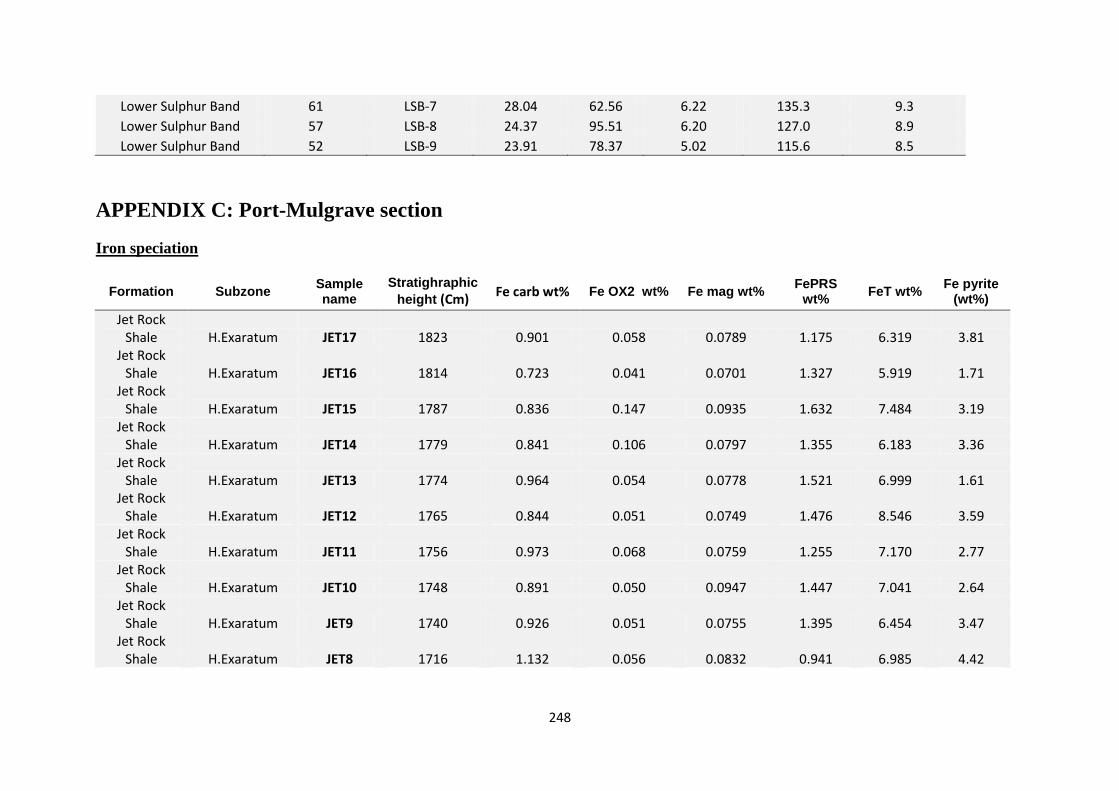
248
Lower Sulphur Band 61 LSB-7 28.04 62.56 6.22 135.3 9.3
Lower Sulphur Band 57 LSB-8 24.37 95.51 6.20 127.0 8.9
Lower Sulphur Band 52 LSB-9 23.91 78.37 5.02 115.6 8.5
APPENDIX C: Port-Mulgrave section
Iron speciation
Formation Subzone Sample name
Stratighraphic
height (Cm) Fe carb wt% Fe OX2 wt% Fe mag wt%
FePRS wt%
FeT wt% Fe pyrite
(wt%)
Jet Rock Shale H.Exaratum JET17 1823 0.901 0.058 0.0789 1.175 6.319 3.81
Jet Rock Shale H.Exaratum JET16 1814 0.723 0.041 0.0701 1.327 5.919 1.71
Jet Rock Shale H.Exaratum JET15 1787 0.836 0.147 0.0935 1.632 7.484 3.19
Jet Rock Shale H.Exaratum JET14 1779 0.841 0.106 0.0797 1.355 6.183 3.36
Jet Rock Shale H.Exaratum JET13 1774 0.964 0.054 0.0778 1.521 6.999 1.61
Jet Rock Shale H.Exaratum JET12 1765 0.844 0.051 0.0749 1.476 8.546 3.59
Jet Rock Shale H.Exaratum JET11 1756 0.973 0.068 0.0759 1.255 7.170 2.77
Jet Rock Shale H.Exaratum JET10 1748 0.891 0.050 0.0947 1.447 7.041 2.64
Jet Rock Shale H.Exaratum JET9 1740 0.926 0.051 0.0755 1.395 6.454 3.47
Jet Rock Shale H.Exaratum JET8 1716 1.132 0.056 0.0832 0.941 6.985 4.42

249
Jet Rock Shale H.Exaratum JET7 1698 0.898 0.046 0.0717 0.833 6.564 4.01
Jet Rock Shale H.Exaratum JET6 1673 0.936 0.041 0.0915 0.781 6.782 3.28
Jet Rock Shale H.Exaratum JET5 1623 0.816 0.044 0.0630 0.737 5.599 3.44
Jet Rock Shale H.Exaratum JET4 1568 0.947 0.079 0.0904 1.187 7.419 3.64
Jet Rock Shale H.Exaratum JET3 1518 0.930 0.092 0.0943 1.027 6.637 4.22
Jet Rock Shale H.Exaratum JET2 1448 0.928 0.081 0.0904 1.095 6.786 2.39
Jet Rock Shale H.Exaratum JET1 1398 0.865 0.116 0.0948 1.115 6.252 3.40
Gray Shale D.Semicelatum TL.5 1358 0.421 0.054 0.0765 1.026 4.910 2.30
Gray Shale D.Semicelatum TL.4 1318 0.608 0.061 0.0792 0.950 5.972 3.16
Gray Shale D.Semicelatum TL.3 1268 0.654 0.057 0.1007 1.042 5.755 1.61
Gray Shale D.Semicelatum TL.2 1218 0.827 0.075 0.0823 1.095 7.521 1.19
Gray Shale D.Semicelatum TL.1 1158 0.646 0.088 0.0778 1.036 6.917 0.17
Gray Shale D.Semicelatum 4-MST7 1035 0.318 0.055 0.0985 1.227 4.889 0.96
Gray Shale D.Semicelatum 4-MST6 945 1.095 0.109 0.2528 1.336 4.734 0.50
Gray Shale D.Semicelatum 4-MST5 843 0.691 0.082 0.1624 1.365 3.398 0.81
Gray Shale D.Semicelatum 4-MST4 783 0.830 0.084 0.1880 1.321 4.649 0.56
Gray Shale D.Semicelatum 4-MST3 733 1.385 0.127 0.2733 1.267 5.576 0.98
Gray Shale D.Semicelatum 4-MST2 678 1.106 0.121 0.2695 1.344 5.155 0.88
Gray Shale D.Semicelatum 4-MST1 628 0.859 0.126 0.1977 1.342 4.143 1.23
Gray Shale Clevelandicum USB10 578.0 1.036 0.911 0.2117 1.335 13.072 3.35
Gray Shale Clevelandicum USB9 576.0 1.112 0.315 0.1982 1.364 11.778 5.84
Gray Shale Clevelandicum USB7 572.0 1.588 0.117 0.2252 1.457 11.562 1.26
Gray Shale Clevelandicum USB6 570 1.669 0.123 0.1964 1.415 8.311 1.47
Gray Shale Clevelandicum USB5 568.0 1.204 0.080 0.1679 1.500 9.654 1.33

250
Gray Shale Clevelandicum USB4 566 1.394 0.106 0.1748 1.637 8.229 4.14
Gray Shale Clevelandicum USB3 564 1.030 0.095 0.1647 1.532 9.378 3.94
Gray Shale Clevelandicum USB2 562 0.893 0.094 0.1579 1.464 6.959 2.70
Gray Shale Clevelandicum USB1 560 0.655 0.084 0.1430 1.300 7.677 2.86
Gray Shale Paltum 3-MST8 546
5.674 1.19
Gray Shale Paltum 3-MST7 501 0.314 0.134 0.1941 1.249 3.554 2.79
Gray Shale Paltum 3-MST6 488
5.579 1.06
Gray Shale Paltum 3-MST5 458 0.365 0.125 0.1898 1.423 3.903 1.68
Gray Shale Paltum 3-MST4 422
6.359 1.35
Gray Shale Paltum 3-MST3 372 0.388 0.118 0.2208 1.325 3.778 0.76
Gray Shale Paltum 3-MST2 307
7.218 2.46
Gray Shale Paltum 3-MST1 297 3.413 0.271 4.8186 2.862 13.631 1.46
Gray Shale Paltum MSB24 294 0.535 0.094 0.2153 1.469 5.229 1.74
Gray Shale Paltum MSB23 292 0.470 0.083 0.2057 1.415 4.850 2.23
Gray Shale Paltum MSB22 290 0.440 0.074 0.1926 1.406 4.674 1.80
Gray Shale Paltum MSB21 289 0.490 0.065 0.1782 1.396 5.737 2.77
Gray Shale Paltum MSB20 287 0.735 0.081 0.2000 1.504 5.976 2.94
Gray Shale Paltum MSB19 285 0.984 0.665 0.2087 1.431 6.699 2.71
Gray Shale Paltum MSB18 283 0.952 0.198 0.1942 1.610 6.710 3.43
Gray Shale Paltum MSB17 281 0.770 0.597 0.2024 1.416 6.556 2.76
Gray Shale Paltum MSB16 278 0.800 0.627 0.2044 1.332 6.013 2.08
Gray Shale Paltum MSB15 275 0.671 0.067 0.1920 1.452 5.527 2.50
Gray Shale Paltum MSB14 273 0.644 0.089 0.1971 1.416 5.694 2.47
Gray Shale Paltum MSB13 269 0.576 0.082 0.2089 1.459 5.287 2.16
Gray Shale Paltum MSB12 266 0.568 0.082 0.2066 1.436 5.234 2.16
Gray Shale Paltum MSB11 263 0.505 0.078 0.2002 1.438 5.109 1.88
Gray Shale Paltum MSB10 258 0.614 0.081 0.2007 1.476 5.503 2.50
Gray Shale Paltum MSB9 254 0.525 0.068 0.1968 1.444 5.182 2.25
Gray Shale Paltum MSB8 251 0.550 0.073 0.1991 1.471 6.300 2.25
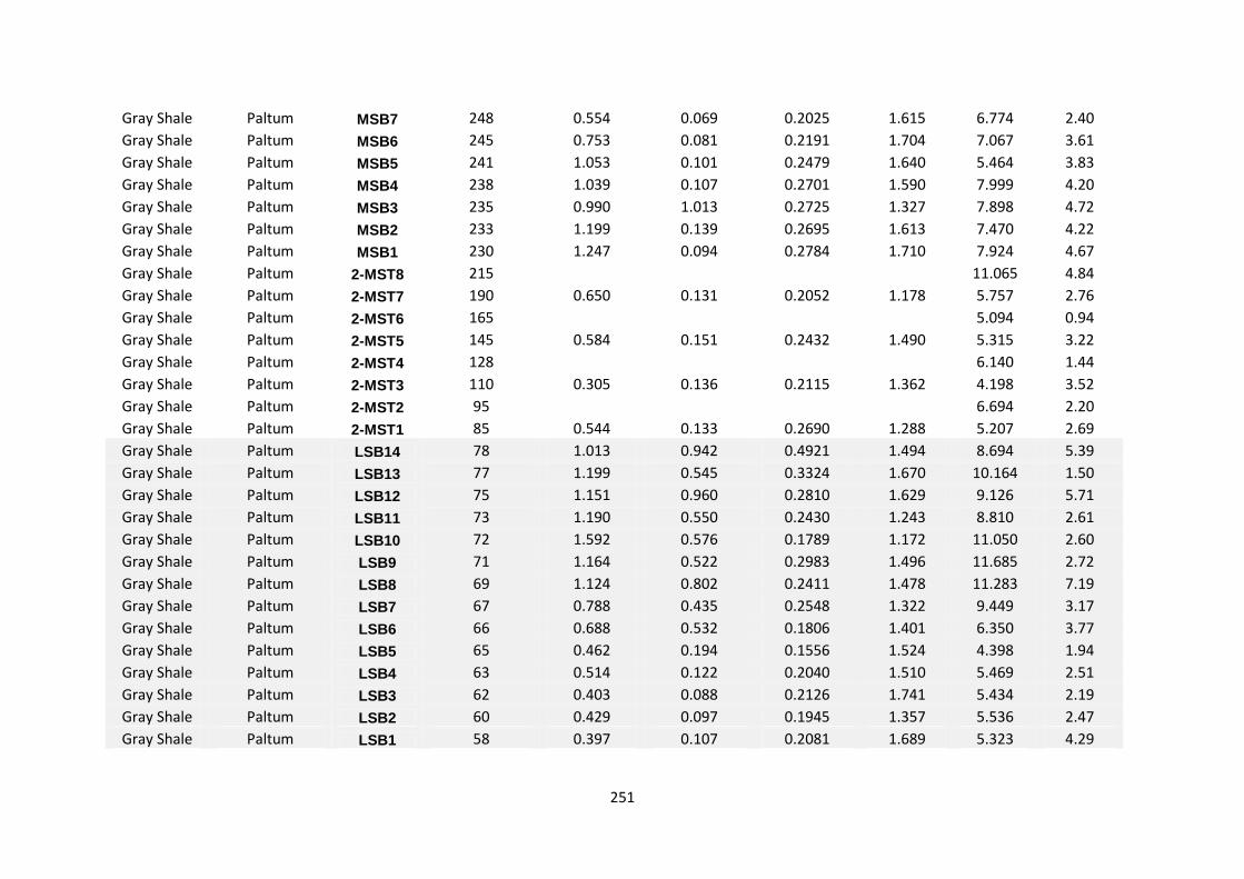
251
Gray Shale Paltum MSB7 248 0.554 0.069 0.2025 1.615 6.774 2.40
Gray Shale Paltum MSB6 245 0.753 0.081 0.2191 1.704 7.067 3.61
Gray Shale Paltum MSB5 241 1.053 0.101 0.2479 1.640 5.464 3.83
Gray Shale Paltum MSB4 238 1.039 0.107 0.2701 1.590 7.999 4.20
Gray Shale Paltum MSB3 235 0.990 1.013 0.2725 1.327 7.898 4.72
Gray Shale Paltum MSB2 233 1.199 0.139 0.2695 1.613 7.470 4.22
Gray Shale Paltum MSB1 230 1.247 0.094 0.2784 1.710 7.924 4.67
Gray Shale Paltum 2-MST8 215
11.065 4.84
Gray Shale Paltum 2-MST7 190 0.650 0.131 0.2052 1.178 5.757 2.76
Gray Shale Paltum 2-MST6 165
5.094 0.94
Gray Shale Paltum 2-MST5 145 0.584 0.151 0.2432 1.490 5.315 3.22
Gray Shale Paltum 2-MST4 128
6.140 1.44
Gray Shale Paltum 2-MST3 110 0.305 0.136 0.2115 1.362 4.198 3.52
Gray Shale Paltum 2-MST2 95
6.694 2.20
Gray Shale Paltum 2-MST1 85 0.544 0.133 0.2690 1.288 5.207 2.69
Gray Shale Paltum LSB14 78 1.013 0.942 0.4921 1.494 8.694 5.39
Gray Shale Paltum LSB13 77 1.199 0.545 0.3324 1.670 10.164 1.50
Gray Shale Paltum LSB12 75 1.151 0.960 0.2810 1.629 9.126 5.71
Gray Shale Paltum LSB11 73 1.190 0.550 0.2430 1.243 8.810 2.61
Gray Shale Paltum LSB10 72 1.592 0.576 0.1789 1.172 11.050 2.60
Gray Shale Paltum LSB9 71 1.164 0.522 0.2983 1.496 11.685 2.72
Gray Shale Paltum LSB8 69 1.124 0.802 0.2411 1.478 11.283 7.19
Gray Shale Paltum LSB7 67 0.788 0.435 0.2548 1.322 9.449 3.17
Gray Shale Paltum LSB6 66 0.688 0.532 0.1806 1.401 6.350 3.77
Gray Shale Paltum LSB5 65 0.462 0.194 0.1556 1.524 4.398 1.94
Gray Shale Paltum LSB4 63 0.514 0.122 0.2040 1.510 5.469 2.51
Gray Shale Paltum LSB3 62 0.403 0.088 0.2126 1.741 5.434 2.19
Gray Shale Paltum LSB2 60 0.429 0.097 0.1945 1.357 5.536 2.47
Gray Shale Paltum LSB1 58 0.397 0.107 0.2081 1.689 5.323 4.29
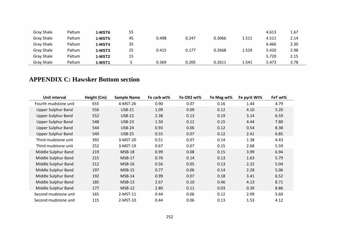
252
Gray Shale Paltum 1-MST6 55
4.613 1.67
Gray Shale Paltum 1-MST5 45 0.498 0.247 0.3066 1.511 4.511 2.14
Gray Shale Paltum 1-MST4 35
6.466 2.30
Gray Shale Paltum 1-MST3 25 0.415 0.177 0.2668 1.529 5.420 2.98
Gray Shale Paltum 1-MST2 15
5.720 2.15
Gray Shale Paltum 1-MST1 5 0.369 0.205 0.2611 1.541 5.473 3.78
APPENDIX C: Hawsker Bottom section
Unit interval Height (Cm) Sample Name Fe carb wt% Fe OX2 wt% Fe Mag wt% Fe pyrit Wt% FeT wt%
Fourth mudstone unit 655 4-MST-26 0.90 0.07 0.16 1.44 4.79
Upper Sulphur Band 556 USB-21 1.09 0.09 0.12 4.10 5.20
Upper Sulphur Band 552 USB-22 2.38 0.13 0.19 3.14 6.59
Upper Sulphur Band 548 USB-23 1.50 0.12 0.15 4.44 7.80
Upper Sulphur Band 544 USB-24 0.93 0.06 0.12 0.54 8.38
Upper Sulphur Band 540 USB-25 0.55 0.07 0.12 2.41 6.85
Third mudstone unit 392 3-MST-20 0.51 0.07 0.14 1.38 4.43
Third mudstone unit 252 3-MST-19 0.67 0.07 0.15 2.68 5.59
Middle Sulphur Band 219 MSB-18 0.99 0.08 0.15 3.99 6.94
Middle Sulphur Band 215 MSB-17 0.76 0.14 0.13 1.63 5.79
Middle Sulphur Band 212 MSB-16 0.56 0.05 0.13 2.22 5.04
Middle Sulphur Band 197 MSB-15 0.77 0.06 0.14 2.28 5.06
Middle Sulphur Band 192 MSB-14 0.99 0.07 0.18 3.41 6.52
Middle Sulphur Band 185 MSB-13 2.67 0.10 0.46 4.13 8.71
Middle Sulphur Band 177 MSB-12 2.80 0.11 0.03 0.39 8.86
Second mudstone unit 165 2-MST-11 0.44 0.06 0.12 2.99 5.60
Second mudstone unit 115 2-MST-10 0.44 0.06 0.13 1.53 4.12

253
Lower Sulphur Band 75 LSB-1 0.48 0.06 0.14 2.13 4.63
Lower Sulphur Band 73 LSB-2 0.42 0.05 0.14 2.30 4.84
Lower Sulphur Band 70 LSB-3 0.41 0.06 0.00 0.40 4.99
Lower Sulphur Band 68 LSB-4 0.48 0.07 0.28 2.10 4.37
Lower Sulphur Band 66 LSB-5 0.53 0.07 0.16 0.35 4.76
Lower Sulphur Band 63 LSB-6 0.50 0.06 0.15 1.01 4.65
Lower Sulphur Band 61 LSB-7 0.52 0.07 0.15 2.12 4.92
Lower Sulphur Band 57 LSB-8 0.51 0.06 0.14 0.28 4.67
Lower Sulphur Band 52 LSB-9 0.51 0.05 0.13 0.51 3.84
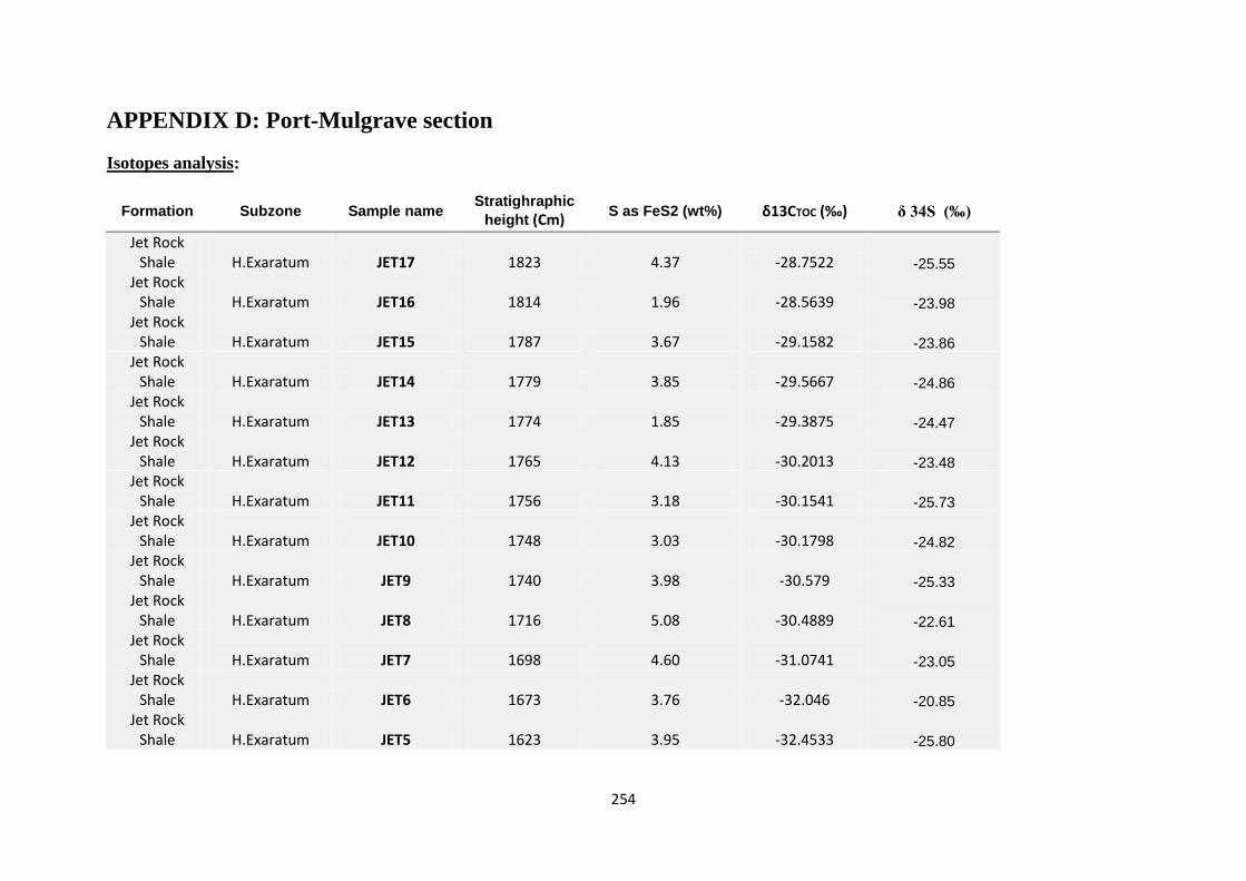
254
APPENDIX D: Port-Mulgrave section
Isotopes analysis:
Formation Subzone Sample name Stratighraphic
height (Cm) S as FeS2 (wt%) δ13CTOC (‰) δ 34S (‰)
Jet Rock Shale H.Exaratum JET17 1823 4.37 -28.7522 -25.55
Jet Rock Shale H.Exaratum JET16 1814 1.96 -28.5639 -23.98
Jet Rock Shale H.Exaratum JET15 1787 3.67 -29.1582 -23.86
Jet Rock Shale H.Exaratum JET14 1779 3.85 -29.5667 -24.86
Jet Rock Shale H.Exaratum JET13 1774 1.85 -29.3875 -24.47
Jet Rock Shale H.Exaratum JET12 1765 4.13 -30.2013 -23.48
Jet Rock Shale H.Exaratum JET11 1756 3.18 -30.1541 -25.73
Jet Rock Shale H.Exaratum JET10 1748 3.03 -30.1798 -24.82
Jet Rock Shale H.Exaratum JET9 1740 3.98 -30.579 -25.33
Jet Rock Shale H.Exaratum JET8 1716 5.08 -30.4889 -22.61
Jet Rock Shale H.Exaratum JET7 1698 4.60 -31.0741 -23.05
Jet Rock Shale H.Exaratum JET6 1673 3.76 -32.046 -20.85
Jet Rock Shale H.Exaratum JET5 1623 3.95 -32.4533 -25.80

255
Jet Rock Shale H.Exaratum JET4 1568 4.18 -31.6361 -26.40
Jet Rock Shale H.Exaratum JET3 1518 4.85 -32.3382 -26.42
Jet Rock Shale H.Exaratum JET2 1448 2.74 -30.2664 -27.46
Jet Rock Shale H.Exaratum JET1 1398 3.91 -31.5761 -26.82
Gray Shale D.Semicelatum TL.5 1358 2.64 -26.4104 -35.93
Gray Shale D.Semicelatum TL.4 1318 3.63 -26.7049 -32.76
Gray Shale D.Semicelatum TL.3 1268 1.85 -28.291 -31.98
Gray Shale D.Semicelatum TL.2 1218 1.36 -27.2885 -26.66
Gray Shale D.Semicelatum TL.1 1158 0.19 -30.5005 -28.46
Gray Shale D.Semicelatum 4-MST7 1035 1.11 -25.6461 -33.22
Gray Shale D.Semicelatum 4-MST6 945 0.57 -25.3766 -32.95
Gray Shale D.Semicelatum 4-MST5 843 0.94 -25.5151 -33.74
Gray Shale D.Semicelatum 4-MST4 783 0.64 -25.4799 -30.60
Gray Shale D.Semicelatum 4-MST3 733 1.13 -25.5215 -30.77
Gray Shale D.Semicelatum 4-MST2 678 1.01 -25.3476 -32.13
Gray Shale D.Semicelatum 4-MST1 628 1.42 -25.6208 -32.05
Gray Shale Clevelandicum USB10 578.0 3.84 -25.8111 -43.85
Gray Shale Clevelandicum USB9 576.0 6.71 -25.9384 -38.85
Gray Shale Clevelandicum USB7 572.0 1.45 -26.4882 -32.63
Gray Shale Clevelandicum USB6 570 1.69 -26.5205
Gray Shale Clevelandicum USB5 568.0 1.53 -25.9892 -32.11
Gray Shale Clevelandicum USB4 566 4.75 -26.0978 -34.40
Gray Shale Clevelandicum USB3 564 4.53 -25.9123 -34.65
Gray Shale Clevelandicum USB2 562 3.10 -25.7566 -34.78
Gray Shale Clevelandicum USB1 560 3.29 -25.7247 -35.64
Gray Shale Paltum 3-MST8 546 1.37 -25.7288 -39.01

256
Gray Shale Paltum 3-MST7 501 3.21 -25.569 -39.30
Gray Shale Paltum 3-MST6 488 1.22 -25.7477 -38.47
Gray Shale Paltum 3-MST5 458 1.93 -25.8221 -31.26
Gray Shale Paltum 3-MST4 422 1.55 -25.7399 -27.10
Gray Shale Paltum 3-MST3 372 0.87 -25.6622 -31.85
Gray Shale Paltum 3-MST2 307 2.82 -26.235 -29.36
Gray Shale Paltum 3-MST1 297 1.68 -27.6012 -32.71
Gray Shale Paltum MSB24 294 2.00 -27.5039 -39.44
Gray Shale Paltum MSB23 292 2.57 -27.2381 -38.23
Gray Shale Paltum MSB22 290 2.07 -26.6727 -41.50
Gray Shale Paltum MSB21 289 3.18 -26.7721 -39.70
Gray Shale Paltum MSB20 287 3.37 -27.2009 -37.06
Gray Shale Paltum MSB19 285 3.11 -27.14 -37.92
Gray Shale Paltum MSB18 283 3.94 -26.9654 -34.18
Gray Shale Paltum MSB17 281 3.16 -26.9295 -35.69
Gray Shale Paltum MSB16 278 2.39 -26.6872 -36.45
Gray Shale Paltum MSB15 275 2.88 -26.6233 -36.88
Gray Shale Paltum MSB14 273 2.84 -26.6955 -39.68
Gray Shale Paltum MSB13 269 2.48 -26.5684 -37.60
Gray Shale Paltum MSB12 266 2.48 -26.617 -38.92
Gray Shale Paltum MSB11 263 2.16 -26.7577 -38.43
Gray Shale Paltum MSB10 258 2.87 -26.8107 -39.25
Gray Shale Paltum MSB9 254 2.58 -26.9554 -36.07
Gray Shale Paltum MSB8 251 2.59 -26.8572 -39.96
Gray Shale Paltum MSB7 248 2.75 -27.1107 -38.16
Gray Shale Paltum MSB6 245 4.14 -27.2449 -34.56
Gray Shale Paltum MSB5 241 4.40 -27.5718 -33.32
Gray Shale Paltum MSB4 238 4.82 -27.7831 -32.99
Gray Shale Paltum MSB3 235 5.42 -27.8665 -32.34
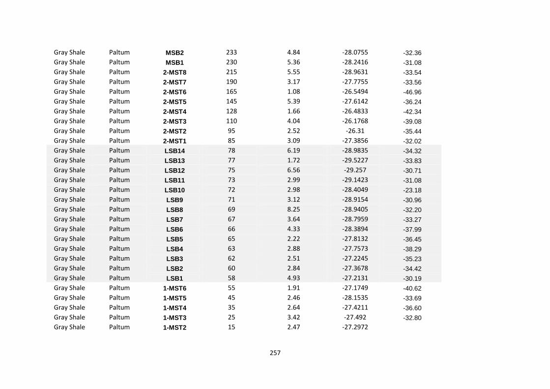
257
Gray Shale Paltum MSB2 233 4.84 -28.0755 -32.36
Gray Shale Paltum MSB1 230 5.36 -28.2416 -31.08
Gray Shale Paltum 2-MST8 215 5.55 -28.9631 -33.54
Gray Shale Paltum 2-MST7 190 3.17 -27.7755 -33.56
Gray Shale Paltum 2-MST6 165 1.08 -26.5494 -46.96
Gray Shale Paltum 2-MST5 145 5.39 -27.6142 -36.24
Gray Shale Paltum 2-MST4 128 1.66 -26.4833 -42.34
Gray Shale Paltum 2-MST3 110 4.04 -26.1768 -39.08
Gray Shale Paltum 2-MST2 95 2.52 -26.31 -35.44
Gray Shale Paltum 2-MST1 85 3.09 -27.3856 -32.02
Gray Shale Paltum LSB14 78 6.19 -28.9835 -34.32
Gray Shale Paltum LSB13 77 1.72 -29.5227 -33.83
Gray Shale Paltum LSB12 75 6.56 -29.257 -30.71
Gray Shale Paltum LSB11 73 2.99 -29.1423 -31.08
Gray Shale Paltum LSB10 72 2.98 -28.4049 -23.18
Gray Shale Paltum LSB9 71 3.12 -28.9154 -30.96
Gray Shale Paltum LSB8 69 8.25 -28.9405 -32.20
Gray Shale Paltum LSB7 67 3.64 -28.7959 -33.27
Gray Shale Paltum LSB6 66 4.33 -28.3894 -37.99
Gray Shale Paltum LSB5 65 2.22 -27.8132 -36.45
Gray Shale Paltum LSB4 63 2.88 -27.7573 -38.29
Gray Shale Paltum LSB3 62 2.51 -27.2245 -35.23
Gray Shale Paltum LSB2 60 2.84 -27.3678 -34.42
Gray Shale Paltum LSB1 58 4.93 -27.2131 -30.19
Gray Shale Paltum 1-MST6 55 1.91 -27.1749 -40.62
Gray Shale Paltum 1-MST5 45 2.46 -28.1535 -33.69
Gray Shale Paltum 1-MST4 35 2.64 -27.4211 -36.60
Gray Shale Paltum 1-MST3 25 3.42 -27.492 -32.80
Gray Shale Paltum 1-MST2 15 2.47 -27.2972

258
Gray Shale Paltum 1-MST1 5 4.34 -27.4666
APPENDIX E1: Port-Mulgrave section
Normal alkanes
normal alkanes
Stratighraphi
c height (Cm) Sample n-C13 n-C14 n-C15 n-C16 n-C17 Prystane n-C18 Phytane n-C19 n-C20 n-C21 n-C22 n-C23
1823 Jet 17 38644 65235 84089 86122 89349 94224 68081 65518 61861 53588 54429 46099 44349
1787 Jet15 185 384 640 657 749 1054 527 738 545 512 469 444 446
1774 Jet 13 17085 68078 12244
5 14381
2 15969
5 213947 12667
5 167464 3677 12062
7 11161
1 92208 91452
1756 Jet 11 280 711 1263 1299 1156 1612 712 1052 784 698 623 590 583
1716 Jet 8 39102 83606 12829
8 14474
4 16155
3 224976 12767
1 178536 12098
1 13251
3 10896
0 87839 83389
1673 Jet 6 41882
5 60907
0 56191
0 55278
8 55668
9 425218 43216
2 367832 34279
6 29058
5 21958
1 17217
4 15930
5
1568 Jet 4 10689
2 16681
9 23204
4 22242
4 22746
3 292568 17404
2 228819 14862
9 15553
4 12294
1 95575 86733
1398 Jet 1 344 533 705 689 781 1207 595 864 607 568 563 501 508
1358 TL.5 7298 20222 34734 41019 48327 53530 35427 19683 39775 28935 26839 29573 26538
1318 TL.4 11773
3 13272
7 13358
3 12797
0 12370
5 165155 98603 79376 91987 76159 69899 62705 60251
1218 TL.2
1158 TL.1 20935 39507 54940 53493 52720 70364 39727 41636 44557 29100 26323 27427 22502
945 4-MST 6 2460 9830 18027 21507 25758 22673 20686 5198 20173 19005 19080 17978 19069
843 4-MST 5
4285 10201 15945 14503 14355 3613 14362 14217 14381 13701 14588
783 4-MST 4 678 4-MST 2
2308 8401 12737 15863 13602 13027 3156 13142 12730 12965 12288 13146

259
628 4-MST 1
2982 11670 18355 24268 21457 20155 5400 18502 20462 20429 19658 21034
578.0 USB10 4915 18971 30981 44903 119170 36250 36695 39640 32582 37107 31322 32238
572.0 USB7
570 USB6 31980 45360 65675 72477 85832 210741 58953 62331 57740 49939 46461 42285 42849
568.0 USB5 41901 62894 83996 88631 10328
7 238129 72191 73632 71330 61600 58861 54507 53877
566 USB4 43903 64339 82283 85899 10329
7 227449 73993 66543 73748 64338 60766 55019 55340
564 USB3 322 649 216 177 168 151
501 3-MST 7
2396 10828 19456 27195 23895 23031 5168 20787 22446 22722 22147 22832
458 3-MST 5
8237 16685 19991 22744 23867 16702 4323 14440 15245 15435 14920 16180
297 3-MST 1 5421 14018 19733 20102 21912 37935 15977 10202 13192 13347 13007 12573 13047
294 MSB24 71 114 53 29 44 39
287 MSB 20 29540 63674 80702 80134 83500 159256 63538 40944 56108 55173 55757 52924 56765
283 MSB18 124 245 89 76 70 63
278 MSB 16 10820 20442 25469 25190 26953 51329 21019 14500 17991 19055 19320 18821 20173
254 MSB 9 8366 17046 21845 22962 25734 39610 20018 9704 17920 18051 18211 17562 18811
251 MSB8 21 34 16 8 14 13
238 MSB 4 7474 20305 30065 30569 33120 66519 24539 21965 20271 20551 20046 19238 19920
233 MSB2 103 213 72 75 52 45
215 2-MST
8 17914 31949 39547 36105 37099 100676 27811 33374 21076 22107 20865 22960 19595
128 2-MST
4 3537 14213 21372 22460 24432 28426 20417 5658 20353 20380 21234 20799 22956
85 2-MST
1 2441 2362 13731 14290 15864 26480 12549 7114 12030 12705 13013 12618 13104
78 LSB14 24431 43370 59536 57478 62517 169670 46703 58116 43136 36726 33451 29235 29927
77 LSB13 45144 75191 10755
3 10826
6 11515
7 310908 88590 113289 79201 68012 61035 52704 53438
75 LSB12

260
73 LSB11 82014 12537
3 18729
6 19988
0 22485
5 624739 17290
6 230515 15899
8 13976
4 12654
1 11197
1 11337
1
72 LSB10 7948 14495 21452 21950 24271 69772 18034 25355 16477 14963 14206 13076 13605
71 LSB9 10570
0 10377
1 11639
6 10071
0 99725 278806 72558 95629 65304 55685 49073 44033 43090
69 LSB8 74 247 46 83 19 14
67 LSB7 10218
9 12346
3 15101
1 13965
4 14189
0 395146 10478
0 141502 92932 27380 77425 69186 61607
66 LSB6 75492 88009 10014
3 88605 91686 236729 65531 81639 59476 50813 45458 41706 40510
65 LSB5 14668 22912 31454 33875 35613 86591 27781 26952 25960 22773 21477 20817 21809
63 LSB 4 1093 3477 4578 5200 9581 4586 2590 4245 4682 5149 5249 6041 5909
62 LSB3 14850 22332 29013 30902 31112 44342 25743 12439 26105 25297 27217 26091 29218
Bitumen LSB 84061 84382 93992 78998 77435 197061 54519 65315 51054 41055 36421 30162 31458
35 1-MST 4
3548 7063 7849 8696 11287 7629 2585 7609 8108 9007 9219 10368

261
APPENDIX E1: Port-Mulgrave section
normal alkanes
Stratighraphic
height (Cm) Sample n-C24 n-C25 n-C26 n-C27 n-C28 n-C29 n-C30 n-C31 n-C32 n-C33 n-C34 n-C35
1823 Jet 17 40560 35871 32496 27581 22424 26960 20571 16062 16393 16711 10990 13026
1787 Jet15 416 348 341 251 245 230 202 326 199 116 65 70
1774 Jet 13 83110 80920 69568 55417 50897 57809 44987 51461 46068 41190 27591 28696
1756 Jet 11 554 458 473 359 351 349 308 545 312 149 86 76
1716 Jet 8 79384 71819 61837 51603 46800 52682 41134 48939 42475 38320 30447 34674
1673 Jet 6 132478 99842 93555 107685 75124 71969 60780 45692 28376 31791 8936 1288
1568 Jet 4 75453 74180 55989 44936 41084 41901 32964 35191 30283 25669 18469 21174
1398 Jet 1 483 425 430 333 324 323 295 473 309 168 107 106
1358 TL.5 23716 25357 21221 22481 16584 23198 16208 15358 11165 12678 7140 6744
1318 TL.4 53236 53346 43232 40700 32474 35927 20131 21793 13262 14175 8423 9977
1218 TL.2
1158 TL.1 21450 17172 16246 11571 9942 11423 8699 7554 6119 6490 4200 4077
945 4-MST 6 16437 17542 14533 15876 10555 13474 8472 7747 4968 7361 2697 3656
843 4-MST 5 12225 14677 11515 12743 8520 11178 6977 8158 4271 6309 2723 3315
783 4-MST 4 678 4-MST 2 11076 13640 10249 11101 7412 9405 6044 3183 3645 5315 2270 2541
628 4-MST 1 17700 21142 15012 17904 12193 15576 10324 12151 7199 8904 4013 4389
578.0 USB10 29558 32664 27858 32566 24457 28341 20439 20638 13153 13801 10025 6388
572.0 USB7
570 USB6 41086 43157 36884 42624 35528 33355 20475 22596 14004 10464 0 0
568.0 USB5 50961 52567 45461 51767 41395 38227 25669 23781 13546 7572 0 0
566 USB4 51839 54975 47028 55706 44211 45104 29392 30110 16461 9077 0 0

262
564 USB3 142 155 130 143 120 127 94 78 56 0 0 0
501 3-MST 7 20155 23186 18940 21352 14763 18047 11672 13044 7829 10523 4484 4731
458 3-MST 5 14042 16707 13695 15392 10781 13060 8789 9055 5119 7026 2998 3210
297 3-MST 1 11955 13267 10664 11441 8823 9694 6875 5753 3754 5106 2701 2455
294 MSB24 36 39 31 30 24 33 17 17 12 0 0 0
287 MSB 20 52067 59902 53350 55615 41039 49245 33294 30068 19486 26797 12311 12317
283 MSB18 66 76 66 69 56 70 37 45 29 9 5
278 MSB 16 18472 21749 19427 20533 14898 17834 11724 10380 6432 8994 4230 4292
254 MSB 9 16899 19747 17236 18205 12891 15755 10488 9565 6198 8627 3751 3929
251 MSB8 16 19 17 18 15 16 11 10 7 0 0 0
238 MSB 4 19541 20967 18003 18792 16342 16186 12473 9289 6065 7952 4143 3717
233 MSB2 42 44 36 43 29 41 25 17 12 4 0 0
215 2-MST 8 18763 20583 17368 17446 13042 15623 10828 9990 6832 9064 4158 3903
128 2-MST 4 20374 24666 19858 22908 15406 19353 12908 12640 8983 13926 4760 5367
85 2-MST 1 11731 12974 11373 11433 8290 10253 6961 6586 4205 5966 2392 2639
78 LSB14 27893 28787 23653 29864 19775 20661 10215 13155 5636 3467 0 0
77 LSB13 51027 51984 44490 43212 30536 31240 16358 18385 8362 3668 0 0
75 LSB12
73 LSB11 106876 109723 95999 103117 70299 76147 39682 50943 27519 22542 0 0
72 LSB10 13135 13738 11805 12396 8513 10454 5860 8853 4861 3693 0 0
71 LSB9 40593 41039 35505 34844 23948 24925 11264 16547 6557 5128 0
69 LSB8 51 53 55 57 59 61 63 64 66 67 69 0
67 LSB7 60269 55776 55713 47215 49325 30533 32414 13035 18349 0 0 0
66 LSB6 38381 40292 34236 35868 25025 25327 13597 19502 11126 1016 0 0
65 LSB5 21050 24212 19241 23579 14910 17886 12190 14476 8834 0 0 0
63 LSB 4 7017 5237 6570 4452 5463 3742 3645 2610 3740 1368 1473 381
62 LSB3 26270 31272 22699 29393 18938 21169 14626 14500 9191 12298 3185 3954
Bitumen LSB 27074 28198 21664 24872 21676 19646 14168 14622 8702 7888 3038 2837

263
35 1-MST 4 9816 12062 8883 11343 7820 9417 6491 6391 4875 6959 2219 2506
APPENDIX E2: Port-Mulgrave section
GC-MS: Steranes + isoreinaratens
αααSteranes Isoreinaraten
Stratighraphic
height (Cm) Sample
27S 27R 28S 28R 29S 29R C27 Diast-
S C27 Diast-R Isore-(ng/µTOC)
1823 Jet 17 35067 41201 7367 29303 43297 56439 328794 216122 1.80
1787 Jet15 265767 24596 61381 15373 224737 31563 186894 129712 2.32
1774 Jet 13 58865 69023 9849 44526 68419 92606 604584 408948 2.07
1756 Jet 11 157560 15087 57972 10158 97494 24430 142496 102174 93.09
1716 Jet 8 82770 92445 22739 63736 112350 136595 877292 556637 31.51
1673 Jet 6 138274 157848 34524 109384 172189 213957 1294583 873165 11.40
1568 Jet 4 84485 95775 20847 63970 108083 135987 860123 574362 15.57
1398 Jet 1 403368 38916 123513 28628 394998 58378 346389 244795 38.74
1358 TL.5 14166 15277 8375 10656 22819 27001 204097 129826 2.05
1318 TL.4 0.28
1218 TL.2 4.27
1158 TL.1 19567 20992 7829 14207 25389 31892 227793 150928 33.86
945 4-MST 6 3403 3840 1928 2349 4962 6098 48849 31205 0.00
843 4-MST 5 6122 4056 2660 2734 6076 8381 50093 33778 0.00
783 4-MST 4 8411 7469 0 4966 12147 15485
0.00
678 4-MST 2 6192 4105 2729 2708 6176 7814 54370 38003 0.00

264
628 4-MST 1 4943 5501 3655 3289 7280 8219 74077 44969 0.00
578.0 USB10 16199 18189 12068 12100 28997 36127 221984 134538 8.69
572.0 USB7 0.72
570 USB6 4975 5831 2104 4484 9525 12099 60995 40171 27.58
568.0 USB5 5639 6483 1306 4519 9980 12120 82235 54613 21.71
566 USB4 10909 12955 2808 10291 21504 26288 140961 95581 32.18
564 USB3 14.78
501 3-MST 7 2425 2703 2162 1778 4237 4339 36268 22848 0.00
458 3-MST 5 1964 2310 1576 1605 3481 3741 29736 18781 0.00
297 3-MST 1 4068 5298 2847 3543 7299 8568 52851 34162 1.82
294 MSB24
11.27
287 MSB 20 8015 4937 2867 3396 7362 9507 66213 44644 2.18
283 MSB18 2.77
278 MSB 16 14642 8290 5882 6298 14896 18645 112857 70968 0.64
254 MSB 9 0.00
251 MSB8 9667 5842 4018 4009 11150 12105 78195 52603 0.86
238 MSB 4 23852 15420 7107 11941 23330 30138 178628 126943 1.23
233 MSB2 25.67
215 2-MST 8 16609 11465 5126 6130 12041 18443 142340 103654 0.00
128 2-MST 4 5151 2897 2485 2322 5528 6610 53590 35860 0.00
85 2-MST 1 6632 3898 2726 2674 6424 7786 57987 37789 0.00
78 LSB14 6756 8488 1643 4451 9893 11545 118847 76118 3.94
77 LSB13 11705 16038 2311 9493 16206 21243 192747 132943 3.88
75 LSB12 6.29
73 LSB11 21921 24285 3989 13834 26344 35066 301568 196880 3.32
72 LSB10 7067 8541 1404 4799 7260 9933 97385 66939 2.39
71 LSB9 11059 12221 2656 7397 13385 16727 151615 99337 6.30
69 LSB8 7.39
67 LSB7 24333 25188 4734 15820 27784 34685 325373 210621 4.74
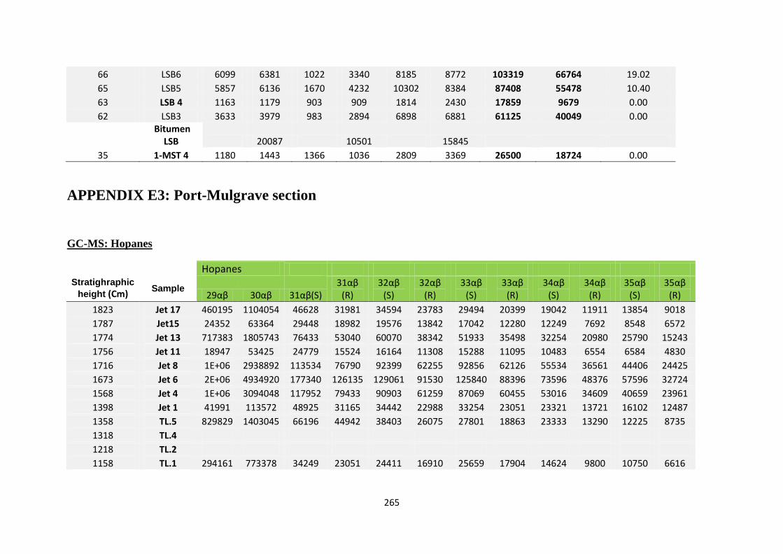
265
66 LSB6 6099 6381 1022 3340 8185 8772 103319 66764 19.02
65 LSB5 5857 6136 1670 4232 10302 8384 87408 55478 10.40
63 LSB 4 1163 1179 903 909 1814 2430 17859 9679 0.00
62 LSB3 3633 3979 983 2894 6898 6881 61125 40049 0.00
Bitumen LSB 20087 10501 15845
35 1-MST 4 1180 1443 1366 1036 2809 3369 26500 18724 0.00
APPENDIX E3: Port-Mulgrave section
GC-MS: Hopanes
Hopanes
Stratighraphic
height (Cm) Sample
29αβ 30αβ 31αβ(S) 31αβ
(R) 32αβ
(S) 32αβ
(R) 33αβ
(S) 33αβ
(R) 34αβ
(S) 34αβ
(R) 35αβ
(S) 35αβ
(R)
1823 Jet 17 460195 1104054 46628 31981 34594 23783 29494 20399 19042 11911 13854 9018
1787 Jet15 24352 63364 29448 18982 19576 13842 17042 12280 12249 7692 8548 6572
1774 Jet 13 717383 1805743 76433 53040 60070 38342 51933 35498 32254 20980 25790 15243
1756 Jet 11 18947 53425 24779 15524 16164 11308 15288 11095 10483 6554 6584 4830
1716 Jet 8 1E+06 2938892 113534 76790 92399 62255 92856 62126 55534 36561 44406 24425
1673 Jet 6 2E+06 4934920 177340 126135 129061 91530 125840 88396 73596 48376 57596 32724
1568 Jet 4 1E+06 3094048 117952 79433 90903 61259 87069 60455 53016 34609 40659 23961
1398 Jet 1 41991 113572 48925 31165 34442 22988 33254 23051 23321 13721 16102 12487
1358 TL.5 829829 1403045 66196 44942 38403 26075 27801 18863 23333 13290 12225 8735
1318 TL.4
1218 TL.2
1158 TL.1 294161 773378 34249 23051 24411 16910 25659 17904 14624 9800 10750 6616

266
945 4-MST 6 500169 581712 31064 20969 15685 10570 10067 7050 6120 4034 1814 1463
843 4-MST 5 520936 686304 39166 26513 21015 14142 12998 10841 10715 6480 3788 1482
783 4-MST 4 91435 119207 62678 43536 34487 23882 20963 14168 14362 8187 5871 3846
678 4-MST 2 7E+06 760440 40677 28952 23325 15743 15507 9604 9717 7366 4172 2064
628 4-MST 1 600418 741855 39710 27548 20154 14170 13059 9470 8256 4879 2005 1748
578.0 USB10 909791 1497908 66055 45750 41785 27976 28016 20178 20408 12550 9703 6961
572.0 USB7
570 USB6 30154 52853 22055 15348 13544 8843 9527 6776 6829 4572 3525 2252
568.0 USB5 50136 84666 36454 25545 22109 14174 14635 10621 10722 6681 5177 2964
566 USB4 75531 129220 56532 39482 33671 22299 23322 17064 17566 11838 8381 6472
564 USB3 184123 289810 129488 89073 73385 48953 52463 36640 40385 23616 18856 12549
501 3-MST 7 301145 508041 26259 18196 14477 9832 8344 5271 5784 3169 2066 1821
458 3-MST 5 385216 438985 22850 16180 12347 8112 6545 4413 5166 2551 1704 1302
297 3-MST 1 138233 286105 12768 8880 7306 4655 4472 2959 3485 2443 1282 1345
294 MSB24 287 MSB 20 342660 533903 27159 19346 17122 10448 10033 7985 9361 5971 2940 3315
283 MSB18
278 MSB 16 523508 829930 45264 31282 25526 16906 19248 12453 18483 9056 6440 4964
254 MSB 9
251 MSB8 418047 649884 32962 23744 18940 12693 13806 9569 12007 6958 5002 3081
238 MSB 4 463150 847441 40629 26804 26038 15358 19299 13207 15913 8867 5496 3244
233 MSB2 185203 346789 154179 106661 91904 60996 71091 50794 54727 32534 25831 18961
215 2-MST 8 467387 892704 41575 28639 25812 17524 21775 13614 14099 9294 4517 4292
128 2-MST 4 480485 723753 34915 24636 18691 13913 12997 8667 9019 7282 3629 1975
85 2-MST 1 267547 417921 18954 13380 10957 7910 10263 8159 5800 2880 2912 2729
78 LSB14 34371 63784 28275 20115 17889 11389 12793 9091 8533 5178 4378 3404
77 LSB13 50342 97055 41108 29085 27127 18354 22603 16281 13349 8139 7375 5672
75 LSB12 77003 165257
73 LSB11 83862 159430 66941 47121 41203 28082 33340 23963 20133 12331 12049 8440
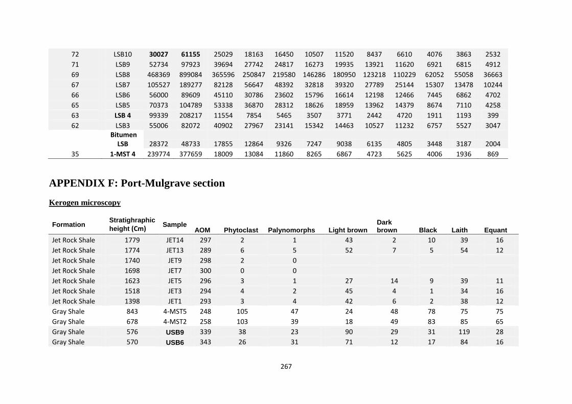
267
72 LSB10 30027 61155 25029 18163 16450 10507 11520 8437 6610 4076 3863 2532
71 LSB9 52734 97923 39694 27742 24817 16273 19935 13921 11620 6921 6815 4912
69 LSB8 468369 899084 365596 250847 219580 146286 180950 123218 110229 62052 55058 36663
67 LSB7 105527 189277 82128 56647 48392 32818 39320 27789 25144 15307 13478 10244
66 LSB6 56000 89609 45110 30786 23602 15796 16614 12198 12466 7445 6862 4702
65 LSB5 70373 104789 53338 36870 28312 18626 18959 13962 14379 8674 7110 4258
63 LSB 4 99339 208217 11554 7854 5465 3507 3771 2442 4720 1911 1193 399
62 LSB3 55006 82072 40902 27967 23141 15342 14463 10527 11232 6757 5527 3047
Bitumen LSB 28372 48733 17855 12864 9326 7247 9038 6135 4805 3448 3187 2004
35 1-MST 4 239774 377659 18009 13084 11860 8265 6867 4723 5625 4006 1936 869
APPENDIX F: Port-Mulgrave section
Kerogen microscopy
Formation Stratighraphic
height (Cm) Sample
AOM Phytoclast Palynomorphs Light brown Dark brown Black Laith Equant
Jet Rock Shale 1779 JET14 297 2 1 43 2 10 39 16
Jet Rock Shale 1774 JET13 289 6 5 52 7 5 54 12
Jet Rock Shale 1740 JET9 298 2 0
Jet Rock Shale 1698 JET7 300 0 0
Jet Rock Shale 1623 JET5 296 3 1 27 14 9 39 11
Jet Rock Shale 1518 JET3 294 4 2 45 4 1 34 16
Jet Rock Shale 1398 JET1 293 3 4 42 6 2 38 12
Gray Shale 843 4-MST5 248 105 47 24 48 78 75 75
Gray Shale 678 4-MST2 258 103 39 18 49 83 85 65
Gray Shale 576 USB9 339 38 23 90 29 31 119 28
Gray Shale 570 USB6 343 26 31 71 12 17 84 16

268
Gray Shale 564 USB3 325 32 43 80 7 13 78 22
Gray Shale 546 3-MST8 264 99 37 67 30 53 86 64
Gray Shale 488 3-MST6 253 102 45 52 51 44 72 78
Gray Shale 422 3-MST4 261 83 56 41 49 60 87 63
Gray Shale 307 3-MST2 272 98 30 30 64 56 83 67
Gray Shale 294 MSB24 233 50 17
Gray Shale 290 MSB22 229 57 14 22 41 87 98 51
Gray Shale 287 MSB20 251 36 13 38 60 52 119 31
Gray Shale 283 MSB18 264 27 9
Gray Shale 278 MSB16 237 44 19
Gray Shale 273 MSB14 231 53 16 21 45 84 88 67
Gray Shale 266 MSB12 240 51 9 36 75 39 89 61
Gray Shale 258 MSB10 238 48 14
Gray Shale 251 MSB8 216 57 27
Gray Shale 245 MSB6 201 61 38 40 42 68 94 56
Gray Shale 238 MSB4 234 46 20 60 47 43 99 51
Gray Shale 233 MSB2 220 51 29 39 51 60
Gray Shale 69 LSB8 261 26 13
Gray Shale 66 LSB6 227 56 17 37 57 56 81 69
Gray Shale 63 LSB4 206 79 15 34 64 52 133 17
Gray Shale 25 1-MST3 178 81 41 30 63 57 115 35

269
APPENDIX G: FT-NIR DATA
DORSET SHALE SAMPLES
Formation Sample TOC
%wt
TS %wt TOS %wt
Blue Lias 20S-1 0.722 0.530 0.000
Blue Lias 20S-2 0.689 1.600 0.926
Blue Lias 20S-3 0.964 0.690 0.135
Blue Lias 22S-1 0.846 2.060 1.466
Blue Lias 22S-10 5.898 5.440 3.278
Blue Lias 22S-11 5.093 6.160 4.136
Blue Lias 22S-12 2.064 3.890 2.390
Blue Lias 22S-2 1.502 1.300 0.892
Blue Lias 22S-3 1.379 1.140 0.541
Blue Lias 22S-4 9.385 7.630 4.940
Blue Lias 22S-5 8.419 7.190 4.133
Blue Lias 22S-6 7.442 6.260 4.000
Blue Lias 22S-7 6.361 6.170 4.090
Blue Lias 22S-8 6.169 6.490 4.275
Blue Lias 22S-9 6.096 5.310 5.133
Blue Lias 24S-1 0.584 1.660 1.092
Blue Lias 24S-2 0.997 2.250 1.465
Blue Lias 24S-3 2.583 2.790 1.938
Blue Lias 24S-4 7.772 6.340 4.323
Blue Lias 24S-5 4.900 4.780 3.329
Blue Lias 24S-6 1.119 2.880 2.058
Blue Lias 26S-1 1.360 2.220 1.434
Blue Lias 26S-2 18.709 9.520 6.459
Blue Lias 26S-3 0.394 3.710 2.644
Blue Lias 26S-4 0.876 1.690 1.180
Blue Lias 28S-1 1.007 2.580 1.733
Blue Lias 28S-2 1.206 2.730 1.803
Blue Lias 28S-3 11.710 7.310 4.612
Blue Lias 28S-4 6.436 5.080 3.271
Blue Lias 28S-5 4.805 4.250 2.876
Blue Lias 28S-6 1.862 3.200 2.010
Blue Lias 28S-7 10.856 7.780 5.046
Blue Lias 28S-8 2.508 2.660 1.783
Blue Lias 30S-1 0.775 2.960 1.915
Blue Lias 30S-10 6.842 6.530 5.029
Blue Lias 30S-11 6.755 6.520 5.200
Blue Lias 30S-12 5.807 8.040 7.359
Blue Lias 30S-13 5.127 7.140 5.886
Blue Lias 30S-14 3.248 5.830 4.145
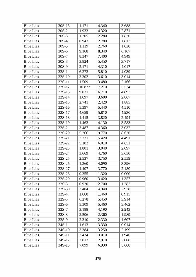
270
Blue Lias 30S-15 1.171 4.340 3.688
Blue Lias 30S-2 1.933 4.320 2.871
Blue Lias 30S-3 1.205 2.280 1.820
Blue Lias 30S-4 0.943 2.780 1.817
Blue Lias 30S-5 1.119 2.760 1.828
Blue Lias 30S-6 9.168 8.340 6.167
Blue Lias 30S-7 8.347 7.400 4.949
Blue Lias 30S-8 3.824 5.450 3.717
Blue Lias 30S-9 2.171 4.310 4.017
Blue Lias 32S-1 6.272 5.810 4.039
Blue Lias 32S-10 3.302 3.610 3.014
Blue Lias 32S-11 1.509 3.480 2.166
Blue Lias 32S-12 10.877 7.210 5.524
Blue Lias 32S-13 9.031 6.710 4.897
Blue Lias 32S-14 1.697 3.600 2.867
Blue Lias 32S-15 2.741 2.420 1.885
Blue Lias 32S-16 5.397 5.440 4.510
Blue Lias 32S-17 4.659 5.810 4.930
Blue Lias 32S-18 1.415 3.820 2.494
Blue Lias 32S-19 1.462 4.130 3.583
Blue Lias 32S-2 3.487 4.360 3.032
Blue Lias 32S-20 5.266 9.770 8.620
Blue Lias 32S-21 2.771 5.420 4.491
Blue Lias 32S-22 5.182 6.010 4.651
Blue Lias 32S-23 1.801 3.040 2.097
Blue Lias 32S-24 3.669 4.760 3.650
Blue Lias 32S-25 2.537 3.750 2.559
Blue Lias 32S-26 1.260 4.090 3.396
Blue Lias 32S-27 1.407 3.770 2.180
Blue Lias 32S-28 0.355 1.320 0.000
Blue Lias 32S-29 0.960 3.420 1.357
Blue Lias 32S-3 0.920 2.700 1.782
Blue Lias 32S-30 3.404 4.940 2.928
Blue Lias 32S-4 1.668 1.460 0.915
Blue Lias 32S-5 6.278 5.450 3.914
Blue Lias 32S-6 5.309 5.460 3.462
Blue Lias 32S-7 3.188 4.190 2.943
Blue Lias 32S-8 2.506 2.360 1.989
Blue Lias 32S-9 2.310 2.330 1.607
Blue Lias 34S-1 1.613 3.330 0.914
Blue Lias 34S-10 3.384 3.250 2.199
Blue Lias 34S-11 2.434 3.010 1.946
Blue Lias 34S-12 2.013 2.910 2.008
Blue Lias 34S-13 7.099 6.930 5.668

271
Blue Lias 34S-14 2.527 3.370 2.354
Blue Lias 34S-15 4.653 4.530 3.197
Blue Lias 34S-16 5.303 5.460 3.661
Blue Lias 34S-17 7.115 6.730 5.312
Blue Lias 34S-18 8.918 6.760 4.497
Blue Lias 34S-19 6.109 5.530 3.476
Blue Lias 34S-2 5.615 5.490 4.492
Blue Lias 34S-3 4.327 4.390 2.818
Blue Lias 34S-4 0.386 0.700 0.368
Blue Lias 34S-5 1.515 3.300 1.808
Blue Lias 34S-6 3.009 3.550 2.686
Blue Lias 34S-7 1.003 3.160 2.069
Blue Lias 34S-8 2.578 4.640 3.559
Blue Lias 34S-9 7.234 6.020 4.478
PORT-MULGRAVE SHALE SAMPLES
Formation Sample TOC %wt TS %wt TOS %wt
Whitby Mudstone JET17 5.050 11.846 7.475
Whitby Mudstone JET16 6.536 10.338 8.373
Whitby Mudstone JET15 6.132 14.013 10.346
Whitby Mudstone JET14 5.741 11.001 7.149
Whitby Mudstone JET13 4.261 14.910 13.059
Whitby Mudstone JET12 5.580 11.781 7.654
Whitby Mudstone JET11 6.036 15.163 11.983
Whitby Mudstone JET10 6.380 11.242 8.208
Whitby Mudstone JET9 4.931 12.418 8.433
Whitby Mudstone JET8 6.148 12.703 7.628
Whitby Mudstone JET7 12.617 12.736 8.135
Whitby Mudstone JET6 14.255 12.807 9.045
Whitby Mudstone JET5 7.135 10.110 6.160
Whitby Mudstone JET4 10.071 13.314 9.129
Whitby Mudstone JET3 9.614 12.088 7.242
Whitby Mudstone JET2 5.466 11.295 8.552
Whitby Mudstone JET1 5.327 9.659 5.753
Whitby Mudstone TL.5 2.903 7.105 4.469
Whitby Mudstone TL.4 3.562 9.740 6.111
Whitby Mudstone TL.3 4.534 9.267 7.417
Whitby Mudstone TL.2 6.141 12.285 10.921
Whitby Mudstone TL.1 6.128 12.161 11.969
Whitby Mudstone 4-MST7 1.927 5.725 4.618
Whitby Mudstone 4-MST6 1.411 3.592 3.023
Whitby Mudstone 4-MST5 1.479 3.938 3.003

272
Whitby Mudstone 4-MST4 1.599 4.177 3.539
Whitby Mudstone 4-MST3 1.392 3.390 2.262
Whitby Mudstone 4-MST2 1.633 3.390 2.381
Whitby Mudstone 4-MST1 1.638 4.485 3.070
Whitby Mudstone USB10 2.638 17.896 14.053
Whitby Mudstone USB9 2.590 16.159 9.453
Whitby Mudstone USB7 3.513 8.920 7.473
Whitby Mudstone USB6 3.137 8.950 7.257
Whitby Mudstone USB5 1.842 7.400 5.871
Whitby Mudstone USB4 2.867 8.320 3.572
Whitby Mudstone USB3 2.428 6.840 2.312
Whitby Mudstone USB2 1.814 7.170 4.070
Whitby Mudstone USB1 1.705 5.530 2.245
Whitby Mudstone 3-MST8 1.230 2.440 1.073
Whitby Mudstone 3-MST7 1.022 1.990 -1.216
Whitby Mudstone 3-MST6 1.229 2.330 1.108
Whitby Mudstone 3-MST5 1.534 3.240 1.313
Whitby Mudstone 3-MST4 1.426 2.960 1.410
Whitby Mudstone 3-MST3 1.370 2.890 2.017
Whitby Mudstone 3-MST2 1.200 4.290 1.468
Whitby Mudstone 3-MST1 2.112 5.030 3.355
Whitby Mudstone MSB24 1.730 3.330 1.328
Whitby Mudstone MSB23 1.440 3.230 0.664
Whitby Mudstone MSB22 1.130 3.390 1.319
Whitby Mudstone MSB21 1.560 6.459 3.277
Whitby Mudstone MSB20 2.200 5.090 1.719
Whitby Mudstone MSB19 2.660 6.990 3.880
Whitby Mudstone MSB18 2.390 7.850 3.915
Whitby Mudstone MSB17 2.380 5.841 2.676
Whitby Mudstone MSB16 2.230 5.450 3.060
Whitby Mudstone MSB15 2.080 5.270 2.394
Whitby Mudstone MSB14 2.080 4.580 1.740
Whitby Mudstone MSB13 1.960 4.130 1.650
Whitby Mudstone MSB12 1.840 4.670 2.186
Whitby Mudstone MSB11 1.710 3.180 1.022
Whitby Mudstone MSB10 1.800 4.640 1.765
Whitby Mudstone MSB9 1.770 4.253 1.669
Whitby Mudstone MSB8 1.660 5.550 2.964
Whitby Mudstone MSB7 1.690 6.817 4.066
Whitby Mudstone MSB6 1.900 6.300 2.158
Whitby Mudstone MSB5 2.850 7.216 2.816
Whitby Mudstone MSB4 3.180 7.850 3.032
Whitby Mudstone MSB3 2.660 10.126 4.705
Whitby Mudstone MSB2 3.330 7.133 2.291

273
Whitby Mudstone MSB1 4.680 8.450 3.090
Whitby Mudstone 2-MST8 2.210 9.048 3.496
Whitby Mudstone 2-MST7 1.100 8.440 5.272
Whitby Mudstone 2-MST6 1.100 13.320 12.236
Whitby Mudstone 2-MST5 1.660 9.310 3.919
Whitby Mudstone 2-MST4 1.210 4.270 2.613
Whitby Mudstone 2-MST3 0.990 3.343 -0.695
Whitby Mudstone 2-MST2 0.970 5.440 2.920
Whitby Mudstone 2-MST1 1.070 0.910 -2.178
Whitby Mudstone LSB14 2.507 11.241 5.049
Whitby Mudstone LSB13 5.726 13.196 11.479
Whitby Mudstone LSB12 6.273 11.892 5.331
Whitby Mudstone LSB11 2.915 12.004 9.009
Whitby Mudstone LSB10 0.802 15.217 12.234
Whitby Mudstone LSB9 6.809 15.583 12.463
Whitby Mudstone LSB8 6.296 15.540 7.287
Whitby Mudstone LSB7 2.333 13.533 9.892
Grey Shale LSB6 1.410 8.699 4.365
Grey Shale LSB5 1.275 5.445 3.221
Grey Shale LSB4 1.160 5.994 3.110
Grey Shale LSB3 1.542 5.263 2.749
Grey Shale LSB2 1.020 5.395 2.559
Grey Shale LSB1 1.305 5.145 0.215
Grey Shale 1-MST6 0.990 4.460 2.545
Grey Shale 1-MST5 0.940 4.150 1.690
Grey Shale 1-MST4 0.990 3.950 1.313
Grey Shale 1-MST3 0.770 4.235 0.819
Grey Shale 1-MST2 0.840 5.235 2.770
Grey Shale 1-MST1 0.330 5.800 1.461
School archived samples
Reference sample TOC
Adrian Piper CGD25 2.500
Adrian Piper CW24 0.880
Adrian Piper CW27 2.270
Adrian Piper CW29 2.940
Adrian Piper CW45 0.720
Adrian Piper CW50 2.820
Adrian Piper H2 1.900
Adrian Piper H22 1.400
Adrian Piper H34 1.800
Alastair Vincent KE41 1.000
Alastair Vincent LBM1 1.000
Alastair Vincent LBT2 1.200

274
Alastair Vincent LOK6 1.200
Ali Nategh PJ43 3.900
Ali Nategh PJ43R 3.900
Ali Nategh PJ49 4.000
Ali Nategh PJ50 6.100
Ali Nategh PJ61-3 6.700
Ali Nategh PJ61-4 6.000
Ali Nategh PJ61-5 5.400
Ali Nategh PJ61-6 6.900
Ali Nategh RG42 2.700
Ali Nategh RG43 1.800
Ali Nategh RG44 1.700
Alastair Vincent RNB13 1.400
Alastair Vincent RNB17 4.400
Alastair Vincent RNB7 1.600
Alastair Vincent RNB9 3.300
Adrian Piper SC40 3.990
Adrian Piper SC45 2.730
Adrian Piper SC48 1.810
Adrian Piper SC57 2.840
Adrian Piper SC69 1.620
Adrian Piper SC70 2.040
Adrian Piper SC77 11.820
Adrian Piper STG1 1.200
Adrian Piper STG11 1.300
Adrian Piper STG11R 1.300
Adrian Piper STG12 1.400
Adrian Piper STG14 1.100
Adrian Piper STG14R 1.100
Adrian Piper STG15 1.100
Adrian Piper STG16 1.200
Adrian Piper STG18 6.000
Adrian Piper STG18R 6.000
Adrian Piper STG25 2.600
Adrian Piper STG25R 2.600
Adrian Piper STG27 1.700
Adrian Piper STG28 2.500
Adrian Piper STG28R 2.500
Adrian Piper STG32 1.300
Adrian Piper STG34 1.400
Adrian Piper STG34R 1.400
Adrian Piper STG35 1.700
Adrian Piper STG36 1.800
Adrian Piper STG39 2.000

275
Adrian Piper STG4 1.400
Adrian Piper STG41 1.800
Adrian Piper STG41R 1.800
Adrian Piper STG42 3.400
Adrian Piper STG42R 3.400
Adrian Piper STG44d 3.200
Adrian Piper STG45 2.000
Adrian Piper STG46 2.100
Adrian Piper STG48 1.800
Adrian Piper STG4R 1.400
Adrian Piper STG6 1.700
Adrian Piper STG8b 6.600
Adrian Piper STG8bR 6.600
Adrian Piper STG9 3.100
Alastair Vincent UOB24 1.300
Alastair Vincent UOB31 6.900
Alastair Vincent UOB34 5.500
Alastair Vincent UOB35 2.600
Adrian Piper YN100 0.790
Adrian Piper YN107 1.780
Adrian Piper YN109 10.890
Adrian Piper YN111 8.020
Adrian Piper YN115 0.920
Adrian Piper YN117 5.760
Adrian Piper YN18 0.690
Adrian Piper YN19 1.120
Adrian Piper YN22 2.960
Adrian Piper YN25 0.560
Adrian Piper YN68 0.780
Adrian Piper YN7 0.890
Adrian Piper YN91 3.680
Adrian Piper YN91R 3.680
Adrian Piper YN92 1.330
Gorden Ross Cblr10-a 0.800
Gorden Ross Cblr13 0.330
Gorden Ross Cblr14 1.390
Gorden Ross Cblr15-a 6.800
Gorden Ross Cblr15-b 5.210
Gorden Ross Cblr17 0.370
Gorden Ross Cblr18-19 2.500
Gorden Ross Cblr21 2.160
Gorden Ross Cblr23 0.600
Gorden Ross Cblr25-a 1.230
Gorden Ross Cblr25-b 8.780

276
Gorden Ross Cblr26 1.200
Gorden Ross Cblr26R 1.200
Gorden Ross Cblr27 9.290
Gorden Ross Cblr2-a 8.850
Gorden Ross Cblr2-b 5.870
Gorden Ross Cblr3 3.400
Gorden Ross Cblr31 8.750
Gorden Ross Cblr31-32 2.450
Gorden Ross Cblr31R 8.750
Gorden Ross Cblr32 6.020
Gorden Ross Cblr33 1.240
Gorden Ross Cblr36 4.580
Gorden Ross Cblr36R 4.580
Gorden Ross Cblr37 2.070
Gorden Ross Cblr38 4.040
Gorden Ross Cblr39 1.900
Gorden Ross Cblr40 7.270
Gorden Ross Cblr41 1.620
Gorden Ross Cblr42 1.440
Gorden Ross Cblr45-a 0.740
Gorden Ross Cblr45-b 1.660
Gorden Ross Cblr46 2.810
Gorden Ross Cblr47 1.530
Gorden Ross Cblr47R 1.530
Gorden Ross Cblr49-50 4.000
Gorden Ross Cblr5 0.670
Gorden Ross Cblr50 4.000
Gorden Ross Cblr53 7.220
Gorden Ross Cblr56 1.040
Gorden Ross Cblr57 4.200
Gorden Ross Cblr58 2.130
Gorden Ross Cblr60 6.560
Gorden Ross Cblr60R 6.560
Gorden Ross Cblr66 2.830
Gorden Ross Cblr67 6.210
Gorden Ross Cblr68 4.280
Gorden Ross Cblr6-a 6.470
Gorden Ross Cblr6-b 7.910
Gorden Ross Cblr7 6.070
Gorden Ross Cblr70 1.620
Gorden Ross Cblr70R 1.620
Gorden Ross Cblr72 1.280
Gorden Ross Cblr8 4.440
Gorden Ross Cblr8R 4.440
Copyright © 2022 FDOKUMEN