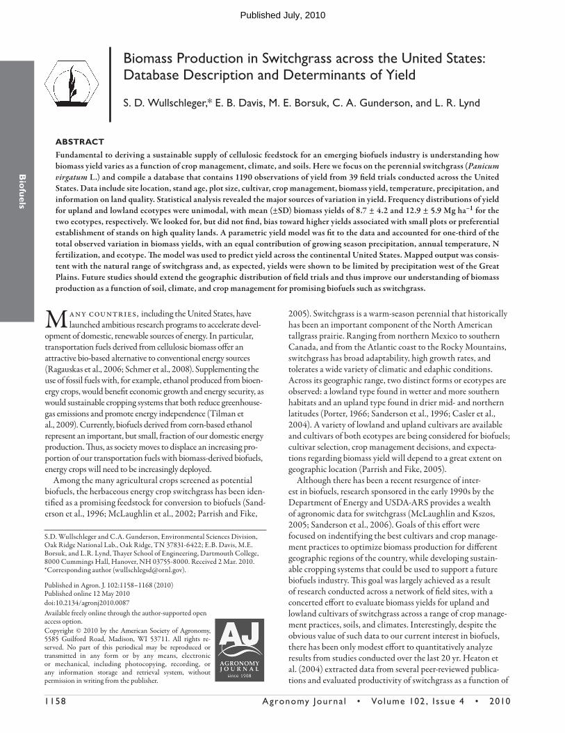
Biomass Production in Switchgrass across the United States: Database Description and Determinants of...
11
Biofuels 1158 Agronomy Journal • Volume 102, Issue 4 • 2010 Published in Agron. J. 102:1158–1168 (2010) Published online 12 May 2010 doi:10.2134/agronj2010.0087 Available freely online through the author-supported open access option. Copyright © 2010 by the American Society of Agronomy, 5585 Guilford Road, Madison, WI 53711. All rights re- served. No part of this periodical may be reproduced or transmitted in any form or by any means, electronic or mechanical, including photocopying, recording, or any information storage and retrieval system, without permission in writing from the publisher. M any countries, including the United States, have launched ambitious research programs to accelerate devel- opment of domestic, renewable sources of energy. In particular, transportation fuels derived from cellulosic biomass offer an attractive bio-based alternative to conventional energy sources (Ragauskas et al., 2006; Schmer et al., 2008). Supplementing the use of fossil fuels with, for example, ethanol produced from bioen- ergy crops, would benefit economic growth and energy security, as would sustainable cropping systems that both reduce greenhouse- gas emissions and promote energy independence (Tilman et al., 2009). Currently, biofuels derived from corn-based ethanol represent an important, but small, fraction of our domestic energy production. us, as society moves to displace an increasing pro- portion of our transportation fuels with biomass-derived biofuels, energy crops will need to be increasingly deployed. Among the many agricultural crops screened as potential biofuels, the herbaceous energy crop switchgrass has been iden- tified as a promising feedstock for conversion to biofuels (Sand- erson et al., 1996; McLaughlin et al., 2002; Parrish and Fike, 2005). Switchgrass is a warm-season perennial that historically has been an important component of the North American tallgrass prairie. Ranging from northern Mexico to southern Canada, and from the Atlantic coast to the Rocky Mountains, switchgrass has broad adaptability, high growth rates, and tolerates a wide variety of climatic and edaphic conditions. Across its geographic range, two distinct forms or ecotypes are observed: a lowland type found in wetter and more southern habitats and an upland type found in drier mid- and northern latitudes (Porter, 1966; Sanderson et al., 1996; Casler et al., 2004). A variety of lowland and upland cultivars are available and cultivars of both ecotypes are being considered for biofuels; cultivar selection, crop management decisions, and expecta- tions regarding biomass yield will depend to a great extent on geographic location (Parrish and Fike, 2005). Although there has been a recent resurgence of inter- est in biofuels, research sponsored in the early 1990s by the Department of Energy and USDA-ARS provides a wealth of agronomic data for switchgrass (McLaughlin and Kszos, 2005; Sanderson et al., 2006). Goals of this effort were focused on indentifying the best cultivars and crop manage- ment practices to optimize biomass production for different geographic regions of the country, while developing sustain- able cropping systems that could be used to support a future biofuels industry. is goal was largely achieved as a result of research conducted across a network of field sites, with a concerted effort to evaluate biomass yields for upland and lowland cultivars of switchgrass across a range of crop manage- ment practices, soils, and climates. Interestingly, despite the obvious value of such data to our current interest in biofuels, there has been only modest effort to quantitatively analyze results from studies conducted over the last 20 yr. Heaton et al. (2004) extracted data from several peer-reviewed publica- tions and evaluated productivity of switchgrass as a function of ABSTRACT Fundamental to deriving a sustainable supply of cellulosic feedstock for an emerging biofuels industry is understanding how biomass yield varies as a function of crop management, climate, and soils. Here we focus on the perennial switchgrass (Panicum virgatum L.) and compile a database that contains 1190 observations of yield from 39 field trials conducted across the United States. Data include site location, stand age, plot size, cultivar, crop management, biomass yield, temperature, precipitation, and information on land quality. Statistical analysis revealed the major sources of variation in yield. Frequency distributions of yield for upland and lowland ecotypes were unimodal, with mean (±SD) biomass yields of 8.7 ± 4.2 and 12.9 ± 5.9 Mg ha –1 for the two ecotypes, respectively. We looked for, but did not find, bias toward higher yields associated with small plots or preferential establishment of stands on high quality lands. A parametric yield model was fit to the data and accounted for one-third of the total observed variation in biomass yields, with an equal contribution of growing season precipitation, annual temperature, N fertilization, and ecotype. e model was used to predict yield across the continental United States. Mapped output was consis- tent with the natural range of switchgrass and, as expected, yields were shown to be limited by precipitation west of the Great Plains. Future studies should extend the geographic distribution of field trials and thus improve our understanding of biomass production as a function of soil, climate, and crop management for promising biofuels such as switchgrass. S.D. Wullschleger and C.A. Gunderson, Environmental Sciences Division, Oak Ridge National Lab., Oak Ridge, TN 37831-6422; E.B. Davis, M.E. Borsuk, and L.R. Lynd, ayer School of Engineering, Dartmouth College, 8000 Cummings Hall, Hanover, NH 03755-8000. Received 2 Mar. 2010. *Corresponding author ([email protected]). Biomass Production in Switchgrass across the United States: Database Description and Determinants of Yield S. D. Wullschleger,* E. B. Davis, M. E. Borsuk, C. A. Gunderson, and L. R. Lynd Published July, 2010
Transcript of Biomass Production in Switchgrass across the United States: Database Description and Determinants of...
Biofuels
1158 Agronomy Journa l • Volume 102 , I s sue 4 • 2010
Published in Agron. J. 102:1158–1168 (2010)Published online 12 May 2010doi:10.2134/agronj2010.0087Available freely online through the author-supported open access option.Copyright © 2010 by the American Society of Agronomy, 5585 Guilford Road, Madison, WI 53711. All rights re-served. No part of this periodical may be reproduced or transmitted in any form or by any means, electronic or mechanical, including photocopying, recording, or any information storage and retrieval system, without permission in writing from the publisher.
Many countries, including the United States, have launched ambitious research programs to accelerate devel-
opment of domestic, renewable sources of energy. In particular, transportation fuels derived from cellulosic biomass off er an attractive bio-based alternative to conventional energy sources (Ragauskas et al., 2006; Schmer et al., 2008). Supplementing the use of fossil fuels with, for example, ethanol produced from bioen-ergy crops, would benefi t economic growth and energy security, as would sustainable cropping systems that both reduce greenhouse-gas emissions and promote energy independence (Tilman et al., 2009). Currently, biofuels derived from corn-based ethanol represent an important, but small, fraction of our domestic energy production. Th us, as society moves to displace an increasing pro-portion of our transportation fuels with biomass-derived biofuels, energy crops will need to be increasingly deployed.
Among the many agricultural crops screened as potential biofuels, the herbaceous energy crop switchgrass has been iden-tifi ed as a promising feedstock for conversion to biofuels (Sand-erson et al., 1996; McLaughlin et al., 2002; Parrish and Fike,
2005). Switchgrass is a warm-season perennial that historically has been an important component of the North American tallgrass prairie. Ranging from northern Mexico to southern Canada, and from the Atlantic coast to the Rocky Mountains, switchgrass has broad adaptability, high growth rates, and tolerates a wide variety of climatic and edaphic conditions. Across its geographic range, two distinct forms or ecotypes are observed: a lowland type found in wetter and more southern habitats and an upland type found in drier mid- and northern latitudes (Porter, 1966; Sanderson et al., 1996; Casler et al., 2004). A variety of lowland and upland cultivars are available and cultivars of both ecotypes are being considered for biofuels; cultivar selection, crop management decisions, and expecta-tions regarding biomass yield will depend to a great extent on geographic location (Parrish and Fike, 2005).
Although there has been a recent resurgence of inter-est in biofuels, research sponsored in the early 1990s by the Department of Energy and USDA-ARS provides a wealth of agronomic data for switchgrass (McLaughlin and Kszos, 2005; Sanderson et al., 2006). Goals of this eff ort were focused on indentifying the best cultivars and crop manage-ment practices to optimize biomass production for diff erent geographic regions of the country, while developing sustain-able cropping systems that could be used to support a future biofuels industry. Th is goal was largely achieved as a result of research conducted across a network of fi eld sites, with a concerted eff ort to evaluate biomass yields for upland and lowland cultivars of switchgrass across a range of crop manage-ment practices, soils, and climates. Interestingly, despite the obvious value of such data to our current interest in biofuels, there has been only modest eff ort to quantitatively analyze results from studies conducted over the last 20 yr. Heaton et al. (2004) extracted data from several peer-reviewed publica-tions and evaluated productivity of switchgrass as a function of
ABSTRACTFundamental to deriving a sustainable supply of cellulosic feedstock for an emerging biofuels industry is understanding how biomass yield varies as a function of crop management, climate, and soils. Here we focus on the perennial switchgrass (Panicum virgatum L.) and compile a database that contains 1190 observations of yield from 39 fi eld trials conducted across the United States. Data include site location, stand age, plot size, cultivar, crop management, biomass yield, temperature, precipitation, and information on land quality. Statistical analysis revealed the major sources of variation in yield. Frequency distributions of yield for upland and lowland ecotypes were unimodal, with mean (±SD) biomass yields of 8.7 ± 4.2 and 12.9 ± 5.9 Mg ha–1 for the two ecotypes, respectively. We looked for, but did not fi nd, bias toward higher yields associated with small plots or preferential establishment of stands on high quality lands. A parametric yield model was fi t to the data and accounted for one-third of the total observed variation in biomass yields, with an equal contribution of growing season precipitation, annual temperature, N fertilization, and ecotype. Th e model was used to predict yield across the continental United States. Mapped output was consis-tent with the natural range of switchgrass and, as expected, yields were shown to be limited by precipitation west of the Great Plains. Future studies should extend the geographic distribution of fi eld trials and thus improve our understanding of biomass production as a function of soil, climate, and crop management for promising biofuels such as switchgrass.
S.D. Wullschleger and C.A. Gunderson, Environmental Sciences Division, Oak Ridge National Lab., Oak Ridge, TN 37831-6422; E.B. Davis, M.E. Borsuk, and L.R. Lynd, Th ayer School of Engineering, Dartmouth College, 8000 Cummings Hall, Hanover, NH 03755-8000. Received 2 Mar. 2010. *Corresponding author ([email protected]).
Biomass Production in Switchgrass across the United States: Database Description and Determinants of Yield
S. D. Wullschleger,* E. B. Davis, M. E. Borsuk, C. A. Gunderson, and L. R. Lynd
Published July, 2010
Agronomy Journa l • Volume 102, Issue 4 • 2010 1159
N fertilization, growing degree days, and precipitation. Th eir analysis, while limited (i.e., 77 observations), showed that yield responded positively to water and N, but not temperature, and that biomass yields averaged 10.3 Mg ha–1 for stands harvested 3 yr or more aft er planting (Heaton et al., 2004). No attempt was made to identify ecotypic variation in patterns of response or to interpret these fi ndings in a geographic context; however, the results illustrate clearly how biomass yield for this species could vary as a function of climate across the United States.
To achieve the ambitious biofuel production goals set forth for the United States and other countries, more information is needed to characterize productivity of bioenergy crops in relation to soil, climate, and management practices. In this study, we compile published literature on biomass yield for lowland and upland ecotypes of switchgrass grown at 39 fi eld sites across the United States. Th e resulting database contains information on cultivar-specifi c biomass yield, site location, plot size, stand age, harvest frequency, fertilizer application, soil texture, temperature, precipitation, and land quality. Th e primary objective of this study was to examine relationships between these factors and yield, and to develop an empirical model that describes biomass yield as a function of signifi cant variables in the database. Our interest in conducting this analysis was motivated by several fac-tors, one of which was the recent work of Johnston et al. (2009), who commented that in communicating potential biofuels production to an increasingly diverse audience, researchers oft en fail to emphasize that yield estimates are collected from numerous disparate sources and sometimes neglect how biomass produc-tion is infl uenced by geographic location, climate, soil type, or agricultural management regime for the crop in question. Com-pilation of a database for biomass yield in switchgrass, as we have undertaken here, attempts to address this concern for switchgrass. Issues of plot size and land quality as sources of potential bias are
also examined. Th e empirical model derived from the database was used to provide a spatially explicit projection of biomass yield across the United States for upland and lowland ecotypes based on precipitation, temperature, and level of N fertilization. We conclude with a discussion of future research needs to better understand and then model biomass production for switchgrass.
MATERIALS AND METHODSData Collection and Characterization
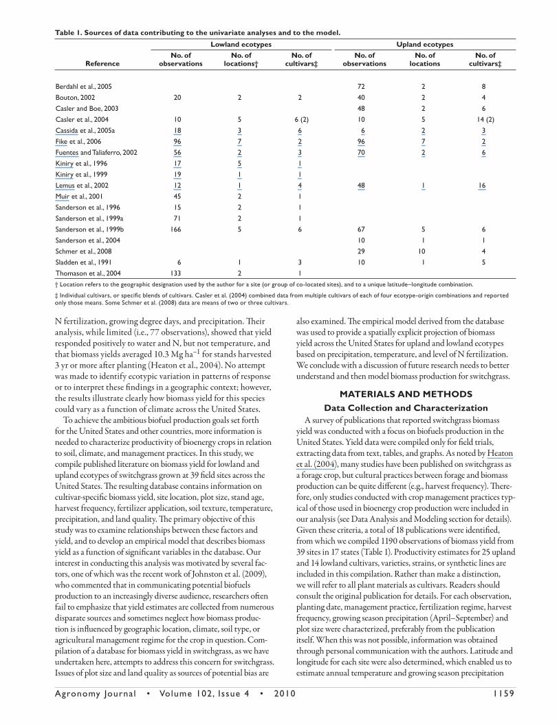
A survey of publications that reported switchgrass biomass yield was conducted with a focus on biofuels production in the United States. Yield data were compiled only for fi eld trials, extracting data from text, tables, and graphs. As noted by Heaton et al. (2004), many studies have been published on switchgrass as a forage crop, but cultural practices between forage and biomass production can be quite diff erent (e.g., harvest frequency). Th ere-fore, only studies conducted with crop management practices typ-ical of those used in bioenergy crop production were included in our analysis (see Data Analysis and Modeling section for details). Given these criteria, a total of 18 publications were identifi ed, from which we compiled 1190 observations of biomass yield from 39 sites in 17 states (Table 1). Productivity estimates for 25 upland and 14 lowland cultivars, varieties, strains, or synthetic lines are included in this compilation. Rather than make a distinction, we will refer to all plant materials as cultivars. Readers should consult the original publication for details. For each observation, planting date, management practice, fertilization regime, harvest frequency, growing season precipitation (April–September) and plot size were characterized, preferably from the publication itself. When this was not possible, information was obtained through personal communication with the authors. Latitude and longitude for each site were also determined, which enabled us to estimate annual temperature and growing season precipitation
Table 1. Sources of data contributing to the univariate analyses and to the model.
Reference
Lowland ecotypes Upland ecotypesNo. of
observationsNo. of
locations†No. of
cultivars‡No. of
observationsNo. of
locationsNo. of
cultivars‡
Berdahl et al., 2005 72 2 8Bouton, 2002 20 2 2 40 2 4Casler and Boe, 2003 48 2 6Casler et al., 2004 10 5 6 (2) 10 5 14 (2)Cassida et al., 2005a 18 3 6 6 2 3Fike et al., 2006 96 7 2 96 7 2Fuentes and Taliaferro, 2002 56 2 3 70 2 6Kiniry et al., 1996 17 5 1Kiniry et al., 1999 19 1 1Lemus et al., 2002 12 1 4 48 1 16Muir et al., 2001 45 2 1Sanderson et al., 1996 15 2 1Sanderson et al., 1999a 71 2 1Sanderson et al., 1999b 166 5 6 67 5 6Sanderson et al., 2004 10 1 1Schmer et al., 2008 29 10 4Sladden et al., 1991 6 1 3 10 1 5Thomason et al., 2004 133 2 1† Location refers to the geographic designation used by the author for a site (or group of co-located sites), and to a unique latitude–longitude combination.
‡ Individual cultivars, or specifi c blends of cultivars. Casler et al. (2004) combined data from multiple cultivars of each of four ecotype-origin combinations and reported only those means. Some Schmer et al. (2008) data are means of two or three cultivars.
1160 Agronomy Journa l • Volume 102, Issue 4 • 2010
(when not available from the publications or authors) from the Parameter-Elevation Regressions on Independent Slopes Model (i.e., PRISM) data set. Th is method of interpolation accounts for spatial variation in climate caused by elevation, terrain orienta-tion, eff ectiveness of terrain as a barrier to fl ow, coastal proximity, moisture availability, a two-layer atmosphere to handle inversions, and topographic position (Daly, 2006). Using ArcInfo (ESRI, Redlands, CA) monthly and annual climate data corresponding to the harvest year at a given site were extracted from the PRISM data set for temperature and precipitation. Latitude and longitude were also used to derive soil texture (e.g., sand, silt, and clay) and to assign a land capability class, as defi ned by the USDA Natural Resources Conservation Service, to each of the fi eld sites. Using this system, eight land capability classes are defi ned, ranging from 1 for soils that have slight limitations that might restrict their use to 8 for soils that have limitations that preclude commercial plant production and restrict their use to wildlife habitat, watershed, recreation, or esthetic purposes. Information on land capability classes for nonirrigated lands was obtained from the Soil Survey Geographic Database (SSURGO).
Data Analysis and Modeling
In addition to descriptive statistics and bivariate plots, we also fi t multivariate statistical models to the data. Th is began with an exploratory data analysis using a generalized additive model (GAM) framework (Hastie and Tibshirani, 1990). In a model of this type, the traditional linear or nonlinear parametric function relating response and predictor variables can be replaced by a non-parametric smoothing function. Th is provides a fl exible method for visualizing relationships when the choice of a parametric func-tion is not obvious. A GAM has the following model form:
1
( )p
i ii
Y f Xα ε=
= + +∑
[1]
where Y is the response variable of interest, α is the overall mean of Y, fi is a smoothing function for the ith of p possible predictor variables Xi, and ε is a normally distributed error term. Th e smoothing functions, which are estimated iteratively using a back-fi tting algorithm, describe locally persistent pat-terns in the data attributable to each predictor variable. Plots of smoothing functions together with partial model residuals can aid in selection of appropriate functional forms for parametric model construction. Th e GAM library (Hastie, 1991), written for the statistical graphics and programming package R (Ikaha and Gentleman, 1996) was used for this analysis.
Based on the GAM results, we then formulated a multiplica-tive, parametric model for biomass yield, ypred, which included a temperature term, ytemp, allowing for an intermediate optimum and the potential for diff ering rising and falling limbs; a precipi-tation term, yprecip, with decreasing marginal eff ect; a linear N fertilization term yfert; and an ecotype (upland vs. lowland) term, ylow, which can be interpreted as the average multiple by which lowland cultivars outperform upland cultivars. To account for the observation that, at high latitudes, upland cultivars are more competitive (Casler et al., 2004), this ecotype term includes an adjustment allowing for a decline in the yield of lowland cultivars as a linear function of degrees north of a latitudinal threshold. Both the threshold and the rate of yield decline are parameters to be estimated from the data. Th e temperature and fertilization
terms in the model include an intercept to account for the fact that a nonzero yield is possible at extreme temperatures with no fertilization. We did not include an intercept term for precipita-tion. Th e full biomass yield model can thus be written as:
ypred = ytemp × yprecip × ylow × yfert [2]
where
temp
2[ ( ) ]t opt1opt t opt
2[ ( ) ] t opt2opt t opt
1 for
1 for
k x t
k x tk e x t
k e x ty
− −
− −
+ ≤
+ >
⎧⎪⎪=⎨⎪⎪⎩ [3]
precip p py k x=
[4]
fert fert f1y k x= + × [5]
{ for uplandlow for lowlandlow lat
1 max(0,lat-lat*) k ky − ×=
[6]
andxt = annual average temperature (ºC)xp = growing season precipitation (mm)xf = N fertilization (kg ha–1)lat = latitude (oN)
and kopt, k1, k2, topt, kp, kfert, klow, klat, and lat* are parameters estimated from the data. Other functional forms could have been chosen for our model, but we felt that those we employed were reasonably robust, yet suffi ciently simple to allow for empirical parameter identifi cation. Parameter estimates were initially allowed to diff er between ecotypes; however, no con-sistent or statistically signifi cant diff erences were revealed by our data. Th erefore, all parameters were assumed to be equiva-lent across ecotypes (with the exception of the parameters of the yield term ylow, which only apply to lowland cultivars).
To estimate parameter values, we used the nonlinear least squares function nls, available for the statistical graphics and programming package R (Ikaha and Gentleman, 1996). To limit k1 and k2 to strictly positive values, the logarithmic transforma-tion of these coeffi cients was used as the fi tted parameter, which was then re-exponentiated. Residual analysis revealed that the assumptions of regression were better met by fi tting a logarithmic transformation of the yield equation. Initial observations con-fi rmed the known association of low yields with fi rst-year stands and four-cut harvest systems (data not shown). Yield data from fi rst-year harvest and four-cut systems were therefore dropped from the regression analyses to better relate yield to variables of interest. Finally, some plots in one study were subjected to N fertilizer application rates of 448 and 896 kg ha–1 (Th omason et al., 2004). Th ese values far exceeded those for other plots in our dataset and exerted disproportionate leverage on the model fi t. We therefore excluded these points from our analysis.
Th e geographic distribution of yield across the continental United States was determined using the multiplicative, para-metric model. We applied equations and parameter coeffi cients to spatially distributed 30-yr climate averages from PRISM and generated a 400 × 400 m resolution thematic raster map using Albers Equal Area Conic projections and ESRI ArcInfo (Red-lands, CA). To represent both ecotypes on a single map, lowland yield projections are represented across the country, up to 38.2°N
Agronomy Journa l • Volume 102, Issue 4 • 2010 1161
latitude, where they generally outperform upland ecotypes, and are thus more likely to be planted. Above 38.2°N lowland yield predictions decrease by 12.5% per degree until 42.2°N above which upland outperforms lowland. While the model was applied to all areas of the continental United States, it is important to note that relatively large areas are extrapolated beyond the limits of the model which could introduce potential error and reduce statistical robustness. Th us, there could be local diff erences that have not been identifi ed in these extrapolated areas.
RESULTS AND DISCUSSIONBiomass Yield, Cultivar Selection,
and Crop Management FactorsTh e compiled database covers 39 fi eld sites across 17 states from
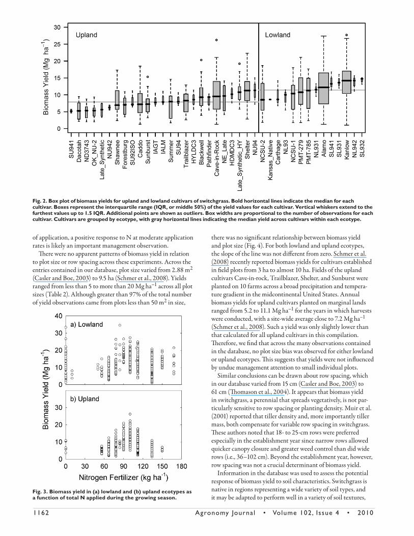
Beeville, TX (Sanderson et al., 1999a) in the south, to Munich, ND (Schmer et al., 2008) in the Midwest, to Rock Springs, PA (Sanderson et al., 2004) in the northeast. Lowland cultivars were generally planted in the south, whereas upland cultivars were planted across the full range of latitudes. For the database com-piled, annual switchgrass yields varied from less than 1 Mg ha–1 to almost 40 Mg ha–1 (Fig. 1a). As indicated by a histogram of the data distribution, the most frequently observed yield classes across all cultivars, soils, climate, and crop management practices were between 10 and 14 Mg ha–1. Th e frequency distribution for the total database was unimodal and skewed to the left , with a long tail at higher yields. Biomass yields greater than 28 Mg ha–1 were uncommon, but were reported for lowland ecotypes (e.g., Kanlow and Alamo) planted at fi eld sites in Alabama, Texas, and Oklahoma (Sladden et al., 1991; Kiniry et al., 2005; Th omason et al., 2004). Th e highest annual yield reported in this compilation was 39.1 Mg ha–1 for the cultivar Alamo under high fertilization (200 kg N ha–1) and in a year with high precipitation and tem-peratures (Kiniry et al., 1999). Frequency distributions for upland (Fig. 1b) and lowland (Fig. 1c) ecotypes were similar in shape (i.e., unimodal, skewed to the left , with long tails), with mean (±SD) biomass yields of 8.7 ± 4.2 Mg ha–1 and 12.9 ± 5.9 Mg ha–1 for the two ecotypes, respectively. Diff erences between ecotypes were signifi cant (p < 0.001).
Just as yield diff erences were observed between upland and lowland ecotypes, there was also considerable variation in biomass yields between cultivars within an ecotype (Fig. 2). Within the lowland ecotype, Alamo, SL941, SL931, Kanlow, NL942 and SL932 were the highest yielding cultivars with median rates of annual biomass production that ranged from 12.2 to 14.8 Mg ha–1 (Fig. 2). Kanlow and Alamo were the two most reported lowland cultivars in this compilation with 240 and 277 yield observations, respectively. Th e high-yielding lowland cultivars SL931, SL932, SL941, and NL942 had only four observations each. According to Cassida et al. (2005b), the cultivars with NL and SL designations are northern and southern lowland synthetic lines from Okla-homa and southern Kansas (i.e., NL942) and from central and southern Texas (i.e., SL931, SL932, and SL941). Among upland ecotypes, Cave-in-Rock, NE Late, HDMDC3, the experimental strain Late Synthetic HY, Shelter, and NU94 were the highest yielding cultivars with median rates of annual biomass production that ranged from 9.6 to 11.4 Mg ha–1 (Fig. 2). For these cultivars, Cave-in-Rock had far more observations associated with it (n = 119) than did NE Late (n = 10), HDMDC3 (n = 3), Late Syn-thetic HY (n = 14), Shelter (n = 62), and NU94 (n = 3).
Although variability was high, there was a distinct response of switchgrass yield to N fertilizer for both ecotypes (Fig. 3). For lowland ecotypes (Fig. 3a), there was a hint of an opti-mum around 100 kg N ha–1, but in many cases the zero fertilizer plantings did as well as fertilized stands. In upland ecotypes (Fig. 3b), yields appeared to respond to total rates of N application up to approximately 100 kg ha–1 and decreased above those rates, although there were fewer observations at higher application rates and none above 160 kg ha–1, making comparison to the lowland responses diffi cult. High levels of fertilization did not guarantee increased biomass production. Th is analysis does not take into account timing of N applica-tion, whether or not other nutrients were added, or the N availability in native soil. Th omason et al. (2004) did not see a strong response of biomass yield to variation in either rate or timing of N application, whereas Muir et al. (2001) saw yields increase with N application from zero to 170 or 224 kg ha–1. Parrish and Fike (2005) summarize the issue of N application in switchgrass as “unsettled” and suggest that the range of recommendations for N management “is not narrowing, nor is a central tendency developing.” Th ey describe switchgrass as a plant that is inherently N-thrift y, especially when managed for biomass production. Although the biomass yield summaries presented here do not indicate an unqualifi ed dependence on fertilization, and certainly not a strong response to high levels
Fig. 1. Frequency distributions showing biomass yields reported for (a) both upland and lowland ecotypes, (b) upland ecotypes, and (c) lowland ecotypes. The number of observations analyzed for each category is shown in parentheses.
1162 Agronomy Journa l • Volume 102, Issue 4 • 2010
of application, a positive response to N at moderate application rates is likely an important management observation.
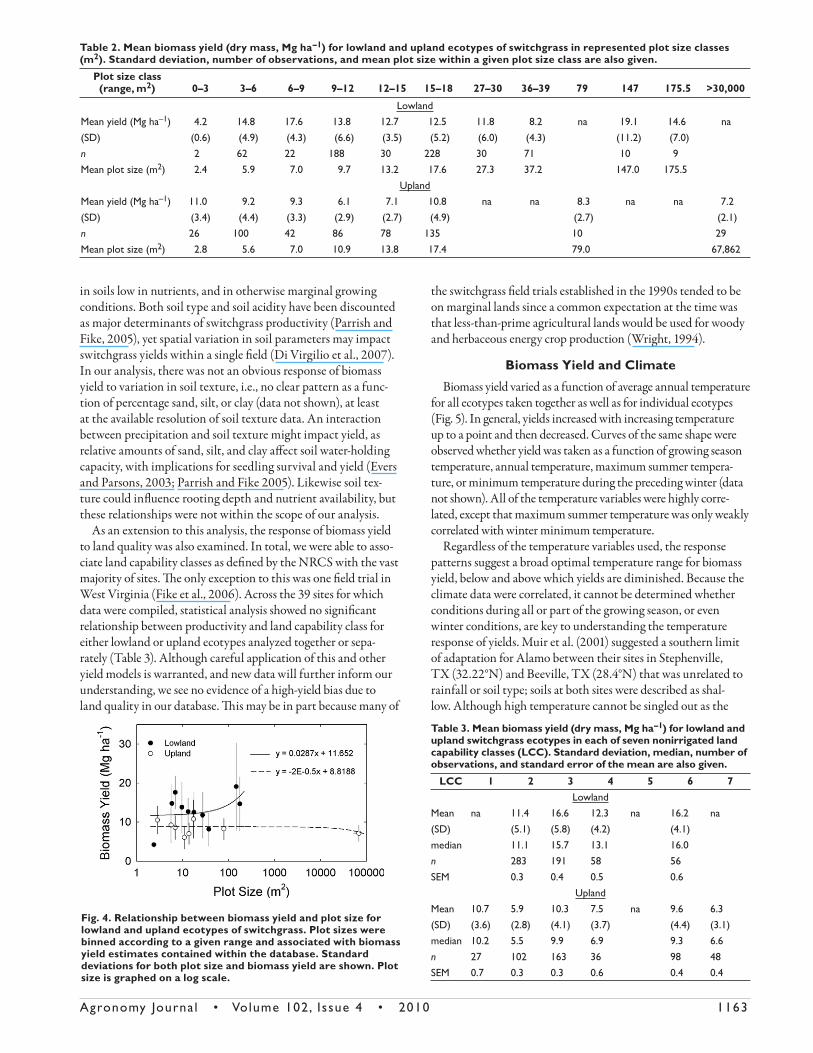
Th ere were no apparent patterns of biomass yield in relation to plot size or row spacing across these experiments. Across the entries contained in our database, plot size varied from 2.88 m2 (Casler and Boe, 2003) to 9.5 ha (Schmer et al., 2008). Yields ranged from less than 5 to more than 20 Mg ha–1 across all plot sizes (Table 2). Although greater than 97% of the total number of yield observations came from plots less than 50 m2 in size,
there was no signifi cant relationship between biomass yield and plot size (Fig. 4). For both lowland and upland ecotypes, the slope of the line was not diff erent from zero. Schmer et al. (2008) recently reported biomass yields for cultivars established in fi eld plots from 3 ha to almost 10 ha. Fields of the upland cultivars Cave-in-rock, Trailblazer, Shelter, and Sunburst were planted on 10 farms across a broad precipitation and tempera-ture gradient in the midcontinental United States. Annual biomass yields for upland cultivars planted on marginal lands ranged from 5.2 to 11.1 Mg ha–1 for the years in which harvests were conducted, with a site-wide average close to 7.2 Mg ha–1 (Schmer et al., 2008). Such a yield was only slightly lower than that calculated for all upland cultivars in this compilation. Th erefore, we fi nd that across the many observations contained in the database, no plot size bias was observed for either lowland or upland ecotypes. Th is suggests that yields were not infl uenced by undue management attention to small individual plots.
Similar conclusions can be drawn about row spacing, which in our database varied from 15 cm (Casler and Boe, 2003) to 61 cm (Th omason et al., 2004). It appears that biomass yield in switchgrass, a perennial that spreads vegetatively, is not par-ticularly sensitive to row spacing or planting density. Muir et al. (2001) reported that tiller density and, more importantly tiller mass, both compensate for variable row spacing in switchgrass. Th ese authors noted that 18- to 25-cm rows were preferred especially in the establishment year since narrow rows allowed quicker canopy closure and greater weed control than did wide rows (i.e., 36–102 cm). Beyond the establishment year, however, row spacing was not a crucial determinant of biomass yield.
Information in the database was used to assess the potential response of biomass yield to soil characteristics. Switchgrass is native in regions representing a wide variety of soil types, and it may be adapted to perform well in a variety of soil textures,
Fig. 2. Box plot of biomass yields for upland and lowland cultivars of switchgrass. Bold horizontal lines indicate the median for each cultivar. Boxes represent the interquartile range (IQR, or middle 50%) of the yield values for each cultivar. Vertical whiskers extend to the furthest values up to 1.5 IQR. Additional points are shown as outliers. Box widths are proportional to the number of observations for each cultivar. Cultivars are grouped by ecotype, with gray horizontal lines indicating the median yield across cultivars within each ecotype.
Fig. 3. Biomass yield in (a) lowland and (b) upland ecotypes as a function of total N applied during the growing season.
Agronomy Journa l • Volume 102, Issue 4 • 2010 1163
in soils low in nutrients, and in otherwise marginal growing conditions. Both soil type and soil acidity have been discounted as major determinants of switchgrass productivity (Parrish and Fike, 2005), yet spatial variation in soil parameters may impact switchgrass yields within a single fi eld (Di Virgilio et al., 2007). In our analysis, there was not an obvious response of biomass yield to variation in soil texture, i.e., no clear pattern as a func-tion of percentage sand, silt, or clay (data not shown), at least at the available resolution of soil texture data. An interaction between precipitation and soil texture might impact yield, as relative amounts of sand, silt, and clay aff ect soil water-holding capacity, with implications for seedling survival and yield (Evers and Parsons, 2003; Parrish and Fike 2005). Likewise soil tex-ture could infl uence rooting depth and nutrient availability, but these relationships were not within the scope of our analysis.
As an extension to this analysis, the response of biomass yield to land quality was also examined. In total, we were able to asso-ciate land capability classes as defi ned by the NRCS with the vast majority of sites. Th e only exception to this was one fi eld trial in West Virginia (Fike et al., 2006). Across the 39 sites for which data were compiled, statistical analysis showed no signifi cant relationship between productivity and land capability class for either lowland or upland ecotypes analyzed together or sepa-rately (Table 3). Although careful application of this and other yield models is warranted, and new data will further inform our understanding, we see no evidence of a high-yield bias due to land quality in our database. Th is may be in part because many of
the switchgrass fi eld trials established in the 1990s tended to be on marginal lands since a common expectation at the time was that less-than-prime agricultural lands would be used for woody and herbaceous energy crop production (Wright, 1994).
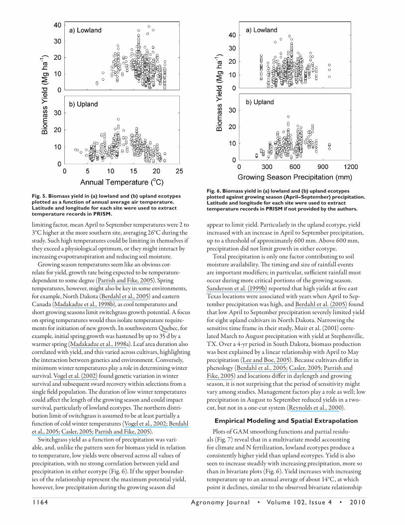
Biomass Yield and Climate
Biomass yield varied as a function of average annual temperature for all ecotypes taken together as well as for individual ecotypes (Fig. 5). In general, yields increased with increasing temperature up to a point and then decreased. Curves of the same shape were observed whether yield was taken as a function of growing season temperature, annual temperature, maximum summer tempera-ture, or minimum temperature during the preceding winter (data not shown). All of the temperature variables were highly corre-lated, except that maximum summer temperature was only weakly correlated with winter minimum temperature.
Regardless of the temperature variables used, the response patterns suggest a broad optimal temperature range for biomass yield, below and above which yields are diminished. Because the climate data were correlated, it cannot be determined whether conditions during all or part of the growing season, or even winter conditions, are key to understanding the temperature response of yields. Muir et al. (2001) suggested a southern limit of adaptation for Alamo between their sites in Stephenville, TX (32.22°N) and Beeville, TX (28.4°N) that was unrelated to rainfall or soil type; soils at both sites were described as shal-low. Although high temperature cannot be singled out as the
Table 2. Mean biomass yield (dry mass, Mg ha–1) for lowland and upland ecotypes of switchgrass in represented plot size classes (m2). Standard deviation, number of observations, and mean plot size within a given plot size class are also given.
Plot size class(range, m2) 0–3 3–6 6–9
9–12 12–15 15–18 27–30 36–39 79 147 175.5
>30,000
LowlandMean yield (Mg ha–1) 4.2 14.8 17.6 13.8 12.7 12.5 11.8 8.2 na 19.1 14.6 na(SD) (0.6) (4.9) (4.3) (6.6) (3.5) (5.2) (6.0) (4.3) (11.2) (7.0)n 2 62 22 188 30 228 30 71 10 9Mean plot size (m2) 2.4 5.9 7.0 9.7 13.2 17.6 27.3 37.2 147.0 175.5
UplandMean yield (Mg ha–1) 11.0 9.2 9.3 6.1 7.1 10.8 na na 8.3 na na 7.2(SD) (3.4) (4.4) (3.3) (2.9) (2.7) (4.9) (2.7) (2.1)n 26 100 42 86 78 135 10 29Mean plot size (m2) 2.8 5.6 7.0 10.9 13.8 17.4 79.0 67,862
Fig. 4. Relationship between biomass yield and plot size for lowland and upland ecotypes of switchgrass. Plot sizes were binned according to a given range and associated with biomass yield estimates contained within the database. Standard deviations for both plot size and biomass yield are shown. Plot size is graphed on a log scale.
Table 3. Mean biomass yield (dry mass, Mg ha–1) for lowland and upland switchgrass ecotypes in each of seven nonirrigated land capability classes (LCC). Standard deviation, median, number of observations, and standard error of the mean are also given.
LCC 1 2 3 4 5 6 7Lowland
Mean na 11.4 16.6 12.3 na 16.2 na(SD) (5.1) (5.8) (4.2) (4.1)median 11.1 15.7 13.1 16.0n 283 191 58 56SEM 0.3 0.4 0.5 0.6
UplandMean 10.7 5.9 10.3 7.5 na 9.6 6.3(SD) (3.6) (2.8) (4.1) (3.7) (4.4) (3.1)median 10.2 5.5 9.9 6.9 9.3 6.6n 27 102 163 36 98 48SEM 0.7 0.3 0.3 0.6 0.4 0.4
1164 Agronomy Journa l • Volume 102, Issue 4 • 2010
limiting factor, mean April to September temperatures were 2 to 3°C higher at the more southern site, averaging 26°C during the study. Such high temperatures could be limiting in themselves if they exceed a physiological optimum, or they might interact by increasing evapotranspiration and reducing soil moisture.
Growing season temperatures seem like an obvious cor-relate for yield, growth rate being expected to be temperature-dependent to some degree (Parrish and Fike, 2005). Spring temperatures, however, might also be key in some environments, for example, North Dakota (Berdahl et al., 2005) and eastern Canada (Madakadze et al., 1998b), as cool temperatures and short growing seasons limit switchgrass growth potential. A focus on spring temperatures would thus isolate temperature require-ments for initiation of new growth. In southwestern Quebec, for example, initial spring growth was hastened by up to 35 d by a warmer spring (Madakadze et al., 1998a). Leaf area duration also correlated with yield, and this varied across cultivars, highlighting the interaction between genetics and environment. Conversely, minimum winter temperatures play a role in determining winter survival. Vogel et al. (2002) found genetic variation in winter survival and subsequent sward recovery within selections from a single fi eld population. Th e duration of low winter temperatures could aff ect the length of the growing season and could impact survival, particularly of lowland ecotypes. Th e northern distri-bution limit of switchgrass is assumed to be at least partially a function of cold winter temperatures (Vogel et al., 2002; Berdahl et al., 2005; Casler, 2005; Parrish and Fike, 2005).
Switchgrass yield as a function of precipitation was vari-able, and, unlike the pattern seen for biomass yield in relation to temperature, low yields were observed across all values of precipitation, with no strong correlation between yield and precipitation in either ecotype (Fig. 6). If the upper boundar-ies of the relationship represent the maximum potential yield, however, low precipitation during the growing season did
appear to limit yield. Particularly in the upland ecotype, yield increased with an increase in April to September precipitation, up to a threshold of approximately 600 mm. Above 600 mm, precipitation did not limit growth in either ecotype.
Total precipitation is only one factor contributing to soil moisture availability. Th e timing and size of rainfall events are important modifi ers; in particular, suffi cient rainfall must occur during more critical portions of the growing season. Sanderson et al. (1999b) reported that high yields at fi ve east Texas locations were associated with years when April to Sep-tember precipitation was high, and Berdahl et al. (2005) found that low April to September precipitation severely limited yield for eight upland cultivars in North Dakota. Narrowing the sensitive time frame in their study, Muir et al. (2001) corre-lated March to August precipitation with yield at Stephenville, TX. Over a 4-yr period in South Dakota, biomass production was best explained by a linear relationship with April to May precipitation (Lee and Boe, 2005). Because cultivars diff er in phenology (Berdahl et al., 2005; Casler, 2005; Parrish and Fike, 2005) and locations diff er in daylength and growing season, it is not surprising that the period of sensitivity might vary among studies. Management factors play a role as well; low precipitation in August to September reduced yields in a two-cut, but not in a one-cut system (Reynolds et al., 2000).
Empirical Modeling and Spatial Extrapolation
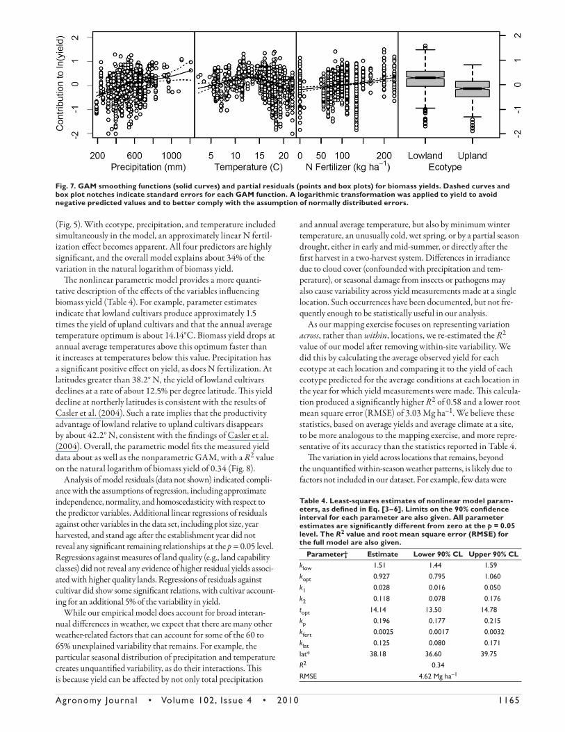
Plots of GAM smoothing functions and partial residu-als (Fig. 7) reveal that in a multivariate model accounting for climate and N fertilization, lowland ecotypes produce a consistently higher yield than upland ecotypes. Yield is also seen to increase steadily with increasing precipitation, more so than in bivariate plots (Fig. 6). Yield increases with increasing temperature up to an annual average of about 14°C, at which point it declines, similar to the observed bivariate relationship
Fig. 5. Biomass yield in (a) lowland and (b) upland ecotypes plotted as a function of annual average air temperature. Latitude and longitude for each site were used to extract temperature records in PRISM.
Fig. 6. Biomass yield in (a) lowland and (b) upland ecotypes plotted against growing season (April–September) precipitation. Latitude and longitude for each site were used to extract temperature records in PRISM if not provided by the authors.
Agronomy Journa l • Volume 102, Issue 4 • 2010 1165
(Fig. 5). With ecotype, precipitation, and temperature included simultaneously in the model, an approximately linear N fertil-ization eff ect becomes apparent. All four predictors are highly signifi cant, and the overall model explains about 34% of the variation in the natural logarithm of biomass yield.
Th e nonlinear parametric model provides a more quanti-tative description of the eff ects of the variables infl uencing biomass yield (Table 4). For example, parameter estimates indicate that lowland cultivars produce approximately 1.5 times the yield of upland cultivars and that the annual average temperature optimum is about 14.14°C. Biomass yield drops at annual average temperatures above this optimum faster than it increases at temperatures below this value. Precipitation has a signifi cant positive eff ect on yield, as does N fertilization. At latitudes greater than 38.2° N, the yield of lowland cultivars declines at a rate of about 12.5% per degree latitude. Th is yield decline at northerly latitudes is consistent with the results of Casler et al. (2004). Such a rate implies that the productivity advantage of lowland relative to upland cultivars disappears by about 42.2° N, consistent with the fi ndings of Casler et al. (2004). Overall, the parametric model fi ts the measured yield data about as well as the nonparametric GAM, with a R2 value on the natural logarithm of biomass yield of 0.34 (Fig. 8).
Analysis of model residuals (data not shown) indicated compli-ance with the assumptions of regression, including approximate independence, normality, and homoscedasticity with respect to the predictor variables. Additional linear regressions of residuals against other variables in the data set, including plot size, year harvested, and stand age aft er the establishment year did not reveal any signifi cant remaining relationships at the p = 0.05 level. Regressions against measures of land quality (e.g., land capability classes) did not reveal any evidence of higher residual yields associ-ated with higher quality lands. Regressions of residuals against cultivar did show some signifi cant relations, with cultivar account-ing for an additional 5% of the variability in yield.
While our empirical model does account for broad interan-nual diff erences in weather, we expect that there are many other weather-related factors that can account for some of the 60 to 65% unexplained variability that remains. For example, the particular seasonal distribution of precipitation and temperature creates unquantifi ed variability, as do their interactions. Th is is because yield can be aff ected by not only total precipitation
and annual average temperature, but also by minimum winter temperature, an unusually cold, wet spring, or by a partial season drought, either in early and mid-summer, or directly aft er the fi rst harvest in a two-harvest system. Diff erences in irradiance due to cloud cover (confounded with precipitation and tem-perature), or seasonal damage from insects or pathogens may also cause variability across yield measurements made at a single location. Such occurrences have been documented, but not fre-quently enough to be statistically useful in our analysis.
As our mapping exercise focuses on representing variation across, rather than within, locations, we re-estimated the R2 value of our model aft er removing within-site variability. We did this by calculating the average observed yield for each ecotype at each location and comparing it to the yield of each ecotype predicted for the average conditions at each location in the year for which yield measurements were made. Th is calcula-tion produced a signifi cantly higher R2 of 0.58 and a lower root mean square error (RMSE) of 3.03 Mg ha–1. We believe these statistics, based on average yields and average climate at a site, to be more analogous to the mapping exercise, and more repre-sentative of its accuracy than the statistics reported in Table 4.
Th e variation in yield across locations that remains, beyond the unquantifi ed within-season weather patterns, is likely due to factors not included in our dataset. For example, few data were
Table 4. Least-squares estimates of nonlinear model param-eters, as defi ned in Eq. [3–6]. Limits on the 90% confi dence interval for each parameter are also given. All parameter estimates are signifi cantly different from zero at the p = 0.05 level. The R2 value and root mean square error (RMSE) for the full model are also given.
Parameter† Estimate Lower 90% CL Upper 90% CLklow 1.51 1.44 1.59kopt 0.927 0.795 1.060k1 0.028 0.016 0.050k2 0.118 0.078 0.176topt 14.14 13.50 14.78kp 0.196 0.177 0.215kfert 0.0025 0.0017 0.0032klat 0.125 0.080 0.171lat* 38.18 36.60 39.75R2 0.34RMSE 4.62 Mg ha–1
Fig. 7. GAM smoothing functions (solid curves) and partial residuals (points and box plots) for biomass yields. Dashed curves and box plot notches indicate standard errors for each GAM function. A logarithmic transformation was applied to yield to avoid negative predicted values and to better comply with the assumption of normally distributed errors.
1166 Agronomy Journa l • Volume 102, Issue 4 • 2010
available for edaphic factors, including diff erences in soil type, structure, water-holding capacity, or fertility, including N avail-ability before fertilization. If these factors are measured and added to future analyses, there may be potential for further reducing the variability that remains unexplained across locations.
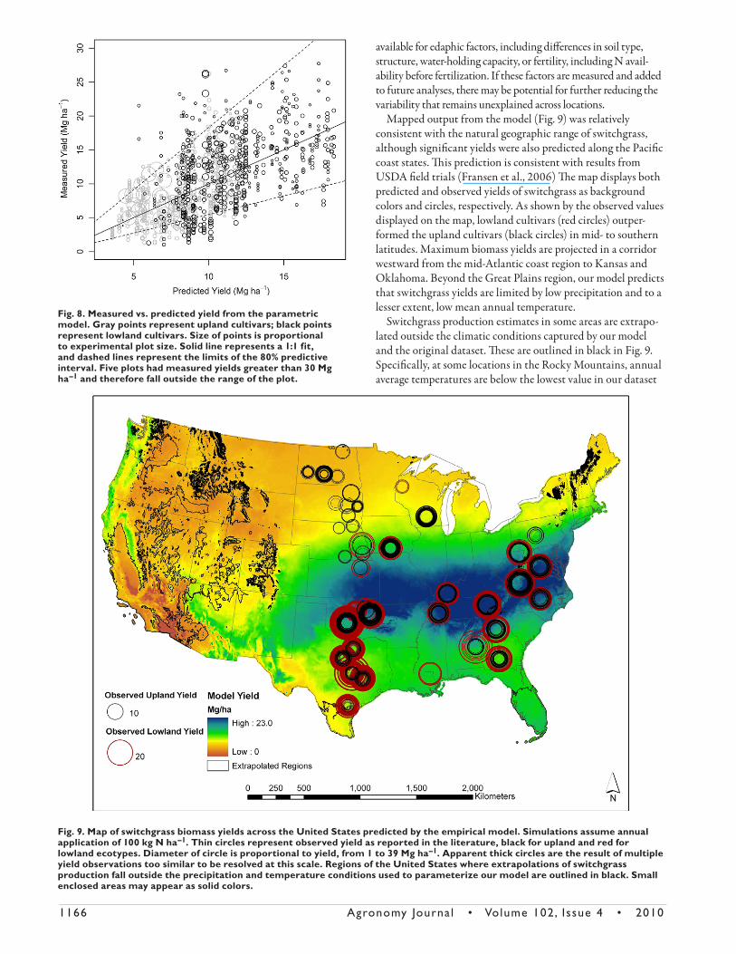
Mapped output from the model (Fig. 9) was relatively consistent with the natural geographic range of switchgrass, although signifi cant yields were also predicted along the Pacifi c coast states. Th is prediction is consistent with results from USDA fi eld trials (Fransen et al., 2006) Th e map displays both predicted and observed yields of switchgrass as background colors and circles, respectively. As shown by the observed values displayed on the map, lowland cultivars (red circles) outper-formed the upland cultivars (black circles) in mid- to southern latitudes. Maximum biomass yields are projected in a corridor westward from the mid-Atlantic coast region to Kansas and Oklahoma. Beyond the Great Plains region, our model predicts that switchgrass yields are limited by low precipitation and to a lesser extent, low mean annual temperature.
Switchgrass production estimates in some areas are extrapo-lated outside the climatic conditions captured by our model and the original dataset. Th ese are outlined in black in Fig. 9. Specifi cally, at some locations in the Rocky Mountains, annual average temperatures are below the lowest value in our dataset
Fig. 8. Measured vs. predicted yield from the parametric model. Gray points represent upland cultivars; black points represent lowland cultivars. Size of points is proportional to experimental plot size. Solid line represents a 1:1 fit, and dashed lines represent the limits of the 80% predictive interval. Five plots had measured yields greater than 30 Mg ha–1 and therefore fall outside the range of the plot.
Fig. 9. Map of switchgrass biomass yields across the United States predicted by the empirical model. Simulations assume annual application of 100 kg N ha–1. Thin circles represent observed yield as reported in the literature, black for upland and red for lowland ecotypes. Diameter of circle is proportional to yield, from 1 to 39 Mg ha–1. Apparent thick circles are the result of multiple yield observations too similar to be resolved at this scale. Regions of the United States where extrapolations of switchgrass production fall outside the precipitation and temperature conditions used to parameterize our model are outlined in black. Small enclosed areas may appear as solid colors.

Agronomy Journa l • Volume 102, Issue 4 • 2010 1167
(2.4°C). In southern Florida and Texas, annual average tem-peratures exceed our highest value of 21.8°C. Arid regions west of the Rockies and east of the Sierra and Cascade ranges receive growing season precipitation lower than the minimum value in our dataset (188 mm). Conversely, the very high precipitation found on the Olympic Peninsula is above our highest observed value (1210 mm). Finally, areas of New England and along the Appalachian mountains are within the temperature range of our dataset, but have higher rainfall for a given temperature than any location included in our dataset.
Refi nement of the current statistical model with additional data from the regions not currently represented in our study might improve the prediction of switchgrass yields with respect to climate and interactions with cultivar and management practices. Th is would assist growers in choosing high-yielding cultivars within the context of local environmental growing conditions. Moreover, geographically distributed models of bioenergy crops, such as this one, can play an important role when investigating issues related to land use, potential regional or national biofuels production and other considerations related to facility siting and supply logistics.
Evaluation of Bias and the Possibility of Yield Overestimation
In their study of biofuel yields from agricultural crops, John-ston et al. (2009) mention that a number of variables can exert a considerable infl uence on yield including geographic location, climate, soils, and management practice. In our analysis, these factors have been evaluated and their impact on biomass yield considered to the extent possible based on available data for switchgrass grown in the United States. Temperature, precipita-tion, N application, ecotype, and latitude exhibit a statistically signifi cant impact on yield, and thus a strong case can be made for including these in an empirical model. However, a surprising number of variables did not exhibit a signifi cant impact on yield for upland or lowland ecotypes: plot size, row spacing, stand age (aft er establishment), soil texture, and land quality. Especially interesting is the observation that no evidence was found to support an eff ect of plot size and land quality on biomass yield. Small plot size and preferential placement of fi eld trials on better than average agricultural land have been cited as factors that contribute to overestimation of yields that might otherwise be realized on typical farm-scale fi elds. For example, Johnston et al. (2009) cited several factors commonly responsible for overesti-mating yield of bioenergy crops, at regional to continental scales, including uncritical application of site-specifi c yield estimates, failure to use regionally specifi c and spatially explicit agricultural data, and use of potentially unrealistic yield estimates that might come from the location of fi eld trials on agricultural research stations. It is indeed important to give these factors due consider-ation and future studies should take great care to fully character-ize the climatic, edaphic, and crop management practices that contribute to reported yields. One of the lessons learned from the current analysis is that more yield data would be desirable over a broader range of conditions (e.g., northern colder and western dryer sites). Although we acknowledge these and other limitations of available data, and the impact they may have on our analysis of yield, we fi nd no evidence for overestimation of yield with respect to the soil, crop management, or climatic
variables considered. We systematically looked for, but did not fi nd, evidence of bias toward higher yields associated with small plots or preferential establishment of stands on high quality land. Th us, we conclude that yield estimates reported in the literature and summarized here for switchgrass are at this time the best available predictors of the yield for this bioenergy crop grown under large-scale cultivation. Biomass yield is, however, just one component of biofuels production. Another is the potential land base available for energy crop production in the United States (Graham, 1994). We believe this to be the greater uncertainty as it includes the relative economics of biofuels production and alternative uses of agricultural land. Th ese uncertainties must be considered, but are well beyond the scope of this analysis.
CONCLUSIONSHere we report a large compilation and analysis of empirical
biomass yield data from across the United States for the biofuels crop switchgrass. Each observation has been identifi ed by lati-tude and longitude, ecotype, cultivar, plot size, stand age, harvest frequency, N fertilization, and year of harvest. Other sources of information were used to associate observations of biomass yield with soil characteristics, temperature and precipitation, and land quality. Of the relationships established between biomass yield and these variables, ecotype, temperature, precipitation, and N fertilization were identifi ed as the most important predictors of yield. Statistical modeling revealed patterns of response that could be used to predict biomass production associated with a given climate. In addition, no systematic bias was observed for an overestimation of yield due to small plot size or preferential establishment of stands on land of high quality. Results thus suggest that fi eld trials conducted and reported in the current lit-erature can be used, as we have, to extrapolate observed biomass yields to larger spatial scales. We acknowledge, however, that this should be done with care and with a full understanding of the uncertainties that accompany such extrapolations.
ACKNOWLEDGMENTS
The authors wish to thank those site investigators who provided additional information and data for the analyses presented. The authors would also like to thank Dr. Jonathan Chipman, the direc-tor of the Applied Spatial Analysis Laboratory at Dartmouth College, for advice, consultation, and access to the lab facilities. This research was sponsored by the U.S. Department of Energy, Office of Energy Efficiency and Renewable Energy, Biomass Program. Oak Ridge National Laboratory is managed by UT-Battelle, LLC for the U.S. Department of Energy under contract DE-05-00OR22725. E.B Davis was supported by a grant from the Morgan Family Fund.
REFERENCES
Berdahl, J.D., A.B. Frank, J.M. Krupinsky, P.M. Carr, J.D. Hanson, and H.A. Johnson. 2005. Biomass yield, phenology and survival of diverse cultivars and experimental strains in western North Dakota. Agron. J. 97:549–555.
Bouton, J. H. 2002. Bioenergy crop breeding and production research in the south-east. Final report for 1996 to 2001. ORNL/SUB-02-19XSV810C/01. Avail-able at http://www.osti.gov/bridge/ (verifi ed 27 Apr. 2010). U.S. Department of Energy, Washington, DC.
Casler, M.D. 2005. Ecotypic variation among switchgrass populations from the northern USA. Crop Sci. 45:388–398.
Casler, M.D., and A.R. Boe. 2003. Cultivar × environment interactions in switch-grass. Crop Sci. 43:2226–2233.
1168 Agronomy Journa l • Volume 102, Issue 4 • 2010
Casler, M.D., K.P. Vogel, C.M. Taliaferro, and R.L. Wynia. 2004. Latitudinal adap-tation of switchgrass populations. Crop Sci. 44:293–303.
Cassida, K.A., T.L. Kirkpatrick, R.T. Robbins, J.P. Muir, B.C. Venuto, and M.A. Hussey. 2005a. Plant-parasitic nematodes associated with switchgrass (Pani-cum virgatum L.) grown for biofuel in the south-central United States. Nema-tropica 35:1–10.
Cassida, K.A., J.P. Muir, M.A. Hussey, J.C. Read, B.C. Venuto, and W.R. Ocump-augh. 2005b. Biomass yield and stand characteristics of switchgrass in south central U.S. environments. Crop Sci. 45:673–681.
Daly, C. 2006. Guidelines for assessing the suitability of spatial climate data sets. Int. J. Climatol. 26:707–721.
Di Virgilio, N., A. Monti, and G. Venturi. 2007. Spatial variability of switchgrass (Panicum virgatum L.) yield as related to soil parameters in a small fi eld. Field Crops Res. 101:232–239.
Evers, E.W., and M.J. Parsons. 2003. Soil type and moisture level infl uence on Alamo switchgrass emergence and seedling growth. Crop Sci. 43:288–294.
Fike, J.H., D.J. Parrish, D.D. Wolf, J.A. Balasko, J.T. Green, Jr., M. Rasnake, and J.H. Reynolds. 2006. Long-term yield potential of switchgrass-for-biofuel sys-tems. Biomass Bioenergy 30:198–206.
Fransen, S.C., H.P. Collins, and R.A. Boydston. 2006. Perennial warm-season grasses for biofuels. In Proc. 2006 Western Alfalfa and Forage Conf., Reno, NV. 11–13 Dec. 2006. Univ. of California, Davis.
Fuentes, R.C., and C.M. Taliaferro. 2002. Biomass yield stability of switchgrass cul-tivars. Trends in New Crops and New Uses. p. 276–282. In J. Janick and A. Whipkey (ed.) ASHS Press, Alexandria, VA.
Graham, R.L. 1994. An analysis of the potential land base for energy crops in the conterminous United States. Biomass Bioenergy 6:175–189.
Hastie, T.J. 1991. Generalized additive models. p. 249–307. In J.M. Chambers and T.J. Hastie (ed.) Statistical models in S. Wadsworth & Brooks/Cole, Cleve-land, OH.
Hastie, T., and R. Tibshirani. 1990. Generalized additive models. Chapman and Hall, London.
Heaton, W., T. Voigt, and S.P. Long. 2004. A quantitative review of comparing the yields of two candidate C-4 perennial biomass crops in relation to nitrogen, temperature and water. Biomass Bioenergy 27:21–30.
Ikaha, R., and R. Gentleman. 1996. R: A language for data analysis and graphics. J. Comput. Graph. Statist. 5:299–314.
Johnston, M., J.A. Foley, T. Holloway, C. Kucharik, and C. Monfreda. 2009. Reset-ting global expectations from agricultural biofuels. Environ. Res. Lett. 4:1–9.
Kiniry, J.R., M.A. Sanderson, J.R. Williams, C.R. Tischler, M.A. Hussey, W.R. Ocumpaugh, J.C. Read, G. van Esbroeck, and R.L. Reed. 1996. Simulating Alamo switchgrass with the ALMANAC model. Agron. J. 88:602–606.
Kiniry, J.R., C.R. Tischler, and G.A. van Esbroeck. 1999. Radiation use effi ciency and leaf CO2 exchange for diverse C4 grasses. Biomass Bioenergy 17:95–112.
Kiniry, J.R., K.A. Cassida, M.A. Hussey, J.P. Muir, W.R. Ocumpaugh, J.C. Read, R.L. Reed, M.A. Sanderson, B.C. Venuto, and J.R. Williams. 2005. Switch-grass simulation by the ALMANAC model at diverse sites in the southern U.S. Biomass Bioenergy 29:419–425.
Lee, D.K., and A. Boe. 2005. Biomass production of switchgrass in central South Dakota. Crop Sci. 45:2583–2590.
Lemus, R., E.C. Brummer, K.J. Moore, N.E. Molstad, C.L. Burras, and M.F. Barker. 2002. Biomass yield and quality of 20 switchgrass populations in southern Iowa, USA. Biomass Bioenergy 23:433–442.
Madakadze, I.C., B.E. Coulman, P. Peterson, K.A. Stewart, R. Samson, and D.L. Smith. 1998a. Leaf area development, light interception, and yield among switchgrass populations in a short-season area. Crop Sci. 38:827–834.
Madakadze, I., B.E. Coulman, K.A. Stewart, P. Peterson, R. Samson, and D.L. Smith. 1998b. Phenology and tiller characteristics of big bluestem and switch-grass cultivars in a short growing season area. Agron. J. 90:489–495.
McLaughlin, S.B., and L.A. Kszos. 2005. Development of switchgrass (Panicum virgatum) as a bioenergy feedstock in the United States. Biomass Bioenergy 28:515–535.
McLaughlin, S.B., D.D. Ugarte, C.T. Garten, L.R. Lynd, M.A. Sanderson, V.R. Tol-bert, and D.D. Wolf. 2002. High-value renewable energy from prairie grasses. Environ. Sci. Technol. 36:2122–2129.
Muir, J.P., M.A. Sanderson, W.R. Ocumpaugh, R.M. Jones, and R.L. Reed. 2001. Biomass Production of ‘Alamo’ switchgrass in response to nitrogen, phospho-rous, and row spacing. Agron. J. 93:896–901.
Parrish, D.J., and J.H. Fike. 2005. Th e biology and agronomy of switchgrass for bio-fuels. Crit. Rev. Plant Sci. 24:423–459.
Porter, C.L. 1966. An analysis of variation between upland and lowland switch-grass, Panicum virgatum L., in central Oklahoma. Ecology 47:980–992.
Ragauskas, A.J., C.K. Williams, B.H. Davison, G. Britovsek, J. Cairney, C.A. Eck-ert, W.J. Frederick, J.P. Hallett, D.J. Leak, C.L. Liotta, J.R. Mielenz, R. Mur-phy, R. Templer, and T. Tschaplinski. 2006. Th e path forward for biofuels and biomaterials. Science 311:484–489.
Reynolds, J.H., C.L. Walker, and M.J. Kirchner. 2000. Nitrogen removal in switch-grass biomass under two harvest systems. Biomass Bioenergy 19:281–286.
Sanderson, M.A., R.L. Reed, S.B. McLaughlin, S.D. Wullschleger, B.V. Conger, D.J. Parrish, D.D. Wolf, C. Taliaferro, A.A. Hopkins, W.R. Ocumpaugh, M.A. Hussey, J.C. Read, and C.R. Tischler. 1996. Switchgrass as a sustainable bioenergy crop. Bioresour. Technol. 56:83–93.
Sanderson, M.A., J.C. Read, and R.L. Reed. 1999a. Harvest management of switch-grass for biomass feedstock and forage production. Agron. J. 91:5–10.
Sanderson, M.A., R.L. Reed, W.R. Ocumpaugh, M.A. Hussey, G. Van Esbroeck, J.C. Read, C.R. Tischler, and F.M. Hons. 1999b. Switchgrass cultivars and germplasm for biomass feedstock production in Texas. Bioresour. Technol. 67:209–219.
Sanderson, M.A., R.R. Schnabel, W.S. Curran, W.L. Stout, D. Genito, and B.F. Tracy. 2004. Switchgrass and big bluestem hay, biomass, and seed yield response to fi re and glyphosate treatment. Agron. J. 96:1688–1692.
Sanderson, M.A., P.R. Adler, A.A. Boateng, M.D. Casler, and G. Sarath. 2006. Switchgrass as a biofuels feedstock in the USA. Can. J. Plant Sci. 86:1315–1325.
Schmer, M.R., K.P. Vogel, R.B. Mitchell, and R.K. Perrin. 2008. Net energy of cel-lulosic ethanol from switchgrass. Proc. Natl. Acad. Sci. USA 105:464–469.
Sladden, S.E., D.I. Bransby, and G.E. Aiken. 1991. Biomass yield, composition, and production costs for eight switchgrass varieties in Alabama. Biomass Bioen-ergy 1:119–122.
Th omason, W.E., W.R. Raun, G.V. Johnson, C.M. Taliaferro, K.W. Freeman, K.J. Wynn, and R.W. Mullen. 2004. Switchgrass response to harvest frequency and time and rate of applied nitrogen. J. Plant Nutr. 27:1199–1226.
Tilman, D., R. Socolow, J.A. Foley, J. Hill, E. Larson, L. Lynd, S. Pacala, J. Reilly, T. Seachinger, C. Somerville, and R. Williams. 2009. Benefi cial biofuels: Th e food, energy, and environment trilemma. Science 325:270–271.
Vogel, K.P., A.A. Hopkins, K.J. Moore, K.D. Johnson, and I.T. Carlson. 2002. Winter survival in switchgrass populations bred for high IVDMD. Crop Sci. 42:1857–1862.
Wright, L.L. 1994. Production technology status of woody and herbaceous crops. Biomass Bioenergy 6:191–209.