Environmental and economic analysis of switchgrass production

for water quality improvement in northeast Kansas

Richard G. Nelson a, James C. Ascough II b,*, Michael R. Langemeier a

a Kansas State University Manhattan, KS 66506 USAb USDA-ARS, Great Plains Systems Research Unit, Fort Collins, CO 80526 USA

Received 28 July 2004; received in revised form 28 May 2005; accepted 21 July 2005

Available online 9 December 2005

Abstract

The primary objectives of this research were to determine SWAT model predicted reductions in four water quality indicators (sediment yield,

surface runoff, nitrate nitrogen (NO3–N) in surface runoff, and edge-of-field erosion) associated with producing switchgrass (Panicum virgatum)

on cropland in the Delaware basin in northeast Kansas, and evaluate switchgrass break-even prices. The magnitude of potential switchgrass water

quality payments based on using switchgrass as an alternative energy source was also estimated. SWAT model simulations showed that between

527,000 and 1.27 million metric tons (Mg) of switchgrass could be produced annually across the basin depending upon nitrogen (N) fertilizer

application levels (0–224 kg N haK1). The predicted reductions in sediment yield, surface runoff, NO3–N in surface runoff, and edge-of-field

erosion as a result of switchgrass plantings were 99, 55, 34, and 98%, respectively. The average annual cost per hectare for switchgrass ranged

from about $190 with no N applied to around $345 at 224 kg N haK1 applied. Edge-of-field break-even price per Mg ranged from around $41 with

no N applied to slightly less than $25 at 224 kg N haK1 applied. A majority of the switchgrass produced had an edge-of-field break-even price of

$30 MgK1 or less. Savings of at least 50% in each of the four water quality indicators could be attained for an edge-of-field break-even price of

$22–$27.49 MgK1.

q 2005 Elsevier Ltd. All rights reserved.

Keywords: SWAT model; Switchgrass production; Economic analysis; Commodity crops; Water quality; Sediment yield; Surface runoff; Soil erosion

1. Introduction

The impact on the environment of greenhouse gases such as

carbon dioxide (CO2), in conjunction with recent increases in

petroleum fuel costs, have prompted a genuine concern

regarding our continued reliance on petroleum-based fuels

and their effect on air quality and energy security. Carbon

dioxide emissions from energy use are projected to increase on

average by 1.5 percent per year from 2002 to 2025, to 8142

million metric tons (United States Department of Energy,

2004). Since 1990, primary energy consumption in the United

States has increased by 14% (28% in the last 25 years) and is

forecast to increase another 40% by 2025 (United States

Department of Energy, 2004). Clearly, the environmental,

economic, and energy consequences associated with imported

petroleum call for additional research.

0301-4797/$ - see front matter q 2005 Elsevier Ltd. All rights reserved.

doi:10.1016/j.jenvman.2005.07.013

* Corresponding author. Tel.: C1 970 492 7371; fax: C1 970 492 7310.

E-mail address: jim.ascough@ars.usda.gov (J.C. Ascough).

Renewable energy has distinct environmental advantages

associated with its production and use. Most renewable energy

technologies such as solar and wind produce no direct

emissions. Biomass energy crops such as agricultural crop

residues can, under judicious management, be harvested for

alternative energy purposes (e.g. bioethanol production) and

still provide adequate protection from soil erosion and needed

soil tilth. Other biomass energy resources, such as herbaceous

and woody energy crops, offer a wide range of environmental

benefits and can have a positive environmental impact. Some

environmental benefits associated with herbaceous and woody

energy crops include:

1. Reduced water and wind produced soil erosion;

2. Reduced surface and subsurface fertilizer and pesticide

migration, improving surface and groundwater quality;

3. Reduced emissions of global warming gases and carbon

sequestration in root systems more extensive than annual

crops; and

4. Improved regional air quality by reducing SO2 and NO2

emissions.

Journal of Environmental Management 79 (2006) 336–347

www.elsevier.com/locate/jenvman

R.G. Nelson et al. / Journal of Environmental Management 79 (2006) 336–347 337

Non-point source (NPS) pollution of streams, lakes, and

reservoirs from sediment, fertilizers, and pesticides is a

significant threat to water supplies, waterways, and wildlife

habitats in many parts of the country. The United States

Environmental Protection Agency (EPA) 2000 National Water

Quality Inventory (United States Environmental Protection

Agency, 2000) found that sedimentation remains one of the

most widespread pollutants affecting assessed rivers and

streams, impairing 84,503 river and stream miles (12% of the

assessed river and stream miles and 31% of the impaired river

and stream miles). Sedimentation alters aquatic habitat,

suffocates fish eggs and bottom-dwelling organisms, and can

interfere with drinking water treatment processes and

recreational use of a river. In addition to rivers and streams,

sedimentation pollutes nearly 1.6 million lake acres (9% of the

assessed lake acres and 21% of the impaired lake acres). Often,

several pollutants and processes impair a single lake. For

example, an activity such as removal of shoreline vegetation

may accelerate erosion of sediment and nutrients into a lake.

Other federal agencies have reported similar findings. The

United States Department of Agriculture-Agricultural

Research Service (USDA-ARS) considers sediment the

primary contaminant in rivers, lakes, and reservoirs. The

United States Geological Survey (USGS) has estimated nearly

one-third of all water bodies in the continental United States

are at least moderately, and in some cases, severely polluted

due to non-point source pollution. Most NPS pollution

problems are attributable to production agriculture. Intense

agricultural land use is leading to rapid sedimentation in many

Kansas reservoirs, including Perry reservoir in the Delaware

basin in northeast Kansas. Sources of non-point source

pollution include sediment from runoff on agricultural

lands, nutrients such as nitrogen (N) and phosphorus (P), and

pesticides. The state of Kansas performed an assessment

(Kansas Department of Health and Environment, 1999)

that prioritized 72 watersheds/reservoirs into three separate

categories for meeting state water quality standards regarding

sediment and nutrient loadings. Category 1 watersheds

were those in need of immediate restoration and protection,

Category 2 watersheds were those in need of protection

only, and Category 3 watersheds were those having

pristine and sensitive conditions associated with them. Over

77% of the state’s watersheds were classified as Category 1;

the watershed considered in this study, the Delaware, was

assigned to this category (Kansas Department of Health and

Environment, 1999).

One promising strategy to help significantly reduce

sediment, surface runoff, and nutrient loading into Kansas

streams, tributaries, and reservoirs is to plant perennial warm

season grasses such as switchgrass (Panicum virgatum) in

selected locations within watersheds. In a recent analysis,

Kansas investigators found that the use of switchgrass resulted

in reduced soil erosion from rainfall as well as general

reductions in nutrient loss in runoff and subsurface flow versus

all conventional commodity crops across the state (King et al.,

1998). Soil erosion from rainfall was reduced an average of

99% and runoff was significantly reduced by bioenergy crop

production.

Switchgrass is regarded as a highly promising energy crop

with an average energy yield of approximately 260.8 GJ haK1

at a production level of approximately 14C Mg haK1 yK1 in

northeast Kansas. Potential markets in Kansas include co-firing

with coal in a utility boiler and pelleting for space and water

heating. Both strategies have energy-profit ratios (energy

output/total energy input) between six and 12. The above

analysis concluded, however, that switchgrass could not

compete with fossil fuels at existing prices (King et al.,

1998).

One strategy for reducing the cost of switchgrass is to

determine the extent of surface water quality benefits

associated with its production and use through a reduction in

soil erosion (sediment transport) and nutrient runoff compared

to conventional commodity crop production, and place a

monetary value on these benefits. The actual monetary value

could be in the form of a payment to either the landowner or

utility based on the amount of soil (sediment) saved or a

percent reduction in N and P transported from the field in

sediment or surface runoff. By planting switchgrass in selected

locations throughout a watershed, it may be possible to add

decades to the physical and economic life of such reservoirs.

Therefore, the major objective of this research was to estimate

the environmental benefits and economic feasibility of

producing switchgrass for water quality improvement in the

Delaware basin of northeast Kansas versus conventional

cropping rotations and quantify the environmental (water

quality) benefits associated with switchgrass production.

Specific objectives were to:

1. Use the soil and water assessment tool (SWAT) model to

evaluate the impact of switchgrass production on sediment

yield, surface runoff, NO3-N in surface runoff, and edge-of-

field erosion in the Delaware basin. Switchgrass production

was evaluated on agricultural croplands that typically

produce corn, soybeans, grain sorghum, and wheat

commodity crops;

2. Use the SWAT model to simulate switchgrass and

commodity crop yields and then evaluate the break-even

cost associated with producing switchgrass versus conven-

tional cropping rotations in the Delaware basin; and

3. Estimate, based on information gained in the first two

objectives, the magnitude of a switchgrass water quality

payment (based on switchgrass production in place of

traditional commodity crops) required to decrease sediment

loadings 10, 25, and 40% into Perry reservoir in the

Delaware basin.

2. Methods

2.1. SWAT model overview

The soil and water assessment tool (SWAT) model (Arnold

et al., 1998; Neitsch et al., 2002) was developed to assist water

R.G. Nelson et al. / Journal of Environmental Management 79 (2006) 336–347338

resource managers in predicting and assessing the impact of

management on water, sediment and agricultural chemical

yields in large ungaged watersheds or river basins. The model

is intended for long-term yield predictions and is not capable of

detailed, single-event flood routing. SWAT is a physically-

based model and has eight major components—hydrology,

weather, sediment transport, soil temperature, crop growth,

nutrients, pesticides, and agricultural management.

For modeling purposes, SWAT partitions watersheds or

basins into a number of sub-watersheds or sub-basins based on

climate, hydrologic response units (HRUs), ponds/reservoirs,

groundwater, and the main channel or reach draining the sub-

basin. HRUs are homogeneous land areas within the sub-basin

comprised of unique land cover, soil, and management

combinations. The daily water budget in each HRU is

computed based on daily precipitation, runoff, evapotranspira-

tion (ET), percolation, and return flow from the subsurface and

groundwater flow. Runoff volume in each HRU is computed

using the Soil Conservation Service or SCS (1972) runoff curve

number approach (USDA Soil Conservation Service, 1972).

A recent addition to SWAT is a Green-Ampt (1911) infiltration

module to compute runoff volume (Green and Ampt, 1911).

Peak runoff rate is computed using a modification to the

Rational method (Williams, 1995) or using the SCS TR-55

method (USDA Soil Conservation Service, 1986). Lateral

subsurface flow is computed using a kinematic storage model

(Sloan et al., 1983) and groundwater flow is calculated using

empirical relations. Channel runoff routing is based on the

variable storage coefficient method (Williams, 1969); channel

flow is computed using Manning’s equation with adjustments

for transmission losses, evaporation, diversions, and return

flow (Arnold et al., 1995). Reservoir flow routing is based on a

water balance approach and user-provided measured or

targeted outflow. Sediment yield is computed using the

Modified Universal Soil Loss Equation (MUSLE) factors

(Williams and Berndt, 1977) expressed in terms of runoff

volume, peak flow, and Universal Soil Loss Equation (USLE)

factors (Wischmeier and Smith, 1978). Channel sediment

routing is based on the stream power concept (Bagnold, 1977),

modified for bed degradation and sediment transport (Wil-

liams, 1980). Bed degradation is adjusted with USLE soil

erodibility and cover factors, and deposition is based on

particle fall velocity. Reservoir sediment routing is based on a

simple continuity equation on volumes and concentrations of

inflow, outflow, and reservoir storage. Amounts of NO3–N

contained in runoff, lateral flow, and percolation are estimated

as products of the water volumes and the average concen-

tration. A single plant growth model that can differentiate

between annual and perennial plants is used to simulate all

types of land covers (Williams, 1995). Annual plants grow

from the planting date to the harvest date or until the

accumulated heat units equal the potential heat units for the

plant. Perennial plants maintain their root systems throughout

the year, becoming dormant after frost. They resume growth

when the average daily air temperature exceeds the minimum,

or base, temperature required. The plant growth model is used

to assess removal of water and nutrients from the root zone,

transpiration, and biomass/yield production.

SWAT tracks the movement and transformation of several

forms of nitrogen and phosphorus in the watershed. Nutrients

may be introduced to the main channel and transported

downstream through surface runoff and lateral subsurface

flow. Plant use of nitrogen is estimated using the supply and

demand approach described in the section on plant growth. In

addition to plant use, nitrate and organic N may be removed

from the soil via mass flow of water. Amounts of NO3–N

contained in runoff, lateral flow and percolation are estimated

as products of the volume of water and the average

concentration of nitrate in the layer. Organic N transport with

sediment is calculated with a loading function developed by

McElroy et al. (1976) and modified by Williams and Hann

(1972) for application to individual runoff events. The loading

function estimates the daily organic N runoff loss based on the

concentration of organic N in the top soil layer, the sediment

yield, and the enrichment ratio. The enrichment ratio is the

concentration of organic N in the sediment divided by that in

the soil. Soluble phosphorous (P) loss in surface runoff is based

on partitioning P between the solution and sediment phases

(Knisel, 1980), and is predicted using the labile P concentration

in the top soil layer, runoff volume, and a partitioning factor.

Sediment transport of P is simulated using a loading function

similar to organic N transport. Pesticide transport is simulated

using methodology from the Groundwater Loading Effects of

Agricultural Management Systems (GLEAMS) model pesti-

cide component (Leonard et al., 1987) which is based on plant

leaf area index, application efficiency, wash-off fraction,

organic carbon adsorption coefficient, and exponential decay

according to pesticide half-life. In-stream nutrient transform-

ations are simulated with a modified form of the QUAL2E

model (Ramanarayanan et al., 1996) with components algae (as

chlorophyll-a) dissolved oxygen, carbonaceous oxygen

demand, organic N, ammonium-N, nitrite-N, nitrate-N, organic

P, and soluble P. Water temperature is estimated from air

temperature using a regression relation (Stefan and Preud’-

homme (1993) developed from numerous river observations.

Major in-stream pesticide processes simulated by SWAT

include settling, burial, re-suspension, volatilization, diffusion

and transformation (Chapra, 1997).

2.2. Delaware basin description and creation of

SWAT input files

The Delaware river basin covers approximately 300,000 ha

in Nemaha, Brown, Jackson, Atchison, and Jefferson Counties

of northeast Kansas of which approximately 119,400 ha are

cultivated cropland. Grassland and woodland cover approxi-

mately 57% of the basin. KSU cooperative extension service

field agents as well as USDA district conservationists were

asked in telephone interviews about the cropping rotations,

approximate percentage of acreage each occupies in the

Delaware river basin, and percent that each rotation was

subjected to conventional, conservation, or no-till in the

Delaware basin.

R.G. Nelson et al. / Journal of Environmental Management 79 (2006) 336–347 339

The four major cropping rotations within the basin are: (1)

corn–soybean; (2) corn–soybean–wheat; (3) grain sorghum–

soybean; and (4) grain sorghum–soybean–wheat. One

extremely minor rotation (!1% of acreage), corn–soybean–

wheat–grain sorghum, was not included in this analysis. The

corn–soybean and grain sorghum–soybean rotations are the

major cropping rotations within the basin covering 63 and 21%

of the total cropland area, respectively. Conservation/reduced

tillage is used in approximately 43% of the basin while

conventional and no-till operations comprise areas of 29 and

28%, respectively.

The first stage in setting up the Delaware basin SWAT

simulation was to define the relative arrangement of the parts or

elements, i.e. the configuration of the watershed. A 30 m digital

elevation model (DEM) of the Delaware basin was imported

into the Geographic Resources Analysis Support System

(GRASS, v. 4.1) geographic information system (GIS). The

GRASS command r.watershed was then used to delineate (i.e.

divide for purposes of flow routing) the Delaware basin into

smaller sub-basins. Fig. 1 shows the 45 sub-basin areas

identified, including location of the main channel and tributary

channels. Individual HRU delineation was performed by

overlaying GIS coverages of Delaware basin land use, major

cropping systems (if land use was agricultural), and the Natural

Resources Conservation Service (NRCS) STATSGO soil

database for Delaware basin soils. Non-agricultural land use

areas were then filtered out and HRU physical characteristics

such as area, slope, dominant soil type, and dominant cropping

system were calculated. A total of 552 distinct HRUs (within

the 45 sub-basins) were identified.

Fig. 1. GRASS GIS delineation of Delaware sub-basins and channels.

SWAT climate files for precipitation and temperature were

developed using historical climate data (1966–1989) collected

from instrumented weather stations within the basin. Data from

nine precipitation stations and five temperature stations were

used. Values for solar radiation, wind speed, and relative

humidity were generated by the model. Detailed historical

climate data were available from 1964–1989, however, the data

from the first 2 years contained many missing values and were

judged to be unreliable. Therefore, the 24-year period from

1966–1989 was used for all SWAT simulations and subsequent

environmental and economic analyses.

General HRU attributes, especially topographic infor-

mation, were chiefly derived using information acquired from

the GRASS GIS watershed delineation exercise. Other HRU

attributes, such as parameters affecting erosion (e.g. USLE

contouring factors) were determined based on information

obtained from KSU cooperative extension service personnel.

Soil input files were developed using the NRCS STATSGO soil

database for the Delaware basin. Land management input files

(e.g. tillage and nutrient applications) were developed using

field management operations obtained from KSU cooperative

extension personnel and from KSU farm management guides.

2.3. Economic budgets

The economic analysis performed in this study was

concerned with determining the break-even price for switch-

grass at which farmers/landowners would be indifferent to

producing switchgrass in place of each of the four cropping

rotations. Farmers will want have at least the same potential

income from switchgrass production (as an alternative energy

source), versus what they currently are producing and what

they feel they will be profitable in future years. In either case,

(conventional commodity crop or switchgrass production) as is

true with agricultural production in general, an element of risk

is always involved.

To accomplish this, the net return to land and management

per hectare associated with each commodity crop production

rotation was estimated for all 552 HRUs and these returns were

used to set the edge-of-field switchgrass break-even price

($ haK1 and $ MgK1). These prices, in conjunction with a

previous analysis of pelleting and using the switchgrass as an

alternative energy source for space heating (King, 1999), were

used to determine a potential state water quality payment

required to entice farmers/landowners to implement switch-

grass production for water quality improvement.

Cost-of-production budgets ($ haK1) were obtained from

KSU cooperative extension personnel and assembled for each

of the four commodity crops for conventional, conservation,

and no-till field operations where applicable. Typical cost

expense estimates were obtained from crop rotation specific

farm management guides for Northeast Kansas. The total cost,

TC, of production for each particular crop considered consists

of production cost (PC), an inflection (extra harvest) cost

(INFC) where applicable, and an interest cost (INTC).

Production costs vary by crop and the type of tillage scenario

employed (e.g. conventional, conservation, or no-till).

R.G. Nelson et al. / Journal of Environmental Management 79 (2006) 336–347340

Production costs include seed, herbicide, insecticides, fertili-

zers and lime, drying, and tillage expenses. The inflection cost

represents an extra cost associated with harvesting operations

and is the product of the difference between the actual yield at

harvest and a crop specific base yield and multiplier. Base yield

values (bushels haK1) and associated multipliers at which the

inflection parameter is applicable are 202.5 and 0.102, 83.9 and

0.126, 150.7 and 0.110, and 56.8 and 0.124 for corn, soybeans,

grain sorghum, and wheat, respectively.

The interest cost is simply the sum of the production and

inflection costs multiplied by 0.05. This is a common method

for estimating interest in commodity crop budgets. Total cost is

the sum of PC, INFC, and INTC. Eq. (1) presents the

relationship between the three parameters for the total cost

associated with commodity crop production:

TC Z PCC INTCC INFC Z ½PCC0:05!ðPCC INFCÞ

C ðYLDciKBaseYLDcÞ! Inflcparm� ð1Þ

where TC is the total cost associated with production ($ haK1),

PC are production costs ($ haK1), INTC is the interest cost

($ haK1), INFC is the inflection cost (function of harvest yield)

($ haK1), YLDci is the harvest yield of a specific crop (bushels

haK1), BaseYLDc is the base yield below which an inflection

cost does not appear (bushels haK1), and Inflcparm is the

inflection cost parameter as a function of yield ($ bushelK1).

Estimates of switchgrass cost of production were obtained

from farm management guides associated with haying

operations in northeast Kansas. Switchgrass production entails

establishment costs and annual costs for harvesting. Establish-

ment costs are concerned with preparing the field for

switchgrass planting and involve tilling the field to prepare

the seedbed. These tilling operations occur only once in the 8–

10 y cycle of production and usually involve, depending upon

the previous cropping rotation, disking and cultivating.

Annual operations involve fertilizer application, harvesting

operations that involve swathing and baling the crop. This

analysis only considered harvesting once per year. Harvesting

costs were presented as a function of the tonnage harvested and

were assigned a value of $10.58 MgK1 harvested. Establish-

ment cost associated with switchgrass production were

amortized to obtain an annualized cost (i.e. seed, planting,

and tillage cost were amortized to obtain an annualized cost).

Net return to land and management represents a residual

return the farmer/landowner can expect to receive for the

commodity crops that comprise the rotation(s) produced on the

particular soil type comprising the HRU farmed. It is a function

of the cropping rotation selected, the field management

practice (i.e. tillage scenario) used, and grain/oilseed price.

The net return per hectare (NR, $ haK1) for each of the four

commodity crops is given by Eq. (2):

NR Z ðCY!HPÞKTC (2)

where CY is crop yield (bushels haK1) and HP is the harvest

price ($ bushelK1). Long-term projected harvest grain and

oilseed crop prices ($ bushelK1) for northeast Kansas were

obtained from an analysis performed by the KSU Department

of Agricultural Economics (Kastens et al., 2000). These prices

were $2.20 for corn, $5.37 for soybeans, $2.11 for grain

sorghum, and $3.17 for winter wheat. These price projections

were used in the subsequent calculations to determine the net

return per hectare for each rotation produced on each HRU.

Net returns to land and management were calculated for

each commodity crop on each of the 552 HRUs for each year of

the analysis, averaged over the 24-year simulation period, and

sorted by each of the four cropping rotations for future analysis.

Net returns were computed using simulated yields derived

from the SWAT model, long-term prices, and total costs

associated with producing each commodity.

For farmers/landowners to be indifferent to producing

switchgrass versus commodity crops, they would need to

realize an edge-of-field net return equal to that of any one of the

four rotations. This required ‘target’ net return helps to set the

edge-of-field break-even price for switchgrass which is directly

related to the final delivered cost of energy-whether it be for

switchgrass pelleting for space and water heating, use as a

co-fire fuel for electricity generation, or as a base feedstock for

bioethanol production. The break-even price is a function of

three factors: the cropping rotation net return per hectare, the

total cost of producing switchgrass (a function of N application

level), and expected yield. The edge-of-field break-even price

of switchgrass (BEPSWG, $ MgK1) is given in Eq. (3):

BEPSWG Z ðNRCTPCSWGÞ=ðYLDSWGÞ (3)

where NR is the net return ($ haK1) from the production of

commodity crops, TPCSWG is the total production cost for

switchgrass ($ haK1), and YLDSWG is switchgrass yield

(Mg haK1).

3. Results and discussion

3.1. Environmental analysis

The environmental analysis portion of this project was

concerned largely with determining the reduction in the

four water quality indicators (sediment yield, surface runoff,

NO3–N in surface runoff, and edge-of-field erosion) entering

Perry reservoir as a function of producing switchgrass on all

parcels of conventional cropland acreage within the Delaware

basin. The analysis was based on the 1966–89 24-year

modeling period using historical climate data as described

above. Annual values were simulated for the four environ-

mental indicators over the 24-year period; simulation averages

were calculated for all HRUs, subject to the cropping rotation

applicable to that particular HRU. Each environmental

indicator was then multiplied by the number of hectares within

each particular HRU to arrive at ‘hectare-weighted’ values by

soil type. Finally, these ‘hectare-weighted’ values were

aggregated for the whole basin and also sorted by cropping

rotation for use in subsequent analyses. A similar ‘hectare-

weighting’ analysis was performed for switchgrass only

production by replacing the conventional commodity crops

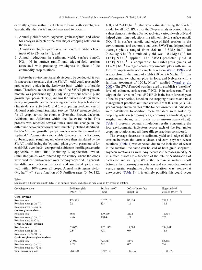
R.G. Nelson et al. / Journal of Environmental Management 79 (2006) 336–347 341

currently grown within the Delaware basin with switchgrass.

Specifically, the SWAT model was used to obtain:

1. Annual yields for corn, soybeans, grain sorghum, and wheat

for analysis in each of the four major cropping rotations in

the basin;

2. Annual switchgrass yields as a function of N fertilizer level

input (0 to 224 kg haK1); and

3. Annual reductions in sediment yield, surface runoff,

NO3 – N in surface runoff, and edge-of-field erosion

associated with producing switchgrass in place of the

commodity crop rotations.

Before the environmental analysis could be conducted, it was

first necessary to ensure that the SWAT model could reasonably

predict crop yields in the Delaware basin within a tolerable

error. Therefore, minor calibration of the SWAT plant growth

module was performed by: (1) adjusting various SWAT plant

growth input parameters; (2) running the SWAT model (with the

new plant growth parameters) using a separate 4-year historical

climate data set (1991–94); and (3) comparing predicted versus

National Agricultural Statistics Service (NASS) average yields

for all crops across the counties (Nemaha, Brown, Jackson,

Atchison, and Jefferson) within the Delaware basin. This

process was repeated several times until the change in the

difference between historical and simulated yield had stabilized;

the SWAT plant growth input parameters were then considered

‘optimal.’ Commodity crop yields (bushels haK1) for corn,

soybeans, grain sorghum, and wheat were then simulated by the

SWAT model (using the ‘optimal’ plant growth parameters) for

each HRU over the 24-year period, subject to the tillage scenario

applicable to that HRU (including N application levels).

Simulated yields were filtered by the county where the crops

were produced and averaged over the 24-year period. In general,

the difference between historical and simulated yields was

well within 10% across all crops. Annual switchgrass yields

(Mg haK1 yK1) as a function of N fertilizer rates (0, 56, 112,

Table 1

Sediment yield, surface runoff, NO3–N in surface runoff, and edge-of-field erosion

Cropping rotation Sediment yield

(Mg yK1)

Surf

(mm

Corn–soybean

Rotation total 176,915 5,65

Rotation average (haK1) 2.61 83.4

Rotation area: 67,767 ha

Corn–soybean–wheat

Rotation total 3681 179,

Rotation average (haK1) 2.26 110.

Rotation area: 1630 ha

Grain sorghum–soybean

Rotation total 65,055 1,65

Rotation average (haK1) 2.84 72.1

Rotation area: 22,908 ha

Grain sorghum–soybean–wheat

Rotation total 24,019 823,

Rotation average (haK1) 2.09 29.1

Rotation area: 11,472 ha

Total across rotations 269,670 8,30

168, and 224 kg haK1) also were estimated using the SWAT

model for all 552 HRUs over the 24-year analysis period. These

values demonstrate the effect of applying various levels of N and

helped determine reductions in sediment yield, surface runoff,

NO3–N in surface runoff, and edge-of-field erosion in the

environmental and economic analyses. SWAT model predicted

average yields ranged from 5.6 to 13.3 Mg haK1 for

0–224 kg N haK1; simulated yield was 10.4 Mg haK1 for

112 kg N haK1 applied. The SWAT-predicted yield at

112 kg N haK1 is comparable to switchgrass yields of

11.4 Mg haK1 averaged across experimental plots with similar

fertilizer inputs in the northern plains region (Walsh, 1994), and

is also close to the range of yields (10.5–12.6 Mg haK1) from

experimental switchgrass plots in Iowa and Nebraska with a

fertilizer treatment of 120 kg N haK1 applied (Vogel et al.,

2002). The SWAT model was then used to establish a ‘baseline’

level of sediment, surface runoff, NO3–N in surface runoff, and

edge-of-field erosion for all 552 HRUs in the basin for each year

of the 24-year period, based on the cropping rotations and field

management practices outlined earlier. From this analysis, 24-

year average annual values of the four environmental indicators

were calculated. In addition, these variables were sorted by

cropping rotation (corn–soybean, corn–soybean–wheat, grain

sorghum–soybean, and grain sorghum–soybean–wheat).

Table 1 presents general simulation results concerning the

four environmental indicators across each of the four major

cropping rotations and all three tillage practices considered.

The average decrease in sediment yield and edge-of-field

erosion between the corn–soybean and corn–soybean–wheat

rotations (Table 1) was expected due to the inclusion of wheat

in the rotation; the same can be said of both grain sorghum–

soybean rotations as well. Any decreases/increases in NO3–N

in surface runoff are a function of the rate of N utilization of

each crop and soil type. While the increase in surface runoff

between the corn–soybean rotation and corn–soybean–wheat

versus grain sorghum–soybean rotation was somewhat

unexpected (Table 1), it is entirely possible this could occur

by cropping rotation

ace runoff

)

NO3–N in surface

runoff (kg)

Edge-of-field

erosion (Mg yK1)

2,102 82,874 788,612

1.2 11.6

879 2132 11,704

4 1.3 7.2

1,831 19,605 284,641

0.9 12.4

311 8146 85,415

0.7 7.4

7,123 112,757 1,170,372

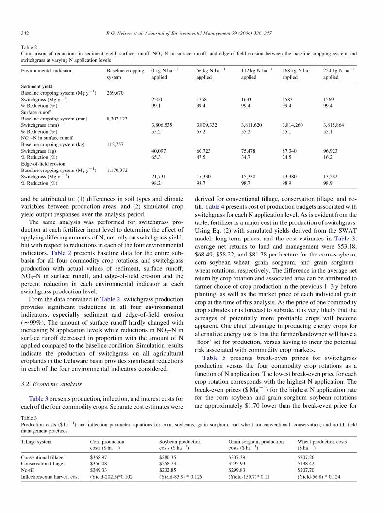
Table 2

Comparison of reductions in sediment yield, surface runoff, NO3–N in surface runoff, and edge-of-field erosion between the baseline cropping system and

switchgrass at varying N application levels

Environmental indicator Baseline cropping

system

0 kg N haK1

applied

56 kg N haK1

applied

112 kg N haK1

applied

168 kg N haK1

applied

224 kg N haK1

applied

Sediment yield

Baseline cropping system (Mg yK1) 269,670

Switchgrass (Mg yK1) 2500 1758 1633 1583 1569

% Reduction (%) 99.1 99.4 99.4 99.4 99.4

Surface runoff

Baseline cropping system (mm) 8,307,123

Switchgrass (mm) 3,806,535 3,809,332 3,811,620 3,814,260 3,815,864

% Reduction (%) 55.2 55.2 55.2 55.1 55.1

NO3–N in surface runoff

Baseline cropping system (kg) 112,757

Switchgrass (kg) 40,097 60,723 75,478 87,340 96,923

% Reduction (%) 65.3 47.5 34.7 24.5 16.2

Edge-of-field erosion

Baseline cropping system (Mg yK1) 1,170,372

Switchgrass (Mg y K1) 21,731 15,330 15,330 13,380 13,282

% Reduction (%) 98.2 98.7 98.7 98.9 98.9

R.G. Nelson et al. / Journal of Environmental Management 79 (2006) 336–347342

and be attributed to: (1) differences in soil types and climate

variables between production areas, and (2) simulated crop

yield output responses over the analysis period.

The same analysis was performed for switchgrass pro-

duction at each fertilizer input level to determine the effect of

applying differing amounts of N, not only on switchgrass yield,

but with respect to reductions in each of the four environmental

indicators. Table 2 presents baseline data for the entire sub-

basin for all four commodity crop rotations and switchgrass

production with actual values of sediment, surface runoff,

NO3–N in surface runoff, and edge-of-field erosion and the

percent reduction in each environmental indicator at each

switchgrass production level.

From the data contained in Table 2, switchgrass production

provides significant reductions in all four environmental

indicators, especially sediment and edge-of-field erosion

(w99%). The amount of surface runoff hardly changed with

increasing N application levels while reductions in NO3–N in

surface runoff decreased in proportion with the amount of N

applied compared to the baseline condition. Simulation results

indicate the production of switchgrass on all agricultural

croplands in the Delaware basin provides significant reductions

in each of the four environmental indicators considered.

3.2. Economic analysis

Table 3 presents production, inflection, and interest costs for

each of the four commodity crops. Separate cost estimates were

Table 3

Production costs ($ haK1) and inflection parameter equations for corn, soybeans

management practices

Tillage system Corn production

costs ($ haK1)

Soybean product

costs ($ haK1)

Conventional tillage $368.97 $280.35

Conservation tillage $356.08 $258.73

No-till $349.33 $232.85

Inflection/extra harvest cost (Yield-202.5)*0.102 (Yield-83.9) * 0

derived for conventional tillage, conservation tillage, and no-

till. Table 4 presents cost of production budgets associated with

switchgrass for each N application level. As is evident from the

table, fertilizer is a major cost in the production of switchgrass.

Using Eq. (2) with simulated yields derived from the SWAT

model, long-term prices, and the cost estimates in Table 3,

average net returns to land and management were $53.18,

$68.49, $58.22, and $81.78 per hectare for the corn–soybean,

corn–soybean–wheat, grain sorghum, and grain sorghum–

wheat rotations, respectively. The difference in the average net

return by crop rotation and associated area can be attributed to

farmer choice of crop production in the previous 1–3 y before

planting, as well as the market price of each individual grain

crop at the time of this analysis. As the price of one commodity

crop subsides or is forecast to subside, it is very likely that the

acreages of potentially more profitable crops will become

apparent. One chief advantage in producing energy crops for

alternative energy use is that the farmer/landowner will have a

‘floor’ set for production, versus having to incur the potential

risk associated with commodity crop markets.

Table 5 presents break-even prices for switchgrass

production versus the four commodity crop rotations as a

function of N application. The lowest break-even price for each

crop rotation corresponds with the highest N application. The

break-even prices ($ MgK1) for the highest N application rate

for the corn–soybean and grain sorghum–soybean rotations

are approximately $1.70 lower than the break-even price for

, grain sorghum, and wheat for conventional, conservation, and no-till field

ion Grain sorghum production

costs ($ haK1)

Wheat production costs

($ haK1)

$307.39 $207.26

$295.93 $198.42

$299.83 $207.70

.126 (Yield-150.7)* 0.11 (Yield-56.8) * 0.124

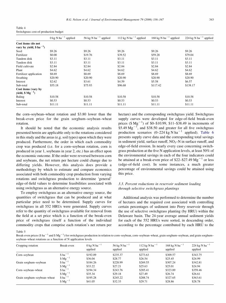
Table 4

Switchgrass cost-of-production budget

0 kg N haK1 applied 56 kg N haK1 applied 112 kg N haK1 applied 168 kg N haK1 applied 224 kg N haK1 applied

Cost items (do not

vary by yield, $ haK1)

Seed $9.26 $9.26 $9.26 $9.26 $9.26

Fertilizer $0.00 $19.76 $39.52 $59.28 $79.04

Tandem disk $3.11 $3.11 $3.11 $3.11 $3.11

Tandem disk $3.11 $3.11 $3.11 $3.11 $3.11

Field cultivate $2.84 $2.84 $2.84 $2.84 $2.84

Plant $4.62 $4.62 $4.62 $4.62 $4.62

Fertilizer application $8.69 $8.69 $8.69 $8.69 $8.69

Swathing $20.90 $20.90 $20.90 $20.90 $20.90

Interest $2.62 $3.61 $4.59 $5.58 $6.57

Sub-total $55.18 $75.93 $96.68 $117.42 $138.17

Cost items (vary by

yield, $ MgK1)

Baling $10.58 $10.58 $10.58 $10.58 $10.58

Interest $0.53 $0.53 $0.53 $0.53 $0.53

Sub-total $11.11 $11.11 $11.11 $11.11 $11.11

R.G. Nelson et al. / Journal of Environmental Management 79 (2006) 336–347 343

the corn–soybean–wheat rotation and $3.80 lower than the

break-even price for the grain sorghum–soybean–wheat

rotation.

It should be noted that the economic analysis results

presented herein are applicable only to the rotations considered

in this study and the areas (e.g. soil types) upon which they were

produced. Furthermore, the order in which each commodity

crop was produced (i.e. for a corn–soybean rotation, corn is

produced in year 1, soybeans in year 2, etc.) has an effect upon

the economic outcome. If the order were reversed between corn

and soybeans, the net return per hectare could change due to

differing yields. However, this analysis does provide a

methodology by which to estimate and compare economics

associated with both commodity crop production from varying

rotations and switchgrass production to determine ‘general’

edge-of-field values to determine feasibilities associated with

using switchgrass as an alternative energy source.

To employ switchgrass as an alternative energy source, the

quantities of switchgrass that can be produced and at what

particular price need to be determined. Supply curves for

switchgrass in all 552 HRUs were generated. Supply curves

refer to the quantity of switchgrass available for removal from

the field at a set price which is a function of the break-even

price of switchgrass (itself a function of the individual

commodity crops that comprise each rotation’s net return per

Table 5

Break-even prices ($ haK1 and $ MgK1) for switchgrass production in relation to cor

soybean–wheat rotations as a function of N application levels

Cropping rotation Break-even 0 kg N haK1

applied

56 k

appl

Corn–soybean $ haK1 $192.09 $235

$ MgK1 $36.04 $28.

Grain sorghum–soybean $ haK1 $184.26 $228

$ MgK1 $33.22 $27.

Corn–soybean–wheat $ haK1 $194.34 $243

$ MgK1 $35.34 $29.

Grain sorghum–soybean–wheat $ haK1 $195.28 $245

$ MgK1 $41.05 $32.

hectare) and the corresponding switchgrass yield. Switchgrass

supply curves were developed for edge-of-field break-even

prices ($ MgK1) of $0–$10.99, $11–$38.49 in increments of

$5.49 MgK1, and $38.50 and greater for all five switchgrass

production scenarios (0–224 kg N haK1 applied). Table 6

presents supply curve data and the corresponding total savings

in sediment yield, surface runoff, NO3–N in surface runoff, and

edge-of-field erosion. In nearly every case concerning switch-

grass production at the five N application levels, at least 50% of

the environmental savings in each of the four indicators could

be attained at a break-even price of $22–$27.49 MgK1 or less

(edge-of-field cost). In some instances, a much greater

percentage of environmental savings could be attained using

this price.

3.3. Percent reductions in reservoir sediment loading

through selective switchgrass plantings

Additional analysis was performed to determine the number

of hectares and the required cost associated with controlling

certain percentages of sediment into Perry reservoir through

the use of selective switchgrass planting (by HRU) within the

Delaware basin. The 24-year average annual sediment yields

for each of the 552 HRUs were sorted, in descending order,

according to the percentage contributed by each HRU to the

n–soybean, corn–soybean–wheat, grain sorghum–soybean, and grain sorghum–

g N haK1

ied

112 kg N haK1

applied

168 kg N haK1

applied

224 kg N haK1

applied

.37 $273.63 $309.57 $343.75

77 $26.54 $25.45 $24.99

.99 $269.55 $307.24 $342.81

21 $25.63 $25.01 $24.94

.76 $285.41 $323.89 $359.46

18 $27.49 $26.74 $26.61

.22 $288.74 $327.65 $363.61

33 $29.71 $28.86 $28.78

Table 6

Switchgrass supply curves and total savings in sediment yield, surface runoff, NO3–N in surface runoff, and edge-of-field erosion

# of metric tons of switchgrass and cumulative sediment yield, surface runoff, NO3–N in surface runoff, and edge-of-field erosion savings

Switchgrass (kg N haK1 applied) $0–$10.99 MgK1 $11.00–$16.49 MgK1 $16.50–$21.99 MgK1 $22.00–$27.49 MgK1 $27.50–$32.99 MgK1 $33.00–$38.49 MgK1 $38.50C Mg–1

0 kg N haK1 applied 4,599 25,064 39,605 91,404 247,343 375,228 580,150

Sediment yield (Mg yK1) 153,236 686,747 1,473,597 4,122,366 11,384,525 18,623,614 34,254,480

Surface runoff (mm) 42 19,080 39,890 115,255 370,314 608,244 882,678

NO3–N in surface runoff (kg) 167,344 819,247 1,263,013 2,165,096 4,415,112 6,325,147 8,499,945

Edge-of-field erosion (Mg yK1) 797 4445 7428 13,976 33,557 52,555 75,562

56 kg N haK1 applied 2623 44,117 81,508 375,202 678,492 797,834 871,654

Sediment yield (Mg yK1) 13 21,201 42,743 156,363 240,788 260,001 272,541

Surface runoff (mm) 34,230 530,392 811,233 2,556,452 3,944,955 4,418,610 4,693,112

NO3–N in surface runoff (kg) 58 3345 5075 23,675 45,056 52,874 54,935

Edge-of-field erosion (Mg yK1) 33 48,695 108,138 555,114 961,990 1,076,278 1,141,647

112 kg N haK1 applied 72 44,073 129,724 664,036 963,421 1,041,606 1,084,655

Sediment yield (Mg yK1) 0.35 14,044 53,540 213,255 255,273 267,503 272,666

Surface runoff (mm) 814 454,557 947,993 3,356,443 4,324,507 4,561,411 4,690,824

NO3–N in surface runoff (kg) 2.28 2010 3412 24,129 37,519 39,356 40,180

Edge-of-field erosion (Mg yK1) 0.75 35,573 158,318 821,369 1,053,280 1,116,823 1,142,908

168 kg N haK1 applied 28,193 160,986 189,179 880,368 1,142,625 1,249,808 1,257,135

Sediment yield (Mg yK1) 5985 63,263 69,248 232,289 259,196 271,896 272,716

Surface runoff (mm) 273,911 909,281 1,183,192 3,720,931 4,392,631 4,668,190 4,688,185

NO3–N in surface runoff (kg) 792 1408 2200 19,207 26,418 28,248 28,318

Edge-of-field erosion (Mg yK1) 14,275 189,073 203,348 919,134 1,073,548 1,138,532 1,143,497

224 kg N haK1 applied 0 11,669 206,260 1,047,363 1,291,440 1,405,171 n/a

Sediment yield (Mg yK1) 0 54 68,968 236,182 260,785 272,730 n/a

Surface runoff (mm) 0 110,488 1,171,505 3,844,828 4,426,641 4,686,581 n/a

NO3–N in surface runoff (kg) 0 79 1012 12,333 17,331 18,735 n/a

Edge-of-field erosion (Mg yK1) 0 108 205,744 952,362 1,081,004 1,143,695 n/a

R.G

.N

elson

eta

l./

Jou

rna

lo

fE

nviro

nm

enta

lM

an

ag

emen

t7

9(2

00

6)

33

6–

34

73

44

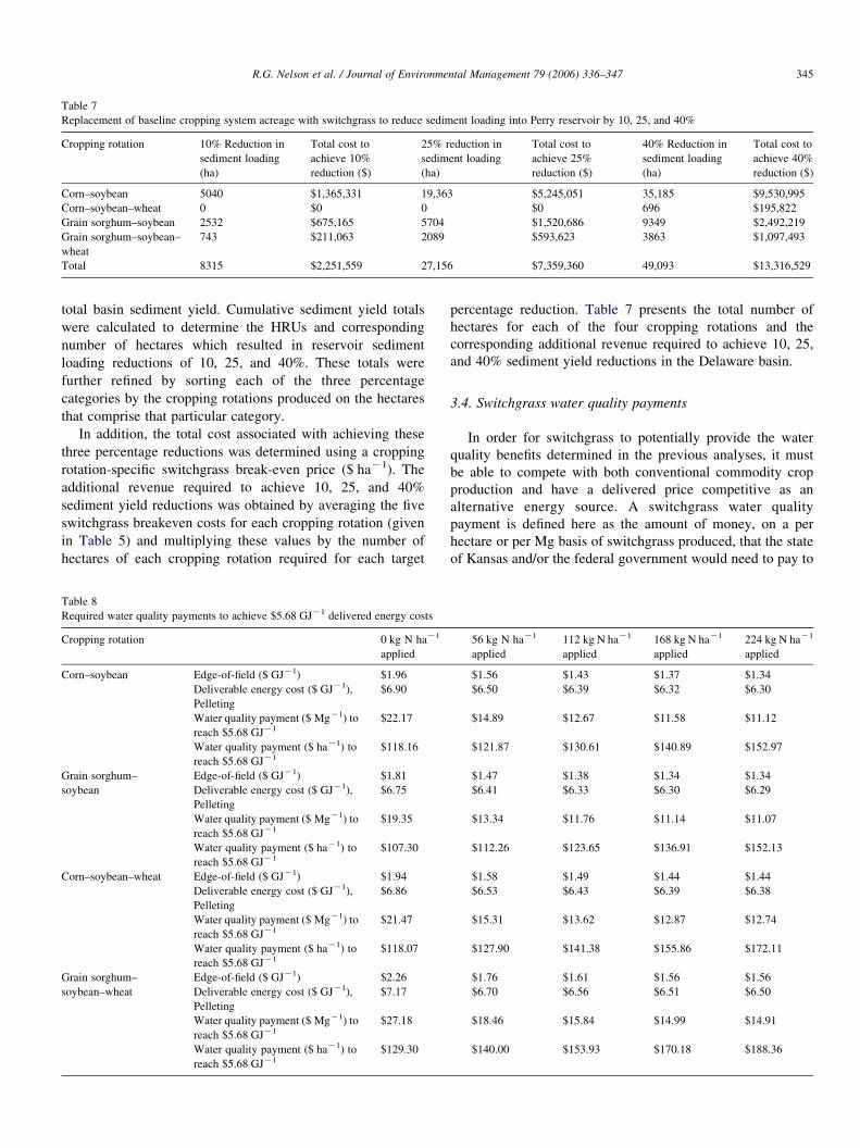
Table 7

Replacement of baseline cropping system acreage with switchgrass to reduce sediment loading into Perry reservoir by 10, 25, and 40%

Cropping rotation 10% Reduction in

sediment loading

(ha)

Total cost to

achieve 10%

reduction ($)

25% reduction in

sediment loading

(ha)

Total cost to

achieve 25%

reduction ($)

40% Reduction in

sediment loading

(ha)

Total cost to

achieve 40%

reduction ($)

Corn–soybean 5040 $1,365,331 19,363 $5,245,051 35,185 $9,530,995

Corn–soybean–wheat 0 $0 0 $0 696 $195,822

Grain sorghum–soybean 2532 $675,165 5704 $1,520,686 9349 $2,492,219

Grain sorghum–soybean–

wheat

743 $211,063 2089 $593,623 3863 $1,097,493

Total 8315 $2,251,559 27,156 $7,359,360 49,093 $13,316,529

R.G. Nelson et al. / Journal of Environmental Management 79 (2006) 336–347 345

total basin sediment yield. Cumulative sediment yield totals

were calculated to determine the HRUs and corresponding

number of hectares which resulted in reservoir sediment

loading reductions of 10, 25, and 40%. These totals were

further refined by sorting each of the three percentage

categories by the cropping rotations produced on the hectares

that comprise that particular category.

In addition, the total cost associated with achieving these

three percentage reductions was determined using a cropping

rotation-specific switchgrass break-even price ($ haK1). The

additional revenue required to achieve 10, 25, and 40%

sediment yield reductions was obtained by averaging the five

switchgrass breakeven costs for each cropping rotation (given

in Table 5) and multiplying these values by the number of

hectares of each cropping rotation required for each target

Table 8

Required water quality payments to achieve $5.68 GJK1 delivered energy costs

Cropping rotation 0 kg N haK1

applied

Corn–soybean Edge-of-field ($ GJK1) $1.96

Deliverable energy cost ($ GJK1),

Pelleting

$6.90

Water quality payment ($ MgK1) to

reach $5.68 GJK1

$22.17

Water quality payment ($ haK1) to

reach $5.68 GJK1

$118.16

Grain sorghum–

soybean

Edge-of-field ($ GJK1) $1.81

Deliverable energy cost ($ GJK1),

Pelleting

$6.75

Water quality payment ($ MgK1) to

reach $5.68 GJK1

$19.35

Water quality payment ($ haK1) to

reach $5.68 GJK1

$107.30

Corn–soybean–wheat Edge-of-field ($ GJK1) $1.94

Deliverable energy cost ($ GJK1),

Pelleting

$6.86

Water quality payment ($ MgK1) to

reach $5.68 GJK1

$21.47

Water quality payment ($ haK1) to

reach $5.68 GJK1

$118.07

Grain sorghum–

soybean–wheat

Edge-of-field ($ GJK1) $2.26

Deliverable energy cost ($ GJK1),

Pelleting

$7.17

Water quality payment ($ MgK1) to

reach $5.68 GJK1

$27.18

Water quality payment ($ haK1) to

reach $5.68 GJK1

$129.30

percentage reduction. Table 7 presents the total number of

hectares for each of the four cropping rotations and the

corresponding additional revenue required to achieve 10, 25,

and 40% sediment yield reductions in the Delaware basin.

3.4. Switchgrass water quality payments

In order for switchgrass to potentially provide the water

quality benefits determined in the previous analyses, it must

be able to compete with both conventional commodity crop

production and have a delivered price competitive as an

alternative energy source. A switchgrass water quality

payment is defined here as the amount of money, on a per

hectare or per Mg basis of switchgrass produced, that the state

of Kansas and/or the federal government would need to pay to

56 kg N haK1

applied

112 kg N haK1

applied

168 kg N haK1

applied

224 kg N haK1

applied

$1.56 $1.43 $1.37 $1.34

$6.50 $6.39 $6.32 $6.30

$14.89 $12.67 $11.58 $11.12

$121.87 $130.61 $140.89 $152.97

$1.47 $1.38 $1.34 $1.34

$6.41 $6.33 $6.30 $6.29

$13.34 $11.76 $11.14 $11.07

$112.26 $123.65 $136.91 $152.13

$1.58 $1.49 $1.44 $1.44

$6.53 $6.43 $6.39 $6.38

$15.31 $13.62 $12.87 $12.74

$127.90 $141.38 $155.86 $172.11

$1.76 $1.61 $1.56 $1.56

$6.70 $6.56 $6.51 $6.50

$18.46 $15.84 $14.99 $14.91

$140.00 $153.93 $170.18 $188.36

R.G. Nelson et al. / Journal of Environmental Management 79 (2006) 336–347346

the farmer/landowner for switchgrass to achieve a ‘target’

market price. In this study, the only alternative energy use

scenario was for the switchgrass to be pelleted and used as a

replacement for propane in space and water heating

applications in homes and business within the Delaware basin.

The switchgrass production break-even price per hectare for

each of the five N application levels for all four cropping

rotations was converted into an analogous payment per Mg by

dividing by the average annual switchgrass yields attainable

over the areas upon which each cropping rotation was

produced. These payments ($ MgK1 of switchgrass produced)

were then converted to an edge-of-field energy payment

($ GJK1) by dividing them by a switchgrass energy conversion

factor of 18.4 GJ MgK1. In the case of employing switchgrass

as an alternative energy source, all costs associated with

converting it into a useable energy source (e.g. transportation,

loading, processing, and conversion) must be considered when

making a valid comparison to the competing alternative fossil-

based fuel source. An analysis was conducted to determine the

final deliverable price associated with transporting switchgrass

to the pelleting mill, processing the switchgrass into useable

pellets, management of the mill, and delivery to the end-use

markets (King, 1999). From this analysis, a cost of

$90.81 MgK1 was allocated to these expenses in addition to

the in-field production cost calculated above. This is the

delivered cost to the end consumer minus any mark-up for

profit.

If this cost is less than the current and/or forecasted propane

cost, then theoretically no water quality payment would be

required and the farmer/landowner could produce switchgrass

at a cost/price indifferent to that of a particular cropping

rotation and the state and/or federal government would reap the

water quality benefits associated with switchgrass production

at no cost. If however, the projected/forecasted cost for energy

were below the deliverable switchgrass energy cost, then the

state and/or federal government would need to provide a

supplemental or assistance payment that would ‘buy down’ the

energy cost from switchgrass production to an amount equal to

the expected propane cost.

Table 8 lists the deliverable energy costs ($ GJK1)

associated with pelleting switchgrass for each of the

commodity cropping rotations and N application levels

considered. In addition, an analysis was run to determine the

additional cost per Mg and hectare to achieve a delivered static

propane energy cost of $5.68 GJK1 from pelletized switch-

grass. This propane energy cost was chosen because it reflected

the latest historical energy price trend for that particular area of

Kansas. These payments ranged from a low of $11.07 MgK1 to

a high of $27.18 MgK1 depending upon switchgrass yield level.

4. Summary and conclusions

This analysis indicates that switchgrass production on

conventional agricultural cropland in northeast Kansas has

distinct environmental advantages versus the traditional

cropping rotations of corn–soybean, corn–soybean–wheat,

grain sorghum–soybean, and grain sorghum–soybean–wheat.

SWAT model simulations showed that sediment yield, surface

runoff, NO3–N in surface runoff, and edge-of-field erosion

were reduced by an average of 99, 55, 34, and 98%,

respectively, over the range (0–224 kg N haK1) of N appli-

cation levels.

Average net returns were $53.18, $68.49, $58.22, and

$81.78 haK1 for the rotations of corn–soybean, corn–soybean–

wheat, grain sorghum, and grain sorghum–wheat, respectively.

These returns translated into break-even prices for switchgrass

production ranging from $184.26 to $363.61 haK1 depending

upon N application level and type of cropping rotation.

In nearly every scenario concerning switchgrass pro-

duction, at least 50% of the environmental savings in

sediment yield, surface runoff, NO3–N in surface runoff, and

edge-of-field erosion could be attained at an edge-of-field

switchgrass price of $22–$27.49 MgK1 or less. In some

instances, a much greater percentage of environmental savings

could be attained within this price range. The conversion to

switchgrass from any conventional commodity crop pro-

duction scenario requires that farmers be fairly confident in

the price they will receive for the crops (commodity or

alternative energy), which in turn dictates the expense of

converting to energy crop production. Hence, the real

conversion expense is fairly variable with an inherent element

of risk. In general, only farmers that believe they can

sustainably produce energy crops at fairly higher yields,

coupled with a potential demand for their crops through a

long-term contract with a utility or energy service provider,

would substantially reduce their expense.

The total deliverable energy cost associated with manu-

facturing switchgrass pellets and using them as a propane

substitute was calculated using break-even prices for all four

cropping rotations and a consideration of transportation,

processing, and conversion costs. Deliverable energy costs

ranged from a low of $6.29 GJK1 to a high of $7.17 GJK1. The

magnitude of switchgrass water quality payments needed to

achieve delivered energy costs of $5.68 GJK1 were determined

and ranged from a low of $11.07 MgK1 to a high of

$27.18 MgK1 depending upon switchgrass yield level.

References

Anon, 1986. Urban Hydrology for Small Watersheds, Tech. Release 55.

USDA-SCS, Washington, DC.

Arnold, J.G., Williams, J.R., Maidment, D.R., 1995. Continuous-time water

and sediment-routing model for large basins. Journal of Hydraulic

Engineering 121 (2), 171–183.

Arnold, J.G., Srinivasan, R., Muttiah, R.S., Williams, J.R., 1998. Large area

hydrologic modeling and assessment Part I: Model development. Journal of

the American Water Resources Association 34 (1), 73–89.

Bagnold, R.A., 1977. Bedload transport in natural rivers. Water Resources

Research 13 (2), 303–312.

Chapra, S.C., 1997. Surface Water Quality Modeling. McGraw-Hill, New

York, NY. 844 pp..

Green, W.H., Ampt, C.A., 1911. Studies on soil physics, I. Flow of water and

air through soils. Journal of Agricultural Sciences 4, 1–24.

Kansas Department of Health and Environment, 1999. Kansas Unified

Watershed Assessment — Final Report. Kansas Department of Health

R.G. Nelson et al. / Journal of Environmental Management 79 (2006) 336–347 347

and Environment, Nonpoint Source Pollution Section, Bureau of Water.

Topeka, KS. 23 pp.

Kastens, T.L., Dhuyvetter, K.C., Jones, R., 2000. Prices for Crop and Livestock

Cost-Return Budgets. Farm Management Guide Report No. MF-1013.

Department of Agricultural Economics and Kansas State University

Agricultural Experiment Station and Cooperative Extension Service,

Kansas State University Manhattan, KS.

King, J.E., 1999. Reducing Bioenergy Cost by Monetizing Environmental

Benefits of Reservoir Water Quality Improvements from Switchgrass

Production, Task 2 Final Report — Pelletized Switchgrass for Space and

Water Heating. Grant No. DE-FG48-97R802102. Kansas Corporation

Commission, Energy Programs Division, Topeka, KS, 82 pp.

King, J.E., Hannifan, J.M., Nelson, R.G., 1998. An Assessment of the

Feasibility of Electric Power Derived from Biomass and Waste Feedstocks.

Report No. KRD-9513. Kansas Electric Utilities Research Program and

Kansas Corporation Commission, Topeka, KS, 280 pp.

Knisel, W.G. (Ed.), 1980. CREAMS: A Field-scale Model for Chemicals,

Runoff, and Erosion from Agricultural Management System. Conservation

Research Report 26. USDA-SEA, Washington, DC.

Leonard, R.A., Knisel, W.G., Still, D.A., 1987. GLEAMS: groundwater

loading effects on agricultural management systems. Transactions of ASAE

30 (5), 1403–1428.

McElroy, A.D., Chiu, S.Y., Nebgen, J.W., Aletic, A., Bennett, R.Q., 1976.

Loading Functions for Assessment of Water Pollution from Nonpoint

Sources. United States Environmental Protection Agency Report No.

EPA 600/2-76-151. USEPA Offices of Res. and Dev., Washington, DC.

123 pp.

Neitsch, S.L., Arnold, J.G., Kiniry, J.R., Srinivasan, R., Williams, J.R., 2002.

Soil and Water Assessment Tool User’s Manual Version 2000. GSWRL

Report 02-02, BRC Report 02-06. Texas Water Resources Institute TR-192,

College Station, TX, 472 pp.

Ramanarayanan, T.S., Srinivasan, R., Arnold, J.G., 1996. Modeling Wister

Lake watershed using a GIS-linked basin-scale hydrologic/water quality

model. Proc. Third International NCGIA Conference/Workshop on

Integrating GIS and Environmental Modeling, Santa Fe, New Mexico,

January, 21–25.

Sloan, P.G., Moore, I.D., Coltharp, G.B., Eigel J.D., 1983. Modeling Surface

and Subsurface Stormflow on Steeply-Sloping Forested Watersheds. Water

Resources Institute Report 142. University of Kentucky, Lexington, KY,

83 pp.

Stefan, H.G., Preud’homme, E.B., 1993. Stream temperature estimation from

air temperature. Water Resources Bulletin 30 (3), 453–462.

United States Department of Agriculture – Soil Conservation Service (SCS),

1972. Hydrology. Section 4. In: National Engineering Handbook. SCS,

Washington, D.C.

United States Department of Energy, 2004. Energy Information Administration

Annual Energy Outlook 2004 (AEO2004), Report No. DOE/EIA-

0383(2004). National Energy Information Center, EI-30, Forrestal

Building, Washington, DC, 278 pp.

United States Environmental Protection Agency, 2000. National Water Quality

Inventory: 2000 Report, http://www.epa.gov/305b/2000report. United

States Environmental Protection Agency, Washington, DC, 324 pp.

Vogel, K.P., Brejda, J.J., Walters, D.T., Buxton, D.R., 2002. Switchgrass

biomass production in the Midwest USA: harvest and nitrogen manage-

ment. Agronomy Journal94, 413–420.

Walsh, M.E., 1994. The cost of producing switchgrass as dedicated energy

crop. Biologue 4th Qtr, 35–36.

Williams, J.R., 1969. Flood routing with variable travel time or variable storage

coefficients. Transactions of ASAE 12 (1), 100–103.

Williams, J.R., 1980. SPNM, a model for predicting sediment, phosphorous,

and nitrogen from agricultural basins. Water Resources Bulletin 16 (5),

843–848.

Williams, J.R., 1995. The EPIC model. In: Singh, V.P. (Ed.), Computer Models

of Watershed Hydrology. Water Resources Publications, Littleton, CO,

pp. 909–1000.

Williams, J.R., Berndt, H.D., 1977. Sediment yield prediction based on

watershed hydrology. Transactions of ASAE 20 (6), 1100–1104.

Williams, J.R., Hann, R.W., 1972. HYMO, a problem-oriented computer

language for building hydrologic models. Water Resources Research 8 (1),

79–85.

Wischmeier, W.H., Smith, D.D., 1978. Predicting Rainfall Erosion Losses—A

guide to Conservation Planning. US Department of Agriculture,

Agricultural Handbook No. 537. US Gov. Print. Office, Washington, DC.