This article was downloaded by: [M. Ivette Gomes]On: 29 November 2014, At: 01:26Publisher: Taylor & FrancisInforma Ltd Registered in England and Wales Registered Number: 1072954 Registeredoffice: Mortimer House, 37-41 Mortimer Street, London W1T 3JH, UK

Statistics: A Journal of Theoretical andApplied StatisticsPublication details, including instructions for authors andsubscription information:http://www.tandfonline.com/loi/gsta20

Bias reduction of a tail index estimatorthrough an external estimation of thesecond-order parameterM. Ivette Gomes a , Frederico Caeiro b & Fernanda Figueiredo ca Faculdade de Ciências (DEIO) and CEAUL , Universidade deLisboa, Edificio c6, Piso 4, Cidade Universitária, Campo Grande ,1749-016, Lisboa, Portugalb Departamento de Matemática , Universidade Nova de Lisboa ,FCT, Portugalc Faculdade de Economia and CEAUL , Universidade do Porto ,PortugalPublished online: 01 Feb 2004.

To cite this article: M. Ivette Gomes , Frederico Caeiro & Fernanda Figueiredo (2004) Biasreduction of a tail index estimator through an external estimation of the second-orderparameter, Statistics: A Journal of Theoretical and Applied Statistics, 38:6, 497-510, DOI:10.1080/02331880412331284304

To link to this article: http://dx.doi.org/10.1080/02331880412331284304

PLEASE SCROLL DOWN FOR ARTICLE

Taylor & Francis makes every effort to ensure the accuracy of all the information (the“Content”) contained in the publications on our platform. However, Taylor & Francis,our agents, and our licensors make no representations or warranties whatsoever as tothe accuracy, completeness, or suitability for any purpose of the Content. Any opinionsand views expressed in this publication are the opinions and views of the authors,and are not the views of or endorsed by Taylor & Francis. The accuracy of the Contentshould not be relied upon and should be independently verified with primary sourcesof information. Taylor and Francis shall not be liable for any losses, actions, claims,proceedings, demands, costs, expenses, damages, and other liabilities whatsoeveror howsoever caused arising directly or indirectly in connection with, in relation to orarising out of the use of the Content.

This article may be used for research, teaching, and private study purposes. Anysubstantial or systematic reproduction, redistribution, reselling, loan, sub-licensing,

systematic supply, or distribution in any form to anyone is expressly forbidden. Terms &Conditions of access and use can be found at http://www.tandfonline.com/page/terms-and-conditions

Dow

nloa

ded

by [

M. I

vette

Gom

es]

at 0

1:26

29

Nov

embe

r 20

14

Statistics, December 2004, Vol. 38(6), pp. 497–510

BIAS REDUCTION OF A TAIL INDEX ESTIMATORTHROUGH AN EXTERNAL ESTIMATION OF

THE SECOND-ORDER PARAMETER

M. IVETTE GOMESa,∗, FREDERICO CAEIROb, and FERNANDA FIGUEIREDOc

aFaculdade de Ciencias (DEIO) and CEAUL, Universidade de Lisboa, Edificio c6, Piso 4, CidadeUniversitaria, Campo Grande, 1749-016 Lisboa, Portugal; bDepartamento de Matematica,

Universidade Nova de Lisboa, FCT, Portugal; cFaculdade de Economia and CEAUL,Universidade do Porto, Portugal

(Received 16 December 2002; Revised 5 January 2004; In final form 15 June 2004)

In this paper, we first consider a class of consistent semi-parametric estimators of a positive tail index γ , parameterisedin a tuning or control parameter α. Such a control parameter enables us to have access, for any available sample, to anestimator of the tail index γ with a null dominant component of asymptotic bias, and consequently with a reasonablyflat mean squared error pattern, as a function of k, the number of top-order statistics considered. Such a controlparameter depends on a second-order parameter ρ, which will be adequately estimated so that we may achieve a highefficiency relative to the classical Hill estimator, provided we use a number of top-order statistics larger than the oneusually required for the estimation through the Hill estimator. An illustration of the behaviour of the estimators isprovided, through the analysis of the daily log-returns on the Euro–US$ exchange rates.

Keywords: Statistical theory of extremes; Semi-parametric Estimation

AMS Subject Classification 1991: Primary: 62G05, 62E25, 62E20; Secondary: 62F35

1 THE CLASS OF SEMI-PARAMETRIC ESTIMATORS

In this paper, we deal with a semi-parametric estimator of the tail index γ , with a null dom-inant component of asymptotic bias. This kind of estimators has revealed nice distributionalproperties (Peng, 1998; Beirlant et al., 1999; Feuerverger and Hall, 1999; Gomes et al., 2000,2002; Gomes and Martins, 2001; Caeiro and Gomes, 2002).

We shall consider here heavy tails, i.e. γ > 0 in the extreme value distribution function(d.f.)

EVγ (x) :={

exp(−(1 + γ x)−1/γ ), 1 + γ x > 0 if γ �= 0

exp(− exp(−x)), x ∈ R if γ = 0,

the only non-degenerate d.f. to which Xn:n := max(X1, . . . , Xn) may be attracted, after suitablelinear normalization. If this happens we say that the underlying model F is in the max-domain

∗ Corresponding author: E-mail: ivette.gomes@fc.ul.pt

ISSN 0233-1888 print; ISSN 1029-4910 online c© 2004 Taylor & Francis LtdDOI: 10.1080/02331880412331284304

Dow

nloa

ded

by [

M. I

vette

Gom

es]

at 0

1:26

29

Nov

embe

r 20

14

498 M. I. GOMES et al.

of attraction of EVγ , and denote this by F ∈ DM(EVγ ). As usual, Xi:n, 1 ≤ i ≤ n, denotes theith ascending order statistic (o.s.) associated with the random sample (X1, . . . , Xn) from theunknown d.f. F .

With U(t) := F←(1 − 1/t), t ≥ 1, F← denoting the generalized inverse function of F , wehave (Gnedenko, 1943; de Haan, 1970),

F ∈ DM(EVγ ), γ > 0, iff 1 − F ∈ RV−1/γ iff U ∈ RVγ , (1)

where RVβ stands for the class of regularly varying functions at infinity with index of regularvariation β, i.e., positive measurable functions g such that limt→∞ g(tx)/g(t) = xβ , for allx > 0.

Apart from the first-order condition in Eq. (1), we shall often assume that there exists afunction A(t) of constant sign near infinity, measuring the rate of convergence of ln U(tx) −ln U(t) towards γ ln x in the first-order condition, i.e., a function A such that

limt→∞

ln U(tx) − ln U(t) − γ ln x

A(t)= xρ − 1

ρ, (2)

for every x > 0, where ρ (≤ 0) is a second-order parameter. The limit function in Eq. (2) mustbe of the stated form, and |A(t)| ∈ RVρ (Geluk and de Haan, 1987). In this paper, we shallrestrict ourselves to the case ρ < 0.

The first class of semi-parametric estimators of γ , herewith considered under a third-orderframework to be introduced in Section 3, is the same class as in Caeiro and Gomes (2002),

γ (α)n (k) := �(α)

M(α−1)n (k)

(M(2α)

n (k)

�(2α + 1)

)1/2

, α ≥ 1. (3)

Such a class is parameterised in the tuning parameter α, which may be controlled at our ease.We have M(0)

n ≡ 1, and

M(α)n (k) := 1

k

k∑i=1

(ln Xn−i+1:n − ln Xn−k:n)α, α > 0, (4)

are consistent estimators of �(α + 1)γ α , whenever k is intermediate, i.e., whenever

k = kn −→ ∞, and k = o(n), as n −→ ∞. (5)

M(1)n (k), also denoted γ H

n (k), is the classical Hill’s estimator (Hill, 1975).The class of estimators in Eq. (3), studied in Caeiro and Gomes (2002), generalizes the

estimator γ (1)n (k) :=

√M

(2)n (k)/2, studied in Gomes et al. (2000). In the class (3), and whenever

ρ < 0, it is possible to find a control parameter α which makes null the dominant componentof asymptotic bias of our tail index estimator. Such a control parameter depends on the second-order parameter ρ, which, contrarily to what has been done in Caeiro and Gomes (2002), isgoing to be here properly estimated on the basis of our sample. We may thus get a secondclass of ‘asymptotically unbiased’ estimators of the tail index γ , now based on an externalestimation of the second-order parameter ρ, and given by

γ (α)n (k) := �(α)

M(α−1)n (k)

(M(2α)

n (k)

�(2α + 1)

)1/2

with α = − ln[1 − ρ − √(1 − ρ)2 − 1]

ln(1 − ρ), (6)

where generally ρ may be any consistent estimator of ρ.

Dow

nloa

ded

by [

M. I

vette

Gom

es]

at 0

1:26

29

Nov

embe

r 20

14

BIAS REDUCTION OF A TAIL INDEX ESTIMATOR 499

As we know from previous papers that these ‘asymptotically unbiased’ estimators behavebetter than the Hill estimator, we shall also consider, for comparison with the class of estimatorsin Eq. (6), an ML-estimator, asymptotically equivalent to the ML-estimator in Gomes andMartins (2002), and given by

γ ML(ρ)n (k) := 1

k

k∑i=1

exp

(D

(i

n

)−ρ)

Ui (7)

where

D ≡ D(k) := 1

nρ

(∑ki=1 i−ρ

) (∑ki=1 Ui

)− k

(∑ki=1 i−ρUi

)(∑k

i=1 i−ρ

) (∑ki=1 i−ρUi

)− k

(∑ki=1 i−2ρUi

) ,

withUi = i{ln Xn−i+1:n − ln Xn−i:n}, 1 ≤ i ≤ k,

denoting the scaled log-spacings. Such an estimator is the one with smallest asymptotic vari-ance, among the ones so far considered in the literature. Such an asymptotic variance isγ 2(1 − ρ)2/ρ2, the lower limit provided in Drees (1998) for the general class of ‘asymptoticallyunbiased’ estimators therewith considered.

In Section 2, we shall briefly refer the asymptotic behaviour of the class of estimators inEq. (3), under a second-order framework, as derived in Caeiro and Gomes (2002), but using anotation adequate to the introduction of the third-order framework. In Section 3, we shall workunder such a third-order framework, and shall make a few comments on a class of estimators ofthe second-order parameter ρ, recently introduced by Fraga Alves et al. (2003). In Section 4,we shall incorporate these ρ-estimators in our class of tail index estimators, removing thedominant component of asymptotic bias. In Section 5, we shall derive, through simulationtechniques, the distributional properties of one of these estimators for finite sample sizes, andfor a few heavy-tailed models. Finally, in Section 6, we shall consider a case-study related tothe daily exchange rates of the Euro against the US$, to illustrate the methodologies advancedin this paper.

2 ASYMPTOTIC PROPERTIES OF THE FIRST CLASS OF ESTIMATORS

Under the first-order condition (1) and the restriction (5) on the level k, the statistics γ (α)n (k) in

Eq. (3) are consistent forγ , and under some extra mild conditions on the second-order behaviourof the model F underlying the data they are asymptotically normal, with an asymptotic biaspossibly non-null, and given by bα(ρ) × limn→∞

√k A(n/k), with A given in Eq. (2) and

where bα(ρ) will be explicited later.Let W denote an exponential r.v., with d.f. FW(x) = 1 − exp(−x), x > 0, and, with the

same notation as in Gomes et al. (2002) and Fraga Alves et al. (2003), let us put

µ(1)α := E[Wα] = �(α + 1), µ(1)

α = 1

σ (1)α := √

Var[Wα] =√

�(2α + 1) − �2(α + 1), σ (1)α := σ (1)

α

µ(1)α

,

µ(2)α (ρ) := E

[Wα−1(eρW − 1)

ρ

]= �(α)(1 − (1 − ρ)α)

ρ(1 − ρ)α, µ(2)

α (ρ) := µ(2)α (ρ)

µ(1)α

,

where � denotes the complete Gamma function, �(α) = ∫ ∞0 xα−1e−x dx, α > 0.

Dow

nloa

ded

by [

M. I

vette

Gom

es]

at 0

1:26

29

Nov

embe

r 20

14

500 M. I. GOMES et al.

We first state, without proof, which may be seen in Gomes and Martins (2001), and hadalready been suggested in Dekkers et al. (1989), the main result used to derive the asymptoticproperties of γ (α)

n (k) in Eq. (3).

PROPOSITION 1 Under the validity of the first-order condition in Eq. (1) and for k intermediate,i.e., k such that Eq. (5) holds, the statistic M(α)

n (k) in Eq. (4) converges in probability towardsγ αµ(1)

α . If we further assume the general second-order framework in Eq. (2), the followingasymptotic distributional representation,

M(α)n (k)

d= γ αµ(1)α + γ ασ (1)

α√k

P(α)k + αγ α−1µ(2)

α (ρ) A(n

k

)(1 + op(1)) (8)

holds, where, with {Wi}i≥1 denoting independent standard exponential r.v.’s, P(α)k :=

((1/k)∑k

i=1 Wαi − µ(1)

α )/σ (1)α is an asymptotically standard normal r.v. Moreover, the r.v.’s

P(α)k and P

(β)

k have a covariance structure given by σα,β := (µ(1)α+β − µ(1)

α µ(1)β )/σ (1)

α σ(1)β .

We next present a result proved in Caeiro and Gomes (2002).

PROPOSITION 2 Under the conditions and notations of Proposition 1, the asymptotic distri-butional representation

γ (α)n (k)

d= γ +(

γ√

vα√k

Z(α)k + bα (ρ)A

(n

k

))(1 + op(1))

holds true for the statistic γ (α)n (k) in Eq. (3), where Z

(α)k is asymptotically standard normal,

and may be written as

Z(α)k = 1√

vα

(σ

(1)2α P

(2α)k

2− σ

(1)α−1P

(α−1)k

),

with P(α)k given in the distributional representation (8) for M(α)

n (k). We have

vα = 1

4

{2�(4α)

2α�2(2α)+ 4�(2α − 1)

�2(α)− 2�(3α)

α�(2α)�(α)− 1

}(9)

andbα(ρ) = αµ

(2)2α (ρ) − (α − 1)µ

(2)α−1(ρ)

=

1

2ρ{(1 − ρ)−2α − 2(1 − ρ)−α+1 + 1} if ρ < 0

1 if ρ = 0.

Then, since k = kn → ∞, γ (α)n (k) is consistent for the estimation of γ , and if

√kA(n/k) →

λ, finite,√

k(γ (α)n (k) − γ ) is asymptotically normal, with asymptotic variance γ 2vα and

asymptotic bias λbα(ρ).Moreover, for every ρ ∈ R

− and α > 1 there is a value α0 ≡ α0(ρ), explicitly given by

α0 ≡ α0(ρ) = − ln[1 − ρ − √(1 − ρ)2 − 1]

ln(1 − ρ), (10)

such that bα0(ρ) = 0, i.e. γ (α0)n (k) has a null asymptotic bias, even when

√k A(n/k) → λ �= 0,

as n → ∞.

Dow

nloa

ded

by [

M. I

vette

Gom

es]

at 0

1:26

29

Nov

embe

r 20

14

BIAS REDUCTION OF A TAIL INDEX ESTIMATOR 501

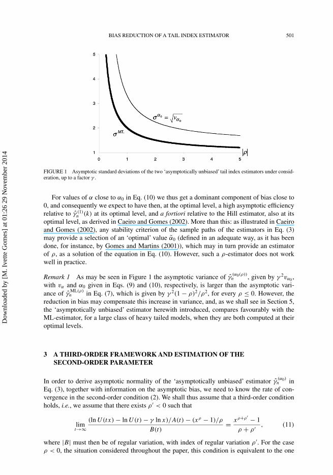
FIGURE 1 Asymptotic standard deviations of the two ‘asymptotically unbiased’ tail index estimators under consid-eration, up to a factor γ .

For values of α close to α0 in Eq. (10) we thus get a dominant component of bias close to0, and consequently we expect to have then, at the optimal level, a high asymptotic efficiencyrelative to γ (1)

n (k) at its optimal level, and a fortiori relative to the Hill estimator, also at itsoptimal level, as derived in Caeiro and Gomes (2002). More than this: as illustrated in Caeiroand Gomes (2002), any stability criterion of the sample paths of the estimators in Eq. (3)may provide a selection of an ‘optimal’ value α0 (defined in an adequate way, as it has beendone, for instance, by Gomes and Martins (2001)), which may in turn provide an estimatorof ρ, as a solution of the equation in Eq. (10). However, such a ρ-estimator does not workwell in practice.

Remark 1 As may be seen in Figure 1 the asymptotic variance of γ(α0(ρ))n , given by γ 2vα0 ,

with vα and α0 given in Eqs. (9) and (10), respectively, is larger than the asymptotic vari-ance of γ

ML(ρ)n in Eq. (7), which is given by γ 2(1 − ρ)2/ρ2, for every ρ ≤ 0. However, the

reduction in bias may compensate this increase in variance, and, as we shall see in Section 5,the ‘asymptotically unbiased’ estimator herewith introduced, compares favourably with theML-estimator, for a large class of heavy tailed models, when they are both computed at theiroptimal levels.

3 A THIRD-ORDER FRAMEWORK AND ESTIMATION OF THESECOND-ORDER PARAMETER

In order to derive asymptotic normality of the ‘asymptotically unbiased’ estimator γ(α0)n in

Eq. (3), together with information on the asymptotic bias, we need to know the rate of con-vergence in the second-order condition (2). We shall thus assume that a third-order conditionholds, i.e., we assume that there exists ρ ′ < 0 such that

limt→∞

(ln U(tx) − ln U(t) − γ ln x)/A(t) − (xρ − 1)/ρ

B(t)= xρ+ρ′ − 1

ρ + ρ ′ , (11)

where |B| must then be of regular variation, with index of regular variation ρ ′. For the caseρ < 0, the situation considered throughout the paper, this condition is equivalent to the one

Dow

nloa

ded

by [

M. I

vette

Gom

es]

at 0

1:26

29

Nov

embe

r 20

14

502 M. I. GOMES et al.

assumed in the papers of Gomes and de Haan (1999), Gomes et al. (2002) and Fraga Alveset al. (2003).

Remark 2 Note that for most of the well-known heavy-tailed models, like the Frechet, thegeneralized Pareto, the Burr, the Student, and a large variety of models in Hall’s class ofdistributions (Hall, 1982; Hall and Welsh, 1985), the models for which we have, with ρ < 0,a tail function of the type

1 − F(x) = Cx−1/γ (1 + D1xρ/γ + D2x

2ρ/γ + o(x2ρ/γ )), as x −→ ∞,

the third-order condition in Eq. (11) holds with ρ ′ = ρ.With the same notation as before, i.e., with W denoting a standard exponential r.v., we shall

still introduce here some extra notation:

σ (2)α (ρ) :=

√Var

[Wα−1(eρW − 1)

ρ

]=

õ

(3)2α (ρ) − (µ

(2)α (ρ))2, σ (2)

α (ρ) := σ (2)α (ρ)

µ(1)α

,

with

µ(3)α := E

[Wα−2

(eρW − 1

ρ

)2]

= 2{µ(2)α−1(2ρ) − µ

(2)α−1(ρ)}

ρ

µ(3)α (ρ) = µ(3)

α (ρ)

µ(1)α

=

1

ρ2ln

(1 − ρ)2

1 − 2ρif α = 1

1

ρ2α(α − 1)

{1

(1 − 2ρ)α−1− 2

(1 − ρ)α−1+ 1

}if α �= 1

.

3.1 The Asymptotic Distributional Behaviour of Our First Class of Tail IndexEstimators Under a Third-Order Framework

In the lines of Proposition 2, we may explain the following.

THEOREM 1 If, with the same notation as before, we further assume the general third-orderframework in Eq. (11), and if we choose the tuning parameter α such that

bα(ρ) = αµ(2)2α (ρ) − (α − 1)µ

(2)α−1(ρ) = 0,

the following asymptotic distributional representation,

γ (α)n (k)

d= γ + γ√

vα√k

Z(α)n + A2(n/k)

2γ(α(2α − 1)µ

(3)2α (ρ) − α2(µ

(2)2α (ρ))2

− (α − 1)(α − 2)µ(3)α−1(ρ) + 2(α − 1)2(µ

(2)α−1(ρ))2)(1 + op(1))

+ A(n

k

)B

(n

k

)(αµ

(2)2α (2ρ) − (α − 1)µ

(2)α−1(2ρ))(1 + op(1)), (12)

holds. Consequently,√

k{γ (α)n (k) − γ } is asymptotically normal with null mean value, not only

when√

k A(n/k) → 0, but also whenever√

k A(n/k) → λ, finite or infinite, provided that

Dow

nloa

ded

by [

M. I

vette

Gom

es]

at 0

1:26

29

Nov

embe

r 20

14

BIAS REDUCTION OF A TAIL INDEX ESTIMATOR 503

√k A2(n/k) → 0, as n → ∞. If

√k A2(n/k) → λA, finite, and

√k A(n/k)B(n/k) → λB ,

also finite, there is a non-null asymptotic bias given by

λA

2γ(α(2α − 1)µ

(3)2α (ρ) − α2(µ

(2)2α (ρ))2 − (α − 1)(α − 2)µ

(3)α−1(ρ)

+ 2(α − 1)2(µ(2)α−1(ρ))2) + λB(αµ

(2)2α (2ρ) − (α − 1)µ

(2)α−1(2ρ)). (13)

Proof Under the third-order condition in Eq. (11), assuming that Eq. (5) holds, and using thesame arguments as in Dekkers et al. (1989), in Lemma 2 of Draisma et al. (1999) and morerecently in Gomes et al. (2002) and Fraga Alves et al. (2003), we may write the distributionalrepresentation(

M(2α)n (k)

µ(1)2α

)1/2

= γ α

(1 + σ

(1)2α

2

P (2α)n√k

+ αµ(2)2α (ρ)A(n/k)

γ+ αµ

(2)2α (ρ)

γ

A(n/k) P (2α)n√

k

+ αA2(n/k)

2γ 2

((2α − 1)µ

(3)2α (ρ) − α(µ

(2)2α (ρ))2

)(1 + op(1))

+ α

γµ

(2)2α (2ρ)A

(n

k

)B

(n

k

)(1 + op(1))

),

where P (2α)n and P (2α)

n are asymptotically standard Normal r.v.’s.In addition(

M(α−1)n (k)

µ(1)α−1

)−1

= γ 1−α

(1 − σ

(1)α−1

P (α−1)n√

k

− α − 1

γµ

(2)α−1(ρ)A

(n

k

)− α − 1

γσ

(2)α−1(ρ)

A(n/k)√k

P (α−1)n

− α − 1

2γ 2A2

(n

k

)((α − 2)µ

(3)α−1(ρ)

− 2(α − 1)(µ(2)α−1(ρ))2)(1 + op(1))

−α − 1

γµ

(2)α−1(2ρ)A

(n

k

)B

(n

k

)(1 + op(1))

).

Then

γ (α)n (k)

d= γ

(1 + 1√

k

(σ

(1)2α P (2α)

n

2− σ

(1)α−1P

(α−1)n

)

+ A(n/k)

γ(αµ

(2)2α (ρ) − (α − 1)µ

(2)α−1(ρ))

+ A(n/k)

γ√

k(ασ

(2)2α (ρ)P (2α)

n − (α − 1)σ(2)α−1(ρ)P (α−1)

n )

+ A2(n/k)

2γ 2

(α(2α − 1)µ

(3)2α (ρ) − α2(µ

(2)2α (ρ))2

−(α − 1)(α − 2)µ(3)α−1(ρ) + 2(α − 1)2(µ

(2)α−1(ρ))2

)(1 + op(1))

+A(n/k)B(n/k)

γ(αµ

(2)2α (2ρ) − (α − 1)µ

(2)α−1(2ρ))(1 + op(1))

).

Dow

nloa

ded

by [

M. I

vette

Gom

es]

at 0

1:26

29

Nov

embe

r 20

14

504 M. I. GOMES et al.

If we choose α such that αµ(2)2α (ρ) − (α − 1)µ

(2)α−1(ρ) = 0, the result in Eq. (12) follows

immediately: the rate of convergence is still of the order of 1/√

k, and the asymptotic bias isnull not only when

√kA(n/k) → 0 but also when

√kA(n/k) → λ �= 0. The bias in Eq. (13)

is also straightforward, and is equal to λA uA if |ρ| < |ρ ′|, since then B(t) = o(A(t)), beingequal to λB uB whenever |ρ| > |ρ ′|, due to the fact that then A(t) = o(B(t)), as t → ∞. �

Remark 3 The experience we have from the second-order framework leads us to state that theminimum asymptotic mean squared error is now going to be attained whenever

√kA(n/k) →

∞ and √kA2(n/k) −→ λA �= 0, finite if |ρ| ≤ |ρ ′|,

√kA(n/k)B(n/k) −→ λB �= 0, finite if |ρ| > |ρ ′|.

Note that if ρ = ρ ′ and√

kA2(n/k) → λA �= 0, finite, then,√

kA(n/k)B(n/k) → λB �= 0,also finite.

3.2 The Estimation of the Second-Order Parameter

We shall consider here particular members of the class of estimators of the second-orderparameter ρ proposed by Fraga Alves et al. (2003). Under adequate general conditions, theyare semi-parametric asymptotically normal estimators of ρ, which show highly stable samplepaths as functions of k, the number of top o.s. used, for a wide range of large k-values. Such aclass of estimators is parameterised in a tuning parameter τ and depends on the statistics

T (τ)n (k) :=

(M(1)n (k))τ − (M(2)

n (k)/2)τ/2

(M(2)n (k)/2)τ/2 − (M

(3)n (k)/6)τ/3

if τ > 0

ln(M(1)n (k)) − (1/2) ln(M(2)

n (k)/2)

(1/2) ln(M(2)n (k)/2) − (1/3) ln(M

(3)n (k)/6)

if τ = 0,

which converge towards 3(1 − ρ)/(3 − ρ), independently of τ , whenever the second-ordercondition (2) holds and k is such that k = o(n) and

√kA(n/k) → ∞, as n → ∞. The

estimators are thus given by

ρ(τ )n (k) := min

(0,

3(T (τ)n (k) − 1)

T(τ)n (k) − 3

). (14)

We shall formalize, without proofs, the main distributional results of the estimators in Eq. (14).Proofs may be found in Fraga Alves et al. (2003).

PROPOSITION 3 If the first-order condition (1) holds, k is a sequence of intermediate integers,i.e., Eq. (5) holds, and if limn→∞

√kA(n/k) = ∞, then ρ(τ )

n (k) in Eq. (14) is consistent forthe estimation of ρ, i.e., converges in probability towards ρ, as n → ∞.

PROPOSITION 4 If the third-order condition (11) holds, k is a sequence of intermediate inte-gers, i.e., Eq. (5) holds, if limn→∞

√kA(n/k) = ∞, but limn→∞

√kA2(n/k) = λ1, finite

and limn→∞√

kA(n/k)B(n/k) = λ2, finite, we may guarantee asymptotic normality of theestimators ρ(τ )

n (k) in Eq. (14), and ρ(τ )n − ρ = Op(1/(

√kA(n/k))).

Dow

nloa

ded

by [

M. I

vette

Gom

es]

at 0

1:26

29

Nov

embe

r 20

14

BIAS REDUCTION OF A TAIL INDEX ESTIMATOR 505

Remark 4 The theoretical and simulated results in Fraga Alves et al. (2003), together with theuse in these estimators in the generalized Jackknife statistics of Gomes et al. (2000) (Gomesand Martins, 2002) led us to advise in practice the consideration of the level

k1 = min

(n − 1,

[2n

ln ln n

])(15)

(not chosen in any optimal way), and of the tuning parameters τ = 0 for the region ρ ∈ [−1, 0)

and τ = 1 for the region ρ ∈ (−∞, −1).Anyway, we advise practitioners not to choose blindlythe value of τ in Eq. (14). It is sensible to draw a few sample paths of ρ(τ )

n in Eq. (14), as functionsof k, and for a few values of τ , like τ = 0, 0.5, 1, electing the value of τ which provides higherstability for large k, by means of any stability criterion. The value of k1 in Eq. (15), although notchosen in any optimal way, may be considered for any chosen value of the tuning parameter τ .

4 DISTRIBUTIONAL PROPERTIES OF THE ‘ASYMPTOTICALLY UNBIASED’ESTIMATORS OF THE TAIL INDEX, BASED ON THE EXTERNALESTIMATION OF ρ

We shall now consider the class of estimators in Eq. (6), where ρ ≡ ρτ = ρ(τ )n (k1) is any of

the estimators in Eq. (14), with k1 in Eq. (15).

THEOREM 2 If the second-order condition (2) holds, if k = kn is a sequence of intermediatepositive integers, i.e., Eq. (5) holds, and if

√kA(n/k) →

n→∞ λ, finite, non-necessarily null, then√k(γ (α)

n (k) − γ ) are asymptotically normal with null mean value. Indeed, with Zk denotingan asymptotically standard normal r.v., we have, for the tail index estimators under study,

γ (α)(k)d= γ + γ ϕ(ρ)√

kZk + op

(A

(n

k

)), (16)

with ϕ(ρ) = vα0 , vα given in Eq. (9) and α0 = α0(ρ) given in Eq. (10). More than this: theresults in Theorem 1 hold true if we replace γ (α)

n (k) by γ (α)n (k) in Eq. (6), where ρ ≡ ρτ =

ρ(τ )n (k1) is any of the estimators in Eq. (14), with k1 in Eq. (15).

Proof The proof for the r.v. γ(α0)n (k), α0 = α0(ρ) follows the same lines of the proof of

Theorem 1, and we get straightforwardly, as a particular case of Eq. (12),

γ (α0)n (k)

d= γ + γ ϕ(ρ)√k

Zk + op

(A

(n

k

)).

The result in Eq. (16) is due to the fact that we may write

γ (α)n (k) = γ (α0)

n (k) + (ρτ − ρ)ξ(k)(1 + op(1)),

with ρτ − ρ = op(1) for all k in the conditions of the theorem, and ξ(k) = Op(1/√

k).

The last part of the theorem comes from the fact that, due to the choice of the level k1

used in the estimation of ρ, ρ − ρ = O((ln ln n)1/(1−2ρ)/√

n). Consequently, if |ρ| ≤ |ρ ′|and

√kA2(n/k) → λA, finite, n/k = O(n1/(1−4ρ)) and ρ − ρ = op(A2(n/k)). Analogously,

if |ρ| > |ρ ′| and√

kA(n/k)B(n/k) → λB , finite, n/k = O(n1/(1−2(ρ+ρ′))) and ρ − ρ =op(A(n/k)B(n/k)). �

Dow

nloa

ded

by [

M. I

vette

Gom

es]

at 0

1:26

29

Nov

embe

r 20

14

506 M. I. GOMES et al.

Remark 5 Note that should we have worked with ρ(k), computed at the same level k, thefact that ρ(k) − ρ = Op(1/(

√kA(n/k))) = Op(1) would lead to an increase in the asymptotic

variance of our tail index estimator.

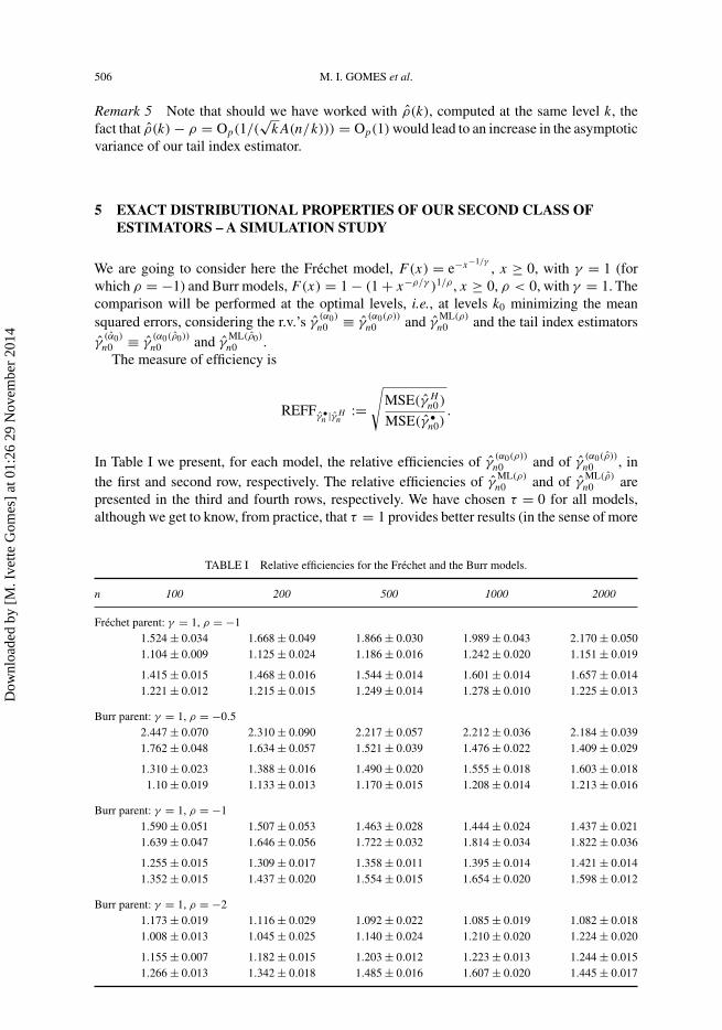
5 EXACT DISTRIBUTIONAL PROPERTIES OF OUR SECOND CLASS OFESTIMATORS – A SIMULATION STUDY

We are going to consider here the Frechet model, F(x) = e−x−1/γ, x ≥ 0, with γ = 1 (for

which ρ = −1) and Burr models, F(x) = 1 − (1 + x−ρ/γ )1/ρ , x ≥ 0, ρ < 0, with γ = 1. Thecomparison will be performed at the optimal levels, i.e., at levels k0 minimizing the meansquared errors, considering the r.v.’s γ

(α0)

n0 ≡ γ(α0(ρ))

n0 and γML(ρ)n0 and the tail index estimators

γ(α0)

n0 ≡ γ(α0(ρ0))

n0 and γML(ρ0)

n0 .The measure of efficiency is

REFFγ •n |γ H

n:=

√MSE(γ H

n0 )

MSE(γ •n0)

.

In Table I we present, for each model, the relative efficiencies of γ(α0(ρ))

n0 and of γ(α0(ρ))

n0 , inthe first and second row, respectively. The relative efficiencies of γ

ML(ρ)n0 and of γ

ML(ρ)n0 are

presented in the third and fourth rows, respectively. We have chosen τ = 0 for all models,although we get to know, from practice, that τ = 1 provides better results (in the sense of more

TABLE I Relative efficiencies for the Frechet and the Burr models.

n 100 200 500 1000 2000

Frechet parent: γ = 1, ρ = −11.524 ± 0.034 1.668 ± 0.049 1.866 ± 0.030 1.989 ± 0.043 2.170 ± 0.0501.104 ± 0.009 1.125 ± 0.024 1.186 ± 0.016 1.242 ± 0.020 1.151 ± 0.019

1.415 ± 0.015 1.468 ± 0.016 1.544 ± 0.014 1.601 ± 0.014 1.657 ± 0.0141.221 ± 0.012 1.215 ± 0.015 1.249 ± 0.014 1.278 ± 0.010 1.225 ± 0.013

Burr parent: γ = 1, ρ = −0.52.447 ± 0.070 2.310 ± 0.090 2.217 ± 0.057 2.212 ± 0.036 2.184 ± 0.0391.762 ± 0.048 1.634 ± 0.057 1.521 ± 0.039 1.476 ± 0.022 1.409 ± 0.029

1.310 ± 0.023 1.388 ± 0.016 1.490 ± 0.020 1.555 ± 0.018 1.603 ± 0.0181.10 ± 0.019 1.133 ± 0.013 1.170 ± 0.015 1.208 ± 0.014 1.213 ± 0.016

Burr parent: γ = 1, ρ = −11.590 ± 0.051 1.507 ± 0.053 1.463 ± 0.028 1.444 ± 0.024 1.437 ± 0.0211.639 ± 0.047 1.646 ± 0.056 1.722 ± 0.032 1.814 ± 0.034 1.822 ± 0.036

1.255 ± 0.015 1.309 ± 0.017 1.358 ± 0.011 1.395 ± 0.014 1.421 ± 0.0141.352 ± 0.015 1.437 ± 0.020 1.554 ± 0.015 1.654 ± 0.020 1.598 ± 0.012

Burr parent: γ = 1, ρ = −21.173 ± 0.019 1.116 ± 0.029 1.092 ± 0.022 1.085 ± 0.019 1.082 ± 0.0181.008 ± 0.013 1.045 ± 0.025 1.140 ± 0.024 1.210 ± 0.020 1.224 ± 0.020

1.155 ± 0.007 1.182 ± 0.015 1.203 ± 0.012 1.223 ± 0.013 1.244 ± 0.0151.266 ± 0.013 1.342 ± 0.018 1.485 ± 0.016 1.607 ± 0.020 1.445 ± 0.017

Dow

nloa

ded

by [

M. I

vette

Gom

es]

at 0

1:26

29

Nov

embe

r 20

14

BIAS REDUCTION OF A TAIL INDEX ESTIMATOR 507

FIGURE 2 Mean values (left) and mean squared errors (right) of γ Hn (k), of the estimators γ

(α0(ρ0))n , γ

ML(ρ0)n and of

the r.v.’s γ(α0(ρ))n , γ

ML(ρ)n , for sample size n = 1000 from a Frechet (γ = 1) model.

stable sample paths as function of k, whenever k is large) for values of |ρ| > 1. The simulationis based on 10 replicates of 1000 runs each.

In Figures 2–4, we illustrate for a sample size n = 1000, and for the Frechet (γ = 1), theBurr (γ = 1, ρ = −0.5) and the Burr (γ = 1, ρ = −2) models, respectively, the mean valueand the mean squared errors functions of γ

(α0(ρ))n , γ

(α0(ρ))n , γ

ML(ρ)n and γ

ML(ρ)n , denoted α0(ρ),

α0(ρ), ML(ρ) and ML(ρ), respectively. For comparison, we also present the Hill estimator,denoted H .

To illustrate the type of the sample paths (the usual situation in practice), we have drawnFigure 5. From this figure, it is possible to see that even for small values of ρ, like ρ = −2,the choice of ρ0 instead of ρ1 is also possible, and leads to similar conclusions.

Table I and the figures suggest the following comments related with the estimator in Eq. (6),with ρ = ρ0:

1. For the Frechet model (Fig. 2), we need to use practically all o.s.’s, both whenever weassume ρ known or we estimate ρ adequately – for this model the bias component of the

FIGURE 3 Mean values (left) and mean squared errors (right) of γ Hn (k), of the estimators γ

(α0(ρ0))n , γ

ML(ρ0)n and of

the r.v.’s γ(α0(ρ))n , γ

ML(ρ)n , for sample size n = 1000 from a Burr (γ = 1, ρ = −0.5) model.

Dow

nloa

ded

by [

M. I

vette

Gom

es]

at 0

1:26

29

Nov

embe

r 20

14

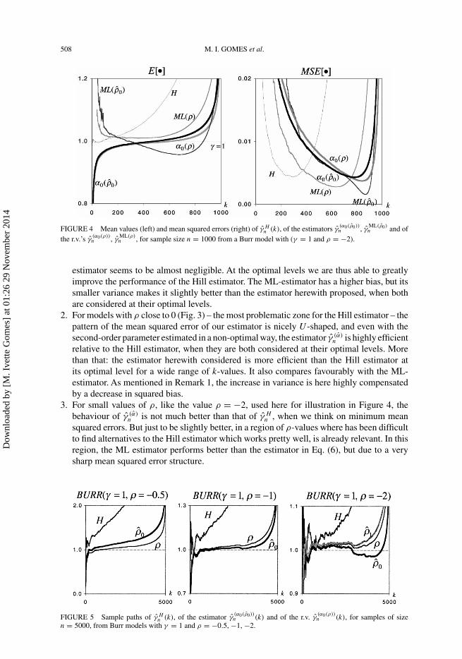
508 M. I. GOMES et al.

FIGURE 4 Mean values (left) and mean squared errors (right) of γ Hn (k), of the estimators γ

(α0(ρ0))n , γ

ML(ρ0)n and of

the r.v.’s γ(α0(ρ))n , γ

ML(ρ)n , for sample size n = 1000 from a Burr model with (γ = 1 and ρ = −2).

estimator seems to be almost negligible. At the optimal levels we are thus able to greatlyimprove the performance of the Hill estimator. The ML-estimator has a higher bias, but itssmaller variance makes it slightly better than the estimator herewith proposed, when bothare considered at their optimal levels.

2. For models with ρ close to 0 (Fig. 3) – the most problematic zone for the Hill estimator – thepattern of the mean squared error of our estimator is nicely U -shaped, and even with thesecond-order parameter estimated in a non-optimal way, the estimator γ (α)

n is highly efficientrelative to the Hill estimator, when they are both considered at their optimal levels. Morethan that: the estimator herewith considered is more efficient than the Hill estimator atits optimal level for a wide range of k-values. It also compares favourably with the ML-estimator. As mentioned in Remark 1, the increase in variance is here highly compensatedby a decrease in squared bias.

3. For small values of ρ, like the value ρ = −2, used here for illustration in Figure 4, thebehaviour of γ (α)

n is not much better than that of γ Hn , when we think on minimum mean

squared errors. But just to be slightly better, in a region of ρ-values where has been difficultto find alternatives to the Hill estimator which works pretty well, is already relevant. In thisregion, the ML estimator performs better than the estimator in Eq. (6), but due to a verysharp mean squared error structure.

FIGURE 5 Sample paths of γ Hn (k), of the estimator γ

(α0(ρ0))n (k) and of the r.v. γ

(α0(ρ))n (k), for samples of size

n = 5000, from Burr models with γ = 1 and ρ = −0.5, −1, −2.

Dow

nloa

ded

by [

M. I

vette

Gom

es]

at 0

1:26

29

Nov

embe

r 20

14

BIAS REDUCTION OF A TAIL INDEX ESTIMATOR 509

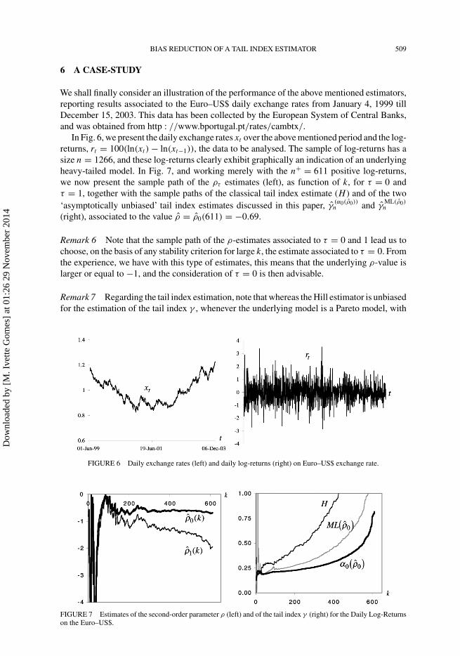
6 A CASE-STUDY

We shall finally consider an illustration of the performance of the above mentioned estimators,reporting results associated to the Euro–US$ daily exchange rates from January 4, 1999 tillDecember 15, 2003. This data has been collected by the European System of Central Banks,and was obtained from http : //www.bportugal.pt/rates/cambtx/.

In Fig. 6, we present the daily exchange rates xt over the above mentioned period and the log-returns, rt = 100(ln(xt ) − ln(xt−1)), the data to be analysed. The sample of log-returns has asize n = 1266, and these log-returns clearly exhibit graphically an indication of an underlyingheavy-tailed model. In Fig. 7, and working merely with the n+ = 611 positive log-returns,we now present the sample path of the ρτ estimates (left), as function of k, for τ = 0 andτ = 1, together with the sample paths of the classical tail index estimate (H ) and of the two‘asymptotically unbiased’ tail index estimates discussed in this paper, γ

(α0(ρ0))n and γ

ML(ρ0)n

(right), associated to the value ρ = ρ0(611) = −0.69.

Remark 6 Note that the sample path of the ρ-estimates associated to τ = 0 and 1 lead us tochoose, on the basis of any stability criterion for large k, the estimate associated to τ = 0. Fromthe experience, we have with this type of estimates, this means that the underlying ρ-value islarger or equal to −1, and the consideration of τ = 0 is then advisable.

Remark 7 Regarding the tail index estimation, note that whereas the Hill estimator is unbiasedfor the estimation of the tail index γ , whenever the underlying model is a Pareto model, with

FIGURE 6 Daily exchange rates (left) and daily log-returns (right) on Euro–US$ exchange rate.

FIGURE 7 Estimates of the second-order parameter ρ (left) and of the tail index γ (right) for the Daily Log-Returnson the Euro–US$.

Dow

nloa

ded

by [

M. I

vette

Gom

es]

at 0

1:26

29

Nov

embe

r 20

14

510 M. I. GOMES et al.

distribution F(x) = 1 − x−1/γ , x ≥ 0 (γ > 0), it exhibits a relevant bias when we have onlyPareto-like tails, as happens here, and may be seen from Figure 7. The other estimators, whichare ‘asymptotically unbiased’ reveal a smaller bias, and enable us to take a decision upon theestimate of γ to be used, with the help of any stability criterion or any heuristic procedure,like the ‘largest run’: here, if we consider the tail index estimates with two decimal figures,the largest run is achieved by the sample path of the estimator in Eq. (6). Such a run has a sizeequal to 43 (86 ≤ k ≤ 128), and is associated to γ

(α0(ρ0))n = 0.21. Should we be happy with

one decimal figure, would we also get the largest run for the same estimator: a run of size 278(4 ≤ k ≤ 281) associated to γ

(α0(ρ0))n = 0.2. For the ML-estimate, and with one decimal figure,

we would also get a tail index estimate equal to 0.2, but with a run of size 130. With this samecriterion, the Hill estimator would provide an estimate equal to 0.3, with a run of size 102.

Acknowledgement

Research partially supported by FCT/POCTI/FEDER.

References

Beirlant, J., Dierckx, G., Goegebeur, Y. and Matthys, G. (1999). Tail index estimation and an exponential regressionmodel. Extremes, 2(2), 177–200.

Caeiro, F. and Gomes, M. I. (2002). A class of asymptotically unbiased semiparametric estimators of the tail index.Test, 11(2), 345–364.

de Haan, L. (1970). On Regular Variation and its Application to the Weak Convergence of Sample Extremes. Mathe-matical Centre Tract 32, Amsterdam.

Dekkers, A. L. M., Einmahl, J. and de Haan, L. (1989). A moment estimator for the index of an extreme-valuedistribution. Ann. Stat., 17, 1833–1855.

Draisma, G., Haan, L., de, Peng, L. and Pereira, T. T. (1999). A bootstrap-based method to achieve optimality inestimating the extreme value index. Extremes, 2(4), 367–404.

Drees, H. (1998). A general class of estimators of the extreme value index. J. Stat. Plan. Infer., 66, 95–112.Feuerverger, A. and Hall, P. (1999). Estimating a tail exponent by modelling departure from a Pareto distribution.

Ann. Stat., 27, 760–781.Fraga Alves, M. I., Gomes, M. I. and de Haan, L. (2003). A new class of semi-parametric estimators of the second

order parameter. Portugaliae Mathematica, 60(2), 193–214.Geluk, J. and de Haan, L. (1987). Regular variation, Extensions and Tauberian Theorems. CWI Tract 40, Center for

Mathematics and Computer Science, Amsterdam, Netherlands.Gnedenko, B. V. (1943). Sur la distribution limite du terme maximum d’une serie aleatoire. Ann. Math., 44, 423–453.Gomes, M. I. and de Haan, L. (1999). Approximation by penultimate extreme value distributions. Extremes, 2(1),

71–85.Gomes, M. I. and Martins, M. J. (2001). Alternatives to Hill’s estimator – asymptotic versus finite sample behaviour.

J. Stat. Plan. Infer., 93, 161–180.Gomes, M. I. and Martins, M. J. (2002). Asymptotically unbiased estimators of the tail index based on external

estimation of the second order parameter. Extremes, 5(1), 5–31.Gomes, M. I., Martins, M. J. and Neves, M. (2000). Alternatives to a semi-parametric estimator of parameters of rare

events – the Jackknife methodology. Extremes, 3(3), 207–229.Gomes, M. I., de Haan, L. and Peng, L. (2002). Semi-parametric estimation of the second order parameter – asymptotic

and finite sample behaviour. Extremes, 5(4), 387–414.Gomes, M. I., Martins, M. J. and Neves, M. (2002). Generalized Jackknife semi-parametric estimators of the tail

index. Portugaliae Mathematica, 59(4), 393–408.Hall, P. (1982). On some simple estimates of an exponent of regular variation. J. Roy. Stat. Soc., B44, 37–42.Hall, P. and Welsh, A. H. (1985). Adaptive estimates of parameters of regular variation. Ann. Stat., 13, 331–341.Hill, B. M. (1975). A simple general approach to inference about the tail of a distribution. Ann. Stat., 3, 1163–1174.Peng, L. (1998). Asymptotically unbiased estimator for the extreme-value index. Stat. Prob. Lett., 38(2), 107–115.

Dow

nloa

ded

by [

M. I

vette

Gom

es]

at 0

1:26

29

Nov

embe

r 20

14