INFERENTIAL STATISTICS

Dr. Efthymia Nikita

Athens 2013

Inferential statistics Inferential statistics is used for making inferences about a population from observations and analyses of a sample.

In practice, it is used to compare two or more samples and draw conclusions about the populations to which they belong.

Independent and paired samples

Two or more samples are independent when each sample has been obtained independently from the others.

A basic characteristic of such samples is that they may have different sizes (number of cases).

For example, when we want to compare the base diameter of the amphorae from three archaeological sites.

Two or more samples are paired when the cases of one sample correspond to those of the other sample.

Therefore, paired samples always have the same size (number of cases).

For example, when we want to compare the dimensions between the right and left side of the humerus in order to examine bilateral asymmetry and subsequent activity patterns.

Independent and paired samples

Independent samples t-test This test is used when we want to compare two independent samples and see if there is a statistically significant difference between the population means from which they originate.

It is a parametric test and therefore a basic prerequisite is that the two samples are normal. If this prerequisite is not fulfilled, a Monte-Carlo test or the non-parametric Mann-Whitney test may be performed.

Independent samples t-test The null hypothesis and the alternative hypothesis are:

Η0: μ1 = μ2

Η1: μ1 μ2

The alternative hypothesis may also be expressed as:

Η1: μ1 > μ2 or Η1: μ1 < μ2

Example – Exercise 7

We have obtained geochemical samples from two different areas in an archaeological site in order to calculate phosphorus concentration since high concentration suggests a possible human usage, e.g. burial site, storage facility etc. The data is given in the table on the right in ppm (parts per million) (file ‘exercise 7’).

Site 1 Site 2560800770390500890950810740910820830

740820690830990360900840630910680550290990800300

Examine whether there is a statistically significant difference between the concentrations in the two areas.

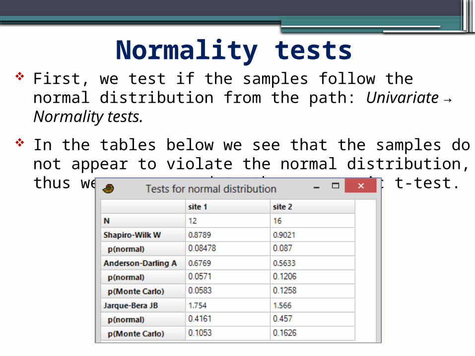
Normality tests First, we test if the samples follow the normal distribution from the path: Univariate →Normality tests.

In the tables below we see that the samples do not appear to violate the normal distribution, thus we can proceed to the parametric t-test.

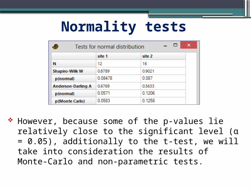
Normality tests

However, because some of the p-values lie relatively close to the significant level (α = 0.05), additionally to the t-test, we will take into consideration the results of Monte-Carlo and non-parametric tests.

Homogeneity of variance issues ...

In order to compare the mean values of the two samples we select the columns with the data from the two sites.

Then we follow the path: Univariate Two-→sample tests (F, t, Ma-Wh, Ko-Sm etc.).

In the results window we examine for more confidence both the parametric and non-parametric results.

However, we should first check whether the two samples exhibit homogeneity of variance or not. This is because the t-test in this case gives two p-values; one when the assumption of homogeneity of variances is valid and the other when this assumption is violated.

Homogeneity of variance issues ...

To check if the samples exhibit homogeneity of variance and subsequently which of the two p values is correct, we click on the F test tab. We observe that p = 0.358, thus the assumption of homogeneity of variances cannot be rejected.

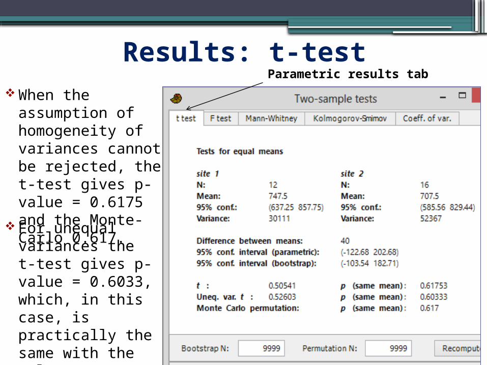
Results: t-testParametric results tab

When the assumption of homogeneity of variances cannot be rejected, the t-test gives p-value = 0.6175 and the Monte-Carlo 0.617.

For unequal variances the t-test gives p-value = 0.6033, which, in this case, is practically the same with the value 0.6175.

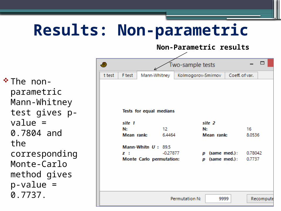
Results: Non-parametric

The non-parametric Mann-Whitney test gives p-value = 0.7804 and the corresponding Monte-Carlo method gives p-value = 0.7737.

Non-Parametric results

Conclusion The null hypothesis (that the samples come from populations with equal mean values) cannot be rejected.

Therefore, it seems that the two areas of the site did not have a different usage. However, since the null hypothesis is not rejected, we do not know how likely it is to be making a mistake.

Only if our samples are large enough, can we be confident that our conclusion is valid.

Mann-Whitney test We already applied the Mann-Whitney test in the previous exercise.

It is the equivalent of the Independent samples t-test, when the sample values do not follow the normal distribution.

However, we should be careful in the statement of the null hypothesis:

Mann-Whitney test

For the alternative we have the following cases:

Η1 : The samples come from different populations with d1 d2

or Η1: The samples come from different populations with d1 > d2

or Η1: The samples come from different populations with d1 < d2

The null hypothesis may be expressed as:Η0 : Both samples come from the same population

Example – Exercise 8

As part of a paleodemographic study we want to compare the number of individuals in seaside and inland archaeological sites. The data is given in the table on the right (file ‘exercise 8’).

Seaside sites

Inland sites

5811522319016189112139167201

5862579114462132152601633250

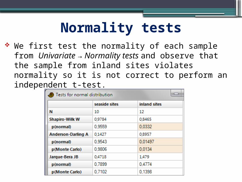
Normality tests We first test the normality of each sample from Univariate Normality tests → and observe that the sample from inland sites violates normality so it is not correct to perform an independent t-test.

Now we select both variables, follow the path Univariate → Two-sample tests (F, t, Ma-Wh, Ko-Sm, etc.) and we click on the Mann-Whitney tab.

Results: Non-parametric tests

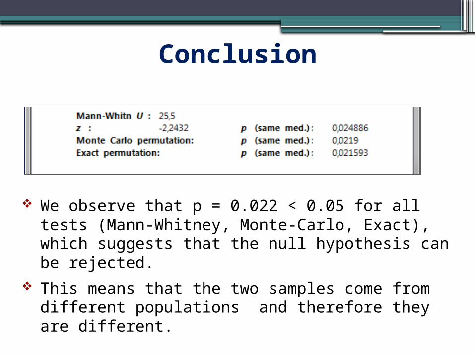
We observe that p = 0.022 < 0.05 for all tests (Mann-Whitney, Monte-Carlo, Exact), which suggests that the null hypothesis can be rejected.

This means that the two samples come from different populations and therefore they are different.

Conclusion

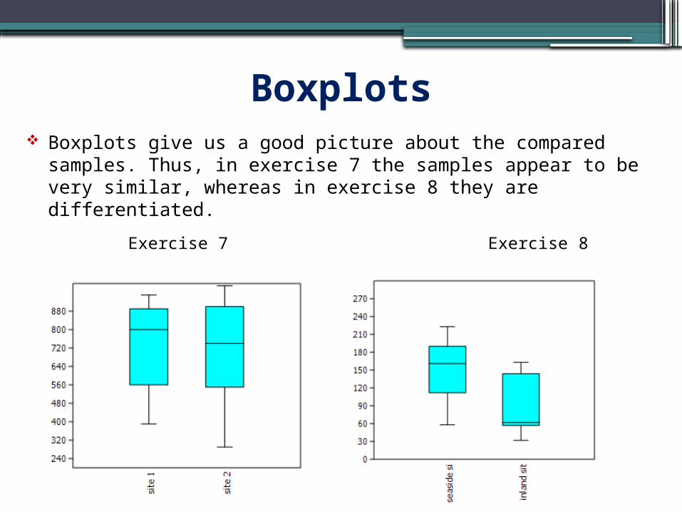
Boxplots Boxplots give us a good picture about the compared samples. Thus, in exercise 7 the samples appear to be very similar, whereas in exercise 8 they are differentiated.

Exercise 7 Exercise 8

Paired samples t-tests It is used in order to compare two paired samples and see if there is a statistically significant difference between them.

A basic prerequisite is that the difference in the paired values of the two samples should be normally distributed.

Paired samples t-tests

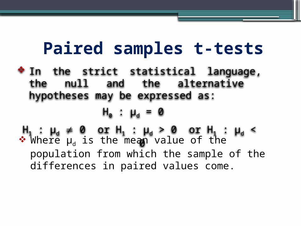
Where μd is the mean value of the population from which the sample of the differences in paired values come.

In the strict statistical language, the null and the alternative hypotheses may be expressed as:

Η0 : μd = 0 Η1 : μd 0 or Η1 : μd > 0 or Η1 : μd <

0

Example – Exercise 9 The data in file ‘exercise 9’ presents the perimeter of the right and left humerus in a Neolithic population. Given that the skeleton deposits new bone tissue when it is subjected to increased mechanical stress, we want to examine whether there is significant bilateral asymmetry, which might be attributed to unilateral daily activities.

Normality test First, we need to check if the differences in the paired values of the two samples are normally distributed. So, we have to create a new column with these differences.

To do that in PAST, we copy - paste the first column to the third column and name it ‘differences’.

Then we select the columns ‘left side’ and ‘differences’, go to Transform Evaluate expression and in the relevant field we type x-l and press Compute.

The column ‘differences’ is filled with the differences in the values of the columns ‘right side’ and ‘left side’.

Normality test

x-l

Normality test

Normality test

We select column ‘differences’ and follow the path: Univariate → Normality tests.

We see that the sample of differences does not seem to violate the normal distribution.

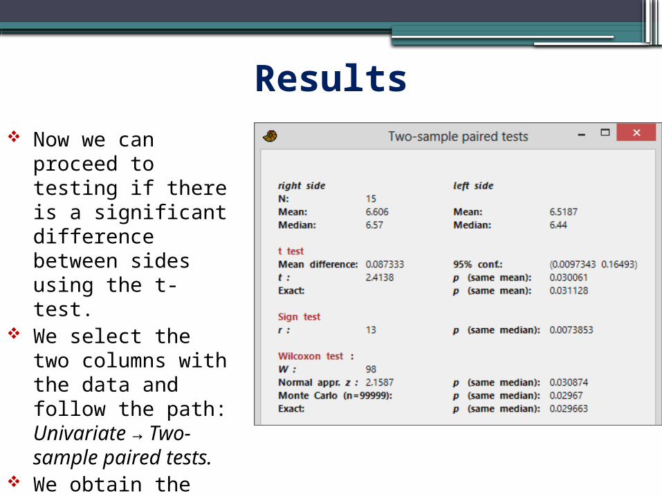
Results Now we can

proceed to testing if there is a significant difference between sides using the t-test.

We select the two columns with the data and follow the path: Univariate → Two-sample paired tests.

We obtain the results shown in the adjacent table:

Since the sample of the differences follows the normal distribution, we check the p value that corresponds to the t test results. We see that p = 0.030 < 0.05, and the same result is obtained from the exact value of p = 0.0311.

Therefore, the null hypothesis that there are no statistically significant differences between the two samples may be rejected.

Results

The rejection of the null hypothesis suggests that there are statistically significant differences between the two sides of the body.

The mean for the right side is 6.6, while for the left side it is 6.5. Thus, it appears that the daily activities of the population under study involved primarily the right side of the upper limbs.

Conclusion

Wilcoxon test It is the non-parametric equivalent to the Paired samples t-test.

An alternative non-parametric test for paired samples is the sign test, which is though less robust than the Wilcoxon test.

Wilcoxon test

Where d is the median of the population from which the sample of the differences in paired values derives.

The null and the alternative hypotheses may be expressed as:

Η0 : d = 0 Η1 : d 0 or Η1 : d > 0 or Η1 : d < 0

Frank Wilcoxon 1892-1965

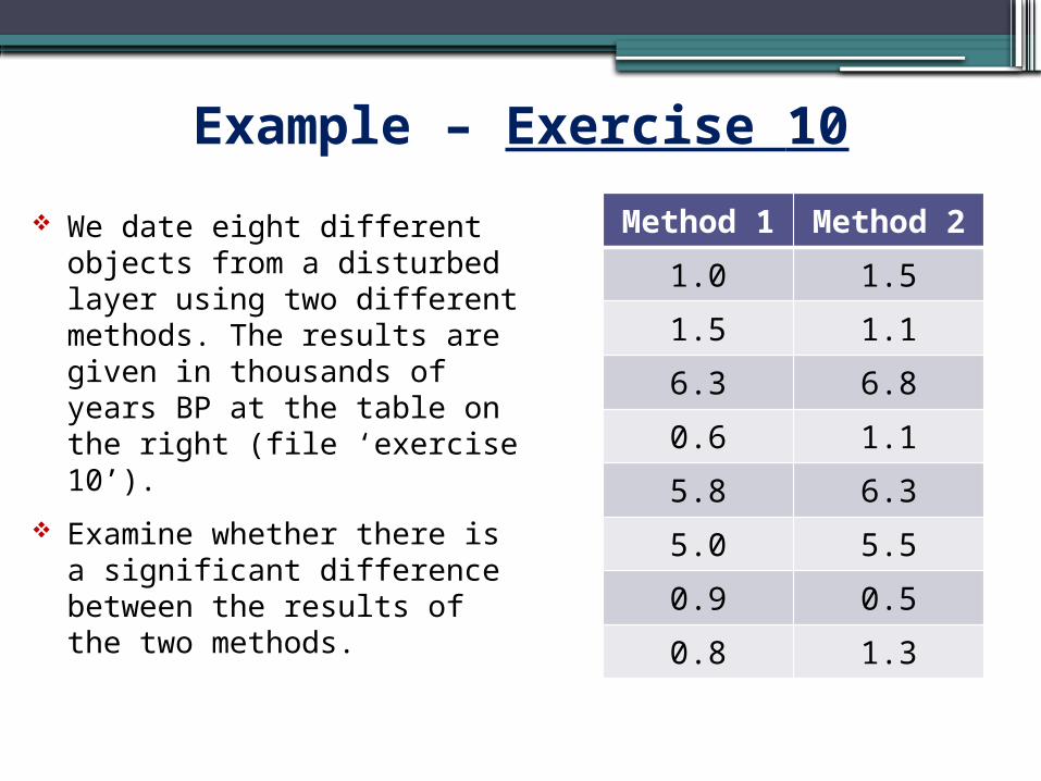
Example – Exercise 10 We date eight different objects from a disturbed layer using two different methods. The results are given in thousands of years BP at the table on the right (file ‘exercise 10’).

Examine whether there is a significant difference between the results of the two methods.

Method 1 Method 21.0 1.51.5 1.16.3 6.80.6 1.15.8 6.35.0 5.50.9 0.50.8 1.3

Normality tests As in the previous example, we first create a new column with the differences in paired values and examine the normality of these values.

Normality tests

We observe that the sample with the differences exhibits strong deviations from normality.

Results We select both variables ‘Method 1’ and ‘Method 2’, follow the path Univariate → Two-sample paired tests, and obtain the following table of results:

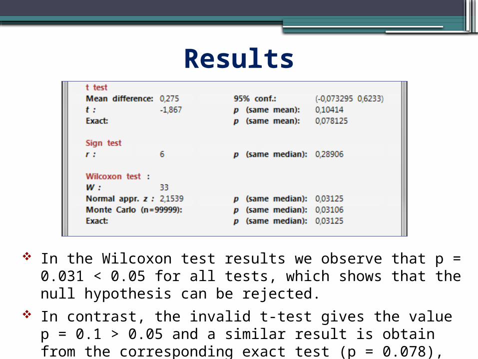
Results

In the Wilcoxon test results we observe that p = 0.031 < 0.05 for all tests, which shows that the null hypothesis can be rejected.

In contrast, the invalid t-test gives the value p = 0.1 > 0.05 and a similar result is obtain from the corresponding exact test (p = 0.078), which retain the null hypothesis.

Conclusion Since the null hypothesis may be rejected, there is a significant difference between the results of the two methods.

Therefore, the two methods are not equivalent and we must find out which one of them is the reliable one.

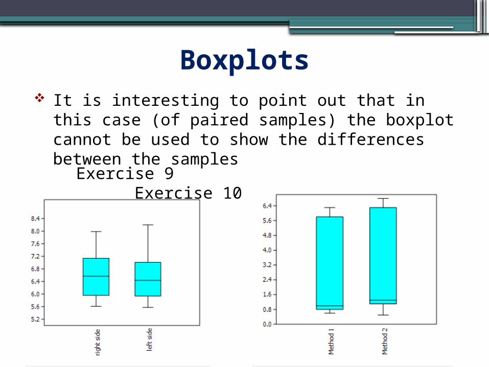
Boxplots It is interesting to point out that in this case (of paired samples) the boxplot cannot be used to show the differences between the samples

Exercise 9 Exercise 10

One-way ANOVA This test is applied in order to explore whether significant differences exist among the mean values of three or more independent samples.

It is a parametric test based on the preconditions: The variances of the different samples should not be significantly different (homogeneity of variance)

The samples must follow the normal distribution. Note: if the sample sizes are equal, the above assumptions are not critical.

Thus, the rejection of the null hypothesis suggests that there are significant differences among some of the samples. However, it does not specify between which pair(s) of samples these differences are traced. For this purpose we employ Post Hoc tests.

The ANOVA null hypothesis in statistical terms is formulated as:

Η0 : μ1 = μ2 = … = μn

The alternative hypothesis, Η1, accepts that at least one of the above equalities is violated.

One-way ANOVA

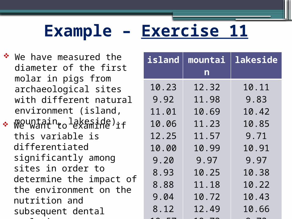
Example – Exercise 11island mountai

nlakeside

10.239.9211.0110.0612.2510.009.208.938.889.048.1210.57

12.3211.9810.6911.2311.5710.999.9710.2511.1810.7212.4910.73

10.119.8310.4210.859.7110.919.9710.3810.2210.4310.669.73

We have measured the diameter of the first molar in pigs from archaeological sites with different natural environment (island, mountain, lakeside). We want to examine if this variable is differentiated significantly among sites in order to determine the impact of the environment on the nutrition and subsequent dental evolution.

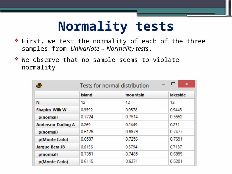
Normality tests First, we test the normality of each of the three samples from Univariate → Normality tests.

We observe that no sample seems to violate normality

Application of ANOVA For the application of ANOVA we select all three columns and follow the path: Univariate

→ Several-sample tests (ANOVA , Kru-Wal). We obtain:

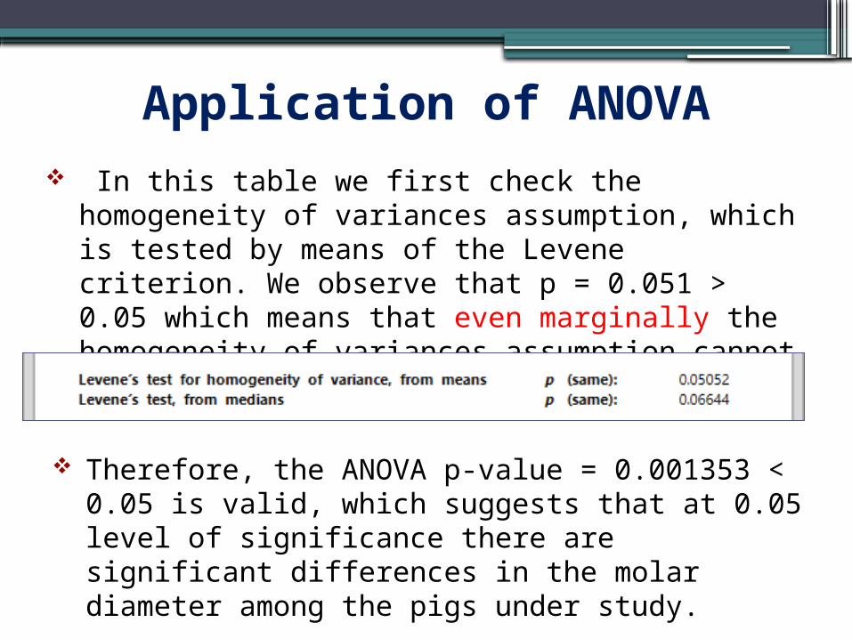
In this table we first check the homogeneity of variances assumption, which is tested by means of the Levene criterion. We observe that p = 0.051 > 0.05 which means that even marginally the homogeneity of variances assumption cannot be rejected.

Application of ANOVA

Therefore, the ANOVA p-value = 0.001353 < 0.05 is valid, which suggests that at 0.05 level of significance there are significant differences in the molar diameter among the pigs under study.

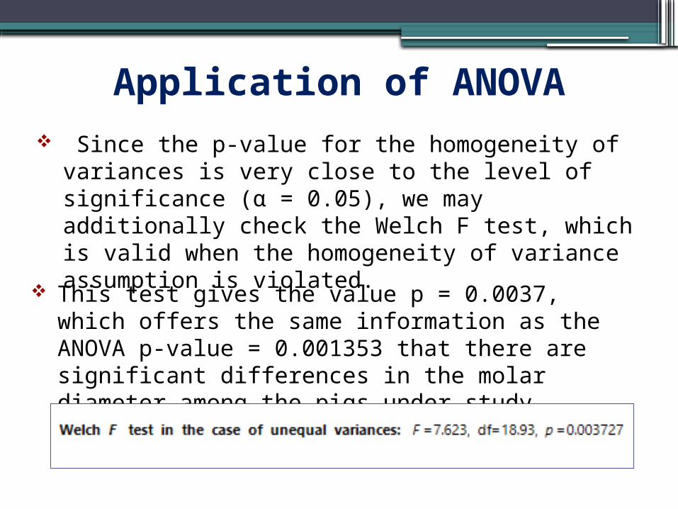
Since the p-value for the homogeneity of variances is very close to the level of significance (α = 0.05), we may additionally check the Welch F test, which is valid when the homogeneity of variance assumption is violated.

Application of ANOVA

This test gives the value p = 0.0037, which offers the same information as the ANOVA p-value = 0.001353 that there are significant differences in the molar diameter among the pigs under study.

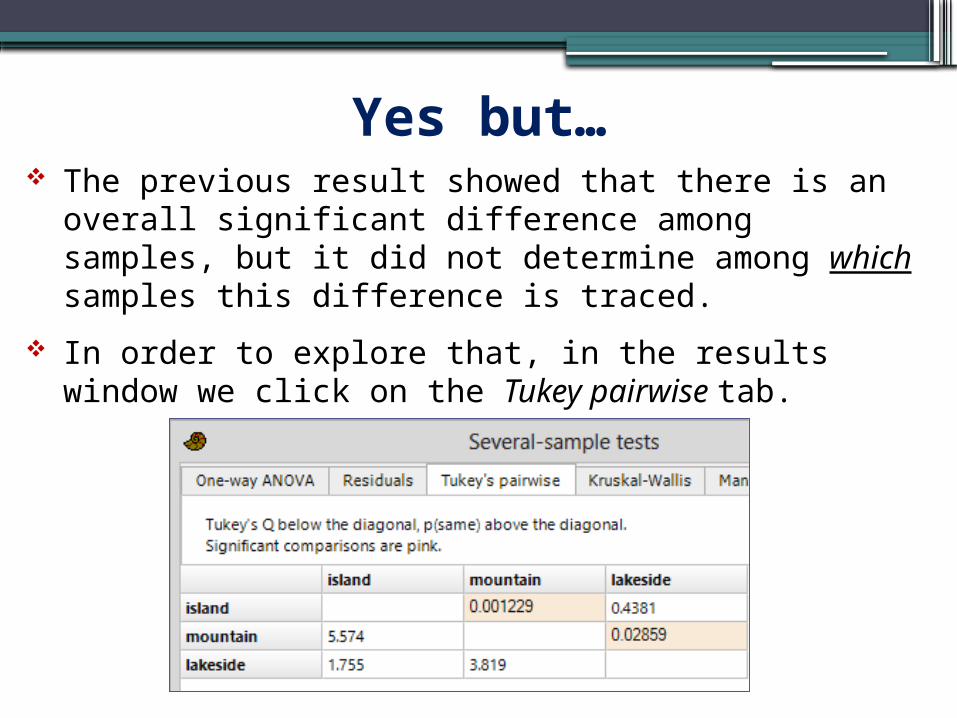
Yes but… The previous result showed that there is an overall significant difference among samples, but it did not determine among which samples this difference is traced.

In order to explore that, in the results window we click on the Tukey pairwise tab.

Yes but… We observe that statistically significant differences are traced between mountain and island, and mountain and lake side. That is, the sample ‘mountain’ is differentiated from the other two.

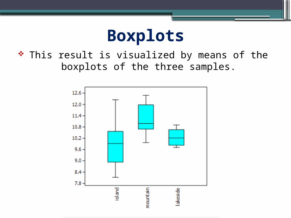
Boxplots This result is visualized by means of the

boxplots of the three samples.

Kruskal-Wallis test It is the non-parametric equivalent to the

One-way ANOVA. The null hypothesis is now stated as:

H0: all samples derive from the same population

and the alternative is:

H1: not H0

Example – Exercise 12 In three archaeological sites we measured the height (in cm) of the adult males based on their skeletal remains. The results are given in file ‘exercise 12’.

Examine if there is a statistically significant difference among the height of individuals from the different sites.

Normality tests We select each variable and check if it follows the normal distribution from Univariate → Normality tests.

We observe that the sample from site 3 violates the normal distribution but the deviation from normality does not seem to be very significant.

What type of test should I use?

Taking into consideration that our samples are very small, thus any statistical test (including tests of normality) is not particularly valid when the null hypothesis is not rejected, we should employ both parametric and non-parametric tests.

ΑΝOVA F test We select all three samples and follow the path:

Univariate → Several-sample tests (ANOVA, Kru-Wal).

In the results window we click on One-way ANOVA:

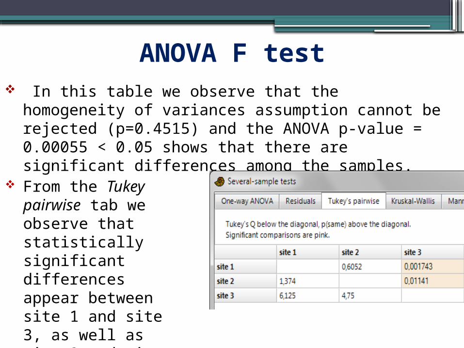
ΑΝOVA F test In this table we observe that the homogeneity of variances assumption cannot be rejected (p=0.4515) and the ANOVA p-value = 0.00055 < 0.05 shows that there are significant differences among the samples.

From the Tukey pairwise tab we observe that statistically significant differences appear between site 1 and site 3, as well as site 2 and site 3.

Kruskal-Wallis test If we click on the Kruskal-Wallis tab, we observe that p = 0.02 so again we conclude that there is a statistically significant difference among samples.

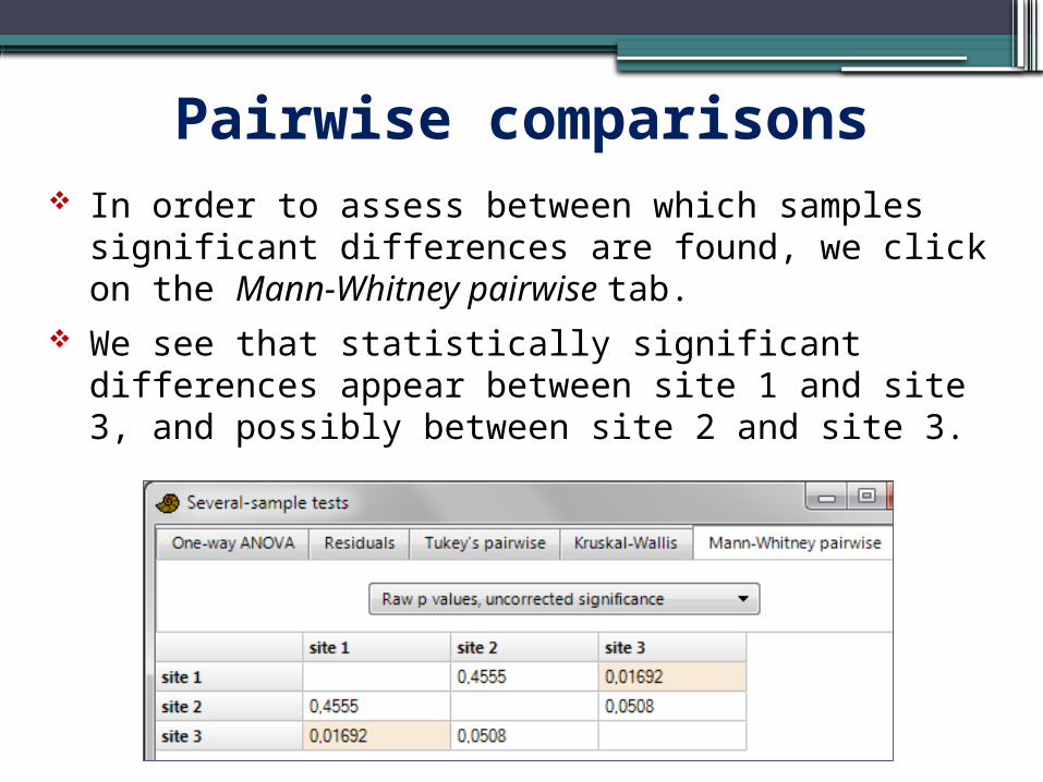
Pairwise comparisons In order to assess between which samples significant differences are found, we click on the Mann-Whitney pairwise tab.

We see that statistically significant differences appear between site 1 and site 3, and possibly between site 2 and site 3.

Pairwise comparisons However, when there are multiple comparisons, the p-values should be corrected. For this purpose PAST uses the Bonferroni correction.

From the drop-down menu at the Mann-Whitney pairwise tab we select the option Bonferroni corrected p values.

We now see that after the Bonferroni correction for multiple comparisons, there is no significant difference between any pair of samples!

Kruskal-Wallis test This result should not surprise us for two reasons:1. The Mann-Whitney test for pairwise

comparisons is not the best one (although there is no other commercially available), and

2. The Bonferroni correction is very conservative.

In such cases boxplots may help us decide.

Boxplots The boxplots show great

differentiation of site 3 from sites 1 and 2.

TESTS ON CATEGORICAL DATA

Dr. Efthymia Nikita

Athens 2013

Focus problem Let’s assume that we have compiled the table below, which presents the frequency of sherds with different non plastics from archaeological sites with different natural environment.

We want to examine if certain non plastics appear preferentially in certain environments. Natural

environment

Non plastics

shells

sand steatite

mountainislandplain

758390

587062

546659

Contrary to the problems we examined so far, in this problem the variables are not continuous quantitative but categorical.

In other words each variable consists of certain categories. For the natural environment these categories are: a) mountain, b) island, c) plain. For the non plastic they are: a) shells, b) sand, c) steatite.

In the current problem we want to examine if there is a significant differentiation in the frequency of shells belonging to each category.

Focus problem

Exercise 13

Based on the data provided in file ‘exercise 13’ examine whether certain non plastics appear preferentially in certain natural environments.

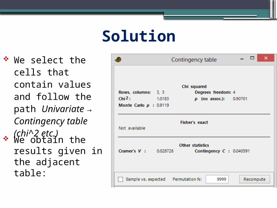
Solution We select the cells that contain values and follow the path Univariate →Contingency table (chi^2 etc.)

We obtain the results given in the adjacent table:

Solution

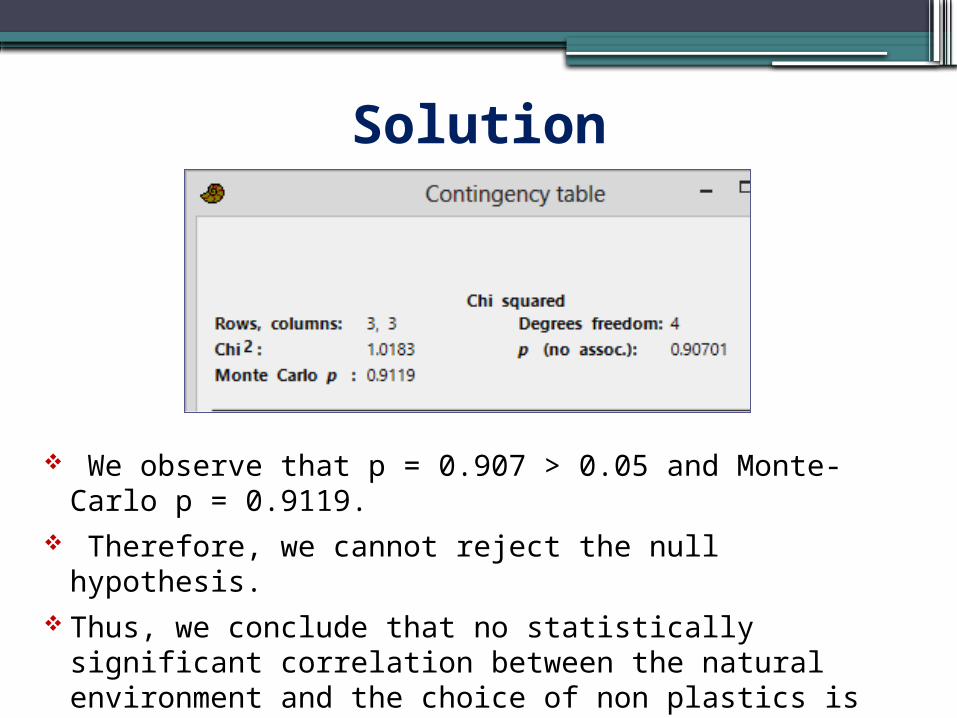
We observe that p = 0.907 > 0.05 and Monte-Carlo p = 0.9119.

Therefore, we cannot reject the null hypothesis.

Thus, we conclude that no statistically significant correlation between the natural environment and the choice of non plastics is detected.

Fisher’s exact test The χ2 test is used when the percentage of cells with expected frequency below 5 is smaller than 20%. If more cells have small frequencies, then the results of the x2 test may not be valid.

In cases where we suspect that the results of the χ2 test may not be accurate, we apply Fisher’s exact test.

Fisher’s exact test is used in 22 tables.

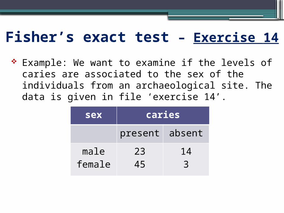
Fisher’s exact test – Exercise 14 Example: We want to examine if the levels of caries are associated to the sex of the individuals from an archaeological site. The data is given in file ‘exercise 14’.

sex cariespresent absent

malefemale

2345

143

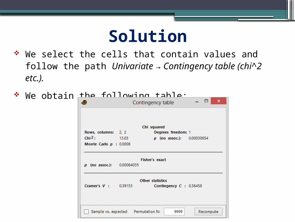
Solution We select the cells that contain values and

follow the path Univariate Contingency table (chi^2 →etc.).

We obtain the following table:

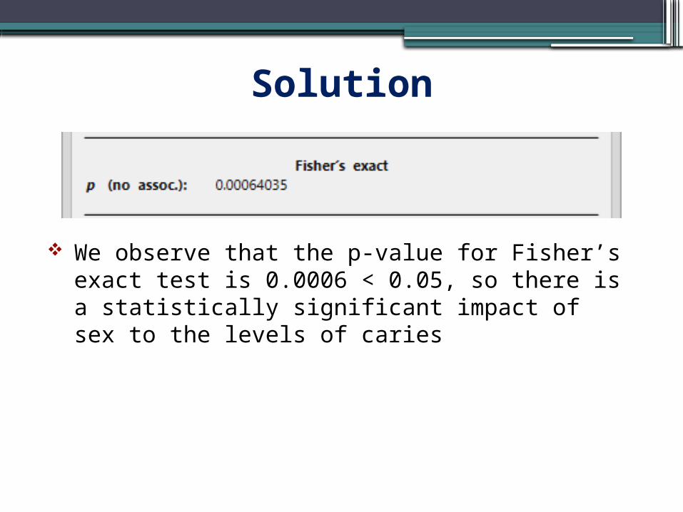
Solution

We observe that the p-value for Fisher’s exact test is 0.0006 < 0.05, so there is a statistically significant impact of sex to the levels of caries

Association among many categorical variables: Correspondence Analysis

When the contingency tables under study have many rows and columns, the x2 test does not offer any particular information since there will definitely be correlations among the different variables.

In cases like this we are interested in finding clusters of data that inter-correlate.

Example – Exercise 15 In the table below we see the frequency of stone tools made of different raw material (file ‘exercise 15’).

We want to see whether there is a correlation between the raw material and the type of tools. Raw material Type of tool

Blades Awls Scrapers

Chisels

Flint 233 56 61 88Obsidian 152 72 28 126Basalt 7 13 54 20Jasper 34 80 55 11Andesite 5 28 8 12

Solution We select all cells that contain values and follow the path Multivariate Ordination → →Correspondence (CA)

In the obtained results window we click on the Scatter plot panel.

Scatter plot

We observe that blades and chisels are associated to flint obsidian, awls to jasper and 5 andesite, and, finally, scrapers to basalt.