Analysis-aware modeling: Understanding quality considerations in modeling for isogeometric analysis

Analysis-aware modeling: Understanding quality considerations in modelingfor isogeometric analysis

E. Cohen a,*, T. Martin a, R.M. Kirby a,b, T. Lyche c, R.F. Riesenfeld a

a School of Computing, University of Utah, Salt Lake City, UT 84112, USAb Scientific Computing and Imaging Institute, University of Utah, Salt Lake City, UT, USAcCMA and Institute of Informatics, University of Oslo, P.O. Box 1053, Blindern, 0316 Oslo, Norway

a r t i c l e i n f o

Article history:Received 8 April 2009Received in revised form 26 August 2009Accepted 7 September 2009Available online 13 September 2009

Keywords:Isogeometric analysisSolid modelingMesh generationMesh qualityModel generationModel quality

a b s t r a c t

Isogeometric analysis has been proposed as a methodology for bridging the gap between computer aideddesign (CAD) and finite element analysis (FEA). Although both the traditional and isogeometric pipelinesrely upon the same conceptualization to solid model steps, they drastically differ in how they bring thesolid model both to and through the analysis process. The isogeometric analysis process circumventsmany of the meshing pitfalls experienced by the traditional pipeline by working directly within theapproximation spaces used by the model representation. In this paper, we demonstrate that in a similarway as how mesh quality is used in traditional FEA to help characterize the impact of the mesh on anal-ysis, an analogous concept of model quality exists within isogeometric analysis. The consequence of theseobservations is the need for a new area within modeling – analysis-aware modeling – in which modelproperties and parameters are selected to facilitate isogeometric analysis.

! 2009 Elsevier B.V. All rights reserved.

1. Introduction

The concept of isogeometric analysis was first introduced byHughes et al. in [1] as a means of bridging the gap between com-puter aided engineering (CAE), including finite element analysis(FEA), and computer aided design (CAD) [2]. Those familiar withthe application of FEA to CAD-based models are well-aware ofthe complications and frustrations which arise when one attemptsto take a ‘‘solid model” (a term which we will define in the contextof the modeling community in Section 2) as produced by a typicalcommercially available CAD system, generate a surface tessellationand corresponding volumetric representation in terms of meshingelements (e.g. triangles and quadrilaterals on the surfaces and tet-rahedra and hexahedra in the volume), and run an analysis. On this‘‘preprocessing” side prior to the actually analysis step, a largeamount of effort is expended in mesh generation and optimization(in terms of mesh quality), sometimes to the point of consumingmore time than what is taken by the actual analysis step. Oncean analysis is run, solution refinement often requires mesh adapta-tion or in worst case regeneration, both of which require consulta-tion with the original CAD-model. Isogeometric analysis claims tobreak this common but insidious cycle by choosing an alternative

route from the solid geometric model to analysis. In isogeometricanalysis, one works with the functions used to generate the modeldirectly by using the function space used for model generation asthe approximating space in which field solutions are built (hencethe name isogeometric).

By circumventing many of the pitfalls that one encounters dur-ing the mesh generation process by working directly with the solidmodel, isogeometric analysis effectively eliminates the geometricerror component of the analysis pipeline. Geometric refinementis no longer necessary; the analyst can focus attention solely onsolution refinement. It is our thesis that although circumventingthe mesh generation pipeline implies that one no longer needs toconsider mesh quality, there are still issues of model quality thatmust be considered. In a similar way as mesh quality is a geometricmeans of assessing the impact of a mesh on the function spacewhich it induces in the classic finite element process, model qualityis a characterization of those properties of the representation of themodel geometry that impact the representation space (or trialspace) used to approximate the fields of interest. The consequenceof these observations is the need for a new area within modeling –analysis-aware modeling – in which model properties and parame-ters facilitate isogeometric analysis.

1.1. Nomenclature

In this section we set up the environment for considering iso-geometric analysis in the context of linear second-order partial dif-

0045-7825/$ - see front matter ! 2009 Elsevier B.V. All rights reserved.doi:10.1016/j.cma.2009.09.010

* Corresponding author. Tel.: +1 801 583 2815; fax: +1 801 581 5843.E-mail addresses: [email protected] (E. Cohen), [email protected] (T. Martin),

[email protected] (R.M. Kirby), [email protected] (T. Lyche), [email protected](R.F. Riesenfeld).

Comput. Methods Appl. Mech. Engrg. 199 (2010) 334–356

Contents lists available at ScienceDirect

Comput. Methods Appl. Mech. Engrg.

journal homepage: www.elsevier .com/locate /cma

http://www.elsevier.com/locate/cma

http://dx.doi.org/10.1016/j.cma.2009.09.010

mailto:[email protected]




http://www.sciencedirect.com/science/journal/00457825

ferential equations (PDEs) with zero Dirichlet boundary conditions.We note that there exists a straightforward extension to nonzeroDirichlet (essential) boundary conditions and also to Neumannboundary conditions. The issues we raise are quite general and willarise in using the isogeometric concept in solving many types ofpartial differential equations: Some examples we will considerand upon which we will comment in the examples section willhave nonzero essential boundary conditions and/or more complexpartial differential operators (such as those found in the modelingof linear elasticity). We do, however, set up here the nomenclatureto illustrate these specific problems in an arbitrary number ofspace dimensions.

Although some of these terms may appear obvious to eitherthose familiar with geometric modeling or those familiar withengineering analysis, we believe it is important for both the geo-metric modeling and finite element analysis communities to beovertly explicit during this time of confluence of ideas.

Let X ! Rs with s 2 N be a bounded domain with boundary @X.X is the physical domain, often called the world space or physicalspace.

Using the notation Dj " D1j to denote the partial derivative with

respect to the jth variable, define

Da :" Da11 # # #Das

s ; $1%

a mixed partial derivative of total order jaj " a1 & # # # & as. Then thecolumn vector

rf " 'D1f ; . . . ;Dsf (T $2%

denotes the gradient of f. Further, let

H1 " H1$X% :" ff : X ! R : Daf 2 L2$X%; jaj 6 1g $3%V " H1

0 " H10$X% :" ff 2 H1$X% : f " 0 on @Xg; $4%

denote the spaces of functions with values and first order partialderivatives in L2 " L2$X%.

Let f/igni"1 ! H1$X% be linearly independent functions in H1$X%.

Moreover we define

J :" fj 2 f1; . . . ;ng : /j 2 Vg and jJj " #fj : j 2 Jg;

that is, the set of indices of those /j that vanish on @X. If s " 1 thentypically J " f2; . . . ; n) 1g. We define the space

Vqh$f/jgj% " Vq

h :"X

j2Jcj/j : cj 2 Rq; j 2 J; q 2 N

( ); $5%

and note that Vh " V1h is a subspace of V. The index h is a flag indi-

cating finite dimensionality and is often a measure of elementdiameter. The space Vq

h forms the space in which the approximationto the solution of the differential equation is made.

Suppose fwjgnj"1 is a set of real-valued linearly independent

functions on a partition of the unit cube H " '0;1(s in Rs, and thefunctions /j are given as

/j$x% " wj * F)1$x%; j " 1; . . . ; n; $6%

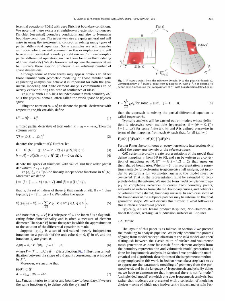
where F " $F1; . . . ; Fs% : H ! X is a bijection. Fig. 1 illustrates a mod-ification between the shape of a w and its corresponding / inducedby F)1.

Moreover, we assume that

F$Ho% ! Xo

r :" Fj@H : @H ! @X; $7%

i.e., F maps interior to interior and boundary to boundary. If we usethe same functions wj to define both the /j’s and F

F "Xn

j"1

cjwj; for some cj 2 Rs; j " 1; . . . ;n; $8%

then the approach to solving the partial differential equation iscalled isogeometric.

Typically analysis will be carried out on models whose defini-tion is piecewise over multiple hypercubes H " fHi " '0;1(s :i " 1; . . . ;Kg for some finite K 2 N, and F is defined piecewise interms of the mappings from each Hi such that, for all i; j; i– j,

F$@Hi%\

F$@Hj% ! @F$Hi%\

@F$Hj%:

Further Fmust be continuous on every non-empty intersection.H iscalled the parametric domain or the reference space.

CAD systems typically create representations of the model thatdefine mappings r from @H to @X, and can be written as a collec-tion of mappings ri : '0;1(s)1 ! Rs; i " 1;2 . . . ;2s that agree ontheir shared boundaries. When s " 3, this representation is some-times suitable for performing isogeometric shell analysis, but in or-der to perform a full volumetric analysis, the model must becompleted. That is, the representation must be extended to com-pletely define the interior. We use the termmodel completion to ap-ply to completing networks of curves from boundary points,networks of surfaces from (shared) boundary curves, and networksof volumes from (shared) boundary surfaces. In each case some ofthe boundaries of the subpiece patches may be internal to the finalgeometric shape. We will discuss this further in what follows asthis is often a non-trivial process.

Typically, w’s are tensor product B-splines, Non-Uniform Ra-tional B-splines, rectangular subdivision surfaces or T-splines.

1.2. Outline

The layout of this paper is as follows. In Section 2 we presentthe modeling to analysis pipeline. We briefly describe the processof going frommodel conceptualization to the solidmodel, and thendistinguish between the classic route of surface and volumetricmesh generation as done for classic finite element analysis fromthe boundary representation and volumetric model generation asdone for isogeometric analysis. In Section 3 we provide the math-ematical and algorithmic descriptions of the isogeometric method-ology employed in this work. In Section 4 we take a step back so asto appreciate the parametric modeling of geometry from the per-spective of, and in the language of, isogeometric analysis. By doingso, we hope to demonstrate that in general there is not ‘‘a model”(a single ideal model) on which one does isogeometric analysis, butrather that modelers are presented with a collection of modelingchoices – some of which may inadvertently impact analysis. In Sec-

Fig. 1. F maps a point from the reference domain H to the physical domain X.Correspondingly, F)1 maps a point from X back to H. With F)1, it is possible todefine basis functions on X as compositions of F)1 with basis function defined onH.

E. Cohen et al. / Comput. Methods Appl. Mech. Engrg. 199 (2010) 334–356 335

tion 5 we present one-, two- and three-dimensional examplescomparing different model completions and demonstrating theimpact of model completion on quality of the solutions one obtainsfrom an isogeometric analysis. In Section 6 we present some of theissues of the geometric representation, including model comple-tion, that can affect the model quality in this new analysis para-digm. We do not seek to characterize all possible issues onemight encounter, but rather to initiate a dialog between modelersand analysts concerning what is needed for analysis-aware model-ing. We conclude in Section 7 with a summary of this work, someconclusions that we can draw and proposals of future work.

2. The modeling to analysis pipeline

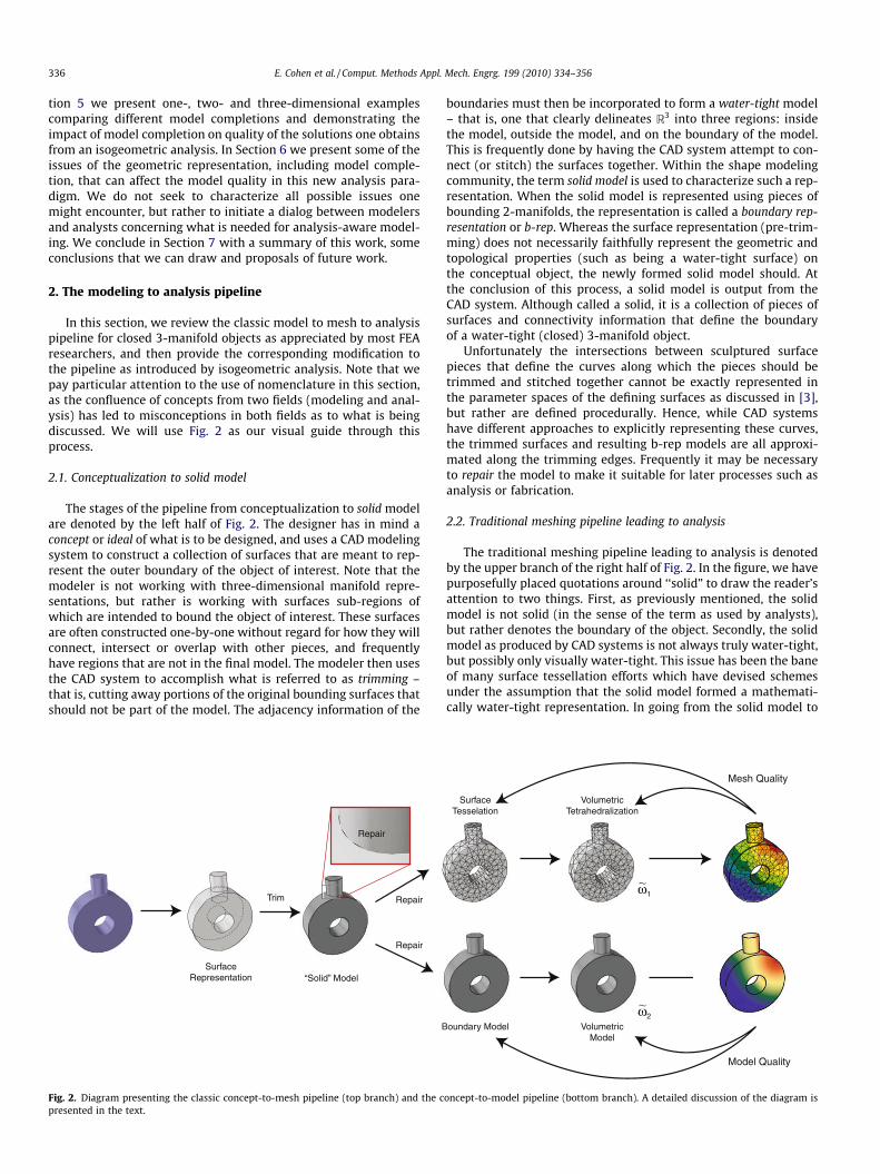
In this section, we review the classic model to mesh to analysispipeline for closed 3-manifold objects as appreciated by most FEAresearchers, and then provide the corresponding modification tothe pipeline as introduced by isogeometric analysis. Note that wepay particular attention to the use of nomenclature in this section,as the confluence of concepts from two fields (modeling and anal-ysis) has led to misconceptions in both fields as to what is beingdiscussed. We will use Fig. 2 as our visual guide through thisprocess.

2.1. Conceptualization to solid model

The stages of the pipeline from conceptualization to solid modelare denoted by the left half of Fig. 2. The designer has in mind aconcept or ideal of what is to be designed, and uses a CAD modelingsystem to construct a collection of surfaces that are meant to rep-resent the outer boundary of the object of interest. Note that themodeler is not working with three-dimensional manifold repre-sentations, but rather is working with surfaces sub-regions ofwhich are intended to bound the object of interest. These surfacesare often constructed one-by-one without regard for how they willconnect, intersect or overlap with other pieces, and frequentlyhave regions that are not in the final model. The modeler then usesthe CAD system to accomplish what is referred to as trimming –that is, cutting away portions of the original bounding surfaces thatshould not be part of the model. The adjacency information of the

boundaries must then be incorporated to form a water-tight model– that is, one that clearly delineates R3 into three regions: insidethe model, outside the model, and on the boundary of the model.This is frequently done by having the CAD system attempt to con-nect (or stitch) the surfaces together. Within the shape modelingcommunity, the term solid model is used to characterize such a rep-resentation. When the solid model is represented using pieces ofbounding 2-manifolds, the representation is called a boundary rep-resentation or b-rep. Whereas the surface representation (pre-trim-ming) does not necessarily faithfully represent the geometric andtopological properties (such as being a water-tight surface) onthe conceptual object, the newly formed solid model should. Atthe conclusion of this process, a solid model is output from theCAD system. Although called a solid, it is a collection of pieces ofsurfaces and connectivity information that define the boundaryof a water-tight (closed) 3-manifold object.

Unfortunately the intersections between sculptured surfacepieces that define the curves along which the pieces should betrimmed and stitched together cannot be exactly represented inthe parameter spaces of the defining surfaces as discussed in [3],but rather are defined procedurally. Hence, while CAD systemshave different approaches to explicitly representing these curves,the trimmed surfaces and resulting b-rep models are all approxi-mated along the trimming edges. Frequently it may be necessaryto repair the model to make it suitable for later processes such asanalysis or fabrication.

2.2. Traditional meshing pipeline leading to analysis

The traditional meshing pipeline leading to analysis is denotedby the upper branch of the right half of Fig. 2. In the figure, we havepurposefully placed quotations around ‘‘solid” to draw the reader’sattention to two things. First, as previously mentioned, the solidmodel is not solid (in the sense of the term as used by analysts),but rather denotes the boundary of the object. Secondly, the solidmodel as produced by CAD systems is not always truly water-tight,but possibly only visually water-tight. This issue has been the baneof many surface tessellation efforts which have devised schemesunder the assumption that the solid model formed a mathemati-cally water-tight representation. In going from the solid model to

SurfaceRepresentation “Solid” Model

VolumetricModel

Trim

SurfaceTesselation

VolumetricTetrahedralization

Mesh Quality

Model Quality

Boundary Model

Repair

Repair

Repair

~!1

~!2

Fig. 2. Diagram presenting the classic concept-to-mesh pipeline (top branch) and the concept-to-model pipeline (bottom branch). A detailed discussion of the diagram ispresented in the text.

336 E. Cohen et al. / Comput. Methods Appl. Mech. Engrg. 199 (2010) 334–356

a surface tessellation, it is often necessary to invoke a repairingprocedure. We mark the repair process as being the point of devi-ation between the traditional pipeline and isogeometric analysis asmany of the repair procedures used in traditional mesh generationassume that the target representation is a piecewise linear tessel-lation. The result of the repair and surface generation process is atessellation of boundary of the object of interest. This tessellationis an approximation to the true geometry (in this case, the CAD-model), where approximation decisions have been made both interms of how repairs are done and in how finely the tessellationcaptures the features of the original model. If a three-dimensionalanalysis is desired, the next step is to generate a volumetric tessel-lation, normally by filling in the volume with elements of theappropriate type (hexahedra or tetrahedra) for the analysis ofinterest.

In the classic finite element procedure, one generates a tessella-tion which approximates the true geometry, and then uses this tes-sellation to induce a function space in which approximations willbe made. For instance, in classic linear finite elements over trian-gles, the triangular tessellation induces a piecewise linear (in totaldegree) space which is C0 continuous along the edges of the trian-gles. As is well known by finite element practitioners, given twotessellations, both of which faithfully represent the geometry,one can get drastically different solutions due to the properties(or richness) of the approximating space that is induced.

A natural feedback loop was generated between analysts andmesh generation experts concerning the impact of meshes on solu-tion quality. These metrics have commonly become known asmeshquality metrics. That is, they are geometric considerations (nor-mally involving things like ratios of angles of elements, aspect ra-tios of edges, etc.) which help guide the development of meshesappropriate for analysis. Although these metrics have deep founda-tions within approximation theory, they are often abstracted awayso that only geometric qualities of the mesh are discussed. We re-mind the reader, however, that maximizing mesh quality is, in itsessence, an attempt to positively shape the approximating functionspace induced by the mesh.

2.3. Isogeometric pipeline leading to analysis

While isogeometric analysis is still a young field, the authorshypothesize that the path often taken when accomplishing isogeo-metric analysis is denoted by the lower branch of the right half ofFig. 2. As in the case of the traditional pipeline, repair is needed toensure that the model being used for analysis meets the requiredtopological constraints (such as closure) of the problem. In the caseof isogeometric analysis, however, this repair process must be donekeeping in mind the original and target representations. A startingpoint for isogeometric discussions in line with the finite elementapproaches is the boundary model, which should be a geometri-cally and topologically correct model of the bounding surfaces ofthe object. If a three-dimensional analysis is desired, volumetricrepresentations must be generated prior to the analysis. Theapproximating space generated during an isogeometric analysisis dependent upon the boundary model (in 2D) or volumetric mod-el (in 3D) that is used. Just as in the case of classic mesh generation,two different volumetric models generated from the same bound-ary model will create two different approximating spaces. Analo-gous to mesh quality impacting analysis, model quality impactsisogeometric analysis.

A different starting point for isogeometric analysis is that con-sideration during the shape (usually boundary) modeling processshould be given to create a representation that lends itself to iso-geometric analysis. There are frequently many modeling opera-tions that lead to different representations for either the exactlysame or closely related boundary shapes. Some of those represen-

tations are better suited to analysis than others, and within thosegroups, some are better suited to certain types of analysis than oth-ers. Similar issues have been recognized in created representationsfor models suitable for the multitude of computer-aided manufac-turing processes and techniques. However, progress has beenmade in developing CAD systems that develop representationsthat, while suitable for design and display, are fabrication-aware,thus enabling a smoother, faster transition between design andfabrication.

Analysis-aware modeling in the context of isogeometric analysismay prove to be a key step towards that progression for design,engineering analysis, and simulation. Towards that end, this paperraises several important issues through a combination of analysisand demonstration in which the interaction between representa-tion and analysis can either enhance or make the product evolutionprocess difficult. Until such time as these issues have been quanti-fied and embedded in analysis-aware modeling systems, the hu-man modeler must be mindful of them.

3. Mathematical formulation

In this section, we first review the basic mathematical represen-tational building blocks on which isogeometric analysis as well asmany CAD and geometric modeling systems represent geometry.An overview of NURBS (Non-Uniform Rational B-Splines) can befound in [4]. All computational algorithms are presented there,so in the following section we discuss definitions of B-spline andNURBS functions and their combinations to define parametricmappings of global geometry. Note that this discussion providesthe mathematical building blocks of modeling, but does not ad-dress how these building blocks are assembled as part of the mod-eling process. We will delve into the mind of the modeler in asubsequent section (Section 4).

3.1. The framework

Let X ! Rs with s 2 N be a bounded domain with boundary @X.The symbols Da and r are defined as in Eqs. (1) and (2), respec-tively. Function spaces H1 and H1

0 are Sobolev spaces, that is, Hil-bert spaces whose norms are defined using informationconcerning both the function and some of its derivatives. In partic-ular, the (Sobolev) norms for both H1 and H1

0 are given by

kuk21 "Z

X$u$x%2 &ru$x%Tru$x%%dx:

Let a : H10 + H1

0 ! R denote the bilinear form

a$u;v% :"Z

Xru$x%Trv$x%dx; $9%

This bilinear form is positive definite on H10, and H1

0 is a Hilbertspace with inner product a$u;v% and associated norm kuk "!!!!!!!!!!!!!!a$u;u%

p. We let

$u;v% :"Z

Xu$x%v$x%dx; u; v 2 L2$X%;

be the usual L2 inner product. For a general review of Sobolev spaceswe refer the reader to [5].

Discussions in this paper will mostly be based on problems thatarise in the relationship between geometry and analysis models.Most studies are focused on two prototypical mathematical modelproblems that arise in analysis, the Poisson problem and a corre-sponding eigenvalue problem, respectively.

)r2u " f on X; u " 0 on @X; $10%)r2u " ku on X; u " 0 on @X: $11%


Given f 2 L2$X% the weak form of (10) is to find u 2 V :" H10$X% such

that

a$u;v% " $f ;v%; v 2 V : $12%

It is well known that (12) has a unique solution u, see [6].The weak form of (11) is to find k 2 R and a nonzero u 2 V such

that

a$u;v% " k$u;v%; v 2 V : $13%

Since this involves finding the eigenvalues and eigenfunctions of acompact, symmetric operator in the Hilbert space $V ; a$#; #%% thereexists an increasing sequence of strictly positive eigenvalues

0 < k1 6 k2 6 # # # 6 kk 6 # # #

with lim kk " 1 and associated eigenfunctions uk, which can beorthogonalized so that

a$uj; uk% " kkdj;k; j; k P 1:

Moreover, the eigenfunctions form a complete system, i.e. the set ofall linear combinations is dense both in V and L2$X%, again see [6].

For Vqh defined as in Eq. (5), the Galerkin method for (12) consists

in finding uh 2 Vqh such that

a$uh; vh% " $f ;vh%; vh 2 Vh:

Writing uh "P

j2Jcj/j, we obtain a linear system for the unknowncoefficients c.

Sc " f ; S " $a$/i;/j%%i;j2J ; f " $$f ;/i%%i2J: $14%

Since the /’s are linearly independent and vanish on @X the stiffnessmatrix S is a symmetric positive definite matrix and (14) has a un-ique solution that is amendable to iterative methods like conjugategradient [7].

The Rayleigh–Ritz method for (13) consists of finding k and anonzero uh 2 Vq

h such that

a$uh; vh% " k$uh; vh%; vh 2 Vh:

Writing uh "P

j2Jcj/j as before we obtain a generalized eigenvalueproblem

Sc " kMc; S " $a$/i;/j%%i;j2J ; M " $$/i;/j%%i;j2J ; $15%

where both S and the mass matrix M are positive definite.Thus the eigenvalues kkh of (15) that approximate the exact

eigenvalues of (13) are positive

0 < k1h 6 # # # 6 kjJjh

and the eigenfunctions uh can be chosen to be orthogonalized sothat

a$ujh; ukh% " kkhdj;k:

Moreover limh!0kkh " kk for 1 6 k 6 jJj, provided limh!0infvh2Vh

kuk ) vhk " 0 for 1 6 k 6 jJj.

3.2. Definition of isogeometric finite element analysis

Suppose the basis functions /j$x% are given as in Eq. (6). More-over, we assume that (7) holds i.e., F maps interior to interior andboundary to boundary, and that F is defined as in Eq. (8). Then theGalerkin and Rayleigh–Ritz methods for (12) or (13) are calledisogeometric.

The elements sij of the stiffness matrix S can be expressed interms of the gradients of the wj basis functions. Let

J " JF :"

D1F1 # # # DsF1

..

. ...

D1Fs # # # DsFs

2

664

3

775 "

rFT1

..

.

rFTs

2

664

3

775 $16%

be the Jacobian of F. Note that the elements of J are functions de-fined on H. We assume that J$t% is non-singular for all t 2 H. Then

sij "Z

Xr/i$x%

Tr/j$x%dx "Z

Hrwi$t%

TN$t%rwj$t%dt; i; j " 1; . . . ;n;

$17%

where

N " jdet$J%jJ)T J)1: $18%

Note that N$t% is positive definite for all t 2 H. Explicitly, for s " 1,

N$t% " 1jF 0$t%j

;

and for s " 2

N " 1jdet$J%j

krF2k22 )rFT1F2

)rFT1F2 krF1k22

" #:

If

K :" jdet$J%j)1=2J "URVT ; R" diag$r1; . . . ;rs%; UTU "VTV " I;

with r1 P r2 P # # # P rs > 0 is the singular value decomposition ofK then

N " UR)2UT

is the spectral decomposition of N. Since N is positive definite theeigenvalues of N are the inverse square of the singular values of Kand the orthonormal eigenvectors of N are the right singular vectorsof K.

3.3. B-splines

For integers n P 1 and d P 0 let s " fsig be a non-decreasingfinite sequence of real numbers. We refer to s as a knot vectorand its components as knots. On s we can recursively define degreed B-splines Bj;d " Bj;d;s : R ! R by

Bj;d$t% "t ) sj

sj&d ) sjBj;d)1$t% &

sj&d&1 ) tsj&d&1 ) sj&1

Bj&1;d)1$t%; t 2 R; $19%

starting with

Bj;0$t% "1; if sj 6 t < sj&1;

0; otherwise:

"

Here we use the convention that terms with zero denominator aredefined to be zero. We let Bd;s " fBj;d;sgj.

A B-spline Bj;d of degree d has the following properties:

1. It depends only on knots sj; . . . ; sj&d&1 and is identically zero ifsj&d&1 " sj.

2. For t 2 $sj; sj&d&1%;0 < Bj;d$t% 6 1 and Bj;d$t% " 0 otherwise. Theinterval 'sj; sj&d&1( is called the support of Bj;d.

3. Its derivative is

DBj;d$t% " dBj;d)1$t%sj&d ) sj

)Bj&1;d)1$t%sj&d&1 ) sj&1

# $;

again with the convention that terms with 0 denominator areset to 0.

4. If m of the sj; . . . ; sj&d1 are equal to one value z, then DrBj;d iscontinuous at z for r " 0; . . . ; d)m and Dd)m&1Bj;d is discon-tinuous at z.

5. Its integral isZ sj&d&1

sjBj;d$t%dt "

sj&d&1 ) sjd& 1

:


6. It is affine invariant, i.e., for u;v ; t 2 RBj;d;us&v $ut & v% " Bj;d;s$t%,where us& v :" $usj & v%j.

Now suppose n; d are integers with 0 < d < n. We say thats " fsign&d&1

i"1 is a $d& 1% extended knot vector on an interval 'a; b( if

a " sd&1 < sd&2; sn < sn&1 " b; si&d&1 > si; i " 1; . . . ; n:

It is $d& 1%-regular or $d& 1%-open if in addition s1 " a andsn&d&1 " b; it is $d& 1%-regular uniform or $d& 1%-open uniform ifsi&1 ) si " h for i " d& 1; . . . ; n and h > 0. The knot vector is uniformif si&1 ) si " h > 0 for i " 1; . . . ;n& d.

On the knot vector s " fsign&d&1i"1 we can define n B-splines of de-

gree d. The linear space of all linear combinations of B-splines isthe spline space defined by

Sqd;s :"

Xn

j"1

cjBj;djcj 2 Rq for 1 6 j 6 n

( ); d P 0; q P 1:

An element f "Pn

j"1cjBj;d of Sd;s " S1d;s is called a spline function if

q " 1 or just a spline of degree d with knots s, and $cj%nj"1 are calledthe B-spline coefficients of f. For q > 1 the combination f "

Pnj"1cjBj;d

is a spline curve.Suppose s " fsign&d&1

i"1 is a $d& 1%-open knot vector on 'a; b(. Aspline f : 'a; b( ! R is by definition continuous from the right. Wedefine f $b% by taking limits from the left. Let f "

Pnj"1cjBj;d. Then

the following properties hold:

(1) B-splines $Bj;d%nj"1 are linearly independent on 'a; b( and there-fore a basis for Sq

d;s.(2) Partition of unity:

Pnj"1Bj;d$t% " 1; t 2 'a; b(.

(3) Convex hull property: f $t%; t 2 'a; b( lies in the convex hull of'c1; . . . ; cn(.

(4) Smoothness: If z occurs m times in s then f has continuousderivatives of order 0, . . ., d)m at z.

(5) Locality: If t is in the interval 'sk; sk&1% for some k in the ranged& 1 6 k 6 n then

f $t% "Xk

j"k)d

cjBj;d$t%; $20%

(6) Affine invariance: If us& v :" $usj & v%n&d&1j"1 then

Xn

j"1

cjBj;d;us&v$ut & v% "Xn

j"1

cjBj;d;s$t%; t 2 'a; b(; u; v 2 R:

$21%

(7) Derivative of a spline:

Df $t% " dXn

j"2

cj ) cj)1

sj&d ) sjBj;d)1$t%; t 2 'a; b(;

where terms with 0 valued denominator are set to 0.(8) Integral of a spline:

Z sn&d&1

s1f $t%dt "

Xn

j"1

sj&d&1 ) sjd& 1

cj: $22%

(9) If z " sj&1 " # # # " sj&d < sj&d&1 for 1 6 j 6 n then f $z% " cj.(10) Marsden’s identity:

$s) t%d "Xn

j"1

Yj&d

i"j&1

$s) si%Bj;d$t%; t 2 'a; b(; s 2 R: $23%

(11) Nodal representation:

t "Xn

j"1

s,j;dBj;d$t%; s,j;d "sj&1 & # # # & sj&d

d; t 2 'a; b(:

The nodal representation follows from Marsden’s identity.

3.4. Knot insertion and degree raising (h- and p-refinement)

Suppose s is a knot vector. Since two or more knots in s can havethe same value, we need to distinguish between the knot vectorand the position of the knots. The distinct knot values in s arecalled break points. We define the multiplicity of z in s as

ls$z% " #fsj 2 s : sj " zg; z 2 R:

Notice that ls$z% " 0 if z is not equal to one of the knots in s. Fork P 0 we define the knot vector s$k% to have the same break pointsas s, and

ls$k% $n% " ls$n% & k for all n 2 s:

Thus we increase the multiplicity of each break point in s by k.If t is another knot vector then we say that s ! t if each break

point n in s is also a break point in t and ls$n% 6 lt$n%.Let d; e be integers, 0 6 d 6 e, let s " $sj%n&d&1

j"1 be $d& 1% ex-tended on 'a; b( and let t " $ti%m&e&1

i"1 be an $e& 1% extended knotvector on the same interval 'a; b(. If s$e)d% ! t then Sd;s ! Se;t , andthere is a matrix A 2 Rm;n transforming the B-splines in Sd;s intothe B-splines in Se;t . Thus

Bj;d;s "Xm

i"1

aijBi;e;t ; j " 1; . . . ;n; or BTd;s " BT

e;tA;

where BTd;s " 'B1;d;s; . . . ;Bn;d;s( and BT

e;t " 'B1;e;t ; . . . ;Bm;e;t ( are rowvectors.

If f "Pn

j"1cjBj;d;s then f "Pm

i"1biBi;e;t , where

b " Ac; c " 'c1; . . . ; cn(T ; b " 'b1 . . . ; bm(T : $24%

The case where e " d is called knot insertion and corresponds to h-refinement in the finite element literature. The situation wheree > d and t " s$e)d% is called degree raising or degree elevation andcorresponds to what is commonly known as p-refinement or p-enrichment [5,8,9]. In the general case where s$e)d% is a proper sub-set of t both knot insertion and degree raising occur. When thistransformation is carried out with degree raising followed by knotinsertion, Hughes et al. [1] introduced the term k-refinement tothe isogeometric literature. Although it is possible to do the trans-formation in opposite order, i.e. a knot insertion followed by a de-gree raising, as observed in [1] in their discussion of k-refinement,this ordering leads to more coefficients and less smooth functions.

There are two algorithms for knot insertion. In Boehm’s algo-rithm one knot at a time is inserted. In particular, if z is insertedin s say between sk and sk&1 so that sk 6 z < sk&1, then we obtain(24) with

bi "ci i " 1; . . . ; k) d;z)si

si&d)sici & si&d)z

si&d)sici)1; i " k) d& 1; . . . ; k;

ci)1 i " k& 1; . . . ;n& 1:

8><

>:$25%

Alternatively, using the Oslo Algorithms [10] we can insert all knotssimultaneously and compute the elements of A row by row. Sup-pose ti is located between sk and sk&1, i.e. sk 6 ti < sk&1, then forrow i,

aj;r$i% "ti&r ) sjsj&r ) sj

aj;r)1$i% &sj&r&1 ) ti&r

sj&r&1 ) sj&1aj&1;r)1$i%;

j " k) r & 1; . . . ; k; r " 1; . . . ;d; $26%starting with aj;k " dj;k. Then we obtain Eq. (24) with ai;j " aj;d$i% forj " k) d; . . . ; k and ai;j " 0 for other values of j.

The recurrence relation in (26) bears a strong resemblance tothe one for B-splines given in (19). Since the numbers aj;d$i% alsohave rather similar properties to Bj;d$t%, they are called discrete B-splines. For example

aj;d$i% P 0; j " 1; . . . ; n;Xn

j"1

aj;d$i% " 1; i " 1; . . . ;m:


For degree raising we also compute the transformation matrix Arow by row [11]. Suppose as for knot insertion that sk 6 ti < sk&1

and set Kj;0;r$i% " dj;k for 0 6 r 6 e, Kj;‘;r$i% " 0 for all j if 0 6 r < ‘,and Kj;‘;r$i% " 0 for all ‘; r if j < k) ‘ or j > k. If we compute

Kj;‘;r$i% "‘

rti&r ) sjsj&r ) sj

Kj;‘)1;r)1$i% &sj&r&1 ) ti&r

sj&r&1 ) sj&1Kj&1;‘)1;r)1$i%

# $

& r ) ‘

rKj;‘;r)1$i%; $27%

for ‘ " 1; . . . ;d; r " ‘; . . . ; e and j " k) ‘; . . . ; k then ai;j " Kj;d;e$i% forj " k) d; . . . ; k and 0 for other values of j. Again terms with 0denominator are set to 0. For e " d we only need to computeKj;‘;‘$i% in (27) and we see that Kj;‘;‘$i% " aj;‘$i% for all j; r. It is shownin [12] that A is a non-negative stochastic matrix:

Kj;d;e$i% P 0; j " 1; . . . ;n;Xn

j"1

Kj;d;e$i% " 1; i " 1; . . . ;m;

0 6 d 6 e:

An algorithm that is a literal implementation of (27) has complexityO$de2m%; however, it is possible to derive faster algorithms for thiskind of conversion. The main advantages are that it is quite stableand simple to implement.

Alternatively, degree raising can be carried out by convertingthe representation to examine individual polynomial pieces, per-forming degree raising on them, and then converting back to theB-spline form.

3.5. Nurbs

Suppose s " fsign&d&1i"1 is a $d& 1%-regular knot vector on 'a; b(.

Given positive numbers w " fwigni"1, we define the associatedNURBS-basis of degree d by

Rj;d$t% :"wjBj;d$t%Pni"1wiBi;d$t%

; t 2 'a; b(; j " 1; . . . ;n; $28%

where Bi;d is the B-spline of degree d with knots si; . . . ; si&d&1. Givencj 2 Rq the sum

f "Xn

j"1

cjRj;d $29%

is called a NURBS function if q " 1 and a NURBS curve if q > 1. Wehave Ri;d " Bi;d when wi " 1 for all i. NURBS curves retains manyof the desirable properties of splines curves. Moreover,

(1) NURBS can represent conic sections exactly.(2) Ri;d has the same local support and smoothness properties as

Bi;d.(3) NURBS-basis functions are non-negative and form a parti-

tion of unity, hence the convex hull property holds.(4) fR1;d; . . . ;Rn;dg is linearly independent on 'a; b(.(5) A NURBS curve is affine invariant.

The exact properties of these functions depend on w as well asthe knot vector s and degree.

3.6. Tensor product splines

Using multi-index notation, an s-variate tensor product B-splinehas the form

Bj;d;T $t% "Ys

i"1

Bji ;di ;si $ti%; where Bji ;di ;si 2 Bdi ;si ;

where d " $d1; . . . ;ds%;T " $s1; . . . ; ss%, and j " $j1; . . . ; js%. Define Bd;T

to be the set of all possible such s-variate combinations. The s-var-iate tensor product spline space is defined by

Sqd;T :"

X

16j6n

cjBj;d;T jcj 2Rq over all Bj;d;T 2Bd;T

( ); dP 0; qP 1:

The definition for the s-variate rational is extended analogously.Let F 2 Ss

d;T , and fix the ith coordinate to be an element of theknot vector in that dimension. The $s) 1% free variables in H forman $s) 1%-dimensional unit cube, ‘i;j$t% " $t1; . . . ; ti)1; sij; ti&1; . . . ; ts%for t " $t1; . . . ; ti)1; ti&1; . . . ; ts% 2 '0;1(s)1, and F$‘i;j$t%% is called ageneralized knot-line.

3.7. NURBS elements

Define hi to be an s-dimensional rectangular parallelepiped(Cartesian product):

hi " 'Ti;Ti&1( :" s1i1 ; s1i1&1

h i+ # # # + ssis ; s

sis&1

% &:

Each nonzero function in Sd;T is a single multivariate polynomialover the interior of hi, and

Sihi " H. Then Xi " F$hi% is an element

or a patch in the physical space. The generalized knot-lines formthe boundaries between the patches.

Sometimes a measure of behavior of the system as a whole isgauged by the behaviors of the collection of localized stiffnessmatrices, one for each element. Denote by Si the matrix formedby integrating over a just the ith element. That is

ai$u;v% :"Z

Xi

ru$x%Trv$x%dx

is used in computing the elements of Si. If s " 3 and d " $3;3;3%,then there are 64 /j that are nonzero over Xi, and Si is (only) a64+ 64 matrix.

Define the d-extended rectangular parallelepiped

hi;d :" 'Ti)d&1;Ti&d(:

The significance of this set is that the value of a polynomial splineon hi only depends on the knots in hi;d.

4. Parametric representation of geometry

In this section we now focus on portraying a modeler’s view ofdefining parametric representations of geometry, what is oftencalled modeling in the CAD world. In general, the creator of theshape model is not the person who performs the analysis. Althoughmany systems have analysis modules, the subsystem to create theshape is focused solely on shape. Furthermore, it would miss thepoint to create a system devoted exclusively to design for analysis,because the created design must be for shape, for analysis, formanufacturing and fabrication, for assembly analysis, versioning,and more. Hence analysis-aware modeling that exploits the cur-rently available modeling flexibility of existing systems should beaimed at supporting the designer to make intelligent decisionsabout modeling that result in models F (defined in Section 1.1) thatare better able to support analysis while preserving the capabilityof supporting the other important facets of the production process.For the most part, we present the discussion in the context ofdimensional models to illustrate the points in the studies of Sec-tion 5.

While the analyst begins the process with a shape, the designerworks towards a shape representation that meets the design spec-ifications as the end goal. Hence the process for attaining the mod-eling goal varies with the design discipline, the individual designer,and the CAD system environment. For certain types of design, fea-ture-lines establish key characteristics of shape. The subsequentsurface must be generated around those features. Surfaces areassembled into models along surface edge curves, matching themcarefully. In another style of modeling four boundary curve ele-


ments define the essence of a surface whose interior representa-tion must be conformally generated. Networks of such regionsform the model. Still other styles of design create reference curvesthat define surfaces through operations such as surface of revolu-tion, extrusion, sweep, and the like. Another style employs namedstandard feature objects like hole, boss, fillet, etc., to describeshape, from which the designer or CAD system can generate thesurfaces. Prevalent practice in design engineering delineates planarregions by bounding curves. The CAD process requires that a tensorproduct surface description is then created for computational pur-poses, typically a difficult process unless a non-tensor product rep-resentation is added to the general representation. Typically, themodel will be bounded by many surfaces, so a volume model willnot be able to be represented as the mapping of a single cube.

It is important to point out that current CAD modeling typicallyfocuses on constructing of the boundaries to define an object.Although it is clearly the case that the boundary representationsalone are sufficient for some types of analysis like shell analysis,they are not sufficient for all types of analysis. In particular, it isimportant to appreciate that modeling systems have nurtured amodeling mindset focused on generating surface representations,not on full volumetric representations. However, it is necessaryto create a fully specified volumetric representation F so that thespace Vh can be defined and used in the analysis. Creating F fromits boundaries is called model completion. To be suitable for a fullvolume analysis, but unnecessary for most design and fabricationrequirements, the interior of the bounded region should have arepresentation as well, i.e., it should be a volumetric model.

However, issues of modeling volumes or completing a boundarymodel to a full volume model have not been the subject of broadresearch focus other than a few scattered efforts [13–16]. We firstexamine some of the challenges of model completion.

4.1. Completion

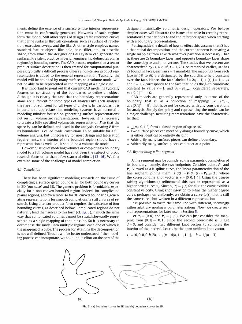
There has been significant modeling research on the issue ofcompleting a surface given boundaries, for both boundary curvesin 2D (our case) and 3D. The generic problem is formidable, espe-cially for a non-convex bounded region. Indeed, for complicatedplanar regions, and even more so for 3D curved boundaries, gener-ating representations for smooth completions is still an area of re-search. Using a tensor product form requires the existence of fourbounding curves, as described below. Complicated regions do notnaturally lend themselves to this form (cf. Fig. 3), in much the sameway that complicated volumes cannot be straightforwardly repre-sented as a single mapping of the unit cube. So it is necessary todecompose the model into multiple regions, each one of which isthe mapping of a cube. The process for attaining the decompositionis not well defined. Thus, it will be better understood if the model-ing process can incorporate, without undue effort on the part of the

designer, intrinsically volumetric design operators. We believesimpler cases will illustrate the issues that arise in creating repre-sentations F that defines X and the reference space when startingwith a boundary representation.

Putting aside the details of how to effect this, assume that X hasa theoretical decomposition, and the current concern is creating asingle mapping from H with whatever partition is necessary. Thatis, there are 2s boundary faces, and opposite boundary faces sharethe same degree and knot vectors. The studies that we present arecharacterized by H;X ! Rs; s " 1;2;3. As remarked earlier, @H has2s bounding faces, each an s) 1 manifold. The mappings from eachface in @H to @X are designated by the coordinate held constantover the face. Hence, the face labeled i " 2$j) 1% & $‘%; j " 1; . . . ; sand ‘ " 1;2 corresponds to the face that holds the j)th coordinateconstant to value ‘) 1, and ri " Fj$@H%i

. Considered separately,ri : '0;1(s)1 ! X.

CAD-models are generally represented only in terms of theboundary, that is, as a collection of mappings A " fapgp,ap : '0;1(2 ! R3, that have not be created with any considerationsfor analysis. Simply designing and representing the model can bea major challenge. Resulting representations have the characteris-tic that:

-S

pap$'0;1(2% form a closed region of space @X.- Two surface pieces can meet only along a boundary curve, which

is either identical or entirely disjoint.- Arbitrarily many surfaces pieces can define a boundary.- Arbitrarily many surface pieces can meet at a point.

4.2. Representing a line segment

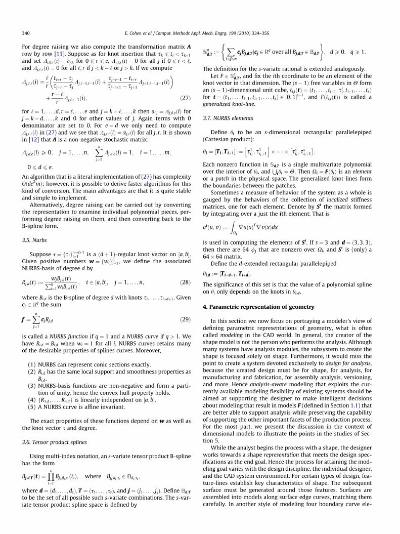
A line segment may be considered the parametric completion ofits boundary, namely, the two endpoints. Consider points P1 andP2. Viewed as a B-spline curve, the linear parameterization of theline segment joining them is c$t% " P1B1;1$t% & P2B2;1$t%, wherethe corresponding knot vector is s " '0;0;1;1(. Using the degreeraising algorithms (p-refinement) this can be represented as ahigher order curve cd. Since cd$t% " c$t% for all t, the curve exhibitsconstant velocity. Using knot insertion to refine the higher degreecurve, perhaps non-uniformly, we obtain a curve ~cd$t%, that is stillthe same curve, but written in a different representation.

It is possible to write the same line with different, seeminglyrather arbitrary nonlinear parameterizations. Now, we create sev-eral representations for later use in Section 5.

Let P1 " $0;0% and P2 " $1;0%. We can just consider the map-ping from '0;1( !' 0;1(, since the second coordinate is 0. Letd " 3, and consider two different knot vectors to complete theinterior of the interval. Let s1, be the open uniform knot vector,

s1 " '0;0;0;0; h;2h; . . . ; $n) 4%h;1;1;1;1(; h " 1=$n) 3%;

Fig. 3. (a) Boundary curves in 2D and (b) boundary curves in 3D.


and let for 0 < a < b < 1=2;n > 8, and d " $1) 2b%=$n) 7%,

s2 " '0;0;0;0;a;b;b& d;b& 2d; . . . ;b& $n) 8%d;1) b;1) a;1;1;1;1(;$30%

where the value of d is chosen so that b; b& d; b& 2d; . . . ; b&$n) 8%d;1) b is a uniform partition of 'b;1) b(. By the nodal repre-sentation property (Section 3.3),

x " Ik$x% :"Xn

j"1

s,k;jBj;3;sk $x%; k " 1;2; $31%

where s,k;j " $sk;j&1 & sk;j&2 & sk;j&3%=3; j " 1; . . . ; n, so that,

s,1 " s,1;j' (n

j"1" 0;

13h; h;2h; . . . ;1) h;1) 1

3h;1

) *; h " 1=$n) 3%:

Define a nonlinear parameterization of the unit interval with uni-formly spaced coefficients given by

Uk$x% "Xn

i"1

i) 1n) 1

Bi;3;sk$x%; k " 1;2: $32%

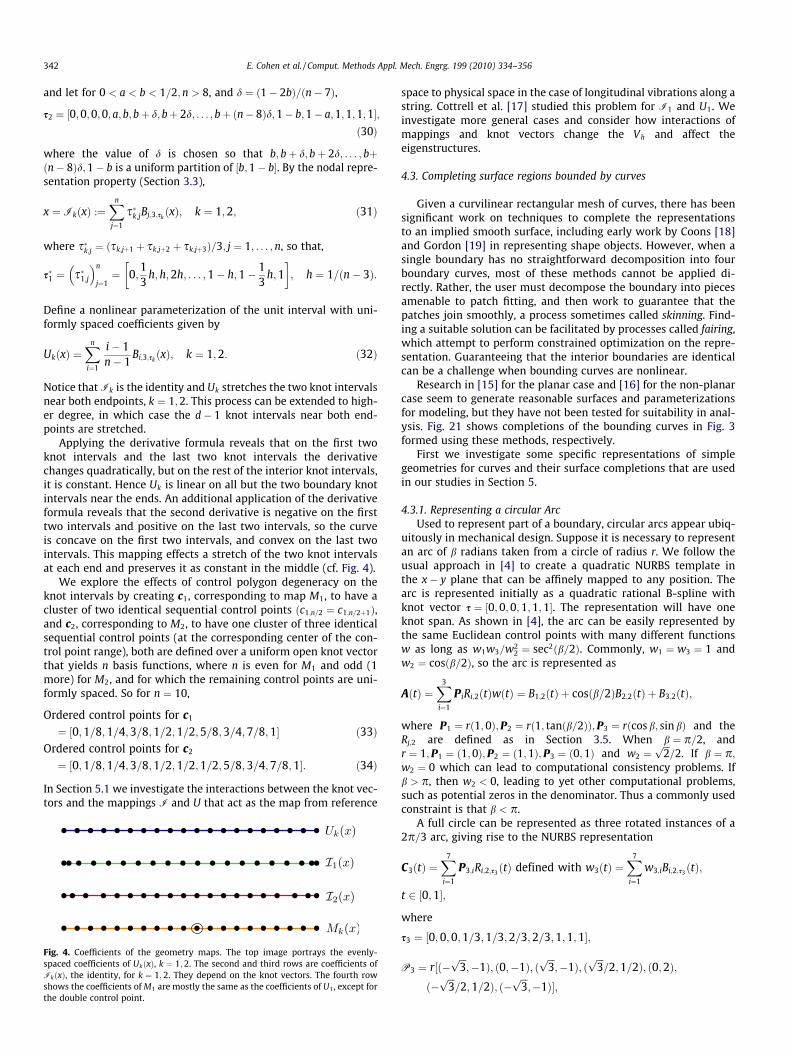
Notice thatIk is the identity and Uk stretches the two knot intervalsnear both endpoints, k " 1;2. This process can be extended to high-er degree, in which case the d) 1 knot intervals near both end-points are stretched.

Applying the derivative formula reveals that on the first twoknot intervals and the last two knot intervals the derivativechanges quadratically, but on the rest of the interior knot intervals,it is constant. Hence Uk is linear on all but the two boundary knotintervals near the ends. An additional application of the derivativeformula reveals that the second derivative is negative on the firsttwo intervals and positive on the last two intervals, so the curveis concave on the first two intervals, and convex on the last twointervals. This mapping effects a stretch of the two knot intervalsat each end and preserves it as constant in the middle (cf. Fig. 4).

We explore the effects of control polygon degeneracy on theknot intervals by creating c1, corresponding to map M1, to have acluster of two identical sequential control points $c1;n=2 " c1;n=2&1%,and c2, corresponding to M2, to have one cluster of three identicalsequential control points (at the corresponding center of the con-trol point range), both are defined over a uniform open knot vectorthat yields n basis functions, where n is even for M1 and odd (1more) for M2, and for which the remaining control points are uni-formly spaced. So for n " 10,

Ordered control points for c1" '0;1=8;1=4;3=8;1=2;1=2;5=8;3=4;7=8;1( $33%

Ordered control points for c2" '0;1=8;1=4;3=8;1=2;1=2;1=2;5=8;3=4;7=8;1(: $34%

In Section 5.1 we investigate the interactions between the knot vec-tors and the mappings I and U that act as the map from reference

space to physical space in the case of longitudinal vibrations along astring. Cottrell et al. [17] studied this problem for I1 and U1. Weinvestigate more general cases and consider how interactions ofmappings and knot vectors change the Vh and affect theeigenstructures.

4.3. Completing surface regions bounded by curves

Given a curvilinear rectangular mesh of curves, there has beensignificant work on techniques to complete the representationsto an implied smooth surface, including early work by Coons [18]and Gordon [19] in representing shape objects. However, when asingle boundary has no straightforward decomposition into fourboundary curves, most of these methods cannot be applied di-rectly. Rather, the user must decompose the boundary into piecesamenable to patch fitting, and then work to guarantee that thepatches join smoothly, a process sometimes called skinning. Find-ing a suitable solution can be facilitated by processes called fairing,which attempt to perform constrained optimization on the repre-sentation. Guaranteeing that the interior boundaries are identicalcan be a challenge when bounding curves are nonlinear.

Research in [15] for the planar case and [16] for the non-planarcase seem to generate reasonable surfaces and parameterizationsfor modeling, but they have not been tested for suitability in anal-ysis. Fig. 21 shows completions of the bounding curves in Fig. 3formed using these methods, respectively.

First we investigate some specific representations of simplegeometries for curves and their surface completions that are usedin our studies in Section 5.

4.3.1. Representing a circular ArcUsed to represent part of a boundary, circular arcs appear ubiq-

uitously in mechanical design. Suppose it is necessary to representan arc of b radians taken from a circle of radius r. We follow theusual approach in [4] to create a quadratic NURBS template inthe x) y plane that can be affinely mapped to any position. Thearc is represented initially as a quadratic rational B-spline withknot vector s " '0;0;0;1;1;1(. The representation will have oneknot span. As shown in [4], the arc can be easily represented bythe same Euclidean control points with many different functionsw as long as w1w3=w2

2 " sec2$b=2%. Commonly, w1 " w3 " 1 andw2 " cos$b=2%, so the arc is represented as

A$t% "X3

i"1

PiRi;2$t%w$t% " B1;2$t% & cos$b=2%B2;2$t% & B3;2$t%;

where P1 " r$1;0%;P2 " r$1; tan$b=2%%;P3 " r$cosb; sinb% and theRj;2 are defined as in Section 3.5. When b " p=2, andr " 1;P1 " $1;0%;P2 " $1;1%;P3 " $0;1% and w2 "

!!!2

p=2. If b " p;

w2 " 0 which can lead to computational consistency problems. Ifb > p, then w2 < 0, leading to yet other computational problems,such as potential zeros in the denominator. Thus a commonly usedconstraint is that b < p.

A full circle can be represented as three rotated instances of a2p=3 arc, giving rise to the NURBS representation

C3$t% "X7

i"1

P3;iRi;2;s3 $t% defined with w3$t% "X7

i"1

w3;iBi;2;s3 $t%;

t 2 '0;1(;

where

s3 " '0; 0;0;1=3;1=3;2=3;2=3;1;1;1(;

P3 " r'$)!!!3

p;)1%; $0;)1%; $

!!!3

p;)1%; $

!!!3

p=2;1=2%; $0;2%;

$)!!!3

p=2;1=2%; $)

!!!3

p;)1%(;

Fig. 4. Coefficients of the geometry maps. The top image portrays the evenly-spaced coefficients of Uk$x%, k " 1;2. The second and third rows are coefficients ofIk$x%, the identity, for k " 1;2. They depend on the knot vectors. The fourth rowshows the coefficients ofM1 are mostly the same as the coefficients of U1, except forthe double control point.


andw3 " '1;1=2;1;1=2;1;1=2;1(:The control points are successive vertices and midpoints, respec-tively, of the sides of an equilateral triangle that inscribes a circleof radius r having the origin as center.

Alternatively we can represent the circle as four rotated imagesof a quarter circle. This gives the NURBS curve

C4$t%"X9

i"1

P4;iRi;2;s4 $t%; definedwithw4$t%"X9

i"1

w4;iBi;2;s4 $t%; t2 '0;1(;

where

s4 " '0;0; 0;1=4;1=4;1=2;1=2;3=4;3=4;1;1;1(;

P4"r2'$)1;)1%;$0;)1%;$1;)1%;$1;0%;$1;1%;$0;1%;$)1;1%;$)1;0%;$)1;)1%(;

w4 " '1;1=!!!2

p;1;1=

!!!2

p;1;1=

!!!2

p;1;1=

!!!2

p;1(:

For this configuration defining the circle in terms of an arc in each ofthe quadrants, the control points are the successively alternatingvertices and midpoints of the sides of a square with that inscribedcircle of radius r centered at the origin. The reader is referred toboth [20,21], that discuss various ways to represent circles in fullerdetail. These representations only guarantee C0 across the bound-aries of each of the arcs.

Both 3-arc and 4-arc representations are rational quadratic. Athird rational representation of a circle is given by two semicirculararcs with cubic representations joined with C1 smoothness. Thisrepresentation, called C2 uses only six control points [20], is shownin Fig. 5(b), and has configuration

knotvector :s"'0;0;0;0;1=2;1=2;1;1;1;1(; $35%weights :w"'9;1;1=3;1=3;1;9( $36%controlcoefficients :P2"f$1;0%;$1;2%;$)1;2%;$)1;)2%;$1;)2%;$1;0%g:

$37%

In the figure, although the radii are drawn with uniformly spacedparameter values, notice the non-uniformity of the disc parameter-ization. That means that uniform h-refinement can well lead to non-uniformly sized analysis elements. That may be desirable for sometangent analysis problems. If it is not desirable then parameterizingthe radii non-uniformly and creating curvilinear radii (to generateelements of more equal size) may be an appropriate completionwhen given C2 as a boundary representation.

Above we have used subscripts to reflect the number of distinctrational arc pieces used to represent a complete circle.

4.3.2. Solid discs from circular boundariesThe disc can be represented in many ways using NURBS. In this

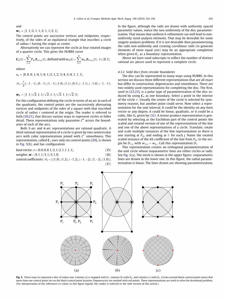
section we discuss three different representations that are all exactbut differ in construction, degeneracies and smoothness. There aretwo widely used representations for completing the disc. The first,used in [22,23], is a polar type of parameterization of the disc in-duced by using C4 as one boundary. Select a point in the interiorof the circle O. Usually the center of the circle is selected for sym-metry reasons, but another point could serve. Now select a repre-sentation for the unit interval. It could be the identity on any knotvector or any degree, it could be linear, quadratic, or it could be acubic, like Uk given by (32). A tensor product representation is gen-erated by selecting as the Euclidean part of the control points thescaled and rotated version of one of the representations of the lineand one of the above representations of a circle. Translate, rotateand scale multiple instances of the line representation so there isone starting at P4;j and ending at O for each j. Name the rotatedscaled instance of the ith coefficient of the line from P4;j to the ori-gin be D1;i;j with w1;i;j " w4;j . Call this representation D1.

This representation creates an orthogonal parameterization ofthe unit circle whose isoparametric lines are either circles or radii.See Fig. 5(a). The mesh is shown in the upper figure; isoparametriclines are drawn in the lower one. In this figure, the radial parame-terization is linear. The lines drawn are showing parameterization,

1 0 7

P6P2

P P P3 4 5

(a) (b)

P

(c)

PP 8P

Fig. 5. Three ways to represent a disc of radius one. Column (a) is mapped with D1, column (b) with D2, and column (c) with D3. Circles around black control points mean thatmore than one control point sits on the black control point location. Degeneracies are marked with red points. These representations are used to solve the drumhead problem.(For interpretation of the references to colour in this figure legend, the reader is referred to the web version of this article.)


but not indicated analysis elements. An analogous solid represen-tation can be generated from C3.

The resulting tensor product representation degenerates onewhole boundary curve to a single point, so JD1

$O% " 0. The rate atwhich it goes to zero can be affected by modifying nearby controlpoints so that the radii are not parameterized linearly, as in Uk.Thus the effect on F " D1 and its power to represent the solutionspace is adjustable without affecting the boundary geometry. Itwill affect the element shapes. The discussion in Section 5.3 con-cerns the impact on the induced function space and the ensuringimpact on analysis results. Call D1 the mapping that embodies C4

as one boundary in representing disc, places the origin as its oppo-site, and represents the radii linearly.

C2 is also a polar type. The initial NURBS representation for thedisc has two rational cubic semicircles. Since there is one interiordouble knot, it is C1 at the join. (Fig. 5(b)). The rest of the surfaceis generated using the same polar approach ad for D1. However,the resulting is not as uniform an angular representation as forthe first case. Call this mapping D2.

Note, that for both mappings, an annulus could easily be mod-eled by choosing the circle representation for the smaller radius asthe inner boundary and using a line representation that terminatesat the control points of the smaller circle instead of the origin. Thew’s that define the rational space remain the same.

The third modeling choice is fundamentally different than thefirst two inasmuch as it uses opposite arcs as the matched bound-aries of the tensor product representation.

r1$v% " A$v%;r2$v% " Rp$A$)v%%;r3$u% " Rp=2$A$u%%;r4$u% " R3p=2$A$)u%%;

where A is the p=2 radian circular arc, Rh$P% means to rotate Pthrough an angle h. Nine control points determine the tensor prod-uct rational quadratic surface, eight of which are specified by theboundary control points. The remaining is chosen to be O and theassociated w set to 1/2. Call this mapping D3, as shown inFig. 5(c). With respect to the number of basis functions, this is themost concise representation of a disc. In this case nine controlpoints are needed as compared to 18 and 12 required for the firsttwo representations, respectively. Furthermore, note that this map-ping exhibits no interior degeneracy, but there are four locations onthe boundaries at which the boundary curves meet at which theJacobian vanishes. The rate at which the Jacobian goes to zero can

be adjusted by modifying the initial NURBS representations of theboundary curves, and adjusting the rate at which the Jacobians goto 0 by modifying the locations of the control points on the interior,particularly those that result from h- or k-refinement. The boundarygeometry is unperturbed by these modifications, but Vh changes,because F is different, even though they are all in a single S2. Thevarious completions are not affine transformations of each other.Note that neither C2 nor C3 are suitable for use with this disc repre-sentation, but are quite reasonable for most other computationaluses encountered in CAD. Again, see the discussion in Section 5.3concerning the impact on the induced function space and the corre-sponding impact on analysis.

4.3.3. Volumetric models such as solid cylinders and solid toriCAD systems generate multiple boundary models from the

three circle representations above, cylinders (without the top andbottom surface), tori, and other types of extruded and swept sur-faces. However, although CAD systems do not generate volumetricmodels, volumetric models of those shapes can be generated fromthe disc surface completions above. A variant of the disc of revolu-tion has been used to generate geometry of vascular structures andto create the trial space for isogeometric analysis of blood throughthose structures [22]. It was used to generate geometry for opticallenses and carry the varying index of refraction volume attributefor computing the optical behavior of those lenses [24]. A sweepsurface is defined as

r$u;v% " A$u% &Mu$S$v%%

where S is the cross section curve, A is a spine curve along which S isswept, and Mu is a transformation incorporating rotation and non-uniform scaling of S$v% as a function of u. Unfortunately this repre-sentation has self-intersections wherever the radius of curvature ofA is less than the first intersection of the curve normal of A withr$u;v%. Generalized cylinders and tori also fall into this category.If the boundary has no self intersections, this can be made into avolumetric sweep by using the surface completion S$v ;w% of S$v%.If there are any self intersections, then this method is unsuitable.

Generalizations of this representation include allowing S to alsobe a function of u, and allowing S to be nonplanar. Both of thosegeneralizations were combined in [25] to create a modeling tech-nique for generalized cylinder-like objects with overhang regions.Such shapes cannot be modeled as a single NURBS patch if thecross section surfaces in the sweep are required to be planar. Be-cause of the complexities of the boundary and some constraintson the isoparametric contours, there are no straightforward tech-

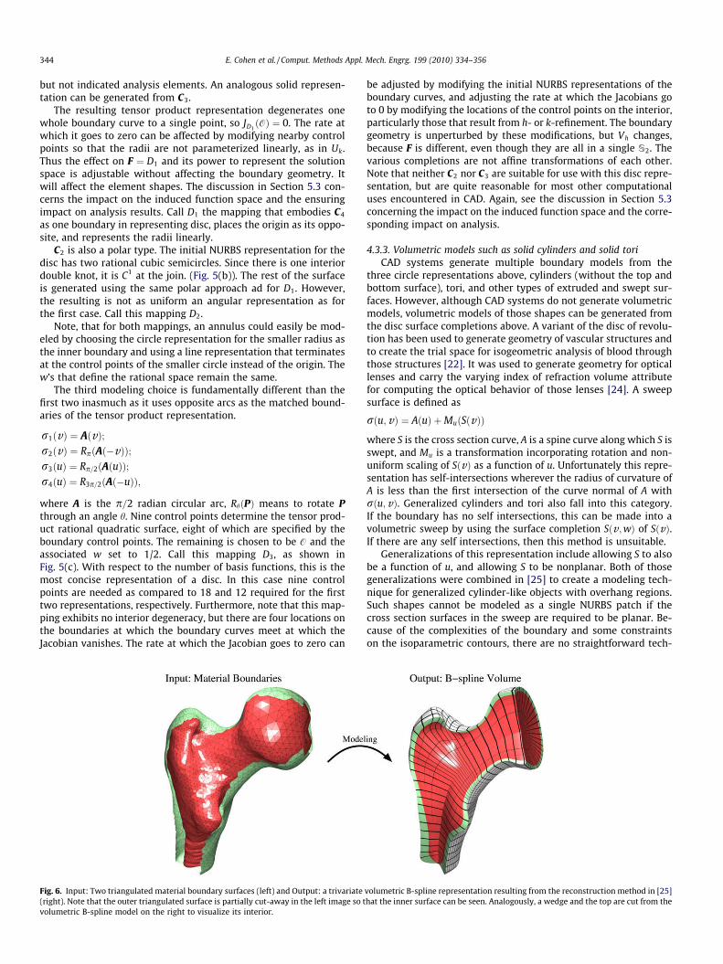
Fig. 6. Input: Two triangulated material boundary surfaces (left) and Output: a trivariate volumetric B-spline representation resulting from the reconstruction method in [25](right). Note that the outer triangulated surface is partially cut-away in the left image so that the inner surface can be seen. Analogously, a wedge and the top are cut from thevolumetric B-spline model on the right to visualize its interior.


niques for modeling some of them as images of multiple 3-cubes.For example, Fig. 6(left) cannot be modeled as a single sweep withplanar cross sections. A partition of the data into multiple H do-mains will create mappings F that also split material properties(bone type), and Young’s modulus (for linear elasticity) in unnatu-ral, ways, not along isoparametric surfaces of the resulting map-pings. Thus, it was deemed appropriate to allow some distortionin the parameterization, while still maintaining a quality modelfor analysis. An example of this approach is studied in Section 5.5.

5. Studies

In this section we examine studies that demonstrate how differ-ent modeling choices, in fact, can easily lead to different simulationresults. The first mathematical model problem (Section 5.1) is thestudy of the eigenstructure of a system under different completionrepresentations. We use a structural vibration analysis problem inboth 1D and 2D. Then in Section 5.4, the Poisson equation is solvedon different physical domains in 2D, where each domain is exactlyrepresented with different choices of geometric model. In both sec-tions h-refinement is applied and convergence rates are compared.Finally, in Section 5.5 we present a 3D study of the linear elasticdeformation of a complex geometric model of a human femur.

5.1. Vibrations

The natural frequencies of a vibrating string are typically mod-eled by Eq. (11). Finding the natural frequencies can correspond-ingly be transformed to solving the system in Eq. (15). While thenon-affine mapping F affects the eigenstructure, so does the choiceof underlying B-spline space S.

5.2. Longitudinal vibrations of a 1D elastic rod

Consider the eigenvalue problem (11) for s " 1 and X " '0;1(

)u00$t% " ku$t%; t 2 $0;1%; u$0% " u$1% " 0: $38%

The exact eigenvalues and eigenfunctions for this problem are

kk " k2p2; uk$t% " sin$kpt%; k " 1;2;3; . . . : $39%

The eigenfunctions uk are orthogonal both with respect to the usualL2 inner product and the energy inner product a$u;v% "R 10 u0$t%v 0$t%dt.Cottrell et al. [17] solved this problem numerically using an iso-

geometric Rayleigh–Ritz method. It was demonstrated that with

uniform knots one can get rid of outliers using a nonlinear map-ping F. We demonstrate here that, with a non-uniform knot vector,a linear F also has no outliers. Also, we show that control meshdegeneracies in the interior of X have a negative effect on theeigenstructure.

We solve (38) numerically by the isogeometric Rayleigh–Ritzmethod (15) using four different spaces Vh generated by differentbases $/i " wi * F

)1%ni"1.We use s1 and s2, as defined in Section 4.2 as knot vectors, pro-

viding uniform open and non-uniform open knots with larger ref-erence space elements near the ends. The mappings to physicalspace are the identity, Ik, and the uniformly spaced coefficients,Uk, over each knot vector, k " 1;2. Then V ‘;Sk is the physical spaceof approximating functions space for the kth knot vector, where‘ 2 fI;Ug. While VI;Sk " Sk is the spline space for the kth knotvector, VU;Sk " spanf/ " w$U)1

k % : w 2 Skg is not a spline space.As we have shown in Section 4.2, both U1 and U2 are increasing,

concave on the first d) 1 intervals, convex on the last d) 1, andlinear in between. Thus, U stretches the intervals near the bound-aries and shrinks the interior ones with a constant scaling. Thesame behavior will be observed for other degrees, as long as n issufficiently large, which occurs when we consider the discrete nor-malized spectrum. The choices of a and b are the stretch factor atthe ends. If they are chosen too large, then the slope of the interiorline segment becomes small. The consequence is that the slope ofU)1

k is large in that region. Since the values of JF and JF)1 affect boththe stiffness and mass matrices, they can adversely affect theeigenstructure. However, an optimal location will depend on thenumber of interior knots as well. This study was run with severaldifferent non-uniform knot vectors, although only one is shownbelow. Note that I0

k . 1, but Uk is more interesting in its behavior.The normalized discrete spectrum is g " 'g0;g1; . . . ;gN)1( where

gk is the ratio between the eigenvalue!!!!!!!kk;h

pand its corresponding

exact solution, (39), i.e.,

gk "

!!!!!!!kk;hkk

s

: $40%

Designed to have knots at prescribed distances from the endpointsof both sides, s2 has its remaining knots evenly-spaced across therest of the interior interval. We demonstrate that the identitymap with this basis creates Vh " Sd;s2 with no optical branches inthe normalized discrete spectrum. It becomes clear that the map-ping F, the space Sd;s2 and the particular DE being solved all interactto affect the appropriation properties of the resulting Vh and the

0.0

0.2

0.4

0.6

0.8

1.0

0.0

0.2

0.4

0.6

0.8

1.0

0.0

0.2

0.4

0.6

0.8

1.0

0.0

0.2

0.4

0.6

0.8

1.0

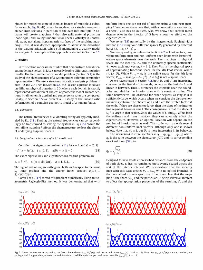
Fig. 7. Given the knot vectors s1 and s2, the first column shows wi;d;sk $U)1k $x%%, and the second shows wi;d;sk $I

)1k $x%%$k " 1;2%. Note that, wi;d;sk $I

)1k $x%% are not stretched, but

setting a and b appropriately causes the end functions to exhibit wider support and more resemble wi;d;sk $Uk%; k " 1;2.


rates at which computed solutions converge towards the truesolution.

Examine the /-basis functions defined on X in Fig. 7 of the fourmappings Uk and Ik where Fig. 4 shows their coefficients. Bystretching the end elements, Uk stretches the basis functions atthe boundaries so they extend farther into the interval and havea more rounded shape, compared to Ik that maintain the uniformknot spacing on X from H.

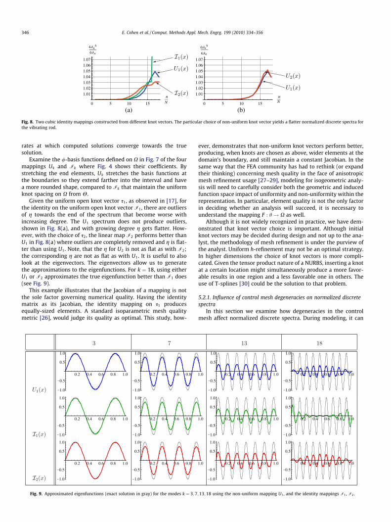
Given the uniform open knot vector s1, as observed in [17], forthe identity on the uniform open knot vector I1, there are outliersof g towards the end of the spectrum that become worse withincreasing degree. The U1 spectrum does not produce outliers,shown in Fig. 8(a), and with growing degree g gets flatter. How-ever, with the choice of s2, the linear map I2 performs better thanU1 in Fig. 8(a) where outliers are completely removed and g is flat-ter than using U1. Note, that the g for U2 is not as flat as with I2;the corresponding g are not as flat as with U1. It is useful to alsolook at the eigenvectors. The eigenvectors allow us to generatethe approximations to the eigenfunctions. For k " 18, using eitherU1 or I2 approximates the true eigenfunction better than I1 does(see Fig. 9).

This example illustrates that the Jacobian of a mapping is notthe sole factor governing numerical quality. Having the identitymatrix as its Jacobian, the identity mapping on s1 producesequally-sized elements. A standard isoparametric mesh qualitymetric [26], would judge its quality as optimal. This study, how-

ever, demonstrates that non-uniform knot vectors perform better,producing, when knots are chosen as above, wider elements at thedomain’s boundary, and still maintain a constant Jacobian. In thesame way that the FEA community has had to rethink (or expandtheir thinking) concerning mesh quality in the face of anisotropicmesh refinement usage [27–29], modeling for isogeometric analy-sis will need to carefully consider both the geometric and inducedfunction space impact of uniformity and non-uniformity within therepresentation. In particular, element quality is not the only factorin deciding whether an analysis will succeed, it is necessary tounderstand the mapping F : h ! X as well.

Although it is not widely recognized in practice, we have dem-onstrated that knot vector choice is important. Although initialknot vectors may be decided during design and not up to the ana-lyst, the methodology of mesh refinement is under the purview ofthe analyst. Uniform h-refinement may not be an optimal strategy.In higher dimensions the choice of knot vectors is more compli-cated. Given the tensor product nature of a NURBS, inserting a knotat a certain location might simultaneously produce a more favor-able results in one region and a less favorable one in others. Theuse of T-splines [30] could be the solution to that problem.

5.2.1. Influence of control mesh degeneracies on normalized discretespectra

In this section we examine how degeneracies in the controlmesh affect normalized discrete spectra. During modeling, it can

0 5 10 15

nN

1.011.021.031.041.051.061.07

nh

n

0 5 10 15

nN

1.011.021.031.041.051.061.07

nh

n

(a) (b)

Fig. 8. Two cubic identity mappings constructed from different knot vectors. The particular choice of non-uniform knot vector yields a flatter normalized discrete spectra forthe vibrating rod.

0.2 0.4 0.6 0.8 1.0

1.0

0.5

0.5

1.0

1.0

0.5

0.5

1.0

1.0

0.5

0.5

1.0

1.0

0.5

0.5

1.0

1.0

0.5

0.5

1.0

1.0

0.5

0.5

1.0

1.0

0.5

0.5

1.0

1.0

0.5

0.5

1.0

1.0

0.5

0.5

1.0

1.0

0.5

0.5

1.0

1.0

0.5

0.5

1.0

1.0

0.5

0.5

1.0

0.2 0.4 0.6 0.8 1.0 0.2 0.4 0.6 0.8 1.0 0.2 0.4 0.6 0.8 1.0

0.2 0.4 0.6 0.8 1.0 0.2 0.4 0.6 0.8 1.0 0.2 0.4 0.6 0.8 1.0 0.2 0.4 0.6 0.8 1.0

0.2 0.4 0.6 0.8 1.0 0.2 0.4 0.6 0.8 1.0 0.2 0.4 0.6 0.8 1.0 0.2 0.4 0.6 0.8 1.0

Fig. 9. Approximated eigenfunctions (exact solution in gray) for the modes k " 3;7;13;18 using the non-uniform mapping U1, and the identity mappings I1, I2.


happen that the resulting control mesh of a model contains controlpoints that coincide. In the following, we examine the mapping M1

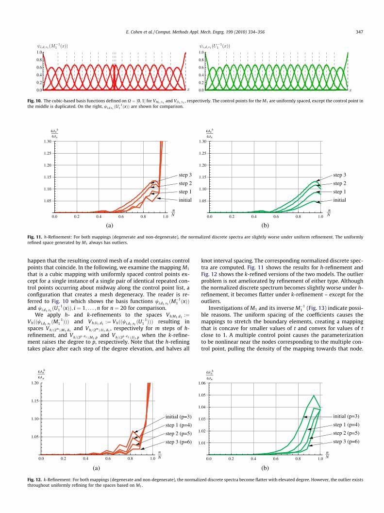
that is a cubic mapping with uniformly spaced control points ex-cept for a single instance of a single pair of identical repeated con-trol points occurring about midway along the control point list, aconfiguration that creates a mesh degeneracy. The reader is re-ferred to Fig. 10 which shows the basis functions wi;d1 ;s1 $M

)11 $x%%

and wi;d1 ;s1 $U)11 $x%%; i " 1; . . . ;n for n " 20 for comparison.

We apply h- and k-refinements to the spaces Vh;M1 ;d1 :"Vh$$wi;d1 ;s1 $M

)11 %%% and Vh;U1 ;d1 :" Vh$$wi;d1 ;s1 $U

)11 %%% resulting in

spaces Vh=$2m%;M1 ;d1 and Vh=$2m%;U1 ;d1 , respectively for m steps of h-refinement, and Vh=$2p)d1 %;M1 ;p

and Vh=$2p)d1 %;U1 ;pwhen the k-refine-

ment raises the degree to p, respectively. Note that the h-refiningtakes place after each step of the degree elevation, and halves all

knot interval spacing. The corresponding normalized discrete spec-tra are computed. Fig. 11 shows the results for h-refinement andFig. 12 shows the k-refined versions of the two models. The outlierproblem is not ameliorated by refinement of either type. Althoughthe normalized discrete spectrum becomes slightly worse under h-refinement, it becomes flatter under k-refinement – except for theoutliers.

Investigations of M1 and its inverse M)11 (Fig. 13) indicate possi-

ble reasons. The uniform spacing of the coefficients causes themappings to stretch the boundary elements, creating a mappingthat is concave for smaller values of t and convex for values of tclose to 1. A multiple control point causes the parameterizationto be nonlinear near the nodes corresponding to the multiple con-trol point, pulling the density of the mapping towards that node.

0.0

0.2

0.4

0.6

0.8

1.0

0.0

0.2

0.4

0.6

0.8

1.0

Fig. 10. The cubic-based basis functions defined on X " '0;1( for VM1 ;S1 and VU1 ;S1 , respectively. The control points for theM1 are uniformly spaced, except the control point inthe middle is duplicated. On the right, wi;d;s1 $U

)11 $x%% are shown for comparison.

0.0 0.2 0.4 0.6 0.8 1.0

nN

1.05

1.10

1.15

1.20

1.25

1.30

nh

n

initial

step 1

step 2

step 3

0.0 0.2 0.4 0.6 0.8 1.0

nN

1.05

1.10

1.15

1.20

1.25

1.30

nh

n

initial

step 1

step 2

step 3

(a) (b)

Fig. 11. h-Refinement: For both mappings (degenerate and non-degenerate), the normalized discrete spectra are slightly worse under uniform refinement. The uniformlyrefined space generated by M1 always has outliers.

0.0 0.2 0.4 0.6 0.8 1.0

nN

1.05

1.10

1.15

1.20

nh

n

initial (p=3)

step 1 (p=4)

step 2 (p=5)

step 3 (p=6)

0.0 0.2 0.4 0.6 0.8 1.0

nN

1.01

1.02

1.03

1.04

1.05

1.06

nh

n

initial (p=3)

step 1 (p=4)

step 2 (p=5)

step 3 (p=6)

(a) (b)

Fig. 12. k-Refinement: For both mappings (degenerate and non-degenerate), the normalized discrete spectra become flatter with elevated degree. However, the outlier existsthroughout uniformly refining for the spaces based on M1.


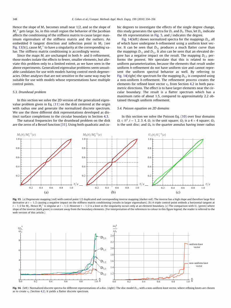
Hence the slope of M1 becomes small near 1/2, and so the slope ofM)1

1 gets large. So, in this small region the behavior of the Jacobianaffects the conditioning of the stiffness matrix to cause larger max-imum eigenvalues of the stiffness matrix and the outliers. Anembedded 0 tangent direction and inflection point in M2 (seeFig. 13(b)), causeM)1

2 to have a singularity at the corresponding va-lue. The stiffness matrix conditioning is accordingly worse.

Since the maps Mi are unchanged in both h- and k-refinement,those modes isolate the effects to fewer, smaller elements, but alle-viate this problem only to a limited extent, as we have seen in theabove experiments. Generalized eigenvalue problems seem unsuit-able candidates for use with models having control mesh degener-acies. Other analyses that are not sensitive in the same way may besuitable for use with models whose representations have multiplecontrol points.

5.3. Drumhead problem

In this section we solve the 2D version of the generalized eigen-value problem given in Eq. (11) on the disk centered at the originwith radius one and generate the normalized discrete spectrum.We use the three different disk representations developed as dis-tinct surface completions to the circular boundary in Section 4.3.

The natural frequencies for the drumhead problem on the diskare the zeros of a Bessel function [31]. Using both quadratic and cu-

bic degrees to investigate the effects of the single degree change,this study generates the spectra for D1 and D3. Thus, let Di;j indicatethe ith representation in Fig. 5, and j indicates the degree.

Fig. 14(left) shows normalized spectra for the mappings Di;j, allof which have undergone h-refinement using a uniform knot vec-tor. It can be seen that D3;j produces a much flatter curve thanthe mappings D1;j and D2;j. It also can be seen that an elevated de-gree has a negative impact on the result. The mapping D2;3 per-forms the poorest. We speculate that this is related to non-uniform parameterization, because the elements that result underuniform h-refinement do not have uniform size and cannot repre-sent the uniform spectral behavior as well. By referring toFig. 14(right) the spectrum for the mapping D3;2 is computed usinga non-uniform h-refinement. The refinement process creates theelements for refined knot vector s2 from Section 4.2 in both para-metric directions. The effect is to have larger elements near the cir-cular boundary. The result is a flatter spectrum which has amaximum ratio of about 1.5, compared to approximately 2.2 ob-tained through uniform refinement.

5.4. Poisson equation on 2D domains

In this section we solve the Poisson Eq. (10) over four domainsXi 2 R2; i " 1;2;3;4. X1 is the unit square; X2 is a 4+ 4 square; X3

is the unit disc; and X4 is the quarter annulus having inner radius

2,3D

D1,3

D1,2

D3,3

D3,2

0.0 0.2 0.4 0.6 0.8 1.0nN

nN0

2

4

6

8

nh

n

uniform knotvector

0.0 0.2 0.4 0.6 0.8 1.0

1.2

1.4

1.6

1.8

2.0

2.2

2.4

nh

n

non!uniform knotvector

Fig. 14. (left): Normalized discrete spectra for different representations of a disc. (right): The disc model D3;2 with a non-uniform knot vector, where refining knots are chosenas to create s2 (Section 4.2). It yields a flatter discrete spectrum.

0.2 0.4 0.6 0.8 1.0

0.2

0.4

0.6

0.8

1.0

0.2 0.4 0.6 0.8 1.0

0.2

0.4

0.6

0.8

1.0

0.2 0.4 0.6 0.8 1.0

0.2

0.4

0.6

0.8

1.0

(a) (b) (c)

Fig. 13. (a) Degenerate mapping (red) with control point 1/2 duplicated and corresponding inverse mapping (darker red). The inverse has a high slope and therefore large firstderivative at t " 1=2 causing a negative impact on the stiffness matrix conditioning (results in larger eigenvalues). (b) A triple control point embeds a horizontal tangent att " 1=2 for M2. Hence M)1

2 is singular at t " 1=2. However t " 1=2 is a knot so the singularity occurs only at an element boundary. (c) The comparison with U1 (green) whereslope of the inverse (dark green) is constant away from the boundary elements. (For interpretation of the references to colour in this figure legend, the reader is referred to theweb version of this article.)


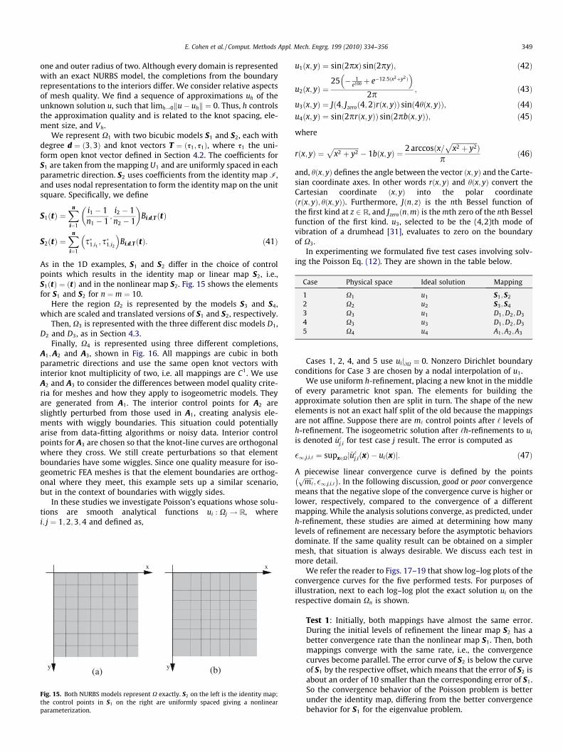
one and outer radius of two. Although every domain is representedwith an exact NURBS model, the completions from the boundaryrepresentations to the interiors differ. We consider relative aspectsof mesh quality. We find a sequence of approximations uh of theunknown solution u, such that limh!0ku) uhk " 0. Thus, h controlsthe approximation quality and is related to the knot spacing, ele-ment size, and Vh.

We represent X1 with two bicubic models S1 and S2, each withdegree d " $3;3% and knot vectors T " $s1; s1%, where s1 the uni-form open knot vector defined in Section 4.2. The coefficients forS1 are taken from the mapping U1 and are uniformly spaced in eachparametric direction. S2 uses coefficients from the identity map I,and uses nodal representation to form the identity map on the unitsquare. Specifically, we define

S1$t% "Xn

i"1

i1 ) 1n1 ) 1

;i2 ) 1n2 ) 1

# $Bi;d;T $t%

S2$t% "Xn

i"1

s,1;i1 ; s,1;i2

' (Bi;d;T$t%: $41%

As in the 1D examples, S1 and S2 differ in the choice of controlpoints which results in the identity map or linear map S2, i.e.,S1$t% " $t% and in the nonlinear map S2. Fig. 15 shows the elementsfor S1 and S2 for n " m " 10.

Here the region X2 is represented by the models S3 and S4,which are scaled and translated versions of S1 and S2, respectively.

Then, X3 is represented with the three different disc models D1,D2 and D3, as in Section 4.3.

Finally, X4 is represented using three different completions,A1;A2 and A3, shown in Fig. 16. All mappings are cubic in bothparametric directions and use the same open knot vectors withinterior knot multiplicity of two, i.e. all mappings are C1. We useA2 and A3 to consider the differences between model quality crite-ria for meshes and how they apply to isogeometric models. Theyare generated from A1. The interior control points for A2 areslightly perturbed from those used in A1, creating analysis ele-ments with wiggly boundaries. This situation could potentiallyarise from data-fitting algorithms or noisy data. Interior controlpoints for A3 are chosen so that the knot-line curves are orthogonalwhere they cross. We still create perturbations so that elementboundaries have some wiggles. Since one quality measure for iso-geometric FEA meshes is that the element boundaries are orthog-onal where they meet, this example sets up a similar scenario,but in the context of boundaries with wiggly sides.

In these studies we investigate Poisson’s equations whose solu-tions are smooth analytical functions ui : Xj ! R, wherei; j " 1;2;3;4 and defined as,

u1$x; y% " sin$2px% sin$2py%; $42%

u2$x; y% "25 ) 1

e100 & e)12:5$x2&y2%' (

2p ; $43%

u3$x; y% " J$4; Jzero$4;2%r$x; y%% sin$4h$x; y%%; $44%u4$x; y% " sin$2pr$x; y%% sin$2pb$x; y%%; $45%

where

r$x; y% "!!!!!!!!!!!!!!!x2 & y2

p) 1b$x; y% "

2arccos$x=!!!!!!!!!!!!!!!x2 & y2

p%

p $46%

and, h$x; y% defines the angle between the vector $x; y% and the Carte-sian coordinate axes. In other words r$x; y% and h$x; y% convert theCartesian coordinate $x; y% into the polar coordinate$r$x; y%; h$x; y%%. Furthermore, J$n; z% is the nth Bessel function ofthe first kind at z 2 R, and Jzero$n;m% is themth zero of the nth Besselfunction of the first kind. u3, selected to be the (4,2)th mode ofvibration of a drumhead [31], evaluates to zero on the boundaryof X3.

In experimenting we formulated five test cases involving solv-ing the Poisson Eq. (12). They are shown in the table below.

Case Physical space Ideal solution Mapping

1 X1 u1 S1; S22 X2 u2 S3; S43 X3 u1 D1;D2;D3

4 X3 u3 D1;D2;D3

5 X4 u4 A1;A2;A3

Cases 1, 2, 4, and 5 use uij@X . 0. Nonzero Dirichlet boundaryconditions for Case 3 are chosen by a nodal interpolation of u1.

We use uniform h-refinement, placing a new knot in the middleof every parametric knot span. The elements for building theapproximate solution then are split in turn. The shape of the newelements is not an exact half split of the old because the mappingsare not affine. Suppose there are m‘ control points after ‘ levels ofh-refinement. The isogeometric solution after ‘h-refinements to ui

is denoted u‘j;i for test case j result. The error is computed as

!1;j;i;‘ " supx2Xju‘j;i$x% ) ui$x%j: $47%

A piecewise linear convergence curve is defined by the points!!!!!!m‘

p; !1;j;i;‘

+ ,. In the following discussion, good or poor convergence

means that the negative slope of the convergence curve is higher orlower, respectively, compared to the convergence of a differentmapping. While the analysis solutions converge, as predicted, underh-refinement, these studies are aimed at determining how manylevels of refinement are necessary before the asymptotic behaviorsdominate. If the same quality result can be obtained on a simplermesh, that situation is always desirable. We discuss each test inmore detail.

We refer the reader to Figs. 17–19 that show log–log plots of theconvergence curves for the five performed tests. For purposes ofillustration, next to each log–log plot the exact solution ui on therespective domain Xn is shown.

Test 1: Initially, both mappings have almost the same error.During the initial levels of refinement the linear map S2 has abetter convergence rate than the nonlinear map S1. Then, bothmappings converge with the same rate, i.e., the convergencecurves become parallel. The error curve of S2 is below the curveof S1 by the respective offset, which means that the error of S2 isabout an order of 10 smaller than the corresponding error of S1.So the convergence behavior of the Poisson problem is betterunder the identity map, differing from the better convergencebehavior for S1 for the eigenvalue problem.

y

x

y

x

(a) (b)

Fig. 15. Both NURBS models represent X exactly. S2 on the left is the identity map;the control points in S1 on the right are uniformly spaced giving a nonlinearparameterization.


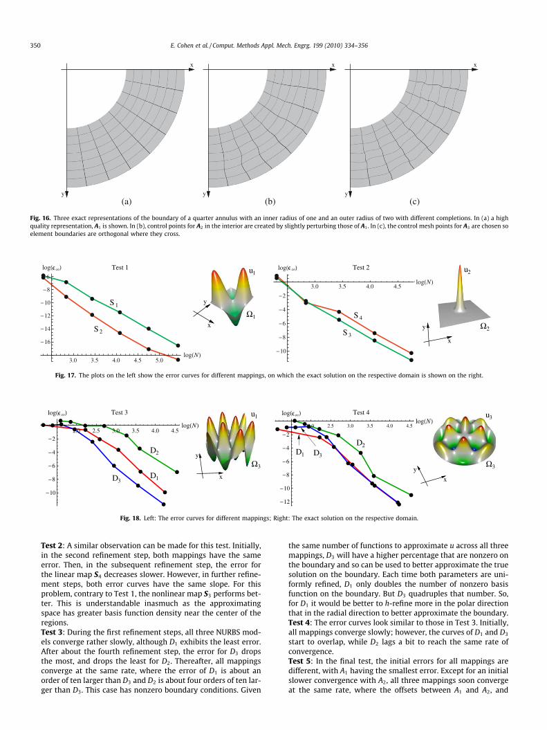
Test 2: A similar observation can be made for this test. Initially,in the second refinement step, both mappings have the sameerror. Then, in the subsequent refinement step, the error forthe linear map S4 decreases slower. However, in further refine-ment steps, both error curves have the same slope. For thisproblem, contrary to Test 1, the nonlinear map S3 performs bet-ter. This is understandable inasmuch as the approximatingspace has greater basis function density near the center of theregions.Test 3: During the first refinement steps, all three NURBS mod-els converge rather slowly, although D1 exhibits the least error.After about the fourth refinement step, the error for D3 dropsthe most, and drops the least for D2. Thereafter, all mappingsconverge at the same rate, where the error of D1 is about anorder of ten larger than D3 and D2 is about four orders of ten lar-ger than D3. This case has nonzero boundary conditions. Given

the same number of functions to approximate u across all threemappings, D3 will have a higher percentage that are nonzero onthe boundary and so can be used to better approximate the truesolution on the boundary. Each time both parameters are uni-formly refined, D1 only doubles the number of nonzero basisfunction on the boundary. But D3 quadruples that number. So,for D1 it would be better to h-refine more in the polar directionthat in the radial direction to better approximate the boundary.Test 4: The error curves look similar to those in Test 3. Initially,all mappings converge slowly; however, the curves of D1 and D3

start to overlap, while D2 lags a bit to reach the same rate ofconvergence.Test 5: In the final test, the initial errors for all mappings aredifferent, with A1 having the smallest error. Except for an initialslower convergence with A2, all three mappings soon convergeat the same rate, where the offsets between A1 and A2, and

x

y

x

y

x

y(a) (b) (c)

Fig. 16. Three exact representations of the boundary of a quarter annulus with an inner radius of one and an outer radius of two with different completions. In (a) a highquality representation, A1 is shown. In (b), control points for A2 in the interior are created by slightly perturbing those of A1. In (c), the control mesh points for A3 are chosen soelement boundaries are orthogonal where they cross.

3.0 3.5 4.0 4.5 5.0log N

16

14

12

10

8

6

log

3.0 3.5 4.0 4.5log N

10

8

6

4

2

log

1

Test 1

S 2

S

S 3

S 4

Test 2

y

x

2"

u2

y

x

"1

u1

# #

Fig. 17. The plots on the left show the error curves for different mappings, on which the exact solution on the respective domain is shown on the right.

2.0 2.5 3.0 3.5 4.0 4.5log N

10

8

6

4

2

2.0 2.5 3.0 3.5 4.0 4.5log N

12

10

8

6

4

2

D1

Test 3

D

3

D2

xy 3"

u3

D1

D

3

D2

Test 4u1

"3

y

x

log # log #

Fig. 18. Left: The error curves for different mappings; Right: The exact solution on the respective domain.


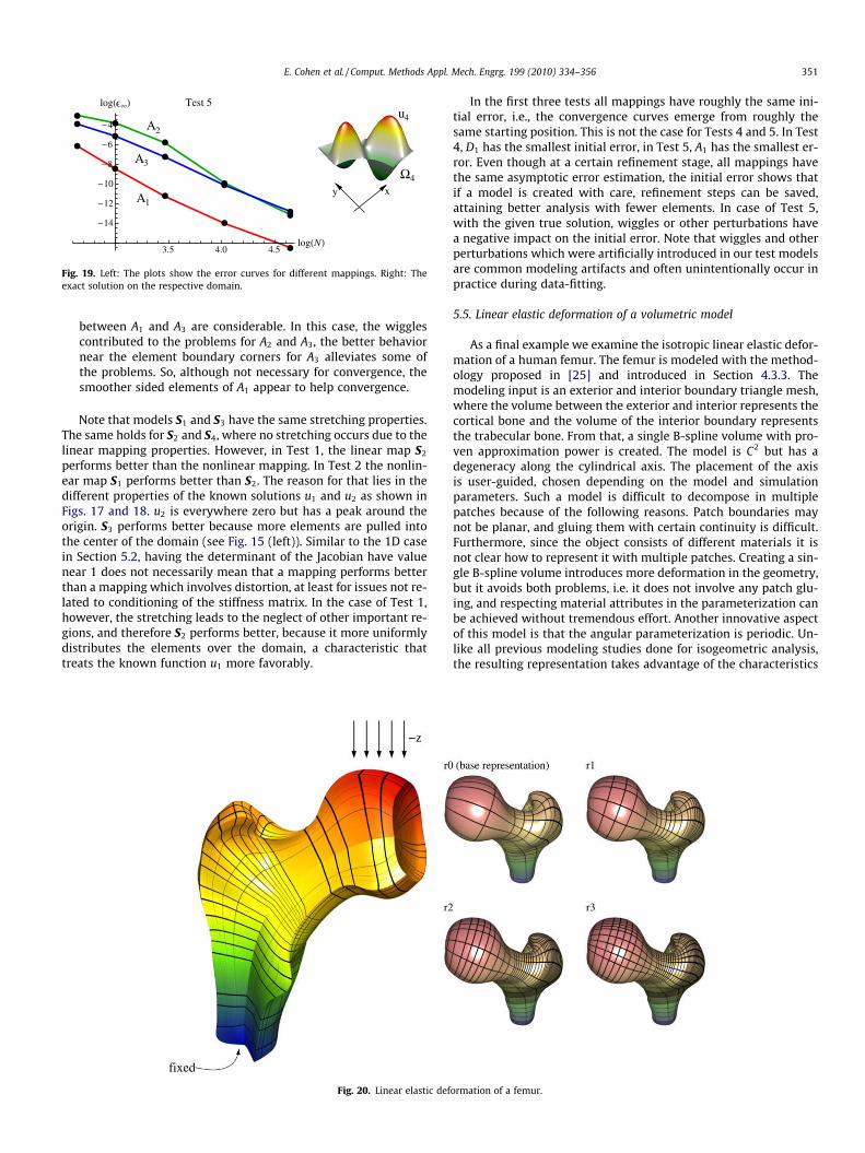
between A1 and A3 are considerable. In this case, the wigglescontributed to the problems for A2 and A3, the better behaviornear the element boundary corners for A3 alleviates some ofthe problems. So, although not necessary for convergence, thesmoother sided elements of A1 appear to help convergence.

Note that models S1 and S3 have the same stretching properties.The same holds for S2 and S4, where no stretching occurs due to thelinear mapping properties. However, in Test 1, the linear map S2

performs better than the nonlinear mapping. In Test 2 the nonlin-ear map S1 performs better than S2. The reason for that lies in thedifferent properties of the known solutions u1 and u2 as shown inFigs. 17 and 18. u2 is everywhere zero but has a peak around theorigin. S3 performs better because more elements are pulled intothe center of the domain (see Fig. 15 (left)). Similar to the 1D casein Section 5.2, having the determinant of the Jacobian have valuenear 1 does not necessarily mean that a mapping performs betterthan a mapping which involves distortion, at least for issues not re-lated to conditioning of the stiffness matrix. In the case of Test 1,however, the stretching leads to the neglect of other important re-gions, and therefore S2 performs better, because it more uniformlydistributes the elements over the domain, a characteristic thattreats the known function u1 more favorably.

In the first three tests all mappings have roughly the same ini-tial error, i.e., the convergence curves emerge from roughly thesame starting position. This is not the case for Tests 4 and 5. In Test4, D1 has the smallest initial error, in Test 5, A1 has the smallest er-ror. Even though at a certain refinement stage, all mappings havethe same asymptotic error estimation, the initial error shows thatif a model is created with care, refinement steps can be saved,attaining better analysis with fewer elements. In case of Test 5,with the given true solution, wiggles or other perturbations havea negative impact on the initial error. Note that wiggles and otherperturbations which were artificially introduced in our test modelsare common modeling artifacts and often unintentionally occur inpractice during data-fitting.

5.5. Linear elastic deformation of a volumetric model

As a final example we examine the isotropic linear elastic defor-mation of a human femur. The femur is modeled with the method-ology proposed in [25] and introduced in Section 4.3.3. Themodeling input is an exterior and interior boundary triangle mesh,where the volume between the exterior and interior represents thecortical bone and the volume of the interior boundary representsthe trabecular bone. From that, a single B-spline volume with pro-ven approximation power is created. The model is C2 but has adegeneracy along the cylindrical axis. The placement of the axisis user-guided, chosen depending on the model and simulationparameters. Such a model is difficult to decompose in multiplepatches because of the following reasons. Patch boundaries maynot be planar, and gluing them with certain continuity is difficult.Furthermore, since the object consists of different materials it isnot clear how to represent it with multiple patches. Creating a sin-gle B-spline volume introduces more deformation in the geometry,but it avoids both problems, i.e. it does not involve any patch glu-ing, and respecting material attributes in the parameterization canbe achieved without tremendous effort. Another innovative aspectof this model is that the angular parameterization is periodic. Un-like all previous modeling studies done for isogeometric analysis,the resulting representation takes advantage of the characteristics

3.5 4.0 4.5log N

14

12

10

8

6

4

A3

A2

Test 5

A

4xy

u4

"

1

log #

Fig. 19. Left: The plots show the error curves for different mappings. Right: Theexact solution on the respective domain.

Fig. 20. Linear elastic deformation of a femur.


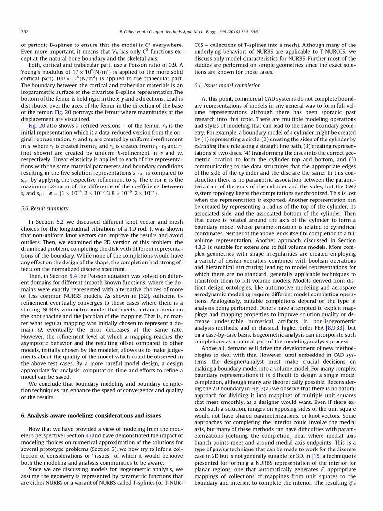
of periodic B-splines to ensure that the model is C2 everywhere.Even more important, it means that Vh has only C2 functions ex-cept at the natural bone boundary and the skeletal axis.

Both, cortical and trabecular part, use a Poisson ratio of 0.9. AYoung’s modulus of 17+ 109$N=m2% is applied to the more solidcortical part; 100+ 106$N=m2% is applied to the trabecular part.The boundary between the cortical and trabecular materials is anisoparametric surface of the trivariate B-spline representation.Thebottom of the femur is held rigid in the x; y and z directions. Load isdistributed over the apex of the femur in the direction of the baseof the femur. Fig. 20 portrays the femur where magnitudes of thedisplacement are visualized.

Fig. 20 also shows h-refined versions ri of the femur. r0 is theinitial representation which is a data-reduced version from the ori-ginal representation. r1 and r0 are created by uniform h-refinementin u, where r1 is created from r0 and r2 is created from r1 # r3 and r4(not shown) are created by uniform h-refinement in v and w,respectively. Linear elasticity is applied to each of the representa-tions with the same material parameters and boundary conditionsresulting in the five solution representations si # si is compared tosi&1 by applying the respective refinement to si. The error ei is themaximum L2-norm of the difference of the coefficients betweensi and si&1 : e " f1+ 10)4;2+ 10)5;3:8+ 10)6;2+ 10)7g.

5.6. Result summary

In Section 5.2 we discussed different knot vector and meshchoices for the longitudinal vibrations of a 1D rod. It was shownthat non-uniform knot vectors can improve the results and avoidoutliers. Then, we examined the 2D version of this problem, thedrumhead problem, completing the disk with different representa-tions of the boundary. While none of the completions would haveany effect on the design of the shape, the completion had strong ef-fects on the normalized discrete spectrum.

Then, in Section 5.4 the Poisson equation was solved on differ-ent domains for different smooth known functions, where the do-mains were exactly represented with alternative choices of moreor less common NURBS models. As shown in [32], sufficient h-refinement eventually converges to these cases where there is astarting NURBS volumetric model that meets certain criteria onthe knot spacing and the Jacobian of the mapping. That is, no mat-ter what regular mapping was initially chosen to represent a do-main X, eventually the error decreases at the same rate.However, the refinement level at which a mapping reaches theasymptotic behavior and the resulting offset compared to othermodels, initially chosen by the modeler, allows us to make judge-ments about the quality of the model which could be observed inthe above test cases. By a more careful model design, a designappropriate for analysis, computation time and efforts to refine amodel can be saved.

We conclude that boundary modeling and boundary comple-tion techniques can enhance the speed of convergence and qualityof the results.

6. Analysis-aware modeling: considerations and issues

Now that we have provided a view of modeling from the mod-eler’s perspective (Section 4) and have demonstrated the impact ofmodeling choices on numerical approximation of the solutions forseveral prototype problems (Section 5), we now try to infer a col-lection of considerations or ‘‘issues” of which it would behooveboth the modeling and analysis communities to be aware.

Since we are discussing models for isogeometric analysis, weassume the geometry is represented by parametric functions thatare either NURBS or a variant of NURBS called T-splines (or T-NUR-

CCS – collections of T-splines into a mesh). Although many of theunderlying behaviors of NURBS are applicable to T-NURCCS, wediscuss only model characteristics for NURBS. Further most of thestudies are performed on simple geometries since the exact solu-tions are known for those cases.

6.1. Issue: model completion

At this point, commercial CAD systems do not complete bound-ary representations of models in any general way to form full vol-ume representations although there has been sporadic pastresearch into this topic. There are multiple modeling operationsand styles of modeling that can lead to the same boundary geom-etry. For example, a boundary model of a cylinder might be createdby (1) representing a circle, (2) creating the sides of the cylinder byextruding the circle along a straight line path, (3) creating represen-tations of two discs, (4) transforming the discs into the correct geo-metric location to form the cylinder top and bottom, and (5)communicating to the data structures that the appropriate edgesof the side of the cylinder and the disc are the same. In this con-struction there is no parametric association between the parame-terization of the ends of the cylinder and the sides, but the CADsystem topology keeps the computations synchronized. This is lostwhen the representation is exported. Another representation canbe created by representing a radius of the top of the cylinder, itsassociated side, and the associated bottom of the cylinder. Thenthat curve is rotated around the axis of the cylinder to form aboundary model whose parameterization is related to cylindricalcoordinates. Neither of the above lends itself to completion to a fullvolume representation. Another approach discussed in Section4.3.3 is suitable for extensions to full volume models. More com-plex geometries with shape irregularities are created employinga variety of design operators combined with boolean operationsand hierarchical structuring leading to model representations forwhich there are no standard, generally applicable techniques totransfrom them to full volume models. Models derived from dis-tinct design ontologies, like automotive modeling and aerospaceaerodynamic modeling require different model completion opera-tions. Analogously, suitable completions depend on the type ofanalysis being performed. Others have attempted to exploit map-pings and mapping properties to improve solution quality or de-crease undesirable numerical artifacts in non-isogeometricanalysis methods, and in classical, higher order FEA [8,9,33], buton a case-by-case basis. Isogeometric analysis can incorporate suchcompletions as a natural part of the modeling/analysis process.

Above all, demand will drive the development of new method-ologies to deal with this. However, until embedded in CAD sys-tems, the designer/analyst must make crucial decisions onmaking a boundary model into a volume model. For many complexboundary representations it is difficult to design a single modelcompletion, although many are theoretically possible. Reconsider-ing the 2D boundary in Fig. 3(a) we observe that there is no naturalapproach for dividing it into mappings of multiple unit squaresthat meet smoothly, as a designer would want. Even if there ex-isted such a solution, images on opposing sides of the unit squarewould not have shared parameterizations, or knot vectors. Someapproaches for completing the interior could involve the medialaxis, but many of these methods can have difficulties with param-eterizations (defining the completion) near where medial axisbranch points meet and around medial axis endpoints. This is atype of paving technique that can be made to work for the discretecase in 2D but is not generally suitable for 3D. In [15] a technique ispresented for forming a NURBS representation of the interior forplanar regions, one that automatically generates F, appropriatemappings of collections of mappings from unit squares to theboundary and interior, to complete the interior. The resulting /’s


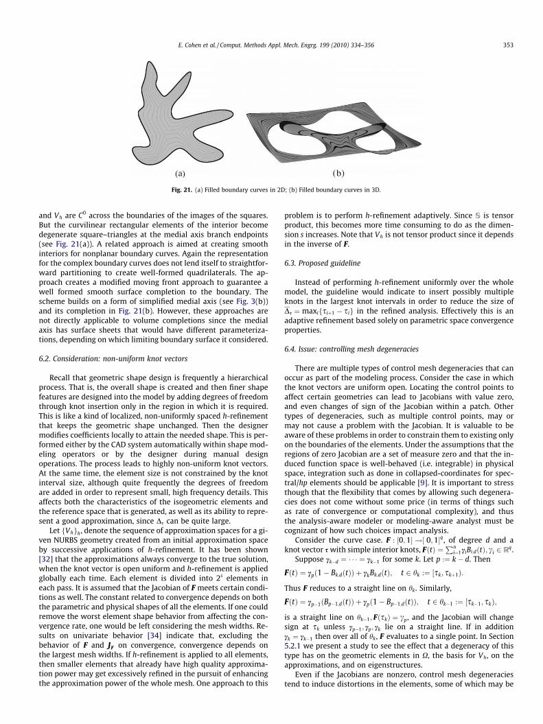
and Vh are C0 across the boundaries of the images of the squares.But the curvilinear rectangular elements of the interior becomedegenerate square–triangles at the medial axis branch endpoints(see Fig. 21(a)). A related approach is aimed at creating smoothinteriors for nonplanar boundary curves. Again the representationfor the complex boundary curves does not lend itself to straightfor-ward partitioning to create well-formed quadrilaterals. The ap-proach creates a modified moving front approach to guarantee awell formed smooth surface completion to the boundary. Thescheme builds on a form of simplified medial axis (see Fig. 3(b))and its completion in Fig. 21(b). However, these approaches arenot directly applicable to volume completions since the medialaxis has surface sheets that would have different parameteriza-tions, depending on which limiting boundary surface it considered.

6.2. Consideration: non-uniform knot vectors

Recall that geometric shape design is frequently a hierarchicalprocess. That is, the overall shape is created and then finer shapefeatures are designed into the model by adding degrees of freedomthrough knot insertion only in the region in which it is required.This is like a kind of localized, non-uniformly spaced h-refinementthat keeps the geometric shape unchanged. Then the designermodifies coefficients locally to attain the needed shape. This is per-formed either by the CAD system automatically within shape mod-eling operators or by the designer during manual designoperations. The process leads to highly non-uniform knot vectors.At the same time, the element size is not constrained by the knotinterval size, although quite frequently the degrees of freedomare added in order to represent small, high frequency details. Thisaffects both the characteristics of the isogeometric elements andthe reference space that is generated, as well as its ability to repre-sent a good approximation, since Ds can be quite large.

Let fVhgh, denote the sequence of approximation spaces for a gi-ven NURBS geometry created from an initial approximation spaceby successive applications of h-refinement. It has been shown[32] that the approximations always converge to the true solution,when the knot vector is open uniform and h-refinement is appliedglobally each time. Each element is divided into 2s elements ineach pass. It is assumed that the Jacobian of F meets certain condi-tions as well. The constant related to convergence depends on boththe parametric and physical shapes of all the elements. If one couldremove the worst element shape behavior from affecting the con-vergence rate, one would be left considering the mesh widths. Re-sults on univariate behavior [34] indicate that, excluding thebehavior of F and JF on convergence, convergence depends onthe largest mesh widths. If h-refinement is applied to all elements,then smaller elements that already have high quality approxima-tion power may get excessively refined in the pursuit of enhancingthe approximation power of the whole mesh. One approach to this

problem is to perform h-refinement adaptively. Since S is tensorproduct, this becomes more time consuming to do as the dimen-sion s increases. Note that Vh is not tensor product since it dependsin the inverse of F.

6.3. Proposed guideline

Instead of performing h-refinement uniformly over the wholemodel, the guideline would indicate to insert possibly multipleknots in the largest knot intervals in order to reduce the size ofDs " maxifsi&1 ) sig in the refined analysis. Effectively this is anadaptive refinement based solely on parametric space convergenceproperties.

6.4. Issue: controlling mesh degeneracies

There are multiple types of control mesh degeneracies that canoccur as part of the modeling process. Consider the case in whichthe knot vectors are uniform open. Locating the control points toaffect certain geometries can lead to Jacobians with value zero,and even changes of sign of the Jacobian within a patch. Othertypes of degeneracies, such as multiple control points, may ormay not cause a problem with the Jacobian. It is valuable to beaware of these problems in order to constrain them to existing onlyon the boundaries of the elements. Under the assumptions that theregions of zero Jacobian are a set of measure zero and that the in-duced function space is well-behaved (i.e. integrable) in physicalspace, integration such as done in collapsed-coordinates for spec-tral/hp elements should be applicable [9]. It is important to stressthough that the flexibility that comes by allowing such degenera-cies does not come without some price (in terms of things suchas rate of convergence or computational complexity), and thusthe analysis-aware modeler or modeling-aware analyst must becognizant of how such choices impact analysis.

Consider the curve case. F : '0;1( !' 0;1(q, of degree d and aknot vector swith simple interior knots, F$t% "

Pni"1ciBi;d$t%; ci 2 Rq.

Suppose ck)d " # # # " ck)1 for some k. Let p :" k) d. Then

F$t% " cp$1) Bk;d$t%% & ckBk;d$t%; t 2 hk :" 'sk; sk&1%:

Thus F reduces to a straight line on hk. Similarly,

F$t% " cp)1$Bp)1;d$t%% & cp$1) Bp)1;d$t%%; t 2 hk)1 :" 'sk)1; sk%;

is a straight line on hk)1; F$sk% " cp, and the Jacobian will changesign at sk unless cp)1; cp; ck lie on a straight line. If in additionck " ck)1 then over all of hk, F evaluates to a single point. In Section5.2.1 we present a study to see the effect that a degeneracy of thistype has on the geometric elements in X, the basis for Vh, on theapproximations, and on eigenstructures.

Even if the Jacobians are nonzero, control mesh degeneraciestend to induce distortions in the elements, some of which may be

Fig. 21. (a) Filled boundary curves in 2D; (b) Filled boundary curves in 3D.


desirable. It is important to note, however, that the resulting modelrepresentationsmay not have sufficient regularity to compute prin-cipal curvatures, principal directions, umbilics and crests.While notin general necessary for the analysis problem, these characteristicsmay be vital for computing assembly planning and manufacturingprocess planning on the volume boundary model.

As another example of a degeneracy, let F represent a univariatecubic $d " 3% geometry model with exactly one doubled controlpoint ck " ck&1, defined over an open knot vector s. The effects ofthe double control point on F 0 show up for t 2 'sk&1; sk&4% It is inthose three intervals that F 0 has only two nonzero terms. Thus,F 0j'sk&1 ;sk&2% lies on a straight line and never is 0. Uniform h-refine-ment is performed and applied to the definition of F to create anew sequence of children coefficients that in the interior generi-cally looks like

c1i "$cj)2 & cj)1%; i " 2j) 1;$cj)2 & 6cj)1 & cj%=8%; i " 2j;

"

leading to the following children coefficients near the original dou-ble point.

..

.

c12k " $ck)2 & 6ck)1 & ck%=8;c12$k&1%)1 " $ck)1 & ck%=2;

c12$k&1% " $ck)1 & 7ck%=8;

c12$k&2%)1 " ck;

c12$k&2% " $7ck & ck&2%=8;

c12$k&3%)1 " $ck & ck&2%=2;

..

.

Notice that h-refinement has split the control points so that there isno longer a double control point. However, observe that ck is a con-trol point again and there are two new control points on the linesegment connecting ck)1 and ck and two more new control pointslie on the line segment between ck " ck&1 and ck&2. Each subsequentlevel of refinement will always have two sets of three control pointspositioned in this way, converging towards each other and to apoint on the curve. The curve in that region looks like a quadraticshape that has nonlinear velocity. Each w 2 S has uniform knots(except near the ends), but the / do not behave that way. Ratherthey tend to cluster near the h’s that have double points.

In higher dimensions this effect is softened. This can be used onthe bounding surface of a model to approximate the behavior of afillet or chamfer, especially when used with NURBS, by allowingpart or all of a row in the surface mesh to merge with part or allof the next row. Then the corresponding internal ‘‘rows” of themesh can be more uniformly spread out.

Another way to use this property is to cluster more / functionsin regions that are expected to need a greater density of approxi-mating functions. If this is done, other regions will have reducedapproximating capabilities without more refinement.

6.5. Proposed guideline

Use of degeneracies in the mesh do not necessarily lead to poorshape behaviors or poor approximating spaces in physical space.The analysis is much more efficient if these degeneracies areavoided in the initial control structure of the volume. The modelershould be aware of these issues and their impact on analysis thatmight follow. However, as was be demonstrated in Section 5, theimpact depends on the FEA being performed. However, the analystwho is making the model should visualize some of the most clus-tered /’s and check that they are in accordance with the expected

density needs for approximating functions in solving the PDE, andthe magnitude of the Jacobian in that localized part of space.

6.6. Issue one or many s-cubes for a reference domain

Sometimes there exists an option to use multiple s-cubes or asingle s-cube for the reference domain. A difficult issue is decom-posing the shape into images of s-cubes to create a compoundmapping F that exhibits the best Jacobian behavior while honoringthe shape and analysis requirements. It is frequently rather diffi-cult to generate an F based on only one s-cube. Even when possible,it may lead to some distortions in the resulting parameterizationcausing Jacobians that are suboptimal. In the study in [17] involv-ing a hyperboloid of revolution of constant cross section, twochoices embodying each possibility of final representation are pre-sented. It is only with knowledge of what should be expected fromanalysis that it is possible to decide which choice is superior. Somemodeling operations will result in shapes better parameterized andcompleted to full volumetric representation for isogeometric anal-ysis. Countervailing issues are the distortions in the parameteriza-tion affecting the quality of F)1 and its Jacobian and the difficultyof decomposing the shape into appropriate images of the s-cube(including the model completion issues). It is only with experiencethat such decisions can be made.

Proposed guideline: Develop ‘‘modeling for isogeometric analy-sis” lore and transform it into design rules that can be embeddedinto templates for families of parts, and templates and design rulesfor assembling them together, and insuring that Vh is C0 acrossshared boundaries of s-cubes. This was done in [22,17] for model-ing and analysis.

6.7. Issue: F may represent the geometry but have parameterizationproblems for analysis

Historically, shape representation has typically been concernedwith its geometric form fidelity, instead of the quality of parame-terization. This can easily arise when a surface comes about asthe result of completing the surface from boundary curves. Theproblem becomes more complex in completing the volume fromsurfaces. One way of addressing this issue is to redesign the repre-sentation to approximate the original representation, but to havebetter properties for analysis. Using facets on the boundary andthe interior, finite element analysis remeshing tends to do this.Creating a new representation is an intrinsic aspect reverse engi-neering approaches to model recovery. Hence adding analysisawareness to this semi-automatic process is auspicious for gener-ating models better suited for both purposes, design and analysis.

6.8. Consideration: analysis-aware parameterization, knot selection,and representation

The most important decisions regarding whether a representa-tion can be used successfully for both shape and analysis are usu-ally made ‘‘uphill” in the design cycle, before consideration ofanalysis. Design feature curves are sometimes not the same asanalysis feature curves. If a single representation is to be amenableto supporting both design and analysis, it must also be extensibleto serve the needs of the other engineering activities such as fabri-cation because current CAD-models already provide limited butbroad support for many diverse processes. Representations foreach engineering methodology that have been developed in isola-tion are nearly invariably incompatible with each other. Part of thenew isogeometric analysis cycle will be to create analysis awarerepresentations whenever this can be done without representa-tional conflicts with other engineering methodologies in design.


Some representation techniques do not lead to F becoming one-to-one. In models from CAD, such singularities occur only on theboundaries of elements, or when there are control mesh degener-acies. Control mesh degeneracies are discussed separately. Othertypes of boundary problems occur when an object like a disc, cyl-inder, or sphere is modeled in a way that transforms the Cartesianpatch into a more polar/cylindrical/spherical coordinate system, asdemonstrated in Section 4.3.

6.9. Consideration: generation of modeling quality metrics

In traditional FEA, it is well acknowledged that the choice of ini-tial mesh greatly impacts the quality of the results. In the best case,the quality of the mesh impacts the constants that exist in theasymptotic error estimates and determines the level of refinementat which the asymptotic regime begins. In the worst case, the meshquality under adaptive refinement leads to a successively worsen-ing ill-conditioned system, one that ultimately renders the compu-tations irrelevant for engineering purposes. In the case of finiteelement analysis, mesh quality is therefore an important issuewhen generating meshes that will be used in engineering analysis.Because of this reliance of analysis in practice on mesh quality,there is a large body of the literature addressing the subject. In par-ticular, the reader is referred to [35] and references therein. Given amesh, the question has to be raised, whether its quality is appro-priate so that successful analysis can be applied to it. Applicationof h-refinement or knot insertion does not improve the initial meshquality. In order to improve the quality of the initial mesh, tremen-dous effort has been devoted to generate high quality meshes usedin finite elements. Generally, schemes are used which relocate thevertex (or node) positions without altering the connectivity of themesh.

The important principle to distill from the mesh quality discus-sion is that the criteria that have been developed for assessingmesh quality are actually, in essence, guidelines aimed at optimiz-ing the space of functions available for approximating the solutionsto classes of analysis problems, albeit there exist specific analysisproblems defined over specific domains for which meshes thatare not compliant with those criteria can give better solutions(e.g. anisotropic meshes used in the study of hyperbolic problems[27–29]). The tacit goal is to optimize the function space of theapproximations to the geometry and analysis at hand.

SupposeH " fHigNi"1 is a collection of curvilinear hexahedra thatintersect only along boundaries in a manner that the intersection iseither null, a corner, an edge curve, or a complete shared curvilin-ear face, and

SNi"1Hi is an approximation to X.

In finite element isoparametric analysis, each Hi has straightedges and bilinear faces, and creates N bijective mappingsF i : '0;1(s ! Hi, that is, it uses N copies of a single reference tem-plate domain, say, hi " '0;1(s; i " 1; . . . ;N. Each F i is smooth on$0;1%s, the interior of the template. F is defined piecewise. Each col-lection fwk;jgj; k " 1; . . . ;N consists of polynomials defined over thereference element to a single Hk. Traditionally the wk;j’s are s-linear,i.e. linear in each of the s-dimensions separately. In high-order FEA,this is extended to becoming d-polynomial per dimension. F i isusually a linear map in each variable separately, even for high-or-der FEA (e.g. solutions use piecewise high-order polynomials asbases that are C0 across hexahedral boundaries), but the geometryis mapped only piecewise trilinearly (again C0). So, the composi-tions wk;j$F

)1% remain polynomials for tetrahedra and for planar-sided rectilinear hexahedra and the solution space is piecewiseC0 polynomials. Unfortunately creating a better approximationspace for the PDE solution usually requires generating a new col-lection H that represents the boundary geometry and interior withhigher fidelity.

Isogeometric analysis, while performed on more highly struc-tured collections of elements, creates spaces for the approximatesolution that can be tailored to both the geometry and the partic-ular analysis while maintaining a desired degree of smoothness inthe solution approximation spaces. Typically there are just a fewparametric domains required to represent X and the bounding sur-face geometry can be represented exactly. In this case Hi " F$hi%can have curvilinear faces and edges. While the bases for Vh remainlocal, the trade-off for attaining higher smoothness is that the sup-port of each basis function grows into adjoining elements. Thus thestiffness matrix is a bit less sparse and its computation is a bitmore complex, and the resulting analysis elements are morestructured.

The factors that enter into model quality are the spaces S cho-sen for each H, the mapping F chosen to represent the geometry,and the particular partial differential equation that must be solved.Since F is almost never s-linear, Vh is not a piecewise polynomialspace, even though we can analyze its behavior in terms of S

and F. Because F represents the physical space exactly, and becauseSd;T defines Vh;h); p- and k-refinements are straightforward. Itmay be desirable to enrich the space for approximating the solu-tion, but there is never a need to improve the quality of thegeometry.

Issues that will confront the analyst in creating good modelswere raised in Section 2. Although it has been shown [32] that iso-geometric analysis solution approximations converge under h-refinement, under certain conditions regarding F and S, the con-stant in the convergence result and the number of refinements re-quired to reach asymptotic behavior can vary widely. Furthermore,many geometric representations of models generated by CAD sys-tems do not meet the conditions required by the convergence the-orem on their boundaries, and almost never can be easilycompleted into a full volumemodel. We discuss the issues and pro-pose guidelines in the context of unifying CAD (the shape design-ers) and CAE (the analysts) for creating a more (isogeometric)analysis-aware geometry representation.

6.10. Advanced issues

Boolean operations provide common modeling operations.Unfortunately, neither NURBS nor T-splines, nor subdivision sur-faces are closed under such operations. Robustly computing theseoperations and suitably representing them is still a difficult vexingissue that has spawned a thriving model repair specialty activity(See Section 2). A variety of approaches has been fabricated fordefining closed representations for surface boundaries with Boo-leans. All require a modified definition of the model boundary nearthe area of the boolean seam. One desirable solution would be anexact re-representation, as is done in the bracket example of[1,36,17]. However, that is only feasible for some models in whichthe Boolean operator has created intersection curves that can berepresented, and the surface in which they occur can be repre-sented exactly using that intersection curve as one of its 4boundaries.

7. Summary and conclusions

Isogeometric analysis has demonstrated itself as a paradigmthat may actually successfully bridge CAD modeling and FEA anal-ysis. With analysis tools able to act natively upon the same math-ematical building blocks employed in the modeling community,there exists a realistic chance that a seamless pipeline based on ashared representation might be in the future. It is importantthough to appreciate that the constraints under which these twocommunities currently work, and will continue to work, are some-


times complementary, often different, and occasionally competing.In this paper, we have attempted to provide insight into the mod-eler’s perspective on the process of model design and construction,and to demonstrate and highlight explicitly that choices that arisewithin the modeling process may have consequences downstreamthe line when analysis is performed on an isogeometric model. Wedetail several of the outstanding issues and considerations withinmodeling and at the interface of modeling and analysis. These fun-damental problems must be explored and addressed as the area ofisogeometric analysis moves forward. We advocate a new area ofresearch – analysis-aware modeling – by which modelers becomecognizant of how their modeling choices impact the quality ofanalysis, and hence can incorporate this knowledge into the bal-ancing act of design considerations and constraints that the mod-eler is already juggling. Isogeometric analysis is a superb vehicleto promote the marriage of CAD and FEA as it represents model-ing-aware analysis. We hope to have demonstrated that there is acorrespondingly important and symmetric need for the modelingcommunity to reciprocate in developing analysis-aware modeling.We conclude by emphasizing that both can only be done throughthe continual interaction and dialog between the twocommunities.

Acknowledgments

This work was supported in part by NSF (CCF0541402), NSF Ca-reer Award CCF0347791, ARO W911NF0810517, and the Norwe-gian Research Council. The authors gratefully acknowledge thecomputational support and resources provided by the ScientificComputing and Imaging Institute at the University of Utah.

References

[1] T.J. Hughes, J.A. Cottrell, Y. Bazilevs, Isogeometric analysis: cad, finite elements,NURBS, exact geometry, and mesh refinement, Comput. Meth. Appl. Mech.Engrg. 194 (2005) 4135–4195.

[2] T. Dokken, V. Skytt, J. Haenisch, K. Bengtsson, Isogeometric representation andanalysis - bridging the gap between CAD and analysis, in: 47th AIAA AerospaceSciences Meeting Including The New Horizons Forum and AerospaceExposition, January 5–8, 2009.

[3] T.W. Sederberg, G.T. Finnigan, X. Li, H. Lin, H. Ipson, ACM Trans. Graphics 27 (3)(2008) 79:1–79:8.

[4] Elaine Cohen, Richard F. Riesenfeld, Gershon Elber, Geometric Modeling withSplines: An Introduction, A.K. Peters, Ltd., Natick, MA, USA, 2001.

[5] Ch. Schwab, p- and hp-Finite Element Methods: Theory and Applications toSolid and Fluid Mechanics, Oxford University Press, USA, 1999.

[6] Philippe G. Ciarlet, The Finite Element Method for Elliptic Problems, Society forIndustrial and Applied Mathematics, Philadelphia, PA, USA, 2002.

[7] Owe Axelsson, Iterative Solution Methods, Cambridge University Press,Cambridge, 1994.

[8] M.O. Deville, E.H. Mund, P.F. Fischer, High Order Methods for IncompressibleFluid Flow, Cambridge University Press, 2002.

[9] G.E. Karniadakis, S.J. Sherwin, Spectral/hp element methods for CFD – seconded., Oxford University Press, UK, 2005.

[10] Elaine Cohen, Tom Lyche, Richard F. Riesenfeld, Discrete B-splines andsubdivision techniques in computer-aided geometric design and computergraphics, Comput. Graphics Image Process. 15 (2) (1980) 87–111.

[11] Elaine Cohen, Tom Lyche, L.L. Schumaker, Algorithms for degree-raising ofsplines, ACM Trans. Graphics 4 (3) (1986) 171–181.

[12] K. Morken, Products of splines as linear combinations of B-splines, Construct.Approx. 7 (1) (1991) 195–208.

[13] M.S. Casale, E.L. Stanton, An overview of analytic solid modeling, IEEE Comput.Graphics Appl. (1985) 45–56.

[14] Karen Lynn Paik, Trivariate B-splines. Master’s Thesis, Department ofComputer Science, University of Utah, June 1992.

[15] William Martin, Elaine Cohen, Surface completion of an irregular boundarycurve using a concentric mapping, in: Proceedings of the Fifth Conference onCurves and Surfaces, Nashboro Press, 2003, pp. 293–302.

[16] Joel D. Daniels II, Elaine Cohen, Surface creation and curve deformationsbetween two complex closed spatial spline curves, in: Springer-Verlag LectureNotes in Computer Science 4077 (GMP 2006), 2006, pp. 221–234.

[17] J.A. Cottrell, T.J.R. Hughes, A. Reali, Studies of refinement and continuity inisogeometric structural analysis, Comput. Meth. Appl. Mech. Engrg. 196 (2007)4160–4183.

[18] Steven A. Coons, Surfaces for computer-aided design of space forms. TechnicalReport MAC-TR-41, MIT, 1967.

[19] William J. Gordon, Spline-blended surface interpolation through curvenetworks, J. Math. Mech. 18 (10) (1969) 931–952.

[20] Leslie Piegl, Wayne Tiller, A menagerie of rational B-spline circles, IEEEComput. Graphics Appl. 9 (5) (1989) 48–56.

[21] James Blinn, How many ways can you draw a circle?, IEEE Comput GraphicsAppl. 7 (8) (1987) 39–44.

[22] Y. Zhang, Y. Bazilevs, S. Goswami, C.L. Bajaj, T.J.R. Hughes, Patient-specificvascular NURBS modeling for isogeometric analysis of blood flow, in:Proceedings of the 15th International Meshing Roundtable, Springer, Berlin,2006, pp. 73–92.

[23] Y. Bazilevs, T.J.R. Hughes, Nurbs-based isogeometric analysis for thecomputation of flows about rotating components, Comput. Mech. 43 (2008)143–150.

[24] William Martin, Elaine Cohen, Representation and extraction of volumetricattributes using trivariate splines, in: Symposium on Solid and PhysicalModeling, 2001, pp. 234–240.

[25] Tobias Martin, Elaine Cohen, Mike Kirby, Volumetric parameterization andtrivariate B-spline fitting using harmonic functions, in: SPM ’08: Proceedingsof the 2008 ACM Symposium on Solid and Physical Modeling, ACM, New York,NY, USA, 2008, pp. 269–280.

[26] Jonathan R. Shewchuk, What is a good linear element? interpolation,conditioning, and quality measures, in: 11th International MeshingRoundtable, 2002, pp. 115–126.

[27] J. Peraire, M. Vahdati, K. Morgan, O.C. Zienkiewicz, Adaptive remeshing forcompressible flow computations, J. Comput. Phys. 72 (2) (1987) 449–466.

[28] M. Berzins, Mesh quality: a function of geometry, error estimates or both, in:Seventh International Meshing Roundtable, 1998, pp. 229–238.

[29] David A. Venditti, David L. Darmofal, Adjoint error estimation and gridadaptation for functional outputs: application to quasi-one-dimensional flow,J. Comput. Phys. 164 (1) (2000) 204–227.

[30] Thomas W. Sederberg, Jianmin Zheng, Almaz Bakenov, Ahmad Nasri, T-splinesand T-NURCCS, ACM Trans. Graphics 22 (3) (2003) 477–484.

[31] Eugene Butkov, Mathematical Physics, Addison-Wesley Publishing Company,Reading, MA, 1968.

[32] L. Bazilevs, Y. amd Beirao da Veiga, J.A. Cottrell, T.J.R. Hughes, G. Sangalli,Isogeometric analysis: approximation, stability and error estimates for h-refined meshes, Math. Meth. Models Appl. Sci. 16 (2006) 1031–1090.

[33] B.A. Szabó, I. Babu!ka, Finite Element Analysis, JohnWiley and Sons, New York,1991.

[34] Larry L. Schumaker, Spline Functions: Basic Theory, second ed., CambridgeUniversity Press, 2007.

[35] Anand Pardhanani, Graham F. Carey, Optimization of computational grids,Numer. Meth. Partial Diff. Equat. 4 (2) (1988) 95–117.

[36] J.A. Cottrell, A. Reali, Y. Bazilevs, T.J.R. Hughes, Isogeometric analysis ofstructural vibrations, Comput. Meth. Appl. Mech. Engrg. 195 (41–43) (2006)5257–5296.


Analysis-aware modeling: Understanding quality considerations in modeling for isogeometric analysis

Documents

Transcript of Analysis-aware modeling: Understanding quality considerations in modeling for isogeometric analysis