AN ABSTRACT OF THE THESIS OF

Ruqi Li for the degree of Doctor of Philosophy in Electrical and

Computer Engineering presented on May 2, 1991.

Title: Dynamic Modeling, Simulation and Stability Analysis of Brush less

Doubly-Fed Machines .

71 nRedacted for Privacy

Abstract Approved:Dr. AlanK Wallace

A brushless doubly-fed machine (BDFM) is a single-frame, self-

cascaded induction machine capable of operating in both the induction

and the synchronous modes. This thesis presents some important

advances concerning dynamic modeling, simulation and analysis of the

BDFM.

Initially, a two-axis model and its associated parameters are developed

and calculated. The development of the model is not subject to the

commonly made assumption that the BDFM is electromagnetically

equivalent to two wound rotor induction motors in cascade connection.

Instead, the model is derived from a rigorous mathematical

transformation of a detailed machine design model. This novel approach

emphasizes not only the analysis of the machine performance in both

dynamic and steady state conditions, but also the design aspects of the

machine by correlating the machine performance with the actual machine

parameters computed from machine geometry.

Using the two-axis model, simulation of the machine dynamic

performance in all conceivable modes of operation is carried out and the

results are compared with test data available with good correlation.

Steady state models, under certain assumptions, are derived based on

the two-axis model. For the synchronous mode, motoring operation, a

solution technique is developed and utilized to perform steady state

performance analysis of the BDFM.

Finally, stability analysis of the machine is examined using the

linearized version of the two-axis model. Since the linearized two-axis

model of the BDFM is time-varying, commonly used eigenvalue analysis

techniques cannot be employed directly to investigate the stability

characteristics of the machine. However, since the system matrix is a

periodic function of time, the theory of Floquet is introduced so that the

original linear time-varying system of equations are transformed into a

set of equivalent system of equations with a constant system matrix.

Eigenvalue analysis is then applied to analyze the stability of the BDFM

system over a wide speed range. Predictions by the eigenvalue analysis

are correlated with test data.

The study concludes that the proposed two-axis model is a good

representation of the BDFM for dynamics, steady state, stability

investigations of the machine and further development of control

strategies for the proposed BDFM system for adjustable speed drive and

variable speed generation applications.

Dynamic Modeling, Simulation and Stability Analysis of

Brush less Doubly-Fed Machines

by

Ruqi Li

A THESIS

submitted to

Oregon State University

in partial fulfillment ofthe requirement for the

degree of

Doctor of Philosophy

Completed May 2, 1991

Commencement June, 1991

APPROVED:

Redacted for PrivacyV

Profds of Electrical and Computer Engineering in charge of major

Redacted for PrivacyHead of Department of Electrical and Computer Engineering

Redacted for Privacy

Dean of GraL. I.G. 6."...11....".11 v

Date thesis is presented May 2 , 1991

Typed by Ruqi Li for Ruqi Li

ACKNOWLEDGEMENTS

I am grateful to Dr. A. K. Wallace, my major professor and thesis

advisor, Dr. R. Spee my thesis co-advisor, for their overall guidance, many

helpful suggestions and encouragement. Their generous advice, assistance

and friendship are greatly appreciated.

I wish to thank Dr. D. Amort, Dr. R. Mohler and Dr. P. Cull for their

serving on my graduate committee and providing me with a lot of

valuable advice.

Special thanks go to the research sponsors, the Bonneville Power

Administration, Electric Power Research Institute, Puget Sound Power and

Light, Chevron U.S.A. and Southern California Edison, for their financial

support.

Thanks are also extended to Dr. G. C. Alexander, Dr. H. K. Lauw, Dr. W.

Kolodziej and many other professors who have taught me during my

graduate study at Oregon State University.

Finally, I would like to express my sincere appreciation to my wife Lei

Luo, my parents and Dr. W. Kraft and Mrs. R. Kraft for their love,

assistance, self-sacrifice and encouragement.

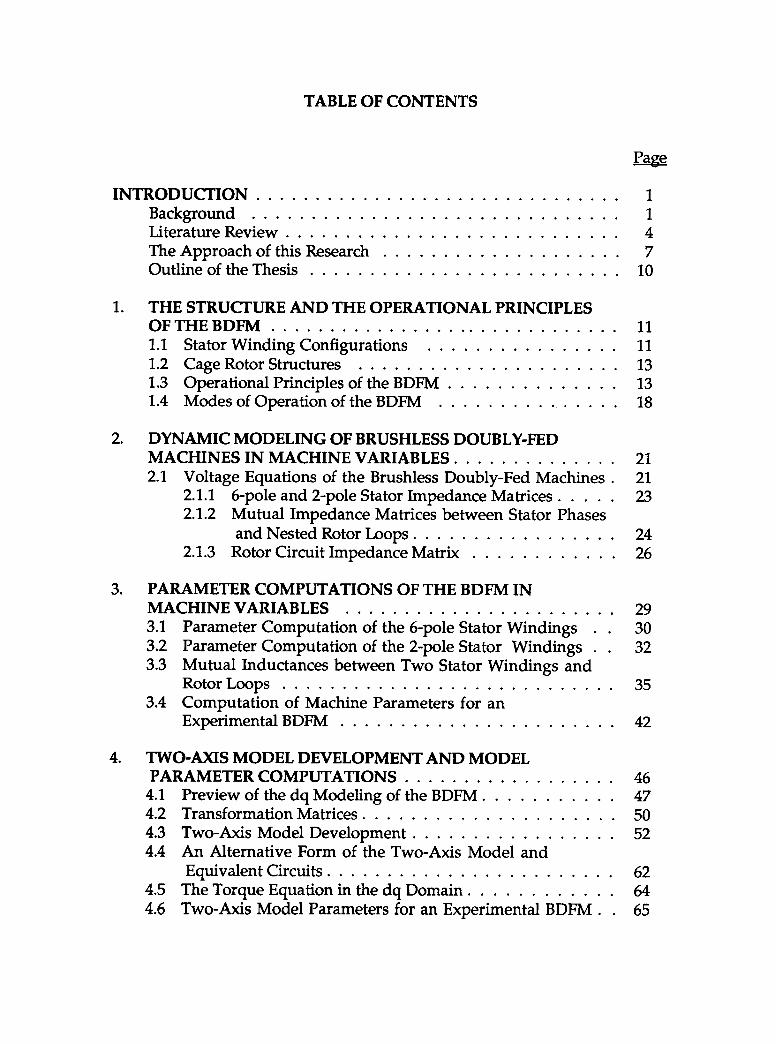
TABLE OF CONTENTS

Page

INTRODUCTION 1

Background 1

Literature Review 4The Approach of this Research 7Outline of the Thesis 10

1. THE STRUCTURE AND THE OPERATIONAL PRINCIPLESOF THE BDFM 111.1 Stator Winding Configurations 111.2 Cage Rotor Structures 131.3 Operational Principles of the BDFM 131.4 Modes of Operation of the BDFM 18

2. DYNAMIC MODELING OF BRUSHLESS DOUBLY-FEDMACHINES IN MACHINE VARIABLES 212.1 Voltage Equations of the Brush less Doubly-Fed Machines 21

2.1.1 6-pole and 2-pole Stator Impedance Matrices 232.1.2 Mutual Impedance Matrices between Stator Phases

and Nested Rotor Loops 242.1.3 Rotor Circuit Impedance Matrix 26

3. PARAMETER COMPUTATIONS OF THE BDFM INMACHINE VARIABLES 293.1 Parameter Computation of the 6-pole Stator Windings . 303.2 Parameter Computation of the 2-pole Stator Windings . 323.3 Mutual Inductances between Two Stator Windings and

Rotor Loops 353.4 Computation of Machine Parameters for an

Experimental BDFM 42

4. TWO-AXIS MODEL DEVELOPMENT AND MODELPARAMETER COMPUTATIONS 46

4.1 Preview of the dq Modeling of the BDFM 474.2 Transformation Matrices 504.3 Two-Axis Model Development 524.4 An Alternative Form of the Two-Axis Model and

Equivalent Circuits 624.5 The Torque Equation in the dq Domain 644.6 Two-Axis Model Parameters for an Experimental BDFM . 65

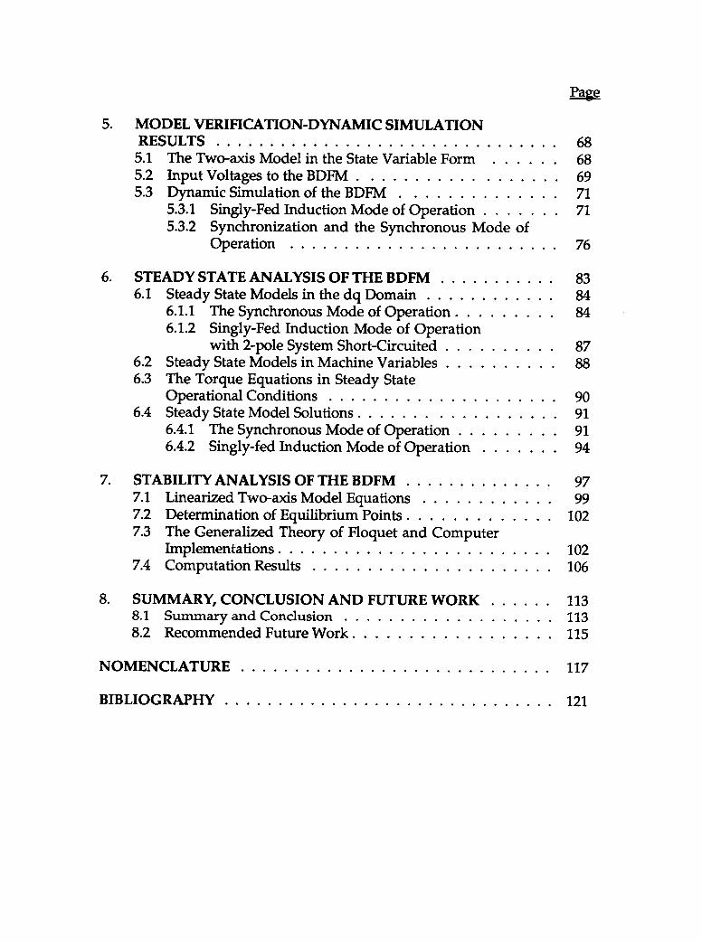
Page

5. MODEL VERIFICATION-DYNAMIC SIMULATIONRESULTS 68

5.1 The Two-axis Model in the State Variable Form 685.2 Input Voltages to the BDFM 695.3 Dynamic Simulation of the BDFM 71

5.3.1 Singly-Fed Induction Mode of Operation 715.3.2 Synchronization and the Synchronous Mode of

Operation 76

6. STEADY STATE ANALYSIS OF THE BDFM 836.1 Steady State Models in the dq Domain 84

6.1.1 The Synchronous Mode of Operation 846.1.2 Singly-Fed Induction Mode of Operation

with 2-pole System Short-Circuited 876.2 Steady State Models in Machine Variables 886.3 The Torque Equations in Steady State

Operational Conditions 906.4 Steady State Model Solutions 91

6.4.1 The Synchronous Mode of Operation 916.4.2 Singly-fed Induction Mode of Operation 94

7. STABILITY ANALYSIS OF THE BDFM 977.1 Linearized Two-axis Model Equations 997.2 Determination of Equilibrium Points 1027.3 The Generalized Theory of Floquet and Computer

Implementations 1027.4 Computation Results 106

8. SUMMARY, CONCLUSION AND FUTURE WORK 1138.1 Summary and Conclusion 1138.2 Recommended Future Work 115

NOMENCLATURE 117

BIBLIOGRAPHY 121

LIST OF FIGURES

Figure Page

a(i) Conventional induction motor drive 2(unidirectional converter at full rating)

(ii) Brush less doubly-fed drive 2(bi-directional converter at fractional rating)

1-1 Stator and rotor configurations of the 6- and 2-pole BDFM . 12

1-2(a) Coil groups and equivalent 6- and 2-pole phases 15

1-2(b) Coil groups and equivalent 6- and 2-pole phases 16

1-2(c) Equivalent 6- and 2-pole phases 16

1-3 Single coil, coil group and 6-pole A-phaseMMF distribution 17

1-4 Single coil, coil group and 2-pole a-phaseMMF distribution 17

2-1 Idealized BDFM 6-pole system 22

2-2 Idealized BDFM 2-pole system 22

2-3 Cage rotor structures of the BDFM 28

2-4 Mesh loop circuit model of the cage rotor of the BDFM . 28

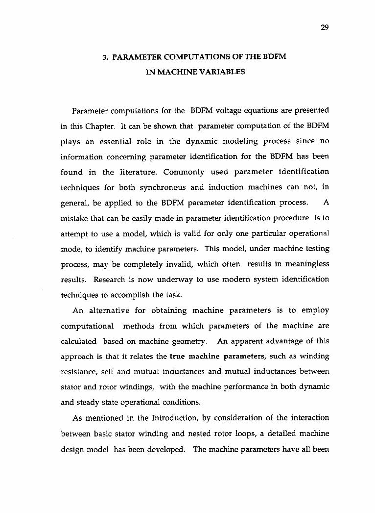
3-1 Equivalent 6-pole phases in terms of 9 coil groups 31

3-2 Equivalent 2-pole phases in terms of 9 coil groups 33

3-3 Mutuals between single stator coil and nested rotor loops 36

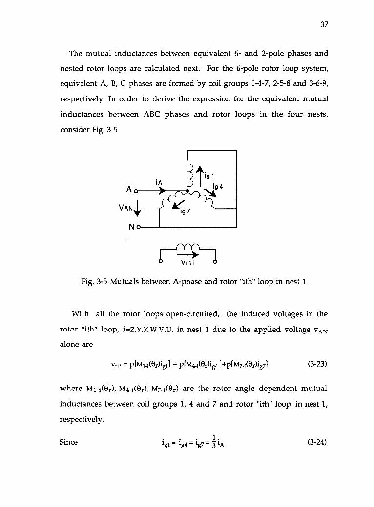
3-4 Mutuals between coil group and nested rotor loops 36

3-5 Mutuals between A-phase and rotor "ith" loop in nest 1 . 37

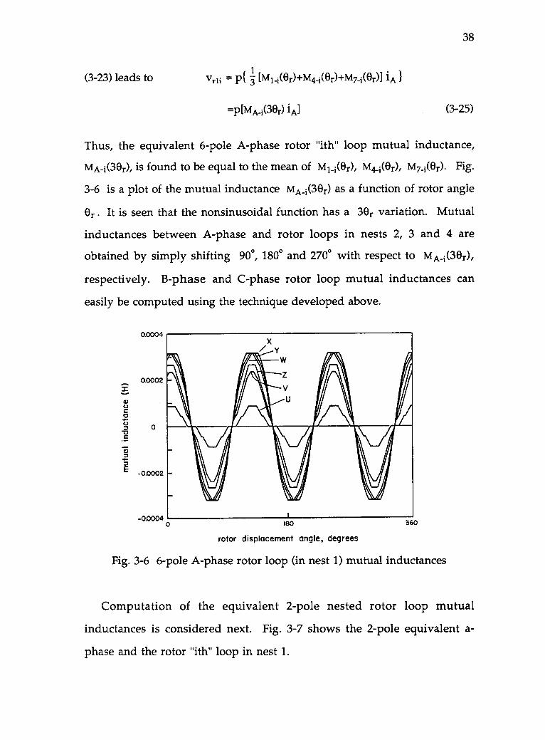
3-6 6-pole A-phase rotor loop (in nest 1) mutual inductances 38

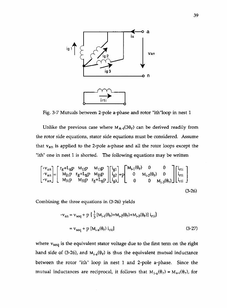
3-7 Mutuals between 2-pole a-phase and rotor "ith" loopin nest 1 39

3-8 2-pole a-phase rotor loop (in nest 1) mutual inductances . . 40

Figure Page

3-9 Harmonic analysis of nonsinusoidal mutual inductancesbetween 6-pole winding and rotor loops 41

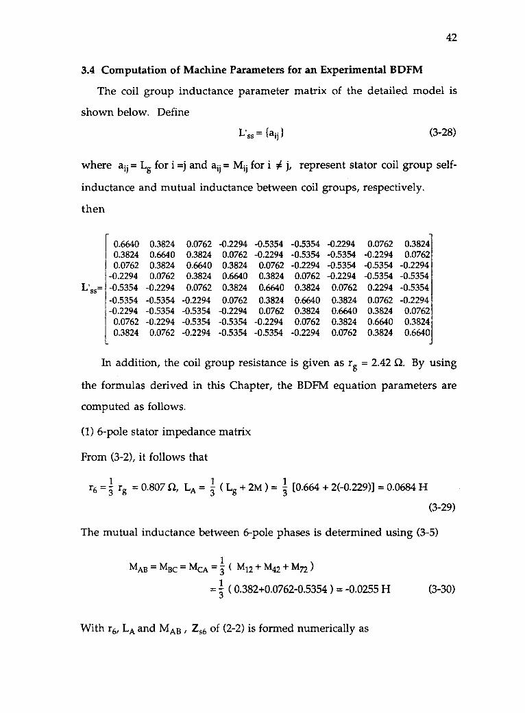
3-10 Harmonic analysis of nonsinusoidal mutual inductancesbetween 2-pole winding and rotor loops 41

4-1 The BDFM rotor loops represented in d-q domain 48

4-2 The 6- and 2-pole BDFM in the d-q domain 49

4-3 Two-axis model equivalent circuit of the BDFM 63

5-1 Run-up q-axis currents and rotor speed 73(a) 6-pole io(b) 2-pole iq2(c) rotor iqr

(d) rotor speed cor

5-2 Predicted and measured 6- and 2-pole line currents 75(a) Predicted 6-pole line current (b) Measured 6-pole line current(c) Predicted 2-pole line current (d) Measured 2-pole line current

5-3 Free acceleration torque-speed characteristics 77(a) 6- and 2-pole torques, Te6 and Tee(b) Total torque Te =Te6+Te2

5-4 DC synchronization simulation 79(a) Speed vs time (b) 2-pole current is

5-5 Synchronous behavior of the BDFM 82(a) 6- and 2-pole torques(b) Total torque and load torque(c) Rotor speed

6-1 Steady state equivalent circuit for synchronous operation . . 86(a) ac excitation on the 2-pole system(b) dc excitation on the 2-pole system

6-2 13 angle vs speed co, for Ti_ = constant and V/Hz = 5.0 96

6-3 Singly-fed induction mode torque speed characteristics . . . 96

Figure Page

7-1 Computer implementation of the theory of Floquet 107

7-2 Real parts of dominate eigenvalues vs 2-poleexcitation frequency f 2 109

7-3 Experimental stability envelopes 110(a) Current control(b) Voltage control

7-4 Steady state operational characteristics 112(a) 6-pole and 2-pole line currents vs 2-pole excitation voltage(b) 2-pole phase angle vs 2-pole excitation voltage

LIST OF TABLES

Table Page

I Operation modes of the BDFM in steady state conditions . . . 20

II Magnitudes of mutual inductances between 6- and 2-polestator phases and rotor loops 44

III Loop resistances, self inductances and mutual inductancesbetween similar loops in different nests 44

DYNAMIC MODELING, SIMULATION AND STABILITY ANALYSIS OF

BRUSHLESS DOUBLY-FED MACHINES

INTRODUCTION

Background

The concept of using a self-cascaded induction machine in conjunction

with a bi-directional power electronic converter as an adjustable speed

drive (ASD) or variable speed generator (VSG) has recently been proposed

at Oregon State University [1,2]. It is based on the research effects of several

years related to ASD and VSG applications. By utilization of a self-cascaded

induction machine, which is now referred to as a brushless doubly-fed

machine or BDFM, operated in its doubly-fed version the slip rings of a

commonly used doubly-fed wound rotor ASD or VSG system can be

eliminated while a much lower rating power electronic converter can still

be used.

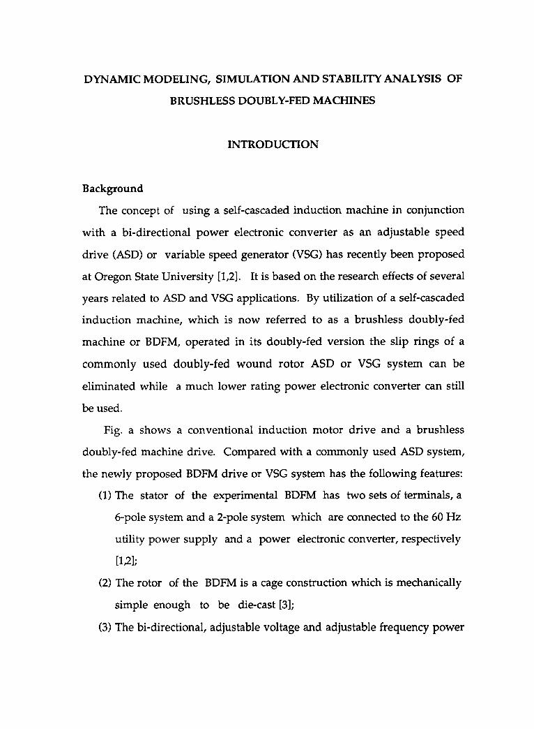
Fig. a shows a conventional induction motor drive and a brushless

doubly-fed machine drive. Compared with a commonly used ASD system,

the newly proposed BDFM drive or VSG system has the following features:

(1) The stator of the experimental BDFM has two sets of terminals, a

6-pole system and a 2-pole system which are connected to the 60 Hz

utility power supply and a power electronic converter, respectively

[1,2];

(2) The rotor of the BDFM is a cage construction which is mechanically

simple enough to be die-cast [3];

(3) The bi-directional, adjustable voltage and adjustable frequency power

2

converter used in the experimental drive is a series resonant con-

verter capable of four quadrant operation. The immediate advan-

tages of the BDFM system are:

(a) Lower cost of machine compared with that of a wound rotor induc-

tion machine;

(b) Lower cost of power converter compared with that of a conventional

induction motor or synchronous motor ASD or VSG systems;

(c) Lower harmonic pollution to the power systems.

POWER SOURCE

fp ...,5-3- phase, 60 Hz

I.

CONVENTIONALCONVERTER(115% rating)

fc3-phase

,_-sadjustable(1 v frequency

O

POWER SOURCE

3-phase, 60 Hz

I,Pp

CONVENTIONALCONVERTER

( 25% rating)

Pc4

3-phaseadjustable

A-5 frequency

CONVENTIONAL 3- PHASE,CAGE-ROTOR, INDUCTION MOTOR DUAL-POLE STATOR,

NESTED-CAGE ROTOR MOTOR

Fig. a(i) Conventional induction motor drive

(unidirectional converter at full rating)

(ii) Brushless doubly-fed drive

(bi-directional converter at fractional rating)

3

Based on the available information in the literature, prototype BDFM's

have been designed and built with a 6-pole and 2-pole structure. However,

laboratory tests showed that although providing insight into the

operational principles, the prototype machines did not achieve the desired

performance in both steady state and dynamic situations which is required

of a practical ASD or VSG system. The performance of the machine can be

significantly improved in terms of efficiency, torque production and

other aspects through stator and rotor redesign. Research was thus planned

for improving the machine performance and it was decided to address the

following aspects

(1) Modeling and analysis of the BDFM, which include

a) Detailed machine design modeling for computer aided design;

b) Dynamic modeling (or d-q modeling) and analysis of the BDFM

for dynamic, stability and control studies;

c) Equivalent circuit modeling for steady state performance and

machine design studies;

d) Machine electromagnetic field analysis;

e) Parameter identification of the machine using modern system

identification techniques;

(2) Practical application studies, which include

a) VSG of the BDFM system for car generator application;

b) Linear BDFM for electrical railroad vehicles.

(3) Potential market studies

This thesis discusses mainly the study of dynamic and steady state

modeling and analysis of the BDFM based on previous investigations of

the machine modeling and design.

4

Literature Review

The earliest means of achieving speed control of induction motors was

by use of external resistors. In order to use external resistors, wound rotor

induction motors had to be utilized. To avoid the use of slip rings,

researchers were looking for other alternatives. In 1893 and 1894,

Steinmetz of U.S.A. and Gorges of Germany independently filed two

patents to claim a new way of achieving speed control through cascade

connection of two induction motors. Later, there were several attempts to

develop a 'single unit' cascade induction motor to reduce the cost and

improve machine performance. It was first shown by Hunt in 1907 [4] that

cascading of two induction motors for the purpose of speed control could

be incorporated in one machine frame through ingenious stator and rotor

winding design.

Creedy [5] made significant improvements on self-cascade induction

motors by designing more effective stator and rotor windings. He proposed

a 6 and 2-pole machine on which the original stator of the lab machine at

OSU was based. Creedy also developed a logic for effective rotor

configuration design.

No additional machine design was reported until in the early 1970's

when notable rotor design progress was achieved by Broadway [3]. The so-

called "Broadway rotor" is a cage structure which resembles closely that of a

conventional induction motor. The advantages of the cage rotor lie in its

simplicity, ruggedness and ease of manufacture. While pursing the design

of the machine for low speed motor and high speed generator applications,

Broadway also developed steady state equivalent circuits for induction and

synchronous modes of operation from the basic assumption that the

5

machine is equivalent to two induction motors connected on a common

shaft. He claimed that the parameters used for the steady state models were

based on computations using well established formulas. However, no

information concerning this can be extracted from the publications [3]. In

the synchronous mode of operation, Broadway restricted himself to dc

excitation on the control winding, hence, he could not achieve wide range

of speed control when the machine was running as a doubly-fed

synchronous motor.

Synchronous behavior of the self-cascaded induction motors over wide

speed ranges was studied by Smith in 1967 [6]. Starting from two separate

induction motors, Smith obtained a simple equivalent circuit with which

he investigated the synchronous operation of the system in steady state

conditions.

Kusko [7] and Shibata [8] investigated the use of a power electronic

converter to extract the slip power of this type of machine in both

induction and synchronous modes of operation. The equivalent circuits

used for this analysis were essentially the same as those by early

researchers.

In the synchronous mode of operation, stability problems may arise

when control over a wide speed range is required. The problem was

studied by Cook and Smith using a linearized model based on two wound

rotor induction motors [9]. The effects of parameter variation on the

dynamic performance of the machine is discussed in [10]. It was shown

that although unstable operation could occur in some speed ranges, simple

feedback schemes could be used to stabilize the machine in the unstable

regions.

6

A common feature of all the above analytical and experimental work is

its basis on the assumption that the machine is equivalent to two

magnetically separated wound rotor motors of different pole numbers

electrically connected and mounted on a common shaft. Although this

approach is appropriate for conceptual understanding of the operation

principles of the BDFM, it is not adequate for detailed machine and drive

system design.

Moreover, most published work is limited to steady state performance

analyses. Dynamic characteristics, such as machine run-up, synchroni-

zation, machine response to sudden change of load torque and many

others have not been addressed.

More recently, Wallace et al have developed a detailed machine design

model to investigate the machine performance under all operating

conditions [11]. The model was developed by considerations of basic stator

coils and nested rotor loops and the interaction between them. By the use

of modern digital computers, the model has been used to investigate the

dynamic performance of the machine by providing time domain solutions

to every stator coil group and rotor loop currents, electromagnetic torque as

well as shaft position and speed [12]. The simulation model has also been

successfully employed to investigate the stator and rotor design based on

steady state performance evaluations.

In [13,15], stator winding design is considered by means of variation of

coil span, distribution of windings, alternative coil-group connections and

adoption of isolated windings. The study concludes that the isolated

winding option for the two stator systems gives a better overall

performance for two given operational conditions at constant load torque.

7

The design of more effective rotor configurations is discussed in [14,15].

The best alternative for the rotor structure is selected in such a way that for

each option the torque contribution from each individual short circuited

loop is computed and the overall machine efficiency is evaluated for two

given control frequencies. Based on the computer simulation results,for

the most promising of its rotor structures examined, the machine efficiency

is increased, on the average, by more than ten percent for the two given

control frequencies compared with the basic Broadway design.

In addition to utilizing the detailed model for machine design,

electromagnetic field analysis has also been carried out by Alexander [16],

which, to a large extent, enhances the understanding by providing

fundamental insight into the operation of the BDFM. The study also

provides information about how to design the machine more effectively.

The Approach of this Research

In this thesis, a simplified dynamic model is developed and used to

perform dynamic simulation in both induction and synchronous modes of

operation [17].

Conventional approaches consider the BDFM as two magnetically

separated wound rotor induction machines connected electrically on the

rotors. This enables well established induction motor d-q models to be

applied directly to perform d-q analysis. Unlike these previous approaches,

the d-q model described here is obtained from the direct mathematical

transformation of the detailed machine design model. Since the detailed

machine design model, under certain assumptions, is a true mathematical

representation of the BDFM the simplified model must also be valid for

describing the dynamic behavior of the machine with specified accuracies.

8

The reason for adopting this approach is based on the argument that

although the BDFM is electrically equivalent to two wound rotor induction

machines in cascade connection, in practice there exists in the single-frame

machine only one rotor capable of providing coupling to both stator

systems. The development of the Broadway rotor makes it even more

difficult, if not impossible, to separate physically the cage structure to obtain

the two equivalent three phase windings and their parameters. Therefore,

for cage rotor BDFM, it is appropriate to work from the original physical

configuration of the machine to develop analytical tools.

As will be shown in the next Chapter, the BDFM under consideration

possesses a much more complex winding structure than those of most

other AC electric machines. Hence, the performance equations for

describing the behavior of the machine are much higher in order than

those of other machines. For the detailed representation of the BDFM, it

has been shown that the machine is represented by a set of 35th order

nonlinear differential equations in machine variables. To transform these

equations into a two-axis model, which is the minimum order dynamic

representation of the BDFM, will undoubtedly provide an ultimate

challenge. In addition, the necessity for obtaining the model parameters

from the detailed model through a rigorous computational process adds

even more complexity.

The main advantage of the modeling approach lies in the fact that it

allows for not only the investigation of the dynamic behavior of the

machine but also the computation of the machine parameters from

machine geometry and the d-q model parameters from the rules of the

transformation process. This is believed to be essential in the present

9

situation when parameter identification techniques for the BDFM are still

being developed.

The development of the two-axis model results in a substantial order

reduction compared with that of the detailed model. Thus, it can be used

for development of control strategies for the BDFM as a possible

alternative drive system.

The two-axis model has been used to perform dynamic simulation

studies and the results are compared with the available test data [18].

Dynamic simulations performed include machine run-up in induction

mode, dc and ac synchronization and synchronous behavior of the

machine.

Steady state equivalent circuits for different modes of operation have

also been derived from the two-axis representation. These steady state

models, although derived using simplifying assumptions, can be shown to

represent the fundamental nature and the basic operational principles of

the BDFM and have thus improved upon the traditionally used equivalent

circuits [3,6,7,8] by providing for all possible modes of operation. A

method for solving the steady state equations in synchronous mode of

operation for ASD applications of the system is developed and used to

carry out steady state performance analysis.

Stability analysis of the BDFM under the synchronous mode of

operation is also carried out using the linearized version of the two-axis

model [19]. The analysis is based on the Lyapunov's indirect method in

which the original nonlinear two-axis model is linearized around some

equilibrium point. Since the two-axis model has to be expressed

exclusively in the rotor reference frame, the resultant linearized system is

10

found to be time-varying and commonly used eigenvalue analysis cannot

be performed directly. A new method is thus proposed in which

eigenvalue analysis is carried out based on a transformed linear time-

invariant model using the generalized theory of Floquet. The theoretical

analysis is correlated with test data and predictions given by the original

nonlinear two-axis model.

Outline of the Thesis

Following the Introduction, the basic structure and operational

principles of the BDFM are discussed in Chapter 1. In Chapter 2, the

dynamic equations of the BDFM in machine variables are derived followed

by the machine parameter computation in Chapter 3. In Chapter 4, a two-

axis model and its parameters are developed and computed. Dynamic

simulation of the BDFM is presented in Chapter 5 and steady state models

and performance analyses are given in both the induction and the

synchronous modes of operation in Chapter 6. Chapter 7 discusses the

stability analysis of the BDFM under the synchronous mode of operation.

11

1. THE STRUCTURE AND THE OPERATIONAL

PRINCIPLES OF THE BDFM

In this chapter, the basic structure of the BDFM is described in detail,

followed by a discussion of the operational principles of the BDFM.

1.1 Stator Winding Configurations

The basic structure of the stator windings, due to the work by Hunt and

Creedy, can have two notable forms: a common winding structure and a

separate (or isolated) winding structure [15]. The first OSU laboratory

prototype was constructed based on the former and the second on the latter.

Since this research work was begun when the first machine was in use, the

entire analyses of the machine started by consideration of the common

winding option. It will be shown later that under certain assumptions

these two forms of winding structure are functionally identical. However,

it is noted that it is much easier to analyze the isolated winding

configuration than the common winding case.

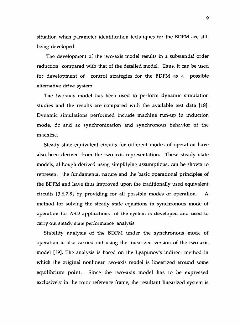
Fig. 1-1 shows the basic stator and rotor configurations of the 6-pole and

2-pole experimental BDFM under consideration. The machine has a

double layer winding in 36 stator slots. 36 individual coils are connected

into 9 coil groups, which, in turn, are arranged in three Y-connected sets.

These coils groups can be considered as being positioned at 0°, 40° and 80°

degrees from a reference axis. Two independent three phase supplies

representing the 60Hz utility grid and the output of an adjustable voltage,

adjustable frequency power converter are applied to the six terminals,

namely A,B,C and a,b,c, respectively. The distribution and interconnection

of the coil groups are such that balanced three phase currents flowing from

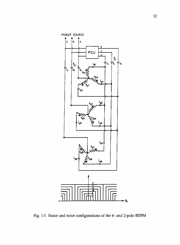
12

POWER SOURCEt

zYxwV

ft er

Fig. 1-1 Stator and rotor configurations of the 6- and 2-pole BDFM

13

the grid produce an airgap field of 6-poles, whereas currents supplied by the

power electronic converter produce an airgap field of 2-poles.

The purpose of two sets of stator winding configuration described above

is to avoid the use of slip rings that would be necessary for either cascade

connection of two individual induction motors or a conventional doubly-

fed generator or motor. Thus, slip-power recovery can be realized in

normal operational conditions through one set of stator windings.

From the design point of view, the advantage of the common winding

scheme has the feature of increasing usage of stator slot space. On the other

hand, however, due to the connection constraints, circulating currents

result because of inherent winding unbalances [16].

1.2 Cage Rotor Structures

In order to support the two airgap rotating fields of different pole

numbers produced by the stator windings, a special rotor structure is

required. In his original work, Hunt developed a wound rotor structure.

Due to the work by Creedy and Broadway [5,3], the rotor has become

mechanically simple enough to be die-cast. For the experimental

prototype, there are four nests, N1, N2, N3, N4 , made up of the cage bars,

also denoted as the z loop. Within each nest there are five short-circuited

loops, Y, x, W, V, U. This structure satisfies the requirement that the

minimum number of cage bars must be equal to the mean of the two

stator pole numbers.

1.3 Operational Principles of the BDFM

Since the BDFM is essentially composed of two induction motors in

cascade connection, its characteristics should resemble those of

conventional induction motors. However, the presence of two stator fields

14

rotating at two different speeds and their corresponding rotor fields make

the machine analysis more complicated than either induction or

synchronous machines in both steady state and dynamic conditions.

In doubly-fed operation, the two stator rotating fields are caused by the

two independent sets of excitation voltages applied to the two stator

winding systems. Ideally, these systems should be independent of one

another because they compose different pole numbers. However, in

practice they are slightly coupled through unbalances and harmonics in

addition to their fundamental interaction via the rotor circuits.

Nevertheless, throughout the thesis, it is assumed that the direct coupling

between the two stator systems is negligible. As a result of this assumption,

the original 9 coil group stator windings can be regarded as being two

independent 3-4) windings namely ABC for the 6-pole and abc for the 2-

pole. The two independent three phase windings are obtained as follows:

When energized from the 6-pole or ABC side, the machine presents a

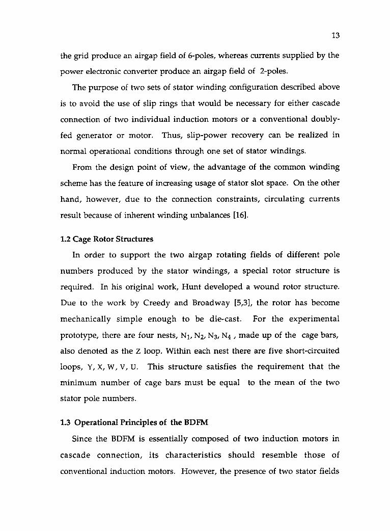
short circuit from the 2-pole or abc side as shown in Fig. 1-2(a). It can be

seen that the equivalent A, B and C phases are composed of coil groups 1 -4-

7, 2-5-8 and 3-6-9, respectively. On the other hand, when the 2-pole or abc

side is subject to an applied voltage, no current should be seen flowing out

from the 6-pole or ABC side to the power supply. When the 6-pole or ABC

side is short circuited, the equivalent a, b and c phases are formed. The a-

phase is composed of coil groups 1-2-3, b-phase, coil groups 4-5-6 and c-

phase coil groups 7-8-9. The results are also shown in Fig. 1-2(a). The two

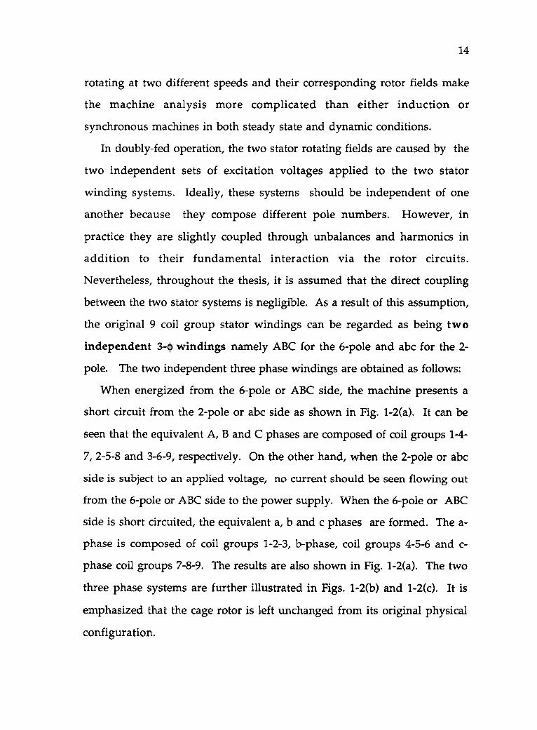
three phase systems are further illustrated in Figs. 1-2(b) and 1-2(c). It is

emphasized that the cage rotor is left unchanged from its original physical

configuration.

15

8

Fig. 1-2(a) Coil groups and equivalent 6- and 2-pole phases

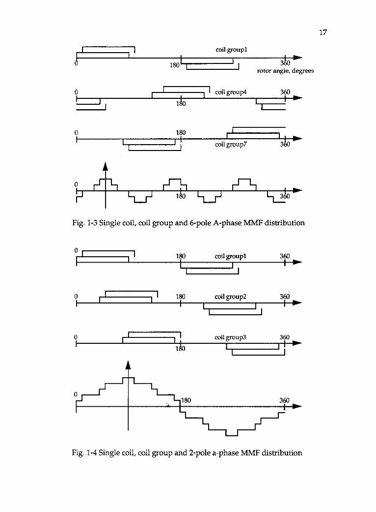
As stated previously, the 6-pole A-phase consists of coil groups 1-4-7 each

of which is, in turn, composed of four single coils positioned in proper

stator slots and connected in series. Fig. 1-3 shows the 6-pole A-phase

spatial MMF distribution as a result of the superposition of single coil and

coil group MMF distribution. It can be seen that the 6-pole A-phase MMF

is distributed spatially with a 38, variation, where Or is the rotor angle in

mechanical degrees.

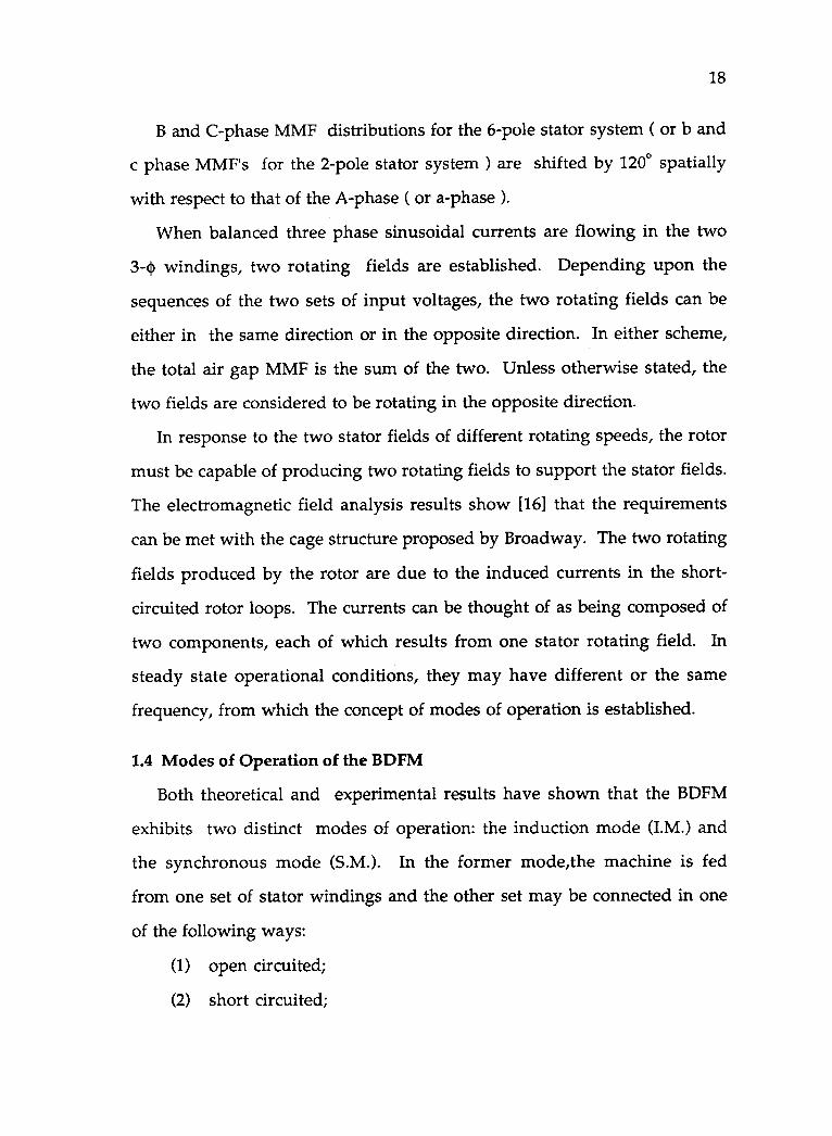
The 2-pole a-phase MMF is shown in Fig. 1-4 which results from

currents flowing in the equivalent 2-pole a-phase winding. Since the

winding is formed by coil groups 1-2-3 that have positive mutual coupling

between them, the resultant MMF magnitude is much higher than that of

the 6-pole A-phase. Within 0° to 360°, the MMF has one cycle of variation.

refaxis

refaxis

Fig. 1-2(b) Coil groups and equivalent 6- and 2-pole phases

6-pole system

16

2-pole system

Fig. 1-2(c) Equivalent 6- and 2-pole phases

17

I coil groupl

0I

180I

1.10

I coil group4

360rotor angle, degrees

360

Lr-- Po

0 180I I

Icoil group? 3

rr-1-1, r-1-1-1LIi-1 180 L-Li-J

Fig. 1-3 Single coil, coil group and 6-pole A-phase MMF distribution

0I 180 coil groupl 360

I

0 I 180 coil group2 360

I

0I

ori

ri

1

1coil group3 360

I0.1I

180 360

Fig. 1-4 Single coil, coil group and 2-pole a-phase MMF distribution

18

B and C-phase MMF distributions for the 6-pole stator system ( or b and

c phase MMF's for the 2-pole stator system ) are shifted by 120° spatially

with respect to that of the A-phase ( or a-phase ).

When balanced three phase sinusoidal currents are flowing in the two

3-0 windings, two rotating fields are established. Depending upon the

sequences of the two sets of input voltages, the two rotating fields can be

either in the same direction or in the opposite direction. In either scheme,

the total air gap MMF is the sum of the two. Unless otherwise stated, the

two fields are considered to be rotating in the opposite direction.

In response to the two stator fields of different rotating speeds, the rotor

must be capable of producing two rotating fields to support the stator fields.

The electromagnetic field analysis results show [16] that the requirements

can be met with the cage structure proposed by Broadway. The two rotating

fields produced by the rotor are due to the induced currents in the short-

circuited rotor loops. The currents can be thought of as being composed of

two components, each of which results from one stator rotating field. In

steady state operational conditions, they may have different or the same

frequency, from which the concept of modes of operation is established.

1.4 Modes of Operation of the BDFM

Both theoretical and experimental results have shown that the BDFM

exhibits two distinct modes of operation: the induction mode (I.M.) and

the synchronous mode (S.M.). In the former mode,the machine is fed

from one set of stator windings and the other set may be connected in one

of the following ways:

(1) open circuited;

(2) short circuited;

19

(3) connected to a passive network to dispatch slip power and

perform speed control;

(4) connected to a power electronic converter to extract slip

power.

Except the first case where the machine behaves essentially like a 6-pole

induction motor, there are induced three phase currents in the unexcited

windings which act upon the system to produce unusual effects. In the

early stage of development of the system, speed control of self-cascaded

induction motors was by means of the third method of winding

connections since sources with variable frequency and voltage were not

readily available at the time of Hunt and Creedy. Today, with the state-of-

the-art power electronic converters, although this mode of operation is not

a major means of achieving speed control, it is found to be an intermediate

mode of operation through which a more preferable mode can be achieved.

Similar to the induction motor torque speed characteristics, the shaft speed

in this mode of operation is dependent on the load conditions.

The induction mode of operation ( also referred to as asynchronous

mode ) may also take place when the BDFM is doubly-fed. The

fundamental difference between the singly-fed induction mode and

doubly-fed induction mode is that in the former the rotor currents have

only one frequency while in the latter two frequencies co-exist. In the case

where the two fields are in the opposite direction of rotation, this mode of

operation was found to cause power losses, pulsating torques and

fluctuating speeds. Thus, this mode of operation, under any normal

circumstances, should be avoided.

20

The synchronous mode of operation is established when the

frequencies of the rotor currents induced by the two counter-rotating fields

of the two stator systems become identical. In the synchronous mode of

operation, the two sets of stator windings are fed from isolated sources of

different frequencies. Like conventional synchronous machines, the

BDFM requires certain synchronization procedures [1]. Once synchronous

operation is established, the shaft speed of the machine is independent of

the load conditions unless a severe disturbance occurs. Compared with the

induction mode of operation, synchronous mode is highly preferred since

precise open loop speed control can easily be obtained. Table I summarizes

the different modes of operation for the experimental BDFM, which has 6-

pole and 2-pole stator winding sets and a Broadway rotor (cage rotor).

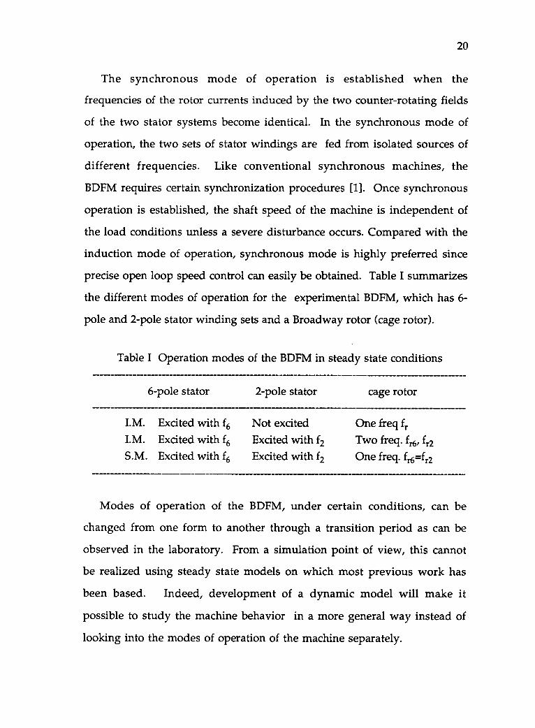
Table I Operation modes of the BDFM in steady state conditions

6-pole stator 2-pole stator cage rotor

I.M. Excited with f6 Not excited One freq frI.M. Excited with f6 Excited with f2 Two freq. fr6, fr2

S.M. Excited with f6 Excited with f2 One freq. 4.6'42

Modes of operation of the BDFM, under certain conditions, can be

changed from one form to another through a transition period as can be

observed in the laboratory. From a simulation point of view, this cannot

be realized using steady state models on which most previous work has

been based. Indeed, development of a dynamic model will make it

possible to study the machine behavior in a more general way instead of

looking into the modes of operation of the machine separately.

21

2. DYNAMIC MODELING OF BRUSHLESS DOUBLY-FED

MACHINES IN MACHINE VARIABLES

The voltage equations to be developed in this Chapter are modified

equations of the BDFM described in [11,12] in order that they can be

transformed into a two-axis model. In order to derive the voltage

equations for the Brush less Doubly-Fed machines, the following

assumptions are made.

(1) The magnetic and electric circuits are linear. Saturation is

neglected.

(2) Spatial harmonics, other than the third harmonic of the 2-pole

system which corresponds to the 6-pole system fundamental, are

negligible.

(3) Direct coupling between the 6-pole and the 2-pole systems is

negligible.

It is noticed that assumptions similar to (1) and (2) are usually made

when analysis of electric machinery is carried out in the two-axis reference

frame. The third assumption which has been made in the previous

Chapter is repeated again for completeness.

2.1 Voltage Equations of the Brushless Doubly-Fed Machines

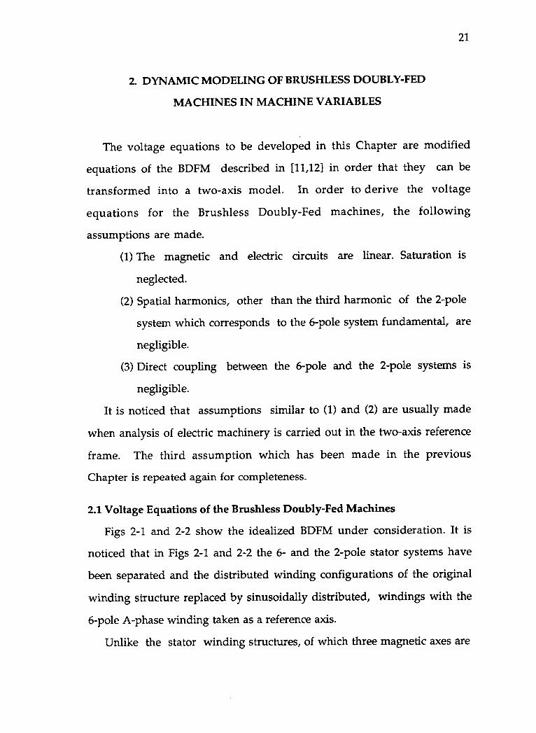
Figs 2-1 and 2-2 show the idealized BDFM under consideration. It is

noticed that in Figs 2-1 and 2-2 the 6- and the 2-pole stator systems have

been separated and the distributed winding configurations of the original

winding structure replaced by sinusoidally distributed, windings with the

6-pole A-phase winding taken as a reference axis.

Unlike the stator winding structures, of which three magnetic axes are

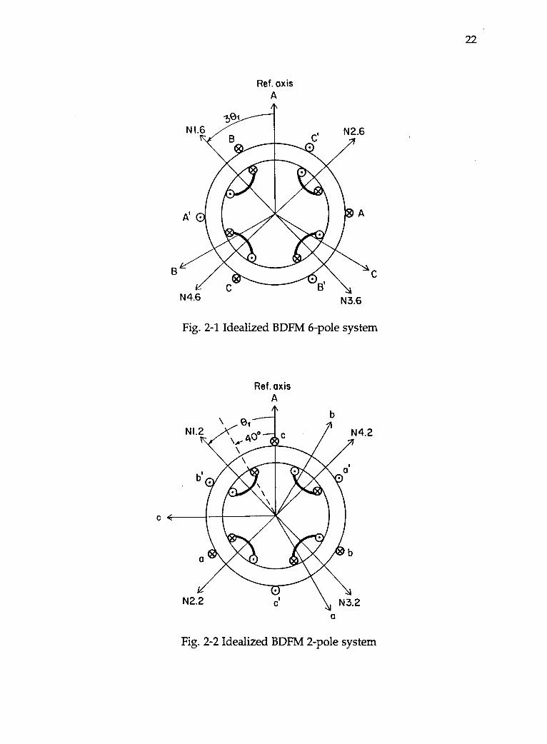
22

Ref. axisA

Fig. 2-1 Idealized BDFM 6-pole system

Ref. axisA

a

Fig. 2-2 Idealized BDFM 2-pole system

23

displaced 120° apart in space, the rotor winding is composed of short

circuited loops and four magnetic axes are 90° apart spatially. The rotor

displacement angle Or is defined as the angle between the reference axis A

and the axis of nest 1, N1.6. Note that in Fig. 2-1, the axis of nest 2, N2.6, is

lagging N1.6 by 90° spatially while in Fig. 2-2 N2.2 is leading N1.2 by 90°.

This is due to the fact that Or is expressed in mechanical degrees and for 6-

pole system 90° mechanical degrees corresponds to 270° electrical degrees.

Based on the two figures, the voltage equations in machine variables

can be expressed as

Zs6

0Vs21 = [ tV, Z s6r

0

1s2Zs2 Zs2r

Zts2r Zr it(2-1)

In the above matrix equations, the subscripts s6, s2 denote variables and

parameters associated with 6-pole (ABC) and 2-pole (abc) stator circuits and

subscript r denotes variables and parameters associated with the cage rotor

circuits. v56,vs2 represent 6- and 2-pole phase voltage vectors while vr

stands for the rotor loop voltage vector. Since all the rotor loops are short

circuited, vr = 0. Three current vectors, is6, is2 and it describe the 6 and 2-

pole phase currents and the rotor loop currents, respectively. Notice that

the mutual impedance matrices between the two independent stator

systems are zero. This results from the third assumption made at the

beginning of this Chapter. The parameter matrices Z56, ;2, Zs6r, Zs2r and Zr

are described in detail below.

2.1.1 6-pole and 2-pole Stator Impedance Matrices

The 6 and the 2-pole stator impedance matrices, denoted as Zs6, Zs2, are

constant 3 by 3 matrices defined by

24

and

Zs6 =

Zs2 =

[r6+LAp

MBAP

mcAp

[r2 +Lap

MbaPMcaP

MAB p

r6 +LApmcBP

Mabp

r2±LaPmcbP

MAC p

MBCPr6 +LAp

MacpMbcP

r2 +LaP

(2-2)

(2-3)

where r6 and r2 are the phase resistance of the 6-pole or the 2-pole system

winding. LA = LAm + L16 and La = Lam + L12 represent the phase self

inductances and LAm and Lam are the phase magnetizing inductances of the

6- and 2-pole systems, respectively. L16, L12 stand for the phase leakage

inductances. M's represent the mutual inductances between ABC or abc

phases.

Since the 9 coil groups form two balanced three phase systems, the

mutual inductances in each of the matrices are all equal. It is noted that

the impedance matrices of either 6 or 2-pole stator system in (2-2) or (2-3)

are similar to that of a conventional induction motor. Moreover,

sinusoidal distribution of stator windings of the two systems suggests that

MAB = - 0.5LAm Mab = -0.5Lam (2-4)

2.1.2 Mutual Impedance Matrices between Stator Phases and Nested

Rotor Loops

Zs6r and Zs2r designate the mutual impedance matrices between the

two sets of 3-4) stator windings and the nested rotor loops. Since there are

in total 24 rotor loops, Zs6r and Zs2r are 3 by 24 matrices, the entries of

which are dependent on the rotor position with respect to the stator

reference axis. Zs6r and Zs2r can be partitioned further as :

Zs6r = Ls6rZ Ls6rY Ls6rX Ls6rW Ls6rV Ls6rU

25

(2-5)

for the 6-pole system and rotor nested loop mutual impedance matrix and

Zs2r = p[ Ls2rz Ls2rY Ls2rX Ls2rW Ls2ry Ls2ru l (2-6)

for the 2-pole system and rotor nested loop mutual impedance matrix

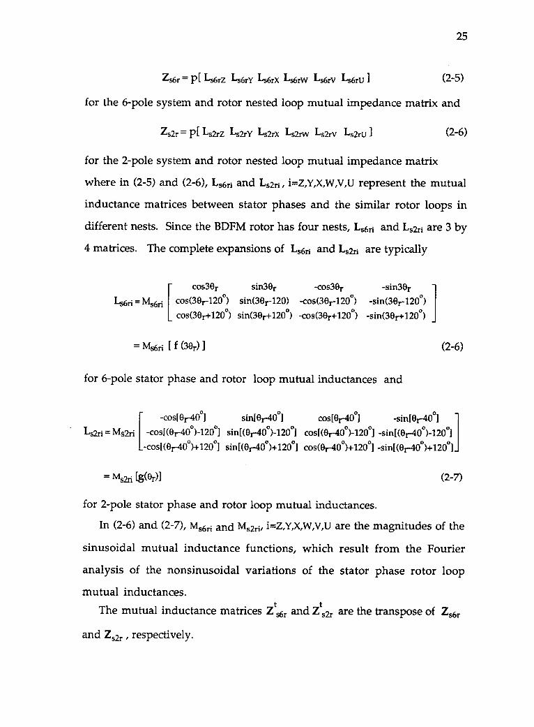
where in (2-5) and (2-6), Ls6ri and Ls2ri i=Z,Y,X,W,V,U represent the mutual

inductance matrices between stator phases and the similar rotor loops in

different nests. Since the BDFM rotor has four nests, Ls6ri and Ls2ri are 3 by

4 matrices. The complete expansions of Ls6ri and Ls2ri are typically

cos3Or sin3Or -cos3Or

[-sin3Or

Ls6ri = Ms6ri cos(3Or-120°) sin(30r-120) -cos(30r120°) -sin(39r-120°)

cos(30r+120°) sin(3Or+120°) -cos(39r+120°) -sin(3Or+120°)

= ms6ri [ f (30r) (2-6)

for 6-pole stator phase and rotor loop mutual inductances and

-cos[Or-400] sin[Or400] cos[Or400]

[-sin[Or-400]

Ls2ri = Ms2ri -cos[(0/-40°)-120) sin[(Or-40°)-120°) cos[(Or-40°)-120°] -sin[(Or-40°)-120°]

-cos[(0r-40°)+12001 sin[(Or-40°)+120°] cos(Or-40°)+120°] -sin[(Or-40°)+120°]

= ms2ri [sod] (2-7)

for 2-pole stator phase and rotor loop mutual inductances.

In (2-6) and (2-7), Ms6ri and Ms2ri, i=Z,Y,X,W,V,U are the magnitudes of the

sinusoidal mutual inductance functions, which result from the Fourier

analysis of the nonsinusoidal variations of the stator phase rotor loop

mutual inductances.

The mutual inductance matrices Zts6r and Z

ts2r are the transpose of Zs6r

and Zs2r respectively.

26

2.1.3 Rotor Circuit Impedance Matrix

Because its function is absolutely unique in electric machine operating

principles, the BDFM rotor has configurations that are not readily

analyzable by conventional means. It can be shown [11], however, that it is

appropriate to represent the cage rotor in terms of a series of coupled mesh

loop circuits as can be shown in Fig. 2-3 and Fig. 2-4, in which only three

out of six loops in each nest are shown.

It is seen from Fig. 2-4 that each rotor loop has a resistance and self

inductance and there exists mutual inductance between loops in the same

nest. In addition, there is also mutual inductance between adjacent nests.

Since the rotor loops are all short circuited at the common endrings, there

is also common endring resistance. Taking all the rotor loops into account,

we can express the rotor impedance matrix as a 24 by 24 matrix, which is

described in detailed in [11,12]. In order to develop the two-axis model in

Chapter 4, the rotor impedance matrix needs to be rearranged from its

original structure. Denoting the rotor impedance matrix as Zr which can

be concisely expressed by the following expression

Zr = ( Zij ) (2-8)

where i and j are rotor loop indentifiers, i.e. i, j= Z,Y,X,W,V,U.

It should be noted that in (2-8) each element of Zr, ; , is also a 4 by 4

symmetrical impedance matrix, each of which is defined as follows:

(1) for i=#z, i, j=Y,x,w,v,u

Zji =

rii +Liip -Miip -mlip -Miip- Map rii +Liip -Miip -Map

MiiI3 -MiiP rii +Liip 'mid)'mid) -map -miiP p rii +Liip

(2-9)

27

where rjj and Li; designate loop resistance and self inductance, respectively.

Mli represents the mutual inductance between the similar loops in different

nests, as is illustrated in Fig. 2-4.

Eqn. (2-9) describes five diagonal elements ( five loops ) in Zr .

(2) for i =j =Z

rzz+Lzzp -ezz-(L'zz+Mzz)p -mzzp -ezz-(L'zz+Mzz)P-ezz-(L'72+Mzz)P rzz+Lzzp -rizz-(Lezz+Mzz)P -Map

Zzz = (2-10)-ezz-(L'zz+M)p rzz+Lzzp -ezz-(Lizz+Mzz)p-rizz-(L'zz+Mzz)p -Mzzp -ezz-(Lizz+mzz)p rzz+1-,zzP

where rzz+Lzzp is the "Z" loop impedance and -(ezz+LizzP) is defined as the

common bar impedance.

This matrix describes the impedance of the outermost loop or cage, i.e.

the "z" loop matrix. It is noted that besides the loop resistance and self

inductance, the Z loop contains common bars which have been taken into

account.

(3) for i4j, i, j=Z,Y,X,W,V,U

=rii+mjp -M'ijp -NCR

rii+mijP- -

(2-11)

where rjj is the "mutual" resistance in one nest and NI ij expresses the

mutual inductance between loops in the same nests. M'jj represents the

mutual inductance between loops in different nests.

There are fifteen possible combinations of i, j. Thus, this matrix

presents 15 submatrices, i.e. the upper diagonal elements of Zr. Notice also

that Zji=Zij, for i4 which expresses another 15 submatrices, i.e. the lower

diagonal elements of Zr.

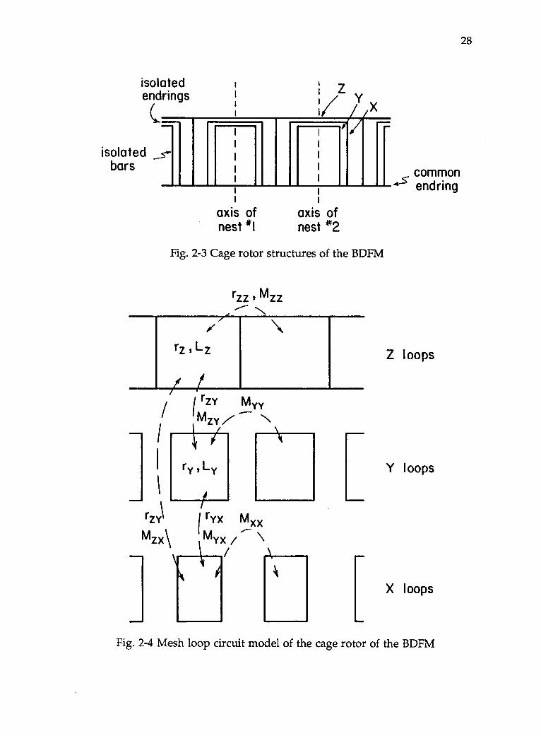
28

isolatedendrings

(...

isolated _511bars

axis ofnest *1

axis ofnest *2

Fig. 2-3 Cage rotor structures of the BDFM

rzz I Mzz.----- Nr/

rz 1 Lz

irZY Myy

MZY /

ir LY I Y

/1

r" MXXMYX /

/ \i k

11110

[

commonA-' endring

Z loops

Y loops

X loops

Fig. 2-4 Mesh loop circuit model of the cage rotor of the BDFM

29

3. PARAMETER COMPUTATIONS OF THE BDFM

IN MACHINE VARIABLES

Parameter computations for the BDFM voltage equations are presented

in this Chapter. It can be shown that parameter computation of the BDFM

plays an essential role in the dynamic modeling process since no

information concerning parameter identification for the BDFM has been

found in the literature. Commonly used parameter identification

techniques for both synchronous and induction machines can not, in

general, be applied to the BDFM parameter identification process. A

mistake that can be easily made in parameter identification procedure is to

attempt to use a model, which is valid for only one particular operational

mode, to identify machine parameters. This model, under machine testing

process, may be completely invalid, which often results in meaningless

results. Research is now underway to use modern system identification

techniques to accomplish the task.

An alternative for obtaining machine parameters is to employ

computational methods from which parameters of the machine are

calculated based on machine geometry. An apparent advantage of this

approach is that it relates the true machine parameters, such as winding

resistance, self and mutual inductances and mutual inductances between

stator and rotor windings, with the machine performance in both dynamic

and steady state operational conditions.

As mentioned in the Introduction, by consideration of the interaction

between basic stator winding and nested rotor loops, a detailed machine

design model has been developed. The machine parameters have all been

30

computed and assembled into four impedance matrices, namely the stator

impedance Z'ss, the stator-rotor mutual impedance matrix Z's the rotor-

stator impedance matrix Z' and finally the rotor impedance matrix Z'rr

[11,12]. Since the BDFM equation in machine variables described in this

thesis is a modified version of that given in [11,12], the parameter matrices

must also be modified accordingly.

It is the purpose of this Chapter to develop additional computational

techniques for evaluation of machine parameters for the modified BDFM

equation, which is more suitable for the development of the two-axis

model.

It is assumed that the four parameter matrices from the detailed model

Z'SS Zisr Zers , and Z'rr parameter matrices are given and it will be shown

that all the parameters in the BDFM Eqn. (2-1) can be calculated according

to the given information and later developed into the d-q model

parameters ( see Chapter 4 ).

3.1 Parameter Computation of the 6-pole Stator Windings

Previous work has been done to calculate the machine parameters at

the coil group level [11]. The equivalent 6- and 2-pole phase quantities can

be identified if the coil group impedance matrix is known. Fig. 3-1 shows

the equivalent 6- pole three phase ( ABC ) windings in term of the 9 coil

groups. When each of the 6-pole phases is energized independently, we

can write a series of equations to calculate the parameters. Since the 6-pole

system is completely balanced, only two quantities, the self impedance of

one phase and the mutual impedance between two phases, are needed to

be computed.

31

Fig. 3-1 Equivalent 6-pole phases in terms of 9 coil groups

Suppose that 6-pole A-phase is subject to an applied voltage VAN, we have

from Fig. 3-1VAN Mp MpVAN = Mp rg +Lgp Mp 1g4

VAN Mp Mp rg+Lgp 1g7

(3-1)

where (rg+Lgp) is the impedance of one coil group. M=M14=M1 7=M 47 is the

mutual inductance between coil groups 1, 4 and 7. Adding the three

equations together and also noting that iA= igi+ig4+ig, we get

vAN=51 Erg+(Lg+2m)p] iA = [r6 + (L16 + LAn., )/31 iA = ZA iA (3-2)

Thus, the equivalent per phase impedance is obtained. Comparing (3-1)

and (3-2), we also get1

1g1 = 1g4 = 1g7 = 3 A (3-3)

32

Equation (3-3) suggests that iA is distributed evenly in coil groups 1, 4 and 7.

The mutual inductance between the 6-pole phases is next computed.

The induced voltage in the B-phase due to the applied voltage VAN is

VBN = M12 P(ig1)+m42 P(lg4)+m72P(ig7) (3-4)

Using (3-3), we have

1

VBN 5 vvii2+-42-1-72/Pk = iviAsPkit;A, ( 3-5)

since MAB= MAC =MBC and the mutual inductances are reciprocal, the 6-pole

inductance matrix can been formed from the two calculated values. This

matrix together with coil resistance is assembled into the 6-pole impedance

matrix denoted by zs6 as has been given in (2-2).

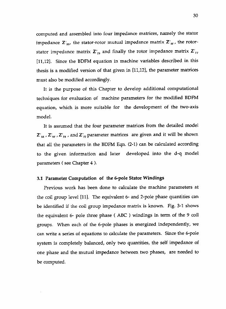
3.2 Parameter Computation of the 2-pole Stator Windings

Fig. 3-2 shows the equivalent abc phases in terms of 9 coil groups.

Suppose that 2-pole a-phase is energized alone. The following two

equations can be written

"Van rg+IIP M12P M13P 1g1

-van = M21P rg +Lgp M23P 1g2 (3-6)-Van_ M31P M32P rg+1-0 ig3

and is = igl+ig2±ig3 ) (3-7)

Since M12 = M23 , but M13 M12 Eqn. (3-6) can not be solved explicitly.

Therefore, an assumption as to how the current is distributed in the

windings has to be made. From the partial symmetry of the three

windings, it is known that igi=ig3. In the 2-pole impedance matrix

computations, it is assumed that the currents in the 1, 2 and 3 coil groups

are distributed in the following way

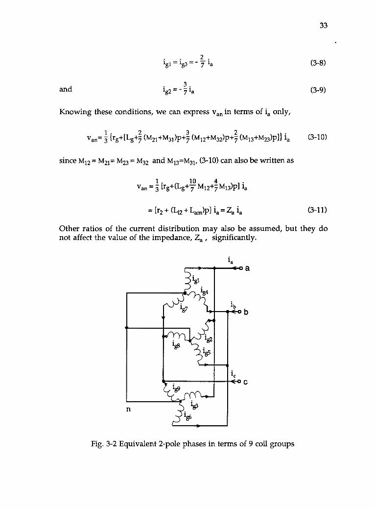
and

33

2igl = ig3 T. la (3-8)

3.ig2 7 la

Knowing these conditions, we can express van in terms of is only,

1 f 2 3 2Van= trg-I-LLg+ (M21+M31)P+ (M12-1-M32)P+ (M13+M23)P1} la

since M12 = M21= M23 = M32 and m13=m31, (3-10) can also be written as

1 10 4Van = 5 [rg +(Lg+ m12 l-M13)P1 la

= [r2 + (L12 + Lam)Pl is = Za is

(3-9)

(3-10)

(3-11)

Other ratios of the current distribution may also be assumed, but they donot affect the value of the impedance, Za , significantly.

gl

ig4

is< o a

ibCo b

n

IC 0 C

Fig. 3-2 Equivalent 2-pole phases in terms of 9 coil groups

34

The mutual inductance between abc phases can be computed by first

considering applying a voltage to a-phase and then calculating the induced

voltages on the b-phase. The following equations are derived

-Vbni =

-Vbn

and

M14P M24P M34P 1g1

M15 M25P M35P 1g2

M16P M26P M36P 1g3

(3-12)

la -( igl+ig2+ig3 ) (3-13)

Combining the three equations in (3-12) leads to

r,

-Vbn= 5 lkM14+M15+M16)P(ig1)+(M24+M25+M26)P( ig2)±(M34+M35+M36 )1)(ig3)1

Similarly, the induced voltage vcn due to the applied van is

M17P Ml8P M19PVcn = M27P M28P M29P ig2

Vcn M37P M38P M39P 1g3

or

(3-14)

(3-15)

1 rVcn= RM17+M18+M19)P( 1g1)+(M27+M28+M29)P(lg2)+(M37±M38+M39)P(lg3)]

(3-16)

vcn may also be expressed if the b-phase is subject to an applied voltage vbn

r,

Vcn= 1-1\447+M48+M49)P( ig4)+(M57+M5S+M59)P(ig5)+(M67+M684-M69)P(ig6)]

(3-17)

With any of the above equations, the mutual inductance among abc phases

could be obtained, provided that the phase current can be expressed in term

of coil group currents. Again, we assume that

and

or

and

35

2.iig1 = g3 = la (3-18)

3.Ig2= 7 la (3-19)

2.lg4 = Ig6= lb (3-20)

. 31g5 = lb (3-21)

for (3-17), the mutual expression is

Mab=Mac= Mbc= HrE20.417-Fmis+mi9)±3(m27÷m281-m29)+2(m37-fm38-1-m39)/ (3-22)

Similar to the formulation of the 6-pole stator impedance matrix Z56, Zs2 is

established as is given in (3-3).

3.3 Mutual Inductances between Two Stator Windings and Rotor Loops

Computation of rotor angle dependent mutual inductances between b-

and 2-pole stator system and nested rotor loops starts with consideration of

single stator coil and nested rotor loop mutual inductances which are

available from previous work [11]. The mutual inductances are computed

numerically using a modified subroutine program developed for the

detailed dynamic model.

Fig. 3-3 shows a plot of the mutual inductances between single coil 1

and 6 rotor loops in nest 1 as a function of rotor angle Or in mechanical

degrees. Obviously, mutual inductances between coil group 1, mcg(Or),

which is composed of four single coils positioned at 0°, 10°, 180° and 190°,

respectively, and the 6 rotor loops can be calculated by utilizing the internal

connection matrix C1 [11,12]. Since the four single coils are connected in

series, Mcg(8r) is simply the sum of the four mutual inductances at every

rotor angle 0° 5 Or 5 360° . The results are shown in Fig. 3-4. Other coil

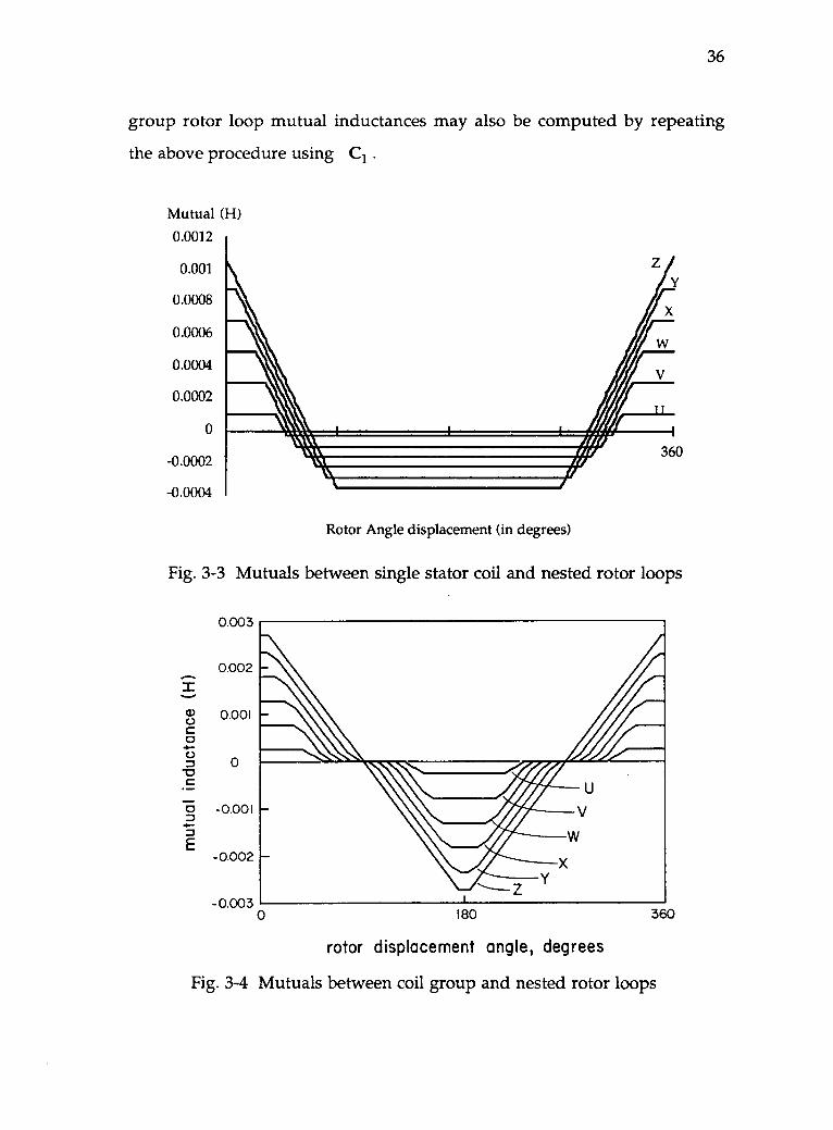
36

group rotor loop mutual inductances may also be computed by repeating

the above procedure using C1 .

Mutual (H)

0.0012

0.001

0.0008

0.0006

0.0004

0.0002

0.0002

0.0004

Rotor Angle displacement (in degrees)

Fig. 3-3 Mutuals between single stator coil and nested rotor loops

0.003

0.002I0.001

0

-0.001

-0.002

- 0.0030 180

rotor displacement angle, degrees

Fig. 3-4 Mutuals between coil group and nested rotor loops

360

37

The mutual inductances between equivalent 6- and 2-pole phases and

nested rotor loops are calculated next. For the 6-pole rotor loop system,

equivalent A, B, C phases are formed by coil groups 1-4-7, 2-5-8 and 3-6-9,

respectively. In order to derive the expression for the equivalent mutual

inductances between ABC phases and rotor loops in the four nests,

consider Fig. 3-5

Vrl i

Fig. 3-5 Mutuals between A-phase and rotor "ith" loop in nest 1

With all the rotor loops open-circuited, the induced voltages in the

rotor "ith" loop, i=Z,Y,X,W,V,U, in nest 1 due to the applied voltage VAN

alone are

Vrii = p[mi_i(er)igil + p[maer)ie i+P[m7-i(er)ig7] (3-23)

where Mi-i(er), m4-i(er), m7-i(er) are the rotor angle dependent mutual

inductances between coil groups 1, 4 and 7 and rotor "ith" loop in nest 1,

respectively.

Since1

igl = ig4 =1g7 = 31A (3-24)

(3-23) leads to vi = 13( 13- Pv114(01-)+M4- i(er)+M74(8r)] lA

=p[mA4(300 jA]

38

(3-25)

Thus, the equivalent 6-pole A-phase rotor "ith" loop mutual inductance,

MA-i(30r), is found to be equal to the mean of Mi_i(Or), M7_i(0r). Fig.

3-6 is a plot of the mutual inductance mA_i(30r) as a function of rotor angle

Or . It is seen that the nonsinusoidal function has a 30r variation. Mutual

inductances between A-phase and rotor loops in nests 2, 3 and 4 are

obtained by simply shifting 90°, 180° and 270° with respect to mA_i(30r),

respectively. B-phase and C-phase rotor loop mutual inductances can

easily be computed using the technique developed above.

0.0004

0.0002

0

-0.0002

-0.0004180

rotor displacement angle, degrees

360

Fig. 3-6 6-pole A-phase rotor loop (in nest 1) mutual inductances

Computation of the equivalent 2-pole nested rotor loop mutual

inductances is considered next. Fig. 3-7 shows the 2-pole equivalent a-

phase and the rotor "ith" loop in nest 1.

39

ig 1

Fig. 3-7 Mutuals between 2-pole a-phase and rotor "ith"loop in nest 1

Unlike the previous case where MA-i(30r) can be derived readily from

the rotor side equations, stator side equations must be considered. Assume

that van is applied to the 2-pole a-phase and all the rotor loops except the

"ith" one in nest 1 is shorted. The following equations may be written

Mup Mup 0 0 irli-Van = M21P rel-gP M23P 1g2 +p 0 mi_2(0r) 0 1r1i

-Van 1\431P m32P rel-gP ig3 0 0 Mi_3(er) irli

Combining the three equations in (3-26) yields

1-Van = vseq + p l -3 [mi_1(ed+mi_2(ed+mi_3(00]

= vseq + P [Mi_a(er) irlil

(3-26)

(3-27)

where vseq is the equivalent stator voltage due to the first term on the right

hand side of (3-26), and mi_a(Or) is thus the equivalent mutual inductance

between the rotor "ith" loop in nest 1 and 2-pole a-phase. Since the

mutual inductances are reciprocal, it follows that mi_a(E)r) = Ma-i(er), for

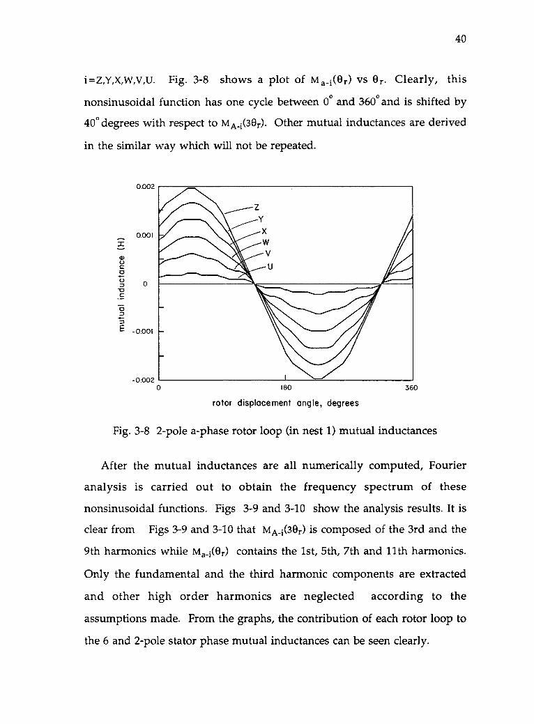
40

i=Z,Y,X,W,V,U. Fig. 3-8 shows a plot of m a_i(Or) vs Or. Clearly, this

nonsinusoidal function has one cycle between 0° and 360° and is shifted by

40° degrees with respect to mA_i(38r). Other mutual inductances are derived

in the similar way which will not be repeated.

0.002

0.001

0

-0.001

-0.0020 180

rotor displacement angle, degrees

360

Fig. 3-8 2-pole a-phase rotor loop (in nest 1) mutual inductances

After the mutual inductances are all numerically computed, Fourier

analysis is carried out to obtain the frequency spectrum of these

nonsinusoidal functions. Figs 3-9 and 3-10 show the analysis results. It is

clear from Figs 3-9 and 3-10 that mA_i(30r) is composed of the 3rd and the

9th harmonics while ma_i(or) contains the 1st, 5th, 7th and 11th harmonics.

Only the fundamental and the third harmonic components are extracted

and other high order harmonics are neglected according to the

assumptions made. From the graphs, the contribution of each rotor loop to

the 6 and 2-pole stator phase mutual inductances can be seen clearly.

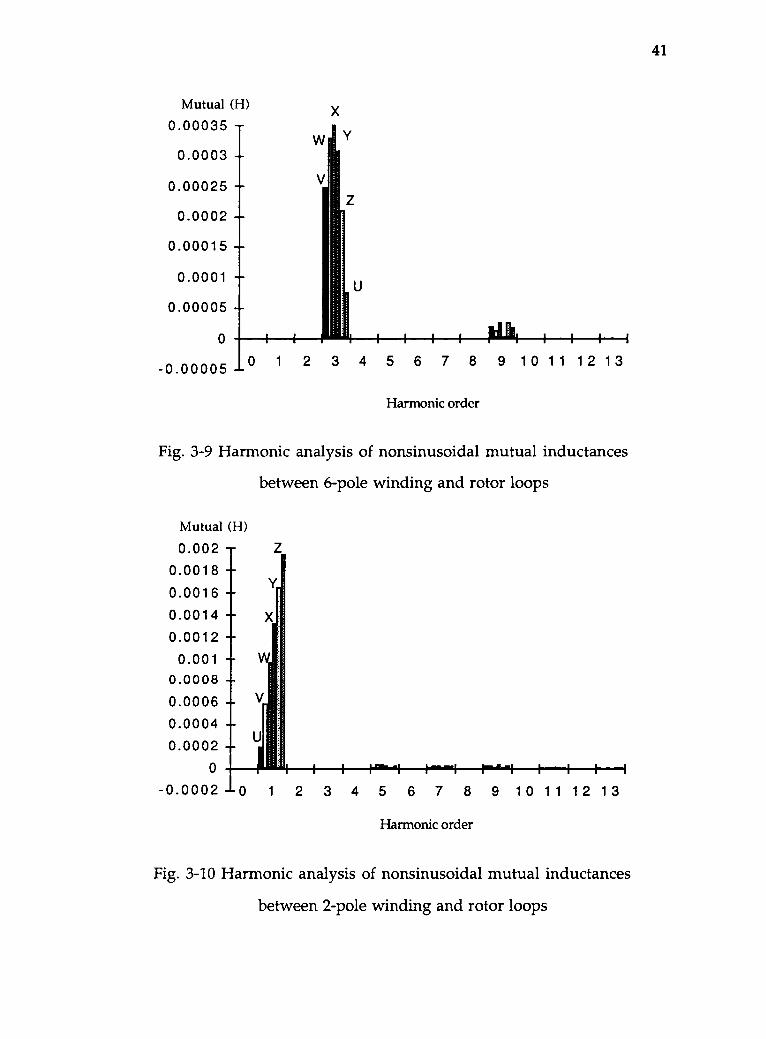
41

Mutual (H)

0.00035

0.0003

0.00025

0.0002

0.00015

0.0001

0.00005

0

-0.00005

X

1 2 3 4 5 6 7 8 9 1 0 1 1 1 2 1 3

Harmonic order

Fig. 3-9 Harmonic analysis of nonsinusoidal mutual inductances

Mutual (H)

0.0020.00180.00160.00140.0012

0.0010.00080.00060.00040.0002

0

-0.0002 0 1 2 3 4 5 6 7 8 9 1 0 1 1 1 2 1 3

between 6-pole winding and rotor loops

Harmonic order

Fig. 3-10 Harmonic analysis of nonsinusoidal mutual inductances

between 2-pole winding and rotor loops

42

3.4 Computation of Machine Parameters for an Experimental BDFM

The coil group inductance parameter matrix of the detailed model is

shown below. Define

L's, = } (3-28)

where a11= Lg for i =j and a11= Mii for i j, represent stator coil group self-

inductance and mutual inductance between coil groups, respectively.

then

uss.

0.6640 0.3824 0.0762 -0.2294 -0.5354 -0.5354 -0.2294 0.0762 0.38240.3824 0.6640 0.3824 0.0762 -0.2294 -0.5354 -0.5354 -0.2294 0.07620.0762 0.3824 0.6640 0.3824 0.0762 -0.2294 -0.5354 -0.5354 -0.2294

-0.2294 0.0762 0.3824 0.6640 0.3824 0.0762 -0.2294 -0.5354 -0.5354-0.5354 -0.2294 0.0762 0.3824 0.6640 0.3824 0.0762 0.2294 -0.5354-0.5354 -0.5354 -0.2294 0.0762 0.3824 0.6640 0.3824 0.0762 -0.2294-0.2294 -0.5354 -0.5354 -0.2294 0.0762 0.3824 0.6640 0.3824 0.07620.0762 -0.2294 -0.5354 -0.5354 -0.2294 0.0762 0.3824 0.6640 0.38240.3824 0.0762 -0.2294 -0.5354 -0.5354 -0.2294 0.0762 0.3824 0.6640

In addition, the coil group resistance is given as rg = 2.42 ). By using

the formulas derived in this Chapter, the BDFM equation parameters are

computed as follows.

(1) 6-pole stator impedance matrix

From (3-2), it follows that

1 1r6 = rg = 0.807 n , LA = -3 ( Lg + 2M) = -3 [0.664 + 2(-0.229)] = 0.0684 H

(3-29)

The mutual inductance between 6-pole phases is determined using (3-5)

1

MAB = MBC = MCA = "3" m12 + m.42 + m72 /

=1

( 0.382 +0.0762 - 0.5354) = -0.0255 H

With r6, LA and MAB , Zs6 of (2-2) is formed numerically as

(3-30)

zs6 =

(2) 2-pole stator impedance

The 2-pole phase

The self inductance

1 10La = ( Lg -T M12

43

[0.807+0.0684p

-0.0255p -0.0255p

-0.0255p 0.807+0.0684p -0.0255p (3-31)-0.0255p -0.0255p 0.807+0.0684p

matrix

resistance r2 is

r2 = r6 = rg = 0.807 Q (3-32)

is computed using (3-11)

4 , 1 10 4+-7M13 )=-3 (0.664+-0.382+-70.0764) = 0.4179 H (3-33)7

The mutual inductance between 2-pole phases are all equal and calculated

according to (3-22).

1

Mab Mbc Mca 21 [2(M17+M18+M19)+3(M27+M28+M29)+2(M374-M38+M39)]

= [2(-0.2294+0.0762+0.3824)+3(-0.5354-0.2294+0.0762)+

2(-0.5354-0.5354-0.2294)] = -0.2004 H (3-34)

With r2, La and Mab , Zs2 of (2-3) is formed numerically as

zs2 = [0.807+0.4179p

-0.2004p -0.2004p

-0.2004p 0.807+0.4179p -0.2004p

-0.2004p -0.2004p 0.807+0.4179p

(3) The magnitudes of the rotor angle dependent mutual inductances

between stator phases and rotor loops

(3-35)

These parameters, given in Table II, result from Fourier analysis of the

nonsinusoidally varying mutual inductances between 6- and 2-pole phase

and rotor loops as illustrated in Fig. 3-9 and Fig. 3-10.

44

Table II Magnitudes of mutual inductances between6- and 2-pole stator phases and rotor loops

RotorLoops

6-pole to rotormutuals (H)

2-pole to rotormutuals (H)

Z 0.000248 0.00200Y 0.000329 0.00169X 0.000350 0.00135W 0.000308 0.00099V 0.000210 0.00060U 0.000075 0.00020

(4) Rotor circuit parameters

As stated previously, in order to derive the two-axis model the stator

equations of the BDFM have been modified from coil group representation

to equivalent phase representation. However, the rotor equations remain

unchanged. The rotor circuit parameters are therefore obtained directly

from the detailed model parameters. These parameters are listed below.

(i) Loop resistances, self inductances and mutual inductances between

similar loops in different nests.

The parameters are given in Table III below.

Table III Loop resistances, self inductances and mutualinductances between similar loops in different nests

Resistances (p.S2) Self inductances (p.H) Mutuals (1.tH)(including 5% leakage)

rzz = 212.0ryy =188.0rxx = 164.0rww = 140.0rvv = 116.0

ruu = 92.0

Lzz = 18.8Lyy =16.31),0( =13.4Lww =10.1Lvv =6.38

Luu =2.23

Mzz = 5.978Myy = 4.002Mxx = 2.421Mww = 1.235Mvv = 0.444Muu = 0.049

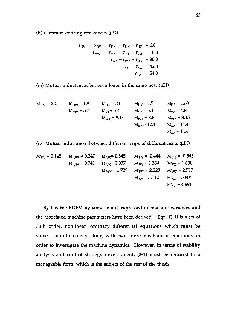
(ii) Common endring resistances (JAI)

ruv = rte,,,rvw

rUX = ruY = rUZ

rVX = rVY = rVZrwx = rwy = rwz

rxy = rxzryz

= 6.0

= 18.0

= 30.0

= 42.0

= 54.0

(iii) Mutual inductances between loops in the same nest (RH)

muv = 2.0 Muw = 1.9

mvw = 5.7

Mux= 1.8

Mvx= 5.4

Mwx = 9.14

Muy = 1.7

Mvy = 5.1

Mwy = 8.6

mxy = 12.1

Muz =1.63

mvz = 4.8Mwz = 8.15

mxz = 11.4

mxz = 14.6

(iv) Mutual inductances between different loops of different nests (P-I)

M'uv = 0.148 M'uw = 0.247

M'vw = 0.741

M'ux= 0.345

M'vx= 1.037

M'wx = 1.729

M'uY = 0.444M'vy = 1.334

m'wy = 2.223

M'xy = 3.112

M'uz = 0.543M'vz = 1.630

m'wz = 2.717

M'xz = 3.804

m'xz = 4.891

45

By far, the BDFM dynamic model expressed in machine variables and

the associated machine parameters have been derived. Eqn. (2-1) is a set of

30th order, nonlinear, ordinary differential equations which must be

solved simultaneously along with two more mechanical equations in

order to investigate the machine dynamics. However, in terms of stability

analysis and control strategy development, (2-1) must be reduced to a

manageable form, which is the subject of the rest of the thesis.

46

4. TWO-AXIS MODEL DEVELOPMENT AND MODEL

PARAMETER COMPUTATIONS

The theory employed to derive the two-axis (d-q) model is the well

known two reaction theory that calls for a change of variables of the

original system equations by which the time-varying mutual inductances

in the voltages equations can be eliminated.

It has been shown [22] that, for three-phase symmetrical induction

machines, in order to eliminate the time-varying terms in the differential

equations the reference frame can be fixed on the stator, rotor or be

synchronously rotating. For synchronous machines, however, due to the

saliency of their magnetic circuits, the reference frame must be fixed on the

rotor.

The analysis of the BDFM in the dq domain also faces the choice of

correctly selecting a reference frame in which the time-varying mutual

terms due to the relative motion between the stator circuits and the rotor

circuits can be eliminated. Owing to the special structure of the BDFM, it is

known that there can be two synchronous speeds (two synchronously

rotating reference frames) co-existing in the machine. They are due

respectively to the 6-pole system excitation and 2-pole system excitation.

Since the sequence of the two sets of input voltages is different , they are

rotating in opposite directions with respect to one another. Moreover,

since the two stator systems comprise two different pole numbers, the

choice of selecting a reference frame is therefore very limited. In fact, it can

be shown that it is not possible to select either stationary or synchronously

rotating reference frames in the dq analysis. However, in the rotor

47

reference frame, since two pairs of stator fictitious windings (d and q) along

with another pair of fictitious rotor windings are rotating at the speed of the

rotor, no relative motion exists between these windings, thus the time-

varying mutual inductances can be eliminated.

This Chapter discusses the use of dq analysis techniques to model the

BDFM and its parameters in the rotor reference frame. Following the

introduction, a preview of the dq modeling for the BDFM is given in 4.1

and in 4.2 the transformation matrices employed to develop the two-axis

model are derived based on a generalized orthogonal transformation

matrix. The development of the two-axis model is presented in section

4.3, followed by the equivalent circuits and the derivation of the torque

equation in the dq domain in sections 4.4 and 4.5. Finally, the two-axis

model parameters of an experimental machine are computed in 4.6.

4.1 Preview of the dq Modeling of the BDFM

As presented in the early Chapters, the process of developing the two-

axis model started with a common winding structure. By assuming that

the direct coupling between the two stator windings is negligible, the

original stator common winding structure has been separated into two

independent 3-0 winding systems with different pole numbers. Then,

Park's transformations can be applied to transform them into two

independent orthogonal sets, namely d and q plus a zero sequence if

unbalanced excitation is considered.

More discussions are needed for the rotor transformation. From the

basic rotor structure, it is known that there are 4 nests each of 6 loops for a

total of 24 rotor loops, which might suggest that 24 rotor states could be

needed to represent the rotor. However, due to the special structure of the

48

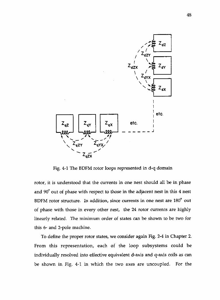
ZqZ ZqY ZqX

Latr IS Msit \ / i , 1 11

S.- .... .......

\ Z\ qZY fqYX/ /,.

...-Zqzx

Ar// ,..7

/ 1-dZY

I\

h-dZX

\ /\ ZdYX\ \

-...

etc.

d

d

d

etc.

Fig. 4-1 The BDFM rotor loops represented in d-q domain

rotor, it is understood that the currents in one nest should all be in phase

and 90° out of phase with respect to those in the adjacent nest in this 4 nest

BDFM rotor structure. In addition, since currents in one nest are 180° out

of phase with those in every other nest, the 24 rotor currents are highly

linearly related. The minimum order of states can be shown to be two for

this 6- and 2-pole machine.

To define the proper rotor states, we consider again Fig. 2-4 in Chapter 2.

From this representation, each of the loop subsystems could be

individually resolved into effective equivalent d-axis and q-axis coils as can

be shown in Fig. 4-1 in which the two axes are uncoupled. For the

49

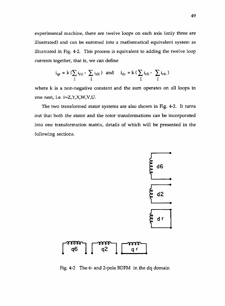
experimental machine, there are twelve loops on each axis (only three are

illustrated) and can be summed into a mathematical equivalent system as

illustrated in Fig. 4-2. This process is equivalent to adding the twelve loop

currents together, that is, we can define

iqr = k (/ irli I ir3i ) and idr = k ( I, ir2i 1 ir4i )i i i i

where k is a non-negative constant and the sum operates on all loops in

one nest, i.e. i=Z,Y,X,W,V,U.

The two transformed stator systems are also shown in Fig. 4-2. It turns

out that both the stator and the rotor transformations can be incorporated

into one transformation matrix, details of which will be presented in the

following sections.

Id:.

d2

d r 1

cri crn Fir Irq;:15\--

Fig. 4-2 The 6- and 2-pole BDFM in the dq domain

50

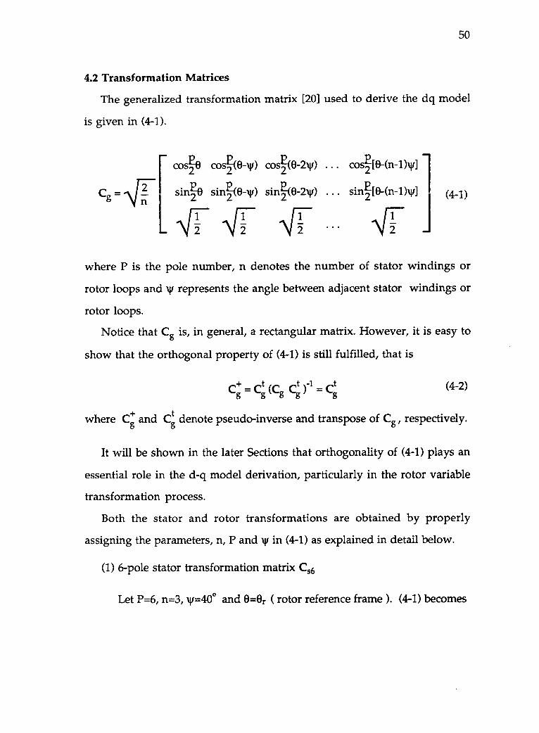
4.2 Transformation Matrices

The generalized transformation matrix [20] used to derive the dq model

is given in (4-1).

cos2 0 cosP22 2

(0-w) cos-(0-20 . . . cos2[9-(n-1)Nd

sin4 sinE2 (0-v) sinE2 203-2v . . .) sinE[0-(n-1)'r]

2

,\IT Vr i 72 2 2 NI 2

(4-1)

where P is the pole number, n denotes the number of stator windings or

rotor loops and v represents the angle between adjacent stator windings or

rotor loops.

Notice that Cg is, in general, a rectangular matrix. However, it is easy to

show that the orthogonal property of (4-1) is still fulfilled, that is

c+ = ct (c ct 1 = ctg g gg g

(4-2)

where C+g

and e denote pseudo-inverse and transpose of Cg , respectively.Cg

It will be shown in the later Sections that orthogonality of (4-1) plays an

essential role in the d-q model derivation, particularly in the rotor variable

transformation process.

Both the stator and rotor transformations are obtained by properly

assigning the parameters, n, P and v in (4-1) as explained in detail below.

(1) 6-pole stator transformation matrix Cs6

Let P=6, n=3, v=40° and 0 =0r ( rotor reference frame ). (4-1) becomes

r cos30r cos(30,-120°) cos(30r+120°)

sin39r sin(39r-120°) sin(30r +120 °)Cs6 =

H\IT 2 2

(2) 2-pole stator transformation matrix Cs2

Let P = 2, n = 3, v = 120 and 0 = (Or - 40°), we get

51

(4-3)

coster-401 cower- 40) -120 cos[(0r-40°) +1201

22I sin[Or- 40] sin[(Or- 40°) -1200] sin[(0r- 40°) +120]

= (4-4)

2 2

(4-3) and (4-4) are easily recognized as the modified Park's transformations

applied to the BDFM system of equations.

(3) 6-pole rotor transformation matrix Cr6

Transformation matrix Cr6 is defined as 2 by 24 matrix which can bepartitioned as

tCr6 = [ Ct6Z Cr6Y Cr6X Crew Cr6v Cr6U (4-5)

Notice that the zero sequence disappears because of the special structure of

the cage rotor. It is also noted that since the 24 rotor loops are grouped into

4 nests and the winding axis of all the loops in the same nest coincide in

the same direction, Cr6i, i = Z,Y,X,W,V,U are all identical.

Assign P = 6, n = 24 and v = 90°, then each of the submatrices of Cr6 can

be expressed as

[ cos%) cos3(0-90°) cos3(0-180°) cos3(0-270°)(4-6)"l'i sin30 sin3(0-90°) sin3(0-180°) sin3(0-270°)

in the rotor reference frame, which implies that 0 = 0, Cr6i becomes

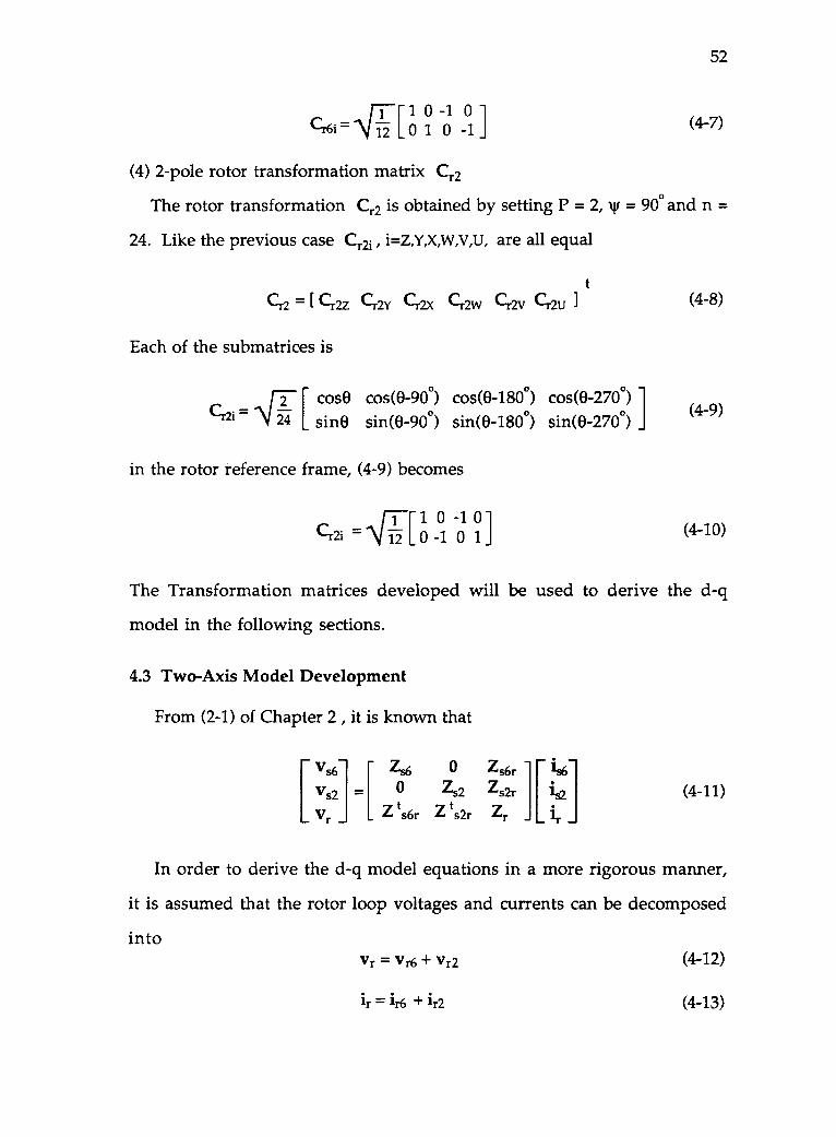
.N/771 0 -1 0 -1-r6i = L 0 0 -1

52

(4-7)

(4) 2-pole rotor transformation matrix Cr2

The rotor transformation Cr2 is obtained by setting P = 2, v = 900 and n =

24. Like the previous case Cr2i , i=Z,Y,X,W,V,U, are all equal

tCr2 = [ Cr2Z Cr2Y Cr2X Cr2W Cr2V Cr2U

Each of the submatrices is

(4-8)

rg

_Jr [ cosh cos(0-90) cos(0-180°) cos(0-270°)sine sin(0-90) sin(9-180°) sin(0-270)

(4-9)

in the rotor reference frame, (4-9) becomes

11- 1 0 -1 0 1Crl = NIT21.0 -1 0 1 J (4-10)

The Transformation matrices developed will be used to derive the d-q

model in the following sections.

4.3 Two-Axis Model Development

From (2-1) of Chapter 2 , it is known that

Vs6

Vs21 =Vr

Zs6

Z ts6r

0Zs2

Z ts2r

ZsbrZs2r

Zr

is6is2

lr(4-11)

In order to derive the d-q model equations in a more rigorous manner,

it is assumed that the rotor loop voltages and currents can be decomposed

intoVr = Vr6 + Vr2

it = ir6 + ir2

(4-12)

(4-13)

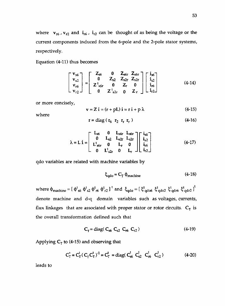
53

where Vr6 , Vr2 and ir6 , 4.2 can be thought of as being the voltage or the

current components induced from the 6-pole and the 2-pole stator systems,

respectively.

Equation (4-11) thus becomes

vs6Vs2

Vr6Vr2

or more concisely,

where

[Zs60

I Z ts6rL o

0Zs2

0

z ts2r

Zs6r Zs6/1Zs2r Zs2rZr 0

0 Zr

is2ir6

1r2

(4-14)

v=Zi=(r+pL)i=ri+pk (4-15)

r = diag ( r6 r2 rr rr ) (446)

Ls6 00 Ls

X.= L i= [ Lts6r 0

0 Lts2r

Ls6r

Ls2rLr

0

Ls6r

Ls2r0

Lr

is2ir6

'r2

(4-17)

qdo variables are related with machine variables by

qdo = CT machine (4-18)

lt[ ots6 ots2 otr6 otr2 i t andwhere do machine = qdo = [ Vqdo6 tcido2 tcidr6 tcidr2 .1

denote machine and d-q domain variables such as voltages, currents,

flux linkages that are associated with proper stator or rotor circuits. CT is

the overall transformation defined such that

CT = diag( Cs6 C2 Cr6 Cr2 ) (4-19)

Applying CT to (4-15) and observing that

C1, = CtT( CrCti. )4 = CT = diag( Cs6 Cs2 Cr6 Cr2 )

leads to

(4-20)

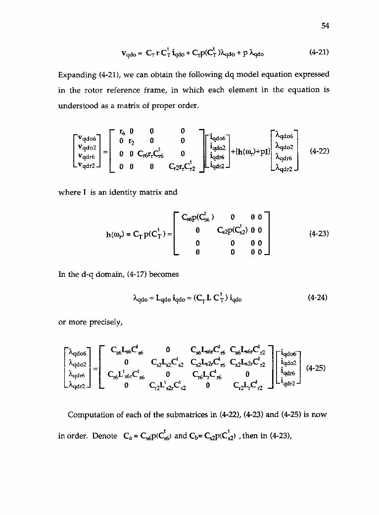
Vgdo = CT r CT iqdo + CrP(CT )Aqdo + p kqdo

54

(4-21)

Expanding (4-21), we can obtain the following dq model equation expressed

in the rotor reference frame, in which each element in the equation is

understood as a matrix of proper order.

r6 0 0 0

0 r 0 0 iqdo6Vcido2

9 dr6 = 0 0 Cr6rrC.tr6 0

2iqdo2 Aqdo2

V iqd I

[Xqdo61

t Aqdr6dr2

2Lqdr2V 9 0 0 0 Cr2rrCr2 lqdr2

where I is an identity matrix and

[Cs6P(Ct6 ) 0 0 0

h(0)r) = CT p(CT) . 0 Cs2P(Cts2) 0 0

0 0 000 0 00

In the d-q domain, (4-17) becomes

kqdo = Lqdo iqdo = (CT L C T) iqdo

or more precisely,

[Xqdo61 Cs6Ls6Cts6

Xqd o2 0

[Aqdr6 i C Lt ctr6 s6r 6

Xqdr2 0

0 Cs646rCtr6

Cs2Ls2Cts2 Cs242rdt6

toCjrCtr6

Cr2Lts2rds2 °

cs646rctr2

Cs2Ls2rCtr2

0

Cr2Lrer2 1

iqdo6-[iqdo2

iqdr6

iqdr2

(4-22)

(4-23)

(4-24)

(4-25)

Computation of each of the submatrices in (4-22), (4-23) and (4-25) is now

in order. Denote Ca = Cs6p(Cts6) and Cb= Cs2P(Cts2) , then in (4-23),

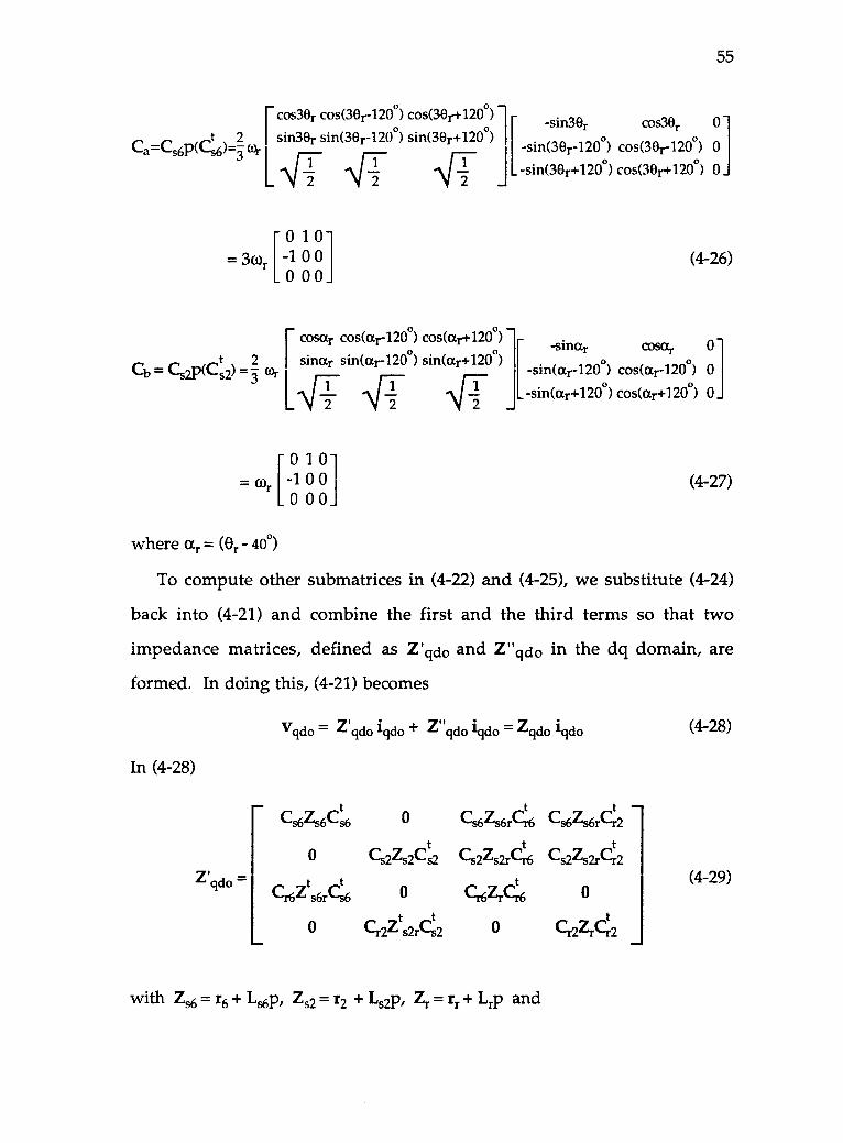
55

cos3Or cos(30/-120°) cos(30r+120°) -sin3Or cos3Or 0

Ca=Cs6P(Cs6)'Ncur

t 2 r sin3Or sin(30r-120°) sin(30r+120°)issii:330Orr+-120°) cos(30/-120°) 0

[111F 417 2

. 120°) cos(30r+120°) 0

30)r0

[ -10

1 0

0 0

00(4-26)

cosar cos(ar-120°) cos(ar+120°) -sinar cosar 0t 2 [ sinar sin(ar-120°) sin(ar+120°)

Cb = Cs21)(Cs2) 5 (or -sin(ar-120°) cos(ar120°) 0

-\rf _J _sin(ar+1200)cos(ar+1200) 0

(or

[0 1 0-1 0 00 00

(4-27)

where ar = (8r 40 )

To compute other submatrices in (4-22) and (4-25), we substitute (4-24)

back into (4-21) and combine the first and the third terms so that two

impedance matrices, defined as Ecido and Z"qdo in the dq domain, are

formed. In doing this, (4-21) becomes

In (4-28)

Vqdo = Z'qdo iqdo Z "qdo iqdo = Zqdo iqdo

tcs6zs6cs6 c,46rer6

0 Cs2Zs2Cs2 Cs2Zs2rCr6qdo = ,.,t

s6r-s6

0

0

t tCr2Zs2rCs2

Cs6Zs6rCr2

tCs2Zs2rCr2

c.zre0 Cr2ZrCr2

r6 0

with Zs6 = r6 + Ls6p, Zs2 = r2 + Ls2p, Zr = r, + Lrp and

(4-28)

(4-29)

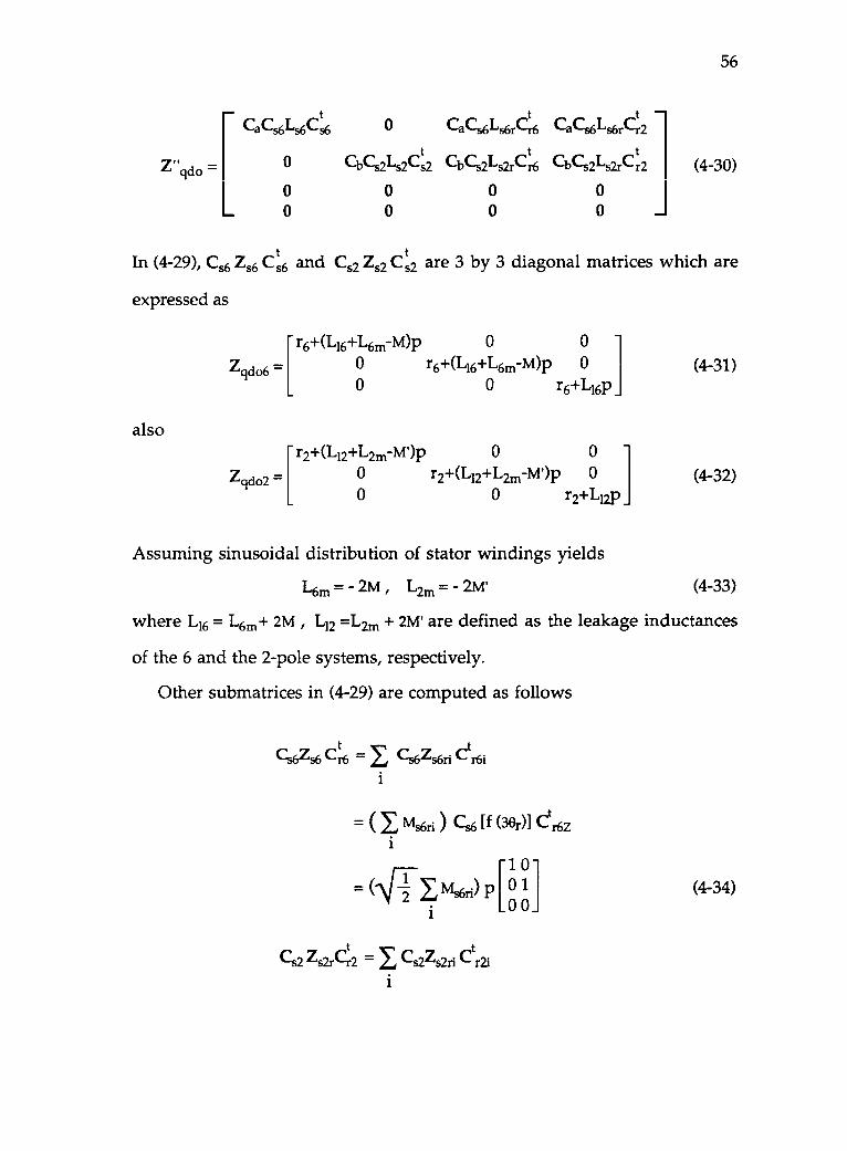
Cac6Ls6Cts6

qdo0

0

0 CaCs6LS6rdr6

CbCs2Ls2Cts2

00

CbCs2Ls2ser6

0

0

cbcs2Ls2rc r2t

CaCs6Ls6rC:2

00 J

56

(4-30)

In (4-29), Cs6 Zs6 Cts6 and Cs2 Zs2 Cts2 are 3 by 3 diagonal matrices which are

expressed as

also

r6+(1..,16+L6m-m)p 0 0

Z006 = 0 r6+(L16+L6,-m)p 00 0 r6+L16p

r2+(L12+L2m-Isc)p 0 0

Zqdo2 = 0 r2 +(L12 +L2m -M')p 00 0 r2+L12p

Assuming sinusoidal distribution of stator windings yields

L6m = 2M , L2m = - 2M'

(4-31)

(4-32)

(4-33)

where L16 = L6m+ 2M , L12 =L2m + 2M' are defined as the leakage inductances

of the 6 and the 2-pole systems, respectively.

Other submatrices in (4-29) are computed as follows

Cs6Zs6 Cr6 = E Cs6zs6ri epsi

= ms6fi Cs6 [f (38r)1 ct,zi

1

= (A/ ms6ri) 4 0 10 0

t tCs2 Zs2rCr2 = Cs2Zs2ri Cr2i

(4-34)

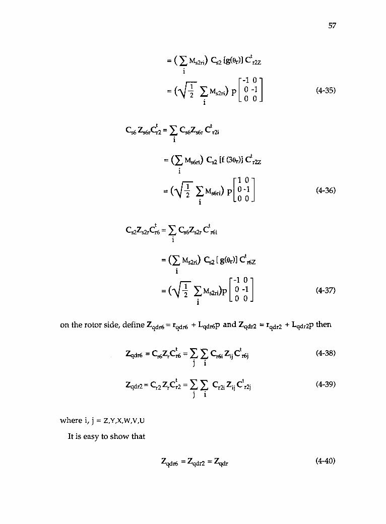
= IsAs2,i) Cs2 [god] er2z

-1 0(-Ng ms2ri) p 0 -1

001

t tCs6 Zs6rCr2 Cs6Zs6r Cr2i

(E Ms6ri) Cs2 [f (30r)] Ctr2z1

10(Ng I Ms6ri) p [ 0 -1

100

tCs2Zs2rCr6 E Cs6Zs2r Cr6i1

= ms2ri) Cs2 [ Or)] ctr6z

-1 0

( \IT Ems2ri)p 0 -1

10 0

57

(4-35)

(4-36)

(4-37)

on the rotor side, define Zqdr6 = rqd6 Lqdr6p and Z qdr2 = rgdr2 + Lqdr2p then

Zgdr6 = cr6zrer6 = cr6j zjj dr6j

Zqdr2 Cr Zrer2 I y Cr2i Zij Ctr2i

where i, j = Z,Y,X,W,V,U

It is easy to show that

Zqdr6 = Zqdr2 = Zqdr

(4-38)

(4-39)

(4-40)

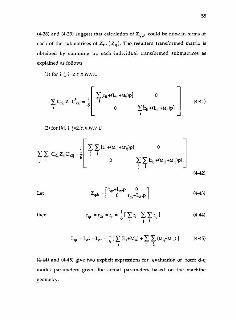
58

(4-38) and (4-39) suggest that calculation of Zqdr could be done in terms of

each of the submatrices of Zr, (Zii }. The resultant transformed matrix is

obtained by summing up each individual transformed submatrices as

explained as follows

(1) for i=j, i=Z,Y,X,W,V,U

r,tCr2i r2i

[1 [rii +(l-ii +MOP]

61 1

L

(2) for N, i, j=Z,Y,X,W,V,U

0

[rij +(mii +m'ii)p][r.,t 1Lr Cr2i r2. =

61

ji0

0

+Mii)131i

0

I [rij +(Aii +M'ij)p]

Let

then

Zqdr

rqr = rdr

C

reLgrp 00 rdr+Ldrp

1= rr = [ ri 4-E

j

I r-- ]

i

1Lqr = Ldr = Ldr = 6 [ (Li+Mii) + I (7,4ij-Fmi 1.j) ]

(4-41)

(4-42)

(4-43)

(4-44)

(4-45)

(4-44) and (4-45) give two explicit expressions for evaluation of rotor d-q

model parameters given the actual parameters based on the machine

geometry.

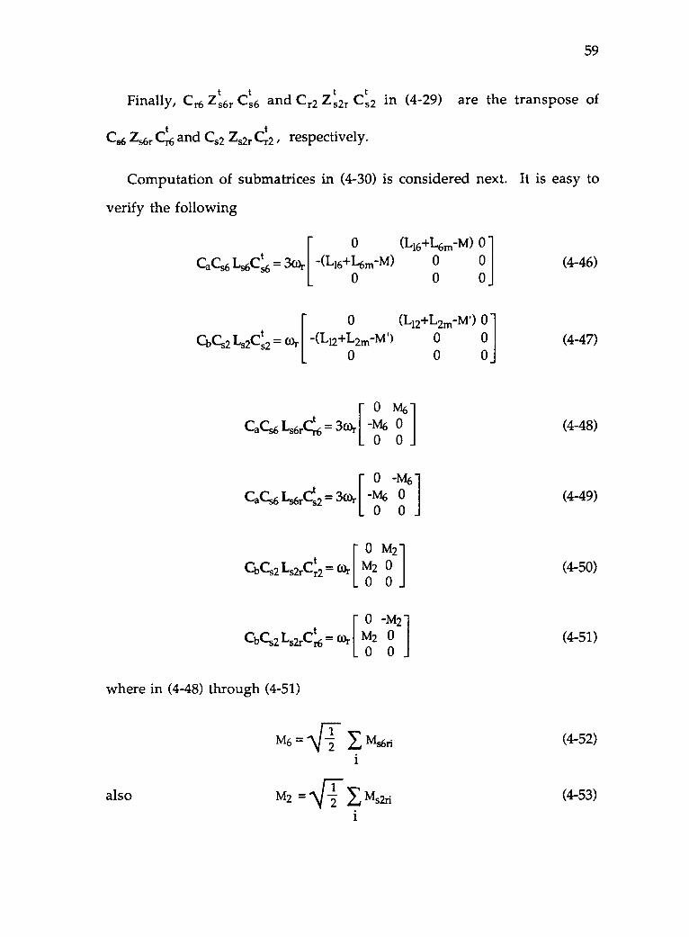
59

Finally, CT.6 Zs6,. C_s6 andand _C r2 Z_ ts2r C ts2 in (4-29) are the transpose of

Cs6 Zs 6r Cr6 and e2 Zs 2r Ctr2 , respectively.

Computation of submatrices in (4-30) is considered next. It is easy to

verify the following

[0 (116+L6m-m) 0

CaCs6 I.,s6Cts6 = 3(or -(1-46+1-6m-M) 0 0

0 0 0

0 (112+1,2m- M') 0

CbCs2 Ls2 Cs2 = (1)r [ -(L12+L2m-MI) 0

0 000

0

CaCs6 Ls6rCr6t = 30)r [ -M6 00 0

0 -M6

CaCs6 Ls6rCts2 = 3w'' [ -M6 00 0

0

CbCs2 Ls2rCtr2 = (1)r [ M2 00 0

0

CbCs2Ls2rdn6 = COr [ M2 00 0

where in (4-48) through (4-51)

also

V iM6

7---IMs6ri

i

M2 = VT-i I Ms2rji

(4-46)

(4-47)

(4-48)

(4-49)

(4-50)

(4-51)

(4-52)

(4-53)

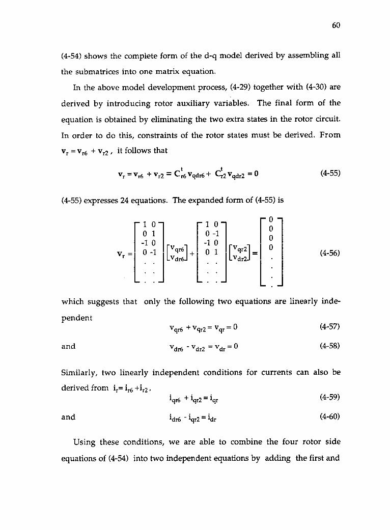
60

(4-54) shows the complete form of the d-q model derived by assembling all

the submatrices into one matrix equation.

In the above model development process, (4-29) together with (4-30) are

derived by introducing rotor auxiliary variables. The final form of the

equation is obtained by eliminating the two extra states in the rotor circuit.

In order to do this, constraints of the rotor states must be derived. From

Vr = Vr6 + vr2 , it follows that

t tVr = Vr6 + Vr2 = C r6 Vqdr6 + Cr2 Vqdr2 = 0

(4-55) expresses 24 equations. The expanded form of (4-55) is

oo 1

o[ o

0 -1

Vr = 0 -1[V qr61 010

2

[Vdr6 vVdr2

0

I O

= I

0

.

(4-55)

(4-56)

which suggests that only the following two equations are linearly inde-

pendent

and

Vqr6 + Vqr2 = Vqr = 0 (4-57)

vdr6 Vdr2 = vdr = (4-58)

Similarly, two linearly independent conditions for currents can also be

derived from ir= ir6 +42

and

q r6 iqr 2 = lqr

idr6 iqr2 = idr

(4-59)

(4-60)

Using these conditions, we are able to combine the four rotor side

equations of (4-54) into two independent equations by adding the first and

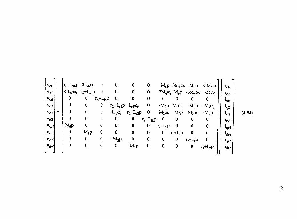
V46

Vd6

r6+Ls6p 3L,60)r

-3Ls6COr r6+Ls6p

0

0

0 0

0 0

0

0M6p 3Mor

-3M" M6pM6p

-3M6wr

-3Mor-M6P

i 64

id6

vo6 0 0 r6 +L16p 0 0 0 0 0 0 0 i06

V420 0 0 r2+Ls2p Ls2Wr 0 -M2p M2Wr -M2p -M2wr iq2

Vd2 = 0 0 0 -Ls2cor r2+Ls2p 0 M2COr M2p M2COr -M2p id2 (4-54)

vo2 0 0 0 0 0 r2+112p 0 0 0 0 io2

Vqr M6p 0 0 0 0 0 rr+Lrp 0 0 0 i4 r6

Vdr 0 M6p 0 0 0 0 0 rr+Lrp 0 0 idr6

Vqr 0 0 0 -Map 0 0 0 0 rr+Lrp 0iqr2

Vdr 0 0 0 0 -M2p 0 0 0 0 rr+Lrp idr2

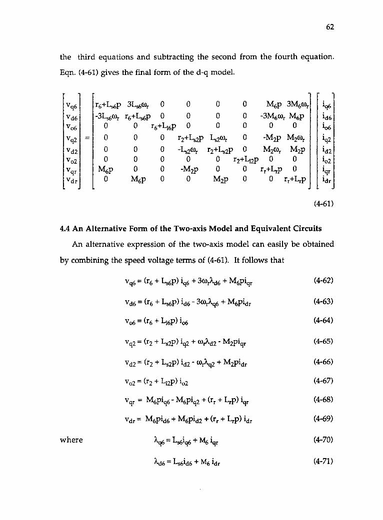
62

the third equations and subtracting the second from the fourth equation.

Eqn. (4-61) gives the final form of the d-q model.

V96

vd6vo6

Vq2

Vd2

vo2Vqr

vdr

=

r6+Ls6p 3Ls6cor 0

-31,s6cor r6+Ls6p 0

0 0 r6+L16p

0 0 0

0 0 0

0 0 0

m6P 0 0

0 M6p 0

o

o0

r2+Ls2p

-1-s240

-M2p0

0 0 M6p 3m6or0 0 -3m6wr M6p0 0 0 0

Ls2cor 0 -M2p M2wrr2+Ls2p 0 1424 M2p

0 r2 +L12p 0 0

0 0 rr+Lrp 0

M2p 0 0 rr+Lrp

i 6

id6

lob

i 2

id2i02

iqridr

(4-61)

4.4 An Alternative Form of the Two-axis Model and Equivalent Circuits

An alternative expression of the two-axis model can easily be obtained

by combining the speed voltage terms of (4-61). It follows that

where

vq6 = (r6 + Ls 6p) iq6 3(1)rkd6 + M6Piqr

vd6 = (r6 Ls6P) id6 34A16 + M6Pidr

V06 = (r6 + L16p) i06

Vq2 = (r2 + Ls2p) iq2 + wrkd2 M2Piqr

vd2 = (r2 Ls2P) 1d2 (1)rkq2 + M2Pidr

vo2 = (r2 I-12P) i02

Vqr = M6piq6- M6piq2 + (rr + Lrp) iqr

vdr = M6Pid6 M6Pid2 (rr LIP) idr

2'q q6 = Ls6i 6 + M6 iqr

kd6 = Ls6id6 + M6 idr

(4-62)

(4-63)

(4-64)

(4-65)

(4-66)

(4-67)

(4-68)

(4-69)

(4-70)

(4-71)

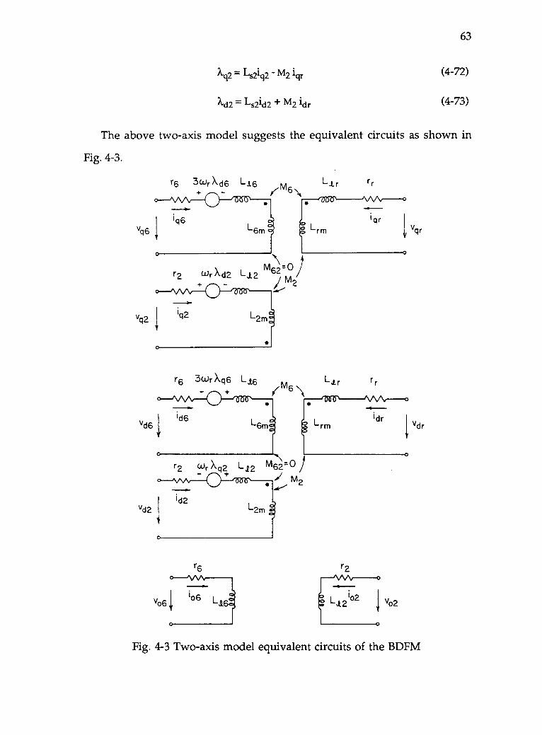
kg = Ls2iq2 M2 iqr

Xd2 = Ls2id2 + m2 idr

63

(4-72)

(4-73)

The above two-axis model suggests the equivalent circuits as shown in

Fig. 4-3.

V46

r6 30-)r X d6 L16 mK 6 \_ ..iq6

L 6m

r2 clir Xd2 L12 M6\2--))

---0-

vq2iq2

vd6

vd2

+ .-II 6

/ mz...

r6 3Wr Xq6 L16+ ( 6 \

ass

LI r

I'M

rr

iqr

rr

idr

V02

Vqr

Fig. 4-3 Two-axis model equivalent circuits of the BDFM

64

4.5 The Torque Equation in the dq Domain

The torque equation in the d-q domain may also readily be derived

from energy considerations.

From

where

it follows that

Te --:' (Cts iqdodt [ ( Zsr ) ] Ctr iqdr

Cs[ Ct s6 0

s 0 Cts2 i ;

Zs6r Zs&

Zsr [ Zs2r Zs2r 1

iqdos = [ icid°6 ;lqdo2

ictr6 0 iLr=L 0 Ct

r2j; iqdr =

iqdr6

q

]

i dr2

t[ ( zs6,) ] ct,6icid,,, + i [ (z2) c id6+Te = iqd06 Cts6aer

qdo2 Cts2 per (Zs2r) r6 q

(4-74)

Cts6a (4 r a

iqdo6 C s6 [ air ( Zs6r) ] Ctr2 iqdr2 + iqdo2 ' s2 L air ( Zs2r) i Ctr2 iqdr2 (4-75)

Simplifying (4-75) results in

[Te = ( I Msbri ) { iqdo6 Cts6 E

ae---f (30r) I Ctr6z iqdr6 + iqd02 C

ts2 l aor g (0r)

i r

l-Ctr6Z iqdr6 + iqdo6 Cts6 [ air f (30r) ] Ctr2z -4dr2 + ildo2 Cts2

r ,..,t

I- ae g(0r) 1 .- r2z iqdr2 1 (4-76)

where the matrix functions [f (30r )1 and [g(Or)] are given in (2-6) and (2-7)

in Chapter 2.

The four terms in (4-76), denoted as Te66, Te26, Te62 and Ten , can be

verified to be of the following

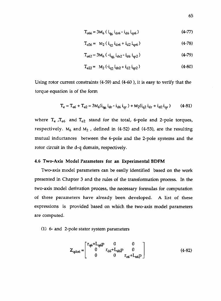
65

Te66 = 3M6 (iq6 1dr6 1d6 iqr6 ) (4-77)

Te26 M2 ( iq2 idr6 id2 iqr6 ) (4-78)

Te62 = 3M6 1dr2 1d6 iqr2 ) (4-79)

Te22 = M2 (-1q2 1dr2 1d2 iqr2 ) (4-80)

Using rotor current constraints (4-59) and (4-60 ), it is easy to verify that the

torque equation is of the form

Te = Tee + Te2 = 3M6(lg6 'dr -id6 -iqr ) M2(iq2 -idr id2 -iqr ) (4-81)

where Te ,Te6 and Tee stand for the total, 6-pole and 2-pole torques,

respectively. M6 and M2 , defined in (4-52) and (4-53), are the resulting

mutual inductances between the 6-pole and the 2-pole systems and the

rotor circuit in the d-q domain, respectively.

4.6 Two-Axis Model Parameters for an Experimental BDFM

Two-axis model parameters can be easily identified based on the work

presented in Chapter 3 and the rules of the transformation process. In the

two-axis model derivation process, the necessary formulas for computation

of these parameters have already been developed. A list of these

expressions is provided based on which the two-axis model parameters

are computed.

(1) 6- and 2-pole stator system parameters

0 0

Z006 = 0 rd6+Ld6p 0

0 0 ro6+Lo6p(4-82)

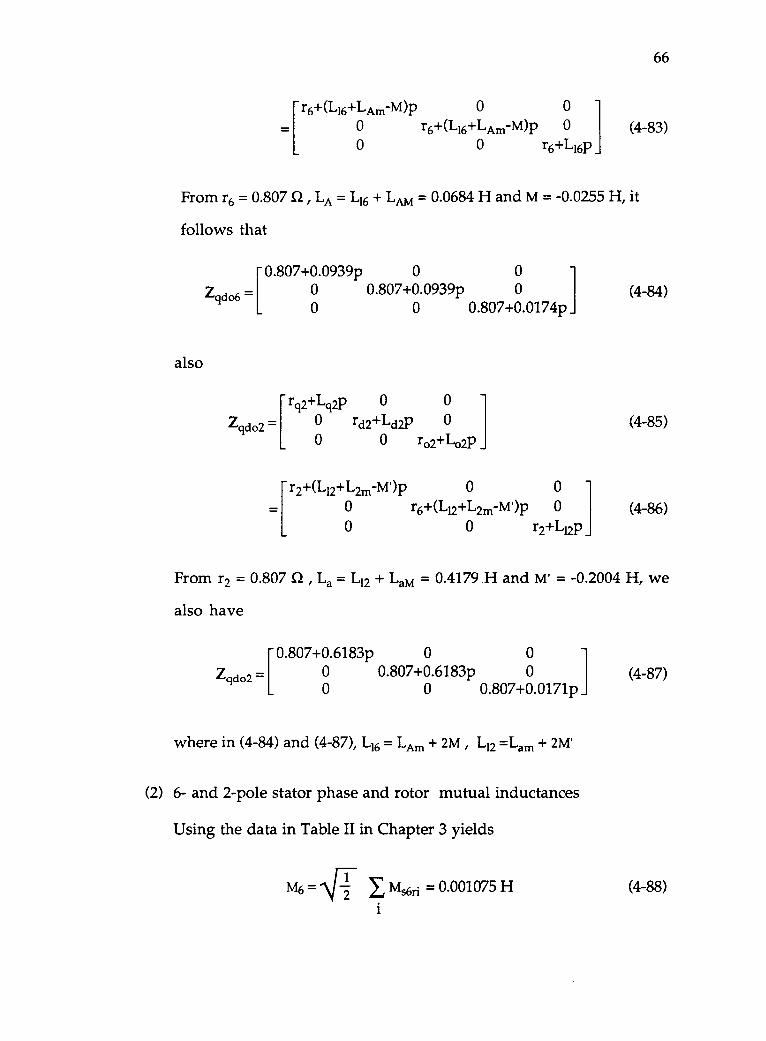
r6+(L16+LAm-m)p 0 0

0 r6+(L16+LAm-m)p 0

0 0 r6+1-16P

66

(4-83)

From r6 = 0.807 Q , LA = L16 + LAM = 0.0684 H and M = -0.0255 H, it

follows that

also

0 0

Zcidc,6 = 0 0.807+0.0939p 00 0 0.807+0.0174p

rq2+Lq2p 0 0

Zqdo2 = 0 rd2+Ld2p 0

0 0 ro2+4,2p

r2+(L12+L2m-MV 0 0

0 r6+(L12+L2m-MV 0

0 0 r2+Lap

(4-84)

(4-85)

(4-86)

From r2 = 0.807 SI , La = L12 + Lam = 0.4179 H and M' = -0.2004 H, we

also have

0 0

Zqdo2 = 0 0.807+0.6183p 00 0 0.807+0.0171p

where in (4-84) and (4-87), L16 = LAm + 2M , L12 =Lam + 2M'

(2) 6- and 2-pole stator phase and rotor mutual inductances

Using the data in Table II in Chapter 3 yields

Frwib

vNJ

ms6ri = 0.001075 H1

(4-87)

(4-88)

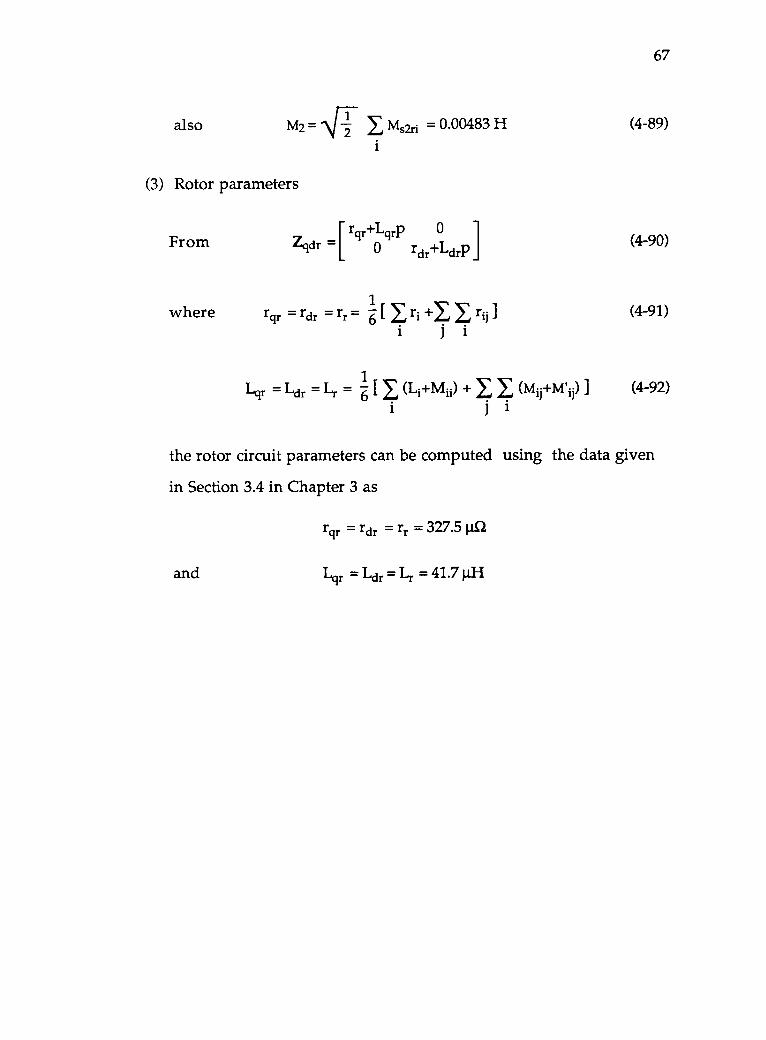
i ,also M2 = Ari 2 ms2ri = 0.00483 H

i

(3) Rotor parameters

Fromrcir+Lcirp 0 ]

Zqdr = 0 rdr+LdrP

1where rqr = rdr = rr = -6- [ E ri +E E r-il

i j i

Lqr = Ldr = Lr = 6 [ E (Li+mii) + E E (mem'ipi i i

67

(4-89)

(4-90)

(4-91)

(4-92)

the rotor circuit parameters can be computed using the data given

in Section 3.4 in Chapter 3 as

rqr = rdr = rr = 327-51112

and Lqr = Ldr = 1..r = 41.7 pH

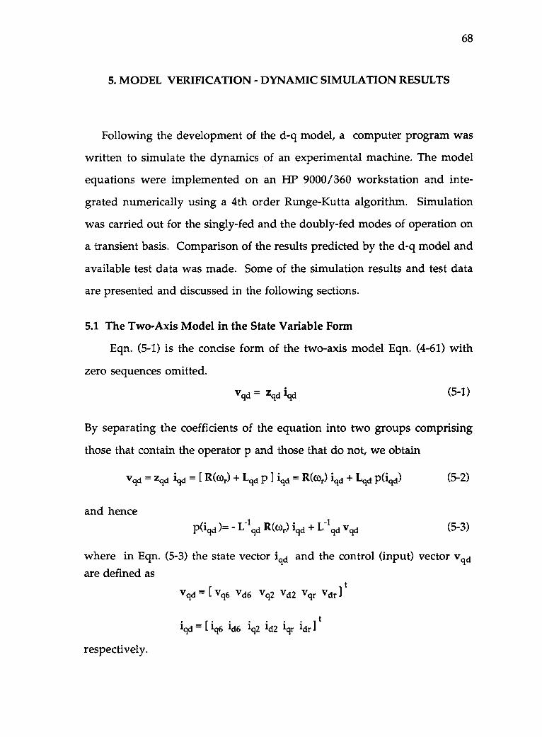
68

5. MODEL VERIFICATION - DYNAMIC SIMULATION RESULTS

Following the development of the d-q model, a computer program was

written to simulate the dynamics of an experimental machine. The model

equations were implemented on an HP 9000/360 workstation and inte-

grated numerically using a 4th order Runge-Kutta algorithm. Simulation

was carried out for the singly-fed and the doubly-fed modes of operation on

a transient basis. Comparison of the results predicted by the d-q model and

available test data was made. Some of the simulation results and test data

are presented and discussed in the following sections.

5.1 The Two-Axis Model in the State Variable Form

Eqn. (5-1) is the concise form of the two-axis model Eqn. (4-61) with

zero sequences omitted.

Vqd -= Zqd iqd (5-1)

By separating the coefficients of the equation into two groups comprising

those that contain the operator p and those that do not, we obtain

Vqd = Zqd iqd = [ R(G)r) + Lqd P kid = R(cor) kid + Lqd p(iqd) (5-2)

and hence

P(iqd )=' riqd R(0)r) iqd riqd Vqd (5-3)

where in Eqn. (5-3) the state vector iqd and the control (input) vector vqdare defined as

tVqd = [ Vq6 Vd6 Vq2 Vd2 Vqr Vdr

tiqd = [ iq6 id6 iq2 id2 iqr ldr

respectively.

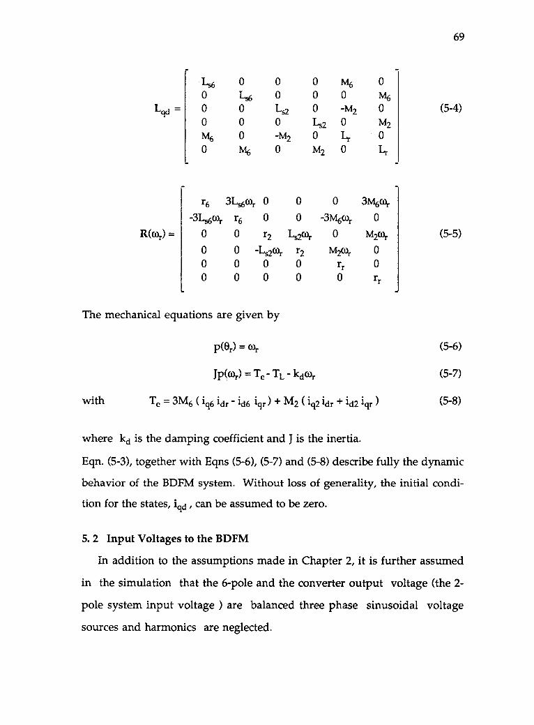
69

Lqd =

4600

0M6

0

046000

M6

00Ls2

0-M2

0

000

1--s2

0

M2

M6

0

-M2

0Lr

0

0

M6

0M20Lr

(5-4)

R(cor) =

r6 3Ls6cor 0 0

-3Ls6cor r6 0 0

0 0 r2 42cor

0 0 -Ls2COr r20 0 0 00 0 0 0

0

-3M6cor

0

m2cor

rr0

3M6cor

0

M2COr

0

0r,

(5-5)

The mechanical equations are given by

with

P(Or) = (or

Jp(cor) = Te- TL - keor

Te = 3M6 1q6 idr 1d6 iqr ) + M2 ( iq2 idr id2 iqr )

(5-6)

(5-7)

(5-8)

where kd is the damping coefficient and J is the inertia.

Eqn. (5-3), together with Eqns (5-6), (5-7) and (5-8) describe fully the dynamic

behavior of the BDFM system. Without loss of generality, the initial condi-

tion for the states, iqd , can be assumed to be zero.

5. 2 Input Voltages to the BDFM

In addition to the assumptions made in Chapter 2, it is further assumed

in the simulation that the 6-pole and the converter output voltage (the 2-

pole system input voltage ) are balanced three phase sinusoidal voltage

sources and harmonics are neglected.

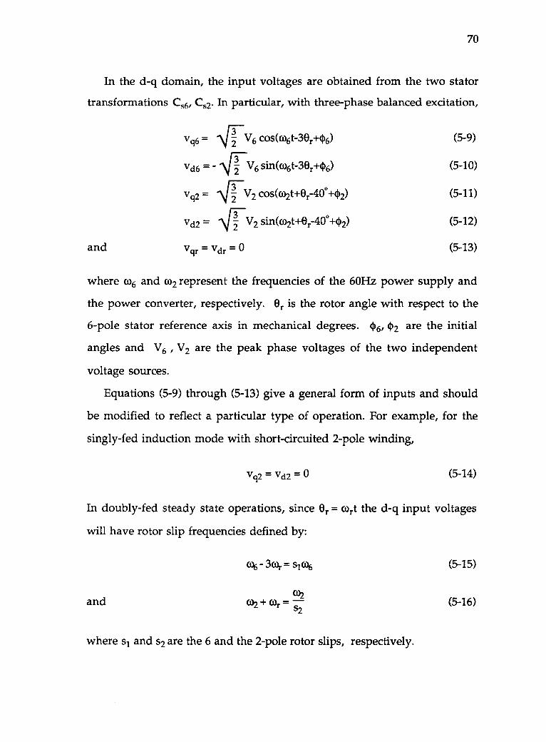
70

In the d-q domain, the input voltages are obtained from the two stator

transformations c6, Cs2. In particular, with three-phase balanced excitation,

and

Vq6 = 4-1V6 cos(o6t-30,.+06) (5-9)

Vd6 = - 2 V6 sin(o6t-30r+46) (5-10)

V q 2 = 2 V2 cos(co2t+Or-40°+42) (5-11)

vd2 = -\13V2 sin(w2t+er-40°+02) (5-12)

Vqr = Vdr = 0 (5-13)

where co6 and 0)2 represent the frequencies of the 60Hz power supply and

the power converter, respectively. Or is the rotor angle with respect to the

6-pole stator reference axis in mechanical degrees. 4)6, 4)2 are the initial

angles and V6 , V2 are the peak phase voltages of the two independent

voltage sources.

Equations (5-9) through (5-13) give a general form of inputs and should

be modified to reflect a particular type of operation. For example, for the

singly-fed induction mode with short-circuited 2-pole winding,

Vq2 =vd2 =0 (5-14)

In doubly-fed steady state operations, since Or = cort the d-q input voltages

will have rotor slip frequencies defined by:

and

co6- 34= sico6

(I)20)2 4" (I)r

where s1 and s2 are the 6 and the 2-pole rotor slips, respectively.

(5-15)

(5-16)

71

Particularly, in synchronous operation when the two rotor frequencies are

the same, it follows that

or

4 34 = (112 + (I3r

w6 (1)2

4 4

(5-17)

(5-18)

Thus the rotor mechanical radian frequency under the synchronous mode

of operation is completely determined by the frequency of the converter

output.

5.3 Dynamic Simulations of the BDFM

5.3.1 Singly-Fed Induction Mode of Operation

To be consistent with the laboratory testing procedure, in the computer

simulation, the 6-pole stator set, ABC, is connected directly to the 60Hz

power supply and the 2-pole terminals, abc, are short circuited.Consequently, vq2=vd2=0.

The predicted stator and rotor q axis currents during free acceleration

are plotted in Fig. 5-1. Similar to a conventional 6-pole induction motor

run up, substantially high but decaying currents can be seen before the

machine enters steady state operation in which both the 2-pole and the

rotor currents go close to zero and the 6-pole current approaches a constant

value. Figs 5-2(a) and 5-2(c) show the predicted 6-pole and 2-pole line

currents iA and is during the start-up period. It is seen that the currents

decay as the speed of the machine increases but pick up again due to the

increasing interactions between the two systems around 900 r/min. The

frequency of the 2-pole winding current is seen to decrease to dc close to 900

r/min, increasing again above 900 r/min before the current magnitude

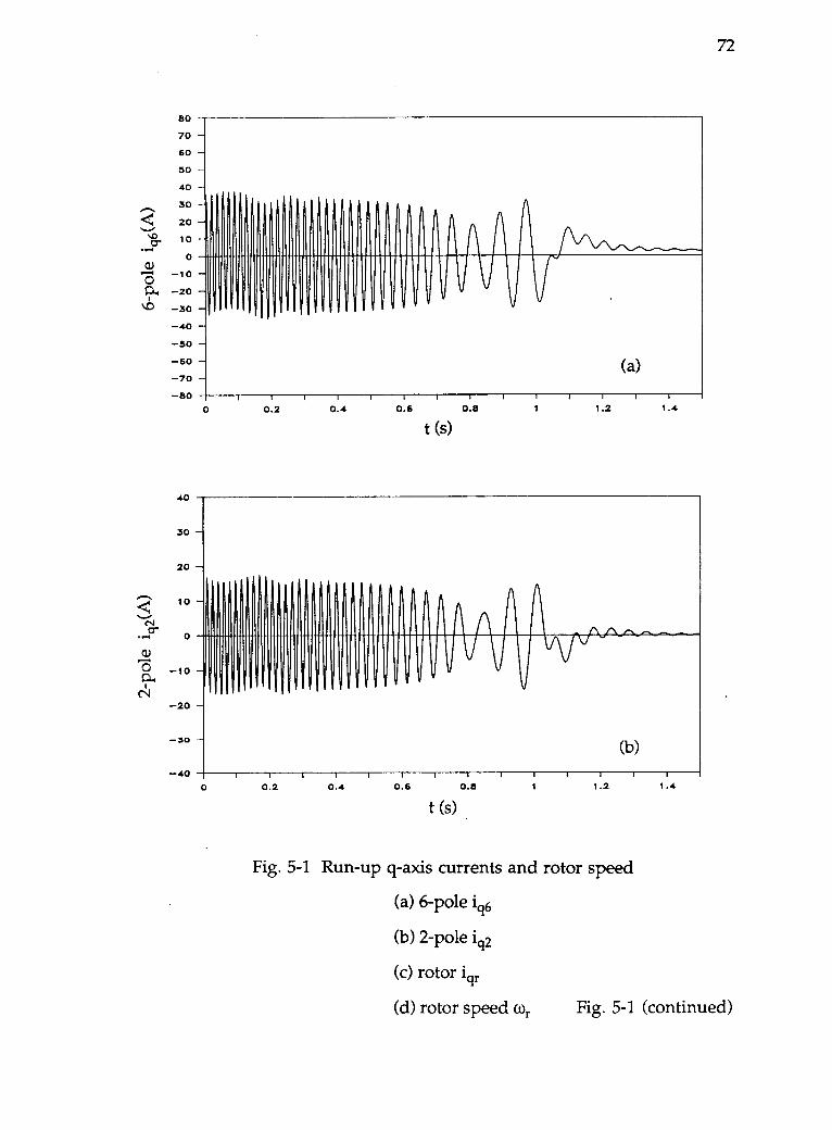
8070

60

50

40

30

R20

Q. 10

0CI)

0 -1004 -20

%IS -30-40-50- 60- 70-80

40

Pli 1 111111 I iplis

1 I I II I I I 1 I 1

(a)

1 i

0.2 0.41 1

0.6 0.8

t (s)1

1 1

1.2 1.4

30 -

20 -

Ii

-20 -

- 30 -

- 40

i

11 ill

1

II

I

W

a 1 1 4

1

(b)

F I I I

0.2 0.4 0.6 0.8 1

t (s)

1 1

1.2 1.4

72

Fig. 5-1 Run-up q-axis currents and rotor speed

(a) 6-pole io

(b) 2-pole ici2

(c) rotor io

(d) rotor speed cor Fig. 5-1 (continued)

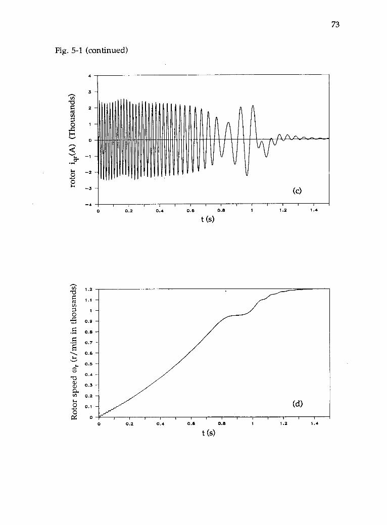
Fig. 5-1 (continued)

3 -

'CS2

0o 1

F-4O

t.

0

I I

-2 H

4

1.2

(c)

0 0.2 0.4I I

0.6 0.8

t (s)1 1.2 1.4

0.9 -

0.8 -

0.7 -

0.6 -

0.5 -

0.4 -

0.3 -

0.2 -

0.1 -

00 0.2 0.4 0.6 0.8

t (s)

(d)

1 1.2 1.4

73

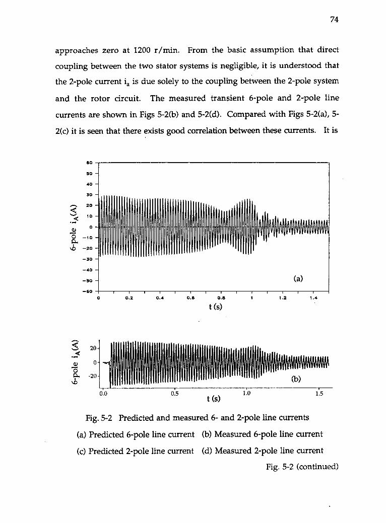
74

approaches zero at 1200 r/min. From the basic assumption that direct

coupling between the two stator systems is negligible, it is understood that

the 2-pole current is is due solely to the coupling between the 2-pole system

and the rotor circuit. The measured transient 6-pole and 2-pole line

currents are shown in Figs 5-2(b) and 5-2(d). Compared with Figs 5-2(a), 5-

2(c) it is seen that there exists good correlation between these currents. It is

-14

60

50

40

30

20

10

1.1o

0 10s.k) 20

30

III 11111 I1IIIIIIIII IIII1IIIIIIIIIg11111111

40 -

-50

60

20

cu 0

09. -20

fill I I Ili 1111111111 11111111111111111

:IWI'Ismat

(a)

0 0.2 0.4 0.6 0.8

t (s)1.2 1.4

6.0 0.5t (s)

1:0 1.5

Fig. 5-2 Predicted and measured 6- and 2-pole line currents

(a) Predicted 6-pole line current (b) Measured 6-pole line current

(c) Predicted 2-pole line current (d) Measured 2-pole line current

Fig. 5-2 (continued)

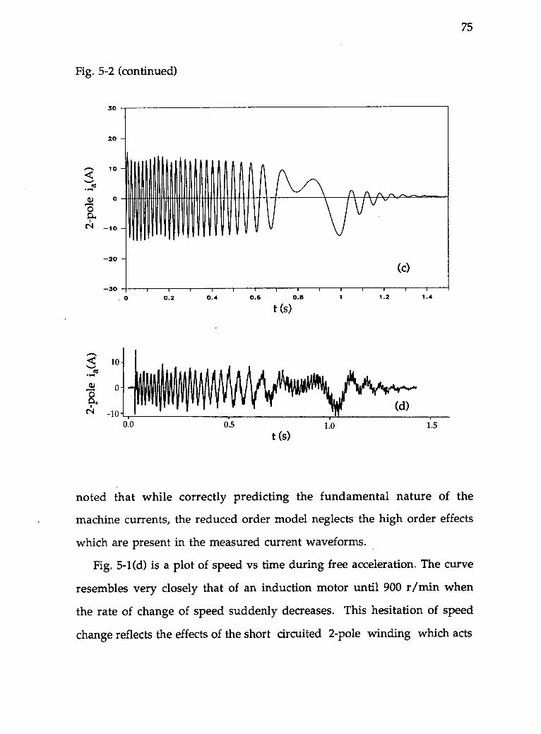
Fig. 5-2 (continued)

30

20 -

-20 -

-30

1010

(c)

0.0

0.2 0.4

0:5

0.6 0.6

t (s)1.2 1.4

t (s)1.0

75

noted that while correctly predicting the fundamental nature of the

machine currents, the reduced order model neglects the high order effects

which are present in the measured current waveforms.

Fig. 5-1(d) is a plot of speed vs time during free acceleration. The curve

resembles very closely that of an induction motor until 900 r/min when

the rate of change of speed suddenly decreases. This hesitation of speed

change reflects the effects of the short circuited 2-pole winding which acts

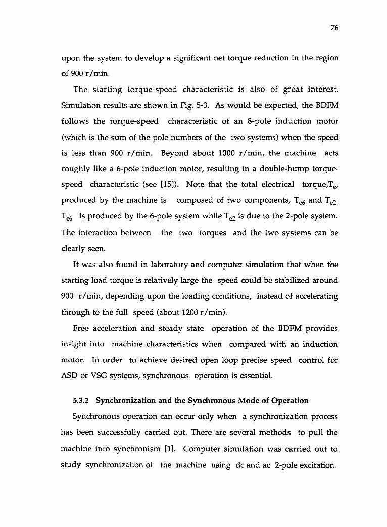
76

upon the system to develop a significant net torque reduction in the region

of 900 r/min.

The starting torque-speed characteristic is also of great interest.

Simulation results are shown in Fig. 5-3. As would be expected, the BDFM

follows the torque-speed characteristic of an 8-pole induction motor

(which is the sum of the pole numbers of the two systems) when the speed

is less than 900 r /min. Beyond about 1000 r/min, the machine acts

roughly like a 6-pole induction motor, resulting in a double-hump torque-

speed characteristic (see [15]). Note that the total electrical torque,Te,

produced by the machine is composed of two components, Te6 and Te2.

Tef, is produced by the 6-pole system while Te2 is due to the 2-pole system.

The interaction between the two torques and the two systems can be

clearly seen.

It was also found in laboratory and computer simulation that when the

starting load torque is relatively large the speed could be stabilized around

900 r/min, depending upon the loading conditions, instead of accelerating

through to the full speed (about 1200 r/min).

Free acceleration and steady state operation of the BDFM provides

insight into machine characteristics when compared with an induction

motor. In order to achieve desired open loop precise speed control for

ASD or VSG systems, synchronous operation is essential.

5.3.2 Synchronization and the Synchronous Mode of Operation

Synchronous operation can occur only when a synchronization process

has been successfully carried out. There are several methods to pull the

machine into synchronism [1]. Computer simulation was carried out to

study synchronization of the machine using dc and ac 2-pole excitation.

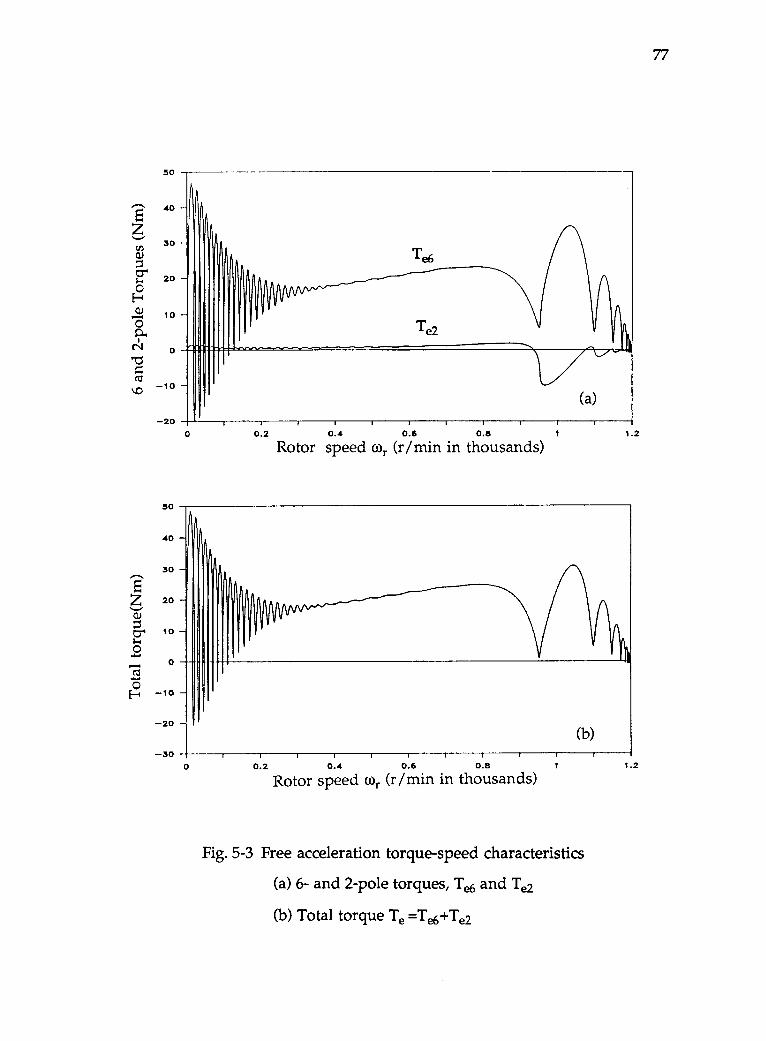
5Z

301

0 -Ci)

0-41.4 20 -0Fcu 10 -o0.4

N 0Ts

trs - 10 -

50

40 -

- 20

50

40

30

20

iiiTe2

(a)

0 0.2 0.4 0.6 0.8 1 1 2

Rotor speed co,. (r/min in thousands)

10 -

i

- 10 -

- 20 -

-30(b)

0 0.2 0.4 0.6 0.8 i

Rotor speed (J),. (r/min in thousands)

Fig. 5-3 Free acceleration torque-speed characteristics

(a) 6- and 2-pole torques, Te6 and Tee

(b) Total torque Te =Tes+Te2

1 2

77

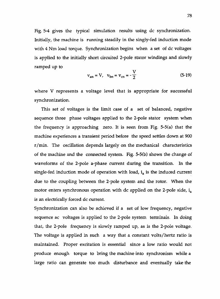
78

Fig. 5-4 gives the typical simulation results using dc synchronization.

Initially, the machine is running steadily in the singly-fed induction mode

with 4 Nm load torque. Synchronization begins when a set of dc voltages

is applied to the initially short circuited 2-pole stator windings and slowly

ramped up toV

Van = V/ Vbn """ Vcn = 2 (5-19)

where V represents a voltage level that is appropriate for successful

synchronization.

This set of voltages is the limit case of a set of balanced, negative

sequence three phase voltages applied to the 2-pole stator system when

the frequency is approaching zero. It is seen from Fig. 5-5(a) that the

machine experiences a transient period before the speed settles down at 900

r /min. The oscillation depends largely on the mechanical characteristics

of the machine and the connected system. Fig. 5-5(b) shows the change of

waveforms of the 2-pole a-phase current during the transition. In the

single-fed induction mode of operation with load, is is the induced current

due to the coupling between the 2-pole system and the rotor. When the

motor enters synchronous operation with dc applied on the 2-pole side, is

is an electrically forced dc current.

Synchronization can also be achieved if a set of low frequency, negative

sequence ac voltages is applied to the 2-pole system terminals. In doing

that, the 2-pole frequency is slowly ramped up, as is the 2-pole voltage.

The voltage is applied in such a way that a constant volts/hertz ratio is

maintained. Proper excitation is essential since a low ratio would not

produce enough torque to bring the machine into synchronism while a

large ratio can generate too much disturbance and eventually take the

1.3

1.2

1.1

1

0.9

0.8

0.7

0.6

0.5

0.4

0.3

0.2

0.1

0

26

(a)

2 3 4 5 6

t (s)

24

22

20

18

16

14.....c9.-t 12

(1) 100 a

ci 6

4

2

0

2 -- 4

6

$

(b)

I T

3 4

t (s)5 6

Fig. 5-4 DC synchronization simulation

(a) Speed vs time (b) 2-pole current is

79

80

machine into stall. Once the machine is running synchronously, the

applied voltage on the 2-pole side can be reduced to a substantially lower

level without losing synchronism. This is of practical importance in

certain applications since reducing the excitation voltage means reducing

the rating requirements of the power converter and hence its cost.

In steady state synchronous operation, the shaft speed can be

determined by the following expression

f6 f2shaft speed (r/min) = 60 (5-20)

where f6 and f2 denote the 6-pole utility power supply frequency and the 2-

pole supply frequency from the power electronic converter, respectively.

P6 and P2 are the pole-pair numbers for the two systems.

Fig. 5-5 shows the synchronous and fault tolerant behavior of the BDFM

system. The following three situations are considered in the simulation:

(a) Machine response to a sudden reduction of 2-pole excitation

voltage.

(b) Machine response to a ramp and a step change of load torque.

(c) Machine response to a sudden loss of 2-pole excitation.

Initially, the motor is running synchronously at 870 r/min ( f2=2Hz )

with load torque equal to zero. At t=3.5 seconds the 2-pole excitation

voltage V2 is step changed to 0.5V2 . This sudden change of excitation

voltage results in lower 6 and 2-pole currents while the machine is still in

synchronous operation.

At t=5.0 seconds, load torque is ramped up from zero to 20 Nm. Similar

to conventional synchronous machines, the BDFM is seen to maintain

synchronous operation at the speed of 870 r/min.

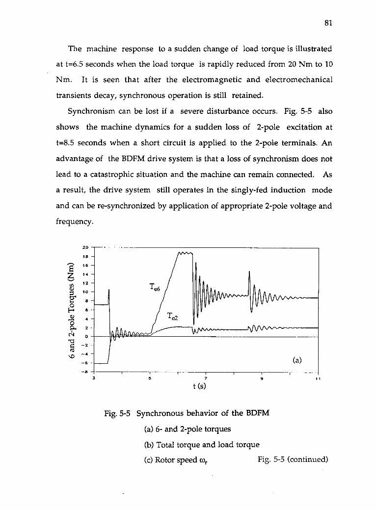
81

The machine response to a sudden change of load torque is illustrated

at t=6.5 seconds when the load torque is rapidly reduced from 20 Nm to 10

Nm. It is seen that after the electromagnetic and electromechanical

transients decay, synchronous operation is still retained.

Synchronism can be lost if a severe disturbance occurs. Fig. 5-5 also

shows the machine dynamics for a sudden loss of 2-pole excitation at

t=8.5 seconds when a short circuit is applied to the 2-pole terminals. An

advantage of the BDFM drive system is that a loss of synchronism does not

lead to a catastrophic situation and the machine can remain connected. As

a result, the drive system still operates in the singly-fed induction mode

and can be re-synchronized by application of appropriate 2-pole voltage and

frequency.

8

6 -PAN-

- 2

- 6

- 8

(a)

5 7

t (s)9

Fig. 5-5 Synchronous behavior of the BDFM

(a) 6- and 2-pole torques

(b) Total torque and load torque

(c) Rotor speed cor Fig. 5-5 (continued)

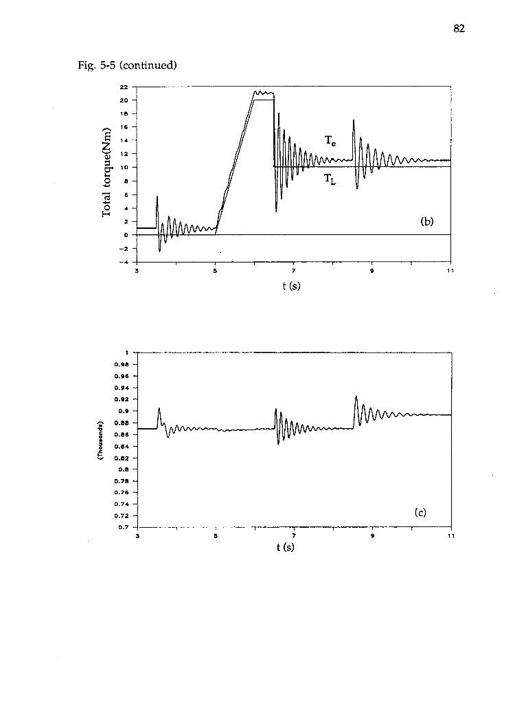
Fig. 5-5 (continued)

22

20

18

16

14

12

10

a

6

4

2

43

1

0.98

0.96

0.94 N

1

'

....

0.92

0.9

0.8833ccl 0.86aln0 0.840.0. 0.02

0.8

0.78

0.76

0.74

0.72

0.7

$

V

Te

Ti,

(b)

5 7

t (s)

9 11

$

(c)

3 5 7

t (s)

82

9 11

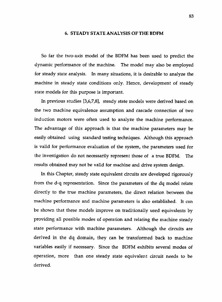
83

6. STEADY STATE ANALYSIS OF THE BDFM

So far the two-axis model of the BDFM has been used to predict the

dynamic performance of the machine. The model may also be employed

for steady state analysis. In many situations, it is desirable to analyze the

machine in steady state conditions only. Hence, development of steady

state models for this purpose is important.

In previous studies [3,6,7,8], steady state models were derived based on

the two machine equivalence assumption and cascade connection of two

induction motors were often used to analyze the machine performance.

The advantage of this approach is that the machine parameters may be

easily obtained using standard testing techniques. Although this approach

is valid for performance evaluation of the system, the parameters used for

the investigation do not necessarily represent those of a true BDFM. The

results obtained may not be valid for machine and drive system design.

In this Chapter, steady state equivalent circuits are developed rigorously

from the d-q representation. Since the parameters of the dq model relate

directly to the true machine parameters, the direct relation between the

machine performance and machine parameters is also established. It can

be shown that these models improve on traditionally used equivalents by

providing all possible modes of operation and relating the machine steady

state performance with machine parameters. Although the circuits are

derived in the dq domain, they can be transformed back to machine

variables easily if necessary. Since the BDFM exhibits several modes of

operation, more than one steady state equivalent circuit needs to be

derived.

84

The development of the steady state models makes it possible to

investigate steady state performance of the BDFM. However, it will be

shown that certain operational modes of the machine require a special

solution technique, which is also developed in this Chapter.

6.1 Steady State Models in the dq Domain

6. 1.1 The Synchronous Mode of Operation

The stator d-q variables are related with physical variables through the

transformations Cs6 and Cs2. In steady state operations, where 9,.=cort, Eqns

(5-9) through (5-12) thus become

Vq6 = P2 V6 COS[((06 - 30)r)t]

Vd6 = VI V6 sin [(co6 - 3cor)t]

Vq2 = Air V2 COS[(0)2+4)t-131

vd2 = 41 V2 Sin((0)2+Cadt-13]

(6-1)

(6-2)

(6-3)

(6-4)

with 06 = 0 and 13 being the angle between the reference voltage vo and vq2 .

In phasor representations, (6-1) through (6-4) can be written as

also

V,- ,.

1 7 -iI3 x T. .7= Vq6 q6 / v d6= j v (36 , v q2 = v q2 e , v d2 = i V q2

1d6 = ilq6 /

(6-5)

1d2 = jiq2 / Idr = jiqr (6-6)

-4-3- .Ni5where Vq6 = 2 V6 and Vq2 = 2 V2 are the rms voltages of the qd variables.

In the d-q domain, all the d-q quantities have the same slip frequency

s1co6 = (0)6-30)r)=(0)2 +4). Thus, replacing the differentiation operator p with

j(0)6-3c)r) or j(o)2+wr) and expanding the first equation of the two axis

model representation (4-61), we obtain

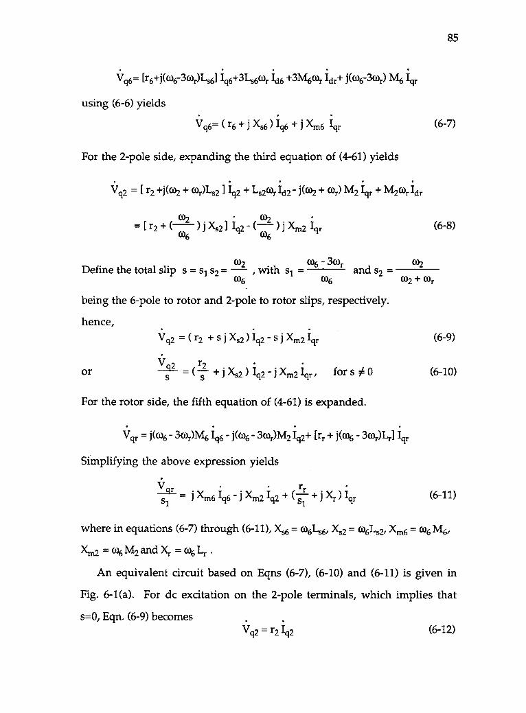
Vq6= Er6+j(C06-3(0r)Ls6] Iq6+3Ls6(0, Id6 +3M6COr Idr+ j((06-3(0r) M6 Iqr

using (6-6) yields

Vq6= ( r6 + j Xs6 ) Iq6 + J Xm6 Iqr

For the 2-pole side, expanding the third equation of (4-61) yields

Vq2 = [ r2 +j(co2 + cor)L,21 Iq2 + Ls2COr Ic12 j(w2 + (Dr) M2 Iqr + M2C°r 'dr

=Er2+(C°6 2 21)iXs2] Iq2-()jXm2 icyC°6

0)2 0)6 30)r 0)2Define the total slip s = si s2 = , with si = and s2w6 (06 0)2 + 0)r

being the 6-pole to rotor and 2-pole to rotor slips, respectively.

hence,

or

Vq2 = ( r2 + S j Xs2 ) Iq2 - S j Xm2 Iqr

V r2AL ,...._s ` s + i Xs2 ) 1q2 i Xm2 Iqr ,

85

(6-7)

(6-8)

(6-9)

for s 0 (6-10)

For the rotor side, the fifth equation of (4-61) is expanded.

. . . .

Vqr = j(0)6 - 3(or)M6 Iq6 - j(0)6 - 3C0r)M2 412+ Err + j(Ca)6 - 3C0r)Lr] Iqr

Simplifying the above expression yields

V rSiIL .

= j Xm6 Iq6 - j Xm2 Iq2 + ( sr + j Xr ) Iqr (6-11)

where in equations (6-7) through (6-11), Xs6 = °3- -646, Xs2 = M--61--s2, Xm6 = C°6 M6,

Xm2 = C°6 M2 and Xr = W6 It

An equivalent circuit based on Eqns (6-7), (6-10) and (6-11) is given in

Fig. 6-1(a). For dc excitation on the 2-pole terminals, which implies that

s=0, Eqn. (6-9) becomes .

Vq2 = r2 412 (6-12)

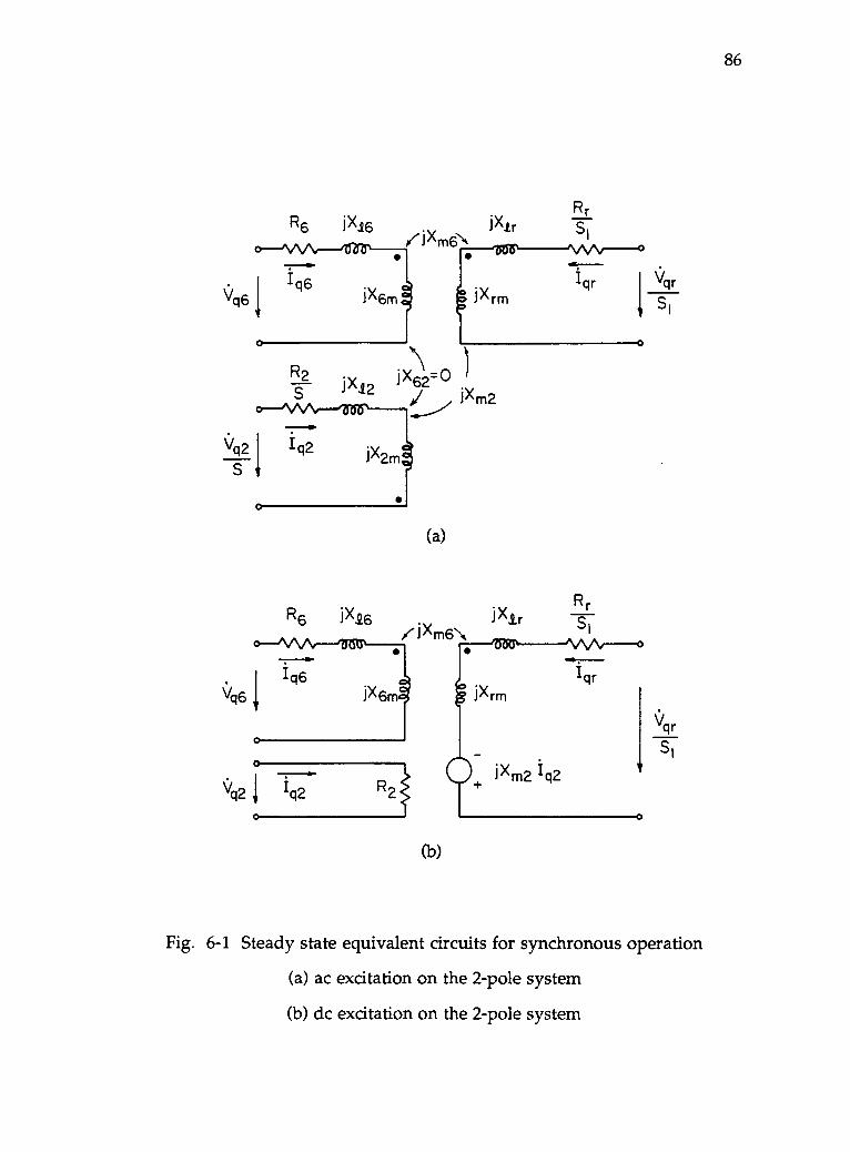
:10,E\

V-12-

RjS\V.4"(

T.) \

dal

87

The equivalent circuit for this operating condition is shown in Fig. 6-1(b)from which it is seen that the 2-pole stator system becomes purely resistive.

6.1.2 Singly-Fed Induction Mode of Operation with 2-pole System

Short-Circuited

A steady state equivalent circuit for the singly-fed induction mode of

operation with 2-pole system short circuited may also be derived using

similar techniques to those shown above. It is easy to verify the following

equations:

Vq6= (r6 + j Xs6 ) 1q6 + j Xm6 iqr (6-13)

. .

0 = ( r2 + s j Xs2) Iq2 - s j Xm2 Iqr (6-14)

r2or ° = (---s + i Xs2) 1q2 i Xm2 'qv for s 0 (6-15)

V rrg l = j Xm6 1q6 j Xm2 I

q Si2 + ( + j Xr ) Iqr (6-16)

Si

It can be shown that in singly-fed induction mode of operation with

2-pole side short circuited, the relation (0)6 30)r) = (0)2 + ()r) still holds.

However, it must be understood that w2 is the induced frequency. From the

above expression, it follows that

0)2 (06 40)rs- -w6 0)6

(6-17)

From equations (6-13), (6-14) and (6-16), an equivalent circuit can be

obtained by short circuiting the 2-pole input terminals in Fig. 6-1(a) for 2-

pole ac excitation. A special case is when the machine is running at 900

r/min. Since s=0 and 1,42 = 0, (6-14) vanishes, which means that at this

speed there are no effects from the short circuited 2-pole winding on the

88

system. The equivalent circuit in this case is the same as that of a

conventional induction motor.

The equivalent circuit expressed in terms of d axis variables can also be

readily obtained. For the synchronous mode of operation, upon substi-

tuting (6-5) and (6-6) into equations (6-7),(6-9) and (6-11), we obtain

Vd6= ( r6 + ) Xs6 ) Id6 + j Xm6 Idr (648)

Vd2 = ( r2 + s ) Xs2 ) 412 +S j Xm2 Idr (649)

Vs

s (S +) xs2 ) 412 +) Xm2 1d2 f for s i 0 (6-20)

sir r,.

= j Xm6 Id6 + j Xm2 Id2 + (Si + j Xr ) Idr (6-21)

These equations can be shown to be equally valid for describing the steady

state behavior of the BDFM under the synchronous mode of operation.

Since d and q variables are linearly dependent in steady state operation,

only one set of equations need be used.

It is important to note the advantage of deriving steady state equivalent

circuits for the singly-fed induction mode and the doubly-fed synchronous

mode of operation from the d-q domain in which all the quantities have

the same rotor slip frequency which depends on the speed of the machine.

Research is now underway to apply these steady state models expressed in

both dq and machine variables for machine and control designs.

6.2 Steady State Models in Machine Variables

Steady State models or equivalent circuits expressed in actual machine

variables, which are useful for correlating test data and deriving machine

parameters from tests, may be obtained from dq domain models or

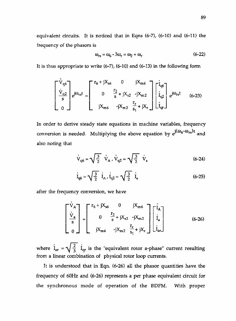
89

equivalent circuits. It is noticed that in Eqns (6-7), (6-10) and (6-11) the

frequency of the phasors is

(ors = 0)6 3(or = 032 + (or (6-22)

It is thus appropriate to write (6-7), (6-10) and (6-13) in the following form

Vq6 iXs6 jXm6 ig6-1

[17q2 eiWrst 0 -?+xmi.X2

+ jX iqr

s2 -Pcn2 ig2

rr LiL 0 _IJxm6

ejCOrst(6-23)

In order to derive steady state equations in machine variables, frequency

conversion is needed. Multiplying the above equation by el(a)6-a/rs)t and

also noting that

3Vq6 =

\FT1q6

Va (6-24)

IA / Iq2 = 2 Ia (6-25)

after the frequency conversion, we have

VA

Va

S

L 0 J

r6 + jXs6

0 + jXs2 -Pcn2 Ia

r2

0 jXm6

p(m6 -Jxm2 as ixr

(6-26)

2 .where Iar = "\F-3 iqr is the "equivalent rotor a-phase" current resultingfrom a linear combination of physical rotor loop currents.

It is understood that in Eqn. (6-26) all the phasor quantities have the

frequency of 60Hz and (6-26) represents a per phase equivalent circuit for

the synchronous mode of operation of the BDFM. With proper

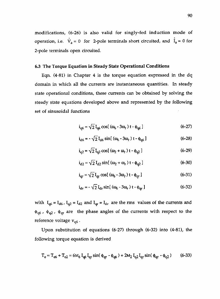
90

modifications, (6-26) is also valid for singly-fed induction mode of

operation, i.e. Va = 0 for 2-pole terminals short circuited, and Ia = 0 for

2-pole terminals open circuited.

6.3 The Torque Equation in Steady State Operational Conditions

Eqn. (4-81) in Chapter 4 is the torque equation expressed in the dq

domain in which all the currents are instantaneous quantities. In steady

state operational conditions, these currents can be obtained by solving the

steady state equations developed above and represented by the following

set of sinusoidal functions

iq6 = .ViIq6, COS[ 0.06 30)r ) t (1)q6 1 (6-27)

id6 = 42-1(16 sin[ (0)6 3(0r ) t (0q6 ] (6-28)

iq2 = 'Nalci2 ws[ ((2 + (ur ) t (I)q2 i (6-29)

1d2 = .\ri 412 sin[ (0)2 + (Or ) t 4)(12 ] (6-30)

iqr = 4iIqr COS[ ((.06 - 30)r ) t - kir ] (6-31)

idr = 'VD& sin[ ((-)6 3(°r ) t -4)qr ] (6-32)

with 416 = 1d6 , 412 = 412 and Iqr = 'dr are the rms values of the currents and

(1),16 , $q2 , (1) are the phase angles of the currents with respect to the

reference voltage vo .

Upon substitution of equations (6-27) through (6-32) into (4-81), the

following torque equation is derived

Te = Tee + Te2 = 6M6 Iq6 Iqr sin( 4qr 4 )(46 ) + 2M2 ki2 Iqr sin( 4qr 4 q2 ) (6-33)

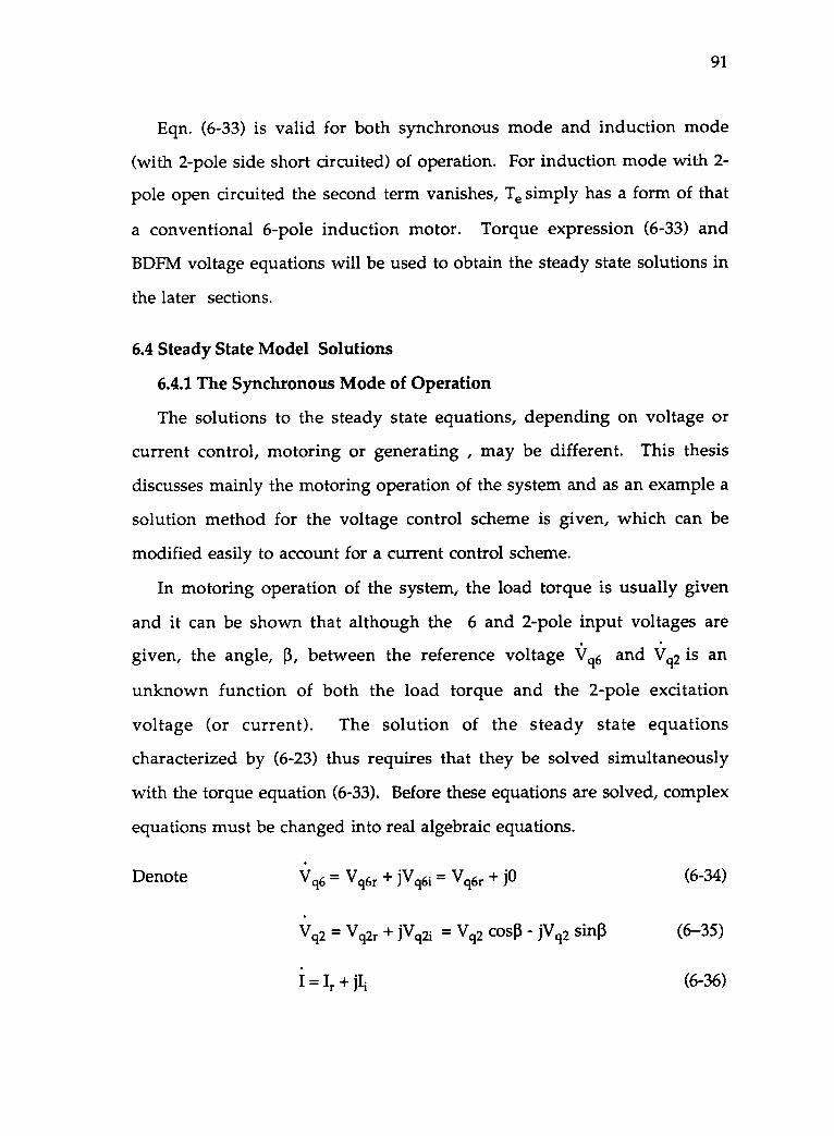
91

Eqn. (6-33) is valid for both synchronous mode and induction mode

(with 2-pole side short circuited) of operation. For induction mode with 2-

pole open circuited the second term vanishes, Te simply has a form of that

a conventional 6-pole induction motor. Torque expression (6-33) and

BDFM voltage equations will be used to obtain the steady state solutions in

the later sections.

6.4 Steady State Model Solutions

6.4.1 The Synchronous Mode of Operation

The solutions to the steady state equations, depending on voltage or

current control, motoring or generating , may be different. This thesis

discusses mainly the motoring operation of the system and as an example a

solution method for the voltage control scheme is given, which can be

modified easily to account for a current control scheme.

In motoring operation of the system, the load torque is usually given

and it can be shown that although the 6 and 2-pole input voltages are

given, the angle, 11, between the reference voltage q6 and Vq 2 is an

unknown function of both the load torque and the 2-pole excitation

voltage (or current). The solution of the steady state equations

characterized by (6-23) thus requires that they be solved simultaneously

with the torque equation (6-33). Before these equations are solved, complex

equations must be changed into real algebraic equations.

Denote Vq6 = Vq6r + iVq6i = Vq6r + j° (6-34)

= Vq2 cos 13Vq2 = Vq2r + iVq2i JVq2 sin (6-35)

I = Ir + jIi (6-36)

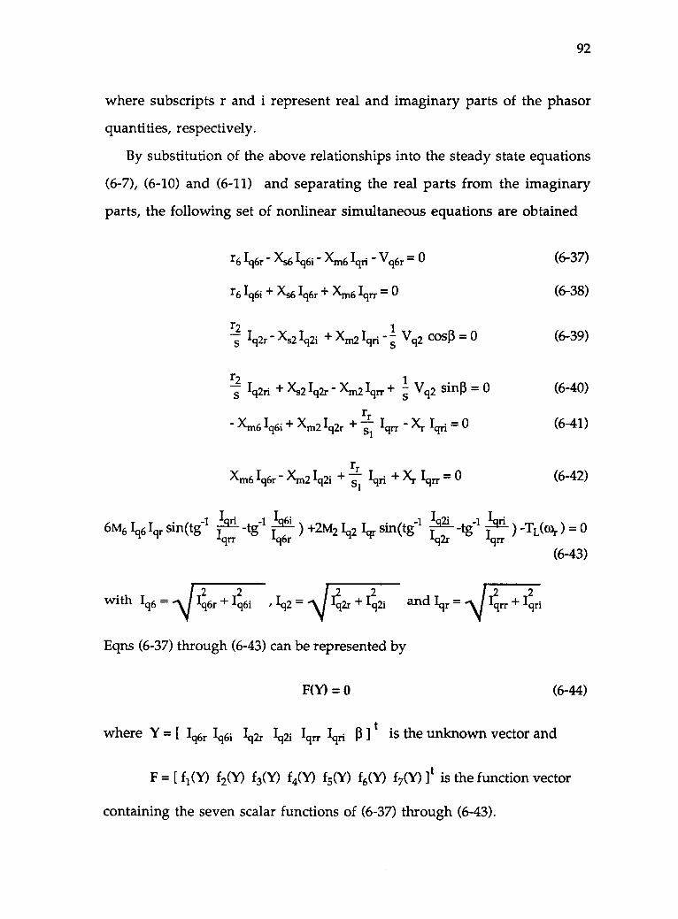
92

where subscripts r and i represent real and imaginary parts of the phasor

quantities, respectively.

By substitution of the above relationships into the steady state equations

(6-7), (6-10) and (6-11) and separating the real parts from the imaginary

parts, the following set of nonlinear simultaneous equations are obtained

6M6 Iq6 Iqr sin(te

r6 Ior - Xs6 Iq6i - Xm6 Iqri - Vol. = 0 (6-37)

r6 Iq6i + ;6 Tor + Xm6 Iqrr = 0 (6-38)

r2 1+ Xm2 Iqri - -s Vq2 COSP = 0 (6-39)s Iq2r Xs2 Iq2i

r2 1Ici2ri + Xs2 Ig2r - Xm2 I

qrr s+ Vq2 sini3 = 0 (6-40)

rr- Xm6 Iq6i + Xm2 Iq2r + si Iqrr - Xr Iqri = 0 (6-41)

rrXm6 Iq6r Xm2 Iq2i 4- si Iqri + Xr Iqrr = ° (6-42)

, 4 &i. sn(t -1 -gLi 4 1-aril ) -TL(cor ) = 0) +2M2 /q2 qr i g T -tg1

iqrr -g Iq6§I

r 1q2r qrr

with Iq6 = Ai 2 2Iq6r + Iq6i ..q .,.2

12 = Iq2r + .1.442i

Eqns (6-37) through (6-43) can be represented by

and Iqr = - 1cirr + I2ciri

(6-43)

F(Y) = 0 (6-44)

where Y = [ Icor Iq6i Iq2r Iq2i Iqrr Iqri 0 ] t is the unknown vector and

F = [ f1(Y) f2(Y) f3(Y) f4(Y) f5(Y) f6(Y) f7(Y) It is the function vector

containing the seven scalar functions of (6-37) through (6-43).

93

Solution techniques for (6-44) are readily available and it was found that

Newton-Raphson's algorithm is adequate in founding the solution. Let i

be the iteration index,

then

y(i) y(i-1) Ay(1-1)

Aya4) r aF 14

F(i -1)

aY

The entries of the Jacobian matrix, [ aFaY

(6-45)

i=1,2,...,7 (6-46)

afmniLaYmnJ n

= 1,2,...7. are

computed as follows:

It is noticed that four out of seven equations in (6-37) through (6-43) are

linear so that the Jacobian matrix entries for these equations are just the

circuit parameters themselves. Other entries of the Jacobian matrix are

given below without providing intermediate results

af3 af4= v 2 sinfi , = V 2 coshr3 s q a13 s q

af, af7- - 61s,46 1q, , - -1V12 , 2IV12 ,aiq6r alq2i

af, 6m6 ici6; 2M2 L2i , = -6M6 Icfir 2M2 Iq2ralqri

The initial values for the solution vector Y(o) , which have to be

reasonably close to the true solution, need to be given in order to start the

algorithm. To ensure good convergence to an acceptable solution, the

initial estimated values can be obtained by an appropriate initial guess for

(3(0) , followed by solutions for the other unknowns using (6-23). So long as

IP) is chosen to be close to the true solution, other initial values are also

94

close to the solution. It was found that that for 230V 6-pole supply voltage

and moderate level of 2-pole excitation voltage, it is appropriate to assign

p(°) = 20° , for 0.5 s TL < 10 (Nm)

Q` °) = 60° , for 10 < TLS 20 (Nm)

13(°) = 9o°, for 20 < TL < 30 (Nm)

Depending on different 2-pole excitation voltage, the 13(0) values may be

adjusted so that fast convergence can be obtained.

Fig. 6-2 shows typical computational results of 13 angle for different

values of constant load torque operation of the BDFM drive system. A

constant V /Hz ratio of 5 is maintained over the entire speed range. Rapid

changes of 0 at low 2-pole frequencies or high speeds, which contribute to

the changes of circuit impedances due to slips (both s1 and s), can be

observed. At low speeds, 13 can be seen remain fairly constant.

6.4.2 Singly-Fed Induction Mode of Operation

The synchronous mode of operation of the BDFM is a highly preferred

operational mode for ASD and VSG applications of the system. However,

as pointed out in Chapters 1 and 5, with the present state converter controls

it can not be realized unless a successful synchronization process has been

carried out from the induction mode. Two possible singly-fed induction

modes of operation exists with 2-pole terminals open and short circuited.

The former case is well known while the latter needs more discussion.

Solving for the steady state equations is a straightforward process. What

is of interest is the torque speed characteristics in this mode of operation. A

closed form solution to Te , which can be obtained by first solving (6 -13)-

(6-16) for currents then substituting them into (6-33), is tedious and

95

complicated thus will not be given. Numerical computation results are

presented and discussed below.

A typical torque speed characteristic is given in Fig. 6-3. It is clearly seen

that for a given load torque/speed characteristic, such as a constant load,

there might exist two possible stable operating points. There also exists a

region between two stable regions in which the motor can not operate

stablely. Conventional induction motors do not possess this feature.

Experimental and computer simulation results reveal, however, that it is

usually easier for the motor to be synchronized if the motor is running

around 900 r /min in the induction mode before synchronization begins.

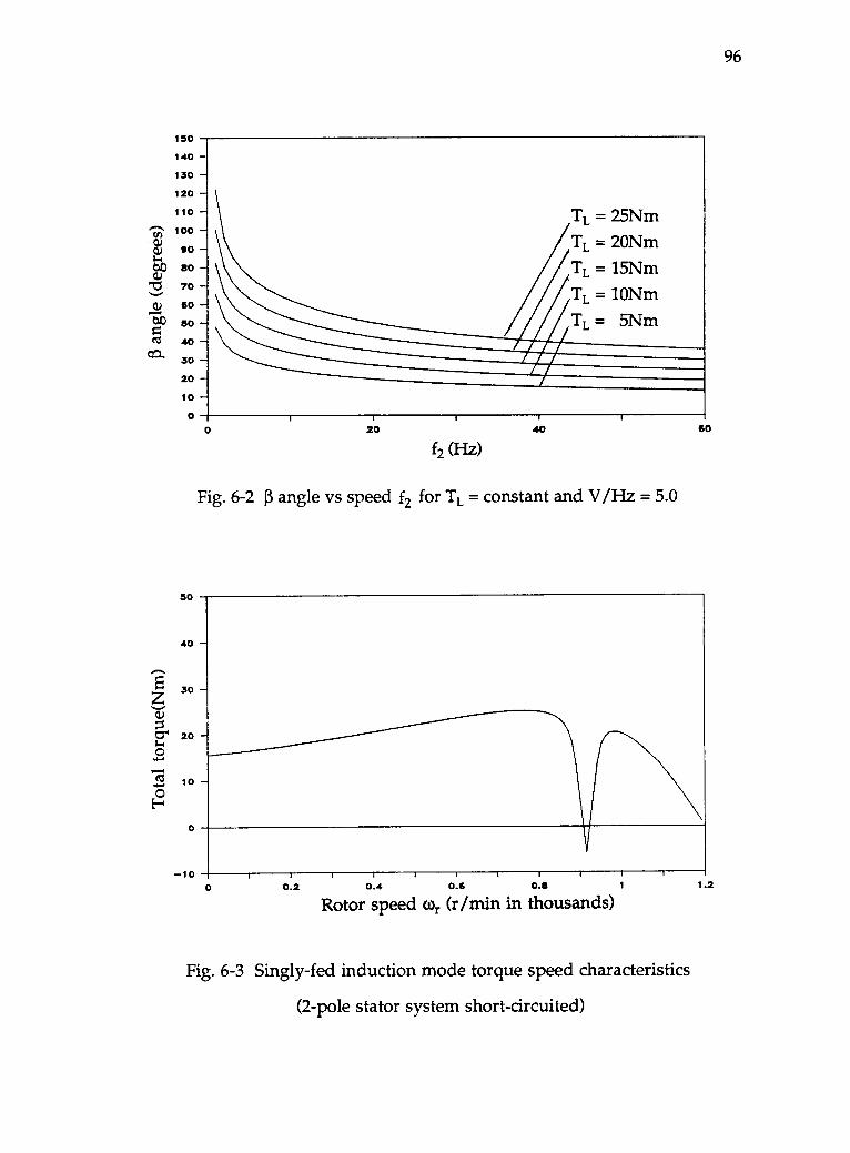
150

140 -130 -120 -110 -

y 10090 -

/§1380 -

"C$ 70

4) 60 -Of) 50 -ZC5 40 -

Ca.. 30 -20 -10 -0

50

TL = 25Nm

/TL = 20Nm

TL = 15Nm

TL = 10Nm

TL = 5Nm

0 20

f2 (Hz)

40

Fig. 6-2 13 angle vs speed f2 for TL = constant and V/Hz = 5.0

60

40 -

30 -

20 -

10 -

0

-100 0.2 0.4 0.6 0.8 1

Rotor speed cor (r/min in thousands)

Fig. 6-3 Singly-fed induction mode torque speed characteristics

(2-pole stator system short-circuited)

1 2

96

97

7. STABILITY ANALYSIS OF THE BDFM

The primary purpose of developing a two-axis model is to analyze the

dynamic behavior of the machine and to develop control strategies for

specific applications of the BDFM system. In Chapter 2, the dynamic

performance of the machine in synchronous mode of operation was

investigated at a fixed 2-pole frequency. It was shown that for 230V 6-pole

input voltage and 2Hz 2-pole excitation, although the response of the

machine to sudden changes of inputs was oscillatory, stable operation

could be maintained after transitions. It was found in the laboratory,

however, that stability problems may arise when a wide range of speed

control is required. It is hence important to investigate the stability of the

machine on a wide speed range basis.

A search of appropriate literature indicates that the stability problems of

this type of machine have been investigated using a two wound rotor

induction machine model in cascade connection. This was necessary

because of a lack of a truly representative model and its parameters for the

single-frame self-cascaded machine. Previous studies have shown that

over much of the potentially useful operating region the machine is either

inherently unstable or its dynamic response is seriously underdamped. It

is concluded from the studies that by appropriate design, certain areas of

instability may be reduced or removed and the response improved, but that

it is not possible, by design changes alone, to remove all such unstable

areas. These results, however, do not seem to be in agreement with the test

results found in the laboratory. Tests showed that for the 6 and 2-pole

BDFM with a common stator winding and a "Broadway rotor", there

existed an unstable region between roughly 630 r/min to 525 r/min (corres-

98

ponding to 18Hz to 25Hz for the 2-pole input frequency), which was not

predicted correctly by [9,10]. For a newly designed BDFM with truly

balanced stator windings [13,15] and a "Broadway rotor", open loop stability

occurs over the entire speed range under proper 2-pole excitation.

In order to carry out stability and control studies in more depth in

conjunction with machine and drive system design, a two-axis model

derived in Chapter 4 is used to investigate the stability of the system in the

synchronous mode of operation.

The stability characteristics of ASDs using either induction machines or

synchronous machines have long been known [19,20]. Stability analyses of

electric machines and drive systems commonly utilize Lyapunov's indirect

method, in which the original nonlinear differential equations are

linearized around an equilibrium point, at which the stability

characteristics of the point are evaluated. The result is then applied to the

original nonlinear system.

In order to use Lyapunov's indirect method, reference frames must be

selected carefully so that the linearized machine or drive equations are as

simple as possible. For example, the stability of an induction machine and

its drive system is usually investigated in the synchronous reference frame

in which all the steady state quantities (equilibrium points) are constants.

This will, in turn, result in a linear time-invariant system afterlinearization has been carried out. For the synchronous machine and its

drive system, since the rotor reference frame coincides with the

synchronous reference frame in steady-state operations, the resulting

linearized-machine and drive equations are also time-invariant.

Unfortunately, this is not true for a BDFM system for which the two-axis

model must be expressed exclusively in the rotor reference frame. In

99

steady state operation, all dq quantities are found to vary sinusoidally at a

slip frequency, with the result that the linearized machine equations are

time-varying. Consequently, commonly used eigenvalue analysis techni-

ques cannot be applied to perform stability studies.

A closer examination of the linearized system of equations of the BDFM

reveals that although the system matrix is time-varying, it is periodic.

Thus, the generalized theory of Floquet can be utilized to transform the

linear time-varying system of equations into an equivalent set of equations

with a constant system matrix. Since the two systems are equivalent in the

sense of Lyapunov, eigenvalue analysis can be performed on the Floquet

transformed system to predict the stability characteristics of the original

nonlinear system at a given equilibrium point.

7.1 Linerized Two-axis Model Equations

Linearized two-axis model equations are obtained using Taylor series

expansion at a given equilibrium point. The results of the linearized

equations are incorporated into one matrix equation as shown in (7-1).

where

Ai0 1 . [ R'(t) + Lp ] [Aer

All Awr

,Atv = [ Avo A ivd6 Avq2 AVd2 0 v

tAl = [ Aiq6 Aid6 Aiq2 Aid2 Aiqr Aidr ]

(7-1)

In doubly-fed operation, the two sets of applied three-phase voltages

with opposite sequence, namely vA , vB , vc from the 6-pole system and

va , vb , vc from the 2-pole system can be transformed into two sets of

orthogonal dq voltages plus the zero sequences through two

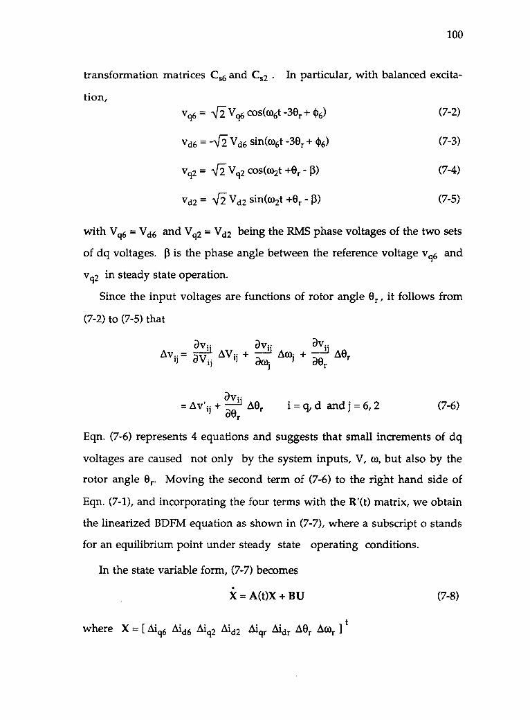
100

transformation matrices Cs6 and Cs2 . In particular, with balanced excita-

tion,Vq6 = .NriVq6 COS(036t -39r + 46) (7-2)

Vd6 = nri, Vd6 sin(o)6t -30/- + 4)6) (7-3)

vq2 = .Nri Vq2 cos(0)2t +Or - (3) (7-4)

Vd2 = Vi Vd2 sin(co2t +Or -13) (7-5)

with Vq6 = -vd6 and Vq2 = Vd2 being the RMS phase voltages of the two sets

of dq voltages. f is the phase angle between the reference voltage vq6 and

vq2 in steady state operation.

Since the input voltages are functions of rotor angle Or , it follows from

(7-2) to (7-5) that

a---vi,av--

ay.iAvii = avi AVii + ac. Aoi + ae AOr

jI

avii= Av ii + AOr i = q, d and j = 6, 2 (7-6)

Eqn. (7-6) represents 4 equations and suggests that small increments of dq

voltages are caused not only by the system inputs, V, co, but also by the

rotor angle Or. Moving the second term of (7-6) to the right hand side of

Eqn. (7-1), and incorporating the four terms with the R'(t) matrix, we obtain

the linearized BDFM equation as shown in (7-7), where a subscript o stands

for an equilibrium point under steady state operating conditions.

In the state variable form, (7-7) becomes

X = A(t)X + BU (7-8)

where X = [ Aio Aid6 Aiq2 Aid2 Aiqr Aidr Aer AWr ] t

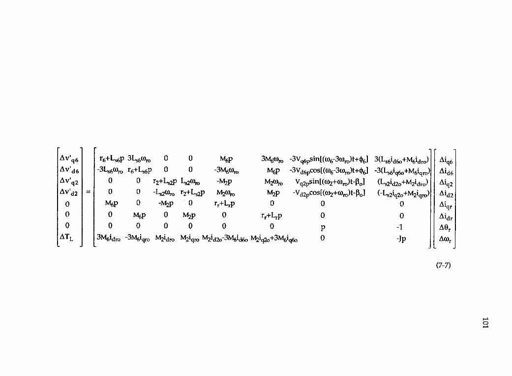
AVq6

AV'd6

AVici2

AVid2 =

r6+Ls6P 31-s6(oro 0 0 M6P 3Moro -3Vc6psin[0.06-3cordt+06]-3L,606 r6+Ls6p 0 0 -3M6coro M6P -3Vd6pCOS[(c06-30)ro)t+06]

o o r2+1-s2P 1-s2(0ro -M2P M203ro Vq2psin[(()2+06)t-001o o -Ls263ro r2+Ls2p M240 M2p -Vd2pcos[002+(ordt-11.]

3(1-s61d6o+M61dro)

-3(Ls6i00+M6igro)

(Ls21d2o±M21dro)

(-1-s21q2o+M2iqro)

Aig6

Aid6

Aiq2

Aid20 m6P 0 -M2p 0 rr+Lrp 0 0 0 Aiqr

0 0 m6P 0 M2p 0 rr+Lrp 0 0 Aidr0 0 0 0 0 0 0 P -1 AOr

A TL 3M6ldro -3m61ciro M2idro M2iciro Isn2id2C3M6id6o IsA2iq2o+3M6iq6o 0 -JP A0),

(7-7)

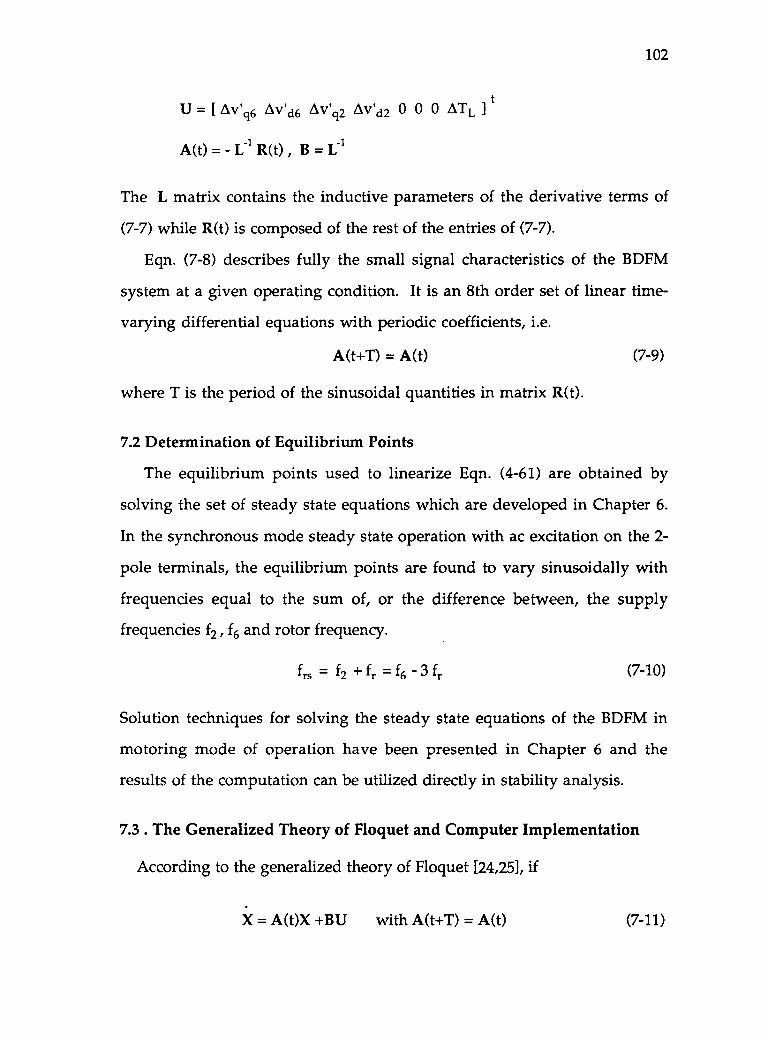
102

U = [ Av'q6 Av'd6 Av'q2 Av'd2 0 0 0 ATL t

A(t) = R(t) , B =

The L matrix contains the inductive parameters of the derivative terms of

(7-7) while R(t) is composed of the rest of the entries of (7-7).

Eqn. (7-8) describes fully the small signal characteristics of the BDFM

system at a given operating condition. It is an 8th order set of linear time-

varying differential equations with periodic coefficients, i.e.

A(t+T) = A(t) (7-9)

where T is the period of the sinusoidal quantities in matrix R(t).

7.2 Determination of Equilibrium Points

The equilibrium points used to linearize Eqn. (4-61) are obtained by

solving the set of steady state equations which are developed in Chapter 6.

In the synchronous mode steady state operation with ac excitation on the 2-

pole terminals, the equilibrium points are found to vary sinusoidally with

frequencies equal to the sum of, or the difference between, the supply

frequencies f2, f6 and rotor frequency.

frs = f2 +fr =f6 3 fr (7-10)

Solution techniques for solving the steady state equations of the BDFM in

motoring mode of operation have been presented in Chapter 6 and the

results of the computation can be utilized directly in stability analysis.

7.3 . The Generalized Theory of Floquet and Computer Implementation

According to the generalized theory of Floquet [24,25], if

X = A(t)X +BU with A(t+T) = A(t) (7-11)

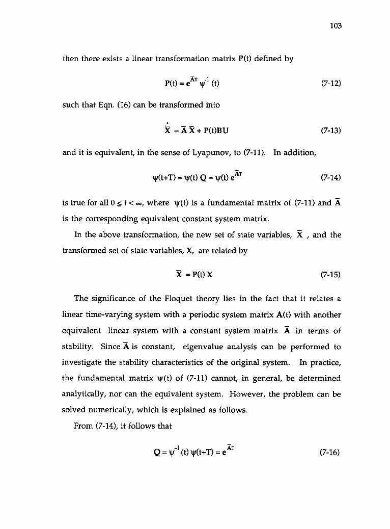
then there exists a linear transformation matrix P(t) defined by

P(t) = eAT yr1 (t)

such that Eqn. (16) can be transformed into

103

(7-12)

= A 5C. + P(t)BU (7-13)

and it is equivalent, in the sense of Lyapunov, to (7-11). In addition,

v(t+T) = N1(t) Q = w(t) eAT (7-14)

is true for all 0 < t < oo, where 41(t) is a fundamental matrix of (7-11) and A

is the corresponding equivalent constant system matrix.

In the above transformation, the new set of state variables, X , and the

transformed set of state variables, X, are related by

= P(t) X (7-15)

The significance of the Floquet theory lies in the fact that it relates a

linear time-varying system with a periodic system matrix A(t) with another

equivalent linear system with a constant system matrix A in terms of

stability. Since A is constant, eigenvalue analysis can be performed to

investigate the stability characteristics of the original system. In practice,

the fundamental matrix v(t) of (7-11) cannot, in general, be determined

analytically, nor can the equivalent system. However, the problem can be

solved numerically, which is explained as follows.

From (7-14), it follows that

Q = yr (t) v(t+T) = e AT (7-16)

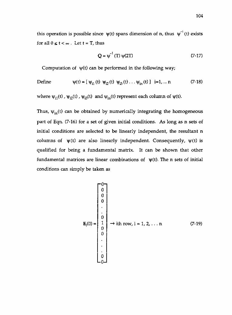
104

this operation is possible since W(t) spans dimension of n, thus v-1 (t) exists

for all 0 s t < 0. . Let t = T, thus

Q = v1 (T) v(2T) (7-17)

Computation of v(t) can be performed in the following way;

Define V(t) = [ veil (t) Wit (t) Wi3 (t) . . . Win (t) I i=1, ... n (7-18)

where vii(t) , vi2(t) , vi3(t) and vin(t) represent each column of v(t).

Thus, vin(t) can be obtained by numerically integrating the homogeneous

part of Eqn. (7-16) for a set of given initial conditions. As long as n sets of

initial conditions are selected to be linearly independent, the resultant n

columns of v (t) are also linearly independent. Consequently, v (t) is

qualified for being a fundamental matrix. It can be shown that other

fundamental matrices are linear combinations of V(t). The n sets of initial

conditions can simply be taken as

Ei(0) =

rl00

01

00

W

---> ith row, i = 1, 2, . . . n (7-19)

105

After the Q matrix is found from (7-22), stability analysis can be performed.For the system characterized by Eqn. (7-18), there exists a similaritytransformation matrix K such that

A=KAIC1 (7-20)

where A is a diagonal matrix whose elements are the eigenvalues of A.

Matrix K is composed of eigenvectors of A.

The solution of the homogeneous part of Eqn. (7-12) is

therefore,

and

R (t) = K eAt K4 TC(0) = eitt R(0) (7-21)

R(T) = 'Clem' K R(0) = e AT TM) = Q TOO) (7-22)

AT -1e =KQK=diag(a_i, 62,63,,450 (7-23)

where al , a2, a3, . .. , an are the eigenvalues of the Q matrix.

The above expression indicates that matrix K can also be used to

diagonalize the Q matrix, in other words, eigenvectors of A and

eigenvectors of Q are the same.

Define A = diag ( Al, L2, X3,..., Xn ) (7-24)

1T eX2T, eX3T, eitnifrom e = diag ( e)'.1

= diag ( al , 02, 63 , . . . . ,an ) (7-25)

we obtain eXiT = ai i = 1,2, .. . n (7-26)

Eqn. (7-26) suggests a conformal mapping from one complex plane to

another. If all the eigenvalues of A are on the left half of W plane, all the

106

eigenvalues of Q will fall into a unit circle on the Z plane, where Xi E W

and ai E Z, i = 1, 2, . . . , n. After all the eigenvalues of Q have been

computed, eigenvalues of the A matrix can be obtained. From (7-26), it

follows that

X i = .,- [ ln I CTi I -I- i te (C5i ) 1 i = 1, 2, . . . n (7-27)

Computation of the A matrix, if required, is performed using Eqn. (7-20)

A = K1A K (7-28)

where the similarity transformation matrix K is composed of eigenvectors

of the Q matrix (or the A matrix).

The flow chart shown in Fig. 7-1 summarizes the computational

algorithm for digital implementation of the theory of Floquet .

7.4 Computation Results

Case studies are given in this section to show the effectiveness of the

method. It is assumed that the drive system is running synchronously

with or without load torque. The shaft speed of the drive in this mode of

operation is determined by the following expression

f6 f2shaft speed(r/min) = 60 (7-29)

hence, when f2 is changed from 1Hz to 60Hz, the shaft speed varies from

885 r/min to standstill. The rotor slip frequency, defined by (6-22), will, in

turn, alter from 15.75Hz to 60Hz. This change of rotor slip frequency can be

shown to cause substantial increase in the rotor resistance due to skin

effect. In the computation process, this has been taken into consideration.

The change of rotor resistance with rotor slip frequency is modeled as a

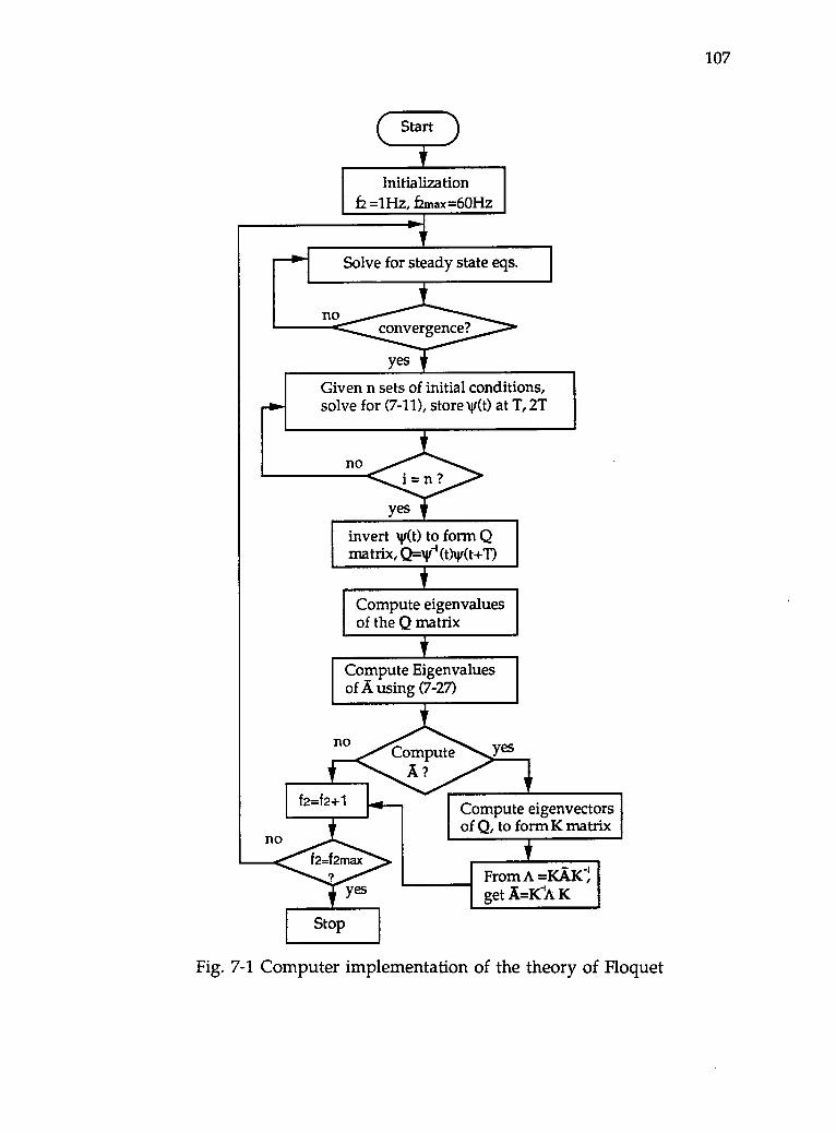
107

( Start

Initializationf2 =1Hz, fzmax =60Hz

Solve for steady state eqs.

Given n sets of initial conditions,solve for (7-11), store w(t) at T, 2T

invert w(t) to form Qmatrix, Q=v-1(t)g(t+T)

Compute eigenvaluesof the Q matrix

Compute Eigenvaluesof A using (7-27)

no

f 2=f 2+1

Stop

Compute eigenvectorsof Q to form K matrix

From A =KAKIget A=IeA K

Fig. 7-1 Computer implementation of the theory of Floquet

108

linear function. The slope of the straight line is determined such that at

60Hz the rotor resistance is 2 to 3 times higher than that at dc at which the

value of the rotor resistance is computed.

Stability characteristics of the BDFM system at any operating point are

evaluated by examination of the eigenvalues of the A matrix. In doing

that, the power converter frequency, f2 , is varied from 1Hz to 60Hz and the

computed real parts of the dominant eigenvalues of the A matrix are

plotted as functions of the converter output frequency. The 2-pole voltage

and frequency is increased in such a way that a constant V /Hz ratio is

maintained. In addition, the load torque is kept constant.

Over most of the operating range, the eigenvalues comprise four

complex conjugate pairs, each of which corresponds to a particular system

(namely the 6-pole stator, 2-pole stator, the rotor and the mechanical

systems). No repeated eigenvalues are expected from practical consi-

derations. Fig. 2(a) and (b) show the typical computational results for no

load conditions in which the real parts of the two critical eigenvalues are

plotted. The third and the fourth ones are not shown since they are always

large and negative. Similar eigenvalue characteristics have been obtained

for different V/Hz ratios and loads. It should be pointed out that at high

V/Hz ratios and loading conditions, eigenvalue analysis predicts that one

eigenvalue approaches zero and becomes slightly positive at high 2-pole

frequency (or low rotor speed). Tests show, however, that no unstable

region exists at low speeds. The discrepancy is due to the difference

between the calculated parameters and the actual parameters which change

with operating conditions. Also, iron loss and other possible losses were

not considered in the calculation.

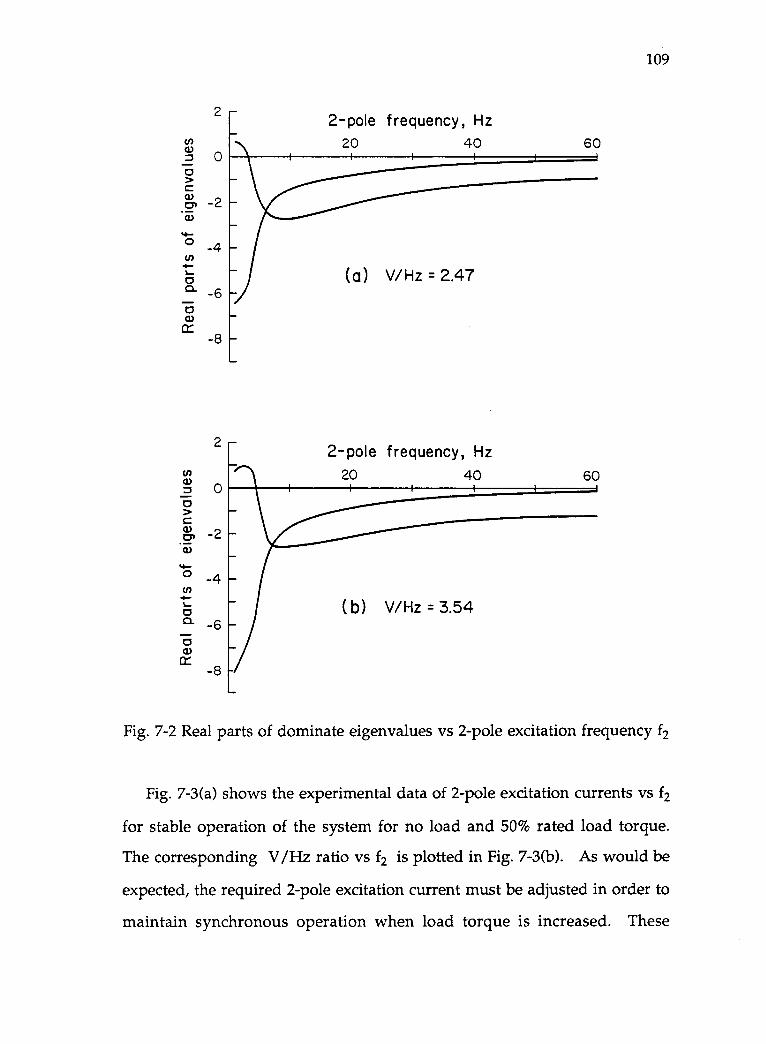
2-pole frequency, Hz20 40 60

2 -

(a) V/Hz = 2.47

2-pole frequency, Hz20 40 60

(b) V/Hz =3.54

109

Fig. 7-2 Real parts of dominate eigenvalues vs 2-pole excitation frequency f2

Fig. 7-3(a) shows the experimental data of 2-pole excitation currents vs f2

for stable operation of the system for no load and 50% rated load torque.

The corresponding V /Hz ratio vs f2 is plotted in Fig. 7-3(b). As would be

expected, the required 2-pole excitation current must be adjusted in order to

maintain synchronous operation when load torque is increased. These

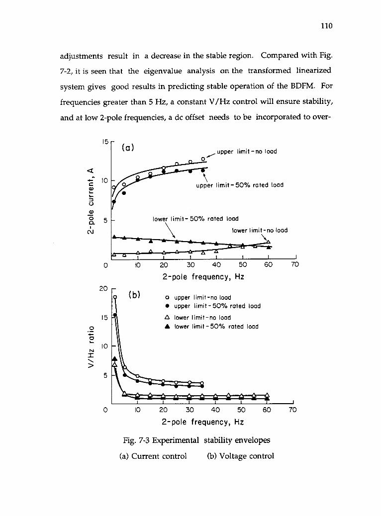
110

adjustments result in a decrease in the stable region. Compared with Fig.

7-2, it is seen that the eigenvalue analysis on the transformed linearized

system gives good results in predicting stable operation of the BDFM. For

frequencies greater than 5 Hz, a constant V/Hz control will ensure stability,

and at low 2-pole frequencies, a dc offset needs to be incorporated to over-

15

I0

5

(a) upper limit-no load...---o

upper limit-50% rated load

lower limit-50% rated load

lower limit-no load

1

0 10 20 30

20

15

045

10

21,..>

(b)

40 50

2-pole frequency, Hz

o upper limit-no loadupper limit 50% rated load

A lower limit-no loadlower limit-50% rated load

60 70

10 20 30 40 50

2-pole frequency, Hz60

Fig. 7-3 Experimental stability envelopes

(a) Current control (b) Voltage control

70

111

come a resistive dominated low frequency impedance in order to push the

eigenvalues into the left half of the complex plane and thus to provide

open-loop stability. It is seen that these considerations are equivalent to

scalar control of conventional induction motor drives. Thus, existing

controllers can easily be adapted to interface with BDFM drives.

It should be noted that the eigenvalue analysis presented above

considers only whether stable operation can be maintained for a given

V/Hz ratio, or 2-pole excitation current. From a steady state operation

point of view, efficiency, power factor and other aspects must also be taken

into account. The converter control algorithms should be such that while

maintaining stable operation of the drive system, at least one of the steady

state performance parameters should be maximized. It was found in the

laboratory and computer simulation that 2-pole excitation (voltage or

current) has profound effects on power factor of the system. Fig. 7-4(a) and

(b) show experimentally how 2-pole excitation voltage affects the 6-pole

current and power factor of the drive for f2=1Hz under no-load conditions.

Similar plots can be drawn for other 2-pole frequencies and various loading

conditions. It can be seen from Fig. 7-4 that control of power factor can be

made by adjusting the 2-pole excitation voltage or current. Increasing

excitation can result in a leading power factor operation. However, there

exists a practical maximum beyond which the phase angle is seen to

decrease. From the consideration of economic operation under a power

factor control constraint, it is appropriate to keep the excitation voltage (or

current) within a certain range. This is desirable since reducing the 2-pole

voltage means reducing the converter KVA requirement and thus the cost

of the system. In addition, the machine tends to be overexcited with high

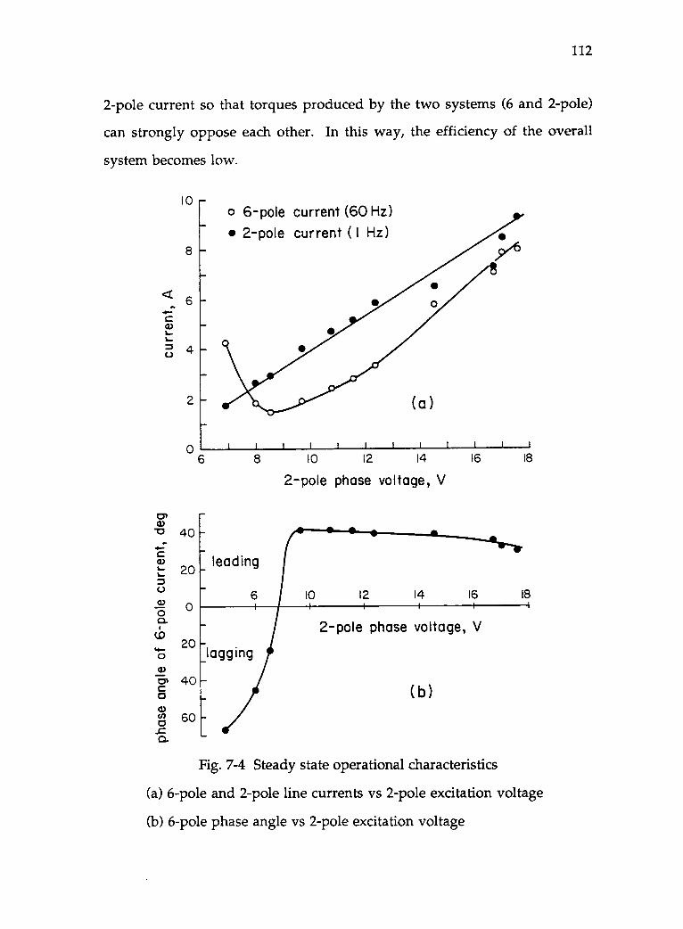
112

2-pole current so that torques produced by the two systems (6 and 2-pole)

can strongly oppose each other. In this way, the efficiency of the overall

system becomes low.

10

8

2

0

40

o 6-pole current (60 Hz)2-pole current (1 Hz)

(a)

I 1 I I I I I 1 1 1

6 8 10 12 14 16 18

2-pole phase voltage, V

leading

10 12 14 16 18

2-pole phase voltage, V

(b)

Fig. 7-4 Steady state operational characteristics

(a) 6-pole and 2-pole line currents vs 2-pole excitation voltage

(b) 6-pole phase angle vs 2-pole excitation voltage

113

8. SUMMARY, CONCLUSION AND FUTURE WORK

8.1 Summary and Conclusion

The primary objective of this research work was to develop a rigorous

two-axis model and its parameters for dynamic simulation, stability and

control studies. In summary, the following have been accomplished.

Starting from a detailed machine design model, which represents a b-

and 2-pole BDFM with a common stator winding and a castable rotor, we

have developed a two-axis model. Methods for calculating the model

parameters in both machine and dq domains are also developed.

Dynamic simulation for different modes of operation has been

performed and correlated with available test data. Simulations include

machine run-up, synchronization dynamics, synchronous behavior as

well as fault tolerant behavior of the machine.

The constraints of specific operating conditions make necessary the

rigorous development of steady state models from the d-q representation

which have been utilized for steady state performance analysis of the

machine. The models, although derived from simplified assumptions,

strive to capture the essence of the operating characteristics of the machine

while maintaining simple computational requirements and are found to

be valuable for machine design and other analysis purposes as well.

A new method for analyzing the stability of the BDFM is developed

by introduction of the theory of Floquet. This was found necessary

because of the time-varying nature of the linearized two-axis model

equations. Using the theory of Floquet allows the eigenvalue analysis

technique to be applied to the stability studies of the BDFM.

114

It is concluded from the studies that the proposed two-axis model is a

valid representation of the BDFM and possesses the following advantages

(1) The resistive and inductive parameters can be determined from

the machine geometries and the rules of the transformations;

(2) No approximations, such as assumed equivalences to two inter-

connected machines, reduce the validity of the predictions obtained

from the model;

(3) When compared with more detailed models, the reduced order of

the two-axis model allows its application to general stability and

control studies;

(4) The model is complete valid for all conceivable operating condi-

tions including

(a) Singly-fed induction mode dynamics

(b) Singly-fed induction mode steady-state characteristics

(c) Doubly-fed synchronous dynamics

(d) Doubly-fed synchronous steady-state characteristics

(e) Doubly-fed asynchronous dynamics

(f) Doubly-fed asynchronous steady-state characteristics

over complete ranges of speed and frequency (induding dc excita-

tion) and for all connection sequences.

Dynamic performance simulation illustrates the following charac-

teristics of a BDFM in adjustable speed drives and variable speed genera-

tion systems

(1) Dynamic synchronization from induction mode;

(2) Synchronous operation without a speed feedback signal;

115

(3) Maintenance of synchronism for both positive and negative

step changes of load torque;

(4) Continued operation after converter failure (reverting to induction

mode).

These features can be realized while maintaining robust and

inexpensive construction similar to induction motors whist utilizing a

power converter whose rating is only a fraction of machine rating.

Stability study presented in this thesis shows that Lyapunov's indirect

method can be applied to analyze the stability characteristics of the BDFM

since a linear transformation matrix P(t) always exists such that the

linearized time-varying system of equations of the BDFM can be

transformed into an equivalent system of equations with a constant system

matrix using the generalized theory of Floquet. Both theoretical and

experimental results show that stable speed control of a BDFM system can

be obtained by control algorithms similar to those for a conventional

induction machine. Constant converter current or constant V/Hz ratio

with an initial low frequency off-set results in open loop stability over the

entire speed range. Within these stable ranges, the converter control

algorithms can be developed in such a way as to produce desirable

operational conditions for efficiency and power factor.

8.2 Recommended Future Work

The results reported in this thesis reflect the evolution of the two-axis

model, model verification against experimental data and initial utilization

of the model for stability studies as well as the exploration on converter

116

control algorithms for stable steady state operation of the system. It is

recommended that future work include the following

(1) More accurate d-q modeling of the BDFM to account for saturation;

(2) More detailed investigation of the machine dynamics inclu-

ding the super-synchronous operation of the BDFM system;

(3) Detailed studies of the steady state performance of the machine

using the steady state models and the solution techniques deve-

loped in this thesis. The investigation should take iron losses

and possibly saturation into account in order to obtain high

accuracy of prediction;

(4) Establishment of control strategies for both dynamic and steady state

operation of the BDFM;

(5) Investigation of system controller design and implementation to

improve both dynamic and steady state performances;

(6) Development of a generalized two-axis model to account for

different pole number combinations of the BDFM.

The above activities can be accomplished using the existing simulation

programs already developed for the purpose of this research. It should be

emphasized that recent development of a simulation program with

graphics capabilities will certainly help enhance investigation into the

above areas that need to be addressed in the future.

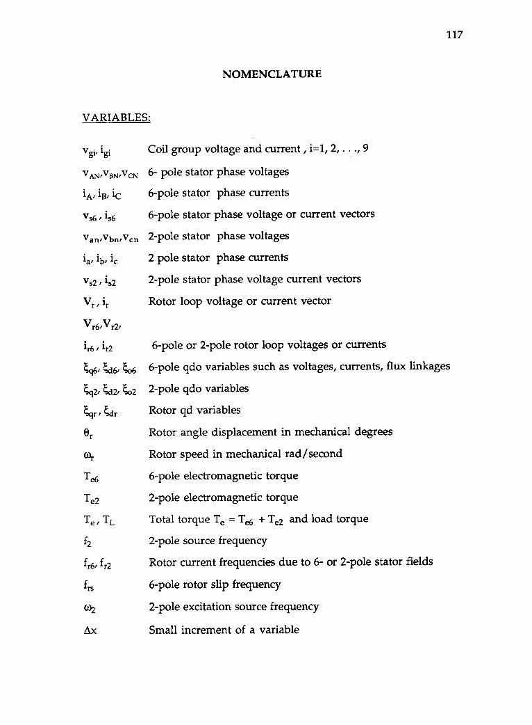
117

VARIABLES:

Vg;, igi

VAN/VBN/VCN

jA/ 1l3/ iC

Vs6 / 1s6

Van,Vbn,Vcn

la, 4)/ is

vs2 / 's2

V ir

Vr6,Vr2,

ir6 ,'r2

(46/ c16/ (:)6

(:121 c12/ 44:32

Exir / Exir

er

cor

Te6

Tel

Te , TL

f2

fr6/ f r2

frs

(62

Ax

NOMENCLATURE

Coil group voltage and current , i=1, 2, . . ., 9

6- pole stator phase voltages

6-pole stator phase currents

6-pole stator phase voltage or current vectors

2-pole stator phase voltages

2 pole stator phase currents

2-pole stator phase voltage current vectors

Rotor loop voltage or current vector

6-pole or 2-pole rotor loop voltages or currents

6-pole qdo variables such as voltages, currents, flux linkages

2-pole qdo variables

Rotor qd variables

Rotor angle displacement in mechanical degrees

Rotor speed in mechanical rad/second

6-pole electromagnetic torque

2-pole electromagnetic torque

Total torque Te = Te6 + Te2 and load torque

2-pole source frequency

Rotor current frequencies due to 6- or 2-pole stator fields

6-pole rotor slip frequency

2-pole excitation source frequency

Small increment of a variable

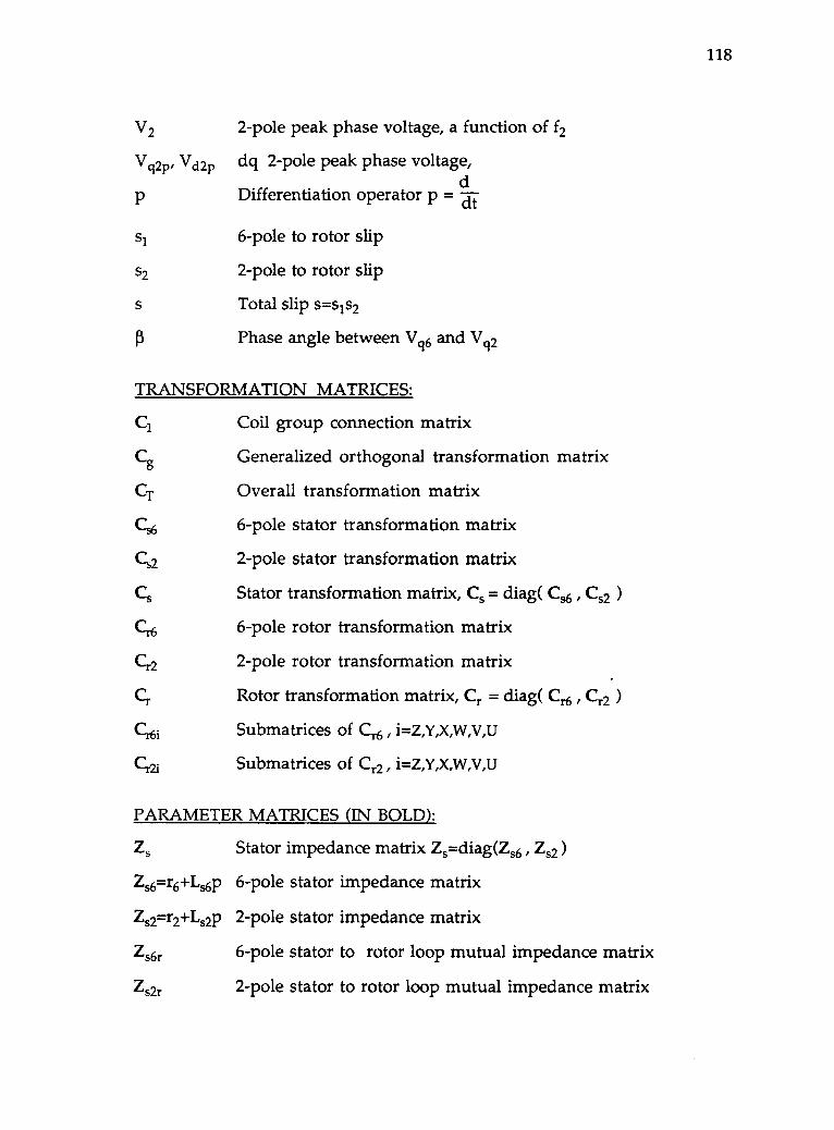
V2 2-pole peak phase voltage, a function of f2

V cpp, Vd2p dq 2-pole peak phase voltage,

p Differentiation operator p = dt

S1 6-pole to rotor slip

S2 2-pole to rotor slip

Total slip s=sis2

Phase angle between Vq6 and Vq2

TRANSFORMATION MATRICES:

C1 Coil group connection matrix

Cg Generalized orthogonal transformation matrix

CT Overall transformation matrix

Cs6 6-pole stator transformation matrix

Cs2 2-pole stator transformation matrix

Cs Stator transformation matrix, Cs = diag( Cs6 , Cs2 )

Cr6 6-pole rotor transformation matrix

Cr2 2-pole rotor transformation matrix

Cr Rotor transformation matrix, Cr = diag( Cr6 , Cr2 )

Cr6i Submatrices of Cr6 , i=Z,Y,X,W,V,U

Cr2i Submatrices of Cr2 , i=Z,Y,X,W,V,U

PARAMETER MATRICES (IN BOLD):

Zs

Zs6=r6+Ls6P

Zs2=r2+Ls2P

Zs 6r

Zs2r

Stator impedance matrix Zs=diag(Zs6 , Zs2 )

6-pole stator impedance matrix

2-pole stator impedance matrix

6-pole stator to rotor loop mutual impedance matrix

2-pole stator to rotor loop mutual impedance matrix

118

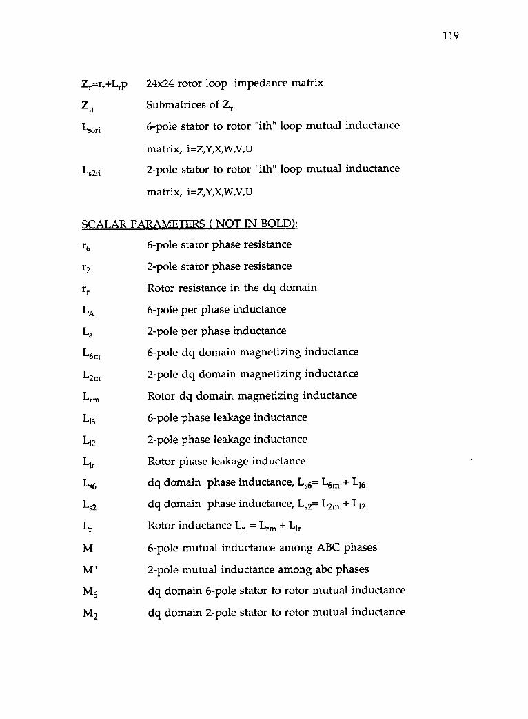
119

Zr=rr+Lrp

Zji

Ls6ri

Ls 2r;

24x24 rotor loop impedance matrix

Submatrices of Zr

6-pole stator to rotor "ith" loop mutual inductance

matrix, i=Z,Y,X,W,V,U

2-pole stator to rotor "ith" loop mutual inductance

matrix, i=Z,Y,X,W,V,U

SCALAR PARAMETERS ( NOT IN BOLD):

r6 6-pole stator phase resistance

r2 2-pole stator phase resistance

rr Rotor resistance in the dq domain

LA 6-pole per phase inductance

La 2-pole per phase inductance

L6m 6-pole dq domain magnetizing inductance

L2m 2-pole dq domain magnetizing inductance

Lrm Rotor dq domain magnetizing inductance

L16 6-pole phase leakage inductance

L12 2-pole phase leakage inductance

Lir Rotor phase leakage inductance

Ls6 dq domain phase inductance, Ls6= L6m + L16

Ls2 dq domain phase inductance, Ls2= L2m + L12

Lr Rotor inductance Lr = Lrm + Lir

M 6-pole mutual inductance among ABC phases

M' 2-pole mutual inductance among abc phases

M6 dq domain 6-pole stator to rotor mutual inductance

M2 dq domain 2-pole stator to rotor mutual inductance

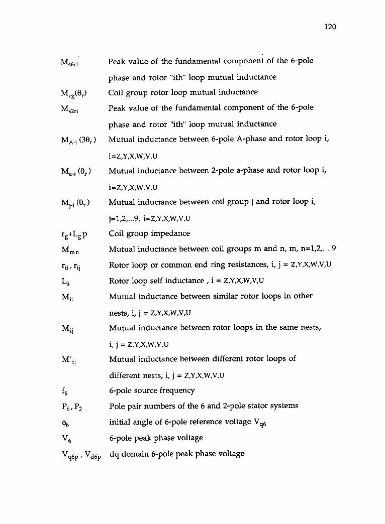
120

Ms6ri Peak value of the fundamental component of the 6-pole

phase and rotor "ith" loop mutual inductance

Mcg(er) Coil group rotor loop mutual inductance

Ms2ri Peak value of the fundamental component of the 6-pole

phase and rotor "ith" loop mutual inductance

MA4 (30r) Mutual inductance between 6-pole A-phase and rotor loop i,

i=Z,Y,X,W,V,U

Ma-i (0r ) Mutual inductance between 2-pole a-phase and rotor loop i,

i=Z,Y,X,W,V,U

Mj-i (Or ) Mutual inductance between coil group j and rotor loop i,

j=1,2,...9, i=Z,Y,X,W,V,U

rg+L

gp Coil group impedance

Mmn Mutual inductance between coil groups m and n, m, n= 1,2,.. 9

rii , rid Rotor loop or common end ring resistances, i, j = Z,Y,X,W,V,U

Rotor loop self inductance , i = Z,Y,X,W,V,U

Mii Mutual inductance between similar rotor loops in other

nests, i, j = Z,Y,X,W,V,U

Mid Mutual inductance between rotor loops in the same nests,

j = Z,Y,X,W,V,U

M'ii Mutual inductance between different rotor loops of

different nests, i, j = Z,Y,X,W,V,U

f6 6-pole source frequency

136, P2 Pole pair numbers of the 6 and 2-pole stator systems

4)6 initial angle of 6-pole reference voltage Vq6

V6 6-pole peak phase voltage

Vq6p Vd6p dq domain 6-pole peak phase voltage

121

BIBLIOGRAPHY

[1] H. K. Lauw, "Characteristics and Analysis of the Brush lessDoubly-Fed Machines," Report for the Bonneville Power Admi-nistration, Contract No, 79-85BP24332-Mod4, June 1989.

[2] A. K. Wallace, R. Spee and H. K. Lauw, "The Potential of BrushlessDoubly-Fed Machines for Adjustable Speed Drives," Conf. Record,IEEE IAS Pulp and Paper Induction Conference, 1990, pp. 45-50.

[3] A. R. Broadway and L. Burbridge, "Self-Cascaded Machine: A LowSpeed Motor or High-Frequency Brushless Alternator," IEE Proc. ,1970, 117(7), pp. 1277-1290.

[4] L. J. Hunt, "A New Type of Induction Motor," J. IEE, 1907, 39, pp.648-667.

[5] F. Creedy "Some Development in Multi-Speed Cascade InductionMotors," ibid., 1921, 59, pp. 511-532.

[6] B. H. Smith, "Synchronous Behavior of Doubly-Fed Twin StatorInduction Machine," IEEE Trans. PAS, Vol. PAS-88, October 1967,pp. 1227-1236.

[7] A. Kusko and C. B. Somuah, "Speed Control of a Single FrameCascade Induction Motor with Slip-Power Pump Back, "IEEE Trans.on IAS, Vol, IA-14, No. 2, pp. 97-105, May/April 1978.

[8] F. Shibata and K. Taka, "Speed Control System for BrushlessCascade Induction Motors in Control Range of sl>1 and s2>1,"IEEEPES Winter Meeting 1986, paper 86WM 226-5.

[9] C. D. Cook and B. H. Smith, "Stability and Stabilization of Doubly-Fed Single-Frame Induction Machines," IEE Proc. , 1979, 126(11), pp.1168-1174.

[10] C. D. Cook and B. H. Smith, "Effects of Machine Parameter Valueson Dynamic Response and Stability Regions of Doubly-FedCascade Induction Machines," IEE Proc. , March 1983, Vol. 130, Pt. B,No. 2, PP. 137-142.

[11] A. K. Wallace, R. Spee and H. K. Lauw, "Dynamic Modeling ofBrushless Doubly-Fed Machines," IEEE Industry Application SocietyAnnual Meeting 1989, San Diego.

122

[12] R. Spee, A. K. Wallace and H. K. Lauw, "Simulation of Brush lessDoubly-Fed Adjustable Speed Drives," IEEE Industry ApplicationSociety Annual Meeting 1989, San Diego.

[13] P. Rochelle, R. Spee and A. K. Wallace, "The Effect of StatorWinding Configuration on the Performance of Brush less Doubly-Fed Machines Adjustable Speed Drives," IEEE Industry Applica-tion Society Annual Meeting , Seattle, WA, Oct. 8-11, 1990.

[14] A. K. Wallace, P. Rochelle and R. Spee,"Rotor Modeling and Deve-lopment for Brush less Doubly-Fed Machines," Int'l Conf. on ElectricMachines, Cambridge, Mass, Aug. 12-15, 1990.

[15] P. Rochelle, "Design and Analysis of the Brush less Doubly-FedMachine," M.S. Thesis, Oregon State University, 1990.

[16] G. C. Alexander, "Characterization of the Brushless Doubly-FedMachines by Magnetic Field Analysis," IEEE Industry ApplicationSociety Annual Meeting , Seattle, WA, Oct. 8-11, 1990.

[17] R. Li, A. K.Wallace, R. Spee and Y. Wang,"Two-axis Model Develop-ment of Cage-Rotor Brushless Doubly-Fed Machines," IEEE PESwinter Meeting 1991, New York, paper 91WM061-2EC, also toappear on IEEE Trans. on Energy Conversion, 1991.

[18] R. Li, A.K. Wallace and R. Spee, "Dynamic Simulation of BrushlessDoubly-Fed Machines," IEEE PES Winter Meeting 1991, New York,paper 91WM060-4EC, also to appear on IEEE Trans. on EnergyConversion, 1991.

[19] R. Li, A.K.Wallace and R. Spee,"Determination of Converter ControlAlgorithms for Stable Brushless Doubly-Fed Drives Using Floquetand Lyapunov Techniques," Power Electronics Specialists Conf. ,

MIT, Boston, June 24-28, 1991.

[20] A. K. Wallace and A. Wright, "Novel Simulation of Cage WindingsBased on Mesh Circuit Model," IEEE PES Summer Meeting andEHVIUHV Conf. , Vancouver, Canada, July 15-20, 1973.

[21] T. A. Lipo and P. Krause, "Stability Analysis of a Rectifier InverterInduction Motor Drive,"IEEE Trans. PAS , Vol. PAS-88, Jan. 1968,pp. 55-66.

[22] P. Krause, Analysis of Electric Machinery, McGraw-Hill, 1986.

123

[23] R. Hoft, "Lyapunov Stability Analysis of Reluctance Motors,"IEEE Trans. PAS, Vol. PAS-87, June 1968, pp. 1485-1491.

[24] C. T. Chen, Linear System Theory and Design, Second Edition,Holt, Rinehart and Winston, 1984.

[25] Henry D'Angelo,Linear Time-Varying Systems:Analysis and Syn-thesis, Allyn and Bacon, Boston, 1970.