Simulation and analysis of dynamic heating in the ultrafast aircraft thermometer measurements

Bogdan Rosa*, Konrad Bajer, Krzysztof E. Haman, Tomasz Szoplik

Institute of Geophysics, Faculty of Physics, Warsaw University, Pasteura 7 Street, 02-093 Warsaw, Poland

ABSTRACT The ultrafast aircraft thermometer is an airborne device designed for measuring temperature in clouds with centimeter spatial resolution. Its sensor consists of 5mm long and 2.5µm thick thermo-resistive wire protected against impact of cloud droplets by a shield in the form of a suitably shaped rod, placed upstream. However the disturbances of airflow around this rod result in noise in the temperature record. Suction applied through slits located on both sides of the rod reduces the noise generated by vortices shed from the rod and lowers the probability of droplet-wire collisions. Our recent theoretical analysis and numerical simulations led to optimization of this device and additionally clarified the role of the sampling method in processing of the analogue output of the thermometer. In this paper we try to deepen our understanding of the nature of the noise as well as to improve calculations of the corrections connected with the dynamic heating. For this purpose we have done extensive three-dimensional numerical simulations of the airflow around the protective rod and the sensing wire, which permitted precise computation of dynamic heating and showed how applying the suction removes the thermal boundary layer from the rod and damps the sources of the noise. Keywords: Ultrafast cloud thermometer, viscous heating, dynamic heating

1. INTRODUCTION The aircraft ultrafast thermometer UFT-F1 was designed for measuring temperature in clouds at speeds up to 100 m/s. Compared with the older version2,3 the main improvement is a new shape of the wind shield. The new shield protects the sensing element (∅ = 2,5 µm thermo-resistive tungsten wire) more efficiently against the impact of cloud droplets that affect the temperature measurement4,5. The wire resistance increases with temperature. The changes are amplified by an electronic system and recorded on a laptop computer. The impact of a droplet decreases the wire resistance and causes the wet-bulb effect altering the temperature recordings. To reduce this effect suction is applied to the protecting shield. Another problem is related to the flow disturbances behind the shield. The adiabatic compression and decompression leads to temperature fluctuations with amplitude of 0.2 K and therefore the measurements are corrupted by noise. The observed frequency of the fluctuations is approximately 3 kHz. The authors of the thermometer design suggest that the fluctuations are directly connected with vortex shedding from the protective shield. To design optimal suction and the shape of the shield that minimizes the noise level and the probability of droplet collision with the sensor we need more information about the air flow. Direct observations are, at present, not possible, hence the need for elaborate numerical simulations. In this work two-dimensional simulations of the air flow are performed. In reality the flow around the thermometer is weakly compressible. Numerically we simulate an incompressible flow and on the basis of the incompressible velocity and pressure fields we derive estimates of the temperature fluctuations to be expected in a weakly compressible flow and to be compared with the experiments.

* rosa@igf.fuw.edu.pl; phone +48 (22) 55-46-855; fax +48 (22) 82-39-824; www.igf.fuw.edu.pl

Please verify that (1) all pages are present, (2) all figures are acceptable, (3) all fonts and special characters are correct, and (4) all text and figures fit within themargin lines shown on this review document. Return to your MySPIE ToDo list and approve or disapprove this submission.

5981-1 V. 4 (p.1 of 10) / Color: No / Format: A4 / Date: 8/22/2005 2:46:18 PM

SPIE USE: ____ DB Check, ____ Prod Check, Notes:

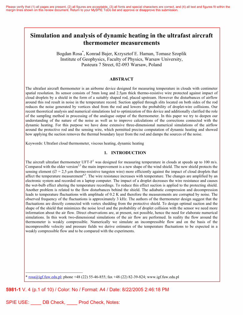
1. VISCOUS HEATING The preliminary account of the problem of viscous heating was given by Rosa et al.6,7 In the regions of strong shear, i.e., in a boundary layer on the shield’s surface, viscous heating becomes significant. Its rate is equal

∑∑= =

=Φ3

1

3

12

i jijij eeµ , (1)

where eij is the strain tensor

⎟⎟⎠

⎞⎜⎜⎝

⎛

∂

∂+

∂∂

=i

j

j

iij x

uxu

e21

(2)

and µ = 1151047,1 −−−⋅ smkg is the dynamic viscosity of air. In Fig. 1 we show the greyscale plots of log(Φ ). The range of Φ is so large that the logarithmic scale is necessary.

Fig. 1. Logarithm of the rate of viscous heating, log(Φ ),: (a) with suction off; (b) with suction on.

The total amount of heat released in a fluid element reaching the sensor is given by the lagrangian integral over the path-

line of the element, dt∫Φτ

0

, where τ is the time that the element spends in the region of strong shear. We have

computed this integral for three selected particles of fluid, path-lines are shown in Fig. 2. The path equations,

vx=

dtd

, (3)

were integrated along with the time-stepping of the Navier-Stokes equation by a subroutine added to the FEATFLOW8 code.

Please verify that (1) all pages are present, (2) all figures are acceptable, (3) all fonts and special characters are correct, and (4) all text and figures fit within themargin lines shown on this review document. Return to your MySPIE ToDo list and approve or disapprove this submission.

5981-1 V. 4 (p.2 of 10) / Color: No / Format: A4 / Date: 8/22/2005 2:46:18 PM

SPIE USE: ____ DB Check, ____ Prod Check, Notes:

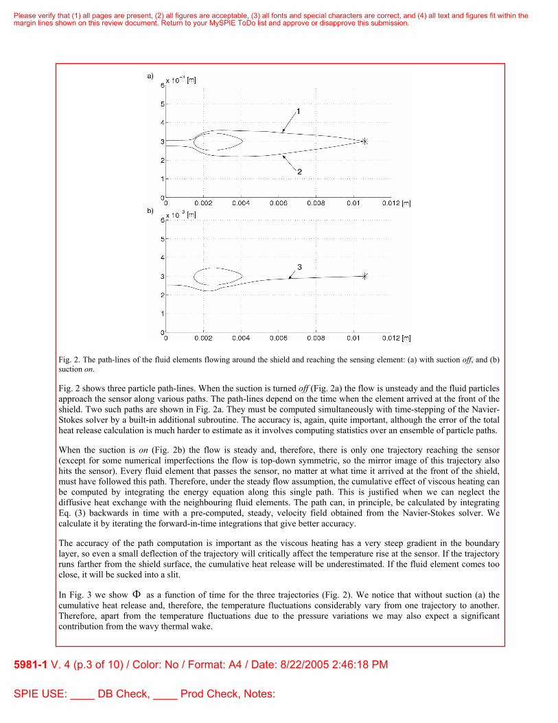
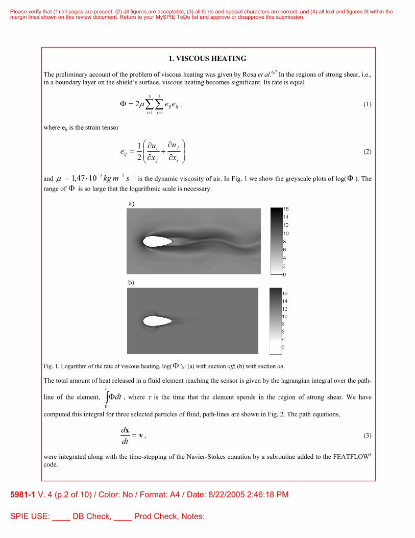
Fig. 2. The path-lines of the fluid elements flowing around the shield and reaching the sensing element: (a) with suction off, and (b) suction on.

Fig. 2 shows three particle path-lines. When the suction is turned off (Fig. 2a) the flow is unsteady and the fluid particles approach the sensor along various paths. The path-lines depend on the time when the element arrived at the front of the shield. Two such paths are shown in Fig. 2a. They must be computed simultaneously with time-stepping of the Navier-Stokes solver by a built-in additional subroutine. The accuracy is, again, quite important, although the error of the total heat release calculation is much harder to estimate as it involves computing statistics over an ensemble of particle paths.

When the suction is on (Fig. 2b) the flow is steady and, therefore, there is only one trajectory reaching the sensor (except for some numerical imperfections the flow is top-down symmetric, so the mirror image of this trajectory also hits the sensor). Every fluid element that passes the sensor, no matter at what time it arrived at the front of the shield, must have followed this path. Therefore, under the steady flow assumption, the cumulative effect of viscous heating can be computed by integrating the energy equation along this single path. This is justified when we can neglect the diffusive heat exchange with the neighbouring fluid elements. The path can, in principle, be calculated by integrating Eq. (3) backwards in time with a pre-computed, steady, velocity field obtained from the Navier-Stokes solver. We calculate it by iterating the forward-in-time integrations that give better accuracy.

The accuracy of the path computation is important as the viscous heating has a very steep gradient in the boundary layer, so even a small deflection of the trajectory will critically affect the temperature rise at the sensor. If the trajectory runs farther from the shield surface, the cumulative heat release will be underestimated. If the fluid element comes too close, it will be sucked into a slit.

In Fig. 3 we show Φ as a function of time for the three trajectories (Fig. 2). We notice that without suction (a) the cumulative heat release and, therefore, the temperature fluctuations considerably vary from one trajectory to another. Therefore, apart from the temperature fluctuations due to the pressure variations we may also expect a significant contribution from the wavy thermal wake.

Please verify that (1) all pages are present, (2) all figures are acceptable, (3) all fonts and special characters are correct, and (4) all text and figures fit within themargin lines shown on this review document. Return to your MySPIE ToDo list and approve or disapprove this submission.

5981-1 V. 4 (p.3 of 10) / Color: No / Format: A4 / Date: 8/22/2005 2:46:18 PM

SPIE USE: ____ DB Check, ____ Prod Check, Notes:

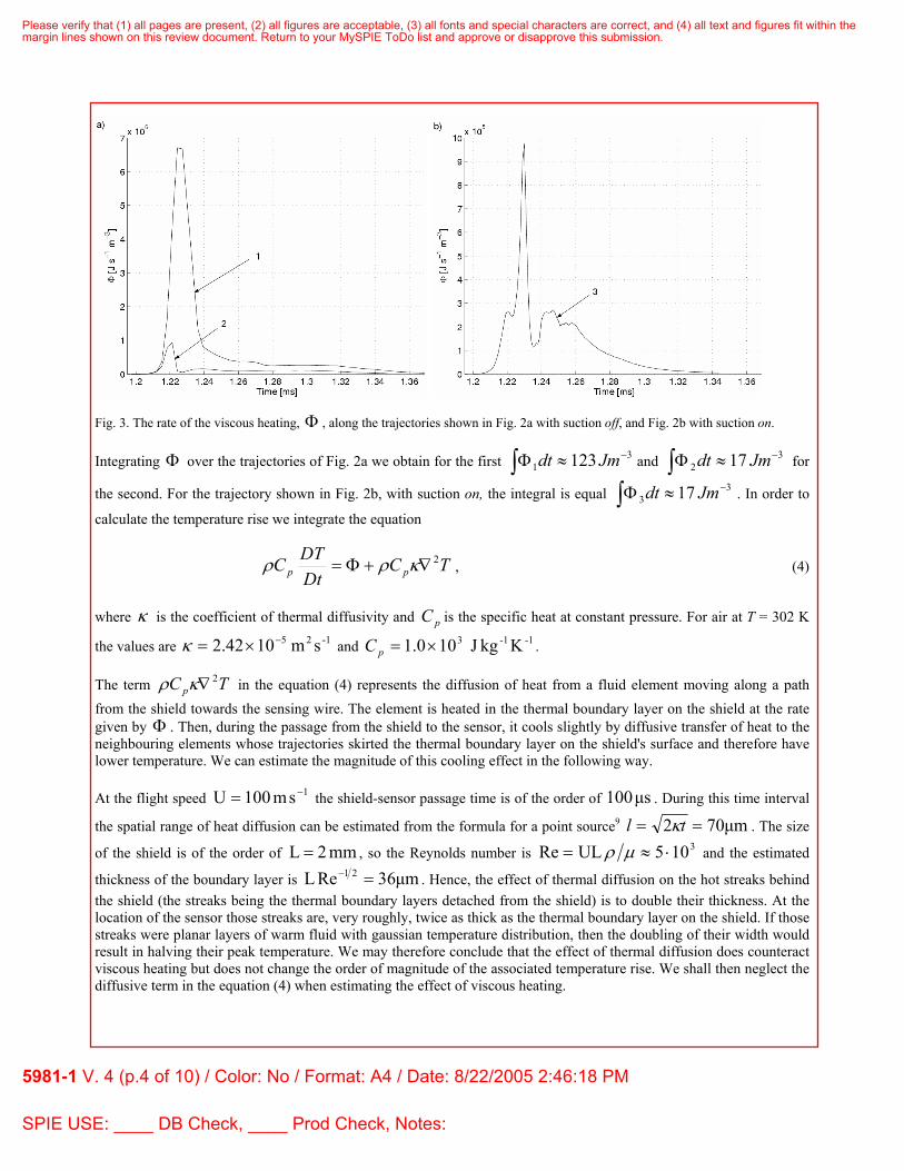
Fig. 3. The rate of the viscous heating, Φ , along the trajectories shown in Fig. 2a with suction off, and Fig. 2b with suction on.

Integrating Φ over the trajectories of Fig. 2a we obtain for the first ∫ −≈Φ 31 123 Jmdt and ∫ −≈Φ 3

2 17 Jmdt for

the second. For the trajectory shown in Fig. 2b, with suction on, the integral is equal ∫ −≈Φ 33 17 Jmdt . In order to

calculate the temperature rise we integrate the equation

TCDtDTC pp

2∇+Φ= κρρ , (4)

where κ is the coefficient of thermal diffusivity and pC is the specific heat at constant pressure. For air at T = 302 K

the values are -125 sm1042.2 −×=κ and -1-13 KkgJ100.1 ×=pC .

The term TC p2∇κρ in the equation (4) represents the diffusion of heat from a fluid element moving along a path

from the shield towards the sensing wire. The element is heated in the thermal boundary layer on the shield at the rate given by Φ . Then, during the passage from the shield to the sensor, it cools slightly by diffusive transfer of heat to the neighbouring elements whose trajectories skirted the thermal boundary layer on the shield's surface and therefore have lower temperature. We can estimate the magnitude of this cooling effect in the following way.

At the flight speed 1sm100U −= the shield-sensor passage time is of the order of µs100 . During this time interval

the spatial range of heat diffusion can be estimated from the formula for a point source9 µm702 == tl κ . The size

of the shield is of the order of mm2L = , so the Reynolds number is 3105ULRe ⋅≈= µρ and the estimated

thickness of the boundary layer is µm36ReL 21 =− . Hence, the effect of thermal diffusion on the hot streaks behind the shield (the streaks being the thermal boundary layers detached from the shield) is to double their thickness. At the location of the sensor those streaks are, very roughly, twice as thick as the thermal boundary layer on the shield. If those streaks were planar layers of warm fluid with gaussian temperature distribution, then the doubling of their width would result in halving their peak temperature. We may therefore conclude that the effect of thermal diffusion does counteract viscous heating but does not change the order of magnitude of the associated temperature rise. We shall then neglect the diffusive term in the equation (4) when estimating the effect of viscous heating.

Please verify that (1) all pages are present, (2) all figures are acceptable, (3) all fonts and special characters are correct, and (4) all text and figures fit within themargin lines shown on this review document. Return to your MySPIE ToDo list and approve or disapprove this submission.

5981-1 V. 4 (p.4 of 10) / Color: No / Format: A4 / Date: 8/22/2005 2:46:18 PM

SPIE USE: ____ DB Check, ____ Prod Check, Notes:

With this assumption we can solve the equation (4) to obtain an expression for the temperature increment of a fluid element,

∫Φ=∆ tC

Tp

d1ρ

, (5)

where the integral is along the trajectory of the fluid element. For the three paths shown in Fig. 2 we obtain

K017,0,K122,0 21 =∆=∆ TT and K017,03 =∆T . The sensor will record such temperature changes when the corresponding fluid elements arrive in its neighbourhood.

It is important to compare the above temperature changes with those resulting from the adiabatic pressure drop in the von Karman vortices shed from the shield when the suction is off. The two effects have opposite sign but similar magnitude, so neither should be neglected in the analysis and interpretation of the experimental data. As the effect of viscous heating strongly depends on the free-flow velocity (cf. eq. 1), such interpretation becomes complicated when comparing data from the flights with different speeds and very difficult indeed for flights with variable speed.

2. DYNAMIC HEATING The most important thermal disturbance experienced by the thermometric unit is due to the so called dynamic heating i.e. transformation of the kinetic energy of the fluid into heat by braking action of the thermometer which is an obstacle to the flow. If the whole kinetic energy of the fluid that comes to the equilibrium thermal contact with the thermometer were turned into heat, its temperature (as well as the temperature of the thermometer) should be higher than that of its temperature in free flow (the so called static temperature) by the amount10

pCVT2

2

=∆ . (6)

Since neither all fluid stops, nor comes to thermal equilibrium with the thermometer, the increase of temperature showed by the thermometer with respect to its static value is rather

pCVrT2

2

=∆ , (7)

where r <1 is the so called ‘recovery factor’ usually determined empirically for particular types of the aircraft thermometers11. In the range of Reynolds numbers characteristic for typical aircraft thermometers the recovery factor r is usually assumed to be practically constant. An exhaustive discussion of this notion and of the problems connected with its application to the airborne measurements of temperature can be found in the paper by P. Nacass12. The formula (6) comes from the Bernoulli's theorem applied to steady isentropic flow13. Here we are going to show, that to a good approximation it can also be applied to the unsteady flow around the shield shedding vortices. For this purpose let us write the kinetic energy equation for a Newtonian fluid,

QxPV

xV

Vt

VV

kk

k

ik

ii +

∂∂

−=⎟⎟⎠

⎞⎜⎜⎝

⎛∂∂

+∂∂

ρ1

, (8)

where Q denotes the work of viscous forces,

ii VvVQ 2∇= . (9) Here we neglected frictional effects associated with compressibility, i.e., we assumed the deviatoric stress tensor of an incompressible fluid. Equation (8) can be now rewritten as

QtP

xPV

tP

xV

Vt

VV

kk

k

ik

ii +

∂∂

+⎟⎟⎠

⎞⎜⎜⎝

⎛∂∂

+∂∂

−=⎟⎟⎠

⎞⎜⎜⎝

⎛∂∂

+∂∂

ρρ11

, (10)

which in turn is equivalent to

Please verify that (1) all pages are present, (2) all figures are acceptable, (3) all fonts and special characters are correct, and (4) all text and figures fit within themargin lines shown on this review document. Return to your MySPIE ToDo list and approve or disapprove this submission.

5981-1 V. 4 (p.5 of 10) / Color: No / Format: A4 / Date: 8/22/2005 2:46:18 PM

SPIE USE: ____ DB Check, ____ Prod Check, Notes:

QtP

DtDP

DtDV

+∂∂

+−=ρρ11

21 2

. (11)

The thermodynamic energy equation for a heat-conducting gas is

TCDtDP

DtDTC pp

2∇+Φ+= κρρ . (12)

Manipulating Q we obtain

( ) ( ) 222122

212 vSVv

xV

xV

vVvQk

i

k

i −Φ

−∇=∂∂

∂∂

−∇=ρ

, (13)

where 2S is the square of the antisymmetric part of the rate of strain tensor. Equation (13) can now be rewritten as

( ) ( ) TCvSVvtP

DtDTCV

DtD

pp222

2122

21 1

∇+−∇+∂∂

=+ κρ

, (14)

which after the integration along a trajectory yields constDCBTCV p ++++Ψ=+2

21 , (15)

where DCB ,,,Ψ denote Lagrangian integrals of the respective terms on the right-hand side of the equation (14). The estimates (6) and (7) are obtained from the Bernoulli's theorem for steady isentropic flow of a perfect gas. With suction off the flow behind the shield of the UFT is unsteady. Because of frictional heating in the boundary layer over the shield surface the flow is not isentropic either. In Section 2 we presented calculations of the temperature increase due to frictional heating. Another departure from isentropy is heat conduction but estimates indicate its secondary role. Now we will again assume the flow to be isentropic and consider, in isolation, the other deviation from the conditions of he Bernoulli's theorem, i.e., the unsteadiness of the flow. This means that we neglect the terms DCB ,, in the equation (15) and calculate the relative magnitude of Ψ and the terms on the left-hand side of the equation (15). The quantity Ψ is an integral along the path of a fluid element of the partial, as opposed to material derivative of pressure as a function of time. Hence it is a Lagrangian integral of an Eulerian quantity

∫ ∂∂

=Ψ dttP

ρ1

. (16)

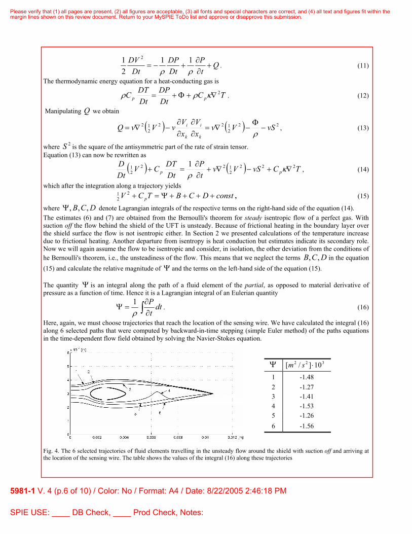
Here, again, we must choose trajectories that reach the location of the sensing wire. We have calculated the integral (16) along 6 selected paths that were computed by backward-in-time stepping (simple Euler method) of the paths equations in the time-dependent flow field obtained by solving the Navier-Stokes equation.

Fig. 4. The 6 selected trajectories of fluid elements travelling in the unsteady flow around the shield with suction off and arriving at the location of the sensing wire. The table shows the values of the integral (16) along these trajectories

Ψ 322 10]/[ ⋅sm

1 -1.48 2 -1.27 3 -1.41 4 -1.53 5 -1.26 6 -1.56

Please verify that (1) all pages are present, (2) all figures are acceptable, (3) all fonts and special characters are correct, and (4) all text and figures fit within themargin lines shown on this review document. Return to your MySPIE ToDo list and approve or disapprove this submission.

5981-1 V. 4 (p.6 of 10) / Color: No / Format: A4 / Date: 8/22/2005 2:46:18 PM

SPIE USE: ____ DB Check, ____ Prod Check, Notes:

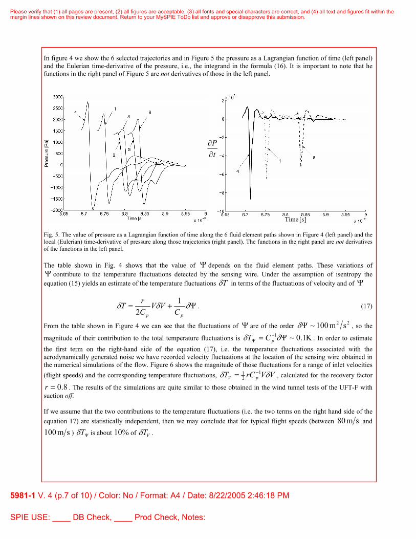
In figure 4 we show the 6 selected trajectories and in Figure 5 the pressure as a Lagrangian function of time (left panel) and the Eulerian time-derivative of the pressure, i.e., the integrand in the formula (16). It is important to note that he functions in the right panel of Figure 5 are not derivatives of those in the left panel.

Fig. 5. The value of pressure as a Lagrangian function of time along the 6 fluid element paths shown in Figure 4 (left panel) and the local (Eulerian) time-derivative of pressure along those trajectories (right panel). The functions in the right panel are not derivatives of the functions in the left panel. The table shown in Fig. 4 shows that the value of Ψ depends on the fluid element paths. These variations of Ψ contribute to the temperature fluctuations detected by the sensing wire. Under the assumption of isentropy the equation (15) yields an estimate of the temperature fluctuations Tδ in terms of the fluctuations of velocity and of Ψ

Ψ+= δδδpp C

VVCrT 1

2. (17)

From the table shown in Figure 4 we can see that the fluctuations of Ψ are of the order 22 sm100~Ψδ , so the

magnitude of their contribution to the total temperature fluctuations is K1.0~1 Ψ= −Ψ δδ pCT . In order to estimate

the first term on the right-hand side of the equation (17), i.e. the temperature fluctuations associated with the aerodynamically generated noise we have recorded velocity fluctuations at the location of the sensing wire obtained in the numerical simulations of the flow. Figure 6 shows the magnitude of those fluctuations for a range of inlet velocities (flight speeds) and the corresponding temperature fluctuations, VVrCT pV δδ 1

21 −= , calculated for the recovery factor

8.0=r . The results of the simulations are quite similar to those obtained in the wind tunnel tests of the UFT-F with suction off. If we assume that the two contributions to the temperature fluctuations (i.e. the two terms on the right hand side of the equation 17) are statistically independent, then we may conclude that for typical flight speeds (between sm80 and

sm100 ) ΨTδ is about %10 of VTδ .

tP∂∂

]s[Time

Please verify that (1) all pages are present, (2) all figures are acceptable, (3) all fonts and special characters are correct, and (4) all text and figures fit within themargin lines shown on this review document. Return to your MySPIE ToDo list and approve or disapprove this submission.

5981-1 V. 4 (p.7 of 10) / Color: No / Format: A4 / Date: 8/22/2005 2:46:18 PM

SPIE USE: ____ DB Check, ____ Prod Check, Notes:

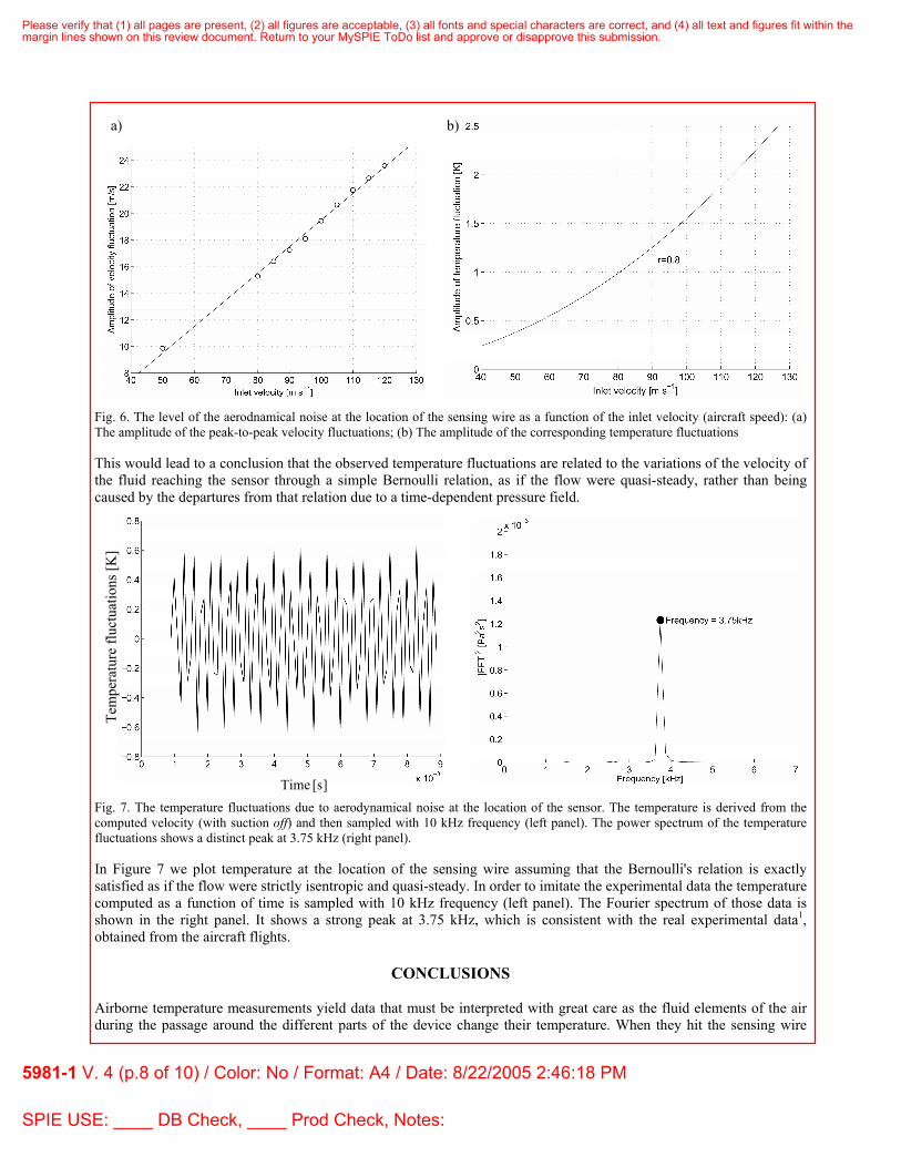
Fig. 6. The level of the aerodnamical noise at the location of the sensing wire as a function of the inlet velocity (aircraft speed): (a) The amplitude of the peak-to-peak velocity fluctuations; (b) The amplitude of the corresponding temperature fluctuations

This would lead to a conclusion that the observed temperature fluctuations are related to the variations of the velocity of the fluid reaching the sensor through a simple Bernoulli relation, as if the flow were quasi-steady, rather than being caused by the departures from that relation due to a time-dependent pressure field.

Fig. 7. The temperature fluctuations due to aerodynamical noise at the location of the sensor. The temperature is derived from the computed velocity (with suction off) and then sampled with 10 kHz frequency (left panel). The power spectrum of the temperature fluctuations shows a distinct peak at 3.75 kHz (right panel).

In Figure 7 we plot temperature at the location of the sensing wire assuming that the Bernoulli's relation is exactly satisfied as if the flow were strictly isentropic and quasi-steady. In order to imitate the experimental data the temperature computed as a function of time is sampled with 10 kHz frequency (left panel). The Fourier spectrum of those data is shown in the right panel. It shows a strong peak at 3.75 kHz, which is consistent with the real experimental data1, obtained from the aircraft flights.

CONCLUSIONS

Airborne temperature measurements yield data that must be interpreted with great care as the fluid elements of the air during the passage around the different parts of the device change their temperature. When they hit the sensing wire

]s[Time

Tem

pera

ture

fluc

tuat

ions

[K]

a) b)

Please verify that (1) all pages are present, (2) all figures are acceptable, (3) all fonts and special characters are correct, and (4) all text and figures fit within themargin lines shown on this review document. Return to your MySPIE ToDo list and approve or disapprove this submission.

5981-1 V. 4 (p.8 of 10) / Color: No / Format: A4 / Date: 8/22/2005 2:46:18 PM

SPIE USE: ____ DB Check, ____ Prod Check, Notes:

they have temperature different from that in the free stream that we intend to measure and the great challenge is to deduce the free stream temperature from the indications of the sensor. Such a precise inverse mapping may be prohibitively difficult or, in fact, impossible but we may try, by combining analytical and numerical tools, to calculate the relations between some characteristics of the recorded and free-stream temperature. By focusing on various effects in isolation we try to order them according the their relative influence on the measured temperature. An obvious approach would be to simulate faithfully the complete system, i.e., to solve the complete set of equations governing the flow of momentum and energy including, possibly, the heat diffusion inside the sensing wire as well as the mechanical flow-structure interaction between the stream of air and the frame of the thermometer. This is a phenomenally complex task that we try to approach in steps by first estimating the relative magnitude of various effects. In this paper we focused on the temperature fluctuations caused by compression and decompression of the fluid elements in the flow field behind the shield of the thermometer. Considering this effect in isolation, i.e. neglecting such processes like frictional heating and heat conduction, we found that dynamic heating may be as important as the frictional heating in the thermal boundary layer over the shield surface. We have also found that this dynamic heating may be, to a good approximation, calculated from the Bernoulli formula despite the unsteadiness of the flow. The Bernoulli formula is, in principle, valid only in the flows with steady pressure field. We find that in the case of the UFT-F the velocity fluctuations are important while the effect of the pressure variations is about one order of magnitude smaller. It should be stressed that the problem that we addressed here is the dynamic heating of air during its passage between the shield and the sensing wire. This is the result of the velocity fluctuations in an unsteady flow. In the operation of the UFT-F there are two other issues that involve dynamic heating, namely the compressive temperature rise near the stagnation points. One stagnation point is located at the front of the shield, which is dynamically heated in this area (this is separate from frictional heating in the entire boundary layer). The other stagnation point is on the surface of the sensing wire. The flow around the wire is a subsonic flow, the Mach number being about 0.3, but the Reynolds number is quite small, 110~Re , so the diffusion of heat from an oncoming fluid element cannot be neglected. Therefore, in the process of direct dynamic heating of the wire the relative importance of the velocity and pressure fluctuations may be different from what we found in the wake of the shield. However, the precise investigation of this problem requires a full compressible gas dynamics code and will be subject of future investigation.

ACKNOWLEGEMENTS Flow modeling was made with the FEATFLOW 1.2d - a finite element software for the incompressible Navier-Stokes equations. We gratefully acknowledge a free FEATFLOW license received from Professor Stefan Turek of the University of Dortmund. This work was supported by the Polish Ministry of Scientific Research and Information Technology grant 3 T10C 045 27 and European Union grant EVK2-CT-2002-80010 CESSAR.

REFERENCES 1. K. E. Haman, S. P. Malinowski, B. D. Struś, R. Busen, A. Stefko, “Two New Types of Ultrafast Aircraft

Thermometer,” J. Atmos. Oceanic Technol. 18, 117-134 (2001). 2. K. E. Haman, A. Makulski, S. P. Malinowski, R. Busen, “A New Ultrafast Thermometer for Airborne

Measurements in Clouds,” J. Atmos. Oceanic Technol. 14, 217-227 (1997). 3. K. E. Haman, ”A New Thermometric Instrument for Airborne Measurements in Clouds,” J. Atmos. Oceanic

Technol. 9, 86-90 (1992). 4. B. Rosa, A. Sagan, K.E. Haman, T. Szoplik, “Visualization of small density fluctuations of the atmosphere with

spatial frequency filters,” SPIE Proc. 5237, 228-237 (2003). 5. B. Rosa, K. Bajer, K. E. Haman, T. Szoplik, “Optimization of the atmospheric temperature field measurements,”

SPIE Proc. 5572, 355-365 (2004). 6. B. Rosa, K. Bajer, K.E. Haman, T. Szoplik, “Theoretical and experimental characterisation of the ultrafast aircraft

thermometer: reduction of aerodynamic disturbances and signal processing,” J. Atmos. Oceanic Technol. 22, 988–1003 (2005).

7. B. Rosa, PhD thesis. Warsaw University, 2005. 8. FEATFLOW numerical package for CFD http://www.featflow.de.

Please verify that (1) all pages are present, (2) all figures are acceptable, (3) all fonts and special characters are correct, and (4) all text and figures fit within themargin lines shown on this review document. Return to your MySPIE ToDo list and approve or disapprove this submission.

5981-1 V. 4 (p.9 of 10) / Color: No / Format: A4 / Date: 8/22/2005 2:46:18 PM

SPIE USE: ____ DB Check, ____ Prod Check, Notes:

9. E. Boeker and R. Grondelle, Environmental Physics (§5). John Wiley & Sons (April 19, 2000). 10. J. R. French, T. L. Crawford, R. C. Johnson and O. R. Coté, “A high-resolution temperature probe for airborne

measurements,” Proc. 11th Symp. Meteorol. Obs. and Instrument., 139-144. Am. Meteorol. Soc., Boston, MA., (2001).

11. V. A. Sandborn, Resistance temperature transducers. Metrology Press, Fort Collins, Colorado, 1972. 12. P. Nacass, Theoretical errors on airborne measurements of: static pressure, impact temperature air flow angle, air

flow speed. NCAR Tech. Note TN-385+STR, 61 pp. [Available from National Center for Atmospheric Research, P.O. Box 3000, Boulder, CO 80307-3000].

13. G. K. Batchelor, An Introduction to Fluid Dynamics (§3.5). Cambridge University Press, 1967.

Please verify that (1) all pages are present, (2) all figures are acceptable, (3) all fonts and special characters are correct, and (4) all text and figures fit within themargin lines shown on this review document. Return to your MySPIE ToDo list and approve or disapprove this submission.

5981-1 V. 4 (p.10 of 10) / Color: No / Format: A4 / Date: 8/22/2005 2:46:18 PM

SPIE USE: ____ DB Check, ____ Prod Check, Notes: