Neural Network based FACTS Controller for enhancement of Power System Dynamic Stability

ISSN: 2319-5967

ISO 9001:2008 Certified International Journal of Engineering Science and Innovative Technology (IJESIT)

Volume 3, Issue 1, January 2014

159

Neural Network based FACTS Controller for

Enhancement of Power System Dynamic

Stability Mithilesh Das, Dr. Ramesh Kumar, Rajib Kumar Mandal

Abstract: This paper presents a Hybrid method for power system dynamic stability enhancement. Hybrid method

consists of Interline Power flow Controller with RBFNN and Lead- Lag as a supplementary Controller. Here for Power

system dynamic stability prospect low power frequency oscillation has been kept into the consideration. For modelling

purposes SMIB System is being used and also for analysis purposes Phillip Heffron model of equivalent SMIB System

has been used. Matlab Simulation provides the time domain analysis of the System.

Keywords: IPFC, RBFNN, SMIB, Lead-Lag Controller and Phillip Heffron Model.

I. INTRODUCTION

Power systems are subjected to low frequency disturbances that might cause loss of synchronism and an

eventual breakdown of entire system. The oscillations, which are typically in the frequency range of 0.2 to 3.0

Hz, might be excited by the disturbances in the system or, in some cases, might even build up spontaneously.

These oscillations limit the power transmission capability of a network and, sometimes, even cause a loss of

synchronism and an eventual breakdown of the entire system. For this purpose, Power system stabilizers (PSS)

are used to generate supplementary control signals for the excitation system in order to damp these low

frequency power system oscillations.

The use of power system stabilizers has become popular in the form of POD controller. By the virtue of

advancement in Technology FACTS controller replaces the Conventional Power System Stabilizer [1]. In this

work, we deal with damping out the low power frequency oscillations. Small deviation (0.01 p.u.) in the

mechanical power (Mechanical Torque) has been taken into consideration for the purposes of analysis. A model

of Power System named as “Phillip- Heffron Model” has been implemented for the time domain analysis. An

Interline Power Flow Controller (IPFC) has been used here as a FACTS controller. A Radial Basis Function

Neural Network (RBFNN) controller and Lead- Lag controller have been used as supplementary controller for

the FACTS controller. Result obtained from RBFNN based FACTS controller and Lead-Lag based FACTS

controller are compared.

II. POWER SYSTEM MODELLING

Fig.1: Single Machine Infinite Bus installed with IPFC

ISSN: 2319-5967



160

Fig. 1 shows a single machine infinite bus installed with Interline Power Flow Controller [3] which consist of

two, three phase GTO based voltage source converters, each providing a series compensation for the two lines is

incorporated in the system. VSCs are connected to the transmission line through their series coupling

transformers. Hence the configuration allows the control of real and reactive power flow of line 1. Here m1 &

m2 are the amplitude modulation ratio and δ1 & δ2 are phase angle of the control signal of each VSCs

respectively, which are the input control signals of IPFC. Vs, Vb, Vpq1, and Vpq2 are the terminal voltage of

generator, voltage of infinite bus, and voltage of VSCs respectively.

Linearized model of SMIB installed with IPFC [2] can be represented as:

Where,

By substituting (2-5) with (1),we can obtain the state variable equation of SMIB Power system installed with

IPFC:

The PH model of the corresponding linearized model is shown in fig. 2 [3]. In this fig, there are so many

constants. These constants are functions of the system parameters and initial operating condition.

The controlled vector u is defined as:

∆u=

Where , , , represent the linearization of the input control signals of the IPFC. Under this

work only one input control signal is taken into consideration at a time for the analysis purposes, viz either we

take or or . And , , and are the row vectors defined as:

ISSN: 2319-5967



161

+ + ∆P

_

+ + ∆ω ∆δ

_ _ _

∆Eq’ +

_ _ _ _

+

∆u + + ∆Vdc

Fig. 2 : PH model of SMIB system installed with IPFC

K8

∑

∑

∑

∑

1

Ms + D

1

Td0′ s + K3

KA

1 + sTA

ω0

s

1

K9 + s

K1

K4 K2

K5

K6

∑

Kp

Kc

K7

Kq Kvv Kv Kvv

Kpv

III. DESIGN OF DAMPING CONTROLLER

Damping Controllers are designed to produce an electrical torque in phase with the speed deviation that damp

out the power system oscillations. For IPFC as damping controller, there is a requirement of supplementary

damping controller. RBFNN and Lead- Lag Controller have been used as supplementary Controller and their

responses are compared. In this supplementary controller, either ∆ω or ∆δ is taken as input.

∆ / ∆δ ∆u

Fig. 3: Block diagram of Supplementary controller

A. Lead Lag Controller To get fast response and good steady-state accuracy, a lead-lag controller is used. It also increases the low

frequency gain and system bandwidth, making the system response fast. In general, the phase lead portion of

this compensator provides large bandwidth and hence shorter rise time and settling time, while the phase lag

portion provides the major damping of the system. In the lead-lag controller, phase lead and lag occur at

different frequency regions. The phase lag occurs in a low frequency regions. The phase lag occurs in a low

frequency region, whereas phase lead occurs in a high frequency region.

SUPPLEMENTARY

CONTROLLER

ISSN: 2319-5967



162

∆ ∆u

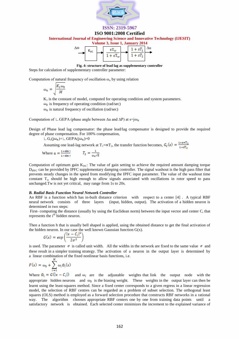
Fig. 4: structure of lead lag as supplementary controller

Steps for calculation of supplementary controller parameter:

Computation of natural frequency of oscillation ωn by using relation

K1 is the constant of model, computed for operating condition and system parameters.

is frequency of operating condition (rad/sec)

is natural frequency of oscillation (rad/sec)

Computation of ∟GEPA (phase angle between ∆u and ∆P) at s=j

Design of Phase lead lag compensator: the phase lead/lag compensator is designed to provide the required

degree of phase compensation. For 100% compensation,

∟Gc(j )+∟GEPA(j )=0

Assuming one lead-lag network at T1=∝T2, the transfer function becomes,

Where

Computation of optimum gain KDC: The value of gain setting to achieve the required amount damping torque

DIPFC can be provided by IPFC supplementary damping controller. The signal washout is the high pass filter that

prevents steady changes in the speed from modifying the IPFC input parameter. The value of the washout time

constant Tw should be high enough to allow signals associated with oscillations in rotor speed to pass

unchanged.Tw is not yet critical, may range from 1s to 20s.

B. Radial Basis Function Neural Network Controller

An RBF is a function which has in-built distance criterion with respect to a center [4] . A typical RBF

neural network consists of three layers (input, hidden, output). The activation of a hidden neuron is

determined in two steps:

First- computing the distance (usually by using the Euclidean norm) between the input vector and center Ci that

represents the ith

hidden neuron.

Then a function h that is usually bell shaped is applied, using the obtained distance to get the final activation of

the hidden neuron. In our case the well known Gaussian function G(x).

is used. The parameter is called unit width. All the widths in the network are fixed to the same value and

these result in a simpler training strategy. The activation of a neuron in the output layer is determined by

a linear combination of the fixed nonlinear basis functions, i.e.

Where and are the adjustable weights that link the output node with the

appropriate hidden neurons and is the biasing weight. These weights in the output layer can then be

learnt using the least-squares method. Since a fixed center corresponds to a given regress in a linear regression

model, the selection of RBF centres can be regarded as a problem of subset selection. The orthogonal least

squares (OLS) method is employed as a forward selection procedure that constructs RBF networks in a rational

way. The algorithm chooses appropriate RBF centers one by one from training data points until a

satisfactory network is obtained. Each selected center minimizes the increment to the explained variance of

KDC

ISSN: 2319-5967



163

the desired output, and so ill conditioning problems occurring frequently in random selection of centers

can automatically be avoided. In contrast to most learning algorithms, which can only work if a fixed network

structure has first been specified, the OLS algorithm is a structural identification technique, where the

centers and estimates of the corresponding weights can be simultaneously determined in a very efficient

manner during learning. OLS learning procedure generally produces an RBF network smaller than a

randomly selected RBF network. Due to its linear computational procedure at the output layer, the RBF takes

less training time compared to its back propagation counterpart.

A major drawback of this method is associated with the input space dimensionality. For large

number of input units, the number of radial basis functions required, can become excessive. If too many

centers are used, the large number of parameters available in the regression procedure will cause the network

to be over sensitive to the details of the particular training set and result in poor generalization performance

(over fit). So the data compression through vector quantization technique has improved the efficiency of

RBF model

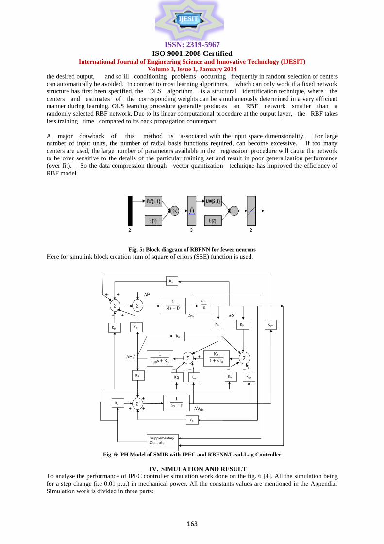
Fig. 5: Block diagram of RBFNN for fewer neurons

Here for simulink block creation sum of square of errors (SSE) function is used.

+ + ∆P

_

+ + ∆ω ∆δ

_ _ _

∆Eq’ +

_ _ _ _

+

+ + ∆Vdc

∑

∑

∑

∑

1

Ms + D

1

Td0′ s + K3

KA

1 + sTA

Supplementary

Controller

ω0

s

1

K9 + s

K1

K4 K2

K5

K6

K8

∑

Kp

Kc

K7

Kq Kvv Kv Kvv

Kpv

Fig. 6: PH Model of SMIB with IPFC and RBFNN/Lead-Lag Controller

IV. SIMULATION AND RESULT

To analyse the performance of IPFC controller simulation work done on the fig. 6 [4]. All the simulation being

for a step change (i.e 0.01 p.u.) in mechanical power. All the constants values are mentioned in the Appendix.

Simulation work is divided in three parts:

ISSN: 2319-5967



164

1. Without any supplementary controller

2. With Lead-Lag controller and

3. With RBFNN controller

0 1 2 3 4 5 6 7 8 9 10-3

-2

-1

0

1

2

3x 10

-3

Time in sec

dw

(p.u

)

Fig. 7: Response of speed deviation (∆ω) without any supplementary controller

0 1 2 3 4 5 6 7 8 9 10-0.2

-0.15

-0.1

-0.05

0

0.05

0.1

0.15

Time in sec

devia

tion in r

oto

r angle

(p.u

)

Fig. 8: Response of Rotor angle deviation (∆δ) without any supplementary

0 1 2 3 4 5 6 7 8 9 10-1

-0.5

0

0.5

1

1.5

2

2.5

3

3.5

4x 10

-5

Time in sec

dw

(p.u

)

Fig. 9: Response of speed deviation (∆ω) for m1 of IPFC controller with Lead-Lag Controller

ISSN: 2319-5967



165

0 1 2 3 4 5 6 7 8 9 100

0.001

0.002

0.003

0.004

0.005

0.006

0.007

0.008

0.009

0.01

Time in sec

devia

tion in r

oto

r angle

(p.u

)

Fig. 10: Response of Rotor angle deviation (∆δ) for m1 of IPFC controller with Lead-Lag Controller

0 1 2 3 4 5 6 7 8 9 10-8

-6

-4

-2

0

2

4

6

8

10

12x 10

-5

Time in sec

dw

(p.u

)

Fig. 11: Response of speed deviation (∆ω) for ∆δ1 of IPFC controller with Lead-Lag Controller

0 1 2 3 4 5 6 7 8 9 100

0.002

0.004

0.006

0.008

0.01

0.012

0.014

Time in sec

devia

tion in r

oto

r angle

(p.u

)

Fig. 12: Response of Rotor angle deviation (∆δ) for δ1 of IPFC controller with Lead-Lag Controller

ISSN: 2319-5967



166

0 1 2 3 4 5 6 7 8 9 10-0.5

0

0.5

1

1.5

2

2.5

3

3.5x 10

-5

Time in sec

dw

(p.u

)

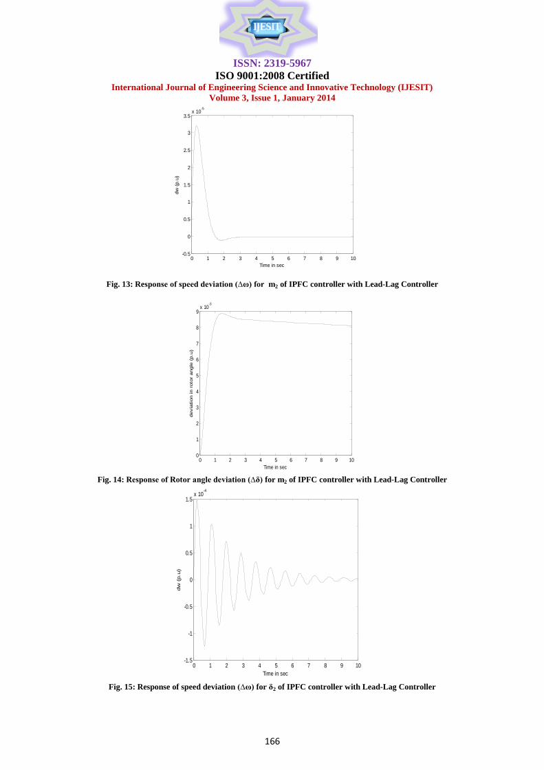
Fig. 13: Response of speed deviation (∆ω) for m2 of IPFC controller with Lead-Lag Controller

0 1 2 3 4 5 6 7 8 9 100

1

2

3

4

5

6

7

8

9x 10

-3

Time in sec

devia

tion in r

oto

r angle

(p.u

)

Fig. 14: Response of Rotor angle deviation (∆δ) for m2 of IPFC controller with Lead-Lag Controller

0 1 2 3 4 5 6 7 8 9 10-1.5

-1

-0.5

0

0.5

1

1.5x 10

-4

Time in sec

dw

(p.u

)

Fig. 15: Response of speed deviation (∆ω) for δ2 of IPFC controller with Lead-Lag Controller

ISSN: 2319-5967



167

0 1 2 3 4 5 6 7 8 9 100

0.002

0.004

0.006

0.008

0.01

0.012

0.014

0.016

Time in sec

devia

tion in r

oto

r angle

(p.u

)

Fig. 16: Response of rotor angle deviation (∆δ) for δ2 of IPFC controller with Lead-Lag Controller

0 1 2 3 4 5 6 7 8 9 10-1.5

-1

-0.5

0

0.5

1

1.5x 10

-4

Time in sec

Roto

r speed d

evia

tion(p

.u)

del1 Controller

del2 Controller

m1 Controller

m2 Controller

Fig. 17: Response of speed deviation (∆ω)

0 1 2 3 4 5 6 7 8 9 100

0.002

0.004

0.006

0.008

0.01

0.012

0.014

0.016

Time in sec

Roto

r angle

devia

tion(p

.u)

del1 Controller

del2 Controller

m1 Controller

m2 Controller

Fig. 18: Response of rotor angle deviation (∆δ)

ISSN: 2319-5967



168

0 1 2 3 4 5 6 7 8 9 10-0.5

0

0.5

1

1.5

2

2.5

3

3.5

4

4.5x 10

-5

Time in sec

dw

(p.u

)

Fig. 19: Response of speed deviation (∆ω) with RBFNN Controller (for m2 IPFC input Parameter)

0 1 2 3 4 5 6 7 8 9 100

1

2

3

4

5

6

7

8

9x 10

-3

Time in sec

devia

tion in r

oto

r angle

(p.u

)

Fig. 20: Response of Rotor angle deviation (∆δ) with RBFNN Controller(for m2 IPFC input Parameter)

0 1 2 3 4 5 6 7 8 9 10-0.5

0

0.5

1

1.5

2

2.5

3

3.5

4

4.5x 10

-5

Time in sec

dw

(p.u

)

RBFNN

Lead Lag

Fig. 21: Response of speed deviation (∆ω)

ISSN: 2319-5967



169

0 1 2 3 4 5 6 7 8 9 100

1

2

3

4

5

6

7

8

9x 10

-3

Time in sec

devitio

n in r

oto

r angle

(p.u

)

RBFNN

Lead lag

Fig. 22: Response of rotor angle deviation (∆δ)

V. CONCLUSION

Response shown in fig. 7 and 8 are for the circuit shown fig. 6 in the absence of supplementary controller.

Response shown in fig. 9-16 are of IPFC used with Lead-Lag controller as supplementary Controller for all the

four input (m1, m2, δ1 and δ2) of IPFC controller. From the response of fig 17 and 18, we observe that m2 input

parameter of IPFC controller gives best among all. Hence, for the next step work, only m2 parameter is taken

into consideration. Response shown in fig. 19 and 20 are of IPFC with RBFNN Controller as supplementary

Controller with m2 input parameter of IPFC controller. From the response of fig. 21 and 22, we observe that the

RBFNN gives the better result in comparison to the Lead-Lag Controller. Hence, it is concluded that the

RBFNN based IPFC controller gives better damping capability than Lead-Lag based IPFC controller.

APPENDIX

A: Parameter of SMIB System with IPFC

Generator

M=8.0

MJ/MVA

Tdo’=5.044s Xd=1.0 pu

Xq=0.6pu Xd’=0.3pu D=0

Reactances Xs=0.15pu Xt1=0.1pu Xt2=0.1pu

Xt=0.1pu XL1=0.5pu XL2=0.5pu

XL=0.5pu

IPFC

parameters

m1=0.15 m2=0.1 δ1=28.10

δ2=-21.10

Excitation

System

KA=50 TA=0.05s

DC link VDC=2.0pu CDC=1.0pu

B: Constant for Lead Lag Controller IPFC

Controller

Input

Lead-lag controller Parameters

KDC

Tw

(s)

T1

(s)

T2

(s)

m1 308.1583 13.2799 0.198 0.0195

m2 300.2638 9.6307 0.1993 0.0198

δ 1 312.4573 9.1681 0.1986 0.0192

δ 2 323.7909 12.2496 0.1931 0.0144

ISSN: 2319-5967



170

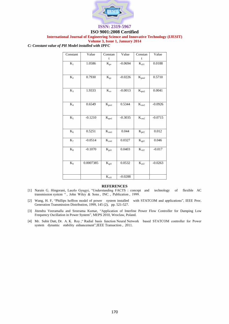
C: Constant value of PH Model installed with IPFC

Constant Value Constan

t

Value Constan

t

Value

K1 1.0586 Kpv -0.0694 Kcδ1 0.0188

K2 0.7930 Kqv -0.0226 Kpm2 0.5710

K3 1.9333 Kvv -0.0013 Kqm2 0.0041

K4 0.6549 Kpm1 0.5344 Kvm2 -0.0926

K5 -0.1210 Kqm1 -0.3035 Kcm2 -0.0715

K6 0.5251 Kvm1 0.044 Kpδ2 0.012

K7 -0.0514 Kcm1 0.0327 Kqδ2 0.046

K8 -0.1070 Kpδ1 0.0403 Kvδ2 -0.017

K9 0.0007385 Kqδ1 0.0532 Kcδ2 -0.0263

Kvδ1 -0.0288

REFERENCES [1] Narain G. Hingorani, Laszlo Gyugyi, “Understanding FACTS : concept and technology of flexible AC

transmission system “ , John Wiley & Sons , INC. , Publication , 1999.

[2] Wang, H. F, “Phillips heffron model of power system installed with STATCOM and applications”, IEEE Proc.

Generation Transmission Distribution, 1999, 145 (2), pp. 521-527.

[3] Jitendra Veeramalla and Sreerama Kumar, “Application of Interline Power Flow Controller for Damping Low

Frequency Oscillation in Power System”, MEPS 2010, Wroclaw, Poland.

[4] Mr. Subir Datt, Dr. A. K. Roy ,“ Radial basis function Neural Network based STATCOM controller for Power

system dynamic stability enhancement”,IEEE Transaction , 2011.

Neural Network based FACTS Controller for enhancement of Power System Dynamic Stability

Documents

Transcript of Neural Network based FACTS Controller for enhancement of Power System Dynamic Stability