Applied Energy 91 (2012) 222–234

Contents lists available at SciVerse ScienceDirect

Applied Energy

journal homepage: www.elsevier .com/ locate/apenergy

Buildings dynamic simulation: Water loop heat pump systems analysisfor European climates

Annamaria Buonomano, Francesco Calise, Adolfo Palombo ⇑DETEC, University of Naples Federico II, P.le Tecchio, 80, 80125 Naples, Italy

a r t i c l e i n f o

Article history:Received 13 June 2011Received in revised form 21 September2011Accepted 21 September 2011Available online 19 October 2011

Keywords:WLHP systemBuilding dynamic simulationHVAC performance analysisEnergy and economic saving

0306-2619/$ - see front matter � 2011 Elsevier Ltd. Adoi:10.1016/j.apenergy.2011.09.031

⇑ Corresponding author.E-mail address: palombo@unina.it (A. Palombo).

a b s t r a c t

In this paper, a purposely designed code for the performance analysis of the Water Loop Heat Pump(WLHP) systems is presented. Hourly, daily and seasonal energy system consumptions, operating eco-nomic costs and environmental impact assessments are dealt with. For the scope of comparison, the per-formances of two reference HVAC system are investigated too. For the computation of the buildingheating and cooling requirements, a suitable dynamic performance simulation model is being developed.All the relevant algorithms are implemented in MATLAB�. A case study of an office building undergoingsimulation in different European climatic areas is being presented. Here, different building thermal fea-tures are considered. In order to maximize the system performance an additional optimization procedureto the operating devices temperatures is carried out. Results show that primary energy savings andavoided CO2 emissions of the WLHP system vary in relation to the compared reference systems andcan be obtained only in several European weather zones. The feasibility of the WLHP system stronglydepends on electricity and natural gas national costs.

� 2011 Elsevier Ltd. All rights reserved.

1. Introduction

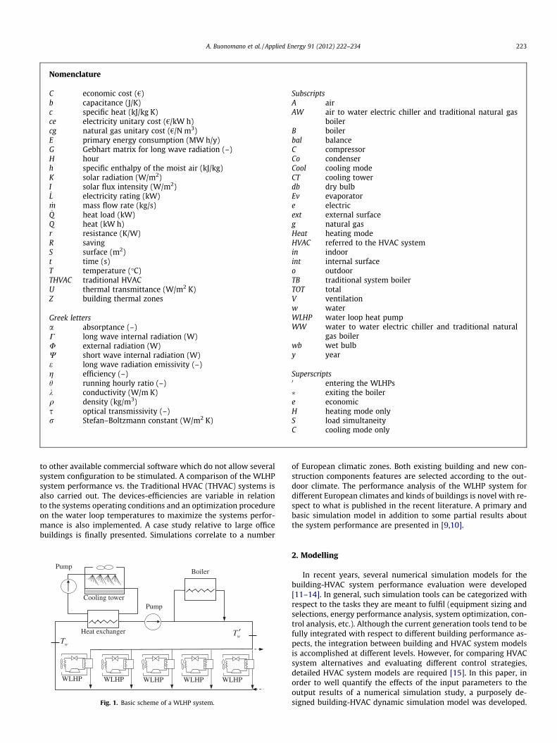
In buildings where space heating and cooling loads simulta-neously occur, a Water Loop Heat Pump (WLHP) system can beconveniently adopted [1,2]. Basically, it consists of a set of heatpumps that reject to a water loop the excess heat from cooledspace. Such heat is recovered by other heat pumps and transferredto spaces in need of heating. In the water loop, the occurring heat-ing or cooling deficits are balanced by additional heaters and/orcooling towers. WLHP systems are typically installed in edificeswith distinguished core and perimeter zones or commercial build-ing with deep freeze or cold stores. A basic scheme of a WLHP sys-tem is reported in Fig. 1.

Such systems were developed in the 1960s in USA, they becamewidely popular and applicable since 1990s mostly in USA andJapan. In recent years, several studies were carried out aiming atevaluating the system component features and relative operatingparameters. An investigation concerning the WLHP system’s envi-ronmental contribution to a green building environmental controlis reported in [3]. In this study, alternative options to increase thebuilding’s energy performance were considered. A comparison be-tween conventional air-conditioning systems and a WLHP systemfor a number of Chinese climatic zones is carried out in [4]. Aninteresting analysis of the WLHP performances on four different

ll rights reserved.

kinds of buildings was presented, where the devices’ efficienciesof the simulation model are kept constant [4]. In order to increasethe system energy saving, other authors studied the combinationof WLHP systems with gas-engine-driven heat pump (GHP) [5]and coupled with low-temperature geothermal sources [6,7]. Inparticular in [6] the evaluation of system performance and energysaving for commercial and public buildings is carried out. The effi-ciencies of the water source heat pumps are considered dependenton the loop water temperature that ranges between 16 and 32 �C. Aconstant cooling load profile is adopted for the core building zone.For the perimeter zone, the heating load is assumed linear to out-door temperatures. In [7] WLHP system is applied to three tower-shaped apartment building in Beijing (China) where well water isused as the low-temperature heat-source. The system perfor-mances are analyzed using a field-test data obtained by runningthe system over two winters and a summer. The system controllingconditions are also investigated. In [8] a given test building loadprofile and a single type of WLHPs equipped with a variable speedcompressor and a cooling tower with a variable speed fan are con-sidered in order to find out the optimal loop water temperatureminimizing the WLHP overall energy consumption.

In this paper, a detailed, purposely-designed performance sim-ulation model for the building-WLHP system is presented. Its com-puter implementation, obtained by MATLAB�, allows assessinghourly, daily and seasonal building-HVAC system performances,from an energy, economic and environmental points of view. Thistool allows the variation of system running parameters in contrast

Nomenclature

C economic cost (€)b capacitance (J/K)c specific heat (kJ/kg K)ce electricity unitary cost (€/kW h)cg natural gas unitary cost (€/N m3)E primary energy consumption (MW h/y)G Gebhart matrix for long wave radiation (–)H hourh specific enthalpy of the moist air (kJ/kg)K solar radiation (W/m2)I solar flux intensity (W/m2)_L electricity rating (kW)_m mass flow rate (kg/s)_Q heat load (kW)Q heat (kW h)r resistance (K/W)R savingS surface (m2)t time (s)T temperature (�C)THVAC traditional HVACU thermal transmittance (W/m2 K)Z building thermal zones

Greek lettersa absorptance (–)C long wave internal radiation (W)U external radiation (W)W short wave internal radiation (W)e long wave radiation emissivity (–)g efficiency (–)h running hourly ratio (–)k conductivity (W/m K)q density (kg/m3)s optical transmissivity (–)r Stefan–Boltzmann constant (W/m2 K)

SubscriptsA airAW air to water electric chiller and traditional natural gas

boilerB boilerbal balanceC compressorCo condenserCool cooling modeCT cooling towerdb dry bulbEv evaporatore electricext external surfaceg natural gasHeat heating modeHVAC referred to the HVAC systemin indoorint internal surfaceo outdoorTB traditional system boilerTOT totalV ventilationw waterWLHP water loop heat pumpWW water to water electric chiller and traditional natural

gas boilerwb wet bulby year

Superscripts0 entering the WLHPs� exiting the boilere economicH heating mode onlyS load simultaneityC cooling mode only

A. Buonomano et al. / Applied Energy 91 (2012) 222–234 223

to other available commercial software which do not allow severalsystem configuration to be stimulated. A comparison of the WLHPsystem performance vs. the Traditional HVAC (THVAC) systems isalso carried out. The devices-efficiencies are variable in relationto the systems operating conditions and an optimization procedureon the water loop temperatures to maximize the systems perfor-mance is also implemented. A case study relative to large officebuildings is finally presented. Simulations correlate to a number

Boiler

Heat exchanger

Pump Cooling tower

Pump

WLHP WLHP WLHP WLHP WLHP

wT ′wT

Fig. 1. Basic scheme of a WLHP system.

of European climatic zones. Both existing building and new con-struction components features are selected according to the out-door climate. The performance analysis of the WLHP system fordifferent European climates and kinds of buildings is novel with re-spect to what is published in the recent literature. A primary andbasic simulation model in addition to some partial results aboutthe system performance are presented in [9,10].

2. Modelling

In recent years, several numerical simulation models for thebuilding-HVAC system performance evaluation were developed[11–14]. In general, such simulation tools can be categorized withrespect to the tasks they are meant to fulfil (equipment sizing andselections, energy performance analysis, system optimization, con-trol analysis, etc.). Although the current generation tools tend to befully integrated with respect to different building performance as-pects, the integration between building and HVAC system modelsis accomplished at different levels. However, for comparing HVACsystem alternatives and evaluating different control strategies,detailed HVAC system models are required [15]. In this paper, inorder to well quantify the effects of the input parameters to theoutput results of a numerical simulation study, a purposely de-signed building-HVAC dynamic simulation model was developed.

224 A. Buonomano et al. / Applied Energy 91 (2012) 222–234

The assessment of the building heating and cooling requirements isthe first step to be carried out in a detailed simulation code. In thefirst part of this paragraph such model is presented in a short form.In the second part, the model created for the performance analysisof both the WLHP and THVAC systems is reported.

2.1. Dynamic model for the building heating and cooling energyassessment

A completely new simulation model was suitably written. Here,the thermal conduction through the opaque and transparent ele-ments is assumed as one-dimensional (thermal bridges are sepa-rately taken into account). The internal heat gain, the buildingventilation and the solar radiation loads are included in the calcu-lation process. The radiation heat transfer of the external opaquesurfaces takes into account the solar and the long wave effects[16,17]. In particular, the sun incidence angles are calculated as afunction of time and surface building orientation [18].

The modelled windows are supposed to be multi-glazed andfilled by different gases to meet the desired thermal transmittance.Solar radiation entering through the windows is absorbed, re-flected and distributed within the internal space by selectedabsorption, reflection and view factors, respectively. The internallong-wave radiation is handled by the Gebhart method [16,17].Depending on the building’s envelope thermal inertia, such ab-sorbed heat contributes to the heat gain during the winter seasonand to the space cooling load in summer. In order to reduce thesummer solar heat gains, the windows external solar shadingsare considered. The control model of their tilt angle, and thus ofthe windows shading coefficient, is here based on the standardrequirement of the average indoor horizontal lighting level [19].

In order to simulate the dynamic thermal response of each build-ing element (wall, ceiling, floor and window), a thermal network ofn nodes is implemented, [20,21]. Here, for each m building element,n depends on the modelled isothermal layers and it is selected by atrade-off analysis taking into account the computational time andthe accuracy of the calculation procedure, simultaneously.

In order to calculate the heating or cooling energy requirement(QHVAC) for each building space, the following system of differentialequations is used:

bm;ndTm;nds ¼ T1;n�1�T1;n

rm;n�1þ T1;nþ1�T1;n

rm;nþ Cm þWm þUm

bindTinds ¼

PMm¼1

Tm;N�Tinrm;N

þ _Q GAIN þ _mV ho � hinð Þ � _Q HVAC

8><>:

Cm ¼ Smem;intrXM

j¼1

Gm;jðT4j;N � T4

m;NÞ

Cm – 0 only for internal surface ðn ¼ NÞWm ¼ Smam;intIm Wm – 0 only for internal surface ðn ¼ NÞ

Um ¼ Sm em;extrðT4sky � T4

m;1Þ þ am;extKm

h i

Um – 0 only for external surface ðn ¼ 1Þm ¼ 1 � � �Mn ¼ 1 � � �N

ð1Þ

where T, r and b are the thermal network temperatures, resistancesand capacitances, respectively. _QGAIN is the total internal gain dueto human activity and electrical devices. I is the total solar radiationflux received by an internal surface and is calculated as the sum ofradiation directly received without considering multiple reflections,plus the sum of the solar irradiance reflected by others surfaces [16]._mV and h represent air ventilation rate and moist air enthalpy,

respectively. _QHVAC is calculated according to a Proportional Integral

(PI) control on the indoor air conditions [18]. Temperature andhumidity can range in fixed intervals, avoiding the HVAC systemactivation.

Note that the results obtained by the mentioned new dynamicmodel were compared with those achieved by a standard simula-tion code (TRNSYS 17, type 56 for buildings [17]). For differentbuilding geometries and European weather data, the detected dif-ferences ranged from 4% to 8%. All the details concerning this spe-cific proposed dynamic simulation code will be presented in afuture paper.

2.2. WLHP system model

Starting from calculation results of space design loads, two dif-ferent logics can be followed by such code. The first one includesspecific purposely sized WLHP for each space while in the secondlogic different WLHPs of the same size are taken into account. Inorder to balance the eventual water loop thermal energy deficitsor excesses due to the WLHPs running, a natural gas boiler or acooling tower are implemented accordingly. Steady state condi-tions are assumed in each systems running hour (H-th) [22].

The eventual heat provided by the boiler in the H-th hour is cal-culated by:

QBðHÞ ¼ ½ _mwðHÞ � c � ðT 0wðHÞ � TwðHÞÞ� � H ð2Þ

where _mwðHÞ � c is the product of the water loop mass flow rate inthe H-th hour by the liquid water specific heat while Tw(H) andT 0wðHÞ are respectively the entering and exiting water temperaturesof the boiler in the H-th hour (Fig. 1). T 0wðHÞ is modelled taking intoaccount the running constraints of the WLHP system devices.

The primary energy consumption and operating economic costof the boiler are calculated as a function of the boiler efficiency, thenatural gas lower heating value and the natural gas unitary cost.

While boilers allow controlling the outgoing water tempera-ture, this is in general not possible when using cooling towers. Inthis model, the steeper the water loop temperature increasingtrend is, the stronger and faster the cooling tower’s reaction is.Here, different operational steps are possible: when the outdoorair temperature is lower than the temperature in the water loopa free cooling of the loop water is activated using the cooling toweras a dry heat exchanger. In the case that such process is not suffi-cient to decrease the water temperature (i.e. for still high exitingtemperature) the cooling tower water pumps are switched on.For medium-difficult working conditions, a first fan set is activatedincreasing the cooling tower efficiency. For heavy working condi-tions, a second fan set in the cooling tower is switched on with afurther increase of its efficiency. This algorithm is implementedin a new simulation code. Subsequently, the hourly water exitingtemperature is iteratively calculated taking into account the designand operating conditions of closed circuit cooling towers [23].

The primary energy consumption and operating economic cost ofthe cooling tower in the H-th hour are calculated according to theconventional average electricity production efficiency in the powerplant and the electricity unitary cost (which vary between coun-tries). The cooling tower water consumption is here disregarded.

The loop water at T 0w (Fig. 1) reaches each WLHP where the fol-lowing calculation is done. Depending on the supply water looptemperatures, variable cooling and heating capacities _Q Ev ðHÞ and_QCoðHÞ and compressor ratings _LCðHÞ are accounted. Since a WLHPon–off regulation is considered, the hourly rate hC(H) in which eachWLHP compressor when switched on is calculate as:

Cooling : hCðHÞ ¼ Q CHVACðHÞ= _QEvðHÞ ð3Þ

Heating : hCðHÞ ¼ Q HHVACðHÞ= _QCoðHÞ ð4Þ

20.0 m

3.50 m

40.0 m

core zone

perimeter zone

perimeter zone N

Fig. 2. Simulated building: plan view.

A. Buonomano et al. / Applied Energy 91 (2012) 222–234 225

where QCHVACðHÞ and QH

HVACðHÞ correspond for each i-th indoor spaceto term: ±QHVAC obtained by equations system (1).

In the occurring H hour the Tw that has to be considered withrespect to the following simulation time step (H + 1) is calculatedby the following energy balance on the water loop:

XZ

i¼1

ð _Q CoðHÞ � hCðHÞÞi;Cool �XZ

i¼1

ð _QEvðHÞ � hCðHÞÞi;Heat

¼ ½ _mwðHÞ � cðTwðHÞ � T 0wðHÞÞ� ð5Þ

where Z is the building’s space. If on the water loop the sum of theheat rejected by the WLHPs running in cooling mode is higher thanthe sum of the cooling load of the heating WLHPs, then: Tw > T 0wand vice versa.

For each building space and relative to hC(H) the system’s pri-mary energy consumption and electricity cost in the H-th hourare calculated. For the whole building and in the same simulationhour the sum of these primary energy consumptions (EWLHP(H))and costs (Ce,WLHP(H)) are added to the eventual ones due to theboiler (EB(H), Cg,B(H)) or to the cooling tower (ECT(H), Ce,CT(H)). Thus,the yearly WLHP system overall primary energy consumption andoperating cost are respectively computed by:

E ¼Xyear

H

ðEWLHPðHÞ þ EBðHÞ þ ECTðHÞÞ ð6Þ

C ¼Xyear

H

ðCe;WLHPðHÞ þ Cg;BðHÞ þ Ce;CTðHÞÞ ð7Þ

A parametric optimization procedure is carried out on the boilerand cooling tower temperature’s activation in order to get the sys-tem’s minimum primary energy consumption, according to theWLHP system constraints. In general, the higher the water looptemperature is, the lower the heating mode WLHP’s energy con-sumption is. This is due to the higher relative COPs. On the otherhand, the consumptions of boiler and cooling mode WLHPs arehigher. Conversely, the lower the loop water temperature is, thelower the cooling mode WLHPs energy costs are. In this case theconsumptions of cooling tower and heating mode WLHPs are high-er. In order to reach the optimal water loop temperatures, the fol-lowing cases have to be distinguished because of the differentsystem constraints:

� case 1. Only heating is supplied to the building spaces by theWLHPs (heating only mode);� case 2. Both heating and cooling are simultaneously supplied to

the spaces by the WLHPs (simultaneous heating and coolingmode);� case 3. Only cooling is supplied to the building spaces by the

WLHPs (cooling only mode).

The optimization procedure in case 2 is obtained by simulatingall the possible combinations of boiler and cooling tower temper-atures activation by an interval of 1 �C.

2.3. THVAC system model

Each building thermal zone is equipped by several 4-pipe fancoils, supplied by chilled or hot water depending on the temporalcooling or heating load. In the present simulation model, it is as-sumed that such processes are obtained by two different referencesystems [24]:

� Air to water electric chiller and Traditional natural gas Boiler(TB) for cooling and heating, respectively. This plant is calledAW traditional system;

� Water to water electric chiller (supported by a cooling tower)and Traditional natural gas Boiler (TB) for cooling and heatingrespectively. This plant is called WW traditional system.

For evaluating the performance of these systems a new suitablemodel was written. The systems devices are sized by the buildingdesign heating and cooling loads previously calculated. The heatprovided to the building by TB and the cooling energy extractedby the AW and WW chillers are calculated by algorithms similarto those considered for the WLHP system boiler and heat pumps.Also in this case variable COPs are taken into account. Thus, theyearly AW and WW traditional systems total operating cost is com-puted by:

CAWðor WWÞ ¼Xyear

H

ðCg;TBðHÞ þ Ce;AW Chillerðor WWÞðHÞÞ ð8Þ

Included here are electricity consumptions from the fans of theAW chiller and cooling tower and the pump of the WW chiller.

For both the WLHP and THVAC systems, the performanceparameters of all the devices are extracted from the manufacturer’sinput regarding a wide range of HVAC operating conditions. Notethat for outdoor air temperature below 20 �C the AW chiller COPincreases while it remains almost constant for the WW chiller. Thisis due to the following reasons: (a) for the AW chiller, the con-denser fans between 20 and 0 �C are proportionally and graduallyturning off, below 0 �C the system is in free-cooling mode (fans andcompressor are switched off); (b) the COP curve value is constantfor the WW chiller when cooling tower water temperatures corre-spond to outdoor air temperatures and are between 20 and 0 �C.

An optimization procedure for minimizing the primary energyconsumptions for the WW chiller cooling tower is also carried out.

For the economic analysis, the capital cost of WLHP and THVACsystems and the operating cost due to the space air diffusion andthe water pumping are assumed to be almost the same [4].

3. Simulation

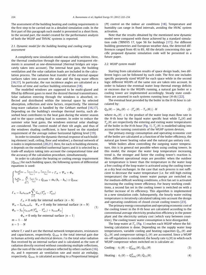
The simulated performance of a WLHP system is compared withthose obtained by the above described traditional systems. Theconsidered case study refers to a multi-floor office building. Lengthand width are 40 and 20 m, respectively, the height of each floor is3.5 m. The building’s longitudinal axis is East–West oriented(Fig. 2). The reported results were generated from a simulated 7-floor building block. For each floor, a core zone (interior zone with-out direct transmission or radiation external loads) is divided bypartition walls with a surrounding perimeter zone (Fig. 2). Forthe present case study, the ratio between the building core zonevolume and the total (core plus perimeter) volume is 0.54. For sucha building block, a self-sufficient HVAC system is considered. Sinceadiabatic partition floors are hypothesized, only nine differentthermal zones are modelled (Fig. 2). The ratio between the win-dows surface areas and the building lateral areas is 0.50. Uniformwindow distribution over the whole lateral surface is considered.

226 A. Buonomano et al. / Applied Energy 91 (2012) 222–234

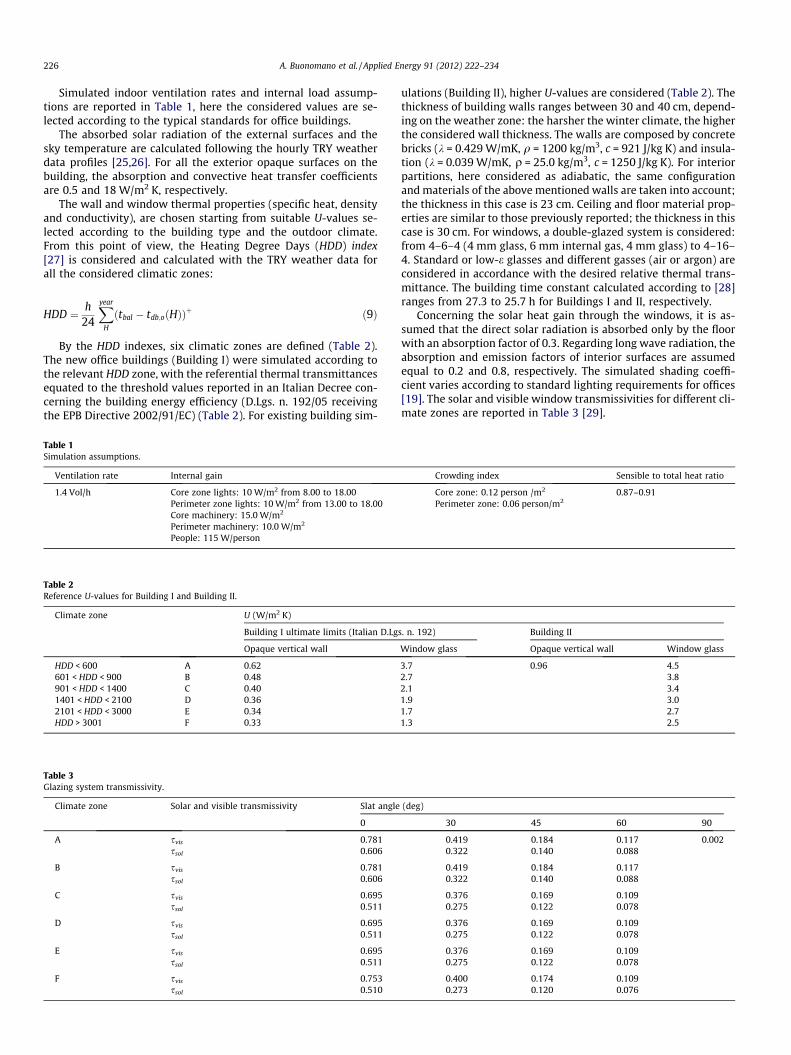
Simulated indoor ventilation rates and internal load assump-tions are reported in Table 1, here the considered values are se-lected according to the typical standards for office buildings.

The absorbed solar radiation of the external surfaces and thesky temperature are calculated following the hourly TRY weatherdata profiles [25,26]. For all the exterior opaque surfaces on thebuilding, the absorption and convective heat transfer coefficientsare 0.5 and 18 W/m2 K, respectively.

The wall and window thermal properties (specific heat, densityand conductivity), are chosen starting from suitable U-values se-lected according to the building type and the outdoor climate.From this point of view, the Heating Degree Days (HDD) index[27] is considered and calculated with the TRY weather data forall the considered climatic zones:

HDD ¼ h24

Xyear

H

ðtbal � tdb;oðHÞÞþ ð9Þ

By the HDD indexes, six climatic zones are defined (Table 2).The new office buildings (Building I) were simulated according tothe relevant HDD zone, with the referential thermal transmittancesequated to the threshold values reported in an Italian Decree con-cerning the building energy efficiency (D.Lgs. n. 192/05 receivingthe EPB Directive 2002/91/EC) (Table 2). For existing building sim-

Table 1Simulation assumptions.

Ventilation rate Internal gain

1.4 Vol/h Core zone lights: 10 W/m2 from 8.00 to 18.00Perimeter zone lights: 10 W/m2 from 13.00 to 18.00Core machinery: 15.0 W/m2

Perimeter machinery: 10.0 W/m2

People: 115 W/person

Table 2Reference U-values for Building I and Building II.

Climate zone U (W/m2 K)

Building I ultimate limits (Italian D.Lg

Opaque vertical wall

HDD < 600 A 0.62601 < HDD < 900 B 0.48901 < HDD < 1400 C 0.401401 < HDD < 2100 D 0.362101 < HDD < 3000 E 0.34HDD > 3001 F 0.33

Table 3Glazing system transmissivity.

Climate zone Solar and visible transmissivity Slat angle

0

A svis 0.781ssol 0.606

B svis 0.781ssol 0.606

C svis 0.695ssol 0.511

D svis 0.695ssol 0.511

E svis 0.695ssol 0.511

F svis 0.753ssol 0.510

ulations (Building II), higher U-values are considered (Table 2). Thethickness of building walls ranges between 30 and 40 cm, depend-ing on the weather zone: the harsher the winter climate, the higherthe considered wall thickness. The walls are composed by concretebricks (k = 0.429 W/mK, q = 1200 kg/m3, c = 921 J/kg K) and insula-tion (k = 0.039 W/mK, q = 25.0 kg/m3, c = 1250 J/kg K). For interiorpartitions, here considered as adiabatic, the same configurationand materials of the above mentioned walls are taken into account;the thickness in this case is 23 cm. Ceiling and floor material prop-erties are similar to those previously reported; the thickness in thiscase is 30 cm. For windows, a double-glazed system is considered:from 4–6–4 (4 mm glass, 6 mm internal gas, 4 mm glass) to 4–16–4. Standard or low-e glasses and different gasses (air or argon) areconsidered in accordance with the desired relative thermal trans-mittance. The building time constant calculated according to [28]ranges from 27.3 to 25.7 h for Buildings I and II, respectively.

Concerning the solar heat gain through the windows, it is as-sumed that the direct solar radiation is absorbed only by the floorwith an absorption factor of 0.3. Regarding long wave radiation, theabsorption and emission factors of interior surfaces are assumedequal to 0.2 and 0.8, respectively. The simulated shading coeffi-cient varies according to standard lighting requirements for offices[19]. The solar and visible window transmissivities for different cli-mate zones are reported in Table 3 [29].

Crowding index Sensible to total heat ratio

Core zone: 0.12 person /m2 0.87–0.91Perimeter zone: 0.06 person/m2

s. n. 192) Building II

Window glass Opaque vertical wall Window glass

3.7 0.96 4.52.7 3.82.1 3.41.9 3.01.7 2.71.3 2.5

(deg)

30 45 60 90

0.419 0.184 0.117 0.0020.322 0.140 0.088

0.419 0.184 0.1170.322 0.140 0.088

0.376 0.169 0.1090.275 0.122 0.078

0.376 0.169 0.1090.275 0.122 0.078

0.376 0.169 0.1090.275 0.122 0.078

0.400 0.174 0.1090.273 0.120 0.076

A. Buonomano et al. / Applied Energy 91 (2012) 222–234 227

The simulation starts at 00:00 of January 1st and ends at 24:00of December 31st. The considered daily HVAC running time is from8:00 to 18:00 (10 h per day). The calculations are carried out for 28different European TRY weather zones (Table 4).

The threshold temperature, above which the HVAC cooling sys-tem is activated, is adjusted between summer and winter monthsto assure satisfactory thermal comfort between zones during thewhole year. Activation temperatures were set at 26 �C and 23 �Cfor summer and winter, respectively. A heating mode was consid-ered for winter months for indoor temperatures lower than 20 �C.The adiabatic behavior hypothesis is supported by these tempera-ture conditions, along with the assumption of thermally well-insu-lated interior partitions (3 cm, k = 0.039 W/mK) [18]. The relativehumidity of the indoor air is maintained between 50% and 60%.The considered WLHPs temperatures constraints and the HVAC

Table 4Climatic zones, HDD index and HDD zones.

Country Climatic area Latit. N� HDD (Kd) HDD zone

UK Lerwick 60�080 4024 FEskdalemuir 55�190 3970 FAberporth 52�080 3178 FKew (London) 51�280 2900 E

Denmark Copenhagen 55�460 3696 FEire Dublin 53�260 3133 F

Valentia 51�560 2741 ENetherlands Eelde 53�080 3427 F

De Bilt 52�060 3194 FVlissingen 51�270 2877 E

Belgium Oostende 51�120 3147 FUccle (Bruxelles) 50�480 3020 FSaint Hubert 50�020 4188 F

France Trappes 48�460 3069 FNancy 48�410 3245 FMacon 46�180 2980 ELimoges 45�490 2899 ECarpentras 44�050 2266 ENice 43�390 1650 D

Italy Bolzano 46�280 3087 FVenezia 45�300 2317 EMilano 45�260 2551 EGenova 44�250 1560 DRoma 41�480 1663 DFoggia 41�310 1759 DCagliari 39�150 1349 CCrotone 39�040 1409 CTrapani 37�550 976 C

Table 5HVAC systems assumptions.

WLHP system AW chiller and boiler

HeatingMinimum WLHP inlet water:

Tw = 8 �C (DT = 6 �C)Design heating water temperatures = 45–40 �C

Maximum inlet water Tw = 23 �C

CoolingMinimum WLHP inlet water

Tw = 13 �CDesign cooling water temperatures = 7–12 �C

Maximum inlet water: Tw = 44 �C(DT = 6 �C)

Boiler efficiency, gB = 1.06 Design AW chiller inlet air, T = 44 �C (DT = 6 �C),minimum inlet air T = 16 �C

Natural gas lower heating value,LHV = 9.59 kW h/N m3

systems simulation assumptions are reported in Table 5. The per-formance of all the considered devices for both WLHP and THVACsystems are calculated for a wide range of HVAC operating condi-tions, as defined by manufacturers.

The operating algorithm of the centralized boiler and coolingtower is summarized in Table 6, and varies according to the WLHPsoperating mode. The logic of the algorithm is as follows: if onlyheating is required by the WLHPs, the loop water temperature ismaintained at the desired boiler exiting temperature ðT�wÞ. Whenboth heating and cooling are simultaneously required by theWLHPs, the loop water temperature is maintained between T�wand the optimal cooling tower activation temperature ðT 0w;CTÞ. Forthe latter scenario, temperature control is achieved through sev-eral strategies: (1) boiler activation; (2) both boiler and coolingtower standby; (3) cooling tower standby; (4) cooling tower free

WW chiller and boiler

Design WW chiller inlet water, Tw = 50 �C (DT = 6 �C), minimum inlet waterTw = 20 �C, design cooling tower water DT = 6 �C

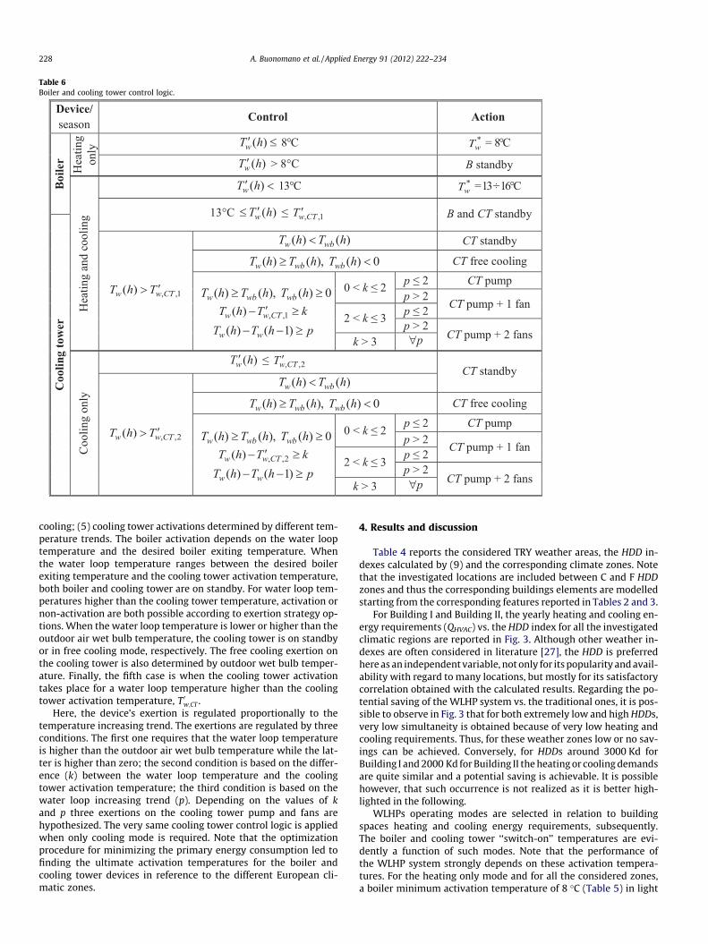
Table 6Boiler and cooling tower control logic.

228 A. Buonomano et al. / Applied Energy 91 (2012) 222–234

cooling; (5) cooling tower activations determined by different tem-perature trends. The boiler activation depends on the water looptemperature and the desired boiler exiting temperature. Whenthe water loop temperature ranges between the desired boilerexiting temperature and the cooling tower activation temperature,both boiler and cooling tower are on standby. For water loop tem-peratures higher than the cooling tower temperature, activation ornon-activation are both possible according to exertion strategy op-tions. When the water loop temperature is lower or higher than theoutdoor air wet bulb temperature, the cooling tower is on standbyor in free cooling mode, respectively. The free cooling exertion onthe cooling tower is also determined by outdoor wet bulb temper-ature. Finally, the fifth case is when the cooling tower activationtakes place for a water loop temperature higher than the coolingtower activation temperature, T 0w;CT .

Here, the device’s exertion is regulated proportionally to thetemperature increasing trend. The exertions are regulated by threeconditions. The first one requires that the water loop temperatureis higher than the outdoor air wet bulb temperature while the lat-ter is higher than zero; the second condition is based on the differ-ence (k) between the water loop temperature and the coolingtower activation temperature; the third condition is based on thewater loop increasing trend (p). Depending on the values of kand p three exertions on the cooling tower pump and fans arehypothesized. The very same cooling tower control logic is appliedwhen only cooling mode is required. Note that the optimizationprocedure for minimizing the primary energy consumption led tofinding the ultimate activation temperatures for the boiler andcooling tower devices in reference to the different European cli-matic zones.

4. Results and discussion

Table 4 reports the considered TRY weather areas, the HDD in-dexes calculated by (9) and the corresponding climate zones. Notethat the investigated locations are included between C and F HDDzones and thus the corresponding buildings elements are modelledstarting from the corresponding features reported in Tables 2 and 3.

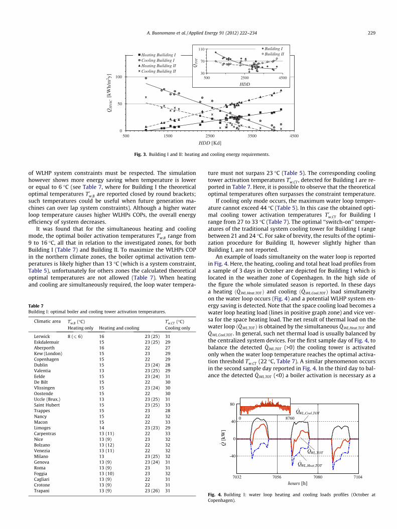
For Building I and Building II, the yearly heating and cooling en-ergy requirements (QHVAC) vs. the HDD index for all the investigatedclimatic regions are reported in Fig. 3. Although other weather in-dexes are often considered in literature [27], the HDD is preferredhere as an independent variable, not only for its popularity and avail-ability with regard to many locations, but mostly for its satisfactorycorrelation obtained with the calculated results. Regarding the po-tential saving of the WLHP system vs. the traditional ones, it is pos-sible to observe in Fig. 3 that for both extremely low and high HDDs,very low simultaneity is obtained because of very low heating andcooling requirements. Thus, for these weather zones low or no sav-ings can be achieved. Conversely, for HDDs around 3000 Kd forBuilding I and 2000 Kd for Building II the heating or cooling demandsare quite similar and a potential saving is achievable. It is possiblehowever, that such occurrence is not realized as it is better high-lighted in the following.

WLHPs operating modes are selected in relation to buildingspaces heating and cooling energy requirements, subsequently.The boiler and cooling tower ‘‘switch-on’’ temperatures are evi-dently a function of such modes. Note that the performance ofthe WLHP system strongly depends on these activation tempera-tures. For the heating only mode and for all the considered zones,a boiler minimum activation temperature of 8 �C (Table 5) in light

0

50

100

500 1500 2500 3500 4500

QH

VA

C [k

Wh/

m2 y

]

HDD [Kd]

Heating Builiding ICooling Building IHeating Building IICooling Building II 30

70

110

500 2500 4500

QTO

T

Building IBuilding II

HDD

Fig. 3. Building I and II: heating and cooling energy requirements.

A. Buonomano et al. / Applied Energy 91 (2012) 222–234 229

of WLHP system constraints must be respected. The simulationhowever shows more energy saving when temperature is loweror equal to 6 �C (see Table 7, where for Building I the theoreticaloptimal temperatures T 0w;B are reported closed by round brackets;such temperatures could be useful when future generation ma-chines can over lap system constraints). Although a higher waterloop temperature causes higher WLHPs COPs, the overall energyefficiency of system decreases.

It was found that for the simultaneous heating and coolingmode, the optimal boiler activation temperatures T 0w;B range from9 to 16 �C, all that in relation to the investigated zones, for bothBuilding I (Table 7) and Building II. To maximize the WLHPs COPin the northern climate zones, the boiler optimal activation tem-peratures is likely higher than 13 �C (which is a system constraint,Table 5), unfortunately for others zones the calculated theoreticaloptimal temperatures are not allowed (Table 7). When heatingand cooling are simultaneously required, the loop water tempera-

Table 7Building I: optimal boiler and cooling tower activation temperatures.

Climatic area T 0w;B (�C) T 0w;CT (�C)Heating only Heating and cooling Cooling only

Lerwick 8 (6 6) 16 23 (25) 31Eskdalemuir 15 23 (25) 29Aberporth 16 22 27Kew (London) 15 23 29Copenhagen 15 22 29Dublin 15 23 (24) 28Valentia 13 23 (25) 29Eelde 15 23 (24) 31De Bilt 15 22 30Vlissingen 15 23 (24) 30Oostende 15 22 30Uccle (Brux.) 13 23 (25) 31Saint Hubert 15 23 (25) 33Trappes 15 23 28Nancy 15 22 32Macon 15 22 33Limoges 14 23 (23) 29Carpentras 13 (11) 22 33Nice 13 (9) 23 32Bolzano 13 (12) 22 32Venezia 13 (11) 22 32Milano 13 23 (25) 32Genova 13 (9) 23 (24) 31Roma 13 (9) 23 31Foggia 13 (10) 23 32Cagliari 13 (9) 22 31Crotone 13 (9) 22 31Trapani 13 (9) 23 (26) 31

ture must not surpass 23 �C (Table 5). The corresponding coolingtower activation temperatures T 0w;CT , detected for Building I are re-ported in Table 7. Here, it is possible to observe that the theoreticaloptimal temperatures often surpasses the constraint temperature.

If cooling only mode occurs, the maximum water loop temper-ature cannot exceed 44 �C (Table 5). In this case the obtained opti-mal cooling tower activation temperatures T 0w;CT for Building Irange from 27 to 33 �C (Table 7). The optimal ‘‘switch-on’’ temper-atures of the traditional system cooling tower for Building I rangebetween 21 and 24 �C. For sake of brevity, the results of the optimi-zation procedure for Building II, however slightly higher thanBuilding I, are not reported.

An example of loads simultaneity on the water loop is reportedin Fig. 4. Here, the heating, cooling and total heat load profiles froma sample of 3 days in October are depicted for Building I which islocated in the weather zone of Copenhagen. In the high side ofthe figure the whole simulated season is reported. In these daysa heating ð _Q WL;Heat;TOTÞ and cooling ð _QWL;Cool;TOTÞ load simultaneityon the water loop occurs (Fig. 4) and a potential WLHP system en-ergy saving is detected. Note that the space cooling load becomes awater loop heating load (lines in positive graph zone) and vice ver-sa for the space heating load. The net result of thermal load on thewater loop ð _Q WL;TOTÞ is obtained by the simultaneous _Q WL;Heat;TOT and_QWL;Cool;TOT . In general, such net thermal load is usually balanced bythe centralized system devices. For the first sample day of Fig. 4, tobalance the detected _QWL;TOT (>0) the cooling tower is activatedonly when the water loop temperature reaches the optimal activa-tion threshold T 0w;CT (22 �C, Table 7). A similar phenomenon occursin the second sample day reported in Fig. 4. In the third day to bal-ance the detected _Q WL;TOT (<0) a boiler activation is necessary as a

hours [h]

,WL TOTQ

Q [

kW]

, ,WL Cool TOTQ

, ,WL Heat TOTQ

0 8760

7032 7056 7080 7104

80

40

0

-40

Fig. 4. Building I: water loop heating and cooling loads profiles (October atCopenhagen).

7032 7056 7080 7104

30

25

20

15

10

5

hours [h]

wT ′

dbTwT′

[°C

]

wbT

0 8760

Fig. 5. Building I: temperature profiles (October at Copenhagen).

230 A. Buonomano et al. / Applied Energy 91 (2012) 222–234

result of the water loop temperature reaching the optimal activa-tion threshold T 0w;B (15 �C, Table 7). All such operating conditionsare clearly visible in Fig. 5, where for Copenhagen the temperatureprofile of the water loop ðT 0w, Fig. 1), for the same above mentionedsample days, are reported. Here, the profiles of the TRY outdoor airdry bulb and wet bulb temperatures are also shown. Both dry andwet bulb temperature profiles are provided for the whole simu-lated season in the high side of the same figure.

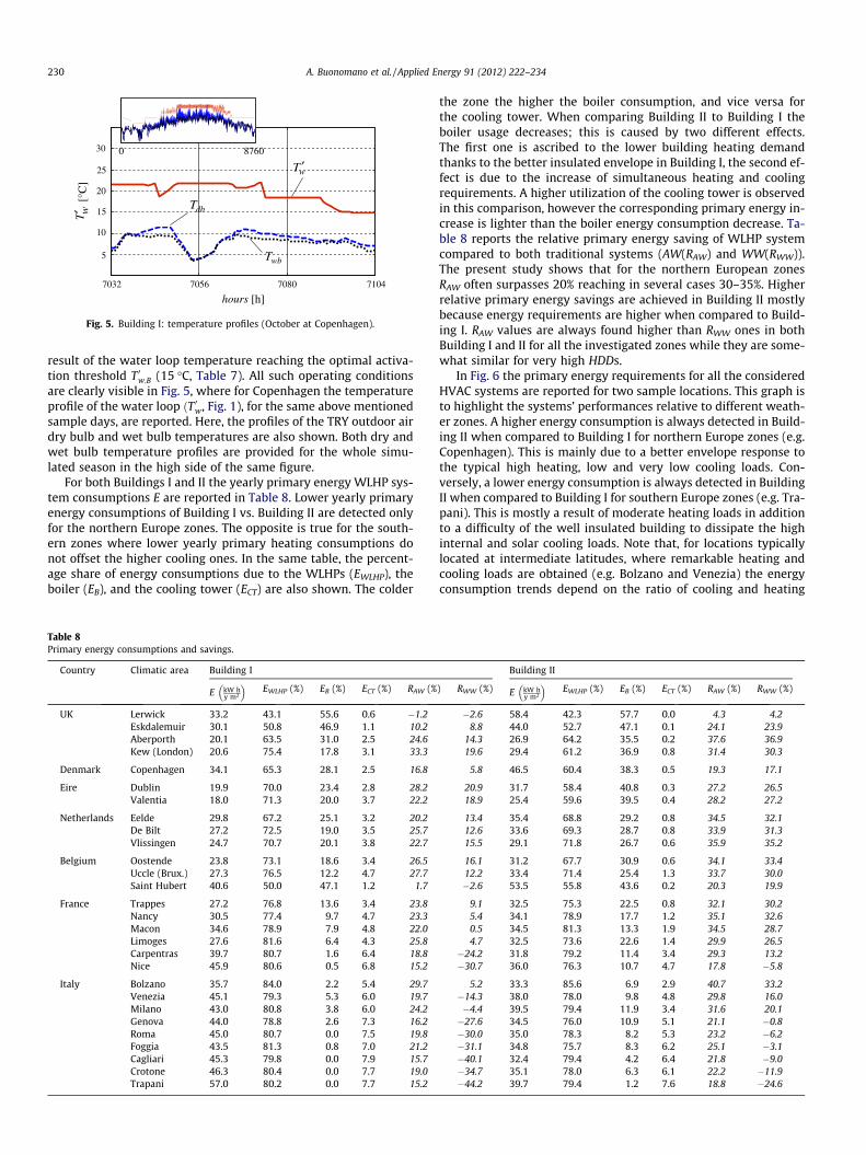
For both Buildings I and II the yearly primary energy WLHP sys-tem consumptions E are reported in Table 8. Lower yearly primaryenergy consumptions of Building I vs. Building II are detected onlyfor the northern Europe zones. The opposite is true for the south-ern zones where lower yearly primary heating consumptions donot offset the higher cooling ones. In the same table, the percent-age share of energy consumptions due to the WLHPs (EWLHP), theboiler (EB), and the cooling tower (ECT) are also shown. The colder

Table 8Primary energy consumptions and savings.

Country Climatic area Building I

E kW hy m2

� �EWLHP (%) EB (%) ECT (%) RAW (%

UK Lerwick 33.2 43.1 55.6 0.6 �1.2Eskdalemuir 30.1 50.8 46.9 1.1 10.2Aberporth 20.1 63.5 31.0 2.5 24.6Kew (London) 20.6 75.4 17.8 3.1 33.3

Denmark Copenhagen 34.1 65.3 28.1 2.5 16.8

Eire Dublin 19.9 70.0 23.4 2.8 28.2Valentia 18.0 71.3 20.0 3.7 22.2

Netherlands Eelde 29.8 67.2 25.1 3.2 20.2De Bilt 27.2 72.5 19.0 3.5 25.7Vlissingen 24.7 70.7 20.1 3.8 22.7

Belgium Oostende 23.8 73.1 18.6 3.4 26.5Uccle (Brux.) 27.3 76.5 12.2 4.7 27.7Saint Hubert 40.6 50.0 47.1 1.2 1.7

France Trappes 27.2 76.8 13.6 3.4 23.8Nancy 30.5 77.4 9.7 4.7 23.3Macon 34.6 78.9 7.9 4.8 22.0Limoges 27.6 81.6 6.4 4.3 25.8Carpentras 39.7 80.7 1.6 6.4 18.8Nice 45.9 80.6 0.5 6.8 15.2

Italy Bolzano 35.7 84.0 2.2 5.4 29.7Venezia 45.1 79.3 5.3 6.0 19.7Milano 43.0 80.8 3.8 6.0 24.2Genova 44.0 78.8 2.6 7.3 16.2Roma 45.0 80.7 0.0 7.5 19.8Foggia 43.5 81.3 0.8 7.0 21.2Cagliari 45.3 79.8 0.0 7.9 15.7Crotone 46.3 80.4 0.0 7.7 19.0Trapani 57.0 80.2 0.0 7.7 15.2

the zone the higher the boiler consumption, and vice versa forthe cooling tower. When comparing Building II to Building I theboiler usage decreases; this is caused by two different effects.The first one is ascribed to the lower building heating demandthanks to the better insulated envelope in Building I, the second ef-fect is due to the increase of simultaneous heating and coolingrequirements. A higher utilization of the cooling tower is observedin this comparison, however the corresponding primary energy in-crease is lighter than the boiler energy consumption decrease. Ta-ble 8 reports the relative primary energy saving of WLHP systemcompared to both traditional systems (AW(RAW) and WW(RWW)).The present study shows that for the northern European zonesRAW often surpasses 20% reaching in several cases 30–35%. Higherrelative primary energy savings are achieved in Building II mostlybecause energy requirements are higher when compared to Build-ing I. RAW values are always found higher than RWW ones in bothBuilding I and II for all the investigated zones while they are some-what similar for very high HDDs.

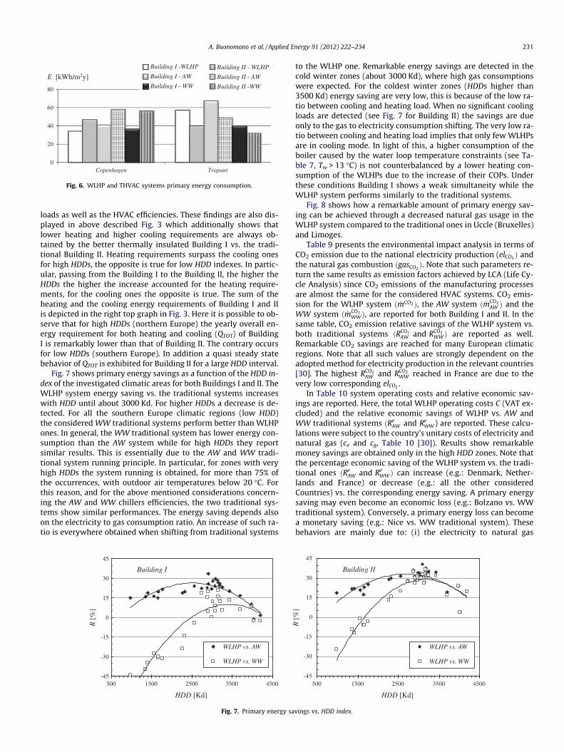
In Fig. 6 the primary energy requirements for all the consideredHVAC systems are reported for two sample locations. This graph isto highlight the systems’ performances relative to different weath-er zones. A higher energy consumption is always detected in Build-ing II when compared to Building I for northern Europe zones (e.g.Copenhagen). This is mainly due to a better envelope response tothe typical high heating, low and very low cooling loads. Con-versely, a lower energy consumption is always detected in BuildingII when compared to Building I for southern Europe zones (e.g. Tra-pani). This is mostly a result of moderate heating loads in additionto a difficulty of the well insulated building to dissipate the highinternal and solar cooling loads. Note that, for locations typicallylocated at intermediate latitudes, where remarkable heating andcooling loads are obtained (e.g. Bolzano and Venezia) the energyconsumption trends depend on the ratio of cooling and heating

Building II

) RWW (%) E kW hy m2

� �EWLHP (%) EB (%) ECT (%) RAW (%) RWW (%)

�2.6 58.4 42.3 57.7 0.0 4.3 4.28.8 44.0 52.7 47.1 0.1 24.1 23.9

14.3 26.9 64.2 35.5 0.2 37.6 36.919.6 29.4 61.2 36.9 0.8 31.4 30.3

5.8 46.5 60.4 38.3 0.5 19.3 17.1

20.9 31.7 58.4 40.8 0.3 27.2 26.518.9 25.4 59.6 39.5 0.4 28.2 27.2

13.4 35.4 68.8 29.2 0.8 34.5 32.112.6 33.6 69.3 28.7 0.8 33.9 31.315.5 29.1 71.8 26.7 0.6 35.9 35.2

16.1 31.2 67.7 30.9 0.6 34.1 33.412.2 33.4 71.4 25.4 1.3 33.7 30.0�2.6 53.5 55.8 43.6 0.2 20.3 19.9

9.1 32.5 75.3 22.5 0.8 32.1 30.25.4 34.1 78.9 17.7 1.2 35.1 32.60.5 34.5 81.3 13.3 1.9 34.5 28.74.7 32.5 73.6 22.6 1.4 29.9 26.5

�24.2 31.8 79.2 11.4 3.4 29.3 13.2�30.7 36.0 76.3 10.7 4.7 17.8 �5.8

5.2 33.3 85.6 6.9 2.9 40.7 33.2�14.3 38.0 78.0 9.8 4.8 29.8 16.0�4.4 39.5 79.4 11.9 3.4 31.6 20.1�27.6 34.5 76.0 10.9 5.1 21.1 �0.8�30.0 35.0 78.3 8.2 5.3 23.2 �6.2�31.1 34.8 75.7 8.3 6.2 25.1 �3.1�40.1 32.4 79.4 4.2 6.4 21.8 �9.0�34.7 35.1 78.0 6.3 6.1 22.2 �11.9�44.2 39.7 79.4 1.2 7.6 18.8 �24.6

0

20

40

60

80

Copenhagen Trapani

E [kWh/m2y]

Building I -WLHP Building II - WLHP

Building I - AW Building II - AW

Building I - WW Building II -WW

Fig. 6. WLHP and THVAC systems primary energy consumption.

A. Buonomano et al. / Applied Energy 91 (2012) 222–234 231

loads as well as the HVAC efficiencies. These findings are also dis-played in above described Fig. 3 which additionally shows thatlower heating and higher cooling requirements are always ob-tained by the better thermally insulated Building I vs. the tradi-tional Building II. Heating requirements surpass the cooling onesfor high HDDs, the opposite is true for low HDD indexes. In partic-ular, passing from the Building I to the Building II, the higher theHDDs the higher the increase accounted for the heating require-ments, for the cooling ones the opposite is true. The sum of theheating and the cooling energy requirements of Building I and IIis depicted in the right top graph in Fig. 3. Here it is possible to ob-serve that for high HDDs (northern Europe) the yearly overall en-ergy requirement for both heating and cooling (QTOT) of BuildingI is remarkably lower than that of Building II. The contrary occursfor low HDDs (southern Europe). In addition a quasi steady statebehavior of QTOT is exhibited for Building II for a large HDD interval.

Fig. 7 shows primary energy savings as a function of the HDD in-dex of the investigated climatic areas for both Buildings I and II. TheWLHP system energy saving vs. the traditional systems increaseswith HDD until about 3000 Kd. For higher HDDs a decrease is de-tected. For all the southern Europe climatic regions (low HDD)the considered WW traditional systems perform better than WLHPones. In general, the WW traditional system has lower energy con-sumption than the AW system while for high HDDs they reportsimilar results. This is essentially due to the AW and WW tradi-tional system running principle. In particular, for zones with veryhigh HDDs the system running is obtained, for more than 75% ofthe occurrences, with outdoor air temperatures below 20 �C. Forthis reason, and for the above mentioned considerations concern-ing the AW and WW chillers efficiencies, the two traditional sys-tems show similar performances. The energy saving depends alsoon the electricity to gas consumption ratio. An increase of such ra-tio is everywhere obtained when shifting from traditional systems

-45

-30

-15

0

15

30

45

500 1500 2500 3500 4500

WLHP vs. AW

WLHP vs. WW

Building I

HDD [Kd]

R [

%]

Fig. 7. Primary energy sa

to the WLHP one. Remarkable energy savings are detected in thecold winter zones (about 3000 Kd), where high gas consumptionswere expected. For the coldest winter zones (HDDs higher than3500 Kd) energy saving are very low, this is because of the low ra-tio between cooling and heating load. When no significant coolingloads are detected (see Fig. 7 for Building II) the savings are dueonly to the gas to electricity consumption shifting. The very low ra-tio between cooling and heating load implies that only few WLHPsare in cooling mode. In light of this, a higher consumption of theboiler caused by the water loop temperature constraints (see Ta-ble 7, Tw > 13 �C) is not counterbalanced by a lower heating con-sumption of the WLHPs due to the increase of their COPs. Underthese conditions Building I shows a weak simultaneity while theWLHP system performs similarly to the traditional systems.

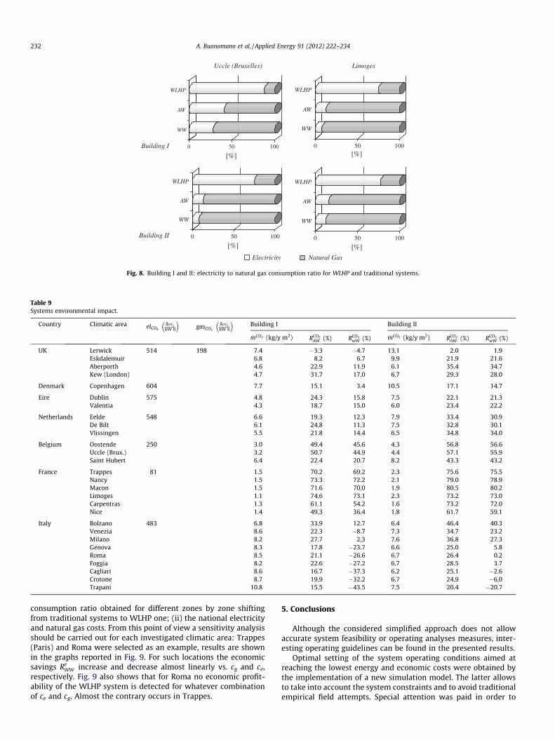
Fig. 8 shows how a remarkable amount of primary energy sav-ing can be achieved through a decreased natural gas usage in theWLHP system compared to the traditional ones in Uccle (Bruxelles)and Limoges.

Table 9 presents the environmental impact analysis in terms ofCO2 emission due to the national electricity production (elCO2 Þ andthe natural gas combustion ðgasCO2

Þ. Note that such parameters re-turn the same results as emission factors achieved by LCA (Life Cy-cle Analysis) since CO2 emissions of the manufacturing processesare almost the same for the considered HVAC systems. CO2 emis-sion for the WLHP system ð _mCO2 Þ, the AW system ð _mCO2

AW Þ and theWW system ð _mCO2

WWÞ, are reported for both Building I and II. In thesame table, CO2 emission relative savings of the WLHP system vs.both traditional systems ðRCO2

AW and RCO2WWÞ are reported as well.

Remarkable CO2 savings are reached for many European climaticregions. Note that all such values are strongly dependent on theadopted method for electricity production in the relevant countries[30]. The highest RCO2

AW and RCO2WW reached in France are due to the

very low corresponding elCO2 .In Table 10 system operating costs and relative economic sav-

ings are reported. Here, the total WLHP operating costs C (VAT ex-cluded) and the relative economic savings of WLHP vs. AW andWW traditional systems ðRe

AW and ReWW ) are reported. These calcu-

lations were subject to the country’s unitary costs of electricity andnatural gas (ce and cg, Table 10 [30]). Results show remarkablemoney savings are obtained only in the high HDD zones. Note thatthe percentage economic saving of the WLHP system vs. the tradi-tional ones ðRe

AW and ReWWÞ can increase (e.g.: Denmark, Nether-

lands and France) or decrease (e.g.: all the other consideredCountries) vs. the corresponding energy saving. A primary energysaving may even become an economic loss (e.g.: Bolzano vs. WWtraditional system). Conversely, a primary energy loss can becomea monetary saving (e.g.: Nice vs. WW traditional system). Thesebehaviors are mainly due to: (i) the electricity to natural gas

-45

-30

-15

0

15

30

45

500 1500 2500 3500 4500

WLHP vs. AW

WLHP vs. WW

Building II

R [

%]

HDD [Kd]

vings vs. HDD index.

Uccle (Bruxelles) Limoges

0 50 100

WW

AW

WLHP

0 50 100

WW

AW

WLHP

0 50 100

WW

AW

WLHP

0 50 100

WW

AW

WLHP

Electricity Natural Gas

Building I

Building II

[%]

[%]

[%]

[%]

Fig. 8. Building I and II: electricity to natural gas consumption ratio for WLHP and traditional systems.

Table 9Systems environmental impact.

Country Climatic area elCO2

gCO2kW h

� �gasCO2

gCO2kW h

� �Building I Building II

_mCO2 (kg/y m2) RCO2AW (%) RCO2

wW (%) _mCO2 (kg/y m2) RCO2AW (%) RCO2

wW (%)

UK Lerwick 514 198 7.4 �3.3 �4.7 13.1 2.0 1.9Eskdalemuir 6.8 8.2 6.7 9.9 21.9 21.6Aberporth 4.6 22.9 11.9 6.1 35.4 34.7Kew (London) 4.7 31.7 17.0 6.7 29.3 28.0

Denmark Copenhagen 604 7.7 15.1 3.4 10.5 17.1 14.7

Eire Dublin 575 4.8 24.3 15.8 7.5 22.1 21.3Valentia 4.3 18.7 15.0 6.0 23.4 22.2

Netherlands Eelde 548 6.6 19.3 12.3 7.9 33.4 30.9De Bilt 6.1 24.8 11.3 7.5 32.8 30.1Vlissingen 5.5 21.8 14.4 6.5 34.8 34.0

Belgium Oostende 250 3.0 49.4 45.6 4.3 56.8 56.6Uccle (Brux.) 3.2 50.7 44.9 4.4 57.1 55.9Saint Hubert 6.4 22.4 20.7 8.2 43.3 43.2

France Trappes 81 1.5 70.2 69.2 2.3 75.6 75.5Nancy 1.5 73.3 72.2 2.1 79.0 78.9Macon 1.5 71.6 70.0 1.9 80.5 80.2Limoges 1.1 74.6 73.1 2.3 73.2 73.0Carpentras 1.3 61.1 54.2 1.6 73.2 72.0Nice 1.4 49.3 36.4 1.8 61.7 59.1

Italy Bolzano 483 6.8 33.9 12.7 6.4 46.4 40.3Venezia 8.6 22.3 �8.7 7.3 34.7 23.2Milano 8.2 27.7 2.3 7.6 36.8 27.3Genova 8.3 17.8 �23.7 6.6 25.0 5.8Roma 8.5 21.1 �26.6 6.7 26.4 0.2Foggia 8.2 22.6 �27.2 6.7 28.5 3.7Cagliari 8.6 16.7 �37.3 6.2 25.1 �2.6Crotone 8.7 19.9 �32.2 6.7 24.9 �6.0Trapani 10.8 15.5 �43.5 7.5 20.4 �20.7

232 A. Buonomano et al. / Applied Energy 91 (2012) 222–234

consumption ratio obtained for different zones by zone shiftingfrom traditional systems to WLHP one; (ii) the national electricityand natural gas costs. From this point of view a sensitivity analysisshould be carried out for each investigated climatic area: Trappes(Paris) and Roma were selected as an example, results are shownin the graphs reported in Fig. 9. For such locations the economicsavings Re

WW increase and decrease almost linearly vs. cg and ce,respectively. Fig. 9 also shows that for Roma no economic profit-ability of the WLHP system is detected for whatever combinationof ce and cg. Almost the contrary occurs in Trappes.

5. Conclusions

Although the considered simplified approach does not allowaccurate system feasibility or operating analyses measures, inter-esting operating guidelines can be found in the presented results.

Optimal setting of the system operating conditions aimed atreaching the lowest energy and economic costs were obtained bythe implementation of a new simulation model. The latter allowsto take into account the system constraints and to avoid traditionalempirical field attempts. Special attention was paid in order to

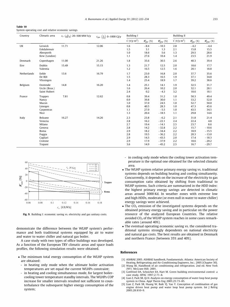
Table 10System operating cost and relative economic savings.

Country Climatic area ce€c

kW h

� �20–500 MW h/y cgas

€GJ

� �0–1000 GJ/y Building I Building II

C (€/y m2) ReAW (%) Re

WW (%) C (€/y m2) ReAW (%) Re

WW (%)

UK Lerwick 11.71 12.06 1.6 �8.6 �10.3 2.8 �4.2 �4.4Eskdalemuir 1.5 3.1 1.3 2.1 15.8 15.5Aberporth 1.0 18.6 5.6 1.3 29.5 28.6Kew (London) 1.1 27.6 10.4 1.4 23.5 21.9

Denmark Copenhagen 11.00 21.26 1.8 35.6 30.5 2.6 40.3 39.4

Eire Dublin 15.49 15.15 1.3 21.7 12.5 2.0 18.6 17.7Valentia 1.2 16.5 12.5 1.6 20.1 18.8

Netherlands Eelde 13.6 16.79 1.7 23.0 16.8 2.0 37.7 35.6De Bilt 1.5 28.3 16.5 1.9 37.1 34.8Vlissingen 1.4 25.4 18.9 1.7 39.2 38.6

Belgium Oostende 14.8 16.20 1.4 25.1 14.1 1.9 32.5 31.7Uccle (Brux.) 1.6 26.4 10.2 2.0 32.1 28.1Saint Hubert 2.4 0.2 �4.3 3.2 18.6 18.1

France Trappes 7.81 12.62 0.8 39.4 31.2 1.0 50.3 49.4Nancy 0.9 39.8 30.0 1.1 53.2 52.0Macon 1.0 37.0 24.5 1.0 52.7 50.0Limoges 0.8 40.5 28.3 1.0 47.3 45.6Carpentras 1.1 27.0 �5.5 1.0 43.5 34.5Nice 1.3 20.4 �18.5 1.1 29.8 14.6

Italy Bolzano 16.27 14.26 2.3 23.8 �6.2 2.1 31.8 21.4Venezia 2.8 16.2 �22.1 2.4 22.4 4.8Milano 2.7 19.4 �14.1 2.5 23.7 8.6Genova 2.8 14.2 �32.8 2.2 15.7 �10.6Roma 2.9 18.2 �34.4 2.2 18.9 �15.5Foggia 2.8 19.5 �36.2 2.2 20.3 �13.0Cagliari 2.9 14.5 �43.5 2.0 17.4 �18.3Crotone 2.9 17.9 �37.9 2.2 18.6 �20.2Trapani 3.6 14.9 �45.2 2.5 16.7 �29.7

-60

-40

-20

0

20

40

60

0.06 0.08 0.1 0.12 0.14 0.16 0.18

ce [ /kWh]

22181410

Roma

Trappes

Roma

Trappes

[%

]R

[%

]W

We

R

Fig. 9. Building I: economic saving vs. electricity and gas unitary costs.

A. Buonomano et al. / Applied Energy 91 (2012) 222–234 233

demonstrate the difference between the WLHP system’s perfor-mance and both traditional systems equipped by air to waterand water to water chiller and natural gas boiler.

A case study with two types of office buildings was developed.As a function of the European TRY climatic areas and space loadsprofiles, the following simulation results were obtained.

� The minimum total energy consumption of the WLHP systemare obtained:- in heating only mode when the ultimate boiler activation

temperatures are set equal the current WLHPs constraint;- in heating and cooling simultaneous mode, for largest boiler-

cooling tower temperature standby intervals. The WLHPs COPincrease for smaller intervals resulted not sufficient to coun-terbalance the subsequent higher energy consumption of thesystem;

- in cooling only mode when the cooling tower activation tem-perature is the optimal one obtained for the selected climaticarea.

� The WLHP system relative primary energy saving vs. traditionalsystems depends on building heating and cooling simultaneity.Concurrently, it depends on the increase of the electricity to gasconsumption ratio obtained by shifting from traditional toWLHP systems. Such criteria are summarized in the HDD index:the highest primary energy savings are detected in climaticareas around 3000 Kd. In weather zones with extreme lowand high HDDs, moderate (or even null in water to water chiller)energy savings were achieved.� The CO2 emission of the investigated systems depends on the

obtained primary energy saving and in particular on the powerresource of the analyzed European Countries. The relativeavoided CO2 of the WLHP system reaches in some cases remark-able rates (around 40%).� The eventual operating economic saving vs. the considered tra-

ditional systems strongly dependents on national electricityand natural gas costs. The best results are obtained in Denmarkand northern France (between 35% and 40%).

References

[1] ASHRAE 2005. ASHRAE handbook, Fundamentals. Atlanta: American Society ofHeating, Refrigerating and Air-Conditioning Engineers, Inc.; 2005 [Chapter 30].

[2] Wang SK. Handbook of air conditioning and refrigeration. 2nd ed. New York(NY): McGraw-Hill; 2001.

[3] Gottfried DA, Schoichet EA, Hart M. Green building environmental control: acase study. HPAC 1997;2:71–8.

[4] Lian Z, Park SR, Qi H. Analysis on energy consumption of water loop heat pumpsystem in China. Appl Therm Eng 2005;25:73–85.

[5] Lian Z, Park SR, Huang W, Baik YJ, Yao Y. Conception of combination of gasengine driven heat pump and water loop heat pump system. Int J Refrig2005;28:810–9.

234 A. Buonomano et al. / Applied Energy 91 (2012) 222–234

[6] Xinguo Li. Thermal performance and energy saving effect of water-loop heatpump system with geothermal. Energy Convers Manage 1998;39(3/4):295–301.

[7] Chen Chao, Sun Feng-ling, Feng Lei, Liu Ming. Underground water-source loopheat-pump air-conditioning system applied in a residential building in Beijing.Appl Energy 2005;82:331–44.

[8] Yuan S, Grabon M. Optimizing energy consumption of a water-loop variable-speed heat pump system. Appl Therm Eng 2011;31:894–901.

[9] Buonomano A, Calise F, Palombo A. Thermodynamic and economic simulationsof water loop heat pump systems: a computer based approach. In: Proceedingsof ECOS 2007 – XX intl conference on efficiency, costs, optimization,simulation and environmental impact of energy systems, Padova, Italy, vol.1; 2007. p. 619–27.

[10] Buonomano A, Calise F, Palombo A. Water loop heat pump systemperformances in European climates. In: Proceedings of CLIMAMED 2007 –energy, climate and indoor comfort in mediterranean countries, Genova, Italy,vol. 1; 2007. p. 471–90.

[11] Zanetti Freire R, Mazuroski W, Abadie MO, Mendes N. Capacitive effect on theheat transfer through building glazing systems. Appl Energy 2011;88:4310–9.

[12] Wong SL, Wan Kevin KW, Lam Tony NT. Artificial neural networks for energyanalysis of office buildings with daylighting. Appl Energy 2010;87:551–7.

[13] Široky J, Oldewurtel F, Cigler J, Prívara S. Experimental analysis of modelpredictive control for an energy efficient building heating system. Appl Energy2011;88:3079–87.

[14] Bichiou Y, Krarti M. Optimization of envelope and HVAC systems selection forresidential buildings. Energy Build 2010. doi:10.1016/j.enbuild.2011.08.031.

[15] Trcka M, Hensen JLM. Overview of HVAC system simulation. AutomatConstruct 2010;19:93–9.

[16] Fissore A, Mottard JM. Thermal simulation of an attached sunspace and itsexperimental validation. Solar Energy 2006;81:305–15.

[17] TRNSYS 17. Manual of TRNSYS. University of Wisconsin-Madison, USA; 2010.

[18] Kreider JF, Rabl A. Heating and cooling of buildings. New York (NY): McGraw-Hill; 1994.

[19] EN 12464-1:2011. Light and lighting – lighting of work places – part 1: indoorwork places.

[20] Wang S, Xu X. A simplified dynamic model for existing buildings using CTF andthermal network models. Int J Therm Sci 2008;47:1249–62.

[21] Shengwei S, Xinhua X. Parameter estimation of internal thermal mass ofbuilding dynamic models using genetic algorithm. Energy Convers Manage2006;47:1927–41.

[22] Bourdouxhe J, Grodent M, Lebrun J. Reference guide for dynamic models ofHVAC equipment. Atlanta: American Society of Heating, Refrigerating and Air-Conditioning Engineers, Inc.; 1998.

[23] Zweifel G, Dorer V, Koschenz M, Weber A. Building energy and systemsimulation programs: model development, coupling and integration, EMPA.

[24] Sparber W, Thuer A, Besana F, Streicher W, Henning HM. Unified monitoringprocedure and performance assessment for solar assisted heating and coolingsystems, Eurosun 2008, Lisbon, Portugal; 2008.

[25] Adelard L, Pignolet-Tardant F, Mara T, Lauret P, Garde F, Hoyer H. Skytemperature modelisation and applications in building simulation. RenewEnergy 1998;15:418–30.

[26] Test Reference Year TRY. Weather data sets for computer simulations of solarenergy systems and energy consumption in buildings – Commission of theEuropean Communities; 1985.

[27] Bellia L, Mazzei P, Palombo A. Weather data for building energy cost-benefitanalysis. Int J Energy Res 1998;22:1205–15.

[28] EN ISO 13789:2007. Thermal performance of building components – dynamicthermal characteristics – calculation methods.

[29] Windows and glazing system software. LBNL. <http://windows.lbl.gov/software>.

[30] Eurostat 2009. Environment an energy, electricity and gas prices. <http://epp.eurostat.ec.europa.eu>.