Milan Janić Analysis, Modeling, and Evaluation of Performances

Advanced Transport Systems

Milan Janić

Analysis, Modeling, and Evaluation of Performances

Milan Janic


Analysis, Modeling, and Evaluationof Performances

123

Milan JanicTransport and Planning DepartmentFaculty of Civil Engineering

and GeosciencesDelft University of TechnologyDelftThe Netherlands

ISBN 978-1-4471-6286-5 ISBN 978-1-4471-6287-2 (eBook)DOI 10.1007/978-1-4471-6287-2Springer London Heidelberg New York Dordrecht

Library of Congress Control Number: 2013955907

� Springer-Verlag London 2014This work is subject to copyright. All rights are reserved by the Publisher, whether the whole or part ofthe material is concerned, specifically the rights of translation, reprinting, reuse of illustrations,recitation, broadcasting, reproduction on microfilms or in any other physical way, and transmission orinformation storage and retrieval, electronic adaptation, computer software, or by similar or dissimilarmethodology now known or hereafter developed. Exempted from this legal reservation are briefexcerpts in connection with reviews or scholarly analysis or material supplied specifically for thepurpose of being entered and executed on a computer system, for exclusive use by the purchaser of thework. Duplication of this publication or parts thereof is permitted only under the provisions ofthe Copyright Law of the Publisher’s location, in its current version, and permission for use mustalways be obtained from Springer. Permissions for use may be obtained through RightsLink at theCopyright Clearance Center. Violations are liable to prosecution under the respective Copyright Law.The use of general descriptive names, registered names, trademarks, service marks, etc. in thispublication does not imply, even in the absence of a specific statement, that such names are exemptfrom the relevant protective laws and regulations and therefore free for general use.While the advice and information in this book are believed to be true and accurate at the date ofpublication, neither the authors nor the editors nor the publisher can accept any legal responsibility forany errors or omissions that may be made. The publisher makes no warranty, express or implied, withrespect to the material contained herein.

Printed on acid-free paper

Springer is part of Springer Science+Business Media (www.springer.com)

To my wife Vesna at the 30th anniversaryof our marriage

Preface

The transport system has, is, and will continue to be a foundation of the economy ofeach country/nation, as well as that of the world. In particular, in the twenty-firstcentury, it will further strengthen its role in integrating and globalizing economicactivities, and will thus also influence the quality of people’s lives. In the past,transport demand in terms of both the number of passengers and the volumes offreight/goods shipments has been constantly growing in the medium- to long-termperiod(s) despite being affected, from time to time, by the local and globaleconomic and political crises. This demand has been satisfied by the capacity of thetransport system generally consisting of the transport infrastructure, transportmeans/vehicles, and workforce. Material, energy, and labor has been consumed inorder to provide transport services according to the specified internal organizationcontaining operating rules and procedures, and under given external regulation andconstraints. On the one hand, such developments have produced the above-mentioned positive contributions to the national economies and social welfare. Onthe other, they have affected the environment and society in terms of land use/takefor expanding the transport infrastructure, energy consumption from non-renewablesources (coal, crude oil, and natural gas) and related emissions of Green HouseGases (GHG), local noise, congestion, and safety (traffic incidents and accidents),Since both passenger and freight transport demand are predicted to double over thenext 20 and triple over the next 50 years, solutions for serving them more efficientlyand effectively while mitigating impacts on the environment and society need to beprovided. Therefore, in addition to creating transport policies and monitoringschemes aiming to reduce physical transport demand (i.e., telecommuting) andimplementing advanced transport planning and operating tools and techniques,potential solutions also lie in developing advanced technologies individually and/orin combination with advanced operational concepts. Generally, this impliesproviding: (i) sufficiently capacitated and environmentally friendlier, i.e., moreenergy/fuel efficient, cleaner, quieter, and safer, technologies based on an increaseduse of renewable energy/fuel sources (such as, for example, biomass fuels (liquid)hydrogen, wind and solar energy), nanotechnologies, and information technologies;and (ii) the advanced organizational and operational forms and concepts of usingtransport infrastructure, transport means/vehicles, and accompanied resources.

Experience so far indicates that commercialization, i.e., development andimplementation, of the advanced components—technologies and related

vii

operational concepts—of the transport system has been an evolutionary rather thana revolutionary process. The main reasons include: (i) a rather long time formaturing up to full commercialization; (ii) an inherent threat from confrontingexisting and forthcoming even stricter institutional/policy regulation/constraints;(iii) relatively high development costs; (iv) frequently uncertain long-term overallcommercial and social feasibility; and (v) a relatively long path for obtainingoperational certification implying full environmental and societal/policy acceptance.Under such circumstances, most such transport technologies and operationalconcepts, except a couple of futuristic ones, have been mostly gradually updated andimproved, usually based on the closest previous counterparts. In the given context,this justifies deeming them ‘‘innovative’’ or ‘‘advanced’’ rather than completely‘‘new’’. In this book, the attribute ‘‘advanced’’ is used for all such technologies andoperational concepts.

The book describes analysis, modeling, and evaluation of performances of theselected advanced transport systems. Some of them have already been commer-cialized, i.e., implemented and operationalized, and/or are planned to be so, whileothers are still at the conceptual level waiting for further elaboration. Theirperformances are considered as derived from the technical/technological design andsolutions of the infrastructure, transport means/vehicles, and supporting facilitiesand equipment used according to the specified operational rules and procedures,and economic, environmental, social, and policy conditions/constraints.

Analysis and modeling implies examination of their infrastructural, technical/technological, operational, economic, environmental, social, and policyperformances. Evaluation based on a Strengths, Weaknesses, Opportunities andThreats (SWOT)-like analysis implies assessment of the advantages and disadvan-tages of these systems. In such context, Strengths and Opportunities are considered asadvantages, while Weaknesses and Threats are considered disadvantages. Both areconsidered from the aspects of academics/researchers, but also from those of par-ticular actors/stakeholders involved such as users of transport services–passengersand freight/goods shippers/receivers, transport infrastructure and service providers/operators, investors, policy makers at different institutional levels (local, national,international), and members of the local community/society.

Particular advanced transport systems have been selected according to thefollowing criteria: (i) the level of advancement of particular performances;(ii) representativeness through transport modes (rail, road, air, water/sea, inter-modal); (iii) their spatial scale (area) of operation (urban and inter-urban);(iv) category of demand served (passengers, freight/goods); (v) availability/accessibility of relevant information (from science-based and publically-accessiblerelevant sources); and (vi) the level of systematic scientific elaboration ascompared to that used in this book.

The selected advanced transport systems are clustered in the book’s chaptersrespecting the type and number of their advanced performances independently ofthe transport mode, spatial/geographical scale of operation, and type of transportdemand they serve.

viii Preface

The widely dispersed and in some cases scarce material collected from thevarious available sources such as research (including my own), literature (booksand papers in scientific and professional journals), and websites is presented fromthe traffic and transport engineering and planning and design perspective. Mostfacts and issues are scientifically supported and accurate regarding the funda-mental relationships between particular variables (parameters). Nevertheless, someof them, particularly those related to futuristic concepts, contain a level of fuzzi-ness in the absolute terms, which, however, does not compromise their relevancein the given context. As such, the book aims to be informative as much as possiblebut by no means exhaustive—to the contrary, it intends to provide academics,researchers, consultants, policy/decision makers, and professionals from thetransport industry and related fields with material for current and future researchand development of the transport system.

October 2013 Milan Janic

Preface ix

Acknowledgments

The author gratefully acknowledges the support of organizations and individuals ingetting this book into publishable form.

Firstly, I would like to thank very much the Transport Institute of DelftUniversity of Technology (Prof. Bart van Arem—Director, and Dr. Arjan vanBinsbergen—Secretary) (TU Delft, Delft, The Netherlands) for some financialsupport in finalizing the work on the book. Secondly, I benefited greatly from thevaluable discussions, materials, exhibits, and data provided by Mr. John P. Christy,Lead Engineer—Operations Airport Technology, Boeing and Ms. Mary E. Kane,Trademark and Copyright Licensing, Boeing Intellectual Property Management(Boeing Company/Commercial Airplanes, Seattle, Washington, USA).

Thirdly, I give my special gratitude to Mr. Andrej Grah Whatmough for hisexcellent help polishing the language.

On the personal side, the great effort of writing this book was continuouslysupported and inspired by my wife Vesna and my son Miodrag, doctor of medi-cine, who was at the same time also working enthusiastically on his Ph.D. thesis.

Milan Janic

xi

Contents

1 Advanced Transport Systems: General . . . . . . . . . . . . . . . . . . . . . 11.1 Definition . . . . . . . . . . . . . . . . . . . . . . . . . . . . . . . . . . . . . . . 11.2 Classification . . . . . . . . . . . . . . . . . . . . . . . . . . . . . . . . . . . . 2

1.2.1 Attributes/Criteria Related to Advanced Components . . . 31.2.2 Attributes/Criteria Related to Level

of Commercialization . . . . . . . . . . . . . . . . . . . . . . . . . 41.3 Performances . . . . . . . . . . . . . . . . . . . . . . . . . . . . . . . . . . . . 4

1.3.1 Definition. . . . . . . . . . . . . . . . . . . . . . . . . . . . . . . . . . 41.3.2 Analyzing, Modeling, and Evaluation . . . . . . . . . . . . . . 8

1.4 Composition of the Book . . . . . . . . . . . . . . . . . . . . . . . . . . . . 8References . . . . . . . . . . . . . . . . . . . . . . . . . . . . . . . . . . . . . . . . . . 9

2 Advanced Transport Systems: Operations and Technologies . . . . . 112.1 Introduction . . . . . . . . . . . . . . . . . . . . . . . . . . . . . . . . . . . . . 112.2 Bus Rapid Transit Systems . . . . . . . . . . . . . . . . . . . . . . . . . . . 12

2.2.1 Definition, Development, and Use. . . . . . . . . . . . . . . . . 122.2.2 Analyzing and Modeling Performances . . . . . . . . . . . . . 142.2.3 Evaluation . . . . . . . . . . . . . . . . . . . . . . . . . . . . . . . . . 40

2.3 High Speed Tilting Passenger Trains . . . . . . . . . . . . . . . . . . . . 422.3.1 Definition, Development, and Use. . . . . . . . . . . . . . . . . 422.3.2 Analyzing and Modeling Performances . . . . . . . . . . . . . 432.3.3 Evaluation . . . . . . . . . . . . . . . . . . . . . . . . . . . . . . . . . 61

2.4 Advanced Subsonic Commercial Aircraft . . . . . . . . . . . . . . . . . 622.4.1 Definition, Development, and Use. . . . . . . . . . . . . . . . . 622.4.2 Analyzing and Modeling Performances . . . . . . . . . . . . . 632.4.3 Evaluation . . . . . . . . . . . . . . . . . . . . . . . . . . . . . . . . . 78

References . . . . . . . . . . . . . . . . . . . . . . . . . . . . . . . . . . . . . . . . . . 79

3 Advanced Transport Systems: Operations and Economics . . . . . . . 833.1 Introduction . . . . . . . . . . . . . . . . . . . . . . . . . . . . . . . . . . . . . 833.2 Advanced Freight Collection/Distribution Networks. . . . . . . . . . 84

3.2.1 Definition, Development, and Use. . . . . . . . . . . . . . . . . 843.2.2 Analyzing and Modeling Performances . . . . . . . . . . . . . 863.2.3 Evaluation . . . . . . . . . . . . . . . . . . . . . . . . . . . . . . . . . 110

xiii

http://dx.doi.org/10.1007/978-1-4471-6287-2_1

http://dx.doi.org/10.1007/978-1-4471-6287-2_1

http://dx.doi.org/10.1007/978-1-4471-6287-2_1#Sec1

















http://dx.doi.org/10.1007/978-1-4471-6287-2_1#Bib1

http://dx.doi.org/10.1007/978-1-4471-6287-2_2

http://dx.doi.org/10.1007/978-1-4471-6287-2_2




























http://dx.doi.org/10.1007/978-1-4471-6287-2_3

http://dx.doi.org/10.1007/978-1-4471-6287-2_3











3.3 Road Mega Trucks . . . . . . . . . . . . . . . . . . . . . . . . . . . . . . . . 1113.3.1 Definition, Development, and Use. . . . . . . . . . . . . . . . . 1113.3.2 Analyzing and Modeling Performances . . . . . . . . . . . . . 1123.3.3 Evaluation . . . . . . . . . . . . . . . . . . . . . . . . . . . . . . . . . 125

3.4 Long Intermodal Freight Train(s) . . . . . . . . . . . . . . . . . . . . . . 1263.4.1 Definition, Development, and Use. . . . . . . . . . . . . . . . . 1263.4.2 Analyzing Performances . . . . . . . . . . . . . . . . . . . . . . . 1273.4.3 Modeling Performances . . . . . . . . . . . . . . . . . . . . . . . . 1323.4.4 Evaluation . . . . . . . . . . . . . . . . . . . . . . . . . . . . . . . . . 144

3.5 Large Commercial Freight Aircraft . . . . . . . . . . . . . . . . . . . . . 1453.5.1 Definition, Development, and Use. . . . . . . . . . . . . . . . . 1453.5.2 Analyzing and Modeling Performances . . . . . . . . . . . . . 1473.5.3 Evaluation . . . . . . . . . . . . . . . . . . . . . . . . . . . . . . . . . 161

References . . . . . . . . . . . . . . . . . . . . . . . . . . . . . . . . . . . . . . . . . . 162

4 Advanced Transport Systems: Technologies and Environment. . . . 1654.1 Introduction . . . . . . . . . . . . . . . . . . . . . . . . . . . . . . . . . . . . . 1654.2 Advanced Passenger Cars . . . . . . . . . . . . . . . . . . . . . . . . . . . . 167

4.2.1 Definition, Development, and Use. . . . . . . . . . . . . . . . . 1674.2.2 Analysis and Modeling Performances . . . . . . . . . . . . . . 1684.2.3 Evaluation . . . . . . . . . . . . . . . . . . . . . . . . . . . . . . . . . 185

4.3 Large Advanced Container Ships. . . . . . . . . . . . . . . . . . . . . . . 1864.3.1 Definition, Development, and Use. . . . . . . . . . . . . . . . . 1874.3.2 Analyzing and Modeling Performances . . . . . . . . . . . . . 1884.3.3 Evaluation . . . . . . . . . . . . . . . . . . . . . . . . . . . . . . . . . 214

4.4 Liquid Hydrogen-Fuelled Commercial Air Transportation . . . . . 2164.4.1 Definition, Development, and Use. . . . . . . . . . . . . . . . . 2164.4.2 Analysis and Modeling Performance . . . . . . . . . . . . . . . 2174.4.3 Evaluation . . . . . . . . . . . . . . . . . . . . . . . . . . . . . . . . . 228

References . . . . . . . . . . . . . . . . . . . . . . . . . . . . . . . . . . . . . . . . . . 229

5 Advanced Transport Systems: Infrastructure, Technologies,Operations, Economics, Environment, and Society/Policy . . . . . . . 2355.1 Introduction . . . . . . . . . . . . . . . . . . . . . . . . . . . . . . . . . . . . . 2355.2 High Speed Transport Systems . . . . . . . . . . . . . . . . . . . . . . . . 236

5.2.1 Definition, Development, and Use. . . . . . . . . . . . . . . . . 2365.2.2 Evaluation . . . . . . . . . . . . . . . . . . . . . . . . . . . . . . . . . 274

References . . . . . . . . . . . . . . . . . . . . . . . . . . . . . . . . . . . . . . . . . . 275

6 Advanced Transport Systems: Future Concepts . . . . . . . . . . . . . . 2776.1 Introduction . . . . . . . . . . . . . . . . . . . . . . . . . . . . . . . . . . . . . 2776.2 Personal Rapid Transit Systems. . . . . . . . . . . . . . . . . . . . . . . . 279

6.2.1 Definition, Development, and Use. . . . . . . . . . . . . . . . . 279

xiv Contents




























http://dx.doi.org/10.1007/978-1-4471-6287-2_4

http://dx.doi.org/10.1007/978-1-4471-6287-2_4




























http://dx.doi.org/10.1007/978-1-4471-6287-2_5

http://dx.doi.org/10.1007/978-1-4471-6287-2_5

http://dx.doi.org/10.1007/978-1-4471-6287-2_5










http://dx.doi.org/10.1007/978-1-4471-6287-2_6

http://dx.doi.org/10.1007/978-1-4471-6287-2_6







6.2.2 Analyzing and Modeling Performances . . . . . . . . . . . . . 2816.2.3 Evaluation . . . . . . . . . . . . . . . . . . . . . . . . . . . . . . . . . 303

6.3 Underground Freight Transport Systems. . . . . . . . . . . . . . . . . . 3056.3.1 Definition, Development, and Use. . . . . . . . . . . . . . . . . 3056.3.2 Analyzing and Modeling Performances . . . . . . . . . . . . . 3066.3.3 Evaluation . . . . . . . . . . . . . . . . . . . . . . . . . . . . . . . . . 319

6.4 Evacuated Tube Transport System. . . . . . . . . . . . . . . . . . . . . . 3226.4.1 Definition, Development, and Use. . . . . . . . . . . . . . . . . 3236.4.2 Analyzing and Modeling Performances . . . . . . . . . . . . . 3256.4.3 Evaluation . . . . . . . . . . . . . . . . . . . . . . . . . . . . . . . . . 340

6.5 Advanced Air Traffic Control Technologiesand Operations for Increasing Airport Runway Capacity . . . . . . 3416.5.1 Definition, Development, and Use. . . . . . . . . . . . . . . . . 3416.5.2 Analyzing Performances . . . . . . . . . . . . . . . . . . . . . . . 3426.5.3 Modeling Performances . . . . . . . . . . . . . . . . . . . . . . . . 3546.5.4 Evaluation . . . . . . . . . . . . . . . . . . . . . . . . . . . . . . . . . 363

6.6 Advanced Supersonic Transport Aircraft . . . . . . . . . . . . . . . . . 3646.6.1 Definition, Development, and Use. . . . . . . . . . . . . . . . . 3646.6.2 Analyzing and Modeling Performances . . . . . . . . . . . . . 3666.6.3 Evaluation . . . . . . . . . . . . . . . . . . . . . . . . . . . . . . . . . 386

References . . . . . . . . . . . . . . . . . . . . . . . . . . . . . . . . . . . . . . . . . . 388

7 Advanced Transport Systems: Contribution to Sustainability . . . . 3917.1 Introduction . . . . . . . . . . . . . . . . . . . . . . . . . . . . . . . . . . . . . 3917.2 Contribution . . . . . . . . . . . . . . . . . . . . . . . . . . . . . . . . . . . . . 3917.3 Some Controversies . . . . . . . . . . . . . . . . . . . . . . . . . . . . . . . . 394

7.3.1 Technical Productivity . . . . . . . . . . . . . . . . . . . . . . . . . 3947.3.2 Energy/Fuel Consumption and Emissions of GHG . . . . . 3967.3.3 Safety . . . . . . . . . . . . . . . . . . . . . . . . . . . . . . . . . . . . 397

Reference . . . . . . . . . . . . . . . . . . . . . . . . . . . . . . . . . . . . . . . . . . . 398

About the Author . . . . . . . . . . . . . . . . . . . . . . . . . . . . . . . . . . . . . . . 399

Index . . . . . . . . . . . . . . . . . . . . . . . . . . . . . . . . . . . . . . . . . . . . . . . . 401

Contents xv









































http://dx.doi.org/10.1007/978-1-4471-6287-2_7

http://dx.doi.org/10.1007/978-1-4471-6287-2_7














Abbreviations

ABD Additional breaking device

ACN Aircaft classification number

AGV Automotice grande vitesse

AMT Automatic manual transmission

ANA Air Nippon Airways

APT Air passenger transport

APU Auxiliary power unit

ASM Available seat mile

ATA Air Transport Association

ATAG Air Transport Action Group

ATC Air traffic control

ATMS Automated manual system

AVL Automatic vehicle location

atm Atmosphere

ATMS Automated manual system

BAU Business as usual

BEV Battery electric vehicle

BR Bypass ratio

BRT Bus rapid transit

CAD Computer aided dispatching

CDA Continuous descent approach

CDB Central business district

CEN Comité Européen de Normalisation

CIA Central Intelligence Agency

CIFT Commercial intermodal freight train

CNG Compressed natural gas

CO Carbon monoxide

CSS Carbon capture and storage

DC Direct-current

DM Decision making (maker)

DPF Diesel particulate filter

xvii

DWT Deadweight tonnage

EADS European Aeronautic Defense and Space Company

EAT Economic analysis technique

EBHA Electrical backup hydrostatic actuators

EC European Commission

ECB European Central Bank

EDS Electro dynamic suspension

EEC Electronic engine controller

EEDI Energy efficiency design index

EEOI Energy efficiency operational indicator

EET Evacuated tube transport

EFB Electronic flight bag

EGR Exhaust gas recirculation

EHA Electro-hydrostatic actuators

EMS Electromagnetic suspension

EPNL Equivalent perceived noise level

EPS Enhanced permissible speed

ETCS European train control system

ETOPS Extended range twin-engine operational performances

EU European Union

FAA Federal Aviation Administration

FAME Fatty acid methyl ester

FL Flight level

FMS Flight management system

g Gravitational acceleration

GAO Government Accountability Office (US)

GDP Gross domestic product

GHG Green house gases

GIS Geographic information system

GS Glide slope

GPS Global positioning satellite

Gt Giga ton

HFCV Hydrogen fuel cell vehicle

HFO Heavy fuel oil

hp Horse power

HPC High pressure compressor

HPT High pressure turbine

HS High speed

HSs Hub-and spoke(s) (network)

HSR High speed rail

HYV Hybrid vehicle

xviii Abbreviations

HV Hydrogen vehicle

IATA International Air Transport Association

ICAO International Civil Aviation Organization

ICE Inter-city-express

ICEV Internal combustion engine vehicle

ICT Information communication technologies

IFR Instrument flight rules

ILS Instrument landing system

IMA Integrated modular avionics

IMC Instrument metrological conditions

IMF International monetary fund

IMO International Maritime Organization

INA Integrated noise area

IPC Intermediate pressure compressor

IPT Intermediate pressure turbine

ITS Intelligent transport systems

JAXA Japan Aerospace eXploration Agency

km Kilometer

Kn Kilo-Newton

kts Knot

kW Kilowatt

kWh Kilowatt-hour

l Liter

LAPCAT Long-Term Advanced Propulsion Concepts and Technologies

lb Pound-mass

LCA Life cycle analysis

LCC Low cost carrier

LEM Linear electric motor

LH2 Liquid hydrogen

LIFT Long intermodal freight train

LIM Linear induction motor

LNG Liquefied natural gas

LPP Lean premixed pre-vaporized (concept)

L/R Line or ring (network)

LSM Linear synchronous motor

LU Loading unit

m Meter

M Mixed (network)

MAGLEV MAGnetic levitation

MCA Multi criteria analysis

MCDM Multi-criteria decision-making (method)

Abbreviations xix

MEPC The Marine Environment Protection Committee

MFD Multi-functional display

MJ Mega joule

MLS Microwave landing system

MLW Maximum landing weight

MS Manual system

MTOW Maximum take-off weight

MW Mega watt

MWh Mega watt hour

MZFW Maximum zero fuel weight

NASA National Aeronautics and Space Administration

NextGen Next generation (air transport system)

nm Nautical mile

NSS Network systems server

NOx Nitrogen oxide

OMs Overall emission(s)

OEW Operating empty weight

Pa Pascal

PDE Pulse detonated engine

PEM Polymer electrolyte membrane

P–P Point-to-point (network)

PS Permissible speed

RFID Radio frequency identification

PR Priority

PRT Personal rapid transit

RAT Ram air turbine

RNAV aRea navigation

ROL Rich-burn/quick-quench/lean-burn

RPK Revenue passenger kilometer

rpm Rotations per minute

RTK Revenue ton-kilometer

SAW Simple additive weighting (method)

SBSP Space-based solar power

SCMR Specific maximum continuous rating

SCR Selective catalytic reduction

SESAR Single European Sky ATM Research

SEEMP Ship energy efficiency management plan

SFC Specific fuel consumption

SN Specific noise

SRM Steam methane reforming

SSP Space solar power

xx Abbreviations

STA Supersonic Transport Aircraft

TCD Trunk line with collecting/distribution forks (network)

TEN Trans-European Transport Network

TEU Twenty foot equivalent unit

TGV Train à grande vitesse

TOPSIS Technique for order preference by similarity to ideal solution(method)

TOW Take-off weight

TRM Transrapid maglev

TSFC Thrust specific fuel consumption

TTW Tank-to-wheel

TU Transport unit

TVM Transmission voie-machine (transmission track-machine)

UFT Underground freight transport

UIC International Union of Railways

ULD Unit load device

U.S. United States

VFR Visual flight rules

VMC Visual meteorological conditions

VOCs Volatile organic compound(s)

WSC World Shipping Council

WHRS Waste heat recovery system

WIF Water in fuel

WTT Well-to-tank

WTW Well-to-wheel

Abbreviations xxi

Chapter 1Advanced Transport Systems: General

1.1 Definition

The transport system can be considered as a physical entity for the mobility ofpersons and physical movements of freight/goods shipments between their (ulti-mate) origins and destinations. The entity consists of infrastructure, transportmeans/vehicles, supporting facilities and equipment, workforce, and organizationalforms of their use. Energy/fuel is consumed to build/manufacture and operate theinfrastructure, transport means/vehicles, and facilities and equipment. The transportsystem includes different forms/modes such as rail, road, water, air, and theirsensible/wise combinations operating as intermodal or multimodal transport servicenetworks. Depending on the volumes and intensity of passenger and freight/goodsdemand, each mode has different self-contained components distinguished mainlywith respect to the type of technologies, resources used, and concepts of providingtransport services. Consequently, in the remaining text, the term ‘‘systems’’ is usedfor these rather complex components of the transport system.

The above-mentioned systems operated by different transport modes provideservices in urban, suburban, and interurban regions, thus covering different spatial/geographical scales implying short, medium, and long transport distances,respectively. These systems include both conventional and advanced elements. Inthe remaining text, those with predominantly advanced elements as compared totheir preceding counterparts are referred to as ‘‘advanced systems.’’ The attribute‘‘advanced’’ implies that the given system is superior compared to its closestpreceding counterpart(s) in the same or different transport mode(s), with respect toone, a few, and/or all infrastructural, technical/technological,1 and/or operational

1 A specific advancement in technical/technological performances is made by use of newmaterials (composites) based on the elements of nanotechnology. This is the science andengineering of examining, monitoring, and modifying materials at nanoscale (atomic and/ormolecular level). By changing the structure of materials in terms of their physical, mechanical,electrical, magnetic properties, heat conduction, and light reflection, this approach will also beable to produce improved and/or new generation of concrete, steel, aluminum, etc., materialscurrently widely used in construction of transport infrastructure and transport means/vehicles(Khan 2011).

M. Janic, Advanced Transport Systems,DOI: 10.1007/978-1-4471-6287-2_1, � Springer-Verlag London 2014

1

performances. In many cases, economic, environmental, and social/policy per-formances are also taken into account to refer to such systems as ‘‘advanced.’’

Similar to their conventional counterparts, advanced transport systems consist ofphysical infrastructure, transport means/vehicles, workforce/labor, and supportingfacilities and equipment. An important part of the latter is ITS (Intelligent TransportSystems),2 which, with components such as sensors and microchips, have alreadybecome and will increasingly continue to be an unavoidable part of the transportsystem. In addition, advanced transport systems consume energy/fuel to performtheir primary function of transporting persons and freight/goods shipmentsaccording to the specified organization of transport services based on the givenoperational rules and procedures. In such context, they are designed to provide safe/secure, efficient, effective, environmentally, and socially friendlier services thentheir conventional (‘‘non-advanced’’) counterparts. The first implies the lack ofincidents and accidents due to known reasons. The second refers to the lower total,average, and marginal costs of services offered to users/passengers and freight/goods shippers/receivers. In particular, lower average costs per unit of output (p-kmand/or t-km) (p-km—passenger kilometer; t-km—ton-kilometer) can make thesesystems commercially more feasible then their conventional counterparts. The thirdimplies the quality of transport services provided to users/passengers and freight/goods shippers/receivers—attributed to the improved accessibility, regularity,punctuality, reliability, and shorter travel/service time, higher riding comfort, etc.The last includes, on the one hand, lower absolute and relative impacts on theenvironment and society in terms of land use (take), energy consumption and relatedemissions of GHG (Green House Gases),3 local noise, congestion, and waste, and onthe other, greater contribution to social welfare such as employment and GDP (GrossDomestic Product) on the local, regional, national, and global scale.

1.2 Classification

Advanced transport systems can be classified with respect to different attributes/criteria. Some relate to their advanced components and some to the level of theircommercialization.

2 The ITS enable collecting, processing, and distribution of information about the system statesand operations thanks to tracking and telematics applications, scheduling services/operations,informing/notification of users/passengers and freight/goods shippers/receivers, monitoringsecurity, and detecting potential all kind of threats.3 The U.S. (United Sates) and EU (European Union) have set up the targets for reducingemissions of GHG (Green House Gases) from transport sector for about 20 and 50 % by the year2020 and 2050, respectively, as compared to the year 1990. In addition, some research suggeststhat if the scenario of the economic and social development continues as BAU (Business AsUsual), the world’s total emissions of GHG in terms of CO2 from transport sector will reach about5 Gt/y (Giga tons/year) by the year 2050. However, if the Green Growth and CSS (CarbonCapture and Storage) scenario is going to be implemented, this amount will likely not be greaterthan 1 Gt/y (Gt—Giga tons) (EC 2010; Hawksworth 2008).

2 1 Advanced Transport Systems: General

1.2.1 Attributes/Criteria Related to Advanced Components

Advanced transport systems can be classified depending on a single and/or com-bination of dominant (prevailing) advanced components and related performancesof their infrastructure, technics/technologies of transport means/vehicles andsupporting facilities and equipment, energy/fuel used, pattern of operations, eco-nomic/business model, and impacts/effects on the environment and society.Consequently, in this book, advanced transport systems are ultimately distin-guished and elaborated, independently on the transport mode, as follows:

• Systems with advanced technics/technologies of transport means/vehicles oftenimplying modified operations and in some specific cases infrastructure such ashigh-speed tilting passenger trains, road mega trucks, large commercial freightaircraft, and advanced commercial aircraft (for example, the most recent BoeingB787-8 and the forthcoming Airbus A350);

• Systems with sometimes slightly modified technics/technologies of transportmeans/vehicles and advanced operations aiming at improving the efficiency andeffectiveness of transport services such as the BRT (Bus Rapid Transit) Systemsystems, advanced freight collection/distribution networks, LIFTs (Long Inter-modal Freight Train(s)) (in Europe), and the APT (Air Passenger Transport)system;

• Systems with advanced technics/technologies of transport means/vehicles andenergy/fuel contributing to the consequent environmental effects/impacts,including advanced passenger cars, large advanced container ships, LH2 (LiquidHydrogen)-fuelled commercial subsonic aircraft and advanced STA (SupersonicTransport Aircraft); the latter two are alternatives to their current counterpartsusing crude-oil derivatives-petrol/diesel and kerosene, respectively; and

• Systems with advanced infrastructure, technics/technologies of transport means/vehicles, and consequently operations and business model such as HSR (High-Speed Rail), TRM (TransRapid MAGLEV (MAGnetic LEVitation)) system,PRT (Personal Rapid Transit) and UFT (Underground Urban Freight) systems inurban areas, and the long-distance ETT (Evacuated Tube Transport) system;additionally, the advanced technologies and procedures in the ATC (Air TrafficControl) system for increasing the airport runway capacity can be categorized inthis category.

At present, except the ETT system, none of the above-mentioned existing and/or forthcoming systems possesses all six—infrastructural, technical/technological,operational, economic, environmental, and social/policy—advanced elements. Onthe one hand, this indicates a lack of completely new systems in the medium- tolong-term future, and on the other, their present and prospective mainly evolu-tionary rather than revolutionary development and commercialization.

1.2 Classification 3

1.2.2 Attributes/Criteria Related to Levelof Commercialization

Advanced transport systems are usually developed in five phases reflecting thelevel of their commercialization as follows:

• Exploratory research delivering ideas and concepts;• Applied research resulting in understanding and further elaboration of the par-

ticular ideas and concepts;• Pre-industrial development resulting in prototypes and carrying out pilot oper-

ational trials;• Industrialization resulting in production/manufacturing; and• Commercialization implying physical implementation and operationalization.

Consequently, advanced transport systems can be categorized into four cate-gories as follows:

• Category I includes systems that have passed all five phases and are fullycommercialized;

• Category II includes systems that have passed all five phases but have beencommercialized on a very limited scope and scale;

• Category III includes systems that have passed two or at most three of theabove-mentioned (five) phases, implying that they are still waiting for or justundergoing pilot operational trials and industrialization; and

• Category IV includes systems in the exploratory phase waiting for the ‘‘greenlight’’ in order to pass to subsequent phase(s).

This book considers advanced transport systems categorized according to thelevel of their commercialization as given in Table 1.1.

1.3 Performances

Dealing with advanced transport systems usually raises the question of theirperformances, i.e., their ability to satisfy current and prospective needs andexpectations of particular actors/stakeholders involved. Such an approach requiresanalyzing, modeling, and evaluating particular performances.

1.3.1 Definition

Advanced transport systems are generally characterized by infrastructural, tech-nical/technological, operational, economic, environmental, social, and policyperformances.


• Infrastructural and technical/technological performances mainly reflect physi-cal, constructive, technical, and technological features of infrastructure, trans-port means/vehicles, and supporting facilities and equipment, respectively,enabling them to carry out the specified transport operations serving the spec-ified volumes of passenger and freight/goods demand under given conditions.

• Operational performances imply quantitative and qualitative capabilities toserve given volumes of passenger and freight/goods demand.

• Economic performances reflect the efficiency of serving given volumes ofpassenger and freight/goods demand expressed by costs of services covered bythe relevant charges (prices).

• Environmental and social performances reflect the intensity and scale ofphysical impacts on the environment and society. If monetized, these impactsare considered as externalities.

• Policy performances reflect compliance with current and future medium- tolong-term transport policy regulations and specified targets.

Although these performances are usually considered independently, they areinherently strongly dependent and interactive with each other as shown in Fig. 1.1.

In the ‘‘top-down’’ consideration, infrastructural performances influence tech-nical/technological performances and consequently create mutual influence

Table 1.1 Classification of advanced transport systems respecting their level ofcommercialization

Category Systems

I BRT (Bus Rapid Transit)High-Speed Tilting TrainsHSR (High-Speed Rails)APT (Air Passenger Transport)a

Advanced Commercial AircraftLarge Commercial Freight Aircraft

II Advanced Freight Collection/Distribution Networks (in Europe)LIFTs (Long Intermodal Freight Trains) (in Europe)Road Mega-Trucks (in Europe)Large Advanced Container ShipsPRT (Personal Rapid Transit)TRM (TransRapid MAGLEV)

III Super HSR (High-Speed Rail) (in Europe)Advanced Passenger Cars

IV UFT (Underground Freight Transport)ETT (Evacuated Tube Transport)Advanced ATC (Air Traffic Control) TechnologiesLH2 (Liquid Hydrogen)-Fuelled Commercial Air TransportationAdvanced STA (Supersonic Transport Aircraft)

a ‘‘The Wright Brothers created the single greatest cultural force since the invention of writing.The airplane became the first World Wide Web, bringing people, languages, ideas, and valuestogether.’’—Bill Gates, CEO, Microsoft Corporation

1.3 Performances 5

between these and all other performances. In the ‘‘bottom-up’’ consideration,social/policy performances influence infrastructural and technical/technologicalperformances and consequently also create mutual influence of these and all otherperformances.

For example, the technical/technological performances of transport means/vehicles and supporting facilities and equipment can require completely newinfrastructure and consequently pattern of operations, which can influence theeconomic, environmental, and social performances. Some examples include HSR(High-Speed Rail), TRM (TransRapid MAGLEV (MAGnetic LEVitation)), andETT (Evacuated Tube Transport). In some other cases, the economic performancescan strongly influence the operational performances. Examples of this includeadvanced freight collection/distribution networks, long intermodal freight trains,and road mega trucks in Europe, as well as large commercial freight aircraft. Inaddition, the technical/technological performances may directly influence theoperational and indirectly the economic performances of particular advancedtransport systems using the existing infrastructure. Examples include the BRT(Bus Rapid Transit) System system in urban areas, high-speed tilting passengertrains, large advanced container ships, advanced commercial subsonic andsupersonic passenger aircraft, and advanced ATC (Air Traffic Control) technolo-gies aimed at increasing the airport runway capacity. Last but not least, therequired environmental and/or social performances can speed up development andcommercialization of completely technically/technologically new systems such asadvanced passenger cars (that use electricity and/or LH2 (Liquid Hydrogen)instead of the currently used crude oil-based petrol/diesel), the PRT (PersonalRapid Transit) and UFT (Underground Freight Transport) system (that useselectricity), and advanced STA (Supersonic Transport Aircraft) (that uses LH2

instead of the crude-oil derivative kerosene (JP-1)).

Infrastructural Technical / technological

Operational

Economic

Social / Policy

Environmental

Bottom-up

Top-down

Fig. 1.1 Potential interaction between advanced transport system performances


The main actors/stakeholders involved in dealing with advanced transportsystems include:

• Investors, constructors/manufacturers of infrastructure, transport means/vehi-cles, supportive facilities and equipment, and suppliers of raw material energy/fuel;

• Providers and operators of transport infrastructure and services, respectively;• Users of transport services (passengers and freight/goods shippers/receivers);• Policy/decision makers at local, regional, national, and international level and

related associations; and• The local population both benefiting and being affected by the given systems.

Their interests and individual objectives can coincide or be in conflict with eachother. For example, investors generally prefer to see a return on their investmentsover the specified/planned period of time. Suppliers of raw material and energy,and all related manufacturers prefer growth of these systems bringing them eco-nomic benefits. In this case, the objectives and interests coincide and influenceeach other downstream the chain of commercialization of the given advancedtransport system(s). Providers and operators of transport infrastructure prefer itsutilization at least at the level of covering operational and maintenance costs underthe given pricing policy. Transport operators prefer efficient, effective, and safetransport means/vehicles providing services attractive to their users. Users/pas-sengers and freight/goods shippers/receivers have the same preferences as trans-port operators, but from the perspective of experiencing the expected quality,safety, and security of the consumed services at reasonable/acceptable prices.Policy/decision makers and related associations at the particular institutional/organizational levels prefer efficient, effective, and safe advanced transport sys-tems fully satisfying the overall user, social, and policy needs. In certain respects,these preferences and objectives, particularly those related to the policy, may be indirect conflict with those of transport infrastructure and service providers, and inindirect conflict with those of raw materials’ suppliers and system manufacturers.Local communities usually have two sets of conflicting preferences. On the onehand, acting as prospective users they prefer advanced transport systems with themaximal availability in space (as close as possible and easily physically accessi-ble) and time (frequent services). On the other, due to their proximity, the samepeople often complain about the impacts of these systems such as local air pol-lution, noise, induced road congestion, and compromised/demolished landscape.Consequently, these last mentioned preferences are essentially conflicting with thepreferences of all other actors/stakeholders involved including those they them-selves experience as users of the systems.

The above-mentioned approach in dealing with performances of advancedtransport systems indicates that it is very difficult if not even impossible tosimultaneously satisfy (conflicting) objectives and interests of all actors/stake-holders involved. However, as it will be shown, it is possible to come very close toachieving some balance between them.

1.3 Performances 7

1.3.2 Analyzing, Modeling, and Evaluation

Analyzing the performances of advanced transport systems implies gaining insightinto their characteristics and the main influencing factors.

Modeling the performances of advanced transport systems implies defining theindicators and measures of performances and establishing the analytical/quanti-tative relationships between them and the main influencing factors. This enablessensitivity analysis to be carried out systematically by providing a range of inputsfor planning and designing the considered system(s). In addition, modeling pro-vides the opportunity to check the quality of particular models/methodologies byusing the inputs from the considered cases and comparing their outputs/resultswith their real-life counterparts. Last but not least, modeling provides input forplanning and design of particular system’s performances according to the ‘‘what-if’’ scenario approach. Consequently, this enables their further evaluationaccording to the given set of attributes/criteria, chosen according to their relevanceto the particular actors/stakeholders involved.

Evaluation of performances of advanced transport systems can generally bequalitative and quantitative. Qualitative evaluation implies identification ofadvantages (Strengths and Opportunities) and disadvantages (Weaknesses andThreats) of the particular advanced system perceived by the current and pro-spective actors/stakeholders, i.e., applying a simplified SWOT analysis. Quanti-tative evaluation implies choosing the preferable among the specified set ofalternatives with respect to the specified attributes/criteria reflecting their perfor-mances relevant for the DM (Decision Maker) by using one of the multicriteriaevaluation methods. This enables ranking and calculating the scores of theavailable alternatives and then choosing the one with the highest score as thepreferred option.

1.4 Composition of the Book

In addition to this introductory chapter, the book consists of six chapters, eachconsisting of sections (subchapters) elaborating on a particular advanced transportsystem. At the beginning of each section, bullet-like historical milestones indevelopment of the given system are provided. At the end of each section, aqualitative evaluation of this system is presented by emphasizing its presumedadvantages and disadvantages viewed by the particular actors/stakeholdersinvolved.

Chapter 2 elaborates the advanced operational and technological performancesof the BRT (Bus Rapid Transit) Systems high-speed tilting passenger train(s), andadvanced commercial subsonic aircraft.

Chapter 3 deals with the operational and economic performances of advancedfreight collection/distribution networks, road mega trucks and LIFTs (Long


http://dx.doi.org/10.1007/978-1-4471-6287-2_2

http://dx.doi.org/10.1007/978-1-4471-6287-2_3

Intermodal Freight Trains) (in Europe), as well as large commercial freightaircraft.

Chapter 4 elaborates the technical/technological and environmental perfor-mances of advanced passenger cars, large advanced container ships, and the LH2

(Liquid Hydrogen)-fuelled commercial air transport system.Chapter 5 deals with the multicriteria ranking of different HS (High-Speed)

passenger transport systems—HSR (High-Speed Rail), APT (Air PassengerTransport), and TRM (TransRapid Maglev)—with respect to their infrastructural,technical/technological, operational, economic, and environmental, and social/policy performances.

Chapter 6 elaborates performances of the future systems such as: PRT (PersonalRapid Transit) and UFT (Underground Freight Transport) as urban and/or sub-urban passenger and freight transport systems, respectively; ETT (Evacuated TubeTransport) as a very high-speed long-distance intercontinental transport system forboth passengers and freight/goods; advanced Air Traffic Control (ATC) technol-ogies and operations aimed at increasing the airport runway capacity; andadvanced long-haul STA (Supersonic Transport Aircraft).

The last Chap. 7 summarizes the potential contribution of the advancedtransport systems to sustainability, i.e., greening, of the transport sector above-mentioned.

References

EC. (2010). EU Transport GHG: Routes to 2050?—Towards the Decarbonisation of the EU’sTransport Sector by 2050. Brussels: European Commission DG Environment.

Hawksworth, J. (2008). The word in 2050: Can rapid global growth be reconciled by moving to alow carbon economy?. London, UK: Pricewaterhose Coopers LLP, Economics.

Khan, S. M. (2011). Nanotechnology in transportation: Evaluation of a revolutionary technology.TR NEWS No. 277, Transportation Research Board of The National Academies, WashingtonD.C., USA, pp. 3–8.

1.4 Composition of the Book 9

http://dx.doi.org/10.1007/978-1-4471-6287-2_4

http://dx.doi.org/10.1007/978-1-4471-6287-2_5

http://dx.doi.org/10.1007/978-1-4471-6287-2_6

http://dx.doi.org/10.1007/978-1-4471-6287-2_7

http://dx.doi.org/10.1007/978-1-4471-6287-2_7

Chapter 2Advanced Transport Systems: Operationsand Technologies

2.1 Introduction

This chapter describes BRT (Bus Rapid Transit) as an advanced mature publictransport system operating in many urban and suburban areas round the world,high-speed tilting passenger trains operating along medium- to long-distancepassenger corridors/markets in many countries worldwide, and an advanced sub-sonic commercial aircraft—the Boeing B787-8, which has recently started com-mercial operation.

The BRT systems are considered as advanced compared to the conventionalurban bus systems mainly thanks to advanced operations. A BRT system can bedefined as a ‘‘rapid modes of transportation that combines the quality of rail transitand flexibility of buses’’ (Thomson 2001).

High-speed tilting trains transport users/passengers along the curved segmentsof the conventional rail lines/tracks at higher speeds than their conventionalcounterparts thanks to advanced technology—the tilting mechanism. This com-pensates increased centrifugal and centripetal forces due to higher speed in thecurved segments of the line by tilting on the opposite side from the direction of theforce, i.e., if the force is directed to the left, the train tilts to the right, and viceversa. Such a tilting mechanism makes these trains advanced transport means/vehicles in terms of technology, despite the fact that some other componentsinfluencing their performances remain similar to those of their conventionalcounterparts.

The subsonic commercial aircraft (Boeing B787-8) is considered advancedthanks to its innovative design and the new materials used in its construction, andperceived superior economic and environmental performances as compared tothose of its conventional counterparts.


11

2.2 Bus Rapid Transit Systems

2.2.1 Definition, Development, and Use

The BRT (Bus Rapid Transit) systems are considered as a flexible rubber-tiredrapid transit mode that combines stations, vehicles, services, running ways, andITS (Intelligent Transport System) into an integrated system with a strong positiveimage and identity. Flexibility implies that these systems can be incrementallyimplemented as permanently integrated systems of facilities, services, and ame-nities that collectively improve the speed, reliability, and identity of bus transit in avariety of environments. In many respects, BRT systems can be considered as arubber-tired LRT (Light Rail Transit)-like systems but with greater operatingflexibility and potentially lower capital and operating costs (Levinson et al. 2002).

The BRT systems started in the U.S. (United States) in the 1960s through theimplementation of exclusive bus lanes. After the first truly dedicated bus way ofthe length of several kilometers was set up in 1972 in Lima (Peru), the stepforward in developing the BRT system concept was made in 1974; the first bus-based public transport network was developed in Curitiba (Brazil) using thebus-way corridors spread as the route/line network throughout the city. Since themid-1990s, the BRT has been intensively promoted in U.S. cities as an advancedurban transit system to alleviate the adverse effects of traffic congestion comparedto the conventional urban bus transit systems at the lower investment/capital costscompared to rail-based urban transit systems such as LRT (Light Rail Transit).At the same time, it has been expected to increase the transport capacity and makethe accessibility of dense urban agglomerations/regions more effective and effi-cient. Designed and implemented on a case-by-case basis in order to meet thespecific needs and characteristics of the given urban and suburban areas, the BRTsystems have been characterized by the dedicated bus corridors, terminals/stations,vehicles/buses, fare collection system, ITS technology, operational concepts(timetable), and branding elements. Consequently, they have offered more effec-tive, efficient, faster, reliable, and punctual transport services under given condi-tions than conventional bus transit systems, which have approached or evenexceeded the services of the rail-based systems (LRT). The main objectives behindimplementation of the BRT concept have been to approach to the capacity andquality of services of LRT while at the same time benefiting from savings ininfrastructure investment costs, flexibility of the bus transit system, and compa-rable fares for users/passengers.

1974 The first BRT (Bus Rapid Transit) system in the world—the ‘‘IntegratedTransportation Network’’—begins operations in Curitiba (Brazil)

1999/2000 The world’s largest BRT system—Transmilenio—begins operations in Bogota(Columbia)

12 2 Advanced Transport Systems: Operations and Technologies

The BRT systems have shown flexibility in terms of feasibility of implemen-tation in urban agglomerations with a population of between 0.2 and 10 million.As such, in many transit corridors/routes, they have represented a test bed beforeimplementing a rail-based urban transit system such as LRT.

Depending on the layout of the city/urban agglomeration, the BRT system canoperate along radial and/or star-shape corridors exclusively or as a complement/connection to the rail transit systems/lines. In addition to ‘Full BRT’ systemsoperating exclusively along dedicated bus-ways, ‘BRT Lite’ systems mainlyoperate along the mixed traffic lanes except in cases of passing through importantintersections where it is given exclusive lanes.

Currently, BRT systems operate in 147 cities/metropolitan areas on all conti-nents. The total length of the dedicated bus-ways is about 3,741 km. The totaldaily number of passengers using the systems is about 24.5 million. Table 2.1gives additional characteristics of the BRT systems used around the world.

Regarding the above-mentioned characteristics, the BRT system has beendeveloped and consequently mostly used in South America and Asia, and the leastin Africa. The relative market share of the system in the total number of dailycommuting users/passengers indirectly reflects such developments. In addition, thedaily number of users/passengers tends to increase almost exponentially as theBRT system network is extended as shown in Fig. 2.1.

This indicates that the system is attractive for both existing users of publictransit systems and those abandoning their cars for the first time.

LRT (Light Rail Transit), often considered as a strong competitor to the BRTsystem, can be defined as an electric railway system with a ‘‘light volume’’capacity for passengers as compared to conventional (heavy) rail. Its performancesare partially presented for comparative purposes. At present, 24 LRT systemsoperate in the U.S. In Europe, LRT systems have often been considered togetherwith urban tramway systems. Some evidence indicates that 170 tram and LRTsystems, comprising 941 lines of a total length of 8,060 km are in operation. In 21cities, 154 existing lines have been extended by about 154 km and 21 new lines ofa length of 455 km are under construction (ERRAC 2005).

Table 2.1 Some characteristics of BRT systems in the world (http://en.wikipedia.org/wiki/Bus_rapid_transit)

Region Numberof cities/urbanagglomerations

Networklength(km)

%of thetotal

Transport volume(s)(passengers/day)(million)

%of thetotal

Europe 42 636 17 0.937 3.8North America 20 585 15.6 0.849 3.5South America 50 1,250 33.4 15.694 64.1Asia 25 882 23.6 6.439 26.3Africa 3 62 1.7 0.238 1.0Oceania 7 326 8.7 0.327 1.3

2.2 Bus Rapid Transit Systems 13

http://en.wikipedia.org/wiki/Bus_rapid_transit


LRT systems may use shared or exclusive rights-of-way, high or low platformfor users/passengers boarding/off-boarding, and multi- and/or single-car trains.

2.2.2 Analyzing and Modeling Performances

2.2.2.1 Background

The BRT systems are characterized by infrastructural, technical/technological,operational, economic, environmental, and social/policy performances. Consid-ered together, they allow the BRT system(s) to be distinguished generally in sevenfeatures as compared to conventional/standard urban bus transit system(s) as givenin Table 2.2 (GAO 2012).

The performances of the BRT system are analyzed, modeled, and evaluatedusing indicators and their measures. Their values are synthesized as averages from40 BRT systems operating around the world—13 in Latin and South America,seven in Asia, three in Australia, eight in Europe, and nine in the U.S. and Canada(Wright and Hook 2007).

2.2.2.2 Infrastructural Performances

The main indicators of the infrastructural performances of BRT systems refer tothe spatial layout of their networks/corridors/routes, the number/density of stationsalong the corridors/routes, and other characteristics.

D = 0.1212e0.0039L

R² = 0.9386

0

2

4

6

8

10

12

14

16

18

0 200 400 600 800 1000 1200 1400

D -

Pas

seng

ers/

day

- m

illio

n

L - Length of the network - km

Fig. 2.1 Relationship between the daily number of passengers and the length of the BRTnetwork in particular regions/continents (http://en.wikipedia.org/wiki/Bus_rapid_transit)



Spatial layout of the network

The BRT system networks operate under the assumption of having regular andsufficient passenger/commuter demand to be served by the relatively frequenttransport (bus, trolleybus) services over a given period of time (hour, day, year) (forexample, C8,000 passenger/h/direction). Consequently, the transport infrastructurenetwork consisting of the corridors/routes with dedicated busways and terminals/stations spread over, pass by and/or through densely populated/demand attractiveareas of the given urban agglomeration—the city center(s) or CBDs (Central Busi-ness District(s)). A simplified spatial layout of the BRT network is shown in Fig. 2.2.

The BRT dedicated busways passing through the high density area continueoutside it as right-of-way bus lanes. Both are connected to the freeway(s) sur-rounding the densely populated area(s) (CBDs). In some cases, the BRT dedicatedbusways or bus-only roadways are built along old rail corridors/lines. The dedi-cated busways are usually provided as two-way lanes in different directions inmixed traffic, as two-way lines on the same side or in the middle, or as a single linein each direction on different sides of the given corridor/route. In some cases, thebus-way is split into two one-way lanes/segments. The grade separation and ele-vation of BRT system routes is also provided, if needed, particularly at intersec-tions of the routes themselves and with those of other traffic. Particular BRTbusways can also be painted (red, yellow, green) in order to enhance visibility andrecognition—by both the other drivers and users/passengers.

Typically, the single BRT corridor spreads between two agglomerations, one ofwhich could be housing and the other CDB, or both CDBs. Given the length of thiscorridor usually defined as the distance between the initial and the end terminal/

Table 2.2 Distinguishing features of the BRT systems compared to conventional bus systems(GAO 2012; Levinson et al. 2003a, b)

Feature Description

Running ways Segregated and dedicated busways or bus-only roadwaysTerminals/stations Enhanced environment (information provided through real-time

schedule systems and additional amenities—safetyimprovements, public art, landscaping, etc.)

Vehicles/buses Standard/articulated, different engine technology (diesel, gashybrid diesel/electric, electric), quieter, higher capacity, wider(usually low-floor) doors

Services Faster, more frequent, punctual, and reliableFare collection Prepaid or electronic passes—speedy fare collection, and boarding

on/off convenienceBranding Marketed as a distinguished service at the terminals/stations and

vehicles/busesITS (Intelligent

Transportation Systems)Prioritization of services at intersections and traffic lights,

monitoring headways between vehicles, real-time informationon vehicle position and schedule


station, width, and the number and area of the terminals/stations along it, the totalarea of land directly taken for building this infrastructure can be estimated asfollows (Vuchic 2007):

A ¼ L � Dþ nðldÞ ð2:1Þ

whereL is the length of corridor (km);D is the width of the corridor (m);N is the number of stations/platforms along the corridor; andl, d is the length and width of the plot of land occupied by the terminal/station

(m), respectively.

For example, the width D of the exclusive bus-way (both directions) within theBRT corridor varies depending on the speed from 10.4–11.6 m (for moderatespeeds B70 km/h) to 14.60 m (for speeds up to 90 km/h). The typical length of thebus stops varies from l = 18–26 m depending on the bus length (for a single bus).The minimum width of the bus stop at the terminal/station is about d = 3.0–3.5 m.However, the width of the area occupied by the terminal/station itself with thesupporting facilities and equipment could be up to 9.0 m. For comparison, thetypical (minimum) width of the corridor for building a double track LRT linerespecting the vehicle’s dynamic envelope is about 7.5 m. The track gauge is1,435 mm. The typical area of the platform of the LRT station can be from12 9 50 m (surface) to 20 9 90 m (grade separated) (Vuchic 2007; Wright andHook 2007).

Exclusive bus-way

Right-of-way

Freeway

Densely populated area or CBD

Fig. 2.2 Schematic layout of a hypothetical BRT network


Number/density of stations

The terminals/stations are important elements for the safe, efficient, and effectiveinter and multimodal transfers on the one hand, and for demonstrating the identityand image of the given BRT system on the other. A BRT terminal/station can be asimple stop, an enhanced stop, designated station, intermodal terminal, and/ortransit center. The number and density of stations mainly depends and increases inline with the length of the BRT system network as shown in Fig. 2.3. In BRTsystems around the world, except those in the People’s Republic of China, thisincrease is of an average rate of 2.0/km. For systems in the PR of China, theaverage rate is 1.0/km. The network length varies from about 2 to 60 km.

BRT terminals/stations usually have passing lanes and sometimes multiplestopping/docking bays, which enable the convoying of busses in different com-binations, if needed. The number of stopping/docking bays influences the requiredlength of the given terminal/station as shown in Fig. 2.4.

Evidently, the length of the BRT terminal/station generally increases more thanproportionally compared to the increase in the number of stopping/docking bays.This length and other dimensions can be larger if the BRT terminal/station isintegrated with terminals/stations of other public transport modes, for example,those of the underground public transport system.

Passenger access to the BRT terminals/stations—either on foot, by bike, car/taxi, and other public transport systems—should be safe, efficient, and effective.This implies good integration including parking and short stop spaces at the rear ofthe stations, as well as providing convenient connections/passages to/from the busplatforms. In particular, at the BRT feeder-trunk systems, cross-platform transfers

Chinan = 1.322L0.9438

R² = 0.9034; N = 15

Rest of the worldn = 2.1733L - 3.5091R² = 0.5774; N = 29

0

20

40

60

80

100

120

140

160

0 10 20 30 40 50 60 70

n -

Num

ber

of s

tatio

ns

L - Network length - km

ChinaRest of the world

Fig. 2.3 Relationship between the number of stations and the length of the BRT system network(Levinson et al. 2003a, b; Wright and Hook 2007; http://en.wikipedia.org/wiki/Bus_rapid_transit)



from the feeder to the trunk buses, and vice versa, should be provided (see below).Some additional indicators of the infrastructural performances of the BRT systemand a comparable LRT system are given in Table 2.3.

l = 29.,848e0.229n

R² = 0.988

0

50

100

150

200

250

2 3 4 5 6 7 8 9

l - R

equi

red

leng

ht -

m

n - Number of substations and stopping bays

Fig. 2.4 Dependence of the required length of terminal/station on the number of substations andstopping/docking bays of the BRT system (Wright and Hook 2007)

Table 2.3 Infrastructural performances of the BRT and LRT system—infrastructure (averages)(GAO 2012; Levinson et al. 2003a, b)

Indicator/measure System

BRT LRTc

Number of systems 147 170Length of the network (km/system) 25.3/15.0c 47.4Number of corridors/lines per system 2 6Number of routes per corridor 5 –Average length of the corridor/line (km) 32a/12.9b (28) 8.6Width/profile of the lane (m) 10.4–14.6 7.5Number of stations (-/route) 32a/23b –Density of stations (-/km) 1a/2b –Location of the station(s) (mainly) Side/curb/off-lane SideWidth/length of the station(s) (m) 9.5/50–9.5/75 12.0/50–20.0/70Type of guideways/lanes—passing lanes Mostly yes YesPlatform height (at the stations) Low Low (or High)Static/spatial capacity of the stations

(vehicles/station)1–3 1–2

Materials used (lanes, stations) Concrete, asphalt Iron/steel, concrete, asphaltConstruction time (km/year) 16–20 1–5a China; b Rest of the world; c Europe


2.2.2.3 Technical/Technological Performances

The technical/technological performances of the BRT system mainly relate to: (i)length, space (seats ? stands) capacity, weight, type and power of engine(s), andriding comfort of vehicles/buses; and (ii) ITS (Intelligent Transport Systems)including the systems for managing transit services along the network/routes,providing the users/passengers with the online information, and collecting fares.

Vehicles/buses

The BRTsystems generally use standard and/or articulated transport vehicles/buses (and trolleybuses) with a typical length of 12, 18, or 24 m, a weight of 13,17, or 24 tons, and the corresponding capacity (seats ? stands) of 75, 100, or 160passengers, respectively. The buses have 3–4 axles. The buses of the above-mentioned 40 BRT systems are generally powered by four types of engines: dieseland diesel Euro II/III/IV (26), CNG (Compressed Natural/Propane Gas) (7), hybrid(diesel ? electricity) (3), and electricity (3). The diesel/buses use diesel fuel forpropulsion and electric power for auxiliary equipment. The CNG buses arepowered by engines similar to diesel engines, but instead of diesel they use amethane mixture for propulsion. The hybrid diesel–electric vehicles/buses use anonboard diesel engine for producing electricity that charges their batteries. Thesein turn provide the electricity to run the electric propulsion motors. The electricvehicles—trolleybuses—use electricity from the overhead power supply infra-structure, i.e., from the catenary wire systems, for powering electric motors andauxiliary equipment. The typical engine power of BRT vehicles/buses is about150–220 kW(kW–kilowatt). A summary of indicators of the technical/techno-logical performances for typical BRT and LRT vehicles is given in Table 2.4:

An important characteristic of BRT vehicles/buses, sometimes more importantthan their size, is the number and width of doors. This influences utilization ofvehicles/buses, consequently the route/line capacity, and otherperformances suchas the average commercialspeed. Some longer buses have four doors, each about1–1.1 m wide. Depending on the location of busways, they can be on the vehicle’sright or left side.

ITS (Intelligent Transport Systems)

Systems for managing transit services

The ITS (Intelligent Transport Systems) managing the transit services of BRTsystems generally include: (i) automated enforcement systems for exclusive buslanes; (ii) an AVL (Automatic Vehicle Location) system; (iii) a CAD (Computer-Aided Dispatching) and advanced communications system; (iv) a precisiondocking at bus stop system; (v) a tight terminal guidancesystem; and (vi) a warningsystem.


• Automated enforcement systems for exclusive bus lanes include the transit signalpriority and the queue jump system; the former changes the timing of the trafficsignals in various ways in order to give priority to BRT vehicles/buses at inter-sections (for example, the system turns the red light to green if it ‘‘recognizes’’ theapproachof a BRT vehicle to the intersection); the latter enables using the separatelane and receiving the green light signal upon closer approach to the intersection;

• The AVL (Automatic Vehicle Location) System is the computer-based systemenabling the real-time tracking of vehicles/buses and providing them with theinformation for the timely schedule adjustments and equipment substitutions; atthe core of this system is GPS (Global Positioning Satellite) technology and GIS(Geographic Information System) displaying the location of the vehicles/buseson the route map grids in the dispatch center;

• The CAD (Computer-Aided Dispatching) and advancedcommunications systemenables adjusting dwell times at vehicle/busstops or transfer points, vehicle/busheadways, rerouting vehicles/buses, adding vehicles/buses to routes, and dis-patching new vehicles/buses to replace incapacitated vehicles/buses; the driversexchange communications with the dispatch center by radiotelephones, cellulartelephones, and/or mobile display terminals;

• The precision docking system uses sensors on the vehicles/buses and on theroadside to indicate the exact place where the vehicle/bus should stop; thisenables users/passengers to be in position for immediate boarding, whichshortens dwell time(s) at the stops;

• The tight terminal guidance system uses sensors similar to those for precisiondocking to assist the vehicles/buses in maneuvering in terminals with limitedspace; the system can contribute to minimizing the amount of space for busterminal operations, as well as to reducing the overall time the bus spends at theterminal/station; and

Table 2.4 Technical/technological performances of the BRT and LRT system vehicles(averages) (AUMA 2007; CE 2008; STSI 2008; Vuchic 2007; Janic 2011)


BRT LRT

Length of a vehicle (m) 12/18/24a 14–30a

Height of a vehicle (m) 3.0–3.2 4.0–6.9b

Width of a vehicle (m) 2.5–2.6 2.20–2.65Cars/vehicle 1 2–4Capacity (spaces/vehicle) 75/100/160 110–250Seat spacing (m) 0.80 0.75–0.90Number of axles/vehicle 3/4/4 4/6/8Tare weight (tons) 13/17/24 25.4–38.8Engine power (kW) 150–220 200–434Maximum speed (km/h) 90–100 60–120Operating speed (km/h) 27–48 40–80a Vehicle can be a set consisting of few cars; b Including pantograph


• The warning system aims at assisting/warning the vehicle/bus drivers in order toavoid collisions, pedestrian proximity, and low tire friction; this improves the-safety, efficiency, and effectiveness of the BRTsystem’s operations.

User/passenger information system

The user/passenger information system at the terminals/stations and onboard thevehicles/buses provides advance information contributing to the efficiency andeffectiveness of travel decisions. For the former, displays provide real-timeinformation on forthcoming arrivals/departures, transfer times and locations, andmaps of the related routes/lines. For the latter, the system automatically announcesthe vehicle/bus approaching its next stop, giving sufficient time for preparation,speeding up disembarking and embarking, and consequently shortening dwell timeat the terminals/stations (see below).

Fare collection systems

The BRT systems generally use three mainly automatedsystems for collectingfares: (i) preboard, onboard, and free-fare collection and verification. Of the 40 ofthe above-mentioned systems, 16 employ preboard, 21 onboard, and 3 free-boardfare collection systems. In particular, the onboard system speeds up the fare col-lection process and eliminates expensive cash handling operations at transitagencies using smart cards. The system uses the read-and-write technology to storethe monetary value on a microprocessor chip inside a plastic card. As passengersboard a vehicle/bus, the card reader determines the card’s value, debits theappropriate amount for the busride, and writes the balance back onto the card, allwithin a fraction of a second.

2.2.2.4 Operational Performances

Operational performances of the BRT system include demand, capacity, quality ofservice, size of fleet, and technical productivity. They are analyzed and modeledbased on the above-mentioned global BRT systems. The corresponding figures forLRT systems are also provided for comparative purposes.

Demand

In general, the volumes of demand for existing and prospective urban transportsystems can be estimated under the assumption of their mutual competition. Insuch case, the BRT system can compete with the individual passenger carand otherpublic transport systems such as taxi, conventional bus, tram, metro, and LRT.Under such conditions, the users/passengers are assumed to usually choose theincluding BRT with respect to their own characteristics (age, gender, personalincome), trip purpose (work, shopping, entertainment, other), and the system’sperformances, both in combination reflecting the generalized travel cost. This cost,


usually represented by the disutility function of using the given transit system(i) between given pair of origin and destination (k) and (l), respectively, Ui/kl(T),can be estimated from either the aggregated trip generation data or disaggregatepassenger survey data, both for a given period of time (T). The MNL (Multi-nomial) Logit model can then be applied to quantify the market share or theprobability of choosing the system (i) as follows (TRB 2008a):

pi=kl Tð Þ ¼ e�U2i=kl

Tð Þ

PI

i¼1e�U2

i=klTð Þ

ð2:2aÞ

whereI is the number of transport systems offering transit services between the origin

(k) and destination (l).

The number of users/passengers choosing the system (i) can be estimated fromEq. 2.2a as follows:

qi=kl Tð Þ ¼ pi=kl Tð Þ � qkl Tð Þ ð2:2bÞ

whereqkl(T) is the total number of users/passengers traveling between the origin (i) and

destination (k) during the time period (T) by all available transportsystems.

The user/passenger demand qkl(T) in Eq. 2.2b can be estimated by applying oneof the causal-gravity-type models based on the trip generation/attraction socio-economic forces of the origin (i) and the destination (k), and the travel ‘‘resis-tance’’ between them (Janic 2010; Vuchic 2004).

The user/passenger demand qi/kl(T) in Eq. 2.2b includes the demand betweenthe origin (k) and destination (l) as well as the demand between each pair of thevehicle/bus stops along the corridor/line (kl) as follows:

qi=kl Tð Þ ¼ qi=kl Tð Þ þXM

m¼1

qi=km Tð Þ þ qi=mlðtÞffi �

þXM�1

m¼1

XM

n¼mþ1

qi=mn Tð Þ ð2:2cÞ

whereqi=kl Tð Þ is the user/passenger demand between the origin (k) and

destination (l) during the time period (T);qi=kl Tð Þ; qi=ml Tð Þ is the user/passenger demand between the origin (k) and the

station/stop (m), and the station/stop (m) and the destination(l), respectively, during the time period (T);

qi=mn Tð Þ is the user/passenger demand between the stations/stops(m) and (n) during the time period (T); and

M is the number of stations/stops along the route (kl).


Demand for BRT services mainly consists of daily users/passengers commutingfrom their home to the place of a given activity (work, shopping, entertainment,others), each located within or outside the given urban agglomeration (or CBD),and vice versa. The potential demand for the BRT, as well as for other urbanpublic transport systems, can be influenced by the size of population, which in turncan influence employment and other commercial and entertainment activities inthe given CBD. Figure 2.5 shows an example of the relationship between the sizeof urban population and employment in a CBD as the potential demand for thegiven BRT system.

Generally as intuitively expected, a larger urban population can generate pro-portionally greater employment in the CBD at an average rate of about 118thousands employees per 1 million of population (as in the above example).Figure 2.6 shows an example of the relationship between the number of employeesin CBD and the number of daily (weekday) users/passengers of BRT systems.

As expected, higher employmentin the CBD generally generates a higher dailydemandfor urban transit including, in this case, the BRT.

Capacity

The transit capacity of the BRT system is one of the most important indicators ofits operational performances mainly due to the requirement to transport relativelylarge numbers of users/passengers under given circumstances. This capacity can beconsidered for a single terminal/station, route/line, and the entire network pro-viding the vehicle/bus capacity is given.

CBEe = 118.91P - 60.504R² = 0.960

0

200

400

600

800

1000

1200

1400

1600

1800

2000

0 2 4 6 8 10 12 14 16 18

CD

Be

- E

mpl

oym

et -

thos

uand

s

P - Population of urbanized area - million

Fig. 2.5 Relationship between population of an urbanized area and employment in thecorresponding CDB (Central Business District) (Levinson et al. 2003a, b)


Service network

The BRT system can generally operate as a ‘‘direct or convoy’’, ‘‘trunk-feeder,’’and ‘‘hybrid’’ service network. The layout of the former two is shown in Fig. 2.7.

• Direct or convoy network consists of routes and related BRT services con-necting different user-passenger origins and destinations, which can be bothwithin and outside a given urban agglomeration. In such case, many differentbus services/lines connecting particular sets of these origins and destinationsoperate within the common/main part of the network(s) and then spread outsideit toward the periphery of the given agglomeration. Consequently, a high

Q = 0.304CDBe + 8.794R² = 0.803

0

20

40

60

80

100

120

140

0 50 100 150 200 250 300 350 400Q -

BR

T s

yste

m u

sers

/pas

seng

ers

- 00

0/da

y

CDBe- employment - 000/CDB

Fig. 2.6 Relationship between the daily number of users/passengers of the BRT system andemployment in the CBD (GAO 2012; Levinson et al. 2003a, b; Wright and Hook 2007)

T1

T2

T1

Feeder services

Feeder services

Direct or convoy servicesDirect services

Trunk services

Transfer terminals - T1,T2

(a)

(b)

Fig. 2.7 Scheme of a BRTsystem service network aDirect or convoy networkb Trunk-feeder network


frequency of mainly direct services (with no or few transfers) is provided tothose users/passengers traveling within the parts of the common/main network.The demand served through the main part of thenetwork by the given BRTservice/line during the time period (T) estimated as in Eqs. 2.2a–c is:Q(T) : qkl(T), where (k) is the origin (k = 1, 2…, K) and (l) is the destinationof the user/passenger flow(s) (l = 1, 2,…, L).

• Trunk-feeder network consists of the feeder and trunk part. The feeder partrepresents the local network connecting the user/passenger origins and desti-nations to the trunk terminal(s)/station(s) by services usually operated by lowercapacity (conventional) vehicles/buses. The trunk terminals are mutually con-nected by services usually operated by the larger (articulated) and/or bi-artic-ulated vehicles/buses. In any case, the size of vehicles/buses and servicefrequency can be easily adapted to the volumes of user/passenger demand.However, the users/passengers are forced to change at the trunk terminals/stations, which does not exclude potential necessary changes at the stationsbetween them.

• Hybrid network represents a combination of a direct or convoy and trunk net-work set up to appropriately adjust the offered capacityto changes in user/passenger demand. This implies flexibility in adapting to the time and spatialpattern, volumes, and intensity of this demand. Consequently, this networkpossesses the combined features of both sub-networks it is comprised of.

The volumes of demand are generally different on the feeder and the trunkroute(s) of the trunk-feeder network(s). For example, on the feeder route con-necting the origin (k) and the trunk terminal/station T1, the volume of this demand

during period (T) is: QðTÞ � qk;T1ðTÞ ¼PL

l¼1 qklðTÞ (k = 1, 2,.., K). On the trunkroute between the transfer terminals/stations T1 and T2, this volume is:

QðTÞ � qT1;T2ðTÞ ¼PK

k¼1

PLl¼1 qklðTÞ, for k = l. Finally, on the feeder route

connecting the trunk terminal/station T2 and the destination (l), the volume of user/

passenger demand is: QðTÞ � qT2;lðTÞ ¼PK

k¼1 qklðTÞ (l = 1, 2,.., L). The user/passenger demand qk,T1(T), qkl(T), and qT2,l(T) can be estimated as in Eqs. 2.2a–c.Consequently, the main differences between the above two network configurationsare as follows:

• At the direct or convoy service network, the lower capacity BRTvehicles/busesdirectly operate between particular origin and destination terminals/stations. Inthis case, the volumes of user-passenger demand per origin–destination pair areusually lower, resulting in the lower service frequency and the lower loadfactorper frequency given thevehicle/bus size/space capacity; as mentioned above, thecapacity of these vehicles/buses is usually 70–75 spaces (seats ? stands) (12 mlength).

• At the trunk-feeder service network, feeder vehicles/buses of a capacity of70–75 spaces (12 m length) transport users/passengers between their origins anddestinations and the trunk terminal(s)/station(s). At these terminals/stations, theusers/passenger change for trunk vehicles/buses, usually with a capacity of


160–200 spaces (18–24 length). Thus, the volumes of users/passengers in boththe feeder routes and the trunk corridor substantively increase, which generallycan justify the increase in the service frequency, the vehicle/bus capacity or bothsimultaneously, and consequently the load factor. Such a BRT network is thusmore effective and efficient.

Furthermore, all above-mentioned types of BRT networks can act as feedersystems to other mass urban (metro, tram, LRT) and inter-urban transit systems(heavyrail).

Station/terminal capacity

The capacity of a station/terminal ls(t) depends on the number of platforms—parking/stopping places—for the vehicles/buses and the average time they occupythem. In general, this capacity can be estimated as follows:

ls Tð Þ ¼ P=ts Tð Þ ð2:3Þ

whereP is the number of available stopping/docking bays on the given terminal/

station; andtsðTÞ is the average occupancy time of a single stopping/docking bay (min)

during time period T.

The average occupancy time tsðTÞ of the stopping/docking bay can change overtime as indicated by Eq. 2.3. Consequently, the capacity or service rate of thestopping bay can also change under conditions of having all designedspacesavailable during the time T (i.e., ls tð Þ ¼ 1=tsðTÞ).

Route/line capacity

The capacity of the route/line can be defined as the maximum number of vehicles/buses (sometimes also the number of passenger spaces), which can pass through itsfixed point (i.e., the ‘‘reference location’’) during the given period of time T(usually 1 h) under conditions of constant demandfor service (Vuchic, 2007). Thiscapacity expressed by the service frequency fkl/max(T) for the route/line connectingthe origin (k) and the destination (l) can be estimated as follows:

fkl=max Tð Þ ¼ T

max Hkl=w=min; Hkl=s=min

� �

" #

ð2:4aÞ

whereHkl/w/min is the minimum headway between the successive vehicles/buses along

the particular sections of the route/line (kl) (min); andHkl/s/min is the minimum terminal/station headway defined as the inter-arrival

time of the successive vehicles/buses at the particular stations along theroute/line (kl) (min).


In the case of satisfied demand with the specified average load factor perservice, the frequency fkl(T) in Eq. 2.4a can be estimated as follows:

fkl Tð Þ ¼ qkl Tð Þkkl Tð ÞNkl

� �

ð2:4bÞ

whereqkl(T) is the user/passenger demand on the route/line (kl) during the period

(T) (determined according to Eqs. 2.2a–c) (passengers);kkl(T) is the average load factor along the route/line (kl) during time (T), andNkl is the vehicle/bus capacity operating along the route (kl) (spaces/vehicle).

In Eq. 2.4a, in most cases: Hkl/w/min [ Hkl/s/min; thus, the terminal/stationheadway(s) determines the capacity of the given route/line. Consequently, thecapacity Ckl(T) expressed by the maximum number of vehicles/buses that can passthrough a given ‘‘reference location’’ of the route/line (kl) during the period oftime (T) can be estimated based on Eq. 2.4a as follows:

Ckl Tð Þ ¼ fkl=max Tð Þ � mkl ð2:4cÞ

wheremkl is the number of vehicles/buses per each single departure/service on the

route (kl).

The offered capacity of the route/line (kl), Ckl/0(T) defined as the number ofpassenger spaces supplied during the given period of time T can be estimated asfollows based on Eq. 2.4c:

Ckl=0 Tð Þ ¼ Ckl Tð Þ � Nkl ð2:4dÞ

where all symbols are analogous to those in the previous equations.In Eq. 2.4d, the vehicle/busspace capacity Nkl depends on its constructive

characteristics and is expressed by the number user/passenger spaces (seats ? -stands) per vehicle/bus.

Speed

Speed as an indicator of operational performances refers to the operating andcommercial speed of vehicles/buses along the routes of a given BRT systemnetwork(s). The operating speed includes acceleration, deceleration, and cruising/operating speed, which depends on the vehicle/bus technical/design characteristicsand prevailing driving/traffic conditions, while the commercial speed vkl(dkl) alongthe BRT route/line (dkl) includes the operational speed and dwell time at stations/terminals. It can be estimated as follows:


vkl dklð Þ ¼ dkl=skl dklð Þ ð2:5Þ

wheredkl is the length of route between the origin (k) and the destination (l) (km);

andskl(dkl) is the total travel time of a vehicle/bus along the route dkl (min).

Some measures of BRT and LRT system capacity have been estimated usingEqs. 2.4a–2.5 and are given in Table 2.5.

The values in Table 2.5 confirm that on average, BRT systems appear quitecomparable and according to some measures even superior to LRT systems.Furthermore, the user/passenger capacityof both large systems can be muchhigher: 5,000–40,000 for BRT and 6,000–15,000 pass/h/direction for LRT sys-tems, which clearly indicates the superiority of BRT systems (Wright 2003).Nevertheless, the supply of this capacity should be adapted to the volumes ofdemand as shown in Fig. 2.8.

In general, peak-hour capacity supply increases at a decreasing rate as thevolumes of corresponding demand increase. For example, in order to serve 5,000users/passengers/h/direction, the BRT) system needs to engage 92 vehicles/buses(N C 54). For 10,000 users/passengers, around 172 vehicles/buses are needed(N C 58). For 20,000 users/passengers, about 323 buses are needed (N C 62).This indicates that as the peak-hour demand increases, both the number and size ofthe vehicles/buses engaged tend to increase.

The number and size of vehicles/buses in the operator’s fleet also depend on thetype of service system/network. For example, the average size of the fleet oper-ating the direct or convoy system/network is about 133 vehicles/buses and of thatoperating the trunk-feeder system/network 197 (80 trunk articulated and 117feeder) vehicles/buses. Specifically, the largest BRT TransMilenio (Bogota,Columbia) operates a fleet of 1,420 (1,013 trunk articulated and 407 feeder)vehicles/buses (Wright and Hook 2007).

Table 2.5 Operational performances of BRT and LRT system—capacity (averages) (ERRAC2004; GAO 2012; Levinson et al. 2003a, b; Vuchic 2007; Wright and Hook 2007)


BRT LRT

Vehicle capacity (passengers seating ? standing) 75–160 110–250Route/line capacity (veh/h) 8–15 5–12Terminal/station dynamic capacity (veh/h) 8–15 5–12Network capacity (veh/h) 56–105 30User-passenger capacity (pass/h/direction) 600–2400 550–3000Commercial speed (km/h) 26.3 20–25


Quality of service

The quality of service of the BRT system is expressed by schedule delays, traveltime or commercial speed, availability, reliability and punctuality, riding comfort,and the overall accessibility of a given BRT route/line and/or network.

Schedule delay

Schedule delay is defined as the time a passenger has to wait for BRT services at agiven terminal/station. Assuming that the users/passengers are familiar with thetimetable and arrive at the BRT station/terminal uniformly during any two suc-cessive vehicle/bus services, the average schedule delay of a user/passenger can beestimated, based on Eqs. (2.4a, b) as follows:

SD Tð Þ ¼ 1=4 T=f Tð Þ½ � ð2:6Þ

where all symbols are as in the previous equations.

Travel time

Travel time depends on the distance of the user/passenger origins and destinationsalong the given route/line, the vehicle/bus operating speed, and the number andduration of intermediate stops. The duration of stops can be influenced by thenumber and width of doors of the vehicles/buses, and the number of user/passengerentries and exits at the particular stops (travel time can be extracted from Eq. 2.7bbelow). The above-mentioned commercial speed, being much higher than that ofconventional bus systems (currently between 27 and 48 km/h), can be viewed asan additional measure. As such, it is close to the commercial speed of LRT. Forexample, the average commercial speed of a TransMilenio (Bogota, Columbia)

n = 21.506Q0.9047

R2 = 0.9557

0

50

100

150

200

250

300

350

400

450

0 5 10 15 20 25 30n -

Cap

acity

- n

umeb

r of

bus

es/p

eak

hour

Q - Passengers/peak - hour/direction - thosuands

Fig. 2.8 Relationship between peak-hour capacity and demand for the selected BRT systems(Levinson et al. 2003a, b)


BRT service operating along the average route length of 13 kms is about 29.5 km/h (Levinson et al. 2003a, b; Saavedra 2011; Vuchic 2007).

Consequently, thanks to these features, BRT systems are considered ‘‘savers’’of travel time. Some figures in the U.S. show that, depending on the system, thesesavings are about 5–35 %, which results in increases in the volumes of user/passenger demand by about 3–60 %, the latter after 1 year of operation, ascompared to existing transit services (GAO 2012).

Availability, reliability, and punctuality

In general, BRT system services are considered highly available, reliable, andpunctual. Availability is achieved through scheduling services during the entireday. Reliability implies operations without cancelation of the scheduled servicesdue to any reasons. High punctuality implies minor deviations of actual fromscheduled arrival times at particular locations/stations along the line(s), which isachieved thanks to operating, in the most cases, along the dedicated bus ways andapplying ITS. Such high indicators are comparable to those of LRT systems.

Riding comfort

Riding comfort is usually influenced by the available space for seating andstanding onboard the vehicles/buses, internal noise, and smoothness of operationsdepending, among other factors, on the driving regime and the quality of surface ofthe bus-ways. Available space per passenger is measured by the seat spacing,which is typically 0.80 m for the vehicles used in most BRT systems. The drivingregime is strongly influenced by acceleration/deceleration rates due to the rela-tively frequent stops along the given route/line. These are about 0.8–1.6/1.1 m/s2

for BRT vehicles/buses compared to 0.9–1.3 m/s2 for LRT trains (Vuchic 2007).

Accessibility

BRT system services are accessible at terminals/stations located at certain dis-tances along the routes/lines on foot, and/or by bike, car, taxi, and/or other publictransport modes. In many cases, pedestrian zones lead directly to BRT terminals/stations, thus making them even more accessible. In addition, good accessibility isachieved through the convenient positioning of BRT routes/lines in the givenurban context, by locating terminals/stations at easily accessible places, providingdedicated parking spaces for bikes and vehicles/cars and convenient connections/passages to BRT vehicles/bus platforms.

Table 2.6 gives some averages of the indicators and measures of the servicequality of BRT and LRT systems.

This confirms that both systems are quite comparable in terms of the quality ofservice and as such are mutually substitutable.

Fleet size

The size of fleet of a given BRT system is expressed by the number of vehicles/buses operating during a given period of time under given conditions (servicefrequency and volume of user/passenger demand). This can be estimated for an


individual route/line and/or entire network. For example, for a route/line (kl)during the period T, the required number of vehicles nkl(T) equals, based onEqs. 2.4a–d:

nklðTÞ ¼ fkl=maxðTÞ � sklðdklÞ ð2:7aÞ

where all symbols are equivalent to those in the previous equations.In Eq. 2.7a, skl(dkl) is the turnaround time of the vehicles/buses on the route/line

dkl, which can be estimated as follows:

skl dklð Þ ¼ tkl=s1 þ 2XMkl�2

j¼1

tkl=sj þXMkl�1

j¼1

dkl=j;jþ1=vkl=j;jþ1 dkl=j;jþ1

� �" #

þ tkl=sM ð2:7bÞ

wheretskl/1, tkl/Mj is the average (scheduled) stop time of the vehicle/bus at the

beginning and end station/terminal of the route/line (kl) (min);tskl/j is the average (scheduled) stop time of the vehicle/bus at the

intermediate station (j) along the route/line (kl) (min);dkl//j jþ1 is the distance between the (j) and (j ? 1) station along the

route/line (kl) (km);vjkl/, jþ1(djkl/, jþj) is the average operating speed of the vehicle/bus along the

segment of the route/line (kl) between (j) and (j ? 1) station(km/h); and

Mkl is the number of stations along the given route/line (kl).

Table 2.6 Operational performances of BRT and LRT system—quality of service (averages)(GAO 2012; Janic 2011; Levinson et al. 2003a, b; Vuchic 2007; Wright and Hook 2007)


BRT LRT

Service frequency (deep/peak-h) 8–15 5–12Schedule delay (peak-h) (min) 1.00–1.875 1.25–3.0Dwell time at stations (s) 24 –Transit time (min/line) 64 –Typical operating speed (km/h)Freeway/bus-way

Nonstop 60–80 70–90All-stop 40–55 40–60

Arterial streets 23–31 –Acceleration/deceleration rate (m/s2) 0.8–1.6/1.1 0.9–1.3Reliability of services High HighPunctuality of services High HighRiding comfort High High


For example, the average fleet size of BRT systems operating a direct or convoynetwork is 133 and of those operating a trunk-feeder network 197 vehicles/buses(the latter excludes the TransMilenio system). The average fleet size of a EuropeanLRT system is 155 vehicles.

Technical productivity

The technical productivity of an individual route and the entire BRT systemnetwork can also be determined. Based on Eqs. 2.4a–2.7b, the technical produc-tivity of the given route/line dkl can be estimated as follows:

TP dklð Þ ¼ Ckl=0 Tð Þ � Nkl � vklðdklÞ ¼ fkl=max Tð Þ � mkl � Nkl � vkl dklð Þ ð2:8Þ

where all symbols are as in the previous equations.For example, the average technical productivity of BRT systems varies

depending on their size and scope from 15,780 to 63,120 s-km/h (excluding theTransMilenio system). The corresponding technical productivity of LRT systemsin Europe varies from 11,000 to -75,000 s-km/h.

2.2.2.5 Economic Performances

The economic performances of BRT systems refer to their costs and revenues.

Costs

BRT system costs include investment costs in infrastructure, facilities, equipmentand in some cases vehicles/buses, as well as operational costs.

The total costs of a given BRT system consist of investment costs and operatingcosts. For the period of 1 year, these costs can be estimated as follows:

CT ¼ CI þ Co ¼ Aþ 365 � V � cvðVÞ ð2:9aÞ

whereA is the annuity paid for investment and capital maintenance of infrastruc-

ture ($US/year);V is the average daily utilization of the vehicle/bus fleet (veh-km/day); andcv(V) is the average operating cost per unit of system output ($US/veh-km).

The average volume of vehicle kilometers carried out per day V can bedetermined as the product of the daily mileage of a single vehicle and the numberof vehicles engaged depending on the volume of demand. Operating costscv(V) generally decrease more than proportionally as the volume V increases.These costs include annuities on bonds for acquiring the vehicles/buses, vehicle/bus insurance costs, the wages of drivers and other support staff, the costs ofvehicle/bus maintenance including wages of personnel and spare parts, energy/fuelcosts, and the costs of using the infrastructure (taxes). Table 2.7 gives an exampleof the typical average costs for selected U.S. BRT and LRT systems.


The differences in the investment costs between BRT and LRT are mainly dueto some specific components needed for LRT and not needed for the BRT systemsuch as, for example, train signal communication, electric power systems withoverhead wires to power the trains, and rails, ties, and switches. In addition, a railmaintenance facility must be built if one doesn’t already exist. Furthermore, theinvestment costs in BRT systems differ for dedicated bus lines and for mixedtraffic lines. For example, on average these amount to 1.2–6.0 $US/km for dedi-cated and 0.03–0.06 million $US/km for mixed traffic lane(s). The average con-struction time is about 16/20 km of lines per year. That said, urban and suburbantransit systems with higher performances will generally require higher investmentcosts as shown by the linear qualitative relationship in Fig. 2.9.

In the example given in Table 2.7, the average cost per p-km and vehicle-km islower in the case of BRT than LRT systems. However, the average cost perpassenger is higher in the case of BRT than in LRT, indicating that LRT systemsprovide services over longer distances.

Table 2.7 Economic performances of selected BRT and LRT systems—cost (averages) (GAO2001, 2012; Janic 2011)

Cost component System

BRT LRT

Infrastructure and vehiclesInfrastructure (millions $US/km)a 8.98 18–25Vehicle (millions/$US/unit) 0.4–1.0 1.5–3.4Amortization period (years)

Infrastructure25 25

Vehicles 12–15 25Operation

$US/p-kmb 0.12 0.23$US/veh-kmc 3.05 8.90$US/passengerd 3.20 2.57

a In the U.S. the average investment costs for 29 LRT systems amounted to about 24 million$US/km; b 5 BRT and 15 LRT systems in the U.S.; c, d Six BRT and LRT systems in the U.S.

Performance - speed,reliability,capacity,image In

vest

men

t cos

t/lin

e le

ngth

BUS

BRT

Semi-rapid transit

Street transit

LRT

Rapid transitMetro

Fig. 2.9 Relationshipbetween the investment costsand performances for selectedurban and suburban passengertransport systems (Vuchic2007)


Revenues

Revenues from operating given BRT system are gained by collecting fares andfrom various subsidies. For the period of 1 year, these revenues can be estimatedas follows:

R ¼ 365 � qp � pþ Su ð2:9bÞ

whereqp is the daily number of users/passengers (users/passengers/day);p is the average fare per user/passenger ($US/user/passenger); andSu is the annual subsidy to a given BRT system.

For example, the average fare of the above-mentioned 40 BRT systems oper-ating around the world is 1.25$US/passenger. About 68 % of the systems (27 of40) need subsidies at an average level of 25–30 %. Similarly, LRT systems alsoneed subsidies at a level of 20–25 % (Tegner 2003; Wright and Hook 2007).

2.2.2.6 Environmental Performances

The environmental performances of BRT systems include energy/fuel consump-tion and related emissions of GHG (Greenhouse Gases), and land use/take.

Energy consumption and emissions of GHG

The energy consumption and emissions of GHG (Greenhouse Gases) by BRTsystem(s) can be considered as direct absolute and relative, and in terms of savingsin these both thanks to the modal shift from other urban transit systems.

Direct energy/fuel consumption and related emissions of GHG are usuallyexpressed in relative terms, i.e., as the average quantities per unit of the system’soutput, i.e., g/p-km or g/s-km (grams/passenger-kilometer or grams/space-kilo-meter). This is usually carried out for the specified vehicle size and occupancy rate(load factor) while always bearing in mind the specific conditions in which a givenBRT system operates. Then, the absolute values can be easily obtained by mul-tiplying these relative values by the corresponding volumes of output over thespecified period of time, or vice versa.

In particular, relative values are convenient for comparison of BRT system(s)with other urban transport systems as given in Table 2.8.

As indicated, in both BRT systems, conventional buses (12 m long) mainlyused in small and medium-sized direct or convoy systems/networks and for feederservices in larger trunk-feeder and hybrid networks consume and generate lessenergy/fuel and related emissions of GHG (CO2), respectively, than their largerarticulated counterparts (18 m long). In addition, in this respect, BRT systemsremain inferior as compared to LRT systems on the one hand, but superior as


compared to individual passenger cars on the other. Both BRT and LRT system aresuperior as compared to individual (diesel-powered) cars. Table 2.9 gives theaverage relative emissions of the other than CO2 GHG—VOC (Organic Com-pounds), NOx (Nitrogen Oxide), and CO (Carbon Monoxide)—generated by BRTand LRT systems in the U.S.

These values generally confirm again that BRT systems, independently on theenergy/fuel used, remain inferior as compared to LRT systems in terms of relativeemissions of the specified GHG. However, these emissions of GHG by LRTsystems always need to be considered respecting the composition of the primarysources for obtaining electricity.

Savings in the energy/fuel and related emissions of GHG by BRT system(s) canbe achieved in different ways. One can be within the system by choosing lowenergy/emissions vehicle/bus technologies, by designing bus ways as straight andas short as possible, and by maximizing the fuel efficiency of the vehicle/busoperations along the routes under given conditions (avoiding stops in traffic jams,minimizing the dwell time at stations, driving at fuel-optimal speeds, etc.).

The other implies keeping existing users/passengers onboard, attracting thoseusing individual car as the mode (j) to shift to BRT system as the mode (i), andattracting new users of public transport systems. These direct savings as theaverage quantities per user/passenger can be estimated as follows:

Table 2.8 Environmental performances of the selected urban transport systems—energy/fuelconsumption and emissions of CO2 (averages) (Vincent and Jerram 2006; VTT 2004; Wright2003)

Impact System

BRTb BRTc LRTb Carb

Vehicle (length or units) 12 m 18 m 18 m 2 units 1 unitEnergy/fuel consumption (g/p-km)a 8.70 11.69 8.09 5.73 40.79Emissions of GHG (CO2) (g/p-km) 27.85 37.41 25.9 18.37 130.53

a Diesel fuel; b U.S. system(s); c BRT TransMilenio (Bogota, Columbia) (Based on 75 passen-gers per BRT and/or LRT vehicle, and 2 passengers per car)

Table 2.9 Environmental performances of the U.S. BRT and LRT systems—emissions of otherthan CO2 GHG (averages) (Puchalsky 2005)

Emissions of GHG System

BRT LRT

Diesel Hybrid CNGa

NOx (g/p-km//g/s-km) 0.7150 0.439/0.336 0.2300/0.1590 0.0278/0.0115VOCs (g/p-km//g/s-km) 0.0063 0.003159/0.002418 0.0112/0.0074 0.000177/0.000073CO (g/p-km//g/s-km) 0.0713 0.00238/0.00182 0.2570/0.1770 0.000522/0.000216a CNG Compressed Natural Gas


sji ¼ kiNið Þ�kjNj

�� ECj � ECi

ffi �� d ð2:10Þ

whereNi, Nj is the vehicle capacity of transport modes (i) and (j), respectively

(spaces);ki, kj is the occupancy rate (i.e., load factor) of vehicles of transport modes

(i) and (j), respectively;ECi, ECj is the average energy/fuel consumption and/or emissions of GHG of

transport modes (i) and (j), respectively (g/p-km); andd is the travel distance (km).

From Table 2.5 it follows that, for example, a BRT bus carrying 75 passengers canreplace 37 individual cars, each with 2 passengers. Assuming, for example, that theaverage commuting distance is 19 km, the savings in the energy/fuel consumption bysuch car/BRT modal shift would be about 28.5 (bus—12 m long) and 28.7 (bus—18 m long) kg of diesel fuel. The corresponding savings in the emissions of GHGwould be about 91.2 and 91 kgCO2, respectively (Vincent and Jerram 2006).

Land use

Land use relates the size of land used for setting up the infrastructure for a givenBRT system. This consists of land for the segregated bus-ways and stations alongthem, and for the buses’ docking/maneuvering, short- and long-term parking(garages), repairs, and maintenance. The size of acquired land for segregatedbusways has already been discussed. But what are the potential savings of theparking and operating land due to the potential replacing of individual cars byBRT systems? For example, the parking space for a conventional (12 m long—70spaces) and for an articulated BRT bus (18 m long—160 spaces) is about 36 and54 m2, respectively. The former can replace 18 and the latter 40 passenger cars (4seats), each occupying 10 m2 of space of at most. The resulting savings of parkingspace otherwise occupied by cars would be about 144 and 346 m2, respectively.

2.2.2.7 Social and Policy Performances

Social/policy performances of BRT system(s) generally include noise, congestion,traffic incidents/accidents (i.e., safety and security) and contribution to socialwelfare.

Noise

BRT system vehicles/buses generate noise while performing transit services. As inthe case of other transport systems, this noise generally depends on their construc-tive-technical/technological characteristics and the pass by speed. It has alreadybeen mentioned that BRT systems operate vehicles/buses powered by differentengine technologies, which crucially influence levels of their noise. For example, the


noise of BRT diesel and CNG buses comes from their exhaust system, engine block,cooling system, air intake components, and tire/pavement interaction. The noisefrom BRT hybrid vehicles/buses comes from both diesel and electric motors. Themain noise sources of BRT trolley buses are interaction between the catenary wireand the pantograph, electric motor, auxiliary equipment, and tire-pavement inter-action (Ross and Staiano 2007). In comparison, the noise by LRT vehicles primarilycomes from interaction between the catenary wire and the pantograph, electricmotors, auxiliary equipment, and wheel-track interaction (CE 2008). Importantfactors influencing received noise from both BRT and LRT system are: (i) thedistance from the noise source, i.e., passing by vehicle(s), and (ii) the existence ofnoise barriers along the lanes. Figure 2.10 shows an example of the dependency ofthe noise on speed of BRT and LRT vehicles. BRT vehicles/buses are 12–18 m long,weighting 13–17 tons empty and 32 tons full (vehicle ? driver ? passengers)with a capacity of 75–100 spaces. LRT vehicles/trains are 20 m long weighting37–44 tons full (vehicle-couple of cars ? driver ? 65–162 spaces/passengers).

In the case of BRT vehicles/buses, the noise increases in line with the operatingspeed at a decreasing rate. In the case of LRT systems, this rate is slightly higher.The noise level from LRT systems is higher than that of BRT buses. One of thereasons is that the distance from the source is three times shorter (5 vs. 15 m)(Urban and suburban buses operating at speeds of about 70 km/h generate noise ofabout 87.5–92.5 dB at a distance of about 5 m from the source (Cebrián 2008)).Nevertheless, it can be said that respecting their noise levels, BRT and LRTsystems appear quite comparable. Noise barriers of a sufficient height along BRT

60

65

70

75

80

85

0 20 40 60 80 100 120

Noi

se le

vel -

dB

A

Speed - km/h

LRT noise - 5m from the track

Diesel buses - 15m from the line

Hybrid buses -15m from the lane

Electric buses-trolleybuses - 15m from the lane

Fig. 2.10 Relationships between the noise and speed of BRT and LRT vehicles (CE 2008; Rossand Staiano 2007)


routes built of brick or concrete contribute to decreasing noise to and below thesustainable level of about 55 dBA (Mishra et al. 2010).

Congestion

BRT system congestion can be considered from three aspects. The first impliescongestion caused by interference between the BRT vehicles/buses and other traffic,and vice versa, while operating along mixed traffic bus lanes. The second impliescongestion due to the clustering of the BRT buses operating along segregated busways—particularly those with single lanes in each direction and without passinglanes at the terminals/stations. This can happen in corridors with several BRTroutes/lines operating relatively frequent services. The trunk part of the feeder-trunknetwork can particularly suffer from this kind of induced congestion causing delaysof the affected services. The last implies the contribution of the BRT system tosavings of own congestion and that of the other traffic, which both contribute tosavings in the overall user/passenger travel time. For example, the savings in traveltime compared to previously used transit services vary from 5 to 35 % at 16 U.S.BRT systems (GAO 2012). In addition, as compared to individual traffic, savings of32 % at TransMilenio (Bogotá, Colombia), 35 % at Metrobús (Mexico City,Mexico), and 45 % at Metrobüs (Istanbul, Turkey) have been reported.

Safety

Traffic incidents/accidents reflect the safety and security of a given BRT system.They are caused by collisions of BRT vehicles/buses with other BRT vehicles/buses and with other vehicles, bikers, and pedestrians, all often resulting in injuriesand death, as well as damages to property. The number of events per unit of thesystem’s output—the number of passengers and/or passenger-kilometer is a con-venient measure. So far, accidents in BRT systems have been relatively rare, thusindicating that the systems safe, and by all means safer than their conventional buscounterparts as shown in Fig. 2.11.

As can be seen, the rate of collisions and injuries of the conventional bussystem operated in Bogota (Columbia) before the BRT system established wasabout 7.7/million passenger trips. Over the 2000–2005 period, thanks to the BRTTransMilenio, despite increasing the number of trips, this rate dropped to about1–2/million passenger trips. In comparison, during the same period for the slightlyhigher number of passenger trips on U.S. LRT systems, this rate was about1.5–3.0/million passenger trips (RITA 2012; http://brt.mercedes-benz.com/content/brt/mpc/Safety.html). That said, both BRT and LRT systems shouldalways be designed and operated to be safe implying that incidents/accidents dueto the already known reasons must not occur.

Social welfare

Social welfare of BRT systems relates to their urban and social effects.


http://brt.mercedes-benz.com/content/brt/mpc/

http://brt.mercedes-benz.com/content/brt/mpc/

Urban effects

The urban effects of BRT systems include changing of the land use and the valueof land and property, redistributive effects, and preceding other more efficient andeffective systems.

• Changing the land use implies (i) taking the land for building the BRT infra-structure; and (ii) building economic and residential objects rather than parkingspaces along the BRT corridors/routes and particularly around the terminals/stations.

• Changing the value of land and property generally implies rising their valuefaster due to being located closer to BRT system terminals/stations and corri-dors/routes. This is because the proximity of the BRT system can save time andmonetary cost of commuting, thus making the properties nearby generallycommercially more attractive for new developments or redevelopments thanotherwise. However, in some cases, the value of land and properties candiminish due to increased noise and emissions of GHG caused by the BRTsystem (Levinson et al. 2003a).

• Redistributive effects imply the contribution of BRT systems to the potentialrelocation of particular businesses/firms from the suburban areas closer to thecity center, and vice versa, i.e., urbanization and de-urbanization of employment.

• Preceding other more efficient and effective systems implies that BRT corridorsare sometimes used to test the overall feasibility of LRT systems (GAO 2012).

0

1

2

3

4

5

6

7

8

9

100 150 200 250 300 350

Acc

iden

ts/m

illio

n pa

ssen

ger

trip

s

Number of users/passengers - million/year

TransMilenio - CollisionsTransMilenio - InjuriesUS LRT - All incidentsBefore TransMilenio

Fig. 2.11 Relationship between the accident rate and the annual volume of traffic at the selectedBRT systems (RITA 2012; Saavedra 2011; http://brt.mercedes-benz.com/content/brt/mpc/Safety.html)


http://brt.mercedes-benz.com/content/brt/mpc/Safety.html

http://brt.mercedes-benz.com/content/brt/mpc/Safety.html

Social effects

The main social effects of BRT systems are their contribution to direct and indirectemployment, social equity, and personal meetings and interactions.

• Direct employment is needed for planning, designing and constructing the BRTsystem, and later on for its operating.

• Indirect employment includes institutional and supportive employment (inentertainment, other amenities-hotels, hospitals, etc.) generated purely becauseof the implementation of the BRT system(s).

• Social equity reflects the ability of the BRT system to, like other urban transportsystems, facilitate accessibility and promote social equity within a city. Forexample, cheap BRT systems give lower income groups greater access to publicservices and economic opportunities (Wright and Hook 2007).

• Personal meetings and interactions imply that effective, efficient, safe, andcheap BRT systems can bring different groups of people in terms of age, gender,and income group to places where they can meet and interact with each other indifferent ways. Such interactions can diminish tensions and improve the mutualunderstanding between such groups.

2.2.3 Evaluation

BRT systems possess both advantages (Strengths and Opportunities) and disad-vantages (Weaknesses and Threats) as compared to other potentially substitutableurban (mass) transit systems, such as conventional bus transit and LRT systems.

Comparison with conventional urban bus transit systems

Advantages

Users/passengers

• Relatively strong spatial coverage of a given urban area with corridors, routes,and lines guaranteeing relatively high quality of the spatial accessibility of thesystem’s services;

• Relatively high service frequency, particularly during peak periods contributingto reducing schedule delay(s) and consequently the urge to shift to other sys-tems/modes;

• Relatively fast and reliable services thanks to running along dedicated buswaysnot affected by other traffic at higher operating speeds with minimal dwell timesat the terminals/stations and stops along the routes/lines;

• Less delays due to general congestion, traffic signals, right turns, and passengerstops; and

• Higher riding comfort thanks to operating rubber-tired, low floor vehicle/busesof a suitable capacity, a sufficient number of wide doorways offering easyboarding and internal comfort, and the information system inside the vehicles/buses and at the terminals/stations/stops.


Transport operators, policy makers, and community members

• Increasing efficiency and effectiveness of operating the available vehicle/busfleet thanks to deploying ITS;

• Offering more competitive services contributing to diminishing use of individualcars and consequently the negative impacts on the environment and society suchas energy/fuel consumption and related emissions of GHG, noise, and conges-tion throughout the network—along the routes/lines and at parking lots;

• Affecting stronger urbanization and suburbanization along particular corridors/routes including development of new commercial and social activities;

• Contributing to increasing numbers of users/passengers switching to publicurban transport systems; and

• Contributing to integrating transit and land use planning.

Disadvantages

Users/passengers

• Some confusion due to clustering too many lines/services at the same stops/stations, particularly at feeder-trunk service systems/networks; and

• Diminishing quality of service if operating along mixed traffic lanes.

Transport operators, policy makers, and community members

• Relatively substantial investments in infrastructure, vehicles/buses, and sup-porting facilities and equipment (for example, building tunnels or acquiringCNG (Compressed Natural Gas) or hybrid buses) including the time ofcommercialization;

• Affecting the space for other traffic and the urban content of the given area/cityby building the BRT infrastructure, the former can temporarily contribute toincreasing congestion, while the latter can deteriorate urban green areas;

• Increasing energy/fuel consumption and related emissions of GHG and noisedue to more voluminous operations despite using more technologicallyadvanced vehicles/buses (hybrid, CNG, etc.); and

• Needing subsidies for services in many cases.

Comparison with LRT (Light Rail Transit) systems

Advantages

• Flexibility and convenience of implementation in a wide range of urban andsuburban areas;

• Gradual implementation and extension of the route network;• Higher frequency and flexibility of services in terms of adjusting to variable

daily demand and re-routing due to any reason, respectively;• Comparable and flexible transport capacity; and• Lower investment and comparable operational costs.


Disadvantages

• Generally requiring more space for setting up the infrastructure;• Lower riding comfort due to the less sizeable and comfortable seats onboard (for

passengers);• Higher energy consumption and related emissions of GHG independently of the

technology used and not absolutely free from traffic congestion;• Rather negative image due to the general perception of LRT usually being slow,

noisy, and polluting;• Lower effects in creating greater land and property value along the corridors/

routes; and• Lower preferences by developers to locate social-economic activities along the

inherently unstable bus routes/stations rather than along more permanent LRTroutes/stations.

Finally, what can be said for BRT transport systems? They are advanced publictransit systems primarily characterized by the advanced organization of transportservices carried out by matured but gradually improving vehicle/bus technology.

2.3 High Speed Tilting Passenger Trains

1973 The 381 series tilting trains operated by JNR (Japan National Railways) begin commercialservices on the Chuo Main Line connecting Nagoya and Nagano (Japan)

1976 Fiat’s ETR401 tilting trains operated by the Italian State Railways begin commercialservices on the Rome-Ancona line (later extended to Rimini) (Italy)

1978 The Spanish tiling trains Talgo operated by RENFE (The Spanish National Railway) begincommercial operations (Spain)


High-speed tilting passenger trains operate at speed of about 200 km/h on upgradedand around 250 km/h or faster on newly built tracks defined by the EU (EuropeanUnion) thanks to their fully operational tilting mechanisms. This mechanism can bedisabled after moving onto high-speed tracks and reaching the speed of 250 km/h.Such an advantage makes these trains highly interoperable in rail networks con-sisting of conventional, upgraded, and completely new (high speed) lines (http://en.wikipedia.org/wiki/Tilting_train). Some tilting trains operating on upgradedtrucks at speeds of about 200 km/h include: Virgin Trains’ Class 390 Pendolinooperating along the West Coast Main Line in the United Kingdom (UK), the Talgo350 train operating on the Spanish AVE high-speed lines, the Italian Pendolino 2tilting train ETR600, the Swedish X2 tilting train, and the E5 Series Shinkansen


http://en.wikipedia.org/wiki/Tilting_train


train operating in Japan. One high-speed tilting train operating on new tracks atspeeds of 250 km/h or higher is the most advanced Japanese tilting train—the N700Series Shinkansen. This train tilts up to one degree and maintains a speed of about270 km/h as compared to its previous speed of 255 km/h while passing throughcurves of a radius of 2,500 m on the Tokaido Shinkansen line.


2.3.2.1 Background

High-speed tilting passenger trains are characterized by their infrastructural,technical/technological, operational, economic, environmental, social, and policyperformances, which all influence each other. In general, these trains are designedto primarily operate along conventional tracks at higher speeds than those ofconventional passenger trains. In such cases, the tracks do not require any par-ticular modifications. Operation at the higher speeds as the main distinguishingfeature of these trains compared to their conventional counterparts is possibleunder given conditions thanks to the tilting capabilities.


The infrastructural performances of high speed tilting trains relate to the charac-teristics of the track design and the related standards that these trains can use.

Track design

In order to fully exploit the technical and operating speeds of high-speed tiltingpassenger trains, conventional tracks need to be upgraded and/or completelyrebuilt anyway. The former implies partial reconstruction/redesign of the existinglines by leveling off high grades (horizontal and longitudinal slopes), increasingthe radii of curved segments, and partially reconstructing tunnels, bridges, cross-ings, and platforms at particular stations. The latter implies building completelynew lines. Both should be carried out according to the specified standards fordesigning rail tracks.

The main elements of rail track design relevant to understanding the operationof high-speed tilting passenger trains are as follows (Persson 2007):

• The track gauge as the distance between the inner faces of the rail heads of thetrack is measured 14 mm below the top of the rail on the inner face. Thestandard track gauge is approximately 1,435 mm. The track gauge has an impacton the lateral behavior of the vehicle which may lead to unstable running. Inaddition, it impacts the lateral behavior of the vehicle, which in turn impactslateral ride comfort.

2.3 High Speed Tilting Passenger Trains 43

• The circular horizontal curve is a curve in the horizontal plane with a constantradius. This curve is characterized by its radius R related to the track center lineand/or curvature as an inverse to the radius. The reduced radius of the circularhorizontal curve increases the lateral track forces, which increases the derail-ment ratio. In addition, it has no impact on ride comfort.

• The transition curve is used to connect the straight track to the circular hori-zontal curve or to connect two circular horizontal curves. The transition curve ischaracterized by its curvature as a function of its longitudinal position. The mostcommon transition curves have linear variation of the curvature and do notaffect safety. The reduced length of the transition curve increases the rate ofchange of the cant deficiency and thereby also the lateral jerk perceived bypassengers. It also increases the roll velocity of tilting trains, which is believedto contribute to motion sickness.

• The track cant (or super elevation) is the amount at which one running rail israised above the other running rail (in the curve). The track cant is positive whenthe outer rail is raised above the inner rail. The UIC has proved that a cant of180 mm is widely acceptable and safe. The track cant does not influence ridecomfort.

• The cant transitions (or super elevation ramps) connect two different trackcants. In most cases, the cant transition has the same longitudinal position as thetransition curve. The cant gradient is characterized by its longitudinal distanceto raise one unit (normally expressed as 1 in X, where X is the longitudinaldistance in units). The ERRI (European Rail Research Institute) has showed thata cant gradient of 1/400 m/m is acceptable. The most common cant transitionhas a constant rate of cant change. Steep cant transitions may cause diagonalwheel unloading, which in turn may lead to derailment due to flange climbing.In addition, cant transitions do not impact ride comfort.

• The rate of cant change is the rate at which the cant is increased or decreased ata defined speed. The rate of cant change is characterized by the cant change pertime unit. This does not impact safety.

• Cant deficiency arises when the installed cant is lower than the cant of equi-librium. Cant deficiency is characterized by additional cant needed to ensureequilibrium. High cant deficiency may lead to high lateral track forces. Highcant deficiency also increases the risk of over-turning.

• The rate of change of cant deficiency is the rate at which the cant deficiencyincreases or decreases at a defined speed. This rate is characterized by the cantdeficiency change per unit of time. The most common transition curve/canttransition has a constant rate of change of the cant deficiency, which does notaffect safety. However, an increased rate of change of the cant deficiencyincreases the lateral jerk perceived by passengers. It also increases the rollvelocity of the tilting vehicles, which is found to contribute to motion sicknesswhile onboard the tilting vehicles.

• The track gradient connects tracks at different altitudes. The gradient, whichaffects both safety and ride comfort, is characterized as a change in altitude perunit of distance (%). In certain countries, it is represented as the longitudinal


distance to raise for one unit (it is expressed as 1 in X, where X is the longi-tudinal distance in units).

• The vertical curve not affecting safety and the ride comfort connects two dif-ferent track gradients and is characterized by its radii.

Design standards (Europe)

The CEN (Comité Européen de Normalisation) provides guidance and standardsfor particular elements of geometric design of conventional rail vehicles (CEN2002). This guidance and standards are revised latter on in order to be also con-venient for high speed tilting train vehicles (CEN 2006). For high-speed tiltingtrains, some standards are given in Table 2.10.

In addition, CEN standards categorize the rail tracks, i.e., the rail traffic lines,based on the categories of services they accommodate, as follows:

(a) Mixed traffic lines for passenger trains traveling at speeds from 80 to 120 km/h;(b) Mixed traffic lines for passenger trains traveling at speeds greater than

120 km/h and up to 200 km/h;(c) Mixed traffic lines for passenger trains traveling at speeds higher than 200 km/h;(d) Mixed traffic lines for passenger trains incorporating special technical design

characteristics; and(e) Dedicated passenger lines for passenger trains traveling at speeds greater than

250 km/h.

High-speed tilting passenger trains operate on lines (b), (c), and (d).


The technical/technological performances of high-speed tilting passenger trainsrelate to tilting principles and tilting technology/mechanism, the vehicle/traintechnical specifications, signaling system, and energy consumption.

Tilting principle

When trains pass the horizontal curves along the line(s), both the vehicles them-selves and passengers onboard are exposed to centrifugal force. This can bereduced by roll inwards, thus enabling trains to pass through curves at higherspeeds while still maintaining passenger ride comfort. In general, this inward rollmay be achieved by the track cant and/or by tilting the train. Trains composed ofcoaches with tilting capabilities are called tilting trains, which can generally be

Table 2.10 Infrastructuralperformances for the high-speed tilting trains inEurope—infrastructurestandards (CEN 2006)

Element Value

Cant (mm) 180Rate of cant change (mm/s) 75Cant deficiency (mm) 306Rate of change of cant deficiency (mm/s) 150


categorized into two categories: (i) passively natural tilted trains (for example inJapan), and (ii) actively tilted trains (in the rest of the world including Europe).Passive tilt trains rely on the natural laws with a tilt center located above the centerof gravity of the coach. Along a curve, under the influence of centrifugal force, thelower part of the coach swings outwards. Conversely, active tilt trains are based onactive technology controlled by a controller and executed by an actuator. The mainprinciple of tilting trains is rolling the coaches inwards the curve as schematicallyshown in Fig. 2.12 in order to reduce the lateral force affecting passengers.

Despite the higher track plane acceleration for the tilting train (right), the lateralforce in the car-body is lower. When a coach/train is running along a horizontalcurve, horizontal acceleration emerges. It can be expressed as follows:

ah ¼ v2=R ð2:11aÞ

wherev is the operating speed (m/s); andR is radius of the curve (m).

The acceleration in the track plane can be reduced compared to horizontalacceleration by arranging the track cant D. The angle between the horizontal planeand the track plane is a function of the track cant and the distance 2b0 between thetwo contact points of the wheel-set, as follows:

/t ¼ arctanðD=2b0Þ ð2:11bÞ

Fig. 2.12 Scheme of tilting principle of high-speed tilting passenger train(s) (Persson 2007)


The acceleration experienced by passengers can further be reduced comparedwith the track plane acceleration by arranging the tilting angle of a coach /c.Acceleration in the coach is called lateral acceleration ac, which can be determinedas follows:

ac ¼ ðv2=RÞ sinð/t þ /cÞ � g sinð/t þ /cÞ ð2:11cÞ

Acceleration in the perpendicular direction is called vertical acceleration av,which can be determined as follows:

av ¼ ðv2=RÞ sinð/t þ /cÞ � g cosð/t þ /cÞ ð2:11dÞ

Reducing the lateral acceleration by increasing the track cant or tilt of a coachcorrelates with a slightly increased vertical acceleration. Some typical values forthe lateral and vertical acceleration are ac = 0.98 m/s2 and av = 0.44 m/s2 for atrain operating at speeds of about: v = 200 km/h, along a track curve with aradius: R = 1,000 m, track cant: D = 150 mm, and tilting angle: /c = 6.5�.

Tilting technology/mechanism

As mentioned above, the tilting technologies/mechanisms are based on two prin-ciples. The first is passive or natural tilting (in Japan), while the other is activetilting (the rest of the world and Europe). Passive tilting uses natural laws with a tiltcenter located well above the center of gravity of the car-body. On a curve, underthe influence of centrifugal force, the lower part of the car-body swings outwards.Active tilting uses tilting mechanisms based on pneumatic systems, where air isshifted from one side to the other of the air suspension. In addition, rollers andpendulums as technological innovations carry the car-body load and providemovement. Then, movement may be controlled by an actuator, which does not needto carry the car-body load, thus resulting in much lower energy consumption.

Actively tilted trains need some kind of control system. Contemporary systemsinclude body feedback with an accelerometer placed in the car-body as a trans-ducer. This can use different information sources. The obvious one is lateralacceleration, but also the roll and yaw velocity can be used. Most tilting trains usemore than one source as the basis for their control. Consequently, they can bedifferentiated in light of the type of tilting mechanism/technology they use asfollows: (i) trains tilting by inertial forces; (ii) trains with active tilting based onsensory information provided by an accelerometer; (iii) trains with tilting con-trolled by a computer; and (iv) the trains with tilting provided by active suspension(http://en.wikipedia.org/wiki/Tilting_train).

Tilting by inertial forces

Some trains tilting by inertial forces include: Talgo (Spain), UAC TurboTrain (US,Canada), and JNR 381 series (Japan). Talgo trains can achieve maximum speeds of175–200 km/h, a tilting angle of 3–3.5�, and DC traction, while Japanese trainsoperate at maximum speeds of 120–160 km/h, a tilting angle of 5�, and AC andDC traction systems (DC—Direct Current; AC—Alternating Current).



Tilting actively by sensory information obtained from accelerometers

Some such trains include Light-Rapid Comfortable (LRC) trains built by Bom-bardier (Canada, US). Depending on the version, these trains operate at maximumspeeds of 155–240 km/h, a tilting angle of 6–10�, and AC and DC traction.

Tilting actively controlled by a computer

Currently, this is the most numerous category of high speed tilting trains. Some ofthem are Acela Express (US), a Bombardier high-speed tilting train operatingbetween Boston and Washington D.C.; British Rail Class 390 ‘‘Pendolino’’ (UK),a high-speed train run by Virgin Trains from London Euston to Liverpool/Man-chester/Glasgow/Birmingham and Wolverhampton; Alfa Pendular (Portugal),ElettroTreno (Italy), ICE-T, also called ICT Technologies)(Germany), a tiltingversion of the German high-speed ICE; ICN (Switzerland), a new generation oftilting trains operated by Swiss Rail, a Bombardier-built high-speed tilting trainoperating between Zurich and Geneva; JetTrain (North America), Bombardier’sexperimental non-electric high-speed train; NSB Class 73 (Norway); SZ series 310(InterCitySlovenija), a high-speed tilting train operating among Ljubljana, Mari-bor, and Koper; RegioSwinger (Germany and Croatia), a diesel regional tiltingtrain; Pendolino (Italy, Finland, the UK, and the Czech Republic), built by Alstom(formerly Fiat); Virgin Train Super Voyager, a Bombardier-built high-speed tiltingtrain operating between London and Holyhead/Wrexham/Chester and Birminghamto Edinburgh or Glasgow; Taroko Express (Taiwan), based on the JR Kyushu 885Series; Tilt Train by QR, diesel and electric tilting Traveltrains (Australia) oper-ating between Brisbane and Cairns (the Electric Tilt Train is based on the JRShikoku 8000 series, X2 (Sweden), with tilting mechanism made by ABB; it isalso used in China under the name Xınshísù); the JR Shikoku 2000 series (Japan1989), the first tilting DMU in the world used on many limited express services inShikoku, including Ashizuri, Ishizuchi, Nanpu, Shimanto, Shiokaze, Uwakai, andUzushio (the upgraded N2000 Series was introduced from 1995), the JR HokkaidoKiHa 281 series (Japan 1992), branded Heat 281 or Furico 281, and used for SuperHokuto limited express service; the JR Shikoku 8000 series (Japan 1992) is usedfor the limited express service on the Yosan Line, namely Ishizuchi and Shiokaze;the JE Fast E351 series (Japan 1993) is used for Super Azusa; the Chizu ExpressHOT7000 series (Japan 1994) is used for Super Hakuto; JR Central 383 series(Japan 1994) is used for Wide View Shinano; JR Kyushu 883 series (Japan 1994)is used for Sonic; the JR Hokkaido KiHa 283 series (Japan 1995), branded asFurico 283 is used for the Super Hokuto, Super Ozora, and Super Tokachi limitedexpress services. The JR West 283 series (Japan 1996) is used for Ocean Arrow;the JR Kyushu 885 series (Japan 1999) is used for Kamome and Sonic; the JRWest KiHa 187 series (Japan 2001) is used for Super Inaba, Super Kunibiki, andSuper Oki (these trains operate at maximum speeds of 170–250 km/h, a tiltingangle of 8–10�, and AC and DC traction systems).


Tilting by active suspension

Some of these trains are: the JR Hokkaido KiHa 201 series (Japan 1996) used forrapid trains around Sapporo; the JR Hokkaido KiHa 261 series (Japan 1999),branded Tilt 261, used for Super Soya; the Meitetsu 1600 series (Japan 1999),branded Panorama Super, mainly used for the Meitetsu Nishio Line; the Meitetsu2000 series (Japan 2004), branded l-Sky, used to connect Nagoya and ChubuCentrair International Airport; the Odakyu 50000 series VSE (Japan 2005) usedfor Romancecar; the N700 Series Shinkansen (except N700-7000/8000 series)(Japan 2007) introduced by JR Central and JR West, used for the Tokaido andSanyo Shinkansen lines; the E5 Series Shinkansen (Japan 2011) introduced by JREast, used for Tohoku Shinkansen lines. These trains operate at maximum speedsof 120–160 km/h and a tilting angle of 5�.

Vehicles/trains

Most of high-speed tilting trains use electric energy from different voltage andcurrent systems; such flexibility represents an important component of theirinteroperability. For example, in Europe, depending on the country, these are1.5 kV and 3 kV DC, 15 kV/16.7 Hz AC and 25 kV 50 Hz AC systems. In theU.S., newly built rail lines are equipped with the 25 kV 60 Hz system. In Europe,one of the largest fleets (52 train sets) of high speed tilting trains is operated byVirgin Trains along the West Coast Main Line in the UK. The technical specifi-cations of these trains are summarized in Table 2.11.

Signaling system

High-speed tilting passenger trains operate using the cab signaling system, whichcommunicates the track status information to the driver’s cab. In general, thesystem transmits information through the rails as electrical signals, which arepicked up by antennas placed under the train, then processed by computers anddisplayed in the cab. The cab signaling system enables controlling the speed ofthese trains while passing through the curves along a given line in order tomaintain it below or at most at the level of PS (Permissible Speed) or EPS(Enhanced Permissible Speed). The latter is slightly under the speed at which thesetrains can overturn. In general, the speed limits can be different for different typesof tilting trains passing though the same curve but usually only one is displayed inorder not to confuse the driver. In order to additionally prevent the confusion ofdriver, the signs for tilting train speeds must be distinctive from those of con-ventional trains. In addition, the total number of different speeds indicated at anygiven location along the line(s) must not be greater than three—one for EPS andtwo for conventional passenger and freight trains. Furthermore, changes in EPS ona route must be signed implying application of the continuous route signing, thepositions of signs for any change in PS and EPS must be coincident, and signs forEPS must not be positioned in isolation (i.e., where provided, they must always


have an accompanying sign for conventional trains). High-speed tilting passengertrains are permitted to operate at EPS through curves only if the speed limitinformation and speed supervision and control are provided by the above-men-tioned cab signaling and automatic train protection system. The cab signalingsystem continuously displays information on the speed limit, which is consistentwith EPS (where applicable), and the speed restrictions on the given line(s).

In addition to the signals along the track, the cab signaling system enables theallowable speed and information about the tracks ahead to be displayed. Fur-thermore, the automatic train protection system added on the top of the cab sig-naling system warns the driver of dangerous conditions ahead including theautomatic activation of brakes able to decelerate and/or bring the train to a stop,but exclusively in cases when the driver misjudges a dangerous condition.


The operational performances of high-speed tilting passenger trains includeinteroperability, speed, turnaround time, required fleet, technical productivity, andinfluence on the rail line capacity.

Table 2.11 Technical/technological performances of a selected high-speed tilting train—tech-nical specifications (Persson 2007)

Specification Systems

TypeOwnerOperator/Franchise (until

2011)

Pendolino, British Class 390Angel Trains (subsidiary of Babcock and Brown)Virgin Trains

Operations area West coast route in UKNumber of units and

configurationDelivered to use (year)

Fifty two 9-car sets (468 cars) (one was lost in the accident inGrayrigg in 2007);

Four new 11-car train sets added over the period 2010—2012;31 older sets received with 2 new cars, with an option for the

21 remaining units.Configuration Driving trailer ? 7 trailers ? driving trailer

1A0A10 ? 1A0A10 ? 2020 ? 1A0A10 ? 2020 ? 1A0A1 ? 2020 ?

1A0A1 ? 1A0A1; After upgrade: driving trailer ? 9 trailers? driving trailer

Length of the train (m)Maximum weight (tons)Capacity (seats/passengers)

217.4 (9-car set); 265 (11-car set)439439 (145 first class; 294 standard class)

Power (MW/hp)Single current versions

5.1/6840(12 9 425 kW) (in Pendolino the power is distributedthroughout the train set; regenerative braking system);

25 kV 50 Hz overheadMaximum technical speed

(km/h)230


Interoperability

As mentioned above, the AEIF (European Association for Railway Interopera-bility) also provides the TSI (Technical Specifications of Interoperability) forTrans-European High-Speed Rail Infrastructure including guidance on the cantand the cant deficiency for non-tilting vehicles (AEIF 2002). However, analogousspecifications and guidance for high-speed tilting passenger trains/vehicles havebeen left to the owners/operators/managers of the corresponding infrastructure.Under such circumstances, interoperability of high-speed tilting passenger trainscan be defined as their flexibility to:

• Operate along the above-mentioned (b), (c), and (d) category of railway lines atoperating speeds that are usually higher than the speeds of their conventionalcounterparts; and

• Use different power (electricity) supply systems (1.5, 3, and/or 25 kV; kV—kilovolt).

Both criteria have already been achieved thanks to tilting mechanism/tech-nologies, multi-system locomotives (power units of the train sets), and particularlyin Europe, thanks to the forthcoming advanced train signaling and control systemdeveloped as components of the ERTMS (European Rail Traffic ManagementSystem) (EC 2010).

Speed

As applies to the other categories, the technical speed, operational speed, andcommercial speed of high-speed tilting trains can be distinguished.

Technical speed is defined as the maximum speed that a given high train canachieve under given conditions (category of rail line and power supply system).Usually, this speed is specified through the train design.

Operational speed is the maximum speed at which a given train commonlyoperates on the given rail line. This speed is lower than or at most equal to thetechnical speed.

Commercial speed is the travel speed of a given train along the given rail lineincluding acceleration, deceleration, intermediate stops, and other maneuversinfluencing the operating speed. This speed is lower than the operating speed. Inaddition to the length of the line, it crucially influences the turnaround time of thegiven train set(s).

Turnaround time

The turnaround time of a given train scheduled to operate along a given rail line isdefined as the total time the train spends between its stations, i.e., from the originto the destination station, and back. This time also includes the train’s stop time atintermediate stations, which mainly depends on the pattern and volume of pas-senger demand to be served in both directions. In addition, the turnaround timeincludes the train’s acceleration and deceleration time to/from the operating/cruising speed. Thus, the train line can be considered as a route consisting of


several segments. If the stops are the same in both directions, the turnaround timeof a given train can be estimated as follows:

ttr ¼ t0 þ 2�XN

i¼1

tiþXK

k¼1

tk

" #

þ td ð2:12aÞ

whereto, td is the train’s stop time at the origin and destination station (terminus),

respectively (min);ti is the train’s running time along the (i)-th segment of the given route (min);tk is the train’s stopping time at the (k)-th intermediate station along the given

route (min);N is the number of segments of the given route; andK is the number of stations along the given route where the train stops

(K = N-1).

The train’s running time along the (i)-th segment of the route in Eq. 2.15a canbe estimated as follows:

ti ¼ vi=ai þ si=vi ð2:12bÞ

wherevi is the train’s operating/cruising speed along the (i)-th segment of the route

(km/h);ai is the train’s acceleration/deceleration rate at the beginning and the end of the

(i)-th segment of the route (m/s2); andsi is the length of the (i)-th segment of the route (km).

In addition, the length of the route in one direction can be estimated as follows:

d ¼XN

i¼1

si ð2:12cÞ

Furthermore, the commercial speed of the train along a given route based onEq. 2.15c can be estimated as follows:

vcðdÞ ¼ d=ttr ð2:12dÞ


Fleet size

The fleet size of the high-speed tilting trains scheduled to operate on the route oflength d during the time period T can be determined, based on Eq. 2.12a, asfollows:

N½d; f ðT; dÞ� ¼ f ðT ; dÞ � ttr ð2:13aÞ


wheref(T, d) is the frequency of train services along the route d during time T.

The frequency f(T, d) in Eq. 2.13a can be determined as follows:

f ðT ; dÞ ¼ QðT; dÞ=½kðT ;DÞ � NðdÞ� ð2:13bÞ

whereQ(T, d) is the passenger demand on the route of length d during the time interval

T (passengers);k(T, d) is the average load factor of a given train service scheduled along the

route of length d during time T; andN(d) is the seating capacity of a given train operating along the route d

(seats).

The other symbols are analogous to those in the previous equations.


The technical productivity of a high speed tilting train can be determined as theproduct of its seating capacity and its technical, operational, and/or commercialspeed. In particular, the latter depends on the route length d. Thus it follows:

TP vðdÞ;NðdÞ½ � ¼ vðdÞ � CðdÞ ð2:14aÞ

In addition, the technical productivity of a given route operated by high-speedtilting trains can be estimated as the product of the total number of seats suppliedduring a given period of time and the average speed of train services as follows:

TP f T; dð Þ; v dð Þ;N dð Þ½ � ¼ f T; dð Þ � v dð Þ � C dð Þ ð2:14bÞ

Obviously, the service frequency f(T) in Eq. 2.14b is an integer as a reciprocalof the time interval(s) between scheduling the train services. Depending on thepattern of passenger demand, these intervals can typically be 1 h (h(d) = 1 h), halfan hour (h(d) = 1/2 h), etc. during the day. Consequently, the technical produc-tivity of the train services along a given line of length d can be expressed as thevolume of passenger-km produced during the period T under given conditions.

Effects on the rail line capacity

High sped tilting trains can contribute to increasing the utilization of the availablecapacity of a given train line. This happens when they replace their conventionalcounterparts. Let’s assume that high-speed tilting and conventional trains arescheduled exclusively along the given line of length d at constant intervals ht andhc, respectively, during the time T. In such case, the following conditions need tobe satisfied:

nt � 1ð Þht þ ttr=t ¼ T ð2:15aÞ


nc � 1ð Þhc þ ttr=c ¼ T ð2:15bÞ

wherent, nc is the number of high-speed tilting and conventional trains, respectively,

scheduled on the line during the time period T.

The other symbols are as in the previous equations. From Eqs. 2.15a, b, thenumber of additional high-speed tilting trains as compared to the number ofconventional trains that can be scheduled on the line d under given conditions canbe estimated as follows:

nt ¼ nc � 1ð Þ � ht=hcð Þ þ ttr=c � ttr=t

� �þ 1 ð2:15cÞ

where all symbols are as in the previous equations. A simplified scheme of thetime-distance diagram is shown in Fig. 2.13.

Let the length of the line be d = 500 km. Both categories of trains areexclusively scheduled along the line with nine intermediate stops, each takingabout 2 min. The stop time at the origin and destination station takes about20 min. The average operating speed of a high-speed tilting train is about 190 km/h and that of a conventional train about 100 km/h. From Eq. 2.15a, the turnaroundtime of both categories of trains is estimated to be tt r/t = 5.3 h and ttr/c = 10 h.Both categories of trains are scheduled along the line in constant intervals ofht = hc = 1 h. From Eqs. 2.15a, b, the number of high-speed tilting trains that canbe scheduled along the line is determined as: nt = nc ? 5. In addition, inclusion ofthe seat capacity of both categories of trains can indicate the real extent of thecontribution of high-speed tilting trains to increasing utilization of the capacity ofa given rail line. However, we should always be aware that scheduling of any ofthese trains is based on the characteristics of demand along a given line, i.e., itsvolume(s) and time pattern(s).

ht

High Speed Tilting Train(s)Conventional train(s)

Dis

tanc

eTime

ht

Fig. 2.13 Time-spacediagram of possible replacingconventional with high-speedtilting trains on a given (rail)line



The economic performances of high-speed tilting passenger trains mainly implytheir operational costs. In general, after the infrastructure has been upgradedaccording to the above-mentioned standards, these costs consist of two compo-nents: infrastructure operational costs related to its exploitation and maintenance,and train operational costs, i.e., the costs of provision of transport services usingthe infrastructure. In many, particularly European countries, the operation andmaintenance of rail infrastructure are managed by agencies/companies indepen-dent of those providing services. Consequently, many rail service providers/operators can access and use the same infrastructure, thus competing with eachother. Under such circumstances, they are charged for using the infrastructure atrates that at least enable the given infrastructure managing company to cover themaintenance costs.

Infrastructure maintenance and operating costs

Infrastructure maintenance and operating costs generally include the costs of thelabor, energy and other material consumed for day-to-day maintenance andoperations of the rail lines/tracks, terminals, stations, energy supplying and sig-naling systems, as well as the traffic management and safety systems. These costsconsist of fixed and variable parts. The former depends on the volumes of oper-ations routinely performed in accordance to technical and safety standards, whilethe latter depends on the intensity of traffic on the given line generating the needfor different kinds of interventions. Some figures provided by UIC indicate that thelabor shares the largest part of the total infrastructure maintenance costs as fol-lows: 55 % for maintenance of electric traction installations, 45 % for mainte-nance of tracks, and 50 % for maintenance of equipment. For example, the averagecost of maintaining new and upgraded high speed rail lines in Europe ranges from28 to 33 thousand euros (2000) per kilometer of a single track (De Rus 2009).

Train operating costs

The operating costs of high-speed tilting passenger trains can be divided into fourmain categories: (i) shunting and train operations (mainly, labor costs); (ii)maintenance of the trains/rolling stock and other equipment; (iii) energy; and (iv)sales and administration. The latter vary across different rail operators dependingon the expected level of traffic, since they mainly include labor costs related toticket sales and providing information at the stations/stops. The other threecomponents vary widely depending on the technology/type of the high-speedtilting train, and the local operating and economic conditions. For example, theaverage operating costs of the ETR480 high-speed tilting train operating in Italysince 1997 is about: c = 0.1756 €/seat-km (This does not include the costs ofacquiring the train and the costs of energy consumption). The former cost appearsto be rather negligible after it is spread over the annual volume of kilometerstravelled (about 150–200 thousands/train) and the train’s amortization period ofabout 30–40 years. The latter cost mainly depends on the above-mentioned factors


influencing the energy consumption and the prices of electricity. The latter areoften conditioned by local agreements between the suppliers and consumers (railoperator) (the ETR480 train set has a length of 296.6 m, weight of 400 tons, power6 MW (8,000 Hp), maximum technical speed of 250 km/h, and 480 seats). Inaddition, the average operating costs of the ICE-T high-speed tilting train thatbegan services in Germany in 1999 amount to about: c = 0.1346 €/seat-km, againexcluding the costs of acquiring the train set and the costs of energy consumption(De Rus 2009) (Depending on the configuration (5 or 7 cars), the train’s length is133–185 m, its weight 270–368 tons, its engine power 3–4 MW, and seat capacityof 250–357 seats (RTR 2005)).


The environmental performances of high-speed tilting passenger trains includeenergy consumption and related emissions of greenhouse gases, and land use/take.

Energy consumption

High-speed tilting passenger trains consume electricity, which, in general, can begenerated by electricity power plants using different primary sources. The pro-portion of particular sources is always region- and country-specific. For example,at present, in the EU27 (European Union) countries, these proportions are asfollows: coal/lignite 28.4 %, oil 4.2 %, gas 21.0 %, nuclear 30.2 %, renewable14.0 %, and others 2.2 % (EEA 2007; Kemp 2007).

Different factors influence the energy consumption of high-speed tilting trains.The most important are design and size of the train influencing the air and tollingresistance, the operating speed, the number of stops, and regenerative braking.

Train/vehicle design

The energy consumption of a given high-speed tilting train is directly proportionalto its size. This implies that in order to lower this consumption per train seat (and/or passenger), the size of the train needs to be reduced. However, instead, par-ticular design parameters could be adjusted during designing a new train set. Theoptions are as follows: car body width (e.g., 5 instead of 3–4 seats per row) and bi-level cars (up to 50 % more seats per meter of the train); the mass per unit of thetrain length has been reduced up to about 2 tons/meter, etc. For example, theaverage weight across almost all existing high speed tilting trains is just above2 tons/m. The Class 390 Pendolino is about 6 % below this average and about30 % above the best in the class—the Shinkansen 700 high-speed tilting train(Henri et al. 1991).

Air and rolling resistance

The air resistance of high-speed tilting trains can be estimated as follows:

FD ¼ 1=2ð Þ � q � v2 � A � Cd ð2:16aÞ


whereq is air density (kg/m3);V is operating speed (m/s);A is reference area (m2); andCd is drag coefficient.

This implies that a lower reference area at a given speed will enable lowerenergy consumption. However, the intention is to reduce this consumption perseat-km or passenger-km, which requires just the opposite, namely widening thetrain’s reference area. The compromise is found in the above-mentioned design ofhigh speed tilting trains in combination with reducing the drag coefficient fromabout 1.8–2.0 (ordinary trains) to 0.11 (Shinkansen 300).

Rolling resistance represents the resultant force that must be overcome by thetractive power of the locomotive to move a given train set at a constant speedalong a level tangent track in still air. This force includes air resistance, traindynamic forces, bearing resistance, and rolling friction between the wheels and thetrack. Consequently, it appears obvious that, in order to overcome a largerresultant force, a larger quantity of energy needs to be consumed by high-speedtilting train(s).

Operating speed

The operating speed influences the energy consumption of a high speed tilting trainthrough the energy required for acceleration and increased air resistance. Ingeneral, kinetic energy and aerodynamic resistance represent the largest part of atrain’s energy consumption. For example, for the selected single-deck Europeanhigh-speed tilting trains, the specific energy consumption depending on theoperating speed is estimated as follows:

EðvÞ ¼ 0:00018v; R2 ¼ 0:787; N ¼ 11� �

ð2:16bÞ

whereE(v) is the energy consumption (kWh/seat-km); andV is the train operating speed (km/h).

In general, a substantial amount of energy is consumed when trains deceleratebefore passing through the curve segments of the line(s). However, in addition tothe tilting mechanisms, the above-mentioned track cants contribute to reducing theneed for substantial deceleration in the curves. Thus, the energy consumption ofhigh-speed tilting trains remains dependent mainly on (higher) operating speed(s).

The number of stops

Stops along the route prolong the journey duration of high-speed tilting trains.Additional energy is consumed during each stop due to the train’s accelerationafter the stop.


Regenerative braking

High sped tilting trains are equipped with technology to convert parts of the kineticenergy back into electric energy during the deceleration and braking phase of thetrip. The portion of energy that can be regained mainly depends on the braking rateand the grid. The most recent capacitor technology (ultra-caps) enables storing thisenergy for subsequent use, providing faster acceleration after stopping. Forexample, some measurements of Pendolino 390 trains operating on the West CoastMain Line (UK) have indicated that the returned energy over the period of 24 hamounts to 16–18 % of the total energy taken from the grid. This total energyincludes all the electricity drawn from the overhead grid including that during trainpreparation and stops at intermediate stations.

Examples

An example for the energy consumption of high speed tilting trains is the above-mentioned Pendolino 390 (Table 2.11). Measurements have shown that, underdifferent operating conditions along the West Coast Main Line (the UK), theaverage energy consumption has been E = 0.040 kWh/seat-km for a 9-car trainset and E = 0.035 kWh/seat-km for a 11-car train set, both operated at themaximum speed of v = 220 km/h (The average for Pendolino trains operating inEurope is E = 0.033 kWh/p-km). Another example is the Swedish X2000 high-speed tilting passenger train in a 5-car configuration with 270 seats and weighting340 tons, which consumes E = 0.042 kWh/seat-km. Its 6-car version, with acapacity of 310 seats and weighing 366 tons, consumes on averageE = 0.0377 kWh/seat-km. Both trains operate at the speed of 200 km/h (Persson2007).

Emissions of GHG

Emissions of GHG (Greenhouse Gases) depend on the energy consumption andemissions from the primary sources used to produce the electricity in question. Asalready mentioned, the composition of these primary sources is region/country-specific. In general, the energy consumption E(v) and emissions of GHG Ee(v) ofthe high sped tilting trains are interrelated as follows:

EeðvÞ ¼ eem � EðvÞ ð2:17Þ

whereeem is the emission rate from producing the electricity in a given region

(country) (kgCO2e/kWh).

For example, if the emission rate of GHG is eem = 0.455 kgCO2e/kWh (UK),the emissions of GHG by a Pendolino 390 train operating at the speed of:v = 200 km/h, will be, based on Eqs. 2.16b and 2.17, equal to Eem

(v) = 0.455 9 0.036 = 0.0164 kgCO2e/seat-km. By multiplying this amount withthe number of seats per train and the running distance, the total emissions of GHGby a given train service can be obtained. Similar estimates of the energy


consumption and related emissions of GHG by high-speed tilting trains operatingin the other regions (countries) can be made.

Land use

High-speed tilting passenger trains can be considered as ‘‘neutral’’ in terms ofusing additional land for building new and/or upgrading existing infrastructure.This is mainly due to them operating on upgraded existing/conventional lines. Insome cases, the upgrading can require additional land, but usually on a negligiblescale as compared to when completely new rail lines are built.

2.3.2.7 Social/Policy Performances

The social/policy performances of high-speed tilting passenger trains relate to theirnoise, congestion, and traffic incidents/accidents (safety).

Noise

Noise from high-speed tilting trains is an important and sensitive issue, as the raillines often pass close to or even through densely populated areas, as well asthrough areas where the ambient noise used to be very low. Recently, this noisewas considered as a parameter of the trains’ ‘‘interoperability’’ causing their speedto be limited in the TSI (Technical Specification for Interoperability) regulativedocument. The aim is to limit noise by all passing trains in Europe (EC 2002).

The main source of noise of high-speed tilting trains is rolling noise andaerodynamic noise. At a given speed, the former depends on the quality of wheels,and the number of axis. The latter is manly dependent on the train’s aerodynamiccharacteristics. The train noise is usually expressed in dB(A), i.e., equivalentsound pressure levels—LAeq,tp.

The lateral distance and height of the point of measurement and the source(s) ofnoise, i.e., passing train(s), is standardized to 25 and 3 m, respectively. Mea-surements throughout Europe indicate that the noise by passing conventional,high-speed tilting, and high-speed trains increases in line with their speedaccording to the ‘‘30 log (v)’’ regression rule, with dominating rolling noise, asfollows (Poisson et al. 2008)

LAeq;tpðvÞ ¼ 30:465 logðv=v0Þ þ 19:909; ðR2 ¼ 0:935; N ¼ 25Þ ð2:18aÞ

wherev is the train operating speed (km/h); andv0 is the reference train speed (v0 = 1)

The index (tp) in Eq. 2.18a denotes a train passing by the noise measurementlocation. As mentioned above, the value of 30 is commonly used in the regressionequation for predicting the rolling noise of conventional trains. This confirms thefact that the contribution of the rolling noise, which is the main noise source of


conventional trains, remains the same (dominating) source of noise of high-speedtilting trains, both comfortably complying with the TSI limits.

Some measurements have indicated that the ETR480 and ETR500 tilting trainsgenerate noise of 90.5 and 88.0 dB(A) while passing at speeds of 250 km/h. Thisis well below the TSI limits of 92 and 94 dB(A) at speeds of 300 and 320 km/h,respectively (EC 2002; Poisson et al. 2008).

It should be mentioned that the noise from passing high-speed tilting trainsexperienced by the local population is always lower than that predicted by theabove-mentioned regression equation. This is due to noise protecting barriers(walls) near noise sensitive areas as well as the distances of these areas from therail line(s), which are usually greater than 25 m.

Congestion

High-speed tilting passenger trains do not cause congestion along the lines theyexclusively operate. However, on lines with mixed traffic, they can cause con-gestion and delays of the lower prioritized conventional passenger and freighttrains. Furthermore, if these trains cause a road to rail modal shift, they cancontribute to mitigating local road congestion. For example, a single tilting trainwith a seat capacity of 440 seats and load factor of 0.5 can replace about 110passenger cars occupied on average by two persons.

Safety

Safe operations of high-speed tilting passenger trains is provided through theirscheduling and by respecting their operational constraints, particularly thoseconcerning the maximum allowable speed along particular segments of the line(s)(along curves). Scheduling, in addition to satisfying passenger demand and theoperators’ perspective, also inherently implies specifying the minimum distancebetween any two trains moving in the same direction. This is the distance at whichthe running trains must stay apart in any case in order to prevent back collisions incases of immediate and/or unpredictable braking. This safe distance mainlydepends on the breaking characteristics of the trains and their operating speed asfollows:

dmin ¼ v2max=2bþ vmax=D ð2:18bÞ

wherevmax is the maximum operating speed (m/s);b is the maximum deceleration rate (m/s2); andD is the minimum time between activating and staring braking.

For example, for a high-speed tilting train operating at the speed ofvmax = 200 km/h, with a deceleration rate b = 0.65 m/s2, and the braking systemreaction time D = 5 s, the minimum breaking distance will be dmin = 2,652 m.

Respecting the maximum allowable speed(s) along the curves and other parts ofthe rail line(s) prevents derailments of the high-speed tilting trains and related


damaging (incidental/accidental) events. However, except reports and descriptionsof individual accidents/incidents, additional aggregate statistical figures on theseevents and their consequences are currently unavailable. Therefore, at thismoment, judgment about the overall safety of these trains can only be madeindirectly by considering the aggregate statistics for the passenger railways in thegiven region. For example, the number of fatalities and injuries in passenger trafficin EU27 Member States has been continuously decreasing over time (the1997–2008 period) and reached about 3.5 fatalities per billion passenger-km in theyear 2009, of which only 1 % was caused by derailments including those of high-speed tilting passenger trains (EC 2009). This suggests that high-speed tiltingpassenger trains in Europe have been overall very safe.

2.3.3 Evaluation

High-speed tilting passenger trains possess both advantages (Strengths andOpportunities) and disadvantages (Weaknesses and Threats).

Advantages

• Operating as the exclusive HS (High Speed) rail alternative in some regions/countries;

• Operating as an intermediate phase from conventional to the full HS trains;• Decreasing investments and maintenance costs for building rail infrastructure as

compared to that of full HS rails;• Increasing utilization of the capacity of given rail lines;• Enabling higher commercial speeds and thus shortening passenger journey time,

which in combination with improved riding comfort makes traveling by railmore attractive for existing and prospective users/passengers;

• Stimulating internal and external modal shift; the former from conventional railservices and the latter mainly from individual passenger cars; and

• Mitigating the environmental and social impacts as compared to those of con-ventional trains after modal shift occurs.

Disadvantages

• Affecting interoperability at border crossings due to the diversity of standardsrelated to the geometry of infrastructure/tracks and train sets, which are mostlycountry/manufacturer/rail line specific; and

• Exposing users/passengers to the inherent risk of motion sickness during tiltingat high speeds through the curves.

Finally, can high-speed tilting passenger trains be considered as an advancedtransport system? The answer is ‘‘yes,’’ particularly as compared to their con-ventional passenger train counterparts.


2.4 Advanced Subsonic Commercial Aircraft

1935 The first flight of the piston engine-powered Douglas DC3 aircraft is carried out (U.S.)1951 The first commercial jet engine-powered aircraft (Comet I) is launched (UK)1957 The first flight of the first commercially successful jet engine-powered Boeing B707

aircraft is carried out (U.S.)1969 The first commercial wide-body Boeing B747 aircraft is launched (U.S.)2012 The Boeing B787-8 aircraft begins commercial operation


The main priorities in aircraft design over the past 30 years for both manufacturersand operators—airlines have been improving safety while reducing operatingcosts. The latter indicates that technology has also been strongly driven by com-mercial/market driving forces. But, what about the future? Most research to datestates that the same priorities will continue in the medium- to long-term future, i.e.,for about 10 to 30 years ahead, without significant and revolutionary changes intechnology. This implies that changes will be mostly evolutionary with theadvancements likely following the current lines of development:

• In the aerodynamic design, reducing drag by about 10 % as compared to thedesign(s) in the 2001;

• In the operating empty weight, reduction by about 15 % thanks to the increaseduse of composite materials in aircraft construction (airframe, engines, and theother systems); and

• In propulsion, increasing the overall efficiency by about 8 % through improvedthermal efficiency—by increasing the overall pressure ratio and turbine inlettemperature on the one hand, and improving combustion technology on theother; this should result in reducing fuel consumption by about 30 % and therelated emissions of NOx (Nitrogen Oxides) by about 8 % (ICAO CAEP/6 NOX

limits) and further by 11–19 % (the proposed EPA Tier 8 NOX limits dependingon the engine pressure ratio) as compared to aircraft/engine technologies in2001 (EPA 2011).

Consequently, aircraft manufacturers have undertaken to design commercialaircraft that will be able to reach the above-mentioned targets. In particular, theU.S. aircraft manufacturer Boeing, using the technology previously developed forthe Sonic Cruiser aircraft, announced at the end of January 2003 design of theconventional configuration, the B7E7 aircraft, which later became the B787-8.Furthermore, in July 2006, the European aircraft manufacturer Airbus begandevelopment of the advanced A350 XWB (Xtra Wide Body) aircraft family as adirect competitor to the above-mentioned Boeing B787-8 and existing B777 air-craft family. Commercial flights of these aircraft with a seating capacity of


270–350 passengers (depending on the version: A350-800, -900, -1000) areexpected to begin in 2014. Because the B787-8 aircraft is already in commercialservice, it is elaborated in more detail. The A350XWB aircraft is still underdevelopment and therefore it is only mentioned for comparison where reasonable.


2.4.2.1 Background

The main idea behind the design of B787 aircraft was to emphasize the conve-nience of smaller mid-size twin-jet compared to the large Airbus A380- andBoeing B747-400/8 aircraft, which could also drive a stronger shift from hub-and-spoke to point-to-point airline air route networks. After being postponed severaltimes, the B787-8 aircraft began commercial operations in October 2012 (Boeing2012).

The B787-8 aircraft is characterized by its infrastructural, technical/techno-logical, operational, economic, environmental, social, and policy performances.


The infrastructural performances of B787-8 aircraft relate to its airport operations.Some of indicators and measures of these performances are given in Table 2.12.As mentioned above, those for the A350-800 aircraft are given for comparativepurposes.

As far as airport operations are concerned, the Boeing 787-8 is categorized as amedium-sized twin-engine long-range aircraft. Respecting the wing span, theaircraft belongs to the E group according to the ICAO (International Civil AviationOrganization) and the V group according to the US FAA (Federal AviationAdministration) classification. Respecting the overall length, the aircraft belongsto the ICAO’s RFF category 8 and FAA’s ARFF Index D (Boeing 2012a). Inaddition, with its final approach speed of about 140 kts (kts-knots), the B787-8belongs to the FAA category IV. The A350-800 aircraft is categorized similarly(Airbus 2012; Boeing 2012a; Horonjeff and Mckelvey 1994).

Since the B787-8 aircraft is designed to perform nonstop flights of and longerthan 9,000 nm (nm—nautical mile: 1 nm = 1.852 km), the take-off runway needto be no shorter than 3,400 m (11,000 ft) (ft—feet: 1 ft = 0.305 m).

Regarding airport maneuverability, the B787-8 is more advanced than itsclosest counterparts, for example, the B767-300ER aircraft. Namely, the geometryof maneuvering an aircraft at the airport is characterized by its turning radii, whichare a function of the nose steering angle. In principle, the larger the steering angle,the smaller the radii, and consequently the greater the maneuverability. From thestandpoint of maneuvering close to buildings and other aircraft, the largest turning

2.4 Advanced Subsonic Commercial Aircraft 63

radius is the most critical (Horonjeff and McKelvey 1994). The minimum turningradius corresponds to the maximum nose steering angle, which is, for example, 65�for the B787-8 aircraft. This enables it to turn on a path (runway, taxiway, apron)42 m wide, which is about 2 m narrower than that of the B767-300ER aircraft withthe maximum steering angle of 61� (44 m). Consequently, the radius of thetaxiway centerline for B787-8 is 32.9 m as compared to that of B767-300ER of33.8 m (AT 20).

In addition, the size of parking stands at the apron gate complex dependsmainly on the aircraft’s overall size, the required buffer space between the aircraftand the permanent fixtures (buildings), temporarily static objects (other aircraftand traffic at the airport), and the type of parking scheme (nose-in, parallel, angled)(Horonjeff and McKelvey 1994). Respecting its dimensions in Table 2.12, the sizeof parking stand of a nose in parked B787-8 aircraft is approximately 5,385 m2

(this includes the aircraft footprint and a buffer space of 7.5 m around it). Forcomparison, the size of the parking stand of nose in a parked B767-300ER aircraftis approximately 4,376 m2, which is about 23 % lower than that of the B787-8aircraft whose scheme of airport/ground servicing is shown in Fig. 2.14.

Table 2.12 Infrastructural performances of the B787-8 and A350-800 aircraft—airport opera-tions (Boeing 2012, Airbus 2012)

Specification Aircraft type

B787-8 A350-800d

Length (m) 56.7 60.6Wingspan (m) 60.1 64.0Wing area (m2) 325 443Wing sweepback (�) 32.2 31.9Height (m) 16.9 17.0Fuselage constant diameter (m) 5.75 5.32Maximum Take-Off Weight (MTOW) (t) 219.5 248Maximum Landing Weight (MLW) (t) 168 193Maximum payload (t) 44.5 35.7Take-off field length (m)a 3,100 751Landing field length (m)b 1,600–1,800 1,525Maximum pavement width (m) 42 –Effective steering angle (�) 65 –Aircraft Classification Number (ACN)c 57–101 65–105

(flexible pavement)57–91

(flexible pavement)59–93

(rigid pavement)(rigid pavement)

a MTOW Maximum Take-off Weight, Sea level pressure altitude, standard day þ15 �C tem-perature, dry runway; b MLW Maximum Landing Weight, sea level pressure altitude, dry runway;m meter; t ton; c ACN is the ratio between the pavement thickness required for a given aircraftand that required for the standard aircraft single wheel load; d Preliminary data


A can be seen, the facilities and equipment for the airport/ground servicing ofB787-8 are similar to those of B777 aircraft. The maximum turnaround time of theaircraft at the apron gate stand is specified to be 41 min and the through time28 min (Boeing 2012a).


The technical/technological performances of B787-8 aircraft relate to its aerody-namic design and materials used for its construction, engines, and aircraft systems.

Aerodynamics and materials

Aerodynamic

The aerodynamic design of the Boeing 787-8 aircraft is ‘‘advanced’’ due to thefollowing reasons:

Fig. 2.14 Scheme of ground servicing of the B787-8 aircraft—regular conditions when APUAuxiliary Power Unit is used (Boeing 2012a)


• Optimal combination of the aircraft weight, drag, and engine performance;• Advanced transonic wing design for improved speed and lift (raked wingtips

optimal for long-haul flights);• High performance, but mechanically simplified high lift system of high reli-

ability and reduced maintenance costs;• Tightly integrated packaging of systems to reduce the size of aerodynamic

fairings for reduced weight and drag; and• Final nose configuration (four windows, fewer posts, pilot vision similar as in a

B777 aircraft, non-opening windows, crew escape door, vertically stowedwipers, etc.).

Materials

The structures of commercial aircraft have been continuously upgraded with anincreased use of composite materials as shown in Fig. 2.15.

As can be seen, the share of composites in the total weight is the greatest in thelatest B787 aircraft. In addition, Table 2.13 shows shares of different materials inthe weight of Boing 787-8 and its current and forthcoming counterparts.

The share of composite materials in the B787-8 is the second greatest—afterthat of the forthcoming A350-800 aircraft. In terms of volume, composite mate-rials account for about 80 % of the B787/8 aircraft total. One of the main reasonsto use substantial amounts of these materials is to reduce the aircraft weight whileretaining the required strength of the construction. In turn, this improves theaircraft efficiency primarily in terms of reduced fuel consumption and simplermaintenance, thus reducing both corresponding costs. Specifically, in the B787-8aircraft, composites (carbon laminate, carbon sandwich, and fiberglass) are mainly

Fig. 2.15 Share of composite materials in the commercial aircraft over time (GAO 2011)


used for the largest part of the fuselage, wings, horizontal, and vertical part of thetail. Aluminum is used on the wing and tail leading edges. Titanium is used mainlyon the engines and fasteners, while steel is used in various places.

In order to illustrate the possible effects of substituting different materials inaircraft construction, let pi be the current share of the material (i) with a specificgravity of gi (g/cm3) to be partially substituted by material (j) with the currentshare pj and a specific gravity of gj (g/cm3). The proportion of material (i) to besubstituted by material (j) is assumed to be qji. Consequently, the relative changeof aircraft weight due to changing the shares of these two materials on account ofeach other can be estimated as follows:

Dwji ¼ 1� pi � qji

� �gi þ pj þ qji

� �gj

ffi ��pigi þ pjgj

� �ð2:19aÞ

The value Dwji in Eq. 2.19a can take positive and negative values. The formerimplies a decrease and the latter an increase in the aircraft weight in relative termsby the given substitution of materials. For example, if the current share of compositematerials of pj = 50 % with a specific gravity of gj = 2.1 g/cm3 was furtherincreased in the construction of B787 by about qji = 5 % on the account of alu-minum with a current share of pi = 20 % and a specific gravity of gi = 2.7 g/cm3,the aircraft weight would be reduced by about 4.5 %. If steel (specific gravitygi = 7.83 g/cm3), with a current share of 10 % was reduced by about 5 % onaccount of composites whose share was increased to 55 %, the aircraft weightwould be further reduced by about 16 %.

Engines

General

The most important performances of contemporary turbofan jet engines are thrust,fuel efficiency, and SFC (Specific Fuel Consumption).

• Thrust (T) is generally derived from the change in momentum of the air throughthe engine and the thrust that occurs due to the static pressure ratio across the final(exhaust) nozzle. Analytically, it can be expressed as (Jenkinson et al. 1999):

Table 2.13 Share of particular materials in the weight of selected aircraft (%) (Boeing 2012;Airbus 2012)

Material Aircraft type

B777 A330-200 B787-8 A350-800c

Compositesa 11 10 50 53Steel 11 19 10 10Titanium 7 8 15 14Aluminum/Al-Lib 70 58 20 19Others 1 2 5 8

a Carbon laminate, Carbon sandwich, fiberglass (Fiberglass = Carbon fiber); b Alloys of Alu-minum and Lithium: c Preliminary data


T ¼ m v1 � v0ð Þ=gþ p� p0ð Þ=A ð2:19bÞ

wherem is the air flow through the engine (kg/s);v1 is the velocity of exhaust jet (m/s);v0 is the velocity of air entering the engine (m/s);g is gravitational acceleration (m/s2);p, p0 is the pressure at the intake and the exhaust station, respectively, (N/m); andA is the nozzle cross sectional area (m2).

The thrust T in Eq. 2.19b is usually expressed in kN (kiloNewton) (SI units) orLibras (lb) (British units).

• Efficiency (ge) directly expresses the rationale of the engine fuel consumption,i.e, higher efficiency implies lower fuel consumption per unit of the enginethrust, and vice versa.

• SFC (Specific Fuel Consumption) expresses the ratio of fuel burned per hour perton of net thrust (Janic 2007). It is expressed in kg of fuel per kg of thrust/h. TheSPC and engine efficiency ge are interrelated as follows:

SFC ¼ M=4 � ge ð2:19cÞ

whereM is the Mach number.

Engines with higher bypass ratios usually have lower SPC. For most contem-porary aircraft turbofan jet engines, this amounts about 0.25–0.30 kg of fuel/kg ofthrust/h. In addition, SFC relates to the jet engine bypass ratio (BR). The nature ofthis relationship is illustrated using the data for the cruising phase of the flight of20 different engines produced by different airspace manufacturers. The regressionrelationship in which the bypass ratio BR is considered as the independent andSFC as the dependent variable is as follows (Janic 2007):

SFC ¼ 0:3435BR�0:1624; ðR2 ¼ 0:425; N ¼ 20Þ ð2:19dÞ

The B787-8 aircraft is powered either by RR (Rolls Royce) TRENT 1000 or byGeneral Electric GEnx1B engines.

RR (Rolls Royce) TRENT 1000 engine

The RR (Rolls Royce) TRENT 1000 engine is considered an advanced turbofan jetengine as compared to its counterparts due to the following features: no-engine-bleed systems, higher bypass ratio and higher pressure ratio compressor, high-flowslower-speed fan, advanced materials and coatings, architecture, low-noisenacelles with chevrons, and interchangeability at wing/pylon interface. Table 2.14gives some important performances of the RR TRENT 1000 engine.


The no-engine-bleed systems of the RR Trent 1000 engine and its tiled enginecombustor suit the need for more electricity in Boeing 787-8 s, and thus enablereduction in the overall aircraft weight, and consequently fuel consumption. Inaddition, the RR Trent 1000 engine has a bypass ratio of about 10.0–11.0, whichgives an average efficiency rate of about ge = 0.908 during the cruising phase offlight at the speed of: M = 0.85. For example, for the BR (Bypass Ratio) = 11, theSFC (Specific Fuel Consumption) will be SPC = 0. 224 kg-fuel/kg-thrust/h(cruise).

Aircraft systems

The systems of the B787-8 aircraft include: (i) Efficiency Systems; (ii) HighlyIntegrated Avionics, and (iii) e-Enabled Airplane Systems (Nelson 2005; Boeing2012a).

Efficiency Systems

Efficiency systems aim at generating, distributing, and consuming energy effi-ciently and effectively. They include the following subcomponents: AdvancedEnergy Management (The More Electric Aircraft), and Flight Controls (VariableCamber Trailing Edge and Drooped Spoilers).

Highly Integrated Avionics

Highly integrated avionics systems enable the efficient and effective navigationduring flight. They include the following subcomponents: Common Core Systemsopen architecture, Integrated Flight Controls Electronics, Integrated Communi-cation/Navigation/Surveillance equipment, and Integrated Aircraft SystemsControl.

Table 2.14 Characteristics of the RR (Rolls-Royce) Trent 1000 aircraft engine (RR 2011)

Parameter Value

Type Three-shaft high bypass ratioturbofan engine

Dimension/weightLength (m) 4.769Fan diameter (m) 2.85Dry weight (tons 6.018PerformancesMaximum thrust (kN) 307–330OPR (Overall Pressure Ratio) 33SFC (Specific Fuel Consumption)a (kg-fuel/kg-thrust/h) 0.224BR (Bypass Ratio) 10.0–11.0Thrust-to-weight ratio (kN/ton) 51.01–54.84a Based on the performance of the RR Trent 800 engine (reduction for about 15 %); t ton


e-Enabled Airplane Systems

e-enabled aircraft systems provide the flight crew with wireless communicationboth inside and outside the aircraft. They include broadband connectivity withinthe aircraft and with the ground (Flight Deck, Crew Information System, OnboardHealth Maintenance, and Cabin systems).


The main operational performances of the B787-8 aircraft include its payload-range characteristics and technical productivity. They are influenced by the aircraftrelevant parameters/indicators given in Table 2.15.

Payload-range characteristics

The payload-range characteristics of the Boeing 787-8 aircraft can be analyticallyexpressed as follows:

Table 2.15 Operational performances of the B787-8/9 and A350-800 aircraft (Airbus 2012;Boeing 2012a)

Indicator/measure Aircraft type

787-8 787-9 A350-800a

Cockpit crew Two TwoSeating capacity (seats) 242 (3-class)

264 (2-class)250–290 (3-class)280 (2-class)

MTOW (tons) 219.5 251 248MLW (tons) 168 193 190MZFW (tons) 156 181 181OEW (tons) 110 115 105Cruising speed (Mach/kts) 0.85/490 at 3,5000 ft/10.700 m 0.85/490

40,000/12,190Maximum speed (Mach/kts) 0.89/515 knots at 35,000 ft/10,700 m) 0.89/515

40,000/12,190Service ceiling (ft/m) 43,000 /13,100 –Range, fully loaded (nm/km) 5,550/10,280 6,500/12,036 5,000/9,375Maximum fuel capacity (000 l) 126 139 129Engines (92)Type

RR Trent 1000 RR Trent 1000 Trent XWB

Thrust (kN) 2 9 307-330 2 9 330 2 9 351

MTOW Maximum Take of Weight; MLW Maximum Landing Weight; MZFW Maximum ZeroFuel Weight; OEW Operating Empty Weight; l liter; ft foot; kts knots; kN Kilo Newton; RR RollsRoycea Preliminary data


PLðRÞ ¼44:5; 0\R\ ¼ 5550

44:5�0:00864 � ðR� 5550Þ; 5550\R\ ¼ 96009:5�0:023 � ðR� 9600Þ; 9600\R\ ¼ 10000

2

4

3

5 ð2:20aÞ

whereR is the range (nm); andPL(R) is the payload (tons).

In addition, the payload-range characteristics for the B787-8, B767-300ER, andA350-800 aircraft are shown in Fig. 2.16.

Evidently, the B787-8 appears superior to its B767-300ER counterpart as it isable to operate along longer nonstop distances with greater payload. The forth-coming A350-800 will at least be comparable to the B787-8 aircraft by carryingseemingly higher payloads on shorter nonstop distances.


The technical productivity of commercial aircraft including the B787-8 can beestimated as the product of their operational/cruising speed and payload. Asmentioned above, the maximum payload of each aircraft changes and depends onthe range. Consequently, technical productivity can be calculated as follows:

TP½vðRÞ;PLðRÞ� ¼ vðRÞ � PLðRÞ ð2:20bÞ

0

10

20

30

40

50

60

70

0 5000 10000 15000 20000

Pay

load

- to

ns

Range - km

B767ERB787-8A350-800

Fig. 2.16 Payload-range characteristics of the selected commercial aircraft (Airbus 2012;Boeing 2012a; http://nl.wikipedia.org/wiki/Airbus_A350)


http://nl.wikipedia.org/wiki/Airbus_A350

wherev(R) is the aircraft operating/cruising speed depending on the range R (km/h or

kts (nm/h)).

The other symbols are analogous to those in previous equations. Thus, forexample, if the B787-8 aircraft performs a flight of the length of R = 9,280 km atan average cruising speed of v(R) = 900 km/h, its technical productivity will beTP [v(R), PL(R)] = 44.5 tons 9 900 km/h = 40,050 ton-km/h. In case of longerflights carried out approximately at the same speed, this productivity will decreasein line with decreasing of the payload carried. It would not be reasonable toinvestigate the influence of the operating/cruising speed on much shorter flightswith the maximum payload since this aircraft is just designed to operate long-haulflights within the airline point-to-point network. The similar seems to apply to theforthcoming A350-800 aircraft and the rest of its family.


The main economic performances of the B787-8 aircraft are its costs and revenues,which can also be said for its conventional counterparts.

Costs

Aircraft costs are roughly divided into operating and non-operating cost. In par-ticular, operating cost can be divided into DOC (Direct Operating Cost) and IOC(Indirect Operating Cost) (Janic 2007). The former consist of the costs of aircraftdepreciation, insurance, maintenance and overhauling (airframe, engines andavionics), and the cost of flight operations (crew, fuel/oil, airport, and navigationcharges). The latter roughly include the costs of aircraft and traffic servicing,promotion and sale, passenger services, general and administrative overheads, andmaintenance and depreciation of the ground property and equipment. In general,both DOC and IOC have shown to increase in line with the aircraft size (i.e.,seating capacity) and stage length.

The aircraft DOC are usually expressed in average monetary units per flight orper unit of flight output (US$ or € per ASK (Available Seat-Kilometer) or PKM(Passenger Kilometer) passenger-km). The ATA (Air Transport Association) ofAmerican method with the necessary modifications of the values of inputs is stillrelevant for estimating and comparing aircraft DOC, particularly of aircraft thatare just at the beginning of their full commercialization such as the B787-8. Anexample of application of this method is shown in Fig. 2.17 (AC 2005; Janic2007).

As can be seen, the average cost per ASK (Available Seat-Kilometer) decreasesmore than proportionally as the stage length increases, thus indicating economiesof distance in the case of the selected aircraft. At the same time, the average costsof the B787 s aircraft are by about 3–11 and 8–11.5 % lower than those of the


B767-200/300/ER and A310/330-200 aircraft, respectively (The cost componentsinclude aircraft price and interests on bonds, i.e., finance charges, navigational andlanding charges, flight attendant and crew costs, and maintenance and fuel cost).The beginning of commercial operations of the B787-8 aircraft has confirmed theabove-mentioned expectations mainly thanks to the lower maintenance airframeand engine costs and lower fuel consumption of increasingly expensive fuel. Theselast two cost components will likely continue to influence the short-term variationsof the DOC. For example, let’s assume that the share of fuel costs in the totaloperating cost of a given long-haul flight is about 30 %. Since the B787-8 aircraftis supposed to consume about 20 % less fuel than its counterparts (B767-300ER,A310-300/A330-200/300), the share of its fuel costs in DOC will decrease from30 % to about 24 %. If the other cost components and their influencing factorsremain unchanged, this will decrease the total cost per flight by about 6 %. Thesavings in DOC from operating the B787-8 aircraft will increase, for example, byabout 10 % if the share of fuel costs mainly caused by increasing of the fuel pricesrises (for example, from 30 to 50 %).

Revenues

As with other aircraft, revenues from operating B787 aircraft are obtained bycharging passengers on the given routes. For example, the average price/airfarecovering the cost of a flight in time T can be estimated as follows:

pijðTÞ�cijðNij; dijÞ

kijNijð2:21Þ

wherecij(Nij, dij) is the cost per flight carried out by an aircraft of the seat capacity Nij

on the route of length dij in time T; and

0

0.5

1

1.5

2

2.5

3

3.5

4

4.5

2000 3000 4000 5000 6000 7000 8000 9000 10000 11000

Ave

rage

uni

t cos

t -

Stage length - km

B787-3/8/9A310-300/A330-200B767-200/300/ER

ASK- Available Seat Kilometer- cent of $US

Fig. 2.17 Relationships between the average operating cost and stage length of the selectedcommercial aircraft (AC 2005)


kij is the average load factor of a flight on the route dij carried out by anaircraft of the seat capacity Nij in time T (0 \ kij B 1).

As Eq. 2.21 indicates, the average price/airfare depends on the cost and theaverage load factor of a given flight carried out by any aircraft, including theB787-8 aircraft.


The environmental performances of the B787-8 aircraft include fuel consumptionand related emissions of GHG (Greenhouse Gases), and land use/take.

Fuel consumption and emissions of GHG

Multiplying the SFC with the thrust per engine and the number of engines peraircraft can give an estimation of the aircraft total fuel consumption per unit oftime (tons/h). In addition, fuel consumption per seat-kilometer can be relevant forcomparison of different aircraft with respect to fuel consumption/efficiency. Someestimates given in Fig. 2.18 indicate that the B787-8 aircraft could be more fuelefficient by about 8, 9, and 18 % than its B767-200ER, B777-200ER, and 777-300ER counterparts, respectively.

The most recent figures obtained by ANA (Air Nippon Airlines, Japan) showthat the fuel savings by operating B787-8 powered by RR Trent 1000 engines onshort-haul routes are 15–20 % and up to 21 % on long-haul (international) routesas compared to the B767-200/300ER aircraft. Some additional savings of up toabout 3 % have been reported by JAL (Japan Airlines) using the B787-8 aircraftpowered by GEnx 1B engines (AW 2012). In addition, Airbus expects the fuelconsumption of the A350-800 to be about 6 % lower than that of B787-8 aircraftas shown in Fig. 2.18.

The related emissions of GHG (Greenhouse Gases) from burning JP1 or JP-Afuel are CO2 (Carbon), H2O (Water vapor), NO (Nitric Oxide) and NO2 (NitrogenDioxide) (together called NOx (Nitric Oxides)), SOx (Sulfur Oxides), and smoke.The emission rates of CO2, H2O, and SO2 are relatively constant—3.18 and1.23 kg/kg, and up to 0.84 g/kg of fuel, respectively (Janic 2007). The emissionrate of NOx (Nitrogen Oxides) changes (increases) in line with increasing of theOPR (Overall Pressure Ratio1) of the given turbofan jet engine. The above-mentioned higher fuel efficiency thanks to the higher engine BR (Bypass Ratio)(11.0) and better combustion makes the related emissions of GHG (particularlyCO2 and NOx) by the B787-8 aircraft proportionally lower than those of its closestcounterparts.

1 The OPR (Overall Pressure Ratio) is defined as the ratio of the total pressure at the compressordischarge and the pressure at the compressor entry (Hunecke 1997; Janic 2007).


Land use

Thanks to its advanced maneuverability, accommodating the B787-8 aircraft atcertified airports does not require use of additional land. Eventual modifications oftaxiways and apron-gate parking stands are to be carried out within the airportarea, i.e., over the already taken land. Thus, the B787-8 aircraft can be consideredas a land use/take ‘‘neutral’’ aircraft.


The social/policy performances of the B787-8 aircraft relate to noise, congestion,and traffic incidents/accidents (safety).

Noise

Noise primarily comes from the aircraft engines while flying near the ground, i.e.,during approach and landing, flyover, and take-off. The noise spreads in front ofand behind the aircraft engine(s). The front noise-spreading generators are theengine(s) compressor and fan. The back noise-spreading generators are the turbine,fan, and jet efflux. The aircraft are certified for noise at various noise certificationlocations around the airport. The maximum noise at these locations must notexceed 108 EPNLdB (this noise is equivalent to about 96 dB (A) measured byA-noise weighted scale) (Huenecke 1997; Horonjeff and McKelvey 1994;

0

5

10

15

20

25

30

35

40A

vera

ge fu

el c

onsu

mpt

ion

-g/

s-km

Existing subsonic aircraftAdvanced subsonic aircraft

3-class passenger configurationNominal take-off weight –cruise

A330-200 B767-200 B767-200ER B787-8 A350-800Aircraft type

Fig. 2.18 Fuel efficiency of the selected commercial aircraft (http://www.lissys.demon.co.uk/boeing787.html)


http://www.lissys.demon.co.uk/boeing787.html

http://www.lissys.demon.co.uk/boeing787.html

Janic 2007). Table 2.16 gives the noise characteristics of selected aircraft at thenoise certification locations.

Evidently, the B787-8 aircraft generates about 5–7, 7 and 0.6–6 dB lowercertificated noise than its counterparts while taking off, flying over, andapproaching, respectively (EASA 2011, 2012). In addition, making a broaderjudgment concerning mitigation of noise by B787-8 can be made by assuming itreplaces the B767-200/200ER aircraft. This implies the gradual increase in thenumber of replacing aircraft (B787-8) on the account of gradually replaced aircraft(B767-200/200ER). The total number of B767-200/200ER aircraft to be replacedis assumed to be 800 (based on the current orders of B787-8). Regarding operatinglong-haul flights, each aircraft of both fleets is assumed to perform the samenumber of flights (2/day). The noise level is considered to be the certified EPNLdB(the case in Europe) (EASA 2011). The total noise exposure by take-off orapproach/landing operating fleet of both aircraft during the day can be estimated asfollows (Smith 2004):

EPNLdB ¼ 1n

X2

i¼1

ni EPNLdBi þ 10 log10ðni � hiÞ½ � ð2:22Þ

whereEPNLdBi is the Effective Perceived Noise Level of the aircraft in decibels (i);ni is the number of aircraft (i) in operation (per day);hi is the average number of flights per day of aircraft (i); andn is the total number of aircraft in operation (per day).

The example is shown in Fig. 2.19.As can be seen, the total potential noise exposure by the entire replacing and

replaced fleet decreases more than proportionally with increasing of the proportionof advanced B787-8 aircraft. By full replacement, this exposure could be reducedby about 3 dB and 6 dB during approach and take-off, respectively. Consequently,

Table 2.16 Social performances of the selected commercial Aircraft—noise (Cohen-Nir 2010;EASA 2011, 2012)

Aircraft type Noise level (EPNLdB)c

TOWa Lateral Flyover Approach

B767-200 144 95.7 91.5 102.1B767-200ER 168 97.8 91.1 98.6B767-300 158 96.0 91.3 98.5B767-30ER 180 95.7 91.5 99.7A330-200 230 97.0 94.4 96.8A330-300 217 97.6 91.6 98.9B787-8 220 90.5 83.0 96.2A350-800b 259 89.0 83.0 95.0a Typical TOW Take-Off-Weight; b Preliminary data; c EPNLdB Effective Perceived Noise Levelin decibels (typical engines)


the ‘‘noise contour’’ or ‘‘noise footprint’’ as the area of constant noise generated byB787-8 aircraft around an airport can be by about 60 % smaller than those of itscounterparts, thus ensuring that noise above the level of 85 dB certainly does notspread outside the airport boundaries. This is achieved mainly thanks to theimproved aerodynamics design on the one hand, and the lower fan speed and lowjet velocity of the RR Trent 1000 engines, on the other. The forthcoming A350-800 aircraft is expected to be even quieter (Cohen-Nir 2010).

Congestion

The B787-8 aircraft is categorized as a heavy aircraft. This implies that as beingthe leading aircraft in the landing sequence, it needs to be separated from A380,other Heavy, Upper and Lower Medium, Small, and Light aircraft by 4, 4, 5, 6, and7 nm, respectively. Currently, the separation amounts to 10 nm (nautical mile;1 nm = 1.875 km). As the leader in the take-off sequence, the B787-8 aircraftneeds to be separated from all other aircraft by 3 min (FAA 2011). Consequently,like the increased proportion of other heavy aircraft in the airport arrival anddeparting streams, an increased proportion of B787-8 aircraft can contribute toincreased overall separation interval(s), which reduces the runway landing andtake-off capacity almost proportionally. Consequently, at saturated capacity-constrained airports, the overall congestion and aircraft delays may increase.

Safety

The B787-8 is an advanced aircraft designed to operate absolutely safely implyingits immunity to incidents and accidents due to all previously known reasons. Theforthcoming more intensive operations will certainly confirm such expectationssince the aircraft is also designed in light of the overall objectives to make the

EPNLdBT/O= 0.0012p22-0.189 p2+ 128.92

R² = 0.995

EPNLdBA= 0.0012p22-0.1562p2+ 132.27

R² = 0.994

120

122

124

126

128

130

132

134

0 20 40 60 80 100Tot

al a

vera

ge n

oise

exp

osur

e le

vel -

EP

NLd

B

p2-Proportion of B787-8 aircraft -%

Take-off: Total fleet 800 aircraft Approach: Total fleet 800 aircraft

B767-200/200ER (1)(EPNLdB)Take-off: 96.7 Approach: 100.35

B787-8 (2)(EPNLdB)Take-off: 90.5 Approach: 96.8

Fig. 2.19 Relationship between the average noise exposure and the proportion of B787-8 aircraftin the fleet


present and future air transport system safer despite its continuous growth. Forexample, in the case of an engine failure during the cruising phase of flight, theETOPS (Extended Range Twin-Engine Operational Performances) capabilitiesenable B787-8 aircraft to stay in the air for up to 180 min, which is, like itscounterparts, sufficient to reach the closest airport and land safely.

2.4.3 Evaluation

The B787-8 aircraft possesses advantages (Strengths and Opportunities) and dis-advantages (Weaknesses and Threats) as compared to its closest counterparts—theBoeing B767-300ER and the Airbus A330-200/300.

Advantages

• Advanced aerodynamic design;• Substantial use of lighter but very strong composites (about 50 and 80 % of the

weight and volume, respectively);• Superior technical productivity over the entire range;• Advanced navigational systems onboard being a part of the forthcoming

NextGen and SESAR research and development initiatives in the USA andEurope, respectively;

• Increased efficiency in terms of fuel consumption and related emissions of GHG(Greenhouse Gases), but still not sufficiently convincible to be in line with thewidely advertised 20 % decrease; and

• Seemingly convincible reduction of noise at source—aircraft engines—butagain slightly lower than advertised.

Disadvantages

• Relatively high price;• Rather modest reduction of direct operating costs due to improvements in the

fuel efficiency, i.e., lower fuel consumption and share of fuel costs in the totaloperating costs;

• Contribution to increasing congestion and delays at capacity constrained airportsbecause of reducing the airport runway capacity affected by increased overallseparation within the arrival and departure stream(s); and

• An inherent uncertainty in the technical and operational reliability of theinnovative technologies and particularly electrical systems and compositesduring the aircraft life-cycle of about 25–30 years.

Finally, the B-787-8 aircraft is certainly an advanced subsonic commercial air-craft. At present, most of its infrastructural and technical/technological performancesare known. However, its remaining operational, economic, environmental, andsocial/policy performances and consequently further advantages and disadvantageswill only be able to be analyzed in more detail after more intensive aircraft use.


References

AC. (2005). Can the 787 & A350 transform the economics of long-haul services?. AircraftCommerce, No. 39 (February/March), pp. 23–30.

AEIF. (2002). Trans-european high-speed rail system, technical specification for interoperability(TSI), infrastructure. European association for Railway interoperability, international union ofRailways. Paris, France.

Airbus. (2012). A350XWB sharping efficiency. Blagnac Cedex: Airbus Company.AUMA. (2007). Towards a light rail transit program: Analysis and recommendations. Alberta,

California: Alberta Urban Municipalities Association.AW. (2012). ANA, JAL boeing 787 fuel burn performance beating expectations. Aviation week &

space technology, AW&ST.com, (June), pp. 20–22.Boeing. (2012a). 787 Airplane characteristics for airport planning. Seattle, Washington: Boeing

Commercial Airplanes.Boeing. (2012). Boeing 787 dreamliner being designed for environmental performance. Seattle,

Washington: Boeing Commercial Airplanes.CE. (2008). Vehicle technology review: City of Edmonton, LRT Projects. Retrieved from

www.edmonton.ca/LRTProjectsCebrián, P. (2008). CNG vehicles for urban transport: An available solution for cleaner air in

cities. BESTUFS (Best Urban Freight Solution) II-8th Workshop, IVECO trucks andcommercial vehicles, March, Madrid, Spain.

CEN. (2002). Track alignment design parameters—track gauges 1435 and wider—part 1: Plainline. Railway Applications. EN13803-1, Comité Européen de Normalisation, Brussels,Belgium.

CEN. (2006). Track alignment design parameters—track gauges 1435 and wider—part 1: Plainline. Railway Applications. Enquire Version EN13803-1, Comité Européen de Normalisation,Brussels, Belgium.

Cohen-Nir, D. (2010). Airbus Program Update, Presentation. Airbus America Inc., Airbus SAS.Herndon, Virginia, USA.

De Rus, C. J. G. (Ed.). (2009). Economic analysis of high speed rail in Europe. Bilbao: BBVAFoundation.

EASA. (2011). Type certificate data-sheet for noise no. EASA. A004 for Airbus A330, EASAIM.A. 115 for boeing 787-8, B767. Koln, Germany: European Aviation Safety Agency.

EASA. (2012). Type certificate data sheet data sheet for noise no. EASA.IM.A.115 for boeing787-8. Koln, Germany: European Aviation Safety Agency.

EC. (2002). Technical specification for interoperability relating to the rolling stock subsystem ofthe trans european high-speed rail system, 30/05/2002. Official Journal of the EuropeanCommissions, No. 12 (September).

EC. (2009). EU energy and transport in figures. Statistical pocket book, directorate general forenergy and transport, Brussels, Belgium.

EC. (2010). Signal. The newsletter of the european rail traffic management system ERTMS, No.21. European Commission, Brussels, Belgium.

EEA. (2007). The emission factors: Technical annex. Copenhagen, Denmark: EuropeanEnvironmental Agency.

EPA. (2011). Control of air pollution from aircraft and aircraft engines; proposed emissionstandards and test procedures, Part II, 40 CER Part 80 and 1068. Environmental ProtectionAgency, Federal Register (Vol. 16, No. 144), Washington D.C., USA.

ERRAC. (2004). Light rail and metro systems in Europe: Current market perspectives andresearch implications. Brussels, Belgium: The European Rail Research Advisory Council.

FAA. (2011). Interim procedures for boeing 747-800 and boeing 787 flights. Notice N JO7110.542, Federal Aviation Administration, US Department of Transportation, Washington,D.C., USA.

References 79

http://www.edmonton.ca/LRTProjects

GAO. (2001). Mass transit: Bus rapid transit shows promise. GAO-01-984, Report toCongressional Requesters, United States Government Accountancy Office, Washington,D.C., USA.

GAO. (2011). Aviation safety: Status of FAA’s actions to oversee the safety of compositeairplanes. Report to Congressional Requesters, Government Accountability Office, GAO-11-849, Washington, D.C., USA.

GAO. (2012). Bus rapid transit: Projects improve transit service and can contribute to economicdevelopment. GAO-12-811, Report to the Committee on Banking, Housing, and UrbanAffairs, United States Government Accountancy Office, Washington, D.C., USA.

Henri, L., Guy, M., & Jürg Z. (1991). Les Structure des Véhicules. Revue Générale des Cheminsde Fer. No. 7–8 (July/August).

Horonjeff, R., & McKelvey, F. R. (1994). Planning and design of airports (3rd ed.). New York:McGraw-Hill Book Company.

Hunecke, K. (1997). Jet engines: Fundamentals of theory, design and operation. UK: AirlifePublications Ltd.

Janic, M. (2007). The sustainability of air transportation: Quantitative analysis and assessment.UK: Ashgate Publishing Company.

Janic, M. (2011). Light rail rapid transit (LRRT) system for more sustainable ground accessibilityof airports. Transportation Planning and Technology, 34(6), 569–592.

Jenkinson, L. R., Simpkin, P., & Rhodes, D. (1999). Civil jet aircraft design. London: ArnoldPublisher.

Kemp, R. (2007). T618: Tracton energy metrics, No. 2, Rail Safety and Standards Board.London, UK.

Levinson, S. H., Zimmerman, S., Butherford, G. S., & Glinger, J. (2002). Bus rapid transit: Anoverview. Journal of Public Transportation, 5(2), 1–30.

Levinson, S. H., Zimmerman, S., Clinger, J., Gast, J., Rutherford, S., Smith, L. R., Cracknell, J.,Soberman, R. (2003a). Bus rapid transit, Volume 1: Case studies in bus rapid transit, Report,TCRP (Transit Cooperative Research Program), TRB (Transportation Research Board),Washington, D.C., USA.

Levinson, S. H., Zimmerman, S., Clinger, J., Gast, J., Rutherford, S., Bruhn, E. (2003b). Busrapid transit, Volume 2: Implementation Guidelines, Report, TCRP (Transit CooperativeResearch Program), TRB (Transportation Research Board), Washington, D.C., USA.

Mishra, K. R., Parida, M., & Rangnecar, S. (2010). Evaluation and analysis of traffic noise alongbus rapid transit corridor. International Journal of Environmental Science and Technology,7(4), 737–750.

Nelson, T. (2005). 787 Systems and Performance, Flight operations engineering. BoeingCommercial Airplanes, Seattle, USA.

Persson, R. (2007). Tilting trains: Description and analysis of the present situation, Literaturestudy ISBN 978-91-7178-608-1. Stockholm: Royal Institute of Technology.

Poisson, F., Gautier, P.E., Letourneaux, F. (2008). Noise sources for high speed trains: A reviewof results in the TGV case. In B. Schulte-Werning et al. (Eds.), Noise and vibrationmitigation. NNFM 99, springerlink.com, Springer, Heidelberg,Germany, pp. 71–77.

Puchalsky, C. M. (2005). Comparison of emissions from light rail transit and bus rapid transit.Transportation Research Record 1927: Public Transportation, pp. 31–37.

RITA. (2012). Safety and security time series data (2002–2011). Research and InnovativeTechnology Administration, U.S. Department of Transportation, National Transit DatabaseWashington, D.C., USA.

Ross, C. J., Staiano, A. M. (2007). A comparison of green and conventional diesel bus noiselevels. Paper presented at Noise-CON Conference, Reno, Nevada, USA, p. 8.

RR. (2011). TRENT100 Factsheet: Optimized for B787 Dreamliner Family. Rolls Royce,COM13797, Issue 9, November 2011, London, England.

RTR. (2005). High speed and network extension. Rail technical review, No. 2. pp. 11–18.Saavedra, S. N. (2011). The evolution of transportation planning in bogota, Report. Traffic and

Transport Research Program, Universidad Nacional de Colombia, Bogota, Columbia.


Smith, J. T. M. (2004). Aircraft noise. Cambridge: Cambridge University Press.STSI. (2008). Light rail vehicles. Siemens Transportation Systems Inc., Rolling Stock Division,

Sacramento, California, USA.Tegner, G. (2003). Comparison of costs between Bus, PRT, LRT, and Metro/Rail. In EC project

European Demonstration of Innovative City Transport (EDICT). European Commission 5thFramework Program, DG VII, Brussels, Belgium.

TRB. (2008). Airport ground access system mode choice models: A synthesis of airport practice.ACRP Synthesis 5. Washington, D.C., USA: TRB.

Vincent, W., Jerram, C. L. (2006). The potential for bus rapid transit to reduce related CO2

emissions. Journal of Public Transportation, Special Edition, pp. 219–237.VTT. (2004). Transit bus emissions study: Comparison of emissions from diesel and natural gas

buses. Research Report, Technical Research Center of Finland, Tampere, Finland.Vuchic, R. V. (2007). Urban public transportation systems and technology. New York: Willey.Wright, L. (2003). Bus rapid transit-mode 3b, Deutsche Gesellshaft fur Technische Zusammen-

arbeit (GTZ) GmbH. Germany: Eschbom.Wright, L., & Hook, W. (2007). Bus rapid transit planning guide (3rd ed.). New York: Institute

for Transportation & Development Policy.

References 81

Chapter 3Advanced Transport Systems: Operationsand Economics

3.1 Introduction

This chapter describes advanced freight collection/distribution networks, roadmega trucks, LIFTs (Long Intermodal Freight Train(s)) as components of theadvanced freight/goods system in Europe, and large commercial freight aircraft.Advanced freight collection/distribution networks can be operated by a single orfew different (integrated) transport modes moving freight/goods consolidated intoloading units such as pallets, containers, swap-bodies, and/or semi-trailers betweenthe doors of particular shippers and receivers. When these networks are operatedexclusively by road, standard or mega trucks are exclusively used. The road megatruck is the largest, i.e., the longest and heaviest, commercial freight vehicleproposed to carry fright/good shipments throughout the EU (European Union)countries. As such, it is longer and heavier that its current largest counterpart—thestandard truck with a length of 18.75 m and a weight of 40–44 tons.

In rail-operated networks, CIFTs (Commercial Intermodal Freight Train(s) orLIFTs can be used along the main route(s). Specifically, LIFTs (Long IntermodalFreight Train(s)) are proposed to carry out large freight/goods shipments on longdistances in Europe. Due to being longer and heavier than their conventionalcounterparts, they are expected to be powered by two instead of one locomotive.Operating as the main mode of the rail/road intermodal transport system, they areexpected to be competitive in terms of operational (internal) costs to the roadtransport system operating either standard or mega trucks.

In intermodal networks, CIFTs, LIFTs, or barges can be used along the mainroutes, and road trucks for the collection and distribution of loading units at thebeginning and from the end intermodal terminal(s), respectively. The intermodalrail/road freight collection/distribution networks operated have been initiated bythe ERRAC (European Research Advisory Council) and the rail freight operatorsin France, Belgium, Germany, and the Netherlands. The aim has been to improvethe market position of freight nonroad transport modes, and consequently mitigatethe impacts of the road freight transport mode on the environment and society.


83

The Boeing B747-8F and Airbus A380-800F are examples of large commercialfreight aircraft. They are advanced mainly due to their size, i.e., payload capacity,and their related operational/economic advantages, both as compared to theirclosest smaller counterpart such as the B-747-400F.

3.2 Advanced Freight Collection/Distribution Networks

1954 The ICC (Interstate Commerce Commission) (U.S.) concludes that the transportationof piggyback trailers on flatcars is not a motor-carrier service and stopped requiringrailroads to have a motor-carrier certificate in order to operate Trailer-On-Flat Car(TOFC) services (U.S.)

1956 Intermodal TOFC (Trailer-On-Flat Car) services are launched by the Trailer TrainCompany set up by the Pennsylvania Railroad and the Norfolk and WesternRailways (U.S.)

1961 The ISO (International Organization for Standardization) set standards for containers(Switzerland)

1972 The ‘‘landbridge’’ intermodal service, where containers are transferred from a ship to atrain on one coast, then transported across the country to the other coast andtransferred back from train to another ship, is introduced by the Southern Pacificrailroad and Sea-Land (U.S.)

1994/1997

The ten Pan-European transport corridors are defined at the second Pan-EuropeanTransport Conference in Crete; additions are made at the third conference inHelsinki (Europe)

1996 Guidelines for the TEN-T (Trans-European Networks-Transport) are initially adoptedby the European Parliament (Europe)

2001 Guidelines for the TEN-T with respect to the seaports, inland ports, and intermodalterminals are amended (Europe)

2004 More fundamental changes of the TEN-T policies are intended to accommodate theenlargement of EU (European Union) and consequent changes in the pattern offreight/goods flows are made (Europe)


Non-road freight transport modes as the main components of the intermodal ormultimodal freight transport networks in Europe have steadily grown stimulatedby both market forces and EC (European Commission) transport policy. Forexample, during the 1990–1999 period, intermodal or multimodal transport withinthe EU (European Union) 15 Member States grew from an annual volume of about119 to about 250 billion t-km1 (tons-kilometers), which resulted in an increase of

1 Of this total about 91 % was international and 9 % domestic traffic. Rail carried about 20 %,inland waterways 2 %, and short-sea shipping 78 % of international traffic. About 97 % ofdomestic traffic was carried by rail and 3 % by inland waterways (EC 1999, 2002).

84 3 Advanced Transport Systems

its market share from about 5 to 9 %. This mainly happened after enhancement ofoperations in the Trans European transport corridors along distances of900–1,000 km where about 10 %t of the total volumes of freight/goods (tons) weretransported. On distances up to about 900 km where about 90 % of these freight/goods volumes were transported, the market share of intermodal or multimodaltransport was negligible—only about 2 % in the total volumes of t-km, and 2–3 %in the total volumes of tons (EC 1999, 2002). Since 1999, the above-mentionedmarket shares have not substantially changed mainly due to the following reasons:(i) the rather low overall unitarization rate2 of freight/goods of only about10–15 %; (ii) the frequent deterioration of the quality of services of intermodal ormultimodal transport main mode(s)—primarily rail—as a result of insufficientfrequency and rather low reliability of service; (iii) the low door-to-door freight/goods delivery speed of only about 18–20 km/h, and consequently long deliverytime; and (iv) further improvements in efficiency and effectiveness of the roadfreight transport sector including initiatives for introducing road mega trucks on awider European scale (CNT 2006; EC 1999, 2000a, 2001a, 2002, 2007).

The above-mentioned developments reflect a part of the visionary policy fordevelopment of the European freight transport sector by 2020 and beyondimplying further consolidation and more intensive use of rail/barge/short-sea onthe account of the road transport mode aiming at making freight and consequentlythe entire transport sector more sustainable (EIRAC 2007). Specifically, in thescope of the above-mentioned policy, the transport and logistics operators haveconsidered the advanced freight collection/distribution networks as options toprovide users/freight shippers/receivers advanced door-to-door transport servicesas compared to other transport (freight) service networks. These networks can beoperated by single or few transport modes. In both cases, the freight shipments areconsolidated into compact units such as pallets and loading units—containers,swap-bodies and semi-trailers. They can be exchanged between vehicles of dif-ferent size/capacity operated by the same or different transport modes at dedicatedterminals. In case when the networks are operated by a single mode, the shipmentsfrom smaller incoming vehicles can be consolidated into those to be carriedconveniently by larger outgoing vehicles such as road standard or mega trucks(with electronic coupling), CIFTs (Conventional Intermodal Freight Train(s)),LIFTs (Long Intermodal Freight Train(s)), large containers ship(s), or largecommercial freight aircraft, and vice versa at the dedicated uni-modal freightterminals. When the network is operated by different transport modes, the vehiclesof particular modes meet at the multimodal terminals where seamless transship-ment of freight shipments between them takes place. The combination of modescan be different, but most frequently the inland systems include road and one of thenonroad transport modes (rail, and/or barge).

2 The unitarization rate refers to the proportion of goods carried in loading units—containers,swap-bodies, and semi-trailers.

3.2 Advanced Freight Collection/Distribution Networks 85


3.2.2.1 Background

Advanced freight collection/distribution networks are based on the advanced orga-nization of transport and transshipment services, in many cases supported byadvanced technologies (EC 1997a, b; Janic et al. 1999; Janic 2005). The advance-ments in organization of transport services imply operating demand-driven direct-fixed or ‘‘shuttle’’ services connecting shippers and receivers, directly and/or viasingle- or multimodal terminals. Advancements in transport technologies includethose of transport means/vehicles and the transshipment of loading units in terminals.The former implies more intensive use of advanced transport means/vehicles such asstandard and mega trucks, multisystem locomotives, special rail cars, barges ofdifferent capacity, etc., and loading units such as containers, swap-bodies, and semi-trailers. The latter includes technologies based on increased automation enablingboth horizontal and vertical transshipment of loading units. These technologiesprovide higher capacity, efficiency, and effectiveness of terminal operations.3

Advanced freight collection/distribution networks can be classified into fivecategories as follows: P–P (Point-to-Point) networks, TCD (Trunk line withCollecting/Distribution forks) networks, HS (Hub-and-Spoke(s)) networksnet-works, L/R (Line or Ring) networks, and M (Mixed) networks (EC 1997a, 1998a;Janic et al. 1999; Janic 2005).

• A P–P (Point-to-Point) network serves relatively substantial and regular freightflows. Loading units from different shippers are collected by road and con-centrated at the origin (begin-) terminal. After being transshipped from thetrucks to the direct-fixed or shuttle train(s) (or barge(s)), they are transported tothe destination (end-) terminal. There, they are transshipped from the train/bargeto the trucks and transported to the final receiver;

• A TCD (Trunk line with Collecting/Distribution forks) network is actually anexpanded P–P (Point-to-Point) network covering a wider area. This networkconsists of two types of terminals: the origin/destination trunk terminals and CD(Collection/Distribution) terminals. Feeder rail or barge services are operatedbetween the origin/destination and CD terminal, and between the CD terminalsthemselves. At the CD terminal(s), these feeder trains/barges can be partly loaded/unloaded by loading units from/to the other origin/destination terminals,respectively. Then, they proceed toward the other CD/destination terminals,respectively. The loading units to/from each terminal of the network are usuallycollected/distributed from/to the doors of shippers/receivers, respectively, by road(EC 1997a, 1998a);

3 For example, horizontal transshipment can be eased by the automatic locking on the containercastings or on the tray castings, in combination with the automatic positioning of the train alongthe loading/unloading floor.


• A HS (Hub-and-Spoke(s)) collection/distribution network is particularly operatedby the rail and/or barge freight transport mode. The network consists of severalbegin-/end-terminals (spokes) and one centrally located (intermediate) terminal(hub). The loading units sent by shippers arrive at the spoke terminal(s) usually byroad. There, they are transshipped from the trucks to the rail wagons or barges.Then, they proceed to the hub, where they are transshipped between the incomingand the outgoing trains/barge shuttle services. The transshipment takes fromseveral minutes to several hours depending on the inbound and outbound time-table and the applied type of transshipment operations. After the outgoing trains/barges from the hub arrive at the spoke(s), the loading units are again transshippedto the trucks and delivered to the door(s) of receivers (EC 1997a, 1998a);

• A L/R (Line or Ring) collection/distribution network consists of a begin- andend-terminal located at both ends of the line/ring and several intermediate (line/ring) terminals located in between. Line train and/or barge services are sched-uled between the begin- and end-terminal. They may stop at one and/or fewintermediate terminals where transshipment of loading units between the sameand/or different transport modes can take place. This implies that the road canalso be used between the terminals of the network and the doors of shippers/receivers of loading units (EC 1997a, 1998a); and

• A M (Mixed) network usually consists of a combination of elements of theabove-mentioned four basic networks.

Advanced freight collection/distribution networks possess network-generic andthe network-specific performances. The former include inventories, delays, and thecosts of processing loading units in the network(s), while the latter include in-frastructural/spatial, technical/technological, operational, economic, environmen-tal, and social/policy performances. Both types of performances can be consideredfrom the aspects of particular actors involved such as: users of network services(freight/goods shippers/receivers), transport and terminal operators, manufacturersof transport and terminal infrastructure facilities and equipment, and DM (Deci-sion-Making) authorities and communities at different institutional levels (local,national, international). Modeling the network-generic performances impliesdeveloping analytical equations for estimating the level of inventories and relateddelays of freight/goods shipments, and the total operating and inventory costs.Modeling the network-specific performances implies quantifying particular indi-cators and measures and then using them as attributes/criteria in the multicriteriaranking of particular network configurations (EC 1997a, 1998a; Hay 1977;Manheim 1979; Tarski 1987).

3.2.2.2 Generic Performances

Network generic-performances such as inventories, delays, and the costs of pro-cessing loading units in the network(s) imply analyzing the network structure and


operations, and then developing the corresponding analytical models based on thefollowing assumptions:

• Demand is expressed by the number of loading units requesting service in thenetwork during a given period (a day, week);

• The available transport and terminal capacity are always sufficient to satisfy thisdemand;

• Terminals represent the network nodes where loading units are exchangedbetween the same and/or different transport modes; in addition, the loading unitscan enter and/or leave the network through these nodes, i.e., terminals;

• Loading units enter and leave the network in batches, which can form inven-tories at particular locations such as the network nodes, i.e., terminals and thenetwork links, i.e., routes;

• Formation of inventories of loading units causes their delays; delays can berepetitive at regular time intervals called network cycles (day or a week)depending on the pattern of demand and supply;

• The level of inventories of loading units during a cycle represents the networkstate;

• The total costs of particular networks consist of inventory costs, transport costs,and terminal costs; inventory costs relate to handling inventories of loadingunits while in a given network; transport cost consists of the operators’ cost totransport loading units between their origin(s) and destination(s); terminal costincludes handling cost of loading units while in and through the terminal(s).(Hall 1987, 1993; Janic et al. 1999; Janic 2005)

P–P (Point-to-Point) network

Inventories and delays

A P–P (Point-to-Point) collection/distribution network operates as follows: theloading units are delivered from their local origins (i.e., doors of the shippers) tothe origin intermodal terminal by road haulage. Then, they are loaded onto a director shuttle train or barge (vessel) and transported to the destination terminal. Fromthere, they are distributed (again by road) to their final destinations (i.e., doors ofthe receivers). Figure 3.1 shows a simplified layout of the network and inventoriesof loading units in it during a cycle.

The flow of loading units qAB is transported between terminal A and B. Thelength of the route connecting the two terminals is lAB and the average speed oftransport units is vAB(lAB). The intensity of collection of loading units at the terminal(A : i) is ki. The loading units are assumed to arrive there by road some timebefore departure of the train, barge, or vessel. This time may vary from the time ofpreceding departure to the time of closing ‘‘new’’ departure for loading. The periodbetween the arrival of the first and the last loading unit of the batch qAB is s0i.

The total loading time is dependent on the size of batch qAB : qij and loadingrate li. After the batch qij is loaded, the transport unit is inspected and dispatchedafter the period s1i. The transport unit arrives at terminal (B : j) after time lAB/vAB(lAB). Then, the batch qij is unloaded. The intensity of unloading at terminal


(B : j) is lj. The inspection and preparation of transport unit for unloading iscarried out in time s1j and s0j, respectively. Similarly as at the origin terminal, theloading units that arrive at the terminal (j) can be either placed in the terminal’s‘‘storage’’ area waiting for being picked-up latter or directly transshipped to theroad trucks, and vice versa. The intensity of their leaving the terminal (j) is kj.

The time for processing batch qij through the network defines the network’scycle, which can be repetitive in both directions. If it is assumed that the suc-cessive cycles do not overlap and thus do not affect each other, the total delay ofloading units accommodated by the network during a single cycle can be estimatedas follows:

Dij ¼ Dbi þ DTij þ Dbj

¼ soi þ s1i þ qij1li� 1

2ki

ffi ��

qij þlijvij

ffi �

qij þ s1j þ s0j þ12

qij

min kj; lj

� �

" #

qij

ð3:1aÞ

The symbols Dbi, DTij, and Dbj denote the ‘‘inventory’’ delay at the originterminal (i), delay along route (ij), and the ‘‘inventory’’ delay at the destinationterminal (j), respectively.

Costs

The total costs of a P–P (Point-to-Point) network can be estimated based onEq. 3.1a as follows:

Cij ¼CI þ CTR þ CTE ¼ Dbi þ DTij þ Dbj

� �� pij � rij þ c d0i;W0ið Þ � f0i

þ c lij;Wij

� �� fij þ c dj0;Wj0

� �� fj0 þ

b0i þ b1i

uiQiþ b0j þ b1j

ujQj

ffi �

� qijð3:1bÞ

Terminal B Terminal A Direct or shuttle trains and/or barges services

A, B - begin- and end-terminal, respectively

Arrivals and loading of loading units at origin terminal

Transport of loading units by shuttle or direct train(s)/barge(s)

Unloading and departure of loading units from destination terminal

A i B j

qij

i

ττ1iq

ij/

i

μ

μ

i

1j 0jq

ij/

j

jμj

qij/

j

Pre- and end-road haulage

Flow qij

TB

TA

0i

qij

λ

τ ≡

λ

λμτ τ

Fig. 3.1 Scheme of a P–P (Point-to-Point) network (Janic et al. 1999; Janic 2005)


whereDbi, DTij, Dbj is the delay of loading units while passing

through the terminal (i), route (ij), and terminal(j), respectively (LU-h) (LU—Loading Unit; h—hour);

pij is the average value of a shipment belonging tothe batch qij (€/LU);

rij is the average ‘‘inventory’’ charge of a shipmentbelonging to the batch qij (€/h);

c(di0,Wi0), c(lij,Wij), c(dj0,Wj0) is the cost of transport unit of capacity Wi0, Wij,and Wj0 along the route di0, lij, and dj0, respec-tively (€/dispatch);

fi0, fij, fj0 is the transport service frequency on the routesdi0, lij, and dj0, respectively (departures/h);

b0i, b1i, b0j, b1j is the total handling and operation cost of theterminals (i) and (j), respectively, (€/year);

Qi, Qj is the volume of demand planned to be handledin terminal (i) and (j), respectively, (LU/year);and

ui, uj is the average utilization of the terminals (i) and(j), respectively.

The transport cost function can be expressed either in linear or log-linear formas follows:

c d;Wð Þ ¼ a0 þ a1 � d þ a2 �W or c d;Wð Þ ¼ a0 � da1 �Wa2 ð3:1cÞ

wherea0 is the fixed transport cost (€/dispatch);a1 is the average cost per unit distance (€/km);a2 is the average cost per unit of capacity of a transport unit (€/tone or €/LU);d is the length of the route (km), andW is the capacity of transport unit (tons/TU or LU/TU; TU—Transport Unit).

For any transport mode, the service frequency on the routes connecting theparticular spokes can be determined based on the assumption that the demand isalways satisfied as follows:

f ¼ q=k �W ð3:1dÞ

whereq is the volume of loading units on a given route (LU/period), andk is the average utilization of transport units running on the route.

The other symbols are analogous to those in previous equations.


TCD (Trunk line with Collecting/Distribution forks) network


A TCD (Trunk line with Collecting/Distribution forks) network consists of originand destination ‘‘local’’ terminals, which are assigned to the corresponding trunkterminals. The loading units move between the ‘‘local’’ terminals via the CDterminals, which can all be single- or multimodal. Figure 3.2 shows a simplifiedspatial layout and inventories of loading units in the network during a cycle.

The origin ‘‘local’’ terminals and the destination ‘‘local’’ terminals are: Tdi

(i = 1, 2, …, N) and Taj (j = 1, 2,…, M), respectively. The flow of loading unitsbetween the origin and destination ‘‘local’’ terminals (i) and (j), respectively, is qij.Handling of these loading units at terminals is carried out as in a P–P (Point-to-Point) network. The loading units are transported by direct or shuttle ‘‘feeder’’trains (or barges) from the ‘‘local’’ to the trunk terminals, and vice versa. Forexample, at the trunk terminal TA, the loading units are regrouped into batchesconvenient for longer direct or shuttle transport units (trains or barges), which arethen dispatched along the trunk route lAB to the trunk terminal TB.

Arrivals of loading units at local/regional terminal(s)

Transport of loading units by local train(s)/barge(s)

Transport of loading unitsby local train(s)/barge(s)

Transport of loading units by 'trunk line' train(s)/barge(s)

Distribution of loading units from regional/local terminal(s)

i

i

0iqiA/

i

qiA T

di

TdN

Td1

qiA T

A TB

T1aA

TiaA

TNaA A

T1dA

TidA

TNdA

T0A

TBj

qBj

TBM

TB1

qBj

τ τ1j 0j

μ

μ

j

λ j

qBj/

j

T0B

qiaA

qjaB

qjdB

T1aB

TjaB

TNaB B

T1dB

TjdB

TMdB

∑ ∑ ∑ ∑N

i

M

j

ijq1 1

N

i

M

j

ijq1 1

Tb1

Ta1

Terminal B Terminal AT

b2

Ta2

Tb3

Ta3

Feedertrain/bargeFeeder

train/barge

Trunk direct train/barge

Tai, T

bi- Begin- and end-terminal (k = 1,2,3)

A, B - CD- terminals

Pre- and end-road-haulage

qidA

dia/id

djb/dj

qBj

/j

0i

τ τ

λ

λμ

μτ

τ

Fig. 3.2 Scheme of a TCD (Trunk line with Collecting/Distribution forks) network (Janic et al.1999; Janic 2005)


In rail-based networks, both ‘‘local’’ and ‘‘trunk’’ terminals may operate like‘‘local’’ and ‘‘regional’’ shunting yards, respectively. In particular, the delays ofloading units during their passing through the ‘‘trunk’’ terminals are dependent onthe number, capacity, and timetable of the inbound ‘‘local’’ trains and the out-bound ‘‘trunk’’ trains. In addition, these delays can be significantly influenced bythe strategy and ‘‘speed’’ of shunting, both depending on the size and type ofshunting yard.

In Fig. 3.2, the arrival time of i-th ‘‘local’’ train at the terminal TA (i = 1, 2, …, N)is TiaA, the departure time of i-th ‘‘trunk’’ train from the terminal TA is TidA, the arrivaltime of i-th ‘‘trunk’’ train at terminal TB is TiaB, and the departure time of i-th ‘‘local’’train from the terminal TB is TidB. In case when all outbound trunk trains have to waitfor all inbound trains in order to exchange wagons and/or loading units, and viceversa, their accumulation and related delays may become rather long. The maximumnumber of loading units that can be accumulated in the terminals TA and TB can be

determined as:PN

i¼1 qiA ¼PN

i¼1

PMj¼1 qij ¼

PMj¼1 qBj; qiA is the batch of loading

units moving between the fork terminal (i) and the trunk terminal TA (‘‘i’’ is assigned

to ‘‘TA’’) (i = 1, 2, …, N), i.e., qiA =PN

j¼1 qij i ¼ 1; 2; . . .;Nð Þ; qiB is the batch ofloading units moving from the trunk terminal TB to the fork terminal (j), (‘‘j’’ isassigned to ‘‘TB’’), (j = 1, 2, …, M), i.e., qBj =

PMi¼1 qij j ¼ 1; 2; : :;Mð Þ; N and M are

the number of origin and destination (local) terminals assigned to the trunk terminalsTA and TB, respectively. The loading units arrive at the origin ‘‘local’’ terminal (i) atthe rate of ki (i = 1, 2, …, N). They may be either directly transshipped to the feedertrain(s) or placed in the terminal storage area. The intensity of loading the feedertrains at the origin terminal (i) is lI, while the intensity of unloading the feeder trainsat the destination terminal (j) is lj. The loading units leave the destination (local)terminal (j) at the rate of kj (j = 1, 2, …, M). The times T0A and T0B are the moments atwhich the trunk terminals TA and TB, respectively, change the operating regime. Atthe time T0A the terminal TA is closed for further arrivals of incoming feeder trains andopened for the departure of the outgoing trunk trains. At the time T0B, the terminal TB

is closed for arrivals of incoming trunk trains and opened for the departures of thefeeder outgoing trains. The total delay of the batch of loading units

PNi¼1

PMj¼1 qij can

be computed as follows:

D ¼DB þ DT ¼XN

i¼1

s0i þ s1i þ qiA �1li� 1

2ki

ffi �ffi �

þ T0A � TiaAð Þ þ TidA � T0A þ sAð Þ� �

� qiA

þ aA �

PN

i¼1

PM

j¼1qij

!2

lAþ aB �

PN

i¼1

PM

j¼1qij

!2

lBþXM

j¼1

T0B � TjaB

� �þ TjdB � T0B þ sB

� �þ

s1j þ s0j þ qBj �1lj� 1

2 min kj; lj

� ��

! !

2

664

3

775 � qBj

þXN

i¼1

qiA �liAviAþXN

i¼1

XM

j¼1

qij �lAB

vABþXM

j¼1

qBj �lBj

vBj

!

ð3:2aÞ


wheres0i, s0j is the time between the arrival and loading of the batch of loading

units qiA at the origin (local) terminal (i), and the time between thearrival and departure of the batch qBj from the destination (local)terminal (j), respectively (minutes, h);

s1i, s2j is the time of preparing the transport unit to depart from the origin(local) terminal (i), and the time of preparing the transport unit forunloading after arrival at the destination (local) terminal (j),respectively, (minutes, h);

aA. aB is a binary variable taking the value ‘‘1’’ if the service of loadingunits at the trunk terminals TA and TB is realized just after thearrival of the whole batches qiA and qiB, respectively, and the value‘‘0,’’ otherwise;

liA, lAB, lBj is the length of route connecting the origin (local) terminal (i) andthe trunk terminal TA, the trunk terminals TA and TB, and the trunkterminal TB and the destination (local) terminal (j), respectively,(km); and

viA, vAB, vBj is the average speed of transport unit (train/barge/vessel) on theroutes liA, lAB, and lBj, respectively (km/h).

Costs

The total costs of a TCD (Trunk line with Collecting/Distribution forks) networkcan be estimated based on Eq. 3.2a as follows:

C ¼ CI þ CTR þ CTE

¼XN

i¼1

XM

j¼1

DbiA þ DTiA þ DbA þ DTAB þ DbB þ DTBj þ DbBj

� �� pij � rij

þ c di0;Wi0ð Þ � fi0 þ c diA;WiAð Þ � fiA þ c dAB;WABð Þ � fAB

þ cBj dBj;WBj

� �� fBj þ c dj0;Wj0

� �� fj0 þ

b0i þ b1i

uiQi� qiA

þ b0A þ b1A

uAQAþ b0B þ b1B

uBQB

ffi �

� qiA þ qBj

�� þ b0j þ b1j

ujQj� qBj

2

66666664

3

77777775

ð3:2bÞ

where all symbols are analogous to those in previous equations.

HSs (Hub-and-Spoke(s)) network


A HSs (Hub-and-Spoke(s)) network usually consists of a hub (the central node—terminal) and several spokes (peripheral nodes—terminals). A simplified layoutand inventories of loading units in this network during a cycle are shown inFig. 3.3.


The spoke terminals Ti (i = 1, 2, …, N) can be connected directly to the hubH and indirectly through the hub H between themselves by direct and/or shuttletrains/barges transporting loading units between their origins and destinations (huband spoke nodes). The loading units enter and/or leave the spoke terminals (i.e.,the network) usually by road. There, they are transshipped from the trucks to director shuttle train(s)/barges which are then dispatched to the hub H, or vice versa.Direct trains or barges operate between particular spokes by passing through thehub, while shuttle trains operate exclusively between spokes and the hub. Loadingunits can pass through the hub H either by staying on the same transport units(wagons/barges) all the time (direct trains/barges) or by changing them (shuttletrains/barges). In the former case of rail, wagons are exchanged between trains,thus implying that the hub terminal actually operates as a conventional shuntingyard. In the latter case of rail, loading units are exchanged between differenttransport units (wagons) while being in the hub, thus implying that the huboperates as an advanced automated rail–rail terminal with vertical transshipmentsof loading units. The ‘‘inventories’’ of loading units have a similar pattern as thoseat a TCD network, i.e., the transshipment of loading units at spoke terminals Ti andshunting of trains at the hub terminal H are analogous to the correspondingoperations carried out at the local terminals Tai and Taj, and the trunk terminals TA

and TB, respectively.If the flow of loading units between spokes (i) and (j) is qij, the resulting flow of

loading units on the routes (iH) and (Hj) will be qiH and qHj, respectively. The totalnumber of loading units passing through the hub H is equal to the sum of allindividual flows qij (i, j [ N; I = j). The total delay of loading units served by thenetwork operated by rail during a cycle can be estimated as follows:

q qi H ijj

N

∑

∑

1

iμ

μ

i

qiH/ i

qiH

1i

Ti

T1 Ti

TI+1

TN

N

iijHj q q

1

jμ

μ

j

τ1jτ0j

qHj/ j

qHj/ j

T0

T1aH T2aH TiaH TNaH H T1dH T2dH TjdH TNdH

Direct/shuttle trains

τ τ0i ∑ ∑N

i

N

jijq

1 1

diH/Hj

qHj

H

λ

λ

λ

τ

=

=

=

=

Fig. 3.3 Scheme of a HS (Hub-and-Spoke) network (Janic et al. 1999; Janic 2005)


D ¼DB þ DT ¼XN

i¼1

s0i þ s1i þ qiH �1li� 1

2ki

ffi �

þ T0 � TiaHð Þ� �

� qiH þ aH�XN

i¼1

XN

j¼1

qij

!2

=lH

þXN

j¼1

TjdH � T0 þ sH

� �þ s0j þ s1j þ qHj �

1lj� 1

2 min kj; lj

� ��

!" #

� qHj þXN

i¼1

XN

j¼1

qij�liH

viHþ lHj

vHj

ffi �

ð3:3aÞ

whereki, kj is the intensity of arrival and departure of loading units at/from the

spoke terminals (i) and (j), respectively (LU/h);li, lj is the intensity of loading/unloading of loading units at the spoke

terminals (i) and (j), respectively (LU/h);TiaH is the arrival time of a train operating between the spoke (i) and hub (H);T0 is the time when all trains arrived from N spokes are ready to be shunted

at the hub H;aH is a binary variable taking the value ‘‘1’’ if shunting starts after the

arrival of the last among N trains at the hub (H), and the value ‘‘0,’’otherwise;

lH is the average rate of shunting assumed to be approximately constantand not dependent on the train and wagon characteristics (trains/h);

TjdH is the departure time of a train operating between the hub H and thespoke (j);

sH is the total time needed for shunting N trains; shunting is assumed tostart just after the arrival of the last train from the batch of N trains(hours);

liH, lHjj is the length of route connecting the spoke (i) and (j), via the hub (H),respectively (km); and

viH, vHj is the travel speed of a train along the routes liH and lHJ, respectively(km/h).

Costs

The total costs of a HSs (Hub-and-Spoke(s)) collection/distribution network can bedetermined based on Eq. 3.3a as follows:

C ¼ CI þ CTR þ CTE

¼XN

i¼1

XN

j¼1

Dbi þ DTiH þ DbH þ DTHj þ Dbj

� �� pij � rij þ c di0;Wi0ð Þ � fi0

þ c dih;Wihð Þ � fiH þ cHj dHj;WHj

� �� fHj þ c dj0;Wj0

� �� fj0

þ b0i þ b1i

uiQi� qiH þ

bH0 þ bH1

uHQH

ffi �

� qiH þ qHj

� �þ b0j þ b1j

ujQj� qHj

2

6664

3

7775

ð3:3bÞ

where all symbols are analogous to those in the previous equations.


L/R (Line or Ring) network


A L/R (Line or Ring) network is a line or ring configuration where single- and/orintermodal terminals are located in a line or ring in relation to the direction inwhich the loading units are moving. Rail and inland navigation (barges/vessels)direct and/or shuttle services usually connect these terminals where the exchangeof loading units can takes place between different transport modes: rail/rail, truck/rail, truck/barge, and truck/short and deep-sea vessels. The loading units can enterand leave the network at any terminal, which can also be their origins and des-tinations. Figure 3.4 shows a simplified layout and inventories of loading units inthis network.

As in the networks presented above, the ‘‘inventories’’ of loading units emergein the terminals where they are collected and/or distributed. For example, at theterminal Ti, the loading units intended to be sent to some other location, arecollected with the intensity kai (loading units/unit of time). After some time, thebatch of loading units qai is formed. Two possibilities for proceeding this batch qai

to its final destination can be applied. First, if a transport unit is immediatelyavailable, the batch can be directly loaded (transshipped) to it. Otherwise, thebatch will be stored in the terminal and wait for a free transport unit to come andpick-up it. In that case, the waiting time of the batch qai will be sai (min/h/days).The intensity of loading depending on the available facilities and equipment in theterminal and/or transport unit itself is lai (LU/h). After being transported to theterminal Ti, the batch qdi is unloaded with the intensity ldi (LU/h). Loading andunloading can be carried out in two ways, sequentially and simultaneously.Sequential loading/unloading implies that the whole batch qdi is unloaded and thenthe whole batch qai is loaded. Simultaneous transshipment is carried out

Fig. 3.4 Scheme of a L/R (Line or Ring) network (Janic et al. 1999; Janic 2005)


‘‘in parts,’’e.g., one loading unit from the batch qdi is unloaded first and then oneloading unit from the batch qai is loaded. After the batch qai is loaded, it istransported to the final destination. The unloaded batch qdi is either directlytransshipped to the other transport units already being in the terminal (trucks,trains, barges, or vessels) or stored in the terminal. The waiting time of the batch tobe picked-up is sdi. The rate of emptying the terminal Ti is kdi (LU/h). The batchqai consists of loading units having their origin at the terminal Ti and destination at

other terminals Tj (i B j B N), e.g., qai ¼PN

j¼1 qij. The batch qdi consists ofloading units having their origin at the terminal Tj and destination at terminals Ti

(1 B j B i), e.g., qdi ¼Pi

j¼1 qij. Thus, the number of loading units transported

between any two terminals Ti and Ti+1 is equal to qi;iþ1 ¼Pi

k¼1

PNj¼iþ1 qkj. The

delay of loading units while passing through the network can be estimated asfollows:

D ¼ DB þ DT

¼

PN

i¼1

aai � a2ai

2kaiþ sad þ sdi þ bi � qdi=ldið Þ � qai

þ sdi þ 12

qdi

min kdi;ldið Þ

�� qdi

0

@

1

A

� ci �q2

ai

2lai� ldi

lai þ ldi

ffi �ffi �

2

66664

3

77775þXN

i¼1

li;iþ1

vi;iþ1� qi;iþ1

ð3:4aÞ

where

qai ¼XN

j¼1q0

ij; qdi ¼Xi

j¼1q0

ji; and qi;iþ1 ¼Xi

k¼1

XN

j¼iþ1q0

kj for

i ¼ 1; 2; . . .; N � 1

sad is the inter-arrival time of batches qai and qdi (minutes/h);ai is a binary variable, which takes the value ‘‘1’’ if the batch qai instantly

emerges at the terminal (i), and the value ‘‘0,’’ otherwise;bi is a binary variable, which takes the value ‘‘1’’ if the batch qai is loaded

after unloading of a complete batch qdi, and the value ‘‘0,’’ otherwise;ci is a binary variable, which takes the value ‘‘1’’ if loading and unloading of

the batches qai and qdi at the terminal (i) are simultaneously performed, andthe value ‘‘0,’’ otherwise;

qij0 is the local flow of loading units originating from the terminal (i) and

sinking in the terminal (j) (i = j; i, j [ N) (LU);li,i+1 is the length of the route connecting terminals (i) and (i ? 1) (km); andvi,i+1 is the average speed of transit unit (train, barge, vessel) operating between

terminals (i) and (i ? 1) (km/h).


Costs

The total costs of a L/R (Line or Ring) network can be estimated based onEq. 3.4a, as follows:

C ¼CI þ CTR þ CTE ¼XN

i¼1

Dbi � pi � ri þ c di0;Wi0ð Þ � fi0 þ c d0i;W0ið Þ � f0i½ �

þXN

i¼2

c di;i�1;Wi;i�1� �

� fi;i�1þXN

i¼1

b0i þ b1i

uiQi

ffi �

� qai þ qdið Þ

ð3:4bÞ


3.2.2.3 Specific Performances

Network-specific performances are expressed by indicators and measures such asthe network size, average route length, capacity of transport vehicles, servicefrequency, schedule delay, average transport speed and time, terminal time,average delivery distance, speed and time, punctuality, reliability, coefficient ofterminal time, transport work, intensity of network services, technical productivity,costs, and externalities. As analyzed, modeled, and quantified, they can be used asthe attributes/criteria for ranking different configurations of advanced freightcollection/distribution networks.

Indicators and measures

Size of the Network (SN)

The network size reflects its physical features such as the number of inter-modalterminals (nodes), routes (links), as well as the number of single- and/or multimodalsubnetworks. In particular, the number of terminals reflects the spatial accessibilityof network services; their geographical (spatial) distribution defines the network’sarea coverage. The number of routes reflects the spatial extension of networkservices. The number of single- and/or multimodal subnetworks indicates the levelof network complexity. This indicator is always preferred to be as high as possible.

Average Route Length (ARL)

The average route length reflects the average travel distance of transport means/vehicles throughout a given network. This can be determined either for the entirenetwork, its subnetworks, and/or for particular routes operated by the same and/ordifferent transport modes. This indicator is preferred to be as low as possible andas high as possible at the same time. This implies that the network should be ableto simultaneously offer services along very short (previously exclusively reservedfor road) to extremely long freight delivery distances (where rail and inlandwaterways/barge transport modes are supposed to dominate).


Capacity of Transport Vehicle (CTV)

The capacity of a transport vehicle reflects the quantity of freight/goods shipmentsin terms of weight and/or volume that can be loaded onto it. This is of relevancefor both transport operators and users-goods shippers/receivers. Generally, thecapacity is preferred to be as high as possible. Transport operators can benefit fromusing transport units of a greater capacity since they can reduce the service fre-quency and consequently operating costs of serving the given volume of demand.Users may benefit and suffer losses at the same time. The benefits may include theincreased possibility to place their shipments on larger transit units, thus enablingthem to depart as soon as possible (i.e., at the desired time), while losses caninclude increased schedule delays of goods due to the reduced service frequency.

Service Frequency (SF)

Service frequency is the number of departures scheduled on a given route of thenetwork during a given period of time (hour, day, and week). It is usually setup to fitthe time pattern of the expected demand and provide feasible operations for transportoperators. The service frequency is proportional to the volumes of freight demandand inversely proportional to the capacity of transport unit(s) and rate of their uti-lization, i.e., load factor. Users prefer the service frequency to be as high as possible.

Schedule Delay (SD)

Schedule delays reflect the way of interaction between the demand represented bythe number of freight/goods shipments (containers, swap-bodies and semi-trailers)and the service frequency on particular routes of a given network. It is defined as thetime between the desired (most convenient) and the actual departure of loading unitsfrom a given origin to a desired destination. This is actually the waiting time ofloading units at the origin terminal(s) for the nearest departure of transport service.This time is mostly dependent on the time pattern of demand, service frequency (i.e.,headway between the successive departures), and punctuality of services (delays).Users and terminal operators prefer the schedule delay do be as short as possible: theformer because shorter schedule delays can make their networks more attractive andcompetitive thanks to more frequent services, while the latter because longerschedule delays may require larger special capacities for handling inventories ofloading and transport vehicles/units during the network/route cycle.

Average Transport Speed (ATS)

The average transport speed is the operating speed of transport means/vehicles(i.e., units) in a given network. Shippers/receivers of loading units prefer this speedto be as high as possible simply due to its contribution to shortening the door-to-door delivery time of shipments Transport and terminal/logistics operators preferthis speed to be as high as possible due to its contribution to generally shorteningthe turnaround time of both transport and loading units. Such shorter turnaroundtime requires engagement of smaller fleets of transport and loading units undergiven circumstances, which generally contributes to decreasing operational costs.


Average Transport Time (ATT)

The average transport time is the time the transport units spend on the routesbetween given origin and destination terminals. Generally, this time may have twoeffects on transport operators: first, a shorter time of transport units can contributeto shortening the total delivery time of loading units; second, the vehicle fleetneeded to serve given volumes of demand can be smaller than otherwise. As in thecase of operating speed, the networks providing the shortest transport times arealways preferable.

Terminal Time (TT)

The terminal time is the time that both transport and loading units spend in theterminal(s) on-route between their origins and destinations. This time is usuallyspent transshipping loading units between transport units operated by the same ordifferent transport modes. The terminal time influences the delivery time ofloading units and consequently the total delivery cycle of both transport andloading units. Transport and terminal operators prefer this time to be as short aspossible since transport operators can offer faster and more reliable services andthus increase their attractiveness, and at the same time increase utilization of theirfleet and reduce operating costs. Terminal operators can improve efficiency andeffectiveness of their services and consequently make them more attractive fortransport operators. In addition, more efficient and effective terminals require lessspace (land) and are considered more environmentally friendly by the relevantdecision makers, authorities, and public.

Average Delivery Distance (ADD)

The average delivery distance is the distance between the origin and destination ofloading units measured along the transport line that connects them. It is mostlydependent on the size of a given network and the spatial pattern of demand. Theaverage delivery distance is preferred to be as short as possible in order to increasethe competitiveness of advanced nonroad freight collection/distribution networkscompared to dominating road transport services on short distances.

Average Delivery Speed (ADS)

The average delivery speed is the speed of movement of loading units between theirorigins and destinations. This is mainly influenced by the average transport speedand terminal time. For a given delivery distance, on the one hand, it increases withincreasing of the transport speed, which decreases the average transport time; on theother, it decreases with increasing of the terminal time. This speed is alwayspreferable to be as high as possible similarly as the average transport speed.

Average Delivery Time (ADT)

The average delivery time is the door-to-door time, i.e., the time loading unitsspend between their origins and destinations in the given network. By definition,this time will be shorter if loading units are delivered on shorter distances at a


higher delivery speed, and vice versa. It is always preferred to be as short aspossible. Generally, shorter average delivery times can yield several macro- andmicro-economic benefits. The main macro-economic benefit implies savings oftime, which can be used either for additional production, i.e., accelerating theproduction and turnover processes, or for other nontransport activities. Transportoperators and users of their services can generate analogous micro-economicbenefits. In addition, the principal social benefit from shortening the averagedelivery time is reducing the ‘‘frozen’’ working capital during its time in thenetwork, which may contribute to improved production and consumption pro-cesses. Consequently, the advanced freight collection/distribution networksoffering the shortest delivery times are always preferable.

Punctuality (P)

Punctuality reflects delivery of loading units from shippers to receivers on-time, i.e.,according to the schedule. This can be expressed by delays expressed as differencesbetween the actual and the scheduled (planned) time of departures and arrivals oftransport and loading units at the particular ‘‘reference locations’’ in a given network.Usually, these include terminals, temporary storage facilities, and the doors ofreceivers. In any case, these delays are preferred to be as short as possible.

Reliability (R)

Reliability is the ratio between the realized and planned (scheduled) transportservices in the given network. In this context, the transport services can be realizedeither in accordance to the timetable or at the time most convenient for users/shippers/receivers of loading units. The reliability is considered to be zero if thescheduled departures do not take place and the loading units do not reach theirdestinations. This can be caused due to the various impacts such as bad weather,technical defects/failures, traffic incidents/accidents, and other reasons (e.g., thestaff industrial actions). The transport and terminal operators, and users prefer thisindicator to be as high as possible.

Coefficient of Terminal Time (CTT)

The coefficient of terminal time expresses the share of the terminal time in the totaldoor-to-door delivery time of loading units. On the one hand, it is relevant fornetwork and terminal operators, while on the other, it is important for terminalmanufacturers. The users/shippers/receivers of loading units consider terminaloperations inherently unproductive. However, they are necessary for exchangingloading units within the same or between different transport modes. As mentionedabove, this time is not exclusively influenced by the terminal’s capacity but also bythe timetable(s) of incoming and outgoing transport services. This time and thecorresponding coefficient are preferred to be as short and as low as possible,respectively. In order to achieve this, terminal operators should speed-up terminaloperations by better using existing or introducing NG (New Generation) increas-ingly automated transshipment technologies. In addition, transport operators needto properly match incoming and outgoing services at these terminals.


Transport Work (TW)

Transport work is the product of the number of loading units and their transportdistance. It increases in line with the number of the above-mentioned componentsindividually and/or both simultaneously. For network operators, this represents oneof the simplest measures of output and is preferred to be as great as possible. Assuch, this output can reflect networks with (i) smaller volumes of loading unitstransported over long distances; (ii) greater volumes of loading units transportedover shorter distances; and (iii) larger volumes of loading units transported overlonger distances. In some freight transport markets, higher output may provide agreater market power and thus make the operator’s position more competitive.

Intensity of Network Services (INS)

Intensity of network services is defined as the transport work carried out over theunit of the network or its route length per unit of time. It is preferred to be as highas possible and can be particularly relevant for the local and central authoritiesaiming to ensure balanced development and proper utilization of transport infra-structure and co-ordination of land-use planning.

Technical Productivity (TP)

Technical productivity reflects the transport work carried out by one or a fleet oftransport units per unit of time. It is estimated as the product of the capacity oftransport unit (or fleet) and transport (operating, commercial) speed. By definition,this indicator increases as either or both factors increase. From the standpoint ofnetwork (transport) operators, it is preferred to be as high as possible.

Costs (C)

The costs reflect the total expenditures to operate a given network. These costsdirectly influence the overall profitability and indirectly competitiveness of thenetwork (transport) and terminal operators. In many cases, both local and centralauthorities can partially subsidize the networks with lower total cost. Conse-quently, this indicator is generally preferred to be as low as possible.

Externalities (E)

Externalities represent the costs of impacts of a given network on the environmentand society. These include energy consumption and related emissions of GHG(Green House Gases), land use, noise, congestion, and traffic safety (incidents/accidents) (EC 1996). Communities and authorities at different (local, national,and international) levels are particularly interested in as low as possible above-mentioned impacts. Consequently, as in case of other transport concepts, advancedcollection/distribution networks with lower impacts will be preferable.


3.2.2.4 A Methodology for the Multicriteria Ranking of Networks

The methodology applied to the multicriteria ranking of advanced freight col-lection/distribution networks enables assessing their overall feasibility as alter-natives respecting the preferences of particular actors/stakeholders involved. Assuch, this methodology includes definitions of the particular attributes/criteria ofnetwork performances, the ranking method, and its application to the selectednetwork cases.

Attributes/criteria

The above-mentioned network-specific indicators of performances are used as theattributes/criteria for ranking different configurations of advanced freight collec-tion/distribution networks. For such a purpose, they are classified as ‘‘benefit’’ and‘‘cost’’ attributes/criteria given in Table 3.1.

The (+) sign denotes a ‘‘positive’’ (‘‘beneficial’’) preference, i.e., as the indi-cator’s value is higher, the corresponding network concept will be more preferable,

Table 3.1 Indicators and measures of performances as ranking attributes/criteria of advancedfreight collection/distribution networks (Janic et al. 1999; Janic 2005)

Indicator Unita Character

‘Benefit’ ‘Cost’

1. Size of the network (SN) - ?

2. Average route length (ARL) (km) ?

3. Capacity of transit vehicle (CTV) (TEU/TU) ?

4. Frequency (F) (TU/h) ?

5. Schedule Delay (SD) (h) 2

6. Average transport speed (ATS) (km/h) ?

7. Average transport time (ATT) (h) 2

8. Terminal time (TT) (h) 2

9. Average delivery distance (ADD) (km) 2

10. Average delivery speed (ADS) (km/h) ?

11. Average delivery time (ADT) (h) 2

12. Punctualityb (P) (min, h) ?

13. Reliabilityb (R) (%) ?

14. Coefficient of terminal time (CTT) 2 2

15. Technical productivity (TP) (TEU-km/h) ?

16. Transport work (TW) (TEU-km) ?

17. Intensity of network services (INS) (TEU-km/km) ?

18. Cost (C) (€/TEU-km) 2

19. Externalitiesb (E) 2

a TEU/TU Twenty Footb Indicators identified as relevant but not applied in the rankingEquivalent Unit/Transit Unit; (km/h) kilometers/hour, (h) hour, (TU/h) Transit Units/hour, (TEU-km/h) TEU-kilometers/hour, TEU-km TEU-kilometers, (TEU-km/km) TEU-kilometers/kilome-ter of network length; (€/TEU-km) €//TEU-kilometer; TEU is an equivalent for 200 (foot)container


and vice versa. The (-) sign denotes a ‘‘negative’’ (‘‘cost’’) preference of theindicator, i.e., if the value of this indicator is greater, the corresponding networkwill be less preferable, and vice versa.

Ranking method

The ranking method consists of its basic structure, techniques for normalizing thevalues of attributes/criteria in order to make them convenient for comparison acrossdifferent network configurations, and the methods/models for assigning weights toattributes/criteria reflecting their preferences for DMs (Decision Maker(s)).

Structure

The simple additive weighting (SAW) method is used as one of the best-knownand widely used multiple-criteria methods for ranking different alternatives, in thiscase advanced freight collection/distribution networks. Its basic structure is asfollows (Hwang and Yoon 1981):

Let m represents the number of alternatives to be ranked and n the number ofcriteria per alternative. Suppose that DM has assigned a set of importance weightsw = (w1, w2, …, wn) to particular criteria. Then the most preferable alternative A*

is selected such that:

A� ¼ maxi Aif g ¼ maxi

Xn

j¼1

wjrij=Xn

j¼1

wj

)

for i ¼ 1; 2; . . .; m: ð3:5Þ

wherePn

j¼1 wj ¼ 1, and rij is the normalized outcome of the alternative Ai withrespect to j-th ‘‘benefit’’ criterion (the ‘‘cost’’ criterion is converted to the ‘‘benefit’’criterion by taking the reciprocal of the former before normalization).

Normalizing the values of attributes/criteria

Normalizing the values of attributes/criteria can be carried out by using differenttechniques such as, for example, the ‘‘vector normalization’’ and the ‘‘linear scaletransformation’’ technique. In the given case, the latter technique is applied bydividing the value of a given attribute/criterion by its maximum value, provided thatall attributes/criteria are defined as ‘‘benefit’ criteria (i.e., the larger the value of theattribute/criterion, the greater its preference, and vice versa). The ‘cost’ attributes/criteria can be treated as the ‘‘benefit’’ attributes/criteria by taking the inverse of theiroutcomes, and vice versa. Let xij be the outcome of the ‘‘benefit’’ attribute/criterion(j) of the alternative (i). Then, the transformed outcome of xij will be equal to:

rij ¼xij

maxi xijð3:6aÞ

It is clear that: 0 B rij B 1 and that the outcome is more favorable as rij

approaches 1.0. The advantage of this scale-transformation is that all outcomes aretransformed in a linear (proportional) way. For the ‘‘cost’’ attribute/criterion xij, thetransformed outcome will be as follows:


rij ¼1=xij

max i 1=xij

� � ð3:6bÞ

Thus, rij = 0 implies the worst outcome and rij = 1 the best outcome of a givenattribute/criterion (Hwang and Yoon 1981).

Assigning weights to attributes/criteria

Assigning weights to particular attributes/criteria to reflect the DM’s preferencefor a given alternative(s) for can be carried out by different methods. In general,weights can be assigned by experts and/or DM (Decision Maker) according itsown preferences. If expert weights are lacking, analytical methods can be applied,one of which is the entropy method used in this chapter but described in detail inChap. 5, (Hwang and Yoon 1981).

3.2.2.5 Application of the Methodology

Input

Sixteen of the 19 indicators of performances of the above-mentioned collection/distribution networks have been estimated in Table 3.1 for the given cases of theabove-mentioned advanced collection/distribution networks. This has uncovered ahigh diversity of particular indicators and measures across the routes and sub-networks of the same and/or different networks. Therefore, the average (i.e.,typical) values of particular indicators and measures have been used. Conse-quently, with the exception of the indicators ‘‘Size of the network’ (1), ‘‘Transportwork’’ (17), and ‘‘Intensity of network services’’ (16), which relate to the entirenetwork, all other indicators relate to an average (typical) route of the givennetwork. This guarantees consistency of the approach, which, at the same time,possesses advantages and disadvantages. The main advantage seems to be the highlevel of simplification and relative easy use of the selected ranking method/model.The main disadvantage seems to be the risk of losing some important details onnetwork performances due to the high level of aggregation of values of particularindicators. The values of indicators and measures of performances of the selectedcases of collection/distribution networks used as the ranking attributes/criteria aregiven in Table 3.2.

Results

The SAW method applied to the above-mentioned 15 advanced collection/distri-bution networks as alternatives has provided estimates of their performances andranks given in Table 3.3.

Among the three P–P collection/distribution networks, the RoadRailer networkappears the one with the best performances followed by the RailRoads andJämsänkoski network. The TCD network concepts have not been identified in theconsidered sample. Among the six evaluated HS collection/distribution networks,


http://dx.doi.org/10.1007/978-1-4471-6287-2_5

http://dx.doi.org/10.1007/978-1-4471-6287-2_5

Tab

le3.

2In

dica

tors

and

mea

sure

sof

perf

orm

ance

sof

the

sele

cted

adva

nced

frei

ghtc

olle

ctio

n/di

stri

buti

onne

twor

ks(a

ccor

ding

toth

eS

AW

met

hod)

(Jan

icet

al.

1999

;Ja

nic

2005

)

Net

wor

kIn

dica

tor/

mea

sure

ofpe

rfor

man

cesa

SN

AR

LC

TV

FS

DA

TS

AT

TT

TA

DD

AD

SA

DT

CT

TT

WT

PIN

SC

Poi

nt-t

o-P

oint

Jäm

sänk

oski

5/4

2009

261

84.0

26.6

75.5

48.0

2009

15.9

126.

10.

381

1044

3772

825

9–

Rai

lRoa

ds8/

511

2142

712

.038

.029

,512

.011

2120

.941

.50.

289

1647

870

1597

294

–R

oadR

aile

r2/

260

745

422

.658

.010

.53.

760

742

.714

.20.

261

3995

2625

9435

5–

Tru

nkli

ne-T

CD

––

––

––

––

––

––

––

––

Hub

-and

-Spo

keW

embl

eyE

FO

C16

/15

300–

1670

407

12.0

40.3

24.1

1.0

766

31.8

25.1

0.38

235

6476

017

3323

2–

Hub

ofM

etz

and

the

Qua

lity

Net

37/3

760

–240

044

283.

035

.522

.74.

316

1931

.451

.70.

083

9576

292

1564

1186

–

‘‘Dre

hsch

eibe

n’–

––

––

––

––

––

––

––

The

NE

N8/

710

0–75

065

421

.032

.35.

428

.837

09.

240

.30.

715

4667

612

2522

603

Bah

ntra

ns11

/10

100–

750

407

12.0

20.6

5.8

6.0

350

15.2

23.0

0.26

191

0000

012

0045

50–

GT

Hup

acb

13/1

232

0–12

5043

99.

345

.219

.724

.086

219

.743

.70.

549

5414

264

1932

638

–L

ine

(or)

Rin

gP

iggy

-bac

k–

––

––

––

––

––

––

––

–R

ingZ

ug10

/116

782

352.

423

.77.

01.

616

719

.48.

60.

186

6232

0019

4654

38–

The

‘‘Lin

ienz

ug’

6/7

259

3424

3.5

95.7

2.7

3.5

259

41.8

6.2

0.56

528

0376

3378

537

–M

ixed

Vol

tri

9/8

140–

1500

277

18.9

60.0

4.2

33.0

251

6.8

37.2

0.87

737

3329

1620

164

–S

ogem

ar26

/19

100–

500

273

28.0

45.7

20.3

28.0

647

14.3

45.3

0.55

210

5297

312

3116

8–

Fle

xNod

e–

––

––

––

––

––

––

––

–

aS

eeS

ect.

3.2.

2.3

and

Tab

le3.

1fo

ran

expl

anat

ion

ofth

eab

brev

iati

ons

bG

TG

atew

ayT

erm

inal


the rail-based Hub of Metz and the Quality Net emerges as the preferable network.The Ring-Zug Rhein-Rhur network appears the preferable L/R collection/distri-bution network, while the Sogemar network is identified as preferable among thethree M collection/distribution networks.

3.2.2.6 Preferable Network(s)

The multicriteria ranking of the above-mentioned advanced freight collection/distribution networks enables us to synthesize the generic performances, whichshould be similar to those of the RoadRailer (P–P), Hub of Metz and the Quality-Net (HSs), Ring Zug Rhein-Rhur (L/R), and Sogemar (M) networks.

The RoadRailer network as the most preferable P–P network suggests thefollowing generic performances of similar networks:

• The network consists of a begin- and end-terminal where the pure sequentialexchange of loading units between road and rail (and vice versa) takes place;

• The network serves relatively large and predictable freight flows in bothdirections, on transport distances of between approximately 400 and 600 km;

• The large volumes of predictable and regular freight flows justify operating shuttle(or direct) trains at a regular frequency; this frequency should be matched with

Table 3.3 Performances and ranks of the selected collection/distribution networks in the givenexample (Janic et al. 1999; Janic 2005)

Network Performance Rank

P–P (Point-to-Point)Jämsänkoski 0.198 3RailRoads 0.686 2RoadRailer 0.745 1TCD (Trunk line-CD forks) – –HSs (Hub-and-Spoke(s))Wembley EFOC 0.430 4Hub of metz and the quality net 0.569 1Drehscheiben – –The NEN 0.314 5Bahntrans 0.550 2GT Hupac 0.472 3L/R (Line or Ring)Piggy-back – –Ring zug 0.695 1The ‘‘Linienzug’ 0.529 2M (Mixed)Voltri 0.585 2Sogemar 0.744 1Flex-node – –


demand (typically, one service per day or one service per 2 days seems to be quiteacceptable);

• Flexibility in adapting the transport capacity to demand through changing theservice frequencies and capacity of transport units (trains) makes this networkboth beneficial for its operators and users (shippers/receivers);

• The relationships between transport speed, delivery distance, and total terminaltime provide the service quality A (delivery in 24 h) and/or B (delivery in 48 h);and

• Operating trains of a relatively large capacity at relatively high transport speedsproduces the concept’s high technical productivity, intensity of networkservices, and transport work; these make such networks competitive to road-haulage in equivalent freight transport markets (characterized by similarvolumes of freight and delivery distances) with respect to the total delivery time,utilization of the available infrastructure, and reduction of the negative impactson the environment and society.

The Hub of Metz and Quality Net network as the most preferable HSs networksuggests the following generic performances of similar networks:

• The network should be as large as possible in terms of the number of terminals(nodes) and routes (links). The hub terminal should be located at the intersectionof important rail-lines (‘‘axis’’), i.e., in a central location with respect to thelocation of the other terminals (spokes); it needs to provide a sequentialexchange of rail wagons and/or wagon groups (and loading units) between theincoming and outgoing trains; the exchange time and the total terminal time ofloading and transport units can be shortened by ensuring proper balance of theinbound and outbound train timetable(s);

• The spoke terminals should be located over a large area (such as half of Europe)in order to provide high spatial accessibility of the network services and deliveryof loading units over a wide spectrum of distances (routes) (from severaltenths—let’s say 60 km to a few thousand—2,500 km); the spatial location ofterminals and high diversity of route lengths allows the establishment of dif-ferent subnetworks (and thus segmentation of markets and related services),which begin and end at the central/common hub;

• Regular services of direct trains should be provided on each route connectingthe spokes and the hub; the frequencies should be sufficient, at least one per day,but adjusted to demand, capacity, and utilization of trains;

• Regarding the frequency (i.e., schedule delay), delivery distance, averagetransport speed (20–40 km/h), and the average terminal time (about four hours),different types of quality of service can be offered: A/B (delivery up to 24 h ondistances up to 800 km), A/C (delivery up to 48 h on distances from 800 to1,600 km), and A/D (delivery up to 72 h on distances over 1,600 km);

• With respect to transport and delivery distances and distribution of the routelengths in the network (long routes prevail), the terminal time is expected tohave a rather negligible influence on the total delivery time of loading units;therefore, introduction of NG terminal transshipment technologies to speed-up


the exchange of loading units between incoming and outgoing trains seems to beof rather low added value; and

• A network of such a configuration and frequency of services is capable to replacethe high volumes of transport work on the particular routes, which otherwisewould be carried out by road; thus, it can offer significant reduction of impacts onthe environment and society over a wide area as compared to road haulage.

The Ring Zug Rhein-Rhur network as the preferable L/R network suggests thefollowing generic performances of similar networks:

• The network should consist of a reasonable number of terminals (say about 10),located at relatively short distances (about 30–40 km) along the line or ring. Thebegin-, end-, and intermediate terminals should provide sequential exchange ofloading units between the same and/or different transport modes. The networkshould cover a relatively small area (region) and should be able to generate andattract big, regular, predictable, and dense freight flows; this justifies frequentshuttle train services (a few per day) delivering loading units to very closedestinations, up to 30–40 km (regional) and up to 200 km international transport;

• The high frequency, i.e., very short schedule delay, short delivery distance,acceptable transport speed, and the short terminal time guarantee A-qualityservices (delivery in up to 24 h); the terminal time may be further reduced byintroducing NG terminal transshipment technologies enabling simultaneous(pure and batch) exchange of loading units; this may additionally rise thecompetitiveness of the network(s) in short distance markets compared to thecurrently dominating road haulage; and

• The high frequency and capacity of trains operating along short distances pro-duce large quantities of transport work, which would otherwise be realized byroad; this could significantly mitigate the environmental and social impacts offreight transport in the given region while improving utilization of the rail andterminal infrastructure.

The Sogemar network as the preferable M network suggest the followinggeneric performances of similar networks:

• The network should consist of a great number of terminals where the sequentialexchange of loading units between the same and/or different transport modestakes place; this makes the layout and corresponding through time of theseterminals more dependent on the inbound and outbound timetable(s) than on thecharacteristics and efficiency of their operations; different subnetworks operat-ing independently from each other and capable to cover a relatively wide area(s)can be established between particular terminals; each subnetwork may includedifferent transport modes such as short-sea, road, and rail; the rail (inland)portion of the specific subnetwork can cover a wide range of distances, fromabout 100 to 1,500 km;

• Regular and frequent services by shuttle trains/barges/vessels matching theoffered capacity to demand as much as possible should be provided on theparticular inland routes; and


• the length of delivery distances (routes), delivery speed(s), and the terminaltime(s) guarantee A-quality services (delivery in up to 24 h); introducing NGterminal transshipment technologies in order to improve the overall terminal andnetwork efficiency and effectiveness can be reasonable; all these make theparticular rail-based inland subnetworks competitive to road haulage.

3.2.3 Evaluation

Advanced freight collection/distribution networks possess both advantages(Strengths and Opportunities) and disadvantages (Weaknesses and Threats).

Advantages

• Larger batches of loading units transported at higher speeds require a smallernumber of larger but highly utilized transport units (means/vehicles), lowerservice frequency, and less labor on the transport side of logistics chain(s); thisincreases the efficiency of operations, thus leading to reduction of transport-related operational cost in both absolute and relative terms;

• The said reduction in transport operational costs partially compensates theadditional costs of loading units due to their inventorying at terminals; and

• Deploying larger trains and barges, or their more frequent services on mainroutes-markets/corridors brings: (i) increased utilization of capacity of the railand inland navigation infrastructure; and (ii) specialization of transport opera-tors for the specific services and consequent improvement of the competitive-ness in the corresponding markets.

Disadvantages

• Formation of inventories of loading units in the network nodes-terminalscausing their delays as a generic feature of these networks;

• Requiring as great as possible inventories of loading units in order to fill rea-sonably frequent and higher capacity direct and shuttle train or barge services onthe main routes of these networks;

• Requiring more storage space, handling facilities, and equipment, energy andworkforce in terminals for handling larger inventories of loading units, thusincreasing the related costs;

• Diminishing the commercial speed and related door-to-door delivery time offreight/goods shipments due to their inventorying at terminals;

• Increasing time of spending larger higher-valued (time-sensitive) freight/goodsshipments in the network due to inventorying of loading units, which propor-tionally depreciates them; and

• Inability to contribute to mitigating impacts on the environment and societyeven more particularly at the local level due to the inevitable use of trucks fordelivering loading units to/from the begin- and end- terminal(s).


Finally, advanced freight collection/distribution networks can be quite rightlyconsidered advanced transport systems mainly thanks to their organizational, opera-tional, and economic advancements as compared to their conventional counterparts.

3.3 Road Mega Trucks

1950s Direct-injection turbo-charged diesel engines become standard; standard-sized steel truckcontainers (that can be fixed to a trailer chassis for use on the road) are developed byMalcom McLean (U.S.)

1996 Common standards/limits/measures on the maximum length and weight of road trucksoperating throughout EU (European Union) Member States are set up by the EC(European Commission) (Directive 96/53/EC) (Europe)

2008 25.25 m long road mega trucks (as compared to the standard length of 18.75 m) areallowed to operate in Finland, Sweden, Norway, Denmark, the Netherlands, andGermany for the period of 3 years (Europe)

2009 The EC (European Commission) begins considering raising the maximum weight of roadtrucks to 60 tons and their length to 25.25 m (as compared to the standards of 40 tonsand 18.75 m, respectively) (Europe)


A road mega truck is defined as the largest truck currently or planned to be usedfor transporting freight/goods by road in a given region (country, continent). Theattribute ‘‘largest’’ refers to the truck size, i.e., its gross weight and length. In thiscase, the size mainly contributes to considering these trucks as ‘‘advanced’’. Theanalysis below refers to these largest and consequently most advanced road trucksin Europe. Their implementation is currently a very pressing issue for the EU(European Union) transport policy makers as they face the dilemma whether toallow their wide implementation throughout the Member States, similarly as in theUSA. Beginning in 1992, the gross weight, number of axles, and length of roadtrucks have been limited (harmonized and standardized) to 40–44 tons, 5–6 axles,and 18.75 m, respectively. This gives a maximum axle load of these vehicles of40–44/5, i.e., between 8 and 8.8 tons/axis. As such, these vehicles have alwaysbeen referred as the ‘‘standard’’ trucks and used as ‘‘term(s) of reference’’ for othertrucks. Thus, trucks heavier or longer than the above-mentioned standard ones canbe can be classified as mega trucks, ‘‘road trains,’’ or ‘‘gigaliners.’’ As far as thescale of using these trucks is concerned, from the beginning of 2009, some cat-egories of mega trucks have been in operations in the Netherlands (weight of50 tons and length of 18.75 m), Sweden (weight of 60 tons and length of25.25 m), and Finland (weight of 44/48 tons and length of 25.25 m), with somepilot trials also being carried out in Germany. Consequently, the EC’s (EuropeanCommission’s) Commissioner for Transport has left each Member State set up its


own limits on the gross weight and length of road mega trucks, but exclusivelywith respect to operations in their own countries. In parallel, the EC has beenconsidering a proposal based on scientific research to allow raising the maximumgross weight of trucks to 60 tons, 7–8 axes, and length to 25.25 m (as it is the casein Sweden). This would represent an increase of the truck’s gross weight by 50 %and length by almost 40 %; the average axle load would remain almost the same oreven decrease in the case of vehicles with 8 axles to 7.5 tons/axle as compared tostandard trucks that typically carry 8 tons/axle (EC 1996; UIC 2008).


3.3.2.1 Background

The road mega tracks are characterized by infrastructural, technical/technological,operational, economic, environmental, and social/policy performances.

The infrastructural performances relate to suitability for using the existing roadnetwork in Europe. The technical/technological performances include the truckdesign and carrying capacity, engine, use of ITS/ICTTechnologies) (IntelligentTransport System/Information Communication Technologies), and technical pro-ductivity. The economic performances related mainly to the operational cost. Theenvironmental performance relate to the fuel consumption and emissions of GHG(Green House gases), and land use. The social/policy performances of mega trucksinclude noise, congestion, and safety (traffic incidents/accidents).


In general, the European road network is designed to meet the existing standardson the weight and length of the heaviest standard trucks. However, there is evi-dence that this network is not completely suitable to efficiently, effectively, andsafely accommodate trucks heavier and longer than the standard ones of a weightof 40–44 tons and a length of 18.75 m (European Directive 96/53/EC (EC 1996)).Consequently, the more widespread use of heavier and longer trucks (megatrucks), with a maximum gross weight of 60 tons and length of 25.25 m, willlikely require modification of the existing road infrastructure as follows (ASECAP2010; UIC 2008):

• Bridge-bearing structures will need to be significantly reinforced in order toaccommodate higher loads and maintain the current safety standards (crashes ofmega trucks inherently create higher dynamic stresses, which need to be absorbedby crash barriers of greater dimensions; in addition, since these dynamic forces arealso absorbed by the bearing structure, this also needs to be reinforced);

• Tunnels will need to be changed structurally including re-sizing the profiles ofthe parking niches/breakdown bays; since the increased load of trucks inherently


increases the risk of fire almost proportionally, this will be need to be carried outin several European countries (Alpine and Pyrenees regions, etc.);

• Access to and the parking areas used for the mandatory breaks of drivers duringtheir journeys will need to be reconstructed;

• Interconnections between primary and secondary roads such as junctions,roundabouts, etc., designed and built according to the regulations related to theabove-mentioned ‘‘standard’’ trucks, will need also to be partially reconstructedand modified; and

• Experience and evidence including data on the true impact of mega trucks onthe wearing and tearing of the road infrastructure will need to be obtainedthrough experimental trials and simulations under different conditions.

Facilitating these shortcomings requires rather substantial investment, despiteuncertainty about exactly how much investment is really needed. For example, dothe roads and turning areas need to be widened? The turning cycle of road megatrucks is also the subject of EU regulation, which states that any vehicle inde-pendently of its configuration must be able to make a turning circle within acorridor bounded by two circles, the inner with the radius of 5.3 m and the outerwith the radius of 12.5 m (EC 1996; Larsson 2009).

Nevertheless, the more widespread use of road mega trucks could bring somebenefits through increased utilization of the capacity of existing road infrastruc-ture. This capacity is expressed by the maximum quantity of goods (tons) trans-ported over a given road link/line or passing through its ‘‘reference location’’during a given period of time under given conditions. For a single mega truckreplacing its standard counterpart, the increase could be about 50 %. This couldmitigate the need for expanding the road infrastructure in order to facilitate theforthcoming expected growth of road freight/goods transport demand efficiently,effectively, and safely. Consequently, the pressure for additional land use/take forbuilding new roads could be mitigated.

3.3.2.3 Technical/Technological and Operational Performances

The technical/technological and operational performances of road mega trucksrelate to their design influencing capacity, i.e., payload, engine influencing fuelconsumption, ITS/ICTTechnologies) (Intelligent Transport System/InformationCommunication Technologies), and technical productivity.

Design and capacity

The design of mega trucks appears to be relatively simple. In addition to a strongerengine, a larger trailer is usually attached to a standard truck weighting 40 tons.Figure 3.5 shows the typical configuration of a standard and mega truck. Contraryto the length, the frontal area of a mega truck is almost the same as that of astandard truck, i.e., about 7.7 m2, which generates an aerodynamic drag coefficientof about 0.6.

3.3 Road Mega Trucks 113

The rolling resistance coefficient is about 0.0068 (AEA 2011). Increase in thegross weight of 50 % increases the payload capacity of a mega truck as comparedto its standard counterpart by about 60 % in terms of weight (40 vs. 25 tons), 50 %in terms of the number of pallets (52 vs. 34), and 42 % in terms of the volume offreight/goods (160 vs. 105 m3). In addition, the ratio between the payload capacityand the gross weight of a mega truck is: 40/60 = 0.667, which is about 6.7 %greater than that of a standard truck: 25/40 = 0.625, which contributes to itshigher overall efficiency. Consequently, the transport capacity of the operator’sfleet will incrementally increase by about 60 % as soon as the fleet of mega trucksis deployed instead of the fleet of their standard counterparts.

Engine

The engines of both standard and mega trucks is designed respecting the Euro Vemissions legislation4 with different volumes of 10, 11, 12, 13, or 16 l in line or 6,12 l V6 or 16 or 18 l V8 configuration. Following the emissions legislation, thesediesel engines require the use of both EGR (Exhaust Gas Recirculation) and SCR(Selective Catalytic Reduction) after treatment to meet the prescribed emissionlimits.

25.25m

7.82m

2.35m

18.75m

7.82m 7.82m

4.50m

13.00m2.35m

4.50m

Fig. 3.5 Scheme of typical configuration of a standard and mega truck (Fraunhofer 2009)

4 In Europe, two solutions to meet emissions legislation are widely adopted at Euro V: one usinghigh levels of EGR along with DPF (Diesel Particulate Filter); and the other using SCR (SelectiveCatalytic Reduction). At Euro VI, it is anticipated that OMs (Overall Emission(s)) will follow thecurrent technologies in Japan and USA using both EGR and SCR to meet the new prescribedemission limits. Both will have an impact on the fuel consumption, which could be reducedthrough engine power transmission technologies available. In Europe, AMT (Automatic ManualTransmission) is favored while in the U.S. and Japan the standard fit transmissions are bothmanual. In particular, AMT can reduce fuel consumption by up to about 7 % depending on thedriver’s skills.


Road mega trucks are expected to have generally stronger engines than standardtrucks, with the power of about: 290–450 kW (1 kW = 1.36 hp; kW—kilowatt;hp—horse power) at 1,700 rpm (rotations per minute). This power can be adjustedduring operation by either ATMS (Automated Manual System) offering 12 to 16 orMS (Manual System) with 12 speed changes.

ITS/ITC (Intelligent Transport System/Information CommunicationTechnologies)

ITS/ICT (Intelligent Transport System/Information Communication Technologies)are deployed to enable efficient, effective, and safe trips of mega trucks. Theyinclude adaptive cruise control, navigation system, fleet board telematics system,and forward collision warning system. The adaptive cruise control and collisionwarning systems are foremost comfort and safety systems, respectively. In addi-tion, they constrain harsh acceleration and braking maneuvers, which, dependingon the driver, may improve efficiency of the fuel consumption by up to 1 %. Thefleetboard telematics system records the data of several vehicle parameters, whichcan be transmitted in real-time or at specified intervals. Typically, these includeinformation/data on the vehicle speed, engine rpm, the rate of braking andacceleration, idling time, etc. Together with the driver ID (Identification) obtainedfrom the digital tachograph, this information/data enable any potential correlationbetween the driving style and fuel consumption to be analyzed (AEA 2011).


Technical productivity is expressed by the quantity of output produced by one unitof production input (in this case a single vehicle) per unit of time. For either aloaded standard or mega truck, this can be estimated as follows:

TP k;PL; v dð Þð Þ ¼ k � PL � v dð Þ ð3:7Þ

wherePL is the vehicle payload capacity (tons/truck);k is the vehicle load factor (between 0 and 1); andv(d) is the vehicle speed dependent on the freight/goods delivery distance d.

The technical productivity TP(,PL, v(d)) expressed in t-km/h (ton-kilometers/hour) increases in proportion with the payload, operating or commercial speed, orboth simultaneously. For example, a full mega truck operating at a speed of70 km/h has the technical productivity of 40 tons 9 70 km/h = 2,800 t-km/h. Afull standard truck operating at the same speed has the productivity of26 tons 9 70 km/h = 1,820 t-km/h.


The main economic performances of standard and mega trucks include theiroperating costs. The operating costs of standard trucks include the costs of vehicle


depreciation (10 %), interest (2 %), insurance (6 %), road tax (2 %), tires (1 %),fuel (30 %), wages/labor (26 %), overheads (18 %), and others (5 %) (The figuresin brackets illustrate the share of particular cost component in the total operatingcosts for a standard truck operated by an EU road freight transport operator (AEA2011)). The structure of operating costs of mega trucks is similar with theexception of a higher proportion of insurance, road tax, and tire costs. Asexpressed in averages such as €/vehicle-km and/or €/t-km, the operating costs ofboth vehicles become relevant for setting the prices of services. In general, thesecosts decrease with increasing of the delivery distance more than proportionally,thus indicating the existence of economies of distance. The typical analyticalrelationship obtained by using the empirical data is as follows (Janic 2007):

c dð Þ ¼ a0 � da1 ð3:8aÞ

wherec(d) is the average unit cost (€/vehicle-km);a0, a1 are coefficients to be estimated; andd is the distance (km).

By dividing the cost c(d) in Eq. 3.8a by the vehicle payload capacity or theactual payload, the average cost per unit of payload per unit distance (€/t-km) canbe estimated as follows:

c d;PL; kð Þ ¼ a0 � da1� �

= k � PLð Þ ð3:8bÞ

where the particular symbols are analogous to those in the previous equations.The payload capacity and corresponding unit costs in Eq. 3.8b can also be

expressed depending on the type of goods transported per pallet and/or per unit ofavailable space on the vehicle (m3).

Comparison between the average unit costs of mega and standard road truckscan be carried out after introducing the following hypothesis (Fraunhofer 2009):The mega truck is more efficient than its standard counterpart mainly thanks to itsgreater payload capacity. Further elaboration in this section is based on the potentialsubstitution of standard trucks with mega trucks and the possible effects. For suchpurpose, the generic model of the substitutive capability of mega trucks as com-pared to that of the standard trucks based on the equivalent quantity of freight/goodsto be transported along the given distance/route is developed. Let (i) and (j) be thestandard and the mega truck, respectively. The number of required vehicles of bothcategories, ni and nj, respectively, can be estimated as follows:

ni dð Þ ¼ Q dð Þ=ki � PLi and nj dð Þ ¼ Q dð Þ=kj � PLj ð3:8cÞ

whereQ(d) is the quantity of goods to be transported either by truck (i) or by truck

(j) on the distance d (tons);ki,kj is load factor of the truck (i) and (j), respectively;


PLi, PLj is the payload capacity of the truck (i) and (j), respectively (tons); andd is the delivery distance of the freight/goods Q(d) (km);

If the trucks (j) substitute the trucks (i), the factor of substitution can be esti-mated as follows:

Sj=i dð Þ ¼ nj dð Þ=ni dð Þ ¼ kj � PLj=ki � PLi ð3:8dÞ

where the symbols are as in the previous equations.Applying Eqs. 3.8a, b, c, d to the above-mentioned data on the payload capacity

of both types of trucks indicates that two full mega trucks can substitute three fullstandard trucks, which a priori represents savings in operators’ costs. But howmuch do these savings amount to? The answer lies in estimating the differencebetween the average unit costs of transporting a given quantity of freight/goodsaccording to the above-mentioned scenario (2 instead of 3 vehicles deployed). Forsuch purpose, the given quantity of freight/goods is assumed to be consolidatedinto TEU (20-Foot Equivalent Unit) containers as the most common in Europe.Each of these containers has an average gross weight of 14.3 tons (12 tons ofgoods plus 2.3 tons of tare) (Janic 2007). Consequently, respecting their payloadcapacity, a standard truck can carry the equivalent of two TEUs and a mega truckthe equivalent of 3 TEUs. Thus, for six TEUs, 3 standard or 2 mega trucks areneeded. Then, applying the regression technique based on (Eqs. 3.9a, b) to theempirical data, the average costs for a standard truck loaded with 2 TEUs isestimated as follows: ci(d) = 5.456d-0.277 (€/vehicle-km) (k = 0.85; N = 26;R2 = 0.781; 25 B d B 1,600 km) (Janic 2007). By taking into account the dif-ference in the payload capacity and the number of required trucks for the above-mentioned task, the average costs for the mega truck are estimated similarly asfollows: cj(d) = 6.913d-0.277 (€/vehicle-km). Both regressions indicate economiesof distance at both standard and mega trucks. At the same time, for the givendistance, the average unit cost of a mega truck is greater by about 27 %, However,by dividing these costs by the corresponding payload capacity and assumed loadfactor, the following average unit costs are obtained for a standard truck and for amega truck, respectively: ci(d, 26, 0.85) = 0.201d-0.277 (€/t-km) and cj(d, 40,0.77) = 0.167d-0.277 (€/t-km). In calculating the mega truck average unit costs, itslower load factor, higher fuel efficiency and share of fuel costs in the total oper-ating costs are taken into account. Consequently, it seems realistic to expect that,for a given distance, the average mega truck unit costs will be by about 20 % lowerthan those of standard trucks under the above-mentioned substitution scenario.


The environmental and social/policy performances of mega trucks relate to theirenergy/fuel consumption and related emissions of GHG (Green House Gases), andland use.


Fuel consumption

The engines of both standard and mega trucks consume diesel fuel as a derivativeof crude oil. If this consumption is at the rate r (l/100 km) for each truck, the totalconsumption of the given convoy of n trucks operating along the distance d can beestimated as follows:

FC nð Þ ¼ n � r � 100 � dð Þ ð3:9aÞ

The main operational factors influencing the fuel consumption are the operatingspeed, and the aerodynamic and the rolling resistance, the latter being higher in thecase of a mega truck compared to a standard truck due to the greater number ofaxes (7/8 vs. 5/6). With increasing speed, the total resistance linearly increasesmainly thanks to an increase in the aerodynamic resistance on the account of therolling resistance (AEA 2011). Figure 3.6 shows an example of the relationshipbetween the average fuel consumption and the operating speed of a mega and astandard truck with 70 % of the maximum payload of 40 and 25 tons, respectively.

As can be seen, the average fuel consumption of both categories of trucks firstdecreases with increasing of the operating speed, then remains relatively constantfor a range of speeds between 40 and 60 km/h, and then increases again. In mostEuropean countries, the maximum speed of these trucks is and will be limited to90 km/h on motorways and 70 km/h on other roads, which implies that the cor-responding fuel consumption will be 29–32 l/100 km for standard and 40–45 l/100 km for mega trucks.

The stronger engines of road mega trucks will enable performances similar tothose of its standard counterpart. For example, if the engine power/gross weightratio remains the same as that of standard trucks, mega trucks will need morepowerful engines by about 50 %. Despite having stronger engines, mega trucks areexpected to be more fuel efficient than standard trucks by about 8, 10/11, 10, and

0

10

20

30

40

50

60

70

10 20 30 40 50 60 70 80 90 100 110 120

r-

Fue

l con

sum

ptio

n -

l/100

km

v - Operating speed - km/h

Standard truck Mega truck

Fig. 3.6 Relationship between the operating speed and the average fuel consumption of the roadstandard and mega trucks (AEA 2011)


3 % with respect to the gross weight and payload capacity in terms of weight, thenumber of pallets, and the volumes of goods, respectively. At the same time,however, mega trucks will certainly consume more fuel in absolute terms (byabout 40 % per unit of distance—l/100 km; l—liter) than their standard counter-parts (UIC 2008; http://lipasto.vtt.fi/yksikkopaastot/tavaraliikennee/tieliikennee/tavara_tiee.htm).

Emissions of GHG

Similarly as fuel consumption, emissions of GHG (Green House Gasses) can beconsidered for a single vehicle and for a convoy of vehicles. For example, theemissions of GHG in terms of CO2e (Carbon-Dioxide equivalents) by a convoy ofstandard or mega trucks operating along the distance d can be estimated as follows:

EM ¼ FC � e ¼ n � r � 100 � dð Þ � e ð3:9bÞ

whereFC is the total fuel consumption of the convoy of n trucks/vehicles (l; l-liter));r is the rate of fuel consumption per a vehicle/truck (l/100 km); ande is the emission rate per unit of fuel consumed (kgCO2e/l of fuel)

The other symbols are as in the previous equations.The rate e usually relates to on-wheel emissions including emissions from

manufacturing fuel and emissions from the direct burning of fuel.Mega and standard trucks consume diesel fuel at the rate r depending on the

operating speed and other conditions as shown in Fig. 3.6. As mentioned above,mega trucks consume by about 40 % more fuel than standard trucks under the sameconditions. However, if convoys are considered, then a convoy of two mega trucksconsumes about 6–8 l/100 km less fuel that a convoy of three standard trucksoperating at a speed of between 50 and 90 km/h. Similar applies to emissions ofGHG. For example, when both mega and standard trucks operate at an average speedof vj = vi = 70 km/h, their fuel consumption rate will be: rj = 40 l/100 km, andri = 29 l/100 km, respectively. The specific gravity of diesel fuel is: 0.82–0.95 kg/l,and its calorific value: 12.777 kWh/kg (EC 2005). This produces an average rate ofenergy consumption of about: SECj = 4.59 kWh/km for mega trucks, and: SECi =

3.33 kWh/km for standard trucks. The emission rate of GHG is: ej = ei =

0.324 kgCO2e/kWh (CO2e includes CO (Carbon Oxide), HC (Hydro Carbons), NOx

(Nitrogen Oxides), and PM (Particulate Matters)). This gives emissions of GHG by aconvoy of two mega trucks of: EMj = 2 * 1.487 = 2.974 kgCO2e/km and for a convoyof three standard trucks of: EMi = 3 * 1.079 = 3.237 (kgCO2e/km). Thus, despitethe emissions of GHG by a single mega truck (1.487 kgCO2e/km) are higher than thatof a single standard truck (1.079 kgCO2e/km), which is in proportion to the differ-ences in the rates of fuel consumption, they appear lower for a convoy of mega truckssubstituting a convoy of standard trucks under the assumed 2/3 scenario. In addition,the average emission intensity is lower for the convoy of mega trucks than that ofstandard trucks, i.e., 53.11 gCO2e/tkm compared to 61.66 gCO2e/tkm, respectively(payload rate is 70 %).


http://lipasto.vtt.fi/yksikkopaastot/tavaraliikennee/tieliikennee/tavara_tiee.htm

http://lipasto.vtt.fi/yksikkopaastot/tavaraliikennee/tieliikennee/tavara_tiee.htm

Land use

As compared to the already operating standard trucks, mega trucks will not requireadditional roads and consequent land use. They will nevertheless need biggerparking and maneuvering spaces, which is greater for a mega truck than for astandard truck by about 35 %, i.e., in proportion to the difference in their length.However, if mega trucks substituted standard trucks at the 2/3 rate, the totaladditional parking space would likely increase by about 23 %.


The social/policy performances of standard and/or mega trucks relate to theirnoise, congestion, and traffic/incidents (safety).

Noise

The noise of standard and/or mega trucks generally depends on the followingfactors:

• Intensity of noise at source;• Distance of the noise source from the receiver(s)/observer(s);• Duration of the noise event(s);• The number of successive noise events during a given period of time; and• Noise mitigating measures.

The intensity of noise at source depends on the constructive (design) charac-teristics of the vehicles (trucks) and their speed while passing the given receiver(s),i.e., the potentially affected inhabitants.

The distance of noise source(s) from the receiver plays an important role sincethe volume of sound at the receiver’s location generally decreases in line with thesquare of the distance from the noise source(s). This implies that highways withintensive truck traffic are preferred to be sufficiently far away from populatedareas.

The duration of noise event implies the time of exposure of a receiver to noisefrom passing truck(s). In general, this time is proportional to the length of truckand its speed.

The number of successive noise events—passing trucks—during a given periodof time reflects the persistency of noise over time.

Noise mitigating measures include diminishing causes of noise through truckdesign and construction, limiting their operating speed, constraining operationduring particular periods of the day (night), and/or installing noise protectingbarriers at particularly ‘‘noise-sensitive’’ locations. In order to estimate the level ofnoise a receiver near a given motorway/highway is exposed to, a convenient modelis developed based on the generic scheme shown in Fig. 3.7.

The shaded polygon represents a convoy of mega trucks of the length Sj movingat an average speed vj along the distance d. A receiver represented by the small


triangle starts to consider an approaching convoy of trucks when it is at distance bfrom the point along the line, which is at the closest right angle distance c fromhim/her. The consideration stops after the convoy moves behind the above-men-tioned closest point again to the distance b. Under such circumstances, the distancebetween a receiver and passing trucks changes over time as follows:

q2 tð Þ¼ ðSj= 2þ b� vjtÞ2 þ c2 for 0 \t \ ¼ ðSj þ 2bÞ=vj ð3:10aÞ

If each truck is of length sj and if the distance between successive trucks in theconvoy moving along the segment d is d (v), the length of a convoy will be asfollows:

Sj ¼ n � sj þ n� 1ð Þ � d vj

� �ð3:10bÞ

where the number of trucks in the convoy ni can be estimated from Eq. 3.8c. Ingeneral, the distance between the trucks in the convoy d (vi) is an increasingfunction of the operating speed vi.

If the level of noise received from the r-th truck passing the receiver at thespeed vi at the shortest distance c is Leq(c, vi), the level of noise during time tj canbe estimated as follows:

Leq q tð Þ; vj

� ¼ Leq c; vj

� �� 8:6562 � ln q tj

� �=c

� ð3:10cÞ

The second term in Eq. 3.10c represents the noise attenuation with distancebetween the noise source and a receiver over an area free of barriers.

The total noise exposure of a receiver(s) from nj successive trucks passing byduring the period of time T can be estimated as follows:

Leq nj

� �¼ 10 log

Xn

r¼1

10Leq q tð Þ;vj½ �

10 ð3:10dÞ

The noise of an individual event is commonly measured as the standard at theright-angle distance of 25 m (m–meter) from the source (i.e., passing trucks) and

γ

Noise receiver(s)

vjtS

i/2

t = 0 tj = (Sj+2 )/vj

(0)(tj)

Sj/2

Sj

Sj

β

β

β

ρ ρ

Fig. 3.7 A scheme for estimating the noise exposure of a receiver by passing road truck(s) (Janicand Vleugel 2012)


at height of 3 m. Typical values depending of the standard truck’s operating speedare as follows (EC 2001a):

Leq 25; vj

� �¼ 5:509 ln vj þ 25:36 dB Að Þ; R2 ¼ 0:988; 10 \vj\90 km=hð Þ

� �

ð3:10eÞ

The noise from mega trucks is expected to be higher mainly because of theirstronger engines and increased rolling resistance due to the greater number ofaxles. In such case the above-mentioned expression needs to be slightly modified.In addition, the exposure to noise of a single mega truck will last longer, likely inproportion to the difference in its length and the length of a standard truck (25.25/18.75, which is about 35 %), However, the exposure to noise from a convoy ofthree standard trucks will be longer than the exposure to that of a convoy of twomega trucks by about 11 %. Furthermore, the equivalent noise level will be higherfor the former than for the later convoy of trucks, i.e., Leq(i) = 55.25 dB(A) andLeq(j) = 53.89 dB(A), respectively, if both move at the same speed of 90 km/hand pass the noise receiver at the same distance.

The above-mentioned estimates of noise exposure by standard and mega truckscan be further generalized by including the frequency of noise events and thenumber of population located close and consequently exposed to these events. Inconsidering the actual exposure of population located close to a highway/motor-way to noise by passing convoy(s) of trucks, it is necessary to take into account theinfluence of noise protective barriers. They are usually set up to protect particu-larly noise-sensitive areas by absorbing the maximum level of noise of about20 dB (A) (single barrier) and 25 dB (A) (double barrier).

Congestion

Congestion caused by a convoy of standard and/or mega trucks is expressed by thetime losses of the individual passenger cars and other smaller vehicles runningbehind while waiting to overtake them. Figure 3.8 shows a simplified scheme of atraffic scenario.

Lane - q

Lane - pp(v

ip)

Δ Δp pgp

Gq

*

vi/q

vp

vp

p(v

p)

vq

pqα

δ δ

Fig. 3.8 Scenario for estimating time losses of smaller vehicles waiting to overtake a convoy ofmega or standard road trucks (Janic and Vleugel 2012)


The convoy moves along the distance d along the far right line of the givenmotorway/highway. The potentially affected vehicles use this (right) lane just afterentering and before leaving a given segment of the highway/motorway. In partic-ular, in the former case, these vehicles follow the convoy by staying behind in theright lane until the opportunity for overtaking it arises. As this happens, they passonto the left lane and move in parallel with the convoy until passing it and finishingovertaking, or even longer. While running behind the convoy at approximately thesame speed, which is generally lower that it would be otherwise, these vehiclesspend extra time between their origins and destinations, which could be consideredas their time losses. In order to quantify these losses, let the right and left lane bedenoted by p and q, respectively, as in Fig. 3.8. The length of a convoy of trucks canbe estimated as in Eq. 3.10b. Each vehicle following the convoy in the same lanestarts and finishes its overtaking at the distance Dp from the last and from the fronttruck in the convoy. In addition, at the moment of entering the lane q, the minimumdistance from the vehicle already being there should be equal at least apq. Conse-quently, a gap between the vehicles in the traffic flow along the lane q needed for thesafe overtaking of the convoy can be estimated as:

G�q ¼ apq þ 2 � Dp þ S ð3:11aÞ

If the convoy of trucks moves at the average speed vp and a vehicle overtakingit at the average speed of vq, the average time the vehicle needs to safely overtakethe convoy can be estimated as follows:

tpq ¼ G�q= vq � vp

� �where vq [ vp ð3:11bÞ

The vehicles behind the convoy try and overtake it after each other, i.e., thenext vehicle does not start overtaking before the preceding one finishes. If theintensity of vehicles intending to overtake the convoy is Kpq (veh/h), the averagewaiting time of the first vehicle in the queue following the convoy along thedistance xpq before starting to overtake it can be estimated analogously as in thetheory of steady-state queues as follows:

wpq ¼ xpq � 1=vq � 1=vp

� �ð3:11cÞ

The total time losses of all vehicles Kp queuing behind a convoy of trucks whilewaiting for the first one to overtake it can be estimated as follows:

W ¼ Kpq � wpq � 1� �

wpq þ tpq

� �ð3:11dÞ

where all symbols are analogous to those in the previous equations and Fig. 3.8. Inaddition to the above-described scenario of moving convoys of mega and standardtrucks, the inputs are specified to illustrate their influence on congestion and delaysimposed on other traffic. Thus, the convoy of mega trucks consists of nj = 2 and theconvoy of standard trucks of ni = 3 vehicles, both moving at an average speed of:vj = vi = 80 km/h. The flow of vehicles with the average intensity of Kpq = 1 veh/min queues behind these convoys at an average distance of xpq = 1 km before


starting to overtake any of them. The free speed of these vehicles is assumed to be:vq = 120 km/h. The length of a standard and mega truck is: si = 18.75 m, andsj = 25.25 m, respectively. The distance between particular trucks in both convoysis: dj(80) = di(80) = 80 m. In addition, the distance between the overtakingvehicles, and the last and the first truck in the convoy is assumed to be: Dp = 100 m.The distance between the overtaking vehicle and the first incoming vehicle in theovertaking lane is: apq = 100 m. Consequently, the waiting time or delay ofa vehicle before starting to overtake either convoy is estimated to be: wj/pq =

wi/pq = 1.5 min. The time for overtaking the convoy of mega trucks is estimated tobe: tj/pq = 0.5 min, and that of the convoy of standard trucks: ti/pq = 0.77 min. Thecorresponding total times of passing are: 2.0 and 2.27 min, respectively. Thus, thewaiting time for overtaking the convoy of mega trucks is shorter by about 13.5 %that that of the convoy of standard trucks, which seemingly indicates benefits of the2/3 substitution scenario.

Safety

The traffic incidents/accidents of standard and/or mega trucks reflect their safety,which is usually measured by the number of actual and/or potential fatalities andinjuries occurred on a given segment of the road. For example, for a convoy ofeither trucks, the number of incidents/accidents along the distance d can be esti-mated as follows:

A ¼ n � k � PL � d � a ð3:12Þ

wherea is the rate of fatalities/severe injuries per unit of output of either truck (events/

t-km).

The other symbols are analogous to those in the previous equations.The rate of fatalities and severe injuries in traffic incidents/accidents of standard

trucks has been estimated by using some figures from the EU27 Member States.These show that the number of fatalities in traffic accidents in which these vehicleshave been involved has generally decreased from 4,586 in 1996 to 3,350 in 2006,which is a reduction of about 27 % (ERSO 2007). Since the volume of transportoutput was 1,528 billion t-km in 2006, the average fatality rate was:a = 2.191 9 10-9 (fatalities/t-km). It is reasonable to expect that mega trucks willbe at least equally if not even safer than their standard counterparts. In order tomeet such safety targets, the following operational issues for mega trucks need tobe considered:

• Impacts of accidents could be more serious in terms of the scale of damage andfatality rate;

• In tunnels, particularly in Alpine regions in Europe, cross-sections, parkingniches/breakdown bays, and ventilation ducts will need to be reconstructed;

• The psychological impacts of mega trucks on the drivers of lighter vehiclesshould be taken into account;


• The existing design standards for guardrails/crash barriers would need to bestrengthened in order to absorb impacts of mega trucks;

• The access space/lanes to the emergency parking in cases of breakdowns wouldneed to be reconstructed; and

• Retrieving mega trucks in cases of breakdown would require special currentlynon-standard equipment and emergency procedures applicable to fire brigadesor the breakdown services.

3.3.3 Evaluation

Mega trucks possess both advantages (strengths and opportunities) and disad-vantages (weaknesses and threats) as compared to their standard truck counter-parts, which can be considered for a single vehicle and/or for a convoy of vehiclessubstituting each other.

Advantages

Single vehicle

• Enabling higher utilization of the capacity of the available road infrastructure;• Operating at the same speed as standard trucks, which in combination with the

greater payload capacity provides higher technical productivity; and• Providing lower average cost per unit of output (t-km) due to economies of

scale/size given an adequate load factor.

Convoy of vehicles

• Reducing the number of vehicles required for transporting the given volumes offreight/goods;

• Preventing uncontrolled escalation of operator costs and impacts on the envi-ronment and society thanks to the lower number of vehicles engaged fortransporting the same volumes of freight/goods; and

• Bringing benefits to almost all actors/stakeholders involved when substituting aconvoy of standard trucks.

Disadvantages

• Extending time for logistics operations such as loading and unloading of freight/goods shipments, which increase the vehicle’s turnaround time, and thus in turn:(i) requires a greater number of vehicles in the operator’s fleet and (ii) increasesthe inventories of freight/goods and the related costs at both ends of the logisticschain(s);

• Increasing the vehicle’s operating costs with likely a higher share of fuel costs inthe total costs;

• Consuming more fuel per service and consequently emitting higher quantities ofGHG (Green House Gases);


• Requiring adaptation/modification of the road infrastructure, which could berather expensive (bridges, tunnels, parking lots, access lanes (paths), freightterminals, emergency routes/paths, etc.);

• Generating higher noise due to stronger engines and longer exposure times dueto their greater length;

• Contributing to increasing congestion due to their greater length;• Graver consequences of traffic incidents/accidents due to their larger size and

weight; and• Possibly affecting the market share of rail and rail-based intermodal freight

transport if commercialized on a wider scale.

Finally, road mega trucks, although technically/technologically maturated, canbe considered, regarding their size, related operations, and economics, as qualifiedcomponents of advanced transport systems.

3.4 Long Intermodal Freight Train(s)

2003/2006 The feasibility of launching longer trains (up to 1,000 m) in the Paris-Amsterdamcorridor is examined as part of the European project led by the SNCF (FrenchNational Railways) (France, The Netherlands)


The LIFTs (Long Intermodal Freight Train(s)) have been initiated by some railfreight operators in France (SNCF FRET), Belgium (B-Cargo), Germany (DB), andthe Netherlands (PRORAIL) as an innovative and presumably more efficientcompetitive product than the current CIFTs (Conventional Intermodal FreightTrains). These trains, longer than conventional ones, are supposed to operate as themain rail services within intermodal or multimodal freight transport networksincluding the above-mentioned advanced collection/distribution networks. Thisimplies that they transport freight/goods shipment consolidated into loading unitssuch as containers, swap-bodies, and semi-trailers. The specific objectives oflaunching LIFTs are to: (i) improve the internal efficiency within the rail freightsector; and (ii) increase the competitiveness of rail compared to road freighttransport in the medium- to long-distance corridors between the North and South ofEurope. Initial trials were carried out between the Netherlands (port of Rotterdam)and France (Paris), and further to the south toward Lyon and other Mediterraneanports (EC 2007; Janic 2008). In addition, the enlargement of the EU (EuropeanUnion) from 15 to 25 Member States in 2004 and to 27 Member States in 2007(when Bulgaria and Romania joined the EU) has seemed to open up new oppor-tunities for such rail services in the long-distance markets (corridors) such as those


between West (Germany) and East (Poland) Europe, as well as between Northwest(North of Germany, Netherlands, Denmark) and Southeast Europe (Greece, andlater on Turkey).

The preconditions for the success of the concept are perceived to be, on the onehand, maintaining the compactness of LIFTs as block trains in order to controlfreight delivery time and costs at a reasonable (competitive) level, and on theother, the sufficient and time regular volumes of freight demand in both directionsalong the corridors.

3.4.2 Analyzing Performances

3.4.2.1 Background

LIFTs (Long Intermodal freight Train(s)) are characterized by their infrastructural,technical/technological, operational, economic, environmental, social, and policyperformances. These performances are elaborated in the scope of the rail/roadintermodal freight transport network in which they operate as the main modeinstead of CIFTs (Conventional Intermodal Freight Train(s)), and the road freighttransport network used for comparative purposes.

3.4.2.2 Infrastructural, Technical/Technological and OperationalPerformances

Rail/road intermodal freight transport network

Components and operations

Rail/road intermodal freight transport network delivers loading units from shippersto receivers in five steps: (i) collection in the origin ‘‘zone’’ and transportation tothe ‘‘origin’’ rail-road intermodal terminal located in the ‘‘shipper’’ area by roadtrucks; (ii) transshipment at the ‘‘origin’’ rail-road intermodal terminal from roadtrucks to CIFTs or LIFTs; (iii) rail haulage between the ‘‘origin’’ and ‘‘destination’’intermodal terminal; the CIFTs or LIFTs running between two terminals are trainswith a fixed composition,5 which use the same technology (infrastructure, trafficcontrol and signaling system, and rolling stock) but have distinct technological/operational characteristics, such as braking systems and operating speed; theformer trains have been operating for a long time while the latter are as a conceptstill under preparation (EC 2006); (iv) transshipment at the ‘‘destination’’

5 This excludes the shunting and marshaling of trains while operating between their origin anddestination intermodal terminal at both ends of a given corridor (market) (EC 2006).

3.4 Long Intermodal Freight Train(s) 127

intermodal terminal in the ‘‘receiver’’ area from the rail to the trucks; and (v)distribution from the ‘‘destination’’ terminal to the destination ‘‘zone’’ by trucks.

The main mode: CIFTs (Conventional Intermodal Freight Train(s))

CIFTs (Conventional Intermodal Freight Train(s)) already operate in manynational/country and Trans-European corridors (EC 2001a, b, 2007). Typically,each train consists of 25–30 four-axle rail flat wagons of an approximate length of20 m, which gives a typical length of a CIFT of about 500–600 m. The emptyweight of a flat wagon depends on its type and varies from about 24 tons (forcarrying containers and swap bodies) to 32 tons (for carrying semi-trailers). Thecarrying capacity of each flat wagon is up to 50 tons. This wagon can carry anequivalent of three TEU (20-Foot Equivalent Unit), each of a length of 20 ft orabout 6 m (the most common in Europe). An empty TEU weighs 2.3 tons (EC2002). Goods in the TEUs and their tare represent the CIFTs’ payload. The lengthof CIFTs depends on the number of wagons. Its weight depends on the weight ofempty flat cars and the locomotive, as well as the payload, i.e., the load factor ofeach wagon and/or of the entire train. Figure 3.9 shows the relationship betweenthe length and typical and maximum gross weight of the CIFTs and LIFTs inparticular European corridors.

The prospective length and weight of LIFTs are shown for comparative purposes.The length of CIFTs, typically varying between 450 and 650 m, is within the currentUIC (International Union of Railways) regulation on the pneumatic braking distance

Conventional trains - Typical weight W = 5.8504S0.892

R2 = 0.823

Conventional trains - Maximum weightW = 5.911S0.897

R2 = 0.859

0

500

1000

1500

2000

2500

3000

3500

250 450 650 850 1050

W-T

rain

gro

ss w

eigh

t -to

ns

S -Train length - m

Conventional trains - Typical weightConventional trains - Maximum weightLong trains - typical length: 800m Long trains - typical length: 1000m

Fig. 3.9 Relationships between the gross weight and the length of CIFTs and LIFTs in Europe(EC 2002, 2006)


of 750 m. The constraints of the current braking system6 as well as commercialreasons, i.e., finding sufficient and regular (stable) quantities of goods flows, are themain factors influencing the above-mentioned length of CIFTs. In addition, theirweight increases at a decreasing rate with increasing of the length in both typical(load factor 75 %) and maximal configuration (load factor 100 %) (EC 2001a, 2002,2006). CIFTs have a fixed composition, which a priori excludes additional shuntingand/or marshaling along the route(s). Due to difference in the electric power supplyin particular European countries (1.5 kV DC, 3 kV DC, 25 kV 50 Hz AC),multisystem 6 MW ALSTOM PRIMA 6000B or SIEMENS CLASS 189 locomo-tives weighing 86–89 tons are usually used to power the CIFTs. Thus, the necessaryinteroperability is provided by eliminating cross-border delays due to locomotivechanging. CIFTs can run at the maximum operating speed of about 120 km/h, but theaverage commercial speed tends to decrease with distance resulting in an average ofabout 40–50 km/h between the short- and medium distance terminals(300–600 km). This happens mainly due to the relatively frequent speed changes andintermediate stops. CIFTs are usually dispatched once to three times per week duringthe weekdays, depending on the volume and time pattern of demand. Such frequencyand speed make these trains relatively competitive alternative to road haulage withrespect to the door-to-door delivery time over longer distances (Janic 2007).

The main mode: LIFTs (Long Intermodal Freight Train(s))

LIFTs (Long Intermodal Freight Train(s)) actually represent extended CIFTscomposed of 38 or 48 flat wagons giving a train length of 800 m and 1,000 m,respectively. LIFTs are also supposed to have a compact-fixed compositionimplying no-intermediate marshaling and/or shunting along the route(s). At anempty weight and load factor of 75 %, the gross weight of a LIFT can vary fromabout 2,400 to 2,800 tons (see Fig. 3.9). The length and weight of LIFTs require abreaking system to be designed, which is, in addition to be the major technical/technological advancement, also the most significant barrier to their immediateimplementation7 (EC 2006). Two instead of one multisystem 6 MW electric

6 The conventional braking system operates as follows: when the braking command is initiatedfrom the locomotive (front side of the train), there is a propagation delay of about a half a minuteper rail wagon before the breaking becomes effective after the air pressure stabilizes within thesystem. This delay increases the train’s braking distance, which is, for example, standardized toabout 950 m for freight trains running at a maximum speed of about 100 km/h and to those trainsof 690 m running at a maximum speed of 120 km/h. New rail wagons for both categories oftrains have a braking distance of about 890 m (Railtrack 1998).7 Freight trains longer than 750 m do not comply with the current UIC braking regulation.However, installing a remote controlled ABD (Additional Braking Device) at the rear end of thetrain in order to distribute pressure more symmetrically towards the middle of the train can shortenthe pressure stabilization delay and thus enable shortening of the braking distance(s) according tothe prescribed standards, and consequently enable trains of up to 1,000 m in length to be operatedsafely. This additional braking device will be controlled by means of a radio-based communicationssystem and related network, whose main features are autonomy without interference with those ofother trains and interoperability across different European countries (EC 2006).


locomotive are supposed to pull LIFTs of both lengths (weights) in order toachieve maximum operating speeds of about 90 km/h and commercial speeds ofabout 45 km/h (EC 2006). The length and speed of LIFTs can interfere with theshorter but faster CIFTs and other passenger trains on the same line(s), thuscausing delays of the latters. These delays can be further extended upstream ofLIFTs due to their intermediate stops on short sidings, passing loops, marshaling,and shunting yards, currently with the maximum length of 775 m, which is shorterthan the LIFTs’ length of 800 or 1,000 m. Nevertheless, despite the above-men-tioned shortcomings, in order to be sufficiently competitive, LIFTs should bedispatched similarly as CIFTs—at least three times per weekday, which impliesthat sufficient volumes of freight/goods need to be provided.

Road freight transport network

The road freight transport network enables delivering loading units between par-ticular shippers and receivers in three steps: (i) collection in the origin ‘‘zone’’ bytruck; (ii) road haulage from the shipper area to the receiver area by the samevehicle without intermediate storage and associated unloading/loading, whichwould also include exchanging vehicles; and (iii) distribution in the destinationzone by the same vehicle (EC 2000a, 2006; Janic 2007, 2008).


The economic performances of intermodal freight transport networks relate to theoperational (internal) costs and revenues of the particular actors involved. Spe-cifically, the operational costs of intermodal transport and terminal operatorsgenerally depend on the service frequencies, delivery distances, the volumes oftransshipment activities in the intermodal terminals, and the prices of basic inputssuch as labor (staff), material (means), and energy (fuel). The costs of loading unitsmainly relate to the costs of their owners–freight/goods shippers and receivers and/or intermodal system operators (EC 2001a, b; Levison et al. 1996). The operational(internal) costs are constant in the short-term for a given volume and intensity ofsystem activities (Janic 2007).

Revenues are obtained by charging users/shippers of loading units for door-to-door services. These are then distributed to the particular actors in proportion totheir operating costs for providing the given services.


The environmental performances of intermodal freight transport networks relate totheir energy consumption and related emissions of GHG (Green House Gases) andland use/take (EC 2001a; Levison et al. 1996).



The trucks carrying out the collection and distribution of loading units usually burndiesel fuel, thus causing emissions of GHG (Green House Gases) with local andglobal impacts, the latter if transported and deposited into the atmosphere (Janic2007; Levison et al. 1996).

Emissions of GHG from CIFTs and/or LIFTs are indirect, depending on theprimary sources for producing the electric energy for their (electric) locomotives.In any case, the energy consumption and related emissions of GHG associated withLIFTs and their external costs are higher than those of CIFTs (The potential use ofdiesel locomotives and their associated impacts is not considered). Large con-temporary intermodal terminals use electric cranes for transshipment of loadingunits, thus generating indirect emissions of GHG (The use of diesel-poweredreachtackers is not considered). The costs of GHG emissions usually reflect themarginal expense of maintaining and/or recovering people’s health, as well as theflora and fauna in the affected areas (EC 2001a, 2006).

Land use

Rail/road intermodal freight transport networks operated by CIFTs or LIFTs do notrequire taking additional land use for modification of rail infrastructure. Someseemingly very limited exceptions can be modifications for extensions of tracks forhandling LIFTs. However, some additional land could be taken by intermodalterminals for expanding storage space for the increasing number of loading units tobe transported by LIFTs.


The social/policy performances of intermodal freight transport networks operatedby LIFTs or CIFTs relate to their noise, congestion, and traffic incidents/accidents(safety) (EC 2001a; Levison et al. 1996).

Noise

Trucks collecting and distributing loading units in the shipper and receiver area,respectively, and the CIFTs and LIFTs operating between them generate noise,which can affect nearby populated areas. Truck noise depends on its weight andoperating speed, while train noise depends on its length, weight, and speed, whichimplies that the bigger but rather slower LIFTs are supposed to generate morepersistent but not necessarily louder noise than CIFTs. In most cases, direct noisefrom the transshipment of loading units in the intermodal terminals is not sig-nificant as it remains inside the terminal.

The costs of noise generated by trucks can include the costs of additional noiseinsulation of the affected houses and the costs of constructing protecting barriersalong the road lanes. The costs of noise from trains can be considered as themarginal cost of setting up noise protection barriers along the rail lines (EC 2006;Janic 2007).


CongestionTrucks performing collection and distribution of loading units usually operate indensely urbanized and/or industrialized ‘‘zones,’’ which frequently experiencecostly congestion and delays. They also impose delays on other vehicles whoseconsequent costs of time losses need to be taken into account as an externality.

CIFTs and LIFTs are assumed to be free of congestion under regular (non-disturbing) conditions, which is provided through their scheduling. This a prioriprevents the mutual interference with other trains, both freight and passenger,operating on the same lines. Thus, the costs of delays that such trains may imposeon each other are negligible. Nevertheless, the slower LIFTs may impose delays onthose CIFTs and other passenger trains behind them even under regular operatingconditions. The costs of these delays as externalities depend on the number ofaffected CIFTs, the value of their time, and the length of imposed delays (EC2006). The loading of units usually bundled in the storage areas of intermodalterminals or onto the trains do not interfere and thus do not impose delays andrelated costs on each other (EC 2006; Janic 2007).

Safety

Traffic incidents/accidents cause injuries and loss of human life, as well as damageand loss of goods and property affecting intermodal transport system operators,third parties, and neighboring people. In particular, trucks performing collectionand distribution of loading units have an accident rate comparable to that of theoverall road freight transport of the same category. LIFTs are expected to have thevery low, if any, incidents/accidents similarly to CIFTs. Accidents at intermodalterminals are shown to be very rare events. The total costs are expressed as thedirect and indirect costs of impacts (EC 2002, 2006; Levison et al. 1996).

3.4.3 Modeling Performances

Modeling performances of the intermodal freight transport networks operated byCIFTs or LIFTs implies developing a methodology consisting of models forestimating the full costs of the particular steps—collection of loading units fromtheir shippers by road haulage, rail-line hauling, and distribution of loading units totheir receivers, again by road haulage. The full costs consist of the operating(internal) and external costs, the latter reflecting the cost of impacts of the systemon the environment and society (EC 2001a, b; Levison et al. 1996; Janic 2007,2008). This actually means modeling the economic and environmental perfor-mances of such networks respecting their close relationship with the technical/technological and operational performances. Modeling includes assumptions andthe basic structure of the methodology for estimating the full costs.


3.4.3.1 Assumptions

The methodology for estimating the full costs of an intermodal freight transportnetwork operated by either CIFTs or LIFTs is based on assumptions related to thegeneral conditions, collection and distribution of loading units by trucks, and therail haulage between intermodal terminals.

General conditions

• The demand is always sufficient for dispatching a train of a given category,either a CIFT or LIFT, with a reasonable frequency and utilization (load factor).

Collection and distribution of loading units

• Trucks of the same capacity and load factor collect and/or distribute loadingunits from/to shippers/receivers in a given origin/destination zone/region aroundthe corresponding intermodal terminal(s) by making tours of the approximatelysame length at a constant average speed;

• The collection step starts at the vehicle’s initial position, which can be anywherewithin the ‘‘shipper’s’’ area and ends at the origin’s intermodal terminal. Thedistribution step starts at the destination intermodal terminal where the vehiclesmay be parked and ends at the ‘‘receiver’s’’ area at the doors of the last receiver(Morlok et al. 1995; Janic 2007, 2008).

Rail haulage between intermodal terminals

• The service frequency of either CIFTs or LIFTs between a given pair ofintermodal terminals follows the practice of many rail operators in Europe,which dispatch few regular weekly services (EC 2001a, 2006);

• CIFTs and/or LIFTs are block trains performing ‘‘shuttle’’ or ‘‘direct’’ trainservices. They consist of a fixed number of rail flat wagons of the same capacity,which, on the one hand, implies their constant capacity, and on the other, theabsence of any additional shunting and/or marshaling along the line (Janic 2007,2008);

• The average speed and anticipated arrival/departure delays of particular trainservices provided either by CIFTs or LIFTs are approximately constant andequal.

3.4.3.2 Structure of the Methodology

The full costs of the intermodal transport system

The full costs of the given intermodal freight transport network operated by eitherCIFTs or LIFTs can be estimated in generic terms as follows (Janic 2008):


• Operational (internal) cost

– Transport cost

Transport Cost ¼ Frequencyð Þ � Cost per Frequencyð Þ¼ Demandð Þ= Load Factor � Vehicle Capacityð Þ½ �� Cost per Frequencyð Þ

ð3:13aÞ

– Handling cost

Handling Cost ¼ Demandð Þ � Cost per Unit of Demandð Þ ð3:13bÞ

• External cost

External cost ¼ Frequencyð Þ � ðExternal cost per FrequencyÞ ð3:13cÞ

The variables in Eq. 3.13a are specific to particular steps of the intermodalfreight transport network. The ‘‘Frequency’’ variable in the collection and distri-bution step relates to the number of truck runs in collecting and/or distributing agiven volume of load units. In zone (k), ‘‘Frequency’’ fk is directly proportional tothe volume of loading units Qk, and inversely proportional to the product of thetruck capacity Mk and load factor kk. The ‘‘Cost/Frequency’’ variable relates to theoperating cost of a truck and is usually expressed in relation to distance (i.e., lengthof the tour) as cok(dk). The distance dk includes the segments between the truck’sinitial position and the first stop xk, the average distances between successive stopsdk, and the distance between the last stop and given intermodal terminal rk. Anal-ogous reasoning for the trip frequencies and distances is used for the distributionstep. In the rail line-hauling step, the ‘‘Frequency’’ variable f is directly proportionalto the total volume of loading units Q and inversely proportional to the product ofthe train carrying capacity Qt and the load factor k. The variable ‘‘Cost per Fre-quency’’ implies the internal (operating) costs per train. It is modeled as dependenton the train’s gross weight W, payload q, and distance d, i.e., as co(W, q, d).

The variables in Eq. 3.13b have the following meaning: the handling costs in thecollection step in zone/region (k) are proportional to the quantity of loading units qk,the unit handling time and costs, thk and chk, respectively. The calculation of thesecosts is the same for the distribution step in zone/region (l). In the rail line-haulingstep, the handling cost is proportional to the total quantity of loading units q and theunit handling cost at both intermodal terminals, ch1 and ch2, respectively. In manycases, these costs can be considered as the costs of loading/unloading a train.

The variables in Eq. 3.13c are as follows: the external cost in the collection stepin zone/region (k) is proportional to the frequency of truck trips fk, which depends ofthe quantity of loading units qk, the truck’s capacity and load factor, i.e., mk and kk,

respectively. The external cost per frequency is given at the aggregate level and fora given truck type depends mainly on the operating distance (i.e., route length) dk,i.e., as cek(dk). Calculation of the external cost (Eq. 3.13c) is the same for thedistribution step in ‘‘zone’’ (l). In the rail line-hauling step, the external costs are


proportional to the total quantity of loading units q, the unit aggregate external costof each intermodal terminal ce1 and ce2, and the unit aggregate external cost pertrain service, i.e., ce(w, q, d). The detailed analytical expressions for particular costcomponents are given as follows: (Janic 2007).

1. Transport operating (internal) cost

(a) Collection/distribution step:

C1=k ¼ Qk=kk �Mkð Þ � cok dkð Þ ð3:14aÞ

(b) Line-haul step:

C1=lh ¼ f � co W ; q; dð Þ ¼ Q=qð Þ � co W ; q; dð Þ ð3:14bÞ

2. Handling cost


C2=k ¼ Qk � thk � chk ð3:15aÞ

(b) Line-haul step:

C2=t ¼ Q � ch1 þ ch2ð Þ ð3:15bÞ

3. External cost


C4=k ¼ Qk=kk �Mkð Þ � cek dkð Þ ð3:16aÞ

(b) Line-haul step:

C3=lh þ C4=lh ¼ Q � ce1 þ ce2ð Þ þ f � ce W ; q; dð Þ¼ Q � ce1 þ ce2ð Þ þ Q=qð Þ � co W ; q; dð Þ ð3:16bÞ

4. Subtotal


X3

i¼1

XK

k¼1

Cc=i=k ð3:17aÞ

(b) Line-haul step:

Clh ¼X4

i¼1

Ci=lh ð3:17bÞ


5. The full (total) cost

CF ¼ Cc þ Clh þ Cd

¼X3

i¼1

Xk

k¼1

Cc=i=k þ f co W ; q; dð Þ þ ce W ; q; dð Þ½ �þX3

i¼1

Xk

k¼1

Cc=i=k ð3:18Þ

where

Q is the quantity of goods to be transported between given origin anddestination intermodal terminals (tons);

nl is the number of locomotives per train;wl is the locomotive weight (tons);nw is the number of flat-wagons;ww is the weight of an empty wagon (tons);nc/w is the carrying capacity of a flat-wagon (loading units/wagon);qc is the average weight (tare ? goods) of a loading unit (tons/unit);k is the train load factor;T is the period of time in which the transport of goods between two

terminals is considered (h);d is the distance of the given rail line connecting two intermodal

terminals (km);v is the commercial speed of a train along a given line (km/h);D is the anticipated delay of a train running between two intermodal

terminals (hours);a is the value of time of goods while waiting for and during

transportation, respectively (€/h-ton);f is the train frequency along a given line (departures/T);W is the gross weight of a train including rolling stock and payload

(tons);w is the weight of the train’s rolling stocks (wagons and locomotive(s)

(tons);q is the payload on the train (tons);co(W, q, d) is the operational cost of a train of the gross weight W over the

distance d (€);nd is the number of drivers;tdp is the driver’s preparation and finishing time before and after the trip

(h);ce(W, q, d) is the external cost of a train of the gross weight W along the

distance d (€);N is the number of different staff categories serving and operating a

given train;ns/i is the number of staff of category (i) serving and operating the train;cs/i is the cost of labor of the staff of category (i) serving and operating

the train (€/h-staff);


ts/i is the time of engagement of staff of category (i) needs to serve andoperate the train (h);

Pj is the price of rolling stock of type (j) (j = 1 for locomotives; j = 2for wagons) (€);

rj is the interest rate on loans for acquiring rolling stock of type (j)(%);nj is the life cycle period of rolling stock of type (j) (years);nr/j is the number of rolling stock of type (j);mr/j is the utilization of rolling stock of type (j) during the life cycle

(km);cmji is the unit maintenance cost of rolling stock of type (j) (€/km);e is the unit energy consumption of a train (kWh/ton-km);ce is the cost per unit of energy consumed (€/kWh);ca is the unit charge of using the railway infrastructure (€/ton-km);Ci is the cost of train insurance (€);a is the quantity of emissions of GHG per unit of energy consumed by

a train (kgCO2e/kWh);cap is the unit cost of damage by emissions of GHG (€/kg);Cn is the cost of additional barriers along a given rail line to protect

people from the noise of a given train (€);U is the utilization of a given train along the line during its life cycle

(km);ar is the train’s accident rate (events/ton-km);cac is the cost per train accident (€/event);De is the delay the a given train imposes on other trains (h);ced is the average cost per unit of delay of other trains (€/h);dk/l is the tour of a road vehicle (truck) collecting/distributing loading

units in the zones (k) and (l), respectively;Mk/l is the capacity of road vehicle collecting/distributing loading units in

the zone (k) and (l), respectively;kk/l is the capacity of road vehicle carrying out collection/distribution of

loading units in zone (k) and (l), respectively.

The average operational (internal), external, and full cost per unit of systemoutput (t-km) can be estimated by dividing the full (total) cost (Eq. 3.18) by thevolume of demand and door-to-door delivery distance. This can be used forcomparisons either within the intermodal freight transport system where exclu-sively CIFTs or LIFTs operate or between these and road transport systemsoperating either standard or mega trucks. In the case of road transport systems,Eqs. (3.17a, b) and (3.18) can be modified using the door-to-door distance betweenthe zones/regions (k) and (l).

The full cost of rail haulage

The full costs of a given rail haulage, i.e., train service, consist of the opera-tional (internal) and external costs, co(W, q, d) and ce(W, q, d) and given in Table3.4 and Table 3.5, respectively.


Operational (internal) cost

The operational (internal) cost co(W, q, d) in Eq. 3.19 consists of six components:(i) investments in rolling stock—wagons and locomotive(s); (ii) the costs ofmaintaining rolling stock–wagons and locomotives; (iii) the costs of using therailway infrastructure, i.e., the infrastructure charge; (iv) the costs of energyconsumption; (v) labor costs for assembling/decoupling and driving the trains; and(vi) the costs of loading/unloading the trains at two intermodal terminals. Thecorresponding equations are given in Table 3.4.

Consequently, the costs co(W, q, d) are equal to the sum of the particular costcomponents (Eq. 3.19a–f) in Table 3.4.

External cost

The external cost ce(W, q, d) (Eq. 3.16) consists of four cost components: (i)emissions of GHG from assembling/decoupling, running, and loading/unloadingthe trains; (ii) noise; (iii) congestion; and (iv) traffic incidents/accidents. Thecorresponding equations are given in Table 3.5.

Consequently, the external cost ce(W, q, d) is equal to the sum of the particularexternal cost components (Eq. 3.20a–d) in Table 3.5). The train’s gross weightW consisting of the weight of the empty train (flat-wagons ? locomotive(s)) andpayload (loading units) in (Eq. 3.19c, d) and Table 3.4 and 3.5 can be calculated asfollows:

Table 3.5 Structure of the train’s external costs ce (W, q, d) (Janic 2008)

Cost component Equation

(i) Emissions of GHG Ce1 ¼ ce1 þ ce2ð Þ þ q � cap � e � a �W � d (3.20a)(ii) Noise Ce2 ¼ Cn=Uð Þ � d (3.20b)(iii) Congestion Ce4 ¼ ced � De (3.20c)(iv) Traffic incidents/accidents Ce3 ¼ car � ar �W � d (3.20d)

Table 3.4 Structure of the train’s operational (internal) cost co (W, q, d) (Janic 2008)

Cost component Equation

(i) Investments in rolling stock (rail flatwagons ? locomotive(s)) C01 ¼

P2

j¼1nr=j � Pj �

rj 1þrjð Þnj

1þrjð Þnj�1

ffi �(3.19a)

(ii) Maintenance of rolling stock (rail flatwagons ? locomotive(s)) C02 ¼

P2

j¼1nm=j � cm=j � d

(3.19b)

(iii) Accessing and using infrastructure C03 ¼ ca �W � d (3.19c)(iv) Energy consumption C04 ¼ ce � e �W � d (3.19d)(v) Labor (staff)

C05 ¼PN

j¼1ns=i � cs=i � tai

(3.19e)

(vi) Loading/unloading C06 ¼ ch1 þ ch2ð Þ � q (3.19f)


W ¼ wþ q ¼ nl � wl þ nw � ww þ k � QtÞ ¼ nl � wl þ nw � ww þ k � nc=w � qc

� �

ð3:21Þ

where all symbols as in previous equations.

3.4.3.3 Application of the Methodology

The proposed methodology for estimating the full costs is applied to the simplifiedEuropean intermodal system operated by LIFTs and CIFTs, and its road truckcounterpart for comparative purposes (EC 2000a; 2001a, b, 2006; Janic 2007,2008).

Input

Loading units

Both systems deliver loading units of 20 ft or about 6 m (TEU-Twenty FootEquivalent Unit), the most common in Europe. Each load unit has an average grossweight of 14.3 metric tons (12 tons of goods plus 2.3 tons of tare) (EC 2001a;Janic 2007).

Collection/distribution by road trucks

In each zone of the intermodal transport system, the average length of tour and thespeed of each vehicle, which is assumed to make only one stop during the col-lection and distribution step, are taken to be as in Table 3.6.

The average collection/distribution distance is assumed to be longer for LIFTsthan for CIFTs because the LIFTs’ loading units are collected and distributed overa wider area, implying the constant spatial concentration of the shippers andreceivers and their generating and attracting potential. The load factor of 0.60reflects the possibility that the train will be partly or completely empty duringreturning trips (EC 2001a, b).

The truck’s operational cost during the collection/distribution step, based on thefull load equivalent of two 20 foot loading units, is determined as the regressionequation, which uses the empirical data: c0(d) = 5.456d-0.277 €/vehicle-km(N = 26; R2 = 0.78; 25 B d B 1,600 km). The average load factor is: k = 0.60,

Table 3.6 Characteristics of the collection/distribution step in the given example (Janic 2007;2008)

Parameter Train category

CIFT LIFT—800 m LIFT—1,000 m

• Collection/distribution distance by road dk/l (km) 50 75 75• Truck’s carrying capacity Mk/l (tons) 2 * 14.3 2 * 14.3 2 * 14.3• Load factor kk/l 0.60 0.60 0.60• Average speed during a tour uk/l (km/h) 35 35 35


implying the possibility that the truck will be partly or even completely emptyduring the returning trip(s). The costs c0(d) already include the handling costs ofloading units (EC 2001a, b; Janic 2007). The same equation is used for deter-mining the operational costs of haulage by standard trucks between particularshippers and receivers with respect to an average load factor of: k = 0.85. Thisload factor has been observed for the most long-distance road operators in Europereflecting, in many cases, full or semi-full returning trips (EC 2001a, b).

From the same sources of data, the externalities comprising local and global airpollution, congestion, noise, and traffic accidents are determined in the followingaggregate regression form: ce(d) = 9.884d-0.6235 €/vehicle-km (N = 36;R2 = 0.70; 25 B d B 1,600 km) (EC 2001a, b; Janic 2007, 2008).

Rail hauling

• The train composition, weight, speed, and anticipated delay

The characteristics of CIFTs and LIFTs running between two intermodal ter-minals are given in Table 3.7 (EC 2006; Janic 2007, 2008):

The load factor of a train of 0.75 reflects operating not always completely fulltrain(s) in both directions along a given route (market-corridor) (EC 2006; Janic2007).

• The train’s operational (internal) cost

The train’s operational (internal) cost co(W, q, d) expressed in €/train is esti-mated as follows (AEAT 2005; Baungartberm 2001; EC 1996a, 1997a, 2000a,2001a, 2006; INFRAS 2000; Janic 2008):

Table 3.7 Characteristics of CIFTs and LIFTs in the given example (EC 2006; Janic 2008)Parameter Train category

CIFT LIFT—800 m LIFT—1,000 m

Train load factor k 0.75 0.75 0.75Payload q (tons) 14.3 * 3 * 26 * 0.75

= 83714.3 * 3 * 38 * 0.75

= 122314.3 * 3 * 48 * 0.75

= 1544Empty weight w (tons)

1 locomotive 24 * 26 * 89 = 713 24 * 38 ? 89 = 1001 24 * 48 ? 89 = 12412 locomotives 24 * 38 ? 2 * 89 = 1090 24 * 48 ? 2 * 89 = 1330

Total weight W (tons)1 locomotive 1550 2224 27852 locomotives (tons) – 2313 2874

Operating speed v (km/h)1 locomotive 110 70 652 locomotives – 95 90

Commercial speed v (km/h)1 locomotive 60 50 452 locomotives – 50 45

Anticipated delay D (h) 1 1 1


co W ; d; qð Þ ¼ 4:60 � nl þ 0:144 � nw þ 0:3ð Þ � d þ 12:98 nl þ nwð Þ þ 5:6qþ 0:0019 �W � d

þXL

l¼1

0:227 � 10�6v2l =ln dl þ 0:000774

� �W � d þ 33nd � tdp þ d=vþ D

� �

The coefficients of particular variables have the following meaning: the firstrepresents the unit cost of depreciation and maintenance of the rolling stock (flatwagons and locomotives) and the monitoring cost of a train while running alongthe line (€/km); the second represents the unit cost of assembling/decomposing thetrain at both ends of the corridor (€/train unit); the third expresses the unit cost ofloading and unloading the train at both ends of the rail-line, i.e., the transshipmentcost of loading units at two intermodal terminals (€/ton); the fourth represents theunit cost of using the rail infrastructure (i.e., the infrastructure charge) (€/t-km);the fifth represents the unit cost of the energy consumption along the line withL segments, i.e., intermediate stops (€/t-km); and the last sixth rate represents theunit cost of the train’s driver(s) (€/h).

• The train’s external cost

The train’s external cost ce(W, q, d) expressed in €/train is estimated as follows(EC 1996a, 1997a, 2000a, 2001a, 2006; INFRAS 2000; Janic 2008):

co W ; d; qð Þ ¼ 0:000128 �W � d þ 0:0549qþXL

l¼1

1:889 � 10�7v2l =In dl þ 0:00064

� �W � d

þ 0 W � d þ 5:6 d � Dm

The coefficients of particular variables have the following meaning: the firstrepresents the unit cost of noise (€/t-km); the second expresses the unit externalcost of the train loading/unloading, i.e., transshipment of loading units at twointermodal terminals (€/ton); the third represents the cost of emissions of GHG dueto energy consumption (€/t-km); the fourth expresses the cost of traffic incidents/accidents (€/t-km); and the fifth rate represents the unit external cost of congestion(€/h-km).

Handling cost

The handling cost of a given loading unit at each intermodal terminal is alreadyincluded in the cost of loading/unloading the train (the third term in the train’sinternal cost function), i.e., at both terminals: ch1 = ch2 = 2.8 €/ton. This is takenas the average value for a given level of utilization of intermodal terminals (EC2001b, c; Janic 2007).

The external costs of intermodal terminals include only the costs of local andglobal air pollution imposed by production of electricity for moving the cranesused for the transshipment of loading units, as follows: ce1 = ce2 = 0.0549 €/ton(EC 2001a).


Results

The results from applying the methodology based on the above-mentioned inputsare shown in Figs. 3.10 and 3.11. For the purpose of the sensitivity analysis, thelength of rail-line hauling distance (i.e., the door-to-door distance) is varied as aparameter for both CIFTs and two categories of LIFTs. The volume of demand isconsidered to be always sufficient for dispatching one train of either category perday, which is, and will be, the preferred departure frequency for many existing andprospective users- customers (and consequently train operators) in Europe (EC2001a, b, 2006; Janic 2007).

Figure 3.10 shows the relationship between the average operational (internal)cost and the door-to-door distance of an intermodal transport system operating aCIFT and different categories of LIFTs. The corresponding cost figures for theroad transport system operating standard and mega trucks are also provided.

The average operational (internal) cost decreases more than proportionally withincreasing the door-to-door distance for both intermodal rail/road and roadtransport, thus indicating the existence of economies of distance. In general, theoperational cost of intermodal transport decreases at a higher rate than that of theroad transport. If CIFTs are used, the costs of intermodal transport equalizes andbecomes increasingly lower than the cost of road transport beyond distances ofabout 1,100 km. If LIFTs of either length are used, this cost-breakeven distanceshortens to 600–650 km. This occurs because the average internal cost of LIFTs of800 m and 1,000 m are lower by about 12–18 % and 18–27 %, respectively, thanthat of CIFTs for the range of door-to-door distances between 300 and 1,300 km.As an illustration, if road mega trucks are used instead of standard trucks, this cost-

0

1

2

3

4

5

6

7

8

9

2 4 6 8 10 12 14 16 18

Ave

rage

ope

ratio

nal c

ost -

cent

/t-km

)

Door-to-door distance - hundred km

CIFTLIFT - 800 mLIFT - 1000 mRoad - Standard trucksRoad - Mega trucks

Fig. 3.10 Relationship between the operational (internal) cost and door-to-door distance ofintermodal CIFTs, LIFTs, and road trucks (Janic 2008)


breakeven distance for both categories of LIFTs extends to about 1,300–1,400 km.The above-mentioned differences between the operational costs indicate theexistence of the economies of scale for LIFTs as compared to CIFTs.

The relationships between the average operational (internal) costs of bothsystems indicate that intermodal transport networks operating CIFTs or LIFTs areand can be competitive alternatives to long-haul road transport operating standardtrucks beyond the above-mentioned ‘‘break-even’’ distances. Therefore, intro-ducing LIFTs under the above-specified conditions and circumstances couldseemingly improve the competitiveness of the intermodal transport by decreasingthe cost-based prices over a wider range of even shorter distance(s) where morevoluminous demand actually exists. Thus, LIFTs could generally improve theefficiency of intermodal (rail) transport operators and eventually contribute tochanging the current modal split, both of which are amongst the importantobjectives of the concept/product. A real threat to such developments could comein the form of more intense introduction of road mega trucks.

Figure 3.11 shows the relationships between the average full cost, as the sum ofoperational (internal) and external cost, and the door-to-door distance for theintermodal transport system operating LIFTs (category of 1,000 m) and roadtransport operating standard and mega trucks.

In the above example, the share of external cost in the full cost of the inter-modal transport system increases by about 20–23 % as the door-to-door distanceextends from about 300 to 1,300 km. The share of the external cost in the full costof road haulage decreases from about 20–13 % for the same range of distancesindependently of the truck type. The external cost of both modes appears to berelatively low as compared to the internal (operating) cost. One of the main

0

1

2

3

4

5

6

7

8

9

200 400 600 800 1000 1200 1400 1600 1800

Ave

rage

full

cost

-ce

nt/t-

km

Door-to-door distance - hundred km

LIFT - 1000mRoad - Standard truckRoad - Mega truck

Fig. 3.11 Relationship between the full (operational and external) cost and door-to-door distanceof intermodal LIFTs and road trucks (Janic 2008)


reasons is that while the internal cost is based on real figures, the external cost isstill based on the above-mentioned caveats including the slight (under) estimatesof the prospective impacts, rather than on their real (market-recognized) values.The full cost of both modes decreases more than proportionally with increasing ofthe door-to-door distance(s). The rate of decrease is again higher for the inter-modal transport system, thus equalizing its full cost with that of its road coun-terpart operating standard trucks at the ‘‘break-even’’ distance of about 700 km.This is longer than in the case where only the operational (internal) cost is con-sidered (about 600 km). In addition, the full cost of road mega truck transport islower than that of the intermodal transport operating LIFTs of the length of1,000 m for the entire range of the door-to-door delivery distances. Since thevolume of demand generally decreases with increasing of the door-to-doordelivery distance, basing the prices on the (higher) full costs may generally affectthe already low (though still present) price-sensitive demand, and thus make itmore difficult for intermodal transport to eventually gain higher market shareseven by using LIFTs. Introducing road mega trucks under the given conditionswould additionally worsen the market position of intermodal transport operatingLIFTs. This again raises the question of the efficiency of EU policies, which expectthat internalizing transport externalities could strengthen the market position of theentire, but particularly rail/road intermodal transport systems in Europe, alsodespite more widespread use of road mega trucks (EC 2001a; Janic 2008).

3.4.4 Evaluation

LIFTs (Long Intermodal Freight Train(s)) possess both advantages (strengths andopportunities) and disadvantages (weaknesses and threats) as compared to CIFTs(Conventional Intermodal Freight Train(s)) and their road counterparts as follows:

Advantages

• The internal and full costs of both intermodal and road transport systemsdecrease more than proportionally with increasing of the door-to-door distance,thus indicating economies of distance; and

• The average operational (internal) and full cost of intermodal transport operatedby LIFTs are lower than those operated by CIFTs, thus indicating economies ofscale;

• The full costs decrease faster with increasing of the door-to-door distance atboth intermodal than at the road transport system; the costs of both types ofintermodal trains equalize at the ‘‘break-even’’ distance(s), thus indicatingconditions for competition by distance.


Disadvantages

• Contributing to improving the internal efficiency and intra- and inter- compet-itiveness of the rail freight transport sector only if there is sufficient demandaround the ‘‘break-even’’ distances guaranteeing the operation of frequent/competitive services; and

• Increasing the ‘‘break-even’’ distances after internalizing externalities, whichwill generally increase and thus push LIFTs to compete with their road coun-terparts in longer distance markets with increasingly diminishing volumes ofdemand; these will not be able to justify the customer-driven services requiredfor successful competition with the road counterpart.

Finally, it can be said that LIFTs possess sufficient advancement in bothoperational and economic performances enabling them to be qualified as thecomponents of advanced transport systems.

3.5 Large Commercial Freight Aircraft

1973 FedEx (Federal Express) begins exclusive freight delivery services (U.S.). as a pure aircargo company

1988 UPS (United Parcel Service) obtains permission from the US FAA (Federal AviationAdministration) to begin operating its own services (U.S.)

2006/2007

Twenty-seven orders for the A380F-800 aircraft are cancelled or converted (France,Germany)

2011 The first B747-8F enters service with the Cargolux airline (Luxembourg)


The large commercial freight aircraft is defined as aircraft with the greatest structuralpayload capacity among existing commercial freight aircraft. Except the singlelargest Antonov An-225,8 two aircraft are currently the largest: the Boeing B747-8Fand the forthcoming Airbus A380-800F. Their size compared to the size of othercommercial freight aircraft qualifies them as advanced in the given context. TheB747-8F aircraft entered service in 2011, while the entry of the latter A380-800F

8 The USSR/Ukrainian 6-turbofan (229 kN thrust each) Antonov An-225 (Mriya—‘‘Dream’’) iscurrently the largest commercial freight aircraft in the world with a length of 84.0 m and awingspan of 88.4 m, a MTOW (Maximum Take-Off Weight) of 640 tons, and a payload capacityof 250 tons (http://en.wikipedia.org/wiki/Antonov_An-225_Mriya).


http://en.wikipedia.org/wiki/Antonov_An-225_Mriya

aircraft has been postponed indefinitely. Both aircraft, together with their smallercounterparts, are supposed to provide sufficient capacity for supporting the currentand future expected growth of air freight transport demand, which is usuallyexpressed in RTKs (Revenue Ton Kilometer(s)). The average annual growth rates ofthe world’s air freight RTKs over the past three decades have been about 6.9 %(1981–1990), 6.1 % (1991–2000), and 3.7 % (2001–2011). According to someforecasts, the volume of 194.5 billion RTK in 2011 will increase to about550–560 billion by 2031. GDP (Gross Domestic Product) will be the main drivingforce behind such growth (Boeing 2012). Figure 3.12 shows that the volumes of airfreight and GDP have been and are very likely continue to be in strong correlation.Industrial production is an essential component of GDP, and has also shown tocorrelate very well with growth of the volumes of air freight demand. In addition,about 80 % of the prospective air freight demand is expected to be long-haulintercontinental demand. Furthermore, about 60 % of the total air freight demand islikely to take place on the US-Europe-Asia Pacific routes (Boeing 2012).

Air freight airlines serve the above-mentioned demand by providing scheduledand charter flights/services. The former account 90–93 % and the latter about 7 %of the total global air freight volumes. These airlines operated 1738 freight aircraftin 2011, of which 31 % were the large aircraft with a payload capacity greater than80 tons. The proportion of these aircraft in the total fleet was 22 % in 2001. Theforecasts suggest that 3198 freight aircraft of which 31 % will be large ones will beneeded by 2031. Such developments will also be influenced by the decreasing roleof passenger aircraft in serving air freight demand (Boeing 2012).

RTM = 0.0067GDP - 75.891R² = 0.933

0

50

100

150

200

250

30000 32000 34000 36000 38000 40000 42000 44000

RTM

-Billi

on/y

ear

GDP- Billion $US/year

Fig. 3.12 Relationship between global volumes of air freight in RTK (Revenue Ton-Kilometer)and GDP (Gross Domestic Product) (period 1995–2011) (Boeing 2012a)



3.5.2.1 Background

The large commercial freight aircraft are characterized by their infrastructural,technical/technological, operational, economic, environmental, social, and policyperformances, which all influence each other. The infrastructural performancesmainly relate to suitability for airport operations. The technical/technologicalperformances relate to the aerodynamic design and materials used, engines, andaircraft systems. The operational performances relate the apron-gate turnaroundtime, payload range characteristics, technical productivity, the service network,and fleet size. The economic performances mainly include operating costs andrevenues. The environmental performances consider fuel consumption and relatedemissions of GHG (Green House gases), and land use. The social policy perfor-mances include noise, congestion, and safety (traffic incidents/accidents).


The infrastructural performances of large commercial freight aircraft such as theB747-8F and A380-800F mainly refer to airport operations. Some of these per-formances are given in Table 3.8.

The 747-8 and A380-800F aircraft are classified into FAA (Federal AviationAdministration) Airplane Design Group VI (Wing Span and Tail Height) andICAO (International Civil Aviation Organization) Aerodrome Reference Code 4F(Wing Span and Outer Main Landing Gear Width) category aircraft. According tothe FAA, both aircraft belong to the speed category D: 141–165 kts. However, interms of ATC wake vortex separation rules during the final approach and landing,the B747-8F is considered a Heavy and the A380-800F a Super Heavy aircraft.

Both B747-8F and A380-800F aircraft can maneuver safely, efficiently, andeffectively on existing airport infrastructure-runways, taxiways, and apron-gatecomplexes. Specifically, the B747-8F aircraft can use runways and taxiways 45and 23 m wide, respectively; the external and internal radius of curvature for theturning angles of 90/135� is 52 and 26 m, respectively. The A380-800F aircraftcan operate on same the runways and taxiways as B747-8F aircraft; the externaland internal radius of curvature for the turning angles of 90/135� is 45.7 and25.9 m, respectively. On runways and taxiways 60 and 30 m wide, respectively,the external and internal radius of curvature for the turning angle of 135� is 51.0and 25.5 m, respectively. In addition, as shown in Fig. 3.13. The B747-8F andA380-800F aircraft occupy the apron-gate parking space of 6,350 and 5,840 m2,respectively, which is larger by about 9.3 and 1.0 %, respectively, then the spaceoccupied by their previously largest counterpart B747-400F (this occupies thespace of 5,810 m2). Furthermore, the B747-8F occupies an about 9 % larger spacethan its A380-800F counterpart (Airbus 2012; Boeing 2012).

3.5 Large Commercial Freight Aircraft 147

Table 3.8 Infrastructural performances of the B747-8F and A380-800F aircraft—airport oper-ations (Airbus 2012; Boeing 2012a)

Aircraft B747-8F A380-800F

Parameter Value

Length (m) 76.25 72.73Wingspan (m) 68.40 79.75Wing area (m2) 554 845Wing sweepback (�) 37.5 33.5Height (m) 19.35 24.45Fuselage constant diameter (m) 6.5 7.14/8.41Maximum take-off weight (MTOW) (t) 448 590Maximum landing weight (t) 346 427Maximum payload (t) 133 151Volume of cargo compartments (m3) 874 938Designed freight density (kg/m3) 152 161Take-off field length (m)a 3150 2900Landing field length (m)b 2250–2350 2150Maximum pavement width (m) 45 45Effective steering angle (�) 70 70Aircraft Classification Number (ACN)c 64–11 (flexible pavement) 66–116 (flexible pavement)

66–102 (rigid pavement) 60–120 (rigid pavement)a MTOW (Maximum Take-off Weight), Sea level pressure altitude, standard day ? 15 �C tem-perature, dry runwayb MLW (Maximum Landing Weight), sea level pressure altitude, dry runway; m meter, t tonc ACN is the ratio between the pavement thickness required for a given aircraft and that requiredfor the standard aircraft single wheel load(The take-off and landing field length of the An-225 aircraft are about 3,200 m)

Fig. 3.13 Scheme of the required apron-gate parking area for B747-8F and A380-800F aircraft(Airbus 2012; Boeing 2012a)


3.5.2.3 Technical/Technological and Operational Performances

The technical/technological performances of the B747-8F and A380-800F largecommercial freight aircraft include their aerodynamic design and materials used,their engines, and aircraft systems.

Aerodynamic design and materials

B747-8F

The aerodynamic design of the B747-8F aircraft has been improved as comparedto that of its predecessor B747-400F. In particular, this refers to the new wingdesign including new airfoils and raked wingtips that replace the winglets. Thewings are thicker and deeper. The new wingtip structures reduce the wingtipvortices at the lateral edges of the wings, thus decreasing wake turbulence andaerodynamic drag, and consequently improving fuel efficiency. Some compositessuch as carbon fiber-reinforced plastic in addition to next generation alloys areused for parts of the airframe primarily in order to reduce the weight. In addition,using fly-by-wire technology for the majority of the lateral controls has addi-tionally contributed to reducing the weight. Nevertheless, the above-mentioneddesign and structural modifications can be considered mainly as evolutionary,rather than revolutionary, as compared to the B747-400F aircraft (Boeing 2012a).

A380-800F

The A380-800F is expected to have stronger wings (and structure) than its currentpassenger version A380. This implies that the most of its fuselage will be made ofthe regular aluminum (7010) rather than of composites, which comprise about20 % of the airframe of the A380 passenger version. In this latter case, compositessuch as carbon-, glass, and quartz-fiber reinforced plastic are used extensively forthe wings, the sections of fuselage such as the undercarriage and the rear end, thetail surfaces, and the doors. However, it remains to be seen what materials will beused for the final version of the A380-800F. What remains pretty certain is that thesmoothly contoured wing cross-section and the central wing box made of carbon-fiber reinforced plastic will stay in place in order to improve aerodynamic effi-ciency, and consequently reduce fuel consumption. Nevertheless, very limited useof composites can be expected in order to preserve the required strength of thestructure, thus making the aircraft design and structure again evolutionary ratherthan revolutionary, this time, as compared to the B-747-8F (Airbus 2012).

The designed freight density of both aircraft is closely adjusted to the medium-to long-term relatively stable average density of the world’s air freight shipmentsof about 155 kg/m3 (Table 3.8). (For comparison, the designed freight density ofthe largest An-225 aircraft is 250 tons/1,300 m3 = 192 kg/m3, which is about24 % greater than the world’s average of 155 kg/m3 (http://www.antonov.com/aircraft/transport-aircraft/an-225-mriya)).


http://www.antonov.com/aircraft/transport-aircraft/an-225-mriya


Engines

The B747-8F and A380-800F large commercial freight aircraft can use two typesof engines—Engine Alliance GP7200 and RR (Rolls-Royce) Trent 900—whosemain characteristics are given in Table 3.9.

It is evident that although both engines have very similar characteristics, this isno guarantee of similar efficiency and effectiveness of the powered aircraft.

Table 3.9 Characteristics of GP7200 and RR Trent 900 aircraft engines (ICAO 2012; Ryck2008)

Characteristic Engine type

GP7200 RR Trent 900

Type Dual rotor, axial airflow, high bypassratio turbofan engine with a singlestage fan with large chord hollowblades, 5-stage LPC (Low PressureCompressor), 9-stage HPC (HighPressure Compressor), annularcombustion chamber, 2-stage HPT(High Pressure Turbine), 6-stageLPT (Low Pressure Turbine), dualchannel FADEC (Full AuthorityDigital Engine C), and EOS(Electronic Over-speed Protection)

Three shaft high bypass ratio, axialflow, turbofan engine with LP(Low Pressure), IP (IntermediatePressure and HP (High Pressure)Compressors driven by separateturbines through coaxial shafts

Dimension/weight

Length (m) 4.92 5.48Fan diameter (m) 2.96 2.95Maximum

diameter (m)3.14 3.94

Dry weight(tons)

6.718 6.246

PerformancesMaximum thrust

(kN)330 310–360

Bypass ratio 8.7 8.02–8.15Overall pressure

ratio36.92 37–39

SFC (Specificfuelconsumption)(kg-fuel/kg-thrust/h)a

0.518 0.518

Trust-to-weightratio (kN/ton)

49.12 49.43–57.40

a Cruise; m meter, kN kilo-Newton, kg kilogram


GP7200

The GP7000 engine is developed by Engine Alliance comprised of two aircraftengine manufacturers—Pratt and Whitney and General Electric. This new engineis intended to be used for both the passenger and freighter version of B747-8 andA380 aircraft. The engine is derived from the GE90 and PW4000 engine families.As such, it is expected to fulfill stricter standards in terms of in-service reliabilityand performance, simplicity of maintenance, and environmental and social impactssuch as fuel consumptions and related emissions of GHG (Green House Gases) andnoise, respectively.

RR (Rolls-Royce) Trent 900

The RR (Rolls-Royce) Trent 900 engine is the largest and one of the most pow-erful engines developed by the manufacturer. It is derived from the RR Trent 1,000engine specifically developed for powering B787-8 aircraft (see Chap. 2). TheTrent 900 engine is a three shaft high bypass ratio, axial flow, turbofan with LP(Low Pressure Compressor), IPC (Intermediate Pressure Compressor), and HPC(High pressure Compressor) driven by separate turbines through coaxial shafts.The combustion system consists of a single annular combustor. The LPC’s andIPC’s assemblies rotate independently in an anti-clockwise direction, and theHPC’s assembly rotates clockwise, when viewed from the rear of the engine. Theengine control system utilizes an EEC (Electronic Engine Controller) which has anairframe interface for digital bus communications. The engine is considered tohave the lowest noise and emissions of GHG per unit of thrust as compared toother large turbofan engines powering other commercial passenger and freightaircraft.

Aircraft systems

The aircraft systems mainly include the flight deck and the systems for actuatingthe aircraft control surfaces such as the flaps, slats, allerons, spoilers, elevators,rudder, and stabilizers.

B747-8F

The flight deck of the B747-8F aircraft is improved as compared to that of theB747-400F aircraft, but at the same time preserving their operational similarity,which contributes to reducing the costs of training crew and the number ofrequired crews. The flight deck architecture is similar to that of the B777 aircraftincluding the new FMS (Flight Management System) with larger memory andincreased functionality, the new VSD (Vertical Situation Display), the integratedmoving map display, and built-in EFB (Electronic Flight Bag).

System improvements include a new RAT (Ram Air Turbine) for additionalhydraulic/electric power, improved interior and cargo handling equipment, and animproved fire suppression system (SSG 2012).


http://dx.doi.org/10.1007/978-1-4471-6287-2_2

http://dx.doi.org/10.1007/978-1-4471-6287-2_2

A380-800F

The A380-800F aircraft is expected to have the same IMA (Integrated Modular Avi-onics) architecture as its passenger version. This technological innovation is based onnetworked computing modules, which support different applications. Data commu-nication networks based on fast-Ethernet reduce the required amount of wiring andminimize latency. The cockpit layout is similar to that of other Airbus aircraft, whichcertainly contributes to reducing the cost of training crews and the overall number ofrequired crews as well. Eight displays including two MFDs (Multi-Functional Dis-play(s)) provide an easy-to-use interface to the flight management system. The NSS(Network Systems Server) as a critical component of the paperless cockpit eliminatesneed for hard-copy manuals and navigational charts and backup paper documents. TheMFDs enable keyboard access to the NSS with the stored data and electronic docu-mentation, required equipment list, navigation charts, and performance calculations.

In addition, the primary hydraulic actuators are backed by power-by-wire flightcontrol actuators with self-contained hydraulic and electrical power supplies. EHA(Electro-Hydrostatic Actuators) are used in the aileron and elevator, electric, andhydraulic motors to drive the slats. EBHA (Electrical Backup Hydrostatic Actu-ators) are used to drive the rudder and some spoilers. Reductions in the weight andsize of pipelines (made of titanium), actuators, and related components is achievedthrough innovative high-pressure hydraulics. Variable frequency electrical gen-erators and aluminum power cables are used as the main components of thecompletely computerized electric power system (Airbus 2012).

Operational performances

The operational performances of the B747-8F and A380-800F aircraft include theapron-gate turnaround time, payload range, technical productivity, the servicenetwork, and fleet size.

Apron-gate turnaround time

The apron-gate turnaround time depends on the quantity of freight to be unloaded/loaded, and the aircraft’s suitability for such operations, usually expressed by theposition, number and size of doors, and the loading/unloading facilities andequipment. For example, for the B747-8F aircraft, this maximum time is 91 min ifthe nose cargo door is used, 98 min if the side doors are used, and 54 min if boththe nose and side doors are used (Boeing 2012a). The turnaround time of theA380-800F is projected to be about 120 ± 20 min depending on the layout of theULD (Unit Load Device) (ULDs appear in two forms: pallets and containers ofdifferent sizes) (Airbus 2012; Boeing 2012a).

Payload range

As also applies to other passenger and freight aircraft, one of the most importantoperational performances of the B747-8F and A380-800F aircraft are the payloadrange characteristics. This is influenced by the other aircraft operational perfor-mance characteristics given in Table 3.10.


Table 3.10 Operational performances of the B747-8F and A380-800F aircraft (Airbus 2012;Boeing 2012a)

Indicator/measure Aircraft type

B747-8F A380-800F

Cockpit crew 2 2MTOW (tons) 448 590MLW (tons) 346 427MZFW (tons) 330 402OEW (tons) 197 251Payload (tons) 133 151CapacityContainersa 2LD1 ? 12 LD6 s 59–71 LD3 sPalletsb 46 66Cruising speed at 35,000 ft/11,000 m (Mach/kts) 0.845/490 0.890/510Maximum speed at 35,000 ft/11,000 m (Mach/kts) 0.92/533 0.96/551Range, fully loaded (nm/km) 4150/7685 5643/10450Maximum fuel capacity (000 l) 226 310Engines (94)Type GEnx2B67 GP7177/Trent 977BThrust (kN) 4 9 296 4 9 340

a Contoured full-width container: 1 LD6 is equivalent to 2 LD3 (1 LD3—volume 4.9 m3 , tareweight 123 kg, maximum gross weight 1588 kg); Contoured half-width containe—LD1b Contoured pallet—width/length 2.44 9 3.18 m; volume 10.8–11.52 m3 ; MTOW MaximumTake of Weight, MLW Maximum Landing Weight, MZFW Maximum Zero Fuel Weight, OEWOperating Empty Weight, l liter, ft foot, kt knot, kN Kilo Newton, GE General electric, GPEngine Alliance of General Electric and Pratt and Whitney Aircraft Engine Manufacturers

0

50

100

150

200

250

0 2000 4000 6000 8000 10000 12000 14000 16000 18000 20000

Pay

load

-to

ns

Range - km

A380-800FB747-8FB747-400FAn-225

Fig. 3.14 Payload-range characteristics of the selected commercial freight aircraft (Airbus 2012;Boeing 2012a; http://www.antonov.com/aircraft/transport-aircraft/an-225-mriya)



In particular, the freight density expressed as the ratio of freight weight carriedand the volume of aircraft indoor space occupied by such weight can be relevantfor setting up the payload range relationship. In such context, the payload can beexpressed in terms of weight, volume, or freight density. Figure 3.14 shows thepayload range diagrams for the B747-400F, B747-8F and A380-800F aircraft(Diagrams for the An-225 and B747-400F aircraft are shown for comparativepurposes).

As can be seen, the A380-800F aircraft appears superior as compared to theother two counterparts from Boeing thanks to it being able to carry the greatestpayload over the longest range. The B747-800F aircraft is superior in a similarway to the B747-400F aircraft. In addition to the cancellation of orders for A380-800F aircraft, this superiority can also explain the dynamism of orders for theB747-7F aircraft: 27 by 2005, 53 by 2006, 66 by 2007, 68 by 2011, and 70 by 2012(http://active.boeing.com/commercial/orders).


Technical productivity is defined as the product of the aircraft payload andcruising speed (see Chap. 2). For the B747-8F and A380-800F aircraft, the pay-load versus range is shown in Fig. 3.14, and the cruising speed is given inTable 3.10. The calculated relationship between the technical productivity and therange affecting the maximum payload for both aircraft is shown in Fig. 3.15.

As can be seen and as intuitively expected, the technical productivity of theA380-800F aircraft exceeds that of the B747-8F aircraft since both influencingfactors—payload and cruising speed—are greater. This difference decreases fromabout 42 % for the corresponding range with the maximum payload to about 20 %for the corresponding range with 60 % of the maximum payload. At the maximumrange, which can be achieved without any payload, the technical productivitybecomes equal to zero by definition at both aircraft.

Service network

The B747-8F and A380-800F large commercial freight aircraft are expected tooperate in the global air freight service network, which will presumably be of themulti hub-and–spoke configuration. The primary network nodes will be large hubslocated on different continents (one or two per continent). Each hub will havespoke airports as the secondary network nodes for feeding and distributing trafficlocated in the regions of the same and/or different continents. Air freight servicesscheduled between particular airports-nodes will act as the links. Figure 3.16shows the simplified scheme of such a network. Long-haul intercontinental ser-vices between hub airports will be carried out by large commercial aircraftincluding the B747-8F and A380-800F. The short- to medium-haul connectingusually daily services will be scheduled between particular hubs and the associatedspokes and carried out by medium size freight aircraft. This ensures the efficientinterlining of services on a global scale. In addition, both the hub and spokeairports of the global network will have to have efficient and effective inland road(and in some instances rail) networks for the collection and distribution of freight


http://active.boeing.com/commercial/orders

http://dx.doi.org/10.1007/978-1-4471-6287-2_2

http://dx.doi.org/10.1007/978-1-4471-6287-2_2

shipments at/to the doors of shippers and receivers, respectively. For example, theEuropean feeder road network of the Cargoulx airline from and/to its hub—Luxembourg airport—spreads over 17 countries with 63 origin/destination cities.The airline also has six road feeder networks from other European airports withtotal of 50 associated origin/destination cities (Cargolux 2011).

0

20

40

60

80

100

120

140

160

6000 9000 12000 15000 18000 21000

TP

(R

) -

Tec

hnic

al P

rodu

ctiv

ity -

000

ton

- km

/h

Range - km

A380-800FB747-8F

Fig. 3.15 Relationship between the technical productivity and range for the B747-8F and A380-800F aircraft (Airbus 2012; Boeing 2012a)

Fig. 3.16 The potential future global air freight transport network (Cargolux 2011)


This makes the involved airports air/road or air/rail/road freight intermodaltransport nodes.

Fleet size

The fleet size of air freight airlines is generally proportional to the product of theservice frequency during any given period of time and the aircraft turnaround timeon the network. For example, LHC (Lufthansa Cargo AG) operates a fleet of 18MD-11F aircraft and has 5 new B777F aircraft on order. The airline network withits main hub at Frankfurt-Main airport includes 211 destinations/cities in 94countries on all continents except Australia served per week (about two destina-tions/cities/country on average). The average service frequency is more than20 flights/day/route. The Cargolux airline with its hub at Luxembourg airportcurrently operates a fleet of 11 B747-400F and B747- 400BCF, and 2 B747-8Faircraft, and has 11 new B747-8F aircraft on order. Its network includes 62 des-tinations/cities on all continents except Australia. It is evident that the fleet of bothairlines is much smaller and more unified in terms of the number and type/size ofaircraft, than that of, for example, some passenger airlines. This is mainly influ-enced by the characteristics of their rather global intercontinental networks and thetype (scheduled, charter) and frequency of the offered services (Cargolux 2011;LHC 2011).


The economic performances of large commercial freight aircraft include theircosts and revenues.

Costs

As with other freight and passenger aircraft, the operating costs of large com-mercial freight aircraft such as the B747-8F and A380-800F aircraft consist of thecosts of aircraft depreciation, flight crew, fuel, maintenance, and other flight costsincluding navigational and airport charges (Morrell 2011). In general, the evidenceto date does not indicate the existence of economies of scale regarding the aircraftsize, but in general, economies of distance do exist as shown in Fig. 3.17.

In addition, the economies of distance appear to be relatively weak in the caseof long-haul freight aircraft as shown in Fig. 3.18.

It should be mentioned that US air freight carriers operate the B747-400F,B747- 400BCF, B747F-100/200F, B767-200F, and MD-11F aircraft. As men-tioned above, Cargolux operates 11 B747-400F and B747- 400BCF, and 2 B747-8F aircraft, while LHC (Lufthansa Cargo AG) operates a fleet of 18 MD-11Faircraft.

The share of fuel costs in the total operating costs of long-haul and particularlythe B747-400F aircraft operated by most freight airlines amounts to about50–70 %. Therefore, if the B747-8F aircraft is expected to have lower fuel con-sumption by about 7–15 % (Table 3.11) than the B474-400F aircraft, its operating


costs will be lower by about 7–15 %. As fuel prices increase, so will the costsavings. The information about the cost of the A380-800F aircraft are not suffi-ciently reliable in order to make more detailed analysis of their potential effects.

Revenues

Revenues are obtained by charging for air freight services. For example, during the2008–2011 period, the above-mentioned Cargolux freight airline recorded average

c(d) = 9209.8d-0.746

R² = 0.881

0

20

40

60

80

100

0 500 1000 1500 2000 2500 3000 3500 4000 4500

c(d)

-Ave

rage

cos

t -¢$

US

/AT

M

d - Average stage length -nm

Fig. 3.17 Relationship between the average operating cost and the average stage length of U.S.commercial freight aircraft (AM 2011)

0

50

100

150

200

250

300

350

400

1000 2000 3000 4000 5000 6000 7000 8000 9000

c-O

pera

ting

cost

-$U

S/A

TK

Average stage length -kms

US air freight carriersB747-400FB747-8F EstimateCargolux 2008-2011Lufthansa Cargo - 2009-2011

¢

Fig. 3.18 Relationship between the average operating costs and the average stage length ofcommercial long-haul freight aircraft (Cargolux 2011; LHC 2011; Morrell 2011)


revenues (i.e., yield) of about 339 €$US/RTK and the Lufthansa Cargo AG freightairline of about 319 €$US/RTK (Cargolux 2011; LHC 2011). Despite there notbeing any strong evidence on the economies of scale relating to the aircraft size, itis reasonable to expect that the fuller and more fuel efficient B747-8F and A380-800F aircraft will enable freight airlines to offer lower rates while still providingsufficient revenues for covering their operational and other costs.


The environmental performances of large commercial freight aircraft include fuelconsumption and related emissions of GHG (Green House Gases) and land use/take.


The main characteristics of the fuel consumption and related emissions of GHG(Green House Gases) of the B747-8F and A380-800F aircraft powered by differentengines are given in Table 3.11.

Specifically, the fuel consumption and related emissions of GHG of the B747-8F aircraft are lower than those of the B747-400F aircraft by about 15–22 %(0.117 kg/ATK). The fuel consumption of the A380-800F aircraft derived from itspassenger version of 0.096 kg/ATK appears to be by about 5–6 % higher than thelowest of B747-8F aircraft. Nevertheless, despite such differences and the inherentuncertainty of the figures for the A380-800F aircraft, the average fuel consumptionand related emissions of GHG (Green House Gases) in terms of CO2e (CarbonDioxide Equivalents) of both large aircraft appear to be quite comparable (ICAO2009). For comparison, the fuel consumption of the largest An-225 aircraftamounts about 23.5 tons/h while flying at the average cruising speed of 800 kmhwith a payload of 200 tons. These give an average fuel consumption of about147 g/ATK and emissions of GHG of about 639 g/ATK (http://www.antonov.com/aircraft/transport-aircraft/an-225-mriya)

Table 3.11 Environmental performances of B747-400F, B747-8F and A380-800F aircraft—fuelconsumption and emissions of GHG (Green House Gases) (Airbus 2012; Boeing 2012a; variouswebsites)

Indicator/measure Aircraft/Engines

B747-400F/PW,GE, RR

B747-8F/GP7200

A380-800/RR Trent900

Fuel consumption (g/ATK) 117 91–101 88–103/113Emissions of GHG (gCO2e

a /ATK)

510 399–438 383–449/492

a CO2e Carbon-Dioxide equivalents, PW Pratt and Whitney, GE General Electric, GP EngineAlliance, RR Rolls Royce, ATK Available Ton Kilometer




Land use

The B747-8F and A380-800F large commercial freight aircraft are designed tooperate on runways and taxiways of ICAO reference code F airports safely, effi-ciently, and effectively. At the apron-gate gate complex in front of the airportcargo terminal(s), parking stands need to be appropriately designed within theexisting airport area (Fig. 3.13). This implies that these aircraft are ‘‘neutral’’regarding additional land use.


The social/policy performances of large commercial freight aircraft include noise,congestion, and traffic incidents/accidents (safety).

Noise

Aircraft noise is discussed in Chap. 2. Table 3.12 gives the noise level at noise-certified locations for the selected freight aircraft.

It is evident that both the B747-8F and A380-800F aircraft are much quieterthan the current long-haul freight aircraft including their closest counterpart—theB747-400F aircraft, namely by about 2.9–4.6 dB, depending on the noise certifi-cation location. In addition, Fig. 3.19 shows that both large aircraft are alsosuperior regarding their SN (Specific Noise) during arrivals and departures.

Consequently, replacing current aircraft with either the B747-8F and/or A380-800F aircraft will significantly contribute to mitigating the aircraft noise aroundairports.

Congestion

The B747-8F and A380-800F large commercial freight aircraft are categorized asHeavy aircraft since their take-off weight is greater than 136 tons (ICAO) and162 tons (CAA UK). Consequently, ATC (Air Traffic Control) separation rules are setup for the arriving and departing sequences in which these aircraft are the leading onesin order to avoid hazards arising from their wake vortices. In such context, the A380-800F aircraft is differentiated from other Heavy aircraft as a Supper Heavy aircraft. Asthe leading aircraft in the arriving sequence, it is separated from other Supper Heavy,Heavy, Upper and Medium Heavy, Small and Light following aircraft at 4, 6, 7, 7, and8 nm, respectively. At the same time, the B747-8F aircraft as the leading aircraft in thearrival sequence is separated from other Supper Heavy, Heavy, Upper and MediumHeavy, Small and Light following aircraft at 4, 4, 5, 6, and 7 nm, respectively. Thisindicates that the presence of an A380-800F in the arriving stream increases theaverage ATC separation rules by about 20 % as compared to the B747-8F aircraft, andthus almost proportionally reduces the airport runway landing capacity under givenconditions. Similarly, the presence of an A380-800F in the departure stream increasesATC separation rules by about 20 % as compared to those applicable to B747-8Faircraft, and thus reduces the corresponding runway capacity (Janic 2012).


http://dx.doi.org/10.1007/978-1-4471-6287-2_2

http://dx.doi.org/10.1007/978-1-4471-6287-2_2

However, operating large commercial freight aircraft rarely has such an impacton the runway capacity since freight flights are usually scheduled during off-peakperiods and/or on the separate runways.

Safety

The traffic incidents/accidents (safety) of large commercial freight aircraft can beconsidered as those of other commercial freight and passenger aircraft (Chap. 2).An additional aspect can be the safety of staff involved in ground operations,particularly in loading and unloading the aircraft. This can be measured similarlyas the safety of aircraft operations in terms of the number of deaths and injuries perquantity of freight handled or per an aircraft kilometer carried out, both for thespecified period of time, which is usually 1 year. Similarly, the safety of freight

Table 3.12 Social performances of the selected commercial freight aircraft—noise (EASA2011)

Aircraft type Aircraft weight (tons) Noise level (EPNLdB)

MTOW/MLW Lateral Flyover Approach

B787-4F 448/346 94.0 94.0 100.9A380-800F 590/427 94.2 95.6 98.0B747-400F 386/296 98.3 98.6 103.8MD-11F 286/223 96.1 95.8 104.4A330-200F 233/187 97.4 90.7 97.1MD10-30F 263/198 97.9 97.4 106.3B777F 287/221 98.7 87.0 99.7

MTOW (Maximum Take-Off-Weight); MLW Maximum Landing WeightEPNLdB Effective Perceived Noise Level in decibels (typical engines)

Departures: SNd = 72.227MTOW-0.955

R² = 0.984

Arrivals::SNa = 172.94MLW-1.093

R² = 0.992

0

0.1

0.2

0.3

0.4

0.5

0.6

0.7

150 200 250 300 350 400 450 500 550 600 650

SN

(S

peci

fic N

oise

) -

EP

NLd

B/to

n

W-MTOW, MLW - tons

DeparturesArrivals

Fig 3.19 Relationship between the SN (Specific Noise) and weight of the commercial freightaircraft (MTOW—Maximum Take-Off Weight; MLW—Maximum Landing Weight) (EASA2011; FAA 1997)


http://dx.doi.org/10.1007/978-1-4471-6287-2_2

http://dx.doi.org/10.1007/978-1-4471-6287-2_2

onboard can be measured by the quantity/value lost per aircraft kilometer.Regarding the B747-8F and A3380-800F aircraft, no judgment on their safety canbe made at this moment since the former has just started and the latter is expectedto begin operations sometime in the future.

3.5.3 Evaluation

The large commercial freight aircraft possess both advantages (strengths andopportunities) and disadvantages (weaknesses and threats) as compared to theirclosest smaller counterparts such as the B747-400F aircraft.

Advantages

The main advantages are as follows:

• The flight deck design enables flight operational commonality implying cross-crew qualification (i.e., qualification for different aircraft types), and conse-quently reducing the crew training time, the number of required crews, andproviding for simpler and cheaper maintenance;

• The designed freight density fits very well with the current and prospectivedensity of air freight shipments around the world;

• The lower fuel consumption and related emissions of GHG (Green HouseGases) in relative and noise in absolute terms (per ATK (Available Ton-Kilo-meter)) are lower as compared to those of their closest counterpart(s);

• The designed range enables non-stop flights on long-haul intercontinental routesconnecting large hub airports on different continents, thus consolidating theglobal air freight multi hub-and-spoke network(s) on the one side and fulfillingrequirements of global companies in terms of just-in-time delivery of shipmentsand made-to-order call frequencies on the other; and

• The required fleet and its number of flights for transporting a given volume of airfreight are smaller, contributing to reducing the related total fuel consumptionand emissions of GHG, and congestion and delays at airport(s) as compared tothose of their closest smaller counterparts.

Disadvantages

The man disadvantages are as follows:

• The actual behavior of composites used for making the structure—airframe andengines—is uncertain during the stressful life-cyclecycle, which consequentlymay increase maintenance cost;

• The time for collecting, loading, unloading, and distributing the larger volumesof freight is longer, which inherently increases the level of inventories andrelated costs at both ends of the given supply chain(s);

• The fuel consumption and related emissions of GHG per individual flight aregrater that those of their closest counterparts;


• Airport infrastructure, particularly at the apron-gate complex where parkingstands and related maneuvering space of the required size need to be provided,need to be modified;

• Adapting to strong and fast fluctuations in the volumes of air freight transport isinherently weak, i.e., the inflexibility in such adaptation is very high; and

• Congestion and delays can increase due to longer ATC separation rules appliedto these and the other aircraft in the arrival and departure streams at a givenairport (that said, the flights of freight aircraft are usually scheduled outside ofthe main peaks and/or on separate runways).

Finally, large commercial freight aircraft can be considered as advanced mainlybecause of their size, operational, and economic performances, which all enableforming and consolidating the global air freight transport network supporting thefurther internationalization and globalization of the world’s economy.

References

AEA. (2011). Reduction and testing of greenhouse gas (GHG) emissions from heavy dutyvehicles—Lot 1: Strategy, Didcot, Oxfordshire, UK: Final Report to the EuropeanCommission, DG Climate Action Ref: DG ENV. 070307/2009/548572/SER/C.

AEAT. (2005). Structure of the costs and charges review—Environmental costs of rail transport,Final Report to the Office of Rail Regulation, London, UK: AEA Technology Rail.

Airbus. (2012). A380 airplane characteristics for airport planning AC, Cedex, France: AirbusBlagnac.

AM. (2011). Block hour operating costs by airplane type for the year 2010: Executive summary.The Airline Monitor, 24(3), 1–49.

ASECAP. (2010). Introduction of longer and heavier vehicles: Impacts on road infrastructure,Brussels, Belgium: Association des Europeennes des Cpncessionaires d’Autoroutes etd’Ouvrages a Peage.

Baungartberm, J. P. (2001). Prices and costs in the railway sector. Lausanne, Switzerland:EPEL—Ecole Politechnique Federale de Lausanne.

Boeing. (2012). World air cargo forecast 2012–2013. Seattle, WA, USA: Boeing CommercialAirplanes.

Boeing. (2012a). 747-8 airplane characteristics for airport planning. Seattle, WA, USA: BoeingCommercial Airplanes.

Cargolux. (2011). Annual Report 2011, Luxembourg, Luxembourg: Cargolux Airlines Interna-tional S.A., Luxembourg Airport.

CNT. (2006). Transport/Europe, bulletin of the observatory on transport policies and strategiesin Europe, Paris, France: Michel Savy, December.

EASA. (2011). Type-certificate data sheet for noise A380, TCDSN EASA, Issue 6. Koln,Germany: European Aviation Safety Agency.

EC. (1996). Council Directive 96/53/EC, Brussels, Belgium: Official Journal of EuropeanCommunities, No. L235/59.

EC. (1996a). Towards fair and efficient pricing in transport: Policy options for internalizing theexternal costs of transport in European Union, Supplement 2/96, Brussels, Belgium:European Commission.


EC. (1997a). Innovative bundling networks in europe, TERMINET, Deliverable D1, WP1, TheTransport RTD Program of the 4th Framework Program, European Commission, (TERM-INET Consortium).

EC. (1997b). New Generation Terminals and Terminal-Node Concepts in Europe, TERMINET,Deliverable D2, WP2, The Transport RTD Programme of the 4th Framework Programme,European Commission, (TERMINET Consortium).

EC. (1998a). Building the blocks for preferable layout of innovative networks, Deliverable D4,WP 3, Final Report, The Transport RTD Programme of the 4th Framework Programme,European Commission, (TERMINET Consortium).

EC. (1999). The common transport policy—Sustainable mobility: Perspectives for the future,Brussels, Belgium: European Commission, Economic and Social Committee and Committeeof the Regions, Directorate General DG VII.

EC. (2000a). Intermodal quality-IQ project, Brussels, Belgium: European Commissions,Directorate General DG VII, RTD 4th Framework Program.

EC. (2000b). The way to sustainable mobility: Cutting the external cost of transport, Brussels,Belgium: Brochure of the European Commission.

EC. (2001a). Real cost reduction of door-to-door intermodal transport—RECORDIT, Brussels,Belgium: European Commission, Directorate General DG VII, RTD 5th FrameworkProgramme.

EC. (2001b). Improvement of pre- and end- haulage—IMPREND, Brussels, Belgium: EuropeanCommissions, Directorate General DG VII, RTD 4th Framework Programme.

EC. (2001c). Towards a new generation of networks and terminals for multimodal freighttransport—TERMINET, Brussels, Belgium: European Commission, Directorate General DGVII, RTD 4th Framework Programme.

EC. (2002). EU intermodal transport: Key Statistical data 1992–1999, Luxembourg: EuropeanCommissions, Office for Official Publications of European Communities.

EC. (2005). Energy and fuel consumption from heavy duty vehicles, COST 346, Final Report onthe Action, Brussels, Belgium: European Cooperation in the Field of Scientific and TechnicalResearch.

EC. (2006). Long innovative intermodal interoperable freight trains, Brussels, Belgium:European Commission, INTERREG IIIB NWE, C041.

EC. (2007). Customer-driven rail-freight services on a european mega corridor based onadvanced business and operating models (CREAM), Integrated Project, Brussels, Belgium:European Commission, Directorate General DG VII, 6th EU Framework Programme.

EIRAC. (2007). Strategic intermodal research agenda 2020. Brussels, Belgium: EuropeanIntermodal Research Advisory Council.

ERSO. (2007). Traffic safety: Basic figures 2007—Heavy goods vehicles and buses, EuropeanRoad Safety Observatory, Safety Net, Transport, http://ec.europa.eu/transport/wcm/road_safety/erso/index.html

FAA. (1997). Noise level for U.S. certified and foreign aircraft, Washington, USA.: AEE-110Federal Aviation Administration, U.S. Department of Transportation.

Fraunhofer. (2009). Long-term climate impacts of the introduction of mega-trucks: Study for theCommunity of European Railway and Infrastructure Companies (CER). Karlsruhe, Germany:The Fraunhofer-Institute for Systems and Innovation Research.

Hay, W. W. (1977). An introduction to transportation engineering. New York, USA: Wiley.Hall, R. W. (1987). Direct versus terminal freight routing on a network with concave costs.

Transportation Research B, 21(4), 287–298.Hall, R. W. (1993). Design for local area freight networks. Transportation Research Part B,

27B(2), 70–95.Hwang, L. C., & Yoon, K. (1981). Multi attribute decision-making: Methods and applications,

lecture series in economics and mathematical systems. Berlin, Germany: Springer.ICAO. (2009). ICAO carbon emissions calculator version 2. Montreal, Canada: International

Civil Aviation Organization.

References 163

http://ec.europa.eu/transport/wcm/road_safety/erso/index.html

http://ec.europa.eu/transport/wcm/road_safety/erso/index.html

ICAO. (2012). ICAO engine exhaust emissions data bank: Subsonic engines. Montreal, Canada:International Civil Aviation Organization.

INFRAS. (2000). External cost of transport: Accident, Environmental and Congestion Costs inWestern Europe. Zurich, Switzerland: INFRAS Consulting Group for Policy Analysis andImplementation.

Janic, M., Reggiani, A., & Nijkamp, P. (1999). Sustainability of the European freight transportsystem: Evaluation of the innovative bundling networks. Transportation Planning andTechnology, 23(2), 129–156.

Janic, M. (2005). Modelling performances of intermodal freight transport networks. Logistics andSustainable Transport, 1(1), 19–26.

Janic, M. (2007). Modelling the full costs of an intermodal and road freight transport network.Transportation Research D, 12(1), 33–44.

Janic, M. (2008). An assessment of the performance of the European long intermodal freighttrains (LIFTs). Transportation Research—A, 42(10), 1326–1339.

Janic, M. (2012). Modeling effects of different air traffic control operational procedures,separation rules, and service disciplines on runway landing capacity, Journal of AdvancedTransportation, August 24, 2012. doi:10.1002/atr.1208

Janic, M., Vleugel, J. (2012). Estimating Potential Reductions in Externalities from Rail-RoadSubstitution in Trans-European Transport Corridors. Transportation Research D, 17(2),154–160

Larsson, S. (2009). Weight and dimensions of heavy commercial vehicles as established bydirective 96/53/EC and the European modular system (EMS). Brussels, Belgium: Workshopon LHVs.

Levison, D., Gillen, D., Kanafani, A., & Mathieu, J. M. (1996). The full cost of intercitytransportation—A comparison of high-speed rail, air and highway transportation incalifornia, USA: Institute of Transportation, University of California, Berkeley, ResearchReport, UCB-ITS-RR-96-3.

LHC. (2011). Thinking ahead: 2011 Annual report, Frankfurt, Germany: Lufthansa Cargo AG,Frankfurt Airport.

Manheim, M. L. (1979). Fundamentals of transportation system analysi:Basic Concepts (Vol. 1).Cambridge, Massachusetts, USA: The MIT Press.

Morlok, E. K., Sammon, J. P., Spasovic, L. N., & Nozick, L. K. (1995). Improving productivity inintermodal rail-truck transportation. In P. Harker (Ed.), The service productivity and qualitychallenge (pp. 407–434). The Netherlands: Kluwer Academic Publishers.

Morrell, S. P. (2011). Moving boxes by air: Economics of air cargo. Farnham, UK: AshgatePublishing Company.

Railtrack, (1998). Braking system and performance for freight trains. London, UK: RailtrackPLC.

Ryck De, H. (2008). Turbofan design for the commercial aircraft. Warsaw, Poland: University ofTechnology, Faculty of Power and Aeronautical Engineering.

SSG. (2012). 747-8 Quick reference pilot guide, Supercritical Simulations Group. http://www.supercritical-simulations.com

Tarski, I. (1987). The time factor in transportation processes, developments in civil engineering15. Amsterdam, The Netherlands: Elsevier.

UIC. (2008). Mega trucks versus rail freight. Paris, France: International Union of Railways.


http://dx.doi.org/10.1002/atr.1208

http://www.supercritical-simulations.com

http://www.supercritical-simulations.com

Chapter 4Advanced Transport Systems:Technologies and Environment

4.1 Introduction

This chapter deals with the performances of advanced passenger cars, largeadvanced container ships, and LH2 (Liquid Hydrogen)-fuelled commercial airtransportation. The prime objective is to show the potential effects of suchadvanced technologies on the environment in terms of energy/fuel consumptionand related emissions of GHG (Green House Gases).

Man-made GHG emissions, particularly those from using nonrenewable energysources, have become an increasing burden on the industry, society, and politics allaround the world. This is because these emissions and particularly their CO2

component (Carbon Dioxide) are perceived to remain in the atmosphere for pro-longed periods of time (presumably hundreds of years) and are proven to contributeto global warming and consequent climate change (Archer 2008). In order tomitigate or even diminish these impacts, both national and international policymakers, industrial organizations, and associations have undertaken a range of dif-ferent measures. For example, in Europe, the EU (European Union) 27 MemberStates have fully institutionalized the problem by introducing national and inter-national legislations and conventions, in addition to setting up specific targets forthe absolute and relative reduction in emissions of particular GHG. These targetsare expected to be achieved by a range of advanced technical/technological andoperational improvements and by monitoring and reporting developmentsthroughout particular air polluting sectors of the economy and society (EEA 2010).The most recent evidence indicates that some results have already been achieved:the total emissions of GHG have decreased by about 20 % over the 1990–2009period, from 5,589 in 1990 to 4,674.5 million tons of CO2e (Carbon Dioxideequivalents) in 2009 (CO2e include CO (Carbon Oxide), CO2 (Carbon Dioxide),SO4 (Sulfur Oxides), NOx (Nitrogen Oxides), H2O (water vapor), and particles).However, at the same time, the share of transport sector in the total emissions ofCO2e has increased from about 17 % in 1990 to about 26 % in 2009, which is anequivalent of about 951 and 1,225 million tons of CO2e, respectively (EC 2010a, b).


165

In particular, road transport and specifically passenger cars have substantiallycontributed to the above-mentioned increase in the total emissions of GHG, as theirshare in the total volumes of vehicle-kilometers by road amounted to about 73 %during the 2005–2009 period. In absolute terms, these total volumes have increasedfrom about 2,433 million in 1995 to about 3,061 million vehicle-kilometers in 2009(EC 2010a, b; EEA 2010).

The world’s economic development and international trade have been stronglysupported by maritime transport whose freight ship fleet has been permanentlygrowing aiming to satisfy growing demand. The fleet consists of different types ofships such as bulk, container, general cargo ships, oil tankers, and other ships. Asubstantial fast-growing part of this fleet consists of large advanced containerships. These and other freight ships use diesel fuel, which, in combination withhigher demand, has resulted in an increase of GHG emissions. Consequently,maritime transport, which is currently not part of the Kyoto Protocol, accounts forabout 3.3 % of the global man-made GHG emissions with the share of its inter-national part in this total of about 2.2 %. Unless global policies aimed at con-trolling these emissions are put into place, they will likely increase by about200–300 % by 2050 as compared to the figures in 2009, mainly driven by theexpected continued growth in international trade. For example, in the EU-27Member States, international maritime transport is the second largest source ofGHG emissions by the transport sector. In 2007, international maritime transportemitted about 176 million tons of CO2e mainly on account of transportation of3,934 million tons of freight/goods. As compared to the emitted volumes in 2002,this represents an overall increase of about 18 % (EEA 2012; UNCDAT 2012).

In order to prevent the above-mentioned negative developments in the EU27and the rest of the world, the shipping industry has undertaken a variety oftechnical/technological and operational measures to improve the sector’s effi-ciency. The aim is two-fold: to reduce operational costs on the one hand andimprove energy efficiency by reducing fuel consumption and related emissions ofGHG on the other. Particularly relevant for large advanced container ships, theformer measures include building fuel-efficient and environmentally friendly shipsand promoting a switch to alternative/cleaner fuels. The latter measures implyadopting slow steaming. In addition, the international community, including theIMO (International Maritime Organization), has undertaken some measures toinfluence the energy efficiency of all, including large advanced container ships,aiming at reducing the rates of emissions of GHG (CO2/ton-mile) below thecurrent level. By combining the technical/technological and operationalimprovements, it seems possible to reduce these emissions by about 15–20 % by2020 and by about 30 % by 2025 and beyond (IMO 2011; MEPC 2012).

The commercial APT (Air Passenger Transport) system mainly driven by eco-nomic/GDP (Gross Domestic Product) growth has grown over the past decadescontributing to both globalization of the world’s and national economies and overallsocial welfare on the one hand, and increasing energy consumption of nonrenewablesources (crude oil), related emissions of GHG and local noise, on the other. Forexample, the number of RPK (Revenue Passenger Kilometers) has increased from

166 4 Advanced Transport Systems: Technologies and Environment

0.5 trillion in 1971 to about 4.25 trillion in 2006. Some long-term forecasts byinternational air transport organizations (IATA, ICAO, ACI), and in particular by thetwo main manufacturers of commercial aircraft Boeing and Airbus, predict the ratherstable long-term growth of RPKs at an average annual rate of 4.6–5 % over the next20 years, mainly on account of average annual GDP growth of about 3.5 %. This willincrease the total volumes of the world’s traffic to about 10.545 trillion RPKs(Airbus 2006) and 11.4 trillion RPKs (Boeing 2007) by 2025/26. At the same time,the number of passengers is predicted to rise at an annual rate of 4.5 %, which willresult in a total of about 6.8 billion in 2025/26 (Boeing 2007). The above-mentionedgrowth of air traffic will require an increasing number of aircraft, from the current18,230 (of which 16,250 are passenger aircraft) in 2006 to about 36,420 (of which32,440 will be passenger aircraft) in 2025/26 (Boeing 2007). Since all these aircraftare assumed to use conventional jet fuel as a derivative of crude oil, the total fuelconsumption and related emissions of GHG will continue to increase, contributing toglobal warming and climate change (Airbus 2006; Boeing 2007; IPCC 1999). Someestimates indicate that the air transport sector emitted about 513 MtCO2 in 1992.This is expected to increase to about 1,468 MtCO2 in 2050. The latter quantity willlikely continue to account for between 3–5.5 % of the total man-made emissions ofCO2 (ICAO 2008; IPCC 1999, 2001).

4.2 Advanced Passenger Cars

1901 Electric cars-taxi cabs appear in New York (U.S.)1911 The first gasoline–electric hybrid car is released by the Woods Motor Vehicle

Company of Chicago (U.S.)1997 The world’s first mass-produced Toyota Prius electric–gasoline hybrid car is

released (Japan)1999 The first Honda Insight hybrid car since the little-known Woods hybrid of 1917 is

sold in North America; sales of the hybrid Toyota Prius substantially increase;many car makers release hybrid models and several began to produce newelectric car prototypes (U.S.)

2008 The first Tesla Roadster all-electric car developed by Tesla Motors in serialproduction is sold to customers (U.S.)

2009/2010 The Mitsubishi i-MiEV electric car is launched (Japan)


At present, the majority of passenger cars use petrol and diesel fuel as a derivative ofcrude oil and natural gas, the burning of which contributes to the above-mentionedemissions of GHG. Consequently, under the assumption that volumes of passenger

4.1 Introduction 167

car use will continue to grow, that the reserves of crude oil and natural gas willbecome depleted and eventually vanish, and that the emissions of GHG will remainin the atmosphere for prolonged periods, thus indicating their continuous increase incumulative amounts, various improvements of existing and developing advancedpassenger car technologies have been undertaken. Among other, they aim, togetherwith other operational, social, and policy measures, to mitigate the above-mentionedemissions of GHG over the medium- to long-term future (IPTS 2008).

4.2.2 Analysis and Modeling Performances

4.2.2.1 Background

Both existing conventional and advanced forthcoming passenger car technologiesare characterized by their technical/technological, operational, economic, envi-ronmental, and social/policy performances. In the given context, the technical/technological performance mainly relates to the vehicle size (the number of seats,weight), and the engine type characterized by its volume/power and energy/fuelefficiency. The operational performances include the maximum and the most fuel/energy efficient speed. The economic performances include the purchase price andoperational costs (fuel, maintenance). The environmental performances mainlyinclude the emissions of GHG, which depend on the energy/fuel used. These couldalso include land use for operating—maneuvering and parking. The social/policyperformances relate to noise, congestion, and general public acceptance.

4.2.2.2 Analyzing Performances

At present, the following passenger car technologies based on the type of energy/fueluse can be distinguished: conventional petrol/diesel/gas ICEVs (Internal Combus-tion Engine Vehicles), HYVs (Hybrid Vehicles), BEVs (Battery Electric Vehicles),HVs (Hydrogen Vehicles), and HFCVs (Hydrogen Fuel Cell Vehicles). The lastthree categories of cars, and particularly the latter two, are expected to moreintensively penetrate the EU27 and other world markets over the forthcomingdecades. However, this can only be expected if they are able to provide an equivalentoverall convenience to their users—at least at the level provided by today’s con-ventional ICEVs and/or if they become exclusive alternatives due to the depletion ofreserves of crude oil, making more convenient ICE cars practically unusable.

ICEVs (Internal Combustion Engine Vehicles)

Conventional ICEVs (Internal Combustion Engine Vehicle(s)) are considered asrelatively low energy/fuel efficient due to the fact that as a result of converting fuelinto propulsion, most of the energy is emitted as heat. Typical petrol ICEVs


engines effectively use only 21 % of the fuel energy content to move the vehicleand their diesel ICE counterparts are efficient up to 25 %. This WTW (Well-to-Wheel) efficiency includes the energy consumed to produce and deliver fuel to thestation (WTT (Well-to-Tank)) and the energy used to fill and consume it in the car(TTW (Tank-to-Wheel)) (Bodek and Heywood 2008).

Currently, in the EU (European Union)-27 Member States, conventional ICEVsare categorized into three categories depending on the engine volume: Small\1.4 l, Medium[1.4 and B2.0 l, and Big[2.0 l (l—liter). Regardless of the fuelused, Small cars are most numerous and their Big counterparts the least. Thetypical engine power of these cars is about 60–80 kW. The engine volume iscorrelated to the car weight, which is related to the fuel efficiency as follows:FE = 0.004 ? 5.249 W (R2 = 0.839) (FE is fuel efficiency, i.e., the average fuelconsumption (l/100 km)); W is the car weight (kg)). In addition, the fuel con-sumption of an average car using petrol, diesel, and/or gas amounts to 6.7l/100 km (0.683 kW-h/km). Specifically, the average fuel consumption of anaverage petrol car is 7.3 l/100 km (0.706 kW-h/km) (this is expected to decreaseto 5.8 l/100 km (0.561 kW-h/km) by 2020), and that of an average diesel/gas car5.8 l/100 km (0.594 kW-h/km), which is expected to decrease to 4.6 l/100 km(0.493 kW-h/km) by 2020. The average age of a passenger car in the EU-27 is7.5 years (this is expected to increase to about 11–13 years by 2020) (IPTS 2003;ICG 2010).

Emissions of GHG by conventional ICEVs are usually considered as closelyrelated to their WTW energy/fuel efficiency. In many cases, both can be stan-dardized and as such become country or region specific. For example, the stan-dards set up for the EU-27 Member States in 2007–2008 were 6–8 l/100 km(0.612–0.760 kW-h/km) of energy/fuel consumption and 165–200 gCO2/km. Thenewly proposed standards are around 6.2 l/100 km (0.632 kW-h/km) and140 g CO2/km. The targets to be achieved by 2030 are energy/fuel consumption ofabout 3.5 l/100 km (0.357 kW-h/km) and emissions of about 82–84 gCO2/km(CO2—Carbon Dioxide) (IPTS 2008).

HYVs (Hybrid Vehicle(s))

HYVs (Hybrid Vehicle(s)) can be considered an advanced passenger car technol-ogy. They are powered by conventional petrol or diesel ICEs and an electromotor.While the former uses petrol or diesel fuel, the latter uses electric energy stored inon-board batteries, which are charged by the energy from the ICE engine. Thismeans that recharging batteries by plugging in at street stations and/or at home isnot possible. In general, the electromotor is used for driving at low speeds pre-dominantly in urban areas, while the power switches to ICE when driving at higherspeeds requiring greater engine power. The WTW energy/fuel efficiency of thesecars is about 40 % (Toyota Prius) and is expected to improve to about 55 % in themid-term future. For example, the most efficient hybrid car in 2005 was the HondaInsight whose WTW energy/fuel efficiency was 0.64 km/MJ (0.391 kW-h/km)followed by the Toyota Prius with 0.56 km/MJ (0.491 kW-h/km), and the petrol

4.2 Advanced Passenger Cars 169

ICE Honda Civic VX with 0.52 km/MJ (0.534 kW-h/km) (MJ—Mega Joule; kW-h—kilowatt hour).

In general, in 2010, the fuel consumption of an average hybrid electric-petrolcar amounted to about 5.4 l/100 km (0.799 kW-h/km) and that of an averagehybrid electric–diesel car to about 4.51 l/100 km (0.483 kW-h/km). The corre-sponding emissions of GHG were 125 and 90 gCO2/km, respectively. Someimprovements particularly to the fuel supply systems in these cars lead toexpectations that their consumption will decrease to about 3.4 l/100 km(0.329 kW-h/km) in the former and to about 2.45 l/100 km (0.251 kW-h/km) inthe latter by 2035. The corresponding emissions of GHG will be 52 and 47 gCO2/km, respectively. This implies that in terms of energy/fuel efficiency and relatedemissions of GHG, electric/petrol and electric/diesel HYVs are more efficient thantheir conventional ICE counterparts by about 25 and 30 %, respectively (Bodekand Heywood 2008).

BEVs (Battery Electric Vehicles)

BEVs (Battery Electric Vehicle(s)) can be considered as an advanced passengercar technology. They are propelled by electromotors using the electric energystored in batteries on-board the vehicle. The batteries are recharged from thepower grid (at home or at street/shop charging stations). The WTW energy effi-ciency of electric cars is expected to reach up to about 80 %. This can be achieved,among other factors, also thanks to converting the stored energy into propelling thecar, not consuming energy while stopping, and regenerating some (about 20 %)through regenerative braking. For example, the Tesla Roadster BEV has a WTWenergy efficiency of about 1.14 km/MJ (0.235 kW-h/km). Other typical electriccars are expected to have a WTW energy efficiency of about 1.125 km/MJ(0.247 kW-h/km) (Hamilton 1980) and 1.583 km/MJ (0.175 kW-h/km) (ToyotaRav4EV) (ICG 2010). It should be mentioned that about 20 % of this energyconsumption is due to inefficiencies in recharging the on-board batteries. These arethe most sensitive parts of electric cars in terms of their specific energy capacityversus the weight, replacement, durability, and the short and full charging time.With a single charge, they need to provide sufficient energy for the car to cover areasonable distance at a reasonable speed as compared to conventional ICEpetrol/diesel cars. Contemporary lithium batteries usually have a specific energycapacity of about 130 W-h/kg, which is one of the reasons for their frequent usedespite their rather limited lifespan. Modified lithium iron phosphate and lithium–titan batteries have an extended life span of up to several thousand cycles and arerelatively easily replaced. Their recharging time also needs to be reasonable. Thisis not particularly important if recharging takes place at home during off-peakhours (Koyanagi and Uriu 1997); however, it becomes very important ifrecharging takes place at street stations. Depending on the car’s charger andbattery technology, the recharging time can be 10–30 min to fill the batteries toabout 70 % of their capacity. For example, the forthcoming models in the EU-27market in 2011 such as Nissan Leaf, Renault Fluence Z. E. and Hyundai Blue have


ranges between 140 and 170 km, top speeds between 130 and 145 km/h, fullcharging times of 6–8 h, and rapid charging times (up to 80 %) of about25–30 min. The above-mentioned characteristics make these cars particularlyconvenient for use in urban and suburban areas with rather short daily drivingdistances (ICG 2010).

Electricity for BEVs can be obtained from different primary nonrenewable andrenewable primary sources (EEA 2008; OI 2011). The former include coal, crudeoil, natural gas, biomass, and nuclear energy, and the latter solar, wind, and hydroenergy. The shares of the above-mentioned primary sources (usually country orregion specific) make GHG emissions by BEVs exclusively dependent on theirWTT (Well-To-Tank) energy/fuel efficiency.

HVs (Hydrogen Vehicles) and HFCVs (Hydrogen Fuel Cell Vehicle(s))

Hydrogen passenger vehicles (cars) are powered by hydrogen fuel. Two categoriesof these vehicles can be distinguished. The first are slightly modified conventionalICEs that use hydrogen instead of petrol/diesel/gas as fuel—HVs (HydrogenVehicle(s)). In order to cover a reasonable distance, hydrogen is highly com-pressed in the fuel storage tanks of these vehicles, mainly thanks to its low density.HFCVs (Hydrogen Fuel Cell Vehicle(s)) represent an advanced technology inpassenger cars. They consist of five components which distinguish them from theirHV counterparts: their fuel cell stack, electric motor, power control unit, hydrogenstorage tank, and high-output batteries. Specifically, the fuel cell stack consists ofindividual fuel cells whose number depends on their size and the required electricenergy. Each fuel cell uses either pure hydrogen from hydrogen-rich sources, oroxygen to generate electric energy. Fuel is used to feed the electric motor thatactually propels the car. The intensity of electric energy delivered from the fuelcells to the electric motor is regulated by the power control unit. Hydrogen as thesource of electricity is stored in the hydrogen storage tank either as a liquid or as ahighly compressed gas. In addition, high-output batteries are installed to accu-mulate the electric energy from the regenerative braking, thus providing additionalpower to the electric motor.

Hydrogen as a prospective fuel exists in nature as a component of natural gas(CH4) and water (H2O). This means that in order to provide hydrogen as fuel forhydrogen fuel cell cars, it needs to be extracted from the above-mentioned sources.This can be carried out by reforming natural gas or through the water electrolysiseither at large plants or at local fuel supply stations. In the former case, distributionfrom the producing plants to local supply stations needs to be provided either bytruck or an underground pipeline network. Hydrogen has more energy per unit ofmass than other crude oil-based fuels including natural gas. On the other hand, it ismuch less dense (Janic 2010). The design of the fuel tanks of HFCVs will have totake the above-mentioned facts into consideration. Nevertheless, the volume ofthese tanks should not be much greater than that of conventional ICEVs as moreenergy per unit of mass of hydrogen is expected to compensate its lower density to


a large extent. In addition, this will enable a similar pattern of utilization ofHFCVs compared to their modern conventional ICEV counterparts.

The primary sources for obtaining hydrogen heavily influence the energy/fuelefficiency of HFCVs. At present, in practice, the WTW energy efficiency of HFCVsreaches about 50–60 % (i.e., 0.85 km/MJ or 0.327 kW-h/km) if hydrogen isobtained from reforming natural gas, and to only about 22 % (i.e., 0.30 km/MJ or0.926 kW-h/km) if it is obtained through water electrolysis. However, the theoreticaloverall efficiency of HFCVs can be nearly 100 % (i.e., 1.39 km/MJ or 0.198 kW-h/km and 2.78 km/MJ or 0.102 kW-h/km, respectively) (http://www.fueleconomy.gov/FEG/fuelcell.shtml).

If hydrogen is derived from water electrolysis, the emissions of GHG byHFCVs will mainly depend on the primary sources of the electric energy used forthis electrolysis. This can be from both nonrenewable and renewable sources,which influences the total WTW emissions of GHG. In the WTT segment, thesewill be zero if electricity is obtained exclusively from renewable sources and muchhigher otherwise. In the TTW segment, the emissions will be zero except for thoseof water vapor (H2O), which will increase by about three times as compared tothose from conventional ICEV and HYV fuels (Janic 2010).

4.2.2.3 Modeling Performances

Modeling the performances of different passenger car technologies is focused ontheir environmental performances in terms of the energy/fuel consumption andrelated emissions of GHG. When and where necessary, other infrastructural,technical/technological, operational, economic, and social policy performances arealso considered. Modeling includes an analysis of the previous efforts, objectives,and assumptions, as well as the basic structure of the methodology for assessingthe above-mentioned impacts/effects on the environment.

Previous efforts

Alterative passenger car technologies and particular dimensions of their perfor-mances (technical/technological, operational, economic, environmental, social,and policy) have been intensely investigated over the past decade. In general,efforts can be classified into the following five segments:

• Market demand: This aspect has focused on investigating the demand foralternative energy/fuel passenger cars and the consequent prospective marketstructure, while respecting the various operational, economic, environmental,and institutional (policy) conditions/constraints. These particularly relate todemand for HYVs and BEVs in specified regions. In such context, differentsupporting tools mainly based on the logit modeling approach have beendeveloped for estimating the relative market share and the dynamics of intro-ducing particular passenger car technologies, as well as their absolute demand


http://www.fueleconomy.gov/FEG/fuelcell.shtml


and supply with both and particularly the latter respecting the long-term plans ofmajor car manufacturers (Ewing et al. 1998; Hörmandinger and Lucas 1996;Heffner et al. 2007; Higgins et al. 2007; ICG 2010; IPTS 2003; Kurani et al.1996; Mabit and Fosgerau 2011).

• Impacts and effects of energy consumption and emissions of GHG in urbanareas: This aspect has focused on investigating the characteristics of energy/fuelconsumption by conventional ICEVs, HYVs, and new BEVs and HFCVs, theoverall logistics for the energy/fuel supply, estimating the demand for theparticular energy/fuel type, and the impacts of this demand on the eventualdepletion of these energy/fuel primary sources. In the above-mentioned cases,the related emissions of GHG affecting the environment at the specified urban,suburban, and wider regional scale have also been estimated (Chi and Stone2005; Coelho and Luzia 2010; DeLuchi 1989; Georgakellos 2008; Hamilton1980; IPTS 2008; Johansson and Åhman 2002; Kang and Recker 2009;Kempton and Letendre 1997; Koyanagi and Uriu 1997; Lave and MacLean2002; Nakata 2000; Rienstra and Nijkamp 1998; Schock et al. 1995; Wang andDeLucchi 1991; Wang et al. 2008).

• Design and performance of new passenger car technologies including infra-structure for energy/fuel supply: This aspect has dealt with the technical/tech-nological solutions (material, design, safety requirements) influencing theoperational, economic, and safety performances of innovative (HYV) and new(BEV and HFCV) technologies. In addition, the characteristics and needs forenergy/fuel supply infrastructure for new passenger car technologies have beeninvestigated (Chen and Ren 2010; Eberhard and Tarpening 2006; Ogden 1997;Schwoon 2007; Spiegel 2004).

• Social costs and benefits: This has focused on assessing the overall social andenvironmental costs and benefits from using innovative HYVs and new BEVsand HFCVs including the economy of providing and using energy/fuel by thesecars in specified regions (Funk and Rabl 1999; Haller et al. 2008; Johansson1999); and

• Policy implications due to introducing alternative passenger car technologies:This research has analyzed energy/fuel economy in various regions of the worldand related emissions of green house gases, and compared them with the stan-dards set up for passenger cars and other transport vehicles (An and Sauer 2004).

Assumptions

The methodology for assessing the prospective medium- to long-term effects of theabove-mentioned advanced passenger car technologies on energy consumptionand related emissions of GHG (CO2e—Carbon Dioxide equivalents) has beendeveloped respecting the following facts:

• The fuel/energy consumption and related emissions of GHG depend on thevolumes of passenger car use, which is mainly driven by the overall socio-economic development;


• The energy/fuel used by currently predominant conventional ICEVs is obtainedfrom exhaustive resources (crude oil), the burning of which generates emissionsof GHG, which after being deposited tend to remain in the atmosphere for a longtime;

• The structure of the passenger car market is expected to gradually change due tothe more intensive use of advanced HYVs, BEVs, and HFCVs, in addition topermanent improvements of conventional ICEVs; and

• Production of electric energy used by BEVs and indirectly by HFCVs isexpected to generally shift toward more intensive use of renewable sources.

In addition, the methodology is based on the following assumptions:

• The particular passenger car technologies remain and/or penetrate the market ofa given region according to the specified ‘‘what-if’’ scenarios, which remainstable (constant) over a given period of time; this approach has been adoptedsince it is at present practically impossible to precisely predict the structure ofthis market based on the users’ acceptance of BEVs and HFCVs even in theshort- and especially in the medium- and long-term future;

• The average (typical) values of the WTW energy/fuel efficiency for particularpassenger car technologies and related emissions of GHG and their gradualimprovements are implicitly taken into account; energy consumption is esti-mated only in relative terms (per unit of car output—veh-km) and used as aninput for calculating the GHG emissions;

• The emissions of GHG by passenger car use over the specified future period oftime are exclusively considered; this implies that the lifetime and related rates ofdissipation of GHG have not been taken into account mainly due to the veryhigh level of uncertainty and diverging expert opinions on these issues; and

• Advanced passenger car technologies are assumed to use energy/fuel mainlyobtained from GHG-neutral primary sources whose shares are also specifiedaccording to the ‘‘what-if’’ scenarios remaining stable (constant) over the givenperiod.

Structure of the methodology

The methodology consists of three components/models: (i) the model for esti-mating the volumes of passenger car use; (ii) the model for estimating the fuel/energy consumption by the above-mentioned passenger car use; and (iii) the modelfor estimating emissions of GHG from the above-mentioned fuels/energyconsumption.

The model for estimating the passenger car use

The existing and future passenger car use in terms of the vehicle kilometers carriedout during a given period of time (year) in a given region can be estimated by twotypes of submodels using empirical data: (i) the time series model; and (ii) thecausal model based on multiple regression analysis.


• The time series submodel

The time series model uses the empirical data on the passenger car use for theperiod and establishes their relationship in dependence of time as follows:

vk ¼ f tnð Þ ð4:1aÞ

wherevk is the volume of passenger car use in the k-th year of the observed period

(k = 1,2,…, N);tn is the variable representing time (years of the observed period); andn is the coefficient estimated by establishing the given relationship.

The submodel (Eq. 4.1a) can be estimated using past data, thus enablingextrapolation of the passenger car use as the dependent variable into future periodof time (the independent variable). In this case, it is implicitly assumed that themain forces influencing the dependent variable in the past period will continue tosimilarly drive future development.

• Causal submodel

This submodel implies that the passenger car use in a given region over a givenperiod (the dependent variable) depend on a set of influencing factors consideredas the independent (explanatory) variables. One of the possible generic forms inthe given context is as follows:

vk ¼ f tnð Þ ð4:1bÞ

whereGDPk is the Gross Domestic Product of a given region in the k-th year of the

observed period (billion currency units);MRk is the motorization rate of a given region in the k-th year of the observed

period (cars/thousand inhabitants); andPk is the population of a given region in the k-th year of the observed period

(million).

The other symbols are analogous to those in Eq. 4.1a.In Eq. 4.1b, the past data of one or more independent variables can be simul-

taneously taken into account to estimate the dependent variable. By specifying thefuture values of particular independent variables, the future volumes of passengercar use in the given region can be estimated (as the dependent variable). Similarlyas in Eq. 4.1a, the driving forces from the past are expected to act in a very similarway in the future.

The model for estimating energy consumption by passenger car use

Let the period of time considered be N years long. During this period, M differentpassenger car technologies are expected to be used. The average fuel/energyconsumption of the passenger car technology (i) in the k-th year of the observedperiod can be estimated as follows:


Eki ¼ vk � pki � 1� rkið Þ � eki ð4:2aÞ

wherepki is the proportion (i.e., market share) of passenger car technology (i) in the

k-th year of the observed period;rki is the average rate of improvement of the fuel/energy efficiency of passenger

car technology (i) in the k-th year of the observed period; andeki is the average energy/fuel consumption of passenger car technology (i) in the

k-th year of the observed period (units of energy/fuel/car-km).

From Eq. 4.2a, the total cumulative energy/fuel consumption from the begin-ning to the year (n) of the observed period can be estimated as follows:

E nð Þ ¼Xn

k¼1

XM

i

Eki ¼Xn

k¼1

XM

i

vk � pki � 1� rkið Þ � eki ð4:2bÞ


The model for estimating emissions of GHG by passenger car use

Based on Eqs. 4.2a and 4.2b, the emissions of GHG by the passenger car tech-nology (i) in the k-th year of the observed period can be calculated as follows:

GHki ¼ Eki � gki ð4:3aÞ

wheregki is the average emission rate of GHG of the passenger car technology (i) in

the k-th year of the observed period (emitted quantity/unit of energy/fuelconsumed)

In Eq. 4.3a, the variable gki takes into account both direct and indirect (WTW)emissions of GHG emitted by the given passenger car technology in the givenyear. In addition, it depends on the structure of primary sources for obtainingenergy/fuel for a given car technology in the given year as follows:

gki ¼XL

j¼1

qkij � ckij ð4:3bÞ

whereqkij is the share of the primary source of type (j) for producing fuel/energy for

the car technology (i) in the k-th year of the observed period;ckij is the average rate of GHG emissions from producing the energy/fuel from

the primary source (j) for the car technology (i) in the k-th year of theobserved period (emitted quantity/unit of energy/fuel consumed); and

L is the number of different primary sources for producing the energy/fuel forpassenger car technologies.


The cumulative GHG emissions from energy/fuel consumption due to thepassenger car use from the beginning until the year (n) of the observed period areestimated as follows:

G nð Þ ¼Xn

k¼1

XM

i

Gki ¼Xn

k¼1

XM

i

Eki � gki ð4:3cÞ


Application of the methodology

Input

• ‘‘What-if’’ scenario approach

The ‘‘what-if’’ scenario approach is characterized by specifying the particularvariables of the proposed above-mentioned methodology for the specifiedmedium- to long-term period, in this case from 2010/15 to 2065 (Rienstra andNijkamp 1998). This includes GDP growth as the main driving force of thevolumes of passenger car use, the composition of the passenger car fleet in termsof the share of particular car technologies, the characteristics of particular cartechnologies in terms of the energy/fuel consumption and related emissions ofGHG respecting gradual improvements over time, and the composition of pri-mary sources for obtaining the energy/fuel to be used by the particular cartechnologies. Three scenarios are considered:

– Scenario 0 is a rather hypothetical one specified mainly for comparativepurposes. It is characterized by the continuing exclusive use of conventionalpetrol/diesel/gas ICEVs whose WTW energy efficiency and related rates ofemissions of GHG continuously improve by 2030/2035. Their hybridcounterparts are not expected to penetrate the market substantially. Inaddition, depletion and vanishing crude oil reserves and increased relatedemissions of GHG do not particularly affect the expected use of these per-manently technical/technologically improved conventional passenger cars.

– Scenario 1 is a semi-hypothetical scenario containing some remaininguncertainty regarding the extent to which advanced, conventional petrol/diesel/gas ICEVs, and their HYV versions with constantly improving WTWenergy/fuel efficiency and related emissions of GHG are assumed to beexclusively used. This again implies that further depletion of crude oilreserves will not significantly affect the use of these passenger car technol-ogies. In addition, the emissions of GHG will be controlled by the technical/technological improvements of advanced innovative HYVs and existingICEVs. Also, advanced BEVs and HFCVs are not assumed to substantiallypenetrate the market.

– Scenario 2 can be considered realistic as it implies depletion of crude oilreserves and the subsequent strong market penetration of advanced passenger


car technologies (BEVs and HFCVs). In addition, there will be a constantincrease in the use of renewable primary sources to produce the energy/fuel forthese cars. According to some forecasts, the known reserves of crude oil will bemostly exhausted by the end of the specified period (around 2065) (Cambell2002; Greene and Hobson 2003; Pfeiffer 2004; IEA 2009). The petrol anddiesel fuels obtained from biomass and synthetic fuels will not be sufficient andwill consequently be too expensive and thus practically unavailable for masspassenger car use. This implies that conventional petrol/diesel/gas ICEVs andtheir hybrids (HYVs) will gradually but certainly disappear from the market,which will be exclusively shared between BEVs and HFCVs.

During the observed period, which is divided into three subperiods, a set offactors are assumed to individually or in combination influence the rate of marketpenetration of each advanced passenger car technology as follows:

– The technical/technological maturity of the advanced car technology andavailability of the energy supply infrastructure in the given region (EU27);

– The familiarity of prospective users with advanced car technologies ascompared to existing conventional technologies;

– Comparable/competitive purchasing prices and operating costs of advancedcar technologies as compared to existing conventional technologies;

– Despite improvements in the TTW (Tank-To-Wheel) efficiency, continu-ously raising operating costs of conventional petrol/diesel/gas ICEVs andtheir hybrids mainly due to raising prices of the increasingly depleting/vanishing crude oil reserves;

– Gradual saturation of the market with advanced car technologies implyingthe market presence of competitive advanced technologies; and

– The overall increasing public awareness of the depletion of crude oil reservesas the fuel source for conventional ICEVs and their hybrids on the one hand,and of BEVs and HFCVs as the only available alternatives on the other.

In the first subperiod, the annual market penetration rate of new passenger carsis assumed to be rather modest due to the predominant influence of factors 1 and 2.In the second period, this rate is assumed to be reasonably high, stable, andinfluenced mainly by the above-mentioned factors 3 and 4. In the final period, thisrate is assumed to again decrease mainly due to the influence of factors 5 and 6.

During the same period, energy for the transport sector and passenger cars isassumed to be increasingly produced from renewable primary sources on accountof coal, crude oil, and natural gas exhaustion (OI, 2011).

• The volumes of passenger car use

The volumes of passenger car use in the given region are estimated by using the pastGDP data as the independent variable in the expression (4.1b) as shown in Fig. 4.1.Implicitly, the average car occupancy rate is adopted to be 1.6 persons/vehicle.

The growth of volumes of passenger car use in the EU27 between 1995 and2009 closely followed GDP growth, albeit at a decreasing rate. Consequently, the


volumes of passenger car use over the forthcoming 2010/15–2065 period areestimated using the constant average annual growth rate of GDP of 2 % (as in thepast period) as shown in Fig. 4.2.

The volumes of passenger car use in the EU27 are expected to continue toincrease during the observed future period at a slightly decreasing rate mainlydriven by the rather constant and stable GDP growth.

• Market share of different passenger car technologies

Considering the above-mentioned factors, the annual rates of market penetrationby the particular advanced passenger car technologies in each of the three sub-periods of the observed period are determined for Scenario 0, 1, and 2, as shown inFig. 4.3a, b, c (ICG 2010).

In all the above-mentioned scenarios, the proportion of conventional petrolICEVs is expected to decrease to a modest 10 % in Scenario 0 and 0 % in Sce-narios 1 and 2. The proportion of conventional diesel ICVs is expected to increase

Vk = 1877.3Ln(GDP) - 14715 R2 = 0.975

2000

2200

2400

2600

2800

3000

3200

3400

9000 10000 11000 12000 13000

V-

Vol

ume

of c

ar u

se -

000

mill

ion

km

GDP - Biliion

Fig. 4.1 Relationship between the annual volumes of passenger car use and GDP in the EU27(1995–2009) (EC 2010)

2000

2500

3000

3500

4000

4500

5000

5500

1985 1995 2005 2015 2025 2035 2045 2055 2065V -

Vol

ume

of c

ar u

se 0

00 m

illio

n k

m

Time - years

Fig. 4.2 Development of thevolumes of passenger car useover time in the EU27(2010–2065)


up to 90 % in Scenario 0, increase and then decrease and stabilize at about 30 % inScenario 1, and increase and then continuously decrease to 0 % until the end of theobserved period in Scenario 2. The proportion of HYVs is expected to increase in

0102030405060708090

100

2005 2015 2025 2035 2045 2055 2065

Sha

re o

f car

tech

nolo

gy -

%

Time - years

Conventional ICEVs-petrolConventional ICEVs-dieselHYVs-petrol/diesel

0102030405060708090

100

2005 2015 2025 2035 2045 2055 2065

Sha

re o

f car

tech

nolo

gy -

%

Time - years

Conventional ICEVs-petrolConventional ICEVs-dieselHYVs-petrol/dieselBEVsHFCVs

0102030405060708090

100

2005 2015 2025 2035 2045 2055 2065

Sha

re o

f car

tech

nolo

gy -

%

Time - years

Conventional ICEVs-petrolConventional ICEVs-diesel

(a) Scenario 0

.

(b) Scenario 1

(c) Scenario 2

Fig. 4.3 Scenarios of the market penetration by different passenger car technologies in the givenexample (EU27–2010/15-2065)


Scenario 1 during the first two-thirds of the observed period to 70 %, and to 35 %during the first half of the observed period in Scenario 2. This proportion remainsat the achieved level in Scenario 1 and decreases to 0 % in Scenario 2 during theremaining observed period. From the time of entering the market, the proportion ofBEVs and HFCVs is expected to increase in Scenario 2 and reach about 70 and30 %, respectively, by the end of the observed period.

• Energy/fuel consumption and emissions of GHG

The average rates of energy/fuel consumption and emissions of GHG of differentpassenger car technologies expected to be used in the EU27 during the observedperiod are given in Table 4.1.

In order for conventional ICEVs and their hybrid versions to fulfill the above-mentioned targets, improvements in both WTT (Well-To-Tank) and particularlyTTW (Tank-To-Wheel) efficiency will be needed. In the former case, suchimprovements will be rather difficult to achieve, while in the latter, improvementswill mainly stem from advanced car design including increased use of generallylighter (composite) materials. In any case, the average annual rate of improve-ments of the WTW efficiency and related emissions of GHG by 2020/2035 willneed to be about 4–5 % for conventional petrol ICEVs, 4.5–5.5 % for conven-tional diesel ICEVs and 4.7–5.7 % for HYVs. The WTW (Well-To-Wheel) energyefficiency of BEVs and HFCVs will also improve while their emissions of GHGwill strongly depend on the primary sources for the production of electric energy(EU-27- 2010/15-2065).

Table 4.1 Environmental performances of the different passenger car technologies—energy/fuelconsumption and emissions of GHG (Bodek and Heywood 2008; IPTS 2003; ICG 2010; IEA2009; http://www.fueleconomy.gov/FEG/fuelcell.shtml)

Technology Basic energy/fuel

Efficiency WTW energyefficiency

WTW emissions ofGHG

0 (kWh/km) (gCO2e/km)

ConventionalICEVs

Petrol/diesel/ 20–21 0.612–0760 165–200Auto gas (e) 25 0.955Petrol/diesel/ 20–21 0.632 140Auto gas (n) – – –Petrol/diesel/ 20–25 0.357 82–84Auto gas (f) – –

HYVs Petrol (e) 40 0.799 125Diesel (e) 55 0.483 90Petrol (e) 50 0.329 52Diesel (e) 65 0.251 47

BEVs Electricity 80 0.175–0.235 (A)HVs Hydrogen 50 0.926 (A)HFCVs Hydrogen 95–100 0.010–0.327 (A)

e existing standards; n new proposed standards to be in place by the year 2020–2035; (A)depending on the primary sources for producing electricity and/or hydrogen



• Primary sources for energy/fuel supply and consumption

A scenario of developing the share of renewable primary sources in the energy/fuelsupply and the energy consumption by the transport sector and particularly byadvanced passenger car technologies is shown in Fig. 4.4.

The share of renewable primary sources in the energy supply is expected tocontinuously grow during the given period according to the ‘‘S-curve power law.’’This implies relatively modest growth rates at the beginning, higher in the middle,and again lower at the end of the observed period. Such dynamism is reasonable ifthe EU-27 Member States intend to mitigate their currently increasing dependencyon imported and increasingly expensive depleting crude oil sources. Since thesereserves are expected to be exhausted by the end of the observed period, renewablesources will remain the exclusive primary energy supply sources in the region. Asubstantial proportion of such energy will be consumed by the transport sector—inproportion to that of the overall supply. This electricity will be mainly consumedby the advanced passenger car technologies dominating the transport sector duringthe observed period according to Scenario 2.

Results

The results in terms of the annual energy consumption and related emissions ofGHG in particular Scenarios of passenger car use in the EU27 states during theobserved period are shown in Figs. 4.5, 4.6, and 4.7.

0

10

20

30

40

50

60

70

80

90

100

2005 2015 2025 2035 2045 2055 2065

Sha

re o

f ren

ewab

le e

nerg

y so

urce

s -

%

Time - years

Energy supply - Vision Energy consumption - transport - Vision Energy consumption - new technology cars

Fig. 4.4 Development of the share of renewable primary sources in the energy supply andconsumption by the transport sector and advanced passenger car technologies (EU27–2010/15-2065) (EEA 2008; OI 2011)


• Energy consumption

The annual energy consumption by passenger car use in the given example isshown in Fig. 4.5. The energy consumed is expressed in terms of crude oilequivalents for comparative purposes.

As intuitively expected, the annual energy consumption differs in differentscenarios. In addition, it changes over the observed period driven mainly by thevolumes of passenger car use on the one hand, and particular passenger cartechnologies in combination with improvements of their WTW energy efficiencyon the other. In particular, in Scenario 0, the annual energy consumption decreasesat the beginning of the observed period despite growing volumes of passenger caruse mainly thanks to improvements in the energy efficiency of conventional(petrol/diesel/auto gas) ICEV passenger cars (Table 4.1). When these improve-ments are exhausted, the annual energy consumption begins and continues toincrease until the end of the observed period mainly driven by growing volumes ofpassenger car use. In Scenario 1, the trend of changing the annual energy con-sumption during the observed period is generally similar to that in Scenario 0. Thedifferences are as follows: the annual energy consumption is always lower thanthat in Scenario 0 mainly thanks to more intensive use of energy efficient HYVcars; the period in which the energy consumption decreases despite growth in thevolumes of passenger car use is longer due to the longer period of exhaustion ofimprovements in the WTW energy efficiency of all three car technologies(Table 4.1). In Scenario 2, the annual energy consumption is the lowest as com-pared to that in the other two scenarios. It continuously decreases despite thegrowing volumes of passenger car use during the observed period (2010/15-–2065). This is achieved by the more intensive and continuous introduction of EVson the one hand, and much more energy efficient BEVs, HVs, and HFCVs on theother (Fig. 4.3 and Table 4.1).

50

70

90

110

130

150

170

190

210

230

250

2005 2015 2025 2035 2045 2055 2065

Ene

rgy

cons

umpt

ion

- 00

0 to

ns

Time - years

Scenario 0Scenario 1Scenario 2

Fig. 4.5 Energy consumption over time in particular scenarios (EU27—period 2010/15–2065)


• Emissions of GHG

Emissions of GHG in terms of CO2e are estimated using the above-mentionedinputs. The results are shown in Figs. 4.6 and 4.7.

In particular, Fig. 4.6 shows the annual emissions of CO2e by passenger car usein the given example (EU27—period 2010/15–2065).

The general trends in particular Scenarios are similar to those of energy con-sumption. In particular, in Scenarios 0 and 1, the annual emissions of GHG (CO2e)decrease during the first part and then increase until the end of the observed period.The main cause of this is the fact that during the first part of the period, the annualrate of technical/technological improvements to passenger cars (only ICEVs inScenario 0 and both ICEVs and HYVs in Scenario 1) is higher than the annual rateof increasing volumes of their use. After the above-mentioned improvements areexhausted, these emissions again start to increase by the end of the observed periodmainly driven by increasing annual volumes of passenger car use. During the entireobserved period, the annual emissions of GHG (CO2e) are greater in Scenario 0 thanin Scenario 1, thus indicating the contribution of the HYVs to their mitigation (byabout 10–15 %). In Scenario 2, the gradually increased use of advanced BEVs andHFCVs contributes to decreasing annual emissions of GHG (CO2e) over the entireobserved period. In addition, in each individual year of this period, these emissionsare lower than those in Scenarios 0 and 1. At the same time, at the end of theobserved period (in 2065), the annual emissions may be close to zero due toproviding the energy/electricity for both advanced passenger car technologiesprevailing in the market exclusively from renewable primary sources.

The cumulative emissions of GHG (CO2e) by the given year of the observedperiod (EU27–2010/15–2065) are shown in Fig. 4.7.

In Scenarios 0 and 1, the cumulative emissions of GHG (CO2e) increase con-tinuously during the observed period. Specifically, they increase during the first

0

100

200

300

400

500

600

2005 2015 2025 2035 2045 2055 2065

Em

issi

ons

of C

O

- m

illio

n to

ns

2e

Time - years


Fig. 4.6 Emissions of GHG (CO2e) over time in particular scenarios (EU27–2010/15–2065)


part of the period at a decreasing rate mainly thanks to improvements of con-ventional ICEVs and both ICEVs and HYVs, respectively, despite continuousgrowth in passenger car use volumes. Over the remaining part of the period, whenthe improvements are exhausted, GHG emissions continue to grow mainly drivenby and in proportion to the growing volumes of passenger car use. Again, thecumulative emissions of GHG (CO2e) in Scenario 0 will always be greater thanthose in Scenario 1, with increasing differences over the observed period. Thisillustrates the increasing positive contribution of the more intensive use of HYVsover time. In Scenario 2, BEVs and HFCVs will contribute to increasing thecumulative emissions of GHG (CO2e) at a decreasing rate during the entireobserved period. They are mainly driven by the growth of volumes of passengercar use. Near the end of the observed period, when both advanced passenger cartechnologies prevail in the market, the cumulative emissions stagnate. In otherwords, in light of the long standing time of CO2 in the atmosphere, these areactually emissions from ICEVs and HYVs before their replacement by their BEVand HFCV counterparts. Last but not least, the cumulative emissions of GHG(CO2e) in Scenario 2 will always be lower than those in Scenarios 0 and 1. Thepositive differences continuously increase and reach the maximum at the end ofthe observed period.

4.2.3 Evaluation

Advanced passenger car technologies and their variations including electric petrol/diesel HYVs (Hybrid Vehicles), BEVs (Battery Electric Vehicles), and HFCVs(Hydrogen Fuel Cell Vehicles) possess both advantages (Strengths and Opportu-nities) and disadvantages (Weaknesses and Threats).

0

500

1000

1500

2000

2500

3000

3500

4000

4500

5000

5500

2005 2015 2025 2035 2045 2055 2065

Em

issi

ons

of C

O

- m

illio

n to

ns

2e

Time - years


Fig. 4.7 Cumulative emissions of GHG (CO2e) by given year of the observed period inparticular scenarios (EU27–2010/15–2065)


Advantages

• Decreasing total energy consumption in terms of crude oil equivalents andrelated emissions of GHG in terms of CO2e (Carbon Dioxide equivalents) despiteincreasing volumes of passenger car use thanks to the technical/technologicalimprovements of conventional ICEVs and HYVs at higher rates of growth ofpassenger car use volumes during the first part of the observed period; and

• Decreasing total energy consumption and related emissions of GHG during theentire observed period despite growing volumes of passenger car use after BEVsand HFCVs penetrate the market more substantially.

Disadvantages

• Contributing to increasing total energy consumption and related emissions ofGHG until the end of the observed period mainly driven by continuously growingvolumes of passenger car use after the potential for further improvements ofICEVs and HYVs is exhausted; the energy consumption and related emissions ofGHG will be lower insofar as HYVs penetrate the market at a higher rate;

• Considering the lifespan of man (car)-made emissions of GHG in the atmosphereof several hundred years, only complete replacement of conventional ICEVs andHYVs with their BEV and HFCV counterparts under the given circumstances canactually stop their further cumulative increase in the given case;

• Achieving an energy density of batteries close to that of gasoline and diesel fuelas derivatives of crude oil, enabling the equivalent driving performances(acceleration, operating speed, and range with a single battery charge) as thoseof ICEVs and HYVs is going to be complex;

• Achieving a selling price comparable to that of both BEVs and HFCVs isuncertain; and

• Penetrating the market more intensively will not contribute to reducing con-gestion in urban and suburban areas.

Finally, advanced passenger cars can be considered a subsystem of theadvanced transport system mainly regarding the techniques/technologies of thepower system (engine) and the energy/fuel supply system, both of which areadapted to type of energy/fuel used.

4.3 Large Advanced Container Ships

1957 The first Sea–Land Gateway City container ship, a modified tanker loaded with 56containers, makes its inaugural voyage between the ports of Newark Miami, Houston,and Tampa (U.S.)

1960 The first Grace Line Santa Eliana fully containerized ship begins international containershipping to Venezuela (U.S.)

2006 The then largest Emma Maersk container ship begins commercial operations (Denmark)



Advanced freight ships are mainly characterized by improved operational, eco-nomic, and environmental performances, the latter in terms of energy consumptionand related emissions of GHG (Green House Gases), as compared to those of theirconventional counterparts. The improvements in performances of these ships cangenerally be achieved by improving existing and/or deploying completely new(advanced) technologies and operations. In particular, due to the continuouslyincreasing use of containers for transporting freight/goods in international trade,improvements of performances will be particularly relevant for the relatively fastand continuously growing fleet of container ships.

Maritime shipping has gained a central role in global trade due to the inter-nalization and globalization of the world’s economies. During the past threedecades, international seaborne trade has continuously grown, and increasingvolumes of freight/goods have been transported in containers as shown in Fig. 4.8.

Despite being relatively modest, the volumes of containerized freight/goodshave increased faster than the total volumes of freight/goods by their share in thetotals of about 2.75 % in 1980, 10.16 % in 2000, and 15.83 % in 2011.

The above-mentioned total freight/goods volumes have been transported by afleet composed of five types of ships respecting the categories of freight/goodssuch as oil tankers, dry bulk, general cargo, container, and other ships. Figure 4.9shows development of the total world’s and particularly the container ship fleet.

As can be seen, both have increased almost exponentially over the past threedecades. In particular, the share of container ship capacity in the capacity of totalfleet has constantly increased from about 1.61 % in 1980 and 8.02 % in 2000 toabout 11.5 % in 2011.

0

1000

2000

3000

4000

5000

6000

7000

8000

9000

10000

1975 1980 1985 1990 1995 2000 2005 2010 2015

Fre

ight

- m

illio

n to

ns lo

aded

Year

TotalContainerized

Fig. 4.8 Development of the global international seaborne trade (million tons loaded) (UNCDAT2012)

4.3 Large Advanced Container Ships 187


4.3.2.1 Background

Container ships have been designed to exclusively carry containers in their holdsand on the deck. The fleet of these ships is usually represented by the annualnumber of ships in operation, their total capacity, the average ship size expressedin TEUs (Twenty foot Equivalent Unit(s)), and DWT (Deadweight Tonnage)1 asgiven in Table 4.2.

Evidently, over the past 25 years, the number of container ships has increasedfivefold, their total capacity about 15-fold, and the average ship size aboutthreefold. Thus, ships with a capacity exceeding 3,000–4,000 TEU can be con-sidered large container ships, implying that the average ship in 2012 can beconsidered as a large container ship. It can also be considered advanced if it ismore operationally, economically, and environmentally efficient and effective thanits conventional predecessors.

Large advanced container ships possess infrastructural, technical/technological,operational, economic, environmental, and social/policy performances. Never-theless, the aim of dealing with particular performances is primarily to emphasizethe contribution of these ships to mitigating impacts on the environment in termsof the energy/fuel consumption and related emissions of GHG (Green HouseGases).

0

200

400

600

800

1000

1200

1400

1600

1800

1975 1980 1985 1990 1995 2000 2005 2010 2015

Cap

acity

- m

illio

n of

DW

T

Year

Total fleetContainer ship fleet

Fig. 4.9 Development of the global freight ship fleet (UNCDAT 2012)

1 This is the total weight (tons) that a given ship can safely carry. It includes payload (cargo),fuel, water, supplies, crew, etc.



The main infrastructural performances of large advanced container ships are therequired space and other conditions at the port container terminals used to handlethem. The required space refers to the number and length of berths, which can beconstructed along linear or sheltered coastline. The length of a berth is directlyrelated to the length of a container ship implying that it can range up to 400 m. Thelength of a quay is then influenced by the number of berths needed to simultaneouslyhandle container ships. The width of a seaside could be up to 60 m. These would bothenable the handling of the largest forthcoming container ships such as Triple EMaersk (see Table 4.3). In addition, the sea water in the terminal accessing channelsand near berths enabling access and docking needs to be sufficiently deep (in theabove-mentioned example at least 17 m). Experience so far indicates that the waterdepth in the main ports has been continuously improved in line with deploying largeadvanced container ships. If the depth is adopted to be 15 m as the required mini-mum, the number of appropriate ports has increased from 17 in 2000 to 25 in 2003,

Table 4.2 Development of the world’s container ship fleet over time (UNCDAT 2012)

Year Number of ships Fleet capacity Average capacity Average carrying capacitya

(TEU) (TEU/ship) (DWT/ship)

1987 1,052 12,122,15 1,155 16,1701997 1,954 3,089,682 1,581 22,1342007 3,904 9,436,377 2,417 33,8382008 4,276 10,760,173 2,516 35,2242009 4,638 12,142,444 2,618 36,6522010 4,677 12,824,648 2,742 38,3882011 4,868 14,081,957 2,893 40,5022012 5,012 15,406,610 3,074 43,036a Based on the standard assumption: 1 TEU = 14 DWT (1 TEU = 2.3 tons of tare weight ? 10tons of average payload; the rest is allocated to the ship’s fuel, fresh water, spares and othersupplies)

Table 4.3 Development of the container ships over time—milestones in size (MAN Diesel2011; Rudolf III 2007; www.worldslargestship.com)

Year/generation Capacity Length Beam Draught Number of engines/power(TEU) (m) (m) (m) (MW)

1968 750 180 25 9.0 1/6.71972 1,500 225 29 11.5 1/141980 3,000 275 32 12.5 1/251987 4,500 275 39 11.0 1/40.11998 7,900 347 43 14.5 1/602006/Emma Maersk 15,000 397 56 15.5–16.0 1/80.12012/CMA/CGM Marco Polo 16,020 396 54 16.0 2/802015/Triple E Maersk 18,000 400 59 16.0 2/64


http://www.worldslargestship.com

and to 28 in 2008. Consequently, the infrastructure of the main ports in the majortrading regions in terms of the required water depth and length of berths is adequatelyprovided for current and forthcoming large advanced container ships (Tozer 2001).


Design

Large advanced container ships have been characterized by a persistent increase insize, capacity, and related engine power over time. Table 4.3 shows the milestonesof such developments over the past 40 years.

In addition, Fig. 4.10 shows the general trend of increasing capacity of the 267largest container ships over the past 15 years.

Three periods can be distinguished: the first (1997/2003) when only ships of acapacity of about 8,000 TEU were built, the second (2003/2005) when ships with acapacity of 8,000–10,000 TEU were built, and the last (2006–2012) when ships ofa capacity between 8,000 and 15–16,000 TEU were built. The latest are usuallycalled ULCS (Ultra Large Container Ships). One of them, the Triple E Maersk tobe launched in 2015, will represent an advanced step in increasing the size to about18,000 TEU/ship. However, the capacity of these ships in terms of TEU and DWTdoes not reflect the standard rule of 14 DWT/TEU as mentioned in Table 4.2, butrather less: from 9.9 DWT/TEU for the largest (Triple E Maersk) to 11.0 DWT/TEU to the smallest (2,800 TEU) container ship. This indicates that they areactually designed assuming that all TEUs on-board will never be completely full.

Advanced container ships have been designed for relatively constant ‘‘design’’conditions. Such conditions have mainly influenced the hull form, rudder andpropeller design, size, and power of the main engine, and the capacity and layoutof auxiliary systems. Consequently, designing of future large advanced container

Fig. 4.10 Development of the capacity of large container ships (period 1997–2012) (http://en.wikipedia.org/wiki/List_of_largest_container_ships)


http://en.wikipedia.org/wiki/List_of_largest_container_ships

http://en.wikipedia.org/wiki/List_of_largest_container_ships

ships will have to be flexible in order to be adaptable to both ‘‘design’’ and ‘‘off-design’’ conditions. The former conditions are characterized by increased resis-tance of the hull due to operating at higher ‘‘design’’ speed(s), which compromisestheir overall energy, economic, and environmental efficiency. The latter conditionsimply operating at lower than design speeds, i.e., slow steaming, which reducesfuel consumption and improves economic and environmental efficiency. In orderto avoid the negative effects of changing conditions, future large advanced con-tainer ships will have to be designed (particularly hull and propulsion system-engines) for a range of the most likely operating speeds and draughts, thus bal-ancing between the two compromising effects: one for reducing the operatingspeed and the other for increasing the capacity.

For example, the forthcoming Triple E Maersk ship is designed with a widerhull in order to accommodate the specified 18,000 TEUs. Such a wider U-shapedhull creates higher propulsion resistance than the narrower V-shape hull of itsclosest counterpart—Emma’s Maersk. However, the Triple E’s operating speed islimited to 23 kts (two engines generate the required power of 65–70 MW whilerunning at 80 rpm (revolutions per minute), while Emma’s is limited to 25 kts (thesingle engine generates the required power of 80 MW while running at 90 rpm).Thus, despite operating at higher propulsion resistance, thanks to operating at alower engine rate and operating/cruising speed, the Triple E Maersk is expected tobe overall more efficient than its closest smaller counterpart Emma Maersk.Figure 4.11 shows the principal differences in design of the two ships.

However, in both cases, utilization of the ships’ available capacity (deadweight)is variable mainly due to frequent oversupply on the one hand and fluctuatingmarket conditions on the other. These conditions which will likely becomeincreasingly common in the future.

Propulsion/engines and propellers

Propulsion system/engines

The propulsion system/engines of large advanced container ships are one of theircrucial components. Some empirical evidence indicates that their power can beroughly estimated from the modified Admiralty formula as follows:

P ¼ cp � V3þk � D2=3 ð4:4Þ

wherecp is the coefficientV is the ship’s designed operating speed (kts); andD is displacement (tons).

The displacement (D) is the actual gross weight of the ship consisting of its ownempty weight and the weight of its cargo, fuel, fresh water, provisions, and crew.As can be seen, the propulsion power is proportional to the ship’s speed (V) to thepower of 3 ? k and to its displacement to the power of 2/3. By proper selection of


the coefficients (cP) and (k), each individual speed–power curve of each individualship can be expressed. In addition, Eq. 4.4 suggests that more engine powerefficiency can be obtained by increasing the ship’s size than by increasing theship’s speed (DNV 2012). Figure 4.12 shows the relationship between the size andengine power of large container ships.

In this case, the engine power increases at a decreasing rate as the ship’s sizeincreases, thus confirming the above-mentioned trend of designing larger containerships assumed to operate at lower speeds. The exception is the forthcoming TripleE Maersk as the largest container ship in the world with a capacity of 18,000 TEUand two engines delivering about 65 MW of power as compared to its currentlylargest counterpart (Emma Maersk) with a capacity of 15,000 TEU and a singleengine delivering 67.7 MW of power (i.e., 3.61 vs. 4.51 kW/TEU, indicating animprovement of the power efficiency of about 25 %) (Table 4.3).

Fig. 4.11 Scheme of large advanced container ships


Propellers

The propulsion system of large advanced container ships is usually placed near themiddle of the ship in order to make the best use of the rigidity of the hull and tomaximize the carrying capacity. Once the main propulsion system is madeavailable, the crucial element to be designed is the propeller. Propellers of existingcontainer ships are made of nickel aluminum bronze usually with six blades. Theirdiameter and weight generally increase at a decreasing rate as the engine SMCR(Specific Maximum Continuous Rating) power for the specified speed increases.For example, for an engine of 60 MW SMCR power, the diameter of a propellerrotating at the speed of 94 r/min is about 9.2 m and its weight 95 tons. For anengine of 100 MW SMCR power rotating at the same speed, the diameter is about10 m weighing 155 tons. For engines of 60 MW SMCR power rotating at thespeed of 104 r/min, the diameter is about 8.5 m and weight 90 tons. For an engineof 100 MW power rotating at the same speed, the diameter is about 9.7 m andweight about 140 tons. This indicates that higher rotating speeds enable the designand construction of propellers with smaller diameter and weight (MAN Diesel2011). For example, the forthcoming Triple E Maersk container ship will beequipped with a twin engine/twin screw propulsion system. Each of the twopropellers will have a diameter of 9.8 m and 4 blades as compared to the EmmaMaersk ship equipped with a single engine/single screw propulsion system wherethe propeller has a diameter of 9.6 m and 6 blades. In the twin screw propulsionsystem, the propellers are lighter, thus reducing any vibration of the hull. Inaddition, such systems provide greater pushing power and lower water resistance(Tozer 2001).

P= 33.17ln(C) - 238.31R² = 0.996

0

10

20

30

40

50

60

70

80

90

100

3000 5000 7000 9000 11000 13000 15000 17000 19000

P -

Eng

ine

SM

CR

pow

er -

000

KW

C - Ship size - maximum number of TEU

Trple E Maersk

Fig. 4.12 Relationship between engine power and size (carrying capacity) of large advancedcontainer ships (SCMR Specific Maximum Continuous Rating) (MAN Diesel 2011)



The operational performances of large advanced container ships include speed,maneuverability, turnaround time, technical productivity, and fleet size/capacity.

Speed

Design speed

The design speed of large advanced container ships generally increases as theengine power increases, albeit at a decreasing rate. Since the engine powerincreases with the size of the ship, the speed also tends to increase in line with thesize of the ship. However, it remains constant and independent of the size of theship and related engine power in ships larger than 5,500 TEU and with an enginepower equal or greater to about 50 MW; the latter is shown in Fig. 4.13.

However, the most recent exception from the above-mentioned rule of thumb isthe largest Triple E Maersk container ship expected to be launched in 2015, with adesign speed of 23 kts and a total twin-engine power of about 645 MW.

Operating/cruising speed

The operating/cruising speed of large advanced container ships differs in practicefrom their design speed due to the various reasons. One of these reasons is thepreference of operators to minimize fuel consumption and related costs byadopting lower speeds. As a result, four speed categories of these ships can bedistinguished as follows:

22

23

24

25

26

20 30 40 50 60 70 80 90

V -

Ave

rage

des

ign

spee

d -

krts

P - Engine SMCR power - MW

Triple E Maersk

Fig. 4.13 Relationship between the design speed and the engine power of large advancedcontainer ships (SCMR Specific Maximum Continuous Rating) (MAN Diesel 2011)


• Nominal speed (20–25 kts; 37.0–46.3 km/h), which represents the optimalcruising speed at which a given container ship and its engine have been designedto operate;

• Slow steaming speed (18–20 kts; 33.3–37.0 km/h), which represents the speedachieved by running the ship’s engines below their capacity in order to reducefuel consumption. (In 2011, more than 50 % of the global container shippingcapacity was operating at this speed);

• Super slow steaming speed (15–18 kts; 27.8–33.3 km/h), which is also knownas the economic speed aiming at minimizing fuel consumption while stillmaintaining a competitive commercial service; and

• Minimal cost speed (12–15 kts; 22.2–27.8 km/h), which represents the lowesttechnically possible speed since even lower speeds do not lead to any significantadditional reduction in fuel consumption. (However, since these speeds and therelated quality of services are commercially unviable, it is unlikely that mari-time shipping companies will adopt them as part of their practice).

The practice of slow steaming emerged during the financial crisis of 2008–2009when on the one hand, the demand for international trade and containerizedshipping was severely affected, and on the other the new capacity ordered duringthe previous years of economic boom was coming into service (Figs. 4.9, 4.10). Inreaction to such an imbalance between the decreased demand and increasedcapacity, maritime shipping companies adopted slow steaming and even extraslow steaming services on particular routes. Since the lower operating/cruisingspeeds required longer ship turnaround times, more ships were needed and indeedwere available thanks to the new additional capacity.

It seems that slow steaming will remain the operational practice of manyshipping companies due to the following reasons: (i) reducing fuel consumptionand related costs, particularly if the trend of increasing fuel prices continues; and(ii) reducing emissions of GHG, thus respecting increasingly stricter environ-mental regulations.

As an innovative operational practice/regime, slow steaming will requireadapting engines through their ‘‘de-rating,’’ namely involving the timing of fuelinjection, adjusting exhaust valves, and exchanging other mechanical components tothe new speed and power level of about 70 % instead of the previously regular 80 %.

Maneuverability

One additional important operational advantage of large advanced container shipsis their maneuverability. Conventional container ships of all sizes generally satisfyall of the IMO (International Maritime Organization) maneuverability criteria byusing conventional steering systems. Some problems emerge around congestedports as the wind loading on the above-water profile of large units can be great.Therefore, for example, on the currently largest Emma Maersk container ship, twobow and two stern thrusters provide port maneuverability, and two pairs of sta-bilizer fins reduce rolling. When the banking angle is 20�, the bridge sways by


about 35 m. In addition, the turning diameter of the ship operating at the speed of24 kts (44.5 km/h) is about 0.81 nm (i.e., 1.5 km).

Turnaround time

The turnaround time of a large container advanced ship scheduled to operate alonga given route is defined as the total round time between the given origin anddestination port, and back. This time includes the ship’s turnaround time at theorigin and destination port, its stop/transit time at the intermediate ports (whichusually depends on the pattern and volumes of freight demand to be served in bothdirections), and the operating/cruising time between the particular ports. Thus, theship’s route between each given origin and destination port can be considered toconsist of several segments. If the stops are the same in both directions, theturnaround time of a given ship can be estimated as follows:

str ¼ s0 þ 2 �XN

i¼1

si þXK

k¼1

sk

" #

þ sd ð4:5aÞ

whereso, sd is the ship’s turnaround time at the origin and destination port,

respectively (days);si is the ship’s operating/cruising time along the (i)-th segment of a given

route (days);sk is the ship stop/transit time at the (k)-th intermediate port along a given

route (days);N is the number of segments of a given route; andK is the number of ports along a given route where the ship stops (K = N - 1).

The ship’s operating time along the (i)-th segment of the route in Eq. 4.5a canbe estimated as follows:

si ¼ si=Vi ð4:5bÞ

wheresi is the length of the (i)-th segment of the route (nm); andVi is the ship’s operating/cruising speed along the (i)-th segment of the route

(kts)

In addition, the length of the route in one direction can be estimated as follows:

d ¼XN

i¼1

si ð4:5cÞ

where all symbols are as in the previous equations.It follows from Eq. 4.5a that reducing the cruising speed increases the ship’s

turnaround time along a given route, which can be partially compensated byshortening its turnaround time at the origin and destination port, and the stop/


transit time(s) at intermediate ports. These times generally depend on the ship’ssize, volume of load/cargo, and the rate of ship/container handling, the latterinfluenced by the available (increasingly automated) loading/unloading facilitiesand equipment at ports (Tozer 2001).

In order to estimate the performance of the additional loading and unloadingfacilities and equipment in ports (cranes) needed to compensate the extra traveltime due to slow steaming, Eq. 4.5b can be modified as follows:

s ¼ s � 1=vs � 1=vrð Þ ð4:5dÞ

whereC is the ship’s capacity (TEU);S is the length of route, i.e., trip distance between origin and destination port

(nm);vr, vs is the regular and slow steaming speed, respectively (kts).

Equation 4.5d states that the ship’s extra trip time will increase in line with theroute length and the difference in the regular and the slow steaming speed. Suchtrip time extensions generally increase the cost of TEU/goods time while in thechain, which can be estimated as in Eq. 3.1a (Chap. 3) as follows:

Dc ¼ b � C � s � 1=vs � 1=vrð Þ ð4:5eÞ

whereDc is the extra cost of freight/goods time ($US/TEU-h);b is the freight/goods time while in transportation ($US/TEU-h).

The other symbols are analogous to the previous equations. The extra trip andcost of freight/goods can be partially compensated by shortening the ship’sloading/unloading time at the origin/destination port, respectively. ModifyingEq. 3.1a (Chap. 3), the time loading units remain in the regular and the slowsteaming supply chain can be estimated, respectively, as follows:

sr ¼ 2C=nr � ar þ s=vr and ss ¼ 2C=ns � as þ s=vs ð4:5fÞ

wherenr, ns is the number of loading/unloading facilities and equipment (cranes) at the

origin and destination port serving regular and slow steaming ships,respectively (-); and

ar, as is the service rate of a single facility (crane) in either port serving a shipoperating under regular or slow steaming regime (TEU/h).

The other symbols are analogous to those in the previous equations. Conse-quently, the loading/unloading capacity for a slow steaming ship that couldcompensate the extra cruising time can be estimated from Eq. 4.5e as follows:

nsas ¼2C � nr � ar

2C � nr � ar � s � 1=vs � 1=vrð Þ [ 0 ð4:5gÞ


http://dx.doi.org/10.1007/978-1-4471-6287-2_3

http://dx.doi.org/10.1007/978-1-4471-6287-2_3

This is reasonable only if the denominator of Eq. 4.5g is positive, i.e., if thereduced speed is not less than:

vr [ns � as � vr � s

vr � C þ nr � ar � sð4:5hÞ

Equation 4.5h states that compensating the ship’s extra trip time due to slowsteaming by increasing the loading/unloading capacity at ports (i.e., shortening thecorresponding time(s)), could be achieved only if the reduced speed is not under acertain threshold. Otherwise, this is not possible, thus forcing users/freight/goodsshippers to adapt and accept such changed quality of service.


As with other vehicles, the technical productivity of a large advanced containership can be determined as the product of its operational/cruising speed and car-rying capacity as follows:

TP ¼ V � C dð Þ ð4:5iÞ

whereC(d) is the capacity of a given container ship operating along the route d (DWT

or TEUs).

The other symbols are as in the previous equations.The technical productivity of a given route for a given period of time (week,

month, year) can be estimated as the product of the technical productivity of asingle ship and the service frequency. In many cases, it is assumed that all servicesare carried out by ships of the same capacity operating at the same speed. Theservice frequency is directly proportional to the quantity of freight to be trans-ported (TEUs) and inversely proportional to the ship size and its load factor(Chap. 2).

Fleet size/capacity

The fleet size/capacity of large container shipping companies can be expressed asthe sum of the capacity of all ships in the fleet. Figure 4.14 shows the relationshipbetween the total fleet capacity expressed in TEUs and the number of ships in thefleet for the 20 largest global container shipping companies.

As can be seen, the total transport capacity expressed in TEUs increases in line(at a constant rate) with the number of ships in the fleet. The average capacity of acontainer ship in a fleet in the given example is about 4,000 TEU.

The number of ships in the fleet of large advanced container ships operating onthe route (d) during the time period (T) can be determined, based on Eq. 4.5a, asfollows:

N d; Tð Þ ¼ f T ; dð Þ � str ð4:6Þ


http://dx.doi.org/10.1007/978-1-4471-6287-2_2

http://dx.doi.org/10.1007/978-1-4471-6287-2_2

wheref(T, d) is the service frequency on the route (d) during time (T).

The other symbols are analogous to those in the previous equations.Equation 4.6 confirms that increasing the ship’s turnaround time due to slow

steaming will require a larger fleet of ships of a given size. As the volumes offreight demand increase, so does the number of ships of a given capacity andutilization in the fleet. At the same time, using larger and better utilized ships willrequire fewer of them.


The economic performances of advanced large container ships include their costsand revenues.

Costs

The costs of container ships, as the costs of other categories of freight/goodstransport vehicles, consist of capital and operating cost including the cost ofcapital, port and terminal call charges, costs of insurance, maintenance and repair,costs of lubes and stores, and fuel, crew, and administration/overhead costs.Experience so far shows that due to economies of scale, the average cost pertransported unit of freight/goods (TEU) on a given distance/route decreases morethan proportionally as the size of a container ship increases. Figure 4.15 shows an

C = 0.004N + 0.0199R² = 0.9677

0

0.5

1

1.5

2

2.5

3

0 100 200 300 400 500 600 700 800

C -

Fle

et c

apac

ity -

mill

ion

TE

U

N - Number of ships

Fig. 4.14 Relationship between the size and capacity of the containership fleet (May 2012)(http://en.wikipedia.org/wiki/Intermodal_freight_transport)


http://en.wikipedia.org/wiki/Intermodal_freight_transport

example for a Transatlantic route of an average length of about 4,000 nm (AE-COM 2012; Nottebon and Rodrigue 2007).

Such diminishing economies of scale pose the question whether large advancedcontainer ships such as the Triple E Maersk will bring more substantial cost-decreasing benefits as compared to their smaller predecessors. In all cases, fuel costsdominate (80–85 %), followed by capital costs (about 8.0 %), Panama Canal tolls(6–10 %), and crew costs (1.2–2.4 %) (AECOM 2012). In addition, for a given shipsize, the average unit cost increases in line with the route length and the operating/cruising speed, both approximately at a decreasing rate. The latter is because theincreased speed requires greater fuel consumption, thus additionally raising the shareof already dominating fuel costs in the total operating costs of the ship.

Revenues

The revenues of container ship operators come from transporting containersbetween ports.

Usually, their rates are set to cover operating costs while respecting highlycompetitive market conditions. Since these conditions are all quite different, therates vary substantially across operators, markets and routes, and prevailing micro-and macroeconomic conditions. In addition, they depend on the transport distanceand sometimes also ship size. In addition, generally speaking, the exporting rateswhen ships are fuller are lower than those of returning trips when ships maytransport only empty containers. An example of such high diversity of the averageunit rates in container shipping is shown in Fig. 4.16.

In the specified month, the average rate for transporting freight/goods of 1 TEUgenerally increased in line with the port-to-port distance in all markets, except

450

500

550

600

650

700

750

800

0 2000 4000 6000 8000 10000 12000 14000 16000 18000

Cos

t $U

S/T

EU

Size of ship - TEU

Fig. 4.15 Relationship between the average cost per TEU and the size of container ship(AECOM 2012; Cullinane and Khanna 2000; Nottebon and Rodrigue 2007; Tozer 2001)


Europe–Asia, US/Canada–Asia, and partially Middle East-Asia markets. In thesemarkets, the rates remained rather independent of the distance, but very distinctiveacross the particular routes. All rates were changed the following month, thusindicating their above-mentioned high fluctuation depending on the short-termmarket and stakeholder-related conditions (DSC 2010).

4.3.2.6 Environmental and Social/Policy Performances

The environmental and social/policy performance factors of large advanced con-tainer ships are considered to be the energy/fuel consumption and related emis-sions of GHG (Green House Gases), land use/take for the container terminals inports handling such ships (environmental), as well as traffic incidents and accidents(safety) (social).


Fuel consumption

Large advanced container ships consume MDO (Marine Diesel Oil), sometimesalso known as No. 6 Diesel or HFO (Heavy Fuel Oil) or Bunker C fuel adapted tothe 2005 standards as MDF (Marine Distillate Fuels) (http://en.wikipedia.org/wiki/

0

500

1000

1500

2000

2500

3000

3500

4000

4500

0 2000 4000 6000 8000 10000 12000 14000

Rat

e -

$US

/TE

U

Port-to-port distance - nm

US/Canada-AsiaEurope-AsiaIntra-AsiaMiddle East-AsiaTransatlanticUS, Europe, Rest of AsiaMiddle East and South Asia

Fig. 4.16 Relationship between the lowest rate and port-to-port distance for transportingcontainers in particular markets—(March 2010) (DSC 2010)


http://en.wikipedia.org/wiki/Heavy_fuel_oil

Heavy_fuel_oil). These are largely unrefined very thick crude oil derivatives, oftenneeded to be heated by steam in order to reduce their viscosity and thus enablethem to flow. The fuel consumption of large container ships generally depends ontheir size and operating speed and usually increases in line with both factorsindividually and/or simultaneously as shown in Fig. 4.17.

As can be seen, the fuel consumption of a container ship of a given sizeincreases more than proportionally as the operating/cruising speed increases. Forexample, large container ships of a capacity of 12,000 TEU such as EmmaMaersk consume about 400 tons of fuel per day while cruising at a speed ofabout 20 kts (the length of route is about 15,000 nm) (AECOM/URS 2012).Ships with a capacity of 10,000 TEU consume about 375 and 200 tons of fuel perday while cruising at the (designed) speed of 25 kts and reduced speed of 21 kts,respectively. For container ships of 4,000–5,000 TEU, the corresponding fuelconsumption is 150 and 85 tons per day, respectively. The forthcoming largestTriple E Maersk ship of a capacity of 18,000 TEU will consume about 360 tonsof fuel per day while cruising at the speed of 25 kts. These figures illustrate thevery high sensitivity of fuel consumption to changes in the ship’s operating/cruising speed.

In addition, fuel consumption can be expressed in other units. For example,currently the world’s largest single diesel Wärtsilä-Sulzer 14RTFLEX96-C enginepowering the Emma Maersk largest container ship delivers the maximum power of80–81 MW for the designed cruising speed of 25 kts. Under such regime it con-sumes about 19,000 l or 16.7 tons of HFO/h or 198 g/KWh. The forthcomingTriple E Maersk container ship with two MAN diesel engines delivering totalpower of 64 MW enabling an operating/cruising speed of 23 kts will consume15.04 tons of HFO/h, or about 231 g of HFO/kWh. At the designed operating/

Triple E Maersk

0

50

100

150

200

250

300

350

400

450

14 16 18 20 22 24 26

Fue

l con

sum

ptio

n -

tons

/day

Operating/cruising speed – kts

Expon. (4000-5000TEU)Expon. (10000TEU)Expon. (12000TEU)

Extra slow steaming

Slow steaming

Nominal speed

Fig. 4.17 Relationship between the fuel consumption and the operating speed and size ofcontainer ships (AECOM/URS 2012; Churchill and Johnson 2012; Notteboom and Carriou 2009)


http://en.wikipedia.org/wiki/Heavy_fuel_oil

cruising speeds, these give 1.39 kg of HFO/TEU/h for Emma Maersk and 0.84 kgof HFO/TEU/h for Triple E Maersk ship, which is a reduction of about 40 %(MAN Diesel 2011; Tozer 2001).

Endeavors to reduce fuel consumption

Modern large advanced container ships use HFO (Heavy Fuel Oil), the burning ofwhich produces GHG such as SOx (sulfur oxides), NOx, (nitrogen oxides), PM(particulate matter), and CO2 (carbon dioxide). Therefore, due to the permanentincrease in the total emissions of GHG, the maritime industry and its national andinternational organizations have made efforts to at least control such emissions.For example, the WSC (World Shipping Council) and its members have beenengaged through the IMO (International Maritime Organization) in numerousefforts to improve the energy efficiency of the maritime sector through reducingthe ships’ fuel consumption and related emissions of GHG. At the level of indi-vidual shipping companies, this has been carried out through medium- to long-term sustainability plans. Figure 4.18 shows the achievements of a large shippingcompany—Maersk Line—over the 2006–2011 period.

As can be seen, the company has certainly followed a downward path towardthe established target of an average fuel consumption of about 10 kg/TEU/day tobe achieved by 2013. This also implies corresponding savings in the emissions ofGHG.

Other efforts have been institutionalized through Annex VI of MARPOL, aninternational treaty developed through the IMO, which has established legallybinding international standards for regulating the energy efficiency of existing andfuture ships. Consequently, the main environmental and social/policy perfor-mances of large advanced container ships are contained in these standards

0

5

10

15

20

25

2005 2006 2007 2008 2009 2010 2011 2012 2013 2014

FC- F

uel c

onsu

mpt

ion

-kg/

TEU

-day

Time - year

AchievedTargets

Fig. 4.18 Changes in the average unit fuel consumption of a large shipping company overtime—Maersk Line (Maersk Line 2011)


specified by the MEPC (The Marine Environment Protection Committee) of theIMO (International Maritime Organization) aimed at reducing the energy con-sumption and related emissions of GHG (Green House Gases) over the forth-coming 2013/14–2025 period and beyond (the standards are also specified for allother types/categories of ships). The main quantitative attributes of these standardsfor container ships with a deadweight of over 15000 tons imply the followingtargets for reducing GHG (CO2) emissions: Phase 0–0 % over 2013–2014; Phase1–10 % over 2015–2019; Phase 2–20 % over 2020–2024; and Phase 3–30 %beyond 2025 (MEPC 2012). This is expected to be achieved by: (i) technical/technological measures; (ii) operational measures; and (iii) economic measures.

• Technical/technological measures

The technical/technological measures aim at enhancing the energy efficiency oflarge advanced container ships through improving their technical/technologicalperformances. For existing ships, this can be carried out through different modi-fications. For new ships, this is to be carried out through their design. Some ofthese measures include:

– Reducing propulsion resistance by modifying the hull form;– Ensuring enhanced propulsion efficiency by modified propeller(s);– Increasing the hull size in order to increase the deadweight (capacity);– Using energy from exhaust heat recovery; and– Using renewable energy (wind, solar power, etc.).

EEDI (Energy Efficiency Design Index): This index is proposed by the IMO inorder to evaluate the effects of the particular above-mentioned technical/techno-logical measures for existing and new ships. In general, the rather complexexpression for the original EEDI can be simplified as follows (IMO 2011; LR 2011):

EEDIref ¼P � SFC � Cf

DWT � VgCO2=ton�mileð Þ ð4:7aÞ

whereP is the engine power including the main engine and auxiliary engines

(kW);SFC is the specific fuel consumption (the recommended value is 190 g/kWh)Cf is the carbon emissions factor (3.1144 gCO2/g of fuel for HFO);DWT is the ship’s deadweight (tons); andV is the speed that can be achieved at 75 % of P of the main engine.

As indicated in Eq. 4.7a, EEDI decreases more than proportionally as the ship’sdeadweight DWT and operating/cruising speed V increase, and increases in pro-portion with the engine power P and fuel efficiency SFC.

Using the data for container ships built over the period 1999–2008, the averageEEDI is calculated and regressed with the deadweight DWT. The averageregression line is obtained as follows (Flikkema et al. 2012; IMO 2011):


EEDIref ¼ 174:22 � DWT�0:201 ð4:7bÞ

where all symbols are as in the previous equations.This Reference Line is used as the terms of reference for existing and especially

new-build ships. If the attained EEDI value of a given ship is above the ReferenceLine, the ship is considered energy inefficient, and vice versa. Consequently, therequired EEDI can be defined as the allowable maximum attained EEDI for agiven container ship, which is below and/or at most at the Reference Line.Regarding the above-mentioned policy targets for improving the energy efficiencyof container ships over the forthcoming period (i.e., by 2025 and beyond), therequired EEDI can be estimated as follows (IMO 2011):

EEDIreq ¼ 1� X=100ð Þ � EEDIref ð4:7cÞ

whereX is the target for improving the energy efficiency of container ships during the

specified period of time (%).

As an example, using Eq. 4.7a, the attained EEDI is calculated for existingPost-Panamax large container ships which entered service over 2003–2008.Capacity utilization (DWT) is assumed to be 70 %, the power 75 % of the max-imum engine power, and the speed 1 kts below the maximum designed speed(MAN Diesel 2011). The required EEDIs respecting the above-mentioned energyefficiency improvement targets can be calculated using Eqs. 4.7b, c. Figure 4.19shows the results. As can be seen, all considered container ships fulfill the required2013–2014 EEDI. Ships larger than 85,000 DWT will be able to satisfy therequired 2015–2019 EEDI. None of these ships will be able to satisfy the required2020–2024 EEDI, or those set for 2025 and beyond.

6

8

10

12

14

16

18

20

60 70 80 90 100 110 120 130 140 150 160 170 180 190

EE

DI -

gC

O /

ton-

mile

2

DWT - Deadweight - 000 tons

Ref. Line - 2013-2014 Ref. Line - 2015-2019 Ref.Line - 2020-2024 Ref. Line - 2025- Attained - 2003-2008

Fig. 4.19 Environmental performances of the large advanced container ships—relationshipbetween the existing and required EEDI, and the capacity (IMO 2011; MAN Diesel 2011)


In addition, Fig. 4.20 shows that container ships larger than 85,000 DWTincluding the largest forthcoming Triple E Maersk to be launched in 2015 will beable to satisfy the required EEDI from 2012 until 2020 and slightly beyond, but notlater. If, however, the Triple E Maersk ship is to be designed as expected(SFC = 168 g/kWh and engine power P = 65 MW), its attained EEDI will becomfortably below the required EEDI over the entire period (2015–2025 andbeyond).

• Operational measures

Operational measures aim at improving the energy efficiency of large advancedcontainer ships through innovative operations. They can be applied to existingships by shipping companies in the scope of their efforts to improve energy andconsequently economic efficiency. Some of these measures include:

– Optimizing operations of individual ships and fleets;– Operating/cruising at reduced speed, i.e., slow steaming;– Entering and leaving ports on time;– Maintaining the hull clean in order to reduce propulsion resistance; and– Ensuring regular maintenance of the ship’s overall machinery.

In order to promote, stimulate, and implement some and/or all above-mentionedoperational measures applicable to existing large advanced container and all otherships, the IMO has also proposed two indicators/tools: EEOI (Energy EfficiencyOperational Indicator) and SEEMP (Ship Energy Efficiency Management Plan).

0

2

4

6

8

10

12

14

16

18

20

1 2 3 4 5

EE

DI -

gC

O /

ton-

mile

2

Time - 1 - 2013/2014; 2 - 2015-2019; 3 - 2020-2024; 4 - 2025-

Ref.Line - 10000TEU; DWT = 101000 tons; 2013- 2014/2015-2019/2020-2024/2025-Attained - 10000TEU; DWT = 101000 tons; 2012

Ref. Line - 18000TEU; DWT =178000 tons; 2013- 2014/2015-2019/2020-2024/2025-Attained - 18000TEU; DWT = 178000 tons; 2012

Triple E Maersk

Fig. 4.20 Environmental performances for the selected large advanced container ships—attainedand required EEDI specified by the MEPC policy for the 2013–2025 period and beyond


EEOI (Energy Efficiency Operational Indicator): This indicator was introducedon a voluntary basis in 2005 and is expected to be used by the owners and operatorsof large advanced container and other ships as an indicator expressing the energyefficiency of a given ship in operation. It can be estimated as follows (IMO 2012):

EEOI ¼ FC � Cf

Wc � dgCO2=ton�mileð Þ ð4:7dÞ

whereFC is the fuel consumption during a trip (tons);Wc is the actual weight of freight/goods (tons); andd is the length of route, i.e., actual trip distance (nm).

The other symbols are analogous to those in the previous equations.Equation 4.7d indicates that EEOI is proportional to the fuel consumed during a

given trip and is inversely proportional to the actual weight of freight/goods on-board and length of route. Thus, the EEOI can be improved by decreasing the fuelconsumption, as mentioned above, through reducing the operating/cruising speed,i.e., slow steaming, while transporting larger quantities of freight on longerdistances.

Despite being expressed in the same units as EEDI, the EEOI is estimated fromthe values of particular variables measured during or just after a given trip.Therefore, it can be used for measuring changes in the energy efficiency of thesame ship operating along different routes/markets under different conditions. Dueto such inherent diversity of the independent variables already used for the sameship, the EEOI appears inappropriate for the comparison of different ships.

SEEMP (Energy Efficiency Management Plan): This management plan is usedfor implementing improvements in the ship’s and fleet’s energy efficiency throughoperational measures. These include planning the trip in terms of weather routing,arrivals and departures from ports on time, optimization of speed, etc., optimizingthe ship’s handling and maintenance of the hull, use of engines and waste heatrecovery, as well as energy management and reporting. The implementation ofSEEMP voluntarily by ship and fleet owners and/or operators can be carried outthrough five procedures comprising the energy efficiency improvement cycle asfollows (Sala 2010):

• Planning identifies measures for improving energy efficiency, sets up the tar-gets, defines the activities and persons in charge, and establishes all these as asystem with a roadmap over a 3–5 year period;

• Implementation implies realization of the energy efficiency improvementsaccording to the plan; these include zero or low cost simple improvements madeduring daily operation and maintenance, less than 2 year pay-back improve-ments of systems by minor conversions during regular operations, andimprovements of the systems and haul requiring the ship to dock;


• Monitoring implies developing the method and performing energy efficiencymonitoring continuously by collecting and processing quantitative information/data during and/or at the end of the improvement cycle; and

• Self-evaluation implies assessing the effects of the implemented measures byusing the monitored results and feeding them back to the next energy efficiencyimprovement cycle; and

• Publication of the results voluntarily implies presenting the results to the pro-fessional public and enabling third party evaluation.

Due to the need for collecting a relatively large quantity of information even fora single trip, different support systems are being developed for calculating, ana-lyzing, and preparing reports on energy efficiency improvement cycle(s).

• Economic measures

Economic measures aim at promoting and implementing the above-mentionedtechnical/technological and operational measures. IMO has proposed severalmeasures classified into two broad categories as follows:

– The fuel pricing system (proposed by Denmark); and– The emissions trading system (proposed by Norway, Germany, and France).

The former measure implies automatically charging an amount on the purchaseof fuel. The collected funds would be used for different projects aiming at reducingemissions of GHG, particularly those in developing countries. In addition, a part ofthe amount collected would be awarded back to ships achieving substantialimprovements in energy efficiency. The latter implies that the total amount ofGHG generated by the shipping industry would be regulated by the emissiontrading system. In such a case, each ship would be assigned a credit in terms of theannual allowable emissions of GHG (CO2). Subsequently, the differences betweenthe actual and credited (assigned) emissions would be traded with other ships and/or the rest of the transport and other non-transport sectors.

Potential impact on global emissions of GHG

The presented EEDI and SEEMP measures are expected to significantly reduceemissions of GHG from the world’s freight ships over the long-term 2010–2050period. Figure 4.21 shows one such scenario.

As can be seen, both EEDI and SEEMP will contribute to reducing the totalemissions of GHG (CO2) as compared to the emission levels in 2010. For example,the reduction will be between 13–23 % over the 2020–2030 period. However,these measures will not be able to prevent a further increase in the total emissionsof GHG according to an upward trend although with some reduced rates ascompared to the BAU (Business As Usual) scenario, mainly driven by theexpected growth in global trade.

The contribution of EEDI and SEEMP will most likely be proportional to theproduct of their share in the total global freight ship fleet and the above-mentioned


required EEDI targets. In addition to the required EEDI targets, let the ‘‘what-if’’scenario assume an increase in the share of large advanced container ships in theglobal fleet at an average rate of 5 %/10 years by 2050. This will amount to sharesin the corresponding totals of 5, 7, 17, 23, 28, and 33 % in 2010, 2013, 2020, 2030,2040, and 2050, respectively. As applied to the total amount of emissions of GHG,this again produces an upward trend as shown in Fig. 4.21. As can be seen, thecontribution to decreasing of the total emissions of GHG (CO2) would be about3–10 % over the observed period (2010–2050).

Future measures and technologies for mitigating emissions of GHG

The main drivers of design of future large advanced container ships will be con-ditioned by the strategic plans of shipping companies and environmental con-straints aiming at:

• Improving economics by reducing the staff and increasing productivity;• Increasing flexibility of services by modifying routes and networks, and ship

deployment;• Optimizing utilization of containers, i.e., securing return freight/goods volumes;• Minimizing delays at ports; and• Minimizing fuel consumption and related emissions of GHG (Green House

Gases) by meeting the current and prospective energy efficiency regulatoryrequirements, i.e., required EEDI.

0

500

1000

1500

2000

2500

3000

2005 2015 2025 2035 2045 2055

Tot

al e

mis

sion

s of

CO

-m

illio

n to

ns2

Year

Scenario BAU - Business As Usual

Scenario with EEDI and SEEMP

Scenario with container ships, EEDI, and SEEMP

Fig. 4.21 Scenarios of development of emissions of GHG (CO2) by the global freight ship fleetover time (IMO 2011; MEPC 2012)


In particular, the options for minimizing fuel consumption and related emis-sions of GHG through ship design include: (i) Reduction of power; (ii) Newtechnology for power generation; and (iii) Renewable fuel/energy primary sources.

• Reduction of power can generally be achieved by designing/developing the hullform, reducing the weight and power for the ship’s own use, frictional and windresistance, and improving the engine efficiency;

• New technologies for power generation include use of alternative fuels such asbiofuels, LNG (liquefied natural gas), LH2 (liquid hydrogen) and fuel cells; and

• Renewable fuel/energy primary sources include solar and wind energy.

In addition, an option for minimizing the fuel consumption and related emis-sions of GHG includes forthcoming trip support systems, one of which is ‘‘Sea-Navi.’’ These are designed to support online optimization of the ship’s routingrespecting the shortest distance, weather, characteristics of the hull, and regime ofengine operation, thus contributing to improving EEOI and SEEMP.

Reduction of power

Some achievements have already been made by reducing power. An example ofusing existing technologies is the Triple E Maersk container ship, which willconsume about 35 % less fuel (HFO) and emit about 20 % less CO2 per TEU ascompared to today’s most energy efficient container ships, and about 50 % less ofboth as compared to the industry average for container ships operating in the Asia–Europe market. Such energy efficiency of about 9 % will be partially achieved alsothanks to an advanced energy efficient waste heat recovery system, the purpose ofwhich is to reduce the engine’s need for fuel and consequent emissions of CO2.The system operates by capturing the heat and pressure contained in the exhaustgases and then using them to move turbines creating mechanical energy foroperating an electrical generator.

In addition, a future container ship concept has been proposed by Odense SteelShipyard Ltd. The reference case is the existing A-class Post-Panamax containership of a capacity of 8,500 TEU, 109000 tons DWT, length 352 m, draught 15 m,the power of main engine 63 MV at 100 rpm, and design speed of 26.5 kts. Inparallel with improving the main engine and propeller design, an innovative WIF(Water in Fuel), WHRS (Waste Heat Recovery System), and EGR (Exhaust GasRecirculation) system aiming at improving the ship’s energy efficiency would beintroduced in four of five designs as shown in Table 4.4 (OSSL 2009).

The given cases indicate that de-rated engine power, modified propeller designand slow steaming, in combination with other systems (WHRS, WIF, and EGR),could improve the ship’s energy efficiency in terms of energy consumption andrelated emissions of GHG (CO2) by about 30 %.

Furthermore, some other advanced container ship designs with existing HFOmay be promising. One of these is the new method of powering large freight shipsdeveloped by Gamma Light and Heavy Industries Ltd. The method implies thatinstead of placing diesel engines at the rear of the ship as is common, the sets of


diesel electric units are placed down the side and along the entire length of theship, enabling much higher efficiency due to much reduced use of the availablepower and proportionally less fuel consumption while maneuvering. Such a con-stellation is expected to improve the nominal (present) energy efficiency of ship(s)by about 75 %.

New technologies

Biofuels are considered as alternative fuels. They include biodiesel/vegetable oilsand biogas. The former is applied to FAME (Fatty Acid Methyl Ester), which canbe used exclusively or as an ingredient of conventional HFO. Generally, it can beproduced from oleaginous crops such as rapeseed, sunflowers, soy beans, palmoils, etc. The latter, also known as SNG (Substitute Natural Gas), can be producedwith similar characteristics as LNG (Liquefied Natural Gas) allowing use in LNGengines. The primary source of biogas is organic waste and energy crops. It can beused by LNG engines and also fuel cells (UniCredit 2009).

LNG is also an alternative fuel, the main component of which is methane. It hascome under focus mainly due to its CO2 content which is about 20–25 %lower than that of HFO. Also, it can reduce emissions of SOx (Sulfur Oxide) byabout 90–95 % and NOx to the level complying with IMO Tier III limits to be ineffect from 2016. In addition, the price of LNG would be comparable to that ofHFO. However, the tanks for storing LNG are much larger than those for storingHFO, thus requiring more space, which can compromise the ship’s loadingcapacity. Nevertheless, this could be compensated by improved energy efficiency.The engines powering the ship would be the dual-fuel hybrid constructionsenabling operation in both HFO and LNG mode. Some designs such as Quantum

Table 4.4 Improving performances through the design of advanced future container ships(OSSL 2009)

Performance 1 2 3 4 5

WHRS No Yes Yes Yes YesWIF and EGR No Yes Yes Yes YesCapacity (TEU) 8,500 8,500 8,500 8,500 8,500Design speed (kts) 26.5 26.5 26.5 24.1 22.08Engine (de-rated) power (MW) 63.0 62.6 58.3 40.9 31.4RPM1) 100 94 94 78 76PropellerDiameter (m) 8.9 9.2 9.2 9.2 8.8Number of blades 6 6 6 6 6Fuel consumption (HFO) (tons/day) 278 246 227 160 121Emissions of GHG (CO2) (tons/day) 866 766 707 498 377

RPM Rotations per minute; (1) A-class as built (reference design); (2) New engine, largerpropeller diameter ? WHRS, ? WIF&EGR; (3) 2 ? New propeller blade design, hull coating,and advanced rudder; (4) 3 ? Lower steaming I; (5) 4 ? New Engine, Smaller propellerdiameter, new propeller blade design, hull coating, advanced rudder ? Lower steaming II


(DNV—Det Norske Veritas) indicate that the EEDIs of large container ships usinga mixture of LNG/HFO could be significantly lower than that required beyond2025 (by about 30 %). In addition, particular attention needs to be devoted to thesafety and reliability of LNG bunkering systems by excluding any spillage (GL2012).

In principle, fuel cells convert chemical energy (for example contained inhydrogen H2 and oxygen O2) directly into electricity used for powering the ship’selectromotor(s). Such direct conversion makes hydrogen fuel cells highly efficient.On container ships they are located inside the container units and they can be ofthe PEM (Polymer Electrolyte Membrane) type characterized by a high powerdensity and flexible behavior in operation. As such, they enable optimization ofpower use on a case by case (trip) basis depending on the prevailing conditions.The NYK Super Eco Ship 2030 is an example of a future container ship that couldalternatively be powered by fuel cells (UniCredit 2009).

Renewable fuel/energy primary sources

Wind energy was commonly used in maritime operations in the middle ages. Onemodern example is the MS Beluga SkySails ship developed by two companies—KiteShip and SkySails—and launched in 2007 (EC 2010b). The wind assistingsystem includes larger sails attached, for example, to the container ship, which pullthe ship through the water by using high-altitude wind(s). Depending on the ship’ssize, the sails can have up to about 5000 m2 of surface area. They are divided intocompartments with compressed air keeping them rigid. Such sails are controlledby computer in addition to an autopilot system used to determine the optimalshipping route(s) depending on the weather (prevailing wind) conditions. In thegiven case, the wind energy is partially used as a means of assistance, since adiesel HFO engine still remains in place. The potential improvement in the ship’senergy efficiency is estimated to be up to about 10–35 %.

In addition, solar and wind energy will be used exclusively and/or in combi-nation with LNG for powering future large container ships. In such cases, bothsolar and wind energy will be harnessed by solar panels (or solar cells on foils) andsails, respectively, and then either directly converted into electricity and consumedor stored for later use. Table 4.5 gives a comparison of the existing MV NYKVEGA and future NYK Super Eco Ship using different power sources.

The future NYK Super Eco ship will be equipped with an LNG engine withabout 30 % less power, but supported by about 5–13 % of renewable (solar andwind) energy. Both will enable improvement of the ship’s energy efficiency byabout 70 %.

Another example is the Aquarius Eco Ship designed by EMP (Eco MarinePower) from Fukuoka (Japan). The central component of the ship is the AquariusMRE System based on EnergySail technology. This is a renewable energy plat-form also designed by EMP fitted with different renewable energy technologiesincorporating solar panels and wind power devices, energy storage modules, and apositioning system. The first enable tapping wind and sun power while at sea or


even in the port. The second enable energy storing for eventual future use. Thelatter contributes to sailing optimization. The solar panels and wind devices arelocated in an array of rigid sails made of composites whose number and areadepend on the required power compensated by the assisting LNG engine. Suchrigid sails would be automatically positioned to best suit the prevailing weatherconditions including being lowered and stored during inconvenient weather. Inaddition to the Aquarius MRE System, the future Aquarius Eco Ship would beequipped with other energy efficiency improving components such as an advancedelectrical propulsion system and waste heat recovery technologies. A computersystem will monitor and control operation of all above-mentioned components.Such combination of technologies could lead to improving the energy efficiency ofAquarius Eco Ship(s) by about 40 % (http://www.ecomarinepower.com).

Land use

Large advanced container ships are handled at the port’s container terminals. Eachterminal consists of water-side berths for ship docking, a large coastal area of landfor the storage of containers, specialized berth cranes and yard cranes for containerloading/unloading to/from the ship and within the storage area, tractors and otherequipment for handling containers from the ships to the storage area, gates forinland road trucks, in many cases yards, and barges and various maintenance andadministrative buildings. The size of this used land generally increases propor-tionally or more than proportionally as the number and size of berths increases, asshown in Fig. 4.22 (an example for seven U.S. port container terminals). Inaddition, most ports set aside ‘land banks’ for future expansion, which can rangefrom a few hundreds to a few thousand percent of the land occupied by existingterminals (CGI 2007).

Safety

Traffic incidents and accidents have happened to all container ships, including largeadvanced ones. Incidents and accidents usually refer to fatalities during particularstages of operations such as loading and unloading at the port terminals, operations in

Table 4.5 Main characteristics of existing and future advanced large container ships (NYKLine/MTI 2010)

Basic characteristics:9000 TEU/25 kts

MV NYK VEGA(2006)

NYK Super Eco Ship(2030)

Length (m) 338 353Weight (m) 45.8 54.6Draught (m) 13.0 11.5Engine type Diesel engine (HFO) Fuel cell (NLG)Required power (MW) 64 40Renewable energy (MW) 0 Solar: 1–2/Wind: 1–3Emissions of CO2 (g/TEU-mile) 195 62


http://www.ecomarinepower.com

ports, restricted and coastal waters, and open sea transit. Similarly as in othertransport modes, the risk of loss of life is expressed by the number per unit of output.In addition, the impacts of incidents and accidents on the environment are taken intoaccount. They are usually expressed in absolute terms. For example, some figuresindicate that the average number of fatalities was 3.52 9 10-3 fatalities/ship-year,the number of environment-pollution events 4.36/year, and the average number oflost containers 182/year, all over the 1993–2004 period (IMO 2007).

In order to assess the risk of potential fatalities in container ship crew members,the main factors of risk include collisions, contact, grounding, fire/explosion, andheavy weather. Respecting this classification, the risk of potential fatalities amongship crew members has been assessed as 9.00 9 10-3, and that for an individualcrew member as 2.25 9 10-4. The latter is lower than the maximum perceivablerisk for a crew member of 10-3, but higher than the ‘‘negligible’’ risk of 10-6. Atthe same time, the perceived environmental risk causing release of substantialquantities of dangerous substances and fuel has been estimated to be 1.01 (IMO2007). This implies that large advanced container ships are at least as safe as theirsmaller counterparts.

4.3.3 Evaluation

Large advanced container ships possess both advantages (Strengths and Oppor-tunities) and disadvantages (Weaknesses and Threats) as compared to their smallercounterparts.

S = 36.782e0.2096N

R² = 0.936

0

50

100

150

200

250

300

0 2 4 6 8 10

S-

Are

a of

req

uire

d la

nd -

ha

N- Number of berths

Fig. 4.22 Relationship between the area of land occupied by U.S. port container terminals andthe number of berths (CGI 2007)


Advantages

• Strongly supporting international trade, thus contributing to further globaliza-tion of the national and global economies;

• Supplying relatively substantial transport capacity per service, which in turn cancompensate the diminishing technical productivity during slow steaming;

• Slow steaming can improve the economic performances by reducing the oper-ating costs and the environmental performance by improving energy efficiency,i.e., reducing fuel consumption and related emissions of GHG (CO2); in addi-tion, slow steaming can contribute to increasing the number of transport units/ships in operation serving given volumes of demand and consequently partiallycompensate short-term capacity oversupply caused by market volatility; and

• Large advanced container ships are convenient in terms of technical/techno-logical feasibility and testing and implementing different alternative technical/technological and operational innovations for improving technical/technologi-cal, operational, economic, and environmental performances (particularlyenergy efficiency).

Disadvantages

• Calling or serving, i.e., being able to access, a limited number of ports due tolimitations of the maximum draught, and efficient and effective maneuverability;

• Requiring substantial investments in some port/terminal infrastructure, facilities,and equipment (berths, cranes, store areas for containers, etc.) for efficient andeffective handling;

• Requiring increasing use of coastal land for building larger berths, terminals,and inland transport infrastructure;

• Vulnerability to market volatility easily creating imbalances between demandand capacity, thus compromising the overall economic feasibility; adapting tosuch conditions requires modification of the service network(s) into strongerhub-and-spoke configuration(s) with a smaller number of ports serving maturemarkets with relatively stable freight demand in both directions;

• Economies of scale disappear rapidly beyond a certain size, i.e., over10,000 TEU;

• Contributing to a decrease in the overall speed of supply chains and prolongingthe period freight/goods remain within the chains, thus causing raising inventorycosts due to slow steaming (Chap. 3);

• Remaining concerns relating to energy efficiency in terms of the current andprospective contribution to total fuel consumption and related emissions ofGHG (CO2) despite forthcoming technical/technological (EEDI) and operational(SEEMP) improvements, at least until HFO is mainly used; and

• Some reservations including criticism as to whether it is correct to use EEDI forassessing energy efficiency, implying the need for further modifications andimprovements.

Finally, regardless of the above-mentioned advantages and disadvantages, thefleet of large advanced container ships will likely continue to grow, while being


http://dx.doi.org/10.1007/978-1-4471-6287-2_3

http://dx.doi.org/10.1007/978-1-4471-6287-2_3

continuously modernized by simultaneously improving their technical/technolog-ical, operational, economic, and environmental performances. In combination withtheir size, these have already and will continue to make such ships advanced.

4.4 Liquid Hydrogen-Fuelled Commercial AirTransportation

1957 The first successful test of the bomber aircraft B57 modified to use LH2

(Liquid Hydrogen) under military auspices (U.S.)1988 The first flight of the TY155 aircraft with modified Engine No.3 by Kuznetsov to use

LH2 or NG (Natural Gas) (USSR)1990 The standard reference book ‘‘Hydrogen Aircraft Technology’’ is published

by D. Brewer (U.S.)1990s The European–Canadian ‘‘Euro-Quebec Hydro-Hydrogen Pilot Project’’ covers many

aspects of hydrogen use (Europe, Canada)2003 The study carried out in the scope of the 5th EC FMP (Framework Program) covers

different aspects of making the transition from conventional to LH2 fuel such as:aircraft configuration, systems and components, propulsion, safety, environmentalcompatibility, fuel sources and infrastructure, and transition processes, from bothglobal and regional perspective (Europe)


Mitigating the medium- to long-term impacts of the APT (Air Passenger Trans-port) system on the environment in terms of energy consumption and relatedemissions of GHG (Green House Gases) and society can be achieved, among otherendeavors, also by further development of aircraft propulsion systems (engines) asfollows:

• Improving existing turbofans in combination with using fuels synthesized fromalternative sources such as coal and natural gas, and biomass from plants andalgae; these engines are expected to be generally more fuel efficient by about15 % and quitter by about 25 dB; and

• Improving existing turbofans by using advanced materials enabling adaptingcombustion thanks to higher combustion temperatures, including developingadvanced concepts such as the following:

– Ultrahigh by-pass ratio engines (Geared turbofan (GTF)) developed by Prattand Whitney and NASA (National Aeronautics and Space Administration) inthe U.S., which would be about 15 % more fuel efficient and 30 dB quitter ascompared to existing turbofans;


– Open-rotor engine (GTF) or Unducted Fan (UDF) developed by GE (GeneralElectric) and NASA, which would be about 25 % more fuel efficient and15–20 dB quitter then their existing counterparts;

– Hybrid and electric engines such as Boeing/NASA SUGAR Volt-hybrid andVoltair (all-electric aircraft concept), which would require major advances inthe battery energy density such as the Lit-Air (Lithium Air) battery concept;the theoretical energy density of this concept is about 11.5 kWh/kg, which isclose to that of gasoline/kerosene of about 13 kWh/kg; and

– Improvements and modification of existing turbofan engines enabling themto use LH2 (Liquid Hydrogen) as fuel.

The latest concept as an alternative for mitigating the global emissions of GHGby APT over the future long-term period implies switching from conventional jetfuels (kerosene) to alternative fuels, one of which is LH2 (Liquid Hydrogen) (Janic2008, 2010).

4.4.2 Analysis and Modeling Performance

4.4.2.1 Liquid Hydrogen (LH2) as Fuel

Manufacturing, logistics, and economics

Some of the methods for manufacturing hydrogen as a fuel are already commer-cially available, but the produced quantities are used only in small niche marketsas a chemical substance and not as an energy commodity. For commercial use ingeneral, hydrogen can be produced from chemically reformed natural gas, fossilfuels, and/or biomass feedstock using conventional chemical processes. In addi-tion, it can also be produced by using electricity or heat, sunlight, and/or spe-cialized microorganisms for dissociating water. In cases of producing relativelylarge quantities, the process will be mainly driven by economic reasons includingthe full logistics costs (Chevron 2006; IEA 2006).

The logistics of hydrogen includes its transport and storage. Hydrogen can betransported and stored after being converted into a highly concentrated form eitherby increasing the pressure or by lowering the temperature. In general, over shorterdistances, it is transported as a compressed gas by dedicated vehicles and/orpipeline systems. Over longer distances, it is exclusively transported as a liquid bydedicated vehicles operated by all transport modes. It is stored in high-pressurecylindrical tanks and containers (IEA 2006).

The economics of hydrogen implies the amount of energy consumed for itsproduction, packaging, transport, and storage, all depending on whether it is a liquidor gas. For example, the energy input could be about 2.12 and 1.65 times higher thanthe energy content of the delivered liquid and gas hydrogen, respectively (i.e.,loss factor). In both cases, the loss factor is considerably higher than that of

4.4 Liquid Hydrogen-Fuelled Commercial Air Transportation 217

conventional jet fuels (about 1.12) (Bossel and Eliasson 2003). In addition, the mostimportant issue in supplying hydrogen as an energy commodity is a competitiveprice. This depends greatly on the primary sources and the related manufacturingprocesses on the one hand, and some market mechanisms such as, for example, taxeson the emissions of CO2 (Carbon Dioxide), on the other. The price of hydrogenshould in general be comparable to that of conventional jet fuel. In this context, in thelong term the prices of conventional jet fuel are expected to increase and that ofhydrogen to decrease, which makes the expectation of comparable prices for bothfuels more realistic. Some estimates indicate that in 2035, the production costs ofhydrogen will range between 0.8 and 3.5 $US/kg H2 (IEA 2006).

Operational and environmental performances

Hydrogen as a fuel for APT is going to be in the liquid aggregate state (i.e., LH2—Liquid Hydrogen). Its main operational characteristics include its specific energy(120 MJ/kg), specific density (0.071 kg/m3 at 15 �C), energy density (8.4 MJ/l),and boiling point (-253 �C) (Chevron 2006; Daggett et al. 2006). As compared toconventional jet fuel, LH2 has the following advantages in terms of emissions ofparticular GHG: 0 versus 0.50 g CO; 0 versus 0.75 kg CO2; 0.78 versus 0.30 kgH2O; 0.02–0.102 versus 0.41 g NOx; and 0 versus 0.20 g UHC (this is based on10 MJ of energy content obtained from 0.5 l of LH2 and 0.3 l of Jet A) (Daggettet al. 2006; EEC 2005). Thus, its burning does not produce CO2 or SOx. Increasedemissions of H2O and NOx (the latter under specific conditions) remain the onlymatter of concern. Figure 4.23a, b and c shows the net relative impact of GHGfrom conventional jet fuel/kerosene (K) and LH2 (H) on global warming.

In general, the net impact of GHG such as H2O and NOx on global warmingincreases more than proportionally, and that of CO2 decreases less than propor-tionally as the aircraft flying altitude increases. In the case of kerosene, increasingthe flying/cruising altitude from 9 to 11 km increases the net impact of NOx byabout a half and that of H2O by about 75 %, the latter due to the formation ofcontrails since the aircraft fly in the troposphere. At the same time, the impact ofCO2 decreases by about 30 %. In the case of LH2, increasing the flying/cruisingaltitude from 9 to 11 km increases the impact of NOx up to about 10 % and that ofH2O by about 50 %. There is no CO2 impact.

Social/policy performances

The main social/policy performances of LH2 are considered to be safety, i.e., notcausing incidents/accidents resulting in injuries, loss of life, or damaging prop-erties due to known reasons. In general, LH2 can be a safe fuel. Nevertheless, itsmain potential disadvantages are its explosive rate of 13–79 % concentration in theair and its very low ignition energy (about only 0.02 mj). LH2 also mixes fasterwith air than jet fuel vapor, and disperses rapidly through the air in contrast to jetfuel, which pools on the ground. It burns with a nearly invisible, colorless, andodorless flame, which is also an important safety concern (IEA 2006).


4.4.2.2 The LH2-Fuelled Commercial Aircraft

Development

Research on using hydrogen for commercial aircraft has been carried out inEurope, the U.S., and the Russian Federation for a considerable length of time.However, the first ideas and related experiments emerged more than 70 years agoand continue until nowadays. Recently, different projects have provided a vision ofthe prospective technical/technological, operational, economic, environmental,

(a) CO2 (Carbon Dioxide)

(b) H2O (Water vapor)

(c) NOx (Nitrogen Oxides)

0

30

60

90

120

150

180

0 2 4 6 8 10 12 14

Rel

ativ

e im

pact

Altitude - km

K-CO2H-CO2

0

30

60

90

120

150

180

0 2 4 6 8 10 12 14

Rel

ativ

e im

pact

Altitude - km

K-H2OH-H2O

0

30

60

90

120

150

180

210

0 2 4 6 8 10 12 14

Rel

ativ

e im

pact

Altitude - km

K-NO xH-NO x

Fig. 4.23 Impacts of GHG(Green House Gases) fromconventional jet fuel(kerosene) and LH2 (LiquidHydrogen) on globalwarming depending on theaircraft flying altitude(Penner 1999)


and social/safety performances of cryogenic aircraft expected to be fully devel-oped by around 2020 and consequently commercialized by around 2040 (EC 2003;EEC 2005).

Technical/technological and operational performances

In light of the characteristics of LH2 as compared to conventional jet fuel (2.8higher specific energy and about 11 times less specific density), LH2 fuelled orcryogenic aircraft will require about 4.3 times more fuel volume for equivalentenergy output than conventional aircraft. Therefore, their main design character-istic will be a relatively large volume of well-insulated cylindrical fuel tanks. Theycan have different positions within the aircraft configuration: above the payload(passengers and freight), above and aft of the payload, and fore and aft of thepayload section. The wings could, with no fuel storage space, be smaller. Theresults will be increased aerodynamic resistance and aircraft empty weight ascompared to conventional aircraft. However, the much lower weight of LH2 isexpected to compensate for such an increase in the empty weight and consequentlycontribute to reducing the maximum take-off weight (Brewer 1991; EC 2003).

Cryogenic jet engines will retain the basic structure of conventional jet enginesbut with some necessary modifications, such as fuel pumps, fuel control unit, andcombustion chambers. Experiments so far have shown that these engines will haveabout 64 % lower Specific Fuel Consumption (SFC) than conventional jet engines(0.0976 vs. 0.2710 (kg/h)/kg for cruising and 0.0512 vs. 0.1420 (kg/h)/kg for thetake-off phase of flight). In addition, they are expected to be 1–5 % more efficientin generating thrust from the given energy content. For Supersonic TransportAircraft (STA), the specific consumption of LH2 and Jet A fuel during cruising isexpected to be about 0.260 (kg/h)/kg and 0.680 (kg/h)/kg, respectively, (the ratiofor Jet A/LH2 is 2.61). Last but not least, the hydrogen engines for either aircraftcategory are expected to operate with a slightly lower turbine entry temperature,which in turn will extend their life and reduce maintenance costs (Brewer 1991;Corchero and Montanes 2005; EC 2003; Guynn and Olson 2002; Svensson et al.2004; http://www.tupolev.ru).Economic performances

Over the 2003–2007 period, the share of fuel cost in the total operating costs ofcommercial airlines stood at about 30 % (EC 2003). Respecting the unit price ofLH2, the latest price of conventional jet fuel, and the lower Specific Fuel Con-sumption of cryogenic engines of about 64 % (i.e., 1 kg Jet A is equivalent to0.36 kg LH2), estimates show that the share of fuel costs in the total operatingcosts of cryogenic aircraft could vary between 45 % (1$US/kg LH2) and 78 %(1.73$US/kg LH2), if the prices of other inputs are assumed constant. Equalizingthe prices of both fuels to 1$US/kg, the shares of corresponding costs wouldamount to about 60 and 35 %, respectively, mainly due to the lower Specific Fuel


http://www.tupolev.ru

Consumption of cryogenic aircraft. This scenario appears realistic since the pricesof conventional jet fuel are expected to continue to rise, while those of LH2 areassumed to decrease as both the efficiency of production and the overall logisticsimprove.

Environmental performances

Cryogenic aircraft powered by LH2 do not emit CO2. However, water vapor (H2O)emitted in quantities about 2.6 times higher than by conventional aircraft at andabove cruising altitudes of 31,000 feet (FL310; FL-Flight Level) will be the mainGHG. However, its impact as compared to that of conventional aircraft appear tobe much lower (Marquart et al. 2005). Reducing the cruising altitude is an optionfor eliminating these impacts. However, this could compromise other perfor-mances. In addition, cryogenic aircraft are assumed to emit about 5–25 % lessNOx than their conventional counterparts, which is expected to be achievedthrough the design of the combustion chamber of cryogenic engines (EC, 2003).Table 4.6 gives the environmental performances of typical long-range conven-tional and cryogenic aircraft in relative terms, mainly for comparative purposes.

Social/policy performances

As with fuel, the main social performance of cryogenic aircraft should be safety.As applies to fuel in general, cryogenic aircraft should be at least as safe as theirconventionally fueled counterparts. In the event of an accident, LH2 burns muchfaster (15–22 s) with low heat radiation, thus mitigating the fire impact in cases ofcollapsing fuselage. This contrasts to the impact of fire from conventional jet fuel.In addition, burning LH2 covers a much smaller surface area (EC 2003). Theoverall safety figure also includes the appropriate design and operation of theairport fuel supply system. It seems likely that the manufacturing of LH2 will takeplace at the airport fuel storage area that reserves will be stored in the large storagetanks, and that fuel will be usually delivered to the aircraft at the airport parkingstands through a dedicated underground pipeline system.

Table 4.6 Environmental performances of typical long-range conventional and cryogenic air-craft—ratio (EC 2003; Janic 2008)

Characteristic Conventional aircraft(Jet A)

Cryogenic aircraft (LH2)

Fuel energy content 1 0.36Volume of fuel 1 11Volume of fuel tanks 1 4.3MTOW 1 0.85–1.05Aerodynamic resistance 1 1.1Pollutants CO, CO2, SOx, HC 1 0H2O 1 2.6NOx 1 0.05–0.25


4.4.2.3 Modeling Performances of a LH2-Fueled Air Transport System

Modeling the performances of a LH2-fuelled commercial air transportationincludes the structure and application of the methodology. The former consists ofthe models for a single and two aircraft fuel technologies. The later embracesderiving the input data and analysis of results.

Structure of the methodology

LH2-fueled APT is expected to be a ‘‘carbon-neutral’’ system. This implies thatdespite the continued growth of commercial air passenger transport demand overthe future period of time, the energy/fuel consumption and related emissions ofGHG of the APT system will remain constant or even decrease. The methodologyfor assessing such developments consists of the models for estimating the annualquantities of emissions of GHG by the APT system using: (i) one single (con-ventional), and (ii) two (conventional and cryogenic) aircraft fuel technologies,both on the global scale (Janic 2008).

The model for a single aircraft fuel technology

The global emissions of GHG generated by commercial air transportation in thegiven year of the observed period can be estimated as follows:

En ¼ V0 � 1þ ivð Þn�FC0 � 1� if

ffi �n�XL

l¼1

el ð4:8aÞ

whereEn is the total emission of GHG in year (n) counted from the beginning of a

given period of N years, i.e., the base year ‘‘0’’ (tons);V0 is the volume of air traffic demand in the base year (0) of a given period

(RPK—Equivalent Revenue Passenger Kilometers)2;FC0 is the average consumption of conventional jet fuel in the base year (0) of a

given period (g/RPK);iv is the average annual rate of growth of traffic demand in terms of equivalent

RPKs over a given period of time (%);if is the average annual rate of improvement of the average unit fuel

consumption over a given period of time (%); andel is the emission rate of the l-th green house gas (g/g of Jet A fuel).

According to Eq. 4.8a, the total emissions En can be affected through theinfluencing variables in the given (target) year (n) as follows:

2 Equivalent RPKs are regarded as the sum of RPKs and RTKs (Revenue Ton Kilometers)(1 RTK = 10 RPK).


• Achieving a rate of improvement of the average unit fuel consumption com-pared to the rates of air traffic growth, i.e., if � iv= 1þ ivð Þ;

• Slowing air traffic growth according to the rate of improvement in the unit fuelconsumption, i.e., iv� if = 1� if

ffi �;

• Constraining air traffic growth by imposing a cap on the total emissions of green

house gases, i.e., iv ¼ E�n=½V0 � FC0 � 1� if

ffi �n�PL

l¼1el�

� �1=n

�1, where E�n is the

‘‘cap’’ on the total emissions of green house gases in the target year (n); and• Affecting the air traffic growth rate by weakening its relationship with the main

internal and external demand-driving forces.

The first three above-mentioned conditions are not likely to be achieved before2025/26 and beyond, mainly because of the relatively wide differences betweenthe current and predicted average annual air traffic growth rates (3.1 %, IPCC1999; 5.4 %, Airbus 2006; Boeing 2007) and the rates of improvement in fuelefficiency (1.2–2.2 %; EEC 2005; IPCC 1999; Learmount 2007; Lee et al. 2004).For example, in the first case if should be not less than 4.3–4.8 %, respectively,which is almost twice as much as the current very optimistic 2.2 %. In the secondcase, the air traffic growth rate iv should not be greater than the expected rate ofimprovement in fuel efficiency, i.e., about 1.2–2.2 %. In the third case, the mainproblem appears to be criteria for setting up the annual cap E�n and its monitoringand control (IPCC 1999, 2001). The last case seems highly uncertain.

Consequently, the above-mentioned expected reductions in fuel consumptionand related emissions of GHG by technological and operational improvementsappears to be the only realistic but certainly insufficient alternative. This indicatesthat achieving a ‘‘carbon-neutral’’ air transport system will be extremely difficult ifnot impossible with conventional aircraft jet fuels.

The model for two aircraft fuel technologies

The introduction of cryogenic aircraft powered by LH2 is expected to be a processof gradually replacing part of the conventional aircraft fleet. This process will beable to start if and after the following conditions are fulfilled:

• A pallet of different categories of cryogenic aircraft are fully developedregarding the size–range (small-short, medium–medium, large–long);

• The sufficient manufacturing capacities of cryogenic aircraft and LH2 areavailable to satisfy the given rate of replacement;

• The airport infrastructure for supplying LH2 is fully operational;• The market prices of LH2 are competitive to the prices of conventional jet fuel;

and• The emissions of GHG during the manufacture of LH2 are captured and stored.


The gradual replacement process will take place over a ‘‘transitional’’ periodduring which both conventional and cryogenic aircraft will be used. The contri-bution of such a ‘‘hybrid’’ fleet to the total emissions of GHG in the year (k) of the‘‘transitional’’ period of K years can be estimated, based on Eq. 4.8a, as follows(Janic 2008):

Ek ¼ V0 � 1þ ivð Þk� FC01 � 1� if

ffi �k� 1� kihð Þ �XL

l¼1

el þ FC02 � kihð Þ �XM

m¼1

em

" #

ð4:8bÞ

whereih is the average share of the total volume of traffic (RPKs) carried out

by cryogenic aircraft in each year of the observed period(0 B kih B 1; k = 1,2, …, K);

FC01, FC01 is the average unit fuel consumption of conventional (Jet A) andcryogen (LH2) fuel, respectively, in the base year (0) of the given‘‘transitional’’ period (g/RPK); and

em is the emission rate of the m-th GHG from cryogen fuel (LH2) (g/g ofJetA fuel).

The other symbols are analogous to those in Eq. 4.8a. The parameter FC01 inEq. 4.8b is assumed to be at the level achieved when the process of introducingcryogenic aircraft starts, i.e., at the beginning of the ‘‘transitional’’ period, and willcontinue to improve over the said period. The parameter EC02 will be lower thanEC01 approximately proportionally to the ratio between the specific energy ofconventional jet fuel and LH2, i.e., 43.2/120 = 0.36. This ratio is assumed toremain constant over the ‘‘transitional’’ period. The cryogenic aircraft replacingconventional aircraft will be introduced each year in constant proportions, thusimplying their constantly increasing share in satisfying air traffic demand (RPKs).In this case, the eventual stabilization and/or even reduction in emissions of GHGin the given (target) year could be achieved by the same alternatives as in Eq. 4.8a.In addition, one additional alternative could consist of adjusting the rate ofintroducing cryogenic aircraft in Eq. 4.8b as follows:

ih ¼ iv � FC01 � 1� if

ffi ��XL

l¼1

el

" #

= FC01 � 1� if

ffi ��XL

l¼1

el � FC02 �XM

m¼1

em

" #

� 1þ iv k þ 1ð Þ½ �( )

ð4:8cÞ

where all symbols are as in previous equations.

Application of the methodology

Input

The methodology is applied to the long–term development of the APT system,related fuel consumption, and emissions of GHG. The time horizon is divided into


three subperiods: 2006–2025/26, 2025/26–2040, and 2040–2065. The first sub-period is specified by the two leading aircraft manufacturers (Airbus 2006; Boeing2007). The second sub-period is specified as the period until the start of the ‘‘en-masse’’ introduction of cryogenic aircraft (2040). The last period represents the‘‘transitional’’ period of gradually replacing a certain proportion of conventionalaircraft with cryogenic aircraft. This implies that at the end of the final period, a‘‘hybrid’’ aircraft fleet consisting of both aircraft categories will operate. Thepotential ‘‘what-if’’ scenarios of prospective development of APT demand andcryogenic aircraft over the specified periods of time are used as inputs for themethodology and are given in Table 4.7.

The growth rates of air traffic demand are assumed to be constant during eachsub-period and to decrease when looking further into the future.3 This reflects theincreasing maturity of the air transport market combined with the weakeningdependency of air transport demand and its main driving forces. The fuel effi-ciency of conventional aircraft is assumed to permanently improve over time,albeit at a decreasing rate. Aircraft utilization is assumed to generally increaseover time at a decreasing rate, which implies the number of aircraft increasing at adecreasing rate. The rate of introduction of cryogenic aircraft is assumed to beconstant in each year of the ‘‘transitional’’ period, thus providing the share ofcryogenic aircraft in the total of RPKs of 22 and 50 % by the end of the year 2065.

Table 4.7 Scenarios of the future development of the APT demand and aircraft fleet (Janic2008)

Input variable Period

2006–2005 2026–2040 2040–2065

Basic annual traffic volume: V0 (trillion Equivalent RPKs) 6.26a 13.78 22.61Average traffic growth rate: iv (%) 5.4a 3.5 2.0The number of aircraft at the beginning of the period 18230a 36420 48823Average aircraft utilization at the beginning of the period

(trillion RPK/year)0.3615 0.3784 0.4632

Rate of improvement of aircraft utilization: (%/year) 1.50 1.25 1.00Average unit fuel consumption of conventional aircraft:

EC01 (g/RPK)27.7 19.66 16.28

Rate of improvement in EC01: if-(%/yr) 1.70 1.25 1.00

Average unit fuel consumption of cryogenic aircraft: EC02

(g/RPK)N/A N/A 5.86

Average share of the total traffic carried out by cryogenicaircraft: ih (%/yr)

0.00 0.00 1.00/2.00

a Airbus 2006; Boeing 2007b EC02 = 0.36 EC01; N/A Not Applicable

3 The average growth rate of APT demand over the entire time horizon is about 3.2 %, which issimilar to the growth rate of 3.1 % over the 1990–2050 period in one of the scenarios of the airtraffic growth developed by IPCCs. This rate produces a total of about 16.5 trillion RPKs in 2050and 26.02 trillion RTKs in 2065 (IPCC 1999).


The eventual improvements in the unit fuel consumption of cryogenic aircraft arenot considered due to the lack of realistic data.

Results

The results from application of the methodology using the above-mentioned inputsin Table 4.7 are shown in Fig. 4.24a, b, c. It shows the development of APTdemand and related emissions of GHG (CO2, H2O, and NOx, respectively) overtime in relative terms (Index).

Figure 4.24a shows that if only conventional aircraft continue to be used, thefuture emissions of CO2 will continue to increase driven by increasing volumes ofair traffic. However, the emissions of CO2 will rise more slowly than the traffic,mainly due to permanent improvements in aircraft fuel efficiency on the one hand,and aircraft utilization on the other. For example, at the end of the period (2065),air traffic will have increased six fold and the related emissions of CO2 by 3.5times as compared to those in the base year (2006). This is lower than in theIPCC’s Reference Scenario where the CO2 emissions in 2050 are predicted to beabout 3.9 times greater than in 2006 (IPCC 1999). Consequently, it becomesevident that independently of the rate of improvement of conventional aircraft,stabilization of the annual global emissions of CO2 will not be possible underconditions of unconstrained growth of air traffic demand implying that achieving a‘‘carbon neutral’’ system will not be possible. However, from the time of intro-ducing cryogenic aircraft even at a modest proportion of only about 1 % per year,the emissions of CO2 will start to gradually slow down, stagnate, and finallystabilize by 2065 at a level about 2.8 times higher than in 2006, despite continuoustraffic growth. If the rate of introduction of cryogenic aircraft is about 2 % peryear, the rate of CO2 will immediately start to decrease and be about 1.8 timeshigher in 2065 as compared to the base year (2006). This indicates that cryogenicaircraft may enable the decoupling of growth of air traffic and related emissions ofCO2 and thus contribute to achieving a ‘‘carbon neutral’’ APT system.

Figure 4.24b shows that emissions of H2O will continue to increase in line withair traffic demand independently of the aircraft technology. If only conventionalaircraft are used, the level of H2O in 2065 will be about 3.3 times greater than inthe base year (2006). At the same time, air traffic demand will be about 7 timeshigher. This indicates that, as in the case of CO2, improving the aircraft fuelefficiency and daily utilization will slow down the increase in H2O emissions.Introducing a relatively low proportion (1 %) of cryogenic aircraft will slightly(negligibly) increase this level during the period of replacement (2040–2065).However, if the proportion of introduced cryogenic aircraft is 2 %, the level ofH2O in 2065 will be about 4.2 times higher than in the base year (2006). Thesefigures confirm the present concern that cryogenic aircraft will not stabilizeemissions of H2O, but, to the contrary, contribute to their substantial rise and thusthe increased risk of more intensive formation of contrails.

Figure 4.24c shows the prospective long-term emissions of NOx. As can be seen,similarly as in the case of the other two green house gases, when conventional


(a) CO emissions 2

(b) H2O emissions

0

100

200

300

400

500

600

700

800

2000 2010 2020 2030 2040 2050 2060 2070

Inde

x -

2006

= 1

00

Year

Emissions of H2O - The conventional aircraftEmissions of H2O - The cryogenic aircraft - 1%Emissions of H2O - The cryogenic aircraft - 2%Traffic

The base year 2006:Traffic: 6.26 Trillion RPKs Emissions of H2O: 216.1 Mt

0

100

200

300

400

500

600

700

800

2000 2010 2020 2030 2040 2050 2060 2070

Inde

x -

2006

= 1

00

Year

Emissions of CO2 - The conventional aircraft

Emissions of CO2 - The cryogenic aircraft - 1%

Emissions of CO2 - The cryogenic aircraft - 2%

Traffic - RPKs

The base year 2006:Traffic: 6.26 Trillion RPKs Emissions of CO2: 554.3 Mt

(c) NOx emissions

0

100

200

300

400

500

600

700

800

2000 2010 2020 2030 2040 2050 2060 2070

Inde

x -

2006

= 1

00

Year

Emissions of NOx - The conventional aircraft Emissions of NOx - The cryogen aircraft - 1%Emissions of NOx - The cryogen aircraft - 2%Traffic

The base year 2006:Traffic: 6.26 Trillion RPKs Emissions of NOx: 2.61*10-6 Mt

Fig. 4.24 Influence of cryogenic aircraft on the long-term global emissions of GHG (Janic 2008)


aircraft are exclusively used over the entire period (2006–2065), emissions of NOx

will continue to rise driven by the growth of air traffic demand, but again at a slowerrate, mainly thanks to improvements in aircraft fuel efficiency and daily utilization.This again indicates that conventional aircraft will not be able to stabilize the level ofNOx and thus make the system ‘‘carbon-neutral’’ under conditions of unconstrainedair traffic growth. For example, the level of NOx in 2065 will be about 3.5 timesgreater than that in the base year (2006), driven by an increase in air traffic demandby about 7 times. If cryogenic aircraft really achieve NOx emission rates of about5–25 % of that of conventional aircraft, their gradual introduction will certainlystabilize and even decrease the total emissions of NOx despite growing air trafficdemand. For example, if the rate of introduction of cryogenic aircraft is 1 %,emissions of NOx in 2065 will stabilize at a level about 2.8 times higher than that inthe base year (2006). If the rate of introducing cryogenic aircraft is 2 %, the emis-sions of NOx will decrease by 2065 to a level of about 2 times higher than in the baseyear (2006).

4.4.3 Evaluation

The LH2 (Liquid Hydrogen)-fueled APT (Air Passenger Transport) system pos-sesses both advantages (Strengths and Opportunities) and disadvantages (Weak-nesses and Threats) as compared to its conventional crude oil-based jet fuel/kerosenecounterpart. In general, the advantages and disadvantages relate to LH2 as a fuel andthe aircraft/engine technology, as well as general environmental effects/impact.

Advantages

• The production cost of LH2 can be comparable to those of conventional fuels byusing primary sources such as solar, wind, and hydro energy, and SRM (SteamMethane Reforming) biofuels and biomass fuels;

• LH2 aircraft engines are slightly more fuel efficient than their conventionalcrude oil-based counterparts;

• The life and related maintenance costs of LH2 aircraft engines can be extendedthanks to LH2 fuel burning at slightly lover turbine temperatures;

• Using LH2 in a wide range of margins enables reduction of NOx emissions dueto its burning characteristics;

• Using LH2 definitely has a potential for mitigating, stabilizing, and evendecreasing the cumulative emissions of GHG (Green House Gases) except H2O(water vapor) in the future medium- to long-term period of time, despite con-tinuous air traffic growth; this could be achieved by the gradual replacement ofconventional aircraft by cryogenic (LH2-fuelled) aircraft over the long-termfuture;

• The lower take-off weight and smaller engines of cryogenic aircraft make themless noisy than their conventional counterparts; and


• Increased use of LH2 ensures national independence of fuel supply since LH2

can, in contrast to crude oil, be produced in any country.

Disadvantages

• Increased emissions of H2O remain a matter of concern;• The benefits from savings in the emissions of GHG by using LH2 only arise if

the primary sources for its production are wind, solar, and hydro energy;• LH2 aircraft engines are just slightly more efficient than their conventional crude

oil-based counterparts;• A relatively substantial commercialization of LH2-fuelled aircraft of a given

category (long range in this case) is needed in order to produce the desiredenvironmental effects;

• These long-range LH2-fuelled aircraft would produce less relative savings inenergy consumption compared to smaller short- and medium-range aircraft;

• LH2-fuelled aircraft, related manufacturing plants for both vehicles and fuel, andthe fuel supply infrastructure at airports do not exist yet and still need to be built;and

• Switching from conventional jet fuel to LH2 seems, at least at present, to betechnologically, economically, and environmentally rather risky; the latter inparticular because the share of emissions of GHG by commercial air transpor-tation in the total man-made emissions of GHG is expected to range between 3and 5 % over the forthcoming medium- to long-term period of time.

Finally, it can be said that LH2 (Liquid Hydrogen) and the related adaptation ofvehicles/aircraft and logistics of fuel manufacturing, supply, and distribution atairports are the main characteristics that will enable further advances of the alreadyadvanced commercial air transport system.

References

AECOM. (2012). NC maritime strategy: Vessel size vs. cost. Prepared for the North CarolinaDepartment of Transportation, Architecture, Engineering, Consulting, Operations andMaintenance Los Angeles, California, USA.

AIRBUS. (2006). Airbus global market forecast. Toulouse: Airbus Industrie.An, P., Sauer, A. (2004). Comparison of passenger vehicle fuel economy and GHG emission

standards around the world. Arlington: World Resource Institute, New Center for GlobalClimate Change.

Archer, D. (2008). The long thaw: How humans are changing the next 100,000 years of earth’sclimate. Princeton: Princeton University.

Bodek, K., & Heywood, J. (2008). Europe’s evolving passenger vehicle fleet: Fuel use and GHGemissions scenarios through 2035. Cambridge: Laboratory for Energy and Environment,Massachusetts Institute of Technology (MIT).

Boeing. (2007). Current market outlook 2007: How will you travel through life? Seattle: BoeingCommercial Airplanes.

Bossel, U., Eliasson, B. (2003). Energy and the hydrogen economy. Baden-Dattwil: Report ABBSwitzerland Ltd. Corporate Research.


Brewer, G. D. (1991). Hydrogen aircraft technology. Boca Raton: CRC Press.Cambell, C. J. (2002). Peak oil: An outlook on crude oil depletion. Retrieved from http://

www.greatchange.org/ov-campbell,outlook.htmlChen, C., & Ren, Y. (2010). Exploring the relationship between vehicle safety and fuel efficiency

in automotive design. Transportation Research D, 15(2), 112–116.Chevron, (2006), Alternative jet fuels, addendum 1 to aviation fuels technical reviews (FTR-3/

A1), Chevron Corporation, USA.CGI. (2007). Container terminal parameters: A white paper. Prepared for Marine Department of

Transportation, The Cornell Group, Inc., Fairfax.Chi, G., Stone, B. Jr. (2005) Sustainable transport planning: Estimating the ecological footprint of

vehicle travel in future years. ASCE Journal of Urban Planning and Development, September,170–180.

Churchill, J., Johnson, B. (2012). Saving billions on bunkers. Maersk Post. May 2012, pp. 9–12.Coelho, M. C., & Luzia, M. B. (2010). Evaluating the energy performance of a SUV hybrid

electric vehicle. Transportation Research D, 15(8), 443–450.Corchero, G., Montanes, J. l. (2005). An approach to use hydrogen for commercial aircraft

engines. Journal of Aerospace Engineering, 219G, 35–44.Cullinane, K., & Khanna, M. (2000). Economies of scale in large containerships: Optimal size

and geographical implications. Journal of Transport Geography, 8(3), 181–195.Daggett, L. D., Hebdicks, L. C., Walhter, R., Corporan, E. (2006). Alternate fuels and their

potential impact on aviation, NASA/TM-2006-214365. National Aeronautics and SpaceAdministration, Glenn Research Centre, Ohio, USA.

DeLuchi, M. A. (1989). Hydrogen vehicles: An evaluation of fuel storage, performance, safety,Environmental impact, and costs. International Journal of Hydrogen Energy, 14(2), 81–130.

DNV. (2012). What is the optimum speed for a 20kTEU container ship? Container Ship Update,1, 15–16.

DSC. (2010). Container freight rate insight: Bi-monthly pricing benchmarks on the CONTAINERmarket. London: Drewry Shipping Consultants Ltd.

Eberhard, M., & Tarpening, M. (2006). The 21st century electric car. Paolo Alto: Tesla MotorsInc., Tesla North America.

EC. (2003). Liquid hydrogen fuelled aircraft- system analysis (CRYOPLANE). EuropeanCommission, 5th R&D Framework Program (Growth 1998–2002), Brussels, Belgium.

EC. (2010a). Energy, transport, and environment indicators, EUROSTAT, Statistical books,European Commission, Luxembourg.

EC. (2010b). EU transport GHG: Routes to 2050? Review of potential radical Future transporttechnologies and concepts. Report VI, The European Commission’s Directorate GeneralEnvironment, European Commission, Brussels, Belgium.

EEA. (2008). EU27 electricity production by fuel. Copenhagen: European EnvironmentalAgency.

EEA. (2010). European union emission inventory report 1990–2008 under the INECE conventionon long range trans boundary air pollution (LRTAP). Copenhagen: European EnvironmentalAgency.

EEA. (2012). The contribution of transport to AIR quality Term 2012: Transport indicatorstracking progress towards environmental targets in Europe. Copenhagen: EuropeanEnvironment Agency.

EEC. (2005). GAES-Future Engine Technology Environmental Impact. Report No. EEC/SEE/2005/002, EUROCONTROL Experimental Centre, Bretigny Sur Orge, France.

Ewing, G. O., Sarigöllü, E., & Gordon, O. (1998). Car fuel-type choice under travel demandmanagement and economic incentives. Transportation Research D, 3(6), 429–444.

Flikkema M., Nieuwenhuis, J. J., Duursema, W. (2012). MIP Project ‘‘EEDI, Ontwikkeling vanalternatieve CO2 index voor kleine handelsvaart schepen en short sea schepen: Current State ofRegulations and Literature Survey. Report 1, MARIN Conoship, Groningen, The Netherlands.

Funk, K., & Rabl, A. (1999). Electric versus conventional vehicles: Social costs and benefits inFrance. Transportation Research D, 4, 397–411.


http://www.greatchange.org/ov-campbell,outlook.html

http://www.greatchange.org/ov-campbell,outlook.html

Georgakellos, D. A. (2008). A polygon-based environmental appraisal of new vehicletechnologies combined with renewable energy sources. Transportation Research D, 13(4),283–288.

GL. (2012). In focus: Containerships: Boosting performance with efficient solutions. Germani-scher Lloyd, Hamburg.

Greene, D. L., & Hopson, J. L. (2003). Running out of and into oil: Analyzing global depletionand transition through 2050 ORNL/TM-2003/259. Oak Ridge: Oak Ridge NationalLaboratory.

Guynn, M. D., Olson, E. D. (2002). Evaluation of an aircraft concept with over-wing hydrogen-fuelled engines for reduced noise and emissions. Technical Memorandum, NASA/TM = 2002-211926, National Aeronautics and Space Administration, Langley Research Centre, Hampton,Virginia, USA.

Haller, M., Welch, E., Lin, J., & Fulla, S. (2008). Economic costs and environmental impacts ofalternative fuel vehicle fleets in local government: An interim assessment of a voluntary ten-year fleet conversion plan. Transportation Research D, 12(3), 219–230.

Hamilton, W. (1980). Energy use of electric vehicles. Transportation Research A, 14A, 415–421.Heffner, R. R., Kurani, K. S., & Turrentine, T. S. (2007). Symbolism in California’s early market

for hybrid electric vehicles. Transportation Research D, 2(6), 396–413.Higgins, C. J. H., Matthews, S., Hendrickson, C. T., & Small, M. J. (2007). Lead demand of

future vehicle technologies. Transportation Research D, 12(2), 103–114.Hörmandinger, G., & Lucas, N. J. D. (1996). Is clean enough? The influence of environmental

externalities on markets for fuel cells in transport. Transportation Research D, 1(1), 63–78.ICAO. (2008). ICAO environmental report 2007. Montreal, Canada: International Civil Aviation

Organization.ICG. (2010). Electric car markets in Europe: 10 countries analysis and strategic review.

Edinburgh: International Consultancy Group Ltd.IEA. (2006). Hydrogen production and storage: Research & development priorities and gaps.

Paris: International Energy Agency.IEA. (2009). Hybrid & Electric Vehicles: Implementing Agreement. IA-HEV Outlook 2009,

International Energy Agency, Paris, FranceIMO. (2007). FSA (Formal Safety Assessment)—Container vessels: Details on the formal safety

assessment, MSC83/INF 8. London: International Maritime Organization.IMO. (2011). Main Events in IMO’s Work on Limitation and Reduction of Green house Gas

Emissions from International Shipping. International Maritime Organization, London, UK.IPCC. (1999). Aviation and the global atmosphere, intergovernmental panel of climate change.

Cambridge: Cambridge University Press.IPCC. (2001). Climate change 2001: Synthesis report. Contribution of Working Groups I, II, and

II and III to the Third Assessment Report of IPCC, Intergovernmental Panel of ClimateChange, Cambridge University Press, Cambridge, UK

IPTS. (2003). Dynamics of introducing of new passenger car technologies: The IPTS transporttechnologies model. Seville: Institute for Progressive Technological Studies, p. 76.

IPTS. (2008). Environmental Improvement of Passenger Cars (IMPRO-car). Seville: Institute forProgressive Technological Studies.

Janic, M. (2008). The potential of liquid hydrogen for the future ‘Carbon Neutral’ air transportsystem. Transportation Research D, 13(7), 428–435.

Janic, M. (2010). Is liquid hydrogen a solution for mitigating air pollution by airports?International Journal of Hydrogen Energy, 35(5), 2190–2202.

Johansson, B. (1999). The economy of alternative fuels when including the cost of air pollution.Transportation Research D, 4(2), 91–108.

Johansson, B., & Åhman, M. (2002). A comparison of technologies for carbon-neutral passengertransport. Transportation Research D, 7(3), 175–196.

Kang, J. E., Recker, W. W. (2009). An activity-based assessment of the potential impacts of plug-in hybrid electric vehicles on energy and emissions using 1-day travel data. TransportationResearch D, 14(8), 541–556.

References 231

Kempton, W., & Letendre, S. E. (1997). Electric vehicles as a new power source for electricutilities. Transportation Research D, 2(3), 157–175.

Koyanagi, F., & Uriu, J. (1997). Modeling power consumption of electric vehicles and its impactson power demand. Electrical Engineering in Japan, 120(4), 41–46.

Kurani, K. S., Turrentine, T. S., & Sperling, D. (1996). Testing electric vehicle demand in‘HYBRID Households’ using a reflexive survey. Transportation Research Part D, 1(2),131–150.

Lave, L. B., & MacLean, H. L. (2002). An environmental-economic evaluation of hybrid electricvehicles: Toyota’s Prius vs. its conventional internal combustion engine corolla. Transpor-tation Research D, 7(2), 155–162.

Learmount, D. (2007). New-technology aircraft to reduce average fuel consumption. Retrievedfrom http://www.flightglobal.com

Lee, J. J., Lukachko, S., Waitz, I. A. (2004). Aircraft and energy use. Encyclopedia of Energy(Vol. 1, pp. 1–11). Philadelphia: Elsevier Science Publisher.

LR. (2011). Assessment of IMO mandated energy efficiency measures for international shipping:Estimated CO2 emissions reduction from introduction of mandatory Technical andoperational energy efficiency measures for ships. MEPC 63/INF.2 Annex, Lloyd’s Register,London, UK.

Mabit, L. S., & Fosgerau, M. (2011). Demand for alternative-fuel vehicles when registration taxesare high. Transportation Research D, 16, 225–231.

Diesel, M. A. N. (2011). Propulsion trends in container vessels. Copenhagen: MAN Diesel-Powering the World.

Marquart, S., Ponater, M., Strom, L., & Gierens, K. (2005). An upgraded estimate of the relativeforcing of cyroplane contrails. Meteorologische Zeitschrift, Gebruder Bontraeger, 14,573–582.

MEPC. (2012). 2012 Guidelines on the Method of Calculation of the Attained Energy EfficiencyDesign Index (EEDI) for New Ships (Vol. 212, no. 63). [Annex 8, Resolution MEPC].London, UK: The Marine Environment Protection Committee.

Line, Maersk. (2011). Sustainability progress report 2011-Route 2. Copenhagen: Maersk Line.Nakata, T. (2000). Analysis of the impact of hybrid vehicles on energy systems in Japan.

Transportation Research D, 5(5), 373–383.Nottebon, T., Rodrigue J. P. (2007). The next fifty years of containerization: container vessels,

linear shipping, and port terminal. In Proceedings of the 52nd Annual Meeting of Associationof American Geographers, San Francisco, California, USA.

Notteboom, T. & Carriou, P. (2009). Fuel surcharge practices of container shipping lines: is itabout cost recovery or revenue making?. In Proceedings of the 2009 International Associationof Maritime Economists (IAME) Conference, June 2009, Copenhagen, Denmark.

NYK Line/MTI. (2010). NYK Super Eco Ship 2030 – Our Concept Ship in the Future.Presentation, Nippon Yusen Kabushiki Kaisha, Tokyo, Japan.

Ogden, M. J. (1997). Infrastructure for hydrogen cell vehicles: A Southern California case study.’97 World car conference, Riverside, California, USA.

OI. (2011). The vision scenario for the European union: 2011 update for the EU-27. Oko-Institute, Institute for Applied Ecology, Berlin, Germany.

OSSL. (2009). Green ship of the future: 8500 TEU container ship concept study. Odense: OdenseSteel Ship Yard Ltd.

Penner, J. E. (1999). Aviation and the global atmosphere (p. 257). Cambridge: CambridgeUniversity Press.

Pfeiffer, A. D. (2004). The end of oil age. Raleigh: Lulu.com.Rienstra, S. A., & Nijkamp, P. (1998). The role of electric cars in Amsterdam’s transport system

in the year 2015: A scenario approach. Transportation Research D, 3(1), 29–40.Rudolf, C. D, I. I. I. (2007). Ship-to-shore productivity: Can it keep up with mega-ship size

increases? Part 1. Port Technology International, 34(3), 1–5.Sala, S. (2010). Energy efficiency and the shipping industry. DELTAMARIN, www.deltamarin.

com


http://www.flightglobal.com

http://www.deltamarin.com

http://www.deltamarin.com

Schock, R. N., Berry, C. D., Smith, R., Rambach, G. D. (1995). Hydrogen as a newtransportation fuel. Lawrence Livermore National Laboratory, University of Melbourne,Australia

Schwoon, M. (2007). A tool to optimize the initial distribution of hydrogen filling stations.Transportation Research D, 12(2), 70–82.

Spiegel, R. J. (2004). Platinum and fuel cells. Transportation Research D, 9(5), 357–371.Svensson, E., Hasselrot, A., & Moldanova, J. (2004). Reduced environmental impact by lowered

cruise altitude for liquid hydrogen-fuelled aircraft. Aerospace Science and Technology, 8,307–320.

Tozer, D. R. (2001). Ultra-Large Container Ships (ULCS). In Proceedings of Lloyd’s RegisterTechnical Association, London, UK.

UNCDAT. (2012). Review of maritime transport 2012, Report of the UNCTAD Secretariat.United Nations conference on trade and development, United Nations, New York, USA.

UniCredit. (2009). Study: Green shipping. HypoVereinsbank, Global shipping division,UniCredit Corporate Banking, Hamburg, Germany.

Wang, Q., DeLucchi, M. A. (1991). Impact of electric vehicles on primary energy consumptionand petroleum displacement. Working Paper UCTC No. 6, University of California TransportCenter, University of California Berkeley, Berkeley, USA.

Wang, G., Ogden, J. M., & Sperling, D. (2008). Comparing air quality impacts of hydrogen andgasoline. Transportation Research D, 13(7), 436–448.

References 233

Chapter 5Advanced Transport Systems:Infrastructure, Technologies, Operations,Economics, Environment, and Society/Policy

5.1 Introduction

This chapter describes selected HS (High Speed) passenger transport systems andtheir multicriteria ranking based on their infrastructural, technical/technological,operational, economic, environmental, and social/policy performances. Theseinclude the constantly growing APT (Air Passenger Transport) and HSR (HighSpeed Rail), as well as forthcoming TRM (TransRapid MAGLEV) systems. Sucha multicriteria approach has proven convenient regarding the general objectivesexpected to be fulfilled by the above-mentioned HS (High Speed) systems as wellas the often conflicting preferences of the increasing number of actors/stakeholdersinvolved in the DM (Decision Making) process (Giuliano 1985; Haimes 1985;Speling 1984).

The main objectives of HS passenger transport systems are as follows:

• Competing against and complementing each other at the same time, particularlyin high volume and density demand transport markets (corridors); the conse-quent effects include redistributing existing and generating new transportdemand, improving the efficiency of particular transport modes based on mar-ket-driven forces, and revitalizing local, regional, and national transport net-works by contributing to their stronger integration in global national andinternational transport networks. Examples in Europe include TENs (Trans-European Transport Network(s)) (EC 1998a, b);

• Influencing the micro and macro spatial, socioeconomic, and political devel-opment of particular regions in which they operate; in general, influence on thestructure and ‘‘spatial redistribution’’ of the current and new socioeconomicactivities is mainly expected;

• Covering much wider areas in a much shorter time than their conventionalcounterparts, thus ensuring the more efficient and effective physical mobility ofpersons and goods and consequently, in addition to telecommunications andinformation technology, further enhancing globalization, internalization, andintegration of the regional and national economies and societies; and


235

• Playing an important role as promising options for the further sustainabledevelopment of the transport sector in terms of supporting further demandgrowth driven by economic growth on the one hand, while mitigating thenegative impacts on the environment and society such as energy consumptionand related emissions of GHG (Green house Gases), land use/take, noise,congestion, and traffic incidents/accidents (i.e., safety), on the other.

5.2 High Speed Transport Systems


The HS (High Speed) passenger transport systems such as APT (Air PassengerTransport), HSR (High Speed Rail), and TRM (Trans Rapid Maglev) possess thecommon performance—‘‘high speed’’—while operating in the given environmentunder given conditions. In addition, each of them possesses specific performancesin the given context. For ATP these are aircraft capabilities, regulation of opera-tions, airline strategy, and mitigating impacts on the society and environment. Foran HSR and TRM these are the infrastructure network, rolling stock, speed, andtraffic. They are a priory considered to mitigate impacts on the environment andsociety by design, construction, and operations.

5.2.1.1 Analysis of Performances

APT (Air Passenger Transport)

The APT (Air Passenger Transport) system emerged in 1950s and as such, atthat time, represented the most advanced transport mode, i.e., the earliest HSsystem. From its very beginnings it has been constantly modernized and improvedin terms of the above-mentioned aircraft capabilities, regulation of operations,airline strategy, and mitigating impacts on the environment and society (particu-larly over the past decade and a half) (Boeing 1998; Janic 2007).

Aircraft capabilities

Development of ‘‘aircraft capabilities’’ includes speed, take-off weight, payload,and range characteristics. Aircraft capabilities have also influenced the other three

1956 The flag carrier of the USSR Aeroflot is the first in the world to sustain regular jet serviceswith the Tupolev Tu-104 aircraft (USSR)

1978 Congress passes the Airline Deregulation Act, thus opening conditions for thedevelopment of a competitive (fully deregulated national) air transport market (USA)

1990s The EU (European Union) air transport market is liberalized, significantly impacting thestructure of air transport industry, shifting toward growing LCCs (Low CostCarrier(s)), partially on the account of traditional national airlines (Europe)


above-mentioned performances, and vice versa. Both speed and payload havecontributed to an enormous increase in aircraft technical productivity—by morethan 100-fold over the past 40 years (Horonjeff and McKelvey 1994). Specifically,this increase in speed is illustrated by relating the speeds of various commercialaircraft to the speed of slowest (Douglas DC3 (238 km/h)) as shown in Fig. 5.1.

As can be seen, the relatively fast (exponential) technological progress overtime has temporarily come to an end with the launch of the Concorde supersonicaircraft in 1974.

In addition, the payload has increased contributing to increasing aircraft tech-nical productivity over longer ranges. Figure 5.2 shows the most recent payloaddevelopments in terms of the number of seats per aircraft and range for Boeing andAirbus long-haul aircraft.

As can be seen, with the exception of Airbus A380 and Boeing B747-8 aircraft,the number of seats varies between 200 and 450, and the range between 6,000 and18,000 km (Some additional figures on the payload-range relationship are alsopresented in Chaps. 2 and 6).

Regulation of operations

‘‘Regulation of operations’’ relates to the airline’s freedom to enter markets, setairfares, supply transport capacity in terms of the number of seats and flightfrequencies, and with regard to ownership structure. For many years, nationalgovernments regulated these three elements through national, international bilat-eral, and multilateral agreements. Under such conditions, the airline industry wasregulated through very constrained airline rights dealing with where, when, andhow to operate, mainly applying the principles of reciprocity. However, at onemoment, regulation became a barrier to the further development of the airlineindustry and particularly its expected role in supporting globalization of the

0

1

2

3

4

5

6

7

8

9

1930 1940 1950 1960 1970 1980

Rat

io o

f inc

reas

e in

spe

ed

Year

Aircraft lowest speed – 246km/h - 1934

Fig. 5.1 Evolution of aircraft speed over time (Boeing 1998; Horonjeff and McKelvey 1994)

5.2 High Speed Transport Systems 237

http://dx.doi.org/10.1007/978-1-4471-6287-2_2

http://dx.doi.org/10.1007/978-1-4471-6287-2_2

http://dx.doi.org/10.1007/978-1-4471-6287-2_6

economy and society. Consequently, deregulation of the U.S. airline industry in1978 and liberalization of the intra-EU air transport market, the later as a gradualprocess during the period 1987–1992 in combination with deregulation of nationalmarkets removed barriers for airlines to freely enter the market(s), set up airfares,and supply transport capacity–seats and flight frequencies. In addition, different‘‘open skies’’ agreements were concluded in international markets to mitigateinternational institutional barriers. At the same time, many airlines were priv-atized, resulting in the removal of any ‘‘governmental protection’’ particularly insubsidizing nonprofitable services.

The above-mentioned developments have had a dramatic impact on the airlineindustry, airports, and users of air transport services—passengers and goodsshippers. For example, in the U.S., many airlines went into bankruptcy whileothers changed the structure of their operational and business models from thepreviously and exclusively used ‘‘point-to-point’’ to the ‘‘hub-and-spoke’’ net-work(s). As a result, airports included in the given airline network started oper-ating as either hub or spoke airports. In general, many airports previously used asairline bases have been converted into hubs. In addition, airports have become thehub of several airlines. Furthermore, the same airline can operate one or severalhub airports (BCG 2004). Many previously connected airports have lost regularconnections while some others have gained connections after being included inairline hub-and-spoke networks.

In Europe, major national (flag) airlines have mainly remained at their baseairports by developing ‘‘star-shaped’’ hub-and-spoke instead of the previously used‘‘star-shaped’’ point-to-point networks. In addition, many national flag airlineshave concluded alliances with their partners from both Europe and other conti-nents. This consolidation process has resulted in three large alliances emerging:

0

100

200

300

400

500

600

0 2000 4000 6000 8000 10000 12000 14000 16000 18000 20000

Cap

acity

- s

eats

Range - km

Boeing FamilyAirbus FamilyB747-400ERA380-800

Fig. 5.2 Relationship between the seat capacity and range for the selected series of aircraft(http://www.boeing.com; http://www.airbus.com/aircraftfamilie)


http://www.boeing.com

http://www.airbus.com/aircraftfamilie

STAR led by Lufthansa (Germany), Oneworld led by British Airways (UK) andSkyTeam led by Air France-KLM (France-The Netherlands) (EC 2003). Thesealliances have consolidated the hub-and-spoke networks of their leading partnersaround their hub airports—Frankfurt Main (Lufthansa), London Heathrow (BritishAirways), and Paris Charles de Gaulle-Amsterdam Schiphol (Air France-KLM),respectively. Consequently, these networks have developed into global meganetworks and their hubs into the global mega-hubs.

In addition, in both the U.S. and Europe air transport market, the LCCs (LowCost Carriers(s)) have emerged as the strong competitors.

Airline strategy

As mentioned above, after deregulation and liberalization of the airline industry,full cost airlines previously exclusively operating ‘point-to-point’ networks fromtheir base airports have changed their business/operational model into star-shaped‘‘hub-and-spoke(s)’’ networks. A simplified scheme is shown in Fig. 5.3.

The main characteristics of the newly emerged ‘‘hub-and-spoke(s)’’ networksinclude increased traffic concentration on routes connecting the hub to spokeairport(s) and consequently increasing proportions of connecting/transfer passen-gers. Table 5.1 shows an example of such early developments at U.S. major

Point-to-point networkBase airport(s) Other airport(s)

Hub-and-spoke network Hub airport (s) Spoke airport(s)

Fig. 5.3 Schemes of airline air route networks


airlines: America West, American, Continental, Delta, Northwest, United, andU.S. Airways Airlines.

In addition, Fig. 5.4 shows an example of the development of the share ofconnecting passenger traffic at London Heathrow airport (UK), which has sig-nificantly increased over the past two decades.

This has occurred mainly due to the stronger concentration of Transatlanticflights at Heathrow airport after liberalization of the EU–US air transport market,the abandonment of BA’s (British Airways) twin-hub strategy, and the growth ofLCCs (Low Cost Carriers) at London Gatwick airport (CAA 2011).

Consequently, the ‘point-to-point’ network(s) shown in Fig. 5.3 have remainedto be mainly operated by LCCs (Low Cost Carrier(s)) as new market entrants. Forexample, large European LCCs have operated several base airports and associatedsubnetworks. One of these, Ryanair operates 17 base airports in different Europeancountries, each with 4–8 stationed aircraft. At this and other European LCCs, thenonintended connectivity of flights at the base airport(s) implies negligible if anyvolumes of transfer passengers. However, some U.S. LCCs have substantialproportions of connecting (transfer) passengers one among the largest ones,Southwest Airlines, has about 25 % of such passengers.

Table 5.1 Connectingpassengers at U.S. majorairlines (http://www.transtats.bts.gov/Tables.asp?DB_ID=125)

Year Proportion (%)

1993 601995 591998 592000 582003 62

0

5

10

15

20

25

30

35

40

1985 1990 1995 2000 2005 2010

Pro

port

ion

of c

onne

ctin

g pa

ssen

gers

-%

Time - years

Fig. 5.4 Trends in the development of connecting passenger traffic at London Heathrow airport(UK) (CAA 2011)


http://www.transtats.bts.gov/Tables.asp?DB_ID=125



In addition to the route network configuration and structure, their operatingcosts are the main difference between the two airline categories—business models/concepts. Figure 5.5 shows an example for the U.S. airline industry.

As can be seen, in the given case, the average unit cost of the conventional(legacy) airlines is higher than that of the LCCs by about 30–40 %. In addition, atboth types of airlines, the unit cost decreases more than proportionally as the stagelength increases, thus indicating the existence of economies of distance.

Mitigating Impacts on the environment and society

The airline industry and aircraft manufacturers have continuously endeavored tomitigate the impacts of their operations on the environment and society, mainly interms of fuel consumption and related emissions of GHG, and noise (Janic 2007).At the same time, reducing fuel consumption has contributed to decreasingoperating cost. Figure 5.6 shows an example of these efforts by the U.S. airlineindustry to improve the energy intensity expressed by ASK (Available SeatKilometers)/kg of fuel over the past 50 years.

The energy intensity of both domestic and international operations hasincreased in line with increasing of the ASK volumes at a decreasing rate. The EI(Energy Intensity) and its rate of international operations have been overall greaterthan that of domestic operations by about 20 %. At the same time, volumes ofdomestic operations are about two times greater than volumes of internationaloperations. Due to their nature, the related intensities of GHG emissions havefollowed a similar pattern, thus indicating gradual but permanent improvements(Janic 2007) (see also Chap. 2). In addition, improvements through investments innew technologies (aircraft engines and airframes) have mitigated aircraft noise at

Fig. 5.5 Relationship between the average unit cost and the stage length—the U.S. domesticmarket (2003) (GAO 2004)


http://dx.doi.org/10.1007/978-1-4471-6287-2_2

http://dx.doi.org/10.1007/978-1-4471-6287-2_2

source. An example of the relationship between SN (Specific Noise) expressed byEPNLdB (Effective Perceived Noise Level in Decibels) per unit of TOW(Take-Off Weight) (ton) and the aircraft TOW (Take-Off-Weight) (tons) is shownin Fig. 5.7. The EPNLdB values represent certified noise levels for Heavy aircraft(TOW [ 100 tons) during the T/O (Take-Off) phase of flight.

International operations: EI i = 4.8307ASK0.2874

R² = 0.8253

Domestic operations:EId = 2.475ASK0.3466

R² = 0.8543

0

5

10

15

20

25

30

35

40

0 200 400 600 800 1000 1200 1400

EI-

Ene

rgy

inte

nsity

-A

SK

/kg

ASK - Available Seat Kilometers -billion/year

Fig. 5.6 Relationships between EI (Energy Intensity) and available capacity of U.S. certifiedairlines (1960–2010) (USDT 2012)

SN = 65.452TOW-0.932

R² = 0.9674

0

0.1

0.2

0.3

0.4

0.5

0.6

0.7

0.8

0.9

1

100 200 300 400 500 600

SN

-Spe

cific

noi

se (

TO

) -E

PN

LdB

/ton

TOW (Take-Off Weight ) -tons

Fig. 5.7 Relationship between the certified T/O (Take-Off) SNL (Specific Noise Level) andTOW (Take-Off-Weight)—heavy aircraft (FAA 1997; EASA 2011)


As can be seen, SN decreases more than proportionally as the aircraft sizeincreases, indicating the substantial achievements in reducing noise while at thesame time increasing the aircraft size, i.e., TOW (Take-Off-Weight).

HSR (High Speed Rail)

HSR (High Speed Rail) is characterized by the above-mentioned infrastructurenetwork, the rolling stock, speed, and traffic.

The infrastructure network

One of the main characteristics of an HSR is the network length. In 2011, thelength of the global HSR network in operation was 15,231 km, of which Europeshared 43.5 %, Asia 54.0 %, and other countries 2.5 %. In addition, 9,172 km ofan HSR network are under construction around the world and nearly 17,594 kmare planned. Consequently, by the end of 2025, the length of the world’s HSRnetwork is expected to reach 41,997 km, of which Europe will still have a sub-stantial share (UIC 2011).

As far as the length of the network of particular countries is concerned, Japanhas the longest HSR network in operation, followed by France, Spain, and Ger-many. This ranking has been made by taking into account also the HSR lines underconstruction in 2011. The total length of China’s HSR network of 4,576 kmincludes the Beijing-Tianjin, Wuhan-Guangzhou, Zhengzhou-Xi’an, and Shang-hai-Nanjing lines (with the highest operating speed in the world). According to theplanning and current construction status, the total operating mileage of an HSR inChina will almost triple by 2020 when it will exceed 13,000 km (UIC 2011).

HSR development in Europe is mainly influenced by institutional attainment,namely the decisions of particular EU (European Union) Member States to buildthe Trans-European HSR network. The planned length of this network is about29,000–12,500 km of which are new lines. Total costs were estimated at about

1933 ‘‘Fliegender Hamburger’’ diesel-powered trains with Jakobs bogies begin regular servicesbetween Hamburg and Berlin with a maximum speed of 160 km/h operated by DeutscheReichsbahn-Gesellschaft, some 50 years before the advent of the TGV train (Train àGrande Vitesse) (Germany)

1964 The first modern Tokaido Shinkansen HS (High Speed) trains begin operations betweenTokyo and Osaka (Japan)

1981 TGV (Train à Grande Vitesse) HS trains begin operations on the first section of the newParis-Lyon high-speed rail line (a distance of 418 km in 2.5 h) (France)

1998 HS Direttissima trains begin operations (Italy)1991 ICE (Intercity-Express) HS trains begin operations on the new Hannover-Würzburg high-

speed rail line (Germany)1992 Class 100 high-speed trains derived from the French TGV begin services on the Madrid–

Seville high-speed rail line (Spain)1994 Eurostar high-speed trains begin operations through the Channel Tunnel between France

and the UK (United Kingdom)2000 Acela Express trains begin operations as the first HS train in North America2004 Construction of the HSR network begins in China


€240Bn (billion), €207Bn of which would be allocated to the rail infrastructureand €33Bn to the rolling stocks. Figure 5.8 shows an example of dynamism ofdevelopment of the HSR network in Europe.

As can be seen, the network length has increased more than proportionally overtime, which appears to be in line with the plans to complete the entire network by2020–2025 (CEC 1993a; 1995; UIC 2011).

Rolling stock

The HSR rolling stock is characterized by infrastructural, technical/technological,operational, economic, environmental, and social performances given for existingTGV (Train à Grande Vitesse) and forthcoming AGV (Automotice Grande Vit-esse) passenger trains in Table 5.2.

The forthcoming AGV train appears superior as compared to its TGV counter-part, mainly with respect to its technical/technological, operational, economic, andenvironmental performances. It is supposed to operate on the same HSR infra-structure as TGV trains. The principal technical/technological difference is thepositioning of bogies between the cars of the train and distribution of the tractionsystem below the floor of cars and not only at the front and the back as in TGV units.This is expected to have an advantage due to maintaining the power of the trainindependent between units/cars and providing more space for passengers. AGVtrains are fully interoperable, which enables them to operate throughout differentEuropean countries with quite different power supply systems. Aluminum and steelare mainly used as construction materials, resulting in a lighter and thus relativelymore energy efficient train. Thanks to the greater seating capacity and operating/cruising speed, the technical productivity of an AGV train is expected to be higherthan that of a TGV train. Since AGV trains are expected to operate on the same

L = 1E -78e0.0936t

R² = 0.9834

0

1000

2000

3000

4000

5000

6000

7000

8000

9000

1975 1980 1985 1990 1995 2000 2005 2010 2015

L-

Leng

th o

f the

net

wor

k -km

t-time (year)

Fig. 5.8 Development of the European HSR network over time (EC 2010, 2012; UIC 2011)


infrastructure, the corresponding investment costs will be almost equivalent.However, its direct operating costs are supposed to be lower mainly due to the lowerenergy consumption and related costs, and lower maintenance costs (by about 15 %)at comparable break-even load factors (during breaking, an AGV train returns about

Table 5.2 Performances of selected HS (High Speed) trains (BBVA 2009; http://en.wikipedia.org/wiki/TGV; Alstom 2008; www.alstom.com)

Performance Type

TGV-All AGV11-14

InfrastructuralWidth of tracks (mm) 1,435 1,435Maximum radius of curves (km) C4 C7Maximum gradient (%) 3.5–4.0 3.5–4.0Technical/technologicalPower supply (kV) 25 kV7 50 Hz AC,

15 kV/16.7 Hz;5 kV DC

25 kV/50 Hz–15 kV/16.7 Hz-3 kV DC-1

Signaling system TVM/ETCSa TVM/ETCSa

Power of locomotive (MW) 6.45–12.24b 9.0Number of bogies 13 11–12Length of train set (m) 200–394 220–252Number of cars (cars/train set) 8–10 11–14Gross weight (tons) 415–816 410–522Empty weight (tones) 383–665 370–425Power/empty weight (ratio) (W/kg) 16.84–18.41 24.32OperationalOperating/cruising speed (km/h) 270–320 320–350Minimum scheduled interval (min) 3 3Transit capacity (seats) 345–750 458–593Technical productivity (000 seat-km/h) 93.15–240.0 146.56–207.550EconomicInvestment in infrastructure (mio€/km) 18 18Direct operating costs (€/seat-km) 0.0935–0.1171 –Break-even load factor (%) 60–65 60–65EnvironmentalEnergy consumption (kWh/train-km) 19.01 16.15Emissions of GHG (gCO2e/train-km) 401.1 341Land use/take (ha/km) 3.2 3.2SocialNoise (dB(A))/Speed (km/h) 92/300 92/360Congestion—delays (min) – –Safety (deaths ? injuries/billion p-km) 0.00114 –PolicyContribution to sustainability Yes Yes

a TVM–Transmission Voie-Machine (Transmission Track-Machine)—a block of the approximatelength of 1.5 km; ETCS (European Train Control System) Level 2; b under 25 kV


http://en.wikipedia.org/wiki/TGV

http://en.wikipedia.org/wiki/TGV

http://www.alstom.com

8 MV of energy to the power supply network). Lower energy consumption alsoimplies lower emissions of GHG(Green house Gases). Despite the AGV train beingfaster than its TGV counterpart, it is less noisy mainly thanks to its lower weight (i.e.,higher power/weight ratio) and improved aerodynamics. Furthermore, like its TGVcounterpart, it is expected to not cause congestion and delays for AGV and othertrains on lines with mixed traffic. Last but not least, AGV trains are expected to besafe, i.e., free of incidents and accidents, again very much like their TGV coun-terparts. Consequently, it can be said that AGV trains will represent a step forwardtoward improving the sustainability of the passenger transport sector through itsHSR component (Alstom 2008).

Speed

In terms of dynamism, the development of passenger train speeds has been muchslower than that of the APT by stretching over more than a century and half.During that time, the speed had increased by more than 10-fold, namely fromabout 50 to more than 500 km/h as shown in Fig. 5.9.

At present, the maximum operating/cruising speed of TGV (Train à GrandeVitesse) is 320 km/h. The Japanese Shinkansen and German ICE (Inter-City-Express) trains currently operate at a maximum speed of about 300 km/h.However, the forthcoming more advanced European AGV (Automotice GrandeVitesse) and Japanese Fastech 360Z trains are expected to operate at an averagespeed of 350 and 360 km/h, respectively. AGV trains have also achieved maxi-mum operating speeds of 574.8 km/h, close to half the speed of sound.

Traffic

Development of the HSR network in Europe has been carried out through severalphases. It started with giving priority to national projects. Later on, with theintroduction of the concept of TENs (Trans-European Transport Networks),international and cohesive projects came to the forefront. As mentioned above, thefirst HSR line started operations in 1981 when the French railways launched theHSR service on the Paris-Lyon line. One of the main reasons for beginning HSRoperations in France was the oil crisis in 1973, which resulted in huge fuel deficits.At that time, electrically powered HSR was expected to reduce the dependence ofthe transport sector on crude oil and thus overall fuel consumption by replacing airtransportation in particular markets. Such development of infrastructure has alsodriven traffic growth, resulting in HSR amounting for 15 % of the total passengermarket share in Europe. Some relationships between development of the HSRinfrastructure and related traffic volumes over the 1981–2010 period are shown inFig. 5.10. As can be seen, traffic volumes have continuously increased, albeit atdecreasing rate.


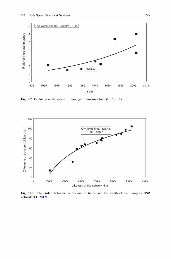
0

2

4

6

8

10

12

14

1925 1935 1945 1955 1965 1975 1985 1995 2005 2015

Rat

io o

f inc

reas

e in

spe

ed

Year

The lowest speed – 47km/h - 1829

HSR era

Fig. 5.9 Evolution of the speed of passenger trains over time (UIC 2011)

Q = 49.564ln(L) -335.43R² = 0.927

0

20

40

60

80

100

120

0 1000 2000 3000 4000 5000 6000 7000

Q-V

olum

e of

tran

spor

t-bi

llion

p-k

m

L-Length of the network -km

Fig. 5.10 Relationship between the volume of traffic and the length of the European HSRnetwork (EC 2012)


TRM (TransRapid MAGLEV)

The TRM (TransRapid MAGLEV—MAGnetic LEVitation) system is based onHerman Kemper’s idea of magnetic levitation from the 1930s. Magnetic levita-tions enables the suspension, guidance, and propelling of MAGLEV vehicles bymagnets rather than by mechanical wheels, axles, and bearings as is the case in HSwheel/rail vehicles. Two forces (lift and thrust/propulsion), both created bymagnets, are needed for operating TRM vehicles. Although the TRM system hasbeen matured to the level of commercialization, the relevant infrastructure hasonly been partially built, mainly connecting airport(s) with city centers, which isstill far from network development comparable to that of HSR (Geerlings 1998;Kertzschmar 1995; Powell and Danby 2007).

Similarly as the HSR, the TRM (TransRapid MAGLEV) system can also becharacterized in the given context as mentioned above by its infrastructure, rollingstock, speed, and traffic.

Infrastructure

The main TRM infrastructure is a guideway consisting of concrete (prefabricated)supporting piers and beams. The concrete piers are located at different distancesdepending on type of the guideway: 31 m—type I, 12 m—type II, and 6.19 m—type III). The beams lying on the solids can have different lengths: 62.92 m—typeI, 24.78 m—type II, and 6.19 m—type III. The height of a beam can be: 2 m—type I, 1 m—type II, and 0.4 m—type III. The total height of the guideway can be:2.2–20.0 m—type I and II, and 1.35–3.5 m—type III. The beam carries the vehicleand provides power to the entire system. Each type of beam has a trapezoidal-likeprofile with the body and the track on top. The beam can be made of steel,concrete, or hybrid (steel/concrete mixture). The three above-mentioned types ofguideway can be single or double (or triple) track constructions. The profile area ofthe guideway is 1.445 m2 (Shibo 2008).

Rolling stock

Principles of operations TRM trains differ from the wheel/rail HS trains in the waythey operate along the tracks. A scheme of TRM system in Fig. 5.11 shows thatthe support and guidance systems follow the principles of magnetic levitation. Theindividually controlled DC (Direct-Current) support and guidance magnets arelocated at the undercarriage of the vehicle. The three phase armature windings or

1970s Research on maglev transportation intensifies (Japan, Germany)1977 The first TRM (TransRapid Maglev) test line of a length of 7 km is built (the test

speed achieved is 517 km/h) (Japan)1993 The TRM test of 1,674 km is carried out (the achieved speed is 450 km/h)

(Germany)1990/1997 The Yamanashi TRM test line of a length of 42.8 km is constructed in 1990 and the

first test is carried out in 1997 (EDS (Electro Dynamic Suspension)) (Japan)2004 The first TRM line between Shanghai and its airport (China) is commercialized


stator windings of the linear electromotor getting power from the modulatedinverter system are installed in the slots of iron core, which is mounted on theunderside of the gateway. The controlled DC suspension magnets getting energyfrom the on board power-conditioning equipment also provides excitation fieldsfor the linear motor. The air gap typically 1 cm is maintained as small as possiblein order to increase efficiency and power factor of the system (He et al. 1992).Such design enables the TRM vehicles to levitate above the tracks supported bymagnets and run on the principle of electromagnetism. As mentioned above, themagnets create two forces—lift and thrust or propulsion for operating the TRMvehicle. The lift force keeps the vehicle above the guideway at a distance of atmost 1 cm but usually 10–15 mm during the trip. The propulsion force enablesacceleration and deceleration as well as overcoming air resistance during thecruising phase of the trip. Thanks to levitation, there is no friction between thetracks and the vehicle’s wheels, thus enabling TRM trains to operate at muchhigher speeds. Figure 5.11 shows a simplified cross-sectional profile containingthe particular components enabling operation. Electric energy is consumed forgenerating both lift and thrust force, but in much greater proportion for the latterthan for the former. In addition, a part of the energy spent during deceleration isreturned to the network, thus also indicating possibilities for saving energy simi-larly as in the case of HSR. Figure 5.12 shows a scheme of the TRM cross-sectionprofile.

Levitation and propulsion Two TRM technologies have been developed tomaturity enabling their full commercial implementation: EMS (ElectromagneticSuspension) and EDS (Electro Dynamic Suspension). They enable three basicfunctions of TRM vehicles: (i) levitation above the track; (ii) propulsion enablingmoving forward in terms of acceleration, cruise, and deceleration; and (iii) guid-ance implying maintaining stability along the guideway.

• EMS technology as a wheel-less system enables TRM trains to levitate above thesteel beam thanks to magnets attached to the vehicle and oriented toward thebeam. This is arranged as a series of C-shaped profiles with the upper partattached to the vehicle and the lower inside part containing the magnets, thuspositioning the rail between the upper and inner part. Due to the high fluctuation

Guidance and Breaking

Vehicle

Levitation and Propulsion Magnet

Guideway

Long- Stator and Iron -Core Armature Windings

Guidance and Braking Rail

Slide Rail Gliding skid

Fig. 5.11 Scheme of themain components of the TRMsystem (He et al. 1992)


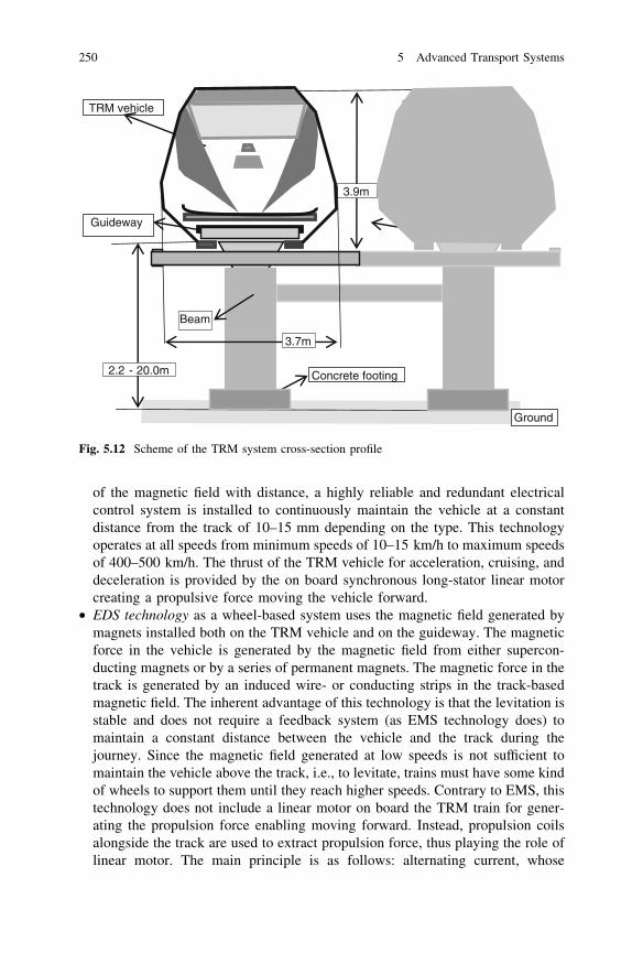
of the magnetic field with distance, a highly reliable and redundant electricalcontrol system is installed to continuously maintain the vehicle at a constantdistance from the track of 10–15 mm depending on the type. This technologyoperates at all speeds from minimum speeds of 10–15 km/h to maximum speedsof 400–500 km/h. The thrust of the TRM vehicle for acceleration, cruising, anddeceleration is provided by the on board synchronous long-stator linear motorcreating a propulsive force moving the vehicle forward.

• EDS technology as a wheel-based system uses the magnetic field generated bymagnets installed both on the TRM vehicle and on the guideway. The magneticforce in the vehicle is generated by the magnetic field from either supercon-ducting magnets or by a series of permanent magnets. The magnetic force in thetrack is generated by an induced wire- or conducting strips in the track-basedmagnetic field. The inherent advantage of this technology is that the levitation isstable and does not require a feedback system (as EMS technology does) tomaintain a constant distance between the vehicle and the track during thejourney. Since the magnetic field generated at low speeds is not sufficient tomaintain the vehicle above the track, i.e., to levitate, trains must have some kindof wheels to support them until they reach higher speeds. Contrary to EMS, thistechnology does not include a linear motor on board the TRM train for gener-ating the propulsion force enabling moving forward. Instead, propulsion coilsalongside the track are used to extract propulsion force, thus playing the role oflinear motor. The main principle is as follows: alternating current, whose

TRM vehicle

2.2 - 20.0m Concrete footing

3.7m

Ground

Guideway

3.9m

Beam

Fig. 5.12 Scheme of the TRM system cross-section profile


frequency is synchronized to match the vehicle’s speed(s), is pushed through thepropulsion coils, thus generating continuously changing magnetic field movingthe vehicle forward along the track. Under such conditions, the counterbalancebetween the strength of the magnetic fields created on board the vehicle and thatfrom the track creates propulsive force moving the vehicle forward. However,this is possible only while operating (cruising) at high speeds. During acceler-ation and deceleration, at low speeds, a secondary propulsive system based onthe conventional electrical linear motor is used in combination with the wheels(‘landing gear’).

Weight and energy consumption The typical weight of an empty TRM vehicleis about 50 tons, which, combined with the weight of payload (passengers) ofabout 20 tons, gives a total gross weight of 70 tons. A portion of the vehicle’sempty weight represents the weight of on board magnets. If the magnet force tomaintain levitation of the vehicle is about 1–2 kW, then the total energy consumedfor this part could be 70–140 kW. Table 5.3 gives some specifications of TRM(TranRrapid MAGLEV) 07.

Usually, similarly as at HSR, the energy consumption of TRM is expressed inthe relative terms, i.e., either per unit of input—supplied seat or per unit of out-put—passenger carried. This is often called SEC (Specific Energy Consumption).Figure 5.13 shows an example of the relationship between the SEC and operatingspeed of TRM07. For the comparative purposes, the corresponding SEC for HSRis also given.

As can be seen, the SEC of both systems increases more than proportionallywith increasing of the operating speed, mainly due to increasing the air resistance.In addition, the SEC of HSR is higher than that of TRM for the range of operatingspeeds (For example, at speed of 300 km/h, this amounts about 33 %).

Control systems Contrary to conventional rail and HSR, TRM systems usingeither technology do not rely on an outside signaling system. TRM systems havefully automated communication systems controlled by the computer system. Thisconsists of the main computer in the system’s command center and that on boardthe vehicle(s). These computers continuously communicate between each other,thus providing the necessary monitoring and control/management of the driverlessvehicles along the line(s). In addition, TRM trains change tracks by using bendingswitches. These consist of bending beams with drive units installed on everysecond solid of the bending switch. There are low-speed and high-speed switches.The former are used near and at stations enabling passing between the tracks atspeeds of about 100 km/h. The former are used along the main portion of theguideway enabling switching between the tracks at speed(s) of about 200 km/h.

Speed

TRM trains can operate at a range of speeds from about 10–15 km/h to about400–500 km/h due to the lack of physical contact with the dedicated guideway.This enables them to cover travel distances of between 500 and 800 km, alsotypical of HSR and short-haul APT system operations, in 1–2 h, respectively. This


Table 5.3 Technical/technological and operational performances of TRM (TransRapidMAGLEV) 07 (He et al. 1992; Janic 2003)

Performance Value

Carriages per train (linked) 2Total length (m) 50Width (m) 3.70Height (m) 3.9Weight of a train (unloaded/loaded) (tons) 90/110Seating capacity (average) (seats) 200Operating speed (km/h) 400–450Maximum speed (km/h) 500Maximum acceleration/deceleration (m/s2) 0.8–1.5Lateral tilting angle (0) 12–16Levitation air gap (mm) 8Maximum thrust (kN) 85Total tractive resistance (kN)Speed (km/h)300 22400 35500 52Guideway loads (at 400 km/h)Longitudinal (kN) 300Lateral (kN/m) 14Vertical (kN/m) 33Track structure Single beam elevated

Span 12 and 16 mTechnical curve radius (m) 2,825–3,580

SEC TRM = 0.0001v 2 + 0.092v + 3.844R² = 0,840

SFC HSR = 0.0002v 2 + 0,119v + 6.911R² = 0.794.

0

10

20

30

40

50

60

70

80

90

50 100 150 200 250 300 350 400 450

SE

C-S

peci

fic E

nerg

y C

onsu

mpt

ion

-(W

-h/s

-km

)

v-Train cruising speed -(km/h)

Fig. 5.13 Relationship between SFC (Specific Energy Consumption) and crusing speed ofTRM07 and HS train(s) (Lukaszevicz and Anderson 2009; TIG 2012)


performance qualifies the TRM system as both a competitive and complementaryalternative to the other two HS systems on comparable distances. Consequently,TRM will be able to connect centers and edges of major cities with airports on theone hand, and provide an intermodal connection with existing APT, HSR, andurban-mass transit and the eventually forthcoming ETT (Evacuated Tube Trans-port) system, on the other. However, similarly as in the case of HSR, both nationaland/or international dedicated infrastructure networks for the long-distance TRMmay take decades to develop up to a level that will have a significant influence onthe existing and prospective transport market(s) (Kertzschmar 1995).

Traffic

Individual TRM lines have been constructed so far for different purposes. Inparticular, in addition to five testing tracks and four tracks (lines) under con-struction, only three lines have been commercialized for public use as follows(http://en.wikipedia.org/wiki/Maglev):

• The Shanghai Maglev Train following the German TRM design, which beganoperations in 2004 in Shanghai (China) by covering the distance of 30 kmbetween the city of Shanghai and its airport in 7 min; this implies an averagecommercial speed of about 268 km/h;

• The ‘‘Urban MAGLEV’’ also known as the Tobu-Kyuryo Line, namely theLinimo system that started operation in 2005 in Aichi (Japan); the length of theline is 9 km with nine stations, a minimum curve radius of 75 m, and a maxi-mum gradient of 6 %; the trains—almost free from noise and quite resistant todisruptions by bad weather—operate at maximum speeds of 100 km/h, thusoffering highly regular and reliable services (nearly 100 %); consequently,nearly 10 million passengers used this system during the first 3 months ofoperation; and

• The urban MAGLEV system UTM-02 in Daejeon (South Korea) began oper-ations in 2008; the length of the line is 1 km connecting the Expo Park andNational Science Museum.

5.2.1.2 Modeling Performances

Background

The DM processes related to HS passenger and other transport systems are mostlybased on different ranking methods. Generally, these methods are commonlyapplied (almost as standard) to ranking alternative systems operating either by thesame or different transport modes including already existing (operated) and/ornonexisting (forthcoming) alternatives. Ranking within the scope of the sametransport mode is necessary for identifying the ‘‘best’’ or ‘‘most preferable’’ amongdifferent available alternatives, while ranking within the scope of different trans-port modes is necessary for identifying the ‘‘most preferable’’ alternative underconditions when both competition and complementarity by substitution between


http://en.wikipedia.org/wiki/Maglev

given HS modes can be expected. Competition is possible in high-density markets(corridors) with sufficient volumes of transport demand supporting efficient andeffective operations of the given HS systems. Complementarity by substitution cantake place in high-density markets-corridors where one HS system fully or par-tially replaces/substitutes another aiming at mitigating its current capacity burden(i.e., congestion) on the one hand, and its overall impact on the environment andsociety, on the other (EC 1998b; Levison et al. 1996; Janic 2003).

Ranking of HS alternatives can be carried out respecting the preferences of thedifferent actors/stakeholders and interest groups involved. Each group can use thespecified methodology/method applied to the selected ranking attributes/criteriarepresented by the indicators and measures of performances of alternative HSpassenger transport systems.

Actors/stakeholders and interest groups

In Europe and the rest of the world, different actors/stakeholders and interestgroups have acted as DM (Decision Makers) in developing and implementing theabove-mentioned HS passenger transport systems. In general, these have beenpublic, semiprivate, and private investors; manufacturers of these systems in thebroadest sense; transport operators; governmental authorities at the local (regionaland national) and global (international) level; users/passengers; the general public;and local community members. Usually, these actors and groups have differentpreferences regarding the full commercialization of such systems. On the positiveside, they have expected benefits from the new systems. On the negative side, theyhave always been reluctant regarding their costs. In such a case, a compromisesolution had to be found.

Both benefits and costs are of different meaning and importance for differentactors. On the benefit side, for example, investors in the HS passenger transportsystem infrastructure and manufacturers of rolling stock and supporting facilitiesand equipment expect at least a return of their investments over the planned periodof time. Local and central governments expect contribution of these systems to theoverall social welfare and the economy. Transport operators expect to profitability.Users/passengers expect to utilize their travel budget more efficiently and effec-tively. Local community members expect local socioeconomic benefits in terms ofnew job opportunities and improved accessibility of their regions.

On the cost side, investors, local and central governments can very likely beconfronted with extremely high infrastructure costs, long return on investmentperiods, and permanent scarcity of monetary funds. In addition, governments at alllevels and local community members can be faced with increased global and localimpacts on the environment and society in terms of energy consumption and relatedemissions of GHG, land use/take, noise, congestion, and traffic incidents/accidents.The systems’ manufacturers can be exposed to an increased risk of economic andsocial failure of the new concepts. Transport operators need to deploy new modelsand knowledge in order to run their businesses profitably. Users/passengers canexpect increased travel costs in absolute terms. Under such conditions, the choice of


the appropriate HS system generally appears to be a very complex process, usuallyresulting in some kind of compromise solution. DMs use different sets of criteriabased on the attributes of performances of particular HS transport systems, whichare either already commercialized or in the planning phase.

Attributes/criteria of performances

The attributes/criteria of performances of the particular HS passenger transportsystems can be selected, defined, and clustered in light of the preferences of theparticular actors/stakeholders involved such as users/passengers, transport opera-tors, local and central government, and local community members.

Users/passengers

Users/passengers are particularly interested in the following attributes/criteria ofperformances of the HS transport systems:

• AccessibilityThis attribute can be quantified by the users-passengers’ generalized costs toreach the services of a given HS transport system. These costs depend on thetotal time the user spends on any of the available urban and suburban transportsystems to reach the HS transport station from his or her location (house, office,shop). The HS transport system’s station can be either the HSR station usuallylocated nearby the center of an urban agglomeration or at an airport. The farepaid for such movement is another factor influencing the generalized costs.Generally, both the travel time and fare depend on the travel distance. Inaddition to individual modes (car, taxi), mass transport modes such as urban andsuburban bus, stretcher, and various rail-based systems can be used (Vuchic2007). This attribute/criterion is preferred to be maximal, implying that acces-sibility costs are preferred to be minimal.

• Generalized travel costsThese costs consist of the costs of users-passengers’ total time spent in a givenHS system and the fare paid for the respective trip. The total time spent in theHS transport system consists of any schedule delay and in-vehicle time. Theformer depends on the departure frequency on a given route during the specifiedperiod of time (an hour, day), while the latter depends mainly on the length ofroute and the vehicle operating speed, as well as on the punctuality of operationsexpressed by delay(s) as deviations of actual arrivals from the schedule. Itshould be mentioned that HS passenger transport systems operate as scheduledtransport systems at which scheduled delays are significantly reduced byadvertising the schedule. Being familiar with the schedule, users-passengerschoose to arrive just in time to meet their scheduled departure. The speed ofHSR and TRM depends on the technical speed and the number and length ofstops along a given route. In APT, the aircraft block speed, which depends onthe aircraft type, cruising altitude, weather and traffic conditions on a route, anddeparting and landing airport, is relevant. In contrast to APT, both HSR andTRM are inherently free of congestion and delays that can exclusively be caused


by imbalances between demand and capacity. In general, these delays can beused for measuring punctuality of services of particular HS transport systems.The fare is primarily dependent on the class of trip (business, leisure), time oftrip (high or low season, weekend or working day, time of day, etc.), length oftravel distance, and the type of ‘yield management system’. This attribute/criterion is preferred to be minimal.

• In-vehicle comfortThe internal comfort, choice of services (drinks, meal, newspapers, videos,possibility of working on board, etc.), and feeling of security are importantattributes (criteria) for users-passengers of a given HS transport system. Theyare preferred to be maximal.

• Reliability of servicesThis attribute reflects the rate of canceled departures. The HS system with thelowest rate is preferable. This attribute/criterion is expected to be maximal,implying that the number of canceled departures in comparison to the number ofrealized ones is preferred to be minimal.

• Security and safetyUsers always expect this attribute to be as high as possible. The choice of HSalternative is always related to the perceived risk for a user to be injured and/orkilled due to potential incidents and/or accidents. The preference is for thisattribute/criterion (security and safety) to be maximal.

Transport operators

Transport operators are expected to consider the following attributes/criteria ofperformances of HS passenger transport systems:

• Operating costsOperating costs are primarily dependent on the constructive characteristics ofparticular HS transport systems, and the volumes and prices of inputs such aslabor, capital, and energy. This attribute/criterion is preferred to be minimal.

• Operating revenuesOperating revenues depend on the internal and external characteristics of bothHS transport systems and their operators. Internal characteristics imply thesystem’s inherent profitability (i.e., some systems are profitable because they areplanned to be so, and others are not) and the capabilities and skills of transportoperators to successfully use and sell their capacities (use of the ‘yield man-agement system’). External characteristics imply the volumes and structure ofdemand and the prevailing market prices under given conditions. This attribute/criterion is always preferred to be as high as possible, i.e., maximal.

• Utilization of resourcesThe art of utilizing the resources engaged to carry out transport services isreflected by the load factor. This is expressed as the ratio between the number ofpassengers on board and the number of offered seats by the given transport ser-vices on a given route/line during a given period of time. HS passenger transportsystem operators prefer systems that can easily provide at least the break-even


load factor. Therefore, from their point of view, this attribute/criterion (the break-even load factor) is preferred to be as low as possible, i.e., minimal.

• Technical productivityOperators always prefer to operate systems with higher technical productivity.Technical productivity is expressed by the volume of services carried out perunit of time. Therefore, technical productivity increases in line with the vehicleand line capacity on the one hand, and the vehicle operating speed on the other(Vuchic 2007). This attribute/criterion is preferred to be maximal.

Local and central government

Local and central governmental authorities can consider the following attributes/criteria of performances of the HS passenger transport systems (Tabucanon andMo-Lee 1995):

• InvestmentsThe investments are always carefully considered in evaluating any HS passengertransport system since the related costs are always very high. Therefore, thisattribute/criterion is always, independent on the investor, preferred to be mini-mal while the return on investment is preferred to be maximal.

• Energy consumptionEnergy consumption is important for planning the energetic balance of thecountry and/or of a given region. In any plan, the proper balance betweendifferent types of primary sources of energy/fuel needs to be established inaddition to minimizing overall energy/fuel consumption. Therefore, in the caseof HS passenger transport systems, planners and policy/decision makers preferthis attribute/criterion to be minimal.

• CongestionCongestion causes delay of transport services and consequently of users-pas-sengers while traveling door-to-door. In general, these delays impose costs onthe affected parties. Operators have to engage more vehicles to serve the samevolumes of demand under given conditions. Users-passengers loose time, whichincreases their generalized travel costs. Both increase the overall social costsand generate the need for building additional infrastructure, which may nega-tively affect the environment through change of land use, increased energyconsumption and related emissions of GHG, and an increased risk of trafficincidents/accidents. In order to minimize these costs, the local and centralgovernment will always prefer the HS transport system that can reduce con-gestion costs, both directly and indirectly.

• ExternalitiesExternalities of HS passenger transport systems include energy consumptionand related emissions of GHG, noise, traffic incidents/accidents, and land use/take. These are preferred to be minimal in both absolute and relative terms.


Local community members

Community member(s) are particularly interested in the following attributes/cri-teria of performances of particular HS passenger transport systems:

• Accessibility costOnce accepting a given HS transport system in their neighborhood, communitymembers are always keen to use its services in the most convenient way. On thelocal scale, they prefer efficient and effective access to services, while on theglobal scale, thanks to the high speed, the preference is to also access manypreviously rather distant regions in shorter (more reasonable) time. Thus, thisattribute/criterion is preferred to be maximal.

• Social welfareSocial welfare expresses some general benefits of the local community arisingfrom the given HS transport system. These can be direct and indirect, part-time,and/or permanent jobs. In addition, these can include the overall increase ofattractiveness of a given community (region(s)) for housing, and business andleisure activities. Therefore, in the given context, this attribute/criterion ispreferred to be maximal.

• Local externalitiesLocal externalities of HS transport systems comprise the environmental andsocial impacts such as energy consumption and related emissions of GHG,noise, traffic incidents/accidents, congestion, and land use (take). However, thistime they are considered at the local community level. For example, changes toland use due to building HS infrastructure can cause displacement of house-holds, creating physical barriers to daily activities, or increase noise, and sim-ilar. Therefore, this attribute/criterion is preferred to be minimal.

The multi-criteria ranking methodology

The multicriteria ranking methodology of HS passenger transport systems asalternatives includes the DM (Decision-Making) problem and process, models ofranking attributes/criteria, and the structure of the ranking method(s).

The DM (Decision Making) problem and process

The DM (Decision-Making) problem of choosing one among several HS passengertransport system alternatives based on their ranking in terms of overall feasibilitycan be structured on three levels as shown in Fig. 5.14.

As can be seen, the first level is occupied by the interest groups. The attributes(criteria) of performances of particular HS passenger transport systems are on thesecond level, while the ranking alternatives, i.e., HS transport systems, occupy thethird and final level.

At least theoretically, membership in particular interest groups is not exclusive,meaning that the same person(s) may belong to different groups simultaneouslyand he or she is assumed to use different attributes/criteria and their weights whilemaking decisions within each group.


The DM process of ranking the selected HS transport system alternativesconsists of two parts. The first deals with modeling particular attributes/criteria ofperformances assumed to be relevant for particular interest groups considering theavailable HS transport systems as alternatives. This enables quantification of theparticular attributes/criteria. The second part consists of the multicriteria rankingmethodology. In this specific case, the methodology includes the TOPSIS(Technique for Order Preference by Similarity to Ideal Solution) method and theentropy method. The methodology enables particular interest groups to carry outmore systematic and consistent evaluation and then selection of the preferable HSsystem alternative (Hwang and Yoon 1981).

Models of attributes/criteria

Modeling attributes/criteria for ranking the HS transport systems enables theirquantification in both absolute and relative terms under given conditions. Inabsolute terms, they can be quantified for a given route (corridor) or for the entire

RANKING HS (HIGH SPEED) PASSENGER TRANSPORT SYSTEMS

Users/Passengers Transport operators Local/central government

• Accessibility• Generalized travel

cost • In-vehicle comfort• Reliability of

services• Safety/security

Alt. No. 1HSR

Alt. No. 2TRM

Alt. No. 3APT

• Operating costs• Operating revenues• Utilization of

resources• Technical

productivity

• Investments• Energy

consumption• Congestion• Externalities

• Accessibility cost• Social welfare• Local externalities

ATTRIBUTES (CRITERIA)

THE HS (HIGH SPEED) PASSENGER TRANSPORT SYSTEM ALTERNATIVES

Local community members

ACTORS AND INTEREST GROUPS

Fig. 5.14 Scheme of the DM (Decision Making) problem and procedure of ranking HSpassenger transport system alternatives (Janic 2003)


network of a given HS system, while in relative terms, the attributes/criteria can bequantified per unit of the system’s output (seat-km, passenger-km, km of infra-structure, etc.). In both cases, estimates are made for the given traffic scenarioimplying operations of the particular HS transport systems along comparable (orthe same) routes/corridors.

• Attributes/criteria for users/passengers

– (A1) AccessibilityThis attribute/criterion for a given HS transport system can be expressed by thegeneralized cost of users/passengers to access its services from their currentlocation as follows:

Ca ¼ a � T dð Þ þ d � p dð Þ ð5:1aÞ

wherea is the value of user-passenger time while traveling (€/pass-h);T(d) is the perceived travel time on the distance d between the user’s location

and the HS transport system station (T(d) = d/v(d) where v(d) is averagespeed of a chosen transport mode operating on the distance d) (min; h);

d is the average travel distance from the user’s temporal location to the HStransport system station (km); and

p(d) is the fare for using a given urban transport mode to arrive at the HSservice (€/p-km; p-km—passenger kilometer).

– (A2) Generalized travel costThe attribute/criterion of a given HS transport system can be estimated asfollows (Janic 1993):

CðDÞ ¼ PðDÞ þ a0 � ½T=4f ðT ;DÞ þ D=vðDÞ þ Td� ð5:1bÞ

whereP(D) is the fare paid by the passenger for traveling on the route of length

D (€/passenger);a0 is the value of passenger time while in a given HS transport system

(both waiting for departure and in-vehicle time) (€/pass-h);D is the length of the route (km);T is the period in which the departures on route D are scheduled (h);f(T) is the service frequency on the route D in time T (-);v(D) is the average operating speed on the route D (km/h); andTd is the anticipated delay on the route D (min; h).

According to Eq. 5.1b, the generalized travel costs will rise in line withthe fare, value of passenger time, and the time of staying in a given HStransport system, the latter depending on the number of departures,length of route, operating speed, and anticipated delay(s).


– (A3) In-vehicle comfortThis attribute/criterion for a given HS transport system refers to its in-vehiclecomfort, security/safety, quality of food/drinks, kindness of cabin attendants,possibilities for on board work, etc. This can be estimated either by interviewingthe users-passengers or by some quantitative estimates such as for example thenumber of different services offered. Generally, the number and diversity ofthese services on shorter routes is smaller than on longer ones.

– (A4) Reliability of servicesThis attribute/criterion for a given HS transport system is usually expressed bythe perceived rate of reliability of services. For the route of length D, this ratecan be determined as:

Rr ¼ NðD; T0Þ=NðD; T0Þ ð5:1cÞ

whereNcd (D,T0) is the number of canceled departures on the route D in time T0; andN(D,T0) is the total number of realized departures on the route D in time T0

(day, week, month, and year).

– (A5) Safety and securityThis attribute/criterion for a given HS transport system is usually expressed bythe ratio between the number of events/causalities (incidents/accidents/deaths/injuries) and the volume of output (vehicle-km, or p-km) carried out during agiven period of time (usually 1 year).

• Attributes/criteria for transport operators

– (B1) Operating costsThis attribute/criterion usually reflects the capital, operating, and maintenancecosts of transport means/vehicles of a given HS transport system. The commonexpressions to estimate these costs can be as follows (Bianco and DiMajo 1991;Janic 1993; ITA 1991):

HSR and TRM

CtðD; StÞ ¼ c0 � D � St ð5:2aÞ

wherec0 is the unit cost per unit of output (€/seat-km); andSt is the average number of seats per departure (seats).

The other symbols are analogous to those in Eq. 5.1a, b and c.

APT

CaðD; SaÞ ¼ a0 þ a1 � Dþ a2 � Sa ð5:2bÞ

whereai is the coefficient estimated by calibration of the regression equation (i = 0,

1, 2).


The other symbols are analogous to those in Eq. 5.2a. The causal relationship(Eq. 5.2a, b) can also be in the log-linear form. As can be intuitively expected, thecost per departure of the given HS transport systems—HSR, TRM, and APT—increases in line with the vehicle (train, aircraft) seating capacity and route length,and vice versa.– (B2) Operating revenues

This attribute/criterion for a given HS transport system can be expressed by thefollowing causal relationship (ITA 1991):

PðDÞ ¼ b0 þ b1 � D ð5:2cÞ

wherebi is the coefficient determined by calibration of the regression model (i = 0, 1).

The other symbols are analogous to those in the previous equations. Evidently, theaverage fare rises in line with the route length (travel distance).– (B3) Utilization of resources (break-even load factor)

This attribute/criterion for a given HS transport system reflects the level ofutilization of its operators’ resources and is expressed as the break-even loadfactor. For a single service on a route, it can be determined after equalizing theoperating costs and the operating revenues as follows:

kbðDÞ ¼ CðDÞ=PðDÞ ð5:2dÞ

whereC(D) is the operating cost per departure on the route D (€/dep); andP(D) is the average fare on the route D (€/passenger).

– (B4) Technical productivityThis attribute/criterion for a given HS transport system can be determined for asingle vehicle as well as for the route where a fleet of vehicles operate asfollows:

Vehicle

Pv ¼ S � vðDÞ ð5:2eÞ

Route

Pl ¼ f T;Dð Þ � S � m Dð Þ ð5:2fÞ

where all symbols are as in the previous equations.Both the above-mentioned attributes/criteria are expressed in seat-km/h. The cri-terion of a single vehicle increases in line with both its seating capacity andoperating speed, while the criterion of the route increases in line the technicalproductivity of a single vehicle and the service frequency of the route.


• Attributes/criteria for the local/central government

– (C1) Investments

HSR and TRMThis attribute/criterion for HSR and TRM reflects construction investments and thecosts of maintaining the infrastructure of a given HS transport system and can beexpressed as follows:

Cti ¼ ðIta � DÞ=Qt ð5:3aÞ

whereIta is the average annual annuity on the investments per unit length of line

(M€/km);D is the length of route (km); andQt is the total number of passengers expected to travel on route D (pass/per

year).As expressed per passenger, this cost is expected to decrease as the passengernumbers on a given route increase. In addition, if the investment and maintenancecosts are additionally divided by the length of route D, the average unit costper p-km during a given period of time can be estimated.

APTThis attribute/criterion for APT reflects the investment and maintenance costs inairports and ATC (Air Traffic Control System) and can be estimated as follows(Manheim 1979):

ra ¼ ðRa � CaÞ=Ia ð5:3bÞ

whereRa is the average annual operating revenues (M€);Ca is the average annual operating cost (M€); andIa is the total investment cost (M€).

– (C2) Energy consumption

HSR and TRMThis attribute/criterion for HSR and TRM is expressed by the energy consumedper p-km on a given route and can be estimated as follows (ITA 1991):

SPCt ¼ ECt=ðkt � StÞ ð5:3cÞ

whereECt is the energy consumption of an HSR or TRM train (KWh/km);kt is the average train’s load factor; andSt is the train’s seating capacity (seats/train).


Multiplying Eq. 5.3c by the number of departures f(D, T) in time T, the routelength D, and the seating capacity of train St, the total energy consumption for agiven traffic volume can be estimated.

APTThis attribute/criterion for APT is expressed by the quantity of energy/fuel con-sumed per p-km and can be estimated as follows:

SFCa ¼FCaðDÞ

k �a Sa � D¼

a0 þ a1 � Tg þ a2 � ð DvðDÞ þ TdÞ

ka � S �a Dð5:3dÞ

whereFCa(D) is the average fuel consumption per flight on the route of length

D (tons/flight);ai is the coefficient determined for each flight; it is dependent on the

aircraft type and length of flight (long, medium, short haul) (i = 0, 1,2); and

Tg is the taxi and/or idle time while the aircraft is on the ground with itsengines turned on (min).

The other symbols are analogous to those in Eqs. 5.1b and 5.3a–5.3c. For a givenflight, SFCa decreases more than proportionally as its length and the aircraft sizeincreases. By multiplying Eq. 5.3d by the flight frequency f(D,T), the aircraftseating capacity Sa, and the route length D, the total energy consumption forcarrying the given volumes of passengers can be estimated.

– (C3) CongestionThis attribute/criterion reflects the total costs of congestion and delays includingthe costs of HS vehicle delays and the costs of user/passenger time losses undergiven conditions. It can be estimated as follows:

CðTdÞ ¼ Td � f ðD; TÞ � CðD; SÞ � vðDÞ=Dþ a � k � S½ � ð5:3eÞ

where the symbols are analogous to the previous equations.– (C4) Externalities

Emissions of GHGThis attribute/criterion for a given HS transport system reflects the total emissionsof GHG generated on the route D in the time period T. It can be estimated asfollows:

TE ¼ ½f ðT;DÞ � k � S � D� �XM

j¼1

SEj ð5:3fÞ

whereSEj is the specific emission of (j)-th type of GHG (g/p-km) ðj ¼ 1:2; . . .;MÞ:

The other symbols are analogous to those in the previous equations.


Land useThis attribute/criterion for a given HS transport system reflects the size and effi-ciency of land use, which can be quantified by the land use coefficient as follows:

oðQ;AÞ ¼ Q=A ð5:3gÞ

whereQ is the volume of output (seat-km or p-km); andA is the area of land acquired for infrastructure of a given HS system (km2).

Specifically, in the case of HSR and TRM, A = s0D, where s0 is the unit area(km2/km) needed for building the line (D is the length of line). In the case of APT,A can be considered as the size of the airport airside area (runways, taxi-ways,apron(s)).NoiseThis attribute/criterion for a given HS transport system can be expressed asmeasured—in decibels on the logarithmic scale dB(A).Incidents/accidents (safety)This attribute/criterion for a given HS system can be determined similarly as in thecase for an individual user/passenger (A5).

• Attributes/criteria for community members

– (D1) Accessibility costsOn the local scale, this attribute/criterion for a given HS transport system can beestimated similarly as that for users/passengers (A1) (Eq. 5.1a). On the globalscale, it can be estimated by the number, diversity, and generalized travel costsof connections between the given and other regions.

– (D2) Social welfareThis attribute/criterion for a given HS transport system reflects the permanentand temporary jobs created by its commercialization. This can be quantified bythe number of new jobs created per thousand of active inhabitants in the givenregion.

– (D3) Local externalitiesThis attribute/criterion for a given HS transport system can be estimated simi-larly as that for local/central governments (C4). In such cases, the externalitiesrelevant for the local community need to be selected.

The multicriteria ranking method

The most common method applied to ranking HS transport systems is the con-ventional ‘‘pure monetary’’ EAT (Economic Analysis Technique). The EATevaluates particular alternatives (projects) on the basis of their ‘‘revenues’’ and‘‘costs’’ during their life cycles. The outputs are expressed exclusively in monetaryterms such as NPV (Net Present Value), BCR (Benefit-Cost Ratio), and/or IRR(Internal Rate of Return). In many cases, the application of EAT is not easy due to


many reasons. First, taking into account the other nonmonetary attributes such asthe environmental and social impacts of particular alternatives adequately andobjectively is not always easy. Second, dealing with sometimes quite oppositeinterests and objectives of the various interested groups involved in the evaluationprocedure is sometimes quite difficult, complex, and time-consuming (Giuliano1985; Tabucanon and Mo-Lee 1995). Consequently, various modifications of theconventional EAT have emerged enabling systematic inclusion of more alterna-tives and ranking attributes/criteria, the latter reflecting specific interests of par-ticular actors/interest groups involved in the DM process. In academic andprofessional literature, these are referred to as MCDM (Multi-Criteria DecisionMaking) methods. In particular, these methods have been proven to cope with theproblems of using a large amount of diverse information, clearly identifying trade-offs between conflicting goals, and comparing the available alternatives in a sys-tematic and consistent way (Geerlings 1998; Hwang and Yoon 1981). One of thestrongest research-based recommendations for using MCDM methods instead of‘‘pure monetary’’ EAT was made in the European COST 328 Action (EC 1998a).1

The multicriteria method presented for ranking three HS passenger transportsystems consists of the entropy method as a commonly used above-mentionedanalytical method for assigning weights to attributes/evaluation criteria and theTOPSIS (Technique for Order Preference by Similarity to Ideal Solution) methodas one multicriteria analytical method alleviating selection of the preferable amongseveral available alternatives. Alternatively, weights can be assigned to criteriaempirically by interviewing representatives of the particular interest groupsinvolved in the DM process (Hwang and Yoon 1981).

• The entropy method

The entropy method implies that the data on the decision matrix representingthe quantitative estimates of the selected attributes/criteria of the given alternativesare known. Let Aiði ¼ 1; 2; 3; . . .;mÞ alternatives need to be evaluated accordingto n attributes/criteria Xj ðj ¼ 1; 2; 3; . . .; nÞ. Let Xij be the outcome of the i-thalternative with respect to the j-th criterion. The values of Xij form the decisionmatrix D containing a certain amount of information. Let pij be the probability thatthe alternative Ai is the ‘best’ per criteria Xj. Then the probability pij can beestimated as follows:

pij ¼ Xij=Xm

i¼1

Xij; 8ðijÞ ð5:4aÞ

Since the choice of the ‘best’ alternative according to any Xj criterion is related tosome measure of uncertainty, the entropy of criteria Ej can be expressed as follows:

1 The MCA (Multi-Criteria Analysis) is proposed as a useful and convenient method forevaluating projects in the scope of Trans-European Transport Networks (s) (TENs).


Ej ¼ �½1= lnðmÞ� �Xm

i¼1

pij � ln pij; 8j ð5:4bÞ

where the expression [1/ln(m)] guarantees fulfillment of the condition: 0 \ Ej \ 1.If the DM (Decision Making) has no reason to prefer one criterion over the other,the weight of criteria Xj can be determined as follows (Hwang and Yoon 1981):

wj ¼ ð1� EjÞ=Xn

j¼1

ð1� EjÞ; 8j ð5:4cÞ

• The TOPSIS method

The TOPSIS method evaluates the decision matrix D½Xij� ði ¼ 1; 2; . . .;m; j ¼1; 2; . . .; nÞ with (m) alternatives each having (n) criteria by assuming that eachcriterion takes either increasing or decreasing utility. This implies that the largerthe criterion outcomes, the grater the preference for the ‘benefit’ criterion and lessthe preference for the ‘cost’ criterion. The computation process of the TOPSISmethod consists of the following steps:

STEP 1: The dimensions of various criteria are transformed into nondimensionalcriteria allowing comparison. This allows a normalized decision matrix R to be setup whose elements are determined as follows (Hwang and Yoon 1981):

rij ¼ Xij=

ffiffiffiffiffiffiffiffiffiffiffiffiffiXm

i¼1

X2ij

s

ð5:5aÞ

STEP 2: The set of weights wjðj ¼ 1; 2; . . .; nÞ obtained by the expression (5.4c)(or provided by the DM) is accommodated to the decision matrix by multiplyingeach column of the matrix R with its associated weight wj. Thus, the normalizeddecision matrix takes the following form:

vij ¼ ½wj � rij�; i ¼ 1; 2; . . .;m; j ¼ 1; 2; . . .; nð Þ

STEP 3: After determining the matrix, V vij

� �the positive and negative ideal

solution A* and A-, respectively, can be estimated as follows:

A� ¼ maxivijjj 2 J� �

; minivijjj 2 J0� �

ji ¼ 1; 2; . . .;m� �

¼ v�1; v�2; . . .; v�j ; . . .; v�n

n oð5:5bÞ

and

A� ¼ minivijjj 2 J� �

; maxivijjj 2 J0� �

ji ¼ 1; 2; . . .;m� �

¼ v�1 ; v�2 ; . . .; v�j ; . . .; v�n

n oð5:5cÞ

where J is associated with the ‘benefit’ and J0 with the ‘cost’ criteria.


STEP 4: Compute the separation of each alternative from the positive and neg-ative ideal solution. A* and A-, respectively as follows:

For the positive ideal solution, it amounts to:

Si� ¼

ffiffiffiffiffiffiffiffiffiffiffiffiffiffiffiffiffiffiffiffiffiffiffiffiffiffiffiffiXn

j¼1

ðvij � v�j Þ2

vuut ; for i ¼ 1; 2; . . .;m ð5:5dÞ

Similarly, for the negative ideal solution, it amounts to:

Si� ¼

ffiffiffiffiffiffiffiffiffiffiffiffiffiffiffiffiffiffiffiffiffiffiffiffiffiffiffiffiffiXn

j¼1

ðvij � v�j Þ2

vuut ; for i ¼ 1; 2; . . .;m ð5:5eÞ

STEP 5: Compute the relative closeness of the alternative Ai with respect to A* asfollows:

Ci� ¼ Si�= Si� þ Si�ð Þ; 0 \ Ci�\ 1; I ¼ 1; 2; . . .;m ð5:5fÞ

Apparently, Ci* = 1 if Ai = A*, and Ci

* = 0 if Ai = A-. An alternative iscloser to A* as Ci

* approaches 1. A set of alternatives can now be ranked indescending order of the value of Ci

* .

Application of the multi-criteria ranking methodology

The multicriteria ranking methodology is applied using the attributes of HSR andAPT performances estimated through real-life data, and those of TRM estimatedthough hypothetical (derived) data.

Input

The estimated values of 15 selected attributes as criteria of performances for threeHS passenger transport systems are given in Table 5.4 including the preferences ofthe particular actors and interest groups. Despite not perfectly coinciding withthose shown in Fig. 5.14, the selected attributes/criteria are sufficiently relevant forthe purpose.

The attributes/criteria in Table 5.4 are expressed in absolute and relative termsand not always by using the above-mentioned quantification models. In addition,the inputs for their estimation have been taken from different sources. Further-more, one should be aware that these sources may change over time. Under suchcircumstances, this ranking should be considered as an illustrative example andguidance for future similar work.

As already explained, the first four criteria (1, 2, 3, and 4) are mostly relevantfor users/passengers. Operators of HS passenger transport systems are mainlyinterested in the next three criteria (5, 6, and 7). The remaining criteria (8, 9, 10,11, 12, 13, 14, and 15) are mostly relevant for the local and central governmentand community members. Furthermore, among the 15 criteria, five are considered


as ‘‘benefit’’ criteria and the other ten as ‘‘cost’’ criteria independently of the actorsor interest group involved in the DM. The particular criteria are quantified asfollows:

• ‘‘Local accessibility’’ is expressed in terms of distance rather than in monetaryterms. Since HSR and TRM terminals are usually located in the center of an(urban) agglomeration, it is assumed that the access distance to these terminalsmay vary from 0.3 to 5 km. The distance of the user-passenger’s location to/from an airport is assumed to vary from 10 to 30 km (Lufthansa 1996).

• ‘‘Generalized travel cost’’ is determined under the assumption that all threealternatives operate according to the same schedule (i.e., they have equal numberof service frequencies along a given route) where all users-passengers haveapproximately the same value of time. Under such conditions, the generalizedtravel costs are dependent only on the in-vehicle time and fare. In this example,the cost of in-vehicle time and fare are expressed in monetary terms per unit oftravel distance. The average value of travel time is adopted to be 32 €/pass/h. Theunit value of travel time per unit of travel distance is calculated as follows: forHSR—32 €/pass/h 9 1 km/270 km/h = 0.119 €/p-km; for TRM—32€/pass/km 9 1 km/400 km/h = 0.080€/p-km; and for APT—32 €/pass/h 9 1 km/600 km/h = 0.053 €/p-km. The fares are 0.069 €/p-km, 0.147 €/p-km and 0.068€/p-km for HSR, TRM, and APT, respectively (CEC 1995; ITA 1991; Levison

Table 5.4 Attributes as criteria for ranking the HS passenger systems in the given example(Janic 2003)

Criterion Objectives forcriteria

The HS alternative

HSR TRM APT

1. Local accessibility (km) ‘‘cost’’-(min) 0.5–3.0 0.5–3.0 10-302. Generalized travel cost (€/p-km) ‘‘cost’’-(min) 0.188 0.257 0.1213. In-vehicle comfort and conveniencea ‘‘benefit’’-(max) 2 2 34. Safety (deaths/100 million p-km) ‘‘cost’’-(min) 0.000009 0.00000 0.04005. Operating costs (€/p-km) ‘‘cost’’-(min) 0.042 0.085 0.0556. Operating revenues (€/p-km) ‘‘benefit’’-(max) 0.069 0.147 0.0687. Technical productivity

(seat-km/hour)‘‘benefit’’- (max) 98,550 132,800 100,200

8. Investments (M€/km)b ‘‘cost’’-(min) 7.14 15.14 14.949. Rate of return on investments (%) ‘‘benefit’’-(max) 13.7 13.5 10.010. Social welfarec ‘‘benefit’’-(max) 138/25 30/10 817/1,27011. Energy consumption (Wh/seat-km) ‘‘cost’’-(min) 60d 42d 230–57012. Emissions of GHG (g/seat-km) ‘‘cost’’-(min) 14.2–25.0e 9.9–17.5e 14013. Land use (ha/km) ‘‘cost’’-(min) 3.2–3.5 1.2 1514. Noise (dB(A)) ‘‘cost’’-(min) 84–105 79–93 46.5–92.515. Congestion (average delay) (min) ‘‘cost’’-(min) 1 1 11.7a The number of different in-vehicle services; b The cost per km of infrastructure; c The numberof part-time/permanent jobs/km of infrastructure; d At the speed of about 300 km/h; e Dependson the primary sources for obtaining electric energy


et al. l996; Witt 1995). Summation of the above values provides the total gen-eralized travel costs for each alternative (Table 5.4).

• ‘‘In-vehicle comfort and convenience’’ is expressed by the number of differentservices provided to users/passengers while on board (SNCF 1996; Lufthansa1996).

• ‘‘Safety’’ is expressed by the number of deaths per volume of output. For HSR,the estimate takes into account the ICE accident of 1998 in which 102 pas-sengers were killed. TRM is assumed to be absolutely safe (no events and noexperience). The risk of death in the APT mode is estimated from current ICAO(International Civil Aviation Organization) figures (Corrie 1994).

• ‘‘Operating costs’’ are estimated for typical operating conditions of HS passengertransport systems as the product of the average cost per seat-km and the load factoradopted to be 65 % (CEC 1995; ITA 1991; Levison et al. 1996; Witt 1995).

• ‘‘Operating revenues’’ are estimated similarly to the ‘‘operating costs,’’ but alsoby assuming that 50 % of first and 50 % of second fare-class passengers use theHSR and APT services. In the case of TRM, only one fare-class is considered(Witt 1995).

• ‘‘Technical productivity’’ is estimated for the typical operating speed that maybe attained on the competing travel distances of 600–800 km. For HSR thisspeed is adopted to be 270 km/h and the seating capacity of a train set 365 seats.The typical operating speed of TRM is adopted to be 400 km/h and the seatingcapacity of a train (the longest version) 332 seats. The typical operating speed ofAPT is assumed to be 600 km/h and the seating capacity 167 seats (A320-200aircraft) (CEC 1995; Ellwagner and Wilckens 1994; Geerlings 1998; ITA 1991;Kertzscmar 1995; MVP 1994; Witt 1995).

• ‘‘Investments’’ are expressed in M€/km of the infrastructure represented by HSRlines, TRM guideways, and airport runway(s). For HSR, this is determined bydividing the total cost of building and upgrading the HSR network in Europe bythe total network length (CEC 1995). For TRM, this is estimated by using datafor the Berlin-Hamburg line (Witt 1995). In order to obtain comparable esti-mates, in the case of APT, the total investments of 25,000 M€ intended toimprove the existing and build new airport and air traffic control capacity duringthe 1994–2000 period are allocated to the total length of runways at 437 airportsin EU (European Union) Member States (CEC 1994b).

• ‘‘Rate of return on investments’’ represents one of the measures of investmenteffectiveness where the pure ‘‘Economics Analysis Technique’’ is applied.Essentially, it expresses the gains on the invested capital expressed in percents. Thistime, this is used as a single attribute (criteria). For the HSR, this is estimated for theentire network (CEC 1995), for TRM for the line Hamburg-Berlin (Witt 1995), andfor APT for the airport and air traffic control infrastructure (Doganis 1992).

• ‘‘Social-welfare’’ is estimated in terms of the newly generated jobs per km ofinfrastructure, i.e., for the entire HSR network, single line of TRM, and 437APT airports in the EU. In the latest case, the jobs at airports, air traffic control,airlines, and supporting airspace industry are taken into account (CEC 1994a;CEC 1995; Doganis 1992; Witt 1995).


• ‘‘Energy consumption’’ is estimated for typical operating conditions of partic-ular HS systems. In case of HSR and TRM, the energy consumption increases inline with the operating speed and is constant as the travel distance and trainseating capacity increase. The values in Table 5.4 correspond to operatingspeeds between 200–320 and 400 km/h for HSR and TRM, respectively. Theenergy/fuel consumption of APT decreases as the nonstop travel distanceincreases. Also, it varies with changes of the aircraft seating capacity. Typicalvalues for A320-200 aircraft flying on routes of between 300 and 800 km areconsidered (ITA 1991; Geerlings 1998).

• ‘‘Emissions of GHG’’ are expressed by the total amount of GHG emitted perseat-km during the specified period of time. The GHG considered are: CO, NOx,SO2, CH, and CO2 (the share of CO2 is about 98.8 % in the total). In the case ofHSR and TRM, these amounts are estimated as generated from the primarysources for obtaining electric energy in the EU15 Member States, while in thecase of APT, the average emissions of GHG are estimated for A320-200 aircraftoperating at speeds of about 500–600 km/h.

• ‘‘Land-use’’ is estimated per kilometer of HSR (tracks), TRM (guideways), andAPT (airport runways) infrastructure. As given, this attribute should be takenwith caution since the absolute values of land use (requirements) for the entireHSR and TRM networks and airports can show quite different relationships(ATAG 1996; CEC 1993b; Witt 1995).

• ‘‘Noise’’ is estimated for the typical operating conditions of HSR (200–300 km/h) and TRM (200–400 km/h) (Geerlings 1998; Kertzshmar 1995; Levison et al.1996). In the case of APT, the ICAO noise certification limits for aircraft ofdifferent weights while taking-off, landing and at the side line are considered(ATAG 1996).

• ‘‘Congestion’’ is expressed by the ‘‘average delay’’ of service operated by eachHS transport system. It is adopted to be 1 min for HSR and TRM. In the case ofAPT it is calculated based on the prevailing demand/capacity ratio of forty EUairports (CEC 1994b).

Results

Two rankings of the three above-mentioned HS transport systems are carried outusing the inputs in Table 5.4. The first produces the preferable alternative withrespect to all 15 criteria, while the second produces the preferable alternative withrespect to the specific set of criteria.

• The preferred HS transport alternative respecting all criteria the normalizeddecision matrix is constructed as the initial step in selecting the preferable HSalternative (Eq. 5.5a) and weights are assigned to particular criteria by using theentropy method (Eq. 5.4) their values are given in Table 5.5. By comparing thevalues in Tables 5.4 and 5.5, it can be seen that the highest weights are assignedto the attributes/criteria with the greatest difference in absolute values, whichemphasizes their relative importance for the dm (decision maker(s)). Forexample, the ‘‘most important’’ criteria appear to be: (1) ‘‘safety’’, (2) ‘‘social


welfare’’, (3) ‘‘congestion’’, (4) ‘‘local accessibility’’, and (5) ‘‘land-use’’.The ideal and the negative-deal solution and the separate measures are calcu-lated by applying Eq. 5.5b–5.5e to the values in Table 5.5. Then, the relativecloseness to the ideal solution is determined using Eq. 5.5f. The results arepresented in Table 5.6.Consequently, the alternatives are ranked according to descending order of Ciz .As can be seen, HSR emerges as the preferred in comparison to the other twoalternatives (TRM and APT). However, as compared to APT, TRM is very closeto HSR.

• The preferred HS transport alternative respecting the specific attributes/criteriaFrom the methodological perspective, selection of the preferred HS transportsystem alternative respecting the specific set of criteria of their performancesrepresents a sensitivity analysis of outputs with respect to changes of inputs, i.e.,the number and type of criteria involved in ranking the alternatives. Accordingto the importance of particular criteria for particular interest groups, the fol-lowing four cases are elaborated:

– Criteria such as ‘‘accessibility,’’ ‘‘generalized travel cost,’’ ‘‘in-vehicle com-fort and convenience,’’ and ‘‘safety’’ relevant for users/passengers and com-munity members while acting as users of HS systems;

Table 5.5 Normalized decision matrix and weights for particular criteria (Janic 2003)

Criterion Normalized value/alternative Weight Rank

A1-HSR A2-TRM A3-APT

1. Local accessibility 0.090 0.090 0.990 0.132 42. Generalized travel cost 0.552 0.754 0.355 0.011 103. In-vehicle comfort and convenience 0.485 0.485 0.728 0.005 124. Safety 0.0003 0.000 0.999 0.271 15. Operating costs 0.383 0.773 0.550 0.011 116. Operating revenues 0.392 0.835 0.386 0.018 87. Technical productivity 0.510 0.687 0.518 0.002 148. Investments 0.318 0.675 0.666 0.012 99. Rate of return of investments 0.632 0.623 0.461 0.002 1310. Social welfare 0.078 0.019 0.997 0.200 211. Energy consumption 0.224 0.585 0.760 0.026 712. Emissions of GHG 0.265 0.216 0.940 0.056 613. Land use 0.211 0.075 0.975 0.107 514. Noise 0.650 0.591 0.478 0.002 1515. Congestion 0.012 0.012 0.143 0.144 3

Table 5.6 Ranks of the HSpassenger transport systemalternatives (Janic 2003)

Alternative Proximity to the ideal solution Ciz Rank

HSR 0.644 1TRM 0.632 2APT 0.358 3


– Criteria such as ‘‘technical productivity,’’ ‘‘operating costs’’, and ‘‘operatingrevenues’’ relevant for transport operators;

– Criteria such as ‘‘investments,’’ ‘‘rate of return on investments,’’ ‘‘socialwelfare,’’ and ‘‘energy consumption’’ relevant for the governmental, public,semipublic, and private institutional and financial authorities and bodies; and

– Criteria representing externalities of particular HS systems such as ‘‘emissionsof GHG’’, ‘‘land use,’’ ‘‘noise,’’ and ‘‘congestion’’ mainly relevant for the localand central governmental authorities, and local community members.

The results of these subevaluations are given in Table 5.7.In the first and third case in Table 5.7, HSR emerges as the preferred alternative

in comparison to TRM and APT systems. TRM appears the preferable alternativein the second case. APT is the least preferred alternative in the first, second, andfourth case. The score indicates that HSR is a favorable alternative for users/passengers, governmental authorities at both local (regional), national, and inter-national level, as well as for potential investors. Transport operators, local andcentral governmental authorities, and local community members, who are mostlyinterested in externalities, favor TRM. However, this alternative appears to be theleast preferable for governmental authorities and investors due to its very highinvestment costs and a rather low contribution to social welfare as compared to theother two alternatives. Nevertheless, this last consequence should be viewed withcaution since only the social effects of a single TRM line have been consideredrather than those of a developed network.

The above-mentioned scores again confirm that rail-based HS systems arecompetitive alternatives to APT systems in short- to medium-haul high-densitytransport corridors/markets. The variations of preferences across the specific setsof criteria indicate why the attitudes of different interest groups must be respectedin the DM process, particularly those related to the development of very importantHS projects. In addition, the sensitivity analysis reveals the high sensitivity ofoutputs to changes of inputs. This may highlight the problem of selecting thenumber, type, and indicators of performances to be included as attributes/criteriain the DM procedure. Furthermore, in addition to application of analytical tools forweighting attributes/criteria, the subjective judgments of representatives/experts ofdifferent interest groups need always to be taken into account if at all possible.

Table 5.7 Sensitivity analysis in ranking the HS passenger transport system alternatives (Janic2003)

Case/criteria Rank/(Ciz)

A1-HSR A2- TRM A3-APT

Case 1/(1, 2, 3, 4) 1/0.980 2/0.955 3/0.450Case 2/(5, 6, 7), 2/0.342 1/0.611 3/0.234Case 3/(8, 9, 10, 11) 1/0.095 3/0.026 2/0.073Case 4/(12, 13, 14, 15) 2/0.955 1/0.999 3/0.009

Ciz—‘‘Closeness’’ to the ideal solution


5.2.2 Evaluation

The HS (High Speed) passenger transport systems—APT (Air Passenger Trans-port), HSR (High-Speed Rail), and TRM (TransRapid MAGLEV)—and themethodology for their ranking as alternatives possess both advantages (Strengthsand Opportunities) and disadvantages (Weaknesses and Threats).

Advantages and disadvantages

HS systems

• HSR has emerged as the preferable alternative as compared to both TRM andAPT with respect to the selected 15 ranking criteria;

• Users/passengers, policy makers, and investors prefer HSR under the givencircumstances;

• TRM appears as the preferable alternative of policy makers and communitymembers, both actors/interest groups primarily interested in transport exter-nalities; and

• APT appears as the least preferable alternative for virtually all actors andinterest groups.

The multicriteria ranking methodology

• Enables ranking of predetermined transport alternatives (both existing andplanned) while respecting the many often conflicting objectives by using attri-butes/criteria of performances of particular HS systems quantified for the given(assumed) traffic scenario(s);

• Ensures flexibility in including additional indicators of performances as attri-butes/criteria in the ranking procedure of existing and completely new HSsystem(s) (still at the conceptual level);

• Can be efficiently and effectively used by particular actors and interest groupsinvolved in the DM process by enabling easier articulating, more transparentlypresenting, and more exactly quantifying the relevant attributes/criteria of theperformances of HS transport alternatives;

• Enables relatively easy verification of the consistency of assigning weights toattributes/criteria including subjective judgments, thus mitigating or completelyavoiding some irrational, time-consuming and unexpected activities and out-comes from the DM process; and

• Seems to be the preferable methodology compared to the conventional EAT(Economic Analysis Technique(s)), thus contributing to more efficient andeffective DM (Decision Making) process relating to the further development andcommercialization of HS passenger transport systems.

Finally, it can be said that HS passenger transport systems can be viewed asadvanced with respect to all their performances taken into account in their mul-ticriteria ranking as mutually substitutable alternatives.


References

Alstom (2008). AGV-a cutting-edge technology integrator. Berlin, Germany: Alstom TransportEurope, INNOTRANS-BERLIN.

ATAG. (1996). Aviation and environment. Geneva, Switzerland: Air Transport Action Group.BBVA. (2009). Economic analysis of high speed rail in Europe. Bilbao, Spain: BBVA Foundation.BCG. (2004). Airports-dawn of new era: Preparing for one of the industry’s biggest shake- ups.

Munich, Germany: Boston Consultancy Group.Bianco, L., & DiMajo, D. (1991). Perspectives of high-speed rail transport in short-medium

period. Transportation Research-A, 25A, 193–202.Boeing (1998). Evolution of the world fleet: Time line. Boeing Aircraft Company. http://www.

boeing.com.CAA (2011) UK airports market-general context, working paper. London, UK: Airport Market

Power Assessment, Civil Aviation Authority.CEC. (1993a). European high-speed rail network: Socio-economic impact study. Commission of

the European Communities, Directorate General for Transport, Final Report, Brussels,Belgium.

CEC. (1993b). The European high-speed train network: Environmental impact assessment.Executive Summary, Commission of the European Communities, Directorate General forTransport, Brussels, Belgium.

CEC. (1994a). Expanding Horizons, A report by Comite de Sages for air transport to theEuropean Commission. Brussels, Belgium: Directorate General for Transport.

CEC. (1994b). Progress report on the guidelines for the Trans-European airport network.Brussels, Belgium: Commission of the European Communities.

CEC. (1995). High-speed Europe, high level group. The European high speed train network.Brussels, Belgium: Commission of the European Communities.

Corrie, S. J. (1994). Potential growth in air travel demands renewed effort to improve safetyrecord (pp. 7–9). Montreal, Canada: ICAO Journal.

Doganis, R. (1992). The airport business. London, UK: Routledge.EASA. (2011). Type-certificate data sheet for noise A380, TCDSN EASA, Issue 6. Koln,

Germany: European Aviation Safety Agency.EC. (1998a). Integrated strategic infrastructure networks in Europe. Final Report on the Action

COST 328, EUR 18165, European Commission, Luxembourg.EC. (1998b). Relationships between high-speed rail and air passenger transport. Final Report on

the Action COST 318, EUR 18165, European Commission, Luxembourg.EC. (2003). Analysis of the European transport industry. European Commission—DG TREN,

Final Report, Brussels, Belgium.EC. (2010). High speed Europe: A sustainable link between Citizens. Luxembourg: European

Commission.EC. (2012). EU transport in figures: Statistical pocketbook 2012. Luxembourg: European

Commission.Ellwagner, G., Wilckens, M. (1994). European high-speed transport: A service with a future.

International 33, 2–12.FAA. (1997). Noise level for U.S. certified and foreign aircraft. Washington, USA: AEE-

110Federal Aviation Administration, U.S. Department of Transportation.Geerlings, H. (1998). The Rise and Fall of new technologies: MAGLEV as technological

substitution? Transportation Planning and Technology, 21, 263–286.Giuliano, G. (1985). A multicriteria method for transportation investment planning. Transpor-

tation Research-A, 19A(1), 29–41.GAO. (2004). Airline financial conditions. Report, The US Government Accountability Office

(GAO), Report, Washington DC, USAHaimes, Y. Y. (1985). Multiple-criteria decision-making: A retrospective analysis. IEEE

Transactions on Systems, Man, and Cybernetics, 15(3), 313–315.

References 275



He, J. L., Rote, D. M., & Coffey, H. T. (1992). Survey of Foreign maglev systems. Argonne,Illinois, USA: Center for Transportation Research, Energy Systems Division, ArgonneNational Laboratory.

Horonjeff, R., & McKelvey, F. X. (1994). Planning and design of airports (4th ed.). New York,USA: McGraw- Hill Book Company.

Hwang, L. C., & Yoon, K. (1981). Multi attribute decision-making: A methods and applications.Lecture series in economics and mathematical systems. Berlin, Germany: Springer.

ITA. (1991). Rail/air complementarity in Europe: The impact of high-speed rail services. Paris,France: Institute du Transport Aèrien.

Janic, M. (1993). A model of competition between high-speed rail and air transport.Transportation Planning and Technology, 17, 1–23.

Janic, M. (2003). Multiple criteria evaluation of high speed rail, transrapid maglev, and air passengertransport systems in Europe. Transportation Planning and Technology, 26(6), 491–512.

Janic, M. (2007). The sustainability of air transportation: A quantitative analysis and assessment.Aldershot, England: Ashgate Publishing Limited.

Kertzschmar, R. (1995). Transrapid maglev: Prospects for fast regional transportation service.Paper presented at the 1st European workshop on high speed maglev transport system:European prospects. Padua, Italy: University of Padua.

Levison, D., Gillian, D., Kanafani, A., & Mathieu, J. M. (1996). The full cost of inter-citytransportation—A comparison of high speed rail, air and highway transportation inCalifornia. Institute of Transportation, Research Report, UCB-ITS-RR-96-3. Berkeley, USA:University of California.

Lukaszevicz, P., & Anderson, E. (2009). Green train energy consumption: Estimation on high-speed rail operations. Stocholm, Sweeden: KTH Engineering Science, KTH Railway Group.

Lufthansa. (1996). Timetable. Frankfurt, Germany.Manheim, M. L. (1979). Fundamentals of transportation system analysis (Vol. 1: Basic

concepts). Cambridge, Massachusetts, USA: The MIT Press.MVP. (1994). Riding of flying? TRANSRAPID and its links with the car, railway and aircraft.

Germany: Versuchs-und Plannungsgesellschaft fur Magnetbahnsysteme MbH.Powell, J., & Dunby, G. (2007). Maglev: Transport mode for 21st century (pp. 44–55). Science

and Technology: EIR.Shibo, S. (2008). Dynamic simulation of the maglev guideway design. MSc Thesis, Faculty of

Civil Engineering and Geosciences, Delft University of Technology, Delft, The Netherlands.Speling, D. (1984). Assessment of technological choices using a pathway methodology.

Transportation Research-A, 18A(4), 343–353.SNCF. (1996). Timetable-TGV/Thalys. Paris, France.Tabucanon, T. M., & Mo Lee, H. (1995). Multiple criteria evaluation of transport system

improvements. Journal of Advanced Transportation, 29(1), 127–143.TIG. (2012). High tech for flying on the ground. Berlin, Germany: Transrapid International

GmbH & Co.UIC. (2011). High speed rail and sustainability. Report, International Union of Railways, Paris,

FranceUSDT. (2012). National transport statistics. U.S. Department of Transportation Research and

Innovative Technology Administration Bureau of Transportation Statistics, Washington DC, USA.Vuchic, R. V. (2007). Urban transit: Systems and technology. Hoboken, New Jersey, USA: Willey.Witt, M. (1995). The transrapid system and the Hamburg-Berlin connection, the 1st European

workshop on high-speed maglev transport systems: European prospects. Padua, Italy:University of Padua.


Chapter 6Advanced Transport Systems:Future Concepts

6.1 Introduction

This chapter describes five concepts of future advanced transport systems: (i) PRT(Personal Rapid Transit) systems; (ii) UFT (Underground Freight Transport)systems; (iii) ETT (Evacuated Tube Transport) system; (iv) advanced ATC (AirTraffic Control) technologies and procedures for increasing airport runwaycapacity; and (v) advanced STA (Supersonic Transport Aircraft).

• PRT (Personal Rapid Transit) systems were elaborated in the 1970s and com-mercialized in the 2010s. They are a fully automated transit systems consistingof dedicated aboveground guideways enabling movement of small passengercar-like vehicles, i.e., capsules. As such, PRT systems are expected to offercompetitive—efficient and effective—transit services by substantially replacingconventional passenger cars, motor- and trolleybuses, and LRT (Light RailTransit) systems in urban and/or suburban areas. At the same time, PRT willcontribute to mitigating the overall impacts of urban transit systems on theenvironment and society in terms of energy consumption and related emissionsof GHG (Green House Gases), land use/take, noise, congestion, and trafficincidents/accidents. PRT commercialization is shown to be a rather gradualprocess mainly due to the high investment costs starting in some niche markets;

• UFT (Underground Freight Transport) systems were elaborated for the first timein the 1970s but particularly in the 1990s and 2000s. They are fully automatedsystems for moving freight/goods shipments of different sizes such as standardpallets, containers, and/or swap bodies along a network of underground pipes/tunnels. Shipments are loaded onto dedicated vehicles/capsules. Undergroundpipes/tunnels connect different freight/goods origins and destinations in a givenurban or suburban area including large intermodal transport nodes such as ports,airports, and inland freight terminals. UFT systems are expected to substantiallyreplace road trucks in congested urban areas and consequently mitigate their


277

impacts on the environment and society. The commercialization of any kind ofUFT system is still under consideration due to the high investment costs relatedto building underground pipes/tunnels.

• Evacuated Tube Transport system was elaborated for the first time in the 1970s,but remained at that stage until recently (Salter 1972). This system is used totransport passengers and freight/goods along long-haul (intercontinental) dis-tances by TRM (TRansRapid MAGLEV) trains running through pipes locatedbelow the ocean’s floor at supersonic speed.1 The EET system’s eventual fullcommercialization will likely be the matter of discussion and decisions in theforthcoming decades since if the decision is taken to design such a system, thiswill certainly not be earlier than around the 2050s or latter. The main issues stillto be resolved are choosing the design of infrastructure (pipes) and proving thesystem’s economic feasibility, mainly due to the very high investment cost forbuilding the infrastructure (underwater pipes);

• Advanced ATC (Air Traffic Control) technologies and procedures for increasingthe airport runway capacity are currently under development in the scope of theU.S. FAA NextGen (Next Generation Air Transport System) and European-EUROCONTROL SESAR (Single European Sky ATM Research) programs(EC 2007; FAA 2010). The advanced procedures supported by these technol-ogies imply the application of ATC mixed horizontal/vertical, exclusivelyvertical distance-based, and time-based separation rules instead of the currenthorizontal distance-based separation rules between landing aircraft. In parallel,ATC can alternatively apply the existing FCFS (First Come First Served) andthe advanced PR (Priority) service discipline for landings on a single runway. Inaddition to maintaining the required level of safety, these advanced technologiesand procedures are expected to increase the airport runway system capacitywithout requiring new land for expanding the infrastructure, i.e., building newrunway(s) (LHR 2010). The full commercialization of these technologies andprocedures is the matter of a decade or so, i.e., by the year 2020/2025; and

• STA (Supersonic Transport Aircraft) were already in commercial operation asthe French-British Concorde and Soviet Union’s TY144 supersonic aircraft. Stillbeing at the conceptual level, the aircraft is supposed to operate at speeds higherthan Mach 2.0. Their full commercialization is likely to occur in about two tothree forthcoming decades (2030/2040). This is because, at present, the mainaircraft manufacturers Airbus and Boeing, and other agencies and institutionsdealing with the visions of development of the commercial air transport systemdo not explicitly consider such developments to occur earlier than around 2030(ACARE 2010; Airbus 2012; Boeing 2012).

1 The supersonic speed is greater than the speed of sound, which depends on the air ambienttemperature. For example, at the sea level with standard temperature of 15 �C, it is 1,225 km/h; atthe cruising altitudes of most commercial jets and supersonic aircraft of 11,000–20,000 m withtemperature of -57 �C, it is 1,062 km/h.

278 6 Advanced Transport Systems: Future Concepts

6.2 Personal Rapid Transit Systems


One of the most dominant social-economic trends during the twentieth century hasbeen urbanization characterized by growing cities and the consequent increase inproportion of the urbanized population. This has reached about three billion, i.e.,about 47 % of the total global population in the year 2000. The current and futuretrends indicate that about 6 billion or two-thirds of the world’s population are likelyto live in the urban areas by the year 2050. In parallel, the urban mobility problemsin terms of provision of sufficient transit capacity, emissions of GHG (Green HouseGases), land use, congestion, and noise have been increasing and becoming morecomplex. This has often required adaptation of the growing urban forms andstructures to the requirements of existing individual and mass urban transit systems,and vice versa (Rodrigue et al. 2006). These urban transit systems referred to hereas conventional are considered to be bikes, motorbikes, individual passenger cars,taxis, motor buses, and trolleybuses (including BRT (see Chap. 2)), trams, and LRT(Light Rail Transit) system(s). Future urban developments will certainly require thecommercialization of advanced urban transit systems in order to support theabove-mentioned conventional ones and satisfy growing demand for urban mobilitymore efficiently, effectively, environmentally friendly, and safely. Some of thesesystems/concepts are: (i) ADAS (Advanced Driver Assistance System) for indi-vidual passenger cars; (ii) PRT (Personal Rapid Transit) system; (iii) Advanced bussystems; and CTS (Cybernetic Transport Systems) with the ‘‘road-based peoplemovers’’ and ‘‘advanced car sharing’’ subsystems (EC 2007).

Specifically, PRT (Personal Rapid Transit) as urban transport systems offer apotential solution for mitigating urban congestion and improving travel accessi-bility. It is designed for use in a variety of cases aiming at replacing mainlyindividual passenger cars and urban motor buses and trolleybuses as:

• An exclusive urban and/or suburban transit system;• A system feeding other mass urban and suburban transit systems (conventional

buses, BRT, LRT, metro);• An airport ground access system/mode complementing to the existing ones;• An inter-airport transit system connecting airports belonging to the same airport

system (for example, New York and/or London airports);

1972/1975 The WVU PRT Morgantown system begins operations (U.S.)2001 The first self-balancing PRT (Personal Rapid Transit) system (Segway PT) is

launched (U.S.)2011 The PRT ULTra (Urban Light Transit) system begins operations at London

Heathrow airport (UK)

6.2 Personal Rapid Transit Systems 279

http://dx.doi.org/10.1007/978-1-4471-6287-2_2

http://dx.doi.org/10.1007/978-1-4471-6287-2_2

• An intra-airport transit system at a large airport connecting distant structuressuch as terminals (the satellite concept) to long-stand parking areas, and viceversa; and

• An exclusive system operating in campus environment such as universities andself-contained business/entertainment parks.

The PRT systems consist of fully automatized small driverless vehicles trans-porting an individual or small group(s) (typically 1–6) persons along dedicatedguideways. These can be elevated, at ground level, and underground. The transitservices, available on demand rather than according to a fixed schedule over mostor all of the day are provided between particular origins and destinations withoutstops at intervening stations, i.e., without the need to transfer. The PRT systemscan be implemented as a single- and dual-mode systems. The most well-knownsingle-mode PRT systems in the U.S. are the earliest WVU PRT Morgantown(1972/1975), Raytheon PRT2000 (1995), and Taxi 2000 HCPRT (High-CapacityPersonal Rapid Transit) (2003). In Europe, the most well-known systems includethe UK ULTra and Dutch 2getThere PRT systems. The most well-known dual-mode PRT system is Denmark’s RUF (Rapid Urban Flexible) Intelligent Auto/Transit concept. This system is designed to operate PRT vehicles both automati-cally and manually. The main element of the RUF system is dedicated guidewaysfor the automatic portion of each trip. The system uses small- and medium-sizedintelligent electric vehicles, which can move along conventional roads/streets aswell as along the automated rail network. Small vehicles with a capacity of 2–4persons could be in the public or individual private ownership and as such in thelatter case parked at the individual’s residence and/or workplace. Larger vehicleswith a capacity of 10 persons are usually publically owned and parked at the publicparking areas similarly to small buses. As such, the concept brings together theconvenience of the individual passenger car and the efficiency of urban railways.While operating on roads/streets in manual mode, the vehicles are powered by theelectricity from the on-board batteries enabling an average range of about 50 km.While operating in automated mode, the vehicles are powered by electricityobtained from the rail electricity supply system, enabling relatively high operatingspeeds over longer distances. Such smart integration of operating modes enablesthe concept/system to offer users/passengers efficient and effective connectionbetween numerous origins and destinations within and through large, dense, andcongested urban agglomerations. Consequently, fully automated computer-con-trolled operations enable traveling free of congestion and potential incidents/accidents (RUF 2008).

To date, three PRT systems have been commercialized: the WVU (WestVirginia University) PRT system (designed by Boeing) started operation during the1972/1975 period; the partially commercialized Cybercab PRT system of the Dutchmanufacturer 2getThere operating in Masdar City (Abu Dhabi) started operation in2010; and the ULTra (Urban Light Transit) system commenced operation atLondon Heathrow airport (London, UK) in May 2011. The forth, the Vectus PRT


system of the Swedish/Korean manufacturer Vectus is planned to start operation in2013 in Suncheon Bay (South Korea) (EC 2007; http://www.advancedtransit.org).In addition, the ULTra system yet to be commercialized in Amristar (Punjab, India)in 2014 will be the world’s first and largest actually urban PRT system. The lengthof its network is planned to be 8.0 km with seven stations accommodating 240vehicles expected to serve peak demand of up to 100,000 passengers/day. Thiscompletely privately financed system is expected to bring savings in the currentjourney time of up to about 30 min (http://www.advancedtransit.org). Furthermore,some prototypes of PRT systems such as the LINT PRT system by the manufacturerModutram (Mexico), the Microrail PRT/Dual Mode system by the manufacturerMegarail Transportation Systems (US), and the Skyweb Express PRT system by themanufacturer Taxi 2000 (US) have been operationalized to the level of test track.


6.2.2.1 Background

The generic characteristics of a PRT system are as follows: automatically guidedhigh-pressure rubber tire or steel wheel vehicles with a capacity of 1–6 personsmove along exclusive/dedicated concrete steel elevated guideways at relativelyhigh speed for the given (urban) conditions. The vehicles are powered by anelectric motor propulsion system controlled by microprocessors, making themreliable, less energy consuming and air polluting, and less noisy, all as comparedto individual cars and other urban mass transit systems. The small and relativelylight vehicles allow for lighter and consequently less costly guideways. Nonstopservices are provided thanks to using off-line stations, which are closely spaced inthe network of interconnected guideways, thus eliminating the need for passengerstransferring between lines. At stations, a few empty vehicles usually wait (simi-larly as at taxi stations) to be picked up by users/passengers. First, passengers needto select their itinerary, buy their ticket, and pass the information from the ticket tothe vehicle’s control system. Then, after the vehicle’s door opens they board thevehicle, the door closes, and the computer control system opens a path to thevehicle. Then, the vehicle accelerates and joins other vehicles passing through agiven station, and then forward toward the destination. The elevated configurationof guideways reduces the required land only to that needed for setting up posts andstations (Anderson 2000, 2005, 2007).

Similarly as the other advanced transport systems, a given PRT system can becharacterized by its infrastructural, technical/technological, operational, economic,environmental, social, and policy performances, all of which are further analyzedand modeled.


http://www.advancedtransit.org



The infrastructural performances of a given PRT system refer to its design,geometry, and material of guideways; spatial layout and coverage of the network;layout, configuration, and number of stations; and switching.

Guideways

The PRT system guideway(s) as an elevated construction(s) usually with top-mounted vehicles gives the visual impression shown in Fig. 6.1. A typical PRTguideway is a U-shaped configuration made of concrete laying on a concrete and/or steel/concrete construction. This construction is supported by pods (solid pil-lars) located at certain distances, thus enabling the relatively uniform distributionof its own weight and the weight of moving vehicles. The cross-section of theU-shape guideway with vehicles determines the square-shaped vehicle dynamicenvelope with a height of about 3 m (from the top of a vehicle to the bottom of theguideway aerial structure) and a width of about 5 m for the two-track guideway(s)shown in Fig. 6.2. The height of the pods (solid pillars) from the ground can varydepending on the roadway and/or pedestrian way clearance requirements.

The guideways are also designed with respect to stress (bending and torsion,natural frequency and critical speed) and passenger ride comfort, generally with orwithout walkways, and with many curves and elevations. Both horizontal andvertical curves need to be designed to provide for the riding comfort of seatingpassengers according to the standards for the lateral and normal acceleration andjerk of about 0.25 g and 0.25 g/s, respectively. In some cases, covers made ofcomposite materials and a thin aluminum layer inside are attached to the sides of

Vehicle(s)

Concrete cellar pod

Guideway

Fig. 6.1 Scheme of the PRT system


the guideway in order to protect the tracks and tires from extreme weather (frostduring cold nights, the accumulation of snow, and solar heating during the sum-mer), and in some cases, from electromagnetism (Anderson 2007).

Network

The PRT network consists of guideways. Its spatial layout is usually adjusted tothe spatial density of user/passenger demand. The network can consist of a singleline connecting a given origin and destination (for example in the case of airportaccess or internal transit systems), a small-scale network of lines feeding otherurban mass transport systems such as BRT, LRT, and/or metro, and a larger scalenetwork operating in a given urban complex as an independent and/or exclusivepublic transport mode. In most cases, network development usually begins bybuilding a single guideway and then gradually expanding by adding new onesthrough adapting to transport needs. Figure 6.3 shows a simplified layout of anexclusive PRT network.

Stations

PRT system stations are designed as off-line guideways located usually betweenintersections of guideways at distances of about 800 m, or shorter or longerdepending on the spatial distribution of user/passenger demand. In the verticalplane, the stations are designed as elevated platforms leveled to the elevatedguideways and standing either alone or incorporated into other existing urban

App. 5m

App. 3m

0.45m

Fig. 6.2 Scheme of the vehicle dynamic envelope for the two-track guideway PRT system


structures. The length of an off-line station can be, depending on the vehicle’soperating speed, about 33–39 m, thus providing safe maneuvering space andberths for about 3–5, and, if needed, after extension for up to 12–14 vehicles.Additional berths are also needed for vehicles waiting due to any reason—forexample, while vacant during off-peak hours, maintenance, or when all tracks areoccupied. Since the passengers are supposed to spend only a short while at thestations during boarding and disembarking the vehicles, the intended space isrelatively small, thus reducing the construction costs, and mitigating the visualimpacts and crowd-related (social) problems. Such off-line stations enable con-tinuous vehicle movement, thus maximizing the transit speed and minimizing thetransit time, while enhancing riding comfort. In addition, stations also providegood spatial accessibility (Anderson 2007).

Switching

Switching is an important component of the PRT infrastructure. At present,switching is based on mechanical back up. In such cases, switches have two stablepositions, are self-stable, and can be thrown manually if required. They areunaffected by centrifugal forces, operable under all weather conditions, andpowered by low-voltage batteries.


The technical/technological performances of a given PRT system relate to itsvehicles (cars), the system for controlling their movement, and the system forinteraction with users/passengers.

International airport

Urban area

Car parking

Building/station

PRT line

Fig. 6.3 Scheme of the prospective fully developed PRT network (Masdar City—Abu Dhabi)(http://www.advancedtransit.org)



Vehicles

The PRT vehicles, designed as small, light, and short as possible—typically 2.7 mlong and 1.65 wide, are usually placed above the guideway(s). Each vehicleconsists of three parts: a passenger cab, a bogie for interface with the guideway,and a propulsion system. The typical capacity of the passenger cab is four personsplus two children (and their baggage between the seats) including space forwheelchairs, bikes, etc. The bogie has rubber-tired or steel wheels, thus guaran-teeing efficient and effective braking at an acceptable noise level. The propulsionsystem is usually an LEM (Linear Electric Motor) (LSM—Synchronous or LIM—Induction) powered by electricity from on-board batteries or from an externalelectricity supply system, and controlled by computer microprocessor. Either lead–acid or lithium iron phosphate batteries can be used. The LEM enables weather-independent acceleration and braking, and a reaction and breaking time of a fewmilliseconds, each as compared to that of humans—0.3–1.7 s, and that ofmechanical brakes of 0.5 s, respectively.

The operating speed of vehicles can vary between 30 and 80 km/h dependingon the type of PRT system, and the location, geometry, and topography ofguideways (the elevation change can be up to 15 % along the distance of 9.0 m).

The vehicle movement control system

The control of vehicles while operating along the guideway is carried out by afully automated centralized dual-redundant computer system providing highdependability and safety. The control function is set up hierarchically at threelevels: (i) vehicle control; (ii) zone control; and (iii) central control. The vehiclecontrol system generally generates the intended routes/paths for each vehicleboarded by an individual and/or group of users/passengers between their intendedorigins and destinations, and accelerates/decelerates, monitors, and controls theoperating speeds and headways between the vehicles. This implies that eachvehicle follows the assigned/commanded trajectory. The zone control systemenables each vehicle to communicate with the zone’s computer controller. Eachvehicle transmits information about its position and speed to this controllerthrough the cable in the guideway, and the controller responds back with themaneuvering commands, both in milliseconds. In addition, the merge-zone-controlcomputer receives and maintains information about the current position and speedof all vehicles within a given merging zone, and resolves any potential mergingconflicts by sending the relevant maneuvering commands to the vehicles involved.The central control system comprised of the central computer controlling thecomputers at the other two lower hierarchal levels.

The user/passenger interaction system

The system for interaction of a given PRT system with its users/passengers gen-erally consists of: (i) the information and communication subsystem; and (ii) thefare collection subsystem.


The information and communication subsystem

The components and functions of the subsystem for informing and communicatingat both vehicles and berths/stations are given in the self-explanatory Table 6.1.

The fare collection subsystem

The subsystem for collecting fares consists of ticketing machines located at thestations/berths. After selecting the destination and paying by an available means(cash, credit, debit card), the user receives a magnetically encoded card. Then, he/she takes the ticket and goes to the boarding platform where the ticket is passedthrough the stanchion in front of an available (empty) vehicle. Then, the infor-mation about the travel itinerary is transferred to the microprocessor on-board thevehicle. The door opens, the vehicle is boarded, the door closes, and the zone andthen the central computer, based on the information received from the givenvehicle, generates and then opens the route/path for the vehicle depending on thesurrounding traffic. The nonstop transit to the intended destination begins. There,after the vehicle’s door opens automatically, the passenger leaves the vehicle.


The operational performances of PRT systems include demand, capacity, servicequality, fleet size, and technical productivity.

Demand

The PRT system is designed to replace individual passenger cars, particularly incongested urban areas. Therefore, the primary category of users are passengersabandoning their cars and those using the system for the first time instead of theircars. Some research has indicated that the proportion of car users switching to thePRT system could be up to 30 %. In addition, switching from other urban transitmodes could also be expected, but the more exact volumes remain the matter offurther investigation on a case by case basis. The PRT system’s services aresupposed to be equally and fairly available to all categories of individuals or smallgroups users/urban passengers regarding their gender, social category, trip pur-pose, and current mode choice.

Table 6.1 The subsystem for informing and communicating within a given PRT system

Component Function

Touch Screen, automated interactive display and audio InformationCCTV, intercom, emergency assistance request button Communications initiation2-way audio intercom and CCTV monitoring CommunicationsApplication dependent Destination selectionCCTV, intercom, operator Emergency responseFacility for ride sharing Yes


Capacity

The capacity of a given PRT system generally includes the capacity of vehicles,lines, and stations. The vehicle capacity is expressed by the number of spaces forusers-passengers. The capacity of lines and stations can be expressed by the trafficcapacity and the transport/transit capacity. The former reflects the number ofvehicles and the latter the number of users-passengers handled and transported,respectively, during the specified period of time (usually 1 h) under conditions ofconstant demand for service.

The traffic capacity of a given PRT system’s line can be estimated as follows:

Ktraffic ¼ T=h ð6:1aÞ

whereT is the period of time (minute, hour); andh is the minimum headway (seconds, minutes).

From Eq. 6.1a, the transport/transit capacity of the same PRT line can beestimated as follows:

Ktransport=transit ¼ Ktraffic � k � n ð6:1bÞ

wherek is the average vehicle’s load factor or occupancy rate; andn is the number of spaces for users/passengers on a vehicle (pass/veh).

The capacity of a PRT system station can be static and dynamic. Its staticcapacity can be expressed by the required number of berths simultaneously usedby PRT vehicles as follows:

Ns ¼ Ks � sþ Nw ð6:1cÞ

whereKs is the intensity of demand for using berths at a given station;s is the average occupancy (i.e., dwell) time of a berth at a given station by an

active (operating) vehicle; andNw is the number of berths for vehicles waiting to be called.

The other symbols are analogous to those in the previous equations.The dynamic capacity or throughput of a given station is expressed by the

number of vehicles processed during a given period of time. For a station with Ns

berths, its capacity or throughput (veh/min or veh/h) can be estimated as follows:

Ks ¼ Ns=s ð6:1dÞ

For example, let the minimum headway in Eq. 6.1a be: h = 0.5 s. This impliesthat the traffic capacity of a line during the time of: T = 1 min can be: Ktraffic =

120 veh/min (Similarly, with a headway of h = 1 and 2.5 s, this capacity will be:


Ktraffic = 60 and 24 veh/min, respectively). If each vehicle has n = 3 spaces/seatsand all are occupied, i.e., k = 1.0, based on Eq. (6.1b), the transport/transitcapacity of a given line will be: Ktransport/transit = 120 9 3 9 1.0 = 360 pass/min(if the traffic capacity is: Ktraffic = 60 and 24 veh/min, this capacity will be 180and 72 pass/min, respectively). After considering a given line as a part of the PRTnetwork by taking into account the more realistic values of the headways and theload factor of vehicle, both capacities will certainly be lower. Nevertheless, theminimum headway must not be shorter than the vehicle breaking distance at areasonable deceleration/braking rate (1.0–1.5 m/sec2).

If the intensity of demand for a given station in Eq. 6.1c is: Ks = 120, 60, and 24veh/min, and the vehicle dwell time at the berth s = 20 s, the required number ofberths will be: Ns = 40, 20, and 8, respectively. Similarly, it follows from Eq. 6.1dthat the maximum throughput of a station with 5, 10, and 20 berths, each occupied bya vehicle for about: s = 20 s, will be: Ks = 15, 30, and 60 veh/min, respectively.

In order to enable efficient and effective operations of a given PRT system, thecapacities of lines, merging segments, and off-line stations need to be balanced.Consequently, the resulting capacity of a given line with the given number of off-line stations will be the minimum among the capacities of these elements.

Quality of service

Measures of the quality of service of a given PRT system can include accessibilityand availability, schedule delay, transit time, punctuality and reliability, and ridingcomfort.

Accessibility and availability

The PRT system is designed to be highly spatially accessible in terms of walkingdistance and related time. Nevertheless, locations for joining the system are not asclose to the users’ residences or workplaces such as those of cars as users have towalk a short distance to one of the PRT stations. Ideally, the distance is about 150 mrequiring up to 5 min walking time. In terms of availability, the PRT system isinherently highly available (some concepts are specified to operate 24 h/day).

Schedule delay

PRT is designed as a demand-responsive system where vehicles wait for users-passengers, which is distinctive from other urban mass transit systems where theusers/passengers usually wait for the vehicles. However, this is not always true.PRT systems may also incur schedule delays as the time difference between themoment a user-passenger makes a request for a free vehicle and the moment itbecomes available. This vehicle can be from a stock waiting at the given station,sent from some other waiting location, or have just arrived and been vacated by itsprevious user(s). Consequently, the schedule delay can be zero, tens of seconds,and/or a few minutes, the latter two during peak and off-peak periods, respectively.Facilitating the users/passengers and vehicles in the first of the above-mentionedcases confirms the claim that at PRT system(s), the vehicles wait for users/pas-sengers rather than vice versa.


Transit time

The transit time depends on the distance between the selected origin(s) and des-tination(s), and operating speed. This time consists of the time of boarding thevehicle after buying a ticket, the time for the vehicle’s acceleration/deceleration(not higher that 1–1.5 m/s2), and the time the vehicle cruises at the operating speedmentioned above. Such composed transit time is continuous, uninterrupted bycongestion, minimal, and highly predictable under the given circumstances.

Reliability and punctuality

Like other public urban public transit systems, the reliability of a given PRTsystem can be expressed as the ratio between the realized and planned servicesduring the specified period of time (day, month, year). The reliability to date ofcurrently operating and planned PRT systems has been very close to 100 %. Thepunctuality of PRT system can be expressed as the proportion of user-passengertrips carried out during the specified period of time, on time, or within the pre-scribed time deviation(s) (in the latter case it is often referred to as dependability).The punctuality of already operating PRT systems has also been very close to100 %. In general, both measures are actually expected to be near 100 % all thetime and under all weather conditions.

Riding comfort

The riding comfort of a given PRT system is expected to be at a higher level thanthat of other urban transit systems. This is achieved through the above-mentioneddesign of the guideways, stations, and vehicles themselves. The guideways enablethe smooth ‘‘gliding’’ of air-conditioned vehicles. The size and pattern of supply oftransport capacity always guarantee a free seat to users-passengers. Thanks to thesystem of controlling the flow(s) and spacing between vehicles, their operatingspeed and acceleration/deceleration are always maintained within the prescribed(comfortable) limits (the later of about 1.0–1.5 m/s2) excluding any unpredictablestrong breaking, for example, due to preventing potential collision(s).

Fleet size

The vehicle fleet of a given PRT system consists of the vehicles in operation and inreserve. The former provide services while the latter are only engaged when theformer need to be out of service due to repair and maintenance. Based on Eq. 6.1b,the maximum number of PRT system vehicles in operation can be roughly esti-mated as follows:

M ¼ Ktraffic � t ð6:2Þ

wheret is the vehicle’s average turnaround time over the PRT network (min).


The turnaround time t in Eq. 6.2 depends on the average distance betweenparticular origins and destinations and the related average speed. This implies thatserving shorter trips at a higher speed will require a smaller vehicle fleet, and viceversa.


The technical productivity of a given PRT system can be estimated for a singlevehicle and for a fleet of vehicles. For a single vehicle, it is equal to:

TPv ¼ n � v ð6:3aÞ

wheren is the number of spaces in a vehiclev is the vehicle operating speed (km/h).

The other symbols are analogous to those in the previous equations.For example, for a vehicle with 4 spaces/seats operating at a speed of 40 km/h,

the technical productivity will be: TPv = 4 9 40 = 160 seat-km/h.Similarly, for a fleet of M vehicles, the technical productivity can be estimated

as follows:

TPfv ¼ N � n � v ð6:3bÞ

where all symbols are analogous to those in the previous equations.For example, the technical productivity of a fleet of N = 20 vehicles, each with

n = 4 spaces/seats and operating at a speed of v = 40 km/h will be:TPfv = 20 9 4 9 40 = 3,200 seat-km/h.


The economic performances of PRT system(s) include the system costs, revenues,and the user/passenger benefits expressed in monetary terms.

Costs

The costs of a given PRT system(s) consists of the capital/investment cost forinfrastructure, vehicle and control systems, operating cost for providing transitservices, and the total cost as the sum of the annual capital/investment andoperating cost.

Capital (investment) costs

The capital (investment) costs relate to the cost for building infrastructure andacquiring the vehicles and control systems for a given PRT system. This cost canbe estimated as follows:


Civ ¼ ci � Lþ cv �M þ Ccs ð6:4aÞ

whereci is the cost of building the PRT system infrastructure (€/km);cv is the cost of acquiring a vehicle (€/veh);Ccs is the cost of the control systems (€); andL is the length of the PRT network (km).

The other symbols are as in the previous equations.The guideways of PRT systems are mainly elevated constructions for all or part

of their length, though the structure can be relatively light. Some estimation ofthese costs are made for different systems and the averages are as follows: 3.8million €/km for the infrastructure and systems, and 75,000 €/vehicle (EC 2007).

Operating costs

The operating costs mainly consist of the costs of material, energy, and labor for(daily) operating and maintaining the system. These costs can be estimated directlyand indirectly: the former, by estimating the quantities of particular cost issuesbased on the perceived (or actual) scenario(s) of operating the system; and thelatter, by assuming theses costs as a portion of the capital/investment cost.

For example, in the direct case, an estimation is arrived at from a base cost for5 km of track and a fleet of 25 vehicles (including staff) plus additions forinfrastructure per km and per vehicle, and for staff per km and per vehicle. Thecausal relationship obtained is: Co = 1600 ? 67.0(L-5) ? 11.0(M-25) (1000 €/year), where L is the length of the single track guideway (km) and M is the numberof vehicles (EC 2007). In the indirect case, typical annual operating costs areestimated at about 3–5 % of the capital/investment costs.

Total costs

The total costs are the sum of the capital/investment costs for infrastructure,vehicles, and control systems, and the operating costs imposed by providing transitservices during the period of exploiting the system, i.e., its life cycle, which is20–30 years. Consequently, the total average unit cost per unit of the system’soutput expressed in pass-km can be estimated as follows:

c ¼ ½Civ � ð1þ qÞ�=½m � 365 � D � s� ð6:4bÞ

whereq is the average proportion of the investment costs taken as operational costs;m is the depreciation period of the given PRT system (years);D is the user/passenger demand (trips/day); ands is the average trip length (km).

The average cost c in Eq. 6.4b expressed in €/pass-km linearly increases withincreasing of the capital/investment and operational costs and decreases more than


proportionally with increasing of the daily demand (passenger trips) and length ofthe system’s depreciation period.

Revenues

The revenues of a given PRT system can be direct and indirect. The former aregained from passenger fares, the potential transportation of freight/goods, adver-tising, and subsidies from local authorities and/or particular interest groups. Thelatter are generally wide and distinctive such as savings in the land use/takecombined with increased land values and improved accessibility, increased rentsfor commercial space located near the system, reduction in traffic congestion,savings in the user-passenger travel time, increased productivity of staff, increasedconvenience for third party partnerships (e.g., hotel user access), operationalsavings, and some financial benefits. In any case, both direct and indirect revenuesshould cover the total costs of the given PRT system.


The environmental performances of a given PRT system include the energyconsumption and related emissions of GHG (Green House Gases), and land use/take.

Energy consumption

PRT systems consume electric energy for their operations. The electricity con-sumption per unit of output (pass-km) depends on many interrelated factors suchas: propulsion efficiency, operating speed, load factor, vehicle weight, drag androlling resistance, the number of stops along the route/path, and requirements forair-conditioning. Some estimates for U.S. transit systems indicate that the elec-tricity consumption of a PRT system can be about 0.404 kWh/pass-km, which islower than that of trolleybuses (1.09), passenger gasoline/diesel cars (1.06), andmotor buses (0.62). Consequently, in the above-mentioned case, PRT systemcommercialization resulting in taking over trolleybus, individual car, and motorbus users/passengers could contribute to energy consumption savings of about0.69, 0.66, and 0.22 kWh/pass-km, respectively. The total savings can be obtainedby multiplying these figures by the volumes of pass-km carried out during thespecified period of time. This advantage of PRT systems is believed to be mainlyderived from substantially reducing or completely eliminating intermediate stopsand increasing the average daily load factor (Anderson 2007).

Emissions of GHG

The emissions of GHG depend on the primary sources for obtaining the electricenergy used for powering PRT systems, which are mainly country/region specific.However, some proposals for installing solar panels on the sides and the top ofguideways for producing the electric energy needed for PRT vehicles have been


made. In such a case, emissions of GHG would be minimal or even nonexistent.Consequently, in this respect, a given PRT system could be considered as com-pletely environmentally neutral.

The savings in emissions GHG can be estimated similarly to those of energyconsumption.

Land use

The land used by a given PRT can be also direct and indirect. Directly, land isneeded for the posts (solid cellars) and stations supporting the elevated guideways.However, the land needed is very small compared to the land taken for building theinfrastructure of other urban transit systems. Specifically, the land underneath theguideways (about 4.5–5.0 m wide) can be used for walking and biking paths, aswell as for vehicle and pedestrian crossings. Indirectly, PRT systems can save landthrough reducing the need for operating and parking individual passenger cars,trolleybuses, and motor buses in the scale and scope to which they are replaced.

6.2.2.7 Social Performances

The social performances of a given PRT system include noise, congestion, trafficincidents/accidents (i.e., safety and security), and social welfare.

Noise

The PRT system is supposed to be a relatively ‘‘silent’’ urban transit mode ascompared to its counterparts—individual passenger cars, trolleybuses and motorbuses, and LRT (Light Rail Transit) systems. This is because the vehicles run onrubber tires along the concrete guideway’s floor and the electric motors do nothave moving components. Some measurements have shown that passing PRTvehicles generate noise of less than 50 dBA at a distance of 2.5 m and 32 dBA at adistance of about 10 m from the observer (EC 2007).

Congestion

PRT is by design a congestion-free system. This implies that the vehicles runrather independently without interfering with each other, thus providing highlypunctual services, i.e., without significant deviations of the actual times at desti-nations from those planned. In particular, PRT can contribute to mitigating roadcongestion by replacing individual passenger cars, trolleybuses, and motor buses.For example, if the average occupancy rate of an individual passenger car is2 pass/car, and that of a PRT vehicle 4 pass/vehicle, then each PRT trip cansubstitute about two car trips. Such substitution removes these and other (substi-tuted) cars from the road traffic flow and thus contributes to mitigating congestionand related overall impacts. Some estimates indicate that about 30 % of present carusers could switch to the PRT system, if an equivalent efficiency and effectivenessof services under given circumstances was provided (Anderson 2005, 2007).


Safety

PRT systems are designed to be absolutely safe implying that incidents/accidentsdo not occur due to known reasons. The following facts support such expectations:(i) the vehicles operate on dedicated, elevated guideways separated and isolatedfrom other interfering urban transit systems; (ii) the spacing between vehicles ismaintained automatically by the three-level computer-based control system par-ticularly controlling their acceleration/deceleration, speed, and breaking; (iii) thevehicles are automatically stopped and the user/passengers allowed to get-off incases of system component failure and/or emergency; (iv) vehicle boarding takesplace individually (or as homogenous groups), thus preventing entry of undesiredpersons; and (v) the stations are relatively small and monitored, thus preventingcollection of too many people, and consequently reducing risk of exposure toantisocial behavior that could compromise both individual and collective security.

Social welfare

The social welfare resulting from a given PRT system consists of urban and socialeffects

Urban effects

The urban effects can be considered at the macro- and microscale. On the micro-scale, these generally imply creating more livable high density urban structures andthe system’s apparent ability to support deurbanization of large urban agglomera-tions and/or the self-contained urban complexes efficiently, effectively, sustainably,and safely (see Chap. 2). On the macroscale, this implies an efficient use of landunder the system’s guideways and stations for some other purposes.

Social effects

Social effects could generally include the following: savings in land for individualcar infrastructure–roads and parking spaces; reducing the frequency of incidents/accidents including the local third party impact; reducing the overall energyconsumption and emissions of GHG; reducing noise emitted by individual cars;making accessibility to the green zones in urban areas on the one hand, and also tothe public activities and services—schools, offices, stores hospitals—on the othereasier; transporting also freight/goods and mail; and being permanently availableand accessible for everybody at acceptable costs. The social impacts could include:reducing the number of employees mainly due to operating driverless vehicles; andsuffering from unprofitability, i.e., an inability to cover the costs, thus requiringsubsidies.

6.2.2.8 Policy Performances

The policy performances of PRT systems mainly refer to the existing and pro-spective barriers to their faster commercialization on a wider urban scale(s). Due


http://dx.doi.org/10.1007/978-1-4471-6287-2_2

http://dx.doi.org/10.1007/978-1-4471-6287-2_2

to their mutual interrelations, the barriers to a given PRT system are summarizedin no specific order as follows:

• Some researchers and academics express skepticism toward the system’s con-troversy in combining two mutually incompatible components, namely elementsof individual passenger cars and elements of other urban mass transit system(s):very small vehicles with very complex infrastructure are considered infeasibleand incapable of handling greater volumes of user/passenger demand in denseurban areas due to insufficient capacity and network spatial coverage; such smallvehicles seem to be very convenient in low density suburban areas due to themoffering sufficient capacity and network coverage but the user/passenger demandis insufficient to be served efficiently and effectively;

• The planners and prospective system operators are faced with much uncertaintyin predicting/forecasting the volumes of user/passenger demand. This makesevaluation of the system’s overall social/economic feasibility complex, unreli-able, and consequently difficult to make investment decisions. Furthermore, thenecessary investments in a PRT system are very high by design;

• Urban authorities are usually concerned with finding funding/investors for thesystem, with its ability to coexist with existing transit systems, and its vulnerabilityto weather conditions. This also relates to the system’s ability to solve all or onlysome of the existing urban mobility problems, and its technical reliability includingthe consequences of technical failures. Furthermore, there is always the inherentconcern that introduction of fully automated systems like PRT can rise localunemployment and consequently compromise local GDP (Gross Domestic Prod-uct). Last but not least, skepticism could arise from the perceived negative impactson the visual appearance of a given urban complex after system construction;

• Users/passengers may be skeptical due to their lack of sufficient knowledgeabout the system they are supposed to use. They could particularly feeluncomfortable when being driven automatically without any ability to controlthe running vehicles themselves. This also relates to being permanently moni-tored, traced, and tracked while in the system. The question whether all socialgroups in terms of age, gender, education, and technical knowledge will be ableto use the system appropriately remains a matter of specific concern; and

• Standardized and harmonized legislation for driverless systems, specifying theresponsibilities during operation/use of PRT services, is lacking in manycountries.

6.2.2.9 Performances of Commercialized PRT Systems

The quantitative performances are illustrated for three already commercialized(WVU, ULTra, and Cybercab), and one forthcoming PRT system (Vectus).2

2 The information is collected from different sources including websites, which are notparticularly cited.


• The WVU PRT system was commercialized, i.e., started operations, under thesame name between 1975 (phase I) and 1979 (phase II) by connecting five WVU(West Virginia University) campuses (Morgantown, West Virginia, USA). Thesystem provides transit services for the University staff and students, as well aslocal residents.

• The ULTra PRT system has been operating from May 2011 under the name‘‘Heathrow pod’’ at London Heathrow airport connecting Terminal 5 and theBusiness Car Park. There are plans to extend the network throughout the airport.

• The Cybercab PRT system started operations in Masdar City (Abu Dhabi) in2010 under the name ‘‘Masdar PRT’’ connecting the North Car Park at MasdarCity and Phase 1a of the Masdar Institute of Science and Technology. Theoriginal plan was to develop the PRT system along with an inter-city LRT(Light Rail Line), both also connecting to the Abu Dhabi airport, which wouldexclude access of all passenger cars to the city center. These would be parked atthe borders of the area covered by the PRT lines as shown in Fig. 6.3.

• The Vectus PRT system is planned to start operations as ‘‘Suncheon WetlandPRT’’ in 2013 connecting Suncheon City Garden Expo site and the worldfamous Suncheon Coastal Wetlands Park. As such, the system is expected toserve mainly visitors to the sites.

The quantitative estimates of indicators and measures of particular perfor-mances of the above-mentioned PRT systems are given in self-explanatoryTables 6.2, 6.3, 6.4, 6.5, and 6.6.

Infrastructural performances

Specifically, Table 6.2 indicates that the length of the network typically being asingle line is relatively short—the longest is that of the earliest WVU PRT system.The guideways are concrete and steel/concrete mainly elevated constructions.They have a similar width (up to 2 m) and maximum gradient (10�), and quitedistinctive turning radii. The area of the square dynamic envelope is between about4 and 8 m2.

The system for maintaining the guideways operational during bad weather iscase specific. Each case has off-line stations enabling the vehicles level entry. Atthese stations, the berth concept prevails either angled independent (30�) orstraight in-line. The minimum berth width is about 4 m. The three recent andforthcoming cases are only with the beginning and end station and the similardynamic capacity, i.e., throughput.

Technical/technological performances

In particular, Table 6.3 indicates that the vehicles of particular PRT systems are ofa similar size, payload, and space capacity with the exception of the earliest WVUsystem.

In addition, all vehicles have rubber wheels except the forthcoming Vectus PRTsystem, which has rail wheels. The power is supplied differently to the vehicles ofparticular systems. For example, in the earliest WVU system, electricity is


Tab

le6.

2In

fras

truc

tura

lpe

rfor

man

ces

ofth

ese

lect

edP

RT

syst

ems

Sys

tem

/Net

wor

k—

——

——

——

——

—P

erfo

rman

ces/

Indi

cato

rsan

dm

easu

res

WV

UP

RT

Cyb

erca

bP

RT

UL

Tra

PR

TV

ectu

sP

RT

Mor

gant

own

(US

A)

(197

5)M

asda

rC

ity

(Abu

Dha

bi)

(201

0)

LH

Ra

(UK

)(2

011)

Sun

cheo

nB

ay,

(Sou

thK

orea

)(2

013)

Gui

dew

ay(s

)L

engt

hof

netw

ork

(km

)13

.91.

73.

95.

3T

rack

wid

th(a

tgr

ade/

elev

ated

)(m

)2.

5/2.

51.

75/1

.85

1.75

/2.1

01.

40/1

.40

Max

imum

trac

kgr

adie

nt(%

)10

1010

10P

osit

ioni

ngpr

ofile

Mai

nly

elev

ated

(65

%)

Mai

nly

elev

ated

Mai

nly

elev

ated

Mai

nly

elev

ated

Squ

are

dyna

mic

enve

lope

(wid

th9

heig

ht)

(m)

2.40

93.

301.

75-1

.85

92.

301.

75–2

.10

92.

002.

109

2.50

Pav

emen

t(t

ype)

Con

cret

eC

oncr

ete

Con

cret

eon

ast

eel

stru

ctur

eS

teel

rail

son

conc

rete

/ste

elst

ruct

ure

Tur

ning

radi

i(m

)9.

16.

15.

25.

0H

eigh

t(m

)A

sne

cess

ary

As

nece

ssar

y5.

7A

sne

cess

ary

Spa

cing

ofpo

ds/(

conc

rete

pill

ars)

(m)

N/A

N/A

1830

/50

Mai

ntai

ning

guid

eway

oper

atio

nal

Hea

ting

No

need

Sno

wan

dic

eve

hicl

eN

/ASt

atio

nsN

umbe

r5

22

2S

paci

ng(k

m)

3.3

1.7

3.9

5.3

Ber

ths

per

stat

ion

6/22

b4–

62–

44

Ber

thle

ngth

(m)

5.0

4.3

at30

�3.

24.

5B

eth

capa

city

(veh

/h)

68/2

10b

120

120

160–

200

aL

ondo

nH

eath

row

Air

port

bE

nd-o

f-li

nest

atio

n/O

ff-l

ine

stat

ion

N/A

Not

Ava

ilab

le


provided through a 575 V AC bus bar system, which runs along the side of thetrack and is electrically heated (similar to the principle of metro trains). In thefollowing two systems, the vehicles are equipped with batteries, which can becharged at stations—either at berths or in dedicated charging rooms at the oper-ation facilities. In the forthcoming Vectus PRT system, power is to be provided tovehicles by a current collection system installed along the guideway(s). Thevehicles are centrally driverless (WVU) or self-managed (others) and controlled bythe central or distributed control system (Vectus PRT). Each vehicle of the above-mentioned systems has an independent CAS (Collision Avoidance System), aswell as two-way communications between operator and passenger(s) on-boardincluding CCTV, air conditioning, and LCD screens displaying journey status andother useful messages for passengers.

Operational performances

Table 6.4 indicates that most operational performances of the given PRT systemsare quite distinctive. The exceptions are partially the minimum headway, themaximum speed, the maximum speed in curves, acceleration/deceleration rates,and reliability and punctuality of services.

Economic performances

The economic performances of the selected PRT systems given in Table 6.5 arerelatively similar. This particularly relates to the unit investment and operationalcosts, and savings in passenger time. The question remains if these systems areeconomically feasible without subsidies.

The environmental and social performances

The environmental and social performances of the considered PRT systems inTable 6.6 are characterized by lower overall relative impacts on the environmentand society as compared to those of individual passenger cars and motor buses.The energy consumption is roughly proportional to the vehicle size (capacity),while the emissions of GHG depends on the energy consumption and the primarysources for obtaining electricity.

Specifically, electricity is obtained from different primary sources staring frompredominantly coal in West Virginia (U.S.), a mixture of primary sources in theUK and South Korea, and exclusively solar panels in Abu Dhabi. Thanks to thepredominantly elevated network of guideways, the above-mentioned cases confirmthe inherent neutrality of the PRT systems in terms of land use/take. In addition,their noise levels are similar under comparative conditions. Last but not least, theyall are absolutely free from occurrence of traffic incidents/accidents, and relatedproperty damages, injuries, and losses of lives.

The performances of the above-mentioned PRT systems indicate that they are,at present, mainly designed and commercialized to serve specific—niche—urbantransit demand by partially replacing individual passenger car, motor-, trolleybus,and sometimes LRT system use. As such, the case-specific and quite distinctive


Tab

le6.

3T

echn

ical

/tec

hnol

ogic

alpe

rfor

man

ces

ofth

ese

lect

edP

RT

syst

ems

Sys

tem

/Net

wor

k—

——

——

–——

–P

erfo

rman

ces/

Indi

cato

rsan

dm

easu

res

WV

UP

RT

Cyb

erca

bP

RT

UL

Tra

PR

TV

ectu

sP

RT

Mor

gant

own

(US

A)

(197

5)

Mas

dar

city

(Abu

Dha

bi)

(201

0)

LH

Ra

(UK

)(2

011)

Sun

cheo

nB

ay(S

outh

Kor

ea)

(201

3)

Veh

icle

sL

engt

h/H

eigh

t/W

idth

(m)

4.72

/2.6

7/2.

013.

90/1

.46/

2.01

3.70

/1.4

7/1.

803.

60/2

.08/

2.42

Wei

ght

(em

pty/

full

)(t

ons)

3.78

/5.4

01.

40/2

.05

0.85

/1.3

01.

5/2.

5P

aylo

ad(t

ons)

1.62

0.65

0.45

1.0

Cap

acit

y(s

pace

s)(a

dult

s?

chil

dren

)20

4?

24

?2

4?

4

Sus

pens

ion/

supp

ort

Rub

ber

whe

eled

Rub

ber

whe

eled

Rub

ber

whe

eled

Rai

l whe

eled

Pow

ersu

pply

(V/k

W)

575

VA

C/5

2B

atte

ries

(Lit

hium

ion)

/-4

9B

atte

ries

(Aci

d)48

/250

0V

DC

/5

Eng

ine

type

Ele

ctri

c-li

near

Ele

ctri

cm

otor

driv

ing

vehi

cle

whe

els

Ele

ctri

cm

otor

driv

ing

vehi

cle

whe

els

Ele

ctri

c-li

near

Con

trol

syst

ems

Gui

danc

e—ve

hicl

eP

assi

vepr

esen

cede

tect

ors

Ref

eren

cem

agne

tic

mar

kers

Ele

ctro

nic

cont

rol

stee

ring

Cap

tive

tost

eel

trac

kC

ontr

ol—

vehi

cle

Cen

tral

syst

emC

entr

alsy

stem

Cen

tral

syst

emD

istr

ibut

edsy

stem

Ope

rati

ons—

vehi

cle

Dri

verl

ess/

cent

rall

ym

anag

edD

rive

rles

s/se

lf-m

anag

edD

rive

rles

s/se

lf-m

anag

edD

rive

rles

s/se

lf-m

anag

eda

Lon

don

Hea

thro

wA

irpo

rt


Tab

le6.

4O

pera

tion

alpe

rfor

man

ces

ofth

ese

lect

edP

RT

syst

ems

Sys

tem

/Net

wor

kW

VU

PR

TC

yber

cab

PR

TU

LT

raP

RT

Vec

tus

PR

T—

——

——

——

——

Per

form

ance

s/In

dica

tors

and

mea

sure

s

Mor

gant

own

(US

A)

(197

5/19

79)

Mas

dar

Cit

y(A

buD

habi

)(2

010)

LH

Ra

(UK

)(2

011)

Sun

cheo

nB

ay(S

outh

Kor

ea)

(201

3)

Dem

and

Pas

seng

ers

(000

/yea

r)22

5025

5–36

550

030

00C

apac

ity

Fle

etsi

ze71

1021

40T

raffi

cca

paci

tyb

(veh

/h/d

ir)

240

720

400

720–

900

Tra

nspo

rtca

paci

tyb

(pas

s/h/

dir)

4800

2880

3600

5760

–720

0

Min

imum

head

way

(sec

)15

56

4–5

Max

imum

spee

d(k

m/h

)50

4040

70M

axim

umsp

eed

incu

rve

(rad

ius

20/5

0/10

0m

)N

/A16

/26/

3618

/28/

40-/

36/4

3T

ypic

al/m

axim

umac

cele

rati

on/d

ecel

erat

ion

(m/s

ec)

1.0/

5.0

0.8/

4.7

1.25

/2.5

–5.0

1.2/

5.0

Tec

hnic

alpr

oduc

tivi

ty(0

00pa

ss-k

m/h

)24

0.0

76.8

64.0

91.9

Qua

lity

ofse

rvic

eA

cces

sibi

lity

(Wal

king

dist

ance

-/ti

me-

min

)10

0–15

0/1.

5–5

100–

150/

1.5–

510

0–15

0/1.

5–5

100–

150/

1.5–

5

Ava

ilab

ilit

ycW

d/S

td/S

nd(h

/day

)16

/7.5

/024

/24/

2422

/22/

22N

/A

(con

tinu

ed)


Tab

le6.

4(c

onti

nued

)

Sys

tem

/Net

wor

kW

VU

PR

TC

yber

cab

PR

TU

LT

raP

RT

Vec

tus

PR

T—

——

——

——

——

Per

form

ance

s/In

dica

tors

and

mea

sure

s

Mor

gant

own

(US

A)

(197

5/19

79)

Mas

dar

Cit

y(A

buD

habi

)(2

010)

LH

Ra

(UK

)(2

011)

Sun

cheo

nB

ay(S

outh

Kor

ea)

(201

3)

Sch

edul

ede

lay

(min

)1–

50–

20.

3N

/AT

rans

itti

me

(min

)11

.52.

56.

07.

0R

elia

bili

ty(%

)98

.599

.099

.7N

/AP

unct

uali

ty(d

elay

s)N

egli

gibl

eN

egli

gibl

eN

egli

gibl

eN

egli

gibl

e

aL

ondo

nH

eath

row

Air

port

bB

ased

onth

em

inim

umhe

adw

ayc

Wd

Wee

kday

,St

dS

atur

day,

Snd

Sun

day,

N/A

Not

Ava

ilab

le


Tab

le6.

5E

cono

mic

perf

orm

ance

sof

the

sele

cted

PR

Tsy

stem

s

Sys

tem

/Net

wor

kW

VU

PR

TC

yber

cab

PR

TU

LT

raP

RT

Vec

tus

PR

T—

——

——

–——

–P

erfo

rman

ces/

Indi

cato

rsan

dm

easu

res

Mor

gant

own

(US

A)

(197

5/19

79)

Mas

dar

Cit

y(A

buD

habi

)(2

010)

LH

Ra

(UK

)(2

011)

Sun

cheo

nB

ay(S

outh

Kor

ea)

(201

3)

Cos

tsIn

vest

men

tco

st(m

illi

on€/

km)b

6.55

3.8c

6.15

6.50

–10.

90O

pera

ting

cost

(mil

lion

€/ye

ar)

2.75

N/A

1.33

N/A

Sub

sidi

es(%

)35

–40

N/A

N/A

N/A

Ope

rati

ngco

st(€

/pas

s)0.

9–1.

1N

/A1.

38N

/AR

even

ues

Use

rch

arge

(€/p

ass)

0.35

/fre

eF

ree

0.70

N/A

Sav

ings

ofpa

ssen

ger

tim

e(m

in)/

(€/m

in)

11.2

/1.6

52.

0/N

/A10

.8/4

.43

N/A

aL

ondo

nH

eath

row

Air

port

bO

ne-w

aygu

idew

ayc

EC

2007

N/A

Not

Ava

ilab

le


performances indicate the lack of standardization of PRT systems. This suggeststhat the future eventual commercialization of PRT systems on a wider urban scalewill need some standardization in order to, at least, improve their economic per-formances, i.e., reduce the overall costs.

6.2.3 Evaluation

PRT system(s) possesses both advantages (Strengths and Opportunities) and dis-advantages (Weaknesses and Threats) as compared to individual passenger carsand other urban mass transit systems, which can be relevant for users/passengers,system operators, and local/regional urban communities and authorities.

Advantages

Users/passengers

• High availability closely following the pattern of demand in terms of time andvolumes;

• Convenient riding comfort regarding the availability of space(s)/seat(s) andexposure to different forces;

• Acceptable travel cost (fares) as compared to those of other urban transportalternatives including individual passenger cars;

Table 6.6 Environmental and social performances of the selected PRT systems

System/Network WVU PRT Cybercab PRT ULTra PRT Vectus PRT———————Performances/Indicators andmeasures

Morgantown(USA)(1975/1979)

Masdar City(Abu Dhabi)(2010)

LHRa

(UK)(2011)

Suncheon Bay(South Korea)(2013)

Energy consumptionb

(kWh/km)0.40 0.19 0.13 0.24

Emissions of GHGc

(gCO2e/pass-km)12.8 Nil 11.4 12.9

Land use N/A N/A N/A N/ANoise (dBA) N/A N/A \50 at 2.5 m \50 at 2.5 mSafety (Incidents/

accidents)Nil Nil Nil Nil

a London Heathrow Airportb Full vehiclec Emission rates: UK- 527gCO2e/kWh, South Korea 430gCO2e/kWh (mixture of primary sour-ces); West Virginia (US)—642gCO2/kWh (mainly coal); Abu Dhabi—0gCO2e/kWh (Solar)N/A Not Available


• Savings in the journey time including high punctuality of services, i.e., a highcertainty of arrival at the selected destination(s) at the scheduled time; and

• Improved physical (spatial) accessibility as compared to that of other urbanmass public transit systems.

System operator(s)

• Low operational costs due to operating driverless and fully automated vehiclesand needing generally few employees; and

• High quality of transport services delivered very closely matching the expec-tations of users/passengers.

Local/regional community and authorities

• Contributing to mitigation of the overall impacts of urban transit systems on theenvironment and society in terms of energy consumption and emissions ofGHG, land use/take, noise, congestion, and traffic incidents/accidents, and

• Contributing to increasing/improving the social/economic/business attractive-ness of particular locations in a given urban area(s).

Disadvantages

Users/passengers

• Slightly diminished physical accessibility for those users/passengers switchingfrom individual passenger cars;

• Concerns of particular categories of users/passengers due to their unfamiliaritywith approaching and using the vehicle(s)/services; and

• The still present, although at a much lower scale, risk of exposure to someelements of antisocial behavior.

System operator(s)

• Setting up the system is costly mainly on account of high infrastructure costs;• Covering the costs exclusively by operations is an inherent weakness; and• The inherent uncertainty of providing sufficient transit capacity comparable to

that of the other cooperating and/or competing urban mass transit systems.

Local/regional community and authorities

• Compromising the environment’s visual impression due to the elevatedinfrastructure;

• Potentially requiring subsidies for covering operational and other costs; and• Inability to resolve all urban transit problems as some authorities may expect.

The experience so far shows that only three of more than 50 conceptual, pro-totype, and fully developed PRT systems have been commercialized. This is mainlybecause of the above-mentioned policy–social barriers to their implementation


where the total system operating costs seemingly dominate. Nevertheless, in thepresent context, PRT possesses all attributes of an advanced urban transit system,which certainly should be carefully considered for gradual implementationrespecting its overall socioeconomic feasibility. This certainly will be a gradualprocess on a case by case basis continuing with niche applications. On the one hand,such development will continue to demonstrate and prove the expected advantages.On the other, it will contribute to the further maturating of PRT systems andconsequently increased interest in their commercialization on a wider scale.Finally, the trends of both strengthening and weakening of the existing level ofurbanization will certainly contribute to the wider use of PRT systems either as acomplement or even an exclusive urban transit system.

6.3 Underground Freight Transport Systems

1970s A British national tube transportation system for general commodity freight (similar toSUBTRANS) is launched by the British Hydro-mechanics Research Association(BHRA) (UK)

1984 The concept of long-haul freight/goods transport in capsules propelled by linear inductionmotors through a tube of a diameter of about 2.0 m called SUBTRANS is patented(U.S.)


Large urban and suburban agglomerations and large multimodal transport nodessuch as ports, airports, and other inland intermodal terminals located close to theseurban agglomerations have increasingly suffered from severe traffic congestionwith the following impacts: (i) lost time of passengers while traveling to and fromtheir workplace and delays in delivery of freight/goods to their final destinations;(ii) incidents/accidents caused by trucks and individual passenger cars resulting ininjuries and death, and damage and loss of property (vehicles); (iii) increasingenergy consumption and related emissions of GHG (Green House gases) by allvehicles (trucks and cars) while in congestion; and (iv) local noise caused bycongested slowly moving traffic. One of the prospective solutions to mitigate suchimpacts and their further escalation due to the prospective growth in freighttransport volumes can be to partially replace trucks used for freight/goods deliv-eries by the UFT (Underground Freight Transport) systems. The UFT systemconcept of is not new. One of the first such systems was The Mail Rail System inLondon (UK) operating from 1927 by Royal Mail for moving mail across the city.At present, some UFT systems have been successfully used in Japan to transportbulk material (Nippon/Daifuku and Sumitomo Electric Industries). In addition,two UFT systems have been operating in Georgia (Tbilisi) for the movement of


crashed rock and in Russia (Petrograd) for moving garbage. The others are twoautomated capsule systems—one for containers and the other for pallets—still atthe conceptual level with some pilot trials conducted under laboratory conditions(Rijsenbrij et al. 2006).

The concept is rather simple: instead of moving freight/goods consolidated intoshipments of different sizes such as standard pallets and/or containers abovegroundby trucks, they are moved through underground pipes/tunnels on automaticallycontrolled dedicated vehicles. The pipes/tunnels, which can be partially above-ground, connect different freight/goods origins and destinations in the given urbanand suburban area(s). The vehicles/capsules, loaded with freight/goods shipments,move completely automatically though the pipes/tunnels. At the beginning, thepipes were expected to have a diameter/width of about 1 or 2 m mainly fortransporting smaller shipments up to the size of pallets. Later on, pipes/tunnelswith a much wider diameter/width have been considered for moving containers,swap bodies, and semi-trailers. This has resulted in emerging two fully automateddistinguished concepts: (i) the Automated Capsule System for Pallets such asCargoCap (Germany), Subtrans (Texas, U.S.), and MTM (U.S.); and (ii) theAutomated Capsule System for Containers such as CargoCapContainer (Germany)and SAFE Freight Shuttle (TTI, Texas, U.S.). Both concepts, but especially thelatter one(s), imply interoperability while connecting to existing (conventional)freight transport systems.. All these systems require building completely newunderground infrastructure—tubes/tunnels, which could be very costly if devel-oped as networks. This is one of the main reasons why none of these concepts havebeen either privately or publically commercialized as yet, despite some positivefeasibility studies (Liu 2004; Rijsenbrij et al. 2006).


6.3.2.1 Background

The UFT systems are characterized by their infrastructural, technical/technologi-cal, operational, economic, environmental, social, and policy performances. In thegiven context, the infrastructural performances relate to guideways, i.e., pipes ortunnels, the network, and stations. The technical/technological performances referto vehicles/capsules, the system for their driving, movement control, and verticaltransportation. The operational performances relate to demand, capacity, andquality of services, vehicle/capsule fleet size, and technical productivity. Theeconomic performances imply the costs and revenues. The environmental per-formances, similarly as at other systems, refer to the energy consumption andrelated emissions of GHG (Green House Gases) and land use. The social perfor-mances include noise, congestion and safety (traffic incidents/accidents).



The infrastructural performances of a given UFT system relate to the character-istics of gudeway(s), i.e., pipes/tunnels, network, and stations/terminals.

Guideways (Pipes/Tunenls)

In general, UFT pipes/tunnels can be circular or rectangular/square. The former isrecommended in cases when the pipes/tunnels are built deeper underground inorder to withstand higher internal pressure.3 Depending on the location, they needto be positioned sufficiently below the surface to avoid any conflict with existingunderground structures such as building foundations, water and gas pipes, metrosystems, etc. This could be from 6–8 to 30–50 m or even deeper. In addition, forpipes with a diameter of less than 1.2 m, the construction costs could be lower dueto the possibility of using standard commercially available steel-made elements.Figure 6.4 shows a scheme of such circle-shaped design of the above-mentionedAutomated Capsule System for Pallets.

As can be seen, to the certain extent, the shape of vehicles/capsules is adaptedto the shape of the pipe/tunnel.

Rectangular/square pipes/tunnels appear to be more convenient respecting theshape of freight shipments, usually in the format of boxes/containers and pallets. Inaddition, the rectangular/squared tunnels can be built by the reinforced concretesimilarly as the large concrete canals, which could substantively reduce the con-struction costs. Figure 6.5 shows an example of the cross-sectional shape of pipes/tunnels of the Automated Capsule System for Containers (Standard container:Length—12.2 m (40 ft), Height—2.60 m (8.5 ft), Width—2.44 m (8 ft); this is anequivalent of 2TEU (Twenty-foot Equivalent Unit) (Liu 2004).

As can be seen, the rectangular shape of pipe/tunnel enables them to moreefficiently and effectively fit with the shape of the container(s) and other similarsized loading units (swap bodies and semi-trailers). Nevertheless, the fitting rate isusually determined by determining the proper blockage ratio defined as the quo-tient between the cross-sectional area of the vehicle/capsule and the inside cross-sectional area of the pipe/tunnel. A higher blockage ratio causes the aerodynamicdrag on the vehicle/capsule to increase requiring increased electricity consump-tion. At the same time, it reduces the risk of collision of vehicles/capsules in caseof power failures.

3 In general, the internal pressure can be estimated as: r = zc, where c is the average specificweight and z is the depth of the soil. This implies that the internal pressure increases linearly withincreasing of the depth of soil. For example, if the average specific weight of soil is: c = 20 kN/m3

and the depth: z = 30 m, the resulting vertical pressure on the upper wall of a pipe/tunnel locatedthere will be: r = 20 9 30 = 600 N/m2 (Pa). In addition, the weight of surface constructions(pavements, tracks, buildings, etc.,) need to be added. The other is the lateral pressure componentby the surrounding soil at a given depth.

6.3 Underground Freight Transport Systems 307

In case of setting up bidirectional tracks within a single pipe/tunnel, its diam-eter/width will have to be at least doubled. Alternatively, twin pipes/tunnels eachwith a single track can be a solution. In both cases, different vehicles/capsules (fulland empty) can move simultaneously in both directions of a given line. Asmentioned above, the main material for building these larger pipes/tunnels can besteel and concrete, which depends on their shape and size as well as undergrounddepth. The floor of pipes/tunnels would be made of concrete or steel with the steeltracks enabling movement of steel-wheeled vehicles/capsules. The alternative canbe just a concrete floor enabling the movement of vehicles/capsules with rubbertires (as is the case in the current applications in Japan).

Tube/tunnel

Vehicle/capsule

Floor

1,6m

Fig. 6.4 Scheme of the UFT Automated Capsule System for Pallets—CargoCap (CC 1999)

Concrete floor

4.57m 3.0m

2.6m

Steel wheels

Pipe/tunnel

3.6m3.0m

2.6m

Vehicle/capsule

Steel wheels

Steel tracks

Fig. 6.5 Scheme of the possible cross-sectional shapes of pipes/tunnels at the UFT system forcontainers—one direction (Liu 2004)


Network

In general, a given UFT system can be designed to operate as a single line or as anetwork of lines. In both cases, the lines connect network nodes/stations, which actas the entries and exits of the vehicles/capsules to/from the system, respectively. Inorder to properly cover an urban or suburban area, the UFT network needs to have asufficient number of nodes/stations, each covering the specified ‘‘service area’’ (fewhundred meters around the station at the surface, i.e., street level). In the horizontalplane, these stations/locations should be at or as close as possible to the intermodalterminals where the transfer of shipments between UCT and other conventionalfreight transport systems/modes, and vice versa, takes place. For example, in caseof Automated Capsule System for Containers, these transshipment locations can bethe port and inland container terminal(s). In case of Automated Capsule System forPallets, the locations can be large logistics and shopping centers. This implies thatthe UFT networks for transporting containers could cover a much wider area thanthose transporting pallets and other smaller shipments. However, the density ofnodes/stations of the latter can be much higher, mainly depending on the size andstructure of activities of a given urban area. In any case, both types of systems areexpected to operate at short- to medium-haul distances, i.e., up to 350–400 km. Themain reason is that the greatest volumes of freight/goods are transported along suchdistances, thus guaranteeing sufficient demand for these systems.

Stations

The stations of the UFT network as its nodes are underground structures designedas platforms with several tracks for handling the incoming and outgoing vehicles/capsules. The area of floor of a given station depends on the number and length oftracks. The latter is influenced by the length of a single vehicle/capsule or thelength of a ‘‘train’’ consisting of few units, i.e., vehicles/capsules. The floor levelof these stations is usually located above the pipe/tunnel level, which enables usinggravity for acceleration of the incoming and deceleration of the outgoing vehicles/capsules, respectively. Each station can have a set of short tunnels at the samelevel, each ending with an elevator (if the station is deep underground), whichenables lifting vehicles/capsules to/from the street level. From there, the vehicles/capsules are delivered to their final destinations, and vice versa. Figure 6.6 showsa horizontal layout of a station/terminal of a UFT system for pallets. The pipes/tunnels connect the given station/terminal to the rest of the network. They all areunderground. Four elevators deliver vehicles/capsules with or without palletsvertically to/from the neighboring streets (Liu 2004).


The technical/technological performances of a given UFT system relate to thecharacteristics of its vehicles/capsules, and the systems for their driving, move-ment control, and vertical transport.


Vehicles/capsules

Depending on the UFT system, the vehicles/capsules can carry (standard) palletsor containers, swap bodies and/or semi-trailers. Their cross-sectional shape wouldbe closely adapted to the shape of pipes/tunnels and their length to the length of theboxes with freight shipments. Their steel wheels mounted on the bottom wouldsupport the gross weight, i.e., the weight of the vehicle/capsule and that of thefreight/goods onboard. The steel wheels would enable movement along the steeltracks, thus considerably reducing the rolling resistance as compared to rubbertires (up to 0.002) and consequently contributing to saving energy. In addition, so-called side wheels can be mounted on the vehicles/capsules in order to providetheir stability during moving through pipes/tunnels and reduce friction betweenthem and the walls of pipes/tunnels.

The vehicles/capsules can operate as single units or be coupled as a ‘‘train’’ oftwo or three units. The typical capacity of a single vehicle/capsule of a UFT systemfor pallets usually corresponds to 2 Euro pallets (800 9 1,200 9 1,500 mm) or toabout 2 tons of freight/goods. The dimensions and carrying capacity of a singlevehicle/capsule of a UFT system for containers and swap bodies usually corre-sponds to one container or a swap body equivalent to 2TEU. Table 6.7 gives somecharacteristics of the vehicles/capsules of a UFT system for pallets and containers.

Station/Terminal

Elevators

Elevators

Pipes/tunnels

Streets

Fig. 6.6 Scheme of the station/terminal of a UFT system for pallets (Liu 2004)


The vehicles/capsules are mainly made from steel with thin outer aluminumcladding of 1–2 mm enabling driving by LIM (Linear Induction Motor). Theloading/unloading of vehicles/capsules can be carried out at both underground andaboveground stations by using the conveyor technique. The roll conveyors on thevehicles/capsules automatically connect to those at the stations enabling loadingunits to pass between them.

The system for driving vehicles/capsules

While moving through pipes/tunnels, the vehicles/capsules are supposed to bemost efficiently and effectively driven by one or more LIMs. The LIM can beconsidered as an electric machine that converts electrical energy directly intomechanical energy in translational motion. It consists of two components: a pri-mary and a secondary. When powered by three-phase electric current, the primarywinding generates a moving flux. Then the current induced in the secondary reactswith this flux and produces mechanical force. The LIMs are placed at convenientdistances along particular lines and particularly at the stations of a given UFTsystem. At so-called LIM stations, usually two LIMs powered by three-phasecurrent are installed at each side of a pipe/tunnel, acting as the motor’s stator, i.e.,the primary windings. Their shape should be adapted as close as possible to theshape of the vehicles/capsules. The primaries of such LIMs interact with thevehicles/capsules acting as the secondary while passing through, which generateselectromagnetic and then mechanical force pushing them as a pump down thepipe(s)/tunnel(s). In order to act as the secondary, the walls of the vehicles/cap-sules are made of two layers—the inner of steel as a ferromagnetic material andthe outer of aluminum as a good conductor. In order to ensure rather good effi-ciency, the air gap between the wall of the vehicle/capsule and the LIM must beabout 1 cm at most. In general, the power, i.e., thrust force, of a given LIM (MW)can be estimated as follows (Liu 2004):

Pin ¼ E � V � A � Dp ð6:5Þ

whereE is the LIM’s efficiency (%);V is the air speed in the pipe/tunnel under steady-state conditions (m/s);

Table 6.7 Characteristics of UFT system vehicles/capsules for pallets and containers (CC 1999;Liu 2004)

Characteristic UFT system

CargoCap (Germany) New York city (USA)

Pallets ContainersLength/Width/Height (m) 4/1.4/1.6 12.81/2.6/3.0Empty weight (tons) 0.8 25Payload (maximal) (tons) 1.5 64Gross weight (tons) 2.3 89Track gage (mm) 800 1,453


A is the size of the inner area of a pipe/tunnel (m2); andDp is the pressure drop along the entire length of the system under steady-state

conditions (Pa(N/m2)).

The thrust Pin in Eq. 6.5 is supposed to be controlled most effectively bychanging the input current frequency, which enables the acceleration/deceleration,cruising at constant speed, and breaking/stopping of the vehicles/capsules. Alter-natively, the vehicles/capsules could have breaking systems similar to those ofconventional rail wagons, i.e., based on the use of compressed air as the energysource to activate brakes. Each vehicle/capsule would have its own tank withcompressed air, whose discharging, and thus activating breaks would be achievedthrough an automatic remote control system and onboard PLC (ProgrammableLogic Controller). The brakes would be activated whenever needed—whileapproaching the stations until complete stop and/or when preserving a safe dis-tance to the vehicle/capsule ahead.

For large LIMs driving UFT systems for containers and swap bodies, therequired thrust could reach a couple of hundred MW and efficiency E should beabout 70–80 %.

In addition, thanks to using rail-based technologies, the steel-wheeled vehicles/capsules could be switched between the steel tracks at stations/terminals orintersections/branches of the pipes/tunnels similarly to conventional rail wagons.The switches could be activated by the central computer when needed.

The system for controlling movement of vehicles/capsules

The vehicles/capsules need to be identified and sorted while moving through agiven UFT network of pipes/tunnels. For such a purpose, the corresponding sys-tems would be installed at the locations such as the entry and leave station(s) andinside the pipes/tunnels at each intersection/branching location. In the former case,the type of freight/goods is identified including shippers and receivers. In the lattercase, the vehicle/capsule destination is identified in order to activate the appro-priate switches. In general, UFT systems for pallets and containers are recom-mended to use a RFID (Radio Frequency Identification) system. This generallyconsist of a transported (identification tag) attached to each vehicles/capsule, anantenna and stationary reader both attached to the wall of the pipe/tunnel, andcentral computer located on the ground. As in the case of aircraft, the repro-grammable transponder sends a high frequency radio signal, which is picked up byantenna, read by the reader, and forwarded to the central computer for processing(Liu 2004).

The system for vertical transport of vehicles/capsules

When the pipes/tunnels of a given UFT system are located deep underground (afew tens of meters), the vertical transfer of both loaded and unloaded vehicles/capsules between the street level and the system needs to be provided. A simplestraightforward solution is to use common elevators. They should be designedaccording to the purpose (UFT system case) with a carrying capacity of one or a


few vehicles/capsules and a reasonable vertical speed of about 1–3 m/s. If thetunnel/pipes, particularly those of a UFT system for pallets, are not so deepunderground, the entry/exit stations/terminals are elevated above the natural streetlevel, thus enabling gravity force to be used for accelerating and deceleratingincoming and outgoing vehicles/capsules, respectively.


The operational performances of a given UFT system are demand, capacity,quality of service, the vehicle/capsule fleet size, and technical productivity.

Demand

Demand for a given UFT system can be expressed in terms of the number ofpallets, containers, and/or swap bodies expected to be served during a given periodof time (usually one year). In most case studies, UFT systems have been expectedto considerably affect the conventional truck transport system in given urban orsuburban areas by counting on taking over the volumes of demand that wouldensure their economic feasibility over their life cycle. This implies that UFTsystems would act as complete substitutes and not as complementary systems toconventional truck transport. In general, demand has shown to substantiallyinfluence the economic performances of UFT systems.

Capacity

The capacity of a given UFT system can be expressed by the maximum volumes offreight/goods consolidated into pallets, and/or containers or swap bodies processedduring a given period of time under given conditions, i.e., constant demand forservice. For example, the capacity of a pipe/tunnel expressed in the weight offreight/goods served can be estimated as follows:

CpðTÞ ¼ f ðTÞ � n � w ð6:6aÞ

whereT is the time period under consideration (hour, day, week, year);f(T) is the frequency of vehicles/capsules passing through a given location in the

pipe/tunnel in a single direction during the time period T;n is the number of vehicles/capsules per train; andw is the weight (or the number of units) of freight/goods on-board the vehicle/

capsule (tons).

The frequency f(T) in Eq. 6.6a can be estimated as follows:

f ðTÞ ¼ T=s ð6:6bÞ


wheres is the minimum inter arrival time between two successive vehicle/capsule

trains (s).

The time interval s can be estimated as:

s ¼ d=v ð6:6cÞ

whered is the minimum distance between any two successive vehicle/capsule trains

(m); andv is the average operating speed of a vehicle/capsule train in the given pipe/

tunnel (m/s).

The typical average operating speed of UFT systems for pallets and containers isplanned to be about v = 30–40 km/h and the maximum speed about 80–90 km/h.

In addition, the capacity of a given UFT system station in terms of the weight offreight/goods served during a given period of time can be estimated analogously asin Eq. (6.6a). In such case, the time interval s represents the average injectioninterval between successive vehicle/capsule trains at a given station (s). Thecapacity of a pipe/tunnel and a station in terms of the volume of freight/goodsserved can be estimated similarly as in Eqs. 6.6a–6.6c.

Quality of service

Quality of service is expressed by indicators and measures such as accessibilityand availability of services, delivery time, and reliability and punctuality ofservices.

Accessibility and availability of services

The accessibility and availability of services depends on the spatial coverage of agiven UFT system and its operating regime. In particular, accessibility would behigh if there were a sufficient number of entry and exit stations of the system inorder to provide access of customers from the given urban or suburban area itserves, as well as at a reasonably close distance from their door. This implies that,in the optimal case, this distance should be about a couple of hundreds of meters.Availability implies that the system needs to be accessible in order to accept anddeliver freight/goods shipments at the time convenient for the (quite different)users/customers. Therefore, most concepts consider 24-h operation, i.e., avail-ability of access, every day of the year.

Delivery time

The delivery time of freight shipments by a given UFT system depends on thelength of pipes/tunnels, i.e., lines, the operating speed of vehicle/capsule trains,and the time needed for their vertical transport between the system and the ground(street) level, and vice versa. This time can be estimated as follows:


td ¼ 2ðh=VÞ þ L=v ð6:6dÞ

whereh is the vertical distance between the system and the ground (street) level with

the entry/leaving stations (m);V is the average speed of the elevators at both ends of a given pipe/tunnel

moving vehicles/capsules vertically (m/s); andL is the length of a given pipe/tunnel (m).

The other symbols area s in the previous equations.

Reliability and punctuality of services

UFT systems are expected to provide reliable and punctual services by design.This would be possible thanks to their full automation based on the centralizedcomputer system monitoring and controlling vehicle/capsule train movements.

Fleet size

The fleet size, i.e., the number of vehicles/capsules, can be estimated as follows:

NðTÞ ¼ max QðTÞ=w; f ðTÞ � tl þ 2ðh=V þ L=vÞ þ tul½ �f g ð6:6eÞ

whereQ(T) is the demand oforf freight/goods to be transported during time (T) (tons);

andtl, tul is the average loading and unloading time of a vehicle/capsule at shippers

and receivers, respectively (min, hours).

The other symbols are as in the previous equations. Equation 6.6e assumes thateach vehicle/capsule, in addition to the time of delivering goods, also spendsloading and unloading time at the shippers and receivers of freight/goods ship-ments, respectively; in addition, each individual vehicle/capsule or train movesfull between freight/goods shippers–receivers and empty back, which impliesutilization of the available capacity N(T)w of about 50 %. This could be improvedby reasonably widening the diversity of freight/goods shipments transported.


The technical productivity of a pipe/tunnel of a given UFT system can be esti-mated from Eq. 6.6a as follows:

TPpðTÞ ¼ CpðTÞ � v ð6:6fÞ

where all symbols are as in the previous equations. This indicates that, as intuitivelyexpected, container UFT systems have much higher technical productivity thanthose for pallets, again explaining the shift in design from the latter to the former.For example, let a specific UFT system deal with containers and swap bodies. Eachvehicle/capsule carries one container or swap body equivalent to 2TEU at an


average speed of v = 35 km/h. If they were injected into the system at stations/terminals every: s = 30 s, during the time: T = 1 h, the technical productivitywould be: TPp(T) = (3600/30) 9 1 9 2TEU 9 35 = 8,400 TEU-km/h.


The economic performances of a given UFT system include its costs and revenues.In assessing the feasibility of particular UFT system concepts, both have usuallybeen expressed per year over the period of the system life cycle of about 30 years.

Costs

The costs of an UFT system include the investment costs and operating costs.The former includes the costs of building the system infrastructure (pipes/

tunnels and stations), and the costs of acquiring: (i) supporting facilities andequipment (rails, elevators, LIMs, equipment in stations, control and communi-cation system, etc.); and (ii) vehicles/capsules. The latter includes the costs of staffoperating the system, the costs of electricity consumption, and the other (mis-cellaneous) costs. By dividing the total annual costs by the total quantity of freighttransported, the average unit costs can be obtained as the basis for setting theprices of services. For example, some studies have indicated that the average unitcosts of the UFT system for pallets serving New Your City (U.S.) could be: 0.177$US/ton. The costs of the UFT system for containers in the same city would be:17.2 $US/TEU (Liu 2004).

Revenues

Revenues are obtained by charging for services provided by a given UFT system.Usually rates are set to at least cover the unit total cost, thus guaranteeing feasibleoperation. Otherwise, subsidies would be needed to cover the negative differencebetween the costs and revenues. In the above-mentioned examples of the UFTsystems serving New Your City, these rates would need to be competitive to thoseof conventional truck services: 20 $US/ton for the UFT system for pallets and30 $US/TEU for the UFT system for containers (Liu 2004). This implies that bothsystems would be profitable even without considering their contribution toreducing externalities.


The environmental performances of UFT systems include energy consumption andrelated emissions of GHG (Green House Gases), and land use/take.


UFT systems consume electrical energy mainly for powering the LIMs pushingvehicles/capsules through the pipes/tunnels. The power of a single LIM based on


the power consumed by the flow of air and vehicles/capsules can be estimated as inEq. 6.5. In general, the total electricity consumption of a given UFT system wouldbe proportional to the product of the number of LIMs deployed, the power of eachof them, and their operating time. Since all three parameters could be high at large-scale UFT systems, it is realistic to expect that they will, operating continuously,consume a substantial amount of electricity. In relative terms, i.e., the energyconsumed per transported shipment, these systems are supposed to be more effi-cient that their conventional truck counterparts serving the same urban and sub-urban areas.

The total emissions of GHG of UFT systems is generally proportional to theproduct of the quantity of electric energy consumed and the emission rates of theprimary sources for obtaining this energy. Again, these emissions with respect toUFT systems are expected to be lower than those of conventional trucks in bothabsolute and relative terms.

The achieved savings in energy consumption and related emissions of GHG byreplacement of truck transport under given conditions could thus be used as one ofthe important criteria for assessing the overall social-economic feasibility of UFTsystems. This could particularly be justifiable if emissions of GHG were inter-nalized, i.e., considered as externalities.

Land use

UFT systems do not use/take additional land since they are predominantlyunderground constructions. Some very limited land may be used/taken at streetlevel for building access to entry/leave stations. By replacing trucks, therequirements for new land for eventually widening the roads and streets includingproviding parking spaces for trucks would be significantly reduced and not com-pletely eliminated. This would be again taken into account in assessing the overallsocial-economic feasibility of UFT systems.


The social performances of a given UFT system include noise, congestion, trafficincidents/accidents (safety and security), and social welfare comprising both urbanand social effects. In contrast to conventional trucks, UFT systems are by designfree of impacts such as noise, congestion, and traffic incidents and accidents, thelatter causing injuries and loss of life. Even more, they are expected to be bene-ficial in relieving a given urban or suburban population from these impacts bytrucks expected to be replaced. Thus, they contribute to overall social welfare,which should be, similarly as above, taken into account in assessing their overallsocial-economic feasibility. However, since such completely automatized systemsdo not require substantive employment, employment in the truck transportationsector due to rather substantial substitution could be affected, thus resulting in anincrease of the total unemployment in the given context.



The main policy performance of UFT systems is their attractiveness for the pro-spective public or private financiers in terms of full commercialization underconditions of completely liberalized freight transport markets (Visser 2010). Inmany cases, this will need additional clarification of the role of private and publicentities interested in commercializing these systems. In addition, such clarificationwould enable overall changes in the perception of both society and DM (Decision-Making) institutions/bodies at different institutional levels (local-urban, regional,and national). Specifically, the government as the public entity and DM can beinvolved in commercialization of a given UFT system at four levels: (i) fullythrough public initiative; (ii) through public–private partnership; (iii) throughsupporting private initiative; and (iv) through providing a legal framework for afully private initiative.

In addition, in order to start participating more actively in the eventual com-mercialization of UFT systems, the government, in general, needs to make threemental shifts (Winkelmans and Notteboom 2000). The first is the cognitive shiftimplying a change in perception toward UFT systems by considering them as asolution for some freight transport-related problems. The second is the strategic shiftimplying defining the strategic policy objectives related to UFT systems. The last isthe operational shift implying acting according to the specified policy objectives.However, to date, the above-mental shift has not appeared to have fully taken placeyet. For example, in the Netherlands, UFT has been the matter of private and public-funded research; governmental-policy consideration including setting up a test sitehave been carried out since mid-1997, but the whole initiative was put on hold in2002. In Japan, many private research and commercialization activities were carriedout on UFT systems in the 1980s and 1990s, but none with the strong governmentsupport. The currently commercialized UFT systems developed by Sumitomo MetalIndustries for transporting different materials such as solid waste, minerals, andconstruction material are owned by private companies. In the UK, in the early 2000s,an initiative to commercialize a UFT system in London based on the Mail Rail tunnelnetwork failed to receive government support at any level: local, regional, ornational. In the USA, different initiatives for commercializing UFT systems havebeen either fully or partially sponsored by the states’ or central government since1990. However, these systems including the above mentioned for pallets and con-tainers in New Your City have not yet received government support for finalcommercialization. In Germany, despite being co-sponsored by the government, it isstill very uncertain whether the CargoCap systems for pallets and containers willobtain government support for full commercialization.

An additional policy performance of UFT systems is represented by access forusers/customers acting as systems operators. The question is whether access willbe granted to one or a few mutually competing operators, like it was in the past andis at present, respectively, within the railway freight transport sector. This seems tobe strongly dependent on the ownership, i.e., on whether the systems will beprivate or public goods. In the former case, the privately built and operated UFT


system would allow access to a single user/operator. In the latter case, accesswould be given to a few users/operators.

In summary, it seems that the above-mentioned policy performances of UFTsystems will need additional time for the overall mental shift to occur, thusopening the path toward their commercialization under given (market) conditions.

6.3.2.9 Quantitative Performances of Selected UFT Systems

The performances of UFT systems are illustrated by two concepts: AutomatedCapsule System for Pallets—CargoCap (Germany) and Subtarns (USA), andAutomated Capsule System for Containers—CargoCapContainer (Germany) andFreight Shuttle (Texas, USA). They are given in the self-explanatory Tables 6.8and 6.9, respectively (Kersting and Draganinska 2005; Rijsenbrij et al. 2006).

Tables 6.8 and 6.9 indicate that UFT systems for pallets and UFT systems forcontainers and swap bodies, despite being designed for application under differentmicro conditions, could be standardized similarly as railways, particularly regardingsome of their infrastructural, technical/technological, and operational performances.

6.3.3 Evaluation

The UFT systems for either pallets or containers possess both advantages(Strengths and Opportunities) and disadvantages (Weaknesses and Threats).

Advantages

• The technology is known and available, thus making such systems for bothpallets and containers technologically feasible, i.e., sustainable;

• Some improvements in the social-economic feasibility could be achieved byoperating 24 h/day and fully automatizing the processes within the logisticschains these systems serve;

• Mitigating the impacts of freight transport on the environment and society in agiven urban or suburban area(s) by direct and indirect savings in the energyconsumption and related emissions of GHG (Green House Gases), local noise,congestion, traffic incident/accidents, and land use/take—all as compared to theequivalent volumes of the presumably substituted transport by road trucks; and

• Flexibility in improving the overall social-economic feasibility by includingdirect and indirect impacts on the society and environment– in case of inter-nalizing externalities in the freight transport sector in a given urban or suburbanarea(s).

Disadvantages

• Requiring completely new, dedicated predominantly underground infrastructure(lines and networks of pipes/tunnels);


Table 6.8 Performances of UFT systems: Automated Capsule System for Pallets—CargoCap/Subtrans (Liu 2004; Rijsenbrij et al. 2006)

Performances/type/indicator Value of indicator

InfrastructuralPipe/tunnel (shape)

Circular (diameter) (single line) (m) 1.2/2.1Pipe/tunnel

Length (km) 80/644Construction material Steel or concrete SteelTracks

Station(s) (number/m) -/1/610Network (type) Point-to-point (corridor)

(Limited number of freight/goods origins anddestinations)

Technical/technologicalVehicle/capsuleBody/Wheels SteelCarrying capacity

Euro pallets/vehicle/capsule(W 9 L 9 H = 800 9 1200 9 1500 mm) 2/6Maximum load (tons) 2/2

The vehicle/capsule driving system LIM/LIMThe vehicle/capsule braking system LIM or compressed air basedOperationalDemand (tons/day)(000—estimated) -/-

Capacity (tons/day)(000—estimated) 113/205Speed (km/h)

Average 36/40Maximum 40/90

Operating time (h/day) 24/24EconomicAverage operating cost (€/ton-km) 0.72/0.54Average total cost (€/ton-km) 1.51/0.67EnvironmentalEnergy consumption (kWh/ton) -/0.17Emissions of GHG (Green House Gases) Depending on the primary sources for

producing electricitySocialNoise Free/FreeCongestion Free/FreeSafety (traffic incidents/accidents) Free/FreePolicyAvailability of technology (Yes/No) Yes/YesLevel of development Prototype without tests/LIM tested in the

laboratoryPerception/acceptance level Low-Fuzzy/Low-Fuzzy


Table 6.9 Performances of UFT systems: Automated Capsule System for Containers—Cargo-CapContainer/Freight Shuttle (Liu 2004; Rijsenbrij et al. 2006)

Performance/type/indicator Value of indicator

InfrastructuralPipe/tunnel (shape)Rectangular (two lines) (width, height) (m) 10, 7Circular (diameter) (single line) (m) 8Pipe/tunnelLength (km) -/116Construction material ConcreteTracks SteelStation(s) (number) -/2Network (type) Point-to-point (Corridor)Technical/technologicalVehicle/capsule 4-axes automotive rail wagonBody/Wheels SteelCarrying capacity (TEU/vehicle/capsule) 2The vehicle/capsule driving system LIM (three-phase current)The vehicle/capsule braking system LIM or Compressed air basedOperationalDemand (TEU/day) (000—estimated) 10/30Capacity (TEU/day) (000—estimated) -/30.2Speed (km/h)Average 40Maximum 80–90Operating time (h/day) 24EconomicAverage operating cost (€/TEU-km) 0.03–0.08Average total cost (€/TEU-km) 0.04–0.35EnvironmentalEnergy consumption (kWh/TEU) -/112.8Emissions of GHG (Green House Gases) Depending on the primary sources for

producing electricitySocialNoise FreeCongestion FreeSafety (traffic incidents/accidents) FreePolicyAvailability of technology (Yes/No) Yes/YesLevel of development Concept/No prototype or demonstrationPerception/acceptance Low-Fuzzy


• Being still at the conceptual level of commercialization—despite the availabilityof the technology, only a few prototypes have been built and limited demon-strations carried out;

• Uncertainty in the overall socioeconomic feasibility due to high infrastructurecosts such as the tunnel-building costs and the highly uncertain average oper-ational costs;

• Requiring additional costly consolidation/deconsolidation of freight/goodsshipments (the systems for pallets) to enable smooth interoperability with otherconventional freight transport systems/modes—particularly road and rail;

• Requiring rather substantial and stable medium- to long-term demand for eco-nomically feasible operations under competitive conditions; at present suchdemand exists only in short-distance markets implying the potential feasibilityof these systems in these markets;

• Inflexibility, i.e., inherent vulnerability, in adapting to changes of the structureof given urban and suburban area(s) due to changing locations of the businessesof particular service users/consumers (i.e., users leaving their locations); and

• Complex and time-consuming decision-making, planning, and building pro-cesses prolonging and increasing the uncertainty in time of the return oninvestment; in addition to difficulties to provide sufficient demand in particularmarkets, these facts make prospective investors hesitant to act.

Finally, it can be said that the UFT systems are still at the conceptual level ofdevelopment and commercialization. At present, prospective investors seem to behesitant to commercialize them mainly due to the systems’ high infrastructurecosts and consequently high uncertainty in the overall social-economic feasibility.Although the technological barriers have been overcome, the policy barriersrelated to the role of particular actors involved in investment, ownership, access,and position in the liberalized freight transport markets in the urban and suburbanareas they serve need further clarification. Nevertheless, it seems very likely thaturbanization, the related conventional freight transport, and consequent environ-mental and social impacts, particularly those of road trucks, will continue to grow.Under such circumstances, UFT systems will have to be reconsidered in all above-mentioned aspects as an alternative and complementary solution for mitigating theimpacts in the medium- to long-term future.

6.4 Evacuated Tube Transport System

1910s The modern concept of a Vactrain with evacuated tubes and maglev technology exploredby U.S. engineer Robert Goddard (USA)

1914 A Vactrain concept offered in the book Motion without friction (airless electric way) ofRussian professor Boris Weinberg (Russia)

1970s A series of elaborate engineering articles about Vactrains published in the year 1972 and1978 by R. M. Salter of RAND (USA)

(continued)


(continued)1980s The experimental German TRM train to operate in the large underground tunnels with

reduced air pressure equivalent to that at the altitude of 68,000 ft (21,000 m)proposed by the Swissmetro (Switzerland)

1980s The transoceanic tube floating above the ocean floor anchored with cables proposed by F.P. Davidson (the chairman of the Channel Tunnel project) and Y. Kyotani (aJapanese engineer) (UK, Japan)


The future economy and society until and beyond the year 2050 will likely mainlybe characterized by demography, resources, and global development (ACARE2010). Demography will be characterized by: (i) continuing growth: the world’spopulation is expected to reach 9–10 billion; (ii) an aging population: by 2,100, theaverage age will be about 40 years in all countries; the largest population groupwill be that of about 50 years old; and both will likely increase the economicpressure on the health system; (iii) growing developing economies: the strength-ening ‘‘middle’’ class in countries like Brazil, India, Russia, China will certainlycreate new increasing demand for mobility; and (iv) urbanization: by 2025 abouttwo-thirds of the world’s population will live in cities, many of which are to bedeveloped into mega-cities.

The resources will be characterized as follows: (i) energy: the cost of energywill continue to increase particularly after the peak of crude oil production, whichis expected around 2030; alternative sources will need to be developed in any casesimply because the conventional ones will start to run out; (ii) technology: ICT(Information and Communication Technologies) will continue to influence andlead to an increasingly dematerialized economy; nanotechnology will be able tocreate new materials with a wide range of applications including in transport; and(iii) environment: the main development will seemingly be a change of the earth’sclimate with its perceivable consequences; certain parts of the world will facelimited availability of fresh water.

Global development will be characterized as follows: (i) geopolitics: the rise ofnew economic and political powers such as China, Brazil, India, and Russia willlead to a multipolar world with the likely gradually decreasing influence of theUSA and (ii) economy and trade: the character of economic development in thelong-term will continue to be ‘growth-leading to-growth’ despite impacts ofeconomic/political crises from time to time; the above-mentioned new emergingeconomic powers will continue to strengthen their influence.

The future transport system will be characterized by continuous growth ofdemand mainly sustained by demographic and economic development (growth).The main attributes of the transport system serving such demand are expected to

6.4 Evacuated Tube Transport System 323

be as follows: (i) connecting people: connecting large urban agglomerations andmarkets thus further fostering globalization of economic and trade; (ii) providingtransport services of refined quality at reasonable costs: transport services willhave to be adapted to the very differentiated users’ needs (business and leisure) interms of sufficient capacity, travel time, reliability, punctuality, safety, and secu-rity, i.e., in terms of the acceptable generalized door-to-door travel costs; (iii)further diminishing the impacts on the environment and society: the energy con-sumption and related emissions of GHG (Green House Gases), local noise, con-gestion, traffic incidents and accidents, and waste will have to be further reducedby advanced technologies and operations; and (iv) contribution to the national andglobal economics: this will continue to be achieved through employment andexpanding, i.e., through synergies of new technologies from other fields/areas.

The ETT (Evacuation Tube Transport) or ‘Vactrain’ defined as a very high-speed long-haul transportation system could potentially be an advanced futuretransport system. The ETT system was elaborated for the first time in the 1910s bythe U.S. engineer Robert Goddard. In general, the concept assumed that the trainswould operate at speeds of about 1,600 km/h in vacuumed4 underground tunnels/tubes. In addition, Russian professor Boris Weinberg designed a ‘Vactrain’ con-cept in 1914. The rather well elaborated concept again emerged in the 1970s(Salter 1972). In the late 1970s and early 1980s, Swissmetro considered operatingexperimental German TRM (TransRapid MAGLEV) trains in large undergroundtunnels with the pressure reduced to the altitude of 68,000 ft (21,000 m). In the1980s, Frank P. Davidson, founder and chairman of the Channel Tunnel project,and Japanese engineer Yoshihiro Kyotani proposed a system consisting of a tubefloating at least 300 m below the ocean surface anchored with cables. The depth offloating would be sufficient to prevent impacts of water turbulence.

In these concepts of the 1970s, the range of operating speeds of ETT systemtrains was supposed to be several thousand km/h (6,400–8,000 km/h, which isabout 5–6 times the speed of sound at sea level and standard conditions-

1,225 km/h). As such, in terms of operating and commercial (travel) speed, theETT system would be superior to conventional and past supersonic (Concorde,TY144) APT, and quite comparable to the forthcoming STA (Supersonic Trans-port Aircraft).

After being fully conceptualized, the ETT system would be able to take oversubstantial numbers of passengers and volumes of freight/goods from the APT (AirPassenger Transport) system and thus, as an environmentally friendlier system/mode, contribute to mitigating the negative impacts on the environment andsociety in terms of energy consumption from nonrenewable resources (crude oil)and related emissions of GHG (Green House Gases), and noise around airports.

4 ‘Vacuum’ is defined as an air-free or almost the air-free space.



6.4.2.1 Background

The main components of a given ETT system are its vacuumed tunnels/tubes,TRM trains, and supporting facilities and equipment for energy supply, main-taining vacuum in the tunnels, train/traffic control/management systems on-boardthe vehicles and on the ground, and fire protection systems. They all influence thesystem’s performances, and vice versa.

Similarly to other transport systems, the ETT system is characterized by itsinfrastructural, technical/technological, operational, economic, environmental, andsocial/policy performances. In general, even under the present conditions of noprototype system existing, they could be analyzed and modeled using the ‘‘what-if’’ scenario approach and bearing in mind the preferences of the particular actors/stakeholders involved such as providers/managers of transport infrastructure,manufacturers of vehicles/trains, users and providers of transport services, gov-erning bodies at different institutional levels (local, regional, national, and inter-national), and local communities.


The infrastructural performances include design of the individual tubes and theirnetwork.

Tubes

The infrastructure of the EET system would be designed according to two con-cepts. The first implies building underground tunnels under the sea floor, while thealternative implies installing undersea floating tubes anchored to the seabed bysteel cables. The latter concept would consist of two designs: (i) two transport andone separate service/maintenance tube; the separate tube would be also sharedwith pipelines for oil, water, gas, electric power transmission lines, communicationlines, etc. and (ii) a single tube divided vertically into three sections—the mainsection with the train lines, the maintenance section above, and the emergencysection below the main section. Figure 6.7a, b shows these designs where TRMtrains would be used (Salter 1972; Sirohiwala 2007).

The floating tubes could be made of two types of materials: either pure steelguaranteeing air-proof at a rather moderate cost or composite materials with steeland concrete where the inner thin layer of steel would be the inside and theconcrete the outside wall of the tube. Due to the need for eliminating heating fromthe tube mainly coming from train operations, materials with good thermal con-ductivity would have to be used. For example, common steel would be better thanstainless steel. Locating tubes deep underwater (300 m) in combination with waterpipes inside the tubes could be a solution for the heating problem (Zhang et al.


2011). The thickness of the tubes’ walls would be sufficient to sustain the waterpressure at a given depth from the outside and almost zero pressure from the inside(at the depth of 300 m the outside pressure is about 30 atm, i.e., the pressureincreases by 1 atm for each 10 m of depth (atm—atmosphere)). The tubes wouldbe composed of prefabricated sections joined together in order to compose anairtight tube. Alternatively, an interlocking mechanism would be incorporated into

TRM vehicle Transport tube

TRM vehicle

D = 6m

Service/maintenance tube

1.15m3.9m

3.70m

D = 3.0m

1.15m 1.15m1.15m

3.7m

TRM vehicle

2.5m

2.5m

3.7m

0.8m0.8m

Emergency section

Main section

Service/maintenance section

1.0m

D = 10.0m

D1 = 5m

Beam

(a)

(b)

Fig. 6.7 Schemes of the tube design for an underwater ETT system, a Double tube, b Singletube


the sections in order to keep them assembled. The vacuum-lock isolation gates atthe specified distance would be constructed in order to evacuate air from particularsections of the tubes more efficiently and thus prevent the spreading of potentiallylarge-scale air leakages throughout the entire tubes. These gates would consist ofvertically up and down moving doors, which could also function as part of the fireprotection system. These doors would be closed during initial evacuation of airfrom the tubes and in the cases of large-scale leakages, and opened otherwise(Salter 1972).

The question arises whether such built and equipped tubes incorporatingadditional TRM guideway(s) would be able to float at the given depth. This willdepend on the resultant buoyant force Wb as the difference between the weight ofthe tube Wp (positive) and the weight of the displaced water Ww (negative) asfollows:

Wb ¼ Wp �Ww ¼ M � q0 � V ð6:7aÞ

whereM is the mass (weight) of the tube(s) (kg);q0 is density of sea water (tons/m3); andV is the volume of displaced water equal to the volume of tube(s) (m3).

If Wb = 0, the tube(s) will float at the surface; if Wb \ 0, the tube(s) will bepushed upwards implying that they would need to be anchored to the ocean floorby a cable system in order to stay at the given depth; if Wb [ 0, the tube(s) willsink to the sea floor.

The mass (weight) of the tube can be determined as the product of the volumeof the shell of a tube DV and the specific gravity of the material sm. The volume ofthe shell of a tube can be calculated as follows:

DV ¼ p � ðR22 � R2

1Þ � L ð6:7bÞ

whereR1, R2 is the inside and outside radius of the tube (m) (R1 \ R2); andL is the length of the tube (m).

The mass (weight) of the tube is as follows:

M ¼ DV � sw � f ¼ p � ðR22 � R2

1Þ � L � sm � f ð6:7cÞ

wheref is the factor of increasing the total mass (weight) of the tube due to its internal

content.

The mass (weight) of the displaced water is equal to the product of the internalvolume of the tube V and (sea) water density q0 as follows:


q0V ¼ q0 � p � R21 � L ð6:7dÞ

where all symbols are as in the previous equations.As shown in Fig. 6.7a, in the case of the two transport and single service/

maintenance concept, the inside and outside diameter of each transport tube wouldbe about D2 = 2R2 = 6.2 and D1 = 2R1 = 6.0 m, and that of the service tubeDs2 = 2Rs2 = 3.2 and Ds1 = 2Rs1 = 3.0 m, respectively. The diameter of trans-port tubes is specified regarding the profile of TRM trains of a width and height of3.70 and 4.16 m, respectively (Table 5.4, Chap. 5). In addition, these tubes wouldaccommodate ‘‘at grade guideways’’ for TRM trains (currently, their height is1.25–3.5 m with a support by of reinforced concrete piers set up at a distance of2.75 m; the height of the steel hybrid guider is 0.4 m (Chap. 5). For example, letthe specific density of ocean water be: q0 = 1.027 tons/m3; the dimensions of thetubes are as above; the factor f = 2 for installing guideway(s) and other systemsinside; the average specific gravity of the tubes’ material is: sm = 5.67 tons/m3

(this is the 60/40 % mix of steel (specific gravity: ss = 7.85 tons/m3) and concrete(specific gravity: sc = 2,400 tons/m3)). Then, for a given length of tube ofL = 1 m, based on Eqs. 6.7a–6.7c, the buoyant force for the transport tube wouldbe: Wb = 21.72–29.02 = -7.3 kg \ 0, which implies that the tube would float andmust thus be anchored to the ocean floor. By carefully adjusting the values of theparameters, particularly factor f, more accurate results could be obtained. Inaddition, the strength of the buoyant force would be used to specify the need foranchoring cables.

In the above-mentioned calculations, the thickness of walls of all tubes has beenadopted to be 200 mm. But would this be necessary? Theoretically, the minimumthickness of a given tube (tm) can be estimated as follows (Antaki 2003):

tmin ¼34

Pa �D2

Bð6:7eÞ

wherePa is the maximum allowable external pressure on the wall of the tube (MPa);

andB is the strength of the material the tube is made of (MPa).

The tube(s) would be evacuated and thus without any significant internalpressure. In the above example, the strength of the material (60/40 steel/concretemix) is: Bm = 1,240 MPa, which is at the same time the collapse pressure Pc

(Bs = 2,000 MPa; Bc = 100 MPa; MPa—Mega Pascal; 1 atm = 0.101325 MPa).Then the maximum allowable pressure for this mixture of materials would be:Pa = (1/3) Pc = 1,240/3 = 413.3 MPa. In addition, the actual pressure at a depthof 300 m where the tubes would be placed is: Pa = 30 atm (i.e., & 3.04 MPa),which is much lower than the above maximum allowable pressure. Then, based onEq. 6.7e, the minimum required thickness of the tube wall would be:


http://dx.doi.org/10.1007/978-1-4471-6287-2_5

http://dx.doi.org/10.1007/978-1-4471-6287-2_5

http://dx.doi.org/10.1007/978-1-4471-6287-2_5

http://dx.doi.org/10.1007/978-1-4471-6287-2_5

tm C 11.03 mm. For example, at a depth of 500 m, this would be: tm C 18.39 mm.Both values are far below the adopted wall depth of 200 mm.

Taking into account the length of the link/line of about 5,664 km (the distancebetween London (UK) and New York (USA)), the quantity of material used tobuild two transport and one service/maintenance tube with 200 mm thick wallsand the specific gravity of the mixture of material (5.67 tons/m3) would amount toabout 152 million tons, In addition, building the given link/line would take at least20 years.

As compared to underground tunnels, this concept seems to be more attractive,mainly due to the nature of the construction work and supporting activities, and theoverall investment costs. In addition, it seems to be more resistant to earthquakesand other kind of large-scale disruptive events on the one hand, but also moreexposed to the eventual terrorist and other attacks on the other. The other detailson the construction process could be found in the reference literature (Salter 1972;Sirohiwala 2007; Zhang et al. 2011).

Network

The individual tubes and intermodal terminals would compose the EET systemnetwork, which would consist of two subnetworks as follows:

• The subnetwork at the higher level consisting of links/lines connecting large(hub) intermodal passenger terminals at the coasts of particular continents. Thelinks/lines as the tunnels/tubes would lie mainly under the sea level with a shortportion as an underground construction (between the coast and the inlandintermodal passenger terminal(s)); and

• The subnetwork at the lower level consisting of links/lines as tunnels/tubesconnecting continental large urban agglomerations and coast terminals; thesewould be completely underground constructions.

The two subnetworks would meet each other at intermodal terminals near thecoast(s). The links/tubes of the higher network would be predominantly underwater. One of the characteristic cases could be the link/line under Atlantic Oceanconnecting Europe and North America (e.g., London and New York). The tubeswould begin and end at the intermodal passenger terminals enabling exchangingpassengers between the ETT system and its feeder systems under the same ‘‘roof’’.Figure 6.8 shows the simplified sheme of an intercontinental higher level ETTsystem/network with a single link/line.


Technical/technological performances relate to the vacuum pumps, vehicles, andtraffic control/management system.


Vacuum pumps

After assembling the tubes, MAGLEV guideways, energy system for both vehi-cles, vacuum pumps, and other supporting facilities and equipment will need to beinstalled. The vacuum pumps would be applied to initially evacuate and latermaintain the required level of vacuum inside the tunnels/pipes. In particular,creating the initial vacuum consists of two steps: (i) large-scale evacuation and (ii)removal of smaller molecules near tunnel walls using heating techniques. Inaddition, any potential leakages of air would need to be dealt with. These requirepowerful vacuum pumps consuming a lot of energy, at least during the initial step.An alternative could be to create a vacuum at very low pressure, for example, atabout 0.01–0.0001 atm (equivalent to the altitude of about 50 km). How would thepumps work? At the initial stage, they would be operating until achieving therequired tube evacuation level. Once the required vacuum conditions were set up,the pumps would automatically stop and the vacuum-lock isolation gates would beopened. In cases of air leakage in some section(s), the corresponding gates wouldbe closed and the pumps activated again. The pumps would be located along thetube(s) in the required number depending on the volumes of air to be evacuated,available time, and evacuation capacity. For example, along the Atlantic line,about 200 units each with a vacuuming capacity of 100 m3/min and energy con-sumption of 260 KW would be located at a distance of about 28 km. The volumeof air to be evacuated from the two tubes with a diameter of 6.0 m and one tube of3.0 m, and a length of 5,564 km would be about 354 million m3. The initialevacuation would take about 12.3 days (Sirohiwala 2007).

Vehicles and propulsion

As mentioned above, the EET system would use TRM (Trans Rapid Maglev) typevehicles. Such as, for example, German TRM07 trains whose technical/technological

Continent 1 Continent 2

TA

TA, T

B– Terminals of the ETT system

Local/regional transport network (tram, bus, metro)National/continental transport network (conventional/HS rail, short-,and medium-haul APT)

TB

ETT system

Sea/Ocean

Sea/Ocean

Fig. 6.8 Scheme of an intercontinental ETT system network with a single link/line (tube)


performances are given in Table 5.3 (Chap. 5). The exceptions from those in this tableare the operating speed and acceleration/deceleration rate(s), which would be, thanksto moving through vacuum, much higher—the operating speed would be about6,400–8,000 km/h and the horizontal acceleration/deceleration to/from these cruisingspeeds about 3.0–5.0 m/s2. The trains would be pressurized similarly to moderncommercial aircraft (about 1 atm) (Zhang et al. 2011).

The ETT TRM trains would very likely be powered by some type of rocketengine, mainly due to the requirements for the very high supersonic speeds in thevacuumed tubes/tunnels. This is because these engines do not rely on the atmo-spheric oxygen. These rocket engines would presumably be powered by nuclearenergy as a propellant. Most of the energy would be consumed during accelerationand deceleration phase of a journey. During cruising phase, due to the vacuumconditions in the tube/tunnel, the TRM trains would move thanks to the inertialforce gained after acceleration. Consequently, the rolling and aerodynamic resis-tance during cursing phase of a journey as the two additional main causes for theenergy consumption would be completely eliminated. In addition, operating in theairless tinnel(s)/tube(s) at the very high speeds would eliminate, on the one hand,the shock waves at the moment of breaking the sound barrier (important forpassing trains in a single tunnel/tube concept), and on the other air friction and theconsequent heating of trains. Even under conditions of the very low air density inthe tubes, the latter two would be negligible. Nevertheless, heat shields would beincorporated in the trains in order to protect them from overheating caused byunpredictable air leakages. Under such circumstances, if, for example, a mass ofthe two-car TRM train was 110 tons (as in Table 5.3), then based based on theNewton’s laws, a rocket engine of about 733 MW would be needed to accelerate/decelerate the train to/from the cruising speed of 8,000 km/h.

Traffic control/management system

The traffic control/management system would be fully automated. The main reasonis the very high speed of TRM trains, which can be monitored but not controlled bytheir drivers. In addition, under such conditions, the driver simply would not havetime to react in unpredicted events. Consequently, the trains would be controlled(guided) automatically analogously to modern unmanned flying vehicles (UAV)5 ,and managed (separated) along the link/line according to TRM principles.


The operational performances relate to demand, capacity, and quality of service,vehicle fleet size, technical productivity, and a ‘‘what-if’’ operating scenario.

5 At present, these are designed pilotless aircraft, but due to transmitted electronic means and/ortheir autonomous on-board flight management control system, they do not need activeintervention by a pilot-flight controller.


http://dx.doi.org/10.1007/978-1-4471-6287-2_5

http://dx.doi.org/10.1007/978-1-4471-6287-2_5

http://dx.doi.org/10.1007/978-1-4471-6287-2_5

Demand

The passenger demand for the above-mentioned higher level ETT subnetworkwould be collected and distributed from the lower level ETT system, short-hauland medium-haul Air Passenger Transport (APT), High-Speed Rail (HSR),TransRapid Maglev (TRM), conventional rail and bus systems, local urban masstransit systems (subway, tram, bus), and individual passenger cars. The corre-sponding modal-based freight transport systems would be used for collecting/distributing the freight/goods shipments. For the lower level EET subnetwork, thedemand would be collected and distributed in a similar way.

The most important attribute of choosing the ETT system would be the totaldoor-to-door travel time. This consists of the accessibility time and the time on-board the ETT system. The time on-board consists of the scheduled delay, i.e., theaverage waiting time for a departure, depending on the departure frequency, andvehicle/transit time. If the value of passenger time is taken into account, thegeneralized cost function can be formulated as follows:

Uðd; TÞ ¼ a hþ 1=2T

f ðTÞ

ffi �

þ bv

gþþ d

vðdÞ þv

g�

ffi �

þ pðd; TÞ ð6:8aÞ

wherea is the value of passenger time of assessing the ETT system and while

waiting for a departure (€/min);h is the time of accessing the EET system (min);b is the value of passenger time while on-board the ETT system (€/-min);T is the period of time (day, h);f(T) is the service frequency during the period (T) (dep/T);v(d) is the cruising speed of the ETT train along the route/line (d) (km/h);gþ, g� is the acceleration/deceleration rate of the EET trains (m/s2); andp(d, T) is the fare for a trip on route/line (d) during time (T) (€/pass).

A similar form of generalized cost function could be used for the ETT system’smain competitor—APT (Air Passenger Transport). Then, the probability ofchoosing the ETT system as mode (1) instead of APT as mode (2) at time (T) canbe estimated as follows:

p1ðTÞ ¼e�U1ðTÞ

P2i¼1 e�UiðTÞ

ð6:8bÞ

The number of passengers choosing mode (1-ETT) at time (T) can be estimatedas follows:

Q1ðTÞ ¼ p1ðTÞ � QðTÞ ð6:8cÞ


whereQ(T) is the total number of passengers intended to travel along the given route/

line at time (T) by competing modes (1-ETT) and (2-APT).

Given the above-mentioned scenario of the future long-term development of thetransport system, operating between large urban (continental and intercontinental)agglomerations appears the most convenient for the ETT system as it would beable to generate sufficient passenger and/or freight/goods demand. This implicitlyimplies competition with the long-haul APT (Air Passnger Transport) system. Onesuch prospective intercontinental passenger market could be the one betweenEurope and North America (Airbus 2012; Boeing 2012). Figure 6.9 showsdevelopment of APT demand in this market for the 2011–2050 period. Its share inthe total global APT6 demand of about 8.3 % in 2011 would decrease to about 6.5or 5.4 % in 2031, thus indicating its increasing maturity over time (Boeing 2012;Airbus 2012).

The development of APT demand in Fig. 6.9 is based on the average annualgrowth rate of 3.8 % over the 2011–2031 period. Beyond the year 2031, this rate is

0

200

400

600

800

1000

1200

1400

1995 2005 2015 2025 2035 2045 2055

RP

Ks

(Rev

enue

Pas

seng

er K

ilom

eter

s) -

billi

ons/

year

Year

RealizedForecasted until 2031Forecasted beyond 2031

Fig. 6.9 Possible development of APT (Air Passenger Transport) demand between Europe andNorth America (Boeing 2012)

6 Generally, for the period (2011–2030/31), both Boeing and Airbus predict annual APT growthin terms of RPK (Revenue Passenger Kilometers) of about 5 % (Airbus 2012; Boeing 2012).


assumed to be 2.5 % for the 2031–2041 period, and 1.75 % for the 2041–2051period, thus indicating further maturation of the market and weakening of itsdemand-driving forces on both sides of the Atlantic.

Beyond the year 2050, the EET system is supposed to be in operation and takeover part of the APT demand. The attracted demand would consist mostly ofbusiness passengers and shippers/receivers of high-value time-sensitive freight/goods, both considering the transport time as one of the most important attributesfor choice of the transport mode/system (currently they use the APT system). Lateron, the ETT system could become increasingly convenient for more massive usealso by ‘‘middle class’’ users-passengers and other categories of freight/goodsshipments. This implies that the main driving force for development of the ETTsystem, in addition to sufficient demand, would be the intention to travel at thesubstantially higher speeds and consequently reducing travel time, in an eco-nomically viable, environmentally acceptable, and safe way, all as compared to thefastest counterpart—the APT system.7

Capacity

The service frequency of the ETT system on a given route/line f1(T) during time(T) satisfying the expected demand can be determined as follows:

f1ðTÞ ¼Q1ðTÞ

k1ðTÞ � n1ðTÞð6:8dÞ

wherek1(T) is the average load factor of an ETT train departing during time (T); andn1(T) is the seating capacity of an ETT train departing during time (T) (seats).

Quality of service

Passengers on-board the ETT TRM trains would be exposed mainly to the hori-zontal acceleration/deceleration, lateral, and vertical acceleration force g(g = 9.81 m/s2). The horizontal force would be: F = ma (a = 3–5 m/s2). Theimpact could be mitigated through the design of the ETT tubes (preferably asstraight as possible in both horizontal and vertical plane) and appropriatearrangements of seats within the trains. The former would be rather complex toachieve particularly in the vertical plane since the long intercontinental tubes haveto align with the Earth’s curvature. In the horizontal plane, the straight line shortest(Great Circle) distances would very likely be followed.

Thus, the lateral component of the g-force would be minimized, and only theother two-horizontal and vertical—would remain. Under such conditions, if thetrains were accelerating/decelerating at the rate of a = 3–5 m/s2, and the vertical

7 Economic viability implies the system’s ability to cover its costs. Environmental acceptabilityimplies at least not additionally contributing to impacts on environment and society. Safetymeans operating without incidents and accidents due to known reasons.


component was always 9.81 m/s2 (i.e., 1 g), the resulting force would be:1.04–1.12 g, which could be acceptable for most passengers due to not particularlyaffecting their riding comfort.

Fleet size

Given the service frequency f1(T) in Eq. 6.8d, the fleet size of the given ETTsystem can be estimated as follows:

N1ðTÞ ¼ f1ðTÞ � ttr ð6:8eÞ

wherettr is the ETT train’s turnaround time (min).

The turnaround (ttr) in Eq. 6.8e can be estimated as follows:

ttr ¼ 2 ts þv

gþþ d

vðdÞ þv

g�

� �

ð6:8fÞ

wherets is the train’s stop time at the beginning and end terminal (min).

The other symbols are as in the previous equations.


Technical productivity for the ETT system can be determined as the product of theoffered capacity per given period of time and the operating speed.

Train/vehicle

TP1=vðTÞ ¼ n1ðTÞ � v1 ð6:8gÞ

Route/line

TP1=rðTÞ ¼ 2f1ðTÞ � n1ðTÞ � v1 ð6:8hÞ


‘‘What-if’’ operating scenario

The ‘‘what-if’’ operating scenario is developed for the year 2050/2051 when theEET system connecting Europe and North America is supposed to be in placecompeting with the APT system. It is assumed that the APT system will not yetoperate STA (Supersonic Transport Aircraft). According to the scenario inFig. 6.9, the APT system is supposed to carry out about 1,350 billion RPKs in2051. The ETT system operating at a speed about nine times higher and havinghigher prices of about 100 % would be able to attract about 45 % of this volume.Assuming the travel distance of 5,564 km (that between London and New York),the annual number of trips in both directions attracted by the ETT system would beabout 109.184 million. The daily number amounts to about 149,567 per direction


(these numbers do not include the induced demand, i.e., that using the system asthe first choice from the beginning). If served by TRM trains of a seating capacityof 2 9 200 = 400 seats and load factor 0.80, the daily service frequency would be456 dep/day or 16 dep/h per direction, i.e., every 3.75 min. Assuming that thetrain’s running time along the route/line of length of 5,564 km would be 54 min(acceleration/deceleration at a rate of 3 m/s and cruising at a speed of 8,000 km/h),the number of trains simultaneously operating in each direction would be17 9 (54/60) & 15, separated by a distance of about 378 km. Respecting thetrain’s running time of 54 min and the stop time at both ends of the route of15 min, the required fleet for service frequency of 16 dep/h would be2 9 (54 ? 15)/60 9 16 & 39 trains. At each end terminal, the required numberof tracks to handle departing and arriving trains would be 2 9 16 9 (15/60) & 8tracks. The length of each track would be about 150–200 m, in order to enablecomfortable passenger embarking and disembarking of train(s).

The technical productivity of a single train during cruising phase of a journeywould be 400 (seats) 9 8,000 (km/h) & 3.2 million s-km/h. The technical pro-ductivity of the system during 1 h would be 2 9 16 (dep/h) 9 400 (seats) 9 8,000(km/h) & 102.4 million s-km/h.


The economic performances of the EET system include costs, revenues, and a‘‘what-if’’ economic scenario.

Costs

Infrastructure

The costs include expenses relating to the infrastructure and rolling stock. Theinfrastructure costs would consist of investment, maintenance, and operating costs.The investment costs generally include the costs of building tubes (2 ? 1), TRMguideways, and terminals at both ends of the given tube/tunnel. They also includethe costs of facilities and equipment such as vacuum pumps, the power supplysystem, traffic control system, communications, and fire protection system (http://tunnelbuilder.com). The maintenance costs include the costs of regular and capitalmaintenance of infrastructure and supporting facilities and equipment. The oper-ational costs mainly include the costs of labor and energy for maintaining vacuumin the tubes.

Rolling stock

The cost of rolling stock would consist of the investment and operational cost. Theformer relates to acquiring the TRM train fleet. The latter includes the cost ofmaintenance, material, labor, and energy to operate the TRM fleet under givenconditions.


http://tunnelbuilder.com

http://tunnelbuilder.com

Revenues

Revenues would be mainly obtained from charging passengers and freight/goodsshippers. In addition, the savings in externalities such as energy consumption andrelated emissions of GHG, noise around airports, congestion, and traffic incidentsand accidents by substituting APT could be taken into account, particularly whenthe EET system is considered from the broader international social/policy per-spective. Furthermore, there could be savings in the costs of passenger timecompared to those of the APT system.

‘‘What-if’’ economic scenario

According to the ‘‘what-if’’ economic scenario, the ETT system connecting Europeand North America is assumed to provide a return on investment over a period of40 years. At present, the investment costs for building tubes appear to be veryuncertain but some estimates indicate that they could be about 13–18 million €/km(i.e., 72–103 billion € for the entire link/line of length of 5,564 km includingterminals at both ends) (http://www.popsci.com/scitech/article/2004-04/trans-atlantic-maglev). The cost of building the TRM guideway in the tube in a singledirection would be similar as at the today’s TRM—about 15 million €/km (i.e., fortwo tracks this gives the total investment cost of: (5,564 km) 9 (2 9 15) million €/km = 167 billion €) (Table 5.4 in Chap. 5). Thus, if the system was built over the20-year period between 2030 and 2050, the total infrastructure investment costwould be about 239–270 billion €, or without taking into account the interest rate(s),5.975–6.750 billion €/year (the cost of facilities and equipment—vacuum pumps,power supply system, traffic control system, and fire protection system are included).As an illustration, the share of the investment costs in the cumulative GDP of Europe(EU) (544.05 trillion €) and North America (USA, Canada) (688.76 trillion €) duringthat period would be about 0.04–0.05 %, and 0.035–0.039 %, respectively.8

The costs of operating infrastructure would amount to about 10 % of theinvestment costs, which would give total infrastructure costs of about 6.573–7.425billion €/year. Assuming that the passenger demand in each year of the invest-ment-returning 40-year period would be at least at the same level as in 2051, i.e.,about 592 billion RPKs, the investment costs would be about: 0.0111–0.0125 €/RPK or 0.0139–0.0157 €/s-km (the load factor is 80 %).

The operational cost of a TRM (Transrapid Maglev) system would be about0.085 €/RPK (similarly as in Table 5.4, Chap. 5). As a result, the total costs of anEET system would be 0.0911–0.0925 €/RPK and 0.11388–0.11568 €/s-km. Theminimum return fare between Europe and North America covering the costs wouldbe about 1014–1029 €/pass, which would be reasonably competitive with today’sAPT business fares in the given market.

8 The base for estimating GDP in Europe and North America during the period 2030–2051 hasbeen GDP in 2011 (CIA 2012). The average annual growth rate of GDP in both areas is assumedto be 3 % over the 2011–2051 period.


http://www.popsci.com/scitech/article/2004-04/trans-atlantic-maglev

http://www.popsci.com/scitech/article/2004-04/trans-atlantic-maglev

http://dx.doi.org/10.1007/978-1-4471-6287-2_5

http://dx.doi.org/10.1007/978-1-4471-6287-2_5

http://dx.doi.org/10.1007/978-1-4471-6287-2_5

http://dx.doi.org/10.1007/978-1-4471-6287-2_5

Savings in the costs of passenger time could also be achieved; thanks to thedifference in travel speed of both systems. For example, if the average value ofpassenger time would be rather low, say about 32 €/pass h (Chap. 5), and thedifference in travel time about 6 h (0.7 h by the ETT system and about 6.7 h byAPT), the total savings in the cost of passenger time in 2051 would be about 20.5billion € [592 (billion RPK)/5,564 (km) 9 6 (h) 9 32 (€/h)].

6.4.2.6 Environmental and Social Performances

The environmental and social performances relate to impacts of a given EET systemin terms of: (i) energy consumption and related emissions of GHG (Green HouseGases) and land use/take (environmental); (ii) noise, congestion, safety (trafficincidents and accidents) (social); and (iii) a ‘‘what-if’’ environmental scenario.


Energy consumption of an ETT system includes the energy for operating TRMtrains, setting up and then maintaining vacuum in the tubes, and powering othersupporting systems, facilities, and equipment. The amounts of energy would besubstantive. For example, only for a single trip (service) the energy consumed foraccelerating a 110 tons TRM train from 0 to 8,000 km/h would be about75.445 MWh. If in this latest and all above-mentioned cases the energy wasobtained from renewable (sun, wind, and hydro) and nonrenewable nuclearsources, this would mean almost zero emissions of GHG. Even if a LCA (LifeCycle Analysis) was considered, these emissions would be almost negligible(IBRD 2012).

Land use

ETT system would occupy additional land only for their coast terminals shouldthey not already be incorporated into the surrounding urban structures.

Noise

ETT system would not generate any noise disturbing the population around thebegin and end terminals. This is because of operating TRM trains at the low speedsin their vicinity.

Congestion

Due to the nature of operations, the ETT system would be free from congestionalong the links/lines. In addition, regarding the intensity of operations, automatedtraffic management systems would have to provide precise guidance in order toachieve almost perfect (in terms of seconds) matching of the actual and scheduleddeparture and arrival times. However, while relieving airports from congestion bytaking over APT demand, ETT system could contribute to increasing congestion inthe areas around the begin and end terminals simply due to the increased intensityof mobility described above.


http://dx.doi.org/10.1007/978-1-4471-6287-2_5

http://dx.doi.org/10.1007/978-1-4471-6287-2_5

Safety

ETT system is expected to be at least as safe as its APT counterpart. This impliesthat incidents and accidents should not occur due to the known reasons. However,special attention would have to be devoted to the external security of infrastructure(tubes), for example, to ways of monitoring and preventing eventual terroristattacks.

‘‘What-if’’ environmental scenario

According to the ‘‘what-if’’ environmental scenario, the propellant/energy used bythe ETT system would be completely obtained from nonpolluting nonrenewable(nuclear) and renewable (solar, wind, and water) sources. In addition, this impliesthat the emissions of GHG from burning these propellants would be negligiblecompared to that from burning today’s kerosene. Under such conditions, takingover the passenger demand from the APT system would reduce the volumes of itsoperations and consequently the overall impacts on the environment and society.Again, it is assumed that the APT system will not operate STA at that time. Let’sassume that an aircraft type similar to the B787-8 would be mostly operated in themarket in 2051. Its average fuel consumption is about 0.0262 kg/s-km or0.0328 kg/RPK (the load factor is assumed to be 80 %) (Chap. 2). The emissionrate of JP-1 fuel is 5.25 kgCO2e/kg of fuel, thus giving the emission rate of theaircraft of about 0.138 kgCO2e/s-km or 0.172 kgCO2e/RPK. For the annual vol-umes of APT traffic taken over by the ETT system of 592 billion RPK, the totalsaved fuel consumption and related emissions of GHG would be about 19.4 and102.0 million tons, respectively.

The cost of CO2e emissions from APT have been estimated according to dif-ferent scenarios. In the first so-called BAU (Business As Usual) or ‘‘high’’ scenarioit is 0.045 €/RPK, which gives the total cost savings of 26.64 billion € (IWW-INFRAS 2004). If NASA’s ‘‘Subsonic Fixed-Wing Research Fuel-ReductionGoals’’ program is realized by the years 2030–2035, the above-mentioned unitemissions could be reduced by about 50–70 % and consequently the unit costswould fall to 0.009 €/RPK (‘‘low’’ scenario). Consequently, the savings in CO2e

emissions in the given case would be about 5.32 billion € in 2051 (GAO 2009;IBRD 2012; IWW-INFRAS 2004).

In addition, the total APT externalities would be: 0.07 €/RPK (emissions ofGHG, noise, incidents and accidents, and land use), thus enabling the ETT systemto achieve annual savings of about 41.44 billion € in 2051 (if being commer-cialized) (IBRD 2012).


The ETT system could have significant policy performances both of the nationaland international (global) character. On the national scale, the main performancewould be its contribution to creating an integrated transport system. On the


http://dx.doi.org/10.1007/978-1-4471-6287-2_2

http://dx.doi.org/10.1007/978-1-4471-6287-2_2

international scale, the main performance would be contribution to creating anintegrated global international very high-speed nonair transport system, whichwould even more strongly contribute to the further globalization of the alreadyhighly global economy and society. The former is explained above. The latter, onthe one hand, would imply engaging transport/logistics operators to manage door-to-door services, i.e., operate the entire intermodal system in which the ETTsubsystem would have the crucial role. On the other, the ETT system project(s)would need substantive knowledge, expertise, and funding, which could be pro-vided efficiently and effectively only through international cooperation. In suchrespect, the implementation of the system would be a platform for integratingmankind and turning it toward similar future projects for a better future.

6.4.3 Evaluation

The described EET system possesses both advantages (Strengths and Opportuni-ties) and disadvantages (Weaknesses and Threats) as follows:

Advantages

• More or at least equally efficient and effective as the conventional existing andfuture APT (Air Passenger Transport) system it is assumed to compete with;

• More environmentally and socially friendly as compared to the conventionalexisting and future APT system;

• Contribution to creating an integrated global transport system for both passen-gers and freight on both national and particularly on the international-globalscale;

• Economically, socially, and politically important on the national and particu-larly on the international scale due to contributing to further: (i) concentration ofexisting and developing new resources (knowledge, skills, materials, building/construction processes, mechanization, etc.); (ii) globalization of economiesthrough the project funding sources (the national and particularly international),and (iii) economic, social, and political integration of the societies involved.

Disadvantages

• The system’s inherent uncertain real social/economic feasibility (who wouldreally need to travel at the offered supersonic speeds and under whatconditions?);

• Very high investment costs, but as a very small proportion of the GDP of theareas involved (this implies that in the given case the principal funding wouldcome from EU and North America (ECB (European Central Bank), U.S. Federalbudget, IMF (International Monetary Fund), World Bank, and large privateenterprises interested in the system/project);

• Long lead time for commercialization (at present the lead time seems to be noshorter than 20 years from when the works begin);


• The unknown technical/technological barriers in developing components, pro-cesses, and techniques, and natural barriers (both could substantively increasethe planned funding and lead time for commercialization);

• Uncertain and inherent instability of the political, economic, and social condi-tions during implementation and operationalization, and latter during fullcommercialization of the system;

• Inherent vulnerability to potential terrorist attacks; and• Facing other emerging and presumably more feasible systems and technologies

in the meantime, i.e., during the lead time for commercialization.

Finally, before the eventual further elaboration of the feasibility of the ETTsystem for its eventual commercialization, the above-mentioned advantages anddisadvantages should be carefully considered. Some numerical figures provided inthis section could change in absolute but not substantially in relative terms includingtheir relationships. They indicate that the ETT system might be, under certain con-ditions, a new promising very high (supersonic) speed long-haul transport system.

6.5 Advanced Air Traffic Control Technologiesand Operations for Increasing Airport RunwayCapacity

1921 ATC (Air Traffic Control) is introduced for the first time at London Croydon Airport (UK)1950s VOR’s and later VORTAC’s (Very High Frequency Omni-directional Range and

Finding), ILS (Instrument Landing System), and approach lighting systems areimplemented (USA)

1950s Radars are widely deployed to control commercial air traffic; aircraft continue to fly alongfixed air corridors (USA)

1960s Aircraft begin to carry radar beacons/transponders identifying them, and thus making theradar more efficient (USA, Europe)

ATC (Air Traffic Control) remains based on radars and flight corridors, but becomesincreasingly computerized (USA, Europe)

2000s Plans to replace radars with satellite-guided systems emerge (U.S. NextGen and EUSESAR Programs) (USA, Europe)


The ultimate capacity of a given airport runway system is defined as the maximumnumber of aircraft that can be accommodated during a given period of time(usually 1 h) under conditions of constant demand for service. At many airports,this capacity and particularly its landing component is considered as the mainconstraint to their future growth (Janic 2006, 2007a). In general, aircraft landings


always have ultimate priority over take-offs when they request service at the samerunway at the same time. This however depends on the pattern of demand for theseparticular operations on the one hand and the number of runways used on theother. At airports with a single runway, the landings and take-offs can interferewith each other when the demand for service reaches the runway ultimate landingor take-off capacity. In such cases, take-offs are usually inserted between suc-cessive landings or vice versa, both at the appropriate time gaps. London Gatwick(London, UK) and NY LaGuardia airport (New York, USA) are characteristicexamples of such runway operations. At airports with several runways, these canbe separately used for landings and take-offs simultaneously or after some time. Inthis case, the two types of operations do not interfere with each other despitedemand for each type reaching the corresponding ultimate runway capacity duringa given period of time (usually one to a few hours). Operating two independentparallel runways in segregated mode (one exclusively for landings and anotherexclusively for take-offs at London Heathrow Airport (UK) at the level of theirultimate capacities during almost the whole day is an illustrative example. Thisand some other airports such as Paris Charles de Gaulle, (Paris, France) andAmsterdam Schiphol (Amsterdam, the Netherlands) airport (hosting the hub-and-spoke network(s) of the SkyTeam alliance), and Frankfurt Main (Frankfurt, Ger-many) airport (hosting the mega hub-and spoke network of STAR alliance) inEurope are examples of the airports where ‘‘waves’’ of landings are followed by‘‘waves’’ of take-offs several times during the day. The incoming ‘‘waves’’ areexclusively served on a given runway(s) operating at its ultimate landing capacity.The ‘‘waves’’ of departing flights are then exclusively served using the samerunway(s), this time at its take-off capacity. In each of these cases, the runwaylanding capacity appears critical because of two reasons. First, it influences thenumber of landings and consequently the number of take-offs latter on both duringthe given period of time. Second, it influences the size of the ‘‘incoming’’ andconsequently of the outgoing ‘‘waves’’ of flights, and thus the overall airline hub-and-spoke network performance.

Under such circumstances, many theoretical and practical endeavors have beenmade to understand, analyze, calculate, increase, and diminish vulnerability of therunway landing capacity to bad weather by identifying the most influential factorsand then finding the corresponding solutions.

6.5.2 Analyzing Performances

6.5.2.1 Technologies

The theoretical and practical endeavors to increase the runway landing capacity arecontained in the current U.S. NexGen and the European-EUROCONTROL SESARresearch and development programs (Thompson 2002; http://www.faa.gov/nextgen;http://www.sesarju.eu). They are focused on developing advanced technologies


http://www.faa.gov/nextgen

http://www.sesarju.eu

aiming at supporting more effective, efficient, and safe operations of the future airtransport system and those of the airport runways as well. Specifically, the tech-nologies to support the advanced landing procedures and consequently contribute toincreasing the runway landing capacity are given in Table 6.10.

The contribution of SESAR technologies is expected to be as follows (http://www.sesarju.eu):

• Reducing the current distance-based separation rules and complementing themwith time-based separation rules during descent and final approach and landing,dynamic wake vortex detection and prediction in addition to recategorization ofthe current aircraft wake vortex categories (ASAS and WVDS onboard theaircraft and as the ATC automated supportive functions (tools));

• Developing the ATC decision support tools for efficient and effectivesequencing of aircraft during their initial and final approach and landing (i.e.,upgrading existing Integrated Arrival/Departure Manager);

• Introducing the initial and final approach procedures with Vertical Guidance(AVP), which can also be part of the 4D P-RNAV trajectories whose incoming(the first) segment is CDA (Continuous Descent Approach) procedure;

• Developing ATC aids for monitoring aircraft along their 4D RNAV trajectoriesand new approach procedures, conflict advisory and resolution, and improve-ment of safety nets (by using aircraft-derived data); and

• Developing ground ATC data link processing and management functionsthrough considering initial data link applications building upon LINK2000+ andfuture enhanced applications.

The NextGen technologies are expected to contribute as follows (FAA 2011a,b, c; http://www.faa.gov/nextgen):

• Enabling efficient and reliable approach and landing at airports not equippedwith ILS under reduced visibility conditions; this particularly refers to airportsoperating closely spaced parallel runways (RNP);

• Enabling precise final approach and landing at secondary airports not equippedwith ILS, thus relieving the complexity of procedures for the aircraftapproaching the primary airports in the same metropolitan area (WAAS orRNP1 and/or RNP with Curved Paths);

• Mitigating uncertainty concerning the current and prospective position of air-craft along their 4D RNAV trajectories including the final approach and landingsegment by double monitoring, on-board the aircraft and at the ATC (ADS-B);

• Implementing CDA as a common practice with the aircraft engine minimumpower, thus enabling mitigation of the environmental impacts (fuel consumptionand related emissions of greenhouse gases, and noise burden); at the same timethe aircraft is precisely guided along the descent trajectory, thus enabling theirvertical separation in the vicinity of the FAG (Final Approach Gate) (CDA,RNP, WAAS as a supplemental system to GNSS); and

• Improving surveillance at airports which currently do not have radarsurveillance.

6.5 Advanced Air Traffic Control Technologies 343




Tab

le6.

10A

dvan

ced

tech

nolo

gies

for

adva

nced

airp

ort

land

ing

proc

edur

es(E

C20

05,

2007

a;F

AA

2010

;ht

tp:/

/ww

w.s

esar

ju.e

u;ht

tp:/

/ww

w.f

aa.g

ov/

next

gen)

Fun

ctio

n/U

ser

Tec

hnol

ogy

Ava

ilab

ilit

y

Air

traf

fic

flow

man

agem

entt

ools

/A

TC

•C

TA

S(C

ente

r/T

RA

CO

NA

utom

atio

nS

yste

m)

assi

sts

inop

tim

izin

gth

ear

riva

lfl

owan

dru

nway

assi

gnm

ent;

Now

•U

pdat

edIn

tegr

ated

Arr

ival

/Dep

artu

reM

anag

eren

abli

ngth

ead

vanc

epl

anni

ngan

dup

dati

ngth

ear

riva

lse

quen

ces

acco

rdin

gto

the

sele

cted

sepa

rati

onru

les

and

serv

ice

disc

ipli

ne

Now

but

stil

lto

beIm

prov

edin

the

med

ium

term

(Nex

tGen

)

Air

traf

fic

surv

eill

ance

/AT

C•

RA

DA

Rof

impr

oved

prec

isio

nen

able

sre

duct

ion

ofth

em

inim

alse

para

tion

betw

een

airc

raft

from

3to

2.5

nm;

Now

wit

had

diti

onal

impr

ovem

ents

inth

em

ediu

mte

rm(N

extG

en)

•P

RM

(Pre

cisi

onR

unw

ayM

onit

or)

cons

isti

ngof

abe

acon

rada

ran

dco

mpu

ter

pred

icti

vedi

spla

ys,

thus

enab

ling

the

inde

pend

ent

use

ofdu

al-

and

trip

le-

depe

nden

tpa

rall

elru

nway

ssp

aced

atle

ssth

an43

00ft

(ft

=fe

et).

Now

•W

VD

S(T

erm

inal

Wak

eV

orte

xD

etec

tion

Sys

tem

)pr

ovid

ing

info

rmat

ion

abou

tth

ecu

rren

tand

pros

pect

ive

wak

evo

rtex

beha

vior

duri

ngla

ndin

gsan

dta

ke-o

ffs

Med

ium

tolo

ngte

rm(N

extG

en)

Avi

onic

s/ai

rcra

ft•

FM

S(F

ligh

tM

anag

emen

tS

yste

m)

inco

mbi

nati

onw

ith

RN

P(R

equi

red

Nav

igat

iona

lP

erfo

rman

ce),

thus

enab

ling

mor

epr

ecis

efo

llow

ing

of4D

P-

RN

AV

traj

ecto

ries

,th

usre

duci

ngai

rcra

ftpo

siti

oner

ror

incl

udin

gth

atof

arri

ving

atth

efi

nal

appr

oach

gate

;

Now

(Nex

tGen

)

•A

DS

-B(A

utom

atic

Dep

ende

ntS

urve

illa

nce

Bro

adca

stin

g)im

prov

ing

situ

atio

naw

aren

ess

onbo

ard

and

wit

hre

spec

tto

othe

rsu

rrou

ndin

gai

rtr

affi

c.is

used

inde

pend

entl

y,bu

tin

addi

tion

toT

CA

San

den

hanc

edC

DT

I(C

ockp

itD

ispl

ayof

Tra

ffic

Info

rmat

ion)

;

Med

ium

tolo

ngte

rm(N

extG

en)

•C

DT

I(C

ockp

itD

ispl

ayof

Tra

ffic

Info

rmat

ion)

prov

ides

inte

grat

edtr

affi

cda

taon

boar

dth

eai

rcra

ft,

whi

chm

ayre

duce

the

sepa

rati

onru

les

betw

een

airc

raft

;M

ediu

mte

rm(N

extG

en)

•A

SA

S(A

irbo

rne

Sep

arat

ion

Ass

ista

nce

(Ass

uran

ce)

Sys

tem

)en

abli

ngai

rbor

nesu

rvei

llan

ce,

disp

lay

oftr

affi

cin

form

atio

n,an

dco

nseq

uent

lyse

quen

cing

and

mer

ging

atth

efi

nal

appr

oach

gate

usin

gda

tafr

omA

DS

-B;

Med

ium

term

(Nex

tGen

;S

ES

AR

)

(con

tinu

ed)





Tab

le6.

10(c

onti

nued

)

Fun

ctio

n/U

ser

Tec

hnol

ogy

Ava

ilab

ilit

y

•A

CA

S(A

irbo

rne

Col

lisi

onA

void

ance

Sys

tem

)im

prov

ing

the

qual

ity

ofin

form

atio

nfo

rA

SA

S,

thus

enab

ling

redu

cing

posi

tion

erro

ral

ong

3DR

NA

Vtr

ajec

tori

esT

CA

S(T

raffi

cA

lert

and

Col

lisi

onA

void

ance

Sys

tem

)in

dica

ting

the

spat

ial

rela

tion

oftw

oai

rcra

ftan

dth

uspr

ovid

ing

inst

ruct

ions

toav

oid

pote

ntia

lco

nflic

t(s)

;

Med

ium

term

(Nex

tGen

)

•T

CA

S–T

raffi

cA

lert

and

Col

lisi

onA

void

ance

Sys

tem

show

sth

esp

atia

lre

lati

onof

two

airc

raft

and

prov

ides

inst

ruct

ions

toav

oid

pote

ntia

lco

nflic

t(s)

;N

ow

•W

VD

S(W

ake

Vor

tex

Det

ecto

rS

yste

m)

onbo

ard

the

airc

raft

enab

les

the

coll

ecti

onan

ddi

spla

yof

info

rmat

ion

onth

eex

isti

ngw

ake

vort

exto

both

pilo

tsan

dA

TC

cont

roll

ers;

Med

ium

tolo

ngte

rm(N

extG

en)

•W

AA

S(W

ide

Are

aA

ugm

enta

tion

Sys

tem

)su

pple

men

ting

and

thus

impr

ovin

gba

sic

GN

SS

posi

tion

accu

racy

;M

ediu

mto

long

term

(Nex

tGen

)

•L

VL

AS

O(L

owV

isib

ilit

yL

andi

ngan

dS

urfa

ceO

pera

ting

Pro

gram

)re

duce

sco

ntro

lsan

dpr

edic

tsth

eru

nway

occu

panc

yti

me;

Med

ium

tolo

ngte

rm(N

extG

en,

SE

SA

R)

•N

ewda

tali

nkin

fras

truc

ture

s(i

mpr

oved

LIN

K20

00+

)en

abli

ngex

chan

ging

ofth

eco

nsta

ntly

upda

ted

airc

raft

curr

ent

and

expe

cted

posi

tion

obta

ined

from

FM

Sto

exte

rnal

reci

pien

ts—

othe

rai

rcra

ft-p

ilot

san

dA

TC

Med

ium

tolo

ngte

rm(S

ES

AR

)

‘‘Mix

ed’’

traf

fic

surv

eill

ance

and

confl

ict

aler

t/A

TC

and

airc

raft

•D

istr

ibut

edA

irG

roun

dS

olut

ion

com

bini

ngA

DS

-B,T

CA

S,a

ndA

TC

tool

s,th

usen

abli

ngsi

mul

tane

ous

airc

raft

-AT

Cai

rtr

affi

csu

rvei

llan

ce,

aler

ting

and

reso

luti

onof

pote

ntia

lco

nflic

ts

Med

ium

term

(Nex

tGen

,S

ES

AR

)


6.5.2.2 Landing Procedures, ATC Separation Rules, and ServiceDisciplines

Landing procedures

The advanced procedures for approach and landing on a single runway to besupported by the above-mentioned advanced technologies are classified into threecategories: (a) Single segment with nominal GS (Glide Slope) angles; (b) Doublesegment with nominal and steeper GS angle(s); and (c) Single segment withultimately arbitrary GS angle(s). Figure 6.10a–c shows a simplified scheme.

i – Leading aircraft ij – Trailing aircraft k

FAG – Final Approach Gate T – Runway landing threshold

L/i and H/k, respectively

Runway

i

I

T FAG

iHii

0

j

visinθ i>vjsinθ j

j




j

Runway

i

ij

T FAGij

vi<= vj




j

Runway

ijT FAG

ji

Outer segment

Inner segment

Hii0

vi>vj




j

Runway

i

ij

T FAGij

vi <= vj vi>vj




j

Runway

i

ij

T FAG

ij




Runway

i

I

T FAG

i Hij0

j

visinθ i<= vjsinθ j j

(a)

(b)

(c)

θ

γδ

θθ

γ

γδ

θ

γ

δ

θθ

θ θ

γ

γ

Fig. 6.10 Schemes of conventional and advanced approach procedures to a single runway (Janic2012), a Single segment with nominal GS angles, b Double segment with nominal and steeper GSangles, c Single segment with ultimately arbitrary GS angles


Single segment—nominal GS angles

This final approach procedure is supported by the ILS (Instrument Landing System)or MLS (Microwave Landing System) where all aircraft use the same GS anglealong the entire final approach path connecting the FAG (Final Approach Gate) andthe landing threshold T. Figure 6.10a shows a simplified scheme in the verticalplane. Currently, at most airports, the ILS provides the standardized-nominal GS(Glide Slope) angle of 3�. In some specific cases such as when mitigating noise oravoiding obstacles in the final approach plane, the GS angle can be steeper, i.e.,greater than the nominal GS. Consequently, all commercial aircrafts are certifiedfor a nominal GS angle of 2.5–3�. Some smaller regional aircraft are certified forboth nominal and steeper GS angles of 3–5.5�, respectively.9

The MLS (Microwave Landing System) has been designed as an alternative tothe ILS offering higher flexibility of GS angles from 2.5 to 7–8�, but again only forcertified aircraft (Kelly and La Berge 1990). However, except in some specificcases, it has not been widely applied. Furthermore, the above-mentioned researchand development programs—US NextGen and European-EUROCONTROL SE-SAR—seemingly do not particularly consider MLS as a future alternative to ILS.Thus, at least presently, GS angle flexibility provided by MLS is not considered.

The ATC exclusively applies the minimum horizontal distance-based separa-tion rules to all types of sequences of landing aircraft differentiated in terms oftheir approach speeds as follows: ‘‘Slow–Slow,’’ ‘‘Slow-Fast,’’ ‘‘Fast-Slow,’’ and‘‘Fast–Fast’’ (Tosic and Horonjeff 1976). Some research also suggests the appli-cation of ATC time-based separation rules under the same conditions, which couldeventually increase the level and stability of the landing capacity with respect toweather (Janic 2008).

Double segment with nominal and steeper GS angles

This final approach procedure is based on the concept of ‘‘Individual FlightCorridor(s)’’ (i.e., 4D RNAV trajectories connecting WP (Way Point) of beginningthe intermediate approach, FAG, and the landing threshold T). Figure 6.10b showsa simplified scheme in the vertical plane. This concept was originally designed forlanding on closely-spaced parallel runways (Rossow 2003). 4D final approachtrajectories consist of outer and inner segments. As applied to a single runway,these 4D trajectories overlap in the horizontal and vertical plane along the Innersegment. They can overlap and/or differ in both horizontal and vertical planesalong the outer segment. This implies that the Inner segment applies a common(usually nominal) GS angle for all aircraft categories. The outer segment can havedifferent (flexible) and/or the same GS angles for particular aircraft categories.Thus, the prime distinction from case (a) is that all aircraft use the common

9 The earliest, De Havilland DHC-6 and DHC-8, were certified as STOL (Short Take-Off andLanding) aircraft. Later, regional aircraft Cessna Citation, BAe RJ 85/100, Fokker 50, Dornier328, Embraer ERJ 135/170, and recently the larger Airbus A318 were certified for the steeper GSangle of 5.50 (EC 2005; TC 2004).


nominal GS angle (3�) along the Inner segment and different GS angles (3–6�)along the outer segment. Under such circumstances, the ATC mixed horizontal andvertical distance-based separation rules can be applied to particular types oflanding sequences. For example, in sequences ‘‘Slow–Slow,’’ ‘‘Fast–Fast,’’ and‘‘Slow-Fast,’’ ATC horizontal distance-based separation rules and in the sequence‘‘Fast-Slow,’’ vertical distance-based separation rules can be applied.

Single segment with ultimately arbitrary GS angles

This final approach procedure is based on 4D RNAV trajectories consisting of asingle straight and/or curved line segment connecting the FAG and the runwaylanding threshold T. For the same and/or different aircraft categories, this segmentcan differ in the horizontal plane except from the very short common portion in thevicinity of the runway landing threshold T. This segment is used for achieving fulllanding configuration and speed. In the vertical plane, the approach trajectories ofparticular aircraft categories can be entirely different due to distinctive GS angles.Figure 6.10c shows a simplified scheme in the vertical plane. In addition, each ofthese trajectories can be considered as the end part of a CDA (Continuous DescentApproach) trajectory aimed at reducing flying time, fuel consumption, relatedemissions of greenhouse gases, and noise around particular airports (Helmke et al.2009). Thus, a range of GS angles (3–6�) can be assigned to particular aircraft.Consequently, contrary to cases (a) and (b), the trajectories of the leading aircraftin all sequences can be higher, the same, and/or lower than those of the trailingaircraft, and vice versa. At the same time, as in case (b), 4D RNAV trajectories aresupported by multiple ILS GP or MLS, as well as other above-mentioned inno-vative and new technologies. The diversity of the actually small GS angles of 4DRNAV final approach trajectories offers an opportunity for the ATC to exclusivelyapply vertical distance-based separation rules to all sequences of landing aircraft.In this manner, depending on the location where this minimum vertical separationis established (the runway landing threshold T or FAG), the trailing aircraft inalmost all sequences can come closer to the leading aircraft while always beingabove and thus fully protected from the wake vortices moving behind and belowthe flight paths of the leading aircraft. Consequently, the horizontal distances inparticular aircraft sequences have become generally shorter than in the cases(a) and (b), i.e., when the current ATC horizontal distance and/or innovative mixedhorizontal/vertical distance-based separation rules are exclusively applied,respectively.

ATC separation rules

Currently, landing aircraft is separated by the ATC (Air traffic Control) minimumhorizontal distance-based separation rules, which for given aircraft approachspeeds generate the minimum interarrival times at the runway threshold as the‘‘reference location’’ for counting operations, and consequently the maximumflow, i.e., the landing capacity (Tosic and Horonjeff 1976). At US (United States)airports, two categories of ATC horizontal distance-based separation rules areapplied depending on the weather: IFR (Instrument Flight Rules) under IMC


(Instrument Metrological Conditions) and VFR (Visual Flight Rules) under VMC(Visual Meteorological Conditions) (FAA 2010; NASA 1999). The former rulesbeing stricter than the later are the sole responsibility of ATC; the latter are in soleresponsibility of the aircraft/pilots. As being shorter, these rules imply higherlanding capacity. Consequently, at the U.S. airports where both rules are applied,the ultimate runway landing capacity appears to be inherently unstable withrespect to the weather conditions. At European airports, IFR are applied under bothIMC and VMC, thus providing relatively higher stability of the runway landingcapacity with respect to the weather (ICAO 2001, 2008).

Supported by the above-mentioned technologies, the ATC is supposed to usefour types of separation rules between landing aircraft exclusively and/or incombination.

Horizontal distance-based separation rules

Thees rules are set up to protect trailing aircraft from the wake vortices of theleading aircraft in the particular landing sequences. In the USA, they are specifiedfor both IMC and VMC as IFR and VFR, as given in Table 6.11 (FAA 2010,2011). In Europe, they are only specified for the IMC as IFR.

Table 6.11 indicates that the current FAA IFR applied under IMC are about40 % stricter than the VFR applied under VMC, which on average makes thelanding capacity under IMC about 30 % lower than that under VMC (FAA 2010,2011). Since the Super Heavy A380 still represents a rarity in the dense arrivalstreams at many airports, it is not given in Table 6.11. Nevertheless, it is worthmentioning that the ATC IFR separation rules vary from 4 nm between twoA380 s to 6, 7, and 8 nm when an A380 is leading and a Small, Large/B757, andHeavy are trailing aircraft in the landing sequence, respectively (ICAO 2008).Furthermore, according to the ICAO rules, aircraft is categorized into four wakevortex categories: light, medium, heavy, and super heavy (A380) (EC 2005; ICAO2007, 2008). The separation rules in Table 6.11 and their ICAO modalities can beapplied to the above-mentioned operational procedure (a).

Mixed horizontal/vertical distance based separation rules

These rules can be applied similarly as horizontal distance-based separation rules,but by replacing the longest horizontal separation intervals in Table 6.11 withthe vertical ones, thus being applicable to the above-mentioned operationalprocedure (b).

Vertical distance-based separation rules

These rules are supposed to be 1,000 ft (ft—feet) for all landing sequences if beingexclusively applied, mainly to the above-mentioned operational procedure (c)(FAA 2010; NASA 1999). However, they can also be made dependent on the typeof landing sequence similarly as their horizontal distance-based and time-basedcounterparts.


Time-based separation rules

These rules can be applied to the above-mentioned operational procedure (a)instead of horizontal distance-based separation rules. An example of these rules isgiven in Table 6.12.

The time-nbased separation rules are actually based on the VFR horizontaldistance-based separation rules in Table 6.12, and typical aircraft final approachspeeds (Small—120 kts; Large—130 kts; B757—and Heavy—155 kts). Theyensure protection of the trailing aircraft from the wake vortices of the leadingaircraft in particular landing sequences on the one hand, and provide a higherstability of the landing capacity to the weather conditions on the other (Janic2008).

The above-mentioned ATC separation rules are under permanent revisionaiming at incorporating advanced knowledge about wake the vortex behavior ofexisting and particularly new aircraft. For example, this includes possible recat-egorization of particular aircraft wake vortex categories and setting up modifiedseparation rules. Thus, the currently medium aircraft can be segregated into UpperMedium (A330, A300, A310, B767, B757-300, B757-200—MTOW [= 120 tonsand \250 tons), Medium (A320, B737-[2|3|4|5|7]00, A321, B737- [8|9], MD 80—MTOW [= 40 tons \120 tons), and Lower medium (CRJ, ERJ, ATR—MTOW [0 7 tons and \40 tons). The remaining categories are Heavy (A380,B747/787, C5A, C17, MD11, A340, B777, DC 10—MTOW [250 tons) andSmall (MTOW \7 tons). The corresponding ATC separation rules can be acombination of the rules given in Table 6.12 (Freville 2008). In addition, the most

Table 6.11 FAA horizontal distance-based separation rules between landing aircraft (nm—nautical miles) (FAA 2010, 2011; NASA 1999)

i/j VFR IFR

Small Large B757 Heavy Small Large B757 Heavy

Small 1.9 1.9 1.9 1.9 2.5 2.5 2.5 2.5Large 2.7 1.9 1.9 1.9 4 2.5 2.5 2.5B757 3.5 3 3 2.7 5 4 4 4Heavy 4.5 3.6 3.6 2.7 5 5 5 4

Table 6.12 Derived ATC minimum time-based separation rules for landing aircraft (minutes)(Janic 2012)

i/j Small Large B757 Heavy

Small 1.0 1.0 1.0 1.0Large 1.5 1.0 1.0 1.0B757 2.0 1.3 1.5 1.2Heavy 2.5 1.5 1.5 1.2


recent example are the separation rules of 10 nm set up for Heavy B787-8 as theleading aircraft in all landing sequences (see Chap. 2).

Service disciplines

ATC is assumed to be able to apply two service disciplines to the aircraft landingon a single runway. The first commonly applied at most airports is the FCFS (FirstCome—First Served) service discipline, where aircraft is accommodated on therunway according to the actual time of their arrival or request for service (landing).The other is the PR (Priority) service discipline, which gives priority to particularaircraft over others irrespective on their actual request for landings. In this case,ATC creates rather homogenous clusters of aircraft in terms of their wake vortexcategories and landing speeds and then serves them according to the specifiedorder. Under such circumstances, except between different clusters, ATC separa-tion rules are uniform within the cluster. Usually, clusters of larger (faster) aircraftare given priority over smaller (slower) aircraft. In order to avoid unnecessarydelays due to clustering, ATC can apply this service discipline most efficiently ifthe aircraft are already in the queue requesting service ultimately at the same time.In some cases, the airlines’ schedule can favor application of this discipline (theairlines’ flight scheduling at their hub airports can consist of ‘‘waves’’ of heavyaircraft followed by ‘‘wave’’ of large and ‘‘wave’’ of small aircraft, both duringlandings and take-offs (Janic 2009)). In any case, the eventual implementation ofthis (PR) service discipline, in addition to be manageable by ATC, would need tobe accepted by the airlines. The former implies safety, efficiency, and effectivenessof execution, while the latter implies making the main prospective advantages anddisadvantages transparent and clear.

6.5.2.3 Implementation of Advanced Landing Procedures

Both the SESAR and NexGen program aim at trajectory-based control implyingperformance-based navigation and aircraft position information (FAA 2011a;http://www.sesarju.eu).

The properly equipped aircraft with SESAR and NextGen technologies will beable to follow 4D P-RNAV (Precision Area Navigation) trajectories from thedeparture to the arrival airport gates. ATC will be able to rather accurately predict theaircraft position over time, i.e., where they will be as compared to the current system,which informs where they currently are. Aircraft will be able to follow these tra-jectories by useing FMS (Flight Management System) and fulfillment of RNP(Required Navigational Performance) (FAA 2011a). The latter will be possiblethanks to continuously improving onboard systems, whose accuracy depends onGNSS (Global Navigation Satellite System) (an additional supplement to increaseaccuracy of GNSS is WAAS (Wide Area Augmentation System) (Table 6.10).

The aircraft position will be continuously and precisely monitored by usingADS-B both at ATC and onboard of other equipped aircraft (ADS-B uses GNSS todetermine the aircraft position in real time, its transponder to provide its identity


http://dx.doi.org/10.1007/978-1-4471-6287-2_2

http://dx.doi.org/10.1007/978-1-4471-6287-2_2


and altitude, and a data link to broadcast and receive positioning information (FAA2011a)).

The ADS-B will enable carrying out the initial and intermediate descent of 4DP-RNAV trajectories as CDA. In particular, while performing the advanced finalapproach procedures, the aircraft will be continuously self-guided and monitored;thanks to 3D view surveillance monitors onboard in combination with CDTI. TheATC will monitor them similarly. Such double monitoring will enable ATC tosystematically apply the current but reduced horizontal, mixed horizontal/vertical,exclusively vertical distance-based, or time-based separation rules between aircraftapproaching and landing at the same and/or different (in advance assigned) GSangles provided by the multiple-angle ILS system. Choice and safe use of theseseparation rules will be supported by ASAS in addition to both on-board andground WVDS (FAA 2011a; http://www.sesarju.eu).

The ATC will sequence the approaching and landing aircraft according to theselected service discipline using the updated Integrated Arrival/Departure Man-ager. The other onboard (existing TCAS) and forthcoming ATC conflict detectionand resolving tool(s) will function constantly. Consequently, the arriving aircraftfrom en-route to the landing threshold will be automatically separated in order toprovide minimum spacing and sequencing achieving the runway landing capacityunder given conditions.

6.5.2.4 Operationalization of Advanced Landing Procedures

Operationalization of the above/mentioned advanced landing procedures in com-bination with applying diverse ATC separation rules and service disciplinesrequires the fulfillment of three sets of conditions as follows:

• Supportive advanced technologies should be available;• The aircraft of particular wake vortex categories should be certified for different

(including steeper) GS angles; and• Both the ATC controllers and pilots should be appropriately trained.

– Some existing and prospective supportive technologies to be in place aregiven in the above-mentioned Table 6.10.

– Since GS angles greater than 2.5–3� are considered steeper, the aircraft mustbe certified. In the given context, these are assumed to be almost all Smalland the majority of Large/B757 aircraft. The range of GS angles for each ofthese aircraft will depend on their aerodynamic characteristics, which impliesthat different aircraft of the same categories can be certified for differentranges of GS angles. In principle, smaller aircraft seem to be able to becertified for steeper GS angles than the larger ones. This certification will be aprecondition for more frequent, systematic, and safe use of ATC mixed andparticularly vertical distance-based separation rules. The distinctions ofapproaching at a steeper instead of a conventional GS angle(s) are as follows:



If DH (Decision Height) at the landing threshold remains 50 ft (15 m) and theflare distance 35 ft (10.5 m), changing the GS angle from 3 to 5.5� willshorten the flare and touchdown distance from 300 m and 160 to 200 m and110 m, respectively (EC 2005);If the aircraft approach speed(s) remains the same along steeper as comparedto conventional final approach trajectory, its horizontal component will belower, thus together with the shorter touchdown distance(s) generallyresulting in a shorter runway landing occupancy time; under such circum-stances, this time will certainly be shorter than the inter-arrival times at thelanding threshold of particular aircraft sequences, thus not causing turn-around affecting the landing capacity.

– Training of ATC controllers will need to relate to modifying if not com-pletely changing their existing mental model(s) used in sequencing landingaircraft. In addition, it will be necessary to develop a convenient tool forconverting the ATC horizontal shown on the ADS-B and/or radar monitorsinto the vertical separation rules to be shown on the 3D view surveillancemonitor(s). The pilots will be trained for approaching at a range of GS anglesand monitoring the angle on the cockpit’s 3D monitor or on vertical profileview surveillance and CDTI monitor(s).

Numerous barriers to fulfilling the above-mentioned conditions may emerge.The simplest one could be the lack of necessity for incremental increase in thelanding capacity by advanced landing procedures, separation rules, and servicedisciplines at many airports despite the expected traffic growth and consequentincreasing of congestion and delays. This can be due to the availability of othermore easily implemented measures for matching the constrained capacity todemand such as slot constraints, spreading peaks, stimulating airlines to use theavailable slots by larger and fuller aircraft, and charging for congestion (Morrisonand Winston 2007).

Additional barriers could be the rather time-consuming and costly operation-alization of the above-mentioned advancements including their full acceptance bythe system, i.e., airlines, airports, pilots, and ATC controllers, as compared to theexpected air traffic growth. This could be because of maintaining the required(target) level of safety and reliability of these inherently more complex systemcomponents including still unsolved dilemmas such as, for example, division ofthe control responsibilities between pilots and ATC controllers for maintaining thegiven (prescribed) separation rules. Therefore, these and other still hidden barriersin combination with an inherent inertia of the system to more radically accept suchrather revolutionary changes could postpone operationalization of the proposedadvancements to the long-term future. A factor to eventually speed up this processa bit could be continuous increase in congestion at airports with strengtheningconstraints to provide additional capacity by building additional runway(s) as wellwith other means.


6.5.3 Modeling Performances

6.5.3.1 Background

The objectives of modeling the airport runway landing capacity are usually todevelop suitable/convenient analytical and simulation models for estimating theultimate capacity based on the advanced operational procedures, ATC separationrules, and service disciplines. In this context, the analytical models are based onthe following assumptions (Janic 2006, 2007a, 2009, 2012; Tosic and Horonjeff1976):

• The three-dimensional approach and landing trajectories of particular aircraftcategories are known in advance; assignment of conventional and/or steeperapproach GS angles depends on the type of arrival sequence(s) in terms of theaircraft wake vortex categories, approach speeds, and the capability to performeither approach procedure;

• Certified aircraft can safely use both conventional and steeper approach tra-jectories with different GS angles;

• The assigned GS angles do not influence the runway landing occupancy times;• The system is error-free, implying that aircraft in all landing sequences appear

on the particular segments of approach trajectories at the time when the ATCexpects them; this implies that the time and space deviations of the actual fromthe prescribed aircraft positions in both horizontal and vertical planes are con-sidered negligible mainly thanks to the above-mentioned new technologiesassumed to be in place at that time (see Table 6.1);

• ATC applies only one type of minimum separation rules and service disciplineat a time; and

• The runway landing threshold is considered as the ‘‘reference location’’ forcounting the capacity.

6.5.3.2 The Runway Capacity Models

Landing capacity

The models for estimating the ultimate landing capacity of a single runway basedon application of the advanced operational procedures, ATC separation rules, andservice disciplines have been categorized as follows (Janic 2008, 2009):

FCFS (First Come-First Served) service discipline

When the FCFS (First Come-First Served) service discipline is applied, the ulti-mate landing capacity of a single runway can usually be estimated as (Janic 2007a,2008; Tosic and Horonjeff 1976):


k1 ¼ T=t ¼ T=X

ij

pi � tij � pj i; j 2 N ð6:9aÞ

whereT is the period of time;t is the minimum average inter-arrival time between successive aircraft

passing through the ‘‘reference location’’, i.e., the runway landingthreshold, where they are counted;

i, j is the index of the leading and trailing aircraft (i) and (j), respectively, inthe landing sequence (ij);

pi, pj is the proportion of aircraft of wake vortex category (i) and (j),respectively, in the landing fleet mix;

tij is the minimum inter-arrival time between an aircraft of wake category(i) followed by an aircraft of wake vortex category (j) at the ‘‘referencelocation’’ for counting landings, i.e., the runway landing threshold; and

N is the number of different aircraft wake vortex categories in the landingfleet mix.

PR (Priority) service discipline

When the PR (Priority) service discipline is applied, Eq. 6.9a is transformed asfollows (Janic 2009):

k2 ¼ T=t ¼ T=XN

i¼1

pi � tii ð6:9bÞ

wherepi is the proportion of aircraft of the wake vortex category (i) in the landing fleet

mix; andtii is the minimum inter-arrival time of the sequence of aircraft of the same wake

vortex category (i) at the ‘‘reference location’’, i.e., the landing threshold.

The other symbols are analogous to those in Eq. 6.9a. This case implies that thearriving aircraft is clustered into rather homogeneous groups respecting their wakevortex and approach speed characteristics, and then landed sequentially, one afterthe other. The order of serving particular groups does not influence the ultimatelanding capacity. This is because the average inter-arrival time at the landingthreshold remains independent of the order of their serving. Carrying out the above-mentioned clustering seems feasible only if a relatively large number of aircraft ofdifferent categories requests landing on the given runway almost at the same time.

Inter-arrival times at the ‘‘reference location(s)’’

Horizontal distance-based separation rules

Currently, ATC applies the minimum horizontal distance-based separation rulesbetween the landing aircraft on a single runway exclusively (Table 6.11). In such


case, the minimum inter-arrival time at landing threshold T of two aircraft inlanding sequence (ij) independently of their GS angles is determined as follows(Janic 2007a, 2008; Tosic and Horonjeff 1976):

tij=h ¼dij=vj; for vi� vj

dij=vj þ cijð1=vj � 1=viÞ for vi [ vj

" #

ð6:10aÞ

wheredij is the minimum ATC horizontal distance-based separation rule between

leading aircraft (i) and trailing aircraft (j) in landing sequence (ij), andcij is the length of the final approach trajectory of aircraft (i) and (j) connecting

the FAG and landing threshold T; andvi, vj is the final approach speed of leading aircraft (i) and trailing aircraft (j),

respectively.

The other symbols are analogous to those in previous equations.The first condition in Eq. 6.10a implies that ATC minimum horizontal sepa-

ration rules between aircraft (i) and (j) in landing sequence (ij) are applied at themoment when leading aircraft (i) arrives at landing threshold T (Fig. 6.10a—casevi \= vj). The second condition implies that these rules are applied at the momentwhen leading aircraft (i) is just at the FAG (Fig. 6.10a—case vi [ vj).

Mixed horizontal/vertical distance-based separation rules

ATC mixed horizontal/vertical distance-based separation rules can be appliedbetween particular sequences of landing aircraft using the above-mentionedIndividual Flight Corridors with two segments, each with different GS angles. Insuch case, the minimum inter-arrival time at landing threshold T of aircraftsequence (ij) can be estimated as follows:

tij=m ¼ ½minðdij=vj; H0ij=vj sinhÞ; for vi� vj; H0

ij=vj sinhj þ cij � ð1=vj

� 1=viÞ; for vi [ vj� ð6:10bÞ

whereH0

ij is the minimum ATC vertical distance-based separation rule betweenleading aircraft (i) and trailing aircraft (j) in landing sequence (ij);

h; hj is the nominal and steeper GS angle on the Inner and Outer segment of theapproach trajectory of the trailing aircraft (j), respectively;

The other symbols are analogous to those in Eq. 6.10a.The first condition in Eq. 6.10b implies that the minimum ATC horizontal or

vertical distance-based separation rules are applied at the moment when leadingaircraft (i) arrives at landing threshold T (Fig. 6.10b—case vi \= vj). The secondcondition in Eq. 6.10b implies that the minimum ATC vertical separation rules areapplied at the moment when leading aircraft (i) is just at the FAG (Fig. 6.10b—case vi [ vj). In this case, the vertical distance-based separation rules can be alsodependent on the type of landing sequence similarly as the horizontal ones


Vertical distance-based separation rules

ATC vertical distance-based separation rules can be applied to particular landingsequences in which the aircraft use different GS angles along their entire finalapproach trajectories. Depending on the approach speeds and GS angles, there canbe 12 different combinations of landing sequences for which the minimum inter-arrival times at the reference location, i.e., the landing threshold, calculated asfollows:

tij=m ¼H0

ij=vj sinhj; for vi� vj sin hj=sinhi

H0ij=vj sinhj þ cij � tghi � ð1=vj sinhj � 1=vi sinhiÞ; for vi [ vj sin hj= sin hi

ffi �

ð6:10cÞ

whereci is the length of the final approach path of leading aircraft (i);hi; hj is the GS angle of leading aircraft (i) and trailing aircraft (j), respectively,

in landing sequence (ij).

The other symbols are analogous to those in the previous equations.The first condition in Eq. 6.10c implies that ATC minimum vertical separation

rules are applied at the moment when the leading aircraft (i) arrives at the landingthreshold T (see Fig. 6.10c—case: vi sinhi \= vj sinhj). The second condition ofEq. 6.10c implies that ATC minimum vertical separation rules for sequence (ij) areapplied at the moment when the leading aircraft (i) is just at the FAG (Fig. 6.10c—case: vi sinhi [ vj sinhj). In all cases, the minimum vertical distance-based sepa-ration rules can depend of type of aircraft landing sequence (ij).

Time-based separation rules

In order to anticipate application of ATC time-based separation rules, the term(dij/vj) in Eqs. 6.10a, 6.10b should be replaced with the term sij/min,—the ATCminimum time interval applicable to aircraft sequence (ij) either at runwaythreshold T (vi \= vj) or at the FAG (vi [ vj) (Janic 2008).

In all above-mentioned cases, the minimum inter-arrival time at the runwaylanding threshold T, tij must be at least equal or greater than the runway landingoccupancy time tai of the leading aircraft (i) in the landing sequence (ij), i.e.,tij [= tai. This ensures safe separation on the runway, namely that only one aircraftcan occupy the runway at any time.

6.5.3.3 Application of the Models

The above-mentioned analytical models are applied to the generic case of calcu-lating the landing capacity of a single runway according to the ‘‘what-if’’ scenarioapproach,


Input

Scenarios

The ‘‘what-if’’ scenario approach is used because at present, the prospective op-erationalization of proposed advanced operational procedures, separation rules, andservice disciplines appears at most airports quite uncertain and thus hypothetical. Insuch context, three attributes characterize each scenario: (a) the aircraft fleet mix;(b) the ATC separation rules and associated operational procedure; and (c) theservice discipline. As a result, eight different scenarios are defined in Table 6.13.

In each scenario, the ATC separation rules are exclusively attributed to theindividual operational procedure. The FCFS service discipline is used in Scenarios1–4 and the PR service discipline in Scenarios 5–8. The aircraft fleet mix iscommon for all Scenarios 1–8. This is specified to reflect the typical situation atmost major airports during peak hours (negligible proportion of Small and B757,and substantive proportions of large and heavy aircraft) on the one hand, andenable consistent comparison of the landing capacity across Scenarios on theother. Scenario 1 in Table 6.13 adopted as the benchmark is characterized by usingthe ATC horizontal distance-based separation rules (IFR) given in Table 6.11, theFCFS service discipline, and the conventional (existing) final operational proce-dure (Fig. 6.10a) (FAA 2010, 2011). In addition, the ATC time-based separationrules in Table 6.12 derived from the VFR distance-based separation rules inTable 6.11 and the aircraft average approach speeds in Table 6.14 are used inScenario 4. The other types of ATC advanced separation rules are used accord-ingly in the remaining Scenarios 2, 3, 5, 6, 7, 8 (Table 6.13).

The length of the common approach path connecting the FAG and the runwaylanding threshold is adopted to be: c = 6.2 nm in all scenarios (Janic 2008)(nm—nautical mile; 1 nm = 1.852 km).

Table 6.13 Characterization of particular ‘‘what-if’’ scenarios for calculating the runway land-ing capacity (Janic 2012)

Scenario ATC separationrules

Operationalprocedure

Prioritydiscipline

Aircraft fleet mix

1 H SS-NGS FCFS Small—5 %2 MH/V DS-NGS SGS FCFS B757—5 %3 V SS—UAGS FCFS Large/Heavy as complements

(0–90 %)4 TB SS-NGS FCFS5 H SS-NGS PR Small—5 %6 MH/V DS-NGS SGS PR B757—5 %7 V SS—UAGS PR Large/Heavy as complements

(0–90 %)8 TB SS-NGS PR

H Horizontal, MH/V Mixed Horizontal/Vertical, V Vertical, TB Time-based, SS-NGS Singlesegment-nominal GS angles, DS-NGS SGS Double segment—nominal and steeper GS angles, SS-UAGS Single segment—ultimately arbitrary GS anglesFCFS First Come First Served, PR Priority


Aircraft fleet and assignment of GS angles

The technical/operational characteristics of the particular aircraft wake vortexcategories including the assigned GS angles are given in Table 6.14.

According to these assignments, small, large, and B757 aircraft are assumed toapproach and land at different (steeper) GS angles while heavy aircraft exclusivelyuse the nominal GS angle of 3�.

Based on Table 6.14 and respecting the two operational procedures when theATC mixed horizontal/vertical and exclusively the vertical distance–based sepa-ration rules are applied, the combinations of GS angles for particular aircraftlanding sequences are given in Table 6.15a, b.

Results

The results from applying the models by using the above-mentioned inputs areshown in Figs. 6.11, 6.12, 6.13, and 6.14.

Figure 6.11 shows the runway landing capacity for Scenarios (1–4) inTable 6.13, i.e., their dependence on the proportion of Heavy aircraft in the fleetmix, type of ATC separation rules, and FCFS service discipline.

As can be seen, the capacity is the highest in Scenario 3 when ATC verticaldistance-based separation rules are applied, followed by the capacity in Scenario 4(ATC time-based separation rules), Scenario 2 (ATC mixed horizontal/verticaldistance-based separation rules), and the benchmarking Scenario 1 (ATC hori-zontal distance-based separation rules).

The landing capacity in Scenario 4 also decreases as the proportion of Heavyaircraft in the fleet mix increases. It is lower than the landing capacity in Scenario3 and the gap increases with the proportion of heavy aircraft in the fleet mix up toabout 6 %.

In the benchmarking Scenario 1, the capacity decreases with increasing of theproportion of heavy aircraft in the mix, up to about 10 % for the given range ofchanges of this proportion. This capacity similarly decreases in Scenarios 3 and 4,up to about 8 and 12 %, respectively, for the given range of changes of theproportion of heavy aircraft (0–90 %). In addition, the landing capacity in Sce-nario 1 is lower than the capacity in Scenario 3 (between 20 and 30 %) and thecapacity in Scenario 4 (between 18 and 28 %). This is as intuitively expected dueto the shortening of distances and consequently the average inter-arrival times

Table 6.14 Characteristics of the aircraft wake vortex categories (averages) (EC 2005; FAA2010; Thompson 2002; Janic 2012)

Aircraft type WeightW(tons)

Weightv(kts)

GS angleh(�)

Runway landing occupancy timeta(s)

Small 20 120 3/4/5.5 30–40Large 55 130 3/4/- 40–50B757 117 155 3/4/- 40–45Heavy 206 155 3/-/- 50–60


between landing aircraft thanks to the application of vertical distance-based andtime-based separation rules. Decreasing capacity in Scenarios 1, 3, and 4 as theproportion of heavy aircraft in the fleet mix increases is mainly due to increasingthe frequency of longer distances between these and other aircraft which could notbe compensated by increasing the average speed of landing flow just thanks to themore frequent presence of these (Heavy) aircraft in the fleet mix.

Contrary to Scenarios 1, 3, and 4, the landing capacity in Scenario 2 increaseswith increasing of the proportion of heavy aircraft in the fleet mix. The differencebetween this and the capacity in Scenario 3 decreases from about 28 to 4 %, andthe capacity in Scenario 4 from about 38 to 2.5 %. At the same time, the positive

Table 6.15 Combinations of GS angles for different ATC separation rules and related opera-tional procedures (�)-degrees) (Janic 2012)

i/j Small Large B757 Heavy

(a) Mixed horizontal/vertical distance-based separation rulesSmall 3/3 3/3 3/3 3/3Large 3/5.5 3/3 3/3 3/3B757 3/5.5 3/4 3/3 3/3Heavy 3/5.5 3/4 3/4 3/3(b) Vertical distance-based separation rulesSmall 3/5.5 3/4 3/4 3/3Large 3/5.5 3/4 3/4 3/3B757 3/5.5 3/4 3/4 3/3Heavy 3/5.5 3/4 3/4 3/3

5% Small5% B757

Scenario 3Scenario 4

Scenario 2

Scenario 1

Fig. 6.11 Relationship between the runway landing capacity and the proportion of heavy aircraftin the mix and different ATC separation rules—FCFS service discipline (Janic 2012)


difference between this and the capacity in Scenario 1 increases by 6–33 % for agiven range of changes in the aircraft fleet mix. This increase of the capacity withincreasing of the proportion of heavy aircraft in the fleet mix in Scenario 2 ismainly due to applying vertical separation rules to the FS (‘‘Fast-Slow’’) sequencesat the FAG, which shortens the horizontal distances between aircraft, and conse-quently the corresponding inter-arrival times at landing threshold T, which in turncontribute to increasing the landing capacity.

Figure 6.12 shows the influence of the ATC service disciplines (FCFS and PR)on the landing capacity given ATC mixed horizontal/vertical and vertical distance-based separation rules (Scenarios 2 and 6, and Scenarios 3 and 7 in Table 6.13,respectively), and the proportion of heavy aircraft in the mix.

As can be seen, the PR service discipline (Scenarios 6 and 7) increases thecapacity only negligibly as compared to the FCFS service discipline (Scenarios 2and 3). At the same time, the influence of heavy aircraft on this capacity appears tobe of the same character for both service disciplines in each pair of the consideredScenarios (3, 7 and 2, 6).

Figure 6.13 shows the dependence of the runway landing capacity on theproportion of heavy aircraft in the mix, ATC horizontal distance-based and time-based separation rules, and service disciplines, i.e., the capacities in Scenarios 1and 5, and Scenarios 4 and 8, respectively.

As can be seen, when ATC horizontal distance-based separation rules are used,the PR service discipline (Scenario 5) contributes to increasing the landing capacity

5% Small5% B757


Scenario 6

Scenario 2

Fig. 6.12 Relationship between the runway landing capacity and the proportion of Heavyaircraft in the mix and ATC mixed and vertical distance-based separation rules—the FCFS andPR service discipline (Janic 2012)


by about 6 to 7 % as compared to the FCFS service discipline (Scenario 1). Thisdifference is the greatest (about 30 %) when the proportion of heavy aircraft in themix is about 40–50 %. When ATC time-based separation rules are used, the PRservice discipline (Scenario 5) contributes to increasing the runway landingcapacity by between 2 and 5 % as compared to the FCFS service discipline (Sce-nario 4) for the specified range of proportions of heavy aircraft in the fleet mix(0–90 %).

Figure 6.14 shows the runway capacity envelopes when different ATC mini-mum separation rules are applied to the landing aircraft. The landing and departingaircraft fleet mix consists of 5 % small, 5 % B757, 40 % heavy, and 50 % largeaircraft, all served according to the FCFS service discipline. In addition, ATCminimum time-based separation rules are exclusively used between successivedepartures (FAA 2010, 2011). As can be seen, when the landings predominate atthe runway, different ATC minimum separation rules provide different landingcapacities, namely the highest when ATC vertical and the lowest when ATChorizontal distance-based separation rules are used. When departures are insertedmore frequently between successive landings, the effects of different ATC sepa-ration rules between landings diminish and almost disappear when the proportionsof both types of operations equalize. After departures start to dominate, the effectsof different ATC separation rules between landings continue to diminish further.

5% Small5% B757

Scenario 1

Scenario 4

Scenario 8

Scenario 5

Fig. 6.13 Relationship between the runway landing capacity and the proportion of Heavyaircraft in the mix and ATC horizontal distance-based and time-based separation rules—theFCFS and PR service discipline (Janic 2012)


6.5.4 Evaluation

Advanced ATC (Air Traffic Control) technologies and procedures for increasingairport runway landing capacity possess some advantages (Strengths and Oppor-tunities) and disadvantages (Weaknesses and Threats).

Advantages

• Contributing to a substantial increase in the runway landing capacity when theFCFS service discipline and ATC vertical distance-based separation rules areapplied. This capacity would be the greatest as compared to that obtained byusing ATC time-based, mixed horizontal/vertical and particularly horizontaldistance-based separation rules, respectively; and

• Contributing to a substantial increase in the runway landing capacity when thePR service discipline is applied instead of the FCFS service discipline incombination with ATC horizontal distance-based and time-based separationrules.

Disadvantages

• Demanding a relatively long time for full operationalization both at the ATCand aircraft;

• Diminishing effects with increasing proportion of heavy aircraft in the landingmix except in the cases of applying the PR service discipline and ATC mixedhorizontal/vertical distance-based separation rules; and

5% Small5% B75740% Heavy50% Large


Scenario 2

Scenario 1

Fig. 6.14 Runway capacity envelopes for cases of application of different ATC minimumseparation rules for landings (Janic 2012)


• Diminishing effects with increasing of the heterogeneity of operations on asingle runway (more take-offs on the account of landings).

Finally, these technologies and procedures can be considered as advancedmainly due to their contribution to the rather substantial increase in the airportrunway landing capacity as compared to their currently used counterparts.

6.6 Advanced Supersonic Transport Aircraft

1947 The rocket-powered Bell X-1 flown by C.Yeager exceeds the speed of sound during thefirst controlled level flight (U.S.)

1967 The air speed record of 3,940 kts (7,297 km/h Mach 6.1) is set by the X-15 aircraft (U.S.)1975 Aeroflot begins regular services with the supersonic TY144 aircraft (USSR)1976 British Airways and Air France begin commercial servicers with the French-British

Concorde aircraft (UK, France)


The STA (Supersonic Transport Aircraft) has already been commercialized as theFrench-British Concorde and the Soviet Union’s TY144 supersonic aircraft. Theirmain characteristics are given in Table 6.16.

Both aircraft had very similar performances. However, during their commercialuse over the limited time span,10 they were unable to fulfill the requirements andexpectations in terms of effectiveness, efficiency, environmental and socialacceptance. This is illustrated by comparing some of the characteristics of Con-corde and the Boeing 747 aircraft given in Table 6.17.

These characteristics indicate that, except as concerns its cruising speed,Concorde was inferior to the B747-400 in all considered aspects. As such, it wasnot so attractive for airlines faced with increased pressure to manage their prof-itability and take care about the environment, both under unstable economicconditions at the time when both aircraft were operating. Figure 6.15a, b addi-tionally supports this perception of airlines by showing the quite substantial dif-ferences in the payload-range and technical productivity-range between Concorde(and TY144D) and the B747-400 aircraft.

In addition, the accident that occurred in 2000 strongly undermined Concorde’sprevious reputation as the safest aircraft. Consequently, the aircraft was retired in

10 Concorde commercially operated during the 1976–2003 period and TY144D during the1977–1983 period (http://en.wikipedia.org/wiki/Concorde; http://en.wikipedia.org/wiki/Tupolev_Tu-144).


http://en.wikipedia.org/wiki/Concorde

http://en.wikipedia.org/wiki/Tupolev_Tu-144


Table 6.16 Characteristics of Concorde and the TY144 supersonic commercial aircraft (http://www.concordesst.com/home.html; http://www.tu144sst.com/index.html)

Characteristic Aircraft type

Concorde Ty144

Number built/used 20/16 15/3Length (m) 61.70 65.50Wingspan (m) 25.60 28.80Height (m) 12.20 12.55Cockpit crew 3 3

Seating capacity (seats) 92–120 120–140MZFWa (tons) 92 92.2Fuel (tons) 74 99.8Payload (tons) 13 15MTOWb (tons) 185 207MLWc (tons) 111 120Engines (number/thrust (kN)) 4/140–170 4/200

Range (km) 7220 6000–6600Rate of climb (ft/min) 5000 3000Cruising speed (Mach/kts) 2.02/1157 2.15/1232

at 60,000 ft/18300 m at 65,600 ft/20000 mAverage take-off speed (kts) 217 192Average landing speed (kts) 161 146Take-off runway length (m) 3599 2930Landing runway length (m) 2169 2560Fuel consumption (kg/s-km) 0.120–0.143 0.080–0.093Maximum nose tip temperature (�C) 127 N/A

a Maximum Zero Fuel Weightb Maximum Take-Off Weightc Maximum Landing Weight

Table 6.17 Characteristics of Concorde and the Boeing 747-400 aircraft (Smith 1989)

Characteristic Aircraft type

Concorde B747-400

Seating capacity (seats) 120 413Cruising speed (Mach/km/h) 2.02/2145 0.85/903Max. range (km) 7,220 14,353Technical productivity (s-km/h) 261480 377069Operating costs (€/s-km) 0.0374 0.0202Fuel efficiency (kg/s-km) 0.120–0.143a 0.025b

Emissions of GHG (kgCO2e/s-km) 0.715 0.133Noisec (arrivals/departures)d (EPNdB) 119/119/116 100.4/96/101.7a Estimated from the total costs of 1.25 billion €, 50,000 flights and length of route of 5,564 km(London-New York)b Estimated from the expression (2.26) for the same routec EPNdB—Effective Perceived Noise Level (dBA); Sideline (450 m)/Take-off (6.5 km)/Approach (2 km)d Smith (1989)

6.6 Advanced Supersonic Transport Aircraft 365

http://www.concordesst.com/home.html

http://www.concordesst.com/home.html

http://www.tu144sst.com/index.html

2003. After crashing in Paris, the TY 144 aircraft was retired in 1978 after just oneyear in commercial service.


6.6.2.1 Background

After retirement of the supersonic Concorde and TY144 aircraft, the questionremained whether there might be sufficient passenger demand for an advancedgeneration of STA (Supersonic Transport Aircraft), which, in addition to speed,

0

10

20

30

40

50

60

70

80

90

0 3000 6000 9000 12000 15000

Pay

load

-to

ns

Range - km

0

10

20

30

40

50

60

70

80

0 3000 6000 9000 12000 15000

Tec

hnic

al p

rodu

ctiv

ity -

000

t-km

/h

Range - km

ConcordeTY144DB747-400A380-800

ConcordeTY144DB747-400A380-800

(a)

(b)

Fig. 6.15 Operational performances of the selected aircraft types (Airbus 2005; Boeing 2002;http://en.wikipedia.org/wiki/Concorde; http://en.wikipedia.org/wiki/Tupolev_Tu-144), a Pay-load-range, b Technical productivity-range


http://en.wikipedia.org/wiki/Concorde


would be also close if not superior to their subsonic conventional counterpartsparticularly in terms of the economic, environmental, and social performances.

The full development, implementation, and operationalization, i.e., commer-cialization of advanced STA seems likely to be a matter of the forthcomingdecades. This is because, at the moment, these currently main aircraft manufac-turers Airbus and Boeing, and other agencies and institutions dealing with thevisions of development of the air transport system, do not and will not take, at leastpublically, such development into account before 2030 (ACARE 2010; Airbus2012; Boeing 2012). Indirectly, this reflects developments in the airline industry,which, at least in the short- to medium-term future, does not expect substantial(mass) increase in the passenger and freight demand for supersonic speed, andconsequently remains uninterested in acquiring and operating such aircraft. In turn,the manufacturers consider in investing in the development of such aircraft toorisky.

Nevertheless, despite such circumstances, some initiatives of developingadvanced STA as successors of Concorde and TY144 have sustained within theaircraft manufacturers and other related agencies. Some concepts that haveemerged after the retirement of Concorde are as follows:

• Toward the end of 2003, EADS (European Aeronautic Defense and SpaceCompany)—the parent company of Airbus—announced its cooperation withJapanese companies to develop a larger and faster STA as a replacement forConcorde. As a result, in mid-2011, EADS unveiled the ZEHST (Zero EmissionHigh-Speed Transport) aircraft concept at the Paris Air Show. This actuallyhypersonic aircraft would be able to fly at a cruising speed of Mach 4.0(4,248 km/h).

• In the last quarter of 2005, JAXA (the Japan Aerospace eXploration Agency)carried out the aerodynamic testing of a scale model of an aircraft supposed tohave the seating capacity of 300 passengers and speed of about Mach 2 (labelNEXST). If shown commercially feasible, it has been expected to start com-mercial operations in around 2020/2025.

• In addition, the LAPCAT (Long-Term Advanced Propulsion Concepts andTechnologies) research program half-funded by the EC (European Commission)examined a design of LH2 (Liquid Hydrogen)-fuelled aircraft with the seatingcapacity of about 300 passengers (called the A2), range of about 20,000 km, andcruising speed of Mach 5.0 (5,110 km/h) (EC 2006; http://en.wikipedia.org/wiki/Supersonic_transport).

• Furthermore, in 2001, the U.S. NASA (National Aeronautics and SpaceAdministration) announced the development, among others, of an EfficientMulti-Mach STA whose sonic boom would be low enough to enable operationsover both land and water. Some specifications of the new EC and US NASASTA concept are given in Table 6.18 (Coen 2011; EC 2006; NAS 2001).


http://en.wikipedia.org/wiki/Supersonic_transport

http://en.wikipedia.org/wiki/Supersonic_transport

Figure 6.16 shows an example of possible design of the advanced STA—ECHydrogen Mach 5 Cruiser A2 (Coen 2011; EC 2008).

The above-mentioned concepts indicate that the main driving force for devel-oping new STA remains to be increasing technical productivity as the product ofcruising speed and payload. For airlines, this is simple: if this productivity ishigher, more services (passenger- or ton-km) can be carried out during a shorterperiod of time, thus requiring a smaller fleet with consequently lower costs. Forpassengers, flying at higher speeds would save time and related travel costs, whichalso would be generally beneficial for society. What remains is making theenvironmental impacts in terms of the energy consumption and related emissionsof GHG, and noise around airports and wider area due to sonic boom, acceptable.

In general, the technical productivity could be increased exclusively byincreasing speed, increasing payload, or both simultaneously. In the above cases ofSTA, the last option has been considered. But how much would this cost?

Operationalization of some of the above-mentioned concepts will likely dependof their overall costs, reflected through prices and operational costs for airlines,which in turn will be reflected through fares for passengers and freight shippers.These costs per unit could be reduced by increasing the number of units (STA)manufactured, which depends on the number of units sold, which itself depends onthe prices per unit, and vice versa. For example, the number of units sold, in additionto price, depends on the level of satisfaction of airline requirements in terms ofefficiency, effectiveness, and environmental and social acceptance on the one side,and the volumes of expected passenger and freight demand on the other. In addition,

32m

7.5m 42m

Fuel tank (LH2)

Flight deck and passenger compartment

Fuel tank (LH2)

Flight deck and passenger compartment

139m

Fig. 6.16 Scheme of possible shape of the advanced STA—EC Hydrogen Mach 5 Cruiser A2(EC 2008)


overall cost reduction could be achieved by improving the five-stage process ofcommercialization (Chap. 1), ensuring greater efficiency of the manufacturingprocess through the learning curve, and maintaining the optimal manufacturing pace(usage of resources—labor, material, and energy), and facilities and equipment).


The infrastructural performances of new STA generally relate to their fitting withexiting airports in terms of the footprint and other operational performances. Forexample, the EC Hydrogen Mach 5 Cruiser STA in Table 6.18 would fit with theICAO Aerodrome Code 4 and Letter D, and IATA (International Air TransportAssociation) Aircraft Size Categorization Scheme 4. Regarding MTOW, the air-craft could be categorized as a Heavy (400 tons) aircraft of the approach categoryE (approach speed C 166 kts (kts—knots (nm/h)). In addition, its MTOW shouldmeet the current maximum allowable ground loads, i.e., wheel number, size, load,and distribution, thus preventing damage to airport runways, taxiways, and aprons.Furthermore, its dimensions (length, wing span, and ground footprint) should copewith the existing layout and size of airport maneuvering spaces (runways, taxi-ways, and aprons). In this context, the length of new STA (139 m in Table 6.18and Fig. 6.16) could become a critical issue.

Ground handling in terms of embarking and disembarking passengers andcargo, fuel supply (either compatible with the existing (kerosene) or new system(LH2)), etc., should enable a reasonable turnaround time of new STA comparableto that of its subsonic counterparts.

In addition, new STA will have to be able to follow the current and future ATC(Air Traffic Control) rules and procedures. This may eventually apply to steeperfinal approach angles, which could be requested at some airports in order toincrease the airport runway capacity on the one hand and reduce noise around theairport on the other (Chap. 3).


New STA would operate under rather extreme conditions generally characterizedas follows (EC 2008):

• Higher cruise altitudes (FL500-600, i.e., 50,000–60,000 ft) than its subsoniccounterparts (FL300-350, i.e., 30,000–35,000 ft) would require higher in-cabinpressure by approximately 25 %,

• Exposure of the structure to a wider range of temperatures, from about -50 �Cto more than +150–200 �C, including thermal cycling under moisture andradiation impacts, and


http://dx.doi.org/10.1007/978-1-4471-6287-2_1

http://dx.doi.org/10.1007/978-1-4471-6287-2_1

http://dx.doi.org/10.1007/978-1-4471-6287-2_3

http://dx.doi.org/10.1007/978-1-4471-6287-2_3

• Comparability to its subsonic counterparts in terms of technical productivity,which would require high utilization and reliability during the life cycle—about25,000 flight cycles and 60,000 h over 20 years.

The above-mentioned conditions will require establishing an optimal balancebetween the required strength of structure and weight of the new STA, which willin turn influence all other technical/technological, operational, economic, envi-ronmental, and social performances.

Table 6.18 Specifications of advanced STA concepts (Coen 2011; EC 2008; NAS 2001)

Specification The STA concept

NASA high-speed civil transport—beyond the year 2030

EC Hydrogen Mach 5Cruiser A2

DesignLength (m)a 89–95 139Wing span (m)a 42–43 42Wing Aspect Ratio – 1.868L/D (Lift-to-Drag) Ratio 10–11 8–9Take-off weight (tons) 276 400Number of engines 4 4Cruise speed (Mach) 2.0–2.4 5.0Range (km) 9000–11000 20000Fuel/weight fraction 0.40–0.45 0.13Payload/weight fraction *0.20 *0.15Payload (passengers) 300 300Fuel efficiencySFC (kg of fuel/kg of thrust/h)b

Kerosene 2.325 –Liquid Hydrogen (LH2)c – 2.208Environmental/social efficiencyEmissions of GHG (gNOx/kg of

fuel)\15 (lower speeds) –B5 (higher speeds) B1

NoiseSonic boom—Low Boom Flight

(EPNdB)65–70 –

Sonic boom—Overwater flight(EPNdB)

75–80 –

Airport noise (cumulative belowstage 3/4) (EPNdB)

10–20 –

a Approximate valuesb TSFC—Thrust Specific Fuel Consumptionc The ratio of heating content: LH2/Kerosene = 2.745


Airframe

Supersonic aerodynamics

Supersonic aerodynamics are quite different from subsonic aerodynamics becauseof the significant increase of the dynamic pressure and fundamental change in thecharacter of the fluid flow at very high cruising speeds (above Mach 1.6–2.0). Thismakes the aerodynamic performances of the new STA particularly importantbecause: (i) the typical (L/D) (Lift-to-Drag) of new STA is generally lower thanthat of the equivalent subsonic aircraft by about 50 %, (ii) the engine size, fuelconsumption and related emissions of GHG are directly influenced by drag, and(iii) the weight of new STA is increased due to the above-mentioned two factors,which in turn compromise all other performances. Consequently, the design ofnew STA generally requires simultaneous balancing of many conflicting issues.For example, supersonic aircraft such as Concorde had relatively low supersonicefficiency measured by the L/D (Lift-to-Drag) ratio, which was not the result of aweak design, but a generic consequence of its supersonic aerodynamics.

Regarding aircraft design, the (L/D) is the most important aerodynamicparameter influencing the most important attributes of economic and environ-mental performances such as the range, payload, fuel consumption and relatedemissions of GHG. Therefore, one of the main design objectives of new STAwould be to increase this ratio at cruising speeds beyond Mach 1.6–2.0. Specifi-cally, the supersonic lift force (L) can generally be expressed as follows:

L ¼ ð1=2Þq � v2 � S ð6:11aÞ

whereq is air density (kg/m3);v is the aircraft speed (km/h);S is the reference wing area (m2); andCL is the lift coefficient.

In Eq. 6.11a, the lift coefficient CL depends on the wing characteristics, i.e., itsairfoil or section (a cross section of the wing parallel to the plane of symmetry ofthe aircraft). This is shaped to generate lift without excessive drag. The supersonicdrag (D) can be expressed as follows (NAS 2001):

D ¼ qSCD0 þW=q � p � b2 þ 128q � V2ol þ ðM2 � 1Þ �W2

� �=ðq � p � l2Þ

ð6:11bÞ

whereb is the wingspan (m);CD0 is the coefficient of parasite drag at zero lift (i.e., skin drag and all other

drag except induced drag);l is the effective length of the aircraft (m);M is the Mach number;


q is the dynamic pressure (N/m2);S is the reference wing area (m2);Vol is the total volume (m3); andW is the total weight of the aircraft (tons).

If the optimal cruising altitude for a given Mach number is selected, the(L/D) ratio can be expressed as follows (NAS 2001; Seebass 1998):

L=Dð Þmax¼4

p � A � Rþ 2 M2 � 1ð Þ

p � A � R1

� �

� CD0 þ CD0wð Þffi ��1=2

ð6:11cÞ

whereAR is the aspect ratio given by b2/S;AR1 is the length aspect ratio given by l2/S; andCD0w is the coefficient of zero lift wave drag depending on the aircraft length,

volume, and wing area.

The other symbols are analogous to those in the previous equations.Using Eq. 6.11c, the ratio (L/D) can be obtained for the specified values of the

particular variables. Alternatively, the maximum achievable ratio (L/D) can beempirically estimated as follows (EC 2006, 2008):

L=Dð Þ ¼ 6 � M þ 2ð Þ=M ð6:11dÞ

where all symbols are analogous to those in the previous equations. Figure 6.17shows a generic relationship between (L/D) and (M).

The (L/D) ratio increases approximately more than proportionally withincreasing of the Mach number up to about M = 1.5; beyond M = 1.5, the ratiodecreases more than proportionally with increasing of the Mach number. Thisimplies a decrease in the aerodynamic performances at higher Mach numbers.Therefore, in order to achieve the required high (L/D) ratio, the drag (D) during thecruise phase of flight should be as low as possible, which could be achieved byincreasing the length of the advanced STA. Such increase would make the aircraftmuch longer than its subsonic counterpart(s) with an equivalent payload. Thiswould create disparity between the design for the best cruise and the design forlow speed, thus causing degradation of the STA aerodynamic performances at lowspeed(s), increasing its weight, and consequently diminishing fuel efficiency andincreasing related emissions of GHG, than otherwise. In order to overcome theseimbalances, some supersonic features such as supersonic laminar flow, methodsfor modifying the flow around the aircraft, unconventional aircraft configuration(preferably long and slender), and computational systems and methodologieswould need to be revolutionized.

Aerodynamic heating

The advanced STA would be exposed to aerodynamic heating during flying atsupersonic speeds. This is caused by heating of the air near the surface of the


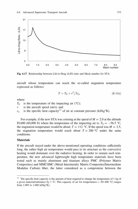
aircraft whose temperature can reach the so-called stagnation temperatureexpressed as follows:

T ¼ T0 þ v2�

2cp ð6:11eÞ

whereT0 is the temperature of the impacting air (�C);v is the aircraft speed (m/s); andcn is the specific heat capacity11 of air at constant pressure (kJ/kg�K).

For example, if the new STA was cruising at the speed of M = 2.0 at the altitudeFL600 (60,000 ft) where the temperature of the impacting air is: T0 = -56.5 �C,the stagnation temperature would be about: T = 112 �C. If the speed was M = 2.5,the stagnation temperature would reach about T = 200 �C under the sameconditions.

Materials

If the aircraft stayed under the above-mentioned operating conditions sufficientlylong, the rather high air temperature would pass to its structure as the convectiveheating would dominate over the radiative heating. In order to sustain such tem-perature, the new advanced lightweight high temperature materials have beentested such as mainly aluminum and titanium alloys PMC (Polymer MatrixComposites) and MMC/IMC (Metal Intermetalic Matrix Composites/IntermediateModulus Carbon) fiber, the latter considered as a compromise between the

5

9

13

17

21

0.5 1.5 2.5 3.5 4.5 5.5 6.5 7.5 8.5 9.5

Lift-

to-D

rag

Rat

io -

(L/

D)

Mach number

Fig. 6.17 Relationship between Lift-to-Drag (L/D) ratio and Mach number for STA

11 The specific heat capacity is the amount of heat required to change the temperature of 1 kg ofa given material/substance by 1 �C. This capacity of air for temperatures (-50–400 �C) rangesfrom 1.005 to 1.068 kJ/kg�K).


required air-thermodynamic performances and costs. In addition, toughenedEpoxy resins and thermoplastic materials have also been considered. In parallel,both the EC and NASA in the US have studied different lightweight advancedmaterials such as sandwich, honeycomb, and superelastic formed/diffusion bondedconcepts (EC 2006, 2008; NAS 2001; Saounatsos 1998).

Range

The most important aerodynamic and operational characteristics of the new STA isits range. In general, this range can be expressed as follows (Breguet rangeequation):

R ¼ HðL=DÞg

� g � ln1

1�WF=W

� �

¼ v � ðL=DÞg � SFC

ln1

1�WF=W

� �

ð6:11fÞ

whereH is the fuel energy content (MJ/kg);g is the overall installed engine efficiency;SFC is Specific Fuel Consumption (kg/kN/h);g is the gravitational acceleration (9.81 m/s2);W is the aircraft take-off weight (tons); andWF is the available trip fuel (tons).

The other symbols are analogous to those in the previous equations. Eq. 6.11findicates that the range R increases linearly with increasing of the energy contentH of the fuel and the overall installed engine efficiency g. By changing the fuelfrom kerosene to LH2 (Liquid Hydrogen), this content and consequently the rangeR can be increased by the factor 2.745 (Chap. 4). For a given type of fuel, therange R of the advanced STA could be increased, on the one hand by increasingthe cruising speed v, improving (L/D), and the amount of fuel carried WF, and onthe other by decreasing the engine SFC. However, at the same time, the SFCincreases with cruising speed and decreases with increasing of the overall enginepropulsion efficiency g as follows:

SFC ¼ M=4g ð6:11gÞ

Figure 6.18 shows some relationships.Specifying the values of particular variables in the above-mentioned expres-

sions, while particularly intending to increase (L/D) as a vital issue for enablingeconomically viable STA, enables setting up some initial specifications for theSTA design similarly to those in Table 6.18.

Propulsion systems

The propulsion systems-engines of the new STA should be designed to fulfill thefollowing requirements (EC 2008):

• Sufficient thrust to enable operating at the designed supersonic cruising speed(s),


http://dx.doi.org/10.1007/978-1-4471-6287-2_4

http://dx.doi.org/10.1007/978-1-4471-6287-2_4

• Relatively high propulsion efficiency implying lower fuel consumption andrelated emissions of GHG, particularly NOx (Nitrogen Oxides), as compared tothat of supersonic predecessors Concorde and TY144, as well as advancedsubsonic aircraft (Chap. 2).

• Lightweight reliable construction materials resistant to high temperatures, and• Meeting the noise requirements of Stage-3/4 during LTO cycle (Landing and

Take-off Cycle) (ICAO 2001).

Thrust

The total thrust, i.e., power, of engines (T) for the new STA should generally besufficient to balance the aerodynamic drag (D) during cruising phase of flight, i.e.,T = D (at the same time the lift force (L) should be in balance with aircraft weight(W), i.e., L = W). Thus, based on Eq. 6.11b, the thrust per engine can be estimatedas follows:

T ¼ 1N

D � M=að Þ½ � ð6:11hÞ

whereN is the number of aircraft engines, anda is the speed of sound at the cruising altitude (m/s).

The other symbols are analogous to those in the previous equations. In com-bination with Eqs. 6.11b, h for aerodynamic drag (D) implies that the requiredthrust for the new STA increases with the third degree of cruising speed.

Propulsion efficiency

The propulsion efficiency of engines powering the advanced STA generallydepends on its cruising speed as follows (empirical relationship):

0

0.5

1

1.5

2

2.5

3

0 0.5 1 1.5 2 2.5 3 3.5 4 4.5 5

SF

C -

Spe

cific

Fue

l Con

sum

ptio

n

Cruising speed - Mach number

η = 0.4

η = 0.6

Fig. 6.18 Relationship between SFC (Specific Fuel Consumption) and the aircraft cruisingspeed, and the engine overall propulsion efficiency


http://dx.doi.org/10.1007/978-1-4471-6287-2_2

http://dx.doi.org/10.1007/978-1-4471-6287-2_2

g ¼ M= M þ 3ð Þ ð6:11iÞ

Figure 6.19 shows an example of this relationship indicating that the overallpropulsion efficiency increases at decreasing rate with increasing of the Machnumber.

This again indicates an inherent conflict with the above-mentioned aerody-namic design of new STA characterized by the substantial drop of the (L/D) ratioas the cruising speed increases.

Materials

In order to reduce the weight and improve performances of new STA, the materialsthe aircraft engines are made out of must at the same time provide low density,high strength, and long life at high temperatures. In particular, high temperaturesrefer to combustion temperatures that which would likely increase to about3,000–3,500 �F (1,650–1,930 �C) and/or nozzle temperatures to about2,300–2,400 �F (1,260–1,370 �C). Critical engine components such as disks, tur-bine airfoils, and nozzles would be exposed to these temperatures for a relativelylong time, i.e., during the cruising phase of flight, which could last 4–5 h (EC2008; NAS 2001). This is quite different compared to subsonic engines exposed toextreme temperatures for a shorter time-only during the take-off and climb lastingabout 15–20 min. In addition, more extensive use of such actually advancedmaterials could contribute to reducing the overall aircraft weight, and conse-quently improve the fuel consumption and related emissions of GHG, and noiseefficiency.

Ceramic Matrix Composites (CMCs) could be a promising solution to simul-taneously reduce the engine weight and increase the above-mentioned engineaerothermodynamics performances. The materials considered have been polymers,

0

0.1

0.2

0.3

0.4

0.5

0.6

0.7

0.8

0.9

1

0.5 1.5 2.5 3.5 4.5 5.5 6.5 7.5 8.5 9.5

η -

Eng

ine

over

all p

ropu

lsio

n ef

ficie

ncy

Mach number

Fig. 6.19 Relationship between propulsion efficiency and Mach number for advanced STA


intermetalics, metal matrix, and ceramics matrix composites. In addition, newfibers and fiber coatings have also been tested as materials to eventually withstandthe high operational temperatures and long operational times of particular enginecomponents. One additional material considered for fabricating the critical enginenozzles has been titanium aluminized and other PETI/5 (Phenylethynul/Termi-nated Imide), the latter particularly considered for high temperatures compositematrices (EC 2008; NAS 2001).

The particular issue would be creating materials for maintaining a safe fueltemperature in the fuel tanks during flying at supersonic speeds. Some preliminaryinvestigations have shown that this could be achieved by advanced coatings withthe desired emissivity, absorptivity, and corrosion ability to maintain the fueltemperatures below the acceptable levels (about 150 �F) reached at the speeds ofabout Mach 2.4 (NAS 2001).

Aircraft systems

Advanced STA would be long and slender lightweight high-temperature durabilityconstructions preventing water absorption during the aircraft life cycle. As such,their construction would be able to fulfill the required aerodynamic performances.This particularly refers to a long pointed nose for drag reduction and delta wingsfor flight at high supersonic speeds on the one hand and high attack angles at lowerspeeds on the other. Such design at low speeds actually compromises the forwardvisibility of the crew from the cockpit. Consequently, this would require either adrop-nose design (similarly to Concorde) or advanced sensors and cockpit displaysfor restoring the required crew visibility. The latter alternative being underdevelopment in the scope of the US NexGen and European SESAR program couldbe promising (Chap. 2). Nevertheless, in order to relieve the crew from only acomputer-generated view of the outside environment, the cockpit windows couldbe located at the lower instead of the traditional upper front location of the aircraftfuselage. This would enable visual contact to the outside during the aircraftapproach, landing, and take-off. In other phases, computer displays would be usedfor controlling and managing the aircraft flight. In addition, a sonic boom shadowtracking system would be added as unique to new STA. Using standard, predicted,or real-time atmospheric conditions, this system would be able to depict location,coverage, predicted path, and strength of the STA sonic boom.


The operational performances of new STA include their payload-range charac-teristics, service quality, and technical productivity, which all should be at leastcomparable to those of the predecessors Concorde and the TY144 and some of thesubsonic counterparts.


http://dx.doi.org/10.1007/978-1-4471-6287-2_2

http://dx.doi.org/10.1007/978-1-4471-6287-2_2

Payload-range characteristics

Possible payload-range characteristics of particular supersonic aircraft and theB747-400 subsonic aircraft are given in Fig. 6.20.

The payload-range characteristics of the Mach 5.0 STA are superior to those ofboth Concorde and the TY144 aircraft. This could be considered as some kind ofincreased capability to penetrate the market, which both predecessors were unableto achieve, and thus provide the necessary economic viability. At the same time,new STA have a longer range than the subsonic B747-400 aircraft has for abouthalf of its payload.

Quality of service

The main attribute of the quality of service offered by STA is travel time. Subsoniccommercial flights usually take place along the shortest—Great Circle routesconnecting particular origins and destinations. However, due to passing throughthe sound barrier, the routes of the new STA are expected to very often deviatefrom the shortest great circle distances in order to avoid the impacts of sonic boomon populated areas. In terms of design, this will require extension of the range. Inan operational sense, this would extend the travel (flight) time thus partiallymitigating the effects of the supersonic speeds as compared to those of its subsoniccounterparts. Figure 6.21 shows the relationship between the flight time and routelength when flown by subsonic aircraft and advanced STA.

As can be seen, the time differences, which can be deemed as savings for bothairlines and users/passengers, appear to be substantial and almost proportional tothe differences in the cruising speeds of both categories of aircraft/flights. In thecase of airlines, this contributes to decreasing the size of the required fleet foroperating a given route network and schedule. In the case of users/passengers, this

0

10

20

30

40

50

60

70

80

90

0 3000 6000 9000 12000 15000 18000

Payl

oad

- ton

s

Range - km

ConcordeTY144DB747-400A380-800Advanced STA

Fig. 6.20 Payload-range characteristics of selected supersonic and subsonic aircraft (differentwebsites)


contributes to decreasing their generalized travel costs shown to be particularlyrelevant for business passengers.


The technical productivity of new STA during the cruising phase of flight can beestimated as follows:

TP ¼ v � PL ¼ M � a � PL ð6:12Þ

wherev is the aircraft speed (km/h);a is the speed of sound (km/h); andPL is the payload (tons).

Based on Eq. 6.12, the technical productivity for an advanced STA cruising atFL600 with the payload PL = 30 tons (300 passengers each weighting togetherwith their baggage about 100 kg) at the speed of M = 5.0, where the speed ofsound is: a = 1,062 km/h, would be: TP = 159,300 t-km/h.


The economic performances of new STA in terms of aircraft operating costs perseat and passenger mile/kilometer need to be comparable to those of their subsoniccounterparts particularly while operating on long distance continental and inter-continental routes for which they are primary planned and designed in order tomaximize savings in the travel time, i.e., to shorten this time from about 7.2–22.5 h

0

5

10

15

20

25

3500 5500 7500 9500 11500 13500 15500 17500

App

roxi

mat

e fli

ght t

ime

-(h

)

Flying distance - (km)

Subsonic aircraftMach 5 aircraft

Fig. 6.21 Relationship between approximate flight time and length of route for subsonic aircraftand STA (Mach 5) (EC 2006)


to about 1.7–3.8 h for a range of routes (6,000–18,000 km). For example, theHydrogen (LH2) M5 Cruiser STA in Table 6.18 has been estimated to cost about639 M€. Its annual operating costs have been estimated to be about 554 M€. Theformer is based on the costs of developing and manufacturing 100 aircraft, while thelatter is based on the average annual utilization—flight frequency of 2 flights/day onthe route of length of about 18,000 km, availability 0.90, load factor 0.75, and thenumber of passengers on the route 148000 (Steelant, 2008). This gives the averageunit operating costs of about 0.1054 €/s-km or 0.208€/p-km, which appears to bequite comparable to the costs of their subsonic counterparts under equivalentconditions. If LH2 was derived from electrolysis of water, the share of the fuel costsin the total STA operating cost would be about 83 %. If LH2 was derived from thesteam reforming of hydrocarbons, the share of fuel costs would be about 30 %,which in turn reduces the total STA operating costs by about 50 %. In this lattercase, the average unit operating cost would be 0.139 €/s-km and 0.104 €/p-kmunder the above-mentioned traffic scenario, which is again competitive to thesubsonic counterparts of STA. If the passenger generalized costs were consideredfor long distance travel, taking into account the savings in the costs of travel timefor all categories of passengers (business, leisure) would indicate an additionaladvantage of new STA over their conventional subsonic counterparts under thegiven conditions. Similar analysis has been carried out for the new STA—KeroseneMach 4.5/5.0 Cruiser (EC 2006; Steelant 2008).


The environmental performances of the new STA would specifically include theenergy/fuel consumption and emissions of GHG (Green House Gases), and landuse/take.

Fuel consumption

Fuel consumption is crucial to the economic and environmental success of newSTA. In terms of efficiency, it is usually expressed as SFC (Specific Fuel Con-sumption), which is closely related to the engine BP (Bypass Ratio). The latter isdefined as the rate between the amount of air flowing around the engine core andthe amount of air passing through the engine. In general, jet engines with a higherbypass ratio usually have lower SFC. Figure 6.22 shows the SFC-BR relationshipsfor the cruise and take-off phase of flight for 20 jet engines powering subsoniccommercial aircraft produced by different airspace manufacturers. These are: CFMCompany (joint corporation of Snecma (France) and General Electric Company(USA)), Rolls-Royce (UK), Pratt and Whitney and General Electric (USA), andIAE (International Aero Engines AG made up of the engine manufacturers Prattand Whitney, Rolls-Royce, MTU (Europe) and Aero Engine Corporation (Japan)).In addition, the SFC-BR relationships for the engines that powered supersonicConcorde and the TY144 are shown for comparison purposes (Janic 2007a).


As can be seen, the SFC of most turbofan engines powering subsonic com-mercial aircraft during take-off varies between 0.25 and 0.40 and during cruisingbetween 0.15 and 0.30 for the given range of BRs, 1–8. For the engines thatpowered the two retired above-mentioned supersonic aircraft, the SFC was greaterthan 0.5 for BRs ranging from 0 to 0.53. These relationships indicate that in orderto make the new STA economically and environmentally viable, its engines wouldneed to have a lower SFC (preferably 0.423 as specified in Table 6.18). This wouldbe a challenge since advanced STA is expected to operate under different engineoperating regimes and speeds (i.e., take-off, subsonic cruise, supersonic cruise,approach, and landing). In general, this implies operating at the subsonic regimerequiring a high propulsive efficiency and the supersonic regime requiring a highspecific thrust. In the former case the engine frontal area should be as wide aspossible in order to provide a high propulsive efficiency at subsonic speeds, whilein the latter it should be as small as possible in order to reduce drag at highsupersonic speeds. One of the options using kerosene could be a variable cycleengine, which is similar to a subsonic mixed-flow turbofan engine, but with anadditional secondary outer bypass duct aimed at increasing the overall bypass ratioand consequently the air flow handling capacity. As opposed to conventionalturbofan engines, a variable cycle engine could change and adapt the bypass ratioto the particular above-mentioned flight conditions. For example, increasing BRduring {XE ‘‘TO (Take-Off)’’} take-off and landing decreases noise around air-ports, while reducing BR during cruise improves the fuel efficiency. Furthermore,for example, increasing BR from 0.5 to 1.0 or even higher for variable cycleengines would require application of more advanced cooling concepts for theturbine blades in combination with the use of lightweight heat resisting materials.

0

0.1

0.2

0.3

0.4

0.5

0.6

0.7

0 1 2 3 4 5 6 7 8 9

SF

C -

kg/

hr/k

g

BR - Bypass Ratio

Cruise - SubsonicTake-off - Subsonic Cruise - Supersonic Concorde, TY144

Fig. 6.22 Relationship between SFC (Specific Fuel Consumption) and BR (Bypass Ratio) fordifferent commercial aircraft (Janic 2007b)


Last but not least, at present, the other alternative engine designs perceived astechnologically, economically, and environmentally feasible include PDE (PulseDetonated Engine), hydrogen-fueled engines, and the fuel-cell based engines(propulsive system).

PDEs are based on detonation waves aimed to initiate rapid combustion of apremixed fuel–oxidizer mixture contained in an array of tubes, which are openedat one end and closed on the other. These engines are expected to be even moreefficient than the current turbofan engines, while enabling high (supersonic)speeds. Consequently, the US NASA has maintained PDE research efforts with thebaseline being a Mach 5 STA (a PDE test was successfully carried out in 2008).

LH2 (Liquid Hydrogen)-fuelled engines would seemingly be relatively easier todesign if carried out by modifying existing turbofan engines (Chap. 4).

Fuel-cell based engines (propulsive systems) would be powered by electricityproduced by fuel cells. The power density in terms of both weight and volume hasalready shown to be the critical in designing these systems for new STA (NAS2001).

Emissions of GHG

The energy consumption of STA has already been discussed. The emissions ofGHG (Green House Gases) would depend on the engines’ injection and com-bustion performances, i.e., on the quality of air/fuel mixture, its distribution in thecombustor primary zone, and the corresponding temperatures. In addition to otherGHG with constant emission rates per unit of fuel burnt (CO2, H2O, etc.) (Chap. 5),the primary concern would be emissions of NOx (Nitrogen Oxides) independentlyof the fuel used—kerosene or LH2 (Liquid Hydrogen). This is because advancedSTA would cruise at altitudes with the maximum concentration/density of O3

(Ozone)-from 14 (FL450) to 26 km (FL850) as shown in Fig. 6.23.O3 protects the Earth from harmful solar UV radiation by absorbing all light with

a wavelength less than 295 nm* (nanometer). However, O3 is sensitive to freeradicals such as atomic chlorine CI, Nitric Oxide NO, and hydroxyl radicals OH.They are formed from the water vapor (H2O) and chlorofluorocarbons (CFCs),products of the fuel burned by the new STA, directly affecting the ozone layerformed in the stratosphere. Near the ground, emissions of NOx and other hydro-carbons contribute to increasing the concentrations of O3, which is considered as apollutant harmful to inhale and a contributor to the formation of smog (Janic 2007b).

Thus, in contrast to its regional impact near airports, the NOx injected into thestratosphere affects the ozone layer globally. In any case, the increased concen-tration of NOx and other GHG might generally cause depletion of the ozone layerwith inevitable impacts. For example, a 10 % depletion of this layer could result inan increase in UV radiation by about 45 %, which certainly could damage almostall biological cells and in particular cause skin cancer in the exposed population.

Currently, in the case of the existing subsonic turbofan engines operating atgiven fuel combustion temperatures, the highest rate of formation of NOx appearsto be when the fuel/air equivalence rate is equal to one (i.e., to the stoichiometricair-to-fuel ratio). Furthermore, in the absolute sense, EINOx (Emission Index of


http://dx.doi.org/10.1007/978-1-4471-6287-2_4

http://dx.doi.org/10.1007/978-1-4471-6287-2_4

http://dx.doi.org/10.1007/978-1-4471-6287-2_5

http://dx.doi.org/10.1007/978-1-4471-6287-2_5

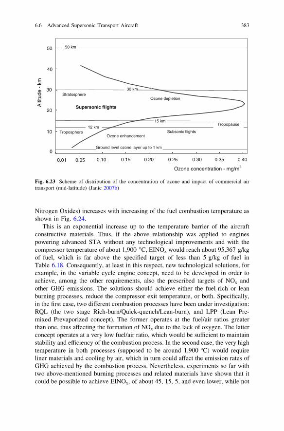
Nitrogen Oxides) increases with increasing of the fuel combustion temperature asshown in Fig. 6.24.

This is an exponential increase up to the temperature barrier of the aircraftconstructive materials. Thus, if the above relationship was applied to enginespowering advanced STA without any technological improvements and with thecompressor temperature of about 1,900 �C, EINOx would reach about 95,367 g/kgof fuel, which is far above the specified target of less than 5 g/kg of fuel inTable 6.18. Consequently, at least in this respect, new technological solutions, forexample, in the variable cycle engine concept, need to be developed in order toachieve, among the other requirements, also the prescribed targets of NOx andother GHG emissions. The solutions should achieve either the fuel-rich or leanburning processes, reduce the compressor exit temperature, or both. Specifically,in the first case, two different combustion processes have been under investigation:RQL (the two stage Rich-burn/Quick-quench/Lean-burn), and LPP (Lean Pre-mixed Prevaporized concept). The former operates at the fuel/air ratios greaterthan one, thus affecting the formation of NOx due to the lack of oxygen. The latterconcept operates at a very low fuel/air ratio, which would be sufficient to maintainstability and efficiency of the combustion process. In the second case, the very hightemperature in both processes (supposed to be around 1,900 �C) would requireliner materials and cooling by air, which in turn could affect the emission rates ofGHG achieved by the combustion process. Nevertheless, experiments so far withtwo above-mentioned burning processes and related materials have shown that itcould be possible to achieve EINOx, of about 45, 15, 5, and even lower, while not

Ozone concentration - mg/m 3

0

0.01 0.05 0.10 0.15 0.20 0.25 0.30 0.35 0.40

Tropopause

10

20

30

40

50

Alti

tude

- k

m

Ozone enhancementSubsonic flights

Stratosphere

Troposphere

15 km

12 km

30 km

50 km

Supersonic flights

Ground level ozone layer up to 1 km

Ozone depletion

Fig. 6.23 Scheme of distribution of the concentration of ozone and impact of commercial airtransport (mid-latitude) (Janic 2007b)


critically compromising the other required performances of the advanced STApropulsion system (engines) (Coen 2011; Saounatsos 1998).

Nevertheless, new STA is expected to contribute to global warming occurringas a result of radiative forcing, i.e., changes in the global balance between theincoming solar radiation and the outgoing infrared radiation. Some estimates haveindicated that presence of advanced STA in the commercial aircraft fleet couldincrease the radiative forcing by commercial aviation by about 42 % in 2050, i.e.,from about 0.2 without to about 0.284 W/m2 with advanced STA (IPCC 1999).

Land use

As mentioned above, advanced STA should be designed to smoothly operatewithin the existing airport clearances. This implies that the aircraft will be pro-vided with the maneuvering and parking space without the need for using addi-tional land.


The social performances of STA relate to noise, congestion, and traffic incidentsand accidents, i.e., safety.

Noise

The main attributes of the noise performances of new STA remain to be the airportlanding, sideline, and take-off noise, and sonic boom while operating at supersonicspeeds.

EINOx = 0.097e0.0085TR² = 0.9562

0

100

200

300

400

500

600

700

0 200 400 600 800 1000 1200

EIN

Ox-g

/kg

of fu

el

Compressor exit temperature - 0K

Fig. 6.24 Relationship between EINOx (Emission Index of NOx) and the compressor exittemperature for subsonic turbofan engines (Coen 2011)


Landing, sideline, and take-off noise

In order to obtain high specific thrust at supersonic speeds, STA engines wouldneed to have a rather high jet exhaust speed at subsonic cruising speeds. In general,this speed could range from about 300–900 m/s (Concorde), but has already beenestablished at around 400 m/s with the average temperature of 600–800 �K. Thiscould also guarantee an acceptable noise level during the aircraft landing, take-off,and sideline, i.e., within the ICAO Chap. 3 Noise Regulation for airports (ICAO2001; Smith 1989).

Sonic boom

Another aspect of the noise of new STA is sonic boom. Sonic boom can be definedas an acoustic phenomenon associated with supersonic flight. A STA flying atsupersonic speeds creates an acoustic wave, which propagates through the atmo-sphere and either strikes the ground or dissipates in the upper atmosphere. Theobservers (people) on the ground usually hear a sonic boom as a sharp double report(Hayes 1971). The signal of sonic boom is usually very short lasting typically from200 to 300 ms. In addition, it is characterized by the sharp head and tail shock,which are actually caused by the sudden jumps in the air pressure of typically1–3 psi (psi—pounds/in2) or 60–120 Pa (Pa—Pascale). The loudness of sonic boomcould reach 136–140 dBA. A typical impact of such loudness is its psychoacousticeffect on people and animals while covering a ground area of about 30–40 km onboth sides of the aircraft track projected on the ground (NAS 2001). For example,Concorde generated an overpressure of 93 Pa, which consequently restricted itssupersonic flying to over water areas and thus substantively diminished its eco-nomic feasibility. Some research indicates that advanced STA could achieve anoverpressure of 85 Pa, but again they would need to be restricted from flying overpopulated areas, which would extend the routes and related flying times and fur-thermore result in additional fuel consumption and related emissions of GHG (EC2006). Therefore, in the given context, the principal task for designers of advancedSTA is to make the sonic boom acceptable for the affected population on theground. This would imply including the sonic boom aspect as one of the criteria foraircraft design, which was not the case at both Concorde and TY144 aircraft.

The sonic boom can generally decrease by decreasing the aircraft weight andincreasing: (i) L/D (Lift–to–Drag) ratio, (ii) length, and (iii) innovative propulsionintegration (NAS 2001). The aircraft weight could be decreased, in addition toselecting a lightweight construction based on lighter materials, by reducing theamount of required trip fuel, which could be achieved by reducing the engine SFC(Specific Fuel Consumption) without compromising the range. The oblique/wingin combination to the relatively long fuselage and innovative integration of thepropulsion systems (engines) have shown promising in providing both satisfactoryaerodynamic (L/D) performances and acceptable sonic boom, particularly forMach numbers of 1.4–2.0 (Kroo 2005; NAS 2001). Thus, because the requiredoperational and economic performances need to be simultaneously fulfilled inorder to make the advanced STA commercially and environmentally/socially


http://dx.doi.org/10.1007/978-1-4471-6287-2_3

http://dx.doi.org/10.1007/978-1-4471-6287-2_3

viable, their design will very likely remain to be highly influenced by the sonicboom reduction requirements. Use of LH2 as a fuel instead of the conventional jetfuel-kerosene could additionally require compromise in its design (Chap. 4).

Congestion

Advanced STAs would operate within the approaching and departing traffic flowsat airports exposed to congestion and delays similarly as other subsonic aircraft. Insome cases, they could be given the ultimate priority in service but the relatedATC (Air Traffic Control) criteria, if any, still need to be elaborated. The length ofthe advanced STA (Table 6.18) could affect smooth traffic at the airport apron/gatecomplex, but this would be resolved by parking and maneuvering on of dedicatedparking positions.

Safety

In addition to the absence of traffic incidents and accidents due to the already knowreasons, the safety of advanced STA would also imply protecting the flight crewand passengers from high-altitude radiation and cabin decompression.

High-altitude radiation refers to primary and secondary cosmic radiation. TheEarth is protected from this radiation by the atmospheric shield which is over1,000 g/cm3 thick at sea level, 200–300 g/cm3 thick at typical cruising altitudes ofsubsonic aircraft (FL 300–400), and only 60 g/cm3 thick at the cruising altitudes ofnew STA (FL600–650). This implies that advanced STA would preferably havesome kind of the very light shield in addition to more careful selection of 4D (fourdimensional) routes based also on the perceived (expected) cosmic radiation.Furthermore, monitoring the exposure of flight crews and frequent fliers to thisradiation would be introduced as a part of STA flight (safety) regulations.

The crew and passengers of advanced STA would be exposed to a high risk ofloss of life in cases of explosive and rapid cabin decompression or sudden airleakage from the STA fuselage occurring at altitudes above FL500 (50,000 ft).Since current regulations do not allow exposure to pressure at altitudes above FL400 (40,000 ft) for any time (as compared to 2 min of allowable exposure to thepressure at an altitude of FL 250 (25,000 ft)), this requirement would be verydifficult and complex to fulfill for the advanced STA. Nevertheless, the possiblesolutions could be using innovative technologies such as self-sealing materials tocontain fuselage pressure leaks, thus providing sufficient time for an emergencydescent initiated by an automatic emergency descent mode in the scope of theaircraft flight control system (NAS 2001).

6.6.3 Evaluation

Advanced STA possess both advantages (Strengths and Opportunities) and dis-advantages (Weaknesses and Threats) as follows:


http://dx.doi.org/10.1007/978-1-4471-6287-2_4

http://dx.doi.org/10.1007/978-1-4471-6287-2_4

Advantages

• Superiority as compared to their supersonic (retired) predecessors and com-petitive to the future subsonic aircraft in terms of the overall efficiency andeffectiveness from the viewpoint of both airlines and users/passengers;

• Complementing to the subsonic and supersonic aircraft fleet operating within thefuture APT (Air Passenger Transport) system;

• Contributing to the creation of an integrated and very high-speed transportsystem on both the national and particularly the international-global scale;

• Compatibility with the existing airport layout enabling smooth, efficient, andeffective maneuvering, parking, and ground handling;

• Environmentally and socially acceptable in terms of the emissions of GHG andnoise, the former globally and the latter both locally around the airports andglobally (sonic boom); and

• Contributing to development of innovative and new knowledge, processes, andmaterials for both airframe and engines, which could be disseminated to othernon-APT (Air Passenger Transport) fields.

Disadvantages

• Uncertainty in the final design (i.e., the most feasible supersonic speed and size,namely seating capacity) that would guarantee economic feasibility for bothairlines and their users/passengers (similarly as at the ETT system: who wouldreally demand to travel at the offered supersonic speed at the given price andunder what conditions);

• Unknown technical/technological barriers, which would eventually need to beovercome to develop the components—fuselage, propulsion systems, and air-craft control systems;

• Diminishing advantages of flying at supersonic speeds due to the prohibition ofpassing over populated areas (creating sonic boom), which may prolong flyingdistance(s) (not always the shortest—Great Cycle ones) and related traveltime(s); and

• The inherent risk of increasing the overall environmental and social impacts interms of global emissions of GHG and noise (sonic boom), the former due toincreasing emissions of NOx and the latter due to some unavoidable passingover populated areas at supersonic speeds.

Finally, any further elaboration of the overall feasibility of advanced STAshould include the above-mentioned and additional (depending on the actors/stakeholders involved) advantages and disadvantages. Some facts provided in thissection indicate that advanced STA might be, under given conditions, a promisingsupersonic complement to the future APT (Air Passenger Transport) system andother long-haul very high-speed systems such as ETT.


References

ACARE, (2010). Beyond vision 2020 (Towards 2050). The Advisory Council for AeronauticResearch in Europe, Directorate-General for Research Aeronautics and Transport. Brussels,Belgium: European Commission.

Airbus, (2012). Delivering the future: Global market forecast 2012–2030. Blagnac, Cedex,France: AIRBUS S.A.S.

Anderson, J. E. (2000). A review of the state of the art of personal rapid transit. Journal ofAdvanced Transportation, 34(1), 3–29.

Anderson, J. E. (2005). ‘‘The Future of High-Capacity PRT’’, Advanced Automated TransitSystems Conference, November 7–8. Italy: Bologna.

Anderson, J. E. (2007). High-capacity personal rapid transit: Rationale, attributes, status,economics, benefits, and courses of study for engineers and planners. Minnesota, US: PRTInternational LLC.

Antaki, A. G. (2003). Piping and pipeline engineering, design, construction, maintenance,integrity, and repair. Boca Raton, FL: CRC Press.

Boeing, (2002). 747-400 Airplane characteristics for airport planning. Seattle, WA, USA:Boeing Aircraft Company.

Boeing, (2012). Current market outlook 2012–2031. Market Analysis. Seattle, WA, USA: BoeingCommercial Airplanes.

CC, (1999). Automated underground transportation of Cargo: The 5th transportation alternativefor the transport of goods in congested urban areas. Bochum, Germany: Brochure, CargoCapGmbH.

CIA, (2012). The world factbook. Washington D.C., USA: Central Intelligence Agency.Coen, P. (2011). Fundamental aeronautic program: Supersonic projects. 2011 Technical

Conference (p. 34). Cleveland, Ohio, USA: National Aeronautic and Aerospace Administration.EC, (2005). Optimal Procedures and Techniques for the Improvement of Approach and

Landing—OPTIMA. Sixth Framework Program, FP6-2002-Aero 1502880, Deliverable 1.2.Brussels, Belgium: European Commission.

EC, (2006). ATLLAS (Aerodynamic and Thermal Load Interactions with Lightweight AdvancedMaterials for High Speed Flight). European Commissions Sixth Framework Programme,Final Public Report. Brussels, Belgium: Thematic Priority 1.4 Aeronautic and Space.

EC, (2007). CityMobil. European Commission, DG Research, 6th FMP (Framework Programme),Thematic priority 1.6, Sustainable Development, Global Change, and Ecosystems, IntegratedProject, No. 031315, Brussels, Belgium.

EC, (2007a). Gaps Identification Airport, TMA, En Route and TBS—Reduced SeparationMinima—RESET. Brussels, Belgium: Deliverable D4.2, EC 6th Framework Program,European Commission.

EC, (2008). LAPCAT (Long/Term Advanced Propulsion Concepts And Technologies). Brussels,Belgium: European Commissions Sixth Framework Programme, Final Public Report,Thematic Priority 1.4 Aeronautic and Space.

Freville, E. (2008). The RECAT project. Brussels, Belgium: Presentation of the TAAM-basedSimulation Tool to Estimate Re-categorisation Impact on Runway Capacity,EUROCONTROL.

FAA, (2010). Air traffic control,- FAA Order JO 7110.65T. Washington DC, USA: FederalAviation Administration, US Department of Transportation.

FAA, (2011). Change 2, order JO 7110.65T. Washington DC, USA: Federal AviationAdministration, US Department of Transportation.

FAA (2011a). NextGen implementation plan. Washington DC, USA: US Department ofTransport, Federal Aviation Administration.

FAA, (2011b). NextGen for Airports. Washington DC, USA: US Department of Transport,Federal Aviation Administration.


FAA, (2011c). NextGen operator and Airport enablers. Washington DC, USA: US Department ofTransport, Federal Aviation Admininistraion.

GAO, (2009). Aviation and climate change: Aircraft emissions expected to grow, buttechnological and operational improvements and government policies can help controlemissions. Report to Congressional Committees- GAO-09-554. Washington D.C., USA:United States Government Accountability Office.

Helmke, H. (Hartmut), Hann, R., Muller, D., Witkowski S., (2009). Time based arrivalmanagement for dual threshold operations and continuous descent approaches. 8th USA/Europe Air Traffic Management Research and Development Seminar (ATM2009), Napa,California, USA.

IBRD, (2012). Air travel and energy efficiency. Transport Papers TP-38, The International Bankfor Reconstruction and Development/The World Bank, Washington D.C., USA.

ICAO, (2001). Aircraft engine noise—Environmental protection, Annex 16, Chapters 3 and 4.Montreal, Canada: International Civil Aviation Organization.

ICAO, (2007). Procedures for air navigation services: Air Traffic Management. Doc. 4444/ATM501, Fifteen Edition. Montreal, Canada: International Civil Aviation Organization.

ICAO, (2008). Wake Turbulence Aspects of Airbus A380-8/000 Aircraft. TEC/OPS/SEP-08-0294.SLG. Neuilly sur Siene, Cedex, France: International Civil Aviation Organization.

IPCC, (1999). Aviation and the global atmosphere. Intergovernmental panel on climate change.Cambridge, UK: Cambridge University Press.

IWW, INFRAS, (2004). External cost of transport: Update study. Summary. Karlsruhe, Zurich,Germany, Switzerland: Universitaet Karlsruhe, INFRAS Zurich.

Janic, M. (2006). A model of ultimate capacity of dual-dependent parallel runways. Transpor-tation Research Record, 1951, 76–85.

Janic, M. (2007a). A steeper approach procedure for increasing the ultimate capacity of closelyspaced parallel runways. Transportation Research Record, 2007, 81–90.

Janic, M. (2007b). The sustainability of air transportation: Quantitative analysis and assessment.UK: Ashgate Publishing Company.

Janic, M. (2008). Towards time-based separation rules for landing aircraft. TransportationResearch Record, 2052, 79–89.

Janic, M. (2009). A concept for prioritizing the aircraft operations at congested airports.Transportation Research Record, 2106, 100–108.

Janic, M. (2012). Modeling Effects of Different Air Traffic Control Operational Procedures,Separation Rules, and Service Disciplines on Runway Landing Capacity. to appear in Journalof Advanced Transportation 24 Aug 2012. DOI: 10.1002/atr.1208

Kelly, R. J., La Berge, F. E. C. (1990). MLS: A total system approach. IEEE AES Magazine(May), p. 10.

Kersting, M., Draganinska, S. (2005). CargoCap: Economic freight transportation in congestedareas. Proceedings of the 4th International Symposium on Underground Freight Transport byCapsule Pipelines and Other Tube/Tunnel Technologies, Shanghai, China.

Kroo, I., (2005). Unconventional configurations for efficient supersonic flight. VKI Lecture Serieson Innovative Configurations and Advanced Concepts for Future Civil Aircraft. StanfordUniversity, USA, p. 25.

LHR, (2010). LHR FEU Annual Report 2010. London, UK: Heathrow Airport.Liu, H. (2004). Feasibility of underground pneumatic freight transport in New York. Final

Report, prepared for The New York State Energy Research and Development Authority(NYSERDA). Columbia, Missouri, USA: Freight Pipeline Company.

Morrison, A. S., & Winston, C. (2007). Another look at airport congestion pricing. The AmericanEconomic Review, 97(5), 1970–1977.

NAS, (2001). Commercial supersonic technology: The way ahead. Washington D.C., USA:National Academy of Science, National Academy Press.

NASA, (1999). Benefit estimates of terminal area productivity program technologies. NASA/CR—1999 208989. Virginia, USA: National Aeronautics and Space Administration.

References 389

http://dx.doi.org/10.1002/atr.1208

Rijsenbrij, J. C., Pielage, B. A., & Visser, J. G. (2006). State of the art on automated(Underground) freight transport systems for the EU TREND project. Delft, The Netherlands:Delft University of Technology.

Rodrigue, J.-P., Comtois, C., & Slack, B. (2006). The geography of transport systems. New York,USA: Routledge.

Rossow, V. J. (2003). Use of individual flight corridors to avoid vortex wakes. Journal ofAircraft, 40(2), 225–231.

RUF, (2008). RUF international: Investment case. Frederiksberg C, Denmark: RUF International.Salter, R.M. (1972). The very high speed transit system. The rand corporation (p. 4874). Santa

Monica, California, USA, p. 18.Saounatsos, G. (1998). Supersonic transport aircraft (SST): Technology readiness and develop-

ment risk. ASCE Journal of Aerospace Engineering 1998, 1–16.Seebass, R. (1998). Supersonic aerodynamics: Lift and drag. Paper presented at the RTO AVT

Course on ‘‘Fluid Dynamics Research on Supersonic Aircraft’’ (p. 6). Rhode-Saint-Gendse,Belgium.

Sirohiwala Y. A., Tandon A., Vysetty R. (2007). Feasibility and economic aspects of vactrains.An Interactive Qualifying Project. Worcester, Massachusetts, USA: The Faculty of theWorcester Polytechnic Institute.

Smith, M. J. T., (1989). Aircraft noise. Cambridge Aerospace Series. Cambridge, UK: CambridgeUniversity Press.

Steelant, J. (2008). LAPCAT: High speed propulsion technology, in Advances on PropulsionTechnology for High-Speed Aircraft. Educational notes RTO-EN-AVT-150, Paper 12.Neuilly-sur-Siene, France, pp. 12-1-12-38.

TC, (2004). Approval of steep approach landing capability of transport category aircraft.Toronto, Canada: Aircraft Certification, Civil Aviation, Transport Canada.

Thompson, S. D. (2002). Terminal area separation standards: Historical development andprocess for change. Lexington, Massachusetts, USA: Lincoln Laboratory, MassachusettsInstitute of Technology.

Tosic, V., & Horonjeff, R. (1976). Effects of multiple path approach procedures on runwaylanding capacity. Transportation Research, 10(5), 319–329.

Zhang, Y., Oster, D., Kumada, M., Yu, J., & Li, S. (2011). Key vacuum technology issues to besolved in evacuated tube transportation. Journal of Modern Transportation, 19(2), 110–113.

Visser, J. G. S. N. (2010). Underground freight transport: What is the role of the public sector iondeveloping a new transport mode. Netherlands Institute for Transport Policy Analysis (KiM).Den Hague, The Netherlands: Ministry of Transportation, Public Works and WaterManagement.

Winkelmans, W., Notteboom, T. (2000). In search of strategic positioning of underground freighttransport in the framework of a coherent transport policy. Proceedings of 2nd InternationalSymposium on Underground Freight Transportation by Capsule Pipelines and Other Tube/Tunnel Systems. 28–29 September 2000, Delft, The Netherlands.


Chapter 7Advanced Transport Systems:Contribution to Sustainability

7.1 Introduction

An important current and prospective medium- to long-term objective of transportsystems worldwide is to continuously improve sustainability. On the one hand, thisimplies handling growing passenger and freight transport demand efficiently,effectively, and safely, and on the other mitigating their direct and indirect impactson the environment and society such as energy consumption and related emissionsof GHG (Greenhouse Gases), local noise, congestion, traffic incidents/accidents,land use/take, and waste on the other. Under such conditions, the main actors/stakeholders involved in dealing with transport system development, operation,and use also need to benefit from the perspective of their specific objectives. Theseinclude manufacturers of transport means/vehicles and supporting facilities andequipment, suppliers of energy/fuel, infrastructure providers and transport opera-tors, users of transport services—passengers and freight shippers/receivers, thelocal population, and associations and policy bodies at different institutional levels(local, regional, national, and international). Consequently, the question of thecontribution of advanced transport systems and their components to the above-mentioned sustainable development of the global transport system can be raised.

7.2 Contribution

Advanced transport systems are generally characterized by advanced infrastruc-ture, transport means/vehicles, energy/fuel used, facilities and equipment, all ofwhich support operations at the operational, tactical, and strategic level, togetherwith the related organization of service networks. These advancements include: (i)design and materials used for building transport infrastructure and manufacturingtransport means/vehicles; (ii) technology, size/capacity, speed, and energy used bytransport means/vehicles; and (iii) different configurations/concepts of transportservice networks aimed at serving the expected passenger and freight transport


391

demand efficiently, effectively, and safely. In order to indicate their contribution tothe sustainability of the transport sector, advanced transport systems have beenscrutinized by analyzing, modeling, and evaluating their infrastructural, technical/technological, operational, economic, environmental, social, and policyperformances.

Most of the considered advanced systems have already been commercializedalthough some are less likely to be commercialized in the medium- to long-termfuture. As far as infrastructural performances are concerned, commercializedadvanced systems can use the same (in some cases partially modified and adapted)infrastructure as their conventional counterparts. In the given context, theseinclude: (i) BRT (Bus Rapid Transit) systems, roadmega trucks, and advancedpassenger cars in the road transport mode; (ii) High-Speed Tilting passenger trains,LIFTs (Long Intermodal Freight Trains), and advanced freight collection/distri-bution network services in the rail and intermodal transport mode; (iii) advancedATC (Air Traffic Control) technologies and operations, advanced conventionallyand LH2 (Liquid Hydrogen)-fuelled subsonic passenger and freight aircraft, andadvanced STA (Supersonic Transport Aircraft) in the air transport mode; and (iv)large advanced container ships in the sea-water transport mode. Others, such as thecommercialized HSR (High-Speed Rail), partially commercialized TRM (Trans-Rapid Maglev), and the non-commercialized UFT (Underground Freight Trans-port), and ETT (Evacuated Tube Transport) systems in the rail, and partiallycommercialized PRT (Personal Rapid Transit) systems in the road transport modewould require completely new dedicated (and very expensive) infrastructure.

The technical/technological performances of the above-mentioned systems arefully developed, while those of the non-commercialized systems require furtherelaboration. The main performances of these systems relate to the transport means/vehicles and facilities and equipment for their control and management. Theformer includes being: (i) made of a greater proportion of lighter (composite)materials; (ii) powered by electric engines (supposedly obtaining energy fromfrom renewable primary sources such as wind, water, and solar energy) andrenewable fuels such as LH2 (Liquid Hydrogen); (iii) having high to large carryingcapacity; and (iv) operating at as high as possible speeds (large advanced containerships, which operate at reduced speed in order to improve both economic andenvironmental performances, the latter in terms of fuel consumption and relatedemissions of GHG, are the exception). The latter includes the rather wide appli-cation of ITS (Intelligent Transport Systems) in direct and indirect supportingoperations. Technical/technological performances are expected to generally con-tribute to improving the operational, economic, environmental, social, and policyperformances of the particular advanced transport systems.

Operational performances, which include the service networks and patterns oftheir operations, are set up as close as possible to the characteristics of user/customer demand. They depend on conventional and/or advanced infrastructuraland technical/technological performances. As such, they directly influence alleconomic and some environmental performances.

392 7 Advanced Transport Systems: Contribution to Sustainability

For example, BRT systems, road mega trucks, large advanced container ships,and freight aircraft, all using existing or slightly modified infrastructure, couldimprove the efficiency and effectiveness of related services. At the same time,however, the latter two can contribute to increasing congestion, particularly whenoperating in congested urban and suburban areas and spatially constrained portsand airports, respectively. Similarly, advanced (mainly electric) passenger carsusing the present roads and streets in combination with modified supportingfacilities and equipment mainly for energy/fuel supply can also contribute tocongestion but not to increasing direct emissions of GHG. On the contrary: PRTand UFT systems, which require completely new dedicated and very expensiveinfrastructure if developed to the network level, can mitigate congestion and bothdirect and indirect emissions of GHG in given urban or suburban area(s). High-speed tilting, HSR, and TRM passenger trains operating on completely newinfrastructure (railway lines) do not contribute to increasing congestion due to thenature of railway operations. In particular, high-speed tilting trains sharinginfrastructure with conventional passenger and freight trains are always given thehighest priority. By taking over medium- to long-distance trips from individualpassenger cars, these trains could indirectly contribute to reducing road congestionand related emissions of GHG.

Advanced freight collecting/distributing networks and LIFTs in Europe oper-ating on current rail/road/inland waterway and rail infrastructure, respectively, cancontribute to improving particularly the economic and environmental perfor-mances of the supply chains served, mainly due to replacing road standard (andprospectively mega) trucks.

Advanced subsonic commercial aircraft and advanced STA remain neutral interms of contributing to congestion as compared to their less advanced counter-parts. They can use existing infrastructure with modified (or new) supportingfacilities and equipment mainly for fuel supply in case of LH2–fuelled models. Therelative fuel consumption and type of fuel used (also LH2) can contribute toimproving the environmental performances in terms of energy/fuel consumptionand related emissions of GHG. Aircraft engine technology in combination withadvanced ATC technologies and operations for increasing airport runway capacitycan contribute to reducing local noise. In addition, they can directly improve thetechnical/technological and operational performances, and indirectly the eco-nomic, environmental, and social performances of a given airport runway sys-tem(s). However, due to operating at supersonic speed, advanced STA create sonicbooms, which, in parallel to the requirement for increased energy/fuel consump-tion and related emissions of GHG, can affect large (also populated) area(s) andconsequently compromise social performances in general.

ETT (Evacuated Tube Transport) systems can apparently contribute toimproving the operational and environmental performances of long-distance(intercontinental) passenger transport. At the same time, economic performancescan be compromised due to the very high costs of completely new infrastructurethat needs to be built and maintained under very specific conditions (underwater).

7.2 Contribution 393

The level of maturing and consequently the dynamics of commercialization ofparticular advanced transport systems can influence their technical/technological,and consequently policy performances. In some cases, the influence is positive,while in others, it is negative. In general, the relevant system must be technically/technologically mature in order to be fully commercialized. However, very often,technical/technological maturity does not imply immediate commercialization.The positive influence of the technical/technological performances on commer-cialization is already present with respect to the fully and/or partially commer-cialized systems such as BRT and PRT systems, high-speed titling passenger trainsand HSR, advanced commercial subsonic passenger and large advanced freightaircraft, advanced freight collection/distribution networks, LIFTs, road megatrucks, and large advanced container ships. The negative influence of these per-formances on commercialization is present in case of currently non-commercial-ized systems such as advanced passenger cars, TRM, UFT, and EET system,advanced ATC technologies and operations for increasing airport runway systemcapacity, and advanced STA.

7.3 Some Controversies

Consequently, many of the above-mentioned advanced transport systems appearcontroversial regarding their contribution to the overall medium- to long-termsustainability of the entire transport sector. This controversy becomes moreobvious after considering their technical productivity, the energy/fuel consumptionand related emissions of GHG, and safety (i.e., traffic incidents and accidents).

7.3.1 Technical Productivity

The evidence so far indicates that the above-mentioned advanced transport sys-tems are characterized by gradually increasing technical productivity partiallythanks to the increasing size/weight/capacity of transport means/vehicles and theirnumber in the fleet to serve growing demand, and primarily thanks to increasingtechnical and operating speed(s).

7.3.1.1 Vehicle Size

The size/capacity/weight of particular transport means/vehicles operated by dif-ferent transport modes has seemingly reached constructive/design limits. But isthat really the case? Where are these limits? Are they contained in the sustain-ability and durability of the vehicle’s structure—design and material? Maybe theylie in constraints in the existing transport infrastructure (roads, railway lines,


inland waterways, airports, and river/sea ports) requiring substantial adjustment inorder to enable efficient, effective, and safe maneuvering of these increasinglylarger transport means/vehicles? Is the limit stricter regulation constraining theabsolute impacts of these vehicles/means and the entire transport sector on theenvironment and society? Or is this the overall shortage of land for expansion ofinfrastructure in combination with an increasing shortage of (and more expensive)currently used energy/fuels? Or perhaps a combination of all the above-mentionedfactors?

What is the general influence of these larger transport means/vehicles on thetransport processes and related effects and impacts?

In general, the increased size/weight/capacity of transport means/vehiclesimplies less frequent services to satisfy a given volume of demand on a givenroute(s), and on the entire network(s). Such less frequent services contribute toincreasing schedule delays of passengers at their origins and the inventory cost offreight shipments at both ends of the given supply chain. In addition, such moresizeable vehicles are designed to operate on medium to long distances, which incombination with the longer loading and unloading (ground handling time) gen-erally require greater fleets to serve the given volumes of passenger and freightdemand during a given period of time. On the other hand, the inherently lowerservice frequencies require a smaller number of these larger vehicles. At the sametime, the investment and operating costs of these vehicles per service are higher,while the unit costs are lower compared to their smaller counterparts thanks toeconomies of scale and density. These larger vehicles also consume more energy/fuel per service, which depending on the type and primary sources of energy/fuelproduction generally create higher total emissions of GHG. However, in relativeterms, these emissions can be lower than those of their smaller counterparts. Thesame applies to the local noise created by these vehicles.

7.3.1.2 Vehicle Speed

The dynamism of raising the technical and operating speed of the commercializedand the non-commercialized advanced transport systems is different. The former isan evolutionary gradual process, while the latter will likely be a revolutionaryprocess. Take for example the case of evolutionary/gradual increase in the speed ofthe urban public passenger transport achieved through operational advancementsin the BRT system. High-speed tilting passenger train(s), HSR (High-Speed Rail)and its modification Super HSR, and TRM are all examples of gradually increasingthe speed by technical/technological modifications. In urban and suburban freighttransport, a gradual increase in the freight/goods delivery speed can be achieved byas yet non-commercialized UFT systems. But, again, how big should such anincrease be combined with the other advantages to justify the generally highinvestment cost in UFT infrastructure? In case of the ETT system and advancedSTA as yet non-commercialized future systems, the increase in speed will likely berevolutionary. At the EET system, this implies an application of TRM technology

7.3 Some Controversies 395

through a vacuum tube enabling a very high (supersonic) operational speed. Incase of STA, this implies development of a new supersonic configuration expectedto be much faster, efficient, effective, safe, and particularly less noisy than theprevious retired models—the Anglo-French Concorde and the Soviet Union’sTU144.

Higher technical and operating speeds generally contribute to shortening thetravel time and related costs for the users/passengers and freight shipments. Inparallel, they enable shorter turnaround times, thus requiring engagement ofsmaller fleets to serve given volumes of demand during a given period of time.This generally diminishes the investment, maintenance, and operational costs ofthe transport means/vehicles. However, higher speeds require higher energy/fuelconsumption, which contributes to increasing the cost per service. Depending onthe type of primary sources for producing the energy/fuel, such increased energy/fuel consumption generates higher emissions of GHG. The noise level generatedby the vehicles passing-by at higher speeds is generally also higher. The questionof the maximum possible technical and operation speed of the above-mentionedsystems also arises. Where are the technical/technological barriers and where arethe commercial constraints? The latter implies who actually needs very high(supersonic) speeds—to what extent are such speeds beneficial and when do theybecome counterproductive? Do savings of the users’ time justify setting up usuallyvery expensive infrastructure, high energy/fuel consumption and related emissionsof GHG, and increase in the local (and global) noise? Large advanced containerships can be considered as a case of such controversy: by reducing operatingspeeds and consequently fuel consumption, these ships can improve their eco-nomic and environmental performances, but only on account of an increased fleetsize and longer delivery time of the freight/goods shipments, which need to beacceptable for both operators and users/customers.

7.3.2 Energy/Fuel Consumption and Emissions of GHG

The environmental performances of particular advanced transport systems areexpected to contribute to sustainability through reducing energy/fuel consumptionand related emissions of GHG (Green House Gases). These performances aregenerally influenced by the vehicle size/weight/capacity, operating speed, the scaleof operations (size of the network and the service frequency), and type of theenergy/fuel used. As mentioned above, the larger size, speed, and scale of oper-ations by using a given fuel require a greater total fuel consumption, which con-sequently generates greater related emissions of GHG, and vice versa. Liquid fuelsas derivatives of nonrenewable primary sources such as crude and LNG (LiquidNatural Gas), electric energy, and LH2 obtained from different nonrenewable andrenewable primary sources are used by these systems. While crude oil and LNG


will seemingly remain the primary source of fuels used by large advanced con-tainer ships and aircraft, road mega trucks, the BRT (Bus Rapid Transit) Systemsystem, and advanced commercial subsonic aircraft. Electric energy obtained fromnonrenewables such as coal, crude oil, LNG, and nuclear, and renewable sourcessuch as water, wind, and solar energy is and will continue to be used by high-speedtilting, HSR, and TRM trains, advanced (electric) passenger cars, and the PRT, andUFT In addition, LH2, which can be obtained from the electrolysis of water,appears to be under consideration as a future fuel for subsonic commercial APTincluding STA. Again, electric energy is needed for producing LH2. Therefore, thequestion arises how to obtain sufficient quantities of electric energy for satisfyinghumanity’s overall (generally growing) needs including those of advanced trans-port systems on the one hand while maintaining the related impacts on the envi-ronment within the prescribed targets, on the other? As well, the he question whichkind of propellant/fuel would be used by the ETT system remains.

Nonrenewable primary sources will be exhausted sooner or later. Water, wind,and solar energy produced using dedicated plants installed on the Earth’s surfacewill remain the most important sources of renewable electric energy. Alternatively,SSP (Space Solar Power) or SBSP (Space-Based Solar Power)1 as a complementto existing sources/plants appear to be the most feasible long-term solution(s).

7.3.3 Safety

Advanced transport systems are expected to be safer, namely freer from trafficincidents and accidents than their conventional counterparts. This implies that,under given conditions, incidents and accidents should not occur due to alreadyknown reasons. In addition to the adequate design and construction of the infra-structure, transport means/vehicles, and supportive facilities and equipment, thiswill be achieved through the increased automation of operations, which will beestablished at the level of an individual vehicle and at the level of a route and/orthe entire network. For example, advanced HS (High Speed) trains and LIFTs,advanced subsonic and supersonic commercial aircraft, and large advanced con-tainer ships and aircraft are guided automatically by autopilots mainly during thecruising phase of their trip. It is only a matter of time when advanced (electric)passenger cars, BRT buses, and mega trucks will start to be guided in a similarway. Analogously, advanced ATC technologies and operations will enable allo-cation of a part of the responsibility for aircraft separation from ATC controllers tothe pilots. PRT and UFT are fully automated driverless systems at both the level of

1 At present, solar energy is routinely used on nearly all spacecraft. On a larger scale, thistechnology combined with already demonstrated wireless power transmission could satisfy nearlyall needs for electricity on Earth. Thus, the SSP system would consist of lower-costenvironmentally friendly launch vehicles, large solar power satellites, and a power transmissionsystem, technologies already known today at least at the conceptual level (NSS 2007).

7.3 Some Controversies 397

an individual vehicle/capsule and the level of the route network. In semi-auto-mated systems, automation helps drivers change their role from the previouslymore intensive controlling and monitoring to the present and future increasingly ifnot exclusively monitoring. In driverless systems, the controlling and monitoringrole is and will be carried out fully automatically by central computer systems.Such developments will certainly bring advantages in terms of improving theefficiency, effectiveness, and inherent safety of these systems. On the other hand,disadvantages may include less employment and increased complexity requiringlonger learning/training time and resulting in higher repair costs in case of tech-nical failure. In addition, safety of operations could be significantly compromisedwhen the drivers again take over a controlling and monitoring role. In light of theabove-mentioned issues, the long-standing principal dilemma about the division oftasks between man and machine and consequently sharing the ultimate responsi-bility remains. In addition, incidents and accidents still remain possible. In suchcases, due to operating at high speed and/or due to large size, the human causalitiesand property damage could be devastating. Therefore, in any case, safety willremain to be of the highest priority in designing and operating both existing andforthcoming advanced transport systems, as well as their conventionalcounterparts.

Reference

NSS. (2007). Space solar power: An investment for today-an energy solution for tomorrow.Washington, D.C.: National Space Society.


About the Author

Dr. Milan Janic is a transport and traffic engineer and planner. At present, he is aSenior Researcher at the Transport and Planning Department of the Faculty ofCivil Engineering and Geosciences of Delft University of Technology (Delft, TheNetherlands) and Research Professor at the Faculty of Traffic and TransportEngineering of the University of Belgrade (Belgrade, Serbia). Previously he was aLeader of the Research Program of the Section Transport and Infrastructure at theOTB Research Institute for the Built Environment of Delft University ofTechnology (Delft, The Netherlands), Senior Researcher at ManchesterMetropolitan University (Manchester, UK) and Loughborough University(Transport Studies Group) (Loughborough, UK), and the Institute of Transport(Ljubljana, Slovenia).

He has been involved in transport-related research and planning projects onboth the national and international scale for almost 30 years. He has also publishedmany scientific and professional transport-related papers, and presented many ofthem at national and international transport conferences. In addition, he haspublished four books: ‘‘Greening Airports: Advanced Technology andOperations’’ (2011), ‘‘Airport Analysis, Planning and Design: Demand, Capacityand Congestion’’ (2009), ‘‘The Sustainability of Air Transportation: AQuantitative Analysis and Assessment’’ (2007), and ‘‘Air Transport SystemAnalysis and Modeling: Capacity, Quality of Services and Economics’’ (2000). Hehas been a member of NECTAR (Network on European Communications andTransport Activity Research), Delft Aviation Centre (Delft University ofTechnology, Delft, and The Netherlands), GARS (German Aviation ResearchSociety, Cologne, Germany), ATRS (Air Transport Research Society), andAirfield and Airspace Capacity and Delay Committee of TRB (TransportationResearch Board) (Washington DC, USA).

M. Janic, Advanced Transport Systems,DOI: 10.1007/978-1-4471-6287-2, � Springer-Verlag London 2014

399

Index

AAccelerometers, 48Accessibility, 2, 12, 29, 30, 40, 98, 108, 254,

255, 260, 273, 279, 288, 292, 294, 304,314, 332

Accidents, 2, 36, 38, 59, 61, 75, 77, 101, 102,124, 126, 131, 132, 140, 141, 147, 159,160, 201, 218, 236, 246, 255–258, 261,265, 277, 280, 293, 294, 298, 304–306,317, 319, 324, 337–339, 384, 391,394, 398

ACN (Aircraft Classification Number), 64, 148Admiralty, 191Advanced, 1–4, 6–8, 11, 12, 20, 42, 43, 51, 62,

65, 66, 68, 75, 76, 78, 84–87, 94, 98,100–105, 110, 111, 126, 145, 162,166–168, 170, 171, 173, 174, 177–179,181, 182, 184–191, 193–196, 198–201,203, 204, 206, 207, 209, 210, 213–216,229, 236, 246, 275, 278, 279, 281, 305,324, 346, 350–354, 358, 364, 367,372–379, 381–387, 391–397

Advantages, 8, 40, 41, 61, 78, 110, 125, 144,161, 186, 215, 228, 274, 303, 319, 340,363, 387

Aerodynamics, 65, 77, 246, 371Air, 1, 7, 37, 47, 56, 57, 67, 78, 140, 141, 146,

154, 156, 157, 161, 162, 165, 167, 212,216, 218, 222–226, 228, 229, 238, 246,249, 251, 270, 271, 278, 281, 298, 311,312, 317, 327, 330, 331, 343, 353, 367,372, 373, 380–383, 385, 386

Airbus, 63, 74, 78, 145, 152, 167, 237, 278,367

Aircraft, 3, 6, 8, 11, 62–64, 66–78, 145–147,149, 151, 152, 154, 156, 158–162, 167,217, 218, 220–226, 228, 229, 236, 237,240–243, 256, 264, 271, 278, 331, 339,341, 343, 347–364, 367, 369, 371, 372,375–378, 380, 381, 384–387, 393, 397

Airframe, 62, 72, 73, 149, 150, 161, 242, 371,387

Airline, 63, 72, 146, 155–157, 236, 237, 239,241, 367, 368

Airport, 3, 6, 9, 49, 63, 64, 72, 75, 77, 78, 147,156, 159, 162, 221, 229, 238, 240, 253,255, 263, 269–271, 278, 279, 296, 305,337, 341–343, 347, 349, 351, 353, 358,364, 369, 384, 387, 393, 395

Alternatives, 3, 8, 103–105, 143, 168, 178,224, 254, 258, 259, 266, 267, 269, 272–275

Altitude, 44, 212, 218, 221, 256, 324, 352,372, 386

Analyzing, 4, 8, 14, 43, 63, 86, 87, 112, 127,147, 168, 188, 208, 281, 306, 325, 342,366, 392

Angle, 46–49, 63, 64, 121, 147, 195, 296,346–348, 352–354, 356, 357, 359, 369

Application, 49, 72, 103, 105, 139, 152, 177,222, 224, 226, 266, 268, 274, 278, 305,319, 323, 343, 347, 352–355, 357–359,369, 381

Approach, 4, 7, 8, 12, 20, 21, 63, 75, 76, 105,147, 172, 174, 177, 235, 325, 341, 343,346–348, 350, 352–355, 357–359, 369, 386

Apron, 64, 65, 75, 147, 152, 159, 162, 369,386

APT (Air Passenger Transport), 3, 9, 166, 216,228, 235, 236, 274, 324, 332, 333, 340, 387

APU (Auxiliary Power Unit), 65ATC (Air Traffic Control), 3, 6, 159, 263, 277,

278, 348, 363, 369, 386, 392Attributes, 2–4, 8, 87, 98, 103–105, 204,

254–263, 265, 266, 268, 269, 271–274,305, 323, 334, 358, 371, 384

Automated, 20, 21, 101, 197, 251, 277, 280,285, 295, 304, 306, 307, 309, 319, 331,338, 343, 398

Availability, 7, 29, 30, 178, 288, 303, 314,322, 323, 353, 380

M. Janic, Advanced Transport Systems,DOI: 10.1007/978-1-4471-6287-2, � Springer-Verlag London 2014

401

BBAU (Business As Usual), 208, 339Benefit, 99, 101, 103, 104, 254, 266–269, 391Berth, 189, 213, 287, 288, 296BEV (Battery Electric Vehicle), 168, 170, 173,

185, 186Boeing, 3, 11, 62, 63, 65, 66, 69, 70, 78, 84,

145–147, 149, 152, 154, 167, 217, 223,225, 236, 237, 278, 280, 333, 364, 367

Boom, 195, 367, 377, 378, 384–387, 393BR (Bypass Ratio), 68, 69, 74, 380, 381Break-even, 143–145, 257, 262Breaking, 60, 129, 246, 285, 288, 289, 294,

312, 331BRT (Bus Rapid Transit) system, 3, 6, 8,

11–17, 19–21, 24–30, 32–41, 279, 283,392–395, 397

Bus, 3, 6, 8, 11–16, 20–24, 26, 27, 29–33, 36,38, 40, 42, 151, 255, 279, 292, 298, 332

CCant, 44–47, 51, 57, 62Capacity, 3, 6, 9, 12, 13, 19, 21, 23, 25–28, 37,

40, 50, 53, 54, 56, 58, 60, 62, 77, 84–86,92, 98, 99, 101, 102, 109, 110, 112–114,116, 117, 119, 125, 128, 133, 134, 137,145, 146, 159, 160, 215, 237, 245, 254,256, 257, 262–264, 270, 271, 278–281,285–289, 295, 296, 304, 306, 310,312–315, 324, 330, 334, 336, 341–343,347–350, 352–355, 357–364, 367, 387,391, 392, 394, 395

Capital, 12, 32, 101, 199, 200, 256, 261, 270,290, 291, 336

Capsule, 277, 307, 309–313, 316, 319, 398Car, 14, 17, 21, 30, 35, 36, 46, 47, 56, 58, 84,

168–186, 255, 279, 280, 286, 292, 293,296, 298

Cargo, 145, 151, 152, 156, 158, 159, 166, 187,191, 197, 369

CDB (Central Business District), 15CIFT (Conventional Intermodal Freight

Train), 85, 126–128, 144CMCs (Ceramic Matrix Composite(s)), 376Coefficient, 57, 98, 101, 113, 116, 141, 192,

265, 372Comfort, 2, 19, 29, 30, 40, 42–45, 61, 115,

256, 261, 270, 273, 282, 284, 288, 289,303, 335

Commercial, 165, 166, 195, 217, 219, 220,222, 229, 249, 253, 278, 292, 324, 331,347, 365, 378, 380, 384, 393, 396, 397

Company, 55, 84, 145, 203, 367, 380

Composite, 62, 66, 67, 78, 149, 161, 181, 182,213, 325, 377, 373, 376, 392

Concorde, 237, 278, 324, 364–366, 371, 375,377, 378, 380, 385, 396

Congestion, 2, 7, 12, 36, 38, 40, 41, 59, 60, 75,77, 102, 120, 122, 123, 131, 132, 138, 140,141, 147, 159, 161, 162, 168, 186, 236,246, 254–258, 264, 271, 273, 277, 279,280, 289, 292, 293, 304–306, 317, 319,324, 337, 338, 353, 384, 386, 391, 393

Consumption, 2, 34, 36, 41, 42, 45, 47, 55–59,62, 66, 68, 69, 73, 74, 78, 101, 102, 112,113, 115, 117–119, 130, 131, 137, 138,141, 147, 149, 150, 156, 158, 161,165–167, 169, 170, 172–175, 177,181–184, 186–188, 191, 194, 195,200–203, 209, 210, 220, 223, 246, 251,252, 257, 264, 271, 277, 292–294, 304,306, 317, 324, 339, 368, 380, 394, 396

Container, 3, 6, 9, 83–86, 99, 111, 117, 126,128, 152, 165, 166, 187–190, 192–195,198–203, 205, 206, 210, 209, 212–215,306, 307, 309, 310, 312–314, 318, 319,392–394, 396, 397

Control, 47, 49, 51, 69, 115, 127, 149, 151,152, 171, 203, 213, 220, 223, 250, 251,270, 281, 285, 290, 294, 295, 298, 309,312, 316, 329, 337, 351, 353, 387

Convenience, 41, 63, 168, 270, 273, 280, 292Conventional, 1, 2, 11–14, 21, 25, 29, 34, 36,

38, 40, 42, 43, 45, 49, 51, 53, 54, 59, 60,62, 72, 83, 85, 94, 111, 126–128, 167–172,174, 177–179, 183, 187, 195, 217–221,223, 224, 226, 228, 251, 275, 279, 306,313, 317, 322, 324, 340, 352, 354, 358,367, 380, 381, 386, 392, 393, 397

Corridor, 11–16, 22, 26, 38–40, 42, 84, 85,110, 113, 126–128, 141, 260, 347

Cost, 2, 5, 7, 12, 21, 32, 33, 39, 41, 55, 61, 62,66, 72–74, 78, 83, 87–90, 93, 95, 98–100,102–104, 110, 112, 115–117, 125, 127,130–144, 150, 152, 156, 158, 161, 195,197, 199, 200, 207, 220, 228, 239, 241,254, 260, 263, 266, 269, 270, 278, 290,291, 303, 316, 323, 332, 337, 339, 380,395, 396

Criteria, 2–4, 8, 9, 51, 87, 98, 103–105, 107,195, 223, 254–258, 261, 266–274, 317

Cruise, 62, 69, 115, 249, 369, 372, 380, 381Cruising, 27, 51, 52, 68, 69, 71, 72, 78, 154,

158, 191, 194–197, 200, 202, 203, 206,207, 221, 245, 246, 249, 250, 256, 312,331, 336, 367, 371, 374–376, 379, 385, 386

Cryogenic, 220–228

402 Index

Curve, 43–47, 49, 57, 60, 61, 182, 192, 253,368

Cycle, 78, 88, 89, 91, 93, 94, 99, 100, 113,207, 208, 291, 316, 370, 375, 381, 383

DDelay(s), 40, 255, 261Delivery, 85, 98–101, 108, 109, 115–117, 127,

129, 130, 137, 144, 145, 161, 305, 314Demand, 1, 5, 15, 21–23, 25, 26, 28, 30, 32,

41, 51, 53, 54, 60, 86, 88, 90, 99, 100, 108,113, 127, 129, 133, 137, 142–146, 166,172, 195, 215, 222, 225, 226, 228, 235,236, 256, 281, 286, 295, 303, 306, 313,322, 323, 331–333, 336, 338, 341, 353,387, 395

Design, 2, 8, 11, 26, 27, 43, 45, 51, 56, 57, 62,63, 66, 77, 78, 112, 113, 120, 147, 149,171, 173, 181, 190, 194, 210, 220, 221,278, 289, 293, 295, 315, 317, 325, 334,371, 372, 374, 376–378, 382, 386, 391

Disadvantages, 8, 40–42, 61, 78, 105, 110,125, 144, 145, 161, 185, 186, 214, 215,219, 228, 229, 274, 303, 304, 319, 341,351, 363, 386, 387, 398

Discipline, 278, 351, 352, 354, 355, 358, 359,361, 363

Distance, 1, 3, 9, 11, 15, 29–31, 33, 36, 37, 43,44, 46, 54, 58–61, 71, 73, 83, 85, 90, 98,100, 102, 107–109, 115–123, 126, 128,130, 134, 137, 139, 142–145, 170, 171,199, 201, 210, 241, 249, 253, 262, 271,288, 293, 314, 327, 335, 349, 353, 357,359, 379

DM (Decision Making), 8, 87, 104, 105, 259Drag, 57, 62, 66, 113, 149, 292, 307, 371, 372,

375, 377Draught, 210, 215Dynamic, 16, 57, 112, 249, 282, 287, 296,

343 , 371, 372

EEC (European Commission), 51, 59–61,

84–87, 102, 111, 112, 179, 244, 247, 367EEDI (Energy Efficiency Design Index),

204–208, 215EEOI (Energy Efficiency Operational Indica-

tor), 206, 207, 210Effectiveness, 3, 21, 41, 85, 86, 100, 110, 150,

270, 293, 351, 364, 368, 387, 393, 398Efficiency, 3, 5, 21, 35, 41, 62, 67–70, 78, 85,

86, 100, 109, 110, 114, 115, 117, 126,

143–145, 148–150, 166, 168–170, 172,174, 177, 178, 181, 184, 192, 203–213,215, 223, 228, 235, 249, 265, 280, 311,312, 351, 364, 368, 371, 372, 374, 380,383, 387, 393, 398

EI (Energy Intensity), 241, 242EINOx (Emission Index of Nitrogen Oxides),

383Electric, 13, 19, 37, 48, 55, 58, 129, 131, 151,

152, 168–172, 174, 181, 211, 217, 292,311, 325, 397

Emergency, 125, 126, 294, 325, 386Emissions, 2, 34–36, 39, 41, 42, 56, 58, 59, 62,

74, 78, 102, 114, 117, 119, 130, 131, 138,147, 151, 158, 161, 165–170, 172–174,176, 177, 181, 184–186, 188, 195, 203,204, 208–211, 218, 219, 223, 224, 226,271, 292, 294, 298, 304, 316, 337, 339,368, 371, 372, 380, 382, 385, 387, 393,395, 396

Employment, 2, 23, 40, 317, 324, 398Energy, 1–3, 7, 32, 34, 35, 41, 42, 47, 49,

55–59, 69, 102, 110, 119, 130, 131, 138,141, 165, 166, 168–173, 175, 177, 178,182–184, 187, 188, 191, 201, 203, 205,210, 212, 215, 217, 220, 224, 241, 249,251, 255, 257, 271, 277, 281, 291, 292,294, 298, 305, 310, 311, 316, 323, 324,330, 331, 337, 338, 382, 391, 394, 395, 397

Engine, 168, 190–194, 202, 205, 206, 210,212, 228, 331, 346, 371, 374, 376,380–383, 385, 393

Entropy, 259, 266, 267, 271Environmental, 168, 172, 187, 188, 191, 201,

203, 214, 215, 218, 221, 229, 244, 258,266, 292, 298, 306, 316, 325, 338, 339,364, 365, 368, 370, 371, 380, 387, 392,393, 396

ETT (Evacuated Tube Transport), 253, 277,278, 322, 324, 329, 331–335, 339, 387,392, 393

EU (European Union), 165, 169, 236, 244Evaluation, 185, 208, 214, 228, 260, 266, 274,

295, 303, 319, 340, 363, 386External, 223, 256, 285, 328, 339Externalities, 258, 264, 265, 273, 274, 316,

317, 319, 337, 340

FFAA (Federal Aviation Administration), 349,

351Factor, 170, 175, 178, 198, 202, 217, 249, 255,

257, 262, 288, 292, 327, 328

Index 403

Fares, 270, 286, 292, 303, 337, 368FCFS (First Come First Served), 278, 354Fleet, 166, 177, 187, 188, 194, 198, 199, 207,

208, 215, 224, 225, 286, 289–291, 313,315, 331, 335, 336, 358–360, 368, 378,394, 396

Flexibility, 209, 274, 319, 347Flight, 216, 220, 237, 240, 243, 264, 342, 347,

348, 351, 356, 372, 375–378, 380, 381,385, 386

Freight, 166, 187, 196–199, 207, 208, 210,215, 277, 292, 294, 305–307, 310,312–315, 318, 324, 332, 333, 337, 367,391–393, 395, 396

Freight collection/distribution networks, 394Freight shuttle, 306, 319Frequency, 26, 198, 251, 255, 263, 264, 282,

294, 312, 313, 332, 335, 336, 360Fuel, 1, 3, 7, 19, 32, 34–36, 41, 62, 67–69,

72–74, 78, 112, 115–119, 125, 131, 149,156, 158, 161, 165–169, 171–173,175–177, 181, 182, 191, 195, 201, 207,212, 217, 220, 222, 223, 241, 369, 374,377, 380, 391, 395, 396

Function, 2, 22, 44, 63, 121, 141, 249, 285,286, 327, 332, 343, 352

GGate, 64, 65, 75, 147, 152, 159, 162, 213, 327,

330, 346, 347, 386Gauge, 16, 43GDP (Gross Domestic Product), 2, 146, 166,

295GHG (Green House Gases), 2, 58, 74, 78, 102,

112, 117, 119, 125, 130, 131, 147, 151,158, 161, 165, 187, 188, 201, 204, 209,216, 228, 236, 246, 277, 279, 292, 305,306, 316, 319, 324, 338, 380, 382, 391

Gigaliners, 111Government, 237, 254, 255, 257, 258, 263,

265, 269, 318Governmental, 238, 254, 257, 272, 318GS (Glide Slope), 346, 347Guidance, 19, 20, 45, 51, 248, 249, 268,

338, 343Guideway, 248–250, 271, 280, 282, 283, 285,

291, 294, 298, 307, 328, 337

HHaulage, 88, 108–110, 127, 129, 130, 132,

137, 140, 143Headway, 27, 99, 285, 287, 288, 298

Heathrow, 239, 240, 280, 296, 343HFCVs (Hydrogen Fuel Cell Vehicles), 168,

171, 185High speed speed tilting passenger train, 11High speed tilting passenger train, 6, 8, 11, 42,

43, 45, 50, 51, 55, 56, 58–62, 392, 395HS (High speed), 9, 51, 61, 235, 273, 397HS (Hub-and-Spoke(s)) network, 86, 215, 238,

343HSR (High Speed rail), 3, 6, 9, 235, 236, 243,

332, 392, 395HV (Hydrogen Vehicle), 168Hydrogen, 171, 172, 212, 217, 218HYV (Hybrid Vehicle), 168, 169, 185

IIATA (International Air Transport Associa-

tion), 369ICAO (International Civil Aviation Organiza-

tion), 63, 147, 270ICEV (Internal Combustion Engine Vehicle),

168ICT (Information and Communication Tech-

nologies), 48, 112, 113, 115, 323IFR (Instrument Flight Rules), 349ILS (Instrument Landing System), 342, 347IMC (Instrument Metrological Conditions),

349Impact, 2, 3, 5, 7, 41, 43, 44, 61, 83, 101, 102,

108–110, 124, 125, 131, 132, 150, 160,165, 172, 173, 188, 208, 214, 216, 219,221, 236, 238, 241, 277, 294, 323, 335,346, 378, 382, 385

Incidents, 2, 36, 38, 59, 61, 75, 77, 101, 102,120, 124, 126, 131, 132, 138, 141, 159,160, 201, 246, 256, 257, 265, 277, 280,293, 294, 298, 304–306, 317, 324, 337,339, 340, 384, 386, 391, 394

Indicators, 8, 14, 18, 19, 23, 30, 63, 71, 87, 98,103, 106, 107, 206, 254, 274, 296, 314

Inertial force, 47, 331Infrastructural, 1, 3–6, 9, 14, 43, 63, 87, 112,

127, 147, 172, 188, 189, 235, 244, 282,307, 325, 368

Infrastructure, 1–3, 5–7, 12, 15, 16, 19, 32, 36,39, 41, 51, 55, 59, 61, 87, 102, 108–110,112, 113, 125–127, 131, 138, 141, 147,162, 173, 178, 190, 215, 229, 236, 243,244, 246, 248, 253, 254, 257, 258, 263,271, 278, 290, 291, 293–295, 306, 325,336, 391

Inputs, 8, 123, 130, 142, 177, 268, 358Inter-arrival time, 26

404 Index

Intermodal, 1, 6, 17, 83–85, 126–134, 137,139, 141–144, 277, 305, 309, 329, 340, 392

Internal, 30, 40, 61, 83, 126, 130, 132, 137,142–145, 147, 168, 223, 256, 307, 327, 328

Interoperability, 49–51, 59, 129, 306, 322In-vehicle, 255, 256, 261, 269, 270, 273Inventory, 87–89, 215, 395Investments, 7, 41, 61, 138, 215, 242, 254,

260, 263, 270, 272, 295ITS (Intelligent Transport Systems), 2, 19, 68,

72–75, 86, 88, 117, 126, 130–133, 135,139–141, 144, 171, 172, 217, 222, 224,241, 254, 260, 261, 347, 350, 351, 354,358, 380

JJanic, 20, 31, 68, 72, 76, 86, 94, 116, 129, 135,

254, 351, 382

KKilometer, 2, 12, 32, 34, 55, 72, 160, 166,

174, 241, 271kt (knot), 63, 369kW (kilowatt), 19, 115, 170kWh (Kilowatt-hour), 58, 119, 170

LLand, 2, 16, 34, 36, 39, 41, 56, 59, 75, 100,

112, 113, 117, 120, 131, 147, 158, 159,168, 201, 213, 236, 257, 258, 265,271–273, 277, 279, 292, 293, 304, 316,317, 319, 338, 380, 384

Landing, 73, 75, 77, 147, 159, 251, 256, 346,348, 352, 354, 355, 357, 359, 360, 385

Layer, 282, 325, 382LCC (Low Cost Carrier), 239, 240L/D (Lift-to-Drag), 371LH2 (liquid hydrogen), 3, 6, 9, 165, 210, 216,

217, 228, 229, 367, 374, 382, 392LIFT (Long Intermodal Freight Train), 3, 8,

83, 85, 126, 127, 129–133, 137, 139,142–144, 392

Line, 11–13, 15, 17, 22, 24, 25, 27, 29, 30–32,38, 40–45, 48, 49, 51, 53–55, 57–60, 62,78, 86, 91, 96, 100, 109, 114, 121, 132,134, 135, 141, 189, 194, 197, 200, 202,204, 205, 227, 244, 246, 253, 260, 262,272, 288

Liquid, 3, 9, 171, 217, 396Load, 25, 27, 34, 47, 60, 99, 112, 117, 129, 133,

134, 139, 140, 152, 245, 257, 262, 288, 336

Load factor, 74Loading, 83, 85–89, 91, 92, 94, 96, 97,

99–102, 107–110, 126, 130–134, 138, 139,141, 152, 161, 195, 197, 198, 211, 213,307, 311, 315, 395

Locomotive, 57, 83, 128, 129, 138London, 48, 239, 240, 280, 296, 305, 318, 329,

342L/R (Line or Ring) network, 86, 96LRT (Light Rail Transit), 12, 277, 279, 293

MMach, 278, 366, 368, 371, 372, 376, 377, 382,

385Maersk, 189–193, 195, 200, 202, 203, 206MAGLEV, 3, 6, 9, 248, 251, 253, 330Maintenance, 7, 32, 33, 36, 55, 61, 66, 67, 72,

73, 141, 151, 156, 161, 168, 199, 207, 213,220, 246, 261, 263, 284, 289, 325, 328,329, 336

Management, 51, 55, 152, 207, 251, 256, 325,329, 331, 338, 343, 392

Maneuverability, 63, 75, 194, 195, 215Market, 11, 13, 22, 62, 83–85, 102, 108, 110,

126, 144, 145, 238, 253Masdar City, 280, 296Material, 7, 11, 55, 62, 66–68, 130, 147, 149,

181, 216, 245, 282, 325, 327, 328, 336,373, 376

Mega, 3, 6, 8, 83, 85, 86, 111–120, 122–126,137, 142–144, 170, 239, 328, 342,392–394, 397

Methodology, 103, 105, 132, 133, 139, 142,172–174, 177, 222, 224, 258, 268, 274

MLS (Microwave Landing System), 347MLW (Maximum Landing Weight), 64, 70,

148, 153, 160, 365Model, 3, 22, 105, 116, 120, 174–176, 222,

223, 260, 354, 357Modeling, 4, 8, 14, 43, 63, 86, 87, 112, 132,

147, 168, 172, 188, 217, 222, 253, 260,281, 306, 325, 354, 365, 392

MTOW (Maximum Take-Off Weight), 145,220

Multicriteria, 8, 9, 87, 103, 107, 235, 253, 258,259, 265, 266, 268, 274

Multimodal, 1, 84–86, 91, 98, 126, 305

NNanoscale, 1Network, 1, 3, 6, 12, 14, 17, 23, 25–28, 32, 34,

41, 63, 83, 85–89, 91–94, 96, 98–101,

Index 405

103–105, 107, 108–112, 126, 127, 130,131, 133, 143, 152, 154, 156, 161, 171,209, 215, 235, 236, 238–240, 243, 246,260, 281, 283, 295, 309, 329, 397

Noise, 7, 36, 37, 41, 59, 60, 75–78, 102,120–122, 131, 138, 151, 159, 161, 166,168, 236, 242, 243, 255, 257, 258, 265,271, 279, 293, 338, 384

OOperating, 1, 11–14, 27, 28, 30, 32, 34, 36–38,

40–43, 48, 51, 54, 55–62, 72, 73, 76, 78, 83,87, 99, 100, 107–109, 115, 118–120, 122,125, 127, 130–132, 134–136, 140, 143, 144,147, 156, 168, 178, 191, 194, 196, 246, 256,261, 262, 270, 280, 285, 330, 335, 393

Operational, 2, 4–7, 9, 14, 21, 27, 32, 42, 50,51, 55, 60, 63, 70, 71, 78, 83, 87, 99,110–113, 124, 127, 130, 132, 137–140,142–144, 147, 151, 152, 161, 165, 166,172, 187, 194, 206, 218, 220, 286, 298,313, 331, 377

Ozone, 382

PPallets, 83, 85, 114, 119, 152, 277, 306, 307,

309, 310, 312–316, 318, 319, 322Passengers, 2, 7, 9, 11–15, 19–21, 23, 25, 29,

35, 36, 38, 41, 42, 44–47, 61, 63, 73, 167,220, 238, 240, 244, 251, 253–257, 260,264, 265, 269, 273, 278, 280–282,284–289, 292, 294, 295, 298, 303–305,329, 332, 334, 340, 367, 369, 378, 380,386, 387, 391, 395, 396

Payload, 70–72, 84, 113–117, 119, 125, 128,134, 138, 145, 146, 152, 154, 158, 220,237, 251, 296, 368, 371, 372, 377, 379

Performance, 1, 3, 4–6, 9, 14, 19, 21, 23, 32,34, 36, 43, 45, 50, 55, 56, 59, 63, 65,67–70, 72, 74, 75, 78, 87, 98, 103, 105,108, 109, 112, 113, 115, 117, 118, 120,127, 130, 132, 147, 149, 152, 156, 158,159, 162, 165, 168, 172, 186–189, 194,199, 201, 218, 220–222, 236, 253, 255,281, 282, 284, 286, 290, 292–296, 298,316, 317, 319, 325, 329, 331, 336, 339,342, 354, 366, 369, 377, 379, 380, 384,392, 396

Plant, 171, 216, 229, 397Policy, 2–7, 9, 14, 36, 43, 59, 63, 75, 78, 84,

87, 111, 127, 147, 159, 165, 168, 173, 201,218, 221, 294, 318, 339

Power, 19, 33, 51, 56, 57, 115, 118, 129, 151,152, 168–170, 190, 192–194, 202, 210,296, 316

PR (Priority), 17, 278, 351, 355Pressure, 59, 62, 67, 68, 74, 113, 151, 152,

210, 217, 281, 307, 323, 324, 326, 328,371, 373, 385, 386

Procedures, 2, 3, 9, 125, 207, 278, 343, 346,351, 352, 358, 363, 370

Productivity, 21, 32, 50, 53, 70–72, 78, 98,102, 108, 112, 113, 115, 125, 147, 152,154, 245, 290

Propellers, 191, 193Propulsion, 19, 62, 168, 191, 193, 213, 249,

251, 330, 374, 375P–P (Point-to-Point), 86, 88, 89, 91, 240PRT (Personal Rapid Transit), 3, 6, 9, 277,

279, 392Pump, 220, 311, 330, 336, 337Punctuality, 2, 29, 30, 98, 99, 101, 255, 288,

289, 298, 304, 314, 315, 324

QQuality, 2, 7, 8, 11, 12, 21, 29, 30, 41, 85,

107–110, 195, 198, 261, 286, 288, 304,306, 313, 314, 324, 331, 334, 377, 378, 382

RRadar, 341, 343, 353Rail, 1, 3, 6, 9, 11–13, 15, 26, 33, 42–45, 48,

49, 51, 54–56, 59–61, 83, 85, 86, 92, 94,96, 107, 109, 110, 126, 127, 131, 133, 134,137, 141, 142, 144, 154, 243, 244,248–251, 273, 280, 296, 305, 312, 318, 393

Range, 8, 41, 63, 70, 78, 109, 118, 142, 143,147, 152, 154, 161, 165, 186, 189, 191,223, 228, 229, 236, 237, 251, 280, 323,324, 348, 352, 359, 369, 374, 378, 380, 385

Ranking, 8, 9, 87, 98, 103–105, 107, 235, 243,253, 254, 258, 259, 265, 268, 272, 274

Regenerative, 56, 58, 170, 171Reliability, 2, 12, 29, 30, 66, 78, 85, 98, 101,

151, 212, 256, 261, 288, 289, 295, 314,315, 324, 353

Resistance, 22, 56, 57, 114, 118, 122, 191,193, 220, 249, 251, 292, 310

Resources, 1, 174, 257, 262, 323, 324, 340Results, 8, 30, 105, 142, 165, 182, 184, 205,

208, 220, 226, 271, 328, 359Revenues, 32, 34, 72, 73, 130, 147, 156, 157,

199, 200, 256, 262, 263, 266, 270, 273,290, 292, 316, 337

406 Index

Road, 1, 3, 6–8, 60, 83–88, 94, 98, 107, 109,111–113, 115, 116, 124–127, 129–132,137, 140, 142–145, 154–156, 166, 213,278–280, 293, 319, 322, 392, 393, 397

Route, 12, 15, 19, 23, 25–27, 29–31, 41,51–53, 57, 63, 73, 83, 89, 91, 98–100, 102,105, 108, 129, 134, 156, 196, 198, 200,241, 255, 260, 262, 264, 286, 292, 332,334, 335, 380, 397

RR (Rolls-Royce), 151, 380RTK (Revenue Ton-Kilometer), 146, 158, 222Rules, 2, 159, 162, 278, 343, 346, 348–350,

352–355, 357, 359, 363Runway, 3, 6, 9, 63, 77, 78, 147, 159, 265,

270, 271, 278, 342, 343, 346, 351–354,357, 362, 364

SSafety, 7, 21, 36, 38, 39, 44, 55, 59, 61, 62, 75,

77, 102, 112, 115, 120, 124, 131, 147, 160,173, 201, 213, 218, 221, 256, 261, 265,270, 272, 273, 285, 294, 338, 343, 353,384, 386

SAW (Simple Additive Weighting), 104, 105Scenario, 8, 117, 119, 122–124, 274, 291Schedule delay, 29, 98, 99, 108, 109, 255, 288,

395SCMR (Specific Maximum Continuous Rat-

ing), 193Seaborne, 187Security, 7, 36, 38, 256, 261, 293, 294, 317,

324, 339SEEMP (Energy Efficiency Management

Plan), 207Separation, 15, 77, 78, 147, 159, 162, 268,

278, 343, 346–350, 352, 354–358, 361, 363Service, 1–3, 7, 12, 19, 23–26, 29, 30, 34, 38,

40–42, 48, 53, 55, 58, 72, 85–88, 90, 96,98–102, 108–110, 116, 125, 126, 130, 133,135, 145, 147, 152, 154, 156, 195, 199,215, 238, 260, 261, 271, 286, 288,313–315, 328, 331, 332, 334, 351, 354,355, 378, 395, 396

SFC (Specific Fuel Consumption), 67, 69, 380,385

Share, 13, 22, 66, 67, 73, 85, 101, 125, 143,144, 156, 165, 166, 172, 176, 179, 182,208, 225, 337, 380

Ship, 85, 165, 166, 186, 188, 190, 191, 193,195, 196, 198, 200, 207, 208, 210–214, 392

Signaling, 45, 49–51, 55, 127, 251SMCR (Specific Maximum Continuous

Rating, 193

SN (Specific Noise), 159, 242SNL (Specific Noise Level), 242Social, 2, 3, 5–7, 9, 36, 39–43, 59, 61, 63, 75,

79, 87, 101, 109, 112, 117, 120, 127, 131,147, 159, 166, 168, 172, 173, 188, 201,218, 221, 235, 254, 257, 258, 265, 266,271–273, 281, 293, 294, 298, 306, 317,337, 338, 340, 341, 384, 393

Sonic, 48, 63, 368, 377, 378, 384, 385Speed, 3, 6, 9, 12, 19, 27, 29, 36, 42–45,

48–51, 53–60, 72, 88, 98, 100, 102, 109,115, 118–123, 125, 129, 130, 133, 147,154, 168, 170, 186, 191, 193, 194, 235,236, 246, 253, 255, 392

STA (Supersonic Transport Aircraft), 3, 6, 9,277, 278, 324, 335, 364, 366, 392

Standard, 14, 19, 43, 55, 61, 83, 85, 86,111–125, 137, 140, 142–144, 169, 190,203, 277, 306, 307, 310, 324, 393

Strategy, 92, 236, 239Subsonic, 3, 6, 8, 11, 62, 78, 339, 367, 369,

371, 375–378, 380–382, 386, 387, 393, 397Supersonic, 3, 6, 220, 237, 331, 341Supply, 19, 28, 51, 88, 129, 161, 170, 171,

173, 182, 197, 221, 229, 237, 244, 289,336, 337, 393

Surveillance, 69, 343, 352, 353Suspension, 47, 49, 248, 249Sustainability, 9, 203, 396Switching, 41, 217, 229, 251, 282, 284System, 1, 3, 6–8, 11, 13, 17, 19–21, 23, 28,

30, 34, 40, 49, 83, 115, 129, 132, 139, 143,151, 152, 166, 186, 191, 207, 210, 212,222, 228, 236, 244, 248, 250, 251, 259,274, 278, 284, 285, 289, 295, 304, 306,311, 312, 374, 377, 393

TTCD (Trunk line with Collecting/Distribution

forks), 86, 91, 93Technical productivity, 21, 32, 53, 71, 102,

115, 194, 198, 215, 237, 257, 262, 263,270, 273, 286, 290, 315, 331, 335–337,368, 377, 379

Technical/technological performances, 5, 6,19, 45, 65, 112, 147, 190, 204, 284, 296,306, 309, 329, 331, 369, 392, 394

Technologies, 3, 9, 35, 36, 47, 51, 62, 78, 86,101, 108, 110, 165, 168, 172–174, 179,209, 211, 223, 342

TENs (Trans-European Transport Network(s)),235

Terminal, 189, 199, 213, 215, 296, 309, 329

Index 407

TEU (Twenty Foot Equivalent Unit), 117, 128,188

Threshold, 198, 347, 348, 353, 355, 356, 358Thrust, 220, 248–250, 312, 374, 375Tilting, 393, 397Time, 26, 73, 74, 165, 167, 170, 175, 196, 264,

287, 289, 290, 313, 314, 332, 350, 357TO (Take-Off), 220, 236TOPSIS (Technique for Order Preference by

Similarity to Ideal Solution), 259, 266, 267Track, 248–250, 291, 308Trade, 166, 187, 195, 208, 266, 323Traffic, 167, 223, 226, 236, 246, 317, 329, 337,

341Train, 244, 249, 253, 270, 313, 315, 330, 332Transition, 216, 224, 226Transport, 165, 166, 178, 217, 222, 235, 236,

255, 256, 260, 261, 272, 279, 312, 391,392, 395

Transportation, 165, 166, 216, 324Travel, 197, 254, 255, 260, 269, 324, 333, 387TRM (TransRapid MAGLEV), 235, 248, 252,

274, 278, 324, 332, 337, 392Truck, 171, 313, 316, 317TTW (Tank-to-Wheel), 178, 181Tube, 305, 306, 324, 325, 327, 328, 331Tunnel, 277, 306–308, 312, 314, 315, 325, 336Turbofan, 216, 381, 382Turnaround, 194–196, 289, 335TY144, 278, 364, 365, 377, 380

UUFT (Underground Freight Transport), 6, 9,

277, 305, 392UK (United Kingdom), 42, 48, 58, 243Units, 44, 45, 51, 68, 72, 83, 85–88, 91, 92, 94,

96, 97, 99–102, 107–110, 126, 127,

130–134, 139–141, 195, 197, 202, 207,211, 212, 215, 244, 251, 307, 309–311, 368

US (United States), 12, 348Use, 2, 6, 12, 19, 21, 34, 36, 39, 41, 43, 47, 49,

55, 56, 62, 67, 75, 78, 85, 102, 107, 112,113, 120, 127, 131, 147, 149, 152, 159,166, 167, 174–176, 178, 216, 279, 293,305, 317, 323, 338, 341, 364, 384

Users, 2, 7, 12, 13, 15, 20, 22, 23, 25, 29, 35,35, 41, 61, 87, 99, 101, 130, 142, 168, 178,238, 256, 273, 286, 288, 293, 303, 304,325, 334, 387, 391, 396

VVacuum, 325, 327, 329–331, 337, 339, 396Vehicle, 1–3, 6, 7, 11, 12, 19–21, 23, 25–30,

32, 33, 35, 36, 38, 41, 43, 45, 51, 83, 98,111, 113, 115, 117, 119, 120, 123–125,130, 132, 133, 139, 168, 169, 229, 249,250, 262, 263, 281, 285, 288–290, 292,293, 307, 311, 312, 330, 336

VFR (Visual Flight Rules), 349VMC (Visual Meteorological Conditions), 349

WWake vortex, 350, 354, 355, 359Weight, 19, 56, 62, 66, 67, 69, 78, 83, 104,

106, 111, 112, 114, 117–119, 126, 128,129, 131, 134, 138, 149, 152, 154, 159,169, 191, 193, 207, 210, 220, 228, 246,251, 267, 282, 310, 313, 314, 327,370–372, 375, 376, 382, 385, 394

Welfare, 2, 36, 39, 166, 254, 258, 265,271–273, 293, 294, 317

WTT (Well-To-Tank), 169, 171, 181

408 Index

Milan Janić Analysis, Modeling, and Evaluation of Performances

Documents

Transcript of Milan Janić Analysis, Modeling, and Evaluation of Performances