Comparison of athletic performances across disciplines

Chris Barnes

ABSTRACT

keywords: Elite sport; performance analysis; Extreme Value theorem; Weibull distribution; performance prediction.

Abstract: The extreme value (EV) distribution describes the asymptotic behaviour of all stationary distributions in terms of a limiting, three parameter distribution function. This result can be used to compare elite sport performances for several purposes.

1. By regressing out most significant fixed and random effects for agiven discipline, gender and class combination, the resulting residuals can be fitted to an EV distribution to determine the optimised parameters describing gender/discipline/class combinationsand their uncertainties. This allows the objective ranking of athletes across events in terms of their percentiles.

2. Use of the regression models allows objective estimates of likelyfuture event standards for performances in heats, semis and finals placings.

3. Determinations of distributional parameters allow comparison between gender, class (including able-bodied or AWD performances) and disciplines via percentiles.

4. Deviations in the regression parameters may indicate the varying effects of performance enhancement over the time-span of Olympic cycles.

Comparison of athletic performances across disciplines and disability classes

Chris Barnes,

Australian Institute of Sport

1.Introduction

In selecting athletes for a track and field team, generally fairly stringent constraints are placed on the number of athletes that can be accommodated. Perhaps the most stringent of these, at least for major meets, are those set inplace by the organisers because of logistic constraints limiting the total number of competitors. There are also constraints imposed by the team management from their own logistics and budget, and also through consideration of the standard of the meet: there is generally little advantage in sending a large number of athletes likely to be eliminated in their first round or heat, or who have no realistic chance of placing near the front of the race. It will almost always be preferable for these athletes to compete at a lower level, andgain experience and confidence from meets where they have somerealistic chance of influencing the major placings.

But these criteria on selection are somewhat nebulous, and without an obvious clear definition of eligibility; whereas eventually a choice must be made that an athlete is, or is not, of the requisite performance standard. Furthermore,since the entrance standard set by the organisers is usually the more stringent, it is often the case that the last athleteselected will be at the expense of an athlete in an entirely different discipline or event. For a number of reasons it is preferable that these decisions should be as transparent as possible, and based on objective criteria (rather than purely on the selectors subjective experience of relative merits).

In Athletes With Disabilities (AWD) track and field competition, there is the additional difficulty that at

anything but World Championship (WCh) or Paralympic level competition, there may be too few competitors in any one classto yield the requisite closeness of competition or excitement that makes a good spectacle; but the entertainment spectacle is where an increasingly large proportion of financial supportoriginates. This is because the numbers of AWD athletes in an event is virtually always less than the potential pool for able-bodied (AB) athletes in their corresponding event; and there are often up to or greater than 30 AWD classes for each equivalent AB event. Even at the highest international level, available numbers are insufficient to guarantee an appropriatelevel of competition in some event/class combinations; let alone at the far more numerous sub-national AWD competitions that allow us to identify athletic talent initially.

In the past, a number of somewhat ad hoc solutions to this dilemma have been experimented with; ranging from a failure to cater for the particular event/class combination (or equivalently, allowing more severely handicapped classes to compete in a higher class, where they will be sorely outgunned), to introducing a class-specific handicap to allow more even competition, but requiring the development of a “fair” handicapping system. This latter choice has been adopted sometimes at the highest levels, but no such handicapping system has been found fully satisfactory, and each system tried has eventually lost support.

Intuitively, for universal acceptance, a handicapping system is required to be fair (at least in the spirit of “amateur” competition on which both the Olympics andParalympics are still ideologically based); but also sufficiently understandable that they can be “seen” to be fair. Such a system is yet to be found, and arguably cannot reasonably be expected to exist, because of the almost diametrically opposite features required by each of these requirements.

Given this last statement, what are the alternatives?

Historically, many handicap schemes for AWD athletics have attempted to err on the side of simplicity, while attempting to maintain as fair a system as possible. So, a number of systems based on the use of the current world’s bestperformance(s) have been proposed and often used. While experienced proposers were often able to do a very good job inmaking their scheme appear fair to the majority of competitors, unfortunately in all cases competitors were foundthat were now patently disadvantaged by the new scheme, leading eventually to the demise of that particular system. Analternative type of handicapping system, while attempting to retain simplicity as far as possible, elected to make fairnesstheir top priority. These systems were necessarily more complex than the first type; but all such systems proposed generally also came up short in terms of fairness. Unsurprisingly, such systems (somewhat complex, and clearly not totally fair, but in a complicated way) enjoyed even less support than the former type in the long-term.

In this paper, we take another look at the second category of solutions to the simplicity vs accuracy dilemma: we introduce a relatively complex type of analysis where fairness is more-or-less guaranteed, at least given sufficientdata. While initially the fairness is only approximately guaranteed, with increasing amounts of data (guaranteed by time) it becomes increasingly more precise. For many AWD event/class combinations, the methodology is already capable of good precision in comparing performances across events and classes; possibly including comparisons between AB and AWD performances. As a side product, it also throws light on variations in elite performances over time, and also on the probability (prediction) of different levels of performance inthe near future.

2.Methodology

This methodology combines a number of statistical and data-mining processes to characterise performances in any

athletics event (or event/class combination) in terms of a small number of parameters specific to each event, but independent of time. In this way, a single elite performance may be compared accurately with other performances achieved under somewhat different conditions at different times. One price paid for this generality is the introduction of a degree of uncertainty in deciding the rankings of superior performances;representing the uncertainty due to unknown (ignored but presumed random) effects on performance.

In summary, we start with a regression model that includes all measured and identified significant effects (suchas gender, wind speed and direction (if known), date of performance etc.); also including the identities of each athlete as random effects, since the data set will normally contain repeated measures for at least some athletes. With all significant effects identified in this way, it is assumed that the residuals (measured-modelled) are independent and identically distributed (iid): in particular they should be independent of time if the regression model is adequate. In other words, given the adequacy of the regression model, the residual series can be represented by a stationary iid distribution.

Under these conditions, the Extreme Value (EV) theorem tells us that the tail of this distribution of residuals asymptotically has a fixed form, fully described by only two (or three) parameters. By considering the average speed, rather than the total time, for track events and similar, we can assume in all athletics events that elite performances arecharacterised by the upper tail of the distribution (bigger isbetter); the relevant form of the distribution is then the Weibull (also known, in transformed form, as the Extreme Value) distribution. This distribution is defined on the [0,∞]interval, so that it is assumed that there is a non-zero possibility of any finite performance, although the likelihoodof really high performances becomes vanishingly small.

However, the asymptotic adherence to the Weibull form does not guarantee the stationarity of the series of residuals: our assumptions require also that the distribution of performance residuals for each year or period should individually follow this same asymptotic form of distribution obtained for the whole series. This somewhat more stringent requirement allows us to examine our assumptions rather more critically.

Putting all this together allows us to characterise performances for a single event as being comprised of three parts:

a) A fixed part that takes into account the known effects (such as gender, time and wind speed);

b) An individual part that allows for the specific prowess of individual athletes (the random effect, representing inter-athlete differences); and

c)A random part that allows for unknown effects that characterise the typical intra-athlete variation in performance for the athlete population in question. An application of the EV theorem shows that the upper part of this distribution is characterised by a Weibull distribution.

3.Results

Recently, (July/August) the 2014 British Commonwealth Games were held in Glasgow, Scotland. Part of these Games took theform of a swimming competition for both men and women, including AWD (Athletes With Disabilities) and AB (Able-Bodied) athletes. To introduce the methodology, we consider results for females for the freestyle swimming stroke at alldistances raced, varying from 50m to 1500m. In order to maximise the accuracy of our prediction analysis, we used a comprehensive dataset obtained from the Infostrada website (www.infostradasports.com). The data importation, and all statistical and mathematical analysis was carried out using SAS JMP, v. 11.2.0. I have adhered to their nomenclature wherever possible.

For free-style (FRS), the data consists of > 23,000 records (extracted on 07 Aug 2014); each record represents an individual race performance (accepted by FINA as an officialtime for all recent performances).

a. The first part of this analysis uses a linear regression model to account for effects due to any of the following that are applicable:i. the Pool Length (SCM or LCM);ii. the race Distance;iii. the Stroke (FRS or free-style, in this

example);iv. Gender (Female);v. Competition Type (Olympics, World

Championships, Grand Prix etc.);

vi. Competition Phase (Heats, Semis, Finals…);vii. the Date of the event; andviii. Athlete identity (since relative athletic

prowess varies with distance, the Random Effectwas taken as race Distance nested within Athlete ID).

The regression y-variable was identified as the natural logarithm of the average speed; this had the happy outcome that small changes in regression coefficients could be interpreted as % relative changes, and also satisfied the “bigger is better” requirement (see above).

In addition, the time-variable (Date) was broken up into two parts: the Olympic quadrennium represented by the OlympicYear (as an ordinal variable), which allowed the aggregation of the data from 4 years rather than just one; and the OlympicCycle (year (mod 4)), which allowed for a periodicity in aggregated performance times that is observed in some events. Interactions between main effects were fitted, but kept in thefinal model only if they were found to be significant in at least one of the regressions.

4 Case study: Female FRS – “Average” elite performance

For women’s freestyle, the resulting fit accounted for 98.8% of the variation (N=19,573 plus 271 from the 2014 Commonwealth Games, which were excluded from the initial analysis). The goodness of fit is somewhat artificially enhanced due to the wide range of Distance included in the models; if Distance was included as a by-variable instead, essentially the same analyses resulted, but with much lower regression R2s.

The actual model fitted in this case was:

Ln (speed) ~ Name [Distance] (Random) +Competition Type + Olympic_Year [Distance] + Olympic_Cycle + Distance,

accounting for 110 degrees of freedom in all for this model. The only interaction term considered for main effects was Olympic_Year [Distance], which allows for the possibility thatvariations of swim speed with time may depend on the distance being swum. Also, with this large number of observations, almost all reasonable interactions may be expected to be significant, even though they are found to be practically negligible. In fact, such was the case for the fixed effect Olympic_Cycle, which was included for comparison with other regressions.

After fitting this regression, we obtain a “profile” of the variation in speed against all the main fixed effects which also shows their interactions. In this case we have fourfixed effects: Olympic Cycle, Competition Type, Olympic Year and Distance; but only the last two have a major influence, although all are statistically highly significant. Graphs of speed against Olympic_Year and Distance account for the vast majority of the regression variance (Figures 1a and 1b).

Fig.1a The profile of “average” swim speed vs time. Other parameters were: Olympic cycle=0; Competition=Olympic Games; Distance=100m. The figures on the left show the swim speed anduncertainty for the Olympic Year 2012. Estimated standard errors are also shown.

Fig.1b The profile of “average” swim speed vs Distance. Parameters same as Fig. 1a.

Figure 1a represents the regression fit for swimming speed, from 1896 to the present, for the Infostrada data. Ignoring the inevitable bias inherent in the data due to the different qualities of the fields and the number of events represented by each 4 year period (the 1896 data is all from the Olympic Games, whereas more recent data includes local, national, regional and global meets), this data shows interesting features of the generally increasing event speed with time. Of particular interest is the section of the graph post 1980, where the regression speed at first peaks and then decreases, before starting to rise relatively rapidly in recent years (especially post 2008). Reasons for this behaviour potentially include interactions between: the use offaster swim suits and their subsequent banning post 2000; a reaction to increasing detection of illegal performance enhancement drugs; and the effects of better coaching techniques coupled with better understanding from sports science, particularly around starts and turns.

Also of interest is the effect of distance on average speed (or pacing) (Fig. 1b), which shows a rapid diminution inspeed as the distance increases from 50m to 200m, perhaps evena suggestion that it diminishes more rapidly between 100m to 200m than between 50m and 100m. This may be influenced by thedifferential effect of the number of turns relative to the start at different distances.

Finally, for the regression model, the values of the random effect estimates, or the BLUP (Best Linear Unbiased Predictor), essentially the overall advantage of a particular swimmer over the “average” swimmer of the regression fit (considered as a % advantage), are also of interest. This gives rise to a normalised ranking list, allowing the comparison of individual swimmers (and distances) over time. For instance, the top 10 Female 100m swimmers from this list are given in Table 1, together with their nationality and years of competitive swimming.

Table 1 Top 10 ranking list for 100m (relative to peers)

Name BLUP

Lower 95%

Upper 95%

Nation

Min(Year)

Max(Year)

Lu Bin 0.110

0.090 0.129 CHN 1992 1994

Libby Trickett 0.102

0.096 0.108 AUS 2003 2012

Jodie Henry 0.099

0.092 0.106 AUS 2000 2007

Le Jingyi 0.096

0.084 0.108 CHN 1992 1996

Cate Campbell 0.095

0.088 0.103 AUS 2007 2014

Britta Steffen 0.094

0.087 0.101 GER 2006 2013

Inge de Bruijn 0.093

0.083 0.102 NED 1991 2004

Nicole Haislett

0.092

0.078 0.107 USA 1991 1994

Marleen Veldhuis

0.092

0.085 0.100 NED 2003 2012

Franziska Van Almsick

0.092

0.083 0.100 GER 1992 2004

The REML analysis shows that only about 4.5% of the variance is accounted for by the fixed effects, while the random effect of “inter-athlete advantage” accounts for over 95% of the overall variance. If the empirical distribution of the 6700 individuals in the database is plotted separately by distance (Figure 3), it is clear that the dispersion is somewhat greater for the lower distances (50m-100m) than for the other distances. In other words, relatively speaking, there is a somewhat greater spread for the smaller distances than for the higher ones.

Figure 2 The BLUP distributions for each of the 6 freestyle distances analysed: Distance=50m, 100m, 200m, 400m, 800m, 1500m.

5 Residual analysis

So far, the analysis has accounted for the important fixed effects and interactions, and the random effects associated with intra-athlete differences. The remaining variance may be considered as irreducible error caused by ignored or unknown effects, such as seasonal effects and taper (only partially included in competition type), or influences such as emotionaland mood swings, factors affecting mental preparation, and so on. This irreducible error still remains even if we have an effectively infinite number of performances by an athlete in our data.

Comparing each individual performance with the value predicted by the regression (including the random effect for the athlete), we obtain the “conditional residual” as the difference:

conditional_residual=speed-conditional_predicted_speed.

Since we have more or less “regressed out” all significant effects, including the repeated measures, we assume that the conditional residuals are iid. The Extreme Value theory affirms that the upper extreme of such a distribution will be asymptotically Weibull, above a certain threshold. We fitted a 3-parameter Weibull distribution (the location parameter ,

the shape parameter , and the threshold parameter ) to the upper part of the empirical cumulative distribution of residual estimates:

conditional_residuals ~ W(, , );

where parameter values and confidence intervals are given in the table:

Parameter

Estimate

ApproxStdErr

alpha 0.0482

0.00019

beta 2.281 0.0072theta -

0.0478

0.00019

Figure 3 Plot of the empirical distribution of residuals(heavy line), and the fitted Weibull distribution, showing theclose fit above a threshold of 0.005, as demanded by the EV theorem. Note that the three estimates () are generally highly correlated.

Although it is possible to determine separate distributions for each athlete, in practice this is likely to lead to difficulties, as many emerging athletes of interest may have few performances on record. By using an average valuefor all athletes it is possible to give a reasonable estimate of the typical variation that has been observed in elite athletes, making for a more robust approach, though potentially slightly less than optimal.

The 5th and 95th percentiles of the above distribution givethe range of the uncertainty inherent in predicting the performance from an elite swimmer, in any individual freestyleevent. In fact, as for the BLUP estimates (cf. Table 1), thereare small differences between results for different distances,but the differences are small and for simplicity we choose to ignore them.

6 Performance prediction

Finally, we can predict the performance of any athlete inthe 2014 Commonwealth Games in Glasgow freestyle competition. Firstly, we calculate the prediction for each athlete in 2014 from the regression equation, augmented by their specific athlete advantage, and also the confidence limits around this expected value which allows for the uncertainties in the athlete advantage explicitly obtained in the same process. This 90% confidence region is further widened by adding the Weibull uncertainties obtained from the pooled residuals analysis above to obtain an approximate confidence interval for the predictions; expecting that about 90% of the data should fall within this augmented region.

The estimated uncertainty in the BLUP estimates for athlete advantage contributes a factor of

F± = exp(±1.96*SEofBLUP)

to the confidence interval, which must be multiplied by the conditional estimate of the speed for each athlete.

We have also shown above that, to a good approximation, the uncertainty bounds in the predicted speed for any athlete is given by the Weibull distribution:

(Wq(0.05, ) , Wq(0.95, ))

Where Wq(x, )) represents the xth quantile of the 3-parameter Weibull distribution.

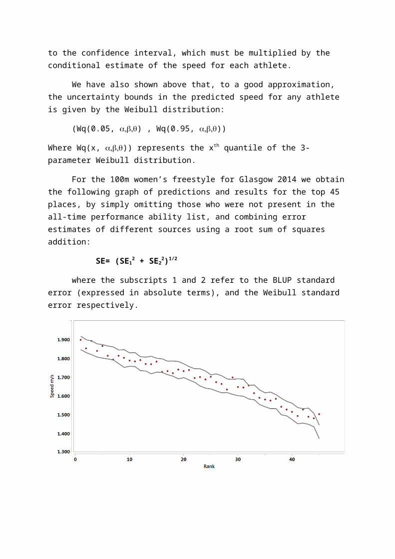
For the 100m women’s freestyle for Glasgow 2014 we obtainthe following graph of predictions and results for the top 45 places, by simply omitting those who were not present in the all-time performance ability list, and combining error estimates of different sources using a root sum of squares addition:

SE= (SE12 + SE2

2)1/2

where the subscripts 1 and 2 refer to the BLUP standard error (expressed in absolute terms), and the Weibull standard error respectively.

Figure 4 Predicted performances (grey lines as 90% confidenceintervals) and ranks for Female 100m FRS at Glasgow 2014, compared with actual performances (closed dots).

The calculated bounds appear to be possibly too loose, asonly 2-3 points appear to lie outside the bounds (all above), whereas 4-5 points may theoretically be expected; but overall the predictions are matched quite well. The variation in ranksfrom those predicted illustrates the uncertainty inherent in those predictions: predicted ranks (1,2,3,4,5,6,7,8,9) becomeactual (1,4,2,5,3,6,9,7,8) for the first 9 competitors). In other words, one athlete who should have expected a silver medal on rankings was relegated to bronze, whereas another potential podium finisher missed out, and a third person was able to gain a silver medal when expectations were not to finish in the top 3 at all.

7 Conclusion

In conclusion we have demonstrated a methodology that essentially ranks athletes against their peers over time, by measuring their relative strength against as many of their peer performances we have available, taking into account all measureable influences through a regression approach. We have shown that this approach can be highly accurate, being largelyfree of the instabilities which have plagued other methods of comparison. This makes it suitable even for comparing athletesacross classes, or even different events, such as is required in selection, or for combining AWD classes in the same event.

We have also shown that the methodology may throw light on the way in which elite performances change over time, having uncovered seemingly irregular behaviour in the generally highly stable average quality of performance over

time. These irregularities suggest further work to disentanglethe influences combining to produce this observed behaviour.

Although due to lack of space, the swimming discipline was chosen as the sole example, it is clear that the same technique (with some modifications) could be used for any athletic event (100m, shot), or for rowing events, for example. Indeed, for AWD events, where we must match performances across disability classes, the same conclusion holds, providing there are sufficient results to guarantee thedesired accuracy; which can be guaranteed by combining resultsfrom a number of events over time through a regression fit.

Finally, we have demonstrated a methodology to characterise the random variations in elite performances, whether for a single athlete or for the whole population of elite athletes. We have shown that, removing temporal influences by regression, the remaining stationary distribution (of residuals) must be characterised by a single type of distribution, the Weibull, whose parameters can be accurately determined for each combination of classes. Equating performances across classes via the distribution percentiles then allows quantitative comparisons of performance merit.

We have shown that the combination of these three parts of this methodology can be used to predict both the expected performance of elite athletes, and also to quantify the uncertainty inherent in those performances. This potentially allows us to study in much greater detail such effects as the efficacy of different types of taper, of mental preparation orof diet, for example.

References

Infostrada (2014): Data obtained by subscription fromhttp://www.infostradasports.com/.

JI McCool, 2012, Using the Weibull Distribution: reliability, modelling and inference, John Wiley.

JMP Pro 11.2.0 (2013) © SAS Institute Inc.