Power quality analysis and techno-economic modeling for ...

DOCTORA L T H E S I S

Jakob Nöm

m Pow

er quality analysis and techno-economic m

odeling for microgrids

Power quality analysis and techno-economic modeling

for microgrids

Jakob Nömm

Electric Power Engineering

Power quality analysis and techno-

economic modeling for microgrids

Jakob Nömm

Luleå University of Technology

Department of Engineering Sciences and Mathematics

Division of Energy Science

Abstract

The work done in this thesis considers microgrids from two different aspects. Power quality and

techno-economics of microgrids. Detailed power quality measurements have been made at a

single house hydrogen-solar microgrid that consists of state-of-the-art energy efficiency

technology, energy production and energy storage. The microgrid can both connect to the grid

and operate in islanded operation. The power quality is quantified from these measurements

where several power quality parameters during islanded operation go beyond the limits set by

standards such as EN 50160 and IEEE 519-2014. The effect on connected equipment from both

frequency variations and voltage quality is also discussed. Four new performance indexes are

presented in the thesis that are based on apparent impedances. The first with the name PHIPI

quantifies how much the harmonic voltage magnitude changes with an increase in harmonic

current magnitude on the same phase. The second with the name SHIPI quantifies how much

the harmonic voltage magnitude changes with an increase in harmonic current magnitude on

another phase. The third with the name AHSI uses the harmonic voltage and current

magnitudes of all phases to create a single performance parameter expressed as an apparent

impedance for the system. The fourth with the name ARMSSI quantifies the phase RMS voltage

drop for a certain phase RMS current rise in terms of an apparent impedance. The thesis also

shows techno-economic modeling with times series energy flow to study the investment risks

related to consumption changes in a standalone microgrid. The results show that consumption

changes are an important parameter when designing a standalone microgrid and that the risk

can be mitigated with changes to the system design, but at a larger system cost. The projected

cost reduction until the year 2050 for standalone hydrogen based microgrids and some risk

aspects with hydrogen based microgrids are also discussed in the thesis.

Acknowledgements

This project has been funded by Skellefteå municipality through Rönnbäret foundation and

Skellefteå Kraft Elnät and the work has been done at Luleå University of Technology. The

financial support is greatly appreciated, and I hope that this thesis will bring knowledge that is

useful for the funders and people interested in the subjects given in this thesis.

I would like to thank my supervisors Sarah Rönnberg and Math Bollen. You have provided

excellent support and guidance throughout this project which has made this thesis possible.

I would also want to thank my colleagues at Luleå University of Technology for providing good

discussions which has helped to make this thesis.

I would also want to thank my family and friends for the support you have given.

Jakob Nömm

Skellefteå, 03/11-2021

List of abbreviations

PV: Photovoltaics

RMS: Root mean square

BEMVLL: Break-even medium voltage line length

BED: Break-even distance

BEDC: Break-even distance per consumption

SoC: State of charge

LCC: Life cycle cost

THD: Total harmonic distortion

FSPC: Frequency-shift power control

AFA: Automatic frequency adjustment

GHP: Geothermal heat pump

MPP: Maximum power point

AHSI: Apparent harmonic system impedance

PHIPI: Primary harmonic impedance performance index

SHIPI: Secondary harmonic impedance performance index

ARMSSI: Apparent RMS system impedance

LV: Low voltage

MV: Medium voltage

PCC: Point of common coupling

CDF: Cumulative distribution function

UCL: Upper confidence limit

SPS: Secure power supply

HVDC: High voltage direct current

Table of Content

1. Introduction ............................................................................................................................................. 1

1.1. Background ...................................................................................................................................... 1

1.2. Motivation ........................................................................................................................................ 1

1.3. Objectives .......................................................................................................................................... 2

1.4. Scope .................................................................................................................................................. 2

1.5. Approach .......................................................................................................................................... 3

1.6. Contribution of the work ................................................................................................................ 4

1.7. Societal Aspects ............................................................................................................................... 5

1.8. Appended Papers ............................................................................................................................ 7

1.9. Outline of thesis ............................................................................................................................... 8

2. Literature overview of microgrids ....................................................................................................... 9

2.1. DC and AC microgrids ................................................................................................................... 9

2.2. Power quality phenomena in microgrids during islanded operation ................................... 10

2.2.1. Frequency variations .............................................................................................................. 10

2.2.2. Current and voltage distortion ............................................................................................. 11

2.3. Economics of microgrids with focus on comparisons between a grid-connection and a

microgrid investment and investment risks of them ...................................................................... 12

3. Definition of a microgrid, nanogrid and a suggestion for improvement ..................................... 14

4. Description of the studied microgrid ................................................................................................ 16

5. Data processing ..................................................................................................................................... 19

6. Frequency variations in islanded operation for a microgrid.......................................................... 20

7. Transition between islanded and grid-connected operation ......................................................... 26

8. Interruptions in Sweden and in a microgrid .................................................................................... 28

9. Voltage variations in a microgrid ....................................................................................................... 29

10. Modes of operation in a microgrid .................................................................................................. 32

11. Constructing a standalone microgrid in Sweden........................................................................... 38

12. Case study of the reliability in rural grids in Sweden ................................................................... 44

13. Techno economic modeling for a standalone microgrid .............................................................. 47

14. Critical review of own research ........................................................................................................ 53

15. Conclusions ......................................................................................................................................... 55

16. Recommendations .............................................................................................................................. 58

17. References ............................................................................................................................................ 59

1

1. Introduction

1.1. Background

In 2010 a PV module cost around 2 euros per Wp, just 3 years later the cost had dropped to 0.7

Euro per Wp [1], in September 2021, the low cost PV modules are listed at 0.16 Euro per Wp [2]

which corresponds to a 92% reduction since 2010. The cost is further expected to decrease by up

to 86.4% from 2018 until 2050 [3]. The weighted average levelized cost of electricity for onshore

wind turbines in Europe have also decreased with 60.2% since 2010 up to 2020 [4] , and the cost

per kW capacity is expected to decrease by up to 56.6% from 2018 until 2050 [5]. The price for

batteries has dropped by about 54% from 2010 to 2020 and is expected to decrease by 82% by

2050 from 2020 [6]. This decrease in price for storage and renewable energy sources would

increase the economic possibility to microgrids as an alternative to the traditional grid-

connection, especially in rural areas with long distribution distances, difficult terrain or low

reliability of electricity supply. Several pilot projects with microgrids have recently been

initiated by Swedish utility companies to investigate the technical feasibility of such systems [7],

[8], [9] which shows that an interest for microgrids exists in the industry.

1.2. Motivation

One of the key questions that arise for future deployment of microgrids is how the power

quality and reliability will be affected. The reliability in rural grids can be poor (shown in

Section 12) and supplying remote customers through a local microgrid can ensure that better

electrical service can be provided [10], [11], [12]. The power quality in an islanded microgrid can

differ significantly from a similar installation connected to the grid which leads to the question

whether the performance of connected equipment will be negatively affected. Research

regarding power quality in islanded operation represents only 2.56% of all research about

microgrids [13] and research is needed in this topic in order to quantify the power quality

performance in islanded operated microgrids in order to define preventative measures. The

economics and investment risks of standalone microgrids is also of interest since utility

companies continuously aims to reduce costs. This can be achieved by avoiding expensive

distribution lines to rural customers with low consumption per unit distribution distance in

comparison to urban customers.

2

1.3. Objectives

The project is aimed towards small microgrids. Reliability and power quality should be

investigated, and economic models should be created where standalone microgrids are

compared with the traditional utility grid operation. A list of the objectives for this thesis is

shown below:

1. Investigate and map the power quality in a microgrid during islanded operation and

compare it to the traditional utility grid-connection (discussed in Paper A, B, C, F and

Section 6 to 10).

2. Identify under which conditions the reliability can be jeopardized during islanded operation

for a microgrid (discussed in Paper B, D and Section 7).

3. Develop power quality performance indexes that are applicable to island operation

(discussed in Paper F and Section 10).

4. Economic models need to be created where the economic operation is compared to the

traditional utility grid. Indexes have to be created to give an estimation whether an

investment in a microgrid is profitable (discussed in Paper E and Section 13).

1.4. Scope

Power quality data has been collected for this thesis for a microgrid described in Section 4. The

scope of the power quality analysis in this thesis is limited to measurements taken at the load

output from one microgrid. No controlled experiments could be made for this thesis. No

information was available about the output of the solar inverters which means that no

information about the production. No information was available about the state of charge of the

lead acid battery which could be an important variable since the internal resistance of a lead acid

battery is dependent on state of charge. No information was available about the different loads

that was active for a specific time, production from the hydrogen fuel cell and consumption of

the electrolyzer in the studied microgrid. This makes it impossible to identify how different

loads and production affect the microgrid reliability and power quality performance.

The economy part of this thesis will limit the scope towards microgrids located in Sweden and

Scandinavia.

3

1.5. Approach

The research approach is divided into two separate sections, one for the power quality analysis

and the other for the economic modeling and is summarized below:

Power quality analysis

• Literature survey of power quality phenomena of microgrids in islanded operation.

• Identify gaps in the literature and see if the gaps can be filled with the objectives for the

thesis.

• Obtain power quality data from a microgrid in islanded and grid-connected operation.

• Create statistical results from the power quality data from both islanded and grid-connected

operation in order to present the difference in magnitude and occurrence.

• Analyze time series of the power quality data to obtain patterns and behaviors that might

enable the explanation of different phenomena.

• Compare the statistical analysis with relevant standards to give an indication of the power

quality in an islanded microgrid versus a grid-connected microgrid.

• Formulate new indexes that can give information on the power quality system performance

and that could detect the modes of operation of the microgrid.

Economic modeling

• Literature survey of the techno-economics of standalone microgrids.

• Identify gaps in the present research and see if the gaps can be filled with the objectives for

the thesis.

• Obtain economic data for low and medium voltage distribution lines, transformers and the

associated maintenance costs in order to make a comparison of a grid-connected customer

and a standalone microgrid connected customer.

• Create a working theoretical system configuration for a standalone microgrid with

renewable energy sources where the energy flow can be simulated.

• Times series measurements/simulations of consumption data, solar production, wind

production has to be obtained in order to obtain a realistic approximated result.

• Obtain economic data for the theoretical system configuration components from the retail

market and publications and make assumptions where economic information from the retail

market and publications is missing.

4

1.6. Contribution of the work

The main contributions of the work are listed below:

1. The analysis of long-term frequency data for a single house microgrid with commercial

equipment and the explanation of why the frequency variation between 49 Hz and 55 Hz

occur during islanded operation. A discussion on how the frequency variations affects

different loads is also given.

2. The analysis of long-term voltage quality data for a single house microgrid with commercial

equipment and a discussion on how the voltage quality affects different loads.

3. The discovery that there exist two main modes of operation in islanded mode with different

harmonic impedance and harmonic voltage distortion. The two main modes of operation

have also two sub modes of operation (night and day operation) with different harmonic

impedance and harmonic voltage distortion.

4. It was shown that the transition from islanded to grid-connected operation have less

interruptions than the transition from grid-connected operation to islanded operation.

5. A techno-economic model was created to compare the investment risks of consumption

changes in a standalone microgrid. It was shown that consumption changes pose a

significant investment risk and that it can be mitigated by increasing the capacity of the

standalone microgrid. However, there is a tradeoff between the risk and the cost since a

decrease in investment risk is associated with an increase in capital investment.

6. Two indexes were developed related to microgrid economics, the first is the BEMVLL that

extended the BED index found in the literature to also incorporate the voltage level and is

independent of low voltage line length in the microgrid. The BEMVLL can be plotted against

the energy consumption of a microgrid, giving the network operator an economic indicator

as a function of energy consumption. The second is the break-even distance per

consumption enables comparisons to be made in the literature where different BED values

exist, but with varying energy consumption and is shown in Paper E.

7. Three new harmonic performance indexes were created to give supplementary information

about the harmonic performance in an islanded microgrid in comparison to a grid-connected

microgrid. The new indexes are the AHSI, PHIPI and SHIPI which is described in detail in

Paper F.

8. A new voltage RMS performance index with the name ARMSSI was created to give

supplementary information about the phase RMS voltage drop due to a phase RMS current

rise and is described in Section 10 and shown in Paper C.

5

1.7. Societal Aspects

This thesis contributes to the development of microgrids in society since the thesis increases the

overall knowledge of power quality in microgrids, the economics of microgrids and the risks of

investing in a standalone microgrid. Microgrids could have several benefits to society such as:

1. Lower cost for served customers [11].

2. Increased revenue and cost savings for utility grid operators due to for instance investment

deferral [11].

3. Provide increased reliability to parts of the grid that are inadequately served by the

traditional grid-connection [10], [11], [12].

4. Increased renewable energy penetration and increasing the electrification in developing

countries [10], [11], [12].

5. For forest rich countries such as Sweden, more efficient land use can be achieved with

standalone microgrids, since more forest can be made available for producing products as no

distribution lines with power line corridor is needed.

However, a possible negative consequence for society could occur if the deployment of

standalone microgrids are done in rural areas. It is important to note that the following

described scenario is speculative and will depend on a country’s regulations. But it is still

important to address since it could be a scenario in which society is negatively affected by the

deployment of standalone microgrids. The following scenario is:

In Figure 1, a picture is shown of a medium voltage distribution line in a rural region in Sweden

above the Arctic Circle. This line connects only a single customer and is approximately 3 km

long. The house is today only used for hunting purposes, which leads to a significantly lower

electricity consumption than a year-around residence in Sweden. If the utility company that

operates this line have to reinvest the line (which can be e.g. due to end of life or if a tree has

fallen over the distribution line) the utility company could decide to invest in a standalone

microgrid instead if the cost of a standalone microgrid is lower than replacing the distribution

line. However, the investment decision can be motivated by the low energy consumption (low

amount of storage and production units in relation to an all-year household). If the house is now

sold to a customer that wants to live in the house all-year, the low amount of storage and

production units makes the household insufficiently served for the all-year residents. The cost of

increasing the microgrid energy storage and production units (solar PV or wind turbines) might

become many times more expensive than just investing in a new distribution line. Now the

question arises if the utility grid operator needs to invest in a new line or if the new customer

needs to do that. The cost of a new 24 kV distribution line is 380582 SEK/km (obtained from a

utility company in Sweden). A 3 km line would constitute over one million SEK, which in this

area could be more than what the house is worth. If the new customer has to pay for this, the

6

new customer would make a financial loss by buying the house which might have significantly

decreased in value since the market becomes limited to customers with similar consumption as

the first owner of the house when it was converted to a standalone microgrid. In order to avoid

negatively affecting rural areas, customers that are already connected by a distribution line

today should be viewed as a virtual distribution line if a standalone microgrid is implemented.

I.e. if the consumption increases, the utility company needs to pay for the necessary upgrades,

either by a new distribution line or upgrades to the standalone microgrid. If this is not possible

to arrange, the customer needs to be informed of the risks in agreeing to disconnect from the

main grid. An external appraiser might also be needed to ensure that the house price is not

negatively affected by a standalone microgrid supply system.

Figure 1. A distribution line with an approximate length of 3 km that connects a single house that is

situated above the Arctic Circle in Sweden.

7

1.8. Appended Papers

Paper A

J. Nömm, S.K. Rönnberg, M.H.J. Bollen

Harmonic voltage measurements in a single house microgrid, 18th International Conference on

Harmonics and Quality of Power (ICHQP), 13-16 May 2018, Ljubljana, Slovenia.

Paper B


An Analysis of Frequency Variations and its Implications on Connected Equipment for a

Nanogrid during Islanded Operation. Energies 2018, 11, 2456.

Paper C


An Analysis of Voltage Quality in a Nanogrid during Islanded Operation. Energies 2019, 12,

614.

Paper D


Energy Flow Based Risk Analysis for Operating A Standalone Solar-Hydrogen Nanogrid in

Northern Scandinavia. IEEE Cigré Norpie 2019, Narvik, Norway, September 25-27, 2019.

Paper E


Techno-economic analysis with energy flow modeling for investigating the investment risks

related to consumption changes within a standalone microgrid in Sweden. Energy, 2021, 225

Paper F


Evaluating the harmonic performance in a microgrid during islanded and grid-connected

operation using apparent harmonic impedance performance indexes. Submitted to International

Journal of Electrical Power & Energy Systems

8

1.9. Outline of thesis

• In Section 2, a literature overview is presented with a study of AC & DC microgrids, power

quality in microgrids and the economics of microgrids with focus on comparisons between a

regular grid-connection and a microgrid investment and investment risks of them.

• The definition of a microgrid is given in Section 3 and a suggestion on how to improve it.

• In Section 4, a description of the studied microgrid is presented.

• In Section 5, a short note on the data processing of this thesis is made

• In Section 6, the frequency variations in a microgrid is presented and discussed.

• In Section 7, the transitions between islanded and grid-connected operation in a microgrid

will be presented and discussed.

• In Section 8, interruption data for a microgrid will be compared to all Swedish costumers.

• In Section 9, voltage variations for a microgrid will be presented and discussed.

• In Section 10, a discussion of the modes of operation of a microgrid is made and some details

about some of the new performance indexes are made.

• In Section 11, a presentation of the possibility and challenges in constructing a standalone

microgrid is made.

• In Section 12, case study data with interruptions of rural grids in Sweden is presented.

• In Section 13, techno economic modeling is discussed for a standalone hydrogen based

microgrid.

• In Section 14, a critical review is made of the research done for this thesis.

• In Section 15, the conclusions of this thesis are presented.

• In Section 16, recommendations for future work is presented.

9

2. Literature overview of microgrids

2.1. DC and AC microgrids

In the beginning of electrical transmission in the 1800s, both AC and DC systems existed. In

1886, George Westinghouse's company launched an AC system that used transformers to either

step down or up the voltage which enabled AC systems to transmit power over longer distances

with lower losses than DC [14]. For transmitting DC in the 1800s, the power station would

normally be located within a mile of the costumers which made DC transmission obsolete

against the improved AC system by George Westinghouse's company [14]. DC transmission

made a comeback in the 1900s where the first commercial subsea high voltage DC (100 kV)

transmission system was constructed between mainland Sweden and the Swedish island

Gotland in 1954 [15]. HVDC transmission has the advantage of lower cost in large transmission

distances and technical benefits such as the ability to connect two unsynchronized networks.

The break-even distance for land-based transmission with HVDC is about 600 km and by sea

cable it is at about 50-100 km according to [15].

The number of DC loads has in modern days increased due to advances in power electronics

[16]. For residential customers almost all of the loads can today be run directly on DC [17].

Furthermore, renewable energy sources such as solar PV produce DC and wind turbines can

also produce DC for certain wind turbine systems [18]. Storage and energy devices such as

batteries, fuel cells and electrolyzes all use DC [16]. Due to this fact, DC powered microgrids are

proposed since they could avoid unnecessary conversion steps between AC and DC since every

conversion step leads to losses [16]. It was reported by [19] that changing infrastructure for LED

lamps from AC to DC can result in up to 15% energy saving, 17% was reported in [20]. In [21] it

was calculated that the potential DC microgrid energy savings was between 15%-40% for a

household appliance. A good illustration of both an AC and DC microgrid with household loads

and generation can be seen in [22]. Another advantage of DC microgrids over AC microgrids is

that only active power exists in the DC microgrid, therefore no control of the power frequency,

reactive power and synchronization of distributed sources is needed [16].

There are some challenges in DC microgrids, one is protection since there is no zero crossing in

the voltage as in AC, therefore faults will be more difficult to interrupt with conventional

methods [23]. One of the main issues when using conventional methods when breaking a DC

current is arcing which leads to longer clearing times [23]. Arcing during a fault can also lead to

fire hazard. There are more sophisticated methods such as solid-state circuit breakers were no

arcing occur [23], [24]. However, the cost for protection devices in a DC microgrid is higher than

for AC microgrids [25]. Another problem with DC microgrids is high impedance ground faults

since they can be hard to detect [26] and off the shelf appliances used in the traditional utility

grid can’t be used in a DC microgrid without modification.

10

2.2. Power quality phenomena in microgrids during islanded operation

2.2.1. Frequency variations

Frequency variations is a normal part in the large interconnected grid since supply and demand

never can be perfectly matched. In the Scandinavian interconnected grid, frequency variations

on 10 s average scale for over a year can be seen in [27] where the variations stay within about

49.65 to 50.3 Hz. In [28], frequency swings between 49.3 to 50.4 Hz is shown. In EN 50160 [29],

the 10 s average frequency value is allowed to be between 47 Hz and 52 Hz for synchronous

interconnected systems. For non-interconnected systems the frequency is allowed to vary

between 42.5 Hz to 57.5 Hz according to EN 50160. In EN 50160/A1 [30] a range between 49 Hz

to 51 Hz is described for systems without synchronous connection to an interconnected system.

In the literature, several papers mention the likelihood of larger frequency variations in a

microgrid due to low inertia characteristics and due to large variations in production and

consumption of an islanded microgrid [31], [32], [33], [34], [35]. This also applies to the large

utility grid as more inverter based renewable energy sources are connected which exhibit low or

zero rotational inertia in comparison to a synchronous generator, but this can be solved with

synthetic inertia by for instance allowing solar PV to operate at sufficient curtailment [36]. In the

literature an energy storage system is also mentioned as an important component for balancing

power due to intermittency of renewable power sources [37]. There exist commercial systems for

microgrids where the battery inverter in a microgrid controls the frequency to signal the solar

inverters if over or underproduction occur so that the MPP controller can select the appropriate

power level. Such a system is called frequency shift power control which uses the battery

voltage as the reference for choosing the frequency [38], something also used in [34]. The use of

the frequency to communicate between converters in order to control the power level has also

been described in the literature [39]. The use of direct solar power without battery interface has

also been implemented to some degree by [40]. They call it secure power supply (SPS) where the

solar inverter can supply small loads such as battery chargers and fans up to a certain fraction of

the rated power of the solar inverter [40].

The performance of actual operating microgrids varies depending on system design and

operation. For a larger 50 kV microgrids dominated by synchronous generators, frequency

variations between about 48.7 Hz and 51.2 Hz was observed during a three hour long test in

[41]. In [42] the frequency variations for a small microgrid were kept within 59.97 Hz and

60.05 Hz during islanded operation for a 60 Hz system. In [27], the 10s variations for 48 weeks of

islanded operation for a microgrid were between about 43.48 Hz and 54.61 Hz and surpassed

the weekly limit described in EN 50160 for 89.6% of the measurement time period.

11

2.2.2. Current and voltage distortion

In [43] the upstream impedance increased from 0.366 Ω in grid-connected operation to 2.184 Ω

in islanded operation and in [44], [45] the network harmonic impedance was shown to be larger

in islanded operation, causing higher voltage distortion in islanded operation than in grid-

connected operation. The level of harmonic distortion varies depending on which microgrid is

considered. In [42], the voltage THD was kept below 5% during one day of measurement where

an electric vehicle was being charged. In [46], voltage THD levels of over 12% were recorded for

a microgrid in islanded operation. In [47], a 13% voltage THD was recorded at 10 min average

and 21.9% at 3s average. Both [46] and [47] makes a comparison towards the limits set by

standards EN 50160 and IEEE 519-2014 and show that the limits are surpassed for both the

voltage THD and some individual harmonics. In [48], the average voltage THD was lower in

islanded operation at 1.19% than in grid-connected operation at 1.5%. In [49], higher levels of

supraharmonics were recorded in a microgrid during islanded operation than in grid-connected

operation. It was shown in [50] that the voltage distortion in the SPS mode of an solar inverter

(mentioned in Section 2.2.1) changes depending on which load is connected where the voltage

THD was 2.3% at no load, 1.8% at 11.5% of the rated power with a nonlinear load, 3.6% at 49%

rated power with a nonlinear load, 9.4% at 95% rated power with a linear resistive load. It was

presented in [43] for a standalone microgrid with battery storage that at 5% load rating the

voltage THD had a value of 1.06% when it supplied a linear load and 3.65% when supplying a

nonlinear load. For a 75 % load ratio for the linear load, the voltage THD was at 1.55% and

17.5% at 75% load ratio for a non-linear load. It was also shown in [51], [52] that when the power

production from the PV installation was lower than rated power the current had higher

distortion levels in both islanded and grid-connected operation. It was concluded in [52] that the

current distortion from the PV inverter was caused by the supply voltage distortion. In [52], it

was also shown that the current THD of the PV inverter was lower in islanded operation than in

grid-connected operation for all power levels due to a lower voltage THD in islanded operation

than in grid-connected operation. Research on mitigating the voltage distortion in a islanded

microgrid with experimental evidence has been shown in [53], [54], [55], [56], [57], [58], [59], [60],

[61].

12

2.3. Economics of microgrids with focus on comparisons between a grid-

connection and a microgrid investment and investment risks of them

Several projects with microgrids have been undertaken in Sweden by utility companies. Such

are Simris by Eon [7] that is a small village in Southern Sweden that is a grid-connected

microgrid that operates on an energy mix of solar, wind, battery storage and a biodiesel

generator. Zero Sun by Skellefteå Kraft [8] that is a standalone microgrid that only gets its

energy from solar PV all year and stores it in both batteries and hydrogen in order for the

microgrid to function in the winter. Arholma by Vattenfall Eldistribution [9] that is a grid-

connected microgrid in a physical island outside of Stockholm that uses battery storage in

combination with solar PV to temporarily be able to disconnect from the main grid. As

mentioned in Section 1.1, the cost of some of the main components used to form a standalone

microgrid is expected to decrease in the future, which increases the possibility of reaching a

lower LCC for a standalone or grid-connected microgrid in comparison to only a grid-

connection for a certain load. There are several studies done that investigate the economics of

standalone microgrids such as [62], [63], [64], [65], [66], [67], [68] which has shown that for a

certain distance to a potential microgrid (break-even distance), a standalone microgrid has lower

LCC than a grid-connection. There are several investment risks related to standalone systems

such as incorrect dimensioning (both under and over dimensioning) of the power supply system

[69], [70]. This can be seen in [71] and [72] where a lower loading of the diesel generator

increases the levelized cost of electrical energy and in [73] where an increase in fuel

consumption per unit of produced electricity occurred. Other factors that could influence the

economic operation of a standalone microgrid are for instance inflation rate [74], diesel fuel

price, [74], [75], [76], [77], [78] and discount rate [76], [77], [79]. In [68], it was shown that changes

in consumption, both amount and time of consumption could influence the LCC of a standalone

microgrid consisting of residential customers and that the most important variable is the

amount of consumption. It has been shown in the literature that the amount of consumption for

a household depends on several factors such as household income [80], age structure and

education [81], weather and location [82], type, amount and use of household appliances [83]

and number of people in the household [84], culture of household residents [85], ambient air

pollution at the household [86]. Household electricity consumption can vary with 200%-300%

even if the household units are close to identical according to [87]. Grid-connected microgrids

have the possibility to reduce the cost of a utility grid by for instance capital investment deferral

and improved reliability, [88], [89], [11]. The investment deferral was achieved in [88] by

implementing a microgrid that supplied the loads in the microgrid and supplied the distribution

grid with electricity. Before, the to be microgrid area was a net consumer of electricity. In [89],

the payback period was 10 years for a distribution system upgrade without a grid-connected

microgrid and 4-6 years if a grid-connected microgrid was implemented instead. Investment

13

risk variables in [89] was also considered such as the microgrid cost, peak demand reduction,

reliability reward, O&M cost reduction for voltage regulation.

14

3. Definition of a microgrid, nanogrid and a suggestion for improvement

The US department of energy defines a microgrid as “A group of interconnected loads and

distributed energy resources within clearly defined electrical boundaries that acts as a single

controllable entity with respect to the grid. A microgrid can connect and disconnect from the

grid to enable it to operate in both grid-connected or island mode” [90].

The international council on large electric systems (CIGRE) WG C6.22 defines microgrids as:

“electricity distribution systems containing loads and distributed energy resources, (such as

distributed generators, storage devices, or controllable loads) that can be operated in a

controlled, coordinated way either while connected to the main power network or while

islanded” [91]. The definition of a nanogrid varies, [92] defines it as “a power distribution

system for a single house/small building, with the ability to connect or disconnect from other

power entities via a gateway. It consists of local power production powering local loads, with

the option of utilizing energy storage and/or a control system”. In [92], a distinction between a

nanogrid and microgrid is also made where it was defined as “A nanogrid is a single

house/building and a microgrid is several nanogrids interconnected to each other where both

can operate in islanded mode”. These three definitions have one common problem, how large

can a microgrid and nanogrid be? Can a nanogrid be the Tesla Gigafactory since it is one

building? One way to avoid subjective definitions such as “single house” could be to provide a

clear measurable definition that would set a lower and upper power constraint. For instance, a

nanogrid could be a grid with loads and power generation that can operate in grid-connected or

islanded operation with a maximum power demand (fuse size) of 100 kW. A microgrid could be

several nanogrids interconnected but not larger than 100 MW (1000 nanogrids at maximum

power rating) but not smaller than 100 kW. In this way, a distinction between smaller grids than

the macro grid could be made. 100 kW would constitute about 10 Swedish households with 16 A

fuses on all three phases.

In Table 1, an example of a simple definition of different grid sizes can be seen. The table also

incorporates picogrid which is a term used by several published papers [93], [94], [95] to

describe a grid that is smaller than a nanogrid.

Table 1. Power levels for different grid sizes.

Macrogrid>100 MW

100 MW≥Microgrid>100 kW

100 kW≥Nanogrid>10 kW

10 kW≥Picogrid

The latest paper in this thesis and the thesis itself does not use the term nanogrid to describe the

studied single house microgrid. This is due to this definition problem discussed in this section. It

15

is difficult to correctly pinpoint in the literature if a certain reference has a nanogrid or a

microgrid. This is since the literature might use the term microgrid while with [92] definition, a

nanogrid is more appropriate. For experimental lab setups with power ratings of just a couple

kW, picogrid might be more appropriate to use since it is not a “single house microgrid”.

16

4. Description of the studied microgrid

The measurements used in this thesis comes from a microgrid located in Göteborg Sweden. The

microgrid can operate in both islanded mode and grid-connected operation. The microgrid is

meant to operate in continuous islanded operation where solar PV modules should supply the

energy to the house all year. This is meant to be achieved by creating hydrogen through

electrolysis in the summer and storing it for later use in the winter were the consumption is

larger (can be seen in Figure 23 in Section 11). The microgrid consists of 20 kWp solar

photovoltaics (PV) on the roof and 2.6 kWp PV on the facade. It has a 48 V, 144 kWh of lead acid

battery storage and 1100 kWh of hydrogen storage. After the measurement period done in the

microgrid, the hydrogen storage was upgraded to 5800 kWh. The battery storage is meant to

supply the loads with energy which includes a 5 kW electrolyzer. The electrolyzer starts when

the SoC is above 85%. During the winter a 5 kW hydrogen fuel cell is the main supply of

electricity that should charge the battery (that supplies the loads). The efficiency of the fuel cell

is about 50% and the waste heat is supplied to the house. The fuel cell starts when the SoC of the

battery is at 30%. The microgrid is split into two parallel systems, each with its own battery pack

(50% each of the 144-kWh battery), one 3-phase SMA Sunny Tripower STP12000TL-10 solar

inverter and three SMA Sunny Island 8.0H battery inverters. All inverters are connected to a

SMA multicluster box 6.3 except one single phase SMA Sunny Boy inverter that is directly

connected to phase 2 at the load side of the multicluster box. This inverter is connected to the

solar PV on the façade of the house. In islanded operation, the microgrid can maximum supply a

3-phase load of 36 kW load continuously. The loads connected to the microgrid is regular

household appliances and two 3-phase chargers for electric vehicles. The microgrid can be

viewed as a “living lab” since the residents in the microgrid house live there all-year. A 15 kVA

diesel generator exists for backup power. The diesel generator was not active during the

measurement period. The microgrid house has 504 m2 of living space and an electricity

consumption per year of 12400 kWh for the house and 3700 kWh for electric car charging. The

house has the latest in energy efficiency technology and has solar collectors on the roof. The

electrolyzer can create hydrogen at a pressure of 10-30 bars but a compressor is needed to

compress the hydrogen to 300-700 bars for the storage tanks. The fuel cell delivers a voltage of

70 V DC and is therefore connected to a DC/DC converter with two outlets for the two battery

units that make each parallel system. The system is rated to operate at 50 Hz and at 230 V per

phase. In Figure 2, a simplified schematic of the microgrid is shown.

17

Figure 2. Schematic of the studied microgrid. EL is the electrolyzer and the FC is the fuel cell.

During the end of the measurement period, about 40% of the battery capacity remained where

the lead acid battery had an expected life of 1500 cycles.

Frequency control in the microgrid

The SMA Sunny Island inverters use the frequency to communicate with the solar inverters. It

has two different modes of regulation. First is the SMA FSPC. The FSPC is used to keep a

balance between the consumption and generation in the microgrid during islanded operation.

Under normal operation the frequency should be 50 Hz. If there is too much production, the

FSPC will regulate down the production from the Tripower and Sunny Boy solar inverters. The

regulation is from 0 to 100% from 51 to 52 Hz.

Since there could be equipment that are synchronized to the power frequency to determine the

time, another frequency regulation exists to compensate for the higher frequency caused by the

FSPC in order for clocks to operate at the correct time. It is the SMA AFA. The AFA shifts the

frequency to 49 Hz on a 12h basis to correct the over frequency occurred by the FSPC in order

for clocks to run at the correct time.

18

The FSPC also has another frequency setting with a value of 55 Hz. It is used when the

microgrid is commencing grid-connected operation mode. The FSPC will increase the frequency

towards 55 Hz in order for the solar inverters to shut down so that the SMA Sunny Island

battery inverters can synchronize to the utility grid.

19

5. Data processing

A significant amount of time has gone towards processing the collected data in order to analyze

it. For Paper A to C, the data needed to be separated into islanded and grid-connected

operation. The grid-connected operation was identified by using the frequency of another

measuring location at Luleå University of Technology as reference. However, even then, the

data was still not of sufficient quality to be used since the microgrid could also operate with the

same frequency as the grid leading to incorrect sorting. This was solved by using the voltage

THD for all phases as a reference. If any of the phases at 1s resolution was above 2.5% voltage

THD and had a frequency that was deviating by more than 0.02 Hz from the reference location

in Luleå University of Technology, it was regarded as islanded operation. These criterions were

determined to be about 99.9% accurate by using the criterions with separated grid-connected

and islanded operation data that had been obtained by visual inspection. The amount of data

spans about 1 to 2 TB since the highest resolution is 1 cycle and was collected with and

Elspec G4430 at the load output of the SMA multicluster box that interconnects the two parallel

systems described in Section 4.

20

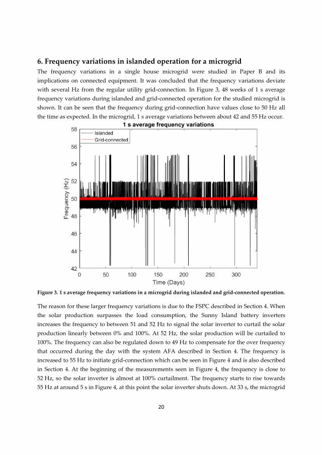
6. Frequency variations in islanded operation for a microgrid

The frequency variations in a single house microgrid were studied in Paper B and its

implications on connected equipment. It was concluded that the frequency variations deviate

with several Hz from the regular utility grid-connection. In Figure 3, 48 weeks of 1 s average

frequency variations during islanded and grid-connected operation for the studied microgrid is

shown. It can be seen that the frequency during grid-connection have values close to 50 Hz all

the time as expected. In the microgrid, 1 s average variations between about 42 and 55 Hz occur.

Figure 3. 1 s average frequency variations in a microgrid during islanded and grid-connected operation.

The reason for these larger frequency variations is due to the FSPC described in Section 4. When

the solar production surpasses the load consumption, the Sunny Island battery inverters

increases the frequency to between 51 and 52 Hz to signal the solar inverter to curtail the solar

production linearly between 0% and 100%. At 52 Hz, the solar production will be curtailed to

100%. The frequency can also be regulated down to 49 Hz to compensate for the over frequency

that occurred during the day with the system AFA described in Section 4. The frequency is

increased to 55 Hz to initiate grid-connection which can be seen in Figure 4 and is also described

in Section 4. At the beginning of the measurements seen in Figure 4, the frequency is close to

52 Hz, so the solar inverter is almost at 100% curtailment. The frequency starts to rise towards

55 Hz at around 5 s in Figure 4, at this point the solar inverter shuts down. At 33 s, the microgrid

21

connects to the grid for 10 s and experiences an interruption for about 1 s and then starts up in

islanded operation again. After the start up, the frequency drops to around 42 Hz and then ramp

up towards 50 Hz. Evidence as to why this 10 s grid-connection occur is yet unknown to the

author. The lower frequency of 42 Hz is something that is not described in the FSPC and contact

with SMA has not yielded any answers as to why this occurs. Something that can also be seen in

Figure 4 is that the 1 cycle RMS voltage and the 1 cycle voltage THD experiences an oscillation

when the microgrid connects to the grid. When the microgrid starts up in islanded operation,

oscillations also occur with longer duration and higher magnitude compared to when the

microgrid connects to the grid.

Figure 4. Frequency regulation in a microgrid in order to synchronize to the utility grid for one of the

phases (the other two phases had similar appearance). The vertical axis has been set to capture the

oscillations and omit the readings for the interruption since the voltage is zero at that time.

A closer view of the oscillations at 1 cycle resolution when the microgrid connects to the utility

grid can be seen in Figure 5. It can be seen that the oscillations last for about 0.5 s and that the

oscillations for the RMS voltage and voltage THD seem to be shifted in time for the three phases.

It can also be seen that the voltage for phase 2 drops momentarily to about 200 V. The voltage

THD increases from about 2% to 3% towards 20% to 30% momentarily and then oscillates at

between 5% to 10% before the microgrid connects to the grid.

22

Figure 5. 1 cycle average frequency, RMS voltage and voltage THD at the transition from islanded to

grid-connected operation for all three phases.

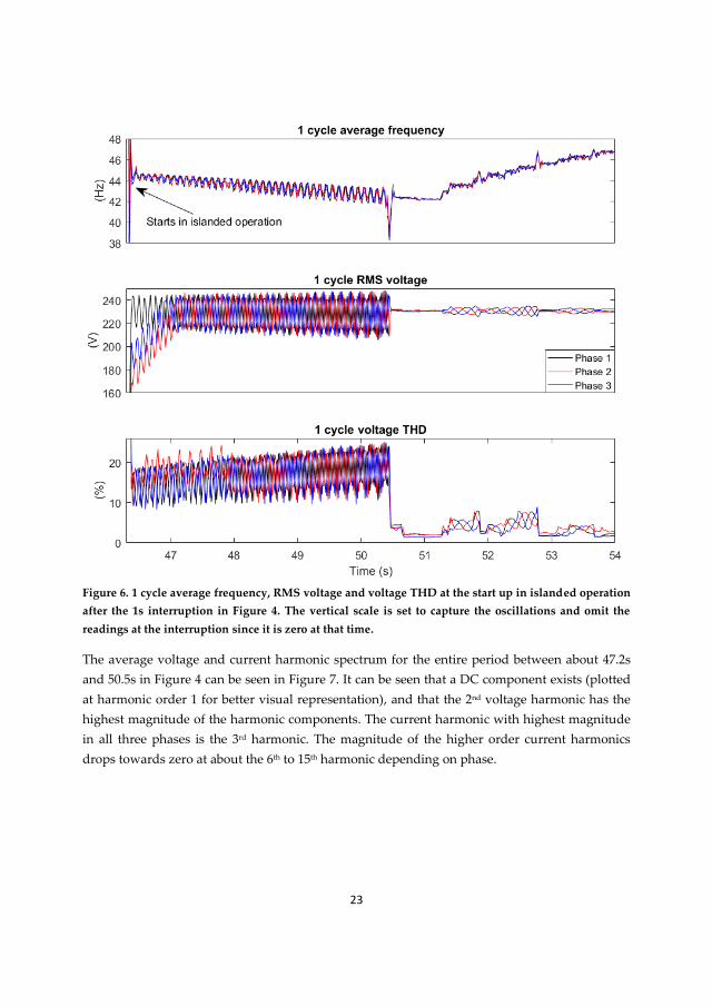
In Figure 6, a closer view of the oscillations in the startup in islanded operation in Figure 4 can

be seen for all three phases at 1 cycle resolution. It can be seen that the voltage oscillates between

210 and 240 V and that the voltage THD oscillates between 10% and 25% for about 4 s. Some

residual oscillations also occur for a couple of seconds at 51s to 54s in Figure 6. The oscillations

also seem to be shifted in time and are not syncronized between the three phases. The frequency

during the startup in islanded operation began at about 44 Hz and whent down for several

seconds to about 42 Hz to then drop momentarely to 38 Hz. After that, the frequency rose to

about 43 Hz and then began a climb towards 47 Hz.

23

Figure 6. 1 cycle average frequency, RMS voltage and voltage THD at the start up in islanded operation

after the 1s interruption in Figure 4. The vertical scale is set to capture the oscillations and omit the

readings at the interruption since it is zero at that time.

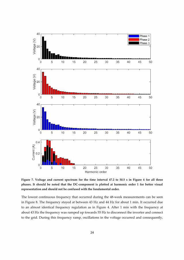
The average voltage and current harmonic spectrum for the entire period between about 47.2s

and 50.5s in Figure 4 can be seen in Figure 7. It can be seen that a DC component exists (plotted

at harmonic order 1 for better visual representation), and that the 2nd voltage harmonic has the

highest magnitude of the harmonic components. The current harmonic with highest magnitude

in all three phases is the 3rd harmonic. The magnitude of the higher order current harmonics

drops towards zero at about the 6th to 15th harmonic depending on phase.

24

Figure 7. Voltage and current spectrum for the time interval 47.2 to 50.5 s in Figure 4 for all three

phases. It should be noted that the DC-component is plotted at harmonic order 1 for better visual

representation and should not be confused with the fundamental order.

The lowest continuous frequency that occurred during the 48-week measurements can be seen

in Figure 8. The frequency stayed at between 43 Hz and 44 Hz for about 1 min. It occurred due

to an almost identical frequency regulation as in Figure 4. After 1 min with the frequency at

about 43 Hz the frequency was ramped up towards 55 Hz to disconnect the inverter and connect

to the grid. During this frequency ramp, oscillations in the voltage occurred and consequently,

25

temporal rise in voltage THD is seen. Only one of the phases is shown for better illustration, the

other phases looked similar.

Figure 8. 1 cycle average frequency, RMS voltage and voltage THD for the lowest continuous

frequency in the 48-week dataset which can be seen from 65s to 127s.

26

7. Transition between islanded and grid-connected operation

The transition from islanded to grid-connected operation and from grid-connected to islanded

operation can have different appearance in terms of voltage, current or frequency. In Figure 9,

two types of transitions from islanded to grid connected operation can be seen.

Figure 9. The different appearances in frequency and voltage for transitions towards grid-connected

operation (type 1 is at the left upper and lower side and type 2 is at the right upper and lower side).

The first that was shown in Figure 4 is where the frequency goes towards 55 Hz in order to shut

down the solar inverter. Then the frequency stays at 50 Hz for a couple of seconds and then goes

up to 52 Hz where the connection to the grid is made. The other type is where the frequency

goes towards 55 Hz to shut down the solar inverter and then goes down to 50 Hz and stays at 50

Hz where soon after, the grid-connection is made. They could be named type 1 (non-

synchronized transition) and type 2 (synchronized transition) respectively. In the type 1

transition, the frequency is ramped up to 52 Hz just before the grid-connection which means

that the microgrid system frequency is not synchronized to the utility grid which operates at 50

Hz. When the transition occurs, the voltage experiences a fluctuation from 200 V to 240 V and an

oscillation in the system frequency occurs at the same time. This can be seen in Figure 9 where

the left side is for type 1 and to the right type 2 can be seen. For type 2 a much smaller difference

in voltage and frequency during the transition occur than for type 1 which is due to the

27

frequency being close to synchronization with the utility grid. The reason for the frequency rise

to 52 Hz before connection to the utility grid for type 1 transition is unknown.

In Figure 10, the different transitions from grid-connected operation to islanded operation can

be seen. The first type can be seen at the top, the second in the midle and the third in the bottom

in Figure 10. The first one, which could be called a synchronized transition, occur with almost no

change in frequency but the voltage drops by 2 V momentarely. The second one which could be

called a non-synchronized transition occur with a voltage dip to to about 95 V and with a drop

in frequency. The third one, which could be called a failed transition, results in a 0.9s to 1s

interruption. The system then recoveres with a frequency that stays below 45 Hz for a couple of

seconds to one minute (see Figure 4 and Figure 8). The voltage RMS value and voltage THD

value oscillates for about 5 s where the voltage THD has a value of about 10% to 25%.

Figure 10. The difference in appearance of the voltage and frequency for transitions towards islanded

operation. The type 1 transition is at the top, the type 2 transition is in the middle and the type 3

transition is at the bottom.

28

8. Interruptions in Sweden and in a microgrid

In Figure 11, the cumulative distribution functions for the unplanned interruptions for all

customers in Sweden between the years 2011 and 2013 can be seen. Data for the different groups

defined in Paper B is presented as well as the total number of interruptions and total

interruption time for the 48-week dataset for islanded operation for the microgrid. It can be seen

that the total number of unplanned interruptions for the microgrid correspond to the upper

confidence limit in the 99.99% confidence interval for the 3 years of interruption data for all

costumers in Sweden. The total interruption time is within the 95% confidence interval for all

customers in Sweden, but the total number of interruptions goes beyond the 95% confidence

interval for all costumers in Sweden. It is however important to note that the microgrid studied

could be conducting maintenance that could add to the interruption data.

Figure 11. Cumulative distribution functions for the unplanned interruptions for all costumers in

Sweden for the years 2011, 2012 and 2013. The interruption data from Paper B is also presented for the

different groups of interruptions.

29

9. Voltage variations in a microgrid

The 1s RMS values for 48 weeks of voltage variations in islanded operation and in grid-

connected operation can be seen in Figure 12. All values with 1 s RMS lower than 200 V have

been removed (including interruption) to get a better visual representation to the variations

against the grid-connected operation. It can be seen that larger variations can occur during

islanded operation compared to in grid-connected operation. The variations are between about

210 V and 240 V during grid-connection which is within the ±10% allowed in standard

EN 50160. The variations are between about 200 V and 250 V during islanded operation which is

outside the ±10% allowed in standard EN 50160. It can also be seen in Figure 12 that the voltage

variations in islanded operation can also be smaller than in grid-connected operation. A more

detailed analysis of the voltage variations can be seen in Paper C.

Figure 12. Voltage variations for both grid-connected (right) and islanded operation (left) for a

microgrid.

In Figure 13 an example is shown of a voltage dip due to a large current being drawn. When the

large current is being drawn, the frequency drops towards 45 Hz during two cycles. In

Figure 14, a voltage transient occurs when a large load is disconnected and the current rapidly

goes from 35 A to 5 A (seen in the beginning of Figure 14). When the large load disconnects, the

frequency goes up to 51 Hz and then goes down to 50 Hz. A pulsating load that is still connected

after the large load is disconnected also causes voltage transients. The load has almost no

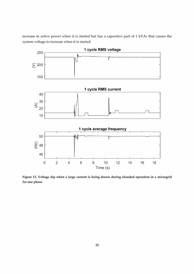
30

increase in active power when it is started but has a capacitive part of 1 kVAr that causes the

system voltage to increase when it is started.

Figure 13. Voltage dip when a large current is being drawn during islanded operation in a microgrid

for one phase.

31

Figure 14. Transient voltage when a large load is disconnected during islanded operation in a

microgrid for one phase.

32

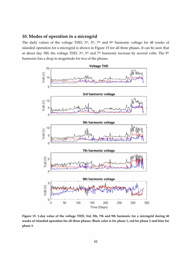
10. Modes of operation in a microgrid

The daily values of the voltage THD, 3rd, 5th, 7th and 9th harmonic voltage for 48 weeks of

islanded operation for a microgrid is shown in Figure 15 for all three phases. It can be seen that

at about day 300, the voltage THD, 3rd, 5th and 7th harmonic increase by several volts. The 9th

harmonic has a drop in magnitude for two of the phases.

Figure 15. 1-day value of the voltage THD, 3rd, 5th, 7th and 9th harmonic for a microgrid during 48

weeks of islanded operation for all three phases. Black color is for phase 1, red for phase 2 and blue for

phase 3.

33

The change in harmonic magnitude around day 300, seen in Figure 15, is caused by half of the

parallel connected systems described in Section 4 to fall offline due to two burnt cells in one of

the parallel batteries, i.e. the system goes into Mode 2 (as defined in Paper F). It was confirmed

by the microgrid owner that the microgrid was shifting to Mode 2 at the instance of the change

in harmonic magnitude (seen at around day 300 in Figure 15). As discussed in Paper C and F,

there are similar measurements of Mode 2 (half of the system active) and Mode 1 (both parallel

systems active) which indicate that there are reconnections into Mode 1 during the supposed

Mode 2 measurement time period. The reason for this is unknown. There are also shorter time

periods of suspected Mode 2 operation in the measurement time period which is shown in

Paper F. As shown in Paper F, the harmonic system impedance has increased when one of the

parallel systems has fallen offline and the harmonic system impedance also increases for some

harmonics when night operation occurs. An analysis of the harmonic levels of the different

modes can be seen in Paper C where the sub modes are also shown (night and day operation).

The transition from different modes of operation can also be seen in Paper F. To detect and

quantify changes in harmonic performance and the modes of operation, a new harmonic

performance index was created, defined in Equation (1), for a single harmonic and (2) for the

THD with the name apparent harmonic system impedance (AHSI). 𝑁 is the number of phases of

the system, 𝑃 is the phase number, ℎ is the harmonic order, 𝑛 is the largest harmonic order

measured in the THD, 𝑉 is the harmonic voltage magnitude and 𝐼 is the harmonic current

magnitude. AHSI incorporates the harmonic voltages and currents of all phases in a system and

calculates an apparent impedance which describes the ratio between two vector lengths (a more

detailed description is given in Paper F). From the AHSI index, the different modes of operation

are clearly visible as seen in Figure 16. The first of the two peaks in the beginning of Figure 16

with values above 14 V/A was discovered only after the AHSI was applied to the data. This

Mode 2 occurrence was not known in Paper C since it was not clearly visible in the voltage

distortion. The night and day operation using the AHSI index are clearly visible in Figure 8 and

Figure 9 in Paper F. An alternate version (version 2 in Figure 16) of the AHSI index is defined in

Equation (3) and (4) which only looks at the total average values of the voltages and currents

magnitudes for all phases. As seen in Figure 16, version 1 and 2 of the AHSI index gives similar

results. However, version 1 (Equation (1) and (2)) was set as the one used in Paper F purely out

of a subjective opinion from the author. There was no time in this thesis to further explore if one

of the versions was better in detecting different modes of operation and is left as future work to

decide this. However, since the AHSI index is not a physical impedance but an apparent

impedance. Both versions are acceptable to use.

34

Version 1

𝑍ℎ+ = √

∑ |𝑉𝑃ℎ|2𝑁𝑃=1

∑ |𝐼𝑃ℎ|2𝑁𝑃=1

(1)

𝑍𝑇𝐻𝐷+ = √

∑ (∑ |𝑉𝑃ℎ|2𝑁𝑃=1 )𝑛

ℎ=2

∑ (∑ |𝐼𝑃ℎ|2𝑁𝑃=1 )𝑛

ℎ=2

(2)

Version 2

𝑍ℎ

+ =∑ |𝑉𝑃ℎ|𝑁

𝑃=1

∑ |𝐼𝑃ℎ|𝑁𝑃=1

(3)

𝑍𝑇𝐻𝐷

+ =∑ (∑ |𝑉𝑃ℎ|𝑁

𝑃=1 )𝑛ℎ=2

∑ (∑ |𝐼𝑃ℎ|𝑁𝑃=1 )𝑛

ℎ=2

(4)

Figure 16. 10 min average of the two different versions of the THD-AHSI.

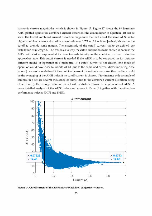
One of the drawbacks of the AHSI index is that a cutoff current has to be chosen. This cutoff

current was subjectively chosen as a harmonic current magnitude that is approximately the

lowest harmonic current magnitude that yields about the same AHSI values as higher values of

35

harmonic current magnitudes which is shown in Figure 17. Figure 17 shows the 9th harmonic

AHSI plotted against the combined current distortion (the denominator in Equation (1)) can be

seen. The lowest combined current distortion magnitude that had about the same AHSI as for

higher combined current distortion magnitude was 0.073 A. 0.1 A is subjectively chosen as the

cutoff to provide some margin. The magnitude of the cutoff current has to be defined per

installation or microgrid. The reason as to why the cutoff current has to be chosen is because the

AHSI will start an exponential increase towards infinity as the combined current distortion

approaches zero. This cutoff current is needed if the AHSI is to be compared in for instance

different modes of operation in a microgrid. If a cutoff current is not chosen, one mode of

operation could have close to infinite AHSI (due to the combined current distortion being close

to zero) or even be undefined if the combined current distortion is zero. Another problem could

be the averaging of the AHSI index if no cutoff current is chosen. If for instance only a couple of

samples in a set are several thousands of ohms (due to the combined current distortion being

close to zero), the average value of the set will be distorted towards large values of AHSI. A

more detailed analysis of the AHSI index can be seen in Paper F together with the other two

performance indexes PHIPI and SHIPI.

Figure 17. Cutoff current of the AHSI index (black line) subjectively chosen.

36

Another performance index that was published in Paper C, is the apparent RMS system

impedance (ARMSSI) defined in Equation (5) with symbol 𝑍𝑅𝑀𝑆+ where 𝑖 is a certain point in

time, 𝑉𝑅𝑀𝑆 is the phase voltage RMS value and 𝐼𝑅𝑀𝑆 is the phase current RMS value . In paper C

it went by the name “short circuit impedance”. It describes the phase RMS voltage drop due to a

certain phase RMS current increase.

𝑍𝑅𝑀𝑆

+ =|𝑉𝑅𝑀𝑆(𝑖)| − |𝑉𝑅𝑀𝑆(𝑖 + 1)|

|𝐼𝑅𝑀𝑆(𝑖 + 1)| − |𝐼𝑅𝑀𝑆(𝑖)| 𝑤ℎ𝑒𝑟𝑒 |𝐼𝑅𝑀𝑆(𝑖 + 1)| > |𝐼𝑅𝑀𝑆(𝑖)| (5)

This index came to be due to the limitations in the measurements. The current and voltage phase

angle in Elspec G4430 is measured for a 10-cycle period. However, voltage regulation occurs on

a shorter time scale as can be seen in the example in Figure 18 as the phase voltage is increased

after a current rise.

Figure 18. Time series example of the phase voltage and current, active and reactive power for one

phase. The resolution is one cycle.

37

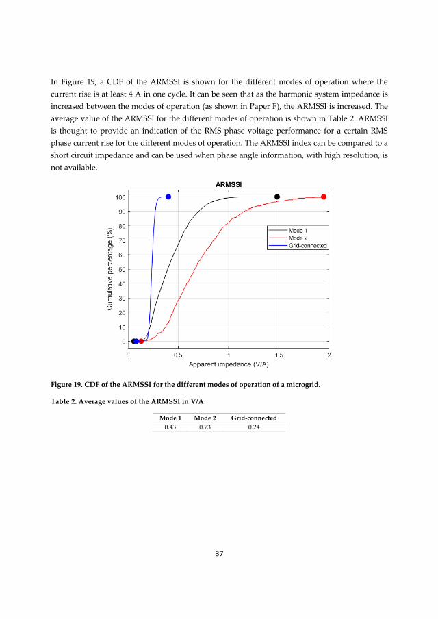
In Figure 19, a CDF of the ARMSSI is shown for the different modes of operation where the

current rise is at least 4 A in one cycle. It can be seen that as the harmonic system impedance is

increased between the modes of operation (as shown in Paper F), the ARMSSI is increased. The

average value of the ARMSSI for the different modes of operation is shown in Table 2. ARMSSI

is thought to provide an indication of the RMS phase voltage performance for a certain RMS

phase current rise for the different modes of operation. The ARMSSI index can be compared to a

short circuit impedance and can be used when phase angle information, with high resolution, is

not available.

Figure 19. CDF of the ARMSSI for the different modes of operation of a microgrid.

Table 2. Average values of the ARMSSI in V/A

Mode 1 Mode 2 Grid-connected

0.43 0.73 0.24

38

11. Constructing a standalone microgrid in Sweden

In northern Sweden, the main challenge with a standalone microgrid is how the electricity will

be produced during winter. A theoretical calculation can be made to study how much energy

storage, solar and wind production is needed for a household in northern Sweden that is

disconnected from the main utility grid. Measured consumption data for a house with heat

pump heating in northern Sweden is obtained from a utility company where the yearly

electricity consumption for the house is about 20674 kWh (which is about the same number used

by Statistics Sweden to represent a house in Sweden with electrical heating (20000 kWh) [96]).

Simulated solar and wind production for four different locations (seen in Table 3) for the year

2014 is obtained from [97], [98], [99]. The yearly mean annual capacity factor with no losses for

2014 for both solar and wind production is also shown in Table 3 for the different locations. It

should be noted that Location 3 (L3) is used only for showing results, if a larger solar annual

mean capacity factor is used than the ones for Location 1 (L1), Location 2 (L2) and Location 4

(L4), even though L3 is located in southern Europe.

Table 3. Annual mean capacity factors for wind and solar production with no system losses for four

different locations in Europe for the year 2014.

Abbreviation L1 L2 L3 L4

Location Skellefteå,

Sweden

Ottenby,

Sweden

Punta Umbria,

Spain

Å,

Norway

Annual mean solar capacity factor with full solar tracking 15.5% 17.6% 27.5% 14.9%

Annual mean wind capacity factor 20 m hub height 7.1% 36.1% 27.7% 45.9%



The following assumptions are also made:

• The house only receives electricity from solar PV or a wind turbine together with an energy

storage unit with no losses.

• No constraints in load flow are made.

• No lower limit of production is assumed for the wind turbine and solar PV installation.

• The measured consumption pattern with the yearly electricity consumption of 20674 kWh

applies for all locations.

• The energy storage can´t contain more energy than 100%. If an excess production occurs

from the solar PV or wind turbine that can´t be stored in the energy storage the production is

curtailed.

39

The simulation is made by taking the hourly consumption in the house and subtract the hourly

production from the solar PV or wind turbine. The difference causes either a discharge or

charging of the energy storage unit.

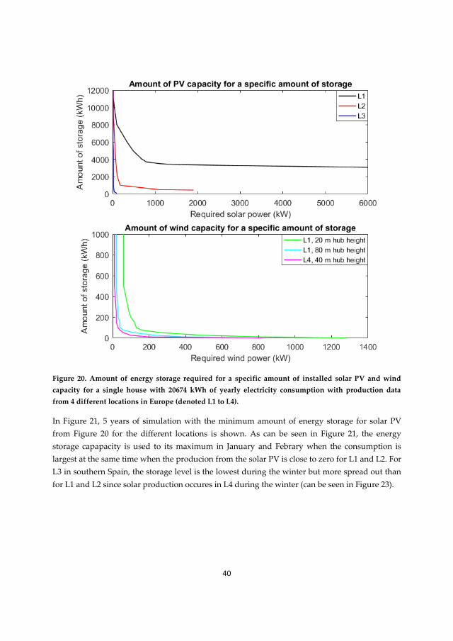
The result of the simulation for the different locations in Table 3 using the measured household

consumption pattern with 20674 kWh of annual electricity consumption can be seen in

Figure 20, where the theoretical amount of PV capacity with full solar tracking and wind

capacity for different hub heights is plotted against the needed energy storage. Only L1 to L3

was chosen for the solar production since L1 and L4 have similar annual mean solar capacity

factors. For the wind production simulations, L1 with 20 m and 80 m hub height and L4 with

40 m hub height were chosen for comparing the results with different capacity factors for wind

production.

It can be seen in the upper part of Figure 20 that the amount of installed PV capacity for the

minimum amount of energy storage of 3000 kWh for L1 (located in northern Sweden) is around

6000 kW. For Ottenby in southern Sweden (L2), the minimum amount of energy storage is

around 500 kWh at almost 2000 kW installed PV capacity. For Punta Umbria in Spain (L3), the

minimum amount of energy storage is 90 kWh for 100 kW installed PV capacity. This means that

less storage is needed with larger annual mean solar capacity factor. These values are obtained

just before the installed PV capacity goes towards infinity for all three locations. This happens

because the solar production is zero at some point in time where consumption occur which

causes infinite capacity to be installed in an attempt to deliver power at that point in time.

It can be seen in the lower part of Figure 20 that it is theoretically possible to operate a

standalone microgrid with zero kWh of storage if 1300 kW wind turbine capacity is installed at

20 m hub height and around 800 kW at 80 m for L1. For Å in Norway (L4), only 40 m hub height

is required for getting approximately the same result as for 80 m in L1 at 820 kW for zero energy

storage. This means that less storage is needed with larger annual mean wind capacity factor

and with higher hub height on the wind turbine. However, if a longer time series with

consumption and production would be taken there would eventually come a point in which the

production from the wind turbine is zero and the consumption of the house is above zero,

resulting in infinite wind capacity to be installed which means that more than zero energy

storage is required. In reality, the wind turbine has a lower limit of usable wind speed which has

not been considered. If it is considered, it will lead to more than zero energy storage. However,

for this year with this specific consumption pattern, it is theoretically possible to achieve zero

energy storage with a wind turbine for the standalone microgrid.

40

Figure 20. Amount of energy storage required for a specific amount of installed solar PV and wind

capacity for a single house with 20674 kWh of yearly electricity consumption with production data

from 4 different locations in Europe (denoted L1 to L4).

In Figure 21, 5 years of simulation with the minimum amount of energy storage for solar PV

from Figure 20 for the different locations is shown. As can be seen in Figure 21, the energy

storage capapacity is used to its maximum in January and Febrary when the consumption is

largest at the same time when the producion from the solar PV is close to zero for L1 and L2. For

L3 in southern Spain, the storage level is the lowest during the winter but more spread out than

for L1 and L2 since solar production occures in L4 during the winter (can be seen in Figure 23).

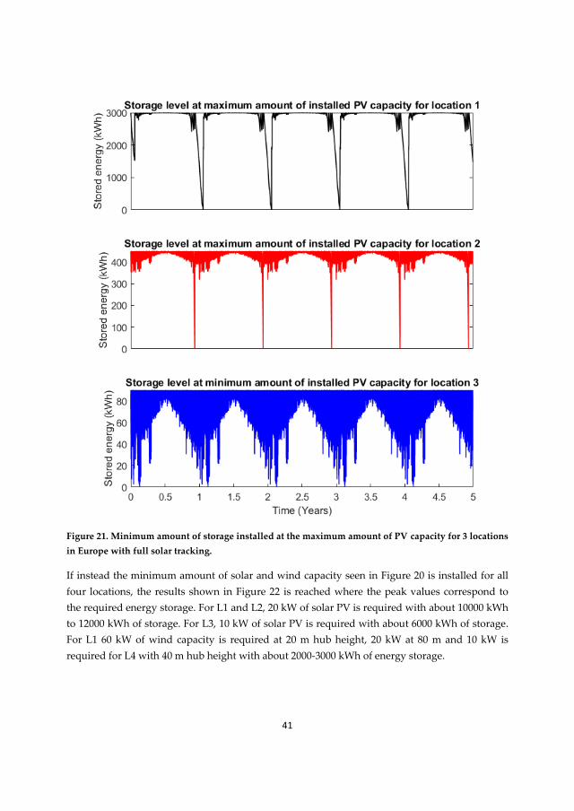
41

Figure 21. Minimum amount of storage installed at the maximum amount of PV capacity for 3 locations

in Europe with full solar tracking.

If instead the minimum amount of solar and wind capacity seen in Figure 20 is installed for all

four locations, the results shown in Figure 22 is reached where the peak values correspond to

the required energy storage. For L1 and L2, 20 kW of solar PV is required with about 10000 kWh

to 12000 kWh of storage. For L3, 10 kW of solar PV is required with about 6000 kWh of storage.

For L1 60 kW of wind capacity is required at 20 m hub height, 20 kW at 80 m and 10 kW is

required for L4 with 40 m hub height with about 2000-3000 kWh of energy storage.

42

Figure 22. Amount of storage required (the peak values) for the minimum amount of installed solar PV

and wind capacity. The yearly electricity consumption was 20674 kWh for a single house. Production

data from 4 different locations in Europe (denoted L1 to L4) was used.

The results presented in Figure 20 to Figure 22 show that it is not an easy task to construct a

solar or wind power based standalone microgrid without some form of energy storage that can

be converted into electricity. One project that has been initiated by a utility company in Sweden

is the Zero Sun project, located in the municipality of Skellefteå (64°45′2″N 20°57′10″E) [8] where

25 kW of solar capacity is combined with 6000 kWh of hydrogen storage and 100 kWh of battery

storage to enable the house to be islanded all year around.

In Figure 23, the measured consumption for a Swedish household located in northern Sweden

and for a simulated household in Spain by [100] can be seen together with the fully tracked solar

production at the same location. The main difference between the household consumption in the

two countries is the amount of energy consumed and when it is consumed. The annual

consumption for the simulated house in Spain is 4800 kWh and in the measured house in

Sweden 20674 kWh which is about 4 times more, mostly due to extra heating. It can be seen in

Figure 23 that a house in Spain has the largest power consumption during the winter and

summer. For the house in northern Sweden, the largest consumption occurs during the winter

where almost zero PV production occur (in the simulated data it is zero due to snow coverage).

It can also be seen that the production from the solar PV is more spread out during the year for

43

Spain and that during the summer, the daily average of the solar production is higher in

northern Sweden than in Spain since the sun is almost up all the time during a 24 hour period.

This mismatch between consumption and production in northern Sweden is a problem for a

standalone microgrid in Sweden. By shifting the consumption to the summer by producing for

instance hydrogen, this mismatch between consumption and production can be solved.

Figure 23. Daily electricity demand for a house in northern Sweden and for a house located in Spain.

The daily production for 1 kW of solar PV for Skellefteå in northern Sweden and Punta Umbria in

southern Spain is also shown with full solar tracking.

44

12. Case study of the reliability in rural grids in Sweden

One important aspect of constructing a standalone microgrid instead of a traditional grid-

connection is the possibility of increased reliability [11], [10], [12]. Detailed data have been

obtained from a Swedish utility company with three rural grids in northern Sweden. This

section is to illustrate what the reliability in a rural grid could be. In Table 4, the average annual

electricity consumption for 10 years, total MV and LV overhead line length and number of

customers for three rural grids located in northern Sweden are presented.

Table 4. Data for three existing rural grids in northern Sweden.

Grid Number of

customers

Average annual electricity

consumption per customer (kWh)

Total MV line length

(m)

Total LV line length

(m)

1 2 1114 1500 627

2 3 10016 2700 822

3 2 9394 2200 761

In Figure 24, the total daily consumption for all the customers in the three grids can be seen for

the years between 2006 and 2015. For Grid 1, the consumption can be zero for several months. In

Grid 1, instances of high consumption with short duration occur after periods of zero

consumption, which could indicate heating of the houses after a prolonged period of zero

electricity consumption.

Figure 24. Total daily electricity consumption for the three rural grids in northern Sweden between the

years 2006-2015.

45

In Table 5, the annual average number of planned and unplanned interruptions is presented

together with the annual average interruption time for the three rural grids. The data for the

interruptions covers the years 2009 to 2015. The percentages in the parentheses correspond to

the average equivalent cumulative percentage for interruption data containing all customers in

Sweden between the years 2011 to 2013 where some indexes of that data can be seen in Table 6.

The interruption data for the three grids are in the upper range of the data for all customers in

Sweden where some parameters are above the upper confidence limit (UCL) for the 95% and

97.5% confidence interval. This shows that a potential exists for improving the reliability of

electricity supply if a standalone microgrid would be implemented for these three rural grids. In

Table 7, the main causes for the unplanned interruptions in the three grids is shown which are

weather related events such as lightning strikes, heavy snow, ice buildup, wind and trees that

fall over the overhead lines. Of the weather-related events, falling trees cause the longest

downtime in the three grids. If all events due to weather are considered, then they amount to

over 70% of the total annual unplanned interruption downtime and over 60% of the annual

unplanned interruptions for the three rural grids. The rest is caused by technical malfunction. A

similar list for grids in a different climate e.g. Spain would give different results.

Table 5. Interruption data for the three rural grids where the percentages in the parentheses represent

the average cumulative percentage for the interruption data for all customers Sweden between the

years 2011 to 2013.

Grid Average number of

unplanned interruptions

per year

Average unplanned

interruption time per

year (h)

Average number of

planned interruptions

per year (rounded

upwards)

Average planned

interruption time

per year (h)

1 11.6 (96.5%) 11.0 (94.8%) 1.3 (98.9%) 2.6 (96.1%)

2 23.7 (99.2%) 17.7 (97.0%) 1.7 (98.9%) 3.9 (97.7%)

3 20.0 (98.7%) 10.8 (94.7%) 1.6 (98.9%) 2.8 (96.4%)

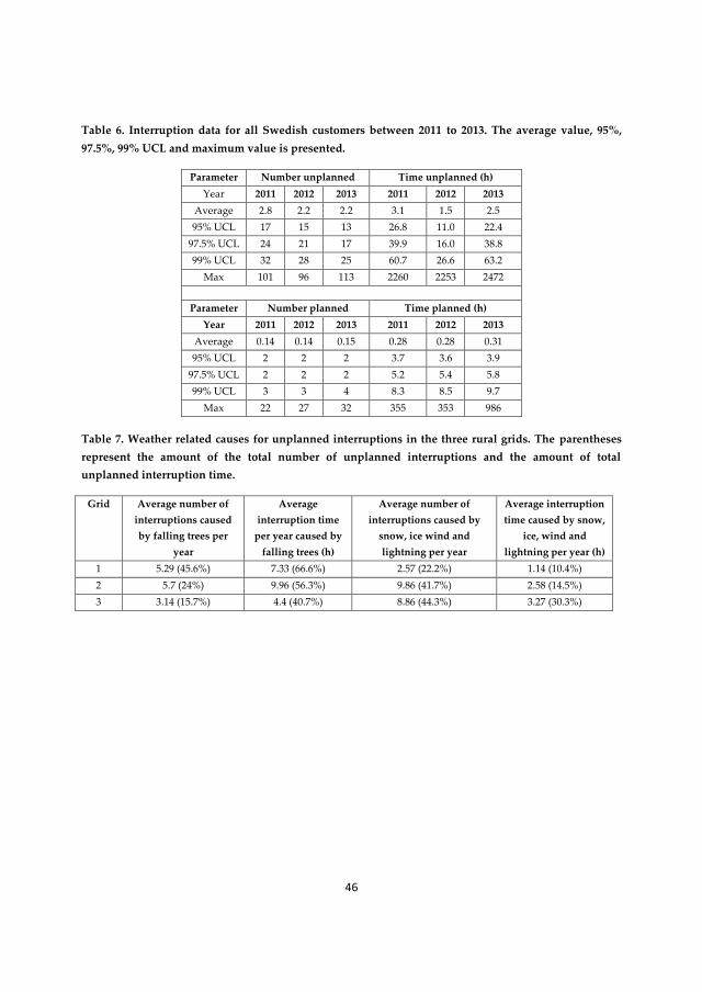
46

Table 6. Interruption data for all Swedish customers between 2011 to 2013. The average value, 95%,

97.5%, 99% UCL and maximum value is presented.

Parameter Number unplanned Time unplanned (h)

Year 2011 2012 2013 2011 2012 2013

Average 2.8 2.2 2.2 3.1 1.5 2.5

95% UCL 17 15 13 26.8 11.0 22.4

97.5% UCL 24 21 17 39.9 16.0 38.8

99% UCL 32 28 25 60.7 26.6 63.2

Max 101 96 113 2260 2253 2472

Parameter Number planned Time planned (h)

Year 2011 2012 2013 2011 2012 2013

Average 0.14 0.14 0.15 0.28 0.28 0.31

95% UCL 2 2 2 3.7 3.6 3.9

97.5% UCL 2 2 2 5.2 5.4 5.8

99% UCL 3 3 4 8.3 8.5 9.7

Max 22 27 32 355 353 986

Table 7. Weather related causes for unplanned interruptions in the three rural grids. The parentheses

represent the amount of the total number of unplanned interruptions and the amount of total

unplanned interruption time.

Grid Average number of

interruptions caused

by falling trees per

year

Average

interruption time

per year caused by

falling trees (h)

Average number of

interruptions caused by

snow, ice wind and

lightning per year

Average interruption

time caused by snow,

ice, wind and

lightning per year (h)

1 5.29 (45.6%) 7.33 (66.6%) 2.57 (22.2%) 1.14 (10.4%)

2 5.7 (24%) 9.96 (56.3%) 9.86 (41.7%) 2.58 (14.5%)

3 3.14 (15.7%) 4.4 (40.7%) 8.86 (44.3%) 3.27 (30.3%)

47

13. Techno economic modeling for a standalone microgrid

In Paper E, a techno economic energy flow model was developed to estimate the LCC for a

standalone microgrid for a specific location. From the LCC, the BEMVLL can be derived with

Equation (5) presented in Paper E which gives a quantitative measurement of comparison to the

traditional grid-connection. It is the length of the medium voltage line that is required for the

traditional grid-connection to get the same LCC as for a standalone microgrid for a certain

amount of annual energy consumption under the assumption that equal low voltage line length

exists in both the grid-connection and standalone microgrid. The BEMVLL gives a

straightforward index of how far away a rural part of the distribution grid needs to be from a

MV PCC for it to be economically feasible to construct a standalone microgrid instead of the

traditional grid-connection. The BEMVLL could be used by utility companies to investigate

which parts of their distribution grid that can be converted to standalone microgrids to lower

the LCC of that part of the distribution grid. The investment risk is an important parameter

when an investment is to be made. For investing in a standalone microgrid, changes in

consumption is an important parameter to consider which was shown in Paper E. The largest

parameter of importance is the amount of annual consumption as shown in Paper E. In addition,

the time of consumption and peak consumption is of importance. Measures such as peak

consumption limitation and shifting of consumption to times with more production from the

wind turbine and solar PV could be incorporated by the customers to enable cost-effective

operation of standalone microgrids. However, results from [101], [102], [103], [104], show that

the willingness of the customers in doing so differ. Another investment risk that was not

discussed in Paper E was the risk of changes to the diesel fuel price which can be illustrated in

Figure 25 where the historical daily 100% renewable diesel fuel price is shown (including 25%

VAT) obtained from two fuel companies in Sweden. The difference between the maximum price

and the minimum price is 103.9% showing that price changes poses an investment risk to a

standalone microgrid that incorporates diesel generators (which was used in Paper E).

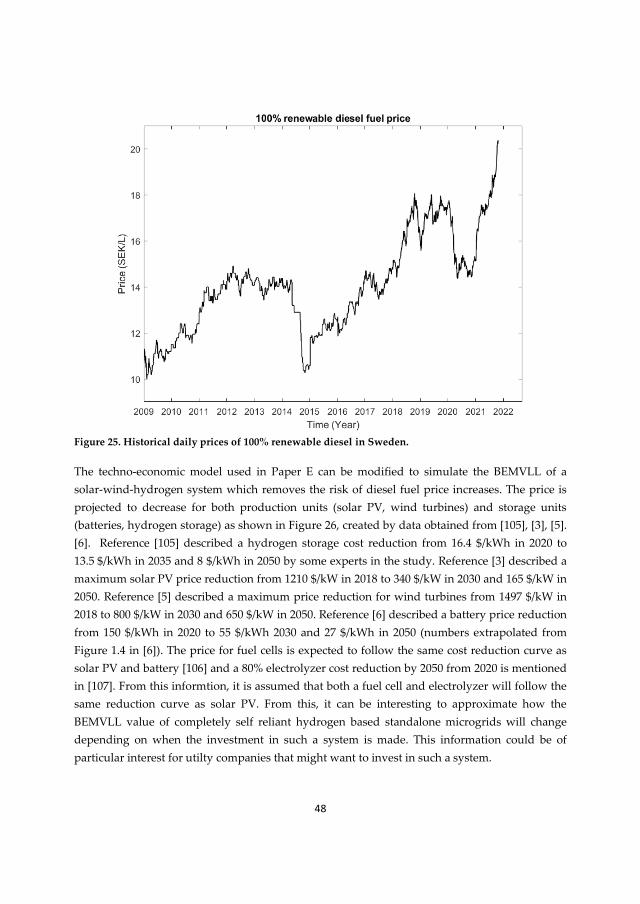
48

Figure 25. Historical daily prices of 100% renewable diesel in Sweden.

The techno-economic model used in Paper E can be modified to simulate the BEMVLL of a

solar-wind-hydrogen system which removes the risk of diesel fuel price increases. The price is

projected to decrease for both production units (solar PV, wind turbines) and storage units

(batteries, hydrogen storage) as shown in Figure 26, created by data obtained from [105], [3], [5].

[6]. Reference [105] described a hydrogen storage cost reduction from 16.4 $/kWh in 2020 to

13.5 $/kWh in 2035 and 8 $/kWh in 2050 by some experts in the study. Reference [3] described a

maximum solar PV price reduction from 1210 $/kW in 2018 to 340 $/kW in 2030 and 165 $/kW in

2050. Reference [5] described a maximum price reduction for wind turbines from 1497 $/kW in

2018 to 800 $/kW in 2030 and 650 $/kW in 2050. Reference [6] described a battery price reduction

from 150 $/kWh in 2020 to 55 $/kWh 2030 and 27 $/kWh in 2050 (numbers extrapolated from

Figure 1.4 in [6]). The price for fuel cells is expected to follow the same cost reduction curve as

solar PV and battery [106] and a 80% electrolyzer cost reduction by 2050 from 2020 is mentioned

in [107]. From this informtion, it is assumed that both a fuel cell and electrolyzer will follow the

same reduction curve as solar PV. From this, it can be interesting to approximate how the

BEMVLL value of completely self reliant hydrogen based standalone microgrids will change

depending on when the investment in such a system is made. This information could be of

particular interest for utilty companies that might want to invest in such a system.

49

Figure 26. Future price decrease of Batteries, Solar PV, Wind turbines and hydrogen storage.

If it is further assumed that inverters will follow the solar PV cost reduction, the main

components for a standalone hydrogen based microgrid has a price in the future and the

BEMVLL can be obtained. By using the same specifications for the fuel cell and electrolyzer

(5 kW) as the stuedied microgrid described in Section 4 and letting the battery size, hydrogen

storage, solar PV and wind turbine be selected from the lowest LCC solution, a simulation can

be made to obtain the BEMVLL for different annual energy consumptions. It is assumed that a

GHP exists to create heat when needed and the leftover heat from the fuel cell and electrolyer is

also incorporated to supply heat to the microgrid. If there is an excess of solar PV or wind

turbine production, the electricity is used to heat water in accumulator tanks throught resisitive

heating elements located in the accumulator tanks. The electrical efficeincy of a fuel cell was

47.9% in [108] and slightly above 50% in [109]. From this 50% is assumed. The electrical

efficiency of the electrolyzer is assumed to be 60% which is a number shown in [110]. The life of

a fuel cell used in stationary applications was 40000 hours in [111] and also 40000 hours for an

electrolyzer in [112]. From this 40000 hours is assumed for the fuel cell and the electrolyzer. The

size of the accumulator tank and the heat loss function of the accumulator tank was the same as

in Paper E. The same heat and electricity demand function as in Paper E was used together with

a measured consumption pattern from a house in northern Sweden that had a geothermal heat

pump as heat source. A compressor with a rating of 0.25 kW per 5 kW electrolyzer is

incorporated in order to compress hydrogen for storage to 300 bars. Location 1 and Location 2 in

50

Paper E was used with the same production data for the solar PV and wind turbine production.

The only difference is that only a 30m hub height is used for this simulation to simplify the

calculations. Another difference to Paper E is that the price per kW of solar PV and wind turbine

was selected to not be dependent on size of installation and was set to the lowest cost per kW to

simplify the calculations. The complete technical specifications and costs for the simulation that

are different from Paper E can be seen in Table 8. All costs for the stove and diesel generator is

removed for this simulation since this calculation does not utiluze them. The costs for the fuel

cell, electrolyzer, hydrogen storage and compressor was obtained from the owner of the studied

microgrid described in Section 4. All other costs are obtained from Paper E except the GHP costs

obtained in the year 2021 from a retaler in Sweden. The GHP drilling cost is only for the initial

investment and only the GHP is reinvested every 20 years. The electrolyzer and fuel cell is

reinvested after every 40000 operational hours. Another change in comparison to Paper E is the

incorporation of an optimization alogarithm that decides the optimal time to start and stop the

electrolyzer and fuel cell in order to maximize the hydrogen production by the electrolyzer and

make sure that the fuel cell keeps the battery SoC above 10%.

Table 8. Technical specifications and costs used for the hydrogen simulation.

Hydrogen storage

cost per kWh

Electrolyzer cost per

kW

Compressor cost per

electrolyzer kW

Fuel cell cost per kW GHP cost

146.4 SEK 86000 SEK 21400 SEK 82000 SEK 56000 SEK

GHP drilling cost Sun cost per kW Wind cost per kW Sun and wind

inverter cost per kW

Electrolyzer and fuel

cell life [111]

104000 SEK 6800 SEK 24435 SEK 700 SEK 40000 hours

Compressor life

(assumed)

Hydrogen tank life

(assumed)

Heat pump life

(assumed)

Fuse size at 230 V

per phase for the

household loads

Heat pump SCOP

(assumed)

20 Years 30 years 20 years 3x25 A 4

Electrical efficiency

fuel cell, assumed

with data from [108]

, [109]

Electrical efficiency

electrolyzer,

assumed from [110]

Fuel cell heat

efficiency (assumed)

Electrolyzer heat

efficiency (assumed)

Compressor power

consumption per 5

kW electrolyzer

50% 60% 40% 30% 0.25 kW

The itteration step size for the battery, solar PV, wind turbine, hydrogen storage that was used

in the simulations can be seen in Table 9.

Table 9. Itteration step size for the energy production and storage variables in the simulations.

Battery Hydrogen storage Solar PV Wind turbine

Step size 13.5 kWh 200 kWh 0.15-10 kW 0.05-10 kW

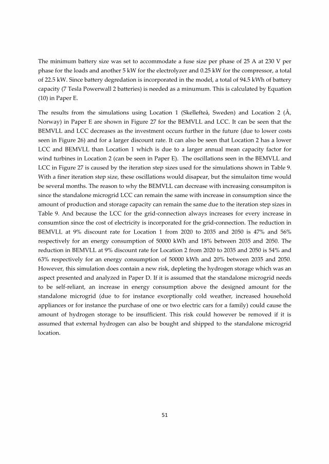
51

The minimum battery size was set to accommodate a fuse size per phase of 25 A at 230 V per

phase for the loads and another 5 kW for the electrolyzer and 0.25 kW for the compressor, a total

of 22.5 kW. Since battery degredation is incorporated in the model, a total of 94.5 kWh of battery

capacity (7 Tesla Powerwall 2 batteries) is needed as a minumum. This is calculated by Equation

(10) in Paper E.

The results from the simulations using Location 1 (Skellefteå, Sweden) and Location 2 (Å,

Norway) in Paper E are shown in Figure 27 for the BEMVLL and LCC. It can be seen that the

BEMVLL and LCC decreases as the investment occurs further in the future (due to lower costs

seen in Figure 26) and for a larger discount rate. It can also be seen that Location 2 has a lower

LCC and BEMVLL than Location 1 which is due to a larger annual mean capacity factor for

wind turbines in Location 2 (can be seen in Paper E). The oscillations seen in the BEMVLL and

LCC in Figure 27 is caused by the iteration step sizes used for the simulations shown in Table 9.

With a finer iteration step size, these oscillations would disapear, but the simulaiton time would

be several months. The reason to why the BEMVLL can decrease with increasing consumpiton is

since the standalone microgrid LCC can remain the same with increase in consumption since the

amount of production and storage capacity can remain the same due to the iteration step sizes in

Table 9. And because the LCC for the grid-connection always increases for every increase in

consumtion since the cost of electricity is incorporated for the grid-connection. The reduction in

BEMVLL at 9% discount rate for Location 1 from 2020 to 2035 and 2050 is 47% and 56%

respectively for an energy consumption of 50000 kWh and 18% between 2035 and 2050. The

reduction in BEMVLL at 9% discount rate for Location 2 from 2020 to 2035 and 2050 is 54% and

63% respectively for an energy consumption of 50000 kWh and 20% between 2035 and 2050.

However, this simulation does contain a new risk, depleting the hydrogen storage which was an

aspect presented and analyzed in Paper D. If it is assumed that the standalone microgrid needs

to be self-reliant, an increase in energy consumption above the designed amount for the

standalone microgrid (due to for instance exceptionally cold weather, increased household

appliances or for instance the purchase of one or two electric cars for a family) could cause the

amount of hydrogen storage to be insufficient. This risk could however be removed if it is

assumed that external hydrogen can also be bought and shipped to the standalone microgrid

location.

52

Figure 27. BEMVLL and LCC for different discount rates, location and initial investment year (2020,

2035 and 2050).

53

14. Critical review of own research

Papers A, B, C, F

The results in Paper A are based on measurements from one microgrid, with specific system

components and loads. The conclusions might not be general for all microgrids as they could be

designed in a different way and contain different types of loads. However, the conclusions are

based on long-term continuous measurements of 48 weeks in islanded operation and 54 weeks

in grid-connected where loads (and combination of loads) inside the microgrid varies. Similar

analysis of the same scope as Paper A, B, C and F of different microgrids have not been found in

the literature. Some papers [44], [45] give the indication that the harmonic voltage levels will be

larger in islanded operation than in grid-operation due to larger harmonic system impedance

which support the findings in Paper A, C and F.

Paper B, C

The papers present several possible negative effects on connected equipment from a change in

grid frequency, higher voltage distortion, higher voltage unbalance and are based on the

assumption that equipment will be negatively affected when the limits in standards are

exceeded. Actual effects on equipment connected in the microgrid (malfunctions etc.) has not

reported by the owner of the microgrid except for clocks that clocks of connected equipment

could run with the wrong time. So even if the limits in standards are surpassed, it is not certain

that the actual equipment will be negatively affected.

Paper D

The paper presents the risks of depleting the hydrogen storage for a microgrid in Northern

Scandinavia. The results should also have been compared towards solar datasets from more

southern parts of the world with a more continuous production throughout the year, as shown

in Figure 1 in Paper D. A comparison against a microgrid with wind production or a

combination of wind and solar production should also have been made since a combination of

solar and wind production could have evened out the yearly production, especially during the

winter. Comparison of results to solar production datasets in the southern parts of the world

should be conducted in future work. Results from an analysis with wind production data or a

combination of solar and wind production should also be made in future work. However, the

paper still brings out the risks of self-sustained energy supply.

54

Paper E

Paper E has not isolated the effect on the LCC and BEMVLL from changes to peak consumption

alone for the HR-SMG. The peak consumption in Paper E for a HR-SMG could not be isolated

because the peak in consumption is actually a time dependent variable, i.e. depending on when

the peak consumption occurs, it will affect the LCC and BEMVLL differently. This is because

peak consumption is also an amount of consumption at a specific time instance since the time

resolution in the TEEFM is in hours. An increase in peak consumption will increase the amount

of system components needed to service the increase in peak consumption for a HR-SMG. If the

increased peak consumption occurs during times with sufficient solar/wind production and/or

sufficient amount of battery SoC, only the cost of additional production (solar/wind) and/or

storage capacity (battery capacity) to service the increased peak consumption occur in the

TEEFM. If the increased peak consumption occurs at times with insufficient solar/wind

production in combination with low battery SoC, an increase in production capacity

(solar/wind) and/or storage capacity (battery) and/or diesel generator capacity occur in the

TEEFM, with a possible increase in diesel fuel consumption and additional operational hours for

the diesel generator. So, depending on the time in which the increased peak consumption

occurs, the LCC and BEMVLL will be affected in different magnitudes.

Paper F

The four new performance indexes might only be applicable to microgrids or in grids with

several different operational modes with sufficient performance difference, since small changes

in performance might just be seen as noise when interpreting the values of the performance

indexes. However, this is also for instance the case for studies conducted with only the voltage

distortion magnitude (Paper A and C). Nonetheless, the indexes have application in microgrids

such as detection and performance quantification. Future work is needed to establish if these

new indexes has application in the regular utility grid.

55

15. Conclusions

This work has led to a deeper understanding on the power quality in microgrids running in

islanded operation and the economic operation and investment risks of standalone microgrids.

A list of the main conclusions from this work is presented below:

1. For the microgrid studied, frequency variations are larger in islanded operation if

curtailment of production has to be made. However, the larger frequency variations can be

completely removed if the microgrid stays in islanded operation i.e. no 55 Hz transition is

needed to shut down the solar inverter in order for the microgrid to synchronize to the

utility grid. If no curtailment of production is needed the frequency variations between 51

and 52 Hz could be removed. If no increase in frequency occurs, then no decrease in

frequency to 49 Hz is needed to compensate for the over frequency in order for e.g. clocks to

operate at correct time, which is done on a 12-hour basis. Under islanded operation when no

curtailment or switching to grid-connected operation occur, the frequency in the islanded

microgrid is close to 50 Hz.

2. Microgrids that have similar frequency control systems as the studied microgrid can go

above the recommended frequency limits for electrical motors defined by IEC Standard

60034-1 and can operate at such a low frequency that there could be single phase electrical

motors that can´t disconnect from its start winding causing malfunction or failure (see Paper

B). Computer power supplies could be affected by the lower than 47 Hz values described in

Paper B. Transformers following IEC 60076-1 could also be affected as discussed in Paper B.

The frequency variations in islanded operation exceeded the weekly limit described in

EN 50160 for 89.6% of the measurement time period.

3. The voltage distortion reaches higher values in islanded operation than in grid-connected

operation. The values in islanded operation can exceed the limits described in standards

IEEE 519-2014 and EN 50160. The voltage unbalance was seen to occasionally reach 4.6%

during islanded operation. This magnitude of voltage unbalance, present for a period of 30

minutes, could cause a temperature rise of 40.5% for a 3-phase motor calculated with a

formula in [113]. On average, the temperature of a 3-phase motor would be lower in

islanded operation since the voltage unbalance is on average lower in islanded operation

than in grid-connected operation. If it is assumed that the Arrhenius model applies (used in

IEEE standard 101) the lifetime of a 3-phase motor might increase in islanded operation.

However, the shorter time periods with larger voltage unbalance causing temperature

increases of over 40% might counteract this effect.

56

4. The Pst and Plt values could be larger in islanded operation which would cause flicker in

incandescent lamps. With today’s LED lamps, it is possible that either more or less light

flicker could occur as shown in [114].

5. Paper B and C reported that connected equipment can be affected by the increased

frequency variations, voltage distortion and voltage unbalance. The residents in the

microgrid house has not reported any malfunction in the equipment other than that the

clocks can operate at some time deviation caused by the larger frequency variations.

6. The total interruption time in the studied microgrid is within the 95% confidence interval

but the total number of interruptions goes beyond the 95% confidence interval for all

costumers in Sweden. The majority of the interruptions occur when the microgrid transitions

into islanded operation from grid-connected operation.

7. Several modes of operation in islanded operation exist. Mode 1 and Mode 2 with their night

and day operation are shown in Paper C and Paper F. Mode 2 has higher voltage distortion

and harmonic system impedance than Mode 1. Mode 2 occurs when one of the parallel

energy systems goes offline in the studied microgrid. The day operation for the microgrid

occurs when the sun is above the horizon and subsequently, night operation occurs when

the sun is below the horizon. Higher voltage distortion occurs during the night operation in

both Mode 1 and Mode 2 as shown in Paper C and Paper F. This could occur because fewer

parallel sources are available for the loads. As discussed in Paper F, filter operations could

also be a cause of the higher voltage distortion that occur during night operation. However,

these two hypotheses have not been possible to verify. The Mode 2 operation suggests that a

microgrid with lower power rating will be more susceptible to higher voltage distortion

since the harmonic system impedance was higher in Mode 2 with 50% microgrid power

supply capacity.

8. The four new performance indexes developed in this thesis (AHSI, PHIPI, SHIPI, ARMSSI)

showed increased values as the harmonic system impedance was increased due to different

modes of operation. All four performance indexes could be used for quantifying the system

performance in terms of an apparent impedance.

9. The THD-AHSI index showed data processing applications such as finding different modes

of operation which was shown in Paper F.

57

10. The SHIPI index increased more nonlinearly compared the AHSI and PHIPI as the harmonic

impedance was increased in the microgrid as shown in Paper F. This shows that increases in

harmonic current magnitude on one phase can cause nonlinear increases in voltage

distortion magnitudes on other phases as the harmonic system impedance is increased.

11. In a hydrogen based self-sustaining microgrid, the risk of running out of stored hydrogen

increases with increased annual energy consumption and/or adverse change in consumption

pattern. The risk of depleting the hydrogen storage also increased when a geothermal heat

pump was used instead of a stove. This is since if the heat consumption is increased, the

electricity consumption also increases. This does not occur for a stove heated microgrid as

shown in Paper D.

12. Paper E showed that changes in consumption pattern is and investment risk for standalone

microgrids. This is since a change in consumption pattern can increase the LCC. Paper E also

showed that an increase in annual energy consumption is the largest consumption related

investment risk for a standalone microgrid. By using a design strategy that scales the

microgrid to accommodate continuous load within a certain fuse size, the investment risk

related to consumption changes can be reduced but at a larger LCC and BEMVLL.

58

16. Recommendations

• According to the owner of the microgrid used in this study, the battery life went from 100%

in the beginning of the measurements to 30% at the end of the 48-week data. An

investigation of how the power quality is affected by a changing battery resistance due to

change in SoC and aging of the battery should be performed.

• For Paper A, B, C, and F, no information was available about which loads were connected at

what time inside the microgrid and no information was available about the output from the

solar inverters. Measurements should be made in a microgrid with the output of the solar

inverters with the possibility to have oversight over the devices connected in order to see if

correlations of power quality data to the connected loads and output of the solar inverters

can be made.

• Since about 74% of the annual energy consumption for a Swedish household is heat

consumption [115], the incorporation of seasonal heat storage should be investigated for the

techno-economic modeling for standalone microgrids to see if it is possible to lower the LCC

of a standalone microgrid.

• The use of machine learning and artificial intelligence should be used to further explore the

power quality data that was used for this thesis. This is since is impossible for a human to

look at well over 90+ variables at the same time and find correlations between the variables.

A computer has this capability.

• The AHSI, PHIPI and SHIPI should be investigated at measurements taken at a distribution

transformer to see if they have application for utility grids.

• Measurements should be made at other islanded operated microgrids to see if similar power

quality performance occurs as shown in this thesis. This has to be made in order to

generalize the power quality performance for islanded microgrids.

• Controlled experiments should be made in a microgrid that has two parallel systems as the

one studied in this thesis. In the controlled experiments, one of the two parallel systems

should be disconnected, and measurements should be made. By doing this, the Mode 1 and

Mode 2 operation could be isolated and more accurately measured than what was done in

this thesis. This is since the Mode 2 data is most likely containing Mode 1 measurements as

discussed in Paper F and Paper C.

59

17. References

[1] "Current and Future Cost of Photovoltaics Long-term Scenarios for Market Development, System

Prices and LCOE of Utility-Scale PV Systems," Agora energiewende, 2015.

[2] pvXchange, [Online]. Available: https://www.pvxchange.com/de/aktuelles/preisindex. [Accessed

2021-10-12].

[3] "Future of Solar Photovoltaic; Deployment, investment, technology, grid integration and socio-

economic aspects," International Renewable Energy Agency, 2019.

[4] "Renewable Power Generation Costs in 2020," International Renewable Energy Agency, 2021.

[5] "Future of Wind; Deployment, investment, technology, grid integration and socio-economic

aspects," International Renewable Energy Agency, 2019.

[6] "Energy Transition Outlook 2020, A global and regional forecast to 2050," DNV GL, 2020.

[7] H. Wilms, D. Mildt, M. Cupelli, A. Monti, P. Kjellen, T. Fischer, D. Panic, M. Hirst, E. Scionti, S.

Schwarz, P. Kessler, L. Hernandez, "Microgrid Field Trials in Sweden: Expanding the Electric

Infrastructure in the Village of Simris," IEEE Electrification Magazine, vol. 6, no. 4, pp. 48-62, 2018.

[8] L. Nohrstedt, "Norrländska huset drivs av solenergi," NyTeknik, 2017.

[9] Vattenfall Eldistribution, "Mikronät på ö i Stockholms skärgård ökar tillgängligheten i elnätet,"

Vattenfall Eldistribution, 2021.

[10] C. Schwaegerl, L. Tao, P. Mancarella, G. Strbac, "Can microgrids provide a new paradigm for

network operation? An evaluation of their technical, commercial and environmental benefits," in

CIRED 2009 - 20th International Conference and Exhibition on Electricity Distribution - Part 1, Prague,

Czech Republic, 2009.

[11] C. Schwaegerl, L.Tao, "Quantification of Technical, Economic, Environmental and Social Benefits of

Microgrid Operation," in Microgrids Architectures and Control, 1st ed, Wiley-IEEE Press, 2014, p. 275–

313.

[12] C. Schwaegerl, L. Tao, P. Mancarella, G. Strbac, "A multi-objective optimization approach for

assessment of technical, commercial and environmental performance of microgrids," European

Transactions on Electrical Power, vol. 21, no. 2, pp. 1269-1288, 2011.

[13] V. Quintero-Molina, A.M. Blanco, M. Romero-L, J. Meyer, A. Pavas, "Power Quality in AC Islanded

Microgrids: Technical Framework and State of the Art Review," Ingeniería e Investigación, vol. 40, no.

3, pp. 29-37, 2020.

[14] Wikipedia, War of the Currents, [Online]. Available:

https://en.wikipedia.org/wiki/War_of_the_currents. [Accessed 2021-11-05].

[15] ABB. Ltd, "ABB Review Special Report 60 years of HVDC," ABB Group R&D and Technology, 2014.

60

[16] J.J. Justo, F. Mwasilu, J. Lee, J.W. Jung, "AC-microgrids versus DC-microgrids with distributed

energy resources: A review," Renewable and Sustainable Energy Reviews, vol. 24, pp. 387-405, 2013.

[17] P.J. dos Santos Neto, T.A.S. Barros, J.P.C. Silveira, E.R. Filho, J.C. Vasquez, J.M. Guerrero, "Power

management techniques for grid-connected DC microgrids: A comparative evaluation," Applied

Energy, vol. 269, 2020.

[18] M.S. Carmeli, F. Castelli-Dezza, G. Marchegiani, M. Mauri, D. Rosati, "Design and analysis of a

Medium Voltage DC wind farm with a transformer-less wind turbine generator," in The XIX

International Conference on Electrical Machines - ICEM 2010, Rome, Italy, 2010.

[19] D.J. Becker, B.J. Sonnenberg, "DC microgrids in buildings and data centers," in 2011 IEEE 33rd

International Telecommunications Energy Conference (INTELEC), Amsterdam, Netherlands, 2011.

[20] A. Jhunjhunwala, K. Vasudevan, P. Kaur, B. Ramamurthi, Kumaravel, S. Bitra, K. Uppal, "Energy

efficiency in lighting: AC vs DC LED lights," in 2016 First International Conference on Sustainable Green

Buildings and Communities (SGBC), Chennai, India, 2016.

[21] P. Savage, R.R. Nordhaus, S.P. Jamieson, "DC Microgrids: Benefits and Barriers," Yale School of

Forestry & Environmental Studies.

[22] I. Cvetkovic, "Modeling, Analysis and Design of Renewable Energy Nanogrid Systems, Master

thesis," Virginia Polytechnic Institute and State University, 2010.

[23] S. Augustine, J.E. Quiroz, M.J. Reno, S. Brahma, "DC Microgrid Protection: Review and Challenges,"

Sandia National Laboratories, California, USA, 2018.

[24] W. Xiang, Y. Hua, J. Wen, M. Yao, N. Li, "Research on fast solid state DC breaker based on a natural

current zero-crossing point," Journal of Modern Power Systems and Clean Energy, vol. 2, no. 1, pp. 30-38,

2014.

[25] E. Planas, J. Andreu, J.I. Gárate, I.M. de Alegría, E. Ibarra, "AC and DC technology in microgrids: A

review," Renewable and Sustainable Energy Reviews, vol. 43, pp. 726-749, 2015.

[26] D. Salomonsson, L. Soder, A. Sannino, "Protection of Low-Voltage DC Microgrids," IEEE

Transactions on Power Delivery, vol. 24, no. 3, pp. 1045-1053, 2009.

[27] J. Nömm, S.K. Rönnberg, M.H.J. Bollen, "An Analysis of Frequency Variations and its Implications

on Connected Equipment for a Nanogrid during Islanded Operation," Energies, vol. 11, no. 9, 2018.

[28] M.H.J. Bollen, M. Häger, "Power quality: interaction between distributed generation, the grid and

other customers," Electric Power Quality and Utilisation, Magazine, vol. 1, no. 1, 2005.

[29] "Cenelec Standard EN 50160, Voltage Characteristics of Electricity Supplied by Public Electricity

Networks," European Committee for Electrotechnical Standardization, Brussels, Belgium, 2010.

[30] "Cenelec Std. EN 50160/A1:2015, Voltage characteristics of electricity supplied by public electricity

networks," European Committee for Electrotechnical Standardization, Brussels, Belgium, 2015.

[31] O. Dag, B. Mirafzal, "On stability of islanded low-inertia microgrids," in 2016 Clemson University

Power Systems Conference (PSC), Clemson, SC, USA, 2016.

[32] A. Ulbig, T.S. Borsche, G. Andersson, "Impact of Low Rotational Inertia on Power System Stability

and Operation," IFAC Proceedings Volumes, vol. 47, no. 3, pp. 7290-7297, 2014.

61

[33] M.J. Hossain, H.R. Pota, M.A. Mahmud, M. Aldeen, "Robust Control for Power Sharing in

Microgrids With Low-Inertia Wind and PV Generators," IEEE Transactions on Sustainable Energy, vol.

6, no. 3, pp. 1067-1077, 2015.

[34] K.O. Oureilidis, E.A. Bakirtzis, C.S. Demoulias, "Frequency-based control of islanded microgrid with

renewable energy sources and energy storage," Journal of Modern Power Systems and Clean Energy, vol.

4, no. 1, pp. 54-62, 2016.

[35] M.H.J. Bollen, R. Das, S. Djokic, P. Ciufo, J. Meyer. S.K. Rönnberg, F. Zavodam, "Power Quality

Concerns in Implementing Smart Distribution-Grid Applications," IEEE Transactions on Smart Grid,

vol. 8, no. 1, pp. 391-399, 2017.

[36] B. Kroposki, B. Johnson, Y. Zhang, V. Gevorgian, P. Denholm, B.M. Hodge, B. Hannegan,

"Achieving a 100% Renewable Grid: Operating Electric Power Systems with Extremely High Levels

of Variable Renewable Energy," IEEE Power and Energy Magazine, vol. 15, no. 2, pp. 61-73, 2017.

[37] S. Koohi-Kamali, V.V. Tyagi, N.A. Rahim, N.L. Panwar, H. Mokhlis, "Emergence of energy storage

technologies as the solution for reliable operation of smart power systems: a review," Renewable and

Sustainable Energy Reviews, vol. 25, pp. 135-165, 2013.

[38] "PV Inverters, Use and Settings of PV Inverters in Off-Grid Systems, Version 4.2," SMA, Niestetal,

Germany, 2014.

[39] E. Serban, H. Serban, "A Control Strategy for a Distributed Power Generation Microgrid Application

With Voltage- and Current-Controlled Source Converter," IEEE Transactions on Power Electronics, vol.

25, no. 12, pp. 2981-2992, 2010.

[40] "PV Inverter Secure Power Supply Technical Description, Version 1.1," SMA, Niestetal, Germany,

2013.

[41] M. Bollen, O. Samuelsson, "Controlled island operation of part of the 50-kV grid in Southern

Sweden," in 2009 IEEE Bucharest PowerTech, 2009.

[42] C. Kurnik, R.S. Butt, I. Metzger, O. Lavrova, S. Patibandla, V. Wagner, M. Frankosky, G. Wiegand,

"Design, Operation, and Controlled-Island Operation of the U.S. Department of Energy Solar

Decathlon 2013 Microgrid," National Renewable Energy Labratory, Denver, Colorado, USA, 2013.

[43] A. Bottenberg, C. Debruyne, J.V. Ryckeghem, J. Rens, J. Knockaert, J. Desmet, "Attenuation Effect

with Nonlinear Loads for Small Stand-Alone Grids," in 2016 17th International Conference on

Harmonics and Quality of Power (ICHQP), Belo Horizonte, Brazil, 2016.

[44] A.M. Blanco, S. Kannan, M. Meinck, C.A. Garzón, M.F. Romero, V. Quintero, A. Pavas, J. Meyer,

"Harmonic Characteristic of an Islanded Microgrid with Residential Loads," in CIRED 26th

International Conference & Exhibition on Electricity Distribution, 2021.

[45] S. Kannan, A.M. Blanco, C. Garzón, A. Pavas, J. Meyer, "Harmonic Impedance Characteristics in an

Islanded Microgrid and its impact on Voltage and Current Harmonics," in 2021 IEEE Madrid

PowerTech, Madrid, Spain, 2021.

62

[46] J. Nömm, S.K. Rönnberg, M.H.J. Bollen, "Harmonic voltage measurements in a single house

microgrid," in 2018 18th International Conference on Harmonics and Quality of Power (ICHQP), 2018.

[47] J. Nömm, S.K. Rönnberg, M.H.J. Bollen, "An Analysis of Voltage Quality in a Nanogrid during

Islanded Operation," Energies, vol. 12, no. 4, 2019.

[48] L. Alibegovic, E.F. Paulsson, "Harmonic Emissions in Microgrids, A Case Study of Simris," Lund

University, 2021.

[49] S.K. Rönnberg, M.H.J. Bollen, J. Nömm, "Power quality measurements in a single-house microgrid,"

CIRED - Open Access Proceedings Journal, vol. 2017, no. 1, pp. 818-822, 2017.

[50] C. Hicks, Y. Baghzouz, S. Haddad, "Power quality of residential PV system under low solar

irradiance and off-grid operation," in 2018 18th International Conference on Harmonics and Quality of

Power (ICHQP), Ljubljana, Slovenia, 2018.

[51] N. Etherden, M. Lundmark, J.M. Fernández, M.H.J. Bollen, "Converter induced resonances in

microgrids," in International Conference on Renewable Energies and Power Quality (ICREPQ’14), 2014.

[52] T. Taylor, O. Gonzalez, Y. Baghzouz, "Analysis of current distortion in a 12 kW photovoltaic system

installation," in 17th International Conference on Harmonics and Quality of Power (ICHQP), 2016.

[53] M.S. Golsorkhi, D.D.C. Lu, M. Savaghebi, J.C. Vasquez, J.M. Guerrero, "A GPS-based control method

for load sharing and power quality improvement in microgrids," in 2016 IEEE 8th International Power

Electronics and Motion Control Conference (IPEMC-ECCE Asia), Hefei, China, 2016.

[54] C. Blanco, F. Tardelli, D. Reigosa, P. Zanchetta, F. Briz, "Design of a Cooperative Voltage Harmonic

Compensation Strategy for Islanded Microgrids Combining Virtual Admittance and Repetitive

Controller," IEEE Transactions on Industry Applications, vol. 55, no. 1, pp. 680-688, 2019.

[55] D.M. Phan, H.H. Lee, "Interlinking Converter to Improve Power Quality in Hybrid AC–DC

Microgrids With Nonlinear Loads," IEEE Journal of Emerging and Selected Topics in Power Electronics,

vol. 7, no. 3, pp. 1959-1968, 2019.

[56] A. Saim, A. Houari, M. Ait-Ahmed, M. Machmoum, J.M. Guerrero, "Active resonance damping and

harmonics compensation in distributed generation based islanded microgrids," Electric Power

Systems Research, vol. 191, 2021.

[57] S.Y.M. Mousavi, A. Jalilian, M. Savaghebi, J.M. Guerrero, "Autonomous Control of Current- and

Voltage-Controlled DG Interface Inverters for Reactive Power Sharing and Harmonics

Compensation in Islanded Microgrids," IEEE Transactions on Power Electronics, vol. 33, no. 11, pp.

9375-9386, 2018.

[58] R. Keypour, B. Adineh, M. H. Khooban, F. Blaabjerg, "A New Population-Based Optimization

Method for Online Minimization of Voltage Harmonics in Islanded Microgrids," IEEE Transactions

on Circuits and Systems II: Express Briefs, vol. 67, no. 6, pp. 1084-1088, 2020.

63

[59] T.V. Hoang, H.H. Lee, "Virtual Impedance Control Scheme to Compensate for Voltage Harmonics

With Accurate Harmonic Power Sharing in Islanded Microgrids," IEEE Journal of Emerging and

Selected Topics in Power Electronics, vol. 9, no. 2, pp. 1682 - 1695, 2021.

[60] H. Moussa, J.P. Martin, S. Pierfederici, F. Meibody-Tabar, N. Moubayed, "Voltage harmonic

distortion compensation with non-linear load power sharing in low-voltage islanded microgrid,"

Mathematics and Computers in Simulation, vol. 158, pp. 32-48, 2019.

[61] A. Micallef, M. Apap, C. Spiteri-Staines, J.M. Guerrero, "Mitigation of Harmonics in Grid-Connected

and Islanded Microgrids Via Virtual Admittances and Impedances," IEEE Transactions on Smart Grid,

vol. 8, no. 2, pp. 651-661, 2017.

[62] K. Kusakana, "Techno-Economic Analysis of Off-Grid Hydrokinetic-based Hybrid Energy Systems

for Onshore/Remote area in South Africa," Energy, vol. 68, pp. 947-957, 2014.

[63] G. Rohani, M. Nour, "Techno-Economical Analysis of Stand-Alone Hybrid Renewable Power System

for Ras Musherib in United Arab Emirates," Energy, vol. 64, pp. 828-841, 2014.

[64] S.K. Nandi, H.R. Ghosh, "Prospect of Wind–PV-Battery Hybrid Power System as an Alternative to

Grid Extension in Bangladesh," Energy, vol. 35, no. 7, pp. 3040-3047, 2010.

[65] A.H. Hubble, T.S. Ustun, "Composition, placement, and economics of rural microgrids for ensuring

sustainable development," Sustainable Energy, Grids and Networks, vol. 13, pp. 1-18, 2018.

[66] T.R. Ayodele, T.C. Mosetlhe, A.A. Yusuff, A.S.O. Ogunjuyigbe, "Off-grid hybrid renewable energy

system with hydrogen storage for South African rural community health clinic," International Journal

of Hydrogen Energy, vol. 46, no. 38, pp. 19871-19885, 2021.

[67] A.K. Raji, D.N. Luta, "Modeling and Optimization of a Community Microgrid Components," Energy

Procedia, vol. 156, pp. 406-411, 2019.

[68] J. Nömm, S.K. Rönnberg, M.H.J. Bollen, "Techno-economic analysis with energy flow modeling for

investigating the investment risks related to consumption changes within a standalone microgrid in

Sweden," Energy, vol. 225, 2021.

[69] J. Hazelton, A. Bruce, I. MacGill, "A review of the potential benefits and risks of photovoltaic hybrid

mini-grid systems," Renewable Energy, vol. 67, pp. 222-229, 2014.

[70] N.J. Williams, P. Jaramillo, J. Taneja, "An investment risk assessment of microgrid utilities for rural

electrification using the stochastic techno-economic microgrid model: A case study in Rwanda,"

Energy for Sustainable Development, vol. 42, pp. 87-96, 2018.

[71] M. Naqvi, J. Yan, E. Dahlquist, S.R. Naqvi, "Off-grid electricity generation using mixed biomass

compost: A scenario-based study with sensitivity analysis," Applied Energy, vol. 201, pp. 363-370,

2017.

[72] R. Rajbongshi, D. Borgohain, S. Mahapatra, "Optimization of PV-biomass-diesel and grid base

hybrid energy systems for rural electrification by using HOMER," Energy, vol. 126, pp. 461-474, 2017.

64

[73] D. Soto, "Modeling and measurement of specific fuel consumption in diesel microgrids in Papua,

Indonesia," Energy for Sustainable Development, vol. 45, pp. 180-185, 2018.

[74] C. Li, D. Zhou, H. Wang, Y. Lu, D. Li, "Techno-economic performance study of stand-alone

wind/diesel/ battery hybrid system with different battery technologies in the cold region of China,"

Energy, vol. 192, 2020.

[75] A. Ajlan, C.W. Tan, A.M. Abdilahi, "Assessment of environmental and economic perspectives for

renewable-based hybrid power system in Yemen," Renewable and Sustainable Energy Reviews, vol. 75,

p. 559–570, 2017.

[76] B.K. Das, F. Zaman, "Performance analysis of a PV/Diesel hybrid system for a remote area in

Bangladesh: Effects of dispatch strategies, batteries, and generator selection," Energy, vol. 169, pp.

263-276, 2019.

[77] O.D.T. Odou, R. Bhandari, R. Adamou, "Hybrid off-grid renewable power system for sustainable

rural electrification in Benin," Renewable Energy, vol. 145, pp. 1266-1279, 2020.

[78] L.M. Halabi, S. Mekhilef, L. Olatomiwa, J. Hazelton, "Performance analysis of hybrid

PV/diesel/battery system using HOMER: A case study Sabah, Malaysia," Energy Conversion and

Management, vol. 144, pp. 322-339, 2017.

[79] B. Ye, K. Zhang, J. Jiang, L. Miao, J. Li, "Towards a 90% renewable energy future: A case study of an

island in the South China Sea," Energy Conversion and Management, vol. 142, pp. 28-41, 2017.

[80] W. Abrahamse, L. Steg, "How do socio-demographic and psychological factors relate to households’

direct and indirect energy use and savings?," Journal of Economic Psychology, vol. 30, no. 5, pp. 711-

720, 2009.

[81] B. Mills, J. Schleich, "Residential energy-efficient technology adoption, energy conservation,

knowledge, and attitudes: An analysis of European countries," Energy Policy, vol. 49, pp. 616-628,

2012.

[82] A. Kavousian, R. Rajagopal, M. Fischer, "Determinants of residential electricity consumption: Using

smart meter data to examine the effect of climate, building characteristics, appliance stock, and

occupants' behavior," Energy, vol. 55, pp. 184-194, 2013.

[83] S. Firth, K. Lomas, A. Wright, R. Wall, "Identifying trends in the use of domestic appliances from

household electricity consumption measurements," Energy and Buildings, vol. 40, no. 5, pp. 926-936,

2008.

[84] Z. Guo, K. Zhou, C. Zhang, X. Lu, W. Chen, S. Yang, "Residential electricity consumption behavior:

Influencing factors, related theories and intervention strategies," Renewable and Sustainable Energy

Reviews, vol. 81, pp. 399-412, 2018.

[85] Z. Hu, M. Wang, Z. Cheng, Z. Yang, "Impact of marginal and intergenerational effects on carbon

emissions from household energy consumption in China," Journal of Cleaner Production, vol. 273,

2020.

[86] J. Eom, M. Hyun, J. Lee, H. Lee, "Increase in household energy consumption due to ambient air

pollution," Nature Energy, vol. 5, p. 976–984, 2020.

65

[87] L. Lutzenhiser, "Social and behavioral aspects of energy use," Annual Review of Energy and the

Environment, vol. 18, pp. 247-289, 1993.

[88] M. Quashie, C. Marnay, F. Bouffard, G. Joós, "Optimal planning of microgrid power and operating

reserve capacity," Applied Energy, vol. 210, pp. 1229-1236, 2018.

[89] H. Bitaraf, B. Buchholz, P. Astorga, J. Glassmire, "Microgrid Value Stacking to Defer Distribution

Capacity Upgrades of Radial Feeders," in 25th International Conference on Electricity Distribution

(CIRED), Madrid, 2019.

[90] D.T. Ton, M.A. Smith, "The U.S. Department of Energy's Microgrid Initiative," The Electricity Journal,

vol. 25, no. 8, pp. 84-94, 2012.

[91] "Microgrids 1: Engineering, Economics, & Experience," The International Council on Large Electric

Systems, CIGRÉ WG C6.22, 2015.

[92] D. Burmester, R. Rayudu, W. Seah, D. Akinyele, "A review of nanogrid topologies and technologies,"

Renewable and Sustainable Energy Reviews, vol. 67, p. 760–775, 2017.

[93] Y. Dafalla, B. Liu, D.A. Hahn, H. Wu, R. Ahmadi, A.G. Bardas, "Prosumer Nanogrids: A

Cybersecurity Assessment," IEEE Access, vol. 8, pp. 131150-131164, 2020.

[94] Y.T. Quek, W.L. Woo, T. Logenthiran, "Smart Sensing of Loads in an Extra Low Voltage DC Pico-

Grid Using Machine Learning Techniques," IEEE Sensors Journal, vol. 17, no. 23, pp. 7775-7783, 2017.

[95] Y.T. Quek, W.L. Woo, L. Thillainathan, "IoT Load Classification and Anomaly Warning in ELV DC

Picogrids Using Hierarchical Extended k -Nearest Neighbors," IEEE Internet of Things Journal, vol. 7,

no. 2, pp. 863-873, 2020.

[96] "Prisutveckling på energi samt leverantörsbyten 3:e kvartalet 2017," Statistics Sweden, 2017.

[97] Renewables Ninja, [Online]. Available: https://www.renewables.ninja/. [Accessed 2021-10-18].

[98] S. Pfenninger, I.Staffell, "Long-term patterns of European PV output using 30 years of validated

hourly reanalysis and satellite data," Energy, vol. 114, pp. 1251-1265, 2016.

[99] I. Staffell, S. Pfenninger, "Using bias-corrected reanalysis to simulate current and future wind power

output," Energy, vol. 114, pp. 1224-1239, 2016.

[100] E.J. Palacios-García, "Stochastic Modelling and Integration of Distributed Energy Resources in the

Smart Grid," University of Córdoba, 2018.

[101] T. Broberg, L. Persson, "Is our everyday comfort for sale? Preferences for demand management on

the electricity market," Energy Economics, vol. 54, pp. 24-32, 2016.

[102] M. Hansen, B. Hauge, "Prosumers and smart grid technologies in Denmark: developing user

competences in smart grid households," Energy Efficiency, vol. 10, p. 1215–1234, 2017.

[103] J. Palm, M. Eidenskog, R. Luthander, "Sufficiency, change, and flexibility: Critically examining the

energy consumption profiles of solar PV prosumers in Sweden," Energy Research & Social Science, vol.

39, pp. 12-18, 2018.

66

[104] M. Kubli, M. Loock, R. Wüstenhagen, "The flexible prosumer: Measuring the willingness to co-create

distributed flexibility," Energy Policy, vol. 114, pp. 540-548, 2018.

[105] M.M. Whiston, I.M. Lima Azevedo, S. Litster, C. Samaras, K.S. Whitefoot, J.F. Whitacre, "Hydrogen

Storage for Fuel Cell Electric Vehicles: Expert Elicitation and a Levelized Cost of Driving Model,"

Environmental Science & Technology, vol. 55, no. 1, pp. 553-562, 2021.

[106] J. Lindorfer, D.C. Rosenfeld, H. Böhm, "23 - Fuel Cells: Energy Conversion Technology," Future

Energy (Third Edition), pp. 495-517, 2020.

[107] "Green Hydrogen Cost Reduction: Scaling up Electrolysers to Meet the 1.5⁰C Climate Goal,"

International Renewable Energy Agency, 2020.

[108] T. Taner, "Energy and exergy analyze of PEM fuel cell: A case study of modeling and simulations,"

Energy, vol. 143, pp. 284-294, 2018.

[109] J. Luna, E. Usai, A. Husar, M. Serra, "Enhancing the Efficiency and Lifetime of a Proton Exchange

Membrane Fuel Cell Using Nonlinear Model-Predictive Control With Nonlinear Observation," IEEE

Transactions on Industrial Electronics, vol. 64, no. 8, pp. 6649 - 6659, 2017.

[110] S.S. Kumar, V. Himabindu, "Hydrogen production by PEM water electrolysis – A review," Materials

Science for Energy Technologies, vol. 2, no. 3, pp. 442-454, 2019.

[111] S. Wilailak, J.H Yang, C.G. Heo, K.S. Kim, S.K. Bang, I.H. Seo, U. Zahid, C.J. Lee, "Thermo-economic

analysis of Phosphoric Acid Fuel-Cell (PAFC) integrated with Organic Ranking Cycle (ORC),"

Energy, vol. 220, 2021.

[112] M.H.A. Khan, R. Daiyan, Z. Han, M. Hablutzel, N. Haque, R. Amal, I. MacGill, "Designing optimal

integrated electricity supply configurations for renewable hydrogen generation in Australia,"

iScience, vol. 24, no. 6, 2021.

[113] P. Pillay, P. Hofmann, M. Manyage, "Derating of Induction Motors Operating With a Combination

of Unbalanced Voltages and Over or Undervoltages," IEEE Transactions on Energy Conversion, vol. 17,

no. 4, pp. 485-491, 2002.

[114] A. Gil-de-Castro, S.K. Rönnberg, M.H.J. Bollen, "Light intensity variation (flicker) and harmonic

emission related to LED lamps," Electric Power Systems Research, vol. 146, pp. 107-114, 2017.

[115] "Energy statistics for one- and two-dwelling buildings in 2016," Swedish Energy Agency.

Paper A

Harmonic voltage measurements in a single house

microgrid

978-1-5386-0517-2/18/$31.00 ©2018 IEEE

Harmonic Voltage Measurements in a Single House Microgrid

Jakob Nömm, Sarah Rönnberg, Math Bollen Department of Engineering Sciences and Mathematics

Luleå University of Technology Skellefteå, Sweden

[email protected], [email protected], [email protected]

Abstract—The harmonic voltage distortion have been measured in a single house microgrid in Sweden. The microgrid can operate in both islanded mode and grid connected mode. A comparison of the voltage harmonic magnitudes has been made between the two operation states and also against relevant standards. Both the 10 minute average and the 3 second average values are presented in the paper. The harmonic voltage magnitudes are higher during island mode and the difference between the 10 minute value and 3 second value is also greater compared to when the microgrid is connected to the grid. At some instances the magnitudes of both total harmonic distortion and of individual harmonics exceed the limits described in the standards.

Index Terms--Islanding, Microgrids, Power quality, Power system harmonics, Total harmonic distortion.

I. INTRODUCTION

Microgrids could have economic and technical benefits for the investor and end user of the microgrid [1]. The microgrid could provide better reliability by having both the option of being connected to the grid or to operate in island mode. The power quality of microgrids in island operation is something that has to be investigated in order to establish that the equipment in the microgrid will not be subjected to harmful levels of power quality phenomena’s that would normally not exist in the national electricity grid. One of the power quality phenomena is the total harmonic distortion (THD) and its respective individual harmonic components. For electricity grids located in Sweden, the Swedish electrical standard SS-EN50160 [2] has specified that the 10 minute average value of the THD for the supply voltage should not exceed 8 % for more than 5 % of one week for a bus voltage of less than 1 kV at the PCC. The 10 minute average value of the odd individual harmonics from the 3rd to the 11th harmonic should not exceed the limits of 5 %, 6 %, 5 %, 1.5 % and 3.5 % of the fundamental frequency for more than 5 % of one week. Another standard that also specifies limits for the voltage THD and individual harmonics is the IEEE standard 519-2014 [3]. For bus voltages less than 1 kV at the PCC, the 10 minute average value of the voltage THD should not exeed 8 % for more than 5 % of one week. The 10 minute average value of the individual harmonics should not exeed 5 % for more than

5 % of one week. The IEEE standard 519-2014 also specifies that the 3 second average values of the voltage THD should not exeed 12 % for more than 1 % of one day. For the individual harmonics the the 3 second average values should not exeed 7.5 % for more than 1 % of one day.

Harmonic voltage distortion measurements have been collected at a single house microgrid located in Sweden. The microgrid is powered by a 22.6 kWp solar photovoltaic installation. The microgrid has both battery and hydrogen storage that enables the microgrid to operate for long periods in island operation. The microgrid has also the ability to connect to the grid. For more information regarding the specifications of the microgrid see [4].

II. HARMONIC VOLTAGE MEASUREMENTS

A. Island operation during a randomly selected day The 10 minute average values of the voltage THD for each

phase in the microgrid during a randomly selected day can be seen in the top part of Figure 1.

Figure 1. The 10 minute average values of the voltage THD of the three phases in the microgrid during island operation (top) and grid connected (bottom). The different colors represent the three phases.

The lower part of the plot is the 10 minute average values of the voltage THD for a day where the microgrid is connected to the grid with slightly higher consumption but similar pattern with loads coming on and off during the day. The plot starts at the time 08.25 and ends 08.25 the following day for both the upper and lower plot. It can be seen that the voltage THD in island operation is higher than in grid operation. However, the 10 minute average values of the voltage THD do not exceed the limits described by SS-EN 50160 and IEEE 519-2014. The corresponding 3 second average values of the voltage THD for Figure 1 can be seen in Figure 2. By comparing the 3 second average values in Figure 2 to the 10 minute average values in Figure 1 it can be seen that the variation between the 3 second and 10 minute average is larger during island operation. The high values with short duration seen in the 3 second average values in two of the phases during island operation are not seen in the corresponding 10 minute average values.

Figure 2. The 3 second average values of the voltage THD of the three phases in the microgrid during island operation (top) and grid connected (bottom). The different colors represent the three phases.

The 10 minute average values of the individual harmonics of the phase with the highest peak value (blue color) in island operation in Figure 1 are plotted in Figure 3. The corresponding 3 second average values of the individual harmonics of Figure 3 are plotted in Figure 4. The fast variations from hour 14 and onwards seen in the 3 second average voltage THD values, is clearly seen in the 3 second average of individual harmonic 3 and 9. These variations are not seen in the 10 minute averages. Only the 9th harmonic is exceeding the 1.5 % limit described by SS-EN 50160 for a large part of the day. This limit can be seen in Figure 3 as the straight line. However, none of the individual harmonics in Figure 3 and Figure 4 go beyond the limits described by IEEE 519-2014.

Figure 3. The 10 minute average values of the odd individual harmonics of the island operation for the phase with the highest peak voltage THD in Figure 1 (blue color). The 3rd harmonic is at the top followed by the 5th to the 11th harmonic at the bottom.

Figure 4. The 3 second average values of the odd individual harmonics of the island operation in Figure 2 for the phase in Figure 1 with the highest peak voltage THD (blue color). The 3rd harmonic is at the top followed by the 5th to the 11th harmonic at the bottom.

B. Island operation with high harmonic voltage distortion On some days the voltage THD is higher than in Figure 1 and Figure 2. This can be observed in Figure 5 where the 10 minute average voltage THD (top of Figure 5) and 3 second average voltage THD (bottom of Figure 5) for two days in island operation is plotted. The plot starts at the time 00.00 and ends at 00.00 two days later. The highest continous levels are seen at nighttime. For the 10 minute average value, one phase exeeds the 8 % limit described in the standards SS-EN 50160 and IEEE 519-2014 for over 10 hours of a 48 hour period. This means that for just this 48 hour period the weekly limit of 8.4 hours that can have a voltage THD higher than 8 % has already been surpased. For the 3 second average values in the bottom Figure 5, one phase has values that are over the 12 % limit for more than the allowed 14.4 minutes for one day described by IEEE 519-2014. The large fluctuation seen for the 3 second average values in one of the phases (red curve) around hour 40 is seen as a more continous value when looking at the corresponding 10 min average in the top of Figure 5. The reason for the high level in voltage THD is unknown, it is only present in one phase and the current drawn in the phase remains somewhat constant at 4.5 A during the timeframe in question. At 4 o’clock (hour 28 in Figure 5) in the morning a three phase load starts to operate, this results in a decrease in voltage THD value to 8 % for the duration of 40 minutes when the load draws current.

Figure 5. The 10 minute average values (top) and the 3 second average values (bottom) of the voltage THD of the three phases in the microgrid during island operation. The 8 % limit described by SS-EN 50160 can be seen as the straight line in the top of the figure and the 12 % limit described by IEEE 519-2014 can be seen in the bottom of the figure. The 10 minute average values of the individual harmonics in the phase with the highest voltage THD in Figure 5 can be seen in Figure 6. It can be seen in Figure 5 that harmonics 5 and 7 are the ones mostly responsible for the high levels of voltage THD during hour 20 and 30. Of the odd harmonics (3rd to 11th) only the 11th remain within the limits described by SS-EN 50160 for the entire two day period. But the 9th and

11th harmonic remains within the limits described by IEEE 519-2014 for the entire two day period. The 3rd, 5th and 7th order harmonics have their highest values during nighttime. The 5th harmonic will exceed the 5 % limit described by IEEE 519-2014 for about 14 hours. The 5th harmonic will also exceed the 6 % limit described by SS-EN 50160 for about 10 hours.

Figure 6. The 10 minute average values of the odd individual harmonics of the island operation for the phase with the highest voltage THD in the top of Figure 5. The 3rd harmonic is at the top followed by the 5th to the 11th harmonic at the bottom. The straight lines represent the limits described by SS-EN 50160 for individual harmonics. The 3 second average values of the individual harmonics in the bottom of Figure 5 can be seen in Figure 7. The sudden decrease in the voltage THD value at hour 28 in Figure 5 is clearly seen in Figure 7 where the 5th harmonic magnitude drops. At the same instance harmonic 9 and 11 increases. The 3rd harmonic goes beyond the 7.5 % limit described by IEEE 519-2014 for just a couple of seconds during the entire two day period. The 5th harmonic goes beyond the 7.5 % limit described by IEEE 519-2014 for several continuous hours which means that the 14.4 minute limit has been surpassed. High levels of harmonics in the voltage could overheat certain equipment, for instance electrical motors and also cause misoperation of electronic equipment [5]. According to [6] electrical motors can suffer from overheating when the voltage THD goes above 8-10 %.

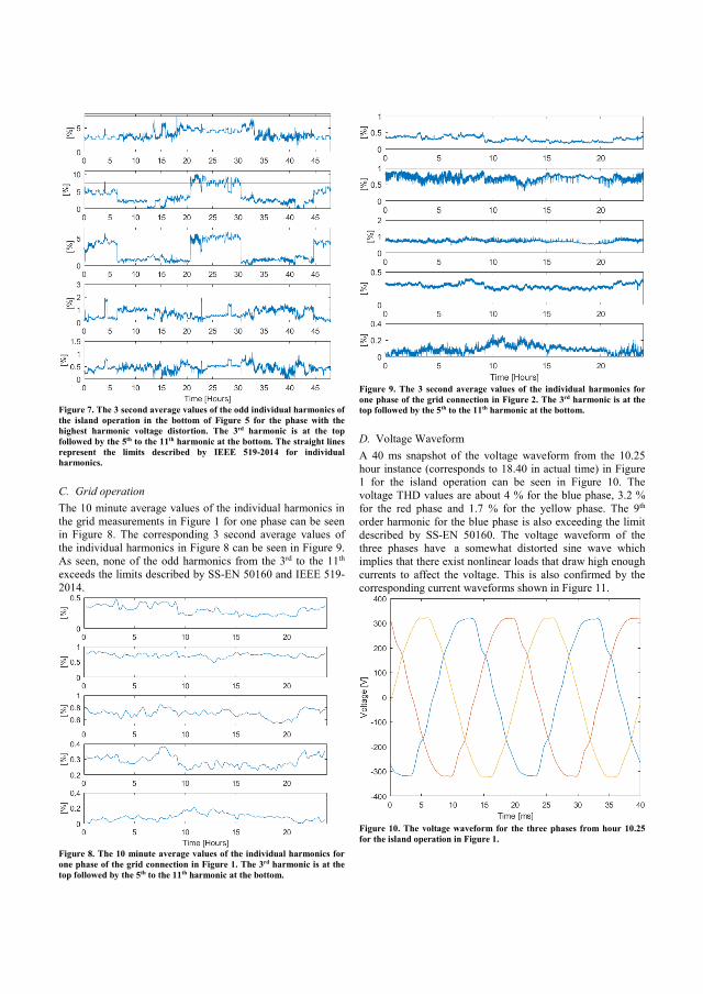
Figure 7. The 3 second average values of the odd individual harmonics of the island operation in the bottom of Figure 5 for the phase with the highest harmonic voltage distortion. The 3rd harmonic is at the top followed by the 5th to the 11th harmonic at the bottom. The straight lines represent the limits described by IEEE 519-2014 for individual harmonics.

C. Grid operation The 10 minute average values of the individual harmonics in the grid measurements in Figure 1 for one phase can be seen in Figure 8. The corresponding 3 second average values of the individual harmonics in Figure 8 can be seen in Figure 9. As seen, none of the odd harmonics from the 3rd to the 11th exceeds the limits described by SS-EN 50160 and IEEE 519-2014.

Figure 8. The 10 minute average values of the individual harmonics for one phase of the grid connection in Figure 1. The 3rd harmonic is at the top followed by the 5th to the 11th harmonic at the bottom.

Figure 9. The 3 second average values of the individual harmonics for one phase of the grid connection in Figure 2. The 3rd harmonic is at the top followed by the 5th to the 11th harmonic at the bottom.

D. Voltage Waveform

A 40 ms snapshot of the voltage waveform from the 10.25 hour instance (corresponds to 18.40 in actual time) in Figure 1 for the island operation can be seen in Figure 10. The voltage THD values are about 4 % for the blue phase, 3.2 % for the red phase and 1.7 % for the yellow phase. The 9th order harmonic for the blue phase is also exceeding the limit described by SS-EN 50160. The voltage waveform of the three phases have a somewhat distorted sine wave which implies that there exist nonlinear loads that draw high enough currents to affect the voltage. This is also confirmed by the corresponding current waveforms shown in Figure 11.

Figure 10. The voltage waveform for the three phases from hour 10.25 for the island operation in Figure 1.

It can be seen that the blue and red phase have high current peaks and that the yellow phase is more sinusoidal which is also seen in the voltage waveform in Figure 10 where the blue and red phase are more distorted.

Figure 11. The current waveform for the three phases from hour 10.25 for the island operation in Figure 1. A 40 ms snapshot of the voltage waveform at hour 22 (corresponding to 22.00 in actual time) in Figure 5 can be seen in Figure 12. The 3rd, 5th and 7th order harmonic exceeds the limits described by SS-EN 50160 for the blue phase at this instance and the voltage THD level is 12.6 % for the blue phase, 6 % for the red phase and 5 % for the yellow phase.

Figure 12. The voltage waveform for the three phases at hour 22 for the island operation in Figure 5. The corresponding current waveform for Figure 12 can be seen in Figure 13. It can be seen that the blue and red phase has a current that is highly distorted.

Figure 13. The current waveform for the three phases at hour 22 for the island operation in Figure 5.

III. CONCLUSIONS

• The microgrid has in most cases a higher voltage THD in island operation than in grid connected mode.

• There are instances during island operation when the voltage THD or individual harmonics go beyond the limits described by SS-EN 50160 and IEEE 519-2014.

• In many cases the 10 minute average values are enough to evaluate the harmonic distortion levels in the microgrid. There is however variations that will not be seen unless using the 3 second average values. These variations are greater when the microgrid is in island operation compared to when it is connected to the grid.

• The highest values of the voltage distortion don’t correspond to instances when the consumption is high but during the night, with low load and in island operation.

• There could be some adverse effects to connected equipment when the harmonic voltage distortion surpassed the limits described by SS-EN 50160 and IEEE 519-2014.

REFERENCES

[1] N. Hatziargyriou, Microgrids Architectures and Control, IEEE press, Wiley, 2014, p. 275.

[2] Voltage characteristics of electricity supplied by public electricity networks, Swedish electrical Std. SS-EN 50160 Version 4, Dec. 2011.

[3] IEEE Recommended Practice and Requirements for Harmonic Control in Electric Power Systems, IEEE Std. 519-2014, Mar 2014.

[4] S. Rönnberg, M. Bollen, J. Nömm, "Power Quality Measurements In a Single House Microgrid," Glasgow, 12-15 June 2017, CIRED 24th International Conference on Electricity Distribution.

[5] M.K Soni, N. Soni, "Review of Causes and Effect of Harmonics on Power System," International Journal of Science, Engineering and Technology Research (IJSETR), Volume 3, Issue 2, February 2014, pp. 216-217.

[6] R. C. Dugan, M. F. McGranaghan, S. Santoso, H. W. Beaty, Electrical Power System Quality, Second Edition, McGraw-Hill, p. 216.

Paper B

An Analysis of Frequency Variations and its

Implications on Connected Equipment for a

Nanogrid during Islanded Operation

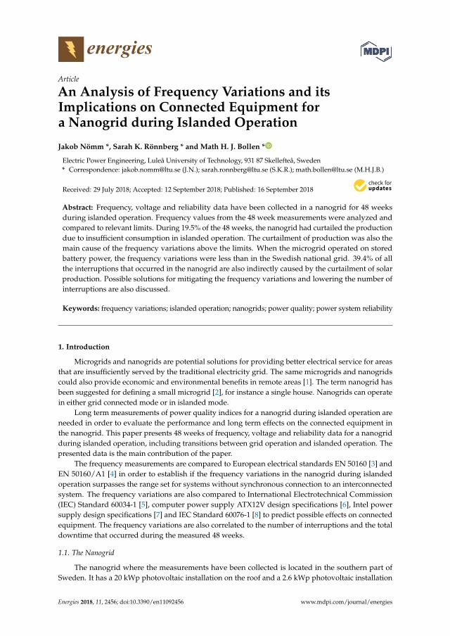
energies

Article

An Analysis of Frequency Variations and itsImplications on Connected Equipment fora Nanogrid during Islanded Operation

Jakob Nömm *, Sarah K. Rönnberg * and Math H. J. Bollen *

Electric Power Engineering, Luleå University of Technology, 931 87 Skellefteå, Sweden* Correspondence: [email protected] (J.N.); [email protected] (S.K.R.); [email protected] (M.H.J.B.)

Received: 29 July 2018; Accepted: 12 September 2018; Published: 16 September 2018

Abstract: Frequency, voltage and reliability data have been collected in a nanogrid for 48 weeksduring islanded operation. Frequency values from the 48 week measurements were analyzed andcompared to relevant limits. During 19.5% of the 48 weeks, the nanogrid had curtailed the productiondue to insufficient consumption in islanded operation. The curtailment of production was also themain cause of the frequency variations above the limits. When the microgrid operated on storedbattery power, the frequency variations were less than in the Swedish national grid. 39.4% of allthe interruptions that occurred in the nanogrid are also indirectly caused by the curtailment of solarproduction. Possible solutions for mitigating the frequency variations and lowering the number ofinterruptions are also discussed.

Keywords: frequency variations; islanded operation; nanogrids; power quality; power system reliability

1. Introduction

Microgrids and nanogrids are potential solutions for providing better electrical service for areasthat are insufficiently served by the traditional electricity grid. The same microgrids and nanogridscould also provide economic and environmental benefits in remote areas [1]. The term nanogrid hasbeen suggested for defining a small microgrid [2], for instance a single house. Nanogrids can operatein either grid connected mode or in islanded mode.

Long term measurements of power quality indices for a nanogrid during islanded operation areneeded in order to evaluate the performance and long term effects on the connected equipment inthe nanogrid. This paper presents 48 weeks of frequency, voltage and reliability data for a nanogridduring islanded operation, including transitions between grid operation and islanded operation. Thepresented data is the main contribution of the paper.

The frequency measurements are compared to European electrical standards EN 50160 [3] andEN 50160/A1 [4] in order to establish if the frequency variations in the nanogrid during islandedoperation surpasses the range set for systems without synchronous connection to an interconnectedsystem. The frequency variations are also compared to International Electrotechnical Commission(IEC) Standard 60034-1 [5], computer power supply ATX12V design specifications [6], Intel powersupply design specifications [7] and IEC Standard 60076-1 [8] to predict possible effects on connectedequipment. The frequency variations are also correlated to the number of interruptions and the totaldowntime that occurred during the measured 48 weeks.

1.1. The Nanogrid

The nanogrid where the measurements have been collected is located in the southern part ofSweden. It has a 20 kWp photovoltaic installation on the roof and a 2.6 kWp photovoltaic installation

Energies 2018, 11, 2456; doi:10.3390/en11092456 www.mdpi.com/journal/energies

http://www.mdpi.com/journal/energies

http://www.mdpi.com

https://orcid.org/0000-0003-4074-9529

http://www.mdpi.com/1996-1073/11/9/2456?type=check_update&version=1

http://dx.doi.org/10.3390/en11092456


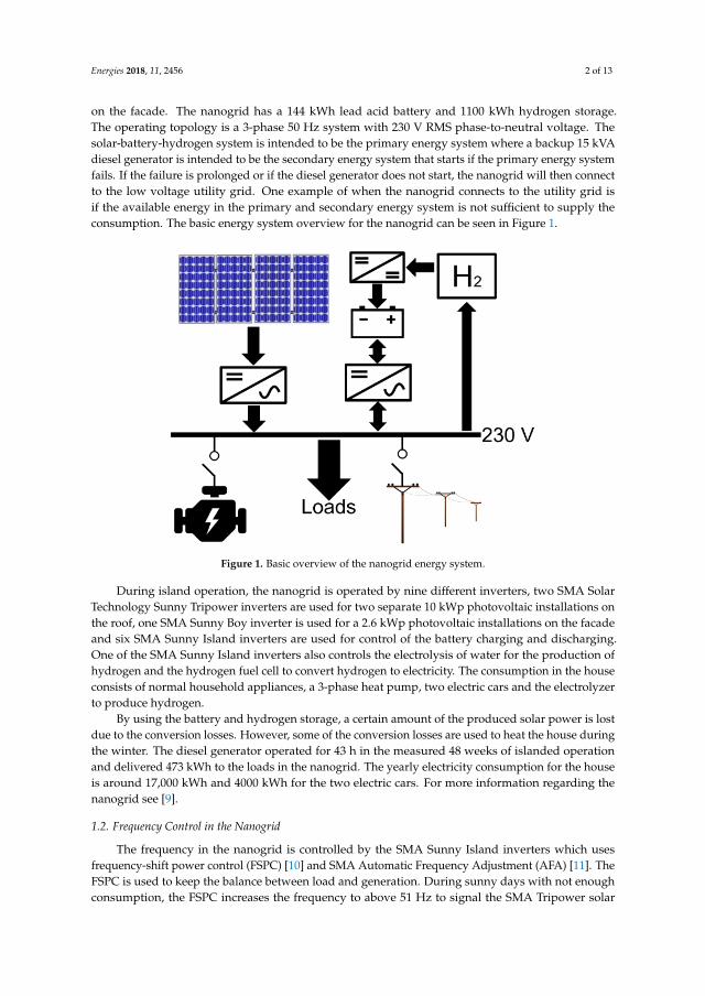
Energies 2018, 11, 2456 2 of 13

on the facade. The nanogrid has a 144 kWh lead acid battery and 1100 kWh hydrogen storage.The operating topology is a 3-phase 50 Hz system with 230 V RMS phase-to-neutral voltage. Thesolar-battery-hydrogen system is intended to be the primary energy system where a backup 15 kVAdiesel generator is intended to be the secondary energy system that starts if the primary energy systemfails. If the failure is prolonged or if the diesel generator does not start, the nanogrid will then connectto the low voltage utility grid. One example of when the nanogrid connects to the utility grid isif the available energy in the primary and secondary energy system is not sufficient to supply theconsumption. The basic energy system overview for the nanogrid can be seen in Figure 1.

Energies 2018, 11, x 2 of 14

1.1. The Nanogrid

The nanogrid where the measurements have been collected is located in the southern part of

Sweden. It has a 20 kWp photovoltaic installation on the roof and a 2.6 kWp photovoltaic installation

on the facade. The nanogrid has a 144 kWh lead acid battery and 1100 kWh hydrogen storage. The

operating topology is a 3‐phase 50 Hz system with 230 V RMS phase-to-neutral voltage. The solar-

battery-hydrogen system is intended to be the primary energy system where a backup 15 kVA diesel

generator is intended to be the secondary energy system that starts if the primary energy system fails.

If the failure is prolonged or if the diesel generator does not start, the nanogrid will then connect to

the low voltage utility grid. One example of when the nanogrid connects to the utility grid is if the

available energy in the primary and secondary energy system is not sufficient to supply the

consumption. The basic energy system overview for the nanogrid can be seen in Figure 1.

Figure 1. Basic overview of the nanogrid energy system.

During island operation, the nanogrid is operated by nine different inverters, two SMA Solar

Technology Sunny Tripower inverters are used for two separate 10 kWp photovoltaic installations

on the roof, one SMA Sunny Boy inverter is used for a 2.6 kWp photovoltaic installations on the

facade and six SMA Sunny Island inverters are used for control of the battery charging and

discharging. One of the SMA Sunny Island inverters also controls the electrolysis of water for the

production of hydrogen and the hydrogen fuel cell to convert hydrogen to electricity. The

consumption in the house consists of normal household appliances, a 3-phase heat pump, two electric

cars and the electrolyzer to produce hydrogen.

By using the battery and hydrogen storage, a certain amount of the produced solar power is lost

due to the conversion losses. However, some of the conversion losses are used to heat the house

during the winter. The diesel generator operated for 43 h in the measured 48 weeks of islanded

operation and delivered 473 kWh to the loads in the nanogrid. The yearly electricity consumption for

the house is around 17,000 kWh and 4000 kWh for the two electric cars. For more information

regarding the nanogrid see [9].

Figure 1. Basic overview of the nanogrid energy system.

During island operation, the nanogrid is operated by nine different inverters, two SMA SolarTechnology Sunny Tripower inverters are used for two separate 10 kWp photovoltaic installations onthe roof, one SMA Sunny Boy inverter is used for a 2.6 kWp photovoltaic installations on the facadeand six SMA Sunny Island inverters are used for control of the battery charging and discharging.One of the SMA Sunny Island inverters also controls the electrolysis of water for the production ofhydrogen and the hydrogen fuel cell to convert hydrogen to electricity. The consumption in the houseconsists of normal household appliances, a 3-phase heat pump, two electric cars and the electrolyzerto produce hydrogen.

By using the battery and hydrogen storage, a certain amount of the produced solar power is lostdue to the conversion losses. However, some of the conversion losses are used to heat the house duringthe winter. The diesel generator operated for 43 h in the measured 48 weeks of islanded operationand delivered 473 kWh to the loads in the nanogrid. The yearly electricity consumption for the houseis around 17,000 kWh and 4000 kWh for the two electric cars. For more information regarding thenanogrid see [9].

1.2. Frequency Control in the Nanogrid

The frequency in the nanogrid is controlled by the SMA Sunny Island inverters which usesfrequency-shift power control (FSPC) [10] and SMA Automatic Frequency Adjustment (AFA) [11]. TheFSPC is used to keep the balance between load and generation. During sunny days with not enoughconsumption, the FSPC increases the frequency to above 51 Hz to signal the SMA Tripower solar

Energies 2018, 11, 2456 3 of 13

inverters that production should be curtailed. The amount of curtailment increases linearly between 51and 52 Hz from 0 to 100%. The FSPC uses the battery voltage to determine the appropriate frequencyin the islanded nanogrid depending on the amount of load that is present.

Another feature of the FSPC is the shutdown of the solar inverters by increasing the frequencytowards 55 Hz. This is done in order for the Sunny Island inverters to synchronize to an externalsource, which for this nanogrid is the utility grid. The AFA compensates for the over frequency bytemporarily shifting the frequency to 49 Hz to enable clocks to run at the correct time. This correctionoccurs on a 12 h basis [11].

2. Results

2.1. Frequency Variations during Island Operation

The 10 s average values of the frequency for the 48 weeks when the nanogrid operated in islandedoperation was used to create an empirical cumulative distribution function. The results are shown inthe top part of Figure 2. For 19.5% of the 48 week period, the nanogrid is not utilizing the entire solarpower production and the FSPC decreases power output. In the figure, this is when the frequencyexceeds 51 Hz. The 49 Hz frequency value that stands for about 30.7% of the 48 week period is causedby the AFA compensating for the over frequency. The Cumulative Distribution Function (CDF) for54 weeks of 10 s average frequency measurements when the nanogrid was in grid-connected operationmode is presented in the lower part of Figure 2 for a comparison with the nanogrid islanded operation.

1.2. Frequency Control in the Nanogrid

The frequency in the nanogrid is controlled by the SMA Sunny Island inverters which uses

frequency-shift power control (FSPC) [10] and SMA Automatic Frequency Adjustment (AFA) [11].

The FSPC is used to keep the balance between load and generation. During sunny days with not

enough consumption, the FSPC increases the frequency to above 51 Hz to signal the SMA Tripower

solar inverters that production should be curtailed. The amount of curtailment increases linearly

between 51 and 52 Hz from 0 to 100%. The FSPC uses the battery voltage to determine the appropriate

frequency in the islanded nanogrid depending on the amount of load that is present.

Another feature of the FSPC is the shutdown of the solar inverters by increasing the frequency

towards 55 Hz. This is done in order for the Sunny Island inverters to synchronize to an external

source, which for this nanogrid is the utility grid. The AFA compensates for the over frequency by

temporarily shifting the frequency to 49 Hz to enable clocks to run at the correct time. This correction

occurs on a 12 h basis [11].

2. Results

2.1. Frequency Variations during Island Operation

The 10 s average values of the frequency for the 48 weeks when the nanogrid operated in

islanded operation was used to create an empirical cumulative distribution function. The results are

shown in the top part of Figure 2. For 19.5% of the 48 week period, the nanogrid is not utilizing the

entire solar power production and the FSPC decreases power output. In the figure, this is when the

frequency exceeds 51 Hz. The 49 Hz frequency value that stands for about 30.7% of the 48 week

period is caused by the AFA compensating for the over frequency. The Cumulative Distribution

Function (CDF) for 54 weeks of 10 s average frequency measurements when the nanogrid was in

grid-connected operation mode is presented in the lower part of Figure 2 for a comparison with the

nanogrid islanded operation.

Figure 2. CDF for the 48 weeks of 10 s average frequency values in the nanogrid during islanded

operation (top) and a corresponding CDF (bottom) for the 54 weeks of 10 s average frequency values

in the nanogrid during grid operation. Note the difference in horizontal scale.

One typical frequency regulation scenario is when there is not enough consumption (including

battery charging and electrolysis of water) during the day when the solar PV installation is producing

power. When this happens, the FSPC increases the frequency above 51 Hz to curtail the production.

During the night the AFA shifts the frequency to a lower value than 50 Hz in order to compensate the

time increase for clocks. One example of this scenario can be observed in Figure 3 where the 10 s average

Figure 2. CDF for the 48 weeks of 10 s average frequency values in the nanogrid during islandedoperation (top) and a corresponding CDF (bottom) for the 54 weeks of 10 s average frequency valuesin the nanogrid during grid operation. Note the difference in horizontal scale.

One typical frequency regulation scenario is when there is not enough consumption (includingbattery charging and electrolysis of water) during the day when the solar PV installation is producingpower. When this happens, the FSPC increases the frequency above 51 Hz to curtail the production.During the night the AFA shifts the frequency to a lower value than 50 Hz in order to compensatethe time increase for clocks. One example of this scenario can be observed in Figure 3 where the 10 saverage frequency is plotted for a 34.5 h period. The plot starts at 01:00 the 15th of April 2017 andends the 16th of April 2017 at 11:30. At the 15th between 01:00 and about 06:03 at sunrise, there isinsufficient solar production and the load is drawing power from the battery storage and therefore theload is matched to the source giving a frequency value near 50 Hz. Between 06:03 and 11:13 the solarproduction together with the battery storage is matched to the load which gives a frequency value near

Energies 2018, 11, 2456 4 of 13

50 Hz, but with some variations that can be observed more clearly in the top part of Figure 4. From11:13 to 18:03 the FSPC curtails the solar production in order to match to the load. The regulation startsat 11:13 at about 60% curtailment and increases to around 90% at 14:27. Between 18:03 the 15th Apriland 06:48 the 16th April the load is served mainly by the battery but since there has been a substantialamount of over frequency during the day, the AFA compensates for the over frequency by operatingthe nanogrid at 49 Hz. Between 06:48 and 11:30 the 16th the load is served by the solar generation andbattery storage, since the generation is matched by the load the frequency value is 50 Hz.

Energies 2018, 11, x 4 of 14

frequency is plotted for a 34.5 h period. The plot starts at 01:00 the 15th of April 2017 and ends the 16th

of April 2017 at 11:30. At the 15th between 01:00 and about 06:03 at sunrise, there is insufficient solar

production and the load is drawing power from the battery storage and therefore the load is matched

to the source giving a frequency value near 50 Hz. Between 06:03 and 11:13 the solar production

together with the battery storage is matched to the load which gives a frequency value near 50 Hz, but

with some variations that can be observed more clearly in the top part of Figure 4. From 11:13 to 18:03

the FSPC curtails the solar production in order to match to the load. The regulation starts at 11:13 at

about 60% curtailment and increases to around 90% at 14:27. Between 18:03 the 15th April and 06:48 the

16th April the load is served mainly by the battery but since there has been a substantial amount of over

frequency during the day, the AFA compensates for the over frequency by operating the nanogrid at

49 Hz. Between 06:48 and 11:30 the 16th the load is served by the solar generation and battery storage,

since the generation is matched by the load the frequency value is 50 Hz.

Figure 3. Frequency variations in the nanogrid from April 15th 2017 01:00 to 11:30 the 16th of April 2017.

When the source is matched to the load, the frequency is much closer to 50 Hz than in the

Swedish national grid. This can be observed in Figure 4 where the top part of the plot shows a zoomed

in view of Figure 3. It can be seen that the frequency starts to vary more just after sunrise when the

solar production starts to increase. The total load in the nanogrid is varying between 0.7 to 5.4 kW in

the duration shown in Figure 4.

Figure 4. Enlarged view of the frequency variations in the nanogrid from Figure 3 (top) and frequency

in the Swedish national grid (bottom) during the same period of time.


When the source is matched to the load, the frequency is much closer to 50 Hz than in the Swedishnational grid. This can be observed in Figure 4 where the top part of the plot shows a zoomed inview of Figure 3. It can be seen that the frequency starts to vary more just after sunrise when the solarproduction starts to increase. The total load in the nanogrid is varying between 0.7 to 5.4 kW in theduration shown in Figure 4.

Energies 2018, 11, x 4 of 14

frequency is plotted for a 34.5 h period. The plot starts at 01:00 the 15th of April 2017 and ends the 16th

of April 2017 at 11:30. At the 15th between 01:00 and about 06:03 at sunrise, there is insufficient solar

production and the load is drawing power from the battery storage and therefore the load is matched

to the source giving a frequency value near 50 Hz. Between 06:03 and 11:13 the solar production

together with the battery storage is matched to the load which gives a frequency value near 50 Hz, but

with some variations that can be observed more clearly in the top part of Figure 4. From 11:13 to 18:03

the FSPC curtails the solar production in order to match to the load. The regulation starts at 11:13 at

about 60% curtailment and increases to around 90% at 14:27. Between 18:03 the 15th April and 06:48 the

16th April the load is served mainly by the battery but since there has been a substantial amount of over

frequency during the day, the AFA compensates for the over frequency by operating the nanogrid at

49 Hz. Between 06:48 and 11:30 the 16th the load is served by the solar generation and battery storage,

since the generation is matched by the load the frequency value is 50 Hz.


When the source is matched to the load, the frequency is much closer to 50 Hz than in the

Swedish national grid. This can be observed in Figure 4 where the top part of the plot shows a zoomed

in view of Figure 3. It can be seen that the frequency starts to vary more just after sunrise when the

solar production starts to increase. The total load in the nanogrid is varying between 0.7 to 5.4 kW in

the duration shown in Figure 4.

Figure 4. Enlarged view of the frequency variations in the nanogrid from Figure 3 (top) and frequency

in the Swedish national grid (bottom) during the same period of time.

Figure 4. Enlarged view of the frequency variations in the nanogrid from Figure 3 (top) and frequencyin the Swedish national grid (bottom) during the same period of time.

2.2. Minimum and Maximum Values Observed

The highest frequency values of 55 Hz occur when there is not enough loads to consume theentire production from the PV installation. This happens when the batteries are fully charged, thehydrogen tank is full and the consumption in the house is low. An example of this can be observed in

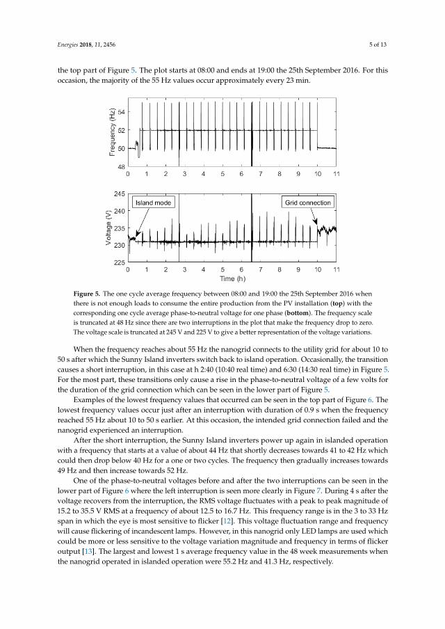
Energies 2018, 11, 2456 5 of 13

the top part of Figure 5. The plot starts at 08:00 and ends at 19:00 the 25th September 2016. For thisoccasion, the majority of the 55 Hz values occur approximately every 23 min.

entire production from the PV installation. This happens when the batteries are fully charged, the

hydrogen tank is full and the consumption in the house is low. An example of this can be observed

in the top part of Figure 5. The plot starts at 08:00 and ends at 19:00 the 25th September 2016. For this

occasion, the majority of the 55 Hz values occur approximately every 23 min.

When the frequency reaches about 55 Hz the nanogrid connects to the utility grid for about 10

to 50 s after which the Sunny Island inverters switch back to island operation. Occasionally, the

transition causes a short interruption, in this case at h 2:40 (10:40 real time) and 6:30 (14:30 real time)

in Figure 5. For the most part, these transitions only cause a rise in the phase-to-neutral voltage of a

few volts for the duration of the grid connection which can be seen in the lower part of Figure 5.

Figure 5. The one cycle average frequency between 08:00 and 19:00 the 25th September 2016 when there

is not enough loads to consume the entire production from the PV installation (top) with the

corresponding one cycle average phase-to-neutral voltage for one phase (bottom). The frequency scale

is truncated at 48 Hz since there are two interruptions in the plot that make the frequency drop to zero.

The voltage scale is truncated at 245 V and 225 V to give a better representation of the voltage variations.

Examples of the lowest frequency values that occurred can be seen in the top part of Figure 6.

The lowest frequency values occur just after an interruption with duration of 0.9 s when the frequency

reached 55 Hz about 10 to 50 s earlier. At this occasion, the intended grid connection failed and the

nanogrid experienced an interruption.

After the short interruption, the Sunny Island inverters power up again in islanded operation

with a frequency that starts at a value of about 44 Hz that shortly decreases towards 41 to 42 Hz

which could then drop below 40 Hz for a one or two cycles. The frequency then gradually increases

towards 49 Hz and then increase towards 52 Hz.

One of the phase-to-neutral voltages before and after the two interruptions can be seen in the

lower part of Figure 6 where the left interruption is seen more clearly in Figure 7. During 4 s after the

voltage recovers from the interruption, the RMS voltage fluctuates with a peak to peak magnitude of

15.2 to 35.5 V RMS at a frequency of about 12.5 to 16.7 Hz. This frequency range is in the 3 to 33 Hz

span in which the eye is most sensitive to flicker [12]. This voltage fluctuation range and frequency

will cause flickering of incandescent lamps. However, in this nanogrid only LED lamps are used

which could be more or less sensitive to the voltage variation magnitude and frequency in terms of

Figure 5. The one cycle average frequency between 08:00 and 19:00 the 25th September 2016 whenthere is not enough loads to consume the entire production from the PV installation (top) with thecorresponding one cycle average phase-to-neutral voltage for one phase (bottom). The frequency scaleis truncated at 48 Hz since there are two interruptions in the plot that make the frequency drop to zero.The voltage scale is truncated at 245 V and 225 V to give a better representation of the voltage variations.

When the frequency reaches about 55 Hz the nanogrid connects to the utility grid for about 10 to50 s after which the Sunny Island inverters switch back to island operation. Occasionally, the transitioncauses a short interruption, in this case at h 2:40 (10:40 real time) and 6:30 (14:30 real time) in Figure 5.For the most part, these transitions only cause a rise in the phase-to-neutral voltage of a few volts forthe duration of the grid connection which can be seen in the lower part of Figure 5.

Examples of the lowest frequency values that occurred can be seen in the top part of Figure 6. Thelowest frequency values occur just after an interruption with duration of 0.9 s when the frequencyreached 55 Hz about 10 to 50 s earlier. At this occasion, the intended grid connection failed and thenanogrid experienced an interruption.

After the short interruption, the Sunny Island inverters power up again in islanded operationwith a frequency that starts at a value of about 44 Hz that shortly decreases towards 41 to 42 Hz whichcould then drop below 40 Hz for a one or two cycles. The frequency then gradually increases towards49 Hz and then increase towards 52 Hz.

One of the phase-to-neutral voltages before and after the two interruptions can be seen in thelower part of Figure 6 where the left interruption is seen more clearly in Figure 7. During 4 s after thevoltage recovers from the interruption, the RMS voltage fluctuates with a peak to peak magnitude of15.2 to 35.5 V RMS at a frequency of about 12.5 to 16.7 Hz. This frequency range is in the 3 to 33 Hzspan in which the eye is most sensitive to flicker [12]. This voltage fluctuation range and frequencywill cause flickering of incandescent lamps. However, in this nanogrid only LED lamps are used whichcould be more or less sensitive to the voltage variation magnitude and frequency in terms of flickeroutput [13]. The largest and lowest 1 s average frequency value in the 48 week measurements whenthe nanogrid operated in islanded operation were 55.2 Hz and 41.3 Hz, respectively.

Energies 2018, 11, 2456 6 of 13

Energies 2018, 11, x 6 of 14

flicker output [13]. The largest and lowest 1 s average frequency value in the 48 week measurements

when the nanogrid operated in islanded operation were 55.2 Hz and 41.3 Hz, respectively.

Figure 6. Enlarged view of the largest frequency variations from Figure 5 (top) and its corresponding

voltage (bottom) for one phase. The scale is truncated at 38 Hz since the frequency drops towards 0

during the interruptions.

Figure 7. Enlarged view of the one cycle RMS voltage for the left interruption in Figure 6.

2.3. Comparison to Standards

According to European Standard EN 50160, the 10 s average frequency should remain between

49 and 51 Hz for 95% of one week and should remain between 42.5 and 57.5 Hz for 100% of the time

for systems without synchronous connection to an interconnected system. The 95% confidence

interval for the islanded operation CDF in Figure 2 spans 48.99 to 51.95 Hz. The lowest 10 s average

value was 43.48 Hz and the highest was 54.61 Hz.

Figure 6. Enlarged view of the largest frequency variations from Figure 5 (top) and its correspondingvoltage (bottom) for one phase. The scale is truncated at 38 Hz since the frequency drops towards 0during the interruptions.

Energies 2018, 11, x 6 of 14

flicker output [13]. The largest and lowest 1 s average frequency value in the 48 week measurements

when the nanogrid operated in islanded operation were 55.2 Hz and 41.3 Hz, respectively.

Figure 6. Enlarged view of the largest frequency variations from Figure 5 (top) and its corresponding

voltage (bottom) for one phase. The scale is truncated at 38 Hz since the frequency drops towards 0

during the interruptions.



According to European Standard EN 50160, the 10 s average frequency should remain between

49 and 51 Hz for 95% of one week and should remain between 42.5 and 57.5 Hz for 100% of the time

for systems without synchronous connection to an interconnected system. The 95% confidence

interval for the islanded operation CDF in Figure 2 spans 48.99 to 51.95 Hz. The lowest 10 s average

value was 43.48 Hz and the highest was 54.61 Hz.



According to European Standard EN 50160, the 10 s average frequency should remain between 49and 51 Hz for 95% of one week and should remain between 42.5 and 57.5 Hz for 100% of the time forsystems without synchronous connection to an interconnected system. The 95% confidence intervalfor the islanded operation CDF in Figure 2 spans 48.99 to 51.95 Hz. The lowest 10 s average value was43.48 Hz and the highest was 54.61 Hz.

Energies 2018, 11, 2456 7 of 13

The grid connected frequency values in Figure 2 always remain within the specified frequencyrange for interconnected systems, according to EN 50160. The islanded operation data divided intoweekly sections is shown in Figure 8 where the vertical axis is the amount of 10 s average valuesoutside of the range 49 to 51 Hz every week.

Energies 2018, 11, x 7 of 14

The grid connected frequency values in Figure 2 always remain within the specified frequency

range for interconnected systems, according to EN 50160. The islanded operation data divided into

weekly sections is shown in Figure 8 where the vertical axis is the amount of 10 s average values

outside of the range 49 to 51 Hz every week.

Figure 8. The amount of 10 s average values of the frequency per week outside the range 49 to 51 Hz.

The straight line represents the 5% limit in EN 50160.

The islanded operation data is an assembly of long and short periods of time where the nanogrid

is operating in islanded operation. This means that not all of the measurements are continuous and

therefore Figure 8 does not have a definitive correlation with the seasons of the year. The straight line

in Figure 8 is the 5% weekly limit of allowed values that can exceed the range 49 to 51 Hz.

In total, 89.6% of the 48 week measurements do not fall in the range that EN 50160 has set for

systems without synchronous connection to an interconnected system. However, all the 10 s average

frequency values remain within the maximum allowed variation set by EN 50160 for systems without

synchronous connection to an interconnected system which is 42.5 to 57.5 Hz. The 95% confidence

interval for the grid measurements in Figure 2 spans 49.92 to 50.09 Hz. The nanogrid is within this

range for 48.3% of the 48 week measurements. This means that one could expect almost half of the

time to have the same frequency quality in the nanogrid as what is normally seen in the Swedish

national grid.

If the nanogrid were to be located in the neighboring country Norway, the requirement in Annex

EN 50160/A1 would apply. This document states that for systems without synchronous connection

to an interconnected system, the frequency shall remain within 49 to 51 Hz for 100% of the time. With

this requirement, the total probability of being outside the frequency range set by EN 50160/A1 is

25% of the 48 week period. The reason to why the EN 50160/A1 Standard has a larger acceptance

number is due to the fact that the entire 48 week period is considered and not individual weeks.

However, the maximum allowed variations from the rated frequency is surpassed in the EN 50160/A1

Standard, but not for the EN 50160 Standard. This is since the EN 50160 Standard allows a larger

frequency span of 42.5 to 57.5 Hz while the EN 50160/A1 Standard allows a frequency of 49 to 51 Hz.

However, any load connected would still see the same frequency variation, regardless of which

standard would apply. A summary of Section 2.3 can be seen in Table 1.

Figure 8. The amount of 10 s average values of the frequency per week outside the range 49 to 51 Hz.The straight line represents the 5% limit in EN 50160.

The islanded operation data is an assembly of long and short periods of time where the nanogridis operating in islanded operation. This means that not all of the measurements are continuous andtherefore Figure 8 does not have a definitive correlation with the seasons of the year. The straight linein Figure 8 is the 5% weekly limit of allowed values that can exceed the range 49 to 51 Hz.

In total, 89.6% of the 48 week measurements do not fall in the range that EN 50160 has set forsystems without synchronous connection to an interconnected system. However, all the 10 s averagefrequency values remain within the maximum allowed variation set by EN 50160 for systems withoutsynchronous connection to an interconnected system which is 42.5 to 57.5 Hz. The 95% confidenceinterval for the grid measurements in Figure 2 spans 49.92 to 50.09 Hz. The nanogrid is within thisrange for 48.3% of the 48 week measurements. This means that one could expect almost half of thetime to have the same frequency quality in the nanogrid as what is normally seen in the Swedishnational grid.

If the nanogrid were to be located in the neighboring country Norway, the requirement in AnnexEN 50160/A1 would apply. This document states that for systems without synchronous connection toan interconnected system, the frequency shall remain within 49 to 51 Hz for 100% of the time. Withthis requirement, the total probability of being outside the frequency range set by EN 50160/A1 is 25%of the 48 week period. The reason to why the EN 50160/A1 Standard has a larger acceptance numberis due to the fact that the entire 48 week period is considered and not individual weeks. However, themaximum allowed variations from the rated frequency is surpassed in the EN 50160/A1 Standard, butnot for the EN 50160 Standard. This is since the EN 50160 Standard allows a larger frequency span of42.5 to 57.5 Hz while the EN 50160/A1 Standard allows a frequency of 49 to 51 Hz. However, any loadconnected would still see the same frequency variation, regardless of which standard would apply.A summary of Section 2.3 can be seen in Table 1.

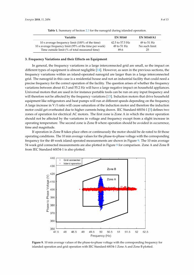
Energies 2018, 11, 2456 8 of 13

Table 1. Summary of Section 2.3 for the nanogrid during islanded operation.

Variable EN 50160 EN 50160/A1

10 s average frequency limit (100% of the time) 42.5 to 57.5 Hz 49 to 51 Hz10 s average frequency limit (95% of the time per week) 49 to 51 Hz No such limit

Time outside limit (% of total measured time) 89.6 25

3. Frequency Variations and their Effects on Equipment

In general, the frequency variations in a large interconnected grid are small, so the impact ondifferent types of equipment is almost negligible [14]. However, as seen in the previous sections, thefrequency variations within an island-operated nanogrid are larger than in a large interconnectedgrid. The nanogrid in this case is a residential house and not an industrial facility that could need aprecise frequency for the correct operation of the facility. The question arises of whether the frequencyvariations between about 41.3 and 55.2 Hz will have a large negative impact on household appliances.Universal motors that are used in for instance portable tools can be run on any input frequency andwill therefore not be affected by the frequency variations [15]. Induction motors that drive householdequipment like refrigerators and heat pumps will run at different speeds depending on the frequency.A large increase in V/f ratio will cause saturation of the induction motor and therefore the inductionmotor could get overheated due to higher currents being drawn. IEC Standard 60034-1 [5] defines twozones of operation for electrical AC motors. The first zone is Zone A in which the motor operationshould not be affected by the variations in voltage and frequency except from a slight increase inoperating temperature. The second zone is Zone B where operation should be avoided in occurrence,time and magnitude.

If operation in Zone B takes place often or continuously the motor should be de-rated to fit thoseoperating conditions. The 10 min average values for the phase-to-phase voltage with the correspondingfrequency for the 48 week island operated measurements are shown in Figure 9. The 10 min average54 week grid connected measurements are also plotted in Figure 9 for comparison. Zone A and Zone Bfrom IEC Standard 60034-1 is also plotted.

Energies 2018, 11, x 8 of 14

Table 1. Summary of Section 2.3 for the nanogrid during islanded operation.

Variable EN 50160 EN 50160/A1

10 s average frequency limit (100% of the time) 42.5 to 57.5 Hz 49 to 51 Hz

10 s average frequency limit (95% of the time per week) 49 to 51 Hz No such limit

Time outside limit (% of total measured time) 89.6 25

3. Frequency Variations and their Effects on Equipment

In general, the frequency variations in a large interconnected grid are small, so the impact on

different types of equipment is almost negligible [14]. However, as seen in the previous sections, the

frequency variations within an island-operated nanogrid are larger than in a large interconnected

grid. The nanogrid in this case is a residential house and not an industrial facility that could need a

precise frequency for the correct operation of the facility. The question arises of whether the

frequency variations between about 41.3 and 55.2 Hz will have a large negative impact on household

appliances. Universal motors that are used in for instance portable tools can be run on any input

frequency and will therefore not be affected by the frequency variations [15]. Induction motors that

drive household equipment like refrigerators and heat pumps will run at different speeds depending

on the frequency. A large increase in V/f ratio will cause saturation of the induction motor and

therefore the induction motor could get overheated due to higher currents being drawn. IEC

Standard 60034-1 [5] defines two zones of operation for electrical AC motors. The first zone is Zone

A in which the motor operation should not be affected by the variations in voltage and frequency

except from a slight increase in operating temperature. The second zone is Zone B where operation

should be avoided in occurrence, time and magnitude.

If operation in Zone B takes place often or continuously the motor should be de-rated to fit those

operating conditions. The 10 min average values for the phase-to-phase voltage with the

corresponding frequency for the 48 week island operated measurements are shown in Figure 9. The

10 min average 54 week grid connected measurements are also plotted in Figure 9 for comparison.

Zone A and Zone B from IEC Standard 60034-1 is also plotted.

Figure 9. 10 min average values of the phase-to-phase voltage with the corresponding frequency for

islanded operation and grid operation with IEC Standard 60034-1 Zone A and Zone B plotted.

Figure 9. 10 min average values of the phase-to-phase voltage with the corresponding frequency forislanded operation and grid operation with IEC Standard 60034-1 Zone A and Zone B plotted.

Energies 2018, 11, 2456 9 of 13

The frequency limits, voltage limits and the amount of time in which the nanogrid during islandedoperation was within Zone A, Zone B and outside Zone B can be seen in Table 2.

Table 2. Limits for each zone described in IEC Standard 60034-1 and the amount of time the nanogridoperated in each defined zone during islanded operation.

Definition Within Zone A Within Zone B Outside Zone B

Allowed frequency variation ±2% +3% and −5% -Allowed voltage variation ±5% ±10% -

Amount of 10 min average values withinspecified zone 79.3% 3.3% 17.4%

The values that are outside Zone A are caused by the curtailment of solar production since thefrequency is higher than 51 Hz. The phase-to-phase voltage never exceeds the limits of Zone A. Thegrid connected 10 min average values are within Zone A for 99.91% of the time and 0.09% in Zone B.It can be seen in Figure 9 that the voltage varies more for the grid connection than islanded operationwhich also causes some grid connected values to end up in Zone B.

3.1. Single Phase Induction Motors

Single phase induction motors have a start winding that only operates for a few seconds to getthe motor spinning. During those few seconds the start winding draws a large current. The timing ofthe centrifugal switch that disconnects the start winding on some single phase induction motors mightget affected with larger frequency variations than what the motor was designed for.

The centrifugal switch disconnects at about 75 to 90% of rated motor speed [16,17]. In a 50 Hz gridthat range would correspond to 37.5 to 45 Hz which is a frequency range that can be partly observedin the measurements from the islanded operation.

If a single phase induction motor with a centrifugal switch would start at a supply frequency lessthan the disconnection speed, the centrifugal switch would not disconnect and leave the start windingoperational until the supply frequency increases sufficiently. Such a case could cause the start windingto get damaged or become non-operational. The occasion where the start winding could get damagedis when the nanogrid recovers from an interruption that followed shortly after the frequency reachedabout 55 Hz. Such a case can be seen in Figure 6 where the frequency was below 45 Hz for about 8 s.A total of 12 occurrences where the frequency stayed below 45 Hz during about 8 s happened duringthe 48 week measurement time period. In one occurrence the frequency stayed at 43.3 to 44 Hz forabout 63 s.

3.2. Computer Power Supplies

Some power supplies for computers follow the ATX12V design specifications which require thatthe power supply should work between 47 and 63 Hz [6]. Intel power supply design specificationsalso specify a frequency range of 47 to 63 Hz [7]. Therefore only frequencies below 47 Hz could bea problem since the nanogrid frequency never exceeds 55.2 Hz. Frequencies below 47 Hz occurred13 times in the 48 week measurements where 12 had duration of about 12 s and one for about 63 s.

3.3. Transformers

IEC Standard 60076-1 [8] states that single phase transformers with larger power rating than1 kVA and 3-phase transformers with larger power rating than 5 kVA must withstand +5% V/f ratiovariation from rated V/f ratio at rated power and frequency. If the voltage would remain constantat rated voltage, the maximum allowed frequency drop would be down to 47.62 Hz for a +5% V/fratio. The transformer should also withstand a V/f ratio of +10% from rated V/f ratio at no load whichcorrespond to a frequency of 45.5 Hz at rated voltage. The frequency dropped to between 47.6 and45.5 Hz for 12 times with duration of about 8 to 12 s in the 48 week measurements. For one occasion

Energies 2018, 11, 2456 10 of 13

the frequency dropped below 45.5 Hz for about 63 s. During these instances a transformer mightget affected.

3.4. Clocks and Harmonic Filters

Other types of equipment that can be affected by the frequency variations are harmonic filterssince they can become de-tuned during periods where there is a large frequency deviation from ratedfrequency [18]. Clocks that depend on the supply frequency will also be affected. But since overfrequency in the nanogrid will be compensated by the AFA, clocks could temporarily get affectedduring daytime. At 52 Hz the clocks would be off by about two min every ho. In for instance Figure 3,the offset by the evening would be about 14 min.

3.5. Equipment Testing

In order to test the effects on home appliances for the large frequency variations seen in thenanogrid, the test procedure in IEC Standard 61000-4-28 [18] could be used. The frequency test level2 for equipment for residential customers connected to the low voltage grid is +4% and −6% whichfor a 50 Hz system corresponds to 47–52 Hz. The transition period from rated frequency to the testedfrequency, is 10 s. Since the frequency variations are larger in the nanogrid, test level 4 could be usedwhich applies for non-interconnected networks where misoperation of equipment is critical. Test level4 uses ±15% (42.5–57.5 Hz) which corresponds closest to the frequency variations measured in thenanogrid. The transition period from rated frequency to the tested frequency is 1 s in test level 4. Thisis something that corresponds closer to what can sometimes be seen in the nanogrid, see for exampleFigure 6. Test level 4 is also more appropriate if one was to consider that some home appliancesmight be critical for maintaining a normal life in the residence. But since the frequency variationsin the nanogrid are between 41.3 and 55.2 Hz at 1 s resolution, test level X could be used where thefrequency range can be adjusted further. In order to establish the impact on equipment operation forthe nanogrid reviewed in this paper, the frequency test level should be at least +10.5% and −17.4%with a transitional period of 1 s.

4. Relationship between Frequency Variations and Interruptions

The interruptions that occurred during the 48 week measurement time period could be dividedinto three groups according to how the nanogrid transitioned between different operational modes:

Group 1 (Island-interruption-grid): Interruptions during islanded operation that transition into grid operation.Group 2 (Grid-interruption-island): Interruptions during grid operation that transition into islanded operation.Group 3 (Island-interruption-island): Interruptions during island operation that transition into islandedoperation.

Grid to grid interruptions are not considered since the nanogrid internal energy system is notoperational in those cases. The individual downtimes of the interruptions for each three groups areplotted in an empirical CDF in Figure 10 where the longest interruption of 1.97 h has been truncatedto give a better visualization of the plot. The primary reason to why the interruptions in each groupoccurred is unknown.

The total number of interruptions and downtimes for the respective groups can be seen in Table 3.Note that the majority of the interruptions last less than 2 s.

In Group 2, 28 interruptions happened shortly after the frequency in the nanogrid reached about55 Hz and lasted for about 0.9 s. These are the same type of interruptions that can be seen in Figures 5and 6 where there is a 10 to 50 second long connection to the utility grid after the frequency reachedabout 55 Hz. These interruptions amount to 39.4% of the total number of interruptions in 48 weeks and78% of Group 2. This means that there is a possibility that the surplus of energy in the nanogrid causesapproximately 39.4% of the total number of interruptions in the nanogrid. However, the downtime ofthese interruptions only corresponds to 0.19% of the total downtime in the nanogrid.

Energies 2018, 11, 2456 11 of 13Energies 2018, 11, x 11 of 14

Figure 10. CDF of individual downtimes for the interruptions in each three groups. The plot is

truncated at 14 min since there was one interruption in Group 1 that lasted for 1.97 h.

The total number of interruptions and downtimes for the respective groups can be seen in Table

3. Note that the majority of the interruptions last less than 2 s.

Table 3. Interruptions and downtime for the different groups.

Group Number of interruptions Downtime Number of Interruptions < 2 s

Group 1 16 2.91 h 3 (19% of group 1)

Group 2 36 3.47 min 33 (92% of group 2)

Group 3 19 42.4 min 6 (32% of group 3)

All groups 71 3.67 h 42 (59% of all groups)

In Group 2, 28 interruptions happened shortly after the frequency in the nanogrid reached about

55 Hz and lasted for about 0.9 s. These are the same type of interruptions that can be seen in Figure 5

and Figure 6 where there is a 10 to 50 second long connection to the utility grid after the frequency

reached about 55 Hz. These interruptions amount to 39.4% of the total number of interruptions in 48

weeks and 78% of Group 2. This means that there is a possibility that the surplus of energy in the

nanogrid causes approximately 39.4% of the total number of interruptions in the nanogrid. However,

the downtime of these interruptions only corresponds to 0.19% of the total downtime in the nanogrid.

The number of transitions between operational states in Group 1 and Group 2 is approximately

1400 in 48 weeks where around 1000 transitions are caused by the 55 Hz phenomena shown in Figure

5 and Figure 6.

The probability of having an interruption in Group 1 and 2 with regards to the number of

transitions between islanded operation and grid operation is 1.1% and 2.5%, respectively, for the 48

weeks.

The probability of having an interruption in Group 2 when the frequency reaches 55 Hz is

around2.8% and if the 55 Hz transitions are excluded the probability is around 2%. Since the

probability for an interruption is higher when the frequency reaches 55 Hz, the nanogrid could be

more sensitive to interruptions when the nanogrid transitions to grid operation.

Figure 10. CDF of individual downtimes for the interruptions in each three groups. The plot istruncated at 14 min since there was one interruption in Group 1 that lasted for 1.97 h.

Table 3. Interruptions and downtime for the different groups.

Group Number of Interruptions Downtime Number of Interruptions < 2 s

Group 1 16 2.91 h 3 (19% of group 1)Group 2 36 3.47 min 33 (92% of group 2)Group 3 19 42.4 min 6 (32% of group 3)

All groups 71 3.67 h 42 (59% of all groups)

The number of transitions between operational states in Group 1 and Group 2 is approximately1400 in 48 weeks where around 1000 transitions are caused by the 55 Hz phenomena shown in Figures 5and 6.

The probability of having an interruption in Group 1 and 2 with regards to the number oftransitions between islanded operation and grid operation is 1.1% and 2.5%, respectively, for the48 weeks.

The probability of having an interruption in Group 2 when the frequency reaches 55 Hz isaround2.8% and if the 55 Hz transitions are excluded the probability is around 2%. Since the probabilityfor an interruption is higher when the frequency reaches 55 Hz, the nanogrid could be more sensitiveto interruptions when the nanogrid transitions to grid operation.

5. Possible Solutions for Reducing over Frequency in Islanded Operation

The over-frequency in the nanogrid is caused by the FSPC used by the Sunny Island batteryinverters to signal the solar inverters to regulate the power production. This is done when there isnot enough load connected in the nanogrid during islanded operation. The over-frequency causedby the FSPC will activate the AFA which lowers the frequency below 50 Hz to compensate for theoccurred over frequency. If instead a direct link with a cable between the battery inverter and solarinverter would be used, the signaling with the power frequency could be avoided and thereforepossibly eliminate the frequency variations. However, it is unclear if the lowest frequency variationsthat happen when the islanded operation initiates after an interruption would be eliminated withthis method.

Energies 2018, 11, 2456 12 of 13

If this solution can’t be done practically, a simple solution would be to have a large resistive load(dump load) that can be activated when the frequency starts to rise above 51 Hz. The solution of usingdump loads to regulate the power frequency in islanded operated microgrids when there is an excessamount of power in the system is described in for instance [19,20].

Another solution would be to increase the storage capacity (which is under construction)and/or increase the electrolyzer power in order to create more hydrogen when there is notenough consumption.

If an increase in energy storage is not feasible and if the objective is to reduce the loss of potentialpower production, one could shift some of the loads towards the day when the solar power production isoccurring. In a single house nanogrid, such loads could be for example the dishwasher, washing machine,electric vehicles, air conditioning units or heat pumps. If such an approach would be taken, the servicelife of the battery would also increase since the cycling of the battery during the night is reduced.

These solutions could reduce the large frequency variations that go beyond the limits in productand grid standards described in this article. An increase in energy storage and consumption whenthe power production occurs would also be necessary in order to reduce the amount of transitionsbetween islanded operation and grid operation. That could in turn reduce the amount of interruptionsthat occur during such transitions.

6. Conclusions

The 10 s average frequency variations in the nanogrid during islanded operation are outside therange set by EN 50160 for systems without synchronous connection to an interconnected system for89.6% of the 48 weeks. However, for Standard EN 50160/A1 which applies in Norway the frequencyvariations are outside the limits for 25% of 48 weeks.

The lower and upper allowed 10 s average frequency limit (52.5 to 57.5 Hz) defined by EN 50160is not surpassed but for EN 50160/A1 the maximum allowed range of 49 to 51 Hz is surpassed.

The frequency variations between 51 and 52 Hz are caused by the FSPC used by the Sunny Islandinverters to curtail production from the solar PV installation when there is not enough consumption.The larger frequency variations from 52 to 55 Hz occur when there is not enough consumption duringthe daytime and when the FSPC increases the frequency towards 55 Hz to shut down the solar invertersin order to synchronize with the utility grid.

The lowest frequency values of about 41 to about 49 Hz are caused by short interruptions afterthe frequency reached about 55 Hz. The frequency values at about 49 Hz are caused by the AFAcompensating for the occurred over frequency in order to enable clocks to run at the correct time.

There might be some adverse effects on certain equipment of these frequency variations. Forinstance, AC motors might be affected since 17.4% of the total time in islanded operation AC motorswill operate outside the limits described by IEC Standard 60034-1. Single phase induction motors mightbe affected if they are started just after the short interruptions that can occur when the frequency hasreached 55 Hz. This is since the frequency can be lower than the centrifugal switch opening frequencyfor about 8 to 63 s at 13 occurrences which in turn could cause damage to the start winding. Computerpower supplies and transformers could also be affected for 13 times in the 48 week measurements forduration of about 8 to 63 s at each occurrence. The frequency variations that go beyond the allowedrange described in grid and product standards could be eliminated by increasing the consumptionby for instance shifting consumption to the daytime when the production occurs. Another solutionwould be to increase the energy storage in order to store the excess generated power or have a directlink between the Sunny Island battery inverter and solar inverter to avoid the communication throughthe power frequency.

Approximately 39.4% of the total number of interruptions could also possibly be eliminated byensuring that the load is matched to the solar production. Since transitions between islanded operationand grid operation increase the risk of interruptions, a constantly islanded nanogrid could have fewerinterruptions than what this case study has presented. It is unclear if the reliability of the nanogrid

Energies 2018, 11, 2456 13 of 13

would increase with the removal of the possibility of connecting to the grid since there could beinstability in the system causing the interruptions in Group 2 presented in this paper.

Author Contributions: Conceptualization, J.N., S.K.R. and M.H.J.B.; Methodology, J.N.; Software, J.N.; Validation,J.N., S.K.R. and M.H.J.B.; Formal Analysis, J.N.; Investigation, J.N.; Resources, S.K.R. and M.H.J.B.; Data Curation,J.N.; Writing-Original Draft Preparation, J.N.; Writing-Review & Editing, J.N., S.K.R. and M.H.J.B.; Visualization,J.N.; Supervision, S.K.R. and M.H.J.B.; Project Administration, S.K.R. and M.H.J.B.; Funding Acquisition, S.K.R.and M.H.J.B.

Funding: This paper has been funded by Skellefteå Kraft Elnät and Rönnbäret foundation.

Conflicts of Interest: The authors declare no conflict of interest.

References

1. Hatziargyriou, N.; Asano, H.; Iravani, R.; Marnay, C. Microgrids. IEEE Power Energy Mag. 2007, 5, 78–94.[CrossRef]

2. Burmester, D.; Rayudu, R.; Seah, W.; Akinyele, D. A Review of Nanogrid Topologies and Technologies.Renew. Sustain. Energy Rev. 2017, 67, 760–775. [CrossRef]

3. Cenelec Standard EN 50160, Voltage Characteristics of Electricity Supplied by Public Electricity Networks; EuropeanCommittee for Electrotechnical Standardization: Brussels, Belgium, 2010.

4. Cenelec Standard EN 50160/A1, Voltage Characteristics of Electricity Supplied by Public Electricity Networks;European Committee for Electrotechnical Standardization: Brussels, Belgium, 2015.

5. IEC Standard 60034-1, Rotating electrical machines—Part 1: Rating and performance; International ElectrotechnicalCommission: Geneva, Switzerland, 2017.

6. Intel Corporation. ATX12V, Power Supply Design Guide, version 2.2; Intel Corporation: Santa Clara, CA, USA, 2005.7. Intel Corporation. Design Guide for Desktop Platform Form Factors, revision 1.31; Intel Corporation: Santa Clara,

CA, USA, 2013.8. IEC Standard 60076-1:2011, Power transformers-Part 1: General; International Electrotechnical Commission:

Geneva, Switzerland, 2011.9. Rönnberg, S.K.; Bollen, M.H.J.; Nömm, J. Power Quality Measurements in a Single House Microgrid.

In Proceedings of the CIRED 24th International Conference on Electricity Distribution, Glasgow, Scotland,12–15 June 2017; pp. 818–822.

10. SMA. PV Inverters, Use and Settings of PV Inverters in Off-Grid Systems, version 4.2; SMA: Niestetal, Germany, 2014.11. SMA. Sunny Island 3324/4248 Installation Guide, version 4.0; SMA: Niestetal, Germany, 2005.12. IEEE Standard 1789-2015, IEEE Recommended Practices for Modulating Current in High-Brightness LEDs for Mitigating

Health Risks to Viewers; The Institute of Electrical and Electronics Engineers: New York, NY, USA, 2015.13. Gil-de-Castro, A.; Rönnberg, S.K.; Bollen, M.H.J. Light intensity variation (flicker) and harmonic emission

related to LED lamps. Electr. Power Syst. Res. 2017, 146, 107–114. [CrossRef]14. Bollen, M.H.J.; Gu, I.Y.H. Signal Processing of Power Quality Disturbances, 1st ed.; Wiley-IEEE Press: Hoboken,

NJ, USA, 2006; p. 159.15. Rajput, R.K. Alternating Current Machines, 1st ed.; Firewall Media: New Delhi, India, 2002; p. 435.16. Brumbach, M.E. Industrial Electricity, 9th ed.; Cengage learning: Boston, MA, USA, 2017; p. 385.17. Shultz, G.P. Transformers and Motors, 1st ed.; Elsivier: New York, NY, USA, 1989; p. 129.18. IEC Standard 61000-4-28, Electromagnetic Compatibility (EMC)–Part 4–28: Testing and Measurement

Techniques-Variation of Power Frequency, Immunity Test for Equipment with input Current not Exceeding 16 A perphase, edition 1.2; International Electrotechnical Commission: Geneva, Switzerland, 2009.

19. Serban, E.; Serban, H. A Control Strategy for a Distributed Power Generation Microgrid Application withVoltage and Current Controlled Source Converter. IEEE Trans. Power. Electron. 2010, 25, 2981–2992. [CrossRef]

20. Baudoin, S.; Vechiu, I. Review of Voltage and Frequency Control Strategies for Islanded Microgrid.In Proceedings of the 16th International Conference on System Theory, Control and Computing (ICSTCC),Sinaia, Romania, 2–14 October 2012.

© 2018 by the authors. Licensee MDPI, Basel, Switzerland. This article is an open accessarticle distributed under the terms and conditions of the Creative Commons Attribution(CC BY) license (http://creativecommons.org/licenses/by/4.0/).

http://dx.doi.org/10.1109/MPAE.2007.376583

http://dx.doi.org/10.1016/j.rser.2016.09.073

http://dx.doi.org/10.1016/j.epsr.2017.01.026

http://dx.doi.org/10.1109/TPEL.2010.2050006

http://creativecommons.org/

http://creativecommons.org/licenses/by/4.0/.

Paper C

An Analysis of Voltage Quality in a Nanogrid

during Islanded Operation

energies

Article

An Analysis of Voltage Quality in a Nanogrid duringIslanded Operation

Jakob Nömm *, Sarah K. Rönnberg * and Math H. J. Bollen *

Electric Power Engineering, Luleå University of Technology, 931 87 Skellefteå, Sweden* Correspondence: [email protected] (J.N.); [email protected] (S.K.R.); [email protected] (M.H.J.B.)

Received: 21 January 2019; Accepted: 13 February 2019; Published: 15 February 2019

Abstract: Voltage quality data has been collected in a single house nanogrid during 48 weeks ofislanded operation and 54 weeks of grid-connected operation. The voltage quality data contains thevoltage total harmonic distortion (THD), odd harmonics 3 to 11 and 15, even harmonics 4 to 8, voltageunbalance, short-term flicker severity (Pst) and long-term flicker severity (Plt) values, and voltagevariations at timescales below 10 min. A comparison between islanded and grid-connected operationvalues was made, were some of the parameters were compared to relevant grid standard limits.It is shown that some parameters exceed the defined limits in the grid-standards during islandedoperation. It was also found that the islanded operation has two modes of operation, one in whichhigher values of the short circuit impedance, individual harmonic impedance, harmonic voltagedistortion and voltage unbalance were reached.

Keywords: harmonics; islanded operation; nanogrids; power quality; voltage unbalance

1. Introduction

Microgrids and nanogrids can provide economical gains in the form of price reductions forconsumers and increased revenue for grid owners [1]. They could also provide an improved technicalsolutions such as energy loss reduction and better reliability than a regular utility connection for certaingeographical areas [1,2]. The international council on large electric systems (CIGRE) WG C6.22 definesmicrogrids as: “electricity distribution systems containing loads and distributed energy resources,(such as distributed generators, storage devices, or controllable loads) that can be operated in acontrolled, coordinated way either while connected to the main power network or while islanded” [3].The term nanogrid was suggested in [4] for defining a small microgrid, which could be a singleresidential house.

There is a lack of published papers that contain voltage quality measurements that spanseveral months or years for nanogrids in islanded operation. These measurements are needed toestablish the differences in performance between islanded operation and grid-connected operation.The measurements would also make it possible to evaluate if problems can appear for connectedequipment during islanded operation.

In this paper, long term measurements of voltage quality are presented that have been collectedin a single house nanogrid during 48 weeks of islanded operation and 54 weeks of grid-connectedoperation. Some of the measured voltage quality parameters have been compared with the limitsdefined in standards EN 50160 [5] and IEEE 519-2014 [6]. The specified standards do not includevoltage quality limits for islanded operation, so the limits in the standards are only used as a referencefor islanded operation.

The main contribution of this paper is the analysis and presentation of long-term voltage qualitymeasurements collected in a nanogrid during islanded operation. All the used equipment in the

Energies 2019, 12, 614; doi:10.3390/en12040614 www.mdpi.com/journal/energies


http://www.mdpi.com

https://orcid.org/0000-0003-4074-9529

http://www.mdpi.com/1996-1073/12/4/614?type=check_update&version=1

http://dx.doi.org/10.3390/en12040614


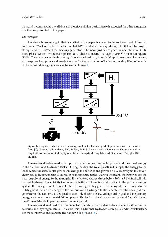
Energies 2019, 12, 614 2 of 24

nanogrid is commercially available and therefore similar performance is expected for other nanogridslike the one presented in this paper.

The Nanogrid

The single house nanogrid that is studied in this paper is located in the southern part of Swedenand has a 22.6 kWp solar installation, 144 kWh lead acid battery storage, 1100 kWh hydrogenstorage and a 15 kVA diesel backup generator. The nanogrid is designed to operate as a 50 Hzthree-phase system where each phase has a phase-to-neutral voltage of 230 V root mean square(RMS). The consumption in the nanogrid consists of ordinary household appliances, two electric cars,a three-phase heat pump and an electrolyzer for the production of hydrogen. A simplified schematicof the nanogrid energy system can be seen in Figure 1.

Energies 2018, 11, x FOR PEER REVIEW 2 of 27

nanogrid is commercially available and therefore similar performance is expected for other nanogrids like the one presented in this paper.

1.1. The Nanogrid

The single house nanogrid that is studied in this paper is located in the southern part of Sweden and has a 22.6 kWp solar installation, 144 kWh lead acid battery storage, 1100 kWh hydrogen storage and a 15 kVA diesel backup generator. The nanogrid is designed to operate as a 50 Hz three-phase system where each phase has a phase-to-neutral voltage of 230 V Root Mean Square (RMS). The consumption in the nanogrid consists of ordinary household appliances, two electric cars, a three-phase heat pump and an electrolyzer for the production of hydrogen. A simplified schematic of the nanogrid energy system can be seen in Figure 1.

Figure 1. Simplified schematic of the energy system for the nanogrid. Reproduced with permission

from [7], Nömm, J.; Rönnberg, S.K.; Bollen, M.H.J. An Analysis of Frequency Variations and its Implications on Connected Equipment for a Nanogrid during Islanded Operation. Energies 2018, 11,

2456.

The nanogrid is designed to run primarily on the produced solar power and the stored energy in the batteries and hydrogen tanks. During the day, the solar panels will supply the energy to the loads where the excess solar power will charge the batteries and power a 5 kW electrolyzer to convert electricity to hydrogen that is stored in high-pressure tanks. During the night, the batteries are the main supply of energy to the nanogrid; if the battery charge drops below 30%, a 5 kW fuel cell will convert hydrogen to electricity to charge the battery. If there is a malfunction in the primary energy system, the nanogrid will connect to the low-voltage utility grid. The nanogrid also connects to the utility grid if the stored energy in the batteries and hydrogen tanks is depleted. The backup diesel generator in the nanogrid is designed to start only if both the low voltage utility grid and the primary energy system in the nanogrid fail to operate. The backup diesel generator operated for 43 h during the 48 week islanded operation measurement period.

The nanogrid switched to grid-connected operation mainly due to lack of energy stored in the batteries and hydrogen tanks. To avoid this, additional hydrogen storage is under construction. For more information regarding the nanogrid see [7] and [8].

2. Methodology

Figure 1. Simplified schematic of the energy system for the nanogrid. Reproduced with permissionfrom [7], Nömm, J.; Rönnberg, S.K.; Bollen, M.H.J. An Analysis of Frequency Variations and itsImplications on Connected Equipment for a Nanogrid during Islanded Operation. Energies 2018,11, 2456.

The nanogrid is designed to run primarily on the produced solar power and the stored energyin the batteries and hydrogen tanks. During the day, the solar panels will supply the energy to theloads where the excess solar power will charge the batteries and power a 5 kW electrolyzer to convertelectricity to hydrogen that is stored in high-pressure tanks. During the night, the batteries are themain supply of energy to the nanogrid; if the battery charge drops below 30%, a 5 kW fuel cell willconvert hydrogen to electricity to charge the battery. If there is a malfunction in the primary energysystem, the nanogrid will connect to the low-voltage utility grid. The nanogrid also connects to theutility grid if the stored energy in the batteries and hydrogen tanks is depleted. The backup dieselgenerator in the nanogrid is designed to start only if both the low voltage utility grid and the primaryenergy system in the nanogrid fail to operate. The backup diesel generator operated for 43 h duringthe 48 week islanded operation measurement period.

The nanogrid switched to grid-connected operation mainly due to lack of energy stored in thebatteries and hydrogen tanks. To avoid this, additional hydrogen storage is under construction.For more information regarding the nanogrid see [7] and [8].

Energies 2019, 12, 614 3 of 24

2. Methodology

The measurements have been collected by an Elspec G4430 (Elspec, Caesarea, Israel) connected atthe load-output of the SMA Multicluster Box (SMA, Niestetal, Germany). The SMA Multicluster Box isused in the nanogrid since there are three independent solar installations, two on the roof, each with acapacity of 10 kW and one on the facade with 2.6 kW power rating.

The parameters measured for the comparison to the limits described in EN 50160 and IEEE519-2014 are the voltage Total Harmonic Distortion (THD), Individual odd harmonics 3rd to 11thand 15th, even harmonics 4th to 8th, Pst, Plt, and voltage unbalance. Two parameters that were alsomeasured with no relation to any standard were the very short variations (VSV) of the voltage and RMSvalue of the neutral current. For the measured parameters, the total time in islanded operation was48 weeks and 54 weeks in grid-connected operation. The 48 and 54 week measurements are assembledfrom shorter time windows in which the nanogrid was in islanded or grid-connected operation.

For the voltage THD measurements, there was a measurement period of 29 weeks of the total48 weeks where the nanogrid operated continuously in islanded operation. These measurements wereused to see the daily voltage THD variations.

For the analysis of the individual harmonics, the odd harmonics 3rd to 11th and 15th and evenharmonics 4th to 8th were chosen since they all surpass the limits defined in either standard EN 50160or IEEE 519-2014 sometime during the 48 week islanded operation measurements.

Another measurement period of about 8 weeks in islanded operation and about 5 weeks ingrid-connected operation was used to study the variations with time in the short circuit impedancemeasured as the voltage drop against a current rise of larger than 4 A within two cycles.

3. Results

3.1. Total harmonic Distortion

The cumulative distribution function (CDF) for the 10 min values of the voltage THD during48 weeks in islanded operation and 54 weeks in grid-connected operation can be seen in the upperpart of Figure 2.

In the lower part of Figure 2, the corresponding CDF for the 3 s values is plotted. As expected,the 3 s voltage THD values reach higher values than the 10 min values during both islanded andgrid-connected operation. It can also be observed in Figure 2 that the voltage THD is always higherduring islanded operation than during grid-connected operation. The maximum values and totalaverage values are also higher for islanded operation which can be seen in Table 1.

Table 1. 95% Confidence interval (CI) for the 10 min values, the maximum 10 min value and totalaverage value for all three phases in islanded and grid-connected operation.

OperationalState

95% CI 10 minValue

Max 10 minValue

95% CI 3 sValue

Max 3 sValue

Total AverageValue

Islanded 1.34 to 8% 7.83 to 13.01% 1.28 to 8.06% 18.3 to 21.9% 2.23 to 3.82%Grid-connected 0.77 to 1.88% 2.41 to 2.47% 0.76 to 1.88% ≈2.5% 1.08 to 1.44%

In Figure 3, the average voltage THD variations for each hour of the day for 29 weeks can be seenfor all three phases. During 29 out of 48 weeks the nanogrid operated in islanded operation that lastedcontinually throughout the day without connections to the utility grid.

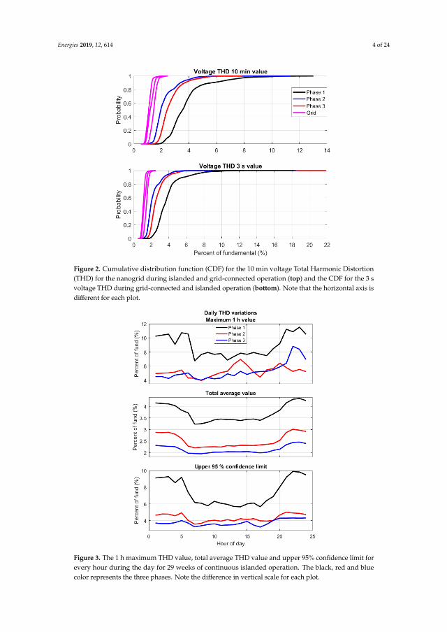
Energies 2019, 12, 614 4 of 24

3. Results

3.1. Total harmonic Distortion

The cumulative distribution function (CDF) for the 10 min values of the voltage THD during 48 weeks in islanded operation and 54 weeks in grid-connected operation can be seen in the upper part of Figure 2.

Figure 2. Cumulative distribution function (CDF) for the 10 min voltage Total Harmonic Distortion(THD) for the nanogrid during islanded and grid-connected operation (top) and the CDF for the 3 svoltage THD during grid-connected and islanded operation (bottom). Note that the horizontal axis isdifferent for each plot.Energies 2018, 11, x FOR PEER REVIEW 5 of 27

Figure 3. The 1 h maximum THD value, total average THD value and upper 95% confidence limit for every hour during the day for 29 weeks of continuous islanded operation. The black, red and blue color represents the three phases. Note the difference in vertical scale for each plot.

The trend in Figure 3 shows larger THD values during the night than during the day. This indicates that when the solar production starts, the voltage THD level drops due to more parallel sources being activated and increases when there are fewer parallel sources available. One example when the voltage THD suddenly increases during the evening at about the time when the sun sets can be seen in Figure 4. It can be seen that even though the active power remains almost constant the

Figure 3. The 1 h maximum THD value, total average THD value and upper 95% confidence limit forevery hour during the day for 29 weeks of continuous islanded operation. The black, red and bluecolor represents the three phases. Note the difference in vertical scale for each plot.

Energies 2019, 12, 614 5 of 24

It can be seen that the maximum 1 h values are reached during the night for phase 1 and 3.For phase 2, the maximum occurs in the middle of the day. The total average value and 95% confidencelimit for each hour during the day reach the highest values in the morning and night for all 3 phases.Phase 3 has however a smaller variation between night and day in the total average value and 95%confidence limit as phase 1 and 2. A more detailed view of the voltage THD variations during one daycan be seen in [9].

The trend in Figure 3 shows larger THD values during the night than during the day. This indicatesthat when the solar production starts, the voltage THD level drops due to more parallel sources beingactivated and increases when there are fewer parallel sources available. One example when the voltageTHD suddenly increases during the evening at about the time when the sun sets can be seen in Figure 4.It can be seen that even though the active power remains almost constant the voltage THD increasesfor all three phases which also can be seen in the voltage waveform. The current THD also increases forphase 1 and 3 and decreases for phase 2 which can also be seen in the current waveform. The reactivepower changes somewhat for the three phases and the frequency throughout Figure 4 was around49 Hz.Energies 2018, 11, x FOR PEER REVIEW 6 of 27

Figure 4. Example of an occasion when the voltage THD increases in the evening. The voltage waveform is at the top followed by the current waveform, active power, reactive power, current THD and voltage THD. The black, red and blue color represents the three phases.

3.2. Individual Harmonics

In Figure 5, the odd voltage and current harmonics 3 to 9 are presented for the 1-cycle period ending at about 20 ms and 80 ms in Figure 4. The 3rd voltage harmonic is about the same for phase 1 and 2 and slightly lower for phase 3. After the transition from 8 to 12% voltage THD (seen at around 40 ms in Figure 4), the 5th voltage harmonic increases for two of the three phases and the 7th and 9th voltage harmonic also increase for all three phases. All of the current harmonics increase for phase 1 but the 3rd harmonic for phase 2 decreases by 1.4% and the 3rd and 7th harmonic for phase 3 decrease

Figure 4. Example of an occasion when the voltage THD increases in the evening. The voltagewaveform is at the top followed by the current waveform, active power, reactive power, current THDand voltage THD. The black, red and blue color represents the three phases.

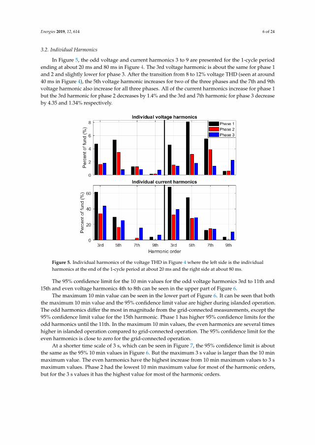
Energies 2019, 12, 614 6 of 24


In Figure 5, the odd voltage and current harmonics 3 to 9 are presented for the 1-cycle periodending at about 20 ms and 80 ms in Figure 4. The 3rd voltage harmonic is about the same for phase 1and 2 and slightly lower for phase 3. After the transition from 8 to 12% voltage THD (seen at around40 ms in Figure 4), the 5th voltage harmonic increases for two of the three phases and the 7th and 9thvoltage harmonic also increase for all three phases. All of the current harmonics increase for phase 1but the 3rd harmonic for phase 2 decreases by 1.4% and the 3rd and 7th harmonic for phase 3 decreaseby 4.35 and 1.34% respectively.Energies 2018, 11, x FOR PEER REVIEW 7 of 27

Figure 5. Individual harmonics of the voltage THD in Figure 4 where the left side is the individual harmonics at the end of the 1-cycle period at about 20 ms and the right side at about 80 ms.

The 95% confidence limit for the 10 min values for the odd voltage harmonics 3rd to 11th and 15th and even voltage harmonics 4th to 8th can be seen in the upper part of Figure 6.

Figure 5. Individual harmonics of the voltage THD in Figure 4 where the left side is the individualharmonics at the end of the 1-cycle period at about 20 ms and the right side at about 80 ms.

The 95% confidence limit for the 10 min values for the odd voltage harmonics 3rd to 11th and15th and even voltage harmonics 4th to 8th can be seen in the upper part of Figure 6.

The maximum 10 min value can be seen in the lower part of Figure 6. It can be seen that boththe maximum 10 min value and the 95% confidence limit value are higher during islanded operation.The odd harmonics differ the most in magnitude from the grid-connected measurements, except the95% confidence limit value for the 15th harmonic. Phase 1 has higher 95% confidence limits for theodd harmonics until the 11th. In the maximum 10 min values, the even harmonics are several timeshigher in islanded operation compared to grid-connected operation. The 95% confidence limit for theeven harmonics is close to zero for the grid-connected operation.

At a shorter time scale of 3 s, which can be seen in Figure 7, the 95% confidence limit is aboutthe same as the 95% 10 min values in Figure 6. But the maximum 3 s value is larger than the 10 minmaximum value. The even harmonics have the highest increase from 10 min maximum values to 3 smaximum values. Phase 2 had the lowest 10 min maximum value for most of the harmonic orders,but for the 3 s values it has the highest value for most of the harmonic orders.

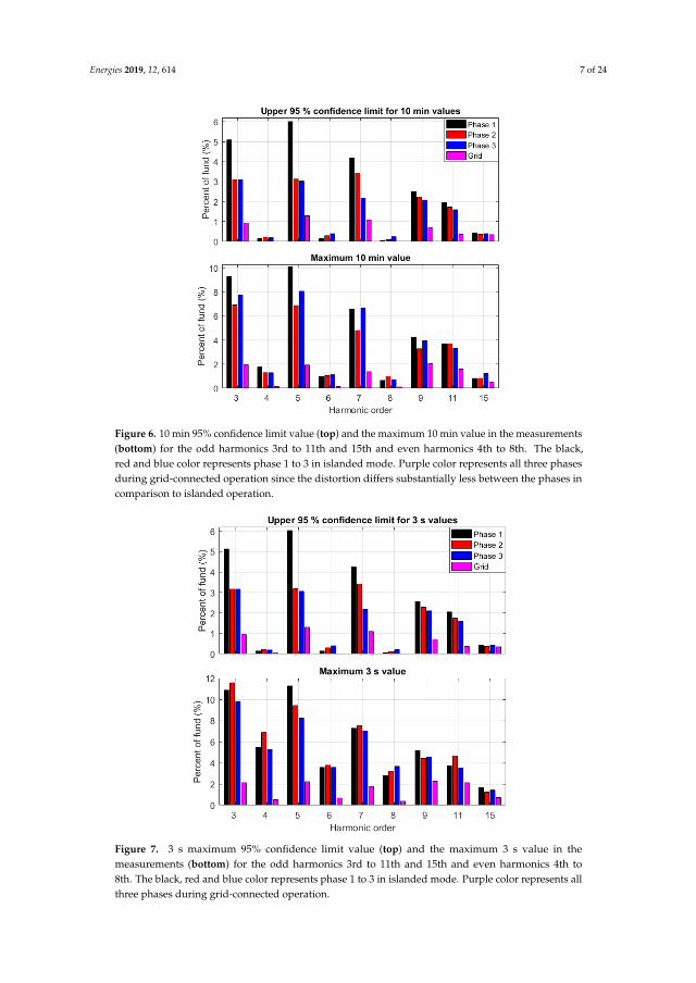
Energies 2019, 12, 614 7 of 24

Figure 5. Individual harmonics of the voltage THD in Figure 4 where the left side is the individual harmonics at the end of the 1-cycle period at about 20 ms and the right side at about 80 ms.

The 95% confidence limit for the 10 min values for the odd voltage harmonics 3rd to 11th and 15th and even voltage harmonics 4th to 8th can be seen in the upper part of Figure 6.

Figure 6. 10 min 95% confidence limit value (top) and the maximum 10 min value in the measurements (bottom) for the odd harmonics 3rd to 11th and 15th and even harmonics 4th to 8th. The black, red and blue color represents phase 1 to 3 in islanded mode. Purple color represents all three phases during grid-connected operation since the distortion differs substantially less between the phases in comparison to islanded operation.

Figure 6. 10 min 95% confidence limit value (top) and the maximum 10 min value in the measurements(bottom) for the odd harmonics 3rd to 11th and 15th and even harmonics 4th to 8th. The black,red and blue color represents phase 1 to 3 in islanded mode. Purple color represents all three phasesduring grid-connected operation since the distortion differs substantially less between the phases incomparison to islanded operation.


The maximum 10 min value can be seen in the lower part of Figure 6. It can be seen that both the maximum 10 min value and the 95% confidence limit value are higher during islanded operation. The odd harmonics differ the most in magnitude from the grid-connected measurements, except the 95% confidence limit value for the 15th harmonic. Phase 1 has higher 95% confidence limits for the odd harmonics until the 11th. In the maximum 10 min values, the even harmonics are several times higher in islanded operation compared to grid-connected operation. The 95% confidence limit for the even harmonics is close to zero for the grid-connected operation.

At a shorter time scale of 3 s, which can be seen in Figure 7, the 95% confidence limit is about the same as the 95% 10 min values in Figure 6. But the maximum 3 s value is larger than the 10 min maximum value. The even harmonics have the highest increase from 10 min maximum values to 3 s maximum values. Phase 2 had the lowest 10 min maximum value for most of the harmonic orders, but for the 3 s values it has the highest value for most of the harmonic orders.

The total average values for both grid-connected and islanded operation can be seen in Table 2.

Table 2. Total average value for each measured voltage harmonic for all three phases.

Operational State

3rd (%)

4th (%)

5th (%)

6th (%)

7th (%)

8th (%)

9th (%)

11th (%)

15th (%)

Islanded 0.95 to

1.96

0.01 to

0.02

0.83 to 2.0

0.016 to 0.04

0.61 to

1.45

0.008 to

0.016

1.20 to 1.38

0.63 to 0.66

0.20 to 0.18

Grid-connected

0.30 to 0.52

≈

0.001

0.66 to

0.90 ≈10-4

0.55 to

0.60 ≈10-5

0.34 to 0.44

0.14 to 0.17

0.10 to 0.15

Figure 7. 3 s maximum 95% confidence limit value (top) and the maximum 3 s value in the measurements (bottom) for the odd harmonics 3rd to 11th and 15th and even harmonics 4th to 8th. The black, red and blue color represents phase 1 to 3 in islanded mode. Purple color represents all three phases during grid-connected operation.

3.3. Voltage Unbalance

Figure 7. 3 s maximum 95% confidence limit value (top) and the maximum 3 s value in themeasurements (bottom) for the odd harmonics 3rd to 11th and 15th and even harmonics 4th to8th. The black, red and blue color represents phase 1 to 3 in islanded mode. Purple color represents allthree phases during grid-connected operation.

Energies 2019, 12, 614 8 of 24

The total average values for both grid-connected and islanded operation can be seen in Table 2.

Table 2. Total average value for each measured voltage harmonic for all three phases.

OperationalState 3rd (%) 4th (%) 5th (%) 6th (%) 7th (%) 8th (%) 9th (%) 11th (%) 15th (%)

Islanded 0.95 to1.96

0.01 to0.02

0.83 to2.0

0.016 to0.04

0.61 to1.45

0.008 to0.016

1.20 to1.38

0.63 to0.66

0.20 to0.18

Grid-connected 0.30 to0.52 ≈0.001 0.66 to

0.90 ≈10-4 0.55 to0.60 ≈10-5 0.34 to

0.440.14 to

0.170.10 to

0.15


The 10 min voltage unbalance for both islanded operation and grid-connected operation can beseen in Figure 8. The voltage unbalance is for the majority of the measured time lower in islandedoperation than in grid-connected operation. The maximum 10 min voltage unbalance was 4.6% forislanded operation and 1.77 for grid-connected operation. In Figures 14–16 the occurrence of themaximum voltage unbalance value can be seen. A summary of the 95% CI, maximum 10 min valueand total average value in islanded and grid-connected operation can be seen in Table 3.


The 10 min voltage unbalance for both islanded operation and grid-connected operation can be seen in Figure 8. The voltage unbalance is for the majority of the measured time lower in islanded operation than in grid-connected operation. The maximum 10 min voltage unbalance was 4.6% for islanded operation and 1.77 for grid-connected operation. In Figures 14–16 the occurrence of the maximum voltage unbalance value can be seen. A summary of the 95% CI, maximum 10 min value and total average value in islanded and grid-connected operation can be seen in Table 3.

Table 3. 95% confidence interval, the maximum 10 min value and total average value for all three phases in islanded and grid-connected operation.

Operational State

95% CI 10 min Value Max 10 min Value Total Average Value

Islanded 0.06 to 0.72% 4.6% 0.22% Grid-connected 0.11 to 0.68% 1.77% 0.31%

Figure 8. CDF for the 10 min voltage unbalance values in the nanogrid during islanded and grid-connected operation.

3.4. Voltage Fluctuations

The CDF of the Pst values for grid-connected and islanded operation can be seen in Figure 9. The islanded operation data reaches lower Pst values than in grid-connected operation for 95% and 33% of the total measured time for phase 2 and 1. Phase 3 has larger Pst values for the majority of the time when comparing to the grid-connected operation Pst values. All three phases have higher maximum values than the grid-connected measurements. A summary of the 95% CI, maximum value and total average value for all three phases in islanded and grid-connected operation can be seen in Table 4.


Figure 8. CDF for the 10 min voltage unbalance values in the nanogrid during islanded andgrid-connected operation.

Table 3. 95% confidence interval, the maximum 10 min value and total average value for all threephases in islanded and grid-connected operation.

Operational State 95% CI 10 min Value Max 10 min Value Total Average Value

Islanded 0.06 to 0.72% 4.6% 0.22%Grid-connected 0.11 to 0.68% 1.77% 0.31%

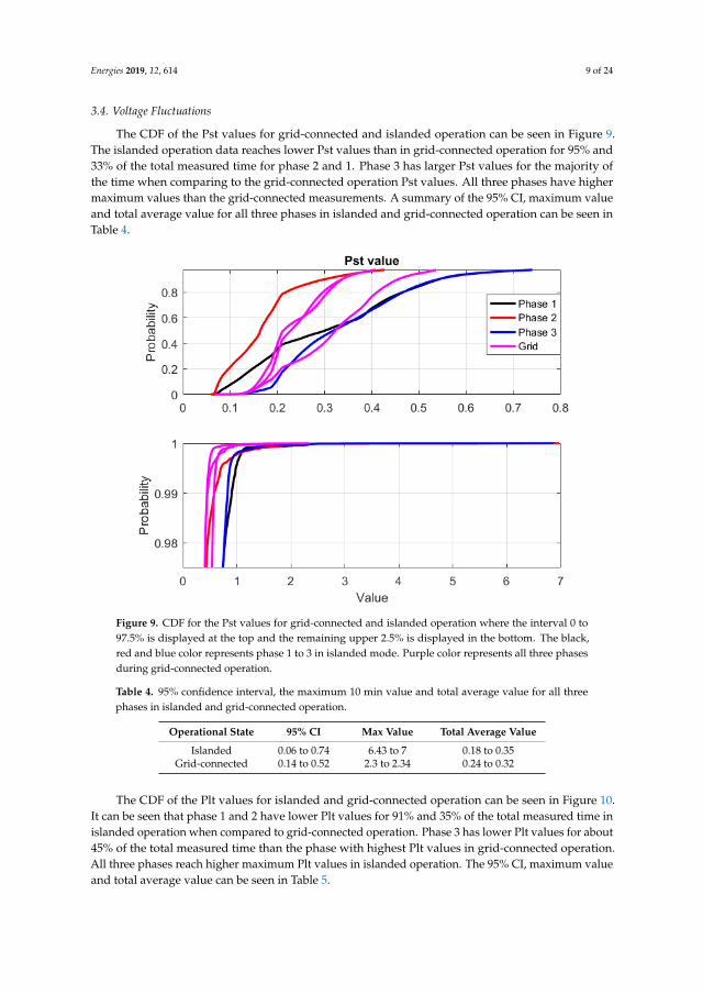
Energies 2019, 12, 614 9 of 24

3.4. Voltage Fluctuations

The CDF of the Pst values for grid-connected and islanded operation can be seen in Figure 9.The islanded operation data reaches lower Pst values than in grid-connected operation for 95% and33% of the total measured time for phase 2 and 1. Phase 3 has larger Pst values for the majority ofthe time when comparing to the grid-connected operation Pst values. All three phases have highermaximum values than the grid-connected measurements. A summary of the 95% CI, maximum valueand total average value for all three phases in islanded and grid-connected operation can be seen inTable 4.


Operational State 95% CI Max Value Total Average Value

Islanded 0.06 to 0.74 6.43 to 7 0.18 to 0.35 Grid-connected 0.14 to 0.52 2.3 to 2.34 0.24 to 0.32

Figure 9. CDF for the Pst values for grid-connected and islanded operation where the interval 0 to 97.5% is displayed at the top and the remaining upper 2.5% is displayed in the bottom. The black, red and blue color represents phase 1 to 3 in islanded mode. Purple color represents all three phases during grid-connected operation.

The CDF of the Plt values for islanded and grid-connected operation can be seen in Figure 10. It can be seen that phase 1 and 2 have lower Plt values for 91% and 35% of the total measured time in islanded operation when compared to grid-connected operation. Phase 3 has lower Plt values for about 45% of the total measured time than the phase with highest Plt values in grid-connected operation. All three phases reach higher maximum Plt values in islanded operation. The 95% CI, maximum value and total average value can be seen in Table 5.


Operational State 95% CI Maximum Value Total Average Value Islanded 0.07 to 0.72 2.78 to 2.99 0.21 to 0.36

Grid-connected 0.19 to 0.52 1.16 to 1.2 0.26% 0.34

Figure 9. CDF for the Pst values for grid-connected and islanded operation where the interval 0 to97.5% is displayed at the top and the remaining upper 2.5% is displayed in the bottom. The black,red and blue color represents phase 1 to 3 in islanded mode. Purple color represents all three phasesduring grid-connected operation.


Operational State 95% CI Max Value Total Average Value

Islanded 0.06 to 0.74 6.43 to 7 0.18 to 0.35Grid-connected 0.14 to 0.52 2.3 to 2.34 0.24 to 0.32

The CDF of the Plt values for islanded and grid-connected operation can be seen in Figure 10.It can be seen that phase 1 and 2 have lower Plt values for 91% and 35% of the total measured time inislanded operation when compared to grid-connected operation. Phase 3 has lower Plt values for about45% of the total measured time than the phase with highest Plt values in grid-connected operation.All three phases reach higher maximum Plt values in islanded operation. The 95% CI, maximum valueand total average value can be seen in Table 5.

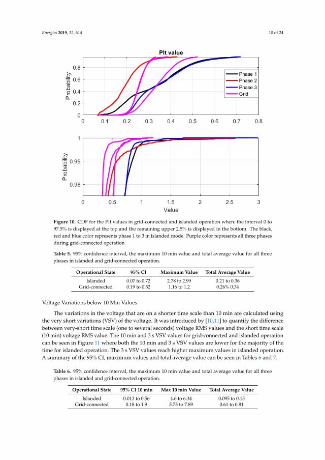
Energies 2019, 12, 614 10 of 24


Figure 10. CDF for the Plt values in grid-connected and islanded operation where the interval 0 to 97.5% is displayed at the top and the remaining upper 2.5% is displayed in the bottom. The black, red and blue color represents phase 1 to 3 in islanded mode. Purple color represents all three phases during grid-connected operation.

3.4.1. Voltage Variations below 10 Min Values

The variations in the voltage that are on a shorter time scale than 10 min are calculated using the very short variations (VSV) of the voltage. It was introduced by [10,11] to quantify the difference between very-short time scale (one to several seconds) voltage RMS values and the short time scale (10 min) voltage RMS value. The 10 min and 3 s VSV values for grid-connected and islanded operation can be seen in Figure 11 where both the 10 min and 3 s VSV values are lower for the majority of the time for islanded operation. The 3 s VSV values reach higher maximum values in islanded operation. A summary of the 95% CI, maximum values and total average value can be seen in Tables 6 and 7.


Operational State 95% CI 10 min Max 10 min Value Total Average Value Islanded 0.013 to 0.56 4.6 to 6.34 0.095 to 0.15

Grid-connected 0.18 to 1.9 5.75 to 7.89 0.61 to 0.81

Table 7. 95% confidence interval, the maximum 3 s value and total average value for all three phases in islanded and grid-connected operation.

Operational State 95% CI 3 s Max 3 s Value Total Average Value Islanded ≈0 to 0.58 15.52 to 18.3 0.07 to 0.11

Grid-connected 0.015 to 2.32 10.6 to 15.7 0.50 to 0.66

Figure 10. CDF for the Plt values in grid-connected and islanded operation where the interval 0 to97.5% is displayed at the top and the remaining upper 2.5% is displayed in the bottom. The black,red and blue color represents phase 1 to 3 in islanded mode. Purple color represents all three phasesduring grid-connected operation.


Operational State 95% CI Maximum Value Total Average Value

Islanded 0.07 to 0.72 2.78 to 2.99 0.21 to 0.36Grid-connected 0.19 to 0.52 1.16 to 1.2 0.26% 0.34

Voltage Variations below 10 Min Values

The variations in the voltage that are on a shorter time scale than 10 min are calculated usingthe very short variations (VSV) of the voltage. It was introduced by [10,11] to quantify the differencebetween very-short time scale (one to several seconds) voltage RMS values and the short time scale(10 min) voltage RMS value. The 10 min and 3 s VSV values for grid-connected and islanded operationcan be seen in Figure 11 where both the 10 min and 3 s VSV values are lower for the majority of thetime for islanded operation. The 3 s VSV values reach higher maximum values in islanded operation.A summary of the 95% CI, maximum values and total average value can be seen in Tables 6 and 7.


Operational State 95% CI 10 min Max 10 min Value Total Average Value

Islanded 0.013 to 0.56 4.6 to 6.34 0.095 to 0.15Grid-connected 0.18 to 1.9 5.75 to 7.89 0.61 to 0.81

Energies 2019, 12, 614 11 of 24


Figure 11. CDF for the 10 min Very Short Variations (VSV) values (top) and the 3 s VSV values (bottom) for islanded and grid-connected operation.

3.5. Neutral Current

The CDF for the 10 min RMS neutral current for 48 weeks of islanded operation and 54 weeks of grid-connected operation can be seen in Figure 12.

Figure 12. CDF for the 10 min RMS neutral current during islanded and grid-connected operation.

Figure 11. CDF for the 10 min very short variations (VSV) values (top) and the 3 s VSV values (bottom)for islanded and grid-connected operation.

Table 7. 95% confidence interval, the maximum 3 s value and total average value for all three phases inislanded and grid-connected operation.

Operational State 95% CI 3 s Max 3 s Value Total Average Value

Islanded ≈0 to 0.58 15.52 to 18.3 0.07 to 0.11Grid-connected 0.015 to 2.32 10.6 to 15.7 0.50 to 0.66


The CDF for the 10 min RMS neutral current for 48 weeks of islanded operation and 54 weeks ofgrid-connected operation can be seen in Figure 12.

The 50 Hz component was always several times larger than the zero sequence components wherethe 3rd harmonic reached a maximum value of 6 A during the 48 week measurement period in islandedoperation. For both islanded and grid-connected operation, the line to neutral voltage was close to0 V. The neutral current reached about the same maximum values of around 42 A in islanded andgrid-connected operation. However, during islanded operation the 10 min values are for the most parthigher than the grid-connected values. A summary of the 95% CI, maximum values and total averagevalue can be seen in Table 8.


Operational State 95% CI 10 min Max 10 min Value Total Average Value

Islanded 2.15 to 17.6 41.4 5Grid-connected 1.2 to 15.1 41.8 3.6

Energies 2019, 12, 614 12 of 24

Figure 11. CDF for the 10 min Very Short Variations (VSV) values (top) and the 3 s VSV values (bottom) for islanded and grid-connected operation.


The CDF for the 10 min RMS neutral current for 48 weeks of islanded operation and 54 weeks of grid-connected operation can be seen in Figure 12.

Figure 12. CDF for the 10 min RMS neutral current during islanded and grid-connected operation. Figure 12. CDF for the 10 min RMS neutral current during islanded and grid-connected operation.

3.6. Operational Modes during Islanded Operation.

The short circuit impedance is extracted from a 13 weeks continuous period. During this13 week period, the nanogrid operated part of the time in islanded operation and part of the timein grid-connected operation, which can be seen in Figures 13–16. The short circuit impedance wasmeasured as the voltage drop against a current rise of larger than 4 A within two cycles. 4 A waschosen since values lower than 2 A could sometimes not affect the voltage, therefore a larger value of4 A giving a 2 A margin was chosen. No correlation between the current rise magnitude (4 to 26 A inthis paper) and the short circuit impedance were found and no correlation between the starting valueof the current (0 to 36 A) and the short circuit impedance was found.

In Figure 13 two different modes of islanded operation can be distinguished, one where the shortcircuit impedance fluctuates between 0.1 and 1 Ω and one in which it fluctuates between 0.1 and2 Ω and sometimes reaching values close to 6 Ω but only for phase 2. During the grid-connectedoperation the values fluctuate between 0.2 and 0.4 Ω. The number of samples for the different phaseswas 31,000, 730 and 11,000 for phase 1 to 3 respectively, giving rise to differences in the horizontalaxis in Figure 13. In Figures 14–16, the 10 min voltage THD, current THD, 3rd, 5th, 7th, 9th harmonicvoltage and voltage unbalance are plotted for the 13 week period. The two different modes of islandedoperation are again indicated. The voltage unbalance reaches the highest levels of about 4.6% duringmode 2 of the islanded operation. The voltage THD, 3rd, 5th and 7th harmonic voltage is also larger inmode 2 for all three phases during the majority of the measured period. The 9th harmonic is for themost part lower in mode 2 for all three phases.

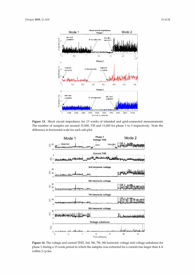
Energies 2019, 12, 614 13 of 24

The short circuit impedance is extracted from a 13 weeks continuous period. During this 13 week period, the nanogrid operated part of the time in islanded operation and part of the time in grid-connected operation, which can be seen in Figure 13 to 16. The short circuit impedance was measured as the voltage drop against a current rise of larger than 4 A within two cycles. 4 A was chosen since values lower than 2 A could sometimes not affect the voltage, therefore a larger value of 4 A giving a 2 A margin was chosen. No correlation between the current rise magnitude (4 to 26 A in this paper) and the short circuit impedance were found and no correlation between the starting value of the current (0 to 36 A) and the short circuit impedance was found.

Figure 13. Short circuit impedance for 13 weeks of islanded and grid-connected measurements.The number of samples are around 31,000, 730 and 11,000 for phase 1 to 3 respectively. Note thedifference in horizontal scale for each sub-plot.


Figure 13. Short circuit impedance for 13 weeks of islanded and grid-connected measurements. The number of samples are around 31,000, 730 and 11,000 for phase 1 to 3 respectively. Note the difference in horizontal scale for each sub-plot.

In Figure 13 two different modes of islanded operation can be distinguished, one where the short circuit impedance fluctuates between 0.1 and 1 Ω and one in which it fluctuates between 0.1 and 2 Ω and sometimes reaching values close to 6 Ω but only for phase 2. During the grid-connected operation the values fluctuate between 0.2 and 0.4 Ω. The number of samples for the different phases was 31,000, 730 and 11,000 for phase 1 to 3 respectively, giving rise to differences in the horizontal axis in Figure 13. In Figures 14–16, the 10 min voltage THD, current THD, 3rd, 5th, 7th, 9th harmonic voltage and voltage unbalance are plotted for the 13 week period. The two different modes of islanded operation are again indicated. The voltage unbalance reaches the highest levels of about 4.6% during mode 2 of the islanded operation. The voltage THD, 3rd, 5th and 7th harmonic voltage is also larger in mode 2 for all three phases during the majority of the measured period. The 9th harmonic is for the most part lower in mode 2 for all three phases.

Figure 14. The voltage and current THD, 3rd, 5th, 7th, 9th harmonic voltage and voltage unbalance for phase 1 during a 13 week period in which the samples was extracted for a current rise larger than 4 A within 2 cycles.

Figure 14. The voltage and current THD, 3rd, 5th, 7th, 9th harmonic voltage and voltage unbalance forphase 1 during a 13 week period in which the samples was extracted for a current rise larger than 4 Awithin 2 cycles.

Energies 2019, 12, 614 14 of 24



Figure 15. The voltage and current THD, 3rd, 5th, 7th, 9th harmonic voltage and voltage unbalance forphase 2 during a 13 week period in which the samples was extracted for a current rise larger than 4 Awithin 2 cycles.Energies 2018, 11, x FOR PEER REVIEW 16 of 27


The average short circuit impedance for each hour during the day for around 8 weeks in islanded operation seen in Figure 13 can be seen in Figure 17. The blue and red line represents mode 1 and mode 2 respectively seen in Figure 13. The amount of samples for phase 1 to 3 is around 31,000, 730, 11,000 respectively, therefore phase 2 doesn’t have samples for some hours during the day. It can be seen that the short circuit impedance is larger during the beginning of the day for phase 1 and larger during the middle of the day for phase 3. For phase 2 there are not enough samples to clearly see the variation during the day. However, for all three phases it can be seen that the short circuit impedance

Figure 16. The voltage and current THD, 3rd, 5th, 7th, 9th harmonic voltage and voltage unbalance forphase 3 during a 13 week period in which the samples was extracted for a current rise larger than 4 Awithin 2 cycles.

Energies 2019, 12, 614 15 of 24

The average short circuit impedance for each hour during the day for around 8 weeks in islandedoperation seen in Figure 13 can be seen in Figure 17. The blue and red line represents mode 1 andmode 2 respectively seen in Figure 13. The amount of samples for phase 1 to 3 is around 31,000, 730,11,000 respectively, therefore phase 2 doesn’t have samples for some hours during the day. It can beseen that the short circuit impedance is larger during the beginning of the day for phase 1 and largerduring the middle of the day for phase 3. For phase 2 there are not enough samples to clearly see thevariation during the day. However, for all three phases it can be seen that the short circuit impedancehas a higher average for each hour during the day during mode 2 in islanded operation.Energies 2018, 11, x FOR PEER REVIEW 17 of 27

Figure 17. The average short circuit impedance for each hour of the day for around 8 weeks in islanded operation for Mode 1 and Mode 2 seen in Figure 13.

The average values for each hour of the day for around 8 weeks in islanded operation for the 3rd to 9th odd harmonic voltages, currents and voltage THD for mode 1 in Figures 14–16 can be seen in Figure 18. Mode 1 has larger 7th and 9th harmonic voltages and currents during the night for all three phases and the 5th harmonic has larger values for phase 1 and 3. The 3rd harmonic is more evenly distributed across the day where the 3rd harmonic has larger average voltage and current values during the middle of the day. The voltage THD has the largest values during the night which corresponds with the result from the longer 29 week measurements presented in Figure 3.

Figure 17. The average short circuit impedance for each hour of the day for around 8 weeks in islandedoperation for Mode 1 and Mode 2 seen in Figure 13.

The average values for each hour of the day for around 8 weeks in islanded operation for the3rd to 9th odd harmonic voltages, currents and voltage THD for mode 1 in Figures 14–16 can be seenin Figure 18. Mode 1 has larger 7th and 9th harmonic voltages and currents during the night for allthree phases and the 5th harmonic has larger values for phase 1 and 3. The 3rd harmonic is moreevenly distributed across the day where the 3rd harmonic has larger average voltage and currentvalues during the middle of the day. The voltage THD has the largest values during the night whichcorresponds with the result from the longer 29 week measurements presented in Figure 3.

Energies 2019, 12, 614 16 of 24


(a) (b)

Figure 18. (a) The odd harmonic voltage 3rd to 9th and THD for mode 1 in Figures 14–16. (b) The odd harmonic current 3rd to 9th and THD for mode 1 in Figures 14–16. The average values are grouped for each hour of the day for around 8 weeks of islanded operation. Note also the difference in vertical scale for the different plots.

The average values for each hour during the day for around 8 weeks in islanded operation for the 3rd to 9th odd harmonic voltages, currents and THD for mode 2 in Figures 14–16 can be seen in Figure 19. The average 3rd harmonic voltage is larger during the middle of the day and with larger magnitude than in Figure 18. The 5th and 7th harmonic has the largest voltage distortion levels during the night for all 3 phases and larger variation between night and day in comparison to mode 1 seen in Figure 18. The 9th harmonic voltage is larger during the night for phase 3 and higher during the middle of the day for phase 1 and 2. The voltage THD has the largest values during the night which corresponds with the result from the longer 29 week measurements presented in Figure 3. The harmonic current levels follow the same pattern for some of the voltage harmonics but have opposite pattern for other voltage harmonics. This indicates that there are more factors that act on the voltage distortion than the current distortion.

Figure 18. (a) The odd harmonic voltage 3rd to 9th and THD for mode 1 in Figures 14–16. (b) The oddharmonic current 3rd to 9th and THD for mode 1 in Figures 14–16. The average values are groupedfor each hour of the day for around 8 weeks of islanded operation. Note also the difference in verticalscale for the different plots.

The average values for each hour during the day for around 8 weeks in islanded operation forthe 3rd to 9th odd harmonic voltages, currents and THD for mode 2 in Figures 14–16 can be seenin Figure 19. The average 3rd harmonic voltage is larger during the middle of the day and withlarger magnitude than in Figure 18. The 5th and 7th harmonic has the largest voltage distortion levelsduring the night for all 3 phases and larger variation between night and day in comparison to mode 1seen in Figure 18. The 9th harmonic voltage is larger during the night for phase 3 and higher duringthe middle of the day for phase 1 and 2. The voltage THD has the largest values during the nightwhich corresponds with the result from the longer 29 week measurements presented in Figure 3.The harmonic current levels follow the same pattern for some of the voltage harmonics but haveopposite pattern for other voltage harmonics. This indicates that there are more factors that act on thevoltage distortion than the current distortion.

In Figure 20, the 1 h average values are plotted for the 3rd and 5th harmonic current and voltagefor around 8 weeks in islanded operation. The blue colored values are for mode 1 and the red coloredvalues are for mode 2 seen in Figures 14–16. The inclination (slope) corresponds to the impedancewhich is higher for mode 2 than for mode 1. However, for mode 1 the values form a more linearbehavior than for mode 2. For the 3rd harmonic in phase 3, there is an appearance of a large area thathas variation in voltage distortion without an increase in current distortion magnitude.

Energies 2019, 12, 614 17 of 24


(a) (b)

Figure 19. (a) The odd harmonic voltage 3rd to 9th and THD for mode 2 in Figures 14–16. (b) The odd harmonic current 3rd to 9th and THD for mode 2 in Figures 14–16. The average values are grouped for each hour of the day for around 8 weeks of islanded operation. Note also the difference in vertical scale for the different plots.

In Figure 20, the 1 h average values are plotted for the 3rd and 5th harmonic current and voltage for around 8 weeks in islanded operation. The blue colored values are for mode 1 and the red colored values are for mode 2 seen in Figures 14–16. The inclination (slope) corresponds to the impedance which is higher for mode 2 than for mode 1. However, for mode 1 the values form a more linear behavior than for mode 2. For the 3rd harmonic in phase 3, there is an appearance of a large area that has variation in voltage distortion without an increase in current distortion magnitude.

Another observation is that some of the measurements for mode 1 and 2 overlap each other which are expected since no criteria for the separation of the two modes exist except for the different time windows in Figures 13 to 16.

Figure 19. (a) The odd harmonic voltage 3rd to 9th and THD for mode 2 in Figures 14–16. (b) The oddharmonic current 3rd to 9th and THD for mode 2 in Figures 14–16. The average values are groupedfor each hour of the day for around 8 weeks of islanded operation. Note also the difference in verticalscale for the different plots.Energies 2018, 11, x FOR PEER REVIEW 20 of 27

(a) (b)

Figure 20. (a) The 1 h 3rd harmonic voltage and current values plotted against each other for Mode 1 and 2 seen in Figures 14–16. (b) The 1 h 5th harmonic voltage and current values plotted against each other for Mode 1 and 2 seen in Figures 14–16.

In Figure 21, the 1 h values are plotted for the 7th and 9th harmonic current and voltage for all three phases for around 8 weeks in islanded operation. The blue colored values are mode 1 and the red colored values are for mode 2 seen in Figures 14–16. The 7th and the 9th harmonic have some linear appearance for mode 1 but not as much as the 3rd and 5th harmonic. For mode 2 the behavior is more nonlinear, where some of the voltage distortion values are located close to zero current distortion for some phases. This indicates that the voltage distortion originates from the voltage source which is one of the possible sources of error in the impedance measurements. This is more evident in the 9th harmonic than in the 7th harmonic.

Figure 20. (a) The 1 h 3rd harmonic voltage and current values plotted against each other for Mode 1and 2 seen in Figures 14–16. (b) The 1 h 5th harmonic voltage and current values plotted against eachother for Mode 1 and 2 seen in Figures 14–16.

Energies 2019, 12, 614 18 of 24

Another observation is that some of the measurements for mode 1 and 2 overlap each other whichare expected since no criteria for the separation of the two modes exist except for the different timewindows in Figures 13–16.

In Figure 21, the 1 h values are plotted for the 7th and 9th harmonic current and voltage for allthree phases for around 8 weeks in islanded operation. The blue colored values are mode 1 and the redcolored values are for mode 2 seen in Figures 14–16. The 7th and the 9th harmonic have some linearappearance for mode 1 but not as much as the 3rd and 5th harmonic. For mode 2 the behavior is morenonlinear, where some of the voltage distortion values are located close to zero current distortion forsome phases. This indicates that the voltage distortion originates from the voltage source which isone of the possible sources of error in the impedance measurements. This is more evident in the 9thharmonic than in the 7th harmonic.Energies 2018, 11, x FOR PEER REVIEW 21 of 27

(a) (b)

Figure 21. (a) The 1 h 7th harmonic voltage and current values plotted against each other for mode 1 and 2 seen in Figures 14–16. (b) The 1 h 9th harmonic voltage and current values plotted against each other for mode 1 and 2 seen in Figures 14–16.

4. Comparison to Reference Values

In this section, some of the measured values presented in Section 3 are compared to the European standard EN 50160 and the IEEE standard 519-2014.

4.1. Voltage THD

The allowed 10 min voltage THD for a low voltage networks is 8% for 95% of the time per week for both IEEE standard 519-2014 and European standard EN 50160. IEEE standard 519-2014 has also a 12% THD limit for 3 s values for 99% of the time for one day at the low voltage Point of Common Coupling (PCC).

During islanded operation the number of weeks that exceeded the 5% allowed time frame in which the 10 min voltage THD could be above 8% is shown in the upper part of Figure 22. The total number of days that the 3 s voltage THD was over 12% for more than 1% of one day can also be seen in the upper part of Figure 22. The amount of time in which the voltage THD was over 8% and 12% can be seen in the lower part in Figure 22. Only phase 1 surpassed the 5% weekly limit for 8% voltage THD in EN 50160 and the 1% daily limit for 12% voltage THD described in IEEE 519-2014. During grid-connected operation no limits was surpassed.

Figure 21. (a) The 1 h 7th harmonic voltage and current values plotted against each other for mode 1and 2 seen in Figures 14–16. (b) The 1 h 9th harmonic voltage and current values plotted against eachother for mode 1 and 2 seen in Figures 14–16.

4. Comparison to Reference Values

In this section, some of the measured values presented in Section 3 are compared to the Europeanstandard EN 50160 and the IEEE standard 519-2014.

4.1. Voltage THD

The allowed 10 min voltage THD for a low voltage networks is 8% for 95% of the time per weekfor both IEEE standard 519-2014 and European standard EN 50160. IEEE standard 519-2014 has alsoa 12% THD limit for 3 s values for 99% of the time for one day at the low voltage Point of CommonCoupling (PCC).

During islanded operation the number of weeks that exceeded the 5% allowed time frame inwhich the 10 min voltage THD could be above 8% is shown in the upper part of Figure 22. The total

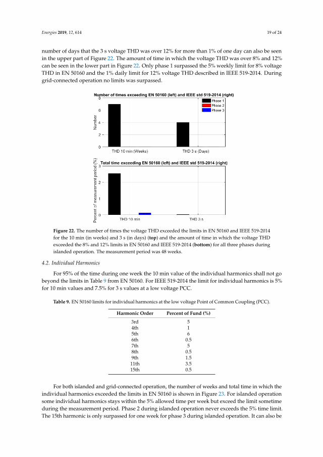
Energies 2019, 12, 614 19 of 24

number of days that the 3 s voltage THD was over 12% for more than 1% of one day can also be seenin the upper part of Figure 22. The amount of time in which the voltage THD was over 8% and 12%can be seen in the lower part in Figure 22. Only phase 1 surpassed the 5% weekly limit for 8% voltageTHD in EN 50160 and the 1% daily limit for 12% voltage THD described in IEEE 519-2014. Duringgrid-connected operation no limits was surpassed.


Figure 22. The number of times the voltage THD exceeded the limits in EN 50160 and IEEE 519-2014 for the 10 min (in weeks) and 3 s (in days) (top) and the amount of time in which the voltage THD exceeded the 8% and 12% limits in EN 50160 and IEEE 519-2014 (bottom) for all three phases during islanded operation. The measurement period was 48 weeks.


For 95% of the time during one week the 10 min value of the individual harmonics shall not go beyond the limits in Table 9 from EN 50160. For IEEE 519-2014 the limit for individual harmonics is 5% for 10 min values and 7.5% for 3 s values at a low voltage PCC.

Table 9. EN 50160 limits for individual harmonics at the low voltage Point of Common Coupling (PCC).

Harmonic Order Percent of Fund (%) 3rd 5 4th 1 5th 6 6th 0.5 7th 5 8th 0.5 9th 1.5

11th 3.5 15th 0.5

For both islanded and grid-connected operation, the number of weeks and total time in which the individual harmonics exceeded the limits in EN 50160 is shown in Figure 23. For islanded operation some individual harmonics stays within the 5% allowed time per week but exceed the limit sometime during the measurement period. Phase 2 during islanded operation never exceeds the 5% time limit. The 15th harmonic is only surpassed for one week for phase 3 during islanded operation. It can also be seen that the 9th harmonic exceeds almost every week for all three phases during islanded operation. For the grid-connected measurements, the 9th harmonic exceeded the 1.5% limit for 1 week.

Figure 22. The number of times the voltage THD exceeded the limits in EN 50160 and IEEE 519-2014for the 10 min (in weeks) and 3 s (in days) (top) and the amount of time in which the voltage THDexceeded the 8% and 12% limits in EN 50160 and IEEE 519-2014 (bottom) for all three phases duringislanded operation. The measurement period was 48 weeks.


For 95% of the time during one week the 10 min value of the individual harmonics shall not gobeyond the limits in Table 9 from EN 50160. For IEEE 519-2014 the limit for individual harmonics is 5%for 10 min values and 7.5% for 3 s values at a low voltage PCC.

Table 9. EN 50160 limits for individual harmonics at the low voltage Point of Common Coupling (PCC).

Harmonic Order Percent of Fund (%)

3rd 54th 15th 66th 0.57th 58th 0.59th 1.511th 3.515th 0.5

For both islanded and grid-connected operation, the number of weeks and total time in which theindividual harmonics exceeded the limits in EN 50160 is shown in Figure 23. For islanded operationsome individual harmonics stays within the 5% allowed time per week but exceed the limit sometimeduring the measurement period. Phase 2 during islanded operation never exceeds the 5% time limit.The 15th harmonic is only surpassed for one week for phase 3 during islanded operation. It can also be

Energies 2019, 12, 614 20 of 24

seen that the 9th harmonic exceeds almost every week for all three phases during islanded operation.For the grid-connected measurements, the 9th harmonic exceeded the 1.5% limit for 1 week.


Figure 23. The number of times the individual harmonics exceeded the 10 min limits in EN 50160 (top) and the amount of time during the measurement period (48 weeks in islanded operation and 54 weeks in grid-connected operation) in which the individual harmonics exceeded the limits in EN 50160 (bottom) for islanded and grid-connected operation. Note the logarithmic vertical scale.

The number of weeks and amount of time in which the individual harmonics exceeded the limits in IEEE 519-2014 are shown in Figure 24.

Figure 24. The number of times the individual harmonics exceeded the 10 min (in weeks) and 3 s limit (in days) in IEEE 519-2014 (top) and the amount of time during the measurement period of 48 weeks in which the individual harmonics exceeded the limits in IEEE 519-2014 (bottom) for islanded operation.

Figure 23. The number of times the individual harmonics exceeded the 10 min limits in EN 50160(top) and the amount of time during the measurement period (48 weeks in islanded operation and54 weeks in grid-connected operation) in which the individual harmonics exceeded the limits in EN50160 (bottom) for islanded and grid-connected operation. Note the logarithmic vertical scale.

The number of weeks and amount of time in which the individual harmonics exceeded the limitsin IEEE 519-2014 are shown in Figure 24.


Figure 23. The number of times the individual harmonics exceeded the 10 min limits in EN 50160 (top) and the amount of time during the measurement period (48 weeks in islanded operation and 54 weeks in grid-connected operation) in which the individual harmonics exceeded the limits in EN 50160 (bottom) for islanded and grid-connected operation. Note the logarithmic vertical scale.

The number of weeks and amount of time in which the individual harmonics exceeded the limits in IEEE 519-2014 are shown in Figure 24.

Figure 24. The number of times the individual harmonics exceeded the 10 min (in weeks) and 3 s limit (in days) in IEEE 519-2014 (top) and the amount of time during the measurement period of 48 weeks in which the individual harmonics exceeded the limits in IEEE 519-2014 (bottom) for islanded operation.

Figure 24. The number of times the individual harmonics exceeded the 10 min (in weeks) and 3 s limit(in days) in IEEE 519-2014 (top) and the amount of time during the measurement period of 48 weeks inwhich the individual harmonics exceeded the limits in IEEE 519-2014 (bottom) for islanded operation.

Energies 2019, 12, 614 21 of 24

It can be seen that the 3rd, 5th and 7th harmonic are the only harmonics in the 10 min valuesthat exceed the 5% limit in IEEE 519-2014 during islanded operation. For the 3 s values the 3rd and5th harmonics are the ones exceeding the 7.5% limit during islanded operation. The limits were notsurpassed during grid-connected operation.

4.3. Long Term Flicker Severity

In EN 50160 only the Plt value is specified which should be lower than 1 for 95% of the time forone week. For phase 1 and 3 the Plt value exceeded the limit for 3 weeks and phase 2 exceeded the limitfor 4 weeks. The grid-connected measurements never exceeded the 5% allowed time limit in EN 50160.In Figure 25 the amount of time during the measurement period in which the Plt value exceeds thespecified limit in EN 50160 for islanded and grid-connected is illustrated. The Plt values for islandedoperation exceeded the limit in EN 50160 for about twice as long than in grid-connected operation.


It can be seen that the 3rd, 5th and 7th harmonic are the only harmonics in the 10 min values that exceed the 5% limit in IEEE 519-2014 during islanded operation. For the 3 s values the 3rd and 5th harmonics are the ones exceeding the 7.5% limit during islanded operation. The limits were not surpassed during grid-connected operation.

4.3. Long Term Flicker Severity

In EN 50160 only the Plt value is specified which should be lower than 1 for 95% of the time for one week. For phase 1 and 3 the Plt value exceeded the limit for 3 weeks and phase 2 exceeded the limit for 4 weeks. The grid-connected measurements never exceeded the 5% allowed time limit in EN 50160. In Figure 25 the amount of time during the measurement period in which the Plt value exceeds the specified limit in EN 50160 for islanded and grid-connected is illustrated. The Plt values for islanded operation exceeded the limit in EN 50160 for about twice as long than in grid-connected operation.

Figure 25. The number of times the Plt values exceeded the limits in EN 50160 (top) and the amount of time during the measurement period of 48 weeks in which the Plt values exceeded the limits in EN 50160 (bottom) for islanded operation.


According to EN 50160 the voltage unbalance should not go beyond 2% for more than 5% of the time for one week. In the grid-connected operation the voltage unbalance never went above 2%. In islanded operation the voltage unbalance went above 2% for 2.34 h, above 3% for 1.5 h in the 48 week measurements. The largest voltage unbalance during the longest consecutive time was 4.5% during 30 min. However, the voltage unbalance was kept below 2% for more than 95% of each week.

5. Discussion

5.1. Effects on Equipment

It is stated in [12] that for a voltage THD between 8 and 10% motors could get overheated. The measurements presented in Section 3 show that there can be levels that go beyond 8 and 10%

Figure 25. The number of times the Plt values exceeded the limits in EN 50160 (top) and the amount oftime during the measurement period of 48 weeks in which the Plt values exceeded the limits in EN50160 (bottom) for islanded operation.


According to EN 50160 the voltage unbalance should not go beyond 2% for more than 5% ofthe time for one week. In the grid-connected operation the voltage unbalance never went above 2%.In islanded operation the voltage unbalance went above 2% for 2.34 h, above 3% for 1.5 h in the 48 weekmeasurements. The largest voltage unbalance during the longest consecutive time was 4.5% during30 min. However, the voltage unbalance was kept below 2% for more than 95% of each week.

5. Discussion

Effects on Equipment

It is stated in [12] that for a voltage THD between 8 and 10% motors could get overheated.The measurements presented in Section 3 show that there can be levels that go beyond 8 and 10%

Energies 2019, 12, 614 22 of 24

distortion in the nanogrid. This can lead to overheating for motors and other equipment sensitive tovoltage harmonics.

Flat topping of the voltage waveform can affect switched-mode power supplies since they needa high peak voltage to effectively charge its capacitor. Since the 10 min voltage THD values canreach up to 13% with up to 9.3% of 3rd harmonic content, equipment that has switched-mode powersupplies could also suffer from excess heating. Especially harmonics 5 and 7 can also cause more lossesin electrical motors and a counter electromotive force that leads to torque and vibration problems.Fluctuations in the voltage can affect several types of equipment (excluding flicker). One of thoseeffects is accelerating or braking torques in motors, deterioration of electronic equipment in which thevoltage fluctuations pass through the power supply to the electronic equipment such as computers,printers, control units, components for telecommunication [13,14]. In a production facility, thesefluctuations could lead to variations in the speed of motors that cause unacceptable variations inproduction parameters such as color and diameter. There is no standard today that defines acceptablelevels of VSV. Since the majority VSV values are lower in islanded operation than for grid-connectedoperation, there is an improvement of the performance in islanded operation when comparing togrid-connected operation. However, more research is needed before any conclusion can be drawn onhow equipment will perform under high VSV values.

The main effect of high Pst and Plt values is light flicker for incandescent lamps. Since thenanogrid only has LED lamps there could be either less or more light flicker depending on which LEDlamp is used [15]. The difference in voltage flicker levels was larger between one phase and the othertwo phases for the majority of the time in islanded operation. This might suggest that the connectedequipment might affect the flicker levels in a certain phase more in islanded operation than in gridoperation since the flicker levels in the three phases during grid operation were closer to each other.

The winding temperature increase in percent above rated temperature as a function of the voltageunbalance can be calculated from Equation (1) [16]:

Temp rise = 2(Percent unbalance)2 (1)

From Equation (1) a temperature rise of 40.5% for 30 min could occur during the 48 weekmeasurements for islanded operation. The maximum temperature rise would be 42.3% for 10 min.The average winding temperature increase for islanded operation is about 0.1% and about 0.2% forgrid-connected operation. The reduction in lifetime of the motor due to temperature increase followingthe Arrhenius model is described in IEEE standard 101 [17]. Since the average winding temperaturefor a 3-phase motor is lower in islanded operation than in grid-connected operation, the lifetime ofa 3-phase motor might increase in islanded operation. However, since there are times in which themotor can run on temperature elevations of up to 42.3% for shorter time periods at the same time asthe voltage THD is above 8% (Mode 2 in Figure 14), a decrease in the lifetime of a motor could happenin comparison to grid-connected operation.

6. Conclusions

The voltage THD and individual harmonics reach larger values in islanded operation thanin grid-connected operation. The difference in magnitude between the phases is also larger inislanded operation.

• Figure 5 shows that the voltage THD increases during the evening without a change in loadwhich suggests that the system impedance increases due to fewer parallel sources being active.This could be due to the shutdown of the solar inverter in the evening. The subsequent decreasein voltage harmonics levels in the morning could be caused by the activation of the solar inverter.

• During islanded operation the Pst and Plt values were lower for the majority of the time for phase2 while the other two are for the majority of the time higher in islanded operation.

Energies 2019, 12, 614 23 of 24

• The 10 min and 3 s VSV value are for the majority of the time lower in islanded operation for allthree phases. It can therefore be concluded that voltage variations on timescales 3 s to 10 min arelower in islanded operation.

• The voltage unbalance is lower for the majority of the time in islanded operation but could reachlevels of over 4.5% for 30 consecutive minutes in islanded operation.

• Figures 13–21 show that there are two modes of performance during islanded operation. Mode 2operates with larger values of the short circuit impedance, voltage THD, voltage unbalance andindividual voltage harmonics 3, 5, 7 for all three phases. For phase 3, the 9th harmonic voltagewas also larger during mode 2. Mode 1 operates with a larger 9th harmonic voltage for phase 1and 2. The 3rd harmonic impedance behaves almost linear in both modes and is larger duringmode 2 for all three phases. The 5th harmonic impedance behaves more nonlinear but is generallylarger during mode 2 for two phases. The 7th and 9th harmonic impedance show nonlinearbehavior and no conclusion can be made regarding the magnitude of the harmonic impedance forthe 7th and 9th harmonic.

• When the islanded operation was compared to the limits defined in grid standard EN 50160it was found that the voltage THD, individual harmonics 3, 5, 6, 7, 9, 15, voltage unbalanceand Plt limits were exceeded. For one week the 9th harmonic exceeded the limit duringgrid-connected operation.

• When the islanded operation was compared to the limits defined in grid standard IEEE 519-2014it was found that the voltage THD, individual harmonics 3, 5, 7 were exceeded. The limits werenot exceeded during grid-connected operation.

More studies with long term measurements are needed to see if similar results are obtained forother nanogrids.

Author Contributions: Conceptualization, J.N., S.K.R. and M.H.J.B.; Methodology, J.N.; Software, J.N.; Validation,J.N., S.K.R. and M.H.J.B.; Formal Analysis, J.N.; Investigation, J.N.; Resources, S.K.R. and M.H.J.B.; Data Curation,J.N.; Writing-Original Draft Preparation, J.N.; Writing-Review & Editing, J.N., S.K.R. and M.H.J.B.; Visualization,J.N.; Supervision, S.K.R. and M.H.J.B.; Project Administration, S.K.R. and M.H.J.B.; Funding Acquisition, S.K.R.and M.H.J.B.

Funding: This paper has been funded by Skellefteå Kraft Elnät and Rönnbäret foundation.

Conflicts of Interest: The authors declare no conflict of interest.

References

1. Hatziargyriou, N. Microgrids Architectures and Control, 1st ed.; Wiley-IEEE Press: Hoboken, NJ, USA, 2014;pp. 310–313.

2. Hatziargyriou, N.; Asano, H.; Iravani, R.; Marnay, C. Microgrids. IEEE Power Energy Mag. 2007, 5, 78–94.[CrossRef]

3. CIGRÉ WG C6.22. Microgrids 1: Engineering, Economics, & Experience; The International Council on LargeElectric Systems: Paris, France, 2015.

4. Burmester, D.; Rayudu, R.; Seah, W.; Akinyele, D. A review of nanogrid topologies and technologies.Renew. Sustain. Energy Rev. 2017, 67, 760–775. [CrossRef]

5. Cenelec Std. EN 50160:2010. Voltage Characteristics of Electricity Supplied by Public Electricity Networks;European Committee for Electrotechnical Standardization: Brussels, Belgium, 2010.

6. IEEE Std. 519-2014. IEEE Recommended Practice and Requirements for Harmonic Control in Electric Power Systems;IEEE Standards Association: Piscataway, NJ, USA, 2014.

7. Nömm, J.; Rönnberg, S.K.; Bollen, M.H.J. An Analysis of Frequency Variations and its Implications onConnected Equipment for a Nanogrid during Islanded Operation. Energies 2018, 11, 2456. [CrossRef]

8. Rönnberg, S.K.; Bollen, M.H.J.; Nömm, J. Power Quality Measurements In a Single House Microgrid.In Proceedings of the CIRED 24th International Conference on Electricity Distribution, Glasgow, Scotland,UK, 12–15 June 2017; pp. 818–822.

http://dx.doi.org/10.1109/MPAE.2007.376583

http://dx.doi.org/10.1016/j.rser.2016.09.073

http://dx.doi.org/10.3390/en11092456

Energies 2019, 12, 614 24 of 24

9. Nömm, J.; Rönnberg, S.K.; Bollen, M.H.J. Harmonic Voltage measurements in a Single House Microgrid.In Proceedings of the ICHQP 18th International Conference on Harmonics and Quality of Power, Ljubljana,Slovenia, 13–16 May 2018; pp. 1–5.

10. Bollen, M.H.J.; Häger, M.; Schwaegerl, C. Quantifying voltage variations on a time scale between 3 secondsand 10 minutes. In Proceedings of the CIRED 18th International Conference and Exhibition on ElectricityDistribution, Turin, Italy, 6–9 June 2005; pp. 1–5.

11. Bollen, M.H.J.; Gu, I.Y.H. Characterization of voltage variations in the very-short time-scale. IEEE Trans.Power Deliv. 2005, 20, 1198–1199. [CrossRef]

12. Dugan, R.C.; McGranaghan, M.F.; Santoso, S.; Beaty, H.W. Electrical Power System Quality, 2nd ed.;McGraw-Hill Education: New York, NY, USA, 2003; p. 216.

13. Schlabbach, J.; Blume, D.; Stephanblome, T. Voltage Quality in Electrical Power Systems; The Institution ofElectrical Engineers: Stevenage, UK, 2001; pp. 115–116.

14. UIE WG 2. Guide to Quality of Electrical Supply for Industrial Installations, Part 5; Flicker and Voltage Fluctuations;International Union for Electricity Applications: Paris, France, 1999; p. 13.

15. Gil-de-Castro, A.; Rönnberg, S.K.; Bollen, M.H.J. Light intensity variation (flicker) and harmonic emissionrelated to LED lamps. Electr. Power Syst. Res. 2017, 146, 107–114. [CrossRef]

16. Pillay, P.; Manyage, M. Derating of Induction Motors Operating With a Combination of Unbalanced Voltagesand Over or Undervoltages. IEEE Trans. Energy Convers. 2002, 17, 485–491. [CrossRef]

17. IEEE Std. 101-1987(R2010). Guide for the Statistical Analysis of Thermal Life Test Data; IEEE StandardsAssociation: Piscataway, NJ, USA, 2010.

© 2019 by the authors. Licensee MDPI, Basel, Switzerland. This article is an open accessarticle distributed under the terms and conditions of the Creative Commons Attribution(CC BY) license (http://creativecommons.org/licenses/by/4.0/).

http://dx.doi.org/10.1109/TPWRD.2005.844253

http://dx.doi.org/10.1016/j.epsr.2017.01.026

http://dx.doi.org/10.1109/TEC.2002.805228

http://creativecommons.org/

http://creativecommons.org/licenses/by/4.0/.

Paper D

Energy Flow Based Risk Analysis for Operating A

Standalone Solar-Hydrogen Nanogrid in Northern

Scandinavia

XXX-X-XXXX-XXXX-X/XX/$XX.00 ©20XX IEEE

Energy Flow Based Risk Analysis for Operating A

Standalone Solar-Hydrogen Nanogrid in Northern

Scandinavia

Jakob Nömm

Department of Engineering Sciences

and Mathematics


Skellefteå, Sweden

[email protected]

Sarah K. Rönnberg


and Mathematics


Skellefteå, Sweden

[email protected]

Math H.J. Bollen


and Mathematics


Skellefteå, Sweden

[email protected]

Abstract—In this paper, an energy flow model for a

standalone nanogrid was used to calculate the needed hydrogen

storage for operation in northern Scandinavia where the

electricity was produced from solar photovoltaics. A range of

different input parameters such as annual energy consumption,

solar production, consumption pattern and heating system was

used to obtain a range of optimal system design parameters.

From this, two average system configurations were created for

two heating systems based on the results from simulated solar

data with 2-axis solar tracking and no solar tracking. The

average value from the results at 30 MWh of annual energy

consumption was used since it is the average energy

consumption for a household in northern Sweden. The average

system configuration was applied for 15 to 40 MWh of annual

energy consumption using 3 measured solar production datasets

and 37 different consumption patterns to study the risk for

depleting the hydrogen storage and counter measures to avoid

depletion. The results show that energy saving measures must

be taken during the winter in order to avoid depletion of the

hydrogen energy storage, which in turn avoids a sustained

interruption until the spring. It was concluded that if 2-axis

solar tracking was used instead of no tracking and a stove was

used for heating instead of using a heat pump, the probability

for depleting the hydrogen storage reduced by 25 % to 47.9 %

at 30 to 40 MWh of annual energy consumption in the nanogrid.

Keywords—Energy storage, Hydrogen storage, Islanding,

Microgrids, Risk analysis

I. INTRODUCTION

A Swedish utility company has adopted a solar-hydrogen

based energy system for a single house that is isolated from

the main utility grid [1]. Hydrogen is produced through

electrolysis during the summer with electricity from solar

photovoltaics (PV). During the winter, the hydrogen is

converted back to electricity with a fuel cell and the waste

heat is used for heating of the single house nanogrid.

One of the possible motivations for constructing a standalone

solar-hydrogen system in northern Scandinavia, is that larger

daily solar production can be achieved during the summer

than in more southern parts of Europe which is shown in

Figure 1. The daily solar production in northern Sweden can

reach almost 14 kWh per kWp and 11 kWh per kWp in

southern Spain during the summer. However, this advantage

might not be adequate since almost no solar irradiation is

present during several weeks during the winter in northern

Scandinavia due to snow coverage and low solar irradiation

which increases the need for energy storage.

Another factor that increases the need for energy storage is

that during the time with zero solar irradiation, the daily

energy consumption for a household in northern Scandinavia

is the highest (see Figure 2).

Figure 1. Measured daily solar electricity production per kWp in

northern Sweden (top) and in southern Spain (bottom). 2-axis

tracking is used in both cases. The plot spans 2 years between the

January 2016 and January 2018.

Figure 2. Measured average daily electricity consumption for 6

households in northern Sweden for 2 years. The plot starts at

January 2016.

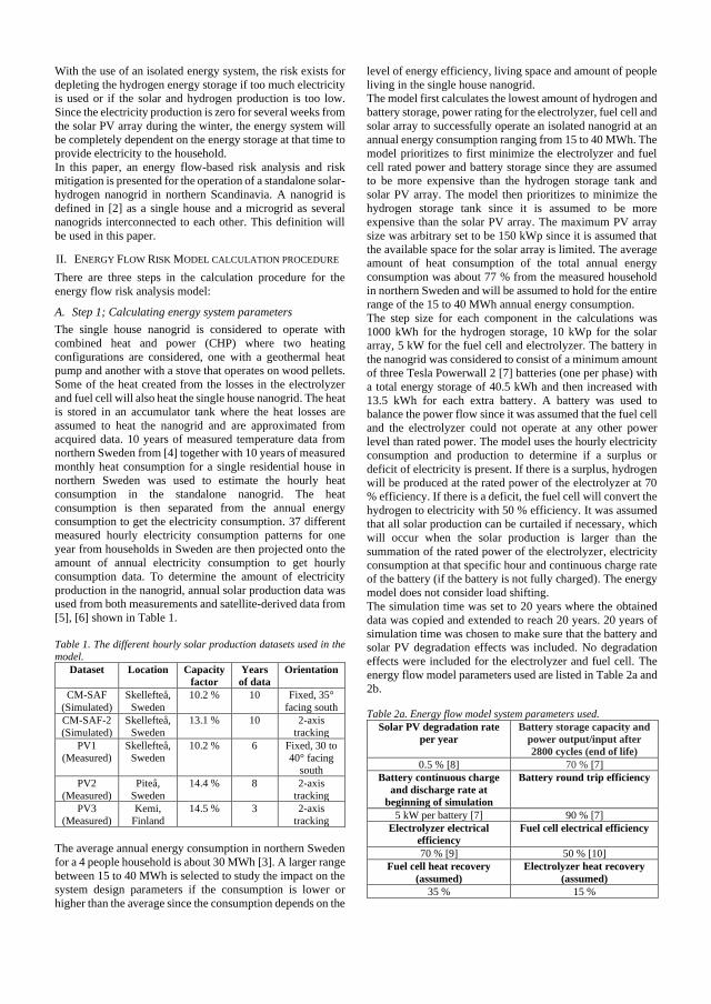
With the use of an isolated energy system, the risk exists for

depleting the hydrogen energy storage if too much electricity

is used or if the solar and hydrogen production is too low.

Since the electricity production is zero for several weeks from

the solar PV array during the winter, the energy system will

be completely dependent on the energy storage at that time to

provide electricity to the household.

In this paper, an energy flow-based risk analysis and risk

mitigation is presented for the operation of a standalone solar-

hydrogen nanogrid in northern Scandinavia. A nanogrid is

defined in [2] as a single house and a microgrid as several

nanogrids interconnected to each other. This definition will

be used in this paper.

II. ENERGY FLOW RISK MODEL CALCULATION PROCEDURE

There are three steps in the calculation procedure for the

energy flow risk analysis model:

A. Step 1; Calculating energy system parameters

The single house nanogrid is considered to operate with

combined heat and power (CHP) where two heating

configurations are considered, one with a geothermal heat

pump and another with a stove that operates on wood pellets.

Some of the heat created from the losses in the electrolyzer

and fuel cell will also heat the single house nanogrid. The heat

is stored in an accumulator tank where the heat losses are

assumed to heat the nanogrid and are approximated from

acquired data. 10 years of measured temperature data from

northern Sweden from [4] together with 10 years of measured

monthly heat consumption for a single residential house in

northern Sweden was used to estimate the hourly heat

consumption in the standalone nanogrid. The heat

consumption is then separated from the annual energy

consumption to get the electricity consumption. 37 different

measured hourly electricity consumption patterns for one

year from households in Sweden are then projected onto the

amount of annual electricity consumption to get hourly

consumption data. To determine the amount of electricity

production in the nanogrid, annual solar production data was

used from both measurements and satellite-derived data from

[5], [6] shown in Table 1.

Table 1. The different hourly solar production datasets used in the

model.

Dataset Location Capacity

factor

Years

of data

Orientation

CM-SAF

(Simulated)

Skellefteå,

Sweden

10.2 % 10 Fixed, 35°

facing south

CM-SAF-2

(Simulated)

Skellefteå,

Sweden

13.1 % 10 2-axis

tracking

PV1

(Measured)

Skellefteå,

Sweden

10.2 % 6 Fixed, 30 to

40° facing

south

PV2

(Measured)

Piteå,

Sweden

14.4 % 8 2-axis

tracking

PV3

(Measured)

Kemi,

Finland

14.5 % 3 2-axis

tracking

The average annual energy consumption in northern Sweden

for a 4 people household is about 30 MWh [3]. A larger range

between 15 to 40 MWh is selected to study the impact on the

system design parameters if the consumption is lower or

higher than the average since the consumption depends on the

level of energy efficiency, living space and amount of people

living in the single house nanogrid.

The model first calculates the lowest amount of hydrogen and

battery storage, power rating for the electrolyzer, fuel cell and

solar array to successfully operate an isolated nanogrid at an

annual energy consumption ranging from 15 to 40 MWh. The

model prioritizes to first minimize the electrolyzer and fuel

cell rated power and battery storage since they are assumed

to be more expensive than the hydrogen storage tank and

solar PV array. The model then prioritizes to minimize the

hydrogen storage tank since it is assumed to be more

expensive than the solar PV array. The maximum PV array

size was arbitrary set to be 150 kWp since it is assumed that

the available space for the solar array is limited. The average

amount of heat consumption of the total annual energy

consumption was about 77 % from the measured household

in northern Sweden and will be assumed to hold for the entire

range of the 15 to 40 MWh annual energy consumption.

The step size for each component in the calculations was

1000 kWh for the hydrogen storage, 10 kWp for the solar

array, 5 kW for the fuel cell and electrolyzer. The battery in

the nanogrid was considered to consist of a minimum amount

of three Tesla Powerwall 2 [7] batteries (one per phase) with

a total energy storage of 40.5 kWh and then increased with

13.5 kWh for each extra battery. A battery was used to

balance the power flow since it was assumed that the fuel cell

and the electrolyzer could not operate at any other power

level than rated power. The model uses the hourly electricity

consumption and production to determine if a surplus or

deficit of electricity is present. If there is a surplus, hydrogen

will be produced at the rated power of the electrolyzer at 70

% efficiency. If there is a deficit, the fuel cell will convert the

hydrogen to electricity with 50 % efficiency. It was assumed

that all solar production can be curtailed if necessary, which

will occur when the solar production is larger than the

summation of the rated power of the electrolyzer, electricity

consumption at that specific hour and continuous charge rate

of the battery (if the battery is not fully charged). The energy

model does not consider load shifting.

The simulation time was set to 20 years where the obtained

data was copied and extended to reach 20 years. 20 years of

simulation time was chosen to make sure that the battery and

solar PV degradation effects was included. No degradation

effects were included for the electrolyzer and fuel cell. The

energy flow model parameters used are listed in Table 2a and

2b.

Table 2a. Energy flow model system parameters used.

Solar PV degradation rate

per year

Battery storage capacity and

power output/input after

2800 cycles (end of life)

0.5 % [8] 70 % [7]

Battery continuous charge

and discharge rate at

beginning of simulation

Battery round trip efficiency

5 kW per battery [7] 90 % [7]

Electrolyzer electrical

efficiency

Fuel cell electrical efficiency

70 % [9] 50 % [10]

Fuel cell heat recovery

(assumed)

Electrolyzer heat recovery

(assumed)

35 % 15 %

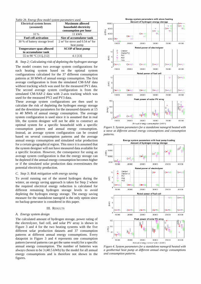
Table 2b. Energy flow model system parameters used.

Electrical system losses

(assumed)

Maximum allowed

household electricity

consumption per hour

10 % 11 kWh

Fuel cell activation Size of accumulator tank

30 % of battery storage level 2 m3 for stove and 0.54 m3 for

heat pump

Temperature span allowed

in accumulator tank

SCOP of heat pump

55 to 90 °C [11], [12] 4.1 [13]

B. Step 2; Calculating risk of depleting the hydrogen storage

The model creates two average system configurations for

each heating system based on the optimal system

configurations calculated for the 37 different consumption

patterns at 30 MWh of annual energy consumption. The first

average configuration is from the simulated CM-SAF data

without tracking which was used for the measured PV1 data.

The second average system configuration is from the

simulated CM-SAF-2 data with 2-axis tracking which was

used for the measured PV2 and PV3 data.

These average system configurations are then used to

calculate the risk of depleting the hydrogen energy storage

and the downtime parameters for the measured datasets at 15

to 40 MWh of annual energy consumption. The average

system configuration is used since it is assumed that in real

life, the system designer will not be able to construct an

optimal system for a specific household with a specific

consumption pattern and annual energy consumption.

Instead, an average system configuration can be created

based on several consumption patterns and the average

annual energy consumption and simulated solar production

for a certain geographical region. This since it is assumed that

the system designer will not have measured data available for

a specific location. However, the consequence for using an

average system configuration is that the energy storage can

be depleted if the annual energy consumption becomes higher

or if the simulated solar production data overestimates the

potential electricity production.

C. Step 3; Risk mitigation with energy saving

To avoid running out of the stored hydrogen during the

winter, an energy saving approach is taken for Step 2 where

the required electrical energy reduction is calculated for

different remaining hydrogen storage levels to avoid

depleting the hydrogen energy storage. The energy saving

measure for the standalone nanogrid is the only option since

no backup generator is considered in this paper.

III. RESULTS

A. Energy system design

The calculated amount of hydrogen storage, power rating of

the electrolyzer, fuel cell, and solar PV array is shown in

Figure 3 and 4 for the two heating systems with the five

different solar production datasets and 37 consumption

patterns at different annual energy consumptions. Every

datapoint in Figure 3 and 4 represents one consumption

pattern (several patterns can get the same result) for a specific

annual energy consumption. The number of batteries was

always chosen to be 3 (40.5 kWh) by the model for all annual

energy consumptions and is therefore not shown in the

figures.

Figure 3. System parameters for a standalone nanogrid heated with

a stove at different annual energy consumptions and consumption

patterns.

Figure 4. System parameters for a standalone nanogrid heated with

a geothermal heat pump at different annual energy consumptions

and consumption patterns.

The amount of hydrogen storage increased when a heat pump

was used instead of a stove. This increase is due to the larger

electricity consumption for generating heat with the heat

pump. The rated power of the electrolyzer stayed at 5 kW for

the entire range of annual energy consumptions when the

nanogrid was heated with a stove but could increase from 5

to 10 kW from 30 to 40 MWh of annual energy consumption

when a heat pump was used. The rated power of the fuel cell

was 5 kW between 15 to 30 MWh and 5 to 10 kW between

35 to 40 MWh of annual energy consumption for both heating

configurations. The amount of solar PV varied depending on

consumption pattern and annual energy consumption and

increased until the maximum limit of 150 kW. When the limit

was reached, the electrolyzer rated power increased since

more hydrogen had to be produced in less time during the

day.

B. Downtime with no energy saving

Two average system configurations from the 37 consumption

patterns at 30 MWh of annual energy consumption were

created from the results shown in Figure 3 and 4 for each

heating system. One from the simulated CM-SAF dataset

which is used for the measured PV1 dataset which had no

solar tracking. The other average system configuration where

created from the simulated CM-SAF-2 dataset which is used

for the measured PV2 and PV3 dataset which had 2-axis solar

tracking. Both configurations can be seen in Table 3.

The average system configurations for the measured datasets

(PV1 to PV3) from Figure 3 and 4 can also be seen in Table

3 for comparison.

Table 3. Average system configurations derived from Figure 3 and

4 at 30 MWh of annual energy consumption. The numbers in the

braces for the simulated data are for the CM-SAF-2 dataset. For the

measured data, the average result of the PV2 and PV3 dataset are

in the braces. The numbers without braces are for the CM-SAF data

in the simulated column and PV1 for the measured column.

Dataset Simulated Measured

Stove heating system

Hydrogen storage (MWh) 7, 7 7.4 6.2

Electrolyzer (kW) 5, 5 5, 5

Fuel cell (kW) 5, 5 5, 5

Solar PV (kWp) 40.3, 30.3 47.6 33.8

Heat pump heating system

Hydrogen storage (MWh) 12, 12 13, 11.7

Electrolyzer (kW) 10, 10 10, 5

Fuel cell (kW) 5, 5 5, 5

Solar PV (kWp) 61.9, 55.9 61.9, 119

The average system configuration was used to see what

probability exists for depleting the hydrogen storage at any

given year. It was also used to get the average downtime for

all 20 simulated years with insufficient hydrogen storage and

the maximum downtime for one year with insufficient

hydrogen storage. These three parameters can be seen in

Figure 5 and Figure 6 for a standalone nanogrid heated with

a stove and heat pump respectively.

The amount of hydrogen storage was sufficient to operate the

nanogrid with both heating systems with an annual energy

consumption of 15 to 25 MWh which is expected since the

system is designed for 30 MWh. Downtime for the nanogrid

started to appear at 30 MWh and increased with more energy

consumption.

Figure 5. Average downtime per year, maximum downtime for one

year and probability for depleting the hydrogen storage where the

nanogrid was heated with a stove.

Figure 6. Average downtime per year, maximum downtime for one

year and probability for depleting the hydrogen storage where the

nanogrid was heated with a geothermal heat pump.

The nanogrid that was heated with a heat pump had a higher

probability to deplete the hydrogen storage for one year

between 30 to 40 MWh of annual energy consumption. The

amount of downtime and the probability for depleting the

hydrogen storage are also impacted by different solar

production datasets and different consumption patterns.

The mean value for all consumption patterns at a specific

annual energy consumption for the PV1 dataset and the mean

value for both the PV2 and PV3 datasets can be seen in the

figures. The 2-axis solar tracking datasets had a lower

probability of depleting the hydrogen energy storage and

lower average downtime for both heating systems. For the

maximum downtime, the PV3 dataset had the lowest amount

of downtime but the PV2 dataset had about the same

downtime as the PV1 dataset at 35 MWh for the stove heating

system. The maximum downtime was always lower for the 2-

axis datasets for the heat pump heating system.

C. Amount of energy saving needed to avoid depleting the

hydrogen energy storage

The average and maximum required amount of electrical

energy savings that must be made during the winter to avoid

depleting the hydrogen storage for the nanogrid that was

heated with a stove can be seen in Figure 7 and with the heat

pump in Figure 8.

Figure 7. Amount of average needed electrical energy savings per

year (top) and maximum amount of needed electrical energy saving

for the year with most insufficient amount of hydrogen storage

(bottom) for a standalone nanogrid heated with a stove.

Figure 8. Amount of average needed electrical energy savings per

year (top) and maximum amount of needed electrical energy saving

for the year with most insufficient amount of hydrogen storage

(bottom) for a standalone nanogrid heated with a geothermal heat

pump.

The standalone nanogrid that was heated with a heat pump

had a higher needed energy saving than the nanogrid with a

stove. This is because the heating is done with electricity

which increases the hydrogen consumption. The amount of

electric energy reduction needed are impacted by the different

solar production datasets and the different consumption

patterns. The 2-axis solar tracking datasets needed less

energy saving than the PV1 dataset that had no tracking

except for the maximum energy saving at 35 MWh of annual

energy consumption for one year for the stove heating

system.

The annual average electric energy consumption that must be

reduced during the winter from different hydrogen storage

levels in which the energy saving starts can be seen in Figure

9 and 10 for the two heating systems. When the energy saving

starts at a lower hydrogen storage level, less time is available

to save the required electrical energy to avoid depleting the

hydrogen energy storage. This results in a higher percentage

of energy saving. For the nanogrid with heat pump heating,

the average percentage value for the needed energy saving for

all datasets are slightly lower than the stove heating system.

The percentage of electric energy reduction needed is

impacted by the different solar production datasets and the

different consumption patterns. The 2-axis solar tracking

datasets needed less energy saving than the PV1 dataset that

had no tracking for all hydrogen storage levels for the heat

pump heating system. For the stove heating system, at 30 %

and 50 % hydrogen storage level, the PV2 dataset had about

the same energy saving requirement as PV1.

Figure 9. Average needed consumption reduction per year at

different hydrogen storage levels at which the savings starts during

the winter for a standalone nanogrid heated with a stove.

Figure 10. Average needed consumption reduction per year at


the winter for a standalone nanogrid heated with a geothermal heat

pump.

The maximum electric energy consumption for one year that

must be reduced from different hydrogen storage levels in

which the energy saving starts can be seen in Figure 11 and

12 for the two heating systems.

Figure 11. Maximum needed consumption reduction for one year at


the winter for a standalone nanogrid heated with a stove.

Figure 12. Maximum needed consumption reduction for one year at


the winter for a nanogrid heated with a heat pump.

The percentage of the maximum amount of electric energy

reduction needed is impacted by the different solar

production datasets and the different consumption patterns.

The PV2 dataset with 2-axis tracking could have higher

saving requirements for certain hydrogen storage levels for

one year than the PV1 dataset which had no tracking.

The average amount of time during the winter in which the

consumption reduction displayed in Figure 9 and 10 is needed

for different hydrogen storage levels and for the two heating

systems can be seen in Figure 13 and Figure 14.

The amount of time in which the electric energy reduction is

needed is impacted by the different solar production datasets

and the different consumption patterns. The 2-axis solar

tracking datasets needed less time for energy saving than the

PV1 dataset that had no tracking for all hydrogen storage

levels for the heat pump heating system. For the stove heating

system, the time could be lower or about the same depending

on the hydrogen storage level in which the energy saving

starts and amount of annual energy consumption in the

nanogrid.

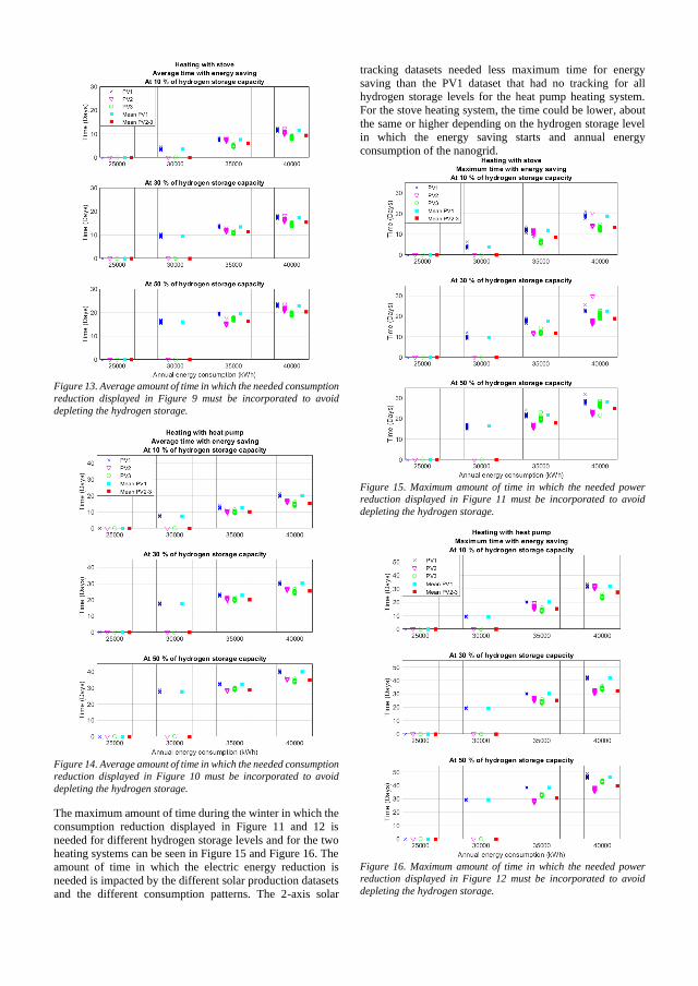
Figure 13. Average amount of time in which the needed consumption

reduction displayed in Figure 9 must be incorporated to avoid

depleting the hydrogen storage.

Figure 14. Average amount of time in which the needed consumption



The maximum amount of time during the winter in which the

consumption reduction displayed in Figure 11 and 12 is

needed for different hydrogen storage levels and for the two

heating systems can be seen in Figure 15 and Figure 16. The

amount of time in which the electric energy reduction is

needed is impacted by the different solar production datasets

and the different consumption patterns. The 2-axis solar

tracking datasets needed less maximum time for energy

saving than the PV1 dataset that had no tracking for all

hydrogen storage levels for the heat pump heating system.

For the stove heating system, the time could be lower, about

the same or higher depending on the hydrogen storage level

in which the energy saving starts and annual energy

consumption of the nanogrid.

Figure 15. Maximum amount of time in which the needed power



Figure 16. Maximum amount of time in which the needed power



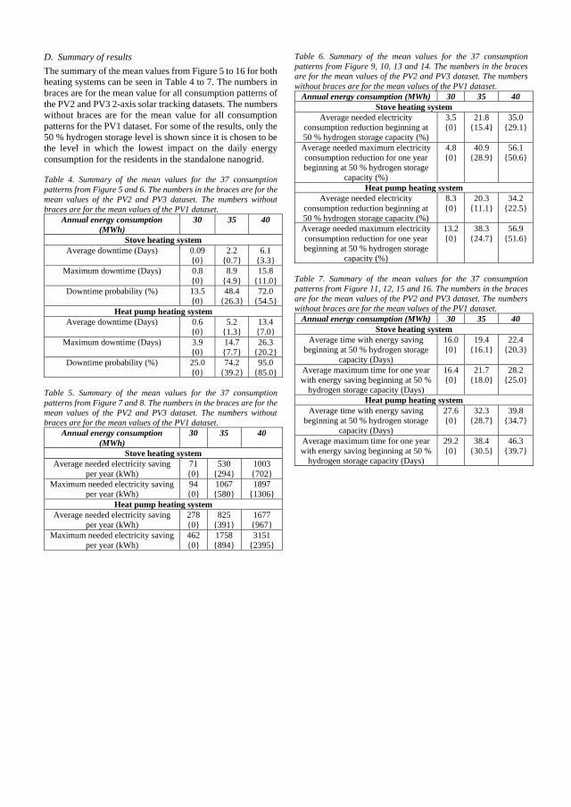
D. Summary of results

The summary of the mean values from Figure 5 to 16 for both

heating systems can be seen in Table 4 to 7. The numbers in

braces are for the mean value for all consumption patterns of

the PV2 and PV3 2-axis solar tracking datasets. The numbers

without braces are for the mean value for all consumption

patterns for the PV1 dataset. For some of the results, only the

50 % hydrogen storage level is shown since it is chosen to be

the level in which the lowest impact on the daily energy

consumption for the residents in the standalone nanogrid.

Table 4. Summary of the mean values for the 37 consumption

patterns from Figure 5 and 6. The numbers in the braces are for the

mean values of the PV2 and PV3 dataset. The numbers without

braces are for the mean values of the PV1 dataset.

Annual energy consumption

(MWh)

30 35 40


Average downtime (Days) 0.09

0

2.2

0.7

6.1

3.3

Maximum downtime (Days) 0.8

0

8.9

4.9

15.8

11.0

Downtime probability (%) 13.5

0

48.4

26.3

72.0

54.5


Average downtime (Days) 0.6

0

5.2

1.3

13.4

7.0

Maximum downtime (Days) 3.9

0

14.7

7.7

26.3

20.2

Downtime probability (%) 25.0

0

74.2

39.2

95.0

85.0


patterns from Figure 7 and 8. The numbers in the braces are for the

mean values of the PV2 and PV3 dataset. The numbers without

braces are for the mean values of the PV1 dataset.

Annual energy consumption

(MWh)

30 35 40


Average needed electricity saving

per year (kWh)

71

0

530

294

1003

702

Maximum needed electricity saving

per year (kWh)

94

0

1067

580

1897

1306


Average needed electricity saving

per year (kWh)

278

0

825

391

1677

967

Maximum needed electricity saving

per year (kWh)

462

0

1758

894

3151

2395


patterns from Figure 9, 10, 13 and 14. The numbers in the braces

are for the mean values of the PV2 and PV3 dataset. The numbers

without braces are for the mean values of the PV1 dataset.

Annual energy consumption (MWh) 30 35 40


Average needed electricity

consumption reduction beginning at

50 % hydrogen storage capacity (%)

3.5

0

21.8

15.4

35.0

29.1

Average needed maximum electricity

consumption reduction for one year

beginning at 50 % hydrogen storage

capacity (%)

4.8

0

40.9

28.9

56.1

50.6


Average needed electricity

consumption reduction beginning at

50 % hydrogen storage capacity (%)

8.3

0

20.3

11.1

34.2

22.5

Average needed maximum electricity

consumption reduction for one year


capacity (%)

13.2

0

38.3

24.7

56.9

51.6


patterns from Figure 11, 12, 15 and 16. The numbers in the braces

are for the mean values of the PV2 and PV3 dataset. The numbers

without braces are for the mean values of the PV1 dataset.

Annual energy consumption (MWh) 30 35 40


Average time with energy saving


capacity (Days)

16.0

0

19.4

16.1

22.4

20.3

Average maximum time for one year

with energy saving beginning at 50 %

hydrogen storage capacity (Days)

16.4

0

21.7

18.0

28.2

25.0


Average time with energy saving


capacity (Days)

27.6

0

32.3

28.7

39.8

34.7

Average maximum time for one year

with energy saving beginning at 50 %

hydrogen storage capacity (Days)

29.2

0

38.4

30.5

46.3

39.7

IV. CONCLUSIONS

The conclusions for this paper are summarized below:

• The developed model shows that different

consumption patterns, amount of energy consumption

and solar production affects the optimal system

configuration and the risk for depleting the hydrogen

energy storage for a solar-hydrogen standalone single

house nanogrid in northern Scandinavia. The risk for

depleting the hydrogen storage increases with

increasing annual energy consumption.

• For an average household in northern Sweden with an

annual energy consumption of 30 MWh operating as a

standalone nanogrid with stove heating, an average of

6.2 to 7.4 MWh of hydrogen storage is required. When

the nanogrid is heated with a geothermal heat pump, an

average of 11.7 to 13 MWh of hydrogen storage is

required. The lower range corresponds to a nanogrid

using 2-axis solar tracking, the upper range

corresponds to no solar tracking.

• The results show that more hydrogen storage and solar

PV capacity can be required for the measured PV1 data

than the simulated CM-SAF data with no solar

tracking. When 2-axis solar tracking was used, the

needed hydrogen storage for the measured PV2 and

PV3 data is generally less than for the simulated CM-

SAF-2 data.

• An energy saving schedule should be incorporated to

reduce the risk for depleting the hydrogen storage. The

energy saving should start as early as possible to limit

the effect on the consumer.

• If no energy saving is made, the probability for

downtime is 72 % for stove heating and 95 % for heat

pump heating at 40 MWh of annual energy

consumption. The probability was 13.5 % for stove

heating and 25 % for heat pump heating at 30 MWh of

annual energy consumption.

• With 2-axis solar tracking, no energy saving was

required at the designed annual energy consumption of

30 MWh for both heating systems.

• The amount of energy saving needed was larger for the

nanogrid with heat pump heating. Since the heat is

generated with electricity in the nanogrid with the heat

pump, the amount of heating in the nanogrid could

therefore be reduced to save energy. This means that

the costumer with stove heating might be more affected

by energy saving since only household appliances

could save the needed power which would affect

everyday life negatively.

• The maximum amount of energy that must be saved for

one year is about 90 % larger than the average value

for 20 simulated years at 40 MWh of annual energy

consumption for both heating systems. At 30 MWh, the

stove heating system had 32 % larger maximum value

and heat pump heating system had 66 % larger

maximum value.

• A nanogrid with 2-axis solar tracking has lower risk of

depleting the hydrogen storage, lower energy saving

requirements and needs less time with energy saving to

avoid depleting the hydrogen energy storage than a

nanogrid with no solar tracking.

• A nanogrid with stove heating has lower risk of

depleting the hydrogen storage, lower energy saving

requirements and needs less time with energy saving to

avoid depleting the hydrogen energy storage than a

nanogrid with heat pump heating.

• Combining both stove heating with 2-axis solar

tracking reduces the probability of depleting the

hydrogen storage with 25 % to 47.9 % at 30 to 40 MWh

of annual energy consumption.

REFERENCES

[1] Zero Sun, Skellefteå Kraft, [Online]. Available:

https://www.zerosun.se/. [Accessed 04-05-2019].

[2] D. Burmester, R. Rayudu, W. Seah, D. Akinyele, "A review of nanogrid topologies and technologies," Renewable and Sustainable

Energy Reviews, vol. 67, pp. 760-775, 2017.

[3] Swedish Energy Agency, Energikalkylen, [Online]. Available: http://energikalkylen.energimyndigheten.se/. [Accessed 25-03-2019].

[4] Swedish Meteorological and Hydrological Institute, [Online].

Available: https://www.smhi.se/data/meteorologi/ladda-ner-meteorologiska-

observationer/#param=airtemperatureInstant,stations=all. [Accessed

06-05-2019].

[5] S. Pfenninger, I. Staffell, "Long-term patterns of European PV output

using 30 years of validated hourly reanalysis and satellite data,"

Energy, vol. 114, pp. 1251-1265, 2016.

[6] Renewables Ninja, [Online]. Available:

https://www.renewables.ninja/. [Accessed 25-03-2019].

[7] Tesla, Inc, [Online]. Available: https://www.tesla.com/sv_SE/powerwall?redirect=no. [Accessed 04-

05-2019].

[8] D.C. Jordan, S.R. Kurtz, "Photovoltaic degradation rates–an analytical review," Progress in Photovoltaics: Research and Applications, vol.

21, pp. 12-29, 2013.

[9] D. Stolten, B. Emonts, Hydrogen Science and Engineering: Materials, Processes, Systems and Technology, John Wiley & Sons, 2016, p.

898.

[10] U.S. Department of Energy, Office of Energy Efficiency & Renewable Energy, "Comparison of Fuel Cell Technologies," 2011.

[11] Boverket, Smittskyddsinstitutet och VVS-Installatörerna, "Legionella

i vatteninstallationer, Tekniska faktorer med risk för samhällsförvärvad," 2006.

[12] Ackumulatortank NIBE VPB 500 750 1000, [Online]. Available:

https://www.nibe.eu/assets/documents/24816/639314-7.pdf. [Accessed 13-06-2019].

[13] Bergvärmepump NIBE F1255, [Online]. Available: https://www.nibe.eu/assets/documents/24488/639574-7.pdf.

[Accessed 13-06-2019].

Paper E

Techno-economic analysis with energy flow

modeling for investigating the investment risks

related to consumption changes within a standalone

microgrid in Sweden

Tinw

JaLu

a

ArReRe13AcAv

KeEnMPoReRu

1.

tu20franlitmcomecaorwco

*

(S

ht03

Contents lists available at ScienceDirect

Energy

journal homepage: www.elsevier .com/locate/energy

Energy 225 (2021) 120156

echno-economic analysis with energy flow modeling for
t riskrid in
ath Hiences and

s t r

chno-ecostment rection inobjectiven that t

vestigating the investmenithin a standalone microg

kob N€omm*, Sarah K. R€onnberg, Mleå University of Technology, Department of Engineering Sc

r t i c l e i n f o

ticle history:ceived 2 March 2020ceived in revised formFebruary 2021cepted 17 February 2021ailable online 22 February 2021

a b

A teinveconntheshow

ywords:ergy system modelingicrogridswer system economics

energy consuthe investmeand reducedminimize thewas conclude

dalone m-connecti

© 2021 The

ncluded that a SMG can bemore economical to implem

Corresponding author.E-mail addresses: [email protected] (J. N€omm), sarah.ron

.K. R€onnberg), [email protected] (M.H.J. Bollen).

tps://doi.org/10.1016/j.energy.2021.12015660-5442/© 2021 The Authors. Published by Elsevier Ltd. This is an

s related to consumption changesSweden

.J. BollenMathematics, Forskargatan 1, 93187, Skellefteå, Sweden

a c t

nomic energy flow model for a standalone microgrid was developed to investigate theisks related to consumption changes and compare the results to a conventional grid-Sweden. Two different design strategies for a standalone microgrid was used, one withto minimize the life-cycle cost and the other to provide a lower investment risk. It washe largest investment risk for both design strategies was a potential increase in annualmption within the standalone microgrid. The design strategy with the objective to reducent risk eliminated the influence on the life-cycle cost from an increase in peak consumptionthe overall investment risk in comparison to the design strategy with the objective tolife-cycle cost. However, a larger life-cycle cost was the drawback of that design strategy. Itd that locations with larger annual mean capacity factors reduced the investment risk for

on had a lower investment risk than a standalone microgrid, since adverse changes in
newable energyral electrification
stangridcons

icrogrids due to lower diesel fuel dependence. It was also concluded that a conventional

umption always increased the life-cycle cost less for a conventional grid-connection than for astandalone microgrid.

Authors. Published by Elsevier Ltd. This is an open access article under the CC BY license

nceth AAEEost aBEDiratAEin Bgiv-levd) adiffas aC ofth

Introduction

The cost of lithium ion batteries, solar panels (SP) and windrbines (WT) are projected to decrease in the future. From the year16e2030, a 73.3% cost reduction for lithium ion batteries [1],om the year 2018e2050, a 60.3%e86.4% cost reduction for SP [2]d a 33.2%e56.6% cost reduction for WT [3] is mentioned in theerature. This would increase the relevance of a standaloneicrogrid (SMG) as an economical option to a conventional grid-nnection (CGC) as time progresses. A utility company (UC)ight choose to invest in a SMG instead of CGC when either theonomic life has expired for the overhead electricity lines (OEL), ifstorm has severely damaged the OEL and requires reinvestment,if new customers that are not connected to the main utility gridants to be supplied with electricity. Several previous studies have

CGC if the distaa SMG in Souconsumption (has the same cconsumption (United Arab Em(4383 MWh ofRef. [6], a SMG10.1 km whichused only highand wind speeBED for severalload profiles wand had a BEDliterature show

ent than a which AEEC and loIf the distance to

UC might consideregarding an invecomparison to aprobability for a fin

[email protected]

open access article under the CC BY licen

(http://creativecommons.org/licenses/by/4.0/).

to the customers is sufficiently large. In Ref. [4],frica with 12.8 MWh of annal electric energyC) had a break-even distance (BED) (where a CGCs a SMG) of 1.76 km or a break-even distance perC) of 0.14 km/MWh. In Ref. [5], a SMG in thees had a BED of 31 km for a 500 kWaverage loadEC) which gives a BEDC of 0.0071 km/MWh. Inangladesh with 58.4 MWh of AEEC had a BED ofes a BEDC of 0.17 km/MWh. A study by Ref. [7]el source data (diesel fuel price, solar irradiancend four Rwandan load profiles to calculate theerent countries. For Sweden, the BED for the fourbout 4.9e27 km for an AEEC of 27e158.2 MWharound 0.17e0.18 km/MWh. These examples ofat a range of results is obtained depending oncation is studied.newor present customers is sufficiently large, a

r investing in a SMG. But the financial risksstment in a SMG must also be considered inCGC where risk in the field of finance is theancial loss with a certain magnitude [8]. Several

se (http://creativecommons.org/licenses/by/4.0/).

http://creativecommons.org/licenses/by/4.0/

mailto:[email protected]

mailto:[email protected]

http://crossmark.crossref.org/dialog/?doi=10.1016/j.energy.2021.120156&domain=pdf

www.sciencedirect.com/science/journal/03605442

http://www.elsevier.com/locate/energy

https://doi.org/10.1016/j.energy.2021.120156

http://creativecommons.org/licenses/by/4.0/


SMlitcrbecaporedeleenunStprcaSMlitpovatrlit

spThellatioinleincowthloAEinUplhoan[2hounonusfobetrtimduefasttosthoelRemchthch

fudiin

a Cthise ugesMGod iwo

ill ben ost (ent

nom

conat cn ecesulThevaryt. ThartsM echaducP, We 50ce tumpfutumeevenbovs aproges,per.

m

timheenectivsevedataorthcuhe

tomsumeq

MGordpe

incoe ber d

nfigco

comicha s

J. N

G investment risk (IR) variables have been identified in theerature. The variability in the demand for electricity, both in-ease (risk of under-dimensioning the SMGwhere demand cannotmet) and decrease (risk of over-dimensioning the SMG wherepacity is not used efficiently) was highlighted in Refs. [9,10] astential IRs and especially if large capital investment is made innewable energy sources [10]. The economic effects of electricitymand variations can be seen in for instance Refs. [11,12] wheress loading in the SMG increases the levelized cost of electricalergy and in Ref. [13] where an increase in fuel consumption perit of electricity produced occurs with lower loading in the SMG.udies has shown that a change in inflation rate [14], diesel fuelice [14e18], capital costs [14,16,18,19] and discount rate [16,17,19]n increase the cost of a SMG, which makes these parameters intoG IR variables. Other factors have also been identified in the

erature that qualifies as IR variables since these factors couldtentially increase the cost of a SMG. For instance, exchange rateriations [20], economic penalties if sufficient amount of elec-icity is not supplied to the customer [21], payment risk and po-ical risk [22].When the BED is calculated for a SMG, it only applies for aecific AEEC and its load profile which creates an IR for the UC.is is since if the AEEC increases (for instance if the customers buyectric cars) or the consumption pattern (CP) changes to one withrger peak consumption (PC) and/or change in time of consump-n (TOC) (for instance if a customer starts working night-shiftsstead of day-shifts), the BED might increase to an unacceptablevel so that the UC makes a financial loss by investing in a SMGstead of a CGC. This is because larger batteries or more SP or WTuld be needed to handle an increased AEEC and/or change in CPithin the SMG. This is in sharp contrast to a CGC since as long ase PC is kept below the maximum rating of a CGC (thermal over-ad could happen otherwise), a CGC can deliver the demandedEC at any time of day under the condition that there is noterruption of the electricity supply. It could also be difficult for aC to predict the AEEC of a specific customer since several factorsays a part in the amount of household AEEC. Some are theusehold income [23], age structure and education [24], weatherd location [25], type, amount and use of household appliances6] and number of people in the household [27]. However,usehold AEEC can vary with 200%e300% even if the householdits are close to identical [28]. Electricity consumption (EC) is notly limited to the amount of electricity used but also when it ised where different people perform activities such as cookingod, washing clothes etc. at different times of the day, which canseen in Ref. [29]. These EC variations in time and magnitude are

oublesome since the production from SP and WT could occur ates with little or zero EC. A large battery would absorb the pro-ction for later use with the drawback of higher cost. A morefective approach is to use the electricity when it is produced sincesmaller battery would be needed since less electricity needs to beored for later use. But this would require customers to be willingshift EC to when production occurs which has been shown in

udies to have mixed results. In Ref. [30] the occupants in house-lds with SP were willing to adopt load shifting to consumeectricity when the sun shined to utilize the SP production and inf. [31] the occupants were largely unmotivated to shift their EC,ostly due to low economic compensation for the inconvenience ofanging consumption behavior. It was also recognized in Ref. [32]at economic compensation is important to a customer as an ex-ange against the inconvenience of shifting load.Although the mentioned literature gives many possibilities for

rther research, an analysis of how the IR of a SMG is affected byfferent consumption changes such as a change in CP and increaseannual energy consumption (AEC) (both heat and electricity) in

comparison tomain focus of(TEEFM) will bsumption chantwo different SCGC. The methregions in theScandinavia wthe presentatiothe life-cycle cowith two differ

2. Techno-eco

The TEEFMmodel (EFM) ththe second is abased on the rinstance AEC).late the IR byreference pointhe different psections. The ECGC. No pricewould be introfor batteries, Sused across thacceptable sinrelated to consyears into thecustomer is asscreates equal ra SMG or CGC aAEC and CP) iTherefore, thesumption chanused in this pa

2.1. Energy flow

The EFM isduction from tactions by theator (DG) is amodeled fromconsumptionhousehold in ninterconnected1e100 MWh wresidential cusinstance threeciencies of theoccurs in the Sincorporated ina 50-year timebattery is alsocapacity and thlifespan. Furthsections.

2.1.1. System coFour system

different mainused to see whlowest LCC for

€omm, S.K. R€onnberg and M.H.J. Bollen

2

GC, is missing in the literature. This gap is thepaper. A techno-economic energy flow modelsed to investigate the IR of a SMG due to con-with several different applying conditions anddesign strategies and compare the results to an this paper can be used to get results for otherrld, but in this study, data from Sweden andused. The main contributions of this paper are

f how changes in CPs and increases in AEC affectLCC) of a SMG and CGC, and how the IR of a SMGdesign strategies compares to a CGC.

ic energy flow model

sists of two parts. The first is an energy flowalculates the hourly energy flow in the SMG andonomic model (EM) where the LCC is calculatedts from the EFM for certain input variables (forresults from the EM can then be used to calcu-ing the CP and amount of AEC from an initiale TEEFM was constructed using Matlab whereand data used is presented in the following

xtends over 50 years to match the lifetime of anges are used in the TEEFM since uncertaintiesed into the result, if a certain change in the priceT and especially the diesel fuel price would be-year calculation period. This simplification ishe main aim of this paper is to study the IRstion changes and not predict the future LCC, 50ure for a SMG. The price of electricity for thed to be the same for both a SMG and CGC, whichue from both. Therefore, any increase in LCC fore the projected LCC (which is based on a certainfinancial loss for the investor (usually the UC).bability of a certain increase in LCC due to con-can be used as a measurement of IR and will be

odel

e series based which factors in the time of pro-SP and WT, consumption by the customer andrgy system, for instance when the diesel gener-ated. The energy consumption in the SMG isral different measured CPs in Sweden and fromcontaining both heat and electricity from aern Sweden. The SMG and CGC will have threestomers (arbitrarily chosen) with an AEC ofre 100 MWh constitutes about three all-yearers in Sweden and 1 MWh could represent former houses. The EFM incorporates the effi-

uipment to account for the energy losses that. The technical lifetime of the equipment is alsoer to establish how many units is required overriod. The degradation rates of the SP, WT andrporated since the SP and WT loses productionattery loses storage capacity over the technicalescription of the EFM is given in the following

urationsnfigurations (SC) was chosen for the SMG withponents listed in Table 1. The different SCs wascombination of main components that has thepecific location with different solar and wind

Energy 225 (2021) 120156

cowjeimcotucoplwAEitsusuin

2.

ofridecomindepenofuarSMThwsethceLCcainmtocucuSMcrfu

2.

arPotebalodeTh

l vals a1 wtermed

C anheCGC are according to Ref. [38] 8%e15%, from this 10%ed

e SM.0Htterth

an bDG wate

d ansimlocaond to, Locidefor Serene20ea

thehe yinribeehoto thre dtheT elere dome

ourhouseholds, three farms and two office buildingsas Cariso

ele(1)ed ftheeamoon

Þ,

heameide1. Tooutshe veas

TaTh

J. N

nditions. Combined heat and power (CHP) are used in the EFMhere all customers have a wood pellets stove and DG which in-cts heat to an accumulator tank (AT) to store heat that can bemediately or later supplied to the households. SCs with CHP wasnsidered essential to use since heat consumption (HC) consti-tes about 74% of the AEC for an average Swedish household due told climate [33]. By having two energy systems, one which sup-ies electricity and one that supplies heat, it is possible to quantifyhich energy form that affects the IR the most for an increase inC. A stovewas chosen as the main heat supplier in the SMG sincecan supply heat to the SMG independently of the electricitypply system. If a heat pump would be used for the main heatpply, it would be coupled to the EC in the SMG since any increaseHC would lead to an increase in EC.

1.2. Standalone microgrid design strategyTwo design strategies for a SMG are investigated to study the IRthem in comparison to a CGC. The first design strategy is the low-sk SMG (LR-SMG) which is designed to have the same powerlivery capability as a CGC which means that it can supplyntinuous power up to the capability of a defined fuse size. Thiseans that the LR-SMG does not need capacity upgrades due to ancreased PC that is within the defined fuse size. This is why it issignated a low-risk SMG. Three 16 A fuses per customer at 230 Vr phase was used in the EFM (11 kW per customer) which isrmally used for district heating customers in Sweden. The samese size will also apply for the CGC. The battery and DG capacitye the system components that are set to a level so that the LR-G can continuously supply 11 kW of electricity per customer.e LR-SMG is still affected by increased AEC and change in TOChich could require an increase in the system components. Thecond design strategy is the high-risk SMG (HR-SMG) which usese minimum amount of system components for each CP (with artain PC and TOC) at a specific AEC. This yields the lowest possibleC for a SMG at a specific AEC and CP, but a HR-SMG could needpacity upgrades due to increased AEC, changed TOC andcreased PC. This is why it is designated as a high-risk SMG. Theaximum allowed fuse size in the simulations for a HR-SMG is setthe same as for the LR-SMG (11 kW per customer). The EC isrtailed to 11 kW per customer if a larger electricity demand oc-rs for both a HR-SMG and LR-SMG in the simulations. These twoG design strategies represents a lower risk for future cost in-

eases but with higher upfront cost (LR-SMG) and higher risk forture cost increases but with lower upfront cost (HR-SMG).

1.3. Technical propertiesThe technical properties used in the EFM for the SMG and CGC

e presented in Table 2. The battery properties are for a Teslawerwall 2 battery [34]. A 10-year warranty is given for the bat-ry if the aggregated throughput is lower than 37.8 MWh [35]. Thettery capacity after 37.8 MWh is set to 70% which is given as thewest percentage in the warranty. If it is assumed that the batterygrades linearly, the total average number of cycles is about 3300.e charge/discharge rate of the battery is assumed to also decrease

to 70% of initiain the EFM waplayed in Fig.about 91.6% delifetime of themby a Swedish Uby Ref. [37]. Tcustomer for alosses are assumis needed in thSunny Island 8Powerwall 2 batemperature inRef. [40] and cficiency of thewith HydrogenRef. [42].

2.1.4. Simulate10 years of

three differentwhich is basedtherefore scaleLocation 1 (L1)chosen to provfactor (AMCF)study how diffthe years 2006

10 years of mat L1 betweenature data for t[52] was usedwhich is descmeasured houswhich is closeThe temperatucomparison oflated SP andWand temperatucorrelates to sexpected.

Measured hSweden for 37which are usedused for comp

2.1.5. Heat andIn equation

SMG is calculatis the AEC, u isyear from the mof the previousmonth and x is

PðiÞ¼ EuðxÞpði

The hourlywhere T is theone month divhousehold at La function ofequation (2). Tture in the m

ble 1e four different SCs where X marks the main system components used in each SC.

SC 1 2 3 4

Battery X X X XDG X X X XSP X XWT X XAT X X X XStove X X X X


3

ue at the end of 3300 cycles of use. The WT usedXANT M21 100 kW with the power curve dis-here the system efficiency at rated power wasined from the data retrieved from Ref. [36]. Theiumvoltage (MV) OEL is estimated to be 50 yearsd 40 years for the distribution transformer (DT)transmission losses from power plant to the

Energy 225 (2021) 120156

. It is also assumed that a master battery inverterG where multiple energy sources exists. A SMAinverter [39] is chosen and used for every Teslay in the SMG. The heat loss as a function of watere AT are estimated from data obtained frome seen in Fig. 2 together with the electrical ef-hich is calculated with a formula from Ref. [41]

d vegetable oil (HVO) diesel specifications from

d measured dataulated hourly SP and WT production data fortions in Scandinavia was obtained from Ref. [36]the papers [50,51]. The data is per kWp and isthe capacity chosen in the end by the TEEFM.ation 2 (L2) and Location 3 (L3) were arbitrarilya variety of values of the annual mean capacityP and WT production in Scandinavia in order tot AMCFs impacts the IR of a SMG. The AMCF for15 for each location are listed in Table 3.suredmonthly EC and HC retrieved from a houseyears 2008e2017 together with hourly temper-ears 2006e2015 from a weather station near L1the modeling of the consumption in the SMG,d in Section 2.1.5. The average AEC for theld was about 36000 kWh consisting of 77.3% HCe average for a Swedish household of 74% [33].ata is used for all three locations to simplify theresults. In Fig. 3, two years of the hourly simu-ctricity production together with the householdata can be seen. The temperature data in Fig. 3degree to the HC in the house at L1 which is

ly EC data for one year was retrieved from

Ps. A theoretical constant consumptionwas alson. In Fig. 4, five of the 43 CPs are shown.

ctricity consumption modeling, the simulated electricity consumption P in theor 1 h iwhere p is the measured EC for one CP, EEC for one month divided by the AEC for that

sured household at L1, m is the number of hoursnths, M is the number of hours for the presente month in the simulation.

XmðxÞþMðxÞ

k¼1þmðxÞpðkÞ (1)

t consumption H is calculated with equation (2)asured temperature at L1 and q is the HC ford by the AEC for that year from the measuredget hourly variations in the monthly HC data aside temperature, variation factors are used inariation factor at the lowest recorded tempera-ured temperature data ðT ¼ 36.5 C) was

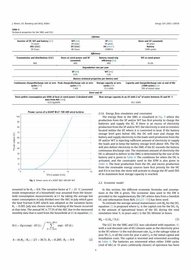
asinhowthR1atm

H

b

2.1.6. Energy flowThe energy flow

production from thbatteries and suppproduction from thlocated within thestorage level goesbattery and supplySP and/or WT is inthe loads and to kewill also deliver elecontinuous discharDG is allowed to debattery and is giveactivated, and theTable 4. The heat production from the DG and excess productionfrom the renewable energy sources have first priority for the HCand if it is too low,of its maximum he

mod

ion,M issupatiotheproof

e Ys

sLÞtheoune r ill thts. Tba15

Table 2Technical properties for the SMG and CGC.

Lifetime

Inverter of SP, WT and battery [43] WT [44] SP [45] Stove and AT (assumed)15 years 20 years 30 years 30 yearsOEL (CGC) DT (CGC) DG [46,47] Battery50 Years 40 Years 15000 h 3300 cycles

Efficiency

Transmission and distribution (CGC) Stove at rated power and SP(assumed)

Battery round-tripefficiency [34]

WT at rated power

90% 90% 90% 91.6%

Degradation rate per year

SP [48] WT [44]0.5% 1.6%

Battery technical properties per battery unit

Continuous charge/discharge rate at zerocycles [34]

Peak charge/discharge rate at zerocycles [34]

Storage capacity at zerocycles [34]

5 kW 7 kW 13.5 kWh

Stove and AT

Stove pellets consumption per kWh of heat at rated power (Calculated withdata from Ref. [49])

Heat storage capacity

0.23 kg/kWh

J. N€omm, S.K. R€onnberg and M.H.J. Bollen Energy 225 (2021) 120156

sumed to be R2 ¼ 0.9. The variation factor at T ¼ 21 C (assumedside temperature of a household) was assumed from the house-ld consumption measurements at L1 by taking the average hotater consumption in July divided over the AEC in July which gavee heat fraction 0.285 which was adopted as the variation factor¼ 0.285. July was chosen since no heating of the house occurredthat time. The annual HC is 77.3% of the AEC due to the measuredonthly data that is used from the household at L1 in equation (2).

ðiÞ¼ EqðxÞexpðbTðiÞÞ, XmðxÞþMðxÞ

k¼1þmðxÞexpðbTðkÞÞ

¼ lnðR2 =R1Þ = ð21þ36:5Þ;R1 ¼0:285; R2 ¼ 0:9 (2)

2.2. Economic

In this secttions in the Eprovided in theUC and inform

To estimateequation (3) isis the amountsimulation tim

Mg ¼GcOhðY

The LCC forwith a real discin the SF) wheryear 50, Cn is ainstallation costo Table 5. The(end of life) or

Fig. 1. Power curve of a XANT M21 100 kW WT.

4

simulation and constraintsin the SMG is visualized in Fig. 5 where the

e SP and/or WT has first priority to charge thely the EC. If there is an excess of electricitye SP and/orWT, the electricity is sent to resistorsAT where it is converted to heat. If the batterybelow 10%, the DG will start and charge theelectricity to the loads until production from thejecting sufficient amount of electricity to supplyep the battery storage level above 10%. The DGctricity to the SMG if the EC exceeds the batteryge rate. The maximum amount of electricity theliver in the SMG is determined by the size of then in Table 4. The conditions for when the DG isconstraints used in the EFM is also given in

Capacity and charge/discharge rate at end of life(3300 cycles) [35]70% of initial value

in an AT with 2 m3 of water between 55 and 95 C

93.1 kWh

the stove will activate to charge the AT until 50%at storage capacity is reached.

el

the different economic formulas and assump-given. The economic data used in the EM isplementary file (SF) where data from a Swedishn from Refs. [43,53e55] has been used.average annual maintenance costMg for the DG,posed where Gc is the capital cost for the DG, Ohoperational hours of the DG during the totalin years and L is the DG lifetime in hours.

(3)

SMG and CGC was calculated with equation (4)t rate of 6% (chosen same as the electricity prices the real discount rate, S50 is the salvage value ate costs for year n and C0 is the initial capital andhe capital is invested and reinvested accordingtteries are reinvested when either 3300 cyclesyears (arbitrarily chosen) of operation has been

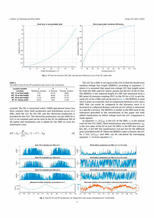
rebeSMinCGalun

LC

The LCC for a SMmedium voltage li

umeG athemma Seceas

phyrrencribtion

(5)C (Ae of

Fig. 2. AT heat loss function (left side) and electrical efficiency curve of

Table 3The AMCF of the SP and WT production data used in the simulations.


ached. The DG is reinvested when 15000 operational hours hasen reached. Since both production and distribution occurs in aG, both the LCC for the OEL and the electricity production is

cluded for the CGC. The electricity production cost per kWh for aC is set constant and can be seen in the SF. An additional 10% ofl capital and installation cost is added for the SMG to cover forforeseen costs.

where it is assfor both the SMThe BEMVLL isMV point of cosame LCC as forsince it gives anSMG that canmeasured in ain a specific cureferences desadded clarificamade against.

In equationcosts for the CGis the rest valu

Location number 1 2 3Location Skellefteå, Sweden Å, Norway Ottenby, Sweden

WT, 12 m hub height 3.7% 41.5% 28.8%WT, 16 m hub height 5.6% 42.6% 31.5%WT, 30 m hub height 11.3% 44.9% 37.3%SP, 35 facing south 10.2% 9.0% 11.9%

C¼C0 þX50n¼1

Cn

ð1þ rÞn S50 (4)

km, MCn is the MVyears provided in tfor a CGC (LCCCGCequation (5) to for

Fig. 3. Data for SP and WT production, air temperature and energy consum

5

G is set equal to the CGC to find the break-evenne length (BEMVLL) according to equation (5)d that equal low voltage (LV) line length existsnd CGC which cancels out the LCC of the LV line.required length of a MV line measured from aon coupling (PCC) to the DT for a CGC to get theMG and can be seen in Fig. 6. The BEMVLL is usedonomic unit of comparison between a CGC and aily be compared to the literature since it issical distance and not an LCC which is measuredcy. The BEMVLL is similar to the BED used in theed in the introduction of this paper but withon which voltage level the LCC comparison is

, LCCSMG is the LCC of the SMG, cn is the annualEEC, fixed maintenance and reinvestments). s50the DT at year 50, MVLC is the MV line cost per

the DG (right side).

line maintenance cost per km for the differenthe SF. When the BEMVLL value is known, the LCCÞ and SMG can be calculated by rearrangingm equation (6).

ption for a household.

BEMVLL ¼ y

,

y ¼ LCCSMGP50n¼1

ðcn=ð1þ

z ¼ MVLCþP50n¼1

ðMCn=

LCCSMG ¼ LCCC

Y ¼ BEMVLL

MVLCþ

P5n¼

Z ¼P50n¼1

ðcn=ð1

The levelized coergy (LCOEE) anddetermine how m

Fig. 4. Five different measured hourly electricity CPs in Sweden.

Fig. 5. Electricity and heat flow in the modeled SMG.

Table 4DG power output, activation of the DG, constraints used and their parameters.

Parameter SymbolStored energy in the battery BElectricity output of the DG GBattery storage capacity BF

Continuous charge/discharge rate of the battery BconPeak charge/discharge rate of the battery Bpeak

Net electricity production from the SP and/or WT (depending on SC) WDG power output

G ¼ BconðiÞþ PðiÞ WðiÞ where 0 G BpeakðiÞActivation of the DG

If BðiÞ=BF ðiÞ 0:1 or PðiÞ WðiÞ>BconðiÞ then BðiÞ ¼ BðiÞþ GConstraints of the EFM

BðiÞ 0PðiÞ BpeakðiÞþ WðiÞ

Table 5Investment and reinvestment of capital for the SMG and the CGC.

Year 0 15 20 30 40 45 Usage dependent

SMGInverters X X X XWT X X XSP X XStove X XAT X XBatteries X XDG X X

CGCDT X XOEL X


6

z

rÞn Þþs50

ð1þrÞn Þ

(5)

GC ¼ Y þ Z0

1ðMCn=ð1þrÞn Þ

þrÞn Þs50

(6)

st of heat (LCOH), levelized cost of electric en-levelized cost of energy (LCOE) is calculated touch each form of energy costs for a SMG. It is

caprfucothan

LC

, X50 n

,

large


lculated in equations (7)e(9) where LCCH is the LCC of the heatoducing and storing components (stoves, ATs) including pelletsel, LCCEE is the LCC of the electricity producing and storingmponents (batteries, SP, WT, DG) including diesel fuel, LCCSMG ise LCC for the entire SMG, EH is the annual HC, EEE is the annual ECd E is the AEC (heat and electricity).

LCOEE¼ LCCEE

LCOE¼ LCCSMG

Fig. 6. The concept of using the BEMVLL to find a potential SMG in a

OH¼ LCCH

, X50n¼1

EH

ð1þ rÞn (7) 2.3. TEEFM calcula

The energy flow

Fig. 7. Simplified schematic of the TEEFM.

7

distribution network.

n¼1

EE ð1þ rÞ (8)

X50 E ð1þ rÞn (9)

n¼1

tion procedure

is calculated for every hour for 20 years in order

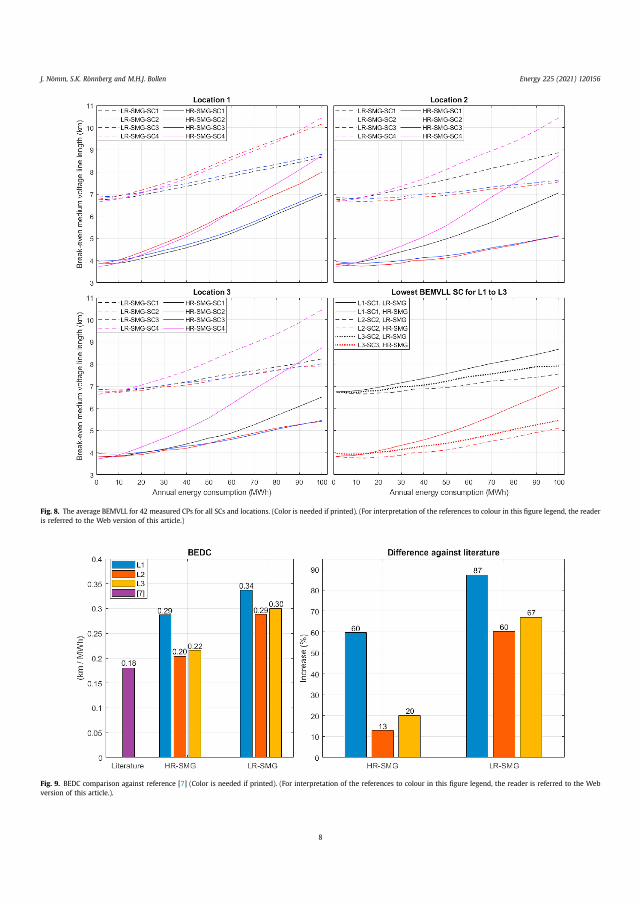
Fig. 8. The average BEMVLL for 42 measured CPs for all SCs and locations. (Color is needed if printed). (For interpretation of the references to colour in this figure legend, the readeris referred to the Web version of this article.)

Fig. 9. BEDC comparison against reference [7] (Color is needed if printed). (For interpretation of the references to colour in this figure legend, the reader is referred to the Webversion of this article.).


8

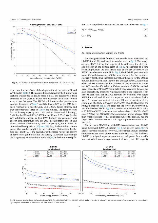
toWseexstpobethfo5Wchlodepofuatdi

the DG. A simplifie

NB ¼ ceilðPmax =B3

CG ¼5NB

3. Results

3.1. Break-even me

The average BEMLR-SMG for all SCs

L SCth

romseeinc

he Ceaseis inhe Sof Sity phatT anrisoSMinof AAEEhe Arenciffer

ed B

Figfig

J. N€omm, S.K. R€onnberg and M.H.J. Bollen

account for the effects of the degradation of the battery, SP andT listed in Table 2. The acquired input data described in previousctions was looped to get 20 years of data. The results were thentended to 50 years to match the economy calculations whichretch over 50 years. The TEEFM will increase the system com-nents described in Table 1 until the lowest LCC for the SMG haveen reached for a specific AEC, CP, SC, SMG design strategy andat the constraints listed in Table 4 are fulfilled. The iteration stepsr the battery capacity was 13.5 kWh (1 Powerwall 2 battery),kW for the DG and 0.15e5 kW for the SP and 0.05e3 kW for theT, arbitrarily chosen. A 13.5 kWh battery per customer wasosen as the minimum for a HR-SMG, also arbitrarily chosen. Thewest amount of batteries NB and DG capacity CG for a LR-SMG istermined by equations (10) and (11). Pmax is the total maximum

average BEMVLalso be seen inseries output fBEMVLL can besome SCs withelectricity for tthe AEC is incrwhen the AECand WT (see tlarger capacitykWh of electricalso be seen tAMCF for a Wused. A compaeconomics of astudy) is madeand 100 MWhat 27 MWh ofsince 77.3% of tthan what refelargest BEDC dHR-SMG.

The increas

Fig. 10. The increase in average BEMVLL for a change from HR-SMG to LR-SMG.

wer that can be supplied to the customers (determined by these size) and B3300 is the peak charge/discharge rate of the battery3300 cycles (end of life for the battery i.e. lowest peak charge/scharge rate). Number five in equation (11) is the iteration step for

using the lowest Blargest increase occcomponents per MLR-SMG is designedfuse size which ca

. 11. Average levelized cost in Swedish krona (SEK) for a HR-SMG (left) and LR-SMG (right). (Color is needed if pure legend, the reader is referred to the Web version of this article.)

9

d schematic of the TEEFM can be seen in Fig. 7.

300Þ (10)

(11)

dium voltage line length

VLL for the 42 measured CPs for a HR-SMG andand locations can be seen in Fig. 8. The lowestfor the majority of the AEC range for L1-L3 can

e bottom right in Fig. 8. An example of a timethe EFM that is used by the EM to calculate then in the SF. In Fig. 8, the BEMVLL goes down forreasing AEC because the cost for the producedGC increases more than the costs for the SMG asd. The slope of the average BEMVLL can reducecreased due to the scale of economics for the SPF). When sufficient amount of AEC is reached,P andWT is installed which reduces the cost perroducedwhich causes the slope to reduce. It canthe BEMVLL reduces for locations with largerd SP which is expected since less diesel fuel isn against reference [7] which investigated theG in Sweden at 27 MWh of AEEC (lowest in theFig. 9. The slope for the lowest SCs between 80EC in Fig. 8 was used to establish the BEDC valueC (which corresponds to about 119 MWh of AECEC is HC). The comparison shows a larger BEDCe [7] has concluded where the LR-SMG has theence since it has larger capital investment than a

EMVLL for a LR-SMG in comparison to a HR-SMGEMVLL SCs from Fig. 8 can be seen in Fig. 10. The

Energy 225 (2021) 120156

urs for lower AEC since larger amount of systemWh of AEC exists in the LR-SMG. This is since ato provide continuous peak power for a specific

uses larger amount of battery and DG capacity

rinted). (For interpretation of the references to colour in this

thpora

3.

mth


s lowa Ct caheat and injected to the ATs. A good example of the

at 10

an a HR-SMG which uses the minimum amount of system com-nents. The average increase in BEMVLL for the 1e100 MWh AECnge was 62.9%, 70.9% and 65.8% for L1-L3 respectively.

is several timeeconomical ifproduction thaconverted into

Fig. 12. PC of all CPs plotted against the BEMVLL in a HR-SMG

2. Levelized cost

In Fig. 11, the average LCOH, LCOEE and LCOE for the 42easured CPs can be seen for the SCs with the lowest BEMVLL fore majority of the AEC range in Fig. 8. It can be seen that the LCOH

mismatch betweenelectricity is consuduring the eveningwith the DG in theachieved which in

Fig. 13. PC of all CPs plotted against the BEMVLL in a LR-SMG at 100

10

er than the LCOEE which reveals that it is un-P has a mismatch between consumption anduses the leftover electricity production to be

0 MWh of AEC.

consumption and production is for SC1. If moremed during the day when the sun shines than, less electricity will be needed to be producedevening and therefore a lower diesel fuel cost isturn reduces the LCC.

MWh of AEC.

3.

atthHBElosaCPasucosediSM

nedPCsomiEMC. N

t ris

ve dfor an bmaG.andt CP

Fig. 14. CDF of all possible LCC increases for a SMG and CGC due to an increase in AEC. (Color is needed if printed). (For interpretation of the references to colour in this figurelegend, the reader is referred to the Web version of this article.)

Fig needth


3. Economic effects of different consumption patterns

In Figs. 12 and 13, the PC of all CPs is plotted against the BEMVLL100 MWh of AEC for both a HR-SMG and LR-SMG. The SCs withe lowest BEMVLL for the majority of the AEC range is used. For aR-SMG, there is a correlation between lower PC and lowerMVLL. The constant CP has the lowest BEMVLL since the PC is thewest possible. It can also be seen that one of several CPs with theme PC can have lower BEMVLL. This comes from the TOC effect.s that have more EC when the SP andWT produce electricity haslower BEMVLL than a CP that has a mismatch between con-mption and production. A mismatch will cause that electricity isnverted into heat which is uneconomical since the LCOEE isveral times larger than the LCOH. For a LR-SMG, the BEMVLLfference between the CPs is less than for a HR-SMG since a LR-G is dimensioned to be able to continuously supply electricity

within the defifrom differentinate the econdifferences in Bby different TO13.

3.4. Investmen

A cumulaticreases in LCCchange in CP caBEMVLL for theused for the SMcludes both PCLCC of differen

. 15. CDF of all possible LCC increases for a SMG and CGC due to an adverse change in PC and TOC. (Color isis figure legend, the reader is referred to the Web version of this article.)

11

fuse size. This eliminates the economic effectswithin the defined fuse size but does not elim-c effects of different TOC, which means that theVLL seen for the LR-SMG in Fig. 13 is only causedote the different horizontal scales in Figs. 12 and

ed if printed). (For interpretation of the references to colour in

k analysis

istribution function (CDF) for all possible in-SMG and CGC due to increased AEC and adversee seen in Figs. 14 and 15. The SCs with the lowestjority of the 1e100MWh AEC range in Fig. 8 wasThe LCC increase for a change in CP (which in-TOC) was calculated by directly comparing thes. The LCC increase related to only the TOC was

cafrusco(6thavFispco10remla

thationincin

hanLR-St ishe fy a cFigsn in

Fig e CPre

Figfig


lculated by choosing CPs with about the same PC (within 1 kWhom each other). The LCC increase for a CGC was calculated bying equation (6) at a fixed BEMVLL value from equation (5) thatrresponds to each SMG LCC, and then varying the AEC in equation). This is why the CGC LCC increase in Fig. 14 is lower for a LR-SMGan a HR-SMG since the BEMVLL is larger for a LR-SMG. Theerage and maximum values for Figs. 14 and 15 can be seen ing. 16 where the maximum value for an increase in AEC corre-onds to an increase from 1 to 100 MWh and the average valuenstitutes the average of all possible LCC increases between 1 and0 MWh. The maximum value for an adverse change in CP cor-

increase in AECstrategies. LocaLCC for an AECdence. The LCCwith adverse cThis is since athe PC since ipower within tonly affected bcan be seen inSMG LCC for a

. 16. Average and maximum value for all possibilities of an LCC increase due to an AEC increase and adversferences to colour in this figure legend, the reader is referred to the Web version of this article.)

sponds to a change from the CP with the lowest PC and/or largestatch to the production from the SP and WT, to the CP with thergest PC and/or least matching to the production from SP andWT.It can be seen in Figs. 14-16 that the LCC increases more to an

duced electricity indue to the constanit is the only increxpenditure for a C

. 17. Average IR reduction when changing from a HR-SMG to a LR-SMG and LR-SMG to a CGC (Color is needed ifure legend, the reader is referred to the Web version of this article.)

12

n an adverse change in CP for both SMG designs with larger AMCF has also a lower increase inrease, which is due to lower diesel fuel depen-creases more for a HR-SMG than for a LR-SMGge in CP which can be seen in Figs. 15 and 16.MG will only be affected by the TOC and not bydimensioned to handle maximum continuoususe size defined in Section 2.1.2. The CGC LCC ishange in the AEC and not by different CPs which. 14e16. The CGC LCC also increases less than acrease in AEC. This is since the cost of the pro-

change. (Color is needed if printed). (For interpretation of the

creases linearly for the CGC as the AEC increasest electricity price used in the TEEFM and becauseeasing cost since all maintenance and capitalGC is related to a constant MV line length.

printed). (For interpretation of the references to colour in this

LRbecathadre(sDPCinadrebeSenoanAE

4.

foprIRCGbomthlacrHofinadAEaninto10aTOinavwminadincobestWatThchCGththprCGtofrecan

we

stat

: Cl anWriourcojecces,ect a

com

s destsflue

en

hasndaforb€araper

upp

tary/10.1

hium7.Reninve.RenhnolTechms f

ourowere41.osh HgridUstur ens8.EssenrucehybrJaramuralcase

n J, Dass c2017, Bore hyb017;1elingPap, Wawindhe coCW,forgy Rean Fin

lectiohand

J. N

The average IR reduction when changing from a HR-SMG to a-SMG (Scenario 1) and from a LR-SMG to a CGC (Scenario 2) canseen in Fig.17 for all three locations. The reduction in IR has beenlculated by taking the average values from Fig. 16 and dividingem. For Scenario 1, the reduction in IR is 96.7%e97.1% for anverse change in CP and 45.5%e49.5% for an AEC increase. Thisduction occurs because the LR-SMG is designed for continuous PCee Section 2.1.2) and because a LR-SMG has a larger battery andG capacity than a HR-SMG due to its ability to supply continuous, which reduces the amount of upgrades needed to supply ancreased AEC. For Scenario 2, the reduction in IR is 100% for anverse change in CP and 23.6%e42.6% for an AEC increase. Thisduction occurs because a CGC is not affected by a change in CPcause it can handle all PCs within the defined fuse size (seection 2.1.2), the electricity production cost per kWh is fixed (doest vary with time) for a CGC (see the SF) and because the capitald maintenance cost does not increase for a CGC due to increasedC or change in CP since the MV line length is fixed.

Conclusions

This paper investigated the IRs related to consumption changesr two different SMG design strategies, one with the objective toovide the lowest LCC (HR-SMG) and the other to provide a lowerfor a SMG (LR-SMG). The IR for both was then compared with aC. In this study, an increase in AEC was the largest IR factor forth a SMG and CGC since an increase in AEC could increase the LCCore than an adverse change in CP. A potential increase in EC wase largest IR factor of the AEC since the LCOEE was several timesrger than the LCOH in the modeled SMG and therefore any in-ease in EC would increase the LCC more than an equal increase inC. This study concurs with previous literature that the variabilitythe AEC constitutes an IR of a SMG [9,10] and has added theformation that an increase in AEC is a larger IR factor than anverse change in CP for a SMG. A change from 1 to 100 MWh ofC constituted an increase in LCC of 125.1%e175.5% for a HR-SMGd 48.8%e65.3% for a LR-SMG for the investigated locations. Thiscrease could happen if for instance three summer house cus-mers with 1 MWh of AEC becomes three all-year residents with0MWh of AEC. An adverse change in CP could increase the LCC ofHR-SMG by 21.9%e22.9% and 6.2%e8.7% for an adverse change inC for the investigated locations. The LR-SMG had a maximumcrease of below 1% for all locations for adverse changes in CP. Theerage value for an LCC increase due to an adverse change in CPas below 1% for both SMG design strategies which shows that theajority of the measured CPs does not contribute to a significantcrease in IR for a SMG. The LR-SMG reduced the average IR for anverse change in CP by over 96% and 45.5%e49.5% for an AECcrease but with an increase in average BEMVLL of 62.9%e70.9% inmparison to a HR-SMG. This shows that there is a clear tradeofftween economic opportunity and IR for the two SMG designrategies. SMGs in locations with larger overall AMCF for SP andT had a lower IR for a potential AEC increase which was mainlytributed to lower diesel fuel dependence as the AMCF increased.e CGC had a 100% lower average IR than a SMG for an adverseange in CP since the cost of electricity was not time varying for aC and because the CGCwas dimensioned to handle all PCs withine defined fuse size. The CGC had a 23.6%e42.6% lower average IRan a LR-SMG for an increase in AEC since the annual electricityoduction cost was the only cost variable that could increase for aC, since the capital and maintenance costs of a CGC was relateda fixed MV line length. However, if the distance to the customersom aMV PCC is larger than the BEMVLL, a SMG could still be moreonomical than a CGC even if the SMG LCC would increase due toAEC increase and/or adverse change in CP, since the SMG LCC

could still be lo

Credit author

Jakob N€ommdation, Formaoriginal draft,R€onnberg: ResSupervision, PrBollen: Resourpervision, Proj

Declaration of

The authorfinancial interappeared to in

Acknowledgem

This paperR€onnb€aret Foueconomic datarameters. R€onncreating this p

Appendix A. S

Supplemenhttps://doi.org

References

[1] Curry C. LitFinance; 201

[2] InternationalDeployment,aspects. 2019

[3] Internationalvestment, tec

[4] Kusakana K.energy syste947e57.

[5] Rohani G, Nrenewable p2014;64:828

[6] Nandi SK, Ghalternative to

[7] Hubble AH,microgrids fo2018;13:1e1

[8] Horcher KA.[9] Hazelton J, B

photovoltaic[10] Williams NJ,

utilities for rgrid model: a

[11] Naqvi M, Yamixed biomAppl Energy

[12] Rajbongshi Rand grid basER. Energy 2

[13] Soto D. Modmicrogrids in

[14] Li C, Zhou Dstand-alonenologies in t

[15] Ajlan A, TanperspectivesSustain Ener

[16] Das BK, Zamremote areagenerator se

[17] Odou ODT, B


13

r than the CGC LCC.

ement

onceptualization, Methodology, Software, Vali-alysis, Investigation. Data curation, Writing e

ting e review & editing, Visualization. Sarah K.es, Data curation, Writing e review & editing,t administration, Funding acquisition. Math H. J.Data curation, Writing e review & editing, Su-dministration, Funding acquisition.

peting interest

eclare that they have no known competingor personal relationships that could have

nce the work reported in this paper.

ts

been funded by Skellefteå Kraft Eln€at AB andtion. Skellefteå Kraft Eln€at AB has provided thesome of the conventional grid-connection pa-et Foundation has not been directly involved for.

lementary data

data to this article can be found online at016/j.energy.2021.120156.

-ion battery costs and market. Bloomberg New Energy

ewable Energy Agency. Future of Solar Photovoltaic;stment, technology, grid integration and socio-economic

ewable Energy Agency. Future of Wind; Deployment, in-ogy, grid integration and socio-economic aspects. 2019.no-economic analysis of off-grid hydrokinetic-based hybridor onshore/remote area in South Africa. Energy 2014;68:

M. Techno-economical analysis of stand-alone hybridsystem for Ras Musherib in United Arab Emirates. Energy

R. Prospect of windePV-battery hybrid power system as anextension in Bangladesh. Energy 2010;35(7):3040e7.n TS. Composition, placement, and economics of ruraluring sustainable development. Sustain Energy Grids Netw

tials of financial risk management. Wiley; 2005. p. 1e3.A, MacGill I. A review of the potential benefits and risks ofid mini-grid systems. Renew Energy 2014;67:222e9.illo P, Taneja J. An investment risk assessment of microgrid

electrification using the stochastic techno-economic micro-study in Rwanda. Energy Sustain Develop 2018;42:87e96.ahlquist E, Naqvi SR. Off-grid electricity generation usingompost: a scenario-based study with sensitivity analysis.;201:363e70.gohain D, Mahapatra S. Optimization of PV-biomass-dieselrid energy systems for rural electrification by using HOM-26:461e74.and measurement of specific fuel consumption in dieselua, Indonesia. Energy Sustain Develop 2018;45:180e5.ng H, Lu Y, Li D. Techno-economic performance study of/diesel/battery hybrid system with different battery tech-ld region of China. Energy 2020;192.Abdilahi AM. Assessment of environmental and economicrenewable-based hybrid power system in Yemen. Renewv 2017;75:559e70.. Performance analysis of a PV/Diesel hybrid system for aBangladesh: effects of dispatch strategies, batteries, andn. Energy 2019;169:263e76.ari R, Adamou R. Hybrid off-grid renewable power system

Energy 225 (2021) 120156


http://refhub.elsevier.com/S0360-5442(21)00405-9/sref1























































[1

[1

[2

[2

[2

[2

[2

[2

[2

[2

[2

[2

[3

[3

[3

[3

[3

esla

ninjaang Zgedigre;Elecdistrechn2016rgy A3.13.rmienewl con0; 20ionacy; 2en R.;66:7Enermodeblecn auEnerS, Ch

min Beirtz SRes

rgy Aningpowe, Stafidate

eoroent of Sweden. Promemoria om kostnaderna f€or nya elpro-

J. N

for sustainable rural electrification in Benin. Renew Energy 2020;145:1266e79.

8] Halabi LM, Mekhilef S, Olatomiwa L, Hazelton J. Performance analysis ofhybrid PV/diesel/battery system using HOMER: a case study Sabah, Malaysia.Energy Convers Manag 2017;144:322e39.

9] Ye B, Zhang K, Jiang J, Miao L, Li J. Towards a 90% renewable energy future: acase study of an island in the South China Sea. Energy Convers Manag2017;142:28e41.

0] Ali F, Ahmar M, Jiang Y, AlAhmad M. A techno-economic assessment of hybridenergy systems in rural Pakistan. Energy 2021;215.

1] Oueid RK. Microgrid finance, revenue, and regulation considerations. Electr J2019;32(5):2e9.

2] Wagemann B, Manetsgruber D. Risk management for mini-grid deploymentin rural areas. Energy Procedia 2016;103:106e10.

3] Abrahamse W, Steg L. How do socio-demographic and psychological factorsrelate to households’ direct and indirect energy use and savings? J EconPsychol 2009;30(5):711e20.

4] Mills B, Schleich J. Residential energy-efficient technology adoption, energyconservation, knowledge, and attitudes: an analysis of European countries.Energy Pol 2012;49:616e28.

5] Kavousian A, Rajagopal R, Fischer M. Determinants of residential electricityconsumption: using smart meter data to examine the effect of climate,building characteristics, appliance stock, and occupants’ behavior. Energy2013;55:184e94.

6] Firth S, Lomas K, Wright A, Wall R. Identifying trends in the use of domesticappliances from household electricity consumption measurements. EnergyBuild 2008;40(5):926e36.

7] Guo Z, Zhou K, Zhang C, Lu X, Chen W, Yang S. Residential electricity con-sumption behavior: influencing factors, related theories and interventionstrategies. Renew Sustain Energy Rev 2018;81:399e412.

8] Lutzenhiser L. Social and behavioral aspects of energy use. Annu Rev EnergyEnviron 1993;18:247e89.

9] Torriti J. Understanding the timing of energy demand through time use data:time of the day dependence of social practices. Energy Res Soc Sci 2017;25:37e47.

0] Hansen M, Hauge B. Prosumers and smart grid technologies in Denmark:developing user competences in smart grid households. Energy Efficiency2017;10:1215e34.

[35] Tesla inc, "T2017.

[36] Renewables[37] Jarman P, W

formers in aconference. C

[38] Internationalmission and

[39] SMA Solar TApplications.

[40] Swedish Ene[41] HOMER Pro[42] Aatola H, La

(HVO) as a rsion, and fue2008-01-250

[43] Lindahl J. NatEnergy Agen

[44] Staffell I, GreEnergy 2014

[45] Internationaltrends in PV

[46] Thomas D, Danalysis of apenetration.

[47] He L, Zhangenergy-basedcommunity i

[48] Jordan DC, KuPhotovoltaics

[49] Swedish Ene[50] Staffell I, Pfen

future wind[51] Pfenninger S

Years of val1251e65.

[52] Swedish Met[53] The governm


1] Palm J, Eidenskog M, Luthander R. Sufficiency, change, and flexibility: criti-cally examining the energy consumption profiles of solar PV prosumers inSweden. Energy Res Soc Sci 2018;39:12e8.

2] Kubli M, Loock M, Wüstenhagen R. The flexible prosumer: measuring thewillingness to co-create distributed flexibility. Energy Pol 2018;114:540e8.

3] Swedish Energy Agency. Energy statistics for one- and two-dwelling build-ings. 2016.

4] Tesla. Inc, "Tesla Powerwall 2 datasheet - North America," 2019-06-11.

duktionsanl€aggninin Sweden). Statecial investigations

[54] Elforsk. Electricity[55] Sumanik-Leary J.

case studies in P2013.

14

Powerwall warranty (European warranty region)," June 9,

[Online]. Available: https://www.renewables.ninja/., Zhong Q, Ishak T. End-of-life modelling for power trans-power system networks. In: 6th southern Africa regional2009.trotechnical Commission. Efficient electrical energy trans-ibution. 2007.ology. Sunny Island 6.0H / 8.0H For Off-Grid and On-Grid.gency.

M, Sarjovaara T, Mikkonen S. Hydrotreated vegetable oilable diesel fuel: trade-off between NOx, particulate emis-sumption of a heavy duty engine. SAE Technical Paper Series08.l survey report of PV power applications in Sweden. Swedish017.How does wind farm performance decline with age? Renew75e86.gy Agency. End-of-Life management of photovoltaic panels:ule recycling technologies. 2018.ker O, Ioakimidis CS. Optimal design and techno-economictonomous small isolated microgrid aiming at high RESgy 2016;116:364e79.en Y, Ren L, Li J. Techno-economic potential of a renewablecrogrid system for a sustainable large-scale residentialjing, China. Renew Sustain Energy Rev 2018;93:631e41.R. Photovoltaic degradation rates; an analytical review. ProgAppl 2013;21:12e29.gency. Pelletskvalitet (Quality of wood pellets). 2014.er S. Using bias-corrected reanalysis to simulate current andr output. Energy 2016;114:1224e39.fell I. Long-term patterns of European PV output using 30d hourly reanalysis and satellite data. Energy 2016;114:

logical and Hydrological Institute.

Energy 225 (2021) 120156

gar i Sverige (Costs of new electricity production facilitiesns offentliga utredningar; 2015 [Swedish government offi-)].from new and future plants. Elforsk Rep 2014;14(45).Small wind turbines for decentralised rural electrification:eru, Nicaragua and Scotland. The University of Sheffield;





























































https://www.renewables.ninja/

















































Paper F

Evaluating the harmonic performance in a

microgrid during islanded and grid-connected

operation using apparent harmonic impedance

performance indexes

Evaluating the harmonic performance in a microgrid during islanded

and grid-connected operation using apparent harmonic impedance

performance indexes

Jakob Nömm1

[email protected]

Sarah K. Rönnberg

[email protected]

Math H. J. Bollen

[email protected]


Department of Engineering Sciences and Mathematics

Forskargatan 1, 93187 Skellefteå, Sweden

Abstract This paper presents three new harmonic performance indexes that are expressed in terms of an apparent impedance.

The first performance index describes the ratio between the harmonic voltage and current magnitudes and is applied

to all phases simultaneously. The second and third performance index describes how much the harmonic voltage

magnitude on one phase is affected due to an increase in harmonic current magnitude in one of the phases. The new

performance indexes are thought to provide additional information about the harmonic performance that can aid grid

surveillance and detect sudden changes in harmonic performance in a grid. The indexes could also be used to generally

describe the harmonic performance of different modes of operation in for instance a microgrid. All performance

indexes were applied to measurements done in a microgrid that operated in both islanded and grid-connected mode.

Larger values of the harmonic performance indexes were seen in the microgrid during islanded operation than in grid-

connected operation and particularly when the microgrid operated with 50% of the battery inverters active. The larger

values were correlated with a larger harmonic system impedance. Time series of transitional harmonic performance

events are also shown in the paper.

1. Introduction A Microgrid is a suggested solution for providing improved electrical service such as improved reliability in parts of

the grid that has poor performance, more economic operation with reduced cost for customers and larger revenue for

the grid owners [1]. The literature has addressed that the island operation (IO) of a microgrid will be more adverse in

terms of power quality than the grid-connected operation (GCO) and that voltage stability issues could occur when

switching between IO and GCO due to switching from voltage controlled operation in IO to current controlled

operation in GCO [2]. Transitions from IO to GCO caused several interruptions reported in [3] for a single house

microgrid. However, the root cause of these interruptions was not determined. The literature has also mentioned that

larger variations in both voltage and frequency is expected due to lower short circuit capacity and lower inertia in

combination with wider range of interactions between the loads and sources [2]. Larger frequency variations than what

could be observed in the national grid in Sweden was shown in [3] for a single house microgrid. Larger PLT and PST

values could occur for the same microgrid in IO than in GCO [4], but lower very short variations (VSV) values was

shown, a measurement unit introduced by [5], [6]. Larger frequency variations were also observed in [7] during IO of

a microgrid. Almost constant frequency operation was observed in [8]. Larger voltage THD and individual harmonic

voltage levels than the specified limits in standards EN 50160 [9] and IEEE 519-2014 [10] was observed in [4], [11]

in a single house microgrid during IO. In the same microgrid, higher levels of supraharmonics was seen in IO compared

to GCO [12]. One possible cause of increased harmonic voltage levels could be an increase in harmonic system

impedance during IO which was concluded in [13], [14]. The literature has described several different harmonic

mitigation techniques for standalone microgrids that have been demonstrated with experiments [15], [16], [17], [18],

[19], [20], [21], [22], [23]. Although the presented literature gives many possibilities for further research, this paper

will investigate the use of new harmonic performance indexes in terms of an apparent impedance 𝑍𝐴 defined in

Equation (1) where 𝑉𝑀 is the harmonic voltage magnitude and 𝐼𝑀 is the harmonic current magnitude at a certain

measurement point. The term apparent impedance is used for instance by distance relays [24], [25], for finding the

location of a fault [26] and in stability analysis [27].

𝑍𝐴 =

𝑉𝑀

𝐼𝑀

(1)

1 Corresponding author

The described indexes in this paper are for performance analysis only and not for determining the real harmonic

impedance of a system. They are meant to be a complement to the voltage THD and individual voltage harmonics in

describing the system harmonic performance. The main contribution of this paper is the presented harmonic

performance indexes which have not been previously described in the literature.

2. Definition of apparent harmonic impedance performance indexes The first suggested harmonic performance index is the apparent harmonic system impedance (AHSI) with symbol 𝑍+

and is defined in Equation (2) for a single harmonic order and in Equation (3) for the total distortion (THD). 𝑁 is the

number of phases of the system, 𝑃 is the phase number, ℎ is the harmonic order, 𝑛 is the largest harmonic order

measured in the THD, 𝑉 is the harmonic voltage magnitude and 𝐼 is the harmonic current magnitude. By this definition,

AHSI can be applied to all of the phases simultaneously giving a single measurement unit of the harmonic performance

for the entire system, either for an individual harmonic or the THD. Mathematically, AHSI can be seen as the ratio

between two vector lengths (voltage and current distortion) in 𝑁 dimensions. For example, if AHSI is applied for three

phases, the voltage and current distortion vector lengths is derived from two separate sets of three independent vectors

(assuming orthogonality for the vectors that represent each phase). Furthermore, the THD-AHSI in Equation (3)

contains the voltage and current THD for each phase which can be seen as a vector length for each phase composed

from 𝑛 harmonic dimensions. Or more simply put, the total RMS value from the composition of orthogonal vectors up

to the 𝑛 order harmonic which is something used in defining the THD of a signal.

𝑍ℎ+ = √

∑ |𝑉𝑃ℎ|2𝑁𝑃=1

∑ |𝐼𝑃ℎ|2𝑁𝑃=1

(2)

𝑍𝑇𝐻𝐷+ = √

∑ (∑ |𝑉𝑃ℎ|2𝑁𝑃=1 )𝑛

ℎ=2

∑ (∑ |𝐼𝑃ℎ|2𝑁𝑃=1 )𝑛

ℎ=2

(3)

The second apparent harmonic performance index is the primary harmonic impedance performance index (PHIPI)

defined in Equation (4) which is a primary emission index. The third apparent harmonic performance index is the

secondary harmonic impedance performance index (SHIPI) defined in Equation (5) which is a secondary emission

index. Both PHIPI and SHIPI has symbol 𝑍− but with different subscripts. PHIPI is somewhat similar to a formula for

measuring the real harmonic impedance described in for instance [28], [29] with the exception that PHIPI does not use

the phase angles. PHIPI measures the harmonic voltage magnitude response due to a harmonic current magnitude

increase on the same phase 𝑃 and SHIPI measures the harmonic voltage magnitude response on phase 𝑃 due to a

harmonic current magnitude increase on another phase 𝑥 at a certain instance in time 𝑖. SHIPI does not have a similar

index in the literature and is the first to quantify with an index the harmonic interaction between the phases. A feature

of the PHIPI and SHIPI is that negative apparent impedance values can be achieved for an increase in harmonic current

magnitude (seen in Equation (4) and (5)) which is when an increase in harmonic current magnitude causes a drop in

harmonic voltage magnitude which is registered by PHIPI and SHIPI as a negative apparent impedance value.

𝑍𝑃− =

|𝑉𝑃(𝑖 + 1)| − |𝑉𝑃(𝑖)|

|𝐼𝑃(𝑖 + 1)| − |𝐼𝑃(𝑖)| where |𝐼𝑃(𝑖 + 1)| > |𝐼𝑃(𝑖)| (4)

𝑍𝑃𝑥− =

|𝑉𝑃(𝑖 + 1)| − |𝑉𝑃(𝑖)|

|𝐼𝑥(𝑖 + 1)| − |𝐼𝑥(𝑖)| where |𝐼𝑥(𝑖 + 1)| > |𝐼𝑥(𝑖)| (5)

PHIPI and SHIPI can be calculated either by using a non-invasive or invasive method to generate harmonic current.

The non-invasive method would use the connected loads for generating harmonic current which is a similar method

used by non-invasive methods for measuring the real harmonic system impedance described in [30], [31], [32], [33],

[34], [35], [36] that uses existing switching events caused by for instance capacitor bank or transformer switching to

calculate the harmonic system impedance. The invasive method would use an external system to inject a harmonic

current into the system which has been studied in for instance [37], [38], [39], [40], [41], [42]. The new performance

indexes can be used as a complement with the conventional measurement indexes such as voltage THD and individual

voltage harmonics that have defined limits in for instance standards such as EN 50160 [9] and IEEE 519-2014 [10].

The new indexes are particularly useful for microgrids that operate with several different system impedances (due to

IO and GCO). This is since AHSI can give a combined value for all phases on how much more/less voltage distortion

per unit current distortion exist in IO than in GCO. And because PHIPI and SHIPI can give a value for the different

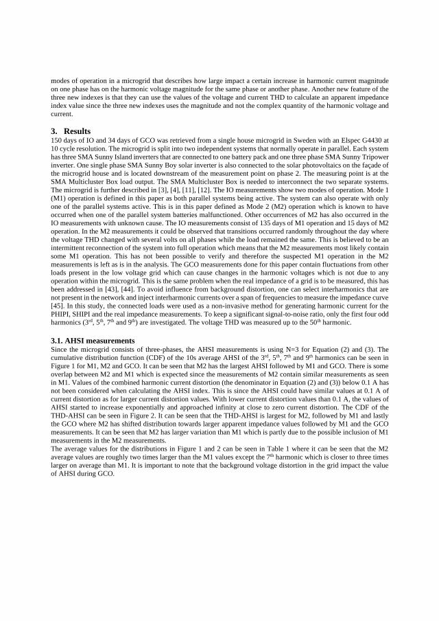
modes of operation in a microgrid that describes how large impact a certain increase in harmonic current magnitude

on one phase has on the harmonic voltage magnitude for the same phase or another phase. Another new feature of the

three new indexes is that they can use the values of the voltage and current THD to calculate an apparent impedance

index value since the three new indexes uses the magnitude and not the complex quantity of the harmonic voltage and

current.

3. Results 150 days of IO and 34 days of GCO was retrieved from a single house microgrid in Sweden with an Elspec G4430 at

10 cycle resolution. The microgrid is split into two independent systems that normally operate in parallel. Each system

has three SMA Sunny Island inverters that are connected to one battery pack and one three phase SMA Sunny Tripower

inverter. One single phase SMA Sunny Boy solar inverter is also connected to the solar photovoltaics on the façade of

the microgrid house and is located downstream of the measurement point on phase 2. The measuring point is at the

SMA Multicluster Box load output. The SMA Multicluster Box is needed to interconnect the two separate systems.

The microgrid is further described in [3], [4], [11], [12]. The IO measurements show two modes of operation. Mode 1

(M1) operation is defined in this paper as both parallel systems being active. The system can also operate with only

one of the parallel systems active. This is in this paper defined as Mode 2 (M2) operation which is known to have

occurred when one of the parallel system batteries malfunctioned. Other occurrences of M2 has also occurred in the

IO measurements with unknown cause. The IO measurements consist of 135 days of M1 operation and 15 days of M2

operation. In the M2 measurements it could be observed that transitions occurred randomly throughout the day where

the voltage THD changed with several volts on all phases while the load remained the same. This is believed to be an

intermittent reconnection of the system into full operation which means that the M2 measurements most likely contain

some M1 operation. This has not been possible to verify and therefore the suspected M1 operation in the M2

measurements is left as is in the analysis. The GCO measurements done for this paper contain fluctuations from other

loads present in the low voltage grid which can cause changes in the harmonic voltages which is not due to any

operation within the microgrid. This is the same problem when the real impedance of a grid is to be measured, this has

been addressed in [43], [44]. To avoid influence from background distortion, one can select interharmonics that are

not present in the network and inject interharmonic currents over a span of frequencies to measure the impedance curve

[45]. In this study, the connected loads were used as a non-invasive method for generating harmonic current for the

PHIPI, SHIPI and the real impedance measurements. To keep a significant signal-to-noise ratio, only the first four odd

harmonics (3rd, 5th, 7th and 9th) are investigated. The voltage THD was measured up to the 50th harmonic.

3.1. AHSI measurements Since the microgrid consists of three-phases, the AHSI measurements is using N=3 for Equation (2) and (3). The

cumulative distribution function (CDF) of the 10s average AHSI of the 3rd, 5th, 7th and 9th harmonics can be seen in

Figure 1 for M1, M2 and GCO. It can be seen that M2 has the largest AHSI followed by M1 and GCO. There is some

overlap between M2 and M1 which is expected since the measurements of M2 contain similar measurements as seen

in M1. Values of the combined harmonic current distortion (the denominator in Equation (2) and (3)) below 0.1 A has

not been considered when calculating the AHSI index. This is since the AHSI could have similar values at 0.1 A of

current distortion as for larger current distortion values. With lower current distortion values than 0.1 A, the values of

AHSI started to increase exponentially and approached infinity at close to zero current distortion. The CDF of the

THD-AHSI can be seen in Figure 2. It can be seen that the THD-AHSI is largest for M2, followed by M1 and lastly

the GCO where M2 has shifted distribution towards larger apparent impedance values followed by M1 and the GCO

measurements. It can be seen that M2 has larger variation than M1 which is partly due to the possible inclusion of M1

measurements in the M2 measurements.

The average values for the distributions in Figure 1 and 2 can be seen in Table 1 where it can be seen that the M2

average values are roughly two times larger than the M1 values except the 7th harmonic which is closer to three times

larger on average than M1. It is important to note that the background voltage distortion in the grid impact the value

of AHSI during GCO.

Figure 1. CDF of the 10s average 3rd, 5th, 7th, 9th AHSI. (Color is needed if printed).

Figure 2. CDF of the 10s average THD-AHSI. (Color is needed if printed).

Table 1. Average values for the CDF in Figure 1 and 2 in V/A.

3rd M1 3rd M2 3rd GCO 5th M1 5th M2 5th GCO 7th M1 7th M2 7th GCO

3.1 6.9 0.75 5.5 11.2 1.7 8.9 25.4 3.3

9th M1 9th M2 9th GCO THD M1 THD M2 THD GCO

16.0 29.7 1.9 5.6 9.9 1.8

3.1.1. Increases in load

The changes in AHSI due to single phase load changes can be observed in Figure 3. Three phase load changes with an

increase in current distortion did not give enough samples for comparison and was therefore excluded in this paper.

The change in fundamental RMS voltage was below 1% for all load changes and did not significantly affect the

harmonic current distortion. The criteria for the single-phase load change was an increase by more than 20 W and an

increase in harmonic current by more than 0.2 A from at least 0.1 A of harmonic current (which was the cut-off current

for calculation the AHSI value described in Section 3.1). 0.2 A was the largest current value that produced enough

samples for comparison between the modes of operation. The other phases needed to be below a 20 W fluctuation

during the load change, a lower active power value did not affect the distribution significantly, but significantly reduced

the number of samples. The active power and harmonic current also needed to be lower than 20 W and 0.03 A variation

respectively for all three phases, three samples earlier from the measured sample up to the measured sample so that

changes in the active power and harmonic current prior to the measured sample is avoided. 0.03 A was also chosen to

get enough samples for comparison, as a lower value significantly reduced the number of samples. The calculation

was done by taking the difference in AHSI value with three sample spacing to avoid transients during the load change

(which can be seen in Section 3.6 in Figure 20, Example 2). 10 cycle values were used. Only the 3rd and 5th harmonic

had sufficient number of samples for all three modes of operation. It can be seen in Figure 3 that the distributions are

skewed to larger values of change in AHSI for M2 followed by M1 and lastly GCO. The GCO values for the THD-

AHSI had always a reduction in AHSI, meaning that as the current distortion increased, the ratio between voltage and

current reduced. This is most likely because the low voltage grid has a much lower system impedance which leads the

voltage distortion largely unaffected from a rise in current distortion from the single house microgrid.

Figure 3. AHSI change due to a single-phase load change. (Color is needed if printed).

The absolute average values for the distributions in Figure 3 can be seen in Table 2 where the 3 rd harmonic and THD

had roughly a 3 times difference between M1 and M2 while the 5th harmonic was roughly 2 times larger in M2 than

M1.

Table 2. Absolute average values for the distributions in Figure 3 in V/A.

3rd M1 3rd M2 3rd GCO 5th M1 5th M2 5th GCO THD M1 THD M2 THD GCO

0.40 1.34 0.12 0.25 0.47 0.25 0.27 0.86 0.21

3.1.2. Constant load

The changes to the AHSI was also investigated during constant load, which is defined in this paper as a variation in

active power consumption less than 20 W for all three phases. A lower active power variation did not affect the

distribution significantly, but it significantly reduced the number of samples. The measurements are done by taking

the difference between 10s average AHSI values with three samples between them when the active power fluctuated

between 20 W of all three phases. Three samples spacing was chosen to capture transitional events that occur in IO

which can be progressive over several 10s of seconds to reach a converged value. This is shown in Section 3.5. It can

be seen in Figure 4 that M2 has a shifted distribution towards larger values than M1 for both the individual harmonics

and THD. The GCO measurements had lower variation than in both M1 and M2. The 5th and 7th harmonic in the GCO

measurements had also several times larger variation than the 3rd and 9th harmonic in the GCO measurements. It is

important to note that the constant load condition is only downstream from the measurement point in the microgrid

and not downstream from the distribution transformer in the low voltage grid in which the microgrid is connected to.

Therefore, the GCO variations are most likely caused by load changes in the low voltage grid i.e. upstream from the

measurement point. The change in AHSI during constant load can be several times larger than during load changes,

which is caused by a change in harmonic system impedance and will be shown later in the paper in Section 3.5.

Figure 4. Change in individual AHSI during constant load during IO (top) and GCO (bottom left) and THD-AHSI (bottom right).

Note the difference in horizontal scale. (Color is needed if printed).

The absolute average values from Figure 4 can be seen in Table 3. It can be seen that the GCO measurements can have

larger values than M1 and M2, which is expected due to variation in the background voltage distortion. The 3rd, 5th and

THD is about two times larger on average in M2 than in M1. The 7th and 9th harmonic are more than four times larger

in M2 than in M1.

Table 3. Absolute average values for the distributions in Figure 4 in V/A.

3rd M1 3rd M2 3rd GCO 5th M1 5th M2 5th GCO 7th M1 7th M2 7th GCO

0.020 0.044 0.017 0.064 0.11 0.28 0.23 1.0 0.38

9th M1 9th M2 9th GCO THD M1 THD M2 THD GCO

0.37 1.75 0.030 0.029 0.047 0.092

3.2. PHIPI and SHIPI measurements The PHIPI and SHIPI measurements done in the microgrid can be seen in Figure 5 and Figure 6. The same

measurement criteria as described in Section 3.1.1. was used with 10 cycle values and with 3 sample spacing for the

harmonic voltage and current in order to use steady state values before and after the load is switched on. Only the

individual harmonics 3rd and 5th had enough samples to be compared between the modes of operation in the microgrid.

It can be seen in Figure 5 and 6 that M2 has the largest variations in PHIPI and SHIPI followed by M1 and lastly the

GCO measurements.

Figure 5. CDF of the PHIPI measurements. (Color is needed if printed).

Figure 6. CDF of the SHIPI measurements. (Color is needed if printed).

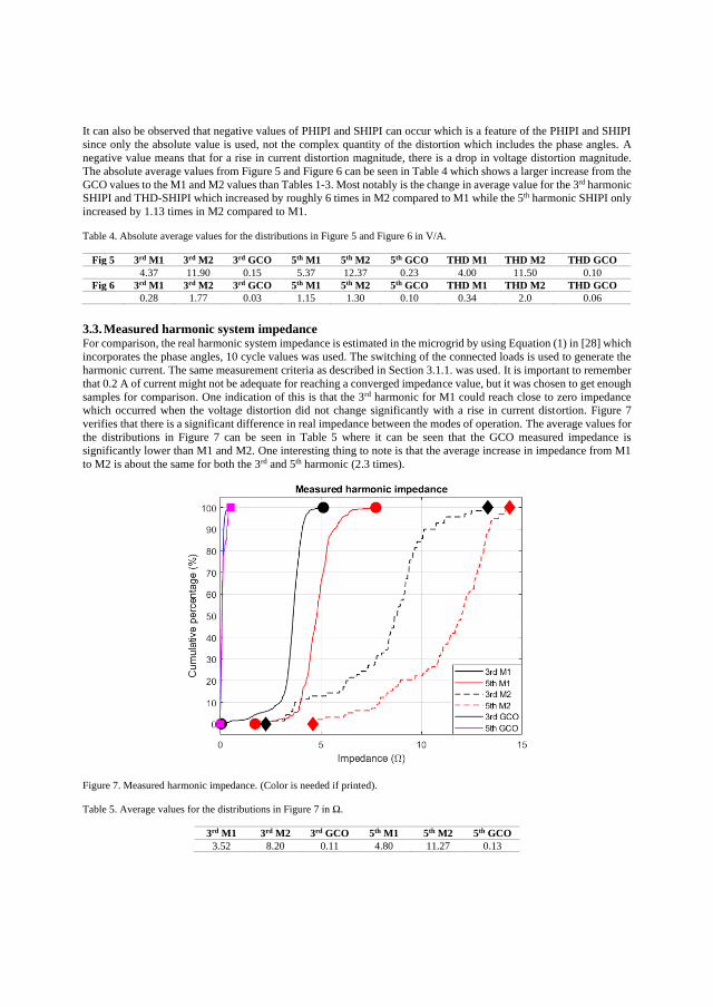
It can also be observed that negative values of PHIPI and SHIPI can occur which is a feature of the PHIPI and SHIPI

since only the absolute value is used, not the complex quantity of the distortion which includes the phase angles. A

negative value means that for a rise in current distortion magnitude, there is a drop in voltage distortion magnitude.

The absolute average values from Figure 5 and Figure 6 can be seen in Table 4 which shows a larger increase from the

GCO values to the M1 and M2 values than Tables 1-3. Most notably is the change in average value for the 3rd harmonic

SHIPI and THD-SHIPI which increased by roughly 6 times in M2 compared to M1 while the 5th harmonic SHIPI only

increased by 1.13 times in M2 compared to M1.

Table 4. Absolute average values for the distributions in Figure 5 and Figure 6 in V/A.

Fig 5 3rd M1 3rd M2 3rd GCO 5th M1 5th M2 5th GCO THD M1 THD M2 THD GCO

4.37 11.90 0.15 5.37 12.37 0.23 4.00 11.50 0.10

Fig 6 3rd M1 3rd M2 3rd GCO 5th M1 5th M2 5th GCO THD M1 THD M2 THD GCO

0.28 1.77 0.03 1.15 1.30 0.10 0.34 2.0 0.06

3.3. Measured harmonic system impedance For comparison, the real harmonic system impedance is estimated in the microgrid by using Equation (1) in [28] which

incorporates the phase angles, 10 cycle values was used. The switching of the connected loads is used to generate the

harmonic current. The same measurement criteria as described in Section 3.1.1. was used. It is important to remember

that 0.2 A of current might not be adequate for reaching a converged impedance value, but it was chosen to get enough

samples for comparison. One indication of this is that the 3rd harmonic for M1 could reach close to zero impedance

which occurred when the voltage distortion did not change significantly with a rise in current distortion. Figure 7

verifies that there is a significant difference in real impedance between the modes of operation. The average values for

the distributions in Figure 7 can be seen in Table 5 where it can be seen that the GCO measured impedance is

significantly lower than M1 and M2. One interesting thing to note is that the average increase in impedance from M1

to M2 is about the same for both the 3rd and 5th harmonic (2.3 times).

Figure 7. Measured harmonic impedance. (Color is needed if printed).

Table 5. Average values for the distributions in Figure 7 in Ω.

3rd M1 3rd M2 3rd GCO 5th M1 5th M2 5th GCO

3.52 8.20 0.11 4.80 11.27 0.13

3.4. Daily variations in AHSI The average daily variations in THD-AHSI can be seen in Figure 8. It can be seen that the THD-AHSI for IO is larger

in night operation than in day operation, this could be because as the solar inverters are switched on with sunrise, more

parallel sources are available causing the harmonic system impedance to drop which reduces the harmonic voltage

distortion. The activation of harmonic filtering could also be a possible explanation which is further discussed in

Section 3.5. An 8-day time series of both 10 min and 3s average values are shown in Figure 9 which also show that

the THD-AHSI is larger during the night and that it is visible with different average values.

Figure 8. Daily average THD-AHSI variations. (Color is needed if printed).

Figure 9. Time series of the THD-AHSI at 10 min and 3s average values. red, black and blue color represents M2, M1 and GCO

respectively. (Color is needed if printed).

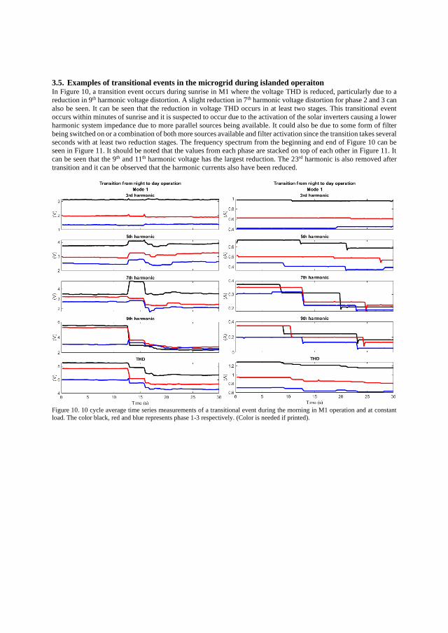
3.5. Examples of transitional events in the microgrid during islanded operaiton In Figure 10, a transition event occurs during sunrise in M1 where the voltage THD is reduced, particularly due to a

reduction in 9th harmonic voltage distortion. A slight reduction in 7th harmonic voltage distortion for phase 2 and 3 can

also be seen. It can be seen that the reduction in voltage THD occurs in at least two stages. This transitional event

occurs within minutes of sunrise and it is suspected to occur due to the activation of the solar inverters causing a lower

harmonic system impedance due to more parallel sources being available. It could also be due to some form of filter

being switched on or a combination of both more sources available and filter activation since the transition takes several

seconds with at least two reduction stages. The frequency spectrum from the beginning and end of Figure 10 can be

seen in Figure 11. It should be noted that the values from each phase are stacked on top of each other in Figure 11. It

can be seen that the 9th and 11th harmonic voltage has the largest reduction. The 23rd harmonic is also removed after

transition and it can be observed that the harmonic currents also have been reduced.

Figure 10. 10 cycle average time series measurements of a transitional event during the morning in M1 operation and at constant

load. The color black, red and blue represents phase 1-3 respectively. (Color is needed if printed).

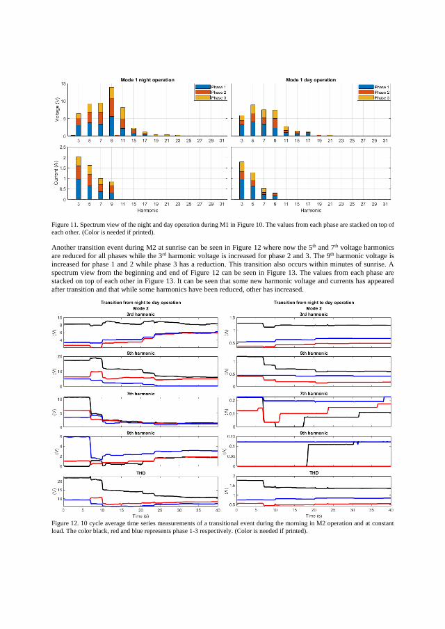
Figure 11. Spectrum view of the night and day operation during M1 in Figure 10. The values from each phase are stacked on top of

each other. (Color is needed if printed).

Another transition event during M2 at sunrise can be seen in Figure 12 where now the 5th and 7th voltage harmonics

are reduced for all phases while the 3rd harmonic voltage is increased for phase 2 and 3. The 9th harmonic voltage is

increased for phase 1 and 2 while phase 3 has a reduction. This transition also occurs within minutes of sunrise. A

spectrum view from the beginning and end of Figure 12 can be seen in Figure 13. The values from each phase are

stacked on top of each other in Figure 13. It can be seen that some new harmonic voltage and currents has appeared

after transition and that while some harmonics have been reduced, other has increased.

Figure 12. 10 cycle average time series measurements of a transitional event during the morning in M2 operation and at constant

load. The color black, red and blue represents phase 1-3 respectively. (Color is needed if printed).

Figure 13. Spectrum view of the night and day operation during M2 in Figure 12. The values from each phase are stacked on top of

each other. (Color is needed if printed).

In Figure 14, a transition from M1 to M2 can be seen where the 3rd, 5th, 7th harmonic voltage is increased together with

the THD while the 9th harmonic voltage is reduced. The current is most notably decreased for the 7th and 9th harmonic

while the THD current is somewhat unchanged during the transition. In Figure 15, a spectrum view of the beginning

and end of Figure 14 can be seen where it can be observed that several even voltage harmonic components have

appeared after transition.

Figure 14. 10 cycle average time series measurements during constant load during a transitional event from M1 to M2 operation.

The color black, red and blue represents phase 1-3 respectively. (Color is needed if printed).

Figure 15. Spectrum view of the M1 and M2 operation in Figure 14. (Color is needed if printed).

In Figure 16, the AHSI is shown for the 3rd, 5th, 7th and 9th harmonic together with the THD. It can be seen that during

the transition in M1, the 3rd harmonic AHSI is somewhat unchanged during the transition and that the 5th, 7th and 9th

are increased while the THD-AHSI is reduced. In M2, the 5th, 7th and 9th harmonic AHSI is reduced together with the

THD-AHSI while the 3rd harmonic AHSI is increased.

Figure 16. 10 cycle average AHSI time series measurements of a transitional event during the morning in M1 and M2 operation and

at constant load seen in Figure 10 and 12.

Looking at the individual harmonics in the M1 transition, it can appear that the harmonic system impedance has

increased after the transition. This shows that the THD-AHSI is more reliable in detecting overall harmonic impedance

changes in the system than the individual harmonic AHSI since it is clear that the overall harmonic system impedance

has decreased as no load changes has occurred during the transition. Even if the harmonic voltage for an individual

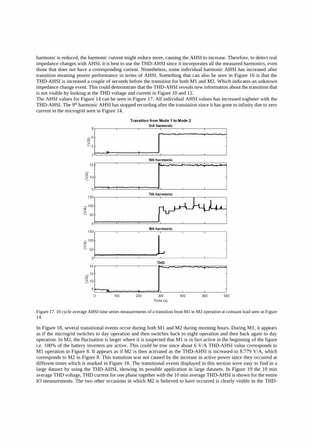
harmonic is reduced, the harmonic current might reduce more, causing the AHSI to increase. Therefore, to detect real

impedance changes with AHSI, it is best to use the THD-AHSI since it incorporates all the measured harmonics, even

those that does not have a corresponding current. Nonetheless, some individual harmonic AHSI has increased after

transition meaning poorer performance in terms of AHSI. Something that can also be seen in Figure 16 is that the

THD-AHSI is increased a couple of seconds before the transition for both M1 and M2. Which indicates an unknown

impedance change event. This could demonstrate that the THD-AHSI reveals new information about the transition that

is not visible by looking at the THD voltage and current in Figure 10 and 12.

The AHSI values for Figure 14 can be seen in Figure 17. All individual AHSI values has increased togheter with the

THD-AHSI. The 9th harmonic AHSI has stopped recording after the transistion since it has gone to infinity due to zero

current in the microgrid seen in Figure 14.

Figure 17. 10 cycle average AHSI time series measurements of a transition from M1 to M2 operation at constant load seen in Figure

14.

In Figure 18, several transitional events occur during both M1 and M2 during morning hours. During M1, it appears

as if the microgrid switches to day operation and then switches back to night operation and then back again to day

operation. In M2, the fluctuation is larger where it is suspected that M1 is in fact active in the beginning of the figure

i.e. 100% of the battery inverters are active. This could be true since about 6 V/A THD-AHSI value corresponds to

M1 operation in Figure 8. It appears as if M2 is then activated as the THD-AHSI is increased to 8.779 V/A, which

corresponds to M2 in Figure 8. This transition was not caused by the increase in active power since they occurred at

different times which is marked in Figure 18. The transitional events displayed in this section were easy to find in a

large dataset by using the THD-AHSI, showing its possible application in large datasets. In Figure 19 the 10 min

average THD voltage, THD current for one phase together with the 10 min average THD-AHSI is shown for the entire

IO measurements. The two other occasions in which M2 is believed to have occurred is clearly visible in the THD-

AHSI at day 8 and day 24 with 14-15 V/A but not clearly visible in the THD voltage. Another thing that can be seen

in Figure 19 is that the THD voltage reached about 21 V at day 82 which was caused by the THD current as seen in

Figure 19. This further shows the application of the AHSI index in finding occasions in large time series data that

shows deviating harmonic performance in a system.

Figure 18. 10s average time series change in THD-AHSI during constant load. The active power is for all three phases and the

black, red and blue lines for the voltage and current represents phase 1-3 respectively. (Color is needed if printed).

Figure 19. Time series of the 10-min average THD voltage, THD current for one phase and the THD-AHSI for all phases for the

entire IO measurements.

3.6. Time series examples from detected PHIPI and SHIPI values Four examples of time series from detected PHIPI and SHIPI values can be seen in Figure 20 during IO where the

voltage and current THD is shown together with the active power for all three phases. It can be seen that an increase

in current THD on one phase can either increase or decrease the voltage THD on other phases. It can also be seen that

as the current THD increases on one phase, the voltage THD on the same phase can decrease, which causes a negative

THD-PHIPI. In Example 4, it can be seen that the current THD of phase 2 increases in two steps and that the voltage

THD on phase 3 first decreases then increases as the active power is increased. In Example 1, it can be seen that as the

current THD is increased for phase 3 the voltage THD is decreased for phase 1 and increased for phase 2 while the

current THD remains constant causing a negative and positive SHIPI respectively. It should be noted that in Example

2, the active power for phase 2 is negative. This is because there is a single-phase solar inverter directly connected to

phase two downstream of the SMA Multicluster Box where the measuring device is located. A more detailed view of

Example 1 and 3 can be seen in Figure 21. It can be seen in Figure 21 that the individual harmonic currents can increase

while the individual harmonic voltage is decreased on the same phase. This causes a negative PHIPI value for the

individual harmonics. It can also be seen that an increase in current distortion for one harmonic can both increase and

decrease the same harmonic voltage on the other phases while the harmonic current of the other phases remains

constant. This causes a positive and negative SHIPI value respectively.

Figure 20. 10 cycle average time series examples from detected PHIPI and SHIPI values. The voltage and current THD are shown

together with the active power. black, red and blue color represents phase 1-3 respectively. (Color is needed if printed).

Figure 21. 10 cycle average individual harmonics and THD of Example 1 and Example 3. (Color is needed if printed).

4. Conclusions Three new indexes for measuring harmonic performance in a grid was shown in this paper denoted AHSI, PHIPI and

SHIPI. The AHSI quantifies the combined ratio between harmonic voltage and current distortion magnitudes for all

phases of a system. PHIPI and SHIPI quantifies the response on the harmonic voltage magnitude due to a harmonic

current magnitude increase that occurs on the same phase or on another phase respectively. The new performance

indexes were applied to measurements done in a microgrid that operated in both IO and GCO. From the displayed

results, it can be concluded that the new indexes are correlated to the harmonic system impedance since as the harmonic

system impedance was increased, an increase of the AHSI, PHIPI and SHIPI occurred.

The transitional events displayed in this paper were easy to find in the dataset with the THD-AHSI showing its possible

application in large datasets. It is recommended to use the THD-AHSI for detecting the different modes of operation

in a microgrid since the individual harmonic AHSI values for the different harmonics investigated could behave

differently than the THD-AHSI and not reveal the different modes of operation. The THD-AHSI can also be measured

continuously and does not need load changes to be quantified, (which PHIPI and SHIPI needs). The THD-AHSI makes

the changes in mode of operation more visible than if one were to only use the harmonic voltage magnitude to decipher

if a change in harmonic system impedance has occurred since you also have to check the harmonic current distortion

magnitude to see if it is causing a change in voltage distortion magnitude (as seen in Figure 19). The largest drawback

of the AHSI index is that one has to select a cut-off current in which the AHSI is measured since it will go towards

infinity at near zero harmonic current. This shows that the AHSI index can’t be used in no-load conditions. Another

feature of the AHSI index is that it also incorporates the harmonic interaction that occur between the phases (shown

by SHIPI) since the harmonic voltage and current distortion of all phases are used in AHSI.

The three new indexes presented in this paper can use the values of the voltage and current THD to calculate an

apparent impedance value. This is since the three new indexes uses the magnitude of the harmonic voltage and current

and not the complex quantity.

The measured 3rd and 5th real harmonic system impedance increased on average by about 2.3 times, when comparing

M2 to M1. The AHSI was on average roughly 2 times larger for M2 for all parameters except the 7 th harmonic which

was closer to 3 times larger. PHIPI had also an average increase by roughly 2-3 times depending on the parameter.

However, the SHIPI increased on average by roughly 6 times in M2 compared to M1 for the 3rd harmonic and the

THD-SHIPI while the 5th harmonic SHIPI only increased on average by 1.13 times in M2 compared to M1. This shows

that SHIPI behaves more non-linear than AHSI and PHIPI when the real harmonic system impedance is increased.

Acknowledgements

This paper has been funded by Skellefteå Kraft Elnät AB and Rönnbäret Foundation.

5. References

[1] C. Schwaegerl, L.Tao, "Quantification of Technical, Economic, Environmental and Social Benefits of Microgrid Operation," in Microgrids

Architectures and Control, 1st ed, Wiley-IEEE Press, 2014, p. 275–313.

[2] M.H.J. Bollen, R. Das, S. Djokic, P. Ciufo, J. Meyer, S.K. Rönnberg, F. Zavodam, "Power Quality Concerns in Implementing Smart Distribution-Grid Applications," IEEE Transactions on Smart Grid, vol. 8, no. 1, pp. 391 - 399, 2017.

[3] J. Nömm, S.K. Rönnberg, M.H.J. Bollen, "An Analysis of Frequency Variations and its Implications on Connected Equipment for a

Nanogrid during Islanded Operation," Energies, vol. 11, no. 9, 2018.

[4] J. Nömm, S.K. Rönnberg, M.H.J. Bollen, "An Analysis of Voltage Quality in a Nanogrid during Islanded Operation," Energies, vol. 12, no.

4, 2019.

[5] M.H.J. Bollen, M. Häger, C. Schwaegerl, "Quantifying voltage variations on a time scale between 3 seconds and 10 minutes," in CIRED

2005 - 18th International Conference and Exhibition on Electricity Distribution, Turin, Italy, 2005.

[6] M.H.J. Bollen, I.Y.H Gu , "Characterization of voltage variations in the very-short time-scale," IEEE Transactions on Power Delivery, vol.

20, no. 2, pp. 1198-1199, 2005.

[7] M. Bollen, O. Samuelsson, "Controlled island operation of part of the 50-kV grid in Southern Sweden," in 2009 IEEE Bucharest

PowerTech, Bucharest, Romania, 2009.

[8] C. Kurnik, R.S. Butt, I. Metzger, O. Lavrova, S. Patibandla, V. Wagner, M. Frankosky, G. Wiegand, "Design, Operation, and Controlled-Island Operation of the U.S. Department of Energy Solar Decathlon 2013 Microgrid," National Renewable Energy Labratory, Denver,

Colorado, USA, 2015.

[9] "Cenelec Std. EN 50160:2010, Voltage Characteristics of Electricity Supplied by Public Electricity Networks," European Committee for Electrotechnical Standardization , Brussels, Belgium, 2010.

[10] "IEEE Std. 519-2014. IEEE Recommended Practice and Requirements for Harmonic Control in Electric Power Systems," IEEE Standards Association, Piscataway, NJ, USA, 2014.

[11] J. Nömm, S.K. Rönnberg, M.H.J. Bollen, "Harmonic voltage measurements in a single house microgrid," in 2018 18th International Conference on Harmonics and Quality of Power (ICHQP), Ljubljana, Slovenia, 2018.

[12] S.K. Rönnberg, M.H.J. Bollen, J. Nömm, "Power quality measurements in a single-house microgrid," in 24th International Conference &

Exhibition on Electricity Distribution (CIRED), Glasgow, UK, 2017.

[13] A.M. Blanco, S. Kannan, M. Meinck, C.A. Garzón, M.F. Romero, V. Quintero, A. Pavas, J. Meyer, "Harmonic Characteristic of an

Islanded Microgrid with Residential Loads," in CIRED 26th International Conference & Exhibition on Electricity Distribution, 2021.

[14] S. Kannan, A.M. Blanco, C. Garzón, A. Pavas, J. Meyer, "Harmonic Impedance Characteristics in an Islanded Microgrid and its impact on Voltage and Current Harmonics," in 2021 IEEE Madrid PowerTech, Madrid, Spain, 2021.

[15] M.S. Golsorkhi, D.D.C. Lu, M. Savaghebi, J.C. Vasquez, J.M. Guerrero, "A GPS-based control method for load sharing and power quality

improvement in microgrids," in 2016 IEEE 8th International Power Electronics and Motion Control Conference (IPEMC-ECCE Asia), Hefei, China, 2016.

[16] C. Blanco, F. Tardelli, D. Reigosa, P. Zanchetta, F. Briz, "Design of a Cooperative Voltage Harmonic Compensation Strategy for Islanded Microgrids Combining Virtual Admittance and Repetitive Controller," IEEE Transactions on Industry Applications, vol. 55, no. 1, pp. 680-

688, 2019.

[17] D.M. Phan, H.H. Lee, "Interlinking Converter to Improve Power Quality in Hybrid AC–DC Microgrids With Nonlinear Loads," IEEE Journal of Emerging and Selected Topics in Power Electronics, vol. 7, no. 3, pp. 1959-1968, 2019.

[18] A. Saim, A. Houari, M. Ait-Ahmed, M. Machmoum, J.M. Guerrero, "Active resonance damping and harmonics compensation in distributed

generation based islanded microgrids," Electric Power Systems Research, vol. 191, 2021.

[19] S.Y.M. Mousavi, A. Jalilian, M. Savaghebi, J.M. Guerrero, "Autonomous Control of Current- and Voltage-Controlled DG Interface

Inverters for Reactive Power Sharing and Harmonics Compensation in Islanded Microgrids," IEEE Transactions on Power Electronics, vol.

33, no. 11, pp. 9375-9386, 2018.

[20] R. Keypour, B. Adineh, M. H. Khooban, F. Blaabjerg, "A New Population-Based Optimization Method for Online Minimization of Voltage

Harmonics in Islanded Microgrids," IEEE Transactions on Circuits and Systems II: Express Briefs, vol. 67, no. 6, pp. 1084-1088, 2020.

[21] T.V. Hoang, H.H. Lee, "Virtual Impedance Control Scheme to Compensate for Voltage Harmonics With Accurate Harmonic Power Sharing in Islanded Microgrids," IEEE Journal of Emerging and Selected Topics in Power Electronics, vol. 9, no. 2, pp. 1682 - 1695, 2021.

[22] H. Moussa, J.P. Martin, S. Pierfederici, F. Meibody-Tabar, N. Moubayed, "Voltage harmonic distortion compensation with non-linear load

power sharing in low-voltage islanded microgrid," Mathematics and Computers in Simulation, vol. 158, pp. 32-48, 2019.

[23] A. Micallef, M. Apap, C. Spiteri-Staines, J.M. Guerrero, "Mitigation of Harmonics in Grid-Connected and Islanded Microgrids Via Virtual

Admittances and Impedances," IEEE Transactions on Smart Grid, vol. 8, no. 2, pp. 651-661, 2017.

[24] Z. Moravej, M. Pazoki, M. Khederzadeh, "Impact of UPFC on Power Swing Characteristic and Distance Relay Behavior," IEEE Transactions on Power Delivery, vol. 29, no. 1, pp. 261-268, 2014.

[25] K. El-Arroudi, G. Joos, D.T. McGillis, "Operation of Impedance Protection Relays With the STATCOM," IEEE Transactions on Power

Delivery, vol. 17, no. 2, pp. 381-387, 2002.

[26] M.S. Sachdev, R. Agarwal, "A technique for estimating transmission line fault locations from digital impedance relay measurements," IEEE


[27] A. Rygg, M. Molinas, "Apparent impedance analysis: A small-signal method for stability analysis of power electronic based systems," IEEE Journal of Emerging and Selected Topics in Power Electronics, vol. 5, no. 4, pp. 1474-1486, 2017.

[28] R. Stiegler, J. Meyer, P. Schegner, D. Chakravorty, "Measurement of network harmonic impedance in presence of electronic equipment," in

2015 IEEE International Workshop on Applied Measurements for Power Systems (AMPS), Aachen, Germany, 2015.

[29] A. Robert et al., "Guide for assessing the network harmonic impedance," in 14th International Conference and Exhibition on Electricity

Distribution. Part 1. Contributions (IEE Conf. Publ. No. 438), Birmingham, UK, 1997.

[30] M.J. Bridgeman, R.E. Morrison, S.B. Tenakoon, "Measurement of harmonic impedance on an LV system utilising power capacitor switching and consequent predictions of capacitor induced harmonic distortion," in 8th International Conference on Harmonics and Quality

of Power. Proceedings (Cat. No.98EX227), Athens, Greece, 1998.

[31] C. Xie, S.B. Tennakoon, R. Langella, D. Gallo, A. Testa, A. Wixon, "Harmonic impedance measurement of 25 kV single phase AC supply systems," in Ninth International Conference on Harmonics and Quality of Power. Proceedings (Cat. No.00EX441), Orlando, FL, USA,

2000.

[32] D. Serfontein, J. Rens, G. Botha, J. Desmet, "Continuous Event-Based Harmonic Impedance Assessment Using Online Measurements," IEEE Transactions on Instrumentation and Measurement, vol. 65, no. 10, pp. 2214-2220, 2016.

[33] W. Xu, E.E. Ahmed, X. Zhang, X. Liu, "Measurement of network harmonic impedances: practical implementation issues and their

solutions," IEEE Transactions on Power Delivery, vol. 17, no. 1, pp. 210-216, 2002.

[34] A.A. Girgis, R.B. McManis, "Frequency domain techniques for modeling distribution or transmission networks using capacitor switching

induced transients," IEEE Transactions on Power Delivery, vol. 4, no. 3, pp. 1882-1890, 1989.

[35] D. Borkowski, A. Wetula, A. Bień, "New method for noninvasive measurement of utility harmonic impedance," in 2012 IEEE Power and Energy Society General Meeting, San Diego, CA, USA, 2012.

[36] M. Nagpal, W. Xu, J. Sawada, "Harmonic impedance measurement using three-phase transients," IEEE Transactions on Power Delivery,

vol. 13, no. 1, pp. 272-277, 1998.

[37] Z. Staroszczyk, "A method for real-time, wide-band identification of the source impedance in power systems," IEEE Transactions on

Instrumentation and Measurement, vol. 54, no. 1, pp. 377-385, 2005.

[38] R. Gretsch, M. Neubauer, "System impedances and background noise in the frequency range 2 kHz to 9 kHz," European Transactions on Electrical Power, vol. 8, no. 5, pp. 369-374, 1998.

[39] G. Moreau, H.H. Le, G. Croteau, G. Beaulieu, E. Portales, "Measurement system for harmonic impedance of the network and validation

steps," in CIGRE/IEEE PES International Symposium Quality and Security of Electric Power Delivery Systems, 2003. CIGRE/PES 2003,

Montreal, QC, Canada, 2003.

[40] M. Sumner, B. Palethorpe, D.W.P. Thomas, "Impedance measurement for improved power quality—part I: the measurement technique," IEEE Transactions on Power Delivery, vol. 19, no. 3, pp. 1442-1448, 2004.

[41] H.L.M. Monteiro, C.A. Duque, L.R.M. Silva, J. Meyer, R. Stiegler, A. Testa, P.F. Ribeiro, "Harmonic impedance measurement based on

short time current injections," Electric Power Systems Research, vol. 148, pp. 108-116, 2017.

[42] R. Stiegler, J. Meyer, M. Höckel, S. Schori, K. Scheida, T. Hanžlík, J. Drápela,, "Survey of network impedance in the frequency range 2-9

KHZ in public low voltage networks in AT / CH / CZ / GE," in 25th International Conference on Electricity Distribution, Madrid, Spain,

2019.

[43] F. Zavoda, "Measurement of the harmonic impedance of LV distribution supply system (120/240V)," in 19th International Conference on

Electricity Distribution (CIRED), Vienna, Austria, 2007.

[44] J. Hui, H. Yang, S. Lin, M. Ye, "Assessing Utility Harmonic Impedance Based on the Covariance Characteristic of Random Vectors," IEEE


[45] D. Chakravorty. J. Meyer, P. Schegner, S. Yanchenko, M. Schocke, "Impact of Modern Electronic Equipment on the Assessment of Network Harmonic Impedance," IEEE Transactions on Smart Grid, vol. 8, no. 1, pp. 382-390, 2017.

Jakob Nöm

m Pow

er quality analysis and techno-economic m

odeling for microgrids

Department of Engineering Sciences and MathematicsDivision of Energy Science

ISSN 1402-1544ISBN 978-91-7790-966-8 (print)ISBN 978-91-7790-967-5 (pdf )

Luleå University of Technology 2021SV

ANENMÄRKET

Trycksak3041 3042

Print: Lenanders Grafiska, 4595318

Power quality analysis and techno-economic modeling for ...

Documents

Transcript of Power quality analysis and techno-economic modeling for ...