Generalized Economic Modeling for Infrastructure and Capital ...

Dow

nloa

ded

from

asc

elib

rary

.org

by

New

Yor

k U

nive

rsity

on

05/1

2/15

. Cop

yrig

ht A

SCE

. For

per

sona

l use

onl

y; a

ll ri

ghts

res

erve

d.

Generalized Economic Modeling for Infrastructureand Capital Investment Projects

Ahmed M. Abdel Aziz, M.ASCE1; and Alan D. Russell, M.ASCE2

Abstract: Economic modeling and risk analysis are important processes for the appraisal of infrastructure and revenue-generatingprojects such as build-operate-transfer �BOT� projects. These processes have been commonly implemented using spreadsheets in whichthe analyst would build several models to analyze a project under varying conditions and risk assumptions. For better efficiencies inbuilding economic structures and evaluation of projects, the current paper defines “classifications” of estimating and cash flow methods,and develops a generalized model. A classification represents a particular domain—construction, revenues, financing, operation andmaintenance, or risk analysis, for example—and holds the estimating methods of that domain. The basic building block behind the modelstructure is a work package/stream that would have its own properties and estimating methods by direct selection from the relevantclassification. By integrating the building blocks together a project economic structure is built and various performance measures areformulated. The model was implemented in a prototype software system called Evaluator. A BOT highway project is used to show anapplication of the concepts and the generalized model.

DOI: 10.1061/�ASCE�1076-0342�2006�12:1�18�

CE Database subject headings: Economic factors; Build/Operate/Transfer; Project management; Risk management; Probabilisticmodels.

Introduction

Economic modeling and risk analysis frameworks are generallydeveloped for project appraisal. Spreadsheets are commonlyused to build project cash flow models. Few specialized softwaresystems were available to aid in building models; the mostcommon in literature include Computer Aided Simulation forProject Appraisal and Review, or CASPAR �Willmer 1991;Thompson and Perry 1992�, Computer Model for FeasibilityAnalysis and Reporting, or COMFAR III Expert �UNIDO 1994�,and INFRISK �Dailami et al. 1999�. While these systems havetheir relative strengths, their underlying economic models repre-sent capital projects at a summarized level of detail that relymainly on using time- and/or quantity-related costs/revenues.Challenged by the different types of projects, the complexity andnumber of estimating methods in a project life cycle and how theywould be incorporated in a model structure, previous models, andspreadsheet analysis had to be at a summarized level. COMFARand INFRISK would accept for each period of time the requiredquantities, prices, and/or loading percentage �e.g., 25% of totalcost� so that a final cash flow would be obtained. CASPAR, with

1Assistant Professor, Dept. of Construction Management, Univ. ofWashington, 116 Architecture Hall, Box 351610, Seattle, WA 98195-1610. E-mail: [email protected]

2Professor and Chair, Computer Integrated Construction, Dept.of Civil Engineering, Univ. of British Columbia, 2324 Main Mall, Van-couver, BC, Canada V6T 1Z4. E-mail: [email protected]

Note. Discussion open until August 1, 2006. Separate discussionsmust be submitted for individual papers. To extend the closing date byone month, a written request must be filed with the ASCE ManagingEditor. The manuscript for this paper was submitted for review and pos-sible publication on February 24, 2004; approved on February 28, 2005.This paper is part of the Journal of Infrastructure Systems, Vol. 12, No.
1, March 1, 2006. ©ASCE, ISSN 1076-0342/2006/1-18–32/$25.00.
18 / JOURNAL OF INFRASTRUCTURE SYSTEMS © ASCE / MARCH 2006

J. Infrastruct. Syst. 2

time- and cost-related charges, extends the process by using anetwork where the allocation of an estimate to a specific timewould follow the dependencies of work activities. The currentwork extends the above developments and addresses the com-plexity of infrastructure by building a generalized model, theconcepts of which are explained next, followed by an applicationon a BOT toll highway.

Generalized Model Structure and Concepts

In order to build a model that addresses the large number ofvariables, estimating, and cash flow methods, the first step wasto differentiate between the phases in a project life cycle. Thestructure of the model, Fig. 1, divides a project life cycle into fourcost/revenue components of four domains, namely: capital expen-diture �CE�, operation and maintenance �OM�, revenue �RV�, andfinancing �FN�, plus one overall “project” component. Eachcomponent is assumed to have its domain’s properties and meth-ods. Properties include time and logic properties �e.g., time units,duration, dependencies� while methods are estimating methods�e.g., demand methods�.

To account for the methods in a particular domain, “classifi-cations” of methods were built: four cost/revenue classifications,“shape functions,” “performance measures,” and “risk analysis.”The objective is to hold all pertinent methods in a classificationsuch that direct selection from these methods would be availablefrom within the model. As explained below, the methods of theabove classifications are the common methods that would be usedin a project. Other methods—for example, of specialized projectssuch as energy projects—would still be integrated without a ne-cessity to restructure the model. That objective of generality wasachieved by building the model as a hierarchical network-based
continuous function structure, using the principles of continuous
006.12:18-32.

Dow

nloa

ded

from

asc

elib

rary

.org

by

New

Yor

k U

nive

rsity

on

05/1

2/15

. Cop

yrig

ht A

SCE

. For

per

sona

l use

onl

y; a

ll ri

ghts

res

erve

d.

modeling �Remer et al. 1984; Tanchoco et al. 1981; Park andSharp-Bette 1990�.

The basic building blocks of the model are called work pack-ages for the CE component and streams for the other components.A building block, Fig. 2, would have its own methods by directselection from the relevant classification, where the method willbe used to obtain an estimate for the building block. An estimateis then distributed over the work package/stream duration, that is,converted into cash flow, by: �1� allowing the variables of theestimating methods to change over time using “shape functions”�time functions, a subset of which is in Appendix I�; or �2� usingdirect loading profiles �shape functions�.” By integrating thebuilding blocks together via the model network and continuousmodeling, a project economic structure would be formed and cashflows and performance measures would be obtained. This isfurther explained below.

Capital Expenditure Component

Through work packages, capital expenditures, such as construc-tion costs, would be added to a project economic structure. At asummarized level of detail, the cash flow function is representedby

fcCE�t�,x� = X�t�� · e�0

t��X�t��dt� �1�

where fcCE�t� ,x�=function name; c defines a single work package;

t� and x�arguments where t�=time in local time unit andx=vector of variables; X�t��=capital expenditure variable repre-senting a lump sum estimate that would be distributed overthe work package duration using loading shape function profiles�Appendix I�; �X�t��=inflation variable, modeled by shape func-tion, and t�=application time referenced to the start of the projector work package. Using this structure, the cash flow could berepresented with or without inflation. For example, by giving avalue of zero to the inflation rate the inflation term will be equalto unity and the analysis will be in “constant dollar.” Alterna-tively, any value given to the inflation rate will make the analysisin “real money.” Governments as well as lending institutions forpublic–private partnership projects �e.g., BOT projects� tend toexplicitly require the inclusion of inflation so that its effectswould be considered in project evaluation.

Fig. 1. Generalized model: interrelated components and buildingblocks

Fig. 2. Building blocks with properties and methods

JOUR


At a detailed level of analysis, the cash flow function of awork package is represented by

fcCE�t�,x� = fcm�t�,x� · e�0

t��m�t��dt� + fcl�t�,x� · e�0t��l�t��dt�

+ fce�t�,x� · e�0t��e�t��dt� + fcs�t�,x� · e�0

t��s�t��dt� �2�

In this function the cash flow is derived based on estimatingmethods commonly used in construction material, labor, equip-ment, and subcontract cost; �m�t�, �l�t�, �e�t�, and �s�t��respec-tive inflation variables. Material cost fcm�t� ,x� is estimated bythree methods in Eq. �3� below: the first has M�t�� as a lump sumestimate, while the second and third methods are unit cost meth-ods that have Cm�t�� as unit cost �e.g., $ /m3�, Q�t�� as quantity�e.g., m3, m3/day�, Pl�t�� as labor productivity �e.g., m3/mhr�,and Ul�t�� as labor usage �e.g., mhrs, mhrs/day�:

fcm�t�,x� = �M�t�� 3a�Cm�t�� · Q�t�� 3b�Cm�t�� · Pl�t�� · Ul�t�� 3c�

�Labor cost fcl�t� ,x� and equipment cost fce�t� ,x� use similarmethods, shown in Eq. �4�, for the labor cost, including:lump sum estimate Hl�t��; “Cost per unit of time,” whereWl�t��=wage rate and Ul�t��=labor usage �e.g., mhrs�; and“Cost per unit of production,” where Cl�t��unit cost

fcl�t�,x� =�Hl�t�� 4a�Wl�t�� · Ul�t�� 4b�Wl�t�� · Q�t��/Pl�t�� 4c�Cl�t�� · Q�t�� 4d�Cl�t�� · Pl�t�� · Ul�t�� 4e�

�The subcontracted estimate, fcs�t� ,x�, has S�t�� representing lumpsum estimates

fcs�t�,x� = S�t�� 5�

Discrete costs are also included; in Eq. �6�, D jCE represents

CE CE

Table 1. Highway Project Constant-Dollar Capital Expenditure andOperation and Maintenance

Total capital expenditure

Design $13 million in 8 months

Construction

Road construction 100% =$84.75 million

Clearing and grubbing 15%, in 5 months, with 4 months’ overlap

C&F, rock blasting,compaction

45%, in 6 months, with 2 months’ overlap

Road Subbase layer 15%, in 7 months, with 1 month overlap

Road base layer 15%, in 7 months, with 6 months’ overlap

Road asphalt pavement 10%, in 7 months, with 3 months’ overlap

Road structures 100% =$15.25 million

Culverts 13%, in 4 months, with 5 months’ overlap

Tunnels 18%, in 4 months, with 5 months’ overlap

Interchanges 49%, in 8 months, with 2 months’ overlap

Bridges 20%, in 8 months, with 2 months’ overlap

Operation and maintenance

Maintenance costs $0.3 million/yr, and ¢6.5 per vehicle

Major maintenance $10 million each 10 yearsafter construction

Toll operation $2.0 million/yr

discrete cost j of a work package, where Dv j and Dt j =value

NAL OF INFRASTRUCTURE SYSTEMS © ASCE / MARCH 2006 / 19

006.12:18-32.

Dow

nloa

ded

from

asc

elib

rary

.org

by

New

Yor

k U

nive

rsity

on

05/1

2/15

. Cop

yrig

ht A

SCE

. For

per

sona

l use

onl

y; a

ll ri

ghts

res

erve

d.

Fig. 3. Semidetailed economic structure for the highway project

Fig. 4. Asphalt paving work package and capital expenditure cash flow, in constant dollars


J. Infrastruct. Syst. 2006.12:18-32.

Dow

nloa

ded

from

asc

elib

rary

.org

by

New

Yor

k U

nive

rsity

on

05/1

2/15

. Cop

yrig

ht A

SCE

. For

per

sona

l use

onl

y; a

ll ri

ghts

res

erve

d.

and time of the discrete cost, and �d�t��inflation variable

D jCE = Dv j

CE · e�0t*

�d�t��dt��t* = Dt jCE if �d is in local time

t* = Dt jCE + ESc if �d is in global time

�

�6�

The versatility of the work package cash flow function pro-vides flexibility in formulating other cash flow functions. InEq. �7�, Fc

CE�t� ,x� provides the cumulative cash flow of a workpackage at any local time t�. It is in two parts: the first is anintegration of the cash flow function �Eq. �1� or �2�� and thesecond is the summation of r discrete costs of a work package�Eq. �6��

FcCE�t�,x� =�

0

t�fc

CE�t�,x�dt� + j=1

r

D jCE

�for each DtjCE�t�� 7�

Eq. �7� can be used to derive a cumulative cash flow for the CEcomponent, as given in Eq. �8� for m work packages. With workpackages having local time units different from that of the project,t−ESci�time conversion in which ESci�early start of work pack-age I �see Appendix II and its example, and Fig. 15�

FCE�t,X� = i=1

m

FcCE�t − Esci,xi�i�for each t�ESci�

�8�

Further, the work package cash flow can be used to determine

Fig. 5. Detailed estimate of an asph

the discounted cash flow to any reference time Td. In Eq. �9�,

JOUR


dfcCE�Td ,x��discounted work package function where Td and

x are arguments. Where y is a nominal annual discount rate, thefirst integration part inside the brackets discounts the cash flow�Eq. �1� or �2�� to the start of its work package using its durationwd, time elapsed inside the work package tn and the converted-to-local-time-units discount rate y. Similarly, the second partdiscounts discrete costs r. The outside term takes the discountingto the reference time Td using the time elapsed before start of awork package, tb

dfcCE�Td,x� = e−y·tb · �

0

wd−tn

fcCE�t� + tn,x� · e−y·t�dt�

+ j=1

r

D jCE · e−y·�Dtj

CE−tn��for each�Dtj

CE�tn� �9�

in which

tb = �Esc − Td if Td � ESc

0 otherwise �10�

and

tn = �Td − Esc if Td � Esc

0 otherwise �11�

Finally, Eq. �9� is used to derive the discounted cost of the

ing work package and its cash flow
alt pav
whole CE component


006.12:18-32.

Dow

nloa

ded

from

asc

elib

rary

.org

by

New

Yor

k U

nive

rsity

on

05/1

2/15

. Cop

yrig

ht A

SCE

. For

per

sona

l use

onl

y; a

ll ri

ghts

res

erve

d.

dfCE�Td,X� = i=1

m

dfcCE�Td,xi�i �12�

The other components have similar formulations with the RV/OMdesignations used instead. Unlike previous models, the methodsbecame part of the model, their variables are changing over time�Appendix I�, and each estimate and work package has its owninflation variables.

Table 2. AADT on the Highway Example Project

Year Time AADT

1978 0 2,880.0

1979 1 3,020.0

1980 2 3,330.0

1981 3 3,510.0

1982 4 3,800.0

1983 5 3,990.0

1984 6 3,820.0

1985 7 4,190.0

1986 8 4,380.0

1987 9 4,530.0

1988 10 4,620.0

1989 11 4,500.0

1990 12 4,450.0

1991 13 4,890.0

1992 14 4,720.0

1993 15 5,100.0

1994 16 5,410.0

1995 17 5,630.0

1996 18 6,030.0

1995 19 6,400.0

1996 20 6,530.0

1997 21 6,520.0

1998 22 6,600.0

1999 23 6,750.0

2000 24 6,900.0

Note: AADT�Average Annual Daily Traffic

Fig. 6. Detailed estimate of cars



Revenue Component

At a summarized level of detail, lump sum revenues RV�t�� wouldbe distributed over a revenue stream duration using shape func-tions where ��scope parameter and �rv�t��revenue inflationvariable modeled by shape functions. A revenue stream cash flowfunction is expressed as

fcRV�t�,x� = � · RV�t�� · e�0

t��rv�t��dt� �13�

In a detailed analysis, the revenue stream cash flow function isderived as the product of demand fcD

RV�t� ,x� and service ratesR�t� ,d�, �both expressed as functions�

fcRV�t�,x� = R�t�,d� · fcD

RV�t�,x� · e�0t��rv�t��dt� �14�

The service rate R�t� ,d� would change over time using shapefunctions. It could also change with the value of demand d asobtained by its stream demand function. The RV classificationhave several methods for measuring demand for a project: �1�summarized, using trend methods �Eq. �15a�; and �2� detailedmethods, using project market share �Eqs.�15b�–�15e��, which is asubset of the total demand volume, TV. Where � is scope param-eter, the demand function is

fcDRV�t�,x� =�

� · TV�t�,x� �15a�� · TV�t�,x� · �R�t�,d�/Ro�� 15b�� · TV�t�,x� · �1 + � · �R�t�,d� − Ro�/Ro� �15c�

� · TV�t�,x� · e−�·�R�t�,d�−Ro� �15d�

� · TV�t�,x� · �1 − 1/�1 + eUt�t�� 15e��

where

Ut�t�� = a0 + a1 · �R�t�,d� − Ro� + a2 · LOS2 + a3 · LOS3

+ a4 · LOS4 �16�

Methods used in Eqs. �15b�, �15c�, and �15d� are elasticity-basedmethods �Meyer and Miller 1984�, which obtain future demandbased on the elasticity � of service rate when it changes fromits base value Ro. Eq. �15e� determines demand based on theutility of individuals, Ut�t��, as they choose among a set ofalternatives different in the level of service; a0 to a4�coefficients

olume of demand �see Eq. �17b��
total v
006.12:18-32.

�Dow

nloa

ded

from

asc

elib

rary

.org

by

New

Yor

k U

nive

rsity

on

05/1

2/15

. Cop

yrig

ht A

SCE

. For

per

sona

l use

onl

y; a

ll ri

ghts

res

erve

d.

and LOS�difference in values of the level of service/utility �e.g.,travel time, toll rate�. The method reflects a method of the statedpreference techniques �Ortuzar and Willumsen 1994; Pearmainand Swanson 1990�. With the model structure and the conceptof classification, other demand methods could be added to theRV classification, such as methods of the energy, power, andpetrochemical projects.

The total demand used in obtaining project market share coulditself be estimated by using several methods, a common subsetof which includes

TV�t��

=�V�t�� 17a�b0 + b1 · G�t�� + b2 · G�t��2 + b3 · G�t��3 + b4 · G�t��4 �17b�b0 + b1 · ln�G�t�� + 1� �17c�

b0 · eb1·G�t�� 17d�

in which b0–b4�parameters. Eq. �17a� is a summarized generaltrend method V�t�� Meyer and Miller 1984�. The other poly-nomial, logarithmic, and exponential dependent-trend methodsestimate demand as it depends on demographic/socioeconomicindicators, G�t�� e.g., population�.

Operation and Maintenance Component

Eq. �18� represents the cash flow of OM stream in which

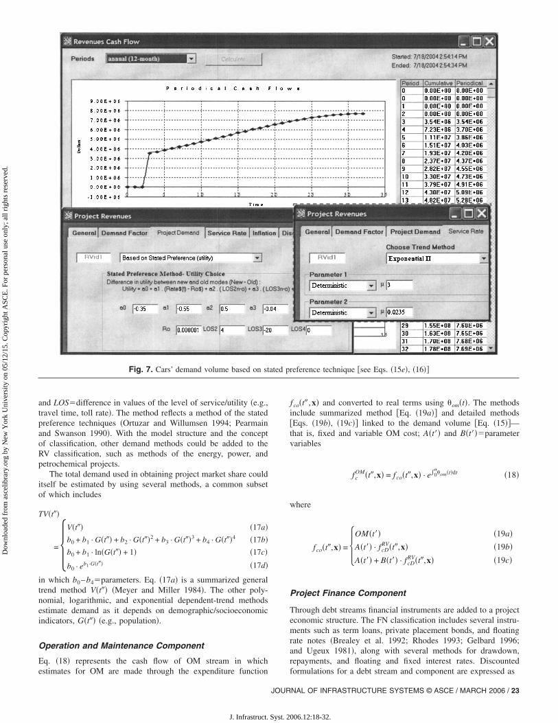
Fig. 7. Cars’ demand volume based on st

estimates for OM are made through the expenditure function

JOUR


fco�t� ,x� and converted to real terms using �om�t�. The methodsinclude summarized method �Eq. �19a�� and detailed methods�Eqs. �19b�, �19c�� linked to the demand volume �Eq. �15��—that is, fixed and variable OM cost; A�t�� and B�t��parametervariables

fcOM�t�,x� = fco�t�,x� · e�0��om�t�dt �18�

where

fco�t�,x� = �OM�t�� 19a�A�t�� · fcD

RV�t�,x� �19b�A�t�� + B�t�� · fcD

RV�t�,x� �19c��

Project Finance Component

Through debt streams financial instruments are added to a projecteconomic structure. The FN classification includes several instru-ments such as term loans, private placement bonds, and floatingrate notes �Brealey et al. 1992; Rhodes 1993; Gelbard 1996;and Ugeux 1981�, along with several methods for drawdown,repayments, and floating and fixed interest rates. Discounted

reference technique �see Eqs. �15e�, �16��
ated p
formulations for a debt stream and component are expressed as


006.12:18-32.

Dow

nloa

ded

from

asc

elib

rary

.org

by

New

Yor

k U

nive

rsity

on

05/1

2/15

. Cop

yrig

ht A

SCE

. For

per

sona

l use

onl

y; a

ll ri

ghts

res

erve

d.

dfcFN�Td,x� =

j=1

m

Tv j · �e−y� ·�Ttj−Td��Ttj�Td

− k=1

o

Rvk · �e−y� ·�Rtk−Td��Rtk�Td

− z=1

p

Ivz · �e−y� ·�Itz−Td��Itz�Td

− w=1

r

Fvw · �e−y� ·�Ftw−Td��Ftw�Td �20�

dfFN�Td,X� = i=1

n

dfcFN�Td,xi�i �21�

Eq. �20� has four parts each discounted to the reference time Tdthrough discount rate y� :1. Tranches: Tt j and Tv j�time and value of each tranche j of m

tranches in a stream;2. Repayments: Rtk and Rvk�time and value of each repay-

ment k of o repayments;3. Interest: Itz and Ivz�time and value of each interest payment

z of p payments; and4. Fees: Ftw and Fvw�time and value of each fee payment w

Fig. 8. Cars’ revenue stream mo

of r fees.



Projects are generally financed by debt and equity capital. Abalance between capital expenditure and the required capital mustbe reached. This is achieved by fixing one of the capitals andderiving the other considering the interest that would be paidduring construction.

Project Component and Risk Analysis

With the network-based continuous model structure of the gener-alized model, the formulation of cash flows and performancemeasures becomes an aggregate process that integrates all theabove formulations of work packages and streams of revenues,OM, and debts. For example, using the four discounted compo-nent cash flows, the net present value �NPV� is expressed as

NPV�Td� = dfRV�Td,XRV� + dfFN�Td,XFN� − dfCE�Td,XCE�

− dfOM�Td,XOM� �22�

Following similar processes, the performance measures classi-fication includes project and component cash flows, NPV, in-ternal rate of return, “aggregate” and “net” benefit-cost ratios,loan-life-cover ratio, and debt-service-cover ratio �Park andSharp-Bette 1990�.

To model the performance measures under uncertainty,spreadsheet models normally use add-in software to carry out riskanalysis. CASPAR and INFRISK, as stand-alone packages, have

by trend method �see Eq. �13��
deled
limited risk quantification methods. The risk analysis framework

006.12:18-32.

Dow

nloa

ded

from

asc

elib

rary

.org

by

New

Yor

k U

nive

rsity

on

05/1

2/15

. Cop

yrig

ht A

SCE

. For

per

sona

l use

onl

y; a

ll ri

ghts

res

erve

d.

of the generalized model reaches all the model variables, in-cluding the subvariables of the shape functions. Its “risk analysis”classification includes: �1� full probability distributions, includingtwo- and four-parameter beta, two- and three-parameter log-normal, normal, exponential, two- and three-parameter gamma,Gumbel, triangular, chi squared, and uniform distributions �Bury1999�; �2� four statistical moments; and �3� three and five percen-tile values �Pearson and Tukey 1965; Keefer and Bodily 1983�.For quantifying the performance measure’s uncertainty, the statis-tical moments approach is used �Kottas and Lau 1982; Siddall1972; Elderton and Johnson 1969; Hahn and Shapiro 1994�.

Example Project

The example project shows an application of the generalizedmodel concepts in building and evaluating a highway developedunder the BOT delivery system. A request for proposal �RFP� wasissued for the development of 45-km four-lane highway under a30-year concession. Table 1 and Fig. 3 give a summary of projectinformation and a cash flow diagram, respectively. Starting withmodeling the capital expenditure estimates in Table 1, the analysthas several options from using summarized to detailed estimatingmethods. For example, at a summarized level and where no de-tails about the estimates are available, a single work package�WP� could be used to represent the $113 million total cost. In a

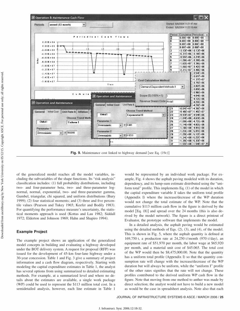
Fig. 9. Maintenance cost linked

semidetailed analysis, however, each line estimate in Table 1

JOUR


would be represented by an individual work package. For ex-ample, Fig. 4 shows the asphalt paving modeled with its duration,dependency, and its lump-sum estimate distributed using the “uni-form total” profile. This implements Eq. �1� of the model in whichthe capital expenditure variable X takes the uniform total profile�Appendix I� where the increase/decrease of the WP durationwould not change the total estimate of the WP. Note that thecumulative $113 million cash flow in the figure is derived by themodel �Eq. �8�� and spread over the 24 months �this is also de-rived by the model network�. The figure is a direct printout ofEvaluator, the prototype software that implements the model.

In a detailed analysis, the asphalt paving would be estimatedusing the detailed methods of Eqs. �2�, �3�, and �4�, of the model.This is shown in Fig. 5, where the asphalt quantity is defined at169,750 t, a production rate at 24,250 t /month �970 t /day�, anequipment rate of $51,970 per month, the labor wage at $65,920per month, and a material unit cost of $45.065. The total costof the WP would then be $8,475,000.00. Note that the quantityhas a uniform total profile �Appendix I� so that the quantity con-sumption rate will change with the increase/decrease of the WPduration but will always be uniform, while the “uniform I” profileof the other rates signifies that the rate will not change. Theseprofiles contributed to the derived uniform WP cash flow in thefigure. Note that moving from one method to anther was made bydirect selection; the analyst would not have to build a new model

ghway demand �see Eq. �19c��
to hi
as would be the case in spreadsheet analysis. Note also that each


006.12:18-32.

Dow

nloa

ded

from

asc

elib

rary

.org

by

New

Yor

k U

nive

rsity

on

05/1

2/15

. Cop

yrig

ht A

SCE

. For

per

sona

l use

onl

y; a

ll ri

ghts

res

erve

d.

variable in the estimate is defined as “deterministic” and it couldhave been a risk variable.

For RV modeling, three streams are used to model cars, smalltrucks, and large trucks with a 30-year duration linked to con-struction completion. Vehicle classes in the region indicate 75%cars, 6.6% small trucks, and 18.4% large trucks. Also, within theproject scope, the car traffic is 82.8%, and truck traffic is 90%. Ina detailed analysis, the “project demand” would be based on itsmarket share. Starting at the “total demand” in the region, it isfound upon regression analysis that the Average Annual DailyTraffic �AADT� �Table 2� is highly correlated to the gross domes-tic product �GDP� �in millions�

AADT�t� = − 898.553 + 0.015 · GDP�t� �23�

Forecasting GDP, however, requires considerable analysis. Forthe project, and using historical data, it is found that future re-gional GDP is best modeled with 3% growth rate as follows

GDP�t� = 5.283 · 1011 · �1 + 0.03�t �24�

Using AADT, GDP, 75% cars traffic with 82.8% in-scope, thecars’ annual demand volume is

Cars Total Demand�t�

= �− 2.4598 · 105 + 4.0403 · 10−6 · GDP�t�� · 0.828 �25�

Fig. 6 shows the demand method selected with the parameters ofthe cars’ total demand �Eq. �25�� and the demand factor, GDP,

Fig. 10. Project cash flo

modeled as growth II �Appendix I� �implementing Eq. �17b��.



A project market share is the portion of that total demand thatwill use the new road. Using the “stated preference” �SP� tech-nique �Ortuzar and Willumsen 1994� the propensity of drivers touse the new highway under various toll rates, number of lanes,and time savings is expressed as

Utility = a0 + a1 · �number of lanes� + a2 · �toll charge�

+ a3 · �time saving� �26�

In this utility function, ao to a3�parameters derived from SPsurvey and analysis: a0=−0.35, a1=0.55 �for new toll rates�,a2=−0.5 �for using four lanes�, and a3=−0.04 �for 20 min timesaving�. Using total demand �Eq. �25�� and the utility function,the cars’ annual demand volume is

Cars’ Demand = Cars’ Total Demand · �1 − 1/�1 + eUtility��

�27�

Fig. 7 shows the parameters of the utility function �see Eq. �15e��and the derived cash flow. The other small and large truck streamscould be defined similarly.

In early appraisal stages, however, projects would only havethe AADT data and then only summarized analysis would beused. Hence, future demand would be derived using the generaltrend methods of Eq. �15a�. For example, regression analysis forthe AADT shows it could be fitted to a linear, second-, or third-order polynomial function; assuming the liner function as a trend

performance measures
w and
method, then

006.12:18-32.

Dow

nloa

ded

from

asc

elib

rary

.org

by

New

Yor

k U

nive

rsity

on

05/1

2/15

. Cop

yrig

ht A

SCE

. For

per

sona

l use

onl

y; a

ll ri

ghts

res

erve

d.

AADT�t� = 2918.615 + 165.115 · t �28�

Using the AADT function and the vehicle class and in-scope data,and assuming 70% traffic likely to use new road, the cars’ annualdemand volume and cash flow would be as in Fig. 8

Cars’ Demand�t� = �1.928988E6 + 4.520023E4 · t� · 0.828 · 0.7

�29�

Comparing the cash flows of Figs. 7 and 8 shows the effectof increasing tolls in lowering the future demand where projectmarket share was derived based on drivers’ choices �i.e., betterthan trend method�. Note that the summarized and detailed meth-ods were available by direct selection; the analyst would not haveto build a new model as would be the case in spreadsheet analy-sis. Note also that even the subvariables of the revenue stream—for example, the toll initial and exponential growth rate—weredefined as “deterministic” and could have been defined as riskvariables.

For modeling the OM costs in Table 1, two OM streams wouldbe defined, each of 30 years’ duration and linked to constructioncompletion. One stream for an annual $2 million operating costwas modeled as “uniform I” profile. The other stream for main-tenance is estimated to have fixed and variable cost sums. It isexpected that $300,000 per year for annual maintenance will beneeded, along with a maintenance that varies with the demand at$0.065 per vehicle and indexed to inflation �2.35%�. This is

Fig. 11. DSCR and pr

modeled in Fig. 9, which implements Eqs. �18� and �19c� of

JOUR


the model in which A�t� is the $300,000 fixed sum per year andB�t� is the variable sum �exponential II�, which is linked to thedemand function �Eq. �29��. In the figure, the valleys in the de-rived cash flow reflect the $10 million discrete overhaul costs ofTable 1.

For FN modeling of the project, the analyst would experimentwith the model to decide which financial structure is best under

erformance measures

Fig. 12. Debt interest and repayments

oject p


006.12:18-32.

Dow

nloa

ded

from

asc

elib

rary

.org

by

New

Yor

k U

nive

rsity

on

05/1

2/15

. Cop

yrig

ht A

SCE

. For

per

sona

l use

onl

y; a

ll ri

ghts

res

erve

d.

the existing project conditions. Assume the basic case �Table 1� of11 work packages �Fig. 4� modeled with a 2.35% inflation rate,three revenue streams �Fig. 8�, and two OM streams �Fig. 9�. Thederived project cash flow, discounted values, and performancemeasures would be as shown in Fig. 10. Note that in year two thecumulative $115.48 million cost represents $113 million capitalexpenditure after adding 2.35% inflation. A closer look at thefigure shows that by securitizing the future $63.75 million “net”discounted revenues �e.g., by issuing revenue bond� the proceedswould not be sufficient to build the project under its current scope�size�, toll rates, and concession period. If the developers wouldprovide the $115.48 million in equity, the investment would not

Table 3. Modeling the Uncertainty of Project Variables

Capital expenditure

Cost inflation

Log N 3 ��=0.026375; �2= �0.0035�2 ; =$0.0205�C&G cost

Log N 3 ��=$13.557E6; �2= �1.50E6�2 ; =$10.5E6�C&F cost

Log N 3 ��=$44.020E6; �2= �9.00E6�2 ; =$32.5E6�Subbase cost

Log N 3 ��=$13.869E6; �2= �2.00E6�2 ; =$10.0E6�Base cost

Log N 3 ��=$13.869E6; �2= �2.00E6�2 ; =$10.0E6�Asphalt pavement cost

Log N 3 ��=$09.122E6; �2= �1.00E6�2 ; =$7.75E6�Bridges cost

Log N 3 ��=$03.345E6; �2= �0.45E6�2 ; =$2.8E6�

Operation and maintenance

Major maintenance

Triangle �$9.5E6, $10.0E6; $13.0E6�

Project Revenues

Cars’ initial traffic volume

Beta 4 ��=1.925E6; �2= �3.65E5�2 ; 1=9.13E5; 2=2.92E6�Small trucks’ initial traffic volume

Beta 4 ��=1.70E5; �2= �1.83E4�2 ; 1=1.24E5; 2=2.21E5�Large trucks’ initial traffic volume

Beta 4 ��=4.71E5; �2= �3.10E4�2 ;1= 3.65E5; 2=5.65E5�Toll inflation

Log N 3 ��=0.026375; �2= �0.0035�2 ; =$0.0205�Notes: �=expected value; �2=variance, and =location parameter �e.g.,

Fig. 13. Modeling cars’ initial



be justified with a negative $42.96 million NPV �8.25% discountrate�, a low 4.76% return on equity, and a 20-year payback period�Fig. 10�.

From these unacceptable results and for the BOT project to beviable, government support might be required, which, in termsof the $65 million contribution, was offered in the first adden-dum. Therefore, another revenue stream was added for $65 mil-lion distributed using uniform total profile over two years’construction. Now, assuming full equity of $50.48 million, theproject net present value became $16.95 million, return on equitywas 10.68%, and the payback period became 13 years. Whilethe results are reasonable, they might not be satisfactory to the

Design duration

Beta 4 ��=8.067; �2= �0.25�2 ; 1=7.5; 2=9�C&G duration

Beta 4 ��=5.33; �2= �0.50�2 ; 1=4.5; 2=7�C&F duration

Beta 4 ��=6.44; �2= �0.6�2 ; 1=5.5; 2=9�Subbase duration

Log Normal 3 ��=7.12; �2= �0.25�2 ; =6.5�Best duration

Log Normal 3 ��=7.12; �2= �0.25�2 ; =6.5�Asphalt duration

Log Normal 3 ��=7.12; �2= �0.25�2 ; =6.5�Bridges duration

Triangle �7.5, 8, 12�

Operations cost inflation

Log N 3 ��=0.026375; �2= �0.0035�2 ; =$2.0205�

Cars’ annual growth

Beta 4 ��=4.57E4; �2= �9.13E3�2 ; 1=1.46E4; 2=8.21E4�Small trucks’ annual growth

Beta 4 ��=4.32E3; �2= �730.00�2 ; 1=2.92E3; 2=8.03E3�Large trucks’ annual growth

Beta 4 ��=1.21E4; �2= �2.19E3�2 ; 1=8.03E4; 2=2.00E4�

and/or upper limits�

d and growth rate �see Fig. 8�

lower

deman

006.12:18-32.

Dow

nloa

ded

from

asc

elib

rary

.org

by

New

Yor

k U

nive

rsity

on

05/1

2/15

. Cop

yrig

ht A

SCE

. For

per

sona

l use

onl

y; a

ll ri

ghts

res

erve

d.

developers, and as such they would investigate other financialstructure—a 30:70 debt-to-equity structure.

With $16.5 million fixed equity �30%� and $65 million grants,$38.44 million debt �70%� would be needed, for a total of$119.94 million. The debt is structured to have a 10.5% interestrate, 1.1% fees, a 15-year grace period, a 32-year term, andblended principal and interest repayments that increase annuallyat $100,000. Such debt characteristics �Figs. 11 and 12�, wouldbe offered in the private placement market by institutional inves-tors, such as pension funds. With $115.48 million expenditure,$0.42 million debt fees, and $4.04 million interest during con-struction, the total becomes $119.94 million, which is balancedby the above credits. With this financial structure, project perfor-mance is better with an 11.83% return on equity and $9.00 mil-lion NPV. For project developers, the performance still may notbe attractive at the low NPV and the return that is only 3.58%higher than an 8.25% yield obtainable on risk-free securities ofsimilar maturities to the project. Also, the debt-service-cover ratio�DSCR� �see Fig. 11�, while higher than the 1.2 ratio generallyrequired by lenders for BOT highways, the DSCR in years 12 and22 will drain previous years’ profits; government most probablywill require a “major maintenance” fund.

Project developers were in doubt about how the project wouldbehave under uncertainty and a risk analysis was required. Upona risk analysis process, several risk variables were identified

Fig. 14. Project NP

in Table 3 in terms of the probability model, expected value,

JOUR


variance, and limit parameters. For example, for the uncertaintyaround the cars’ initial demand, a 4-parameter beta distribution�see Fig. 13� is used with a lower limit established at 912,500cars/year, an upper limit at 2,920,000 cars/year, and an averagevalue at 1,925,105 cars/year and variance �365,000�2. Note thedistribution will give the 1,928,988 cars/year the most likelyvalue used in the deterministic analysis in Fig. 8. With all riskvariables defined similarly, risk analysis could be done on anyapplicable performance measure. Fig. 14 shows the derived, nega-tively skewed NPV probability distribution and its $2.8 millionexpected value at a 44.65% probability. What is more trouble-some, however, is that the NPV has 36% probability of failure�probability that NPV is less than zero�. This high risk justifiedthe developers’ doubts and therefore they were dropping theirequity and would only seek debt financing. Realizing this, thegovernment decided developers would earn their profits onlythrough construction contracts and that concession period wouldend once debt is retired.

The above analysis reflects one project scenario; other sce-narios could also be established to reflect other toll schemes,demand methods, maintenance plans, and financial structures.Unlike previous models and spreadsheet analysis, however, therewill be no need to build new models since the estimating methods

bability distribution
V Pro
are already integrated within the generalized model structure.


006.12:18-32.

Dow

nloa

ded

from

asc

elib

rary

.org

by

New

Yor

k U

nive

rsity

on

05/1

2/15

. Cop

yrig

ht A

SCE

. For

per

sona

l use

onl

y; a

ll ri

ghts

res

erve

d.

Summary

The work presented here explained some concepts used in build-ing a generalized economic model for project evaluation and riskanalysis. The model has a hierarchical network-based continuousmodel structure that integrates the properties and estimatingmethods of the common infrastructure project phases �domains�:CE, OM, FN, and RV. The estimating methods are built withinclassifications �e.g., RV and FN classifications�.

The basic building blocks of the model are called workpackages and streams. Using the model, a project economic struc-ture could be built by integrating the cash flows of the buildingblocks together via the model network and continuous modeling.Each building block can have its own time and logic properties,as well as its own estimating and cash flow methods by directselection from the classifications. A cash flow for a buildingblock estimate is derived through the profiles of the variables

b represents total duration.



of the selected estimating methods, or by direct use of a loadingprofile.

Based on the above concepts, the structure of the generalizedmodel achieves better efficiencies as it allows for building theeconomic structures of different types of projects using anynumber of building blocks, any selected summarized or detailedmethods, and adding other methods to the classifications—without rebuilding the model structure.

A highway project example was used to show some applica-tions for the generalized model. Conclusions from the exampleshow the model could be used: �1� to build and evaluate severalscenarios for infrastructure project development; �2� to define theapproach to debt structuring for large infrastructure; �3� to evalu-ate whether government subsidies are needed and how large theyshould be; �4� to identify key risk variables so that they could bebetter managed; and �5� to forecast economic impact of large-scale projects.

Appendix I. Shape Functions

Pattern Shape function: fs�t ,y� Remarks

Uniform I Qu Qu=value per time unit

Uniform �total� Qt /b Qt=total value

Linear Qs+Qr · t Qs, Qr=start value, rate

Linear �total� �2·Qt−Qr ·b2� /2 ·b+Qr · t Qt, Qr=total value, rate

Exponential I Qs ·Qrt Qs, Qr=start value, rate

Exponential I �total� Qt · ln�Qr� ·Qrt / �Qrb−1� Qt, Qr=total value, rate

Exponential II Qs ·eQr·t Qs, Qr=start value, rate

Exponential II �total� Qt ·Qr ·eQr·t / �eQr·b−1� Qt, Qr=total value, rate

Exponential III Qs · t ·e−Qr·t Qs, Qr=magnifier, rate

Exponential III �total�− Qt · Qr2

exp�− b · Qr� · b · Qr + exp�− b · Qr� − 1· t · exp�− Qr · t�

Qt=total valueQr=growth rate

Logarithmic Qs+Qr · ln�t+1� Qs, Qr=start value, rate

Logarithmic �total� Qt · ln�t+1� / �ln�b+1� ·b−b+ln�b+1�� Qt=total value

Growth I Qs+Qa · �1−e−Qr·t� Qs=start valueQa, Qr=amplitude, rate

Growth I �total�Qt · Qr

b · Qr + exp�− b · Qr� − 1· �1 − exp�− Qr · t�� Qt=total value

Qr=growth rate

Growth II Qs · �1+Qr�t Qs, Qr=start value, rate

Growth II �total� Qt · ln�1 + Qr�exp�b · ln�1 + Qr�� − 1

· �1 + Qr�t Qt=total valueQr=growth rate

Polynomial Q0+Q1· t+Q2· t2+Q3· t3+Q4· t4 Q0 to Q4=parameters

Normal I Qs + �Qm − Qs� · exp �t − ��2

2 �Qm=maximum value

Qs=start value�=time at max. value

=shape factor

Normal I �total�Qb

b+ �Qt − Qb� · � 1

· �2 · �· exp− 1

2· � t − �

�2�

where: �ª0.5·b and ª0.5·b /3.9

Qt=total valueQb=total base value

Sinusoidal Qs + Qr · t + Qa · sin�2 · �

Qc· t� Qs, Qr=start value, rate

Qa=amplitude, cycle length

Note: Shape functions: �1� “rate” functions describe time-related functions; and �2� total functions describe rate functions with constrained total value;

006.12:18-32.

Dow

nloa

ded

from

asc

elib

rary

.org

by

New

Yor

k U

nive

rsity

on

05/1

2/15

. Cop

yrig

ht A

SCE

. For

per

sona

l use

onl

y; a

ll ri

ghts

res

erve

d.

Appendix II. Local and Global Time Units

To allow flexibility in modeling a project economic structure, thebuilding blocks �work packages and streams� of the generalizedmodel could have their own properties and estimating methods.Among these properties is the time unit, where a work packagecould have its time units in month units and a revenue streamcould have its time units in year units. These time units of thebuilding blocks are called local time units �LTU�.

A global time unit �GTU� is a time unit that belongs to theproject as a whole and could be used for discounted analysis andfor calculating periodical and cumulative cash flows for a projectcomponent or for the whole project.

To derive a project cash flow in global time units, the localtime units of the work packages and streams will need to beconverted to the global time units �t−ESci as in Eq. �8��. Forexample, as shown in Fig. 15, a construction work package hasduration of nine months �i.e., the LTU is in month units�, and it isrequired to calculate a project cumulative cash flow in the thirdyear �t=3 years� �i.e., GTU is in year units�.

With the work package having an early start Esc of 2.5 years,we need to include 0.5 years �GTU� of the cumulative cash flowof the work package. Since the work package is defined in monthLTU, we need to convert the 0.5 years GTU into the work pack-age LTU. The conversion factor is defined as

Global to local time conversion

�GtoL� = GTU �in months�/LTU �in months� �30�

In this example, GtoL=12/1=12The work package required time, t�, is then

t� = �t − Esc�*GtoL; �31�

then t� = �3 − 2.5�*12 = 6�months�

If the work package was defined in terms of quarter time unitsinstead of month units, then

GtoL = 12/3 = 4

t� = �3 − 2.5�*4 = 2�quarters�

Notation

The following symbols are used in this paper:A�t� ,B�t� � two parameter variables in the OM

component;a0 to a4 � coefficients of a utility function;

BC � benefit-cost ratio, can be aggregated �g� ornetted �n�;

b0 to b4 � parameters of a polynomial regression

Fig. 15. Conversion of global to local time units

function;

JOUR


CE,OM,RV,FN� subscript or superscript to the capital

expenditure, operation and maintenance,revenue, and financing components,respectively;

Cl�t�� labor �equipment if subscripted to e� cost perunit of Q�t�� in a CE work package;

Cm�t� � unit cost of material �e.g., $ /m3� in a CEwork package;

D � vector of current dollar discrete costs, can besuperscripted to CE, RM, and OM denoting aspecific component;

Dv ,Dt � vectors of constant dollar discrete costs anttimes in a construct, can be superscripted toCE, RV, and OM denoting a component;

Esc � early start of a construct;G�t� � variable representing demographic and

socioeconomic trends/indicators;Hl�t� � gross labor �equipment if subscripted to e�

cost per unit of time in a CE work package;LOS � vector of four attributes in a utility function;M�t� � gross material cost per unit of time in a CE

work package;OM�t� � variable representing future recurring OM

costs;Pl�t� � labor productivity in placing a unit of

quantity �e.g., m3/mhr� in a CE work package;Q�t� � work package scope/quantity placed per unit

of time in a CE work package;R�t ,d� � service charge variable �e.g., dollar tolls�, d is

demand level at time t;Ro � a base service charge;

RV�t� � constant dollar revenue variable;S�t� � subcontract/indirect cost per unit of time in a

CE work package;Tt ,Rt ,It ,Ft � time in GTU of single tranche, repayment,

interest, and fee payment, respectively;Tv ,Rv ,Iv ,Fv

� dollar value of single tranche, repayment,interest, and fee payment, respectively;

t � time defined in GTU and referenced toproject start;

t−ESci � time elapsed in a construct and convertedfrom GTU to LTU;

t � dummy variable used in integrationcalculations;

t� � time defined in LTU and referenced toconstruct start;

t� � time defined in either of t or t�;tb � time before start of a construct, converted

from GTU to annual time unit;Td � time defined in GTU and referenced to

project start;tn � time elapsed in a construct, converted from

GTU to LTU;Ul�t� � labor usage/input per unit of time �e.g., mhrs/

day� in a CE work package;Wl�t�� labor �equipment if subscripted to e� cost per

unit of time in a CE work package;wd � duration of a work package/stream in LTU;X � matrix of variables made of all x vectors in a

component, can be subscripted by CE, OM,RV, or FN, denoting the component it represents;


006.12:18-32.

Dow

nloa

ded

from

asc

elib

rary

.org

by

New

Yor

k U

nive

rsity

on

05/1

2/15

. Cop

yrig

ht A

SCE

. For

per

sona

l use

onl

y; a

ll ri

ghts

res

erve

d.

X�t�� constant dollar capital expenditure variable inthe CE component;

x � vector of variables, can be subscripted by CE,OM, RV, or FN, denoting the construct type towhich it belongs;

y � vector of variables representing a shapefunction, Appendix II;

y � annual discount rate representing minimumacceptable rate of return �MARR�;

y � y converted from annual to LTU;y� � y converted from annual to GTU;� � elasticity variable;� � scope variable;

�m�t� ,�l�t� ,�e�t�,�s�t� ,�X�t� ,�d�t�

� inflation variables of the material, labor,equipment, subcontract, capital expenditure, anddiscrete costs in the CE component; and

�rv�t� ,�om�t� � variables of revenues and OM costsrespectively.

References

Brealey, R., Myers, S., Sick, G., and Giammarino, R. �1992�. Principlesof corporate finance, McGraw-Hill, New York.

Bury, K. �1999�. Statistical distributions in engineering, Cambridge Univ.Press, New York.

Dailami, M., Lipkovich, I., and Van Dyck, J. �1999�. “INFRISK: A com-puter simulation approach to risk management in infrastructureproject finance transactions.” Policy Research Working Paper 2083,World Bank, Washington, D.C.

Elderton, W., and Johnson, N. �1969�. Systems of frequency curves, Cam-bridge Univ. Press, New York.

Gelbard, S. �1996�. “Institutional private placements and other financingalternatives.” Private placements, R. C. Nash, R. R. Plumridge, andR. Stevenson, eds., Practicing Law Institute, New York, 205–248.



Hahn, G., and Shapiro, S. �1994�. Statistical models in engineering,Wiley, New York.

Keefer, D., and Bodily, S. �1983�. “Three-point approximations for con-tinuous random variables.” Manage. Sci., 29�5�, 595–609.

Kottas, J., and Lau, H. �1982�. “A four-moments alternative to simulationfor a class of stochastic management models.” Manage. Sci., 28�7�,749–758.

Meyer, M., and Miller, E. �1984�. Urban transportation planning: Adecision—oriented approach, McGraw-Hill, New York.

Ortuzar, J., and Willumsen, L. �1994�. Modeling transport, Wiley,New York.

Park, C., and Sharp-Bette, G. �1990�. Advanced engineering economics,Wiley, New York.

Pearmain, D., and Swanson, J. �1990�. “The use of stated preferencetechniques in the quantitative analysis of travel behavior.” The Insti-tute of Mathematics and its Application, U.K., Proc., IMA Conferencein Transport Planning and Control, Univ. of Cardiff, Wales, 411–420.

Pearson, E. S., and Tukey, J. W. �1965�. “Approximate means and stan-dard deviations based on distances between percentage points of fre-quency curves.” Biometrika, 52�3�, 533–546.

Remer, D. S., Tu, J. C., Carson, D. E., and Ganiy, S. A. �1984�. “Thestate of the art of present worth analysis of cash flow distributions.”Engineering Costs and Production Economics, Elsevier, U.K., 7�4�,257–278.

Rhodes, T. �1993�. Syndicated lending—practice and documentation, Eu-romoney PLC, London.

Siddall, J. S. �1972�. Analytical decision-making in engineering design,Prentice-Hall, Upper Saddle River, N.J.

Tanchoco, J., Buck, J., and Leung, L. �1981�. “Modeling and discountingof continuous cash flows under risk.” Engineering Costs and Produc-tion Economics, Elsevier, U.K., 5, 205–216.

Thompson, P. A., and Perry, J. �1992�. “Engineering constructionrisks—A guide to project risk analysis and risk management.”Thomas Telford, London, U.K.

Ugeux, G. �1981�. Floating rate notes, Euromoney PLC, London.United Nations Industrial Development Organization �UNIDO�. �1994�.

COMFAR III Expert—Computer model for feasibility analysis andreporting, UNIDO, Austria.

Willmer, G. �1991�. “Time and cost risk asnalysis.” Comput. Struct.,41�6�, 1149–1155.

006.12:18-32.

Generalized Economic Modeling for Infrastructure and Capital ...

Documents

Transcript of Generalized Economic Modeling for Infrastructure and Capital ...