Predictive Modeling and Expectable Loss Analysis for ...

Journal of Modern Accounting and Auditing, May 2018, Vol. 14, No. 5, 231-251 doi: 10.17265/1548-6583/2018.05.001

Predictive Modeling and Expectable Loss Analysis for Borrower

Defaults of Mortgage Loans

Omer L. Gebizlioglu, A. Belma Ozturkkal

Kadir Has University, Istanbul, Turkey

Home mortgage loan lending firms are exposed to many business risks. This paper focuses on the mortgage loan

borrower risks and proposes a prospective loss analysis approach in regard to loan repayment defaults of borrowers.

For this purpose, a predictive modeling is presented in three stages. In the first stage, occurrence of borrower defaults

in a mortgage loans portfolio is modeled through the generalized linear models (GLMs) type regressions for which

we specify a logistic distribution for default events. The second stage of modeling develops a survival analysis in

order to estimate survival probability and hazard rate functions for individual loans. Ultimately, an expectable loss

amount model is presented in the third stage as a function of conditional survival probabilities and corresponding

hazard rates at loan levels. Throughout all modeling stages, a large and real data set is used as an empirical analysis

case by which detailed interpretations and practical implications of the obtained results are stated.

Keywords: mortgage loan, borrower default, default loss, risk measurement, GLMs, logistic and log-logistic

distributions, survival and hazard rate functions

Introduction

Mortgage loans have been the subject matter of many research studies due to their importance as fixed

income instruments for mortgage holders, and as money market defining financial products for investors.

Although these loans normally provide fixed cash flow streams as periodical loan repayment earnings for

mortgage holders, there may be exceptions to this when mortgage loan contracts allow for early repayment of

loan balances or application of adjustable interest rates on repayment schemes. Anywise, it is known from the

past and current evidences that business losses in mortgage loans industry arise vastly from definite and

insufficiently covered loan repayment defaults of borrowers. From this point of view, this paper aims to submit a

modeling approach on the modeling of borrower repayment defaults and quantification of corresponding

expected losses that business planners, auditors, and risk managers of mortgage loan entities can make use for

their financial evaluations and risk management decisions. In line with this aim, using a real data set on a home

mortgage loan portfolio as an empirical study case, we first present a GLM type predictive model for the

determination of statistically significant predictors of borrower repayment defaults, and then, built a proper

predictive loan survival model and default hazard rate function in order to set a basis for loss predictions.

Consequently, we show our ultimate model for the estimation of borrower default losses that mortgage holders

may anticipate in the remaining lifetimes of their active mortgage loans.

Omer L. Gebizlioglu, Professor, Faculty of Management, Kadir Has University. Email: [email protected]. A. Belma Ozturkkal, Assistant Professor, Faculty of Management, Kadir Has University.

DAVID PUBLISHING

D

PREDICTIVE MODELING AND EXPECTABLE LOSS ANALYSIS

232

The remaining part of the paper is organized as follows. Next section gives a review of the literature in

relevance to the subject matter of this paper. Thereafter, we describe the data that we use as an empirical case

analysis in our modeling steps. In the fourth section, we pursue the construction of GLMs type logistic and

classified logistic regression models to identify the major predictors of default occurrences and to estimate

default event probabilities. Section five concentrates on the lifetimes of observed defaulted loans and active

loans in a mortgage loans portfolio and presents a log-logistic type survival modeling and hazard rate analysis

for default predictions. In the same section, we propose and compute a measure of expectable loss amounts on

the loans that are detected in no default status over a given time period, and discuss the practical implications of

this measure. An overall discussion of the obtained results is given in section six and the last section concludes

the paper.

Literature Review

The work of this paper has an obvious coalescence with the existing literature on the borrower default

risks of mortgage loans. Here, a survey on this literature is given in the time perspective of the last 50 years.

Starting with the early 70s, Von Furstenberg (1970) and Von Furstenberg and Green (1974) investigated the

investment quality of residential mortgages and reported that mortgage delinquency rates increase as

loan-to-value ratios increase and decrease as income levels ascend, and Gau (1978) in the same decade

presented a taxonomic model for the risk rating of mortgages. As of the next decade, Webb (1982) studied

borrower risks for several mortgage instruments, Campbell and Dietrich (1983) pointed out the fact that

availability of suitable data is a severe constraint to the understanding of default determinants on the mortgage

loan defaults and highlighted the importance of borrower income levels alongside the loan-to-value and

unemployment rates variables, Green and Shoven (1986) analyzed the effects of interest rates on the mortgage

prepayments, and Quigley (1987) showed the close relation between the interest rate variations and early

mortgage loans prepayments. Thereafter, Quercia and Stegman (1992) presented a literature review on the

default probabilities, Kau, Keenan, and Kim (1994) and Capozza, Kazarian, and Thomson (1996) focused on

the default probabilities in the context of repayment contingencies, Deng (1997) presented that high rates of

unemployment and large values of loan-to-value ratios create an overwhelming triggering effect on the

mortgage defaults, Deng, Quigley, and Van Order (2000) calculated the mortgage risks with an option pricing

mechanism and showed that the increasing levels of unemployment rates and loan-to-value ratios are the main

causes of the increasing number of mortgage defaults, and Deng and Gabriel (2006) proposed a risk-based

pricing for the enhancement of the availability of mortgage loans in the high credit risks populations.

We see that a large number of papers on the mortgage loan defaults during and after the U.S. subprime

mortgage crises have a deeper concern on the macroeconomic factors and the mortgage loan market

characteristics regarding the individual loan and portfolio level default investigations. Among the ones that

have a close relevance to the present paper, Miles and Pillonca (2008) presented a regional housing situation for

Europe and focused on the mortgage market conditions of the European countries, Keys, Mukherjee, Seru, and

Vig (2010) reported that a large increase in the mortgage defaults emerges from the portfolios that have

similarities with respect to the weaker screening schemes for loan lending, Coleman, LaCour-Little, and

Vandell (2008) asserted that the dynamics of housing prices and returns on mortgage related assets create a

severe mortgage crises potential when they are not well recognized in time by the mortgage holders, Coates

(2008) denoted several loan and market variables for defaults and compared the loan default situation of the


233

Irish residential mortgage market with the U.S. subprime mortgage crises, Danis and Pennington-Cross (2008)

applied a multinomial logit model and discussed the reasons for mortgage delinquencies in a certain

geographical location at several borrower age classes and several housing market factors, Mian and Sufi (2009)

investigated the U.S. mortgage default crisis as a consequence of the expanding size of the mortgage loans at

the time, Qi and Yang (2009) presented a study on the loss-given-default measure for a large set of residential

mortgage loan data that involve high loan-to-value ratios, Tsai, Liao, and Chiang (2009) presented an analysis

on the yield, duration and convexity features of the mortgages that are risky due to the prepayment and

ability-to-payment problems, Ali and Daly (2010) investigated an evidence on the macroeconomic determinants

of credit risks in a cross country study, Bastos (2010) investigated the bank loans loss-given-default amounts

and conducted a forecasting modeling, and Piskorski and Tchistyi (2010) proposed a theoretical risk

minimizing optimal design for the mortgage loan businesses in general. In the following decade, Capozza and

Van Order (2011) and Kau, Keenan, Lyubimov, and Slawson (2011) performed retrospective studies on the

subprime mortgage crisis era from the default risk perspectives of economic conditions and market attitudes,

Goodman and Smith (2010) and Lin, Lee, and Chen (2011) explored some demographic characteristics,

country-specific legal frameworks, contract contents and collateral characteristics for residential mortgage

defaults at loan levels, and Demyanyk and Hemert (2011) investigated the rise of the housing prices and the

uncontrolled rise of mortgage defaults and presented the relation of these factors with the subprime crisis of

year 2007. Lately, Magri and Pico (2011) gave the results of an investigation on a country case and discussed

the relation between mortgage interest rates and rising risk-based pricing for the mortgage products, Brueckner,

Calem, and Nakamura (2012) expressed that there is a strict link between the house price expectations of

mortgage lenders and the extent of subprime mortgages, and Lin, Prather, Chu, and Tsat (2013) considered the

differential default risks among the traditional and non-traditional mortgage products and presented a model to

quantify the credit risks and to design the mortgage products with protective capital adequacy standards. A

recent paper by Li (2014) gave an up-to-date review on the liner models that can be considered for the

residential mortgage default probability estimations and loan life analysis. Another recent study by Frontczak

and Rostek (2015) made use of default probability, exposure at default and loss given default factors along with

some other stochastic collaterals and gave a model-based explanation on the size of mortgage losses.

Mortgage Loans Data and Preliminary Analysis

The empirical analysis and practical implication aspects of our models are established by the use of a huge

data set on a recent and real case of home mortgage loans and borrower loan repayment defaults. This set

contains 97,771 individual records at loan levels that come from a major banking firm of Turkey which has an

almost 8% share of the rapidly growing loans market of this country in the 2002-2011 period. This time interval

coincides with a market volatility variation that can be attributed also to the major global financial crisis of

2008, major macroeconomic changes and structural reforms with the IMF stand-by program, and the strong

enforcement of the government enabling the inflation to decline from two-digit to one-digit levels. A legislative

regulation on loan-to-value ratio restriction enacted in 2007 is embodied in the data set due to its importance for

inclusion in the modeling of default loss contingencies. Complementing the loan level data at hand, we choose

and add in the analysis some critical and considerable external variables on the economic, social, demographic,

and market conditions over the same observation period.


234

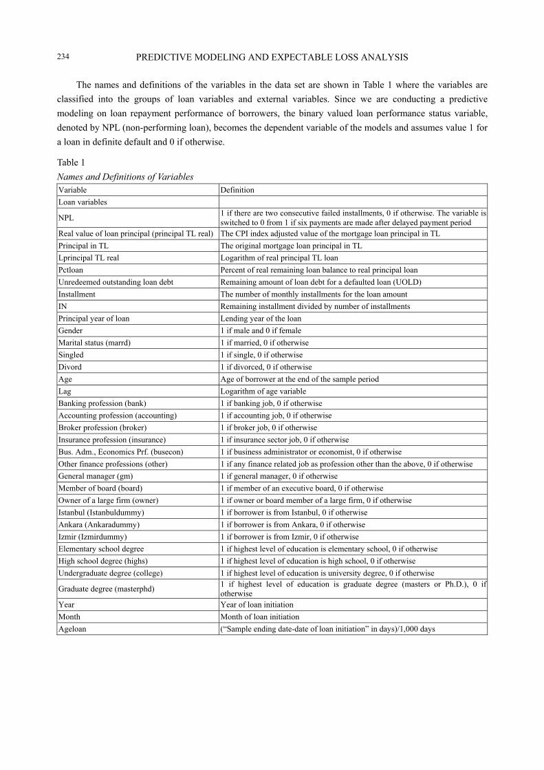
The names and definitions of the variables in the data set are shown in Table 1 where the variables are

classified into the groups of loan variables and external variables. Since we are conducting a predictive

modeling on loan repayment performance of borrowers, the binary valued loan performance status variable,

denoted by NPL (non-performing loan), becomes the dependent variable of the models and assumes value 1 for

a loan in definite default and 0 if otherwise.

Table 1

Names and Definitions of Variables Variable Definition

Loan variables

NPL 1 if there are two consecutive failed installments, 0 if otherwise. The variable is switched to 0 from 1 if six payments are made after delayed payment period

Real value of loan principal (principal TL real) The CPI index adjusted value of the mortgage loan principal in TL

Principal in TL The original mortgage loan principal in TL

Lprincipal TL real Logarithm of real principal TL loan

Pctloan Percent of real remaining loan balance to real principal loan

Unredeemed outstanding loan debt Remaining amount of loan debt for a defaulted loan (UOLD)

Installment The number of monthly installments for the loan amount

IN Remaining installment divided by number of installments

Principal year of loan Lending year of the loan

Gender 1 if male and 0 if female

Marital status (marrd) 1 if married, 0 if otherwise

Singled 1 if single, 0 if otherwise

Divord 1 if divorced, 0 if otherwise

Age Age of borrower at the end of the sample period

Lag Logarithm of age variable

Banking profession (bank) 1 if banking job, 0 if otherwise

Accounting profession (accounting) 1 if accounting job, 0 if otherwise

Broker profession (broker) 1 if broker job, 0 if otherwise

Insurance profession (insurance) 1 if insurance sector job, 0 if otherwise

Bus. Adm., Economics Prf. (busecon) 1 if business administrator or economist, 0 if otherwise

Other finance professions (other) 1 if any finance related job as profession other than the above, 0 if otherwise

General manager (gm) 1 if general manager, 0 if otherwise

Member of board (board) 1 if member of an executive board, 0 if otherwise

Owner of a large firm (owner) 1 if owner or board member of a large firm, 0 if otherwise

Istanbul (Istanbuldummy) 1 if borrower is from Istanbul, 0 if otherwise

Ankara (Ankaradummy) 1 if borrower is from Ankara, 0 if otherwise

Izmir (Izmirdummy) 1 if borrower is from Izmir, 0 if otherwise

Elementary school degree 1 if highest level of education is elementary school, 0 if otherwise

High school degree (highs) 1 if highest level of education is high school, 0 if otherwise

Undergraduate degree (college) 1 if highest level of education is university degree, 0 if otherwise

Graduate degree (masterphd) 1 if highest level of education is graduate degree (masters or Ph.D.), 0 if otherwise

Year Year of loan initiation

Month Month of loan initiation

Ageloan (“Sample ending date-date of loan initiation” in days)/1,000 days


235

(Table 1 continued)

Variable Definition

External variables

d2005 Year dummy for year 2005







Logloan Logarithm of the mortgage loan size over all Turkey for the month loan initiated

Unempn Unemployment rate of the year as per loan month

Unempnextyearn Unemployment next year as per month

t2yearn Two year market interest rate

d75ltv Dummy for the “maximum loan to value percentage 75%” regulation

Marriedchgyear Marriage rate change yearly

Lagchgmarriage Lag of marriage rate change yearly, divorce rate of the city in 2011

Divorceratecity2011a Divorce rate of the city minus the divorce rate of Turkey 1.62% as 2011

Immigrate20072011a Immigration rate between 2007 and 2011

Yrchgcostconst Change of construction cost from last year

Lagyearcostconst Lag of change of construction cost from last year

Chghome Home sales change from last year for home sales between 2007 and 2012

Intersin Interaction of single and male

Intercity Interaction of divorced and divorce rate of city in 2011

Interdiv Interaction of divorced and male

Spread Market two year interest rate minus mortgage rate of the loan

Aggregated values of the loan principal and default loss amounts variables on individual loans are given

in Table 2 below, in domestic currency (TL) denomination. It is observed that 95.4% of the mortgage loans are

in the local currency terms, while 2% of them in US dollars, 1% in Euro and almost 1% in Swiss Francs. The

worth of the mortgage loans generated by the banking firm under concern happens to be 6,930,922,056 TL in

nominal terms and 3,222,170,239 TL in real terms for the 2002-2011 period. Out of the 97,771 individual

mortgage loans in the data, the number of foreign currency denominated loans happens to be 923 and

amounting to 242,446,084 TL (3.6%) in foreign currency denominations. Table 2 gives an idea on the rates of

inflation, interest, and unemployment too as the reflections of the overall economic conditions of the study

period. We also observe that the loans generated in years 2007 and 2008 have a surge up of default rates. It is

also indicated that the default rate of the mortgages starts to increase just previous to the boosting of the

unemployment rate and keeps to increase thereafter. It is important to mention another aspect of economic

conditions in the said years that the countrywide mortgage default rate shows a change between 0.1% and a

peaking ratio of 1.8%, where the latter is for the amount of loans generated in year 2008. This peak can be

attributed to the incident of 57% increment in the loans that are lent out in this particular year.


236

Table 2

Default Loss Amounts by Loan Origination Years

Loan origination year

Number of loans generated

Total amount of loans (TL)

Number of loans in default

Defaulted loan amounts (%)

End-of-year reference interest rate for mortgages (%)

End-of-year reference inflation rate for mortgages (%)

End-of-year unemployment rate (%)

2002 2 98,687 - - - 29.8 -

2003 13 1,937,780 - - - 18.4 -

2004 7 614,373 - - - 9.3 -

2005 2,657 142,645,981 15 0.7 - 10.5 11.5

2006 4,728 302,972,942 23 0.5 - 9.7 10.9

2007 4,676 367,574,101 53 1.2 7.1 8.4 10.9

2008 7,849 575,887,101 138 1.8 11.1 10.1 14.0

2009 19,879 1,353,051,536 131 0.7 5.3 6.5 13.5

2010 39,908 2,905,428,805 179 0.5 9.2 6.4 11.4

2011 19,052 1,280,710,731 20 0.1 6.2 10.5 9.8

All 97,771 6,930,922,056 509 0.6

Note that year 2007 in the data is an important time period for not only being a starting year of a surge up

of borrower repayment defaults, but also for being the year of enactment of a national law that limits the

individual loan amounts to the maximum loan-to-value ratio of 75%. So, instead of the loan level loan-to-value

ratios that we lack in our sample data, we use a dummy variable, denoted by the acronym d75ltv, in our models

in order to see the effect of this stringency.

Default Probability Modeling

It is well known from the literature that a predictive study on default probabilities and default loss amounts

for mortgage loans can be performed by the reduced or structural models. The reduced models mostly take the

form of random functions of time and get implemented by stochastic process representations. The structural

models on the other hand can be performed for fixed time periods. The logistic regression model, being a

member of generalized linear models, belongs to the second category for the cross sectional data analyses and

accepts in all types of variables, being predicted or predictor, with continuous or discrete values and with

count, nominal, ordinal or categorical variable features. The essential theory and methodology on logistic

regression models can be found in the texts of McCullagh and Nelder (1989) and McCullagh and Searle (2001),

among many others. In our modeling attempts, we predict the loan level default occurrence probabilities by the

binary logistic regression model which can bear all types of the predictor variables we have listed above.

The predicted variable labeled with NPL in our data base is a zero-one valued binary random variable, and we

symbolize it in the model equations with Y such that Pr(Yi = 1) = p stands for probability of default, and

Pr(Yi = 0) = 1 p no default for the i-th loan, i = 1, …, m, where m = 97,771 number of individual loans in our

sample data.

Very briefly, a logistic regression model estimates p[0, 1] as the probability Pr{Y = 1} = p that a mortgage

borrower default occurs due to the observable values of predictor variables (X1, …, Xk) such that:

0 1 1( ... )

1( 1 ) ( )

1 i n iki X Xp Y X p X

e

(1)


237

Then, the odds of a mortgage default event at loan levels can be expressed as a binary logit function

i = ln[p(X)/1 p(X)] = X consisting of loan variables vector XL and external variables vector XE in vector

X = (1, XL, XE) = (1, X1, …, Xk), as the vector of predictor variables in our models the corresponding vector of

model parameters = (0, 1, …, k) to be estimated. Function implies that p and the odds of mortgage

borrower defaults are the same at all levels of Xj if j = 0, j = 1, …, k, whereas for j > 0 (j < 0), it implies that

p and the odds increase (decrease) with respect to Xj as Xj increases (decreases) when the values of other

variables are kept constant. In this line, we specify the following logistic regression model to explain and

predict the borrower default probabilities for loans:

01

k

i i i j ij ij

y X

(2)

with 0i j ijjX X and error term i, i = 1, …, m and j = 1, …, k, where yi stands for the

observable value of Yi for loan i and k stands for the number of variables employed in the model. The usual

estimation results of these regression fittings are shown in Table 3 below, in three distinct model versions

containing “all variables”, (XA), solely “loan variables”, (XL), and solely “external variables”, (XE), as the

predictors. Significance tests for each predictor variable and the goodness of fit tests for the overall

explanatory, or predictive, power of these models are also displayed in the same table. By the construction of

these models, we test a hypothesis, hypothesis H1, asserting that borrower default probabilities can be

estimated best by the inclusion of all variables in the predictive Model (2) against the alternative hypothesis

that better predictions can be attained when solely loan variables or solely external variables are contained in

it. We test this hypothesis through the alternative methods of usual estimation and the stepwise estimation

procedures. So in this way, we can also compare the two alternative estimation methods while we compare the

predictive powers of the three versions of Model (2) and conduct significance tests on the predictor variables

they contain.

Hypothesis testing results for H1 with usual fitting procedure are reported in Panel A of Table 3. It is

shown that the best estimation of default occurrences is obtained by the “all variables” model

0

A A

i j ij ijy X , in comparison to the other versions of Model (2) with solely loan variables,

0

L L

i j ij ijy X and with solely external variables,

0

E E

i j ij ijy X . This decision is

based on the magnitudes of the likelihood ratio, Wald chi-square and Akaike Information Criterion (AIC)

values shown at the bottom of the same table. The risk management implications of the predictor variables in

these models, and in the other models of this paper as well, can be inferred from the signs and magnitudes of

the corresponding parameter estimations. So that, a positive sign for the estimated parameter of a predictor

variable implies that the variable obtains an inciting and increasing effect (positive effect) on the predicted

outcome variable, while the impact size of this effect is implied by the magnitude of the estimated parameter

value itself. Similarly, a negative sign for the estimated parameter value of a predictor variable is an indication

of its reducing effect (negative effect) on the predicted variable, and the size of reduction is pointed out by the

magnitude of its estimated value. From this standpoint, the all variables model, obtained as the most predictive

model among the tree model versions, shows that highly significant positive effects are imposed on the defaults


238

(NPL = 1) by the predictor loan variables of logarithm of loan principal (lprincipaltlreal) amount in real TL

terms, ratio of remaining installment amount to total installment amount (IN), having high school graduation

(highs), and two-year interest rate (t2yearn), the last being an external variable with the largest positive effect

on default occurrences. Whereas, it is seen so for the same model that statistically highly significantly negative

effects on NPL come from the loan variables of being single (singled), being married (marrd), having college

education (college), having a master and/or Ph.D. degree (masterphd), and external variables for countrywide

total loan amounts for loan origination periods (logloan), and difference between two-year market interest rate

and mortgage loan rate (spread), the last being an external variable and having among others the largest

negative effect on default outcomes.

Table 3

Logistic Regression for Borrower Defaults (Probability Modeled is NPL = 1)

Predictor variables

Panel A Panel B

Parameter estimate

Standard error

Wald chi-square

Pr > Chi sq.Parameter estimate

Standard error

Wald chi-square

Pr > Chi sq.

All variables Loan variables

Intercept 525.5000 1,177.6000 0.1992 0.6554 226.3000 166.2000 1.8542 0.1733

lprincipaltlreal 0.9279 0.1069 75.356 *** < 0.0001 0.7778 0.0820 89.9450 *** < 0.0001

pctloan -1.2250 1.2290 0.9935 0.3189 5.0885 0.9044 31.6559 *** < 0.0001

Installment -0.0024 0.0031 0.6033 0.4373 0.0036 0.0022 2.5823 0.1081

IN 6.3522 1.3755 21.325 *** < 0.0001 -4.5572 1.0920 17.4172 *** < 0.0001

year -0.2599 0.5866 0.1963 0.6578 -0.1195 0.0828 2.0839 0.1489

genderdummy 0.0044 0.1734 0.0006 0.9798 0.1966 0.1298 2.2914 0.1301

marrd -0.6420 0.2505 6.5708 ** 0.0104 -0.3106 0.2198 1.9965 0.1577

singled -1.2155 0.4865 6.2413 ** 0.0125 -0.3009 0.2495 1.4541 0.2279

divord 0.6770 2.1404 0.1000 0.7518 0.4284 0.4447 0.9282 0.3353

agelast 0.0037 0.7397 0.0000 0.9960 -0.5629 0.6197 0.8251 0.3637

bank -0.1698 1.0266 0.0274 0.8686 -0.8402 1.0069 0.6962 0.4041

accounting -0.0442 0.4225 0.0109 0.9167 0.0267 0.3102 0.0074 0.9315

broker -12.2487 6,068.0000 0.0000 0.9984 -11.7723 2,177.900 0 0.9957

insurance -12.6088 639.6000 0.0004 0.9843 -11.8053 464.5000 0.0006 0.9797

busecon -12.1587 486.0000 0.0006 0.9800 -11.7843 279.1000 0.0018 0.9663

otherfin 1.3102 1.0404 1.5859 0.2079 0.7683 1.0319 0.5543 0.4566

gm -0.1249 0.6162 0.0411 0.8394 0.0569 0.4692 0.0147 0.9035

board -15.2538 9,348.6000 0.0000 0.9987 -13.3723 5,840.900 0 0.9982

owner -12.4591 681.9000 0.0003 0.9854 -11.9694 417.8000 0.0008 0.9771

Istanbuldummy -0.0008 0.1530 0.0000 0.9960 -0.0801 0.1159 0.4771 0.4897

Ankaradummy 0.0432 0.2131 0.0411 0.8394 -0.2796 0.1578 3.1399 * 0.0764

Izmirdummy -0.2293 0.3819 0.3603 0.5483 -0.5521 0.2889 3.6515 * 0.0560

element 0.1715 0.2031 0.7134 0.3983 -0.1217 0.1688 0.5192 0.4712

highs 0.3888 0.1696 5.2525 ** 0.0219 0.0653 0.1396 0.2189 0.6399

college -0.4589 0.2200 4.3520 ** 0.0370 -0.7609 0.1686 20.3722 *** < 0.0001

masterphd -0.5713 0.3446 2.7477 * 0.0974 -1.2944 0.2964 19.0664 *** < 0.0001


239

(Table 3 continued)

Predictor variables

Panel A Panel B

Parameter estimate

Standard error

Wald chi-square


Standard error

Wald chi-square

Pr > Chi sq.

External variables

Intercept -9.5194 11.6406 0.6688 0.4135

logloan -2.4168 1.1100 4.7405 ** 0.0295 0.0902 1.0324 0.0076 0.9304

unempn -1.8240 8.8326 0.0426 0.8364 -1.8708 8.5607 0.0478 0.8270

unempnextyrn 1.5439 8.5301 0.0328 0.8564 1.5741 8.2943 0.0360 0.8495

t2yearn 467.5000 41.5451 126.638 *** < 0.0001 374.6000 42.0578 79.3187 *** < 0.0001

d2005 0

d2006 0

d2007 -0.8164 2.1286 0.1471 0.7013 -0.4628 1.1497 0.1620 0.6873

d2008 -0.3956 1.4174 0.0779 0.7801 -0.2946 0.7175 0.1686 0.6814

d2009 -0.7136 0.6385 1.2489 0.2638 -0.5887 0.2738 4.6232 ** 0.0315

d2011 0 -0.3744 0.5855 0.4088 0.5226

month 0

d75ltv -0.6430 0.5294 1.4754 0.2245 -0.6935 0.5284 1.7228 0.1893

marriedchgyear 0

lagchgmarriage 0.0306 0.1187 0.0666 0.7963 0.0131 0.1091 0.0145 0.9041 divorceratecity2011a

1.7926 18.7177 0.0092 0.9237 1.0213 15.8458 0.0042 0.9486

divorcespread 0 1.0563 1.9621 0.2898 0.5903 immigrate20072011a

-0.8868 1.2993 0.4659 0.4949 -0.2965 1.1723 0.0640 0.8003

yearchg 0

yrchgconstcost 0

lagyrconscost 0

chghome -0.0172 0.0977 0.0308 0.8607 -0.0275 0.0958 0.0825 0.7740

intersin 0.7846 0.4805 2.6659 0.1025 0.1578 0.1851 0.7267 0.3940

intercity -24.2682 106.2000 0.0522 0.8193 -19.2457 97.1467 0.0392 0.8430

interdiv -0.4095 1.2267 0.1114 0.7385 0.1306 1.1344 0.0133 0.9084

spread -470.5000 43.3210 117.9390 *** < 0.0001 -377.8000 44.0257 73.6392 *** < 0.0001

Model tests All variables model Loan variables model External variables model

Number of obs. read 97,749 97,749 97,749

Number of obs. used 53,654 84,657 53,654

-2 log likelihood 2,956.40 4,883.61 3,168.55

Likelihood ratio chi-square 460.9935 251.8536 248.8414

Model LR test Pr > chi sq. < 0.0001 < 0.0001 < 0.0001

Wald test chi-square 513.7423 276.8287 269.5840

Model Wald test Pr > chi sq. < 0.0001 < 0.0001 < 0.0001

Model AIC (intercept only) 3,419.39 5,137.47 3,419.39

Model AIC (intcpt & covarts) 3,042.40 4,937.61 3,206.55

Notes. ***: Statistically significant at level 0.0001 or less; **: Statistically significant at level 0.05 or less; *: Statistically significant at level 0.10 or less (in this and all other tables).

We consider the stepwise estimation procedure for our models more important than the usual estimation

procedure. Because this procedure selects predictors into a model in a step by step fashion using in every step

the criterion that a predictor variable is entered into the model equation in addition to intercept term other

already selected variables if among all the other variables waiting to be selected it has the largest possible


240

partial correlation with the outcome variable to be predicted, and if it also improves the predictive power of the

model itself in a significant way. This routine is continued sequentially until the highest possible level of

prediction power is attained.

Application of the stepwise estimation procedure on the all variables version of Model (2),

0

A A

i j ij ijy X yields the best equation, as compared to the loan variables and external variables

versions of the same model, for the prediction of borrower default occurrences:

-4.68 0.9 6.12 1.52 1.2 0.62 0.55

0.65 0.31 1.28 472.00 1.12

1.64 469.2 0 81

iy lprincipaltlreal IN pctloan singled married college

masterphd highs other finance professions spread d75ltv

logloan t2yearn + . intersi

in +0.03yrchgconstcost +

(3)

Table 4

Stepwise Logistic Regression for Borrower Defaults (Probability Modeled is NPL = 1)

Predictor variables

Panel A Panel B Parameter estimate

Standard error

Wald chi-square


Standard error

Wald chi-square

Pr > Chi sq.

All variables Loan variables

Intercept -4.6758 6.3413 0.5437 0.4809 216.40 164.60 1.7276 0.1887

lprincipaltlreal 0.9020 0.1008 80.0192 *** < 0.0001 0.7470 0.0765 95.4323 *** < 0.0001

logloan -1.6350 0.5785 7.9882 ** 0.0047 - - - - -

singled -1.2465 0.4625 7.2643 ** 0.0070 - - - - -

marrd -0.6268 0.2217 7.9939 ** 0.0047 - - - - -

genderdummy 0.1842 0.1283 2.0617 0.1510

pctloan -1.5249 1.1601 1.7277 0.1887 5.0217 0.8954 31.4675 *** < 0.0001

college -0.5538 0.1984 7.7900 ** 0.0053 -0.8211 0.1380 35.3999 *** < 0.0001

IN 6.1168 1.3288 21.1891 *** < 0.0001 -4.4530 1.0797 17.0102 *** < 0.0001

installment - - - - - 0.0037 0.0022 2.7374 * 0.0980

agelast - - - - - - - - - -

masterphd -0.6499 0.3301 3.8749 ** 0.0490

highs 0.3052 0.1408 4.7004 ** 0.0302

year - - - - - -0.1146 0.0820 1.9549 0.1621

divord - - - - - 0.6618 0.3935 2.8292 * 0.0926

otherfin 1.2830 1.0315 1.5472 0.2135 - - - - -

yrchgconstcost 0.0325 0.0153 4.5190 ** 0.0335 - - - - -

intersin 0.8120 0.4475 3.2926 * 0.0696 - - - - -

element - - - - - -0.1928 0.1363 2.0001 0.1573

Ankaradummy - - - - - -0.2473 0.1506 2.6974 0.1005

İzmirdummy - - - - - -0.5181 0.2838 3.3319 * 0.0679 External variables

Intercept -8.7626 0.3025 839.358 *** < 0.0001

t2yearn 469.20 39.2303 143.0559 *** < 0.0001 370.20 38.5911 92.0453 *** < 0.0001

spread -472.00 41.4272 129.8366 *** < 0.0001 -371.40 40.2720 85.0488 *** < 0.0001

lagyrconscost - - - - - -0.0353 0.0098 12.9713 *** 0.0003

d75ltv -1.1183 0.2985 14.0368 *** 0.0002 -0.6798 0.2750 6.1093 ** 0.0134

divorcespread 0.6784 0.4568 2.2057 0.1375


241

(Table 4 continued)

Model tests All variables model Loan variables model External varaibles model

-2 log likelihood 2,965.11 4,894.81 3,170.00

Likelihood ratio chi-square 452.28 240.65 247.40

Model LR Pr > chi sq. < 0.0001 < 0.0001 < 0.0001

Wald test chi-square 506.74 267.89 268.27

Model Wald test Pr > chi sq. < 0.0001 < 0.0001 < 0.0001

AIC (intercept only) 3,419.34 5,137.47 3,419.39

AIC (intercept + predictors) 2,997.11 4,920.81 3,182.00

Panel A of Table 4 shows the parameter values and significance test results for the predictor variables

and the goodness-of-fit test results for the fitting in Model (3). Part B of Table 4 shows the estimations for

the other versions of Model (2), obtained in the same way, and it is clearly indicated by the likelihood ratio

(LR), Wald chi-square criteria and AIC values in this table that all variables version of Model (4) is the

superior one.

Having this fundamental outcome at hand and testifying that H1 is proven true on the empirical grounds,

right away we put forward another hypothesis, H2, in order to investigate further if loan origination years might

have a significant influence on borrower defaults. We test H2 by the construction of a GLMs type “classified

logistic regression” model for the default situations. We estimate this model for our exemplary case with a

design that contrasts the loan classification years 2007, 2008, 2009, and 2010 with the loan classification year

2011, the last being the latest loan origination year in the sampled data set, so we choose it as the benchmark

year of comparisons. The estimated parameters and significance test results for the model are displayed in

Table 5 below, where we see that the predictive power of the estimated model equation is big and very

significant according to the goodness-of-tests results.

Table 5

Classified Logistic Regression Model for Borrower Defaults (Probability Modeled is NPL = 0)

Variable Parameter estimate

Standard error

Wald chi-square

Wald test Pr > Chi sq.

Odd ratio estimates (with percent concordant = 77.4)

Point estimate for the effect

95% wald confidence limits

intercept -3.0832 12.2348 0.0635 0.8010 - - -

lprincipaltlreal -0.9279 0.1069 75.3556 *** < 0.0001 0.395 0.321 0.488

pctloan 1.2250 1.2290 0.9935 0.3189 3.404 0.306 37.858

Installment 0.00242 0.00311 0.6033 0.4373 1.002 0.996 1.009

IN -6.3522 1.3755 21.3254 *** < 0.0001 0.002 < 0.001 0.026

year 2007 -0.0884 0.9266 0.0091 0.9240 vs. 2011: 0.800 0.056 11.499

year 2008 -0.2494 0.5048 0.2240 0.6213 vs. 2011: 0.681 0.114 4.080

year 2009 0.3258 0.3617 0.8246 0.3638 vs. 2011: 1.214 0.333 4.425

year 2010 -0.1253 0.3778 0.1100 0.7402 vs. 2011: 0.771 0.244 2.435

genderdummy -0.00438 0.1734 0.0006 0.9798 0.996 0.709 1.398

marrd 0.6420 0.2505 6.5708 ** 0.0104 1.900 1.163 3.105

singled 1.2155 0.4865 6.2413 ** 0.0125 3.372 1.299 8.751

divord -0.6770 2.1404 0.1000 0.7518 0.508 0.008 33.725

agelast -0.00367 0.7397 0.0000 0.9960 0.996 0.234 4.247

bank 0.1698 1.0266 0.0274 0.8686 1.185 0.158 8.864

accounting 0.0442 0.4225 0.0109 0.9167 1.045 0.457 2.392


242

(Table 5 continued)


Standard error

Wald chi-square


Odd ratio estimates (with percent concordant = 77.4)

Point estimate for the effect

95% wald confidence limits

broker 12.2382 6,036.3 0.0000 0.9984 > 999.99 < 0.01 > 999.99

insurance 12.6237 644.4 0.0004 0.9844 > 999.99 < 0.01 > 999.99

busecon 12.1584 486.0 0.0006 0.9800 > 999.99 < 0.01 > 999.99

otherfin -1.3102 1.0404 1.5859 0.2079 0.270 0.035 2.073

gm 0.1249 0.6162 0.0411 0.8394 1.133 0.339 3.791

board 15.2538 9,348.6 0.0000 0.9987 > 999.99 < 0.01 > 999.99

owner 12.4709 685.9 0.0003 0.9855 > 999.99 < 0.01 > 999.99

Istanbuldummy 0.000776 0.1530 0.0000 0.9960 1.001 0.742 1.351

Ankaradummy -0.0432 0.2131 0.0411 0.8394 0.958 0.631 1.454

Izmirdummy 0.2293 0.3819 0.3603 0.5482 1.258 0.595 2.659

element -0.1715 0.2031 0.7134 0.3983 0.842 0.566 1.254

highs -0.3888 0.1696 5.2525 ** 0.0219 0.678 0.486 0.954

college 0.4589 0.2200 4.3520 ** 0.0370 1.582 1.028 2.435

masterphd 0.5713 0.3446 2.7477 * 0.0974 1.770 0.901 3.479

logloan 2.4186 1.1100 4.7405 ** 0.0295 11.210 1.273 98.735

unemp 1.8240 8.8326 0.0426 0.8364 6.196 < 0.001 > 999.99

unempnextyrn -1.5439 8.5301 0.0328 0.8564 0.214 < 0.001 > 999.99

t2yearn -467.5 41.5451 126.6376 *** < 0.0001 < 0.001 < 0.001 < 0.001

d75ltv 0.6430 0.5294 1.4754 0.2245 1.902 0.674 5.369

lagchmarriage -0.0306 0.1187 0.0666 0.7963 0.970 0.768 1.224

divorceratecity2011a -1.7926 18.7177 0.0092 0.9237 0.167 < 0.001 > 999.99

immigrate20072011a 0.8868 1.2993 0.4659 0.4949 2.427 0.190 30.981

chghome 0.0172 0.0977 0.0308 0.8607 1.017 0.840 1.232

intersin -0.7846 0.4805 2.6659 0.1025 0.456 0.178 1.170

intercity 24.2682 106.2 0.0522 0.8193 > 999.99 < 0.001 > 999.99

interdiv 0.4095 1.2267 0.1114 0.7385 1.506 0.136 16.675

spread 470.5 43.3210 117.9390 *** < 0.0001 > 999.99 > 999.99 > 999.99

Model fitting statistics Model goodness-of-fit tests

AIC (intercept and covariates) = 3,042.398 Likelihood ratio chi-square = 460.99 with Pr > Chi sq. = < 0.0001

-2 log L (intercept and covariates) = 2,956.398 Wald chi-square = 513.74 with Pr > Chi sq. = < 0.0001

SC = 3,424.682 Score chi-square = 601.28 with Pr > Chi sq. = < 0.0001

Notes. Dependent variable: loan default status (NPL); class: year; class level values: 2007, 2008, 2009, 2010, 2011; model: binary logit; probability modeled is NPL = 0; optimization technique: Fisher’s scoring.

Even though the estimated classified logistic regression model itself is obtained highly significant, it is

found that neither the individual classification years nor their contrasts with classification year 2011 are found

significant for the exemplary case. However, it is noticeable that among the all loan origination years, year

2008 obtains the smallest negative effect on the survival performances of loans. Whereas, the odds ratio

estimate of the loan origination year 2009 against the benchmarking loan origination year 2011 comes out with

the largest positive effect among the others. This can be explained well by the collectively changing values of

the most significant variables of the model during 2008 and 2009.


243

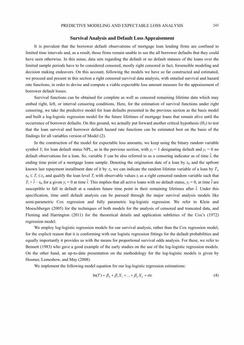
Survival Analysis and Default Loss Appraisement

It is prevalent that the borrower default observations of mortgage loan lending firms are confined to

limited time intervals and, as a result, those firms remain unable to see the all borrower defaults that they could

have seen otherwise. In this sense, data sets regarding the default or no default statuses of the loans over the

limited sample periods have to be considered censored, mostly right censored in fact, forsensible modeling and

decision making endeavors. On this account, following the models we have so far constructed and estimated,

we proceed and present in this section a right censored survival data analysis, with entailed survival and hazard

rate functions, in order to devise and compute a viable expectable loss amount measure for the appraisement of

borrower default losses.

Survival functions can be obtained for complete as well as censored remaining lifetime data which may

embed right, left, or interval censoring conditions. Here, for the estimation of survival functions under right

censoring, we take the predictive model for loan defaults presented in the previous section as the basis model

and built a log-logistic regression model for the future lifetimes of mortgage loans that remain alive until the

occurrence of borrower defaults. On this ground, we actually put forward another critical hypothesis (H3) to test

that the loan survival and borrower default hazard rate functions can be estimated best on the basis of the

findings for all variables version of Model (2).

In the construction of the model for expectable loss amounts, we keep using the binary random variable

symbol Yi for loan default status NPL, as in the previous section, with yi = 1 designating default and yi = 0 no

default observations for a loan. So, variable Y can be also referred to as a censoring indicator as of time t ̃, the

ending time point of a mortgage loans sample. Denoting the origination date of a loan by t0i and the upfront

known last repayment installment date of it by i, we can indicate the random lifetime variable of a loan by Ti,

t0i Ti i, and qualify the loan level Ti with observable values ti as a right censored random variable such that

Ti > t ̃ – t0i for a given yi = 0 at time t.̃ This implies that all active loans with no default status, yi = 0, at time t ̃are

susceptible to fall in default at a random future time point in their remaining lifetimes after t ̃. Under this

specification, time until default analysis can be pursued through the major survival analysis models like

semi-parametric Cox regression and fully parametric log-logistic regression. We refer to Klein and

Moeschberger (2005) for the techniques of both models for the analysis of censored and truncated data, and

Fleming and Harrington (2011) for the theoretical details and application subtleties of the Cox’s (1972)

regression model.

We employ log-logistic regression models for our survival analysis, rather than the Cox regression model,

for the explicit reason that it is conforming with our logistic regression fittings for the default probabilities and

equally importantly it provides us with the means for proportional survival odds analysis. For these, we refer to

Bennett (1983) who gave a good example of the early studies on the use of the log-logistic regression models.

On the other hand, an up-to-date presentation on the methodology for the log-logistic models is given by

Hosmer, Lemeshow, and May (2008).

We implement the following model equation for our log-logistic regression estimations:

0 1 1ln( ) ... k kT X X (4)


244

Here, is the scale parameter of the model and is the error term with a logistic distribution

function F() = exp()/(1 + exp()) and density function f() = exp()/(1 + exp())2 that underlie the model in

Equation (4). We note that, since has a logistic distribution, then ln(T) too must have a logistic distribution

and T in turn possesses a log-logistic distribution. Here, the hazard rate and survival functions for T, as the

critical functions for loan defaults analysis, can be derived from the log-logistic distribution of T as follows: 1( )

( | )1 ( )

th t X

t

and 1

( | )1 ( )

S t Xt

(5)

with X standing for the vector of all predictor variables in Model (4), t referring to ti as time until default for

loan i, = exp{-[0 + 1X1 +… + kXk]} and = 1/. Consequently, we can write the following model for the

log odds of survivals, or log odds of lifetimes until borrower defaults:

* * * *0 1 1

( | )ln ... ln ;

1 ( | )i

k k i

S t XX X t

S t X

(6)

This expression clearly implies that a log-logistic regression model can be estimated by the logistic regression procedures. Here, the log ratio ln[ ( | ) /(1 ( | )]S t X S t X in Equation (6) is known as the odds of no

default lifetime up to a given t. Hence, it implies that for the fixed values of all the other variables in vector X,

the effect of a unit increase in the j-th variable Xj, j = 1, …, k, on the odds ratio can be written as

*

[ ( | ) /(1 ( | )] /[ ( | ) /(1 ( | )] j

j j j jS t X S t X S t X S t X e where Xj + denotes a one unit incremented Xj, and +j

*

and -j* indicate the log odds ratios due to Xj

+ for no default and default situations, respectively. The effect of

increments in several multiples of variables on the odds ratio can be expressed analogously with similar

interpretations on the corresponding * parameters.

In case of having no information on the default times of already defaulted loans in a mortgage loans

sample, ending time point of the sample period can be taken as a proxy for the loan lifetime calculations at

individual loan levels, ti = t ̃– t0i. In this way, a ti value for an active loan in a sample stands as its age at t ̃, or

lifetime until t ̃, while for the already defaulted loans in the sample it stands as time until default notification.

Having this sort of loan lifetime calculations for the right-censored sample data in our hand, we estimate

Model (4) for exemplary case, as displayed in Table 6 below, where the statistically significant predictors of the

model, with negative and positive effects on the outcome variable loan lifetime until defaults, are clearly

indicated. In that regard, it is seen that loan principals, monthly repayments, countrywide amount of mortgage

loans, market interest rates, legislative regulations, marital and educational statuses, and unemployment rates

are important factors.

Following the numerical results for Model (4), estimation of the required survival and hazard rate

functions for further uses can be easily performed by the use of the expressions we give in (5) and (6) above.

All in all, the obtained results for Models (4), (5), and (6) herefully support the hypothesis H3 of this section,

and in this way we prove that the set of statistically significant variables of Model (4) overlaps well with that of

the all variables version of Model (2).


245

Table 6 Log-Logistic Regression for Mortgage Loan Lifetime Analysis


Standard error

95% confidence limits Chi-square Pr > Chi sq.

Lower Upper

Intercept 21.5212 2.2691 17.0738 25.9685 89.95 *** < 0.0001

lprincipaltlreal -0.0972 0.0126 -0.1218 -0.07826 59.81 *** < 0.0001

pct loan 0.2732 0.1394 -0.0000 0.5463 3.84 ** 0.0500

installment 0.0002 0.0003 -0.0005 0.0009 0.39 0.5344

IN -0.8224 0.1555 -1.1272 -0.5175 27.95 *** < 0.0001

genderdummy 0.0005 0.0185 -0.0358 0.0368 0.00 0.9794

marrd 0.0735 0.0270 0.0207 0.1264 7.44 ** 0.0064

singled 0.1304 0.0522 0.0282 0.2327 6.26 ** 0.0124

divord -0.0610 0.2189 -0.4901 0.3681 0.08 0.7804

agelast -0.0096 0.0882 -0.1628 0.1437 0.02 0.9024

bank 0.0199 0.1093 -0.1942 0.2341 0.03 0.8552

accounting 0.0051 0.0451 -0.0833 0.0936 0.01 0.9092

broker 1.7607 4,423.70 -8,668.54 8,672.06 0.00 0.9997

insurance 2.1313 2,861.21 -5,605.73 5,609.99 0.00 0.9994

busecon 2.1414 2720.01 -5,328.97 5,333.26 0.00 0.9994

otherfin -0.1486 0.1108 -0.3657 0.0685 1.80 0.1796

gm 0.0147 0.0650 -0.1128 0.1422 0.05 0.8216

board 1.9423 4,112.98 -8,059.35 8,063.24 0.00 0.9996

owner 2.1182 2,856.64 -5,596.79 5,601.02 0.00 0.9994

istanbuldummy 0.0021 0.0164 -0.0300 0.0341 0.02 0.9001

ankaradummy -0.0003 0.0228 -0.0449 0.0443 0.00 0.9896

izmirdummy 0.0329 0.0407 -0.0468 0.1126 0.65 0.4185

element -0.0174 0.0217 -0.0600 0.0251 0.64 0.4220

highs -0.0345 0.0183 -0.0704 0.0013 3.56 0.0592

college 0.0523 0.0238 0.0056 0.0990 4.82 ** 0.0281

masterphd 0.0690 0.0370 -0.0035 0.1414 3.48 * 0.0621

logloan -2.0213 0.1716 -2.3576 -1.6849 138.76 *** < 0.0001

unemp 0.07785 1.0009 -1.1833 2.7403 0.60 0.4367

unempnextyrn 3.9214 1.0432 1.8767 5.9661 14.13 ** 0.0002

t2yearn -45.6346 5.2096 -55.8452 -35.4240 76.73 *** < 0.0001

d75ltv -0.6489 0.0614 -0.7693 -0.5286 111.69 *** < 0.0001

marriedchyear 9.0659 4.6619 -0.0713 18.2030 3.78 0.0518

lagchmarriage -0.0021 0.0127 -0.0271 0.0229 0.03 0.8694

divorceratecity2011a -0.4252 1.9943 -4.3340 3.4336 0.05 0.8312

immigrate20072011a 0.0979 0.1383 -0.1731 0.3689 0.50 0.4788

yearchg 4.3613 2.9199 -1.3616 10.0843 2.23 0.1353

yrchgconstcost 0.0851 0.0641 -0.0406 0.2107 1.76 0.1846

lagytconstcost 0.0205 0.0190 -0.0168 0.0577 1.16 0.2818

chghome 9.0015 0.0104 -0.0190 0.0219 0.02 0.8892

intersin -0.0814 0.0514 -0.1821 0.0193 2.51 0.1130

intercity 2.1806 10.6853 -18.7622 23.1234 0.04 0.8383

interdiv 0.0956 0.1409 -0.1805 0.3717 0.46 0.4973

spread 47.5099 5.3475 37.0290 57.9907 78.94 *** < 0.0001

Scale 0.1064 0.0057 0.0958 0.1182

Notes. Dependent variable: log (ageloan); censoring variable: loan default status (NPL); censoring value: NPL = 0; number of observations read: 97,749; number of observations used: 53,659; right censored values: 53,382; log likelihood: -1,064.39.


246

Now, making use of the all modeling results up to here, we can present our measure and model for the

expression and computation of expectable loss amounts due to the borrower defaults. In this regard, we

consider the equation in (4) as the underlying model and propose the following loan level expectable loss

amount (ELA) measure for each ending time point of future installment periods:

0 0

0 0

,( ) ,( )

( ) ( )( ) (1 ) (1 )

i i

i i

i t t u t i t t u t

i u tt t t t t uu t u tPV ELA E p q

r r

(7)

Here, the components p and q stand for the conditional survival and related hazard rate functions to be

computed through the use of Model (4)’s estimation results. In Expression (7), random variable U denotes the

future loan lifetime variable with discretely observable values u = 0, 1, …, i, i denotes the age of a loan at its

final prospective installment period, t ̃ – t0i stands for the age of a loan as of the end of sample period t ̃, 0,( )ii t t u

denotes the outstanding loan balance, or total amount of all remaining repayments to be made at the end of each

future installment period (t ̃ – t0i) + u, u + t is for a one month increment in loan age, r is a discount rate for the

time t ̃ present value (PV) computation, and (1/(1+r)u+t) expresses the present value of one unit loss:

0 0 0 0 0( ) Pr( ( ) | ( )) (( ) | ) / ( | )i iiu i i i i T i T it tp T t t u T t t S t t u X S t t X (8)

The survival probability component in Equation (7) is a conditional survival probability expression for

loan i, and 0( )it t t uq

is the discrete time version of the continuous time hazard rate function h(tX) given in

(5). In order to proceed further with PVt ̃(ELAi) computations, we obtain, below, the discrete time version of the

hazard rate function that we need in terms of the random survival (lifetime) variable T:

0 0 0 0( ) Pr(( ) ( ) | ( ) )it i i i i it t uq t t u T t t u t T t t u (9)

Computation of this function can be achieved through the use of the survival functions, as shown below:

0 0 0 0( ) [ (( ) | ) (( ) | )] / (( ) | )i i iit T i T i T it t uq S t t u X S t t u t X S t t u X (10)

Hence, the factor “0 0( ) ( )i iu tt t t t up q ” in Equation (7) expresses the probability that loan i will survive in

no default status from its known age (t ̃ – t0i) at time t ̃, ending time point of the sample, to a random time point

(t ̃– t0i) + u in the future, and then fall in default by the end of next payment period from time point (t ̃– t0i) + u to

time point (t ̃– t0i) + u + t. Given all these, the measure we propose in Equation (7) turns out to be a concrete

financial valuation measure for a mortgage loan which is alive and at known age of (t ̃ – t0i), as of time t.̃

In the rest of this section, we present the numerical calculation details for PVt ̃ (ELAi), and also discuss its

practical implications for realistic applications. For this purpose, we take a loan with ID number 87469 chosen

from the sample as an exemplary case. This loan, standing with no default status at time t ̃ as the end of the

concerned sample period, that is March 11, 2011, happens to have 36 monthly repayments already completed

and 24 remaining repayments to be made. The reported outstanding loan amount for the loan at time t ̃ is

193,536.19 TL, with remaining monthly repayments of 8,064.01 TL over the next 24 months. As part of our

computations for the sample period of 2005-2011, we express one month of a year in 0.03 units, so the

observed age of this particular loan is specified as 1.08 time units (36 months) at time t ̃ while its remaining

lifetime without defaults can be 0.72 time units, maximum, over the time span of all remaining installment

periods.


247

Given all these for the exemplary case, Table 7 below shows the end of month values of expectable loss

measure PVt ̃(ELAi) for each and every month of the remaining repayment installments of this loan, such that a

random and irrevocable borrower default event may occur within each of these months and a consequent

mortgage loan loss then may be realized. Regarding the PVt ̃ (ELAi) computations in Table 7, it is important to

remind that the function , given in the survival function in expression (5), connects the collective predictive

effects of all predictor variables it contains to the outcome variable of potential and random loan lifetimes.

Following from the log-logistic regression fitting results of Table 6, we obtain the estimated value of as

= exp{-[0 + 1X1 +… + kXk]} = 0.86596904 at time t ̃ when potential losses are predicted. Thus, the

expectable loss amount PVt (ELAi) computations in Table 7 delivers the time t ̃ present values of all possible

future loss amounts that can be thought for loan i.

Table 7

Numerical Example for Expectable Loss Amounts

Installment month of remaining repayments

u Loan age t = t ̃ + u

Survival probability at age t (Equation 5)

( )it

S t X

Conditional survival probability (Equation 8)

0( )iu t tp

Borrower default hazard rate (Equation 9)

01 ( )it t uq

PVt (ELAi) (Equation 7) with monthly discount rate r = 0.0095

37 0 1.10 0.61223786 1.00000000 0.10037567 19,225.32

38 0.03 1.13 0.55078407 0.89962433 0.11145641 18,399.45

39 0.06 1.16 0.48939566 0.79935543 0.12163936 17,061.78

40 0.09 1.19 0.42986588 0.70212235 0.13067093 15,362.98

41 0.12 1.22 0.37369491 0.61037537 0.13840284 13,468.31

42 0.15 1.25 0.32197447 0.52589768 0.14478727 11,529.31

43 0.18 1.28 0.27535666 0.44975439 0.14985898 9,665.53

44 0.21 1.31 0.23409200 0.38235466 0.15371156 7,957.81

45 0.24 1.34 0.19810935 0.32358233 0.15647391 6,450.53

46 0.27 1.37 0.16711041 0.27295013 0.15829032 5,158.86

47 0.30 1.40 0.14065845 0.22974477 0.15930602 4,077.63

48 0.33 1.43 0.11825071 0.19314505 0.15965767 3,189.30

49 0.36 1.46 0.09937108 0.16230796 0.15946819 2,470.31

50 0.39 1.49 0.08352455 0.13642500 0.15884460 1,895.36

51 0.42 1.52 0.07025713 0.11475463 0.15787783 1,440.13

52 0.45 1.55 0.05916508 0.09663741 0.15664384 1,082.65

53 0.48 1.58 0.04989724 0.08149976 0.15520514 803.92

54 0.51 1.61 0.04215293 0.06885058 0.15361267 587.99

55 0.54 1.64 0.03567771 0.05827426 0.15190757 421.72

56 0.57 1.67 0.03025799 0.04942196 0.15012286 294.46

57 0.60 1.70 0.02571558 0.04200259 0.14828484 197.70

58 0.63 1.73 0.02190235 0.03577424 0.14641439 124.66

59 0.66 1.76 0.01869553 0.03053638 0.14452797 70.00

60 0.69 1.79 0.01599350 0.02612302 0.14263848 29.54

Notes. u: increment in loan age (loan lifetime); t = t ̃ + u: random age of loan after time t ̃ (additional survival lifetime); loan ID number (i): 87469; reported “outstanding loan balance” as of the end date of the sample period (t)̃ = 193,536.19 TL; = 0.1064;

= 1/ = 9.398496; (t ̃– t0i) = 1.10; 0

(1.10 )( )iS Xt t = 0.61223786; total lifetime of loan: 60 months; remaining lifetime of loan:

24 months, under no defaults; amount of repayment per installment: 8,064.01 TL.


248

The standard deviation of the computed PVt ̃(ELAi) values for this loan obtains a value of 6,553 TL, which

can be considered a measure of variability for default loss expectations. Lastly, by performing similar

computations for all the other active individual loans in the sample portfolio, the portfolio level PVt ̃(ELAportfolio)

can be obtained by aggregation and used for portfolio level risk management purposes.

Mortgage loan lending institutions are urged by these results in many aspects of the management of

borrower risks. Most importantly, it is clearly shown here that contingent loss amounts for active loans become

larger if borrower defaults happen at smaller loan ages. So, it is imperative for mortgage loan lending firms that

survival ages of loans have to be made as long as possible and amounts of possible default losses have to be

kept at possible minimums. In this regard, for every mortgage loan lending firm it is essential to determine and

pay due attention to the impacts of significant factors and variables as the primary risk factors for borrower

defaults. Then the ways of control over the default loss amounts should be devised and applied through the

several instruments and mechanisms regarding the risk transfer, insurance, mortgage backed securities, and

financial risk hedging initiatives. Alongside all these, having sufficient collateral prudence for potential default

losses is a critical issue for risk handlings. In this connection, as proposed and shown in detail above, a

plausible expectable loss amount measure, as we propose here, proves to be essential and indispensable. As

such that, if the value of collateralized asset(s) for a mortgage loan, usually home of a loan borrower, happens

to be larger than that of expectable loss amount measure PVt ̃ (ELAi) in pertinence, then it is meant for the lender

of that mortgage loan that potential losses in expected value terms can be covered to a reasonable extent.

Otherwise, the loan lender may incur a large loss on the planned cash income streams from the concerned loan

or even on the capital assets that are allocated to the overall business of such risky loans.

Lastly, a theoretical and methodological designation arises in our numerical implementations. This is the

designation that the conditional survival probability is a decreasing function of loan age, and the hazard

function first increases and then decreases as loan age ascends, depending upon the value of scale parameter of

Model (4). More clearly, because of the less than one value of the scale parameter of our log-logistic model,

= 0.1064, the discrete time version of the hazard function that we write for our own modeling purposes first

moves upward until a random loan age at default is attained and then turns afterwards into a downward

movement mode for the rest of the remaining but randomly attainable loan ages. Hence, hereby we also verify a

theoretical assertion that takes place in the literature of our subject matter.

Discussion

Considering the risk measuring, modeling, and management needs of the mortgage loans business entities,

a valid and viable predictive modeling is presented in this paper. To this end, using real life sample data, loan

survival and discrete time hazard rate functions are successfully constructed and estimated for the predictions

on default occurrence and loan lifetime outcome variables. An overall summary of the most influential

predictors of these outcome variables are listed together in Table 8. Therein, the positive and negative impacts

and impact sizes of predictors are displayed again for the attention of mortgage loan managers. In this regard,

with respect to the magnitudes of estimated parameter values for the exemplary case, remaining repayment

amount (IN), as a loan variable, and two-year ahead debt market interest rate (t2yearn) and difference between

t2yearn and loan interest rate at origination (spread), as external variables, seem to be the most remarkable risk

triggering variables, alongside the other significant predictors.


249

Table 8

Summary of Predictive Models and the Most Significant Predictors

Model variables having the statistical confidence levels of 90% or more

Logistic regression (stepwise fitting):

probability modeled for default (NPL = 1)

Log-logistic regression for time to default (loan lifetime) analysis: probability modeled for survival time until default

Parameter estimate


Parameter estimate


Intercept term - - - 21.5212 *** < 0.0001

Amount of loan principle (lprincipaltlreal) 0.9020 *** < 0.0001 -0.0972 *** < 0.0001

Ratio of remaining loan balance to loan principal (pctloan) - - - 0.2732 ** 0.0500

Remaining repayment amount per installment period (IN) 6.1168 *** < 0.0001 -0.8224 *** < 0.0001

Marital status (married) -0.6268 ** 0.0047 0.0735 ** 0.0064

Single status (singled) -1.2465 ** 0.0070 0.1304 ** 0.0124

High school education status (highs) 0.3052 ** 0.0302 - -

College education status (college) -0.5538 ** 0.0053 0.0523 ** 0.0281

Graduate education status (masterphd) -0.6499 ** 0.0490 0.0690 * 0.0621Countrywide size of mortgage loans in month of loan origination (logloan)

-1.6350

**

0.0047

-2.0213

***

< 0.0001

Two year ahead debt market interest rate for the country in month of loan origination (t2yearn)

469.20

***

< 0.0001

-45.6346

***

< 0.0001

Difference between two year ahead loan market interest rate and mortgage loan interest rate at origination (spread)

-472.00

***

< 0.0001

47.5099

***

< 0.0001

Dummy for 2007 regulation on maximum 75% loan to value ratio (d75ltv)

-1.1183

***

0.0002

-0.6489

***

< 0.0001

Change in construction cost from last year (yrchgconstcost) 0.0325 ** 0.0335 - -

Interaction of marital and single statuses (intersin) 0.8120 * 0.0696 - - Next year’s unemployment rate on monthly basis (unempnextyearn)

-

- -

3.9214

**

0.0002

The distinctive feature of the paper comes through the censored data approach we apply for the borrower

default and loan lifetime estimations towards the obtainment of expectable loss amounts modeling that we

propose for currently active but prospectively loss prone mortgage loans. Prediction of such expectable losses

serves to the determination of efficient risk reserve and economic capital allocation requirements of mortgage

loan businesses, and other installment loan businesses as well. It is a known fact in this regard that many local

and global regulatory arrangements require from the banks and loan lending institutions to do the necessary

capital apportionments for the sustainment of their business activities under market and client risk conditions

and for the coverage of their liabilities to their equity holders and business partners. With this view, we believe

that the models, computational procedures, and the expectable loss amount measure of this paper will prove to

be comprehensive, veritable, and viable tools for a vast variety of applications in the income planning, business

developing, risk handling, and financial management activities of the mortgage loan sectors and related

financial areas.

Conclusion

This paper shows that three main investigations should be bound together in a predictive financial

modeling study on the borrower defaults of mortgage loans. Being the fundamental stage of all three, the first

investigation is about capturing the association between predictor variables and borrower default events from

past occurrences and using them to predict future default outcomes. The second is for the determination of


250

future survival and hazard contingencies of the loans that are active and under ongoing debt obligations. And,

the third is about the estimation of future loss amounts that may stem from future borrower defaults. Clearly,

the last investigation stage puts the results of the previous two to the good use of loan businesses when dealing

with financial uncertainties and financial loss reserving decisions. In this respect, the expectable loss amount

model of this paper bears critical importance.

From this standpoint, turning the stationary structure of the logistic regression model of our first

investigation stage into a dynamic one appears to us as the most pertinent and immediate topic worth

researching on. Once the outcomes on this research topic become internalized into our expectable loss amount

model, its estimations can then be performed more flexibly under the time dynamic and evolving, as well as

stationary, relations of default events, and their predictors. On the other hand, considering a random outcome

vector in our models consisting of multifarious modes of borrower defaults, rather than considering borrower

defaults on loan repayments only, would bring about truly useful multivariate and even multidimensional

modeling research topics for us. So, with a long perspective outlook in this respect, we see many practical

application and theoretical development opportunities in researching on the improvement of our models for the

multivariate modeling and multimodal financial risk management matters of loan business entities.

References Ali, A., & Daly, K. (2010). Macroeconomic determinants of credit risk: Recent evidence from a cross country study. International

Review of Financial Analysis, 19(3), 165-171. Bastos, J. A. (2010). Forecasting bank loans loss-given-default. Journal of Banking and Finance, 34(10), 2510-2517. Bennett, S. (1983). Log-logistic regression models for survival data. Applied Statistics, 32(2), 165-171. Brueckner, J. K., Calem, P. S., & Nakamura, L. I. (2012). Subprime mortgages and the housing bubble. Journal of Urban

Economics, 71(2), 230-243. Campbell, T. S., & Dietrich, J. K. (1983). The determinants of default on insured conventional residential mortgage loans. The

Journal of Finance, 38(5), 1569-1581. Capozza, D. R., & Van Order, R. (2011). The great surge in mortgage defaults 2006-2009: The comparative roles of economic

conditions, underwriting and moral hazard. Journal of Housing Economics, 20(2), 141-151. Capozza, D. R., Kazarian, D., & Thomson, T. A. (1998). The conditional probability of mortgage default. Real Estate Economics,

26(3), 259-289. Coates, D. (2008). The Irish sub-prime residential mortgage sector: International lessons for an emerging market. Journal of

Housing and the Built Environment, 23(2), 131-144. Coleman, M., LaCour-Little, M., & Vandell, K. D. (2008). Subprime lending and housing bubble: Tail wags dog? Journal of

Housing Economics, 17(4), 272-290. Cox, D. R. (1972). Regression models and life tables. Journal of the Royal Statistical Society, 34(2), 187-220. Danis, M. A., & Pennington-Cross, A. (2008). The delinquency of subprime mortgages. Journal of Economics and Business,

60(1-2), 67-90. Demyanyk, Y., & Van Hemert, O. (2011). Understanding the subprime mortgage crisis. Review of Financial Studies, 24(6),

1848-1880. Deng, Y. (1997). Mortgage termination: An empirical hazard model with a stochastic term structure. Journal of Real Estate Finance

and Economics, 14(3), 309-331. Deng, Y., & Gabriel, S. (2006). Risk-based pricing and the enhancement of mortgage credit availability among underserved and

higher credit-risk populations. Journal of Money, Credit and Banking, 38(6), 1431-1460. Deng, Y., Quigley, J. M., & Van Order, R. A. (2000). Mortgage terminations, heterogeneity and the exercise of mortgage options.

Econometrica, 68(2), 275-307. Fleming, T. R., & Harrington, D. P. (2011). Counting processes and survival analysis. New York, NY: John Wiley & Sons. Frontczak, R., & Rostek, S. (2015). Modeling loss given default with stochastic collateral. Economic Modelling, 44, 162-170. Gau, G. W. (1978). A taxonomic model for the risk-rating of residential mortgages. Journal of Business, 51(4), 678-706.


251

Goodman, A. C., & Smith, B. C. (2010). Residential mortgage default: Theory works and so does policy. Journal of Housing Economics, 19(4), 280-294.

Green, J., & Shoven, J. B. (1986). The effects of interest rates on mortgage prepayments. Journal of Money, Credit and Banking, 18(1), 41-59.

Hosmer, D. W., Lemeshow, S., & May, S. (2008). Applied survival analysis: Regression modeling of time to event data. New York, NY: John Wiley & Sons.

Kau, J. B., Keenan, D. C., & Kim, T. (1994). Default probabilities for mortgages. Journal of Urban Economics, 35(3), 278-296. Kau, J. B., Keenan, D. C., Lyubimov, C., & Slawson, V. C. (2011). Subprime mortgage default. Journal of Urban Economics,

70(2), 75-87. Keys, B. J., Mukherjee, T., Seru, A., & Vig, V. (2010). Did securitization lead to lax screening? Evidence from subprime loans.

The Quarterly Journal of Economics, 125(1), 307-362. Klein, J. P., & Moeschberger, M. L. (2005). Survival analysis: Techniques for censored and truncated data. New York, NY:

Springer. Li, M. (2014). Residential mortgage probability of default models and methods. British Columbia Financial Institutions

Commission. Retrieved from http://www.fic.gov.bc.ca/pdf/fid/14-0877-sup.pdf Lin, C. C., Prather, L. J., Chu, T. H., & Tsat, J. T. (2013). Differential default risk among traditional and non-traditional mortgage

products and capital adequacy standards. International Review of Financial Analysis, 27, 115-122. Lin, T. T., Lee, C. C., & Chen, C. H. (2011). Impacts of borrower’s attributes, loan contract contents, and collateral characteristics

on mortgage loan default. The Service Industries Journal, 31(9), 1385-1404. Magri, S., & Pico, R. (2011). The rise of risk-based pricing of mortgage interest rates in Italy. Journal of Banking and Finance,

35(5), 1277-1290. McCullagh, C. E., & Searle, S. R. (2001). Generalized linear and mixed models. New York, NY: John Wiley & Sons. McCullagh, P., & Nelder, J. A. (1989). Generalized linear models. New York, NY: Chapman and Hall. Mian, A., & Sufi, A. (2009). The consequences of mortgage credit expansion: Evidence from the U.S. mortgage default crisis. The

Quarterly Journal of Economics, 124(4), 1449-1496. Miles, D., & Pillonca, V. (2008). Financial innovations and European housing and mortgage markets. Oxford Review of

Economics, 24(1), 145-175. Piskorski, T., & Tchistyi, A. (2010). Optimal mortgage design. The Review of Financial Studies, 23(8), 3098-3140. Qi, M., & Yang, X. (2009). Loss given default of high loan-to-value residential mortgages. Journal of Banking and Finance, 33(5),

788-799. Quercia, R. G., & Stegman, M. A. (1992). Residential mortgage default: A review of the literature. Journal of Housing Research,

3(2), 341-379. Quigley, J. M. (1987). Interest rate variations, mortgage prepayments and household mobility. Review of Economics and Statistics,

69(4), 636-643. Tsai, M. S., Liao, S. L., & Chiang, S. L. (2009). Analyzing yield, duration and convexity of mortgage loans under prepayment and

default risks. Journal of Housing Economics, 18(2), 92-103. Von Furstenberg, G. M. (1970). The investment quality of home mortgages. The Journal of Risk and Insurance, 37(3), 437-445. Von Furstenberg, G. M., & Green, J. (1974). Home mortgage delinquencies: A cohort analysis. The Journal of Finance, 29(5),

1545-1548. Webb, B. G. (1982). Borrower risk under alternative mortgage instruments. The Journal of Finance, 37(1), 169-183.

Predictive Modeling and Expectable Loss Analysis for ...

Documents

Transcript of Predictive Modeling and Expectable Loss Analysis for ...