Credibility in Loss Development:

Credibility in Loss Development:Nonproportional Treaty Pricing Application

CAS Seminar on Reinsurance; June 4-5 2018David R. Clark

Agenda

1) Review of Reinsurance Submission for Skipper Insurance Company

2) Credibility Theory for Loss Development

3) Final Pricing

a) Experience Rating

b) Credibility Blending Experience and Exposure Rates

c) Aggregate Distribution Creation

d) Calculating Final Price

2

Submission from Skipper Insurance Company

3

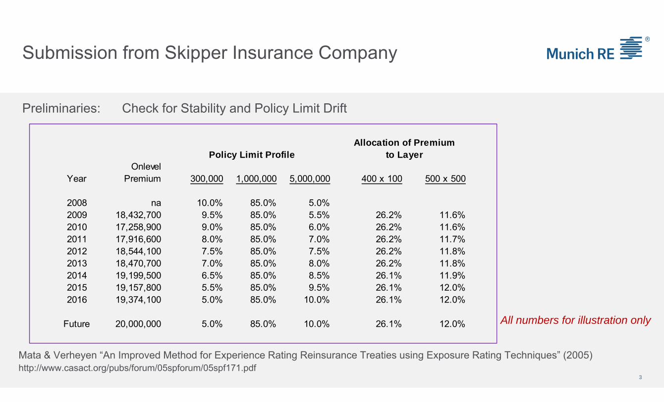
Preliminaries: Check for Stability and Policy Limit Drift

Mata & Verheyen “An Improved Method for Experience Rating Reinsurance Treaties using Exposure Rating Techniques” (2005)http://www.casact.org/pubs/forum/05spforum/05spf171.pdf

Policy Limit ProfileOnlevel

Year Premium 300,000 1,000,000 5,000,000 400 x 100 500 x 500

2008 na 10.0% 85.0% 5.0%2009 18,432,700 9.5% 85.0% 5.5% 26.2% 11.6%2010 17,258,900 9.0% 85.0% 6.0% 26.2% 11.6%2011 17,916,600 8.0% 85.0% 7.0% 26.2% 11.7%2012 18,544,100 7.5% 85.0% 7.5% 26.2% 11.8%2013 18,470,700 7.0% 85.0% 8.0% 26.2% 11.8%2014 19,199,500 6.5% 85.0% 8.5% 26.1% 11.9%2015 19,157,800 5.5% 85.0% 9.5% 26.1% 12.0%2016 19,374,100 5.0% 85.0% 10.0% 26.1% 12.0%

Future 20,000,000 5.0% 85.0% 10.0% 26.1% 12.0%

to LayerAllocation of Premium

All numbers for illustration only

Submission from Skipper Insurance Company

4

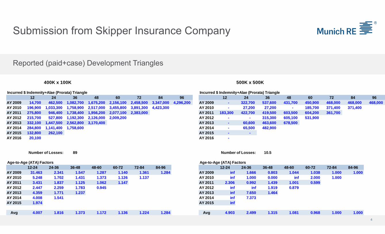
400K x 100K 500K x 500K

Incurred $ Indemnity+Alae (Prorata) Triangle Incurred $ Indemnity+Alae (Prorata) Triangle12 24 36 48 60 72 84 96 12 24 36 48 60 72 84 96

AY 2009 14,700 462,500 1,082,700 1,675,200 2,156,100 2,458,500 3,347,000 4,296,200 AY 2009 - 322,700 537,600 431,700 450,900 468,000 468,000 468,000 AY 2010 196,900 1,033,300 1,758,900 2,517,000 3,455,800 3,891,300 4,423,300 AY 2010 - 27,200 27,200 - 185,700 371,400 371,400 AY 2011 275,800 946,400 1,738,400 1,956,200 2,077,100 2,383,000 AY 2011 183,300 422,700 419,500 603,500 604,200 361,700 AY 2012 215,700 527,800 1,192,300 2,126,000 2,009,200 AY 2012 - - 315,300 605,100 531,900 AY 2013 332,100 1,447,500 2,562,800 3,170,400 AY 2013 - 60,600 463,600 678,500 AY 2014 284,800 1,141,400 1,758,600 AY 2014 - 65,500 482,900 AY 2015 132,800 262,100 AY 2015 - - AY 2016 20,100 AY 2016 -

Number of Losses: 89 Number of Losses: 10.5

Age-to-Age (ATA) Factors Age-to-Age (ATA) Factors12-24 24-36 36-48 48-60 60-72 72-84 84-96 12-24 24-36 36-48 48-60 60-72 72-84 84-96

AY 2009 31.463 2.341 1.547 1.287 1.140 1.361 1.284 AY 2009 inf 1.666 0.803 1.044 1.038 1.000 1.000AY 2010 5.248 1.702 1.431 1.373 1.126 1.137 AY 2010 inf 1.000 0.000 inf 2.000 1.000AY 2011 3.431 1.837 1.125 1.062 1.147 AY 2011 2.306 0.992 1.439 1.001 0.599AY 2012 2.447 2.259 1.783 0.945 AY 2012 inf inf 1.919 0.879AY 2013 4.359 1.771 1.237 AY 2013 inf 7.650 1.464AY 2014 4.008 1.541 AY 2014 inf 7.373AY 2015 1.974 AY 2015 inf

Avg 4.007 1.816 1.373 1.172 1.136 1.224 1.284 Avg 4.903 2.499 1.315 1.081 0.968 1.000 1.000

Reported (paid+case) Development Triangles

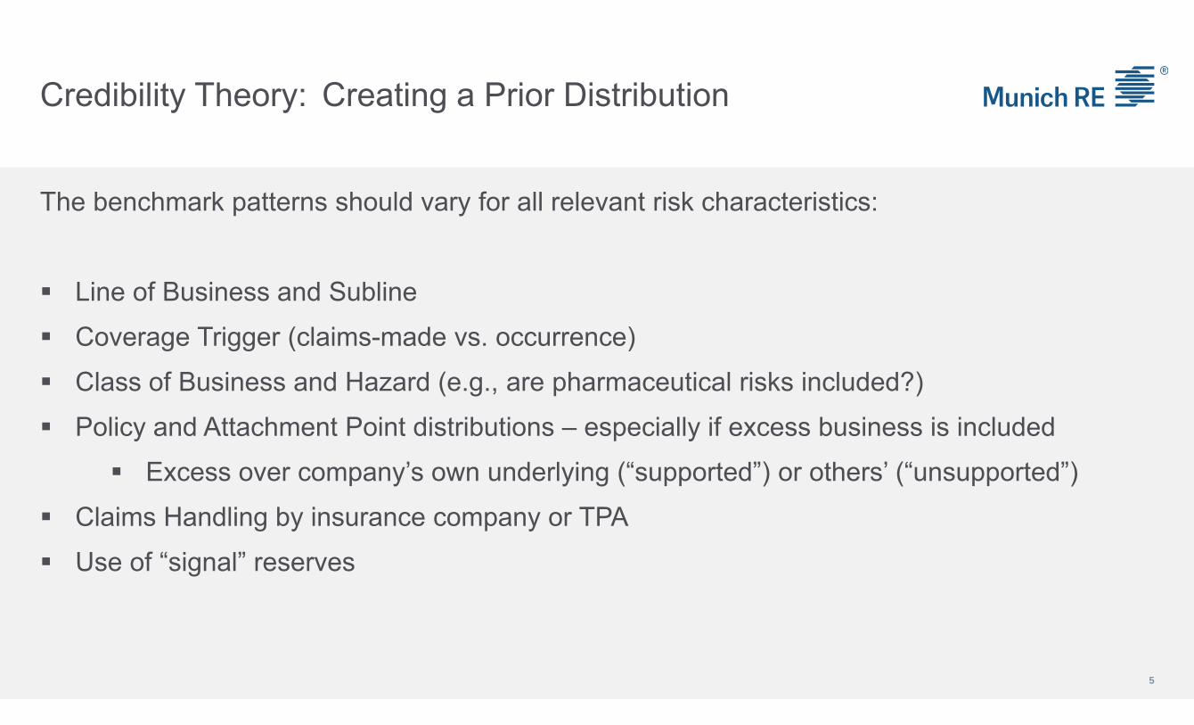
Credibility Theory: Creating a Prior Distribution

The benchmark patterns should vary for all relevant risk characteristics:

Line of Business and Subline

Coverage Trigger (claims-made vs. occurrence)

Class of Business and Hazard (e.g., are pharmaceutical risks included?)

Policy and Attachment Point distributions – especially if excess business is included

Excess over company’s own underlying (“supported”) or others’ (“unsupported”)

Claims Handling by insurance company or TPA

Use of “signal” reserves

5


6

We can estimate the distribution of tail factors (LDF at age 96 months) as a finite mixture of three categories.

But this still means the tail factor is somewhere between 1.050 and 1.500.

Ideally, these Fast/Medium/Slow categories would correspond to specific risk characteristics.



7

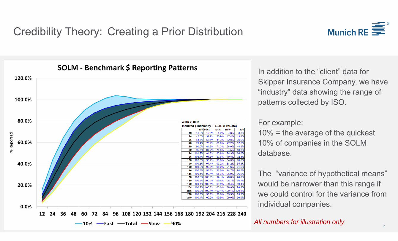
In addition to the “client” data for Skipper Insurance Company, we have “industry” data showing the range of patterns collected by ISO.

For example:10% = the average of the quickest 10% of companies in the SOLM database.

The “variance of hypothetical means” would be narrower than this range if we could control for the variance from individual companies.



8

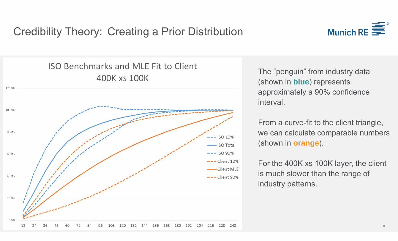
The “penguin” from industry data (shown in blue) represents approximately a 90% confidence interval.

From a curve-fit to the client triangle, we can calculate comparable numbers (shown in orange).

For the 400K xs 100K layer, the client is much slower than the range of industry patterns.


9

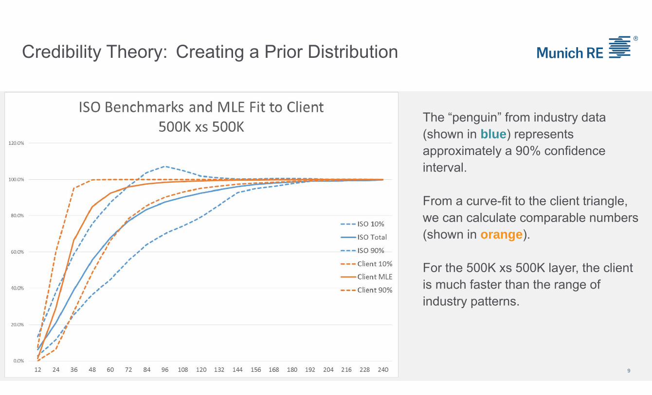
The “penguin” from industry data (shown in blue) represents approximately a 90% confidence interval.

From a curve-fit to the client triangle, we can calculate comparable numbers (shown in orange).

For the 500K xs 500K layer, the client is much faster than the range of industry patterns.

Credibility Theory: Bayesian Philosophy

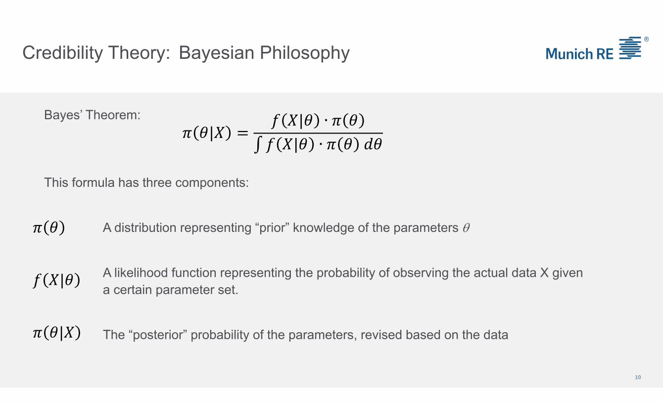
Bayes’ Theorem:

This formula has three components:

A distribution representing “prior” knowledge of the parameters

A likelihood function representing the probability of observing the actual data X given a certain parameter set.

The “posterior” probability of the parameters, revised based on the data

10

|

|

|| ∙| ∙

Credibility Theory: Conjugate Priors

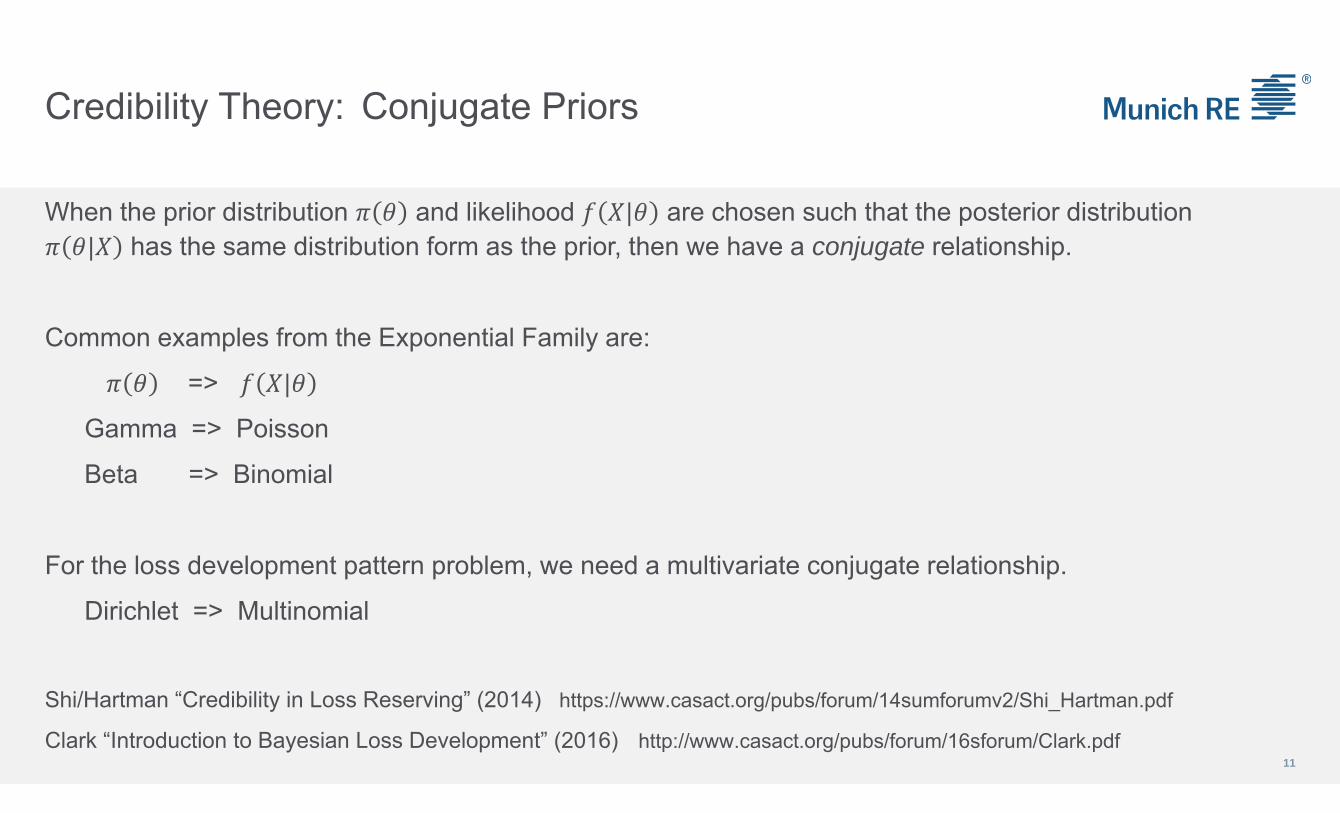
When the prior distribution and likelihood | are chosen such that the posterior distribution | has the same distribution form as the prior, then we have a conjugate relationship.

Common examples from the Exponential Family are:

=> |

Gamma => Poisson

Beta => Binomial

For the loss development pattern problem, we need a multivariate conjugate relationship.

Dirichlet => Multinomial

Shi/Hartman “Credibility in Loss Reserving” (2014) https://www.casact.org/pubs/forum/14sumforumv2/Shi_Hartman.pdf

Clark “Introduction to Bayesian Loss Development” (2016) http://www.casact.org/pubs/forum/16sforum/Clark.pdf11

Credibility Theory: Conjugate Priors

“Conjugate priors… have the desirable feature that prior information can be viewed as ‘fictitious sample information’ in that it is combined with the sample in exactly the same way that additional sample information would be combined.

“The only difference is that the prior information is ‘observed’ in the mind of the researcher, not in the real world.”

- Bayesian Econometric Methods; Koop, Poirier & Tobias

For actuaries, our “prior” knowledge comes from:

• Understanding the loss-generating process

• Having reviewed many, many triangles in the past (this should take the form of “as if” observed data)

12

Credibility Theory: Application

For our example, the creation of the credibility model follows these steps:

Select Expected Fast/Medium/Slow patterns

Create distribution around these patterns to mimic the range of the “penguins”

Estimate the “process” variance/mean ratio for the excess layers

Dispersion parameter in ODP model

Variance/Mean from exposure rating ≈ E[X2] / E[X]

13


14

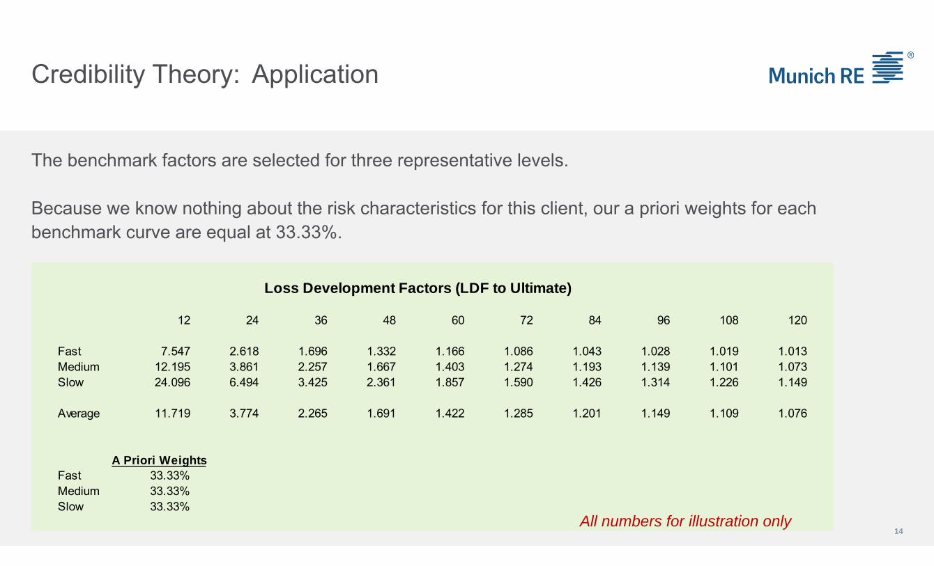
The benchmark factors are selected for three representative levels.

Because we know nothing about the risk characteristics for this client, our a priori weights for each benchmark curve are equal at 33.33%.

Loss Development Factors (LDF to Ultimate)

12 24 36 48 60 72 84 96 108 120

Fast 7.547 2.618 1.696 1.332 1.166 1.086 1.043 1.028 1.019 1.013Medium 12.195 3.861 2.257 1.667 1.403 1.274 1.193 1.139 1.101 1.073Slow 24.096 6.494 3.425 2.361 1.857 1.590 1.426 1.314 1.226 1.149

Average 11.719 3.774 2.265 1.691 1.422 1.285 1.201 1.149 1.109 1.076

A Priori WeightsFast 33.33%Medium 33.33%Slow 33.33%



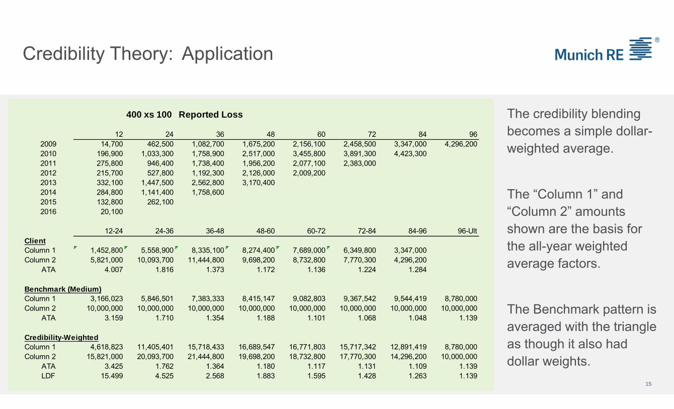
The credibility blending becomes a simple dollar-weighted average.

The “Column 1” and “Column 2” amounts shown are the basis for the all-year weighted average factors.

The Benchmark pattern is averaged with the triangle as though it also had dollar weights.

15

400 xs 100 Reported Loss

12 24 36 48 60 72 84 962009 14,700 462,500 1,082,700 1,675,200 2,156,100 2,458,500 3,347,000 4,296,2002010 196,900 1,033,300 1,758,900 2,517,000 3,455,800 3,891,300 4,423,3002011 275,800 946,400 1,738,400 1,956,200 2,077,100 2,383,0002012 215,700 527,800 1,192,300 2,126,000 2,009,2002013 332,100 1,447,500 2,562,800 3,170,4002014 284,800 1,141,400 1,758,6002015 132,800 262,1002016 20,100

12-24 24-36 36-48 48-60 60-72 72-84 84-96 96-UltClientColumn 1 1,452,800 5,558,900 8,335,100 8,274,400 7,689,000 6,349,800 3,347,000Column 2 5,821,000 10,093,700 11,444,800 9,698,200 8,732,800 7,770,300 4,296,200

ATA 4.007 1.816 1.373 1.172 1.136 1.224 1.284

Benchmark (Medium)Column 1 3,166,023 5,846,501 7,383,333 8,415,147 9,082,803 9,367,542 9,544,419 8,780,000Column 2 10,000,000 10,000,000 10,000,000 10,000,000 10,000,000 10,000,000 10,000,000 10,000,000

ATA 3.159 1.710 1.354 1.188 1.101 1.068 1.048 1.139

Credibility-WeightedColumn 1 4,618,823 11,405,401 15,718,433 16,689,547 16,771,803 15,717,342 12,891,419 8,780,000Column 2 15,821,000 20,093,700 21,444,800 19,698,200 18,732,800 17,770,300 14,296,200 10,000,000

ATA 3.425 1.762 1.364 1.180 1.117 1.131 1.109 1.139LDF 15.499 4.525 2.568 1.883 1.595 1.428 1.263 1.139


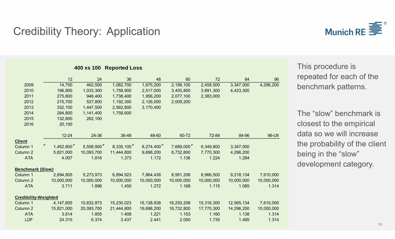
This procedure is repeated for each of the benchmark patterns.

The “slow” benchmark is closest to the empirical data so we will increase the probability of the client being in the “slow” development category.

16

400 xs 100 Reported Loss

12 24 36 48 60 72 84 962009 14,700 462,500 1,082,700 1,675,200 2,156,100 2,458,500 3,347,000 4,296,2002010 196,900 1,033,300 1,758,900 2,517,000 3,455,800 3,891,300 4,423,3002011 275,800 946,400 1,738,400 1,956,200 2,077,100 2,383,0002012 215,700 527,800 1,192,300 2,126,000 2,009,2002013 332,100 1,447,500 2,562,800 3,170,4002014 284,800 1,141,400 1,758,6002015 132,800 262,1002016 20,100

12-24 24-36 36-48 48-60 60-72 72-84 84-96 96-UltClientColumn 1 1,452,800 5,558,900 8,335,100 8,274,400 7,689,000 6,349,800 3,347,000Column 2 5,821,000 10,093,700 11,444,800 9,698,200 8,732,800 7,770,300 4,296,200

ATA 4.007 1.816 1.373 1.172 1.136 1.224 1.284

Benchmark (Slow)Column 1 2,694,805 5,273,973 6,894,923 7,864,438 8,561,208 8,966,500 9,218,134 7,610,000Column 2 10,000,000 10,000,000 10,000,000 10,000,000 10,000,000 10,000,000 10,000,000 10,000,000

ATA 3.711 1.896 1.450 1.272 1.168 1.115 1.085 1.314

Credibility-WeightedColumn 1 4,147,605 10,832,873 15,230,023 16,138,838 16,250,208 15,316,300 12,565,134 7,610,000Column 2 15,821,000 20,093,700 21,444,800 19,698,200 18,732,800 17,770,300 14,296,200 10,000,000

ATA 3.814 1.855 1.408 1.221 1.153 1.160 1.138 1.314LDF 24.315 6.374 3.437 2.441 2.000 1.735 1.495 1.314


17

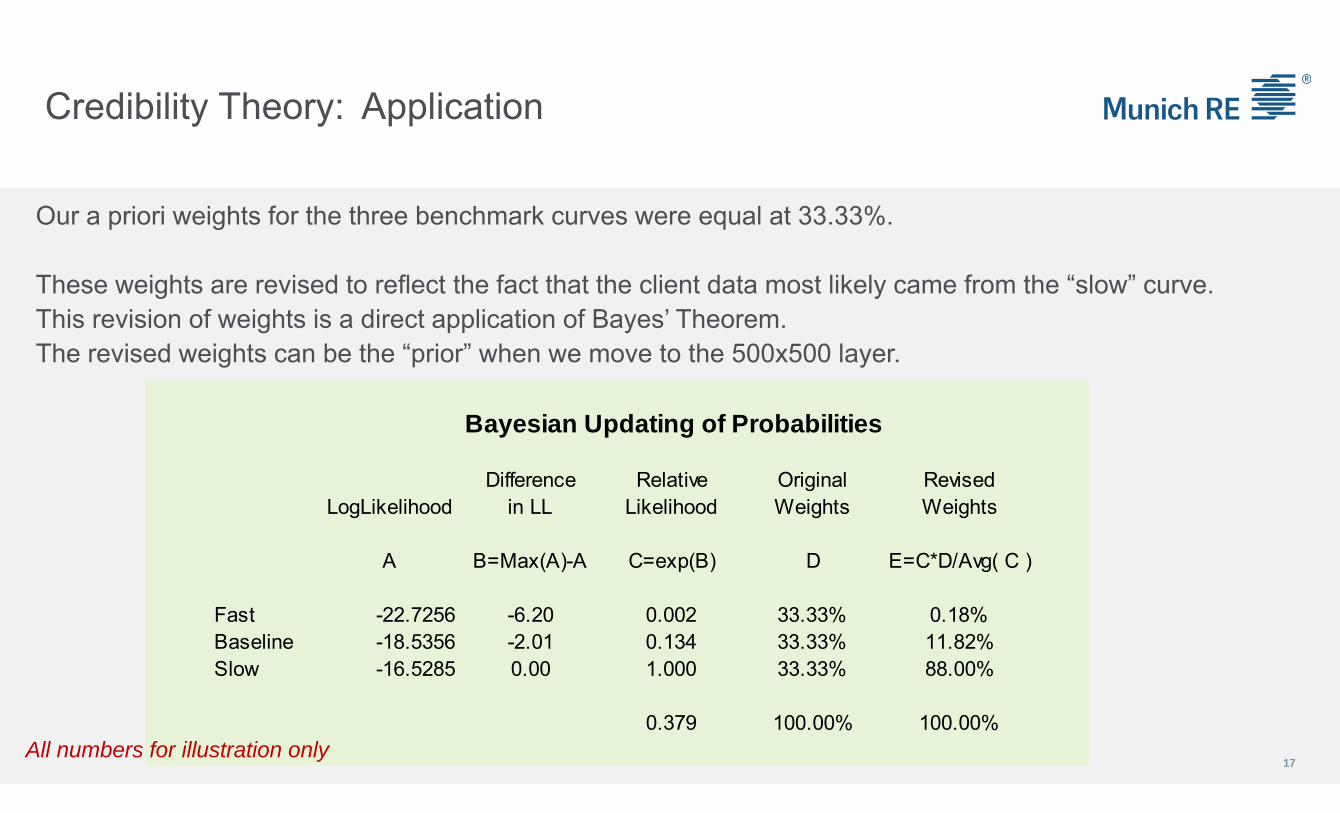
Our a priori weights for the three benchmark curves were equal at 33.33%.

These weights are revised to reflect the fact that the client data most likely came from the “slow” curve. This revision of weights is a direct application of Bayes’ Theorem.The revised weights can be the “prior” when we move to the 500x500 layer.

Bayesian Updating of Probabilities

Difference Relative Original RevisedLogLikelihood in LL Likelihood Weights Weights

A B=Max(A)-A C=exp(B) D E=C*D/Avg( C )

Fast -22.7256 -6.20 0.002 33.33% 0.18%Baseline -18.5356 -2.01 0.134 33.33% 11.82%Slow -16.5285 0.00 1.000 33.33% 88.00%

0.379 100.00% 100.00%All numbers for illustration only


18

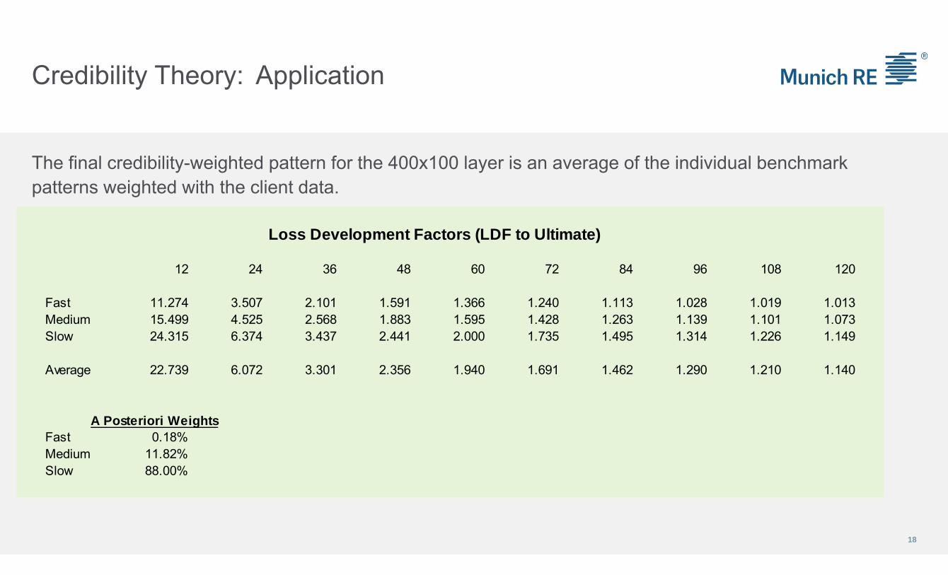
The final credibility-weighted pattern for the 400x100 layer is an average of the individual benchmark patterns weighted with the client data.


12 24 36 48 60 72 84 96 108 120

Fast 11.274 3.507 2.101 1.591 1.366 1.240 1.113 1.028 1.019 1.013Medium 15.499 4.525 2.568 1.883 1.595 1.428 1.263 1.139 1.101 1.073Slow 24.315 6.374 3.437 2.441 2.000 1.735 1.495 1.314 1.226 1.149

Average 22.739 6.072 3.301 2.356 1.940 1.691 1.462 1.290 1.210 1.140

A Posteriori WeightsFast 0.18%Medium 11.82%Slow 88.00%


19

The same procedure is followed for the 500x500 layer.

Instead of the initial 33.33% weights for each benchmark, however, we can start with the result from the 400x100 layer. Because of the low credibility for the 500x500 layer, the final pattern is close to the “slow” benchmark.


12 24 36 48 60 72 84 96 108 120

Fast 9.909 3.242 1.866 1.399 1.203 1.084 1.038 1.025 1.020 1.015Medium 16.705 4.811 2.474 1.760 1.462 1.286 1.195 1.143 1.109 1.081Slow 33.051 7.635 3.480 2.416 1.965 1.638 1.454 1.343 1.267 1.201

Average 29.273 7.087 3.303 2.303 1.880 1.582 1.414 1.313 1.244 1.184

A Posteriori WeightsFast 0.16%Medium 12.81%Slow 87.03%

Final Pricing: Experience Rating 400x100 Layer

20

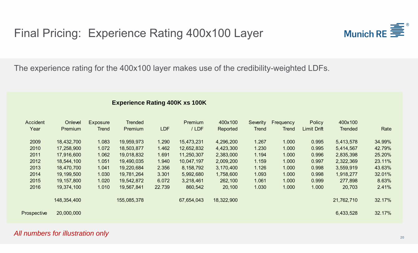
The experience rating for the 400x100 layer makes use of the credibility-weighted LDFs.


Experience Rating 400K xs 100K

Accident Onlevel Exposure Trended Premium 400x100 Severity Frequency Policy 400x100Year Premium Trend Premium LDF / LDF Reported Trend Trend Limit Drift Trended Rate

2009 18,432,700 1.083 19,959,973 1.290 15,473,231 4,296,200 1.267 1.000 0.995 5,413,578 34.99%2010 17,258,900 1.072 18,503,877 1.462 12,652,832 4,423,300 1.230 1.000 0.995 5,414,567 42.79%2011 17,916,600 1.062 19,018,832 1.691 11,250,307 2,383,000 1.194 1.000 0.996 2,835,398 25.20%2012 18,544,100 1.051 19,490,035 1.940 10,047,197 2,009,200 1.159 1.000 0.997 2,322,369 23.11%2013 18,470,700 1.041 19,220,684 2.356 8,158,792 3,170,400 1.126 1.000 0.998 3,559,919 43.63%2014 19,199,500 1.030 19,781,264 3.301 5,992,680 1,758,600 1.093 1.000 0.998 1,918,277 32.01%2015 19,157,800 1.020 19,542,872 6.072 3,218,461 262,100 1.061 1.000 0.999 277,898 8.63%2016 19,374,100 1.010 19,567,841 22.739 860,542 20,100 1.030 1.000 1.000 20,703 2.41%

148,354,400 155,085,378 67,654,043 18,322,900 21,762,710 32.17%

Prospective 20,000,000 6,433,528 32.17%

Final Pricing: Experience Rating 500x500 Layer

21

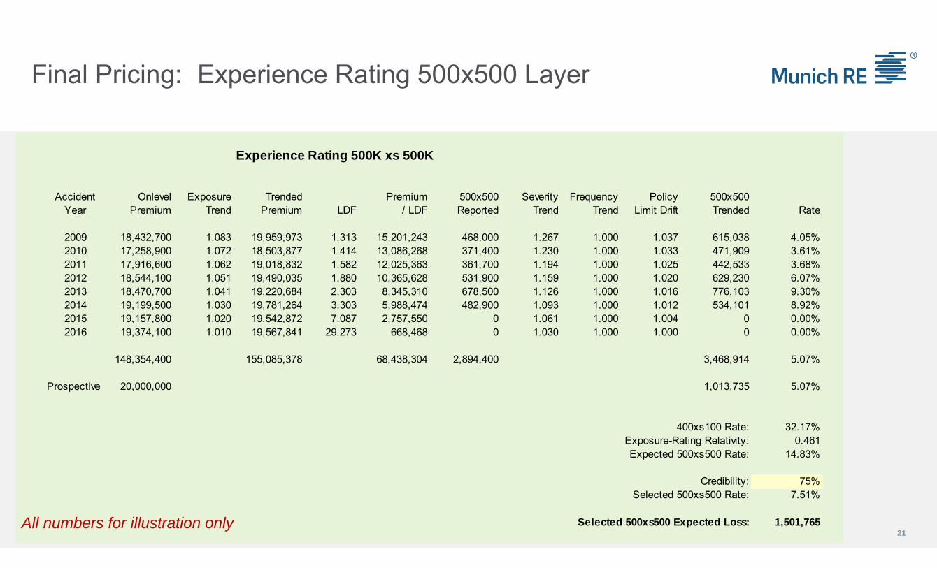
Experience Rating 500K xs 500K

Accident Onlevel Exposure Trended Premium 500x500 Severity Frequency Policy 500x500Year Premium Trend Premium LDF / LDF Reported Trend Trend Limit Drift Trended Rate

2009 18,432,700 1.083 19,959,973 1.313 15,201,243 468,000 1.267 1.000 1.037 615,038 4.05%2010 17,258,900 1.072 18,503,877 1.414 13,086,268 371,400 1.230 1.000 1.033 471,909 3.61%2011 17,916,600 1.062 19,018,832 1.582 12,025,363 361,700 1.194 1.000 1.025 442,533 3.68%2012 18,544,100 1.051 19,490,035 1.880 10,365,628 531,900 1.159 1.000 1.020 629,230 6.07%2013 18,470,700 1.041 19,220,684 2.303 8,345,310 678,500 1.126 1.000 1.016 776,103 9.30%2014 19,199,500 1.030 19,781,264 3.303 5,988,474 482,900 1.093 1.000 1.012 534,101 8.92%2015 19,157,800 1.020 19,542,872 7.087 2,757,550 0 1.061 1.000 1.004 0 0.00%2016 19,374,100 1.010 19,567,841 29.273 668,468 0 1.030 1.000 1.000 0 0.00%

148,354,400 155,085,378 68,438,304 2,894,400 3,468,914 5.07%

Prospective 20,000,000 1,013,735 5.07%

400xs100 Rate: 32.17%Exposure-Rating Relativity: 0.461Expected 500xs500 Rate: 14.83%

Credibility: 75%Selected 500xs500 Rate: 7.51%

Selected 500xs500 Expected Loss: 1,501,765All numbers for illustration only

Final Pricing: Aggregate Distribution

22

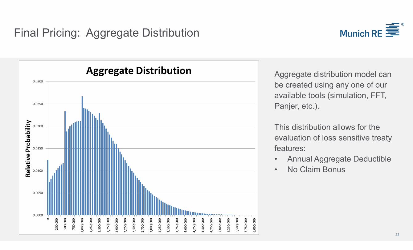
Aggregate distribution model can be created using any one of our available tools (simulation, FFT, Panjer, etc.).

This distribution allows for the evaluation of loss sensitive treaty features:• Annual Aggregate Deductible• No Claim Bonus

Final Pricing

The selection of expected losses to the 500K xs 500K layer is the starting point for our pricing.

Additional Costs for ECO/XPL?

Aggregate Distribution for loss-sensitive features

Investment Income and NPV calculation

Profit and Expense loads

23

Thank YouDave ClarkMunich Reinsurance America, [email protected]://twitter.com/DaveclarkR

© Copyright 2018 Munich Reinsurance America, Inc. All rights reserved. "Munich Re" and the Munich Re logo are internationally protected registered trademarks. The material in this presentation is provided for your information only, and is not permitted to be further distributed without the express written permission of Munich Reinsurance America, Inc. or Munich Re. This material is not intended to be legal, underwriting, financial, or any other type of professional advice. Examples given are for illustrative purposes only. Each reader should consult an attorney and other appropriate advisors to determine the applicability of any particular contract language to the reader's specific circumstances.

Credibility in Loss Development:

Documents

Transcript of Credibility in Loss Development: