WATER HAMMER MODELING AND ANALYSIS FOR ...

WATER HAMMER MODELING AND ANALYSIS FOR

KHOBAR-DAMMAM WATER TRANSMISSION RING LINE

HUSSAIN TALEB AMMAR

CIVIL AND ENVIRONMENTAL ENGINEERING

MAY 2014

iii

© Hussain Taleb Ammar

2014

iv

To My Parents, Wife, Brothers and Sister.

v

ACKNOWLEDGMENTS

In the name of Allah, the Most Merciful, the Most Compassionate

I would like to express my sincere appreciation and gratitude to the chairman of my

thesis committee Dr. Muhammad Al-Zahrani for his valuable guidance, support and

encouragement throughout this work. I highly acknowledge the encouragement and

valuable suggestions from thesis committee members Dr. Shakhwat Choudhury and Dr.

Mohammad Al-Suwiyan.

I am deeply grateful to the Civil and Environmental Engineering Department at

King Fahd University of Petroleum & Minerals and Al Khobar branch of the General

Directorate of Water in Eastern Region for providing the necessary support to conduct this

study. Special thank goes to Eng. Faleh Al-Faleh, Eng. Mohammed Al-Abbad, and Eng.

Suhail Al-Moamen for providing the necessary data for this research study and for

facilitating the access to the KDRL facilities.

I would like to extend my thanks to Dr. Adel Abu-Jouda for his constructive

suggestion with the hammer analysis and to Eng. Mohammed Hisham for his assistance

with the surge protection analysis. My thanks also go to Mr. Adnan Al-Hajji and Dr. Amin

Abo-Monaser for his support and valuable technical suggestions. I am also thankful to

Eng. Khalid and Eng. Ashraf of Aramoon International Company, Eng. Abbas and Eng.

Mohammed Hamza of the CWC for helping me with data collection.

A special gratitude and dedication of this work is due to my parents, my wife,

brothers, sister, grandmothers, uncles and aunts for their support and encouragement

throughout this period.

vi

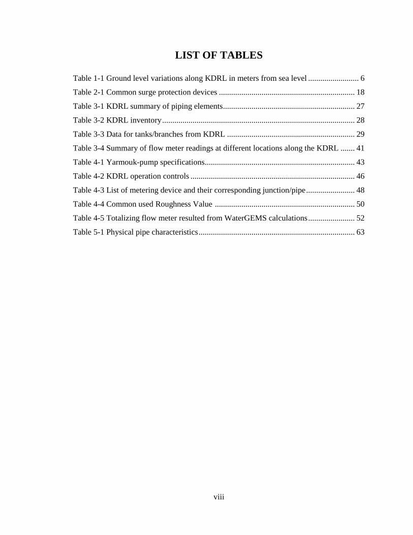
TABLE OF CONTENTS

ACKNOWLEDGMENTS ............................................................................................................. V

TABLE OF CONTENTS ............................................................................................................. VI

LIST OF TABLES ..................................................................................................................... VIII

LIST OF FIGURES ...................................................................................................................... IX

LIST OF ABBREVIATIONS ...................................................................................................... XI

ABSTRACT ................................................................................................................................ XII

ARABIC ABSTRACT .............................................................................................................. XIV

CHAPTER 1 INTRODUCTION ................................................................................................. 1

1.1 Background ..................................................................................................................................... 1

1.2 Problem Statement ......................................................................................................................... 4

1.3 Objectives of the Research .............................................................................................................. 6

1.4 Research Methodology ................................................................................................................... 8

CHAPTER 2 LITERATURE REVIEW ................................................................................... 10

2.1 Introduction .................................................................................................................................. 10

2.2 Water Distribution System Hydraulics .......................................................................................... 11

2.3 Water Hammer Governing Equations............................................................................................ 13

2.4 Modeling and Analysis of the Water System ................................................................................. 16

2.5 Water Hammer Protections .......................................................................................................... 17

2.6 Previous Researches ..................................................................................................................... 19

CHAPTER 3 KHOBAR-DAMMAM WATER RING LINE .................................................. 23

3.1 Characteristics of KDRL ................................................................................................................. 23

3.2 Flow and Pressure Measurements ................................................................................................ 35

vii

CHAPTER 4 HYDRAULIC MODELING OF KDRL ............................................................. 42

4.1 Model Construction and Execution ............................................................................................... 42

4.2 Model Calibration ......................................................................................................................... 52

CHAPTER 5 WATER HAMMER MODELING & ANALYSIS ............................................ 58

5.1 Background ................................................................................................................................... 58

5.2 Scenario 1: Power Failure and Pump Sudden Shutdown ............................................................... 64

5.3 Scenario 2: Sudden Closure of All Valves ....................................................................................... 69

5.3.1 Sudden Closure of KFUPM Valve .............................................................................................. 69

5.3.2 Sudden Closure of Doha3 Valve ................................................................................................ 71

5.3.3 Sudden Closure of All Valves .................................................................................................... 74

CHAPTER 6 WATER HAMMER CONTROL ....................................................................... 76

6.1 Background ................................................................................................................................... 76

6.2 Isolating Branched Pipes from KDRL ............................................................................................. 76

6.3 Power Failure Protection .............................................................................................................. 83

6.4 All Valves Sudden Closure Protection ............................................................................................ 86

CHAPTER 7 CONCLUSION AND RECOMMENDATIONS ................................................ 89

REFERENCES............................................................................................................................. 92

APPENDICES ............................................................................................................................. 95

Appendix A ............................................................................................................................................ 96

Appendix B ........................................................................................................................................... 100

Appendix C ........................................................................................................................................... 103

Appendix D .......................................................................................................................................... 113

VITAE ....................................................................................................................................... 118

viii

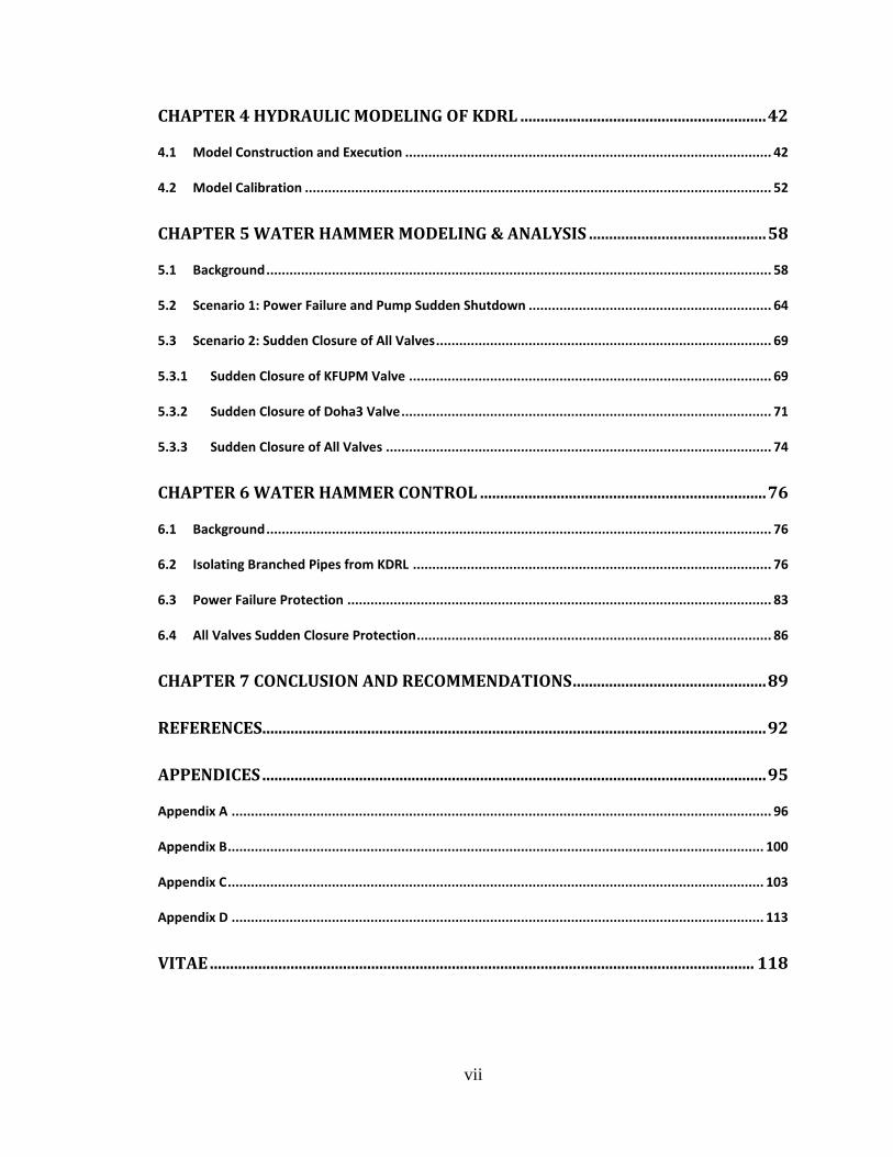
LIST OF TABLES

Table 1-1 Ground level variations along KDRL in meters from sea level ......................... 6

Table 2-1 Common surge protection devices ................................................................... 18

Table 3-1 KDRL summary of piping elements................................................................. 27

Table 3-2 KDRL inventory ............................................................................................... 28

Table 3-3 Data for tanks/branches from KDRL ............................................................... 29

Table 3-4 Summary of flow meter readings at different locations along the KDRL ....... 41

Table 4-1 Yarmouk-pump specifications.......................................................................... 43

Table 4-2 KDRL operation controls ................................................................................. 46

Table 4-3 List of metering device and their corresponding junction/pipe ........................ 48

Table 4-4 Common used Roughness Value ..................................................................... 50

Table 4-5 Totalizing flow meter resulted from WaterGEMS calculations ....................... 52

Table 5-1 Physical pipe characteristics ............................................................................. 63

ix

LIST OF FIGURES

Figure 1-1 Schematic drawing showing KDRL.................................................................. 5

Figure 2-1 Wave characteristics in x-t plan to express the MOC [5] ............................... 15

Figure 3-1 Daily water supply from KDRL for the month of October, 2013 ................... 24

Figure 3-2 GIS map of the layout of KDRL ..................................................................... 25

Figure 3-3 Ground elevation and locations of branched pipelines along the KDRL ........ 26

Figure 3-4 Sample washout valve in KDRL ..................................................................... 30

Figure 3-5 Sample air valves installed in KDRL .............................................................. 31

Figure 3-6 Sample branching connection in KDRL ......................................................... 32

Figure 3-7 Types of flow/pressure meters installed in KDRL .......................................... 34

Figure 3-8 Installed flow/pressure meters on-site ............................................................. 34

Figure 3-9 Location of flow/pressure meter. .................................................................... 36

Figure 3-10 Flow and pressure readings at KFUPM collected on 1st and 2nd May13 ..... 38

Figure 3-11 Flow and pressure readings at Dana collected on 1st and 2nd May13 ............ 38

Figure 3-12 Flow and pressure readings at Khaleej collected on 1st and 2nd May13 ........ 38

Figure 3-13 Flow and pressure readings at Yarmouk from 18th to 23rd August13 ........... 39

Figure 3-14 Flow and pressure readings at KFUPM from 18th to 23rd August13 ............ 39

Figure 3-15 Flow and pressure readings at Doha-3 from 18th to 23rd August13 .............. 40

Figure 3-16 Flow and pressure readings at Dana from 18th to 23rd August13 .................. 40

Figure 4-1 KDRL schematic from WaterGEMS .............................................................. 44

Figure 4-2 Representation of Yarmouk tank station in the network ................................. 45

Figure 4-3 Details schematic of a branch from KDRL ..................................................... 47

Figure 4-4 HGL over KDRL (Steady-State Analysis) ...................................................... 51

Figure 4-5 water level variation calculated over the period 28-30 Oct 2013 ................... 53

Figure 4-6 Pumped flow during 28-30 October 2013 ....................................................... 53

Figure 4-7 Sub-model calibration correlation results ....................................................... 55

Figure 4-8 KDRL model calibration correlation results ................................................... 55

Figure 4-9 Comparison of water level variation at Yarmouk tank ................................... 56

Figure 4-10 Comparison of the pumped flow ................................................................... 56

Figure 4-11 HGL at Yarmouk flow meter (28-30 Oct) based on the calibrated model .... 57

Figure 5-1 Pressure/surge wave split from small to larger pipe ...................................... 61

x

Figure 5-2 Pressure/surge wave split from large to smaller pipe, with a dead end .......... 61

Figure 5-3 Pressure/surge wave movement and reflection through a pipe segments ....... 62

Figure 5-4 Sample effects of water hammer ..................................................................... 65

Figure 5-5 Surge wave effect along KDRL due to pump sudden shut down ................... 67

Figure 5-6 Surge wave effect along KFUPM branch due to pump sudden shut down .... 67

Figure 5-7 Surge wave effect along Doha3 branch due to pump sudden shut down ........ 68

Figure 5-8 Surge wave effect along Doha1 branch due to pump sudden shut down ........ 68

Figure 5-9 Surge wave variation along KDRL due to sudden valve closure at KFUPM . 70

Figure 5-10 Surge wave variation along KFUPM due sudden valve closure at KFUPM 70

Figure 5-11 Surge wave variation at Doha3 due to sudden valve closure at KFUPM ..... 71

Figure 5-12 Surge wave variation along KDRL due to sudden valve closure at Doha3 .. 72

Figure 5-13 Surge wave variation at KFUPM due to sudden valve closure at Doha3 ..... 72

Figure 5-14 Surge wave variation at Doah3 due to sudden valve closure at Doha3 ........ 73

Figure 5-15 Surge wave variation along DKRL due to sudden closure of all valves ....... 74

Figure 5-16 Surge wave variation at KFUPM due to sudden closure of all valves .......... 75

Figure 5-17 Surge wave variation at Doah3 due to sudden closure of all valves ............. 75

Figure 6-1 Existing setup, tank valve and check valve in the upstream ( case A )........... 77

Figure 6-2 Proposed setup, tank valve upstream and check valve downstream ( case B )77

Figure 6-3 Proposed setup, tank valve and check valve downstream the pipe ( case C ) . 77

Figure 6-4 Hammer analysis results comparison for cases A, B, and C– main pipeline .. 79

Figure 6-5 Hammer analysis results comparison for cases A, B, and C – KFUPM ........ 81

Figure 6-6 Water hammer analysis comparison for cases A, B, and C – Doha3 .............. 82

Figure 6-7 Surge protection using surge vessel – main pipeline ...................................... 84

Figure 6-8 Surge protection using surge vessel – KFUPM .............................................. 84

Figure 6-9 Surge protection using surge vessel – Doha3 ................................................. 85

Figure 6-10 Optimized protection at sudden closure of all pipes – main pipeline ........... 88

Figure 6-11 Optimized protection considering sudden closure of all pipes – KFUPM ... 88

xi

LIST OF ABBREVIATIONS

KDRL : Khobar-Dammam Ring Line

MOC : Method of Characteristics

WCM : Wave Characteristics Method

GIS : Geographic Information Systems

EPA : Environmental Protection Agency (USA)

DI : Ductile Iron Pipe

FRP : Fiber Reinforced Polymer Pipe

UPVC : Un-plasticized polyvinylchloride Pipe

CCP : Circular Concrete Pipe

PRV : Pressure Relief Valve – Surge Control

FCV : Flow Control Valve

P3 : Pressure Sensor and Logger (continues logging)

FM : Flow Meter

HGL : Hydraulic Grade Line

WaterGEMS : Water Modeling Program with GIS capabilities (Bentley)

xii

ABSTRACT

Full Name : HUSSAIN TALEB AMMAR

Thesis Title : Water Hammer Modeling and Analysis for Khobar-Dammam Water

Transmission Ring Line

Major Field : Civil & Environmental Engineering - Water Resources and

Environmental Engineering

Date of Degree : May 2014

Water hammer or hydraulic transient is a common problem in water distribution

systems especially for water transmission pipelines. Hydraulic transient events in water

distribution system can cause significant damage and disruption in the system, thus, it has

been a subject of many research studies. One major pipeline that connects the water supply

of two major cities (Khobar and Dammam) in the Eastern Province of Saudi Arabia is the

Khobar-Dammam Ring Line (KDRL). This transmission line is vulnerable to a potential

water hammer problem as it is controlled by the water level in two main tanks at its both

ends. In addition, six other sub tanks along the KDRL are expected to increase the

probability of water hammer occurrences in the system.

In this research, two widely used hydraulic simulation models were adapted to model

and analyze the hydraulic and transient (water hammer) behavior in the KDRL. The two

hydraulic programs were WaterGEMS and HAMMER. The WaterGEMS was used to

simulate the hydraulics of the transmission pipeline under normal conditions, while the

xiii

HAMMER was used to analyze the occurrence of the water hammer and simulate different

water hammer protection scenarios.

Based on the analysis, several water hammer protection devices were tested and

approved to provide a complete protection against the water hammer for the system.

Moreover, appropriate operational control measures were proposed to be adopted by the

Water Authority to minimize the probability of water hammer occurrence and to protect

the KDRL form the water hammer.

xiv

ملخص الرسالة

حسين طالب أحمد بن عمار :م الكاملاالس

اه بين مدينتي الدمام و الخبر.لميالناقل لالنمذجة والتحليل لمطرقة المياه للخط الحلقي :عنوان الرسالة

هندسة مصادر المياه و البيئة -الهندسة المدنيه و البيئه التخصص:

4102 مايو تاريخ الدرجة العلمية:

أحد المشاكل الشائعة في أنظمة توزيع المياه وبالخصوص في الخطوط الناقلة. لذلك كان هذا لمياه مطرقة اتعتبر

الباحثين. إن عملية التشغيل للخط الحلقي الناقل للمياه بين مدينتي الدمام و الخبر تعتمد على مام الموضوع محل إهت

لخط الحلقي الناقل وباتصله ضافة إلى الخزانا المفي الدمام باإل 55مستوى المياه بخزان اليرموك في الخبر و خزان

مائيه للمطرقه التعرض الخط الناقل من إحتمالية مما يزيد وهذا ما يجعل من عملية التشغيل معقدة على إمتداده،الواقعه

بشكل متكرر.

لنمذجة وتحليل مطرقة اسعي االنتشار اذج المحاكاة الهيدروليكيه ونماثنين من في هذا البحث تم استخدام

. HAMMERو WaterGEMS البرنامجان الهيدروليكيان المستخدمان هما (. KDRLأنبوب الماء ) في الماء

في ظل ظروف طبيعية، في حين تم استخدام للمحاكاة الهيدروليكية لخط أنابيب الماء WaterGEMSوقد تم استخدام

HAMMER حدوث المطرقة المائية. عندمختلفة لحماية أنبوب الماء حلولاة لتحليل حدوث المطرقة المائية ومحاك

دروليكيةهيتم اختبارها وأثبتت التحاليل الوالتي استنادا إلى التحليل، تم اختيار مجموعة من مختلف أجهزة الحماية

ليتم تدابير مناسبة الحماية الكاملة من المطرقة المائية لألنبوب . وعالوة على ذلك، تم اقتراح جدراتها في توفير

KDRL نقل المياهأنبوب للتقليل من احتمال حدوث المطرقة المائية وحماية اعتمادها من قبل مصلحة المياة

المطرقة المائية. من

1

1 CHAPTER 1

INTRODUCTION

1.1 Background

Water Hammer, which is known as a water surge, is a pressure wave caused when there

is a sudden change in flow or pressure condition at a point in the system, e.g. sudden valve

closure. These waves propagate throughout the system causing change in pressure and

flow, positive transient waves called up-surge while negative transient waves called down-

surge.

Water hammer has been responsible for water distribution network component failure,

pipeline breakage or collapse, loose at connections, and intrusion of dirty water into the

water distribution system. Therefore, water hammer is considered to be a threat to the

public in terms of cost, health and safety. Negative pressure in the system for example,

represents a major risk of introducing unwanted and possibly hazardous species like

bacteria into the water system. This will significantly affect water quality. Thus, the control

of water hammer pressure in transmission pipelines is essential for economical and safe

operation.

2

The following are some of the general causes of water hammer [1]:

o Pump startup/shutdown.

o Valve opening/closing.

o Rapid change in demand in certain location(s) (e.g. hydrant flushing).

o Change in transmission condition (e.g. pipe breakage).

o Pipe filling or draining (e.g. air release from pipe).

o Change in boundary condition (e.g. pressure change in tank).

One of following solutions can generally mitigate water hammer [1]:

o Altering piping system characteristics.

o Improvement of operational procedure and operational control conditions.

o Installation of surge protection system.

There has been significant research in the area to investigate and propose solutions to

the water hammer phenomenon. The most widely accepted approximate equations to

model the water hammer are:

1- Method of Characteristics (MOC).

2- Wave Characteristics Method (WCM).

3

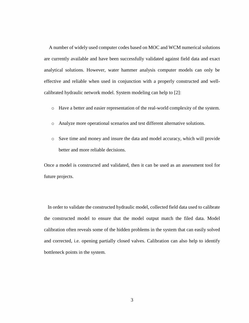
A number of widely used computer codes based on MOC and WCM numerical solutions

are currently available and have been successfully validated against field data and exact

analytical solutions. However, water hammer analysis computer models can only be

effective and reliable when used in conjunction with a properly constructed and well-

calibrated hydraulic network model. System modeling can help to [2]:

o Have a better and easier representation of the real-world complexity of the system.

o Analyze more operational scenarios and test different alternative solutions.

o Save time and money and insure the data and model accuracy, which will provide

better and more reliable decisions.

Once a model is constructed and validated, then it can be used as an assessment tool for

future projects.

In order to validate the constructed hydraulic model, collected field data used to calibrate

the constructed model to ensure that the model output match the filed data. Model

calibration often reveals some of the hidden problems in the system that can easily solved

and corrected, i.e. opening partially closed valves. Calibration can also help to identify

bottleneck points in the system.

4

For the purpose of hydraulic modeling; especially for complex systems, a simplified

representation of the hydraulic network usually used. A process called “Skeletonization”

where selected pipes (main) chosen to represent original network while preserving the

operational performance and integrity of the larger original system [2]. This a common

practice in hydraulic modeling and analysis, but should be avoided in the water hammer

analysis, as it would lead to wrong decisions, skelatel model is not capable of representing

the origin model in case of hammer analysis, as the hammer analysis is strongly dependent

on the system characteristics.

1.2 Problem Statement

In this research, the Dammam-Khobar Water Transmission Ring Line (KDRL) will be

investigated for the water hammer problem. KDRL is an 18-kilometer water transmission

pipeline with a diameter of 700 mm, connecting Yarmouk water tank in Khobar to tank-55

in Dammam. The pipeline was designed to operate for emergency conditions to ensure no

water shortages will occur in any one of the two cities. Later, it was decided to use KDRL

for delivering water directly to districts located along the pipeline. Currently, there are six

additional sub tanks connected to the KDRL, and one direct connection to a sub network.

Figure 1.1 shows a schematic drawing of the KDRL and all the sub tanks connected to it.

5

Figure 1-1 Schematic drawing showing KDRL

Dammam and Khobar are the two main cities in the eastern region of the Kingdom of

Saudi Arabia with the highest population density in the region. Tank-55 is the only

desalinated water source for Dammam city. This desalinated water is mixed with

groundwater at blending stations before it is distributed to the city. On the other hand,

Yarmouk Tank is the only desalinated water source for Khobar. Any failure in the KDRL

will impact the desalinated water supply to districts along the KDRL, necessitating the use

of backup raw water (groundwater) supply.

Moreover, the high-water pressure KDRL is laid along the highway with a high traffic

density. Therefore, in case any sudden rupture occurs along the pipeline, then there will

be a potential life-threatening incident to the highway users or to the people living close

by. The layout of the pipeline and the water hydraulic regime create several high and low

pressure points, which raise the risk of developing a water hammer phenomenon. Table 1.1

6

shows the ground level layout variations in the KDRL, which cause pressure variations

along the pipeline which seriously impact and complicate the pipeline operation.

Table 1-1 Ground level variations along KDRL in meters from sea level

Start Highest Lowest 2nd High End

Level Level Level Level Level

29.5 52.5 26 51 33

KDRL is operated and controlled by the water levels of the eight different tanks along

it. The water pressure along the pipeline is affected by the operation conditions of the

valves (opening/closing) and the pumps (off/on), which could generate surge waves in the

system. Therefore, it is recommended that the current daily KDRL operation be

investigated to come up with an operational strategy that help controlling or minimizing

the risk of water hammer.

1.3 Objectives of the Research

Water hammer causes a rapid change in the pressure that creates a wave of large

magnitude fluctuating along the pipeline, affecting the network components. In addition,

high pressure could exceed the safe operational pressure of the system causing pipe rapture.

Even if a safe operating pressure is not exceeded, the fatigue load of cyclic surge pressure

will reduce the life span of the system component. On the other hand, low pressure can

lead to cavitation, column separation, and can cause pipe collapse or promote intrusion of

7

outside water, air, or contaminants. Also, water hammer can cause a hydraulic vibration

of the pipeline at its connections and supports, causing leak or connections loose.

Therefore, water hammer analysis is more important than the conventional steady-state

analysis carried out by piping system designers, and it should be considered in the structural

design of the pipeline. “It has been reported that any optimized design that fails to properly

account for water hammer effects is likely to be, at best, suboptimal and, at worst,

completely inadequate” [3].

The main objectives of this study are:

(a) Construct a reliable water hydraulic model for the water transmission ring-line

connecting Dammam and Khobar (KDRL) to simulate the existing operation.

(b) Use the model to investigate the water hammer phenomenon in the KDRL and

simulate the effect of different protections in order to assist the Water Authority to

control or reduce the risk associated with water hammer.

(c) Identify existing major factors effecting the KDRL operation as well as revealing

problems in existing operational policy based on field observations.

(d) Recommend proper control devices that can help resolving or minimizing the

occurrence of water hammer along KDRL transmission line.

8

1.4 Research Methodology

To achieve the objectives of the study, several operational scenarios and approaches

will be analyzed using WaterGEM and HAMEER simulation programs. First hydraulic

simulation of KDRL will be conducted using WaterGEM followed by a water hammer

analysis using HAMMER simulation model. Following are the procedures to achieve the

goals of this study:

o Collection of data relevant to operational procedure and control conditions of the

KDRL.

o Field Survey to collect data about KDRL component and pipeline profile.

o Installation of flow/pressure meters at both ends of the KDRL and all branches from

the main pipeline to the sub tanks.

o Construction of GIS model of the KDRL to be exported to the Hydraulic Modeling

Program WaterGEMS.

o Initial runs of the model to simulate the operational conditions.

o Model analysis for the steady-state and extended-period simulation using

WterGEMS.

o Data collection from all metering points.

o Model calibration using real-field operational data, including readings collected at

the metering points.

o Correction of all field problems as revealed by the calibration process.

o Simplification of the model for the water hammer analysis after a reliable hydraulic

model is obtained.

9

o Investigation of the water hammer in the KDRL using HAMMER.

o Simulation of the protection mechanism using surge protection devise or

combination of devises. Table 2.1 lists major protection devices under

consideration.

o Recommendations to improve the current operational procedure to minimize the

probability of the occurrence of the water hammer in the KDRL.

10

2 CHAPTER 2

LITERATURE REVIEW

2.1 Introduction

Delivery of sufficient and safe water is essential for the community. However,

water delivery through a large pipeline network is usually associated with different

problems such as water hammer or hydraulic transient. Water hammer usually

occurred when the flow is caused to suddenly stop or change direction, leading to a

surge of propagating wave. Several actions during pipe network operation can generate

water hammer phenomena such as a sudden valve closure or during a water pump

startup/shutdown. This phenomenon can cause major problems such as noise/vibration,

or pipe rupture/collapse. In addition, the water transient flow during a water hammer

event will have significant impact on the water quality and, therefore, health

implications.

Water hammer has become one of the major research area in hydraulic studies due

to its major impact on the process of water delivery. This chapter will cover the

following:

The basic fundamentals of water hydraulics.

Causes of unsteady flow and the governing equations.

Water hammer modeling programs adopted in this research.

11

General mitigations and protections against water hammer.

Previous studies.

2.2 Water Distribution System Hydraulics

Water distribution network consists of pipes connected to a water source such as a

reservoir or a tank to transport water from a source to customers in the required quantity

and within acceptable quality measures. The pipeline is equipped with valves, nodes

or junctions, pumps, and other components like flow/pressure meters, and fittings.

Analysis of water distribution involves the determination of nodal pressure (head) and

pipe flow rates that satisfy the principles of mass and energy conservations. The mass

conservation or continuity states that the algebraic sum of the flow rates in all the

elements meeting at a junction, together with any external flows, is zero. The energy

conservation, on the other hand, states that the algebraic sum of the headlosses in each

element, combined with any head generated by pumps, around any closed loop formed

by hydraulic components, is zero.

There are many alternative formulations for the system governing equations and

techniques to solve these equations. The process of the water transmission within a

close conduit is governed by the conservation of mass equation (Eq. 2.1), and the

energy law presented (Eq. 2.2) [2, 4].

12

The general form of the continuity equation is as follows:

∑ 𝑄𝐼𝑁 ∆t = ∑ 𝑄𝑂𝑈𝑇 ∆t + ∆𝑉𝑠 (2.1)

Where,

QIN = Total flow into the node

QOUT = Total demand at the node

Z = Elevation

Vs = Change in storage volume

t = Change in time

The energy equation between any two points can be express as:

𝑃1

𝛾+ 𝑍1 +

𝑉12

2𝑔+ ℎ𝑃 =

𝑃2

𝛾+ 𝑍2 +

𝑉22

2𝑔+ ℎ𝐿 (2.2 )

Where,

P = Pressure

γ = Specific weight

Z = Elevation

V = Velocity

hp = Head gain

hL = Combined head loss

The combined headloss in the above equation account for losses in the energy is

due to friction and other minor losses such as at valves or fittings. Different equations

are used to compute the friction losses in the water network distribution such as Hazen-

William and Darcy-Weisbach.

13

2.3 Water Hammer Governing Equations

The general cause of the water hammer is a rapid change in the velocity of the fluid.

Such event could occur if there is a sudden valve closure, pump startup/shutdown, or a

sudden change in flow direction. This sudden change generates a pressure wave that

propagates throughout the system at supersonic speed, causing a change in the flow

and pressure.

The governing equations for the unsteady/transient flow (during the water hammer

event) are derived from the basic laws of physics: the low of conservation of mass and

the law of conservation of energy. The first law is presented as the continuity equation

whereas the latter is presented as the momentum equation. Both equations are

simplified to the case of one dimensional incompressible fluid flow, which matches the

objective of this research study [1, 2, 5].

The simplified form of the Continuity Equation is as follows:

𝜕𝐻

𝜕𝑡+

𝑎2

𝑔

𝜕𝑉

𝜕𝑥= 0 (2.3)

Where

a = Pressure wave speed

V = Average velocity in the x direction

H = Hydraulic grade line (HGL)

14

The momentum equation, can be expressed as:

𝜕𝑉

𝜕𝑡+ 𝑔

𝜕𝐻

𝜕𝑥+

𝑓 𝑉 |𝑉|

2𝐷= 0 (2.4)

Where

a = Pressure wave speed

V = Average velocity in the direction of x

H = HGL

f = Darcy-Weisbach friction coefficient

D = Inside diameter of the pipe

The above equation is valid under the following assumptions:

o Fluid is homogeneous

o Fluid and pipe wall are linearly elastic

o Flow is one-dimensional

o Pipe flow is full

o Average velocity is used

o Viscous losses are similar to steady-state

The most widely used method, Method of Characteristics (MOC), solve these

equations for the transient flow by transforming the two partial differential equations

to a pair of equations to solve for H and V for every point and time step. Other available

numerical solutions to express the behavior of the water hammer compute the change

in head and velocity at the junctions, such as, at both ends of pipes or at valves.

15

Whereas, The MOC calculates the resulted change of head and velocity along the pipes.

The MOC is expressed mathematically as follows [5]:

𝜕𝑉

𝜕𝑡+

𝑔

𝑎 𝜕𝐻

𝜕𝑡+

𝑓 𝑉 |𝑉|

2𝐷= 0

𝜕𝑥

𝜕𝑡= +𝑎

(2.5)

𝜕𝑉

𝜕𝑡+

𝑔

𝑎 𝜕𝐻

𝜕𝑡+

𝑓 𝑉 |𝑉|

2𝐷= 0

𝜕𝑥

𝜕𝑡= − 𝑎

The MOC cannot be solved analytically but can be expressed graphically as shown in

Figure 2.1. Detailed of the MOC can be found at (Larock et al, 2000) [5].

Figure 2-1 Wave characteristics in x-t plan to express the MOC [5]

C+

C-

16

2.4 Modeling and Analysis of the Water System

Modeling water hydraulics and transient problems to find practical solutions of the

complex phenomenon has become easier with the availability of advanced modeling

packages. The adopted programs: WaterGEMS and HAMMER in this research are

product of Bentley Systems, Inc [2, 6, 7]. Both are widely trusted hydraulic simulation

and analysis programs.

The WaterGEMS is a water network modeling and simulation program integrated

with the Geographic Information System (GIS). The hydraulic computation and

network solver used in the WaterGEMS is based on EPANET's computational engine

[2, 7]. For complete and comprehensive engineering analysis, WaterGEMS is equipped

with a different module such as the designer, optimized calibration, scheduler and

skelebrator modules. In addition, Genetic Algorithm (GA) optimization engines are

included in the program. These optimization engines were used in this study to perform

calibration in order to minimize the difference between model output and collected

field data. Both WaterGEMS and HAMMER programs contain all the commonly used

water network components such as pipes, pumps, valves and tanks. The WaterGEMS

is used for regular hydraulic analysis under normal operation and can be extended for

emergency operations, e.g. hydrant flushing, while the HAMMER is specialized for

transient analysis and simulation.

17

HAMMER was developed by collaboration between the Bentley’s Haestad

Methods Solution Center and Environmental Hydraulics Group (GENIVAR) of

Toronto, Canada [7]. The hydraulic solver of the WaterGEMS is built-in the

HAMMER to calculate the water system’s initial steady-state condition, which will be

elaborated in the water hammer analysis. The HAMMER program adopted an iterative

procedure in conjunction with the MOC solver to advance the solution results of

transient analysis. The HAMMER is equipped with several surge protection devices,

including surge tank (open, spilling, one-way, orifice, variable area, differential), check

valve, air valves, anticipator valve, and pressure relief valve, these are examples of

available devices in the program. The HAMMER is also capable of simulating special

transient events that include, for example, cavitation and column separation [7]. The

HAMMER is a powerful decision support tool for hydraulic and environmental

engineers.

2.5 Water Hammer Protections

The water system behavior during the water hammer transient flow, its major

factors, and different protection methods has been extensively investigated in the

literature. For a complete protection strategy, water hammer mitigation with improved

operation, such as the enforcement of delayed valve closure, should be considered in

the first place. Different protection devices are available to control and protect the

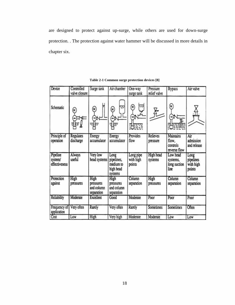
piping system from undesired water hammer effect. Table 2.1 lists major protection

devices under consideration in this research. As shown in the table, some surge devices

18

are designed to protect against up-surge, while others are used for down-surge

protection. . The protection against water hammer will be discussed in more details in

chapter six.

Table 2-1 Common surge protection devices [8]

19

2.6 Previous Researches

A reduced rate flow change, through a slower valve action is an effective and more

economical satisfactory solution to many problems. The surge tank serves as a partial

reflection point for the pressure waves, thereby protecting long tunnels from a short

period pressure wave propagation. Air chambers and surge tanks are probably

considered the safest and less long term cost solutions to the water hammer. Both could

be used for the up-surge case as well as for the down-surge if placed properly and

accordingly, while pressure relief valve is a common up-surge control device. Rapture

disk is also an alternative to protect the system against up-surge but it causes a trouble

when it needs replacement [9].

Thorley indicated the necessity of a check valve installation for water hammer

protection using a surge tank. He also illustrates the sensitivity of the protection to

valve response time [9].

With a proper design of the surge protection devices and enforcement of a proper

operational procedures, water hammer will be generally controlled within allowable

limits. Surge tanks are the recommended options, followed by other flow and pressure

limiting devices, such as a pressure relief valve, check valves, and air valves [9].

20

Lohrasbi and Attarnejad [10] have developed a MOC-based computer solution for

the water hammer effect that can be made public by numerically integrating the

characteristic relations of the full equations. The program was called the “method of

specified time intervals”.

The modeling and simulation of the water hammer phenomenon was investigated

using GIS [11]. The authors compared the results with those from the MOC and the

regression of the relationship between the dependent and independent variables from

the lab experiments and concluded that using numerical MOC solution is more

accurate. Also, the research pays attention to operational procedure suggesting that the

slow valves closure should reduce the risk of system damage or failure due to

hammering.

Anton and Arris [12] have studied the parameters affecting the shape and timing of

the water hammer wave considering the unsteady friction, cavitation, and number of

fluid-structure interaction (FSI). The authors used MOC for developing a mathematical

model combining all three factors. The study concludes that cavitation, column

separation, and FSI can cause hammer larger than classical water hammer theory.

The WCM (Wave Characteristics Method) modeling of water hammer was

extended to model the water column separation in the water distribution networks [13].

21

The methodology was based on the physical concept that when a sub-atmospheric

pressure is reached within the system, the vapor cavity forms and continue to grow

while the sub-atmospheric pressure is maintained, and suddenly collapses at the instant

the cavity volume is reduced to zero. This developed approach proved to be robust and

straight-forward and producing results identical to those obtained from an Eulerian-

based MOC implementation approach.

Dhandayudhapani et al. [14], contrasted the two popular transient modeling

approaches: WCM and MOC by paying close attention to the computational efficiency

and the numerical accuracy of the solutions. Although both methods solved the same

governing equations using similar assumptions, they differed significantly in their

approaches. The primary difference between both models was the way the pressure

wave was tracked between the two boundaries of the pipeline segment. The MOC

tracked a disturbance in the time–space grid using a numerical method based on

characteristics whereas the WCM tracked the disturbance on the basis of wave-

propagation mechanics. Compared with the WCM, the results indicated that the first-

and the second-order MOC schemes needed a substantially greater number of segments

within a pipeline for the same level of accuracy. The authors also explored the

computational efforts for short, long pipelines, and a pipelines network associated with

the first- and second-order MOC schemes and the WCM where the results highlighted

the computational advantages of the WCM and the difference in computational effort

could be several orders of magnitude, depending on the time step chosen.

22

The effect of the pipe slope on the water hammer was investigated and it was found

that the slope of the water hydraulic grade line relative to the pipeline slope was an

important factor controlling the formation of cavitation during the water hammer [15].

The water hammer protection of a water system considering two demand

approaches: the pressure-sensitive demand and the nodal demand was investigated

[16]. It was concluded that the nodal demand significantly overestimated the risk of

the contaminant intrusion due to the down-surge pressure which lead to an increased

protection cost but not necessarily provide better safety. The pressure-sensitive demand

modeling is a must. This is because the nodal demand ignores the implicit relation

between demand and pressure, does not account for the transient discharge dependency

on the elevation at the point of demand, and exaggerates the surge wave leading to an

overestimated negative pressure in the system. Therefore, WaterGEMS adopted a built-

in pressure-dependent demand (PDD) model to effectively model the nodal demand as

a function of pressure [17, 18].

Bong et al. [19], investigated water distribution model skeletonization for surge

analysis. Study shows that unlike the steady-state analysis where the result obtained

from a skeletonized model will have the same result as the complete system, surge

analysis results are strongly affected by the level of skeletonization. Thus, surge

analysis should only be performed on a detailed representative network model to

determine, locate, and size the effective surge protection devices.

23

3 CHAPTER 3

KHOBAR-DAMMAM WATER RING LINE

3.1 Characteristics of KDRL

Khobar Dammam Ring Line ( KDRL ) is of great importance and a case sensitive water

transmission pipeline for local water utility as it is the only source of desalinated water for

five major communities namely:

1- KFUPM Campus

2- Doha District

3- Dana District

4- District No. 537

5- Khaleej Royal Palace

In addition, it is considered as a secondary or emergency water supply for the major water

blending stations in Dammam.

The KDRL transmits approximately 40,000 m3 of desalinated water daily. Any failure

in the system will deprive the five communities from the desalinated water supply and,

therefore, they have to revert to raw groundwater supplies. Figure 3.1 shows the daily

water supply of KDRL during the month of October, 2013.

24

Figure 3-1 Daily water supply from KDRL for the month of October, 2013

The KDRL is running through a terrain of varying topographies, resulting in too many

tops and bottoms at the pipeline. This makes the system’s operation a challenging task to

optimize. Figures 3.2 and 3.3 show the layout and the profile of KDRL, respectively. The

figures highlight the branching point’s stations, ground level, and the length of the

branched pipeline from the station zero at Khobar pumping station.

37

,48

0

39

,57

0

34

,18

0

33

,49

5

35

,91

9

37

,27

9

33

,09

0

26

,89

2

36

,44

1

42

,01

5

33

,19

9

39

,89

0

38

,67

7

34

,51

0 37

,91

1

40

,22

7

40

,19

9

32

,86

7

33

,40

5

29

,38

8

28

,44

3

40

,97

5

40

,26

0

37

,85

7

32

,30

8

36

,83

5

39

,62

7

38

,96

2

38

,52

4

27

,57

2

17

,62

3

0

5,000

10,000

15,000

20,000

25,000

30,000

35,000

40,000

45,000

01 02 03 04 05 06 07 08 09 10 11 12 13 14 15 16 17 18 19 20 21 22 23 24 25 26 27 28 29 30 31

Dai

ly W

ate

r Su

pp

ly (

m3

)

Day of Oct, 2013

25

Figure 3-2 GIS map of the layout of KDRL

26

Figure 3-3 Ground elevation and locations of branched pipelines along the KDRL

27

A field survey was conducted to help constructing the pipeline contour to accurately

evaluate the layout and topography of the KDRL. Figure 3.3 shows the ground level

variations as well as the branching points along the KDRL. Detailed field data from all

KDRL components was saved into a GIS Database. Tables 3.1 and 3.2 summarize the

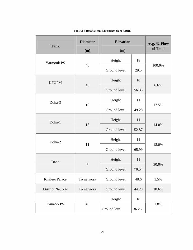
inventory and layout data of the KDRL in the GIS database, respectively. Table 3.3

summarizes information about the tanks connected to the KDRL. Figures 3.4, 3.5 and 3.6

show examples of KDRL components.

Table 3-1 KDRL summary of piping elements

Khobar PS Branching Point Branch Pipe Branch

ending

Level Tank

station

Station

(m)

Elevation

(m)

Diameter

(mm)

Material Length

(m) KFUPM 2,844 32.49 400 UPVC 1,268 56.35

Doha-3 4,361 47.7 200 UPVC 446 49.28

Doha-1 5,755 44.77 200 UPVC 292 49.87

Doha-2 8,272 33.24 300 FRP 1010 57.01

Dana 11,202 48.02 400 DI 255 55.58

Palace 13,692 48.05 300 FRP 285 /

Dist-537 16,270 39.72 300 FRP 740 /

Dam-55 18,055 / 700 CCP 18,055 36.25

28

Table 3-2 KDRL inventory

Pressure Pipes Inventory

Diameter CCP FRP DI UPVC All Materials

(mm) (m) (m) (m) (m) (m)

200 0 0 0 738 738

300 0 2,045 0 0 2,045

400 0 0 255 1,268 1,523

600 0 0 85 0 85

700 18,086 0 0 0 18,076

All Dia. 18,086 2,045 340 2,006 22,477

Components Inventory

Chambers Discharge Isolation

Valve

Pressure

reduce valve

Air

Valves Metering Point

31 27 58 3 14 11

Pipe Segments Junctions/Pipe fittings Pumps

212 201 1

29

Table 3-3 Data for tanks/branches from KDRL

Tank

Diameter

(m)

Elevation

(m)

Avg. % Flow

of Total

Yarmouk PS

40

Height 18

100.0%

Ground level 29.5

KFUPM

40

Height 10

6.6%

Ground level 56.35

Doha-3

18

Height 11

17.5%

Ground level 49.28

Doha-1

18

Height 11

14.0%

Ground level 52.87

Doha-2

11

Height 11

18.0%

Ground level 65.99

Dana

7

Height 11

30.0%

Ground level 70.54

Khaleej Palace To network Ground level 48.6 1.5%

District No. 537 To network Ground level 44.23 10.6%

Dam-55 PS 40

Height 18

1.8%

Ground level 36.25

30

Figure 3-4 Sample washout valve in KDRL

31

Figure 3-5 Sample air valves installed in KDRL

32

Figure 3-6 Sample branching connection in KDRL

33

The detailed survey shows some discrepancy between the data collected by the

surveyor’s and the KDRL as-built drawings. Appendix A shows the difference between

these data. In this study, the analysis was performed based on the surveyed data.

In order to achieve a robust model for the KDRL, operational and historical data related

to KDRL were gathered and were entered into the GIS database. Moreover, eleven flow

and pressure meters were installed along the KDRL. Figure 3.7 shows the types of the

flow/pressure meter installed according to the site conditions. Two flow/pressure meters

were installed at both Khobar and Dammam ends of the KDRL. Additional seven

flow/pressure meters were installed at each branch connecting to the KDRL in order to

measure the water flow and the pressure to the tanks at the metering point. These nine

flow/pressure meters provide a reading of the pressure and flow every 15 minutes.

Additionally, two on-line pressure meters that provide instantaneous and continues

readings were installed at other points on the KDRL ends. Figure 3.8 shows sample of

installed flow/pressure meter.

34

Figure 3-7 Types of flow/pressure meters installed in KDRL

Figure 3-8 Installed flow/pressure meters on-site

35

3.2 Flow and Pressure Measurements

Flow/Pressure meters were installed in April 2013 along the KDRL to send log data

every 15 minutes. Collected data were directed to the GIS database and linked to a

corresponding element in the KDRL system. Figure 3.9 shows the location of

flow/pressure meters. These flow/pressure meters were continually monitored for the water

flow and pressure. Flow meter data indicated that there were some operational problems in

the system as there was a non-working or defect element. For example, a flow meter

installed prior to the non-return valve shows a reverse flow in the pipe which indicates that

the non-return valve is defected. A major problem faced during data collection was related

to the rapid pressure variation along the pipeline due to the development of the water

hammer which damages three installed devices. All the operational problems were fixed

prior to the start of KDRL hydraulic analysis.

36

Figure 3-9 Location of flow/pressure meter.

37

Flow and pressure data using proper devices installed at different locations along the

KDRL were collected over a period of six months (May 2013 to October 2013). The data

indicated that an extreme water hammer has developed along the pipeline. Figure 3.10

shows the readings at the KFUPM branch after a sudden closure of the tank’s valve. As a

result, the flow became zero and a surge wave developed. The generated wave increased

the pressure in the KFUPM branch pipeline to more than 16bars, causing a serious damage

to the flow/pressure meter. The sudden closure of the valve at KFUPM tank was, most

probably, not the only cause of this problem since the flow/pressure meter survived from

similar previous incidents many times. Sudden closure of other valves at other branches

might have contributed to this incident. Later in the analysis, it will be shown clearly that

KFUPM branch was the part of KDRL that was the most affected during the water hammer

event. Figure 3.11 shows the reading at Dana branch at the same time when the KFUPM

pressure meter was damaged. The reading indicates that a suction pressure up to 3-bar was

created. The behavior at Khaleej Palace where valves are open to fill tank for 2-hours in a

day then closed suddenly is depicted in Figure 3.12.

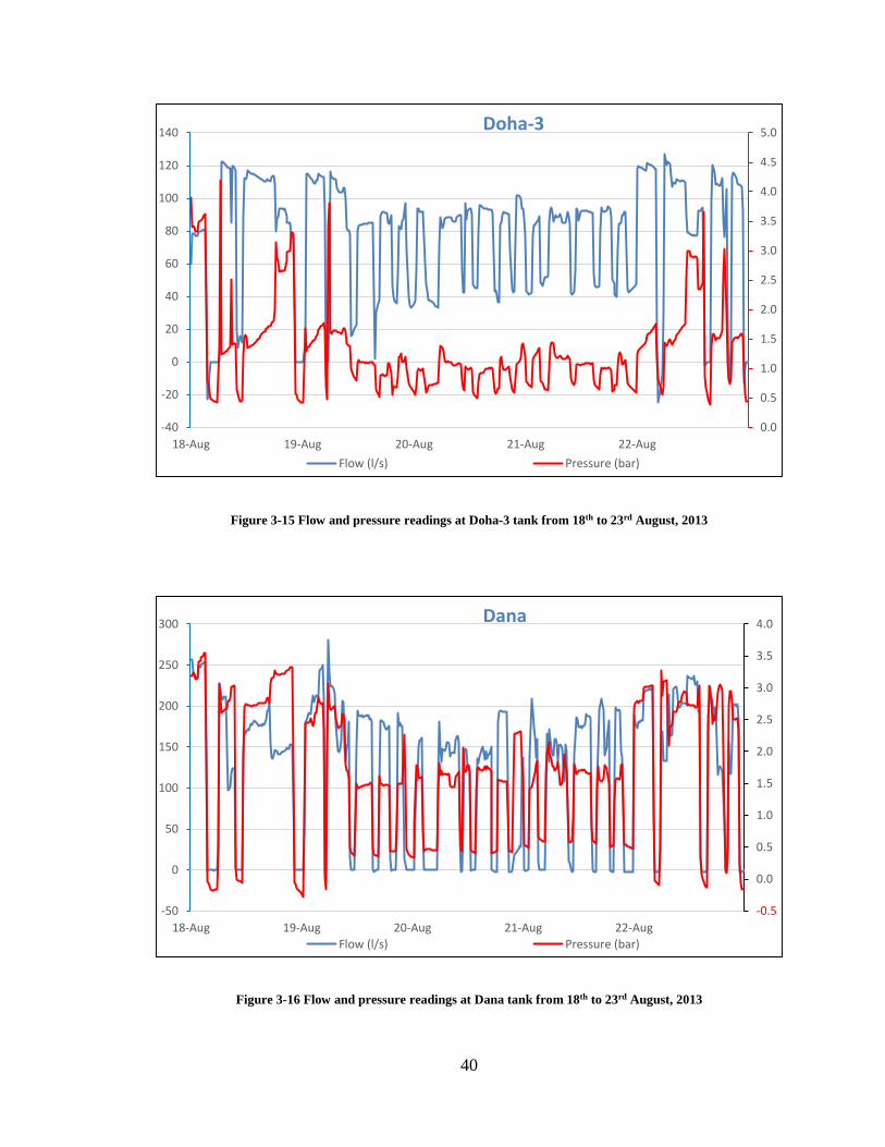
During the period of 18th to 23rd of August 2013 there was a deviation from the normal

operation due to an abnormal flow condition. This serious flow condition over long-period

which affected all branch pipelines was most probably caused by a malfunctioning valve

at the KFUPM tank as displayed in Figures 3.13, 3.14, 3.15 and 3.16.

38

Figure 3-10 Flow and pressure readings at KFUPM branch collected on 1st and 2nd May, 2013

Figure 3-11 Flow and pressure readings at Dana branch collected on 1st and 2nd May, 2013

Figure 3-12 Flow and pressure readings at Khaleej branch collected on 1st and 2nd May, 2013

39

Figure 3-13 Flow and pressure readings at Yarmouk tank from 18th to 23rd August, 2013

Figure 3-14 Flow and pressure readings at KFUPM tank from 18th to 23rd August, 2013

0.0

1.0

2.0

3.0

4.0

5.0

6.0

7.0

8.0

0

100

200

300

400

500

600

700

18-Aug 19-Aug 20-Aug 21-Aug 22-Aug

Yarmouk Pump

Flow (l/s) Pressure (bar)

0.0

2.0

4.0

6.0

8.0

10.0

12.0

14.0

16.0

18.0

20.0

-250

-150

-50

50

150

250

350


KFUPM


40

Figure 3-15 Flow and pressure readings at Doha-3 tank from 18th to 23rd August, 2013

Figure 3-16 Flow and pressure readings at Dana tank from 18th to 23rd August, 2013

0.0

0.5

1.0

1.5

2.0

2.5

3.0

3.5

4.0

4.5

5.0

-40

-20

0

20

40

60

80

100

120

140


Doha-3


-0.5

0.0

0.5

1.0

1.5

2.0

2.5

3.0

3.5

4.0

-50

0

50

100

150

200

250

300


Dana


41

The total supply of the KDRL in one month (October, 2013) and the fluctuations in the

flow and pressure during the same period in all branches are listed in Table 3.4.

Table 3-4 Summary of flow meter readings at different locations along the KDRL during October 2013

Flow Meter

Location

Total Water

Supply (m3)

Max Flow

(l/s)

Avg Flow

(l/s)

Max

Pressure

(bar)

Avg

Pressure

(bar)

Yarmouk 1,095,135 673.86 408.88 7.92 5.25

KFUPM 73,069 200.56 27.66 / 7.45

Doha3 192,449 124.66 71.83 4.42 1.39

Doha1 154,772 117.06 57.77 3.98 1.28

Doha2 197,969 189.37 73.89 3.95 0.86

Dana 349,862 273.41 130.62 4.81 1.85

Palace 15,681 88.78 6.14 5.62 2.67

Dist-537 115,661 100.66 43.17 2.5 1.74

Dam-55 19,836 58.81 7.41 1.95 1.21

The flow and pressure measurements collected during the six month period (May –

October, 2013) indicate the need to perform a detailed water hydraulic analysis of the

KDRL. This is an essential step that needs to be performed prior to the water hammer

analysis. This is because the water hydraulic analysis will help enhance the performance

of the KDRL by optimizing its operation, and identify critical points in the system.

42

4 CHAPTER 4

HYDRAULIC MODELING OF KDRL

4.1 Model Construction and Execution

Water hydraulic modeling of the KDRL has to be performed before the analysis of water

hammer is conducted. Such modeling is essential to understand the behavior of the system

under normal conditions and to validate the results from the model with the field data. In

case there is a discrepancy between the model results and the field data, then the model

will be calibrated and corrected accordingly. For the purpose of the water hydraulic

modeling, two program packages, namely ESRI ArcMap GIS and WaterGEMS were used.

ESRI ArcMap GIS program was used to construct the model and automate the elevation

projection to the model using field survey data. On the other hand, WaterGEMS program,

which is a widely known water hydraulic modeling and simulation package that enables

integration with the GIS, was used for the water hydraulic analysis. Darwin Calibrator,

which is an extension to WaterGEMS, was used to optimize the automatic calibration. The

main goal of the water hydraulic analysis was to calibrate the model and assure its adequacy

to represent the real condition in order to run water hammer analysis and simulate different

protections for the KDRL from water hammer.

The Yarmouk station at Khobar receives water from two sources: desalinated water from

the SWCC and raw groundwater from local water wells. The water, which is coming from

43

these sources, is blended in Yarmouk tank and then distributed to Khobar city. The average

water supply to Yarmouk station is about 5,600 m3/h. Approximately 63% of this amount

(3,500 m3/h) is supplied to Khobar Central station and to Makkah station. The water

amount transported through the KDRL is approximately 2,100m3/h. KDRL is operated

using one pump located at Yarmouk station (Yar-Pump). Table 4.1 shows the

characteristic curve for this pump.

Table 4-1 Yarmouk-pump specifications

Yar-Pump Shut-off Design Max Inertia

(Kg.m2)

Speed

(rpm)

Specific

Speed Flow

(L/S)

0 500 1,000

Head

(m)

89 67 0 19,000 1,171 76

Each of the six sub tanks that are connected to the KDRL is serving a large community.

Therefore, each tank is connected to a local water well to make up for water supply

shortages during the high water demand. KDRL also is feeding District No. 537 from a

branching pipe connected directly to the district sub network.

Using GIS data, a model was built and exported to WaterGEMS. A schematic of the

KDRL as imported from the WaterGEMS is depicted in Figure 4.1, showing the locations

of each tanks, sub tanks, pump, and air valves.

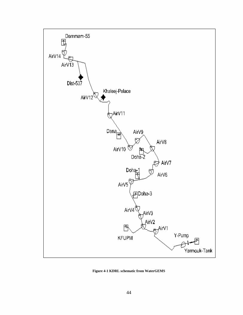
44

Figure 4-1 KDRL schematic from WaterGEMS

45

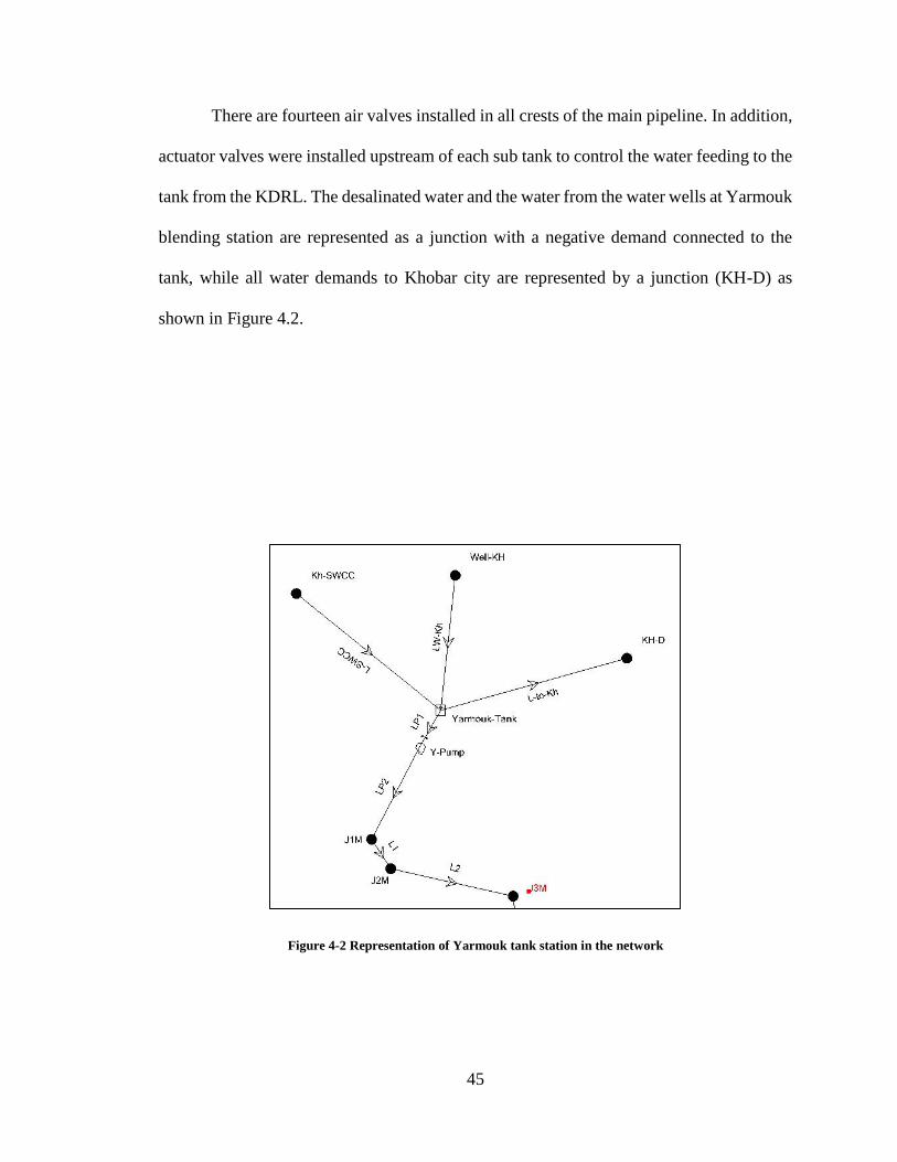
There are fourteen air valves installed in all crests of the main pipeline. In addition,

actuator valves were installed upstream of each sub tank to control the water feeding to the

tank from the KDRL. The desalinated water and the water from the water wells at Yarmouk

blending station are represented as a junction with a negative demand connected to the

tank, while all water demands to Khobar city are represented by a junction (KH-D) as

shown in Figure 4.2.

Figure 4-2 Representation of Yarmouk tank station in the network

46

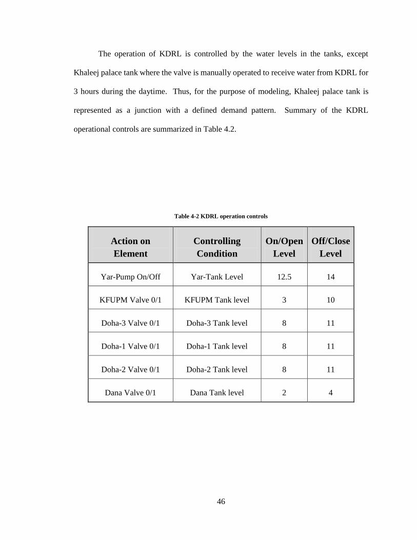
The operation of KDRL is controlled by the water levels in the tanks, except

Khaleej palace tank where the valve is manually operated to receive water from KDRL for

3 hours during the daytime. Thus, for the purpose of modeling, Khaleej palace tank is

represented as a junction with a defined demand pattern. Summary of the KDRL

operational controls are summarized in Table 4.2.

Table 4-2 KDRL operation controls

Action on

Element

Controlling

Condition

On/Open

Level

Off/Close

Level

Yar-Pump On/Off Yar-Tank Level 12.5 14

KFUPM Valve 0/1 KFUPM Tank level 3 10

Doha-3 Valve 0/1 Doha-3 Tank level 8 11



Dana Valve 0/1 Dana Tank level 2 4

47

When constructing the water hydraulic model for KDRL, the community water

demands as supplied from the tanks are modeled as a demand junctions located after the

tank. For example, Figure 4.3 shows the schematic layout of the junction demand for Dana

tank. The demands for the communities are estimated by collecting relevant data from the

corresponding flow meter. A one-month long reading (every 15 min) from each flow meter

is stored in the GIS database, averaged, and then assigned to the demand node after the

tank. The flow meter readings used to create a pattern for the demand as well.

Figure 4-3 Details schematic of a branch from KDRL

Table 4.3 summarizes the data from the installed flow/pressure meters and their

corresponding element to represent the reading during the calibration.

48

Table 4-3 List of metering device and their corresponding junction/pipe

Meter ID ELEVATION Junction @ Model Flow @ Model

Khubar 27.002 FM-Yarmouk @ 27.5 L7

KFUPM 34.643 FM1-KFUPM @ 34.68 LT1-1

DOHA 3 49.288 FM2-Doha3 @ 49.29 LT2-3

DOHA 1 52.873 FM3-Doha1 @ 52.87 LT3-5

DOHA 2 60.814 FM4-Doha2 @ 60.81 LT4-2

Dana 55.650 FM5-Dana @ 55.66 LT5-3

Palace 49.388 FM6-Khaleej @ 48.74 LT6-1

Dist 537 41.220 FM7-p537 @ 42.25 LT7-1

TANK 55 39.601

AirV10 assumed to be

@ FM-Tank55

L97

P3- YAR 27.214 AirV1 assume @ J9M NON

P3-T55 36.25 @ Junction Dm55-P3 NON

Appendix B contains sample data of the junctions and pipes used to create this model,

initial conditions, and all other input data to construct and run the model, along with the

results of initial hydraulic analysis results in a tabular form.

49

Upon the completion of the model construction and data input, the model calculation

option is chosen to be based on Hazen-Williams equation. The general form of H-W

equation is [2, 4]:

𝑄 = 𝑘 ∙ 𝐴 ∙ 𝑅0.63 ∙ 𝑆0.54 (4.1)

Where,

Q = Discharge in the section

C = Hazen-Willliams roughness coefficient

A = Flow area

R = Hydraulic radius

S = Friction slope

K = Constant (0.85 for SI units or 1.32 for US units)

The H-W roughness coefficient can be estimated from Table 4.4. Initially, all C-values

are set to be 130. The adjusted values from the calibration process will be applied to each

element at a later stage.

Initial run of the model was successful as presented by the WaterGEM output shown in

Figure 4.4. The figure reveals that, under normal conditions, the HGL is decreasing in the

direction of the flow along the KDRL and it is always above the ground level.

50

Table 4-4 Common used Roughness Value [2, 19]

51

Figure 4-4 HGL over KDRL (Steady-State Analysis)

52

4.2 Model Calibration

After the model was constructed, it needed to be calibrated by comparing the model

output with the field data. For this purpose, two day duration (28th-30th October 2013) was

selected. Field data related to the flow and pressure at different locations along the KDRL

were collected during the same period from 28th - 30th October, 2013. The first initial

conditions of this period were used as input to the constructed model which was executed

for a period of 48 hours with a time step of 15 minutes. The 15-minute time step was

selected to match the time interval that was considered when the readings were collected

using the flow/pressure meters. The total flow through the system based on the WaterGEM

calculation is summarized in Table 4.5. Sample output of the WaterGEM model is in

Appendix B. The water level variation in Yarmouk tank and the pumped flows for the

testing period are presented in Figures 4.5 and 4.6, respectively.

Table 4-5 Totalizing flow meter resulted from WaterGEMS calculations

Element Label Net Volume

(m³) % of KDRL amount

Yar-

Sta

tion

Kh-SWCC -238,769.09 /

Well-KH -46,704.06 /

KH-D 197,685.00 /

KD

RL

KFUPM-D 8,059.90 9.18

Doha3-D 13,074.12 14.89

Doha1-D 10,105.50 11.51

Doha2-D 14,614.21 16.65

Dana-D 23,565.13 26.84

Khaleej-Palace 1238.92 1.41

Dist-537 7,587.09 8.64

Dm55-D 3,837.47 4.37

53

Figure 4-5 water level variation calculated over the period 28-30 Oct 2013

Figure 4-6 Pumped flow during 28-30 October 2013

54

For an optimized calibration, two stage processes were adopted. Firstly, a scenario was

built considering a sub-model based on Yarmouk station up to the point of Yarmouk flow

meter (Yarmouk FM) only. For this case, a demand value equals to the pumped quantity

has been assigned to the junction at Yarmouk FM and a pattern demand similar to the total

flow pumped to KDRL was adopted. Thus, a reading from only one meter (Yarmouk FM)

is used for the sub-model calibration, while the reading from all eleven meters were used

in calibrating the full model. Next “Darwin Calibrator” feature of the WaterGEM model

used for calibration based on flow/pressure reading collected from filed (during the 28th to

30th October, 2013 period) and the WaterGEM calculation output. The calibration analysis

shows a small fitness value (0.001) indicating that model output is very close to field data.

Figures 4.7 and 4.8 show the correlation results for both sub-model and full model,

respectively. Sample of the calibration results for both model and sub-model are presented

in Appendix C along with the sample of observed field data.

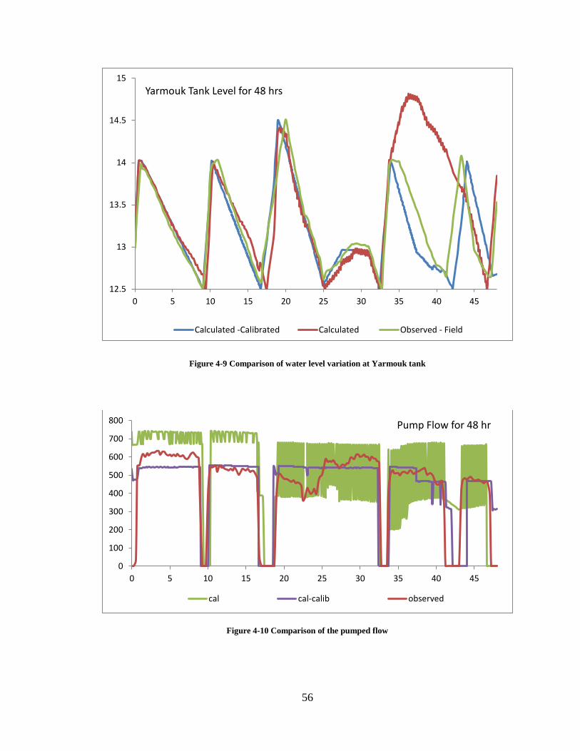
Calibration process adjustment to both roughness coefficients and demands were

applied to the model elements. A comparison between the water level variation obtained

from the WaterGEM and that collected from the field is depicted in Figure 4.9. The Figure

shows a strong match between the two calculated (after calibration) and the observed field

data curves, indicating the capability of the model to simulate field conditions. Similar

conclusion can also be drawn for the pumped flow as indicated form Figure 4.10. Both

figures clearly show the added value to the calculation capability and its adjustment to

ensure model output is similar to filed data.

55

Figure 4-7 Sub-model calibration correlation results

Figure 4-8 KDRL model calibration correlation results

56

Figure 4-9 Comparison of water level variation at Yarmouk tank

Figure 4-10 Comparison of the pumped flow

12.5

13

13.5

14

14.5

15

0 5 10 15 20 25 30 35 40 45

Yarmouk Tank Level for 48 hrs

Calculated -Calibrated Calculated Observed - Field

0

100

200

300

400

500

600

700

800

0 5 10 15 20 25 30 35 40 45

Pump Flow for 48 hr

cal cal-calib observed

57

Results above indicate that the constructed hydraulic model using WaterGEM can

accurately represent conditions likely to be experienced in the KDRL. The model is

calibrated to adequately represent the actual field conditions using field measurements and

observations.

The HGL at Yarmouk flow meter junction over a period of 48 hours (28-30 October

2013) based on the calibrated model is shown in Figure 4.11. The graph shows an extreme

negative pressure at 42 hour. This indicates that close investigation is required as well as

proper protection for such an incident is mandatory.

Figure 4-11 HGL at junction Yarmouk flow meter (28-30 Oct) based on the calibrated model

Once a hydraulic model for the KDRL was constructed and calibrated, the next step was

to investigate the occurrence and control of a water hammer that might occur at any point

along the pipeline.

58

5 CHAPTER 5

WATER HAMMER MODELING & ANALYSIS

5.1 Background

Water hammer or hydraulic transients in pipelines mainly occur due to the following:

a) Water Pumps startup or shut down

b) Main valves opening or closure.

c) Sudden power failure, causing water pumps to shut down.

Pumps startup or shutdown usually does not cause major transient in the system if

proper operational procedure has been adopted, such as soft starter or delayed shutdown.

Currently the Water Authority of Khobar city is practicing operational control to prevent

water hammer in KDRL, by enforcing gradual operation for the pump and all valves. This

practice, however, is of no value in the case of power outage and/or pipe breaks. The worst

case, for down-surge development, is after a power failure where a sudden pump shutdown

takes place. Valves closure will have a minor effect if operated properly and not suddenly

closed. However, human intervention in the system operation by unskilled operators can

lead to a disaster. Thus, the study will consider the worst case scenarios. Accordingly, the

following two scenarios will be investigated:

1) Power failure and a sudden pump shutdown at Yarmouk station, and

2) Simultaneous and sudden closure of all valves located prior to sub tanks.

59

To get a feeling of the pressure change during a water hammer, the Joukowski Equation

[1, 2] for calculation was used. The equation states that the change in the head pressure

(during water hammer) equal to the change in the fluid velocity multiplied by the

supersonic speed (c) divided by the specific gravity (g). Mathematically it can be expressed

as:

∆𝐻 = 𝑐 . ∆𝑉𝑔⁄ (5.1)

where,

ΔH = change in head

ΔV = change in fluid velocity

To compare this with a sample calculation at a specific location along the KDRL,

consider the junction located at the Doha-2 branch, in the case of Doha-2 valve closure.

Following are the conditions at this specific location:

- HGL at the point is 71 m

- Pipe wave speed is 702 m/s

- Change in Speed is from 3.24 m/s to zero = 3.24 m/s

- Change in head = 702 * 3.24 /9.81 = 231.8 m

- Resulting Up-Surge Head = 71+231.8 = 302.8 m!! 300% increment.

Moreover, pressure wave travel along the pipe in a supersonic speed, split at junctions

to all branches’ pipelines, and reflect back. The wave magnifies when it splits from a wider

pipeline to a narrower pipeline and magnifies at the dead ends. This is the case in all

branches of the KDRL. When two wave passes by each other, they change and magnify

60

the flow and pressure but don not effect each other, cancel each other, subtract from each

other, or add to each other. For example, consider two waves A and B. If wave A is 5 bar

and wave B is -3 bar when they meet the change in magnitude will be 2 bar but after they

pass each other, wave A and B will be intact (A is 5 bar and B is -3 bar). The schematic of

the wave behavior at a splitting point from a wider to a narrower pipeline or vice versa with

sample values is depicted in Figures 5.1, 5.2 and 5.3 [7].

To investigate the occurrence of the water hammer, Bentley HAMMER program,

will be used. Table 5.1 summarizes the calculated wave speed based on the characteristics

of the pipeline materials and the liquid using HAMMER.

61

Figure 5-1 Pressure/surge wave split from small to larger pipe [20]

Figure 5-2 Pressure/surge wave split from large to smaller pipe, with a dead end [20]

62

Figure 5-3 Pressure/surge wave movement and reflection through a pipe segments [20]

63

Table 5-1 Physical pipe characteristics

Pipe

Line Material

Dia Length Wave

Speed

Nominal

Pressure C

(mm) (m) (m/s) (bar)

KFUPM UPVC 400 1,268 352 16 140

Doha-3 UPVC 200 446 485 16 140

Doha-1 UPVC 200 292 485 16 140

Doha-2 FRP 300 1010 702 16 130

Dana DI 400 255 1,265 16 130

Palace FRP 300 285 702 16 130

Dist-537 FRP 300 740 702 16 130

Main Line CCP 700 18,055 1,124 24 110

64

5.2 Scenario 1: Power Failure and Pump Sudden Shutdown

When the water pump suddenly shuts down at Yarmouk station, the high water inertia

will keep it running, causing a water column separation and cavitation. The cavitation will

cause the water to vaporize and thus vapor pockets are created. When these pockets

collapse water will travel rapidly generating pressure spikes that might damage the

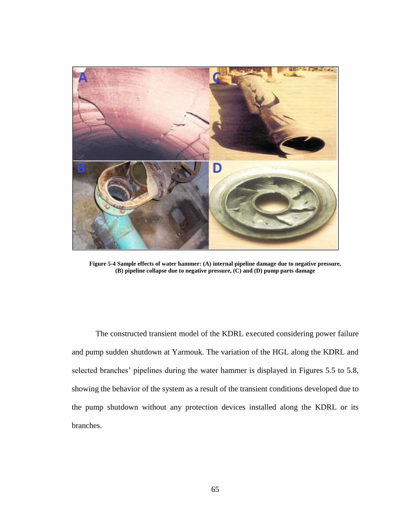
pipeline, pump or any other water network component. Figure 5.4 shows few examples of

the damages that might be caused by the water hammer.

For any pipeline system similar to the KDRL, in case of power failure, then it is

expected that a high negative pressure wave will develop and travel downstream to the

pump station causing pressure drop along the whole pipeline up to its end. This pressure

wave may be reflected backwards as a positive pressure wave up to the pump station. If a

fast closing check valve is installed at the pump discharge, the high-pressure wave is

normally eliminated. In case of severe negative pressures are allowed to occur along the

pipeline, the cement mortar lining can breakdown. Therefore, no negative pressure shall be

allowed along the KDRL.

65

Figure 5-4 Sample effects of water hammer: (A) internal pipeline damage due to negative pressure,

(B) pipeline collapse due to negative pressure, (C) and (D) pump parts damage

The constructed transient model of the KDRL executed considering power failure

and pump sudden shutdown at Yarmouk. The variation of the HGL along the KDRL and

selected branches’ pipelines during the water hammer is displayed in Figures 5.5 to 5.8,

showing the behavior of the system as a result of the transient conditions developed due to

the pump shutdown without any protection devices installed along the KDRL or its

branches.

66

The figures indicate that the major effect of the power failure is the initiation of a

high negative pressure wave that travels downstream to the pump station and causes

pressure drop along the pipeline up to the highest point of the pipeline. Thus, the first two

branches (KFUPM and Doha-3) are severely affected by the down-surge compared to the

other branches that are far away from the pump. As revealed from the figures, the pressure

decreases until it reaches ( -1 bar ) in some locations. As a result, the water hammer

analysis for this scenario clearly proves the development of a huge sever negative pressure

which requires close attention and deep investigation for a surge protection to resolve this

serious problem.

Note: color coding in all graphs of water hammer analysis results, is as follows:

Green : Pipeline profile elevation from sea level.

Black : Steady-State operation hydraulic grade line HGL.

Blue : Minimum pressure (max down-surge).

Red : Maximum pressure (max up-surge).

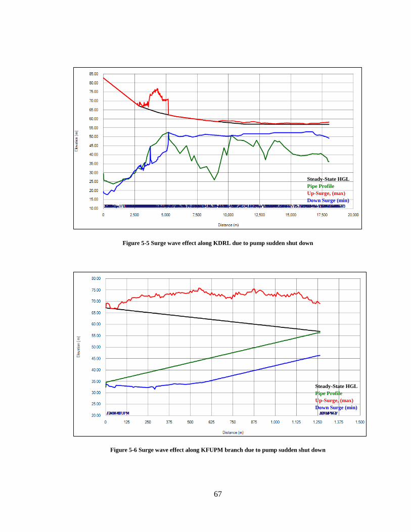
67

Figure 5-5 Surge wave effect along KDRL due to pump sudden shut down

Figure 5-6 Surge wave effect along KFUPM branch due to pump sudden shut down

Steady-State HGL

Pipe Profile

Up-Surge, (max)

Down Surge (min)

Steady-State HGL

Pipe Profile

Up-Surge, (max)

Down Surge (min)

68

Figure 5-7 Surge wave effect along Doha3 branch due to pump sudden shut down

Figure 5-8 Surge wave effect along Doha1 branch due to pump sudden shut down

Steady-State HGL

Pipe Profile

Up-Surge, (max)

Down Surge (min)

Steady-State HGL

Pipe Profile

Up-Surge, (max)

Down Surge (min)

69

5.3 Scenario 2: Sudden Closure of All Valves

The second possible worst scenario that might occur is the case when all main valves

installed in the branches along KDRL are closed suddenly while the pump is still operating.

Such an action would cause the following:

o Decrease in the amount of the water pumped to the system.

o Pump goes back in its curve and produces more head pressure

o High energy consumption

If all valves are closed simultaneously, then maximum pressure will be created within

the KDRL. This scenario represents the worst maximum up-surge pressure that could be

generated in the system. The following sections present the analysis and simulation of the

two situations:

A) A single valve closure (KFUPM valve and Doha3 valve), and

B) Simultaneous closure of all branches’ main valves installed along the KDRL.

5.3.1 Sudden Closure of KFUPM Valve

One possible scenario for the development of a water hammer is the case when one of

the valves installed along the KDRL is closed suddenly. For example, the sudden closure

of KFUPM valve. Such incidents have occurred frequently in the past. Figures 5.9 to 5.11

show the system transient behavior at selected locations. As revealed from the figures that

the main pipeline and all other branches are severely affected by the generated surge wave.

70

Figure 5-9 Surge wave variation along KDRL due to the sudden valve closure at KFUPM

Figure 5-10 Surge wave variation along KFUPM branch due to the sudden valve closure at KFUPM

Steady-State HGL

Pipe Profile

Up-Surge, (max)

Down Surge (min)

Steady-State HGL

Pipe Profile

Up-Surge, (max)

Down Surge (min)

71

Figure 5-11 Surge wave variation at Doha3 due to the sudden valve closure at KFUPM

The figures also show that the pressure decreases until it reaches ( -1 bar ) at some

locations. Thus, a surge protection is essential for this case. Moreover, corrections to the

system setup maybe required to eliminate or minimize the effect from the branches on the

network, including the main pipeline and the other branches’ pipeline.

5.3.2 Sudden Closure of Doha3 Valve

Another example for a single valve closure is the case when the valve at Doha3 is

suddenly closed. Figures 5.12 to 5.14 show the system behavior and the HGL variations

at selected locations along the KDRL. The development of huge pressure acting on the

pipelines is evident. Negative pressure is also clear at certain sections of the pipeline.

Steady-State HGL

Pipe Profile

Up-Surge, (max)

Down Surge (min)

72

Figure 5-12 Surge wave variation along KDRL due to sudden valve closure at Doha3

Figure 5-13 Surge wave variation at KFUPM due to sudden valve closure at Doha3

Steady-State HGL

Pipe Profile

Up-Surge, (max)

Down Surge (min)

Steady-State HGL

Pipe Profile

Up-Surge, (max)

Down Surge (min)

73

Figure 5-14 Surge wave variation at Doah3 branch due to sudden valve closure at Doha3

The effect of a sudden closure of Doha3 valve will propagate to the main pipeline

and all other branches. However, the effect due to Doha3 valve closure is less than the

effect of KFUPM valve closure but it is still unacceptable. Such incidents have occurred

frequently in the past, which requires an immediate action to protect the main line as well

as the branched pipelines form water hammer.

Steady-State HGL

Pipe Profile

Up-Surge, (max)

Down Surge (min)

74

5.3.3 Sudden Closure of All Valves

Another possible scenario is the case when all valves installed in the branches along

the KDRL are closed suddenly at the same time. As expected a huge surge wave will

develop which will propagate upstream/downstream along the pipeline. Figures 5.15 to

5.17 show the surge wave variation at selected locations. It is obvious that an action should

be taken to control this huge pressure; otherwise, the pipeline or the installed devices along

the pipeline will be damaged.

Figure 5-15 Surge wave variation along DKRL due to sudden closure of all valves

Steady-State HGL

Pipe Profile

Up-Surge, (max)

Down Surge (min)

75

Figure 5-16 Surge wave variation at KFUPM due to sudden closure of all valves

Figure 5-17 Surge wave variation at Doah3 due to sudden closure of all valves

Steady-State HGL

Pipe Profile

Up-Surge, (max)

Down Surge (min)

Steady-State HGL

Pipe Profile

Up-Surge, (max)

Down Surge (min)

76

6 CHAPTER 6

WATER HAMMER CONTROL

6.1 Background

Water hammer protection is not only about installation of surge protection devices to

resolve the water hammer issue. It is more about preventing any potential or minimize the

probability of a water hammer occurrence by controlling the system setup and operation.

Therefore, the operational procedures and controls of the system need to be optimized first.

Then, water hammer mitigation devices should be installed to absorb upsurge and down-

surge waves in extreme cases, e.g. power outage.

6.2 Isolating Branched Pipes from KDRL

As mentioned previously, branch pipelines, with the current setup of placing the

isolation and check valve at the far end of the branch pipeline (prior to the sub tank), are

affecting the KDRL hydraulics even when they are closed. This is due to the surge waves

and water column returning from the branch pipeline back to the system. For example, in

the KFUPM branch, which is 1,268 meter long with an elevation difference between the

tank base and the branch connection point to the KDRL is about 24 meter, the backflow

from the branch during the water hammer is large enough to severely affect the system. To

resolve this problem, the branches’ effects to the main line should be eliminated by

77

installing an isolation valve and a check valve just upstream of the branching point. Figures

6.1 to 6.3 shows a schematic diagram of the existing and proposed setups.

Figure 6-1 Existing system setup, tank valve and check valve in the upstream ( case A )

Figure 6-2 Proposed setup, tank valve upstream and check valve downstream ( case B )

Figure 6-3 Proposed setup, tank valve and check valve downstream the pipe ( case C )

78

The following sections will discuss the effect of the valve closure on the surge wave

development when isolating the branch from its connection point with the main pipeline.

The analysis is performed for the following cases of operational controls:

a) Closure of the valve upstream of the tank with no check valve installed in the

branching point (current practice).

b) Closure of the valve upstream of the tank with a check valve installed in the

branching point.

c) Closure of the valve at the branching point.

Figures 6.4 to 6.6 show the results of the HAMMER for the above-mentioned cases.

The figures represent the situation when KFUPM valve is suddenly closed while the other

valves were still open. Figure 6.4 shows the effect of KFUPM valve closure for the above-

mentioned cases on the main pipeline. The figure indicates that the down-surge extreme

effect on KDRL will occur for case A when the valve is closed upstream of the branched

pipeline. On the other hand, the effect is minimal in the case of isolating the KFUPM

branch pipeline from the main pipeline by either placing a check valve at the branching

pint (case B) or closing the valve at downstream of the branch pipeline (case C). The figure

also indicates that case C has the minimum up-surge effect.

79

Figure 6-4 Water hammer analysis results comparison for cases A, B, and C– main pipeline

A

B

C

Steady-State HGL

Pipe Profile

Up-Surge, (max)

Down Surge (min)

80

Figure 6.5 shows the effect of KFUPM closure for the above-mentioned cases on the

KFUPM branch pipeline, it is clearly shown that case A is the worst for both up-surge and

down-surge wave development in the system. On the other hand, case B has no risk of

down-surge, and the developed upsurge is less than (case A). Finally, case C shows a risk

of down-surge development whereas, the up-surge development is minimal. For the effect

on KFUPM branch case C is acceptable, even with the risk of down-surge development,

because the effect could be controlled easier when there is no outside effect. Figure 6.6

shows the effect of KFUPM closure for the above-mentioned cases on the Doha-3 branch

pipeline. The figure reveals that case A is the worst for both up-surge and down-surge

wave development in the system. On the other hand, case C seems to be the best which

shows that the developed up-surge is minimal and there no risk of down-surge. Moreover,

case B is still accepted and could be mitigated within the branch pipeline without

transferring the effect back to the main pipeline.

Similar analysis can be performed to all branches. Therefore, according to the above

analysis, the branch pipeline is recommended to be isolated from the main pipeline at the

branching point (downstream of the branch pipeline) which will minimize the surge waves

that could propagate from the branched pipes to the KDRL. Even in the case where a worse

situation in the branch pipeline takes place, it will be easier to be resolved. Moreover, it

will be less costly and risky if it fails and takes less time to be retrieved from a failure

where only one part of the system will be out of service. The out-of-service part can still

be served with raw water pumped from groundwater wells. However, if KDRL fails, all

communities will be out of service.

81

Figure 6-5 Water hammer analysis results comparison for cases A, B, and C – KFUPM branch

A

B

C

Steady-State HGL

Pipe Profile

Up-Surge, (max)

Down Surge (min)

82

Figure 6-6 Water hammer analysis comparison for cases A, B, and C – Doha3

A

B

C

Steady-State HGL

Pipe Profile

Up-Surge, (max)

Down Surge (min)

83

6.3 Power Failure Protection

The power failure has also been studied. For this scenario, several model simulations

have been performed in order to identify the best surge preventive solution. As the water

hammer action causes a negative pressure in the pipeline, the most effective ways to handle

this situation is by using surge vessels downstream the pump. The surge vessels and air

valves are particularly effective when there is a loss of power and a negative pressure

(down-surge) wave develops. The residual pressure in the surge vessel reduces the liquid

column, compensates for the loss of the pressure due to the pumps shutdown, and

accordingly prevents the negative pressure. Air valve settings were optimized to ensure

their effectiveness for the surge wave resistance as vacuum breakers, where all air valves

were set to intake air fast but release it slowly.

After several runs of the model, it has been observed that using a surge vessel and air

valves with the following specifications will solve the problem of the negative pressure:

A) Surge vessel with an effective volume of 13m3 and a maximum working pressure

of 8 bars.

B) Existing air valves with an inlet orifice of 150mm and an Outlet orifice of 50mm.

The effect of the surge preventing equipment on the KDRL and the selected branches

are presented in Figures 6.7, 6.8 and 6.9.

84

Figure 6-7 Surge protection using surge vessel – main pipeline

Figure 6-8 Surge protection using surge vessel – KFUPM

Steady-State HGL

Pipe Profile

Up-Surge, (max)

Down Surge (min)

Steady-State HGL

Pipe Profile

Up-Surge, (max)

Down Surge (min)

85

Figure 6-9 Surge protection using surge vessel – Doha3

As revealed from the figures the wave pressure due to the transient condition drops

dramatically indicting the efficiency of the installing surge vessel and air valves along the

pipeline.

Steady-State HGL

Pipe Profile

Up-Surge, (max)

Down Surge (min)

86

6.4 All Valves Sudden Closure Protection

The water hammer action of a rapid valve closure of the water supply branches causes a

high pressure along the pipeline. The following solutions are the common solutions to

eliminate the effect of the high pressure:

- Installation of a pressure relief valve

- Installation of a surge vessel

- Extension of the closure time of the valves

- Installation of a rigid pipeline that can sustain high pressure

As stated earlier, changing the route of the KDRL is not an option. Moreover, any

operational correction policy is eliminated keeping in mind the worst case of having a non-

skilled operator. Thus, installation of a pressure relief valve is suggested since there is

already a surge vessel installed at Khobar PS. Also, it might be an option to install another

surge vessel at Dammam PS. Pressure Relief Valves (PRVs) installations at different

locations along the KDRL were tested. These locations are proposed at sites where washout

chambers already installed and the available space can accommodate for additional valve

installation. After several model runs (details are available in Appendix D) an optimized

solution was achieved. This model was achieved while monitoring the change in the

maximum and minimum surge pressure and the amount of water expelled out from the

system at each point.

87

According to water hammer simulation, the proposed solution is to install three Pressure

Relief Valves with the following specifications:

- Threshold Pressure = 6 bars

- Diameter = 600 mm

- Spring Constant = 150 lb/in

The proposed PRVs are recommended to be installed at the following locations:

- Yarmouk station and connected with an overflow pipe to the tank to assure no water

wasted ( the over flow from the PRV = 41 m3)

- Chamber of washout valve No 5. ( overflow = 2 m3 )

- Chamber of washout valve No 13. (overflow = 4 m3)

Figure 6.10 shows the effect of surge preventing equipment on the KDRL. In addition,

after resolving the water hammer problem in the KDRL, it has been noticed that all water

hammer/transient problems in the branches were also resolved. Figure 6.11 depicts the

protected model results for the KFUPM branch, where there is no suction pressure at any

point along the pipeline and the maximum pressure is within the nominal pressure of the

pipeline.

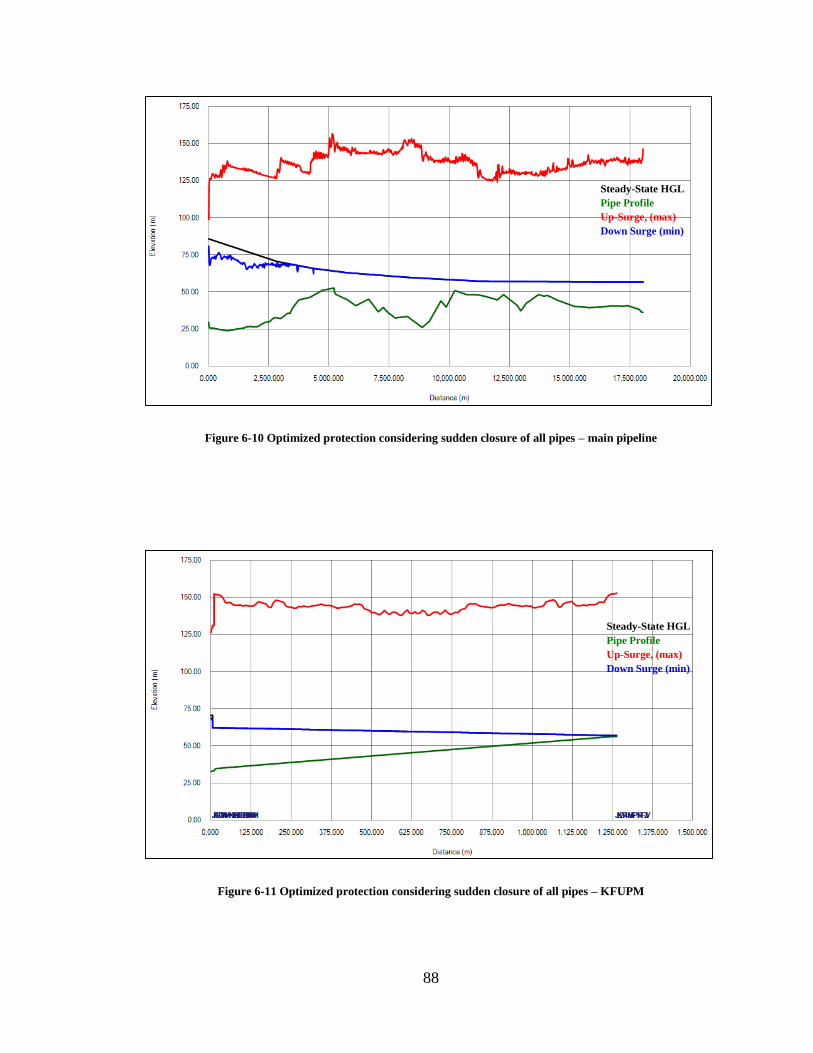
88

Figure 6-10 Optimized protection considering sudden closure of all pipes – main pipeline

Figure 6-11 Optimized protection considering sudden closure of all pipes – KFUPM

Steady-State HGL

Pipe Profile

Up-Surge, (max)

Down Surge (min)

Steady-State HGL

Pipe Profile

Up-Surge, (max)

Down Surge (min)

89

7 CHAPTER 7

CONCLUSION AND RECOMMENDATIONS

Khobar-Dammam Ring Line (KDRL) is of great importance to the water supply network

of Khobar as well as Dammam cities. Two main potential problems associated with water

hammer that need to be mitigated to keep this water network operational: the up-surge and

the down-surge because they can cause pipe rupture and backflow of dirty water into the

water distribution system. The main cause of the two phenomenon is a sudden change in

flow condition such as during the daily startup or shutdown of a pump or closing a valve,

leading to a pressure spike forming a surge wave that travels with a supper sonic speed

through the system. Thus, the control of these two phenomenon is essential not only to

keep the water running but also to provide a safe water supply to two highly populated

cities in the eastern region.

The current practice for protection of the KDRL from the water hammer are:

1- A soft startup/shutdown of the pump

2- Main valve closure 10 second before the pump shutdown.

These operational constrains are of no value in case of power failure.

90

To mitigate the water hammer problems, a model was constructed for the KDRL

network. The model was reliable and representative to the real operation conditions as it

was calibrated with field data.

Water hammer has been investigated in KDRL for two cases:

1- Power failure in pumping station.

2- Rapid close of actuator valves at 5 tank at the same time, assuming other two branches

are closed.

The calculations of the surge wave for water hammer show the following effects:

1. During the power failure: negative water pressure along the pipeline goes up to the

point where the pipeline is at a maximum elevation.

2. During the rapid valves closure: high water pressure along the KDRL was observed

to increase from the normal working pressure of 6-7.5 bar to a surge pressure of >20

bar.

From the water surge study results, the following recommendations were made to solve the

surge problem:

1- A 13 m3 surge vessel with a maximum working pressure of 8 bar be installed

downstream of the pumping station.

91

2- Pressure Relief Valves with the following specifications be installed at three

locations: downstream of the pump station, and at washout chambers number five and

thirteen.

a- Diameter if 600 mm

b- Spring Constant of 150 lb/in.

c- Threshold pressure of 6 bars.

3- Configure Air Valves to slowly release air, outlet orifice should not exceed 2-3”.

In addition, the following actions were recommended to protect the KDRL network:

1- A standby pump be added to operate in emergency cases (during the primary pump

failure).

2- A non-return flow control valve be installed at the branching point to prevent back

flow to main pipeline and eliminate the effect of branches on the main pipeline.

3- Valves be installed, in the same place, to isolate all branches from the main KDRL at

the branching point close to the served water tank. These valves better to be as

pressure control valves or flow control valve to control the amount of water delivered

to the tank and to maintain the delivering pressure to the branch pipe.

4- Enforce a policy of time delay in start-up/shutdown of a pump, or closing and opening

of a valve.

92

References

[1] D. J. Wood, S. Lingireddy and P. F. Boulos, Pressure Wave Analysis of Transient

Flow in Pipe Distribution System, Pasadena, California USA: MWHsoft, 2005.

[2] Haested-Methods, T. M. Walski, D. V. Chase, D. A. Savic, W. Grayman, S.

Beckwith and E. Koelle, Advanced Water Distribution Modeling and Analysis,

Exton, Pennsylvania USA: Bentley Institute Press, 2007.

[3] B. S. Jung, B. W. Karney, P. F. Boulos and D. J. Wood, "The Need for

Comprehensive Transient Analysis of Distribution Systems," AWWA, vol. 99, no.

1, 2007.

[4] P. F. Boulos, K. E. Lansey and B. W. Karney, Comprehensive Water Distribution

Analysis Handbook for Engineers and Planners, Pasadena, California USA:

MWHsoft, 2006.

[5] B. E. Larock, R. W. Jeppson and G. Z. Watters, Hydraulics of Pipeline Systems,

USA: CRC Press, 2000.

[6] Haested Methods Inc., WaterGEMS for ArcGIS, Waterbury, USA: Haested

Methods Inc., 2003.

[7] Bentley, "E-Doc," Bentley, 2004. [Online]. Available: www.bentley.com.

[Accessed 2013].

93

[8] A. Bergant, A. R. Simpson and E. Sijamhodzic, Water Hammer Analysis of

Pumping Systems for Control of Water in Underground Mines, Ljubljana,

Slovenia, Yugoslavia: Pro, 1991.

[9] E. B. Wylie and V. L. Streeter, Fluid Transient, USA: McGraw-Hill, 1978.

[10] A. Lohrasbi and R. Attarnejad, "Water Hammer Analysis by Characteristic

Method," American J. of Engineering and Applied Sciences, vol. 1, no. 4, pp. 287-

294, 2008.

[11] K. H. Asli, A. K. Haghi, H. H. Asli and E. S. Eshghi, "Water Hammer Modeling

and Simulation by GIS," Modelling and Simulation in Engineering, vol. 2012,

2012.

[12] A. Bergant and A. Tijsseling, Parameters Affecting Water Hammer Wave

Attenuation, Shape and Timing, Technische Universiteit Eindhoven, 2001.

[13] B. S. Jung, P. F. Boulos, D. J. Wood and C. M. Bros, "A Lagrangian Wave

Characteristic Method for Simulating Transient Water Column Separation,"

AWWA, vol. 101, no. 6, 2009.

[14] D. Ramalingam, S. Lingireddy and D. J. Wood, "Using The WCM for Transient

Modeling of Water Distribution Networks," AWWA, vol. 101, no. 2, 2009.

[15] A. R. Simpson, Large Water Hammer Pressures Due to Column Separation in

Sloping Pipes (Transient), ProQuest Dissertation & Thesis, 1986.

94

[16] B. S. Jung, P. F. Boulos and D. J. Wood, "Effect of Pressure-Sensitive Demand on

Surge Analysis," AWWA, vol. 101, no. 4, 2009.

[17] Z. Y. Wu and T. M. Walski, "Pressure Dependent Hydraulic Modeling for Water

Distribution Systems under Abnormal Conditions," in IWA World Water

Congress, 2006.

[18] Y. W. Zheng, R. H. Wang, T. M. Walski, S. Y. Yang, D. Bowdler and C. Baggett,

"Efficient Pressure Dependent Demand Model for Large Water Distribution

System Analysis," in 8th Annual International Symposium on Water Distribution

System Analysis, Cincinnati, Ohio, 2006.

[19] B. S. Jung, P. F. Boulos and D. J. Wood, "Pitfalls of Water Distribution Model

Skeletonization for Surge Analysis," AWWA, vol. 99, no. 12, 2007.

[20] KYPipe LLC, "Learning about KYPipe," KYPipe LLC, [Online]. Available:

www.KYPipe.com. [Accessed 2013].

[21] P. F. Boulos, B. W. Karney, D. J. Wood and S. Lingireddy, "Hydraulic Transient

Guidelines for Protecting Water Distribution System," AWWA, vol. 97, no. 5,

2005.

95

8 APPENDICES

96

Appendix A

Field Survey Results

Table A-1: Survey elevation Vs as-built elevations

CODE STATION ELEV ELEV (ABD) DIFF Notice

TANK 0 29.323 29.5 -0.177 Yarmouk Tank

DisV1 776.833 23.427 23.76 -0.333 G-ELEVATION

FM-Yar 1503.463 27.002 25.78 1.222 G-ELEVATION - Main FM

AirV1 1797.863 27.214 26.7 0.514 P3

xxx 1883.413 27.339 25.98 1.359 ROAD CROSSING

J11M 1952.813 28.177 26.6 1.577 ROAD CROSSING

DisV4 2013.123 27.822 26.45 1.372

AirV2 2799.213 35.17 32.68 2.49

J25M-1T 2846.333 34.643 31 3.643 KFUPM FM

DisV6 2986.453 34.291 32.05 2.241

AirV3 3305.273 37.855 35.59 2.265

J30M 3318.113 37.771 35.59 2.181 PLUG

DisV8 3379.883 37.471 35.4 2.071

AirV4 3752.903 46.791 44.58 2.211

DisV10 4225.793 48.33 46.36 1.97 G-ELEVATION

DisV12 4362.753 50.139 47.7 2.439 Doha-3 FM

AirV5 5208.543 57.415 52.57 4.845 G-ELEVATION

J38M-3T 5758.153 47.745 44.77 2.975 Doha-1 FM

DisV16 6121.673 43.543 40.68 2.863

AirV6 6649.143 48.182 45.13 3.052

DisV18 7057.323 40.098 36.6 3.498

AirV7 7255.393 43.025 39.51 3.515

J41M 7452.043 39.332 35.8 3.532 PLUG

xxx 7576.863 36.005 32.44 3.565 G-ELEVATION

AirV8 8273.213 37.142 33.44 3.702 G-ELEVATION

97

CODE STATION ELEV ELEV (ABD) DIFF Notice

J44M-4T 8279.873 37.059 33.24 3.819 Doha-2 FM

DisV19 8884.313 30.619 26.03 4.589

AirV9 9655.153 48.045 43.93 4.115

AirV10 10226.363 50.748 50.85 -0.102 G-ELEVATION

48M 10723.363 51.283 49.11 2.173 PLUG

xxx 10734.473 51.18 49.09 2.09 PLUG

J49M-5T 11209.773 50.008 48.02 1.988 Dana FM

J50M 11536.753 48.679 46.77 1.909

DisV23 11998.783 46.561 44.61 1.951

xxx 12013.643 46.702 44.63 2.072 PLUG

AirV11 12257.923 49.968 48.08 1.888

DisV23 12971.923 39.387 37.25 2.137

J53M 12990.923 40.29 37.36 2.93 ROAD CROSSING

J54M 13092.953 39.786 37.65 2.136 ROAD CROSSING

J57M-6T 13699.843 48.761 48.06 0.701 Palace FM

AirV12 14077.223 49.204 47.61 1.594

DisV25 14475.053 46.27 44.54 1.73 G-ELEVATION

J58M 15177.783 37.974 40.31 -2.336

J65M-7T 15611.783 42.23 40 2.23 Dist-537 FM

J66M 16709.783 43.95 40.57 3.38

DisV27 17230.033 40.49 40.4 0.09

AirV14 17412.713 41.2 40.68 0.52 FM

Dm55-P3 18039.713 36.25 33.16 3.09 P3

98

Table A-2: Air valve locations

SN NODE_ID DIA X_COO Y_COO ELEVATION

1 AIR-1 150 417214.706 2909167.53 27.214

2 AIR-2 150 416421.541 2909410.18 35.17

3 AIR-3 150 416257.4968 2909886.09 37.855

4 AIR-4 150 416046.712 2910274.32 46.791

5 AIR-5 150 415644.701469 2911569.59 50.24

6 AIR-6 150 416923.539 2912041.75 48.182

7 AIR-7 150 417239.98 2912436.52 43.025

8 AIR-8 150 416998.123732 2913166.14 24.7

9 AIR-9 150 415587.422 2913190.4 50.748

10 AIR-10 150 416043.732 2913529.15 48.045

11 AIR-11 150 414289.238 2914748.06 49.968

12 AIR-12 150 413395.51 2915744.2 49.204

13 AIR-13 150 412503.3859 2917338.51 40.985

14 AIR-14 150 411392.737 2917769.27 39.601

99

Figure A-1: Survey elevation Vs as-built elevation

100

Appendix B

Sample Input Data

&

Sample Hydraulic Analysis Results

Table B-1: Sample hydraulic analysis results - tanks

Label Dia (m)

Elev (m)

Level (m) (Initial)

Flow In (L/s)

Level (m)

Status

Dammam-55 40 36.25 5 8 5.4 Filling

Dana 7 56 2.4 7 1.49 Filling

Doha-1 18 49.87 8.64 -47 4.02 Emptying

Doha-2 18 59 2 -13 3.62 Emptying

Doha-3 11 49.28 9.2 -23 2.67 Emptying

KFUPM 40 56.35 2.3 26 3.71 Filling

Yarmouk-Tank 40 29.5 13 -1,819 18 Emptying

Table B-2: Sample hydraulic analysis results - pump

Label Elev (m)

HGL (Suction)

(m)

HGL (Discharge)

(m)

Flow (Total) (L/s)

Pump Head (ft)

Y-Pump 29.5 47.42 108.7 560 201.07

Table B-3: Sample hydraulic analysis results – air valve

ID Label Elev (m)

Air Valve Type

Dia (mm) (Inflow)

Dia (mm) (Outflow)

HGL (m)

325 AirV1 26.7 Double Acting 150 150 92.24





330 AirV7 39.51 Double Acting 150 150 68







101

Table B-4: Sample hydraulic analysis results - pipes

Label Length

(m) Start

Node Stop Node

Dia (mm)

Mat. Vel.

(ft/s) Flow (L/s)

HL (ft)

L1 4 J1M J2M 600 DI 6.19 534 0.2

L2 13 J2M J3M 700 CCP 4.55 534 0.34

L3 48 J3M J4M 700 CCP 4.55 534 1.3

L32 80 J26M J27M 700 CCP 2.92 343 0.96

L33 48 J27M J28M 700 CCP 2.92 343 0.57

L34 61 J28M AirV3 700 CCP 2.92 343 0.74

L66 218 AirV9 J45M 700 CCP 1.83 215 1.1

L67 349 J45M J46M 700 CCP 1.83 215 1.77

L68 16 J46M AirV10 700 CCP 1.83 215 0.08

L69 494 J47M AirV10 700 CCP 1.83 -215 2.5

L70 477 J47M J48M-5T 700 CCP 1.83 215 2.41

L71 327 J48M-5T J49M 700 CCP 0.43 50 0.11

L72 461 J49M DisV13 700 CCP 0.43 50 0.16

L84 704 DisV15 J57M 700 CCP 0.43 50 0.24

L85 364 J57M J58M 700 CCP 0.43 50 0.12

L86 254 J58M J59M 700 CCP 0.43 50 0.09

L90 457 AirV13 J62M 700 CCP 0.29 34 0.08

L91 52 DisV16 J62M 700 CCP 0.29 -34 0.01

L97 11 Dm55-P3 Dam-CV 600 DI 0.4 34 0

LT1-1 3 J24M-1T FM1-KFUPM 400 DI 4.98 191 0.17

LT1-2 1,253 FM1-KFUPM J24M-1T2 400 DI 4.98 191 77.54

LT2-1 5 J33M-2T Doha3-PRV 200 UPVC 3.54 34 0.19

LT2-2 60 Doha3-PRV J33M-2T2 200 UPVC 3.54 34 2.39

LT3-1 9 J37M-3T Doha1-PRV 200 UPVC 2.3 22 0.16

LT3-2 87 Doha1-PRV J37M-3T2 200 UPVC 2.3 22 1.56

LT4-1 4 J42M-4T Doha2-PRV 300 FRP 3.35 72 0.08

LT4-2 4 Doha2-PRV J42M-4T2 300 FRP 3.35 72 0.07

LT5-1 89 J48M-5T FM5-Dana 400 DI 4.3 165 4.21

LT5-2 35 FM5-Dana J48M-5T2 400 DI 4.3 165 1.64

LT6-1 4 J55M-6T FM6-Khaleej 300 FRP 0 0 0

LT6-2 285 FM6-Khaleej KhaleejPalace 300 FRP 0 0 0

LT7-1 60 J61M-7T FM7-p537 300 FRP 0.74 16 0.06

LT7-2 734 FM7-p537 Dist-537 300 FRP 0.74 16 0.78

102

Table B-5: Sample hydraulic analysis results - junctions

Label Elev (m)

Demand (L/s)

HGL (m)

Max HGL (m)

Min HGL (m)

Dana-D 55 0 57.98 59.58 55

Dist-537 41.87 16 60.85 114.24 56.71

Dm55-D 36 0 41.25 43.17 41.25

Dm55-P3 36.25 0 61.01 114.13 57.14

Doha1-D 49 1 58.51 58.66 49

Doha2-D 58 1 61 65.34 58

Doha3-D 49 1 58.48 59.32 49

FM-Tank55 40.7 0 61.05 114.24 57.17

FM-Yarmouk 25.78 0 93.74 127.2 93.74

FM1-KFUPM 34.68 0 82.53 124.17 81.79

FM2-Doha3 49.29 0 58.56 59.45 49.52

FM3-Doha1 49.87 0 58.56 58.78 50.23

FM4-Doha2 59 0 61.17 65.54 59.16

FM5-Dana 49 0 60.35 115.65 57.49

FM6-Khaleej 48.04 0 61.38 115.05 57.51

FM7-p537 39.89 0 61.09 114.42 57.18

J1M 26.6 0 106.14 130.55 106.14

J2M 26.6 0 106.08 130.54 106.08

J32M 41 0 79.89 122.52 78.4

J33M-2T 47.7 0 77.01 120.75 74.59

J34M 51.07 0 75.89 120.18 73.27

J36M 48.5 0 74.27 119.35 71.36

J37M-3T 44.77 0 72.8 118.6 69.63

J38M 37 0 69.45 117.46 66.5

J41M 32.44 0 67.54 116.82 64.71

J42M-4T 33.24 0 66.16 116.35 63.42

J43M 29.27 0 64.88 116.15 62.17

J47M 48.12 0 62.37 115.76 59.48

J48M-5T 48.02 0 61.64 115.65 58.51

J49M 46.77 0 61.6 115.57 58.38

J54M 42.18 0 61.43 115.17 57.72

J55M-6T 48.05 0 61.38 115.05 57.52

J56M 47.15 0 61.35 114.99 57.49

J60M 39.5 0 61.14 114.5 57.25

J61M-7T 39.72 0 61.11 114.44 57.22

J62M 40.43 0 61.06 114.28 57.18

KFUPM-D 20 0 58.65 66.36 58.65

103

Appendix C

Model Calibration

Table C-1: Calibration result table field observed reading Vs model calculated data

Field Data Snapshot

Pipe Observed Flow (L/s)

Simulated Flow (L/s)

Difference (L/s)

28/Oct Yar 1:00PM L7 589 593 4

28/Oct Yar 1:15PM L7 586 590 4

28/Oct Yar 1:30PM L7 593 598 4

28/Oct Yar 1:45PM L7 613 618 5

28/Oct Yar 2:00PM L7 618 623 5

28/Oct Yar 2:15PM L7 612 617 5

28/Oct Yar 2:30PM L7 595 600 4

28/Oct Yar 2:45PM L7 590 594 4

28/Oct Yar 3:00PM L7 335 338 3

28/Oct Yar 3:15PM L7 0 0 0

28/Oct Yar 3:30PM L7 0 0 0

28/Oct Yar 3:45PM L7 0 0 0

28/Oct Yar 4:00PM L7 389 392 3

28/Oct Yar 4:15PM L7 538 542 4

28/Oct Yar 4:30PM L7 539 543 4

28/Oct Yar 4:45PM L7 541 545 4

28/Oct Yar 5:00PM L7 549 553 4

28/Oct Yar 5:15PM L7 515 519 4

28/Oct Yar 5:30PM L7 548 552 4

28/Oct Yar 5:45PM L7 540 544 4

28/Oct Yar 6:00AM L7 0 0 0

28/Oct Yar 6:00PM L7 540 544 4

28/Oct Yar 6:15AM L7 0 0 0

28/Oct Yar 6:15PM L7 530 534 4

28/Oct Yar 6:30AM L7 32 32 0

28/Oct Yar 6:30PM L7 527 531 4

28/Oct Yar 6:45AM L7 547 551 4

28/Oct Yar 6:45PM L7 524 528 4

28/Oct Yar 7:00AM L7 549 553 4

28/Oct Yar 7:00PM L7 532 536 4

28/Oct Yar 7:15AM L7 596 600 4

28/Oct Yar 7:15PM L7 522 526 4

28/Oct Yar 7:30AM L7 611 615 5

104

Field Data Snapshot



Difference (L/s)

28/Oct Yar 7:30PM L7 537 541 4

28/Oct Yar 7:45AM L7 595 600 4

28/Oct Yar 7:45PM L7 522 526 4

28/Oct Yar 8:00AM L7 614 619 5

28/Oct Yar 8:00PM L7 500 503 4

28/Oct Yar 8:15AM L7 604 608 5

28/Oct Yar 8:15PM L7 505 509 4

28/Oct Yar 8:30AM L7 616 621 5

28/Oct Yar 8:30PM L7 530 534 4

28/Oct Yar 8:45AM L7 620 624 5

28/Oct Yar 8:45PM L7 527 531 4

28/Oct Yar 9:00AM L7 620 624 5

28/Oct Yar 9:00PM L7 524 528 4

28/Oct Yar 9:15AM L7 627 631 5

28/Oct Yar 9:15PM L7 532 536 4

28/Oct Yar 9:30AM L7 630 634 5

28/Oct Yar 9:30PM L7 515 519 4

28/Oct Yar 9:45AM L7 609 614 5

28/Oct Yar 9:45PM L7 519 523 4

28/Oct Yar 10:00AM L7 625 629 5

28/Oct Yar 10:00PM L7 521 524 4

28/Oct Yar 10:15AM L7 625 630 5

28/Oct Yar 10:15PM L7 498 502 4

28/Oct Yar 10:30AM L7 614 618 5

28/Oct Yar 10:30PM L7 477 480 4

28/Oct Yar 10:45AM L7 604 608 5

28/Oct Yar 10:45PM L7 57 58 0

28/Oct Yar 11:00AM L7 608 613 5

28/Oct Yar 11:00PM L7 0 0 0

28/Oct Yar 11:15AM L7 601 605 5

28/Oct Yar 11:15PM L7 0 0 0

28/Oct Yar 11:30AM L7 609 613 5

28/Oct Yar 11:30PM L7 0 0 0

28/Oct Yar 11:45AM L7 599 603 4

28/Oct Yar 11:45PM L7 0 0 0

28/Oct Yar 12:00PM L7 612 617 5

28/Oct Yar 12:15PM L7 598 603 4

28/Oct Yar 12:30PM L7 598 603 4

28/Oct Yar 12:45PM L7 606 610 5

105

Field Data Snapshot



Difference (L/s)

29/Oct Yar 1:00AM L7 379 382 3

29/Oct Yar 1:00PM L7 595 600 4

29/Oct Yar 1:15AM L7 498 502 4

29/Oct Yar 1:15PM L7 578 583 4

29/Oct Yar 1:30AM L7 503 506 4

29/Oct Yar 1:30PM L7 598 602 4

29/Oct Yar 1:45AM L7 487 491 4

29/Oct Yar 1:45PM L7 590 595 4

29/Oct Yar 2:00AM L7 474 478 4

29/Oct Yar 2:00PM L7 585 590 4

29/Oct Yar 2:15AM L7 476 480 4

29/Oct Yar 2:15PM L7 574 578 4

29/Oct Yar 2:30AM L7 471 475 4

29/Oct Yar 2:30PM L7 565 569 4

29/Oct Yar 2:45AM L7 463 467 3

29/Oct Yar 2:45PM L7 0 0 0

29/Oct Yar 3:00AM L7 461 464 3

29/Oct Yar 3:00PM L7 0 0 0

29/Oct Yar 3:15AM L7 468 471 4

29/Oct Yar 3:15PM L7 0 0 0

29/Oct Yar 3:30AM L7 453 457 3

29/Oct Yar 3:30PM L7 0 0 0

29/Oct Yar 3:45AM L7 458 461 3

29/Oct Yar 3:45PM L7 407 410 3

29/Oct Yar 4:00AM L7 452 456 3

29/Oct Yar 4:00PM L7 503 507 4

29/Oct Yar 4:15AM L7 436 439 3

29/Oct Yar 4:15PM L7 523 527 4

29/Oct Yar 4:30AM L7 359 362 3

29/Oct Yar 4:30PM L7 508 512 4

29/Oct Yar 4:45AM L7 376 379 3

29/Oct Yar 4:45PM L7 507 510 4

29/Oct Yar 5:00AM L7 426 429 3

29/Oct Yar 5:00PM L7 507 510 4

29/Oct Yar 5:15AM L7 413 416 3

29/Oct Yar 5:15PM L7 497 500 4

29/Oct Yar 5:30AM L7 395 398 3

29/Oct Yar 5:30PM L7 510 513 4

29/Oct Yar 5:45AM L7 405 408 3

106

Field Data Snapshot



Difference (L/s)

29/Oct Yar 5:45PM L7 513 517 4

29/Oct Yar 6:00AM L7 423 426 3

29/Oct Yar 6:00PM L7 511 515 4

29/Oct Yar 6:15AM L7 393 396 3

29/Oct Yar 6:15PM L7 506 510 4

29/Oct Yar 6:30AM L7 465 468 3

29/Oct Yar 6:30PM L7 521 525 4

29/Oct Yar 6:45AM L7 488 491 4

29/Oct Yar 6:45PM L7 519 522 4

29/Oct Yar 7:00AM L7 497 501 4

29/Oct Yar 7:00PM L7 501 505 4

29/Oct Yar 7:15AM L7 550 554 4

29/Oct Yar 7:15PM L7 510 514 4

29/Oct Yar 7:30AM L7 586 590 4

29/Oct Yar 7:30PM L7 516 520 4

29/Oct Yar 7:45AM L7 570 575 4

29/Oct Yar 7:45PM L7 520 524 4

29/Oct Yar 8:00AM L7 575 579 4

29/Oct Yar 8:00PM L7 528 532 4

29/Oct Yar 8:15AM L7 570 575 4

29/Oct Yar 8:15PM L7 532 536 4

29/Oct Yar 8:30AM L7 576 580 4

29/Oct Yar 8:30PM L7 535 539 4

29/Oct Yar 8:45AM L7 557 562 4

29/Oct Yar 8:45PM L7 500 504 4

29/Oct Yar 9:00AM L7 554 558 4

29/Oct Yar 9:00PM L7 503 506 4

29/Oct Yar 9:15AM L7 535 539 4

29/Oct Yar 9:15PM L7 505 509 4

29/Oct Yar 9:30AM L7 551 555 4

29/Oct Yar 9:30PM L7 497 500 4

29/Oct Yar 9:45AM L7 553 557 4

29/Oct Yar 9:45PM L7 476 480 4

29/Oct Yar 10:00AM L7 550 554 4

29/Oct Yar 10:00PM L7 450 453 3

29/Oct Yar 10:15AM L7 562 566 4

29/Oct Yar 10:15PM L7 447 450 3

29/Oct Yar 10:30AM L7 563 567 4

29/Oct Yar 10:30PM L7 456 459 3

107

Field Data Snapshot



Difference (L/s)

29/Oct Yar 10:45AM L7 591 596 4

29/Oct Yar 10:45PM L7 464 468 3

29/Oct Yar 11:00AM L7 588 592 4

29/Oct Yar 11:00PM L7 334 336 3

29/Oct Yar 11:15AM L7 587 591 4

29/Oct Yar 11:15PM L7 0 0 0

29/Oct Yar 11:30AM L7 609 614 5

29/Oct Yar 11:30PM L7 0 0 0

29/Oct Yar 11:45AM L7 607 612 5

29/Oct Yar 11:45PM L7 0 0 0

29/Oct Yar 12:00AM L7 0 0 0

29/Oct Yar 12:00PM L7 595 600 4

29/Oct Yar 12:15AM L7 0 0 0

29/Oct Yar 12:15PM L7 600 604 4

29/Oct Yar 12:30AM L7 0 0 0

29/Oct Yar 12:30PM L7 606 611 5

29/Oct Yar 12:45AM L7 0 0 0

29/Oct Yar 12:45PM L7 595 599 4

30/Oct Yar 1:00AM L7 0 0 0

30/Oct Yar 1:15AM L7 404 407 3

30/Oct Yar 1:30AM L7 467 471 4

30/Oct Yar 1:45AM L7 479 482 4

30/Oct Yar 2:00AM L7 473 477 4

30/Oct Yar 2:15AM L7 480 483 4

30/Oct Yar 2:30AM L7 487 491 4

30/Oct Yar 2:45AM L7 477 481 4

30/Oct Yar 3:00AM L7 469 473 4

30/Oct Yar 3:15AM L7 469 472 4

30/Oct Yar 3:30AM L7 474 477 4

30/Oct Yar 3:45AM L7 466 470 3

30/Oct Yar 4:00AM L7 460 464 3

30/Oct Yar 4:15AM L7 450 454 3

30/Oct Yar 4:30AM L7 461 465 3

30/Oct Yar 4:45AM L7 455 459 3

30/Oct Yar 5:00AM L7 388 391 3

30/Oct Yar 5:15AM L7 0 0 0

30/Oct Yar 5:30AM L7 0 0 0

30/Oct Yar 5:45AM L7 0 0 0

108

Table C-2: Field flow meter reading for all metering points 28th to 30th Oct, 2013

Date TIME Yar UPM Doha3 Doha1 Doha2 Dana palace P537 Dm55

28th

6:00AM 0.00 0.00 0.00 0.00 0.00 0.00 0.00 37.89 -46.78

6:15AM 0.00 0.00 0.00 0.00 0.00 0.00 0.00 40.98 -48.23

6:30AM 32.04 0.00 0.00 0.00 0.00 0.00 0.00 41.86 -49.29

6:45AM 547.06 0.00 89.67 78.51 89.54 158.51 0.00 61.64 -2.05

7:00AM 548.90 0.00 104.18 89.92 110.66 194.61 0.00 53.74 20.12

7:15AM 595.72 126.83 90.00 78.51 73.06 140.46 0.00 51.44 17.13

7:30AM 610.51 159.50 86.04 73.97 50.78 137.53 46.34 47.51 8.07

7:45AM 595.11 138.85 83.62 79.22 39.94 137.53 73.77 48.09 -0.03

8:00AM 614.21 162.50 83.40 79.12 41.96 135.82 73.19 46.37 16.07

8:15AM 603.73 162.50 83.18 79.02 43.55 136.56 73.12 46.94 13.57

8:30AM 616.05 138.47 81.09 75.99 29.38 183.88 71.38 45.79 7.01

8:45AM 619.75 141.85 80.65 75.79 25.62 196.08 71.02 46.10 -0.03

9:00AM 619.75 149.36 81.75 77.20 34.01 169.00 72.03 47.21 8.07

9:15AM 626.53 145.23 81.53 77.30 32.13 173.39 71.82 46.63 2.00

9:30AM 629.61 141.47 82.63 78.11 39.21 152.17 72.75 46.10 12.02

9:45AM 609.28 131.71 80.98 75.29 24.90 193.88 71.02 46.10 -0.03

10:00AM 624.68 136.97 82.52 77.71 36.61 160.71 71.96 46.10 8.55

10:15AM 625.29 156.49 81.20 75.79 25.76 191.93 70.66 45.79 12.60

10:30AM 613.59 151.99 82.52 77.71 34.73 197.79 53.19 46.37 15.11

10:45AM 603.73 145.23 85.82 81.44 57.29 193.88 0.00 45.22 19.06

11:00AM 608.05 142.60 85.71 81.04 58.30 194.37 0.00 39.88 21.57

11:15AM 600.65 164.76 85.49 80.53 59.32 192.91 0.00 44.38 20.12

11:30AM 608.66 159.12 85.27 80.13 59.75 198.03 0.00 44.95 19.06

11:45AM 598.80 148.98 85.16 79.83 60.33 195.35 0.00 44.95 18.58

12:00PM 612.36 145.60 86.15 81.14 67.56 174.37 0.00 46.63 19.06

12:15PM 598.19 156.49 87.14 82.15 74.36 154.85 0.00 47.21 20.60

12:30PM 598.19 158.75 86.81 81.64 73.06 156.31 0.00 45.79 22.14

12:45PM 605.58 159.12 86.59 81.44 73.20 158.51 0.00 45.79 20.12

1:00PM 588.95 159.50 86.48 81.24 73.49 158.02 0.00 45.22 21.57

1:15PM 585.87 156.87 86.48 81.14 74.65 155.83 0.00 44.95 20.60

1:30PM 593.26 150.11 85.27 79.63 70.16 175.83 0.00 44.11 20.60

1:45PM 612.97 155.74 83.95 78.11 64.67 196.08 0.00 42.97 18.58

2:00PM 617.90 153.49 83.84 77.91 65.25 197.05 0.00 42.13 21.08

2:15PM 612.36 134.71 83.73 77.71 65.82 195.10 0.00 44.38 20.60

2:30PM 595.11 151.61 86.04 81.34 74.50 160.22 0.00 46.63 21.08

2:45PM 589.56 167.38 89.34 84.07 86.94 107.53 0.00 45.79 25.13

109

3:00PM 335.13 125.33 59.33 48.54 50.64 92.65 0.00 41.29 14.05

3:15PM 0.00 0.00 6.01 0.00 0.00 0.00 0.00 39.88 -17.57

3:30PM 0.00 0.00 0.00 0.00 0.00 0.00 0.00 37.32 -44.28

3:45PM 0.00 0.00 0.00 0.00 0.00 0.00 0.00 37.32 -47.26

4:00PM 389.35 0.00 61.86 61.96 64.38 105.09 0.00 55.42 -17.09

4:15PM 537.82 0.00 105.28 101.32 116.01 183.88 0.00 55.42 22.14

4:30PM 539.05 0.00 105.50 102.03 118.47 173.39 0.00 53.74 21.57

4:45PM 540.90 0.00 104.40 101.02 115.57 182.90 0.00 53.43 21.57

5:00PM 548.90 0.00 104.84 101.93 117.45 172.66 0.00 55.15 22.14

5:15PM 515.02 0.00 104.73 101.93 118.47 172.66 0.00 55.99 21.08

5:30PM 547.67 0.00 103.19 100.62 113.26 190.22 0.00 56.56 19.64

5:45PM 539.66 0.00 102.97 100.52 112.97 188.76 0.00 57.67 17.61

6:00PM 540.28 0.00 102.97 100.52 114.13 185.34 0.00 57.13 18.58

6:15PM 530.42 0.00 102.75 100.21 113.40 186.32 0.00 55.42 18.10

6:30PM 526.73 0.00 102.53 99.91 113.84 187.30 0.00 55.15 18.58

6:45PM 524.26 0.00 102.20 99.51 113.40 189.73 0.00 53.16 21.57

7:00PM 531.65 0.00 101.98 99.10 113.26 188.27 0.00 53.74 21.08

7:15PM 521.80 0.00 101.76 98.80 113.55 191.93 0.00 51.44 21.08

7:30PM 537.20 0.00 101.54 98.29 112.83 191.93 0.00 51.44 23.11

7:45PM 522.41 0.00 102.31 99.41 116.88 177.29 0.00 51.44 23.11

8:00PM 499.62 0.00 105.94 103.14 130.18 115.33 0.00 51.44 27.16

8:15PM 505.16 0.00 104.62 101.12 125.99 132.65 0.00 49.76 27.16

8:30PM 529.81 0.00 100.77 96.88 113.55 189.73 0.00 47.78 25.62

8:45PM 526.73 0.00 100.33 96.28 112.25 194.37 0.00 44.95 26.10

9:00PM 524.26 1.41 100.00 95.77 112.39 194.37 0.00 45.22 28.12

9:15PM 531.65 0.00 99.67 93.55 112.25 195.10 0.00 44.95 30.15

9:30PM 515.02 0.00 100.88 72.86 116.30 207.30 0.00 44.95 28.70

9:45PM 519.33 0.00 100.44 72.66 116.01 207.79 0.00 45.79 28.70

10:00PM 520.57 0.00 95.60 72.96 117.17 209.49 0.00 44.95 28.70

10:15PM 498.39 0.00 90.11 76.80 132.06 159.49 0.00 48.35 30.15

10:30PM 476.83 0.00 91.32 77.81 136.40 134.12 0.00 47.78 30.63

10:45PM 57.29 0.00 18.66 10.40 25.04 32.15 0.00 22.62 -14.10

11:00PM 0.00 0.00 0.00 0.00 0.00 0.00 0.00 28.00 -45.72

11:15PM 0.00 0.00 0.00 0.00 0.00 0.00 0.00 28.27 -43.70

11:30PM 0.00 0.00 0.00 0.00 0.00 0.00 0.00 29.99 -45.24

11:45PM 0.00 0.00 0.00 0.00 0.00 0.00 0.00 28.00 -45.72

29th

12:00AM 0.00 0.00 0.00 0.00 0.00 0.00 0.00 27.70 -45.24

12:15AM 0.00 0.00 0.00 0.00 0.00 0.00 0.00 28.58 -47.75

12:30AM 0.00 0.00 0.00 0.00 0.00 0.00 0.00 28.58 -48.23

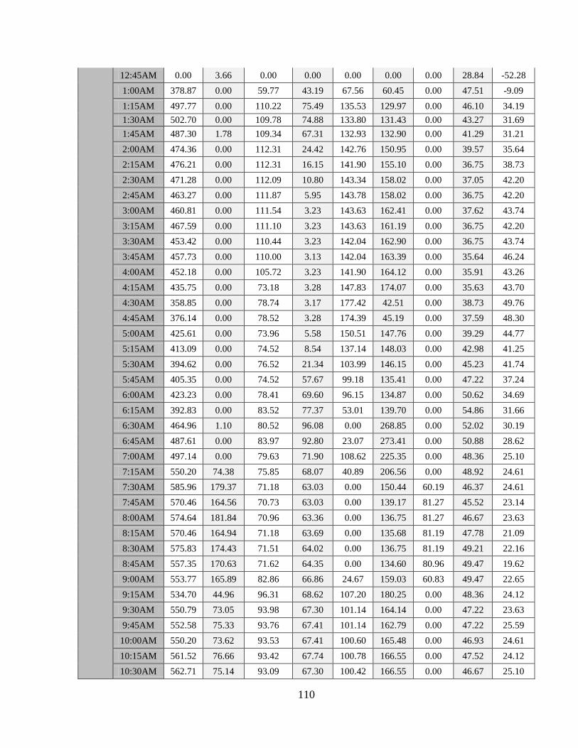
110

12:45AM 0.00 3.66 0.00 0.00 0.00 0.00 0.00 28.84 -52.28

1:00AM 378.87 0.00 59.77 43.19 67.56 60.45 0.00 47.51 -9.09

1:15AM 497.77 0.00 110.22 75.49 135.53 129.97 0.00 46.10 34.19

1:30AM 502.70 0.00 109.78 74.88 133.80 131.43 0.00 43.27 31.69

1:45AM 487.30 1.78 109.34 67.31 132.93 132.90 0.00 41.29 31.21

2:00AM 474.36 0.00 112.31 24.42 142.76 150.95 0.00 39.57 35.64

2:15AM 476.21 0.00 112.31 16.15 141.90 155.10 0.00 36.75 38.73

2:30AM 471.28 0.00 112.09 10.80 143.34 158.02 0.00 37.05 42.20

2:45AM 463.27 0.00 111.87 5.95 143.78 158.02 0.00 36.75 42.20

3:00AM 460.81 0.00 111.54 3.23 143.63 162.41 0.00 37.62 43.74

3:15AM 467.59 0.00 111.10 3.23 143.63 161.19 0.00 36.75 42.20

3:30AM 453.42 0.00 110.44 3.23 142.04 162.90 0.00 36.75 43.74

3:45AM 457.73 0.00 110.00 3.13 142.04 163.39 0.00 35.64 46.24

4:00AM 452.18 0.00 105.72 3.23 141.90 164.12 0.00 35.91 43.26

4:15AM 435.75 0.00 73.18 3.28 147.83 174.07 0.00 35.63 43.70

4:30AM 358.85 0.00 78.74 3.17 177.42 42.51 0.00 38.73 49.76

4:45AM 376.14 0.00 78.52 3.28 174.39 45.19 0.00 37.59 48.30

5:00AM 425.61 0.00 73.96 5.58 150.51 147.76 0.00 39.29 44.77

5:15AM 413.09 0.00 74.52 8.54 137.14 148.03 0.00 42.98 41.25

5:30AM 394.62 0.00 76.52 21.34 103.99 146.15 0.00 45.23 41.74

5:45AM 405.35 0.00 74.52 57.67 99.18 135.41 0.00 47.22 37.24

6:00AM 423.23 0.00 78.41 69.60 96.15 134.87 0.00 50.62 34.69

6:15AM 392.83 0.00 83.52 77.37 53.01 139.70 0.00 54.86 31.66

6:30AM 464.96 1.10 80.52 96.08 0.00 268.85 0.00 52.02 30.19

6:45AM 487.61 0.00 83.97 92.80 23.07 273.41 0.00 50.88 28.62

7:00AM 497.14 0.00 79.63 71.90 108.62 225.35 0.00 48.36 25.10

7:15AM 550.20 74.38 75.85 68.07 40.89 206.56 0.00 48.92 24.61

7:30AM 585.96 179.37 71.18 63.03 0.00 150.44 60.19 46.37 24.61

7:45AM 570.46 164.56 70.73 63.03 0.00 139.17 81.27 45.52 23.14

8:00AM 574.64 181.84 70.96 63.36 0.00 136.75 81.27 46.67 23.63

8:15AM 570.46 164.94 71.18 63.69 0.00 135.68 81.19 47.78 21.09

8:30AM 575.83 174.43 71.51 64.02 0.00 136.75 81.19 49.21 22.16

8:45AM 557.35 170.63 71.62 64.35 0.00 134.60 80.96 49.47 19.62

9:00AM 553.77 165.89 82.86 66.86 24.67 159.03 60.83 49.47 22.65

9:15AM 534.70 44.96 96.31 68.62 107.20 180.25 0.00 48.36 24.12

9:30AM 550.79 73.05 93.98 67.30 101.14 164.14 0.00 47.22 23.63

9:45AM 552.58 75.33 93.76 67.41 101.14 162.79 0.00 47.22 25.59

10:00AM 550.20 73.62 93.53 67.41 100.60 165.48 0.00 46.93 24.61

10:15AM 561.52 76.66 93.42 67.74 100.78 166.55 0.00 47.52 24.12

10:30AM 562.71 75.14 93.09 67.30 100.42 166.55 0.00 46.67 25.10

111

10:45AM 591.33 138.36 89.75 65.99 95.79 92.18 0.00 43.53 27.64

11:00AM 587.75 168.93 85.19 60.85 76.01 158.50 0.00 45.52 21.09

11:15AM 586.56 150.13 82.52 58.98 65.31 200.65 0.00 45.82 20.11

11:30AM 609.21 155.64 82.41 59.09 66.38 201.99 0.00 46.37 18.05

11:45AM 607.42 152.98 82.41 59.20 66.74 199.85 0.00 46.08 18.64

12:00PM 595.50 153.93 82.41 59.31 67.45 196.62 0.00 45.82 19.13

12:15PM 599.67 163.99 82.41 59.42 68.16 198.77 0.00 46.08 20.60

12:30PM 606.23 157.35 79.96 59.64 69.77 198.77 0.00 44.68 20.60

12:45PM 594.90 167.98 79.41 59.75 70.30 199.85 0.00 44.38 20.60

1:00PM 595.50 152.60 79.41 59.86 70.48 197.70 0.00 43.27 22.65

1:15PM 578.21 153.74 79.41 59.86 71.73 198.50 0.00 42.42 22.16

1:30PM 597.88 156.02 79.41 59.97 71.73 197.43 0.00 41.84 22.65

1:45PM 590.14 158.29 80.41 61.17 76.72 182.66 0.00 41.57 24.12

2:00PM 585.37 160.38 82.41 63.03 86.52 146.15 0.00 42.68 25.10

2:15PM 574.04 148.80 82.41 63.14 86.70 144.27 0.00 42.68 25.59

2:30PM 564.50 159.05 81.30 80.32 81.00 140.78 0.00 39.88 25.10

2:45PM 0.00 48.18 5.45 0.66 0.00 13.24 0.00 25.45 -30.69

3:00PM 0.00 0.72 0.00 0.00 0.00 0.08 0.00 34.20 -48.21

3:15PM 0.00 0.00 0.00 0.00 0.00 0.00 0.00 36.48 -49.78

3:30PM 0.00 0.00 0.00 0.00 0.00 0.08 0.00 36.74 -50.27

3:45PM 406.54 0.00 65.17 75.73 85.27 67.75 0.00 58.81 -13.07

4:00PM 503.11 0.00 101.65 111.84 135.89 114.46 0.00 55.97 22.16

4:15PM 522.78 0.00 106.88 111.29 132.51 113.39 0.00 55.71 22.16

4:30PM 507.87 0.00 106.99 111.08 130.90 114.46 0.00 54.01 23.63

4:45PM 506.68 0.00 106.77 110.86 131.26 114.20 0.00 54.57 24.61

5:00PM 506.68 0.00 106.43 110.64 130.90 114.20 0.00 54.86 22.16

5:15PM 496.55 0.00 106.10 110.31 130.37 115.27 0.00 56.26 21.09

5:30PM 509.66 0.00 105.77 109.98 130.37 113.93 0.00 56.56 20.60

5:45PM 513.24 0.00 105.54 109.76 130.55 115.00 0.00 55.71 22.16

6:00PM 511.45 0.00 105.43 109.32 129.83 115.27 0.00 54.86 22.65

6:15PM 506.09 0.00 105.32 108.89 128.94 115.27 0.00 53.16 22.65

6:30PM 520.99 0.00 105.10 108.34 129.30 116.34 0.00 54.57 22.16

6:45PM 518.60 0.00 105.10 107.90 128.94 117.69 0.00 55.42 22.65

7:00PM 501.32 0.00 104.88 107.35 129.65 116.08 0.00 53.42 23.63

7:15PM 510.26 0.00 104.65 106.81 128.23 117.15 0.00 52.87 24.12

7:30PM 516.22 0.00 102.21 103.31 120.74 152.05 0.00 51.17 25.59

7:45PM 519.80 0.00 99.21 99.91 110.05 195.55 0.00 49.47 24.12

8:00PM 527.55 0.00 98.98 99.37 110.05 196.36 0.00 48.36 24.12

8:15PM 531.72 0.00 98.76 98.82 109.69 194.48 0.00 47.52 24.61

112

8:30PM 535.29 0.00 98.54 98.93 110.76 196.62 0.00 45.82 25.59

8:45PM 500.12 0.00 103.10 103.74 128.59 118.49 0.00 46.93 29.70

9:00PM 502.51 0.00 102.76 103.20 127.69 119.57 0.00 45.82 30.68

9:15PM 505.49 0.00 98.54 103.20 128.59 121.44 0.00 44.68 32.15

9:30PM 496.55 0.00 78.41 104.40 131.26 129.23 0.00 44.68 32.64

9:45PM 476.28 0.00 74.63 84.92 136.78 132.45 0.00 45.23 33.22

10:00PM 450.05 0.00 52.38 58.66 148.90 150.17 0.00 43.83 37.24

10:15PM 447.07 0.00 52.38 58.77 147.48 149.64 0.00 45.52 35.67

10:30PM 456.01 0.00 52.49 58.77 146.94 150.71 0.00 45.23 34.20

10:45PM 464.36 0.00 52.49 58.88 148.01 151.52 0.00 45.52 35.67

11:00PM 333.81 0.00 44.15 35.02 122.35 131.38 0.00 32.24 32.64

11:15PM 0.00 0.00 0.00 0.00 0.00 0.08 0.00 32.79 -39.21

11:30PM 0.00 0.00 0.00 0.00 0.00 0.08 0.00 31.68 -41.75

11:45PM 0.00 0.00 0.00 0.00 0.00 0.08 0.00 30.25 -41.26

30th

12:00AM 0.00 0.00 0.00 0.00 0.00 0.08 0.00 30.25 -41.75

12:15AM 0.00 0.00 0.00 0.00 0.00 0.08 0.00 30.25 -40.67

12:30AM 0.00 0.00 0.00 0.00 0.00 0.08 0.00 28.29 -45.76

12:45AM 0.00 0.00 0.00 0.00 0.00 0.08 0.00 28.84 -50.27

1:00AM 0.00 0.00 0.00 0.00 0.00 0.08 0.00 27.14 -49.29

1:15AM 403.56 0.00 69.51 15.98 81.35 51.10 0.00 47.52 -3.48

1:30AM 467.34 0.00 113.66 24.73 143.02 148.03 0.00 44.12 33.71

1:45AM 478.67 0.00 112.66 24.62 141.95 152.05 0.00 39.58 32.64

2:00AM 473.30 0.00 109.88 24.08 133.58 185.62 0.00 37.04 34.69

2:15AM 479.86 0.00 109.10 24.08 134.29 186.69 0.00 35.63 38.21

2:30AM 487.01 0.00 102.76 24.19 134.11 190.72 0.00 32.79 41.74

2:45AM 477.47 0.00 92.64 24.19 136.43 195.82 0.00 32.53 42.23

3:00AM 469.13 0.00 92.31 24.08 135.36 196.62 0.00 31.68 44.28

3:15AM 468.53 0.00 92.09 24.08 135.71 196.89 0.00 32.24 43.21

3:30AM 473.90 0.00 91.64 24.08 134.82 198.50 0.00 32.53 43.70

3:45AM 466.15 0.00 91.86 15.65 136.07 198.50 0.00 33.64 43.70

4:00AM 460.19 0.00 92.20 6.13 138.03 200.92 0.00 33.64 42.72

4:15AM 450.48 0.00 91.93 6.13 137.20 199.10 0.00 35.07 44.74

4:30AM 461.47 0.00 91.71 6.13 137.34 199.10 0.00 35.61 42.19

4:45AM 455.36 0.17 91.49 6.13 136.78 200.29 0.00 37.02 42.19

5:00AM 388.22 0.00 88.69 5.47 129.38 197.11 0.00 30.83 41.17

5:15AM 0.00 0.00 0.64 0.00 0.00 1.38 0.00 22.05 -22.15

MAX 629.61 181.84 113.66 111.84 177.42 273.41 81.27 61.64 49.76

AVG 442.68 47.03 76.42 57.93 83.01 136.83 7.39 43.80 14.58

113

Appendix D

PRV Optimization

Figure D-1: Possible locations for PRVs at the washout chambers

114

Tab

le D

-1:

PR

V o

pti

miz

ati

on

tria

ls

T

rial

1

Tri

al 2

T

rial

3

Tri

al 4

T

rial

5

Tri

al 6

T

rial

7

Tri

al 8

S

et

V

Set

V

S

et

V

Set

V

S

et

V

Set

V

Set

V

Set

V

(m3)

(m3)

(m3)

(m3)

(m3)

(m3)

(m3)

(m3)

Yar

-

PS

8

0

6

35

6

36

6

31

6

40

6

39

6

X

6

X

WC

-

1

6

32

8

0.1

8

0.2

WC

-

5

6

0.5

6

0.6

6

0.6

6

0.7

6

1.3

6

2

6

X

WC

-

10

6

0.1

6

0.2

WC

-

11

6

0.4

6

2.7

6

6

6

7

7

1.5

WC

-

12

6

13

7

3.8

WC

-

13

6

0

6

1.4

WC

-

14

6

0

6

0

6

0.3

6

1.1

6

3.2

6

4

6

X

WC

-

16

6

0.2

6

0

6

1.7

115

Figure D-2: PRV trial 1 resulted protection


Steady-State HGL

Pipe Profile

Up-Surge, (max)

Down Surge (min)

Steady-State HGL

Pipe Profile

Up-Surge, (max)

Down Surge (min)

116

Figure D-4: PRV trial 6 resulted protection (proposed solution)


Steady-State HGL

Pipe Profile

Up-Surge, (max)

Down Surge (min)

Steady-State HGL

Pipe Profile

Up-Surge, (max)

Down Surge (min)

117

Figure D-6: Final proposed combination of surge protection devices

118

Vitae

Name :Hussain Taleb Ammar

Nationality :Saudi Arabia

Date of Birth :11/23/1981

Email :[email protected]

Address :Dammam, Saudi Arabia.

Academic Background :B.Sc (Civil Engineering),

May 2005

King Fahd University of Petroleum and Minerals

Saudi Arabia.

WATER HAMMER MODELING AND ANALYSIS FOR ...

Documents

Transcript of WATER HAMMER MODELING AND ANALYSIS FOR ...