Citation: Song, R.; Liu, X.; Zhu, B.;

Guo, S. Modeling of Water

Distribution System Based on

Ten-Minute Accuracy Remote Smart

Demand Meters. Water 2022, 14, 1934.

https://doi.org/10.3390/w14121934

Academic Editor: Stefano Alvisi

Received: 14 May 2022

Accepted: 13 June 2022

Published: 16 June 2022

Publisher’s Note: MDPI stays neutral

with regard to jurisdictional claims in

published maps and institutional affil-

iations.

Copyright: © 2022 by the authors.

Licensee MDPI, Basel, Switzerland.

This article is an open access article

distributed under the terms and

conditions of the Creative Commons

Attribution (CC BY) license (https://

creativecommons.org/licenses/by/

4.0/).

water

Article

Modeling of Water Distribution System Based on Ten-MinuteAccuracy Remote Smart Demand MetersRuiping Song 1, Xinyue Liu 2, Bo Zhu 3 and Shuai Guo 2,*

1 College of Resources and Environmental Sciences, China Agricultural University, Beijing 100083, China;rpsong423@126.com

2 Department of Municipal Engineering, Hefei University of Technology, Hefei 230009, China;18856332678@163.com

3 Hefei Water Group, Hefei 230011, China; nationsteed@outlook.com* Correspondence: guoshuai@hfut.edu.cn; Tel.: +86-153-7534-4372

Abstract: In the process of water distribution system modeling, nodal demands have been deemed tobe the most significant input parameters causing uncertainties. Conventionally, users of the sametype are assigned the same demand pattern, which does not reflect the variability in demand patterns.In Hefei City, a lot of remote smart demand meters were installed in recent years, providing real-timewater consumption data for different water user sites. In this study, the water consumption databased on 10 min accuracy were collected and used in the established EPANET model of the studyarea. A 48 h simulation, including workdays and weekends, was carried out, and each node’s basedemand and demand pattern were accurately calculated according to the remote data. The resultsshow that the accuracy of the model has met the modeling criteria (less than 2 m for all pressuremonitoring points), and there is no need to calibrate the nodal demand. The established offlinehydraulic model can better reflect the water consumption characteristics of each type of user and hasrevealed the significant influence of secondary water supply systems.

Keywords: EPANET; GIS; smart demand meters; nodal demand; water distribution system

1. Introduction

Hydraulic models of water distribution systems (WDSs) have been increasingly ap-plied by water utilities and researchers for various purposes, such as planning and man-agement of systems [1] and leakage detection and location [2–4]. The main factors affectingthe accuracy of a WDS hydraulic model are divided into two categories: deterministicparameters and uncertain parameters [5]. The deterministic parameters are the basic dataof the WDS (the elevation of nodes; the material, length and diameter of pipes), whereasthe uncertainty parameters mainly include the nodal demands and pipe roughness co-efficients [6]. The deterministic parameters can be modified accurately according to themeasured data, but the uncertainty parameters are the most uncertain input variables ina simulation model because they are not directly measurable [7–9]. Therefore, how todetermine the nodal demands and pipe roughness coefficients more accurately, so as toimprove the modeling accuracy to the greatest extent, is an urgent problem to be solved.

In the past few decades, numerous methods have been developed for the calibrationof pipe roughness coefficients, such as trial-and-error or empirical methods [10,11], explicitor hydraulic simulation methods [12,13] and implicit or optimization methods [14–18].At present, robust algorithms have been developed for the automatic calibration of piperoughness coefficients and compiled in commercial software, such as WaterGEMS [19].However, for nodal demands, because of a lack of remote demand meters in the pipenetwork in the past [20], the traditional two-step method is used in most cases to build anoffline hydraulic model, i.e., the base demand at each node is firstly calculated based onthe population served, the consumption records or engineering experience [21,22]. Then,

Water 2022, 14, 1934. https://doi.org/10.3390/w14121934 https://www.mdpi.com/journal/water

Water 2022, 14, 1934 2 of 13

to reduce the number of unknowns and make the problem solvable, nodes with the sametype of users (residential, commercial, industrial) are grouped and assumed to have thesame demand pattern in a day [23]. Although some researchers have proposed variouscalibration methods for the nodal demand to improve the accuracy of the offline hydraulicmodel, nodal demands are still deemed to be the most significant input parameters causinguncertainties [24].

In recent years, with the rapid development of the Internet of Things and 5G, a largenumber of smart demand meters have been used in WDSs in some cities worldwide [25].Smart demand meters provide consumption data with high spatial and temporal resolutionfor all types of users [26] and enable a much better understanding of the users’ diurnaldemand patterns [27]. Therefore, some scholars have explored establishing a real-timehydraulic WDS model. Machell et al. [28] established an online model using Aquis softwareand a SCADA system. Shafiee et al. [29] modified the core EPANET engine and combinedthe demand meter readings of all nodes with a WDS model to establish a dynamic real-timehydraulic model. However, compared to the offline model, the accuracy of a real-timemodel is affected by more factors, which will produce large errors [30]. In addition, the com-plex algorithms and high cost of building a real-time hydraulic model limit its applicabilityin cities, and many water utilities still prefer a high-accuracy off-line hydraulic model.

In this study, a high-precision offline hydraulic modeling process based on 10 minaccuracy remote smart demand meters is presented. The base demand and demand patternof each node were accurately calculated. Uncertainties caused by nodal demands wereeffectively resolved. Comparisons between simulated results and measured results verifiedthat the established model meets pressure criteria. Some new findings based on the modelare presented and analyzed.

2. Methodology2.1. Study Area

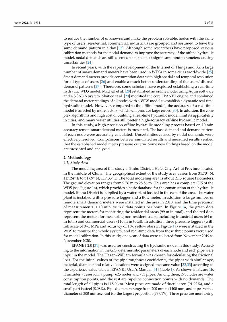
The modeling area of this study is Binhu District, Hefei City, Anhui Province, locatedin the middle of China. The geographical extent of the study area varies from 31.73◦ N,117.24◦ E to 31.69◦ N, 117.33◦ E. The total modeling area is about 21.5 square kilometers.The ground elevation ranges from 9.76 m to 28.56 m. This area has a complete GIS of theWDS (see Figure 1a), which provides a basic database for the construction of the hydraulicmodel. Binhu District is supplied by a water plant located in the east of the area. The waterplant is installed with a pressure logger and a flow meter. In addition, a large number ofremote smart demand meters were installed in the area in 2018, and the time precisionof measurements is 10 min, with 6 data points per hour. In Figure 1a, the green dotsrepresent the meters for measuring the residential areas (99 m in total), and the red dotsrepresent the meters for measuring non-resident users, including industrial users (64 min total) and commercial users (110 m in total). In addition, three pressure loggers (withfull scale of 0~1 MPa and accuracy of 1%, yellow stars in Figure 1a) were installed in theWDS to monitor the whole system, and real-time data from these three points were usedfor model calibration. In this study, one year of data were collected from November 2019 toNovember 2020.

EPANET 2.0 [31] was used for constructing the hydraulic model in this study. Accord-ing to the information in the GIS, deterministic parameters of each node and each pipe wereinput in the model. The Hazen–William formula was chosen for calculating the frictionalloss. For the initial values of the pipe roughness coefficients, the pipes with similar age,material, diameter and relative locations were assigned the same value [32,33] according tothe experience value table in EPANET User’s Manual [31] (Table 1). As shown in Figure 1b,it includes a reservoir, a pump, 625 nodes and 753 pipes. Among them, 273 nodes are waterconsumption points, and the rest are pipeline connection points with no demands. Thetotal length of all pipes is 118.0 km. Most pipes are made of ductile iron (91.92%), and asmall part is steel (8.08%). Pipe diameters range from 200 mm to 1400 mm, and pipes with adiameter of 300 mm account for the largest proportion (73.01%). Three pressure monitoring

Water 2022, 14, 1934 3 of 13

points are numbered as Node 217, Node 506 and Node 544. The pressure logger in thewater plant is numbered as Node 619.

Water 2022, 14, x FOR PEER REVIEW 3 of 13

according to the experience value table in EPANET User’s Manual [31] (Table 1). As shown in Figure 1b, it includes a reservoir, a pump, 625 nodes and 753 pipes. Among them, 273 nodes are water consumption points, and the rest are pipeline connection points with no demands. The total length of all pipes is 118.0 km. Most pipes are made of ductile iron (91.92%), and a small part is steel (8.08%). Pipe diameters range from 200 mm to 1400 mm, and pipes with a diameter of 300 mm account for the largest proportion (73.01%). Three pressure monitoring points are numbered as Node 217, Node 506 and Node 544. The pressure logger in the water plant is numbered as Node 619.

(a)

(b)

Figure 1. Study area: (a) GIS map; (b) the established EPANET model.

Figure 1. Study area: (a) GIS map; (b) the established EPANET model.

Table 1. Initial values of the pipe roughness coefficient [30].

Condition Node NumberDiameter (mm)

200–300 300–600 600–1000 >1000

Ductile iron pipe

New pipe 140Five years 125 130 135 135Ten years 115 120 130 130

Twenty years 105 110 120 120

Water 2022, 14, 1934 4 of 13

Table 1. Cont.

Condition Node NumberDiameter (mm)

200–300 300–600 600–1000 >1000

Steel pipe

New pipe 120Five years 115Ten years 110

Twenty years 105

2.2. Ten-Minute Accuracy Water Consumption Data for Different Types of Users

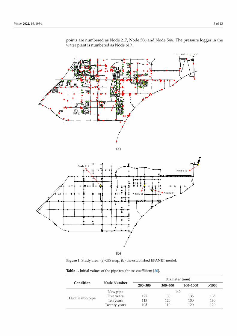
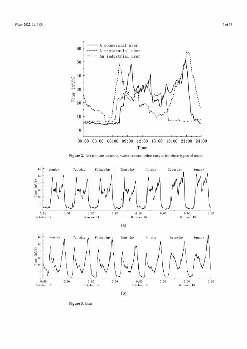
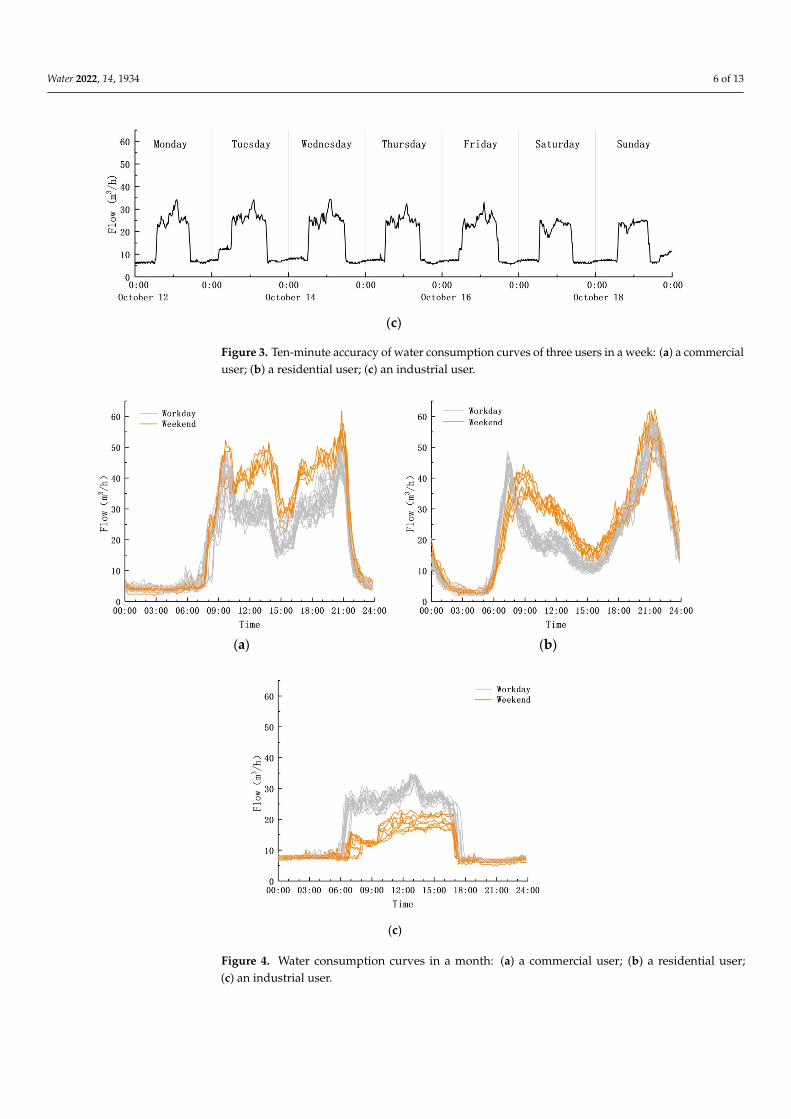
In order to better show the ten-minute accuracy water consumption data and waterconsumption characteristics of users, three nearby nodes within a district of the study arearepresenting different types of users, a commercial user, a residential user and an industrialuser, were selected for detailed analysis. Figure 2 shows the ten-minute accuracy waterconsumption curves for three types of users. Firstly, it can be seen that different types ofusers show very different diurnal patterns. Both the commercial and residential users havetwo peak times, whereas the industrial user has a relatively steady water consumptionduring the daytime (between 7:00 a.m. and 17:00 p.m.). Secondly, the morning peak timeof the residential user happens at 7:00 a.m., while it is delayed three hours (at 10:00 a.m.)for the commercial user. To better compare the diurnal pattern of the three users, theirwater consumption data in one week are plotted separately in Figure 3. From Figure 3, it isfirstly noticeable that the industrial user has very different diurnal patterns in one week.On workdays, from Monday to Friday, only one peak time happens, at 12:00 am, and themaximum flow is 35 m3/h. However, on Saturday and Sunday, no obvious peak time exists,and the total water consumption on the weekend is obviously less than on a workday.Actually, differences in the daily water consumption between workdays and weekendsalso exist for the commercial and residential users. To better show this phenomenon, dailywater consumption in one month (October 2020) is plotted in Figure 4 for the three types ofusers. In Figure 4, black curves show workdays’ consumption in the month, while yellowcurves represent the weekends’ data. Two different water demand patterns for workdaysand weekends can be clearly distinguished for all three users in the figure. Therefore,to improve the accuracy of the model, it is necessary to calculate the base demand and de-mand pattern for both workdays and weekends. Actually, these daily, weekly and monthlywater consumption patterns are closely related to local working and living characteristics.In addition, it is also easy to understand that water consumption differs greatly in differentmonths (complete monthly data are from December 2019 to October 2020), as shown inFigure 5. For the residential user, the minimum water consumption happens in February,and the maximum consumption happens in August. The ratio of the maximum valueto the minimum value is 1.56. For the industrial user, the minimum water consumptionhappens in February, and the maximum consumption happens in December. The ratio ofthe maximum value to the minimum value is 2.19. However, for the commercial user, thetotal water consumption in August reaches as much as 15.94 times the value for February.Considering that the base demand of each user varies from month to month, to improvethe accuracy of the model, the base demand and demand pattern of each node should beupdated every month.

Based on the ten-minute accuracy data, the base demand and demand pattern of eachnode for every day, week and year can be calculated. However, from the above analysis,it is found that the daily water consumption pattern only differs greatly between workdaysand weekends and among months. To reduce the data processing and modeling time,it is reasonable to calculate the monthly averaged base demand and demand pattern forworkdays and weekends for each node and input the results into the EPANET hydraulicmodel of the study area. To achieve this, the calculation method of the monthly averagedbase demand and demand pattern is explained in the next section.

Water 2022, 14, 1934 5 of 13

Water 2022, 14, x FOR PEER REVIEW 5 of 13

time, it is reasonable to calculate the monthly averaged base demand and demand pattern for workdays and weekends for each node and input the results into the EPANET hy-draulic model of the study area. To achieve this, the calculation method of the monthly averaged base demand and demand pattern is explained in the next section.

Figure 2. Ten-minute accuracy water consumption curves for three types of users.

(a)

(b)

Figure 2. Ten-minute accuracy water consumption curves for three types of users.

Water 2022, 14, x FOR PEER REVIEW 5 of 13

time, it is reasonable to calculate the monthly averaged base demand and demand pattern for workdays and weekends for each node and input the results into the EPANET hy-draulic model of the study area. To achieve this, the calculation method of the monthly averaged base demand and demand pattern is explained in the next section.

Figure 2. Ten-minute accuracy water consumption curves for three types of users.

(a)

(b)

Figure 3. Cont.

Water 2022, 14, 1934 6 of 13Water 2022, 14, x FOR PEER REVIEW 6 of 13

(c)

Figure 3. Ten-minute accuracy of water consumption curves of three users in a week: (a) a commer-cial user; (b) a residential user; (c) an industrial user.

(a) (b)

(c)

Figure 4. Water consumption curves in a month: (a) a commercial user; (b) a residential user; (c) an industrial user.

Figure 3. Ten-minute accuracy of water consumption curves of three users in a week: (a) a commercialuser; (b) a residential user; (c) an industrial user.

Water 2022, 14, x FOR PEER REVIEW 6 of 13

(c)

Figure 3. Ten-minute accuracy of water consumption curves of three users in a week: (a) a commer-cial user; (b) a residential user; (c) an industrial user.

(a) (b)

(c)

Figure 4. Water consumption curves in a month: (a) a commercial user; (b) a residential user; (c) an industrial user.

Figure 4. Water consumption curves in a month: (a) a commercial user; (b) a residential user;(c) an industrial user.

Water 2022, 14, 1934 7 of 13

Water 2022, 14, x FOR PEER REVIEW 7 of 13

Figure 5. Comparison of total water consumption in different months.

2.3. Calculation Method of Monthly Averaged Base Demand and Demand Pattern According to the data of the remote smart demand meter corresponding to each

node, the monthly averaged base demand and demand pattern at each node were calcu-lated by the water consumption curve method. The basic steps are given below: 1. Hourly average water consumption in a month: according to the remote flow data of

node i, the water consumption in each hour t in the 24 h period in each day in a month was summed up and then divided by the total number of days in the month (work-days and weekends are calculated, respectively):

,1

,

Nji t

ji t

Dq

N==

(1)

where qi,t is the hourly average water consumption (m3/h) of node i in tth hour of a day, t = 1, 2, 3…24; ,

ji tD is the water consumption (m3/h) in jth day in tth hour of the node i; and

N represents total days in a month. 2. Base demand at each node: The hourly average water consumption at each hour was

added up and then divided by 24:

24

,1

24

i tt

i

qq ==

(2)

where qi is the base demand of node i (m3/h). 3. Hourly variation coefficients: The ratio of hourly average water consumption in tth

hour to the base demand is the hourly variation coefficient:

,,

i ti t

i

qX

q=

(3)

where Xi,t is the hourly variation coefficient of node i in tth hour, and it is a fixed value in each hour.

4. Demand pattern input: Taking time as abscissa and Xi,t as ordinate, then the demand pattern at node i can be input. A 48 h simulation (a 24 h simulation for the workday and a 24 h simulation for the weekend) was proposed and conducted.

Figure 5. Comparison of total water consumption in different months.

2.3. Calculation Method of Monthly Averaged Base Demand and Demand Pattern

According to the data of the remote smart demand meter corresponding to each node,the monthly averaged base demand and demand pattern at each node were calculated bythe water consumption curve method. The basic steps are given below:

1. Hourly average water consumption in a month: according to the remote flow dataof node i, the water consumption in each hour t in the 24 h period in each day in amonth was summed up and then divided by the total number of days in the month(workdays and weekends are calculated, respectively):

qi,t =

N∑

j=1Dj

i,t

N(1)

where qi,t is the hourly average water consumption (m3/h) of node i in tth hour of aday, t = 1, 2, 3 . . . 24; Dj

i,t is the water consumption (m3/h) in jth day in tth hour ofthe node i; and N represents total days in a month.

2. Base demand at each node: The hourly average water consumption at each hour wasadded up and then divided by 24:

qi =

24∑

t=1qi,t

24(2)

where qi is the base demand of node i (m3/h).3. Hourly variation coefficients: The ratio of hourly average water consumption in tth

hour to the base demand is the hourly variation coefficient:

Xi,t =qi,t

qi(3)

where Xi,t is the hourly variation coefficient of node i in tth hour, and it is a fixed valuein each hour.

4. Demand pattern input: Taking time as abscissa and Xi,t as ordinate, then the demandpattern at node i can be input. A 48 h simulation (a 24 h simulation for the workdayand a 24 h simulation for the weekend) was proposed and conducted.

Water 2022, 14, 1934 8 of 13

3. Results and Discussions3.1. Comparison between Simulation and Measured Pressures

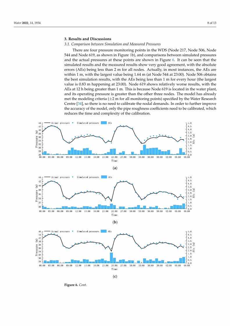
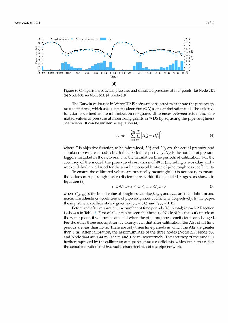
There are four pressure monitoring points in the WDS (Node 217, Node 506, Node544 and Node 619, as shown in Figure 1b), and comparisons between simulated pressuresand the actual pressures at these points are shown in Figure 6. It can be seen that thesimulated results and the measured results show very good agreement, with the absoluteerrors (AEs) being less than 2 m for all nodes. Actually, in most instances, the AEs arewithin 1 m, with the largest value being 1.64 m (at Node 544 at 23:00). Node 506 obtainsthe best simulation results, with the AEs being less than 1 m for every hour (the largestvalue is 0.83 m happening at 23:00). Node 619 shows relatively worse results, with theAEs at 12 h being greater than 1 m. This is because Node 619 is located in the water plant,and its operating pressure is greater than the other three nodes. The model has alreadymet the modeling criteria (±2 m for all monitoring points) specified by the Water ResearchCentre [34], so there is no need to calibrate the nodal demands. In order to further improvethe accuracy of the model, only the pipe roughness coefficients need to be calibrated, whichreduces the time and complexity of the calibration.

Water 2022, 14, x FOR PEER REVIEW 8 of 13

3. Results and Discussions 3.1. Comparison between Simulation and Measured Pressures

There are four pressure monitoring points in the WDS (Node 217, Node 506, Node 544 and Node 619, as shown in Figure 1b), and comparisons between simulated pressures and the actual pressures at these points are shown in Figure 6. It can be seen that the simulated results and the measured results show very good agreement, with the absolute errors (AEs) being less than 2 m for all nodes. Actually, in most instances, the AEs are within 1 m, with the largest value being 1.64 m (at Node 544 at 23:00). Node 506 obtains the best simulation results, with the AEs being less than 1 m for every hour (the largest value is 0.83 m happening at 23:00). Node 619 shows relatively worse results, with the AEs at 12 h being greater than 1 m. This is because Node 619 is located in the water plant, and its operating pressure is greater than the other three nodes. The model has already met the modeling criteria (±2 m for all monitoring points) specified by the Water Research Centre [34], so there is no need to calibrate the nodal demands. In order to further improve the accuracy of the model, only the pipe roughness coefficients need to be calibrated, which reduces the time and complexity of the calibration.

(a)

(b)

(c)

Figure 6. Cont.

Water 2022, 14, 1934 9 of 13Water 2022, 14, x FOR PEER REVIEW 9 of 13

(d)

Figure 6. Comparisons of actual pressures and simulated pressures at four points: (a) Node 217; (b) Node 506; (c) Node 544; (d) Node 619.

The Darwin calibrator in WaterGEMS software is selected to calibrate the pipe rough-ness coefficients, which uses a genetic algorithm (GA) as the optimization tool. The objec-tive function is defined as the minimization of squared differences between actual and simulated values of pressure at monitoring points in WDS by adjusting the pipe rough-ness coefficients. It can be written as Equation (4):

2, ,

1 1min | |

HN TA Si t i t

i tF H H

= =

= −

(4)

where F is objective function to be minimized; ,Ai tH and ,

si tH are the actual pressure and

simulated pressure at node i in tth time period, respectively; NH is the number of pressure loggers installed in the network; T is the simulation time periods of calibration. For the accuracy of the model, the pressure observations of 48 h (including a workday and a week-end day) are all used for the simultaneous calibration of pipe roughness coefficients.

To ensure the calibrated values are practically meaningful, it is necessary to ensure the values of pipe roughness coefficients are within the specified ranges, as shown in Equation (5):

min , max ,j initial j initialc C C c C≤ ≤ (5)

where Cj,initial is the initial value of roughness at pipe j; cmin and cmax are the minimum and maximum adjustment coefficients of pipe roughness coefficients, respectively. In the pa-per, the adjustment coefficients are given as cmin = 0.85 and cmax = 1.15.

Before and after calibration, the number of time periods (48 in total) in each AE sec-tion is shown in Table 2. First of all, it can be seen that because Node 619 is the outlet node of the water plant, it will not be affected when the pipe roughness coefficients are changed. For the other three nodes, it can be clearly seen that after calibration, the AEs of all time periods are less than 1.5 m. There are only three time periods in which the AEs are greater than 1 m. After calibration, the maximum AEs of the three nodes (Node 217, Node 506 and Node 544) are 1.44 m, 0.85 m and 1.36 m, respectively. The accuracy of the model is further improved by the calibration of pipe roughness coefficients, which can better reflect the actual operation and hydraulic characteristics of the pipe network.

Figure 6. Comparisons of actual pressures and simulated pressures at four points: (a) Node 217;(b) Node 506; (c) Node 544; (d) Node 619.

The Darwin calibrator in WaterGEMS software is selected to calibrate the pipe rough-ness coefficients, which uses a genetic algorithm (GA) as the optimization tool. The objectivefunction is defined as the minimization of squared differences between actual and sim-ulated values of pressure at monitoring points in WDS by adjusting the pipe roughnesscoefficients. It can be written as Equation (4):

minF =NH

∑i=1

T

∑t=1

∣∣∣HAi,t − HS

i,t

∣∣∣2 (4)

where F is objective function to be minimized; HAi,t and Hs

i,t are the actual pressure andsimulated pressure at node i in tth time period, respectively; NH is the number of pressureloggers installed in the network; T is the simulation time periods of calibration. For theaccuracy of the model, the pressure observations of 48 h (including a workday and aweekend day) are all used for the simultaneous calibration of pipe roughness coefficients.

To ensure the calibrated values are practically meaningful, it is necessary to ensurethe values of pipe roughness coefficients are within the specified ranges, as shown inEquation (5):

cmin·Cj,initial ≤ C ≤ cmax·Cj,initial (5)

where Cj,initial is the initial value of roughness at pipe j; cmin and cmax are the minimum andmaximum adjustment coefficients of pipe roughness coefficients, respectively. In the paper,the adjustment coefficients are given as cmin = 0.85 and cmax = 1.15.

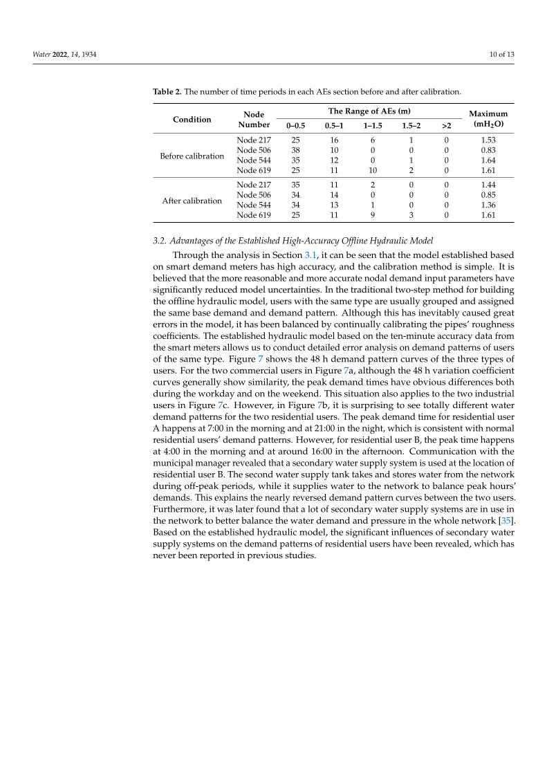
Before and after calibration, the number of time periods (48 in total) in each AE sectionis shown in Table 2. First of all, it can be seen that because Node 619 is the outlet node ofthe water plant, it will not be affected when the pipe roughness coefficients are changed.For the other three nodes, it can be clearly seen that after calibration, the AEs of all timeperiods are less than 1.5 m. There are only three time periods in which the AEs are greaterthan 1 m. After calibration, the maximum AEs of the three nodes (Node 217, Node 506and Node 544) are 1.44 m, 0.85 m and 1.36 m, respectively. The accuracy of the model isfurther improved by the calibration of pipe roughness coefficients, which can better reflectthe actual operation and hydraulic characteristics of the pipe network.

Water 2022, 14, 1934 10 of 13

Table 2. The number of time periods in each AEs section before and after calibration.

Condition NodeNumber

The Range of AEs (m) Maximum(mH2O)0–0.5 0.5–1 1–1.5 1.5–2 >2

Before calibration

Node 217 25 16 6 1 0 1.53Node 506 38 10 0 0 0 0.83Node 544 35 12 0 1 0 1.64Node 619 25 11 10 2 0 1.61

After calibration

Node 217 35 11 2 0 0 1.44Node 506 34 14 0 0 0 0.85Node 544 34 13 1 0 0 1.36Node 619 25 11 9 3 0 1.61

3.2. Advantages of the Established High-Accuracy Offline Hydraulic Model

Through the analysis in Section 3.1, it can be seen that the model established basedon smart demand meters has high accuracy, and the calibration method is simple. It isbelieved that the more reasonable and more accurate nodal demand input parameters havesignificantly reduced model uncertainties. In the traditional two-step method for buildingthe offline hydraulic model, users with the same type are usually grouped and assignedthe same base demand and demand pattern. Although this has inevitably caused greaterrors in the model, it has been balanced by continually calibrating the pipes’ roughnesscoefficients. The established hydraulic model based on the ten-minute accuracy data fromthe smart meters allows us to conduct detailed error analysis on demand patterns of usersof the same type. Figure 7 shows the 48 h demand pattern curves of the three types ofusers. For the two commercial users in Figure 7a, although the 48 h variation coefficientcurves generally show similarity, the peak demand times have obvious differences bothduring the workday and on the weekend. This situation also applies to the two industrialusers in Figure 7c. However, in Figure 7b, it is surprising to see totally different waterdemand patterns for the two residential users. The peak demand time for residential userA happens at 7:00 in the morning and at 21:00 in the night, which is consistent with normalresidential users’ demand patterns. However, for residential user B, the peak time happensat 4:00 in the morning and at around 16:00 in the afternoon. Communication with themunicipal manager revealed that a secondary water supply system is used at the location ofresidential user B. The second water supply tank takes and stores water from the networkduring off-peak periods, while it supplies water to the network to balance peak hours’demands. This explains the nearly reversed demand pattern curves between the two users.Furthermore, it was later found that a lot of secondary water supply systems are in use inthe network to better balance the water demand and pressure in the whole network [35].Based on the established hydraulic model, the significant influences of secondary watersupply systems on the demand patterns of residential users have been revealed, which hasnever been reported in previous studies.

Water 2022, 14, 1934 11 of 13Water 2022, 14, x FOR PEER REVIEW 11 of 13

(a)

(b)

(c)

Figure 7. Demand patterns of users of the same type: (a) two commercial users; (b) two residential users; (c) two industrial users.

Figure 7. Demand patterns of users of the same type: (a) two commercial users; (b) two residentialusers; (c) two industrial users.

Water 2022, 14, 1934 12 of 13

4. Conclusions

In this paper, an applicable method for how to reduce uncertainties in a WDS modelcaused by the nodal demands was proposed. A high-accuracy offline hydraulic model ofWDS in Binhu District of Hefei City in Anhui Province was established by using EPANET2.0 based on data collected from 10 min accuracy remote smart demand meters. Firstly,the base demands and demand patterns of all nodes were accurately calculated, usingmonthly average data, by the water consumption curve method. Then, a total of 48 hof simulation were conducted, including workdays and the weekend. Compared to themeasured pressures, the AEs at all pressure monitoring points were less than 2 m duringsimulation time, and there is no need to calibrate the nodal demand. The Darwin calibratorin WaterGEMS software was used to calibrate the pipe roughness coefficients and hasfurther improved the model’s accuracy. Based on the model, the significant influences ofsecondary water supply systems on the network have been noticed and revealed for thefirst time. In addition, more pressure monitoring points are currently being installed in thenetwork, and more data will be collected for comparison and calibration in the future.

Author Contributions: Conceptualization, S.G.; methodology, R.S. and S.G.; software, X.L.; dataresources, B.Z.; writing, R.S. and X.L. All authors have read and agreed to the published version ofthe manuscript.

Funding: This work was supported by the National Science Foundation of Anhui Province (grantnumber: 1908085QE211; Funder: Anhui Provincial Department of Science and Technology) and theKey Research and Development Program in Anhui Province (grant number: 202104i07020012; 1;Funder: Anhui Provincial Department of Science and Technology).

Institutional Review Board Statement: Not applicable.

Informed Consent Statement: Not applicable.

Data Availability Statement: The data presented in this study are available on request from thecorresponding author. The data are not publicly available due to due to conditions of the ethicscommittee of our university.

Conflicts of Interest: The authors declare no conflict of interest.

References1. Marsili, V.; Meniconi, S.; Alvisi, S.; Brunone, B.; Franchini, M. Stochastic approach for the analysis of demand induced transients

in real water distribution systems. J. Water Res. Plan. Manag. 2022, 148, 04021093. [CrossRef]2. Kang, D.; Lansey, K. Novel approach to detecting pipe bursts in water distribution networks. J. Water Res. Plan. Manag. 2014, 140,

121–127. [CrossRef]3. Tao, T.; Huang, H.; Li, F.; Xin, K. Burst detection using an artificial immune network in water-distribution systems. J. Water Res.

Plan. Manag. 2014, 140, 04014027. [CrossRef]4. Meniconi, S.; Brunone, B.; Frisinghelli, M. On the role of minor branches, energy dissipation, and small defects in the transient

response of transmission mains. Water 2018, 10, 187. [CrossRef]5. Alvisi, S.; Franchini, M. Pipe roughness calibration in water distribution systems using grey numbers. J. Hydroinform. 2010, 12,

424–445. [CrossRef]6. Do, N.C.; Simpson, A.R.; Deuerlein, J.W.; Piller, O. Calibration of water demand multipliers in water distribution systems using

genetic algorithms. J. Water Res. Plan. Manag. 2016, 142, 04016044. [CrossRef]7. Kang, D.; Lansey, K. Demand and roughness estimation in water distribution syste-ms. J. Water Res. Plan. Manag. 2011, 137,

20–30. [CrossRef]8. Zanfei, A.; Menapace, A.; Santopietro, S.; Righetti, M. Calibration procedure for water distribution systems: Comparison among

hydraulic models. Water 2020, 12, 1421. [CrossRef]9. Du, K.; Long, T.-Y.; Wang, J.-H.; Guo, J.-S. Inversion model of water distribution systems for nodal demand calibration. J. Water

Res. Plan. Manag. 2015, 141, 04015002. [CrossRef]10. Walski, T.M. Case study: Pipe network model calibration issues. J. Water Res. Plan. Manag. 1986, 112, 238–249. [CrossRef]11. Bhave, P.R. Calibrating water distribution network models. J. Environ. Eng. 1988, 114, 120–136. [CrossRef]12. Ormsbee, L.E.; Wood, D.J. Explicit pipe network calibration. J. Water Res. Plan. Manag. 1986, 112, 166–182. [CrossRef]13. Boulos, P.F.; Wood, D.J. Explicit calculation of pipe-network parameters. J. Hydraul. Eng. 1990, 116, 1329–1344. [CrossRef]14. Ormsbee, L.E. Implicit network calibration. J. Water Res. Plan. Manag. 1989, 115, 243–257. [CrossRef]

Water 2022, 14, 1934 13 of 13

15. Savic, D.A.; Walters, G.A. Genetic Algorithm Techniques for Calibrating Network Models; Rep. No. 95/12; Centre for Systems andControl Engineering, University of Exeter: Exeter, UK, 1995.

16. Kapelan, Z.S.; Savic, D.A.; Walters, G.A. Calibration of water distribution hydra-ulic models using a Bayesian-type procedure.J. Hydraul. Eng. 2007, 133, 927–936. [CrossRef]

17. Walski, T.M.; DeFrank, N.; Voglino, T.; Wood, R.; Whitman, B.E. Determining the accuracy of automated calibration of pipenetwork models. In Proceedings of the 8th Annual Water Distribution Systems Analysis Symposium, (CD-ROM), Cincinnati, OH,USA, 27–30 August 2006; ASCE: Reston, VA, USA, 2008.

18. Koppel, T.; Vassiljev, A. Calibration of a model of an operational water distribution system containing pipes of different age. Adv.Eng. Softw. 2009, 40, 659–664. [CrossRef]

19. Mentes, A.; Galiatsatou, P.; Spyrou, D.; Samaras, A.; Stournara, P. Hydraulic simulation and analysis of an urban center’saqueducts using emergency scenarios for network operation: The case of Thessaloniki City in Greece. Water 2020, 12, 1627.[CrossRef]

20. Lawrence, L.; Yskandar, H.; Adnan, A.M. Estimation of water demand in water distribution systems using particle swarmoptimization. Water 2017, 9, 593. [CrossRef]

21. Kang, D.; Lansey, K. Real-time demand estimation and confidence limit analysis for water distribution systems. J. Hydraul. Eng.2009, 135, 825–837. [CrossRef]

22. Zhang, Q.; Zheng, F.; Duan, H.F.; Jia, Y.; Zhang, T.; Guo, X. Efficient numerical approach for simultaneous calibration of piperoughness coefficients and nodal demands for water distribution systems. J. Water Res. Plan. Manag. 2018, 144, 04018063.[CrossRef]

23. Jung, D.; Choi, Y.H.; Kim, J.H. Optimal node grouping for water distribution system demand estimation. Water 2016, 8, 160.[CrossRef]

24. Pasha, M.; Lansey, K. Analysis of uncertainty on water distribution hydraulics and water quality. In Proceedings of the WorldWater and Environmental Resources Congress, Anchorage, AK, USA, 15–19 May 2005; pp. 1–12. [CrossRef]

25. Creaco, E.; Campisano, A.; Fontana, N.; Marini, G.; Page, P.R.; Walski, T. Real time control of water distribution networks:A state-of-the-art review. Water Res. 2019, 161, 517–530. [CrossRef] [PubMed]

26. Zhang, Q.; Zheng, F.; Jia, Y.; Savic, D.; Kapelan, Z. Real-time foul sewer hydraulic modelling driven by water consumption datafrom water distribution systems. Water Res. 2021, 188, 116544. [CrossRef] [PubMed]

27. Marsili, V.; Meniconi, S.; Alvisi, S.; Brunone, B.; Franchini, M. Experimental analysis of the water consumption effect on thedynamic behaviour of a real pipe network. J. Hydraul. Res. 2021, 59, 477–487. [CrossRef]

28. Machell, J.; Mounce, S.R.; Boxall, J.B. Online modelling of water distribution systems: A UK case study. Drink. Water Eng. Sci.2010, 3, 21–27. [CrossRef]

29. Shafiee, M.E.; Rasekh, A.; Sela, L.; Preis, A. Streaming smart meter data integration to enable dynamic demand assignment forreal-time hydraulic simulation. J. Water Res. Plan. Manag. 2020, 146, 06020008. [CrossRef]

30. Shafiee, M.E.; Barker, Z.; Rasekh, A. Enhancing water system models by integrating big data. Sustain. Cities Soc. 2017, 37, 485–491.[CrossRef]

31. Rossman, L.A. EPANET 2: Users’ Manual; National Risk Management Research Laboratory, Office of Research and Development,United Sates Environmental Protection Agency (EPA): Cincinnati, OH, USA, 2000.

32. Kumar, S.M.; Narasimhan, S.; Bhallamudi, S.M. Parameter estimation in water distribution networks. Water Res. Manag. 2010, 24,1251–1272. [CrossRef]

33. Dini, M.; Tabesh, M. A new method for simultaneous calibration of demand pattern and Hazen-Williams coefficients in waterdistribution systems. Water Resour. Manag. 2014, 28, 2021–2034. [CrossRef]

34. WRC (Water Research Centre). Network Analysis—A Code of Practice; Water Research Centre: Swindon, UK, 1989.35. Xu, Q.; Chen, Q.; Qi, S.; Cai, D. Improving water and energy metabolism efficiency in urban water supply system through

pressure stabilization by optimal operation on water tanks. Ecol. Inform. 2015, 26, 111–116. [CrossRef]