ORIGINAL PAPER

Multivariate classification and modeling in surface waterpollution estimation

A. Astel & S. Tsakovski & V. Simeonov & E. Reisenhofer &

S. Piselli & P. Barbieri

Received: 21 July 2007 /Revised: 24 September 2007 /Accepted: 11 October 2007 /Published online: 15 November 2007# Springer-Verlag 2007

Abstract The present study deals with the application of self-organizing maps (SOM) and multiway principal-componentsanalysis to classify, model, and interpret a large monitoringdata set for surface water quality. The chemometric methodsapplied made it possible to reveal specific quality patterns ofthe chemical and biological parameters used to monitor thewater quality (relation between water temperature, turbidity,

hardness, colibacteria), seasonal impacts during the longperiod of observation and the relative independence on thespatial location of the sampling sites (water supply sources forthe City of Trieste).

Keywords Chemometrics . Surface water . N-way PCA .

SOM . City of Trieste

Introduction

This study offers a statistical multivariate technique formonitoring environmental dynamic systems (freshwater ofthe karstic area surrounding the City of Trieste (northeasternItaly)). In a series of previous studies the traditional chemo-metric approaches like cluster analysis, principal-componentsanalysis, and time-series analysis have been tried in order togain specific information about the structure of monitoringdata from the region of interest [1–5]. In the papers cited theregion of City of Trieste is also considered with respect towater quality assessment by chemometrics but for a verylimited time period. They confirm our deep conviction thatwater pollution estimation using many available parametersand time-series could be improved if additional chemometricstrategies are applied in order to classify, model, andinterpret monitoring data of the same area. These strategiesnow involve, for instance, self-organizing maps (SOM) ofKohonen and N-way principal components analysis.

Due to the calcitic–dolomitic nature of this area, many ofthe water courses flowing here are subterranean: e.g., theTimavo River has a surface course of about 50 km inSlovenia, then sinks into a limestone fissure near the Italianborder, and assumes a variety of routes, mainly hypoge-nous, before emerging near the coast and flowing into theAdriatic Sea. This condition is favorable for preserving the

Anal Bioanal Chem (2008) 390:1283–1292DOI 10.1007/s00216-007-1700-6

A. Astel (*)Biology and Environmental Protection Institute, EnvironmentalChemistry Research Unit, Pomeranian Academy,22a Arciszewskego Str.,76 200 Slupsk, Polande-mail: astel@pap.edu.pl

S. TsakovskiPhysical Chemistry, Faculty of Chemistry,University of Sofia “St. Kl. Okhridski,J. Bourchier Blvd. 1,1164 Sofia, Bulgaria

V. SimeonovAnalytical Chemistry, Faculty of Chemistry,University of Sofia “St. Kl. Okhridski,J. Bourchier Blvd. 1,1164 Sofia, Bulgaria

E. Reisenhofer : P. BarbieriDepartment of Chemical Sciences, University of Trieste,Via Giorgieri 1,34127 Trieste, Italy

P. Barbierie-mail: barbierp@units.it

S. PiselliACEGAS-APS,Via Maestri del Lavoro 8,34123 Trieste, Italy

quality of these waters, but, at the same time, hinders notonly a detailed knowledge of the hydrology of thesubterranean water courses but also the sampling andmonitoring operations necessary for adequate understand-ing of the behavior and properties of this complexhydrological system. A further factor of complexity is dueto the permeability of the karstic soils that induces mutualoverflowing among the contiguous watersheds of this area.In previous work [2] we have verified these overflowingphenomena, which obviously depend on the differentseasonal rain conditions and cause occasional intrusion ofwaters from the northern Isonzo and Vipacco rivers into thesouthern karstic wells related to Timavo River. Thesewaters are relevant because they contribute to the municipalsupply of the Province of Trieste. In particular, the watersof the three wells Sablici, Moschenizze Nord, and Sardos,indicated in Fig. 1 as SB, MN, and SA respectively, arecollected for drinking use. In this work, we consider thespring of Timavo River—in Italy, where water emergesafter a path under the karstic limestone (TI in Fig. 1). Thesespring waters are occasionally characterized by turbidityderived from soil runoff occurring after relevant meteorol-ogical event in the Slovenian epigeous tract, that can alsocondition Sardos wells.

We report here a study based both on chemical andphysical analyses and on biological monitoring of thesewaters. All data have been obtained in the framework of along-term water-quality-monitoring program at the foursampling stations which are important for drinking watersupply of the City of Trieste.

The main aim of the study is to demonstrate how moreadvanced multivariate statistical approaches could contributeto better understanding of the data collected during monitor-

ing episodes for a long period of observation. Similaritiesbetween different sampling sites in the multivariate space ofquality parameters can be revealed, which is an important stepin optimizing drinking water monitoring of the region ofinterest. Further, the seasonal behavior of the water qualitycan be proved and used practically. Finally, the linkagebetween the water-quality parameters may give informationabout the effect of various natural or anthropogenicallyinfluenced factors on the overall spring water quality. Thetotal assessment taking into account chemical, geological, andanthropogenic impacts is possible only if the monitoring dataare interpreted in a multivariate way.

Experimental

Sampling sites, sampling and chemical analysis

Four sampling sites are considered. Sardos (SA), Sablici(SB), and Moschenizze Nord (MN) are the three historicalkarstic wells that contributes to the water supply of themunicipality of Trieste. Timavo (TI) represents the springof the river flowing underground for 40 km (see Fig. 1).Water samples were taken with monthly frequency for11 years from January 1995 to December 2005, andanalyzed within 48 h in the Laboratory for Analysis andControl of ACEGAS-APS of Trieste. The analyticaldeterminations followed the official procedures of theItalian Law [6] and the standard methods of the AmericanPublic Heath Association [7]. Turbidity (TURB, measure-ment unit: Jackson turbidity unit, JTU), temperature(TEMP, °C), and conductivity (COND, μS cm−1, correctedto 25 °C) were determined in situ whereas all other

Fig. 1 Location of monitoringpoints of the water supply sys-tem of the City of Trieste (Italy)

1284 Anal Bioanal Chem (2008) 390:1283–1292

parameters were measured in the laboratory. These were:chlorides (Cl−, mg L−1), sulfates (SO2�

4 , mg L−1), totalhardness (HARD, °F), dissolved oxygen (DOXY, mg L−1),nitrates (NO�

3 , mg L−1), nitrites (NO�2 , mg L−1), ammonia

(NH3, mg L−1), orthophosphates (PO3�4 , mg L−1), UV-

absorbing organic constituents determined by spectropho-tometry at 253.7 nm using cells of 5 cm path length as ameasure of organic compounds (i.e. humic acids, aromaticcompounds, tannins, lignins, etc.) in the freshwaters (UV,A), total coliforms (CT, most probable number MPN/100 mL), fecal coliforms (CF, MPN/100 mL), and fecalstreptococci (SF, MPN/100 mL). When the concentration ofanalytes was below the limit of detection (LOD), a value ofone-third LOD was used in the data set due to chemometricrequirements [8]. In the case of Cl−, SO2�

4 , NO�3 , and

DOXY the number of replacements did not exceed 0.5% ofthe total number of samples. In the case of NO�

2 , NH3 andPO3�

4 more than 95% of the results obtained were belowLOD, which for particular ions was: NO�

2 0:015 mg L�1,NH3 0.03 mg L−1, and PO3�

4 0:03 mg L�1. Because ofnegligible variance and informative value these ions wereexcluded from further chemometric evaluation.

Chemometric methods

Self-organizing maps (SOM)

The self-organizing map (SOM) algorithm was proposed byKohonen [9] and is a neural-network model that imple-ments a characteristic nonlinear projection from the high-dimensional space of sensory or other input signals on to alow-dimensional array of neurons [10]. The term “self-organizing” refers to the ability to learn and organizeinformation without being given the associated-dependentoutput values for the input pattern [11]. SOM shares withthe conventional ordination methods the basic idea ofdisplaying a high-dimensional signal manifold on a muchlower-dimensional network in an orderly fashion (usuallytwo-dimensional space). A SOM consists of neuronsorganized on a regular low-dimensional grid. The numberof neurons may vary from a few dozen up to severalthousand. The neurons are connected to adjacent neuronsby a neighborhood relation, which dictates the topology, orstructure of the Kohonen map and thus similar objects (inour case sampling points) should be mapped close togetheron the grid. A training algorithm constructs the nodes in theSOM in order to represent the whole data set and theirweights are optimized at each iteration step. In each step,one sample vector x from the input data set is chosenrandomly and the distance between it and all the weightvectors of the SOM are calculated using some distancemeasure. Thus, an optimal topology is expected. In our

study the non-hierarchical K-means classification algorithmwas applied. The different values of k (predefined numberof clusters) were tried and the sum of squares for each runwas calculated. Finally, the best classification with thelowest Davies–Bouldin index was chosen [12].

The network organizes itself by adjusting the synapticweights as the input patterns are presented to it; hence,discovery of a new pattern is possible at any instant.Moreover, SOM is noise tolerant; this property is highlydesirable when site-measured data are used. InterestingSOM applications have been reported in mainly threefields [13]:

– exploratory data analysis or data mining;– identification and monitoring of complex process

states; and– pattern classification.

For the SOM algorithm, there are no precise rules for thechoice of the different parameters [13]. In this work, theKohonen map has been chosen as a rectangular grid withnumber of nodes (n) determined using the formula: n ¼5� ffiffiffiffiffiffiffiffiffiffiffiffiffiffiffiffiffiffiffiffiffiffiffiffiffiffiffiffiffiffiffiffiffiffiffiffiffiffi

number of samplesp

[14] and, moreover, a hexagonallattice was preferred because it does not favor thehorizontal or vertical directions [15]. Subsequently, formonthly averages the dimensionality of Kohonen’s mapwas determined as 9� 12 n ¼ 5� ffiffiffiffiffiffiffiffi

528p � 115

� �. Basical-

ly, the two largest eigenvalues of the training data werecalculated and the ratio of the side lengths of the map gridwas set to the ratio of the two maximum eigenvalues. Theactual side lengths were then set so that their product wasclose to the determined number of map units as statedbefore. Both color-tone pattern and the color-tone barlabeled “d” deliver information regarding species abun-dance calculated through the SOM learning process. Color-tone bar can be understood as the term of the range of theparticular species variation whereas color-tone SOMreflects species abundance in the space of the samplinglocations. Similar conditions were applied in the studypresented by Park et al. [16].

N-way principal-components analysis

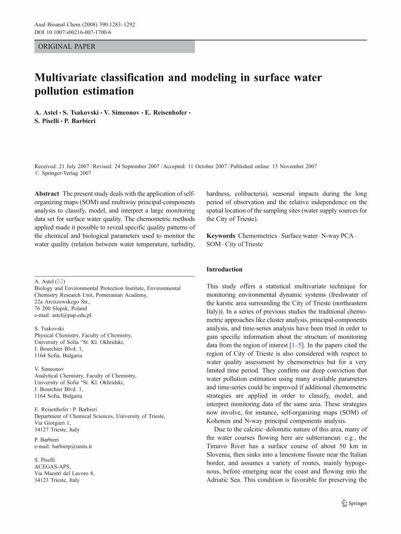
In this work, a three-way principal-component analysisusing the Tucker-3 model [17–19] was applied to the dataset. The dimensions of the three ways approach very ofteninvolve the water-quality parameters (mode A), the sam-pling periods (mode B), and the sampling sites (mode C)that identify each sampling episode. Analyzed data werearranged in three-way array of dimensionality 12 (param-eters)×12 (months)×4 (sampling sites). Thus, the qualityparameters, months, and sampling points constitute themodes of the array. The arrangement is schematicallypresented in Fig. 2.

Anal Bioanal Chem (2008) 390:1283–1292 1285

The Tucker-3 model constitutes a factorization of theX = {xijk} data array of (n × p × q) dimensions. Very often,xijk is the value of the chemical, physical, or biologicalparameter i (going from 1 to n), on month j of sampling(from 1 to p), at site k (from 1 to q), accordingly theequation:

xijk ¼Xr

u¼1

Xs

v¼1

Xt

w¼1

aiubjvckwguvw þ eijk :

In this equation, the r, s, and t indices represent thenumber of components chosen for describing the first, thesecond, or the third way of the data array, respectively, whileaiu, bjv, and ckw are the elements of the three componentmatrices A, B, and C. The A(n × r) matrix describes themeasured parameters, while B(p × s) describes the samplingmonths, and C(q × t) describes the sampling sites. Each ofthese matrices can be interpreted in the same manner as aloading matrix of the classical two-way PCA, since they areall columnwise orthogonal. The equation term guvw repre-sents an element of G, an array with (r × s × t) dimensions,called the “core” of the model. The core matrix element guvwweighs the products of the u component of the first way bythe v component of the second way and the w component ofthe third way. The component matrices A, B, and C areconstrained to be orthogonal, and the matrix columns arescaled to unit length. In this way, the squared value of thecore element, i.e. g2uvw, shows the entity of the interactionsamong the u, v, and w components of the X = {xijk} dataarray. The last element, eijk, constitutes the residual, i.e., thepart of the data not accounted for by the model. The Tucker-

3 model is computed by an iterative procedure based on the“alternating least square” (ALS) algorithm [20], and thesolution permits partition of the sum of the squares of the Xelements as:

SS Xð Þ ¼ SS modelð Þ þ SS residualð Þ:The SS(model)/SS(X) ratio can be used to evaluate the

strength of the model in representing its objects. In thefollowing, we will call this ratio the “explained variation”of the model. The data array is usually pre-treated, bycentering across mode A and scaling within mode B inorder to remove differences between water-quality param-eters due to their magnitudes and different units of measure.

The A, B, C matrices and the G core array can berotated, as in classical factor analysis. A recently proposedrotation method, the “variance of squares” [21], optimizesthe variance of the squared core elements, by distributingthe total variance among a small number of elements thatfurnishes models that are easier to interpret. This rotationmethod can be used with advantage on models withdifferent component numbers in the different ways.

All calculations in this study were performed byapplying MatLab 6.5 computing environment running ona Windows 2000/XP platform. To perform SOM-basedclassification a free Teuvo Kohonen toolbox (SOM Tool-box 2.0) was applied; this can be downloaded together withdocumentation [14] from http://www.cis.hut.fi/projects/somtoolbox/, while for Tucker-3 modeling the N-waytoolbox of Andersson and Bro [22], which estimates themissing data by use of an expectation/maximization-typealgorithm, was applied.

Fig. 2 Graphical representationof the three-way data array

1286 Anal Bioanal Chem (2008) 390:1283–1292

Due to software limitations all chemical indicatorsymbols are presented in the figures without superscriptsor subscripts.

Results and discussion

In Fig. 3 the SOMs for all sites and the water-qualityparameters for the whole period of monitoring are indicat-ed. It is readily seen that the distribution of the turbidityparameter for all sites and monitoring periods resemblesvery much the distribution pattern of the biologicalparameters (CT, CF, and SF) and even the UV (lightabsorbance) factor. This is a logical linkage since theturbidity of the water mass is closely related to the bacterialactivity and, besides, determines the light absorbanceability. At the SOMs high turbidity levels are alwaysassociated with high concentrations of coliforms and highlight absorbance.

It is quite important to detect relationships between theparameters observed for all sites and periods of monitoring.These relationships are shown in Fig. 4. The plot presentsthe grouping of all the water-quality parameters. Thelocation and distance between variables’ SOMs on the

Fig. 4 Quality parameterssimilarity pattern obtained byself-organizing mapping (thedistance between variables onthe map connected with analysisof color-tone patterns providessemi-quantitative informationabout the nature of correlationsbetween them)

Fig. 3 SOM for all samplingsites, parameters, and timeperiod (U-matrix visualizesdistances between neighboringmap units, and helps to identifythe cluster structure of the map:high values of the U-matrixindicates a cluster border, uni-form areas of low values indi-cate clusters themselves; eachcomponent plane shows thevalues of one variable in eachmap unit; both color-tone pat-tern and color-tone bar labeledas “d” delivers information re-garding species abundance cal-culated through the SOMlearning process)

Anal Bioanal Chem (2008) 390:1283–1292 1287

map, with analysis of color-tone patterns, provide semi-quantitative information about the correlation coefficient.Every “island” on the graph can be assessed and interpretedseparately. The variables grouped in one, separate “island”are positively correlated, while with increasing distancebetween variables the correlation coefficient decreases. Aquite homogeneous group of similar patterns is formed forthe bacterial forms in the water, turbidity, and lightabsorbance factor (SF-CT-CF-UV-TUR). The overall saltcontent expressed by the conductivity factor is hardlyrelated to water hardness and chloride (Cl−-HARD-COND),and less to sulfate concentration, since all these naturalsolutes are commonly influenced by meteorological dilu-tion factor. The rest of the parameters (dissolved oxygen,temperature, and nitrates) do not belong to either of theother two major groups and obviously possess a morespecific function in determining the water quality.

In Fig. 5 the clusters formed by the objects ofobservation (four sampling sites for 132 episodes ofchecking—monthly for 11 years) are presented as SOM.The number of the significant clusters is determined by thelowest value of the Davis–Bouldin index (four in this case).

In Table 1 application of the Kołmogorov–Smirnov testof differences between levels of quality indicators of river

water quality for clusters (I–IV) obtained by use of theSOM algorithm is shown. It might be concluded that theclusters are quite homogeneous.

Cluster I (top left on the SOM) contains dominantlyepisodes from the sites Moschenizze Nord and Sablici(the exact content of the clusters is presented in Table 2) forthe period of sampling between November to May, i.e. thewinter period. Significantly less are the episodes from Sardosand Timavo (only 11.4% and 1.5%, respectively, of the totalnumber of observations for these sites). In Ref. [2] it hasbeen suggested that during winter, water from MN and SB isinfluenced by massive ingressions of water from the Isonzoriver, lowering water conductivity at these sites.

Cluster II (bottom left on the SOM) consists mainly ofSardos and Timavo samples, which is an indication of thespatial separation of both groups of sites. The contributionof the other two sites in this cluster is limited to 4.5% of allepisodes for Moschenizze Nord and the same figure forSablici.

The third cluster (top right on the SOM) involves theremaining episodes for MN and SB, but for the summerperiod of monitoring and much less from TI and SA. Thisdistribution of the objects of observation indicates that awell-formed seasonality pattern could be revealed domi-

Fig. 5 SOM classification ofchemical variables and clusteringpattern according to theDavies–Bouldin index minimumvalue (both color scale hexagonsin each SOM unit and digitsrepresent the number of samplesbelonging to particular clusters)

1288 Anal Bioanal Chem (2008) 390:1283–1292

nantly for the Moschenizze Nord and Sablici water sources,because for Timavo and Sardos the seasonality is not sodefinitively expressed.

The last, fourth, cluster (bottom right on the SOM)contains a relatively small number of hits from all foursampling sites. It is characterized by high levels ofcontamination by bacteria and in this sense is a “bacterial”outlier compared with the other three groups. The fact thatjust a small number of episodes is marked by higherbacterial contamination is a indirect proof of the good waterquality of the water catchment under consideration.

Next step in the intelligent data analysis was theapplication of N-way PCA in order to produce a factorialmodel accounting for most of data set variability whileproviding evidence of where and when specific chemicalpatterns play a role. The dimensions of the three ways (i.e.,the quality parameters, the sampling months, and the

sampling sites) are 12, 132, and 4, respectively. The Tucker3 model as described above was used to interpret the wholesystem of quality parameters, time period and samplinglocation.

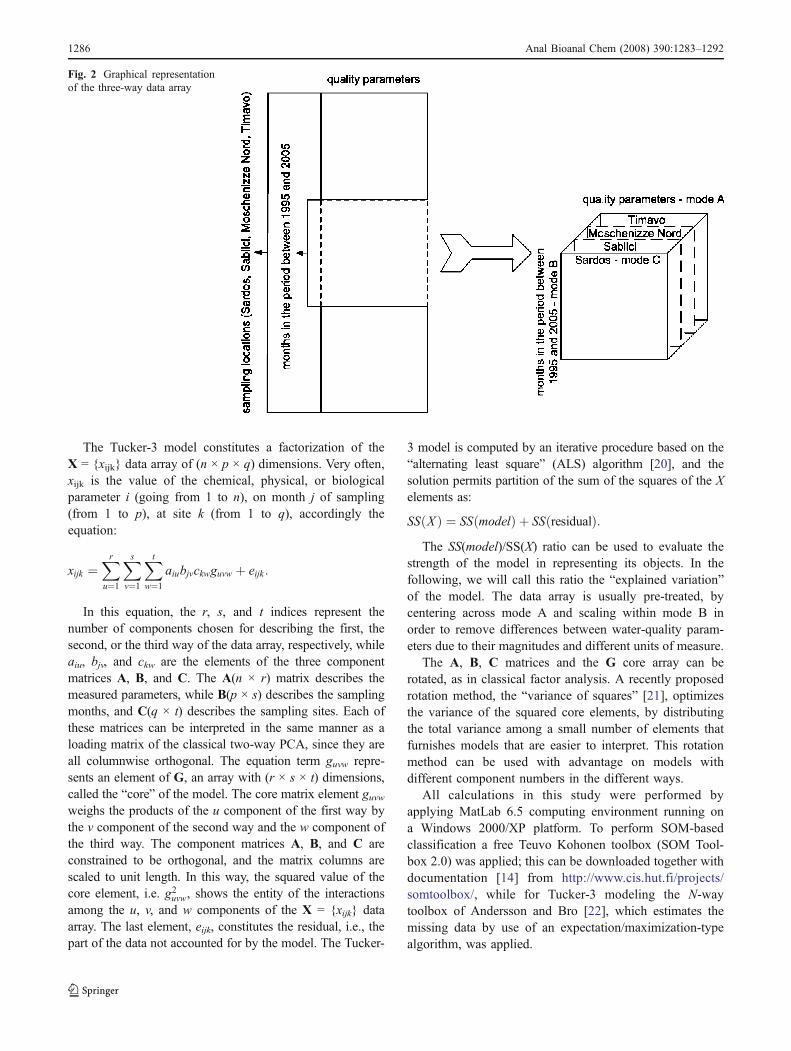
In Fig. 6 selection of the optimal model of the type (2 21) is indicated. From this plot it is readily seen that model 22 1 describes almost 96% of the total variance of thesystem. The model involves two components in the water-quality parameters mode, two components in the samplingtime mode, and one component in the sampling site mode.Other models with higher number of components werediscarded because their fitting increment scarcely adds anymore useful information.

In Table 3 the core array of the (2 2 1) Tucker3 model ispresented. The core array achieved is straightforward tointerpret, because of the small number of significantinteractions and because no rotation is necessary.

Cluster Sampling location

Moschenizze Nord Sablici Sardos Timavo

I 50.0% (66) 49.2% (65) 11.4% (15) 2.3% (3)II 4.6% (6) 4.6% (6) 60.6% (80) 80.3% (106)III 42.4% (56) 42.4 (56) 23.5% (31) 2.3% (3)IV 3.0% (4) 3.8% (5) 4.5% (6) 15.1% (20)

Table 2 Cluster episodesdistribution

Table 1 Statistical assessment (Kołmogorov–Smirnov test) of differences between levels of chemical indicators of river-water quality for clustersI–IV obtained by the SOM algorithm

Variable Mean values Kołmogorov–Smirnov test

Clusters Clusters combination

I II III IV I–II I–III I–IV II–III II–IV III–IV

Monthlyaverages

Turbidity 0.90 2.0 1.0 12.50 +++ p>0.10 +++ +++ +++ +++Temperature 11.30 12.10 12.90 11.90 +++ +++ +++ +++ p>0.10 +++Conductivity 335.0 384.0 321.0 371.0 +++ +++ +++ +++ p>0.10 +++Cl− 5.10 7.40 4.80 5.50 +++ +++ ++ +++ +++ ++SO2�

4 9.50 10.30 8.40 9.50 +++ +++ p>0.10 +++ ++ +++Hardness 19.0 23.0 18.0 22.0 +++ +++ +++ +++ p>0.10 +++Dissolved oxygen 8.60 8.60 7.50 9.10 p>0.10 +++ + +++ 0.05<p<0.10 +++NO�

3 7.20 7.30 6.10 6.30 p>0.10 +++ +++ +++ +++ p>0.10Total coliforms 136.0 230.0 264.0 1044.0 +++ +++ +++ +++ +++ +++Faecal coliforms 35.0 51.0 57.0 267.0 ++ +++ +++ +++ +++ +++Faecal streptococci 12.0 30.0 31.0 103.0 +++ +++ +++ p>0.10 +++ +++UV absorption 0.06 0.08 0.07 0.16 +++ +++ +++ +++ +++ +++

(To avoid frequent repetition and to improve the clarity of the table statistical levels of significance (p) lower than 0.001 are marked “+++”, thosein the range 0.0001≤p<0.01 are marked “++”, and those in the range 0.01≤p<0.05 are marked “+”.) The variables’ units are indicated in the text

Anal Bioanal Chem (2008) 390:1283–1292 1289

The next step in interpretation using also the figuresfrom the core matrix was the construction of loading plotsfor the modes A and B (Figs. 7 and 8).

In Fig. 7 the loading plot for mode A is shown. Itrepresents the relation between the water-quality parame-ters. In addition to the SOM classification one gets, in thiscase, additional information about the linkage between thewater temperature, on the one hand, and the rest of theparameters, on the other. From the loadings plot it is readilyseen that factor A1 shows how high turbidity, bacteriacontent, and organic matter coincide with water having lowtemperature, conductivity, and dissolved oxygen (thesecould be called “cold runoff water”). Factor A2 shows acontrast between dissolved oxygen and nitrates at one sideand temperature and bacteria at the other side; cold,bacterially clean waters can dissolve oxygen and nitrates.This reflects the seasonal behavior of the water-qualityparameters as additionally indicated in Fig. 8. The plotpresents loadings B1 and B2 and clearly indicates theseasonality already detected by SOM classification. The

baseline model of the time series (B1) is accompanied by awell expressed seasonal pattern (B2) with predominantlywinter minima and summer maxima values. The environ-mental meaning of seasonal factor will be discussed laterwhen core element (A2, B2, C1) is discussed.

Factor loadings of sampling stations in mode C are quitesimilar and do not indicate a difference between them.

The core matrix informs quite convincingly that the mostsignificant variation in the data set should be sought in theA1, B1, C1 interaction, where even the constant back-ground time factor differentiates the bacterial water-qualityparameters and water turbidity (mainly by the temperatureeffect) and the spatial mode does not affect the overallwater quality of the region of interest. The other importantinteraction (A2, B2, C1) highlights the most relevantdynamic factor regarding the considered water-qualityparameters in this spring water system—high temperatureand low dissolved oxygen and nitrates occur duringsummer (the values of A2 are multiplied by positive valuesof B2) while in winter (negative sign in B2) the relationshipbetween quality parameters changes sign; this shows thatcold waters obviously have more dissolved oxygen but alsohigher nitrates and lower bacterial content. The ratherevident sinusoidal trend of B2 shows the gradual transitionbetween the two extreme summer and winter situations.Sites SA, SB, MN, and TI are similarly affected by thisdynamic factor. These two patterns of variation appear asthe most relevant ones in respect of substantially constantand good water quality, according to the factorial model.

Table 3 Core array elements of the (2 2 1) Tucker3 model

Combinationof modes

Core value Combinationof modes

Core value

A1, B1, C1 −306.19 A1, B2, C1 5.21×10−5

A1, B1, C1 0.00012 A1, B2, C1 28.668

Fig. 6 Percentage of data vari-ance explained by three-wayTucker models of differentcomplexities

1290 Anal Bioanal Chem (2008) 390:1283–1292

Conclusion

This study has shown that the combined application ofthe strategies of self-organizing maps and N-way princi-pal components analysis is very suitable for handling anenvironmental dataset describing variations of 11 chem-ical and biological quality parameters, sampled monthlyfor 11 years at four sampling sites. Visualization of themonitoring results by SOM makes it possible to classify

different water-quality patterns for all sites under consid-eration and for the whole monitoring period, whichremain undetected by other data-projection options. Theoutput of the Tucker3 modeling is more compact andinformative than classical two-way principal componentsanalysis for detection of spatial and temporal patterns.All this makes the SOM and N-way PCA very promisingtools for integration in environmental decision-supportsystems.

Fig. 8 Two-factors plot for temporal changes (mode B) (vertical axis represents factor loadings values)

Fig. 7 Two-factors plot forwater-quality parameters(mode A) (vertical axis repre-sents factor loadings values)

Anal Bioanal Chem (2008) 390:1283–1292 1291

Acknowledgement One of the authors (V. Simeonov) would like toexpress his sincere gratitude to the Bulgarian National Fund forScientific Research (Project VHU 02/05 – 2437) for financial support.Thanks are also due for financial support of A. Astel by a project(Optimization of chemometric techniques of exploration and modelingresults originating from environmental constituents pollution monitor-ing No.1439/T02/2007/32) sponsored by the Polish Ministry ofScience and Higher Education. S. Tsakovski acknowledges alsofinancial support by a CNR-NATO Senior Fellowship (Ann. No217.36 S).

References

1. Reisenhofer E, Adami G, Barbieri P (1996) Toxicol EnvironChem 54:233–241

2. Reisenhofer E, Adami G, Barbieri P (1998)Water Res 32:1193–12033. Barbieri P, Adami G, Reisenhofer E (1998) Ann Chim 88:381–3914. Barbieri P, Adami G, Reisenhofer E (1999) Ann Chim 89:639–6485. Barbieri P, Adami G, Piselli S, Gemiti F, Reisenhofer E (2002)

Chemometr Intell Lab Syst 62:89–1006. PR 236/88 Decree of the President of the Italian Republic, May

24, 19887. Eaton A, Clesceri L (1995) American Public health Association,

water environment federation, American Water Works Associa-

tion, Standard methods for the examination of water andwastewater, Washington DC

8. Astel A, Mazerski J, Polkowska Ż, Namiestnik J (2004) AdvEnviron Res 8:337–349

9. Kohonen T (1982) Biol Cybern 43:59–6910. Kohonen T, Oja E, Simula O, Visa A, Kangas J (1996) Proc IEEE

84:1358–138411. Mukherjee A (1997) J Comput Civil Eng 11:74–7712. Vesanto J, Alhoniemi E (2000) Proc IEEE 11(3):58613. Kohonen T (1995) Self-organizing maps. Springer, Berlin

Heidelberg New York14. Vesanto J, Himberg J, Alhoniemi E Parhankagas J (2000) SOM

Toolbox for Matlab 5, Report A57, http://www.cis.hut.fi/projects/somtoolbox/

15. Kohonen T (2001) Self-organizing maps, 3rd edn. Springer,Berlin

16. Park YS, Tison J, Lek S, Giraudel JL, Coste J, Delmas F (2006)Ecol Inform 1:247–257

17. Tucker L (1966) Psychometrika 31:279–31118. Henrion, R (1994) Chemom Intel Lab Syst 25:1–2319. Zeng Y, Hopke P (1990) Chemom Intel Lab Syst 7:237–25020. Andersson C, Bro R (1998) Chemom Intel Lab Syst 42:93–10321. Henrion R, Andersson C (1999) Chemom Intel Lab Syst 47:

189–20422. Andersson C, Bro R (1999) N-way Toolbox: http://models.kvldk/

srccode.htlm

1292 Anal Bioanal Chem (2008) 390:1283–1292