Modeling Leakage in Water Distribution Systems - Diginole ...

Florida State University Libraries

Electronic Theses, Treatises and Dissertations The Graduate School

2007

Modeling Leakage in Water DistributionSystemsKristin Brown

Follow this and additional works at the FSU Digital Library. For more information, please contact [email protected]

http://fsu.digital.flvc.org/

mailto:[email protected]

THE FLORIDA STATE UNIVERSITY

COLLEGE OF ENGINEERING

MODELING LEAKAGE IN WATER DISTRIBUTION SYSTEMS

By

KRISTIN BROWN

A Thesis submitted to the Department of Civil and Environmental Engineering

in partial fulfillment of the requirements for the degree of

Master of Science

Degree Awarded: Spring Semester, 2007

ii

The members of the Committee approve the thesis of Kristin Brown defended on March 2, 2007.

______________________________ Amy Chan Hilton Professor Directing Thesis ______________________________ Soronnadi Nnaji Committee Member __________________________________ Wenrui Huang Committee Member

Approved: _____________________________________________ Kamal Tawfiq, Chair, Department of Civil Engineering _____________________________________________ Ching‐Jen Chen, Dean, College of Engineering

The Office of Graduate Studies has verified and approved the above named committee members.

iii

TABLE OF CONTENTS

List of Tables ……………………………………………………………………………….. iv List of Figures ……………………………………………………………………………… v Abstract …………………………………………………………………………………….. vi 1. INTRODUCTION…………………………………………………………..……….. 1 Historical Sources of Water Leaks ……………………………………………. 1 Consequences of Water Leaks ………………………………………………… 4 Objectives of Research …………………………………………………………. 7 2. LITERATURE REVIEW……………………………………………………………... 9 Methods for Leak Detection ……………………………………………….….. 9 Alternatives ……………………………………………………….…..………… 12 Introduction of Computer Simulations ………………………………….…… 14 Background …………………………………………………………..…….…… 20 3. METHODOLOGY ………………………………………………….……………….. 23 Background …………………………………..………………………..………… 23 Overview of Research Tasks………………..……………………..…………… 27 WaterCAD Modeling Software……………..…………………….…………… 27 Development of WaterCAD Model………..……….…………….…………… 29 4. RESULTS ….…………………………………………………..……………………… 33 5. DISCUSSION ………………………………………………….…………………….. 53 Possible Modeling Errors/Calibrations……………………………..………… 53 Discussion of Results…………………………………….……………………… 54 Additional Experiments – Scenario 7 and Scenario 8 ……………………….. 59 6. CONCLUSION……………………………………………………………………….. 63 Summary of Research Results………………………….…………….………... 64 Limitations of Work …………………………………………………..………... 67 Future Work …………………………………………………………...………... 68 REFERENCES………………………………………………………………………………. 70 BIOGRAPHICAL SKETCH……………………………………….………………...…….. 73

iv

LIST OF TABLES

TABLE 3.1: Experimental Results …………………………………………………….… 25 TABLE 3.2: Characteristics of Pipes within the WaterCAD Model …………………. 30 TABLE 3.3: Explanation of Each Scenario …………………………………………..…. 32 TABLE 4.1: Calibration Results – No Leak Scenario ………………….………………. 33 TABLE 4.2: Pressure Measurements under Scenario 1‐3 …………….…………….…. 35 TABLE 4.3: Differential Pressure Measurements for Scenario 1‐3….……………..…. 36 TABLE 4.4: Pressure Measurements under Scenario 4‐6 …………………………….. 38 TABLE 4.5: Differential Pressure Measurements for Scenario 4‐6 ….…………….…. 39 TABLE 4.6: Power Usage for Scenarios 1‐6 ………………………….…………………. 40 TABLE 4.7: Pipe Head Losses in Scenario 0‐3 …………………………………………. 42 TABLE 4.8: Pipe Head Losses in Scenario 4‐6 ………………………………………….. 43 TABLE 5.1: Pressure Measurements from Scenario 7 and Scenario 8 ……………….. 61

v

LIST OF FIGURES FIGURE 1.1: Distribution System Losses ………………………………………………. 3 FIGURE 1.2: Water System Usage ……………………………………………………… 6 FIGURE 2.1: Typical Pressure Dependent Demand Curve ………..……….………… 17 FIGURE 2.2: Water System Hydraulic Grade Line …………………………….……… 21 FIGURE 2.3: Schematic View of a Diffuser …………………………………………….. 22 FIGURE 3.1: Experimental Facility at Instituto Superior Tecnico…………………….. 24 FIGURE 3.2: Transient Pressure at Six Measurement Sites…………………..……….. 26 FIGURE 3.3: Enlarged View of Transient Head at T1 Transducer …………………… 26 FIGURE 3.4: WaterCAD Model Setup ………………………………………………….. 29 FIGURE 4.1: Pressure Profile Path for the Left Side of Model ……………………….. 44 FIGURE 4.2: Left Side Pressure Profile for Scenario 0‐6……………………………….. 45 FIGURE 4.3: Enlarged Pressure Profile for Scenario 0‐6 (Left Side) …………..…….. 46 FIGURE 4.4: Enlarged Pressure Profile for Scenario 0‐6 (Left Side) ……………..….. 46 FIGURE 4.5: Pressure Profile Path for Middle of Model ……………………………... 47 FIGURE 4.6: Middle Pressure Profile for Scenario 0‐6……………………………..….. 48 FIGURE 4.7: Enlarged Pressure Profile for Scenario 0‐6 (Middle) …………….…….. 48 FIGURE 4.8: Enlarged Pressure Profile for Scenario 0‐6 (Middle) …………….…….. 49 FIGURE 4.9: Pressure Profile Path for the Right Side of Model …………….……….. 50 FIGURE 4.10: Right Side Pressure Profile for Scenario 0‐6……………………..…….. 51 FIGURE 4.11: Enlarged Pressure Profile for Scenario 0‐6 (Right Side) ………..…….. 51 FIGURE 4.12: Enlarged Pressure Profile for Scenario 0‐6 (Right Side) ………..…….. 52

vi

ABSTRACT Due to the continuous need to improve water supply sources, water operators

are looking towards ways to conserve water and protect water quality through leakage

protection. Currently computer generated models have been used to try to identify

leakage areas and develop a relationship between leakage and pressure variations in

water systems. The method of the leakage prediction has used both transient analysis

and inverse transient analysis to determine the relationship between leakage and

pressure variations. Currently there has been limited success in both these methods.

The experiment expressed in this research will explore the accuracy of the WaterCAD

software to develop a relationship between pressure variations and leakage quantities

and leakage locations. Engineers and owners of water systems use the WaterCAD

software to develop models of both proposed and existing water distribution systems.

If these same models could be calibrated using post‐condition pressure values and

using system parameters (roughness coefficients, etc.) pressure differences in the

system which do not match the calibrated computer generated model could be

identified thereby indicating a leakage and possibly suggest a location for the leakage.

Using a previous transient experiment for both reference and calibration, the

effects of leakage on pressure variations within a distribution system were explored.

The results found within this experiment suggest that there is a relationship between

pressure variations and leakage quantities. The location of leakage areas also affects the

pressures within the distribution system. By examining the results of this experiment,

both engineers and water operators can learn how leakage affects pressure within a

water system and become more aware of these symptoms for leakage prevention.

1

CHAPTER 1

INTRODUCTION

Historical Sources of Water Leaks

In the last decade the changing climatic condition, in which the extreme events of

floods and droughts have been increasingly more frequent, have led to shortages and

water restrictions in many countries. As a result, leakage control and demand

management have become high priorities for water supply utilities and authorities.

One early survey revealed that Chicago was pumping more than twice the water

required, a level still not rare today. A typical range for unaccounted for water (UFW)

in Europe is 9‐30%, while rates for Malaysia of 43% or for Bangladesh of 56% have been

reported. In North America, Brothers (2001) suggests that some utilities experience

water losses of 20‐50%. Leakage is the dominant component of unaccounted for water

(Colombo, Karney, 2002).

The American Water Works Association has identified three major categories of

“losses” in a water distribution system. These categories are:

1. Accounted for losses

2. Real losses

3. Apparent losses

Accounted for losses occur at metered locations. Water meters are typically

placed at service connections to monitor the amount of water that a billable customer

uses and may also be placed on service connections to non‐paying customers who put

the water to beneficial use. Non‐billable customers typically include municipal users

and the fire stations. All water that is metered, whether billable or un‐billable, can be

identified and quantified by the utility so that accurate records of water usage can be

2

recorded. All usage of water which is metered, regardless of billable or un‐billable, is

classified as accounted for losses.

Real losses are the physical losses of water from the distribution system which

cannot be tracked by the utility. Typically they occur because the utility did not meter

the quantity of water leaving the plant. These losses inflate the water utility’s

production costs and stress water resources since they represent water that is extracted

and treated, yet never reaches beneficial use. Examples of this type of loss include

leakage, storage overflows and breaks in the water mains.

Controlling real losses effectively relies up on a proactive leakage management

program which will include a means to identify hidden leaks, optimize repair functions

and upgrade piping infrastructure before its useful life ends. Many effective strategies

now exist to allow water utilities to identify, measure, reduce or eliminate leaks in a

manner that is consistent with their cost of doing business. This research will focus

primarily on the real losses within a water system and try to determine a means to

identify leaks through pressure variations.

The third type of water loss, apparent losses, are the paper losses that occur in

utility operations due to customer meter inaccuracies, billing system data error,

unauthorized consumption and authorized un‐metered consumption. This is water

which is consumed but not properly measured, accounted or paid for. These losses cost

utilities revenue and distort data on customer consumption patterns. Authorized un‐

metered consumption losses are typically put to beneficial use by the municipality or

utility and are commonly used for flushing water mains and fire fighting.

Because providing quality drinking water is a critical service that generates

revenues for water utilities, specific measures can be taken to prevent apparent losses.

These revenues rely upon efficient systems of customer metering, meter reading, and

billing that prevent revenue loss from occurring. By assessing their policies and

3

mapping the working of the customer billing system for a flow chart, errors within the

system can be located (AWWA, 2006).

Leaks in pipe networks can result for several situations. A water operator must

have an understanding of the causes of leaks so that they can be both repaired and

prevented in the future. The main source of leaks in water mains is external corrosion.

Corrosion is the root, if not the immediate, cause of most breaks in metal pipes. Some

researchers believe that corrosion occurs due to metals have a natural tendency to

return to their ore state (Stathis, 1999). Because corrosion is more susceptible in a

specific environment, pipes in wet, humid soils are more likely to corrode externally as

compared to pipes in drier soils. The low redox potential and low resistivity in wet

soils lead to significant corrosion problems. Several other factors can work with

corrosion to cause leakage. These factors include physical pipe characteristics, soil type,

pressure within the water system, and installation procedures. As the pipes within the

system age, they have a higher tendency to be susceptible to weakness. A good water

operator should know the types of pipes within the system and be cautious of areas

susceptible to water main leaks or ruptures.

Although it may seem obvious to properly utilize leak reduction methods for the

financial benefits, there are several additional reasons to implement these methods.

TOTAL WATER WITHIN

DISTRIBUTION SYSTEM

ACCOUNTED FOR LOSSES

1. Metered Potable Water

REAL LOSSES

1. Leakage

2. Breaks

3. Storage Overflow

APPARENT LOSSES

1. Fire Fighting

2. Flushing Mains

3. Meter Inaccuracies

Figure 1.1: Distribution System Losses (AWWA, 2006)

4

Other reasons for controlling leakage within a water distribution system include:

(Stathis, 1999)

� Avoided costs for treatment plant and distribution system expansion

� Increased knowledge of the water distribution system

� Reduced risk of water contamination

� Increased fire fighting capability

� Less wear and tear on pumps, treatment plants and distribution systems due to

less water going into the system

� Less property damage resulting in fewer insurance claims or lawsuits

� Enhanced public relations through more efficient service to customers

� Delayed expansion of treatment plant and distribution system

� More efficient leak repair, resulting in fewer “surprise” leaks or breaks

� Less overtime required of utility workers for fixing leaks at odd hours

� Reduced flow to wastewater treatment plants due to less inflow into sanitary or

combined sewers

� Improved overall environmental quality

� Increased revenue to the utility

Consequences of Water Leaks

Leakage in a pipe network incurs several consequences on utilities and

agricultural users. It can contribute to the cost of pumping, treating and distributing

water to be unnecessarily higher than normal. When treatment of the potable water is

utilized, chemicals and energy are used to treat the quantity of water produced.

However, due to the leakage within the system, more resources (especially chemicals)

are being used than are normally required. This additional usage can add up to

significant cost for the utility over time. Because there is no return on this additional

5

treated water, the utility will suffer a temporary financial loss and shift this cost/loss to

the consumer by dividing the total cost among the paying customers.

If extreme leakage occurs, it can cause utilities to look forward and develop a

plan to expand the existing water treatment plant. Premature expansion of a water

treatment plant may incur unnecessary costs that could be avoided simply by

increasing the capacity of the distribution system through leak detection and repair

programs. If the leakage occurs in areas of extreme dryness or areas prone to drought,

it can cause utilities to prematurely develop alternative water sources. Water resources

in these areas are precious and in short supply. Any effort to conserve water and

eliminate waste in a water distribution system will provide great benefits in terms of

delaying further development of water resources.

Aside from monetary consequences of leakage within a water system,

environmental consequences should not be overlooked. The main environmental

concern with leakage is the fact of any opening in a pipe will allow potential

contaminants to enter the water supply. The water quality can be compromised by

unwanted sediment and chemicals entering the network, thereby posing a hazardous

situation to the community.

Other environmental concerns which could occur during extremely large

quantities of leakage include the effects of the groundwater and the effects on a local

sanitary sewer system. Should the large leakage seep to the groundwater level it could

cause an unwanted rise in the water table. If the additional water from leakage should

flow into the sanitary sewer system, the extra flow could increase the necessary capacity

of the wastewater plant thereby incurring greater treatment costs and the expansion of

the wastewater treatment facility. If sewer pipes cannot sufficient hold the additional

volume, combined sewer overflows could provide harm to the receiving waters.

The ultimate goal of any water utility should be to maximize the quantity of

revenue‐producing water in the system. It is estimated that 70% of the water produced

6

by a utility shows a form of return on investments in the form of metered water sales.

The remaining 30% of water produced does not produce any revenue for the utility. It

is also estimated that 14% of the water which does not produce revenue is lost due to

underground leakage in water mains. Inaccurate meter readings account for 10% of the

non‐revenue produced usage (Stathis, 1999).

The amount of real losses and unaccounted for losses in a system must be

determined before an evaluation of the pipe network and its ability to function

adequately in terms of reliability and service can be determined. It is detrimental to a

utility to known whether their system is functioning as it was designed. If these losses

are excessive then remedial measures should be taken to restore the system to its full

capacity (Stathis, 1999). The repair of inaccurate water meters and leaks within mains

should be focused on primarily. This research will focus on developing a relationship

between the pressure variations within a water system caused by leakage. By

examining both the leakage quantity and leakage location and their effects on pressure

variations, a relationship between leakage and pressure fluctuations will be identified.

It is possible that this relationship between leakage and pressure will allow water

utilities to identify is losses are occurring within the water system.

10%

6%

14%

70% 30%

Produces Revenue

Produces No Revenue

Lost due to Leakage

Inaccurate Meters

Other

Figure 1.2: Water System Usage (Stathis, 1999)

7

Objectives of Research

Because the transient analysis is dependent upon pressures within the system to

determine the location of leaks within the system, it is questioned as to whether reliance

on pressures alone can determine the location of leaks. This research will analyze the

accuracy of pressure dependence on leak detection and determine whether there is a

relationship between the pressures within a water system and leakage. With the use of

the hydraulic computer simulation software WaterCAD different leakage scenarios will

be created. These scenarios will vary both the leakage quantity at a specific node as

well as the leakage location. Pressure variations due to these scenarios will be observed

and duly noted so that any relationship between both leakage location and pressure

fluctuations can be derived. The relationship between pressure variations within a

water system and various leakage flow rates will also be evaluated. If there is a

relationship between pressure variations and quantity of leakage, it is possible water

system operators could record unusually low pressures or pressure decreases within

the system and potentially locate the area of leakage.

Typical computer programs which simulate water system usage and pressures

rely on the continuity equation to calculate the flow throughout the water system. If all

the water usage quantities throughout the water system are known, it is possible that

potential leakage could be identified solely based on the continuity equation. However,

it is often difficult for water system personnel to accurately track every gallon of water

which leaves the plant site for potable usage. Typically water operators rely on

pressure data at certain areas within the system to acknowledge whether a problem

may be occurring within the system. In fact, even citizens can notice unusually low

pressures within the system and refer this information to the water utility as a possible

problem area. Because pressure is commonly used to acknowledge potential problems

(including leakage) it is important to note the relationship between pressure and

8

leakage. Perhaps the relationship between pressure variations and leakage could help

operators identify the possibility of a potential leak based on the variations from

“normal” pressures within the system.

The accuracy of the computer simulation as compared to laboratory data will

also be examined. It is vital that the software used for these simulations has the ability

to produce highly comparable calibrated results as computer simulations are used more

frequently to design water systems and water system upgrades. The importance of the

WaterCAD software is discussed in greater depth in Chapter 3.

9

CHAPTER 2

LITERATURE REVIEW

Methods for Leak Detection

In the last decade, leakage reduction and control has become a high priority for

water supply utilities and authorities. Through much research over the past decade

several methods have been developed for detecting leaks within water distribution

systems. Consequently, there has been a significant interest in the application of the

Inverse Transient Analysis for leak detection and calibration in water pipe systems

(Covas and Ramos, 2003).

In 1994 two professors, Liggett and Chen, at Cornell University developed an

innovative technique to determine, from unsteady pressure traces at a number of nodes

in the network, the locations and magnitudes of any leaks that are occurring and the

friction factor for each pipe in the network (Vitkovsky et al, 1999). This technique is

known as the inverse transient analysis. They hypothesized that the leakage locations

could be identified with the use of generating transients within a water system rather

than using steady state analysis. The results of their research concluded that the use of

hydraulic transients would in fact provide results that could produce pressure

variations which would strongly suggest the possible location of leaks. Part of the

accuracy obtained from the inverse transient analysis is due to the ability of this method

to correctly simulate the friction factors within pipes of the system.

Over time, the friction factor of a pipe changes due to tuberculation or the build

up of deposits on the pipe wall. This can cause friction factor values to increase with

age. Different pipes in a network are subject to different conditions including variations

in dissolved solids loadings, flow, pressure and temperature. Thus, in an aging

network, reliable estimates of friction factors can be difficult to obtain. Pudar and

10

Liggett (1992) introduced the inverse steady state analysis that used a set of measured

steady state pressure data at different nodal positions to both calibrate pipe roughness

and locate leaks in pipe networks. They developed a looped network with several

leakage nodes in the system. Using steady state data they calibrated their model and

solved for the head measurements at the leakage nodes, comparing the calculated head

measurements with the head measurements used for calibration. Pudar and Liggett

concluded that leak detection by static methods is unlikely to provide definitive results

that would supersede more conventional methods. However, the inverse problem

could serve as a supplement to leak surveys. The effectiveness of inverse type problems

relies solely on large quantities of accurate data. The existence of massive data makes

the inverse problem both solvable and correct information is more likely to be derived

from the computer simulation. The purpose for the research performed by Pudar and

Liggett was primarily to compare the results of the undetermined problem with the

results from the over determined problem.

A potential problem predicted by Pudar and Liggett (1992) was the applicability

of their solution method to very large water distribution networks. Liggett and Chen

posed a solution to this potential shortcoming that was to use analysis of transient

events rather than steady state calibration (Vitkovsky et al, 1999).

Another inverse transient analysis experiment was performed in 2003 by Covas,

Ramos, Graham, Maksimovic, Kapelan, Savic and Walters. The research work was

performed jointly by Exeter University and Imperial College, both located in London,

U.K. The application of inverse transient analysis was tested using physical data

collected in the laboratory and under quasi‐field conditions. The inverse transient

analysis proved to be successful in the detection and location of leaks of a ‘reasonable’

size, provided that physical and hydraulic characteristics of the system are known.

Leak location uncertainties depended on the leak size and location, flow regime and

location where the transient event is generated. Although further research was

11

necessary to assess the success of this technique in real life systems, the inverse

transient analysis appears to be useful for the diagnosis, monitoring and control of

existing systems, not only to estimate leak locations and sizes, but also for a better

understanding of the causes of pipe bursts induced by transient events (Covas et al,

2003).

In essence, hydraulic transients are pressure waves that propagate in the pipe

system as a response to relatively rapid flow adjustments. Transients have the potential

to burst a pipe (due to high pressure) or to cause regions of low pressure of vacuum

conditions. Specifically, leaks may enhance the likelihood that foreign matter is drawn

into a pipe when a low pressure transient event occurs. Matter drawn into the pipe

might include potentially toxic pollutants, pathogens, and soil constituents. Pathogens

pose a direct health risk by increasing the likelihood of waterborne disease and certain

soil compounds, though not directly toxic, may act as disinfectant byproduct

precursors. The extent of transient intrusion depends on the severity and duration of

internal pressure changes, the external groundwater pressure, and the orifice

parameters of the leak (Colombo and Karney, 2002).

Transient analysis has historically been used during the design period to

simulate the effects of leaks and transients in a water system. Through this transient

analysis, it can be determined whether pipe sizes are adequate to handle potential

surges which may occur during the life of the water system. The transient analysis

utilizes prevention of line ruptures or breaks as compared to locating leaks after their

occurrence. Research, as that previously mentioned, has used transient analysis and

inverse transient analysis to determine whether leaks can accurately be located using

known pressures from areas of concern in an existing water system.

12

Alternatives

Although the use of pressure results from laboratory experiments to possibly

determine leakage locations (i.e. transient analysis) has gained popularity there are

other methods which have gained recognition as well. These methods include: genetic

algorithms, acoustic emission testing and inverse transient analysis.

Genetic algorithms mimic the way populations of species genetically evolve to

suit their environment over many generations. Using this analogy a process can be

used to evolve a population of potential solutions representing engineering design

problems towards improved solutions. These solutions will satisfy the specified

constraints while minimizing or maximizing one or more objective functions (Vitkovsky

et al, 2000).

Acoustic emission testing (AET) is currently being implemented in the field

today to detect leaks on existing water systems. This method is effective because it

utilizes sensors to detect the sound of leakage beneath the ground. When a pre‐

stressing wire breaks or releases pre‐stress, it generates a sudden release of energy that

can be detected using an appropriate sensor. The sound from such an event is known

to propagate through the pipe core, inducing vibration in the pipe wall, and into the

column of water within the pipe. Recent advances in instrumentation and sensor

technology have meant that it is possible to use of non‐intrusive, surface mounted

accelerometers instead of hydrophones. The use of these sensors mounted on the

surface of prestressed concrete pipe has negated the need to tap the pipelines to allow

the insertion of hydrophones. In addition, because of the use of surface mounted

accelerometers, acoustic monitoring of water mains can be conducted without worrying

about occupational safety issues. Specifically, if the baseline condition of a pipeline is

well understood, acoustics offers a powerfully view into the ongoing health of the line

(Kong and Mergelas, 2005).

13

This method is generally expensive to use and therefore is more cost efficient if

used with another leakage detection method. If the location of possible leaks could be

confined to a general area of the water distribution system using the transient analysis,

the acoustic emission testing could be used to locate the exact location of pipe in which

the leak occurs.

Another successful way to control leakage is to construct a water main break

database. To reduce contamination risks and optimize investments in aging

infrastructure, a utility must be able to predict breaks. Break prediction is possible,

however, only if the utility possess reliable data on factors such as pipe age, diameter

and material, along with the number and nature of all breaks. Surveys and literature

indicate that such data are typically scarce. Collecting, recording, and monitoring break

data are important to utility managers because the information can yield insights in to

the management of the entire network. The analysis of water main breaks, although

vital to the health of a distribution system, is limited by common utility challenges –

limited personnel and resources, missing and conflicting data, and non‐computerized

information. Most municipalities do have some information about their water pipes

and conditions, but few have been maintaining records of pipe breaks for longer than a

decade. In addition, very little information is typically available about individual pipes

in a given network (Wood et al, 2007).

Many utilities have developed improved data acquisition and management

strategies for water main breaks in recent years. In some cases, they are using third

parties to obtain and analyze specialized data such as soil conductivity. Wood and

Lence (2006) surveyed North American utilities and conducted detailed interviews to

determine the richness of data available for analyzing water main breaks. They observe

that break information varies widely among utilities and that many utilities do not

collect data of the breadth and richness necessary for comprehensive analyses.

Determining the exact condition of buried pipes is difficult because they do not lend

14

themselves to comprehensive inspection. At a minimum, utilities should maintain a

database of water main breaks because the occurrence of breaks may reflect pipe

conditions. In addition, the number of annual water main breaks is typically used as a

surrogate for the condition of the network. Breaks do not, however, necessarily reflect

pipe condition because breaks can result pipe condition because breaks can result from

a number of causes (e.g., damage from adjacent construction or frost heave). The

hydraulic model and the pipe network often do not have a one‐to‐one relationship, and

the hydraulic model is commonly a skeleton of the network (where a link in the model

may actually represent a number of pipes in the real system) (Wood et al, 2007).

Introduction of Computer Simulations

Only a few years ago, these solutions were made by a trial and error hand

computation, but recent applications using digital computers have made the older

methods obsolete. Even with these advances the engineer charged with the design or

analysis of such a system must understand the basic hydraulics of the system to be able

to interpret the results properly and to make good engineering decisions based on the

results.

In order for an engineer to predict pressures throughout the network for various

operating conditions, the solution of the problem must satisfy three basic requirements

(Roberson et al, 1998):

1. Continuity must be satisfied. That is, the flow into a junction of the network must

equal the flow out of the junction. This must be satisfied for all junctions.

2. The head loss between any two junctions must be the same regardless of the path

in the series of pipes taken to get from one junction point to the other. This

15

requirement results because pressure must be continuous throughout the

network (pressure cannot have two values at a given point). Therefore, if we

consider flow around a given loop of a network, the summation of head loss for

flow in pipes with a clockwise sense around the loop must be equal to the

headloss for flow having a counter‐clockwise sense around the loop.

3. The flow and head loss must be consistent with the appropriate velocity‐head loss

equation.

Computer simulations of water systems have become a vital tool for water

supply utilities and consultants. However, one of the largest unknowns in developing

these models is the condition of the pipes, particularly the older pipes. This unknown

contributes greatly to the estimation of friction factors. It is very difficult to obtain

reliable estimates of the roughness for each pipe in the system using steady state

analysis.

A water distribution model is created by using a link‐node formulation that is

governed by two conservation laws, namely mass balance at nodes and energy

conservation around hydraulic loops. The node is a point where water consumption is

allocated and defined as demand, which is treated as a known value so that nodal

hydraulic head can be solved. This formulation is valid only if the hydraulic pressures

at all nodes are adequate so that the demand is independent of pressure. All nodes are

connected by pipes. The characteristics of each pipe (i.e. diameter, material, roughness

coefficient, length, etc) can be defined in the model. Other hydraulic structures such as

wells, tanks, pumps, and reservoirs can be incorporated within the model so a more

accurate model can be generated, hence more accurate results.

There are several types of computer programs which simulate the conditions and

pressures of a water system using the parameters previously mentioned. Popular

16

computer programs which simulate both steady state and extended period analysis

include WaterCAD and EPANET. Much research has been completed using the

EPANET software which was originally developed by the Water Supply and Water

Resources Division (formerly the Drinking Water Research Division) of the U.S.

Environmental Protection Agencyʹs National Risk Management Research Laboratory

(User’s Manual, 2000). It is public domain software that may be freely copied and

distributed, however there is no formal support offered for EPANET. Both the

WaterCAD and EPANET softwares have the capabilities to perform extended period

simulations and determine water quality behavior within pressurized pipe networks.

EPANET is typically used by researchers due to the free availability while engineers are

more prone to utilize the WaterCAD software because of its user friendly capabilities

and technical support.

A limitation of both the EPANET and WaterCAD software is the lack of use of

the pressure dependent demand function to calculate the pressures within a water

system. A typical pressure dependent demand power function is illustrated in Figure 3.

As can be seen in the figure, the actual demand increases to the full requested demand

(100%) as pressure increases, but remains constant after the pressure is greater than the

pressure threshold, namely the percent of pressure threshold is greater than 100%.

Pressure percentage is the ratio of actual pressure to a nodal threshold pressure while

demand percentage is the ratio of the calculated demand to the reference demand (Yi

Wu et al, 2006).

Pressure may drop below a reference level, so called reference pressure for

supplying 100% of the desired demand or reference demand. Whenever the pressure is

below the reference pressure, nodal demand, the water available at a location, is

certainly dependent on the pressure at the node. In other words, unlike the

conventional approach of demand driven analysis, demand is a function of pressure in

pressure dependent demand.

17

Figure 2.1: Typical Pressure Dependent Demand Curve (Yi Wu et al, 2006)

Walski (2006) noted that pressure reduction within a distribution system may not

only decrease leakage rates from existing leaks but also may reduce the rate at which

new leaks occur. Walski determined that when pressures were reduced, the percentage

of unaccounted for water was reduced from 21.6 to 15.0%. Simply reducing the

pressure at the source results in a number of undesirable consequences. Most notably,

the pressure to customers in higher elevations is reduced and the number of nodes in a

model with unacceptable pressure increases. It is possible that low pressure problems

can be avoided by reducing the pressure only during nighttime hours. Of course, the

potential for reducing leakage is reduced and the effect on customer pressure is

minimized. If this alternative is taken it is recommended the pressure be decreased

after 9 p.m. and before 6 a.m.

In inverse problems we know the characteristics of the system and the demands,

but some quantities are unknown. These unknown quantities correspond to leaks, or

18

unaccounted outflows. If the known quantities are extended to a sufficient number of

pressures we can, in principle, find the leaks. The inverse problem can be formulated in

many different ways. In the case of design we know the demands, have target

pressures and would like to determine the characteristics of the system to meet the

demands and pressures.

There are three major types of classification for inverse problems. Inverse

problems can be even‐determined where a pressure or flow rate is given for every

unknown demand or parameter, underdetermined where there are more unknowns

than equations, or overdetermined where there are more extra measurements and

equations than unknowns. The latter case is the most desirable form the point of view

of parameter determination or leak detection as it gives than dependable results. An

underdetermined system, however, can still give information. Computer simulations

are very useful for solving the underdetermined system solutions. In addition to the

aforementioned categories a system can be mixed‐determined where there are as many

or more measurements and equations than unknowns, but still insufficient information

to find a unique solution to the problem (Pudar and Liggett, 1992).

Modeling leakage depends on understanding the hydraulics of leaks and how to

incorporate those hydraulics into existing models of the water distribution system.

Existing models attempt to model leakage using some approximation of the orifice flow

equation. A general form of the orifice flow equation is used to estimate the

effectiveness of pressure reduction is shown below:

(Eqn. 1)

in which P1 is the pressure inside the pipe, Q1 is the flow from the leak at pressure i, N is

the exponent relating flow and pressure, subscript 1 is the condition before the

implementation of the corrective measure, and subscript 2 is the condition after

19

implementation. If the leakage at one pressure is known, the leakage at another

pressure can be determined with Equation 1. If the leak behaves as an orifice, the

exponent N is 0.5. Hikki found exponents of 0.5 for holes drilled in pipes. Ashcroft and

Taylor found values for slits ranging from 1.39 to 1.72 (Walski et al, 2006). Most leaks

that persist tend to be smaller leaks with a fixed orifice size. Larger leaks are usually

found and repaired quickly.

Equation 1 compares the pressure from two leakage areas so that flow can be

determined at one of the sites. However if the pressures, both upstream and

downstream, of a single leak need to be compared the following orifice equation should

be used (Alonso et al, 2000):

q = K(p1‐p2) (Eqn. 2)

Taking into account that permanent leakage is the consequence of defects in the

network, leakage characterization may be based on the equation for a discharge

through an orifice. Parameters within this equation include p1 = pressure upstream of

the orifice, p2 = pressure downstream of the orifice, = exponent taking the value of 0.5

according to both theory and laboratory experiments and K = coefficient that depends

on the shape and size of the orifice.

Previous research shows that more scientists and engineers are depending upon

computer simulations to design water systems. The speed of the computers and

accuracy of certain softwares is sufficient to provide accuracy to the design of

distribution systems, water plant improvements, fire flow tests, pressure predictions

and other aspects of design. Although steady state analysis for water system modeling

is not preferred method, it has not been proven to be a completely inaccurate way to

determine leakage than steady state. Because the average day usage, maximum day

usage or peak hour usage within any given water system is not steady state, the steady

state analysis is not going to provide completely correct results which fit all field data

20

derived from the existing system. This is another reason researchers are expanding

their modeling capabilities and laboratory experiments to include transient analysis.

Transient analysis has become the latest method in trying to determine leakage

areas within a system. Although there is not much research available, the preliminary

results and experiments, have verified researchers’ hypotheses and present promising

results for predicting leakage. However, in order to create an accurate model much

data is needed. Perhaps the largest challenge is to create a model which accurately suits

a water system, hence producing accurate results. Several research experiments,

including both steady state and transient analysis, were examined before the

experiment presented in this thesis was created.

Background

For this experiment, the Bernoulli equation can be used since we are assuming

non‐viscous, one dimensional, incompressible flow. Bernoulli’s equation shows that

pressure differences within the pipes are also dependent upon velocity, gravity, unit

weight of the fluid, elevation and head losses, as shown in Equation 3. The vast

majority of computer simulations are dependent upon this equation for determining

pressure measurements at each node. Bernoulli’s equation is defined as:

(Eqn. 3)

where z is the elevation above an arbitrary datum, p is the pressure intensity, V is the

mean velocity in the pipe, g is the gravitational acceleration, is the specific weight of

the fluid, is the kinetic energy correction factor (for most of the practical cases ≈

1.05, hence, it will be subsequently omitted), and hL is the head loss. Subscripts 1 and 2

refer to cross sections normal to the flow field. All the terms in the above equation are

21

heads (or lengths), actually energies per unit weight. Different expressions are used for

hL, depending on their type, namely, losses due to frictional resistance of the pipe or

losses due to flow transition in the pipe (such as vanes, fittings, inlets, outlets, etc.)

Another way to compare the characteristics of a system is through a hydraulic

grade line (HGL). A sample hydraulic grade line is shown in Figure 2.2 for a typical

water system. In this figure an elevated storage tank is used to generate the high head

and pressure for the remaining distribution system to use. Note that the variables

which generate this graph are the exact variables in Equation 3.

Figure 2.2: Water System Hydraulic Grade Line

By allowing the modeler to examine a HGL, the computer model can help locate

which individual pipes are in need of repair or rehabilitation (Haestad et al, 2004). The

hydraulic grade line can show the pressure head and elevation head of water within the

system. By creating a HGL for a water system, the characteristics of the system can be

determined. If accurate pressure data is obtained from a water system a HGL should be

able to be generated from that data and compared to the accurate grade line of the

system. If these graphs vary (i.e. collected data has a lower grade line than the accurate

22

grade line of the system) then areas of potential low pressure can be identified.

Determining the cause of discrepancy between the HGLs is dependent upon good

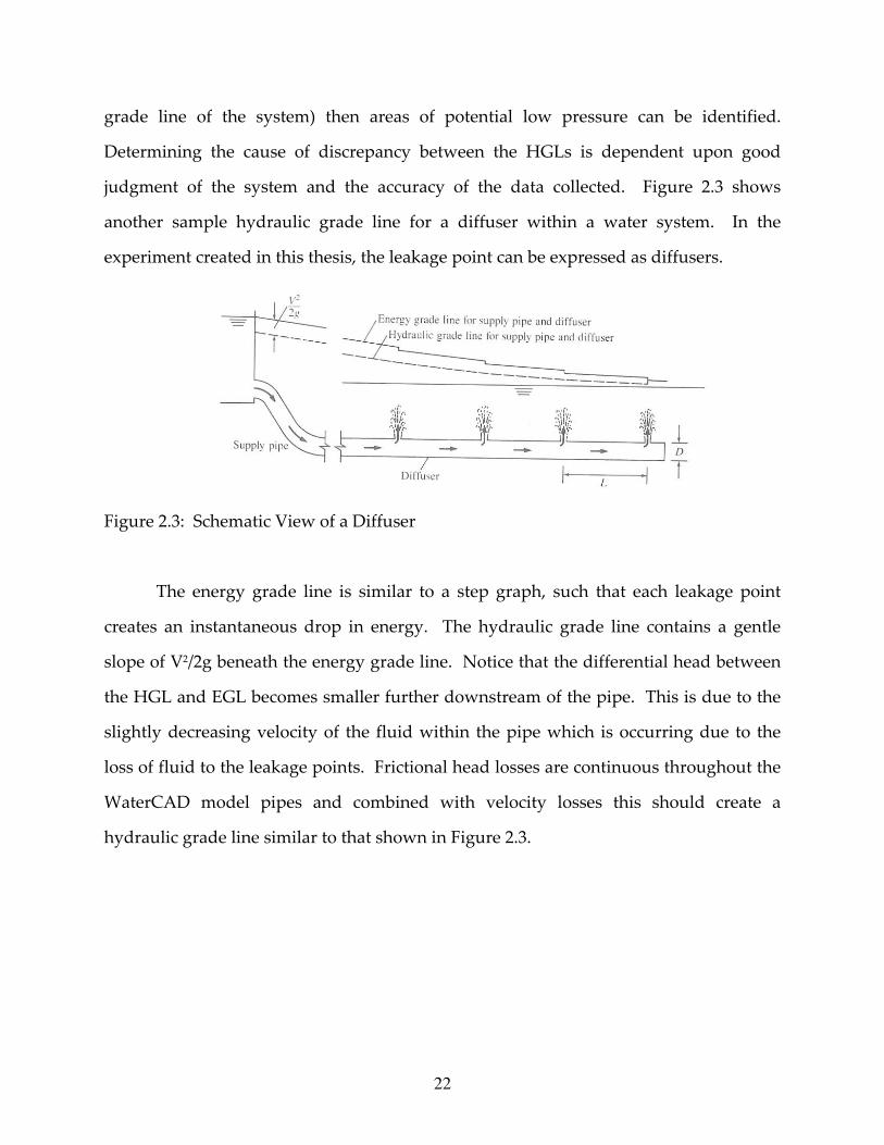
judgment of the system and the accuracy of the data collected. Figure 2.3 shows

another sample hydraulic grade line for a diffuser within a water system. In the

experiment created in this thesis, the leakage point can be expressed as diffusers.

Figure 2.3: Schematic View of a Diffuser

The energy grade line is similar to a step graph, such that each leakage point

creates an instantaneous drop in energy. The hydraulic grade line contains a gentle

slope of V2/2g beneath the energy grade line. Notice that the differential head between

the HGL and EGL becomes smaller further downstream of the pipe. This is due to the

slightly decreasing velocity of the fluid within the pipe which is occurring due to the

loss of fluid to the leakage points. Frictional head losses are continuous throughout the

WaterCAD model pipes and combined with velocity losses this should create a

hydraulic grade line similar to that shown in Figure 2.3.

23

CHAPTER 3

METHODOLOGY

Background

The experiment created and explained within this thesis was based on an

experiment previously performed by two researchers in Libson. Covas and Ramos

developed an experimental facility with a looped system at the Technical University of

Libson in 2000. This facility was specially designed for two reasons. The first reason

was to collect leakage transient data so that it could be placed in a transient database

(Transdat). The second reason is to test and analyze the inverse transient leakage

detection methodology (Covas & Ramos, 2001).

The configuration of their experimental set‐up consists of a pipe network with

six square loops, having each loop 2m x 2m, supplied by a pressurized vessel with a

constant head of approximately 26 meters. The pipes are massively anchored in several

sites along its length, in order to avoid any longitudinal movement in the several

fittings of the system during the transient event. The pipes are made of transparent

PVC PN10 (nominal pressure 10 kg‐m‐2), with 45 mm internal diameter and 2.4 mm of

wall thickness.

At the downstream end of the network, there are two valves: a gate valve, to

control the flow that discharges to the atmosphere, and a ball valve, immediately

upstream the former, to generate the transient event. The closure of the water hammer

valve is carried out manually.

The leaks are located at interior sections of the hydraulic system and are

simulated by small ball valves with 9 mm of inner diameter discharging directly to the

atmosphere. An electromagnetic flow meter was used to measure steady state flow at

the upstream end after the pressurized vessel. See Figure 3.1 for the experimental

network layout.

24

Figure 3.1: Experimental Facility at Instituto Superior Tecnico (Covas and Ramos, 2001)

Covas and Ramos performed two important tests with this facility. The first one

corresponds to the system without leakage and the other one with a leak located at

node 26 and with the size of 0.00003 m2. For both tests, the initial steady state flow at

the downstream end is 6 liter per second (l/s). The hydraulic transients were generated

by the closure of the downstream water hammer valve.

Covas and Ramos assumed that the initial flow through the distribution system

model was 6 l/s with no leakage. From this trial run, a background or control transient

could be generated. This control transient, at most node locations, is crucial to the

model because it allows comparison of the leak scenarios. It also allows the water

operator or engineer to determine the transients at specific node locations to verify if

leaks are occurring.

In the second trial, a leak of 0.67 l/s was modeled in two locations with an

effective leaks size of 0.00003 m2. In addition to the leak flow, an initial flow of 6 l/s was

25

maintained within the distribution system model. The variance of transient curves

comparing the “no leak” scenario with the “leakage” scenario is shown in Figure 3.2.

Table 3.1: Experimental Results (Covas and Ramos, 2001)

Test Initial Flow at Downstream Initial Leak Flow Leak Effective Size* No Leak 6 l/s ‐ ‐ Leak 1 6 l/s 0.670 l/s 0.00003 m2 (*) Leakʹs Effective size is Aef = Discharge Coefficient (Cd) multiplied by the area of the orifice (AL)

Despite the differences of each scenario within the Covas/Ramos experiment,

these scenarios did share a common characteristic. Figure 3.2 displays the transient

curves derived from both leakage scenarios. Although these transient curves vary in

head, they do share a common head measurement from 0.1 to 0.2 seconds. An enlarged

view of this specific time frame is shown in Figure 3.3 and contains a head of

approximately 26 meters. This value, which is steady state prior to the generation of the

transient, was used to calibrate the WaterCAD model.

Through this experiment, they were able to prove that with adequate

experimental data, a computer generated model of the water system could be created

and calibrated. This model when calibrated can create transient curves at junctions

within the system that match the transients created in the laboratory experiment. Thus

there is excellent correlation between experimental data and information obtained from

the computer model as shown in Figure 3.2. Covas and Ramos were able to

successfully develop a relationship between transient and inverse transient analysis.

Their results provide a beginning and foundation for similar transient experiments by

providing proof that there is a correlation between laboratory data and computer

simulated results.

26

Figure 3.2: Transient Pressure at Six Measurement Sites (Covas & Ramos, 2001)

Figure 3.3: Enlarged View of Transient Head at T1 Transducer (Covas & Ramos, 2001)

27

Overview of Research Tasks

It is the intention of this thesis and research to use the experimental data from

Covas and Ramos facility and create a model of the experimental facility using the

Haestad WaterCAD Version 7 software. The two leakage scenarios used by Covas and

Ramos will be utilized to detect the pressure variations throughout the system caused

by the potential leak. They will also be used to calibrate the model generated with

WaterCAD software. Different leakage scenarios will then be performed with the

calibrated model to determine the relationship between pressure variations within a

water system and the location of these leaks. An explanation of each scenario is

detailed in Table 3.3. These leakage scenarios vary in both the quantity of leakage at a

specific point and in the location of the leakage point. The model will also be used to

determine if a relationship between the effective size of the leak and pressure variations

exist. If a relationship between the leakage quantities and pressure variations exist,

water operators will be able to detect the possibility of leakage in their respective water

system and fix it, thereby reducing the amount of revenue lost and protecting the water

quality.

WaterCAD Modeling Software

Covas and Ramos (2001) utilized the TRANSDAT software (2001) after they had

obtained experimental data from their laboratory pipe model. The TRANSDAT

software is beneficial in modeling transients created in a water system. With enough

correct information to enter into the software program, TRANSDAT will solve the over‐

determined model. From both the computer model results and laboratory results that

Covas and Ramos (2001) obtained, it was found that both sets of results were

comparable to each other as seen in Figure 3.3. The TRANSDAT software used the

method of characteristics to solve for unknown pressures at nodes within the model.

28

This method is popular for handling hydraulic transients. It converts the two partial

differential equations (PDEs) of continuity and momentum into four ordinary

differential equations that are solved numerically using finite difference techniques

(Haestad et al, 2004).

The WaterCAD Version 7 software (User’s Guide, 2005) which was used within

the experiment explained in this thesis utilizes the parameters entered for the pipes and

nodes (demands) to solve for the pressures at each node and within the pipes. The

pressures at all nodes which are calculated by WaterCAD are independent of pressures

needed to satisfy the inputed demands. Therefore it is essential that calculated

pressures be viewed and compared to the inputed demands to verify whether the

results are reasonable. Due to small leakage rates incorporated within the model, the

results generated should be justified as reasonable. Of course, laboratory results

justifying all other scenarios would be needed to verify the accuracy of the WaterCAD

software. It is important to note that this software utilizes the continuity equation and

Bernoulli’s equation to solve for pressure and balance the flows within the model.

The WaterCAD software was chosen due to its popular usage by engineers and

municipalities. The EPANET software seems to be more heavily used by researchers

due to its free availability. However if municipalities are leaning toward the usage of

the software then the accuracy of the software and ability to simulate leakage in water

systems needed to be explored. Hence, the WaterCAD software was chosen to simulate

the water system expressed in this thesis.

Overall, the WaterCAD software is believed to be sufficient for this experiment.

Although TRANSDAT is used for solving pressure waves due to transients at specific

nodes, something which was not observed in this experiment, it was able to find

common similarities (i.e. pressure) with the capabilities of WaterCAD.

29

Development of WaterCAD Model When the computer model was initially developed a few trial runs were

performed so that the extent of the calibration needed could be detected. All pipes were

set to be Polyvinyl chloride (PVC) with a Hazen‐Williams coefficient of 150. Interior

diameters were 45 mm and the lengths of pipe were created as shown in Table 3.2. In

order to create a pressurized vessel, as Covas and Ramos did in their experiment, a

pump downstream of a reservoir was created. This pump has logical controls which

force the pump to turn on when the pressure is below 254 kPa and turn off when the

pressure is above 255 kPa. These pump settings allow the pipe system to maintain a

continuous pressure of approximately 254 kPa, which is comparable to the pressures

within the Covas and Ramos experiment. This also allows the pump to become a

pressurized vessel that Covas and Ramos used in their experiment rather than behaving

as a typical pump with a pump curve.

Figure 3.4: WaterCAD Model Setup

30

Table 3.2: Characteristics of Pipes within the WaterCAD Model

Label Length (m) Diameter (mm) Material Roughness Coefficient

P‐1 2.0 45 PVC 150

P‐2 2.0 45 PVC 150

P‐3 2.0 45 PVC 150

P‐4 2.0 45 PVC 150

P‐5 2.0 45 PVC 150

P‐7 2.0 45 PVC 150

P‐9 2.0 45 PVC 150

P‐12 2.0 45 PVC 150

P‐13 2.0 45 PVC 150

P‐14 2.0 45 PVC 150

P‐15 2.0 45 PVC 150

P‐17 2.0 45 PVC 150

P‐18 1.0 45 PVC 150

P‐19 1.0 45 PVC 150

P‐20 1.0 45 PVC 150

P‐21 1.0 45 PVC 150

P‐22 0.15 45 PVC 150

P‐24 0.9 45 PVC 150

P‐25 0.1 45 PVC 150

P‐26 1.0 45 PVC 150

P‐27 0.5 45 PVC 150

P‐28 0.5 45 PVC 150

P‐29 0.55 45 PVC 150

P‐30 1.3 45 PVC 150

P‐31 0.5 45 PVC 150

P‐33 0.5 45 PVC 150

P‐34 10.0 45 PVC 150

P‐35 3.4 45 PVC 150

P‐36 11.58 152.4 PVC 150

Table 3.2 shows the characteristics and parameters of every pipe within the

WaterCAD model. The lengths, diameters and material of pipe were derived from the

31

Covas/Ramos model. The roughness coefficient of 150 is standard for PVC pipe and

was verified through the calibration process. Pipe P‐36 was given a larger diameter to

reduce the head losses caused by friction. This was used so that the model would

achieve higher calibration results and better suit the Covas/Ramos model.

Seven different scenarios were run with the WaterCAD software. A summary of

these scenarios can be seen in Table 3.3. The first scenario, Scenario 0, was used as a

calibration trial run and was modeled with no leakage. The only flow which was

generated was used to flow to the reservoir downstream of the model, similar to the

Covas/Ramos experiment. This flow was equal to 6 l/s. The second scenario, Scenario

1, was also similar to the Covas/Ramos experiment. A leakage at a specific node of 0.67

l/s was generated in addition to the normal flow of 6 l/s through the system. This

leakage is approximately 11% of the total base flow throughout the water system. This

scenario was used as a double calibration to verify the accuracy of the inputted

parameters, such as pipe, nodes and pump characteristics. Scenarios 2‐6 were used to

vary the leakage rates and leakage locations in the WaterCAD model.

Scenarios 1, 2 and 3 will vary the leakage quantity at a constant node (Leak 1).

The original leakage quantity of 0.67 l/s will be halved in Scenario 2 and doubled in

Scenario 3. The purpose of these three scenarios will determine how leakage quantity

affects pressure measurements throughout a water system. Scenario 4, 5 and 6 will be

used to compare the affects of leakage location to calculated pressure measurements.

The leakage rate of 0.67 l/s will be maintained at a constant value while the leak is

located at three different locations within the water system. These locations are located

at different distances from the pump. Scenario 6 will utilize two locations to simulate

the effects of two leaks within a system. However, the total combined leakage quantity

will be 0.67 l/s from both leaks. The pressure variations which occurred due to these

leakage scenarios are discussed in further detail in the following chapters.

32

Table 3.3: Explanation of Each Scenario

Scenario No. Description

Scenario 0 No Leakage, used for calibration purposes

Scenario 1 Leak 1 = 0.67 l/s



Scenario 4 Leak 1 moved closer to Pump at T3 = 0.67 l/s


Scenario 6 Leak 1 = 0.335 l/s Leak 2 = 0.335 l/s

Figure 3.2 shows the comparison between the experimental laboratory data and

the computer simulation that Covas and Ramos obtained. Although this information is

due to transient analysis, the initial 0.1 second is steady state rather than transient. This

is due to the short time lag required for the effects of the transient to affect the pressures

and head at the measurement nodes. This steady state data at all six measurement

nodes was used to calibrate the WaterCAD model. These values, along with the

calibration percent errors, can be seen in Table 4.1.

Comparison of Leak Quantities

Comparison of Leak Location

Control Scenario

33

CHAPTER 4

RESULTS

The comparison between the Covas/Ramos (2001) experimental results and

initial WaterCAD scenario results from Leak #1 having a leakage of 0.67 l/s are very

similar. The no leakage scenario, Scenario 0, did provide some pressure differences

within the system as compared to the Covas/Ramos experiment, however these

differences were small and can be expected to be insignificant. The units used to

display pressure (Pascal) are very small which allow almost insignificant changes in

pressure to be noticed. The comparison of a Pascal to pounds per square inch, which is

commonly used in the U.S. is 1 pascal = 0.00014503 psi. This is beneficial since small

changes within the pressures of the model need to be considered. Initial calibration of

the WaterCAD model with a comparison of the pressure results from the Covas/Ramos

model and the WaterCAD model are shown in Table 4.1. The variations of pressure

were converted to error percentages which are small enough to confirm a successful

calibration of the WaterCAD model. With minimal calibrations, both models seem to

contain results which are comparable.

Table 4.1: Calibration Results – No Leak Scenario

Covas/Ramos Model WaterCAD Model

Node Head (m) Pressure (kPa) Head (m) Pressure (kPa) Percent Error (%)

T1 26 254 26.20 256.70 0.769

T2 26 254 26.07 255.29 0.269

T3 26 254 26.05 255.12 0.192

T4 26 254 26.03 254.92 0.115

T5 26 254 26.03 254.89 0.115

T6 26 254 25.83 252.95 0.654

34

After the model was properly calibrated using the no leak scenario pressures

throughout the model were compared. With the no leak scenario all pressures within

the distribution system were stabilized to an average pressure of 254‐255 kPa. The

highest pressure generated (258.16 kPa) was located in close proximity to the pump,

which was expected since the pump is responsible for charging the system. When

scenario #1 was performed using a leakage rate of 0.67 l/s at Leak #1 node, the pressures

at all nodes downstream of the pump in the system were affected. The node pressures

were decreased an average of 2.5 kPa at each node for a total system pressure of

approximately 251‐252 kPa. This decrease in pressure is not unusual or unexpected for

pipes downstream of the leak.

Data collected from both leakage scenarios revealed that the pump delivered

adequate flow to all nodes to satisfy their demands, however more power was needed

when Leak #1 was in operation due to the slightly larger demand of flow. Pump heads

remained the same for both scenarios. Approximately 10.5% more power is required to

operate the pump and deliver the additional flow as compared to the no leak scenario.

During Scenario #2 the demand of leakage for Leak #1 was reduced from 0.67 l/s

to 0.335 l/s. The results from scenario #2 are not surprising. As could be expected, the

pressure values from this scenario are larger than scenario #1 (Leak #1 = 0.67 l/s) and

smaller than the scenario which involved no leakage. Due to a smaller quantity of

water being released from the system through leakage, pressures within the system are

expected to be larger as compared to when greater quantities of water are released

through leakage. The pressure drop from this scenario is approximately half of the

pressure drop difference between the no leak and leakage of 0.67 l/s scenario. This can

be expected due to the leakage rate of 0.335 l/s is one half of the original leakage of 0.67

l/s used in Scenario 1. An average pressure drop of 1.28 kPa was experienced

throughout the system as compared to the no leak scenario. The effect of the pressure

variations occurred at all nodes downstream of the pump. The power required to

35

operate the pump for Scenario #2 is approximately 5.3% larger than the no leak

scenario.

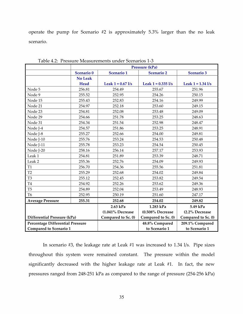
Table 4.2: Pressure Measurements under Scenarios 1‐3 Pressure (kPa)

Scenario 0 Scenario 1 Scenario 2 Scenario 3

No Leak Head Leak 1 = 0.67 l/s Leak 1 = 0.335 l/s Leak 1 = 1.34 l/s

Node 5 256.81 254.49 255.67 251.96 Node 9 255.52 252.95 254.26 250.15 Node 15 255.43 252.83 254.16 249.99 Node 21 254.97 252.18 253.60 249.15 Node 23 254.81 252.08 253.48 249.09 Node 29 254.66 251.78 253.25 248.63 Node 31 254.34 251.54 252.98 248.47 Node J‐4 254.57 251.86 253.25 248.91 Node J‐8 255.27 252.66 254.00 249.81 Node J‐10 255.76 253.24 254.53 250.48 Node J‐11 255.78 253.23 254.54 250.45 Node J‐20 258.16 256.14 257.17 253.93 Leak 1 254.81 251.89 253.39 248.71 Leak 2 255.36 252.76 254.09 249.93 T1 256.70 254.36 255.56 251.81 T2 255.29 252.68 254.02 249.84 T3 255.12 252.45 253.82 249.54 T4 254.92 252.26 253.62 249.36 T5 254.89 252.04 253.49 248.93 T6 252.95 250.19 251.60 247.17 Average Pressure 255.31 252.68 254.02 249.82

Differential Pressure (kPa)

2.63 kPa (1.041% Decrease Compared to Sc. 0)


5.49 kPa (2.2% Decrease

Compared to Sc. 0) Percentage Differential Pressure Compared to Scenario 1

48.8% Compared to Scenario 1

209.1% Compared to Scenario 1

In scenario #3, the leakage rate at Leak #1 was increased to 1.34 l/s. Pipe sizes

throughout this system were remained constant. The pressure within the model

significantly decreased with the higher leakage rate at Leak #1. In fact, the new

pressures ranged from 248‐251 kPa as compared to the range of pressure (254‐256 kPa)

36

from the no leak scenario, creating the largest decrease in pressure. The calculated

water power was 1.96 kW, also a significant increase in power usage. This is

approximately 21.7% more power needed to operate the pump as compared to Scenario

0. See Table 4.2 for exact pressure measurements at each node in Scenarios 1‐3. Table

4.3 has been included to show the differential pressure decrease at each node. Although

there are slight variations throughout the model, the pressure variations are fairly

uniform throughout the distribution system.

Table 4.3: Differential Pressure Measurements for Scenarios 1‐3 Differential Pressure

Scenario 0 No Leakage




Pressure Measurement

(kPa)


Percent Decrease1 (%)





Node 5 256.81 2.32 0.903 1.14 0.444 4.85 1.889 Node 9 255.52 2.57 1.006 1.26 0.493 5.37 2.102

Node 15 255.43 2.6 1.018 1.27 0.497 5.44 2.130 Node 21 254.97 2.79 1.094 1.37 0.537 5.82 2.283 Node 23 254.81 2.73 1.071 1.33 0.522 5.72 2.245 Node 29 254.66 2.88 1.131 1.41 0.554 6.03 2.368 Node 31 254.34 2.8 1.101 1.36 0.535 5.87 2.308 Node J‐4 254.57 2.71 1.065 1.32 0.519 5.66 2.223

Node J‐8 255.27 2.61 1.022 1.27 0.498 5.46 2.139 Node J‐10 255.76 2.52 0.985 1.23 0.481 5.28 2.064 Node J‐11 255.78 2.55 0.997 1.24 0.485 5.33 2.084 Node J‐20 258.16 2.02 0.782 0.99 0.383 4.23 1.639 Leak 1 254.81 2.92 1.146 1.42 0.557 6.1 2.394 Leak 2 255.36 2.6 1.018 1.27 0.497 5.43 2.126

T1 256.7 2.34 0.912 1.14 0.444 4.89 1.905 T2 255.29 2.61 1.022 1.27 0.497 5.45 2.135 T3 255.12 2.67 1.047 1.3 0.510 5.58 2.187 T4 254.92 2.66 1.043 1.3 0.510 5.56 2.181 T5 254.89 2.85 1.118 1.4 0.549 5.96 2.338 T6 252.95 2.76 1.091 1.35 0.534 5.78 2.285

Percent Decrease1 : This is compared to Scenario 0 (No Leakage Scenario)

37

There appears to be a linear relationship between the leakage quantity and

pressure decreases within the system. The pressure decrease from Scenario 3 is

approximately double (209.1%) as the pressure decrease of Scenario 1. This is

significant because of the leakage quantity factors for each scenario. Also, in Scenario 2

the pressure decrease is approximately half (48.8%) of the pressure decrease as

compared to Scenario 1, which is the approximately the same factor when comparing

the leakage quantity between the two scenarios.

In Scenario 4, the only leakage rate was 0.67 l/s at a node closer to the pump

(node T1). The purpose of this scenario was to determine how a leakage rate moved

closer to the pumps would cause the pressure variations to respond. After the new

leakage rate was simulated, the pressures at all nodes decreased. The pressure drop

was an average of 2.33 kPa at most nodes thereby creating an average pressure within

the experimental water system of 252‐253 kPa. The calculated water power was 1.78

kW, approximately 5.3% larger than the no leak scenario.

Scenario 5 was used to create a new leakage location on the right side of the

model. Leak 2 was used to generate a leak of 0.67 l/s. This node was the sole leakage

location. The pressure results shown in Table 4.4 show that a pressure drop was

experienced throughout the system due to this leakage. An average pressure decrease

of 2.58 kPa occurred as compared to Scenario 0. The calculated water power was 1.78

kW, approximately 5.3% larger than the no leak scenario.

In Scenario #6, another leak was incorporated into the model from a total of two

leaks. Leak #1 was adjusted so that the demand was 0.335 l/s. In Leak #2 a leakage rate

of 0.335 l/s was also incorporated into the model at a location away from Leak #1. The

purpose of this scenario was to observe the variations in pressure due to two leakage

points at opposite ends of the water system. The results of this scenario indicate that

with two different leakage locations in a water system, the pressures throughout the

system are significantly impacted. The average pressures at all nodes ranged from 252‐

38

253 kPa creating an approximate 2.6 kPa pressure decrease in the system. These

decreases in pressure are affected throughout the system in both pipes upstream and

downstream of the leakage locations.

Table 4.5 displays the differential pressure at each node within the model and the

corresponding pressure decrease percentage. From this table it can be seen that there

are slightly higher pressure changes at nodes very close to the leakage nodes as

compared to nodes located further away from the leakage nodes. Slightly higher

pressure changes are also visible in pipes downstream of both leak locations and are

common to both leaks.

Table 4.4: Pressure Measurements under Scenarios 4‐6 Pressure (kPa)


No Leak Head T1 = 0.67 l/s Leak 2 = 0.67 l/s Leak 1 & 2= 0.335

l/s Node 5 256.81 254.49 254.49 254.49 Node 9 255.52 253.18 252.81 252.88 Node 15 255.43 253.09 252.8 252.82 Node 21 254.97 252.62 252.38 252.28 Node 23 254.81 252.47 252.19 252.14 Node 29 254.66 252.31 252.05 251.92 Node 31 254.34 252.00 251.73 251.64 Node J‐4 254.57 252.23 251.91 251.89 Node J‐8 255.27 252.94 252.54 252.61 Node J‐10 255.76 253.43 253.17 253.21 Node J‐11 255.78 253.44 253.28 253.25 Node J‐20 258.16 256.14 256.14 256.14 Leak 1 254.81 252.47 252.21 252.06 Leak 2 255.36 253.02 252.58 252.67 T1 256.70 254.35 254.37 254.36 T2 255.29 252.95 252.55 252.62 T3 255.12 252.78 252.50 252.48 T4 254.92 252.58 252.23 252.25 T5 254.89 252.55 252.29 252.17 T6 252.95 250.61 250.31 250.26 Average Pressure 255.31 252.98 252.73 252.71





39

Table 4.5: Differential Pressure Measurements for Scenarios 4‐6

Differential Pressure (kPa) Scenario 0 Scenario 4 Scenario 5 Scenario 6

No Leakage Leak at T1 = 0.67 l/s Leak 2 = 0.67 l/s Leak 1 & 2 = 0.335 l/s


(kPa)







Node 5 256.81 2.32 0.903 2.32 0.903 2.32 0.903 Node 9 255.52 2.34 0.916 2.71 1.061 2.64 1.033

Node 15 255.43 2.34 0.916 2.63 1.030 2.61 1.022 Node 21 254.97 2.35 0.922 2.59 1.016 2.69 1.055 Node 23 254.81 2.34 0.918 2.62 1.028 2.67 1.048 Node 29 254.66 2.35 0.923 2.61 1.025 2.74 1.076 Node 31 254.34 2.34 0.920 2.61 1.026 2.7 1.062 Node J‐4 254.57 2.34 0.919 2.66 1.045 2.68 1.053

Node J‐8 255.27 2.33 0.913 2.73 1.069 2.66 1.042 Node J‐10 255.76 2.33 0.911 2.59 1.013 2.55 0.997 Node J‐11 255.78 2.34 0.915 2.5 0.977 2.53 0.989 Node J‐20 258.16 2.02 0.782 2.02 0.782 2.02 0.782 Leak 1 254.81 2.34 0.918 2.6 1.020 2.75 1.079 Leak 2 255.36 2.34 0.916 2.78 1.089 2.69 1.053

T1 256.7 2.35 0.915 2.33 0.908 2.34 0.912 T2 255.29 2.34 0.917 2.74 1.073 2.67 1.046 T3 255.12 2.34 0.917 2.62 1.027 2.64 1.035 T4 254.92 2.34 0.918 2.69 1.055 2.67 1.047 T5 254.89 2.34 0.918 2.6 1.020 2.72 1.067 T6 252.95 2.34 0.925 2.64 1.044 2.69 1.063

Percent Decrease1 : This is compared to Scenario 0 (No Leakage Scenario)

By initial assumption, it would be predicted that the pressures upstream of a leak

location should not be affected by a leak. However, as the computer simulations

demonstrate upstream pressures are affected by leakage. In order to overcome these

pressure fluctuations upstream of the leaks, a proper pump must be chosen which can

provide additional flow to overcome the amount of water lost in leakage.

40

Although the evaluation of power usage was not a research objective, it was

evaluated. Table 4.6 shows the power usage of Scenario 0‐6. There appears to be a

correlation between the leakage quantity and the power usage. Scenario 1, 4, 5 and 6

have a leakage quantity of 0.67 l/s and share the same power usage of 1.78 kW. The

remaining scenarios share a relationship between power and leakage such that the

power usage increases as the leakage quantity increases and decreases when the

leakage quantity decreases. It is important to note that the no leakage scenario requires

the least amount of power to operate the pump.

Table 4.6: Power Usage for Scenarios 1‐6

Scenario No. Power Usage (kW) Scenario 0 1.61

Scenario 1 1.78

Scenario 2 1.69

Scenario 3 1.96

Scenario 4 1.78

Scenario 5 1.78

Scenario 6 1.78

The results of the leak location analysis, though significant, are not surprising. A

leak present at any node causes every node to respond. Moreover, leaks at downstream

nodes cause a greater degree of pressure reduction, both in terms of the magnitude of

reduction and the number of nodes with reductions over a given quantity.

Equation 2 states that while there are pressure differences within a pipe, there is

leakage of flow through an orifice. This has proven true for the results of this

experiment as points of leakage have caused a fairly significant change in pressure both

upstream and downstream of the leakage.

Table 4.7 and 4.8 show the head losses within each pipe in the WaterCAD model.

When each scenario is compared, several data similarities were noted. There are two

41

pipes within the system that never had a change in head losses, despite the different

leakage rate in each scenario. Pipes P‐33 and P‐34 had a constant headloss of 2.775

meters/kilometers and 0.943 meters, respectively. This is possibly due to the location of

each pipe. P‐33 is located upstream of the flow control valve (FCV), while P‐34 is

located downstream of the flow control valve suggesting that the valve controls the

flow in each pipe regardless of the leakage rate. It is reasonable to expect the head

losses in close proximity of the valve to be affected, however it is not expected that the

head losses could be completely controlled by the valve. A combination of the effects

from the pump or pressurized vessel with the FCV could generate an effect which

would have amore dominant effect on the velocity of flow through the pipes and hence

a larger weight of pipe head losses.

By comparing the total head loss from each scenario, it is observed that Scenario

3 (Leak 1 = 1.34 l/s) produces the greatest total head loss from friction and related pipe

head losses. This could be expected because of the largest flows through the system (a

total of 7.34 l/s). When Scenario 1 and 4 were compared it can be seen that Scenario 1

produced a higher total pipe headloss, which at first glance would suggest that a leak

closer to the pump would produced less pipe headloss. Recall that Scenario 1 and 4

have the same leakage rate (0.67 l/s), but a different locations on a pipeline. However

when Scenario 1 and Scenario 5 were compared, it was observed that Scenario 1 had a

slightly high pipe headloss value. This comparison would suggest that a leak closer to

the pump will produce more pipe headloss, contrary to what was originally suggested.

Overall the smallest pipe headloss resulted from the no leak scenario which is

reasonable because this contained the smallest flow through the model (6 l/s).

42

Table 4.7: Pipe Head Losses in Scenario 0‐3

Head Losses due to Friction


Node ID Length (m)

Headloss Gradient (m/km)

Pipe Headloss (m)


Pipe Headloss (m)


Pipe Headloss (m)


Pipe Headloss (m)

P‐1 2.00 15.91 0.032 12.08 0.024 14 0.028 8.31 0.017 P‐2 2.00 71.25 0.143 66.78 0.134 70.05 0.140 66 0.132 P‐3 2.00 82.68 0.165 85.37 0.171 83.97 0.168 88.49 0.177 P‐4 2.00 12.52 0.025 10.85 0.022 11.68 0.023 9.23 0.018 P‐5 2.00 23.95 0.048 27.45 0.055 25.6 0.051 31.72 0.063 P‐7 2.00 7.87 0.016 5.21 0.010 6.46 0.013 3.17 0.006 P‐9 2.00 7.77 0.016 8.36 0.017 8.05 0.016 9.12 0.018 P‐12 2.00 12.48 0.025 14.67 0.029 13.55 0.027 17.12 0.034 P‐13 2.00 17.2 0.034 20.98 0.042 19.05 0.038 25.11 0.050 P‐14 2.00 18.28 0.037 20.74 0.041 19.45 0.039 23.67 0.047 P‐15 2.00 41.75 0.084 53.89 0.108 47.73 0.095 66.71 0.133 P‐17 2.00 53.27 0.107 63.89 0.128 58.44 0.117 75.59 0.151 P‐18 1.00 31.34 0.031 38.36 0.038 34.74 0.035 46.2 0.046 P‐19 1.00 31.34 0.031 38.36 0.038 34.74 0.035 46.21 0.046 P‐20 1.00 36.09 0.036 40.85 0.041 38.38 0.038 46.32 0.046 P‐21 1.00 36.09 0.036 40.85 0.041 38.38 0.038 46.32 0.046 P‐22 0.15 12.48 0.002 14.68 0.002 13.55 0.002 17.12 0.003 P‐24 0.90 104.38 0.094 128.25 0.115 116.07 0.104 154.08 0.139 P‐25 0.10 104.39 0.010 128.25 0.013 116.06 0.012 154.08 0.015 P‐26 1.00 15.91 0.016 12.09 0.012 14 0.014 8.31 0.008 P‐27 0.50 15.91 0.008 29.07 0.015 22.12 0.011 44.85 0.022 P‐28 0.50 15.91 0.008 29.07 0.015 22.12 0.011 44.85 0.022 P‐29 0.55 12.49 0.007 14.67 0.008 13.55 0.007 17.12 0.009 P‐30 1.30 12.48 0.016 14.67 0.019 13.54 0.018 17.12 0.022 P‐31 0.50 277.49 0.139 337.59 0.169 306.87 0.153 403.08 0.202 P‐33 0.50 277.49 0.139 277.49 0.139 277.49 0.139 277.49 0.139 P‐34 10.00 277.49 2.775 277.49 2.775 277.49 2.775 277.49 2.775 P‐35 3.40 277.49 0.943 337.6 1.148 306.87 1.043 403.07 1.370 P‐36 11.58 0.73 0.008 0.89 0.010 0.81 0.009 1.06 0.012 Total Head Loss: 5.030 5.378 5.201 5.773

43

Table 4.8: Pipe Head Losses in Scenario 4‐6

Head Losses due to Friction


Node ID Length (m)


Pipe Headloss (m)


Pipe Headloss (m)


Pipe Headloss (m)


Pipe Headloss (m)

P‐1 2.00 15.91 0.032 15.88 0.032 16.58 0.033 14.29 0.029 P‐2 2.00 71.25 0.143 71.22 0.142 72.28 0.145 70.52 0.141 P‐3 2.00 82.68 0.165 82.71 0.165 81.58 0.163 83.47 0.167 P‐4 2.00 12.52 0.025 12.47 0.025 14.47 0.029 12.58 0.025 P‐5 2.00 23.95 0.048 23.96 0.048 23.77 0.048 25.53 0.051 P‐7 2.00 7.87 0.016 7.8 0.016 9.39 0.019 7.14 0.014 P‐9 2.00 7.77 0.016 7.71 0.015 13.35 0.027 10.71 0.021 P‐12 2.00 12.48 0.025 12.61 0.025 18.37 0.037 16.51 0.033 P‐13 2.00 17.2 0.034 17.52 0.035 18.86 0.038 19.87 0.040 P‐14 2.00 18.28 0.037 17.94 0.036 24.16 0.048 22.4 0.045 P‐15 2.00 41.75 0.084 41.56 0.083 46.02 0.092 49.91 0.100 P‐17 2.00 53.27 0.107 54.05 0.108 67.19 0.134 65.53 0.131 P‐18 1.00 31.34 0.031 31.42 0.031 31.25 0.031 34.66 0.035 P‐19 1.00 31.34 0.031 31.42 0.031 31.25 0.031 34.66 0.035 P‐20 1.00 36.09 0.036 36.18 0.036 32.37 0.032 36.53 0.037 P‐21 1.00 36.09 0.036 36.18 0.036 32.37 0.032 36.53 0.037 P‐22 0.15 12.48 0.002 12.62 0.002 5.41 0.001 9.53 0.001 P‐24 0.90 104.38 0.094 103.32 0.093 123.78 0.111 126.01 0.113 P‐25 0.10 104.39 0.010 142.69 0.014 123.78 0.012 126.02 0.013 P‐26 1.00 15.91 0.016 15.88 0.016 16.58 0.017 14.29 0.014 P‐27 0.50 15.91 0.008 15.88 0.008 16.58 0.008 22.47 0.011 P‐28 0.50 15.91 0.008 15.88 0.008 16.58 0.008 22.47 0.011 P‐29 0.55 12.49 0.007 12.61 0.007 5.4 0.003 9.54 0.005 P‐30 1.30 12.48 0.016 12.61 0.016 18.37 0.024 16.51 0.021 P‐31 0.50 277.49 0.139 337.59 0.169 337.6 0.169 337.6 0.169 P‐33 0.50 277.49 0.139 277.49 0.139 277.49 0.139 277.49 0.139 P‐34 10.00 277.49 2.775 277.49 2.775 277.49 2.775 277.49 2.775 P‐35 3.40 277.49 0.943 337.6 1.148 337.6 1.148 337.6 1.148 P‐36 11.58 0.73 0.008 0.89 0.010 0.89 0.010 0.89 0.010 Total Head Loss: 5.030 5.271 5.364 5.371

44

From the results of the seven scenarios performed with the WaterCAD software,

pressure profiles at specific routes within the model were generated. In fact, there were

three primary routes which were chosen to generate pressure profiles. The first route,

shown in Figure 4.1, begins at node R‐2 and ends 36 meters later at the Reservoir node.

This route incorporates the Leak 1 node so that pressure variations around this node

can be compared. The complete profile can be viewed in Figure 4.2. This figure shows

that the initial pressure at node R‐2 was zero and remained zero until it reached the

pump which dramatically increased to approximately 268.5 kPa. The final pressure at

the Reservoir node was also zero due to the water coming in contact with surface

pressure. More detailed views of the profile between the pump and the flow control

valve can be seen in Figures 4.3 and 4.4.

Figure 4.1: Pressure Profile Path for the Left Side of Model

Pressure Profile Path

45

Pressure Profile for Left Side (Scenario 0‐6)

0

30

60

90

120

150

180

210

240

270

0 5 10 15 20 25 30 35 40

Distance (m)

Pressure (kPa)

Scenario 0Scenario 1Scenario 2Scenario 3Scenario 4Scenario 5Scenario 6

Figure 4.2: Left Side Pressure Profile for Scenario 0‐6

Figure 4.4 shows the variations of pressure between each scenario with great

clarity. At a distance of 19.5 meters is the Leak 1 node. Pressure downstream of this

node seems to decrease fairly sharp as a result of any leakage from this area. There

appears to be a large variation in pressure decreases due to leakage quantity between

Scenarios 1‐3. Scenario 3 is mostly outside the graph area due to extremely low

pressures from the high leakage rate at Leak 1. However, when pressure variations due

to changes in leakage location are compared, there does not appear to be much

variation in pressure quantities. It is important to note that the highest pressures come

from Scenario 0 which has no leakage.

46


245

250

255

260

265

270

10 12 14 16 18 20 22 24 26 28 30

Distance (m)

Pressure (k

Pa)


Figure 4.3: Enlarged Pressure Profile for Scenario 0‐6 (Left Side)


250

250.5

251

251.5

252

252.5

253

253.5

254

254.5

255

255.5

256

256.5

257

257.5

258

14 15 16 17 18 19 20 21 22 23 24 25 26 27 28

Distance (m)

Pressure (k

Pa)


Figure 4.4: Enlarged Pressure Profile for Scenario 0‐6 (Left Side)

47

The second pressure profile was created using the route shown in Figure 4.5.

This route begins at node R‐2 and ends at the Reservoir node for a total distance of 36

meters. This route contains no leakage points and is located half the distance between

Leak 1 and Leak 2. Figure 4.6 shows the pressure profile for the entire 36 meter route.

The pressure located at the pump location appears to be the same as shown in Figure

4.2. The pressures at a distance of 0 and 36 meters are zero due to the surface pressure

at each reservoir. More detailed views of the pressures between the pump and the flow

control valve are shown in Figures 4.7 and 4.8.

Figure 4.5: Pressure Profile Path for Middle of Model


48

Pressure Profile for Middle (Scenario 0‐6)

0

30

60

90

120

150

180

210

240

270

0 5 10 15 20 25 30 35 40

Distance (m)

Pressure (kPa)


Figure 4.6: Middle Pressure Profile for Scenario 0‐6


245

250

255

260

265

270

10 12 14 16 18 20 22 24 26 28 30

Distance (m)

Pressure (k

Pa)


Figure 4.7: Enlarged Pressure Profile for Scenario 0‐6 (Middle)

49


250

250.5

251

251.5

252

252.5

253

253.5

254

254.5

255

255.5

256

14 15 16 17 18 19 20 21 22 23 24 25 26 27 28

Distance (m)

Pressure (kPa)


Figure 4.8: Enlarged Pressure Profile for Scenario 0‐6 (Middle)

Figure 4.8 shows a more spread out display of pressures from each scenario.

However, the pressures caused by Scenario 1, 4, 5 and 6 are closely grouped together.

Scenario 3 continues to display low pressures which stretch outside the graph area.

Scenario 0 remains the pressure profile with the highest pressures in the model.

Scenario 2, with a leakage rate at Leak 1 of 0.335 l/s, has the second highest pressures in

the model. It appears that the pressures begin to sharply decrease at a distance of 20.5

meters from the node R‐2. This distance corresponds to node T3 which is located

almost directly in the middle of the model, both horizontally and vertically.

50

The third and final pressure profile is located on the right side of the model. This

layout is shown in Figure 4.9 and includes the Leak 2 node. Similar to the previous two

profiles, this route begins at node R‐2 and ends at the Reservoir node which is a total of

36 meters long. Figure 4.10 displays the entire pressure profile for this route. The

pump continues to increase the pressure to approximately 268.5 kPa. Pressures at both

the beginning and ending reservoirs are zero due to surface water pressures. See

Figures 4.11 and 4.12 form ore detailed views of the pressures at each scenario between

the pump location and the flow control valve.

Figure 4.9: Pressure Profile Path for the Right Side of the Model


51

Pressure Profile for Right Side (Scenario 0‐6)

0

30

60

90

120

150

180

210

240

270

0 5 10 15 20 25 30 35 40

Distance (m)

Pressure (kPa)


Figure 4.10: Right Side Pressure Profile for Scenario 0‐6


245

250

255

260

265

270

10 12 14 16 18 20 22 24 26 28 30

Distance (m)

Pressure (k

Pa)


Figure 4.11: Enlarged Pressure Profile for Scenario 0‐6 (Right Side)

52


251

251.5

252

252.5

253

253.5

254

254.5

255

255.5

256

14 15 16 17 18 19 20 21 22 23 24 25 26 27 28

Distance (m)

Pressure (kPa)


Figure 4.12: Enlarged Pressure Profile for Scenario 0‐6 (Right Side)

Figure 4.12 shows a detailed view of the pressures between the distance of 15

meters and 25 meters. Similar to the pressure profile for the middle, Scenarios 0, 2 and

3 seem to be disbursed more. Scenarios 1, 4, 5 and 6 are spaced very close to each other.

Scenarios 5 and 6 are the only scenarios which involved leakage within the Leak 2 node.

Due to their similar pressure with scenarios 1 and 4 it appears that which the leakage

rate throughout the system was 0.67 l/s the pressures at the nodes where similar. Recall

that the total leakage rate in each of the four scenarios was 0.67 l/s.

53

CHAPTER 5

DISCUSSION

Possible Modeling Errors/Calibrations

It is important to note that a model is only as good as the data that it contains.

Thus the more accurate information and data that comprises the computer model, the

more accurate the results will be. A lack of information will lead to uncertainty and

almost always be visible in the final results. As engineers it is important to note these

assumptions so that calibrations can be performed after the initial results are derived. If

the use of calibrating the model seems futile, the use of certain assumptions should be

duly recorded so that an explanation of the results can be compiled.

If the characteristics of the system are well known, the need for field procedures

is greatly lessened; analysis can be done with much less data by using computational

algorithms. Essentially the same inverse techniques can be used to calibrate

distribution systems (Pudar and Liggett, 1992).

Covas and Ramos (2001) developed their experiment using the metric units, as is

typically customary in foreign countries. The use of measuring pressure within this

experiment in units of kilopascals (kPa) is extremely beneficial. A pascal (Pa) is a

sensitive measurement unit and compared to English units is equal to 1.4503x10‐4 psi or

1 psi is equal to 6,895 pascals. Therefore, the use of this metric unit is beneficial in

detecting small changes of pressure within the WaterCAD model. With a more

sensitive measurement perhaps the leakage detection and location approximation can

become more accurate and more beneficial to the outcome of the experiment. The

results in Table 4.1 demonstrate a successful calibration of the model. This is essential

to providing accurate results for the different scenarios and their corresponding

leakage.

54

Discussion of Results

As previously mentioned in Chapter 2, the Bernoulli equation is relevant for this

experiment and can be simplified based on parameters used within this research. The

parameters specific to this experiment are shown below:

= 9.81 kN/m3

V1,2 = assumed to be the same for both upstream and downstream of the leak location

g1,2 = 9.81 m2/s for both upstream and downstream of the leak location

z1,2 = 0 for both upstream and downstream of the leak location

1,2 = 1.05 for both upstream and downstream of the leak location

Using these parameters, the Bernoulli equation can be simplified to the following

form:

(p1 / ) = (p2 / ) + hL

p1 = p2 + hL•

Δp = (p1‐p2) = hL• (Eqn. 4)

Equation 4, which is specific only to this example, states that the pressure drop

within a pipe segment is dependent upon the head losses and unit weight of water. All

elevations of pipes and nodes have been set to zero; therefore there is no head loss due

to static head. Note that the velocity both upstream and downstream of the leak have

been assumed to be equal. Although this assumption is not entirely true, the velocity

difference surrounding the leakage point is small enough to disregard and can be

assumed to be equal for equation simplification purposes. In this simple experiment

the only head losses which could occur are due to friction losses through pipe

roughness and leakage. This is reasonable due to the simplicity of this model.

55

Although the experiment expressed in this research relies on a single pump to

provide pressure for the distribution system, the hydraulic grade lines at each water

source should be similar. The pressure head at the pump should be the highest point

on the hydraulic grade line, as demonstrated in Figure 4.3, 4.7, and 4.11. The HGL is

composed of both the elevation (z) and the pressure head (p/ ), but because all

elevations within the experiment have been set at zero, the hydraulic grade line is

affected only by pressure head. The head losses in this experiment are affected by

pressure heads upstream and downstream of the leak as well. Equation 4 can be

rearranged to generate:

hL = p1/ – p2/ (Eqn. 5)

This equation simply states the difference in pressure heads at the upstream and

downstream locations of the leakage is equal to the head losses at the leakage point.

Therefore, the head losses in the distribution system were primarily dependent upon

pressure head.

Frictional losses were not expected to be large because of the short lengths of

pipe within the experiment and fairly low velocity flowing through the pipes. The

headloss results for each scenario of the experiment, shown in Table 4.7 and 4.8, confirm

this initial assumption. The differential head loss in each scenario is fairly small when

compared with Scenario 0. For the no leak scenario a total head loss due to pipe head

loss was 5.03 meters. When a leakage of 0.67 l/s at Leak 1 node was incorporated into

the model the pipe headloss increased to 5.378 meters. Very similar pipe headloss

results were obtained from Scenario 5 and 6 (5.364 and 5.371 meters, respectively).

When the leakage location was moved to the Leak 2 node in Scenario 6, the headloss

value varied 0.007 meters from the headloss value from Scenario 1. Scenario 5

generated a total pipe headloss which decreased 0.014 meters as compared to Scenario

1. It appears that the location of the leakage does have an effect on the quantity of

56

headloss, however this effect is minimal. Scenario 4, which moved the leakage location

to the T1 node (closer to the pump), produced a decrease in pressure of 0.107 meters, as

compared to Scenario 1, which confirms the fact that leakage location does affect

headloss values. It is important to note that all headloss variations from Scenarios 1‐6

increased the head loss quantities as compared to the no leak scenario.

The effects of leakage quantities on headloss values were evaluated as well.

Headloss values were the highest when a leakage rate of 1.34 l/s was generated at the

Leak 1 node during Scenario 3 (5.773 meters). The value was lowest, excluding the no

leak scenario, when the leakage rate of 0.335 l/s in Scenario 2 was generated (5.201

meters). It appears that there is a relationship between the headloss values generated

within the pipes and the quantity of leakage. This is no surprise since pipe headloss is

primarily controlled by headloss through friction which is strongly dependent upon

velocity of fluid within the pipe. The higher the velocity of the fluid within a pipe

segment, the higher the friction losses should be. Of course the pipe characteristics such

as diameter, length and roughness coefficient also have a contribution to producing

headloss, however these factors are not as dominant as the velocity of fluid. It is also

important to note that velocity is contingent upon the diameter of pipe which the fluid

is flowing through. Velocity not only contributes to the headloss quantities within the

pipes, but also to the hydraulic and energy grade line as shown in Figure 2.2 and 2.3. In

fact the difference between the HGL and EGL is the velocity head (V2/2g).

Decrease in pressure in Scenario #1, #2, and #3 resulting from leakage within the

experimental water system seems to be fairly uniform across all nodes. If a pressure

decrease occurs, as in scenario #1, #2, and #3, the differential decrease seems to be

constant across the nodes both upstream and downstream of the leakage location.

Nodes upstream of the pump do not seem to be affected by the leakage. This is

reasonable due to the pump being the sole provider of pressure within the system.

Pressures are also unaffected at nodes downstream of the flow control valve (node

57

FCV‐1). This is justifiable since the water within the pipe being discharged to the

Reservoir which contains surface pressures of 0 kPa. Although pressure within pipe P‐

34 just downstream of FCV‐1 is not zero, WaterCAD calculates pressures within pipes

at the most downstream point. For node P‐36 this point of pressure will be located at

the Reservoir and is equal to zero, thus the result shown in the pressure profiles in

Figures 4.2 ‐ 4.13.

From the pressure results due to Scenarios 4‐6, several comparisons can be made.

Because Covas and Ramos (2001) utilized a leakage rate of 0.67 l/s during the course of

their experiment, the same total leakage rate was frequently maintained within this

experiment. Scenarios 1, 4, 5 and 6 utilized a total leakage of 0.67 l/s. From the node

pressures expressed in Table 4.4 and 4.5, it can be observed that these scenarios contain

fairly similar pressures at each node. In fact, the pressure results shown for Scenarios 1,

4, 5 and 6 are similar to each other suggesting that leakage location has a minimal effect

on pressure variations, however it does have an effect. It appears that the pressure

decreases throughout the water system are fairly uniform and there is not a linear

relationship between the leakage location and the pressure decreases. When the

leakage of 0.67 l/s was moved closer to the pump, in Scenario 4, the pressure

measurements at all nodes increased slightly which implies that as the leakage is moved

further from the source of pressure for the system (i.e. pumps, elevated tank, etc.) the

pressure measurements will decrease throughout the system. The pressure variations

in Scenario 4 also suggest that the closer a leak is located to the water source (pump,

elevated tank, etc.) the more likely the pressure results are to be slightly higher

throughout the system. The comparison of Scenario 1 and Scenario 5 imply the same

results. Leak 1 is closer to the pump as a compared to Leak 2, thus most likely the

reasoning behind pressures in the system being approximately 0.1 kPa higher than the

pressure results derived from Scenario 5.

58

Although Scenario 2 and 3 varied from the standard leakage rate of 0.67 l/s, the

purpose of these scenarios was to compare the variation of leakage at a single source.

Based on the comparison of Scenario 1, 2 and 3, Scenario 3 (leakage of 1.34 l/s) produced

results the lowest pressure values, while Scenario 2 (leakage of 0.335 l/s) produced the

highest pressure values excluding the no leak scenario. These results imply that the

larger the leakage quantities the smaller the residual pressure values will be. There

appears to be a linear relationship between the leakage quantity and the pressure

decreases within the system. If the leakage rate is increased to twice the original

leakage quantity (as in Scenario 3) the pressure decreases will increase approximately

twice the original amount. In an overall comparison of all scenarios, it can be observed

that leakage at any node regardless of the quantity or location will reduce the pressure

within a distribution system.

As shown in Figures 4.2 ‐ 4.13, a line displaying the pressure at three specific

routes was generated for all six scenarios. These figures are beneficial in comparing

pressures from one scenario in different pipes. The first profile included a path on the

left side of the experimental distribution system and Figure 4.4 shows an enlarged view

of the pressure profile. This profile shows that the higher the leakage rate the lower the

pressures within the system whereas no leakage produces higher pressures within the

system. The lower the leakage rate and the closer the leakage locations are to the pump

the more likely the pressures are to be larger. Of course, it is important to note that no

leakage will produce the highest pressure. Figure 4.8 and 4.12 show the pressure

profiles for the middle and right side section of pipes within the distribution system.

The results discussed above are applicable for both pressure profiles in the middle and

right side as well as the left side profile.

Analysis of the single leaky pipe within this experiment indicated it cannot be

determined whether leak location affects energy consumption of the pump. Although

direct extrapolation of this analytical result is not feasible for distribution networks, it is

59

logical to expect that leaks situated at the most downstream portions of a network will

often involve a larger energy cost, because the larger flows must be transmitted through

a great portion of the system. Also, the power required to push larger flows

downstream in a system will result in larger frictional head losses, thus requiring more

energy for the pump. However, it is important to note that additional head losses, such

as static head, much also be considered. The energy required to operate the pumps and

other pressure control apparatus’ is based on total dynamic head (TDH), which

accounts for all head losses, both frictional and static. Therefore the TDH should

always be considered before a definite conclusion can be derived. In this experiment,

all elevations were set at 0, thereby making static head a null factor.

In fact, it appears that the power usage results from the WaterCAD software

were dependent solely upon the quantity of leakage. For Scenarios 1, 4, 5, and 6, all

contained a total leakage rate of 0.67 l/s and the power usage calculations yielded a

usage of 1.78 kW for each scenario. Scenario 2 contained a total leakage rate one half

the amount as used in Scenario 1, 4, 5 and 6 and the power usage proved to be

approximately one half of the quantity used in Scenario 1, 4, 5, and 6. See Table 4.6 for

exact quantities of power usage results for each scenario. Because there is no calibration

technique for the verification of the power usage calculations it is difficult to discern the

accuracy of these calculations. However it is reasonable to assume that the power

needed to operate a pump would be dependent upon the quantity of water the pump

must deliver to a water system. This is, in fact, also dependent upon the length of time

the pump will need to operate.

Additional Experiments – Scenario 7 and Scenario 8

After the evaluation of the results derived from Scenarios 0‐6, another test was

performed to determine if there is a relationship between the pressure decreases in a

water system due to leakage and the size of the water system. The existing model, as

60

previously discussed in the Methodology section, was scaled to two times the size of the

original model for the evaluation of Scenario 7 and 8. All pipes lengths were increased

to two times the original lengths. The pipe diameters were kept at the original

parameters of 45 mm. The leakage rate in Scenario 7 was kept to the constant 0.67 l/s

leakage rate, similar to quantity used in Scenarios 1, 4, 5 and 6. However Scenario 8

utilized a leakage rate of 1.34 l/s (twice the original 0.67 l/s leakage rate). The purpose

of these experiments was to compare how the size of a water distribution system can

affect pressures within the system. The calculated pressures from this experiment are

shown in Table 5.1.

Scenario 7 involved the original leakage rate of 0.67 l/s at the Leak 1 node and the

constant base flow of 6 l/s. This provides a leakage rate of approximately 11.2%. The

purpose of this scenario was to determine the effects of the distribution size on the

pressure variations. The only variation between Scenario 7 and Scenario 1 are the pipe

lengths.

Scenario 8 was performed to evaluate effects of increasing the leakage rate to 1.34

l/s while maintaining a base flow of 6 l/s. This provides a leakage rate of approximately

22.3% which is comparable to the leakage quantity in Scenario 3. Again, the pipe

lengths were twice the original lengths (similar to Scenario 7).

From the results for both Scenario 7 and 8 it can be observed that much larger

pressure decreases are experienced at each node within the water system model due to

the increase in pipe lengths. Furthermore it appears that the pressure decreases are

fairly uniform across each node as in the previous experiment discussed in Chapters 3

and 4. However, some nodes located closer to the leakage location appear to have

larger pressure decreases as compared to the remaining nodes within the water system

model. The pressure decreases in the nodes upstream of the leakage are smaller

decreases compared to the nodes downstream of the leakage location. The nodes which

are downstream of the leakage contain pressure decreases which are larger than any

61

other nodes in the water system. This suggests that pressure decreases from Scenario 7

and 8 are affected by the location of the nodes relative to the leakage node. However, it

is important to note that all pressures within the system downstream of the pump are

affected by the leakage location.

Table 5.1: Pressure Measurements from Scenario 7 and Scenario 8

Differential Pressure Scenario 0 Scenario 7 Scenario 8

No Leakage Leak 1 = 0.67 l/s Leak 1 = 1.34 l/s


(kPa)


(kPa)



(kPa)


Node 5 256.81 251.94 1.90 246.87 3.87 Node 9 255.52 250.12 2.11 244.51 4.31

Node 15 255.43 249.97 2.14 244.28 4.37 Node 21 254.97 249.11 2.30 243.04 4.68 Node 23 254.81 249.08 2.25 243.08 4.60 Node 29 254.66 248.61 2.38 242.30 4.85 Node 31 254.34 248.46 2.31 242.31 4.73 Node J‐4 254.57 248.88 2.24 242.97 4.56

Node J‐8 255.27 249.79 2.15 244.08 4.38 Node J‐10 255.76 250.47 2.07 244.94 4.23 Node J‐11 255.78 250.42 2.09 244.85 4.27 Node J‐20 258.16 253.92 1.64 249.49 3.36 Leak 1 254.81 248.68 2.41 242.30 4.91 Leak 2 255.36 249.90 2.14 244.23 4.36

T1 256.7 251.78 1.92 246.68 3.91 T2 255.29 249.81 2.15 244.12 4.38 T3 255.12 249.51 2.20 243.68 4.48 T4 254.92 249.34 2.19 243.52 4.47 T5 254.89 248.91 2.35 242.67 4.79 T6 252.95 247.15 2.29 241.10 4.68

Average Percent Decrease (%) 2.16 4.41 Percent Decrease1 : This is compared to Scenario 0 (No Leakage Scenario)

62

Scenario 7 and Scenario 8 differ in the respect that the leakage rate in Scenario 8

is double the leakage rate in Scenario 7. Pressure decreases from these two scenarios

suggest a linear relationship. Furthermore, the comparison between the pressure

variations from Scenario 1 (which contains a leak at the Leak 1 node = 0.67 l/s) and

Scenario 7 (which also contains a leak at the Leak 1 node = 0.67 l/s) suggests a linear

relationship between the two scenarios. The decrease in pressure variations for

Scenario 7 is approximately double the decrease in pressure as compared to Scenario 1.

The same conclusion can be derived for the linear relationship between Scenario 3 and

Scenario 8. The pressure decreases from Scenario 8 are approximately double the

pressure decreases from Scenario 3.

One conclusion which can be formed from these additional experiments or

scenarios is that as the leakage quantity increases within a water system, the pressure

within the system will decrease as well. It is reasonable to assume that the large

variances in pressure decreases caused by expanding the pipe lengths are a result of the

additional head losses within the additional pipe lengths. The head losses from these

two scenarios should be twice as large as compared to Scenario 1 and 3 due to twice the

quantity of pipe within the distribution system. However, the relationship between the

head losses and leakage flow has not been observed in detail.

63

CHAPTER 6

CONCLUSION

Leaks are expensive for a variety of reasons, including the loss of water and

treatment chemicals, the increased risk of water quality deterioration, unnecessary

capacity expansion, and the increased energy expenditure required to feed the leaks.

Given current typical prices, lost water costs upstage those associated with energy

wastage. Moreover, if either water or energy prices continue to rise the importance of

leak repair will become even more pronounced. For both pipe segments and

distribution networks, leaks are shown to substantially increase energy costs.

Although there are many reasons for minimizing leakage in municipal water

distribution networks, perhaps the most important relates to quality of service. A

network with physical failures may be exposed, under certain operating conditions, to

pathogen intrusions that affect the quality of water. Every leakage control program has

a water balance of the system as a common starting point.

Leak detection in pipelines is necessary to avoid economic losses, ensure safety,

and control environmental problems. The leak detection methods presently available

have several limitations and can only be employed in specific situations. The purpose

of the experiment presented in this thesis was to examine pressure throughout a system

at specific locations and review how the pressures at these locations will vary with

different leakage rates and different locations of leaks. The accuracy of the WaterCAD

software was also evaluated.

With the continuing increase of technology, water operators have easier ways to

account for the total water used within their system. Residential water meters are now

electronic and equipped with SCADA capabilities so that all water usage can be sent

directly to the water department in spreadsheet form. The use of water meters on

hydrants can help regulate and account for municipality water usage. Electronic flow

64

meters at well or plant sites will allow the water department to know the exact quantity

of water leaving the plant and entering the system for water consumption. If the

capabilities for accountability are available, leak detection through water accountability

is possible. This is perhaps the simplest and cheapest way to determine if leaks are

occurring within a system.

Summary of Research Results

Previous research in leak detection has utilized both the steady state and

transient analysis to identify the location of leaks based on pressure measurements

within laboratory experiments. The research presented through these experiments

focuses on the relationship between pressure measurements and leakage. This

relationship was determined by altering the leakage quantity and leakage location.

Perhaps through this research engineers and water operators can look at areas of

unusual pressure decreases and have a better understanding if these decreases were or

could be caused by leakage.

The research presented through these experiments varies from previous research

performed for leakage detection for several reasons. The reasons include:

� Identifying the relationship between leakage quantities and pressure

variations within a water system

� Identifying the relationship between leakage location and pressure variations

within a water system

� Utilizes laboratory data derived for a transient analysis experiment to calibrate

a inverse steady state analysis water model.

� Evaluates the accuracy of the WaterCAD software to properly generate a

water model and obtain results similar to those obtained from a previous

laboratory experiment.

65

The WaterCAD software produced results which were very similar to the results

within the Covas/Ramos experiment. This suggests that this software is sufficient and

capable of providing results which can be comparable with actual field or laboratory

results. This software is used by operators to simulate changes in existing water

systems so the effects can be predicted before they occur. These simulations can include

breaks in pipes, flow surges, excess fire flow and other various situations. It is also

heavily used by engineers for the design of proposed water systems and improvements

to existing systems. The ability of this software to generate results similar to field

conditions will be a tremendous asset to water operators and engineers who utilize this

software to simulate existing water systems.

Through this research, pressure variations in a distribution system due to

leakage locations and leakage quantities have been identified. The six scenarios which

examine the pressure variations were successful in developing a theoretical correlation

of pressures with respect to leakage location and quantity. It has been shown that the

higher the leakage quantity the larger the decrease in pressure as compared to the no

leakage scenario. Also, as the leakage location moves further from the source of

pressure for the distribution system, the pressures within the system are more likely to

decrease.

It is important to note that the pressure variations experienced through this

research and the scenarios were uniform across the entire network. Due to the pressure

variations occurring both upstream and downstream of the leakage locations, it is

difficult to determine the location of leakage from the fluctuations in pressure. More

research is needed to identify a solution to identifying leakage locations.

A relationship between the head losses in a system and the quantity of leakage

was identified as well. As the amount of leakage increases the head losses within a

system will increase as well. Scenario 3 contained the highest leakage quantity of 1.34

66

l/s and produced the highest head losses within the pipes of the experimental water

system. There is also a correlation between the location of leakage and the calculated

head losses. It appears that location may have an affect on the head loss values;

however this affect is minimal and is difficult to conclude an exact result. Scenario 4

provides a leakage of 0.67 l/s within a close distance to the pump. The corresponding

head loss values from Scenario 4 are smaller as compared to the remaining scenarios,

thereby suggesting that the closer a leak is to the water source or pressurized vessel, the

lower the head loss values will be. The percent difference between the head values of

similar scenarios (particularly Scenario 1, 4, 5, and 6) is very small which may suggest

that location of leakage has a minimal affect on head losses.

In order for this research to be applicable to existing water systems an accurate

model must be generated. One of the primary characteristics of the water system which

must be considered when creating a model of a water system is the typical water usage

in specific areas. Water usage databases are useful when determining this information.

Pressure measurements within specific areas of the existing water system are also

needed. Pressure gauges and modern pressure recorders are typically used to assist

water operators in obtaining this data. One an accurate water model is generated, the

existing water system can be compared to the model and discrepancies within the

computer model can be viewed closer. Unusually low pressure within the existing

system can suggest potential leakage; however the water balance of the system must be

viewed closely before any definite conclusions concerning leakage can be derived. Of

course, the most accurate identification of leakage within a water system is the

continuity equation or the water balance. This suggests that all water which flows in

the system must flow out. Good water usage records will help conclude whether a

leakage can exist, however accounting for every gallon of water used is easier said than

done.

67

It is perhaps the smaller leakage rates which can cause water operators the most

concern. Larger leaks usually have a tendency to surface, especially with the sandy soil

and high water tables which are prevalent in Florida. Once they have surfaced they can

be located easier and fixed more rapidly. Smaller leaks, however, produce a constant

steady loss of water and can go unnoticed. Not only do they contribute to water loss

and revenue, they also present an open space for bacteria and other containments to

enter the water system, thereby compromising water quality. However, as this research

has proven, small leaks such as shown in Scenario #2, do produce pressure reductions

within the system, thereby giving the consumers and water department personnel a

small indication that a problem may be present. Further research is needed to

determine the exact location of the leak.

Limitations of Work

Although this software has excellent calibration between laboratory data and

computer simulations there are certain aspects of this research which contain

limitations. The lack of pressure dependency for demand calculations could produce

invalid results for certain water systems with high leakage concerns. As the leakage

values are entered into the software as demands at specific nodes, the results for

pressure values may be below the reference pressure thereby producing results which

contain high error. This research focused primarily on the effects of smaller leakage

quantities rather than the larger quantities, therefore the lack of pressure dependent

demand calculation capabilities should not have adversely affected the pressure

calculations and results. This is the reasoning behind the successful correlation of the

model.

Another limitation of this research is the ability to produce field or laboratory

results which can calibrate each scenario. It is important to note that the results derived

within this experiment are theoretical only and need to be field verified. Cadman once

68

said “A little experience often upsets a lot of theory”. The research expressed within

this thesis is no exception.

Future Work

Although additional research, particularly field or laboratory research, is needed

to accompany this thesis before any viable conclusions can be reached, it is reasonable

to conclude that the unexpected decrease in pressure within a water system could

possibly be the results of leaks. Further actions need to be taken to adequately

determine whether leakage is the most probable cause of decreasing pressure. An

increase in water consumption in a possible area of decreasing pressure could be the

cause for concern. Pudar and Liggett (1992) suggested using the inverse steady state

analysis as a means for supplementing other leakage location identification solutions.

The results from this research confirm Pudar and Liggett’s suggestion. Perhaps the

most accurate type of leakage control or identification used today is the water database

previously discussed in Chapter 2. Every municipality must rely on large quantities of

accurate data derived from their water system to identify the characteristics of the

system. This data can include monthly operating reports, water usage within specific

areas of a water system, fluctuations in water increases during particular months of the

year, etc. After a database has been established and the personnel within the water

department are familiar with it, exceptions or variations within the system can be

identified. These variations, along with any pressure decreases suggested in this

research, can help locate any potential area of leakage. Hence, the research presented in

this thesis is sufficient and would be an asset to supplement a water system database or

any successful leakage identification program or tool.

Possible areas of improvement for this research include a lack of water usage in

the model. Although a flow of 6 l/s was discharged through the distribution system in

addition to the leakage quantities, this flow is very small and does not simulate the

69

water usage similar to that of field conditions. The simplicity of the model was efficient

for the comparison of the Covas/Ramos model; however it did not accurately portray

the conditions of actual water systems in the aspect of demands being spread

throughout the distribution system. By spacing the demands throughout the system

these demands would serve to simulate residences or metered connections. Perhaps a

larger scale model with more flow would provide a simulation similar to the existing

water systems and a better correlation between any laboratory experiment and field

conditions could be derived.

Previous research has suggested that transient analysis has great potential to

identify leakage location. Therefore, future research may utilize transient software to

identify the relationship between leakage quantity and location and pressure variations

rather than the steady state analysis presented here. Perhaps even additional research

can be performed on the identification of leakage locations within various size water

systems.

70

REFERENCES

Almandoz, J., Cabrer, E., et al. 2005. Leakage Assessment through Water Distribution Network Simulation. Journal of Water Resources Planning and Management. American Society of Civil Engineers. Nov/Dec 2005, p. 458‐466.

Alonso, J., Alvarruiz, F., et al. Parallel Computing in Water Network Analysis and

Leakage Minimization. Journal of Water Resources Planning and Management. July/Aug. 2000, p. 251‐260.

American Water Works Association (AWWA). Apparent and Real Losses. 2006.

http://www.awwa.org/WaterWiser/waterloss/Docs/02Apparent_Real_Loss.cfm Burnell, D., Race, J. Water Distributions Systems Analysis: Patterns in Supply‐Pipe

Leakage. 2000 Joint Conference on Water Resources Engineering and Water Resources Planning & Management. Vol. 104, Issue 40517, July 2000.

Colombo, A., Karney, B. Energy and Costs of Leaky Pipes: Toward Comprehensive

Picture. Journal of Water Resources Planning and Management. Nov/Dec. 2002, p. 441‐450.

Covas, D., Ramos, H. Hydraulic Transients used for Leakage Detection in Water

Distribution Systems. 2001 International Conference on Water Pipeline Systems. York, UK, March 2001.

Covas, D., Ramos, H., Graham, H., Maksimovia, C. An Assessment of the application of

inverse transient analysis for leak detection. Advances in water supply management; Proceeding of the International Conference on Computing and Control for the Water Industry. 15‐17 September 2003.

Covas, D., Ramos, H., Graham, H. Application of hydraulic transients for leak detection

in water supply systems. Water Science & Technology. Vol. 4, Issue 5‐6, 2004, p. 365‐374.

Crowe, C., Elger, D., Roberson, J. Engineering Fluid Mechanics. Seventh Edition, 2001. EPANET 2 User’s Manual, Cincinnati, Ohio, National Risk Management Research

Laboratory, United States Environmental Protection Agency, September 2000.

71

Haestad, Walski, T., Chase, D., Savic, D., Grayman, W., Beckwith, S., Koelle E. Advanced Water Distribution Modeling and Management. First Edition, 2004.

Kong, X., Mergelas, B. Condition Assessment of Small Diameter Water Transmission

Main. Optimizing Pipeline Design, Operations, and Maintenance in Today’s Economy. Pipelines 2005: Proceeding of the Pipeline Division Specialty Conference. P. 252‐262, 2005.

Mpesha, W., Gassman, S., Chaudhry, M. Leak Detection in Pipes by Frequency

Response Method. Journal of Hydraulic Engineering. Vol. 127, Issue 2, p. 134‐147. Feb. 2001.

Pudar, R., Liggett, J. Leaks in Pipe Networks. Journal of Hydraulic Engineering,

American Society of Civil Engineers. Vol. 118, Issue 7, July 1992. P. 1031‐1046. Roberson, J., Cassidy, J., Chaudhry, M. Hydraulic Engineering. Second Edition, 1998. Stathis, J., Loganathan, G.V. Analysis of Pressure‐Dependent Leakage in Water

Distribution Systems. Preparing for the 21st Century: Water Resources Planning and Management Conference 1999 Proceedings. 1999.

TRANSDAT Database and Software. University of New Castle. http://www.surge‐

net.info/workpack03.html. 2001. Vela, A., Perez, R., Espert, V. Incorporation of Leakages in the Mathematical Model of a

Water Distribution Network. Department of Hydraulic Engineering and Environment; Polytechnial University of Valencia, Spain. International Conference on Computer Methods and Water Resources. P. 245‐257. 1991.

Vitkovsky, J., Simpson, A., Lambert, M. Leak Detection and Calibration of Water

Distribution Systems Using Transients and Genetic Algorithms. Preparing for the 21st Century: Water Resources Planning and Management Conference. 1999.

Vitkovsky, J., Simpson, A., Lambert, M. Leak Detection and Calibration Using

Transients and Genetic Algorithms. Journal of Water Resources Planning and Management. July/Aug 2000, p. 262‐265.

Walski, T., Bezts, W., Posluszny, E., Weir, M., Whitman, B., 2006. Modeling Leakage

Reduction through Pressure Control. American Water Works Association Journal; Vol 94, Issue 4, P. 147‐155.

72

WaterCAD User’s Guide, Waterbury, Connecticut, Haestad Methods, 2005. Wood, A., Lence, B., Liu, W. Constructing Water Main Break Databases for Asset

Management. American Water Works Association; Vol 99, Issue 1, P. 52‐65. Yi Wu, Z., Sage, P. Water Loss Detection Via Genetic Algorithm Optimization‐Based

Model Calibration. Water Distribution System Analysis Symposium, Cincinnati, Ohio. Aug 2006.

Yi Wu, Z., Wang, R., Walski, T., Yang, S., Bowdler, D., Baggett, C. Efficient Pressure

Dependent Demand Model for Large Water Distribution System Analysis. Water Distribution System Analysis Symposium, Cincinnati, Ohio. Aug 2006.

73

BIOGRAPHICAL SKETCH

EEEDDDUUUCCCAAATTTIIIOOONNN:::

B.S. in Civil Engineering, December 2004

Florida State University

Tallahassee, FL GPA: 3.86

Florida Board of Professional Engineers

Fundamentals of Engineering Exam, Passed April 2004

WWWOOORRRKKK EEEXXXPPPEEERRRIIIEEENNNCCCEEE:::

Preble-Rish, Inc. May 2004 - Current

Bristol, FL

Project Engineer

* Experience in Permitting: FDEP Dredge and Fill, FDOT Utility Permit, FDOT

Connection Permit, and Northwest Florida Water Management District Consumptive

Use Permits

* Design of Water Systems, Wastewater Treatment Plants, Wastewater Collection

Systems, Highway Design, Stormwater Drainage, Low Water Crossings

HHHOOONNNOOORRRSSS:::

* Phi Theta Kappa Member

* Phi Theta Phi Member

* Phi Sigma Theta Member

Modeling Leakage in Water Distribution Systems - Diginole ...

Documents

Transcript of Modeling Leakage in Water Distribution Systems - Diginole ...