analysis, modeling and enhancement of lte-a heterogeneous ...

ANALYSIS, MODELING AND ENHANCEMENT OF LTE-A

HETEROGENEOUS NETWORKS IN A REAL-WORLD

ENVIRONMENT

A Thesis

Submitted to the Faculty of Graduate Studies and Research

In Partial Fulfillment of the Requirements

for the Degree of

Doctor of Philosophy

in

Electronic Systems Engineering

University of Regina

By

Haijun Gao

Regina, Saskatchewan

June 2021

Copyright 2021: Haijun Gao

UNIVERSITY OF REGINA

FACULTY OF GRADUATE STUDIES AND RESEARCH

SUPERVISORY AND EXAMINING COMMITTEE

Haijun Gao, candidate for the degree of Doctor of Philosophy in Electronic Systems Engineering, has presented a thesis titled, Analysis, Modeling and Enhancement of LTE-A Heterogeneous Networks in a Real-World Environment, in an oral examination held on April 14, 2021. The following committee members have found the thesis acceptable in form and content, and that the candidate demonstrated satisfactory knowledge of the subject material.

External Examiner: *Dr. Vijay Mago, Lakehead University

Supervisor: *Dr. Raman Paranjape, Electronic Systems Engineering

Committee Member: *Dr. Paul Laforge, Electronic Systems Engineering

Committee Member: *Dr. Irfan Al-Anbagi, Electronic Systems Engineering

Committee Member: *Dr. David Gerhard, Department of Computer Science

Chair of Defense: *Dr. Christine Ramsay, Faculty of Media, Arts, andPerformance

*via ZOOM Conferencing

i

Abstract

During the past decades, cellular networks have been greatly developed. An increasing

number of devices such as tablets and mobile phones are connected to cellular networks.

The heterogeneous networks (HetNets) play an important role in serving users with

different requirements and huge data demands. LTE-A HetNets have been extensively

studied for many years. However, most research works have focused on theoretic studies

of LTE-A HetNets. Only a few researchers have a chance to access and study the actual

HetNets.

A big gap exists between theories and actual applications for cellular networks. It is

essential to understand the mechanism of HetNets in real-world environments for better

network performance. Building a traffic model that is more suitable for the real-world

environment is necessary not only for network operators to provide better service and

save costs, but also for users to have better experience with strong received signals. This

thesis analyzes and evaluates measured data from a real-world LTE-A HetNet, models

user traffic in the actual environment, and optimizes the HetNet using the developed

models.

In this thesis, the real-world LTE-A HetNet is studied in detail. Both the aggregate

data and UE (user equipment)’s data are investigated. The main goal is to study the

actual environment, understand the mechanisms of the actual system, and model and

optimize the users’ actual data traffic in the real-world environment in this thesis.

The aggregate data (cell level data) for the HetNet at the University of Regina are

analyzed and modeled in detail for all the cells in the actual HetNet. Four indicators are

ii

introduced to evaluate the performance of cell level data. In addition, a series of data

collection activities are performed at the University of Regina to better understand the

real-world LTE-A HetNet. These tests are intended to analyze and evaluate the baseline

of the network and measure the dynamic response of the system when the network

settings are adjusted. The activities include handover tests with adjusting A3 event

handover parameters and indoor cell-splitting tests with interference mitigation

techniques (e.g., Almost Blank Subframe (ABS)). The characteristics of the actual

scheduler of the HetNet are analyzed in depth by comparing allocated resource blocks of

each test device. The performance of different typical and popular schedulers (e.g.,

Proportional Fair) is compared with the measured data from the real-world. A fairness

guaranteed scheduler is proposed to maintain the fairness of user throughput since the

fairness is a crucial indicator. This innovative scheduler is developed using the

generalized proportional fair (PF) scheduler and control theory.

A simulation model is developed to predict user downlink data rate in a dynamic

environment with algorithms and measurement. Some indicators are also proposed for

the model. Furthermore, both enhancement strategies and algorithms are proposed for

the HetNet to increase cell throughput of the overall networks. This model is useful to

predict user data rate more accurately and to help the network operators produce

effective cell planning and provide seamless service to users. Studying the actual cellular

networks will bring more insights about how the actual network behaves and will be

beneficial for the deployments of 5G networks in the future, because many features in

LTE-A (e.g., small cells) are also crucial to the 5G networks.

iii

Acknowledgements

I would like to sincerely express my strong appreciation to my supervisor Dr. Raman

Paranjape for his patience, kindness, and support during my studies in the university. He

is a knowledgeable, humble, and diligent person. I would not have finished my studies

without his inspiration and guidance during the past four years. As an international

student, life is always tough in a foreign country, but he is always encouraging me in my

studies and life by his personal characteristics and actions.

In addition, I acknowledge the advice and help from SaskTel employees, especially

the help from Dr. Diego Alberto Castro-Hernandez. Dr. Castro-Hernandez often gives

me patient explanations and useful suggestions for my work. It would have been difficult

and taken much longer to conduct my research without his guidance and advice. The

managers of SaskTel, Edward Stewart and Peter Dang, are also incredibly kind and

gentle persons who helped me a lot and provided me with much important data. I truly

appreciate their help.

At last, I am also sincerely grateful to my fellow students Tina Hu, Harrison Otis,

Aaron Brezinski, and Japjot Singh Bawa who all helped me in editing my articles and

improving my English. In addition, I want to express the depth of my gratitude to the

faculty of Electronic Systems and Engineering, who provided excellent studying

environments for me.

iv

Post Defense Acknowledgement

Special thanks to the members of my Ph.D. committee: Dr. Paul Laforge, Dr. Irfan

Al-Anbagi, Dr. David Gerhard, and Dr. Vijay Mago.

v

Dedication

I am deeply grateful for the support from my family (my parents and my brother) and

my relatives (my aunt’s family, my cousin, etc.). They always encourage and support me.

I am so honored by and grateful for that. Their support makes me have a better and

glorious life.

vi

Table of Contents

Abstract .............................................................................................................................. i

Acknowledgements .......................................................................................................... iii

Post Defense Acknowledgement .................................................................................... iv

Dedication ......................................................................................................................... v

Table of Contents ............................................................................................................ vi

List of Tables ................................................................................................................... xi

List of Figures ................................................................................................................ xiii

List of Abbreviations .................................................................................................... xix

Chapter 1 .......................................................................................................................... 1

Introduction ...................................................................................................................... 1

1.1 Introduction to LTE-A networks .............................................................................. 1

1.1.1 Introduction to the architecture of LTE-A networks ......................................... 1

1.1.2 Introduction to the frame structure of LTE-A networks .................................... 3

1.1.3 Introduction to the handover procedures ........................................................... 4

1.2 Challenges and opportunities for LTE-A cellular wireless networks ...................... 6

1.2.1 Operator challenges ........................................................................................... 6

1.2.2 Coverage challenges .......................................................................................... 6

1.2.3 Capacity and QoS challenges ............................................................................ 7

1.2.4 Opportunities ..................................................................................................... 7

1.3 Overview of LTE-Advanced heterogeneous networks ............................................ 7

1.4 Small cell deployment options in HetNets ............................................................... 9

1.4.1 Intra-frequency deployment ............................................................................... 9

1.4.2 Inter-frequency deployment ............................................................................... 9

1.5 Introduction to techniques for LTE-A HetNets ...................................................... 10

1.5.1 Basic and important information in LTE-A ..................................................... 10

1.5.2 Enhanced inter-cell interference coordination (eICIC) ................................... 10

1.5.3 Cell Range Extension (CRE) ........................................................................... 11

1.6 Challenges and issues of LTE HetNets .................................................................. 12

vii

1.7 Methodology of this thesis ..................................................................................... 14

1.8 Introduction to the LTE-A HetNet installed at the University of Regina campus . 17

1.8.1 Introduction to the cell-level data of the HetNet ............................................. 18

1.8.2 HO test environment and data collection process ............................................ 19

1.8.3 Indoor cell-splitting test environment and data collection process ................. 21

1.9 Contributions in this thesis ..................................................................................... 24

1.9.1 Organization of the thesis ................................................................................ 27

Chapter 2 ........................................................................................................................ 28

Literature Review .......................................................................................................... 28

2.1 Literature review of analysis of cell level data ....................................................... 28

2.2 Literature review of HO and LTE-A HetNet ......................................................... 30

2.3 Literature review of schedulers in LTE-A network ............................................... 32

2.4 Literature review of propagation models and traffic models ................................. 34

2.4.1 Literature review of propagation models ......................................................... 34

2.4.2 Literature review of cellular traffic models ..................................................... 37

2.5 Literature review of increasing cell throughput using cell-splitting ...................... 39

Chapter 3 ........................................................................................................................ 43

Measurement and Analysis of Acquired Data in a Real-world LTE-A HetNet ....... 43

3.1 Introductions ........................................................................................................... 43

3.2 Analysis and modeling of aggregate data from base stations in a real-world LTE-A

HetNet .......................................................................................................................... 44

3.2.1 Introduction to ANOVA and PCE ................................................................... 46

3.2.2 Analysis of cell-level data from the actual LTE-A HetNet ............................. 48

3.2.3 Modeling of the data ........................................................................................ 55

3.2.4 Modeling results .............................................................................................. 57

3.3 Analysis and modeling of the handover in a real-world LTE-A HetNet ............... 61

3.3.1 Introduction to the response surface method ................................................... 61

3.3.2 Measurement plans and the ANOVA design plan ........................................... 62

3.3.3 Analysis results of measured RSRP, throughput, SINR and HO distances ..... 63

3.3.4 Modeling of the HO performance .................................................................... 70

3.3.5 Discussion ........................................................................................................ 75

3.4 Measurement and analysis of small cell splitting in a real-world LTE-A HetNet .. 76

3.4.1 Test environment and test plans ...................................................................... 77

3.4.2 Results and analysis of throughput, ABS, modulation schemes ..................... 78

3.4.3 Discussion ........................................................................................................ 87

viii

3.5 Analysis of acquired indoor LTE-A data from an actual HetNet cellular

deployment ................................................................................................................... 89

3.5.1 Test plan ........................................................................................................... 90

3.5.2 Modeling and measurement results ................................................................. 91

3.5.3 Measurement, results and explanations ........................................................... 93

3.5.4 Analysis of handover performance for the moving phones ............................. 99

3.5.5 Analysis of relationships among parameters ................................................. 100

3.5.6 Discussion ...................................................................................................... 102

3.6 Conclusion ............................................................................................................ 105

Chapter 4 ...................................................................................................................... 107

Evaluation of a Real-world LTE-A HetNet, and a Fairness Guaranteed PF

Scheduler with Control Theory .................................................................................. 107

4.1 Introductions ......................................................................................................... 107

4.2 An evaluation of the proportional fair scheduler in a physically deployed LTE-A

network ....................................................................................................................... 108

4.2.1 Proportional fair scheduling .......................................................................... 110

4.2.2 Test environment and data collection plans ................................................... 111

4.2.3 Data collection deployment and results ......................................................... 113

4.2.4 Discussion ...................................................................................................... 120

4.3 A fairness guaranteed dynamic PF scheduler in LTE-A networks ...................... 121

4.3.1 Introduction to PI controller .......................................................................... 122

4.3.2 Fairness guaranteed dynamic PF scheduler ................................................... 124

4.3.3 Measurement of actual downloading data ..................................................... 127

4.3.4 Performance evaluation and simulation results ............................................. 127

4.3.5 Discussion ...................................................................................................... 133

4.4 Conclusion ............................................................................................................ 134

Chapter 5 ...................................................................................................................... 136

Development of a Realistic LTE-A HetNet Traffic Model ....................................... 136

5.1 Introductions ......................................................................................................... 138

5.2 An efficient ray-tracing path-loss propagation model of LTE-A HetNet ............ 138

5.2.1 Introduction to path loss prediction model .................................................... 139

5.2.2 Introduction to development of outdoor and indoor propagation models ..... 143

5.2.3 Modeling results of propagation models ....................................................... 148

5.2.4 Discussion ...................................................................................................... 153

5.3 Building a realistic LTE-A HetNet traffic model ................................................. 154

5.3.1 Introduction to the users’ information in the developed model ..................... 155

ix

5.3.2 User mobility model. ..................................................................................... 156

5.3.3 Calculate users’ SINR .................................................................................... 157

5.3.4 Introduction to the QoS scheduler in the model ............................................ 157

5.3.5 Calculation of user throughput ...................................................................... 157

5.3.6 Introduction to the performance metrics and indicators ................................ 158

5.4 Verifying the prediction results of the developed traffic model .......................... 161

5.4.1 Verifying the modeling results with handover tests in Riddell Center .......... 162

5.4.2 Verifying the modeling results in Kinesiology Building ............................... 163

5.4.3 Evaluating the accuracy of parts of indicators ............................................... 166

5.4.4 Discussion ...................................................................................................... 168

5.5 Conclusion ............................................................................................................ 171

Chapter 6 ...................................................................................................................... 172

Increasing Cell Throughput and Network Capacity in a Real-world HetNet

Environment ................................................................................................................. 172

6.1 Introductions ......................................................................................................... 172

6.2 System modeling and problem formulation ......................................................... 174

6.2.1 Cell layout of the HetNet and simulation model ........................................... 174

6.2.2 Problem formulation ...................................................................................... 175

6.2.3 Deciding the number of sectors (value of the k) and initialization of k centroids

for k-means clustering ............................................................................................ 176

6.3 Introduction to the algorithm ................................................................................ 177

6.3.1 Introduction to the k-means clustering method ............................................. 177

6.3.2 ........................................................................................................................ 178

Introduction to the indicator (SGIR) ....................................................................... 178

6.3.3 Introduction to the cell-planning algorithm ................................................... 178

6.4 Simulation and measurement results .................................................................... 180

6.4.1 Applying the algorithm to scenario one inside the building .......................... 181

6.4.2 Applying the algorithm to scenario two inside the building. ......................... 182

6.4.3 Applying the algorithm to scenario three inside the building ........................ 183

6.4.4 ........................................................................................................................ 185

Using measurement data to verify the algorithm results for scenario three inside the

building ................................................................................................................... 185

6.5 Two schemes for increasing real-world indoor cell throughput ........................... 186

6.5.1 Introduction to the schemes ........................................................................... 186

6.5.2 Measurement results of the two schemes ...................................................... 187

6.6 Discussion ............................................................................................................ 189

6.7 Conclusion ............................................................................................................ 190

x

Chapter 7 ...................................................................................................................... 192

Conclusions ................................................................................................................... 192

7.1 Summary .............................................................................................................. 192

7.2 Future research directions .................................................................................... 199

References ..................................................................................................................... 201

Appendix A ................................................................................................................... 221

A.1 Introduction ......................................................................................................... 221

A.2 Introduction to ANOVA ...................................................................................... 221

Appendix B ................................................................................................................... 223

B.1 Introduction .......................................................................................................... 223

B.2 Related work for Section 3.4 ............................................................................... 223

B.3 Related work for Section 3.5 ............................................................................... 224

xi

List of Tables

Table 1.1: 3GPP specification releases [1]. ....................................................................... 1

Table 1.2 : System parameters for cell-level data. ........................................................... 18

Table 3.1: Parts of class schedule in building A in 2017. ................................................ 51

Table 3.2: Parts of results from factorial ANOVA .......................................................... 57

Table 3.3: Fitted distributions of variables. ..................................................................... 58

Table 3.4: Modeling results for three locations. .............................................................. 60

Table 3.5: Handover test plan. ......................................................................................... 63

Table 3.6: SINR and HO success rate of handover for different tests. ............................ 67

Table 3.7: Distance between user HO locations and reference points (meters)............... 68

Table 3.8: UE’s downlink throughput (Mbps) during HO at each door. ......................... 69

Table 3.9 : Different types of QCI [1]. ............................................................................ 70

Table 3.10 : Accuracy of the model. ................................................................................ 73

Table 3.11: Test plan. ....................................................................................................... 78

Table 3.12: System cell throughput (CT: Mbps) for different sectors with 64 QAM. .... 81

Table 3.13: System cell throughput (CT) and SINR for different tests. .......................... 84

Table 3.14: Test plans. ..................................................................................................... 91

Table 3.15: Test results after splitting bandwidth. ........................................................... 93

Table 3.16: Test Results after enabling ABS for co-channel deployment. ...................... 94

Table 3.17: Comparison between the split bandwidth and the co-channel bandwidth. ... 95

Table 3.18: The effect of ABS on static phones under inter-frequency deployment for

Tests 1 - 8. ........................................................................................................................ 95

Table 4.1: Modulation scheme and spectral efficiency. ................................................. 112

Table 4.2: Mean absolute errors of three schedulers for each phone (unit: Mbps). ....... 119

Table 4.3: Calculating the PID controller parameters .................................................... 127

Table 4.4: Mean absolute errors between the data from simulation and measured data for

each phone (unit: Mbps). ............................................................................................... 130

xii

Table 5.1: Antenna model and antenna heights. ............................................................ 148

Table 5.2: Modeling results before and after tuning the results for indoor predicted signal

strength ........................................................................................................................... 153

Table 5.3: System parameters for the simulation model ................................................ 155

Table 5.4: Root mean square error and mean absolute error for predicted results in RC.

........................................................................................................................................ 163

Table 5.5: RMSE and MAE for the prediction results of ten mobile phones. ............... 166

Table 5.6: Prediction accuracy for each scenario and correlations between predicted

results and measured data. ............................................................................................. 168

Table 6.1: Simulation results for scenario one under different cell load levels ............. 181

Table 6.2: Simulation results for scenario two under different cell load levels ............. 182

Table 6.3: Simulation results for scenario three ............................................................ 184

Table 6.4: Simulation results for scenario three ............................................................ 184

Table 6.5: Measurement results from phones and database ........................................... 186



Table A.1: Analysis of variance for two-way factorial design ...................................... 222

List of Figures

Figure 1.1. A typical architecture of LTE/LTE-A networks [2] ........................................ 2

Figure 1.2 (a) Slots using the normal and extended cyclic prefix ...................................... 3

Figure 1.3. LTE/LTE-A resource grid in the time and the ................................................ 4

Figure 1.4. An example of the handover process. .............................................................. 5

Figure 1.5. An example of the HetNet deploying mix of macro, pico, femto, and micro

cells [6] ............................................................................................................................... 8

Figure 1.6. The ABS in the eICIC for LTE-A [16]. ......................................................... 11

Figure 1.7. A simple illustration of CRE in HetNets. ...................................................... 12

Figure 1.8. (a) The methodology of this thesis. (b) Main structures for the thesis. ......... 15

Figure 1.9. Locations of base stations on the University of Regina campus at A, B and C

.......................................................................................................................................... 17

Figure 1.10. Building layout and locations of doors (door areas are marked by circles,

red dots are user trajectories, and black dots are reference points. This building refers to

the location A in Figure 1.9). ........................................................................................... 19

Figure 1.11. The test spot (the figure is from U of R website). ....................................... 21

Figure 1.12. First floor of the gym3 (The black round symbols are pRRus. The pRRus

circled by red are neighboring antennas for cells inside the gym. This building refers to

the location B in Figure 1.9). ........................................................................................... 21

Figure 1.13. Second floor of the gym3 (The black round symbols are pRRus, and two

pRRus on the second floor of the gym are marked by blue circles). ............................... 22

Figure 1.14. Locations and trajectories of the phones inside the gymnasium with three

cells .................................................................................................................................. 23

Figure 3.1. (a) CDF of mean traffic volume (x axis in MB) at A. (b) CDF of mean

downlink throughput at A for each day (x axis is throughput in Mbps). ......................... 49

Figure 3.2. (a) CDF of mean number of users in A. (b) CDF of mean CQI in ............... 50

Figure 3.3. (a) Aggregate throughput time series from Monday to Sunday (0:00 to 24:00,

half an hour time interval). (b) Time series of the number of users in a week ................ 51

Figure 3.4. (a) CDF of traffic volume in location B. (b) CDF of downlink aggregate .... 52

xiv

Figure 3.5. (a) CDF of the number of users in location B. (b) CDF of mean CQI in

location B for different days in weeks. ............................................................................ 53

Figure 3.6. CDF of mean CQI values (left) and CDF of aggregate throughput of macro

cell (right). ........................................................................................................................ 53

Figure 3.7. (a) CDF of traffic volume in three locations. (b) CDF of the number of

connected users in three locations .................................................................................... 54

Figure 3.8. (a) CDF of CQI mean in three locations. (b) CDF of aggregated DL ........... 55

Figure 3.9. A flow chart for the mathematical modeling of cellular data. ....................... 55

Figure 3.10. (a) Plot of normal probability for residuals. (b) CDF of predicted data and

test data. ........................................................................................................................... 59

Figure 3.11. Test results for three Thursdays by using the training data from Monday,

Tuesday, and Wednesday ................................................................................................. 60

Figure 3.12. Boxplot (a) and interval plot (b) of measured results at door 1. .................. 64

Figure 3.13. Normal plot of standardized effects of TTT and A3 offset for serving cell

RSRP (a) and target cell RSRP (b). ................................................................................. 65

Figure 3.14. (a) Boxplot of HO execution time for different sets of parameters at door 1.

(b) Boxplot of user SINR during the HO. ........................................................................ 65

Figure 3.15. (a) Surface plot of RSRP of target cell with respect to TTT and A3 offset at

door 1 (on the left). (b) Contour plot of target cell’s RSRP (on the right). ..................... 66

Figure 3.16. HO Success Rate of eight tests for three days (results are averaged per hour).

.......................................................................................................................................... 68

Figure 3.17. Modeling of user buffer [109]. .................................................................... 72

Figure 3.18. Layout of the building, user locations, and user trajectories in the simulation.

.......................................................................................................................................... 73

Figure 3.19. Measured SINR and predicted SINR during the process of HO. ................ 74

Figure 3.20. Measured downlink throughput and predicted throughput during the process

of HO. ............................................................................................................................... 74

Figure 3.21. Mean UE throughput of low load and high load level for different numbers

of sectors. ......................................................................................................................... 78

Figure 3.22. Mean user SINR of low load level and high load level for the different

number of sectors ............................................................................................................. 79

Figure 3.23. Mean SINR of each static phone without ABS and with ABS for two sectors.

.......................................................................................................................................... 80

xv

Figure 3.24. Mean DL throughput of each static phone without ABS and with ABS for

two sectors. ....................................................................................................................... 81

Figure 3.25. Comparison of cell throughput for 64 QAM and 256 QAM ....................... 83

Figure 3.26. Comparison of mean user SINR for 64 QAM and 256 QAM ..................... 83

Figure 3.27. (a) Mean user throughput with respect to cell PRB utilization. (b) Mean

SINR per minute of Phone A with respect to PRB utilization of cell 3. .......................... 85

Figure 3.28. (a) Relationship between SINR and mean SE (b) Relationship between

SINR and Mean SE piecewise. ........................................................................................ 87

Figure 3.29. predicted aggregate throughput for deploying split bandwidth. .................. 92

Figure 3.30. Mean throughput of individual phones for test1, test 2, test 10, and test 11

(bigger symbols mean that the phone is connected to cell 1). ......................................... 96

Figure 3.31. (a)Mean SINR of individual phones for test 1~test 4. (b) Mean SINR of

individual phones for test 5~test 8 (bigger symbols mean that the phone is connected to

cell 1). ............................................................................................................................... 96

Figure 3.32. Average TBS in terms of PRB utilization and CQI index. .......................... 98

Figure 3.33. Average SINR of phone A with different numbers of simultaneously

downloading phones. ....................................................................................................... 98

Figure 3.34. SINR values during handover of phone I with no artificial load. ................ 99

Figure 3.35. SINR values during handover of phone I with artificial load. ................... 100

Figure 3.36. Relationship between neighboring cell 1’s PRB utilization and SINR of

phone A and B. ............................................................................................................... 100

Figure 3.37. Predicted user throughput by equation (3.14) and by regression using

scanner data. ................................................................................................................... 101

Figure 4.1. User throughput for each phone. ................................................................. 113

Figure 4.2. Estimated allocated PRBs for each phone. .................................................. 114

Figure 4.3. Fairness value for throughput (left) and assigned PRBs (right). ................. 114

Figure 4.4. Throughputs versus number of phones. ....................................................... 115

Figure 4.5. Fairness of throughput versus cell throughput with phones increase from 1 to

7. ..................................................................................................................................... 116

Figure 4.6. Phone throughput time-series and estimated allocated PRBs for each phone.

........................................................................................................................................ 117

Figure 4.7. Predicted user throughput by short-term data rate PF scheduler. ................ 117

xvi

Figure 4.8. Predicted user throughput by long-term data rate PF scheduler. ................. 118

Figure 4.9. Comparison between mean actual throughput and mean predicted throughput

for each phone. ............................................................................................................... 118

Figure 4.10. CDF of cell throughput for different types of schedulers. ......................... 119

Figure 4.11. Fairness value for throughput (a) and assigned PRBs (b). ........................ 120

Figure 4.12. A block diagram of PID controller. ........................................................... 123

Figure 4.13. Cascade compensation of PI controller. .................................................... 124

Figure 4.14. The CDF of the system cell throughput of measured data and simulation

results for case 1 (the modified scheduler is introduced in Chapter 4). ......................... 129

Figure 4.15.Mean data rate for each phone over 89 seconds for case 1. ....................... 130

Figure 4.16. Fairness value of user throughput for simulation results and measurement

for case 1. ....................................................................................................................... 131


results for case 2 (the modified scheduler is introduced in Chapter 4). ......................... 132

Figure 4.18. Fairness value of user data rate per second for simulation results and

measurement for case 2. ................................................................................................. 132

Figure 4.19. Fairness of user data rate during tuning of the controller. ......................... 133

Figure 5.1. The process of developing the traffic model. .............................................. 137

Figure 5.2. Diffraction modeling by half planes. ........................................................... 141

Figure 5.3. Example of image theory to calculate reflection path loss. ......................... 141

Figure 5.4. Illustration of a transmitted ray through a wall. .......................................... 143

Figure 5.5. Flow chart of building outdoor propagation. ............................................... 143

Figure 5.6. Building data layout generated from ArcGIS for outdoor. .......................... 144

Figure 5.7. Examples of simplifying building layout when processing the building data.

........................................................................................................................................ 145

Figure 5.8. A simplified building layout information of Figure 2.1 for the outdoor from

ArcGIS software (Red dots are locations for measured data). ....................................... 149

Figure 5.9. Predicted path loss and measured path loss. ................................................ 149

Figure 5.10. Simplified building structure of building A (the blue dots are user

trajectories). .................................................................................................................... 150

xvii

Figure 5.11. The simplified building structure of building B (Black dots represent

antennas and blue circles are user trajectories). ............................................................. 150

Figure 5.12. Predicted RSRP before and after tuning the results for building A. .......... 151

Figure 5.13. Cumulative distribution function of the mean error before and after tuning

the model for building A. ............................................................................................... 151

Figure 5.14. Predicted RSRP before and after tuning the results for building B. .......... 152


the model for building B. ............................................................................................... 152

Figure 5.16. User density for different locations inside the building (xi and yi are GPS

coordinates). ................................................................................................................... 156

Figure 5.17. Generate building layouts and user locations by the traffic model (refers to

the locations in Figure 1.8). ........................................................................................... 161

Figure 5.18. (a) Layout of Riddell Center and some user locations. (b) Measured RSRP

and predicted RSRP values for the test in RC. .............................................................. 162

Figure 5.19. (a) Measured SINR and predicted SINR values for the test in RC. (b)

Measured throughput and predicted user throughput for the test in RC. ....................... 162

Figure 5.20. (a) Measured throughput and predicted throughput of phone A in one sector

case. (b) Measured SINR and predicted SINR of phone A in one sector case. ............. 163

Figure 5.21. Measured RSRP and predicted RSRP of phone A in one sector case. ...... 164

Figure 5.22 (a). Predicted user RSRP and measured RSRP of phone I in one sector case.

(b). Predicted user SINR and measured SINR of phone I in one sector case. ............... 165

Figure 5.23. Predicted user throughput and measured throughput of phone I in one sector

........................................................................................................................................ 165

Figure 5.24. Predicted results from indicator CTI and measured results in scenario one

(results are normalized). ................................................................................................. 167

Figure 5.25. Predicted results from indicator CTI and measured results in scenario

one(results are normalized). ........................................................................................... 168

Figure 5.26. Predicted throughput by equation in [34] (throughput 1) and by the method

of the thesis (throughput 2), and measured throughput. ................................................ 169

Figure 5.27. SINR from the iBwave simulation for one sector case. ............................ 170

Figure 5.28. DL throughput from the iBwave simulation for one sector case. .............. 170

Figure 6.1. Spatial distributions of users and small cells, and their clustering results when

clustering number is 2 (k=2). ......................................................................................... 180

xviii


clustering number is 2 (k=2). ......................................................................................... 182


clustering number is 3 (k=3) for three sector case in scenario three. ............................. 183

Figure 6.4. Small cells that are turned off for increasing cell throughput inside the

building. ......................................................................................................................... 186

xix

List of Abbreviations

ABS Almost Blank Subframe

ANOVA Analysis of Variance

BS Base Station

CP Cyclic Prefix

CQI Channel Quality Indicator

CRE Cell Range Extension

CRS Cell Specific Reference Signal

DL Downlink

eICIC Enhanced Inter-Cell Interference Coordination

FDD Frequency Division Duplex

GBR Guaranteed Bit Rate

GPF Generalized Proportional Fairness

HO Handover

KPI Key Performance Indicator

LTE Long Term Evolution

MIMO Multiple-Input and Multiple-Output

MCS Modulation Coding Scheme

PF Proportional Fairness

PRB Physical Resource Blocks

pRRu Pico Remote Radio Units

QAM Quadrature Amplitude Modulation

QoS Quality of Services

RE Resource Element

RF Radio Frequency

xx

RSSI Reference Signal Strength Indicator

RSRP Reference Signal Received Power

RSRQ Reference Signal Received Quality

SC-FDM Single-Carrier Frequency-Division Multiplexing

SE Spectral Efficiency

SINR Signal-to-Interference-Plus-Noise Ratio

SOF Self Organizing Network

TTI Transmission Time Interval

TTT Time-to-Trigger

UE User Equipment

UL Uplink

3GPP Third Generation Partnership Project

1

Chapter 1

Introduction

1.1 Introduction to LTE-A networks

1.1.1 Introduction to the architecture of LTE-A networks

Long Term Evolution (LTE) was designed by the Third Generation Partnership Project

(3GPP). LTE was first introduced in Release 8 of the 3GPP specifications. LTE was

evolved from an earlier 3GPP system known as the Universal Mobile

Telecommunication System (UMTS) [1]. Table 1.1 shows 3GPP specification releases

for UMTS and LTE [1]. LTE-Advanced was introduced in Release 10 that enhances the

capability of LTE. The architecture of LTE-A has three main parts: user equipment (UE),

the evolved UMTS terrestrial radio access network (E-UTRAN), and the evolved packet

core (EPC). Figure 1.1 presents a typical architecture of LTE/LTE-A.

Table 1.1: 3GPP specification releases [1].

2

Figure 1.1. A typical architecture of LTE/LTE-A networks [2]

LTE-A networks contain two parts: the access network which has the enhanced

NodeB (eNodeB or eNB) and the core network (EPC) which contains the Mobility

Management Entity (MME), the Serving Gateway (S-GW), the Home Subscriber Server

(HSS), the Packet Data Network (PDN), the Gateway (P-GW), and the Policy Charge

and Rules Function (PCRF) [2].

Each eNB acts as a base station that manages the user equipment. The serving

gateway (S-GW) behaves as a high-class router and transmits data between the base

station and the PDN gateway. Each user device is allocated to a single S-GW, but the S-

GW can be modified if the user device moves sufficiently far away [2]. The mobility

management entity (MME) is responsible for the users’ upper level issues such as

security and the management of data streams, which are unrelated to radio

communications [2]. The home subscriber server (HSS) serves as a dominant database

that stores information about the network operator’s subscribers. EPC utilizes the packet

data network gateway (P-GW) to contact the outside world. Each PDN gateway utilizes

the SGi interface to exchange information with one or more external devices or packet

data networks [2], such as the network operator’s servers, the internet, etc.

3

1.1.2 Introduction to the frame structure of LTE-A networks

LTE uses orthogonal frequency-division multiplexing (OFDM) for downlink (DL)

transmission and single-carrier frequency-division multiplexing (SC-FDM) for uplink

(UL) transmission [1]. In LTE-A, the UE uses discrete Fourier transform spread

orthogonal frequency division multiple access (DTS-S-OFDMA) [1]. For DL and UL,

the basic time unit is an OFDM (SC-FDM) symbol, and the basic frequency unit is a

subcarrier. The time and frequency formulate frame structure for TDD and FDD. In the

time domain, a time unit (which is the shortest time interval to the physical channel

processor) of LTE transmission is defined as:

1seconds 32.6ns

2048*15000sT = (1.1)

(a)

(b)

Figure 1.2 (a) Slots using the normal and extended cyclic prefix (b) Frame structure

(FDD mode) [1]

4

Physical resource blocks (PRBs) are essential for LTE-A wireless networks in the

frame structure. The subcarrier spacing is 15 kHz, and one OFDM symbol duration is

66.67 μs. Inter-symbol interference is suppressed by appending a cyclic prefix (CP) after

each OFDM or SC-FDM symbol. There are two types of CP. The duration of normal CP

is 4.7 μs, and the duration of extended CP is 16 μs, as shown in Figure 1.2 (a).

The resource element (RE) is composed of one subcarrier and one OFDM symbol.

Seven symbols are grouped into one slot (0.5 ms). Each subframe is composed of two

slots [3], and each frame contains ten subframes, as shown in Figure 1.2 (b). Figure 1.3

represents the structure of a resource block (RB), which is the minimum resource that the

transmitter schedules for DL or UL in LTE-A. It contains 12 sub-carriers in the

frequency domain (i.e., 180 kHz) and one slot in the time domain (i.e., 0.5 ms).

Figure 1.3. LTE/LTE-A resource grid in the time and the

frequency domains in the normal CP [1]

1.1.3 Introduction to the handover procedures

A served user has to perform handover from one cell to other cells when the link quality

5

is not strong enough for the services of users. When the serving cell’s RSRP becomes

worse, the UE is triggered by a message (about handover measurement requirements and

report configurations) from the serving base station to perform certain measurements.

The mobile will send the measurement report to the serving cell according to report

configurations. The intra-frequency handover is triggered by the A3 event in the LTE-A

network in this study. The A3 event is represented by equation (1.2) as [1]:

Of Oc Of Oc Off Hysn n n s s sM M+ + + + + + (1.2)

where nM and sM are measured signal strength of serving cell and target cell,

respectively (the neighboring cell typically utilizes the same bandwidth with the serving

cell in A3 event handover), Hys is a hysteresis parameter that is used for reducing

unnecessary triggering of HO, Ofn and Ofs

are the optional frequency-specific offsets for

neighboring and serving cell, respectively, Ocn and Ocs are cell-specific offsets, Off is a

hysteresis parameter for HO that prevents the UE from connecting to the previous base

station until the signal has changed twice the value of parameter Off . The UE will start to

send measurement reports if the A3 event condition in equation (1.2) is satisfied at least

for time-to-trigger (the value of TTT is from 0 to 5120 milliseconds). Appropriate values

of TTT help the system reduce the triggering of unnecessary handovers.

Figure 1.4. An example of the handover process.

6

The handover process is depicted in Figure 1.4. When a UE moves away from cell 1

to cell 2, the A3 event is triggered after the time of TTT. The UE sends periodical

measurement reports during the HO process. Finally, the UE is switched from cell 1 to

cell 2 [1, 4, 5].

1.2 Challenges and opportunities for LTE-A cellular wireless networks

1.2.1 Operator challenges

It is essential to satisfy high levels of demands and increase network capacities in

different locations. For the past several years, the demands for faster data-rates and

greater data usage have increased significantly. Cisco Visual Networking Index [6]

reported that cellular data traffic has increased by eighteen times over the past five years.

69% of the mobile data was accounted for by LTE-A traffic in 2016. About 429 million

new mobile devices were connected to the cellular network in 2016. The connection

speed of the mobile network increased more than threefold in 2016. Sixty percent of total

cellular data traffic was generated by mobile video traffic in 2016. According to [7],

cellular data volume will grow sevenfold between 2016 and 2021 globally. Between

2016 and 2021, cellular data traffic will be 48.3 EB per month (growing at a compound

annual growth rate of 46%). Also, it is almost common to agree that the amount of

bandwidth assigned to wireless cellular networks is severely inadequate [8].

1.2.2 Coverage challenges

Existing macro cell networks always have difficulty to cover a special region like urban

areas fully. Drawbacks among macro cells are obvious for the following reasons [8]: 1)

shadowing from surrounding buildings; 2) inability to place antennas in ideal locations;

and 3) the lack of necessary infrastructures (power, backhaul facilities, etc.) and ideal

7

places to deploy macro cells. Adequate coverage within buildings is also difficult to

guarantee due to the attenuation of radio signals through building structures. Some

distinctive buildings like airports and stadiums are quite hard to cover due to their

irregular layouts and dense population. In addition, locations like rural sites may be

poorly covered not because of technical difficulties, but because of the high costs of

installing a traditional macro cell.

1.2.3 Capacity and QoS challenges

It is challenging to provide satisfactory and reliable mobile services to the connected

customer in urban areas or areas with dense population such as universities and shopping

malls due to lack of ideal locations for macro cells. As a result, capacity issues and poor

user experience occur [8]. Overloaded macro cells in urban areas will bring low bit rates

and high latency to users. It is even worse when UEs have to increase power to connect

to a distant site, thus reducing battery life and increasing interference for other users.

1.2.4 Opportunities

Increasing data-rate and spectral efficiency and improving user experience are essential

for LTE-A networks. HetNets can be a solution to the above issues. The term “small

cells” proposed by ‘Small Cell Forum’ in HetNets refers to low-powered radio access

nodes. The network that includes macro cells mixed with small cells is called a

heterogeneous network [9]. 3GPP has considered heterogeneous networks as the primary

technique in LTE/LTE-A deployments [10, 11].

1.3 Overview of LTE-Advanced heterogeneous networks

LTE-A HetNets utilize different sizes of small cells in required areas (around macro cells)

to improve spectral efficiency and fully utilize radio resources. The small cells have been

8

an valuable tool to solve the challenges that traditional mobile wireless networks faced

[9]. Small cells have many advantages like cost-effectiveness, convenience for indoor or

outdoor deployments, etc. Low power small cells aim to improve the cellular network’s

coverage and link capacity. There are different sizes of small cells like pico cells, femto

cells, and micro cells, etc [3].

Pico cells have lower transmitted power than traditional macro cells, which is the only

difference between pico cells and macro cells. Femtocells or Home eNodeBs (HeNBs),

which refer to consumer deployed low power base stations, are generally utilized for

indoor application. Microcells are used to provide additional coverage and capacity for

outdoor deployments with 1 - 5 W transmit power.

Figure 1.5 presents an example of a HetNet in LTE/LTE-A. This wireless network

system contains macro cells that generally have high transmit power (5W - 40W). The

macro cells are overlaid with relay nodes, femto and pico cells, which are generally

deployed in a relatively flexible manner [6].

Figure 1.5. An example of the HetNet deploying mix of macro, pico, femto, and micro

cells [6]

HetNets in LTE-A have many advantages: 1) Cost-effectiveness. In [3], a

combination of femto cells or femtocells could save up to 70% of costs in urban areas; 2)

9

Convenience. It is convenient to deploy small and low-power cells with macro cells.

These small cells can be easily installed on the ceiling or the wall and connected by

cables to the core networks; 3) Optimization. Small cells can increase data capacity and

balance load by offloading users from the overloaded macro base stations to light-loaded

small cells [12].

1.4 Small cell deployment options in HetNets

When small cells are utilized to offload traffic for macro cells, the choice of radio

spectrum has an important impact on the system of HetNets. There are two types of

deployments of radio spectrum: intra-frequency deployment and inter-frequency

deployment [13].

1.4.1 Intra-frequency deployment

Both macro and small cells (low power nodes) are deployed with the same frequency to

transmit information. Mobiles can take measurement and trigger handover without

tuning to a different frequency, but this will bring interference for each cell because they

are operating on the same channel. The interference will cause poor performance (high

latency, low throughput, etc.) for the network [8].

1.4.2 Inter-frequency deployment

Macro cells and small cells can use different radio frequencies if more spectrum is

available for operators to deploy [8]. This deployment can eliminate co-channel

interference among different cells. However, inter-frequency deployment will make the

handover procedures complex because it is more difficult to determine if a user from a

macro cell will enter the area of smalls and make handover from a macro base station to

neighboring small cells. Thus, the small cells may be under-utilized.

10

1.5 Introduction to techniques for LTE-A HetNets

Key features and functions are introduced in LTE-A, such as ICIC, eICIC, etc. Those

features aim to increase user DL throughput and improve user experience in the HetNets.

1.5.1 Basic and important information in LTE-A

Reference Signal Received Power (RSRP) is the average transmission power of the

resource elements that carry reference signals (RSs) over the entire bandwidth [1, 14].

RSRP can be used for cell selection and handover. By calculating the RSRP, mobile

phones can know the signal strength of base stations.

Multiple-Input and Multiple-Output (MIMO) is utilized to increase radio links’

capacity using multiple transmit and receive antennas. The MIMO channel provides

multiple spatial paths that are not present for single-input single-out between the

transmitter and the receiver [15].

Modulation techniques: a modulator encodes a sequence of bits onto the carrier signal

by adjusting amplitude and phase [1]. LTE-A has some modulation schemes like QPSK

(Quadrature Phase Shift Keying), 64-QAM, etc. Different modulation schemes will be

selected according to different indexes of Channel Quality Indicator (CQI).

1.5.2 Enhanced inter-cell interference coordination (eICIC)

Enhanced Inter-Cell Interference Coordination (eICIC) was defined in Release 10 of

LTE standards. It is used for co-channel interference mitigation. The basic idea is to

mute specific subframes of a macro cell, and these subframes are called Almost Blank

Subframes (ABS) [16], Only certain signal information (mainly common reference

signals) is transmitted during ABS, as shown in Figure 1.5. In this way, the neighboring

small cells will get less interference from the neighboring macro cell during ABS. This

11

approach will reduce the interference for small cells and increase the small cell users’

throughput.

Figure 1.6. The ABS in the eICIC for LTE-A [16].

1.5.3 Cell Range Extension (CRE)

In a co-channel deployment of HetNets, there are many types of cells with different

levels of received reference signal strength. The small BSs will be affected by the strong

interfering signal from the macro cell in HetNets because of its high transmission power.

The strong interference limits the coverage of small cells and in turn results in fewer

users being connected to small cells because users will always select the cell with the

strongest received signal strength. In addition, the unbalanced distributions of users for

different cells will bring poor throughput performance for users in macro cells. Besides,

the uplink transmission of small cells would also be destroyed by cell-edge users in

macro cells.

To solve the issues above, biasing is introduced, as shown in Figure 1.6. Biasing is

utilized to enlarge the coverage of low power small cells and offload users to small cells

by force when the signal level of small cells is weaker than the macro cell. An offset is

12

added onto the small cell’s signal strength when cell selection is conducted so that the

small cell will be selected by users.

Macro-

cell Pico

cell

Extended coverage area

of pico with CRE

Coverage area of

Pico without CRE

Figure 1.7. A simple illustration of CRE in HetNets.

1.6 Challenges and issues of LTE HetNets

However, HetNets will also bring challenges and issues for designers and users.

First, the HetNets in co-channel deployment would bring disparity between UL and

DL coverage. The macro cell users can greatly interfere with the small cells on the

uplink. Even in the optimized locations of small antennas, small cells may still have

fewer users due to user mobility changes in traffic demand and smaller coverage sizes

[11]. Furthermore, some of the installed femtocells may have enforced restricted

association. The coverage hole of enforced restricted association can worsen the

interference problem in HetNets [11].

Second, the increasing complexity of network planning is another challenge because

of the increasing density of low power cells per macro-cell. In general, low power nodes

are deliberately installed to provide RBs to heavy data demand areas, known as traffic

hotspots. It is common for users within the areas of traffic hotspots to receive the

strongest downlink transmit power from the macro cell because of the difference in

13

transmitted power between the small cells and macro cells. Thus, these low power small

cells will typically be under-loaded [10].

Third, for co-channel deployment, interference problems will occur for low-power

small cells. Therefore, interference coordination techniques are considered as a necessary

solution to these problems, such as adaptive resource partitioning or resource restricted

measurements. The weak signal strength impacts cell-edge users from the serving cell

due to various types of path losses from the user to the base station. Thus, cell edge UE

often receive the lowest throughput with lower SINR within the coverage of the cell.

Furthermore, handovers bring a high system overhead due to numerous small cells

with different types of backhaul links [17]. Handovers are important for seamless

services when users come in/out the coverage of base stations. It is also important to

balance the traffic load by moving users from one cell to another cell.

Although many features and algorithms are developed to solve the problems

mentioned above, these features and solutions are only for specific problems and have

their own disadvantages [3].

First, CRE and adjustment of handover boundary are quite limited and may result in

poor radio frequency conditions for cell-edge users and handover users. Pico cells are

utilized to enlarge hotspot coverage. By appropriately adjusting the biased value and

revising the handover boundaries between the macro cell and pico cells, improved

performance can be achieved. When a macro cell is over-loaded, it can deliver UEs to a

neighboring pico cell early [3]. But handover to a cell with very weak received power

could cause connection failure because of the strong co-channel interference from

surrounding neighboring cells.

14

Last but not least, the statically use of eICIC is not very efficient since it is difficult to

decide the optimal percentage of ABS to be muted and the network traffic is dynamically

changed during a day for HetNets. For example, if a macro cell is enabled for eICIC to

protect the users in small cells, it would be inefficient when there are multiple users in

the macro cell during a peak traffic period but with few users inside the small cells at the

same time.

1.7 Methodology of this thesis

The main objective of this thesis is to investigate and model a real-world LTE-A HetNet.

It aims to help develop a deep understanding of actual HetNet behaviors under various

operating conditions. Thus, multiple measurement tasks are performed to evaluate the

real-world HetNet and develop the related traffic model. Modeling of the HetNet and

predicting user traffic are achieved in this thesis, which is useful for network operators to

effectively plan networks.

To fully capture the actual behaviors of the HetNet and better develop the user traffic

model, different tasks are conducted in this thesis. Figure 1.8 (a) shows a diagram of the

methodology in this thesis. Figure 1.8 (b) shows the main chapters in this thesis.

The methodology of this thesis has four steps, as shown in Figure 1.8 (a) including: 1)

Studying the baseline of the HetNet; 2) Studying the HetNet behaviors under various

operating conditions; 3) Developing the related traffic model; 4) Enhancing the HetNet.

All the tasks are necessary and performed to understand the behaviors of actual HetNet,

build and enhance the traffic model.

For studying the baseline of the HetNet, both aggregate data and individual user data

are collected for the system under normal operating conditions. Aggregate data (e.g.,

15

mean user throughput, cell throughput, etc.) of the HetNet from Splunk are analyzed in

detail in Section 3.2. In addition, important parameters such as SINR, RSRP, etc. are

recorded during handover tests and walk tests. Static and moving phones are used to

measure the data in the indoor small cell environments. These studies are provided in

Section 3.3, Section 3.4, and Section 3.5 in detail.

Studying the baseline

of the HetNet

Studying the HetNet

behaviors under

various operating

conditions

Developing the traffic

model using the

measurement and

algorithms

Improvement of the

HetNet

Analysis and modeling of

cell level data of the

HetNet (Chapter 3)

Various types of tests in

the actual LTE-A HetNet

(Chapter 3)

Evaluating the scheduler

of the real-world LTE-A

network (Chapter 4)

Building the traffic model

and indicators (Chapter 5)

Algorithms and schemes

to increase cell throughput

based on the model

(Chapter 6)

Providing user location, number of

users, environments, and system

limit information, etc.

Providing interference and RSRP

characteristics, extracted spectral

efficiency, a practical indicator,

etc. for building the model

Providing valuable scheduler

information

Providing measured data and further

indication for increasing throughput

Figure 1.8. (a) The methodology of this thesis. (b) Main structures for the thesis.

For studying the dynamics of the actual HetNet, data collection activities are

performed under various system operating conditions using static and moving phones.

The system is modified with different parameters for the handover tests. Cell-splitting,

ABS, higher-order modulation schemes, and separated bandwidth are utilized on the

indoor small cells for downloading tests, which is presented in Chapter 3.

16

For developing the traffic model, the measured data, propagation models, extracted

information from the measurement, and developed algorithms are applied. Some

practical indicators based on the analysis of Chapter 3 are also proposed.

For improving the HetNet, an enhancing algorithm is proposed to increase total cell

throughput of the HetNet. The measurement in Chapter 3 verifies the results.

Understanding the data of the HetNet in different levels is significant to build and

improve a traffic model. As shown in Figure 1.8 (b), all the activities and studies are

important to understand the real-world HetNet and build the model. Analyzing cell-level

HetNet data provides important user information (user locations and the number of users

during a day), cell throughput and PRB utilization information, which are important to

understand the limits of the network and build the model. The predicted cell throughput

in Chapter 3 provides predictions on cell levels and can also be used for optimization in

the future.

Various types of tests including handover tests and interference mitigation tests are

performed in Chapter 3. These tests are significant to understand the characteristics of

the actual HetNet and the system behaviors under different operating conditions, and

provide valuable information like practical and important indicators, system limits,

characteristics of the fading, measured RSRP data, spectral efficiency, etc. for the

developed model. For instance, HO is an important part for the model. The interference

mitigation tests (e.g., ABS, 256QAM, cell-spliting, turning off pRRus) indicate

significant directions for improving the HetNet. The scheduler is one of the key elements

for the LTE-A system and for building a traffic model. Types of schedulers are studied in

detail in Chapter 4. Propagation models based on the test data are built to support the

17

traffic model in Chapter 5. A traffic model is developed to predict user SINR and DL

throughput in Chapter 5 using the measured data and some algorithms. A developed

algorithm is implemented on the indoor parts of the developed traffic model to further

increase cell throughput of small cells in Chapter 6.

1.8 Introduction to the LTE-A HetNet installed at the University of

Regina campus and data collecting process

Figure 1.9. Locations of base stations on the University of Regina campus at A, B and C

Test environments, test processes, and descriptions of data processing are introduced

in this part. Cell-level data and measured data of device are analyzed. Two types of tests

(HO tests and cell-splitting tests) are performed in the campus.

The LTE-A HetNet is located at the University of Regina. Figure 1.9 shows three

buildings A, B, and C. Numerous small cells are installed inside Building A (Riddell

Center) and Building B (Kinesiology Building). A macro cell that covers the entire area

of the university is located on the top of Building C. Building A is a common area where

students congregate to have food and drink. Building B consists of three gyms and a

swimming pool. This deployed HetNet (including a macro and small cell hot spots) is

very generalized and can be applied to HetNets of other locations such as University of

18

Calgary, etc. For example, they all contain multiple mobile users moving from one place

to other places (libraries, etc.) and from coverage of small cells to macrocells during

various time. Furthermore, this thesis mainly investigates the interference impact on the

HetNet. Thus, the study of this thesis can be easily extended for other HetNet locations

including various interference levels, as indicated by thesis results.

1.8.1 Introduction to the cell-level data of the HetNet

The aggregate data of the HetNet (for locations A, B, and C) are from a database that is

maintained by the network providers, and they can assess the database from their own

sites using a tool called Splunk [18].

Table 1.2 : System parameters for cell-level data.

Configurations Location A Location B Location C

DL frequency channel number 2850 2150 2150

Bandwidth 20MHz

MIMO 2X2

Highest modulation scheme 64 QAM

The Splunk [18] was used to examine aggregate network data from the HetNet

between the periods of September 1, 2017 and January 31, 2018 at the University of

Regina. This examination is presented in Section 3.2 in detail. Splunk accesses the

database in which each data point is an aggregated value from cellular mobile devices in

the HetNet calculated over 30 minutes; thus, there are in total 48 data points in a day.

The data includes time series of aggregated traffic volumes, mean CQI values, mean

control channel element (CCE), aggregated downlink throughput, PRB utilization, the

number of connected users, etc. It is noticeable that the mean CQI can also represent a

certain level of the location distribution of users. A higher value of mean CQI represents

that users are located closer to the location of antennas. It is worth noting that users at

19

cell edges outside of the building may still connect to the indoor antennas. The system

parameters of the installed LTE-A network are summarized in Table 1.2.

1.8.2 HO test environment and data collection process

For the handover (A3 event) tests as studied in Section 3.3, outbound handover (from

small cells to the macro cell) is measured at the doors of Buildings A and B in the same

way (for simplicity, only the measurement at Building A is introduced), as shown in

Figure 1.10.

Figure 1.10. Building layout and locations of doors (door areas are marked by circles,

red dots are user trajectories, and black dots are reference points. This building refers to

the location A in Figure 1.9).

The data collection activities are conducted at four different doors of Riddell Center

(RC) Building at the University of Regina at noon when many students are inside the

buildings, as shown in Figure 1.10. Figure 1.10 indicates the building layout and

locations of each door that are marked by black circles. Black dots represent the

reference points. The distance of the point where the handover happens from a door is

20

calculated by measuring the perpendicular distance of the line drawn between these two

dots (reference points within the same circle, and each door has two dots) from the

handover location.

The RC building is within the coverage area of a macro cell, which is installed on the

right side of the building. Three small antennas are installed inside the RC building to

provide services. The LTE-A network system inside the building operates in FDD mode

with 20MHz bandwidth (100 RBs) that is shared with the macro cell. The channel

number 2850 is deployed for the carrier. The MIMO configuration is 2X2 for all the cells.

SaskTel provides a high-precision RF scanner and Android phones that are utilized in

this thesis due to their better accessibility and more available mobile applications

compared with iPhone. Thus, iPhones are not utilized in this thesis. Two phones (one is

‘Samsung S8’ and another is ‘Sony Xperia’) connected to a RF (product type: ‘SeeGull

IBflex’) scanner through an app ‘Walk Air’ are used to measure essential handover

related information such as serving and neighboring cell’s RSRP, SINR, CQI, user

downlink throughput, etc. every 100 ms. The accuracy of the RF scanner for power

measurement and GPS location is ±1 dB and ±2.5 meters, respectively. These devices

are carried by users who walk through the door back and forth at least five times at noon

when many students are inside the building. User locations of the devices are recorded

manually on the map of the device every two or three steps at normal walking speed (0 -

1.8m/s) during the HO. The user locations and trajectories are shown in Figure 1.10 by

red dots and yellow lines (or green lines) at door 1 of RC building.

21

Important parameters such as SINR, DL throughput, user HO locations are extracted

around the time ‘handover initiated’ and ‘handover finished’, respectively. These values

are averaged over the total tested times.

1.8.3 Indoor cell-splitting test environment and data collection process

Figure 1.11. The test spot (the figure is from U of R website).

The tests are provided in Sections 3.4 and 3.5, respectively. The measurement is

conducted in a gymnasium (gym3) of Location B in the University of Regina. Figure

1.11 shows the test spot environment. These measurements are used throughout of the

thesis.

Figure 1.12. First floor of the gym3 (The black round symbols are pRRus. The pRRus

circled by red are neighboring antennas for cells inside the gym. This building refers to

the location B in Figure 1.9).

22

Figure 1.13. Second floor of the gym3 (The black round symbols are pRRus, and two

pRRus on the second floor of the gym are marked by blue circles).

28 small cells (Huawei LampSite [91], pico remote resource unit, pRRu) are deployed

inside the whole building. The building layout is shown in Figure 1.12 and Figure 1.13

for the first floor and the second floor, respectively.

In the data collection activities, two types of tests are performed for different

scenarios. The two types of tests are:

1. Low load test: All the moving phones were downloading 10 Gb FTP file each

simultaneously

2. High load test: All the moving phones and static phones were downloading a 10

Gb FTP file (using an app called ‘FTP cafe’) at the same time.

Concepts of one sector case, two sector case, and much more are explained as follows:

1. One sector case: All the pRRus inside the Kinesiology building (as shown in

Figures 1.12 and 1.13) at the university campus worked as one sector (cell 1).

23

2. Two sector case: Four directional antennas inside the gymnasium operated as one

sector (cell 2) and all the pRRus outside the gymnasium operated as a second

sector (cell 1).

3. Three sector case: Four directional antennas inside the gymnasium are split into

two parts (left part as cell 2 and right part as cell 3) from the middle as shown in

Figure 1.14. Other pRRus outside of the gymnasium are operated as cell 1.

4. Artificial load (SimULoad) is a mechanism that is used by the network provider to

simulate the interference by using the resource blocks of neighboring cells. By

enabling artificial load, the practical impact from loading interference can be

analyzed. In this test, 80% of PRBs are reserved for artificial load in cell 1.

Figure 1.14 shows the locations of 8 static phones (location A to location H) and

trajectories of 2 moving phones (trajectory J (zigzag dashed line) and trajectory I

(diagonal line)).

Figure 1.14. Locations and trajectories of the phones inside the gymnasium with three

cells

The tests are conducted when few people are inside the gym in the morning. During

the data collection, eight Samsung S8 phones are placed at the locations from A to H in

Figure 1.14. Phone A, C, F, and H used the Bell network and other phones installed with

24

the SaskTel sim card. Moving phones are moved along the trajectories of I and J (The

number (2 -5) of moving phones depending on the types of tests, which is introduced in

the specific tests in different sections). Phones are started one by one and then once all

phones are started, then all download the data simultaneously. If a phone finished

downloading, it will be reconfigured to download immediately during the tests (It takes

about 10 -30 minutes for a phone to receive 10 GB data, depending on the user

throughput). Key parameters such as RSRP, RSRQ, UE downlink throughput, and SINR

are recorded by an app ‘G-NetTrack Pro’ with accuracy ±6 dB. The accuracy of the

measurement is acceptable and does not affect the model accuracy significantly in the

thesis. This app can be downloaded from ‘Google Paly’ and was utilized in much

research. The data are recorded every second. Control format indicator (CFI), which

determines the number of REs per RB, is frequently changed from 1 to 3 during the tests.

Mean values of recorded parameters are calculated for each phone during the time

only when all the tested phones downloaded the data simultaneously. The PRB

utilizations of all the cells inside the building are observed from Splunk.

1.9 Contributions in this thesis

The main contribution of this thesis is that we investigate the actual LTE-A HetNet at the

University of Regina in detail. The performance of the installed HetNet is evaluated in

detail. A HetNet traffic model is developed using measured data. An algorithm is

proposed to increase total cell throughput of the HetNet. According to the literature

review in Chapter 2, to date, not much research has focused on studying real-world

HetNets. Most of the research is based on unrealistic assumptions and is not verified by

actual networks.

25

The contributions of this thesis are summarized in detail as follows:

1. Analysis and modeling of aggregate data from base stations in a real-world

LTE-A HetNet. In Section 3.2, aggregate data in terms of base stations such as

mean user CQI, mean number of users, mean PRB utilization, etc. are analyzed

in detail. Data from both small cells and a macro cell are investigated. A

methodology is proposed to predict mean cell throughput using data sets

spanning over four months in half an hour interval time series. The modeling

results show that using Polynomial Chaos Expansion (PCE) and Analysis of

Variance (ANOVA) can estimate cell throughput more accurately than other

methods. In addition, some indicators are proposed to better evaluate the

performance of aggregate data.

2. Measurement and analysis of acquired data from various types of tests in an

actual LTE-A HetNet. A series of data collection activities are performed in the

real-world HetNet in Sections 3.3 to 3.5. These tests include handover tests from

small cells to the macro cell and indoor small cell tests from one sector case to

three sector case with enabling interference mitigation techniques (e.g., ABS,

higher modulation scheme, etc.). There has been little research which has studied

the real-world networks due to lack of full access to it and the complexity of the

actual HetNets. The performance of acquired data is analyzed in detail. Some

significant findings and analysis are presented in this chapter.

3. Evaluation of the scheduler in the real-world HetNet and proposal of a

fairness guaranteed PF scheduler with control theory. In Chapter 4, the

actually installed scheduler in the real-world LTE-A HetNet of the University of

26

Regina is investigated with downloading tests. Allocated RBs of each device are

estimated. The performance of the actual scheduler is compared with PF, GPF,

and SINR-based schedulers. With this study, a new understanding of the

scheduler in practical applications is provided. In addition, a novel scheduler is

proposed by combining the PF scheduler and control theory. This scheduler can

roughly maintain the fairness of resource allocation at a fixed value specified by

designers.

4. Development of a traffic model based on the actual LTE-A HetNet. A traffic

model is built based on the HetNet at the University of Regina in Chapter 5. This

model includes user location and moving information, ray-tracing propagation

models for both indoor and outdoor environments, key performance indicators

(KPIs), a scheduler, etc. The predicted results indicate that this model provides

more accurate results and is valuable to better estimate user traffic.

5. Increasing cell throughput in an actual small cell environment. An algorithm

is proposed to increase cell throughput of overall networks in a real-world small

cell deployment in Chapter 6. The algorithm is developed with k-means

clustering and cell-splitting techniques. An indicator is also assisted to help

identify potential antennas that are useful for increasing cell throughput in the

algorithm. Both simulation and measured results indicate that this algorithm can

boost the overall cell throughput by about 8% to 45% compared with solely

using k-means clustering. To the best of the author’s knowledge, limited

research has focused on studying both cell-splitting and k-means clustering to

increase cell throughput.

27

1.9.1 Organization of the thesis

The remainder of the thesis is organized as follows: Chapter 2 introduces the literature

review of LTE-A HetNets. Chapter 3 presents an analysis of cell-level data and various

data collection tests which are performed in the actual LTE-A HetNet. These tests

include handover tests and indoor cell-splitting tests of small cells. Chapter 4

demonstrates the evaluation of the real-world LTE-A HetNets and development of a

fairness guaranteed PF scheduler with control theory. In Chapter 5, the development of

an LTE-A HetNet traffic model is presented. The increasing of indoor cell throughput in

the HetNet is provided in Chapter 6 in detail.

Some of the sections are quoted verbatim from following various papers written by the

author in this thesis: ‘Measurement and Analysis of Small Cell Splitting in a Real-world

LTE-A HetNet’ [19] in Section 3.3, ‘Analysis of Acquired Indoor LTE-A Data from an

Actual HetNet Cellular Deployment’ [20] in Section 3.4, ‘An Evaluation of the

Proportional Fair Scheduler in a Physically Deployed LTE-A Network’ [21] in Section

4.2, and ‘A Fairness Guaranteed Dynamic PF Scheduler in LTE-A Networks’ [22] in

Section 4.3. Chapter 6 provides ‘Increasing Cell Throughput and Network Capacity in a

Real-world HetNet Environment’ in detail, and this work is highlighted in [23].

28

Chapter 2

Literature Review

2.1 Literature review of analysis of cell level data

For the past several years, numerous studies have been performed on the characterization

and modeling of aggregated mobile cellular traffic data from macro cells. It is essential

to understand traffic patterns and utilize network resources judicially. Analysis and

modeling of network traffic data in terms of cells are presented in [24-29]. Paul [24]

examined 3G network data from thousands of base stations and analyzed both the data of

users and base stations separately. He focused on analysis of individual user’s usage

behaviour, mobility, and traffic usage as well as evaluated spatial and temporal

characteristics of traffic time series. However, his research data only spans in one week

that is shorter than the period of four-month data in this thesis, and only aggregated

traffic volume of 3G homogeneous networks were analyzed.

Shafiq [28] did a full analysis of spatial and temporal dynamics of 3G operational

data. His research focused on the distribution of aggregated traffic volume, temporal

dynamics of logged traffic volume, cellular device types, and traffic distributions with

respect to different mobile apps. This author also proposed a Markov chain to model the

aggregated traffic volume data. The data used for this study spanned over a week and the

time series had one-hour granularity. In [25], Wang analyzed a large volume of 3G and

LTE data focusing on temporal and spatial distribution of traffic data. Aggregated traffic

patterns were evaluated and identified for different geographical areas such as business

29

and residential districts in a city. In addition, a model was derived by using quadratic

programming so that traffic patterns of arbitrary base stations could be represented by a

linear combination of four representative cellular towers.

Four types of network traffic data from mobile devices were studied in [27]. The time

series of data were characterized by using concepts of burstiness and self-similarity. The

α-Stable distribution was applied to model the traffic volumes. After characterizing

related traffic time series data in [29], the author proposed a Markov model for daily

traffic with better accuracy.

In [26, 30, 31] , they proposed mathematical models to capture network traffic

characteristics. In [26], the author modeled four types of traffic data respectively by

using the k-factor Gegenbauer ARMA model with a simplified adaptive prediction

scheme for parameters estimation. In [32], the authors model a time series of relative

changing rate of temporal gene expression at one particular point as Gaussian

distribution. Subsequent time series of repeated points are modeled with a multivariate

Gaussian distribution considering the correlation among these points. Other research

focusing on estimation of user throughput are explained in [33-36]. These literature is

also helpful in modeling and better understanding the LTE-A network. In [33], the

statistical distribution of user throughput was derived. However, the results were only

verified by assumed data that may not be accurate for actual cellular data.

In all the studies above, most of the measured data spanned less than one month, and

their time series had a granularity of one hour. Furthermore, most of the research only

studied traffic volume of 3G or LTE data in homogeneous networks. For the work in

Section 3.2, we not only analyze the aggregated traffic data in an actual LTE-A HetNet

30

but also investigate characteristics of the network data such as CQI mean, aggregated

downlink throughput, and the number of connected users of cells in detail. In addition,

the data is collected over a period of 4-5 months and has a granularity of 30 minutes,

which is more accurate and comprehensive. Furthermore, downlink traffic cell

throughput is modeled with related operational data rather than traffic volume in this

work.

2.2 Literature review of HO and LTE-A HetNet

Literature such as [37-40] is about evaluating handover performance based on simulation

models. The authors in [37] analyzed the impacts of user speed and handover parameters

on an LTE macro/pico co-channel deployed network by a system simulator. Different

sets of user speed and values of time-to-trigger were adjusted to analyze the performance

metrics (e.g., ping-pong rate, radio link failure (RLF), and HO failure). Their results

indicated that for a user with a lower speed, a smaller TTT should be assigned. The

simulation results in [38] obtained a similar conclusion as [37]: that increasing the TTT

will increase RLF and decrease ping-pong rate, and it has a worse impact on the high

speed users.

A simulation study of inter-handover in LTE networks was performed in [40] and

showed that increasing the A3 threshold can increase the HO failure rate, and the TTT

value has a different impact on users with various moving speeds. However, these

simulations are conducted by simulators which cannot fully justify the representation of

characteristics of handover performance in HetNets.

Extensive research works [41-44] are about optimization schemes for load balancing

or enhanced mobility management based on operating HO parameters. The authors in

31

[41] proposed to optimize the mobility management by using context-based scheduling

and learning-based load optimization scheme to optimize the cell range bias value and

maintain a high fairness for all the users. The scheme reduced the HO failure rate and

increased the cell edge user throughput while also improving the total cell throughput.

But this scheme needed certain level signaling overhead to deliver information such as

user historical velocities and throughput, and the scheme was also evaluated by a

hexagonal grid which is not practical.

An optimization criteria was developed in [45] using three performance indicators:

call drop ratio, HO failure rate (HOF), and ping-pong rate. This criterion was chosen

based on numerous available simulation results. However, due to this, its accuracy is

reduced when applying this to other models. Sangchul in [42] proposed a user cell

selection method to optimize user traffic loads. The algorithm allocated moving users of

overloaded cells to the cell with less load by adjusting the value of A3 event offset for

candidate target cells. The results indicated that mean user throughput is increased by

4.1% and average delay is reduced by 12.9%. The algorithm is more efficient for moving

users than static users. An optimization scheme was developed to coordinate the load

balancing algorithm and handover optimization by periodically monitoring the handover

performance statics and cell load information in [43]. The load balancing algorithm and

handover optimization process were coordinated at different times during the process of

monitoring by the coordinator. However, all the above work is based on simulation

models which are not very accurate and practical to be implemented in the actual

environment.

Since most of the research, done in the past, were focused on studying system

32

simulations [46] and many of them were based on theoretical assumptions such as the

full buffer model [47], the measured data from an actual environment can provide more

valuable, insightful and useful information. For more information, please refer to

Appendix B (on page 253). Thus, handover tests, cell-splitting tests and bandwidth

splitting tests with enabling multiple interference mitigation techniques are conducted in

Chapter 3.

2.3 Literature review of schedulers in LTE-A network

Many research works about the PF scheduler have been published during past decades.

Wengerter analyzed throughput and fairness for generalized proportional fair frequency

scheduling in [48]. They also proposed utilization of the PF scheduler in the time and the

frequency domains to improve the performance of the scheduler. A system level

simulation was performed to evaluate different types of the PF schedulers. However, the

simulation model using a hexagonal grid was idealized and further individual user

throughputs were not analyzed.

Kwan proposed a multiuser scheduler with PF as a joint optimization problem in [49].

Its objective was to maximize total user throughput by optimizing allocations of PRBs

and Modulation Coding Schemes (MCSs). Barayan evaluated PF scheduling

performance using a system level simulation in [50] and cell throughput for three types

of schedulers (Round Robin (RR), PF, Maximum Rate (MR)). The results showed that

the PF scheduler has a better performance in comparison to RR and MR. Other papers

presented analytic expressions of PF scheduling in [51, 52]. The Gaussian approximation

method was applied in [51] to calculate an expression of user throughput and cell

throughput. The authors in [52] modified the PF scheduler by replacing the instantaneous

33

rate and average user throughput with SNR and average SNR to approximate the PF

scheduler. The authors in [53] proposed a QoS scheduler which was modified from the

PF schedule to predict actual daily user throughput on the cell edge.

However, most of the literature is about testing the scheduler in simulation models,

not much research is about studying the scheduler in real-world network. Therefore, the

actual scheduler of LTE-A networks is evaluated in Chapter 4.

Several schedulers have been developed to improve the performance of resource

allocation. The PF scheduler is a popular method that is adopted by many network

providers. It maintains a good balance between system cell throughput and fairness of

resource allocations for users. The LTE-A specifications does not define any specific

schedulers which gives more freedom for network vendors to deploy their own

schedulers [54]. Mohamad in [55] proposed a cell enhanced scheduler to improve the

capacity performance of the system. A parameter was added on the PF scheduler to

reduce the opportunities of scheduling cell edge users. By slightly compromising

fairness, it allocated more RBs to high data rate users. However, this method can

significantly reduce the fairness of throughput if the parameters are not properly

selected. Moreover, finding the proper parameters that are related to a certain level of

fairness can be difficult.

Christian investigated fairness and cell throughput for generalized proportional

fairness (GPF) frequency scheduling in an OFDMA system in [48]. They proposed a

new algorithm by allocating RBs to users separately for each sub-band both in the time

domain and the frequency domain. Simulation results were presented with different sets

of parameters for the generalized proportional scheduler. It showed that GPF frequency

34

scheduling can achieve higher short-term fairness of both throughput and RB allocations.

Xu developed a dynamic PF scheduler to improve the cell edge performance in [56]. One

of the parameters (denominator) of the GPF was dynamically updated by monitoring

users’ SINR and users’ period of stay in the cell center and cell edge areas. The

simulation displayed that this scheduler can improve the cell edge users’ data rates while

slightly reducing the system’s cell throughput. However, the threshold value of SINR

and other parameters need to be considered which complicates the situation.

In [54], a two-level scheduler for real-time multimedia services in LTE networks was

proposed. The first level is to control the allocation bandwidth by using discrete time

linear control theory, and the second level is to control fairness by using a PF scheduler.

However, this model is complicated and needs to consider many parameters.

Even though many schedulers have been developed above over the past several years,

it is difficult to properly select values for their parameters and maintain a fixed fairness

of user throughput. Hence, a new scheduler for adjusting allocation fairness is developed

in Chapter 4.

2.4 Literature review of propagation models and traffic models

2.4.1 Literature review of propagation models

There are several different categories of propagation models: empirical, semi-empirical,

and deterministic as mentioned in [57]. Empirical path-loss models can be viewed as

system level models which do not require specific terrain information and it is used for a

rough estimation in a large area [57]. Parameters such as path-loss decay and average

propagation environment information are inputs. The Okumura-Hata-Model [58] and

Lee’s model [59] are examples of this type of models. Semi-empirical models are based

35

on a combination of deterministic and empirical models with low level resolution

geographic data [57]. Deterministic models rely on detailed profiles of buildings (e.g.,

building layouts and structures) with concepts of electromagnetic wave theory,

geometrical optical (GO) and uniform theory of diffraction (UTD). Among these three

types of models, the deterministic models provide the best accuracy if sufficient building

information is defined. But the disadvantage of this model is the computation complexity

especially for large areas.

Ray tracing models are one type of deterministic models which have been widely

studied since the 1990’s [60]. It traces the paths of radio waves which are generated from

transmitter to receiver. The radio waves can be reflected, diffracted, scattered, or directly

transmitted within the range of propagation environment. Extensive literature has been

conducted about building outdoor propagation models. The authors in [61] presented a

comprehensive uniform theory of diffraction (UTD) propagation model to predict path-

loss of microcells. Their model works well for microcell communication environments.

A new approach of 3D Ray tracing propagation was proposed in [62]. The author

proposed to find the path of radio waves from the vertical plane while satisfying certain

requirements. Their results showed better accuracy compared with the 2D method.

However, the methods mentioned above are time-consuming and need to require

relatively detailed building information.

Some literature focuses on speeding up the ray tracing technique, so that the

computation cost of the propagation model is reduced. Fernando at el. in [63] proposed

to reduce ray tracing computation by using repeated visible trees (ray paths from one

object to other objects) and bound boxes to reduce searching area between Tx and Rx.

36

Their results are accurate, and the mean error is about 4 dB. However, the algorithms of

visible tree and bounding box are complicated to implement, and detailed building

information is needed, which makes it difficult to apply by other people. The author in

[64] also developed some speed up techniques for large area ray tracing field prediction

models. Searching areas that contain important buildings were selected by optimization

parameters, and shapes of buildings were simplified. However, it is complicated to select

optimization parameters. In addition, the preparation of city building information is not

mentioned in their work.

GIS is an effective tool to get information about buildings, but limited literature

utilized this software in building outdoor propagation models. In [65], GIS is used with

empirical propagation models to predict outdoor field signal strength. This new GIS-

based model can predict coverage of cellular networks and provide visualizing of

predicted signal strength. But the prediction is not very accurate due to the use of

empirical models. The author in [60] developed two algorithms for tuning of site-specific

propagation path loss models for microcell environments. The algorithm used some

parameters to adjust the values of different path losses with measured data. The

disadvantage of this method is that there may not be enough collected data and people

need detailed information of building environments. More literature about outdoor

propagation models are in [66, 67].

Much research about indoor propagation models have been done during the past

decades. Literature [68, 69] is about indoor models with the ray tracing method.

Francisco in [70] developed an indoor ray tracing propagation model by using GO and

UTD. The accuracy of prediction results is reasonable and mean error is about 3 dB.

37

Many empirical models are proposed in [71-75]. In [71], a new empirical model was

developed by incorporating some propagation phenomena of UTD (e.g., path-loss

exponent, wall and floor attenuation factor). The parameters of the models were

calculated by using measured data.

For all the outdoor propagation models mentioned above, these models either are too

complicated or have high costs for computation. For the indoor propagation models,

most of literature focused on tuning of empirical models, and few of them are about

tuning of indoor ray tracing models with small cells. In addition, processing of building

data information is also a difficult task which is not mentioned in most of the literature.

Thus, in section 5.2 Chapter 5, we integrate most of the advantages of outdoor

propagation models to build an outdoor path-loss model with the ArcGIS software, some

speeding up strategies, and measured data. Furthermore, a new tuning method is

proposed for predicting received RSRP of indoor propagation path loss model in a small

cell environment.

2.4.2 Literature review of cellular traffic models

Multiple types of traffic models for HetNets were developed within the past ten years.

One type of popular models is built based on Stochastic Geometry [9]. Stochastic

Geometry is a mathematical method that offers spatial average (average over a large

number of cells at different locations or over network realizations like interference,

SINR, and achievable downlink data rate, etc.) [9]. Those network realizations can be

represented by the distribution of users, cell locations, interference, or different

combinations of these.

38

Literature of [47, 76-81] developed HetNets traffic models by using stochastic

geometry. The main idea is to model the location of cells and user locations as different

distributions, respectively. Then, expressions of SINR and other key metrics (like outage

probability) can be derived by using the theory of assumed distributions. The authors in

[82] investigated coverage and downlink throughput in HetNets. They proposed a new

theoretical framework for the simulation and analysis of HetNets using random spatial

models. Macrocell-only networks were typically simulated using the regular hexagon

model, where macrocells are uniformly distributed in spatial domain and all cells have an

identical size of coverage area. The authors proposed the use of a Poisson Point Process

(PPP) to model cell locations of each layer of HetNets, where the deployment of base

stations in each tier is characterized by a spatial density (the number of base stations per

unit of area). Their simulation results showed that user experience can be improved up to

four times with HetNets even in uncoordinated and untuned deployments. These results

were validated with an actual outdoor microcell deployment in Europe. However, their

analysis did not include user mobility information. Dhillon in [83] developed a

theoretical model for the downlink of a multi-layer cellular HetNet. The authors in [82]

developed an analytical model to derive the expression of probability distribution of the

SINR and the outage probability in terms of the cell density for each layer using

proposed random spatial model. This is one of the first attempts to analytically study the

different trade-offs between the performance parameters of HetNets, and a similar

analytical model was proposed by Mukherjee in [47]. One of the disadvantages of this

model is that they assume a uniform distribution of static users, but in most situations

like a hotspot, users are not uniformly distributed.

39

The analytical model proposed in [83] was extended by the author in [84] to analyze

the capacity of HetNets (including WiFi access points) to effectively offload users from

the macrocell. Instead of adopting the assumption in [83] that user locations follow

uniform distribution within the area of coverage, an independent PPP was utilized to

model user locations. One of the main conclusions was that the optimal macro cell

offloading is highly dependent on the tuning of cell association rules. If biased received

power-based association is applied (e.g., cell range extension), close-form expressions

for the optimal macrocell traffic offloading that maximizes SINR coverage are derived.

However, this optimal traffic offloading was derived assuming that users are static, no

specific traffic model was included in the analysis.

Chapter 5 aims to provide a traffic model that is more realistic and can predict more

accurate user throughput with practical indicators. This model is verified by the actual

network.

2.5 Literature review of increasing cell throughput using cell-splitting.

The proper placement of small cells in the HetNet will optimize the allocation of

resources and improve the system performance of all the networks. In [85], the author

explored the benefits of placing small cells at three different locations in a typical

hexagon coverage of macro cells. The cell resources were allocated to users in an

optimal way that maximizes the total sum of the user data rate. Their simulation results

showed that their placement scheme achieved a significant gain of 45% for the geometric

mean throughput. However, their placement schemes are simple and operate under the

idealized assumption of hexagonal coverage of macro cells, which is unrealistic in the

real-world. Gwo-Jong [86] proposed an algorithm of small cell deployment based on k-

40

means clustering. Small cells can be placed at the centroid of the small cell clusters with

k-means clustering. The authors compared the performance of cell deployment with

weighted k-means clustering (the demands of users were used as weights) and k-means

clustering methods. Simulation results displayed that installing the small cells at the

center of the clusters improved the cell throughput significantly. But the author did not

discuss the user distributions, and the demands of individual users are also unpredictable

in the real-world networks. The author in [87] proposed a cell-planning model which

states by iteratively increasing the number of pico cells, the total provided traffic is

maximized. CRE (cell range extension) and different ratios of ABS were utilized to

satisfy the optimization problem with the objective of using the minimum number of

pico cells.

Reducing the co-channel interference is beneficial for increasing radio channel quality

and boosting user throughput in the HetNet [88]. The authors in [89] developed an

algorithm to turn on/off cells in hyper dense small cell networks for the purpose of

power saving. The algorithm defined a performance metric signal (sum of the received

signal of served users in the interfering cell) to generate interference ratio (the

interference caused from the interfering cell for users in the serving cell) to decide which

small cell should be turned off. Thus, interference is reduced, and the energy efficiency

of the system is improved. However, the author did not evaluate the throughput

performance.

Supratim proposed a novel algorithm to determine the percentage of RBs (resource

blocks) to be used for ABS, and association rules connecting UE (user devices) to the

pico cells in [90]. Their optimization algorithm is very efficient, and the results depicted

41

that throughput gain can be 200% for some cell edge users. In [91], the performance of

eICIC was evaluated by executing extensive simulations in a LTE-A HetNet. Different

sets of parameters of cell range extension and ABS (almost blank subframe) were tested

in the simulations. The simulation results showed that the throughput gain could rise to

142% for the cell edge user (5%-percentile) in the HetNets. However, the eICIC is not

evaluated in the real-world. Low power ABS was studied in [92]. The percentage of

ABS and the value of transmission power during ABS from macro cells were calculated

from their formulated optimization problem. Results showed that cell throughput was

increased after applying their algorithms. However, most of the algorithms and models

are simulated in an idealized environment. It is not clear as to how well their

performance will be in the physical world.

Cell-splitting was utilized in [93] to maximize energy efficiency in massive MIMO

networks. However, it was based on the idealized hexagonal network which is not very

practical. Theoretical analysis of transmit power on the spectral efficiency gain of cell-

splitting per unit area was studied in [94]. The author showed that increasing cell density

can reduce the total transmit power while keeping linear area spectral efficiency gain.

However, the analysis considered an idealized unbounded environment that is not

realistic.

According to the literature review, most research is simulated in the idealized

conditions, and few studies are about cell-splitting techniques in a real-world

environment. Not much research considered to increase the cell throughput in terms of

controlling the cell IDs of the small cells near the cell edges, because they mainly

focused on handling of cell edge users. Thus, a new algorithm is proposed in Chapter 6

42

to increase total cell throughput in a real-world small cell environment.

43

Chapter 3

Measurement and Analysis of Acquired

Data in a Real-world LTE-A HetNet

This chapter has following sections: Section 3.2 and Section 3.3 provide analysis and

modeling of aggregate data from base stations and handover in a real-world LTE-A

HetNet, respectively. Measurement and analysis of small cell splitting in a real-world

LTE-A HetNet [19] is represented in Section 3.4. Section 3.5 provides analysis of

acquired indoor LTE-A data from an actual HetNet cellular deployment in detail [20].

The conclusion is provided in section 3.6 in detail.

3.1 Introductions

LTE-A has been studied for many years. However, to date, not much research has

studied real-world LTE-A HetNet in detail and most published literature is about

theoretical analysis. In this chapter, the relationship between characteristics of LTE-A

network (such as the number of users, data traffic volumes, etc.) and downlink

throughput in a real-world heterogeneous network environment, handover performance,

cell splitting, and the performance of interference mitigation techniques (e.g., ABS,

bandwidth splitting, etc.) are studied in detail in a real-world LTE-A HetNet.

Various parameters impact the performance of the LTE-A HetNets. Analyzing these

parameter patterns and their relationships with system downlink throughput is helpful to

clearly understand the dynamics of LTE-A networks and to better utilize network

resources. Operational data containing valuable information can be extracted from

44

network logs using a software tool called Splunk [18].

The handover is the main procedure of mobility management in the HetNets [43] [13].

The most common handover is the X2 based handover which refers to the situation

where base stations contact with users over the X2 interface [1]. Handover plays a

significant role for providing users with satisfactory services in the HetNet. It is utilized

for ensuring uninterrupted services when a UE moves from the coverage of one base

station to other cells [13]. Thus, it is important to study the HO in the LTE-A HetNet.

More information is provided in Appendix B on page 233. The A3 handover process is

studied in the actual network in this thesis.

3.2 Analysis and modeling of aggregate data from base stations in a

real-world LTE-A HetNet

In this section, characteristics of operational data from the LTE-A cellular HetNet are

analyzed, and a model is built for predicting aggregated downlink throughput (cell

throughput) using factorial analysis of variance (ANOVA) design and polynomial chaos

expansion (PCE) techniques. This model yields a better estimation of the aggregate

throughput using related aggregate LTE-A data of the network. This prediction model

will be beneficial to better understand characteristics of HetNets and 5G networks in the

future.

The generalized Polynomial Chaos Expansion (PCE) allows the uncertainty

quantification of both input and output parameters by using probability distributions for

polynomial variables [95]. Before applying the PCE to build the model, input parameters

must be appropriately selected. This is difficult because Splunk network data typically

contains more than 20 types of parameters. The relative significance of different

45

variables is, therefore, evaluated using analysis of variance (ANOVA). ANOVA is a

statistical analysis method for designing experiments that assumes the Gaussian

distribution under the null hypothesis [96]. Two main areas where modeling of Splunk

data is beneficial are load balancing and resource allocation optimization in HetNets,

which are explained in following two paragraphs.

Load balancing: in a scenario that a overloaded macro cell with adjacent smaller base

stations available to shift additional load, macro-cell users can be handed off to the

lightly loaded base stations to maintain a desired system throughput [97]. These transfers

of users can be performed based on estimated cell throughput from developed models.

Resource allocation: the average cell throughput represents capacity performance of

actual base stations in a commercial network [98]. According to [52], maximum cell

throughput raises a serious fairness issue. The network history data can be utilized for

designing an appropriate scheduler to better address a good trade-off between fairness

and cell throughput.

The contributions of this chapter are listed below.

1. Splunk network time series data averaged every thirty minutes from almost five

months of an operational HetNet is investigated in detail. This analysis is more

accurate than the data typically utilized in the literature such as [28] [25] and

provides detailed information about the actual operations of the HetNet.

2. A methodology is proposed to predict cell throughput. The ANOVA and

modeling method PCE are combined to model the cell throughput of an LTE-A

HetNet with Splunk data. This approach has been rarely, if ever, used in the field

of wireless communication to model a multidimensional LTE-A system.

46

3. Methods about transformation of arbitrary distributions to the normal distribution

are summarized. Transformations of the probability distributions of various

network parameters to the normal distribution are completed. These

transformations are required to use the modelling methods presented in this work.

Models are built by the data obtained from two small cell sites and one macro

cell site that are located on the campus of the University of Regina.

3.2.1 Introduction to ANOVA and PCE

3.2.1.1 Introduction to ANOVA

Following [96], we present the theory of two-factor ANOVA in this section.

A factorial design defines that observations are made from all possible combinations

of different levels of input variables in an experiment [96]. The effect model using

factorial design can be represented by equation (3.1):

1, 2,...,

1, 2,...,( )

1, 2,...,

pqk pp q pq qk

p c

q d

k l

y = + + + +

=

=

=

(3.1)

where µ is the overall mean impact, is the impact of the pth level of row factor P,

is the impact of the qth level of column factor Q, (τβ)pq is the interaction impact between

and , pqk is an error which follows a Gaussian distribution, c and d are the levels of

factor P and Q， respectively, l is the number of replicates; There are in total cdl

observations. It is assumed that the factors are fixed (treatments are selected

specifically). Deviations from the overall mean are defined as treatment effects. The

testing hypothesis about the equality of row treatment effects, say [96]:

0 1 2

1

: 0

: at least one 0

c

p

H

H

= = = =

L (3.2)

47

Testing hypotheses about equality of column treatment effects and interactions of row

and column treatment effects are defined in the same way. For detailed information

please refer to Appendix A (on page 231) and [96].

3.2.1.2 Introduction to polynomial chaos expansion

PCE can be viewed as a spectral representation by using random variables that follow

different distributions [95, 99-102]. PCE has many advantages including: fast and

efficient, easy to implement as it uses orthogonal spectral representation for random

variables by using orthogonal basis functions, and lower computation cost when

compared to Monte-Carlo simulations [101].

For the sake of simplicity, univariate orthogonal polynomials are first introduced. For

an independent input random vector { iX i=1,…,D}, they have the joint distribution

( )Xf x and marginal distribution ( )Xi if x such that 1

( ) ( )M

X Xi iif x f x

== . For each

variable ix and two function ,a b : Xix D ( XiD is the support of x), a functional inner

product is defined as [95, 100, 102]:

, ( ) ( ) ( )a b a b Xix x f x dx =

where a , b are two arbitrary functions. The right side of the equation is the expectation

of ( )a x , ( )b x with respect to the marginal distribution Xif . If these two functions are

orthogonal, the left side of the equation is equal to zero. According to the above

definition, the family of orthogonal polynomials { , }i

k k N satisfies the equation (3.3)

[95, 102]:

, ( ) ( ) ( ) ( ) ( )i i i i i i i

k j k i j i k i j i Xi k kjE X X X X f x dx a = = = (3.3)

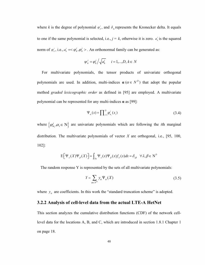
48

where k is the degree of polynomial i

k , and

kj represents the Kronecker delta. It equals

to one if the same polynomial is selected, i.e., j = k, otherwise it is zero. i

ka is the squared

norm of i

k , i.e., ,

k

i i i

k ka = . An orthonormal family can be generated as:

1,..., ,i i i

k k ka i D k N = =

For multivariate polynomials, the tensor products of univariate orthogonal

polynomials are used. In addition, multi-indices α ( )DN that adopt the popular

method graded lexicographic order as defined in [95] are employed. A multivariate

polynomial can be represented for any multi-indices α as [99]:

1( ) ( )

i

D i

iix x

= = (3.4)

where , Ni

ii are univariate polynomials which are following the ith marginal

distribution. The multivariate polynomials of vector X are orthogonal, i.e., [95, 100,

102]:

( ) ( ) ( ) ( ) ( ) ,D

XDx

X X x x f x dx

= =

The random response Y is represented by the sets of all multivariate polynomials:

( )DN

Y Xy

= (3.5)

where y are coefficients. In this work the “standard truncation scheme” is adopted.

3.2.2 Analysis of cell-level data from the actual LTE-A HetNet

This section analyzes the cumulative distribution functions (CDF) of the network cell-

level data for the locations A, B, and C, which are introduced in section 1.8.1 Chapter 1

on page 18.

49

3.2.2.1 Analysis of data of small cells in building A.

In Figure 3.1 (a), the CDFs of mean traffic volume of the cell per half an hour in

Building A is presented. Saturday and Sunday have a similar traffic volume demand

whereas weekdays show a slightly different pattern as shown in Figure 3.1 (a).

Significant traffic demand difference between weekdays and weekends is observed.

There are typically more people on campus on weekdays than on weekends as shown in

Figure 3.2 (a). Variations among weekdays are due to different class schedules. For 90%

of samples during weekends and weekdays, the aggregated traffic volumes are less than

100MB and 600MB, respectively.

Figure 3.1. (a) CDF of mean traffic volume (x axis in MB) at A. (b) CDF of mean

downlink throughput at A for each day (x axis is throughput in Mbps).

Figure 3.1 (b) shows CDF of aggregated downlink throughput for different days.

Variations of the CDF from around 5Mbps to 20Mbps are noticeable. Even in the range

from 40Mbps - 80Mbps, the CDFs are slightly different. This is difficult to explain

because the throughput performance is impacted by many characteristics (or parameters)

like the number of connected mobile devices, CQI, or available PRBs and location of the

users. These factors simultaneously influence the cell throughput. More importantly, the

aggregate throughput never exceeds 150 Mbps which is the maximum throughput under

50

the current configuration in Building A.

Figure 3.2 (a) presents the CDF of “number of users” for each day. Fewer people are

on campus on weekends than on weekdays, which is the same with the pattern in traffic

volume. Small differences among weekdays are noted as well. During weekends, for

90% of the observations, there were only about 10 users represented by each sample

whereas the average number of users is typically 30 represented on weekdays, as shown

in Figure 3.2 (a).

Figure 3.2. (a) CDF of mean number of users in A. (b) CDF of mean CQI in

location A for different days in weeks

Figure 3.2 (b) indicates the CDF of the “CQI mean” for each day. The median value

of CQI is typically close to 13. The deviations in these curves are caused by the location

of users. Since these CQI values are calculated according to user devices’ periodic

reports, the users’ locations throughout the day have a large impact on the mean CQI. If

users sit near the antennas inside the building, a higher CQI will be generated. Further,

factors like the weather (humidity, temperature) have a large impact on the SINR, which

consequently affects the CQI. Even through the antennas are inside the building, users at

the cell edge (outside of the building) may still connect to the antennas. During rainy

days, more people tend to stay inside the building with a higher humidity, which affects

51

the signal.

Table 3.1: Parts of class schedule in building A in 2017.

Location Monday Tuesday Wednesday Thursday Friday

RC

11:30 AM-

02:15 PM

11:30 AM-

02:15 PM

04:00 PM-

05:15 PM

02:30 PM-

03:45 PM

09:30 AM-

12:50 PM

02:30 PM-

05:15 PM

02:30 PM-

03:45 PM -

11:30 AM-

02:15 PM -

02:30 PM-

05:15 PM

05:30 PM -

08:15 PM

05:30 PM -

08:15 PM

02:30 PM-

05:15 PM -

04:00 PM-

05:15 PM - -

02:30 PM-

03:45 PM -

(a) (b)

Figure 3.3. (a) Aggregate throughput time series from Monday to Sunday (0:00 to 24:00,

half an hour time interval). (b) Time series of the number of users in a week

Figure 3.3 (a) depicts the time series data of aggregate throughput and the number of

users per half an hour each day for about five months. Many peaks appear randomly at

different times on different days, but an obvious pattern is still noticeable. Peak

throughputs appear on the x axis (from 6:00 and 23:00) as shown in Figure 3.3 (a). These

peaks may be closely related to the class schedule, as listed in Table 3.1 for Building A

(RC). In addition, some peaks appear from 0 to 5 on the x-axis (12:00 AM to 5:00 AM)

though there are few users present during that time. Maybe mobile apps of UEs were

52

updating during that time.

Figure 3.3 (b) presents the number of users from Monday to Sunday in 24 hours. It is

noticeable that several peaks exist frequently around 22:00 because a bar is open inside

the building.

3.2.2.2 Analysis data of small cells in Building B.

Figure 3.4. (a) CDF of traffic volume in location B. (b) CDF of downlink aggregate

throughput in location B for each day.

Figure 3.4 (a) represents CDF of traffic volume (in log scale) per half an hour of

Building B. These curves show a similar pattern that traffic volume is lower than

3000Mb (around 8 in log scale) for 97% of the samples. Lesser data is used on weekends

and Monday than other days in Building B because fewer people are there, or students

may be busy on Monday. Figure 3.4 (b) outlines the CDF of downlink aggregate

throughput for each day. Small variations from 6 Mbps to 22 Mbps are evident due to

users’ different schedules, but overall, the CDF follows a similar changing rate because

most people have fixed schedules for exercising at the gym each day.

Figure 3.5 (a) depicts the CDF of the number of connected users in Building B. The

number of users recorded on Saturday and Sunday is less than 18 for 55% of the

observations. The number of users from Wednesday to Friday is larger than other days.

53

Figure 3.5 (b) shows CDF of CQI mean of cell one in various patterns each day inside

the Building B. The mean CQI on weekends is better than other days. The locations of

users and mobility of users account for this fluctuation. From the practical observations,

people tend to stay at some seats that are close to the antennas on weekends, whereas

more people are near the cell edges on weekdays.

Figure 3.5. (a) CDF of the number of users in location B. (b) CDF of mean CQI in

location B for different days in weeks.

3.2.2.3 Analysis data of the macro cell in the whole campus.

Figure 3.6. CDF of mean CQI values (left) and CDF of aggregate throughput of macro

cell (right).

Figure 3.6 illustrates the CDF of mean CQI (left) and the CDF of aggregate

54

throughput (right) of the macro cell on sector 1. A consistent CDF trend of aggregate

throughput for each day is obtained as compared to Figure 3.1 (b) and Figure 3.4 (b) of

indoor small cells. For the CDF of mean CQI in Figure 3.6, similarly, a consistent trend

is obtained in comparison to Figure 3.2 (b) and Figure 3.5 (b) of indoor small cells. The

reasons for this consistency are that sector 1 covers a fixed area of office building (on the

upper right side of building C) and the users in the building have regular behaviors.

3.2.2.4 Comparisons the CDF of data in three locations

From Figure 3.7 to Figure 3.8, deviations among three locations are compared for traffic

volume, the number of connected users, aggregate DL throughput, and CQI mean,

respectively. Figure 3.7 indicates that small cell environments (locations A and B) have a

more similar pattern compared to Location C. People in locations A and B generate more

small traffic (6KB -1MB) than it is in Location C as Locations A and B are places for

entertainment.

Figure 3.7. (a) CDF of traffic volume in three locations. (b) CDF of the number of

connected users in three locations

In Figure 3.8 (a), indoor environments have a much better CQI than the outdoor

environment since buildings prevent certain levels of interference from the outside

55

environments. For Figure 3.8 (b), the aggregated DL throughput of small cells inside

buildings has a more similar pattern than the macro cell.

Figure 3.8. (a) CDF of CQI mean in three locations. (b) CDF of aggregated DL

throughput in three locations.

Sub-section 3.2.3.2 to 3.2.3.4 explains that external environments, users’ behaviors

(daily schedules, data demands, etc.), and user mobility have a significant impact on the

mean CQI and aggregate throughput performance.

3.2.3 Modeling of the data

The procedures of modeling of the aggregated downlink throughput is introduced in this

section. Figure 3.9 shows a flow chart of the modeling work. The procedures are

described in following subsections.

Transform

the response

variable

(throughput)

into normal

distribution

Apply

ANOVA

Select

appropriate

input

variables and

find their

distributions

Transform

input

variables

into normal

distributions

Implement

PCE

Figure 3.9. A flow chart for the mathematical modeling of cellular data.

3.2.3.1 Transforming data to normal distribution

The ANOVA is used to select proper input parameters for the model. ANOVA assumes

56

that a constant variance exists in response which follows normal distribution. If the

method is properly applied, the residuals should be structureless and contain no obvious

patterns [96]. In [96, 103, 104], methods of transformation of response variables are

summarized as follows:

1. Box-Cox method. The transformed response is obtained by using following

equation [96] [104]:

( ) 1

10

ln 0

y

y y

y y

−

−

=

=

(3.6)

The value of λ is usually selected to minimize SSE(λ).

2. Johnson transformation

There are three types of Johnson distribution families, which can be found in [26]

[104]. For instance, Johnson distribution-SU 1

sinh ( )x

Y

− −= + .

3. Using inverse CDF of standard normal distribution [105]

1 1( ) 2 (2 1)x erf x− − = − (3.7)

4. Fitting the distribution of data and finding its relationship with a normal distributed

variable.

3.2.3.2 Selecting important input parameters for the model

Generalized Linear Model (GLM) is used for conducting ANOVA in this study. Since

the parameters are correlated at a certain level during a certain period in the time series,

thus, a non-orthogonal and unequal sample size design with ‘type III Sum of Squared’ is

performed. Important variables are attained from results of ANOVA by choosing the

significant level less than 0.05 or 0.1 depending upon the value of α. These variables

57

have significant impacts on the throughput. A python code that contains more than 80

kinds of distributions is used to fit the best distributions of data.

3.2.3.3 Implementing PCE

After selecting input parameters, Hermite orthogonal polynomials are generated for

multi-input variables by using the tensor-product of single variables. Least-Squares

Minimization method is employed to estimate parameters. The data sets (which contain

about 7000 data sets) are split into 7:3 (for training and testing, respectively). Modeling

results are shown in the next section.

3.2.4 Modeling results

Three indicators: root mean square error (RMSE), R squared and mean absolute error

(MAE) are applied for measuring fitness of the models in this section. The modeling

results for three locations are summarized in Table 3.5. Since there are three locations

(Building A, B, and C in Figure 1.8), for simplicity, only modeling results of location B

is explained in detail.

3.2.4.1 Results from ANOVA

Table 3.2: Parts of results from factorial ANOVA

Items Type III SoS DF MS F Sig.

USER 4.359 1 4.359 7.743 .006

PRB .107 1 .107 .191 .662

CQI 3.246 1 3.246 5.766 .017

CCE 2.449 1 2.449 4.351 .037

USAGE 104.672 1 104.672 185.928 .000

USER * PRB 9.716 1 9.716 17.259 .000

Table 3.2 lists parts of the results from ANOVA analysis for the Building B. In the

“Sig” column of the table, it indicates that the number of connected users, traffic volume,

and CQI are the three most important factors impacting the throughput. Other rows show

58

the relative importance of combined factors’ effects on throughput. For more detailed

information please refer to [96].

For the adequacy checking, Figure 3.10 (a) shows residuals normal probability plot.

Some outliers exist on the upper right side, but according to [96], it is still reasonable

because only about 1.2% of residual data falls outside the straight line.

3.2.4.2 Results of PCE modeling

Table 3.3: Fitted distributions of variables.

Locations User Number Throughput CQI Data Usage

A Levy Levy Genlogistic Alpha

B Levy Levy Invgauss Levy

C Exponnorm Johnsonsb Johnson_su Recipinvgauss

Table 3.3 indicates best fitted distributions of some important variables for the three

locations according to a rule of ‘minimum sum of square error’. After transforming the

selected input parameters into normal distribution, the PCE is used to model the selected

LTE-A data.

Equation (3.8) ( ; , )F x c is the CDF expression for levy distribution, where c is the

scale parameter, and is the location parameter and it can shift the curve to right by an

amount . For instance, (-0.53, 2.07) and (-5.14, 17.62) are fitted ( , )c values of ‘the

number of users’ and ‘cell throughput’ at location B, respectively. The relationship

between the complementary error function and the standard normal distribution can

be expressed by equation (3.9):

( )( ; , ) ( )2( )

cF x c erfc

x

=

− (3.8)

2 ( / 2)( )

2

erfc xx

− = (3.9)

59

Therefore, the normal distributed variable y is represented by x if x follows levy

distribution as:

-1(1- 0.5* (( / (2))))2( )

y erfc sqrtc

x =

− (3.10)

Figure 3.10. (a) Plot of normal probability for residuals. (b) CDF of predicted data and

test data.

By using the similar transformation for all the other input variables, and then using

PCE, the model can be built. The order of the polynomials can be found by maximizing

the R squared and minimizing the MAE and the RMSE both in the training set and test

set. In Figure 3.10 (b), it depicts comparison of CDF for data of test set and predicted

data. The CDF of predicted data is very close to the actual CDF.

10-fold cross validation is applied to prevent over fitting, and its results are accurate

and validated as well. In addition, the data from Monday, Tuesday, and Wednesday is

solely used for training the model. This model is used to predict the throughput of

Thursday. The testing results are also accurate except some peak throughputs, which

demonstrates that the overfitting issue is insignificant. Table 3.4 represents modeling

performance indicators for training set and test set, respectively. The R squared of all the

three predictions are above 0.7 and RMSE is around 5.5.

60

Figure 3.11 shows a segment of time series testing results for Thursday (the x axis is

the time from 0:00 AM to 24:00 PM). In Figure 3.11, many peak throughputs show up

periodically because users’ behaviors are partly impacted by their class schedules

regularly each week. Thus, the numbers of users and users’ data usage behaviors also

have certain patterns (depending on class schedules). Those patterns can be processed by

machine learning methods for clustering and classification.

Table 3.4: Modeling results for three locations.

Locations Training Set Testing Set

R2 MAE RMSE R2 MAE RMSE

A 0.84 2.6 4.7 0.8 2.9 5.5

B 0.82 3.2 5.2 0.85 3.7 6.6

C 0.81 1.7 2.6 0.71 1.79 3.5

Figure 3.11. Test results for three Thursdays by using the training data from Monday,

Tuesday, and Wednesday

As mentioned in section 3.2.1, the gene time series expression data in [32] is quite

similar to the data used in this work. However, using the method in [1] to model the

aggregate data does not produce an acceptable result. R squared is only 0.29 and RMSE

61

is up to 95. The possible reason for the poor performance of the method in [1] is that the

network data does not satisfy the assumption of normal distribution. Therefore, the

method used in this work generates better prediction results.

3.3 Analysis and modeling of the handover in a real-world LTE-A

HetNet

In this section, handover performance (e.g., RSRP, SINR, variations of HO distance,

etc.) is analyzed in a real-world LTE-A HetNet environment in detail. To the best of the

author’s knowledge, limited research has studied the HO performance of an actual

HetNet in depth. The contributions of this section are listed as follows:

1. Data collection tests are carried out in a real-world HetNet environment by

adjusting HO parameters such as TTT and A3 offset for multiple times.

2. The impacts of these parameters are analyzed by ANOVA factorial design in

detail. The impacts of HO parameters on the serving cell and target cell RSRP,

SINR, HO execution time, HO distance variations, and user downlink throughput

are investigated in detail. Response surface method is utilized to model the

relationship between target cell’s RSRP and HO parameters (TTT and A3 event

offset). The measured results show that these two parameters have different

impacts on the serving cell RSRP and target cell RSRP. The impacts of these two

parameters vary from location to location due to different path loss and fading

environments, etc.

3. A modified QoS scheduler is proposed for predicting the handover performance.

3.3.1 Introduction to the response surface method

For detailed introduction of ANOVA, please refer to Section 3.2.1 (on page 45) or

62

Appendix A on page 231. Following [96], the theory of response surface methodology

(RSM) is presented in this part. Response surface methodology is utilized for the purpose

of modeling and analysis of data by a set of mathematical and statistical techniques. For

example, if an engineer wants to find the levels of variables x1 and x2 that maximize the

response y of a process. This yields a function of variables x1 and x2 which is expressed

by equation (3.11) as [96]:

1 2( , )y f x x = + (3.11)

where is the noise or error that is observed in the response y. The expectation of y is

denoted by 1 2( ) ( , )E y f x x = = , then the surface that is represented by input variables is

called a response surface. In the RSM problems, the relationship between input variables

and the response is unknown. The first step is to find an appropriate approximation for

the unknown relationship between response and independent variables. Polynomial

models are used to approximate the relationship because they usually work quite well for

small regions [96]. The first-order model for input kx (k ϵ 1, …, N) is presented by

equation (3.12) as:

0 1 1 k ky x x = + + + +L (3.12)

where k are regression parameters. If the curvature exists in the system, higher order

polynomials must be utilized. For more detailed information, please refer to [96].

3.3.2 Measurement plans and the ANOVA design plan

The HO test environment and test process are introduced in section 1.8.1 Chapter 1 on

page 17 - 24.

3.3.2.1 Adjustment of handover parameter plans

63

The test plan for adjusting handover parameters is listed in Table 3.5.

Table 3.5: Handover test plan.

TTT (ms)

A3_off (dB) 40 128 640 1280

3 Test 1 Test 3 Test 5 Test 7

6 Test 2 Test 4 Test 6 Test 8

The offset of A3 event and TTT are adjusted for evaluating the performance of the

handover. The A3 offset value is operated at 3 and 6 dB with different values of TTT

from 40 ms to 1280 ms. Other handover parameters such as Hysteresis are not adjusted.

Table 3.5 can also be utilized for 2 factor ANOVA design with two independent

variables TTT and A3 offset (A3_off). The response is obtained (from the mobile app)

for serving cell’s RSRP and target cell’s RSRP for different values of TTT and A3 offset.

In this work, outbound handover is mainly considered performance when users move

from indoors to outdoors.

3.3.3 Analysis results of measured data

3.3.3.1 Analysis of the impact on RSRP from parameters

Figure 3.12 shows results of measured data for outbound handover at door 1 of RC

building. The serving cell RSRP and target cell RSRP are calculated for different sets of

parameters. A boxplot is a graph that indicates how the values in data are distributed

[106]. As shown in Figure 3.12 (a), different values of A3 offset (A3_threshold) and

TTT have different impacts on the RSRP of the serving cell and the neighboring cell.

Noticeably some outliers existed when TTT is 40 ms and A3 offset is 6dB in Figure 3.12

(a). Figure 3.12 (a) also presents that adjusting the A3 offset value does not have a fixed

impact on the distribution of the serving RSRP and target RSRP, but the difference

64

between the mean of serving cell’s RSRP and neighboring cell’s RSRP is always larger

than the value of A3 offset.

TTT

A3_offset

Target RSRPServing RSRP

128064012840128064012840

6363636363636363

-85

-90

-95

-100

-105

-110

RS

RP

(d

Bm

)

Boxplot of Serving Cell RSRP and Target Cell RSRP

TTT

A3_offset

Target RSRPServing RSRP

128064012840128064012840

6363636363636363

-90

-92

-94

-96

-98

-100

-102

-104

-106

RS

RP

(d

Bm

)

95% CI for the Mean

Individual standard deviations were used to calculate the intervals.

Interval Plot of Serving Cell RSRP, Target Cell RSRP

(a) (b)

Figure 3.12. Boxplot (a) and interval plot (b) of measured results at door 1.

Figure 3.12 (b) displays interval plot (mean value of RSRP with 95% confidence

intervals) for both source cell and target cell RSRP. It depicts that all the values of RSRP

are increased after adjusting A3 offset from 3dB to 6 dB as except when the TTT is 128

ms. Figure 3.12 (b) also illustrates that the target cell’s RSRP does not necessarily

increase with the increase of TTT and A3 offset, because it is also impacted by the

serving cell’s RSRP values.

3.3.3.2 Applying ANOVA and response surface method

After applying the factorial design on the response of serving cell RSRP and target cell

RSRP, effects of variables TTT and A3 offset are analyzed. The test results (for checking

the accuracy of the model) indicate that the measurement data satisfies the assumptions

of normal distribution and equal variance.

Figures 3.13 (a) and (b) represent that TTT has a significant impact on the serving cell

RSRP, and A3 offset has an important impact on the RSRP of the target cell. The results

65

of HO execution time from ‘HO initiated’ to ‘HO succeed’ are indicated by the boxplot

in Figure 3.14 (a).

(a) (b)

Figure 3.13. Normal plot of standardized effects of TTT and A3 offset for serving cell

RSRP (a) and target cell RSRP (b).

TTT

A3 threshold

128064012840

63636363

0.150

0.125

0.100

0.075

0.050

Ha

nd

over_

tim

e_

du

ra

tio

n (

seco

nd

)

Boxplot of Handover_time_duration

(a) (b)

Figure 3.14. (a) Boxplot of HO execution time for different sets of parameters at door 1.

(b) Boxplot of user SINR during the HO.

Figure 3.14 (a) represents that the HO process is completed less than 100 ms for most

of the time which is almost identical with the measurement results in [107]. When the

TTT equals 128ms, HO will take less time to finish. Users’ mean SINR during the HO is

shown in Figure 3.14 (b). It describes that peak SINR is recorded when increasing the

66

TTT value from 40 ms to 1280 ms. However, the PRB utilization of neighboring cells

may be different for various tests that also have an impact on the variation of SINR.

To find the optimal values of HO parameters, relationships between the adjusted

parameters and various responses are developed by regression models. We find that a

second order polynomial can better approximate the relationship between adjusted HO

parameters and target cell’s RRSP for HO after implementing RSM to the measured data.

Their relationship is represented by equation (3.13) as:

arg _RSRP = 96.935 0.78* 3_

0.00332* 10 ^ (-6)* ^ 2

4.02*10 ^ (-4)* 3_ *

T et cell A offset

TTT TTT

A offset TTT

− +

+ −

−

(3.13)

The P-value of the ‘lack of fit’ regression equation (3.13) is 0.384 which means that

lack of fit is not a significant issue. The ‘R squared’ of the regression is up to 0.86,

which indicates the accuracy is reasonable as well.

3 4 5

49-

39-

021 0080

4 0006

39-

- 29

)mBd( PRSR

TTT

tesffo 3A

urface Plot of Target_Ce 3l_RSRP vs TTT, AS offsetl

A3 offset

TT

T

6.05.55.04.54.03.53.0

1200

1000

800

600

400

200

> – – – – < -94.5

-94.5 -94.0-94.0 -93.5-93.5 -93.0-93.0 -92.5

-92.5

Target_RSRP

Contour Plot of Target_RSRP vs TTT, A3

(a) (b)

Figure 3.15. (a) Surface plot of RSRP of target cell with respect to TTT and A3 offset at

door 1 (on the left). (b) Contour plot of target cell’s RSRP (on the right).

Figure 3.15 (a) and (b) represent a surface plot of the target cell’s RSRP and contour

plot in terms of TTT and A3 offset. Figure 3.15 (b) shows that setting A3 >5.5 dB and

TTT >800 ms will result in a maximum value for the target cell’s RSRP. The above

67

results are from handover performance of door 1, however, the variation in results is

noticeable at different doors due to various path loss environments.

3.3.3.3 Analysis of the impact on SINR and HO distances

Table 3.6 depicts SINR during the HO process at different doors for various sets of HO

parameters. The values of SINR indicate that a curvature (second order) relationship may

exist with respect to TTT and A3 offset. However, SINR tends to be higher in test 3. If

the values of TTT and A3 offset are either too small or too large, then lower values of

SINR are recorded due to interference from other neighboring cells with varying loads.

The common trend in the measured data is that when increasing the TTT to 1280 ms,

measured SINR at each door show worst results around -4 dB as shown in Table 3.6 (this

SINR can be measured before or after or during the HO in millisecond interval by the

scanner). It is notable that HO Success Rate (HSR) for the outbound handover (averaged

per half an hour for all the users during the measurement) is always quite high, above

99%.

Table 3.6: SINR and HO success rate of handover for different tests.

Test Number SINR (dB)

Mean HO Success Rate Door 1 Door 2 Door 3 Door 4

Test 1 0.98 1.58 0.28 1.43 99.8%

Test 2 3.78 3.5 1.68 5.26 99.7%

Test 3 5.09 5.2 4.75 6.26 99.8%

Test 4 2.56 6.16 -0.7 0.27 99.8%

Test 5 6.6 6.56 0.85 4.08 99.6%

Test 6 -0.7 2.12 -2.3 -0.38 99.8%

Test 7 -1.5 -0.6 -1.43 -0.14 99.5%

Test 8 -4.5 -4.48 -6.9 -6.87 99.4%

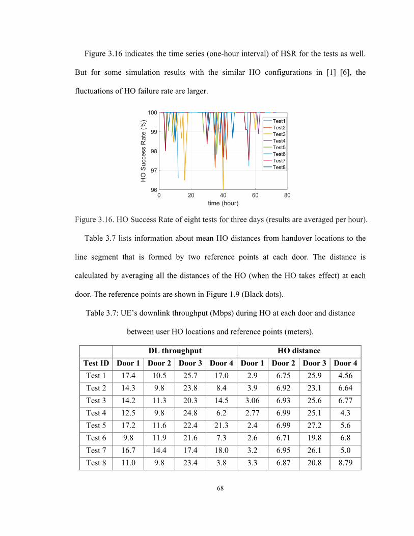
68

Figure 3.16 indicates the time series (one-hour interval) of HSR for the tests as well.

But for some simulation results with the similar HO configurations in [1] [6], the

fluctuations of HO failure rate are larger.

Figure 3.16. HO Success Rate of eight tests for three days (results are averaged per hour).

Table 3.7 lists information about mean HO distances from handover locations to the

line segment that is formed by two reference points at each door. The distance is

calculated by averaging all the distances of the HO (when the HO takes effect) at each

door. The reference points are shown in Figure 1.9 (Black dots).

Table 3.7: UE’s downlink throughput (Mbps) during HO at each door and distance

between user HO locations and reference points (meters).

DL throughput HO distance

Test ID Door 1 Door 2 Door 3 Door 4 Door 1 Door 2 Door 3 Door 4

Test 1 17.4 10.5 25.7 17.0 2.9 6.75 25.9 4.56

Test 2 14.3 9.8 23.8 8.4 3.9 6.92 23.1 6.64

Test 3 14.2 11.3 20.3 14.5 3.06 6.93 25.6 6.77

Test 4 12.5 9.8 24.8 6.2 2.77 6.99 25.1 4.3

Test 5 17.2 11.6 22.4 21.3 2.4 6.99 27.2 5.6

Test 6 9.8 11.9 21.6 7.3 2.6 6.71 19.8 6.8

Test 7 16.7 14.4 17.4 18.0 3.2 6.95 26.1 5.0

Test 8 11.0 9.8 23.4 3.8 3.3 6.87 20.8 8.79

69

Table 3.7 shows that handover happens at different distances from the reference line

segment based on different values of HO parameters. For instance, the average HO

location of test 8 moves 40 centimeters further compared to test 1 at door 1. Whereas it

takes 30 centimeters less for HO to occur during test 6 in comparison with test 1 at door

1. With higher TTT and A3 offset in test 7 and test 8, users have to walk further to

complete HO compared with test 1 and 2 for door 1, 2 and 4. For door 3, however, users

walk shorter distances to complete HO in test 8. No significant deviation is recorded due

to variations of RSRP at different times with multipath fading, fast execution of HO, etc.

The impact of adjusting HO parameters is not the same as what we expected (longer HO

distances with larger values of A3 and TTT) for some doors.

3.3.3.4 Analysis of the UE’s throughput during HO

Table 3.7 presents UE’s downlink throughput when the UE is performing HO tests at

different doors. Table 3.7 depicts some important observations: first, the average user

throughput is constantly higher than 6 Mbps for most of the cases (SINR varies from -7

to 6.3 dB). Secondly, the UE at different doors receives different throughput during the

HO process. On comparison of each row of Table 3.6 and Table 3.7, it indicates that the

UE with lower SINR gets higher data rate at different doors (e.g., test 1 and test 7).

Thirdly, as the SINR decreases in Table 3.6, for each door, the user’s data rate is reduced

slightly as well. In addition, the UE at door 3 always receives higher throughput during

HO. It is possible that more RBs are available while collecting data at door 3.

Furthermore, door 3 is the closest door to the macro cell. Perhaps, the scheduler of the

system tends to allocate more RBs to users with low SINR and to maintain fairness for

users.

70

3.3.4 Modeling of the HO performance

To model the actual HO process on the University of Regina campus, a simulation model

is developed in this section. A modified scheduler is proposed based on some

information of the antennas [108] which are installed inside the actual LTE-A networks

in the university. The modified scheduler is intended to allocate RBs to different Quality

of Service (QoS) users on packet flow levels. The propagation model of transmitter’s

signal strength is based on a ray tracing path-loss propagation model and measured data.

Multipath fading is modeled as Rayleigh Fading. Even though numerous schedulers are

developed, very few of them focus on applying the scheduler to predict actual user

downlink throughput.

3.3.4.1 Introduction to a defined QoS scheduler

Table 3.8 : Different types of QCI [1].

LTE-A specifications define Evolved Packet Core (EPS) bearers for users to

communicate with transmitters [1]. Bearers are defined as two types: Guaranteed Bit

71

Rate (GBR) and non-GBR. GBR bearers include real-time services such as voice and

real-time games and are guaranteed with the lowest bit rate by the base station. A non-

GBR bearer is not guaranteed with a minimum data rate; thus, it is suitable for non-real

time services. In addition, an important parameter Quality of Service class identifier

(QCI) classifies these two types of bearers into different type of services with various

priorities. Table 3.8 presents different services with diverse QCI priorities.

Calculating the user performance metric is significant for the scheduler to determine

which user should be allocated with RBs. Based on the technical document [108], a

modified performance metric of GRB users is presented as:

*GRB jP CQI Delay= (3.14)

where CQI is channel quality indicator of user j, Delay is the user’s packet waiting time

represented as hol

jd for user j. The performance score of scheduling non-GRB users is

calculated as:

* / * *non GRB j his priorityP k CQI R QCI Delay− = (3.15)

where k is a parameter proposed to balance the priorities of GRB and non-GRB services.

CQI is channel quality indicator of users. hisR is historical user downlink throughput

during previous time window, priorityQCI is the priority of non-GRB services. Increasing

the value of k will increase the chance of non-GRB users to be scheduled by the

scheduler.

Since the main goal is to predict user throughput, thus the delay is considered in a

simplified way as shown in equation 3.16. This simplification does not violate the

mathematical and resource allocation framework[109]. The packet delay is modeled as

72

head of line (HOL) delay as mentioned in [109]. The HOL packet delay of a generic user

j at time n+1 is calculated by a recursive equation as [109]:

[ ]*1[ 1] [ ] *( )

TTI

jhol hol TTI

j j hol

j

R n td n d n t

L b+ = + − (3.16)

where TTIt is the time of one TTI in second, L is packet arrival rate, [ ]jR n is the

instantaneous rate of user j at time n. hol

jb is the packet size. It is assumed that the packet

size is sufficiently small so that the duration of one slice of packet is 1/L as shown in

Figure 3.17 (packet size (hol

jb ) equals 256 kb and L equals 500 in the simulation). The

minimum packet delay is defined as zero, and the maximum is the value of the packet

delay budget of the corresponding QCI.

Figure 3.17. Modeling of user buffer [109].

During the resource allocation process, the scheduler will classify different QoS and

calculate their priorities. The GRB services will be served first, then, non-GRB services

are served by the network with best efforts. If the current RBs are enough to satisfy

users’ requirements, these users will not be assigned with RBs. The user throughput and

SINR are measured during the HO process in the actual HetNet environment of the

University of Regina.

73

Figure 3.18. Layout of the building, user locations, and user trajectories in the simulation.

Figure 3.18 indicates the layout of the modeled indoor building RC with user

locations, and predefined user trajectories. The red circles and blue dots are two types of

trajectories for moving users as shown in Figure 3.18. In addition, a macro cell is

installed outside of the campus and covers the RC building. The handover process is

modeled for moving users from small cells to the macro cell in 60 seconds.

53 users (including moving and static users) are randomly generated and distributed

with different QoS inside the building, and some of them are around the locations of

each door. According to the information from the database (from the network provider),

the PRB utilizations of the macro cell and small cells (inside the building) are always

less than 50%.

3.3.4.2 Simulation results of the handover process

Table 3.9 : Accuracy of the model.

Metrics SINR

(dB) the new scheduler (Mbps) the PF scheduler (Mbps)

Mean error -1.8 -3.8 53.9

MAE 5 27 61.6

RMSE 7 32 53.9

74

Figure 3.19. Measured SINR and predicted SINR during the process of HO.

Figure 3.20. Measured downlink throughput and predicted throughput during the process

of HO.

Table 3.10 indicates mean error, mean absolute error (MAE), and root mean square

error (RMSE) of the SINR and the throughput over 60 seconds for the developed

scheduler and PF scheduler, respectively. Table 3.10 shows that the developed model

predicts reasonable results for the overall mean SINR (-1.8 dB) during 60 second

simulation time. The proposed scheduler has better performance than the PF scheduler

(full buffer and does not consider QoS). The higher values of the MAE and the RMSE

present that more user dynamic information such as users’ varying demands should be

75

considered in the model because the measurement is conducted when the environment

has high level user mobility. Figure 3.19 and Figure 3.20 display predicted SINR and

downlink throughput with measured data, respectively.

3.3.5 Discussion

Firstly, in most of the cases, increasing the value of A3 offset does not greatly impact the

serving cell’s RSRP when the HO is completed. The maximum variation in RSRP value

is about 2 dBm in test 2.

Furthermore, the complicated physical environment reduces the measurement

accuracy of handover due to the structures of doors and variations in walking speeds of

the UEs, etc. The effects of parameter TTT are invisible when its value is quite small

(lower than 500ms). Therefore, HO occurs at the same location for users walking with

normal speeds. When the TTT is at the smallest value of 40 ms, measurements of SINR

are not captured by the RF scanner between the time when HO is initiated and the time

when HO is completed. The measurement results indicate that one set of optimal HO

parameters should exist between test 1 and test 8. Contrary to the simulation results in [1]

[6], increasing TTT and offset do not bring severe handover failure in the actual tests of

this study. The measured results indicate that this physical HetNet system is substantially

stable to adjustment of parameters with the handover success rate constantly above 96%.

Thirdly, the results show that the target cell’s RSRP greatly impacts the HO

performance of each door. Different doors show variation in HO performance in terms of

HO distance and RSRP of the neighboring cell. The network designer should consider

the HO performance of all the doors when deciding to set the system handover

parameters.

76

At last, precise path loss propagation models, a scheduler with better approximation to

the actual scheduler, and cell loading information are important to accurately estimate

user throughput. The simulation model will be more accurate if more user information is

considered. In addition, some neighboring macro cells around the campus also have

impacts on the results.

3.4 Measurement and analysis of small cell splitting in a real-world

LTE-A HetNet

In this section, instead of pure theoretical research, extensive measurements are

conducted in a real-world LTE-A HetNet environment. The cell-splitting strategy is

applied in a real-world LTE-A HetNet. Four directional antennas operate as one cell and

two cells, respectively in an indoor gymnasium sharing a 20MHz bandwidth in the

University of Regina. Optimization techniques such as Almost Blank Subframe (ABS)

are utilized to mitigate interference and increase UE (user equipment) SINR inside the

gymnasium. The average SINR of both static and moving users and system cell

throughput are used to evaluate the performance of the tests. The analyzed results show

that operating the small cells from one cell to three cells for the whole building, the

SINR inside the gymnasium decreased from 29 dB to 5 dB，and cell throughput

decreased from 140 Mbps to 88Mbps. Even though the throughput performance of cells

inside the gymnasium is slightly lowered, the overall network capacity of the building is

enhanced. Moreover, the impact of an actual neighboring cell’s load interference on the

serving cell inside the gymnasium is also analyzed. This test environments and test

procedures are displayed in Section 1.8.3 Chapter 1. Furthermore, the spectral efficiency

is extracted from the measured data of the RF scanner.

77

In this section, following two questions will be answered: first, does splitting cells

bring benefits for the hotspot (the gymnasium where numerous people will gather) or for

the whole network in a real-world environment. Second, is enabling ABS on the main

interfering cell beneficial for the users in the serving cell? The answers to these questions

are justified by the mathematical analysis done using simulations according to the

literature review, but few people have a chance to verify the results in real-world cellular

networks.

The remainder of this section is organized as follows. Test environments and test

plans are described in Section 3.4.1 and Section 1.7 Chapter 1. Section 3.4.2 provides the

result and analysis in detail. Some questions are discussed and explained in Section 3.4.3.

For more detailed information about ABS and artificial load, please refer to section 1.5.2

in Chapter 1 (on page 12) (In this test, 80% of PRBs are reserved for artificial load in

cell 1).

3.4.1 Test environment and test plans

Test environment, test procedures and the definitions of cases are introduced in section

1.7.2 Chapter 1 on page 18. Three test scenarios are considered in the data collection

tests. Five moving phones (three phones are connected to the scanner) and eight static

phones are used in the tests. The three scenarios are: Scenario 1-one sector case,

Scenario 2-two sector case, Scenario 3-three sector case.

Test scenario 2 and 3 are performed with/without enabling artificial load so that the

impacts from neighboring cell’s interference on the users inside the gymnasium are

analyzed. In addition, two pRRus on the second floor of the gymnasium, as shown in

Figure 1.12, are turned off during the tests when artificial load is enabled on cell 1. The

78

ABS is always enabled on cell 1 for two sector and three sector tests. Table 3.10 shows

the test plan in detail. Modulation schemes are adjusted with 64QAM and 256QAM.

Table 3.10: Test plan.

Cases Modulation

and artificial load

Interference

cancellation

on Cell 1

Modulation

and artificial

load

Interference

cancellation

on Cell 1

1 sector 64QAM No ABS 256QAM No ABS

2 sectors 64QAM+Artificial Load No ABS 64QAM No ABS


2 sectors 64QAM +Artificial Load ABS 64QAM ABS

2 sectors 256QAM+Artificial Load ABS 256QAM ABS





3.4.2 Results and analysis of throughput, ABS, modulation schemes

3.4.2.1 Analyzing the difference between low load level and high load level tests

Figure 3.21. Mean UE throughput of low load and high load level for different numbers

of sectors.

The main difference between low load level and high load level is that they have

different numbers of downloading phones. In Figure 3.21, the average user throughput

79

for different load levels (64 QAM without ABS and artificial load) is shown. With a

greater number of downloading UEs increased in the network, the average throughput of

the UE decreased. When one cell turned into two or three sectors, the throughput values

dropped marginally because of the intra-cell interference.

Figure 3.22. Mean user SINR of low load level and high load level for the different

number of sectors

Figure 3.22 shows that mean UE SINR is dropped from one sector to three sectors.

Increasing the number of sectors causes a spike in interference inside the gymnasium,

especially when neighboring cells have high PRB utilization.

3.4.2.2 Analyzing the impact of ABS.

By enabling ABS for 10% of PRBs on cell 1, the cell throughput can be increased 10 –

18 Mbps for two and three sector cases and the SINR is increased about 1 – 6 dB. But,

increased neighboring cell load and the varying number of connected phones make the

results coarse.

Figure 3.23 presents the mean SINR of each static phone (from phone A to phone H)

with ABS off and on for two sector case with 64 QAM and artificial load. It shows that

phone B and phone E connect to neighboring cells, because location B and E are cell

80

edge areas which are not strongly covered by the directional antennas. Switching from

ABS off to ABS on, most of UEs’ SINR decline because phone B is downloading files

from a macro cell outside the gymnasium and phone E is downloading from neighboring

cell 1. Thus, the SINR of phone A, phone C and phone F dropped due to rise in

interference from neighboring cells. The cell edge phone G’s SINR improved from 6 to

10.5 dB by enabling ABS.

Figure 3.23. Mean SINR of each static phone without ABS and with ABS for two sectors.

Figure 3.24 displays the mean user data-rate of individual static phones with ABS off

and on for two sector case with artificial load. It shows that even though most of the

UEs’ SINR are reduced, their downlink throughput is increased because two phones

(phones B and E) are connected to the neighboring cells, hence causing a growth in UEs’

data rates after ABS is enabled. Therefore, enabling ABS should be better utilized with

cell range extension (CRE) [110] to ensure that cell edge users are always connected to

the cells inside the gymnasium.

81

Figure 3.24. Mean DL throughput of each static phone without ABS and with ABS for

two sectors.

3.4.2.3 Analyzing system cell throughput

Table 3.11: System cell throughput (CT: Mbps) for different sectors with 64 QAM.

Sector

type

Other

settings

Cell

ID

Mean

measured

CT

Mean

CT from

counter

PRB

utilization Total CT

1

sector

No ABS,

No Artificial

Load

Cell 1 144 - 90%

(estimated) 150Mbps

2

sectors

ABS,

Artificial

load

Cell 1 - - 7.8%

>120Mbps Cell 2 106 ≈123 98%

3

sectors

ABS,

Artificial

load

Cell 1 - ≈48 86%

>141Mbps Cell 2 34 ≈34 98%

Cell 3 33 ≈45 98%

Since there are so many test results, for simplicity, only some important results are listed.

Table 3.11 represents system cell throughput (CT) for one sector, two sectors, and three

82

sectors with different settings, respectively. Mean CT and PRB utilization from counters

of the network provider are also indicated.

Table 3.11 indicates that splitting cells into more sectors decreases the cell throughput

of the gymnasium from 144 Mbps to 67 Mbps, but the overall network capacity is

increased because 80% of cell 1’s PRB is reserved. It also depicts that the cell

throughput from tested phones is almost the same with the values from the database of

one-minute counter. Besides the test phones, some other users present inside the

gymnasium may also utilize the available PRBs.

When artificial load (80% of PRBs of cell 1 is set to be utilized) is enabled for two

sector case and three sector case, the total cell throughput is reduced nearly by half from

106 Mbps to 67 Mbps. However, the total throughput for all the cells is improved

compared with one sector case having total cell throughput around 144 Mbps. For the

three sector case, the total throughput of all the three cells is about 141Mbps, but 80% of

PRBs of cell 1 is utilized to generate artificial load and some phones’ data rate are

throttled by the network service provider during the tests. Thus, the total cell throughput

is much more than 141Mbps. This reveals that deploying small cells with new cell ID

and the same bandwidth for a hotspot will increase capacity of the whole network at the

cost of reducing the SINR near the coverage edge of the small cells.

3.4.2.4 Analyzing the effect from 64QAM to 256QAM

Figure 3.25 and Figure 3.26 represents some test results of 64 QAM and 256 QAM

without ABS for different cases. Figure 3.25 presents cell throughput for different cases

from 64 QAM to 256 QAM. Figure 3.26 shows mean user SINR for different cases from

64 QAM to 256 QAM. The SINR from 256 QAM is dropped slightly compared to 64

83

QAM due to increase in neighboring cells’ load. Cell throughput increased slightly for

most of the cases because 256 QAM does not work properly when the user’s SINR is

very small. For one sector case, the 256 QAM modulation can improve the cell

throughput by 13 Mbps. It is noticeable that SINR is reduced when enabling 256QAM

since some phones are connected to neighboring cells which generates interference for

other phones in Figure 3.26.

Figure 3.25. Comparison of cell throughput for 64 QAM and 256 QAM

Figure 3.26. Comparison of mean user SINR for 64 QAM and 256 QAM

3.4.2.5 Analyzing the effect of artificial load and turning off the 2 pRRus

84

Table 3.12 shows test results with and without artificial load from one sector to three

sectors (for the one sector case, it has high interference from other macro cells). The

modulation scheme of the results in Table 3.12 is 64 QAM and ABS is not enabled.

Table 3.12: System cell throughput (CT) and SINR for different tests.

Without artificial load With artificial load

Type Cell throughput (Mbps) SINR (dB) Cell throughput (Mbps) SINR

(dB)

One sector 143.8 28 81 14

Two sectors 65.9 14.7 63.4 8.1

Three sectors 79 7 63 6

Table 3.12 indicates that SINR and cell throughput are reduced when enabling the

artificial load. However, the SINR does not decrease dramatically because some of the

cell edge phones (phone B, D, E, and G) are connected to neighboring cell 1, which

improves the average SINR for all the UEs.

3.4.2.6 The relationship between PRB utilization and mean user throughput.

In literature [111], it stated that average user scheduled throughput is represented as

(1 )schT C = − under the assumption of Poisson distributed number of users and equally

shared resources, where C is link bandwidth and ρ is PRB utilization. However, Figure

3.27. (a) indicates that mean user throughput does not have a quite clear relationship with

PRB utilization as opposite to the expected linear degradation in [111]. The reason for

this inconsistency is that the cell resources are not equally shared in the studied real-

world LTE-A environment.

85

Figure 3.27. (a) Mean user throughput with respect to cell PRB utilization. (b) Mean

SINR per minute of Phone A with respect to PRB utilization of cell 3.

Figure 3.27. (b) indicates relationship between mean SINR per minute of phone A and

PRB utilization of neighboring cell 3, which is the main interfering cell for phone A.

With increasing of the neighboring cell’s PRB utilization, phone A’s SINR is reduced

from 4.2 to 2 dB.

3.4.2.7 Extracting the spectral efficiency based on the measured data

The actual spectral efficiency (SE) is extracted with data from the RF scanner in LTE-A

environment (as mentioned in Section 3.3 Chapter 3) with 2X2 MIMO in this section.

In wireless networks, SE plays an important role in radio network planning. In many

literature, SE is calculated by the Shannon capacity formula that is applied to

approximate the maximum channel capacity. This formula only gives upper bound for

the channel, and it overestimates the spectral efficiency compared with the actual SE as

shown in [112]. However, channel capacity is not only impacted by signal strength but

also affected by many factors such as radio environments, traffic properties, etc. [112].

Considering all these factors is difficult and complicated. SE is closely related to the

estimation of network resources, and over-estimation of SE will lead to failures of

86

network planning, defective network services, and increased operation costs [112]. Thus,

it is essential to obtain realistic values of SE for more accurate network planning and

capacity estimation.

Instead of using multiple operational parameters in [112], only three parameters (time

transmission interval (TTT), user data rate, and the number of allocated PRBs) are

utilized to calculate the SE. The number of utilized PRBs is calculated as:

( )* / ( _ * )PRBN R t TTI Spectral efficiency = (3.17)

where represent the number of REs in one PRB, which is decided by control format

indicator (CFI) (if CFI is 1, each PRB has 150 REs. If CFI is 2, each PRB has 138 REs).

( )R t is user downlink throughput in one TTI. Thus, the expression of

_Spectral efficiency is calculated as:

_ ( )* / ( * )PRBSpectral efficiency R t TTI N = (3.18)

Figure 3.28 (a) shows the extracted relationship between mean spectral efficiency and

SINR. Figure 3.28 (b) shows mean spectral efficiency at each integer SINR value.

Curves of extracted SE are presented at two different values of CFI (CFI=1 and CFI=2).

These curves are also compared with two mapping tables (Mode 222 and Mode 322) as

mentioned in [113].

Figures 3.28 (a) and (b) indicate that some variations are shown in the curves of the

extracted SE. The possible explanations are that: first, users experience fading, multipath

and other environment issues (e.g., weather, etc.) in the actual environment. Secondly,

the RF scanner may have limited time resolution to measure the data or measurement

error or noise that is unavoidable [112]. Figure 3.28 also depicts that a significant

difference exists between extracted SE and the SE in other two mapping tables in the

87

literature. But it is reasonable because these mapping tables between SINR and SE are

typically defined by vendors.

(a) (b)

Figure 3.28. (a) Relationship between SINR and mean SE (b) Relationship between

SINR and Mean SE piecewise.

The proposed data-driven method can be used to extract mean spectral efficiency. It is

mentioned in [112] that SE may vary from cell to cell due to different network

environments (such as different radio wave propagation conditions). With the extracted

SE, the estimation of network capacity will be more accurate. Network operators can

predict user throughput more precisely.

3.4.3 Discussion

The two questions mentioned at the beginning can be answered: splitting the cells will

reduce the SINR but with increased capacity for the whole network. Enabling ABS (10%

of each frame) does not improve the serving cell’s performance dramatically due to

varying conditions (e.g., neighboring load and number of connected users). Many other

things from the data collection tests need to be discussed.

First, enabling 256 QAM is not hugely useful when SINR levels of phones are lower

than 30 dB. 256 QAM will be more beneficial when SINR is above 30 dB in the network.

88

The measurement indirectly verifies that 256 QAM needs higher SINR to increase

throughput over 65 QAM as mentioned in [114].

In addition, solely enabling 10% ABS for the serving cell is not effective to increase

cell edge users’ SINR because some cell edge phones will connect to neighboring cells

with higher RSRP. The effect is also not significant for the serving cell with more than

one neighboring cell.

Furthermore, even though splitting cells will reduce the SINR levels in the

gymnasium, more capacity is added to the network for usage. According to the measured

results in this study, for three sector case, at least an extra 50 Mbps throughput is added

for cell 1 with 40 Mbps reduced inside the gymnasium for the number of test phones. As

mentioned in [111], increased neighboring cell load will not only degrade spectral

efficiency of the serving cell but also improve PRB utilization. Thus, the three sector

case does not seem very appealing because two cells inside the gymnasium interfere with

each other without any physical isolation between them. Moreover, the neighboring

cell’s PRB utilization has a large impact on the serving cell. According to the definition,

PRB utilization has an inverse proportional relationship with SINR. But, when there are

more users at the center of the gymnasium, the three sector case will bring more benefits

because it has more resources available than the two sector case.

At last, most of the simulations cannot fully represent the characteristics of real-world

LTE-A environments. Different schedulers will bring different impacts to the system as

mentioned in section 3.4.5.

89

3.5 Analysis of acquired indoor LTE-A data from an actual HetNet

cellular deployment

This section aims to find the best practical solution to increase user throughput in an

actual HetNet (Heterogeneous Network) deployment where many small cells are

deployed inside a building. An inter-frequency deployment is implemented in the actual

LTE-A HetNet environment. A series of data collections were conducted in the HetNet

environment with optimization strategies such as ABS and turning off/on interfering

antennas. Detailed findings and analysis are provided to better understand the

complicated actual HetNet environment. This work is also important to understand the

future 5G network since the small cells and HetNet will continue to play an important

role in the 5G network.

In the measurements, two optimization strategies are proposed. Firstly, an inter-

frequency deployment, which is splitting the 20 MHz bandwidth (it was for co-channel

deployment before) into two 10 MHz bandwidths, is utilized, and these two 10 MHz

bandwidths are deployed for two different cells respectively inside the gymnasium.

Secondly, the impact of two neighboring small antennas which are positioned adjacent to

the coverage of the cells inside the gym is measured. The loading interference from

neighboring cells for the two cells inside the gym is also measured and analyzed.

The contribution of this section: 1) A detailed data collection and analysis is done

based on an actual LTE-A HetNet environment. To the best of the author’s knowledge,

few studies have studied the data from an actual physical environment in detail.

Therefore, the study in this section provides better insights into operations of real-world

LTE-A networks in contrast to the simulation models worked on in the previous

90

literature. 2) A simple model is developed by using the PF scheduler to predict the user

throughput in a full buffer model. 3) The impact of small cells operating on smaller but

separate bandwidths simultaneously within the same environment is also studied. 4)The

impact of using ABS on small cells instead of macro cells (applied in general) is also

investigated. 5) Detailed results are presented along with the explanations for the results

obtained.

3.5.1 Test plan

Three moving phones and eight static phones are used in the tests. The test environment,

system configurations, and test process are introduced in section 1.8 Chapter 1 on page

16 in detail.

For the test plans, there are two main parts: firstly, we test the performance of inter-

frequency deployment for cells cell 2 and cell 3 inside the gym as shown in Figure 1.13,

and meanwhile the effects of interference from neighboring cell (cell 1) and ABS are

evaluated. Secondly, we test the effect of ABS on cell 1 and cell 2 when all the three

cells are deployed with co-channel deployment. The detailed configurations are shown in

Table 3.14. Also, two pRRus (on the right and left side of the gym as shown in Figure

1.12) on the second floor of the gym are turned on and off in the test to evaluate their

impact on the downloading rates inside the gym.

Table 3.13 shows the test configurations. When splitting the bandwidth for the cells

inside the gym, cell 2 (carrier frequency is 2100 MHz) and cell 3 (carrier frequency is

2200 MHz) will use two different channel carriers in test 1 to test 8. Cell 2 and cell 3 will

still share 10 MHz overlapped bandwidth with cell 1. All the three cells use the same

channel with channel carrier frequency 2150 MHz (20MHz bandwidth) for test 9 to test

91

11. The fifth column in Table 3.13 shows the operations of two interfering antennas

located on the second floor of the gym (shown in Figure 1.11). These two antennas are

very close to the cells inside the gym and can produce strong interference to the cell

inside the gym.

Table 3.13: Test plans.

Test

number

Cell ID and

channel number

(MHz)

Artificial load on

Cell 1

Interference

cancellation

2 pRRus

on the

2nd floor

1 Cell 1 – 2150

Cell 2 – 2100

Cell 3 – 2200

SimULoad OFF No ABS

Turn on

2 SimULoad ON No ABS

3 SimULoad ON Enable ABS on cell 1

4 SimULoad OFF Enable ABS on cell 1

5 Cell 1 – 2150

Cell 2 – 2100

Cell 3 – 2200

SimULoad OFF No ABS

Turn off 6 SimULoad ON No ABS

7 SimULoad ON Enable ABS on cell 1

8 SimULoad OFF Enable ABS on cell 1

9

All three cells

2150

SimULoad OFF Enable ABS on cell 2

Turn off 10 SimULoad ON Enable ABS on cell 1

& 2

11 SimULoad OFF No ABS

3.5.2 Modeling and measurement results

Before conducting the data collections for the test, a model of the indoor test results by

implementing PF (proportional fairness) scheduler to simulate the full buffer

downloading is built for splitting the bandwidth for cell 2 and cell 3.

3.5.2.1 Modeling of the full buffer traffic for inter-frequency deployment

Based on the previous tests about two sector case (there is one cell inside the gym and

one cell outside of the gym) and three sector case (two cells are inside the gym and one

cell outside of the gym), the mapping relationship between SINR and CQI (channel

92

quality indicator) index can be extracted. The SINR data of two sector case (measured

before) can be used to simulate the inter-frequency deployment test. Then, the PF

scheduler can be used to allocate the resource blocks according to the CQI values.

According to [10, 115], the PRBs (physical resource blocks) are allocated according to a

metric or priority score which is calculated by the PF scheduler (introduced in detail in

Chapter 4).

3.5.2.2 Predicted aggregated throughput for inter-frequency deployment

Figure 3.29. predicted aggregate throughput for deploying split bandwidth.

Figure 3.29 shows the simulation result of deploying split bandwidth for cell 2 and cell 3

inside the gym for 10 second. Since both two cells are using different bandwidth, there is

no interference between cell 2 and cell 3, and the only interference is from their

neighboring cell 1 that is outside of the gym. Thus, the SINR which was measured from

the previous two sector case where the cell inside the gym only has the interference from

cell 1 can be used to predict the mobile phones’ throughput.

Figure 3.29 shows that the predicted aggregate throughput is higher than the actual

download data rate with co-channel deployment in three sector case when there are two

93

cells inside the gym and one cell outside of the gym. The mean aggregate throughput

from the simulation model for 10 seconds is 83.15 Mbps which is higher than the mean

actual download data rate of 71.58 Mbps (16% above the actual value). There is a

significant increase for the predicted aggregate throughput in time interval from 6 to 10

second in Figure 3.30 because of the increase in SINR values.

3.5.3 Measurement, results and explanations

Table 3.14 shows the summarized results for the inter-frequency deployment. Aggregate

throughput (DL rate), average SINR and PRB utilization of the neighboring cell are

calculated as listed in the second column and third column, respectively. Values of DL

rate from test 3-8 are not listed as the downloading speeds were throttled by the network

operator during these tests.

Table 3.14: Test results after splitting bandwidth.

Test

number

Artificial load/

ABS/2 pRRus Results (Mbps and dB)

PRB utilization of

cell 1

1 off/off/turned on DL rate=64.94

Ave SINR=14.39 72.77%

2 on/off/turned on DL rate=66.17

Ave SINR=15.09 72.77%

3 on/on/turned on Ave SINR=16.58 13.73%

4 off/on/turned on Ave SINR=15.90 74.18%

5 off/off/turned off Ave SINR=11.40 5.53%

6 on/off /turned off Ave SINR=6.95 98.51%

7 on/on /turned off Ave SINR=6.57 98.31%

8 off/on/ turned off Ave SINR=8.81 98.36%

Table 3.15 shows summarized results of test 10 and test 11. Similarly, downloading

speeds were throttled during test 9. The first thing to observe is that the SINR increased

by 87.86% from 7.66dB to 14.39dB by deploying split bandwidth for the 2 cells with 10

94

MHz for each cell inside the gym instead of deploying 20 MHz co-channel bandwidth on

both, as shown in the first row of Table 3.14 and in the last row of Table 3.15. From test

1 to test 4, the SINR is around 15 dB. Test 5 shows a better SINR compared with test 6,

test 7, and test 8. The reason for this is that all the mobile phones are connected to cell 3

as no handover occurs as opposed to the simulation model. It results in a low PRB

utilization of cell 1 because none of the cell edge phones are connected to cell 1. The cell

edge phone issue will be discussed in detail in Section 3.4.6 Chapter 3.

Table 3.15: Test Results after enabling ABS for co-channel deployment.

Test

number Artificial load/ ABS/2 pRRus

Results (unit: Mbps

and dB)

PRB utilization

of cell 1

9 Off/on Cell 2/turned off Ave SINR=9.47 63.05%

10 On/on Cell 2 and Cell 1/turned

off

DL rate=101.24

Ave SINR=8.96 98.23%

11 Off/no ABS /turned off DL rate=98.05

Ave SINR=7.66 98.68%

Moreover, on comparing the first four rows and last four rows of Table 3.14, it is

evident that 2 pRRus on the second floor do not have a large impact on the aggregate

throughput. However, the values of mean SINR are reduced about 45% and may be

impacted by the PRB utilization of the neighboring cell 1 due to usage of the overlapped

spectrum which will bring interference to each cell. Enabling the ABS does not increase

aggregate throughput and mean SINR significantly in either cases which is explained in

the discussion part. Table 3.15 presents the results of enabling ABS. It can be observed

that the aggregate throughput from test 11 improved 3.3% by enabling ABS on cell 2 and

cell 1. However, the results are also impacted by the number of serving phones for each

cell. During a period of high interference, several cell edge phones may have a very low

95

SINR from the cells inside the gym and choose to connect to the cell 1 outside the gym

3.

Table 3.16 and Table 3.17 show the summarized results for the tests below. Table

3.16 indicates that splitting the bandwidth increased the mean SINR 87.86% compared

with co-channel deployment. But the aggregate throughput by splitting bandwidth

decreased 33.77%.

Table 3.16: Comparison between the split bandwidth and the co-channel bandwidth.

Statistics Separated channel VS Co-channel

Mean SINR Increased 87.86%

Aggregate Throughput Decreased 33.77%

Table 3.17 shows that the ABS worked on both two kinds of scenarios (two

neighboring pRRus turned on/off). The reason for the 22% decrease of SINR on the

second column is that some cell edge phones (phone 4 and phone 5) occasionally

connected to the neighbor cell and generated interference to the system inside the gym.

We will explain this in detail in the next section.

Table 3.17: The effect of ABS on static phones under inter-frequency deployment for

Tests 1 - 8.

2 pRRus Static phones No artificial load With artificial load

Turned on Mean SINR 13.2% increase 9.9% increase

Turned off Mean SINR 22% decrease 4.4% increase

Figure 3.30 shows the throughput of phones for test 1, test 2, test 10, and test 11.

(main difference between test 1-2 and test 10-11 is that two pRRus on the second floor of

the gym are turned off during test 10-11 and the bandwidth is 20MHz). The bigger size

symbol in Figure 3.30 and Figure 3.31 indicate that phones are connected to cell 1 which

is outside of the gym. According to the data from Table 3.15, Figure 3.30, and Figure

96

3.31, it can be observed that phone C, F, G and H are more impacted by the turning off

the two pRRus on the second floor of the gym since the SINR of phone C, F, G and H

was reduced. Also, the SINR of each phone in Figure 3.31 (b) is smaller than it is in the

test 1 to test 4 as seen in Figure 3.31 (a).

Figure 3.30. Mean throughput of individual phones for test1, test 2, test 10, and test 11

(bigger symbols mean that the phone is connected to cell 1).

(a) (b)

Figure 3.31. (a)Mean SINR of individual phones for test 1~test 4. (b) Mean SINR of

individual phones for test 5~test 8 (bigger symbols mean that the phone is connected to

cell 1).

97

Since there is no access to each individual antenna, the probable cause for this effect

is that there are four antennas which are parts of cell 1 and located near the phone C and

H outside of the gym (as shown in Figure 1.13). When antennas on the second floor are

turned off then users present both on the second floor and outside of the gym will tend to

connect to antennas outside the gym. In addition, when there is a large load demand for

the Cell 1 while artificial load is enabled, those nearby antennas will also generate

interference that reduces the SINR of phone C, F, G, H. It may be noted that when the

cell edge phone D or phone E are connected to the cell 1 with a large downloading data

rate, this will also bring large interference to the phones inside the gym and reduce their

SINR.

Enabling ABS (from test 1 to test 4, from test 2 to test 3) can always increase the

SINR of phone A, C, and G when the two pRRus are turned on. However, the situation

gets complicated as shown in Figure 3.31 (b)) when turning off two antennas because

there is more interference. The throughput of each phone is impacted not solely by SINR

and CQI but also by allocated PRBs and the number of connected phones. For instance,

phone C gets throughput of 36 Mbps when there are seven users in total for the test 6.

Figure 3.32 shows the results of average transport block size (TBS) in terms of CQI

index and PRB utilization for inter-frequency deployment test and co-channel

deployment test respectively at that very instant. Figure 3.32 shows that the average

TBSs of co-channel deployment is always higher than it is in the splitting bandwidth test.

Although splitting the 20 MHz bandwidth and deploying them for cell 2 and cell 3 will

eliminate the interference for the two cells and increase the SINR and CQI values

(increase CQI about from 8 to 11), it also reduced the total available PRBs from 100 to

98

50 for the phones. Therefore, the increase in the SINR does not show a significant

improvement for user throughput in the tests, which is contrary to the idealized

simulation results in [116].

Figure 3.32. Average TBS in terms of PRB utilization and CQI index.

Figure 3.33. Average SINR of phone A with different numbers of simultaneously

downloading phones.

Figure 3.33 shows the average SINR of phone A when there is an increasing number

of phones that are downloading data at the same time. The results are obtained when

there is only one cell within the gym (the four directional antennas are all set up as single

cell 2) that covers the whole gym and another cell outside of the gym. With the number

99

of phones increasing, the mean SINR of phone A is also changed, possibly due to

interference of the neighboring cell which explains the reason for smaller SINR of phone

C, F, G and H in Figures 3.31-3.32.

3.5.4 Analysis of handover performance for the moving phones

Figure 3.34. SINR values during handover of phone I with no artificial load.

The mobility performance of moving phones is analyzed in the publication [115].

From test 1 with no artificial load and no ABS to test 4 with no artificial load and ABS,

the effect of ABS is shown in Figure 3.34. It depicts that with ABS during the period of

no artificial load, the SINR value of the phone I increased. Note that, in Figures 3.34-

3.35, x-axis depicts the time taken before and after the handover is finished (negative

time and positive time respectively) from the serving cell to the target cell. In theory, the

ABS should not only increase the SINR values but throughput values as well. On the

contrary, in actual tests sometimes similar results were not achieved as expected. The

probable reason is that other cell edge phones’ throughputs were increased and there

were limited resources available for phone I.

100

From test 2 having artificial load and no ABS to test 3 having artificial load with

ABS, the effect of ABS on phone I’s handover performance is shown in Figure 3.35.

Figure 3.35. SINR values during handover of phone I with artificial load.

3.5.5 Analysis of relationships among parameters

Figure 3.36. Relationship between neighboring cell 1’s PRB utilization and SINR of

phone A and B.

The user throughput is impacted by many parameters such as SINR, allocated RBs,

neighboring cells’ PRB utilizations, the number of served users, etc. With the increasing

of neighboring cells’ PRB utilizations, the SINR of users and user throughput are

reduced. Figure 3.36 presents SINR of phone A and B per minute in terms of PRB

101

utilization per minute of cell 1, respectively. Both phone A and B ‘s SINR are reduced as

the neighboring PRB utilization increased to around 75 % in Figure 3.36.

When all the users are downloading simultaneously, the fewer number of served users

in the cell, the higher the user throughput are. User throughput at time t is represented as:

( ) _ * /RER t Spectral efficiency N TTI= (3.19)

where ‘Spectral_efficiency’ is calculated by SINR from a mapping table. REN is the total

number of resource elements allocated to the user at time t which can be obtained from

the RF scanner. Regression for user throughput with SINR and allocated PRBs ( PRBN ) is

presented:

1 2 3* PRBThroughput k k SINR k N= + + (3.20)

where k1 , k2 and k3 are regression fitting parameters. Parameters k1, k2 and k3 are attained

after training the system using the training set (derived from the data obtained by the

Scanner during the experiment). Increasing either the SINR or allocated RBs will both

boost the user throughput.

Figure 3.37. Predicted user throughput by equation (3.14) and by regression using

scanner data.

102

Figure 3.37 displays regression results (throughput rate). The mean absolute error

(MAE) and the root mean square error (RMSE) are 6.7 and 11.7, respectively, which is

better than the results by equation (3.24) (24.1 and 23.9 for the MAE and the RMSE,

respectively).

3.5.6 Discussion

Enhanced algorithms and splitting bandwidth have been studied extensively in the LTE-

A HetNet. However, most of the published literature does not have an opportunity to

analyze the real-world networks in such a detailed process as the work did in this section.

Many optimization strategies work well in the simulation as mentioned in [116] but may

not work properly in a real-world network as the analysis of this section revealed.

Although test results vary for different locations, however, we learn how the

interference, the system and internal mechanism behaves from the acquired information

in the actual environment. Few parameters and results might differ for different locations

depending upon the network structure, but the results obtained in this research explain

the general behaviour of the wireless network irrespective of the design of the network.

Majority of interference within the HetNet comes from a macro cell in the campus and

the intracell interference from cell 1 when bandwidth splitting is utilized. Moreover, it is

unfair to compare the test results with other existing literature with the exact same

system settings since most of them are simulation results and do not have access to the

real-world environment.

Simulation results in [117] showed that splitting the bandwidth for picos and macro

cells brought the worst mean user throughput (with partly the same system settings (2X2

MIMO and 10 MHz bandwidth for each cell)). But the measurement of this study

103

indicates that splitting the bandwidth would only slightly reduce user throughput.

Literature [118] presented that the setting of splitting bandwidth cannot perform better

than co-channel deployment for macro and pico cells, but on the contrary, the

measurement of this study found that splitting bandwidth is beneficial for users with

greatly increased SINR and the total cell throughput (cell 1 to cell 3) differs slightly

(around 130Mbps) with the co-channel for pico cells.

The main reason behind deploying two separate 10 MHz bands instead of single 20

MHz bandwidth is interference. Earlier 3 sectors (cell 1, cell 2, and cell 3) were using the

same 20 MHz bandwidth which was the predominant factor causing high interference

values in the system. To reduce interference, we proposed that 2 sectors operate within

smaller but separate bandwidths i.e., 10 MHz bandwidth.

Many observations of this work are now further discussed. Firstly, the modeling

results predict better throughputs than the actual measured data because most of the time,

the actual system is highly dynamic and time-variant and is significantly impacted by

interference. Secondly, the change of mean SINR can not correctly indicate the behavior

of throughput as shown in Table 3.14 and Table 3.15 because of the number of

connected users, associated interference, and the downlink data speed throttling by

network operators.

Thirdly, Figure 3.31 illustrates the uncertain behavior of phone C, F, G and H. When

there are five to seven phones, phone D and E may connect to cell 1 and create

interference for the phones inside the gym, causing phone A’s mean SINR value to be

reduced. This is an important observation because cell edge phones (if they connect to

neighboring cells and download data with fast data rate above 40 Mbps) will always

104

reduce the mean SINR and cell throughput of the serving cell inside the gym, and

sabotage the performance of ABS. Enabling ABS is mainly intended to benefit cell edge

phones, but, enabling ABS may make those phones connect to the interfering cell (as

observed in the tests, some static cell edge phones connect to cell 1 after enabling ABS)

which in turn generate more interference rather than reducing it as shown in Table 3.15.

However, most of the published literature does not mention this as full buffer model is

also assumed in most of the works. Further tests from the environment verified this

phenomenon.

Furthermore, the impact of turning off the 2 neighboring pRRus on the second floor

of gym3, however, does not show an expected performance as less interference comes

with less interfering pRRus. Measured data indicates that some static phones connect to

cell 1 and the mean SINR is lower as shown in Table 3.16. The explanation can be that

earlier the two pRRus on the second floor are used to serve the users on the second floor

generating less interference on cell 2 and cell 3 because phone A, phone C, phone E and

F are shielded by the wall at the corners, and other phones have a long distance (about 22

meters) to the two pRRus. But, turning off the 2 pRRus shifts some users of the second

floor to the two pRRus. But, turning off the 2 pRRus shifts some users of the second

floor to the nearby pRRus as shown in Figure 1.11 which brings strong interference to

cell 2 and cell 3. Unfortunately, we cannot do further tests to verify this inference. But

this explains why load balancing and small cells’ on/off problems are so complicated

because of the distributed small cells with the same cell ID.

In addition, the PRB utilizations of cell 1 are shown in Table 3.14. Maximum value of

PRB utilization achieved during the tests is 95%. After turning on artificial load (from

105

test 4 to test 8), 80% of the total PRBs is reserved to transmit power and only 20% of the

total is available for users. Therefore, it is much easier to achieve 90% utilization of the

available PRBs on cell 1. It is noticeable that this neighboring cell PRB utilization does

not necessarily reduce the SINR of gym3 because it depends on locations of the heavily

loaded pRRus. Moreover, from the results obtained it is observed that there is no impact

on the downlink data rates of phones because of the throttling of data rates of other

phones. Ideally throttling of data speeds free up the resources for other phones and boost

their data speeds, but this trend was not observed as expected. This explains that the free

resources are not allocated to other phones. Therefore, resources are not being used

optimally rendering lower performance efficiency of the system.

Lastly, splitting the bandwidth in this environment seems to have a positive impact

because the aggregate data rate only reduced about 33% whereas there is an increase of

SINR value by 50% which is recorded.

3.6 Conclusion

In this chapter, characteristics of LTE-A cellular data of different cells are analyzed such

as CQI mean and aggregate downlink throughput for three locations in Section 3.2. The

differences of these data are compared for different days. Third, a mathematical model is

built to predict aggregate DL throughput and the result is very accurate (the R square is

above 0.7). The study of this chapter benefits network operators to predict cell

throughput and to make plans for efficient usage of network resources.

In addition, a series of data collection activities are performed at the University of

Regina in Sections 3.3 to 3.5. The HO performance of A3 event from small cells to the

macro cell is recorded in the actual HetNet in Section 3.3. The parameters of TTT and

106

A3 offset are adjusted to test the response of the HetNet. The measured RSRP, SINR and

HO distances indicate that the overall impact of these parameters basically agree with the

simulation results in other literature, but the data also shows some unexpected results at

certain doors (test 3 and test 4). Furthermore, sectorizations of small cells are operated at

an indoor building with enabling interference mitigation techniques such as ABS,

256QAM, etc. in Section 3.4. The results of ABS show slightly improvement to sector

edge users in two-sector scenario. The three-sector case show degradation in the

throughput and SINR which is less beneficial compared with the results in two sector

case. But both two and three sector cases improve the total capacity of the whole

network compared to one sector case. Furthermore, the results of Section 3.5 indicate

that splitting the bandwidth increases the mean user SINR but reduces the cell

throughput slightly.

All the measurement in this chapter indicate that the actual HetNet environment is

complicated, highly dynamic, and significantly different from the idealized simulation

models, and the co-channel interference from neighboring cells is a main issue for

serving cell to achieve better SINR and higher cell throughput. More attention should be

paid to the real-world factors for cell designing and network planning.

107

Chapter 4

Evaluation of a Real-world LTE-A HetNet,

and a Fairness Guaranteed PF Scheduler

with Control Theory

In this chapter, Section 4.1 provided the introduction in detail. An evaluation of the

proportional fair scheduler in a physically deployed LTE-A network [21] is provided in

Section 4.2. Section 4.3 presents a fairness guaranteed PF scheduler with control theory

[22] in detail. The conclusion is provided in Section 4.4.

4.1 Introductions

According to users’ link conditions (such as channel quality conditions), base stations

assign suitable Modulation Coding Schemes (MCS) [119] to users in the LTE-A

networks. Base stations also determine the number of Physical Resource Blocks (PRBs)

to be sent to each user per millisecond based on a scheduling policy. The downlink

scheduling of the LTE-A system is a very complicated process, where the scheduler

considers the inputs like buffer status, Quality of Service (QoS), Channel Quality

Indicator (CQI), etc., of each bearer and considers the outputs like resource blocks,

transport block size (TBS), etc. [1]. Therefore, resource scheduling plays a significant

role in determining user throughput and cell throughput. It is necessary to study practical

scenarios in real-world environments to improve understanding of system operations.

The PF scheduler has been widely considered as a very efficient algorithm since it

108

provides a good balance between the maximum data rate and the fairness of resource

allocation.

The resource allocation of the scheduler can also be explained in terms of queuing

theory. It is assumed that the interarrival times of users are independent and finite for the

system. The users may join the system one by one or in batches. The service times are

assumed to be independent and finite and have identical distributions. The service times

are independent of interarrival times [120]. Each serving system (cell) has a limitation

for the number of users they can process. In this chapter, we also make the above

assumptions and further assume the scheduler system is stable and the ratio between

customer arrival rate and service rate is less than one. In addition, we assume that the BS

has good knowledge of the user data rates at each TTI.

In general, the research work of schedulers is theoretical and is verified in idealized or

non-realistic settings. Minimum research has been done to study or assess the

performance of PF schedulers in actual real-world environments.

4.2 An evaluation of the proportional fair scheduler in a physically

deployed LTE-A network

The Proportional Fair (PF) scheduler has been extensively studied in wireless

communications research. Most of the research done, however, focuses on theoretical or

simplistic simulations.

In this section, both theory and practical measurements for a PF scheduler are studied.

Two data collections are conducted to verify the performance of the scheduler in an

actual LTE-A network (small cells) environment. Allocated physical resource blocks

(PRBs) and throughput of each phone used in the data collection are estimated. Three

109

different types of PF schedulers (PF, generalized PF, and SINR-based scheduler) are

implemented to predict user throughput. The results show that the scheduler maintains

good fairness for both user throughputs and PRB allocation. Furthermore, it is shown

that generated results, derived from actual recorded data, are different from those derived

from simulation models presented in the literature [48] [49]. Similarly, the cell

throughput and fairness values are dynamic and randomly distributed with the time in an

actual LTE-A network in contrast to simulation models. This study demonstrates that the

generalized PF scheduler produces a more accurate prediction of the user throughput. It

can be concluded that this real-world LTE-A network study is more essential in

enhancing the understanding of actual 4G and future 5G networks.

In addition, the performance of an actual enhanced PF scheduler is evaluated (the

exact implemented algorithm of the PF scheduler is confidential) for downlink

transmission in a deployed LTE-A network. Cell throughput, individual user throughput,

PRB utilizations, short-term and long-term average of historical data rate [48] are

recorded and analyzed. To further showcase the validity of this work, a comparison was

carried out between the simulation results from the previous studies as mentioned above

are compared with the results obtained from a real-world physically implemented LTE-A

network, as mentioned in Chapter 1.8.3.

The structure of this subsection is organized as follows: Section 4.2.1 introduces

definitions of the PF scheduler and the generalized PF scheduler. Section 4.2.2 presents

the actual LTE-A environment of data collections, system parameters and detailed data

collection plans. The testing and simulation results are shown in Section 4.2.3.

Discussion is presented in Section 4.2.4.

110

4.2.1 Proportional fair scheduling

PRBs are introduced in Chapter 1 in detail. The scheduling policy can have a large

impact on cell throughput and user fairness [50].

4.2.1.1 Proportional Fair Scheduler

The PF scheduler is a popular scheduling algorithm in wireless communication systems,

especially in OFDMA-based networks [53]. The PF scheduler allocates RBs to specific

users by calculating the performance score , ( )j lS n using equation (1) below, as follows

from [53, 121]:

,

,

( )( )

( )

j l

j l

j

r nS n

R n= (4.1)

Where j is the user id, l is the index of the RB, and n is the TTI index. , ( )j lr n is the

instantaneous data rate if RB l is assigned to the user j. ( )jR n are the average of

historical received data rate of user j up to time n. The RB l will be allocated to any user

who has a maximum performance score in the system. ( )jR n can be represented as [48]:

,( ) (1 1/ ) ( 1) 1/ * ' ( 1)j t j t j lR n N R n N r n= − − + − (4.2)

where tN denotes the time average constant and ,' ( 1)j lr n − is achieved data rate of user j

at time n-1. With this PF scheduler for downlink, the user with smaller SINR would get

more RBs (because they always have a low downlink data rate) so that fairness is

maintained among users.

4.2.1.2 Generalized Proportional Fair Scheduler

The Generalized Proportional Fair (GPF) scheduler is represented by the basic PF

scheduler with weighting parameters and as shown in [48]:

111

,

,

[ ( )]( ) [0, ), [0, )

[ ( )]

j l

j l

j

r nS n

R n

= + + (4.3)

Tuning of parameters and respectively can adjust the probability of users with

high and low data rate to be scheduled.

4.2.1.3 SINR-based PF scheduler

Another type of PF scheduler which is mentioned in [35] for theoretical analysis is

defined as:

,

,,

( )( )

( )

j l

j lj W

SINR nS n

SINR n= (4.4)

where , ( )j WSINR n is the average SINR during the last time window W until time n.

, ( )j lSINR n is for user j with respect to RB l at TTI n.

4.2.2 Test environment and data collection plans

4.2.2.1 Test environment

The test environment and basic data collection process are introduced in detail in section

1.8 Chapter 1 on page 17. The difference is that one sector and three sector cases are

considered in this chapter.

4.2.2.2 Data collection plans

Two types of tests are performed inside Gym3:

1. Equal SINR condition: seven Samsung S8 phones (at locations A - C and E - H

with roughly the same SINR) are used to keep downloading 10 GB file from an

ftp server in one sector case as shown in Figure 1.13.

2. Unequal SINR condition: In the three-sector case deployment, five Samsung S8

phones (at locations A - E, SINR varies from 2.8 dB to 14dB) are used in the

coverage area of cell 2.

112

4.2.2.3 Methods and equations

The allocated PRBs for each phone are calculated by the measured data SINR and DL

throughput. The instantaneous user throughput ( )R t at the time TTI can be calculated as

[122]:


where REN is the total number of resource elements allocated to the user at time t. Thus,

the number of assigned PRBs is represented as (assume 150 REs/PRB):

( )* / ( _ *150)PRBN R t TTI Spectral efficiency= (4.6)

Table 4.1: Modulation scheme and spectral efficiency.

CQI Modulation

scheme

SINR

(dB)

Spectral

efficiency CQI

Modulation

scheme

SINR

(dB)

Spectral

efficiency

1 QPSK -6.036 0.1523 8 16QAM 6.525 1.9141

2 QPSK -5.146 0.2344 9 16QAM 8.573 2.4063

3 QPSK -3.18 0.377 10 64QAM 10.366 2.7305

4 QPSK -1.253 0.6016 11 64QAM 12.289 3.3223

5 QPSK 0.761 0.877 12 64QAM 14.173 3.9023

6 QPSK 2.699 1.1758 13 64QAM 15.888 4.5234

7 16QAM 4.694 1.4766 14 64QAM 17.814 5.1152

15 64QAM 19.829 5.5547

Table 4.1 lists the adaptive modulation and coding scheme for calculating the number

of PRBs [122].

In addition, two fairness criteria are considered in this section: PRB allocation

fairness and throughput fairness. PRB allocation fairness is used to measure the fairness

of allocated resources for users within the time interval and is defined as [48]:

2 2

1 1( ) ( ( )) ( * ( ) )

Nu Nu

PRB n nn nF t P t Nu P t

= = = (4.7)

113

where Nu is total number of users, and ( )nP t is the number of allocated PRBs for n users

within the time interval t . Throughput fairness indicates the fairness for all user’s

achieved throughput within the time interval and is defined as:

2 2

1 1( ) ( ( )) ( * ( ) )

Nu Nu

T n nn nF t T t Nu T t

= = = (4.8)

where Nu is the total number of users, and ( )nT t is the achieved throughput for n users

within the time interval t .

4.2.3 Data collection deployment and results

In this section, results for the two test scenarios (equal SINR and unequal SINR

conditions) are listed, respectively.

4.2.3.1 Equal SINR condition

In the equal SINR condition test, seven Samsung S8 phones are downloading a 10GB

file at the same time (phones are located at location A, B, C, E, F, G, H corresponding to

the phone label 1 to 7 as shown in Figure 1.13 having their SINR values around 20dB.

Detailed test environments and deployments are introduced in section 1.7 Chapter 1.

Figure 4.1. User throughput for each phone.

Figure 4.1 indicates measured throughput for each phone in the time series. It shows

that most of the phones have a similar pattern and the same throughput since their SINR

114

does not have a large difference. Noticeably, the data rates of phone 1 and phone 2 drop

down to low values or zero at some points. This happened because the PRBs are not

scheduled to them at that particular instance of time or sometimes due to an error in the

mobile app while recording the data.

Figure 4.2. Estimated allocated PRBs for each phone.

Figure 4.2 shows the estimated allocated PRBs of each phone. They have the same

pattern with the user throughput because those phones are static and their SINR did not

change significantly. Figure 4.3 presents the fairness values for throughput and PRB

allocations at different time ( t =1s). It shows very high fairness (above 0.75) not only

for user throughput but also for PRB assignments, which means that the actual scheduler

maintains a high-level fairness when users are static and have similar SINR values.

Figure 4.3. Fairness value for throughput (left) and assigned PRBs (right).

115

Figure 4.4. Throughputs versus number of phones.

Figure 4.4 demonstrates the relationship between three types of throughput with the

number of phones. Cell throughput increases with the number of downloading phones.

The standard deviation of the cell throughput is up to 40Mbps at some points because of

the complicated real-world environments such as varying load and varying TBS.

Furthermore, average user throughput decreases with the number of phones because the

average of SINR is reduced with the newly joined users and limited resource blocks.

This is also different from the results presented in [49] which indicate that the average

data rate increases with the number of users, however, no configuration information for

the system is given.

Figure 4.5 depicts the relationship between fairness of the throughput and system cell

throughput when the total number of phones that started downloading data varied from 1

to 7. As shown in Figure 4.4, cell throughput increases with the number of phones.

However, as seen in Figure 4.5, the fairness points are randomly scattered. This is

significantly different from the results in [48] which depicts this relationship as a smooth

curve, because the actual network is different from simulation models.

116

Figure 4.5. Fairness of throughput versus cell throughput with phones increase from 1 to

7.

4.2.3.2 Unequal SINR condition

The SINR of phones is reduced after the deployment of three cells inside the building. In

this unequal SINR condition test, five Samsung S8 phones download a 10 GB file

simultaneously (phones are located at location A, B, C, D, E corresponding to the phone

label 1 to 5 as shown in Figure 1.13). Different values of SINR are observed ranging

from 2.8 to 13 dB. Figure 4.6 (a) indicates one segment of the phone throughput time-

series. The throughput is relatively stable due to small variance with the static phones’

SINR.

(a) (b)

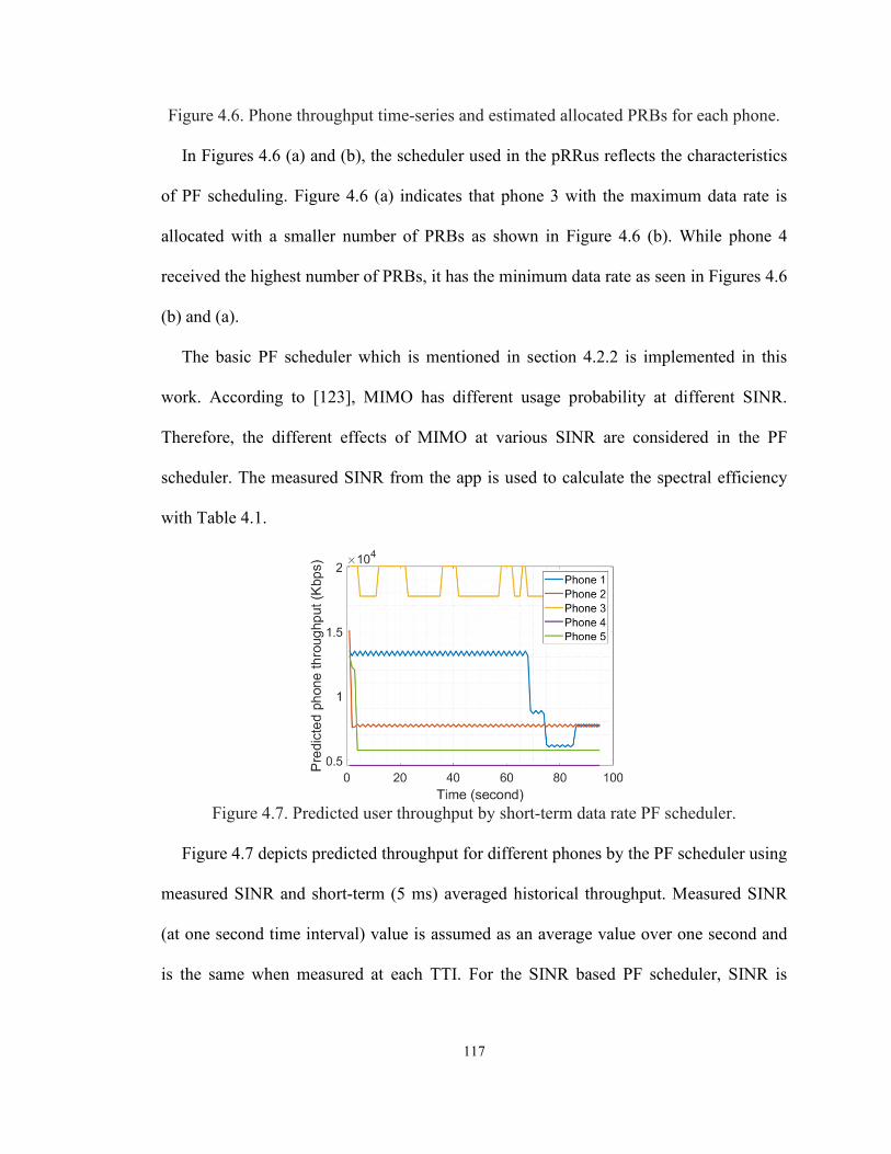
117

Figure 4.6. Phone throughput time-series and estimated allocated PRBs for each phone.

In Figures 4.6 (a) and (b), the scheduler used in the pRRus reflects the characteristics

of PF scheduling. Figure 4.6 (a) indicates that phone 3 with the maximum data rate is

allocated with a smaller number of PRBs as shown in Figure 4.6 (b). While phone 4

received the highest number of PRBs, it has the minimum data rate as seen in Figures 4.6

(b) and (a).

The basic PF scheduler which is mentioned in section 4.2.2 is implemented in this

work. According to [123], MIMO has different usage probability at different SINR.

Therefore, the different effects of MIMO at various SINR are considered in the PF

scheduler. The measured SINR from the app is used to calculate the spectral efficiency

with Table 4.1.

Figure 4.7. Predicted user throughput by short-term data rate PF scheduler.

Figure 4.7 depicts predicted throughput for different phones by the PF scheduler using

measured SINR and short-term (5 ms) averaged historical throughput. Measured SINR

(at one second time interval) value is assumed as an average value over one second and

is the same when measured at each TTI. For the SINR based PF scheduler, SINR is

118

randomly generated at each TTI by assuming measured SINR as the mean with variance

of 2dB because all the cells are fully loaded (SINR is the same for all PRBs at each TTI).

Figure 4.8. Predicted user throughput by long-term data rate PF scheduler.

Figure 4.8 illustrates the predicted user throughput with long-term averaged data

(100ms). Some data rate peaks on phone 3 can be noted as compared with Figure 4.8

after increasing the time of averaging historical data rate. Comparing Figure 4.7 and 4.8

with Figure 4.8, it is apparent that the scheduler inside the pRRus is a PF scheduler. The

predicted throughput of each phone has the same order of magnitude as seen in Figure

4.8. Noticeably, phone 3 (phone C) always has the maximum DL data rate while phone 4

and phone 5 have the minimum data rates in all the three figures.

Figure 4.9. Comparison between mean actual throughput and mean predicted throughput

for each phone.

119

The differences in the mean user throughput between actual user data rate and the

results of implementing the GPF and PF scheduler are shown in Figure 4.9. This figure

indicates that GPF has a better accuracy with proper tuning of the parameters (α=0.6,

β=0.9) than the results of the PF scheduler. The mean absolute errors of predicted

throughput for each phone are listed in Table 4.2. The CDF of cell throughput by

different schedulers are compared in Figure 4.10. GPF has a better approximation to the

actual cell throughput than PF scheduler. The SINR-based PF scheduler gives the best

result because it can always maintain a high fairness value.

Table 4.2: Mean absolute errors of three schedulers for each phone (unit: Mbps).

Type Phone 1 Phone 2 Phone 3 Phone 4 Phone 5

GPF 1.92 1.23 1.16 1.11 1.58

PF 3.42 0.50 4.19 0.56 1.65

SINR-based 1.63 1.40 2.9 1.76 1.50

Figure 4.10. CDF of cell throughput for different types of schedulers.

120

(a) (b)

Figure 4.11. Fairness value for throughput (a) and assigned PRBs (b).

Figure 4.11 indicates the fairness value of allocated PRBs and achieved user

throughput for each phone ( t =1s). It shows that the fairness of both resource allocation

and throughput is high. However, the fairness of throughput is still smaller than the value

of the PRB allocations. Compared with Figure 4.6 (a), higher fairness is achieved when

users have equal SINR.

4.2.4 Discussion

Based on the previous two test results, it is evident that there is a discrepancy between

theory and the actual application of the PF scheduler. First, in the simulations, the

number of REs per PRB is fixed, but it is dynamically changed (impacted by load and

format requirements) in an actual LTE-A system. Many uncertainties exist in the actual

LTE-A networks which contribute to the discrepancy. Fast fading and multipath fading

[60] directly impact the accuracy of SINR and MCS index. Secondly, it is very difficult

to accurately predict the actual user throughput, however, the results are improved when

considering the impact of MIMO with GPF scheduler. Thus, considering more

characteristics is useful for the modeling of user throughput. Thirdly, the historical data

121

rate with longer-term average generates more peaks in the throughput than the short-term

does for high data rate phones. Since the users with high SINR will lower the long-term

average data rate greatly as compared with the users with low SINR, the scheduler will

then allocate more PRBs to the user with good SINR resulting in a peak throughput. The

result of the SINR-based scheduler is the closest to the measured cell throughput because

it can maintain a high fairness for the phones which are static and have stable SINR

values. The scheduler inside the lampsites maintains a good trade-off among PRB

allocations and user throughput. The fairness values of both the PRBs and throughput are

above 0.75.

4.3 A fairness guaranteed dynamic PF scheduler in LTE-A networks

In this section, a new scheduler is developed by using the control theory and PF

(proportional fair) scheduler. The fairness of user data rate is dynamically adjusted by

setting a threshold in the new scheduler. A PI (proportional integral) controller is added

on the generalized PF scheduler to formulate a closed-loop feedback system. In addition,

the scheduler is verified using measured data with SINR of both static and moving users

from a real-world LTE-A network environment. Comparisons are made among the

results of the new scheduler, the PF scheduler, and the measured data. The simulation

results show that the scheduler can adjust the fairness and cell throughput properly

according to the requirements from the designer’s perspective. This lightweight and

flexible scheduler will help base stations better allocate the resource blocks.

Cell edge users are often not well serviced if they encounter strong interference with

low SINR. Thus, it is very important for the LTE-A network to properly allocate the RBs

to users to maintain a good fairness and reasonable system cell throughput. In this

122

subsection, a new scheduler is developed by utilizing the fundamentals of control theory

and a generalized PF scheduler. A proportional integral (PI) controller is applied during

the process of resource allocations in the developed scheduler. By creating a closed-loop

feedback system and inputting a threshold that is related to the fairness of user data rate,

different fairness values for user data rate and system cell throughput are achieved. To

note, the parameters of the scheduler are found based on control theory. This foundation

makes the scheduler more reliable and stable regardless of how complicated the users’

radio conditions are. A method for tuning of the controller is also introduced. Simulation

results are compared with the PF scheduler and measured data in a real-world LTE-A

environment. With this scheduler, network providers can control the fairness of RB

allocation. Adjusting the fairness value of the scheduler is also possible and

straightforward.

The structure of this section is organized as follows: the generalized PF scheduler and

basic PID control theory are introduced in section 4.3.2. The fairness guaranteed

dynamic PF scheduler is presented in section 4.3.3. Measurement plan, performance

evaluation, and simulation results of the scheduler are displayed in section 4.3.4 and

section 4.3.5, respectively. Section 4.3.6 presents the discussion about the scheduler.

4.3.1 Introduction to PI controller

4.3.1.2 PID Controller

123

Figure 4.12. A block diagram of PID controller.

Controllers are widely utilized in industrial control systems to monitor large electrical

machines and systems. The controller can manipulate the error of the output and make

changes to the control actions based on the error. There are two types of controllers:

digital controllers and analog controllers. Digital controllers have many advantages over

analog controllers such as higher speed, lower cost, more flexibility, and higher accuracy

[124].

In this section, a PI controller is used to make control actions for allocation of RBs.

Figure 4.12 shows a typical block diagram of PID (proportional–integral–derivative)

controller in feedback loop. Where, y(t) is output; e(t) is the error between output y(t)

and setpoint r(t). Proportional control obtains a response where the term P is proportional

to the error. It means that if the error is positive, the control output will also be positive.

If the proportional gain is too high, the system may become unstable. But, if the gain is

too small, it will make system control action too small for disturbances. Using the P

controller alone will generate an error between the setpoint and output, which makes it

difficult to accurately control the system. This problem is addressed by also integrating

the error signal over the past time. Integration is used to eliminate the residual error

created by the P controller. The D part of a PID controller is used to estimate the future

trend of the error based on the current error changing rate and to prevent the error from

124

changing too rapidly. The overall control function for continuous-time PID can be

represented as:

0

( ) ( ) ( ) ( )

t

p i d

du t K e t K e d K e t

dt = + + (4.9)

where Kp, Ki, and Kd are gain values for the P controller, I controller, and D controller,

respectively.

4.3.2 Fairness guaranteed dynamic PF scheduler

In this subsection, a new scheduler which can control the level of fairness is introduced.

The detailed information about generalized PF scheduler is introduced in Section 4.2.1.2

on page 115.

4.3.2.1 Introduction to the fairness guaranteed dynamic scheduler

In this work, rather than a PID control, a PI control is used. Figure 4.13 illustrates the

system with the added PI controller. Fairness of user throughput is calculated during

fixed time intervals, then, it is defined by the set point of fairness in the figure. The error

signal generated is now fed back into the PI controller as new input. Since this is a closed

loop system, the controller repeatedly minimizes the error to achieve a desired output.

PI

controllerSystem

+

-

Setpoint of fairnesserror Output fairness

Figure 4.13. Cascade compensation of PI controller.

To adjust the fairness and cell throughput the authors in [55] proposed an exponential

function to calculate the parameter . For the method in this study, similar to [55], both

125

PI controller and exponential function are combined to calculate the parameter . The

new scheduler is presented as:

,

,

[ ( )]( ) , [0, )

[ ( )]

k l

k l

k

r nS n

R n = + (4.10)

1 21

exp( * _ * ( ) )m

ik error f k error i di

== − − (4.11)

where k1 and k2 are the parameters of PI control which can be calculated by various

methods as indicated in [125]. The error _error f is the difference between calculated

fairness from scheduler and input threshold value. The integral part is for the time

duration from 1 to m. Fairness of user data rate is calculated as:

2 2

1 1( ) ( ( )) ( * ( ) )

Nu Nu

T n nn nF t T t Nu T t

= = = (4.12)

where Nu is the total number of users, and ( )nT t is the achieved DL throughput for user

n within the time interval t (here, it is set as 100 ms to calculate fairness and subtract

the controller’s setpoint).

The scheduler initially performs as a PF scheduler with 1 = . Then, during the

allocation of RBs, the scheduler will calculate the fairness value within a time interval

t . The difference between calculated fairness and the input threshold value is used as

an error for calculating PI controller. The parameter will be updated by equation

(4.13) at next TTI. If the error is positive, it means the fairness is higher than the

threshold value, and will be reduced to allocate more RBs to users with higher data

rates. Otherwise, the will be increased to adjust the fairness. New scheduler

performance metric will be calculated by equation (4.12) with the updated . During

this process, the fairness of user data rate is maintained properly.

126

4.3.2.2 Empirical tuning of the controller parameters

The value of is not only impacted by the error but also by the parameter k1 and k2.

Therefore, tuning of the PI controller is also significant in order to generate the desired

result. In this section, the parameters of the controllers are tuned by Ziegler-Nichols

method [10] because the transfer function of the system is difficult to find. Ziegler-

Nichols’ close loop method is based on experiments (a real control system or a simulated

system) making it easier to find the parameters of the scheduler. The Ziegler-Nichols’

close loop method is explained as follows [126]:

Step 1: Ensure the process is as close as possible to the specific operating point of the

control system and make the controller represent the process dynamic during the

tuning.

Step 2: Turn the controller into a P controller by setting Ki= 0, and Kd=0 and setting

the initial value Kp=0 and then stepwise increase Kp.

Step 3: Sustained oscillations are recorded in the system after increasing Kp to an

appropriate value. The signal enters into the oscillations from an excitation which can

be a step in the setpoint. The step must be small (e.g., 5% of the setpoint). Then, at this

moment Kpu= Kp where Kpu is called ultimate gain, and it must be the smallest value of

Kp.

Step 4: Measure the ultimate period Pu of the oscillations in step 3.

Step 5: Calculate the controller parameters according to Table 4.3, which is shown

below for different types of controllers. (If the stability of the close-loop system is poor,

try to reduce the Kp (e.g., reduce by 20%) to increase the stability). More detailed

information can be found in [126].

127

Table 4.3: Calculating the PID controller parameters

Kp Ki Kd

P controller 0.5Kpu 0 0

PI controller 0.45Kpu 1.2/Pu 0

PID controller 0.6Kpu 2/Pu Pu/8

4.3.3 Measurement of actual downloading data

To verify this developed scheduler, a data collection was conducted in a real-world LTE-

A network where another type of enhanced PF scheduler is installed. In the next section,

the newly developed scheduler is implemented based on this real-world environment in

the simulation model.

The test environment, basic test process, and system configurations are introduced in

section 1.8.2 Chapter 1 on page 17. The only difference is that different number of

phones and sectors are selected in this section. Downloading tests are conducted under

two scenarios (case 1 is for static users, and case 2 is for both static and moving users):

1. Case 1: five static Samsung S8 phones (on locations A to E as shown in Figure

1.13) download a 10 GB file from an ftp server simultaneously in the three sector

case.

2. Case 2: ten mobile phones downloaded the 10GB files at the same time in two

sector case.

4.3.4 Performance evaluation and simulation results

In this section, both PF scheduler and the developed scheduler are implemented in a

Matlab code to simulate the performance of each phone for both cases 1 and 2.

The CDF (cumulative distribution function) of cell throughput from measured data,

the PF scheduler, and the proposed scheduler is presented in this section and compared.

128

Mean user data rate over the downloading time for each phone are predicted and

compared. Fairness of user data rate is also compared for these three types of data. The

simulation is performed by using the measured data such as SINR and phone throughput

from section 4.2.2, which significantly reduced the simulation complexity and improved

the accuracy. Since the measured SINR is recorded every second, it is assumed that the

SINR is the average of SINR over 1000 ms. For case 2, SINR at each TTI is generated

by a normal distribution using mean (equal to the value of measured SINR) and variance

(equal to 4). The first recorded throughput is used as the initial average historical rate of

each user.

4.3.4.1 Methods and equations in the simulation

User downlink throughput is calculated by their allocated RBs, and spectral efficiency is

calculated by looking up a mapping table with users’ SINR. In the LTE-A system,

adaptive Modulation Coding Schemes (MCS) are utilized to adapt different users’ SINR.

Users with different SINR and CQI will be assigned different modulation schemes [119]

as shown in Section 4.1.3.3.

According to [127] [123], MIMO has different usage probability at different SINR,

which is considered in this work. The instantaneous user downlink throughput at each

TTI is calculated as equation (4.13) in the simulation model [122].


4.3.4.2 Simulation results

129


results for case 1 (the modified scheduler is introduced in Chapter 3).

Results and comparisons are listed in this section after performing the simulation and

tuning the parameters of the controller. PF scheduler and the developed scheduler are

simulated. Figure 4.14 shows CDF for different types of data. Two varying threshold

values are set in the simulation for the new algorithm. As the Figure 4.14 shows, the

fairness of the scheduler can be adjusted by the threshold (th) value. With lower

threshold value, the system throughput can be very high because more RBs are used for

users with higher spectral efficiency. The PF scheduler has a higher cell throughput

compared to the measured data. The scheduler in this study has the closest CDF

performance to the PF scheduler when the threshold is 0.9. The modified scheduler as

introduced in Chapter 3 approximates better to the CDF of the measured data than other

schedulers.

The mean data rate of phones for different schedulers during the simulation time (89

seconds) are shown in Figure 4.15. The figure demonstrates that the user data rates are

distributed unequally with a smaller threshold. Phone C at location C has a good SINR

(around 18 dB) and receives high throughput.

130

Figure 4.15.Mean data rate for each phone over 89 seconds for case 1.

Table 4.4 indicates the mean absolute errors (MAE) of each phone between the results

of simulations and measurement. When the threshold is equal to 0.3, larger MAE values

exist. The MAEs are smaller for phone D and phone E, while the developed scheduler

(th=0.9) makes MAEs more uniform.

Table 4.4: Mean absolute errors between the data from simulation and measured data for

each phone (unit: Mbps).

Type Phone A Phone B Phone C Phone D Phone E

PF 3.76 1.65 4.86 0.43 1.32

The proposed method th=0.9 1.50 0.75 2.13 1.21 1.82

The proposed method th=0.3 5.68 2.48 6.88 3.63 3.75

Modified scheduler 2.18 0.52 2.31 1.13 1.87

Figure 4.16 shows fairness value (calculated by equation (4.14) with time interval of

one second) of user throughput per second. Higher fairness can be achieved more

frequently by adjusting the threshold value of the developed scheduler and tuning the

controller parameters according to the tuning procedures mentioned in section 4.2.3.

When the threshold equals 0.9, it has a higher fairness value of around 0.9 during the

simulation. Noticeably, the scheduler in the real LTE-A network system also maintains a

131

high fairness around 0.82. For the PF scheduler, it shows that the fairness value is

slightly smaller than it is in the measured data with time interval one second and

undergoes more oscillations than the developed scheduler. The developed scheduler is

also compared with the scheduler in Chapter 4 as shown in Figure 4.18. The generated

scheduler (th=0.9) still generates a more stable fairness than the modified scheduler.

Figure 4.16. Fairness value of user throughput for simulation results and measurement

for case 1.

By comparing Figure 4.15 and Figure 4.16, it is observed that the new scheduler

maintains a high fairness of user data rate with cell throughput which is slightly reduced

compared to the PF scheduler. The variance of the curves in Figure 4.17 and Figure 4.18

depict that the situation is complicated when moving users are considered in the model.

A slight drop of the fairness in Figure 4.18 is due to the impact of moving user’s SINR.

The drop implies that user mobility has an impact on the system performance. However,

the new scheduler (when th=0.9) still maintains a higher fairness (around 0.9) which is

similar to the PF scheduler when moving users’ SINR changed significantly. But the PF

scheduler cannot maintain the fixed fairness when conditions are different, as

132

demonstrated in case 1. The CDF of cell throughput by the developed scheduler is also

similar to the PF scheduler. The modified scheduler in Chapter 3 is closer to the

measured data than other schedulers when considering the CQI, historical data rates, and

packet delay.


results for case 2 (the modified scheduler is introduced in Chapter 3).

Figure 4.18. Fairness value of user data rate per second for simulation results and

measurement for case 2.

133

4.3.5 Discussion

Firstly, the motivation for developing this scheduler is to fairly serve cell edge and cell

center users co-existing in the same LTE-A network. Since QoS is important to users, it

is defined in the LTE-A specifications [54]. Thus, fairness of user throughput should be

maintained with different user services. The developed scheduler can be utilized by

vendors to set up different values of fairness in wireless cellular networks. In addition,

the downlink data rate of cell edge users is easily adjusted with different fairness values

using this scheduler. Increasing the threshold value will allocate more RBs to cell edge

users and vice versa.

Secondly, the convenience of the generated scheduler is that it has only two

parameters making it easy to tune the PI controller and find the parameters. The

drawback of the scheduler is that the parameters need to be readjusted when the users’

radio conditions changes. This can be done by monitoring the users’ SINR and

adaptively tuning the controller’s parameters, however, this method is not considered in

this work. Furthermore, the fairness value is different for different time intervals

according to [48]. In this simulation, the time interval is set to 100 ms to calculate the

fairness value followed by the error between this value and the threshold (setpoint).

Figure 4.19. Fairness of user data rate during tuning of the controller.

134

Figure 4.19 depicts the fairness value per 1 ms over a time interval of 2000 ms in the

scheduler when the threshold is 0.9. The fairness value is then kept consistent by the

controller. Although a value as low as 0.3 is encountered around 800ms, the impact on the

overall fairness is negligible. By precisely tuning the controller, a more stable closed-loop

system can be achieved.

4.4 Conclusion

To summarize, the performance of each type of PF schedulers (PF, GPF, and SINR-

based) is evaluated in a real-time deployed LTE-A network in section 4.2. Discrepancies

were found between the measured data in this study against the data presented in

literature reviews. Two different tests are performed inside the Kinesiology building in

the University of Regina. The basic PF scheduler is implemented to predict user

throughput. The results show that the scheduler installed inside the LampSites is a PF

scheduler. Moreover, inconsistency are also observed when compared with the basic PF

scheduler. An important observation to highlight is that fairness and cell throughput do

not have a clear relationship in the measured data which is contrary to the published

literature. Results have shown that the actual scheduler cannot maintain a stable fairness

for the varying user throughputs.

The measured data and the two test results show that a significant gap exists between

theory and reality. Thus, it can be concluded that studying actual environments is crucial

to understand the true behavior of the system and to provide cell users with satisfactory

services.

In this subsection 4.3, an easy to implement, new scheduler is developed based on PID

control theory and the conventional PF scheduler. It can maintain different levels of

135

fairness for user data rates providing it with the flexibility to serve the users fairly in

various scenarios. The tuning process of the controller is also performed by using the

well-known Ziegler-Nichols’ close loop method. The simulation results show that the

developed scheduler can maintain different trade-offs between fairness and cell

throughput for both static and mobile users. At the threshold of 0.9, the scheduler

maintains a better fairness than the PF scheduler with slight reduction of cell throughput

for static users. At last, simulation results indicate that the scheduler in section 3.3

Chapter has a better throughput performance than other schedulers.

In the future, other features such as QoS and automatic adjustment for moving users

will be considered into the scheduler to enhance its practicality and stability.

136

Chapter 5

Development of a Realistic LTE-A HetNet

Traffic Model

The structure of this chapter is as follows: Section 5.2 depicts an efficient ray-tracing

path-loss propagation model for the LTE-A HetNet. Section 5.3 provides the

development of an LTE-A HetNet traffic mode in detail. Section 5.4 verifies the

accuracy of predicted results from the model. The conclusions are exhibited in Section

5.5.

An accurate traffic model is essential to narrow the gap between theoretical research

and actual networks. A traffic model that can accurately predict user RF conditions and

user downlink data rate will be beneficial for network operators to reduce costs and to

provide users with reliable service. In addition, such a traffic model is useful to provide

both the lower and upper limits of system performance, evaluate the potential of new

technologies, and implement new algorithms [128]. The simulation results will also offer

relatively accurate predictions and a better understanding of the effect from new settings

that may be difficult to set up in the actual systems.

In this chapter, a novel realistic matlab-based traffic model of LTE_A HetNet is

developed based on the knowledge derived from previous measured data at the

University of Regina as mentioned in Chapter 3. Both indoor and outdoor environments

are provided in this model. Characteristics such as fast fading, and user locations are

extracted from measurement and database, therefore enhancing the accuracy of the

137

simulation results. In addition, the model has some important performance metrics: cell

throughput, individual user throughput, an indicator of the variation of cell throughput

and an indicator of the potential of a small cell to be incorporated into neighboring cells

or not. The methodology of developing the model is introduced in detail in this chapter.

With the traffic model designed by the methodology in this thesis, network operators

will have guidance to better understand the HetNets and to optimize the networks based

on this traffic model. To the best of the author’s knowledge, limited research about

studies of HetNet traffic models is based on real-world HetNet cellular network

environments.

RF propagation

models

Generate user

Profiles (locations,

velocities, etc.)

Calculate User

SINR

Get cell load

information from

cell-level data

Allocate Resource

Blocks to Users

by the Scheduler

Calculate User

Downlink Throughput

and Performance

Indicators

Extracted spectral

efficiency from

Chapter 3

Generate

environment

profiles Monitoring the HO and radio

link failure during the

simulation in the model [11]

Figure 5.1. The process of developing the traffic model.

Figure 5.1 depicts the procedure of building the realistic model. The first three

components are: developing a path-loss propagation model that is utilized to calculate

the RSRP received from the transmitter to users, generating both user locations and user

mobility model, and estimating cell load information from the database. Users’ SINRs

are calculated according to the above information. Then, a new scheduler is developed to

138

calculate user download throughput using extracted SE from the test data. The next

section describes the modeling of propagation for both outdoor and indoor environments.

5.1 Introductions

RF propagation models are crucial for designing networks and cell deployment planning.

Obstructions around the transmitter and receiver can always make the results difficult to

be predicted accurately. The prediction errors will lead to misunderstanding of the

coverage and capacity of the networks and reduce the performance of cellular networks

[60]. Therefore, generating environment profiles for the propagation model and properly

tuning of the output results are highly important.

In Section 5.2, a new methodology is proposed to develop pseudo-3D path-loss

propagation models for a site-specific LTE-A HetNet. Both outdoor and indoor

propagation models are developed. Some efficient strategies are proposed to simplify the

building of structure data so that computation costs are reduced. A tuning method for the

results of the indoor small cell propagation model is also proposed. For the outdoor

propagation model, the software of geographic information system (ArcGIS) is used to

generate building profiles that are efficient and accurate. The prediction shows that the

simulation results are accurate, and the mean absolute error is around 6 dB. In addition,

the developed small cell indoor propagation model can also be implemented for 5G

networks in the future.

5.2 An efficient ray-tracing path-loss propagation model for LTE-A

The structure of Section 5.2 is organized as follows: Section 5.2.1 presents path loss

models of different propagation mechanisms. The procedures for developing propagation

139

models are indicated in Section 5.2.2. Section 5.2.3 represents modeling results. Section

5.2.4 performs the discussion.

5.2.1 Introduction to path loss prediction model

In this section, the basic equations in [60] are utilized to calculate path loss. These

equations are based on ray tracing rules and UTD which was proposed by Kouyoumjian

and Pathank. Propagation mechanisms of the line-of-sight, first order of reflections,

diffractions, and transmission are utilized in this work. Only main traveling paths of rays

for users at each location are captured because the tuning method is utilized for the final

predicted results.

In actual environments, radio waves from a transmitter will undergo a multipath

channel and be reflected, diffracted, and scattered by the objects in the environments.

The received signal of user devices is a combination of all the waves along different

paths from the transmitter. According to the UTD in [60], the total received electric field

is represented as a sum of electric field from different ray paths:

1

m

Rx j

j

E E=

= (5.1)

Where m is the number of rays from transmitter to receiver, jE is the received electric

field from jth ray. m is the number of total paths.

1. LOS Propagation

If a ray is directly transmitted from transmitter (Tx) to receiver ( 1Q ) without any

obstructions, this path is called line-of-sight (LOS). Then, the received electric field at

1Q for LOS is calculated as:

140

1

jkr

Q Tx

eE E

r

−

= (5.2)

Where r is the distance of LOS, k is propagation constant (k=2π/λ, where λ is

wavelength). TxE is the electric field at the transmitter.

2. Diffraction Propagation

According to UTD, if an electric field from one path is reflected or diffracted at a

series of points nQ (n=1,…N) as shown in Figure 1, and the electric field which is

received at point S from 1Q is calculated as [60]:

/

1

1

( ) ( )N

i R D j

j n n

n

E S E Q A e

=

= (5.3)

where /R D

n is coefficient of reflection or diffraction, nA is a spreading factor. 1( )iE Q is

the LOS electric field calculated by equation (5.2). The total field attenuation and phase

shift of propagation path for jth ray is presented as [60]:

/

1

1j

NjkrR D

j n n

nlos

W A er

−

=

= (5.4)

where losr is the distance of LOS, jr is the total distance of the propagation path for jth

ray. The overall attenuation and shift are calculated as:

1

l

j

j

W W=

= (5.5)

Two types of ways to model the diffraction propagation path loss are: over-rooftop

and vertical-edge diffractions for the outdoor propagation model.

For over-rooftop diffraction, building heights are modeled as heights of half planes on

the ground, and the edge of half planes are assumed to be perpendicular to the line

141

connecting the transmitter and the receiver [60]. Diffraction coefficients are given by

[60]:

/4' 2( , , ) [ cos ( / 2)]

2 2 cos( / 2)

jD

n n n n n

eL F kL

k

− = (5.6)

where n is diffracted angle and '

n is angle of the incident ray of nth half plane as shown

in Figure 5.2. is the difference between n and '

n . Distance factor of nL given by [60]

is presented as:

1

1

n nn

n n

s sL

s s

−

+

=+

(5.7)

ns is shown in Fig.1. Transition function of F is calculated by Fresnel integral:

2

( ) 2 jx ju

xF x j xe e du

−= (5.8)

Spreading factor of nth half plane is calculated as:

1

0

1

0( )

n

kkn n

n k nk

sA

s s s

−

=

−

=

=+

(5.9)

The vertical-edge diffraction coefficients are calculated in a similar way as roof-top

diffraction. Corners of buildings to the line of connecting transmitter and receiver are

modeled as half planes to calculate the coefficients as shown in Figure 5.2.

Figure 5.2. Diffraction modeling by half planes. Figure 5.3. Example of image theory to

calculate reflection path loss.

142

3. Reflection Propagation

Reflection coefficient R

n for vertical polarization of transmitter is calculated as [60]:

2

2

sin cos

sin cos

in inR

n

in in

− + − =

+ − (5.10)

where in is incident angle (angle between incident ray and normal vector of the

reflecting surface), is relative permittivity of the reflecting surface. When calculating

the reflection, image theory [70] is used for both the outdoor and indoor propagation.

Figure 5.3 shows the image antenna of Tx. The reflection point can be found easily on

the wall.

4. Transmission Propagation

According to [129], for a ray transmitted throughput a wall with thickness and real

dielectric permittivity r , transmitted field expression of GO is given by:

0

,

02

1 2 1 2

( )( )( )

ijk s

tT e

E Rx Es l s s l s

−

⊥=

+ + + +

P (5.11)

where 0k is wall number in free space, in is reflection angle with the wall,1( )r −= ,

cos( ) / cos( )in t = , and / cos( )tl = . t is the refraction angle which is calculated

from in and r with Snell-Descartes law. 0E is the source electric field. ,T⊥ P are

transmission coefficients for perpendicular and parallel polarization, respectively. 1s and

2s are the distance of incident ray to the wall and transmitted ray through the wall to the

receiver respectively, as shown in Figure 5.4. It is represented as [129]:

2

,

, 2 2

,

(1 ( , ))

1 ( , )

j

in r

j

in r

R eT

R e

−

⊥

⊥ −

⊥

−=

−

P

P

P

(5.12)

143

where , ( , )in rR ⊥ P are Fresnel reflection coefficients for perpendicular and parallel

polarization, respectively. The is expressed as: 2

0 sin ( )r ink = − . Figure 5.4

depicts an example of a single ray transmitted through a wall.

Figure 5.4. Illustration of a transmitted ray through a wall.

5. Equations for Calculating Propagation Path Loss

The calculation of path loss (in dB) is defined as [60]:

1020log ( | |)4

dBL W

= (5.13)

where W is the total attenuation and phase shift by different types of propagation

mechanisms.

5.2.2 Introduction to development of propagation models

In this section, the procedures of building outdoor and indoor propagation path loss

models are introduced. Figure 5.5 indicates the flow chart of building the outdoor

propagation model.

Generate

building

information from

GIS

Building data

information

reduction

Utilizing data

reduction methods

Tuning

of the

results

Calculate

different types

of attenuations

Figure 5.5. Flow chart of building outdoor propagation.

144

5.2.2.1 Introduction to the ArcGIS and simplified method

ArcGis is a suite of software produced by ESRI. It has many functions [130]: view and

query maps with the other products; view spatial data; create maps; and operate basic

spatial analysis, etc. In this study, the ArcGIS is used to generate basic building data of

the University of Regina and provide accurate GPS coordinates of each location. Figure

5.6 displays a layout of the buildings from ArcGIS. The building data are composed of

coordinates and building heights for each vertice.

Figure 5.6. Building data layout generated from ArcGIS for outdoor.

Figure 5.6 shows multiple vertices for each building, thus, the data reduction method

is that the buildings are modeled as quadrangles when searching buildings and

calculating the diffractions. Figure 5.7 represents an example of simplifying the building

structure. The blue color is used to replace the black color building layout for searching

and modeling purposes as shown in Figure 5.7 (a). The simplification is reasonable

because few people would stay at the corners of buildings according to the author’s

observation. When searching the buildings between users and the transmitter, the four

corner points of the blue polygon are representative for the building. For the indoor

rooms, two rooms can be merged into one quadrilateral as indicated in Figure 5.7 (b) if

these rooms are not significant and have few users inside them.

145

(a) (b)

Figure 5.7. Examples of simplifying building layout when processing the building data.

Furthermore, when searching for the related buildings to the receiver, only the

buildings within the circle which is centered at the receiver with the distance between Tx

and Rx as radius for the circle as shown in Figure 5.6. The proposed method is similar to

the method in [64], but this method is easier than that one and it does not have a

significant impact on the final prediction results. At last, the prediction results will be

adjusted by a tuning method, thus, missing selecting some buildings does not have a

large impact on the final results.

For tuning of calculated path loss, the same procedure will be utilized by the method

from the literature [60]. Semi-global tuning and local tuning methods are introduced in

[60] to improve the accuracy of prediction results. This method is also extended in this

study for predicting RSRP in small cell indoor environments in Section V. Semi-global

tuning method applies least mean square (LMS) method for different groups of locations

which are categorized by the surrounding environment of users (the number of

obstruction buildings between the transmitter and the receiver) to calculate optimal

parameters. The total adjusted attenuation and phase shift is represented as [60]:

1 2 3 4LOS RD VD RW wW w W w W w W w= + + + + (5.14)

146

where LOSW is the attenuation and phase shift for LOS, RDW is for roof-top diffraction,

VDW is for vertical edge diffraction, and RW is for reflection, iw (i=1, 2, 3, 4) is tuning

parameters. nS is the calculated signal strength from the serving antenna by equation

(5.15) as [60]:

n Tx Tx RxS P G G path loss= + + − (5.15)

where TxP is transmission power, andTx RxG G is antenna gain for transmitter and receiver,

respectively.

The local tuning method can be viewed as a refined version of semi-global tuning

method. It utilizes the LMS for the users to calculate adjusting parameters with measured

data that contains the same dominated propagation mechanism with that user. It has

following steps [60]:

Step one: define a set of measurement locations centered at one receiver point (x, y)

within the range of a radius (20 meter).

Step two: collect data at the locations in step one where the main propagation

mechanism is identical with one of the receiver location (x, y). The main propagation

mechanism is identified as:

( ) ( ) ( ) ( )max{| |,| |, | |,| |}Main FS i RD i VD i VD iW W W W W=

Step three: apply the LMS for the measured data in step two to calculate optimal

parameters in equation (5.14) for the receiver at (x, y). If the parameters are troublesome

to calculate, the Semi-global method is utilized.

5.2.2.2 Development of indoor propagation model

For the indoor propagation model, because there are no available building layout input

data, thus, the data has to be generated manually. The same method of simplification as

147

mentioned in Figure 5.7 is utilized because for the edge areas of buildings, few people

will stay there, and it has few impacts on the prediction results. For the calculations of

different propagation mechanisms, pseudo-3D modeling of buildings is constructed for

the indoor propagation models. Building heights, walls, and ceilings are considered to

find ray paths on these surfaces.

After the building data is prepared, the results should be tuned properly with

measured data. The proposed algorithm of this study is similar to the method in [60], but

this method is used on the tuning of weights of the signals nS (n ≥ 1) from different

numbers of small cells because users will receive signal from many indoor small cells.

Since the final received path loss is used to calculate signal strength and user devices

will receive signal from more than one antenna, the coefficients are used to adjust the

weights of the received signal from different small cells.

The adjusted RSRP signal is represented as:

1 1 2 2* * ... *a n nS w S w S w S w= + + + + (5.16)

where n is the number of antennas that users receive signal from them, nw is model

parameter, and the utilized algorithm contains three steps:

Step one: for different rooms and hallways inside a building, we categorize them into

different groups due to that UEs will experience similar path loss in the same room.

Step two: calculate optimized parameters in equation (5.16) with Least Mean Square

for each group in step one by using measured data from the location of each group,

respectively. In case, if there are some negative values generated, these values will be

replaced by the original predicted values.

148

Step three: calculate the received signal strength of users by using equation (5.16) for

other locations.

5.2.3 Modeling results of propagation models

5.2.3.1 Collection of experimental data

Table 5.1 represents some information about antennas at three different locations.

Table 5.1: Antenna model and antenna heights.

Locations Antenna model Antenna Height

(meter)

Carrier

Frequency

Outdoor 80010865 28.5 2.6GHz, 2.1GHz

Building A PEAR M5277i 4.5 2.6GHz

Building B pRRU3901, ExTENT

D5777i,

around 4 and 14 for 1st

and 2nd floors,

respectively

2.1GHz

To obtain the path loss and signal strength data, and to verify the propagation models,

a RF scanner called ‘Nemo handy’ was utilized to record the data for the marked

locations of the outdoor and buildings A and B, as shown in Figure 5.8, Figure 5.10, and

Figure 5.11. respectively. The device is introduced in Section 1.8 Chapter 1 in detail.

The height of receiver is assumed to be 1.5 meter.

5.2.3.2 Results of the outdoor propagation model

In this work, the campus of the University of Regina is used for the outdoor propagation

model. The picture of the campus is shown in Figure 1,7 Chapter 1 (on page 16).

Building A and building B are deployed with small cells inside. The indoor propagation

is modeled for the two buildings.

149

Figure 5.8. A simplified building layout information of Figure 1.9 for the outdoor from

ArcGIS software (Red dots are locations for measured data).

Figure 5.8 indicates the result of building layout by using ArcGIS software. These

building structures are composed of vertices of polygons. The red dots in Figure 5.8

means the test locations for verifying the outdoor model. A macro antenna is installed on

the roof-top of one building as marked ‘Tx’ in Figure 5.8.

Figure 5.9. Predicted path loss and measured path loss.

Figure 5.9 presents predicted path loss and measured path loss. The MAE is about 3.5

dB. The reason for the blue lines becoming flat is because only the diffraction is the

dominant mechanism for the test locations. Thus, it is difficult to apply the local tuning

method.

150

5.2.3.3 Results of the indoor propagation model

Figure 5.10. Simplified building structure of building A (the blue dots are user

trajectories).

Figure 5.10 presents the simplified building layout data of building A (as shown in

Figures 1.10 and 1.12) in 2D view. The blue dots are trajectories for walk tests where

RSRP data is measured. The quadrangles represent rooms. Figure 5.11 represents the

simplified building layout data of Building B (as shown in Figures 1.12 and 1.13) in 2D

view (The blue circles are trajectories for walk tests where RSRP data is measured. The

black dots are antennas).

Figure 5.11. The simplified building structure of building B (Black dots represent

antennas and blue circles are user trajectories).

151

As shown in Figure 5.10 and Figure 5.11, the building data information is reduced

significantly. Most of the simplification parts are the locations where few people will

occupy. Figure 5.12 and Figure 5.13 displays parts of estimated RSRP results. For the

tuning process, 50% of the measured data is used for training, and the rest 50% is

utilized for testing. For Figure 5.12, the MAE is reduced from 36 to 7.73 dB after using

the proposed tuning method. There is a big gap between measured RSRP and initially

predicted RSRP, because many people walk and stay inside building A which makes

some path loss difficult to be accurately captured.

Figure 5.12. Predicted RSRP before and after tuning the results for building A.


the model for building A.

152

Figure 5.13 exhibits cumulative distribution function (CDF) of the mean error before

and after tuning the model for building A. In 70% of the cases, the initially predicted

results show an over-estimation of the signal strength over 40 dB.

Figure 5.14. Predicted RSRP before and after tuning the results for building B.

As indicated in Figure 5.14, after applying the tuning algorithm, the predicted RSRP

is closer to the measured results. The MAE decreased from 4.48 to 3.8 dB. Figure 5.15

indicates cumulative distribution function of mean error before and after tuning the

model for building B. For 60 % of the cases, the predicted RSRP shows an over-

estimation of 4 dB, but the mean error is 0 dB for the results after tuning.


the model for building B.

153

Table 5.2 displays results of modeling indoor signal strength before and after applying

the tuning method. The MAE, mean error, and standard deviation are utilized to evaluate

the performance of the modeling results. It indicates that the tuning method is very

beneficial for building A due to a large reduction of the MAE from 37.8 to 8.1 dB. The

mean error and standard deviation are also reduced. For building B, the predicted results

have a small error before tuning, but the tuning method can still reduce the MAE about

1.2 dB.

Table 5.2: Modeling results before and after tuning the results for indoor predicted signal

strength

Locations Type MAE (dB) Mean error (dB) Standard deviation

Building A

Before tuning 37.87 -37.8 9

After tuning 8.07 -6.7 6.5

Building B

Before tuning 5.17 4.43 4.5

After tuning 3.88 0.0165 5.0

5.2.4 Discussion

For the indoor environments with multiple low power cells deployed, a new algorithm is

proposed to appropriately tune the predicted user RSRP. The prediction results show that

the MAE of the outdoor propagation path loss model is about 4 dB, and for the indoor

model, the MAE of predicted RSRP is about 4 - 7dB which is reasonable. The path loss

of radio waves is dynamically changed due to the varying environments, the number of

users, weather, etc. The radio waves may have multiple paths to travel from transmitters

to receivers, but capturing the main paths is sufficient to calculate the results according

to the final results. For more accurate results, the locations should be classified into more

groups with clustering techniques, such as k-means clustering.

154

These propagation models are beneficial for predicting received RSRP and better

planning of the network coverage and maximizing network capacity. Accurately

predicting the RSRP of macro cells and small cells is necessary to design seamless

network services and efficient handover procedures. The two developed models are also

useful for 5G networks in the future as a large number of small cells will be deployed in

the 5G according to [131].

5.3 Building a realistic LTE-A HetNet traffic model

In this section, a simulated traffic model of LTE-A HetNet is developed by integrating

the path-loss propagation model and measured data from Chapter 3. The model is

designed to accurately predict the user traffic of the HetNet at the University of Regina.

This traffic model is a data-driven model and is developed based on the collected data by

mobile devices and the statistics from Splunk. Since the main goal of the model is to

predict user SINR and user throughput, and the model has detailed preparation

(propagation model and measurement, etc.), unnecessary communication procedures in

the LTE stack layers are simplified. The accuracy of predicted results (e.g., RRSP,

SINR, and throughput) from the model is high. The value of this model is to provide a

detailed procedure to build an accurate traffic model based on an actual environment in

detail.

Table 5.3 lists most of system configurations for the model. Both static and moving

users are generated in the model (the number of the users depends on specific scenarios).

Infinite buffer and finite buffer (some users may keep requiring for data during the

simulation) are defined for each user with each type of random allocated QoSs. We

assume that each user has only one QoS during the simulation and the data rate of each

155

QoS is from [132]. For the finite buffer size, the data sizes are extracted from the Splunk

data as mean data volume per user (aggregate traffic volume divided by the number of

user). Buffer sizes, buffer types and types of services are randomly defined for each user

according to specified probabilities for each cell. The number of users at specific time

can be obtained from the CDFs of the number of users in Chapter 3. For simulating the

RC HO test, the number of users is 80. For the cell-splitting test, the number of phones in

KC building is 10.

Table 5.3: System parameters for the simulation model

Bandwidth 20MHz Radio link failure

settings

-8 dB, -6dB for out and

in. [11]

Handover

type A3 Number of cells

1 macro cell at C and 2

clusters of small cells at

A and B as shown in

Figure 1.8.

Timer 310 500ms [11] Connection failure RSRP<-115dBm

A3 offset 3 dB Time to Triger 300ms

Buffer type

Finite /full buffer

by configurations

for each user

User type

Static users and moving

users in predefined

trajectories and random

walk model

Fast fading Extracted from the

RF scanner

Moving users’

speed 1.25 m/s

Number of

users

From cell-level

data Scheduler

The scheduler in Section

3.3.4

Packet size 256 kb Packet arrival rate 500

5.3.1 Introduction to the users’ information in the developed model

The user locations are generated by historical daily data from the network service. The

user location information is extracted by 50 m X 50 m bins. The probability of different

locations where users may appear is presented in Figure 5.16. The peak shape represents

that users are more likely to stay in the areas corresponding to that GPS coordinates as

shown in Figure 5.16.

156

Figure 5.16. User density for different locations inside the building (xi and yi are GPS

coordinates).

5.3.2 User mobility model.

In the developed traffic model, locations of static users are generated according to the

empirical user location distribution. Mobile users have two types: one type is moving

according to predefined trajectories that are used in the measurement mentioned in

Chapter 3, and another one is moving by using the random walk model with the

restriction of building boundaries. The second type of users cannot directly walk across

the building boundaries unless they are on the trajectories of handover at different doors.

The random walk model is presented as follows [133]:

A mobile user i will obtain a new direction and speed randomly in each time interval.

The location of user i at time t+1 is presented mathematically as:

( 1) ( ) ( )i i is t s t w t+ = + (5.17)

where the distribution of ( )iw t is uniformly at random in a disk of radius RWR centered at

( )is t , and RWR is mobility range and is user speed. ( )is t is the location of user i at time

t.

157

5.3.3 Calculate users’ SINR

As for the cell load information, when running the simulation model, cell loading

information are estimated according to the historical data in Splunk. From practical

observations, indoor users within the HetNet are not strongly impacted by the

neighboring macro cells as the signals are shielded from building structures. Indoor users

are mainly impacted by the macro cell of the HetNet and indoor neighboring small cells.

Outdoor users are partly affected by the neighboring macro cells.

The SINR of user i at location (x,y) is calculated as [83, 127]:

2

1

( , )

*

serving

i N

neighboring n

n

RSRPSINR x y

RSRP PRB =

=

+ (5.18)

where nPRB is PRB utilization of neighboring cell n. 2 is the constant additive noise

power. In this developed model, the maximum SINR is set to 30 dB because

measurement data shows that the maximum SINR is no more than 30 dB.

5.3.4 Introduction to the QoS scheduler in the model

Section 3.3.4 (on page 71) in Chapter 3 introduced the information of the scheduler and

types of services in detail.

5.3.5 Calculation of user throughput

The throughput of user j at time t is calculated as:

( ) _ * /j RER t Spectral efficiency N TTI= (5.19)

where ‘Spectral_efficiency’ is calculated by SINR from a mapping table in the measured

data as shown in Chapter 3. REN is the total number of resource elements allocated to the

user at time t which is decided by the scheduler.

158

5.3.6 Introduction to the performance metrics and indicators

1. Mean user throughput

1

/U

mean jjT R U

== (5.20)

where jR is downlink throughput of user j and U is the total number of users.

2. Cell throughput

Cell throughput is defined as total throughput of all the users [52]:

1

U

cell jjT R

== (5.21)

3. Mean user SINR

1/

U

mean jjSINR SINR U

== (5.22)

4. Cell throughput Indicator (CTI)

From the previous measurement results, as mentioned in Chapter 3, the increase of

mean user SINR does not indicate an increment of cell throughput when applying a

different setting on the system. Thus, Cell throughput Indicator is developed for

predicting the increasing or decreasing of cell throughput solely based on the user SINR

values. According to [35], the conventional PF scheduler, as mentioned in Chapter 4, can

be approximated by using SINR to replace the user data rate. Therefore, the performance

metric of the scheduler to allocate RBs to selected users is presented as [35]:

,

,,

( )( )

( )

j l

j lj W

SINR nS n

SINR n= (5.23)

where , ( )j WSINR n is the average SINR during the last time window W until time n.

, ( )j lSINR n is for user j with respect to RB l at TTI n. The SINR of user j at RB l can be

presented as [35]:

159

0, , 0, ,

, 2

, , , ,1

( )( )

( ) ( )

j l j l

j l I

i j l i j li

p X nSINR n

p n X n =

=+

(5.24)

where 0, ,j lp and , ,i j lp are averaged received power from the serving cell (i=0) and

neighboring cells i (i >0) on RB l, respectively. 0, , ( )j lX t is fading component. The RB l

will be allocated to the user with maximum score , ( )j lS n . It is assumed that the fading

component is random and follows the well-known Rayleigh-fading distribution. The user

downlink data rate at time t is calculated as [35]:

, ,z | 1( ) ,1 0( ) ( ) ( 1)

j l j l

N

user S z j lnT t C z f P S dz

=== = (5.25)

where , ( )j lfz z is the probability that the RB l is allocated to user j, and , ,z | 1( )j l j lS zf = is the

SINR probability density function. After transformation and substituting the PDF and

CDF of SINR into the equation (5.12), the user throughput is expressed as:

,

,l ,1 0\ j,

( )( ) ( ) ( ( )

( )

N g l

user Zg j lng J j l

E SINRT t C z F fz z dz

E SINR

=

= (5.26)

where N is the number of RBs, and ( )C z is SINR-to-payload size mapping function. The

Cell throughput Indicator (CTI) is defined as the difference of cell throughput between

time t1 and time t2:

CTI= 2 1( ) ( )user userT t T t− (5.27)

With this indicator, the network operators can predict whether the cell throughput will

increase or decrease after changing network settings by only using SINR.

5. SGIR

SGIR is used to indicate the importance of a specific antenna in terms of neighboring

cells in the small cell environments. This indicator is initially proposed as an indicator

160

for deciding to turn off the small cells so as to reduce interference in [89]. In this work,

this indicator can be utilized to switch a small cell from one cell cluster to other clusters.

Generated interference (GI) is represented as the sum of interference power which is

generated from one small cell to its surrounding non-served users. For the small cell m,

its GI is represented as [89]:

,

m

k m

m r

k U

GI P

= (5.28)

where mU is served user set of cell m, ,k m

rP is interference power received by user k from

small cell m. It is typically presented as:

,k m

r tP Hd P−= (5.29)

Where random variable H follows a log normal distribution and models the shadowing

effect in the transmission environment, d is the distance between the user k and the small

cell m, α is the path loss exponent, and tP is the transmit power of the small cell. The

indicator SGIR for small cell m which indicates the level of the importance of a small

cell to be merged into the target cell ID is defined as [89]:

, ,/m m

k m k m

m r r

k U k U

SGIR P P

= (5.30)

Therefore, it is the ratio between aggregate signal strength of users connected to small

cell m and aggregate interference of users which are impacted by the cell m. A smaller

value of SGIR means that this serving antenna provides weaker signal strength to its

serving devices and has a larger impact on other non-served users. The smaller the value

of SGIR, the less significant the cell is. Thus, this small cell can be incorporated into the

target cell ID. With this indicator, the cell edge small cell m with less served users will

be assigned with the target cell ID. In this way, the SINR of the target cells are

161

improved, and neighboring cells are less impacted due to less users around the small cell

m.

6. Fairness of throughput allocation

As indicated in [128], fairness should be an important metric to measure the

distribution of user throughput in the HetNet. Thus, the fairness for all the users’

downlink data rates and the fairness of throughput distribution among base stations [48]

in the HetNet is expressed as equations 5.31 and 5.32, respectively:

2 2

1 1( ) ( ( )) ( * ( ) )

Nu Nu

Tu n u nn nF t T t N T t

= = = (5.31)

2 2

1 1( ) ( ( )) ( * ( ) )

Ns Ns

Ts s s sn nF t T t N T t

= = = (5.32)

Where Nu/ Ns is the total number of users/cells in the HetNet, and ( )nT t / ( )sT t is cell

throughput of user n/cell s within the time interval t . This metric (5.32) represents the

distribution of cell throughput among the cells within the HetNet.

5.4 Verifying the prediction results of the developed traffic model

Figure 5.17. An example of generate building layouts and user locations by the traffic

model (refers to the locations in Figure 1.8).

162

Figure 5.17 shows the HetNet environment with users’ locations. The RC building

and KB buildings are marked in Figure 5.17, which refers to the locations in Figure 1.8.

The buildings’ coordinates in the figure are converted from the GIS software. The

outdoor users’ locations are generated by using passion process distribution in Figure

5.17.

5.4.1 Verifying the modeling results with handover tests in RC

(a) (b)

Figure 5.18. (a) Layout of Riddell Center and some user locations. (b) Measured RSRP

and predicted RSRP values for the test in RC.

(a) (b)

Figure 5.19. (a) Measured SINR and predicted SINR values for the test in RC. (b)

Measured throughput and predicted user throughput for the test in RC.

163

The handover walk tests are described in Section 3.4 Chapter 3. Users walk through

following predefined trajectories at door 1 of the RC building. Figure 5.18 (a) presents

the building layout of RC and locations of some users. Figure 5.18 (b) and Figure 5.19

present predicted results from the model.

Table 5.4: Root mean square error and mean absolute error for predicted results in RC.

RSRP (dBm) SINR (dB) Throughput (Mbps)

RMSE 7.6 6.1 21.9

MAE 6.0 4.7 14.8

Table 5.4 lists the RMSE and the MAE for the prediction results in the handover tests

at door one of RC. The accuracy is acceptable because the test was performed in a very

complicated and highly dynamic environment with the unknown number of users inside

the RC. The number of connected users and user locations are dynamically changed and

bring a large variance in user throughput.

5.4.2 Verifying the modeling results in Kinesiology Building

(a) (b)

Figure 5.20. (a) Measured throughput and predicted throughput of phone A in one sector

case. (b) Measured SINR and predicted SINR of phone A in one sector case.

164

As mentioned in Section 3.3 Chapter 3, ten phones are downloading a 10 GB data

from an ftp server simultaneously. The generated model predicts downlink throughput

for the ten phones when they are downloading data at the same time. For simplicity, only

parts of prediction figures are listed. Figure 5.20 and Figure 5.21 present predicted

results of phone A from the model in one sector case. Figure 5.20 (a) presents predicted

downlink throughput of phone A and measured throughput. Figure 5.20 (b) shows

predicted user SINR and measured SINR of phone A.

Figure 5.20 (a) presents predicted user throughput and measured results of phone A in

500 seconds. Within the first 20 seconds on Figure 5.20 (a), the measured results are

higher than the predictions due to the phones being turned on to download data one by

one until they downloaded simultaneously in which phone A was the first phone to be

turned on. Thus, the measured data is slightly higher than the simulation results of the

model. In addition, the variations of the predictions are decided by the average time

window of the scheduler. The measured data is averaged over one second.

Figure 5.21. Measured RSRP and predicted RSRP of phone A in one sector case.

Figure 5.21 shows the same phenomenon that prediction results have more variations

due to the fast fading of received signal strength generated by the model.

165

(a) (b)

Figure 5.22 (a). Predicted user RSRP and measured RSRP of phone I in one sector case.

(b). Predicted user SINR and measured SINR of phone I in one sector case.

Figure 5.23. Predicted user throughput and measured throughput of phone I in one

sector

Figure 5.22 and Figure 5.23 present predicted results of RSRP, SINR, and downlink

throughput of phone I (moving device) in one sector case. Figure 5.22 indicates that it is

more difficult to predict the results for moving users due to the deviations of user

locations, different path-loss fading of the received signal strength, etc. Previous results

of the measured data indicate that RSRP values are not identical even on two different

166

days. Figure 5.23 presents that some values of throughput are almost zero due to the

issue of the mobile app that happens occasionally.

Table 5.5 represents the MAE and the RMRE of predicted RSRP, SINR and user

throughput for ten phones in one sector case, respectively. The table indicates that the

prediction results are accurate and reasonable. The mean MAE and the mean RMSE of

SINR over all the phones are around 0.9 dB, which is very close to the actual value. The

minimum MAE of predicted user throughput is only around 3 Mbps.

Table 5.5: RMSE and MAE for the prediction results of ten mobile phones.

MAE RMSE

Label RSRP SINR Throughput RSRP SINR Throughput

Phone A 1.8 0.1 4.7 2.4 0.3 6.1

Phone B 3.8 0.8 8.8 4.1 2.4 13.7

Phone C 8.2 1.0 6.7 8.4 1.0 10.0

Phone D 2.1 2.7 2.9 2.6 2.7 3.5

Phone E 1.7 0.2 5.3 2.1 0.3 6.1

Phone F 6.3 0 4.9 6.5 0 6.4

Phone G 2.2 0.2 3.9 2.5 0.3 4.6

Phone H 4.1 0.1 4.7 4.7 0.3 6.0

Phone I 5.8 0.5 2.9 6.5 0.7 3.7

Phone J 9.1 0.6 17.7 10.2 0.8 24.2

Mean value of all

the phones 4.4 0.6 6.2 4.9 0.9 8.3

5.4.3 Evaluating the accuracy of parts of indicators

The performance of the cell throughput indicator (CTI) is evaluated in this subsection.

Two different data collection activities (Scenario one-one sector case and Scenario two-

two sector case) are performed in a large gym at the University of Regina. Figures 1.10

and 1.12 show the building layouts of the test area and locations of phones inside the

gym, respectively.

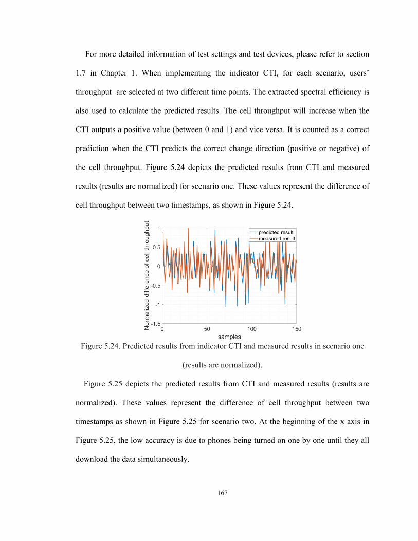
167

For more detailed information of test settings and test devices, please refer to section

1.7 in Chapter 1. When implementing the indicator CTI, for each scenario, users’

throughput are selected at two different time points. The extracted spectral efficiency is

also used to calculate the predicted results. The cell throughput will increase when the

CTI outputs a positive value (between 0 and 1) and vice versa. It is counted as a correct

prediction when the CTI predicts the correct change direction (positive or negative) of

the cell throughput. Figure 5.24 depicts the predicted results from CTI and measured

results (results are normalized) for scenario one. These values represent the difference of

cell throughput between two timestamps, as shown in Figure 5.24.

Figure 5.24. Predicted results from indicator CTI and measured results in scenario one

(results are normalized).

Figure 5.25 depicts the predicted results from CTI and measured results (results are

normalized). These values represent the difference of cell throughput between two

timestamps as shown in Figure 5.25 for scenario two. At the beginning of the x axis in

Figure 5.25, the low accuracy is due to phones being turned on one by one until they all

download the data simultaneously.

168

Figure 5.25. Predicted results from indicator CTI and measured results in scenario two

(results are normalized).

Table 5.6: Prediction accuracy for each scenario and correlations between predicted

results and measured data.

Scenarios Accuracy Correlation

Scenario one 0.86 0.9

Scenario two 0.78 0.49

Table 5.6 lists prediction accuracy and correlations with measured data. It indicates

that scenario one has better results than scenario two when UEs have better RF

conditions. The overall accuracy of the indicator is acceptable.

The usage of indicator SGIR is demonstrated in Chapter 6.

5.4.4 Discussion

Not much reseach is about modeling of the actual HetNet traffic according to litreature

reviews. The author developed a walk test simulation model for a real-world LTE-A

wireless network in [53]. However, this simulator is only about two sectors of a macro

cell and is not about HetNets. In addition, the MAE of the predicted results from the

developed model in this chapter is reduced by 25% in comparison to the model in [53].

169

Furthermore, this traffic model has more practical indicators such as CTI, fairness of cell

throughput and much more. Other models in literature [83] [82] are generic theoretical

models that are tough to be exactly applied into actually deployed networks. Literature

[134] and [83] calculated the downlink data rate using the log function, which apparently

overestimate the user throughput. The author in [35] derived the expression of mean user

throughput, however, the number of RBs allocated to the user is required for the

calculation of data rate and is not provided by the author.

Figure 5.26. Predicted throughput by equation in [35] (throughput 1) and by the method

of the thesis (throughput 2), and measured throughput.

Assuming the number of utilized RBs is known, Figure 5.26 presents predicted

throughput (throughput 1) by the equation in [35] and by equation (5.6) with extracted

SE (throughput 2). The method in this thesis reduces the MAE by 28% in comparison to

the equation in [35]. Thus, the generated model of this chapter is more accurate and

complete.

170

Figure 5.27. SINR from the iBwave simulation for one sector case.

Figure 5.28. DL throughput from the iBwave simulation for one sector case.

In addition, iBwave that is a powerful tool for in-building wireless design planning is

utilized to simulate the one sector case deployment in the thesis. The SINR and

achievable throughput are generated from the simulation, as shown in Figure 5.27 and

Figure 5.28, respectively.

Figure 5.27 and Figure 5.28 show that predicted SINR is higher than 32 dB, and

achievable throughput is 112.1 Mbps, which are both much greater than the actual results.

This software also cannot provide user information. Thus, the developed model of this

chapter is more precise and complete.

171

5.5 Conclusion

In this chapter, the development of a traffic model is presented with the data from an

actual LTE-A HetNet environment. The model contains user information, RF

propagation models, layouts of buildings, a scheduler of resource allocation,

performance indicators, etc. The model results indicate that the predicted results are

more accurate than the models in certain literature. For estimating indoor user traffic, the

mean RMSE is less than 8 Mbps. Many factors contribute to the inaccuracy of predicted

results. For example, user behaviors are confidential information that cannot be

publicized. Complicated radio wave conditions and multipath fading also reduce the

accuracy of the predictions. Many hidden information (e.g., spectral efficiency in the

actual environment) can be extracted from the measured data as shown from Chapter 3.

The methodology of building the model can also be implemented and extended to build

models for other locations. This model can not only predict user throughput for network

planning and estimating the limits of networks, but also be used for optimization.

172

Chapter 6

Increasing Cell Throughput and Network

Capacity in a Real-world HetNet

Environment

This chapter is structured as follows: Section 6.1 introduce the contents of the chapter.

Section 6.2 introduces the target problem. The algorithm is presented in Section 6.3. The

results of simulation and measurement are displayed in Section 6.4. Section 6.5

introduces the two schemes for a real-world network. Section 6.6 presents the discussion

section. Finally, conclusions are introduced in Section 6.7.

6.1 Introductions

In this chapter, a novel algorithm is proposed to increase the indoor cell throughput in a

small cell indoor environment. The algorithm combines k-means clustering and cell-

splitting technique. Instead of solely using k-means clustering to cluster locations of both

users and small cells, an indicator is assisted to help identify potential antennas that are

useful for increasing cell throughput. Simulations are performed using a developed LTE-

A model taking into the consideration of different distributions of users. In addition, a

series of data collections for verifying the developed algorithm is performed in a real-

world LTE-A HetNet. The simulation results indicate that this proposed algorithm can

boost cell throughput of the whole system by up to 43% compared to the initial setting of

directly using cell-splitting. The results of the measured data show that the algorithm can

improve the cell throughput of the hotspot by about 36% in terms of basic cell-splitting

173

settings. This algorithm will be beneficial for the network when it does not have enough

capacity for users in small cell environments.

To the best of the author’s knowledge, limited research in the past focused on the real-

world HetNet environments and explored the cell-splitting method to increase

throughput. Therefore, a new algorithm is proposed for cell-planning and increasing

LTE-A HetNet cell throughput in this section. The algorithm is based on k-means

clustering and cell-splitting techniques to increase network cell throughput. The

effectiveness of the algorithm is validated not only by simulations but also by measured

data from a real-world LTE-A HetNet environment. In addition, two useful schemes are

considered to increase the network throughput for the physical LTE-A network.

The main contributions of this chapter are as follows:

1. An algorithm for cell-planning and increasing user downlink throughput is

proposed. Both simulation model results and actual measured data justify that the

algorithm can enhance cell throughput of overall networks by 36% - 43% in

comparison to the k-means clustering method. The data is collected from a real-

world small cell indoor environment.

2. Two schemes are proposed to increase cell throughput by enabling ABS and

deploying new bandwidth for neighboring cells in a real-world LTE-A HetNet

environment. The performance of the two schemes is evaluated by implementing

them in the actual environment. The effect of ABS in the real-world LTE-A

network is studied. The collected data indicate that both schemes are beneficial to

improve the cell throughput of a hotspot in the physical world.

174

3. Different scenarios of users’ locations are analyzed in the simulation model. By

incorporating user’ location, the simulation results indicate that the developed

algorithm is practical and valuable for cell-splitting and increment of cell

throughput.

This work will not only be useful for the 4G networks, but it will also be beneficial for

the 5G networks with ultra-dense small cells deployments in the future [135, 136].

6.2 System modeling and problem formulation

6.2.1 Cell layout of the HetNet and simulation model

Data collections are conducted in a real-world LTE-A HetNet that is deployed on the

University of Regina campus. Figure 1.9 shows a picture of the HetNet map. A macro

cell is located at the rooftop of the library, and some small cells (pico cell remote

resource units (pRRus)) are installed inside the building, as shown in Figure 1.9.

Multiple carriers (2850 MHz, 2150 MHz, etc.) are deployed on the macro cell, whereas

2150 MHz is used for the small cells inside the building.

Figures 1.11 and 1.12 depicts the layout of 28 Huawei LampSites (pRRus), which are

distributed inside the building on the first floor and second floor. There are two types of

antennas: directional antennas and omnidirectional antennas. Four directional antennas

are installed inside a gymnasium (which can accommodate more than 300 people) as

displayed in Figure 1.12 on page 21.

The simulation model is developed according to the ray-tracing rules, geometrical

optical (GO), and uniform theory of diffraction (UTD) which can accurately predict user

received Reference Signal Receive Power (RSRP). Proportional fair (PF) scheduler is

implemented in the simulation model.

175

6.2.2 Problem formulation

Small cell deployment is playing significant roles in wireless communications as

mentioned in [135]. Thus, it is essential to boost the UE’s data rate and cell throughput in

the small cell environment. In cellular networks, the average cell throughput, which is

the aggregate of the individual UE’s data rate, is one of the most significant theoretical

measures that can better represent actual base station performance in a commercial

network [52, 98].

For the baseline (one sector) setting (all the small cells in Figure 6.2 are using the

same bandwidth and share only one common physical cell ID), the resource blocks (RBs)

are limited, and the system cannot meet user demands when there are over limited users

over capacity inside the building especially in the gym. For example, if more users inside

the gym download data simultaneously from the cellular network with 100% PRB

utilization, users in other locations will be devoid of resources. Hence, this section aims

to increase the cell throughput of the whole networks inside the building.

The proposed method aims at finding appropriate allocations of the small cells into

proper cell IDs so that maximum cell throughput is achieved for the overall network.

The initial plan is to split the four directional antennas in Figure 1.12 into two sectors,

as mention in section 1.7 (two sector case) resulting in 3 cells (three sector case) in the

system (as shown in Figure 1.13). However, the previous data collection from the gym

does not exhibit a reasonable result of cell throughput for cells inside the gym, as

mentioned in section 3. Even though the whole network throughput increased by 30 - 40

Mbps, the throughput inside the gym reduced from 140 Mbps to 90 Mbps.

The optimization problem can be formulated as:

176

arg max ( )j j,c

c C j Jc

M U R

=

where M is the local optimal cell association set of the small antennas in terms of

different cell IDs. It contains the cell IDs for each antenna. C is the number of the cells.

Jc is the user set of cell c. ( )j j,cU R is a utility function of user j in cell c.

Manipulating the memberships of 28 small cells (as shown in Figure 1.12) to have the

right cell ID numbers can be time-consuming. It is exhausting and costly to try all the

small cells one by one. Thus, an algorithm is necessary to help network designers

properly plan cell splitting and assist them in installing new antennas in the right

locations. The newly developed algorithm for finding proper cell ID for each small cell

is introduced in the next section.

6.2.3 Deciding the number of sectors (value of the k) and initialization

of k centroids for k-means clustering

The number of clusters, k, should be decided by network operators. As it is a common

belief that using the cell-splitting technique would increase cell throughput, but it will

also bring more interference. The developed algorithm aims to increase cell throughput

based on k-mean clustering.

The initialization method of k centroids for clusters is from [137]. The method can be

described as follows:

Step one. Calculate the center location, 0c , of the data set m= (xi, yi) as

0

1

1 n

i

i

c mn =

= ( n is the total number of points).

Step two. Convert all the data set into polar coordinate in terms of the center point 0c .

177

Step three. Divide the angle (2pi) of the polar coordinate into k sectors equally.

Calculate the centroids of each sector using the data points within each sector.

After generating the k initialized centroids, they can be utilized for the k-means

clustering.

6.3 Introduction to the algorithm

In this section, a new algorithm for cell-planning and increasing cell throughput is

proposed. It is based on k-means clustering and has an important indicator: aggregate

signal to generated interference ratio (SGIR) to select whether to add surrounding

neighboring small cells into the target cell ID (the network whose throughput we want to

boost).

6.3.1 Introduction to the k-means clustering method

K-means clustering is a popular method to cluster data into k different clusters [86, 97].

McQueen proposed the algorithm in 1967 and it is one of the most prominent algorithms

in machine learning because of its simplicity [97]. In this study, the k-means clustering

is utilized to cluster the user locations, then locations of small cells are grouped based on

the centroids of user clusters. The value of k should be known in advance before

applying the algorithm. The k-means clustering is performed in four main steps [97, 138]:

1. K random positions are typically selected for the k clusters as the centroids of

each cluster.

2. Calculate the distance between each element in the data and the centroids and

allocate each element into different clusters with minimum Euclidean distance.

3. Recalculate the new centroids for each cluster after the assigning in step 2.

4. Repeat the calculation and assignment in step 2 and step 3 until there is no

178

change in the centroids.

6.3.2 Introduction to the indicator (SGIR)

As proposed in [89], generated interference (GI) is represented as a sum of interference,

which is produced from one small cell to its surrounding non-served users. For more

detailed information of SGIR, please refer to 5.3.6 Chapter 5 on page 168.

6.3.3 Introduction to the cell-planning algorithm

According to the observations in the campus and literature reviews, the spatial

distribution of users and small cells greatly impacts the system’s performance. When

cells are deployed at the center of the cluster of users, better throughput performance will

be achieved. In addition, users at the cell edge will always be a burden for the network

due to the low PRB utilization efficiency. Thus, it is consequential to properly place the

small cells according to the user’s spatial distribution. Furthermore, in the physical world,

installing small cells at ideal locations may be difficult or costly. Sometimes, once the

layout of small cells is conducted, it is inconvenient to change. Therefore, an algorithm

is necessary to increase cell throughput.

For the algorithm, when all the small cells’ locations are fixed, the cell ID is decided

by using k-mean clusters for those small cells and users. To increase the cell throughput

of the whole network, the surrounding neighboring cells should be evaluated according

to the SGIR one by one, and the cell with a higher value of SGIR should be incorporated

into the target cell ID. The algorithm 1 depicts how it works to increase cell throughput.

The algorithm assumes that each small cell has information about how many users it is

serving. The algorithm is described below.

Algorithm 1:

179

Input: clustering number k (the number of sectors), user locations, and small cell

location information

Output: Membership of small cells for cell IDs (1~k): M

1: Initializing k centroids for k-means cluster using the method as mentioned in

section D

2: Performing clustering of user locations using the k centroids in line 1.

3: Using the k centroids from clustering results of user locations as fixed centroids of

small cells

4: Allocating small pico cells into the user cluster that has the closest distance from

the centroid of the cluster to the small cell. Get the membership M according to

the cell ID of each small cell.

5: Finding the edge small cells

6: Calculating SGIR for edge small cell i where i=1, 2, …w

7: S=sort SGIR in ascending order

C= set of cell IDs of the edge small cell i in S

If C contains more than one cell ID, select the cell ID c that has the minimum

mean

SGIR

8: for i= 1 to w (the number of selected small cells in C) do

if SGIR(i) < mean SGIR of S(cell ID ==c)

9: get small cell ID from S corresponding to the value of SGIR

10: incorporate the cell ID of small cell m into target network

end

180

Update M

11: end

12: return M

It is noticeable that only antennas with the same cell ID should be selected to change

their ID as indicated in line 7, when more than one cell IDs exit among selected

antennas. By applying algorithm 1, a lesser number of small cells are used to calculate

throughput in the simulation model, which significantly reduces computation (because

only certain cell edge small cells are evaluated by the metric), and accurate small cell ID

results are found based on the user distribution.

6.4 Simulation and measurement results


clustering number is 2 (k=2).

To verify the effectiveness of the proposed algorithm, various types of scenarios are

simulated. Scenario 1: two clusters of cells. Scenario 2: two clusters of cells (different

user and antenna locations). Scenario 3: three clusters in a practical case. Scenario 3

listed will also assist in solving the problem mentioned in Section 6.3.2 (increasing the

cell throughput in the gym for three sector cases, as shown in Figure 6.3). The simulation

181

model is utilized to calculate user throughput. The system parameters are listed in Table

1.2 in Section 1.8.1 Chapter 1. 68 users are generated in the simulation.

6.4.1 Applying the algorithm to scenario one inside the building

Figure 6.1 depicts the locations of users and small cells within the Kinesiology Building

on the campus. The rectangles represent layouts of rooms. It depicts centroids of users,

and small cells are very close to each other as mentioned in scenario one. Users and

small cells are clustered into two groups.

Table 6.1: Simulation results for scenario one under different cell load levels

Low Interference Level High Interference Level

Settings Total Cell throughput

(Mbps)

Total Cell throughput

(Mbps)

Initial settings (by k-

means) 189.5 145.4

After adjusting Cell ID 190 163.7

Table 6.1 shows simulation results after using the algorithm by incorporating cluster

edge cells into the cluster for two different interference levels. Users will get lower SINR

values when it is in high interference mode and vice versa. The edge cells are marked by

circles (with numbers) in Figure 6.1. The indicator of SGIR works better in both the high

interference and low interference model. The maximum cell throughput can be increased

by 18.3%. A smaller value of SGIR tends to indicate that overall cell throughput will be

increased more by turning the cell ID into neighboring cell ID. Sometimes, a higher

value of SGIR also brings a higher throughput and it may potentially be due to the

complicated actual path-loss environments.

182

6.4.2 Applying the algorithm to scenario two inside the building.

Figure 6.2 represents a situation when user cluster centroid is not covered by small cells.

The neighboring small cells (marked with blue circle) are merged into the target cell ID

with yellow users one by one.


clustering number is 2 (k=2).

Table 6.2: Simulation results for scenario two under different cell load levels


Settings Total Cell throughput (Mbps) Total Cell throughput (Mbps)

Initial settings

(by k-means) 196.7 153.4

After adjusting

Cell ID 221.8 176.7

Simulation results are listed in Table 6.2. Cells with a lower SGIR value will facilitate

higher cell throughput for the system. Thus, allocating the same cell ID to these small

cells is more beneficial to the system. But, sometimes, the accuracy is lowered in case of

high interference, which is impacted by the number of users served by the edge cells as

183

well. Comparing Figure 6.1 and Figure 6.2, it illustrates that installing small cell groups

close to the center of user clusters will yield more benefits, as explained in section 6.4.3.

6.4.3 Applying the algorithm to scenario three inside the building


clustering number is 3 (k=3) for three sector case in scenario three.

For scenario 3, the surrounding small cells are identified and then merged into the

target cell ID. The user spatial distribution is generated by daily historical data from the

network service provider. The user location information is extracted by 50 m X 50 m

bins. More users are also added inside the gym to simulate the hotspot. As mentioned in

the previous section, the goal is to increase the throughput of cell 2 and cell 3 since the

majority of games happen inside this gym. Figure 6.3 depicts different clusters of users

and small cells. The blue color represents the users served by cell 2, whereas the yellow

color represents users served by cell 3.

The detailed procedures of applying the algorithm are described as: primarily, using k-

means clustering to cluster the small cells into two groups. The directional antennas of

cell 2 and cell 3 with other pRRus (outside the gym and on the second floor of the gym)

are clustered into group one. Small cells in the cluster one except cell 2 and cell 3 are

184

evaluated according to the value of SGIR. Afterwards, allocating them to cell 2 or cell 3

depending on the shortest distance between the small cell and the target cell.

Table 6.3: Simulation results for scenario three


Merging

Cell ID SGIR Cell throughput (Mbps) SGIR

Cell throughput

(Mbps)

Initial setting - 256.9 - 167.1

Merge antenna 1’s ID 0.19 260.5 1.97 171.0







Table 6.4: Simulation results for scenario three


Setting Cell throughput (Mbps) Cell throughput (Mbps)

Initial settings (designer

specifying) 210.2 125.77

After adjusting Cell ID 302.7 190.57

Table 6.3 lists calculated SGIR and simulation results of cell throughput by merging

the neighboring cells one by one in detail. It shows that small cell IDs 3-5 gave the best

results after merging them into cell 2 and cell 3. The location on the second floor of the

gym is responsible for the lower cell throughput of small cell 1 and 2. These small cells

have minimal positive impacts on the throughput of users inside the gym due to user

distributions and building structures (verified by the previously measured data in Chapter

3). Thus, the users’ surroundings should be considered while implementing this

algorithm.

185

Table 6.4 lists simulation results of cell throughput after directly applying the

algorithm. The cell throughput increased by about 90 and 65 Mbps for the low and high

interference levels, as shown in Table 6.4.

6.4.4 Using measurement data to verify the algorithm results for

scenario three inside the building

Since small cells 3 to 5 (shown in Figure 6.4) can increase the throughput of the gym as

validated by the simulation results in Table 6.4, an additional measurement test is carried

out in the actual location to verify the simulation results. Instead of merging small cell 3

to 5 into the cell 2 and cell 3 inside the gym, they are turned off due to the physical

restrictions of the environment. Turning off these antennas can be viewed as lower

bound for increasing the system throughput because interference is reduced from these

neighboring cells. It can be observed that only a few users are strongly impacted by

small cell 3 to 5 (where hallways are there). Furthermore, the bandwidth of neighboring

cell 1 as shown in Figure 1.13 is reduced to 10 MHz because few people will

exhaustively use the resources of cell 1 according to the daily observations (about 20%

PRB utilization).

Table 6.5 shows measurement results from the phones and compared with the old test

results (without turning off surrounding small cells) in three sector cases. Table 6.5

shows that the combined cell throughput of cell 2 and cell 3 is increased by about 29

Mbps. The cell edge users inside the gym like phone D and E will get higher SINR by

turning off the neighboring cells as marked in Figure 6.4. The measurement data verified

that the proposed algorithm is reasonable and useful to increase local cell throughput for

the network. In the meantime, 94% of PRBs are available to the users outside of the gym.

186

Table 6.5: Measurement results from phones and database

Test type Cell ID

Cell throughput

(Mbps) Mean SINR on

trajectory I and J

PRB

utilizations Individual Sum

Turning Off

Small Cells

Cell 1 - - 6%

Cell 2 57.4 108 9.1 dB

98%

Cell 3 50.6 98%

Without

Turning Off

Small cells

Cell 1 35 -

Cell 2 40 79 5.3 dB

-

Cell 3 39 -

6.5 Two schemes for increasing real-world indoor cell throughput

6.5.1 Introduction to the schemes

Figure 6.4. Small cells in circles that are turned off for increasing cell throughput inside

the building.

As shown in Table 6.6, cell 1 is assigned a new 15MHz bandwidth for scheme 1 (test

1 and test 2), and the bandwidth of cell 1 is reduced to half by turning off three pRRus

for the scheme 2 (test 3 and test 4) as shown in Figure 6.4. The impact of ABS on the

network is evaluated in the tests as well. Moreover, artificial load (making 80% PRBs of

cell 1 transmitting power) is enabled on cell 1 in test 4 to increase interference level for

187

users that are served by cell 2 and cell 3 since these three cells are utilizing the same

bandwidth (10 MHz common bandwidth).


Scheme Test

number

Channel in each

cell and bandwidth ABS on the cell 2 Small cells

Scheme

1

1

Cell 1-2325 (15

MHz)

Cell 2-2150 (20

MHz)

Cell 3-2150 (20

MHz)

No ABS

N/A

2 With ABS

Scheme

2

3

Cell 1-2150 (10

MHz)

Cell 2-2150 (20

MHz)

Cell 3-2150 (20

MHz)

No ABS Turn off pRRus

as marked in

Figure 6.8. 4

With ABS,

Artificial Load on

Cell 1

The same data collection procedures are applied for the two schemes.

6.5.2 Measurement results of the two schemes

The measurement results for the data collection activities are summarized in Table 6.7.

The table represents the mean SINR of each phone, mean SINR per cell edge user, total

cell throughput of cell 2 and cell3, and PRB utilization of each cell. Furthermore, the

results for increasing cell throughput are compared with the data from previous tests (3

sector baseline deployments), as shown in Figure 1.13. Table 6.7 demonstrates several

observations: firstly, both practical schemes work very well for improving cell

throughput and reducing interference from neighboring cell 1. Mean user SINR is

increased from 7 dB to 10 dB. Mean cell edge user SINR is improved from 1.1 dB to 7.3

dB. The cell throughput has grown from 79 Mbps to 123 Mbps inside the gym.


188

Tests Mean user / cell

edge SINR (dB)

Number of

connected

phones

Cell

throughput

(Mbps)

PRB

utilization

Previous

test 7.0 1.1 10 79.3

cell1 -

cell2 -

cell3 -

Test 1 9.3 5.2 10 109.5

cell1 7%

cell2 93%

cell3 92%

Test 2 10.2 7.3 8 109.1

cell1 94%

cell2 79%

cell3 91%

Test 3 8.9 4.7 11 108.3

cell1 5%

cell2 98%

cell3 98%

Test 4 7.8 3.3 11 123.8

cell1 6%

cell2 86%

cell3 98%

Secondly, the ABS (10% of the total PRB utilization) that is activated on cell 2 makes

0.15 dB decrease of SINR on phone F, G, and H, which are served by cell 3 in test 1 and

test 2. But, the mean SINR of phones A, B and C change from 13.1 to 11.8 dB from test

1 to test 2 (data are not presented here). After checking the PRB utilizations of cell 2

(79%) and cell 3 (91%), it is observed that blanking certain subframes of cell 2

completely exposes other PRBs to the interference from cell 3 (91% of PRB utilization).

It also indicates that the effect of ABS varies at different times depending on how the

scheduler allocates the RBs in the dynamic network due to the presence of moving

phones.

Thirdly, deploying new bandwidth in tests 1 and 2 increases mean cell edge user

SINR about 4 - 5 dB. However, turning off the neighboring small cells brings relatively

189

the same effect for the system. Even when there is the artificial load in test 4, the cell

throughput achieves the maximum value of 123.8 Mbps which is almost identical to the

simulation results.

Lastly, the mean user SINR is not a good indicator to measure the variation of cell

throughput. As shown in Table 6.7, the higher SINR does not guarantee higher cell

throughput compared with the previous tests. This is because the number of cell-edge

user users and RB allocations are different in different tests. The percentages of

aggregate throughput over total cell throughput are 44% and 59% for cell center users in

test 3 and test 4, respectively.

6.6 Discussion

According to literature reviews, minimal research has been conducted to study real-

world LTE-A networks. The author in [10] utilized weighted k-means clustering for cell

planning; however, the user demands are difficult to obtain in the practical. Cell-splitting

was analyzed in [139] based on active antennas. Different scenarios were simulated by

only adjusting different sizes of beams and antenna tilts. Instead of cell deployment, this

study aims to increase the total network throughput based on the k-means clustering. The

proposed algorithm is to further increase cell throughput in terms of user locations. Very

limited literature has considered iteratively deciding the association of small cells.

In addition, a smaller value of SGIR tends to indicate that the overall cell throughput

will be increased more by turning the cell ID into neighboring cell ID. Sometimes, a

higher value of SGIR also brings a higher throughput, maybe because of the complicated

actual path-loss environments. The algorithm works very well when more users are

presented as shown in scenario three.

190

According to the simulation results, the algorithm works well and can help the

network system to find potential neighboring cells that increase the cell throughput. The

algorithm’s main objective is to improve the SINR of cell edge users according to the

user distribution. With the help of k-means clustering technique, user distributions, and

small cell distributions, the proper cell-splitting for small cells is achieved.

Measured data in the walk tests also validate that deploying new bandwidth is

beneficial to increase users’ SINR, but it will also utilize more frequency resources and

increase the cost for network operators. With the isolation of building structures, more

cell deployment can enhance cell throughput and provide users with satisfying services.

For example, the maximum cell throughput is less than 150 Mbps for one cell, but it is

more than 150 Mbps when there are three cells inside the building. Properly turning off

neighboring cells reduces certain levels of interference. If these neighboring small cells

are utilized by users causing high PRB utilizations, it will generate interference and

reduce SINR for users connected to the main cells. Furthermore, the increased PRB

utilization will be detrimental to the spectral efficiency of the neighbor cells [111].

At last, signaling overhead of the system is reduced compared with typical load

balancing algorithms that offload cell-edge users to neighboring cells in HetNets. This is

because the number of small cells is always lower than the number of cell edge users

during high load status in the network with dense small cells.

6.7 Conclusion

In this chapter, an algorithm for increasing cell throughput of LTE-A HetNet is

proposed. The algorithm is based on the k-means clustering. With an indicator, potential

small cells, which can increase the cell throughput are identified. The algorithm helps to

191

identify the allocations of cell ID for small cells. Computation cost is reduced with the

help of the clustering technique. The algorithm improves cell throughput according to

the simulation and measurement results.

Furthermore, two different plans are proposed to increase the cell throughput of the

deployed LTE-A network inside the building with three cells. The measurement results

show that the proposed schemes raise the cell throughput about 30 - 40 Mbps. Moreover,

the impact of enabling ABS (10% of PRB utilization) on the full buffer loaded cells is

negligible. Studying real-world networks will not only decrease the gap between

theoretical studies and applications, but also provide a better understanding of practical

HetNets. The algorithm can also be beneficial for 5G networks that contain multiple

small cells.

In the future, modeling of user traffic and load balancing strategies in a real-world

LTE-A HetNet will be focused.

192

Chapter 7

Conclusions

7.1 Summary

LTE-A HetNets has the benefits of maximizing network capacity, increasing user

throughput and enhancing well-covered signal strength for users. HetNets deploy

network densification (multiple types of small cells) to boost network capacity, increase

coverage areas and shift loads to improve network services. However, increased cells

from different layers will bring interference to each other in the co-channel bandwidth

deployment. Thus, many important features (e.g., ABS, eICIC, etc.) are defined in the

LTE-A that are intended to mitigate interference and increase mean user throughput. The

benefits of LTE-A HetNets have been explored widely by different types of models.

However, most literature about HetNets focuses on pure theoretical analysis or

formulated based on idealized simulation models (e.g., hexagonal cell or full buffer, etc.)

for simplicity and mathematical tractability. Only a few researchers have had access to

evaluate and study the real-world HetNet environments in depth. These theoretical

models provided results that are significant in indicating the upper bound of the networks

and revealing the potential of new technologies. However, network operators may

overestimate the performance of the HetNets generated by these models, and the

theoretical analysis are not practical for the applications (e.g., network designing) in real-

world environments. Thus, a traffic model that can predict relatively accurate user

193

throughput and user SINR with practical indicators is necessary not only for correct

network planning but also for better user experience.

In this thesis, the deployed LTE-A HetNet at the University of Regina has been

investigated in detail. Multiple data collection activities are completed. The performance

of measured data from Splunk and test devices are analyzed. A traffic model is

developed using measured data from a real-world HetNet. This model can predict user

DL throughput and capture parts of the actual characteristics of the current environment.

The accuracy of predicted results is high. The maximum RMSE of SINR and mean user

throughput are 0.9 and 8.3, respectively.

The data from Splunk and the measurement of the HetNet are investigated in detail in

Chapter 3. The data from the actual HetNet present many new insights. The analysis

results show that different aggregate data (e.g., aggregate throughput, mean CQI, etc.) of

each cell has different patterns. These patterns are related to users’ locations and

behaviors, and they vary on a daily basis. The peak cell throughput tends to appear

around the time when classes are scheduled in the building. The indoor environments

have shown to achieve a better mean CQI in comparison to the outdoor due to the

building structures shields the interference from outside. Though the cell throughput

seems unpredictable, polynomial chaos expansion can be utilized to model the mean cell

throughput. Based on the analysis of Chapter 3, this model is proven to be accurate, and

the RMSE of throughput is around 5.

To further enhance the understanding of the mechanism of the actual LTE-A HetNet, a

series of data collection activities are conducted at the University of Regina as

introduced in Sections 3 - 5 Chapter 3. For the HO tests, data are collected by the RF

194

scanner at different doors of each building for multiple times. By adjusting HO system

parameters, the analyzed results show that the actual environment produces a more stable

outcome than the simulated settings in literature reviews. The HO failure rate and the

throughput of each test are always higher than 95% and 3 Mbps, respectively. It is

noticeable that the performance (e.g., measured RSRP, handover location changing, etc.)

of HO exhibits different patterns for different doors. Thus, network designers should

consider the actual environment of each door while setting the optimized parameters.

Multiple downloading tests are carried out to evaluate the performance of low power

base stations of the HetNet in a gym inside a building in Chapter 3. Higher modulation

schemes, cell-splitting, ABS, etc. are all investigated in the LTE-A HetNet. All

important data related to the network users are recorded when these small cells are

operated as one, two, and three sectors with 20 MHz co-channel bandwidth. The

measured results indicate that the actual network is a highly dynamic system and is more

complicated than the idealized simulation models. The actual network has a type of PF

scheduler that maintains a good trade-off between cell throughput and the fairness of

resource allocation. The analysis presents that 256 QAM modulation has fewer

improvements on cell throughput when the mean SINR is below 30 dB. Moreover, when

the indoor small cells are operated as two sector case, it has better SINR and higher cell

throughput inside the gym. Even though three sector case brings lower SINR, the cell

throughput of the overall networks is increased by a minimum of 50 Mbps. Thus, the

results demonstrate that network densification is quite useful for increasing network

capacity and total cell throughput.

195

The performance of ABS is also evaluated in the tests in Chapter 3. Results show that

the impact of ABS is evident when the interference is high in the network. However,

solely using the mean SINR and cell throughput is not an effective measure for the

impact of SINR. As the system is dynamic and cell edge users switching to neighboring

cells periodically, the interference level is different due to distributed neighboring small

cells. Therefore, the mean SINR and cell throughput varies in different tests. The

analysis presents that ABS is useful for both two sector case and three sector case. It is

noticeable that the data rates of some phones are throttled by network providers during

the tests. The actual results should be slightly better than the measured results. Moreover,

the issue of the small cell on/off is investigated in this thesis. Two neighboring small

antennas (pRRus) that are on the second floor of the gym are turned on and off during

the test of three sector case, respectively. Results indicate that the performance of the

cells inside the gym is worse than it is when the two pRRus are turned on. A possible

explanation to this phenomenon is that the interference from neighboring indoor cells is

increased due to this shift.

To explore a practical solution to increase the indoor capacity and throughput, inter-

frequency deployment in the actual installation of LTE-A HetNet was studied in detail

and presented in Section 5 Chapter 3. A series of data collection tests were conducted to

measure the performance of deploying split bandwidth and enabling ABS for a three-

sector case cellular configuration.

The measured results show that using non-overlapped bandwidth will reduce the

interference and increase SINR by about 80% at the cost of reduced cell throughput. In

addition, enabling the ABS on cell 2 helps increase the throughput of cell 3 that receives

196

the strongest interference from cell 2 (cell 2 and cell 3 are both inside the gym). After

splitting bandwidth, the mean CQI is increased from 8 to 11, but the mean PRBs

allocated to each phone is reduced. If there were more available PRBs that could be

allocated to users and the network providers did not throttle certain phones’ throughput,

the throughput would increase significantly. Thus, the actual results should be larger than

the measured data. Overall, the system’s performance improves with splitting of

bandwidth due to the decrease in co-channel interference which is the major contributor

to poor network performance. This valuable data collection test indicates that the

proposed strategies can be obtained only when taking into account all characteristics (the

number of users, cell center and cell edge users, neighboring cell load information, etc.).

Following the summary of Chapter 3, Chapter 4 presents the evaluation of the

scheduler’s performance that is installed on the actual system. The results show that this

scheduler is one type of PF scheduler and the measured data indicate parts of

characteristics of PF scheduler. The scheduler also maintains a high fairness value of

resource allocation. The performance of PF scheduler, GPF, and SINR-based scheduler

are also evaluated. Results indicate that the GPF scheduler can predict more accurate

results compared with measured data. Most literature evaluates schedulers via simulation

models that are not practical. Studying the actual scheduler is not only beneficial for

better understanding the real-world HetNets, but also for accurately predicting user

throughput. As a result, an innovative scheduler is proposed using PF scheduler and

control theory to reform the PF scheduler in Chapter 4. A kind of PI controller is utilized

on the scheduler during allocation of RBs. Simulation results indicate that this scheduler

can maintain a fixed fairness value (a threshold set by network operators) of resource

197

allocation. The network operators can set specific fairness values to better adjust the

networks.

A traffic model of the actual LTE-A HetNet is developed and introduced in Chapter 5.

This model is built using a combination of algorithms and measured data. The model

includes signal strength data, user related information, scheduler, and some other

important indicators. The development of propagation models is the first step for

building the traffic model. An effective propagation model is not only useful for

accurately predicting radio signal strength, but also beneficial for network planning in

wireless communication systems. UEs’ received signal strength are predicted with rules

of ray-tracing and tuned by least mean squares. The results show that the predictions are

accurate and improves with tuning. The propagation models of both indoor and outdoor

environments are introduced in this thesis. A modified version of PF scheduler is also

introduced based on the information about the actual network. This scheduler considers

characteristics of QoS as defined in 3GPP. Predictions from the traffic model indicate

that the developed model can predict user throughput within the coverage of the HetNet

with low errors (around 1 dB and 8 Mbps for SINR and throughput, respectively).

Furthermore, the mean SINR does not correctly reflect the change of cell throughput

as indicated by the measurement mentioned in Chapter 3. Hence, an indicator (i.e., CTI)

is proposed to predict cell throughput variation solely using the values of each user’s

SINR in Chapter 5. The accuracy of the indicator is around 70% - 80% by implementing

the measured data from the walk tests in the indoor small cell environment. This

indicator will be beneficial for cell planning and estimating cell throughput. The network

designers will save costs if they can predict the cell throughout by only using SINR

198

information and disregard actual settings. One of the other indicators (SGIR) is also

introduced for increasing cell throughput in Chapter 6, and this indicator was previously

used for tuning small cells on / off in literature. It was found that this indicator can also

be utilized to pinpoint the necessity of switching a small cell from one cell ID to another

cell ID if multiple sectors are deployed. The simulation results demonstrated that this

indicator is useful to increase cell throughput and to reflect the relative importance of an

individual antenna with good accuracy, as indicated in Chapter 6.

In summary, the real-world LTE-A HetNet at the University of Regina is studied in

detail. A series of data collection activities are conducted within the coverage area of the

network. Both the performance of handover and indoor small cells are evaluated in detail

with adjusting system parameters. The measured results of indoor small cells reveal that

the actual system is highly dynamic due to external environments such as user mobility

and channel fading on the radio links. Special attentions should be paid to cell edge users

in the HetNet. Solely enabling ABS (10% of one PRB) is not entirely effective to boost

cell throughput. The key points of modeling the user traffic are accurate path-loss

propagation models and a good approximation to the actual scheduler. This developed

traffic model and its methodology are valuable for better cell planning and enhanced user

experience. The studies in this thesis are not only beneficial for leaning real-world LTT-

A HetNets, but also for better understanding the 5G networks in the future. These

significant findings and algorithms in this thesis are favorable for improving the

performance of real-world networks.

199

7.2 Future research directions

It is recommended to focus on optimization of HetNets in the future as increasing

spectral efficiency per link will always be significant to practical applications. More

algorithms will be developed to mitigate interference in HetNets and to utilize RBs

efficiently. In addition, ultra-dense small cells and massive MIMO will be investigated in

the future [46] as these two areas both play an important role in the 5G networks.

Massive MIMO is a useful feature to increase spectral efficiency for HetNets and

future 5G networks. The beamforming can improve spectral efficiency around 100b

/s/Hz as shown in [46]. Massive MIMO also has many benefits: no extra site costs,

supporting cell-wide and inter-cell load balancing, the flexibility of signal processing,

and much more. [46]. The author in [46] demonstrates that massive MIMO can be

utilized in combination with other interference mitigation techniques. Thus, it is worth

studying massive MIMO and increasing user throughput in the future.

Ultra-dense networks will be a feasible solution to extremely increased traffic load in

the world due to the networks’ considerable benefits of short distance transmission and

co-channel deployment as introduced in [135]. The studies in this thesis have shown that

the small cell deployment has significant potential for expanding network capacity.

Increasing the number of sectors also brings more available resources for the overall

networks. In addition, coordination in the HetNets is necessary to better utilize the

resources and increase spectral efficiency. The coordination includes: user association,

interference mitigation, allocation of RBs, and much more. [135]. These aspects should

be considered with more practical applications such as overhead, complexity, etc. in

realistic network deployments.

200

Studying actual networks is essential as a significant gap exists between theories and

practical applications [128] as indicated in the results in this thesis. For modeling of user

traffic, more practical characteristics should be considered such as user behaviors, user

density, opportunistic scheduling, and so on. [128]. For performing data collections,

more detailed parameters that are directly related to the KPIs should be recorded. Many

measurements were calculated in previous literature [140] [141]. However, more

analysis should be investigated in depth to get more apparent and more accurate results.

Furthermore, due to the huge amount of data increasingly generated from exponential

connected devices, these data can be utilized by big data analysis and machine learning

methods to predict important performance indicators [142, 143]. These huge volumes of

data can also be utilized by big data frameworks and used further for self-healing

functions in the SON to maintain a certain quality of service [143]. More useful and

practical KPIs should be developed as shown in this thesis. Since KPIs represent general

behaviors of base stations, root causes of problems can be detected in the networks by

monitoring KPIs [143].

201

References

[1] C. Cox, "An introduction to LTE: LTE, LTE-advanced, SAE and 4G mobile

communications," John Wiley & Sons, 2012, p. 325.

[2] A. A. Jasim and S. A. Mawjoud, "LTE heterogeneous network: a case study,"

International Journal of Computer Applications, vol. 61, no. 8, 2013.

[3] A. Damnjanovic et al., "A survey on 3GPP heterogeneous networks," IEEE

Wireless communications, vol. 18, no. 3, 2011.

[4] M. Anas, F. D. Calabrese, P.-E. Ostling, K. I. Pedersen, and P. E. Mogensen,

"Performance analysis of handover measurements and layer 3 filtering for

UTRAN LTE," in 2007 IEEE 18th International Symposium on Personal, Indoor

and Mobile Radio Communications, 2007, pp. 1-5: IEEE.

[5] M. Anas, F. D. Calabrese, P. E. Mogensen, C. Rosa, and K. I. Pedersen,

"Performance evaluation of received signal strength based hard handover for

UTRAN LTE," in 2007 IEEE 65th Vehicular Technology Conference-VTC2007-

Spring, 2007, pp. 1046-1050: IEEE.

[6] V. N. I. Cisco, "Global Mobile Data Traffic Forecast Update, 2015–2020 White

Paper," Document ID, vol. 958959758, 2016.

[7] C. V. N. I. Cisco, "Global mobile data traffic forecast update, 2013–2018," white

paper, 2014.

[8] A. Solutions, Small Cell RF Planning and Deployment. 2016.

[9] H. ElSawy, E. Hossain, and M. Haenggi, "Stochastic geometry for modeling,

analysis, and design of multi-tier and cognitive cellular wireless networks: A

202

survey," IEEE Communications Surveys & Tutorials, vol. 15, no. 3, pp. 996-1019,

2013.

[10] D. Castro-Hernandez and R. Paranjape, "Dynamic Analysis of Load Balancing

Algorithms in LTE/LTE-A HetNets," Wireless Personal Communications, vol.

96, no. 3, pp. 3297-3315, 2017.

[11] A. Khandekar, N. Bhushan, J. Tingfang, and V. Vanghi, "LTE-advanced:

Heterogeneous networks," in Wireless Conference (EW), 2010 European, 2010,

pp. 978-982: IEEE.

[12] A. Damnjanovic, J. Montojo, J. Cho, H. Ji, J. Yang, and P. Zong, "UE's role in

LTE advanced heterogeneous networks," IEEE Communications Magazine, vol.

50, no. 2, 2012.

[13] A. Karandikar, N. Akhtar, and M. Mehta, Mobility Management in LTE

Heterogeneous Networks. Springer, 2017.

[14] V. Raida, M. Lerch, P. Svoboda, and M. Rupp, "Deriving Cell Load from RSRQ

Measurements," in 2018 Network Traffic Measurement and Analysis Conference

(TMA), 2018, pp. 1-6: IEEE.

[15] J. Acharya, L. Gao, and S. Gaur, Heterogeneous Networks in LTE-advanced.

John Wiley & Sons, 2014.

[16] K. I. Pedersen, Y. Wang, B. Soret, and F. Frederiksen, "eICIC functionality and

performance for LTE HetNet co-channel deployments," in Vehicular Technology

Conference (VTC Fall), 2012 IEEE, 2012, pp. 1-5: IEEE.

203

[17] D. Lopez-Perez, I. Guvenc, G. De la Roche, M. Kountouris, T. Q. Quek, and J.

Zhang, "Enhanced intercell interference coordination challenges in heterogeneous

networks," IEEE Wireless communications, vol. 18, no. 3, 2011.

[18] D. Carasso, "Exploring splunk," Published by CITO Research, New York, USA,

ISBN, pp. 978-0, 2012.

[19] J. S. B. Haijun Gao, Dr. Raman Paranjape, "Measurement and Analysis of Small

Cell Splitting in a Real-world LTE-A HetNet," presented at the THE ANNUAL

IEEE CANADIAN CONFERENCE ON ELECTRICAL AND COMPUTER

ENGINEERING, London, Canada, Aug 30, 2020

[20] H. Gao, J. S. Bawa, and R. Paranjape, "Analysis of Acquired Indoor LTE‑A Data

from an Actual HetNet Cellular Deployment," WIRELESS PERSONAL

COMMUNICATIONS, 2020.

[21] H. Gao, J. S. Bawa, and R. Paranjape, "An Evaluation of the Proportional Fair

Scheduler in a Physically Deployed LTE-A Network," in 2019 IEEE

International Conference on Advanced Networks and Telecommunications

Systems (ANTS), 2019, pp. 1-6: IEEE.

[22] J. S. B. Haijun Gao, Dr. Raman Paranjape, "A Fairness Guaranteed Dynamic PF

Scheduler in LTE-A Networks," presented at the THE ANNUAL IEEE

CANADIAN CONFERENCE ON ELECTRICAL AND COMPUTER

ENGINEERING, London, Canada, Aug,30, 2020.

[23] J. S. B. Haijun Gao, Dr. Raman Paranjape, "Increasing Cell Throughput and

Network Capacity in a Real-world HetNet Environment," presented at the IEEE

204

International Conference on Advanced Networks and Telecommunications

Systems 2020, Delhi,India, 2020

[24] U. Paul, A. P. Subramanian, M. M. Buddhikot, and S. R. Das, "Understanding

traffic dynamics in cellular data networks," in INFOCOM, 2011 Proceedings

IEEE, 2011, pp. 882-890: IEEE.

[25] H. Wang, F. Xu, Y. Li, P. Zhang, and D. Jin, "Understanding mobile traffic

patterns of large scale cellular towers in urban environment," in Proceedings of

the 2015 Internet Measurement Conference, 2015, pp. 225-238: ACM.

[26] N. Sadek and A. Khotanzad, "Multi-scale high-speed network traffic prediction

using k-factor Gegenbauer ARMA model," in Communications, 2004 IEEE

International Conference on, 2004, vol. 4, pp. 2148-2152: IEEE.

[27] C. Qi, Z. Zhao, R. Li, and H. Zhang, "Characterizing and modeling social mobile

data traffic in cellular networks," in Vehicular Technology Conference (VTC

Spring), 2016 IEEE 83rd, 2016, pp. 1-5: IEEE.

[28] M. Z. Shafiq, L. Ji, A. X. Liu, and J. Wang, "Characterizing and modeling

internet traffic dynamics of cellular devices," ACM SIGMETRICS Performance

Evaluation Review, vol. 39, no. 1, pp. 265-276, 2011.

[29] H. D. Trinh, N. Bui, J. Widmer, L. Giupponi, and P. Dini, "Analysis and

modeling of mobile traffic using real traces," in Personal, Indoor, and Mobile

Radio Communications (PIMRC), 2017 IEEE 28th Annual International

Symposium on, 2017, pp. 1-6: IEEE.

[30] B. Zhou, D. He, Z. Sun, and W. H. Ng, "Network traffic modeling and prediction

with ARIMA/GARCH," in Proc. of HET-NETs Conference, 2005, pp. 1-10.

205

[31] Z. Chen, B.-r. Yang, F.-g. Zhou, L.-n. Li, and Y.-f. Zhao, "A new model for

multiple time series based on data mining," in Knowledge Acquisition and

Modeling, 2008. KAM'08. International Symposium on, 2008, pp. 39-43: IEEE.

[32] H.-B. Fang, D. Deng, G.-L. Tian, L. Shen, K. Duan, and J. Song, "Analysis for

temporal gene expressions under multiple biological conditions," Statistics in

Biosciences, vol. 4, no. 2, pp. 282-299, 2012.

[33] N. Bui, F. Michelinakis, and J. Widmer, "A model for throughput prediction for

mobile users," in European Wireless 2014; 20th European Wireless Conference;

Proceedings of, 2014, pp. 1-6: VDE.

[34] O. Østerbø, "Scheduling and capacity estimation in LTE," in Proceedings of the

23rd International Teletraffic Congress, 2011, pp. 63-70: International

Teletraffic Congress.

[35] D. Parruca and J. Gross, "Throughput analysis of proportional fair scheduling for

sparse and ultra-dense interference-limited OFDMA/LTE networks," IEEE

Transactions on Wireless Communications, vol. 15, no. 10, pp. 6857-6870, 2016.

[36] K. Chang and R. P. Wicaksono, "Estimation of network load and downlink

throughput using RF scanner data for LTE networks," in Performance Evaluation

of Computer and Telecommunication Systems (SPECTS), 2017 International

Symposium on, 2017, pp. 1-8: IEEE.

[37] S. Barbera, P. H. Michaelsen, M. Säily, and K. Pedersen, "Mobility performance

of LTE co-channel deployment of macro and pico cells," in 2012 IEEE Wireless

Communications and Networking Conference (WCNC), 2012, pp. 2863-2868:

IEEE.

206

[38] Y. Lee, B. Shin, J. Lim, and D. Hong, "Effects of time-to-trigger parameter on

handover performance in SON-based LTE systems," in 2010 16th Asia-Pacific

Conference on Communications (APCC), 2010, pp. 492-496: IEEE.

[39] M. Mehta, N. Akhtar, and A. Karandikar, "Impact of handover parameters on

mobility performance in LTE HetNets," in 2015 Twenty First National

Conference on Communications (NCC), 2015, pp. 1-6: IEEE.

[40] P. Legg, G. Hui, and J. Johansson, "A simulation study of LTE intra-frequency

handover performance," in 2010 IEEE 72nd Vehicular Technology Conference-

Fall, 2010, pp. 1-5: IEEE.

[41] M. Simsek, M. Bennis, and I. Guvenc, "Mobility management in HetNets: a

learning-based perspective," EURASIP Journal on Wireless Communications and

Networking, vol. 2015, no. 1, p. 26, 2015.

[42] S. Oh, H. Kim, J. Na, and Y. Kim, "User performance impacts by mobility load

balancing enhancement for self-organizing network over lte system," in 2017

XVII Workshop on Information Processing and Control (RPIC), 2017, pp. 1-5:

IEEE.

[43] A. Lobinger, S. Stefanski, T. Jansen, and I. Balan, "Coordinating handover

parameter optimization and load balancing in LTE self-optimizing networks," in

2011 IEEE 73rd vehicular technology conference (VTC Spring), 2011, pp. 1-5:

IEEE.

[44] T.-L. Sheu and J.-Y. Sie, "A dynamic adjustment scheme in handover thresholds

for off-loading LTE small cells," in 2018 IEEE International Conference on

Applied System Invention (ICASI), 2018, pp. 180-183: IEEE.

207

[45] F. ICT-SOCRATES, "Handover parameter optimization in LTE self-organizing

networks."

[46] V. Jungnickel et al., "The role of small cells, coordinated multipoint, and massive

MIMO in 5G," IEEE Communications Magazine, vol. 52, no. 5, pp. 44-51, 2014.

[47] S. Mukherjee, "Distribution of downlink SINR in heterogeneous cellular

networks," IEEE Journal on Selected Areas in Communications, vol. 30, no. 3,

pp. 575-585, 2012.

[48] C. Wengerter, J. Ohlhorst, and A. G. E. von Elbwart, "Fairness and throughput

analysis for generalized proportional fair frequency scheduling in OFDMA," in

2005 IEEE 61st vehicular technology conference, 2005, vol. 3, pp. 1903-1907:

IEEE.

[49] R. Kwan, C. Leung, and J. Zhang, "Proportional fair multiuser scheduling in

LTE," IEEE Signal Processing Letters, vol. 16, no. 6, pp. 461-464, 2009.

[50] Y. Barayan and I. Kostanic, "Performance evaluation of proportional fairness

scheduling in LTE," in Proceedings of the World congress on engineering and

computer science, 2013, vol. 2, pp. 712-717.

[51] E. Liu and K. K. Leung, "Proportional fair scheduling: Analytical insight under

rayleigh fading environment," in 2008 IEEE Wireless Communications and

Networking Conference, 2008, pp. 1883-1888: IEEE.

[52] J.-G. Choi and S. Bahk, "Cell-throughput analysis of the proportional fair

scheduler in the single-cell environment," IEEE Transactions on Vehicular

Technology, vol. 56, no. 2, pp. 766-778, 2007.

208

[53] D. Castro-Hernandez and R. Paranjape, "Walk test simulator for LTE/LTE-A

network planning," in 2016 17th International Telecommunications Network

Strategy and Planning Symposium (Networks), 2016, pp. 56-61: IEEE.

[54] G. Piro, L. A. Grieco, G. Boggia, R. Fortuna, and P. Camarda, "Two-level

downlink scheduling for real-time multimedia services in LTE networks," IEEE

Transactions on Multimedia, vol. 13, no. 5, pp. 1052-1065, 2011.

[55] M. I. Elhadad, E.-S. M. El-Rabaie, and M. Abd-Elnaby, "Capacity enhanced

scheduler for LTE downlink system based on PF algorithm," in 2016 Fourth

International Japan-Egypt Conference on Electronics, Communications and

Computers (JEC-ECC), 2016, pp. 5-8: IEEE.

[56] N. Xu, G. Vivier, W. Zhou, and Y. Qiang, "A dynamic PF scheduler to improve

the cell edge performance," in 2008 IEEE 68th Vehicular Technology Conference,

2008, pp. 1-5: IEEE.

[57] F. Letourneux, S. Guivarch, and Y. Lostanlen, "Propagation models for

heterogeneous networks," in 2013 7th European Conference on Antennas and

Propagation (EuCAP), 2013, pp. 3993-3997: IEEE.

[58] M. Hata, "Empirical formula for propagation loss in land mobile radio services,"

IEEE transactions on Vehicular Technology, vol. 29, no. 3, pp. 317-325, 1980.

[59] C. Lee William, "Mobile Communications Design Fundamentals, John

Wiley&Sons," ed: Inc, 1993.

[60] D. Castro-Hernandez and R. Paranjape, "Local tuning of a site-specific

propagation path loss model for microcell environments," Wireless Personal

Communications, vol. 91, no. 2, pp. 709-728, 2016.

209

[61] S. Tan and H. Tan, "A microcellular communications propagation model based

on the uniform theory of diffraction and multiple image theory," IEEE

Transactions on Antennas and Propagation, vol. 44, no. 10, pp. 1317-1326, 1996.

[62] G. Liang and H. L. Bertoni, "A new approach to 3-D ray tracing for propagation

prediction in cities," IEEE Transactions on Antennas and Propagation, vol. 46,

no. 6, pp. 853-863, 1998.

[63] F. A. Agelet, A. Formella, J. H. Rabanos, F. I. De Vicente, and F. P. Fontan,

"Efficient ray-tracing acceleration techniques for radio propagation modeling,"

IEEE transactions on Vehicular Technology, vol. 49, no. 6, pp. 2089-2104, 2000.

[64] V. Degli-Esposti, F. Fuschini, E. M. Vitucci, and G. Falciasecca, "Speed-up

techniques for ray tracing field prediction models," IEEE Transactions on

Antennas and Propagation, vol. 57, no. 5, pp. 1469-1480, 2009.

[65] X. Chen, H. Wu, and T. M. Tri, "Field strength prediction of mobile

communication network based on GIS," Geo-Spatial Information Science, vol. 15,

no. 3, pp. 199-206, 2012.

[66] A. G. Kanatas, I. D. Kountouris, G. B. Kostaras, and P. Constantinou, "A UTD

propagation model in urban microcellular environments," IEEE Transactions on

Vehicular Technology, vol. 46, no. 1, pp. 185-193, 1997.

[67] B. Y. Hanci and I. H. Cavdar, "Mobile radio propagation measurements and

tuning the path loss model in urban areas at GSM-900 band in Istanbul-Turkey,"

in IEEE 60th Vehicular Technology Conference, 2004. VTC2004-Fall. 2004,

2004, vol. 1, pp. 139-143: IEEE.

210

[68] W. Tam and V. Tran, "Propagation modelling for indoor wireless

communication," Electronics & Communication Engineering Journal, vol. 7, no.

5, pp. 221-228, 1995.

[69] S. Grubisic and W. P. Carpes Jr, "An efficient indoor ray-tracing propagation

model with a quasi-3D approach," Journal of Microwaves, Optoelectronics and

Electromagnetic Applications, vol. 13, no. 2, pp. 166-176, 2014.

[70] F. S. De Adana, O. G. Blanco, I. G. Diego, J. P. Arriaga, and M. F. Cátedra,

"Propagation model based on ray tracing for the design of personal

communication systems in indoor environments," IEEE transactions on vehicular

technology, vol. 49, no. 6, pp. 2105-2112, 2000.

[71] K.-W. Cheung, J.-M. Sau, and R. D. Murch, "A new empirical model for indoor

propagation prediction," IEEE transactions on Vehicular Technology, vol. 47, no.

3, pp. 996-1001, 1998.

[72] B. Błaszczyszyn and M. Karray, "Linear-regression estimation of the

propagation-loss parameters using mobiles’ measurements in wireless cellular

network," Proc. of WiOpt, Paderborn, 2012.

[73] N. R. Zulkefly, T. A. Rahman, A. M. Al-Samman, A. M. Mataria, and C. Y.

Leow, "Indoor path loss model for 4G wireless network at 2.6 GHz," in 2015 1st

International Conference on Telematics and Future Generation Networks

(TAFGEN), 2015, pp. 117-120: IEEE.

[74] S. Hosseinzadeh, H. Larijani, K. Curtis, A. Wixted, and A. Amini, "Empirical

propagation performance evaluation of LoRa for indoor environment," in 2017

211

IEEE 15th International Conference on Industrial Informatics (INDIN), 2017, pp.

26-31: IEEE.

[75] P. R. de Freitas and H. Tertuliano Filho, "Parameters Fitting to Standard

Propagation Model (SPM) for Long Term Evolution (LTE) using nonlinear

regression method," in 2017 IEEE International Conference on Computational

Intelligence and Virtual Environments for Measurement Systems and

Applications (CIVEMSA), 2017, pp. 84-88: IEEE.

[76] Y. Wang and Q. Zhu, "Modelling and analysis of heterogeneous cellular

networks using a matern cluster process," IET Communications, vol. 11, no. 18,

pp. 2783-2791, 2017.

[77] M. Mirahsan, R. Schoenen, and H. Yanikomeroglu, "HetHetNets: Heterogeneous

traffic distribution in heterogeneous wireless cellular networks," IEEE Journal on

Selected Areas in Communications, vol. 33, no. 10, pp. 2252-2265, 2015.

[78] H.-S. Jo, Y. J. Sang, P. Xia, and J. G. Andrews, "Heterogeneous cellular

networks with flexible cell association: A comprehensive downlink SINR

analysis," IEEE Transactions on Wireless Communications, vol. 11, no. 10, pp.

3484-3495, 2012.

[79] R. W. Heath, M. Kountouris, and T. Bai, "Modeling heterogeneous network

interference using Poisson point processes," IEEE Transactions on Signal

Processing, vol. 61, no. 16, pp. 4114-4126, 2013.

[80] N. Deng, W. Zhou, and M. Haenggi, "Heterogeneous cellular network models

with dependence," IEEE Journal on selected Areas in Communications, vol. 33,

no. 10, pp. 2167-2181, 2015.

212

[81] Y. J. Chun, M. O. Hasna, and A. Ghrayeb, "Modeling heterogeneous cellular

networks interference using poisson cluster processes," IEEE Journal on Selected

Areas in Communications, vol. 33, no. 10, pp. 2182-2195, 2015.

[82] A. Ghosh et al., "Heterogeneous cellular networks: From theory to practice,"

IEEE communications magazine, vol. 50, no. 6, 2012.

[83] H. S. Dhillon, R. K. Ganti, F. Baccelli, and J. G. Andrews, "Modeling and

analysis of K-tier downlink heterogeneous cellular networks," IEEE Journal on

Selected Areas in Communications, vol. 30, no. 3, pp. 550-560, 2012.

[84] S. Singh, H. S. Dhillon, and J. G. Andrews, "Offloading in heterogeneous

networks: Modeling, analysis, and design insights," IEEE Transactions on

Wireless Communications, vol. 12, no. 5, pp. 2484-2497, 2013.

[85] R. Sappidi, S. Mosharrafdehkordi, C. Rosenberg, and P. Mitran, "Planning for

small cells in a cellular network: Why it is worth it," in 2014 IEEE Wireless

Communications and Networking Conference (WCNC), 2014, pp. 2277-2282:

IEEE.

[86] G.-J. Yu and K.-Y. Yeh, "A k-means based small cell deployment algorithm for

wireless access networks," in 2016 International Conference on Networking and

Network Applications (NaNA), 2016, pp. 393-398: IEEE.

[87] S. Kaneko, T. Matsunaka, and Y. Kishi, "A cell-planning model for HetNet with

CRE and TDM-ICIC in LTE-Advanced," in 2012 IEEE 75th Vehicular

Technology Conference (VTC Spring), 2012, pp. 1-5: IEEE.

213

[88] M. S. Ali, "An overview on interference management in 3GPP LTE-advanced

heterogeneous networks," International Journal of Future Generation

Communication and Networking, vol. 8, no. 1, pp. 55-68, 2015.

[89] L.-P. Tung, L.-C. Wang, and K.-S. Chen, "An interference-aware small cell

on/off mechanism in hyper dense small cell networks," in 2017 International

Conference on Computing, Networking and Communications (ICNC), 2017, pp.

767-771: IEEE.

[90] S. Deb, P. Monogioudis, J. Miernik, and J. P. Seymour, "Algorithms for

enhanced inter-cell interference coordination (eICIC) in LTE HetNets,"

IEEE/ACM transactions on networking, vol. 22, no. 1, pp. 137-150, 2013.

[91] Y. Wang and K. I. Pedersen, "Performance analysis of enhanced inter-cell

interference coordination in LTE-Advanced heterogeneous networks," in 2012

IEEE 75th Vehicular Technology Conference (VTC Spring), 2012, pp. 1-5: IEEE.

[92] Y. Chen, X. Fang, and B. Huang, "Joint ABS power and resource allocations for

eICIC in heterogeneous networks," in The Sixth International Workshop on

Signal Design and Its Applications in Communications, 2013, pp. 92-95: IEEE.

[93] O. Apilo, M. Lasanen, A. Maemmelae, and J. Wang, "Cell Splitting for Energy-

Efficient Massive MIMO," in 2017 IEEE 86th Vehicular Technology Conference

(VTC-Fall), 2017, pp. 1-6: IEEE.

[94] C. Galiotto, N. Marchetti, and L. Doyle, "The role of the total transmit power on

the linear area spectral efficiency gain of cell-splitting," IEEE communications

letters, vol. 17, no. 12, pp. 2256-2259, 2013.

214

[95] D. Xiu, "Numerical methods for stochastic computations: a spectral method

approach," Princeton University Press, 2010, pp. 25-67.

[96] D. C. Montgomery, "Design and analysis of experiments," John Wiley & Sons,

2017, pp. 65-304.

[97] D. Castro-Hernandez and R. Paranjape, "Classification of user trajectories in LTE

HetNets using unsupervised shapelets and multiresolution wavelet

decomposition," IEEE Transactions on Vehicular Technology, vol. 66, no. 9, pp.

7934-7946, 2017.

[98] R. L. Motorola, "Performance-From Peak Rate to Subscriber Experience," URL:

http://www. motorolasolutions. com/web/Business/_Documents/static%

20files/Realistic_LTE_Experience_White_Paper_ FINAL. pdf, 2014.

[99] D. Xiu and G. E. Karniadakis, "Modeling uncertainty in steady state diffusion

problems via generalized polynomial chaos," Computer methods in applied

mechanics and engineering, vol. 191, no. 43, pp. 4927-4948, 2002.

[100] B. Sudret, "Polynomial chaos expansions and stochastic finite element methods,"

Risk and reliability in geotechnical engineering, pp. 265-300, 2014.

[101] S. Tyson, Donovan, D., Thompson, B., Lynch, S., & Tas, M., "Uncertainty

modeling with polynomial chaos expansion: Stage 1 – Final Report.," 2015.

[102] T. Crestaux, O. Le Maıtre, and J.-M. Martinez, "Polynomial chaos expansion for

sensitivity analysis," Reliability Engineering & System Safety, vol. 94, no. 7, pp.

1161-1172, 2009.

http://www/

215

[103] Minitab. Tips and Tricks for Analyzing Non-Normal Data [Online]. Available:

https://www.qualitymag.com/ext/resources/files/white_papers/minitab/Tips-and-

Tricks-for-Analyzing-Non-Normal-Data-002.pdf

[104] S. M. LaLonde, "Transforming variables for normality and linearity—when, how,

why and why not's," in SAS conference proceedings NESUG, 2005, pp. 11-14.

[105] S. J. van Albada and P. A. Robinson, "Transformation of arbitrary distributions to

the normal distribution with application to EEG test–retest reliability," Journal of

neuroscience methods, vol. 161, no. 2, pp. 205-211, 2007.

[106] M. Galarnyk. (Sep. 11. 2018). Understanding Boxplots. Available:

https://towardsdatascience.com/understanding-boxplots-5e2df7bcbd51

[107] A. Elnashar and M. A. El-Saidny, "Looking at LTE in practice: A performance

analysis of the LTE system based on field test results," IEEE Vehicular

Technology Magazine, vol. 8, no. 3, pp. 81-92, 2013.

[108] "Huawei LTE Scheduling Principles."

[109] F. R. P. Cavalcanti, "Resource Allocation and MIMO for 4G and Beyond,"

Springer, 2014, p. P100.

[110] K. I. Pedersen, Y. Wang, B. Soret, and F. Frederiksen, "eICIC functionality and

performance for LTE HetNet co-channel deployments," in 2012 IEEE Vehicular

Technology Conference (VTC Fall), 2012, pp. 1-5: IEEE.

[111] J. Salo, "LTE Radio Load versus User Throughput."

[112] M. Toril, R. Acedo-Hernández, A. Sánchez, S. Luna-Ramírez, and C. Úbeda,

"Estimating Spectral Efficiency Curves from Connection Traces in a Live LTE

Network," Mobile Information Systems, vol. 2017, 2017.

https://www.qualitymag.com/ext/resources/files/white_papers/minitab/Tips-and-Tricks-for-Analyzing-Non-Normal-Data-002.pdf

https://www.qualitymag.com/ext/resources/files/white_papers/minitab/Tips-and-Tricks-for-Analyzing-Non-Normal-Data-002.pdf

https://towardsdatascience.com/understanding-boxplots-5e2df7bcbd51

216

[113] M. T. Kawser, N. I. B. Hamid, M. N. Hasan, M. S. Alam, and M. M. Rahman,

"Downlink snr to cqi mapping for different multipleantenna techniques in lte,"

International Journal of Information and Electronics Engineering, vol. 2, no. 5, p.

757, 2012.

[114] S. O. Elbassiouny and A. S. Ibrahim, "Link level performance evaluation of

higher order modulation in Small Cells," in 2014 International Wireless

Communications and Mobile Computing Conference (IWCMC), 2014, pp. 850-

855: IEEE.

[115] D. Castro-Hernandez and R. Paranjape, "Walk test simulator for LTE/LTE-A

network planning," in Telecommunications Network Strategy and Planning

Symposium (Networks), 2016 17th International, 2016, pp. 56-61: IEEE.

[116] S. Strzyz, K. I. Pedersen, J. Lachowski, and F. Frederiksen, "Performance

optimization of pico node deployment in LTE macro cells," in 2011 Future

Network & Mobile Summit, 2011, pp. 1-9: IEEE.

[117] C. Coletti et al., "Heterogeneous deployment to meet traffic demand in a realistic

LTE urban scenario," in 2012 IEEE Vehicular Technology Conference (VTC

Fall), 2012, pp. 1-5: IEEE.

[118] C. Qvarfordt and P. Legg, "Evaluation of LTE HetNet deployments with realistic

traffic models," in 2012 IEEE 17th International Workshop on Computer Aided

Modeling and Design of Communication Links and Networks (CAMAD), 2012,

pp. 307-311: IEEE.

217

[119] S. Hadi and T. Tiong, "Adaptive Modulation and Coding for LTE Wireless

Communication," in IOP Conference Series: Materials Science and Engineering,

2015, vol. 78, no. 1, p. 012016: IOP Publishing.

[120] I. Adan and J. Resing, "Queueing theory," ed: Eindhoven University of

Technology Eindhoven, 2002.

[121] S. O. Aramide, B. Barakat, Y. Wang, S. Keates, and K. Arshad, "Generalized

proportional fair (GPF) scheduler for LTE-A," in 2017 9th Computer Science and

Electronic Engineering (CEEC), 2017, pp. 128-132: IEEE.

[122] G. Basilashvili, "Study of Spectral Efficiency for LTE Network," American

Scientific Research Journal for Engineering, Technology, and Sciences

(ASRJETS), vol. 29, no. 1, pp. 21-32, 2017.

[123] X. Zhang, "LTE Optimization Engineering Handbook," John Wiley & Sons,

2018, p. P162 P747.

[124] M. S. Fadali and A. Visioli, "Digital control engineering: analysis and design,"

Academic Press, 2012, p. P2 P156.

[125] M. S. Fadali and A. Visioli, "Digital control engineering: analysis and design,"

Academic Press, 2012.

[126] F. Haugen, "Ziegler-nichols’ closed-loop method," Artikel. Tech Teach, 2010.

[127] K. Chang and R. P. Wicaksono, "Estimation of network load and downlink

throughput using RF scanner data for LTE networks," in 2017 International

Symposium on Performance Evaluation of Computer and Telecommunication

Systems (SPECTS), 2017, pp. 1-8: IEEE.

218

[128] S. Schwarz, J. C. Ikuno, M. Šimko, M. Taranetz, Q. Wang, and M. Rupp,

"Pushing the limits of LTE: A survey on research enhancing the standard," IEEE

Access, vol. 1, pp. 51-62, 2013.

[129] E. Plouhinec and B. Uguen, "Ray-tracing correction for through-the-wall

propagation: Application to UWB indoor positioning," in 2009 IEEE

International Conference on Ultra-Wideband, 2009, pp. 240-244: IEEE.

[130] J. Biebuma and O. BO, "Path Loss Model Using Geographic Information System

(GIS)," International Journal of Engineering and Technology, vol. 3, no. 3, pp.

269-275, 2013.

[131] F. Al-Turjman, E. Ever, and H. Zahmatkesh, "Small cells in the forthcoming

5G/IoT: Traffic modelling and deployment overview," IEEE Communications

Surveys & Tutorials, vol. 21, no. 1, pp. 28-65, 2018.

[132] L. Korowajczuk, "How to Dimension User Traffic in 4G Networks," CelPlan

International, Inc.

[133] Z. Gong and M. Haenggi, "Interference and outage in mobile random networks:

Expectation, distribution, and correlation," IEEE Transactions on Mobile

Computing, vol. 13, no. 2, pp. 337-349, 2012.

[134] M. Di Renzo, A. Guidotti, and G. E. Corazza, "Average rate of downlink

heterogeneous cellular networks over generalized fading channels: A stochastic

geometry approach," IEEE Transactions on Communications, vol. 61, no. 7, pp.

3050-3071, 2013.

219

[135] A. Gotsis, S. Stefanatos, and A. Alexiou, "UltraDense networks: The new

wireless frontier for enabling 5G access," IEEE Vehicular Technology Magazine,

vol. 11, no. 2, pp. 71-78, 2016.

[136] R. Research, "LTE to 5G: cellular and broadband innovation," Rysavy

Research2017, Available: https://rysavy.com/.

[137] J. E. Z. Gbadoubissa, A. A. A. Ari, and A. M. Gueroui, "Efficient k-means based

clustering scheme for mobile networks cell sites management," Journal of King

Saud University-Computer and Information Sciences, 2018.

[138] J. Lin, M. Vlachos, E. Keogh, and D. Gunopulos, "Iterative incremental

clustering of time series," in International Conference on Extending Database

Technology, 2004, pp. 106-122: Springer.

[139] M. Caretti, M. Crozzoli, G. Dell'Aera, and A. Orlando, "Cell splitting based on

active antennas: Performance assessment for LTE system," in WAMICON 2012

IEEE Wireless & Microwave Technology Conference, 2012, pp. 1-5: IEEE.

[140] K. Uludağ and Ö. Korçak, "Energy and rate modeling of data download over

LTE with respect to received signal characteristics," in 2017 27th International

Telecommunication Networks and Applications Conference (ITNAC), 2017, pp.

1-6: IEEE.

[141] I. Oussakel, P. Owezarski, and P. Berthou, "Experimental Estimation of LTE-A

Performance," in 15th International Conference on Network and Service

Management (CNSM 2019), 2019.

https://rysavy.com/

220

[142] P. Torres et al., "Data analytics for forecasting cell congestion on LTE

networks," in 2017 Network Traffic Measurement and Analysis Conference

(TMA), 2017, pp. 1-6: IEEE.

[143] E. J. Khatib, R. Barco, P. Muñoz, I. De La Bandera, and I. Serrano, "Self-healing

in mobile networks with big data," IEEE Communications Magazine, vol. 54, no.

1, pp. 114-120, 2016.

[144] F. Afroz, R. Subramanian, R. Heidary, K. Sandrasegaran, and S. Ahmed, "SINR,

RSRP, RSSI and RSRQ measurements in long term evolution networks,"

International Journal of Wireless & Mobile Networks, 2015.

[145] A. Ghosh et al., "Heterogeneous cellular networks: From theory to practice,"

IEEE communications magazine, vol. 50, no. 6, pp. 54-64, 2012.

[146] K. I. Pedersen, Y. Wang, S. Strzyz, and F. Frederiksen, "Enhanced inter-cell

interference coordination in co-channel multi-layer LTE-advanced networks,"

IEEE Wireless Commun., vol. 20, no. 3, pp. 1-0, 2013.

221

Appendix A

A.1 Introduction

This appendix provides supplementary materials used for each chapter in this thesis. A.2

introduces the theory of ANOVA in detail.

A.2 Introduction to ANOVA

Follow section 2.3.2 Chapter 2, some definitions are expressed below [96]:

.. ....1 1

. . . .. .1 1

. ..1

... ......1 1 1

/

/

/

/

d l

p pqk ppq k

c l

q pqk qqp k

l

pq pqk pqpqk

c d l

pqkp q k

y y y y dl

y y y y cl

y y y y l

y y y y cdl

= =

= =

=

= = =

= =

= =

= =

= =

The total sum of squares (SS) is represented as follows:

2 2 2

... ...1 1 1 1 1... .. . .

2

. .. . . ...1 1

2

1 1 1 .

( ) ( ) ( )

( )

( )

c d l c d

pqkp q k p qp q

c d

pq p qp q

c d l

pqkp q k pq

y y dl y y cl y y

l y y y y

y y

= = = = =

= =

= = =

− = − + −

+ − − +

+ −

(A.1)

where is the total of all output results for the pth level of the factor P, y.q. is the total

of all output results under the qth level of the factor Q, ypq. is the total of all observations

generated by cell of pth level of factor P and qth level of factor Q, and y... is the total of

all the output results. For each part of equation (A.2), it can be represented as follows:

2 2

...1 1 1 1... ..

2 2

... .. . . ...1 1 1. . .

2

1 1 1 .

( ) ( )

( ) ( )

( )

c d l c

Total pqk Pp q k p p

d c d

Q PQ p qq p qq pq

c d l

E pqkp q k pq

Total P Q PQ E

SS y y SS dl y y

SS cl y y SS l y y y y

SS y y

SS SS SS SS SS

= = = =

= = =

= = =

= − = −

= − = − − +

= −

= + + +

(A.2)

222

where , ,P Q PQSS SS SS are the sum of squares due to corresponding treatments. ESS is the

sum of squares due to error. Each part of the sum of squares divided by its degrees of

freedom is a mean square (MS), as shown in equation (A.3):

/ ( 1) / ( 1)

/ [( 1)( 1)] / [ ( 1)]

P P Q Q

PQ PQ E E

MS SS c MS SS d

MS SS c d MS SS cd l

= − = −

= − − = − (A.3)

If the factors have no effects on the output, items in equation (A.4) should equal to 2 .

2 2 2 2

1 1

2 2

1 1

2

( ) / ( 1) ( ) / ( 1)

( ) ( ) / [( 1)( 1)]

( ) ( / [ ( 1)])

c d

P p Q q

p q

c d

PQ pq

p q

E E

E MS dl c E MS cl d

E MS l c d

E MS E SS cd l

= =

= =

= + − = + −

= + − −

= − =

(A.4)

By using decomposition of the total sum of squares, a table is derived for an ANOVA

as shown in Table A.1 [96]. 0 /Treatments EF MS MS= follows F distribution with their

corresponding degrees of freedom, e.g., /P E

MS MS distributed as F with c-1 and cd(l-1)

degrees of freedom. If 0 , 1, ( 1)c cd lF F − −

(significant level α=0.05), the hypothesis 0H of

the P treatment effects should be rejected implying that the factor has a significant

impact on observations. Otherwise the hypothesis can not be rejected.

Table A.1: Analysis of variance for two-way factorial design

Source of variation Sum of squares Degree of freedom MS F0

P treatments PSS c-1

PMS /

P EMS MS

Q treatments QSS d-1

QMS /

Q EMS MS

Interaction PQSS (c-1)(d-1)

PQMS /

PQ EMS MS

Error ESS cd(l-1)

EMS

Total SS TotalSS cdl-1

223

Appendix B

B.1 Introduction

This appendix provides supplementary materials (introductions, background information,

and related work) from the published papers [19] [20] that are used for Chapter 3 in this

thesis. B.2 provides the introduction and related work from the published paper [19] in

Section 3.4. B.3 presents the introduction and related work [20] for Section 3.5 Chapter 3.

B.2 Related work for Section 3.4

The downlink throughput was estimated in LTE-A network using RF scanner in [127].

The author proposed an algorithm to calculate the throughput based on data such as

RSRP, SINR and RSRQ with PRBs fully utilized which were recorded on an RF scanner

with lesser complexity. The author performed a test with full buffer downloading at each

of the UE moving under different radio conditions. Network load was estimated using

RF scanner data. The impact of SNR on downlink throughput in an LTE-A network was

studied in [144]. The author discussed the inter-relation between SNR, RSRP, RSSI and

RSRQ using a measurement tool called NEMO Handy. In [145], throughput and

coverage were analyzed in a single cell framework. Mathematical computation of SINR

was represented for the HetNet system model.

The author in [145] explained that coverage probability of LTE networks is not

impacted by the number of tiers, the number of base stations, and transmission power of

pico or macro cells. Thus, adding the small cells in the LTE network does not change the

SINR value if the network is interference-limited and the device connects with the

strongest base station. However, in real-world networks, improperly adding small cells

224

will bring more interference than benefits. In paper [110], the author provided the

detailed explanation of eICIC. During Almost Blank Subframe (ABS), the macro cell

only transmits the control signals at low power and less interference is generated for the

pico cell UEs. This eICIC concept is utilized to solve the problem of inter-cell

interference. The CQI reported by UE does not tell the variations in the interference

caused by eICIC. The paper described the mechanism of ABS working in detail in [110].

Pedersen in [146] performed a simulation about eICIC with different sets of

parameters. Offloading more users into small cells could obtain higher gain. However,

the authors did not discuss it for the full buffer model and the maximum offered load is

only about 50 Mbps. In [114], the author evaluated link level performance of 256 QAM

in small cells. The results showed that 256 QAM modulation can improve throughput

23.1% over 64 QAM at SNR equals to 40 dB with AWGN channel. In this study, the

effect of 256 QAM in a real-world environment will be verified. Walk tests were

performed in [53] in order to analyze the user downlink throughput, RSRP and SINR

during handover. A simulator was developed using two different traffic models: Full

Buffer and Quality of Service (QoS) with some user information. However, there is still

a gap between results of the simulator and measured data.

B.3 Related work for Section 3.5

The fourth-generation communication technology LTE-Advanced (long term evolution)

has been used in the world for almost ten years. It has the benefits of low latency, high

data rate and high reliability. The architecture of LTE-A has three main parts: user

equipment (i.e., mobile devices), the evolved UMTS terrestrial radio access network (E-

UTRAN) and the evolved packet core (EPC) [1]. There are also many important features,

225

such as ABS and MIMO, introduced in the specifications of LTE-A. The 5th Generation

network, which is coming in the near future, can have peak download data rate up to 1

Gbps [136], support small cells and heterogeneous networks, and support for 4G LTE-A

networks, etc.

Interference management and HetNet bandwidth deployments are always important

issues to consider, and a significant amount of research has been done related to it [117].

Claudio investigated HetNet deployment schemes using co-channel and inter-frequency

deployment for cells inside the simulated HetNet, respectively in [117]. Their results

showed that deploying a dedicated bandwidth for small cells (pico or femto cells)

brought lowest network outage probability. It also indicated that a lower average user

data rate was achieved when small cells were fully loaded. Christer evaluated LTE

HetNet deployments with realistic full buffer traffic models (FTP, HTTP, and real-time

video traffics) in [118]. Two spectrum allocation schemes (co-channel and separate

channel) and eICIC were considered for different numbers of pico cells under macro

cells. The simulation results presented that mean cell throughput increased with the

number of pico nodes per macro. But the measured results show that splitting a cell into

three sectors does not necessarily increase the mean cell throughput. In addition, their

work did not consider the effect of eICIC on users’ SINR.

However, these all are based on simulation models which are not very accurate and

practical to be implemented in the actual environment. For example, in this work the

actual peak downlink throughput for an individual user is not even close to the

theoretical prediction of 150 Mbps for the test location. Thus, it is essential, valuable,

and necessary to study the LTE-A HetNet in its actual environment.

226

The interference is a significant issue in co-channel deployment in HetNets when all

the cells are sharing the same bandwidth. Thus, the research proposal of this study is to

see the impact of splitting total bandwidth and enabling ABS for the important cells on

the throughput and SINR values.

The measurement and analysis of the actual LTE-A HetNet traffic will help the

community to focus on the effects of LTE-A techniques such as ABS in real world

environments. Studying the inter-frequency deployment also helps in the understanding

of how to increase the spectral efficiency which is beneficial to the narrow band IoT

(Internet of things) in 5G networks.

analysis, modeling and enhancement of lte-a heterogeneous ...

Documents

Transcript of analysis, modeling and enhancement of lte-a heterogeneous ...