Intelligent Control and Automation, 2011, 2, 299-309 doi:10.4236/ica.2011.24035 Published Online November 2011 (http://www.SciRP.org/journal/ica)

Copyright © 2011 SciRes. ICA

An Adaptive Fuzzy Sliding Mode Control Scheme for Robotic Systems

Abdel Badie Sharkawy*, Shaaban Ali Salman Mechanical Engineering Department, Faculty of Engineering, Assiut University, Assiut, Egypt

E-mail:*ab.shark@aun.edu.eg Received August 7, 2011; revised September 1, 2011; accepted September 8, 2011

Abstract In this article, an adaptive fuzzy sliding mode control (AFSMC) scheme is derived for robotic systems. In the AFSMC design, the sliding mode control (SMC) concept is combined with fuzzy control strategy to obtain a model-free fuzzy sliding mode control. The equivalent controller has been substituted for by a fuzzy system and the uncertainties are estimated on-line. The approach of the AFSMC has the learning ability to generate the fuzzy control actions and adaptively compensates for the uncertainties. Despite the high nonlinearity and coupling effects, the control input of the proposed control algorithm has been decoupled leading to a simpli-fied control mechanism for robotic systems. Simulations have been carried out on a two link planar robot. Results show the effectiveness of the proposed control system. Keywords: Sliding Mode Control (SMC), Adaptive Fuzzy Sliding Mode Control (AFSMC), Fuzzy Logic

Control (FLC), Adaptive Laws, Robotic Control

1. Introduction Performance of many tracking control systems is limited by variation of parameters and disturbances. This specially applies for direct drive robots with highly nonlinear dy-namics and model uncertainties. Payload changes and/or its exact position in the end effector are examples of uncer-tainties. The control methodologies that can be used are ranging from classical adaptive control and robust control to the new methods that usually combine good properties of the classical control schemes to fuzzy [1,2], genetic al-gorithms [3], neuro-fuzzy [4,5] and neural network [6] based approaches. Classical adaptive control of manipula-tors requires a precise mathematical model of the system’s dynamics and the property of linear parameterization of the system’s uncertain physical parameters [7].

The study of output tracking problems has a long- standing history. Sliding mode control (SMC) is often fa-vored basic control approach, because of the insensitivity to parametric uncertainties and external disturbances [7-10]. The theory is based on the concept of changing the struc-ture of the controller to achieve a desired response of the system. By using a variable high speed switching feedback gain, the trajectory of the system can be forced on a chosen manifold, which is called sliding surfaces or switching sur-faces, and remains thereafter. The design of proper switch-

ing surfaces to obtain the desired performance of the sys-tem is very important and has been the topic of many pre-vious works [11,12]. With the desired switching surface, we need to design a SMC such that any state outside the switching surface can be driven to the switching surface in finite time. Generally, in the SMC design, the uncertainties are assumed to be bounded. This assumption may be rea-sonable for external disturbance, but it is rather restrictive as far as unmodelled dynamics are concerned.

Nowadays, fuzzy logic control (FLC) systems have been proved to be able to solve complex nonlinear control prob-lems. They provide an effective means to capture the ap-proximate nature of real world. Examples are numerous; see [13] for instance. While non-adaptive fuzzy control has proven its value in some applications [1,2,14], it is some-times difficult to specify the rule base for some plants, or the need could arise to tune the rule-base parameters if the plant changes. This provides the motivation for adaptive fuzzy control, where the focus is on the automatic on-line synthesis and tuning of fuzzy controller parameters. It means the use of on-line data to continually “learn” the fuzzy controller, which will ensure that the performance objectives are met. This concept has proved to be a prom-ising approach for solving complex nonlinear control problems [15,16].

Recently, adaptive fuzzy sliding mode control design has

A. B. SHARKAWY ET AL.

Copyright © 2011 SciRes. ICA

300

drawn much attention of many researchers. Because, con-trol chattering, an inherent problem associated with SMC, can evoke un-modeled and undesired high frequency dy-namics, Ho et al. [17] have proposed an adaptive fuzzy sliding mode control with chattering elimination for nonli-near SISO systems. The adaptive laws, however, rely on the projection algorithms, which can hardly be satisfied in practical problems. In [18], the authors have established an adaptive sliding controller design based on T-S fuzzy sys-tem models. The fuzzy system used is rather complicated and the upper bound of the uncertainty is needed to syn-thesize the controller. A robust fuzzy tracking controller for robotic manipulator which uses sliding surfaces in the con-trol context can be found in [19]. The control scheme, however, depends heavily on the properties of the dynamic model of robotic manipulators and similar to [17], the au-thors use the projection algorithms which have practical limitations.

More recently, Li and Huang [20] have designed a MI-MO adaptive fuzzy terminal sliding mode controller for robotic manipulators. In the first phase of their work, the fuzzy control part relied on some expert knowledge and a trial-and-error procedure is needed to determine the output singletons. In the second phase, they designed an adaptive control scheme that determines these parameters on-line. The rule base, however is restricted to five rules per each joint and the fuzzy singletons should have values within specified ranges to enforce stability.

In this work, an adaptive fuzzy sliding mode control (AFSMC) scheme is proposed for robotic systems. The scheme is based on the universal approximation property of fuzzy systems and the powerfulness of SMC theory. A one dimensional adaptive FLC is designed to generate the ap-propriate control actions so that the system’s trajectories stick to the sliding surfaces. Adaptive control laws are de-veloped to determine the fuzzy rule base and the uncertain-ties. With respect to SMC, the proposed algorithm elimi-nates the usual assumptions needed to synthesize the SMC and better performance can be achieved.

The paper is organized as follows. In Section 2, the equivalent control method is used to derive a SMC for rigid robots. Section 3 introduces the proposed AFSMC which is a model free approach. Simulation results which include comparison between AFSMC and SMC are presented in Section 4. Section 5 offers our concluding remarks. 2. Sliding Mode Control (SMC) Design In this Section, the well-developed literature is used to demonstrate the main features and assumptions needed to synthesis a SMC for robotic systems. SMC employs a discontinuous control effort to derive the system trajec-tories toward a sliding surface, and then switching on

that surface. Then, it will gradually approach the control objective, the origin of the phase plane. To this end, con-sider a general n-link robot arm, which takes into ac-count the friction forces, unmodeled dynamics, and dis-turbances, with the equation of motion given by

( ) ( , ) ( ) ( ) ( ) ( )d s dM x x C x x x G x F x F x T t t

(1) where

nx R joint angular position vector of the robot;

nR applied joint torques (or forces);

( ) n nM x R inertia matrix, positive definite;

( , ) nC x x x R effect of Coriolis and centrifugal forces;

( ) nG x R gravitational torques;

n ndF R

diagonal matrix of viscous and/or dynamic friction coefficient;

( ) nsF x R

vector of unstructured friction effects and static friction terms;

ndT R

vector of generalized input due to disturbances or unmodeled dynamics.

The controller design problem is as follows. Given the desired trajectories ,,, ddd xxx with some (or all) sys-tem parameters being unknown, derive a control law for the torque (or force) input ( )t such that the position vector x and the velocity vector x can track the de-sired trajectories, if not exactly then closely. For simplic-ity, let (1) rewritten as:

( ) ( , ) ( )M x x f x x t (2)

where the vector

( , ) ( , ) ( ) ( ) ( ). d s df x x C x x x G x F x F x T t

The following assumptions are needed to synthesis a SMC:

Assumption 1: The matrix ( )M x is bounded by a known positive definite matrix ˆ ( )M x .

Assumption 2: There exists a known estimate ),(ˆ xxf for the vector function ),( xxf in (2).

The tracking control problem is to force the state vec-tor to follow desired state trajectories )(txd . Let

)()()( txtxte d be the tracking error vector. Further, let us define the linear time-varying surface )(ts [21],

( ) ( ) ( )s t e t t , 1 2( , ) ( ), ( ), , ( ) T

ns x t s t s t s t (3)

where )()()( txtxte d and )(t is a time varying linear function. Thus from (2) and (3), we can get the equivalent control (also called ideal controller):

])[(),()( deq xxMxxft (4)

where )(teq is equivalently the average value of )(t which maintains the system’s trajectories (i.e. tracking errors) on the sliding surface 0)( ts . To ensure that they attain the sliding surface in a finite time and the-

A. B. SHARKAWY ET AL.

Copyright © 2011 SciRes. ICA

301

reafter maintains the error ( )e t on the sliding manifold, generally the control torque )(t consists of a low fre-quency (average) component eq t and a hitting (high frequency) component ht

as follows

)()()( ttt hteq (5)

The role of )(tht acts to overcome the effects of the uncertainties and bend the entire system trajectories to-ward the sliding surface until sliding mode occurs. The hitting controller )(tht is taken as [8,21]

)sgn(sKht (6)

where, 1, , nK diag k k , 0ik , and

1 2sgn sgn ,sgn , ,sgn ns s s s T .

To verify the control stability, let us first get an ex-pression for )(ts . Using (3)-(5), the first derivative of (3) is:

ht

id

d

txtxfxM

ttxtx

ttetxs

)(),()(

)()()(

)()(),(

1

(7)

Choosing a Lyapunov function

)(2

1 2

11 tsV i

n

i (8)

and differentiating using (6) and (7), we obtain:

.0

)()()(

2

1

11

i

n

i i

ihtii

n

i i

sk

tststsV (9)

which provides an exponentially stable system. Since the parameters of (2) depend on the manipulator

structure and payload it carries, it is difficult to obtain completely accurate values for these parameters. In SMC theory, estimated values are usually used in the control context instead of the exact parameters. So that (4) can be written as:

])[(ˆ),(ˆ)( 1 deq xxMxxft (10)

where )(ˆ xM , ),(ˆ xxf are bounded estimates for )(xM , and ),( xxf respectively. As mentioned earlier in As-sumption 1 and 2, they are assumed to be known in ad-vance.

In sliding mode, the system trajectories are governed by [9]:

,0)( tsi 0)( tsi , ni ,,1 (11)

So that, the error dynamics are determined by the function )(t . If coefficients of )(t were chosen to correspond to the coefficients of a Hurwitz polynomial, it is thus implying that 0)(lim tet . This suggests )(t taking the following form:

dt)( 21 iiiii ectec , with 0, 21 ii cc (12)

So that, in a sliding manifold, the error dynamics is:

0)()()( 21 tectecte iiiii (13)

and the desired performance is governed by the coeffi-cients 1c and 2c .

In summary, the sliding mode control in (5), (6) and (10) can guarantee the stability in the Lyapunov sense even under parameter variations. As a result, the system tra-jectories are confining to the time varying surfaces (3). With this in hand, the error dynamics is decoupled i.e. each degree of freedom is dependent on its perspective error function, (13). The control law (10) however, shows that the coupling effects have not eliminated since the control signal for each degree of freedom is dependent on the dynamics of the other degrees of freedom. Indepen-dency is usually preferred in practice. Furthermore, to satisfy the existence condition, a large uncertainty bound should be chosen in advance. In this case, the controller results in large implementation cost and leads to chatter-ing efforts. 3. Decoupled Robot Tracking Control Design In this Section, we propose a fuzzy system that would approximate the equivalent control (4). The main chal-lenge facing the application of fuzzy logic is the devel-opment of fuzzy rules. To overcome this problem, an adaptive control law is developed for the on-line genera-tion of the fuzzy rules. The input of the fuzzy system is the sliding surfaces (3), and the output is a fuzzy controller, which substitutes for the equivalent (4). With this choice, no bounds are needed about the system functions. Fur-thermore, the uncertainties are estimated and conti-nuously compensated for, which means that the hitting controller htu (6) is adaptively determined on-line. The coming Subsection gives a brief introduction to fuzzy logic systems and characterizes them with the type, which is utilized in this contribution. 3.1. Fuzzy Logic Systems A fuzzy logic system consists of a collection of L fuzzy IF-THEN rules. A one-input one-output fuzzy system has the following form:

Rule : IF is THEN is ll fl s A (14)

where 1,2, , l L is the rule number, s and f are respectively, the input and output variables. lA is the antecedent linguistic term in rule l ; and l , 1, , l L is the label of the rule conclusion, a real number called fuzzy singleton. The conclusion of each rule (control ac-

A. B. SHARKAWY ET AL.

Copyright © 2011 SciRes. ICA

302

tion), a numerical value not a fuzzy set, can be considered as pre-defuzzified output. Defuzzification maps output fuzzy sets defined over an output universe of discourse to a crisp output, f . In this work, we have adopted sin-gleton fuzzifier, product inference, the center-average defuzzifier which reduces the fuzzy rules (14) into the following fuzzy logic system:

1

1

( )( , )

( )

l

l

Ll

Al

f L

Al

ss

s

(15)

where lA is the membership grade of the input s into

the fuzzy set lA . In (15), if l ’s are free (adjustable) parameters, then it can be rewritten as:

( , ) ( )Tf s s (16)

where 1( , )L is the parameter vector and 1( ) [ ( ), , ( )] L Ts s s is a regression vector given by

1

( )( )

( )

l

l

l AL

Al

ss

s

(17)

Generally, there are two main reasons for using the fuzzy systems in (16) as building blocks for adaptive fuzzy controllers. Firstly, it has been proved that they are universal approximators [22]. Secondly, all the parame-ters in ( )s can be fixed at the beginning of adaptive fuzzy systems expansion design procedure so that the only free design parameter vector is . In this case,

( , )s is linear in parameters. This approach is adopted in synthesizing the adaptive control law in this paper.

Without loss of generality, Gaussian membership functions have been selected for the input variables. A Gaussian membership function is specified by two para-meters ,c :

21

( ) gaussian( ;c, ) exp2

lj

jj jA

x cx x

where c represents the membership function’s center and determines its width.

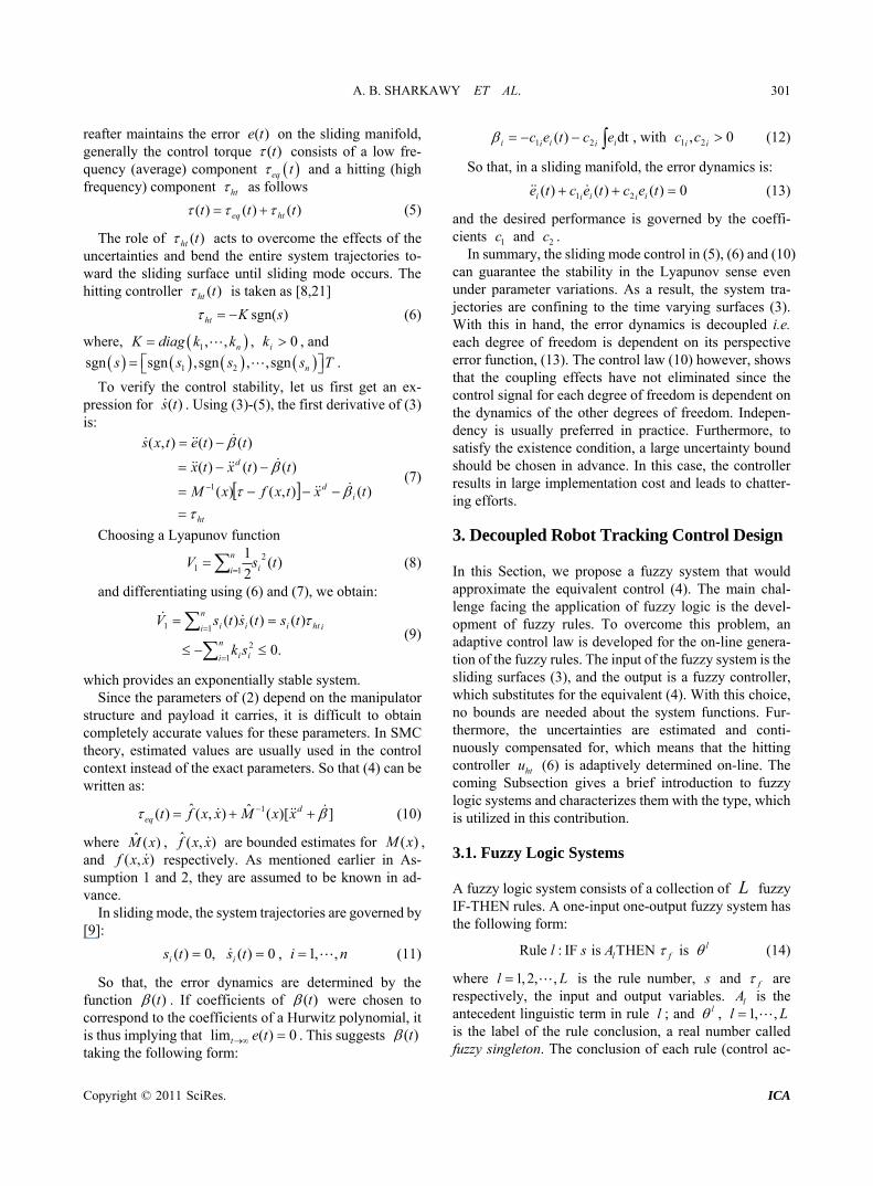
The fuzzy system used in this contribution is one input one output system, (14). The input of the fuzzy system is normalized using L number of equally spaced Gaussian membership functions inside the universe of discourse. Slopes are identical, see Figure 1.

The described fuzzy system is used to approximate the nonlinear dynamics of robotic systems. In a decoupled manner, the control action is computed for each degree of freedom, based on the corresponding sliding surface. The control actions l (output singletons) which are con-tained in the parameter vector should be known. In the

1l 3l2l Ll

3c1c 2c Lc

Figure 1. Input fuzzy sets. coming Subsection, adaptive laws are derived to do this task. The antecedent part is fixed with Gaussian mem-bership functions.

3.2 The Adaptation Mechanism

Fuzzy systems are universal function approximators. They can approximate any nonlinear function within a predefined accuracy if enough rules are used. This im-plies the necessity of using expert knowledge in the form of large number of rules and suitable membership func-tions. Usually trial and error procedure is needed to achieve the requested accuracy. Assigning parameters of the fuzzy systems (or some of them) adaptively greatly facilitates the design (e.g. reduce the number of rules) and enhances the performance (saves the computation resources).

In this Subsection, we derive an adaptive control law to determine the consequent part (control actions con-tained in parameter vector ) of the fuzzy system which is used to approximate the unknown nonlinear dynamics of robotic systems. The proposed scheme saves the need to expert knowledge and tedious work needed to assign parameters of the fuzzy system. Furthermore, distur-bances, approximation errors and uncertainties are de-termined compensate for on-line leading to a stable closed loop system.

Lyapunov stability analysis is the most popular ap-proach to prove and evaluate the convergence property of nonlinear controllers, e.g., sliding mode control, fuzzy control system. Here, Lyapunov analysis is employed to investigate the stability property of the proposed control system. By the universal approximation theorem [22], there exists a fuzzy controller ),( sf in the form of (16) such that

( ) ( , ) Teqi f i i i i i it s , 1, ,i n (18)

where i is the approximation error and is bounded by

i iE . Employing a fuzzy controller ˆˆ ( , )if i is to approximate )(t

ieq as ˆ ˆˆ ( , ) T

if i i i is (19)

where i is the estimated value of the parameter vector

i . Now, the SMC in (5) can be rewritten as:

A. B. SHARKAWY ET AL.

Copyright © 2011 SciRes. ICA

303

ˆˆ( ) ( , ) ( ) i f i i i ht i it s s (20)

where the fuzzy controller ˆˆ ( , ) f i i is is designed to

approximate the equivalent controller ( )eqi t . Define

ˆˆ ( , ) f i eqi f i i is , ˆ

i i i , and use (17), then it is obtained that

Tif i i i (21)

An expression for ( )s t can be expressed as follows:

1 1

1 1

( , ) ( ) ( )

( ) ( ) ( )

( ) ( ) ( , ) ( )

( )( ) ( ) ( , ) ( )

d

d

deq ht

s x t e t t

x t x t t

M x M x f x x x t

M x M x f x x x t

(22)

Substituting from (19-21): 1( )( )hts M x u (23)

where 1 1 2 2, , ,T T T Tn n

. Now, assume that 1( )M x

can be approximated by known constant posi-tive definite diagonal matrix M . Unlike constant con-trol gain schemes (see [23,24] for example), this assump-tion has been taken into account as follows. Equation (23) can be rewritten as

, ( )Ti i i ht i i i is M u E , 1, ,i n (24)

where iE is the sum of approximation errors and un-certainties. A control goal would be the on-line determi-nation of its estimate, ˆ ( )iE t . The estimation error is de-fined by

ˆ( ) ( )i i iE t E E t , 1, ,i n (25)

Define a Lyapunov function as

2

22 , ,1

1 2

1( ), ,

2 2 2

Tn i i i

i i i i iii i

EV s t E s M M

(26) where 1 and 2 are positive constants. Differentiat-ing (25) with respect to time and using (23), it is ob-tained that

2 , ,11 2

, ,

Tn i i i i

i i i i i i i i i iii i

E EV s E s s M M

, , ,11 2

( )T

n T i i i ii i i ht i i i i i i i ii

i i

E Es M u E M M

, , ,11 2

[ ( )] ( )n jT i i

i i i i i i i i ht i i i iii i

E EM s M s u E M

To satisfy 2 0V , the adaptive laws can be selected as

1i i i is (27)

ˆ sgn( )ht i i iu E s (28)

Using (20)

2ˆ ( )i i i iE t E s (29)

then (22) can be rewritten as

22 ,1

,1

ˆ( ), , [ sgn( ) ]

ˆ ( ) 0

n

i i i i i i i ii

m

i i i i ii

V s t E M s E s E s E

s M E E

(30)

Therefore, 2V is reduced gradually and the control system is stable which means that the system trajectories converge to the sliding surfaces ( )s t while and E remain bounded. Now, if we let

, 21ˆ( )

m

i i i i iiΓ(t) s M E E V

(31)

and integrate Γ(t) with respect to time, then it is shown that

2 20( )d ( (0), , ) ( ( ), , ) t

Γ V s E V s t E (32)

Because 2 ( (0), , )V s E is bounded and

2 ( ( ), , )V s t E is non-increasing and bounded, it implies that

0lim ( )d

t

t Γ (33)

Furthermore, Γ is bounded, so that by Barbalat's

lemma [7], it can be shown that 0

lim ( )d 0 t

t Γ . That is, ( ) 0s t as 0t . As a result, the proposed AFSMC is asymptotically stable.

Hence, the control law (18) can be rewritten as follows

ˆ ˆˆ( ) ( , ) sgn( ) i f i i i i iu t u s E s , ni ,,1 (34)

In summary, the adaptive fuzzy sliding mode control-ler (34) has two terms;

ˆˆ ( , )f iu s given in (19) with the parameter i adjusted by (27) and the uncertainties and approximation bound ˆ

iE adjusted by (29). By applying these adaptive laws, the AFSMC is model free and can be guaranteed to be stable for any nonlinear system has the form of (2).

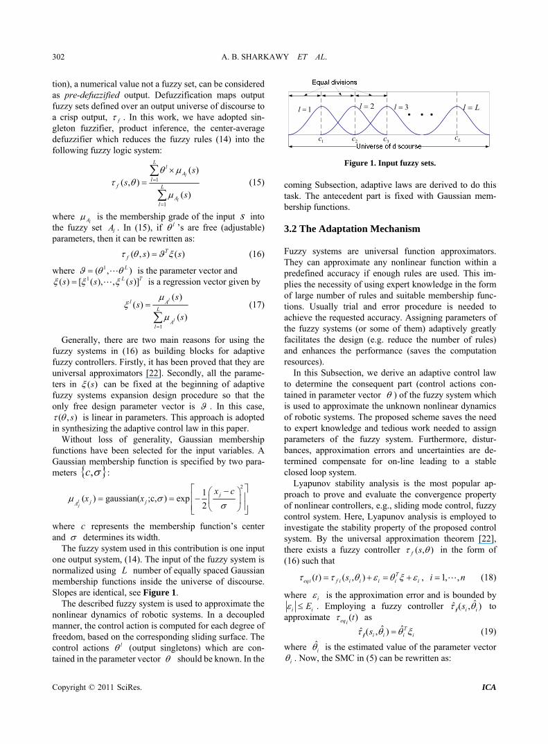
It should be noted that implementing the algorithm implies that the both error dynamics and control signals has been decoupled, since each of them is dependent only on the perspective sliding surface. Unlike SMC, the proposed AFSMC does not require any knowledge about the system functions nor their bounds. It adaptively de-termines and compensates for the unknown dynamics and external disturbances leading to a stable closed loop system. Figure 2 shows the main elements of the control system.

Remark 1. Since the control laws (6) and (34) contain the sign function, direct application of such control sig-nals to the robotic system may result in chattering caused

A. B. SHARKAWY ET AL.

Copyright © 2011 SciRes. ICA

304

ets )(equ

htu

u x

dx

E

Figure 2. The closed loop control system utilizing AFSMC. by the signal discontinuity. To overcome this problem, the control law is smoothed out within a thin boundary layer [7,21] by replacing the sign function by a satura-tion function defined as:

sgn 1

sat

1

i i

i ii

i i i

i i

s s

s

s s

4. Simulation Results

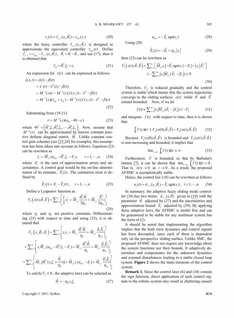
In this Section, we simulate the AFSMC and SMC on a two link robot; Figure 3. Simulation tests are carried out using MATLAB R2009a, version 7.8 under Windows 7 environment. A two link robot arm with varying loads is used to generate data in the simulation tests. The arm is depicted as 2-input, 2-ouput nonlinear system. The con-trol architecture shown in Figure 2 represents the closed loop system, in which the robot is the plant to be con-trolled. The detailed descriptions of the matrices )(xM ,

( , )C x x and )(xG in (1) for this robot are given in Ap-pendix A. We consider the state variable vector as the joint positions; i.e. 1 2[ , ]Tx x x . They are usually avail-able feedback signals through encoders mounted on the motor shafts.

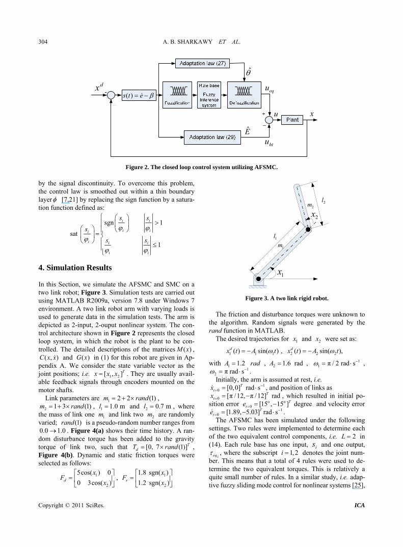
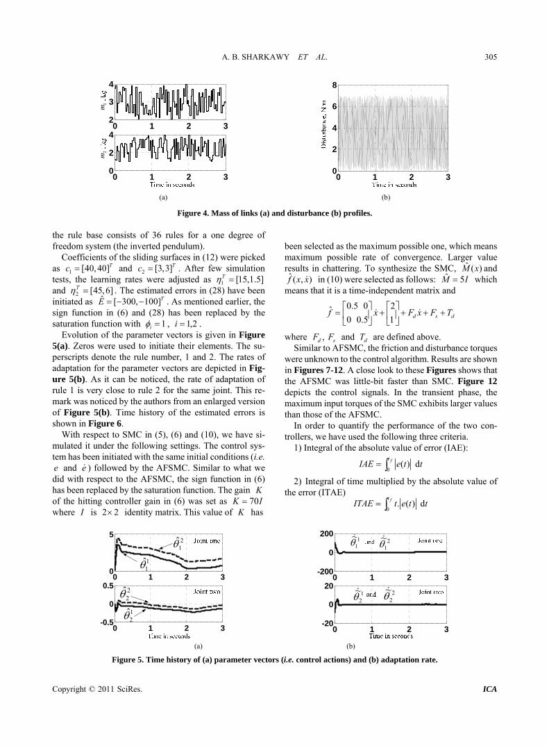
Link parameters are 1 2 2 (1)m rand ,

2 1 3 (1)m rand , 1 1.0 ml and 2 0.7 ml , where the mass of link one 1m and link two 2m are randomly varied; )1(rand is a pseudo-random number ranges from

0.10.0 . Figure 4(a) shows their time history. A ran-dom disturbance torque has been added to the gravity torque of link two, such that [0, 7 (1)]T

dT rand , Figure 4(b). Dynamic and static friction torques were selected as follows:

1

2

5cos( ) 0

0 3cos( )d

xF

x

, 1

2

1.8 sgn( )

1.2 sgn( )

s

xF

x

1x

2x

1l

2l

1m

2m

Figure 3. A two link rigid robot.

The friction and disturbance torques were unknown to the algorithm. Random signals were generated by the rand function in MATLAB.

The desired trajectories for 1x and 2x were set as:

1 1 1 2 2 2( ) sin( ) , ( ) sin( ), d dx t A t x t A t

with 1 1.2 A rad , 2 1.6 radA , 11 π / 2 rad s ,

12 π rad s . Initially, the arm is assumed at rest, i.e.

10 [0,0] rad s T

tx , and position of links as

0 [π /12, π /12] rad Ttx , which resulted in initial po-

sition error o o0 [15 , 15 ] degree T

te and velocity error 1

0 [1.89, 5.03] rad s Tte . The AFSMC has been simulated under the following

settings. Two rules were implemented to determine each of the two equivalent control components, i.e. 2L in (14). Each rule base has one input, is and one output,

ieq , where the subscript 1,2i denotes the joint num-ber. This means that a total of 4 rules were used to de-termine the two equivalent torques. This is relatively a quite small number of rules. In a similar study, i.e. adap-tive fuzzy sliding mode control for nonlinear systems [25],

A. B. SHARKAWY ET AL.

Copyright © 2011 SciRes. ICA

305

1m

2m

0 1 2 32

3

4

0 1 2 30

2

4

0 1 2 3

0

2

4

6

8

(a) (b)

Figure 4. Mass of links (a) and disturbance (b) profiles. the rule base consists of 36 rules for a one degree of freedom system (the inverted pendulum).

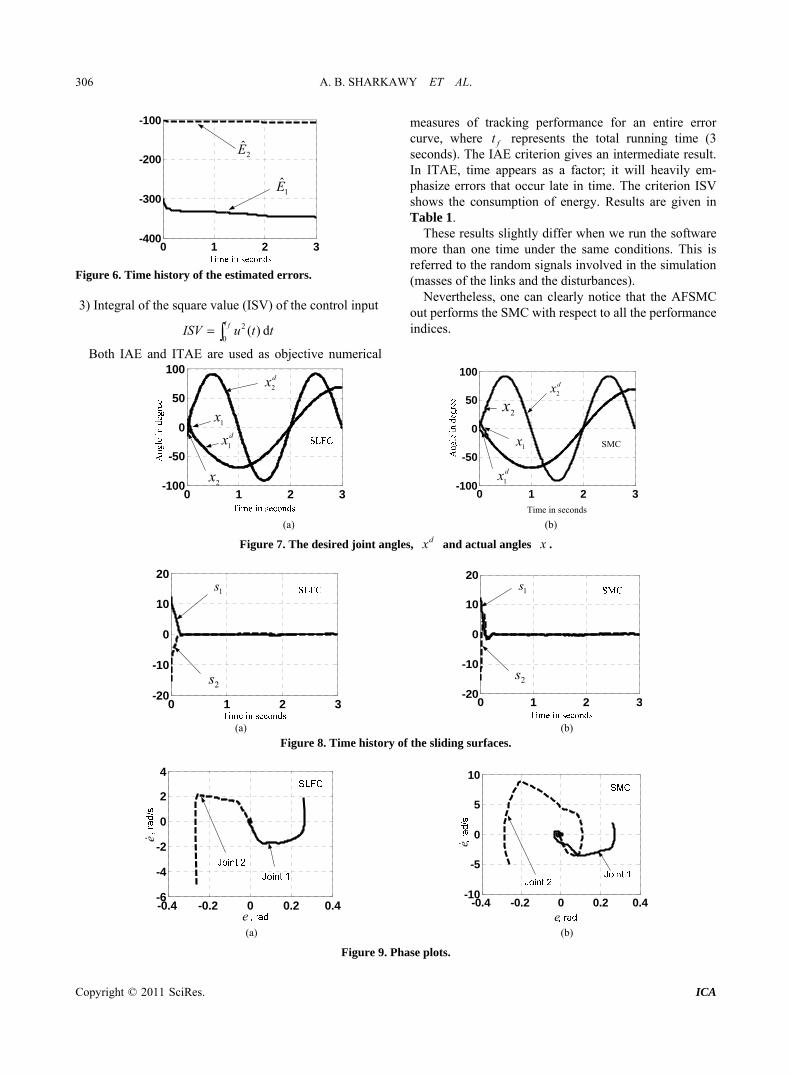
Coefficients of the sliding surfaces in (12) were picked as 1 [40, 40]Tc and 2 [3,3]Tc . After few simulation tests, the learning rates were adjusted as 1 [15,1.5]T and 2 [45,6]T . The estimated errors in (28) have been initiated as ˆ [ 300, 100]TE . As mentioned earlier, the sign function in (6) and (28) has been replaced by the saturation function with 1i , 2,1i .

Evolution of the parameter vectors is given in Figure 5(a). Zeros were used to initiate their elements. The su-perscripts denote the rule number, 1 and 2. The rates of adaptation for the parameter vectors are depicted in Fig-ure 5(b). As it can be noticed, the rate of adaptation of rule 1 is very close to rule 2 for the same joint. This re-mark was noticed by the authors from an enlarged version of Figure 5(b). Time history of the estimated errors is shown in Figure 6.

With respect to SMC in (5), (6) and (10), we have si-mulated it under the following settings. The control sys-tem has been initiated with the same initial conditions (i.e. e and e ) followed by the AFSMC. Similar to what we did with respect to the AFSMC, the sign function in (6) has been replaced by the saturation function. The gain K of the hitting controller gain in (6) was set as 70K I where I is 22 identity matrix. This value of K has

been selected as the maximum possible one, which means maximum possible rate of convergence. Larger value results in chattering. To synthesize the SMC, ˆ ( )M x and ˆ ( , )f x x in (10) were selected as follows: ˆ 5M I which

means that it is a time-independent matrix and

0.5 0 2ˆ0 0.5 1 d s df x F x F T

where , d sF F and dT are defined above. Similar to AFSMC, the friction and disturbance torques

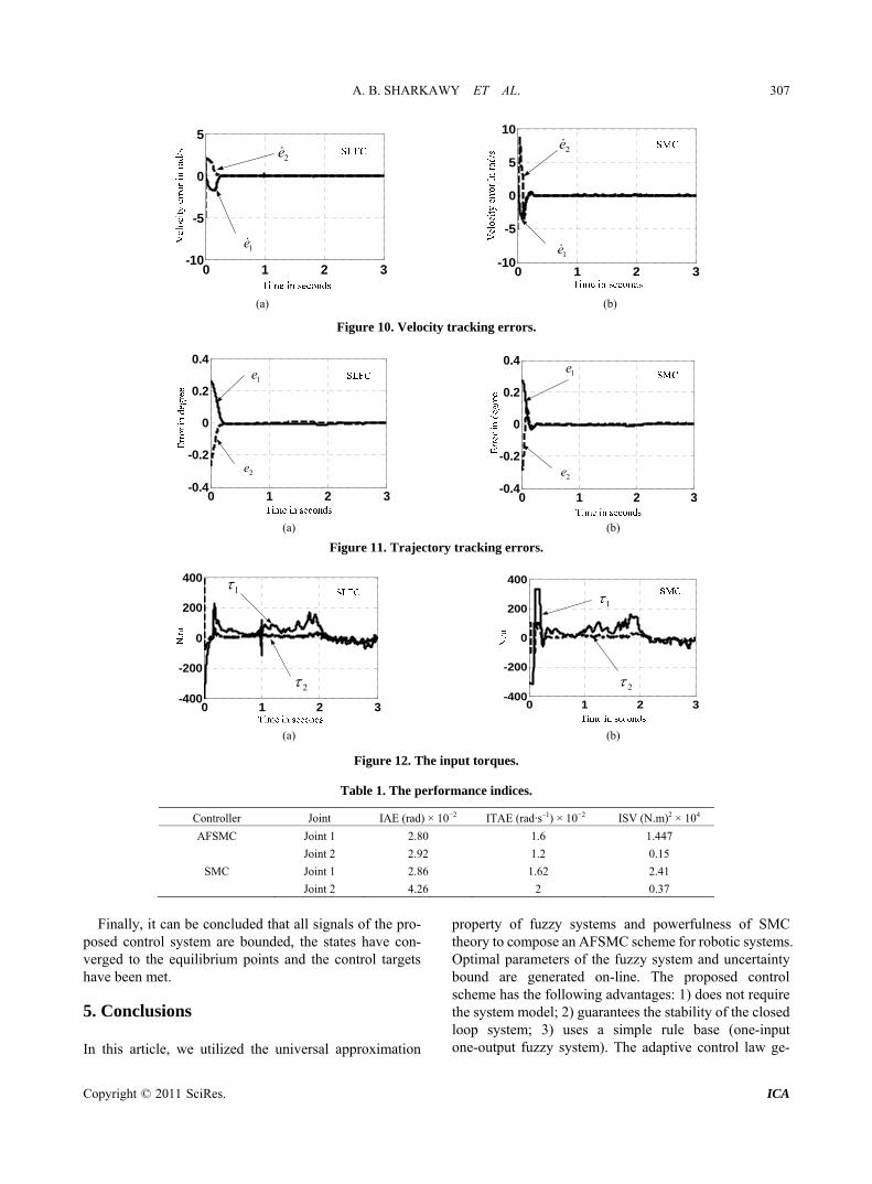
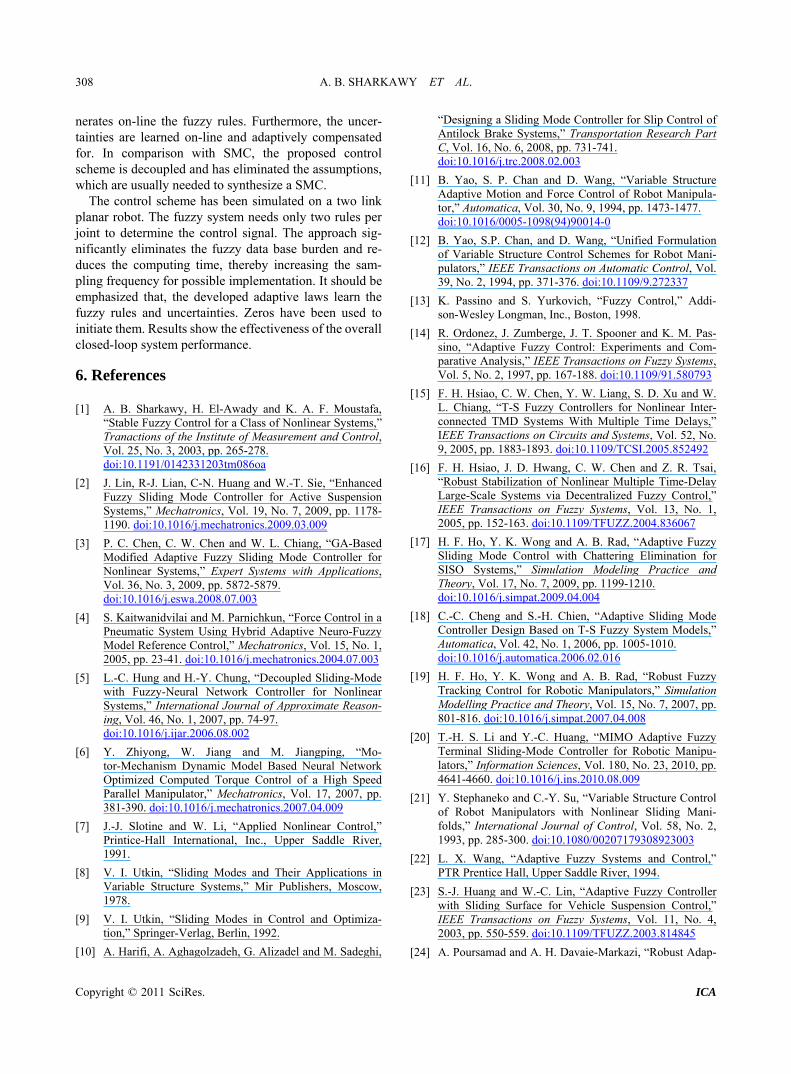
were unknown to the control algorithm. Results are shown in Figures 7-12. A close look to these Figures shows that the AFSMC was little-bit faster than SMC. Figure 12 depicts the control signals. In the transient phase, the maximum input torques of the SMC exhibits larger values than those of the AFSMC.

In order to quantify the performance of the two con-trollers, we have used the following three criteria.

1) Integral of the absolute value of error (IAE):

0( ) d

ftIAE e t t

2) Integral of time multiplied by the absolute value of the error (ITAE)

0. ( ) d

ftITAE t e t t

0 1 2 30

5

0 1 2 3-0.5

0

0.5

12

21

11

22

0 1 2 3-200

0

200

0 1 2 3-20

0

20

21

~

22

~12

~

11

~

(a) (b)

Figure 5. Time history of (a) parameter vectors (i.e. control actions) and (b) adaptation rate.

A. B. SHARKAWY ET AL.

Copyright © 2011 SciRes. ICA

306

0 1 2 3-400

-300

-200

-100

1E

2E

Figure 6. Time history of the estimated errors. 3) Integral of the square value (ISV) of the control input

2

0( ) dft

ISV u t t

Both IAE and ITAE are used as objective numerical

measures of tracking performance for an entire error curve, where ft represents the total running time (3 seconds). The IAE criterion gives an intermediate result. In ITAE, time appears as a factor; it will heavily em-phasize errors that occur late in time. The criterion ISV shows the consumption of energy. Results are given in Table 1.

These results slightly differ when we run the software more than one time under the same conditions. This is referred to the random signals involved in the simulation (masses of the links and the disturbances).

Nevertheless, one can clearly notice that the AFSMC out performs the SMC with respect to all the performance indices.

0 1 2 3-100

-50

0

50

100

1xdx1

2x

dx2

0 1 2 3-100

-50

0

50

100

Time in seconds

1x

dx1

2x

dx2

SMC

(a) (b)

Figure 7. The desired joint angles, dx and actual angles x .

0 1 2 3-20

-10

0

10

201s

2s

0 1 2 3-20

-10

0

10

201s

2s

(a) (b)

Figure 8. Time history of the sliding surfaces.

-0.4 -0.2 0 0.2 0.4-6

-4

-2

0

2

4

e

e

-0.4 -0.2 0 0.2 0.4-10

-5

0

5

10

e

e

(a) (b)

Figure 9. Phase plots.

A. B. SHARKAWY ET AL.

Copyright © 2011 SciRes. ICA

307

0 1 2 3-10

-5

0

5

1e

2e

0 1 2 3

-10

-5

0

5

10

1e

2e

(a) (b)

Figure 10. Velocity tracking errors.

0 1 2 3-0.4

-0.2

0

0.2

0.4

1e

2e

0 1 2 3

-0.4

-0.2

0

0.2

0.41e

2e

(a) (b)

Figure 11. Trajectory tracking errors.

0 1 2 3-400

-200

0

200

4001

2

0 1 2 3

-400

-200

0

200

400

1

2

(a) (b)

Figure 12. The input torques.

Table 1. The performance indices.

Controller Joint IAE (rad) × 10−2 ITAE (rad·s–1) × 10−2 ISV (N.m)2 × 104

AFSMC Joint 1 2.80 1.6 1.447

Joint 2 2.92 1.2 0.15

SMC Joint 1 2.86 1.62 2.41

Joint 2 4.26 2 0.37

Finally, it can be concluded that all signals of the pro-

posed control system are bounded, the states have con-verged to the equilibrium points and the control targets have been met. 5. Conclusions In this article, we utilized the universal approximation

property of fuzzy systems and powerfulness of SMC theory to compose an AFSMC scheme for robotic systems. Optimal parameters of the fuzzy system and uncertainty bound are generated on-line. The proposed control scheme has the following advantages: 1) does not require the system model; 2) guarantees the stability of the closed loop system; 3) uses a simple rule base (one-input one-output fuzzy system). The adaptive control law ge-

A. B. SHARKAWY ET AL.

Copyright © 2011 SciRes. ICA

308

nerates on-line the fuzzy rules. Furthermore, the uncer-tainties are learned on-line and adaptively compensated for. In comparison with SMC, the proposed control scheme is decoupled and has eliminated the assumptions, which are usually needed to synthesize a SMC.

The control scheme has been simulated on a two link planar robot. The fuzzy system needs only two rules per joint to determine the control signal. The approach sig-nificantly eliminates the fuzzy data base burden and re-duces the computing time, thereby increasing the sam-pling frequency for possible implementation. It should be emphasized that, the developed adaptive laws learn the fuzzy rules and uncertainties. Zeros have been used to initiate them. Results show the effectiveness of the overall closed-loop system performance. 6. References [1] A. B. Sharkawy, H. El-Awady and K. A. F. Moustafa,

“Stable Fuzzy Control for a Class of Nonlinear Systems,” Tranactions of the Institute of Measurement and Control, Vol. 25, No. 3, 2003, pp. 265-278. doi:10.1191/0142331203tm086oa

[2] J. Lin, R-J. Lian, C-N. Huang and W.-T. Sie, “Enhanced Fuzzy Sliding Mode Controller for Active Suspension Systems,” Mechatronics, Vol. 19, No. 7, 2009, pp. 1178- 1190. doi:10.1016/j.mechatronics.2009.03.009

[3] P. C. Chen, C. W. Chen and W. L. Chiang, “GA-Based Modified Adaptive Fuzzy Sliding Mode Controller for Nonlinear Systems,” Expert Systems with Applications, Vol. 36, No. 3, 2009, pp. 5872-5879. doi:10.1016/j.eswa.2008.07.003

[4] S. Kaitwanidvilai and M. Parnichkun, “Force Control in a Pneumatic System Using Hybrid Adaptive Neuro-Fuzzy Model Reference Control,” Mechatronics, Vol. 15, No. 1, 2005, pp. 23-41. doi:10.1016/j.mechatronics.2004.07.003

[5] L.-C. Hung and H.-Y. Chung, “Decoupled Sliding-Mode with Fuzzy-Neural Network Controller for Nonlinear Systems,” International Journal of Approximate Reason-ing, Vol. 46, No. 1, 2007, pp. 74-97. doi:10.1016/j.ijar.2006.08.002

[6] Y. Zhiyong, W. Jiang and M. Jiangping, “Mo-tor-Mechanism Dynamic Model Based Neural Network Optimized Computed Torque Control of a High Speed Parallel Manipulator,” Mechatronics, Vol. 17, 2007, pp. 381-390. doi:10.1016/j.mechatronics.2007.04.009

[7] J.-J. Slotine and W. Li, “Applied Nonlinear Control,” Printice-Hall International, Inc., Upper Saddle River, 1991.

[8] V. I. Utkin, “Sliding Modes and Their Applications in Variable Structure Systems,” Mir Publishers, Moscow, 1978.

[9] V. I. Utkin, “Sliding Modes in Control and Optimiza-tion,” Springer-Verlag, Berlin, 1992.

[10] A. Harifi, A. Aghagolzadeh, G. Alizadel and M. Sadeghi,

“Designing a Sliding Mode Controller for Slip Control of Antilock Brake Systems,” Transportation Research Part C, Vol. 16, No. 6, 2008, pp. 731-741. doi:10.1016/j.trc.2008.02.003

[11] B. Yao, S. P. Chan and D. Wang, “Variable Structure Adaptive Motion and Force Control of Robot Manipula-tor,” Automatica, Vol. 30, No. 9, 1994, pp. 1473-1477. doi:10.1016/0005-1098(94)90014-0

[12] B. Yao, S.P. Chan, and D. Wang, “Unified Formulation of Variable Structure Control Schemes for Robot Mani-pulators,” IEEE Transactions on Automatic Control, Vol. 39, No. 2, 1994, pp. 371-376. doi:10.1109/9.272337

[13] K. Passino and S. Yurkovich, “Fuzzy Control,” Addi-son-Wesley Longman, Inc., Boston, 1998.

[14] R. Ordonez, J. Zumberge, J. T. Spooner and K. M. Pas-sino, “Adaptive Fuzzy Control: Experiments and Com-parative Analysis,” IEEE Transactions on Fuzzy Systems, Vol. 5, No. 2, 1997, pp. 167-188. doi:10.1109/91.580793

[15] F. H. Hsiao, C. W. Chen, Y. W. Liang, S. D. Xu and W. L. Chiang, “T-S Fuzzy Controllers for Nonlinear Inter-connected TMD Systems With Multiple Time Delays,” IEEE Transactions on Circuits and Systems, Vol. 52, No. 9, 2005, pp. 1883-1893. doi:10.1109/TCSI.2005.852492

[16] F. H. Hsiao, J. D. Hwang, C. W. Chen and Z. R. Tsai, “Robust Stabilization of Nonlinear Multiple Time-Delay Large-Scale Systems via Decentralized Fuzzy Control,” IEEE Transactions on Fuzzy Systems, Vol. 13, No. 1, 2005, pp. 152-163. doi:10.1109/TFUZZ.2004.836067

[17] H. F. Ho, Y. K. Wong and A. B. Rad, “Adaptive Fuzzy Sliding Mode Control with Chattering Elimination for SISO Systems,” Simulation Modeling Practice and Theory, Vol. 17, No. 7, 2009, pp. 1199-1210. doi:10.1016/j.simpat.2009.04.004

[18] C.-C. Cheng and S.-H. Chien, “Adaptive Sliding Mode Controller Design Based on T-S Fuzzy System Models,” Automatica, Vol. 42, No. 1, 2006, pp. 1005-1010. doi:10.1016/j.automatica.2006.02.016

[19] H. F. Ho, Y. K. Wong and A. B. Rad, “Robust Fuzzy Tracking Control for Robotic Manipulators,” Simulation Modelling Practice and Theory, Vol. 15, No. 7, 2007, pp. 801-816. doi:10.1016/j.simpat.2007.04.008

[20] T.-H. S. Li and Y.-C. Huang, “MIMO Adaptive Fuzzy Terminal Sliding-Mode Controller for Robotic Manipu-lators,” Information Sciences, Vol. 180, No. 23, 2010, pp. 4641-4660. doi:10.1016/j.ins.2010.08.009

[21] Y. Stephaneko and C.-Y. Su, “Variable Structure Control of Robot Manipulators with Nonlinear Sliding Mani-folds,” International Journal of Control, Vol. 58, No. 2, 1993, pp. 285-300. doi:10.1080/00207179308923003

[22] L. X. Wang, “Adaptive Fuzzy Systems and Control,” PTR Prentice Hall, Upper Saddle River, 1994.

[23] S.-J. Huang and W.-C. Lin, “Adaptive Fuzzy Controller with Sliding Surface for Vehicle Suspension Control,” IEEE Transactions on Fuzzy Systems, Vol. 11, No. 4, 2003, pp. 550-559. doi:10.1109/TFUZZ.2003.814845

[24] A. Poursamad and A. H. Davaie-Markazi, “Robust Adap-

A. B. SHARKAWY ET AL.

Copyright © 2011 SciRes. ICA

309

tive Fuzzy Control of Unknown Chaotic Systems,” Ap-plied Soft Computing, Vol. 9, No. 3, 2009, pp. 970-976. doi:10.1016/j.asoc.2008.11.014

[25] M. Roopaei, M. Zolghadri and S. Meshksar, “Enhanced Adaptive Fuzzy Sliding mode Control for Uncertain

Nonlinear Systems,” Communications in Nonlinear Science and Numerical Simulation, Vol. 14, No. 9-10, 2009, pp. 3670-3681. doi:10.1016/j.cnsns.2009.01.029

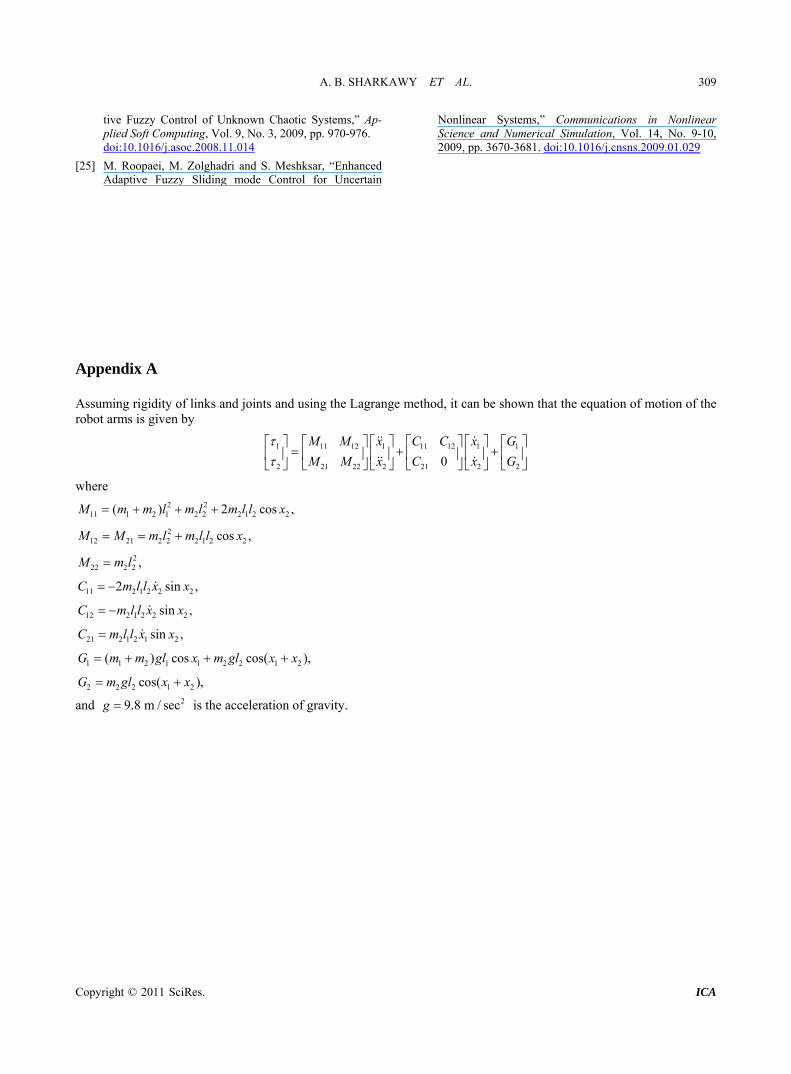
Appendix A Assuming rigidity of links and joints and using the Lagrange method, it can be shown that the equation of motion of the robot arms is given by

1 11 12 1 11 12 1 1

2 21 22 2 21 2 2

0

M M x C C x G

M M x C x G

where 2 2

11 1 2 1 2 2 2 1 2 2( ) 2 cos ,M m m l m l m l l x

212 21 2 2 2 1 2 2cos ,M M m l m l l x

2

22 2 2 ,M m l

11 2 1 2 2 22 sin ,C m l l x x

12 2 1 2 2 2sin ,C m l l x x

21 2 1 2 1 2sin ,C m l l x x

1 1 2 1 1 2 2 1 2( ) cos cos( ),G m m gl x m gl x x

2 2 2 1 2cos( ),G m gl x x

and 29.8 m / secg is the acceleration of gravity.