Abstract- This paper presents a synthesis of fault diagnosis method for nonlinear systems through the parameter estimation using higher order sliding modes. Initially the uncertain parameters of nonlinear system using robust exact differentiator are estimated. Then residual signal is reconstructed using the estimated parame-ters, inputs, outputs and their estimated derivatives. The novelty of the method is the determination of unknown, uncertain system parameters by calculating accurate derivatives of the measured system inputs and outputs. To validate the technique, simulations have been performed for a uncertain nonlinear Three Tank Sys-tem. The convergence in this approach is shown to be faster than similar existing techniques by an order of magnitude even in the presence of measurement noise. The proposed fault diagnosis technique requires no prior information about uncertain/unknown process parameters and statistical knowledge of process. Index Terms- Fault detection and isolation, parameter estimation, uncertain nonlinear systems, robust exact differentiator, higher order sliding modes, three tank system.

I. INTRODUCTION OR the safety related processes like aircrafts, trains, au-tomobiles, power and chemical plants, the advanced me-thods for supervision, control and fault diagnosis are

becoming increasingly important. These methods improve the reliability, availability, safety, efficiency and ever demanding performance. An effective means to assure the reliability and safety is to detect and diagnose faults in the system quickly and prompt remedial action taken accordingly. When a system ex-periences an abnormal condition, a fault is deemed to occur, such as a malfunction in the actuators or sensors or even the system itself. The primary purpose of Fault Detection and Iso-lation (FDI) is to generate an alarm and identify its location when a fault occurs. The main approaches to address the FDI problem are history based and observer based [1]. History based approaches depend on knowledge processed from past experiences, whereas model-based methods rely on interactions between system variables. Over the past two decades a number model based methods for FDI have been developed among them a commonly used approach is residual-based method [1]- [4]. Most of the FDI schemes provide means of updating sys-tem parameters for robust control or effective fault detection and isolation. The problem of fault detection, isolation and re-covery of nonlinear systems with uncertain parameters has been investigated by Jiang, Khorasani and Tafazoli [4], C. Join et al [5] and Fliess and Sira-Ramirez [6], Alwi and Edwards [10].

1. Postgraduate student at Center for Advance Studies in Engineering (CASE)

Islamabad Pakistan; (e-mail: iqbal@case.edu.pk). 2. Dr. A. I. Bhatti is Professor at Mohammad Ali Jinnah University (MAJU)

Islamabad Pakistan; (e-mail: aib@jinnah.edu.pk). 3. Postgraduate students at Mohammad Ali Jinnah University (MAJU) Islama-

bad Pakistan; (e-mail: sayubi@gmail.com, qudratullahqau@gmail.com).

Sliding mode techniques have been used extensively for FDI of linear as well as nonlinear systems in recent years. Sliding Mode Observers (SMO) have been used for a number of engi-neering applications to parameter estimation and fault detection by recreating fault signals [10], [14]-[18]. A novel concept of sliding mode control for controlling a nonlinear system in the presence of uncertainties associated with parameters and mod-eling errors has been investigated by Alwi and Edwards [10]. A sliding observer was utilized to reconstruct fault rather than to detect the presence of a fault through residual signal. The re-constructed fault is utilized directly in fault tolerant control of an aerospace system. A generic FDI scheme in terms of fault reconstruction using sliding mode observers is developed by Edwards et al [16]. Tan and Edwards [17] extended this work for robust reconstruction of sensor and actuator faults. Ng and Tan et al [18] have further extended the fault reconstruction method that is applicable to a wider class of systems with rela-tive degree higher than one and for systems with more un-known inputs than outputs using two SMO’s in cascade. Chen and Chowdhury [14] have used sliding mode observer (SMO) combined with Luenberger observer to make the fault detection residual sensitive to incipient faults while being robust to dis-turbances.

Parameter estimation using differentiators has been investi-gated in literature [5], [13]. The main difficulty in real-time differentiation is due to differentiation sensitivity to input nois-es. The high gain differentiators in [19], [20] provide an exact derivative provided their gains tend to infinity which also leads to higher sensitivity to small high-frequency noises. Another drawback of the high-gain differentiators is their peaking ef-fect, i.e., the maximal output values during the transient grows infinitely when gains tend to infinity. Join et al [5] has deter-mined estimation of time derivative for FDI of an analytic func-tion using the truncated series of Taylor expansion. This in-volves iterative integration process to low pass filter high-frequency perturbation or noise, which is computationally time consuming and also can have numerical issues in online im-plementation, in the mentioned numeric technique the deriva-tive approximations become invalid which needs periodic reset-ting the calculations [6]. This paper has extended FDI scheme of [5] for parameter estimation of uncertain nonlinear systems using robust exact differentiator. The presented framework does not need the development of an observer or numeric diffe-rentiator and no prior knowledge of statistical properties of the nonlinear system is required. In our approach the exact deriva-tives have been calculated by successive implementation of robust exact first-order differentiator with finite-time conver-gence. The differentiator is based on 2-sliding mode and is proved to feature the best possible asymptotically converging derivative provided the second time derivative of the base sig-nal is bounded [7] - [9].

Fault Diagnosis of Nonlinear Systems Using Higher Order Sliding Mode Technique

M. Iqbal1, A. I. Bhatti2 Member IEEE, S. Iqbal3, Q. Khan3, I. H. Kazmi3

F

Proceedings of the 7th Asian Control Conference,Hong Kong, China, August 27-29, 2009

FrA6.3

978-89-956056-9-1/09/©2009 ACA 875

Authorized licensed use limited to: College of Engineering. Downloaded on October 24, 2009 at 11:17 from IEEE Xplore. Restrictions apply.

As per the author’s best knowledge, the Higher Order Slid-ing Modes (HOSM) based differentiator is used perhaps for the first time for parameters estimation based FDI of nonlinear systems. The estimated parameters are utilized for fault signal reconstruction i.e., generation of residual. The reconstructed residual carries the information about the presence of fault, its location and magnitude. The organization of remainder of this paper is as follows: In Section II problem formulation of para-meters estimation based FDI of nonlinear systems is briefly described. It also contains description of robust exact differen-tiator being used for the estimation of time derivatives. Three Tank System model descriptions, its viscosity coefficients es-timation and their use for the fault signal reconstruction is dis-cussed in Section III. Section IV presents the simulation results. Section V contains the concluding remarks followed by refer-ences.

II. PROBLEM FORMULATION Consider a system of the form : , , g , , , , (1) where, is a measureable state vector, is a control input vector, g , is a known nonlinear function with g , 0. is the unknown/uncertain parameter vector in parameter space , , 1,2, , .

. can be a nonlinear continuous function. is a finite set of perturbation variables which assumed here as high frequency noises. , , is a smooth nonlinear function, and functions , satisfy the following assumptions [13]: Assumption 1: , , αT , , , , , , , , (2) where , are known nonlinear functions and linearly independent. are the combinations of ; q denotes the dimension of . Assumption 2: (3) where is a positive and non-zero constant. is a measur-able and 0 0. As the bounds of are given, the bounds of can also be obtained and the following assumption can be introduced. Assumption 3: , (4) Suppose is the uncertain parameter vector of the estimator and is a time varying parameter vector which is calculated in terms uncertain parameter and its bounds: if if if (5)

In the following paragraphs, we will omit the elements of some functions for simplicity.

A. Observability & Identifiability of Nonlinear System Identifiability is the possibility to identify the parameters of a

control system from its input-output map. The identifiability property, a prerequisite for parameter estimation guarantees

that the model parameters can be determined uniquely from measured data. The identifiability property is well characterized and algorithms for ordinary differential equation exist. In lite-rature different methods are used to test the observability of nonlinear systems, the differential geometry and algebraic ap-proach. Rank test condition is being used for both the ap-proaches, where observability of a system is determined by calculating the dimension of the space spanned by gradients of the Lie-derivatives of its output functions. For this, one has to find the rank of the following Jacobian matrix [21]:

O =

If this Jacobian matrix is a full rank (Rank (O) = n), then system is algebraically observable. The problem of parameter identifiability can be treated as special case of observability problem by considering parameters as state variables with time derivative zero i.e., 0, so the observability rank test can used to determine parameter identifiability. For nonlinear sys-tem (1) with assumption 0, and are considered as the same type of variables. Without initial conditions for x, the non-observable variables can be both in and in . Suppose that we are given a full set of initial conditions on . . , 0 . Then the problem of observability of the

variables disappears [21], what is left is exactly the problem of identifiability for the parameters, the set of parameters that realizes a given input-output map, at least locally. This can be determined by the rank test using differential geometry and algebraic approaches. For analytical system (1) the rank test amounts to calculating the rank of the following Jacobean for 1,2, , , 1,2, , and 1,2, , 1:

(6)

If rank of matrix is n, then the system (1) is identifiable.

B. Estimation of HOSM Based Robust Derivatives: The sliding mode control (SMC) methods are developed to

design a stable system with high rate of convergence to the desired state and low sensitivity to plant parameter variations. The sliding mode control is based on keeping exactly a proper-ly chosen constraint by means of high frequency control switching. The biggest advantage of SMC is its insensitivity to variation in system parameters, external disturbances and mod-eling errors. The main idea of higher order sliding modes is to act on higher order derivatives of sliding variables as compared to the 1st order derivative in standard sliding mode technique. This gives all the advantages of standard sliding modes with additional advantage leading to removal of chattering effect. The r-sliding mode is determined by 0, which form an r-dimensional condition on

7th ASCC, Hong Kong, China, Aug. 27-29, 2009 FrA6.3

876

Authorized licensed use limited to: College of Engineering. Downloaded on October 24, 2009 at 11:17 from IEEE Xplore. Restrictions apply.

state of the dynamic system. The sliding order is a measure of the smoothness of the sliding variable in the vicinity of the slid-ing mode. In general any r-sliding controller that keeps 0, needs , , , to be made available [7]-[9]. Sliding mode techniques are known to be robust with a straight forward design formulation and thus provide a robust solution to parameter estimation, control and fault diagnosis. A robust exact differentiator developed by [8], [9], [15], as a part of the arbitrary order sliding mode controllers, with finite-time con-vergence has been adapted for the purpose of parameter estima-tion and is presented here for completeness of proposed scheme.

Consider an input signal a function defined on [0, ∞), consisting of a bounded Lebesgue-measureable noise with un-known features and unknown base signal with nth deriva-tive having a known Lipschitz constant 0 resulting from a real time noisy measurement [7]-[9]. The unknown sampling noise is assumed to be bounded. Assume that the associated differential inclusion discussed in [11] exist as a solution to (1), which causes boundedness of , allowing the implementation of 1st order robust differentiator with finite time convergence. The task is to find real estimates of , using only values of (t) and number L. The estimates are to be exact in the absence of noise, when . Let the noises be absent. Introduce an auxiliary dynamic system ,, . The task is to make and vanish in finite time by means of continuous control using only mea-surements of i.e. to establish a 2-sliding mode. The modified version of the super-twisting controller is applied, producing the close-loop system [11]. | | / , . Here and is chosen sufficiently large with respect to . The 2-sliding mode 0, | | / 0 is established in finite time. Thus in the presence of noise and are considered as estimates and respectively.

Thus, with recursive iterations, the th order differentiator [3] has the form: , | | / , , | | / ,

, | | / , , (7)

Where 0 are chosen sufficiently large in the reverse order. Note that it contains actually all the lower-order differentiators and each recursive step requires tuning one parameter only. Parameters tuned for 1, the parameters are easily recal-culated for any value of by / . The values of Lipschitz Constant can be computed by taking into account the maximum frequency component and maximum amplitude of the function f(t). C. Estimation of Uncertain Nonlinear System Parameters:

The nth order robust exact differentiator is utilized to estimate the derivatives of input and outputs using the measured system data. The technique used for the estimation of parameters ex-ploits the main features of the higher order sliding modes. As-sume that the unknown parameters , , , satisfy some natural identifiability conditions (6), then for 1, , : , , , , , , (8) where is a nonlinear function of its arguments. An accurate estimate α of α is obtained by replacing the derivatives of control input and output variables in equation (8) with their estimates obtained by robust exact differentiator estimator (7): , , , , , , , , (9) This gives a relationship for the estimates of the parameters in terms of input, output and their derivatives. The required deriv-atives are obtained through estimation of HOSM based robust exact derivative technique discussed below. D. Residual Construction

The fault diagnosis problem requires the generation of fault indicator signals known as ‘residuals’, which indicates the presence or absence of a fault in the system. The fault vector

can be written as [6]: , , , , , , , , , (10) where φ is a nonlinear function of its arguments. Uncertainties in system parameters make the fault detection and isolation problem more complex. It is sometimes difficult to distinguish the fault effects from those perturbations due to parametric un-certainties. Flies and Sira-Ramirez [6] has discussed the issues related to parametric variations and used their estimated values for fault detection. They have proposed the suitable combina-tion of parameter estimation and residual generation provided parameter estimation is carried out in very short time interval of time. It is assumed that faults don’t occur during this short in-terval. Here, we have developed the scheme for parameter es-timation based on higher order sliding mode technique which is much faster than assumed time intervals. A residual corres-ponding to fault can be written as: , , , , , , , , , (11)

The proposed fault detection scheme using HOSM based ro-bust differentiator is shown in Figure 1.

III. THREE TANK SYSTEM DESCRIPTION Three tank system represents a typical process system in

process industry, fuel management system of airplanes in air-crafts and flight vehicles. Parameters like viscosity coefficients are uncertain because of change in liquid characteristics, aging

Figure 1. Parameter estimation based fault detection scheme using HOSM based robust differentiator

7th ASCC, Hong Kong, China, Aug. 27-29, 2009 FrA6.3

877

Authorized licensed use limited to: College of Engineering. Downloaded on October 24, 2009 at 11:17 from IEEE Xplore. Restrictions apply.

effects and change operating environments. The full system model is adapted from [5]: | | | | | | | | | |

, , (12)

where is the liquid level in tank i and 2 . The control signals and are input flow rates respective-ly, and are actuator faults/disturbances which perturb the behavior of the system. The flow coefficients are as-sumed unknown/uncertain and are to be estimated, α , α , α . The typical parameters values of the three tank system are given in Table 1. Assumptions 1 and 2 are analyzed and validated for the system (12), , , are very small constants taken as minimum bounds of viscosity coefficients, maximum bounds of viscosity coefficients and control inputs are given in Table 1. In order to carry out identi-fiability analysis of the system we have: , | || | | || | | |

, 1/1/0 & ,

The function , , can be easily represented in terms of α s and in form of equation (2). The Jacobean of Lie-derivatives (6) of output for system (12) is:

, 1,2,3

In matrix form Jacobian is written as:

J =

For system (12) the Lie-derivatives 0, with this the

determinant of the Jacobian matrix comes out to be: det 0 for (13) So Rank (J) = 3, also n= 3, thus the Jacobean J does not loose rank, so the system parameters are identifiable. Since, identi-fiability is a special case of observability implying the observa-bility of the system equation (12). The uncertain/unknown flow coefficients are estimated using the following equation [5]:

2 | | 2 | |

| | (14)

Subject to the conditions: 1 3y y− ≠0, 3 2y y− ≠0 and 2y ≠0. The equations (14) give the estimated parameters in terms of inputs, outputs and their estimated derivatives. The fault variables and can be computed by following equations:

1 1 1 3 1 3 1

2 3 3 2 3 2 | | (15) And the fault indicating residuals can be conveniently com-puted by replacing the estimated viscosity coefficients in equa-tion (12) with the nominal values as under: 2 | | 2 | | + 2 | | (16)

IV. SIMULATION RESULTS The parameter estimation based FDI strategy developed in pre-vious section is tested using simulations of three tank system. The unknown/uncertain parameters are viscosity coefficients µ , µ and µ of interconnecting pipes between the tanks. Their nominal values along with other parameters used in simu-lations are given in Table 1. The system is assumed to be work-ing in close loop state feedback configuration with nonlinear PI controller adapted from [5]. The controller is further tuned to have faster dynamics by order of magnitude (response times) so that it can respond quickly to the sudden changes in the system. The simulations are carried out for operating conditions with system states to satisfy the full rank conditions for parameter identifiability (13). The simulation scheme for fault diagnosis using HOSM based differentiator is detailed in Figure 1. Inputs and outputs of the close loop fault free system shown in Figure 2 are fed to the robust exact differentiator based parameter estimator. The estimated parameters for fault free case are shown in Figure 3. The coef-ficient estimates converge asymptotically to their nominal val-ues. The convergence time is about one second, which is rea-sonably fast considering the slow dynamics of the three tank system. The performance of the parameter estimator in the

Figure 2. Process outputs with state feedback nonlinear PI Con-troller. The desired steady state water levels to be maintained by controller are y1=0.60, y2= 0.4.

0 5 10 15 20 25 30 35 40 45 500

0.20.40.60.8

1Outputs of the Plant

0 5 10 15 20 25 30 35 40 45 500

0.2

0.4

0.6

0 5 10 15 20 25 30 35 40 45 500

0.02

0.04

0.06

Time (Sec)

Y1

Y2

Y3

7th ASCC, Hong Kong, China, Aug. 27-29, 2009 FrA6.3

878

Authorized licensed use limited to: College of Engineering. Downloaded on October 24, 2009 at 11:17 from IEEE Xplore. Restrictions apply.

presence of noise is shown in Figure 4.The convergence time has increased in the presence of measurement noise. For noise free case the convergence time is much shorter (by an order of 100) as compared with convergence time using algebraic tech-niques [5], [6] and Sensitivity-Model-Based Adaptive Filters [12]. The convergence in this approach is faster than similar existing techniques by an order of magnitude even in the pres-ence of noise and is global in nature. Careful analysis of Figure 2 &3 shows that estimates does not depend on a particular op-erating condition. The estimated parameters are used for the reconstruction of fault indication signals using equation (16).

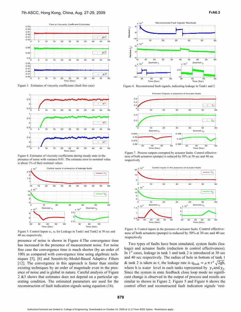
Two types of faults have been simulated, system faults (lea-kage) and actuator faults (reduction in control effectiveness). In 1st cases, leakage in tank 1 and tank 2 is introduced at 30 sec and 40 sec respectively. The radius of hole in bottom of tank 1 & tank 2 is taken as r, the leakage rate is q π r 2gh, where h is water level in each tanks represented by y and y . Since the system in state feedback close loop mode no signifi-cant change is observed in the output of process and results are similar to shown in Figure 2. Figure 5 and Figure 6 shows the control effort and reconstructed fault indication signals ‘resi-

Figure 7. Process outputs corrupted by actuator faults. Control effective-ness of both actuators (pumps) is reduced by 50% at 30 sec and 40 sec respectively

0 10 20 30 40 50 600

0.2

0.4

0.6

Process Outputs in presence of Actuator faults

y1

0 10 20 30 40 50 600

0.2

0.4

y2

30 40 50 600.56

0.575

0.59

0.605Zoomed y1

Time (Sec)30 40 50 60

0.385

0.39

0.395Zoomed y2

Time (Sec)

Figure. 8. Control inputs in the presence of actuator faults. Control effective-ness of both actuators (pumps) is reduced by 50% at 30 sec and 40 sec respectively

0 10 20 30 40 50 60

0

10

20x 10-4 Control inputs in the presence of actuator faults

0 10 20 30 40 50 600

5

10

15x 10-4

35 40 45 50 55 600.8

1

1.2x 10-4 Zoomed u1

Time (Sec)35 40 45 50 55 60

3

4

5x 10-5 Zoomed u2

Time (Sec)

u2

u1

Figure 3. Estimates of viscosity coefficients (fault free case)

0 5 10 15 20 25 30 35 40 45 500.450.470.490.510.530.55

Flow or Viscosity Coefficient Estimates

0 5 10 15 20 25 30 35 40 45 500.6

0.64

0.68

0 5 10 15 20 25 30 35 40 45 500.450.470.490.510.530.55

Time (Sec)

μ3

μ2

μ1

Figure 5. Control Inputs u1, u2 for Leakage in Tank1 and Tank2 at 30 sec and 40 sec respectively.

10 15 20 25 30 35 40 45 50 55 60

11.5

2

2.5x 10-4 Control inputs in prresence of leakage faults

0 10 20 30 40 50 600

5

10

15x 10-4

20 30 40 50 607

8

9

x 10-5 Zoomed u1

Time (Sec)30 40 50

2.5

3

3.5x 10-5 Zoomed u2

Time (Sec)

u1

u2

Figure 6. Reconstructed fault signals, indicating leakage in Tank1 and 2

0 10 20 30 40 50 60-10

-8

-6x 10-5 Reconstructed Fault Signals 'Residuals

Res

idua

l (r 1)

15 20 25 30 35 40 45 50 55 60-4

-3

-2x 10-5

Res

idua

l (r 2)

30 40 50 60-10

-5x 10-5 Zoomed r1

Time (Sec)35 40 45 50

-3

-2.5

x 10-5 Zoomed r2

Time (Sec)

Figure 4. Estimates of viscosity coefficients during steady state in the presence of noise with variance 0.01. The estimate error to nominal value is about 1% of their nominal values

0 5 10 15 20 25 30 35 40 45 50-0.5

0

0.5

1

0 5 10 15 20 25 30 35 40 45 50-0.5

0

0.5

1

0 5 10 15 20 25 30 35 40 45 50-0.5

0

0.5

1

Time (Sec)

μ3

μ2

μ1

7th ASCC, Hong Kong, China, Aug. 27-29, 2009 FrA6.3

879

Authorized licensed use limited to: College of Engineering. Downloaded on October 24, 2009 at 11:17 from IEEE Xplore. Restrictions apply.

duals’ respectively. The behavior of residual (Figure 6) changes at 30 sec and 40 sec demonstrates the effectiveness of the fault diagnosis strategy. Any adaptive thresholding technique can be utilized for unsupervised online fault detection and identifica-tion.

Table 1 Typical Parameter Values of Three Tank System Parameter Value

S, Area of the tanks 0.0154 m2 Sp, Area of pipes, p=1,2,3 5x10-5 m2 u1max, u2max (input flow rates) 100 ml/s

, , 0.5, 0.675, 0.5 , , , , 0 , , 1.0, 1.0, 1.0

In the 2nd case actuator faults are considered. Here control ef-fectiveness of both the actuators (pumps) is reduced by 50% as 0.5 and 0.5 at 30 sec and 40 sec respectively. Figure 7, Figure 8 and Figure 9 shows the of process outputs, control inputs and fault signals ‘residuals’. Figure 7 shows that the reduction in control effectiveness of actuators has affected the close loop process outputs severely. Figure 9 shows the behavior of residual changes. It may be noted that for the actua-tor faults the residuals change have opposite sign as compared to that of leakage changes. This opposite change in residual can be utilized for isolation between actuator and system leakage faults. The magnitude of the residual can be manipulated to estimate the fault size.

V. CONCLUSIONS A synthesis of fault diagnosis scheme is presented. The con-

vergence of parameter estimates is faster than similar existing techniques by an order of magnitude even in the presence of noise. Proposed fault diagnosis technique uses no prior infor-mation about the uncertain/unknown process parameters and statistical knowledge of process. Therefore completely un-known and uncertain process parameters can be estimated using this technique for online fault diagnosis and controller design.

ACKNOWLEDGEMENT This work was partially supported by Higher Education Com-mission (HEC) of Pakistan. The authors are also thankful to the research fellows at Control and Signal Processing Research

(CASPR) group, M. A. Jinnah University, Islamabad for their useful technical help and support.

REFERENCES [1] R. Isermann, “Model-Based fault Detection and Diagnosis-Status and

Applications”, 16th IFAC Symposium on Automatic Control in Aero-space, St. Petersburg, 14-18 June 2004.

[2] C. Angeli, “On-line Fault detection techniques for technical systems: A Survey” Int’l Journal of Computer Science and Applications, 2004.

[3] J. J. Gertler, “Survey of Model-Based Failure detection and isolation in complex plants” IEEE Control Systems Magzine, 1988.

[4] T. Jiang, K. Khorasani, and S. Tafazoli, “Parameter Estimation Based Fault Detection, Isolation and Recovery for Nonlinear Satellite Models”, IEEE Transactions on Control Systems Technology, Vol. 16, No. 4, July 2008.

[5] C. Join, H. Sira-Ramirez . M. Flies, “Control of an uncertain Three-Tank system via online parameter identification and fault detection”, IFAC, 2005.

[6] M. Flies, H. Sira-Ramirez, “Control via State Estimations of some Nonli-near Systems”, Proceedings Symp. Nonlinear Control Systems (NOLCOS), Stuttgart, 2004.

[7] A. Levant, “Higher-order sliding modes, differentiation and output feed-back control”, International Journal of Control, Vol. 76, 2003

[8] A. Levant, “Robust Exact Differentiation via Sliding Mode Technique”, Automatica, Vol. 34, No. 3, 1998.

[9] A. Levant, “Exact Differentiation of Signals with Unbounded Higher Derivatives”, Proc. of the 45th IEEE Conference on Decision and Con-trol, San-Diego, California, December 14-17, 2006

[10] H. Alwi, C. Edwards, “Fault Detection and Fault Tolerant Sliding Mode Control of a Civil Aircraft Using a Sliding-Mode-Based Scheme”, IEEE Transactions on Control Systems Technology”, Vol. 16, May 2008.

[11] A. Levant, “Exact Differentiation of Signals with Unbounded Higher Derivatives”, Proc. of the 45th IEEE Conference on Decision and Con-trol, San-Diego, California, December 14-17, 2006

[12] C. Bhon, “Recursive Parameter Estimation for Nonlinear Continuous-Time Systems through Sensitivity-Model-Based Adaptive Filters”, PhD dissertation, Department of Electrical Engineering and Information Sciences, Ruhr-University Bochum, 2000.

[13] Z. Ke-qin, Z. Kai-yu, S. U. Hong-ye, C. Jian, G. Hong, “ Sliding Mode Identifier for parameter uncertain nonlinear dynamic systems with nonli-near input”, Journal of Zhejiang University SCIENCE V. 3, No. 4, P.426-430 Sep. - Oct. 2002.

[14] W. Chen, F. N. Chowdhury, “Design of Sliding Mode Observers with Sensitivity to Incipient Faults”, 16th IEEE International Conference on Control Applications Part of IEEE Multi-onference of Systems and Con-trol, Singapore, 1-3 October, 2007.

[15] M. Smaoui, X. Brun, D. Thonassat, “A Robust Differentiator Controller Design for an Electropneumatic System”, Proceedings of 44th CDC and ECC, Seville, Spain, December 12-15 2005.

[16] C. Edwards, S.K. Spurgeon and R. J. Patton, “Sliding Mode Observers for Fault Detection”, Automatica vol. 36, 2000.

[17] C. P. Tan and C. Edwards, “Sliding mode observers for robust detection and reconstruction of actuator and sensor faults,” Int. J. Robust Nonlinear Control, vol. 13, pp. 443–463, 2003.

[18] K. Y Ng, C. P. Tan, C. Edwards and Y. C. Kuang, “New Result in Robust Actuator Fault Reconstruction with Applications to an Aircraft”, 16th IEEE International Conference on Control Applications Part of IEEE Multi-onference of Systems and Control, Singapore, 1-3 October, 2007.

[19] A. Dabroom, H. K. Khalil, “Numerical Differentiation Using High-Gain Observers”, Proceeding of the 36th Conference on Decision & Control, California, USA, December 1997.

[20] Y. Chitour, “Time-Varying High-Gain Observers for Numerical Differen-tiation”, IEEE Transactions on Automatic Control, Vol. 47, No. 9, Sep-tember 2002

[21] M. Anguelova, “ Observability and Identifiability of nonlinear systems with applications in biology”, PhD Thesis, Department of Mathematical Sciences, Chalmers University of Technology and Göteborg University, Göteborg, Sweden, 2007.

Figure 9. Reconstructed fault signals, indicating the actuator 1 and actuator 2 failures

0 10 20 30 40 50 60-20

-10

0x 10-5 Reconstructed Fault Signals (Residuals)

Res

idua

l r1

0 10 20 30 40 50 60-6

-4

-2

x 10-5

Res

idua

l r2

35 40 45 50 55 60-1.5

-1

-0.5x 10-4 Zoomed r1

Time (Sec)35 40 45 50 55 60

-5

0x 10-5 Zoomed r2

Time (Sec)

7th ASCC, Hong Kong, China, Aug. 27-29, 2009 FrA6.3

880

Authorized licensed use limited to: College of Engineering. Downloaded on October 24, 2009 at 11:17 from IEEE Xplore. Restrictions apply.