A Sliding Mode Controller Design for Thermal Comfort in ...

Engineering Transactions, 67(4): 475–489, 2019, doi: 10.24423/EngTrans.974.20190725Polish Academy of Sciences • Institute of Fundamental Technological Research (IPPT PAN)

Université de Lorraine • Poznan University of Technology

Research Paper

A Sliding Mode Controller Design for Thermal Comfortin Buildings

Paweł SKRUCH, Marek DŁUGOSZ∗

AGH University of Science and TechnologyFaculty of Electrical Engineering, Automatics, Computer Science and Biomedical Engineering

Department of Automatic Control and RoboticsAl. Mickiewicza 30, 30-059 Kraków, Poland

∗Corresponding Author e-mail: [email protected]

One of the factors determining comfort in buildings is the indoor air temperature of therooms. A control system, part of the home automation system, should stabilise air temperatureto the desired level, despite various disturbances such as the presence of random or occasionalsources of heat. Inaccurate models of the dynamics of air temperature changes in buildingsprescribe the use of robust control methods, a type of which is the sliding mode controller.This article presents the application of a sliding mode controller (SMC) to home automationsystems, designed to control air temperature inside a building. The sliding-mode controllermakes use of sliding surfaces, which are defined by the assumed trajectory and the systemoutput. The control law is designed in such a way that the trajectory of the system tends tothe sliding surface from any initial point and remains on it after reaching the sliding surface.In this article, a model at air temperature change dynamics inside a building is presented. Themodelling approach relies on the lumped-parameter methodology, in which distributed physicalproperties are represented by lumped parameters (such as thermal capacity or resistance). Themodel takes into account the loss of heat through conduction and ventilation, as well as internalheat gain. The parameters of the model can be obtained easily from the thermal properties ofthe construction materials. Theoretical considerations were applied in simulation experimentsand the results of these experiments confirm the performance improvement achieved by theproposed solutions.

Key words: control systems design; sliding-mode control; building temperature dynamics;sliding surface.

1. Introduction

The sliding mode control (SMC) is a robust method that can be successfullyused for the control of non-linear and linear systems [1, 2]. The SMC is charac-terised by the fact that the structure of the control system may vary during thecontrol process. This type of control method is widely used in different applica-

476 P. SKRUCH, M. DŁUGOSZ

tions such as power transmission [3], position control [4] and anti-lock brakingsystem [5]. In this method, first of all, a proper sliding surface is defined [6] and,then, a controller is designed aimed at deriving the system states to the definedsliding (or switching) surface. One of the most notable features of the slidingmode control is that after reaching the sliding mode, the closed-loop system isstable against model parameter variations and external disturbances. The slid-ing mode control can be designed in two types. Firstly, the linear sliding controlmode can be used for the asymptotic stabilisation of the closed-loop system.This controller guarantees that the system state will reach the equilibrium pointin infinite time [1]. Secondly, the terminal sliding mode control is based on non-linear, non-smooth differential equations and enables finite time convergence tothe equilibrium [7, 8]. In this paper, a modification of the terminal sliding modecontroller proposed in [9] has been applied to control the air temperature in thebuildings. The SMC method is only one of the control methods used in homeautomation systems. In addition, other types of regulators are used to stabiliseindoor air temperatures such as PI controller [10] or PID controls for the dif-ferent control areas of the heating, ventilation, and air conditioning (HVAC)systems [11].

The main objectives of the paper are as follows:1) Design a control law that forces the trajectory of the dynamic system from

any initial condition to the sliding surface in finite time. After reaching thesliding surface, the trajectory of the system should remain on it.

2) Describe a general thermal model of the building. The model will be rel-atively simple but will incorporate the major features of heat transfer dy-namics. The parameters of the model will be easily estimated already atthe design stage of the building. The model will be prepared in a form thatallows simulating the indoor temperature dynamics in every room of thebuilding.

The modelling approach, which is used in this paper, is based on the well-known heat conduction equation presented by Joseph Fourier in 1822 [12]. Themathematical theory of heat conduction has been the topic of a great number ofpublications, textbooks and monographs, such as [13] or [14] which present a verydetailed analysis of heat transfer aspects. A systematic review of the historicaldevelopment of mathematical models applied in the development of buildingtechnology can be found in articles [15, 16]. The review with the references giventherein provides an insight into various modelling approaches, including physicalmodelling, neural networks, expert systems, fuzzy logic and genetic models.

The physical phenomena of thermal conductivity are very complex and usu-ally described by non-linear partial differential equations. These equations alsodepend on time and space variables. For these reasons, it is extremely difficult

A SLIDING MODE CONTROLLER DESIGN. . . 477

to obtain a single complete thermal model of a building. Conversely, the math-ematical model is crucial in the design process for control algorithms. In theliterature, we distinguish three methods frequently used to obtain and identifyan approximated thermal model of a building. The first method is called the im-pulse response method [17, 18]. It is based on the output response of the modelif the excitation of input is a unit impulse. Under additional assumptions andwith the help of the Laplace transform, the output response of the wall to unitimpulse excitation function can be expressed as a time series.

The second method is the finite difference method. This is a numerical methodfor solving partial differential equations of heat conduction [17, 18]. The finitedifference method is based on the approximation of derivatives by algebraic equa-tions. The building wall is divided into a finite number of layers, and temperaturefor each layer is computed using a set of algebraic equations.

The third method is known as the lumped parameter method (or the lumpedcapacitance method). This method is based on the assumption that the transferof the heat flux between two spaces, which are divided by a partition (wall),can be modelled by the equivalent electrical RC circuit [19, 20]. Resistances inthe electrical RC circuit are interpreted as thermal resistances; capacitances areinterpreted as heat capacities of the modelled elements. The physical propertiesof the construction materials of the building are represented by resistors andcapacitors. The lumped parameter method describes changes in air temperatureat one (lumped) point. The mathematical model, which is obtained by using thelumped parameter method, takes the form of linear differential equations andcan be simplified by the reduction of the number of states which are unobservable[23]. The model can be then easily solved by analytical or numerical methods.In this paper, a certain modification of the lumped parameter method is appliedin order to obtain a model of the building that can be used for the design of thesliding mode controller.

The mathematical models of dynamic systems in the form of linear dif-ferential equations with integer-order derivatives can be expanded to modelsin the form of differential equations with fractional-order derivatives. Lowerprices of computers and their increasing computing capacities enable to use fractional-order calculus in practical solutions. More information about usingfractional-order calculus for the modelling of heat transfer processes can be foundin [24] where authors presents results of modeling the heat transfer in media andwith assumption that heat flux is dispersed. The paper [25] presents how toimplement non-integer order calculus to model one-dimensional heat transferprocess with the use of Caputo-Fabrizio operator. Practical confirmation of theusefulness of fractional calculus for modeling dynamic changes in air temperaturecan be found in [26]. The current paper is organised as follows. In the next sec-tion, a general mathematical model for the temperature dynamics in buildings is


introduced. In Subsec. 2.2, the design process for the sliding mode controller isdescribed. The following section applies the concept to an exemplary buildingstructure consisting of five rooms. Conclusions are presented in Sec. 4.

2. Methodology

2.1. Model description

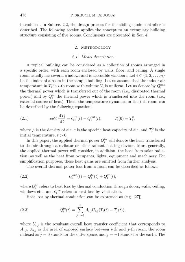
A typical building can be considered as a collection of rooms arranged ina specific order, with each room enclosed by walls, floor, and ceiling. A singleroom usually has several windows and is accessible via doors. Let i ∈ {1, 2, . . . , n}be the index of a room in the sample building. Let us assume that the indoor airtemperature in Ti in i-th room with volume Vi is uniform. Let us denote by Qout

i

the thermal power which is transferred out of the room (i.e., dissipated thermalpower) and by Qin

i the thermal power which is transferred into the room (i.e.,external source of heat). Then, the temperature dynamics in the i-th room canbe described by the following equation:

(2.1) cρVidTidt

= Qini (t)−Qout

i (t), Ti(0) = T 0i ,

where ρ is the density of air, c is the specific heat capacity of air, and T 0i is the

initial temperature, t > 0.In this paper, the applied thermal power Qin

i will denote the heat transferredto the air through a radiator or other radiant heating devices. More generally,the applied thermal power will consider, in addition, the heat from solar radia-tion, as well as the heat from occupants, lights, equipment and machinery. Forsimplification purposes, these heat gains are omitted from further analysis.

The overall thermal power loss from a room can be described as follows:

(2.2) Qouti (t) = Qtc

i (t) +Qvei (t),

where Qtci refers to heat loss by thermal conduction through doors, walls, ceiling,

windows etc., and Qvei refers to heat loss by ventilation.

Heat loss by thermal conduction can be expressed as (e.g. [27])

(2.3) Qtci (t) =

n∑j=−1

Ai,jUi,j(Ti(t)− Tj(t)),

where Ui,j is the resultant overall heat transfer coefficient that corresponds toAi,j , Ai,j is the area of exposed surface between i-th and j-th room, the roomindexed as j = 0 stands for the outer space, and j = −1 stands for the earth. The


resultant heat transfer coefficient Ui,j can be calculated as a weighted average ofthe elements that the surface Ai,j is composed of, that is [28]

(2.4) Ui,j =

∑k

Ai,j,kUi,j,k∑k

Ai,j,k,

where∑k

Ai,j,k = Ai,j .

The loss of heat due to ventilation with heat recovery can be expressed as(e.g. [29])

(2.5) Qvei (t) = (1− β)cρqi (Ti(t)− T0(t)) ,

where qi denotes air volume flow, and β stands for heat recovery efficiency.Finally, the model of the air temperature dynamics in the building can be

expressed by Eqs (2.1)–(2.5) and written using the state space notation in thefollowing form:

(2.6) Ex(t) = Ax(t) + Bu(t) + Zz(t), x(0) = x0,

where

x(t) = [x1(t) x2(t) ... xn(t)]T ∈ Rn, xi(t) = Ti(t), i = 1, 2, ..., n,(2.7)

u(t) = [u1(t) u2(t) ... un(t)]T ∈ Rn, ui(t) = Qini (t), i = 1, 2, ..., n,(2.8)

(2.9)z(t) = [z1(t) z2(t)]T ∈ R2, z1(t) = T0(t), z2(t) = T−1(t),

t > 0, x0 ∈ Rn,

(2.10) E = cρ diag(V1, V2, ..., Vn),

(2.11) A=

−n∑j=1

A1,jU1,j A1,2U1,2 . . . A1,nU1,n

A2,1U2,1 −n∑j=1

A2,jU2,j . . . A2,nU2,n

......

. . ....

An,1Un,1 An,2Un,2 . . . −n∑j=1

An,jUn,j

−(1−β)cρ

q1

q2...qn

In,

(2.12) B = diag(b1, b2, ..., bn),


bi =

1, if i-th room is equipped with a heating device,

0, otherwise,(2.13)

Z =

A1,0U1,0 + (1− β)cρq1 A1,−1U1,−1

A2,0U2,0 + (1− β)cρq2 A2,−1U2,−1

......

An,0Un,0 + (1− β)cρqn An,−1Un,−1

.(2.14)

The output equations of the state space representation are based on themeasurement of sensors that relate to the air temperature in the rooms

(2.15) y(t) = Cx(t),

where

y(t) = [y1(t) y2(t) ... yn(t)]T ∈ Rn, yi(t) = Ti(t), i = 1, 2, ..., n,(2.16)

C = diag(c1, c2, ..., cn),(2.17)

ci =

1, if i-th room is equipped with a temperature sensor,

0, otherwise.(2.18)

2.2. Synthesis of a sliding mode controller

We consider the situation where every room is equipped with a heating device,which means that B = In. We also assume that in every room a sensor measuresindoor temperature, therefore, y(t) = x(t). Under these assumptions, we candefine the sliding surface for the system (2.6), (2.15) in the following form:

(2.19) s(t) = x(t)− xd(t),

where xd(t) is the desired trajectory. The problem is to find a control law thatguarantees the existence of the sliding mode around the defined surface (2.19).

Let us consider the following formula:

(2.20) u(t) = −B−1 (Ax(t)−Exd(t))−B−1S(t)zmax

− σB−1S(t)sη(t)− γB−1s(t),


where σ > 0, γ > 0 are positive coefficients, and zmax ∈ Rn is a vector whoseelements are the upper bounds of the corresponding elements of Zz(t), that is

zmax = maxt≥0

Zz(t) ≥ 0,(2.21)

S(t) = diag(sgn(s1(t)), sgn(s2(t)), ..., sgn(sn(t))

),(2.22)

sη(t) =[|s1(t)|η |s2(t)|η ... |sn(t)|η

]T,(2.23)

η is a ratio of two odd positive integers satisfying 0 < η < 1.Theorem 2.1. The trajectory of the system (2.6) is forced by the control (2.8)from any initial condition to the surface (2.19) in finite time and, then, remainson it.Proof. The proof is approached by imposing the following Lypunov function:

(2.24) V (t) = 0.5s(t)Ts(t).

The derivative of the functional V with respect to time t and along the solutionsof the system (2.6) becomes

(2.25) V (t) = s(t)Ts(t) = s(t)T (x(t)− xd(t))

= s(t)T(E−1Ax(t) + E−1Bu(t) + E−1Zz(t)− xd(t)

).

Substitution of (2.20) by (2.25) yields

(2.26) V (t) = −s(t)TE−1S(t)zmax − s(t)TE−1σS(t)sη(t)

− s(t)TE−1γs(t) + s(t)TE−1Zz(t).

From (2.21) it follows that

(2.27) V (t) ≤ −γλmin(E−1) ‖s(t)‖2 − σλmin(E−1) ‖s(t)‖η+1

= −2γλmin(E−1)V (t)− 2η+12 σλmin(E−1)V (t)

η+12 .

By taking α = 2γλmin(E−1) > 0, β = 2η+12 σλmin(E−1) > 0, κ = η+1

2 it can beconcluded from Lemma 2.1 that the system state will reach the sliding modesurface in finite time calculated as follows:

(2.28) tr =1

α(1− κ)lnαV (0)1−κ + β

β,


where

(2.29) V (0) = 0.5s(0)Ts(0).�

Lemma 2.1 ([9, 30]). Assuming that a continuous positive-definite function V (t)satisfies the following differential inequality

(2.30) V (t) ≤ −αV (t)− βV (t)κ, ∀t≥t0 , V (t0) ≥ 0,

where α and β are positive constants, and κ is a ratio of two odd positive integers,such as 0 < κ < 1. Then, for any given time t0, V (t) converges to zero at leastwithin a finite time

(2.31) tr = t0 +1

α(1− κ)lnαV (t0)1−κ + β

β.

Proof. The proof of this lemma can be found in [9].�

3. Case study

We consider a single-family house, see Figs 1 and 2. The house consists offive rooms, including bedroom, living-room, bathroom, kitchen, and anteroom,see Table 1.

Fig. 1. Floor plan of the house.


Fig. 2. 3D projection of the house.

Table 1. List of rooms with associated indexes. Earth and outer space are also consideredas rooms with special indexes: −1 and 0 respectively.

Room name Earth Outer space Bedroom Bathroom Living-room Kitchen AnteroomIndex −1 0 1 2 3 4 5

The outer walls have a thickness of 47 cm and are built with four layers:structural clay tile (30 cm), mineral wool as an insulating material (15 cm), andinternal (1 cm) and external (1 cm) cement-lime plasters. The internal wallshave a thickness of 12 cm and are made of brick (10 cm) with 1 cm cement-limeplaster on both sides. The roof is isolated with mineral wool of 20 cm thickness.The building construction elements and geometry parameters are presented inTables 2–5. The house is equipped with a heat recovery system (with an efficiencyof 80%) and mechanical ventilation. It was assumed that air volume flow isconstant for each room. The parameters of the ventilation system are summarisedin Table 4.

Table 2. Areas of the surfaces between separated zones.

Ai,j [m2] −1 0 1 2 3 4 5

1 7.51 21.18 0 6.90 0 0 6.77

2 5.31 10.11 6.90 0 6.90 0 4.80

3 36.43 79.36 0 6.90 0 6.87 4.75

4 13.02 31.07 0 0 6.87 0 11.8

5 9.39 14.14 6.77 4.80 4.75 11.8 0


Table 3. Resultant overall heat transfer coefficients corresponding to the surfaces Ai,j .

Ui,j [W/(m2 ·K)] −1 0 1 2 3 4 5

1 0.30 0.27 0 0.80 0 0 1.00

2 0.30 0.30 0.80 0 0.8 0 1.08

3 0.30 0.30 0 0.80 0 0.99 1.08

4 0.30 0.28 0 0 0.99 0 0.91

5 0.30 0.34 1.00 1.08 1.08 0.91 0

Table 4. Volumes of rooms and ventilation rates.

1 2 3 4 5

Vi, [m3] 18.78 13.28 91.08 32.55 23.48

qi [m3/h] 20 50 60 70 10

Table 5. Other building geometry parameters and thermal properties of buildingconstruction elements.

Parameter Symbol Value UnitSpecific heat capacity of air c 1005 J/(kg ·K)Density of air ρ 1.205 kg/m3

Heat recovery efficiency β 0.8 –Surface area of exterior doors Ai,j,k 2.31 m2

Surface area of interior doors Ai,j,k 1.89 m2

Surface area of a single window Ai,j,k 1.17 m2

Surface area of a double window Ai,j,k 2.52 m2

Overall heat transfer coefficient of exterior doors Ui,j,k 0.25 W/(m2 ·K)Overall heat transfer coefficient of interior doors Ui,j,k 0.8 W/(m2 ·K)Overall heat transfer coefficient of a window Ui,j,k 0.9 W/(m2 ·K)

The house is equipped with a central heating system, whereby every roomhas its own radiator. A thermostat unit is mounted on every radiator controllingthe flow of hot central heating water into the radiator. We assume that all radi-ators in the house can be controlled by a central unit that implements a controlalgorithm. The outdoor air and earth temperatures are measured using externalsensors. In addition, every room is equipped with a sensor that measures indoortemperature.

The dynamics of the indoor air temperature can be described by Eq. (2.6)with n = 5. The earth temperature is assumed to be stable at a level of 15.0◦C.The daily profile of the outside temperature that has been used in the simulation


experiments is presented in Fig. 3. The desired temperature profile for every roomis defined by the following function:

(3.1) xdi(t) = −2 cos

(2π

24(t− 4)

)+ 20, i = 1, 2, ..., 5.

Fig. 3. Outdoor air temperature over the course of the simulation experiment.

The temperature (3.1) is given in Celsius, as well as the initial condition

x(0) = [15.0 16.0 17.0 15.0 14.0]T.

The central unit implements the sliding mode control algorithm (2.20) withthe following parameters:

σ = 100, γ = 106, η = 3/5,

zmax = 107 · [1.003 0.608 4.397 1.627 0.982]T.

Every element of the vector zmax represents heat power expressed in watts. Inaddition, we take into consideration the following constraints imposed by theradiator construction:

0 [W] ≤ u1(t) ≤ 500 [W],(3.2)

0 [W] ≤ u2(t) ≤ 500 [W],(3.3)

0 [W] ≤ u3(t) ≤ 3000 [W],(3.4)

0 [W] ≤ u4(t) ≤ 800 [W],(3.5)

0 [W] ≤ u5(t) ≤ 400 [W].(3.6)


The sample simulation results are presented in Figs 4 and 5. The upper plotsshow temperatures change during the whole simulation and the bottom plots showtemperatures change in the zoomed time window. As can be noticed, at the be-

Fig. 4. The trajectory x1 (black line) of the closed-loop system with the sliding mode controllerand the desired trajectory xd1 (grey line). The trajectory x1 represents the indoor temperature

in the bedroom. The same simulation results are shown in different time windows.

Fig. 5. The trajectory x5 (black line) of the closed-loop system with the sliding mode controllerand the desired trajectory xd5 (grey line). The trajectory x5 represents the indoor temperature

in the anteroom. The same simulation results are shown in different time windows.


ginning of the simulation the indoor air temperature changes faster until the de-sired temperature is reached. When this happens, the internal air temperaturechanges according to the desired temperature, despite external disturbances,such as the outside temperature. Figure 5 shows the air temperature changes inthe anteroom. It can be noticed that this temperature changes slowly before itreaches the desired temperature xd5(t). This is due to the fact that the anteroomhas relatively the smallest radiator.

4. Conclusions

An efficient and practical way for modelling heat transfer dynamics in a build-ing, which can be an office area, apartment house, industrial plant etc., was pre-sented in this paper. The resulting mathematical model is represented by first-order differential equations. The number of rooms where the indoor air temper-ature is controlled determines the order of the dynamical model. The presentedmodelling approach allows the incorporation of to incorporate various forms ofheat loss and heat gain. One of the main advantages of the such modelling ap-proach is that the model parameters can be determined easily and uniquely fromthe geometry of the building and the thermal properties of the building materi-als. As a result, the formal identification of the model parameters is not required.This approach leads to mathematical models that can be used for the design oftemperature control algorithms. In this paper, a proposed sliding mode controllerguarantees the existence of the sliding mode around the defined sliding surface.The trajectory of the closed-loop system reaches the sliding surface after a finitetime and, then, remains on it. The simulation example has shown the effective-ness of the proposed method. Numerical calculations and computer simulationswere performed in the MathWorksTM MATLABr/Simulinkr environment.

References

1. Edward C., Spurgeon S., Sliding mode control: theory and appliations, Taylor andFrancis, London, 1998.

2. Pisano A., Usai E., Sliding mode control: a survey with application in math, Mathematicsand Computers in Simulation, 81(5): 954–979, 2011.

3. Długosz M., Optimization problems of power transmission in automation and robotics,Przeglad Elektrotechniczny, 87(9A): 238–242, 2011.

4. Abid M., Mansouri A., Aissaoui A., Belabbes B., Sliding mode application in posi-tion control of an induction machine, Journal of Electrical Engineering, 59(6): 322–327,2008.

5. Perić S.L., Antić D.S., Nikolić V.D., Mitić D.B., Milojković M.T., Niko-lić S.S., A new approach to the sliding mode control design: anti–lock braking systemas a case study, Journal of Electrical Engineering, 65(1): 37–43, 2014.


6. Bandyopadhyay B., Deepak F., Kim K.S., Sliding mode control using novel slidingsurfaces, Springer-Verlag, Berlin, Heidelberg, 2010.

7. Liu J., Sun F., A novel dynamic terminal sliding mode control of uncertain nonlinearsystems, Journal of Control Theory and Applications, 5(2): 189–193, 2007.

8. Man Z., Yu X.H., Terminal sliding mode control of MIMO linear systems, IEEE Trans-actions on Circuits and Systems I: Fundamental Theory and Applications, 44(11): 1065–1070, 1997.

9. Mobayen S., Majd V.J., Sojoodi M., An LMI-based composite nonlinear feedbackterminal sliding-mode controller design for disturbed MIMO systems, Mathematics andComputers in Simulation, 85(11): 1–10, 2012.

10. Kulkarni M.R., Hong F., Energy optimal control of a residential space-conditioningsystem based on sensible heat transfer modeling, Building and Environment, 39(1): 31–38,2004.

11. Blasco C., Monreal J., Benítez I., Lluna A., Modelling and PID control of HVACsystem according to energy efficiency and comfort criteria, [in:] Sustainability in Energyand Buildings, N. M’Sirdi, A. Namaane, R.J. Howlett, L.C. Jain (Eds), pp. 365–374,Springer, Berlin, Heidelberg, 2012.

12. Fourier J., The analytical theory of heat, Dover Publicatons, Inc., New York, USA, 1955.

13. Jakob M., Heat transfer, John Willey & Sons, New York, USA, 1949.

14. Gröber H., Erk S., Fundamentals of Heat Transfer, McGraw-Hill, 1961.

15. Lu X., Clements-Croome D., Viljanen M., Past, present and future mathematicalmodels for buildings: focus on intelligent buildings (part 1), Intelligent Buildings Interna-tional, 1(1): 23–38, 2009.

16. Lu X., Clements-Croome D., Viljanen M., Past, present and future mathematicalmodels for buildings: focus on intelligent buildings (part 2), Intelligent Buildings Interna-tional, 1(2):131–141, 2009.

17. Clarke J., Energy simulation in building design, Butterworth Heinemann, Woburn, USA,2001.

18. Underwood C.P., Yik F., Modelling methods for energy in buildings, Blackwell Science,Oxford, United Kingdom, 2004.

19. Gouda M.M., Danaher S., Underwood C.P., Low-order model for the simulation ofa building and its heating system, Building Services Engineering Research and Technology,21(3): 199–208, 2000.

20. Gouda M.M., Danaher S., Underwood C.P., Building thermal model reduction usingnonlinear constrained optimization, Building and Environment, 37(12): 1255–1265, 2002.

21. Bergman T.L., Incropera F.P., DeWitt D.P., Lavine A.S., Fundamentals of heatand mass transfer, John Wiley & Sons, 2011.

22. Davies M.G., Building Heat Transfer, John Wiley & Sons, 2004.

23. Długosz M., Aggregation of state variables in an RC model, Building Services Engineer-ing Research and Technology, 39(1): 66–80, 2018.


24. Sierociuk D., Dzieliński A., Sarwas G., Petras I., Podlubny I., Skovranek T.,Modelling heat transfer in heterogeneous media using fractional calculus, PhilosophicalTransactions of the Royal Society A: Mathematical, Physical and Engineering Sciences,371(1990): 20120146, 2013.

25. Oprzędkiewicz K., Non integer order, state space model of heat transfer process usingCaputo-Fabrizio operator, Bulletin of the Polish Academy of Sciences: Technical Sciences,66(3): 249–255, 2018, doi: 10.24425/122105.

26. Długosz M., Skruch P., The application of fractional-order models for thermal processmodelling inside buildings, Journal of Building Physics, 39(5): 440– 451, 2016.

27. Polish Committee for Standardization, PN-EN ISO 13790:2009. Thermal performance ofbuildings – Calculation of energy use for space heating and cooling, http://www.pkn.pl(accessed: August 29, 2012), 2009.

28. Polish Committee for Standardization,PN-EN ISO 6946:2008. Building components andbuilding elements. Thermal resistance and thermal transmittance – Calculation method,http://www.pkn.pl (accessed: August 29, 2012), 2008.

29. Polish Committee for Standardization, PN-B-03430:1983. Ventilation in dwelling and pub-lic utility buildings – Specifications, http://www.pkn.pl (accessed: August 29, 2012), 1983.

30. Moulay E., Perruquetti W., Finite time stability and stabilization of a class of con-tinuous systems, Journal of Mathematical Analysis and Applications, 323(2): 1430–1443,2006.

Received October 19, 2018; accepted version May 6, 2019.

Published on Creative Common licence CC BY-SA 4.0

A Sliding Mode Controller Design for Thermal Comfort in ...

Documents

Transcript of A Sliding Mode Controller Design for Thermal Comfort in ...